methods related to the

� � � � � � �

�

� � �� ! �"#�� $%��

&('*),+-)(./+-)0.21434576/),+98,:%;<)>=,'41/? @%3*)BAC:D8E+%=B891GF*),+H;I?H1KJ2.21K8L1GMNAPO45Q5R)S;S+T? =RU ?H1*)>./+EAVOKAPM;<),5�?H1G;P8W.XAVO4575R)S;S+Y? =Z8L1*)/[%\Z1*)]AB3*=,'Q;<)B=,'41/? @%3*)RAP8LU F*)BA(;S'*)Z)>@%3/? F*.4U ),1G;^U ?H1*)>./+APOKAP;_),5a`Rbc`^dfeg`Rbih,jk=>.4U U )Blm;B'*)n1K84+o5R.EUp)B@%3*.K;q? 8L1KA>[r\0:D;_),1Ejp;B'/? A2.4s4s/+t8/.,=,'? A7.KFK84? l4)>lu?H1vs,+D.*=S;q? =>)m6/)>=>.43KA<)W;B'*)w=B8E)IxW=K? ),1G;W5R.K;S+Y? yn` b `z? AW5Q3*=,'|{}84+-A_)=B8L1*l9? ;I? 891*)>lX;B'*.41Q`7[r~k8K{i)IF*),+NjL;B'*)71K8E+o5R.4U4)>@%3*.G;I? 891KA0.4s4s/+t8�.*=,'w5R.BOw6/)Z.,l4)IM@%3*.K;_)7?H17A_8L5R)QAI? ;S3*.K;q? 8L1KA>[p��1*l4)>)>l�j9;B'*),+-)Q./+-)Q)SF*),1�.Es4s4U ? =>.K;q? 8L1KA(?H1Q{R'/? =,'W? ;R? As/+-)S:Y),+o+D)Blm;_8|;B'*)W3KAB3*.4Ur�c+HO4U 8,F|AS346KABs*.,=B)Q;_)>=,'41/? @%3*)BAB[�&('/? A]=*'*.EsG;_),+}=B8*F*),+tA7? ;PM),+-.K;q? F*)75R)S;S'K8El�Ai{^'/? =,'Z./+-)R)K? ;B'*),+pl9?�+D)B=S;BU OR84+k?H5Qs4U ? =K? ;BU O2+-),U .G;<)Bl7;_82;S'*)Q1K84+o5R.EU)>@%3*.G;I? 891KA>[

��m��W��X��(�f�Q��-��u�K�

In order to solve the linear system �7�� when � is nonsymmetric, we can solve theequivalent system

� b �¡��¢� b £N¤ [�¥K¦which is Symmetric Positive Definite. This system is known as the system of the normalequations associated with the least-squares problem,

minimize §* R¨©�7�ª§*«9¬ £N¤ [ �¦Note that (8.1) is typically used to solve the least-squares problem (8.2) for over-determined systems, i.e., when � is a rectangular matrix of size ®°¯�± , ±�²³® .

A similar well known alternative sets �f�¢� bi´ and solves the following equation for´:

�7� b ´ �! �¬ £N¤ [ µ�¦¶p¶p·

¶�� ~�� &�� 9&^~ \��p&��&ª\³&^~��}\�� p&^� \��Once the solution

´is computed, the original unknown � could be obtained by multiplying´

by � b . However, most of the algorithms we will see do not invoke the´

variable explic-itly and work with the original variable � instead. The above system of equations can beused to solve under-determined systems, i.e., those systems involving rectangular matricesof size ®°¯v± , with ®°² ± . It is related to (8.1) in the following way. Assume that ®"! ±and that � has full rank. Let ��# be any solution to the underdetermined system �Q�³� .Then (8.3) represents the normal equations for the least-squares problem,

minimize §G��#Z¨�� b ´ § « ¬ £N¤ [ $�¦Since by definition � bi´ � � , then (8.4) will find the solution vector � that is closest to� # in the 2-norm sense. What is interesting is that when ® ²!± there are infinitely manysolutions � # to the system �Q�¡� , but the minimizer

´of (8.4) does not depend on the

particular � # used.The system (8.1) and methods derived from it are often labeled with NR (N for “Nor-

mal” and R for “Residual”) while (8.3) and related techniques are labeled with NE (Nfor “Normal” and E for “Error”). If � is square and nonsingular, the coefficient matricesof these systems are both Symmetric Positive Definite, and the simpler methods for sym-metric problems, such as the Conjugate Gradient algorithm, can be applied. Thus, CGNEdenotes the Conjugate Gradient method applied to the system (8.3) and CGNR the Conju-gate Gradient method applied to (8.1).

There are several alternative ways to formulate symmetric linear systems having thesame solution as the original system. For instance, the symmetric linear system%'& �� b (*) %,+

� ) � % - ) £N¤ [ ./¦with

+ �¢ 0¨f�Q� , arises from the standard necessary conditions satisfied by the solution ofthe constrained optimization problem,

minimize /0 § + ¨� 9§ «« £N¤ [ 1/¦subject to � b + � - ¬ £N¤ [ 2/¦

The solution � to (8.5) is the vector of Lagrange multipliers for the above problem.Another equivalent symmetric system is of the form% ( �� b ( ) % �Q�� )!� % � b ) ¬

The eigenvalues of the coefficient matrix for this system are 3,4�5 , where 4 5 is an arbitrarysingular value of � . Indefinite systems of this sort are not easier to solve than the origi-nal nonsymmetric system in general. Although not obvious immediately, this approach issimilar in nature to the approach (8.1) and the corresponding Conjugate Gradient iterationsapplied to them should behave similarly.

A general consensus is that solving the normal equations can be an inefficient approachin the case when � is poorly conditioned. Indeed, the 2-norm condition number of � b � isgiven by 687�9;:

«�<V� b �>=��§K� b �m§*«�§?<N� b �>=A@�BL§K«4¬Now observe that §K� b �m§ « �C4 «D�EAF <N�,= where 4 D�EAF <V�>= is the largest singular value of �

�� r\�� r\�� &^� \�� 9&�~}\�� ¶��which, incidentally, is also equal to the 2-norm of � . Thus, using a similar argument forthe inverse <V� b �>= @�B yields687�9;:

«�<N� b �>=R�z§K�n§ «« §K� @�BE§ «« � 687�9;: «« <V�>=K¬ £N¤ [ ¤ ¦The 2-norm condition number for � b � is exactly the square of the condition number of� , which could cause difficulties. For example, if originally

687?9 :« <V�>=v� / - , then an

iterative method may be able to perform reasonably well. However, a condition number of/ - B�� can be much more difficult to handle by a standard iterative method. That is becauseany progress made in one step of the iterative procedure may be annihilated by the noisedue to numerical errors. On the other hand, if the original matrix has a good 2-norm condi-tion number, then the normal equation approach should not cause any serious difficulties.In the extreme case when � is unitary, i.e., when �� X�¢� &

, then the normal equations areclearly the best approach (the Conjugate Gradient method will converge in zero step!).

�Z�� X�Z�� ]��-�f��ª�u�w��|��u��

When implementing a basic relaxation scheme, such as Jacobi or SOR, to solve the linearsystem

� b �7��¢� b �� £N¤ [ ��¦or

�7� b ´ �! �� £N¤ [�¥��¦it is possible to exploit the fact that the matrices � b � or �7� b need not be formed explic-itly. As will be seen, only a row or a column of � at a time is needed at a given relaxationstep. These methods are known as row projection methods since they are indeed projectionmethods on rows of � or � b . Block row projection methods can also be defined similarly.

�! #"! %$ &�')(+*,*.-/*1032#4503687:9<;>=?0@9�7:A!BC'56D0FEG(�'�;>2H7�9!*

It was stated above that in order to use relaxation schemes on the normal equations, onlyaccess to one column of � at a time is needed for (8.9) and one row at a time for (8.10).This is now explained for (8.10) first. Starting from an approximation to the solution of(8.10), a basic relaxation-based iterative procedure modifies its components in a certainorder using a succession of relaxation steps of the simple form´3IJLK � ´NMPO 5RQ 5 £N¤ [�¥,¥K¦where Q 5 is the S -th column of the identity matrix. The scalar

O 5 is chosen so that the S -thcomponent of the residual vector for (8.10) becomes zero. Therefore,<V R¨©�X� b < ´NMPO 5 Q 5 =T� Q 5 =�� - £N¤ [�¥>�¦

¶��p¶ � ~�� &�� 9&^~ \��p&��&ª\³&^~��}\�� p&^� \��which, setting

+ �! R¨©�X� bc´ , yields,

O 5 � < + � Q 5 =§K� b Q 5S§ «« ¬ £N¤ [�¥Gµ/¦

Denote by � 5 the S -th component of . Then a basic relaxation step consists of taking

O 5i� � 5 ¨ <N� bi´ �S� b Q 5 =§K� b Q 5 § «« ¬ £N¤ [�¥ $�¦

Also, (8.11) can be rewritten in terms of � -variables as follows:

� IJLK �� M O 5N� b Q 5q¬ £N¤ [�¥A./¦The auxiliary variable

´has now been removed from the scene and is replaced by the

original variable �� bi´ .Consider the implementation of a forward Gauss-Seidel sweep based on (8.15) and

(8.13) for a general sparse matrix. The evaluation ofO 5 from (8.13) requires the inner prod-

uct of the current approximation �� b ´ with � b Q 5 , the S -th row of � . This inner productis inexpensive to compute because � b Q 5 is usually sparse. If an acceleration parameter �is used, we only need to change

O 5 into � O 5 . Therefore, a forward SOR sweep would be asfollows.

��n��-�w�� #�� n��K�(��a� �� 1. Choose an initial � .2. For Sª� / � 0 �*¬*¬,¬T�I® Do:

3.O 5c�!�#"%$ @'&)(�* J $,+ F.-/ ( *

J$ /100

4. � � �� MPO 5P� b Q 55. EndDo

Note that � b Q 5 is a vector equal to the transpose of the S -th row of � . All that is needed isthe row data structure for � to implement the above algorithm. Denoting by ®�2�5 the numberof nonzero elements in the S -th row of � , then each step of the above sweep requires0 ®�2 5 M 0

operations in line 3, and another0 ®�2 5 operations in line 4, bringing the total to3 ®�2 5 M 0

. The total for a whole sweep becomes3 ®�2 M 0 ® operations, where ®�2 represents

the total number of nonzero elements of � . Twice as many operations are required for theSymmetric Gauss-Seidel or the SSOR iteration. Storage consists of the right-hand side, thevector � , and possibly an additional vector to store the 2-norms of the rows of � . A betteralternative would be to rescale each row by its 2-norm at the start.

Similarly, a Gauss-Seidel sweep for (8.9) would consist of a succession of steps of theform

� IJ/K �� MPO 5 Q 5S¬ £N¤ [�¥A1/¦Again, the scalar

O 5 is to be selected so that the S -th component of the residual vector for(8.9) becomes zero, which yields<N� b R¨�� b � <N� M O 5 Q 5 = � Q 5 =^� - ¬ £N¤ [�¥A2/¦

�� r\�� r\�� &^� \�� 9&�~}\�� ¶��With

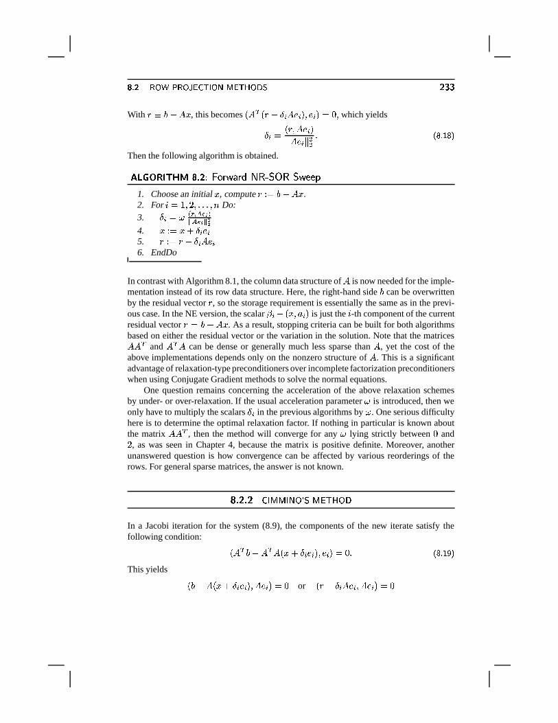
+�� ]¨©�7� , this becomes <V� b < + ¨ O 5 � Q 5 = � Q 5 =�� - � which yields

O 5 � < + �B� Q 5 =§K� Q 5 § «« ¬ £N¤ [�¥ ¤ ¦

Then the following algorithm is obtained.

�� n� �D�w�� t¶�� 1� � � �K�(��a� � � �� 1. Choose an initial � , compute

+ � �� R¨��Q� .2. For S0� / � 0 �,¬*¬,¬ �I® Do:3.

O 5i� � & � + (J$ -/ (

J$ /100

4. � � �� M O 5%Q 55.

+ � � + ¨ O 5V� Q 56. EndDo

In contrast with Algorithm 8.1, the column data structure of � is now needed for the imple-mentation instead of its row data structure. Here, the right-hand side can be overwrittenby the residual vector

+, so the storage requirement is essentially the same as in the previ-

ous case. In the NE version, the scalar ��5 ¨ <o� �� 5 = is just the S -th component of the currentresidual vector

+ �a ]¨ �Q� . As a result, stopping criteria can be built for both algorithmsbased on either the residual vector or the variation in the solution. Note that the matrices�7� b and � b � can be dense or generally much less sparse than � , yet the cost of theabove implementations depends only on the nonzero structure of � . This is a significantadvantage of relaxation-type preconditioners over incomplete factorization preconditionerswhen using Conjugate Gradient methods to solve the normal equations.

One question remains concerning the acceleration of the above relaxation schemesby under- or over-relaxation. If the usual acceleration parameter � is introduced, then weonly have to multiply the scalars

O 5 in the previous algorithms by � . One serious difficultyhere is to determine the optimal relaxation factor. If nothing in particular is known aboutthe matrix �X� b , then the method will converge for any � lying strictly between

-and0

, as was seen in Chapter 4, because the matrix is positive definite. Moreover, anotherunanswered question is how convergence can be affected by various reorderings of therows. For general sparse matrices, the answer is not known.

�! "! #" ��2 BDB 2 9�7�� * BD0 ;>=�7:4

In a Jacobi iteration for the system (8.9), the components of the new iterate satisfy thefollowing condition: <N� b R¨�� b ��<o� M O 5%Q 5 =T� Q 5 =R� - ¬ £N¤ [�¥��¦This yields <P ^¨ ��<o� MPO 5RQ 5 = �B� Q 5 =�� -

or < + ¨ O 5 � Q 5 �S� Q 5 =^� -

¶�� ~�� &�� 9&^~ \��p&��&ª\³&^~��}\�� p&^� \��in which

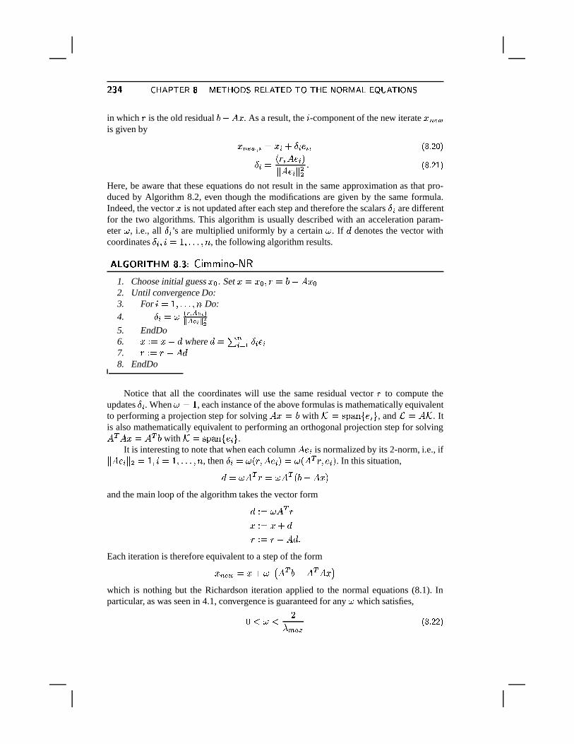
+is the old residual (¨��7� . As a result, the S -component of the new iterate � IJ/K

is given by

� IJLK + 5 �� 5 M O 5 Q 5 � £N¤ [ �/¦O 5 � < + �B� Q 5 =

§K� Q 5B§ «« ¬ £N¤ [ 9¥G¦Here, be aware that these equations do not result in the same approximation as that pro-duced by Algorithm 8.2, even though the modifications are given by the same formula.Indeed, the vector � is not updated after each step and therefore the scalars

O 5 are differentfor the two algorithms. This algorithm is usually described with an acceleration param-eter � , i.e., all

O 5 ’s are multiplied uniformly by a certain � . If � denotes the vector withcoordinates

O 5 � Sª� / �*¬,¬*¬T�S® , the following algorithm results.

��n��-�w�� 4� �1. Choose initial guess �� . Set �� + �! R¨©�7��2. Until convergence Do:3. For Sª� / �,¬*¬,¬T�I® Do:4.

O 5c� � & � + (J$ -/ (

J$ /100

5. EndDo6. � � �� M � where �m�� I5�� B O 5 Q 57.

+ � � + ¨��8. EndDo

Notice that all the coordinates will use the same residual vector+

to compute theupdates

O 5 . When �³� / , each instance of the above formulas is mathematically equivalentto performing a projection step for solving �Q�°�� with � ��

9��Q 5�� , and �!� �� . It

is also mathematically equivalent to performing an orthogonal projection step for solving� b �Q��¢� b with �z� ��9!�Q 5"� .

It is interesting to note that when each column � Q?5 is normalized by its 2-norm, i.e., if§K� Q 5 §K«7� / ��S0� / �*¬*¬,¬T�I® , thenO 5 � � < + �S� Q 5 =�� <N� b + � Q 5 = . In this situation,

�m� �^� b + � �^� b <V R¨��Q� =and the main loop of the algorithm takes the vector form

� � � �^� b +� � �� M �+ � � + ¨��C¬

Each iteration is therefore equivalent to a step of the form

� IJLK �� M �$#V� b R¨�� b �Q��%which is nothing but the Richardson iteration applied to the normal equations (8.1). Inparticular, as was seen in 4.1, convergence is guaranteed for any � which satisfies,- ² � ²

0& D�EAF £N¤ [ //¦

�� r\�� r\�� &^� \�� 9&�~}\�� ¶��where

& D�EAF is the largest eigenvalue of � b � . In addition, the best acceleration parameteris given by

��0� 0& D 5 I�M & D�EAFin which, similarly,

& D 5 I is the smallest eigenvalue of � b � . If the columns are not nor-malized by their 2-norms, then the procedure is equivalent to a preconditioned Richardsoniteration with diagonal preconditioning. The theory regarding convergence is similar butinvolves the preconditioned matrix or, equivalently, the matrix �� obtained from � by nor-malizing its columns.

The algorithm can be expressed in terms of projectors. Observe that the new residualsatisfies + IJLK � + ¨ I 5�� B � < + �S� Q 5 =§K� Q 5 § «« � Q 5S¬ £N¤ [ ,µ�¦Each of the operators � 5 � + ¨ � < + �S� Q 5 =

§K� Q 5B§ «« � Q 5 �� 5 + £N¤ [ �$4¦

is an orthogonal projector onto � Q?5 , the S -th column of � . Hence, we can write+ IJ/K �� & ¨ � I 5�� B� 5�� + ¬ £N¤ [ .�¦

There are two important variations to the above scheme. First, because the point Jacobiiteration can be very slow, it may be preferable to work with sets of vectors instead. Let� B � � « �*¬,¬*¬T� � � be a partition of the set

� / � 0 �*¬,¬*¬ �S® � and, for each �� , let � � be the matrixobtained by extracting the columns of the identity matrix whose indices belong to �� .Going back to the projection framework, define � 5 � �� 5 . If an orthogonal projectionmethod is used onto � � to solve (8.1), then the new iterate is given by

� IJ/K �� M �� 5 � 5 � 5 £N¤ [ 1�¦

� 5 � <�� b5 � b �� 5 = @�B�� b5 � b + � <N� b5 � 5 =A@�BG� b5 + ¬ £N¤ [ 2�¦Each individual block-component � 5 can be obtained by solving a least-squares problem�� 9� § + ¨©� 5 � §K«9¬An interpretation of this indicates that each individual substep attempts to reduce the resid-ual as much as possible by taking linear combinations from specific columns of ��5 . Similarto the scalar iteration, we also have+ IJLK � � & ¨ � I 5�� B

� 5 � +where

� 5 now represents an orthogonal projector onto the span of � 5 .Note that � B �B�7«�*¬*¬,¬ �B� � is a partition of the column-set

�� Q 5 � 5�� B +�� + I and this parti-

tion can be arbitrary. Another remark is that the original Cimmino method was formulated

¶�� ~�� &�� 9&^~ \��p&��&ª\³&^~��}\�� p&^� \��for rows instead of columns, i.e., it was based on (8.1) instead of (8.3). The alternativealgorithm based on columns rather than rows is easy to derive.

�2�f�:� ��7�^�u��m�R�8�v�o�]�X� � �N�#�w��0��Q��-�f�W��v��

A popular combination to solve nonsymmetric linear systems applies the Conjugate Gra-dient algorithm to solve either (8.1) or (8.3). As is shown next, the resulting algorithms canbe rearranged because of the particular nature of the coefficient matrices.

�! ��! $ �+&)9?A

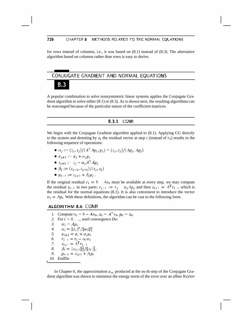
We begin with the Conjugate Gradient algorithm applied to (8.1). Applying CG directlyto the system and denoting by 2 5 the residual vector at step S (instead of

+ 5 ) results in thefollowing sequence of operations:

� � � � <�2 � � 2 � = ��<N� b �� =�� < 2 � � 2 � =��<V�� B�� = � � � B � �� M � � � 2 � � B � � 2 � ¨ � � b �� < 2 � � B � 2 � � B =��<�2 � � 2 � = � � � B � �#2 � � B M � � � � .

If the original residual+ 5 � �¨��Q� 5 must be available at every step, we may compute

the residual 2 5 � B in two parts:+ � � B � � + � ¨ � �� and then 2 5 � B � � b + 5 � B which is

the residual for the normal equations (8.1). It is also convenient to introduce the vector� 5 �� 5 . With these definitions, the algorithm can be cast in the following form.

��n��-�w�� n�1. Compute

+ ��¢ R¨��Q� � , 2 �X�¢� b + � , ��X� 2 � .2. For Sª� - �*¬,¬*¬ , until convergence Do:3. � 5 �� 54. 5ª�z§ 2 5B§ « �r§ � 5S§ ««5. � 5 � B �� 5 M 5�� 56.

+ 5 � B � + 5 ¨ 5 � 57. 2 5 � B �¢� b + 5 � B8. � 5c��§ 2 5 � B § «« �p§ 2 5I§ «« ,9. � 5 � B � 2 5 � B M � 5 � 5

10. EndDo

In Chapter 6, the approximation � D produced at the ± -th step of the Conjugate Gra-dient algorithm was shown to minimize the energy norm of the error over an affine Krylov

�� \��3� �� p&�� &"�� }\�� p&�� \�� ¶��subspace. In this case, � D minimizes the function

� <N� = � <N� b ��<o� # ¨©� = � <o� # ¨©� = =over all vectors � in the affine Krylov subspace

� � M � D <V� b ��B� b + � =R�� M �� 9!� � b + � �S� b �7� b + � �,¬*¬,¬T� <V� b �>= D @�B � b + � � �in which

+ � �! }¨��Q� � is the initial residual with respect to the original equations �Q��! ,and � b + � is the residual with respect to the normal equations � b �7� � � b . However,observe that

� <o� =R� <V� <o��#Z¨©� =T�S� <N��#7¨©� = =R�z§* R¨��Q�0§ «« ¬Therefore, CGNR produces the approximate solution in the above subspace which has thesmallest residual norm with respect to the original linear system �Q� � . The differencewith the GMRES algorithm seen in Chapter 6, is the subspace in which the residual normis minimized.

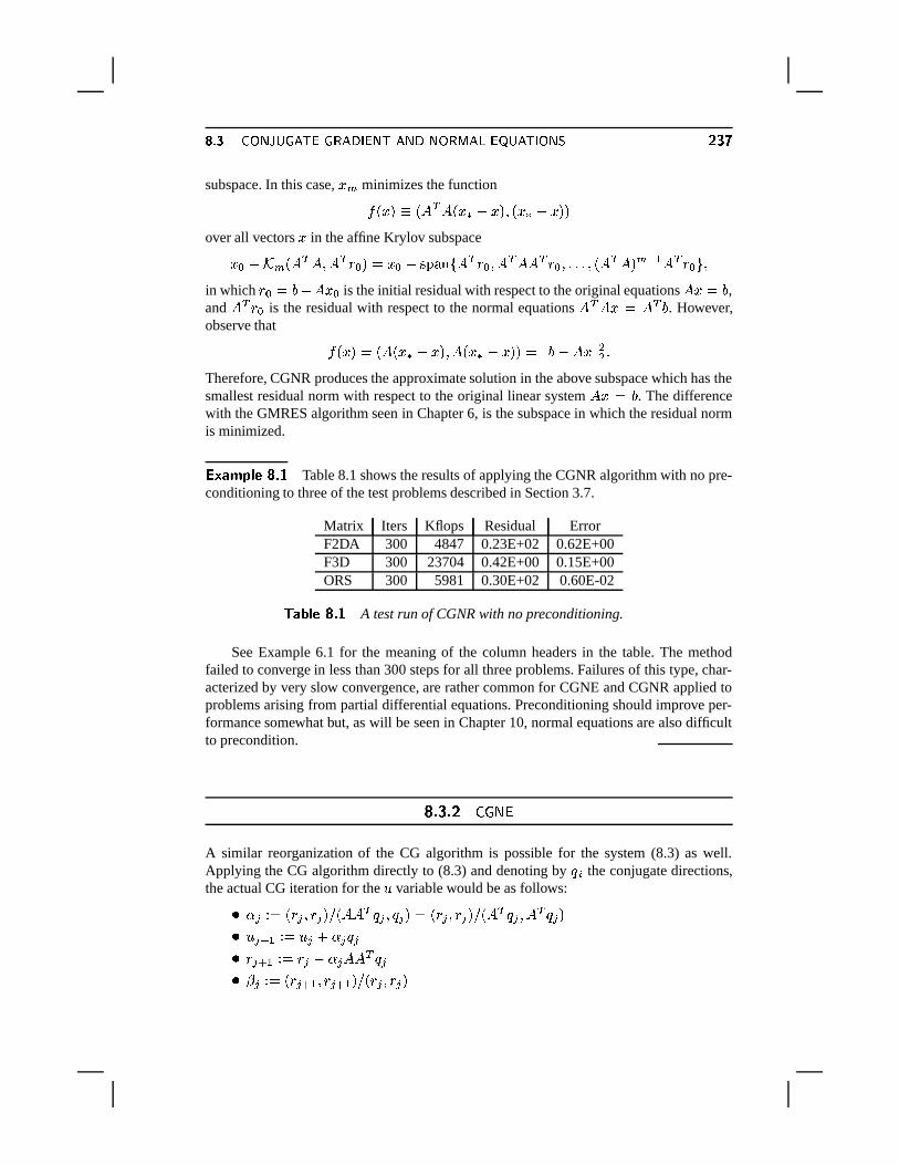
�� #�Table 8.1 shows the results of applying the CGNR algorithm with no pre-

conditioning to three of the test problems described in Section 3.7.

Matrix Iters Kflops Residual ErrorF2DA 300 4847 0.23E+02 0.62E+00F3D 300 23704 0.42E+00 0.15E+00ORS 300 5981 0.30E+02 0.60E-02

�� #�A test run of CGNR with no preconditioning.

See Example 6.1 for the meaning of the column headers in the table. The methodfailed to converge in less than 300 steps for all three problems. Failures of this type, char-acterized by very slow convergence, are rather common for CGNE and CGNR applied toproblems arising from partial differential equations. Preconditioning should improve per-formance somewhat but, as will be seen in Chapter 10, normal equations are also difficultto precondition.

�! ��! #" ��&)9?0

A similar reorganization of the CG algorithm is possible for the system (8.3) as well.Applying the CG algorithm directly to (8.3) and denoting by � 5 the conjugate directions,the actual CG iteration for the

´variable would be as follows:

� � � < + � � + � =��<N�X� b � � �� =�� < + � � + � =��<V� b � � �S� b � � = ´ � � B � � ´ � M � � � + � � B � � + � ¨ � �X� b � � � � � � < + � � B � + � � B = ��< + � � + � =

¶�� ~�� &�� 9&^~ \��p&��&ª\³&^~��}\�� p&^� \�� B � � + � � B M � � � � .

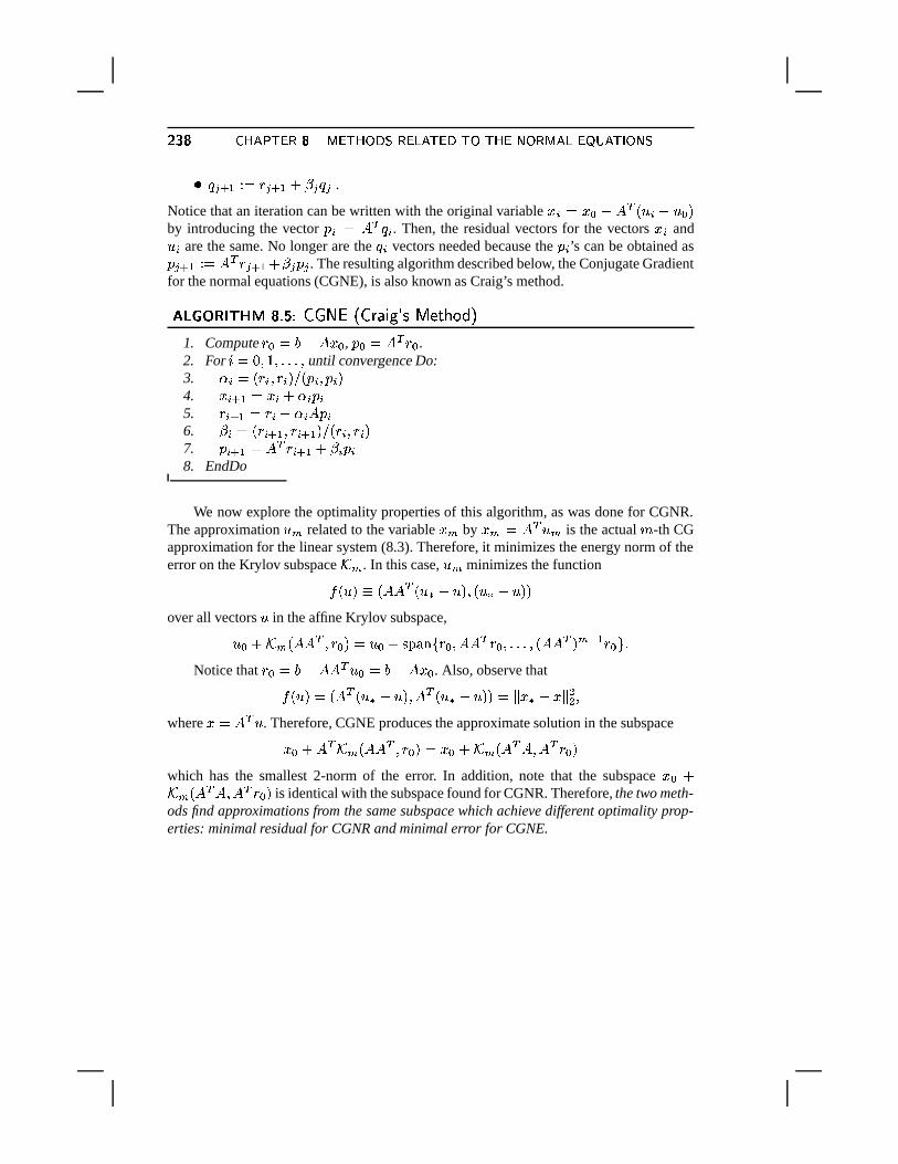
Notice that an iteration can be written with the original variable � 5 �a�� M � b < ´ 5 ¨ ´ � =by introducing the vector � 5 �� b � 5 . Then, the residual vectors for the vectors � 5 and´ 5 are the same. No longer are the � 5 vectors needed because the � 5 ’s can be obtained as� � � B � �� b + � � B M � � � � . The resulting algorithm described below, the Conjugate Gradientfor the normal equations (CGNE), is also known as Craig’s method.

��n��-�w�� m�� ,� �� '� �1. Compute

+ � �¢ R¨��Q� � , � � �� b + � .2. For Sª� - � / �*¬*¬,¬T� until convergence Do:3. 5ª� < + 5 � + 5 = ��< � 5/�� 5 =4. � 5 � B �� 5 M 5�� 55.

+ 5 � B � + 5 ¨ 5V�� 56. � 5 � < + 5 � B � + 5 � B =��< + 5 � + 5 =7. � 5 � B �¢� b + 5 � B M � 5 � 58. EndDo

We now explore the optimality properties of this algorithm, as was done for CGNR.The approximation

´ D related to the variable � D by � D �a� bi´ D is the actual ± -th CGapproximation for the linear system (8.3). Therefore, it minimizes the energy norm of theerror on the Krylov subspace � D . In this case,

´ D minimizes the function� < ´ = � <V�7� b < ´ # ¨ ´ =T� < ´ # ¨ ´ = =

over all vectors´

in the affine Krylov subspace,´ � M � D <V�7� b � + � =�� ´ � M �� 9 � + � �S�X� b + � �*¬*¬,¬ � <N�7� b = D @�B + � �%¬Notice that

+ � �¢ R¨��7� bc´ � �� R¨©�7� � . Also, observe that� < ´ =�� <N� b < ´ #2¨ ´ = �B� b < ´ #]¨ ´ = =R�z§G��#Z¨©�ª§ «« �

where �� bc´ . Therefore, CGNE produces the approximate solution in the subspace

�� M � b � D <N�X� b � + � =^�� M � D <V� b ��S� b + � =which has the smallest 2-norm of the error. In addition, note that the subspace �!� M� D <N� b � �S� b + � = is identical with the subspace found for CGNR. Therefore, the two meth-ods find approximations from the same subspace which achieve different optimality prop-erties: minimal residual for CGNR and minimal error for CGNE.

�� ?4M �p\Q� � & ��r\��; � ¶��p·�ª�8� �v�c��]��o�� ]��w�i�Z� ��u��

Now consider the equivalent system% & �� b (*) % +� ) � % - )

with+ �! �¨©�Q� . This system can be derived from the necessary conditions applied to the

constrained least-squares problem (8.6–8.7). Thus, the 2-norm of ¨ + ��Q� is minimizedimplicitly under the constraint � b + � -

. Note that � does not have to be a square matrix.This can be extended into a more general constrained quadratic optimization problem

as follows:

minimize� <o� = � /0 <N�7� �S� =(¨ <o��B = £N¤ [ ¤ ¦

subject to � b ��4¬ £N¤ [ ��¦The necessary conditions for optimality yield the linear system% � �

� b ( ) % � ) � % � ) £N¤ [ µ ��¦

in which the names of the variables+ �I� are changed into � � for notational convenience.

It is assumed that the column dimension of � does not exceed its row dimension. TheLagrangian for the above optimization problem is

� <o� � =�� /0 <V�Q��I� =^¨ <o� �> = M < � <�� b �v¨ � = =and the solution of (8.30) is the saddle point of the above Lagrangian. Optimization prob-lems of the form (8.28–8.29) and the corresponding linear systems (8.30) are important andarise in many applications. Because they are intimately related to the normal equations, wediscuss them briefly here.

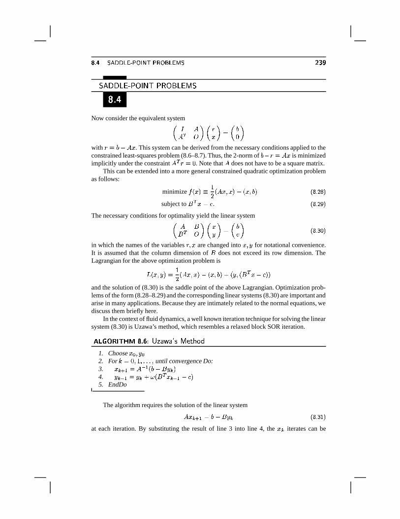
In the context of fluid dynamics, a well known iteration technique for solving the linearsystem (8.30) is Uzawa’s method, which resembles a relaxed block SOR iteration.

�� n� �D�w�� 1. Choose � � � �2. For � � - � / �*¬,¬*¬T� until convergence Do:3. �� B �� @�B <P ]¨ � � =4.

� � B � � M � <�� b �� B ¨ � =

5. EndDo

The algorithm requires the solution of the linear system

�7� � � B �¢ R¨�� £N¤ [ µE¥K¦at each iteration. By substituting the result of line 3 into line 4, the � � iterates can be

¶�� ~�� &�� 9&^~ \��p&��&ª\³&^~��}\�� p&^� \��eliminated to obtain the following relation for the

� ’s,

� � B � � M � # � b � @�B <V R¨�� =ª¨�� %which is nothing but a Richardson iteration for solving the linear system

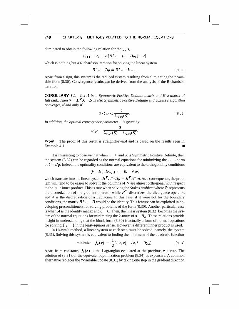
� b � @�B � � � b � @�B R¨��4¬ £N¤ [ µ//¦Apart from a sign, this system is the reduced system resulting from eliminating the � vari-able from (8.30). Convergence results can be derived from the analysis of the Richardsoniteration.

� � � � � ��w� � ��#�Let � be a Symmetric Positive Definite matrix and � a matrix of

full rank. Then � �� b � @�B � is also Symmetric Positive Definite and Uzawa’s algorithmconverges, if and only if - ² ��² 0& D�EAF <��= ¬ £N¤ [ µ/µ/¦In addition, the optimal convergence parameter � is given by

� �� 0& D 5 I <��= M & D�EAF <��= ¬��

The proof of this result is straightforward and is based on the results seen inExample 4.1.

It is interesting to observe that when �2� -and � is Symmetric Positive Definite, then

the system (8.32) can be regarded as the normal equations for minimizing the � @�B -normof (¨ � . Indeed, the optimality conditions are equivalent to the orthogonality conditions<P ]¨ � � � � = ( � � � - �� which translate into the linear system � b � @�B � � � b � @�B . As a consequence, the prob-lem will tend to be easier to solve if the columns of � are almost orthogonal with respectto the � @�B inner product. This is true when solving the Stokes problem where � representsthe discretization of the gradient operator while � b discretizes the divergence operator,and � is the discretization of a Laplacian. In this case, if it were not for the boundaryconditions, the matrix � b � @�B � would be the identity. This feature can be exploited in de-veloping preconditioners for solving problems of the form (8.30). Another particular caseis when � is the identity matrix and �Q� -

. Then, the linear system (8.32) becomes the sys-tem of the normal equations for minimizing the 2-norm of c¨ � . These relations provideinsight in understanding that the block form (8.30) is actually a form of normal equationsfor solving �

�! in the least-squares sense. However, a different inner product is used.In Uzawa’s method, a linear system at each step must be solved, namely, the system

(8.31). Solving this system is equivalent to finding the minimum of the quadratic function

minimize� � <o��= � /0 <V�Q� �S� =�¨ <N� �B ]¨�� =G¬ £N¤ [ µ $�¦

Apart from constants,� � <N� = is the Lagrangian evaluated at the previous

iterate. The

solution of (8.31), or the equivalent optimization problem (8.34), is expensive. A commonalternative replaces the � -variable update (8.31) by taking one step in the gradient direction

�� ?4M �p\Q� � & ��r\��; � ¶��3�for the quadratic function (8.34), usually with fixed step-length � . The gradient of

� � <o��= atthe current iterate is �Q� ��¨ <P R¨ � � = . This results in the Arrow-Hurwicz Algorithm.

�� n� �D�w�� 1. Select an initial guess �� to the system (8.30)2. For � � - � / �*¬,¬*¬T� until convergence Do:3. Compute �� B �� M � <V R¨��Q��¨ � � =4. Compute

� � B � � M � <�� b �� B ¨ � =

5. EndDo

The above algorithm is a block-iteration of the form% & (¨ � � b & ) % � � � B

� � B )¢�% & ¨��>� ¨�� ( & ) % � �

� ) M % �G ¨ � � ) ¬Uzawa’s method, and many similar techniques for solving (8.30), are based on solving

the reduced system (8.32). An important observation here is that the Schur complementmatrix �

� � b � @�B � need not be formed explicitly. This can be useful if this reducedsystem is to be solved by an iterative method. The matrix � is typically factored by aCholesky-type factorization. The linear systems with the coefficient matrix � can also besolved by a preconditioned Conjugate Gradient method. Of course these systems must thenbe solved accurately.

Sometimes it is useful to “regularize” the least-squares problem (8.28) by solving thefollowing problem in its place:

minimize� <o��= � /0 <V�Q� �S� =�¨ <N� �B �= M� <� � =

subject to � b �� in which

�is a scalar parameter. For example, can be the identity matrix or the matrix

� b � . The matrix resulting from the Lagrange multipliers approach then becomes% � �� b � ) ¬

The new Schur complement matrix is

�� ¨�� b � @�B �v¬�� t¶

In the case where g�� b � , the above matrix takes the form

� �� b < � & ¨�� @�B�=��u¬Assuming that � is SPD, � is also positive definite when

� � /& D 5 I <V�>= ¬However, it is also negative definite for

� ! /& D�EAF <V�>= �

¶��r¶ � ~�� &�� 9&^~ \��p&��&ª\³&^~��}\�� p&^� \��a condition which may be easier to satisfy on practice.

��Z�5�w�t�]�ª�

1 Derive the linear system (8.5) by expressing the standard necessary conditions for the problem(8.6–8.7).

2 It was stated in Section 8.2.2 that when � `�� e�� for e��, the vector � defined in

Algorithm 8.3 is equal to � ` �� .�� What does this become in the general situation when � `�� e�� ?� � Is Cimmino’s method still equivalent to a Richardson iteration? !� Show convergence results similar to those of the scaled case.

3 In Section 8.2.2, Cimmino’s algorithm was derived based on the Normal Residual formulation,i.e., on (8.1). Derive an “NE” formulation, i.e., an algorithm based on Jacobi’s method for (8.3).

4 What are the eigenvalues of the matrix (8.5)? Derive a system whose coefficient matrix has theform "$#&%(' e %*) %�+ ``,� - ) �and which is also equivalent to the original system

`Rd e�h. What are the eigenvalues of

".#&%('?

Plot the spectral norm of

"$#&%('as a function of

%.

5 It was argued in Section 8.4 that when / e10the system (8.32) is nothing but the normal

equations for minimizing the`3254

-norm of the residual� e�h76 "98

.�� Write the associated CGNR approach for solving this problem. Find a variant that requiresonly one linear system solution with the matrix

`at each CG step [Hint: Write the CG

algorithm for the associated normal equations and see how the resulting procedure can bereorganized to save operations]. Find also a variant that is suitable for the case where theCholesky factorization of

`is available.� � Derive a method for solving the equivalent system (8.30) for the case when / e:0 and then

for the general case wjen /;�e<0 . How does this technique compare with Uzawa’s method?

6 Consider the linear system (8.30) in which / e=0 and

"is of full rank. Define the matrix> e + 6 ".#?" � "�' 2�4 " � �

�� Show that>

is a projector. Is it an orthogonal projector? What are the range and null spacesof>

?� � Show that the unknownd

can be found by solving the linear system> ` > dWe > h�� £N¤ [ µ ./¦in which the coefficient matrix is singular but the system is consistent, i.e., there is a nontriv-ial solution because the right-hand side is in the range of the matrix (see Chapter 1). !� What must be done toadapt the Conjugate Gradient Algorithm for solving the above linearsystem (which is symmetric, but not positive definite)? In which subspace are the iteratesgenerated from the CG algorithm applied to (8.35)?

�� ?�� }\�&�?� ¶��;�� Assume that the QR factorization of the matrix

"is computed. Write an algorithm based on

the approach of the previous questions for solving the linear system (8.30).

7 Show that Uzawa’s iteration can be formulated as a fixed-point iteration associated with thesplitting � e�� 6��

with

� e % ` -6 �" � + ) ��ze % - 6 "- + ) �

Derive the convergence result of Corollary 8.1 .

8 Show that each new vector iterate in Cimmino’s method is such thatd�� ue�d�� ` 254 � > �&� �where

> �is defined by (8.24).

9 In Uzawa’s method a linear system with the matrix`

must be solved at each step. Assume thatthese systems are solved inaccurately by an iterative process. For each linear system the iterativeprocess is applied until the norm of the residual

�� 4 e # h�6 "98 � ' 6°`Rd �� 4 is less than acertain threshold � �� 4 .� � Assume that � is chosen so that (8.33) is satisfied and that � � converges to zero as � tends to

infinity. Show that the resulting algorithm converges to the solution.� � Give an explicit upper bound of the error on

8 �in the case when � � is chosen of the form

� e% �

, where

%� �

.

10 Assume � h36�`Rd � is to be minimized, in which`

is��

with��

. Letd��

be theminimizer and

� e h36�`Rd �. What is the minimizer of �

# h � % � ' 6 `^d � , where

%is an

arbitrary scalar?

NOTES AND REFERENCES. Methods based on the normal equations have been among the first tobe used for solving nonsymmetric linear systems [130, 58] by iterative methods. The work by Bjorkand Elfing [27], and Sameh et al. [131, 37, 36] revived these techniques by showing that they havesome advantages from the implementation point of view, and that they can offer good performancefor a broad class of problems. In addition, they are also attractive for parallel computers. In [174], afew preconditioning ideas for normal equations were described and these will be covered in Chapter10. It would be helpful to be able to determine whether or not it is preferable to use the normalequations approach rather than the “direct equations” for a given system, but this may require aneigenvalue/singular value analysis.

It is sometimes argued that the normal equations approach is always better, because it has arobust quality which outweighs the additional cost due to the slowness of the method in the genericelliptic case. Unfortunately, this is not true. Although variants of the Kaczmarz and Cimmino algo-rithms deserve a place in any robust iterative solution package, they cannot be viewed as a panacea. Inmost realistic examples arising from Partial Differential Equations, the normal equations route givesrise to much slower convergence than the Krylov subspace approach for the direct equations. Forill-conditioned problems, these methods will simply fail to converge, unless a good preconditioner isavailable.

� � � � � � �

�

�� $4 $%��$4 �� $%��

�(U ;S'K8L3KJL'Q;S'*)w5R)S;S'K8El�A�A<)>),1w?H1|s/+-)SF/? 893KA^=,'*.EsG;_),+tA^./+D)Z{i),U U4:Y8L341*l4)Bl|;S'*)B84+D)I;I? M=B.EU U OGj/;B'*)IO7./+D)].EU ULU ?��S),U O^;_8XAB3��r),+p:P+t895 ABU 8K{�=B8L1GF*)*+-J/),1*=>)]:D8E+is/+t8964U ),5^Ac{^'/? =,'./+Y? A_)X:P+t8L5!;oO4s/? =>.4U .4s4s4U ? =>.G;I? 891KARAS3*=,'m.*A�p3/? l l/O41*.45Z? =BA284+ª),U )>=S;S+t8L1/? =Wl4)IF/? =>)Aq?H5Q34U .K;q? 8L1E[��k+-)>=B8L1*l9? ;I? 891/?H1KJ�? AW.�S)SO�?H1KJL+-)>l9? ),1G;Q:Y84+R;S'*)mAB3*=B=>)BA_A|8,:��c+HO4U 8*FAS346KABs*.,=B)Q5R)S;S'K8El�A�?H1R;B'*)BA<)R.Es4s4U ? =>.G;I? 891KA>[�&('/? A0=*'*.EsG;_),+pl9? A<=*3KA_A<)BAª;S'*)Qs,+-)>=B8L1GMl9? ;I? 891*)>lWF*),+tAI? 8L1KAR8,:};B'*)�? ;_),+-.K;q? F*)W5])I;B'K8El�AR.EU +-)>.*l/OWA_)>),1Ejk643G;({(? ;B'K893G;26�)G?H1KJASs�)>=G? �L=�.46/893G;^;S'*) s*./+H;I? =,34U ./+is/+-)>=B891*l9? ;I? 891*),+tA73KA_)>l�[r&�'*)7AP;<.41*l4./+-lus/+-)>=S8L1*l9? M;q? 8L1/?�1KJ7;_)>=,'41/? @%3*)BAi{�?�U U%6/)Z=B8*F*),+-)>l ?�12;B'*)X1*)IyK;0=,'*.4sG;<),+N[

�o��Z��:�Z��-��v�K�

Lack of robustness is a widely recognized weakness of iterative solvers, relative to directsolvers. This drawback hampers the acceptance of iterative methods in industrial applica-tions despite their intrinsic appeal for very large linear systems. Both the efficiency androbustness of iterative techniques can be improved by using preconditioning. A term intro-duced in Chapter 4, preconditioning is simply a means of transforming the original linearsystem into one which has the same solution, but which is likely to be easier to solve withan iterative solver. In general, the reliability of iterative techniques, when dealing withvarious applications, depends much more on the quality of the preconditioner than on theparticular Krylov subspace accelerators used. We will cover some of these precondition-ers in detail in the next chapter. This chapter discusses the preconditioned versions of theKrylov subspace algorithms already seen, using a generic preconditioner.

¶��

� � � �� \��^� &�� \�� \��1� � � �p&�� & ¶�� 7��2��C�v�t��D�f�n� � �2��G� � �7��u� �m�R�8�v�o�]�X�

�u��

Consider a matrix � that is symmetric and positive definite and assume that a precondi-tioner � is available. The preconditioner � is a matrix which approximates � in someyet-undefined sense. It is assumed that � is also Symmetric Positive Definite. From apractical point of view, the only requirement for � is that it is inexpensive to solve linearsystems �g�¡� . This is because the preconditioned algorithms will all require a linearsystem solution with the matrix � at each step. Then, for example, the following precon-ditioned system could be solved:

� @�BK�Q�� @�B* £ �9[�¥K¦or

�� @�B ´ �! �� @�B ´ ¬ £ �9[ �¦Note that these two systems are no longer symmetric in general. The next section considersstrategies for preserving symmetry. Then, efficient implementations will be described forparticular forms of the preconditioners.

�! "! $ �!A!0,*101A�� 2 9�&P*>B BD0 ;>A�

When � is available in the form of an incomplete Cholesky factorization, i.e., when

� � � � b �then a simple way to preserve symmetry is to “split” the preconditioner between left andright, i.e., to solve

� @�BK� � @ b ´ � � @�BK �� @ b ´ � £ �9[ µ�¦which involves a Symmetric Positive Definite matrix.

However, it is not necessary to split the preconditioner in this manner in order topreserve symmetry. Observe that � @�B � is self-adjoint for the � -inner product,<N� � =�� < �g� � =�� <N� �� =since < � @�BK�Q�� = � � <V�Q� � =^� <N� �S� =^� <N� �� < � @�BK�>= =R� <N� �� @�BG� = � ¬Therefore, an alternative is to replace the usual Euclidean inner product in the ConjugateGradient algorithm by the � -inner product.

If the CG algorithm is rewritten for this new inner product, denoting by+ � �! 0¨��7� �

the original residual and by 2 � �� @�B + � the residual for the preconditioned system, thefollowing sequence of operations is obtained, ignoring the initial step:

�� < 2 � � 2 � =�� < � @�B �� =�� B � �� M � � �

¶�� ~�� &�� \�� &�� \�� ³� &��p&^� \�� + � � B � � + � ¨ � �� and 2 � � B � �� @�B + � � B� � � � � � < 2 � � B � 2 � � B = � ��<�2 � � 2 � = �� B � � 2 � � B M � � � �

Since <�2 � � 2 � = � � < + � � 2 � = and < � @�B �� = � � <N�� = , the � -inner products donot have to be computed explicitly. With this observation, the following algorithm is ob-tained.

��n��-�w�� ·��#�� ,�� 1. Compute

+ � � �! R¨©�7� � , 2 � �� @�B + � , and � � � � 2 �2. For �m� - � / �*¬*¬,¬ , until convergence Do:3. � � � < + � � 2 � =��<N�� =4. � � � B � �� M � � �5.

+ � � B � � + � ¨ � �� 6. 2 � � B � � � @�B + � � B7. � � � � < + � � B � 2 � � B = ��< + � � 2 � =8. � � � B � � 2 � � B M � � � �9. EndDo

It is interesting to observe that � @�B � is also self-adjoint with respect to the � inner-product. Indeed,< � @�B �Q�� = ( � <V� � @�B �Q�� =^� <o� �B� � @�B � =�� <o�� @�B � = (and a similar algorithm can be written for this dot product (see Exercise 1).

In the case where � is a Cholesky product � � � � b, two options are available,

namely, the split preconditioning option (9.3), or the above algorithm. An immediate ques-tion arises about the iterates produced by these two options: Is one better than the other?Surprisingly, the answer is that the iterates are identical. To see this, start from Algorithm9.1 and define the following auxiliary vectors and matrix from it:

�� b � �´ � � � b � ��+ � � � b 2 � � � @�B + ��¢� � @�B � � @ b ¬

Observe that < + � � 2 � =�� < + � � � @ b � @�B + � =�� < � @�B + � � � @�B + � =^� < �+ � � �+ � =K¬Similarly, <N�� =R� <N� � @ b �� @ b �� =�< � @�B � � @ b �� =^� < �� =G¬All the steps of the algorithm can be rewritten with the new variables, yielding the follow-ing sequence of operations:

� � � � � < �+ � � �+ � =��< �� =� � ´ � � B � � ´ � M � ��

� � � �� \��^� &�� \�� \��1� � � �p&�� & ¶�� + � � B � � �+ � ¨ � �� < �+ � � B � �+ � � B =��< �+ � � �+ � =� � �� B � � �+ � � B M � � �� .

This is precisely the Conjugate Gradient algorithm applied to the preconditioned system�� ´ � � @�B

where´ � � b � . It is common when implementing algorithms which involve a right pre-

conditioner to avoid the use of the´

variable, since the iteration can be written with theoriginal � variable. If the above steps are rewritten with the original � and � variables, thefollowing algorithm results.

�� n� �D�w�� ·��t¶�� ,�� 1. Compute

+ � � �¢ ^¨��Q� � ; �+ � � � @�B + � ; and � � � � � @ b �+ � .2. For �n� - � / �,¬*¬,¬ , until convergence Do:3. � � � < �+ � � �+ � = ��<N�� =4. � � � B � �� M � � �5.

�+ � � B � � �+ � ¨ � � @�B �� 6. � � � � < �+ � � B � �+ � � B =��< �+ � � �+ � =7. � � � B � � � @ b �+ � � B M � � � �8. EndDo

The iterates � � produced by the above algorithm and Algorithm 9.1 are identical, providedthe same initial guess is used.

Consider now the right preconditioned system (9.2). The matrix � � @�B is not Hermi-tian with either the Standard inner product or the � -inner product. However, it is Hermi-tian with respect to the � @�B -inner product. If the CG-algorithm is written with respect tothe

´-variable and for this new inner product, the following sequence of operations would

be obtained, ignoring again the initial step:�� < + � � + � = � � � ��<N�� @�B � � �� = � � �� ´ � � B � � ´ � M � � �� + � � B � � + � ¨ � �� @�B � �� < + � � B � + � � B = � � � ��< + � � + � = � � �� B � � + � � B M � � � � .

Recall that the´

vectors and the � vectors are related by �� @�B ´ . Since the´

vectorsare not actually needed, the update for

´ � � B in the second step can be replaced by � � � B � �� M � � @�B � � . Then observe that the whole algorithm can be recast in terms of � � �� @�B � � and 2 � �� @�B + � .

�� < 2 � � + � =��<N� � � �� =�� B � �� M � � �� + � � B � � + � ¨ � � � � and 2 � � B �� @�B + � � B� � � � � � <�2 � � B � + � � B = ��< 2 � � + � =

¶�� ~�� &�� \�� &�� \�� ³� &��p&^� \�� B � � 2 � � B M � � � � .Notice that the same sequence of computations is obtained as with Algorithm 9.1, the

left preconditioned Conjugate Gradient. The implication is that the left preconditioned CGalgorithm with the � -inner product is mathematically equivalent to the right precondi-tioned CG algorithm with the � @�B -inner product.

�! #"! #" 0�� 2 ��2#019+; 2#B �+6,01BD019+;3'3; 2 7:9 *

When applying a Krylov subspace procedure to a preconditioned linear system, an opera-tion of the form

� � � �� @�BG� �or some similar operation is performed at each step. The most natural way to perform thisoperation is to multiply the vector � by � and then apply � @�B to the result. However,since � and � are related, it is sometimes possible to devise procedures that are moreeconomical than this straightforward approach. For example, it is often the case that

��¢��¨��in which the number of nonzero elements in � is much smaller than in � . In this case, thesimplest scheme would be to compute � �� @�B � � as

� �� @�B � � �� @�B < � M � = � � � M � @�B � � ¬This requires that � be stored explicitly. In approximate

��factorization techniques, �

is the matrix of the elements that are dropped during the incomplete factorization. Aneven more efficient variation of the preconditioned Conjugate Gradient algorithm can bederived for some common forms of the preconditioner in the special situation where � issymmetric. Write � in the form

�¢�� 2¨ � ¨ � b £ �L[ $�¦in which ¨ � is the strict lower triangular part of � and � � its diagonal. In many cases,the preconditioner � can be written in the form

� � <� ¨ � =�� @�B <�� ¨ � b = £ �L[ ./¦in which � is the same as above and � is some diagonal, not necessarily equal to � � .For example, in the SSOR preconditioner with �� / , � �

� � . Also, for certain typesof matrices, the IC(0) preconditioner can be expressed in this manner, where � can beobtained by a recurrence formula.

Eisenstat’s implementation consists of applying the Conjugate Gradient algorithm tothe linear system

�� ´ � <� ¨ � = @�B* £ �L[ 1/¦with

�� <� ¨ � = @�BK��<� ¨ � b =A@�B �� <��¨ � b = @�B ´ ¬ £ �L[ 2/¦

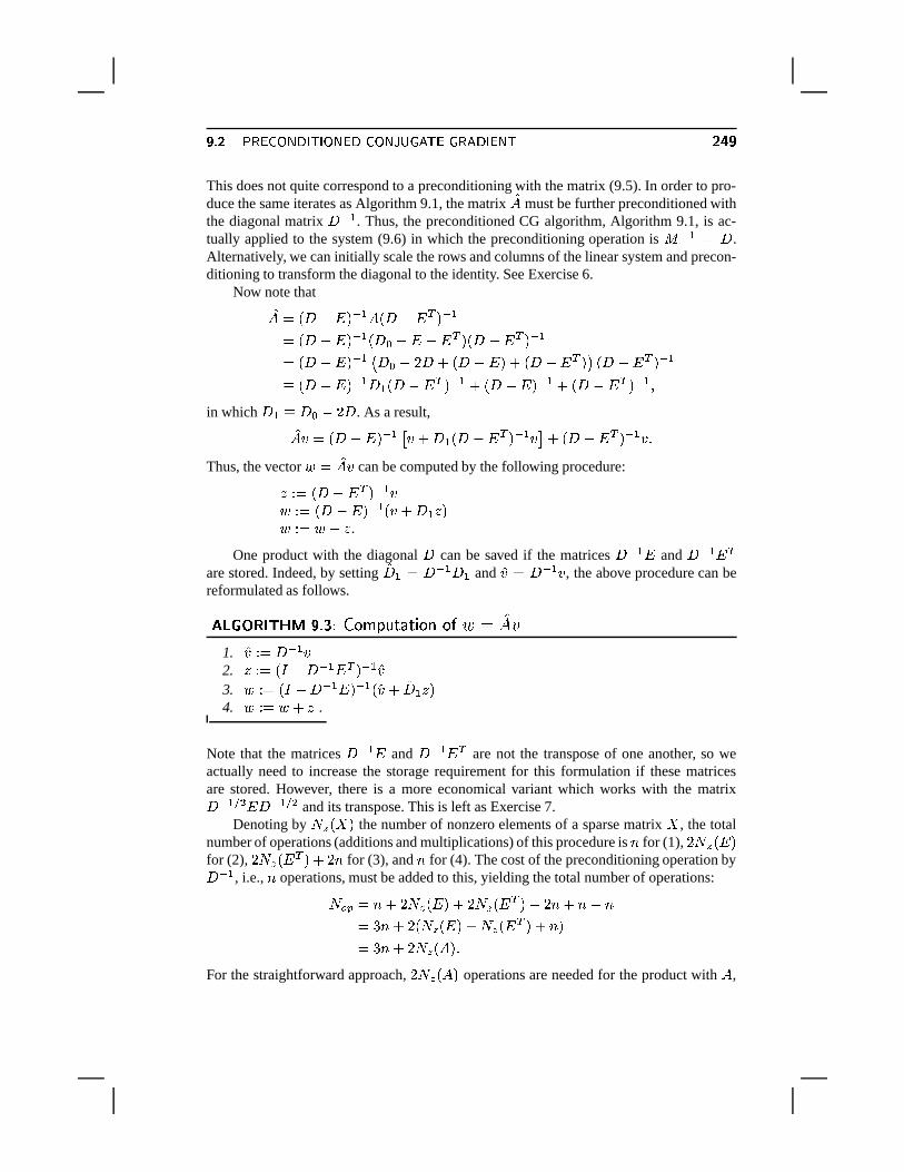
� � � �� \��^� &�� \�� \��1� � � �p&�� & ¶��r·This does not quite correspond to a preconditioning with the matrix (9.5). In order to pro-duce the same iterates as Algorithm 9.1, the matrix

�� must be further preconditioned withthe diagonal matrix � @�B . Thus, the preconditioned CG algorithm, Algorithm 9.1, is ac-tually applied to the system (9.6) in which the preconditioning operation is � @�B � � .Alternatively, we can initially scale the rows and columns of the linear system and precon-ditioning to transform the diagonal to the identity. See Exercise 6.

Now note that��!� <�� ¨ ��= @�B*� <�� ¨ � b = @�B� <�� ¨ ��= @�B?<� � ¨ � ¨ � b = <�� ¨ � b =A@�B� <�� ¨ ��= @�B #�� Q¨ 0 � M <� ¨ � = M <� ¨ � b =�%�<� ¨ � b = @�B� <�� ¨ ��= @�B � B <��¨ � b = @�B M <�� ¨ � =A@�B M <� ¨ � b = @�B��

in which � B � � �7¨ 0 � . As a result,�� <�� ¨ ��= @�B � � M � B <� ¨ � b = @�B �� M <�� ¨ � b = @�B � ¬

Thus, the vector � � �� can be computed by the following procedure:

2 � � <� ¨ � b = @�B �� <� ¨ � = @�B < � M � B 2 =� � � � M 2 .

One product with the diagonal � can be saved if the matrices � @�B � and � @�B � bare stored. Indeed, by setting

�� B � � @�B � B and

�� @�B � , the above procedure can bereformulated as follows.

�� n� �D�w�� ·��

1.�� @�B �

2. 2 � � < & ¨ � @�B � b = @�B ��3. � � � < & ¨ � @�B ��= @�B < �� M �

� B 2 =4. � � � � M 2 .

Note that the matrices � @�B � and � @�B � b are not the transpose of one another, so weactually need to increase the storage requirement for this formulation if these matricesare stored. However, there is a more economical variant which works with the matrix� @�B�� « � � @�B�� « and its transpose. This is left as Exercise 7.

Denoting by �� <��"= the number of nonzero elements of a sparse matrix � , the totalnumber of operations (additions and multiplications) of this procedure is ® for (1),

0 � ��< � =for (2),

0 �� <�� b = M 0 ® for (3), and ® for (4). The cost of the preconditioning operation by� @�B , i.e., ® operations, must be added to this, yielding the total number of operations:

� � � ��® M 0 ��< � = M 0 ��?<�� b = M 0 ® M ® M ®��E® M 0 <�� <��= M � � < � b = M ®�=��E® M 0 � � <N�>=K¬

For the straightforward approach,0 � � <N�,= operations are needed for the product with � ,

¶�� ~�� &�� \�� &�� \�� ³� &��p&^� \��0 ��?<��= for the forward solve, and ® M 0 � � <�� b = for the backward solve giving a total of0 � ��<N�>= M 0 � ��<�� = M ® M 0 � ��<�� b =�� 3 � ��<N�>=(¨°®(¬Thus, Eisenstat’s scheme is always more economical, when � � is large enough, althoughthe relative gains depend on the total number of nonzero elements in � . One disadvantageof this scheme is that it is limited to a special form of the preconditioner.

�� ·��#�For a 5-point finite difference matrix, � � <N�>= is roughly

� ® , so that withthe standard implementation / � ® operations are performed, while with Eisenstat’s imple-mentation only / �9® operations would be performed, a savings of about B� . However, if theother operations of the Conjugate Gradient algorithm are included, for a total of about / - ®operations, the relative savings become smaller. Now the original scheme will require

0�� ®operations, versus

0 �E® operations for Eisenstat’s implementation.

�X�X��Q�f�N�v�H��D�f�n� � �m��X�ª��v��

In the case of GMRES, or other nonsymmetric iterative solvers, the same three options forapplying the preconditioning operation as for the Conjugate Gradient (namely, left, split,and right preconditioning) are available. However, there will be one fundamental difference– the right preconditioning versions will give rise to what is called a flexible variant, i.e.,a variant in which the preconditioner can change at each step. This capability can be veryuseful in some applications.

�! ��! $ 6,0��.; -��+A!0 �+7:9?4?2 ;>2H7:9?014P&)BDA!0,*

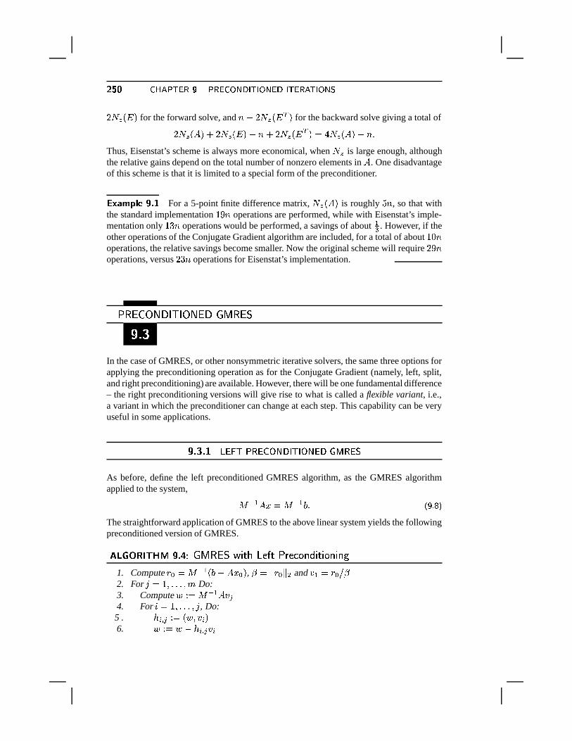
As before, define the left preconditioned GMRES algorithm, as the GMRES algorithmapplied to the system,

� @�BK�Q�� @�B* �¬ £ �L[ ¤ ¦The straightforward application of GMRES to the above linear system yields the followingpreconditioned version of GMRES.

��n��-�w�� ·�� m��X�ª� � � �� 1� � � � � � � � �� 1. Compute

+ �� @�B <V ]¨��Q� � = , �°�z§ + � §K« and � B � + � �%�2. For �m� / �*¬,¬*¬T�S± Do:3. Compute � � �� @�B � � �4. For Sª� / �,¬*¬,¬T� � , Do:5 . � 5 + � � � < � � � 5 =6. � � � � ¨�� 5 + � � 5

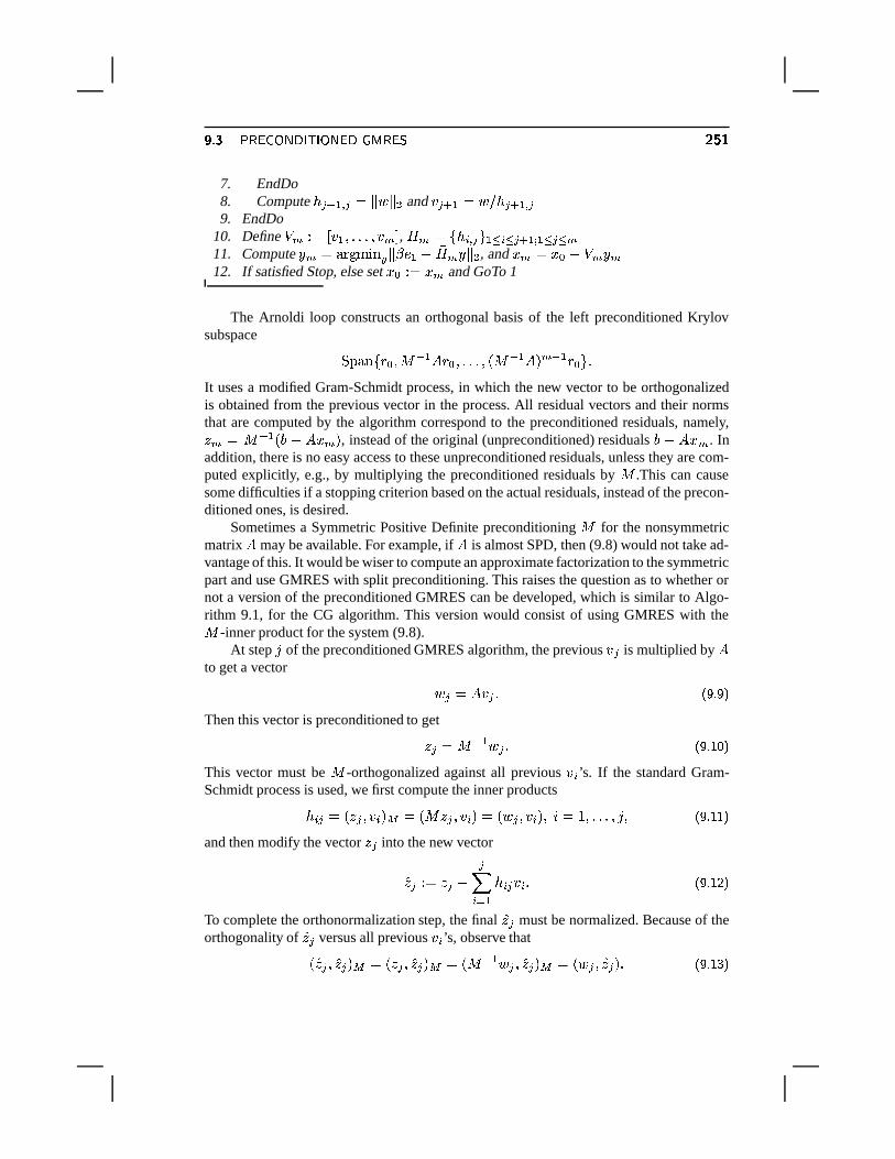
� � � �� \��^� &�� \�� ?� ¶��3�7. EndDo8. Compute � � � B + � ��§ � §K« and � � � B � � � � � � B + �9. EndDo

10. Define� D � �� B �*¬*¬,¬T� � D�� , �� D � � � 5 + � � B� 5 � � � B� B� � � D

11. Compute D � � �� 9 � § � Q B ¨�� D §K« , and � D �� M � D D

12. If satisfied Stop, else set �� D and GoTo 1

The Arnoldi loop constructs an orthogonal basis of the left preconditioned Krylovsubspace �

��9 � + �� @�BG� + �.�*¬*¬,¬T� < � @�BK�>= D @�B + � �L¬

It uses a modified Gram-Schmidt process, in which the new vector to be orthogonalizedis obtained from the previous vector in the process. All residual vectors and their normsthat are computed by the algorithm correspond to the preconditioned residuals, namely,2 D � � @�B <V Z¨¡�Q� D = , instead of the original (unpreconditioned) residuals Z¨ �Q� D . Inaddition, there is no easy access to these unpreconditioned residuals, unless they are com-puted explicitly, e.g., by multiplying the preconditioned residuals by � .This can causesome difficulties if a stopping criterion based on the actual residuals, instead of the precon-ditioned ones, is desired.

Sometimes a Symmetric Positive Definite preconditioning � for the nonsymmetricmatrix � may be available. For example, if � is almost SPD, then (9.8) would not take ad-vantage of this. It would be wiser to compute an approximate factorization to the symmetricpart and use GMRES with split preconditioning. This raises the question as to whether ornot a version of the preconditioned GMRES can be developed, which is similar to Algo-rithm 9.1, for the CG algorithm. This version would consist of using GMRES with the� -inner product for the system (9.8).

At step � of the preconditioned GMRES algorithm, the previous � � is multiplied by �to get a vector

� � �� ¬ £ �9[ ��¦Then this vector is preconditioned to get

2 � �� @�B � � ¬ £ �L[�¥��¦This vector must be � -orthogonalized against all previous � 5 ’s. If the standard Gram-Schmidt process is used, we first compute the inner products

� 5 � � <�2 � � � 5 = � � < � 2 � � � 5 =�� < � � � � 5 = �+S0� / �,¬*¬*¬ � � � £ �L[�¥,¥K¦and then modify the vector 2 � into the new vector

�2 � � � 2 � ¨ � 5�� B � 5 � � 5I¬ £ �L[�¥>�¦To complete the orthonormalization step, the final

�2 � must be normalized. Because of theorthogonality of

�2 � versus all previous � 5 ’s, observe that< �2 � � �2 � = � � <�2 � � �2 � = � � < � @�B � � � �2 � = � � < � � � �2 � =K¬ £ �L[�¥>µ�¦

¶��r¶ � ~�� &�� \�� &�� \�� ³� &��p&^� \��Thus, the desired � -norm could be obtained from (9.13), and then we would set

� � � B + � � � < �2 � � � � = B�� « and � � � B � �2 � � � � � B + � ¬ £ �L[�¥ $�¦One serious difficulty with the above procedure is that the inner product < �2 � � �2 � = � as

computed by (9.13) may be negative in the presence of round-off. There are two remedies.First, this � -norm can be computed explicitly at the expense of an additional matrix-vectormultiplication with � . Second, the set of vectors � � 5 can be saved in order to accumulateinexpensively both the vector

�2 � and the vector � �2 � , via the relation

� �2 � � � � ¨ � 5�� B � 5 � � � 5 ¬A modified Gram-Schmidt version of this second approach can be derived easily. Thedetails of the algorithm are left as Exercise 12.

�! ��! #" A+2 &)=!; -��+A!0 �+7:9?4?2 ;>2H7:9?014P&)BDA!0,*

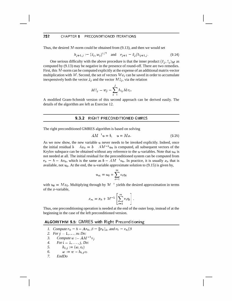
The right preconditioned GMRES algorithm is based on solving

�� @�B ´ �¢ �� ´ ��g�i¬ £ �L[�¥A./¦As we now show, the new variable

´never needs to be invoked explicitly. Indeed, once

the initial residual X¨¡�7� �f� 7¨ � � @�B ´ � is computed, all subsequent vectors of theKrylov subspace can be obtained without any reference to the

´-variables. Note that

´ � isnot needed at all. The initial residual for the preconditioned system can be computed from+ �°� �¨��Q�� , which is the same as �¨�� @�B ´ � . In practice, it is usually �� that isavailable, not

´ � . At the end, the´

-variable approximate solution to (9.15) is given by,

´ D � ´ � MD 5�� B � 5��?5

with´ � � �g� � . Multiplying through by � @�B yields the desired approximation in terms

of the � -variable,

� D �� M � @�B � D 5�� B � 5��?5�� ¬Thus, one preconditioning operation is needed at the end of the outer loop, instead of at thebeginning in the case of the left preconditioned version.

��n��-�w�� ·�� m��X�ª� � � �� 1. Compute

+ � �¢ R¨��Q� � , ��§ + � § « , and � B � + � � �2. For �m� / �*¬,¬*¬T�S± Do:3. Compute � � �� @�B � �4. For Sª� / �,¬*¬,¬T� � , Do:5. � 5 + � � � < � � � 5 =6. � � � � ¨�� 5 + � � 57. EndDo

� � � �� \��^� &�� \�� ?� ¶��;�8. Compute � � � B + � ��§ � §K« and � � � B � � � � � � B + �9. Define

� D � � � � B �,¬*¬*¬ � � D�� , �� D �� 5 + � � B� 5 � � � B� B � � � D10. EndDo

11. Compute D � � �� 9 � § � Q B ¨�� D §K« , and � D �� M � @�B � D D .

12. If satisfied Stop, else set �� D and GoTo 1.

This time, the Arnoldi loop builds an orthogonal basis of the right preconditionedKrylov subspace �

��9 � + ��S�� @�B + �.�*¬*¬,¬T� <V� � @�B = D @�B + � �L¬

Note that the residual norm is now relative to the initial system, i.e., 7¨³�7� D , since thealgorithm obtains the residual 2¨��7� D �z Z¨ �� @�B ´ D , implicitly. This is an essentialdifference with the left preconditioned GMRES algorithm.

�! �! � * �+6 2 ;��!A!0 ��7�9)4?2 ; 2 7:9)2#9 &

In many cases, � is the result of a factorization of the form

� � �� ¬Then, there is the option of using GMRES on the split-preconditioned system

� @�B � � @�B ´ � � @�B �� @�B ´ ¬In this situation, it is clear that we need to operate on the initial residual by

� @�B at the startof the algorithm and by

� @�B on the linear combination� D D in forming the approximate

solution. The residual norm available is that of� @�B <V R¨��Q� D = .

A question arises on the differences between the right, left, and split preconditioningoptions. The fact that different versions of the residuals are available in each case mayaffect the stopping criterion and may cause the algorithm to stop either prematurely or withdelay. This can be particularly damaging in case � is very ill-conditioned. The degreeof symmetry, and therefore performance, can also be affected by the way in which thepreconditioner is applied. For example, a split preconditioner may be much better if �is nearly symmetric. Other than these two situations, there is little difference generallybetween the three options. The next section establishes a theoretical connection betweenleft and right preconditioned GMRES.

�! ��! �� +7:B � ' A+2 *F7�9 7 �@A+2 &)=+; ' 9?4 6,0�� ;�!A!0 ��7�9)4?2 ; 2 7:9)2#9 &

When comparing the left, right, and split preconditioning options, a first observation tomake is that the spectra of the three associated operators � @�B � , � � @�B , and

� @�B � � @�Bare identical. Therefore, in principle one should expect convergence to be similar, although,as is known, eigenvalues do not always govern convergence. In this section, we comparethe optimality properties achieved by left- and right preconditioned GMRES.

¶�� ~�� &�� \�� &�� \�� ³� &��p&^� \��For the left preconditioning option, GMRES minimizes the residual norm

§ � @�B R¨ � @�B �Q�0§K« �among all vectors from the affine subspace

� � M ��D �� M � �� 9 � 2 � �� @�B � 2 � �,¬*¬*¬ � < � @�B �,= D @�B 2 � � £ �L[�¥A1/¦in which 2 � is the preconditioned initial residual 2 � � � @�B + � . Thus, the approximatesolution can be expressed as

� D �� M � @�B�� D @�B < � @�BG�>= 2 �where � D @�B is the polynomial of degree ± ¨ / which minimizes the norm

§ 2 �2¨ � @�B �� < � @�B �>= 2 ��§K«among all polynomials � of degree !¢± ¨ / . It is also possible to express this optimalitycondition with respect to the original residual vector

+ � . Indeed,

2 �2¨ � @�BG�� < � @�BK�>= 2 �W� � @�B � + �7¨�� < � @�BG�,=�� @�B + � � ¬A simple algebraic manipulation shows that for any polynomial � ,

� < � @�B �>=�� @�B + � � @�B � <N� � @�B = + � £ �L[�¥A2/¦from which we obtain the relation

2 � ¨ � @�BG�� < � @�BK�>= 2 � � � @�B � + � ¨�� @�B�� <N�� @�B = + � � ¬ £ �L[�¥ ¤ ¦Consider now the situation with the right preconditioned GMRES. Here, it is necessary

to distinguish between the original � variable and the transformed variable´

related to �by �� @�B ´ . For the

´variable, the right preconditioned GMRES process minimizes

the 2-norm of+ �� ]¨�� @�B ´ where

´belongs to´ � M � �D � ´ � M � � � 9 � + � �S� � @�B + ��*¬,¬*¬ � <N�� @�B�= D @�B + � � £ �L[�¥ �/¦

in which+ � is the residual

+ �� Q¨�� @�B ´ � . This residual is identical to the residualassociated with the original � variable since � @�B ´ � �g� � . Multiplying (9.19) through tothe left by � @�B and exploiting again (9.17), observe that the generic variable � associatedwith a vector of the subspace (9.19) belongs to the affine subspace

� @�B ´ � M � @�B � �D �� M � �� 9 � 2 � �� @�B � 2 � ¬*¬,¬T� < � @�B �,= D @�B 2 � �%¬This is identical to the affine subspace (9.16) invoked in the left preconditioned variant. Inother words, for the right preconditioned GMRES, the approximate � -solution can also beexpressed as

� D �� M � D @�B <N�� @�B = + �%¬However, now � D @�B is a polynomial of degree ± ¨ / which minimizes the norm

§ + �Q¨©�� @�B � <N� � @�B = + � §K« £ �L[ �/¦among all polynomials � of degree !�± ¨ / . What is surprising is that the two quantitieswhich are minimized, namely, (9.18) and (9.20), differ only by a multiplication by � @�B .Specifically, the left preconditioned GMRES minimizes � @�B + , whereas the right precon-ditioned variant minimizes

+, where

+is taken over the same subspace in both cases.

� � � � ��^� �� &�� ¶�� R� �n� �� -�� ·��#�

The approximate solution obtained by left or right preconditionedGMRES is of the form

� D �� M � D @�B < � @�BK�>= 2 �X�� M � @�B � D @�B <V� � @�B�= + �where 2 �� @�B + � and � D @�B is a polynomial of degree ±�¨ / . The polynomial � D @�Bminimizes the residual norm §* 2¨¡�Q� D § « in the right preconditioning case, and the pre-conditioned residual norm § � @�B <V R¨ �Q� D =,§ « in the left preconditioning case.

In most practical situations, the difference in the convergence behavior of the twoapproaches is not significant. The only exception is when � is ill-conditioned which couldlead to substantial differences.

� �c� ��w�i��R� ��H� ��m��u��

In the discussion of preconditioning techniques so far, it is implicitly assumed that the pre-conditioning matrix � is fixed, i.e., it does not change from step to step. However, in somecases, no matrix � is available. Instead, the operation � @�B � is the result of some unspeci-fied computation, possibly another iterative process. In such cases, it may well happen that� @�B is not a constant operator. The previous preconditioned iterative procedures will notconverge if � is not constant. There are a number of variants of iterative procedures devel-oped in the literature that can accommodate variations in the preconditioner, i.e., that allowthe preconditioner to vary from step to step. Such iterative procedures are called “flexible”iterations. One of these iterations, a flexible variant of the GMRES algorithm, is describednext.

�! �� %$ �F6,0 2�� 6,0D&)BDA!0,*

We begin by examining the right preconditioned GMRES algorithm. In line 11 of Algo-rithm 9.5 the approximate solution � D is expressed as a linear combination of the precon-ditioned vectors 2 5X� � @�B � 5�� SW� / �,¬*¬*¬ �I± . These vectors are also computed in line 3,prior to their multiplication by � to obtain the vector � . They are all obtained by applyingthe same preconditioning matrix � @�B to the � 5 ’s. As a result it is not necessary to savethem. Instead, we only need to apply � @�B to the linear combination of the � 5 ’s, i.e., to� D D in line 11. Suppose now that the preconditioner could change at every step, i.e., that2 � is given by

2 � �� @�B� � � ¬Then it would be natural to compute the approximate solution as

� D �� M� D D

¶�� ~�� &�� \�� &�� \�� ³� &��p&^� \��in which

D � � 2 B �,¬*¬,¬ � 2 D�� , and D is computed as before, as the solution to the least-

squares problem in line 11. These are the only changes that lead from the right precondi-tioned algorithm to the flexible variant, described below.

��n��-�w�� ·�� m��7�0� � � �m��X�ª� �1. Compute

+ ��¢ R¨��Q� � , ��§ + �%§K« , and � B � + � � �2. For �m� / �*¬,¬*¬T�S± Do:3. Compute 2 � � � � @�B� � �4. Compute � � �� 2 �5. For Sª� / �,¬*¬,¬T� � , Do:6. � 5 + � � � < � � � 5 =7. � � � � ¨�� 5 + � � 58. EndDo9. Compute � � � B + � �z§ � §K« and � � � B � � �� B + �

10. Define D � � � 2 B �*¬*¬,¬ � 2 D�� , �� D � � � 5 + � � B� 5 � � � B� B � � � D11. EndDo

12. Compute D � � �� 9 � § � Q B ¨ �� D § « , and � D �� M� D D .

13. If satisfied Stop, else set ��#� D and GoTo 1.

As can be seen, the main difference with the right preconditioned version, Algorithm9.5, is that the preconditioned vectors 2 � �� @�B� � � must be saved and the solution updatedusing these vectors. It is clear that when � � � � for � � / �,¬*¬,¬ �I± , then this methodis equivalent mathematically to Algorithm 9.5. It is important to observe that 2 � can bedefined in line 3 without reference to any preconditioner. That is, any given new vector2 � can be chosen. This added flexibility may cause the algorithm some problems. Indeed,2 � may be so poorly selected that a breakdown could occur, as in the worst-case scenariowhen 2 � is zero.

One difference between FGMRES and the usual GMRES algorithm is that the actionof � � @�B� on a vector � of the Krylov subspace is no longer in the span of

� D � B . Instead,it is easy to show that

� D � � D � B �� D £ �L[ 9¥G¦in replacement of the simpler relation <N� � @�B = � D � � D � B �� D which holds for thestandard preconditioned GMRES; see (6.5). As before,

� D denotes the ±�¯�± matrixobtained from �� D by deleting its last row and

�� B is the vector � which is normalizedin line 9 of Algorithm 9.6 to obtain � � � B . Then, the following alternative formulation of(9.21) is valid, even when � D � B + D � -

:

� D � � D � D M �� D � B Q bD ¬ £ �L[ //¦An optimality property similar to the one which defines GMRES can be proved.

Consider the residual vector for an arbitrary vector 2�� M D in the affine space� � M � � �%®� D � . This optimality property is based on the relations

R¨�� 2m�! R¨©��<o� � M D =� + �7¨©� D £ �L[ /µ/¦

� � � � ��^� �� &�� ¶�� B ¨ � D � B �� D � � D � B � � Q B ¨ �� D � ¬ £ �L[ �$4¦

If � D < = denotes the function

� D < =��§, �¨�� M D � § « �observe that by (9.24) and the fact that

� D � B is unitary,

� D < =��§ � Q B ¨ �� D § « ¬ £ �L[ .�¦Since the algorithm minimizes this norm over all vectors

´in �

Dto yield

D , it is clearthat the approximate solution � D �� M D D has the smallest residual norm in �� M��9�� D � . Thus, the following result is proved.

�R� �n� �� -�� ·��t¶The approximate solution � D obtained at step ± of FGMRES

minimizes the residual norm §, ^¨��Q� D §*« over � � M��9 � D � .

Next, consider the possibility of breakdown in FGMRES. A breakdown occurs whenthe vector � � � B cannot be computed in line 9 of Algorithm 9.6 because � � � B + � � -

. Forthe standard GMRES algorithm, this is not a problem because when this happens then theapproximate solution � � is exact. The situation for FGMRES is slightly different.

�R� �n� �� -�� ·�� Assume that �!��§ + � § «�� -

and that �v¨ / steps of FGMREShave been successfully performed, i.e., that ��5 � B + 5 �� -

for SZ² � . In addition, assume thatthe matrix

� � is nonsingular. Then � � is exact, if and only if � � � B + � � -.

�� If � � � B + � � -

, then � � � � � � � , and as a result

� � < =^��§ � � B ¨�� §K«7��§ � � B ¨ � � � � � §K«7��§ � Q B ¨ � � � §K«4¬If� � is nonsingular, then the above function is minimized for

� � � @�B� < � Q B = and thecorresponding minimum norm reached is zero, i.e., � � is exact.

Conversely, if � � is exact, then from (9.22) and (9.23),- �! ^¨��Q� � � � � � � Q B ¨ � � � � M �� B Q b� � ¬ £ �L[ 1�¦We must show, by contraction, that

�� B � -. Assume that

�� B �� -. Since

�� B , � B ,� « , ¬*¬*¬ , � D , form an orthogonal system, then it follows from (9.26) that � Q B ¨ � � � � -and Q b� � � -

. The last component of � is equal to zero. A simple back-substitution for

the system� � � � � Q B , starting from the last equation, will show that all components of � are zero. Because

� D is nonsingular, this would imply that �� -and contradict the

assumption.

The only difference between this result and that of Proposition 6.10 for the GMRESalgorithm is that the additional assumption must be made that

� � is nonsingular since it isno longer implied by the nonsingularity of � . However,

� D is guaranteed to be nonsingu-lar when all the 2 � ’s are linearly independent and � is nonsingular. This is a consequenceof a modification of the first part of Proposition 6.9. That same proof shows that the rank of� D is equal to the rank of the matrix � D therein. If � D is nonsingular and � D � B + D � -

,then

� D is also nonsingular.

¶�� ~�� &�� \�� &�� \�� ³� &��p&^� \��A consequence of the above proposition is that if � 2 � � � � , at a certain step, i.e., if

the preconditioning is “exact,” then the approximation � � will be exact provided that� �

is nonsingular. This is because � �z� 2 � would depend linearly on the previous � 5 ’s (it isequal to � � ), and as a result the orthogonalization process would yield

�� B � -.

A difficulty with the theory of the new algorithm is that general convergence results,such as those seen in earlier chapters, cannot be proved. That is because the subspace ofapproximants is no longer a standard Krylov subspace. However, the optimality propertyof Proposition 9.2 can be exploited in some specific situations. For example, if within eachouter iteration at least one of the vectors 2 � is chosen to be a steepest descent directionvector, e.g., for the function � <o� =R�z§* (¨��Q�0§ «« , then FGMRES is guaranteed to convergeindependently of ± .

The additional cost of the flexible variant over the standard algorithm is only in theextra memory required to save the set of vectors

�2 � � � � B +�� + D . Yet, the added advantage of

flexibility may be worth this extra cost. A few applications can benefit from this flexibility,especially in developing robust iterative methods or preconditioners on parallel computers.Thus, any iterative technique can be used as a preconditioner: block-SOR, SSOR, ADI,Multi-grid, etc. More interestingly, iterative procedures such as GMRES, CGNR, or CGScan also be used as preconditioners. Also, it may be useful to mix two or more precondi-tioners to solve a given problem. For example, two types of preconditioners can be appliedalternatively at each FGMRES step to mix the effects of “local” and “global” couplings inthe PDE context.

�! �� " 4�E &)B A!0,*

Recall that the DQGMRES algorithm presented in Chapter 6 uses an incomplete orthogo-nalization process instead of the full Arnoldi orthogonalization. At each step, the currentvector is orthogonalized only against the � previous ones. The vectors thus generated are“locally” orthogonal to each other, in that < � 5 � � � =�� O 5 � for � SL¨ ��%² � . The matrix �� D be-comes banded and upper Hessenberg. Therefore, the approximate solution can be updatedat step � from the approximate solution at step � ¨ / via the recurrence

� � � /+ � � � �� ¨ � @�B5�� @ � � B + 5 � � 5��@� � � �� @�B M� � � � £ �L[ 2/¦in which the scalars

� � and+ 5 � are obtained recursively from the Hessenberg matrix �� .

An advantage of DQGMRES is that it is also flexible. The principle is the same asin FGMRES. In both cases the vectors 2 � � � @�B� � � must be computed. In the case ofFGMRES, these vectors must be saved and this requires extra storage. For DQGMRES, itcan be observed that the preconditioned vectors 2 � only affect the update of the vector � �in the preconditioned version of the update formula (9.27), yielding

� � � /+ � � �� @�B� � � ¨ � @�B5�� @ � � B + 5 � � 5 ��f¬

As a result, � @�B� � � can be discarded immediately after it is used to update � � . The same

� � � �� \��^� &�� \�� \�v&^~��}\�� p&^� \�� ¶��r·memory locations can store this vector and the vector � � . This contrasts with FGMRESwhich requires additional vectors of storage.

��7��2��C�v�t��D�f�n� � � � � ��z�u�n�z�W��X��(�f�Q�^��-��u��

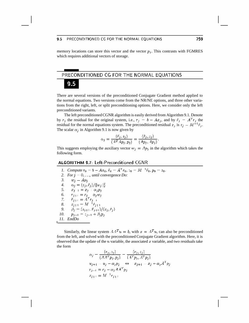
There are several versions of the preconditioned Conjugate Gradient method applied tothe normal equations. Two versions come from the NR/NE options, and three other varia-tions from the right, left, or split preconditioning options. Here, we consider only the leftpreconditioned variants.

The left preconditioned CGNR algorithm is easily derived from Algorithm 9.1. Denoteby

+ � the residual for the original system, i.e.,+ � � W¨��Q� � , and by �

+ � � � b + � theresidual for the normal equations system. The preconditioned residual 2 � is 2 � � � @�B �+ � .The scalar � in Algorithm 9.1 is now given by

� � <��+ � � 2 � =<N� b �� = � <��+ � � 2 � =<V�� S�� = ¬This suggests employing the auxiliary vector � � �z�� in the algorithm which takes thefollowing form.

�� n� �D�w�� ·�� 1� � � � � � � � �� 1. Compute

+ �W�� R¨©�7�� , �+ �� b + � , 2 �X�� @�B �+ � , ��X�#2 � .

2. For �n� - �*¬*¬,¬ , until convergence Do:3. � � �¢�� 4. � � < 2 � ��+ � =��p§ � � § ««5. � � � B �� M � � �6.

+ � � B � + � ¨ � � �7. �

+ � � B �¢� b + � � B8. 2 � � B �� @�B �+ � � B9. � � � <�2 � � B ��+ � � B = ��<�2 � ��+ � =

10. � � � B �#2 � � B M � � � �11. EndDo

Similarly, the linear system �7� bi´ � , with � � � bi´ , can also be preconditionedfrom the left, and solved with the preconditioned Conjugate Gradient algorithm. Here, it isobserved that the update of the

´variable, the associated � variable, and two residuals take

the form

� � < + � � 2 � =<N�X� b � � � � � = � < + � � 2 � =<V� b � � �B� b � � =´ � � B � ´ � M � � � � � � � B �� M � � b � �+ � � B � + � ¨ � �7� b � �2 � � B �� @�B + � � B

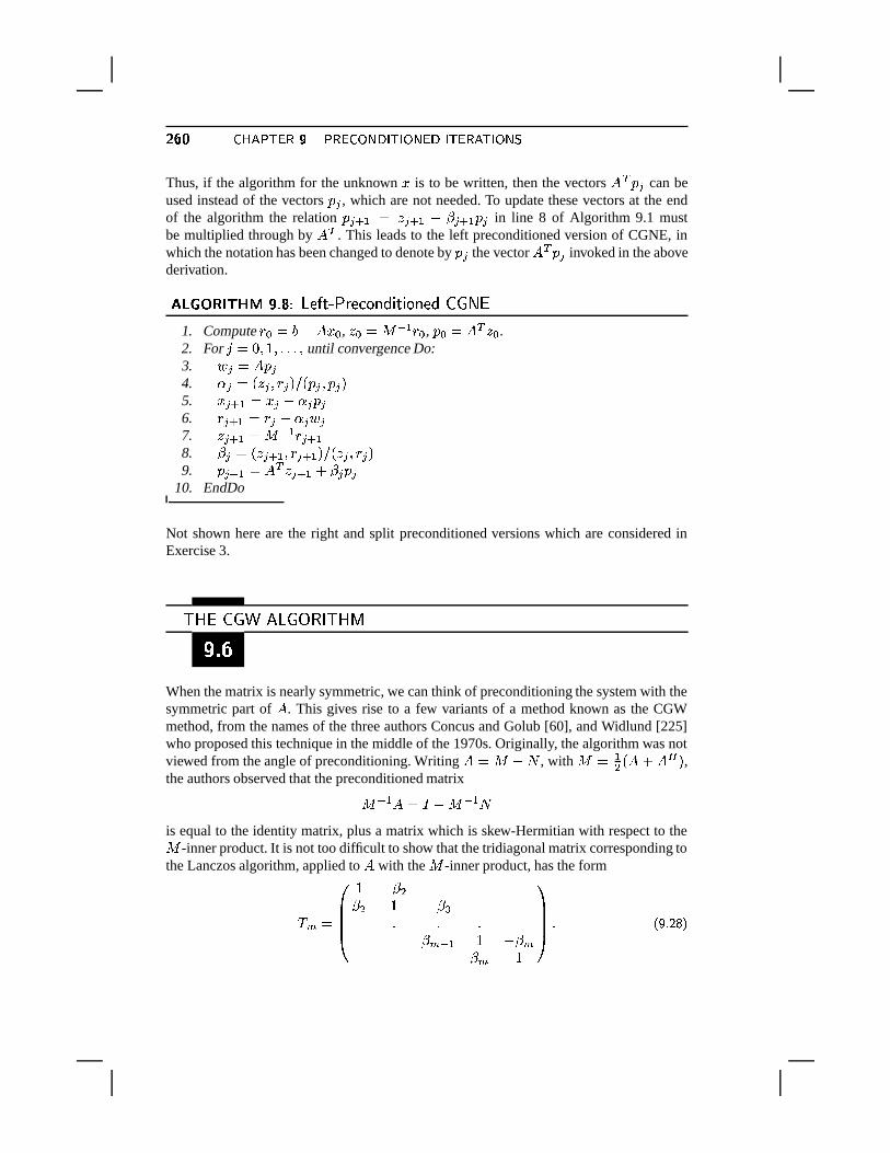
¶�� ~�� &�� \�� &�� \�� ³� &��p&^� \��Thus, if the algorithm for the unknown � is to be written, then the vectors � b � � can beused instead of the vectors � � , which are not needed. To update these vectors at the endof the algorithm the relation � � � B � 2 � � B M � � � B � � in line 8 of Algorithm 9.1 mustbe multiplied through by � b . This leads to the left preconditioned version of CGNE, inwhich the notation has been changed to denote by � � the vector � b � � invoked in the abovederivation.

��n��-�w�� ·�� 1� � � � � � � � � � �� m�1. Compute

+ � �¢ R¨��Q� � , 2 � �� @�B + � , � � �� b 2 � .2. For �m� - � / �*¬*¬,¬T� until convergence Do:3. � � �¢�� 4. � � <�2 � � + � = ��<�� =5. � � � B �� M � � �6.

+ � � B � + � ¨ � � �7. 2 � � B � � @�B + � � B8. � � � < 2 � � B � + � � B = ��<�2 � � + � =9. � � � B �� b 2 � � B M � � � �

10. EndDo

Not shown here are the right and split preconditioned versions which are considered inExercise 3.

�u�n� � �5� �� X�t�u� ��v��

When the matrix is nearly symmetric, we can think of preconditioning the system with thesymmetric part of � . This gives rise to a few variants of a method known as the CGWmethod, from the names of the three authors Concus and Golub [60], and Widlund [225]who proposed this technique in the middle of the 1970s. Originally, the algorithm was notviewed from the angle of preconditioning. Writing �!� � ¨ � , with � � B« <V� M �> = ,the authors observed that the preconditioned matrix

� @�B �¢� & ¨ � @�B �is equal to the identity matrix, plus a matrix which is skew-Hermitian with respect to the� -inner product. It is not too difficult to show that the tridiagonal matrix corresponding tothe Lanczos algorithm, applied to � with the � -inner product, has the form

� D ��/ ¨ � «� « / ¨ � �¬ ¬ ¬

� D @�B / ¨ � D� D /

�� ¬ £ �L[ ¤ ¦

�� ?�� }\�&�?� ¶��

As a result, a three-term recurrence in the Arnoldi process is obtained, which results in asolution algorithm that resembles the standard preconditioned CG algorithm (Algorithm9.1).

A version of the algorithm can be derived easily. From the developments in Section6.7 relating the Lanczos algorithm to the Conjugate Gradient algorithm, it is known that� � � B can be expressed as

� � � B �� M � � � ¬The preconditioned residual vectors must then satisfy the recurrence

2 � � B �#2 � ¨ � � @�B �� and if the 2 � ’s are to be � -orthogonal, then we must have <�2 � ¨ � � @�B �� 2 � = � � -

.As a result,

� � < 2 � � 2 � = �< � @�B �� 2 � =�� < + � � 2 � =<V�� 2 � = ¬Also, the next search direction � � � B is a linear combination of 2 � � B and � � ,

� � � B � 2 � � B M � � � � ¬Thus, a first consequence is that<N�� 2 � = � � < � @�BK�� ¨ � � @�B � � @�B = � � < � @�BK�� = � � <N�� =because � @�B �� is orthogonal to all vectors in � � @�B . In addition, writing that � � � B is� -orthogonal to � @�B �� yields

� � �a¨ <�2 � � B �� @�B �� = �< � � �� @�B �� = � ¬Note that � @�B �� ¨ B�� <�2 � � B ¨ 2 � = and therefore we have, just as in the standard PCGalgorithm,

� � � <�2 � � B � 2 � � B = �< 2 � � 2 � =�� <�2 � � B � + � � B =<�2 � � + � = ¬

� ��]� �W�-�]�ª�

1 Let a matrix`

and its preconditioner�

be SPD. Observing that� 2�4q`

is self-adjoint withrespect to the

`inner-product, write an algorithm similar to Algorithm 9.1 for solving the pre-

conditioned linear system� 2�4 `Rd e�� 2�4 h

, using the`

-inner product. The algorithm shouldemploy only one matrix-by-vector product per CG step.

2 In Section 9.2.1, the split-preconditioned Conjugate Gradient algorithm, Algorithm 9.2, was de-rived from the Preconditioned Conjugate Gradient Algorithm 9.1. The opposite can also be done.Derive Algorithm 9.1 starting from Algorithm 9.2, providing a different proof of the equivalenceof the two algorithms.

¶��p¶ � ~�� &�� \�� &�� \�� ³� &��p&^� \��3 Six versions of the CG algorithm applied to the normal equations can be defined. Two versions

come from the NR/NE options, each of which can be preconditioned from left, right, or ontwo sides. The left preconditioned variants have been given in Section 9.5. Describe the fourother versions: Right P-CGNR, Right P-CGNE, Split P-CGNR, Split P-CGNE. Suitable innerproducts may be used to preserve symmetry.

4 When preconditioning the normal equations, whether the NE or NR form, two options are avail-able in addition to the left, right and split preconditioners. These are “centered” versions:` � 254 ` �� e�h�� d e � 254 ` ��for the NE form, and ` � � 254 `^d|e ` � � 254 hfor the NR form. The coefficient matrices in the above systems are all symmetric. Write downthe adapted versions of the CG algorithm for these options.

5 Let a matrix`

and its preconditioner�

be SPD. The standard result about the rate of conver-gence of the CG algorithm is not valid for the Preconditioned Conjugate Gradient algorithm,Algorithm 9.1. Show how to adapt this result by exploiting the

�-inner product. Show how to

derive the same result by using the equivalence between Algorithm 9.1 and Algorithm 9.2.

6 In Eisenstat’s implementation of the PCG algorithm, the operation with the diagonal�

causessome difficulties when describing the algorithm. This can be avoided.�� Assume that the diagonal

�of the preconditioning (9.5) is equal to the identity matrix.

What are the number of operations needed to perform one step of the PCG algorithm withEisenstat’s implementation? Formulate the PCG scheme for this case carefully.� � The rows and columns of the preconditioning matrix

�can be scaled so that the matrix

�

of the transformed preconditioner, written in the form (9.5), is equal to the identity matrix.What scaling should be used (the resulting

�should also be SPD)? !� Assume that the same scaling of question b is also applied to the original matrix

`. Is the

resulting iteration mathematically equivalent to using Algorithm 9.1 to solve the system (9.6)preconditioned with the diagonal

�?

7 In order to save operations, the two matrices� 254��

and� 2�4��

must be stored when comput-ing

�`��by Algorithm 9.3. This exercise considers alternatives.�� Consider the matrix

" � �` �

. Show how to implement an algorithm similar to 9.3 formultiplying a vector

�by

". The requirement is that only

� � 254must be stored.� � The matrix

"in the previous question is not the proper preconditioned version of

`by

the preconditioning (9.5). CG is used on an equivalent system involving

"but a further

preconditioning by a diagonal must be applied. Which one? How does the resulting algorithmcompare in terms of cost and storage with an Algorithm based on 9.3? !� It was mentioned in Section 9.2.2 that

�`needed to be further preconditioned by

� 254. Con-

sider the split-preconditioning option: CG is to be applied to the preconditioned system as-sociated with � e � 4� �` � 4� . Defining

�� e � 2�4� � � 254� show that,

� e#&+ 6 ��

' 2�4 � #&+ 6 ��

' 2 � � #&+ 6 ��' 254 � #&+ 6 ��

' 2 �where

� is a certain matrix to be determined. Then write an analogue of Algorithm 9.3using this formulation. How does the operation count compare with that of Algorithm 9.3?

8 Assume that the number of nonzero elements of a matrix`

is parameterized by� � # � ' e % �

.How small should

%be before it does not pay to use Eisenstat’s implementation for the PCG

algorithm? What if the matrix`

is initially scaled so that�

is the identity matrix?

�� ?�� }\�&�?� ¶��9 Let

��e��be a preconditioner for a matrix

`. Show that the left, right, and split precondi-

tioned matrices all have the same eigenvalues. Does this mean that the corresponding precon-ditioned iterations will converge in (a) exactly the same number of steps? (b) roughly the samenumber of steps for any matrix? (c) roughly the same number of steps, except for ill-conditionedmatrices?

10 Show that the relation (9.17) holds for any polynomial � and any vector�.

11 Write the equivalent of Algorithm 9.1 for the Conjugate Residual method.

12 Assume that a Symmetric Positive Definite matrix�

is used to precondition GMRES for solv-ing a nonsymmetric linear system. The main features of the P-GMRES algorithm exploitingthis were given in Section 9.2.1. Give a formal description of the algorithm. In particular give aModified Gram-Schimdt implementation. [Hint: The vectors

� � �’s must be saved in addition to

the��

’s.] What optimality property does the approximate solution satisfy? What happens if theoriginal matrix

`is also symmetric? What is a potential advantage of the resulting algorithm?

NOTES AND REFERENCES. The preconditioned version of CG described in Algorithm 9.1 is dueto Meijerink and van der Vorst [149]. Eisenstat’s implementation was developed in [80] and is of-ten referred to as Eisenstat’s trick. A number of other similar ideas are described in [153]. Severalflexible variants of nonsymmetric Krylov subspace methods have been developed by several authorssimultaneously; see, e.g., [18], [181], and [211]. There does not seem to exist a similar techniquefor left preconditioned variants of the Krylov subspace methods. This is because the preconditionedoperator

� 2�4�`

now changes at each step. Similarly, no flexible variants have been developed for theBCG-based methods, because the short recurrences of these algorithms rely on the preconditionedoperator being constant.

The CGW algorithm can be useful in some instances, such as when the symmetric part of`

canbe inverted easily, e.g., using fast Poisson solvers. Otherwise, its weakness is that linear systems withthe symmetric part must be solved exactly. Inner-outer variations that do not require exact solutionshave been described by Golub and Overton [109].

� � � � � � �

��

�� $4 $%��$C�� $% �"�¢�

�9?�1*l9?H1KJ7.QJ,848El s/+-)>=B891*l9? ;I? 891*),+�;P8�A_89U F*)Z.QJE? F*),1ZABs*./+tA<)XU ?H1*)B./+ APOKAP;_),5�? Aª8,:-;<),1F/? )S{i)>lf.KA|.�=B89576/?�1*.K;q? 8L1n8,:7./+H;w.41*l A<=K? )*1*=>)/[c&�'*)B84+-)S;q? =>.4U0+-)BAB34U ;PA|./+D)u+D./+-).41*lfA_8L5R)f5R)S;B'K8El�Aw{}84+ �vAB34+os/+Y? AI?H1KJ9U Ov{i),U U�jc8,:-;<),1�l4)BABs/? ;_)�)IyEs/)>=S;<.G;I? 8L1KA>[ �s,+-)>=B8L1*l9? ;I? 891*),+i=>.41u6/)Wl4) �p1*)>lv.KAQ.E1GO AB346KAq? l9? ./+HO .Es4s,+t8Gy�?�5].G;<)XA_8LU F*)*+c{^'/? =,'? A]=B895Q6/?H1*)>l {(? ;S'w.41W8L3G;_),+ª? ;_),+-.K;q? 8L17;<)>=*'41/? @%3*)/j%;oO4s/? =>.4U U O7891*)X8,:c;B'*)|�c+HO4U 8*FAS346KABs*.,=B)7? ;<),+-.G;I? 891KA(A<)>),1w?H1ws,+D)IF/? 8L3KA^=,'*.4sG;<),+tA>[%&�'/? AR=*'*.EsG;_),+ =S8,F*),+tAÂ_8L5R)Q8,:;S'*)75^8/AV;(AB3*=>=>)SA_AP:P34UE;_)>=,'41/? @%3*)BA�3KA<)>lW;P8ms/+-)>=S8L1*l9? ;q? 8L1Q.QJ�)*1*),+-.EU4ASs*./+-A_)�U ?H1*)>./+AVOKAP;<),57[ � 8*;<)m.K;Q;B'*)w893G;_A<)S;Q;S'*.K;2;S'*),+-)m./+-) F/?�+t;S3*.EU U Ov1K8�U ?H5Z? ;_A2;_8u.GF*.�?�U .E64U )89sG;I? 891KAX:D8E+]8L6G;_.�?H1/?�1KJuJ,848El�s/+-)>=B891*l9? ;I? 891*),+tA>[ �,84+R)Iy,.45Qs4U )/j�s/+-)>=B891*l9? ;I? 891*),+tA=B.E126/)(l4),+Y? F*)>lZ:P+t895 �/1K8G{Û )>l�J/)08,: ;B'*)c8E+Y? J4?H1*.4U�s4'GOKAI? =>.4U/s,+t8L64U ),5Â :V+-895©{^'/? =,';S'*)QU ?H1*)>./+�AVOKAP;<),5¡./+Y? A<)SA>[p~ 8G{i)SF*),+Nj9.7=S8L5Q5^8L12:T)B.K;S34+D)^8,:r;B'*)Qs/+-)>=B891*l9? ;I? 891*),+tAl9? A<=,3KA_A<)Bln?�17;S'/? A�=,'*.4sG;<),+ ? A(;B'*.G;0;S'*)SOX./+D)W643/?HU ;ª:P+t895�;B'*)Z84+Y? JE?�1*.EUE=S8E)SxW=G? ),1G;5R.G;B+Y? y9[

�o��Z��:�Z��-��u�K�

Roughly speaking, a preconditioner is any form of implicit or explicit modification of anoriginal linear system which makes it “easier” to solve by a given iterative method. Forexample, scaling all rows of a linear system to make the diagonal elements equal to oneis an explicit form of preconditioning. The resulting system can be solved by a Krylovsubspace method and may require fewer steps to converge than with the original system(although this is not guaranteed). As another example, solving the linear system

� @�BG�Q� � � @�B* where � @�B is some complicated mapping that may involve FFT transforms, integral cal-culations, and subsidiary linear system solutions, may be another form of preconditioning.Here, it is unlikely that the matrix � and � @�B � can be computed explicitly. Instead,

¶��

�� H� �A� � \��}�Hj �%\� j �� "� ��\� �� \�� &^� \�� ¶��the iterative processes operate with � and with � @�B whenever needed. In practice, thepreconditioning operation � @�B should be inexpensive to apply to an arbitrary vector.

One of the simplest ways of defining a preconditioner is to perform an incomplete fac-torization of the original matrix � . This entails a decomposition of the form �!� � � ¨ �where

�and

�have the same nonzero structure as the lower and upper parts of � respec-

tively, and � is the residual or error of the factorization. This incomplete factorizationknown as ILU(0) is rather easy and inexpensive to compute. On the other hand, it of-ten leads to a crude approximation which may result in the Krylov subspace acceleratorrequiring many iterations to converge. To remedy this, several alternative incomplete fac-torizations have been developed by allowing more fill-in in

�and

�. In general, the more

accurate ILU factorizations require fewer iterations to converge, but the preprocessing costto compute the factors is higher. However, if only because of the improved robustness,these trade-offs generally favor the more accurate factorizations. This is especially truewhen several systems with the same matrix must be solved because the preprocessing costcan be amortized.

This chapter considers the most common preconditioners used for solving large sparsematrices and compares their performance. It begins with the simplest preconditioners (SORand SSOR) and then discusses the more accurate variants such as ILUT.

�p�:�2��w��(��0�n�N� �0�0�� X�X��2�f�N�v�H��-��m�Z�R��v� �

As was seen in Chapter 4, a fixed-point iteration for solving a linear system

�Q��¢ takes the general form

� � � B �� @�B �f� � M � @�BK £ ¥ �9[�¥K¦where � and � realize the splitting of � into

�¢�� ¨ ��¬ £ ¥ �9[ �¦The above iteration is of the form

�� B ��W�� M � £ ¥ �9[ µ�¦where

� �� @�B and

� �� @�B � �� @�B < � ¨©�,=� & ¨ � @�B � ¬ £ ¥ �9[ $4¦

Thus, for Jacobi and Gauss Seidel it has been shown that

�� ( <N�,=^� & ¨ � @�BG� £ ¥ �9[ .�¦�� <N�,=^� & ¨ <�� ¨ � =A@�B*�� £ ¥ �9[ 1�¦

where �¢� � ¨ �g¨ � is the splitting defined in Chapter 4.

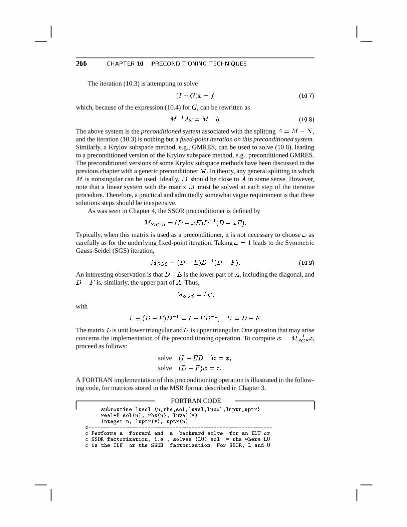
¶�� ~�� &�� \�� &^� \��0� � �°&� � ~ �0� ��?�The iteration (10.3) is attempting to solve< & ¨ ��=<�� £ ¥ �9[ 2/¦

which, because of the expression (10.4) for � , can be rewritten as

� @�B �Q�� @�B �¬ £ ¥ �9[ ¤ ¦The above system is the preconditioned system associated with the splitting �¢� � ¨ � ,and the iteration (10.3) is nothing but a fixed-point iteration on this preconditioned system.Similarly, a Krylov subspace method, e.g., GMRES, can be used to solve (10.8), leadingto a preconditioned version of the Krylov subspace method, e.g., preconditioned GMRES.The preconditioned versions of some Krylov subspace methods have been discussed in theprevious chapter with a generic preconditioner � . In theory, any general splitting in which� is nonsingular can be used. Ideally, � should be close to � in some sense. However,note that a linear system with the matrix � must be solved at each step of the iterativeprocedure. Therefore, a practical and admittedly somewhat vague requirement is that thesesolutions steps should be inexpensive.

As was seen in Chapter 4, the SSOR preconditioner is defined by

� � � � � � <�� ¨ � ��=�� @�B <� ¨ � ��=G¬Typically, when this matrix is used as a preconditioner, it is not necessary to choose � ascarefully as for the underlying fixed-point iteration. Taking � � / leads to the SymmetricGauss-Seidel (SGS) iteration,

� � �u� <�� ¨ � = � @�B <� ¨��=G¬ £ ¥ �9[ �/¦An interesting observation is that �¢¨ � is the lower part of � , including the diagonal, and� ¨ � is, similarly, the upper part of � . Thus,

� � � � �� with

� � <��¨ � = � @�BQ� & ¨ � � @�B�� ¨ �Z¬The matrix

�is unit lower triangular and

�is upper triangular. One question that may arise

concerns the implementation of the preconditioning operation. To compute � � � @�B� � � ,proceed as follows:

solve < & ¨ � � @�B�= 2m�� solve <� ¨ ��= � � 2r¬

A FORTRAN implementation of this preconditioning operation is illustrated in the follow-ing code, for matrices stored in the MSR format described in Chapter 3.

FORTRAN CODE�� !��"��#��$��%��$��'&��!��(*)+��'&,�-��.�/&,�0�� !��1(& ��2��*�3�4�5��$��1(�&,�6��$��%��/&

#�7�7�7�7�7�7�7�7�7�7�7�7�7�7�7�7�7�7�7�7�7�7�7�7�7�7�7�7�7�7�7�7�7�7�7�7�7�7�7�7�7�7�7�7�7�7�7�7�7�7�7�7�7�7�7�7�7�7�7#98��:*��;<�=!>:*��?!*��@�!��@A!B�!�#�C�?�!��@D��* ��E:*��!��GF�H�IG*�#3J�J�K�L+:!�#��*�� M!�� 4�N �O��O��P�� Q��H*I<&R��TSR��U?��VH�I#= ��V�*��+F�H*IW*�3�*��+J�J�K�LX:!�#��*�� M!�� YO-Z��J�J�K�L��[HG!��@VI

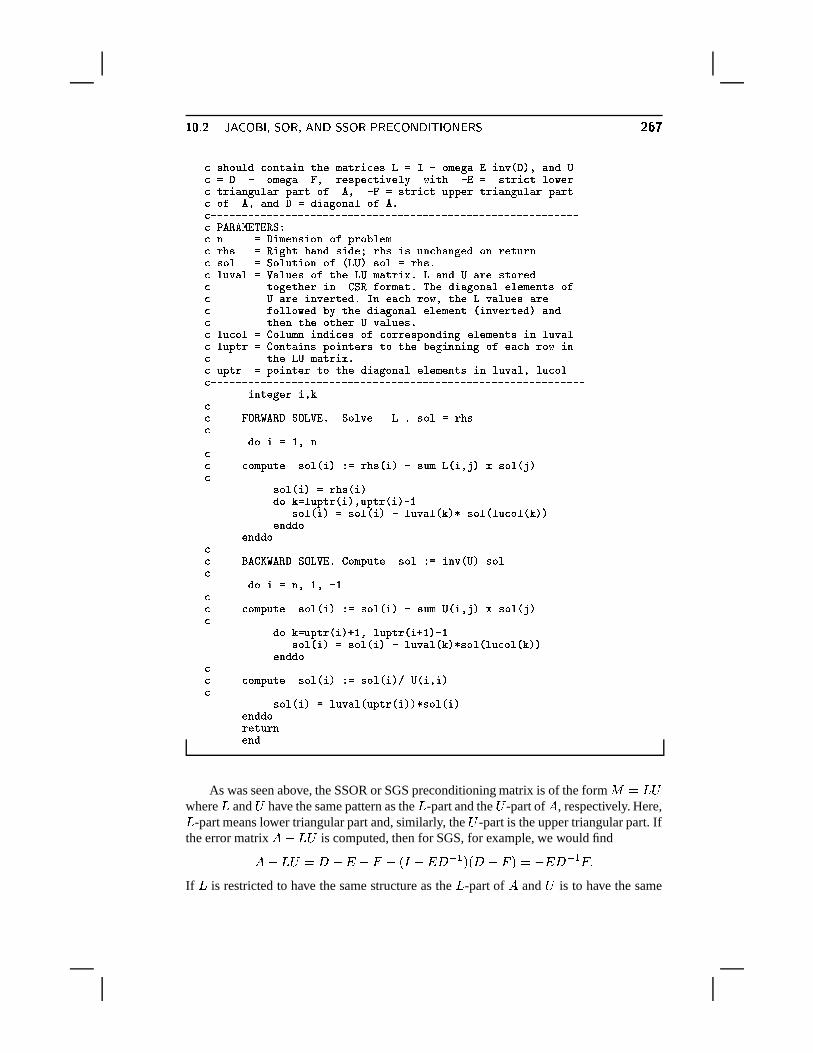
�� H� �A� � \��}�Hj �%\� j �� "� ��\� �� \�� &^� \�� ¶��#=��*@G#*��!� ��U;/!�� #*��VH+S�FV7= ;'��2�! � �� %��/&,�5!��@RI#RS��A7 ;'��2! Z�� $�#�� ?� �� 7 � SX�� #��?��#V�� !��2��!*�=$�!*��*:��%� 7*Z+S=�� #��=��$�$�*�=�� !��2��!��$!*��#3*:��-!��@��SV@� �!*2��!��+*:��O#�7�7�7�7�7�7�7�7�7�7�7�7�7�7�7�7�7�7�7�7�7�7�7�7�7�7�7�7�7�7�7�7�7�7�7�7�7�7�7�7�7�7�7�7�7�7�7�7�7�7�7�7�7�7�7�7�7�7�7#98��*L�� L�J��#9� S�� ;'�*�� *:V$��*��;#V�� S9L� �2��=�!��@G�� @��6��= ��9��#��!��2��@G��+��*��#=�� S3J�� *: �.H�I<&R��3S3��O#3�� !��3S��!��=*:=��VH�IV;/!�� 4O[H�!��@RI�!*��*��@# �*2��*�� J�L+:��;/!*�4O � ��3@� �!�2��!��=��;'�*��=*:# ID!*�� @4O0F��!�#��+��?4�6��VH= !��=!*��# :��?��@+��3�*��3@� �!�2��!��=��;'�*�� 1 �� *��@'&R!��@# ��*��+*��*�RI+ !��O#3��#��3S��;� ��@� �#��=*:G#��$��@� ��2D��;'�*��+ �� !��#3��$��+S��!� ��R$�� R�9��R��2� �� 2G*:+��!�#��+��?D ��# ��RH�IV;/!*�� 4O#9��$�� S9$�� +�R��3@� �!*2��!��=��*��;'�*��+ ��G�� !��5��#��#�7�7�7�7�7�7�7�7�7�7�7�7�7�7�7�7�7�7�7�7�7�7�7�7�7�7�7�7�7�7�7�7�7�7�7�7�7�7�7�7�7�7�7�7�7�7�7�7�7�7�7�7�7�7�7�7�7�7�7�7

��2��D �� C## ZK�L��L��GJ�K�H�� O J��* �� H O5��3SR��#

@3 RS��<� �## #� ;�$��A��1 &��S3�� &V7+��;GH4�1 ��& �G��!��&#

��1 �&9S3�� 1 &@UC�S��$��%�1 &,��$��1 �&�7"��1 &VS=��1 �&R73�� !��.C<&�(G�*��#��.C/&�&

�*��@�@�*��@�@�

## #��$��L��DJ�K�H�� O%�� ;�$��A��&��S� �� I<&R��#

@3 RSV�4�'�<�57"�## #� ;�$��A��1 &��S�� &V7+��;�IY�1 ��& �G��!��&#

@UC�S��$�� &�()�<�P��$��1 �()��&�7"��1 &VS=��1 �&R73�� !��.C<&�(��"��#��.C<&�&

�*��@�@## #� ;�$��A��1 &��S�� &�*VIY�1 �1 &#

��1 �&9S+�� !��$��1 &�&*(��1 &�*��@�@��*��@

As was seen above, the SSOR or SGS preconditioning matrix is of the form � � ��where

�and

�have the same pattern as the

�-part and the

�-part of � , respectively. Here,�

-part means lower triangular part and, similarly, the�

-part is the upper triangular part. Ifthe error matrix ��¨ � � is computed, then for SGS, for example, we would find

��¨ �� ¨ �g¨ �!¨ < & ¨ � � @�B = <� ¨ ��=��z¨ � � @�B �Z¬If�

is restricted to have the same structure as the�

-part of � and�

is to have the same

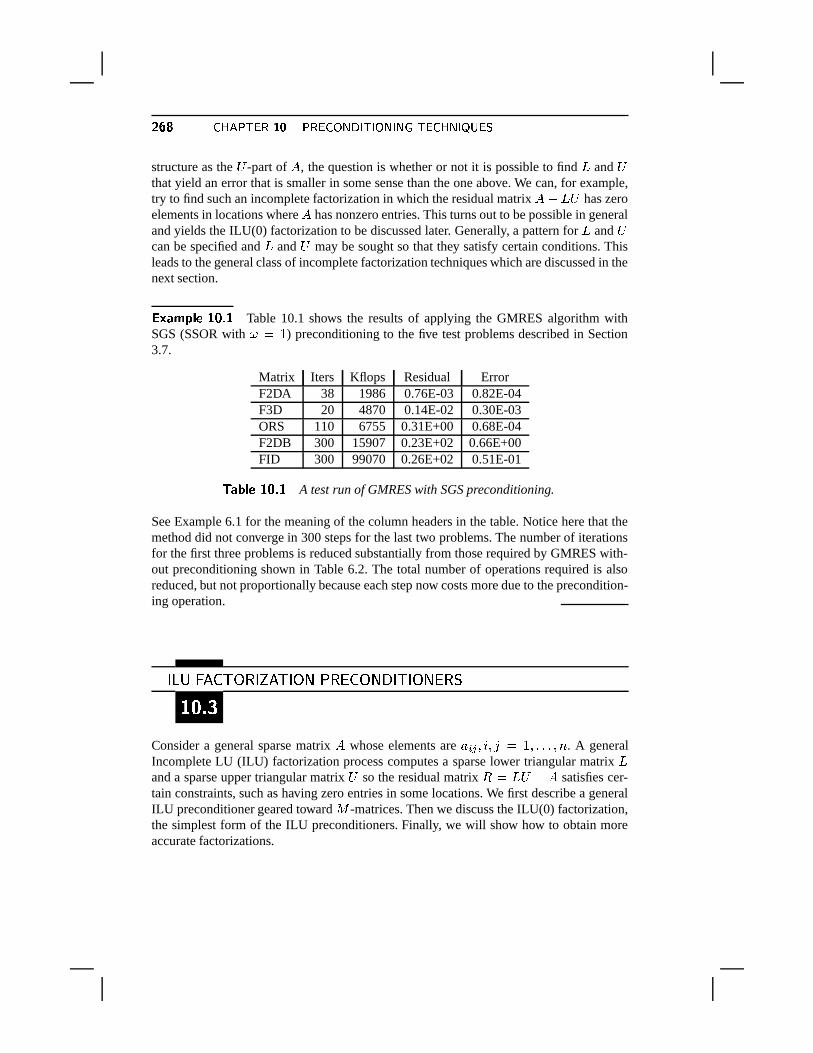
¶�� ~�� &�� \�� &^� \��0� � �°&� � ~ �0� ��?�structure as the

�-part of � , the question is whether or not it is possible to find

�and

�

that yield an error that is smaller in some sense than the one above. We can, for example,try to find such an incomplete factorization in which the residual matrix ��¨ �� has zeroelements in locations where � has nonzero entries. This turns out to be possible in generaland yields the ILU(0) factorization to be discussed later. Generally, a pattern for

�and

�

can be specified and�

and�

may be sought so that they satisfy certain conditions. Thisleads to the general class of incomplete factorization techniques which are discussed in thenext section.

�� #�Table 10.1 shows the results of applying the GMRES algorithm with

SGS (SSOR with � � / ) preconditioning to the five test problems described in Section3.7.

Matrix Iters Kflops Residual ErrorF2DA 38 1986 0.76E-03 0.82E-04F3D 20 4870 0.14E-02 0.30E-03ORS 110 6755 0.31E+00 0.68E-04F2DB 300 15907 0.23E+02 0.66E+00FID 300 99070 0.26E+02 0.51E-01

� �� #�A test run of GMRES with SGS preconditioning.

See Example 6.1 for the meaning of the column headers in the table. Notice here that themethod did not converge in 300 steps for the last two problems. The number of iterationsfor the first three problems is reduced substantially from those required by GMRES with-out preconditioning shown in Table 6.2. The total number of operations required is alsoreduced, but not proportionally because each step now costs more due to the precondition-ing operation.

�N�c� � �:�]� ��]��-�f� ��7��2��C�v�t��D�f�n�]�]��u��

Consider a general sparse matrix � whose elements are � 5 � ��S�� / �*¬,¬*¬T�S® . A generalIncomplete LU (ILU) factorization process computes a sparse lower triangular matrix

�and a sparse upper triangular matrix

�so the residual matrix � � �� ¨ � satisfies cer-

tain constraints, such as having zero entries in some locations. We first describe a generalILU preconditioner geared toward � -matrices. Then we discuss the ILU(0) factorization,the simplest form of the ILU preconditioners. Finally, we will show how to obtain moreaccurate factorizations.

�� ?� � � � &ª\� � ��p&�� \�� \�� &^� \�� ¶��p·$��! �! %$ 2 9 �+7:B ��6,0 ; 0�6 ( � ' � ;)7:A+2��'3; 2 7:9 *

A general algorithm for building Incomplete LU factorizations can be derived by perform-ing Gaussian elimination and dropping some elements in predetermined nondiagonal posi-tions. To analyze this process and establish existence for � -matrices, the following resultof Ky-Fan [86] is needed.

�w�|��n�R� � ��#�Let � be an � -matrix and let � B be the matrix obtained from the

first step of Gaussian elimination. Then � B is an � -matrix.

�� Theorem 1.17 will be used to establish that properties 1, 2, and 3 therein are

satisfied. First, consider the off-diagonal elements of � B :��B5 � � � 5 � ¨ � 5 B � B �

� B B ¬Since � 5 � � � 5 B �� B � are nonpositive and � B B is positive, it follows that � B5 � ! -

for S �� .Second, the fact that � B is nonsingular is a trivial consequence of the following stan-

dard relation of Gaussian elimination

�¢� � B � B where� B � � �,# + B

� B B � Q «� Q � �,¬*¬,¬ Q I�� ¬ £ ¥ �L[�¥��¦Finally, we establish that � @�BB is nonnegative by examining � @�BB Q � for �� / �*¬,¬*¬T�S® .

For � � / , it is clear that � @�BB Q B � BE �� Q B because of the structure of � B . For the case� �� / , (10.10) can be exploited to yield

� @�BB Q � �¢� @�B � @�BB Q � �� @�BTQ � � - ¬Therefore, all the columns of � @�BB are nonnegative by assumption and this completes theproof.

Clearly, the <N®�¨ / =]¯"<N®�¨ / = matrix obtained from � B by removing its first row and firstcolumn is also an � -matrix.

Assume now that some elements are dropped from the result of Gaussian Eliminationoutside of the main diagonal. Any element that is dropped is a nonpositive element whichis transformed into a zero. Therefore, the resulting matrix �� B is such that

�� B �� B M �N�where the elements of � are such that

+ 5 5 � - � + 5 � � -. Thus,

� B ! �� Band the off-diagonal elements of �� B are nonpositive. Since � B is an � -matrix, theorem1.18 shows that �� B is also an � -matrix. The process can now be repeated on the matrix�� < 0 � ® � 0 � ®�= , and then continued until the incomplete factorization of � is obtained. The

above arguments shows that at each step of this construction, we obtain an � -matrix andthat the process does not break down.

The elements to drop at each step have not yet been specified. This can be done stat-ically, by choosing some non-zero pattern in advance. The only restriction on the zeropattern is that it should exclude diagonal elements because this assumption was used in the

¶�� ~�� &�� \�� &^� \��0� � �°&� � ~ �0� ��?�above proof. Therefore, for any zero pattern set

�, such that�� <%S � � = � S �� / !<S�� ! ® � � £ ¥��L[�¥/¥G¦

an Incomplete LU factorization,& � ��

, can be computed as follows.

��n��-�w�� #�� ,� � � � � � � �<� � � � �� N�c�1. For � � / �,¬*¬*¬ �I® ¨ / Do:2. For Sª� � M / �I® and if <%S � ��= �� Do:3. � 5 � � � � 5 � � � � �4. For �m� � M / �*¬,¬*¬T�S® and for < S�� = ��

�Do:

5. � 5 � � � � 5 � ¨ � 5 �� 6. EndDo7. EndDo8. EndDo

The For loop in line 4 should be interpreted as follows: For �n�� M / �,¬*¬*¬ �I® and only forthose indices � that are not in

�execute the next line. In practice, it is wasteful to scan �

from � M / to ® because there is an inexpensive mechanism for identifying those in this setthat are in the complement of

�.

Using the above arguments, the following result can be proved.

�w�|��n�]� ��t¶Let � be an � -matrix and

�a given zero pattern defined as in

(10.11). Then Algorithm 10.1 is feasible and produces an incomplete factorization,

�¢� � � ¨�� £ ¥��L[�¥G/¦which is a regular splitting of � .

�� At each step of the process, we have

�� M � � � � � � � � �� @�Bwhere, using

( � to denote a zero vector of dimension � , and � D� I + � to denote the vectorof components � 5 + � ��Sª��± �,¬*¬,¬T�I® ,

� �W� & ¨ /� & � -� �

% ( ��<�� M / � ® � ��= )@Q b � ¬From this follow the relations

�� M � � � � � �� @�B M � � ¬Applying this relation recursively, starting from � ��® ¨ / up to �� / , it is found that

�� I @�B � � I @�B ¬,¬*¬ � B � M � I @�B ¬,¬*¬ � « � B M ¬,¬*¬ M � I @�B � I @ « M � I @�B ¬ £ ¥��L[�¥Gµ/¦Now define

� � < � I @�B ¬*¬,¬ � B = @�B�� I @�B ¬

�� ?� � � � &ª\� � ��p&�� \�� \�� &^� \�� ¶��

Then,� � � @�B � M �

with

� � � I @�B ¬*¬,¬ � « � B M ¬*¬,¬ M � I @�B � I @ « M � I @�B ¬Observe that at stage � , elements are dropped only in the <o® ¨ ��=Z¯ <o® ¨��;= lower part of� � . Hence, the first � rows and columns of � � are zero and as a result

� I @�B ¬*¬,¬ � � � B � � � � I @�B ¬,¬*¬ � B � �so that � can be rewritten as

� � � I @�B ¬,¬*¬ � «?<�� B M ��« M ¬,¬*¬ M � I @�B =G¬If � denotes the matrix

�!�� B M ��« M ¬*¬,¬ M � I @�B �then we obtain the factorization

�!� �� ¨ �N�where < � � = @�B � � @�B � @�B is a nonnegative matrix, � is nonnegative. This completes theproof.

Now consider a few practical aspects. An ILU factorization based on the form of Al-gorithm 10.1 is difficult to implement because at each step � , all rows � M / to ® are beingmodified. However, ILU factorizations depend on the implementation of Gaussian elimi-nation which is used. Several variants of Gaussian elimination are known which depend onthe order of the three loops associated with the control variables S , � , and � in the algorithm.Thus, Algorithm 10.1 is derived from what is known as the �1��S�� variant. In the context ofIncomplete LU factorization, the variant that is most commonly used for a row-contiguousdata structure is the S�� 3� � variant, described next for dense matrices.

�� n� �D�w�� t¶ � � � � � � � � �� G� � �� 1. For S0� 0 �*¬*¬,¬T�I® Do:2. For � � / �*¬*¬,¬T��Sc¨ / Do:3. � 5 � � � � 5 � � � � �4. For �m� � M / �*¬*¬,¬T�I® Do:5. � 5 � � � � 5 � ¨ � 5 � � � � �6. EndDo7. EndDo8. EndDo

The above algorithm is in place meaning that the S -th row of � can be overwritten bythe S -th rows of the

�and

�matrices of the factorization (since

�is unit lower triangular,

its diagonal entries need not be stored). Each step S of the algorithm generates the S -th row

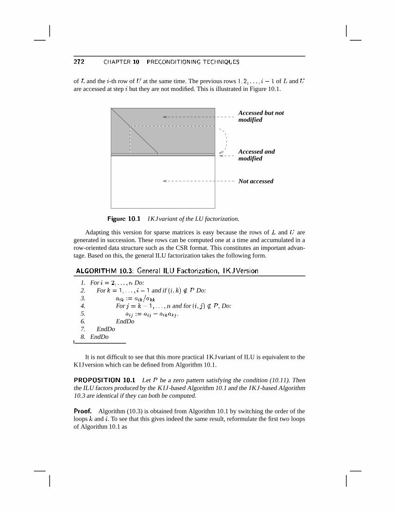
¶��p¶ � ~�� &�� \�� &^� \��0� � �°&� � ~ �0� ��?�of�

and the S -th row of�

at the same time. The previous rows / � 0 �*¬,¬*¬ ��Sª¨ / of�

and�

are accessed at step S but they are not modified. This is illustrated in Figure 10.1.

Not accessed

Accessed but not

Accessed and modified

modified

�� @��#�IKJvariant of the LU factorization.

Adapting this version for sparse matrices is easy because the rows of�

and�

aregenerated in succession. These rows can be computed one at a time and accumulated in arow-oriented data structure such as the CSR format. This constitutes an important advan-tage. Based on this, the general ILU factorization takes the following form.

��n��-�w�� ,� � �N�c� � � � � �� v� �� 1. For Sª� 0 �*¬,¬*¬T�S® Do:2. For �� / �*¬,¬*¬T� Si¨ / and if <%S � ��= �� Do:3. � 5 � � � � 5 � � � � �4. For �m�� M / �*¬,¬*¬T�S® and for < S�� = �� , Do:5. � 5 � � � � 5 � ¨ � 5 � � � � .6. EndDo7. EndDo8. EndDo

It is not difficult to see that this more practical IKJvariant of ILU is equivalent to theKIJversion which can be defined from Algorithm 10.1.

�R� �n� �� D�� #�Let

�be a zero pattern satisfying the condition (10.11). Then

the ILU factors produced by the KIJ-based Algorithm 10.1 and the IKJ-based Algorithm10.3 are identical if they can both be computed.

�� Algorithm (10.3) is obtained from Algorithm 10.1 by switching the order of the

loops � and S . To see that this gives indeed the same result, reformulate the first two loopsof Algorithm 10.1 as

�� ?� � � � &ª\� � ��p&�� \�� \�� &^� \�� ¶��For �� / �I® Do:

For Sª� / �I® Do:if �u² S and for < S�� ;=�� Do:

ope(row(i),row(k))¬,¬*¬,¬*¬*¬in which ope(row(i),row(k)) is the operation represented by lines 3 through 6 of both

Algorithm 10.1 and Algorithm 10.3. In this form, it is clear that the � and S loops can besafely permuted. Then the resulting algorithm can be reformulated to yield exactly Algo-rithm 10.3.

Note that this is only true for a static pattern ILU. If the pattern is dynamically determinedas the Gaussian elimination algorithm proceeds, then the patterns obtained with differentversions of GE may be different.

It is helpful to interpret the result of one incomplete elimination step. Denoting by � 5 # ,´ 5 # , and ��5 # the S -th rows of�

,�

, and � , respectively, then the � -loop starting at line 2of Algorithm 10.3 can be interpreted as follows. Initially, we have

´ 5 # � � 5 # . Then, eachelimination step is an operation of the form´ 5 # � � ´ 5 # ¨�� 5 � ´ � # ¬However, this operation is performed only on the nonzero pattern, i.e., the complement of�

. This means that, in reality, the elimination step takes the form´ 5 # � � ´ 5 #]¨�� 5 � ´ � # M + & � -5 # �in which

+ & � -5 � is zero when < S�� = ��

and equals � 5 � ´ � � when <%S � � = � �. Thus, the row+ & � -5 # cancels out the terms � 5 � ´ � � that would otherwise be introduced in the zero pattern. In

the end the following relation is obtained:

´ 5 #X� � 5 #2¨ 5 @�B� � B� � 5 � ´ � #]¨ + & � -5 #�� ¬

Note that � 5 �W� -for < S�� = � �

. We now sum up all the+ & � -5 # ’s and define+ 5 # � 5 @�B

� � B + & � -5 # ¬ £ ¥ �L[�¥ $4¦The row

+ 5 # contains the elements that fall inside the

�pattern at the completion of the

� -loop. Using the fact that � 5 5c� / , we obtain the relation,

� 5 #X� 5� � B � 5 � ´ � #Z¨ + 5 #E¬ £ ¥ �L[�¥ .�¦

Therefore, the following simple property can be stated.

�R� �n� �� -�� t¶Algorithm (10.3) produces factors

�and

�such that

�¢� �� ¨��in which ¨ � is the matrix of the elements that are dropped during the incomplete elimina-tion process. When <%S � � = � �

, an entry+ 5 � of � is equal to the value of ¨ ��5 � obtained at

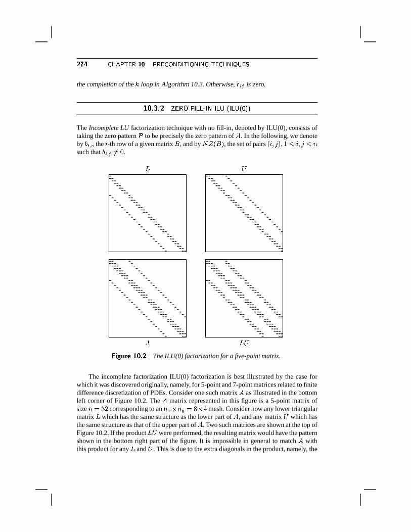
¶�� ~�� &�� \�� &^� \��0� � �°&� � ~ �0� ��?�the completion of the � loop in Algorithm 10.3. Otherwise,

+ 5 � is zero.

$��! ��! #" �!01A 7 � 2 6 6�-�2 9 2 6 (�� 2 6 (��

The Incomplete LU factorization technique with no fill-in, denoted by ILU(0), consists oftaking the zero pattern

�to be precisely the zero pattern of � . In the following, we denote

by 5 + # the S -th row of a given matrix � , and by � <��= , the set of pairs <%S � � = � / ! S�� ! ®such that 5 + � �� -

.

�

� �

� �� @��t¶

The ILU(0) factorization for a five-point matrix.

The incomplete factorization ILU(0) factorization is best illustrated by the case forwhich it was discovered originally, namely, for 5-point and 7-point matrices related to finitedifference discretization of PDEs. Consider one such matrix � as illustrated in the bottomleft corner of Figure 10.2. The � matrix represented in this figure is a 5-point matrix ofsize ®�� 0 corresponding to an ® F ¯X® � ��Z¯ 3 mesh. Consider now any lower triangularmatrix

�which has the same structure as the lower part of � , and any matrix

�which has

the same structure as that of the upper part of � . Two such matrices are shown at the top ofFigure 10.2. If the product

��were performed, the resulting matrix would have the pattern

shown in the bottom right part of the figure. It is impossible in general to match � withthis product for any

�and

�. This is due to the extra diagonals in the product, namely, the

�� ?� � � � &ª\� � ��p&�� \�� \�� &^� \�� ¶��diagonals with offsets ® F ¨ / and ¨2® F M / . The entries in these extra diagonals are calledfill-in elements. However, if these fill-in elements are ignored, then it is possible to find

�and

�so that their product is equal to � in the other diagonals. This defines the ILU(0)

factorization in general terms: Any pair of matrices�

(unit lower triangular) and�

(uppertriangular) so that the elements of ��¨ �� are zero in the locations of � <V�>= . Theseconstraints do not define the ILU(0) factors uniquely since there are, in general, infinitelymany pairs of matrices

�and

�which satisfy these requirements. However, the standard

ILU(0) is defined constructively using Algorithm 10.3 with the pattern

�equal to the zero

pattern of � .

�� n� �D�w�� N�c� �� 1. For S0� 0 �*¬*¬,¬T�I® Do:2. For � � / �*¬*¬,¬T��Sc¨ / and for <%S � ��= � � <V�>= Do:3. Compute � 5 �|� � 5 � � � � �4. For �m� � M / �*¬*¬,¬T�I® and for < S�� = � � <N�>= , Do:5. Compute � 5 � � � � 5 � ¨ � 5 � � � � .6. EndDo7. EndDo8. EndDo

In some cases, it is possible to write the ILU(0) factorization in the form

� � <� ¨ � =�� @�B <�� ¨ ��=T� £ ¥ �L[�¥ 1�¦where ¨ � and ¨ � are the strict lower and strict upper triangular parts of � , and � is acertain diagonal matrix, different from the diagonal of � , in general. In these cases it issufficient to find a recursive formula for determining the elements in � . A clear advantageis that only an extra diagonal of storage is required. This form of the ILU(0) factorization isequivalent to the incomplete factorizations obtained from Algorithm 10.4 when the productof the strict-lower part and the strict-upper part of � consists only of diagonal elementsand fill-in elements. This is true, for example, for standard 5-point difference approxima-tions to second order partial differential operators; see Exercise 4. In these instances, boththe SSOR preconditioner with � � / and the ILU(0) preconditioner can be cast in the form(10.16), but they differ in the way the diagonal matrix � is defined. For SSOR( �� / ),� is the diagonal of the matrix � itself. For ILU(0), it is defined by a recursion so thatthe diagonal of the product of matrices (10.16) equals the diagonal of � . By definition,together the

�and

�matrices in ILU(0) have the same number of nonzero elements as the

original matrix � .

�� t¶Table 10.2 shows the results of applying the GMRES algorithm with

ILU(0) preconditioning to the five test problems described in Section 3.7.

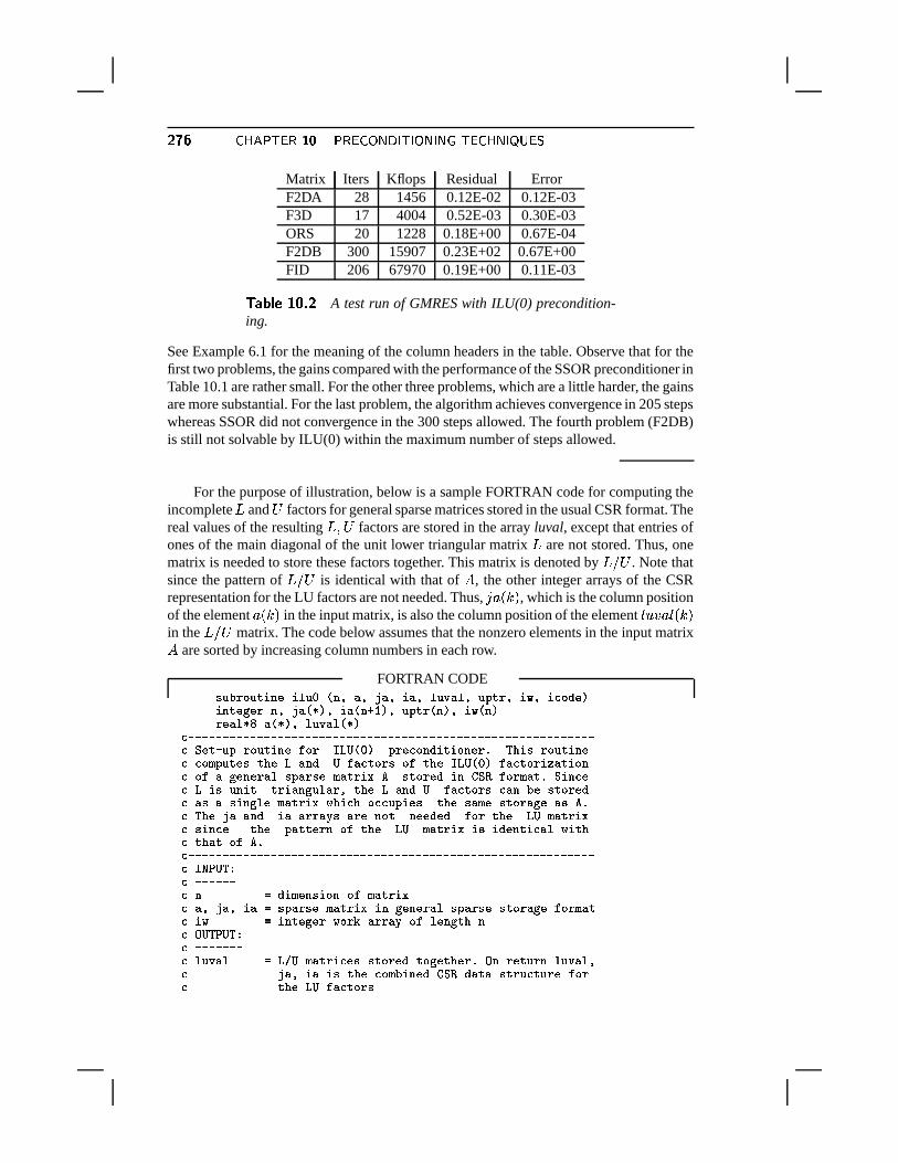
¶�� ~�� &�� \�� &^� \��0� � �°&� � ~ �0� ��?�Matrix Iters Kflops Residual ErrorF2DA 28 1456 0.12E-02 0.12E-03F3D 17 4004 0.52E-03 0.30E-03ORS 20 1228 0.18E+00 0.67E-04F2DB 300 15907 0.23E+02 0.67E+00FID 206 67970 0.19E+00 0.11E-03

� �� t¶A test run of GMRES with ILU(0) precondition-

ing.

See Example 6.1 for the meaning of the column headers in the table. Observe that for thefirst two problems, the gains compared with the performance of the SSOR preconditioner inTable 10.1 are rather small. For the other three problems, which are a little harder, the gainsare more substantial. For the last problem, the algorithm achieves convergence in 205 stepswhereas SSOR did not convergence in the 300 steps allowed. The fourth problem (F2DB)is still not solvable by ILU(0) within the maximum number of steps allowed.

For the purpose of illustration, below is a sample FORTRAN code for computing theincomplete

�and

�factors for general sparse matrices stored in the usual CSR format. The

real values of the resulting� � � factors are stored in the array luval, except that entries of

ones of the main diagonal of the unit lower triangular matrix�

are not stored. Thus, onematrix is needed to store these factors together. This matrix is denoted by

� � � . Note thatsince the pattern of

� � � is identical with that of � , the other integer arrays of the CSRrepresentation for the LU factors are not needed. Thus, � ��<��;= , which is the column positionof the element ��< ��= in the input matrix, is also the column position of the element � ´ � � � <��=in the

� � � matrix. The code below assumes that the nonzero elements in the input matrix� are sorted by increasing column numbers in each row.

FORTRAN CODE�� D �� 4�5!�� !��- �!��5�� !��6��$��0 �?��0 �#�*@��& ��2��*�=�4� ��!��(&,�0 �!�� ()��&<�6��$��.�/&,�P �?4�.�/&��!��(*)�!��1(&,�5�� !��(&

#�7�7�7�7�7�7�7�7�7�7�7�7�7�7�7�7�7�7�7�7�7�7�7�7�7�7�7�7�7�7�7�7�7�7�7�7�7�7�7�7�7�7�7�7�7�7�7�7�7�7�7�7�7�7�7�7�7�7�7#3J��7��$+�� =:��AF�H�I4��& $��#��@ �� 4O � �� 9�� #=#� ;�$��R��RH�!��@ I�:!�#��*��R*:=��+F�H�IY��&9:!�#�� M!*� ��#3*:+!V2��*��!��$�!*��*�U;/!*�� *��*@D �� J�L=:*��;/!��4O-J� ��#*�#9HG ��U�� T�� !��2��!*�%�0�*��RH�!��@RIX:�!�#��*��+#�!��=��=��*��@#3!��R!=�� 2�*�U;/!*�� =?�� #��G�#�#��$� *��T��+��! ;��G��*�!�2��+!�� O# � �� !3!��@X �!=!*��!��=!*��R��*� ��@��*@E:*�3��TH�I9;/!*�� #=�� #�� T$�!*��G*:3�� H*I ;/!*�� D ��R �@��*�� #�!��3?� ��*�#V��!*�+*:�4O#�7�7�7�7�7�7�7�7�7�7�7�7�7�7�7�7�7�7�7�7�7�7�7�7�7�7�7�7�7�7�7�7�7�7�7�7�7�7�7�7�7�7�7�7�7�7�7�7�7�7�7�7�7�7�7�7�7�7�7#=F��8�I � �#37�7�7�7�7�7#9� SV@� ;'�� *: ;/!*�� #3!�� !��0 �!3S=��$�!*��*�9;/!*�� D ��=2��*��!��$�!*��G��*�!�2��3:*��;/!*�#= �? S= ��*2��=?�*��CD!*��!��G*:+��2��+�#3K�I � 8*I � �#37�7�7�7�7�7�7#3�� !�� S9H *�IR;'!*�� #��+��*��@+�*2��*��4O5K��+��G�� !��# ��!��0 *!+ ��V��#� ;�� @ ��J�L=@!*��!��#��=:��# ��RH*I�:!�#��*��

�� ?� � � � &ª\� � ��p&�� \�� \�� &^� \�� ¶��#U��$�� SV$�� +�V��3@� *!*2��!��=��;'��+ ��3��J�L# @!*��!+��#��G�� !�� !��0 �!#3 �#**@�� S+ ��2��D ��@� �#�!*� ��2��*�D#�*@��=��+��*��# �#��@��+S � � ��*��;/!��R��# �#��@��+S9C �[�*��#��*@G!RM��9$� � *�+!*�G��$3C##�7�7�7�7�7�7�7�7�7�7�7�7�7�7�7�7�7�7�7�7�7�7�7�7�7�7�7�7�7�7�7�7�7�7�7�7�7�7�7�7�7�7�7�7�7�7�7�7�7�7�7�7�7�7�7�7�7�7�7# �� !�� M��E?�*�*CD!��!��D �?3�RM��*�=!��@+�� !��3!*��!��+��3!

@ � �+ VS �<�- �!��()��&�7"�� !�� &VS+!��1 �&

� � #�� @ � �9 *S)�<�[�

�?4�1 &VS �� #�� #�7�7�7�7�7�7�7�7�7�7�7�7�7�7�7�7�7�7�7�7�7�7�7 �!� ��G��$

@�� VC�S �/�[��"� S+ �!�� C<&��RS+ �!�� C ()��&�7 �@ � � � ��S��"�<� �� ?4�!��!��!��&�&VS�

� � � #�� S��"�

�� *��?�S ��!��!��&#�7�7�7�7�7�7�7�7�7�7�7�7�7�7�7�7�7�7�7�7�7�7�7 � �� G �:3@� �!�2��!��+��*��;'�*�� V��!�#��@

�: �!�*��? O�2��O C/&U2*�� #�7�7�7�7�7�7�7�7�7�7�7�7�7�7�7�7�7�7�7�7�7�7�7�� ;�$��3�� ;��*�� $�� *��:�� *��?4O

��RS=�� !��!��&�(�� !��$��!�*��?/&�&�� !��!�&VS3��

#�7�7�7�7�7�7�7�7�7�7�7�7�7�7�7�7�7�7�7�7�7�7�7�8��:��; �� !*�D#� ;�� !*� ��@ �� VSR��$��!�*��?/&�()�<�N �!��!�*��?�()��&�7"��?+S� �?4�!��!��&�& �: �!��? O.��O ��&V�� !��!��?'&�S�� !��!��?'&�7*��(*�� !�� &

�� #�� S��()� �: �!��O"�*��O ��& 2*� ��

#�7�7�7�7�7�7�7�7�7�7�7�7�7�7�7�7�7�7�7�7�7�7�7 J*�*��V$�� +�R@� *!*2��!��=��;'�� $��.C<&VS�

�: �!�*��? O.��O C O"*�4O-�� !��&QO��4O ��O ��@��&92*�� !��!�&VS �,O ��@ ��*�� !��!��&

#�7�7�7�7�7�7�7�7�7�7�7�7�7�7�7�7�7�7�7�7�7�7�7�L��:��G!��R�*�� =*:G �?=�VM��*�%O@�� )�V 9S �"�<�%�� ?4�!��!��1 &�&VS �

� �)� #�� #�� #�7�7�7�7�7�7�7�7�7�7�7�7�7�7�7�7�7�7�7�7�7�7�7 ��*��;/!��R��

�#�*@��+S ��

#�7�7�7�7�7�7�7�7�7�7�7�7�7�7�7�7�7�7�7�7�7�7�7 � ��*� �[M��9$� � *�� #�*@��+S9C

��*��@

$��! �! �� 6,0�>03687 � �F2 6 6C' 9?4 2 6 (��

The accuracy of the ILU(0) incomplete factorization may be insufficient to yield an ade-quate rate of convergence as shown in Example 10.2. More accurate Incomplete LU fac-torizations are often more efficient as well as more reliable. These more accurate factoriza-

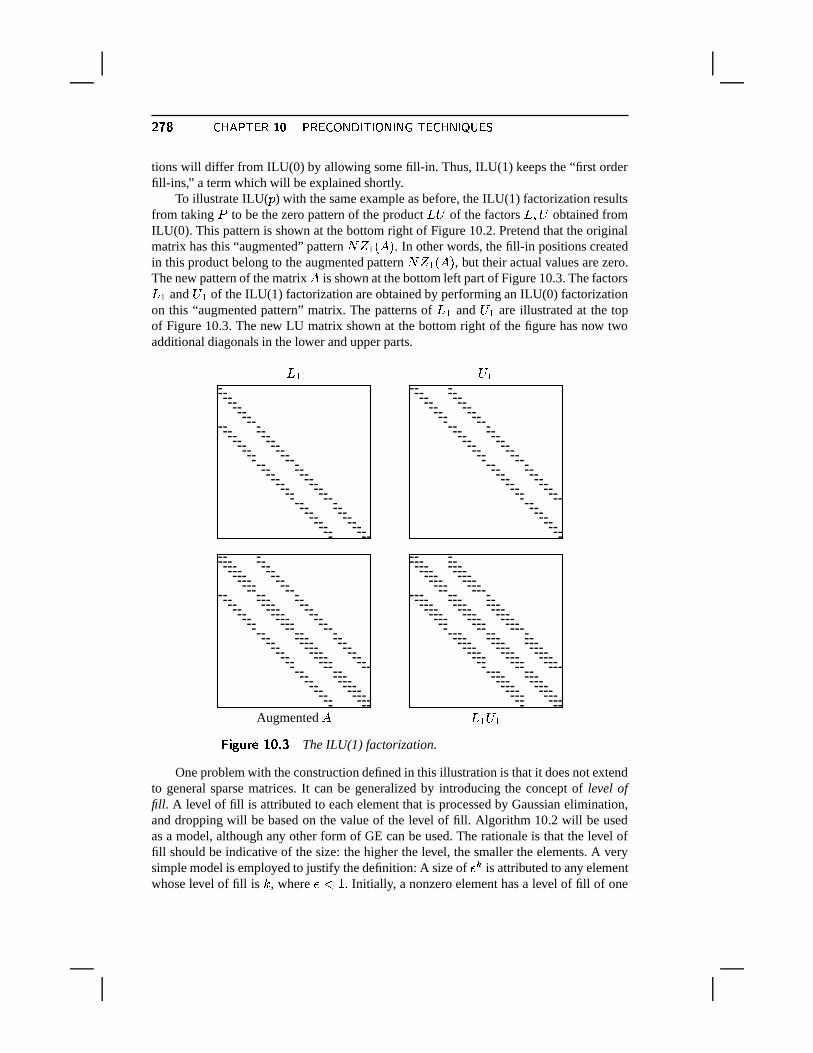
¶�� ~�� &�� \�� &^� \��0� � �°&� � ~ �0� ��?�tions will differ from ILU(0) by allowing some fill-in. Thus, ILU(1) keeps the “first orderfill-ins,” a term which will be explained shortly.

To illustrate ILU(� ) with the same example as before, the ILU(1) factorization resultsfrom taking

�to be the zero pattern of the product

��of the factors

� � � obtained fromILU(0). This pattern is shown at the bottom right of Figure 10.2. Pretend that the originalmatrix has this “augmented” pattern � B <V�>= . In other words, the fill-in positions createdin this product belong to the augmented pattern � B <N�,= , but their actual values are zero.The new pattern of the matrix � is shown at the bottom left part of Figure 10.3. The factors� B and

� B of the ILU(1) factorization are obtained by performing an ILU(0) factorizationon this “augmented pattern” matrix. The patterns of

� B and� B are illustrated at the top

of Figure 10.3. The new LU matrix shown at the bottom right of the figure has now twoadditional diagonals in the lower and upper parts.

Augmented �

� B � B

� B � B�� @��

The ILU(1) factorization.

One problem with the construction defined in this illustration is that it does not extendto general sparse matrices. It can be generalized by introducing the concept of level offill. A level of fill is attributed to each element that is processed by Gaussian elimination,and dropping will be based on the value of the level of fill. Algorithm 10.2 will be usedas a model, although any other form of GE can be used. The rationale is that the level offill should be indicative of the size: the higher the level, the smaller the elements. A verysimple model is employed to justify the definition: A size of � � is attributed to any elementwhose level of fill is � , where �w² / . Initially, a nonzero element has a level of fill of one

�� ?� � � � &ª\� � ��p&�� \�� \�� &^� \�� ¶��p·

(this will be changed later) and a zero element has a level of fill of � . An element � 5 � isupdated in line 5 of Algorithm 10.2 by the formula

� 5 � � � 5 � ¨ � 5 �n¯ � � � ¬ £ ¥ �L[�¥ 2�¦If � Q � 5 � is the current level of the element � 5 � , then our model tells us that the size of theupdated element should be

� 5 � � � � � J�� $ � ¨�� J�� $ � ¯ � � J�� J�� $ � ¨�� J�� $ � � � J�� ¬Therefore, roughly speaking, the size of �;5 � will be the maximum of the two sizes � � J�� $ �and � � J�� $ � � � J�� , and it is natural to define the new level of fill as,

� Q � 5 � � � �� 9 � � Q � 5 � � � Q � 5 � M � Q � � � �L¬In the common definition used in the literature, all the levels of fill are actually shiftedby ¨ / from the definition used above. This is purely for convenience of notation and toconform with the definition used for ILU(0). Thus, initially � Q � 5 � � -

if � 5 � �� -, and� Q � 5 � �� otherwise. Thereafter, define recursively

� Q � 5 � � �� 9 � � Q � 5 � � � Q � 5 � M � Q � � � M / �L¬� � � � ��D�� #�The initial level of fill of an element ��5 � of a sparse matrix � is

defined by

� Q � 5 � � � - � � 5 � �� - � 7 � S0� �� 7�� ¬

Each time this element is modified in line 5 of Algorithm 10.2, its level of fill must beupdated by

� Q � 5 � � �� 9 � � Q � 5 � � � Q � 5 � M � Q � � � M / �L¬ £ ¥ �L[�¥ ¤ ¦Observe that the level of fill of an element will never increase during the elimination. Thus,if � 5 � �� -

in the original matrix � , then the element in location S�� will have a level offill equal to zero throughout the elimination process. The above systematic definition givesrise to a natural strategy for discarding elements. In ILU < ��= , all fill-in elements whose levelof fill does not exceed � are kept. So using the definition of zero patterns introduced earlier,the zero pattern for ILU(� ) is the set� �w� � <%S�� = � � Q � 5 �� !�.�where � Q � 5 � is the level of fill value after all updates (10.18) have been performed. The case�v� -

coincides with the ILU(0) factorization and is consistent with the earlier definition.In practical implementations of the ILU(� ) factorization it is common to separate the

symbolic phase (where the structure of the�

and�

factors are determined) from the nu-merical factorization, when the numerical values are computed. Here, a variant is describedwhich does not separate these two phases. In the following description, � 5 # denotes the S -throw of the matrix � , and � 5 � the < S�� = -th entry of � .

�� n� �D�w�� N�c� �� 1. For all nonzero elements � 5 � define � Q � < � 5 � =�� -2. For S0� 0 �*¬*¬,¬T�I® Do:

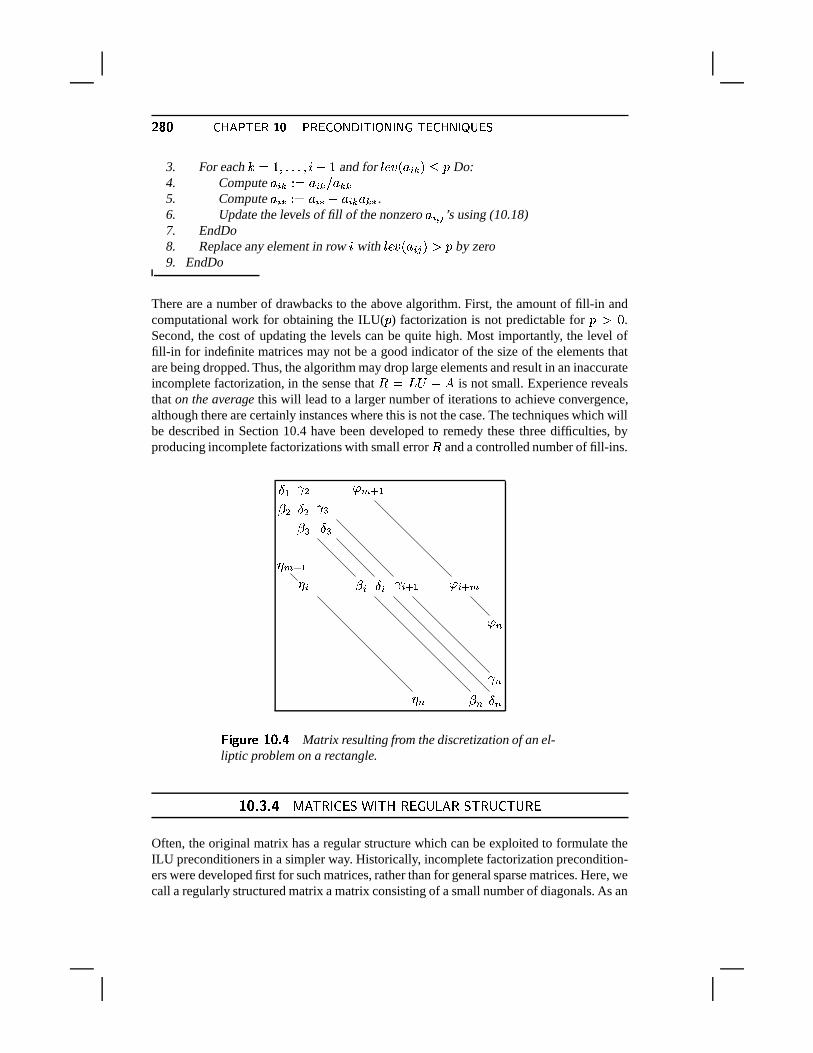
¶�� ~�� &�� \�� &^� \��0� � �°&� � ~ �0� ��?�3. For each �� / �,¬*¬,¬T��Sc¨ / and for � Q � < � 5 � = ! � Do:4. Compute � 5 � � � � 5 � � � � �5. Compute � 5 # � � � 5 # ¨ � 5 � � � # .6. Update the levels of fill of the nonzero � 5 + � ’s using (10.18)7. EndDo8. Replace any element in row S with � Q � < ��5 � = � � by zero9. EndDo

There are a number of drawbacks to the above algorithm. First, the amount of fill-in andcomputational work for obtaining the ILU(� ) factorization is not predictable for � � -

.Second, the cost of updating the levels can be quite high. Most importantly, the level offill-in for indefinite matrices may not be a good indicator of the size of the elements thatare being dropped. Thus, the algorithm may drop large elements and result in an inaccurateincomplete factorization, in the sense that � � �� ¨ � is not small. Experience revealsthat on the average this will lead to a larger number of iterations to achieve convergence,although there are certainly instances where this is not the case. The techniques which willbe described in Section 10.4 have been developed to remedy these three difficulties, byproducing incomplete factorizations with small error � and a controlled number of fill-ins.

O B � « � D � B�k« O « � �� O �

� D � B� 5 � 5 O 5 � 5 � B � 5 � D�I

� I � I O I��I

�� @�� Matrix resulting from the discretization of an el-

liptic problem on a rectangle.

$��! �! � BC'�; A�2 ��0,*�� 2 ; = A!0F& (�6�' A *,;>A+( � ; ()A+0

Often, the original matrix has a regular structure which can be exploited to formulate theILU preconditioners in a simpler way. Historically, incomplete factorization precondition-ers were developed first for such matrices, rather than for general sparse matrices. Here, wecall a regularly structured matrix a matrix consisting of a small number of diagonals. As an

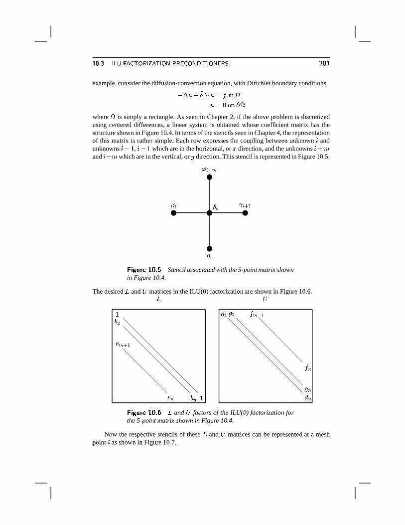
�� ?� � � � &ª\� � ��p&�� \�� \�� &^� \�� ¶��

example, consider the diffusion-convection equation, with Dirichlet boundary conditions

¨�� ´8M�� /¬�� ´ � � � 9 �´ � - 7?9 � �where

�is simply a rectangle. As seen in Chapter 2, if the above problem is discretized

using centered differences, a linear system is obtained whose coefficient matrix has thestructure shown in Figure 10.4. In terms of the stencils seen in Chapter 4, the representationof this matrix is rather simple. Each row expresses the coupling between unknown S andunknowns S M / , Sk¨ / which are in the horizontal, or � direction, and the unknowns S M ±and S�¨w± which are in the vertical, or

direction. This stencil is represented in Figure 10.5.

� 5 � BO 5� 5

�?5

� 5 � D

�� Stencil associated with the 5-point matrix shown

in Figure 10.4.

The desired�

and�

matrices in the ILU(0) factorization are shown in Figure 10.6.

/ G«

I /

Q D � B

Q I

� B � «

� I� I

� D � B

� I

� �

�� and

�factors of the ILU(0) factorization for

the 5-point matrix shown in Figure 10.4.

Now the respective stencils of these�

and�

matrices can be represented at a meshpoint S as shown in Figure 10.7.

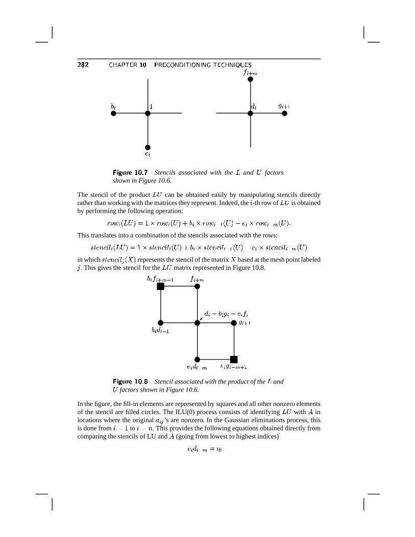
¶��p¶ � ~�� &�� \�� &^� \��0� � �°&� � ~ �0� ��?�

Q 5/ 5

� 5 � D� 5 � 5 � B

�� @�� Stencils associated with the

�and

�factors

shown in Figure 10.6.

The stencil of the product��

can be obtained easily by manipulating stencils directlyrather than working with the matrices they represent. Indeed, the S -th row of

� �is obtained

by performing the following operation:+�� 5 < �� =�� / ¯ +�� 5 < � = M 5 ¯ +�� 5 @�B < � = M Q 5 ¯ +�� 5 @ D < � =G¬This translates into a combination of the stencils associated with the rows:

� � Q ® � S � 5 < �� =�� / ¯ � � Q ® � S � 5 < � = M 5 ¯ � � Q ® �TS � 5 @�B < � = M Q 5 ¯ � � Q ® � S � 5 @ D < � =in which � � Q ® � S � � <��"= represents the stencil of the matrix � based at the mesh point labeled� . This gives the stencil for the

��matrix represented in Figure 10.8.

� 5 � B� 5 M 5 � 5 M Q 5 � 5�

5 � 5 @�B

� 5 � D

Q 5 � 5 @ D

5 � 5 � D @�B

Q 5 � 5 @ D � B�� @��

Stencil associated with the product of the�

and�factors shown in Figure 10.6.

In the figure, the fill-in elements are represented by squares and all other nonzero elementsof the stencil are filled circles. The ILU(0) process consists of identifying

��with � in

locations where the original � 5 � ’s are nonzero. In the Gaussian eliminations process, thisis done from S�� / to S��® . This provides the following equations obtained directly fromcomparing the stencils of LU and � (going from lowest to highest indices)

Q 5 � 5 @ D � �?5

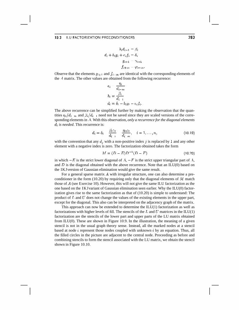
�� ?� � � � &ª\� � ��p&�� \�� \�� &^� \�� ¶�� 5 � 5 @�B � � 5� 5 M 5 � 5 M Q 5 � 5 � O 5� 5 � B � � 5 � B� 5 � D � � 5 � D ¬

Observe that the elements � 5 � B and� 5 � D are identical with the corresponding elements of

the � matrix. The other values are obtained from the following recurrence:

Q 5i� �?5� 5 @ D A5i� � 5� 5 @�B� 5 � O 5 ¨� 5 � 5 ¨ Q 5 � 5 ¬The above recurrence can be simplified further by making the observation that the quan-tities ��5 � � 5 @ D and � 5 � � 5 @�B need not be saved since they are scaled versions of the corre-sponding elements in � . With this observation, only a recurrence for the diagonal elements� 5 is needed. This recurrence is:

� 5 � O 5 ¨ � 5 � 5� 5 @�B ¨ �?5 � 5��5 @ D � S(� / �,¬*¬,¬T�I® � £ ¥ �L[�¥��¦with the convention that any � � with a non-positive index � is replaced by / and any otherelement with a negative index is zero. The factorization obtained takes the form

�� <� ¨ � =�� @�B <� ¨��= £ ¥ �L[ ��¦in which ¨ � is the strict lower diagonal of � , ¨ � is the strict upper triangular part of � ,and � is the diagonal obtained with the above recurrence. Note that an ILU(0) based onthe IKJversion of Gaussian elimination would give the same result.

For a general sparse matrix � with irregular structure, one can also determine a pre-conditioner in the form (10.20) by requiring only that the diagonal elements of � matchthose of � (see Exercise 10). However, this will not give the same ILU factorization as theone based on the IKJvariant of Gaussian elimination seen earlier. Why the ILU(0) factor-ization gives rise to the same factorization as that of (10.20) is simple to understand: Theproduct of

�and

�does not change the values of the existing elements in the upper part,

except for the diagonal. This also can be interpreted on the adjacency graph of the matrix.This approach can now be extended to determine the ILU(1) factorization as well as

factorizations with higher levels of fill. The stencils of the�

and�

matrices in the ILU(1)factorization are the stencils of the lower part and upper parts of the LU matrix obtainedfrom ILU(0). These are shown in Figure 10.9. In the illustration, the meaning of a givenstencil is not in the usual graph theory sense. Instead, all the marked nodes at a stencilbased at node S represent those nodes coupled with unknown S by an equation. Thus, allthe filled circles in the picture are adjacent to the central node. Proceeding as before andcombining stencils to form the stencil associated with the LU matrix, we obtain the stencilshown in Figure 10.10.

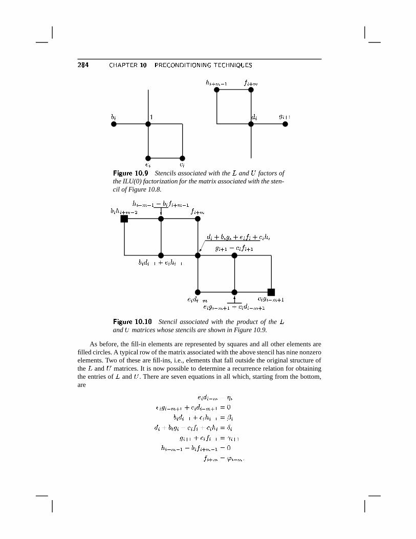
¶�� ~�� &�� \�� &^� \��0� � �°&� � ~ �0� ��?�

Q 5/ 5

� 5

� 5 � D� 5 � 5 � B

�;5 � D @�B

�� @��t·Stencils associated with the

�and

�factors of

the ILU(0) factorization for the matrix associated with the sten-cil of Figure 10.8.

5 � 5 � D @ «� 5 � D @�B M 5 � 5 � D @�B�

� 5 � D

5 � 5 @�B M Q 5 � 5 @�B��5 M A5 � 5 M Q 5 � 5 M � 5 � 5

�� 5 � B M � 5 � 5 � B

Q 5 � 5 @ D Q 5 � 5 @ D � B M � 5 � 5 @ D � B� � 5 � 5 @ D � B�� @��#��

Stencil associated with the product of the�

and�

matrices whose stencils are shown in Figure 10.9.

As before, the fill-in elements are represented by squares and all other elements arefilled circles. A typical row of the matrix associated with the above stencil has nine nonzeroelements. Two of these are fill-ins, i.e., elements that fall outside the original structure ofthe

�and

�matrices. It is now possible to determine a recurrence relation for obtaining

the entries of�

and�

. There are seven equations in all which, starting from the bottom,are

Q 5 � 5 @ D � �?5Q 5 � 5 @ D � B M � 5 ��5 @ D � B � -

A5 � 5 @�B M Q 5 � 5 @�B � � 5� 5 M A5 � 5 M Q 5 � 5 M � 5 � 5i� O 5� 5 � B M � 5 � 5 � B � � 5 � B

� 5 � D @�B M 5 � 5 � D @�B � -� 5 � D � � 5 � D ¬

�� ?� � � � &ª\� � ��p&�� \�� \�� &^� \�� ¶��This immediately yields the following recurrence relation for the entries of the

�and

�

factors:

Q 5 � �?5 � � 5 @ D� 5 �a¨ Q 5 � 5 @ D � B � � 5 @ D � B 5i� <�� 5 ¨ Q 5 � 5 @�B = � ��5 @�B��5ª� O 5 ¨� 5 � 5 ¨ Q 5 � 5 ¨�� 5 �;5� 5 � B � � 5 � B ¨ ��5 � 5 � B

� 5 � D @�B �a¨7 A5 � 5 � D @�B� 5 � D � � 5 � D ¬In proceeding from the nodes of smallest index to those of largest index, we are in effectperforming implicitly the IKJversion of Gaussian elimination. The result of the ILU(1)obtained in this manner is therefore identical with that obtained by using Algorithms 10.1and 10.3.

$��! ��! �� B 7:4?2 �F2#014 2 6 (�� B 2 6 ( �

In all the techniques thus far, the elements that were dropped out during the incompleteelimination process are simply discarded. There are also techniques which attempt to re-duce the effect of dropping by compensating for the discarded entries. For example, apopular strategy is to add up all the elements that have been dropped at the completion ofthe � -loop of Algorithm 10.3. Then this sum is subtracted from the diagonal entry in

�.

This diagonal compensation strategy gives rise to the Modified ILU (MILU) factorization.Thus, in equation (10.14), the final row

´ 5 # obtained after completion of the � -loop ofAlgorithm 10.3 undergoes one more modification, namely,´ 5 5 � � ´ 5 5 ¨ < + 5 # Q =in which Q � < / � / �*¬,¬*¬T� / = b . Note that

+ 5 # is a row and+ 5 # Q is the sum of the elements

in this row, i.e., its row sum. The above equation can be rewritten in row form as´ 5 # � �´ 5 # ¨ < + 5 # Q = Q b5 and equation (10.15) becomes

� 5 #Q� 5� � B � 5 � ´ � # M < + 5 # Q = Q b5 ¨ + 5 #9¬ £ ¥ �L[ E¥K¦

Observe that

� 5 # Q � 5� � B � 5 � ´ � # Q M < + 5 # Q = Q b5 Q ¨ + 5 # Q � 5 @�B

� � B � 5 � ´ � # Q � �� Q ¬This establishes that � Q � �� Q . As a result, this strategy guarantees that the row sums of� are equal to those of

��. For PDEs, the vector of all ones represents the discretization

of a constant function. This additional constraint forces the ILU factorization to be exactfor constant functions in some sense. Therefore, it is not surprising that often the algorithmdoes well for such problems. For other problems or problems with discontinuous coeffi-cients, MILU algorithms usually are not better than their ILU counterparts, in general.

¶�� ~�� &�� \�� &^� \��0� � �°&� � ~ �0� ��?��

For regularly structured matrices there are two elements dropped at theS -th step of ILU(0). These are 5 � 5 � D @�B and Q 5 � 5 @ D � B located on the north-west and south-east corners of the stencil, respectively. Thus, the row sum

+ 5 + # Q associated with step S is

� 5ª� � 5�� 5 � D @�B� 5 @�B M �?5 � D @ 5 � B� 5 @ Dand the MILU variant of the recurrence (10.19) is

� 5i� � 5 � 5 � D @�B� 5 @�B M � 5 � D @ 5 � B� 5 @ D��5ª� O 5 ¨ � 5 � 5� 5 @�B ¨ � 5 � 5� 5 @ D ¨ � 5S¬The new ILU factorization is now such that � � �� ¨ � in which according to (10.21)the S -th row of the new remainder matrix � is given by+ & I JLK -5 + # � < + 5 # Q = Q b5 ¨ + 5 #whose row sum is zero.

This generic idea of lumping together all the elements dropped in the elimination pro-cess and adding them to the diagonal of

�can be used for any form of ILU factorization.

In addition, there are variants of diagonal compensation in which only a fraction of thedropped elements are added to the diagonal. Thus, the term � 5 in the above example wouldbe replaced by � � 5 before being added to

´ 5 5 , where � is typically between 0 and 1. Otherstrategies distribute the sum � 5 among nonzero elements of

�and

�, other than the diago-

nal.

�u� �7�0�]�W�� ª��R��u��m�o�0�� C� �N�c�Q��u��

Incomplete factorizations which rely on the levels of fill are blind to numerical values be-cause elements that are dropped depend only on the structure of � . This can cause somedifficulties for realistic problems that arise in many applications. A few alternative methodsare available which are based on dropping elements in the Gaussian elimination processaccording to their magnitude rather than their locations. With these techniques, the zeropattern

�is determined dynamically. The simplest way to obtain an incomplete factor-

ization of this type is to take a sparse direct solver and modify it by adding lines of codewhich will ignore “small” elements. However, most direct solvers have a complex imple-mentation which involves several layers of data structures that may make this approachineffective. It is desirable to develop a strategy which is more akin to the ILU(0) approach.This section describes one such technique.

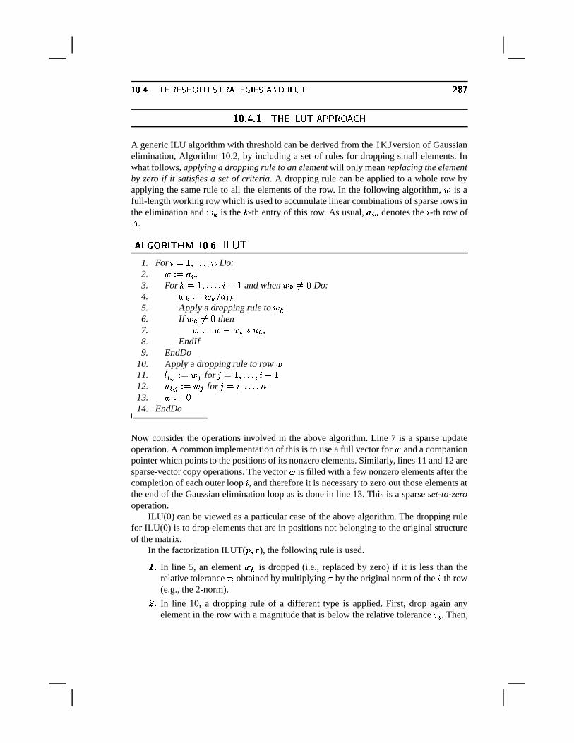
�� &�~ �?�C~ \��?�*�L&��p&��ª� ?� �� ³� ��k& ¶��$��! �� $ ; =)0@2 6 (+; ' � �!A 7�' ��=

A generic ILU algorithm with threshold can be derived from the IKJversion of Gaussianelimination, Algorithm 10.2, by including a set of rules for dropping small elements. Inwhat follows, applying a dropping rule to an element will only mean replacing the elementby zero if it satisfies a set of criteria. A dropping rule can be applied to a whole row byapplying the same rule to all the elements of the row. In the following algorithm, � is afull-length working row which is used to accumulate linear combinations of sparse rows inthe elimination and � � is the � -th entry of this row. As usual, � 5 # denotes the S -th row of� .

�� n� �D�w�� N�c�Q�1. For S0� / �*¬*¬,¬T�I® Do:2. � � � � 5 #3. For � � / �*¬*¬,¬T��Sc¨ / and when � � �� -

Do:4. � � � � � � � � � �5. Apply a dropping rule to � �6. If � � �� -

then7. � � � � ¨ � � � ´ � #8. EndIf9. EndDo

10. Apply a dropping rule to row �11. � 5 + � � � � � for �m� / �,¬*¬,¬T��Sc¨ /12.

´ 5 + � � � � � for �m� S �,¬*¬,¬T�I®13. � � � -14. EndDo

Now consider the operations involved in the above algorithm. Line 7 is a sparse updateoperation. A common implementation of this is to use a full vector for � and a companionpointer which points to the positions of its nonzero elements. Similarly, lines 11 and 12 aresparse-vector copy operations. The vector � is filled with a few nonzero elements after thecompletion of each outer loop S , and therefore it is necessary to zero out those elements atthe end of the Gaussian elimination loop as is done in line 13. This is a sparse set-to-zerooperation.

ILU(0) can be viewed as a particular case of the above algorithm. The dropping rulefor ILU(0) is to drop elements that are in positions not belonging to the original structureof the matrix.

In the factorization ILUT(� �� ), the following rule is used.��

In line 5, an element � � is dropped (i.e., replaced by zero) if it is less than therelative tolerance � 5 obtained by multiplying � by the original norm of the S -th row(e.g., the 2-norm).��In line 10, a dropping rule of a different type is applied. First, drop again anyelement in the row with a magnitude that is below the relative tolerance � 5 . Then,

¶�� ~�� &�� \�� &^� \��0� � �°&� � ~ �0� ��?�keep only the � largest elements in the

�part of the row and the � largest elements

in the�

part of the row in addition to the diagonal element, which is always kept.

The goal of the second dropping step is to control the number of elements per row. Roughlyspeaking, � can be viewed as a parameter that helps control memory usage, while � helpsto reduce computational cost. There are several possible variations on the implementationof dropping step 2. For example we can keep a number of elements equal to ® ´ < S = M � inthe upper part and ® � < S = M � in the lower part of the row, where ® � < S = and ® ´ <%S = are thenumber of nonzero elements in the

�part and the

�part of the S -th row of � , respectively.

This variant is adopted in the ILUT code used in the examples.Note that no pivoting is performed. Partial (column) pivoting may be incorporated at

little extra cost and will be discussed later. It is also possible to combine ILUT with one ofthe many standard reorderings, such as the ordering and the nested dissection ordering, orthe reverse Cuthill-McKee ordering. Reordering in the context of incomplete factorizationscan also be helpful for improving robustness, provided enough accuracy is used. For ex-ample, when a red-black ordering is used, ILU(0) may lead to poor performance comparedwith the natural ordering ILU(0). On the other hand, if ILUT is used by allowing graduallymore fill-in, then the performance starts improving again. In fact, in some examples, theperformance of ILUT for the red-black ordering eventually outperforms that of ILUT forthe natural ordering using the same parameters � and � .

$��! �� " ' 9�'56� *32H*

Existence theorems for the ILUT factorization are similar to those of other incompletefactorizations. If the diagonal elements of the original matrix are positive while the off-diagonal elements are negative, then under certain conditions of diagonal dominance thematrices generated during the elimination will have the same property. If the original ma-trix is diagonally dominant, then the transformed matrices will also have the property ofbeing diagonally dominant under certain conditions. These properties are analyzed in detailin this section.

The row vector � resulting from line 4 of Algorithm 10.6 will be denoted by´ � � B5 + # .

Note that´ � � B5 + � � -

for � ! � . Lines 3 to 10 in the algorithm involve a sequence ofoperations of the form

� 5 � � � ´ �5 � � ´ � � £ ¥��L[ //¦if � � 5 � � small enough set � 5 �|� -else:´ � � B5 + � � � ´ �5 + � ¨�� 5 � ´ � + � ¨ + �5 � �m� � M / �,¬*¬,¬T�I® £ ¥��L[ /µ/¦

for �� / �*¬*¬,¬T��Si¨ / , in which initially´ B5 + # � � � 5 + # and where

+ �5 � is an element subtractedfrom a fill-in element which is being dropped. It should be equal either to zero (no drop-ping) or to

´ �5 � ¨ � 5 � ´ � � when the element´ � � B5 + � is being dropped. At the end of the S -th

step of Gaussian elimination (outer loop in Algorithm 10.6), we obtain the S -th row of�

,´ 5 + # � ´ 55 @�B + # £ ¥��L[ $�¦

�� &�~ �?�C~ \��?�*�L&��p&��ª� ?� �� ³� ��k& ¶��p·

and the following relation is satisfied:

� 5 + #7� 5� � B � � + � ´ �5 + # M + 5 + #�

where+ 5 + # is the row containing all the fill-ins.

The existence result which will be proved is valid only for certain modifications ofthe basic ILUT <�� ;= strategy. We consider an ILUT strategy which uses the followingmodification:

Drop Strategy Modification. For any S�² ® , let � 5 + � $ be the element of largestmodulus among the elements � 5 + � � �¡� S M / �,¬*¬*¬I® , in the original matrix. Thenelements generated in position < S�� 5 = during the ILUT procedure are not subject tothe dropping rule.

This modification prevents elements generated in position < S�� 5 = from ever being dropped.Of course, there are many alternative strategies that can lead to the same effect.

A matrix�

whose entries � 5 � satisfy the following three conditions:

� 5 5 � -for / !<S^² ® and � I I � - £ ¥ �L[ .�¦

� 5 � ! -for S�� / �,¬*¬,¬T�I® and S �� £ ¥��L[ 1/¦I� ��5 � B � 5 � ² - � for / !<SR²³® £ ¥ �9[ 2�¦

will be referred to as an�� matrix. The third condition is a requirement that there be at

least one nonzero element to the right of the diagonal element, in each row except the last.The row sum for the S -th row is defined by+

� < � 5 + # =�� 5 + #TQ �I� � B � 5 + � ¬

A given row of an�� matrix

�is diagonally dominant, if its row sum is nonnegative. An�

� matrix�

is said to be diagonally dominant if all its rows are diagonally dominant. Thefollowing theorem is an existence result for ILUT. The underlying assumption is that anILUT strategy is used with the modification mentioned above.

�w�|��n�R� � �� If the matrix � is a diagonally dominant

�� matrix, then the rows´ �5 + # � � � - � / � 0 �*¬,¬*¬ � S defined by (10.23) starting with

´ � 5 + # � -and

´ B5 + # � � 5 + # satisfy thefollowing relations for � � / �,¬*¬,¬T� �´ �5 � ! - � �� S £ ¥ �L[ ¤ ¦+

� < ´ �5 + # = � +��< ´ � @�B5 + # = � - � £ ¥ �L[ ��¦´ �5 5 � -

when SR²¡® and´ �I I � - ¬ £ ¥ �L[ µ ��¦

�� The result can be proved by induction on � . It is trivially true for �� -

. To provethat the relation (10.28) is satisfied, start from the relation´ � � B5 + # � � ´ �5 + # ¨�� 5 � ´ � + #2¨ + �5 #

¶p·�� ~�� &�� \�� &^� \��0� � �°&� � ~ �0� ��?�in which � 5 �C! - � ´ � + � ! -

. Either+ �5 � is zero which yields

´ � � B5 � ! ´ �5 � ! -, or

+ �5 �is nonzero which means that

´ � � B5 � is being dropped, i.e., replaced by zero, and thereforeagain

´ � � B5 � ! -. This establishes (10.28). Note that by this argument

+ �5 � � -except when

the � -th element in the row is dropped, in which case´ � � B5 � � -

and+ �5 � � ´ �5 � ¨ � 5 � ´ � + � ! -

.Therefore,

+ �5 � ! -, always. Moreover, when an element in position <%S�� = is not dropped,

then ´ � � B5 + � � � ´ �5 + � ¨�� 5 � ´ � + � ! ´ �5 + �and in particular by the rule in the modification of the basic scheme described above, forS�² ® , we will always have for �n� � 5 , ´ � � B5 + � $ ! ´ �5 + � $ £ ¥��L[ µ9¥G¦in which � 5 is defined in the statement of the modification.

Consider the row sum of´ � � B5 # . We have+

� < ´ � � B5 + # =�� +��< ´ �5 + # =ª¨�� 5 � +

� < ´ � + # =ª¨ +� < + �5 # =

� +��< ´ �5 + # =ª¨�� 5 � +

� < ´ � + # = £ ¥��L[ µ//¦� +��< ´ �5 + # = £ ¥��L[ µ/µ/¦

which establishes (10.29) for � M / .It remains to prove (10.30). From (10.29) we have, for S^² ® ,´ � � B5 5 � � � � � B + I ¨ ´ � � B5 + � � � � � � B + I � ´ � � B5 + � � £ ¥��L[ µ $�¦� � ´ � � B5 + � $ � � � ´ �5 + � $ � � ¬*¬,¬ £ ¥��L[ µ ./¦� � ´ B5 + � $ �9� � � 5 + � $ �H¬ £ ¥��L[ µ 1/¦

Note that the inequalities in (10.35) are true because´ �5 + � $ is never dropped by assumption

and, as a result, (10.31) applies. By the condition (10.27), which defines�� matrices, � � 5 + � $ �

is positive for S�² ® . Clearly, when SQ��® , we have by (10.34)´ I I�� -

. This completesthe proof.

The theorem does not mean that the factorization is effective only when its conditions aresatisfied. In practice, the preconditioner is efficient under fairly general conditions.

$��! �� 2 B ��6,01BD019!;3'�;>2H7�9 450 ;3'52 6*

A poor implementation of ILUT may well lead to an expensive factorization phase, andpossibly an impractical algorithm. The following is a list of the potential difficulties thatmay cause inefficiencies in the implementation of ILUT.

� �Generation of the linear combination of rows of � (Line 7 in Algorithm 10.6).� �Selection of the � largest elements in

�and

�.

� �Need to access the elements of

�in increasing order of columns (in line 3 of

Algorithm 10.6).

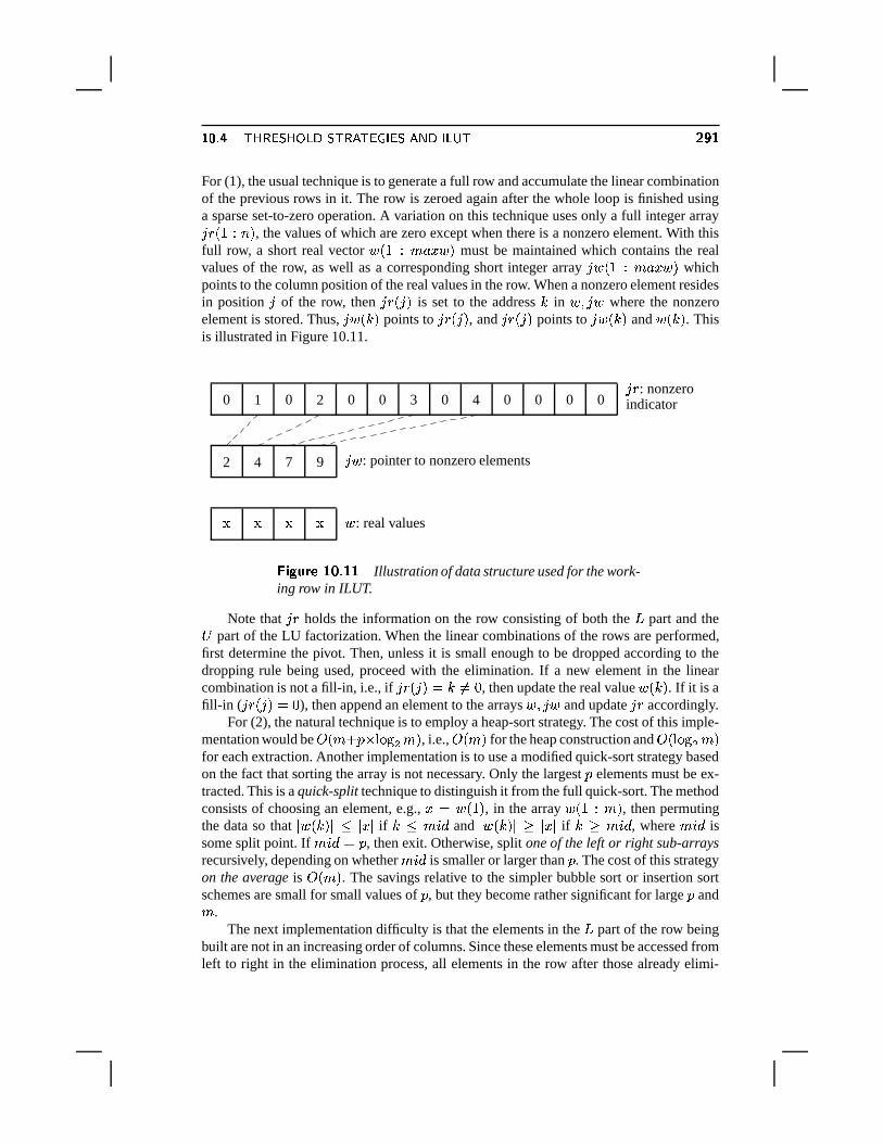
�� &�~ �?�C~ \��?�*�L&��p&��ª� ?� �� ³� ��k& ¶p·��

For (1), the usual technique is to generate a full row and accumulate the linear combinationof the previous rows in it. The row is zeroed again after the whole loop is finished usinga sparse set-to-zero operation. A variation on this technique uses only a full integer array�+ < / � ®�= , the values of which are zero except when there is a nonzero element. With this

full row, a short real vector � < / � ± �L� � = must be maintained which contains the realvalues of the row, as well as a corresponding short integer array � � < / � ± �%� � = whichpoints to the column position of the real values in the row. When a nonzero element residesin position � of the row, then �

+ < � = is set to the address � in � � � � where the nonzeroelement is stored. Thus, � � < ��= points to �

+ < � = , and �+ < � = points to � � <��= and � <��;= . This

is illustrated in Figure 10.11.

1

2

0 0 2

4

0 0 3

7

0 4

9

0 0 0 0

� � � � � : real values

� � : pointer to nonzero elements

�+: nonzero

indicator

�� #�,�Illustration of data structure used for the work-

ing row in ILUT.

Note that �+

holds the information on the row consisting of both the�

part and the�part of the LU factorization. When the linear combinations of the rows are performed,

first determine the pivot. Then, unless it is small enough to be dropped according to thedropping rule being used, proceed with the elimination. If a new element in the linearcombination is not a fill-in, i.e., if �

+ < � =R�� -, then update the real value � < ��= . If it is a

fill-in (�+ < � =^� -

), then append an element to the arrays � � � � and update �+

accordingly.For (2), the natural technique is to employ a heap-sort strategy. The cost of this imple-

mentation would be( <o± M �^¯ �

7� « ± = , i.e.,

( <o± = for the heap construction and( < �

7� « ± =

for each extraction. Another implementation is to use a modified quick-sort strategy basedon the fact that sorting the array is not necessary. Only the largest � elements must be ex-tracted. This is a quick-split technique to distinguish it from the full quick-sort. The methodconsists of choosing an element, e.g., �¡� � < / = , in the array � < / � ± = , then permutingthe data so that � � <��;= � ! � � � if � ! ±DS"� and � � < ��= � � � � � if � � ±DS�� , where ± S�� issome split point. If ±DS�� , then exit. Otherwise, split one of the left or right sub-arraysrecursively, depending on whether ± S�� is smaller or larger than � . The cost of this strategyon the average is

( <N± = . The savings relative to the simpler bubble sort or insertion sortschemes are small for small values of � , but they become rather significant for large � and± .

The next implementation difficulty is that the elements in the�

part of the row beingbuilt are not in an increasing order of columns. Since these elements must be accessed fromleft to right in the elimination process, all elements in the row after those already elimi-

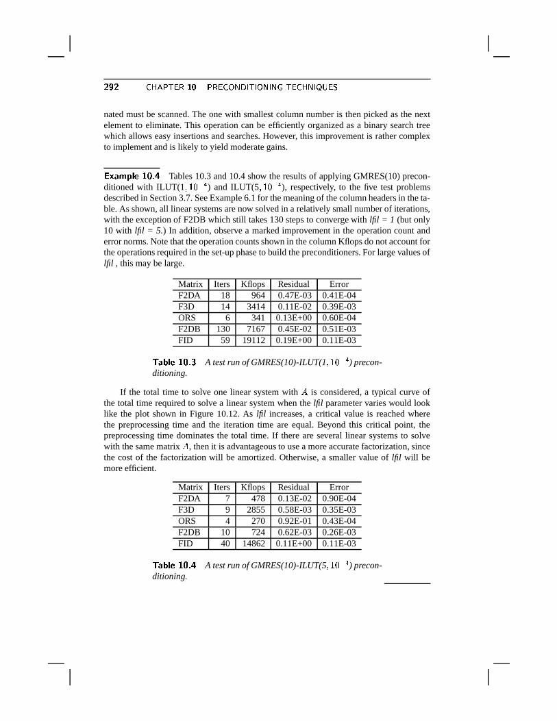
¶p·p¶ � ~�� &�� \�� &^� \��0� � �°&� � ~ �0� ��?�nated must be scanned. The one with smallest column number is then picked as the nextelement to eliminate. This operation can be efficiently organized as a binary search treewhich allows easy insertions and searches. However, this improvement is rather complexto implement and is likely to yield moderate gains.

�� Tables 10.3 and 10.4 show the results of applying GMRES(10) precon-

ditioned with ILUT(1 � / - @ �

) and ILUT(5 � / - @ �

), respectively, to the five test problemsdescribed in Section 3.7. See Example 6.1 for the meaning of the column headers in the ta-ble. As shown, all linear systems are now solved in a relatively small number of iterations,with the exception of F2DB which still takes 130 steps to converge with lfil = 1 (but only10 with lfil = 5.) In addition, observe a marked improvement in the operation count anderror norms. Note that the operation counts shown in the column Kflops do not account forthe operations required in the set-up phase to build the preconditioners. For large values oflfil , this may be large.

Matrix Iters Kflops Residual ErrorF2DA 18 964 0.47E-03 0.41E-04F3D 14 3414 0.11E-02 0.39E-03ORS 6 341 0.13E+00 0.60E-04F2DB 130 7167 0.45E-02 0.51E-03FID 59 19112 0.19E+00 0.11E-03

� �� A test run of GMRES(10)-ILUT(1 � / - @ �

) precon-ditioning.

If the total time to solve one linear system with � is considered, a typical curve ofthe total time required to solve a linear system when the lfil parameter varies would looklike the plot shown in Figure 10.12. As lfil increases, a critical value is reached wherethe preprocessing time and the iteration time are equal. Beyond this critical point, thepreprocessing time dominates the total time. If there are several linear systems to solvewith the same matrix � , then it is advantageous to use a more accurate factorization, sincethe cost of the factorization will be amortized. Otherwise, a smaller value of lfil will bemore efficient.

Matrix Iters Kflops Residual ErrorF2DA 7 478 0.13E-02 0.90E-04F3D 9 2855 0.58E-03 0.35E-03ORS 4 270 0.92E-01 0.43E-04F2DB 10 724 0.62E-03 0.26E-03FID 40 14862 0.11E+00 0.11E-03

� �� A test run of GMRES(10)-ILUT(5 � / - @ �

) precon-ditioning.

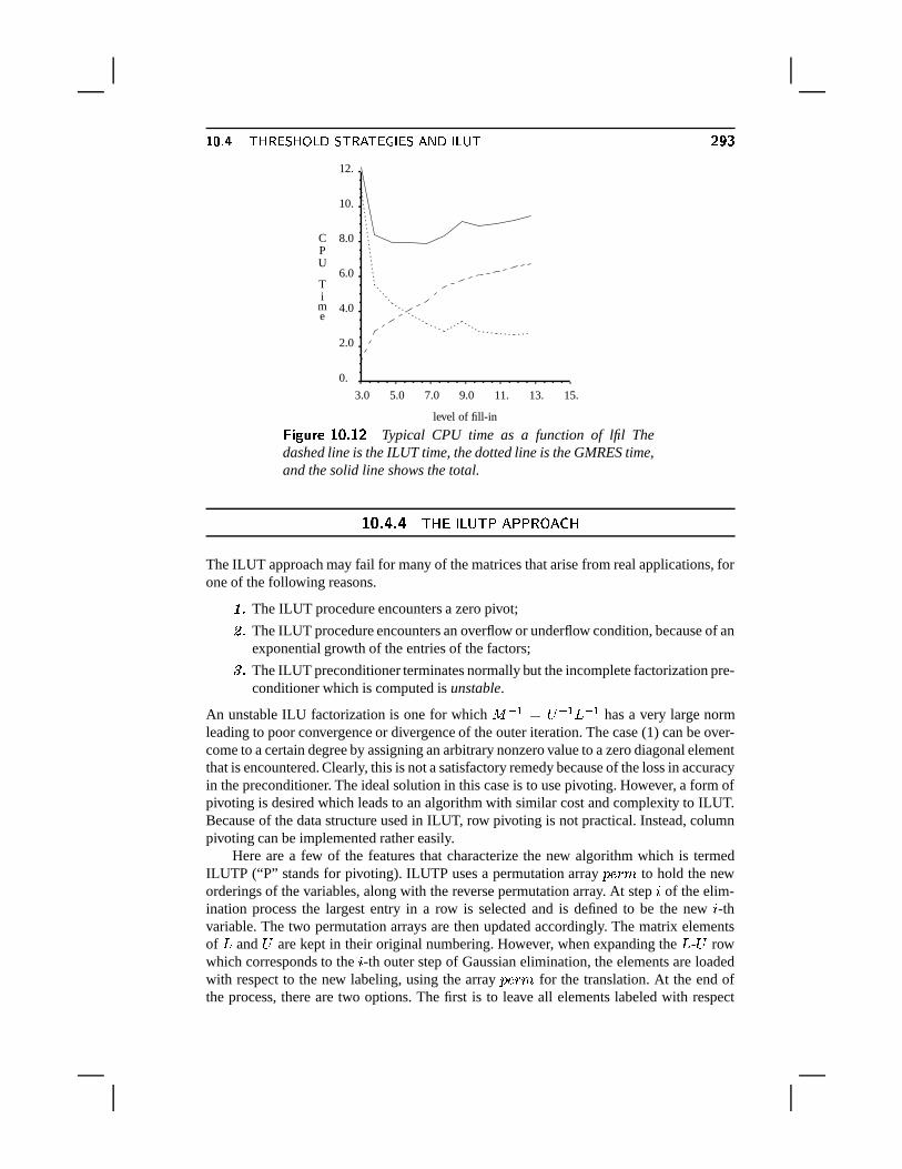
�� &�~ �?�C~ \��?�*�L&��p&��ª� ?� �� ³� ��k& ¶p·��

level of fill-in

CPU

Time

3.0 5.0 7.0 9.0 11. 13. 15.

0.

2.0

4.0

6.0

8.0

10.

12.

�� #�%¶Typical CPU time as a function of lfil The

dashed line is the ILUT time, the dotted line is the GMRES time,and the solid line shows the total.

$��! �� ;>=?0@2 6 (�; ��' � �!A 7�' ��=

The ILUT approach may fail for many of the matrices that arise from real applications, forone of the following reasons.

��The ILUT procedure encounters a zero pivot;��The ILUT procedure encounters an overflow or underflow condition, because of anexponential growth of the entries of the factors;

� �The ILUT preconditioner terminates normally but the incomplete factorization pre-conditioner which is computed is unstable.

An unstable ILU factorization is one for which � @�B � � @�B � @�B has a very large normleading to poor convergence or divergence of the outer iteration. The case (1) can be over-come to a certain degree by assigning an arbitrary nonzero value to a zero diagonal elementthat is encountered. Clearly, this is not a satisfactory remedy because of the loss in accuracyin the preconditioner. The ideal solution in this case is to use pivoting. However, a form ofpivoting is desired which leads to an algorithm with similar cost and complexity to ILUT.Because of the data structure used in ILUT, row pivoting is not practical. Instead, columnpivoting can be implemented rather easily.

Here are a few of the features that characterize the new algorithm which is termedILUTP (“P” stands for pivoting). ILUTP uses a permutation array � Q + ± to hold the neworderings of the variables, along with the reverse permutation array. At step S of the elim-ination process the largest entry in a row is selected and is defined to be the new S -thvariable. The two permutation arrays are then updated accordingly. The matrix elementsof�

and�

are kept in their original numbering. However, when expanding the�

-�

rowwhich corresponds to the S -th outer step of Gaussian elimination, the elements are loadedwith respect to the new labeling, using the array � Q + ± for the translation. At the end ofthe process, there are two options. The first is to leave all elements labeled with respect

¶p·�� ~�� &�� \�� &^� \��0� � �°&� � ~ �0� ��?�to the original labeling. No additional work is required since the variables are already inthis form in the algorithm, but the variables must then be permuted at each preconditioningstep. The second solution is to apply the permutation to all elements of � as well as

� � � .This does not require applying a permutation at each step, but rather produces a permutedsolution which must be permuted back at the end of the iteration phase. The complexityof the ILUTP procedure is virtually identical to that of ILUT. A few additional optionscan be provided. A tolerance parameter called � Q + ± � � � may be included to help determinewhether or not to permute variables: A nondiagonal element �;5 � is candidate for a per-mutation only when

� � �Z¯ � ��5 � � � � � 5 5 � . Furthermore, pivoting may be restricted to takeplace only within diagonal blocks of a fixed size. The size ± � � � of these blocks must beprovided. A value of ±f � � � � ® indicates that there are no restrictions on the pivoting.

For difficult matrices, the following strategy seems to work well:� �

Always apply a scaling to all the rows (or columns) e.g., so that their / -norms areall equal to 1; then apply a scaling of the columns (or rows).� �Use a small drop tolerance (e.g., �]� / - @ �

or �Z� / - @ � = .� �

Take a large fill-in parameter (e.g., � � S � � 0 -).

� �Do not take a small value for � Q + ± � � � . Reasonable values are between

- ¬ � and- ¬ - / , with- ¬ � being the best in many cases.

� �Take ± � � �Z��® unless there are reasons why a given block size is justifiable.

�� Table 10.5 shows the results of applying the GMRES algorithm with

ILUTP(1 � / - @ �

) preconditioning to the five test problems described in Section 3.7. Thepermtol parameter is set to 1.0 in this case.

Matrix Iters Kflops Residual ErrorF2DA 18 964 0.47E-03 0.41E-04F3D 14 3414 0.11E-02 0.39E-03ORS 6 341 0.13E+00 0.61E-04F2DB 130 7167 0.45E-02 0.51E-03FID 50 16224 0.17E+00 0.18E-03

� �� A test run of GMRES with ILUTP(1) precondi-

tioning.

See Example 6.1 for the meaning of the column headers in the table. The results are identi-cal with those of ILUT(1 � / - @ �

) shown in Table 10.3, for the first four problems, but thereis an improvement for the fifth problem.

$��! � �� ; =?0@2 6 (+* ' � �!A 7�' ��=

The ILU preconditioners discussed so far are based mainly on the the IKJvariant of Gaus-sian elimination. Different types of ILUs can be derived using other forms of Gaussian

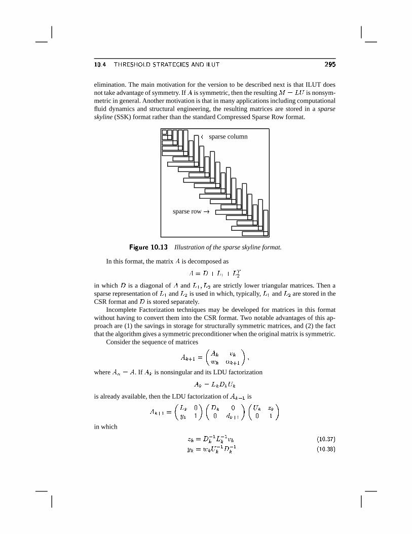
�� &�~ �?�C~ \��?�*�L&��p&��ª� ?� �� ³� ��k& ¶p·��elimination. The main motivation for the version to be described next is that ILUT doesnot take advantage of symmetry. If � is symmetric, then the resulting � � �� is nonsym-metric in general. Another motivation is that in many applications including computationalfluid dynamics and structural engineering, the resulting matrices are stored in a sparseskyline (SSK) format rather than the standard Compressed Sparse Row format.

sparse row �

� sparse column

�� #� �Illustration of the sparse skyline format.

In this format, the matrix � is decomposed as

�¢�� M � B M � b«in which � is a diagonal of � and

� B � � « are strictly lower triangular matrices. Then asparse representation of

� B and� « is used in which, typically,

� B and� « are stored in the

CSR format and � is stored separately.Incomplete Factorization techniques may be developed for matrices in this format

without having to convert them into the CSR format. Two notable advantages of this ap-proach are (1) the savings in storage for structurally symmetric matrices, and (2) the factthat the algorithm gives a symmetric preconditioner when the original matrix is symmetric.

Consider the sequence of matrices

� � � B � % � � � �� B ) �where � I �� . If � � is nonsingular and its LDU factorization

� � � � � � � � �is already available, then the LDU factorization of � � � B is

� � � B � % � � -� / )

%� � -- � � � B )

% � � 2 �- / )in which

2 � �� @�B� � @�B� � � £ ¥ �L[ µ 2�¦�W� � � � @�B� � @�B� £ ¥ �L[ µ ¤ ¦

¶p·�� ~�� &�� \�� &^� \��0� � �°&� � ~ �0� ��?�� B � � � B ¨ � � �%2 �%¬ £ ¥��L[ µ �/¦

Hence, the last row/column pairs of the factorization can be obtained by solving two unitlower triangular systems and computing a scaled dot product. This can be exploited forsparse matrices provided an appropriate data structure is used to take advantage of thesparsity of the matrices

� � , � � as well as the vectors � � , � � ,� , and 2 � . A convenient data

structure for this is to store the rows/columns pairs � � � � b� as a single row in sparse mode.All these pairs are stored in sequence. The diagonal elements are stored separately. This iscalled the Unsymmetric Sparse Skyline (USS) format. Each step of the ILU factorizationbased on this approach will consist of two approximate sparse linear system solutions anda sparse dot product. The question that arises is: How can a sparse triangular system besolved inexpensively? It would seem natural to solve the triangular systems (10.37) and(10.38) exactly and then drop small terms at the end, using a numerical dropping strategy.However, the total cost of computing the ILU factorization with this strategy would be( <o® « = operations at least, which is not acceptable for very large problems. Since only anapproximate solution is required, the first idea that comes to mind is the truncated Neumannseries,

2 �w�� @�B� � @�B� � �|� � @�B� < & M � � M � «� M ¬,¬*¬ M � �� = � � £ ¥��L[ $��/¦in which � � � & ¨ � � . In fact, by analogy with ILU(� ), it is interesting to note that thepowers of � � will also tend to become smaller as � increases. A close look at the structureof � �� shows that there is indeed a strong relation between this approach and ILU(� ) inthe symmetric case. Now we make another important observation, namely, that the vector� �� can be computed in sparse-sparse mode, i.e., in terms of operations involving prod-ucts of sparse matrices by sparse vectors. Without exploiting this, the total cost would stillbe

( <o® « = . When multiplying a sparse matrix � by a sparse vector � , the operation canbest be done by accumulating the linear combinations of the columns of � . A sketch of theresulting ILUS algorithm is as follows.

��n��-�w�� V�i�7� �� 1. Set � B �� B � � B B , � B � � B � /2. For Sª� / �*¬,¬*¬T�S®�¨ / Do:3. Compute 2 � by (10.40) in sparse-sparse mode4. Compute

� in a similar way

5. Apply numerical dropping to� and 2 �

6. Compute � � � B via (10.39)7. EndDo

If there are only S nonzero components in the vector � and an average of � nonzero elementsper column, then the total cost per step will be

0 ¯ SX¯�� on the average. Note that thecomputation of � � via (10.39) involves the inner product of two sparse vectors which isoften implemented by expanding one of the vectors into a full vector and computing theinner product of a sparse vector by this full vector. As mentioned before, in the symmetriccase ILUS yields the Incomplete Cholesky factorization. Here, the work can be halvedsince the generation of

� is not necessary.

�� r\ �R� ��p&�� ;��;�� \�� &�� \�� ¶p·��

Also note that a simple iterative procedure such as MR or GMRES(m) can be usedto solve the triangular systems in sparse-sparse mode. Similar techniques will be seenin Section 10.5. Experience shows that these alternatives are not much better than theNeumann series approach [53].

�8� �X�Z�.�v�V��u��N� ��Z�R�]� ��7��2��C�v�t��D�f�n�]�]��v� �

The Incomplete LU factorization techniques were developed originally for � -matriceswhich arise from the discretization of Partial Differential Equations of elliptic type, usu-ally in one variable. For the common situation where � is indefinite, standard ILU fac-torizations may face several difficulties, and the best known is the fatal breakdown due tothe encounter of a zero pivot. However, there are other problems that are just as serious.Consider an incomplete factorization of the form

�¢� �� M � £ ¥ �L[ $9¥K¦where � is the error. The preconditioned matrices associated with the different forms ofpreconditioning are similar to

� @�BK� � @�B2� & M � @�B � � @�B4¬ £ ¥ �L[ $/�¦What is sometimes missed is the fact that the error matrix � in (10.41) is not as importantas the “preconditioned” error matrix

� @�B � � @�B shown in (10.42) above. When the matrix� is diagonally dominant, then�

and�

are well conditioned, and the size of� @�B � � @�B re-

mains confined within reasonable limits, typically with a nice clustering of its eigenvaluesaround the origin. On the other hand, when the original matrix is not diagonally dominant,� @�B or

� @�B may have very large norms, causing the error� @�B � � @�B to be very large and

thus adding large perturbations to the identity matrix. It can be observed experimentallythat ILU preconditioners can be very poor in these situations which often arise when thematrices are indefinite, or have large nonsymmetric parts.

One possible remedy is to try to find a preconditioner that does not require solvinga linear system. For example, the original system can be preconditioned by a matrix �which is a direct approximation to the inverse of � .

$��! � $ ' � �!A 7 2#BC'�;>2 9�& ; =?0@2#9 �>01A1*10 7 � ' * � ' A1*10BC'3;>A+2

A simple technique for finding approximate inverses of arbitrary sparse matrices is to at-tempt to find a sparse matrix � which minimizes the Frobenius norm of the residual matrix& ¨©�� , � < � =��§ & ¨�� § «� ¬ £ ¥ �L[ $/µ�¦

¶p·�� ~�� &�� \�� &^� \��0� � �°&� � ~ �0� ��?�A matrix � whose value � < � = is small would be a right-approximate inverse of � . Sim-ilarly, a left-approximate inverse can be defined by using the objective function

§ & ¨ � �m§ «� ¬ £ ¥��L[ $ $�¦Finally, a left-right pair

� � � can be sought to minimize

§ & ¨ � � � § «� ¬ £ ¥��L[ $ ./¦In the following, only (10.43) and(10.45) are considered. The case (10.44) is very

similar to the right preconditioner case (10.43). The objective function (10.43) decouplesinto the sum of the squares of the 2-norms of the individual columns of the residual matrix& ¨�� , � < � =��§ & ¨©�� § «� �

I� � B § Q � ¨©�7± � § «« £ ¥��L[ $ 1/¦in which Q � and ± � are the � -th columns of the identity matrix and of the matrix � ,respectively. There are two different ways to proceed in order to minimize (10.46). Thefunction (10.43) can be minimized globally as a function of the sparse matrix � , e.g., bya gradient-type method. Alternatively, the individual functions

� � <N± =��§ Q � ¨©�7±�§ «« � �m� / � 0 �,¬*¬*¬ �I® £ ¥��L[ $ 2/¦can be minimized. The second approach is appealing for parallel computers, although thereis also parallelism to be exploited in the first approach. These two approaches will bediscussed in turn.

$��! �� " & 6 7 �1'56D2 ; 01A�'�;>2H7:9

The global iteration approach consists of treating � as an unknown sparse matrix andusing a descent-type method to minimize the objective function (10.43). This function is aquadratic function on the space of ® ¯f® matrices, viewed as objects in �

I 0. The proper

inner product on the space of matrices, to which the squared norm (10.46) is associated, is� � �� <�� b �"=K¬ £ ¥��L[ $ ¤ ¦

In the following, an array representation of an ® « vector � means the ®�¯m® matrix whosecolumn vectors are the successive ® -vectors of � .

In a descent algorithm, a new iterate � IJ/Kis defined by taking a step along a selected

direction � , i.e.,

� IJLK �� M �in which is selected to minimize the objective function � < � IJLK = . From results seenin Chapter 5, minimizing the residual norm is equivalent to imposing the condition that�g¨ �� be orthogonal to � � with respect to the

�� inner product. Thus, the optimal is given by

��N�B� �� 8�B� ��

�� <�� b � ��=�

� < <V� ��= b � ��= ¬ £ ¥��L[ $��/¦

�� r\ �R� ��p&�� ;��;�� \�� &�� \�� ¶p·p·

The denominator may be computed as §K��v§ «� . The resulting matrix � will tend to be-come denser after each descent step and it is therefore essential to apply a numerical drop-ping strategy to the resulting � . However, the descent property of the step is now lost,i.e., it is no longer guaranteed that � < � IJ/K =,! � < � = . An alternative would be to applynumerical dropping to the direction of search � before taking the descent step. In this case,the amount of fill-in in the matrix � cannot be controlled.

The simplest choice for the descent direction � is to take it to be equal to the residualmatrix � � & ¨f� � , where � is the new iterate. Except for the numerical dropping step,the corresponding descent algorithm is nothing but the Minimal Residual (MR) algorithm,seen in Section 5.3.2, on the ® « ¯w® « linear system � � � &

. The global Minimal Residualalgorithm will have the following form.

�� n� �D�w�� 1. Select an initial �2. Until convergence Do:3. Compute � �¢� � and � � � & ¨4. Compute �

�� < � b ��= �r§ �§ «�

5. Compute � � � � M �6. Apply numerical dropping to �7. EndDo

A second choice is to take � to be equal to the direction of steepest descent, i.e., thedirection opposite to the gradient of the function (10.43) with respect to � . If all vectorsas represented as 2-dimensional ®©¯�® arrays, then the gradient can be viewed as a matrix� , which satisfies the following relation for small perturbations � ,� < � M � =�� < � = M � �8� � � M � <S§ �u§�=K¬ £ ¥ �L[ . ��¦This provides a way of expressing the gradient as an operator on arrays, rather than ® «vectors.

�R� �n� �� -�� The array representation of the gradient of � with respect to �

is the matrix

�a�z¨ 0 � b �in which � is the residual matrix �g� & ¨�� .

�� For any matrix � we have� < � M � =0¨ � < � =��

� � < & ¨�� < � M � = = b < & ¨�� < � M � = = �¨�� < & ¨�� < � = b < & ¨�� < � = �

�� <��¨�� = b <��¨�� =(¨ � b � �

�a¨�� <V�� = b � M � b ��g¨ <V�� = b <N��= �

�a¨ 0 � � <� b �� = M �� <N��= b <N��= �

�a¨ 0 � � b �N� �� M � �� S�� ¬

�� ~�� &�� \�� &^� \��0� � �°&� � ~ �0� ��?�Comparing this with (10.50) yields the desired result.

Thus, the steepest descent algorithm will consist of replacing � in line 3 of Algorithm10.8 by ��!� b � �!� b < & ¨ � � = . As is expected with steepest descent techniques, thealgorithm can be quite slow.

��n��-�w�� t·�� 1. Select an initial �2. Until convergence Do:3. Compute �g� & ¨�� , and � � �¢� b � ;4. Compute ��§ �v§ «� �r§K��v§ «�5. Compute � � �� M �6. Apply numerical dropping to �7. EndDo

In either steepest descent or minimal residual, the � matrix must be stored explicitly.The scalars §*� �v§ «� and

�� < � b ��= needed to obtain in these algorithms can be com-

puted from the successive columns of �� , which can be generated, used, and discarded.As a result, the matrix �� need not be stored.

$��! �� +7G6 ( BD9�-/7�A�2#019!;>014 '56 & 7:A+2 ;>=?B8*

Column-oriented algorithms consist of minimizing the individual objective functions(10.47) separately. Each minimization can be performed by taking a sparse initial guessand solving approximately the ® parallel linear subproblems

�7± � � Q � � �n� / � 0 �,¬*¬,¬ �I® £ ¥��L[ .9¥G¦with a few steps of a nonsymmetric descent-type method, such as MR or GMRES. If theselinear systems were solved (approximately) without taking advantage of sparsity, the costof constructing the preconditioner would be of order ® « . That is because each of the ®columns would require

( <o®�= operations. Such a cost would become unacceptable for largelinear systems. To avoid this, the iterations must be performed in sparse-sparse mode, aterm which was already introduced in Section 10.4.5. The column ± � and the subsequentiterates in the MR algorithm must be stored and operated on as sparse vectors. The Arnoldibasis in the GMRES algorithm are now to be kept in sparse format. Inner products andvector updates involve pairs of sparse vectors.

In the following MR algorithm, ® 5 iterations are used to solve (10.51) approximatelyfor each column, giving an approximation to the � -th column of the inverse of � . Eachinitial ± � is taken from the columns of an initial guess, � � .

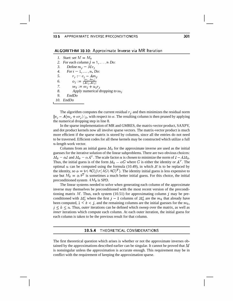
�� r\ �R� ��p&�� ;��;�� \�� &�� \�� 3�� n� �D�w�� #�� 1� � �� ,� � � �

1. Start: set �� 2. For each column �n� / �*¬*¬,¬T�I® Do:3. Define ± � �� Q �4. For Sª� / �,¬*¬*¬ �I® 5 Do:5.

+ � � � Q � ¨��Q± �6. � � � & � � + ( � � -&)( � � + ( � � -7. ± � � ��± � M � + �8. Apply numerical dropping to ± �9. EndDo

10. EndDo

The algorithm computes the current residual+ � and then minimizes the residual norm§ Q � ¨f��<o± � M + � =,§ « , with respect to . The resulting column is then pruned by applying

the numerical dropping step in line 8.In the sparse implementation of MR and GMRES, the matrix-vector product, SAXPY,

and dot product kernels now all involve sparse vectors. The matrix-vector product is muchmore efficient if the sparse matrix is stored by columns, since all the entries do not needto be traversed. Efficient codes for all these kernels may be constructed which utilize a full® -length work vector.

Columns from an initial guess � � for the approximate inverse are used as the initialguesses for the iterative solution of the linear subproblems. There are two obvious choices:� �7� & and � �X� � b . The scale factor is chosen to minimize the norm of

& ¨ � � � .Thus, the initial guess is of the form � �|� � where � is either the identity or � b . Theoptimal can be computed using the formula (10.49), in which � is to be replaced bythe identity, so �

�� <V� ��=�� <N�� <N��= b = . The identity initial guess is less expensive to

use but � � � � b is sometimes a much better initial guess. For this choice, the initialpreconditioned system � � � is SPD.

The linear systems needed to solve when generating each column of the approximateinverse may themselves be preconditioned with the most recent version of the precondi-tioning matrix � . Thus, each system (10.51) for approximating column � may be pre-conditioned with � �� where the first ��¨ / columns of � �� are the ± � that already havebeen computed, / !� ² � , and the remaining columns are the initial guesses for the ± � ,��!� !�® . Thus, outer iterations can be defined which sweep over the matrix, as well asinner iterations which compute each column. At each outer iteration, the initial guess foreach column is taken to be the previous result for that column.

$��! � �� ; =?0F7:A!0 ; 2 �1'56 �+7:9 *32#4501A '3; 2 7:9 *

The first theoretical question which arises is whether or not the approximate inverses ob-tained by the approximations described earlier can be singular. It cannot be proved that �is nonsingular unless the approximation is accurate enough. This requirement may be inconflict with the requirement of keeping the approximation sparse.

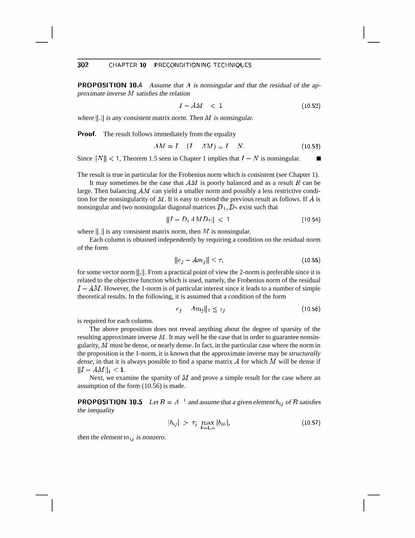
��r¶ � ~�� &�� \�� &^� \��0� � �°&� � ~ �0� ��?��R� �n� �� D��

Assume that � is nonsingular and that the residual of the ap-proximate inverse � satisfies the relation

§ & ¨�� § ² / £ ¥��L[ .//¦where §4¬T§ is any consistent matrix norm. Then � is nonsingular.

�� The result follows immediately from the equality

� � � & ¨ < & ¨�� = � & ¨ �f¬ £ ¥��L[ ./µ/¦Since § �³§X² / , Theorem 1.5 seen in Chapter 1 implies that

& ¨ � is nonsingular.

The result is true in particular for the Frobenius norm which is consistent (see Chapter 1).It may sometimes be the case that � � is poorly balanced and as a result � can be

large. Then balancing � � can yield a smaller norm and possibly a less restrictive condi-tion for the nonsingularity of � . It is easy to extend the previous result as follows. If � isnonsingular and two nonsingular diagonal matrices � B � � « exist such that

§ & ¨ � B �� «L§ ² / £ ¥��L[ . $�¦where §4¬T§ is any consistent matrix norm, then � is nonsingular.

Each column is obtained independently by requiring a condition on the residual normof the form

§ Q � ¨��Q± � §,! �,� £ ¥��L[ . ./¦for some vector norm §4¬T§ . From a practical point of view the 2-norm is preferable since it isrelated to the objective function which is used, namely, the Frobenius norm of the residual& ¨f�� . However, the 1-norm is of particular interest since it leads to a number of simpletheoretical results. In the following, it is assumed that a condition of the form

§ Q � ¨©�7± � § B ! � � £ ¥��L[ . 1/¦is required for each column.

The above proposition does not reveal anything about the degree of sparsity of theresulting approximate inverse � . It may well be the case that in order to guarantee nonsin-gularity, � must be dense, or nearly dense. In fact, in the particular case where the norm inthe proposition is the 1-norm, it is known that the approximate inverse may be structurallydense, in that it is always possible to find a sparse matrix � for which � will be dense if§ & ¨�� § B ² / .Next, we examine the sparsity of � and prove a simple result for the case where anassumption of the form (10.56) is made.

�R� �n� �� D�� Let �� @�B and assume that a given element 5 � of � satisfies

the inequality � 5 � � � � � � � �� B + I � 5 � � � £ ¥��L[ . 2/¦then the element ± 5 � is nonzero.

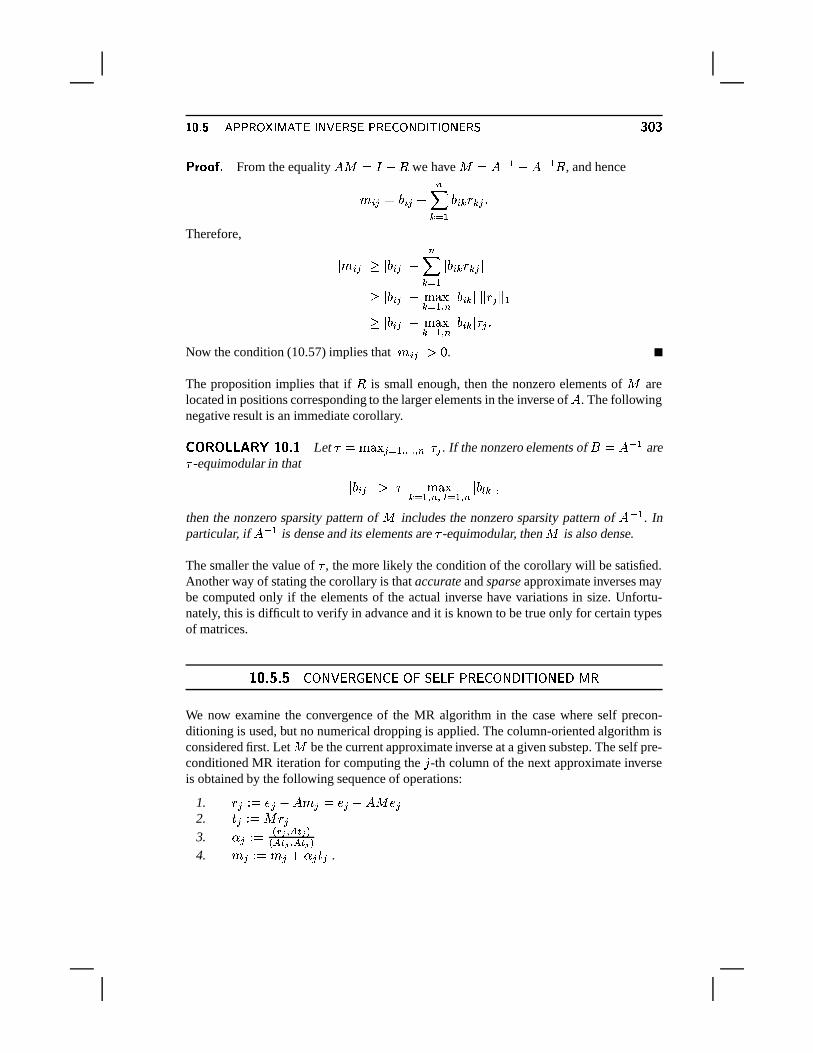
�� r\ �R� ��p&�� ;��;�� \�� &�� \�� ;��

From the equality �� & ¨�� we have � �¢� @�B ¨�� @�B � , and hence

± 5 � �¢ 5 � ¨ I� � B 5 � + � � ¬

Therefore, � ±�5 � � � � A5 � ��¨ I� � B � 5 � + � � �� 5 � ��¨ � � �� B + I � 5 � �%§ + � § B� � 5 � ��¨ � � �� B + I � 5 � � � � ¬

Now the condition (10.57) implies that � ± 5 � � � -.

The proposition implies that if � is small enough, then the nonzero elements of � arelocated in positions corresponding to the larger elements in the inverse of � . The followingnegative result is an immediate corollary.

� �n� � � �%�|� � ��#�Let �v� � � � � � B +�� + I � � . If the nonzero elements of �� @�B are

� -equimodular in that � A5 � � � �� B + I + � � B + I � � � � �

then the nonzero sparsity pattern of � includes the nonzero sparsity pattern of � @�B . Inparticular, if � @�B is dense and its elements are � -equimodular, then � is also dense.

The smaller the value of � , the more likely the condition of the corollary will be satisfied.Another way of stating the corollary is that accurate and sparse approximate inverses maybe computed only if the elements of the actual inverse have variations in size. Unfortu-nately, this is difficult to verify in advance and it is known to be true only for certain typesof matrices.

$��! �� +7:9 �>01A1&)019 ��0D7 � * 036 � �!A!0 ��7�9)4?2 ; 2 7:9?014 BDA

We now examine the convergence of the MR algorithm in the case where self precon-ditioning is used, but no numerical dropping is applied. The column-oriented algorithm isconsidered first. Let � be the current approximate inverse at a given substep. The self pre-conditioned MR iteration for computing the � -th column of the next approximate inverseis obtained by the following sequence of operations:

1.+ � � � Q � ¨��Q± � � Q � ¨�� Q �

2.� � � �� + �

3. � � � & � � + ( � � -&)( � � + ( � � -4. ± � � ��± � M � � � .

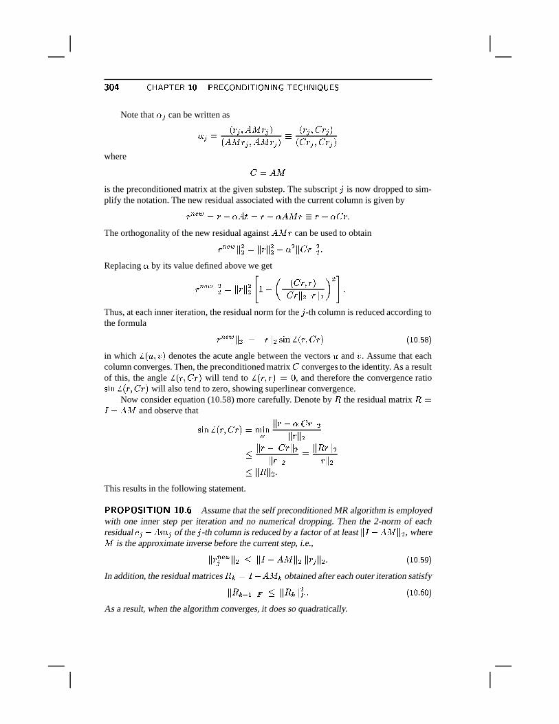
�� ~�� &�� \�� &^� \��0� � �°&� � ~ �0� ��?�Note that � can be written as

� � < + � �S�� + � =<N�� + � �S�� + � = � < + � � + � =<� + � � + � =where

a�� is the preconditioned matrix at the given substep. The subscript � is now dropped to sim-plify the notation. The new residual associated with the current column is given by+ I JLK � + ¨ � � � + ¨ �� +�� + ¨ + ¬The orthogonality of the new residual against � � +

can be used to obtain

§ + IJLK § «« �z§ + § «« ¨ « § + § «« ¬Replacing by its value defined above we get

§ + IJLK § «« ��§ + § «« � / ¨ % < + � + =§ + §*«%§ + §*« ) « � ¬

Thus, at each inner iteration, the residual norm for the � -th column is reduced according tothe formula

§ + IJLK § « � § + § « � � 9 � < + � + = £ ¥��L[ . ¤ ¦in which

� < ´ � � = denotes the acute angle between the vectors´

and � . Assume that eachcolumn converges. Then, the preconditioned matrix converges to the identity. As a resultof this, the angle

� < + � + = will tend to� < + � + = � -

, and therefore the convergence ratio� � 9 � < + � + = will also tend to zero, showing superlinear convergence.Now consider equation (10.58) more carefully. Denote by � the residual matrix ��& ¨�� and observe that

� � 9 � < + � + =R� � � 9�

§ + ¨ + §*«§ + § «! § + ¨ + §K«

§ + §*« � § � + §*«§ + §K«!a§ ��§K«4¬

This results in the following statement.

�R� �n� �� D�� Assume that the self preconditioned MR algorithm is employed

with one inner step per iteration and no numerical dropping. Then the 2-norm of eachresidual Q � ¨f�Q± � of the � -th column is reduced by a factor of at least § & ¨f� � §�« , where� is the approximate inverse before the current step, i.e.,

§ + IJLK� § « ! § & ¨©�� § « § + � § « ¬ £ ¥��L[ . �/¦In addition, the residual matrices � � � & ¨v� � � obtained after each outer iteration satisfy

§ � � � B § � ! § � � § «� ¬ £ ¥��L[ 1 �/¦As a result, when the algorithm converges, it does so quadratically.

�� r\ �R� ��p&�� ;��;�� \�� &�� \��

Inequality (10.59) was proved above. To prove quadratic convergence, first usethe inequality § �¡§,« !a§ �¡§ �

and (10.59) to obtain

§ + IJLK� §*« !�§ � � + � § � § + � §K«9¬Here, the � index corresponds to the outer iteration and the � -index to the column. Note thatthe Frobenius norm is reduced for each of the inner steps corresponding to the columns,and therefore,

§ � � + � § � ! § � � § � ¬This yields

§ + IJ/K� § «« !�§ � �p§ «� § + � § ««which, upon summation over � , gives

§ � � � B § � !a§ � � § «� ¬This completes the proof.

Note that the above theorem does not prove convergence. It only states that when the al-gorithm converges, it does so quadratically at the limit. In addition, the result ceases to bevalid in the presence of dropping.

Consider now the case of the global iteration. When self preconditioning is incor-porated into the global MR algorithm (Algorithm 10.8), the search direction becomes � � � � � � , where � � is the current residual matrix. Then, the main steps of the al-gorithm (without dropping) are as follows.

1. � � � � & ¨�� 2.

� � �� 3. � � � � � � + ( � �� ( � � + ( � � �4. � � � B � � � � M � �

At each step the new residual matrix � � � B satisfies the relation

� � � B � & ¨�� B � & ¨�� < � � M � � =�� 7¨ �4� ��¬An important observation is that � � is a polynomial in � � . This is because, from the aboverelation,

� � � B �� X¨ �4�� w� � ��¨ ��< & ¨ � � =�� |� < / ¨ � = � � M � � «� ¬ £ ¥ �L[ 1E¥K¦Therefore, induction shows that � � � B � � « � <�� = where � � is a polynomial of degree � .Now define the preconditioned matrices,

� � � �� & ¨�� ¬ £ ¥ �L[ 1,�¦Then, the following recurrence follows from (10.61),

� � � B � � � M � � � < & ¨�� = £ ¥ �L[ 1,µ�¦and shows that � � � B is also a polynomial of degree

0 � in �� . In particular, if the initial�� is symmetric, then so are all subsequent � � ’s. This is achieved when the initial � is amultiple of � b , namely if � �X� �/� b .

�� ~�� &�� \�� &^� \��0� � �°&� � ~ �0� ��?�Similar to the column oriented case, when the algorithm converges it does so quadrat-

ically.

�R� �n� �� D�� Assume that the self preconditioned global MR algorithm is

used without dropping. Then, the residual matrices obtained at each iteration satisfy

§ � � � B § � !a§ � «� § � ¬ £ ¥��L[ 1 $�¦As a result, when the algorithm converges, then it does so quadratically.

�� Define for any ,

� < =^� < / ¨ = � � M � «�Recall that � achieves the minimum of § � < =*§ �

over all ’s. In particular,

§ � � � B § � � �� 9�§ � < =*§ �!g§ � < / =,§ � ��§ � «� § � £ ¥��L[ 1 ./¦!g§ � �p§ «� ¬

This proves quadratic convergence at the limit.

For further properties see Exercise 16.

$��! �� ' � ;?7:A!014 ' � �+A 7 2 BC'3;>0@2#9 �>01A1*10,*

A notable disadvantage of the right or left preconditioning approach method is that it isdifficult to assess in advance whether or not the resulting approximate inverse � is non-singular. An alternative would be to seek a two-sided approximation, i.e., a pair

�,�

, with�lower triangular and

�upper triangular, which attempts to minimize the objective func-

tion (10.45). The techniques developed in the previous sections can be exploited for thispurpose.

In the factored approach, two matrices�

and�

which are unit lower and upper trian-gular matrices are sought such that

� � �� where � is some unknown diagonal matrix. When � is nonsingular and

� � � � � , then� � � are called inverse LU factors of � since in this case � @�B � � � @�B � . Once more, thematrices are built one column or row at a time. Assume as in Section 10.4.5 that we havethe sequence of matrices

� � � B � % � � � �� B )in which � I � � . If the inverse factors

� �.� � � are available for � � , i.e.,� �4� � � �W� � ��

�� r\ �R� ��p&�� ;��;�� \�� &�� \�� then the inverse factors

� � � B � � � � B for � � � B are easily obtained by writing% � � -¨ � / )

% � � � �� B )% � � ¨�2 �- / ) � %

� � -- O � � B ) £ ¥ �L[ 1 1�¦in which 2 � ,

� , and

O � � B are such that

� �%2 �W� � � £ ¥ �L[ 1 2�¦�� w� � � £ ¥ �L[ 1 ¤ ¦O � � B � � � B ¨ � �%2 �W� � � B ¨ � � ��¬ £ ¥ �L[ 1 ��¦

Note that the formula (10.69) exploits the fact that either the system (10.67) is solvedexactly (middle expression) or the system (10.68) is solved exactly (second expression) orboth systems are solved exactly (either expression). In the realistic situation where neitherof these two systems is solved exactly, then this formula should be replaced by

O � � B � � � B ¨ � � 2 � ¨ � � � M � � � 2 � ¬ £ ¥ �L[ 2 ��¦The last row/column pairs of the approximate factored inverse can be obtained by solvingtwo sparse systems and computing a few dot products. It is interesting to note that the onlydifference with the ILUS factorization seen in Section 10.4.5 is that the coefficient matricesfor these systems are not the triangular factors of � � , but the matrix � � itself.

To obtain an approximate factorization, simply exploit the fact that the � � matrices aresparse and then employ iterative solvers in sparse-sparse mode. In this situation, formula(10.70) should be used for

O � � B . The algorithm would be as follows.

�� n� �D�w�� #�,�� 1� � �� v� � � �� 1. For � � / �*¬,¬*¬T�S® Do:2. Solve (10.67) approximately;3. Solve (10.68) approximately;4. Compute

O � � B � � � B ¨ � � 2 � ¨ � � � M � � � 2 �5. EndDo

A linear system must be solved with � � in line 2 and a linear system with � b � in line 3.This is a good scenario for the Biconjugate Gradient algorithm or its equivalent two-sidedLanczos algorithm. In addition, the most current approximate inverse factors can be usedto precondition the linear systems to be solved in steps 2 and 3. This was termed “selfpreconditioning” earlier. All the linear systems in the above algorithm can be solved inparallel since they are independent of one another. The diagonal � can then be obtained atthe end of the process.

This approach is particularly suitable in the symmetric case. Since there is only onefactor, the amount of work is halved. In addition, there is no problem with the existencein the positive definite case as is shown in the following lemma which states that

O � � B isalways � -

when � is SPD, independently of the accuracy with which the system (10.67)is solved.

�C� �� #�Let � be SPD. Then, the scalar

O � � B as computed by (10.70) is positive.

�� ~�� &�� \�� &^� \��0� � �°&� � ~ �0� ��?��

In the symmetric case, � �w� � b� . Note thatO � � B as computed by formula (10.70)

is the <�� M / � � M / = element of the matrix� � � B � � � B � b � � B . It is positive because � � � B is

SPD. This is independent of the accuracy for solving the system to obtain 2 � .In the general nonsymmetric case, there is no guarantee that

O � � B will be nonzero,unless the systems (10.67) and (10.68) are solved accurately enough. There is no practicalproblem here, since

O � � B is computable. The only question remaining is a theoretical one:Can

O � � B be guaranteed to be nonzero if the systems are solved with enough accuracy?Intuitively, if the system is solved exactly, then the � matrix must be nonzero since it isequal to the � matrix of the exact inverse factors in this case. The minimal assumption tomake is that each � � is nonsingular. Let

O #� � B be the value that would be obtained if at leastone of the systems (10.67) or (10.68) is solved exactly. According to equation (10.69), inthis situation this value is given by

O #� � B � � � B ¨ � �4� @�B� � ��¬ £ ¥��L[ 29¥G¦If � � � B is nonsingular, then

O #� � B �� -. To see this refer to the defining equation (10.66)

and compute the product� � � B � � � B � � � B in the general case. Let

+ � and � � be the residualsobtained for these linear systems, i.e.,+ � � � � ¨�� 2 � � � � � � � ¨ � � � ¬ £ ¥��L[ 2//¦Then a little calculation yields

� � � B � � � B � � � B � % � �� + �� O � � B ) ¬ £ ¥��L[ 2/µ/¦

If one of+ � or � � is zero, then it is clear that the term

O � � B in the above relation be-comes

O #� � B and it must be nonzero since the matrix on the left-hand side is nonsingular.Incidentally, this relation shows the structure of the last matrix

� I � I � I � � � � . Thecomponents / to �|¨ / of column � consist of the vector

� � + � , the components 1 to �m¨ /of row S make up the vector � � � � , and the diagonal elements are theO 5 ’s. Consider now

the expression forO � � B from (10.70).

O � � B � � � B ¨ � � 2 �Q¨ � � � M �� 2 �� B ¨ � �9� @�B� < � ��¨ + �?=0¨ < � ��¨ � � =I� @�B� � � M < � ��¨ + � =q� @�B� < � ��¨ � �?=� � � B ¨ � �4� @�B� � � M + �4� @�B� � �� O #� � B M + � � @�B� � � ¬

This perturbation formula is of a second order in the sense that � O � � B ¨ O #� � B �¡�( <S§ + �p§�§ � � §�= . It guarantees thatO � � B is nonzero whenever � + �4� @�B� � � � ² � O #� � B � .

$��! � �� 2 B �+A 7 � 2#9 & '��!A!0 ��7�9)4?2 ; 2 7:9?01A

After a computed ILU factorization results in an unsatisfactory convergence, it is difficultto improve it by modifying the

�and

�factors. One solution would be to discard this

factorization and attempt to recompute a fresh one possibly with more fill-in. Clearly, thismay be a wasteful process. A better alternative is to use approximate inverse techniques.Assume a (sparse) matrix � is a preconditioner to the original matrix � , so the precondi-

�� /\ � � �� \�� &�� \��;�� r·tioned matrix is

�� @�B � ¬A sparse matrix � is sought to approximate the inverse of � @�B � . This matrix is then to beused as a preconditioner to � @�B � . Unfortunately, the matrix is usually dense. However,observe that all that is needed is a matrix � such that

� � � �g¬Recall that the columns of � and � are sparse. One approach is to compute a least-squaresapproximation in the Frobenius norm sense. This approach was used already in Section10.5.1 when � is the identity matrix. Then the columns of � were obtained by approxi-mately solving the linear systems �� 5 � Q 5 . The same idea can be applied here. Now, thesystems

�� 5 ��± 5must be solved instead, where ± 5 is the S -th column of � which is sparse. Thus, thecoefficient matrix and the right-hand side are sparse, as before.

�w� �D� � �X�X��Q�f�N�v�H��-�f�n�Z�R��v� �

Block preconditioning is a popular technique for block-tridiagonal matrices arising fromthe discretization of elliptic problems. It can also be generalized to other sparse matrices.We begin with a discussion of the block-tridiagonal case.

$��! ��! %$ � 6 7 �� -L;>A+2#4?2 '�& 7:9+'56 BC'�; A+2 ��0,*

Consider a block-tridiagonal matrix blocked in the form

�!�� B � «� « � « � �

. . .. . .

. . .� D @�B � D @�B � D� D � D�� ¬ £ ¥ �L[ 2�$4¦

One of the most popular block preconditioners used in the context of PDEs is based onthis block-tridiagonal form of the coefficient matrix � . Let � be the block-diagonal matrixconsisting of the diagonal blocks � 5 , � the block strictly-lower triangular matrix consistingof the sub-diagonal blocks � 5 , and

�the block strictly-upper triangular matrix consisting

of the super-diagonal blocks � 5 . Then, the above matrix has the form

�!� � M � M � ¬

�� ~�� &�� \�� &^� \��0� � �°&� � ~ �0� ��?�A block ILU preconditioner is defined by

� � < � M � = � @�B < � M � = � £ ¥��L[ 2 ./¦where

�and

�are the same as above, and � is a block-diagonal matrix whose blocks � 5

are defined by the recurrence:

��5ª� � 5 ¨ � 5 � 5 @�B � 5�� £ ¥��L[ 2 1/¦in which

� � is some sparse approximation to � @�B� . Thus, to obtain a block factorization,approximations to the inverses of the blocks � 5 must be found. This clearly will lead todifficulties if explicit inverses are used.

An important particular case is when the diagonal blocks � 5 of the original matrix aretridiagonal, while the co-diagonal blocks � 5 and � 5 are diagonal. Then, a simple recur-rence formula for computing the inverse of a tridiagonal matrix can be exploited. Only thetridiagonal part of the inverse must be kept in the recurrence (10.76). Thus,

� B � � B � £ ¥��L[ 2 2/¦� 5 � � 5 ¨ � 5 � & � -5 @�B � 5 � S(� / �,¬*¬,¬ �I± � £ ¥��L[ 2 ¤ ¦

where� & � -� is the tridiagonal part of � @�B� .< � & � -� = 5 + � � < � @�B� = 5 + � for � Sc¨ �� ! / ¬

The following theorem can be shown.

�w�|��n�]� �� Let � be Symmetric Positive Definite and such that

� 5 5 � - � S(� / �,¬*¬,¬T�I® , and � 5 � ! -for all � �� S .

The matrices � 5 are all (strict) diagonally dominant.

Then each block � 5 computed by the recurrence (10.77), (10.78) is a symmetric � -matrix.In particular, � is also a positive definite matrix.

We now show how the inverse of a tridiagonal matrix can be obtained. Let a tridiagonalmatrix � of dimension � be given in the form

� �� B ¨ �C«¨ � « « ¨ � �

. . .. . .

. . .¨ � � @�B � @�B ¨ � �¨ � � �

��

and let its Cholesky factorization be

� � � � � b �with

� �: � � � � O 5 �

�� \�� &�� \�� /\�v&�~ ��}\�� p&�� \�� ,�and

� ��

/¨ � « /. . . . . .¨ � � @�B /¨ � � /

� �� ¬

The inverse of � is� @ b � @�B � @�B . Start by observing that the inverse of

� bis a unit upper

triangular matrix whose coefficients´ 5 � are given by´ 5 � � � 5 � B � 5 � « ¬*¬,¬ � � @�B � � for / ! S^² ��² �q¬

As a result, the � -th column � � of� @ b is related to the < �W¨ / = -st column � � @�B by the very

simple recurrence,

� � � Q � M� � � � @�B � for � � 0starting with the first column � B � Q B . The inverse of � becomes

� @�B2� � @ b � @�B � @�BZ� �� B /O � � � � b� ¬ £ ¥ �L[ 2 ��¦See Exercise 12 for a proof of the above equality. As noted, the recurrence formulas forcomputing � @�B can be unstable and lead to numerical difficulties for large values of � .

$��! �! #" &)019?01A�'56 BC'3;>A+2 ��0,*

A general sparse matrix can often be put in the form (10.74) where the blocking is ei-ther natural as provided by the physical problem, or artificial when obtained as a result ofRCMK ordering and some block partitioning. In such cases, a recurrence such as (10.76)can still be used to obtain a block factorization defined by (10.75). A 2-level precondi-tioner can be defined by using sparse inverse approximate techniques to approximate

� 5 .These are sometimes termed implicit-explicit preconditioners, the implicit part referring tothe block-factorization and the explicit part to the approximate inverses used to explicitlyapproximate � @�B5 .

��7��2��C�v�t��D�f�n�]�]� � ��a�u�n�z�w��0��Q��D�f�W��v��

When the original matrix is strongly indefinite, i.e., when it has eigenvalues spread on bothsides of the imaginary axis, the usual Krylov subspace methods may fail. The ConjugateGradient approach applied to the normal equations may then become a good alternative.Choosing to use this alternative over the standard methods may involve inspecting the spec-trum of a Hessenberg matrix obtained from a small run of an unpreconditioned GMRESalgorithm.

��%¶ � ~�� &�� \�� &^� \��0� � �°&� � ~ �0� ��?�If the normal equations approach is chosen, the question becomes how to precondition

the resulting iteration. An ILU preconditioner can be computed for � and the precondi-tioned normal equations,

� b < �� = @ b < �� = @�B �Q��¢� b < � � = @ b < � � = @�B ��can be solved. However, when � is not diagonally dominant the ILU factorization pro-cess may encounter a zero pivot. Even when this does not happen, the resulting precon-ditioner may be of poor quality. An incomplete factorization routine with pivoting, suchas ILUTP, may constitute a good choice. ILUTP can be used to precondition either theoriginal equations or the normal equations shown above. This section explores a few otheroptions available for preconditioning the normal equations.

$��! ��! %$ � ' �+7 � 2�� *F7:A��' 9?4 ��' A+2 ' 9+;)*

There are several ways to exploit the relaxation schemes for the Normal Equations seen inChapter 8 as preconditioners for the CG method applied to either (8.1) or (8.3). Consider(8.3), for example, which requires a procedure delivering an approximation to <N�7� b = @�B �for any vector � . One such procedure is to perform one step of SSOR to solve the system<N�X� b = � � � . Denote by � @�B the linear operator that transforms � into the vector result-ing from this procedure, then the usual Conjugate Gradient method applied to (8.3) canbe recast in the same form as Algorithm 8.5. This algorithm is known as CGNE/SSOR.Similarly, it is possible to incorporate the SSOR preconditioning in Algorithm 8.4, whichis associated with the Normal Equations (8.1), by defining � @�B to be the linear transfor-mation that maps a vector � into a vector � resulting from the forward sweep of Algorithm8.2 followed by a backward sweep. We will refer to this algorithm as CGNR/SSOR.

The CGNE/SSOR and CGNR/SSOR algorithms will not break down if � is nonsin-gular, since then the matrices �X� b and � b � are Symmetric Positive Definite, as are thepreconditioning matrices � . There are several variations to these algorithms. The standardalternatives based on the same formulation (8.1) are either to use the preconditioner on theright, solving the system � b � � @�B � , or to split the preconditioner into a forwardSOR sweep on the left and a backward SOR sweep on the right of the matrix � b � . Sim-ilar options can also be written for the Normal Equations (8.3) again with three differentways of preconditioning. Thus, at least six different algorithms can be defined.

$��! ��! " 2 � �� 7:A ; =?0@9�7:A!B '56D0FEG( '3; 2 7:9 *

The Incomplete Cholesky IC(0) factorization can be used to precondition the NormalEquations (8.1) or (8.3). This approach may seem attractive because of the success ofincomplete factorization preconditioners. However, a major problem is that the Incom-plete Cholesky factorization is not guaranteed to exist for an arbitrary Symmetric Pos-itive Definite matrix � . All the results that guarantee existence rely on some form ofdiagonal dominance. One of the first ideas suggested to handle this difficulty was touse an Incomplete Cholesky factorization on the “shifted” matrix � M & . We refer toIC(0) applied to � � � b � as ICNR(0), and likewise IC(0) applied to � � �X� b

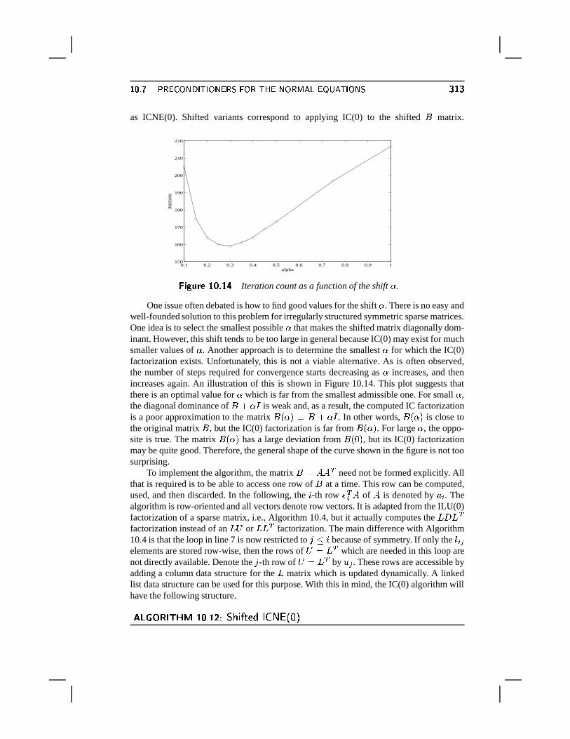
�� \�� &�� \�� /\�v&�~ ��}\�� p&�� \�� as ICNE(0). Shifted variants correspond to applying IC(0) to the shifted � matrix.

0.1 0.2 0.3 0.4 0.5 0.6 0.7 0.8 0.9 1150

160

170

180

190

200

210

220

alpha

itera

tions

�� #� �Iteration count as a function of the shift .

One issue often debated is how to find good values for the shift . There is no easy andwell-founded solution to this problem for irregularly structured symmetric sparse matrices.One idea is to select the smallest possible that makes the shifted matrix diagonally dom-inant. However, this shift tends to be too large in general because IC(0) may exist for muchsmaller values of . Another approach is to determine the smallest for which the IC(0)factorization exists. Unfortunately, this is not a viable alternative. As is often observed,the number of steps required for convergence starts decreasing as increases, and thenincreases again. An illustration of this is shown in Figure 10.14. This plot suggests thatthere is an optimal value for which is far from the smallest admissible one. For small ,the diagonal dominance of � M & is weak and, as a result, the computed IC factorizationis a poor approximation to the matrix ��< = � � M & . In other words, � < = is close tothe original matrix � , but the IC(0) factorization is far from � < = . For large , the oppo-site is true. The matrix � < = has a large deviation from � < - = , but its IC(0) factorizationmay be quite good. Therefore, the general shape of the curve shown in the figure is not toosurprising.

To implement the algorithm, the matrix � �g�7� b need not be formed explicitly. Allthat is required is to be able to access one row of � at a time. This row can be computed,used, and then discarded. In the following, the S -th row Q b5 � of � is denoted by � 5 . Thealgorithm is row-oriented and all vectors denote row vectors. It is adapted from the ILU(0)factorization of a sparse matrix, i.e., Algorithm 10.4, but it actually computes the

� � � bfactorization instead of an

��or� � b

factorization. The main difference with Algorithm10.4 is that the loop in line 7 is now restricted to � !<S because of symmetry. If only the � 5 �elements are stored row-wise, then the rows of

� � � b which are needed in this loop arenot directly available. Denote the � -th row of

� � � b by´ � . These rows are accessible by

adding a column data structure for the�

matrix which is updated dynamically. A linkedlist data structure can be used for this purpose. With this in mind, the IC(0) algorithm willhave the following structure.

�� n� �D�w�� #�%¶ � � � � � �� #�W�m� � � �

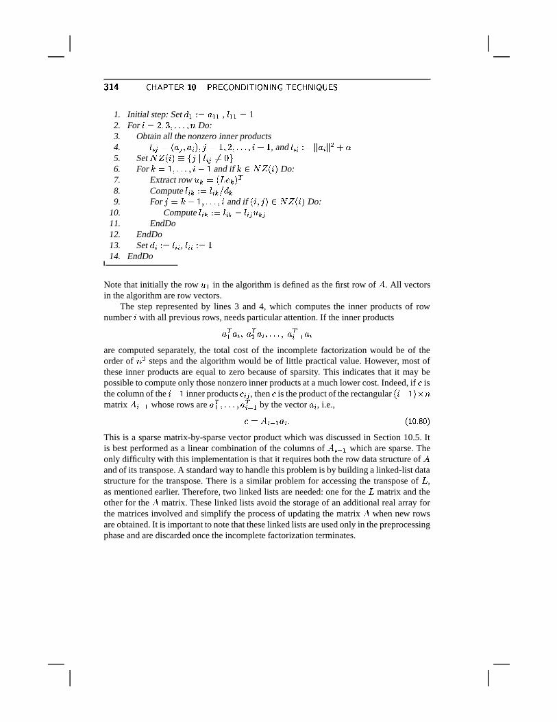
�� ~�� &�� \�� &^� \��0� � �°&� � ~ �0� ��?�1. Initial step: Set � B � � � B B , � B B � /2. For Sª� 0 ��F�*¬*¬,¬T�I® Do:3. Obtain all the nonzero inner products4. � 5 � � < � � � � 5 =T� �n� / � 0 �,¬*¬,¬ ��Si¨ / , and � 5 5 � ��§ � 5 § « M 5. Set � < S = � � � � � 5 � �� - �6. For �� / �*¬,¬*¬T� Si¨ / and if � � � <%S = Do:7. Extract row

´ � � < � Q � = b8. Compute � 5 � � � � 5 � � � �9. For �m� � M / �*¬,¬*¬T� S and if < S�� = � � <%S = Do:

10. Compute � 5 � � � � 5 � ¨�� 5 � ´ � �11. EndDo12. EndDo13. Set � 5 � � � 5 5 , � 5 5 � � /14. EndDo

Note that initially the row´ B in the algorithm is defined as the first row of � . All vectors

in the algorithm are row vectors.The step represented by lines 3 and 4, which computes the inner products of row

number S with all previous rows, needs particular attention. If the inner products

�b B � 5 � � b« � 5 �*¬*¬,¬ � � b5 @�B � 5

are computed separately, the total cost of the incomplete factorization would be of theorder of ® « steps and the algorithm would be of little practical value. However, most ofthese inner products are equal to zero because of sparsity. This indicates that it may bepossible to compute only those nonzero inner products at a much lower cost. Indeed, if � isthe column of the S4¨ / inner products � 5 � , then � is the product of the rectangular <%S4¨ / =r¯Q®matrix �>5 @�B whose rows are � b B �*¬*¬,¬ �� b5 @�B by the vector � 5 , i.e.,

�Q�� 5 @�B � 5 ¬ £ ¥��L[ ¤ �/¦This is a sparse matrix-by-sparse vector product which was discussed in Section 10.5. Itis best performed as a linear combination of the columns of � 5 @�B which are sparse. Theonly difficulty with this implementation is that it requires both the row data structure of �and of its transpose. A standard way to handle this problem is by building a linked-list datastructure for the transpose. There is a similar problem for accessing the transpose of

�,

as mentioned earlier. Therefore, two linked lists are needed: one for the�

matrix and theother for the � matrix. These linked lists avoid the storage of an additional real array forthe matrices involved and simplify the process of updating the matrix � when new rowsare obtained. It is important to note that these linked lists are used only in the preprocessingphase and are discarded once the incomplete factorization terminates.

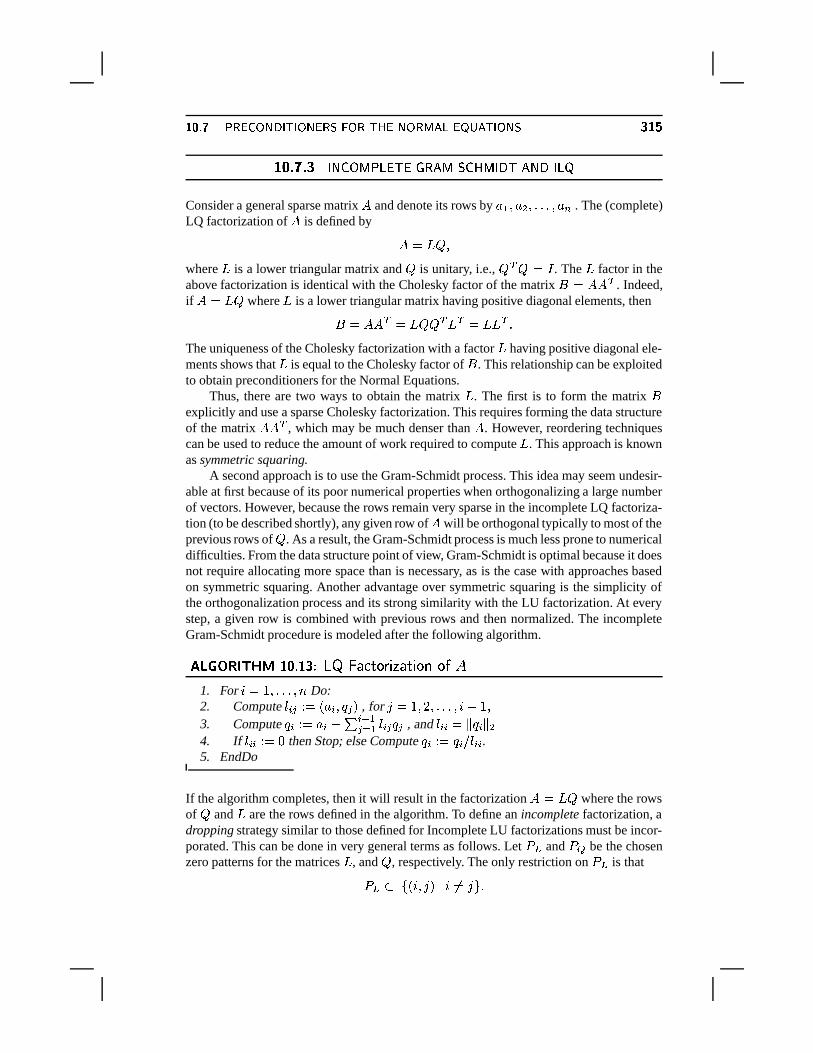
�� \�� &�� \�� /\�v&�~ ��}\�� p&�� \�� $��! ��! �� 2 9 �+7:B ��6,0 ; 0D&)A�' B�-/* ��=?B 2#4 ;P' 9?4 2 6 E

Consider a general sparse matrix � and denote its rows by � B ��%«�*¬,¬*¬T�� I . The (complete)LQ factorization of � is defined by

�¢� �� where

�is a lower triangular matrix and

�is unitary, i.e.,

� b � � &. The

�factor in the

above factorization is identical with the Cholesky factor of the matrix � �g�X� b . Indeed,if �¢� �� where

�is a lower triangular matrix having positive diagonal elements, then

��¢�7� b � �� b � b � � � b ¬The uniqueness of the Cholesky factorization with a factor

�having positive diagonal ele-

ments shows that�

is equal to the Cholesky factor of � . This relationship can be exploitedto obtain preconditioners for the Normal Equations.

Thus, there are two ways to obtain the matrix�

. The first is to form the matrix �explicitly and use a sparse Cholesky factorization. This requires forming the data structureof the matrix �X� b , which may be much denser than � . However, reordering techniquescan be used to reduce the amount of work required to compute

�. This approach is known

as symmetric squaring.A second approach is to use the Gram-Schmidt process. This idea may seem undesir-

able at first because of its poor numerical properties when orthogonalizing a large numberof vectors. However, because the rows remain very sparse in the incomplete LQ factoriza-tion (to be described shortly), any given row of � will be orthogonal typically to most of theprevious rows of

�. As a result, the Gram-Schmidt process is much less prone to numerical

difficulties. From the data structure point of view, Gram-Schmidt is optimal because it doesnot require allocating more space than is necessary, as is the case with approaches basedon symmetric squaring. Another advantage over symmetric squaring is the simplicity ofthe orthogonalization process and its strong similarity with the LU factorization. At everystep, a given row is combined with previous rows and then normalized. The incompleteGram-Schmidt procedure is modeled after the following algorithm.

�� n� �D�w�� #� � � � � �� 1. For S0� / �*¬*¬,¬T�I® Do:2. Compute � 5 � � � < � 5 � � � = , for �m� / � 0 �*¬*¬,¬T��Sc¨ / �3. Compute � 5 � � � 5 ¨ � 5 @�B� � B � 5 � � � , and � 5 5 ��§ � 5 §*«4. If � 5 5 � � -

then Stop; else Compute � 5 � � ��5 � � 5 5 .5. EndDo

If the algorithm completes, then it will result in the factorization � � �� where the rowsof�

and�

are the rows defined in the algorithm. To define an incomplete factorization, adropping strategy similar to those defined for Incomplete LU factorizations must be incor-porated. This can be done in very general terms as follows. Let

�� and

�� be the chosen

zero patterns for the matrices�

, and�

, respectively. The only restriction on

�� is that�

�

� � <%S�� = � S �� L¬

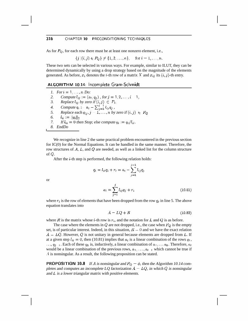
�� ~�� &�� \�� &^� \��0� � �°&� � ~ �0� ��?�As for

�� , for each row there must be at least one nonzero element, i.e.,�

� � <%S � � = � � � � �� / � 0 �,¬*¬*¬ �S® � � 7 ��S(� / �*¬*¬,¬T�I®(¬These two sets can be selected in various ways. For example, similar to ILUT, they can bedetermined dynamically by using a drop strategy based on the magnitude of the elementsgenerated. As before, ��5 denotes the S -th row of a matrix � and ��5 � its <%S�� = -th entry.

��n��-�w�� #� �� ,� � �K� � � � � �1. For Sª� / �*¬,¬*¬T�S® Do:2. Compute � 5 � � � < � 5 � � � = , for �m� / � 0 �*¬,¬*¬ � Si¨ / �3. Replace � 5 � by zero if <%S�� = � �

�4. Compute � 5 � � � 5}¨ � 5 @�B� � B � 5 � � � ,5. Replace each � 5 � � �n� / �*¬,¬*¬T�S® by zero if < S�� = � �

�

6. � 5 5 � ��§ � 5S§ «7. If � 5 5c� -

then Stop; else compute � 5 � � ��5 � � 5 5 .8. EndDo

We recognize in line 2 the same practical problem encountered in the previous sectionfor IC(0) for the Normal Equations. It can be handled in the same manner. Therefore, therow structures of � ,

�, and

�are needed, as well as a linked list for the column structure

of�

.After the S -th step is performed, the following relation holds:

� 5 � � 5 5 � 5 M + 5 � � 5 ¨ � @�B� � B � 5 � � �or

� 5 � �� B � 5 � � � M + 5 £ ¥��L[ ¤ ¥G¦where

+ 5 is the row of elements that have been dropped from the row � 5 in line 5. The aboveequation translates into

�¢� �� M � £ ¥��L[ ¤ /¦where � is the matrix whose S -th row is

+ 5 , and the notation for�

and�

is as before.The case where the elements in

�are not dropped, i.e., the case when

�� is the empty

set, is of particular interest. Indeed, in this situation, �g� -and we have the exact relation� � ��

. However,�

is not unitary in general because elements are dropped from�

. Ifat a given step � 5 5 � -

, then (10.81) implies that � 5 is a linear combination of the rows � B ,¬*¬,¬ , � � @�B . Each of these � � is, inductively, a linear combination of � B �*¬,¬*¬ � � . Therefore, � 5would be a linear combination of the previous rows, � B �*¬*¬,¬ �� 5 @�B which cannot be true if� is nonsingular. As a result, the following proposition can be stated.

�R� �n� �� D�� If � is nonsingular and

�� , then the Algorithm 10.14 com-

pletes and computes an incomplete LQ factorization �z� ��, in which

�is nonsingular

and�

is a lower triangular matrix with positive elements.

�� \�� &�� \�� /\�v&�~ ��}\�� p&�� \�� A major problem with the decomposition (10.82) is that the matrix

�is not orthogonal in

general. In fact, nothing guarantees that it is even nonsingular unless�

is not dropped orthe dropping strategy is made tight enough.

Because the matrix�

of the complete LQ factorization of � is identical with theCholesky factor of � , one might wonder why the IC(0) factorization of � does not alwaysexist while the ILQ factorization seems to always exist. In fact, the relationship betweenILQ and ICNE, i.e., the Incomplete Cholesky for � �a�X� b , can lead to a more rigorousway of choosing a good pattern for ICNE, as is explained next.

We turn our attention to Modified Gram-Schmidt. The only difference is that the row� � is updated immediately after an inner product is computed. The algorithm is describedwithout dropping for

�for simplicity.

�� n� �D�w�� #� �� '� � � � � � �,� � �G� � �� 1. For S0� / �*¬*¬,¬T�I® Do:2. � 5 � � � 53. For �m� / �,¬*¬*¬ ��Si¨ / , Do:

4. Compute � 5 � � � � - � < S�� = � � �< � 5 � � � = 7��

5. Compute � 5 � � � 5 ¨�� 5 � � � .6. EndDo7. � 5 5 � �z§ � 5 §K«8. If � 5 5ª� -

then Stop; else Compute � 5 � � � 5 � � 5 5 .9. EndDo

When � is nonsingular, the same result as before is obtained if no dropping is used on�

, namely, that the factorization will exist and be exact in that � � ��. Regarding the

implementation, if the zero pattern

�� is known in advance, the computation of the inner

products in line 4 does not pose a particular problem. Without any dropping in�

, thisalgorithm may be too costly in terms of storage. It is interesting to see that this algorithmhas a connection with ICNE, the incomplete Cholesky applied to the matrix �X� b . Thefollowing result is stated without proof.

�w�|��n�R� � �� Let � be an ®�¯w± matrix and let ��7� b . Consider a zero-pattern

set

�� which is such that for any / ! S � � � � ! ® , with Sm² � and Sn² � , the following

holds: <%S�� = � � � � 9;: <%S � ��= �� < � � ��= � � � ¬

Then the matrix�

obtained from Algorithm 10.15 with the zero-pattern set

�� is identi-

cal with the�

factor that would be obtained from the Incomplete Cholesky factorizationapplied to � with the zero-pattern set

�� .

For a proof, see [222]. This result shows how a zero-pattern can be defined which guaran-tees the existence of an Incomplete Cholesky factorization on �7� b .

�� ~�� &�� \�� &^� \��0� � �°&� � ~ �0� ��?��Z�5�w�t�]�ª�

1 Assume that`

is the Symmetric Positive Definite matrix arising from the 5-point finite differ-ence discretization of the Laplacean on a given mesh. We reorder the matrix using the red-blackordering and obtain the reordered matrix" e % � 4 �

�9� � ) �We then form the Incomplete Cholesky factorization on this matrix.�� Show the fill-in pattern for the IC(0) factorization for a matrix of size

�³e � )associated

with a � �� mesh.� � Show the nodes associated with these fill-ins on the 5-point stencil in the finite differencemesh. !� Give an approximate count of the total number of fill-ins when the original mesh is square,with the same number of mesh points in each direction. How does this compare with thenatural ordering? Any conclusions?

2 Consider a � � � tridiagonal nonsingular matrix`

.�� What can be said about its ILU(0) factorization (when it exists)?� � Suppose that the matrix is permuted (symmetrically, i.e., both rows and columns) using thepermutation � e�� !��!� ) � � � � �� Show the pattern of the permuted matrix.�� Show the locations of the fill-in elements in the ILU(0) factorization.�� Show the pattern of the ILU(1) factorization as well as the fill-ins generated.�� Show the level of fill of each element at the end of the ILU(1) process (including the

fill-ins). � What can be said of the ILU(2) factorization for this permuted matrix?

3 Assume that`

is the matrix arising from the 5-point finite difference discretization of an ellipticoperator on a given mesh. We reorder the original linear system using the red-black ordering andobtain the reordered linear system% � 4 �� ) % d 4d ) e % h 4h ) �� Show how to obtain a system (called the reduced system) which involves the variable

d only.� � Show that this reduced system is also a sparse matrix. Show the stencil associated withthe reduced system matrix on the original finite difference mesh and give a graph-theoryinterpretation of the reduction process. What is the maximum number of nonzero elementsin each row of the reduced system.

4 It was stated in Section 10.3.2 that for some specific matrices the ILU(0) factorization of`

canbe put in the form � e # � 6 �

'� 254 # � 6 � '

in which6 �

and6 �

are the strict-lower and -upper parts of`

, respectively.

�� ?�� }\�&�?� ��%·� � Characterize these matrices carefully and give an interpretation with respect to their adja-

cency graphs.� � Verify that this is true for standard 5-point matrices associated with any domain � . !� Is it true for 9-point matrices?� � Is it true for the higher level ILU factorizations?

5 Let`

be a pentadiagonal matrix having diagonals in offset positions6 � � 6*� ��0 ��

. Thecoefficients in these diagonals are all constants: � for the main diagonal and -1 for all others. Itis assumed that �� . Consider the ILU(0) factorization of

`as given in the form (10.20).

The elements � � of the diagonal�

are determined by a recurrence of the form (10.19).� � Show that � � � � � � for e:�� .� � Show that � � is a decreasing sequence. [Hint: Use induction]. !� Prove that the formal (infinite) sequence defined by the recurrence converges. What is itslimit?

6 Consider a matrix`

which is split in the form`¢e �� 6 ��6 �

, where��

is a block diag-onal matrix whose block-diagonal entries are the same as those of

`, and where

6 �is strictly

lower triangular and6 �

is strictly upper triangular. In some cases the block form of the ILU(0)factorization can be put in the form (Section 10.3.2):

� e # � 6 �'� 2�4 # � 6 � ' �

The block entries of�

can be defined by a simple matrix recurrence. Find this recurrence rela-tion. The algorithm may be expressed in terms of the block entries the matrix

`.

7 Generalize the formulas developed at the end of Section 10.6.1 for the inverses of symmetrictridiagonal matrices, to the nonsymmetric case.

8 Develop recurrence relations for Incomplete Cholesky with no fill-in (IC(0)), for 5-point matri-ces, similar to those seen in Section 10.3.4 for ILU(0). Same question for IC(1).

9 What becomes of the formulas seen in Section 10.3.4 in the case of a 7-point matrix (for three-dimensional problems)? In particular, can the ILU(0) factorization be cast in the form (10.20) inwhich

6 �is the strict-lower diagonal of

`and

6 �is the strict upper triangular part of

`, and�

is a certain diagonal?

10 Consider an arbitrary matrix`

which is split in the usual manner as` e � 6 � 6 �

, in which6 �and

6 �are the strict-lower and -upper parts of

`, respectively, and define, for any diagonal

matrix�

, the approximate factorization of`

given by� e # � 6 �

'� 2�4 # � 6 � ' �

Show how a diagonal�

can be determined such that`

and�

have the same diagonal elements.Find a recurrence relation for the elements of

�. Consider now the symmetric case and assume

that the matrix�

which is positive can be found. Write�

in the form� e # � 4� 6 � � 254� ' # � 4� 6 � � 2�4� ' � � 4 � � 4 �

What is the relation between this matrix and the matrix of the SSOR

#�'

preconditioning, in theparticular case when

� 2�4� e �+

? Conclude that this form of ILU factorization is in effect anSSOR preconditioning with a different relaxation factor � for each equation.

11 Consider a general sparse matrix`

(irregularly structured). We seek an approximate LU factor-ization of the form � e # � 6 �

'� 2�4 # � 6 � '

�p¶�� ~�� &�� \�� &^� \��0� � �°&� � ~ �0� ��?�in which

6 �and

6 �are the strict-lower and -upper parts of

`, respectively. It is assumed that`

is such that� � � � 0 � � � � � � � � 0 for ��Xe�� By identifying the diagonal elements of

`with those of

�, derive an algorithm for generat-

ing the elements of the diagonal matrix�

recursively.� � Establish that if � � � 0 for� � then � � � � � � . Is it true in general that � � � 0 for all

�? !� Assume that for e ��96 �

we have � � �% ��0

. Show a sufficient condition underwhich � � �

%. Are there cases in which this condition cannot be satisfied for any

%?� � Assume now that all diagonal elements of

àre equal to a constant, i.e., � � � e � for

� e�� . Define

% � and let

� � � 254�� 4 �

� � � � � �� 4 � � � � � � � �

Show a condition on�

under which � � �% ��7e�� ) ��

12 Show the second part of (10.79). [Hint: Exploit the formula` " � e � � � 4 � � h �� where � � �_h �

are the�-th columns of

ànd

", respectively].

13 Let a preconditioning matrix�

be related to the original matrix`

by��e�` � �

, in which�is a matrix of rank � .�� Assume that both

ànd

�are Symmetric Positive Definite. How many steps at most are

required for the preconditioned Conjugate Gradient method to converge when�

is used asa preconditioner?� � Answer the same question for the case when

ànd

�are nonsymmetric and the full GM-

RES is used on the preconditioned system.

14 Formulate the problem for finding an approximate inverse�

to a matrix`

as a large� � �

linear system. What is the Frobenius norm in the space in which you formulate this problem?

15 The concept of mask is useful in the global iteration technique. For a sparsity pattern�

, i.e., a setof pairs

# ��'

and a matrix

", we define the product � e

"�� to be the matrix whose elements/ � � are zero if

# ��'

does not belong to�

, andh�� otherwise. This is called a mask operation

since its effect is to ignore every value not in the pattern�

. Consider a global minimization ofthe function

�� # � ' � ��=#&+ 6�` � ' �� .�� What does the result of Proposition 10.3 become for this new objective function?� � Formulate an algorithm based on a global masked iteration, in which the mask is fixed and

equal to the pattern of`

. !� Formulate an algorithm in which the mask is adapted at each outer step. What criteria wouldyou use to select the mask?

16 Consider the global self preconditioned MR iteration algorithm seen in Section 10.5.5. Definethe acute angle between two matrices as

�� #�� ! ' "� � $#

�� Following what was done for the (standard) Minimal Residual algorithm seen in Chapter 5,

establish that the matrices

" � e ` � �and % � e

+ 6 " �produced by global MR without

dropping are such that

�&% �� 4 �� % � �� ')( � # % � �" � % �

' �

�� ?�� }\�&�?� �p¶�� Let now

� e % ` �so that

" �is symmetric for all � (see Section 10.5.5). Assume that, at

a given step � the matrix

" �is positive definite. Show that

�� # % � �" � % �

'�� #?" � '��#?" � '

in which�� #?" � '

and��#?" � '

are, respectively, the smallest and largest eigenvalues of" �.

17 In the two-sided version of approximate inverse preconditioners, the option of minimizing

�#� � � ' e �

+ 6 �i` � � �was mentioned, where

�is unit lower triangular and

�is upper triangular.� � What is the gradient of

�#� � � '

?� � Formulate an algorithm based on minimizing this function globally.

18 Consider the two-sided version of approximate inverse preconditioners, in which a unit lowertriangular

�and an upper triangular

�are sought so that

�i` ��+

. One idea is to use analternating procedure in which the first half-step computes a right approximate inverse

�to�i`

,which is restricted to be upper triangular, and the second half-step computes a left approximateinverse

�to` �

, which is restricted to be lower triangular.� � Consider the first half-step. Since the candidate matrix�

is restricted to be upper trian-gular, special care must be exercised when writing a column-oriented approximate inversealgorithm. What are the differences with the standard MR approach described by Algorithm10.10?� � Now consider seeking an upper triangular matrix

�such that the matrix

#�c` ' �

is close tothe identity only in its upper triangular part. A similar approach is to be taken for the secondhalf-step. Formulate an algorithm based on this approach.

19 Write all six variants of the preconditioned Conjugate Gradient algorithm applied to the NormalEquations, mentioned at the end of Section 10.7.1.

20 With the standard splitting`ge � 6 �:6 �

, in which�

is the diagonal of`

and6 �;�6 �

its lower- and upper triangular parts, respectively, we associate the factored approximate inversefactorization, #&+ � � � 2�4 ' ` #&+ � � 254 � ' e � � % � £ ¥ �L[ ¤ µ�¦� � Determine % and show that it consists of second order terms, i.e., terms involving products

of at least two matrices from the pair�;� �

.� � Now use the previous approximation for� � % � 4 6 � 4 6 � 4 ,#&+ � � 4 � 2544

' #� � %

' #&+ � � 2�44 � 4 ' e � 4 � % 4 �Show how the approximate inverse factorization (10.83) can be improved using this newapproximation. What is the order of the resulting approximation?

NOTES AND REFERENCES. A breakthrough paper on preconditioners is the article [149] by Mei-jerink and van der Vorst who established existence of the incomplete factorization for

�-matrices

and showed that preconditioning the Conjugate Gradient by using an ILU factorization can result inan extremely efficient combination. The idea of preconditioning was exploited in many earlier papers.For example, in [11, 12] Axelsson discusses SSOR iteration, “accelerated” by either the Conjugate

�p¶p¶ � ~�� &�� \�� &^� \��0� � �°&� � ~ �0� ��?�Gradient or Chebyshev acceleration. Incomplete factorizations were also discussed in early papers,for example, by Varga [212] and Buleev [45]. Thus, Meijerink and van der Vorst’s paper played anessential role in directing the attention of researchers and practitioners to a rather important topic andmarked a turning point. Many of the early techniques were developed for regularly structured matri-ces. The generalization, using the definition of level of fill for high-order Incomplete LU factoriza-tions for unstructured matrices, was introduced by Watts [223] for petroleum engineering problems.

Recent research on iterative techniques has been devoted in great part to the development ofbetter iterative accelerators, while “robust” preconditioners have by and large been neglected. Thisis certainly caused by the inherent lack of theory to support such methods. Yet these techniquesare vital to the success of iterative methods in real-life applications. A general approach based onmodifying a given direct solver by including a drop-off rule was one of the first in this category[151, 157, 235, 98]. More economical alternatives, akin to ILU(� ), were developed later [179, 183,68, 67, 226, 233]. ILUT and ILUTP, are inexpensive general purpose preconditioners which arefairly robust and efficient. However, many of these preconditioners, including ILUT and ILUTP, canfail. Occasionally, a more accurate ILUT factorization leads to a larger number of steps neededfor convergence. One source of failure is the instability of the preconditioning operation. Thesephenomena of instability have been studied by Elman [81] who proposed a detailed analysis of ILUand MILU preconditioners for model problems. The theoretical analysis on ILUT stated as Theorem10.3 is modeled after Theorem 1.14 in Axelsson and Barker [16] for ILU(0).

Some theory for block preconditioners is discussed in Axelsson’s book [15]. Different forms ofblock preconditioners were developed independently by Axelsson, Brinkkemper, and Il’in [17] andby Concus, Golub, and Meurant [61], initially for block matrices arising from PDEs in two dimen-sions. Later, some generalizations were proposed [137]. Thus, the 2-level implicit-explicit precon-ditioning introduced in [137] consists of using sparse inverse approximations to � 254� for obtaining� � .

The current rebirth of approximate inverse preconditioners [112, 62, 137, 54] is spurred by bothparallel processing and robustness considerations. Other preconditioners which are not covered hereare those based on domain decomposition techniques. Some of these techniques will be reviewed inChapter 13.

On another front, there is also increased interest in methods that utilize Normal Equations inone way or another. Earlier, ideas revolved around shifting the matrix

" e ` � `before applying the

IC(0) factorization as was suggested by Kershaw [134] in 1977. Manteuffel [148] also made somesuggestions on how to select a good

%in the context of the CGW algorithm. Currently, new ways

of exploiting the relationship with the QR (or LQ) factorization to define IC(0) more rigorously arebeing explored; see the recent work in [222].

� � � � � � �

� �

� � � � �¡� �� $C� �� $L��

�L./+-.EU U ),U4=S8L5Qs43G;I?H1KJw? Aª:Y.*AP;]6�)>=S8L5Z?H1KJw.41�?H1*)IyEs/),1KAI? F*)2.4U ;_),+o1*.K;q? F*)^;P8�;B'*)]AV;<.41GMl4./+-l|AS34s�),+-=B895Qs43G;<),+k.Es4s,+t8�.*=,'Q:Y84+ A_89U F/?H1KJ U ./+tJ/)ZA<=>.4U )�s/+t8L64U ),5Â0;B'*.G;(./+Y? A<)7?H1A<=K? )*1G;I? �L=2.41*lw),1KJE?H1*)B),+Y?H1KJW.4s4s4U ? =>.G;I? 8L1KA>[ ��?H1*=>)Q? ;_),+-.K;q? F*)X5R)S;S'K8El�AR./+-)2.4s4s�)B.EU M?H1KJ�:D8E+ªU ./+tJ�)WU ?H1*)>./+rAPOKAV;<),5Â^8,:i)>@%3*.G;I? 891KA>j�? ;R? AZ1K8wAB34+os,+T? A<)Z;B'*.G;0;B'*)SOX./+-)Z;B'*)s/+Y?H5R)Z=>.41*l9? l4.G;<)BAi:Y84+ ?H5Qs4U ),5R),1G;<.G;I? 8L1KA}8L1|s*./+-.EU U ),U/./+D=*'/? ;<)>=I;B34+-)BA>[E&('*),+-)�'*.KF*)6�)B),12;o{}8�;B+-.*l9? ;I? 891*.EU,.4s4s/+t8�.*=,'*)BAc:Y84+ l4)SF*)*U 8Ls/?H1KJ|s*./+-.EU U ),U4? ;<),+-.G;I? F*)�;<)>=*'41/? @%3*)BA;B'43KA0:Y./+V[%&�'*) �p+tAP;^)IyK;S+-.,=S;PA2s*./+D.4U U )*U ? AB5 {^'*),1*)SF*),+is,8/A_AI?�64U )]:P+t8L5 AP;<.41*l4./+-l|.EU MJ/84+Y? ;B'45Â>[9&('*)].*l/F*.E1G;_.*J/)^8*:k;S'/? AiF/? )S{Rs,8E?�1G;(? Ai;S'*.K;0? ;0? Aª)>.*Aq? ),+ ;_8|341*l4),+tAP;_.E1*l?H1ZJ/),1*),+-.4U/AI?�1*=>)�;S'*)7341*l4),+oU O/?�1KJW5])I;B'K8El '*.KA�1K8,;ª=,'*.E1KJ/)>l7:V+t8L5 ? ;PAcA<)B@%3*),1G;I? .4U)>@%3/? F*.4U ),1G;B[�&('*)Â<)B=B8L1*lW.4s4s/+t8/.,=,'Q? A};_87l4)SF*),U 89s2.4U ;<)*+N1*.G;I? F*)^.4U J,8E+Y? ;S'45Â}{^'/? =,''*.KF*)R),14'*.41*=>)>lws*./+D.4U U )*U ? AB57[,&�'/? Ac=,'*.4sG;<),+%{�?HU U,J4? F*)].41Z8*F*),+HF/? )S{�8,:}?H5Qs4U ),5R),1GM;<.G;I? 891KAi.E1*lZ{(?HU U*),5Qs4'*.KAI? �>)Z5R)S;S'K8El�A0?�1R;S'*) �r+tAP;c=>.G;<)SJ/84+HOG[4&('*)QU .G;<)*+ =,'*.4sG;<),+tA{�?�U UG=B891KAI? l4),+%.4U ;<),+o1*.G;I? F*)c.EU J/84+Y? ;B'45Âk;S'*.K;i'*.KF*)]6/)>),1^l4)IF*),U 8Ls/)>lZABs/)>=K? �%=B.EU U O0:Y84+s*./+-.EU U ),U4=B895Qs43G;I?H1KJX),1GF/?H+t8L145R),1G;PA>[

�N�X��]�@��:�]��-��|� �*�

The remaining chapters of this book will examine the impact of high performance com-puting on the design of iterative methods for solving large linear systems of equations.Because of the increased importance of three-dimensional models combined with the highcost associated with sparse direct methods for solving these problems, iterative techniquesare starting to play a major role in many application areas. The main appeal of iterativemethods is their low storage requirement. Another advantage is that they are far easier toimplement on parallel computers than sparse direct methods because they only require arather small set of computational kernels. Increasingly, direct solvers are being used inconjunction with iterative solvers to develop robust preconditioners.

The first considerations for high-performance implementations of iterative methods in-volved implementations on vector computers. These efforts started in the mid 1970s whenthe first vector computers appeared. Currently, there is a larger effort to develop new prac-�p¶��

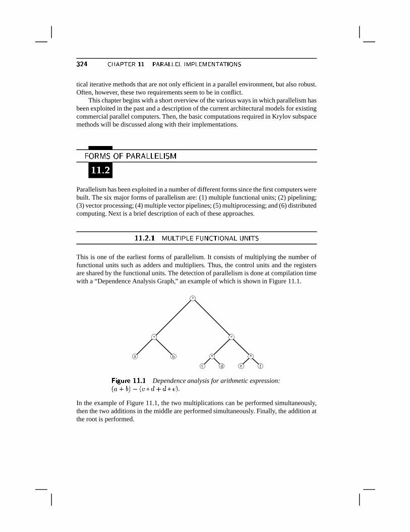
�p¶�� ~�� &�� ?��m� ��?; �� &��p&�� \��tical iterative methods that are not only efficient in a parallel environment, but also robust.Often, however, these two requirements seem to be in conflict.

This chapter begins with a short overview of the various ways in which parallelism hasbeen exploited in the past and a description of the current architectural models for existingcommercial parallel computers. Then, the basic computations required in Krylov subspacemethods will be discussed along with their implementations.

� �� !� � � ��R� �ª�c�]�ª�t�Z��|�m��

Parallelism has been exploited in a number of different forms since the first computers werebuilt. The six major forms of parallelism are: (1) multiple functional units; (2) pipelining;(3) vector processing; (4) multiple vector pipelines; (5) multiprocessing; and (6) distributedcomputing. Next is a brief description of each of these approaches.

$1$ #"! %$ B ( 6 ;>2 �+6,0 � ( 9 � ;>2H7�9�'56D( 9)2 ; *

This is one of the earliest forms of parallelism. It consists of multiplying the number offunctional units such as adders and multipliers. Thus, the control units and the registersare shared by the functional units. The detection of parallelism is done at compilation timewith a “Dependence Analysis Graph,” an example of which is shown in Figure 11.1.

+

+ +

a b * *

c d e f

�� @�,��#�Dependence analysis for arithmetic expression:< � M = M < � � � M � � Q = .

In the example of Figure 11.1, the two multiplications can be performed simultaneously,then the two additions in the middle are performed simultaneously. Finally, the addition atthe root is performed.

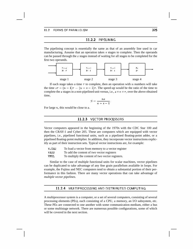
� � �H� �/\�� >�n\ � � ��?�?;�9� � �p¶��$1$ #"! " �+2 �!036 2 9)2#9�&

The pipelining concept is essentially the same as that of an assembly line used in carmanufacturing. Assume that an operation takes � stages to complete. Then the operandscan be passed through the � stages instead of waiting for all stages to be completed for thefirst two operands.

�

� F $ � �� $ � � �

stage 1

F $ � 0� $ � 0 �

stage 2

F $ � �� $ � � �

stage 3

F $� $ �

stage 4

If each stage takes a time � to complete, then an operation with ® numbers will takethe time � � M <o®�¨ / = �°� <o® M ��¨ / = � . The speed-up would be the ratio of the time tocomplete the � stages in a non-pipelined unit versus, i.e., ��¯X®n¯ � , over the above obtainedtime,

�� ® �® M �Q¨ / ¬

For large ® , this would be close to � .

$1$ #"! � �>0 � ;)7:A �+A 7 ��0,*,*F7:A1*

Vector computers appeared in the beginning of the 1970s with the CDC Star 100 andthen the CRAY-1 and Cyber 205. These are computers which are equipped with vectorpipelines, i.e., pipelined functional units, such as a pipelined floating-point adder, or apipelined floating-point multiplier. In addition, they incorporate vector instructions explic-itly as part of their instruction sets. Typical vector instructions are, for example:

��To load a vector from memory to a vector register

��To add the content of two vector registers

�� To multiply the content of two vector registers.

Similar to the case of multiple functional units for scalar machines, vector pipelinescan be duplicated to take advantage of any fine grain parallelism available in loops. Forexample, the Fujitsu and NEC computers tend to obtain a substantial portion of their per-formance in this fashion. There are many vector operations that can take advantage ofmultiple vector pipelines.

$1$ #"! � B ( 6 ;>2 �!A 7 ��0,*F*32 9�& ' 9)4 4?2H* ;>A+2�� (�;>014 ��7:B �+(�; 2#9�&

A multiprocessor system is a computer, or a set of several computers, consisting of severalprocessing elements (PEs), each consisting of a CPU, a memory, an I/O subsystem, etc.These PEs are connected to one another with some communication medium, either a busor some multistage network. There are numerous possible configurations, some of whichwill be covered in the next section.

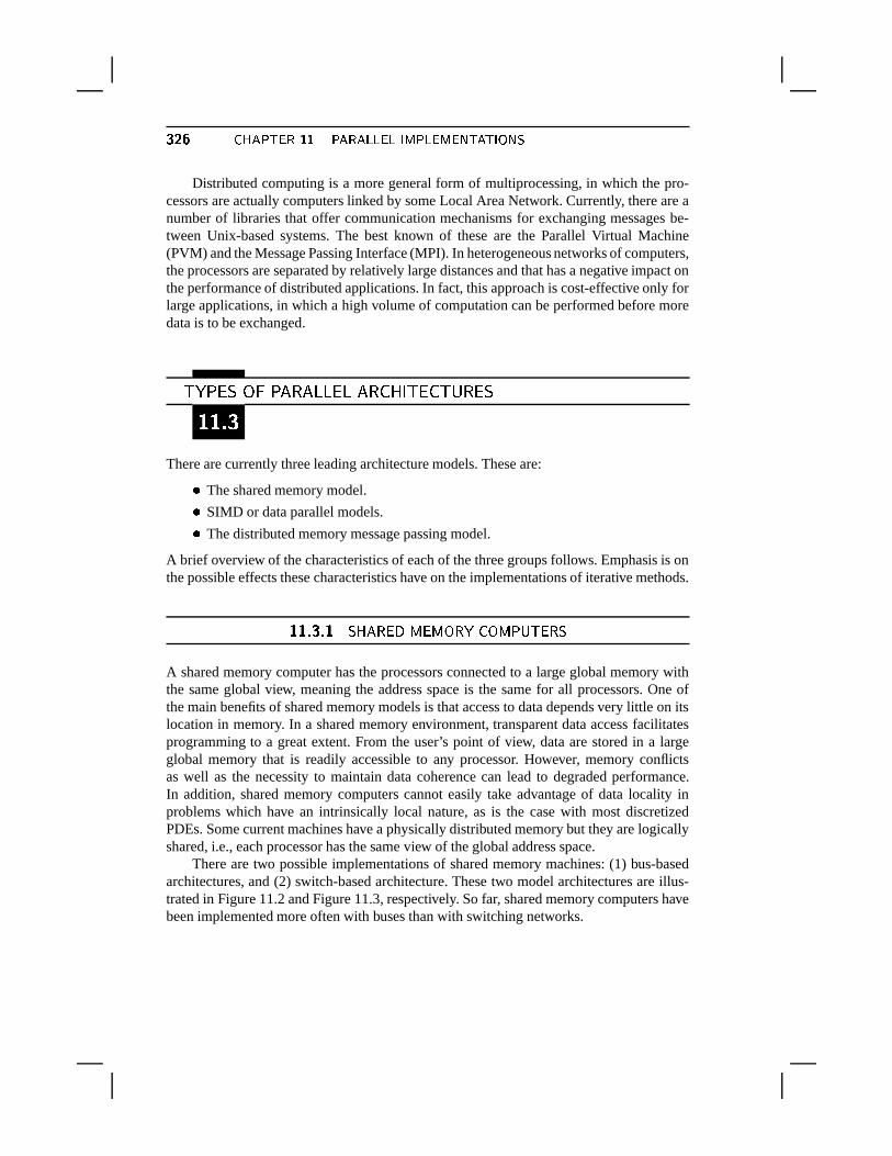
�p¶�� ~�� &�� ?��m� ��?; �� &��p&�� \��Distributed computing is a more general form of multiprocessing, in which the pro-

cessors are actually computers linked by some Local Area Network. Currently, there are anumber of libraries that offer communication mechanisms for exchanging messages be-tween Unix-based systems. The best known of these are the Parallel Virtual Machine(PVM) and the Message Passing Interface (MPI). In heterogeneous networks of computers,the processors are separated by relatively large distances and that has a negative impact onthe performance of distributed applications. In fact, this approach is cost-effective only forlarge applications, in which a high volume of computation can be performed before moredata is to be exchanged.

��7�0�!� � � ��^��ª�i�Z��5�W�n�t�u��]�� 7�0��|�m��

There are currently three leading architecture models. These are: The shared memory model. SIMD or data parallel models. The distributed memory message passing model.

A brief overview of the characteristics of each of the three groups follows. Emphasis is onthe possible effects these characteristics have on the implementations of iterative methods.

$1$ �! %$ *1=+' A!014 BD01B87:A� ��7:B �+(�;>01A1*

A shared memory computer has the processors connected to a large global memory withthe same global view, meaning the address space is the same for all processors. One ofthe main benefits of shared memory models is that access to data depends very little on itslocation in memory. In a shared memory environment, transparent data access facilitatesprogramming to a great extent. From the user’s point of view, data are stored in a largeglobal memory that is readily accessible to any processor. However, memory conflictsas well as the necessity to maintain data coherence can lead to degraded performance.In addition, shared memory computers cannot easily take advantage of data locality inproblems which have an intrinsically local nature, as is the case with most discretizedPDEs. Some current machines have a physically distributed memory but they are logicallyshared, i.e., each processor has the same view of the global address space.

There are two possible implementations of shared memory machines: (1) bus-basedarchitectures, and (2) switch-based architecture. These two model architectures are illus-trated in Figure 11.2 and Figure 11.3, respectively. So far, shared memory computers havebeen implemented more often with buses than with switching networks.

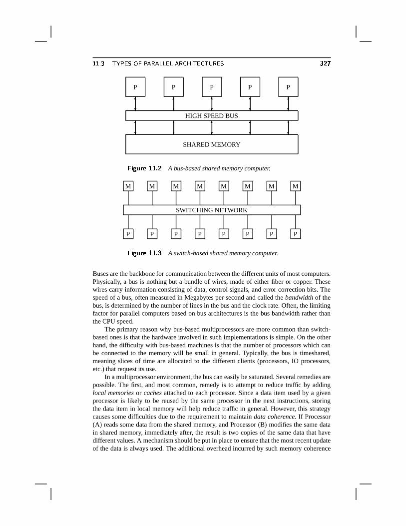
� � �� &��?�v\ � � ��?��>�� ~0� &� � &�� ?� �p¶��P P P P P

SHARED MEMORY

HIGH SPEED BUS

� � � � �

� � � � �

� � � � �

� � � � �

�� ,��t¶A bus-based shared memory computer.

P P P P P P P P

SWITCHING NETWORK

M M M M M M M M

�� ,�� A switch-based shared memory computer.

Buses are the backbone for communication between the different units of most computers.Physically, a bus is nothing but a bundle of wires, made of either fiber or copper. Thesewires carry information consisting of data, control signals, and error correction bits. Thespeed of a bus, often measured in Megabytes per second and called the bandwidth of thebus, is determined by the number of lines in the bus and the clock rate. Often, the limitingfactor for parallel computers based on bus architectures is the bus bandwidth rather thanthe CPU speed.

The primary reason why bus-based multiprocessors are more common than switch-based ones is that the hardware involved in such implementations is simple. On the otherhand, the difficulty with bus-based machines is that the number of processors which canbe connected to the memory will be small in general. Typically, the bus is timeshared,meaning slices of time are allocated to the different clients (processors, IO processors,etc.) that request its use.

In a multiprocessor environment, the bus can easily be saturated. Several remedies arepossible. The first, and most common, remedy is to attempt to reduce traffic by addinglocal memories or caches attached to each processor. Since a data item used by a givenprocessor is likely to be reused by the same processor in the next instructions, storingthe data item in local memory will help reduce traffic in general. However, this strategycauses some difficulties due to the requirement to maintain data coherence. If Processor(A) reads some data from the shared memory, and Processor (B) modifies the same datain shared memory, immediately after, the result is two copies of the same data that havedifferent values. A mechanism should be put in place to ensure that the most recent updateof the data is always used. The additional overhead incurred by such memory coherence

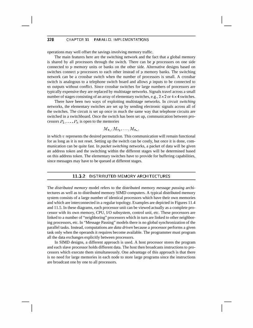
�p¶�� ~�� &�� ?��m� ��?; �� &��p&�� \��operations may well offset the savings involving memory traffic.

The main features here are the switching network and the fact that a global memoryis shared by all processors through the switch. There can be � processors on one sideconnected to � memory units or banks on the other side. Alternative designs based onswitches connect � processors to each other instead of � memory banks. The switchingnetwork can be a crossbar switch when the number of processors is small. A crossbarswitch is analogous to a telephone switch board and allows � inputs to be connected to± outputs without conflict. Since crossbar switches for large numbers of processors aretypically expensive they are replaced by multistage networks. Signals travel across a smallnumber of stages consisting of an array of elementary switches, e.g.,

0 ¯ 0 or3 ¯ 3 switches.

There have been two ways of exploiting multistage networks. In circuit switchingnetworks, the elementary switches are set up by sending electronic signals across all ofthe switches. The circuit is set up once in much the same way that telephone circuits areswitched in a switchboard. Once the switch has been set up, communication between pro-cessors

�B �*¬,¬*¬T�

�I

is open to the memories

�� 0 �,¬*¬,¬T��in which � represents the desired permutation. This communication will remain functionalfor as long as it is not reset. Setting up the switch can be costly, but once it is done, com-munication can be quite fast. In packet switching networks, a packet of data will be givenan address token and the switching within the different stages will be determined basedon this address token. The elementary switches have to provide for buffering capabilities,since messages may have to be queued at different stages.

$1$ �! " 4?2 *,;>A+2 � (+;>014 BD01B 7:A�<' A ��=)2 ;>0 � ; ()A+0,*

The distributed memory model refers to the distributed memory message passing archi-tectures as well as to distributed memory SIMD computers. A typical distributed memorysystem consists of a large number of identical processors which have their own memoriesand which are interconnected in a regular topology. Examples are depicted in Figures 11.4and 11.5. In these diagrams, each processor unit can be viewed actually as a complete pro-cessor with its own memory, CPU, I/O subsystem, control unit, etc. These processors arelinked to a number of “neighboring” processors which in turn are linked to other neighbor-ing processors, etc. In “Message Passing” models there is no global synchronization of theparallel tasks. Instead, computations are data driven because a processor performs a giventask only when the operands it requires become available. The programmer must programall the data exchanges explicitly between processors.

In SIMD designs, a different approach is used. A host processor stores the programand each slave processor holds different data. The host then broadcasts instructions to pro-cessors which execute them simultaneously. One advantage of this approach is that thereis no need for large memories in each node to store large programs since the instructionsare broadcast one by one to all processors.

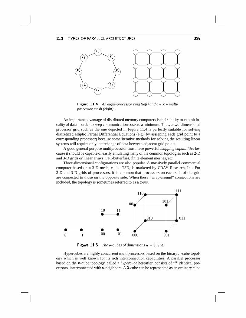
� � �� &��?�v\ � � ��?��>�� ~0� &� � &�� ?� �p¶p·> 4 >

>��

>��>��

>��

>��

>��

�� ,�� An eight-processor ring (left) and a

3 ¯ 3 multi-processor mesh (right).

An important advantage of distributed memory computers is their ability to exploit lo-cality of data in order to keep communication costs to a minimum. Thus, a two-dimensionalprocessor grid such as the one depicted in Figure 11.4 is perfectly suitable for solvingdiscretized elliptic Partial Differential Equations (e.g., by assigning each grid point to acorresponding processor) because some iterative methods for solving the resulting linearsystems will require only interchange of data between adjacent grid points.

A good general purpose multiprocessor must have powerful mapping capabilities be-cause it should be capable of easily emulating many of the common topologies such as 2-Dand 3-D grids or linear arrays, FFT-butterflies, finite element meshes, etc.

Three-dimensional configurations are also popular. A massively parallel commercialcomputer based on a 3-D mesh, called T3D, is marketed by CRAY Research, Inc. For2-D and 3-D grids of processors, it is common that processors on each side of the gridare connected to those on the opposite side. When these “wrap-around” connections areincluded, the topology is sometimes referred to as a torus.

10 11

010010

101

111110

100

010 011

001000

�� ,�� The ® -cubes of dimensions ®f� / � 0 �� .

Hypercubes are highly concurrent multiprocessors based on the binary ® -cube topol-ogy which is well known for its rich interconnection capabilities. A parallel processorbased on the ® -cube topology, called a hypercube hereafter, consists of

0 Iidentical pro-

cessors, interconnected with ® neighbors. A � -cube can be represented as an ordinary cube

�� ~�� &�� ?��m� ��?; �� &��p&�� \��in three dimensions where the vertices are the � � 0 �

nodes of the 3-cube; see Figure 11.5.More generally, one can construct an ® -cube as follows: First, the

0 Inodes are labeled by

the0 I

binary numbers from-

to0 I ¨ / . Then a link between two nodes is drawn if and

only if their binary numbers differ by one (and only one) bit.The first property of an ® -cube graph is that it can be constructed recursively from

lower dimensional cubes. More precisely, consider two identical <o® ¨ / = -cubes whosevertices are labeled likewise from 0 to

0 I @�B . By joining every vertex of the first <N®f¨ / = -cube to the vertex of the second having the same number, one obtains an ® -cube. Indeed, itsuffices to renumber the nodes of the first cube as

-��;5 and those of the second as / �

��5where � 5 is a binary number representing the two similar nodes of the <N®�¨ / = -cubes andwhere

�denotes the concatenation of binary numbers.

Separating an ® -cube into the subgraph of all the nodes whose leading bit is 0 andthe subgraph of all the nodes whose leading bit is 1, the two subgraphs are such that eachnode of the first is connected to one node of the second. If the edges between these twographs is removed, the result is 2 disjoint <o®f¨ / = -cubes. Moreover, generally, for a givennumbering, the graph can be separated into two subgraphs obtained by considering all thenodes whose S �� bit is 0 and those whose S �� bit is 1. This will be called tearing along theS �� direction. Since there are ® bits, there are ® directions. One important consequence ofthis is that arbitrary meshes with dimension !¡® can be mapped on hypercubes. However,the hardware cost for building a hypercube is high, because each node becomes difficultto design for larger dimensions. For this reason, recent commercial vendors have tended toprefer simpler solutions based on two- or three-dimensional meshes.

Distributed memory computers come in two different designs, namely, SIMD andMIMD. Many of the early projects have adopted the SIMD organization. For example,the historical ILLIAC IV Project of the University of Illinois was a machine based on amesh topology where all processors execute the same instructions.

SIMD distributed processors are sometimes called array processors because of theregular arrays that they constitute. In this category, systolic arrays can be classified as anexample of distributed computing. Systolic arrays are distributed memory computers inwhich each processor is a cell which is programmed (possibly micro-coded) to performonly one of a few operations. All the cells are synchronized and perform the same task.Systolic arrays are designed in VLSI technology and are meant to be used for specialpurpose applications, primarily in signal processing.

��7�0�!� � �@�7�Z�^��-��|�m��

Now consider two prototype Krylov subspace techniques, namely, the preconditioned Con-jugate Gradient method for the symmetric case and the preconditioned GMRES algorithmfor the nonsymmetric case. For each of these two techniques, we analyze the types of oper-ations that are performed. It should be emphasized that other Krylov subspace techniquesrequire similar operations.

� � � � &��?�v\ �w\��p&�� \�� $1$ � $ �+A!0 �+7:9?4?2 ;>2H7:9?014 �+&

Consider Algorithm 9.1. The first step when implementing this algorithm on a high-performance computer is identifying the main operations that it requires. We distinguishfive types of operations, which are:

��Preconditioner setup.��Matrix vector multiplications.

� �Vector updates.

� �Dot products.

� �Preconditioning operations.

In the above list the potential bottlenecks are (1), setting up the preconditioner and (5),solving linear systems with � , i.e., the preconditioning operation. Section 11.6 discussesthe implementation of traditional preconditioners, and the last two chapters are devotedto preconditioners that are specialized to parallel environments. Next come the matrix-by-vector products which deserve particular attention. The rest of the algorithm consistsessentially of dot products and vector updates which do not cause significant difficulties inparallel machines, although inner products can lead to some loss of efficiency on certaintypes of computers with large numbers of processors.

$1$ � #" &)B A!0,*

The only new operation here with respect to the Conjugate Gradient method is the orthog-onalization of the vector � � 5 against the previous � ’s. The usual way to accomplish this isvia the modified Gram-Schmidt process, which is basically a sequence of subprocesses ofthe form:

Compute � < � � = . Compute

� � � ¨ � .

This orthogonalizes a vector

against another vector � of norm one. Thus, the outer loop ofthe modified Gram-Schmidt is sequential, but the inner loop, i.e., each subprocess, can beparallelized by dividing the inner product and SAXPY operations among processors. Al-though this constitutes a perfectly acceptable approach for a small number of processors,the elementary subtasks may be too small to be efficient on a large number of processors.An alternative for this case is to use a standard Gram-Schmidt process with reorthogonal-ization. This replaces the previous sequential orthogonalization process by a matrix opera-tion of the form

� � ¨ � � b , i.e., BLAS-1 kernels are replaced by BLAS-2 kernels.Recall that the next level of BLAS, i.e., level 3 BLAS, exploits blocking in dense

matrix operations in order to obtain performance on machines with hierarchical memories.Unfortunately, level 3 BLAS kernels cannot be exploited here because at every step, thereis only one vector to orthogonalize against all previous ones. This may be remedied byusing block Krylov methods.

��p¶ � ~�� &�� ?��m� ��?; �� &��p&�� \��$1$ �� >0 � ;?7:A 7��!01A�'�;>2H7:9 *

These are usually the simplest operations to implement on any computer. In many cases,compilers are capable of recognizing them and invoking the appropriate machine instruc-tions, possibly vector instructions. In the specific case of CG-like algorithms, there are twotypes of operations: vector updates and dot products.

Vector Updates Operations of the form

y(1:n) = y(1:n) + a * x(1:n),

where � is a scalar and

and � two vectors, are known as vector updates or SAXPYoperations. They are typically straightforward to implement in all three machine modelsdiscussed earlier. On an SIMD computer, the above code segment can be used on manyof the recent systems and the compiler will translate it into the proper parallel version.The above line of code is written in FORTRAN 90, which is the prototype programminglanguage for this type of computers. On shared memory computers, we can simply writethe usual FORTRAN loop, possibly in the above FORTRAN 90 style on some computers,and the compiler will translate it again in the appropriate parallel executable code.

On distributed memory computers, some assumptions must be made about the wayin which the vectors are distributed. The main assumption is that the vectors � and

are

distributed in the same manner among the processors, meaning the indices of the compo-nents of any vector that are mapped to a given processor are the same. In this case, thevector-update operation will be translated into � independent vector updates, requiring nocommunication. Specifically, if ® � � � is the number of variables local to a given processor,this processor will simply execute a vector loop of the form

y(1:nloc) = y(1:nloc) + a * x(1:nloc)

and all processors will execute a similar operation simultaneously.

Dot products A number of operations use all the components of a given vector to com-pute a single floating-point result which is then needed by all processors. These are termedReduction Operations and the dot product is the prototype example. A distributed versionof the dot-product is needed to compute the inner product of two vectors � and

that are

distributed the same way across the processors. In fact, to be more specific, this distributeddot-product operation should compute the inner product

� �� b of these two vectors andthen make the result

�available in each processor. Typically, this result is needed to per-

form vector updates or other operations in each node. For a large number of processors, thissort of operation can be demanding in terms of communication costs. On the other hand,parallel computer designers have become aware of their importance and are starting to pro-vide hardware and software support for performing global reduction operations efficiently.Reduction operations that can be useful include global sums, global max/min calculations,etc. A commonly adopted convention provides a single subroutine for all these operations,and passes the type of operation to be performed (add, max, min, multiply,. . . ) as one ofthe arguments. With this in mind, a distributed dot-product function can be programmedroughly as follows.

� � � � &��?�v\ �w\��p&�� \�� "!��#��!�$��%�&�%�'(��'�%�)��*�+,��-��$.�/!��0��-��$�-��-�21 ��34��-��-��/��#��"!��!�$ �� 1�5�6�� -7�6��8�-��9:)� � ;9<$%��

The function DDOT performs the usual BLAS-1 dot product of x and!

with stridesincx and incy, respectively. The REDUCE operation, which is called with “add” as theoperation-type parameter, sums all the variables “tloc” from each processor and put theresulting global sum in the variable � S � � � � � in each processor.

$1$ �� A!0�>01A3* 0 ��7�B B ( 9)2 �1'3; 2 7:9

To conclude this section, the following important observation can be made regarding thepractical implementation of Krylov subspace accelerators, such as PCG or GMRES. Theonly operations that involve communication are the dot product, the matrix-by-vector prod-uct, and, potentially, the preconditioning operation. There is a mechanism for delegatingthe last two operations to a calling program, outside of the Krylov accelerator. The result ofthis is that the Krylov acceleration routine will be free of any matrix data structures as wellas communication calls. This makes the Krylov routines portable, except for the possibleredefinition of the inner product distdot.

This mechanism, particular to FORTRAN programming, is known as reverse commu-nication. Whenever a matrix-by-vector product or a preconditioning operation is needed,the subroutine is exited and the calling program unit performs the desired operation. Thenthe subroutine is called again, after placing the desired result in one of its vector arguments.

A typical execution of a flexible GMRES routine with reverse communication isshown in the code segment below. The integer parameter icode indicates the type of oper-ation needed by the subroutine. When icode is set to one, then a preconditioning operationmust be applied to the vector � � / . The result is copied in � � 0 and FGMRES is calledagain. If it is equal to two, then the vector � � / must be multiplied by the matrix � . Theresult is then copied in � � 0 and FGMRES is called again.

�� %(1>=? ��@��-%

��)��(��&�A-'�%-�B��C�DDAE��'�F ��D��G�<.�0H�H��0IC�JI�K ? �LI�K�M;�:%�N ��* A )�� .�<��<�� %-$��O�<�� %4P0%�QCP ? $R��F-%��

��)�� N�'�%-��0�C��I�K ? �"I�K�M�$TSU� ��%�'�9D�VN�'�%-�� -%�'&�� ?

%��%W��4�@�� %4P�%�QCP"M�$R��F�%��)��XA�)��H�%-�B��0I�K ? �UI�K�M�$TSU� ��%�'�9D�YA )��H�%-�&�� ?

%��

Reverse communication enhances the flexibility of the FGMRES routine substantially.For example, when changing preconditioners, we can iterate on a coarse mesh and do the

�� ~�� &�� ?��m� ��?; �� &��p&�� \��necessary interpolations to get the result in � � 0 in a given step and then iterate on the finemesh in the following step. This can be done without having to pass any data regarding thematrix or the preconditioner to the FGMRES accelerator.

Note that the purpose of reverse communication simply is to avoid passing data struc-tures related to the matrices, to the accelerator FGMRES. The problem is that these datastructures are not fixed. For example, it may be desirable to use different storage formatsfor different architectures. A more elegant solution to this problem is Object-OrientedProgramming. In Object-Oriented Programming languages such as C++, a class can bedeclared, e.g., a class of sparse matrices, and operators can be defined on them. Data struc-tures are not passed to these operators. Instead, the implementation will recognize the typesof the operands and invoke the proper functions. This is similar to what exists currently forarithmetic. For operation � � 2 M

, the compiler will recognize what type of operand is

involved and invoke the proper operation, either integer, double real, or complex, etc.

�� Z�n�� X�Z��:�Z�m��|�m��

Matrix-by-vector multiplications (sometimes called “Matvecs” for short) are relativelyeasy to implement efficiently on high performance computers. For a description of storageformats for sparse matrices, see Chapter 3. We will first discuss matrix-by-vector algo-rithms without consideration of sparsity. Then we will cover sparse Matvec operations fora few different storage formats.

$1$ �� %$ ;>=?0 � '�*10�7 �@45019 *10 BC'3;>A+2 ��0,*

The computational kernels for performing sparse matrix operations such as matrix-by--vector products are intimately associated with the data structures used. However, thereare a few general approaches that are common to different algorithms for matrix-by-vectorproducts which can be described for dense matrices. Two popular ways of performing theseoperations are (1) the inner product form described in Algorithm 11.1, and (2) the SAXPYform described by Algorithm 11.2.

��n��-�w�� ,��#�� 1�'� � � � �� 1. Do i = 1, n2. y(i) = dotproduct(a(i,1:n),x(1:n))3. EndDo

The dot product operation dotproduct(v(1:n),w(1:n)) computes the dot product of the twovectors v and w of length ® each. If there is no ambiguity on the bounds, we simply writedotproduct(v,w). The above algorithm proceeds by rows. It computes the dot-product ofrow S of the matrix � with the vector � and assigns the result to

< S = . The next algorithm

� � � � ��p&� � �}M � �}M �� &c\� ��r\�� &�� uses columns instead and results in the use of the SAXPY operations.

�� n� �D�w�� ,��t¶ � �ª��8� � �� 1. y(1:n) = 0.02. Do j = 1, n3. y(1:n) = y(1:n) + x(j) * a(1:n,j)4. EndDo

The SAXPY form of the Matvec operation computes the result � �Q� as a linear com-

bination of the columns of the matrix � . A third possibility consists of performing theproduct by diagonals. This option bears no interest in the dense case, but it is at the basisof many important matrix-by-vector algorithms in the sparse case.

�� n� �D�w�� ,�� v�H� �� 1. y(1:n) = 02. Do k = – n+1, n – 13. Do i = 1 – min(k,0), n – max(k,0)4. y(i) = y(i) + a(i,k+i)*x(k+i)5. EndDo6. EndDo

The product is performed by diagonals, starting from the leftmost diagonal whose offset is¨2® M / to the rightmost diagonal whose offset is ®�¨ / .$1$ � #" ; =?0 ��*1A�' 9?4 ��* � � 7�A+BC'3; *

One of the most general schemes for storing sparse matrices is the Compressed Sparse Rowstorage format described in Chapter 3. Recall that the data structure consists of three arrays:a real array A(1:nnz) to store the nonzero elements of the matrix row-wise, an integer arrayJA(1:nnz) to store the column positions of the elements in the real array A, and, finally, apointer array IA(1:n+1), the S -th entry of which points to the beginning of the S -th row inthe arrays A and JA. To perform the matrix-by-vector product

��Q� in parallel using thisformat, note that each component of the resulting vector

can be computed independently

as the dot product of the S -th row of the matrix with the vector � . This yields the followingsparse version of Algorithm 11.1 for the case where the matrix is stored in CSR format.

�� n� �D�w�� ,�� Z�Z� �� 1�'� � � � �� 1. Do i = 1, n2. k1 = ia(i)3. k2 = ia(i+1)-14. y(i) = dotproduct(a(k1:k2),x(ja(k1:k2)))5. EndDo

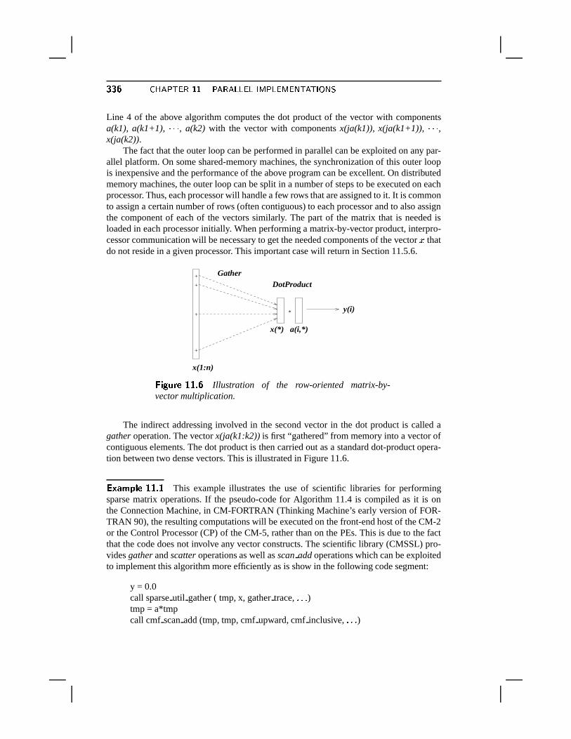
�� ~�� &�� ?��m� ��?; �� &��p&�� \��Line 4 of the above algorithm computes the dot product of the vector with componentsa(k1), a(k1+1),

� � �, a(k2) with the vector with components x(ja(k1)), x(ja(k1+1)),

� � �,

x(ja(k2)).The fact that the outer loop can be performed in parallel can be exploited on any par-

allel platform. On some shared-memory machines, the synchronization of this outer loopis inexpensive and the performance of the above program can be excellent. On distributedmemory machines, the outer loop can be split in a number of steps to be executed on eachprocessor. Thus, each processor will handle a few rows that are assigned to it. It is commonto assign a certain number of rows (often contiguous) to each processor and to also assignthe component of each of the vectors similarly. The part of the matrix that is needed isloaded in each processor initially. When performing a matrix-by-vector product, interpro-cessor communication will be necessary to get the needed components of the vector � thatdo not reside in a given processor. This important case will return in Section 11.5.6.

+

+

+

+

DotProductGather

*

x(*) a(i,*)

x(1:n)

y(i)

�� @�,��Illustration of the row-oriented matrix-by-

vector multiplication.

The indirect addressing involved in the second vector in the dot product is called agather operation. The vector x(ja(k1:k2)) is first “gathered” from memory into a vector ofcontiguous elements. The dot product is then carried out as a standard dot-product opera-tion between two dense vectors. This is illustrated in Figure 11.6.

�� ,��#�This example illustrates the use of scientific libraries for performing

sparse matrix operations. If the pseudo-code for Algorithm 11.4 is compiled as it is onthe Connection Machine, in CM-FORTRAN (Thinking Machine’s early version of FOR-TRAN 90), the resulting computations will be executed on the front-end host of the CM-2or the Control Processor (CP) of the CM-5, rather than on the PEs. This is due to the factthat the code does not involve any vector constructs. The scientific library (CMSSL) pro-vides gather and scatter operations as well as scan add operations which can be exploitedto implement this algorithm more efficiently as is show in the following code segment:

y = 0.0call sparse util gather ( tmp, x, gather trace, ¬*¬,¬ )tmp = a*tmpcall cmf scan add (tmp, tmp, cmf upward, cmf inclusive, ¬*¬,¬ )

� � � � ��p&� � �}M � �}M �� &c\� ��r\�� &�� call sparse util scatter ( y, scatter pointer, tmp,

scatter trace, ¬*¬*¬ )The sparse util gather routine is first called to gather the corresponding entries from thevector � into a temporary array

� ± � , then the multiplications are carried out element-by-element in parallel. The cmf scan add routine from the CM Fortran Utility Library is usedto perform the summation for each row. Finally, the call to sparse util scatter copies theresults. Segmented scan-adds are particularly useful for implementing sparse matrix-by-vector products when they are provided as part of the libraries. Note that the sparse util-gather setup and sparse util scatter setup routines must be called to compute the com-

munication patterns, gather trace and scatter trace, before this algorithm is called. Thesetend to be expensive operations.

Now assume that the matrix is stored by columns (CSC format). The matrix-by-vectorproduct can be performed by the following algorithm which is a sparse version of Algo-rithm 11.2.

�� n� �D�w�� ,�� Z�� ª�� 1. y(1:n) = 0.02. Do i = 1, n3. k1 = ia(i)4. k2 = ia(i + 1)-15. y(ja(k1:k2)) = y(ja(k1:k2)) + x(j) * a(k1:k2)6. EndDo

The above code initializes

to zero and then adds the vectors ��< � =n¯ ��< / � ® � � = for� � / �*¬,¬*¬T�S® to it. It can also be used to compute the product of the transpose of a matrixby a vector, when the matrix is stored (row-wise) in the CSR format. Normally, the vectory(ja(k1:k2)) is gathered and the SAXPY operation is performed in vector mode. Then theresulting vector is “scattered” back into the positions ja(*), by what is called a Scatteroperation. This is illustrated in Figure 11.7.

A major difficulty with the above FORTRAN program is that it is intrinsically sequen-tial. First, the outer loop is not parallelizable as it is, but this may be remedied as will beseen shortly. Second, the inner loop involves writing back results of the right-hand sideinto memory positions that are determined by the indirect address function ja. To be cor-rect, y(ja(1)) must be copied first, followed by y(ja(2)), etc. However, if it is known thatthe mapping ja(i) is one-to-one, then the order of the assignments no longer matters. Sincecompilers are not capable of deciding whether this is the case, a compiler directive fromthe user is necessary for the Scatter to be invoked.

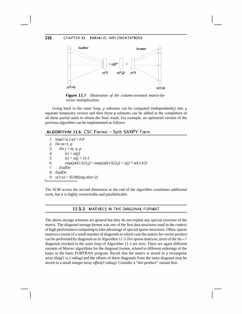
�� ~�� &�� ?��m� ��?; �� &��p&�� \��

+

+

+

+

+

+

+

+

Gather

+ x(j)*

y(1:n)

y(*)

y(1:n)

=

Scatter

y(*) a(*,j)

�� @�,�� Illustration of the column-oriented matrix-by-

vector multiplication.

Going back to the outer loop, � subsums can be computed (independently) into �separate temporary vectors and then these � subsums can be added at the completion ofall these partial sums to obtain the final result. For example, an optimized version of theprevious algorithm can be implemented as follows:

��n��-�w�� ,�� 2�� ª��8� � �� 1. tmp(1:n,1:p) = 0.02. Do m=1, p3. Do j = m, n, p4. k1 = ia(j)5. k2 = ia(j + 1)-16. tmp(ja(k1:k2),j) = tmp(ja(k1:k2),j) + x(j) * a(k1:k2)7. EndDo8. EndDo9. y(1:n) = SUM(tmp,dim=2)

The SUM across the second dimension at the end of the algorithm constitutes additionalwork, but it is highly vectorizable and parallelizable.

$1$ �� B '3; �>0 ��* 2 9 ; =?0 4?2 ' & 7:9+'56 � 7:A!B '3;

The above storage schemes are general but they do not exploit any special structure of thematrix. The diagonal storage format was one of the first data structures used in the contextof high performance computing to take advantage of special sparse structures. Often, sparsematrices consist of a small number of diagonals in which case the matrix-by-vector productcan be performed by diagonals as in Algorithm 11.3. For sparse matrices, most of the

0 ®^¨ /diagonals invoked in the outer loop of Algorithm 11.3 are zero. There are again differentvariants of Matvec algorithms for the diagonal format, related to different orderings of theloops in the basic FORTRAN program. Recall that the matrix is stored in a rectangulararray diag(1:n,1:ndiag) and the offsets of these diagonals from the main diagonal may bestored in a small integer array offset(1:ndiag). Consider a “dot-product” variant first.

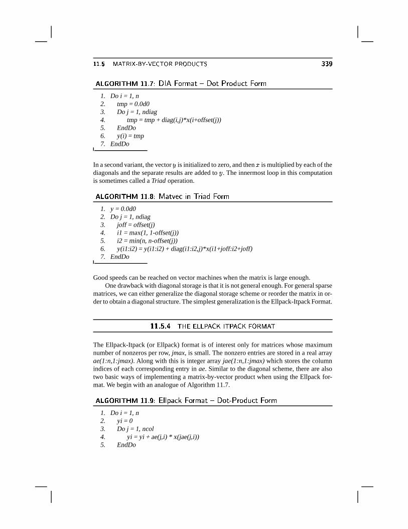
� � � � ��p&� � �}M � �}M �� &c\� ��r\�� &�� p·�� n� �D�w�� ,�� v�H� �� 1�'� � � � ��

1. Do i = 1, n2. tmp = 0.0d03. Do j = 1, ndiag4. tmp = tmp + diag(i,j)*x(i+offset(j))5. EndDo6. y(i) = tmp7. EndDo

In a second variant, the vector

is initialized to zero, and then � is multiplied by each of thediagonals and the separate results are added to

. The innermost loop in this computation

is sometimes called a Triad operation.

�� n� �D�w�� ,�� ©� � � �� 1. y = 0.0d02. Do j = 1, ndiag3. joff = offset(j)4. i1 = max(1, 1-offset(j))5. i2 = min(n, n-offset(j))6. y(i1:i2) = y(i1:i2) + diag(i1:i2,j)*x(i1+joff:i2+joff)7. EndDo

Good speeds can be reached on vector machines when the matrix is large enough.One drawback with diagonal storage is that it is not general enough. For general sparse

matrices, we can either generalize the diagonal storage scheme or reorder the matrix in or-der to obtain a diagonal structure. The simplest generalization is the Ellpack-Itpack Format.

$1$ �� ;>=?0 036 6 �' �� -�2 ; � ' � � � 7:A!BC'�;

The Ellpack-Itpack (or Ellpack) format is of interest only for matrices whose maximumnumber of nonzeros per row, jmax, is small. The nonzero entries are stored in a real arrayae(1:n,1:jmax). Along with this is integer array jae(1:n,1:jmax) which stores the columnindices of each corresponding entry in ae. Similar to the diagonal scheme, there are alsotwo basic ways of implementing a matrix-by-vector product when using the Ellpack for-mat. We begin with an analogue of Algorithm 11.7.

�� n� �D�w�� ,��t· � � � � �� 1. Do i = 1, n2. yi = 03. Do j = 1, ncol4. yi = yi + ae(j,i) * x(jae(j,i))5. EndDo

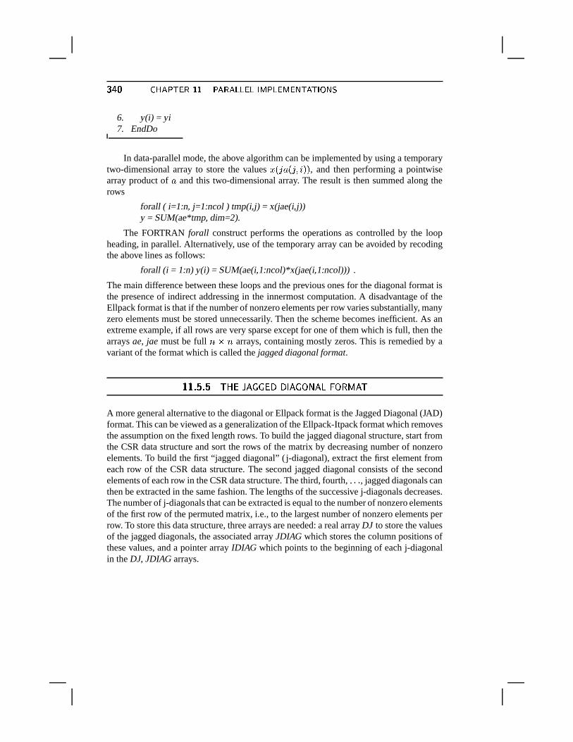
�� ~�� &�� ?��m� ��?; �� &��p&�� \��6. y(i) = yi7. EndDo

In data-parallel mode, the above algorithm can be implemented by using a temporarytwo-dimensional array to store the values � < � ��< �� S = = , and then performing a pointwisearray product of � and this two-dimensional array. The result is then summed along therows

forall ( i=1:n, j=1:ncol ) tmp(i,j) = x(jae(i,j))y = SUM(ae*tmp, dim=2).

The FORTRAN forall construct performs the operations as controlled by the loopheading, in parallel. Alternatively, use of the temporary array can be avoided by recodingthe above lines as follows:

forall (i = 1:n) y(i) = SUM(ae(i,1:ncol)*x(jae(i,1:ncol))) .

The main difference between these loops and the previous ones for the diagonal format isthe presence of indirect addressing in the innermost computation. A disadvantage of theEllpack format is that if the number of nonzero elements per row varies substantially, manyzero elements must be stored unnecessarily. Then the scheme becomes inefficient. As anextreme example, if all rows are very sparse except for one of them which is full, then thearrays ae, jae must be full ®¡¯�® arrays, containing mostly zeros. This is remedied by avariant of the format which is called the jagged diagonal format.

$1$ � �� ;>=?0 � ' & &)014 4?2 ' & 7:9+'56 � 7:A!BC'�;

A more general alternative to the diagonal or Ellpack format is the Jagged Diagonal (JAD)format. This can be viewed as a generalization of the Ellpack-Itpack format which removesthe assumption on the fixed length rows. To build the jagged diagonal structure, start fromthe CSR data structure and sort the rows of the matrix by decreasing number of nonzeroelements. To build the first “jagged diagonal” (j-diagonal), extract the first element fromeach row of the CSR data structure. The second jagged diagonal consists of the secondelements of each row in the CSR data structure. The third, fourth, ¬*¬,¬ , jagged diagonals canthen be extracted in the same fashion. The lengths of the successive j-diagonals decreases.The number of j-diagonals that can be extracted is equal to the number of nonzero elementsof the first row of the permuted matrix, i.e., to the largest number of nonzero elements perrow. To store this data structure, three arrays are needed: a real array DJ to store the valuesof the jagged diagonals, the associated array JDIAG which stores the column positions ofthese values, and a pointer array IDIAG which points to the beginning of each j-diagonalin the DJ, JDIAG arrays.

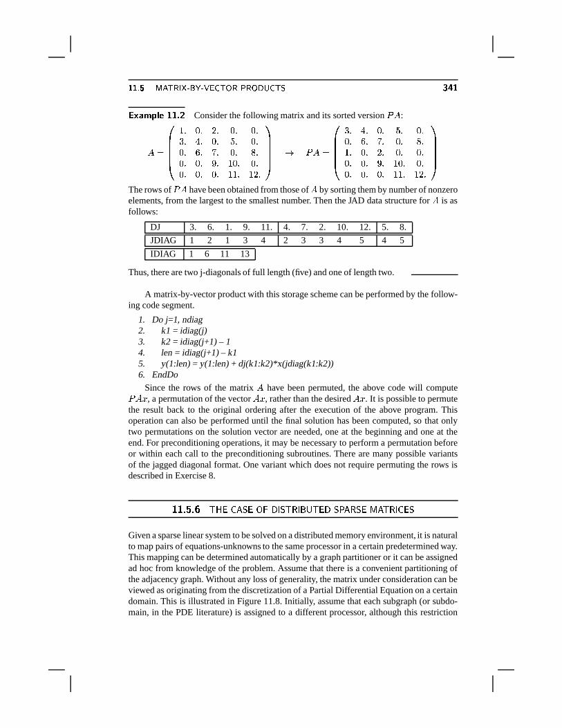
� � � � ��p&� � �}M � �}M �� &c\� ��r\�� &�� 3�� ,��t¶

Consider the following matrix and its sorted version

�� :

�¢��

/ ¬ - ¬ 0 ¬ - ¬ - ¬�p¬ 3 ¬ - ¬ � ¬ - ¬- ¬��r¬��¬ - ¬ �r¬- ¬ - ¬ � ¬ / - ¬ - ¬- ¬ - ¬ - ¬ /?/ ¬ / 0 ¬

��

�¢��p¬ 3 ¬ - ¬ � ¬ - ¬- ¬��r¬��¬ - ¬ �r¬/ ¬ - ¬ 0 ¬ - ¬ - ¬- ¬ - ¬ � ¬ / - ¬ - ¬- ¬ - ¬ - ¬ /�/ ¬ / 0 ¬

��

The rows of

�� have been obtained from those of � by sorting them by number of nonzero

elements, from the largest to the smallest number. Then the JAD data structure for � is asfollows:

DJ 3. 6. 1. 9. 11. 4. 7. 2. 10. 12. 5. 8.

JDIAG 1 2 1 3 4 2 3 3 4 5 4 5

IDIAG 1 6 11 13

Thus, there are two j-diagonals of full length (five) and one of length two.

A matrix-by-vector product with this storage scheme can be performed by the follow-ing code segment.

1. Do j=1, ndiag2. k1 = idiag(j)3. k2 = idiag(j+1) – 14. len = idiag(j+1) – k15. y(1:len) = y(1:len) + dj(k1:k2)*x(jdiag(k1:k2))6. EndDo

Since the rows of the matrix � have been permuted, the above code will compute��Q� , a permutation of the vector �7� , rather than the desired �7� . It is possible to permute

the result back to the original ordering after the execution of the above program. Thisoperation can also be performed until the final solution has been computed, so that onlytwo permutations on the solution vector are needed, one at the beginning and one at theend. For preconditioning operations, it may be necessary to perform a permutation beforeor within each call to the preconditioning subroutines. There are many possible variantsof the jagged diagonal format. One variant which does not require permuting the rows isdescribed in Exercise 8.

$1$ � �� ;>=?0 � '�*10D7 �@4?2 * ; A+2 � (+;>014<* � ' A1*10 BC'�; A+2 ��0,*

Given a sparse linear system to be solved on a distributed memory environment, it is naturalto map pairs of equations-unknowns to the same processor in a certain predetermined way.This mapping can be determined automatically by a graph partitioner or it can be assignedad hoc from knowledge of the problem. Assume that there is a convenient partitioning ofthe adjacency graph. Without any loss of generality, the matrix under consideration can beviewed as originating from the discretization of a Partial Differential Equation on a certaindomain. This is illustrated in Figure 11.8. Initially, assume that each subgraph (or subdo-main, in the PDE literature) is assigned to a different processor, although this restriction

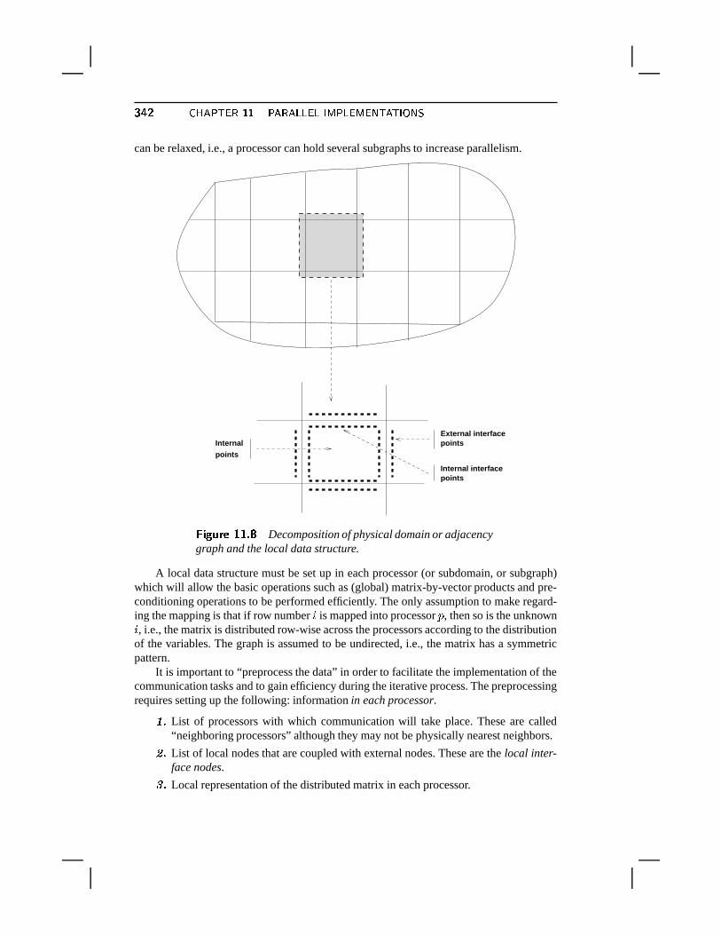
��r¶ � ~�� &�� ?��m� ��?; �� &��p&�� \��can be relaxed, i.e., a processor can hold several subgraphs to increase parallelism.

Internal

points

External interface points

points Internal interface

�� @�,�� Decomposition of physical domain or adjacency

graph and the local data structure.

A local data structure must be set up in each processor (or subdomain, or subgraph)which will allow the basic operations such as (global) matrix-by-vector products and pre-conditioning operations to be performed efficiently. The only assumption to make regard-ing the mapping is that if row number S is mapped into processor � , then so is the unknownS , i.e., the matrix is distributed row-wise across the processors according to the distributionof the variables. The graph is assumed to be undirected, i.e., the matrix has a symmetricpattern.

It is important to “preprocess the data” in order to facilitate the implementation of thecommunication tasks and to gain efficiency during the iterative process. The preprocessingrequires setting up the following: information in each processor.

� �List of processors with which communication will take place. These are called“neighboring processors” although they may not be physically nearest neighbors.� �List of local nodes that are coupled with external nodes. These are the local inter-face nodes.

� �Local representation of the distributed matrix in each processor.

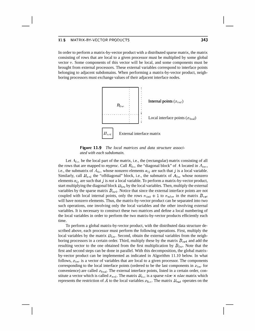
� � � � ��p&� � �}M � �}M �� &c\� ��r\�� &�� ;�In order to perform a matrix-by-vector product with a distributed sparse matrix, the matrixconsisting of rows that are local to a given processor must be multiplied by some globalvector � . Some components of this vector will be local, and some components must bebrought from external processors. These external variables correspond to interface pointsbelonging to adjacent subdomains. When performing a matrix-by-vector product, neigh-boring processors must exchange values of their adjacent interface nodes.

� J F ��

Local interface points ( �� I � )Internal points ( � 5 I � )

External interface matrix

Internal points

�� ,��t·The local matrices and data structure associ-

ated with each subdomain.

Let � � �� be the local part of the matrix, i.e., the (rectangular) matrix consisting of allthe rows that are mapped to myproc. Call � � �� the “diagonal block” of � located in � � �� ,i.e., the submatrix of � � �� whose nonzero elements � 5 � are such that � is a local variable.Similarly, call � J F � the “offdiagonal” block, i.e., the submatrix of � � �� whose nonzeroelements � 5 � are such that � is not a local variable. To perform a matrix-by-vector product,start multiplying the diagonal block � � �� by the local variables. Then, multiply the externalvariables by the sparse matrix � J F � . Notice that since the external interface points are notcoupled with local internal points, only the rows ® 5 I � M / to ® I � �� in the matrix � J F �will have nonzero elements. Thus, the matrix-by-vector product can be separated into twosuch operations, one involving only the local variables and the other involving externalvariables. It is necessary to construct these two matrices and define a local numbering ofthe local variables in order to perform the two matrix-by-vector products efficiently eachtime.

To perform a global matrix-by-vector product, with the distributed data structure de-scribed above, each processor must perform the following operations. First, multiply thelocal variables by the matrix � � �� . Second, obtain the external variables from the neigh-boring processors in a certain order. Third, multiply these by the matrix � J F � and add theresulting vector to the one obtained from the first multiplication by � � �� . Note that thefirst and second steps can be done in parallel. With this decomposition, the global matrix-by-vector product can be implemented as indicated in Algorithm 11.10 below. In whatfollows, � � �� is a vector of variables that are local to a given processor. The componentscorresponding to the local interface points (ordered to be the last components in � � �� forconvenience) are called �� I � . The external interface points, listed in a certain order, con-stitute a vector which is called � J F � . The matrix � � �� is a sparse ® � � �2¯v® � � � matrix whichrepresents the restriction of � to the local variables � � �� . The matrix � J F � operates on the

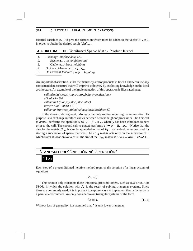
�� ~�� &�� ?��m� ��?; �� &��p&�� \��external variables � J F � to give the correction which must be added to the vector � � �� in order to obtain the desired result <N�7� = � �� .��n��-�w�� ,��#�� %� �� %� � � � �1�'� � � � � �� 1. Exchange interface data, i.e.,2. Scatter � � I � to neighbors and3. Gather � J F � from neighbors4. Do Local Matvec:

� � � �� 5. Do External Matvec:

� M � J F �_� J F �An important observation is that the matrix-by-vector products in lines 4 and 5 can use anyconvenient data structure that will improve efficiency by exploiting knowledge on the localarchitecture. An example of the implementation of this operation is illustrated next:

call bdxchg(nloc,x,y,nproc,proc,ix,ipr,type,xlen,iout)y(1:nloc) = 0.0call amux1 (nloc,x,y,aloc,jaloc,ialoc)nrow = nloc – nbnd + 1call amux1(nrow,x,y(nbnd),aloc,jaloc,ialoc(nloc+1))

In the above code segment, bdxchg is the only routine requiring communication. Itspurpose is to exchange interface values between nearest neighbor processors. The first callto amux1 performs the operation

� � M � � �� , where

has been initialized to zeroprior to the call. The second call to amux1 performs

� � M � J F � � J F � . Notice that thedata for the matrix � J F � is simply appended to that of � � �� , a standard technique used forstoring a succession of sparse matrices. The � J F � matrix acts only on the subvector of �which starts at location ®i >®!� of � . The size of the � J F � matrix is ® + � � ��® � � �k¨n®i >®!� M / .�c�Z� �N�7��>� ��7��2��C�v�t��-��n�N� � ��X�]�R��D�f�W��|�m��

Each step of a preconditioned iterative method requires the solution of a linear system ofequations

� 2 � ¬This section only considers those traditional preconditioners, such as ILU or SOR or

SSOR, in which the solution with � is the result of solving triangular systems. Sincethese are commonly used, it is important to explore ways to implement them efficiently ina parallel environment. We only consider lower triangular systems of the form

� ��¢ �¬ £ ¥/¥/[H¥G¦Without loss of generality, it is assumed that

�is unit lower triangular.

� � �� L&�� \�� &�� \��0� � �©\��p&�� \�� $1$ ��! %$ � ' A�'56 6,036 2 * B 2 9� 7:A � ' A!4 * � 010 �1*

Typically in solving a lower triangular system, the solution is overwritten onto the right-hand side on return. In other words, there is one array � for both the solution and theright-hand side. Therefore, the forward sweep for solving a lower triangular system withcoefficients � � <%S � � = and right-hand-side � is as follows.

�� n� �D�w�� ,��#�,�� 1. Do i=2, n2. For (all j such that al(i,j) is nonzero) Do:3. x(i) := x(i) – al(i,j) * x(j)4. EndDo5. EndDo

Assume that the matrix is stored row wise in the general Compressed Sparse Row (CSR)format, except that the diagonal elements (ones) are not stored. Then the above algorithmtranslates into the following code segment:

1. Do i=2, n2. Do j=ial(i), ial(i+1) – 13. x(i)=x(i) – al(j) * x(jal(j))4. EndDo5. EndDo

The outer loop corresponding to the variable S is sequential. The � loop is a sparse dotproduct of the S �� row of

�and the (dense) vector � . This dot product may be split among

the processors and the partial results may be added at the end. However, the length of thevector involved in the dot product is typically short. So, this approach is quite inefficientin general. We examine next a few alternative approaches. The regularly structured and theirregularly structured cases are treated separately.

$1$ ��! #" 6,0�>036N* ��=?014?(�6 2#9�&��,;>=?0 �1'�*10 7 ��-�� 7G2 9!;BC'�; A�2 ��0,*

First, consider an example which consists of a 5-point matrix associated with a3 ¯ � mesh

as represented in Figure 11.10. The lower triangular matrix associated with this mesh isrepresented in the left side of Figure 11.10. The stencil represented in the right side ofFigure 11.10 establishes the data dependence between the unknowns in the lower triangularsystem solution when considered from the point of view of a grid of unknowns. It tells usthat in order to compute the unknown in position < S�� = , only the two unknowns in positions< SZ¨ / � � = and < S�� ¨ / = are needed . The unknown � B B does not depend on any othervariable and can be computed first. Then the value of � B B can be used to get � B + « and �C« + Bsimultaneously. Then these two values will in turn enable � � + B �I�k« + « and � B + � to be obtainedsimultaneously, and so on. Thus, the computation can proceed in wavefronts. The steps forthis wavefront algorithm are shown with dashed lines in Figure 11.10. Observe that the

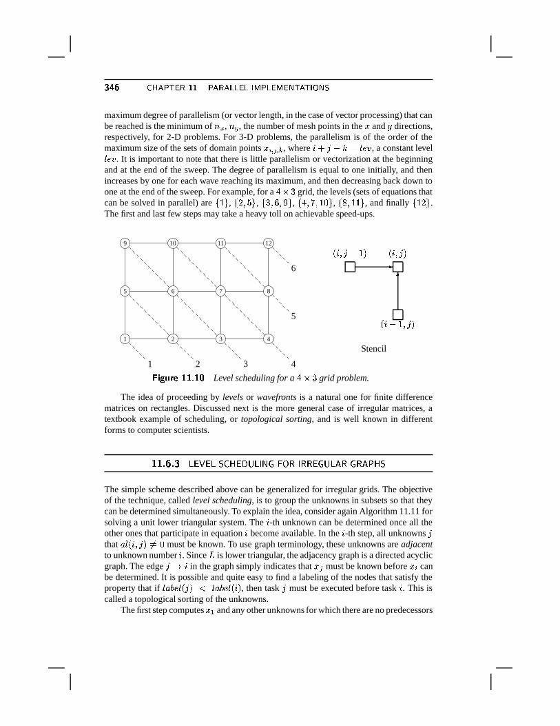
�� ~�� &�� ?��m� ��?; �� &��p&�� \��maximum degree of parallelism (or vector length, in the case of vector processing) that canbe reached is the minimum of ® F , ® � , the number of mesh points in the � and

directions,

respectively, for 2-D problems. For 3-D problems, the parallelism is of the order of themaximum size of the sets of domain points � 5 + � + � , where S M � M �� Q � , a constant level� Q � . It is important to note that there is little parallelism or vectorization at the beginningand at the end of the sweep. The degree of parallelism is equal to one initially, and thenincreases by one for each wave reaching its maximum, and then decreasing back down toone at the end of the sweep. For example, for a

3 ¯ � grid, the levels (sets of equations thatcan be solved in parallel) are

� / � , � 0 � � � , � �F� �,� � � , � 3 � � � / - � , � �F� /�/ � , and finally

� / 0 � .The first and last few steps may take a heavy toll on achievable speed-ups.

1 2 3 4

5 6 7 8

9 10 11 12

1 2 3 4

5

6

< S�� =

<%Si¨ / � � =

<%S�� w¨ / =�

�

Stencil

�� @�,��#��Level scheduling for a

3 ¯ � grid problem.

The idea of proceeding by levels or wavefronts is a natural one for finite differencematrices on rectangles. Discussed next is the more general case of irregular matrices, atextbook example of scheduling, or topological sorting, and is well known in differentforms to computer scientists.

$1$ �! � 6,0�>0368* ��=)014?( 6 2 9�& � 7:A 2#A!A+0F& ( 6�' A &)A�' �+= *

The simple scheme described above can be generalized for irregular grids. The objectiveof the technique, called level scheduling, is to group the unknowns in subsets so that theycan be determined simultaneously. To explain the idea, consider again Algorithm 11.11 forsolving a unit lower triangular system. The S -th unknown can be determined once all theother ones that participate in equation S become available. In the S -th step, all unknowns �that � � < S�� = �� -

must be known. To use graph terminology, these unknowns are adjacentto unknown number S . Since

�is lower triangular, the adjacency graph is a directed acyclic

graph. The edge � � S in the graph simply indicates that � � must be known before � 5 canbe determined. It is possible and quite easy to find a labeling of the nodes that satisfy theproperty that if � � Q � < � =a² � � Q � < S = , then task � must be executed before task S . This iscalled a topological sorting of the unknowns.

The first step computes � B and any other unknowns for which there are no predecessors

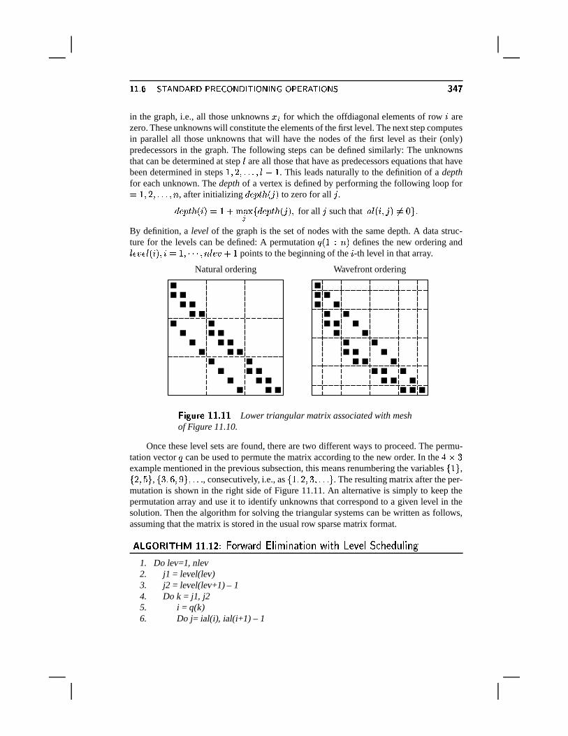
� � �� L&�� \�� &�� \��0� � �©\��p&�� \�� in the graph, i.e., all those unknowns � 5 for which the offdiagonal elements of row S arezero. These unknowns will constitute the elements of the first level. The next step computesin parallel all those unknowns that will have the nodes of the first level as their (only)predecessors in the graph. The following steps can be defined similarly: The unknownsthat can be determined at step � are all those that have as predecessors equations that havebeen determined in steps / � 0 �*¬,¬*¬T� �i¨ / . This leads naturally to the definition of a depthfor each unknown. The depth of a vertex is defined by performing the following loop for� / � 0 �,¬*¬*¬ �I® , after initializing � Q � � � < � = to zero for all � .

� Q � � ��<%S =�� / M � � �� Q � � ��< � = � for all � such that � � <%S�� = �� - �L¬By definition, a level of the graph is the set of nodes with the same depth. A data struc-ture for the levels can be defined: A permutation ��< / � ®�= defines the new ordering and� Q � Q � < S = � Sc� / � � � � �I® � Q � M / points to the beginning of the S -th level in that array.

Natural ordering Wavefront ordering

�� ,��#�,�Lower triangular matrix associated with mesh

of Figure 11.10.

Once these level sets are found, there are two different ways to proceed. The permu-tation vector � can be used to permute the matrix according to the new order. In the

3 ¯ �example mentioned in the previous subsection, this means renumbering the variables

� / � ,� 0 � � � , � �F� �,� � �.�*¬*¬,¬ , consecutively, i.e., as

� / � 0 � �,�,¬*¬*¬ � . The resulting matrix after the per-mutation is shown in the right side of Figure 11.11. An alternative is simply to keep thepermutation array and use it to identify unknowns that correspond to a given level in thesolution. Then the algorithm for solving the triangular systems can be written as follows,assuming that the matrix is stored in the usual row sparse matrix format.

�� n� �D�w�� ,��#�%¶ �� 1. Do lev=1, nlev2. j1 = level(lev)3. j2 = level(lev+1) – 14. Do k = j1, j25. i = q(k)6. Do j= ial(i), ial(i+1) – 1

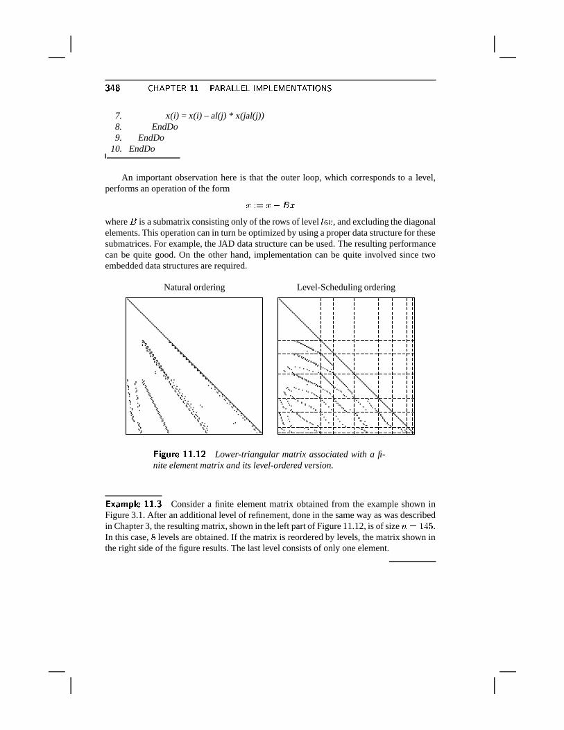
�� ~�� &�� ?��m� ��?; �� &��p&�� \��7. x(i) = x(i) – al(j) * x(jal(j))8. EndDo9. EndDo

10. EndDo

An important observation here is that the outer loop, which corresponds to a level,performs an operation of the form

� � ��u¨ � �where � is a submatrix consisting only of the rows of level � Q � , and excluding the diagonalelements. This operation can in turn be optimized by using a proper data structure for thesesubmatrices. For example, the JAD data structure can be used. The resulting performancecan be quite good. On the other hand, implementation can be quite involved since twoembedded data structures are required.

Natural ordering Level-Scheduling ordering

�� @�,��#�%¶Lower-triangular matrix associated with a fi-

nite element matrix and its level-ordered version.

�� ,�� Consider a finite element matrix obtained from the example shown in

Figure 3.1. After an additional level of refinement, done in the same way as was describedin Chapter 3, the resulting matrix, shown in the left part of Figure 11.12, is of size ®�� / 3 � .In this case, � levels are obtained. If the matrix is reordered by levels, the matrix shown inthe right side of the figure results. The last level consists of only one element.

�� ?�� }\�&�?� ��r·� ��]� �W�-�]�ª�

1 Give a short answer to each of the following questions:� � What is the main disadvantage of shared memory computers based on a bus architecture?� � What is the main factor in yielding the speed-up in pipelined processors? !� Related to the previous question: What is the main limitation of pipelined processors inregards to their potential for providing high speed-ups?

2 Show that the number of edges in a binary�

-cube is� ) 2�4

.

3 Show that a binary � -cube is identical with a torus which is a � � � mesh with wrap-aroundconnections. Are there hypercubes of any other dimensions that are equivalent topologically totoruses?

4 A Gray code of length � e ) is a sequence � � �� 2�4 of�

-bit binary numbers such that (a)any two successive numbers in the sequence differ by one and only one bit; (b) all

�-bit binary

numbers are represented in the sequence; and (c) � and � � 254 differ by one bit.� � Find a Gray code sequence of length � e � and show the (closed) path defined by thesequence of nodes of a 3-cube, whose labels are the elements of the Gray code sequence.What type of paths does a Gray code define in a hypercube?� � To build a “binary reflected” Gray code, start with the trivial Gray code sequence consistingof the two one-bit numbers 0 and 1. To build a two-bit Gray code, take the same sequenceand insert a zero in front of each number, then take the sequence in reverse order and insert aone in front of each number. This gives � e��0 0 � 0!� �� 0�� . The process is repeated untilan�

-bit sequence is generated. Show the binary reflected Gray code sequences of length 2,4, 8, and 16. Prove (by induction) that this process does indeed produce a valid Gray codesequence. !� Let an

�-bit Gray code be given and consider the sub-sequence of all elements whose first

bit is constant (e.g., zero). Is this an� 6 �

bit Gray code sequence? Generalize this to any ofthe�

-bit positions. Generalize further to any set of � � � bit positions.� � Use the previous question to find a strategy to map a) � � ) 0

mesh into an

# � 4 � � '-cube.

5 Consider a ring of � processors which are characterized by the following communication perfor-mance characteristics. Each processor can communicate with its two neighbors simultaneously,i.e., it can send or receive a message while sending or receiving another message. The time fora message of length

�to be transmitted between two nearest neighbors is of the form

� � �� A message of length

�is “broadcast” to all processors by sending it from

> 4 to> and then

from> to

> �, etc., until it reaches all destinations, i.e., until it reaches

> �. How much time

does it take for the message to complete this process?� � Now split the message into packets of equal size and pipeline the data transfer. Typically,each processor will receive packet number from the previous processor, while sendingpacket 6=� it has already received to the next processor. The packets will travel in chainfrom

> 4 to> , �� , to

> �. In other words, each processor executes a program that is described

roughly as follows:��+ �S)�<� ��;��$�!�# C��

�� ~�� &�� ?��m� ��?; �� &��p&�� \��L��#*� � ��38!�#�C��R��;��*�D 9:�� ;G8�� V8��#*��**�J��@38�!�# C��=��;��G V�� 38��#��*�

� ��@��

There are a few additional conditionals. Assume that the number of packets is equal to � 6 � .How much time does it take for all packets to reach all � processors? How does this comparewith the simple method in (a)?

6 (a) Write a short FORTRAN routine (or C function) which sets up the level number of eachunknown of an upper triangular matrix. The input matrix is in CSR format and the output shouldbe an array of length

�containing the level number of each node. (b) What data structure should

be used to represent levels? Without writing the code, show how to determine this data structurefrom the output of your routine. (c) Assuming the data structure of the levels has been deter-mined, write a short FORTRAN routine (or C function) to solve an upper triangular systemusing the data structure resulting in the previous question. Show clearly which loop should beexecuted in parallel.

7 In the jagged diagonal format described in Section 11.5.5, it is necessary to preprocess the matrixby sorting its rows by decreasing number of rows. What type of sorting should be used for thispurpose?

8 In the jagged diagonal format described in Section 11.5.5, the matrix had to be preprocessed bysorting it by rows of decreasing number of elements.�� What is the main reason it is necessary to reorder the rows?� � Assume that the same process of extracting one element per row is used. At some point the

extraction process will come to a stop and the remainder of the matrix can be put into aCSR data structure. Write down a good data structure to store the two pieces of data and acorresponding algorithm for matrix-by-vector products. !� This scheme is efficient in many situations but can lead to problems if the first row is veryshort. Suggest how to remedy the situation by padding with zero elements, as is done for theEllpack format.

9 Many matrices that arise in PDE applications have a structure that consists of a few diagonalsand a small number of nonzero elements scattered irregularly in the matrix. In such cases, it isadvantageous to extract the diagonal part and put the rest in a general sparse (e.g., CSR) format.Write a pseudo-code to extract the main diagonals and the sparse part. As input parameter, thenumber of diagonals desired must be specified.

NOTES AND REFERENCES. Kai Hwang’s book [124] is recommended for an overview of parallelarchitectures. More general recommended reading on parallel computing are the book by Bertsekasand Tsitsiklis [25] and a more recent volume by Kumar et al. [139]. One characteristic of high-performance architectures is that trends come and go rapidly. A few years ago, it seemed that mas-sive parallelism was synonymous with distributed memory computing, specifically of the hypercubetype. Currently, many computer vendors are mixing message-passing paradigms with “global addressspace,” i.e., shared memory viewpoint. This is illustrated in the recent T3D machine built by CRAYResearch. This machine is configured as a three-dimensional torus and allows all three programmingparadigms discussed in this chapter, namely, data-parallel, shared memory, and message-passing. Itis likely that the T3D will set a certain trend. However, another recent development is the advent ofnetwork supercomputing which is motivated by astounding gains both in workstation performanceand in high-speed networks. It is possible to solve large problems on clusters of workstations and to

�� ?�� }\�&�?� ��3�obtain excellent performance at a fraction of the cost of a massively parallel computer.

Regarding parallel algorithms, the survey paper of Ortega and Voigt [156] gives an exhaustivebibliography for research done before 1985 in the general area of solution of Partial DifferentialEquations on supercomputers. An updated bibliography by Ortega, Voigt, and Romine is available in[99]. See also the survey [178] and the monograph [71]. Until the advent of supercomputing in themid 1970s, storage schemes for sparse matrices were chosen mostly for convenience as performancewas not an issue, in general. The first paper showing the advantage of diagonal storage schemes insparse matrix computations is probably [133]. The first discovery by supercomputer manufacturers ofthe specificity of sparse matrix computations was the painful realization that without hardware sup-port, vector computers could be inefficient. Indeed, the early CRAY machines did not have hardwareinstructions for gather and scatter operations but this was soon remedied in the second-generationmachines. For a detailed account of the beneficial impact of hardware for “scatter” and “gather” onvector machines, see [146].

Level scheduling is a textbook example of topological sorting in graph theory and was discussedfrom this viewpoint in, e.g., [8, 190, 228]. For the special case of finite difference matrices on rectan-gular domains, the idea was suggested by several authors independently, [208, 209, 111, 186, 10]. Infact, the level scheduling approach described in this chapter is a “greedy” approach and is unlikelyto be optimal. There is no reason why an equation should be solved as soon as it is possible. Forexample, it may be preferable to use a backward scheduling [7] which consists of defining the levelsfrom bottom up in the graph. Thus, the last level consists of the leaves of the graph, the previous levelconsists of their predecessors, etc. Dynamic scheduling can also be used as opposed to static schedul-ing. The main difference is that the level structure is not preset; rather, the order of the computation isdetermined at run-time. The advantage over pre-scheduled triangular solutions is that it allows pro-cessors to always execute a task as soon as its predecessors have been completed, which reduces idletime. On loosely coupled distributed memory machines, this approach may be the most viable sinceit will adjust dynamically to irregularities in the execution and communication times that can causea lock-step technique to become inefficient. However, for those shared memory machines in whichhardware synchronization is available and inexpensive, dynamic scheduling would have some dis-advantages since it requires managing queues and generates explicitly busy waits. Both approacheshave been tested and compared in [22, 189] where it was concluded that on the Encore Multimaxdynamic scheduling is usually preferable except for problems with few synchronization points and alarge degree of parallelism. In [118], a combination of prescheduling and dynamic scheduling wasfound to be the best approach on a Sequent balance 21000. There seems to have been no comparisonof these two approaches on distributed memory machines or on shared memory machines with mi-crotasking or hardware synchronization features. In [22, 24] and [7, 8], a number of experiments arepresented to study the performance of level scheduling within the context of preconditioned Conju-gate Gradient methods. Experiments on an Alliant FX-8 indicated that a speed-up of around 4 to 5can be achieved easily. These techniques have also been tested for problems in Computational FluidDynamics [214, 216].

methods related to the

Documents