CU-CSSC-91-24 CENTER FOR SPACE STRUCTURES AND CONTROL

MEMBRANE TRIANGLES WITHCORNER DRILLING FREEDOMSI. The EFF Element

by

K. Alvin, H. M. de la Fuente,B. Haugen and C. A. Felippa

August 1991Rev. May 1992

COLLEGE OF ENGINEERINGUNIVERSITY OF COLORADOCAMPUS BOX 429BOULDER, COLORADO 80309

Membrane Triangles with Corner Drilling Freedoms

Part I: The EFF Element

Ken Alvin, Horacio M. de la Fuente,

Bjorn Haugen and Carlos A. Felippa

Department of Aerospace Engineering Sciences andCenter for Space Structures and Controls

University of ColoradoBoulder, Colorado 80309-0429, USA

August 1991Revised May 1992

Report No. CU-CSSC-91-24

Paper appeared in Finite Elements Anal. Des., 12, 163–187, 1992. Research supported byNASA Langley Research Center under Grant NAG1-756, NASA Lewis Research Centerunder Grant NAG 3-934, and the National Science Foundation under Grant ASC-8717773.

MEMBRANE TRIANGLES WITH CORNERDRILLING FREEDOMS: I. THE EFF ELEMENT

Ken Alvin, Horacio M. de la Fuente,

Bjorn Haugen and Carlos A. Felippa

Department of Aerospace Engineering Sciencesand Center for Space Structures and Controls

University of ColoradoBoulder, Colorado 80309-0429, USA

SUMMARY

This paper is the first of a three-Part series that studies the formulation of 3-node, 9-dof membrane elements withnormal-to-element-plane rotations (the so-called drilling freedoms) within the context of parametrized variationalprinciples. These principles supply a unified basis for several advanced element-construction techniques; inparticular: the free formulation (FF), the extended free formulation (EFF) and the assumed natural deviatoricstrain (ANDES) formulation. In Part I we construct an element of this type using the EFF. This derivationillustrates the basic steps in the application of that formulation to the construction of high-performance, rank-sufficient, nonconforming elements with corner rotations. The element is initially given the 12 degrees offreedom of the linear strain triangle (LST), which allows the displacement expansion to be a complete quadraticin each component. The expansion basis contains the 6 linear basic functions and 6 energy-orthogonal quadratichigher order functions. Three degrees of freedom, defined as the midpoint deviations from linearity alongthe triangle-median directions, are eliminated by kinematic constraints. The remaining hierarchical midpointfreedoms are transformed to corner rotations. The performance of the resulting element is evaluated in Part III.

1

1. INTRODUCTION

The idea of including normal-rotation degrees of freedom at corner points of plane-stress finiteelements — the so-called drilling freedoms — is an old one. The main motivations behind this ideaare:

1. To improve the element performance while avoiding the use of midpoint degrees of freedom.Midpoint nodes have lower valency than corner nodes, demand extra effort in mesh definitionand generation, and can cause modeling difficulties in nonlinear analysis and dynamics.

2. To solve the “normal rotation problem” of smooth shells analyzed with finite elements programsthat carry six degrees of freedom per node.

3. To simplify the modeling of connections between plates, shells and beams, as well as thetreatment of junctures between shells and/or plates.

Many efforts to develop membrane elements with drilling freedoms were made during the period1964–1975 with inconclusive results. A summary of this early work is given in the Introduction ofan article by Bergan and Felippa [1], where it is remarked that Irons and Ahmad in their 1980 book[2] had dismissed the task as hopeless. In fact, the subject laid largely dormant during the late 1970s,but it has been revived in recent publications [3,1,4–8] that present several solutions to this challenge.Especially noteworthy is the study by Hughes and Brezzi [9] of variational principles that includeindependent displacement and rotation fields. A membrane element with drilling freedoms based onthese principles has recently been constructed by Ibrahimbegovic [10].

The first successful triangles with drilling freedoms were presented by Allman in 1984 [3] and Berganand Felippa in 1985 [1]. Both elements are nonconforming and pass displacement-specified patchtests. In addition the Bergan-Felippa triangle, being rank sufficient, passes traction-specified patchtests. The original Allman element, based on the concept of vertex rotations, had remaining problemssuch as rank deficiency, which were corrected in an improved version published in 1988 [7]. The twoapproaches share procedural similarities, such as the use of incompatible displacement functions.But the element construction methods are entirely different: Allman used the conventional potentialenergy formulation whereas Bergan and Felippa used the free formulation (FF) of Bergan and Nygard[11]. Furthermore Bergan and Felippa, following mid-1960s work at Berkeley and Trondheim [12–15] exploited the concept of continuum-mechanics rotations, sometimes referred to as true rotations.A discussion of the relative performance of these elements is given in Part III of this series [16].

Both approaches can be extended to quadrilateral elements with drilling freedoms for plane stressand shell analysis. Extensive experience with Allman-type quadrilateral shell elements is reportedby Frey and coworkers; see the excellent survey article [17] and references therein. A FF-basedquadrilateral called FFQ was constructed by Nygard in his thesis [18] using quadratic and cubichigher order functions; this is presenly a workhorse shell element in the nonlinear program FENRIS[19].

At the time the Bergan-Felippa element was constructed (summer 1984) the free formulation lackeda variational basis. This deficiency was remedied five years later by the introduction of parametrizedvariational principles in a series of recent publications [20–23]. Therein it is shown that the energy-orthogonal FF with scaled higher order stiffness can be accommodated in the framework of a one-parameter d-generalized hybrid variational principle that reduces to hybrid versions of the potential

2

energy and Hellinger-Reissner’s principle as special cases. This rigorous justification of the FFopened the door to a variant called the extended free formulation or EFF [24], which circumvents amajor kinematic restriction of the FF.

The present work may be viewed as a continuation of two mid-80 papers [1,6] but now on firmertheoretical grounds. Our main objective is to illustrate the application of the EFF to the construction ofa triangular membrane element with drilling freedoms that initially has complete quadratic polynomialexpansions in each displacement component. The use of complete quadratic expansions as departurepoint requires a total of 12 degrees of freedom. Nine freedoms are defined at the corner nodes in theusual fashion, i.e., six translations and three drilling rotations. Three additional degrees of freedoms,to be subsequently eliminated, are needed. In the EFF such additional freedoms can be eliminated inthree ways: duality pairing with divergence-free stresses, static condensation of augmenting degreesof freedom, or a posteriori application of kinematic constraints. The present derivation uses the lasttechnique.

Four choices of “eliminable midpoint freedoms” intrinsically related to the triangle geometry wereconsidered: side directions, normal-to-sides, median directions and normal-to-medians. It was foundthat only the third choice provides for stable elimination. Once this key discovery was made, theremaining element derivation steps, though laborious, could be followed in a systematic way.

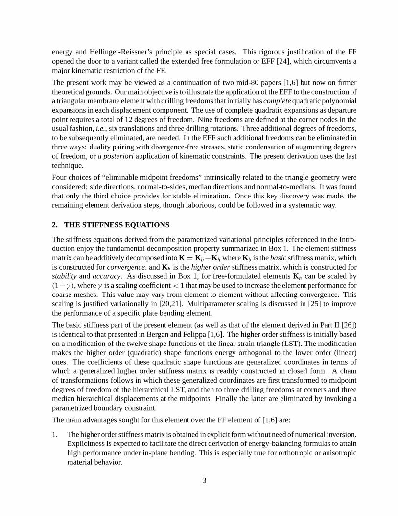
2. THE STIFFNESS EQUATIONS

The stiffness equations derived from the parametrized variational principles referenced in the Intro-duction enjoy the fundamental decomposition property summarized in Box 1. The element stiffnessmatrix can be additively decomposed into K = Kb +Kh where Kb is the basic stiffness matrix, whichis constructed for convergence, and Kh is the higher order stiffness matrix, which is constructed forstability and accuracy. As discussed in Box 1, for free-formulated elements Kh can be scaled by(1−γ ), where γ is a scaling coefficient < 1 that may be used to increase the element performance forcoarse meshes. This value may vary from element to element without affecting convergence. Thisscaling is justified variationally in [20,21]. Multiparameter scaling is discussed in [25] to improvethe performance of a specific plate bending element.

The basic stiffness part of the present element (as well as that of the element derived in Part II [26])is identical to that presented in Bergan and Felippa [1,6]. The higher order stiffness is initially basedon a modification of the twelve shape functions of the linear strain triangle (LST). The modificationmakes the higher order (quadratic) shape functions energy orthogonal to the lower order (linear)ones. The coefficients of these quadratic shape functions are generalized coordinates in terms ofwhich a generalized higher order stiffness matrix is readily constructed in closed form. A chainof transformations follows in which these generalized coordinates are first transformed to midpointdegrees of freedom of the hierarchical LST, and then to three drilling freedoms at corners and threemedian hierarchical displacements at the midpoints. Finally the latter are eliminated by invoking aparametrized boundary constraint.

The main advantages sought for this element over the FF element of [1,6] are:

1. The higher order stiffness matrix is obtained in explicit form without need of numerical inversion.Explicitness is expected to facilitate the direct derivation of energy-balancing formulas to attainhigh performance under in-plane bending. This is especially true for orthotropic or anisotropicmaterial behavior.

3

2. Shorter formation time for Kh , which dominates the computation of K.

3. The coarse-mesh performance should be comparable to that of the linear strain triangle (LST)without the encumbrance of midpoint nodes.

Experience with the EFF element, as reported in Part III [16], indicates that the first two advantageswere realized, but the last one was not. Its performance turned out to be similar to that of the originalFF element, except for some regular-mesh problems where explicit energy balancing was able tomake a difference. The performance is, however, substantially better than all other elements testedfor large element aspect ratios.

Aside from its intrinsic value as illustration of a powerful new technique for constructing high-performance elements, the present derivation serves as prelude to a far more challenging task: theconstruction of a rank-sufficient element in three dimensions (a 24-dof, rank-18 tetrahedron with 12corner rotations).

3. THE FREE FORMULATION

The original free formulation (FF) was developed by Bergan and Nygard [11] for the construction ofdisplacement-based, incompatible finite elements. This work consolidated a decade of research ofBergan and coworkers at Trondheim, milestones of which may be found in [27,28,19]. The productsof this research have been finite elements of high performance, especially for linear and nonlinearanalysis of plate and shell structures. As noted in the Introduction, a theoretical justification basedon parametrized hybrid variational principles is provided in references [20–23].

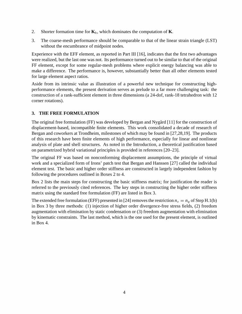
The original FF was based on nonconforming displacement assumptions, the principle of virtualwork and a specialized form of Irons’ patch test that Bergan and Hanssen [27] called the individualelement test. The basic and higher order stiffness are constructed in largely independent fashion byfollowing the procedures outlined in Boxes 2 to 4.

Box 2 lists the main steps for constructing the basic stiffness matrix; for justification the reader isreferred to the previously cited references. The key steps in constructing the higher order stiffnessmatrix using the standard free formulation (FF) are listed in Box 3.

The extended free formulation (EFF) presented in [24] removes the restriction nv = nq of Step H.1(b)in Box 3 by three methods: (1) injection of higher order divergence-free stress fields, (2) freedomaugmentation with elimination by static condensation or (3) freedom augmentation with eliminationby kinematic constraints. The last method, which is the one used for the present element, is outlinedin Box 4.

4

Box 1 Decomposition of the Element Stiffness Equations

Let K be the element stiffness matrix, v the visible element degrees of freedom (thosedegrees of freedom in common with other elements, also called the connectors) and pthe corresponding element node forces. Then the element stiffness equations decomposeas

Kv = (Kb + Kh) v = p. (1)

Kb and Kh are called the basic and higher order stiffness matrices, respectively. Thebasic stiffness matrix, which is usually rank deficient, is constructed for convergence.The higher order stiffness matrix is constructed for stability and (in more recent work)accuracy. A decomposition of this nature, which also holds at the assembly level, wasfirst obtained by Bergan and Nygard in the derivation of the free formulation [11].

In the unified formulation presented in [22, 23] the following key properties of thedecomposition (1) are derived.

1. Kb is formulation independent and is defined entirely by an assumed constant stressstate working on element boundary displacements. As detailed in Box 2, no knowl-edge of the interior displacements is necessary for this stiffness component. Theextension of this statement to C0 plate and shell elements is not straightforward,however, and special considerations are necessary in order to obtain Kb for thoseelements.

2. Kh has the general form

Kh = j33Kh33 + j22Kh22 + j23Kh23. (2)

The three parameters j22, j23 and j33 characterize the source variational principle inthe following sense:

(a) The FF is recovered if j22 = j23 = 0 and j33 = 1 − γ , where γ is a Kh

scaling coefficient studied in [1,6,25]. The original FF of [11] is obtained ifγ = 0. The source variational principle is a one-parameter form that includesthe potential energy and stress-displacement Reissner functionals as specialcases.

(b) The ANDES variant of ANS is recovered if j23 = j33 = 0 whereas j22 is ascaling parameter. The source variational principle is a one-parameter formthat includes Reissner’s stress-displacement and Hu-Washizu’s functionals asspecial cases.

(c) If j23 is nonzero, the last term in (2) may be viewed as being produced by aFF/ANDES combination. Such a combination remains unexplored.

5

Box 2 Construction of the Basic Stiffness Kb

Step B.1. Assume a constant stress field, σ, inside the element. The associatedboundary tractions are σn = σ.n, where n denotes the unit external normal on theboundary S.

Step B.2. Assume boundary displacements, d, over S. This field is described in termsof the visible element node displacements v (also called the connectors) as

d = Nd v, (3)

where Nd is an array of boundary shape functions. The boundary motions (2) must satisfyinterelement continuity and contain rigid-body and constant-strain motions exactly.

Step B.3. Construct the “force lumping matrix”

L =∫

SNdn d S, (4)

that consistently maps the boundary tractions σn = σ.n into element node forces, p,conjugate to v in the virtual work sense. That is,

p =∫

SNnσn d S = Lσ. (5)

In the above, Ndn = Nd .n are boundary-system projections of Nd that work on the surfacetractions σn .

Step B.4. The basic stiffness matrix for a three-dimensional element is

Kb = 1

VLELT , (6)

where E is the stress-strain constitutive matrix of elastic moduli, which are assumedto be constant over the element, and V = ∫

V dV is the element volume measure. Fortwo-dimensional or one-dimensional elements, V is replaced by the element area A orlength , respectively, if the remaining dimensions are incorporated in the constitutivematrix E.

6

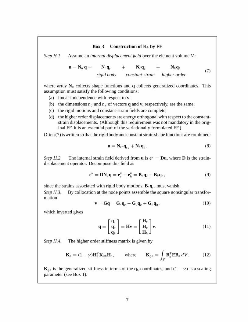
Box 3 Construction of Kh by FF

Step H.1. Assume an internal displacement field over the element volume V :

u = Nu q = Nr qr + Ncqc + Nhqh

rigid body constant-strain higher order(7)

where array Nu collects shape functions and q collects generalized coordinates. Thisassumption must satisfy the following conditions:

(a) linear independence with respect to v;(b) the dimensions nq and nv of vectors q and v, respectively, are the same;(c) the rigid motions and constant-strain fields are complete;(d) the higher order displacements are energy orthogonal with respect to the constant-

strain displacements. (Although this requirement was not mandatory in the orig-inal FF, it is an essential part of the variationally formulated FF.)

Often (7) is written so that the rigid body and constant strain shape functions are combined:

u = Nrcqrc + Nhqh . (8)

Step H.2. The internal strain field derived from u is eu = Du, where D is the strain-displacement operator. Decompose this field as

eu = DNuq = euc + eu

h = Bcqc + Bhqh, (9)

since the strains associated with rigid body motions, Br qr , must vanish.Step H.3. By collocation at the node points assemble the square nonsingular transfor-mation

v = Gq = Gr qr + Gcqc + Ghqh, (10)

which inverted gives

q =[ qr

qcqh

]= Hv =

[ Hr

Hc

Hh

]v. (11)

Step H.4. The higher order stiffness matrix is given by

Kh = (1 − γ )HTh KqhHh, where Kqh =

∫V

BTh EBh dV . (12)

Kqh is the generalized stiffness in terms of the qh coordinates, and (1 − γ ) is a scalingparameter (see Box 1).

7

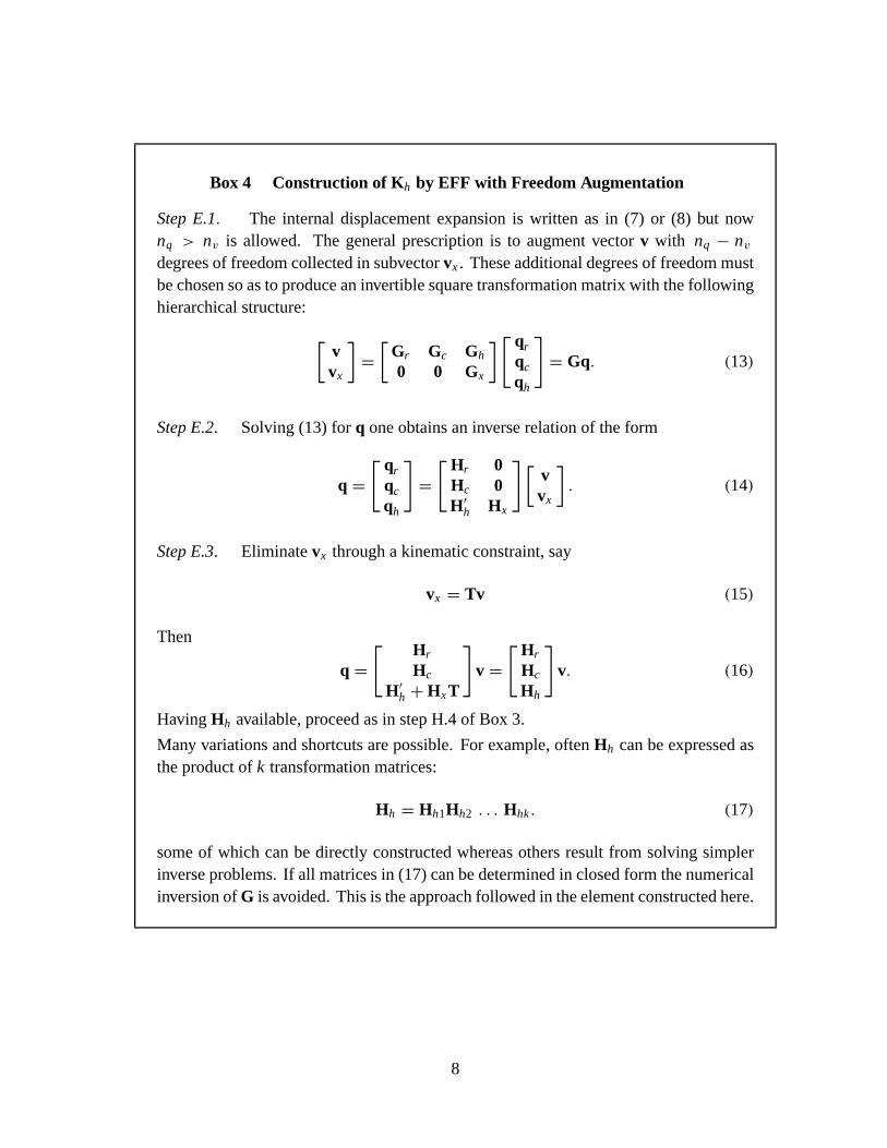
Box 4 Construction of Kh by EFF with Freedom Augmentation

Step E.1. The internal displacement expansion is written as in (7) or (8) but nownq > nv is allowed. The general prescription is to augment vector v with nq − nv

degrees of freedom collected in subvector vx . These additional degrees of freedom mustbe chosen so as to produce an invertible square transformation matrix with the followinghierarchical structure:

[vvx

]=

[Gr Gc Gh

0 0 Gx

] [ qrqcqh

]= Gq. (13)

Step E.2. Solving (13) for q one obtains an inverse relation of the form

q =[ qr

qcqh

]=

[ Hr 0Hc 0H′

h Hx

] [vvx

]. (14)

Step E.3. Eliminate vx through a kinematic constraint, say

vx = Tv (15)

Then

q =[ Hr

Hc

H′h + Hx T

]v =

[ Hr

Hc

Hh

]v. (16)

Having Hh available, proceed as in step H.4 of Box 3.

Many variations and shortcuts are possible. For example, often Hh can be expressed asthe product of k transformation matrices:

Hh = Hh1Hh2 . . . Hhk . (17)

some of which can be directly constructed whereas others result from solving simplerinverse problems. If all matrices in (17) can be determined in closed form the numericalinversion of G is avoided. This is the approach followed in the element constructed here.

8

4. ELEMENT GEOMETRY

The geometry of an individual triangle is illustrated in Figures 1 and 2. The triangle has straightsides. Its geometry is completely defined by the location of its three corners, which are labeled 1,2,3,traversed counterclockwise. The element is referred to a local Cartesian system (x , y). The Cartesiandistances from the nodes to the triangle centroid x0 = (x1 + x2 + x3)/3, y0 = (y1 + y2 + y3)/3 aredenoted by xi0 = xi − x0 and yi0 = yi − y0. It follows that

x10 + x20 + x30 = 0, y10 + y20 + y30 = 0. (18)

Node coordinate differences are abbreviated by writing xi j = xi − xj , etc. The signed triangle areaA is given by the formulas

2A = x21 y31 − x31 y21 = x32 y12 − x12 y32 = x13 y23 − x23 y13, (19)

and we require that A > 0. We shall also make use of dimensionless triangular area coordinates ζ1,ζ2, ζ3 linked by the constraint

ζ1 + ζ2 + ζ3 = 1. (20)

The following well known relation between the area and Cartesian coordinates of a straight-sidedtriangle is noted for further use:

ζi = 1

2A

[xi yk − xk yj + (x − x0)yjk + (y − y0)xk j

], (21)

where i , j and k denote positive cyclic permutations of 1, 2 and 3; for example, i = 2, j = 3, k = 1.(If the origin is taken at the centroid, x0 = y0 = 0.) It follows that

2A∂ζ1

∂x= y23, 2A

∂ζ2

∂x= y31, 2A

∂ζ3

∂x= y12,

2A∂ζ1

∂y= x32, 2A

∂ζ2

∂y= x13, 2A

∂ζ3

∂y= x21.

(22)

Other intrinsic dimensions of use in subsequent derivations are

i j = j i =√

x2i j + y2

i j , ai j = aji = 32

√x2

k0 + y2k0, bi j = 2A/ai j ,

S1 = 14 (2

12 − 231), S2 = 1

4 (223 − 2

12), S3 = 14 (2

13 − 223).

(23)

in which j and k denote the positive cyclic permutations of i ; for example i = 2, j = 3, k = 1. Theai j are the lengths of the triangle medians (see Figure 2).

In addition to the corner nodes 1, 2 and 3 we shall also use the element midpoints 4, 5 and 6for intermediate derivations although these nodes will not appear in the final equations. These arelocated opposite corners 3, 1 and 2, respectively. As shown in Figures 1 and 2, two intrinsic coordinatesystems are used on each side:

n21, s21, n32, s32, n13, s13, (24)

9

1 (x , y )

4

5

6

n = n5 32

5 32t = t

t = t6 13

n =n6 13

t = t4 21

n =n4 21

x

y

1 1

3 (x , y )

2 (x , y )2 2

3 3

Figure 1. Triangle geometry, showing Cartesian andnormal/tangential coordinate systems.

1

2

3

4

5

6

0

m = m5 32

5 32s = s

s = s6 13

m = m6 13

s = s4 21

m = m4 21

b21

a21

x

y

Figure 2. Intrinsic triangle dimensions and median/normal-to-mediancoordinate systems.

10

m21, t21, m32, t32, m13, t13. (25)

Here n and s are oriented along the external normal-to-side and side directions, respectively, whereasm and t are oriented along the triangle median and normal-to-median directions, respectively. Notethat the two coordinate sets (24)-(25) coincide only for equilateral triangles. The origin of thesesystems is left “floating” and may be adjusted as appropriate. If the origin is placed at the midpoints,subscripts 4, 5 and 6 may be used instead of 21, 32 and 13, respectively, as illustrated in Figure 2.

The visible degrees of freedom of the element collected in vector v are

vT = [ vx1 vy1 θ1 vx2 vy2 θ2 vx3 vy3 θ3 ] . (26)

Here vxi and vyi denote the nodal values of the translational displacements ux and uy along x and y,respectively, and θ are the “drilling rotations” about z defined by

θ = θz = 12

(∂uy

∂x− ∂ux

∂y

). (27)

5. THE BASIC STIFFNESS

The assumed constant stress field of Step B.1 of Box 2 is

σxx = σ xx , σyy = σ yy, τxy = τ xy . (28)

For Step B.2, the boundary displacements (dn , ds) along side j–k opposite corner i in the nor-mal/tangential side coordinate system (njk , sjk) may be expressed in terms of the visible node dis-placements as

[dn

ds

]=

[ψnj 0 αbψθ j ψnk 0 αbψθk

0 ψs j 0 0 ψsk 0

]

vnj

vs j

θj

vnk

vsk

θk

(29)

with the shape functions

ψnj = 14 (1 − ξ)2(2 + ξ), ψθj = 1

8(1 − ξ)2(1 + ξ),

ψnk = 14 (1 + ξ)2(2 − ξ) ψθk = − 1

8(1 + ξ)2(1 − ξ),

ψs j = 12 (1 − ξ), ψsk = 1

2 (1 + ξ).

(30)

Here ξ is the isoparametric side coordinate ξ = (2s/) − 1, which varies from −1 at node j (s = 0)to +1 at node k (s = ); s being the side distance from node j and = jk the triangle sidelength. A scaling factor αb has been introduced on the shape functions that relate boundary normaldisplacements to the corner rotations. The significance of this factor is discussed by Bergan andFelippa [1]. (In that work this parameter is called α. The subscript b is used here to distinguish thisparameter from a similar one that appears in the derivation of the higher order stiffness.)

11

The surface tractions along a side of the element are

σn =[

σ nn

σ ns

]=

[cos2 ω sin2 ω 2 sin ω cos ω

− sin ω cos ω sin ω cos ω cos2 ω − sin2 ω

] [σ xx

σ yy

σ xy

], (31)

in which ω = ωjk is the angle of the external normal with x . In [1] it is shown that on carrying outthe boundary integrals of Eq. (4) one obtains the force lumping matrix

L = 12

y23 0 x32

0 x32 y2316αb y23(y13 − y21)

16αbx32(x31 − x12)

13αb(x31 y13 − x12 y21)

y31 0 x13

0 x13 y3116αb y31(y21 − y32)

16αbx13(x12 − x23)

13αb(x12 y21 − x23 y32)

y12 0 x21

0 x21 y1216αb y12(y32 − y13)

16αbx21(x23 − x31)

13αb(x23 y32 − x31 y13)

. (32)

If αb = 0 the force lumping matrix of the constant strain triangle (CST) results, in which case allnodal forces are associated with translations only. Once L is available, it is a simple matter to form thebasic stiffness Kb according to the prescription (6), which for a two-dimensional element becomes

Kb = 1

AL (hE) LT , (33)

where h is the mean thickness of the element and E the plane stress constitutive matrix arranged asa symmetric 3 × 3 matrix in the usual manner:

E =[ E11 E12 E13

E21 E22 E23

E13 E23 E33

](34)

Often the thickness-integrated constitutive matrix Dm = hE is specified instead of E. This isparticularly useful for nonhomogeneous plates where E varies through the thickness.

6. THE HIGHER ORDER STIFFNESS

6.1. The Internal Displacement Field.

The construction of the EFF higher order stiffness requires a considerable amount of analyticalderivations, the details of which are given in the Appendix. In the present Section only the key resultsare reported. One starts by expressing the internal displacement field u of Boxes 3–4 as

[ux

uy

]=

[qx1 qx2 qx3 qx4 qx5 qx6

qy1 qy2 qy3 qy4 qy5 qy6

]

φ1

φ2

φ3

φ4

φ5

φ6

(35)

12

where the q’s are generalized coordinates, and

φ1 = ζ1, φ2 = ζ2, φ3 = ζ3,

φ4 = (ζ1 − ζ2)2 = ζ 2

12, φ5 = (ζ2 − ζ3)2 = ζ 2

23, φ6 = (ζ3 − ζ1)2 = ζ 2

31.(36)

This expansion befits the form (7), with

qTrc = [ qx1 qx2 qx3 qy1 qy2 qy3 ] (37)

qTh = [ qx4 qx5 qx6 qy4 qy5 qy6 ] (38)

Note that rigid body and constant strain terms coalesce into one set of linear shape functions. It isshown in Section A.2 of the Appendix that the six basis functions (36) enjoy the following properties:

1. They span a complete quadratic basis.

2. The higher order base functions φ4, φ5 and φ6 are energy orthogonal to the basic functions φ1,φ2 and φ3.

6.2. Gradients and Strains.

The displacement gradients are obtained by differentiating (35) with respect to x and y:

∂ux∂x∂ux∂y∂uy

∂x∂uy

∂y

= 1

2A

qx1 qx2 qx3 0 0 0 qx4 qx5 qx6 0 0 00 0 0 qx1 qx2 qx3 0 0 0 qx4 qx5 qx6

qy1 qy2 qy3 0 0 0 qy4 qy5 qy6 0 0 00 0 0 qy1 qy2 qy3 0 0 0 qy4 qy5 qy6

y23

y31

y12

x32

x13

x21

6ζ21 y30

6ζ32 y10

6ζ13 y20

6ζ21x30

6ζ32x10

6ζ13x20

(39)

where use of (18) has been made in the derivation of the last six entries in the rightmost vector. Thedisplacement-derived element strains may be conveniently split as in (9):

eu =[

εxx

εyy

γxy

]=

[∂ux/∂x∂uy/∂y

∂ux/∂y + ∂uy/∂x

]= eu

c + euh = Brcqrc + Bhqh (40)

where euc and eu

h are associated with constant strain and higher order terms, respectively, as discussedin Box 3. The strain-displacement matrices are

Brc = 1

2A

[ y23 y31 y12 0 0 00 0 0 x32 x13 x21

x32 x13 x21 y23 y31 y12

](41)

13

and

Bh = 3

A

[ζ21 y30 ζ32 y10 ζ13 y20 0 0 0

0 0 0 ζ12x30 ζ23x10 ζ31x20

ζ12x30 ζ23x10 ζ31x20 ζ21 y30 ζ32 y10 ζ13 y20

]= BhZ, (42)

where

Bh = 3

A

[y30 y10 y2 0 0 00 0 0 −x30 −x10 −x20

−x30 −x10 −x20 y30 y10 y20

], Z =

ζ21 0 0 0 0 00 ζ32 0 0 0 00 0 ζ13 0 0 00 0 0 ζ21 0 00 0 0 0 ζ32 00 0 0 0 0 ζ13

. (43)

6.3. The Generalized Higher Order Stiffness Matrix.

The higher order stiffness matrix in terms of qh is given by the second of (12), which for a plate ofthickness h becomes

Kqh =∫

ABT

h (hE) Bh d A. (44)

For constant hE we can express (44) in closed form as

Kqh6×6

= A BTh

6×6hE3×3

Bh3×6

∗ J6×6

, (45)

where the asterisk denotes entry-by-entry matrix product, and J is a purely numeric matrix:

J = 1

A

∫A

ζ21

ζ32

ζ13

ζ21

ζ32

ζ13

[ ζ21 ζ32 ζ13 ζ21 ζ32 ζ13 ] d A = 1

12

2 −1 −1 2 −1 −1−1 2 −1 −1 2 −1−1 −1 2 −1 −1 2

2 −1 −1 2 −1 −1−1 2 −1 −1 2 −1−1 −1 2 −1 −1 2

. (46)

The explicit expression for the upper triangle entries of Kqh is as follows:

Kqh[1, 1] = 2k(E11 y230 − 2E13x30 y30 + E33x2

30)

Kqh[1, 2] = k((E13x10 − E11 y10)y30 + (E13 y10 − E33x10)x30)

Kqh[1, 3] = k((E13x20 − E11 y20)y30 + (E13 y20 − E33x20)x30)

Kqh[1, 4] = 2k(E13 y230 − (E33 + E12)x30 y30 + E23x2

30)

Kqh[1, 5] = k((E12x10 − E13 y10)y30 + (E33 y10 − E23x10)x30)

Kqh[1, 6] = k((E12x20 − E13 y20)y30 + (E33 y20 − E23x20)x30)

Kqh[2, 2] = 2k(E11 y210 − 2E13x10 y10 + E33x2

10)

Kqh[2, 3] = k((E13x10 − E11 y10)y20 + (E13 y10 − E33x10)x20)

14

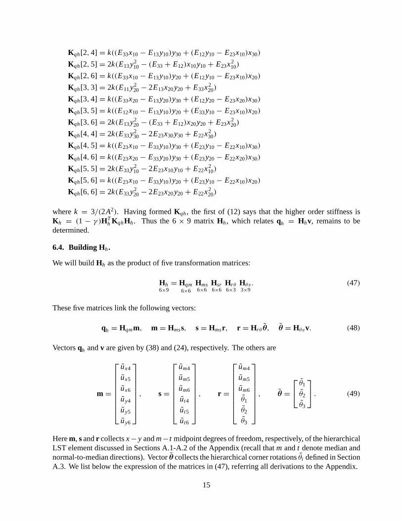
Kqh[2, 4] = k((E33x10 − E13 y10)y30 + (E12 y10 − E23x10)x30)

Kqh[2, 5] = 2k(E13 y210 − (E33 + E12)x10 y10 + E23x2

10)

Kqh[2, 6] = k((E33x10 − E13 y10)y20 + (E12 y10 − E23x10)x20)

Kqh[3, 3] = 2k(E11 y220 − 2E13x20 y20 + E33x2

20)

Kqh[3, 4] = k((E33x20 − E13 y20)y30 + (E12 y20 − E23x20)x30)

Kqh[3, 5] = k((E12x10 − E13 y10)y20 + (E33 y10 − E23x10)x20)

Kqh[3, 6] = 2k(E13 y220 − (E33 + E12)x20 y20 + E23x2

20)

Kqh[4, 4] = 2k(E33 y230 − 2E23x30 y30 + E22x2

30)

Kqh[4, 5] = k((E23x10 − E33 y10)y30 + (E23 y10 − E22x10)x30)

Kqh[4, 6] = k((E23x20 − E33 y20)y30 + (E23 y20 − E22x20)x30)

Kqh[5, 5] = 2k(E33 y210 − 2E23x10 y10 + E22x2

10)

Kqh[5, 6] = k((E23x10 − E33 y10)y20 + (E23 y10 − E22x10)x20)

Kqh[6, 6] = 2k(E33 y220 − 2E23x20 y20 + E22x2

20)

where k = 3/(2A2). Having formed Kqh , the first of (12) says that the higher order stiffness isKh = (1 − γ )HT

h KqhHh . Thus the 6 × 9 matrix Hh , which relates qh = Hhv, remains to bedetermined.

6.4. Building Hh .

We will build Hh as the product of five transformation matrices:

Hh6×9

= Hqm6×6

Hms6×6

Hsr6×6

Hrθ6×3

Hθv3×9

. (47)

These five matrices link the following vectors:

qh = Hqmm, m = Hmss, s = Hmsr, r = Hrθ θ, θ = Hθvv. (48)

Vectors qh and v are given by (38) and (24), respectively. The others are

m =

ux4

ux5

ux6

u y4

u y5

u y6

, s =

um4

um5

um6

ut4

ut5

ut6

, r =

um4

um5

um6

θ1

θ2

θ3

, θ = θ1

θ2

θ3

. (49)

Here m, s and r collects x − y and m − t midpoint degrees of freedom, respectively, of the hierarchicalLST element discussed in Sections A.1-A.2 of the Appendix (recall that m and t denote median andnormal-to-median directions). Vector θ collects the hierarchical corner rotations θi defined in SectionA.3. We list below the expression of the matrices in (47), referring all derivations to the Appendix.

15

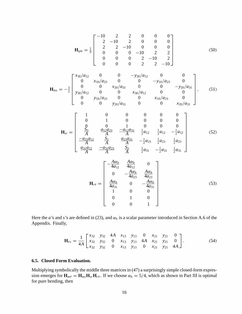
Hqm = 19

−10 2 2 0 0 02 −10 2 0 0 02 2 −10 0 0 00 0 0 −10 2 20 0 0 2 −10 20 0 0 2 2 −10

(50)

Hms = − 32

x30/a12 0 0 −y30/a12 0 00 x10/a23 0 0 −y10/a23 00 0 x20/a31 0 0 −y20/a31

y30/a12 0 0 x30/a12 0 00 y10/a23 0 0 x10/a23 00 0 y20/a31 0 0 x20/a31

, (51)

Hsr =

1 0 0 0 0 00 1 0 0 0 00 0 1 0 0 0S3A

a12a23A

−a12a31A

12 a12

12 a12 − 1

2 a12

−a23a12A

S1A

a23a31A − 1

2 a2312 a23

12 a23

a31a12A

−a31a23A

S2A

12 a31 − 1

2 a3112 a31

(52)

Hrθ =

− Aαh4a12

Aαh4a12

0

0 − Aαh4a23

Aαh4a23

Aαh4a31

0 − Aαh4a31

1 0 0

0 1 0

0 0 1

(53)

Here the a’s and s’s are defined in (23), and αh is a scalar parameter introduced in Section A.6 of theAppendix. Finally,

Hθv = 1

4A

[ x32 y32 4A x13 y13 0 x21 y21 0x32 y32 0 x13 y13 4A x21 y21 0x32 y32 0 x13 y13 0 x21 y21 4A

]. (54)

6.5. Closed Form Evaluation.

Multiplying symbolically the middle three matrices in (47) a surprisingly simple closed-form expres-sion emerges for Hmθ = HmsHsr Hrθ . If we choose αh = 5/4, which as shown in Part III is optimalfor pure bending, then

16

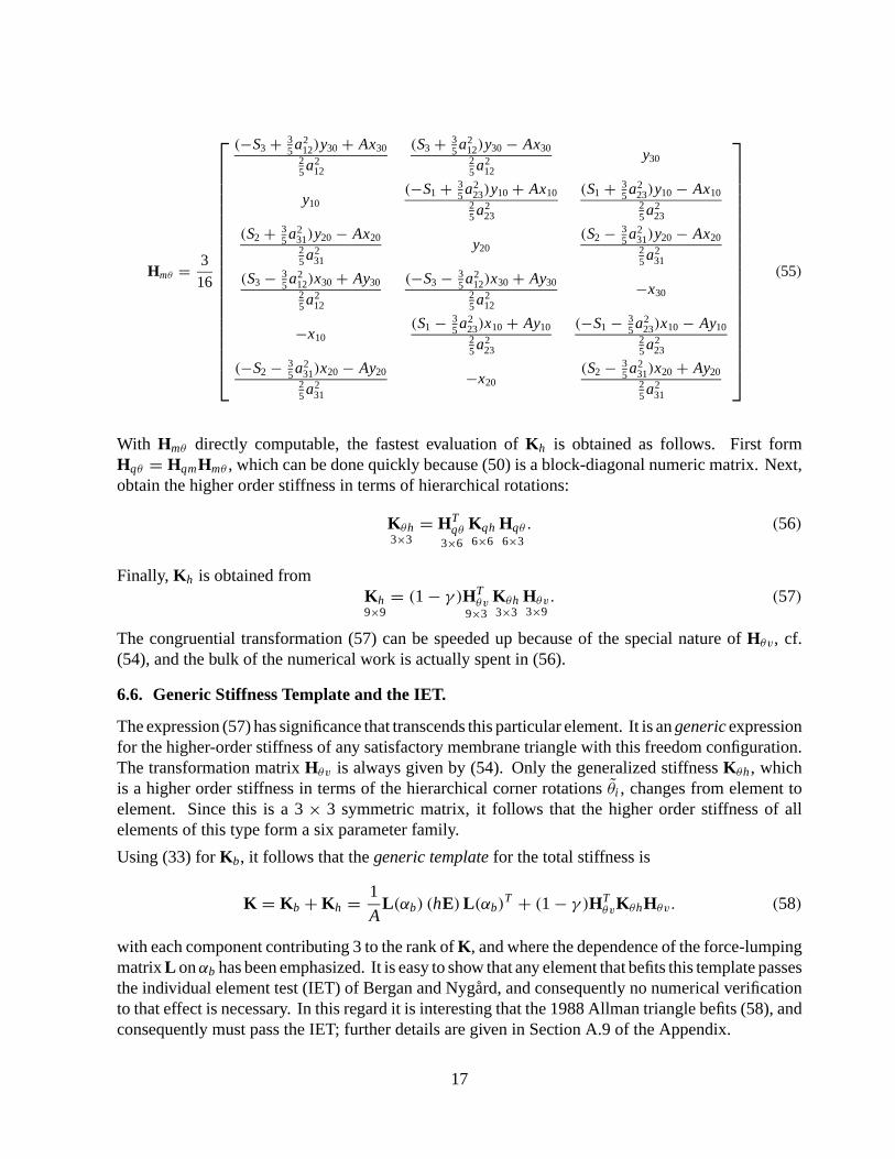
Hmθ = 3

16

(−S3 + 35 a2

12)y30 + Ax3025 a2

12

(S3 + 35 a2

12)y30 − Ax3025 a2

12

y30

y10(−S1 + 3

5 a223)y10 + Ax10

25 a2

23

(S1 + 35 a2

23)y10 − Ax1025 a2

23

(S2 + 35 a2

31)y20 − Ax2025 a2

31

y20(S2 − 3

5 a231)y20 − Ax2025 a2

31

(S3 − 35 a2

12)x30 + Ay3025 a2

12

(−S3 − 35 a2

12)x30 + Ay3025 a2

12

−x30

−x10(S1 − 3

5 a223)x10 + Ay1025 a2

23

(−S1 − 35 a2

23)x10 − Ay1025 a2

23

(−S2 − 35 a2

31)x20 − Ay2025 a2

31

−x20(S2 − 3

5 a231)x20 + Ay2025 a2

31

(55)

With Hmθ directly computable, the fastest evaluation of Kh is obtained as follows. First formHqθ = HqmHmθ , which can be done quickly because (50) is a block-diagonal numeric matrix. Next,obtain the higher order stiffness in terms of hierarchical rotations:

Kθh3×3

= HTqθ

3×6

Kqh6×6

Hqθ

6×3. (56)

Finally, Kh is obtained fromKh9×9

= (1 − γ )HTθv

9×3Kθh3×3

Hθv3×9

. (57)

The congruential transformation (57) can be speeded up because of the special nature of Hθv , cf.(54), and the bulk of the numerical work is actually spent in (56).

6.6. Generic Stiffness Template and the IET.

The expression (57) has significance that transcends this particular element. It is an generic expressionfor the higher-order stiffness of any satisfactory membrane triangle with this freedom configuration.The transformation matrix Hθv is always given by (54). Only the generalized stiffness Kθh , whichis a higher order stiffness in terms of the hierarchical corner rotations θi , changes from element toelement. Since this is a 3 × 3 symmetric matrix, it follows that the higher order stiffness of allelements of this type form a six parameter family.

Using (33) for Kb, it follows that the generic template for the total stiffness is

K = Kb + Kh = 1

AL(αb) (hE) L(αb)

T + (1 − γ )HTθvKθhHθv. (58)

with each component contributing 3 to the rank of K, and where the dependence of the force-lumpingmatrix L on αb has been emphasized. It is easy to show that any element that befits this template passesthe individual element test (IET) of Bergan and Nygard, and consequently no numerical verificationto that effect is necessary. In this regard it is interesting that the 1988 Allman triangle befits (58), andconsequently must pass the IET; further details are given in Section A.9 of the Appendix.

17

7. CONCLUDING REMARKS

We have presented the derivation of a plane stress triangle with drilling freedoms using the extendedfree formulation (EFF). The main advantage over the FF triangle derived in [1] is that an explicitform is obtained for the higher order stiffness. This simplifies the symbolic determination of optimalparameters by energy balance, as investigated in Section 2 of Part III. In addition the explicit derivationreveals an generic template form that all elements of this type must fit. Other element implementationdetails, such as consistent node force calculations, as well as performance of the EFF element withrespect to other 9-dof triangles, are discussed in Part III.

Acknowledgements

This work grew up of a 1990 term project assigned to Advanced Finite Element Methods, a course offered everytwo years by one of the authors (CAF). Subsequent research has been supported by NASA Langley ResearchCenter under Grant NAS1-756, NASA Lewis Research Center under Grant NAG3-934 and by the NationalScience Foundation under Grant ASC-8717773.

References

[1] P. G. Bergan and C. A. Felippa, A triangular membrane element with rotational degrees of freedom,Computer Methods in Applied Mechanics & Engineering, 50, 1985, pp. 25–69

[2] B. M. Irons and S. Ahmad, Techniques of Finite Elements, Ellis Horwood, Chichester, England, 1980

[3] D. J. Allman, A compatible triangular element including vertex rotations for plane elasticity analysis,Computers & Structures, 19, 1984, pp. 1–8

[4] R. D. Cook, On the Allman triangle and a related quadrilateral element, Computer & Structures, 22,1986, pp. 1065–1067

[5] R. D. Cook, A plane hybrid element with rotational D.O.F. and adjustable stiffness, International Journalof Numerical Methods in Engineering, 24, 1987, pp. 1499–1508

[6] P. G. Bergan and C. A. Felippa, Efficient implementation of a triangular membrane element with drillingfreedoms, Finite Element Handbook series, ed. by T. J. R. Hughes and E. Hinton, Pineridge Press, 1986,pp. 139–152

[7] D. J. Allman, A compatible triangular element including vertex rotations for plane elasticity analysis,International Journal of Numerical Methods in Engineering, 26, 1988, pp. 2645–2655

[8] R. H. MacNeal and R. L. Harder, A refined four-noded membrane element with rotational degrees offreedom, Computer & Structures, 28, 1988, pp. 75–88

[9] T. J. R. Hughes and F. Brezzi, On drilling degrees of freedom, Computer Methods in Applied Mechanics& Engineering, 72, 1989, pp. 105–121

[10] A. Ibrahimbegovic (1990), A novel membrane finite element with an enhanced displacement interpola-tion, Finite Elements in Analysis and Design, 7, 167–179

[11] P. G. Bergan and M. K. Nygard, Finite elements with increased freedom in choosing shape functions,International Journal of Numerical Methods in Engineering, 20, 1984, pp. 643–664

[12] C. A. Felippa, Refined finite element analysis of linear and nonlinear two-dimensional structures, Ph. D.Dissertation, Department of Civil Engineering, University of California at Berkeley, Berkeley, CA, 1966

[13] A. J. Carr, A refined finite element analysis of thin shell structures including dynamic loadings, Ph. D.Dissertation, Department of Civil Engineering, University of California at Berkeley, Berkeley, CA, 1968

18

[14] P. G. Bergan, Plane stress analysis using the finite element method. Triangular element with 6 parametersat each node, Division of Structural Mechanics, The Norwegian Institute of Technology, Trondheim,Norway, 1967

[15] J. L. Tocher and B. Hartz, Higher order finite element for plane stress, Proc. ASCE, Journal of theEngineering Mechanics Division, 93, EM4, pp. 149–174, 1967

[16] C. A. Felippa and S. Alexander, Membrane triangles with corner drilling freedoms: III. Implementationand performance evaluation, in this report.

[17] F. Frey, Shell finite elements with six degrees of freedom per node, in Analytical and ComputationalMethods for Shells, CAD Vol. 3, ed. by A. K. Noor, T. Belytschko and J. C. Simo, American Societyof Mechanical Engineers, ASME, New York, 1989, pp. 291–316

[18] M. K. Nygard, The free formulation for nonlinear finite elements with applications to shells, Dr. Ing. The-sis, Div. of Structural Mechanics, Norwegian Institute of Technology, Trondheim, Norway, 1986

[19] P. G. Bergan and M. K. Nygard, Nonlinear shell analysis using free formulation finite elements, Proc.Europe-US Symposium on Finite Element Methods for Nonlinear Problems, held at Trondheim, Norway,August 1985, Springer-Verlag, Berlin, 1986

[20] C. A. Felippa, Parametrized multifield variational principles in elasticity: I. Mixed functionals, Com-munications in Applied Numerical Methods, 5, 1989, pp. 69–78

[21] C. A. Felippa, Parametrized multifield variational principles in elasticity: II. Hybrid functionals and thefree formulation, Communications in Applied Numerical Methods, 5, 1989, pp. 79–88

[22] C. A. Felippa and C. Militello, Developments in variational methods for high-performance plate andshell elements, in Analytical and Computational Methods for Shells, CAD Vol. 3, ed. by A. K.Noor, T. Belytschko and J. C. Simo, American Society of Mechanical Engineers, ASME, New York,1989, pp. 191–216

[23] C. A. Felippa and C. Militello, Variational formulation of high performance finite elements: parametrizedvariational principles, Computers and Structures, 36, 1990, pp. 1–11

[24] C. A. Felippa, The extended free formulation of finite elements in linear elasticity, Journal of AppliedMechanics, 56, 1989, pp. 609–616

[25] C. A. Felippa and P. G. Bergan, A triangular plate bending element based on an energy-orthogonal freeformulation, Computer Methods in Applied Mechanics & Engineering, 61, 1987, pp. 129–160

[26] C. A. Felippa and C. Militello, Membrane triangles with corner drilling freedoms: II. The ANDESelement, in this report.

[27] P. G. Bergan and L. Hanssen, A new approach for deriving ‘good’ finite elements, MAFELAP IIConference, Brunel University, 1975, in The Mathematics of Finite Elements and Applications – VolumeII, ed. by J. R. Whiteman, Academic Press, London, 1976

[28] P. G. Bergan, Finite elements based on energy orthogonal functions, International Journal of NumericalMethods in Engineering, 15, 1980, pp. 1141–1555

[29] C. A. Felippa and R. W. Clough, The finite element method in solid mechanics, in Numerical Solutionof Field Problems in Continuum Physics, ed. by G. Birkhoff and R. S. Varga, SIAM–AMS ProceedingsII, American Mathematical Society, Providence, R.I., 1969, pp. 210–252

19

APPENDIX A. AUXILIARY DERIVATIONS

A.1 THE LST INTERPOLATION

Let w = w(ζ1, ζ2, ζ3) denote any quantity being quadratically interpolated over the six-node linear strain triangle(LST), for example the displacement components. The node values of w are wi , i = 1, . . . 6. The hierarchicalLST interpolation is [29]

w = [ w1 w2 w3 w4 w5 w6 ]

ϕ1

ϕ2

ϕ3

ϕ4

ϕ5

ϕ6

= wT

ζ1

ζ2

ζ3

4ζ1ζ2

4ζ2ζ3

4ζ3ζ1

= wT ϕ. (59)

where the hierarchical nodal values w4, w5 and w6 are defined as the midpoint deviations from linearity

w4 = 12 (w1 + w2) + w4, w5 = 1

2 (w2 + w3) + w5, w6 = 12 (w3 + w1) + w6. (60)

If one sets w4 = w5 = w6 = 0, (60) collapses to the linear interpolation of the three-node constant straintriangle (CST), a property characteristic of hierarchical elements.

Two types of shape functions appear in (60). Following the free-formulation (FF) terminology, the three linearshape functions associated with the corner nodes, namely ϕ1 = ζ1, ϕ2 = ζ2, and ϕ3 = ζ3, are called basicshape functions, because they provide the rigid-body and constant strain motions when w is identified with thedisplacement components ux and uy . The three quadratic shape functions associated with the midpoint nodes,namely ϕ4 = 4ζ1ζ2, ϕ5 = 4ζ2ζ3 and ϕ6 = 4ζ3ζ1, are called higher order shape functions. The higher orderfunctions are not energy orthogonal to the lower order ones according to the definitions given below. As weshall see, (60) is not suitable as a departure point for the internal displacement expansion of an EFF element,but it is useful as an intermediate step.

A.2 GENERALIZED INTERPOLATION

A generalization of the quadratic interpolation (60) is

w =6∑

i=1

qiφi (ζ1, ζ2, ζ3) = [ q1 q2 q3 q4 q5 q6 ]

φ1

φ2

φ3

φ4

φ5

φ6

, (61)

in which the coefficients qi are not necessarily node values but may be interpreted as generalized coordinates.The associated functions φi are called generalized shape functions. These functions no longer enjoy the nodalinterpolation properties of the ordinary shape functions ϕi .

To construct EFF elements we shall keep the same three basic shape functions in (62):

φ1 = ϕ1 = ζ1, φ2 = ϕ2 = ζ2, φ3 = ϕ3 = ζ3, (62)

As for the higher order shape functions, the most general choice may be written

φ4 = µ1(ζ21 + ζ 2

2 ) + µ2ζ23 + µ3ζ1ζ2 + µ4(ζ2ζ3 + ζ3ζ1)

φ5 = µ1(ζ22 + ζ 2

3 ) + µ2ζ21 + µ3ζ2ζ3 + µ4(ζ3ζ1 + ζ1ζ2)

φ6 = µ1(ζ23 + ζ 2

1 ) + µ2ζ22 + µ3ζ3ζ1 + µ4(ζ1ζ2 + ζ2ζ3)

(63)

20

where µ1, µ2, µ3 and µ4 are numerical coefficients, at least one of which must be nonzero. Because thefunctions may be scaled by an arbitrary nonzero common factor, only three coefficients are in fact independent.The grouping of the terms in (64) is dictated by triangular symmetries. In subsequent developments we shallrestrict the choice to energy orthogonal functions defined below. The general case is briefly commented uponin subsection A.8.

A.3 ENERGY ORTHOGONAL SHAPE FUNCTIONS

A higher order shape function φj ( j = 4, 5, 6) is said to be energy orthogonal with respect to the basic shapefunctions φi (i = 1, 2, 3) if the area integral of any product of their triangle-coordinate derivatives is zero. [Thisdefinition applies strictly to the case in which the thickness and material properties are constant over the element.But these conditions hold in the limit of infinitesimally small elements, which is the same limit of interest forthe patch test.] This condition can be expressed as∫

A

∂φi

∂ζm

∂φj

∂ζnd A = 0, i, m, n = 1, 2, 3, j = 4, 5, 6. (64)

But since all derivatives of φi are constant, (65) is equivalent to∫A

∂φj

∂ζnd A = 0, (65)

which expresses the fact that the element mean value of the first derivatives of an energy orthogonal shapefunction must vanish.

Applying this condition to (64) we find that the higher order shape functions are energy orthogonal if

2µ1 + µ3 + µ4 = 0, µ2 + µ4 = 0. (66)

Given µ1 and µ2, which may not be simultaneously zero, these relations determine µ3 and µ4. Because (as notedabove) only three coefficients in (64) are actually independent, it follows that the energy orthogonal subclassforms a one-parameter family. Note that (60), in which µ3 = 4, others zero, violates (67).

Two physically transparent sets of shape functions supplied by these relations are[φ4

φ5

φ6

]=

[(ζ1 − ζ2)

2

(ζ2 − ζ3)2

(ζ3 − ζ1)2

], (67)

φ4

φ5

φ6

=

(ζ3 − 1

3 )2

(ζ1 − 13 )2

(ζ2 − 13 )2

= 2

9

(−ζ1 − ζ2 + 2ζ3)

2

(−ζ2 − ζ3 + 2ζ1)2

(−ζ3 − ζ1 + 2ζ2)2

, (68)

which correspond to taking µ1 = 1, µ2 = 0, and µ1 = −2/9, µ2 = 8/9, respectively. The first set vanisheson the triangle medians, whereas the second set vanishes on lines parallel to sides passing through the centroid.Any linear combination of these functions, such as

φ4 = c1(ζ3 − 13 )2 + c2(ζ1 − ζ2)

2 (69)

is also energy orthogonal. Moreover, the sets (68) and (69) are not independent because they can be linkedthrough the linear transformations

(ζ1 − 13 )2

(ζ2 − 13 )2

(ζ3 − 13 )2

= 2

3 Q

(ζ1 − ζ2)

2

(ζ2 − ζ3)2

(ζ3 − ζ1)2

,

(ζ1 − ζ2)

2

(ζ2 − ζ3)2

(ζ3 − ζ1)2

= 3

2 QT

(ζ1 − 1

3 )2

(ζ2 − 13 )2

(ζ3 − 13 )2

, (70)

21

where

Q = 13

[−1 2 22 −1 22 2 −1

](71)

is an orthogonal matrix. Thus we confirm that all energy orthogonal sets can be related by a linear transformation,and all of them would produce the same higher order stiffness. Consequently the choice of basis for the higherorder functions is merely a matter of convenience. For the element derived here we select (68) as this choiceleads to a fairly simple generalized higher order stiffness matrix Kqh , derived in Section 4. Thus the generalizedinterpolation formula (62) becomes

w = [ q1 q2 q3 q4 q5 q6 ]

ζ1

ζ2

ζ3

(ζ1 − ζ2)2

(ζ2 − ζ3)2

(ζ3 − ζ1)2

= qT φ. (72)

A.4 FREEDOM TRANSFORMATIONS

We need to establish the transformations q = Tqww, w = T−1qwq that connect nodal values to generalized

coordinates. Formulas (73) and (60) are related by equating their left hand sides because they both correspondto complete quadratic expansions referred to linearly independent bases:

w = wT ϕ = qT φ = wT TTqwφ. (73)

Thus ϕ = TTqwφ. Evaluating this relation at the six nodes yields

1 0 0 12 0 1

2

0 1 0 12

12 0

0 0 1 0 12

12

0 0 0 1 0 0

0 0 0 0 1 0

0 0 0 0 0 1

= TTqw

1 0 0 12

12 0

0 1 0 0 12

12

0 0 1 12 0 1

2

1 1 0 0 14

14

0 1 1 14 0 1

4

1 0 1 14

14 0

(74)

Solving we get

Tqw =

1 0 0 89 − 4

989

0 1 0 89

89 − 4

9

0 0 1 − 49

89

89

0 0 0 − 109

29

29

0 0 0 29 − 10

929

0 0 0 29

29 − 10

9

T−1qw =

1 0 0 1 0 1

0 1 0 1 1 0

0 0 1 0 1 1

0 0 0 −1 − 14 − 1

4

0 0 0 − 14 −1 − 1

4

0 0 0 − 14 − 1

4 −1

(75)

Setting w to ux and uy in turn we can write[qx

qy

]=

[Tqw 0

0 Tqw

] [mx

my

]. (76)

From this 12 × 12 transformation we extract the 6 × 6 matrix Hqm given in (50).

22

A.5 HIERARCHICAL DRILLING FREEDOMS

We now study the “migration” of freedoms of the hierarchical LST into drilling and eliminable freedoms. Thecontinuum-mechanics rotation about the z axis, positive counterclockwise, is defined by formula (27). For thehierarchical LST element we set w to ux and uy in turn and evaluate θ making use of (39) to get

θ = 1

4A[ ux1 ux2 ux3 uy1 uy2 uy3 ux4 ux5 ux6 u y4 u y5 u y6 ]

x23

x31

x12

y23

y31

y12

4(ζ1x31 + ζ2x23)

4(ζ2x12 + ζ3x31)

4(ζ3x23 + ζ1x12)

4(ζ1 y31 + ζ2 y23)

4(ζ2 y12 + ζ3 y31)

4(ζ3 y23 + ζ1 y12)

(77)

Note that θ varies linearly over the element. It follows that only three independent drilling freedoms may bedefined, and the obvious locations are the corner points. Any additional drilling freedom (chosen, for example,at the centroid) would not be linearly independent. The three corner drilling rotations θ1, θ2 and θ3 at the cornersare related to the other freedoms by replacing the corner triangular coordinates in (78):

[θ1

θ2

θ3

]= 1

4A

[x23 x31 x12 y23 y31 y12 4x31 0 4x12 4y31 0 4y12

x23 x31 x12 y23 y31 y12 4x23 4x12 0 4y23 4y12 0x23 x31 x12 y23 y31 y12 0 4x31 4x23 0 4y31 4y23

]

ux1

ux2

ux3

uy1

uy2

uy3

ux4

ux5

ux6

u y4

u y5

u y6

(78)

Subsequent manipulations are facilitated by defining the hierarchical rotations θi = θi − θ0, i = 1, 2, 3, whereθ0 is the CST rotation, that is, the mean rotation obtained if one sets ux4 = ux5 . . . u y6 = 0 :

θ0 = 1

4A

(x23ux1 + x31ux2 + x12ux3 + y23uy1 + y31uy2 + y12uy3

)(79)

Then (79) simplifies to a matrix relation that involves only the hierarchical midpoint displacements:

θ =

θ1

θ2

θ3

= 1

A

[x31 0 x12 y31 0 y12

x23 x12 0 y23 y12 00 x31 x23 0 y31 y23

]

ux4

ux5

ux6

u y4

u y5

u y6

= Hθmm. (80)

23

For reasons explained in subsection A.6, we shall link θ to vector s of (49) as θ = HθmHmss. Matrix Hms , whichis given in (51), can be constructed by inspection of Figure 2. Carrying out this multiplication and using thedefinitions in (23) we obtain

θ1

θ2

θ3

=

− S3 + a212

Aa120 − S2 − a2

31Aa31

a−112 0 a−1

31

− S3 − a212

Aa12− S1 + a2

23Aa23

0 a−112 a−1

23 0

0 − S1 − a223

Aa23− S2 + a2

31Aa31

0 a−123 a−1

31

um4

um5

um6

ut4

ut5

ut6

. (81)

A.6 CHOOSING ELIMINABLE FREEDOMS

The 12 − 9 = 3 eliminable freedoms must be displacements because no more linearly independent drillingfreedom choices remain. From symmetry and invariance considerations four possible choices emerge:

(1) The hierarchical midpoint freedoms directed along the side directions: us4, us5, us6.

(2) The hierarchical midpoint freedoms directed along the normal directions: un4, un5, un6.

(3) The hierarchical midpoint freedoms directed along the median directions: um4, um5, um6.

(4) The hierarchical midpoint freedoms directed along the normal-to-the-median directions: ut4, ut5, ut6.

Choices (1) and (4) lead to transformation matrices that are singular for any triangle. Choice (2) leads to atransformation matrix that is singular for right-angled triangles. That leaves choice (3), which as shown belowhas a well conditioned inverse. The necessary relation relating θ to s is available in (82). This is rendered squareby augmenting it with the trivial relations umi = umi , i = 4, 5, 6:

um4

um5

um6

θ1

θ2

θ3

=

1 0 0 0 0 00 1 0 0 0 00 0 1 0 0 0

− S3 + a212

Aa120 − S2 − a2

31Aa31

a−112 0 a−1

31

− S3 − a212

Aa12− S1 + a2

23Aa23

0 a−112 a−1

23 0

0 − S1 − a223

Aa23− S2 + a2

31Aa31

0 a−123 a−1

31

um4

um5

um6

ut4

ut5

ut6

(82)

or r = Hrss in the notation of (46). The determinant of Hrs is a12a23a31/2A3. Thus Hrs is nonsingular for anynondegenerate triangle. Symbolic inversion of this transformation provides matrix Hsr given in (52).

A.7 ELIMINATION OF HIERARCHICAL MEDIAN DISPLACEMENTS BY COLLOCATION

We now proceed to eliminate um4, um5 and um6 through kinematic constraints. To fix the ideas consider um4.From the boundary expansion (29) on side 1–2 we can obtain the normal displacement dn in terms of the freedomson that side. The hierarchical value at 4 is

dn4 = dn4 − 12 (dn1 + dn2)

=[ψn1(ξ)dn1 + ψn2(ξ)dn2 + αh

(ψθ1(ξ)θ1 + ψθ2(ξ)θ2

)]ξ=0

− 12 (dn1 + dn2)

= 18 αh12(θ2 − θ1) = 1

8 αh12(θ2 − θ1).

(83)

Here parameter αb of (29) has been renamed αh to emphasize the fact that we can vary both independently forthe basic and higher order stiffness. Assuming the collocation

um4 = un4 cos(n12, m12) = dn4(b12/12), (84)

24

where the bi j are defined in (23), we find

um4 = 18 αhb12(θ2 − θ1). (85)

Repeating this procedure for the other two sides and collecting into one matrix equation we get

um4

um5

um6

= 1

8 αh

[−b12 b12 00 −b23 b23

b31 0 −b31

] θ1

θ2

θ3

. (86)

Augmenting this with the trivial equations θi = θi (i = 1, 2, 3) as last three rows and replacing bi j = 2A/ai j

yields the transformation matrix Hrθ listed in (53). An energy balance analysis presented in Section 2 of PartIII shows that the best value for αh is

αh = 5/4, (87)

a value that has been hardwired into (55).

A.8 WHAT HAPPENS FOR NON ENERGY-ORTHOGONAL FUNCTIONS?

The original FF does not depend on the energy orthogonality concept although the variational justification ofRefs. [21–24] does. To assess the effect of that condition on this element, symbolic experiments (with Macsyma)were conducted with elements derived with the general assumption (62) for the higher order shape functions.The orthogonality condition (67) was replaced by

2µ1 + µ3 + µ4 = δ1, µ2 + µ4 = δ2, (88)

where δ1 and δ2 may be regarded as deviations from energy orthogonality.

The EFF higher order stiffness depends on two parameters: γ and αh , where γ defines the scaling of Kh as perEq. (12). These parameters are selected to match pure-bending energies on regular mesh units, as described inPart III [16]. When the energy orthogonal sets are selected, the matching can be made so that a set (γ , αh) worksfor all aspect ratios. With (89) it was found that such matching was possible only if

δ2 = 12 δ1. (89)

One choice that verifies this condition is

[φ4

φ5

φ6

]=

[(ζ1 − ζ2)

2 + δ2 φB

(ζ2 − ζ3)2 + δ2 φB

(ζ3 − ζ1)2 + δ2 φB

], (90)

in which φB = ζ1ζ2 + ζ2ζ3 + ζ3ζ1. This is not energy orthogonal if δ2 = 0. Closer examination, however,showed that the same higher order stiffness matrix Kh was produced for any value of δ2; thus adding φB has noeffect.

Any deviation from the condition (90) made matching impossible: only specific element aspect ratios could beenergy balanced. Thus it appears that the main effect of departure from energy orthogonality is a degradationin element accuracy. Consequently the general assumption (62)–(64) was not pursued further.

25

7.1. Allman Triangles Fit the Generic Template.

The rank-sufficient Allman triangle [7] was constructed with incompatible cubic shape functions. Numericallyintegrated versions of this element have been symbolically analyzed as prelude to the evaluation presented inPart III. Four triangle integration rules, labeled as follows, were considered:

1c The 1-point centroidal integration rule.

3m The 3-midpoint rule of quadratic accuracy.

3i The 3-interior point rule, also of quadratic accuracy, with points at ζi = 2/3, ζj = ζk = 1/6.

7i The 7-interior point rule of cubic accuracy.

The resultant (total) stiffness matrices will be denoted by KA1c, KA3m , KA3i and KA7, respectively. All of themwere found to fit the generic template (58) in the sense that

KA1c = Kb(4/3)

KA3m = Kb(1) + K3mh = Kb(1) + HT

θvK3mqh Hθv

KA3i = Kb(1) + K3ih = Kb(1) + HT

θvK3iqhHθv

KA7i = Kb(1) + K7ih = Kb(1) + HT

θvK7iqhHθv

(91)

where the argument of Kb is the value of αb obtained by setting constant stress states. The centroid-integratedstiffness KA1c is of course rank deficient by 3. The 3-point-integrated Allman elements are effectively linear-strain, quadratic displacement triangles because such sampling “filters out” quadratic strain variations. Thehigher order stiffness of these 3-point integrated elements does not fit into the present EFF family except forspecific geometries. For example, for the equilateral triangle, K3m

h coincides with EFF’s Kh if 1 − γ = 1/4and αh = (32 ± √

82)/24, whereas K3ih is obtained if 1 − γ = 1/36 with the same αh = (32 ± √

82)/24. Toachieve equivalence for more general geometries, however, it becomes necessary to generalize the present EFFformulation by allowing three αh coefficients, one per side, with αhi depending on the magnitude of the oppositeangle.

The main practical value of the decomposition (92) is that it shows that the numerically integrated Allmanelements pass the patch test without any numerical experiments. The equivalent EFF elements, however,have parameter values that do not agree with the optimal ones determined in Part III. As a consequence, theperformance of all Allman triangles deteriorates for high aspect ratios.

26