Vision Res. Vol. 29, No. 5, pp. 627437, 1989 ~2-6989~89 $3.00 + 0.00 Printed in Great Britain. All rights reserved Copyright 0 1989 Pergamon Press plc

MEASUREMENT OF SPATIAL CONTRAST SENSITIVITY WITH THE SWEPT CONTRAST VEP

ANTHONY M. NORCIA, CHRISTOPHER W. TYLER, RU~~ZELL D. HAMER and WOLFCANG WFSEMANN’

Smith-Kettlewell Eye Research Institute, 2232 Webster St, San Francisco, CA 9411.5, U.S.A. and ‘Laboratory of Medical Optics, University Eye Clinic, Martinistr. 52, 2 Hamburg 20, F.R.G.

(Received 27 October 1987; in revised form 27 June 1988)

Abstract-Contrast response functions (CRFs) for the VEP were obtained with a Discrete Fourier Transform (DFT) technique employing swept contrast gratings. VEP CRFs in infants were found to have a form similar to those observed in adults, being linear functions of log contrast over a range of near- threshold contrasts. CRFs with low and high contrast lobes were present in infants, as they are in adults. Contrast thresholds were estimated by extrapolation of the CRF to zero microvolts.

The effects of additive EEG noise and of the DFT data window on the shape of the measured CRF are considered. For large signals, the measured CRF is nearly independent of the additive noise, but at small signal values additive noise introduces a small bias towards larger amplitudes. The VEP signal-ply-noi~ dist~bution was modeled as a family of Rice distributions in order to evaluate the effects of bias on the estimates of threshold. The amount of bias depends inversely upon the slope of the CRF. The amount of bias introduced by a smoothing window also depends upon slope of the CRF as well as the sweep rate. The combined effects of additive noise and window bias were such that the total bias was nearly independent of CRF slope. Sweep VEP contrast thresholds were shown empirically to be unaffected by changes in the range of contrast swept.

The measurement of the contrast sensitivity function (CSF) involves the determination of thresholds at a number of spatial frequencies. This can be a time consuming and frustrating process, particularly in infants, as a result of their limited attention span and rapidly chang- ing state.

A promising method for obtaining contrast thresholds in infants involves the use of the steady-state VEP, coupled with a swept param- eter display. Spectral analysis of the steady-state VEP allows real-time extraction of the VEP from the EEG and other background noise sources (Regan, 1966; Tyler et al., 1979; Seiple et al., 1984; Norcia and Tyler, 1985). A number of investigators have used the swept parameter technique to measure grating resolution (Regan, 1977; Tyler et al., 1979; Weiner et al., 1985) and contrast sensitivity in the adult (Seiple et al., 1984; Allen et al., 1986).

While the state of the infant changes rapidly and fixation and attention are difficult to con- trol, infants have quite large VEP amplitudes, at least partially as a result of the thinness of their skulls relative to those of adults. Thus the VEP signal is larger in infants relative to sources of

noise extrinsic to the brain, such as muscle activity. The high signal to noise ratio of the infant steady state VEP and the infant’s short fixation span lead naturally to the use of swept parameter dislays and spectral analysis. Infant grating acuity has been measured using the swept parameter technique (Norcia and Tyler, 1985), as has contrast sensitivity (No&a et al., 1986; Norcia et al., 1988).

We describe below a number of meth- odological issues related to the use of swept contrast gratings for the measurement of infant or adult contrast sensitivity. We consider the form of the infant contrast response function, whether contrast ~reshold depends upon the particular parameters of the sweep technique and the significance of two sources of bias inherent in swept threshold estimations based on extrapolations to zero amplitude.

METHODS

Apparatus

Display. Vertical sinusoidai luminance gra- tings were generated on a Joyce (Cambridge Electronics) display scope. Space average lumi- nance was 220 cd/m*. Z-axis contrast linearity was verified to be within 2% of nominal con-

627

628 ANTHONY MNORCIA et at.

trast up to 90% contrast using a Spectra-Pritchard Model 1980A photometer. Contrast remained within 70% of full contrast up to 4 c/cm as determined photometrically and psychophysically. The gratings were square wave alternated at 12 contrast reversals per sec.

VEP recording. The EEG was pre-ampli~ed by Grass P51 IJ amplifiers equipped with iso- lated cables (Grass IG3/PSll). Two bipolar placements of 0, vs 0, and 0, were used. The amplifier bandwidth was l-100 Hz at -6 dB and the EEG was digitized to 8 bits accuracy at 180 Hz. A programmable gain stage was used after the pre-amplifiers in order to optimize the 8 bit range of the A/D converters. The pre-trial EEG was continuously sampled and the average amplitude over a 1 set window immediately preceding data collection was used to set the gain of the programmable amplifiers. The EEG pre-amplifiers were run at a gain of 10,000 and the programmable stage could add an addi- tional gain of between 2 and 256. Additionally, I set of the stimulus presentation preceded the beginning of the sweep and actual data collection.

Spectrum analysis. The amplitude and phase of the pattern reversal response at 12 Hz were calculated using a Discrete Fourier Transform (DFT), as was the amplitude of the EEG during the trial at 14 Hz (Norcia and Tyler, 1985; Norcia et al., 1985). The DFT was performed over a running 2 set data window which was 50% cosine tapered (Tukey window). The posi- tion of the data window along the data array was incremented every 90 datum points or 0.5 set, yielding 17 amplitude and phase values over each 10 set data record. The changes in data window position corresponded exactly to the changes in the swept parameter. The data in each bin was thus 75% overlapped with each neighboring bin. The combination of the 75% overlap and the 50% taper resulted in each bin being 72.7% correlated with its neighbor. The bandwidth of the Fourier analysis with the above windowing conditions was 0.56 Hz (see Harris, 1978 for details on the use of data windows with the DFT).

The second frequency, offset by 2 Hz from the response frequency, was used as an estimate of the background noise level during the trial at the response frequency. The noise frequency was kept 2 Hz away from the response frequency to ensure that it was at a frequency where the modulus of the Fourier transform of both 1 and 2 set 50% Tukey windows is zero. This choice

Of’ noise frequency offset minimizes leakage of power at the response frequency into the noise estimate and is the closest offset which can be used for a 1 set 50% Tukey window.

The Tukey window was chosen primarily to allow recovery of useful info~ation from ep- ochs which included some saturated response cycles. When a saturated datum point was en- countered, the entire response cycle to which it belonged was discarded and the DFT was calcu- lated on an epoch which was shorter by an integer number of cycles. The missing cycle(s) were taken out of the untapered portion of the Tukey window. An epoch was rejected entirely if more than 50% of the cycles in that epoch had saturated points. Scavenging of saturated cycles occurred on approximately 10% of all cycles. Completely rejected bins occurred much less frequently.

For both infant and adult EEG, the ampli- tude at 14 Hz is very similar, on average, to that at 12 Hz (Nor&a and Tyler, 1985). For record- ing frequencies where the EEG spectrum has a significant slope, the use of two noise fre- quencies, one above and one below the response frequency, provides a more accurate estimate of noise at the response frequency. For response frequencies other than 12 Hz, an empirical de- termination of the slope of the EEG spectrum should be made to determine the best choice of noise frequencies.

Threshold estimation. Contrast thresholds and grating acuity were estimated by linear extrapo- lation to zero amplitude of the VEP amplitude versus log contrast function (Norcia et al., 1986; Allen et al., 1986) or VEP amplitude versus linear spatial frequency functions respectively (Norcia and Tyler, 1985; Norcia et al., 1985). Regression lines were fit automatically by com- puter using a set of signal-to-noise ratio (SNR) and phase consistency criteria which were de- rived from an extensive empirical data set.

The amplitude at the response frequency had to exceed by a factor of 3 that at the adjacent “noise” frequency, averaged over the 10sec epoch. The 3 : 1 criterion was derived empirically from a sampling distribution of over 5000 10 set trials. In portions of the record used for the regression, there could be no local EEG tran- sients which elevated the amplitude of the noise frequency to more than 70% of that at the response frequency. This value was set empir- ically.

For contrast sweeps, the phase of the re- sponse had to either be constant or gradually

Measurement of spatial contrast sensitivity 629

10&V

a

Fig. 1. Prototypical contrast response functions obtained with the swept contrast VEP. Solid curves plot the amplitude (upper panels) and phase (lower panels) of the steady state VEP occurring at 12 Hz. (0) plot the EEG amplitude at 14 Hz. Regression lines were calculated on the data between the vertical dashed

lines to estimate the contrast threshold.

leading the stimulus as contrast increased. This constraint was introduced since it is known that evoked response latency is shorter for higher contrasts (Kulikowski, 1977). For spatial sweeps, the response phase was required to either be constant, as for the contrast sweeps, or gradually lagging the stimulus as spatial fre- quency sweeps. This constraint was introduced since evoked response latency is known to in- crease with increasing spatial frequency (Parker and Salzen, 1977).

The false alarm rate for the automatic extrap- olation procedure and windowing conditions used in the present experiment was found to be less than 2% of records when tested on a large sample of adult spontaneous EEG.

Choice of endpoints for the extrapolation

The threshold estimation algorithm searched the VEP record for a range of increasing re- sponse values upon which to perform the re- gression to zero amplitude. Various criteria were included to minimize distortion of the extrapolation by noise at low signal levels and by response saturation at high signal levels.

Starting at the low contrast end of the record, each point and its neighbor were checked on the phase and local artifact criteria. A range was then defined as beginning at the point where the amplitude function rose and stayed above a SNR of 1.5. A regression line was then fit if a range of at least three points was found, one of which exceeded a SNR of 3 (or a range of 2 points if both exceeded a SNR of 3). The end- points of the linear regression included the first

point in the range (SNR > 1.5) if the phase of the point at the next lowest contrast was incon- sistent (leading the phase obtained at a higher contrast). If the phase was consistent (within 20 deg of lead or 90 deg of lag), then the next lowest point below the range was used. These phase boundaries were derived empirically. The high contrast endpoint was chosen simply as the highest monotone point above a SNR of 3. Thus saturated portions of the CRF were not used in the extrapolation. If a record contained more than one range with a peak larger than 3 : 1 (see below), the lower contrast peak was used.

RESULTS

Form of the sweep VEP contrast response func- tion

Examples of the functional relationship be- tween VEP amplitude and phase vs log contrast are shown in Figs 1 and 2. Amplitude and phase values are plotted at the average contrast of each 2 set bin. As initially reported by Campbell and Maffei (1970) VEP amplitude is, in many cases, a linear function of log stimulus contrast over a considerable range of contrast. The re- sponse phase may be constant (panel a) but typically shows a phase lead with increasing contrast (panels b, d). A phase lead is indicated by a downward trend on the phase plot, and is consistent with a speeding of the response as contrast increases. Figure la plots a single 10 set sweep record recorded at 2 c/deg from infant Andrew, who was 10 weeks old. Threshold (arrow) was estimated to be 4.9% contrast,

630 ANTHONY M. NORCIA et al.

a

b

01 1 .0 10 01 10 10

% conrrast % Contrast

Fig. 2. Prototypical contrast response functions with low and high contrast lobes. Panels (a) and (b) are successive 10 set records from 15 week old infant Seth taken at 0.5 c/deg, Panels (c) and (d) show records taken at 1 c/deg from David. The recordings were made two weeks apart at 19 and 21 weeks of age.

corresponding to a sensitivity of 20.3. Note that the response phase is constant down to a con- trast which is within a factor of 1.6 of the estimated threshold. Peak SNR in this record was 25: 1. Figure lb plots a 10 set sweep record from infant Jacob, 9 weeks of age, taken at 1 c/deg. Threshoid was estimated to be 0.64% or a sensitivity of 156, but the response phase shifted by 135 deg between 0.64 and 17% contrast.

The VEP amplitude versus contrast function may saturate at higher contrast (Fig. lc) or may appear to oversaturate (Fig. ld) as described by Tyler and Apkarian (1985). The data in Fig. lc consisted of a vector average of two 1Osec sweeps. The vector average was formed as the Pythagorean sum of the mean of the sine and cosine coefficients obtained for each bin taken across the trials composing the vector average. The data in Fig. lc were taken at 4 c/deg from infant Robbie who was 22 weeks of age. Thresh- old was estimated as 1.91% contrast, The ap- parent discontinuity in the phase plot is due to the use of a linear plot for the phase variable which is modular over a range of 2 pi, The phase changes continuously in Fig. lc and this can be seen if the plot is shifted downward by 360 deg. The data of Fig. ld were formed from a vector average of three 10 see sweeps taken at 0.25 c/deg and were from infant Andrew whose data at 2 c/deg were shown in Fig. la. In Fig. Id, the amplitude at 17% contrast was only 25% of that recorded at 7% contrast. Threshold was estimated at 1.2% contrast.

The infant VEP CRF often consists of two

lobes, particularIy at lower spatial frequencies (Tyler et al., 1987). The first lobe, found at low contrasts, consists of a linear increase in VEP amplitude with increases in log contrast. The CRF then ceases to increase and may even dip below the amplitude attained at lower contrast. A second increasing segment is then observed, usually beginning at 5-10% contrast. Examples of two-lobed functions are presented in Figs 2a and b which show successive 10 set records taken at 0.5 c/deg from infant Seth who was 15 weeks old. Figures 2c and d show two-lobed sweeps records obtained at 1 c/deg. The data are for David and were recorded at 19 and 21 weeks of age. The two lobes were evident on both of David’s recording sessions and in each individ- ual trial making up the vector averages, The first lobe in each record extends to almost 10% contrast. Strong response nulls are seen at about 8-10% contrast, followed by a second mono- tonic response increase. The function in Fig. Id may in fact be only the low contrast lobe of a two-lobed function.

Fixed contrast vs swept contrast measurements

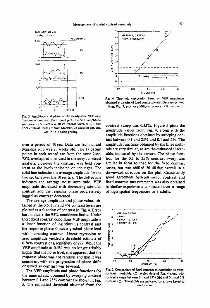
It is important to show that the contrast thresholds measured by the sweep technique are in no significant way dependent upon the use of swept contrast or upon the rate at which con- trast is swept. Figure 3 shows the results of an experiment in which the amplitude of the YEP was measured at a series of fixed contrasts, using the general analysis scheme employed for the swept contrast measurements, Each panel of Fig, 3 plots the amplitude and phase of the VEP

Measurement of spatial contrast sensitivity 631

MARLENA: 23 wks

1 c/deg. 12 rps

% CONTRAST

0 5 10 set

Fig. 3. Amplitude and phase of the steady-state VEP as a function of contrast. Each panel plots the VEP amplitude and phase over successive 10 set records taken at 2, 1 and 0.5% contrast. Data are from Marlena, 23 weeks of age, and

are for a 1 c/deg grating.

over a period of 10 sec. Data are from infant Marlena who was 23 weeks old. The 17 datum points in each record are from the same 2 set, 75% overlapped bins used in the swept contrast analysis, however the contrast was held con- stant at the levels indicated on the right. The solid line indicates the average amplitude for the two set bins over the 10 set trial. The dotted line indicates the average noise amplitude. VEP amplitude decreased with decreasing stimulus contrast and the response phase progressively lagged as contrast decreased.

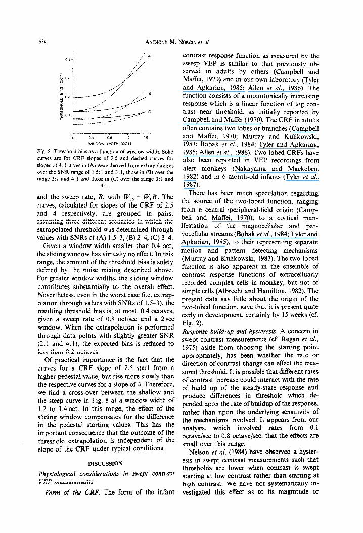
The average amplitude and phase values ob- tained at the 0.5, 1, 2 and 4% contrast levels are plotted as a function of contrast in Fig. 4. Error bars indicate the 95% confidence limits. Under these fixed contrast conditions VEP amplitude is a linear function of log stimulus contrast and the response phase shows a gradual phase lead with increasing contrast. Linear regression to zero amplitude yielded a threshold estimate of 0.36% contrast or a sensitivity of 279. While the VEP amplitude at 0.5% was no longer reliably higher that the noise level, it is apparent that the response phase was not random and that it was consistent with the progression of phase shifts observed as contrast was lowered.

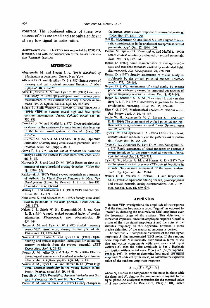
The VEP amplitude and phase functions for the same infant, obtained by sweeping contrast between 0.1 and 25% contrast are shown in Fig, 5. The estimated threshold obtained from the

6- MARLENA. 23 WKS

FIXED CONTRASTS

O-

-n 0.1 0.3 1.0 3.0 10

% CONTRAST

Fig. 4. Threshold exploration based on VEP amplitudes obtained at a series of fixed contrast levels. Data are derived

from Fig. 3, plus an additional point at 4% contrast.

contrast sweep was 0.33%. Figure 5 plots the amplitude values from Fig. 4, along with the amplitude functions obtained by sweeping con- tast between 0.1 and 25% and 0.1 and 2%. The amplitude functions obtained by the three meth- ods are very similar, as are the estimated thresh- olds, indicated by the arrows. The phase func- tion for the 0.1 to 25% contrast sweep was similar in form to that for the fixed contrast series, but was shifted 30-40 deg overall in a downward direction on the plot. Consistently good agreement between swept contrast and fixed contrast measurements was also obtained in similar experiments conducted over a range of high spatial frequencies in 3 adults.

MARLENA. 23 WKS

6 SWEPT 10.1-26X1

6 0 SWEPT lO.l-2%)

$4

2 93 4

$2

0.1 0.3 1.0 3.0

CONTRAST 1%)

Fig. 5. Comparison of fixed contrast extrapolation to swept contrast thresholds. (0) replot data of Fig. 4 along with contrast sweeps between 0.1 and 25% (a) and 0.1 and 2% contrast (0). Thresholds are indicated by arrows keyed to

each curve.

632 ANTHONY M. NORCIA et al.

-L’L’

01 0 .2 05 1 .0 2 5 10 20 50 100

% contrast

Fig, 6. Threshold estimates obtained at different sweep rates. For each infant, the bars indicate the contrast sweep ranges used. For each sweep range thresholds on repeated

measures are indicated by (@),

Independence of sweep VEP contrast thr~~h~l~ from the rate of the contrast sweep

When swept contrast gratings are used to measure threshold, the experimenter must choose how wide a range of contrast to sweep and where to place the starting contrast level of the sweep. If the likely range of the threshold is uncertain, it is desirable to sweep a wide range of contrasts, so as to ensure that the sweep spans the threshold. The range of contrast swept determines the rate of contrast change during the sweep-the wider the range of contrast swept, the faster the rate of contrast change. A very wide sweep range with its resulting fast sweep rate may ultimately have two undesirable consequences, First is that the CRF will be sampled coarsely in the threshold region, lead- ing to variable estimates. Starting the contrast sweep at too low a contrast will yield only a few samples of the suprathreshold contrast function, while starting too high could lead to an under- estimation of the contrast threshold. Secondly, the rate of contrast change at some point will become too rapid to aHow the response sufficient time to reach the steady state. The present device is limited to a maximum range of 8 octaves to be displayed over a fixed length sweep of 10 set, or a rate of 0.8 octaves per sec.

The rate of the contrast sweep was changed in recordings made on 20 infants who were tested either with sweeps starting at the same initial contrast and ending at different points, or with

sweeps starting at different points and ending at the same contrast. In this manipulation both the range and the rate differ, although it is the rate of the sweep that is most likely to affect the VEP threshold, if the range is chosen correctly so as to span the threshold. A range change at a constant rates should not affect the threshold- provided the range spans the threshold-since this should simply translate the measured function laterally on the sweep plot.

Figure 6 plots data from 6 infants from 5 to 26 weeks of age who were tested on more than one sweep rate at a given spatial frequency. The datum points plotted were selected from all infants who yielded more than one criterion record from either channel on each range tested. Three additional infants yielded only 1 criterion estimate on one of the ranges tested, but in each case that value was within the range of values obtained on the other range tested. Four infants were tested with a sweep range that was inap- propriate i.e. did not cover the threshold mea- sured on another range. Four infants failed to produce a criterion response on one of the ranges tested; for three only one trial was at- tempted on one of the ranges.

As can be seen from Fig. 6, the dist~butions of thresholds are all overlapping regardless of the rate or starting point. Thus there appear to be no large effects of sweep parameters, within the range of rates, starting levels and spatial frequencies tested, provided of course that start- ing points are chosen appropriately for the infant’s threshold.

Eflect of additive noise on the CRF

The zero-amplitude extrapolation procedure assumes that the evoked response is actually zero at some value of stimulus contrast and that the response then increases linearly as log contrast increases. This underlying contrast response function for the VEP can never be measured directly because of the presence of extrinsic noise.

There are several consequences of the added noise. The first is that the empirical CRF con- sists of a noise baseline in the region below the contrast threshold. Secondly, over a range of VEP amplitudes which are comparable to the background activity, the measured values are on average larger than the actual VEP. Finally, at higher SNRs, the observed CRF is nearly un- contaminated by the background.

To estimate the effects of noise-mixing on the empirical CRF, we used a dete~inistic model

Measurement of spatial contrast sensitivity 633

I / /

9 LOG CONTRAST <REL. UNITS> C B A

Fig. 7. Theoretical contrast response functions. Dotted line indicates a linearly increasing CRF with threshold (A). Dashed line indicates the CRF obtained with the addition of Rayleigh noise. Extrapolation of this curve yields thresh- old (B). Solid curve represents the CRF obtained after convolution of the dashed CRF with the data window.

Extrapolation of this curve yields threshold (C).

for the signal consisting of a linearly increasing function with a threshold. The EEG noise was assumed to be Gaussian in terms of its sine and cosine coefficients. This assumption was found to be empirically valid for infant EEG up to at least +3 SD, after which the observed distribu- tion showed longer tails than expected for Gaussian noise. To this extent, the noise ampli- tude will have a Rayleigh distribution (Papoulis, 1965) with the mean equal to n/2 times the standard deviation of the sine/cosine com- ponents of the noise. The addition of a sine wave to the Rayleigh noise yields a distribution whose amplitudes correspond to the Rice distri- bution (see Appendix; and Rice, 1945).

The resulting change in the shape of the empirical CRF due to the mixing of un- correlated EEG noise is shown as the dashed curve in Fig. 7 which plots the expected value of the Rice distribution as a function of the under- lying signal strength. The “noise-free” CRF, depicted by the dotted line with a threshold at (A), is systematically biased towards higher response/noise (R/N) values. A maximal ampli- tude bias of 36% is obtained at the point where the empirical CRF and the noise have equal amplitudes. Note however that the deviation of the Rice function from the empirical CRF de- creases rapidly with increasing SNR, Points above a SNR of 3 : 1 are almost ~contaminat~ by uncorrelated EEG noise and thus provide an unbiassed representation of the true VEP ampli- tude.

Since the measured values of the evoked

response contaminated by noise are always larger than the actual VEP, a threshold extra- polation through datum points with very low SNR results in a biased estimate (Fig. 7; B) of the actual threshold, the bias being in the direc- tion of a lower threshold. The magnitude of this bias was estimated from the Rice distribution and the experimentally determined slopes of the CRFs. These slopes ranged from 2.5 to 4.0 SNR-units per octave of contrast, resulting in over-estimates of threshold by 0.2-0.125 oc- taves, respectively. In making these estimates, we assumed that the extrapolation was per- formed through datum points having a SNR of 1.5 and 3. This range of SNR represents the worst case condition for the extrapolation algo- rithm we use, one that would give the greatest amount of bias, since the evoked response is extremely small and therefore most vulnerable to contamination by noise. If the threshold were calculated through points with higher SNR, the bias would be smaller. For example, if SNRs of between 2 and 4 are used, the bias is reduced to 0.12 and 0.07 octaves, respectively. Threshold estimates calculated through points with SNRs above 3 : 1 are virtually uncontaminated by the ambient EEG noise. Note that the Rice func- tion in Fig. 7 shows the general relationship between underlying signal and sisal-plus-noise distributions, independent of CRF slope.

Eflect of a smooothing window on the CRF

In the course of the swept VEP measurement, the stimulus contrast is increased every 0.5 set, but the DFT of the sampled waveform is per- formed over a sliding window that is 2 set wide. This procedure damps amplitude fluctuations and increases the SNR by a factor of two. On the other hand, a smoothing window alters the shape of the CRF in regions of changing gra- dient and tends to increase the bias in the threshold extrapolation over that which is pro- duced by noise mixing alone. The smoothing effect of the window, which is a function of window width, slope of the CRF, and sweep rate, can be evaluated numerically by con- volving the Rice function with the sliding win- dow. The result of such a calculation is shown as the solid curve in Fig. 7, which extrapolates to the threshold (C).

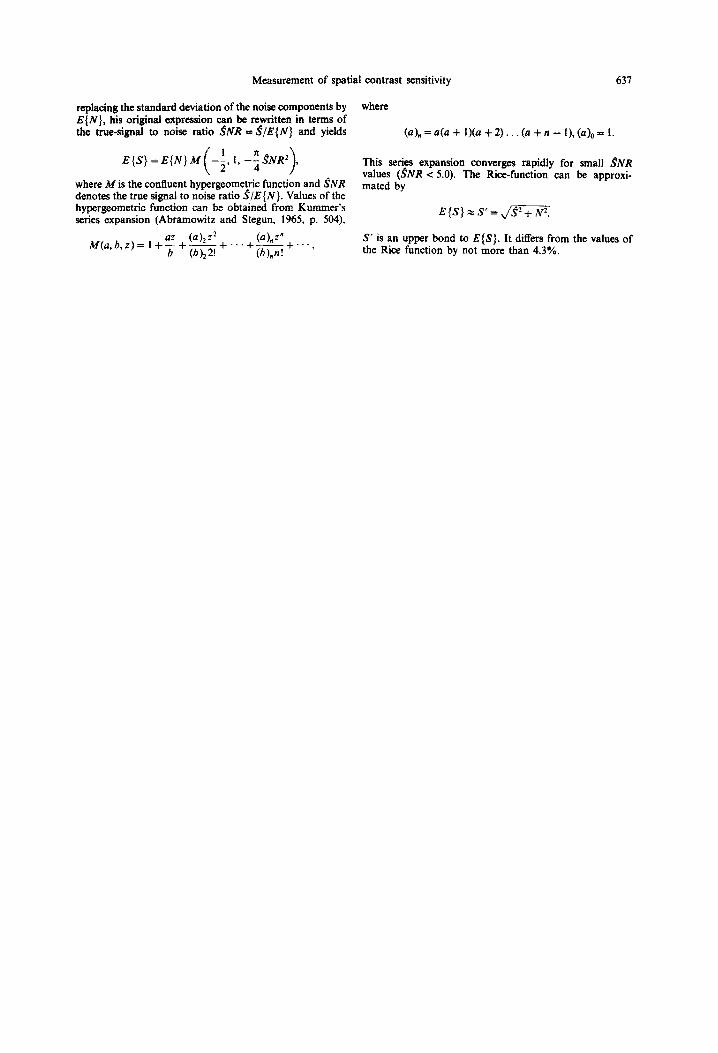
The magnitude of the threshold bias as a function of the window width in octaves, W,,, is illustrated in Fig. 8, assuming a window with a 50% cosine envelope. W,,, is obtained as the product of the window length in seconds, W,,

ANTHONY M. NORCIA ef af

0 04 08 12 16

WINElOW WIDTH lOCTi

Fig. 8. Threshold bias as a function of window width. Solid curves are for CRF slopes of 2.5 and dashed curves for slopes of 4. Curves in (A) were derived from extrapolations over the SNR range of 1.5: 1 and 3 : 1, those in (3) over the range 2: 1 and 4: I and those in (C) over the range 3: 1 and

4:l.

and the sweep rate, I(, with W,,, = W$R. The curves, calculated for slopes of the CRF of 2.5 and 4 respectively, are grouped in pairs, assuming three different scenarios in which the extrapolated threshold was determined through values with SNRs of (A) 1.5-3, (B) 2-4, (C) 3-4.

Given a window width smaller than 0.4 act, the sliding window has virtually no effect. In this range, the amount of the threshold bias is solely defined by the noise mixing described above. For greater window widths, the sliding window contributes substa~tialIy to the overall effect. Nevertheless, even in the worst case (i.e. extrap- olation through values with SNRs of 1.5-3), the resulting threshold bias is, at most, 0.4 octaves, given a sweep rate of 0.8 octlsec and a 2 set window. When the extrapolation is performed through data points with slightly greater SNR (2:l and 4: 1), the expected bias is reduced to less than 0.2 octaves.

Of practical importance is the fact that the curves for a CRF slope of 2.5 start from a higher pedestal value, but rise more slowly than the respective curves for a slope of 4. Therefore, we find a cross-over between the shallow and the steep curve in Fig. 8 at a window width of 1.2 to 1.4 act. In this range, the efI%ct of the sliding window compensates for the difference in the pedestal starting values. This has the important consequence that the outcome of the threshold extrapolation is independent of the slope of the CRF under typical conditions.

DISCUSSION

Form of the CRF. The form of the infant

COntraSt response function as measured by &he sweep VEP is similar to that previously ob- served in adults by others (Campbell and ~a~ei, 1970) and in our own laboratory (Tyler and Apkarian, 1985; Allen et al., 1986). The function consists of a monotonically increasing response which is a linear function of log con- trast near threshold, as initially reported by Campbell and Maffei (1970). The CRF in adults often contains two lobes or branches (Campbell and Maffei, 1970; Murray and ~ulikowski, 1983; Bobak et af., 1984; Tyler and Apkarian, 1985; Allen et al., 1986). Two-lobed CRFs have also been reported in VEP recordings from alert monkeys (Nakayama and Mackeben, 1982) and in 6 month-old infants (Tyler et al., 1987).

There has been much s~culation regarding the source of the two-lobed function, ranging from a central-/pe~pheral-field origin (Camp- bell and Maffei, 1970); to a cortical man- ifestation of the magnocellular and par- vocellular streams (Bobak et al., 1984; Tyler and Apkarian, 1985), to their representing separate motion and pattern detecting m~hanisms (Murray and Kulikowski, 1983). The two-lobed function is also apparent in the ensemble of contrast response functions of extracelluarly recorded complex cells in monkey, but not of simple ceils (Albrecht and Hamilton, t 982). The present data say little about the origin of the two-lobed function, save that it is present quite early in development, certainly by IS weeks (cf. Fig. 2). ~e~~o~se ~~~~~-u~ and hysteresis. A concern in swept contrast measurements (cf. Regan et al., 1975) aside from choosing the starting point appropriately, has been whether the rate or direction of contrast change can effect the mea- sured threshold. It is possible that different rates of contrast increase could interact with the rate of build up of the steady-state response and produce differences in threshold which de- pended upon the rate of b~ldup of the response, rather than upon the underlying sensitivity of the mechanisms involved. It appears from our analysis, which involved rates from 0-l octave~s~ to 0.8 octave~s~, that the effects are small over this range.

Nelson et al (1984) have observed a hyster- esis in swept contrast meas~ements such that thresholds are lower when contrast is swept starting at low contrast rather than starting at high contrast. We have not systematically in- vestigated this effect as to its magnitude or

Measurement of spatial contrast sensitivity 635

generality, but given Nelson ef al.‘s finding, this Signal processing considerations in swept con- point deserves further attention. trast VEP measurement

The ~port~n~e of me~ring response phase. We have observed that the response phase often shows a progressive phase lead with increasing contrast (Fig. lb), Phase-insensitive detection, such as that afforded by the DFT, is optimal in such situations, since the starting phase is un- known and because large phase shifts can easily occur (Peli et al., 1988).

The progressive phase leads that we observe as contrast increases are consistent with a speed- ing of the evoked response at higher contrast. Similarly, transient VEP implicit time (Kulikowski, 1977) and psychophysical reaction time (Harwerth and Levi, 1978) have been shown to decrease with increasing contrast. On the basis of this apparently general phys- iological finding, the computer algorithm for threshold extrapolation requires that the re- sponse phase not show a slowing with increased contrast. The use of a priori knowledge of this physiological constraint on the direction of phase shift with increasing contrast, combined with a rate limit on the phase change, leads to a nonlinear decision criterion which restricts the acceptable response range to substantially less than 360 deg. Thus the analysis is no longer strictly phase-insensitive, with the result being an improved ability to di~~minate signal from noise without the need for accurate knowledge of the absolute phase of the response.

over-estimation of sensitivity at low SNR. The extrapolation technique, when used at low sig- nal to noise ratios, tends to overestimate sensi- tivity to a small extent, due to the nature of signal and noise additivity. To the extent that the experimental noise is Gaussian in its Fourier coefficients, the mixture of signal plus noise amplitudes will follow the Rice distribution, which becomes the Rayleigh distribution at a SNR of zero (Rice, 1945). The bias in the threshold measurement becomes negligible as SNR increases and the effects of noise mixing can be almost completely avoided by using points above a SNR of 3 for the extrapolation.

In any application of the DFT technique, it is necessary to employ a data window of some duration. Wider windows have the advantage of providing higher SNR, but when combined with the swept-parameter technique they smooth the shape of the CRF. The smoothing has its great- est effect at points of changing gradient, such as the inflection point where the signal rises out of the noise. The effect of smoothing on the thres- nold estimate can be avoided by using higher SNR points which are removed from the region of greatest change in gradient.

The fact that the response phase may not be random at contrasts which fail to produce a significant amplitude response (Fig. 3) suggests that phase coherence measures may be of use at low signal to noise ratios (Eizenman et al., 1987).

Extrapolation to zero versus aJixed amplitude criterion. The amount of contrast required to generate a fixed amplitude signal has been used in the past as a criterion for contrast sensitivity (Regan, 1978; Pirchio et al., 1978). The use of this method assumes that all contrast functions have the same form, that of a simple monotonic increase. If the contrast response function changes shape as a function of the stimulus parameters, then this criterion can lead to in- consistent estimates of the threshoid. It appears that this could be particularly problematic at low spatial frequencies where the CRF often consists of 2 lobes. If the criterion is set too high, it is possible that a low contrast limb will be missed altogether.

The particular choice of data window has not been explored in detail. It is clear that any smooth window is superior to the rectangular window (no window) on aggregate figures of merit (Harris, 1978). Fine adjustments of the window shape may improve performance, but the actual ~rfo~an~ of many windows may be less than theoretically possible when used with machine arithmetic of limited precision,

Resistance of the extrapolation technique to changes in CRF slpe. CRFs can be measured using a range of sweep rates and window widths. Experimental conditions and individual differences between observers will result in differing SNRs. The CRF will also have a characteristic slope or gain which may also depend upon conditions or observers. However, it is interesting to note that, over a range of sweep rates and window widths which we have found to be useful experimentally, the combined effects of noise mixing and window bias remain essentially constant. This is simply due to the fact that as the gain of the CRF increases, the effects of noise mixing decrease while at the same time the window smoothing effect in- creases. Since the two effects are of the same size, the combination of the two effects remains

636 ANTHONY M. NORCIA et al.

constant. The combined effects of these two sources of bias are small and are only significant at very low signal to noise ratios.

Acknowledgements-This work was supported by EYO6579, EY06883, and with the cooperation of the Kaiser Founda- tion Research Institute.

REFERENCES

Abramowitz M. and Stegun I. A. (1965) ~~dbook of‘ Mathematical Functions. Dover, New York.

Albrecht D. G. and Hamilton D. B. (1982) Striate cortex of monkey and cat: contrast response function. J. Neu- rophysiol. 48, 217-237.

Allen D., Norcia A. M. and Tyler C. W. (1986) Compara- tive study of electrophysiological and psychophysical measurement of the contrast sensitivity function in hu- mans. Am. J. Optom. physiol. Opt. 63, 442-449.

Bobak P., Bodis-Wollner I.. Harnois C. and Thornton J. (1984) VEPS in humans reveal high and low spatial contrast mechanisms. Invest. Ophthal. Gwul Sci. 25, 98C983.

Campbell F. W. and Maffei L. (1970) Electrophysiological evidence for the existence of orientation and size detectors in the human visual system. J. P/r~.siol., Land. 207, 635652.

Eizenman M., Schneck M. and Skarf B. (1987) Optimum estimation of acuity using visual evoked potentials. Inoesr. Ophthal. visual Sci. (Suppl.) 28, 5.

Harris F. J. (1978) On the use of windows for harmonic analysis with the discrete Fourier transform. Proc. IEEE 66, 51-83,

Harwerth R. S. and Levi D. M. (1978) Reaction time as a measure of suprathreshold grating detection. Vision Res. 18, 1579-1586.

Kulikowski J. (1977) Visual evoked potentials as a measure of visibility. In Visual Evoked Potentials in Man: New Dellefopments (Edited by Desmedt J. E.), pp. 168-183. Clarendon Press, Oxford.

Murray I. J. and Kulikowski J. J. (1983) VEPs and contrast. Vision Res. 23, 1741-1743.

Nakayama I(. and Mackeben M. (1982) Steady state visual evoked potentials in the alert primate. Vision Res. 22, 1261-1271.

Nelson J. I., Seiple W. H., Ku~rsmith M. J. and Carr R. E. (1984) A rapid evoked potential index of cortical adaptation. Electraenceph. din. Neurophysiol. 59, 454464.

Norcia A. M. and Tyler C. W. (1985) Spatial frequency sweep VEP: visual acuity during the first year of life. Vision Res. 25, 1399-1408.

Norcia A. M., Clarke M. and Tyler C. W. (1985) DigitaI filtering and robust regression techniques for estimating sensory thresholds from the evoked potential. IEEE Engng Med. Biol. 4, 2632.

Norcia A. M., Allen D. and Tyler C. W. (1986) Electro- physiolo~cal assessment of contrast sensitivity in human infants. Am. J. Optom. physiol. Opt. 61, 12-15.

Norcia A. M., Tyler C. W. and Hamer R. D. (1988) High visual contrast sensitivity in the young human infant. invest. Ophthal, visual Sei. 29, 4449.

Papoulis A. (1965) Probability, Random Variables and Sto- chastic Processes. McGraw-Hill, New York.

Parker D. M. and Salten E. A. (1977) Latency changes in

the human visual evoked response to sinusoidal gratings. Vision Res. 17, 1201-1204.

Peli E., McCormack G. and Sokol S. (1988) Signal to noise ratio considerations in the analysis of sweep visual evoked potentials. Appl. Opt. 27, 10941098.

Pirchio M., Spinelli D., Fiorentini A. and Maffei L. (1978) Infant contast sensitivity evaluated by evoked potentials. Brain Res. 141, 179-184.

Regan D. (1966) Some characteristics of average steady- state and transient responses evoked by modulated light. Electroenceph. clin. Neurophysiol. 20, 238-248.

Regan D. (1977) Speedy assessment of visual acuity in amblyopia by the evoked potential method. Uphthal- mogica 175, 159-164.

Regan D. (1978) Assessment of visual acuity by evoked potentials: ambiguity caused by temporal dependence of spatial frequency selectivity. Vision Res. 18, 439-443.

Regan D., Schellart N. A. M., Spekreijse H. and van den Berg T. J. T. P. (1975) Photometry in goldfish by electro- physiological recording. Vision Res. 15, 799-807.

Rice S. 0. (1945) Mathematical analysis of random noise. Bell System Tech. J. 24, 46 156.

Seiple W. H., Kupersmith M. J.. Nelson J. I. and Carr R. E. (1984) The assessment of evoked potential contrast thresholds using real-time retrieval. Invest. Ophthal. visual Sci. 25, 627-63 1.

Tyler C. W. and Apkarian P. A. (1985) Effects of contrast, orientation and binocularity on the pattern evoked poten- tial. Vision Res. 25, 755-766.

Tyler C. W., Apkarian P., Levi D. M. and Nakayama K. (1979) Rapid assessment of visual function: an electronic sweep technique for the pattern evoked potential. Invest. Ophthal. visual Sci. 18, 703-l 13.

Tyler C. W., Norcia A. M. and Hamer R. D. (1987) Two mechanisms revealed by sweep VEP contrast functions in infants. Non-invasive assessment of the visual system. Tech. Dig. Opt. Sot. Am. MB-Z.

Weiner D. E., Wellish K., Nelson J. I. and Kupersmith M. J. (1985) Comparisons among Snellen, psychophysical and evoked potential acuity determinations. Am. J. Op- tom. physiol. Opt. 62, 669-679.

APPENDIX

In most VEP investigations, the amplitude of the response S at the stimulus frequency is called “signal” as opposed to “noise” N, denoting the uncorrelated EEG amplitude over the frequency range of the analysis. This definition is somewhat imprecise, since the amplitude response S itself is a sum of the true signal amplitude s and the noise at the stimulus frequency. In this Appendix, however, a more precise definition of the measured response is derived.

The recorded VEP amplitude S consists of the true signal amplitude 3 plus uncorrelated EEG noise. If the random noise amplitude N is normally distributed in terms of the sine and cosine components with zero mean and equal variance u2, then the noise amplitude N has a Rayleigh distribution with expected value E {N} = 6 & (Papoulis, 1965; p. 195). In order to determine how much the signal amplitude S is biased by the noise, we calculate the expected value of the random amplitude response:

s = ( +N,,)‘+ N:

where N,, denotes the component of the noise in phase with the signal and N,. denotes the component orthogonal to the signal phase. An analytical expression for the expected value of S was published by Rice (Rice, 1945; p. 101). After

Measurement of spatial contrast sensitivity 637

replacing the standard deviation of the noise components by E{N}, his original expression can be rewritten in terms of the true-signal to noise ratio &‘R = s/E(N) and yields

> ,

where M is the confluent hypergeometric function and $NR denotes the true signs1 to noise ratio S/E{N}. Values of the hypergeometric function can be obtained from Kummer’s series expansion (Abramowitz and Stegun, 1965, p. 504).

M(a,b,I)=*+~+~+...+~+ . . . . 2 N

where

(a),=a(a+I)(u+Z)...(a+n-l),(u),=l.

This series expansion converges rapidly for small $NR values (JNR c 5.0). The Rice-function can be approxi- mated by

S’ is an upper bond to E{S). It differs from the values of the Rice function by not more than 4.3%.