Measure and Integration on

Lipschitz-Manifolds

Joachim Naumann and Christian G. Simader

Abstract. The first part of this paper is concerned with various definitions of a k-dimensionalLipschitz manifold Mk and a discussion of the equivalence of these definitions. The secondpart is then devoted to the geometrically intrinsic construction of a σ-algebra L(Mk) ofsubsets of Mk and a measure µk on L(Mk).

Contents

1 Introduction 3

2 k-dimensional Lipschitz manifolds 52.1 Definitions. Equivalent characterizations . . . . . . . . . . . . . . . . . . . . 52.2 Examples . . . . . . . . . . . . . . . . . . . . . . . . . . . . . . . . . . . . . 14

3 The measure space(Mk,L(Mk), µk

)25

3.1 The σ-algebra L(Mk) . . . . . . . . . . . . . . . . . . . . . . . . . . . . . . 253.2 The measure µk . . . . . . . . . . . . . . . . . . . . . . . . . . . . . . . . . . 283.3 Integration . . . . . . . . . . . . . . . . . . . . . . . . . . . . . . . . . . . . . 353.4 The space Lp(Mk,L(Mk), µk) . . . . . . . . . . . . . . . . . . . . . . . . . . 42

References 43

2

Measure and Integration on Lipschitz-Manifolds

Joachim Naumann and Christian G. Simader

1 Introduction

In the case of k-dimensional manifolds of class Cm (m ≥ 1) in RN there is a variety of equiv-alent definitions. If we replace the assumption of continuous differentiability by Lipschitzresp. bi-Lipschitz properties of certain maps we find several different possibilities to definek-dimensional Lipschitz manifolds (see Definitions 2.3, 2.6–2.9). The natural question arisesif these definitions are equivalent. Here a certain hint is given by another consideration. Ifwe consider a k-dimensional manifold Mk ⊂ RN of class Cm and if an open neighborhoodU of Mk is mapped by a diffeomorphism φ of class Cm on an open set U∗ ⊂ RN , thenφ(Mk) ⊂ U∗ ⊂ RN is clearly again a k-dimensional manifold of class Cm in RN . As spe-cial (N − 1) - dimensional Lipschitz-manifolds Grisvard [4] considered boundaries of opensubsets in RN . He gave two definitions. His Definition 1.2.1.1 (see [4, p.5]) coincides withour Definition 2.6 of a (N − 1)-dimensional Lipschitz manifold in graph representation. Thesecond definition of Grisvard (see [4, Definition 1.2.1.2, p. 6/7]) coincides with our Defini-tion 2.3. Then Grisvard ([4, Lemma 1.2.1.3, p. 7]) pointed out that his Definition 1.2.1.2 isinvariant under bi-Lipschitz homeomorphisms of a neighborhood of the manifold. But withthe help of a very interesting counterexample (see [4, Lemma 1.2.1.4, p. 8/9]) he succeededin proving that the graph representation needs not to be invariant under bi-Lipschitz home-omorphisms. We prove in Theorem 2.13 that our Definitions 2.3 and 2.8 are invariant underbi-Lipschitz homeomorphisms. In Theorem 2.11 we prove the equivalence of the definitionsof a k-dimensional Lipschitz-manifold Mk in graph representation, in regular parametricrepresentation and in implicit representation. Further, in Theorem 2.10 we prove that a k-dimensional Lipschitz-manifold in graph representation is a k-dimensional Lipschitz-manifoldin the sense of Definition 2.3. Finally, Theorem 2.12 states that a k-dimensional Lipschitz-manifold in the sense of Definition 2.3 is a k-dimensional Lipschitz-manifold in parametricrepresentation. We derive the following diagram:

3

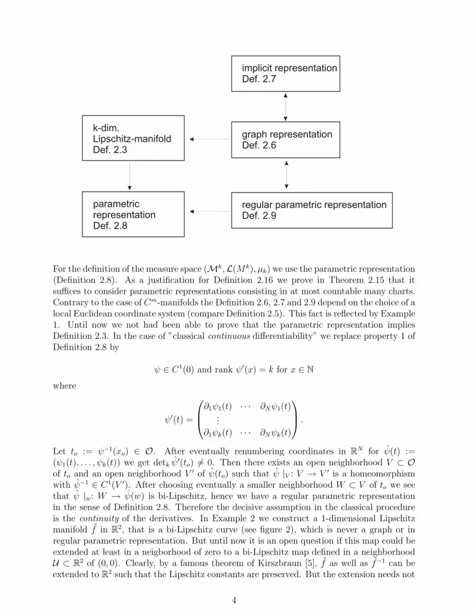
For the definition of the measure space (Mk,L(Mk), µk) we use the parametric representation(Definition 2.8). As a justification for Definition 2.16 we prove in Theorem 2.15 that itsuffices to consider parametric representations consisting in at most countable many charts.Contrary to the case of Cm-manifolds the Definition 2.6, 2.7 and 2.9 depend on the choice of alocal Euclidean coordinate system (compare Definition 2.5). This fact is reflected by Example1. Until now we not had been able to prove that the parametric representation impliesDefinition 2.3. In the case of ”classical continuous differentiability” we replace property 1 ofDefinition 2.8 by

ψ ∈ C1(0) and rank ψ′(x) = k for x ∈ N

where

ψ′(t) =

∂1ψ1(t) · · · ∂Nψ1(t)...

∂1ψk(t) · · · ∂Nψk(t)

.

Let to := ψ−1(xo) ∈ O. After eventually renumbering coordinates in RN for ψ(t) :=(ψ1(t), . . . , ψk(t)) we get detk ψ

′(to) 6= 0. Then there exists an open neighborhood V ⊂ Oof to and an open neighborhood V ′ of ψ(to) such that ψ |V : V → V ′ is a homeomorphismwith ψ−1 ∈ C1(V ′). After choosing eventually a smaller neighborhood W ⊂ V of to we seethat ψ |w: W → ψ(w) is bi-Lipschitz, hence we have a regular parametric representationin the sense of Definition 2.8. Therefore the decisive assumption in the classical procedureis the continuity of the derivatives. In Example 2 we construct a 1-dimensional Lipschitzmanifold f in R2, that is a bi-Lipschitz curve (see figure 2), which is never a graph or inregular parametric representation. But until now it is an open question if this map could beextended at least in a neigborhood of zero to a bi-Lipschitz map defined in a neighborhoodU ⊂ R2 of (0, 0). Clearly, by a famous theorem of Kirszbraun [5], f as well as f−1 can beextended to R2 such that the Lipschitz constants are preserved. But the extension needs not

4

to be bi-Lipschitz. Therefore the equivalence of Definitions 2.3 and 2.8 is an open problem.

In the third section we construct the measure space(Mk,L(Mk), µk

). In section 3.1 the

σ-algebra of measurable subsets of Mk is constructed and the measurability of a functionf : Mk → R is defined. Here one has to prove that both definitions are independent of thespecial parametric representation. After several preparations in section 3.2 the measure µkcan be defined on the σ-Algebra L(Mk) (Definition 3.6 and Theorem 3.7). Finally, equiv-alent characterizations of sets of measure zero (Theorem 3.8) are given. Once a measurespace is constructed, the integral is defined at least for non-negative measurable functions.In section 3.3 we prove some elementary properties of this integral. First, a relation betweenthis integral and integrals using the parametric representation is studied (Theorem 3.9 andCorollary 3.10). For the remaining part of section 3.3 it is assumed that Mk has a finiteparametric representation. Then estimates for the integral of nonnegative integrable func-tions are derived (Theorem 3.11 and Corollary 3.12) and a formula for the calculation of theintegral with the help of a partition of unity is derived (Theorem 3.13). Finally, in section3.4 we introduce the space Lp(Mk,L(Mk), µk).

Acknowledgements. The authors thank the DFG for supporting this research via thegrant (SI 333/4-1). Moreover, they are greatly indepted to Dr. Matthias Stark for manyvaluable discussions and remarks.

2 k-dimensional Lipschitz manifolds

2.1 Definitions. Equivalent characterizations

Definition 2.1 Let G ⊂ Rn be an open set. A mapping u : G → Rm (m,n ∈ N) is calledbi-Lipschitz in G if there are constants 0 < L1 ≤ L2 such that

(2.1) L1‖x− x′‖n ≤ ‖u(x)− u(x′)‖m ≤ L2‖x− x′‖n ∀x, x′ ∈ G

We summarize the following properties of bi-Lipschitz mappings.

Theorem 2.2 Let G ⊂ Rn be open and let u : G→ Rm (m,n ∈ N) satisfy (2.1).

1. There is a subset N ⊂ G, |N | = 0, such that u is totally differentiable at each x ∈ G\N .For the total derivative

u′(x) = (Diuk(x)) ∈M(m× n), x ∈ G \N

we have the estimate

(2.2) L1‖η‖n ≤ ‖u′(x)η‖m ≤ L2‖η‖n ∀x ∈ G \N,∀η ∈ Rn

Therefore m ≥ n and rank u′(x) = n ∀x ∈ G \N .

5

2. Let m = n. Then u is open, i.e. for every open V ⊂ G the image u(V ) is open too.

For the proof we refer e.g. to [7, Theorems 1.6 and 4.5]. In the sequel, let N, k ∈ N, N ≥ 2and let 1 ≤ k ≤ N − 1.

Definition 2.3 A subset Mk ⊂ RN is called a k-dimensional Lipschitz-manifold if for everyx0 ∈ Mk there exists an open set U ⊂ RN and a bi-Lipschitz mapping φ : U → φ(U) ⊂ RN

such that xo ∈ U and φ(Mk ∩ U) = RN−ko ∩ φ(U) where RN−k

o = {x ∈ RN : xk+1 = . . . =xN = 0}.

Sometimes the following equivalent characterization is more convenient.

Theorem 2.4 For x = (x1, . . . , xn) ∈ RN we write x′ := (x1, . . . , xk) ∈ Rk, x′′ := (xk+1, . . . , xN) ∈RN−k, x = (x′, x′′). A subset Mk ⊂ RN is a k-dimensional Lipschitz-manifold if and onlyif for every xo ∈ Mk, xo = (x′o, x

′′o), there exist open subsets V ′ ⊂ Rk and V ′′ ⊂ RN−k such

that with V := V ′ × V ′′ ⊂ RN−k holds true:

1. x′o ∈ V ′, x′′o ∈ V ′′, xo = (x′o, x′′o) ∈ V .

2. There exists a bi-Lipschitz mapping H : V → H(V ) such that

H(Mk ∩ V ) = {(x′, x′′) ∈ H(V ) : x′′ = 0}

Proof

1. Let Mk be a k-dimensional Lipschitz manifold. Let xo ∈ Mk and U ⊂ RN andφ : U → φ(U) be according Definition 2.3. Since U is open and xo ∈ U there existsε > 0 such that Bε(x) ⊂ U . Let V ′ := B′

ε√2

(x′o) ⊂ Rk, V ′′ := B′′ε√2

(x′′o) ⊂ RN−k. Then

V := V ′ × V ′′ ⊂ Bε(x). Let H := φ |V .

2. Clearly the converse statement holds true with U := V and φ := H.

Definition 2.5 Let ei := (δ1i, . . . , δNi), i = 1, . . . , N , denote the canonical basis in RN

and let xo ∈ RN . We say that [Oxo , f1, . . . , fN ] is a local Euclidean coordinate system withorigin at xo if there exists an orthogonal matrix S such that fi = Sei, i = 1, . . . , N . For

x =N∑i=1

xiei ∈ RN let

y =: Tx = S(x− xo) = S

(N∑i=1

(xi − x′oi)ei

)=

N∑i=1

(xi − xoi)fi

and conversely

T−1y = Sty + xo = St

(N∑i=1

(xi − xoi)fi

)+ xo =

=N∑i=1

(xi − xoi)Stfi + xo =

N∑i=1

(xi − xoi)ei + xo = x− xo + xo = x

6

Definition 2.6 A subset Mk ⊂ RN is called a k-dimensional Lipschitz-manifold in graphrepresentation if for every xo ∈ Mk there exists a local Euclidean coordinate system[Oxo , f1, . . . , fN ] with origin in xo and

1. there are open subsets V ′ ∈ Rk and V ′′ ⊂ RN−k, V := V ′ × V ′′ and Oxo ∈ V .

2. there exists a Lipschitz mapping h : V ′ → V ′′ with

Mk ∩ V = {(x′, h(x′)) : x′ ∈ V ′}

Definition 2.7 A subset Mk ⊂ RN is called a k-dimensional Lipschitz-manifold in im-plicit representation if for every xo ∈Mk there exists a local Euclidean coordinate system[Oxo , f1, . . . , fN ] with origin Oxo in xo such that

1. there are open subsets V ′ ⊂ Rk, V ′′ ⊂ RN−k, V := V ′ × V ′′ and Oxo ∈ V

2. there exists a mapping F : V → RN−k with F (Oxo) = 0 and there are two constantsLF > 0, KF > 0 such that

(2.3) ‖F (x′, x′′)− F (y′, y′′)‖N−k ≤ LF (‖x′ − y′‖k + ‖x′′ − y′′‖N−k)∀x = (x′, x′′), ∀y = (y′, y′′) ∈ V

and

(2.4) ‖F (x′, y′′)− F (x′, z′′)‖N−k ≥ KF‖y′′ − z′′‖N−k ∀x′ ∈ V ′, ∀y′′, z′′ ∈ V ′′.

3. Mk ∩ V = {x ∈ V : F (x) = 0}

Definition 2.8 A subset Mk ⊂ RN is called a k-dimensional Lipschitz-manifold in para-metric representation if for every xo ∈Mk there exists an open set U ⊂ RN and an openset O ⊂ Rk and a mapping ψ : O → RN such that

1. ψ : O → ψ(O) is bi-Lipschitz

2. xo ∈ U

3. ψ(O) = Mk ∩ U

Definition 2.9 A subset Mk ⊂ RN is called a k-dimensional Lipschitz-manifold in regularparametric representation if for every xo ∈Mk there exists a local Euclidean coordinatesystem [Oxo , f1, . . . , fN ] with origin Oxo in xo such that

1. there is an open set U ⊂ RN with Oxo ∈ U and an open set O ⊂ Rk and a mappingψ : O → RN such that

(a) ψ : O → ψ(O) is bi-Lipschitz

7

(b) ψ(O) = Mk ∩ U(c) with

ψ(t) := (ψ1(t), . . . , ψk(t)) t ∈ O

the mapping ψ : O → ψ(O) ⊂ Rk is bi-Lipschitz.

Theorem 2.10 A k-dimensional Lipschitz-manifold Mk in graph representation (Definition2.6) is a k-dimensional Lipschitz-manifold in the sense of Definition 2.3.

Proof Let xo ∈ Mk and let [Oxo , f1, . . . , fN ] be a local Euclidean coordinate system withorigin at xo, fi = Sei, i = 1, . . . , N with an orthogonal matrix S. Let the points y ∈ RN

be described with respect to the [Oxo , f1, . . . , fN ] frame. Let V ′ ⊂ Rk, V ′′ ⊂ RN−k be open,Oxo ∈ V := V ′ × V ′′ and let h : V ′ → V ′′ be a Lipschitz mapping with

Mk ∩ V = {(y′, h(y′)) : y′ ∈ V ′} .

Let U := {T−1y = Sty + xo : y ∈ V } (where T is defined according Definition 2.5). Forx ∈ U we write y := Tx = ((Tx)′, (Tx)′′) ∈ V ′ × V ′′. Let now φ : U → Rn be defined byφ(x) = ((Tx)′, h((Tx)′)− (Tx)′′). Then for x ∈ U

φ(x) ∈ RN−ko ⇔ (Tx)′′ = h ((Tx)′) ⇔

((Tx)′, h ((Tx)′)) ∈ {(y′, h(y′)) : y′ ∈ V ′} = Mk ∩ V.

We prove that φ is bi-Lipschitz. Let Lh > 0 such that

‖h(y′)− h(y′′)‖N−k ≤ Lh‖y′ − y′′‖k.

Then, for x, z ∈ U

‖φ(x)− φ(z)‖2N = ‖(Tx)′ − (Tz)′‖2

k + ‖h ((Tx)′)− h ((Tz)′) + (Tz)′′ − (Tx)′′‖2N−k ≤

≤ ‖(Tx)′ − (Tz)′‖2k + (Lh‖(Tx)′ − (Tz)′‖k + ‖(Tz)′′ − (Tx)′′‖N−k)2 ≤

≤ (1 + 2L2h)‖(Tx)′ − (Tz)′‖2

k + 2‖(Tz)′′ − (Tx)′′‖2N−k

With C := (1 + 2 max(1, L2h))

12 > 0 we see

‖φ(x)− φ(z)‖2N ≤ C2

(‖(Tx)′ − (Tz)′‖2

k + ‖(Tx)′′ − (Tz)′′‖2N−k

)=

= C2‖Tx− Tz‖2N = C2‖Sx− Sz‖2

N = C2‖x− z‖2N

Let now x ∈ U and φ(x) = z ∈ φ(U). Then

(Tx)′ = z′ and h((Tx)′)− (Tx)′′ = z′′

whence h(z′)− z′′ = (Tx)′′. Therefore

8

Tx = ((Tx)′, (Tx)′′) = (z′, h(z′)− z′′)

and

x = St ((z′, h(z′)− z′′)) + xo = φ−1 (z′, h(z′)− z′′) .

Then for z, w ∈ φ(U)

∥∥φ−1 (z′, h(z′)− z′′)− φ−1 ((w′, h(w′)− w′′))∥∥2

N=

= ‖(z′, h(z′)− z′′)− (w′, h(w′)− w′′)‖2N =

= ‖z′ − w′‖2k + ‖h(z′)− h(w′) + w′′ − z′′‖2

N−k

As above, we see ∥∥φ−1(z)− φ−1(w)∥∥N≤ C‖w − z‖N ,

whence u for x, z ∈ U

C−1‖x− z‖N ≤ ‖φ(x)− φ(z)‖N ≤ C‖x− z‖N

Theorem 2.11 LetMk ⊂ RN . Then there are equivalent: Mk is a k-dimensional Lipschitz-manifold

1. in graph representation (Definition 2.6)

2. in regular parametric representation (Definition 2.9)

3. in implicit representation (Definition 2.7)

Proof Througout this proof let xo ∈ Mk and let [Oxo , f1, . . . , fN ] be a local Euclideancoordinate system with origin in xo such that the respective representations hold true.

1. ”1◦ ⇒ 2◦” : Let O := V ′ ⊂ Rk and let ψ : O → RN be defined by

ψi(x′) := xi, i = 1, . . . , k

ψi(x′) := hi−k(x

′), i = k + 1, . . . , N

(x′ ∈ O). Then for x′, y′ ∈ O

‖ψ(x′)− ψ(y′)‖2N = ‖x′ − y′‖2

k + ‖h(x′)− h(y′)‖2N−k ≤ (1 + L2

h)‖x′ − y′‖2k

where Lh denotes the Lipschitz constant of h. Clearly

‖ψ(x′)− ψ(y′)‖2N ≥

k∑i=1

‖ψi(x′)− ψi(y′)‖2

k = ‖x′ − y′‖2k

and with ψ(x′) := (ψ1(x′), . . . , ψk(x

′)) = x′ we see that ψ is a regular parametricrepresentation.

9

2. ”2◦ ⇒ 3◦”: Assume

(2.5) L1‖x′ − y′‖k ≤ ‖ψ(x′)− ψ(y′)‖k ≤ L2‖x′ − y′‖k ∀ x′, y′ ∈ O,

where 0 < L1 ≤ L2. Let

ˆψ(x′) := (ψk+1(x

′), . . . , ψN(x)) for x′ ∈ O

Since ψ : O → RN is Lipschitz,ˆψ : O → RN−k is Lipschitz too, and there is K > 0

such that

(2.6) ‖ ˆψ(x′)− ˆ

ψ(y′)‖N−k ≤ K‖x′ − y′‖k ∀x′, y′ ∈ O.

Since ψ : O → ψ(O) ⊂ Rk is bi-Lipschitz, V ′ := ψ(O) ⊂ Rk is open ([7, Theorem4.7]). Let V ′′ := RN−k and V := V ′ × V ′′ ⊂ RN . We define F : V → RN−k by

F (z′, z′′) :=ˆψ(ψ−1(z′)

)− z′′, (z′, z′′) ∈ V ′ × V ′′

z = (z′, z′′) ∈Mk ∩ U ⇔ ∃1x′ ∈ O such that

ψ(x′) =(ψ(x′),

ˆψ(x′′)

)= (z′, z′′) ⇔ ψ(x′) = z′ ∈ V ′,

z′′ =ˆψ(x′′) =

ˆψ(ψ−1(z1)

)∈ RN−k ⇔ (z′, z′′) ∈ V and F (z′, z′′) = 0

For z = (z′, z′′), w = (w′, w′′) ∈ V and x′ = ψ−1(z′), y′ := ψ−1(w′), by (2.5)

‖x′ − y′‖k ≤ L−11 ‖z′ − w′‖k

and by (2.6)

‖ ˆψ(ψ−1(z′)

)− ˆψ(ψ−1(w′)

)‖N−k ≤ KL−1

1 ‖z′ − w′‖k

Therefore

‖F (z′, z′′)− F (w′, w′′)‖N−k ≤

≤∥∥∥ ˆψ(ψ−1(z′)

)− ˆψ(ψ−1(w′)

)∥∥∥N−k

+ ‖z′′ − w′′‖N−k ≤

≤ KL−11 ‖z′ − w′‖k + ‖z′′ − w′′‖N−k ≤ LF (‖z′ − w′‖k + ‖z′′ − w′′‖N−k)

where LF := max(1, KL−1

1

). Furthermore, for t′ ∈ V ′, z′′, w′′ ∈ V ′′

‖F (t′, z′′)− F (t′, w′′)‖N−k = ‖z′′ − w′′‖N−k.

10

3. ”3◦ ⇒ 1◦”: By the Lipschitz variant of the implicit function theorem (compare e.g. [7,Theorem 4.8, p. 41/42]) there exists an open set W ′ ⊂ V ′ ⊂ Rk and a Lipschitz mapg : W ′ → RN−k such that (Oxo)

′ ∈ W ′ and

(a) (x′, g(x′)) ∈ V ∀x′ ∈ W ′

(b) F (x′, g(x′)) = 0 ∀x′ ∈ W ′

(c) {(x′, x′′) ∈ W ′ × V ′′ : F (x′, x′′) = 0} = {(x′, g(x′)) : x′ ∈ W ′}

Therefore with W := W ′ × V ′′ we see

Mk ∩W = {x ∈ W : F (x) = 0} .

Theorem 2.12 Let Mk ⊂ RN be a k-dimensional Lipschitz-manifold in the sense of Defi-nition 2.3. Then it is a k-dimensional Lipschitz-manifold in parametric representation too.

Proof Let xo ∈Mk and let U ⊂ RN be open, φ : U → φ(U) ⊂ RN be bi-Lipschitz such thatxo ∈ U and φ(Mk ∩ U) = RN−k

o ∩ φ(U). By [7, Theorem 4.6], φ(U) is open. Let

O :={x′ ∈ Rk : (x′, 0) ∈ RN−k

o ∩ φ(U) = φ(Mk ∩ U)}.

We prove that O is open. Let (x′, 0) ∈ RN−ko ∩ φ(U). Since φ(U) ⊂ RN is open, there is

ε > 0 such that{y ∈ RN : ‖y − (x′, 0)‖N < ε

}⊂ φ(U). Let

B′ε(x

′) :={y′ ∈ Rk : ‖y′ − x′‖k < ε

}.

For y′ ∈ B′ε(x

′) we see ‖(y′, 0)−(x′, 0)‖N = ‖y′−x′‖k < ε and therefore (y,0) ∈ φ(U)∩RN−ko ,

that is B′ε(x

′) ⊂ O. Let ψ : O → RN , ψ(x′) := φ−1 ((x′, 0)), x′ ∈ O. Then ψ(O) = Mk ∩ Uand because φ is bi-Lipschitz, ψ is bi-Lipschitz too.

In the case of k-dimensional C1-manifolds it is easy to see that the parametric map ψ : O →Mk ∩ U can be locally extended to a diffeomorphism of an open set O ⊂ RN to an openset U ⊂ U such that ψ ((x′, 0)) = ψ(x′) for x′ ∈ O. In the underlying case we had not beenable to prove that a k-dimensional Lipschitz manifold in parametric representation is a kdimensional Lipschitz manifold in the sense of Definition 2.3. Conversely until now we couldnot find a counterexample too.

Theorem 2.13 Let Mk ⊂ RN be a k-dimensional Lipschitz manifold in the sense of Defi-nition 2.3 (resp. in parametric representation). Let W ⊂ RN be open and f : W → RN bebi-Lipschitz. Let Mk ⊂ W. Then Mk := f(Mk) is a k-dimensional Lipschitz manifold inthe sense of Definition 2.3 (resp. in parametric representation).

Proof

1. Let Mk be a k-dimensional Lipschitz manifold in the sense of Definition 2.3. Letxo ∈ Mk. Then there exists a unique xo ∈ Mk such that xo = f(xo). By Definition2.3, there exists an open set U ⊂ RN and a bi-Lipschitz mapping φ : U → φ(U) ⊂ RN

11

such that xo ∈ U and φ(Mk ∩U) = RN−ko ∩φ(U). Let U := f(U). Then U is open (see

Theorem 2.2). Further, φ := φ ◦ f−1 : U → RN is bi-Lipschitz and by injectivity of f

φ(Mk ∩ U) = φ(f−1(Mk ∩ U)) = φ(f−1(f(Mk) ∩ f(U))

)=

= φ(Mk ∩ U) = RN−ko ∩ φ(U) = RN−k

o ∩ φ(f−1f(U)) =

= RN−ko ∩ φ(f−1(U)) = RN−k

o ∩ φ(U).

2. LetMk ⊂ RN be a k-dimensional Lipschitz-manifold in parametric form. Let xo ∈ Mk.Then there is a unique xo ∈ Mk such that xo = f(xo). By Definition 2.8 there is anopen set U ⊂ RN , an open setO ⊂ Rk and a bi-Lipschitz mapping ψ : O → ψ(O) ⊂ RN

such that xo ∈ U and ψ(O) = Mk∩U . Let U := f(U) and let ψ : O → RN , ψ := f ◦ψ.Then ψ : O → ψ(O) is bi-Lipschitz and

ψ(O) = f(ψ(O)) = f(Mk ∩ U) = f(Mk) ∩ f(U) = Mk ∩ U .

Obviously the definition of a k-dimensional Lipschitz manifold Mk in parametric repre-sentation is the most general one and it is invariant under bi-Lipschitz transforms of aneighborhood W of Mk. So we use Definition 2.8 for the remaining part of the paper. Forthe sake of brevity, in the sequel we call Mk ⊂ RN a k-dimensional Lipschitz-manifold ifDefinition 2.8 applies to Mk. As a preparation we need

Lemma 2.14 Let Mk ⊂ RN be a k-dimensional Lipschitz-manifold. Then there exists asequence (Kn)n∈N ⊂Mk such that

1. Kn is compact ∀n ∈ N

2. Kn ⊂ Kn+1 ∀n ∈ N

3. Mk =∞⋃n=1

Kn

Proof

1. Let xo ∈ QN , q ∈ Q and

Bq(xo) :={x ∈ RN : ‖x− xo‖N < q

}.

Then B :={Bq(xo) : q ∈ Q, xo ∈ QN

}forms a countable basis of the topology of RN .

We choose an arbitrary but fixed numeration of B and write B = {Ui : i ∈ N}. ThenBk := {Vi := Mk ∩ Ui : i ∈ N} is a countable basis of the topology of Mk.

2. We prove now that for each xo ∈ Mk there exists jo ∈ N such that xo ∈ Vjo , Vjo iscompact and Vjo ⊂ Mk. Let xo ∈ Mk. Then there is an open O ⊂ Rk, an openU ⊂ RN , xo ∈ U , and a bi-Lipschitz mapping ψ : O → ψ(0) such that ψ(0) = M∩U .There exists a unique yo ∈ O such that xo = ψ(yo). Since O is open there exists ε > 0

12

such that Bε(yo) ⊂ Bε(yo) ⊂ O. Since Bε(yo) is compact, ψ(Bε(yo)) ⊂ Mk ∩ U iscompact too. Because of the continuity of ψ−1 and ψ(Bε(yo)) = (ψ−1)−1(Bε(yo)) ⊂Mk ∩ U the set ψ(Bε(yo)) is open in Mk ∩ U . Since (Vi)i∈N is a basis of the topologyof Mk ∩ U there exists jo ∈ N, Vjo ⊂ Bk such that xo ∈ Vjo ⊂ ψ(Bε(yo)). Then

Vjo ⊂ ψ(Bε(yo)) ⊂Mk ∩ U and Vjo is compact.

3. The set W := {Vj ∈ Bk : Vj compact, Vj ⊂ Mk} is either finite or at most countableinfinite. Let

Kn :=n⋃j=1

Vj∈W

Vj.

Then Kn is compact, Kn ⊂Mk and Kn ⊂ Kn+1. Therefore∞⋃n=1

Kn ⊂Mk. If conversely

xo ∈ Mk, then by part 2 of proof there exists Vjo ∈ W such that xo ∈ Vjo ⊂ Vjo ⊂∞⋃n=1

Kn, whence Mk ⊂∞⋃n=1

Kn.

Theorem 2.15 Let Mk ⊂ RN be a k-dimensional Lipschitz-manifold. Then there is an atmost countable set Λ ⊂ N such that

1. for each i ∈ Λ there exists an open set Oi ⊂ Rk, an open set Ui ⊂ RN and a bi-Lipschitzmapping ψi : Oi → ψi(Oi) such that ψi(Oi) = Mk ∩ Ui

2. Mk =⋃i∈Λ

Mk ∩ Ui =⋃i∈Λ

ψi(Oi)

Proof Let the sequence (Kn)n∈N ⊂Mk be according Lemma 2.14. For each xo ∈ Kn thereexists an open Oxo ⊂ Rk, an open Uxo ⊂ RN and a bi-Lipschitz ψxo : Oxo → ψ(Oxo) suchthat ψxo(Oxo) = Mk ∩ Uxo . Then for each n ∈ N

{Mk ∩ Uxo : xo ∈ Kn}

is an open covering of the compact set Kn. Therefore there exists pn ∈ N and x(n)j ∈ Kn,

j = 1, . . . , pn, such that

Kn ⊂pn⋃j=1

Mk ∩ Ux(n)j.

Then

Mk =∞⋃n=1

Kn =∞⋃n=1

pn⋃j=1

Mk ∩ Ux(n)j.

The set{x

(n)j : n ∈ N, j = 1, . . . , pn

}is at most countable infinite. Let the set of corre-

sponding pairs of indizes be numbered consecutively which gives Λ. If i ∈ Λ, xi = x(n)j ,

j ∈ {1, . . . , pn}, then let Ui := Ux(n)i

, ψi := ψx(n)j

, Oi := Ox(n)j

.

Theorem 2.15 justifies the following definition.

13

Definition 2.16 Let Mk ⊂ RN be a k-dimensional Lipschitz manifold.

1. A pair (O, ψ) with an open set O ⊂ Rk and a bi-Lipschitz mapping ψ : O → ψ(O)such that there exists an open set U ⊂ RN with the property ψ(O) = Mk ∩ U is calleda (local) parametric representation of Mk or chart of Mk ∩ U .

2. Let either Λ = {1, . . . , s} (s ∈ N) or Λ = N. A system {(Oi, ψi) : i ∈ Λ}, each (Oi, ψi)being a chart of Mk, is called a parametric representation or atlas of Mk.

Remark 2.17 Let Mk be a k-dimensional Lipschitz manifold. For i = 1, 2 let Oi ⊂ Rk andUi ⊂ RN be open, let ψi : Oi → ψ(Oi) be bi-Lipschitz such that

ψi(Oi) = Mk ∩ Ui (i = 1, 2).

Then U := ψ1(O1) ∩ ψ2(O2) is a relatively open subset of Mk. Then the sets ψ−1i (U) ⊂ Rk

are open (i = 1, 2). The mapping ψ−12 ◦ ψ1 is a bi-Lipschitz mapping from ψ−1

1 (U) ontoψ−1

2 (U) (as a mapping from a subset of Rk into Rk).

2.2 Examples

Example 1

For k ∈ Z let

I(k)1 :=]2−2k−2, 2−2k−1],

I(k)2 :=]2−2k−1, 2−2k],

I(k) := I(k)1 ∪ I(k)

2

Let gi : R+ → R (R+ := {t ∈ R : t ≥ 0}, i = 1, 2) be defined by

g1(t) :=

0 if t = 0

0 if t ∈ I(k)1

1 if t ∈ I(k)2

(E.1)

g2(t) :=

0 if t = 0

1 if t ∈ I(k)1

0 if t ∈ I(k)2

(E.2)

Then gi are measurable and bounded. Let for t ∈ R+

(E.3) fi(t) :=

t∫0

gi(s)ds, i = 1, 2

Then fi is differentiable in I(k)1 and I

(k)2 (at the right endpoint of I

(k)j from the left side,

j = 1, 2)

14

Denote by giε the mollification of gi(ε > 0) and define

f(ε)i (t) :=

t∫0

giε(s)ds

Then f(ε)i ∈ C∞(R+), f

(ε)′

i (t) = giε(t)

|fi(t)− f(ε)i (t)| ≤

t∫0

|gi(s)− giε(s)|ds→ 0 (ε→ 0)

and for all t ∈ R. Furthermore, for R > 0

R∫0

|gi(t)− giε(t)|dt→ 0 (ε→ 0)

Let ϕ ∈ C∞0 (R+) and choose R > 0 such that suppϕ ⊂ [0, R]. Then

∫R+

fi(t)ϕ′(t)dt =

R∫0

fi(t)ϕ′(t)dt = lim

ε→0

R∫0

f(ε)i (t)ϕ′(t)dt = − lim

ε→0

R∫0

giε(t)ϕ(t)dt =

= −R∫

0

gi(t)ϕ(t)dt

whence gi is the weak derivative of fi, fi, f′i = gi ∈ L1([0, R]) for all R > 0, i = 1, 2. Let

t, t′ ∈ R+. Then

(E.4) |fi(t)− fi(t′)| ≤

∣∣∣∣∣∣t∫

t′

|gi(s)|ds

∣∣∣∣∣∣ ≤ |t− t′|

We write f(t) := (f1(t), f2(t)). Then f : R+ → R2. For x = (x1, x2) ∈ R2 we denote by

‖x‖ :=(x2

1 + x22

) 12

the Euclidean norm of x. By (E.4) we see

(E.5) ‖f(t)− f(t′)‖ ≤√

2|t− t′| ∀t, t′ ∈ R+.

If t ∈ R+, t > 0 then there is a unique ko ∈ Z such that t ∈ I(ko). From the definition (E.3)

we calculate easily fi. Let i = 1 and t ∈ I(ko)1 . Observing (E.1) we see

f1(t) =

2−2ko−2∫0

g1(s)ds =∞∑

k=ko+1

2−2k∫2−2k−1

ds =1

32−2ko−1

15

Let t ∈ I(ko)2 . Then

f1(t) =1

32−2ko−1 +

t∫2−2ko−1

ds = t− 1

32−2ko

Similarly we calculate f2. The result is

(E.6) f(t) = (f1(t), f2(t)) =

0 if t = 0(

132−2k−1, t− 1

32−2k−1

)if t ∈ I(k)

1(t− 1

32−2k, 1

3 2−2k)

if t ∈ I(k)2

Let for t ∈ R+ y = (y1, y2) := (f1(t), f2(t)). Then we see from (E.6)

(E.7) t = y1 + y2 = f1(t) + f2(t) ∀t ∈ R+,

whence

t− t′ = f1(t) + f2(t)− f1(t′)− f2(t

′)

and

|t− t′| ≤ |f1(t)− f1(t′)|+ |f2(t)− f2(t

′)|

≤√

2[(f1(t)− f1(t

′))2+ (f2(t)− f2(t

′))2] 1

2=√

2‖f(t)− f(t′)‖.

Because of (E.5) we finally see

(E.8)1√2|t− t′| ≤ ‖f(t)− f(t′)‖ ≤

√2|t− t′| ∀t, t′ ∈ R+

We extend now f to R. Let

(E.9) f(t) :=

{f(t) if t ≥ 0

−f(−t) if t < 0

Because of (E.6), (E.7) we immediately see that f |R+ and f |{x∈R,x<0} are bi-Lipschitz.

By (E.9) we see that (E.7) continues to hold for t < 0 and fi replaced by fi, whence the firstinequality in (E.8) holds true for all t, t′ ∈ R. Let t > 0 > t′. Then by (E.5)

‖f(t)− f(t′)‖ = ‖f(t) + f(−t′)‖ ≤ ‖f(t)‖+ ‖f(−t′)‖ ≤√

2(t+ (−t′)) =

=√

2|t− t′|

16

Therefore (E.8) is satisfied with f in place of f and for all t, t′ ∈ R.

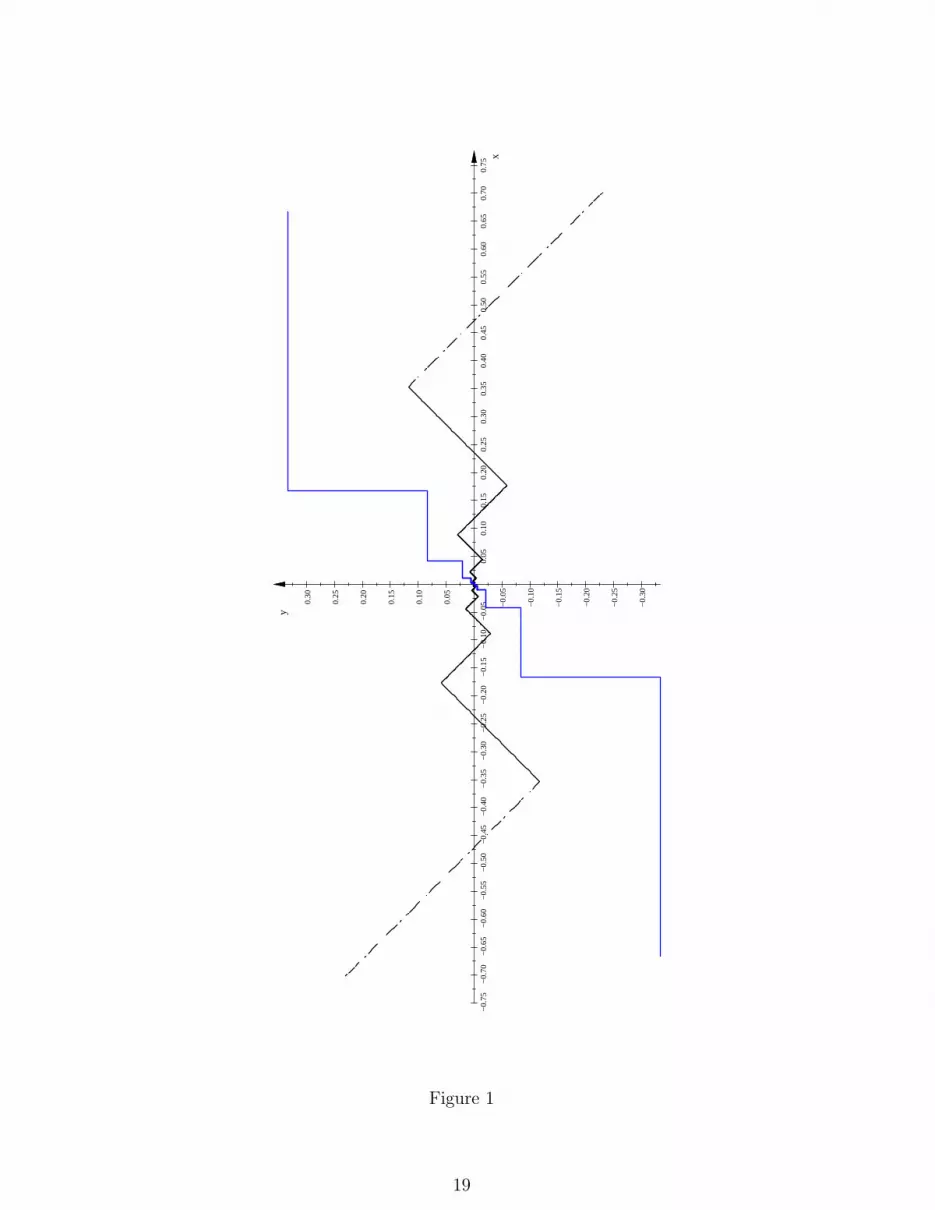
It follows immediately from (E.62) that f is not a graph of a map h : R → R2. This canalso be seen from the continuous line in figure 1. Further for every ε > 0 the interval ]− ε, ε[contains infinitely many intervals I

(k)i of constancy of fi (k ≥ ko(ε) ∈ N) whence f is not in

regular parametrization in a neighborhood of zero. Then, because of Theorem 2.10 it can’tbe in implicit representation too.

But let now a := cos π4

= 1√2

and we set

S :=

(a a−a a

)Then S is an orthogonal matrix. Let

h(t) :=

(h1(t)

h2(t)

):= S

(f1(t)

f2(t)

)=

(a(f1(t) + f2(t))

a(f2(t)− f1(t)

))Because of (E.7) we see h1(t) = at for t ∈ R. Further by (E.6) for t > 0.

(E.10) h2(t) =

{a(t− 1

32−2k

)if t ∈ I(k)

1

a(

132−2k+1 − t

)if t ∈ I(k)

2

, t > 0

If t < 0 because of fi(t) = −fi(−t)

(E.11) h2(t) =

{a(t+ 1

32−2k

)if − t ∈ I(k)

1

a(−t− 1

32−2k+1

)if − t ∈ I(k)

2

= −h2(−t)

Let s := at. Then

|t| ∈ I(k)1 ⇔ |s| ∈ J (k)

1 :=]a2−2k−2, a2−2k−1

]|t| ∈ I(k)

2 ⇔ |s| ∈ J (k)2 :=

]a2−2k−1, a2−2k

]Let ϕ : R+ → R,

ϕ(s) = h2

(sa

)=

0 if s = 0

s− a32−2k if s ∈ J (k)

1a32−2k+1 − s if s ∈ J (k)

2

We set

ϕ(s) :=

{ϕ(s) for s ≥ 0

−ϕ(−s) for s < 0

For t, t′ ∈ R by (E.8) we see

17

|h2(t)− h2(t′)| ≤ ‖h(t)− h(t′)‖ = ‖S (f(t)− f(t′)) ‖ ≤

√2|t− t′|

Therefore (s = at, s′ = at′)

(E.12) |ϕ(s)− ϕ(s′)| ≤√

2

a|s− s′|

and ϕ : R → R is Lipschitz. Further

H := {h(t) : t ∈ R} = {(s, ϕ(s)) : s ∈ R}

and H is the graph of the function ϕ. See in addition the interrupted line in figure 1. Clearly,H is in regular parametric representation too. Let F : R2 → R be defined by

F (x1, x2) := ϕ(x1)− x2.

Then (x1, x2) ∈ H if and only if F (x1, x2) = 0. Let V ′ = V ′′ = R. Then (0, 0) ∈ V ,F (0, 0) = 0. Further

|F (x1, x2)− F (y1, y2)| ≤ |ϕ(x1)− ϕ(y1)|+ (x2 − y2) ≤

≤ max

(√2

a, 1

)(|x1 − y1|+ |x2 − y2|)

and

|F (x1, y2)− F (x1, z2)| = |y2 − z2|

that is, (2.1) and (2.2) of Definition 2.6 are satisfied too, and H is given in implicit repre-sentation.

18

−0.

75−

0.70

−0.

65−

0.60

−0.

55−

0.50

−0.

45−

0.40

−0.

35−

0.30

−0.

25−

0.20

−0.

15−

0.10

−0.

050.

050.

100.

150.

200.

250.

300.

350.

400.

450.

500.

550.

600.

650.

700.

75

−0.

30

−0.

25

−0.

20

−0.

15

−0.

10

−0.

05

0.05

0.10

0.15

0.20

0.25

0.30

x

y

Figure 1

19

Example 2

We want now to construct a bi-Lipschitz curve f : R → R2 passing through xo = 0 ∈ R2

such that there doesn’t exist a local Euclidean coordinate system with origin at xo = 0 suchthat f could be represented as a graph.

Let a := 2−4. Then

(E.13) − π

2 ln 2ln ak = 2kπ for k ∈ Z

For t > 0 let

(E.14) f(t) = (f1(t), f2(t)) = t

(cos

(−π

2 ln 2ln t

), sin

(− π

2 ln 2ln t))

Because of (E.13), (E.14) we see immediately the following scaling property

(E.15) f(akf) = akf(t) ∀t > 0, ∀k ∈ Z

We prove now that f : R+ → f(R+) (where R± := {x ∈ R : x >(<)

0} ) is bi-Lipschitz. From

the definition (E.14) of f it follows

(E.16) ‖f(t)‖ = t for 0 < t ∈ R

Let now t, t′ > 0. Then

(E.17) |t− t′| = |‖f(t)‖ − ‖f(t′)‖| ≤ ‖f(t)− f(t′)‖

Further

f ′1(t) = cos(− π

2 ln 2ln t)

+ t sin(− π

2 ln 2ln t)· π

2 ln 2· 1

t

whence

|f ′1(t)| ≤ 1 +π

2 ln 2=: C

The same estimate holds true for f ′2(t). If t > t′ > 0 then for i = 1, 2

|fi(t)− fi(t′)| =

∣∣∣∣∣∣t′∫t

f ′i(s)ds

∣∣∣∣∣∣ ≤ C|t′ − t|

and therefore

‖f(t)− f(t′)‖ =(|f1(t)− f1(t

′)|2 + |f2(t)− f2(t′)|2) 1

2 ≤√

2C|t− t′|

20

Because of (E.17) we see

(E.18) |t− t′| ≤ ‖f(t)− f(t′)‖ ≤√

2C|t− t′| ∀t, t′ > 0

Let now f : R → R2 be defined by

(E.19) f(t) :=

f(t) if t > 0

0 if t = 012f(−t) if t < 0

Trivially f |R+ and f |R− are both bi-Lipschitz and

(E.20)1

2|t− t′| ≤ ‖f(t)− f(t′)‖ ≤

√2C

2|t− t′| for t, t′ ∈ R−.

It remains to consider the case s > 0 > t. Let α := − π2 ln 2

. Then

‖f(s)− f(t)‖2 =

[s cos(α ln s) +

1

2t cos(α ln(−t))

]2

+

+

[s sin(α ln s) +

1

2t sin(α ln(−t))

]2

=

= s2 +t2

4+ st [cos(α ln s) cos(α ln(−t)) + sin(α ln s) sin(α ln(−t))] =

= s2 +t2

4+ st cos

(α ln

(− ts

))=

= s2 − 2st+ t2 + 2st− 3

4t2 + st cos

(α ln

(− ts

))=

= (s− t)2 + st

[2 + cos

(α ln

(− ts

))]− 3

4t2

Since 2 + cos(α ln

(− ts

))≥ 1, s > 0 and t < 0 we see

‖f(s)− f(t)‖2 ≤ (s− t)2

whence

(E.21) ‖f(s)− f(t)‖ ≤ |s− t|

For the estimate from below we observe

(E.22)‖f(s)− f(t)‖2

|s− t|2= 1 +

st[2 + cos

(α ln

(− ts

))]− 3

4t2

s2 − 2st+ t2=

= 1 +ts

[2 + cos

(α ln

(− ts

))]− 3

4

(ts

)21− 2 t

s+(ts

)221

Let z := − ts> 0 and let

h(z) :=

{−z[2+cos(α ln z)]− 3

4z2

(1+z)2if z > 0

0 if z = 0

We prove now that there exists a constant Co > −1 such that

(E.23) h(z) ≥ Co > −1 ∀z ≥ 0

For z > 0 we see

h(z) ≥−3z − 3

4z2

(1 + z)2=−3(z + 1

4z2)

(1 + z)2:= w(z)

and

w′(z) =3(

12z − 1

)(1 + z)3

for z ≥ 0

w′(z)

< 0 for 0 ≤ z < 2

= 0 for z = 2

> 0 for z > 2.

Therefore w has at z = 2 an isolated minimum, w(2) = −1. On the other hand

h(2) =−2[2 + cos π

2

]− 3

32= −7

9> −1

Since h is continuous and h(z) ≥ w(z) > −1 for z 6= 2, h attains its minimum at a pointzo ∈ [0, 3], h(zo) > −1. By strong monotonicity of w in [3,∞],

h(z) ≥ w(z) ≥ w(3) = −63

64> −1.

With Co := min(h(zo),−63

64

)> −1 we see h(z) ≥ Co for 0 ≤ z <∞ and by (E.22)

(E.24)‖f(s)− f(t)‖2

|s− t|2≥ 1 + Co > 0

With L1 := min(

12,√

1 + Co)> 0 and L2 := max

(1,√

2C)> 0 we get from (E.18), (E.20)

and (E.23)

(E.25) L1|s− t| ≤ ‖f(s)− f(t)‖ ≤ L2|s− t| for all s, t ∈ R.

Clearly every straight line starting from 0 ∈ R2 cuts the curve f at infinitely many points,whence f is not a graph of a function (see figure 2).

22

Because of the equivalences proved in Theorem 2.10, this two dimensional manifold can’tbe in regular parametric representation too. But this can be seen directly. Any orthogonalmatrix is either of type (β ∈ [0, 2π[)

A(β) =

(cos β − sin βsin β cos β

), detA(β) = 1

or of type

B(β) =

(cos β sin βsin β − cos β

), detB(β) = −1.

We consider e.g.

A(β)

(f1(t)

f2(t)

)=

(f1(t) cos β − f2(t) sin β

f1(t) sin β + f2(t) cos β

)=:

(g1(t)

g2(t)

)If we assume that g2 is bi-Lipschitz in a neighborhood of zero, then there exists ε > 0 andC > 0 such that

(E.26) C|t− t′| ≤ |g2(t)− g2(t′)|

for all t, t′ with |t|, |t′| ≤ ε. Since(α := − π

2 ln 2

)g2(t)− g2(t

′) = t sin β cosαt+ t cos β sinαt− t′ sin β cosαt′ − t′ cos β sinαt′ =

= t sin(β + α ln t)− t′ sin(β + α ln t′).

We choose ko ∈ N such that 2−4ko ≤ ε and j > ko + 1, r = j + k with k ∈ N. Let

t := 2−4j+ 2βπ , t′ = 2−4r−1+ 2β

π .

Then t, t′ ≤ ε,

sin(β + α ln t) = sin

(β +

π

2 ln 2

(4j − 2β

π

)ln 2

)= sin 2πj = 0

sin(β + α ln t′) = sin

(β +

π

2 ln 2

(4r + 1− 2β

π

)ln 2

)= sin

π

2= 1

and by (E.25)

22 βπ

∣∣2−4j − 2−4r−1∣∣ ≤ C−1 |g2(t

′)| = C−1t′ = 22 βπ 2−4r−1

whence ∣∣2−4j+4r+1 − 1∣∣ ≤ 1.

Since −4j + 4r + 1 = 4k + 1 (k ∈ N) and 24k+1 →∞ (k →∞) we get a contradiction. Theother cases can be handled similarly.

23

−0.

25−

0.20

−0.

15−

0.10

−0.

050.

050.

100.

150.

200.

250.

300.

350.

400.

450.

500.

550.

600.

650.

700.

750.

800.

850.

900.

951.

00

−0.

12

−0.

10

−0.

08

−0.

06

−0.

04

−0.

02

0.02

0.04

0.06

0.08

0.10

0.12

0.14

0.16

0.18

0.20

0.22

0.24

0.26

0.28

0.30

0.32

0.34

0.36

0.38

0.40

0.42

0.44

0.46

0.48

0.50

0.52

0.54

x

y

Figure 2

24

3 The measure space(Mk,L(Mk), µk

)Throughout this section, we use the following notations:

L(Rk) = σ-algebra of Lebesgue-measurable subsets of Rk,

λk = Lebesgue-measure on L(Rk).

3.1 The σ-algebra L(Mk)

We begin by proving

Proposition 3.1 Let Mk ⊂ RN be a k-dimensional Lipschitz manifold. Let

{(Oi, ψi) : i ∈ Λ} ,{

(Oj, ψj) : j ∈ Λ}

be two parametric representations of Mk. For E ⊆ Mk, the following statements 1. and 2.are equivalent:

1. ψ−1i (E ∩ ψi(Oi)) ∈ L(Rk) ∀i ∈ Λ;

2. ψ−1j

(E ∩ ψj(Oj)

)∈ L(Rk) ∀j ∈ Λ.

Proof 1. ⇒ 2. Observing that Mk =⋃i∈Λ

ψi(Oi) we obtain for any j ∈ Λ

E ∩ ψj(Oj) =(E ∩Mk

)∩ ψj(Oj) =

⋃i∈Λ

(E ∩ ψi(Oi) ∩ ψj(Oj)

)=⋃i∈Λ

(E ∩ ψi(Oi)) ∩ Uij,

where

Uij := ψi(Oi) ∩ ψj(Oj).

It follows

ψ−1i

(E ∩ ψj(Oj)

)=⋃i∈Λ

ψ−1i [(E ∩ ψi(Oi)) ∩ Uij] =

⋃i∈Λ

ψ−1i (E ∩ ψi(Oi)) ∩ ψ−1

i (Uij)[for ψ−1

i is injective],

and therefore

(3.1) ψ−1j

(E ∩ ψj(Oj)

)=(ψ−1j ◦ ψi

) [ψ−1i

(E ∩ ψj(Oj)

)]=⋃i∈Λ

{(ψ−1j ◦ ψi

) [ψ−1i (E ∩ ψi(Oi))

]}∩(ψ−1j ◦ ψi

) [ψ−1i (Uij)

][for ψ−1

j ◦ ψi is injective].

25

By 1., ψ−1i (E ∩ ψi(Oi)) is a measurable subset of Rk which is contained in Oi. The mapping

ψ−1j ◦ ψi being bi-Lipschitz from Oi(⊂ Rk) into Rk, it follows that(

ψ−1j ◦ ψi

) [ψ−1i (E ∩ ψi(Oi))

]∈ L(Rk) ∀i ∈ Λ.

Finally, by construction, for every i ∈ Λ, the set(ψ−1j ◦ ψi

) [ψ−1i (Uij)

]= ψ−1

j (Uij)

is open in Rk. Now (3.1) implies

ψ−1j

(E ∩ ψj(Oj)

)∈ L(Rk).

Whence the claim.

The implication 2. =⇒ 1. is established by changing the roles of {(Oiψi) : i ∈ Λ} and{(Oj, ψj) : j ∈ Λ

}in the proof above.

Definition 3.2 Let Mk ⊂ Rn be a k-dimensional Lipschitz-manifold. Let {(Oi, ψi) : i ∈ Λ}be any parametric representation of Mk.

Define

L(Mk) :={E ⊆Mk : ψ−1

i (E ∩ ψi(Oi)) ∈ L(Rk) ∀i ∈ Λ}.

By Proposition 3.1, the system L(Mk) of subsets ofMk is intrinsically defined, i.e. L(Mk) isindependent of the parametric representation ofMk under consideration. Thus, (Mk,L(Mk))is a measurable space.

Remark 3.3 An analogous Definition is given in [1].

Theorem 3.4 L(Mk) is a σ-algebra of subsets of Mk.

Proof Clearly, the empty set is in L(Mk). Next, given l ∈ Λ, for every i ∈ Λ the setψ−1i (ψi(Oi) ∩ ψi(Oi)) is open in Rk. Thus

(3.2) ψl(Ol) ∈ L(Mk) ∀l ∈ Λ.

Let E ∈ L(Mk). Define EC := Mk \ E : We prove EC ∈ L(Mk). Indeed, for any i ∈ Λ,

ψi(Oi) = (E ∩ ψi(Oi)) ∪(EC ∩ ψi(Oi)

),

and therefore

Oi =[ψ−1i (E ∩ ψi(Oi))

]∪[ψ−1i

(EC ∩ ψi(Oi)

)].

Here the two sets in brackets on the right hand side are disjoint (for ψ−1i is injective). Hence

26

ψ−1i

(EC ∩ ψi(Oi)

)= Oi \

[ψ−1i (E ∩ ψi(Oi))

]∈ L(Rk),

i.e. EC ∈ L(Mk).

Let El ∈ L(Mk) (l = 1, 2, . . .). Define E :=∞⋃l=1

El. Then, for any i ∈ Λ,

E ∩ ψi(Oi) =∞⋃l=1

(El ∩ ψi(Oi)) .

It follows

ψ−1i (E ∩ ψi(Oi)) =

∞⋃l=1

ψ−1i (El ∩ ψi(Oi)) ∈ L(Rk),

i.e. E ∈ L(Mk).

Representation of Mk by a disjoint union of sets of L(Mk)

Let Mk ⊂ RN be a k-dimensional Lipschitz-manifold, and let {(Oi, ψi) : i ∈ Λ} be aparametric representation of Mk. We pass from the sets ψi(Oi) ∈ L(Mk) to a disjointsystem of sets in L(Mk) with union Mk. Define

(3.3)

U1 := ψ1(O1),

Ui := ψi(Oi) \i−1⋃l=1

ψl(Ol) (i = 2, 3, . . .).

By (3.2), Ui ∈ L(Mk) for all i ∈ Λ. On the other hand, the following properties of thesystem {Ui : i ∈ Λ} are readily seen:

1. Ui ∩ Ui′ = φ for i, i′ ∈ Λ, i 6= i′;

2.i⋃l=1

Ul =i⋃l=1

ψl(Ol) ∀i ∈ Λ;

3. Mk =⋃i∈Λ

Ui.

Thus, for every E ∈ L(Mk) we have the disjoint union

(3.4) E =⋃i∈Λ

(E ∩ Ui), (E ∩ Ui) ∈ L(Mk).

Measurable functions

Let Mk ⊂ RN be a k-dimensional Lipschitz manifold. A function f : Mk → R is calledmeasurable (with respect to the measure space (Mk,L(Mk))) if

27

∀a ∈ R :{ξ ∈Mk : f(ξ) ≥ a

}∈ L(Mk).

Let {(Oi, ψi) : i ∈ Λ} be a parametric representation of Mk. Observing that, for any i ∈ Λand any a ∈ R,

ψ−1i

({ξ ∈Mk : f(ξ) ≥ a

}∩ ψi(Oi)

)= {x ∈ Oi : f (ψi(x)) ≥ a} ,

we obtain:

f : Mk → R is measurable ⇔∀i ∈ Λ, ∀a ∈ R : {x ∈ Oi : f (ψi(x)) ≥ a} ∈ L(Rk)

3.2 The measure µk

Preliminaries (I)

Let 1 ≤ k < N . We consider the matrix

A =

a11 · · · a1k

· · · · · · · · ·aN1 · · · aNk

.

Define

ar :=

a1r...aNr

(r = 1, . . . , k),

and

〈ar, as〉N :=N∑l=1

alrals (r, s = 1, . . . , k).

Then

G(a1, . . . , ak) := det(A>A) = det

〈a1, a1〉N · · · 〈a1, ak〉N· · · · · · · · ·

〈ak, a1〉N · · · 〈ak, ak〉N

is called Gram’s determinant of {a1, . . . , ak}. The following properties of G(a1, . . . , ak) arewell-known.

28

1. Let {a1, . . . , ak} and {b1, . . . , bk} be related by the (k × k)-matrix M = (mrs)r,s=1,...,k,i.e.

ar =k∑l=1

mrlbl (r = 1, . . . , k).

Then

G(a1, . . . , ak) = (detM)2G(b1, . . . , bk).

2. Let A be an (N × k)-matrix as above. For any k-tuple {i1, . . . , ik} ⊂ {1, . . . , N} with1 ≤ i1 < i2 < . . . < ik ≤ N , define

Ai1,...,ik :=

ai1,1 · · · ai1,k· · · · · · · · ·aik,1 · · · aik,ik

.

Then

G(a1, . . . , ak) =∑

1≤i1<i2<...<ik≤N

(detAi1,...,ik)2 .

Let O ⊂ Rk be open. Let

ψ =

ψ1...ψN

: O −→ RN

be Lipschitzian. This is equivalent to the Lipschitz-continuity of each component ψl : O → R(l = 1, . . . , N). By a theorem of Rademacher, ψl is differentiable a.e. in O. The par-

tial derivatives∂ψl∂xr

(l = 1, . . . , N ; r = 1, . . . , k) are bounded measurable functions in O;(∂ψl∂x1

(x), . . . ,∂ψl∂xk

(x)

)represent the tangential vectors to Mk at x ∈ O.

Next, define

ψ′(x) :=

∂ψ1

∂x1

(x) · · · ∂ψ1

∂xk(x)

· · · · · · · · ·∂ψN∂x1

(x) · · · ∂ψN∂xk

(x)

for a.e. x ∈ O, and

Gψ := Gψ(x) = det((ψ′(x))

>ψ′(x)

)for a.e. x ∈ O. The function Gψ is bounded and measurable in O.

29

Preliminaries (II)

Let O ⊂ Rk be open. Let ψ : O → RN be bi-Lipschitz, i.e. there exists Li = const > 0(i = 1, 2) such that

L1‖x− y‖k ≤ ‖ψ(x)− ψ(y)‖N ≤ L2‖x− y‖k ∀x, y ∈ O.As above, by a theorem of Rademacher, there exists N ⊂ O with λk(N ) = 0 such that ψ isdifferentiable at every x ∈ O \ N . The matrix ψ′(x) satisfies

L1‖ξ‖k ≤ ‖ψ′(x)ξ‖N ≤ L2‖ξ‖k ∀ξ ∈ Rk, ∀x ∈ O \ N(see [7]).

Next, fix any x ∈ O \ N . There exist

D =

σ1 0 · · · 00 σ2 · · · 0· · · · · · · · · · · ·0 0 · · · σk

and S ∈ O(Rk) (= set of orthogonal k-matrices) such that

ψ′(x)>ψ(x) = S>DS.

Thus, given η ∈ Rk there exists ξ ∈ Rk with Sξ = η, and therefore

〈ψ′(x)>ψ(x)ξ, ξ〉k = 〈DSξ, Sξ〉k =k∑l=1

σlη2l .

It follows that

L21‖η‖2

k ≤k∑l=1

σlη2l ≤ L2

2‖η‖2k.

Hence

L21 ≤ σl ≤ L2

2, l = 1, . . . , k.

Observing that

Gψ(x) = det(ψ′(x)>ψ′(x)

)= (detS)2 detD =

k∏l=1

σl,

we obtain

(3.5) L2k1 ≤ Gψ(x) ≤ L2k

2 , x ∈ O \ N .

The following result forms the basis for the definition of the measure on L(Mk).

30

Theorem 3.5 Let Mk ⊂ RN be a k-dimensional Lipschitz-manifold. Let {(Oi, ψi) : i ∈ Λ}and

{(Oj, ψj

): j ∈ Λ

}be two parametric representations of Mk, and let {Ui : i ∈ Λ} resp.{

Uj : j ∈ Λ}

denote the system of disjoint sets associated with the parametric representation

according to (3.3).

Then, for every E ∈ L(Mk),

(3.6)∑i∈Λ

∫ψ−1

i (E∩Ui)

√Gψi

dλk =∑j∈Λ

∫ψ−1

j (E∩Uj)

√Gψj

dλk,

i.e. if the left (resp. right) hand side of (3.6) is finite then the other side does and thereholds equality, or if the left (resp. right) hand side of (3.6) is equal to +∞ then the otherdoes.

Proof We divide the proof into two parts.

1 For any i ∈ Λ and any j ∈ Λ, we have

(3.7)

∫ψ−1

i (E∩Ui∩Uj)

√Gψi

dλk =

∫ψ−1

i (E∩Ui∩Uj)

√Gψj

dλk

Indeed, define

Tij := ψ−1i ◦ ψj.

Then Tij : ψ−1j

(ψi(Oi) ∩ ψj(Oj)

)→ ψ−1

i

(ψi(Oi) ∩ ψj(Oj)

)is bi Lipschitz. Observing that

ψ−1i

(E ∩ Ui ∩ Uj

)= Tij

(ψ−1j (E ∩ Ui ∩ Uj)

),

the change of variables formula reads

(3.8)

∫ψ−1

i (E∩Ui∩Uj)

√Gψi

dλk =

∫ψ−1

i (E∩Ui∩Uj)

√Gψi

◦ Tij| detT ′ij|dλk

(see [6], [7] for a detailed discussion of the transformation of Lebensgue measure and integralunder bi-Lipschitz mappings; these works contain also many references to this topic).

On the other hand, the definition of Tij is equivalent to ψj = ψi ◦ Tij. Hence, by the chainrule,

ψ′j(x) = ψ′i(Tij(x))T′ij(x) for a.e. x ∈ Vij

[or, in coordinate form,

31

∂ψjm∂xr

(x) =k∑l=1

∂ψim∂ξl

(Tij(x))∂Tij,l∂xr

(x)

(m = 1, . . . , N ; r = 1, . . . , k)]. Now from preliminaries (I)/1., it follows that

(3.9) Gψj= (detT ′ij)

2Gψi(Tij(.)).

Taking the square root on both sides of this equality and inserting this into (3.8) implies (3.7).

2 Let i ∈ Λ and j ∈ Λ be arbitrary. We have

E ∩ Ui =⋃j∈Λ

(E ∩ Ui ∩ Uj), E ∩ Uj =⋃i∈Λ

(E ∩ Ui ∩ Uj).

Therefore

ψ−1i (E ∩ Ui) =

⋃j∈Λ

ψ−1i (E ∩ Ui ∩ Uj),

ψ−1i (E ∩ Uj) =

⋃j∈Λ

ψ−1i (E ∩ Ui ∩ Uj).

Here both unions on the right hand side are disjoint (for ψ−1i and ψ−1

j are injective). Ob-serving the countable additivity of the integral, we obtain

∫ψ−1

i (E∩Ui)

√Gψi

dλk =∑j∈Λ

∫ψ−1

i (E∩Ui∩Uj)

√Gψi

dλk =

=∑j∈Λ

∫ψ−1

j (E∩Ui∩Uj)

√Gψj

dλk [by (3.7)]

≤∑l∈Λ

∑j∈Λ

∫ψ−1

j (E∩Ul∩Uj)

√Gψj

dλk =∑j∈Λ

∑l∈Λ

∫ψ−1

j (E∩Ul∩Uj)

√Gψj

dλk =

=∑j∈Λ

∫ψ−1

j (E∩Uj)

√Gψj

dλk.

An analogous reverse inequality is readily obtained by the same reasoning.

The assertion of the theorem is now easily seen by a standard argument.

Definition of the measure µk

We now introduce

32

Definition 3.6 Let Mk ⊂ RN be an k-dimensional Lipschitz-manifold. Let {(Oi, ψi) : i ∈Λ} be a parametric representation of Mk, and let {Ui : i ∈ Λ} be the associated system ofdisjoint subsets of L(Mk) according to (3.3) Define

µk(∅) := 0

µk(E) :=∑i∈Λ

∫ψ−1

i (E∩Ui)

√Gψi

dλk, E ∈ L(Mk).

By Theorem 3.5, for E ∈ L(Mk) the number µk(E) is intrinsically defined for the measurablespace (Mk,L(Mk)), i.e. µk(E) does not depend on the parametric representation of Mk

under consideration.

Theorem 3.7 µk is a measure on the σ-algebra L(Mk).

Proof By definition, µk(E) ≥ 0 for all E ∈ L(Mk). Now, fix any parametric representation{(Oi, ψi) : i ∈ Λ}. Let {Ui : i ∈ Λ} denote the associated system of disjoint subsets ofL(Mk) according to (3.3).

Let El ∈ L(Mk) (l ∈ N) be a family of disjoint sets. Define E :=∞⋃l=1

El. Then, for every i ∈ Λ

E ∩ Ui =∞⋃l=1

(El ∩ Ui) disjoint.

Hence

ψ−1i (E ∩ Ui) =

∞⋃l=1

ψ−1i (El ∩ Ui) disjoint,

and therefore

µk(E) =∑i∈Λ

∫ψ−1

i (E∩Ui)

√Gψi

dλN−1 =∑i∈Λ

∞∑l=1

∫ψ−1

i (El∩Ui)

√Gψi

dλN−1 =

=∞∑l=1

∑i∈Λ

∫ψ−1

i (El∩Ui)

√Gψi

dλN−1 =∞∑l=1

µk(El)

Combining Theorems 3.5 and 3.7 we obtain:(Mk,L(Mk), µk) is a measure space (for general notation see e.g. [2], [3]). This measurespace is a well-defined intrinsic object associated with the manifold Mk. It follows that forany µk-integrable function f : Mk → R the real number∫

Mk

fdµk

33

is well defined in the sense of the theory of the integral.

We have:

•∫E

fdµk :=

∫Mk

fχEdµk, E ∈ L(Mk);

• if Mk =

(m⋃l=1

El)∪N , with El disjoint and µk(N ) = 0, then

∫Mk

fdµk =m∑l=1

∫El

fdµk.

Sets of measure zero

Theorem 3.8 Let Mk ⊂ RN be an k-dimensional Lipschitz-manifold. Let {(Oi, ψi) : i ∈ Λ}be a parametric representation of Mk, and let {Ui : i ∈ Λ} be the associated system of dis-joint subsets of L(Mk) according to (3.3).

Then, for a set E ⊂ L(Mk) the following statements 1., 2., 3. are equivalent:

1. λk(ψ−1i (E ∩ ψi(Oi))

)= 0 ∀i ∈ Λ;

2. λk(ψ−1i (E ∩ Ui)

)= 0 ∀i ∈ Λ;

3. µk(E) = 0.

Proof 1. ⇐⇒ 2. The implication 1. =⇒ 2. is obvious, since Ui ⊆ Oi, Ui ∈ L(Mk) for alli ∈ Λ.

To prove 2. =⇒ 1., note that for every i ∈ Λ

E ∩ ψi(Oi) =⋃l∈Λ

(E ∩ Ul ∩ ψi(Oi)) [see (3.4)].

Hence

ψ−1i (E ∩ ψi(Oi)) =

⋃l∈Λ

(ψ−1i ◦ ψl

)ψ−1l (E ∩ Ul ∩ ψi(Oi)) .

Now ψ−1l (E ∩ Ul ∩ ψi(Oi)) ≤ ψ−1

l (E ∩ Ul), and 2. implies:

ψ−1l (E ∩ Ul ∩ ψi(Oi)) is Lebesgue-measurable,

λk(ψ−1l (E ∩ Ul ∩ ψi(Oi))

)= 0

34

Therefore

λk[(ψ−1i ◦ ψl

)ψ−1l (E ∩ Ul ∩ ψi(Oi))

]= 0, l ∈ Λ.

Whence the implication 2. =⇒ 1.

2. ⇐⇒ 3. The implication 2. =⇒ 3. is an immediate consequence of the definition of µk(E).

We prove 3. =⇒ 2. From

Li1‖ξ‖k ≤ ‖ψ′(x)ξ‖N ≤ Li2‖ξ‖k ∀ξ ∈ Rk, for a.e. x ∈ Oi

(Li1, Li2 = const > 0; i ∈ Λ; see Preliminaries (II)) it follows

L2ki1 ≤ Gψi

(x) ≤ L2ki2 for a.e. x ∈ Oi

(see (3.6)). Thus

µk(E) ≥ Lki1λk(ψ−1i (E ∩ Ui)

), i ∈ Λ.

Now 2. follows.

With the above notations (see Preliminaries (II)), define

α1 := infi∈Λ

Lki1, α2 := supi∈Λ

Lki2.

Assume α1 > 0, α2 < +∞. Then, for every E ∈ L(Mk),

α1

∑i∈Λ

λk(ψ−1i (E ∩ Ui)

)≤ µk(E) ≤ α2

∑i∈Λ

λk(ψ−1i (E ∩ Ui)

).

We note that the measure µk is complete, i.e. for E ∈ L(Mk), µk(E) = 0 and F ⊂ E itfollows F ∈ L(Mk). Indeed, we have

ψ−1i (F ∩ ψi(Oi)) ⊆ ψ−1

i (E ∩ ψi(Oi)) ∀i ∈ Λ.

The Lebesgue measure λk on L(Rk) being complete, we obtain ψ−1i (F ∩ ψi(Oi)) ∈ L(Rk)

for all i ∈ Λ.

3.3 Integration

Theorem 3.9 Let Mk ⊂ RN be a k-dimensional Lipschitzmanifold. Let {(Oi, ψi) : i ∈ Λ}be a parametric representation of Mk, and let {Ui : i ∈ Λ} be the associated system ofdisjoint subsets of L(Mk) according to (3.3).Then, for any L(Mk)-measurable function f : Mk → [0,+∞] and any E ∈ L(Mk) thefollowing statements 1. and 2. are equivalent:

35

1.

∫E

fdµk < +∞;

2. ∃ C0 = const:

m∑i=1

∫ψ−1

i (E∩Ui)

f ◦ ψi√Gψi

dλk ≤ C0 ∀m ∈ N.

In either case,

(3.10)

∫E

fdµk =∑i∈Λ

∫ψ−1

i (E∩Ui)

f ◦ ψi√Gψi

dλk.

Proof Let E ∈ L(Mk). We divide the proof into two parts.

1 Assume there exists i ∈ Λ such that E ⊆ Ui.

1.1 Assume f : Mk → [0,+∞] a step function, i.e. f =m∑l=1

alχFl, where al ∈ R,

Fl ∈ L(Mk). We obtain ∫E

fdµk =

∫Mk

fχEdµk =m∑l=1

alµk(E ∩ Fl).

By the definition of µk,

µk(E ∩ Fl) =

∫ψ−1

i (E∩ Fl∩Ui)

√Gψi

dλk [ for E ∩ Uj = φ ∀j 6= i]

=

∫ψ−1

i (E∩Fl)

√Gψi

dλk =

∫ψ−1

i (E)

χψ−1i (E∩Fl)

(ψi(x))√Gψi

(x)dλk =

=

∫ψ−1

i (E)

χFl(ψi(x))

√Gψi

(x)dλk,

for

χψ−1i (E∩Fl)

(ψi(x)) = χFl(ψi(x)) ∀x ∈ ψ−1

i (E).

It follows that

m∑l=1

alµk(E ∩ Fl) =

∫ψ−1

i (E)

m∑l=1

alχFl(ψi(x))

√Gψi

(x)dλk =

∫ψ−1

i (E)

f ◦ ψi√Gψi

dλk.

36

Thus,

∫E

fdµk < +∞⇐⇒∫

ψ−1i (E)

f ◦ ψi√Gψi

dλk <∞,(3.11)

∫E

fdµk = +∞⇐⇒ ∃ l ∈ {1, . . . ,m} :

∫ψ−1

i (E)

χFl◦ ψi

√Gψi

dλk = +∞.(3.12)

1.2 Assume f : Mk → [0,+∞] is L(Mk)-measurable. Then there exist step functionsfS : Mk → [0,+∞[ (s = 1, 2, . . .) such that

fs(ξ) ≤ fs+1(ξ), lims→∞

fs(ξ) = f(ξ) ∀ξ ∈Mk.

We obtain

fs(ψi(x))√Gψi

(x) ≤ fs+1(ψi(x))√Gψi

(x) for a.e. x ∈ Oi,

lims→∞

fs(ψi(x))√Gψi

(x) = f(ψi(x))√Gψi

(x) for a.e. x ∈ Oi.

By part 1.1 , (3.11) and (3.12) hold with fs in place of f , and∫ψ−1

i (E)

fs(ψi(x))√Gψi

(x)dλk =

∫E

fsdµk (s = 1, 2 . . .).

The claim now follows from the monotone convergence theorem.

2 For any E ∈ L(Mk),

E =⋃i∈Λ

(E ∩ Ui) disjoint, (E ∩ Ui) ∈ L(Mk)

(see (3.4)). Let f : Mk → [0,+∞] be any L(Mk)-measurable function. By part 1 , forevery m ∈ N, ∫

m⋃i=1

(E∩Ui)

fdµk =m∑i=1

∫E∩Ui

fdµk =m∑i=1

∫ψ−1

i (E∩Ui)

f ◦ ψi√Gψi

dλk.

Thus ∫E

fdµk ≥m∑i=1

∫ψ−1

i (E∩Ui)

f ◦ ψi√Gψi

dλk,

resp.

37

∫m⋃

i=1(E∩Ui)

fdµk ≤∑l∈Λ

∫ψ−1

l (E∩Ul)

f ◦ ψl√Gψl

dλk.

Whence the claim.

Corollary 3.10 Notations as in Theorem 3.9.

Let E ∈ L(Mk), and let f : E → R be µk-integrable. Then∫E

fdµk =∑i∈Λ

∫ψ−1

i (E∩Ui)

f ◦ ψi√Gψi

dλk.

Proof By a standard argument, we write f = f+ − f− and apply Theorem 3.9 to both f+

and f− to obtain the claim.

Let Mk ⊂ RN be a k-dimensional Lipschitz-manifold. Let {(Oi, ψi) : i ∈ Λ} be a parametricrepresentation of Mk, an let {Ui : i ∈ Λ} be the associated system of disjoint subsets ofL(Mk) according to (3.3). Let f : Mk → R be µk-integrable. Then, by Theorem 3.9,∫

Mk

fµk =∑i∈Λ

∫ψ−1

i (Ui)

f ◦ ψi√Gψi

dλk.

For what follows, assume

Λ = {1, . . . , s} .

Estimates of

∫Mk

fdµk from below and above for nonnegative f .

Theorem 3.11 Let Mk ⊂ RN be a k-dimensional Lipschitz-manifold with parametric rep-resentation {(Oi, ψi) : i = 1, . . . , s}. Let {Ui : i = 1, . . . , s} denote the associated system ofdisjoint subsets of L(Mk) according to (3.3).Then, there exists co = const > 0 (depending on {(Oi, ψi) : i = 1, . . . , s}) such that, forevery µk-integrable f : Mk → [0,+∞],

(3.13) co

s∑i=1

∫Oi

f ◦ ψi√Gψi

dλk ≤s∑i=1

∫ψ−1

i (Ui)

f ◦ ψi√Gψi

dλk ≤s∑i=1

∫Oi

f ◦ ψi√Gψi

dλk.

Proof To begin with, we note

Oi =s⋃l=1

ψ−1i (Ul ∩ ψi(Oi)) , i = 1, . . . , s.

38

It follows that ∫Oi

f ◦ ψi√Gψi

dλk =s∑l=1

∫ψ−1

i (Ul∩ψi(Oi))

f ◦ ψi√Gψi

dλk.

Next, as above define

Til := ψ−1i ◦ ψl, l = 1, . . . , s.

Then Til is a bi-Lipschitz-mapping of ψ−1l (ψl(Ol) ∩ ψi(Oi)) onto ψ−1

i (ψl(Ol) ∩ ψi(Oi)). Ob-serving that ψi ◦ Til = ψl, we obtain

∫ψ−1

i (Ul∩ψi(Oi))

f ◦ ψi√Gψi

dλk =

∫ψ−1

l (Ul∩ψi(Oi))

f ◦ ψl√Gψi

◦ Til| detT ′il|dλk

[by change of variables]

≤ Lki2 ess supψ−1

l (Ul∩ψi(Oi))

| detT ′il|∫

ψ−1l (Ul)

f ◦ ψldλk [Lki2 from (3.6)]

≤ Lki2Lkl1

ess supψ−1

l (Ul∩ψi(Oi))

| detT ′il|∫

ψ−1l (Ul)

f ◦ ψl√Gψl

dλk

(see Preliminaries (II)).

Thus, ∫Oi

f ◦ ψi√Gψi

dλk ≤ Lki2Mi

s∑l=1

∫ψ−1

l (Ul)

f ◦ ψl√Gψl

dλk,

where

Mi := maxj=1,...,s

1

Lkj1ess sup

ψ−1j (Uj∩ψi(Oi))

| detT ′ij|.

Then the first inequality (3.11) follows with

1

co:=

s∑i=1

Lki2Mi.

The second inequality is obvious.

From Theorem 3.11 we obtain

Corollary 3.12 Notations as in Theorem 3.11. Then

39

(3.14) co

s∑i=1

∫Oi

f ◦ ψi√Gψi

dλk ≤∫Mk

fdµk ≤s∑i=1

∫Oi

f ◦ ψi√Gψi

dλk

(co = const as in (3.11)), and

(3.15)

∃ c1, c2 = const > 0 such that

c1s∑i=1

∫Oi

f ◦ ψidλk ≤∫Mk

fdµk ≤ c2

s∑i=1

∫Oi

f ◦ ψidλk.

Proof Inequality (3.13) is identical to (3.12). To prove the first inequality in (3.14) we notethat, for i = 1, . . . , s,

∫Oi

f ◦ ψidλk ≤1

Lki1

∫Oi

f ◦ ψi√Gψi

dλk [by (3.6)]

≤ Lki2Mi

Lki1

s∑l=1

∫ψ−1

l (Ul)

f ◦ ψl√Gψl

dλk =Lki2Mi

Lki1

∫Mk

fdµk

The first inequality in (3.14) follows with

1

c1:=

s∑i=1

Lki2Mi

Lki2.

The second inequality in (3.14) is readily seen with

c2 := maxj=1,...,s

Lkj2

Calculation of

∫Mk

fdµk by a partition of unity

Let {(Oi, ψi) : i = 1, . . . , s} be a parametric representation of Mk. Then

ψi(Oi) = Mk ∩ Ui, Ui ⊂ RN open (i = 1, . . . , s).

Let Mk be compact. Then there exists a partition of unity subordinated to {U1, . . . , Us},i.e. there exist ζi ∈ C∞c (Ui) (i = 1, . . . , s), such that

ζi(ξ) ≥ 0 ∀ξ ∈ Ui (i = 1, . . . , s),s∑i=1

ζi(ξ) = 1 ∀ξ ∈Mk.

With these notations we have

40

Theorem 3.13 Let f : Mk → R be µk-integrable. Then∫Mk

fdµk =s∑i=1

∫Oi

(f ◦ ψi)(ζi ◦ ψi)√Gψi

dλk.

Proof First, we have ∫Mk

fdµk =s∑i=1

∫ψi(Oi)

fζidµk.

By Corollary 3.10, ∫ψi(Oi)

fζidµk =s∑l=1

∫ψ−1

l (ψi(Oi)∩Ul)

(f ◦ ψl)(ζi ◦ ψl)√Gψl

dλk.

The mapping Tli := ψ−1l ◦ψi is bi-Lipschitz continuous of ψ−1

i (ψi(Oi) ∩ ψl(Ol)) onto ψ−1l (ψi(Oi) ∩ ψl(Ol)).

We obtain

∫ψ−1

l (ψi(Oi)∩Ul)

(f ◦ ψl)(ζi ◦ ψl)√Gψl

dλk

=

∫ψ−1

i (ψi(Oi)∩Ul)

(f ◦ ψi)(ζi ◦ ψi)√Gψl

(Tli)| detT ′li|dλk [by change of variables]

=

∫ψ−1

i (ψi(Oi)∩Ul)

(f ◦ ψi)(ζi ◦ ψi)√Gψi

dλk [by the chain rule, and (3.9)].

Observing that

Oi =s⋃l=1

ψ−1i (ψi(Oi) ∩ Ul) disjoint,

we obtain

∫ψi(Oi)

fζidµk =s∑l=1

∫ψ−1

i (ψi(Oi)∩Ul)

(f ◦ ψi)(ζi ◦ ψi)√Gψi

dλk =

=

∫Oi

(f ◦ ψi)(ζi ◦ ψi)√Gψi

dλk.

The claim follows.

41

3.4 The space Lp(Mk,L(Mk), µk)

Let Mk ⊂ RN be a k-dimensional Lipschitz-manifold, and let {(Oi, ψi) : i ∈ Λ} be aparametric representation of Mk. Let 1 ≤ p < +∞. As usual, define

Lp(Mk,L(Mk), µk) := vector space of all equivalence classes of

L(Mk)-measurable functions

f : Mk → R such that

∫Mk

|f |pdµk < +∞

[recall that a function f : Mk → R is L(Mk)-measurable if

∀i ∈ Λ, ∀a ∈ R : ψ−1i ({ξ : f(ξ) ≥ a} ∩ ψi(Oi)) ∈ L(Rk)].

Further, two measurable functions f, g : Mk → R are called equivalent if there is N ⊂Mk,µk(N) = 0 and f(x) = g(x) ∀x ∈ Mk \ N ]. Lp(Mk,L(Mk), µk) is a normed vector spacewith respect to

‖f‖Lp :=

∫Mk

|f |pdµk

1p

.

By (3.9), ∫Mk

|f |pdµk =∑i∈Λ

∫ψ−1

i (Ui)

|f ◦ ψi|p√Gψi

dλk.

We have: Lp(Mk,L(Mk), µk) is complete (see [2], [3]).

Let Λ = {1, . . . , s}. Then from Corollary 3.12 it follows that

(3.16) co

s∑i=1

∫Oi

|f ◦ ψi|p√Gψi

dλk ≤∫Mk

|f |pdµk ≤s∑i=1

∫Oi

|f ◦ ψi|p√Gψi

dλk,

and

(3.17) c1

s∑i=1

∫Oi

|f ◦ ψi|pdλk ≤∫Mk

|f |pdµk ≤ c2

s∑i=1

∫Oi

|f ◦ ψi|pdλk

(with co, c1, c2 as in Corollary 3.12).

42

References

[1 ] Amann, H. and Escher, J.: Analysis III. Birkhauser-Verlag, Basel 2001.

[2 ] Bauer, H.: Maß- und Integrationstheorie. 2. Aufl., de Gruyter, Berlin 1992.

[3 ] Elstrodt, J.: Maß- und Integrationstheorie. 5. Aufl., Springer-Verlag, Heidelberg2007.

[4 ] Grisvard, P.: Elliptic problems in nonsmooth domains. Pitman Publishing Inc.,Boston 1985.

[5 ] Kirszbraun, M. D.: Uber die zusammenziehende und Lipschitzsche Transformationen.Fund. Math. 22 (1934), 77–108.

[6 ] Naumann, J.: Transformation of Lebesgue measure and integral by Lipschitz map-pings. Preprint Nr. 2005-8, Inst. f. Mathematik, Humboldt-Univ. zu Berlin.http://www.math.hu-berlin.de/Publikationen .

[7 ] Simader, C. G.: A homotopy argument and its applications to the transformation rulefor bi-Lipschitz mappings, the Brouwer fixed point theorem and the Brouwer degree.URL: http://opus.ub.uni-bayreuth.de/volltexte/2006/244/.

Further reading:

Alt, H. W.: Lineare Funktionalanalysis. 5., uberarb. Aufl., Springer-Verlag, Berlin 2006[A 6.2 Lipschitz-Rand, A 6.5 Randintegral].

Griepentrog, J. A.: Zur Regularitat linearer elliptischer und parabolischer Randw-ertprobleme mit nichtglatten Daten. Logos Verlag, Berlin 2000 [S. 21-25].

Necas, J.: Les methodes directes en theorie des equations elliptiques. Academie,Prague 1967 [p. 14-16, 27-28; 55; 119-120].

Wloka, J.: Partielle Differentialgleichungen. B. G. Teubner, Leipzig, Stuttgart 1982[Paragraph I §2].

Joachim NaumannDepartment of MathematicsHumboldt-UniversityD-10099 BerlinGermany

e-mail:jnaumann@mathematik.hu-berlin.de

Christian G. SimaderDepartment of MathematicsUniversity of BayreuthD-95440 BayreuthGermany

e-mail:christian.simader@uni-bayreuth.de

43