arX

iv:1

404.

4148

v1 [

mat

h.O

C]

16

Apr

201

4Noname manuscript No.(will be inserted by the editor)

Mean Field Games with a Dominating Player

A. Bensoussan · M. H. M. Chau · S. C. P. Yam

Received: date / Accepted: date

Abstract In this article, we consider mean field games between a dominating player and a group of repre-sentative agents, each of which acts similarly and also interacts with each other through a mean field termbeing substantially influenced by the dominating player. We first provide the general theory and discuss thenecessary condition for the optimal controls and game condition by adopting adjoint equation approach. Wethen present a special case in the context of linear-quadratic framework, in which a necessary and sufficientcondition can be asserted by stochastic maximum principle; we finally establish the sufficient condition thatguarantees the unique existence of the equilibrium control. The proof of the convergence result of finite playergame to mean field counterpart is provided in Appendix.

Keywords : Mean field games; Dominating player; Wasserstein Metric; Adjoint equation approach/Stochasticmaximum principle; Stochastic Hamilton-Jacobi-Bellman equations; Linear quadratic; Separation principle;Banach fixed point theorem.

1 Introduction

For long, modeling the joint interactive behaviour of individual objects(agents) in a large population in vari-ous dynamic systems has been one of the major problems. For instance, physicists often apply the traditionalvariational methods in Lagrangian and/or Hamiltonian mechanics to study interacting particle systems, whichleft a shortcoming of extremely high computational cost that made this microscopic approach almost math-ematically intractable. To resolve this matter, a completely different macroscopic approach from statisticalphysics had been gradually developed, which eventually leads to the primitive notion of mean field theory.The novelty of this approach is that particles interact through a medium, namely the mean field term, whichaggregates by action and reaction on other particles. Moreover, by passing the number of particles to theinfinity in these macroscopic models, the mean field term become a functional of the density function whichrepresents the whole population of particles. This leads to mathematical problems of much less computationalcomplexity.

From the economic perspective, due to the dramatic population growth and rapid urbanization, urgent needsof in-depth understanding of collective strategic interactive behavior of a huge group of decision makers iscrucial in order to maintain a sustainable economic growth. Since the vector of fair prices is determined by

A. BensoussanInternational Center for Decision and Risk Analysis,Jindal School of Management, The University of Texas at DallasDepartment of Systems Engineering and Engineering Management, College of Science and Engineering, City University of HongKongE-mail: axb046100@utdallas.edu

M. H. M. Chau, S. C. P. YamDepartment of Statistics, The Chinese University of Hong KongE-mail: s1008603213@sta.cuhk.edu.hk, scpyam@sta.cuhk.edu.hk

2 A. Bensoussan, M. H. M. Chau, S. C. P. Yam

both demand and supply, it is natural to utilize the aggregation effect from the players’ states as a canonicalcandidate of mean-field term, and then we employ the mean-field models in place of the correspondingclassical equilibrium models; moreover, as the decision makers control the evolution of a dynamic system,it is necessary to also incorporate the theory of stochastic differential games (SDGs) in these mean-fieldmodels. Over the past few decades, the theory of SDGs has been a major research topic in control theoryand financial economics, especially in studying the continuous-time decision making problem between non-cooperative investors; in regard to the one-dimensional setting the theory of two person zero-sum games isquite well-developed via the notion of viscosity solutions, see for example Elliott (1976), and Fleming andSouganidis (1989). Unfortunately, most interesting SDGs are N -player non-zero sum SDGs; see Bensoussanand Frehse [2,3] and Bensoussan et al. [4], yet there are still relatively few results in the literature.

As a macroscopic equilibrium model, et al. [11,12] investigated stochastic differential game problems involvinginfinitely many players under the name “Large Population Stochastic Dynamic Games”; and independently,Lasry and Lions [7,8,9] studied similar problems from the viewpoint of the mean-field theory in physics andtermed “Mean-Field Games (MFGs)”. As an organic combination of mean field theory and theory of stochasticdifferential games, MFGs provide a more realistic interpretation of individual dynamics at the microscopiclevel, so that each player will be able to optimize his prescribed objectives, yet with the mathematicaltractability in a macroscopic framework. To be more precise, the general theory of MFGs has been builtby combining various consistent assumptions on the following modeling aspects: (1) a continuum of players;(2) homogeneity in strategic performance of players; and (3) social interactions through the impact of meanfield term. The first aspect is describing the approximation of a game model with a huge number of playersby a continuum one yet with a sufficient mathematical tractability. The second aspect is assuming that allplayers obey the same set of rules of the interactive game, which provide guidance on their own behavior thatpotentially leads them to optimal decisions. Finally, due to the intrinsic complexity of the society in whichthe players participate in, the third aspect is explaining the fact that each player is so negligible and can onlyaffect others marginally through his own infinitesimal contribution to the society. In a MFG, each player willbase his decision making purely on his own criteria and certain summary statistics (that is, the mean fieldterm) about the community; in other words, in explanation of their interactions, the pair of personal andmean-field characteristics of the whole population is already sufficient and exhaustive. Mathematically, eachMFG will possess the following forward-backward structure: (1) a forward dynamic describes the individualstrategic behavior; (2) a backward equation describes the evolution of individual optimal strategy, such asthose in terms of the individual value function via the usual backward recursive techniques. For the detail ofthe derivation of this system of equations with forward-backward feature, one can consult from the works ofHuang et al. [12], Lasry and Lions [7,8,9] and Bensoussan et al. [5].

In this article, we consider a class of MFG problems, in which there is a ‘significantly big’ player playingtogether with a huge group of ‘small’ players; the first work along this direction has been investigated byHuang et al. [13]. In their work [13], the authors regard the mean field term as exogenous to the whole controlproblem for both the big (the authors called it,‘major’) and small (minor) players; in contrast, we hereconsider the mean field term as endogenous for the big (we rephrase as ‘dominating’ in order to emphasizeour distinction from the previous works) player. That is to say, changes in the control of the big (dominating)player would directly affect and even essentially determine the mean field term. Our present setting appearsto be natural in the economic literature related to ‘actual’ governance, as the governor can often take up theinitiative or key role on setting up rubrics and regulations to be followed by citizens. To avoid ambiguity,we here regard the ‘dominating’ major player as a “Dominating Player”, and all other minor players as“Representative Agents” throughout the whole paper. In our work, we assume that this dominating playercan influence both the mean field term and representative agents directly. We first discuss the necessarycondition for the optimality under the most general setting in which both the state coefficients and theobjective functions are sufficiently regular (e.g. differentiable); we then consider the Linear-Quadratic case byapplying the results obtained in the general theory, which results in three adjoint equations. It is noted thatHuang et.al. [14] also considered the non-stationary case and obtained the intermediary result with only twoadjoint equations, which represents a particular case of our present theory. Besides, concerning the relatedfixed point issue in any standard MFG problem in order to achieve the equilibrium strategy, we here onlyneed to involve one single affine map, that simplifies much than that in [14], in which the authors need acouple of two similar mappings; apart from the simiplicity of the sufficient condition provided here, it is alsodirectly expressed in terms of the data (coefficients) of the underlying model.

Mean Field Games with a Dominating Player 3

The paper is organized as follows: In Section 2, we present the general theory of the Mean Field Games in thepresence of a dominating Player, in which both the state coefficients and the objective functions are sufficientlyregular. The necessary condition for optimality and equilibrium is also provided there. Firstly, solving for thecontrol problem of the representative agent, and then the game condition leads to a coupled Hamilton-Jacobi-Bellman and Fokker Planck equations. As the mean field term is endogenous to the dominating Player, in orderto achieve an optimal control, he/she should take into account of the coupled equations when deciding his owncontrolling strategy. The related fixed point problem is described by six equations. In Section 3, we study aspecial case with linear states together with linear quadratic objective functions. Due to natural coercivenessof the problem formulation, a necessary and sufficient condition for the optimality can be guaranteed. Wewrite down both the stochastic maximum principle and the corresponding adjoint equations. In Section 4,the corresponding fixed point problem is then tackled by considering the related Riccati equation, with whichthe equilibrium could be achieved. We then provide a ‘practical’ sufficient condition, which only involves thedata (coefficients) of the model without referring to any specific solution of any Riccati equations, for theexistence of the equilibrium strategy. In Appendix, proof of the approximate Nash equilibrium for the generalsetting is also provided.

2 GENERAL THEORY

Consider a probability space (Ω,F , P ), a fixed terminal time T and two independent standard Brownianmotion W0(t) and W1(t) taking values in R

d0 and Rd1 respectively. Also consider two independent initial

state random variables ξ0 ∈ Rn0 and ξ1 ∈ R

n1 , which are also assumed to be independent of both W0(t) andW1(t). Define the filtrations as follows, in which F0

t and F1t are clearly independent to each other,

F0t := σ(ξ0,W0(s), s ≤ t),

F1t := σ(ξ1,W1(s), s ≤ t),

Gt := F0t ∨ F1

t .

Let P2(Rn1) be the space of probability measures equipped with the 2nd Wasserstein metric (for example,

see [17]), W2(·, ·) such that for any µ and ν in P2(Rn1),

W2(ν1, ν2) := infγ∈Γ (ν1,ν2)

(∫

Rn×Rn

|x− y|2dγ(x, y)

)1

2

,

where the infimum is taken over the family Γ (ν1, ν2), the collection of all joint measures with respectivemarginals ν1 and ν2. Denote dλ to be the Lebesgue measure on R

n1 .

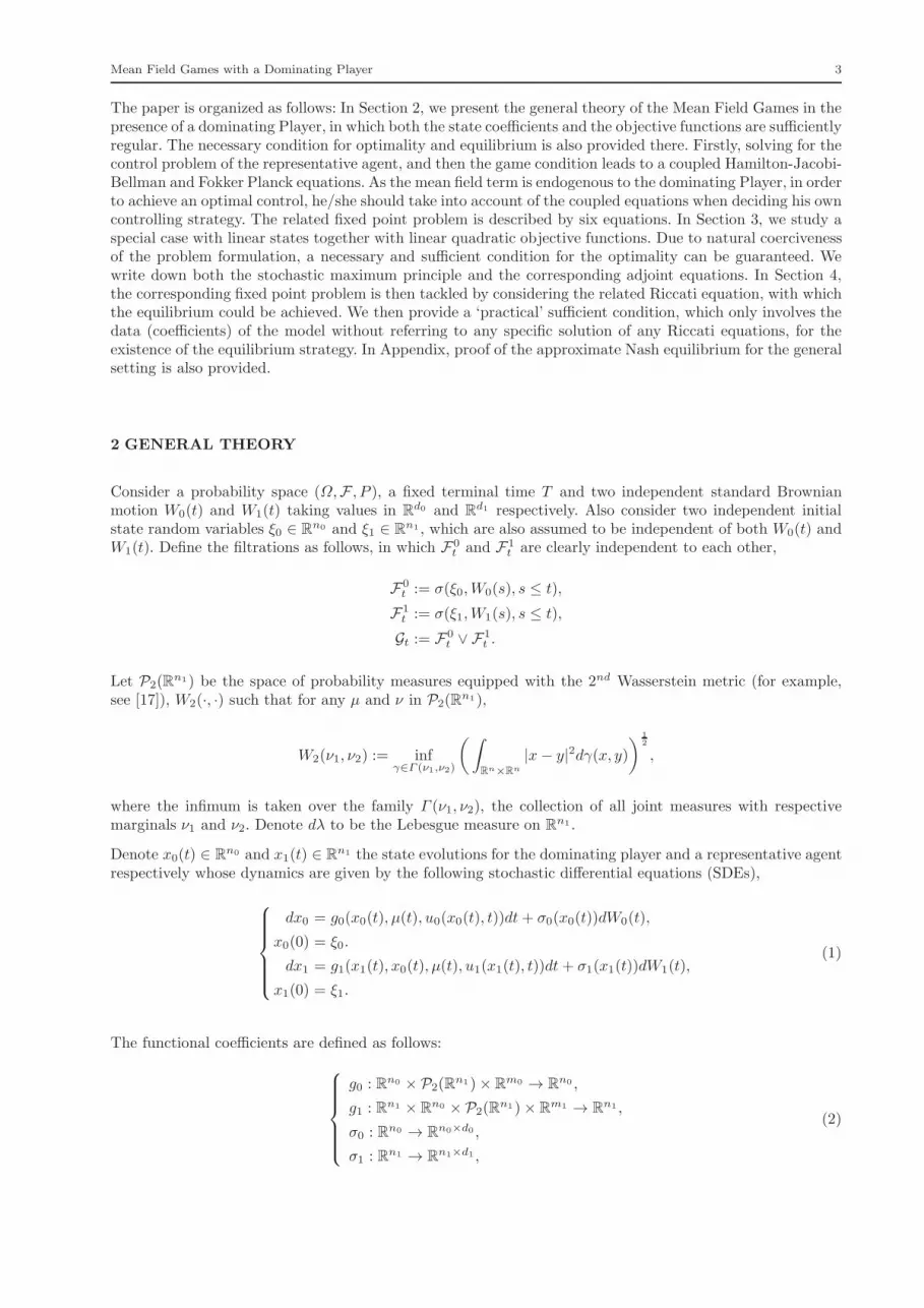
Denote x0(t) ∈ Rn0 and x1(t) ∈ R

n1 the state evolutions for the dominating player and a representative agentrespectively whose dynamics are given by the following stochastic differential equations (SDEs),

dx0 = g0(x0(t), µ(t), u0(x0(t), t))dt+ σ0(x0(t))dW0(t),

x0(0) = ξ0.

dx1 = g1(x1(t), x0(t), µ(t), u1(x1(t), t))dt+ σ1(x1(t))dW1(t),

x1(0) = ξ1.

(1)

The functional coefficients are defined as follows:

g0 : Rn0 × P2(Rn1)× R

m0 → Rn0 ,

g1 : Rn1 × Rn0 × P2(R

n1)× Rm1 → R

n1 ,

σ0 : Rn0 → Rn0×d0 ,

σ1 : Rn1 → Rn1×d1 ,

(2)

4 A. Bensoussan, M. H. M. Chau, S. C. P. Yam

with their regularities to be described as below. Denote a1(x) = 12σ1(x)σ

∗1 (x), and define the second order

operator A1 and its adjoint operator A∗1,

A1ϕ(x, t) = −tra1(x)D2ϕ(x, t),

A∗1ϕ(x, t) = −

n∑

i,j=1

∂2

∂xi∂xj(aij1 (x)ϕ(x, t)).

We assume that the eigenvalues for a1 are uniformly bounded away from 0, i.e. the operators A1 and A∗1 are

uniformly elliptic, and hence they are also non-degenerate.

Here u0 ∈ Rm0 and u1 ∈ R

m1 represent the respective Markovian controls of dominating player and represen-tative agent. The controls u0 and u1 are respectively adapted to the filtrations F0

t and Gt. We further assumethat the functional form (being a function of (x1(t), t)) of u1 is adapted to F0

t even though its value evaluatedat x1 would be adapted to Gt instead; loosely speaking the dominating player takes his own privilege of settingup the framework to be followed by the representative agent. We shall then define the classes of admissiblecontrols for the dominating player and the representative agent by A0 and A1 respectively, where Ai is asubset of all Holder continuous processes (with some exponent β > 0) in the family of all F i−progressivelymeasurable processes which are in L2(Ω × [0, T ];Rni), for i = 0, 1.

The mean field term, µ(t) ∈ P2(Rn1), is the probability measure of the state of the representative agent at

time t. Indeed, the dominating player sets rules for representative agent to take into account. One naturalconsideration is that the dominating player is incapable of tracing the state of each individual’s evolution,but only takes account of the overall performance of the community subject to the rules he set, that is hisown flow of information, F0

t . By the same token, each agent cannot fully keep track of any other agents’states and they can only rely on the summarized information of the community provided by the dominatingplayer. Thus it is justifiable to assume that the mean field term, µ(t), is adapted to F0

t . The dominatingplayer can directly influence both the representative agent and the mean field term, thus we consider µ(t) asendogenous in the consideration of optimal behavior of x0(t) rather than as an exogenous variable commonlyfound in the literature such as that of [13].

Under this consideration, we assume the mean field term to be the probability measure of x1(t) given F0t . In

particular, in accordance with the uniform ellipticity of A∗, the mean field term does possess a probabilitydensity function mx0

: Rn1 × [0, T ] → R+ which also fulfills

1. mx0(t)(·, t) ∈ L2(Rn1);2. mx0(t)(·, t)dλ is F0

t -measurable and measure-valued;

for all time 0 < t ≤ T (more explanation will be provided after Equation (7)).

For i ∈ 0, 1, the functional coefficients (2) satisfy the following assumptions

1. gi is a deterministic function, continuously differentiable in xi ∈ Rni and ui ∈ R

mi ; it is also uniformlyLipschitz continuous in ν ∈ P2(R

n1), i.e.

|gi(xi, ν1, ui)− gi(xi, ν2, ui)| ≤ KiW2(ν1, ν2),

for some Ki > 0 independent of the choices of xi and ui. Moreover, for m ∈ L2(Rn1), gi is Gateauxdifferentiable in mdλ ∈ P2(R

n1), i.e.

d

dθ

∣

∣

∣

∣

θ=0

gi(xi, (m+ θm)dλ, ui) =

∫

Rn

∂gi

∂m(xi,mdλ, ui)(ξ)m(ξ)dξ,

for some ∂gi∂m

(xi,mdλ, ui)(·) ∈ L2(Rn1);2. σi is a deterministic continuously differentiable function.

Consider the following real value functions:

f0 : Rn0 × P2(Rn1)× R

m0 → R,

f1 : Rn1 × Rn0 × P2(R

n1)× Rm1 → R,

h0 : Rn0 × P2(Rn1) → R,

h1 : Rn1 × Rn0 × P2(R

n1) → R,

(3)

Mean Field Games with a Dominating Player 5

For i ∈ 0, 1, the functionals (3) satisfy the following assumptions3. fi and hi are deterministic functions, continuously differentiable in xi ∈ R

ni and ui ∈ Rmi and also

uniformly Lipschitz continuous in ν ∈ P2(Rn1) with respect to the 2nd Wasserstein metric, W2. Moreover,

for m ∈ L2(Rn1), fi and hi are Gateaux differentiable in mdλ as defined above;

Define a pair of mutually dependent control problems for the dominating player and the representative agentas below:

Problem 21 Control of Representative AgentGiven the process x0 and an exogenous probability measure-valued process ν, find a control u1 ∈ A1 whichminimizes the cost functional

J1(u1, x0, ν) := E

[

∫ T

0

f1(x1(t), x0(t), ν(t), u1(x1(t), t))dt + h1(x1(T ), x0(T ), ν(T ))

]

. (4)

Problem 22 Game ConditionGiven an exogenous probability measure-valued process ν, let M(ν)(t) be the measure induced by the corre-sponding optimal x1(t) found in Problem 21 conditioning on F0

t . Find the probability measure-valued processµ such that M(µ)(·) = µ(·).

Problem 23 Control of the Dominating PlayerFind a control u0 ∈ A0 which minimizes the cost functional

J0(u0) := E

[

∫ T

0

f0(x0(t), µ(t), u0(x0(t), t))dt+ h0(x0(T ), µ(T ))

]

, (5)

where µ is the solution given in Problem 22.

Remark The setting of our problem is different from those mean field related problems with a major player(not a dominating player) commonly found in the literature, such as that in [13]. Indeed, in [13], the corre-sponding objective functions for the major player and i-th minor player are respectively

J0(u0, z) = E∫ T

0

| x0 −H0z − η |2Q0+u∗0R0u0

dt,

Ji(ui, z) = E∫ T

0

| xi −Hx0 − H0z − η |2Q +u∗Ru

dt,

where the mean field term z is exogenous to both control optimization problems for J0 and Ji. Instead, wehere consider the mean field term ν, as established in Problem 22, as endogenous for the dominating playerin Problem 23. In particular, changes in control u0 would affect and even completely determine the mean fieldterm ν accordingly. Our setting appears to be natural in the economic context related to governance, as thegovernor can sometimes take the initiative to set-up rubrics to be obeyed and followed by citizens; this latternotion is covered in [10].

We first establish the necessary condition of optimality for the representative agent (Problem 21) and thegame condition (Problem 22) by the adjoint equation approach. Let xu1

1 be the solution of the SDE for therepresentative agent with respect to control u1. For any test function f , by Ito’s lemma,

EF

0

t [f(xu1

1 (t))] = EF

0

t

[

f(ξ1) +

∫ t

0

(

∂t + g ·D +A1

)

fds

]

, (6)

Assume the conditional density function pu1(x, t) exists, i.e. EF

0

t [f(xu1

1 (t))] =∫

Rn1f(x)p(x, t)dx. Integration

by parts results in the following Fokker Planck (FP) equation.

∂pu1

∂t= −A∗

1pu1(x, t)− div(g1(x, x0(t), µ(t), u1(x, t))pu1

(x, t)),

pu1(x, 0) = ω(x),

(7)

6 A. Bensoussan, M. H. M. Chau, S. C. P. Yam

where ω(x) is the initial density function of ξ1. By the uniform ellipticity of A∗1, the very existence of the

conditional density function pu1is justified at the first place (see Theorem 2.1 in [16]). By reversing the steps,

the conditional density of xu1

1 given F0t is well defined. After resolving Problem 22, we can guarantee that the

mean field term µ and the conditional probability measure of pu1dλ given F0 coincides, i.e. the conditional

density function, mx0, does exists. For notational simplicity, in the rest of this paper we write µ := mx0

dλ asmx0

in all functional coefficients. Note that mx0(t)(·, t) is Markovian in x0(t) and in L2(Rn1). To simplify, wewrite mx0(t)(·, t) := mx0(t)(t) unless specifically emphasize. Recall that x0(t), the functional form of u1(·, t)and now together with mx0(t)(·, t) are Markovian in x0(t).

We can then rewrite the cost functional (4) for the representative agent as

J1(u1, x0, ν)

=E

[

∫ T

0

EF

0

t f1(x1(t), x0(t), ν(t), u1(x1(t), t))dt+ EF

0

T h1(x1(T ), x0(T ), ν(T ))

]

=E

[

∫ T

0

∫

Rn1

pu1(x, t)f1(x, x0(t), ν(t), u1(x, t))dxdt +

∫

Rn

pu1(x, T )h1(x, x0(T ), ν(T ))dx

]

.

Let χu1(x, t) be a F0

t -measurable Markovian random field satisfying the backward random (not quite stochas-tic) partial differential equation:

−∂χu1

∂t= g1(x, x0(t), ν(t), u1(x, t))Dχu1

(x, t)−A1χu1(x, t)

+f1(x, x0(t), ν(t), u1(x, t)),

χu1(x, T ) = h1(x, x0(T ), ν(T )).

(8)

The existence of χu1is again guaranteed by the non-degeneracy of A1. In accordance with the FP equation

(7), integration by parts gives

0 =

∫ T

0

∫

Rn

(

∂pu1

∂t+ A∗

1pu1(x, t) + div(g1(x, x0(t), ν(t), u1(x, t))pu1

(x, t))

)

χu1(x, t)dxdt

=

∫

Rn

(pu1(x, T )χu1

(x, T )− pu1(x, 0)χu1

(x, 0)) dx

+

∫ T

0

∫

Rn

pu1(x, t)

(

−∂χu1

∂t−Dχu1

(x, t)g1(x, x0(t), ν(t), u1(x, t)) +A1χu1(x, t)

)

dxdt

=

∫

Rn

(pu1(x, T )h1(x, x0(T ), ν(T ))− ω(x)χu1

(x, 0)) dx

+

∫ T

0

∫

Rn

pu1(x, t)f1(x, x0(t), ν(t), u1(x, t))dxdt.

Taking expectation on both sides, we then have the expression of the cost functional,

J1(u1, x0,m) =

∫

Rn

ω(x)E[χu1(x, 0)]dx

: =

∫

Rn

ω(x)E[Ψu1(x, 0)]dx,

(9)

where Ψu1(x, t) := E

F0

t χu1(x, t). By further taking conditional expectations given F0

t on both sides of (8), weobtain

−EF

0

t∂χu1

∂t= DΨu1

(x, t)g1(x, x0(t), ν(t), u1(x, t))−A1Ψu1(x, t)

+f1(x, x0(t), ν(t), u1(x, t)),

Ψu1(x, T ) = h1(x, x0(T ), ν(T )).

Mean Field Games with a Dominating Player 7

On the other hand, for any τ ≤ t,

EF

0

τ

(

Ψu1(x, t) −

∫ t

0

EF

0

s∂χu1

∂s(x, s)ds

)

=EF

0

τ

(

χu1(x, t) −

∫ t

τ

∂χu1

∂s(x, s)ds

)

−

∫ τ

0

EF

0

s∂χu1

∂s(x, s)ds

=Ψu1(x, τ) −

∫ τ

0

EF

0

s∂χu1

∂s(x, s)ds,

where second equality results from an application of the fundamental theorem of calculus, that∫ t

τ

∂χu1

∂s(x, s)ds =

χu1(x, t)− χu1

(x, τ). Therefore, we deduce that

Ψu1(x, t)−

∫ t

0

EF

0

s∂χu1

∂s(x, s)ds (10)

is a F0−martingale. By Martingale Representation Theorem, there uniquely exists a F0 adapted function,Ku1

, such that

Ψu1(x, t)−

∫ t

0

EF

0

s∂χu1

∂s(x, s)ds = Ψu1

(x, 0) +

∫ t

0

Ku1(x, s)dW0(s).

In particular, Ψu1(x, t) satisfies the following backward stochastic partial differential equation (BSPDE):

−∂tΨu1= f1(x, x0(t), ν(t), u1(x, t)) +DΨu1

(x, t)g1(x, x0(t), ν(t), u1(x, t))

−A1Ψu1(x, t)dt−Ku1

(x, t)dW0(t),

Ψu1(x, T ) = h1(x, x0(T ), ν(T )).

(11)

This BSPDE will be used to derive the following Stochastic Hamilton-Jacobi-Bellman Equation (SHJB), see[15]. Here ∗ stands for the transpose of the corresponding matrix.

Lemma 24 (Necessary condition for Problem 21)Given x0 and ν as in Problem 21, the control u1 ∈ A1 is optimal only if it satisfies the following SHJB:

−∂tΨ = (H1(x, x0(t), ν(t), DΨ(x, t)) −A1Ψ(x, t))dt −K(x, t)dW0(t),

Ψ(x, T ) = h1(x, x0(T ), ν(T )),(12)

where

H1(x, x0, ν, q) = infu1

L(x, x0, ν, u1, q),

L(x, x0, ν, u1, q) = f1(x, x0, ν, u1) + qg1(x, x0, ν, u1).

and the infimum is uniquely attained at u1, i.e. H1(x, x0, ν, q) = L(x, x0, ν, u1, q).

Remark As in the work [6], convenient assumptions on f1 and g1 which ensure the unique existence of theminimizer u1 = argminL(x, x0, ν, u1, q) are their convexity and coerciveness in u1, namely: the convexity ofg1 in u1 means that g1(·, u

′1) ≥ g1(·, u1) + g∗1,u1

(·, u1)(u′1 − u1) + K1|u

′1 − u1|

2, where the inequality sign isunderstood in the component-wise sense; while the coerciveness of g1 in u1 refers to that |g1(·, u1)| → ∞ as|u1| → ∞. Similar conditions are assumed for f1.

Proof To express a necessary condition for optimality, we equate the Gateaux derivative of the expression(9) with zero; for any u1 ∈ A1,

0 =d

dθ

∣

∣

∣

∣

θ=0

J1(u1 + θu1, x0, ν) =

∫

Rn

ω(x)EΨ (x, 0)dx,

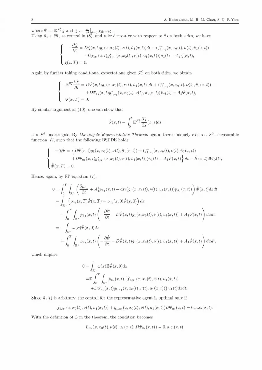
8 A. Bensoussan, M. H. M. Chau, S. C. P. Yam

where Ψ := EF

0

t χ and χ := ddθ

∣

∣

θ=0χu1+θu1

.Using u1 + θu1 as control in (8), and take derivative with respect to θ on both sides, we have

−∂χ

∂t= Dχ(x, t)g1(x, x0(t), ν(t), u1(x, t))dt + (f∗

1,u1(x, x0(t), ν(t), u1(x, t))

+Dχu1(x, t)g∗1,u1

(x, x0(t), ν(t), u1(x, t)))u1(t)−A1χ(x, t),

χ(x, T ) = 0;

Again by further taking conditional expectations given F0t on both sides, we obtain

−EF

0

t∂χ

∂t= DΨ(x, t)g1(x, x0(t), ν(t), u1(x, t))dt + (f∗

1,u1(x, x0(t), ν(t), u1(x, t))

+DΨu1(x, t)g∗1,u1

(x, x0(t), ν(t), u1(x, t)))u1(t)−A1Ψ(x, t),

Ψ(x, T ) = 0.

By similar argument as (10), one can show that

Ψ(x, t)−

∫ t

0

EF

0

s∂χ

∂s(x, s)ds

is a F0−martingale. By Martingale Representation Theorem again, there uniquely exists a F0−measurablefunction, K, such that the following BSPDE holds:

−∂tΨ =

DΨ(x, t)g1(x, x0(t), ν(t), u1(x, t)) + (f∗1,u1

(x, x0(t), ν(t), u1(x, t))

+DΨu1(x, t)g∗1,u1

(x, x0(t), ν(t), u1(x, t)))u1(t)−A1Ψ(x, t)

dt− K(x, t)dW0(t),

Ψ(x, T ) = 0.

Hence, again, by FP equation (7),

0 =

∫ T

0

∫

Rn

(

∂pu1

∂t+A∗

1pu1(x, t) + div(g1(x, x0(t), ν(t), u1(x, t))pu1

(x, t))

)

Ψ(x, t)dxdt

=

∫

Rn

(

pu1(x, T )Ψ(x, T )− pu1

(x, 0)Ψ(x, 0))

dx

+

∫ T

0

∫

Rn

pu1(x, t)

(

−∂Ψ

∂t−DΨ(x, t)g1(x, x0(t), ν(t), u1(x, t)) +A1Ψ(x, t)

)

dxdt

=−

∫

Rn

ω(x)Ψ(x, 0)dx

+

∫ T

0

∫

Rn

pu1(x, t)

(

−∂Ψ

∂t−DΨ(x, t)g1(x, x0(t), ν(t), u1(x, t)) +A1Ψ(x, t)

)

dxdt,

which implies

0 =

∫

Rn

ω(x)EΨ (x, 0)dx

=E

∫ T

0

∫

Rn

pu1(x, t) f1,u1

(x, x0(t), ν(t), u1(x, t))

+DΨu1(x, t)g1,u1

(x, x0(t), ν(t), u1(x, t)) u1(t)dxdt.

Since u1(t) is arbitrary, the control for the representative agent is optimal only if

f1,u1(x, x0(t), ν(t), u1(x, t)) + g1,u1

(x, x0(t), ν(t), u1(x, t))DΨu1(x, t) = 0, a.e.(x, t).

With the definition of L in the theorem, the condition becomes

Lu1(x, x0(t), ν(t), u1(x, t), DΨu1

(x, t)) = 0, a.e.(x, t),

Mean Field Games with a Dominating Player 9

which provides a necessary condition for the minimization problem. As the minimizer is assumed to beattained at u1, which depends on x, x0, ν, and DΨu1

, we can rewrite the BSPDE (11), denote Ψu1and Ku1

by Ψ and K for simplicity, we arrive for the SHJB Equation.

−∂tΨ = (infuL(x, x0(t), ν(t), u1(x, t), DΨ(x, t)) −A1Ψ(x, t))dt −K(x, t)dW0(t),

= (H1(x, x0(t), ν(t), DΨ(x, t)) −A1Ψ(x, t))dt −K(x, t)dW0(t)

Ψ(x, T ) = h1(x, x0(T ), ν(T )).

⊓⊔

Replace the arbitrary measure ν by the mean field measure µ. Equating µ := mx0dλ with pu1

dλ, the measureof the optimal state of the representative agent conditioning on F0

t ; the couple (7) and (12) give the followingcorollary.

Corollary 25 (Necessary condition for Problems 21 and 22)The control for the representative agent is optimal and the game condition holds only if the SHJB-FP coupledequations are satisfied

−∂tΨ = (H1(x, x0(t),mx0(t)(t), DΨ(x, t)) −A1Ψ(x, t))dt −K(x, t)dW0(t),

Ψ(x, T ) = h1(x, x0(T ),mx0(T )(T )).∂mx0

∂t= −A∗

1mx0(t)(x, t) − div(G(x, x0(t),mx0(t)(x, t), DΨ(x, t))mx0(t)(x, t)),

mξ0(x, 0) = ω(x),

(13)

where G(x, x0,mx0, q) = g1(x, x0,mx0

, u1(x, x0,mx0, q)).

The SHJB-FP coupled equations (13) allow us to obtain the control of the representative agent in terms ofa given trajectory of the dominating player x0 while the game condition also holds.

We then turn to the optimal problem for the dominating player. As mx0is not external to the dominating

player, the dominating player has to consider both its own dynamic evolution and (13).

Lemma 26 Necessary condition for Problem 23The control for the dominating player u0 is optimal only if

f0(x0,mx0, u0) + p · g0(x0,mx0

, u0) = infu0

f0(x0,mx0, u0) + p · g0(x0,mx0

, u0)

: = H0(x0,mx0, p)

where p(t) satisfies the following adjoint processes

−dp =

[

g∗0,x0(x0(t),mx0(t)(t), u0(t))p(t) + f0,x0

(x0(t),mx0(t)(t), u0(t))

+

∫

Gx0(x, x0(t),mx0(t)(t), DΨ(x, t))Dq(x, t)mx0(t)(x, t)dx

+

∫

r(x, t)Hx0(x, x0(t),mx0(t)(t), DΨ(x, t))dx

]

dt

−∑d0

l=1 ql(t)dW0l +∑d0

l=1 σ∗0l,x0

(x0)ql(t)dt,

p(T ) = h0,x0(x0(T ),mx0

(T )) +

∫

r(x, T )h1,x0(x, x0(T ),mx0(T )(T ))dx;

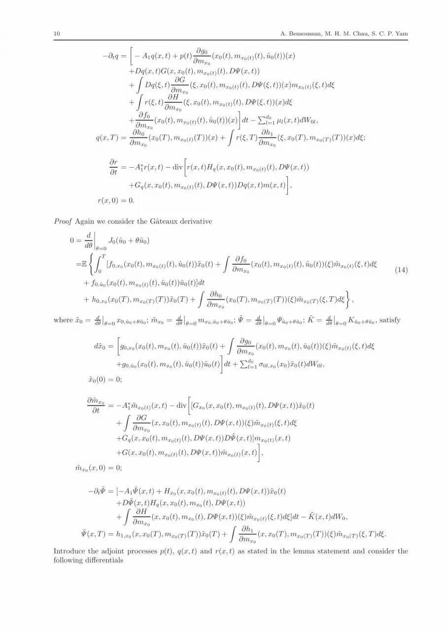
10 A. Bensoussan, M. H. M. Chau, S. C. P. Yam

−∂tq =

[

−A1q(x, t) + p(t)∂g0

∂mx0

(x0(t),mx0(t)(t), u0(t))(x)

+Dq(x, t)G(x, x0(t),mx0(t)(t), DΨ(x, t))

+

∫

Dq(ξ, t)∂G

∂mx0

(ξ, x0(t),mx0(t)(t), DΨ(ξ, t))(x)mx0(t)(ξ, t)dξ

+

∫

r(ξ, t)∂H

∂mx0

(ξ, x0(t),mx0(t)(t), DΨ(ξ, t))(x)dξ

+∂f0

∂mx0

(x0(t),mx0(t)(t), u0(t))(x)

]

dt−∑d0

l=1 µl(x, t)dW0l,

q(x, T ) =∂h0

∂mx0

(x0(T ),mx0(t)(T ))(x) +

∫

r(ξ, T )∂h1

∂mx0

(ξ, x0(T ),mx0(T )(T ))(x)dξ;

∂r

∂t= −A∗

1r(x, t) − div

[

r(x, t)Hq(x, x0(t),mx0(t)(t), DΨ(x, t))

+Gq(x, x0(t),mx0(t)(t), DΨ(x, t))Dq(x, t)m(x, t)

]

,

r(x, 0) = 0.

Proof Again we consider the Gateaux derivative

0 =d

dθ

∣

∣

∣

∣

θ=0

J0(u0 + θu0)

=E

∫ T

0

[f0,x0(x0(t),mx0(t)(t), u0(t))x0(t) +

∫

∂f0

∂mx0

(x0(t),mx0(t)(t), u0(t))(ξ)mx0(t)(ξ, t)dξ

+ f0,u0(x0(t),mx0(t)(t), u0(t))u0(t)]dt

+ h0,x0(x0(T ),mx0(T )(T ))x0(T ) +

∫

∂h0

∂mx0

(x0(T ),mx0(T )(T ))(ξ)mx0(T )(ξ, T )dξ

,

(14)

where x0 = ddθ

∣

∣

θ=0x0,u0+θu0

; mx0= d

dθ

∣

∣

θ=0mx0,u0+θu0

; Ψ = ddθ

∣

∣

θ=0Ψu0+θu0

; K = ddθ

∣

∣

θ=0Ku0+θu0

, satisfy

dx0 =

[

g0,x0(x0(t),mx0

(t), u0(t))x0(t) +

∫

∂g0

∂mx0

(x0(t),mx0(t), u0(t))(ξ)mx0(t)(ξ, t)dξ

+g0,u0(x0(t),mx0

(t), u0(t))u0(t)

]

dt+∑d0

l=1 σ0l,x0(x0)x0(t)dW0l,

x0(0) = 0;

∂mx0

∂t= −A∗

1mx0(t)(x, t)− div

[

[Gx0(x, x0(t),mx0(t)(t), DΨ(x, t))x0(t)

+

∫

∂G

∂mx0

(x, x0(t),mx0(t)(t), DΨ(x, t))(ξ)mx0(t)(ξ, t)dξ

+Gq(x, x0(t),mx0(t)(t), DΨ(x, t))DΨ (x, t)]mx0(t)(x, t)

+G(x, x0(t),mx0(t)(t), DΨ(x, t))mx0(t)(x, t)

]

,

mx0(x, 0) = 0;

−∂tΨ = [−A1Ψ(x, t) +Hx0(x, x0(t),mx0(t)(t), DΨ(x, t))x0(t)

+DΨ(x, t)Hq(x, x0(t),mx0(t), DΨ(x, t))

+

∫

∂H

∂mx0

(x, x0(t),mx0(t), DΨ(x, t))(ξ)mx0(t)(ξ, t)dξ]dt − K(x, t)dW0,

Ψ(x, T ) = h1,x0(x, x0(T ),mx0(T )(T ))x0(T ) +

∫

∂h1

∂mx0

(x, x0(T ),mx0(T )(T ))(ξ)mx0(T )(ξ, T )dξ.

Introduce the adjoint processes p(t), q(x, t) and r(x, t) as stated in the lemma statement and consider thefollowing differentials

Mean Field Games with a Dominating Player 11

d(p∗x0)

= −x∗0(t)

[

f0,x0(x0(t),mx0(t)(t), u0(t)) +

∫

r(x, t)Hx0(x, x0,mx0

, DΨ)dx

+

∫

Gx0(x, x0(t),mx0(t)(t), DΨ(x, t))Dq(x, t)mx0(t)(x, t)dx

]

dt

+p∗(t)

[ ∫

∂g0

∂mx0

(x0(t),mx0(t)(t), u0(t))(ξ)mx0(t)(ξ, t)dξ

+g0,u0(x0(t),mx0

(t), u0(t))u0(t)

]

dt+ . . . dW0.

d

∫

q(x, t)mx0(x, t)dx

=

∫

q(x, t)

[

− div[

[Gx0(x, x0(t),mx0(t)(t), DΨ(x, t))x0

+Gq(x, x0(t),mx0(t)(t), DΨ(x, t))DΨ ]mx0(t)(x, t)]

]

dxdt

−

∫

[

p(t)∂g0

∂mx0

(x0(t),mx0(t)(t), u0(t))(x) +

∫

r(ξ, t)∂H

∂mx0

(ξ, x0(t),mx0(t)(t), DΨ(ξ, t))(x)dξ

+∂f0

∂mx0

(x0(t),mx0(t)(t), u0(t))(x)]

mx0(t)(x, t)dxdt + . . . dW0.

d

∫

r(x, t)Ψ (x, t)dx

=

∫ [

− div[

Gq(x, x0(t),mx0(t)(t), DΨ(x, t))Dq(x, t)mx0(t)(x, t)]

]

Ψ(x, t)dxdt

−

∫

r(x, t)

[

[Hx0(x, x0(t),mx0(t)(t), DΨ(x, t))x0(t)

+

∫

∂H

∂mx0(t)

(x, x0(t),mx0(t)(t), DΨ(x, t))(ξ)mx0(t)(ξ, t)dξ]dt

]

dxdt + . . . dW0.

Using the results above, we have

d

p∗x0 +

∫

q(x, t)mx0(x, t)dx −

∫

r(x, t)Ψ (x, t)dx

=

[

− x∗0(t)f0,x0(x0(t),mx0(t)(t), u0(t)) + p∗(t)g0,u0

(x0(t),mx0(t)(t), u0(t))u0(t)

−

∫

∂f0

∂mx0

(x0(t),mx0(t)(t), u0(t))(x)mx0(t)(x, t)dx

]

dt+ . . . dW0.

Integrating and taking expectation on both sides gives

E

[

(h0,x0(x0(T ),mx0(T )(T )) +

∫

r(x, T )h1,x0(x, x0(T ),mx0(T )(T ))dx)x0(T )dx

+

∫

[ ∂h0

∂mx0

(x0(T ),mx0(T )(T ))(x) +

∫

r(ξ, T )∂h1

∂mx0

(ξ, x0(T ),mx0(T )(T ))(x)dξ]

mx0(T )(x, T )dx

−

∫

r(x, T )[

h1,x0(x, x0(T ),mx0(T )(T ))x0(T ) +

∫

∂h1

∂mx0

(x, x0(T ),mx0(T )(T ))(ξ)mx0(T )(ξ, T )dξ]

dx

]

= E

∫ T

0

− x∗0(t)f0,x0(x0(t),mx0(t)(t), u0(t)) + p∗(t)g0,u0

(x0(t),mx0(t), u0(t))u0(t)

−

∫

∂f0

∂mx0

(x0(t),mx0(t)(t), u0(t))(x)mx0(t)(x, t)dx

dt.

Finally we consider (14) and obtain

0 = E

∫ T

0

f0,u0(x0,mx0

, u0) + p∗g0,u0(x0,mx0

, u0)

u0dt.

Since u0 is arbitrary, the control is optimal for the dominating player only if

f0,u0(x0,mx0

, u0) + p∗g0,u0(x0,mx0

, u0) = 0, a.e. t.

12 A. Bensoussan, M. H. M. Chau, S. C. P. Yam

Again, we are considering a minimization problem with the first order condition given above. Since the uniqueexistence of a minimizer, u0 is assumed, we conclude that u0 satisfies the infimum

f0(x0,mx0, u0) + p · g0(x0,mx0

, u0) = infu0

f0(x0,mx0, u0) + p · g0(x0,mx0

, u0)

.

⊓⊔

Let G0(x,mx0, p) = g0(x0,mx0

, u0(x0,mx0, p)). We then conclude the main result in this section.

Theorem 27 The necessary condition for Problems 21, 22 and 23 is provided by the following six equations

−∂tΨ = (H(x, x0(t),mx0(t)(t), DΨ(x, t)) −A1Ψ(x, t))dt −Ku0(x0(t),mx0(t),p(t))(x, t)dW0(t),

Ψ(x, T ) = h1(x, x0(T ),mx0(T )(T )).

∂mx0

∂t= −A∗

1mx0(t)(x, t)− div(G(x, x0(t),mx0(t)(t), DΨ(x, t))mx0(t)(x, t)),

mξ0(x, 0) = ω(x).

dx0 = g0(x0(t),mx0(t)(t), u0(x0(t),mx0(t), p(t)))dt + σ0(x0(t))dW0(t),

x0(0) = ξ0.

−dp =

[

H0,x0(x0(t),mx0(t)(t), p(t)) +

∫

r(x, t)Hx0(x, x0(t),mx0(t)(t), DΨ(x, t))dx

+

∫

Gx0(x, x0(t),mx0(t)(t), DΨ(x, t))Dq

∗(x, t)mx0(t)(x, t)dx

]

dt

−∑k0

l=1 qldW0l +∑k0

l=1 σ∗0l,x0

(x0(t))qldt,

p(T ) = h0,x0(x0(T ),mx0(T )(T )) +

∫

r(x, T )h1,x0(x, x0(T ),mx0(T )(T ))dx.

−∂tq =

[

−A1q(x, t) +∂H0

∂mx0

(x0(t),mx0(t)(t), p(t))(x)

+Dq(x, t)G(x, x0(t),mx0(t)(t), DΨ(x, t))

+

∫

Dq(ξ, t)∂G

∂mx0

(ξ, x0(t),mx0(t)(t), DΨ(ξ, t))(x)m(ξ, t)dξ

+

∫

r(ξ, t)∂H

∂mx0

(ξ, x0(t),mx0(t)(t), DΨ(ξ, t))(x)dξ

]

dt−

k0∑

l=1

µl(x, t)dW0l(t),

q(x, T ) =∂h0

∂mx0

(x0(T ),mx0(T )(T ))(x) +

∫

r(ξ, T )∂h1

∂mx0

(ξ, x0(T ),mx0(T )(T ))(x).

∂r

∂t= −A∗

1r(x, t) − div

[

r(x, t)Hq(x, x0(t),mx0(t)(t), DΨ(x, t))

+Gq(x, x0(t),mx0(t)(t), DΨ(x, t))Dq∗(x, t)mx0(t)(x, t)

]

,

r(x, 0) = 0.

3 Linear Quadratic Case

In this section we present a special case of the problem in the Linear Quadratic setting in which both necessaryand sufficient condition could be established. Suppose that the state evolutions of the processes x0(t), x1(t)

Mean Field Games with a Dominating Player 13

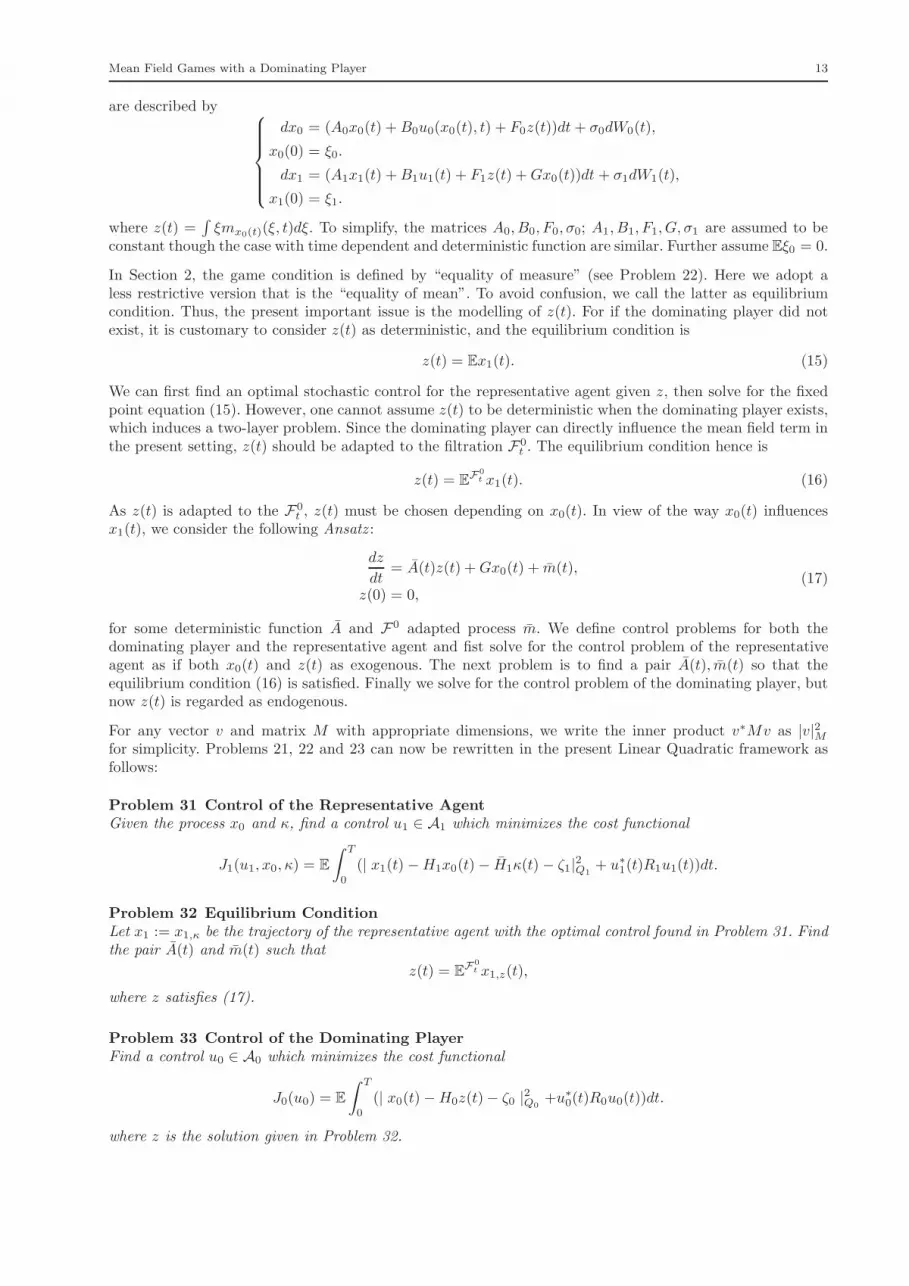
are described by

dx0 = (A0x0(t) +B0u0(x0(t), t) + F0z(t))dt+ σ0dW0(t),

x0(0) = ξ0.

dx1 = (A1x1(t) +B1u1(t) + F1z(t) +Gx0(t))dt + σ1dW1(t),

x1(0) = ξ1.

where z(t) =∫

ξmx0(t)(ξ, t)dξ. To simplify, the matrices A0, B0, F0, σ0; A1, B1, F1, G, σ1 are assumed to beconstant though the case with time dependent and deterministic function are similar. Further assume Eξ0 = 0.

In Section 2, the game condition is defined by “equality of measure” (see Problem 22). Here we adopt aless restrictive version that is the “equality of mean”. To avoid confusion, we call the latter as equilibriumcondition. Thus, the present important issue is the modelling of z(t). For if the dominating player did notexist, it is customary to consider z(t) as deterministic, and the equilibrium condition is

z(t) = Ex1(t). (15)

We can first find an optimal stochastic control for the representative agent given z, then solve for the fixedpoint equation (15). However, one cannot assume z(t) to be deterministic when the dominating player exists,which induces a two-layer problem. Since the dominating player can directly influence the mean field term inthe present setting, z(t) should be adapted to the filtration F0

t . The equilibrium condition hence is

z(t) = EF

0

t x1(t). (16)

As z(t) is adapted to the F0t , z(t) must be chosen depending on x0(t). In view of the way x0(t) influences

x1(t), we consider the following Ansatz :

dz

dt= A(t)z(t) +Gx0(t) + m(t),

z(0) = 0,(17)

for some deterministic function A and F0 adapted process m. We define control problems for both thedominating player and the representative agent and fist solve for the control problem of the representativeagent as if both x0(t) and z(t) as exogenous. The next problem is to find a pair A(t), m(t) so that theequilibrium condition (16) is satisfied. Finally we solve for the control problem of the dominating player, butnow z(t) is regarded as endogenous.

For any vector v and matrix M with appropriate dimensions, we write the inner product v∗Mv as |v|2Mfor simplicity. Problems 21, 22 and 23 can now be rewritten in the present Linear Quadratic framework asfollows:

Problem 31 Control of the Representative AgentGiven the process x0 and κ, find a control u1 ∈ A1 which minimizes the cost functional

J1(u1, x0, κ) = E

∫ T

0

(| x1(t)−H1x0(t)− H1κ(t)− ζ1|2Q1

+ u∗1(t)R1u1(t))dt.

Problem 32 Equilibrium ConditionLet x1 := x1,κ be the trajectory of the representative agent with the optimal control found in Problem 31. Findthe pair A(t) and m(t) such that

z(t) = EF

0

t x1,z(t),

where z satisfies (17).

Problem 33 Control of the Dominating PlayerFind a control u0 ∈ A0 which minimizes the cost functional

J0(u0) = E

∫ T

0

(| x0(t)−H0z(t)− ζ0 |2Q0+u∗0(t)R0u0(t))dt.

where z is the solution given in Problem 32.

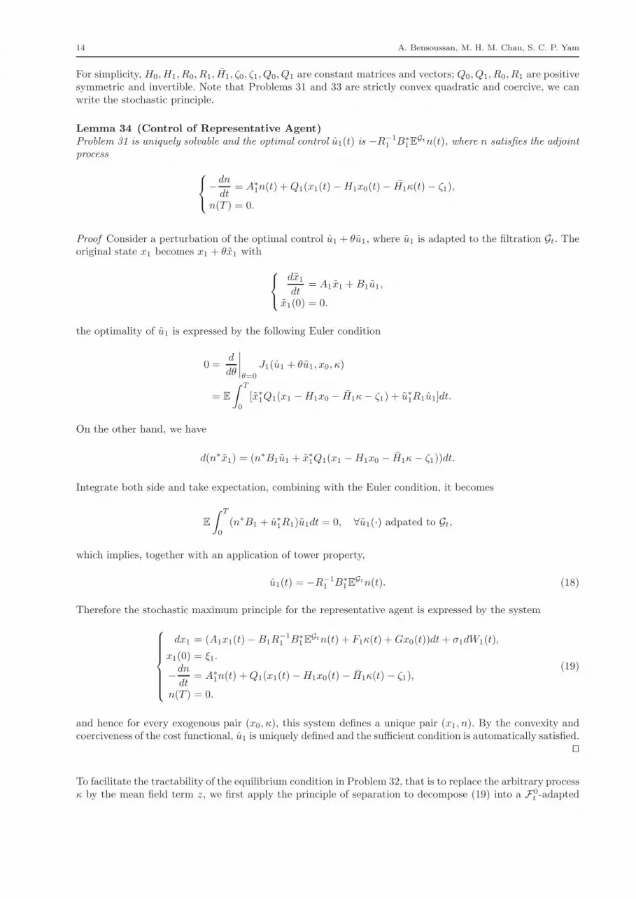
14 A. Bensoussan, M. H. M. Chau, S. C. P. Yam

For simplicity, H0, H1, R0, R1, H1, ζ0, ζ1, Q0, Q1 are constant matrices and vectors; Q0, Q1, R0, R1 are positivesymmetric and invertible. Note that Problems 31 and 33 are strictly convex quadratic and coercive, we canwrite the stochastic principle.

Lemma 34 (Control of Representative Agent)Problem 31 is uniquely solvable and the optimal control u1(t) is −R

−11 B∗

1EGtn(t), where n satisfies the adjoint

process

−dn

dt= A∗

1n(t) +Q1(x1(t)−H1x0(t)− H1κ(t)− ζ1),

n(T ) = 0.

Proof Consider a perturbation of the optimal control u1 + θu1, where u1 is adapted to the filtration Gt. Theoriginal state x1 becomes x1 + θx1 with

dx1

dt= A1x1 +B1u1,

x1(0) = 0.

the optimality of u1 is expressed by the following Euler condition

0 =d

dθ

∣

∣

∣

∣

θ=0

J1(u1 + θu1, x0, κ)

= E

∫ T

0

[x∗1Q1(x1 −H1x0 − H1κ− ζ1) + u∗1R1u1]dt.

On the other hand, we have

d(n∗x1) = (n∗B1u1 + x∗1Q1(x1 −H1x0 − H1κ− ζ1))dt.

Integrate both side and take expectation, combining with the Euler condition, it becomes

E

∫ T

0

(n∗B1 + u∗1R1)u1dt = 0, ∀u1(·) adpated to Gt,

which implies, together with an application of tower property,

u1(t) = −R−11 B∗

1EGtn(t). (18)

Therefore the stochastic maximum principle for the representative agent is expressed by the system

dx1 = (A1x1(t)−B1R−11 B∗

1EGtn(t) + F1κ(t) +Gx0(t))dt+ σ1dW1(t),

x1(0) = ξ1.

−dn

dt= A∗

1n(t) +Q1(x1(t)−H1x0(t)− H1κ(t)− ζ1),

n(T ) = 0.

(19)

and hence for every exogenous pair (x0, κ), this system defines a unique pair (x1, n). By the convexity andcoerciveness of the cost functional, u1 is uniquely defined and the sufficient condition is automatically satisfied.

⊓⊔

To facilitate the tractability of the equilibrium condition in Problem 32, that is to replace the arbitrary processκ by the mean field term z, we first apply the principle of separation to decompose (19) into a F0

t -adapted

Mean Field Games with a Dominating Player 15

system (x1,0, n0) and a F1t -adapted system (x1,1, n1), such that x1 = x1,0 + x1,1 and n = n0 + n1, where

dx1,0(t) = (A1x1,0(t)−B1R−11 B∗

1EF

0

t n0(t) + F1z(t) +Gx0(t))dt,

x1,0(0) = 0.

−dn0

dt= A∗

1n0 +Q1(x1,0(t)−H1x0(t)− H1z(t)− ζ1),

n0(T ) = 0.

dx1,1 = (A1x1,1(t)−B1R−11 B∗

1EF

1

t n1(t))dt+ σ1dW1(t),

x1,1(0) = ξ1.

−dn1

dt= A∗

1n1(t) +Q1x1,1(t),

n1(T ) = 0.

(20)

The existence of the unique solutions of both the FBODE and FBSDE in (20) could be guaranteed in lightof the affine form of the corresponding drivers.

Lemma 35 The conditional expectation of n(t) given Gt can be expressed as:

EGtn(t) = Ptx1(t) + E

F0

t g0(t)

where

Pt + PtA1 +A∗1Pt − PtB1R

−11 B∗

1Pt +Q1 = 0,

PT = 0.

−dg0

dt= (A1 −B1R

−11 B∗

1Pt)∗g0(t)

+(PtG−Q1H1)x0(t) + (PtF1 −Q1H1)z(t)−Q1ζ1,

g0(T ) = 0.

Proof Since Pt always exists as the solution of the symmetric Riccati equation, g0(t) is a well-defined solutionof the first order differential equation as above. We can then define

g1(t) := g0(t) +

∫ T

t

eA∗

1(τ−t)PτB1R

−11 B∗

1(g0(τ) − EF

0

τ g0(τ))dτ.

By using tower property, we deduce that EF0

t g1(t) = EF

0

t g0(t) and

−dg1

dt= A∗

1g1(t)− PtB1R−11 B∗

1EF

0

t g0(t) + (PtG−Q1H1)x0(t) + (PtF1 −Q1H1)z(t)−Q1ζ1,

g1(T ) = 0.

Evaluate the derivative

−d(Ptx1,0 + g1)

dt= PtB1R

−11 B∗

1EF

0

t

(

n0(t)− Ptx1,0(t)− g1(t))

+A∗1(Ptx1,0(t) + g1(t)) +Q1(x1,0(t)−H1x0(t)− H1z(t)− ζ1).

By using the first system in (20), we deduce that

n0 = Px1,0 + g1. (21)

On the other hand, let φ be the fundamental solution to (A1 −B1R−11 B∗

1P ) and define

h(t) :=

∫ T

t

φ∗(τ, t)Pτσ1dW1(τ).

16 A. Bensoussan, M. H. M. Chau, S. C. P. Yam

Further compute the differential

−d(Ptx1,1 + h+

∫ T

t

eA∗

1(τ−t)PτB1R

−11 B∗

1hdτ)

=(

PtB1R−11 B∗

1(Ptx1,1(t)− EF

1

t n1(t))− A∗1Ptx1,1(t) +Q1x1,1(t)

)

dt− Ptσ1dW1(t)

+(A1 −B1R−11 B∗

1Pt)∗h(t)dt+ Ptσ1dW1(t)

+A∗1

(

∫ T

t

eA∗

1(τ−t)PB1R

−11 B∗

1h(τ)dτ)

dt+ PtB1R−11 B∗

1h(t)dt

=(

PtB1R−11 B∗

1(Ptx1,1(t)− EF

1

t n1(t))

+A∗1(Ptx1,1(t) + h(t) +

∫ T

t

eA∗

1(τ−t)PB1R

−11 B∗

1h(τ)dτ) +Q1x1,1(t))

dt.

Since EF1

t (h+

∫ T

t

eA∗

1(τ−t)PτB1R

−11 B∗

1hdτ) = 0 and x1,1 is F1t -adapted, by using the second system in (20),

we similarly deduce that

n1 = Px1,1 + h+

∫ T

t

eA∗

1(τ−t)PB1R

−11 B∗

1hdτ. (22)

Combine (21) and (22),

EGtn(t) = E

F0

t n0(t) + EF

1

t n1(t)

= EF

0

t (Ptx1,0(t) + g1(t)) + Ptx1,1(t)

= Ptx1(t) + EF

0

t g0(t).

⊓⊔

Theorem 36 (Equilibrium Condition)Under the assumed form as in Ansatz (17), the equilibrium condition stated in Problem 33 holds if and onlyif the following conditions are satisfied:

A(t) = A1 −B1R−11 B∗

1Pt + F1,

m(t) = −B1R−11 B∗

1EF

0

t g0(t).

Proof By substituting the decomposition in Lemma 35 in (19), we can rewrite (19)

dx1 =(

(A1 −B1R−11 B∗

1Pt)x1(t)− B1R−11 B∗

1EF

0

t g0(t) + F1z(t) +Gx0(t))

dt+ σ1dW1(t),

x1(0) = ξ1.

−dg0

dt= (A1 −B1R

−11 B∗

1Pt)∗g0(t) + (PtG−Q1H1)x0(t) + (PtF1 −Q1H1)z(t)−Q1ζ1,

g0(T ) = 0.

Thus we have

d

dtEF

0

t x1(t) = (A1 −B1R−11 B∗

1Pt)EF

0

t x1(t)−BR−1B∗EF

0

t g0(t) + F1z(t) +Gx0(t),

EF

0

0x1(0) = 0.

Comparing the coefficients of the last equation with (17) with that of the Ansatz (17), the equilibrium

condition EF

0

t x1(t) = z(t) holds if and only if

A(t) = A1 −B1R−11 B∗

1Pt + F1, m(t) = −B1R−11 B∗

1EF

0

t g0(t).

⊓⊔

We next proceed on the problem of the dominating player.

Mean Field Games with a Dominating Player 17

Lemma 37 (Control of the Dominating Player)

Problem 33 is uniquely solvable and the optimal control u0(t) is −R−10 B∗

0EF

0

t p(t), where the adjoint processesp, q and r satisfy

−dp

dt= A∗

0p(t) +G∗q(t) + (PtG−Q1H1)∗r(t) +Q0(x0(t)−H0z(t)− ζ0),

p(T ) = 0.

−dq

dt= A∗(t)q(t) + F ∗

0 p(t) + (PtF1 −Q1H1)∗r(t) −H∗

0Q0(x0(t)−H0z(t)− ζ0),

q(T ) = 0.dr

dt= A(t)r(t) −B1R

−11 B∗

1EF

0

t q(t)

r(0) = 0.

Here A and m are defined as in Theorem 36.

Proof Consider u0 + θu0 the perturbation of the optimal control, where u0 is adapted to the filtration F0t .

The original states x0, z, g0 become x0 + θx0, z + θz, g + θg0 with

dx0

dt= A0x0(t) +B0u0(t) + F0z(t),

x(0) = 0.dz

dt= A(t)z(t) +Gx0(t)−B1R

−11 B∗

1EF

0

t g0(t),

z(0) = 0.

−dg0

dt= (A1 −B1R

−11 B∗

1Pt)∗g0(t) + (PtG−Q1H1)x0(t) + (PtF1 −Q1H1)z(t)

g0(T ) = 0.

The corresponding maximum principle for u0 is

0 =d

dθ

∣

∣

∣

∣

θ=0

J0(u0 + θu0)

= E

∫ ∗

0

[(x0 −H0z − ζ0)∗Q0(x0 −H0z) + u∗0R0u0]dt.

(23)

On the other hand, we have

d(p∗x0 + q∗z − r∗g0) = (p∗B0u0 − (x0 −H0z − ζ0)∗Q0(x0 −H0z))dt.

Integrating and also taking expectation on both sides of the last equation, together with an application of(23), we deduce that

E

∫ T

0

(p∗B0 + u∗0R0)u0dt = 0, ∀u0 adapted to F0t ,

which implies the desired result by again the application of tower property,

u0(t) = −R−10 B∗

0EF

0

t p(t). (24)

⊓⊔

Summarizing the results we obtained so far, we present the main theorem in this section.

18 A. Bensoussan, M. H. M. Chau, S. C. P. Yam

Theorem 38 Under the form of Ansatz (17), the necessary and sufficient conditions for the unique existenceof the solution to Problems 31, 32 and 33 are described by the following six equations, in which m(t) =

−B1R−11 B∗

1EF

0

t g0(t):

−dg0

dt= (A1 −B1R

−11 B∗

1Pt)∗g0(t) + (PtG−Q1H1)x0(t) + (PtF1 −Q1H1)z(t)−Q1ζ1,

g0(T ) = 0.

dz

dt= (A1 −B1R

−11 B∗

1Pt + F1)z(t) +Gx0(t) + m(t),

z(0) = 0.

dx0 = (A0x0(t)−B0R−10 B∗

0EF

0

t p(t) + F0z(t))dt+ σ0dW0(t),

x0(0) = ξ0.

−dp

dt= A∗

0p(t) +G∗q(t) + (PtG−Q1H1)∗r(t) +Q0(x0(t)−H0z(t)− ζ0),

p(T ) = 0.

−dq

dt= (A1 −B1R

−11 B∗

1Pt + F1)∗q(t) + F ∗

0 p(t) + (PtF1 −Q1H1)∗r(t)

−H∗0Q0(x0(t)−H0z(t)− ζ0),

q(T ) = 0.

dr

dt= (A1 −B1R

−11 B∗

1Pt)r(t) −B1R−11 B∗

1EF

0

t q(t),

r(0) = 0.

(25)

Remark One can easily compare these six equations with those stated in Theorem 27. We obtain the sameresults by applying the general theory, however, it is more convenient to acquire these six equations directlyunder the Linear Quadratic setting, which also illuminates the power of using the principle of separation. Oncomparison with the intermediary result obtained in [14]. The latter work did not take account of the thirdadjoint equation r since it fails to consider the impact on g0 with respect to the change of the control of thedominating player.

4 Fixed Point Problem

In this section, we provide a sufficient condition, which solely depends on the coefficients of the mean fieldgame system, for the unique existence of the solution to Problems 31, 32 and 33 by means of tackling aRiccati equation. From the equilibrium condition z(t) = E

F0

t x1(t), taking the conditional expectation of bothsides in (19) yields:

dz

dt= (A1 + F1)z(t)−B1R

−11 B∗

1EF

0

t n(t) +Gx0(t),

z(0) = 0.

−dn

dt= A∗

1n(t) +Q1(I − H1)z(t)−Q1H1x0(t)−Q1ζ1,

n(T ) = 0.

We also have the SDE for the state of the dominating player

dx0 = (A0x0(t)− B0R−10 B∗

0EF

0

t p(t) + F0z(t))dt+ σ0dW0(t),

x0(0) = ξ0,

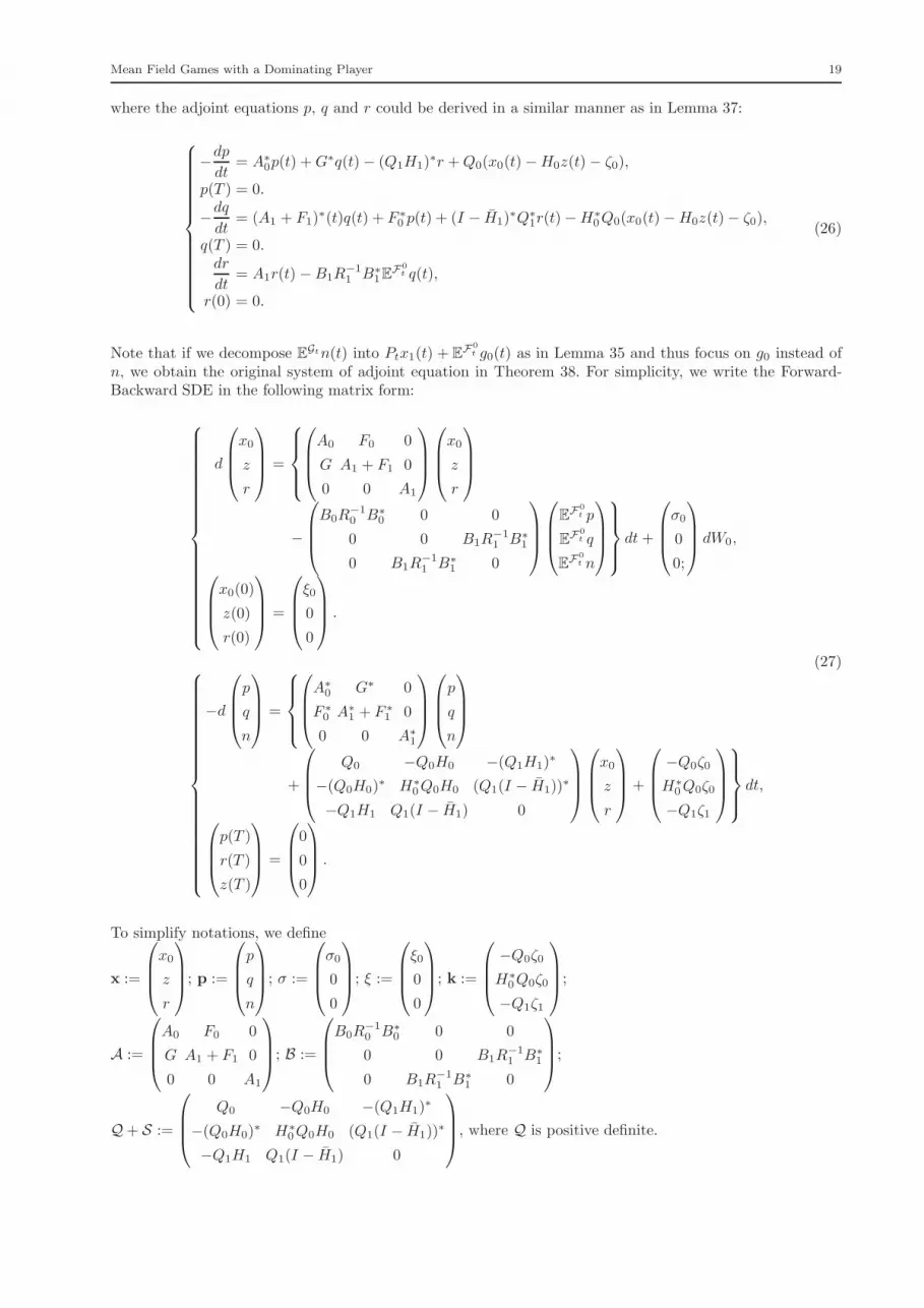
Mean Field Games with a Dominating Player 19

where the adjoint equations p, q and r could be derived in a similar manner as in Lemma 37:

−dp

dt= A∗

0p(t) +G∗q(t)− (Q1H1)∗r +Q0(x0(t)−H0z(t)− ζ0),

p(T ) = 0.

−dq

dt= (A1 + F1)

∗(t)q(t) + F ∗0 p(t) + (I − H1)

∗Q∗1r(t)−H∗

0Q0(x0(t)−H0z(t)− ζ0),

q(T ) = 0.dr

dt= A1r(t) −B1R

−11 B∗

1EF

0

t q(t),

r(0) = 0.

(26)

Note that if we decompose EGtn(t) into Ptx1(t) + E

F0

t g0(t) as in Lemma 35 and thus focus on g0 instead ofn, we obtain the original system of adjoint equation in Theorem 38. For simplicity, we write the Forward-Backward SDE in the following matrix form:

d

x0

z

r

=

A0 F0 0

G A1 + F1 0

0 0 A1

x0

z

r

−

B0R−10 B∗

0 0 0

0 0 B1R−11 B∗

1

0 B1R−11 B∗

1 0

EF

0

t p

EF

0

t q

EF

0

t n

dt+

σ0

0

0;

dW0,

x0(0)

z(0)

r(0)

=

ξ0

0

0

.

−d

p

q

n

=

A∗0 G∗ 0

F ∗0 A∗

1 + F ∗1 0

0 0 A∗1

p

q

n

+

Q0 −Q0H0 −(Q1H1)∗

−(Q0H0)∗ H∗

0Q0H0 (Q1(I − H1))∗

−Q1H1 Q1(I − H1) 0

x0

z

r

+

−Q0ζ0

H∗0Q0ζ0

−Q1ζ1

dt,

p(T )

r(T )

z(T )

=

0

0

0

.

(27)

To simplify notations, we define

x :=

x0

z

r

; p :=

p

q

n

; σ :=

σ0

0

0

; ξ :=

ξ0

0

0

; k :=

−Q0ζ0

H∗0Q0ζ0

−Q1ζ1

;

A :=

A0 F0 0

G A1 + F1 0

0 0 A1

; B :=

B0R−10 B∗

0 0 0

0 0 B1R−11 B∗

1

0 B1R−11 B∗

1 0

;

Q+ S :=

Q0 −Q0H0 −(Q1H1)∗

−(Q0H0)∗ H∗

0Q0H0 (Q1(I − H1))∗

−Q1H1 Q1(I − H1) 0

, where Q is positive definite.

20 A. Bensoussan, M. H. M. Chau, S. C. P. Yam

The system (27) becomes

dx = (Ax − BEF0

t p)dt+ σdW0,

x(0) = ξ.

−dp = (A∗p+ (Q+ S)x + k)dt,

p(T ) = 0.

(28)

Consider the following Riccati equation and backward ODE:

dΓ

dt+A∗Γ + ΓA− ΓBΓ + (Q+ S) = 0,

Γ (T ) = 0.

−dg

dt= (A∗ − ΓB)g+ k,

g(T ) = 0.

(29)

With respect to the affine form of EF0

t p(t) = Γtx(t)+ g(t), the equation (28) admits a unique solution if andonly if (29) admits a unique solution. In accordance with Theorem 2.4.3 in Ma and Young [18] or [1], we havethe following proposition.

Proposition 41 Suppose the following forward-backward ordinary differential equations

dχ

dt= Aχ− Bψ

χ(0) = 0.

−dψ

dt= A∗ψ + (Q+ S)χ,

ψ(T ) = 0.

admits a unique solution for any t0 ∈ [0, T ]. Then there is a unique solution of (29).

Define L2Q([0, T ];R

n0+n1+n1) to be the Hilbert space endowed with the inner product.

〈χ, ψ〉Q :=

∫ T

0

χ∗sQψsds.

Finally, we give the sufficient condition that the six equations in (27) admits a unique solution in the followingtheorem:

Theorem 42 Suppose that‖Q− 1

2SQ− 1

2 ‖ < 1,

where ‖ · ‖ stands for usual Euclidean norm. Then there exists a unique solution of equation (27), and hencea unique equilibrium exists.

Proof For a given function η ∈ L2Q([0, T ];R

n0+n1+n1), the forward-backward ordinary differential equation

dχ

dt= Aχ− Bψ

χ(0) = 0.

−dψ

dt= A∗ψ +Qχ+ Sη,

ψ(T ) = 0.

corresponds to a well-defined linear control problem since B and Q are positive definite. Hence the pair (χ, ψ)always exists. It suffices to show that the affine function η 7→ χ mapping L2

Q([0, T ];Rn0+n1+n1) into itself is

a contraction. Consider the differential

d(χ∗ψ) = (−ψ∗Bψ − χ∗Qχ− χ∗Sη)dt,

Mean Field Games with a Dominating Player 21

which implies that

‖χ‖2Q =

∫ T

0

(

− ψ∗sBψs − χ∗

sSηs

)

ds

≤ −

∫ T

0

χ∗sSηsds.

By Cauchy-Schwarz inequality, we have

‖χ‖2Q ≤ −

∫ T

0

χ∗sSηsds.

≤ ‖χ‖Q · ‖Q− 1

2SQ− 1

2 ‖ · ‖η‖Q

(30)

which shows that η 7→ χ is a contraction if

‖Q− 1

2SQ− 1

2 ‖ < 1.

Note that this condition does not depend on T . ⊓⊔

5 Conclusion

In this paper, by adopting adjoint equation approach, we provide the general theory and discuss the necessarycondition for optimal controls for both the dominating player and the representative agent, and study thecorresponding fixed point problem in relation to the game condition. A convenient necessary and sufficientcondition has been provided under the Linear Quadratic setting; in particular, a illuminative sufficient con-dition, which only involves the coefficient of the mean field game system, for the unique existence of theequilibrium control has been given. Finally, proof of the convergence result of finite player game to meanfield counterpart is provided in Appendix. Applications of the present model in connection with central banklending and systematic risk in financial context will be provided in the future work.

6 Acknowledgments

The first author-Alain Bensoussan acknowledges the financial support of the Hong Kong RGC GRF 500113.The second author-Michael Chau acknowledges the financial support from the Chinese University of HongKong, and the present work constitutes a part of his work for his postgraduate dissertation. The third author-Phillip Yam acknowledges the financial support from The Hong Kong RGC GRF 404012 with the projecttitle: Advanced Topics In Multivariate Risk Management In Finance And Insurance, The Chinese Universityof Hong Kong Direct Grants 2010/2011 Project ID: 2060422 and 2011/2012 Project ID: 2060444. PhillipYam also expresses his sincere gratitude to the hospitality of both Hausdorff Center for Mathematics andHausdorff Research Institute for Mathematics of the University of Bonn during the preparation of the presentwork.

A Appendix

A.1 ǫ-Nash Equilibrium

We now establish that the solutions of Problems 21 and 22 is an ǫ-Nash Equilibrium. Suppose that there are N representativeagents behaving in similar manner, so that the state of the i-th agent, yi, satisfies the following SDE:

dyi = g1

yi(t), x0(t),1

N − 1

N∑

j=1,j 6=i

δyj(t), ui(t)

dt + σ1(yi(t))dW i,

yi(0) = ξ1,i;

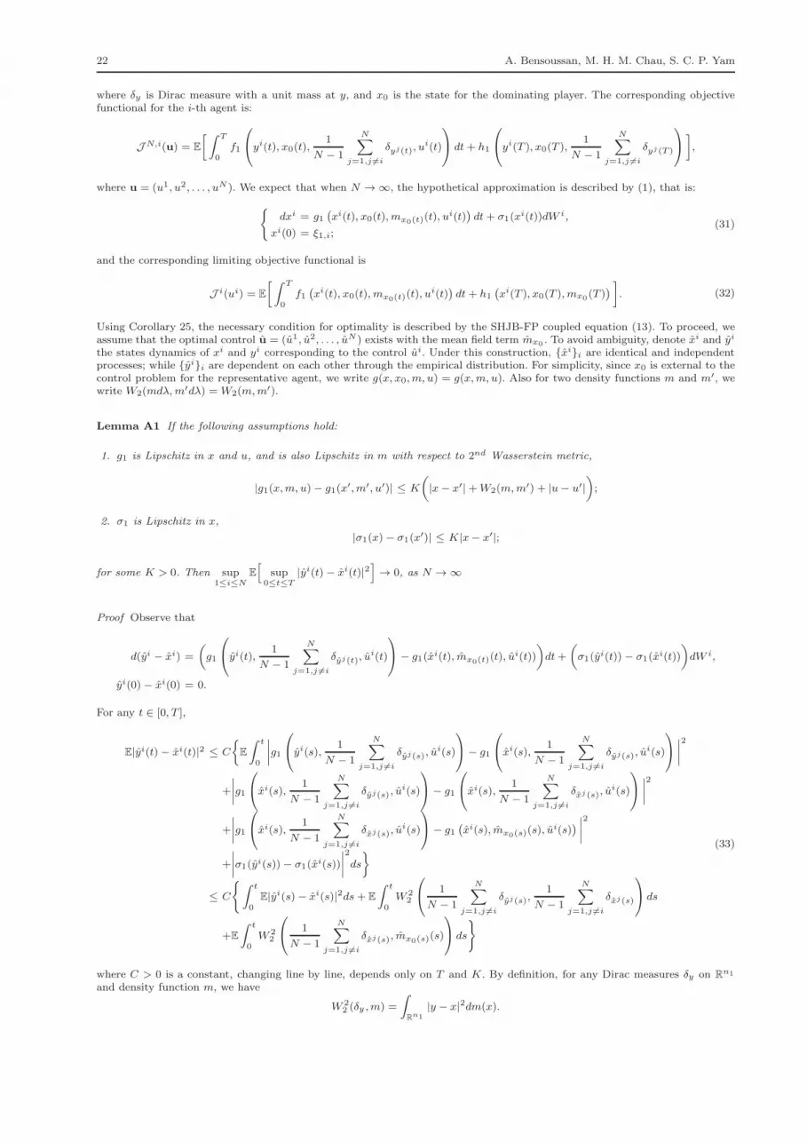
22 A. Bensoussan, M. H. M. Chau, S. C. P. Yam

where δy is Dirac measure with a unit mass at y, and x0 is the state for the dominating player. The corresponding objectivefunctional for the i-th agent is:

JN,i(u) = E

[ ∫ T

0f1

yi(t), x0(t),1

N − 1

N∑

j=1,j 6=i

δyj(t), ui(t)

dt+ h1

yi(T ), x0(T ),1

N − 1

N∑

j=1,j 6=i

δyj(T )

]

,

where u = (u1, u2, . . . , uN ). We expect that when N → ∞, the hypothetical approximation is described by (1), that is:

dxi = g1(

xi(t), x0(t), mx0(t)(t), ui(t))

dt+ σ1(xi(t))dW i,

xi(0) = ξ1,i;(31)

and the corresponding limiting objective functional is

J i(ui) = E

[ ∫ T

0f1(

xi(t), x0(t), mx0(t)(t), ui(t))

dt+ h1(

xi(T ), x0(T ), mx0(T ))

]

. (32)

Using Corollary 25, the necessary condition for optimality is described by the SHJB-FP coupled equation (13). To proceed, weassume that the optimal control u = (u1, u2, . . . , uN ) exists with the mean field term mx0

. To avoid ambiguity, denote xi and yi

the states dynamics of xi and yi corresponding to the control ui. Under this construction, xii are identical and independentprocesses; while yii are dependent on each other through the empirical distribution. For simplicity, since x0 is external to thecontrol problem for the representative agent, we write g(x, x0,m, u) = g(x,m, u). Also for two density functions m and m′, wewrite W2(mdλ,m′dλ) = W2(m,m′).

Lemma A1 If the following assumptions hold:

1. g1 is Lipschitz in x and u, and is also Lipschitz in m with respect to 2nd Wasserstein metric,

|g1(x,m, u)− g1(x′,m′, u′)| ≤ K

(

|x− x′|+W2(m,m′) + |u− u′|)

;

2. σ1 is Lipschitz in x,

|σ1(x)− σ1(x′)| ≤ K|x− x′|;

for some K > 0. Then sup1≤i≤N

E

[

sup0≤t≤T

|yi(t) − xi(t)|2]

→ 0, as N → ∞

Proof Observe that

d(yi − xi) =

(

g1

yi(t),1

N − 1

N∑

j=1,j 6=i

δyj(t), ui(t)

− g1(xi(t), mx0(t)(t), ui(t))

)

dt+

(

σ1(yi(t)) − σ1(xi(t))

)

dW i,

yi(0) − xi(0) = 0.

For any t ∈ [0, T ],

E|yi(t) − xi(t)|2 ≤ C

E

∫ t

0

∣

∣

∣

∣

g1

yi(s),1

N − 1

N∑

j=1,j 6=i

δyj(s), ui(s)

− g1

xi(s),1

N − 1

N∑

j=1,j 6=i

δyj(s), ui(s)

∣

∣

∣

∣

2

+

∣

∣

∣

∣

g1

xi(s),1

N − 1

N∑

j=1,j 6=i

δyj(s), ui(s)

− g1

xi(s),1

N − 1

N∑

j=1,j 6=i

δxj(s), ui(s)

∣

∣

∣

∣

2

+

∣

∣

∣

∣

g1

xi(s),1

N − 1

N∑

j=1,j 6=i

δxj(s), ui(s)

− g1(

xi(s), mx0(s)(s), ui(s)

)

∣

∣

∣

∣

2

+

∣

∣

∣

∣

σ1(yi(s))− σ1(xi(s))

∣

∣

∣

∣

2

ds

≤ C

∫ t

0E|yi(s)− xi(s)|2ds+ E

∫ t

0W 2

2

1

N − 1

N∑

j=1,j 6=i

δyj(s),1

N − 1

N∑

j=1,j 6=i

δxj(s)

ds

+E

∫ t

0W 2

2

1

N − 1

N∑

j=1,j 6=i

δxj(s), mx0(s)(s)

ds

(33)

where C > 0 is a constant, changing line by line, depends only on T and K. By definition, for any Dirac measures δy on Rn1

and density function m, we have

W 22 (δy ,m) =

∫

Rn1

|y − x|2dm(x).

Mean Field Games with a Dominating Player 23

Also observe that the joint measure 1N−1

∑Nj=1,j 6=i δ(yj(s),xj(s)) on R

n1 × Rn1 has respective marginals 1

N−1

∑Nj=1,j 6=i δyj(s)

and 1N−1

∑Nj=1,j 6=i δxj(s) on R

n1 . Using the definition of Wasserstein metric, we evaluate the second term in (38),

E

∫ t

0W 2

2

1

N − 1

N∑

j=1,j 6=i

δyj(s),1

N − 1

N∑

j=1,j 6=i

δxj(s)

ds

≤ E

∫ t

0

∫

Rn1×R

n1

|y − x|2d

1

N − 1

N∑

j=1,j 6=i

δ(yj(s),xj(s))(y, x)

ds

≤ 1

N − 1

N∑

j=1,j 6=i

∫ t

0E|yj(s) − xj(s)|2ds;

further, by symmetry on yj − xjNj=1, we also have

E

∫ t

0W 2

2

1

N − 1

N∑

j=1,j 6=i

δyj(s),1

N − 1

N∑

j=1,j 6=i

δxj(s)

ds ≤∫ t

0E|yi(s)− xi(s)|2ds.

Combining the last inequality with (38), we deduce that

E|yi(t) − xi(t)|2 ≤ C

∫ t

0E|yi(s)− xi(s)|2ds+ E

∫ T

0W 2

2

1

N − 1

N∑

j=1,j 6=i

δxj(s), mx0(s)(s)

ds

By applying Gronwall’s inequality,

E|yi(t) − xi(t)|2 ≤ CeCtE

∫ T

0W 2

2

1

N − 1

N∑

j=1,j 6=i

δxj(s), mx0(s)(s)

ds. (34)

It is clear that xjj are in L2 and i.i.d. with a common conditional density function, mx0, given F0

t . An application of the

Strong Law of Large Number implies that the empirical measure1

N − 1

N∑

j=1,j 6=i

δxj(s) converges almost surely (and hence weakly)

to mx0(s)(s); by the same token, the empirical second moment1

N − 1

N∑

j=1,j 6=i

|xj(s)|2 also converges to the theoretical second

moment E[

∣

∣x1∣

∣

2]

. By the equivalence between of Wasserstein metric and both the weak* convergence in measure and the second

moment convergence, the Wasserstein metric W 22

1

N − 1

N∑

j=1,j 6=i

δxj(s), mx0(s)(s)

converges to 0 almost surely.

Denote the sample mean 1n

∑ni=1 αi by αn. On the other hand,

W 22

1

N − 1

N∑

j=1,j 6=i

δxj(s), mx0(s)(s)

≤ 1

N − 1

N∑

j=1,j 6=i

∫

Rn1

|xj(s)− x|2dmx0(s)(x, s)

≤ 2

(

sup0≤s≤T

|x(s)|2)

N−1

+ sup0≤s≤T

E

[

∣

∣x1(s)∣

∣

2]

(35)

Sine xjj are i.i.d., we have

E

(

sup0≤s≤T

|x(s)|2)

N−1

;

(

sup0≤s≤T

|x(s)|2)

N−1

> c

= E

sup0≤s≤T

|x1(s)|2;

(

sup0≤s≤T

|x(s)|2)

N−1

> c

,

which clearly converges to zero as c → ∞ by an application of Burkholder-Davis-Gundy’s inequality. We conclude that

W 22

1

N − 1

N∑

j=1,j 6=i

δxj(s), mx0(s)(s)

is uniformly integrable, and hence

limN→∞

E

W 22

1

N − 1

N∑

j=1,j 6=i

δxj(s), mx0(s)(s)

= 0.

By using (35) and Dominating Convergence Theorem, we can send N → ∞ in (34) and yields

sup1≤i≤N

E

[

sup0≤t≤T

|yi(t) − xi(t)|2]

→ 0.

⊓⊔

24 A. Bensoussan, M. H. M. Chau, S. C. P. Yam

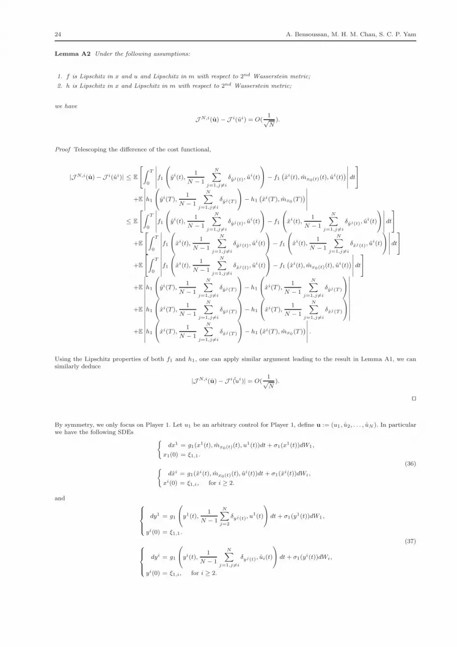
Lemma A2 Under the following assumptions:

1. f is Lipschitz in x and u and Lipschitz in m with respect to 2nd Wasserstein metric;

2. h is Lipschitz in x and Lipschitz in m with respect to 2nd Wasserstein metric;

we have

JN,i(u)−J i(ui) = O(1√N

).

Proof Telescoping the difference of the cost functional,

|JN,i(u)−J i(ui)| ≤ E

∫ T

0

∣

∣

∣

∣

∣

∣

f1

yi(t),1

N − 1

N∑

j=1,j 6=i

δyj(t), ui(t)

− f1(

xi(t), mx0(t)(t), ui(t))

∣

∣

∣

∣

∣

∣

dt

+E

∣

∣

∣

∣

∣

∣

h1

yi(T ),1

N − 1

N∑

j=1,j 6=i

δyj(T )

− h1

(

xi(T ), mx0(T ))

∣

∣

∣

∣

∣

∣

≤ E

∫ T

0

∣

∣

∣

∣

∣

∣

f1

yi(t),1

N − 1

N∑

j=1,j 6=i

δyj(t), ui(t)

− f1

xi(t),1

N − 1

N∑

j=1,j 6=i

δyj(t), ui(t)

∣

∣

∣

∣

∣

∣

dt

+E

∫ T

0

∣

∣

∣

∣

∣

∣

f1

xi(t),1

N − 1

N∑

j=1,j 6=i

δyj(t), ui(t)

− f1

xi(t),1

N − 1

N∑

j=1,j 6=i

δxj(t), ui(t)

∣

∣

∣

∣

∣

∣

dt

+E

∫ T

0

∣

∣

∣

∣

∣

∣

f1

xi(t),1

N − 1

N∑

j=1,j 6=i

δxj(t), ui(t)

− f1(

xi(t), mx0(t)(t), ui(t))

∣

∣

∣

∣

∣

∣

dt

+E

∣

∣

∣

∣

∣

∣

h1

yi(T ),1

N − 1

N∑

j=1,j 6=i

δyj(T )

− h1

xi(T ),1

N − 1

N∑

j=1,j 6=i

δyj(T )

∣

∣

∣

∣

∣

∣

+E

∣

∣

∣

∣

∣

∣

h1

xi(T ),1

N − 1

N∑

j=1,j 6=i

δyj(T )

− h1

xi(T ),1

N − 1

N∑

j=1,j 6=i

δxj(T )

∣

∣

∣

∣

∣

∣

+E

∣

∣

∣

∣

∣

∣

h1

xi(T ),1

N − 1

N∑

j=1,j 6=i

δxj(T )

− h1(

xi(T ), mx0(T ))

∣

∣

∣

∣

∣

∣

.

Using the Lipschitz properties of both f1 and h1, one can apply similar argument leading to the result in Lemma A1, we cansimilarly deduce

|JN,i(u)− J i (ui)| = O(1√N

).

⊓⊔

By symmetry, we only focus on Player 1. Let u1 be an arbitrary control for Player 1, define u := (u1, u2, . . . , uN ). In particularwe have the following SDEs

dx1 = g1(x1(t), mx0(t)(t), u1(t))dt + σ1(x1(t))dW1,

x1(0) = ξ1,1.

dxi = g1(xi(t), mx0(t)(t), ui(t))dt + σ1(xi(t))dWi,

xi(0) = ξ1,i, for i ≥ 2.

(36)

and

dy1 = g1

y1(t),1

N − 1

N∑

j=2

δyj(t), u1(t)

dt + σ1(y1(t))dW1 ,

yi(0) = ξ1,1.

dyi = g1

yi(t),1

N − 1

N∑

j=1,j 6=i

δyj(t), ui(t)

dt+ σ1(yi(t))dWi,

yi(0) = ξ1,i, for i ≥ 2.

(37)

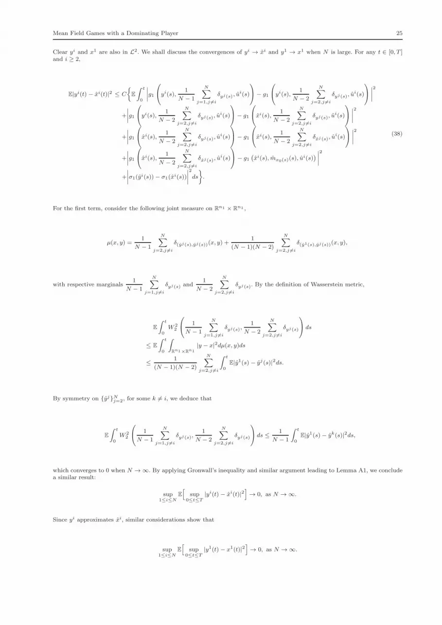
Mean Field Games with a Dominating Player 25

Clear yi and x1 are also in L2. We shall discuss the convergences of yi → xi and y1 → x1 when N is large. For any t ∈ [0, T ]and i ≥ 2,

E|yi(t) − xi(t)|2 ≤ C

E

∫ t

0

∣

∣

∣

∣

g1

yi(s),1

N − 1

N∑

j=1,j 6=i

δyj(s), ui(s)

− g1

yi(s),1

N − 2

N∑

j=2,j 6=i

δyj(s), ui(s)

∣

∣

∣

∣

2

+

∣

∣

∣

∣

g1

yi(s),1

N − 2

N∑

j=2,j 6=i

δyj(s), ui(s)

− g1

xi(s),1

N − 2

N∑

j=2,j 6=i

δyj(s), ui(s)

∣

∣

∣

∣

2

+

∣

∣

∣

∣

g1

xi(s),1

N − 2

N∑

j=2,j 6=i

δyj(s), ui(s)

− g1

xi(s),1

N − 2

N∑

j=2,j 6=i

δxj(s), ui(s)

∣

∣

∣

∣

2

+

∣

∣

∣

∣

g1

xi(s),1

N − 2

N∑

j=2,j 6=i

δxj(s), ui(s)

− g1(

xi(s), mx0(s)(s), ui(s)

)

∣

∣

∣

∣

2

+

∣

∣

∣

∣

σ1(yi(s))− σ1(xi(s))

∣

∣

∣

∣

2

ds

.

(38)

For the first term, consider the following joint measure on Rn1 × R

n1 ,

µ(x, y) =1

N − 1

N∑

j=2,j 6=i

δ(yj(s),yj(s))(x, y) +1

(N − 1)(N − 2)

N∑

j=2,j 6=i

δ(y1(s),yj(s))(x, y),

with respective marginals1

N − 1

N∑

j=1,j 6=i

δyj(s) and1

N − 2

N∑

j=2,j 6=i

δyj(s). By the definition of Wasserstein metric,

E

∫ t

0W 2

2

1

N − 1

N∑

j=1,j 6=i

δyj(s),1

N − 2

N∑

j=2,j 6=i

δyj(s)

ds

≤ E

∫ t

0

∫

Rn1×R

n1

|y − x|2dµ(x, y)ds

≤ 1

(N − 1)(N − 2)

N∑

j=2,j 6=i

∫ t

0E|y1(s) − yj(s)|2ds.

By symmetry on yjNj=2, for some k 6= i, we deduce that

E

∫ t

0W 2

2

1

N − 1

N∑

j=1,j 6=i

δyj(s),1

N − 2

N∑

j=2,j 6=i

δyj(s)

ds ≤ 1

N − 1

∫ t

0E|y1(s)− yk(s)|2ds,

which converges to 0 when N → ∞. By applying Gronwall’s inequality and similar argument leading to Lemma A1, we concludea similar result:

sup1≤i≤N

E

[

sup0≤t≤T

|yi(t) − xi(t)|2]

→ 0, as N → ∞.

Since yi approximates xi, similar considerations show that

sup1≤i≤N

E

[

sup0≤t≤T

|y1(t) − x1(t)|2]

→ 0, as N → ∞.

26 A. Bensoussan, M. H. M. Chau, S. C. P. Yam

Finally, using the similar techniques to telescope the difference of the cost functional,

|JN,1(u)− J 1(u1)| ≤ E

∫ T

0

∣

∣

∣

∣

∣

∣

f1

y1(t),1

N − 1

N∑

j=2

δyj(t), u1(t)

− f1(

x1(t), mx0(t)(t), u1(t)

)

∣

∣

∣

∣

∣

∣

dt

+E

∣

∣

∣

∣

∣

∣

h1

y1(T ),1

N − 1

N∑

j=2

δyj(T )

− h1

(

x1(T ), mx0(T ))

∣

∣

∣

∣

∣

∣

≤ E

∫ T

0

∣

∣

∣

∣

∣

∣

f1

y1(t),1

N − 1

N∑

j=2

δyj(t), u1(t)

− f1

x1(t),1

N − 1

N∑

j=2

δyj(t), u1(t)

∣

∣

∣

∣

∣

∣

dt

+E

∫ T

0

∣

∣

∣

∣

∣

∣

f1

x1(t),1

N − 1

N∑

j=2

δyj(t), u1(t)

− f1

x1(t),1

N − 1

N∑

j=2

δxj(t), u1(t)

∣

∣

∣

∣

∣

∣

dt

+E

∫ T

0

∣

∣

∣

∣

∣

∣

f1

x1(t),1

N − 1

N∑

j=2

δxj(t), u1(t)

− f1(

x1(t), mx0(t)(t), u1(t)

)

∣

∣

∣

∣

∣

∣

dt

+E

∣

∣

∣

∣

∣

∣

h1

y1(T ),1

N − 1

N∑

j=2

δyj(T )

− h1

x1(T ),1

N − 1

N∑

j=2

δyj(T )

∣

∣

∣

∣

∣

∣

+E

∣

∣

∣

∣

∣

∣

h1

x1(T ),1

N − 1

N∑

j=2

δyj(T )

− h1

x1(T ),1

N − 1

N∑

j=2

δxj(T )

∣

∣

∣

∣

∣

∣

+E

∣

∣

∣

∣

∣

∣

h1

x1(T ),1

N − 1

N∑

j=2

δxj(T )

− h1

(

x1(T ), mx0(T ))

∣

∣

∣

∣

∣

∣

.

We conclude from the similar procedures that

|JN,1(u)−J 1 (u1)| = O(1√N

).

Theorem A3 u is an ǫ-Nash equilibrium.

Proof Summarizing all the obtained results in th section, we can conclude

|JN,i(u)− J i(ui)| = O(1√N

);

|JN,1(u) −J 1(u1)| = O(1√N

).

Since ui is optimal control, we have J i(ui) ≤ J 1(u1). We deduce

JN,i(u) ≤ JN,1(u) + O(1√N

).

Hence, u is an ǫ-Nash equilibrium. ⊓⊔

References

1. A. Bensoussan, K. C. J. Sung, S. C. P. Yam and S. P. Yung (2011). Linear-Quadratic Mean Field Games. Submitted.2. A. Bensoussan and J. Frehse (2000). Stochastic Games for N players. Journal of Optimization Theory and Applications,

105(3), 543-565.3. A. Bensoussan and J. Frehse (2009). On Diagonal Elliptic and Parabolic Systems with Super-quadratic Hamiltonians.

Communications on Pure and Applied Analysis, 8, 83-94.4. A. Bensoussan, J. Frehse and J. Vogelgesang (2010). Systems of Bellman Equations to Stochastic Differential Games

with Non-compact Coupling. Discrete and Continuous Dynamical Systems, 27(4), 1375-1389.5. A. Bensoussan, J. Frehse and S.C.P. Yam (2013). Mean Field Games and Mean Field Type Control Theory. To appear

in Springer Verlag.6. R. Carmona, F. Delarue (2013). Probabilistic Analysis of Mean-Field Games. SIAM Journal on Control and Optimization

51 (4), 2705-2734.7. Lasry, J.-M., Lions, P.-L. (2006a). Jeux a champ moyen I - Le cas stationnaire. Comptes Rendus de l’Academie des

Sciences, Series I, 343, 619-625.8. Lasry, J.-M., Lions, P.-L. (2006b). Jeux a champ moyen II. Horizon fini et controle optimal. Comptes Rendus de l’Academie

des Sciences, Series I, 343, 679-684.9. Lasry, J. M., Lions, P. L. (2007). Mean Field Games. Japanese Journal of Mathematics 2(1), 229-260.

10. George Cooper (2008). The Origin of Financial Crises: Central Banks, Credit Bubbles, and the Efficient Market Fallacy.Harriman House Limited .

Mean Field Games with a Dominating Player 27

11. Huang, M., Caines, P.E., Malhame, R.P. (2003). Individual and Mass Behaviour in Large Population Stochastic WirelessPower Control Problems: Centralized and Nash Equilibrium Solutions. Proceedings of the 42nd IEEE Conference on Decision

and Control, Maui, Hawaii, December 2003, 98 - 103.12. Huang, M., Malhame, R.P., Caines, P.E. (2006). Large Population Stochastic Dynamic Games: Closed-loop McKean-

Vlasov Systems and the Nash Certainty Equivalence Principle. Communications in Information and Systems, 6 (3), 221-252.13. S.L., Nguyen and M. Huang. Linear-Quadratic-Gaussian Mixed Games With Continuum-Parametrized Minor Players.

SIAM Journal on Control and Optimization 50 (5), 2907-2937.14. S.L., Nguyen and M. Huang. Mean Field LQG Games with Mass Behavior Responsive to A Major Player. 51st IEEE

Conference on Decision and Control (), .15. Peng, S. (1992). Stochastic Hamilton-Jacbi-Bellman Equations. SIAM Journal on Control and Optimization 30 (2), 284-

304.16. T. Deck and S. Kruse (2002). Parabolic Differential Equation with Unbounded Coefficients - A Generalization of the

Parametrix Method. Acta Applicandae Mathematicae 74 , 71-91.17. Cedric Villani (1999). Forward-Backward Stochastic Differential Equations and Their Applications. Lecture Notes in

Mathematics 1702, Springer.18. MA, J., YONG, J. (1999). Forward-Backward Stochastic Differential Equations and Their Applications. Lecture Notes in

Mathematics 1702, Springer.