matlab programming - i m.sc.,(mathematics) - sri
TRANSCRIPT
IM.Sc., _MATLAB Programming-Lecture Notes
Sub.Code: MMAF181P50 Page 1
MATLAB PROGRAMMING I M.Sc.,(Mathematics)
Code: MMAF181P50
Lecture Notes
Dr.K.Srinivasa Rao Professor & Head
Department of Mathematics
Sri Chandra Sekharendra Saraswathi Viswa Mahavidyalaya
Enathur, Kanchipuram, Tamilnadu

IM.Sc., _MATLAB Programming-Lecture Notes
Sub.Code: MMAF181P50 Page 2
IM.Sc., _MATLAB Programming-Lecture Notes
Sub.Code: MMAF181P50 Page 3
1. GETTING STARTED WITH MATLAB
What Is MATLAB?
MATLAB is an efficient user-friendly interactive software package, which is very effective
for solving engineering, mathematical, and system problems.
MATLAB Windows
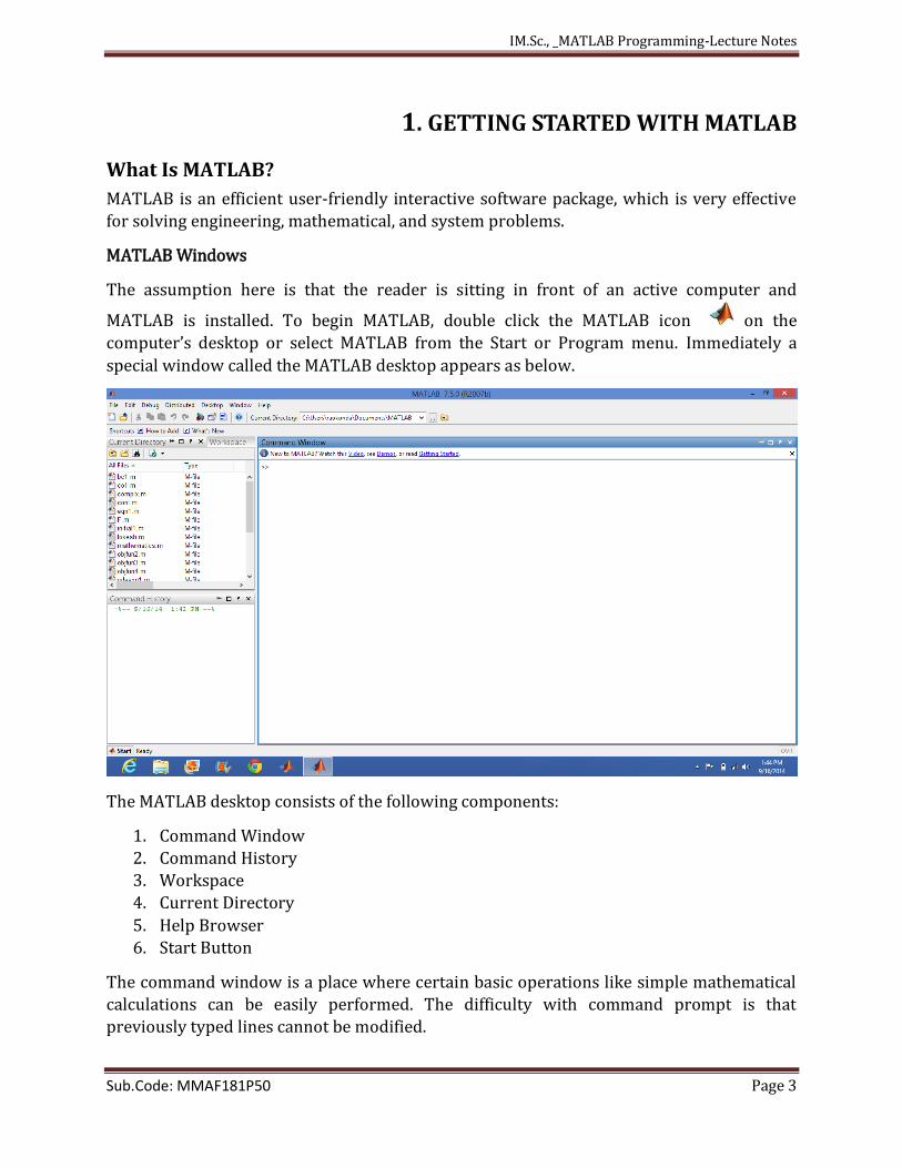
The assumption here is that the reader is sitting in front of an active computer and
MATLAB is installed. To begin MATLAB, double click the MATLAB icon on the
computer’s desktop or select MATLAB from the Start or Program menu. Immediately a
special window called the MATLAB desktop appears as below.
The MATLAB desktop consists of the following components:
1. Command Window
2. Command History
3. Workspace
4. Current Directory
5. Help Browser
6. Start Button
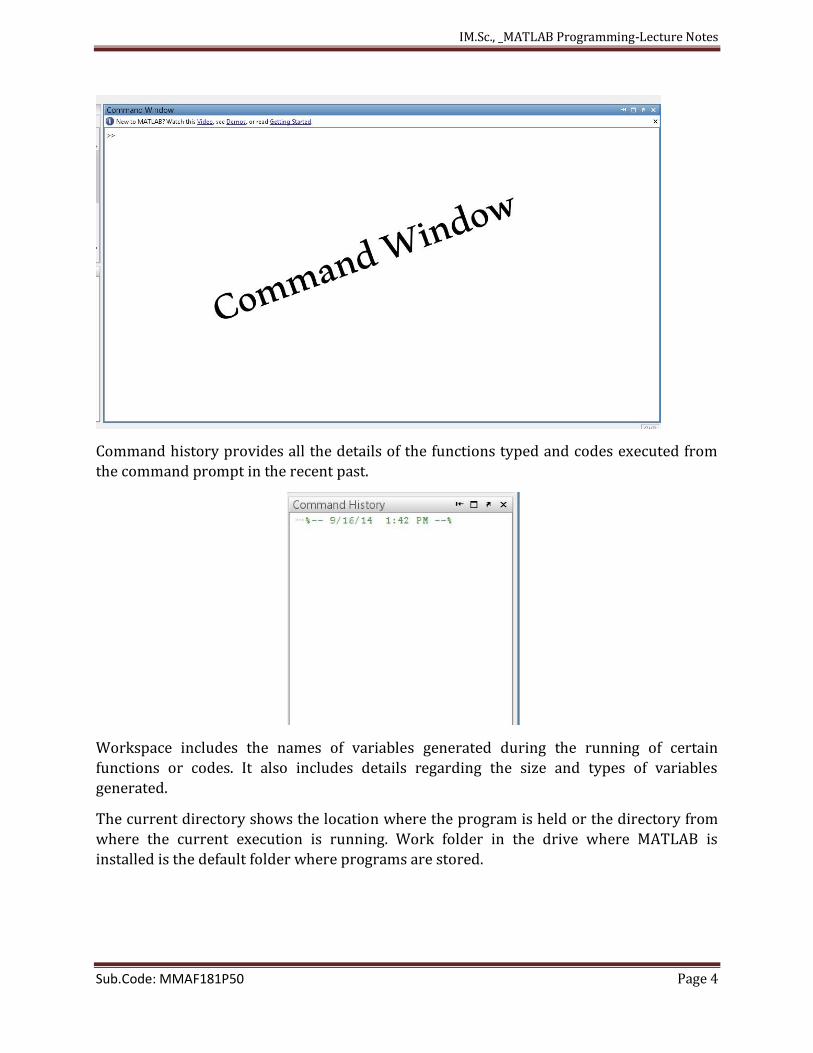
The command window is a place where certain basic operations like simple mathematical
calculations can be easily performed. The difficulty with command prompt is that
previously typed lines cannot be modified.
IM.Sc., _MATLAB Programming-Lecture Notes
Sub.Code: MMAF181P50 Page 4
Command history provides all the details of the functions typed and codes executed from
the command prompt in the recent past.
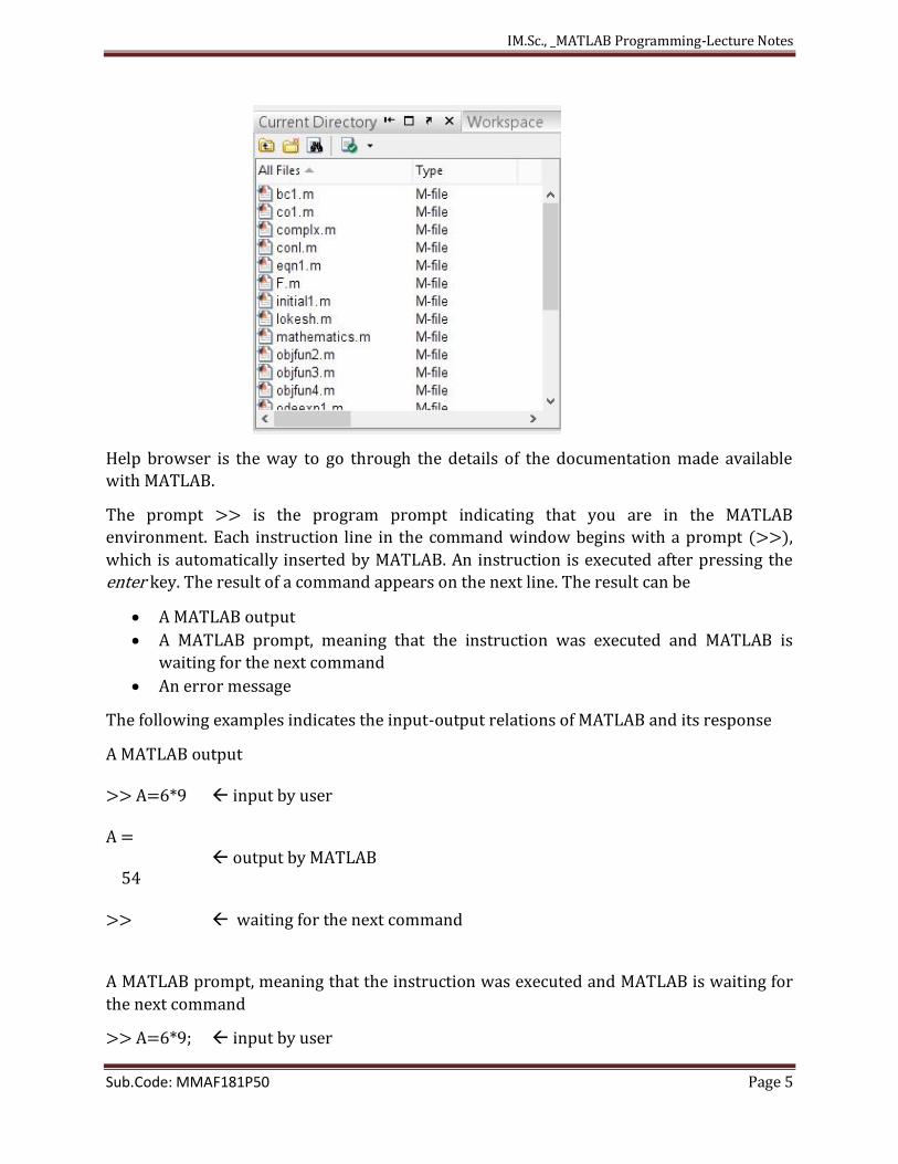
Workspace includes the names of variables generated during the running of certain
functions or codes. It also includes details regarding the size and types of variables
generated.
The current directory shows the location where the program is held or the directory from
where the current execution is running. Work folder in the drive where MATLAB is
installed is the default folder where programs are stored.
IM.Sc., _MATLAB Programming-Lecture Notes
Sub.Code: MMAF181P50 Page 5
Help browser is the way to go through the details of the documentation made available
with MATLAB.
The prompt >> is the program prompt indicating that you are in the MATLAB
environment. Each instruction line in the command window begins with a prompt (>>),
which is automatically inserted by MATLAB. An instruction is executed after pressing the
enter key. The result of a command appears on the next line. The result can be
A MATLAB output
A MATLAB prompt, meaning that the instruction was executed and MATLAB is
waiting for the next command
An error message
The following examples indicates the input-output relations of MATLAB and its response
A MATLAB output >> A=6*9 input by user A = output by MATLAB 54 >> waiting for the next command A MATLAB prompt, meaning that the instruction was executed and MATLAB is waiting for
the next command
>> A=6*9; input by user
IM.Sc., _MATLAB Programming-Lecture Notes
Sub.Code: MMAF181P50 Page 6
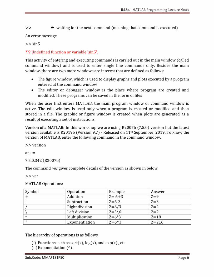
>> waiting for the next command (meaning that command is executed)
An error message
>> sin5
??? Undefined function or variable 'sin5'.
This activity of entering and executing commands is carried out in the main window (called
command window) and is used to enter single line commands only. Besides the main
window, there are two more windows are interest that are defined as follows:
The figure window, which is used to display graphs and plots executed by a program
entered at the command window
The editor or debugger window is the place where program are created and
modified. These programs can be saved in the form of files
When the user first enters MATLAB, the main program window or command window is
active. The edit window is used only when a program is created or modified and then
stored in a file. The graphic or figure window is created when plots are generated as a
result of executing a set of instructions.
Version of a MATLAB: In this workshop we are using R2007b (7.5.0) version but the latest version available is R2019b (Version 9.7) - Released on 11th September, 2019. To know the version of MATLAB, enter the following command in the command window.
>> version
ans =
7.5.0.342 (R2007b)
The command ver gives complete details of the version as shown in below
>> ver
MATLAB Operations:
Symbol Operation Example Answer + Addition Z= 6+3 Z=9 - Subtraction Z=6-3 Z=3 / Right division Z=6/3 Z=2 \ Left division Z=3\6 Z=2 * Multiplication Z=6*3 Z=18 ^ Exponentiation Z=6^3 Z=216
The hierarchy of operations is as follows
(i) Functions such as sqrt(x), log(x), and exp(x) , etc (ii) Exponentiation (^)
IM.Sc., _MATLAB Programming-Lecture Notes
Sub.Code: MMAF181P50 Page 7
(iii) Products and division (*, /) (iv) Addition and subtraction (+,-)
Difference between the commands home, clc and clear
>>home
home moves the cursor to the upper-left corner of the Command Window. You can use the scroll bar to see the history of previous functions.
>> clc
clc clears all input and output from the Command Window display, giving you a "clean+ screen."
After using clc, you cannot use the scroll bar to see the history of functions, but you still can use the up arrow to recall statements from the command history.
>>clear
clear removes all variables from the workspace. This frees up system memory.
Display Format of Numbers:
It always attempts to display integers (whole numbers) exactly. However, if the integer is
too large, it is displayed in scientific notation with five significant digits, e.g. 1234567890 is
displayed as 1.2346e+009 (i.e. 1.2346×10⁹). Check this by first entering 123456789 at the
command line, and then 1234567890.
Numbers with decimal parts are displayed with four significant digits. If the value x is in the
range 0.001 1000x it is displayed in fixed point form, otherwise scientific (floating
point) notation is used, in which case the mantissa is between 1and 9.9999, e.g. 1000.1 is
displayed as 1.0001e+003. Check this by entering following numbers at the prompt (on
separate lines): 0.0011, 0.0009, 1/3, 5/3, 2999/3, 3001/3
This is what is called the default format, i.e. what normally happens. However, you can
change from the default with variations on the format command, as follows. If you want
values displayed in scientific notation (floating point form) whatever their size, enter the
command
format short e
All output from subsequent display statements will be in scientific notation with five
significant digits, until the next format command is issued. Enter this command and check
it with the following values: 0.0123456, 1.23456, 123.456 (all on separate lines). If you
want more accurate output, you can use
format long e
This also gives scientific notation, but with 15 significant digits. Try it out on 1/7.
IM.Sc., _MATLAB Programming-Lecture Notes
Sub.Code: MMAF181P50 Page 8
Use format long to get fixed point notation with 15 significant digits, e.g. try 100/7 and pi.
If you’re not sure of the order of magnitude of your output you can try format short g or
format long g. The g stands for ‘general’. MATLAB decides in each case whether to use fixed
or floating point. Use format bank for financial calculations; you get fixed point with two
decimal digits (for the cents). Try it on 10000/7.
Use format hex to get hexadecimal display.
Use format rat to display a number as a rational approximation (ratio of two integers), e.g.
pi is displayed as 355/113, a pleasant change from the tired old 22/7. Please note that even
this is an approximation! Try out format rat on √2 ande (exp(1)). The symbols + , - and a
space are displayed for positive, negative and zero elements of a vector or matrix after the
command format +. In certain applications this is a convenient way of displaying matrices.
The command format by itself reverts to the default format. You can always try help format
if you are confused!
Format Short, Format Long, Format Bank & Format Rat
We can change the format to format long by typing
>>format long
View the result of value of by typing
>>sqrt(3)
ans =
1.732050807568877
When the format is set to format short
>>format short
>> sqrt(3)
ans =
1.7321
When the format is set to format bank
>>format bank
>> sqrt(3)
ans =
1.73
When the format is set to format rat
IM.Sc., _MATLAB Programming-Lecture Notes
Sub.Code: MMAF181P50 Page 9
>> format rat
>> sqrt(3)
ans =
1351/780
Note : The format function affects only how numbers are displayed, not how MATLAB computes or saves them.
Difference between commands fix, round, ceil and floor
>> round(6.628)
ans =
7 % round command rounds the element of x to towards nearest integer
>> fix(6.628)
ans =
6 % fix command rounds the element x to nearest integer towards zero
>> ceil(6.628)
ans =
7 % ceil command rounds the element x to nearest integer towards infinity
>> floor(6.628)
ans =
6
% floor command rounds the element x to nearest integer towards minus infinity
Worksheet-I
Calculate the following values using Matlab
1. 83 9 2.
24 7 3.
5
6
2
2 1 4. 125
10log 5.
10loge
6. cos( / 4) 7. 2sin ( / 3) 8.
5e 9. 5
loge
e
IM.Sc., _MATLAB Programming-Lecture Notes
Sub.Code: MMAF181P50 Page 10
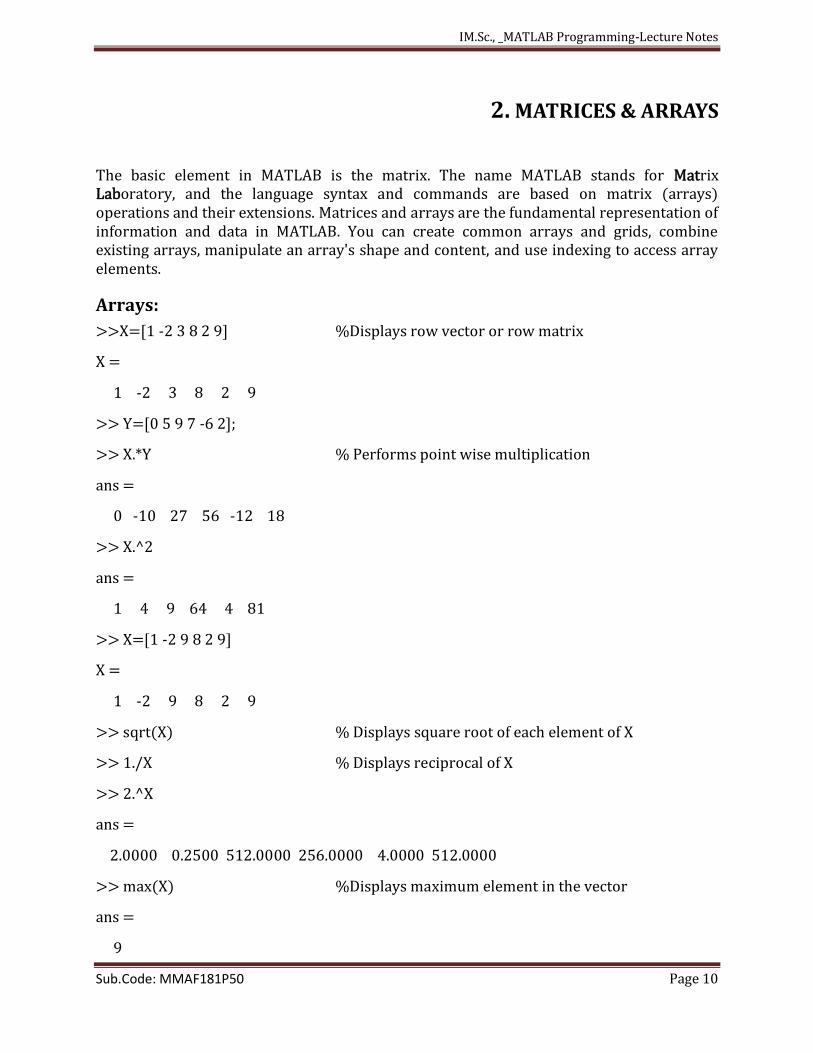
2. MATRICES & ARRAYS
The basic element in MATLAB is the matrix. The name MATLAB stands for Matrix Laboratory, and the language syntax and commands are based on matrix (arrays) operations and their extensions. Matrices and arrays are the fundamental representation of information and data in MATLAB. You can create common arrays and grids, combine existing arrays, manipulate an array's shape and content, and use indexing to access array elements.
Arrays:
>>X=[1 -2 3 8 2 9] %Displays row vector or row matrix
X =
1 -2 3 8 2 9
>> Y=[0 5 9 7 -6 2];
>> X.*Y % Performs point wise multiplication
ans =
0 -10 27 56 -12 18
>> X.^2
ans =
1 4 9 64 4 81
>> X=[1 -2 9 8 2 9]
X =
1 -2 9 8 2 9
>> sqrt(X) % Displays square root of each element of X
>> 1./X % Displays reciprocal of X
>> 2.^X
ans =
2.0000 0.2500 512.0000 256.0000 4.0000 512.0000
>> max(X) %Displays maximum element in the vector
ans =
9
IM.Sc., _MATLAB Programming-Lecture Notes
Sub.Code: MMAF181P50 Page 11
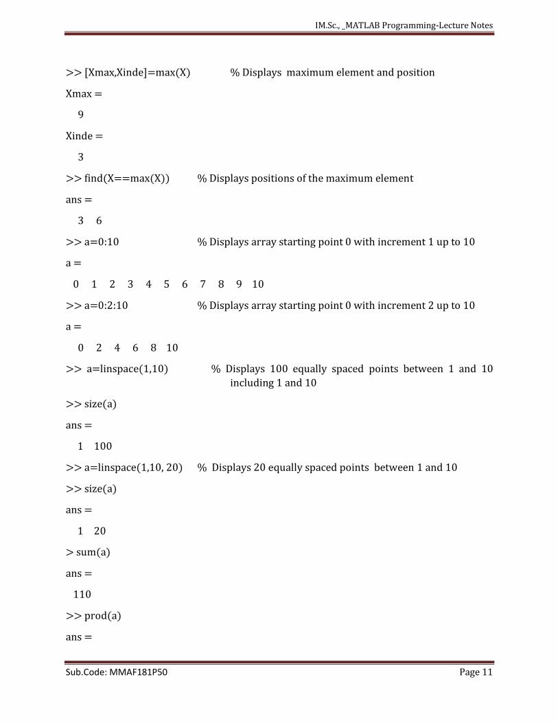
>> [Xmax,Xinde]=max(X) % Displays maximum element and position
Xmax =
9
Xinde =
3
>> find(X==max(X)) % Displays positions of the maximum element
ans =
3 6
>> a=0:10 % Displays array starting point 0 with increment 1 up to 10
a =
0 1 2 3 4 5 6 7 8 9 10
>> a=0:2:10 % Displays array starting point 0 with increment 2 up to 10
a =
0 2 4 6 8 10
>> a=linspace(1,10) % Displays 100 equally spaced points between 1 and 10
including 1 and 10
>> size(a)
ans =
1 100
>> a=linspace(1,10, 20) % Displays 20 equally spaced points between 1 and 10
>> size(a)
ans =
1 20
> sum(a)
ans =
110
>> prod(a)
ans =
IM.Sc., _MATLAB Programming-Lecture Notes
Sub.Code: MMAF181P50 Page 12
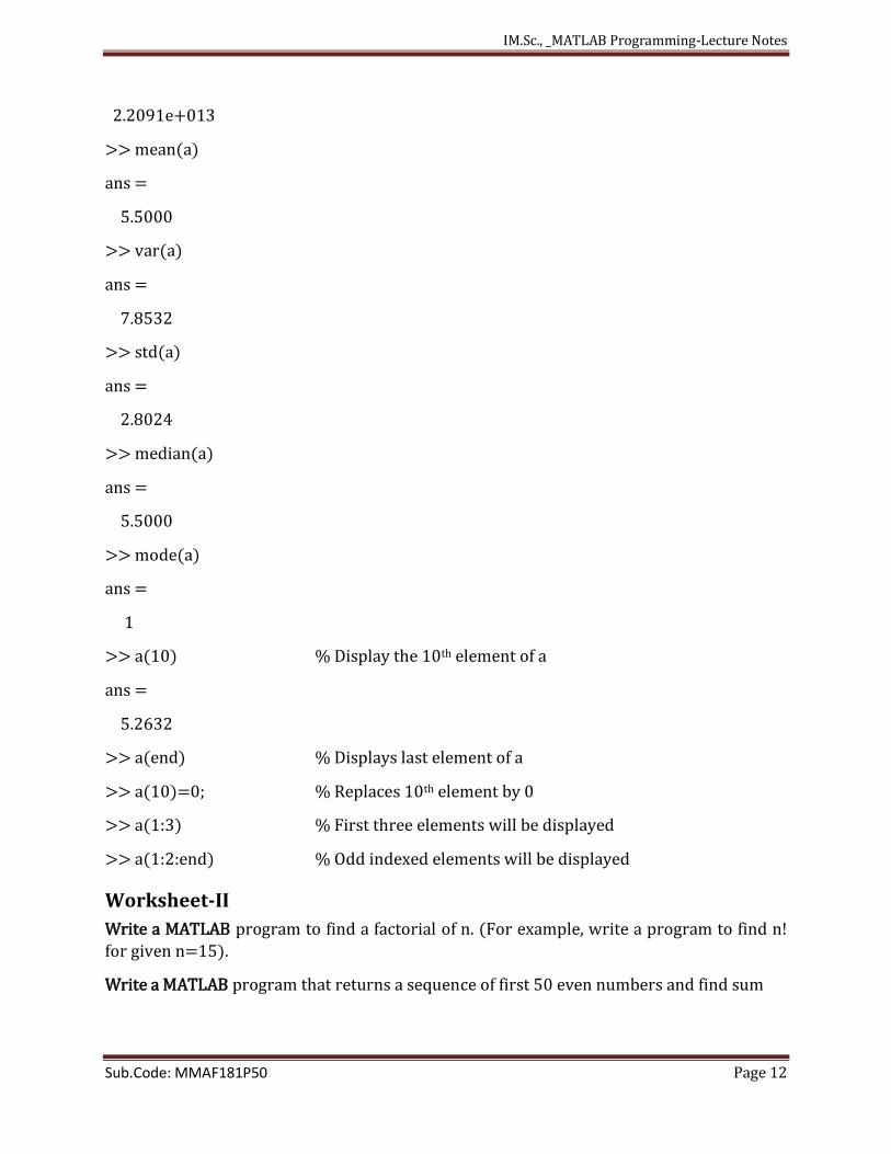
2.2091e+013
>> mean(a)
ans =
5.5000
>> var(a)
ans =
7.8532
>> std(a)
ans =
2.8024
>> median(a)
ans =
5.5000
>> mode(a)
ans =
1
>> a(10) % Display the 10th element of a
ans =
5.2632
>> a(end) % Displays last element of a
>> a(10)=0; % Replaces 10th element by 0
>> a(1:3) % First three elements will be displayed
>> a(1:2:end) % Odd indexed elements will be displayed
Worksheet-II
Write a MATLAB program to find a factorial of n. (For example, write a program to find n!
for given n=15).
Write a MATLAB program that returns a sequence of first 50 even numbers and find sum
IM.Sc., _MATLAB Programming-Lecture Notes
Sub.Code: MMAF181P50 Page 13
Write a MATLAB program that returns a sequence, consists of sequence of square of first 50
even numbers and find sum
Write a MATLAB program to find , for a=0.5; N=11 and N=21
Write a MATLAB program that adds all elements of X with even indexes (Here x is vector
containing particular number of elements).
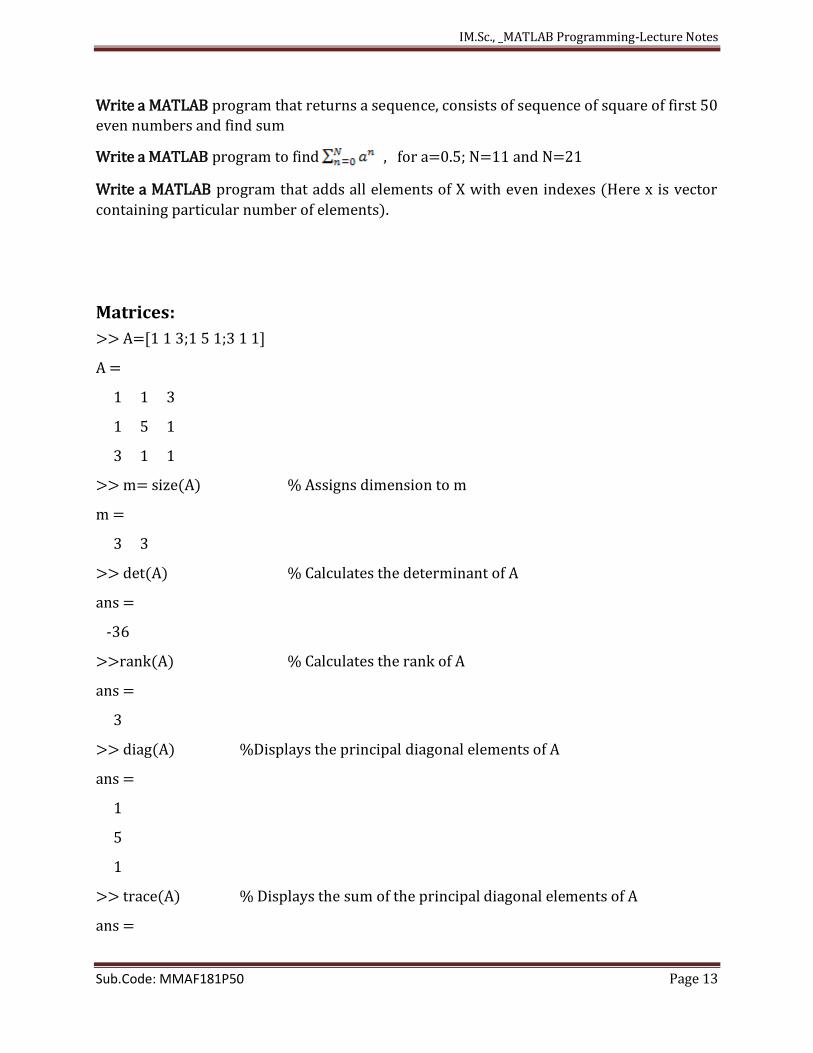
Matrices:
>> A=[1 1 3;1 5 1;3 1 1]
A =
1 1 3
1 5 1
3 1 1
>> m= size(A) % Assigns dimension to m
m =
3 3
>> det(A) % Calculates the determinant of A
ans =
-36
>>rank(A) % Calculates the rank of A
ans =
3
>> diag(A) %Displays the principal diagonal elements of A
ans =
1
5
1
>> trace(A) % Displays the sum of the principal diagonal elements of A
ans =
IM.Sc., _MATLAB Programming-Lecture Notes
Sub.Code: MMAF181P50 Page 14
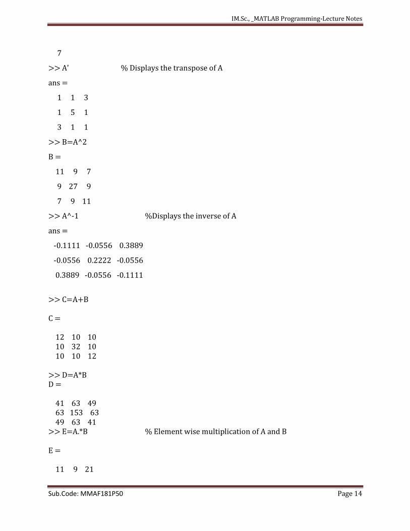
7
>> A' % Displays the transpose of A
ans =
1 1 3
1 5 1
3 1 1
>> B=A^2
B =
11 9 7
9 27 9
7 9 11
>> A^-1 %Displays the inverse of A
ans =
-0.1111 -0.0556 0.3889
-0.0556 0.2222 -0.0556
0.3889 -0.0556 -0.1111
>> C=A+B C = 12 10 10 10 32 10 10 10 12 >> D=A*B D = 41 63 49 63 153 63 49 63 41 >> E=A.*B % Element wise multiplication of A and B E = 11 9 21
IM.Sc., _MATLAB Programming-Lecture Notes
Sub.Code: MMAF181P50 Page 15
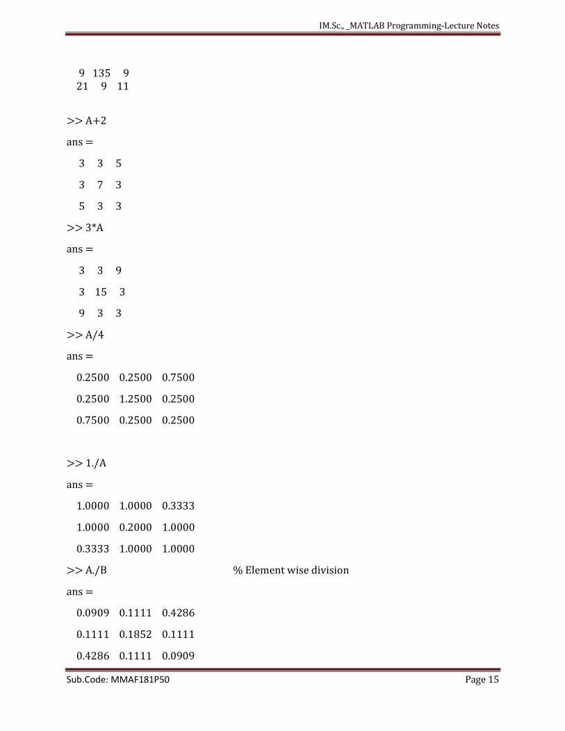
9 135 9 21 9 11
>> A+2
ans =
3 3 5
3 7 3
5 3 3
>> 3*A
ans =
3 3 9
3 15 3
9 3 3
>> A/4
ans =
0.2500 0.2500 0.7500
0.2500 1.2500 0.2500
0.7500 0.2500 0.2500
>> 1./A
ans =
1.0000 1.0000 0.3333
1.0000 0.2000 1.0000
0.3333 1.0000 1.0000
>> A./B % Element wise division
ans =
0.0909 0.1111 0.4286
0.1111 0.1852 0.1111
0.4286 0.1111 0.0909
IM.Sc., _MATLAB Programming-Lecture Notes
Sub.Code: MMAF181P50 Page 16
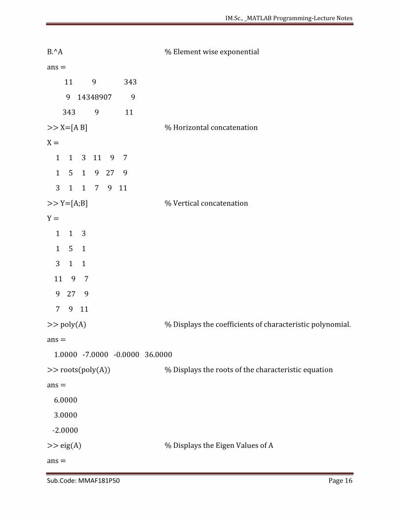
B.^A % Element wise exponential
ans =
11 9 343
9 14348907 9
343 9 11
>> X=[A B] % Horizontal concatenation
X =
1 1 3 11 9 7
1 5 1 9 27 9
3 1 1 7 9 11
>> Y=[A;B] % Vertical concatenation
Y =
1 1 3
1 5 1
3 1 1
11 9 7
9 27 9
7 9 11
>> poly(A) % Displays the coefficients of characteristic polynomial.
ans =
1.0000 -7.0000 -0.0000 36.0000
>> roots(poly(A)) % Displays the roots of the characteristic equation
ans =
6.0000
3.0000
-2.0000
>> eig(A) % Displays the Eigen Values of A
ans =
IM.Sc., _MATLAB Programming-Lecture Notes
Sub.Code: MMAF181P50 Page 17
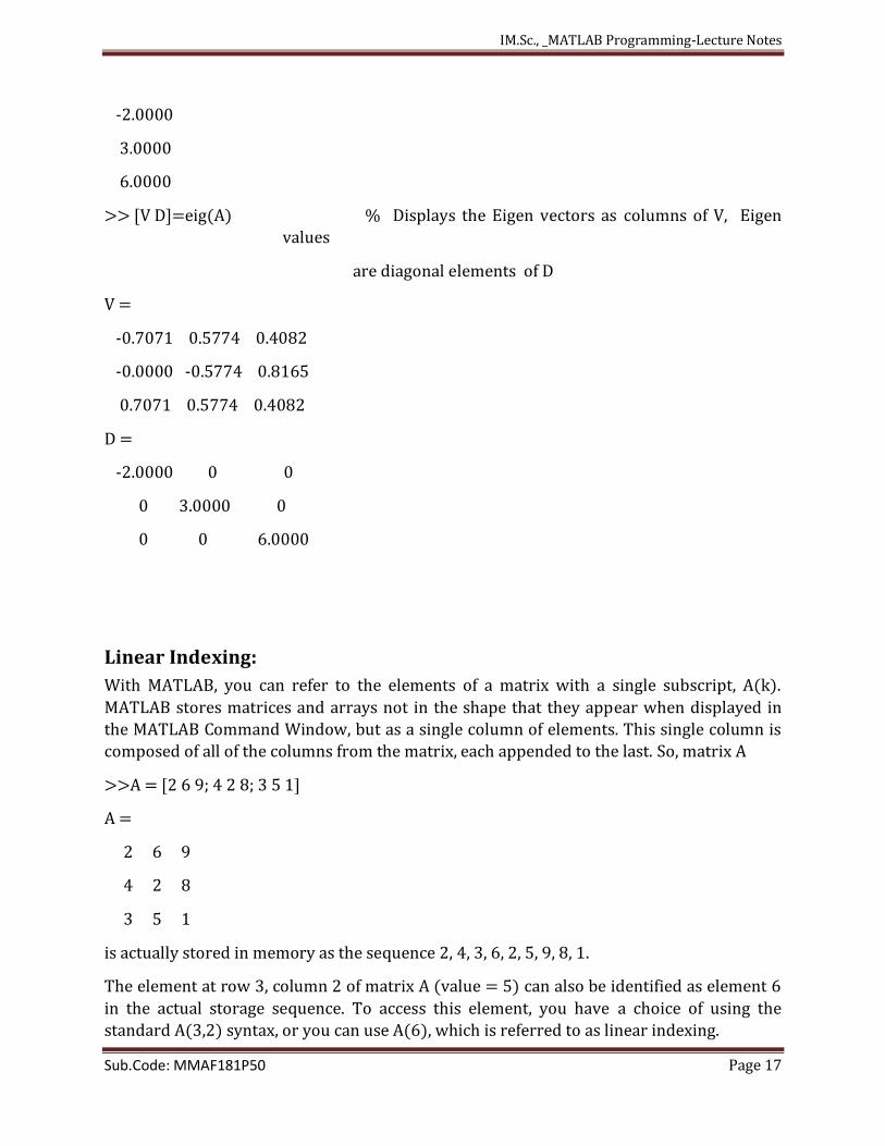
-2.0000
3.0000
6.0000
>> [V D]=eig(A) % Displays the Eigen vectors as columns of V, Eigen
values
are diagonal elements of D
V =
-0.7071 0.5774 0.4082
-0.0000 -0.5774 0.8165
0.7071 0.5774 0.4082
D =
-2.0000 0 0
0 3.0000 0
0 0 6.0000
Linear Indexing:
With MATLAB, you can refer to the elements of a matrix with a single subscript, A(k).
MATLAB stores matrices and arrays not in the shape that they appear when displayed in
the MATLAB Command Window, but as a single column of elements. This single column is
composed of all of the columns from the matrix, each appended to the last. So, matrix A
>>A = [2 6 9; 4 2 8; 3 5 1]
A =
2 6 9
4 2 8
3 5 1
is actually stored in memory as the sequence 2, 4, 3, 6, 2, 5, 9, 8, 1.
The element at row 3, column 2 of matrix A (value = 5) can also be identified as element 6
in the actual storage sequence. To access this element, you have a choice of using the
standard A(3,2) syntax, or you can use A(6), which is referred to as linear indexing.
IM.Sc., _MATLAB Programming-Lecture Notes
Sub.Code: MMAF181P50 Page 18
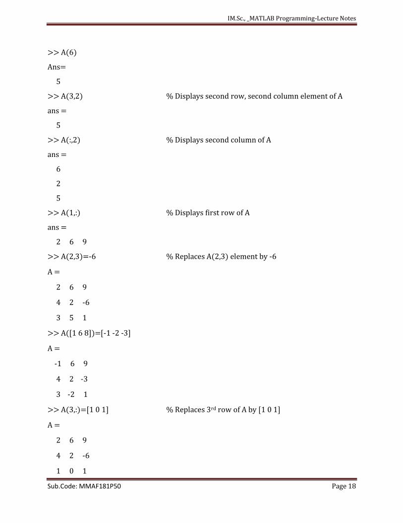
>> A(6)
Ans=
5
>> A(3,2) % Displays second row, second column element of A
ans =
5
>> A(:,2) % Displays second column of A
ans =
6
2
5
>> A(1,:) % Displays first row of A
ans =
2 6 9
>> A(2,3)=-6 % Replaces A(2,3) element by -6
A =
2 6 9
4 2 -6
3 5 1
>> A([1 6 8])=[-1 -2 -3]
A =
-1 6 9
4 2 -3
3 -2 1
>> A(3,:)=[1 0 1] % Replaces 3rd row of A by [1 0 1]
A =
2 6 9
4 2 -6
1 0 1
IM.Sc., _MATLAB Programming-Lecture Notes
Sub.Code: MMAF181P50 Page 19
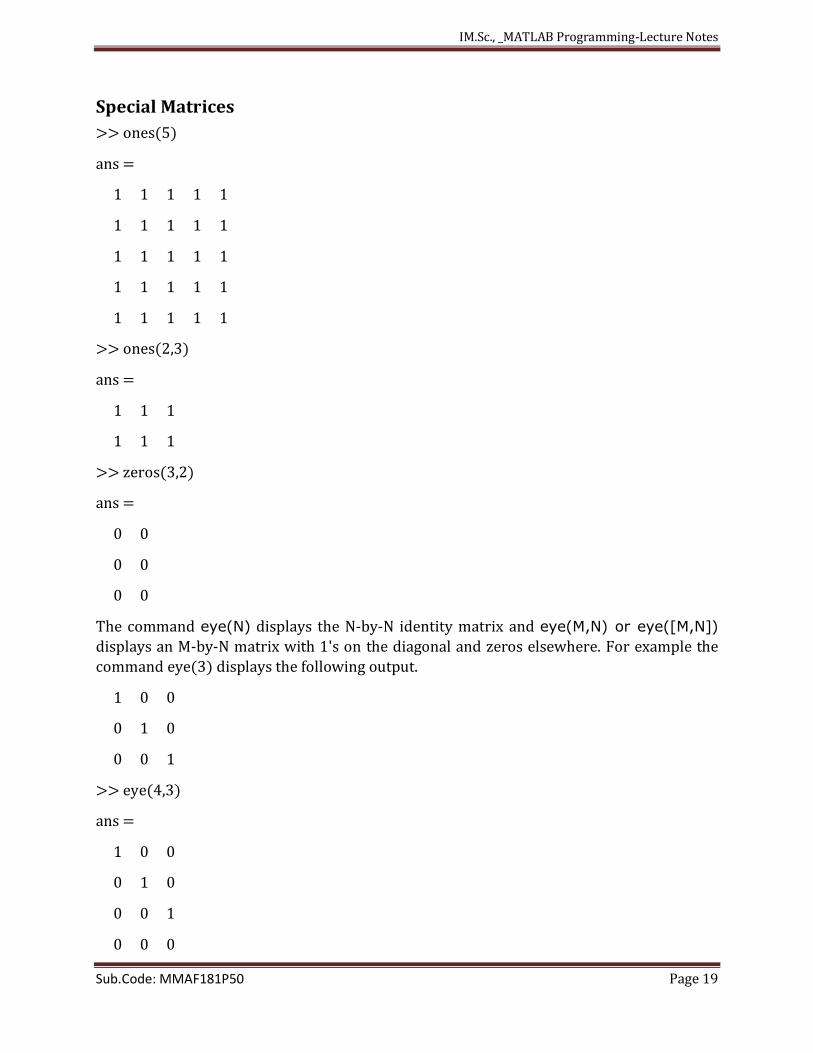
Special Matrices
>> ones(5)
ans =
1 1 1 1 1
1 1 1 1 1
1 1 1 1 1
1 1 1 1 1
1 1 1 1 1
>> ones(2,3)
ans =
1 1 1
1 1 1
>> zeros(3,2)
ans =
0 0
0 0
0 0
The command eye(N) displays the N-by-N identity matrix and eye(M,N) or eye([M,N])
displays an M-by-N matrix with 1's on the diagonal and zeros elsewhere. For example the
command eye(3) displays the following output.
1 0 0
0 1 0
0 0 1
>> eye(4,3)
ans =
1 0 0
0 1 0
0 0 1
0 0 0
IM.Sc., _MATLAB Programming-Lecture Notes
Sub.Code: MMAF181P50 Page 20
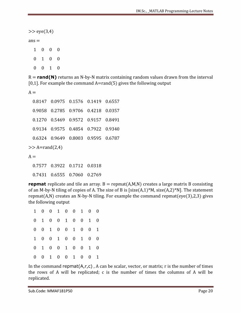
>> eye(3,4)
ans =
1 0 0 0
0 1 0 0
0 0 1 0
R = rand(N) returns an N-by-N matrix containing random values drawn from the interval
[0,1]. For example the command A=rand(5) gives the following output
A =
0.8147 0.0975 0.1576 0.1419 0.6557
0.9058 0.2785 0.9706 0.4218 0.0357
0.1270 0.5469 0.9572 0.9157 0.8491
0.9134 0.9575 0.4854 0.7922 0.9340
0.6324 0.9649 0.8003 0.9595 0.6787
>> A=rand(2,4)
A =
0.7577 0.3922 0.1712 0.0318
0.7431 0.6555 0.7060 0.2769
repmat replicate and tile an array. B = repmat(A,M,N) creates a large matrix B consisting
of an M-by-N tiling of copies of A. The size of B is [size(A,1)*M, size(A,2)*N]. The statement
repmat(A,N) creates an N-by-N tiling. For example the command repmat(eye(3),2,3) gives
the following output
1 0 0 1 0 0 1 0 0
0 1 0 0 1 0 0 1 0
0 0 1 0 0 1 0 0 1
1 0 0 1 0 0 1 0 0
0 1 0 0 1 0 0 1 0
0 0 1 0 0 1 0 0 1
In the command repmat(A,r,c) , A can be scalar, vector, or matrix; r is the number of times
the rows of A will be replicated; c is the number of times the columns of A will be
replicated.
IM.Sc., _MATLAB Programming-Lecture Notes
Sub.Code: MMAF181P50 Page 21
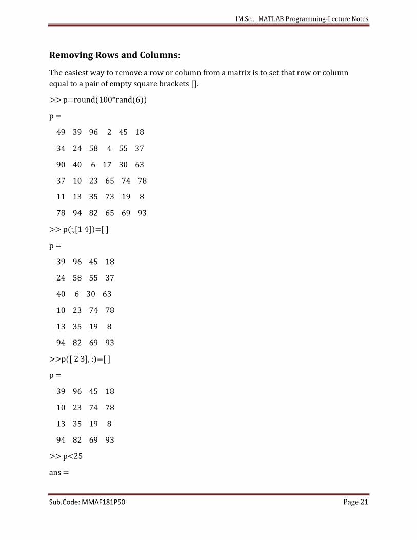
Removing Rows and Columns:
The easiest way to remove a row or column from a matrix is to set that row or column
equal to a pair of empty square brackets [].
>> p=round(100*rand(6))
p =
49 39 96 2 45 18
34 24 58 4 55 37
90 40 6 17 30 63
37 10 23 65 74 78
11 13 35 73 19 8
78 94 82 65 69 93
>> p(:,[1 4])=[ ]
p =
39 96 45 18
24 58 55 37
40 6 30 63
10 23 74 78
13 35 19 8
94 82 69 93
>>p([ 2 3], :)=[ ]
p =
39 96 45 18
10 23 74 78
13 35 19 8
94 82 69 93
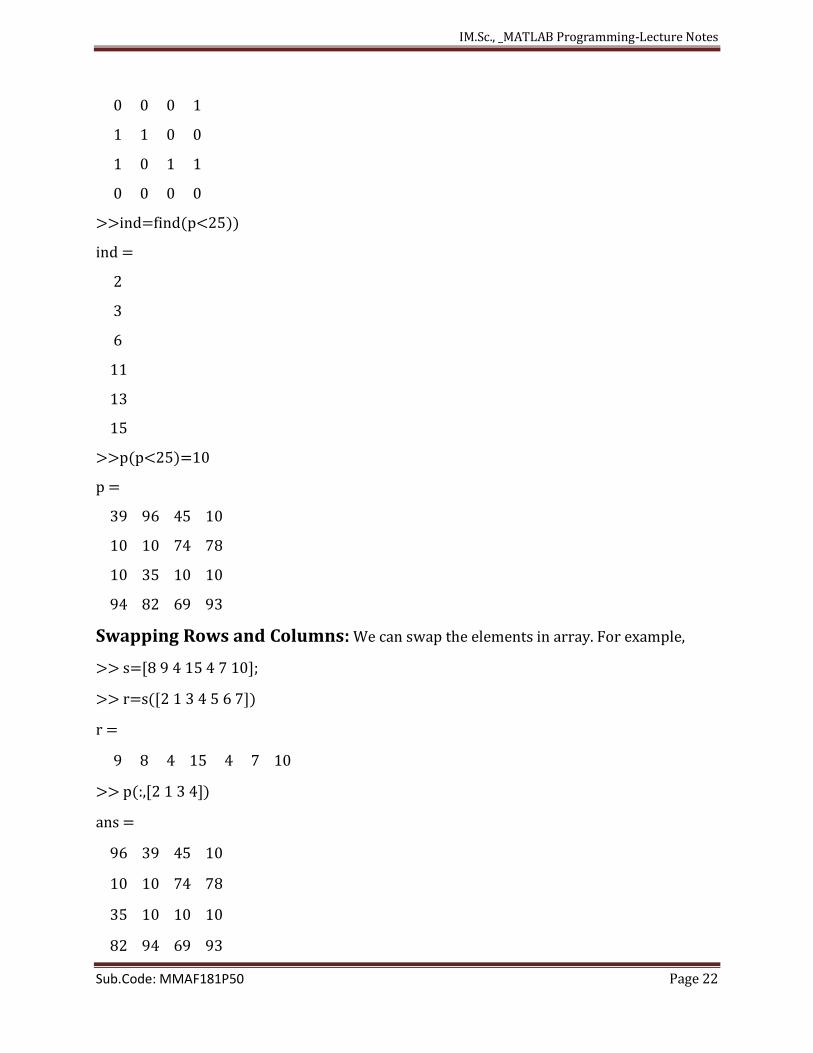
>> p<25
ans =
IM.Sc., _MATLAB Programming-Lecture Notes
Sub.Code: MMAF181P50 Page 22
0 0 0 1
1 1 0 0
1 0 1 1
0 0 0 0
>>ind=find(p<25))
ind =
2
3
6
11
13
15
>>p(p<25)=10
p =
39 96 45 10
10 10 74 78
10 35 10 10
94 82 69 93
Swapping Rows and Columns: We can swap the elements in array. For example,
>> s=[8 9 4 15 4 7 10];
>> r=s([2 1 3 4 5 6 7])
r =
9 8 4 15 4 7 10
>> p(:,[2 1 3 4])
ans =
96 39 45 10
10 10 74 78
35 10 10 10
82 94 69 93
IM.Sc., _MATLAB Programming-Lecture Notes
Sub.Code: MMAF181P50 Page 23
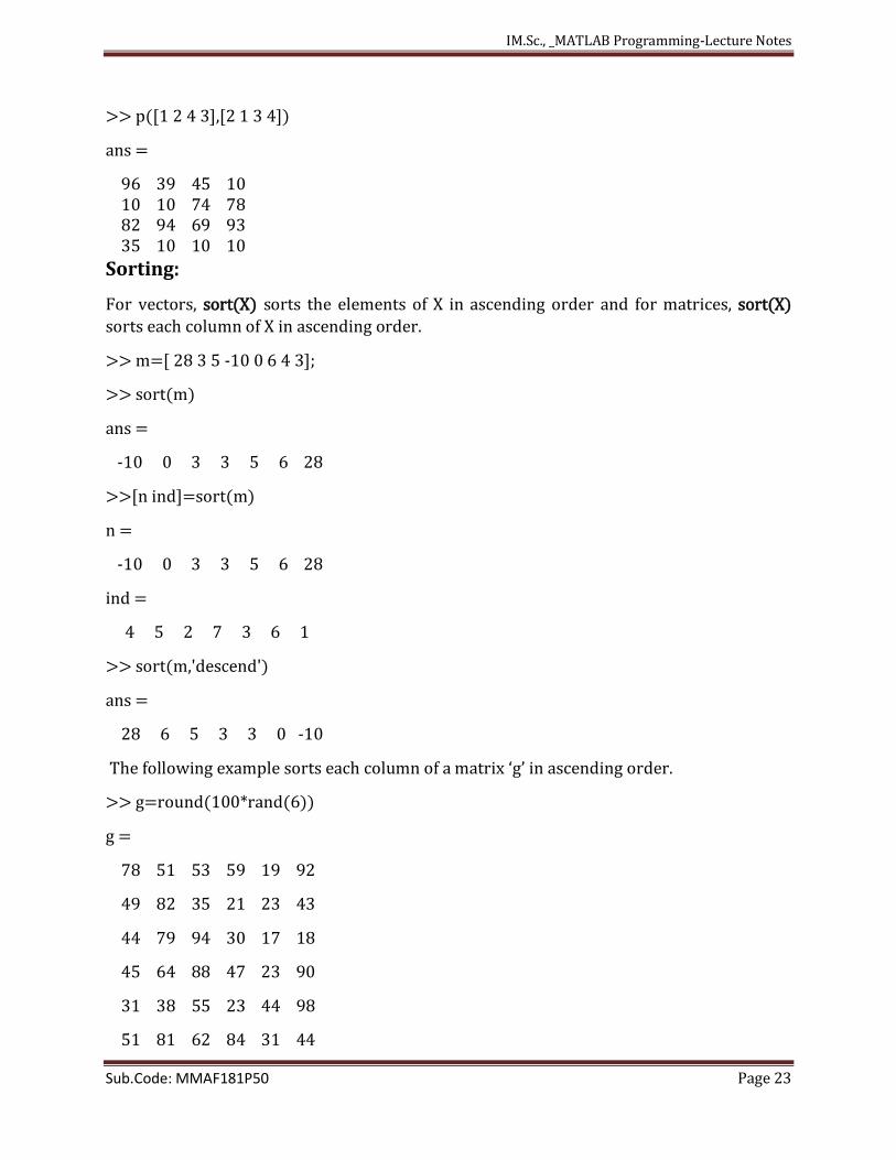
>> p([1 2 4 3],[2 1 3 4])
ans =
96 39 45 10 10 10 74 78 82 94 69 93 35 10 10 10
Sorting:
For vectors, sort(X) sorts the elements of X in ascending order and for matrices, sort(X)
sorts each column of X in ascending order.
>> m=[ 28 3 5 -10 0 6 4 3];
>> sort(m)
ans =
-10 0 3 3 5 6 28
>>[n ind]=sort(m)
n =
-10 0 3 3 5 6 28
ind =
4 5 2 7 3 6 1
>> sort(m,'descend')
ans =
28 6 5 3 3 0 -10
The following example sorts each column of a matrix ‘g’ in ascending order.
>> g=round(100*rand(6))
g =
78 51 53 59 19 92
49 82 35 21 23 43
44 79 94 30 17 18
45 64 88 47 23 90
31 38 55 23 44 98
51 81 62 84 31 44
IM.Sc., _MATLAB Programming-Lecture Notes
Sub.Code: MMAF181P50 Page 24
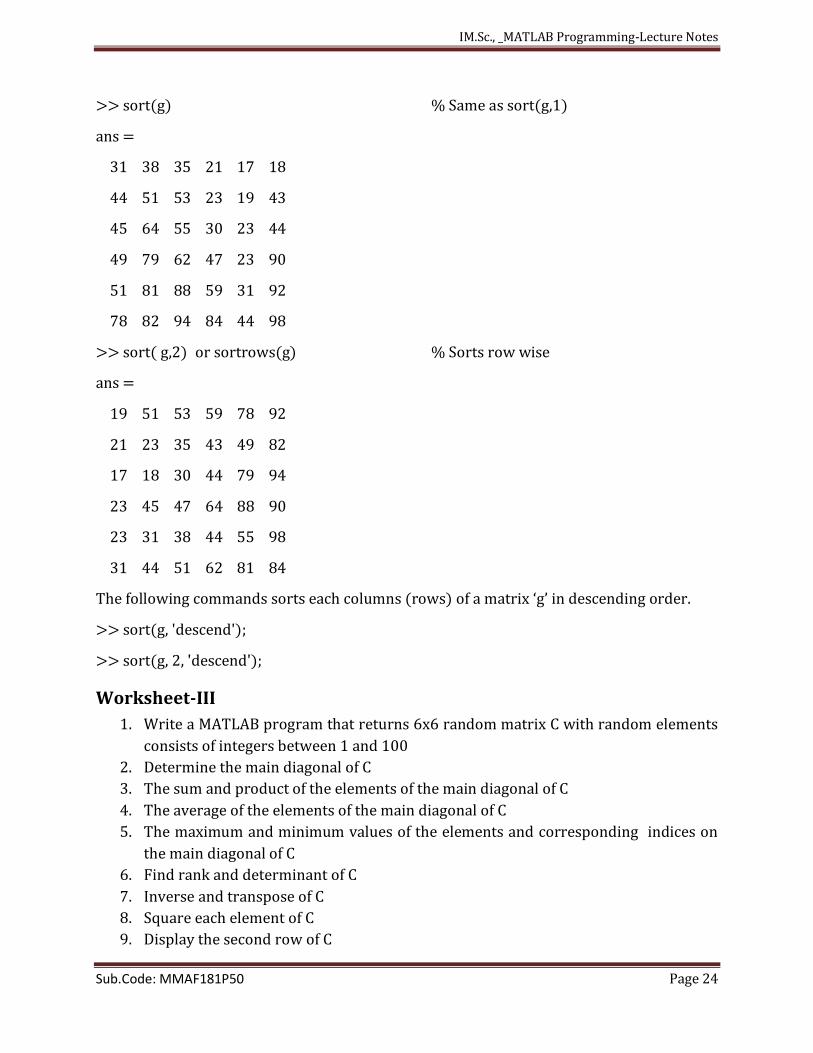
>> sort(g) % Same as sort(g,1)
ans =
31 38 35 21 17 18
44 51 53 23 19 43
45 64 55 30 23 44
49 79 62 47 23 90
51 81 88 59 31 92
78 82 94 84 44 98
>> sort( g,2) or sortrows(g) % Sorts row wise
ans =
19 51 53 59 78 92
21 23 35 43 49 82
17 18 30 44 79 94
23 45 47 64 88 90
23 31 38 44 55 98
31 44 51 62 81 84
The following commands sorts each columns (rows) of a matrix ‘g’ in descending order.
>> sort(g, 'descend');
>> sort(g, 2, 'descend');
Worksheet-III
1. Write a MATLAB program that returns 6x6 random matrix C with random elements
consists of integers between 1 and 100
2. Determine the main diagonal of C
3. The sum and product of the elements of the main diagonal of C
4. The average of the elements of the main diagonal of C
5. The maximum and minimum values of the elements and corresponding indices on
the main diagonal of C
6. Find rank and determinant of C
7. Inverse and transpose of C
8. Square each element of C
9. Display the second row of C
IM.Sc., _MATLAB Programming-Lecture Notes
Sub.Code: MMAF181P50 Page 25
10. Display second fourth and fifth rows
11. Reshape the matrix C into a 4X9 and 9x4 matrices
12. The matrix consisting of the square root of each element of C
13. Replace the (2,3) element of C by -7 and name the new matrix as D
14. Replace the 5th row by [1 0 1 0 1] and name the new matrix by E
15. Write MATLAB program to find 8!
16. Create two matrices P and Q each of size 2X5
17. Perform horizontal concatenation
18. Perform vertical concatenation
19. Create an array S of size 1x10 with arbitrary elements
20. Display even index elements of S by a command
21. Replace 5th element of S by -100
22. Create a matrix T of size 2 x3 with arbitrary elements and perform command
repmat (T,2,4) and observe the out put
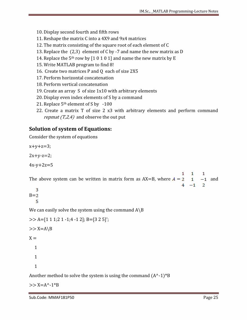
Solution of system of Equations:
Consider the system of equations
x+y+z=3;
2x+y-z=2;
4x-y+2z=5
The above system can be written in matrix form as AX=B, where and
B=
We can easily solve the system using the command A\B
>> A=[1 1 1;2 1 -1;4 -1 2]; B=[3 2 5]';
>> X=A\B
X =
1
1
1
Another method to solve the system is using the command (A^-1)*B
>> X=A^-1*B
IM.Sc., _MATLAB Programming-Lecture Notes
Sub.Code: MMAF181P50 Page 26
X =
1.0000
1.0000
1.0000
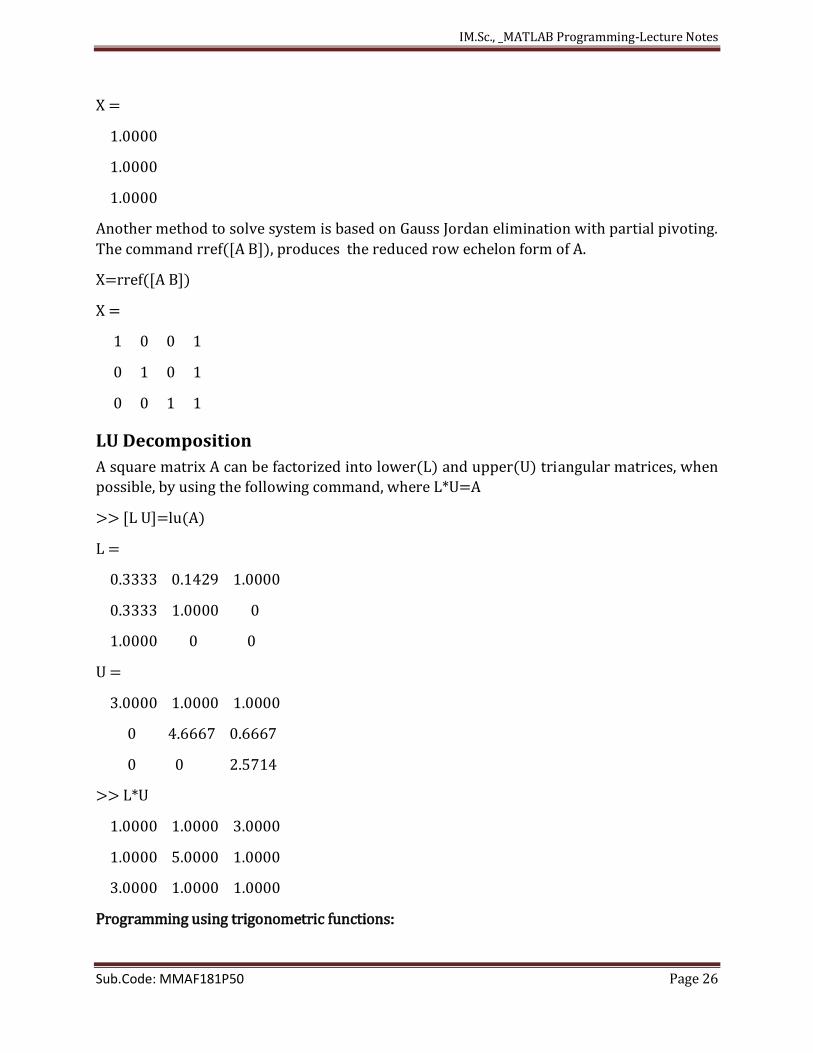
Another method to solve system is based on Gauss Jordan elimination with partial pivoting.
The command rref([A B]), produces the reduced row echelon form of A.
X=rref([A B])
X =
1 0 0 1
0 1 0 1
0 0 1 1
LU Decomposition
A square matrix A can be factorized into lower(L) and upper(U) triangular matrices, when
possible, by using the following command, where L*U=A
>> [L U]=lu(A)
L =
0.3333 0.1429 1.0000
0.3333 1.0000 0
1.0000 0 0
U =
3.0000 1.0000 1.0000
0 4.6667 0.6667
0 0 2.5714
>> L*U
1.0000 1.0000 3.0000
1.0000 5.0000 1.0000
3.0000 1.0000 1.0000
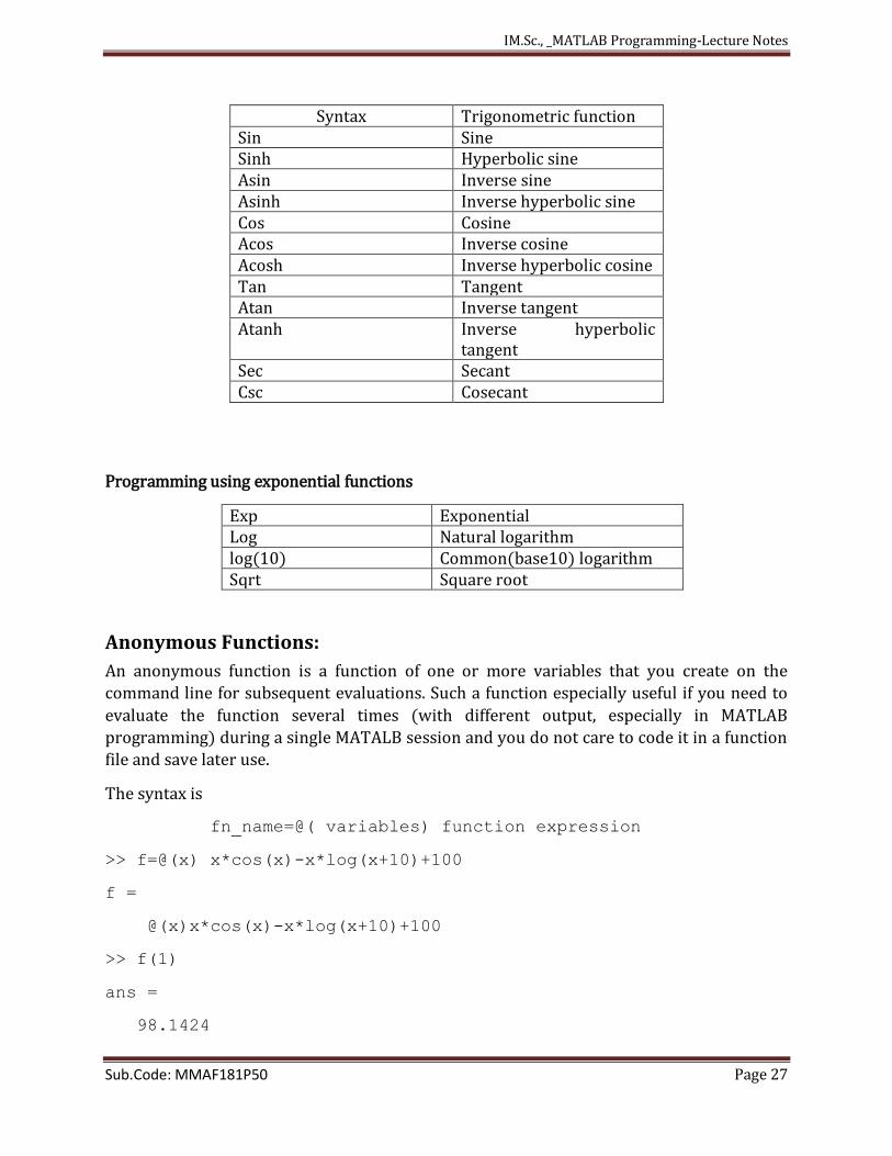
Programming using trigonometric functions:
IM.Sc., _MATLAB Programming-Lecture Notes
Sub.Code: MMAF181P50 Page 27
Syntax Trigonometric function Sin Sine Sinh Hyperbolic sine Asin Inverse sine Asinh Inverse hyperbolic sine Cos Cosine Acos Inverse cosine Acosh Inverse hyperbolic cosine Tan Tangent Atan Inverse tangent Atanh Inverse hyperbolic
tangent Sec Secant Csc Cosecant
Programming using exponential functions
Exp Exponential Log Natural logarithm log(10) Common(base10) logarithm Sqrt Square root
Anonymous Functions:
An anonymous function is a function of one or more variables that you create on the
command line for subsequent evaluations. Such a function especially useful if you need to
evaluate the function several times (with different output, especially in MATLAB
programming) during a single MATALB session and you do not care to code it in a function
file and save later use.
The syntax is
fn_name=@( variables) function expression
>> f=@(x) x*cos(x)-x*log(x+10)+100
f =
@(x)x*cos(x)-x*log(x+10)+100
>> f(1)
ans =
98.1424
IM.Sc., _MATLAB Programming-Lecture Notes
Sub.Code: MMAF181P50 Page 28
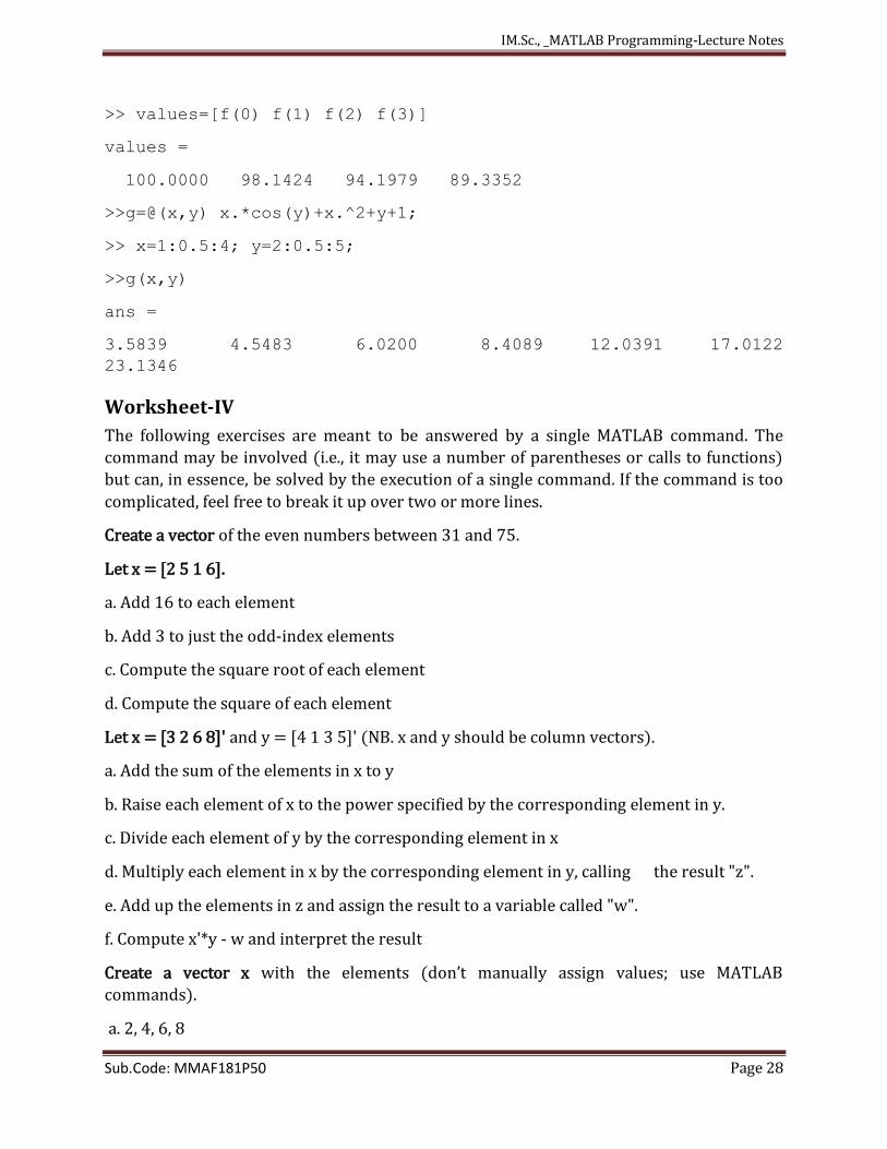
>> values=[f(0) f(1) f(2) f(3)]
values =
100.0000 98.1424 94.1979 89.3352
>>g=@(x,y) x.*cos(y)+x.^2+y+1;
>> x=1:0.5:4; y=2:0.5:5;
>>g(x,y)
ans =
3.5839 4.5483 6.0200 8.4089 12.0391 17.0122
23.1346
Worksheet-IV
The following exercises are meant to be answered by a single MATLAB command. The
command may be involved (i.e., it may use a number of parentheses or calls to functions)
but can, in essence, be solved by the execution of a single command. If the command is too
complicated, feel free to break it up over two or more lines.
Create a vector of the even numbers between 31 and 75.
Let x = [2 5 1 6].
a. Add 16 to each element
b. Add 3 to just the odd-index elements
c. Compute the square root of each element
d. Compute the square of each element
Let x = [3 2 6 8]' and y = [4 1 3 5]' (NB. x and y should be column vectors).
a. Add the sum of the elements in x to y
b. Raise each element of x to the power specified by the corresponding element in y.
c. Divide each element of y by the corresponding element in x
d. Multiply each element in x by the corresponding element in y, calling the result "z".
e. Add up the elements in z and assign the result to a variable called "w".
f. Compute x'*y - w and interpret the result
Create a vector x with the elements (don’t manually assign values; use MATLAB
commands).
a. 2, 4, 6, 8
IM.Sc., _MATLAB Programming-Lecture Notes
Sub.Code: MMAF181P50 Page 29
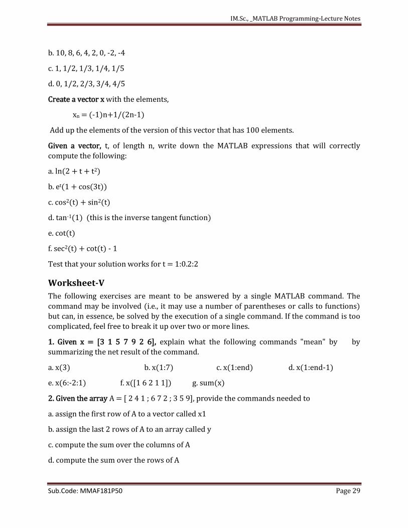
b. 10, 8, 6, 4, 2, 0, -2, -4
c. 1, 1/2, 1/3, 1/4, 1/5
d. 0, 1/2, 2/3, 3/4, 4/5
Create a vector x with the elements,
xn = (-1)n+1/(2n-1)
Add up the elements of the version of this vector that has 100 elements.
Given a vector, t, of length n, write down the MATLAB expressions that will correctly
compute the following:
a. ln(2 + t + t2)
b. et(1 + cos(3t))
c. cos2(t) + sin2(t)
d. tan-1(1) (this is the inverse tangent function)
e. cot(t)
f. sec2(t) + cot(t) - 1
Test that your solution works for t = 1:0.2:2
Worksheet-V
The following exercises are meant to be answered by a single MATLAB command. The
command may be involved (i.e., it may use a number of parentheses or calls to functions)
but can, in essence, be solved by the execution of a single command. If the command is too
complicated, feel free to break it up over two or more lines.
1. Given x = [3 1 5 7 9 2 6], explain what the following commands "mean" by by
summarizing the net result of the command.
a. x(3) b. x(1:7) c. x(1:end) d. x(1:end-1)
e. x(6:-2:1) f. x([1 6 2 1 1]) g. sum(x)
2. Given the array A = [ 2 4 1 ; 6 7 2 ; 3 5 9], provide the commands needed to
a. assign the first row of A to a vector called x1
b. assign the last 2 rows of A to an array called y
c. compute the sum over the columns of A
d. compute the sum over the rows of A
IM.Sc., _MATLAB Programming-Lecture Notes
Sub.Code: MMAF181P50 Page 30
e. compute the standard error of the mean of each column of A (NB. the standard error of
the mean is defined as the standard deviation divided by the square root of the number of
elements used to compute the mean.)
3. Given the arrays x = [1 4 8], y = [2 1 5] and A = [3 1 6 ; 5 2 7],
Determine which of the following statements will correctly execute and provide the result.
If the command will not correctly execute, state why it will not. Using the command whos
may be helpful here. a. x + y b. x + A c. x' + y d. A -
[x' y']
e. [x ; y'] f. [x ; y] g. A - 3
4. Given the array A = [2 7 9 7 ; 3 1 5 6 ; 8 1 2 5], explain the results of the following
commands:
a. A' b. A(:,[1 4]) c. A([2 3],[3 1])
d. reshape(A,2,6) e. A(:) f. flipud(A)
g. fliplr(A) h. [A A(end,:)] i. A(1:3,:)
j. [A ; A(1:2,:)] k. sum(A) l. sum(A')
m. sum(A,2) n. [ [ A ; sum(A) ] [ sum(A,2) ; sum(A(:)) ] ]
5. Given the array A from problem 4, above, provide the command that will
a. assign the even-numbered columns of A to an array called B
b. assign the odd-numbered rows to an array called C
c. convert A into a 4-by-3 array
d. compute the reciprocal of each element of A
e. compute the square-root of each element of A
Worksheet-VI
1. Create a two random matrices M, N of order 6X6, whose elements consists from 1 to 100.
2. Using command delete the second row of the matrix M and name it as P
3. Using command delete the 6th column of the matrix N and name it as Q
4. Add the second column of M and to the first column of N
5. Convert the matrix M to column and row vectors
6. Using command create the matrix R consisting of maximum values of either M or N
7. Using command create the matrix S consisting of minimum values of either M or N
IM.Sc., _MATLAB Programming-Lecture Notes
Sub.Code: MMAF181P50 Page 31
8. Using command create a matrix T by replacing all the elements above the main diagonal
of M by zeros
9. Using command create a matrix U by replacing all the elements below the main diagonal
of N by zeros
10. Perform the command cumprod(M), observe the output
11. Perform the command sort(M), observe the output
12. Perform the command sqrt(M), observe the output
13. Perform the command sqrtm(M), observe the output
14. Create the function 2( ) cos 2 /f x x x x and (a) evaluate f(0), f(1), f(pi/2) (b)
Evaluate f(x) where x=[0 1 pi/2 pi]
15. Create the following functions:
f(x) = x4-8x3+17x2-4x-20
g(x) = x2-4x+4
h(x) = x2-4x-5
(a) Evaluate f(x)-g(x)h(x) at x=3
(b) Evaluate f(x)-g(x)h(x) at x=[1 2 3 4 5]
(c ) Evaluate f(x)/g(x) –h(x) for any x
IM.Sc., _MATLAB Programming-Lecture Notes
Sub.Code: MMAF181P50 Page 32
3. PLOTTING
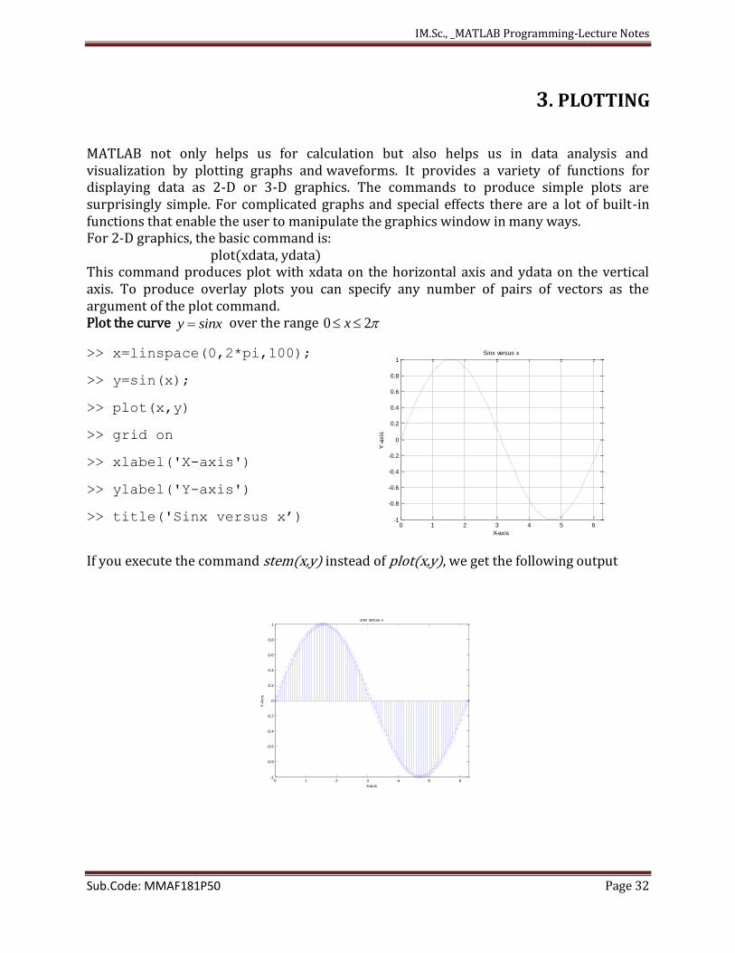
MATLAB not only helps us for calculation but also helps us in data analysis and visualization by plotting graphs and waveforms. It provides a variety of functions for displaying data as 2-D or 3-D graphics. The commands to produce simple plots are surprisingly simple. For complicated graphs and special effects there are a lot of built-in functions that enable the user to manipulate the graphics window in many ways. For 2-D graphics, the basic command is: plot(xdata, ydata) This command produces plot with xdata on the horizontal axis and ydata on the vertical axis. To produce overlay plots you can specify any number of pairs of vectors as the argument of the plot command. Plot the curve y sinx over the range 0 2x
>> x=linspace(0,2*pi,100);
>> y=sin(x);
>> plot(x,y)
>> grid on
>> xlabel('X-axis')
>> ylabel('Y-axis')
>> title('Sinx versus x’) 0 1 2 3 4 5 6
-1
-0.8
-0.6
-0.4
-0.2
0
0.2
0.4
0.6
0.8
1
X-axis
Y-a
xis
Sinx versus x
If you execute the command stem(x,y) instead of plot(x,y), we get the following output
0 1 2 3 4 5 6-1
-0.8
-0.6
-0.4
-0.2
0
0.2
0.4
0.6
0.8
1
X-axis
Y-A
xis
sinx versus x
IM.Sc., _MATLAB Programming-Lecture Notes
Sub.Code: MMAF181P50 Page 33
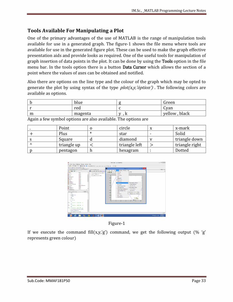
Tools Available For Manipulating a Plot
One of the primary advantages of the use of MATLAB is the range of manipulation tools
available for use in a generated graph. The figure-1 shows the file menu where tools are
available for use in the generated figure plot. These can be used to make the graph effective
presentation aids and provide looks as required. One of the useful tools for manipulation of
graph insertion of data points in the plot. It can be done by using the Tools option in the file
menu bar. In the tools option there is a button Data Cursor which allows the section of a
point where the values of axes can be obtained and notified.
Also there are options on the line type and the colour of the graph which may be opted to
generate the plot by using syntax of the type plot(x,y,’óption’) . The following colors are
available as options.
b blue g Green r red c Cyan m magenta y , k yellow , black
Again a few symbol options are also available. The options are
. Point o circle x x-mark + Plus * star - Solid s Square d diamond v triangle down ^ triangle up < triangle left > triangle right p pentagon h hexagram : Dotted
Figure-1
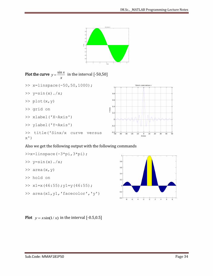
If we execute the command fill(x,y,’g’) command, we get the following output (% ‘g’
represents green colour)
IM.Sc., _MATLAB Programming-Lecture Notes
Sub.Code: MMAF181P50 Page 34
0 1 2 3 4 5 6-1
-0.8
-0.6
-0.4
-0.2
0
0.2
0.4
0.6
0.8
1
X-axis
Y-a
xis
Sinx versus x
Plot the curve sin x
yx
in the interval [-50,50]
>> x=linspace(-50,50,1000);
>> y=sin(x)./x;
>> plot(x,y)
>> grid on
>> xlabel('X-Axis')
>> ylabel('Y-Axis')
>> title('Sinx/x curve versus
x')
-50 -40 -30 -20 -10 0 10 20 30 40 50-0.4
-0.2
0
0.2
0.4
0.6
0.8
1
X-Axis
Y-A
xis
Sinx/x curve versus x
Also we get the following output with the following commands
>>x=linspace(-3*pi,3*pi);
>> y=sin(x)./x;
>> area(x,y)
>> hold on
>> x1=x(46:55);y1=y(46:55);
>> area(x1,y1,'facecolor','y')
-8 -6 -4 -2 0 2 4 6 8-0.4
-0.2
0
0.2
0.4
0.6
0.8
1
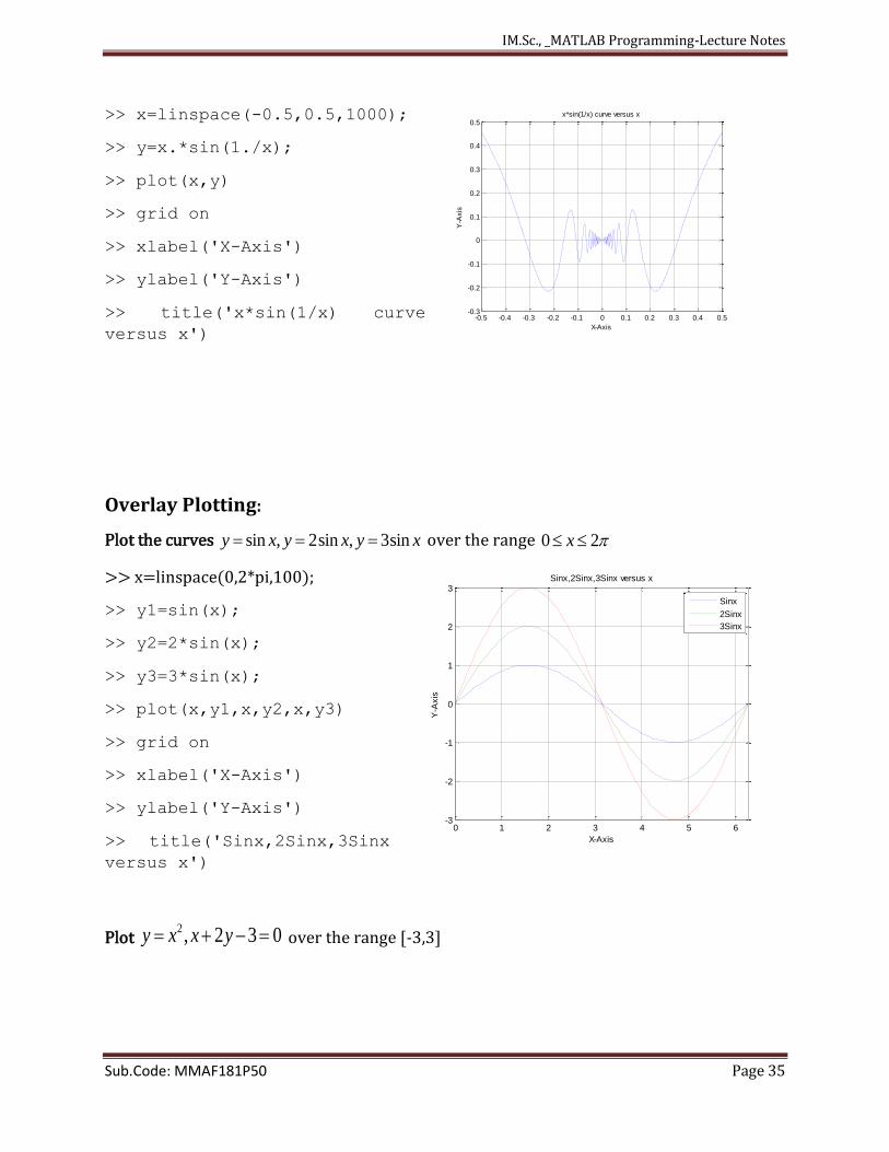
Plot sin(1/ )y x x in the interval [-0.5,0.5]
IM.Sc., _MATLAB Programming-Lecture Notes
Sub.Code: MMAF181P50 Page 35
>> x=linspace(-0.5,0.5,1000);
>> y=x.*sin(1./x);
>> plot(x,y)
>> grid on
>> xlabel('X-Axis')
>> ylabel('Y-Axis')
>> title('x*sin(1/x) curve
versus x')
-0.5 -0.4 -0.3 -0.2 -0.1 0 0.1 0.2 0.3 0.4 0.5-0.3
-0.2
-0.1
0
0.1
0.2
0.3
0.4
0.5
X-Axis
Y-A
xis
x*sin(1/x) curve versus x
Overlay Plotting:
Plot the curves sin , 2sin , 3siny x y x y x over the range 0 2x
>> x=linspace(0,2*pi,100);
>> y1=sin(x);
>> y2=2*sin(x);
>> y3=3*sin(x);
>> plot(x,y1,x,y2,x,y3)
>> grid on
>> xlabel('X-Axis')
>> ylabel('Y-Axis')
>> title('Sinx,2Sinx,3Sinx
versus x')
0 1 2 3 4 5 6-3
-2
-1
0
1
2
3
X-Axis
Y-A
xis
Sinx,2Sinx,3Sinx versus x
Sinx
2Sinx
3Sinx
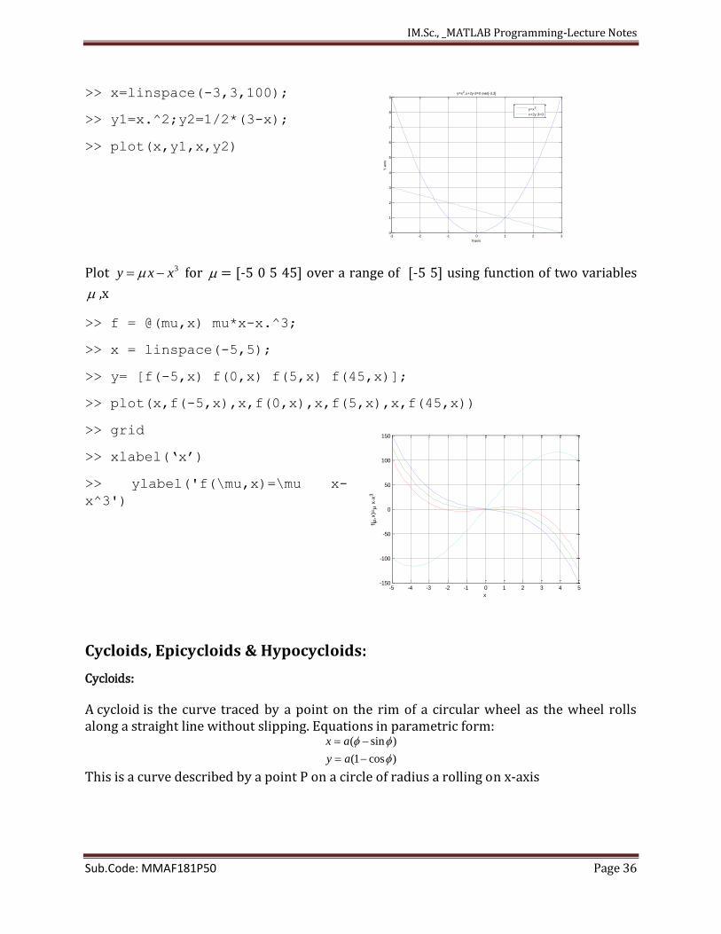
Plot 2 , 2 3 0y x x y over the range [-3,3]
IM.Sc., _MATLAB Programming-Lecture Notes
Sub.Code: MMAF181P50 Page 36
>> x=linspace(-3,3,100);
>> y1=x.^2;y2=1/2*(3-x);
>> plot(x,y1,x,y2)
-3 -2 -1 0 1 2 30
1
2
3
4
5
6
7
8
9
X-axis
Y-a
xis
y=x2,x+2y-3=0 over[-3,3]
y=x2
x+2y-3=0
Plot 3y x x for = [-5 0 5 45] over a range of [-5 5] using function of two variables
,x
>> f = @(mu,x) mu*x-x.^3;
>> x = linspace(-5,5);
>> y= [f(-5,x) f(0,x) f(5,x) f(45,x)];
>> plot(x,f(-5,x),x,f(0,x),x,f(5,x),x,f(45,x))
>> grid
>> xlabel(‘x’)
>> ylabel('f(\mu,x)=\mu x-
x^3')
-5 -4 -3 -2 -1 0 1 2 3 4 5-150
-100
-50
0
50
100
150
x
f(
,x)=
x-x
3
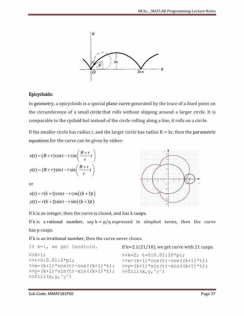
Cycloids, Epicycloids & Hypocycloids:
Cycloids: A cycloid is the curve traced by a point on the rim of a circular wheel as the wheel rolls along a straight line without slipping. Equations in parametric form:
( sin )
(1 cos )
x a
y a
This is a curve described by a point P on a circle of radius a rolling on x-axis
IM.Sc., _MATLAB Programming-Lecture Notes
Sub.Code: MMAF181P50 Page 37
Epicycloids:
In geometry, a epicycloids is a special plane curve generated by the trace of a fixed point on
the circumference of a small circle that rolls without slipping around a larger circle. It is
comparable to the cycloid but instead of the circle rolling along a line, it rolls on a circle.
If the smaller circle has radius r, and the larger circle has radius R = kr, then the parametric
equations for the curve can be given by either:
( ) ( ) cos cos
( ) ( )sin sin
R rx t R r t r t
r
R ry t R r t r t
r
or
( ) ( 1)cos cos ( 1)
( ) ( 1)sin sin ( 1)
x t r k t r k t
y t r k t r k t
If k is an integer, then the curve is closed, and has k cusps.
If k is a rational number, say k = p/q expressed in simplest terms, then the curve
has p cusps.
If k is an irrational number, then the curve never closes.
If k=1, we get Cardioid.
>>k=1;
>>t=0:0.01:2*pi;
>>x=(k+1)*cos(t)-cos((k+1)*t);
>>y=(k+1)*sin(t)-sin((k+1)*t);
>>fill(x,y,'y')
If k=2.1(21/10), we get curve with 21 cusps.
>>k=2; t=0:0.01:20*pi;
>>x=(k+1)*cos(t)-cos((k+1)*t);
>>y=(k+1)*sin(t)-sin((k+1)*t);
>>fill(x,y,'y')
IM.Sc., _MATLAB Programming-Lecture Notes
Sub.Code: MMAF181P50 Page 38
-3 -2.5 -2 -1.5 -1 -0.5 0 0.5 1 1.5-3
-2
-1
0
1
2
3
-5 -4 -3 -2 -1 0 1 2 3 4 5
-5
-4
-3
-2
-1
0
1
2
3
4
5
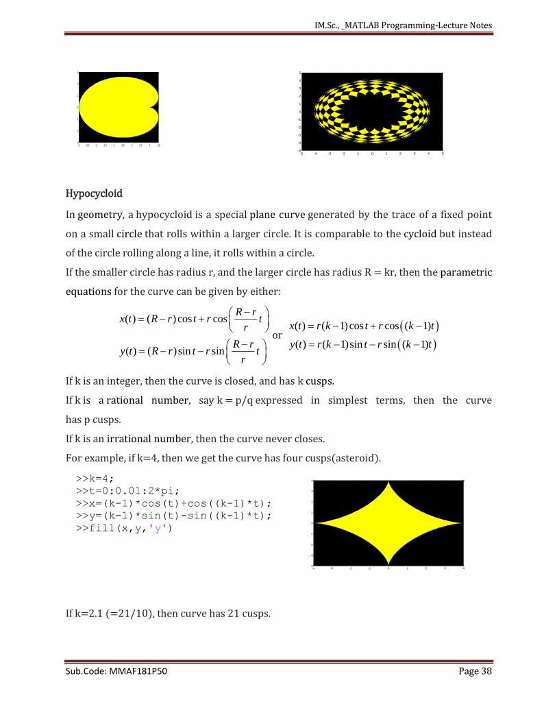
Hypocycloid
In geometry, a hypocycloid is a special plane curve generated by the trace of a fixed point
on a small circle that rolls within a larger circle. It is comparable to the cycloid but instead
of the circle rolling along a line, it rolls within a circle.
If the smaller circle has radius r, and the larger circle has radius R = kr, then the parametric
equations for the curve can be given by either:
( ) ( ) cos cos
( ) ( )sin sin
R rx t R r t r t
r
R ry t R r t r t
r
or
( ) ( 1)cos cos ( 1)
( ) ( 1)sin sin ( 1)
x t r k t r k t
y t r k t r k t
If k is an integer, then the curve is closed, and has k cusps.
If k is a rational number, say k = p/q expressed in simplest terms, then the curve
has p cusps.
If k is an irrational number, then the curve never closes.
For example, if k=4, then we get the curve has four cusps(asteroid).
>>k=4;
>>t=0:0.01:2*pi;
>>x=(k-1)*cos(t)+cos((k-1)*t);
>>y=(k-1)*sin(t)-sin((k-1)*t);
>>fill(x,y,'y')
-4 -3 -2 -1 0 1 2 3 4-4
-3
-2
-1
0
1
2
3
4
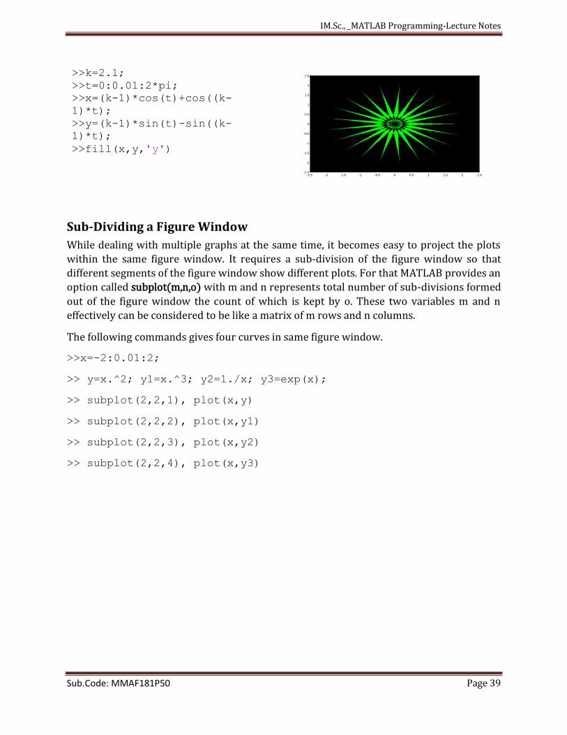
If k=2.1 (=21/10), then curve has 21 cusps.
IM.Sc., _MATLAB Programming-Lecture Notes
Sub.Code: MMAF181P50 Page 39
>>k=2.1;
>>t=0:0.01:2*pi;
>>x=(k-1)*cos(t)+cos((k-
1)*t);
>>y=(k-1)*sin(t)-sin((k-
1)*t);
>>fill(x,y,'y')
-2.5 -2 -1.5 -1 -0.5 0 0.5 1 1.5 2 2.5-2.5
-2
-1.5
-1
-0.5
0
0.5
1
1.5
2
2.5
Sub-Dividing a Figure Window
While dealing with multiple graphs at the same time, it becomes easy to project the plots
within the same figure window. It requires a sub-division of the figure window so that
different segments of the figure window show different plots. For that MATLAB provides an
option called subplot(m,n,o) with m and n represents total number of sub-divisions formed
out of the figure window the count of which is kept by o. These two variables m and n
effectively can be considered to be like a matrix of m rows and n columns.
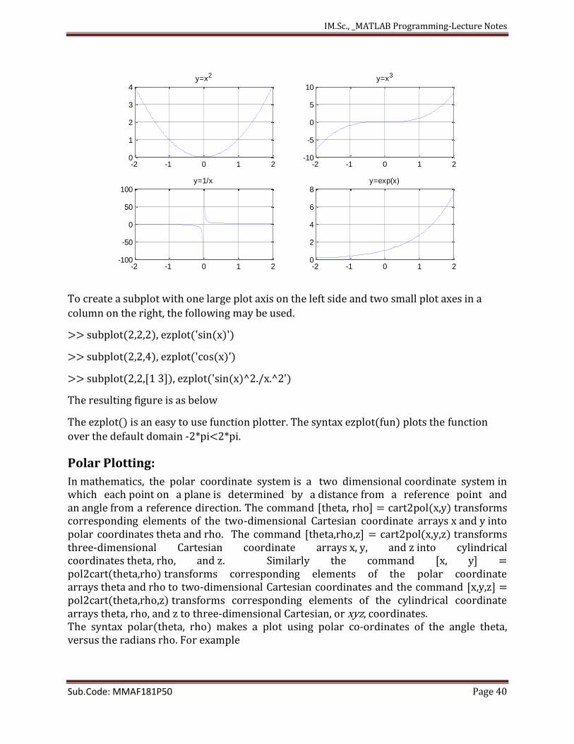
The following commands gives four curves in same figure window.
>>x=-2:0.01:2;
>> y=x.^2; y1=x.^3; y2=1./x; y3=exp(x);
>> subplot(2,2,1), plot(x,y)
>> subplot(2,2,2), plot(x,y1)
>> subplot(2,2,3), plot(x,y2)
>> subplot(2,2,4), plot(x,y3)
IM.Sc., _MATLAB Programming-Lecture Notes
Sub.Code: MMAF181P50 Page 40
-2 -1 0 1 20
1
2
3
4y=x2
-2 -1 0 1 2-10
-5
0
5
10y=x3
-2 -1 0 1 2-100
-50
0
50
100y=1/x
-2 -1 0 1 20
2
4
6
8y=exp(x)
To create a subplot with one large plot axis on the left side and two small plot axes in a
column on the right, the following may be used.
>> subplot(2,2,2), ezplot('sin(x)')
>> subplot(2,2,4), ezplot('cos(x)')
>> subplot(2,2,[1 3]), ezplot('sin(x)^2./x.^2')
The resulting figure is as below
The ezplot() is an easy to use function plotter. The syntax ezplot(fun) plots the function
over the default domain -2*pi<2*pi.
Polar Plotting:
In mathematics, the polar coordinate system is a two dimensional coordinate system in which each point on a plane is determined by a distance from a reference point and an angle from a reference direction. The command [theta, rho] = cart2pol(x,y) transforms corresponding elements of the two-dimensional Cartesian coordinate arrays x and y into polar coordinates theta and rho. The command [theta,rho,z] = cart2pol(x,y,z) transforms three-dimensional Cartesian coordinate arrays x, y, and z into cylindrical coordinates theta, rho, and z. Similarly the command [x, y] = pol2cart(theta,rho) transforms corresponding elements of the polar coordinate arrays theta and rho to two-dimensional Cartesian coordinates and the command [x,y,z] = pol2cart(theta,rho,z) transforms corresponding elements of the cylindrical coordinate arrays theta, rho, and z to three-dimensional Cartesian, or xyz, coordinates. The syntax polar(theta, rho) makes a plot using polar co-ordinates of the angle theta, versus the radians rho. For example
IM.Sc., _MATLAB Programming-Lecture Notes
Sub.Code: MMAF181P50 Page 41
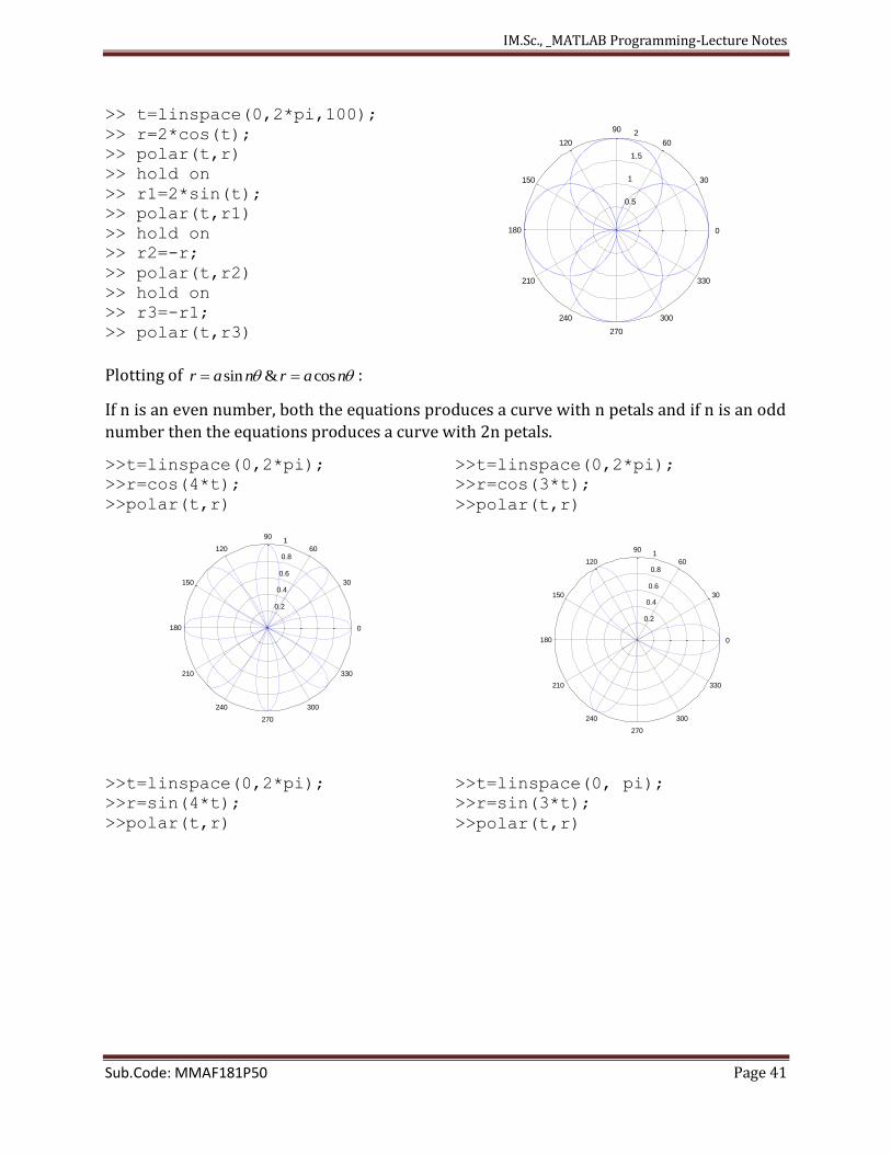
>> t=linspace(0,2*pi,100);
>> r=2*cos(t);
>> polar(t,r)
>> hold on
>> r1=2*sin(t);
>> polar(t,r1)
>> hold on
>> r2=-r;
>> polar(t,r2)
>> hold on
>> r3=-r1;
>> polar(t,r3)
0.5
1
1.5
2
30
210
60
240
90
270
120
300
150
330
180 0
Plotting of sin & cosr a n r a n :
If n is an even number, both the equations produces a curve with n petals and if n is an odd
number then the equations produces a curve with 2n petals.
>>t=linspace(0,2*pi);
>>r=cos(4*t);
>>polar(t,r)
0.2
0.4
0.6
0.8
1
30
210
60
240
90
270
120
300
150
330
180 0
>>t=linspace(0,2*pi);
>>r=cos(3*t);
>>polar(t,r)
0.2
0.4
0.6
0.8
1
30
210
60
240
90
270
120
300
150
330
180 0
>>t=linspace(0,2*pi);
>>r=sin(4*t);
>>polar(t,r)
>>t=linspace(0, pi);
>>r=sin(3*t);
>>polar(t,r)
IM.Sc., _MATLAB Programming-Lecture Notes
Sub.Code: MMAF181P50 Page 42
0.2
0.4
0.6
0.8
1
30
210
60
240
90
270
120
300
150
330
180 0
0.2
0.4
0.6
0.8
1
30
210
60
240
90
270
120
300
150
330
180 0
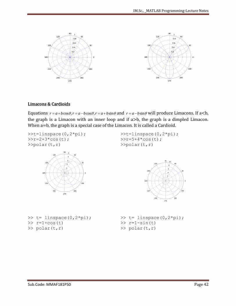
Limacons & Cardioids
Equations cos , cos , sinr a b r a b r a b and sinr a b will produce Limacons. If a<b,
the graph is a Limacon with an inner loop and if a>b, the graph is a dimpled Limacon.
When a=b, the graph is a special case of the Limacon. It is called a Cardioid.
>>t=linspace(0,2*pi);
>>r=2+3*cos(t);
>>polar(t,r)
1
2
3
4
5
30
210
60
240
90
270
120
300
150
330
180 0
>>t=linspace(0,2*pi);
>>r=5+4*cos(t);
>>polar(t,r)
2
4
6
8
10
30
210
60
240
90
270
120
300
150
330
180 0
>> t= linspace(0,2*pi);
>> r=1+cos(t)
>> polar(t,r)
>> t= linspace(0,2*pi);
>> r=1-sin(t)
>> polar(t,r)
IM.Sc., _MATLAB Programming-Lecture Notes
Sub.Code: MMAF181P50 Page 43
0.5
1
1.5
2
30
210
60
240
90
270
120
300
150
330
180 0
0.5
1
1.5
2
30
210
60
240
90
270
120
300
150
330
180 0
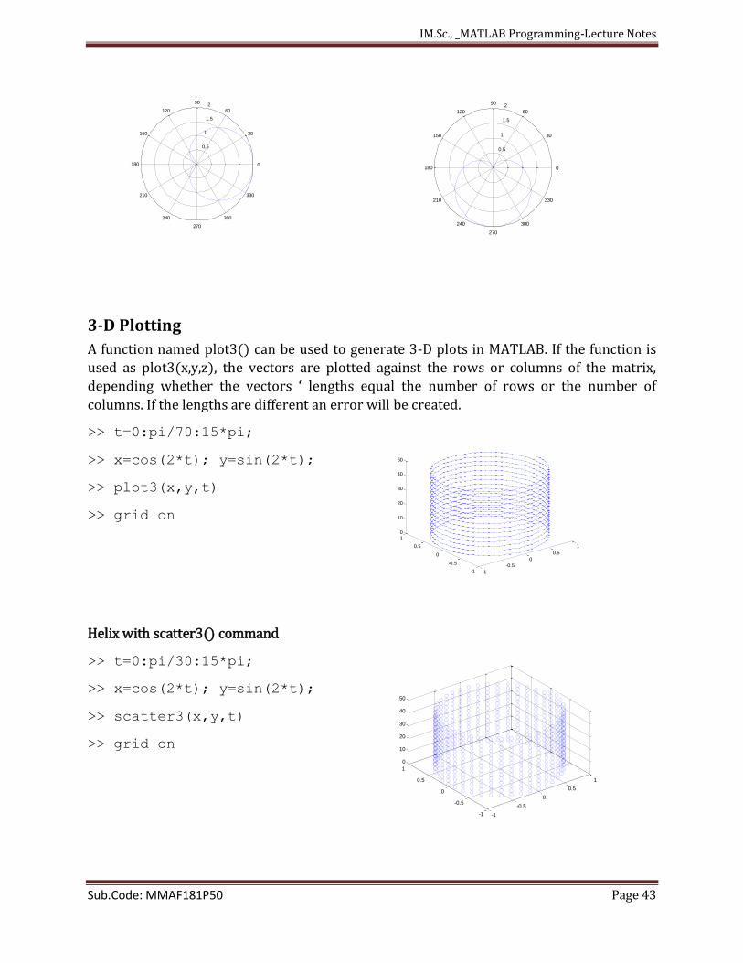
3-D Plotting
A function named plot3() can be used to generate 3-D plots in MATLAB. If the function is
used as plot3(x,y,z), the vectors are plotted against the rows or columns of the matrix,
depending whether the vectors ‘ lengths equal the number of rows or the number of
columns. If the lengths are different an error will be created.
>> t=0:pi/70:15*pi;
>> x=cos(2*t); y=sin(2*t);
>> plot3(x,y,t)
>> grid on
-1
-0.5
0
0.5
1
-1
-0.5
0
0.5
10
10
20
30
40
50
Helix with scatter3() command
>> t=0:pi/30:15*pi;
>> x=cos(2*t); y=sin(2*t);
>> scatter3(x,y,t)
>> grid on
-1
-0.5
0
0.5
1
-1
-0.5
0
0.5
1
0
10
20
30
40
50
IM.Sc., _MATLAB Programming-Lecture Notes
Sub.Code: MMAF181P50 Page 44
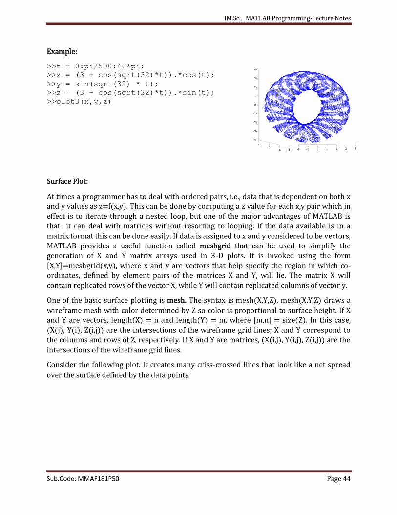
Example:
>>t = 0:pi/500:40*pi;
>>x = (3 + cos(sqrt(32)*t)).*cos(t);
>>y = sin(sqrt(32) * t);
>>z = (3 + cos(sqrt(32)*t)).*sin(t);
>>plot3(x,y,z)
-4 -3 -2 -1 0 1 2 3 4-10
1
-4
-3
-2
-1
0
1
2
3
4
Surface Plot:
At times a programmer has to deal with ordered pairs, i.e., data that is dependent on both x
and y values as z=f(x,y). This can be done by computing a z value for each x,y pair which in
effect is to iterate through a nested loop, but one of the major advantages of MATLAB is
that it can deal with matrices without resorting to looping. If the data available is in a
matrix format this can be done easily. If data is assigned to x and y considered to be vectors,
MATLAB provides a useful function called meshgrid that can be used to simplify the
generation of X and Y matrix arrays used in 3-D plots. It is invoked using the form
[X,Y]=meshgrid(x,y), where x and y are vectors that help specify the region in which co-
ordinates, defined by element pairs of the matrices X and Y, will lie. The matrix X will
contain replicated rows of the vector X, while Y will contain replicated columns of vector y.
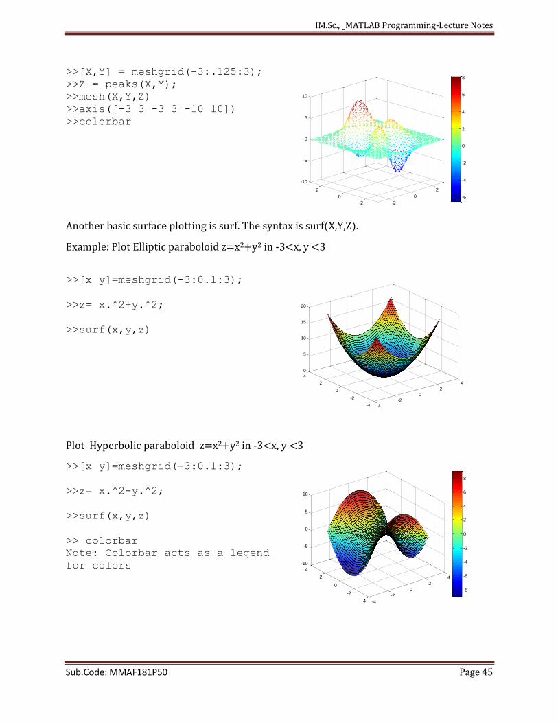
One of the basic surface plotting is mesh. The syntax is mesh(X,Y,Z). mesh(X,Y,Z) draws a
wireframe mesh with color determined by Z so color is proportional to surface height. If X
and Y are vectors, length(X) = n and length(Y) = m, where [m,n] = size(Z). In this case,
(X(j), Y(i), Z(i,j)) are the intersections of the wireframe grid lines; X and Y correspond to
the columns and rows of Z, respectively. If X and Y are matrices, (X(i,j), Y(i,j), Z(i,j)) are the
intersections of the wireframe grid lines.
Consider the following plot. It creates many criss-crossed lines that look like a net spread
over the surface defined by the data points.
IM.Sc., _MATLAB Programming-Lecture Notes
Sub.Code: MMAF181P50 Page 45
>>[X,Y] = meshgrid(-3:.125:3);
>>Z = peaks(X,Y);
>>mesh(X,Y,Z)
>>axis([-3 3 -3 3 -10 10])
>>colorbar
-2
0
2
-2
0
2
-10
-5
0
5
10
-6
-4
-2
0
2
4
6
8
Another basic surface plotting is surf. The syntax is surf(X,Y,Z).
Example: Plot Elliptic paraboloid z=x2+y2 in -3<x, y <3
>>[x y]=meshgrid(-3:0.1:3);
>>z= x.^2+y.^2;
>>surf(x,y,z)
-4
-2
0
2
4
-4
-2
0
2
40
5
10
15
20
Plot Hyperbolic paraboloid z=x2+y2 in -3<x, y <3
>>[x y]=meshgrid(-3:0.1:3);
>>z= x.^2-y.^2;
>>surf(x,y,z)
>> colorbar
Note: Colorbar acts as a legend
for colors
-4
-2
0
2
4
-4
-2
0
2
4
-10
-5
0
5
10
-8
-6
-4
-2
0
2
4
6
8
IM.Sc., _MATLAB Programming-Lecture Notes
Sub.Code: MMAF181P50 Page 46
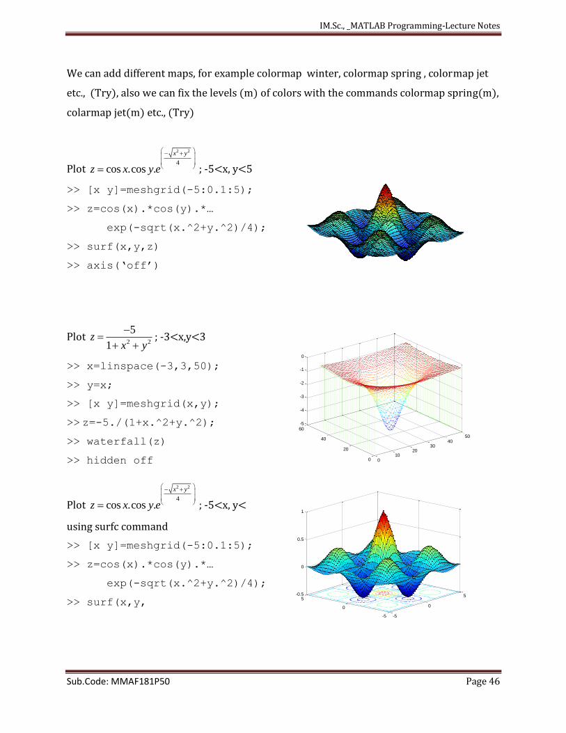
We can add different maps, for example colormap winter, colormap spring , colormap jet
etc., (Try), also we can fix the levels (m) of colors with the commands colormap spring(m),
colarmap jet(m) etc., (Try)
Plot
2 2
4
cos .cos .
x y
z x y e
; -5<x, y<5
>> [x y]=meshgrid(-5:0.1:5);
>> z=cos(x).*cos(y).*…
exp(-sqrt(x.^2+y.^2)/4);
>> surf(x,y,z)
>> axis(‘off’)
Plot 2 2
5
1z
x y
; -3<x,y<3
>> x=linspace(-3,3,50);
>> y=x;
>> [x y]=meshgrid(x,y);
>> z=-5./(1+x.^2+y.^2);
>> waterfall(z)
>> hidden off 010
2030
4050
0
20
40
60-5
-4
-3
-2
-1
0
Plot
2 2
4
cos .cos .
x y
z x y e
; -5<x, y<
using surfc command
>> [x y]=meshgrid(-5:0.1:5);
>> z=cos(x).*cos(y).*…
exp(-sqrt(x.^2+y.^2)/4);
>> surf(x,y,
-5
0
5
-5
0
5-0.5
0
0.5
1
IM.Sc., _MATLAB Programming-Lecture Notes
Sub.Code: MMAF181P50 Page 47
Worksheet-VII
1. Plot f(x) and ( )
( ) ( )
f x
g x h xover [ 5 5]x where f(x), g(x) and h(x) are in problem number
15, worksheet VI.
2. Plot y=cosx and 2 2
12 24
x xz for 0 x
3. Plot y= sinx; y=x and 3 5
6 150
x xz x in 0 x
4. Plot 2 2sin sinz x y in –pi/2<x,y<pi/2
5. Plot 2 2
2 2
( )xy x yz
x y
in -3<x,y<3
6. Plot z= sinx+cosy in 0<x,y <10
7. Plot the contour plot
2 2
4cos cos
x y
z x ye
in -5 < x, y<5 using the command surfc(z)
8. Plot the above with the command surfl(z) . (Use commands ‘shading interp’ and
colormap hot commands to get different colours).
Hint: The command ‘shading interp’ gets rid of black lines in the surface plot
IM.Sc., _MATLAB Programming-Lecture Notes
Sub.Code: MMAF181P50 Page 48
4. MATLAB PROGRAMMING
MATLAB provides its own language, which incorporates many features from C. In some
regards, it is a higher-level language than most common programming languages, such as
Pascal, Fortran, and C, meaning that you will spend less time worrying about formalisms
and syntax. For the most part, MATLAB’s language feels somewhat natural.
Disp, Input and Fprint Commands:
Disp Command:
The general form of disp for a numeric variable is
disp( variable )
When you use disp, the variable name is not displayed, and you don’t get a line feed before
the value is displayed, as you do when you enter a variable name on the command line
without a semi-colon. disp generally gives a neater display.
>> x=2
x =
2
>> disp(x)
2
You can also use disp to display a message enclosed in single quotes (called a string). Single
quotes which are part of the message must be repeated, e.g.
>> disp( 'Srinivas, ’’What is Matlab?’’' )
Srinivas, ’’What is Matlab?’’
To display a message and a numeric value on the same line use the following trick:
>> x = 2;
>> disp(['Your value is ',num2str(x)])
Your value is 2
You can display more than one number on a line as follows:
disp( [x y z] )
The square brackets create a vector with three elements, which are all displayed.
Input Command
IM.Sc., _MATLAB Programming-Lecture Notes
Sub.Code: MMAF181P50 Page 49
The input function has the following format
n=input('Enter the value of n')
When we run a program containing input statement, it will prompt the message inside the
single quote and then wait for the user to give input values. As soon as user presses return
key after entering the value, the value will be assigned to the variable n. Let us write a
simple program on command line.
>> n=input('Enter the value of n\n') % \n to introduce a new line
Enter the value of n
6
n =
6
>> n=input('Enter the value of n\n')
Enter the value of n
[4 5 6;2 0 3]
n =
4 5 6
2 0 3
fprintf Command
It is used for writing formatted data to a file or on screen similar to fprintf in C language.
However, we shall mainly discuss here how fprintf can produce formatted output on
display screen.
It has the following format
fprintf ( format_specifier, list_of_variables)
which writes or prints the values of variables in the list on screen in the format specified by
format-specifier string. The format-specifier symbols are written with the % preceding
them. The following is a list of commonly used format-specifiers
Format
symbol
Description
d For an integer value
u For an unsigned integer
IM.Sc., _MATLAB Programming-Lecture Notes
Sub.Code: MMAF181P50 Page 50
f For a floating point integer
e For a number in exponential number
g For an exponential or floating notation which
ever suits best
The format-specifiers are to be enclosed within a single quote. We have to provide
matching format-specifier for the data to be printed. Otherwise, wrong or undesired output
will be displayed. Also, all format-specifiers listed above except the string-specifier can be
preceded by an integer indicating the width attribute. For example, %3d denotes 3 spaces
are reserved for an integer value. For floating point format-specifiers, such as f,e and g, in
addition to width attribute, it has another attribute known as precision attribute. So, a
floating format-specifier is in general can be written as %w.p, where w denotes the width
of spaces to be reserved for the floating point number, p denotes the number spaces out of
w to be set for precision p. So, p can’t be greater than w. If so, it is ignored and the default
width is used. For example
a=10;
>> fprintf('The value of a is %d \n',a)
The value of a is 10
Note: \n in the string to introduce new line
One more example is
>> fprintf('The square of %d is %d \n',a,a^2)
The square of 10 is 100
fprintf('%s proved that square of %d is %d \n','Srinivas',a,a^2)
Srinivas proved that square of 10 is 100
Programs
Example 1: Write a MATLAB program to find a factorial of a number?
>> n=1:10;
>> fact=prod(n)
IM.Sc., _MATLAB Programming-Lecture Notes
Sub.Code: MMAF181P50 Page 51
Example 2: Write a MATLAB program that returns the sequence consisting of square of the
first 50 even numbers, and identify and display the first, fifth, and tenth element of the
sequence.
>> n=0:2:98;
>>sq_even=n^.2
>> sq_even(5) % To identify 5th element
Introduction to M-file Scripts:
A script file is usually a sequence of executable commands typed and saved in a file with
extension .m which would indicate that it is a MATLAB program file. MATLAB has another
form of program called function which is also saved in a filename with extension .m. When
a script file is created, the filename of the script file becomes command. That is, we can
execute the script file by typing only the filename, i.e., all the executable commands in the
file will be automatically executed in same sequence they are written in the file. So, once a
script file has been made for a problem we need to type only the filename to find its
solution whenever required.
Creating, Saving and Running an M-file:
We can type in your program code using any text editor or using the MATLAB
Editor/Debugger. Writing program codes in the Editor/Debugger is easier and handy as it
has special facilities to edit and debug the file. We can create a new blank M-file for writing
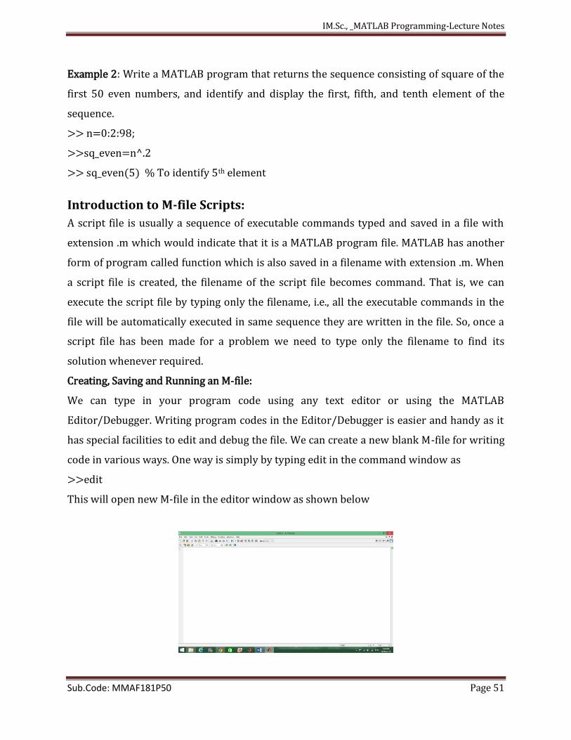
code in various ways. One way is simply by typing edit in the command window as
>>edit
This will open new M-file in the editor window as shown below
IM.Sc., _MATLAB Programming-Lecture Notes
Sub.Code: MMAF181P50 Page 52
Another way is just by clicking the New M-file icon from the toolbar of the command
window. Or, select File menu and from the dropdown menu select New and then select M-
file. When a new window is opened, we can type program codes in it.
Once we open a new file in editor window, we can save it at any time, just at the beginning
or at very end of writing the program code or in the middle of writing the program. Most
often we save it in the middle or after we finish typing the code. There are two save options
available: Save and Save as. Save as option allows us to save the program in any directory
and Save will save the file in the current working directory. In either case, the Save dialog
box will appear and we have to enter appropriate file name. This filename will be used as
command when running the program. Hence, a suitable name may be given to remind us of
about the purpose of the file.
Once a program file is saved, we can run it easily in different ways. We can directly run the
program from the editor window by clicking the save and run icon present in the toolbar. If
there is a error, the line number and accompanying error message will be displayed.
Modify if there is any syntax error, then save and run it. If there is no error, it should run
properly. Once a script file is tested OK, then its filename becomes command. We can run
the program by typing its filename in the command window.
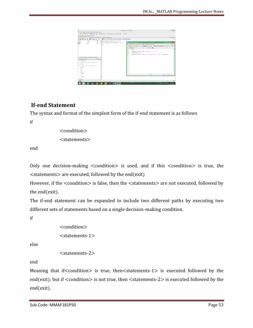
Writing & Executing the Script File
Open a new editor and type the following lines as shown below. Save the file with suitable
name and run the program
clc
n=input(‘Enter the Value of n=’);
fact=prod(1:n);
fprintf(‘The factorial value of %d is %d\n’, n,fact)
IM.Sc., _MATLAB Programming-Lecture Notes
Sub.Code: MMAF181P50 Page 53
If-end Statement
The syntax and format of the simplest form of the if-end statement is as follows
if
<condition>
<statements>
end
Only one decision-making <condition> is used, and if this <condition> is true, the
<statements> are executed, followed by the end(exit)
However, if the <condition> is false, then the <statements> are not executed, followed by
the end(exit).
The if-end statement can be expanded to include two different paths by executing two
different sets of statements based on a single decision-making condition.
if
<condition>
<statements-1>
else
<statements-2>
end
Meaning that if<condition> is true, then<statements-1> is executed followed by the
end(exit); but if <condition> is not true, then <statements-2> is executed followed by the
end(exit).
IM.Sc., _MATLAB Programming-Lecture Notes
Sub.Code: MMAF181P50 Page 54
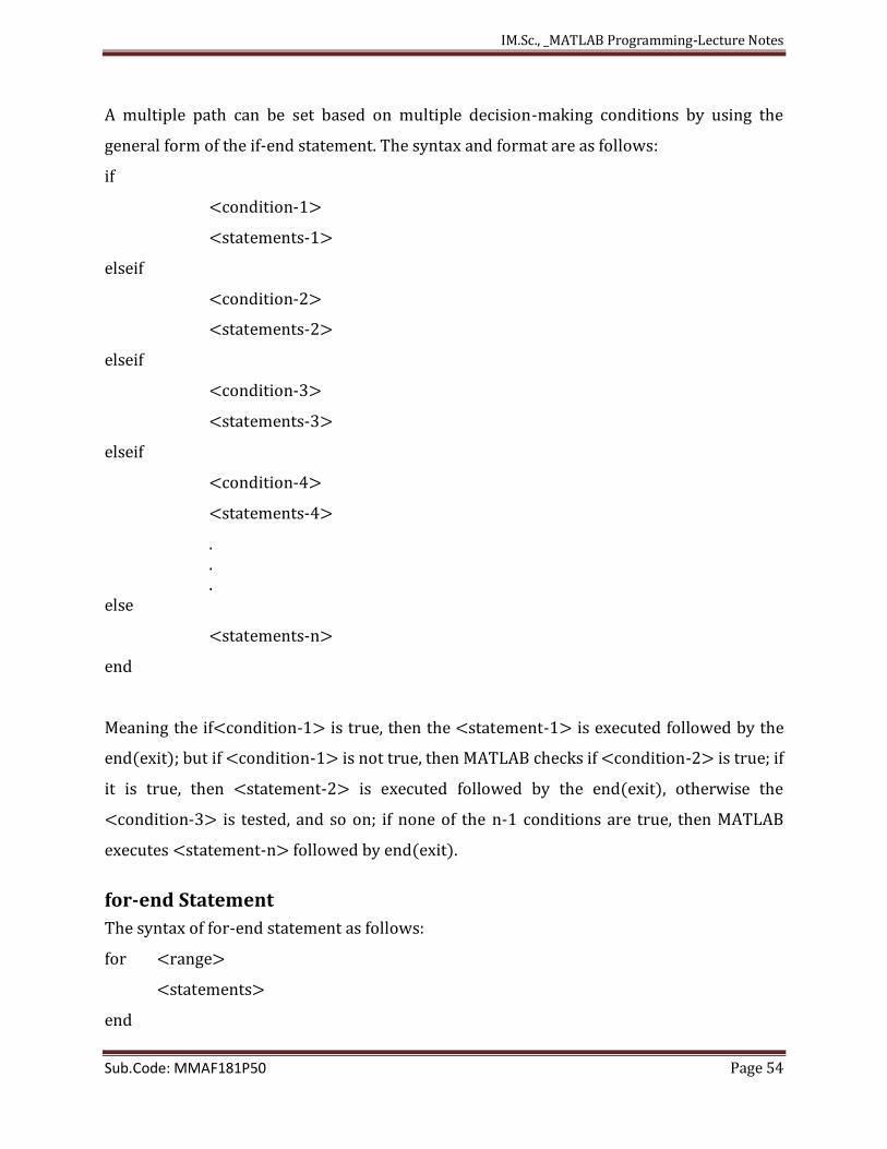
A multiple path can be set based on multiple decision-making conditions by using the
general form of the if-end statement. The syntax and format are as follows:
if
<condition-1>
<statements-1>
elseif
<condition-2>
<statements-2>
elseif
<condition-3>
<statements-3>
elseif
<condition-4>
<statements-4>
. .
. else
<statements-n>
end
Meaning the if<condition-1> is true, then the <statement-1> is executed followed by the
end(exit); but if <condition-1> is not true, then MATLAB checks if <condition-2> is true; if
it is true, then <statement-2> is executed followed by the end(exit), otherwise the
<condition-3> is tested, and so on; if none of the n-1 conditions are true, then MATLAB
executes <statement-n> followed by end(exit).
for-end Statement
The syntax of for-end statement as follows:
for <range>
<statements>
end
IM.Sc., _MATLAB Programming-Lecture Notes
Sub.Code: MMAF181P50 Page 55
referred as the for-end statement is used to create a loop that executes repetitively the
<statements> a fixed number of times based on the specified <range>. The specified
<range> is frequently given by a vector or a matrix.
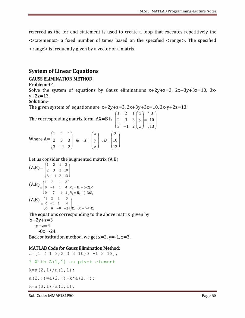
System of Linear Equations
GAUSS ELIMINATION METHOD Problem:-01 Solve the system of equations by Gauss eliminations x+2y+z=3, 2x+3y+3z=10, 3x-y+2z=13. Solution:- The given system of equations are x+2y+z=3, 2x+3y+3z=10, 3x-y+2z=13.
The corresponding matrix form AX=B is
13
10
3
213
332
121
z
y
x
Where A=
13
10
3
,&
213
332
121
B
z
y
x
X
Let us consider the augmented matrix (A,B)
(A,B)=
13
10
3
213
332
121
(A,B)
133
122
)3(
)2(
4
4
3
170
110
121
RRR
RRR
(A,B)
233 )7(24
4
3
800
110
121
RRR
The equations corresponding to the above matrix given by x+2y+z=3 -y+z=4 -8z=-24. Back substitution method, we get x=2, y=-1, z=3. MATLAB Code for Gauss Elimination Method: a=[1 2 1 3;2 3 3 10;3 -1 2 13];
% With A(1,1) as pivot element
k=a(2,1)/a(1,1);
a(2,:)=a(2,:)-k*a(1,:);
k=a(3,1)/a(1,1);
IM.Sc., _MATLAB Programming-Lecture Notes
Sub.Code: MMAF181P50 Page 56
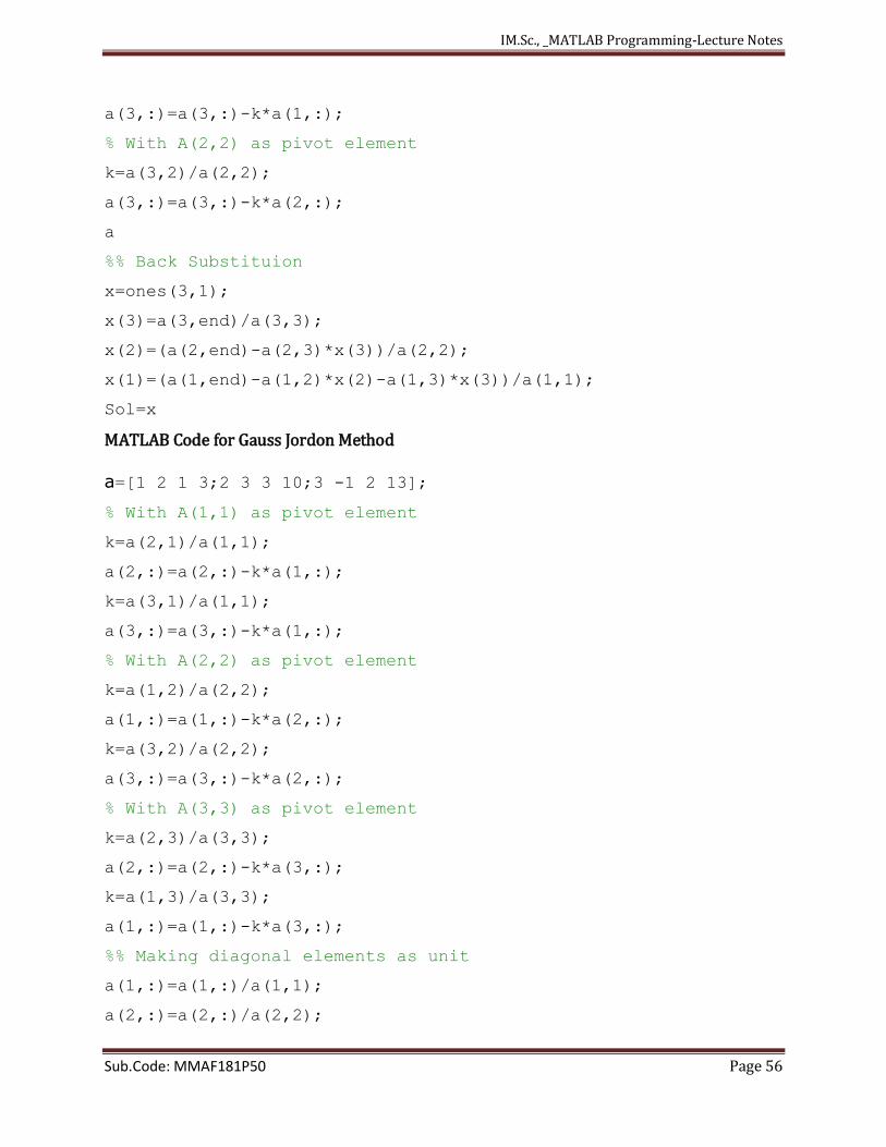
a(3,:)=a(3,:)-k*a(1,:);
% With A(2,2) as pivot element
k=a(3,2)/a(2,2);
a(3,:)=a(3,:)-k*a(2,:);
a
%% Back Substituion
x=ones(3,1);
x(3)=a(3,end)/a(3,3);
x(2)=(a(2,end)-a(2,3)*x(3))/a(2,2);
x(1)=(a(1,end)-a(1,2)*x(2)-a(1,3)*x(3))/a(1,1);
Sol=x
MATLAB Code for Gauss Jordon Method
a=[1 2 1 3;2 3 3 10;3 -1 2 13];
% With A(1,1) as pivot element
k=a(2,1)/a(1,1);
a(2,:)=a(2,:)-k*a(1,:);
k=a(3,1)/a(1,1);
a(3,:)=a(3,:)-k*a(1,:);
% With A(2,2) as pivot element
k=a(1,2)/a(2,2);
a(1,:)=a(1,:)-k*a(2,:);
k=a(3,2)/a(2,2);
a(3,:)=a(3,:)-k*a(2,:);
% With A(3,3) as pivot element
k=a(2,3)/a(3,3);
a(2,:)=a(2,:)-k*a(3,:);
k=a(1,3)/a(3,3);
a(1,:)=a(1,:)-k*a(3,:);
%% Making diagonal elements as unit
a(1,:)=a(1,:)/a(1,1);
a(2,:)=a(2,:)/a(2,2);
IM.Sc., _MATLAB Programming-Lecture Notes
Sub.Code: MMAF181P50 Page 57
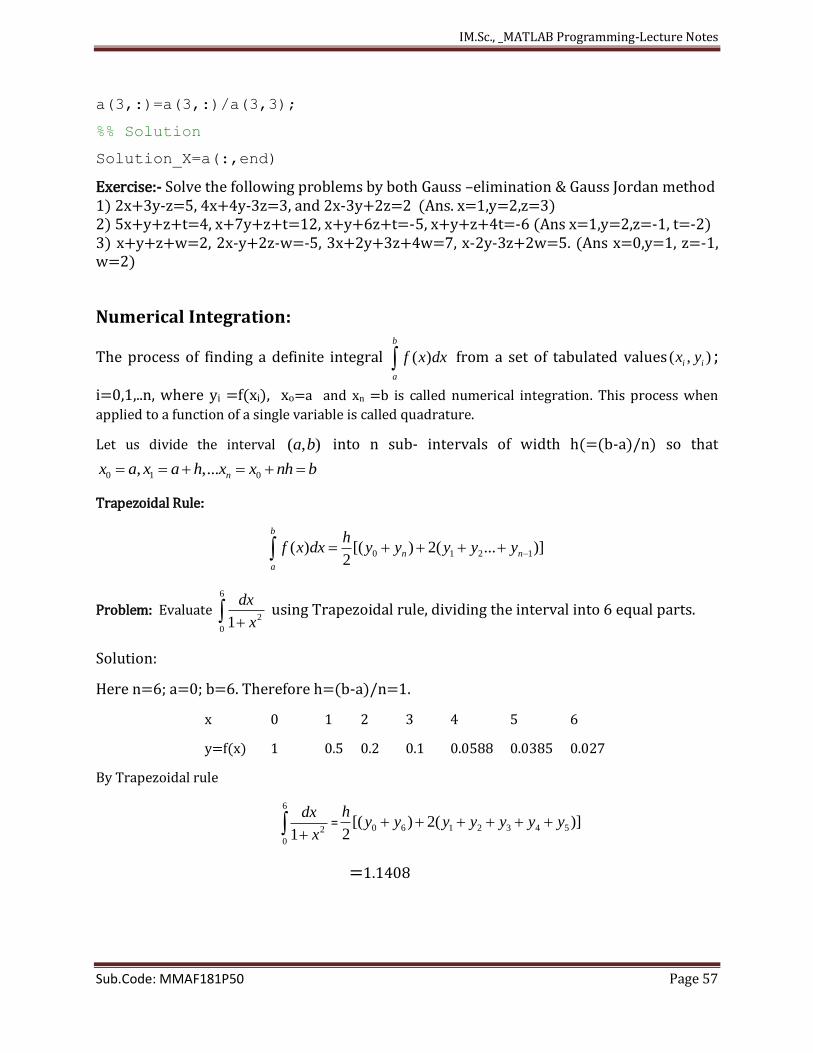
a(3,:)=a(3,:)/a(3,3);
%% Solution
Solution_X=a(:,end)
Exercise:- Solve the following problems by both Gauss –elimination & Gauss Jordan method 1) 2x+3y-z=5, 4x+4y-3z=3, and 2x-3y+2z=2 (Ans. x=1,y=2,z=3) 2) 5x+y+z+t=4, x+7y+z+t=12, x+y+6z+t=-5, x+y+z+4t=-6 (Ans x=1,y=2,z=-1, t=-2) 3) x+y+z+w=2, 2x-y+2z-w=-5, 3x+2y+3z+4w=7, x-2y-3z+2w=5. (Ans x=0,y=1, z=-1, w=2)
Numerical Integration:
The process of finding a definite integral ( )
b
a
f x dx from a set of tabulated values ( , )i ix y ;
i=0,1,..n, where yi =f(xi), xo=a and xn =b is called numerical integration. This process when
applied to a function of a single variable is called quadrature.
Let us divide the interval ( , )a b into n sub- intervals of width h(=(b-a)/n) so that
0 1 0, ,... nx a x a h x x nh b
Trapezoidal Rule:
0 1 2 1( ) [( ) 2( ... )]2
b
n n
a
hf x dx y y y y y
Problem: Evaluate 6
2
01
dx
x using Trapezoidal rule, dividing the interval into 6 equal parts.
Solution:
Here n=6; a=0; b=6. Therefore h=(b-a)/n=1.
x 0 1 2 3 4 5 6
y=f(x) 1 0.5 0.2 0.1 0.0588 0.0385 0.027
By Trapezoidal rule
6
2
01
dx
x= 0 6 1 2 3 4 5[( ) 2( )]
2
hy y y y y y y
=1.1408
IM.Sc., _MATLAB Programming-Lecture Notes
Sub.Code: MMAF181P50 Page 58
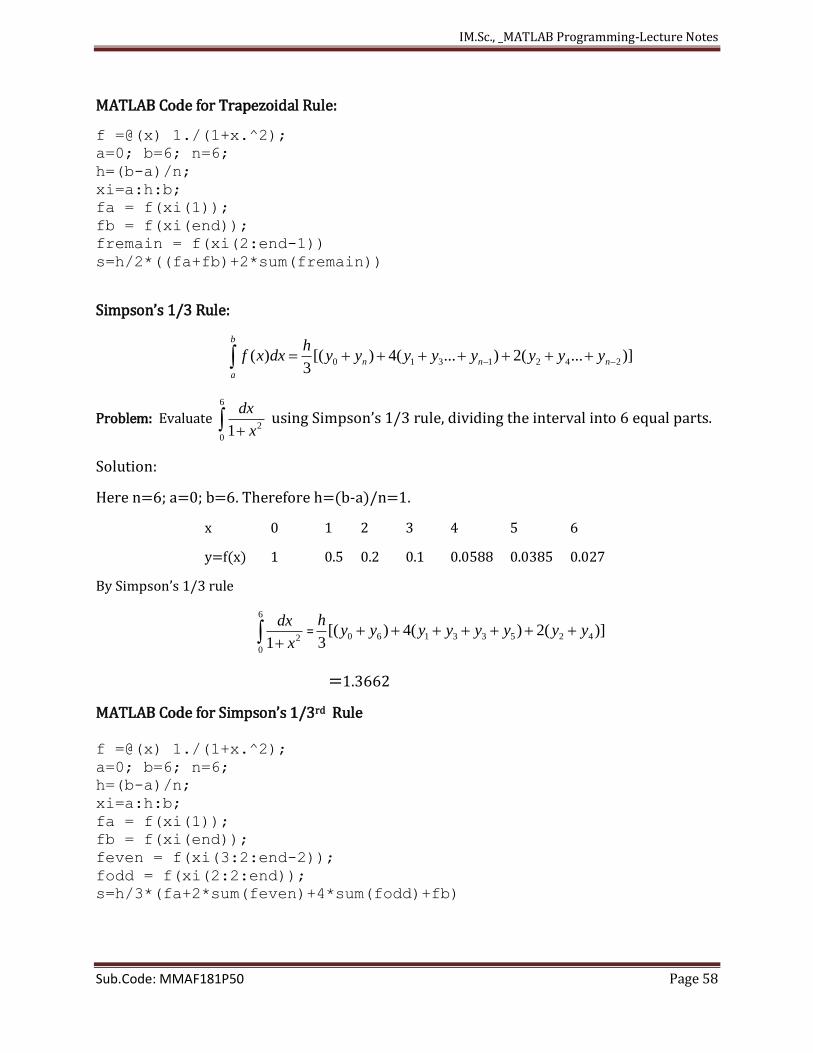
MATLAB Code for Trapezoidal Rule:
f =@(x) 1./(1+x.^2);
a=0; b=6; n=6;
h=(b-a)/n;
xi=a:h:b;
fa = f(xi(1));
fb = f(xi(end));
fremain = f(xi(2:end-1))
s=h/2*((fa+fb)+2*sum(fremain))
Simpson’s 1/3 Rule:
0 1 3 1 2 4 2( ) [( ) 4( ... ) 2( ... )]3
b
n n n
a
hf x dx y y y y y y y y
Problem: Evaluate 6
2
01
dx
x using Simpson’s 1/3 rule, dividing the interval into 6 equal parts.
Solution:
Here n=6; a=0; b=6. Therefore h=(b-a)/n=1.
x 0 1 2 3 4 5 6
y=f(x) 1 0.5 0.2 0.1 0.0588 0.0385 0.027
By Simpson’s 1/3 rule
6
2
01
dx
x= 0 6 1 3 3 5 2 4[( ) 4( ) 2( )]
3
hy y y y y y y y
=1.3662
MATLAB Code for Simpson’s 1/3rd Rule f =@(x) 1./(1+x.^2);
a=0; b=6; n=6;
h=(b-a)/n;
xi=a:h:b;
fa = f(xi(1));
fb = f(xi(end));
feven = f(xi(3:2:end-2));
fodd = f(xi(2:2:end));
s=h/3*(fa+2*sum(feven)+4*sum(fodd)+fb)
IM.Sc., _MATLAB Programming-Lecture Notes
Sub.Code: MMAF181P50 Page 59
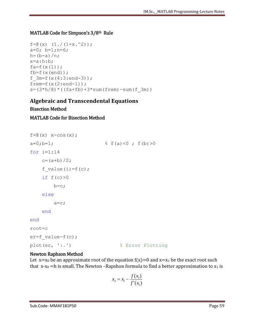
MATLAB Code for Simpson’s 3/8th Rule f=@(x) (1./(1+x.^2));
a=0; b=1;n=6;
h=(b-a)/n;
x=a:h:b;
fa=f(x(1));
fb=f(x(end));
f_3m=f(x(4:3:end-3));
frem=f(x(2:end-1));
s=(3*h/8)*((fa+fb)+3*sum(frem)-sum(f_3m))
Algebraic and Transcendental Equations
Bisection Method
MATLAB Code for Bisection Method
f=@(x) x-cos(x);
a=0;b=1; % f(a)<0 ; f(b)>0
for i=1:14
c=(a+b)/2;
f_value(i)=f(c);
if f(c)>0
b=c;
else
a=c;
end
end
root=c
er=f_value-f(c);
plot(er, ':.') % Error Plotting
Newton Raphson Method Let x=x0 be an approximate root of the equation f(x)=0 and x=x1 be the exact root such
that x-x0 =h is small. The Newton –Rapshon formula to find a better approximation to x1 is
12 1
1
( )
( )
f xx x
f x
IM.Sc., _MATLAB Programming-Lecture Notes
Sub.Code: MMAF181P50 Page 60
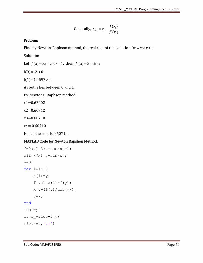
Generally, 1
( )
( )
ii i
i
f xx x
f x
Problem:
Find by Newton-Raphson method, the real root of the equation 3 cos 1x x
Solution:
Let ( ) 3 cos 1f x x x , then ( ) 3 sinf x x
f(0)=-2 <0
f(1)=1.4597>0
A root is lies between 0 and 1.
By Newtons- Raphson method,
x1=0.62002
x2=0.60712
x3=0.60710
x4= 0.60710
Hence the root is 0.60710.
MATLAB Code for Newton Rapshon Method:
f=@(x) 3*x-cos(x)-1;
dif=@(x) 3+sin(x);
y=0;
for i=1:10
a(i)=y;
f_value(i)=f(y);
x=y-(f(y)/dif(y));
y=x;
end
root=y
er=f_value-f(y)
plot(er,'.:')
IM.Sc., _MATLAB Programming-Lecture Notes
Sub.Code: MMAF181P50 Page 61
Bibliography
Introduction to MATLAB, K.Srinivasa Rao, IMRF International Publications
Getting Started with MATLAB by Rudra Pratap, Oxford University Press
Practical MATLAB-Basics for Engineers, CRC Press, Misza Kalechman
Engineering Problem solving with MATLAB, D.M.Etter, Printice-Hall
A MATLAB Primer, Kermit Sigmon , Timothy A. Davis.
MATLAB Demystified, Basic Concepts and Applications, K K Sarma, Vikas Publishing
House Pvt Ltd
Applied Numerical Methods with MATLAB by Steven C. Chapra, 3rd Edition, McGrawHill
Numerical Analysis using MATLAB and Spread sheets by Steven T. Karris, 2nd edition,
Orchard Publications
An Introduction to MATLAB, by David F. Griffiths, Department of Mathematics,
University of Dundee
Useful MATLAB Website:
http://www.mathworks.in/
Critical evaluation and suggestions for improvement of this
material will be highly appreciated and gratefully acknowledged.
Dr.K.Srinivasa Rao Professor & Head
Department of Mathematics SCSVMV University, Kanchipuram
[email protected] 96666 95525