Math/Phys 594: Homework 6 Solutions

February 20, 2019

5.1.9 Consider the system x = −y, y = −x.

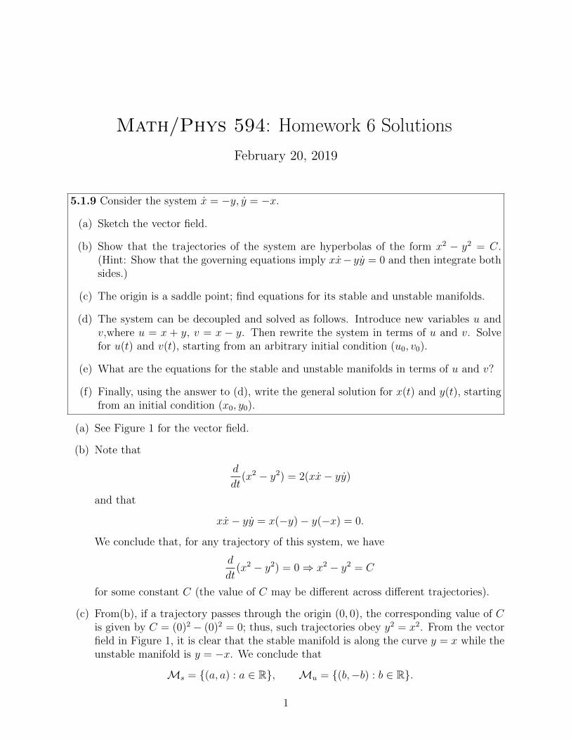
(a) Sketch the vector field.

(b) Show that the trajectories of the system are hyperbolas of the form x2 − y2 = C.(Hint: Show that the governing equations imply xx− yy = 0 and then integrate bothsides.)

(c) The origin is a saddle point; find equations for its stable and unstable manifolds.

(d) The system can be decoupled and solved as follows. Introduce new variables u andv,where u = x + y, v = x − y. Then rewrite the system in terms of u and v. Solvefor u(t) and v(t), starting from an arbitrary initial condition (u0, v0).

(e) What are the equations for the stable and unstable manifolds in terms of u and v?

(f) Finally, using the answer to (d), write the general solution for x(t) and y(t), startingfrom an initial condition (x0, y0).

(a) See Figure 1 for the vector field.

(b) Note that

d

dt(x2 − y2) = 2(xx− yy)

and that

xx− yy = x(−y)− y(−x) = 0.

We conclude that, for any trajectory of this system, we have

d

dt(x2 − y2) = 0⇒ x2 − y2 = C

for some constant C (the value of C may be different across different trajectories).

(c) From(b), if a trajectory passes through the origin (0, 0), the corresponding value of Cis given by C = (0)2 − (0)2 = 0; thus, such trajectories obey y2 = x2. From the vectorfield in Figure 1, it is clear that the stable manifold is along the curve y = x while theunstable manifold is y = −x. We conclude that

Ms = {(a, a) : a ∈ R}, Mu = {(b,−b) : b ∈ R}.

1

Figure 1: Problem 5.1.9(a)

(d) Setting u = x+ y and v = x− y gives

u = x+ y = −y − x = −u, v = x− y = −y + x = v.

This decoupled system can be solved easily: we obtain u(t) = u0e−t and v(t) = v0e

t.

(e) Observe that a trajectory (u(t), v(t)) = (u0e−t, v0e

t) converges to (0, 0) as t → ∞ ifand only if v0 = 0; as a result, we say that Ms = {(u0, 0) : u0 ∈ R}. Similarly,(u0e

−t, v0et)→ (0, 0) as t→ −∞ if and only if u0 = 0 so thatMs = {(0, v0) : v0 ∈ R}.

(These ordered pairs now refer to the (u, v) values, as opposed to the (x, y) values in(c))

(f) We have

u(t) = x(t) + y(t) = (x0 + y0)e−t, v(t) = x(t)− y(t) = (x0 − y0)et.

Adding the two equations and dividing by 2 gives

x(t) = x0

(e−t + et

2

)+ y0

(e−t − et

2

)= x0 cosh(t)− y0 sinh(t)

and likewise subtracting them gives

y(t) = x0

(e−t − et

2

)+ y0

(e−t + et

2

)= −x0 sinh(t) + y0 cosh(t).

2

5.1.10 For each of the following systems, decide whether the origin is attracting, Liapunovstable, asymptotically stable, or none of the above.

(a) x = y, y = −4x.

(b) x = y, y = x.

(c) x = 0, y = x.

(d) x = 0, y = −y.

(e) x = −x, y = −5y.

(f) x = x, y = y.

(a) For x = y, y = −4x, we have A =

(0 1−4 0

)so τ = 0 and ∆ = 4. The origin is a

center, implying that it is Liapunov stable but not attracting.

(b) For x = y, y = x, we have A =

(0 11 0

)so that ∆ = −1. The origin is again a saddle

point so it is neither attracting, not Liapunov stable.

(c) For x = 0, y = x, we have A =

(0 01 0

)so τ = 0 and ∆ = 0. This is a case that lies at

the intersection of non-degenerate curve (τ 2 − 4∆ = 0) and the vertical axis (∆ = 0)in the (τ,∆) stability diagram and corresponds to a shear flow. As a result, the originis neither attracting, not Liapunov stable.

(d) For x = 0, y = −y, we have A =

(0 00 −1

)so τ = −1 and ∆ = 0. The origin is

therefore part of a line of non-isolated stable fixed points so we deduce that the originis Liapunov stable but not attracting. (It fails to be attracting because in any discaround the origin, there exist solutions that do not converge to it)

(e) For x = −x, y = −5y, we obtain A =

(−1 00 −5

)so τ = −6 and ∆ = 5. Since

τ 2 − 4∆ = 16 > 0, we infer that the origin is a stable spiral. As a result, it is bothattracting and Liapunov stable and hence asymptotically stable.

(f) For x = x, y = y, we have A =

(1 00 1

)so τ = 2 and ∆ = 1. Since τ 2 − 4∆ = 0, this

is an instance of repeated eigenvalues. Moreover, we have a full set of eigenvectors sothe origin is an unstable star. We conclude that it is neither attracting, not Liapunovstable.

3

5.2.2 (Complex eigenvalues) This exercise leads you through the solution of a linear systemwhere the eigenvalues are complex. The system is x = x− y, y = x+ y.

(a) Find A and show that it has eigenvalues λ1 = 1 + i, λ2 = 1 − i, with eigenvectorsv1 = (i, 1), v2 = (−i, 1). (Note that the eigenvalues are complex conjugates, and soare the eigenvectors – this is always the case for real A with complex eigenvalues.)

(b) The general solution is x(t) = c1eλ1tv1 + c2e

λ2tv2. So in one sense we’re done! Butthis way of writing x(t) involves complex coefficients and looks unfamiliar. Expressx(t) purely in terms of real-valued functions. (Hint: Use eiωt = cos(ωt) + i sin(ωt) torewrite x(t) in terms of sines and cosines, and then separate the terms that have aprefactor of i from those that don’t.)

(a) We have A =

(1 −11 1

)so τ = 2 and ∆ = 2 ⇒ τ 2 − 4∆ = −4. As a result, the

eigenvalues are given by

λ1,2 =2±√−4

2= 1± i.

For λ1 = 1 + i, the corresponding eigenvector v1 =

(ab

)obeys

(A− λ1I)v1 = 0⇒(−i −11 −i

)(ab

)=

(00

)⇒ a = ib.

Thus, v1 =

(i1

)is an eigenvector corresponding to λ1. We can similarly find v2

corresponding to λ2 but it is much simpler to note that λ2 = λ1 so

Av2 = λ2v2 ⇒ Av2 = λ2v2 ⇒ Av2 = λ1v2

since A is real. This is simply the eigenvalue problem for λ1 so we can choose v2 so

that v2 = v1, with the result that v2 =

(−i1

).

(b) Let λ1 = a+ ib and v1 = u + iw, where a, b ∈ R and u,w ∈ R2. We obtain

x(t) = c1eateibt(u + iw) + c2e

ate−ibt(u− iw)

= c1eat(cos(bt) + i sin(bt))(u + iw) + c2e

at(cos(bt)− i sin(bt))(u− iw)

= (c1 + c2)eat(cos(bt)u− sin(bt)w) + i(c1 − c2)eat(sin(bt)u + cos(bt)w)

where we collected the terms with and without prefactors of i. Next, note that for x(t)to be real, we must have c2 = c1; let c1 = P

2− iQ

2to get c1 + c2 = P and i(c1− c2) = Q

so that

x(t) = Peat(cos(bt)u− sin(bt)w) +Qeat(sin(bt)u + cos(bt)w)

4

which can also be expressed as

x(t) = eat(u w

)( cos(bt) sin(bt)− sin(bt) cos(bt)

)(PQ

)where P and Q are to be determined from the initial conditions.

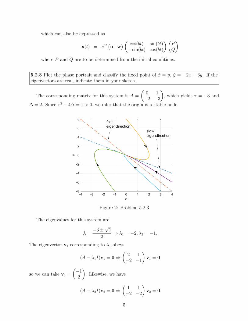
5.2.3 Plot the phase portrait and classify the fixed point of x = y, y = −2x − 3y. If theeigenvectors are real, indicate them in your sketch.

The corresponding matrix for this system is A =

(0 1−2 −3

), which yields τ = −3 and

∆ = 2. Since τ 2 − 4∆ = 1 > 0, we infer that the origin is a stable node.

Figure 2: Problem 5.2.3

The eigenvalues for this system are

λ =−3±

√1

2⇒ λ1 = −2, λ2 = −1.

The eigenvector v1 corresponding to λ1 obeys

(A− λ1I)v1 = 0⇒(

2 1−2 −1

)v1 = 0

so we can take v1 =

(−12

). Likewise, we have

(A− λ2I)v2 = 0⇒(

1 1−2 −2

)v2 = 0

5

so that v2 =

(1−1

). Observe that v1 describes the fast direction and v2 the slow direction.

The phase portrait is shown in Figure 2.

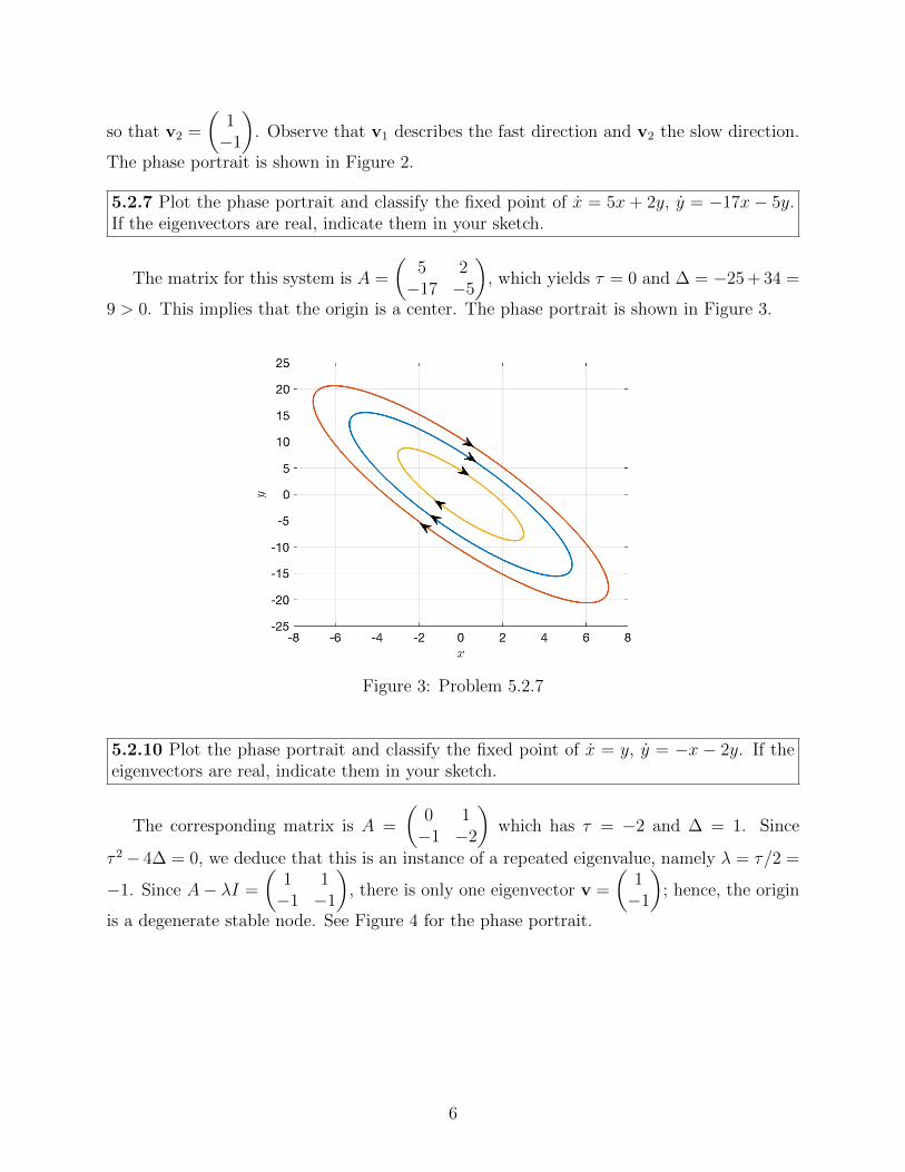
5.2.7 Plot the phase portrait and classify the fixed point of x = 5x + 2y, y = −17x− 5y.If the eigenvectors are real, indicate them in your sketch.

The matrix for this system is A =

(5 2−17 −5

), which yields τ = 0 and ∆ = −25 + 34 =

9 > 0. This implies that the origin is a center. The phase portrait is shown in Figure 3.

Figure 3: Problem 5.2.7

5.2.10 Plot the phase portrait and classify the fixed point of x = y, y = −x − 2y. If theeigenvectors are real, indicate them in your sketch.

The corresponding matrix is A =

(0 1−1 −2

)which has τ = −2 and ∆ = 1. Since

τ 2− 4∆ = 0, we deduce that this is an instance of a repeated eigenvalue, namely λ = τ/2 =

−1. Since A− λI =

(1 1−1 −1

), there is only one eigenvector v =

(1−1

); hence, the origin

is a degenerate stable node. See Figure 4 for the phase portrait.

6

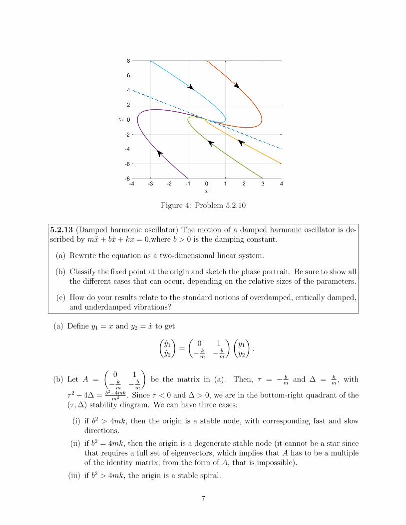
Figure 4: Problem 5.2.10

5.2.13 (Damped harmonic oscillator) The motion of a damped harmonic oscillator is de-scribed by mx+ bx+ kx = 0,where b > 0 is the damping constant.

(a) Rewrite the equation as a two-dimensional linear system.

(b) Classify the fixed point at the origin and sketch the phase portrait. Be sure to show allthe different cases that can occur, depending on the relative sizes of the parameters.

(c) How do your results relate to the standard notions of overdamped, critically damped,and underdamped vibrations?

(a) Define y1 = x and y2 = x to get(y1y2

)=

(0 1− km− bm

)(y1y2

).

(b) Let A =

(0 1− km− bm

)be the matrix in (a). Then, τ = − b

mand ∆ = k

m, with

τ 2− 4∆ = b2−4mkm2 . Since τ < 0 and ∆ > 0, we are in the bottom-right quadrant of the

(τ,∆) stability diagram. We can have three cases:

(i) if b2 > 4mk, then the origin is a stable node, with corresponding fast and slowdirections.

(ii) if b2 = 4mk, then the origin is a degenerate stable node (it cannot be a star sincethat requires a full set of eigenvectors, which implies that A has to be a multipleof the identity matrix; from the form of A, that is impossible).

(iii) if b2 > 4mk, the origin is a stable spiral.

7

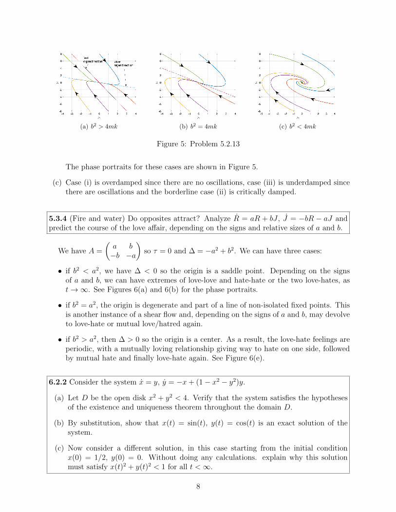
(a) b2 > 4mk (b) b2 = 4mk (c) b2 < 4mk

Figure 5: Problem 5.2.13

The phase portraits for these cases are shown in Figure 5.

(c) Case (i) is overdamped since there are no oscillations, case (iii) is underdamped sincethere are oscillations and the borderline case (ii) is critically damped.

5.3.4 (Fire and water) Do opposites attract? Analyze R = aR + bJ , J = −bR − aJ andpredict the course of the love affair, depending on the signs and relative sizes of a and b.

We have A =

(a b−b −a

)so τ = 0 and ∆ = −a2 + b2. We can have three cases:

• if b2 < a2, we have ∆ < 0 so the origin is a saddle point. Depending on the signsof a and b, we can have extremes of love-love and hate-hate or the two love-hates, ast→∞. See Figures 6(a) and 6(b) for the phase portraits.

• if b2 = a2, the origin is degenerate and part of a line of non-isolated fixed points. Thisis another instance of a shear flow and, depending on the signs of a and b, may devolveto love-hate or mutual love/hatred again.

• if b2 > a2, then ∆ > 0 so the origin is a center. As a result, the love-hate feelings areperiodic, with a mutually loving relationship giving way to hate on one side, followedby mutual hate and finally love-hate again. See Figure 6(e).

6.2.2 Consider the system x = y, y = −x+ (1− x2 − y2)y.

(a) Let D be the open disk x2 + y2 < 4. Verify that the system satisfies the hypothesesof the existence and uniqueness theorem throughout the domain D.

(b) By substitution, show that x(t) = sin(t), y(t) = cos(t) is an exact solution of thesystem.

(c) Now consider a different solution, in this case starting from the initial conditionx(0) = 1/2, y(0) = 0. Without doing any calculations. explain why this solutionmust satisfy x(t)2 + y(t)2 < 1 for all t <∞.

8

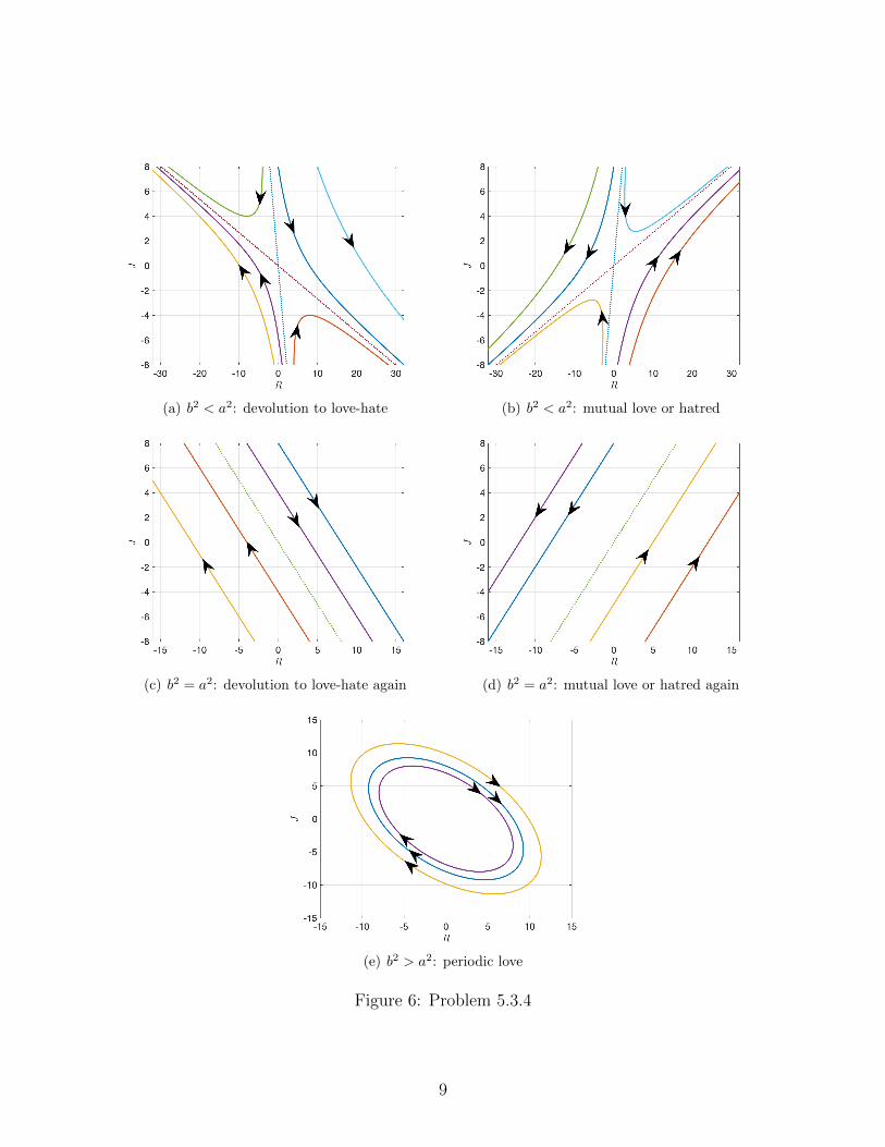
(a) b2 < a2: devolution to love-hate (b) b2 < a2: mutual love or hatred

(c) b2 = a2: devolution to love-hate again (d) b2 = a2: mutual love or hatred again

(e) b2 > a2: periodic love

Figure 6: Problem 5.3.4

9

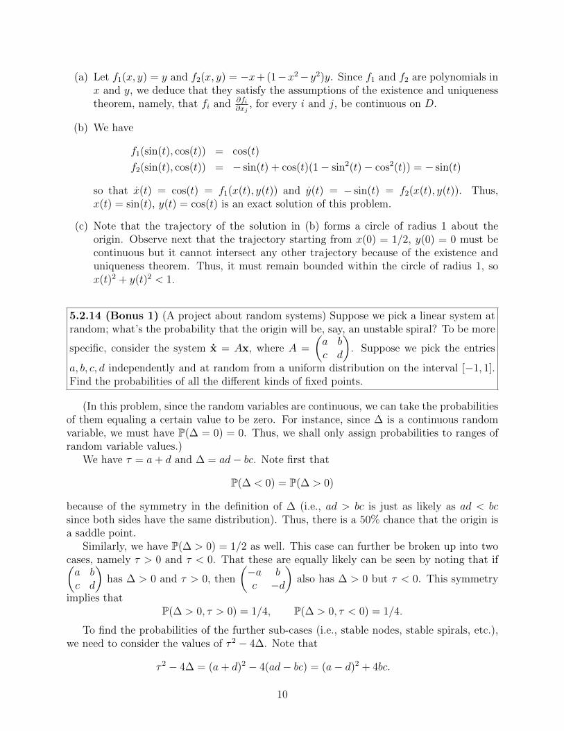
(a) Let f1(x, y) = y and f2(x, y) = −x+ (1−x2− y2)y. Since f1 and f2 are polynomials inx and y, we deduce that they satisfy the assumptions of the existence and uniquenesstheorem, namely, that fi and ∂fi

∂xj, for every i and j, be continuous on D.

(b) We have

f1(sin(t), cos(t)) = cos(t)

f2(sin(t), cos(t)) = − sin(t) + cos(t)(1− sin2(t)− cos2(t)) = − sin(t)

so that x(t) = cos(t) = f1(x(t), y(t)) and y(t) = − sin(t) = f2(x(t), y(t)). Thus,x(t) = sin(t), y(t) = cos(t) is an exact solution of this problem.

(c) Note that the trajectory of the solution in (b) forms a circle of radius 1 about theorigin. Observe next that the trajectory starting from x(0) = 1/2, y(0) = 0 must becontinuous but it cannot intersect any other trajectory because of the existence anduniqueness theorem. Thus, it must remain bounded within the circle of radius 1, sox(t)2 + y(t)2 < 1.

5.2.14 (Bonus 1) (A project about random systems) Suppose we pick a linear system atrandom; what’s the probability that the origin will be, say, an unstable spiral? To be more

specific, consider the system x = Ax, where A =

(a bc d

). Suppose we pick the entries

a, b, c, d independently and at random from a uniform distribution on the interval [−1, 1].Find the probabilities of all the different kinds of fixed points.

(In this problem, since the random variables are continuous, we can take the probabilitiesof them equaling a certain value to be zero. For instance, since ∆ is a continuous randomvariable, we must have P(∆ = 0) = 0. Thus, we shall only assign probabilities to ranges ofrandom variable values.)

We have τ = a+ d and ∆ = ad− bc. Note first that

P(∆ < 0) = P(∆ > 0)

because of the symmetry in the definition of ∆ (i.e., ad > bc is just as likely as ad < bcsince both sides have the same distribution). Thus, there is a 50% chance that the origin isa saddle point.

Similarly, we have P(∆ > 0) = 1/2 as well. This case can further be broken up into twocases, namely τ > 0 and τ < 0. That these are equally likely can be seen by noting that if(a bc d

)has ∆ > 0 and τ > 0, then

(−a bc −d

)also has ∆ > 0 but τ < 0. This symmetry

implies thatP(∆ > 0, τ > 0) = 1/4, P(∆ > 0, τ < 0) = 1/4.

To find the probabilities of the further sub-cases (i.e., stable nodes, stable spirals, etc.),we need to consider the values of τ 2 − 4∆. Note that

τ 2 − 4∆ = (a+ d)2 − 4(ad− bc) = (a− d)2 + 4bc.

10

Let γ = P(∆ > 0, τ > 0, τ 2 − 4∆ > 0). By symmetry, P(∆ > 0, τ < 0, τ 2 − 4∆ > 0) = γas well. Thus,

P(τ 2 − 4∆ > 0) = P(∆ < 0) + P(∆ > 0, τ 2 − 4∆ > 0)

=1

2+ 2γ (1)

where we used the fact that ∆ < 0 implies τ 2 > 4∆. Next, we consider P(τ 2 − 4∆ > 0) =P((a− d)2 + 4bc > 0). Observe that

P((a− d)2 + 4bc > 0) = P((a− d)2 + 4bc > 0 | bc > 0)P(bc > 0) +

P((a− d)2 + 4bc > 0 | bc < 0)P(bc < 0) (2)

Note that we always have (a− d)2 + 4bc > 0 when bc > 0; since P(bc > 0) = 1/2, we get

P((a− d)2 + 4bc > 0 | bc > 0)P(bc > 0) =1

2. (3)

Similarly, we have P(bc < 0) = 1/2 but computing P((a − d)2 + 4bc > 0 | bc < 0) istrickier (there has to be a point at which symmetry arguments lose steam after all!). Notethat we can express this as

|a− d| > 2√−bc⇒ a > d+ 2

√bc or a < d− 2

√bc.

Since a and d are uniformly distributed over [−1, 1], we can interpret the above conditionas an area problem in the (a, d) plane. It follows that

P(|a− d| > 2√−bc | bc < 0) =

∫∫bc<0

(2− 2√−bc)2

8db dc.

This integral can be computed by breaking it up into symmetric parts and expandingthe integrand:∫∫

bc<0

(2− 2√−bc)2

8db dc =

(4)(2)

8

∫ c=1

c=0

∫ b=0

b=−1

1− 2√−bc− bc db dc

= 1− 2

(2

3

)2

+

(1

2

)2

=13

36. (4)

Combining (3) and (4) as they appear in (2) gives

P((a− d)2 + 4bc > 0) =1

2+

1

2

(13

36

).

Plugging this in (1) then yields

1

2+

13

72=

1

2+ 2γ ⇒ γ =

13

144.

Hence, the probability of obtaining a stable node is 13/144. We summarize our resultsin Table 1.

11

Saddle Point Stable Node Stable Spiral Unstable Node Unstable Spiral1/2 13/144 23/144 13/144 23/144

Table 1: Probabilities of getting various fixed points.

These results can be confirmed by a Monte Carlo simulation. We simply generate a largenumber of matrices randomly and find the proportions of saddle points, stable nodes, etc.Results from one such simulation are shown in Table 2; we generated 106 matrices with theentries distributed uniformly over [−1, 1]. The resulting frequencies are fairly similar to thecalculated probabilities in Table 1.

Saddle Point Stable Node Stable Spiral Unstable Node Unstable Spiral0.499662 0.089978 0.159580 0.090461 0.160319

Table 2: Results of the Monte Carlo simulation.

Having established that Monte Carlo simulations yield pretty accurate results, we canapply it to the case where the entries are drawn from a normal distribution. More precisely,we now assume that a, b, c, d are normally distributed with mean 0 and standard deviation1. The corresponding results are shown in Table 3. Observe that the probability of getting asaddle point is the same as that was deduced from symmetry arguments and hence is inde-pendent of the distribution the entries are drawn from. However, obtaining stable/unstablenodes is slightly more likely than in the uniform case.

Saddle Point Stable Node Stable Spiral Unstable Node Unstable Spiral0.500297 0.103990 0.145867 0.103337 0.146509

Table 3: Monte Carlo simulation with entries drawn from the standard normal distribution.

See the attached MCSim.m file for the code.

6.1.12 (Bonus 2) (Saddle connections) A certain system is known to have exactly twofixed points, both of which are saddles. Sketch phase portraits in which

(a) there is a single trajectory that connects the saddles;

(b) there is no trajectory that connects the saddles.

(a) Such a system can be designed by choosing the fixed points to lie on the x–axis andhaving one of them stable and the other one unstable. In the y direction, we wouldlike the stabilities to be switched so the fixed points are saddle points. An instance ofsuch a system is

x = x2 − 1, y = −xy.

This has fixed points at (±1, 0) and both of them are saddles. Moreover, there is atrajectory along the x–axis that goes from (1, 0) to (−1, 0). See Figure 7 for the phaseportrait.

12

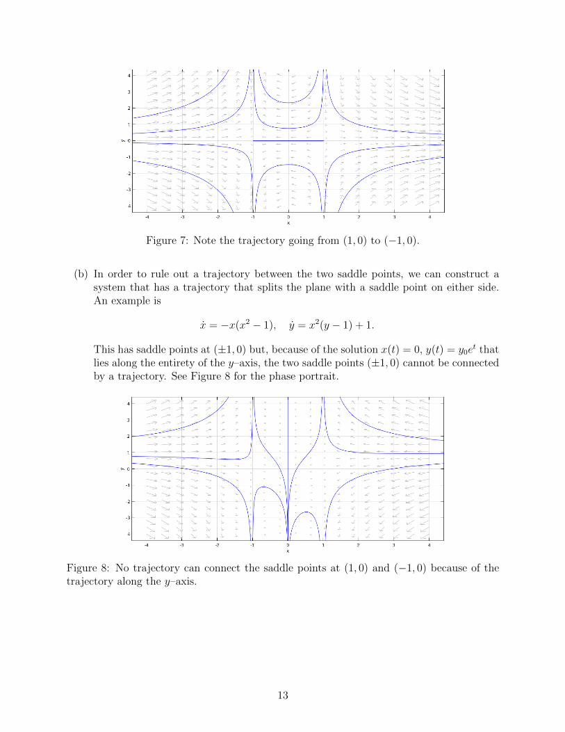
Figure 7: Note the trajectory going from (1, 0) to (−1, 0).

(b) In order to rule out a trajectory between the two saddle points, we can construct asystem that has a trajectory that splits the plane with a saddle point on either side.An example is

x = −x(x2 − 1), y = x2(y − 1) + 1.

This has saddle points at (±1, 0) but, because of the solution x(t) = 0, y(t) = y0et that

lies along the entirety of the y–axis, the two saddle points (±1, 0) cannot be connectedby a trajectory. See Figure 8 for the phase portrait.

Figure 8: No trajectory can connect the saddle points at (1, 0) and (−1, 0) because of thetrajectory along the y–axis.

13