mathematical aspects of the bcs theory of superconductivity
TRANSCRIPT

Mathematical Aspects of the BCS Theory ofSuperconductivity and Related Theories
Dissertationder Mathematisch-Naturwissenschaftlichen Fakultät
der Eberhard Karls Universität Tübingenzur Erlangung des Grades einesDoktors der Naturwissenschaften
(Dr. rer. nat.)
vorgelegt vonGerhard Albert Bräunlich
aus Zürich/Schweiz
Tübingen 2014

Tag der mündlichen Qualifikation: 15.09.2014Dekan: Prof. Dr. Wolfgang Rosenstiel1. Berichterstatter: Prof. Dr. Christian Hainzl2. Berichterstatter: Prof. Dr. Robert Seiringer

DanksagungAllen voran danke ich meinem Hauptbetreuer, Prof. Dr. Christian Hainzl.Ein besserer Doktorvater wäre schwer zu finden gewesen. Dies nicht nur imwissenschaftlichen Sinne – ich durfte mit ihm auch einige unvergesslichenStunden bei geselligen und sportlichen Unternehmungen teilen.Mein besonderer Dank gilt auch meinem externen Gutachter, Prof. Dr.
Robert Seiringer am IST Austria für die Co-Autorenschaft bei Publikatio-nen und für wichtige wissenschaftliche Anregungen, sowie meinem zweitenBetreuer Prof Dr. Stefan Teufel für zahlreiche wertvolle Diskussionen.Ferner richte ich einen spezieller Dank an Andreas Deuchert, Dennis
Zelle sowie meinen Vater, Reinhold Bräunlich für das Korrekturlesen derDissertation.Sehr fördernd für das Gelingen der Arbeit war die angenehme und pro-
duktive Arbeitsatmosphäre, für welche meine Arbeitskollegen stets gesorgthaben. Dafür danke ich meinen ersten Kollegen in meiner Tübinger Zeit:Andreas Wöhr, Hans Stiepan und Marco Schreiber, sowie Max Lein, derlange Zeit mein Zimmergenosse war. Ausserdem danke ich Falk Anger alsAnsprechpartner für experimental-physikalische Fragen, Carla Cederbaumfür wertvolle Tipps zu meinen wissenschaftlichen Bewerbungen, SebastianEgger, Johannes von Keler, Sebastian Debrelli-Boelzle, Jonas Lampart,Stefan Haag, Pascal Kilian, Silvia Freund, Wolfgang Gaim, Tim Tsana-theas, Stefan Keppeler und Frank Loose.
iii

iv

Contents
1 German Summary . . . . . . . . . . . . . . . . . . . . . . . vii2 List of Publications in the Thesis . . . . . . . . . . . . . . . xii
2.1 Accepted Papers . . . . . . . . . . . . . . . . . . . . xii2.2 Ready for Submission Manuscripts . . . . . . . . . . xii
3 Personal Contribution . . . . . . . . . . . . . . . . . . . . . xii
1 History 11.1 History of Superconductivity and Superfluidity . . . . . . . 11.2 Applications . . . . . . . . . . . . . . . . . . . . . . . . . . . 10
2 The BCS theory 132.1 Quantum Mechanics . . . . . . . . . . . . . . . . . . . . . . 142.2 Derivation of the BCS Functional . . . . . . . . . . . . . . . 18
2.2.1 Step 1: Restriction to Quasi-free States . . . . . . . 202.2.2 Step 2: Assuming SU(2) Invariance . . . . . . . . . 222.2.3 Step 3: Assuming Translation Invariance . . . . . . . 25
2.3 The Simplified Translation Invariant BCS Functional . . . . 27
Appendix to Chapter 2 372.A The entropy for quasi-free states . . . . . . . . . . . . . . . 37
3 Results 433.1 The Full Translation Invariant BCS Functional . . . . . . . 43
3.1.1 Contact interactions as limits of short-range potentials 483.2 The Link to the Gross-Pitaevskii Theory . . . . . . . . . . . 51
Bibliography 55
v
Contents
A Publications in the Thesis 67A.1 Accepted papers . . . . . . . . . . . . . . . . . . . . . . . . 67
A.1.1 On Contact Interactions as Limits of Short-RangePotentials . . . . . . . . . . . . . . . . . . . . . . . . 67
A.1.2 On the BCS gap equation for superfluid fermionicgases . . . . . . . . . . . . . . . . . . . . . . . . . . . 80
A.1.3 Translation-invariant quasi-free states for fermionicsystems and the BCS approximation . . . . . . . . . 92
A.2 Ready for submission manuscripts . . . . . . . . . . . . . . 130A.2.1 The Bogolubov-Hartree-Fock theory for strongly in-
teracting fermions in the low density limit . . . . . . 130
vi
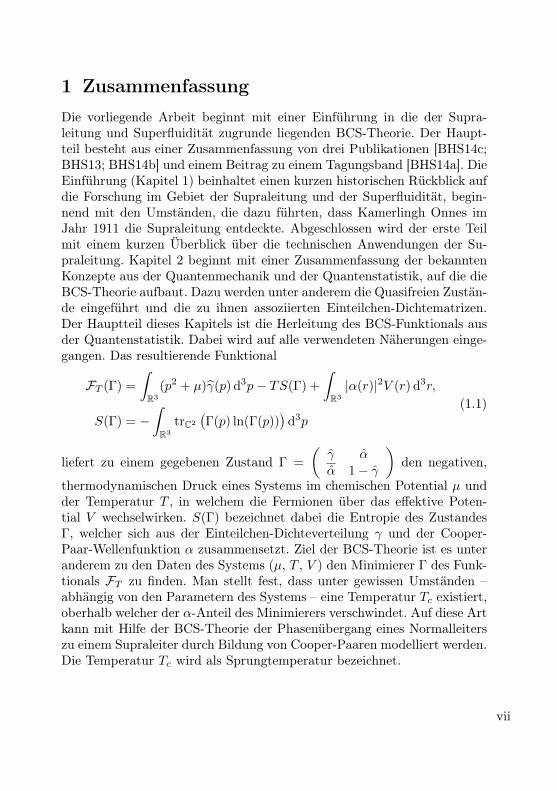
1 ZusammenfassungDie vorliegende Arbeit beginnt mit einer Einführung in die der Supra-leitung und Superfluidität zugrunde liegenden BCS-Theorie. Der Haupt-teil besteht aus einer Zusammenfassung von drei Publikationen [BHS14c;BHS13; BHS14b] und einem Beitrag zu einem Tagungsband [BHS14a]. DieEinführung (Kapitel 1) beinhaltet einen kurzen historischen Rückblick aufdie Forschung im Gebiet der Supraleitung und der Superfluidität, begin-nend mit den Umständen, die dazu führten, dass Kamerlingh Onnes imJahr 1911 die Supraleitung entdeckte. Abgeschlossen wird der erste Teilmit einem kurzen Überblick über die technischen Anwendungen der Su-praleitung. Kapitel 2 beginnt mit einer Zusammenfassung der bekanntenKonzepte aus der Quantenmechanik und der Quantenstatistik, auf die dieBCS-Theorie aufbaut. Dazu werden unter anderem die Quasifreien Zustän-de eingeführt und die zu ihnen assoziierten Einteilchen-Dichtematrizen.Der Hauptteil dieses Kapitels ist die Herleitung des BCS-Funktionals ausder Quantenstatistik. Dabei wird auf alle verwendeten Näherungen einge-gangen. Das resultierende Funktional
FT (Γ) =
∫
R3
(p2 + µ)γ(p) d3p− TS(Γ) +
∫
R3
|α(r)|2V (r) d3r,
S(Γ) = −∫
R3
trC2
(Γ(p) ln(Γ(p))
)d3p
(1.1)
liefert zu einem gegebenen Zustand Γ =
(γ α
α 1− γ
)den negativen,
thermodynamischen Druck eines Systems im chemischen Potential µ undder Temperatur T , in welchem die Fermionen über das effektive Poten-tial V wechselwirken. S(Γ) bezeichnet dabei die Entropie des ZustandesΓ, welcher sich aus der Einteilchen-Dichteverteilung γ und der Cooper-Paar-Wellenfunktion α zusammensetzt. Ziel der BCS-Theorie ist es unteranderem zu den Daten des Systems (µ, T , V ) den Minimierer Γ des Funk-tionals FT zu finden. Man stellt fest, dass unter gewissen Umständen –abhängig von den Parametern des Systems – eine Temperatur Tc existiert,oberhalb welcher der α-Anteil des Minimierers verschwindet. Auf diese Artkann mit Hilfe der BCS-Theorie der Phasenübergang eines Normalleiterszu einem Supraleiter durch Bildung von Cooper-Paaren modelliert werden.Die Temperatur Tc wird als Sprungtemperatur bezeichnet.
vii

Kapitel 3 erklärt die Ergebnisse aus den oben erwähnten Publikatio-nen. In der Arbeit [BHS14c] wird die Gültigkeit einer Näherung bei derHerleitung des BCS-Funktionals untersucht. Es handelt sich dabei um dieVernachlässigung des so genannten exchange term
Aex(Γ) = −∫
R3
|γ(r)|2V (r) d3r
und des direct term
Adir(Γ) = 2[γ(0)]2∫
R3
V (r) d3r
in der vollständigen Form
FVT (Γ) =
∫
R3
(p2 + µ)γ(p) d3p+ T
∫
R3
trC2
(Γ(p) ln(Γ(p))
)d3p
+
∫
R3
|α(r)|2V (r) d3r +Aex(Γ) +Adir(Γ)
(1.2)
des Funktionals (1.1). Bei Berücksichtigung dieser beiden Terme ist dieCharakterisierung oder gar Definition einer Sprungtemperatur viel schwie-riger als im Fall von (1.1). Die Situation vereinfacht sich, wenn man sich aufkurzreichweitige Wechselwirkungspotentiale V` beschränkt, bei denen dieFermionen nur mit anderen Fermionen im Abstand von höchstens ` 1wechselwirken. Dieser Sachverhalt wurde schon in der Physik-Literatur[Leg80] heuristisch motiviert mit dem Argument, dass für kurzreichweitigePotentiale der einzige Effekt der vernachlässigten Terme eine Renormie-rung des chemischen Potentials ist. Diese Behauptung wird in [BHS14c]auf einer mathematisch rigorosen Basis gerechtfertigt. Darüber hinaus wirddurch die so genannte effektive Gap-Gleichung eine Definition und Cha-rakterisierung einer Sprungtemperatur ermöglicht. Diese Gleichung,
− 1
4πa=
1
(2π)3
∫
R3
(1
K0,∆T,µ
− 1
p2
)d3p (1.3)
findet sich auch in [Leg80] wieder. Hier bezeichnet a die Streulänge desPotentials V ,
∆(p) =2
(2π)3/2
∫
R3
V (p− q)α(q) d3q
viii

1 German Summary
die spektrale Energie-Lücke ∆ und die Grösse Kγ,∆T,µ ist definiert durch
Kγ,∆T,µ (p) =
Eγ,∆µ (p)
tanh(Eγ,∆µ (p)
2T
) ,
Eγ,∆µ (p) =√
(εγ(p)− µγ)2 + |∆(p)|2.
Die Gleichung (1.3) ist im Limes `→ 0 (Punktwechselwirkung) gültig undstellt die zu einem Minimierer gehörende spektrale Energie-Lücke ∆ inBeziehung zur Streulänge. Dies ermöglicht im Limes `→ 0 eine Definitionder kritischen Temperatur Tc. Dazu nutzt man aus, dass ab der Tempe-ratur Tc die Cooper-Paar-Wellenfunktion α und somit auch die spektraleEnergie-Lücke verschwinden. Fordert man ∆ = 0 in (1.3), so erhält manzusammen mit dem Ausdruck für das renormierte chemische Potential µein Gleichungssystem für Tc und µ,
− 1
4πa=
1
(2π)3
∫
R3
(tanh
(p2−µ2Tc
)
p2 − µ − 1
p2
)d3p ,
µ = µ− 2V(2π)3/2
∫
R3
1
1 + ep2−µTc
d3p ,
wobei V = lim`→0 V`(0).Eine echte Renormierung µ 6= µ erhält man allerdings nur für Potentiale
mit V 6= 0. Eines der einfachsten Beispiele zur Approximation von Punkt-wechselwirkungen, nämlich die Methode aus [Alb+88], liefert hier keineechte Renormierung. Diese Methode startet mit einem Referenz-PotentialV und skaliert dieses gemäss
V`(x) = λ(`)`−2V (x` ), λ(0) = 1, λ(`) < 1 for ` > 0. (1.4)
Die Funktion λ bestimmt dabei die Streulänge im Limes `→ 0. Nach Kon-struktion gilt hier V = 0. Es muss eine allgemeinere Klasse von FamilienV``>0 herangezogen werden, um V 6= 0 zu erreichen. Ein Beispiel wirdin [BHS14c] konstruiert.Familien der Art (1.4) approximieren Punktwechselwirkungen. In der
Quantenmechanik in drei Dimensionen werden diese durch selbst-adjun-gierte Erweiterungen des Laplace-Operators −∆|C∞0 (R3\0) beschrieben
ix

(Punktwechselwirkung im Punkt 0). Eine wichtige Aussage in [Alb+88] ist,dass der Schrödingeroperator −∆ + V` im Norm-Resolventen-Sinn gegeneine durch die Streulänge a = lim`→0 a(V`) bestimmte, selbst-adjungierteErweiterung konvergiert. Da Punktwechselwirkungen in der Physik einewichtige Rolle spielen, wurde eine eigene Arbeit [BHS13] verfasst, derenInhalt es ist, zu zeigen, dass auch Familien V` mit V 6= 0 auf die selbeArt zur Approximation von Punktwechselwirkungen herangezogen werdenkönnen.
In einer letzten Arbeit [BHS14b] wird der Zusammenhang mit der Gross-Pitaevskii-Theorie untersucht. Seit den 80er Jahren ist bekannt [Leg80;NSR85], dass aus der fermionischen, mikroskopischen BCS-Theorie die bo-sonische makroskopische Gross-Pitaevskii-Theorie hergeleitet werden kann.Falls man nämlich genügend starke Paar-Wechselwirkungen V betrachtet,bilden die Fermionen bosonische Zwei-Atomige Moleküle, die sich zu ei-nem Bose-Einstein-Kondensat verdichten können. In [HS12; HS13] wurdediese Herleitung auf eine mathematisch rigorose Basis gestellt. Die Arbeit[BHS14b] kommt bei einem anderen Systemaufbau zum selben Schluss.Ausgangspunkt ist ein System von N Fermionen bei Temperatur T = 0,eingeschränkt durch ein externes Potential W . Die Paar-Wechselwirkungder Fermionen wird durch ein Potential V vermittelt, welches stark genugist um zweiatomige, gebundene Zustände zu bilden. Zusätzlich wird an-genommen, dass die Skala des externen Potentials W viel grösser ist alsdie Skala von V und dass die Dichte des Systems sehr klein ist. DiesenGegebenheiten wird mathematisch Rechnung getragen, indem ein kleinerParameter h eingeführt wird, mit dem das Verhältnis der beiden Skaleneingestellt werden kann. W übernimmt dabei die Rolle eines Referenzpo-tentials, welches gemäss W (x) → W (hx) skaliert wird. Gleichzeitig wirdmit h die Teilchenzahl N gemäss N → N/h angepasst und die Stärkedes externen Potentials mit h2 skaliert. Da auf diese Art das Volumen desSystems wie h−3 skaliert, führt dies auf eine Teilchen-Dichte, der Grös-senordnung h2. Unter diesen Annahmen kann gezeigt werden, dass dieGrundzustandsenergie gemäss dem translations-varianten BCS-Funktionalin makroskopischen Variablen (xh = hx, yh = hy, αh(x, y) = h−3α(xh ,
yh ),
x

1 German Summary
γh(x, y) = h−3γ(xh ,yh ))
EBHF(Γ) = tr(−h2∆ + h2W )γ +1
2
∫
R6
V(x− y
h
)|α(x, y)|2 d3xd3y
− 1
2
∫
R6
|γ(x, y)|2V(x− y
h
)d3x d3y
+
∫
R6
γ(x, x)γ(y, y)V(x− y
h
)d3x d3y,
(1.5)
zur führenden Ordnung in h durch die Bindungsenergie der Fermion-PaareEb
N2h gegeben ist. In der nächsten Ordnung (die makroskopische Dichtef-
luktuation) taucht dann das Gross-Pitaevskii-Potential
EGP(ψ) =
∫
R3
(1
4|∇ψ(x)|2 +W (x)|ψ(x)|2 + g|ψ(x)|4
)d3x
auf. Dabei wird der Parameter g durch Grössen aus dem BCS-Funktionalbestimmt. Die Funktion ψ geht aus der Cooper-Paar-Wellenfunktion α desGrundzustands von (1.5) hervor und beschreibt die räumlichen Fluktuatio-nen der Fermion-Paare. Im Gegensatz zu [HS12] wird hier der direct termund der exchange term (die letzten beiden Summanden in (1.5)) berück-sichtigt. Auch unterscheiden sich die zugrunde liegenden Systeme. Wäh-rend in [HS12] ein unendlich ausgedehntes, in alle drei Raum-Richtungenperiodisches System betrachtet wird, ist in [BHS14b] das System in demexternen Potential W eingeschlossen und es sind keine periodischen Rand-bedingungen nötig.
xi

2 List of Publications in the Thesis
2.1 Accepted Papers[BHS13] G. Bräunlich, C. Hainzl, and R. Seiringer. On contact inter-
actions as limits of short-range potentials. Methods Funct.Anal. Topology 19.4 (2013), pp. 364–375.URL: http://mfat.imath.kiev.ua/html/papers/2013/4/bra-ha-se/art.pdf.
[BHS14a] G. Bräunlich, C. Hainzl, and R. Seiringer. On the BCS gapequation for superfluid fermionic gases. Mathematical Resultsin Quantum Mechanics: Proceedings of the QMath12 Confer-ence. World Scientific, Singapore, 2014, pp. 127–137.URL: http://www.worldscientific.com/worldscibooks/10.1142/9250.
[BHS14c] G. Bräunlich, C. Hainzl, and R. Seiringer. Translation invari-ant quasi-free states for fermionic systems and the BCS ap-proximation. Reviews in Mathematical Physics 26.7 (2014),p. 1450012.DOI: 10.1142/S0129055X14500123.URL: http://www.worldscientific.com/doi/abs/10.1142/S0129055X14500123.
2.2 Ready for Submission Manuscripts[BHS14b] G. Bräunlich, C. Hainzl, and R. Seiringer. The Bogolubov-
Hartree-Fock theory for strongly interacting fermions in thelow density limit. 2014.
3 Personal ContributionAll the publications [BHS14c; BHS13; BHS14b; BHS14a] are joint workwith Prof. Dr. Christian Hainzl and Prof. Dr. Robert Seiringer. Theproblems are a continuation of prior works of Hainzl, Seiringer and cowork-ers. The analysis was worked out by the author. Both Prof. Dr. ChristianHainzl and Prof. Dr. Robert Seiringer were available for discussions andhelped to find and partially to fix some gaps and errors in the arguments.They also simplified the proofs and polished the manuscript.
xii

Chapter 1
History and Applications ofSuperconductivity and Superfluidity
1.1 History of Superconductivity andSuperfluidity1
Discovery of Superconductivity Before 1910, the dependence of elec-trical resistance on temperature was unexplored at low temperatures. JamesDewar, John Ambrose Fleming and other experimental physicists havebeen collecting measurement data on many different metals down to thetemperature of boiling liquid oxygen (−200C) [KOGG91, p. xix.]. Theextrapolation of the data raised hope that the resistance of metals couldvanish at absolute zero or even at finite temperatures. However, theoristssuch as Lord Kelvin (William Thomson, 1824-1907) suggested [Kel02, §27., p. 272 and § 30., p. 274] that the electrons should start to conden-sate onto their parent atoms at temperatures close to absolute zero, thusmaking electron movement impossible. For that reason, he expected thefollowing dependence of resistance from temperature: Resistance shouldfirst decrease with falling temperature, then reach a minimum and in-crease again, diverging to infinity at absolute zero where the electronsare immobile. It is remarkable that both predictions could be verified.Semiconductors exhibit the behaviour predicted by Lord Kelvin, while su-perconductors reach zero resistance at temperatures T > 0K. However,what physicists at that time did not expect was the abrupt transitionfrom a finite resistance to zero resistance at a material specific tempera-ture, the so called critical temperature. Additionally, normal conductors
1This section is based on [Rei04; DK10]
1

Chapter 1 History
where observed, for which the resistance converges to a constant value asthe temperature reaches absolute zero.This was the situation when Heike Kamerlingh Onnes (Figure 1.1) was
Figure 1.1: Kamer-lingh Onnes (Copy-right is by MuseumBoerhaave)
appointed 1882 to the Chair of Experimental Physicsand Meteorology. The sentence
But the character of laws of nature becomesapparent only when one varies the measur-able quantities through the entire range ofpossible values.
in his inaugural lecture in Leiden on the 11 Novem-ber [Lae02, p. 270.] pretty well describes, what he dealtwith for the next decade. He built a cryogenic labora-tory, which became the most sophisticated in the worldat this time. He was the first one who liquefied helium,for which he received the Nobel Prize for Physics in1913. Although he announced in his inaugural lecturethat he would focus on molecular physics and that hewould promote the convergence of physics and chem-istry, he also was aware of the measurements of the
resistance of metals at low temperatures. In fact he supported Kelvin’ssuggestion [KO04, pp. 27-28; 55-56]. He started to investigate the electri-cal conductivity of platinum and gold. He soon turned to mercury whichcould be purified better. Due to its fluid state at room temperatures, itcould be distilled repeatedly. This lead him to the discovery of supercon-ductivity on the 26 October 1911. According to an anecdote, his teamcould not believe the abrupt jump to zero (see Figure 1.2) in theresistance. They repeated the measurement several times to exclude an
electrical short circuit when finally the “blue-boy”2, controlling the vaporpressure in the cryostat fell asleep. This caused an increase in the pressureand the temperature raised again over the critical temperature. Suddenlythe resistance attained its previous value. However, the notebook entry[KO] only reads: “At 4.00 [K] not yet anything to notice of rising resistance.2To construct the complex apparatus for his laboratory, Kamerlingh Onnes foundedthe Leidse Instrumentmakersschool (Leiden School for Instrument Makers). Theterm “blue-boys” school is called after the color of the overalls of the mechanics,machinists, and glassblowers, trained there.
2

1.1 History of Superconductivity and Superfluidity
At 4.05 [K] not yet either. At 4.12 [K] resistance begins to appear.”[DK10]not mentioning the “blue boy”.
Figure 1.2: Historicplot of resistance [Ω]versus temperature[K] for mercuryfrom the 26 October1911 experiment(research notebookof Kamerlingh Onnes[KO]).
Discovery of Superfluidity It is remarkable thatthe Leiden team at the same time observed the phasetransition of fluid helium to its superfluid state butwithout being aware of it. This also is recorded inthe notebook [KO]. It took until 1928 that Keesomand Wolfke [KW28] postulated, that there was a phasetransition at 2.18K. They introduced the terms He Iand He II for the two phases. The next discovery wasmade in 1932, when Keesom and Clusius [KC32] mea-sured a jump in the specific heat. For the following de-velopment, John Cunningham McLennan, head of theDepartment of Physics at the University of Torontoplayed an important role. Importing the know-how ofKamerlingh Onnes, he built up the second low temper-ature laboratory in the world capable of liquefying 4He.In 1932 he noted [MSW32] that the bubble formationappearing at 4.2K abruptly disappears at the transi-tion temperature and below. Among others John F.Allen and Austin Donald Misener were graduate stu-dents in his cryogenic lab. After finishing his Ph.D.,Allen successfully applied for a position in Cambridge and worked with Pe-ter Kapitza who came from the Soviet Union as a graduate student underRutherford. With the help of funds Rutherford got from the Royal Society,he built the Mond Laboratory (named after Dr. Ludwig Mond, in recogni-tion of his bequest to the Royal Society) including a new helium liquefierwith a new innovative design in 1933. At the time when Allen arrivedin Cambridge, Kapitza was put under house arrest on one of his regularfamily visits. He was provided with a huge funding to build a new lab inMoscow. With the permission of Rutherford and the acting Director of theMond Lab he got assistance from Cambridge by two senior technicians andresearch equipment. From that point on, Kapitza continued his research inMoscow. In the mean time, Allen took root in Cambridge and effectivelybecame the leader of the research group. Misener, still in Toronto, fin-
3
Chapter 1 History
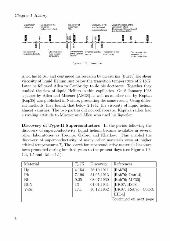
Figure 1.3: Timeline
ished his M.Sc. and continued his research by measuring [Bur35] the shearviscosity of liquid Helium just below the transition temperature of 2.18K.Later he followed Allen to Cambridge to do his doctorate. Together theystudied the flow of liquid Helium in thin capillaries. On 8 January 1938a paper by Allen and Misener [AM38] as well as another one by Kaptza[Kap38] was published in Nature, presenting the same result. Using differ-ent methods, they found, that below 2.18K, the viscosity of liquid heliumalmost vanishes. The two parties did not collaborate. Kapitza rather hada rivaling attitude to Misener and Allen who used his liquefier.
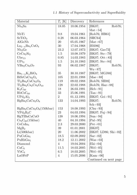
Discovery of Type-II Superconductors In the period following thediscovery of superconductivity, liquid helium became available in severalother laboratories as Toronto, Oxford and Kharkov. This enabled thediscovery of superconductivity of many other materials even at highercritical temperatures Tc The search for superconductive materials has sincebeen promoted during hundred years to the present days (see Figures 1.3,1.4, 1.5 and Table 1.1).
Material Tc [K] Discovery ReferencesHg 4.154 26.10.1911 [Rob76]Pb 7.196 31.05.1913 [Rob76; Onn14]Nb 9.25 08.07.1930 [Rob76; MF30]NbN 13 01.01.1941 [BK07; HS68]V3Si 17.1 30.12.1952 [BK07; Rob76; Col53;
HH54]Continued on next page
4
1.1 History of Superconductivity and Superfluidity
Material Tc [K] Discovery ReferencesNb3Sn 18.05 10.06.1954 [BK07; Rob76;
Mat+54]NbTi 9.8 19.04.1961 [Rob76; HB61]SrTiO3 0.28 06.03.1964 [SHC64]AlGeNb 20 05.05.1967 [Mat+67]La2−xBaxCuO4 30 17.04.1968 [BM86]Nb3Ge 23.2 12.07.1973 [BK07; Gav73]CeCu2Si2 1.5 10.08.1979 [BK07; Ste+79]Ube13 0.85 14.03.1983 [BK07; Ott+83]UPt3 1.5 24.10.1983 [BK07; Ste+84]YBa2Cu3O7 93 06.02.1987 [BK07; Rob76;
Wu+87]Ba1−xKxBiO3 35 30.10.1987 [BK07; MGJ88]BiSrCaCu2Ox 105 22.01.1988 [Mae+88]Tl2Ba2CaCu3O8 119 09.02.1988 [Rob76; SH88]Tl2Ba2Ca2Cu3O10 128 22.02.1988 [Rob76; Haz+88]K3C60 18 26.03.1991 [Heb+91]RbCsC60 33 25.06.1991 [Tan+91]UPd2Al3 2 01.12.1991 [BK07; Gei+91]HgBa2CaCu3O8 133 14.04.1993 [BK07; Rob76;
Sch+93]HgBa2CaCu3O8(150kbar) 153 18.08.1993 [Chu+93]YPd2B2C 23 04.03.1994 [BK07; Fuj+94]HgTlBaCaCuO 138 18.06.1994 [Sun+94]Cs3C60(15kbar) 40 04.10.1994 [Pal+95]CeCoIn5 2.3 29.03.2000 [Pet+01]MgB2 39 01.01.2001 [BK07]Li(500kbar) 20 11.06.2002 [BK07; LD86; Shi+02]PuCoGa5 18.5 02.09.2002 [Sar+02]PuRhGa5 18.2 12.11.2002 [Was+03]Diamond 4 19.04.2004 [Eki+04]CaC6 11.5 18.03.2005 [Wel+05]YbC6 6.5 18.03.2005 [Wel+05]LaOFeP 4 15.05.2006 [Kam+06]
Continued on next page
5

Chapter 1 History
Material Tc [K] Discovery ReferencesLaO1−xFxFeAs 26 23.02.2008 [Kam+08]SmFeAsO 55 16.04.2008 [Ren+08]
Table 1.1: Table of selected superconductors
It was discovered, that not only metals exhibit superconductivity butalso intermetallic compounds such as Nb3Sn (Tc = 18K) or metal oxidessuch as TiO (Tc = 1K). However, not long after the discovery of thesuperconductivity, it was observed that starting at a critical current den-sity superconductivity brakes down. This was related to the discovery ofthe Meissner-Ochsenfeld effect in 1933, named after Walther Meissner andRobert Ochsenfeld. External applied magnetic fields are expelled com-pletely from the inside, as long as they don’t exceed a critical magneticfield Hc. Stronger magnetic fields destroy the effect of superconductiv-ity. At this time all the materials studied exhibited values for Hc faint-ing the prospects of implementing superconductivity in technical purposessuch as the generation of large magnetic fields. In 1936, Schubnikow etal. [Shu+08] found the appearance of a new type of superconductivity.There exist materials for which an external magnetic field, starting ata certain value Hc1 but not exceeding another critical value Hc2, pene-trates the conductor without breaking its superconductivity. Below Hc1,the material shows the Meissner-Ochsenfeld effect and above Hc2 the su-perconductivity breaks down, while in between the magnetic field lowersthe critical temperature (see Figure 1.6 (b)). The current understandingof this range is that the magnetic field penetrates the superconductor inform of non-superconducting tubes of magnetic flux, passing through thematerial, surrounded by a circulating supercurrent. As the external mag-netic field increases more and more of these vortices enter, until at Hc2,they fill the whole conductor and prevent superconductivity.Such materials are nowadays referred to as tpye-II superconductors. Al-
though it took until 1961 for most of the physicists to recognize thisdiscovery (in principle type-II superconductors already showed up in theGinzburg-Landau theory from 1950), this kind of superconductors allowedmuch higher magnetic fields and are therefore in use in many technicalapplications today.
6

1.1 History of Superconductivity and Superfluidity
0
20
40
60
80
100
120
140
160
1910 1920 1930 1940 1950 1960 1970 1980 1990 2000 2010
Liquid He
Liquid H2
Liquid N2
Crit
ical
Tem
pera
ture
[K]
Year of discovery
Metals / Compounds
Pb
Hg
Nb
NbN
Nb3Sn
V3Si
Li (500 kbar)
NbTi
AlGeNb
Nb3Ge YPd2B2C
SrTiO3
Cuprates
La2-xBaxCuO4
YBa2Cu3O7
BiSrCaCu2Ox
Tl2Ba2CaCu3O8
Tl2Ba2Ca2Cu3O10
HgBa2CaCu3O8
HgTlBaCaCuO
HgBa2CaCu3O8 (150 kbar)
Oxypnictide
LaOFeP
LaO1-xFxFeAs
SmFeAsO
Fullerides
Cs3C60 (15 kbar)
K3C60
RbCsC60
Unusual superconductors
Ba1-xKxBiO3
MgB2
Covalent superconductors
Diamond
CaC6
YbC6
Heavy fermion superconductors
CeCu2Si2Ube13UPt3
UPd2Al3 CeCoIn5
PuRhGa5PuCoGa5
Figure 1.4: Critical temperature plotted against discovery dates of some selected super-conductors. See Table 1.1 for the underlying references.
7

Chapter 1 History
Figure 1.5: Periodic table of the elements with period number and critical temperature[K]. Black: Superconducting element, Black top left corner: Superconducting elementunder pressure, White: Non-superconducting, Hatched: Not yet studied. Values takenfrom [BK07].
8

1.1 History of Superconductivity and Superfluidity
(a) Type-I
(b) Type-II
Figure 1.6: Tempera-ture versus magneticfield phase diagram ofa type-I and type-IIsuperconductor
Discovery of High Temperature Superconduc-tivity In 1975, Arthur W. Sleight at DuPont found[SGB75] that the ceramic compound BaPb1−xBixO3
became superconducting below Tc = 13K. This andother works in the field of solid state physics lead Jo-hannes Georg Bednorz und Karl Alexander Müller atthe IBM Zurich Research Laboratory to start exper-iments with perovskite structures in 1983. In 1986they measured a critical temperature Tc = 35K forthe substance BaxLa5−xCu5O5(3−y). More precisely,they found an abrupt decrease by up to three or-ders of magnitude starting at 35K (so called Tc on-set) and reaching zero resistance at 13K. Bednorzand Müller received the Nobel Price in Physics alreadyone year later. Currently, the superconductor with thehighest transition temperature is mercury barium cal-cium copper oxide with a substitution of Tl for Hg(Tl0.2Hg0.8Ba2Ca2Cu3O8) at around 138K [Sun+94].
Developement of the Underying Theory In themean time, theorists developed the first explanationsfor superconductivity. The first phenomenological the-ory was developed by the London brothers Fritz andHeinz in 1935. By means of a set of two equations, theysucceeded in explaining the Meissner-Ochsenfeld effect.In 1950, Ginzburg and Landau put up their theory [GL50] to explain themacroscopic properties of superconductors. They took a Schrödinger-likeequation as a basis and could distinguish between the two types of super-conductors. Finally, in 1957 Bardeen, Cooper and Schrieffer [BCS57] pro-posed the first microscopic theory for superconductivity. Later, it could beextended to the context of superfluidity [Leg80; NSR85] and in 1959, LevGor’kov [Gor59] (formally) demonstrated the connection to the Ginzburg-Landau theory. Close to the critical temperature, the BCS theory reducesto the Ginzburg-Landau theory. The remarkable finding was, that it con-cerned a relationship between a macroscopic and a microscopic theory.
9

Chapter 1 History
1.2 Applications
Creation of Strong Magnetic Fields Strong magnetic fields are veryimportant in today’s world. Even physicist are impressed by it’s capabili-ties (see Figure 1.7).
Figure 1.7: A live frog levitatesinside a 32mm diameter verticalbore of a Bitter solenoid in a mag-netic field of about 16T at the Ni-jmegen High Field Magnet Labo-ratory. The frog, as many otheranimals, consists mainly of waterwhich as a diamagnetic substancerepels a magnetic field. Permis-sion granted for this photo to be li-censed under the GNU-type licenseby Lijnis Nelemans, High FieldMagnet Laboratory, Radboud Uni-versity Nijmegen.
Superconducting coils can generate verystrong magnetic fields while they don’t dis-sipate any energy aside from the power con-sumed by the refrigeration equipment tocool down the coil below the critical tem-perature. In 2007, a collaboration betweenthe National High Magnetic Field Labo-ratory in Tallahassee, Florida and indus-try partner SuperPower Inc. built a mag-net with windings of the high tempera-ture superconductor YBCO and achieved aworld record critical field of 26.8T [Mag].Though it is possible to construct resistiveelectromagnets (normal conductors) reach-ing even higher field strengths, such mag-nets consume huge amounts of power andrequire cooling water circulating throughpipes. In 2010 the National High MagneticField Laboratory established a new recordfor the world’s strongest resistive magnet.The system had a maximum field strengthof 36.2T and consisted of hundreds of sep-arate so called “Bitter plates”. It consumes19.6MW of electric power [Flu]. Therefore,in practical applications superconducting
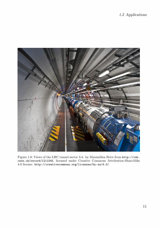
magnets are preferred. At the Large Hadron Collider, CERN (Geneva,Switzerland) NbTi superconductors are used as magnets (see Figure 1.8)to hold the particles on the ring [EB08]. They are cooled down below 2Kusing superfluid helium and operate at fields above 8T.However, the largest consumer of superconducting materials is high-
field magnetic resonance imaging (MRI) [HS11]. There also NbTi is mostwidely used. Another material frequently used for magnets is Nb3Sn. It
10
1.2 Applications
Figure 1.8: Views of the LHC tunnel sector 3-4. by Maximilien Brice from http://cds.cern.ch/record/1211045, licensed under Creative Commons Attribution-ShareAlike4.0 license: http://creativecommons.org/licenses/by-sa/4.0/
11

Chapter 1 History
can withstand higher magnetic fields than NbTi but is also more expensive.
Measurement of Extremely Weak Magnetic Fields Superconduc-tors are as well in use for precision measurements. A SQUID (for supercon-ducting quantum interference device, see Figure 1.9)
Figure 1.9: A SQUID by Zureks (Own work)[CC-BY-SA-3.0 (http://creativecommons.org/licenses/by-sa/3.0) or GFDL(http://www.gnu.org/copyleft/fdl.html)], via Wikimedia Commonshttp://commons.wikimedia.org/wiki/File%3ASQUID_by_Zureks, source: http://upload.wikimedia.org/wikipedia/commons/9/98/SQUID_by_Zureks
utilizes the fact, that in a supercon-ducting ring placed in a magneticfield, the enclosed magnetic flux isquantized and has to be an integermultiple of the magnetic flux quan-tum Φ0 = h
2e ≈ 2.067833758(46) ×10−15 Vs. This is caused by a circu-lar current through the ring, whosecontribution to the total magneticflux exactly compensates the devia-tion of the flux of the magnetic fieldto the next integer multiple of Φ0.This way, by changing the externalelectric field, the current changesits direction every time the flux isincreased by a half of the mag-netic flux quantum Φ0. Insertingtwo Josephson junctions (insulatingbarrier or a short section of non-superconducting metal) into the su-perconducting ring, it is possible toexploit the so called Josephson ef-fect, to measure the circular current
and thus also the flux of the external magnetic field. A SQUID is sensitiveenough to measure field changes as low as 5 · 10−18 T [Ran04, p. 26] andis used in medicine for measuring ion current caused waves in the brain(magnetoencephalography).
12

Chapter 2
Physical Background: The BCSTheory
In this chapter, the BCS theory is recapitulated, which was introducedin 1957 by Bardeen, Cooper, and Shrieffer [BCS57] to describe supercon-ductivity. It is a microscopic description of fermionic gases with localpair interactions at low temperatures. It acts on the assumption that thephysical environment and/or the inter particle forces create an effectivepair interaction between the fermions. The pairing mechanism is realizedby a two body interaction potential V . Given such a potential V , theBCS theory provides an expression for thermodynamic grand potential forthe fermionic gas, depending besides the temperature T and the chemicalpotential µ on the interaction potential V , the momentum distributionγ and the Cooper pair wave function α. The BCS theory was later ex-tended to the context of superfluidity [Leg80; NSR85] and connectionsto the theory of Bose-Einstein condensates (BEC) [Leg80; NSR85; PS03]where established. Thus, the theory covers the whole spectrum of the socalled BCS-BEC crossover [Ran96], where the system smoothly changesfrom a superfluid state of delocalized Cooper pairs for weak interactionsto a BEC of bosonic-like diatomic molecules for strong interactions. Forboth the regime, where the attraction is weak as well as the regime, wherethe attraction is strong, the BCS theory could be linked to an older the-ory, limited only to the particular regime. In the case of the former,this concerns the Ginzburg-Landau theory and in the case of the latter,the Gross-Pitaevskii equation. Both theories could be derived from theBCS theory by Gor’kov [Gor59], and Leggett, Noziéres and Schmitt-Rink[Leg80; NSR85] respectively - at least formally. Mathematical rigorousderivations were given in [Fra+08] and [HS12; HS13] respectively.In the following sections we will deduce the BCS theory from quantum
13

Chapter 2 The BCS theory
physics in two steps. First, by restricting the allowed states of the systemto quasi-free states and second by assuming translation invariance andSU(2) rotation invariance. We start with an brief overview of quantummechanics.
2.1 Quantum MechanicsPhysical States The states of a quantum mechanical system Σ (forexample a finite number of atomic nuclei and electrons in a region Λ ⊆ R3)are given by unit rays [ψ] = zψ|z ∈ C, |z| = 1 for ‖ψ‖ = 1 in a Hilbertspace HΣ. Depending on the system Σ one wants to describe, the Hilbertspace has to be chosen appropriately. In the following we will refer to astate as a representative of [ψ]. We denote by 〈·, ·〉 the scalar product inthe Hilbert space and as usual by ‖ψ‖ =
√〈ψ,ψ〉 the norm of HΣ. For
the scalar product, we use the convention, where 〈·, ·〉 is anti-linear in thefirst argument and linear in the second argument.
Physical Observables Physical observables are realized by self-adjointlinear operators A : HΣ → HΣ. The set of possible values for measure-ments of the observable is then given by the spectrum σ(A) of the operatorA. Let a ∈ σ(A) be the result of a measurement of the observable cor-responding to A in the state ψ ∈ HΣ. If A =
∫σ(A)
λdEλ is the spectraldecomposition of A, then
P (a ∈ S) = 〈ψ,∫
S
dEλψ〉
is the probability that the value a lies in the set S ⊆ σ(A). The expectationvalue of the result is therefore given by
E(a) = 〈ψ,Aψ〉.
Mixed States in Statistical Mechanics Since we will be interested insolid state physics where we have to deal with a huge number of particlesit is hopeless to keep the view of the exact state of the whole system.Instead we will change to a statistical description of the system, namely tothe framework of statistical mechanics. There the concept of a state (pure
14

2.1 Quantum Mechanics
state) is generalized to mixed states, i.e. a statistical ensemble of severalpure quantum states. A mixed state on the Hilbert space HΣ is defined asa density matrix 1, that is a positive trace class operator ρ, with tr(ρ) = 1.The expectation value of a measurement of the observable A in the stateρ in this case is
〈A〉ρ := tr(ρA)
and pure states ψ ∈ HΣ correspond to ρ = Pψ := ψ〈ψ, · 〉. Using thespectral decomposition of ρ,
ρ =
∞∑
k=1
wkPψk
with w1 ≥ w2 ≥ . . . ≥ 0,∑∞k=1 wk = 1 and pairwise orthogonal ψk, we
see, that each density matrix is a convex combination of pure states Pψk .
Fock Space In statistical mechanics, there are situations where the par-ticle number changes. Even more radical, the constraint of a fixed particlenumber is dropped. As a consequence, mathematics simplifies in somesituations. Therefore, for the Hilbert space HΣ we choose a special one,providing the structure to deal with more than just one particle. It isbased on an abstract Hilbert space H describing the states of a single fer-mion. The corresponding Hilbert space describing a system consisting ofn identical fermions is constructed by H(n) =
∧nH. A simple vector inH(n) is of the form
ψ1 ∧ · · · ∧ ψn :=∑
σ∈Sn(−1)σψσ(1) ⊗ · · · ⊗ ψσ(n), for ψi ∈ H,
where Sn denotes the set of all permutations of n elements, i.e. the sym-metric group, where (−1)σ is the sign of a permutation σ and ⊗ is thetensor product. An arbitrary vector in H(n) then is a (possibly infinite)linear combination of simple vectors.1In [BLS94] a mixed state is a linear map ρ : L(HΣ)→ C, with the properties
ρ(1) = 1, ρ(A∗A) ≥ 0.
Here L(HΣ) denotes the set of all linear operators on HΣ and A∗ the adjoint of A.However, the assignment ρP (A) := tr(PA) yields a one to one correspondence
between density matrices P and linear mappings ρP .
15

Chapter 2 The BCS theory
However, the n-particle space H(n) still can’t describe systems consist-ing of a changing or undetermined number of fermions. Therefore, weintroduce the so called Fock space
FH :=
∞⊕
n=0
H(n),
where H(0) := CΩ and Ω is the vacuum state with 〈Ω,Ω〉 := 1. Note thatFH is a Hilbert space on its own with the natural scalar product induced bythe vector space sum. In particular sectors of different particle numbersare orthogonal to each other. To any vector φ ∈ H in the one-particleHilbert space, we associate a creation operator a†(φ) : FH → FH and anannihilation operator a(φ) : FH → FH. We define the creation operatora†(ψ) for a vector ψ = (ψ(0), ψ(1), ...) ∈ FH, ψ(n) ∈ H(n) by
(a†(φ)ψ
)(n+1):= (n+ 1)−1/2φ ∧ ψ(n),
where φ ∧ Ω = φ. The annihilation operator a(ψ) is defined to be theadjoint operator of a†(ψ) and acts as follows: If ψ(n) = ψ1∧ · · ·∧ψn is thepart in the n-particle space H(n) of ψ, then
(a(φ)ψ
)(n−1)=√n
n∑
i=1
(−1)i−1〈φ, ψi〉ψ1 ∧ · · · ∧ ψi ∧ · · · ∧ ψn,
where the hat indicates that ψi is omitted in the wedge product. Notethat a(φ)|H(0) ≡ 0. By this construction, the creation and annihilationoperators fulfill the canonical anti-commutation relations
a(φ), a†(ψ) = 〈φ, ψ〉1FHa(φ), a(ψ) = a†(φ), a†(ψ) = 0,
where A,B = AB +BA is the anti-commutator.
Bogoliubov Transformations A Bogoliubov transformation of FH isa unitary operator W : FH → FH such that there exists linear operatorsv, w : H → H of such that for ψ ∈ H, we have
Wa†(ψ)W ∗ = a†(vψ) + a(wψ),
16

2.1 Quantum Mechanics
where ψ(x) = ψ(x) is the complex conjugation2. As a unitary operator,Wleaves invariant the canonical anticommutation relations, i.e. Wa†(ψ)W ∗
and Wa(ψ)W ∗ satisfy the canonical anticommutation relations. This inturn is equivalent to
U :=
(v ww v
): H⊕H → H⊕H
being unitary, where Tψ := Tψ for an arbitrary operator T : H → H.
Quasi-free States Since it is still very difficult to describe the systemwith pure quantum statistics, in the BCS theory only so called quasi-free states are considered. The idea behind comes from thermodynamics.There one is interested in equilibrium states, i.e. states which remain in-variant under time evolution. In quantum statistics such states are calledGibbs states and are of the form ρ = Z−1 exp(−βH), where H is a Hamil-tonian on the Fock space and Z = tr
(exp(−βH)
)< ∞. As it turns out,
Gibbs states are a special case of quasi-free states. A mixed state ρ is aquasi-free state if the following “Wick’s Theorem” holds.
〈a#1 a
#2 · · · a#
2n〉ρ =∑
σ∈S′n
(−1)σ〈a#σ(1)a
#σ(2)〉ρ · · · 〈a
#σ(2n−1)a
#σ(2n)〉ρ
〈a#1 a
#2 · · · a#
2n+1〉ρ = 0,
where each # can stand for † or nothing and where S′n is the subset of Sncontaining the permutations σ which satisfy σ(1) < σ(3) < . . . < σ(2n−1)and σ(2j − 1) < σ(2j) for all 1 ≤ j ≤ n.
One-particle Density Matrices To each quasi-free state we associatea self-adjoint operator Γ : H⊕H → H⊕H, called the one-particle density2We could have chosen a different antiunitary map C : H → H. instead of the complexconjugation. In this case the linear map w also has to be adjusted. This dependenceon the antiunitary map comes from the antilinearity of the annihilation operator. Ifwe would define the annihilation operator to accept as its argument an element ofH∗ instead of H (i.e. if we replace a by a, where a(Jψ) = a(ψ) with J : H → H∗being the conjugate linear map such that (Jψ)(φ) = 〈ψ, φ〉) then the antilinearitywould be naturally absorbed in J This is basically the approach of [Sol].
17
Chapter 2 The BCS theory
matrix of ρ defined by
〈(φ1, φ2),Γ(ψ1, ψ2)〉 = ρ([a†(ψ1) + a(ψ2)][a(φ1) + a†(φ2)]
). (2.1.1)
Again, this definition depends on the choice of the antiunitary map Cwhich we here specified to be the ordinary complex conjugation.The operator Γ for fermions has an important property. Namely,
0 ≤ Γ ≤ 1
as an operator. This is seen as follows. Let (φ, ψ) ∈ H ⊕ H with ‖φ‖2 +‖ψ‖2 = 1. Then
〈(φ, ψ),Γ(φ, ψ)〉 = ρ([a(φ) + a†(ψ)]∗[a(φ) + a†(ψ)]
)≥ 0.
Moreover, by using the anti-commutation rules for a and a†, we obtain
[a(φ)+a†(ψ)]∗[a(φ)+a†(ψ)] = ‖φ‖2 +‖ψ‖2− [a(φ)+a†(ψ)][a(φ)+a†(ψ)]∗
and we conclude〈(φ, ψ),Γ(φ, ψ)〉 ≤ 1.
2.2 Derivation of the BCS FunctionalWe start with a quantum mechanical system Σ consisting of an indefinitenumber of spin 1
2 fermions in a cubic box Λ ⊂ R3 of side length L, withperiodic boundary conditions. The interaction between the fermions isdefined by a two-body potential V ∈ L1(Λ). Moreover, the system shallbe exposed to external electric and magnetic fields, W (x) and B(x) =curlA(x). We then aim to take the limit Λ → R3 and to find the stateminimizing the grand potential ΦG. In the following we will specify theHilbert space for the system Σ under consideration and define the physicalobservable corresponding to the grand potential.
Hilbert Space We consider the Hilbert space HΣ = FH, where the un-derlying one-particle Hilbert space consists of vector valued wave functionsand is given by
H = L2per(Λ)⊕ L2
per(Λ) ∼= L2per(Λ)⊗ C2,
18

2.2 Derivation of the BCS Functional
where we choose an orthonormal basis e↑, e↓ for C2.Vectors in H(n) are totally antisymmetric wave functions
ψ(z1, . . . , zn),
where zi = (xi, σi) ∈ Λ×C2 denotes a space-spin variable for one particle.
Observables The grand potential of thermodynamics is given by ΦG =U − TS − µN , where U is the internal energy, T is the temperature, Sis the entropy, µ is the chemical potential and N is the particle number.The quantities T and µ are scalars and can be interpreted as Lagrangemultiplicators, i.e. if we minimize ΦG, we actually minimize U under theconstraint that S and N are constant. We are interested in a quantumstatistical description for ΦG. Thus, we have to define quantum mechanicalexpressions for for U , S and N . The internal energy U corresponds to theenergy observable, i.e. the (densely defined) Hamiltonian which is givenby
H = T + UV + UW ,
T |H(n) =
n∑
j=1
(− i∇xj +A(xj)
)2,
UV |H(n) =1
2
n∑
j,k=1j 6=k
V (xj − xk),
UW |H(n) =
n∑
j=1
W (xj),
The quantum mechanical counterpart toN is the particle number operatorN , defined by N |H(n) = n1. Finally, we describe S by the von-Neumannentropy of a state ρ, which is given by
S(ρ) = − tr(ρ ln(ρ)
).
The quantum mechanical grand potential of a state ρ then is
ΦG(ρ) = 〈H〉ρ − TS(ρ)− µ〈N〉ρ.
19

Chapter 2 The BCS theory
2.2.1 Step 1: Restriction to Quasi-free States
As a first simplification, we restrict the grand potential ΦG to quasi-freestates (see the corresponding paragraph in Section 2.1). ΦG(ρ) then re-duces to expressions in the operators γ, α : H → H, defined by
〈φ, γψ〉 = 〈a†(ψ)a(φ)〉ρ〈φ, αψ〉 = 〈a(ψ)a(φ)〉ρ.
(2.2.1)
This is easy to see for a so called 1-body operator like T , UW , and N ,i.e. an operator A : FH → FH of the form
A|H(n) =
n∑
j=1
(j−1⊗
k=1
1
)⊗A(1) ⊗
n⊗
k=j+1
1
,
for some operator A(1) : H → H. Let ϕjj∈N be an orthonormal basisof H. Then such operators can be expressed in terms of the creation andannihilation operators a†(ϕj) and a(ϕj) according to
A =∑
j,k∈N〈ϕj , A(1)ϕk〉a†(ϕj)a(ϕk).
Consequently, expectation values are given by
〈A〉ρ = 〈ϕj , A(1)ϕk〉〈ϕkγϕj〉 = trH(A(1)γ).
An analogous procedure can be given for 2-body operators, like UV . Bymeans of Wick’s Theorem, which for quartic monomials in the creationand annihilation operators, reduces to
〈a#1 a
#2 a
#3 a
#4 〉ρ = 〈a#
1 a#2 〉ρ〈a#
3 a#4 〉ρ−〈a#
1 a#3 〉ρ〈a#
2 a#4 〉ρ+ 〈a#
1 a#4 〉ρ〈a#
2 a#3 〉ρ,
a similar computation using
UV =∑
j,k,l,m∈N〈ϕj ⊗ ϕk, V (x− y)ϕl ⊗ ϕm〉a†(ϕj)a†(ϕk)a(ϕm)a(ϕl)
20

2.2 Derivation of the BCS Functional
shows
〈UV 〉ρ =1
2
∑
σ,τ∈↑,↓
∫
Λ×Λ
|α(x, σ, y, τ)|2V (x− y) d3xd3y
− 1
2
∑
σ,τ∈↑,↓
∫
Λ×Λ
|γ(x, σ, y, τ)|2V (y − x) d3x d3y
+1
2
∑
σ,τ∈↑,↓
∫
Λ×Λ
γ(x, σ, x, σ)γ(y, τ, y, τ)V (x− y) d3x d3y,
where γ(x, σ, y, τ) and α(x, σ, y, τ) are the integral kernels of γ and αrespectively.Another calculation (see Appendix 2.A) shows that in terms of Γ, the
entropy functional S(ρ) can be expressed as
S(Γ) = − trH⊕H(Γ ln(Γ)
).
Thus we obtain for the grand potential the functional
ΦG(Γ) = trH(((−i∇+A)2 + µ+W )γ
)− TS(Γ)
+1
2
∑
σ,τ∈↑,↓
∫
Λ×Λ
|α(x, σ, y, τ)|2V (x− y) d3x d3y
− 1
2
∑
σ,τ∈↑,↓
∫
Λ×Λ
|γ(x, σ, y, τ)|2V (y − x) d3xd3y
+1
2
∑
σ,τ∈↑,↓
∫
Λ×Λ
γ(x, σ, x, σ)γ(y, τ, y, τ)V (x− y) d3xd3y.
(2.2.2)
We define the BCS functional as the formal infinite volume limit
FBCS(Γ) := limΛ→R3
ΦG(Γ), (2.2.3)
i.e. we replace Λ by R3 in the expression for ΦG(Γ).The BCS theory studies the minimizers of FBCS. The term trH
((−i∇+
A)2γ)corresponds to the kinetic energy and S is the entropy. The term
21
Chapter 2 The BCS theory
involving the Cooper pair wave function α is the pairing energy of theCooper pairs. If this pairing energy lowers the BCS energy, i.e. if theminimizer of FBCS has a non-vanishing α, then we say that the systemexhibits a Cooper pair condensate and has a superfluid or superconductingphase. If the minimizer Γ0 of FBCS has α ≡ 0, the system is said tobe in a normal state. The last two summands of (2.2.2) are referred toas direct and exchange term, respectively. They correspond to density-density interactions between the fermions and are in general difficult tohandle. Therefore they are being neglected usually.The reason behind the interpretation of α as the Cooper pair wave
function is that the system displays macroscopically coherent behavior assoon as α 6= 0. To see that, we examine the correlation function of a pairat x and a pair at y, formally given by 〈a†x,↑a
†x,↓ay,↓ay,↑〉ρ. We will see
later, that for SU(2) invariant states ρ, the operators γ and α satisfy
γ(x, σ, y, τ) = δστ γ(x, y),
α(x, σ, y, τ) = (1− δστ )α(x, y),
for some reduced operators γ and α. In this case, 〈a†x,↑a†x,↓ay,↓ay,↑〉ρ =
|γ(x, y)|2+α(x, x)α(y, y). If in addition the system is translation invariant,i.e. γ(x, y) = γ(x + δ, y + δ) and γ(x, y) = γ(x + δ, y + δ), the expressionfor the correlation reduces to
|α(0, 0)|2 + |γ(x− y, 0)|2.
For far apart x and y, |γ(x− y, 0)|2 converges to 0 whereas |α(0, 0)|2 staysconstant. Therefore the pairs stay correlated over large distances, whichis referred to as long range order.
2.2.2 Step 2: Assuming SU(2) Invariance
We denote vectors ψ ∈ H = L2(R3)⊕ L2(R3) ∼= L2(R3)⊗ C2 by
ψ = (ψ↑, ψ↓).
For example, if φ ∈ L2(R3) then the state ψ = φ ⊗ e↑ ∈ H is given byψ = (φ, 0). In other words, we think of ψ as an element of L2(R3,C2)
22
2.2 Derivation of the BCS Functional
such that ψ(x) ∈ C2. Rotating the spin space is described by a matrixS ∈ SU(2) which acts on H according to
(Sψ)(x) = Sψ(x).
On the fock space FH the action of S ∈ SU(2) is given by the Bogoliubovtransformation WS ∈ L(FH), which transforms the creation and annihila-tion operators according to
WSa†(ψ)W ∗S = a†(Sψ)
WSa(ψ)W ∗S = a(Sψ).
A state ρ is said to be invariant under spin rotations or shortly SU(2)invariant if
〈WSAW∗S〉ρ = 〈A〉ρ. (2.2.4)
In the following, we will restrict FBCS to SU(2) invariant states. Thereason behind this approximation is that we know that a pure state ψ ∈ H,minimizing some HamiltonianH which is SU(2) invariant, i.e. [H,WS ] = 0has to be SU(2) invariant itself, i.e. WSψ = ψ. In our case, H is in factSU(2) invariant but ΦG also contains the non-linear entropy functionalS. Therefore it is apriori not clear if the minimizer(s) of ΦG are SU(2)invariant and the restriction is an approximation.For quasi-free states the condition to be SU(2) invariant, translates to
a transformation law for the operators α, γ via (2.2.1), i.e.
γ 7→ S∗γS
α 7→ S∗αS.
If a matrix M ∈ C2×2 has the property S∗MS = M for all S ∈ SU(2),then M must be a multiple of 1. Analogously if S∗MS = M , then M =λ(
0 −ii 0
).
Therefore, for a quasi-free SU(2) invariant state the operators γ, α musthave the form
γ = γ ⊗ 1α = α⊗
(0 −ii 0
),
23
Chapter 2 The BCS theory
for corresponding, reduced operators γ, α : L(R3)→ L(R3) satisfying
γ∗ = γ, αT = α.
We will now show, that the BCS functional FBCS for SU(2) invariantstates only depends on the reduced one-particle density matrix
Γ =
(γ α
α∗ 1− γ
).
To see this, we use the notation (φ⊗ v, ψ ⊗ v) = (φ, ψ)⊗ v, such that wehave the relations
Γ[(φ, ψ)⊗ v1] = [Γ(φ, ψ)]⊗ v1
Γ[(φ, ψ)⊗ v2] = [(
1 00 −1
)Γ(φ, ψ)
(1 00 −1
)]⊗ v2,
where v1 = 1√2
(1i
)and v2 = 1√
2
(1−i)are the eigenvectors of
(0 −ii 0
). We
conclude that 0 ≤ Γ ≤ 1 as an operator and
S(Γ) = trH⊕H(Γ ln(Γ)
)= 2 trL2(R3)
(Γ ln(Γ)
)=: 2S(Γ).
Therefore, the grand potential becomes
ΦG(Γ) :=1
2ΦG(Γ) = trL2(R3)
(((−i∇+A)2 + µ+W )γ
)− T S(Γ)
+1
2
∫
R3×R3
|α(x, y)|2V (x− y) d3xd3y
− 1
2
∫
R3×R3
|γ(x, y)|2V (y − x) d3xd3y
+
∫
R3×R3
γ(x, x)γ(y, y)V (x− y) d3xd3y,
(2.2.5)
The functionalFBCS(Γ) = ΦG(Γ)
is the starting point in many papers [BHS14b; HS13; Fra+08] (usuallyagain discarding the last two summands, i.e. the direct and the exchangeterm).
24

2.2 Derivation of the BCS Functional
2.2.3 Step 3: Assuming Translation Invariance
We start with the SU(2) invariant functional FBCS(Γ) from above withfinite volume Λ, i.e. we don’t yet perform the formal limit Λ → ∞. Wewill work with the reduced quantities Γ, α, γ, and S but we will drop the“ ”. For the same reason for which we have restricted to SU(2) invariantstates we will make another approximation.The translation of a state ψ ∈ L2(R3) is given by
(Tδψ)(x) = ψ(x+ δ).
On the Fock space FL2(R3), this translates to a Bogoliubov transformationdefined by Wδa
#(ψ)W ∗δ = a#(Tδψ). Translation invariant states ρ areagain characterized by
〈WδAW∗δ 〉ρ = 〈A〉ρ.
Again, [H,Wδ] = 0, which motivates the restriction to translation invariantstates. For quasi-free states the one-particle density matrix Γ obtains theproperty
Γ(x, y) = Γ(x−δ, y−δ)⇔ Γ(x, y) = Γ(x−y) =
(γ(x− y) α(x− y)
α(y − x) 1− γ(x− y)
).
Like in the case of the SU(2) invariance, the BCS functional FBCS onlydepends on the reduced one-particle density matrix Γ(x − y): On theorthonormal basis ψk(x) = eikx√
|Λ|the operators γ, α are diagonal, namely
γψk = γ(k)ψk, αψk = α(k)ψk,
γ(k) =
∫
Λ
γ(x)e−ikx d3x, α(k) =
∫
Λ
α(x)e−ikx d3x.
Therefore the entropy S becomes
S(Γ) = −∑
k∈ 2πL Z3
trC2
(Γ(k) ln(Γ(k))
),
for
Γ(p) =
(γ(p) α(p)
α(p) 1− γ(−p)
), 0 ≤ Γ(p) ≤ 1.
25

Chapter 2 The BCS theory
The grand potential per volume (without external electromagnetic field)now reads
1
2|Λ|ΦG(Γ) =1
|Λ|∑
p∈ 2πL Z3
(p2 + µ)γ(p) + T1
|Λ|∑
k∈ 2πL Z3
trC2
(Γ(k) ln(Γ(k))
)
+1
2
∫
Λ
|α(r)|2V (r) d3r
− 1
2
∫
Λ
|γ(r)|2V (r) d3r + [γ(0)]2∫
Λ
V (r) d3r.
Taking the limit Λ → R3 and defining α := (2π)3/2α, γ := (2π)3/2γ tohave the convention
f(p) = (2π)−3/2
∫
R3
f(x)e−ipx d3x,
we obtain
FBCS(Γ) := limΛ→R3
(2π)3
2|Λ| ΦG(Γ)
=
∫
R3
(p2 + µ)γ(p) d3p+ T
∫
R3
trC2
(Γ(p) ln(Γ(p))
)d3p
+1
2
∫
R3
|α(r)|2V (r) d3r
− 1
2
∫
R3
|γ(r)|2V (r) d3r + [γ(0)]2∫
R3
V (r) d3r.
(2.2.6)
Again the first term comes from the kinetic energy. The second term∫
R3
trC2
(Γ(p) ln(Γ(p))
)d3p
is the negative entropy, which is minimal for α ≡ 0. It therefore competesthe pairing energy of the Cooper pairs, 1
2
∫R3 |α(r)|2V (r) d3r, which can
lower FBCS if α 6= 0. Therefore, if T is lowered, possibly the effect ofpairing energy may exceed the one of the entropy. In this case, the systemundergoes a phase transition. Like in the previous functionals, the last twosummands, i.e. the direct and the exchange term, respectively are beingneglected usually.
26

2.3 The Simplified Translation Invariant BCS Functional
2.3 The Simplified Translation Invariant BCSFunctional
In this section, we study the translation invariant and SU(2) invariantBCS functional. For simplicity, we also drop the direct and the exchangeterm. In [BHS14c] we attempt to extend the following results, includingthese terms. An overview over the results obtained is given in Section 3.1The first investigation concerns the existence of a minimizer of the BCS
functional
FT (Γ) =
∫
R3
(p2 + µ)γ(p) d3p− TS(Γ) +1
2
∫
R3
|α(r)|2V (r) d3r,
S(Γ) = −∫
R3
trC2
(Γ(p) ln(Γ(p))
)d3p.
(2.3.1)
Proposition 2.1 (Existence of minimizers). Let µ ∈ R, 0 ≤ T <∞, andlet V ∈ L1(R3)∩L3/2(R3) be real-valued. Then FT is bounded from belowand attains a minimizer Γ on
D =
Γ(p) =
(γ(p) α(p)
α(p) 1− γ(−p)
) ∣∣∣∣γ∈L1(R3,(1+p2) d3p),α∈H1(R3, d3x),
0 ≤ Γ ≤ 1C2
.
Proof (taken from [Hai+08]). We first show that FT dominates both theL1(R3, (1+p2) d3p) norm of γ and the H1(R3, d3x) norm of α. Hence anyminimizing sequence will be bounded in these norms. We have
FT (Γ) ≥ C1 +3
4
∫
R3
(p2 − µ)γ(p) d3p+1
2
∫
R3
|α(x)|2V (x) d3x ,
where
C1 = infΓ∈D
[1
4
∫
R3
(p2 − µ)γ(p) d3p− TS(Γ)
]= −T
∫
R3
ln(1 + e−p2−µ
4T ) d3p .
Since V ∈ L3/2 by assumption, it is relatively bounded with respect to−∆ (in the sense of quadratic forms), and hence C2 = inf spec (p2/4 + V )is finite. Using |α(p)|2 ≤ γ(p), we thus have that
1
4
∫
R3
p2γ(p) d3p+1
2
∫
R3
V (x)|α(x)|2 d3x ≥ C2
∫
R3
γ(p) d3p .
27

Chapter 2 The BCS theory
Using again that |α(p)|2 ≤ γ(p) ≤ 1, it follows that
FT (Γ) ≥ −A+1
8‖α‖2H1(R3, d3x) +
1
8‖γ‖L1(R3,(1+p2) d3p) , (2.3.2)
whereA = −C1 −
∫
R3
[p2/4− 3µ/4− 1/4 + C2
]− d3p ,
with [ · ]− = min · , 0 denoting the negative part.To show that a minimizer of FT exists in D, we pick a minimizing
sequence Γn(p) =(γn(p) αn(p)
αn(p) 1−γn(−p)
)∈ D, with FT (Γn) ≤ 0. From (2.3.2)
we conclude that ‖αn‖2H1 ≤ 8A, and hence we can find a subsequence thatconverges weakly to some α ∈ H1. Since V ∈ L3/2(R3), this implies that
limn→∞
∫
R3
V (x)|αn(x)|2 d3x =
∫
R3
V (x)|α(x)|2 d3x
[LL01, Thm. 11.4].It remains to show that the remaining part of the functional,
F0T (Γ) =
∫
R3
(p2 − µ)γ(p) d3p− TS(Γ) , (2.3.3)
is weakly lower semicontinuous. Note that F0T is convex in Γ, and that
its domain D is a convex set. We already know that αn α weakly inH1(R3). Moreover, since γn is uniformly bounded in L1(R3) ∩ L∞(R3),we can find a subsequence such that γn ˜γ weakly in Lp(R3) for some1 < p <∞. We can then apply Mazur’s theorem [LL01, Theorem 2.13] toconstruct a new sequence as convex combinations of the old one, which nowconverges strongly to (˜γ, α) in Lp(R3)×L2(R3). By going to a subsequence,we can also assume that Γn → Γ pointwise [LL01, Theorem 2.7]. Becauseof convexity of F0
T , this new sequence is again a minimizing sequence.Note that the integrand in (2.3.3) is bounded from below independently
of γ and α by −T ln(1 + e−(p2−µ)/T ). Since this function is integrable, wecan apply Fatou’s Lemma [LL01, Lemma 1.7], together with the pointwiseconvergence, to conclude that lim inf F0
T (Γn) ≥ F0T (Γ).
We have thus shown that
FT (Γ) ≤ lim infn→∞
FT (Γn) .
28

2.3 The Translation Invariant Functional
It is easy to see that Γ ∈ D, hence it is a minimizer. This proves theclaim.
Now that we know about the existence of a minimizer, we want tocharacterize it. We therefore have a look at the Euler-Lagrange equation.
Lemma 2.1 (Euler-Lagrange and gap equation). The Euler-Lagrangeequations for a minimizer Γ(p) =
(γ(p) α(p)
α(p) 1−γ(−p)
)∈ D of FT are of the
form
γ(p) =1
2− p2 − µ
2K∆T,µ(p)
(2.3.4a)
α(p) =1
2∆(p)
tanh(E∆
µ (p)
2T
)
E∆µ (p)
, (2.3.4b)
where we use the abbreviations
∆ = V α (2.3.5a)
K∆T,µ(p) =
E∆µ (p)
tanh(E∆
µ (p)
2T
) , (2.3.5b)
E∆µ (p) =
√(p2 − µ)2 + |∆(p)|2 , (2.3.5c)
In particular, the function ∆ satisfies the BCS gap equation
1
2(2π)3/2
∫
R3
V (p− q) ∆(q)
K∆T,µ(q)
d3q = −∆(p) (2.3.6)
We note that the BCS gap equation (2.3.6) can equivalently be writtenas
(K∆T,µ + V/2)α = 0,
where K∆T,µ is interpreted as a multiplication operator in Fourier space,
and V as multiplication operator in configuration space. This form of theequation will turn out to be useful later on.
29

Chapter 2 The BCS theory
Taken from [BHS14c]. We first restrict our attention to T > 0. A mini-mizer Γ of FT fulfills the inequality
0 ≤ d
dt
∣∣∣∣t=0
FT(Γ + t(Γ− Γ)
)(2.3.7)
for arbitrary Γ ∈ D. Here we may assume that Γ stays away from 0 and 1by arguing as in [Hai+08, Proof of Lemma 1]. A simple calculation using
S(Γ) = −∫
R3
trC2(Γ ln Γ) d3p = −1
2
∫
R3
trC2
(Γ ln(Γ)+(1−Γ) ln(1−Γ)
)d3p
shows that
d
dt
∣∣∣∣t=0
FT(Γ + t(Γ− Γ)
)
=1
2
∫
R3
trC2
[H∆(Γ− Γ) + T (Γ− Γ) ln
( Γ
1− Γ
)]d3p,
withH∆ =
(p2 − µ ∆∆ −(p2 − µ)
),
using the definition ∆ = V α. Separating the terms containing no Γ andmoving them to the left side in (2.3.7), we obtain
∫
R3
trC2
(H∆
(Γ− ( 0 0
0 1 ))
+ T Γ ln( Γ
1− Γ
))d3p
≤∫
R3
trC2
(H∆
(Γ− ( 0 0
0 1 ))
+ T Γ ln( Γ
1− Γ
))d3p.
Note that∫R3 trC2
(H∆Γ
)d3p is not finite but
∫R3 trC2
(H∆
(Γ−( 0 0
0 1 )))
d3p
is. Since Γ was arbitrary, Γ also minimizes the linear functional
Γ 7→∫
R3
trC2
(H∆
(Γ− ( 0 0
0 1 ))
+ T Γ ln( Γ
1− Γ
))d3p, (2.3.8)
whose Euler-Lagrange equation is of the simple form
0 = H∆ + T ln
(Γ
1− Γ
), (2.3.9)
30

2.3 The Translation Invariant Functional
which is equivalent to
Γ =1
1 + e1T H∆
.
This in turn implies (2.3.4a) and (2.3.4b). Indeed,
Γ =1
1 + e1T H∆
=1
2− 1
2tanh
(1
2TH∆
).
For the simple reason, that tanh(x)x = g(x2) is an even function and
H2∆ = [E∆
µ ]2 1C2 , the expression simplifies to
Γ =1
2−1
2H∆
tanh(E∆
µ
2T
)
E∆µ
=1
2− 1
2K∆T,µ
H∆ =
12 −
p2−µ2K∆
T,µ
− ∆2K∆
T,µ
− ∆2K∆
T,µ
12 + p2−µ
2K∆T,µ
.
We now turn to T = 0. By inspecting (2.3.8), we note that there are nocritical points in the interior of D. We thus have to impose the additional(pointwise) condition Γ(p) = 0 or Γ(p) = 1 on Γ. This is equivalent toΓ(1 − Γ) = 0 which holds if and only if trC2
(Γ(1 − Γ)
)= 0 and either
γ(p) = γ(−p) or α(p) = 0. It will turn out, that already imposing thecondition on the trace suffices to find a critical point which also has thesymmetry γ(p) = γ(−p) or α(p) = 0. We thus minimize
∫
R3
(p2 + µ)γ(p) d3p+1
2
∫
R3
|α(r)|2V (r) d3r + λ trC2
(Γ(1− Γ)
),
with the Lagrange multiplicator λ. Varying this functional with respectto Γ, yields for the critical point Γ
H∆ = λ(1− 2Γ).
Using the constraint Γ(1 − Γ) = 0, we obtain λ = E∆µ and solving for Γ
yields
Γ =1
2− 1
2E∆µ
H∆.
Performing the convolution with V on both sides of (2.3.4b) and using therelation ∆ = (2π)−3/2V ∗ α gives the BCS-gap equation (2.3.6).
31

Chapter 2 The BCS theory
Clearly, the minimizer of the non-interacting case V = 0 which is givenby
Γ0(p) =1
1 + e1T H0(p)
=
(γ0(p) 00 1− γ0(−p)
)
solves the Euler-Lagrange equation, where
γ0(p) =1
1 + e1T (p2−µ)
, H0 =
(p2 − µ 00 −(p2 − µ)
).
We will refer to this state as the normal state. The key question, whichwill decide if the system is superfluid is whether the BCS functional has aminimum at the normal state or just a saddle point. In order to examinethat we need the second variation of the BCS functional.
Lemma 2.2 (Second variation of the BCS functional). Let Γ =( γ α
α 1−γ)
be a critical point of FT , i.e. Γ satisfies the Euler-Lagrange equationsΓ = 1
1+e1TH∆
. Let G =( ρ ϕϕ −ρ
), for ϕ in the domain of K∆
T,µ + V/2 and
ρ =
αϕ+αϕ1−2γ , α(p) 6= 0
0, α(p) = 0.
Then
d2
dt2
∣∣∣∣t=0
FT (Γ + tG) = 2〈ϕ, (K∆T,µ + V/2)ϕ〉+ 2〈ρ,K∆
T,µρ〉. (2.3.10)
Proof. By taking the second derivative, only the entropy term and the αterm survive. The second derivative of the latter is simply 〈ϕ, V ϕ〉. Forthe entropy term, we introduce s(z) = 1
2
(z ln(z) + (1− z) ln(1− z)
), such
that−S(Γ) =
∫
R3
trC2
(s(Γ)
)d3p.
As an initial point, we take the first derivative of the integrand
d
dttrC2
(s(Γ + tG)
)= trC2
(s′(Γ + tG)G
)
=1
2πitrC2
[∫
C
s′(z)1
z − (Γ + tG)Gdz
],
32

2.3 The Translation Invariant Functional
where C is a closed curve enclosing the interval (0, 1). We have to dif-ferentiate this expression a second time at t = 0. The definition of ρis constructed, such that Γ and G satisfy the anti-commutation relationΓ, G = G. Therefore,
G,
1
z − Γ
=
1
z − ΓG, z − Γ 1
z − Γ= (2z − 1)
1
z − ΓG
1
z − Γ
= (2z − 1)d
dt
∣∣∣∣t=0
1
z − (Γ + tG)
and we obtain
d
dt
∣∣∣∣t=0
trC2
(s′(Γ + tG)G
)=
1
2πitrC2
[∫
C
s′(z)2z − 1
1
z − Γ, G
Gdz
].
We use the cyclicity of the trace to conclude that
1
2
d2
dt2
∣∣∣∣t=0
trC2
(s(Γ + tG)
)=
1
2πitrC2
[∫
C
s′(z)2z − 1
1
z − ΓG2 dz
]
= trC2
[s′(Γ)
2Γ− 1G2
].
Now note thats′(z)
2z − 1
∣∣∣∣z= 1
1+ex
=1
2
x
tanh(x)
and that Γ = 1
1+e1TH0
. Therefore,
s′(Γ)
2Γ− 1=K∆T,µ
2T,
which implies
d2
dt2
∣∣∣∣t=0
trC2
(s(Γ + tG)
)=K∆T,µ
TtrC2(G2).
Inserted into the expression for d2
dt2
∣∣∣t=0− TS(Γ + tG), this finishes the
proof.
33

Chapter 2 The BCS theory
This observation together with the Euler-Lagrange and gap equationmay be combined in the following theorem
Theorem 2.1. Let V ∈ L3/2(R3), µ ∈ R, and 0 ≤ T < ∞. Then thefollowing statements are equivalent:
(i) The normal state Γ0 is unstable under pair formation, i.e.,
infΓ∈DFT (Γ) < FT (Γ0).
(ii) There exists Γ ∈ D, with α = 0, such that ∆ = V α satisfies the BCSgap equation
∆ =1
2(2π)3/2V ∗ ∆
K∆T,µ
.
(iii) The linear operator
K0T,µ + V/2, K0
T,µ(p) =tanh(p
2−µT )
p2 − µ ,
has at least one negative eigenvalue.
Proof. (i) ⇒ (ii): Assumption (i) together with the existence of a mini-mizer (Proposition 2.1) immediately implies the existence of a minimizerwith α 6= 0, which has to satisfy the Euler-Lagrange equation and thusalso the gap equation.(ii) ⇒ (iii): Let us observe now that
x 7→ KxT,µ(p)
is a monotone increasing function for all p. Therefore, as we can bring thegap equation into the form
(K∆T,µ + V/2)α = 0,
as soon as α 6= 0,〈α, (K0
T,µ + V/2)α〉 < 0,
34

2.3 The Translation Invariant Functional
because K∆T,µ(p) > K0
T,µ(p) for all p where ∆(p) 6= 0, which is the sameset where α(p) 6= 0.(iii) ⇒ (i): This is Lemma 2.2 applied to the normal state Γ0 with
G =(
0 ϕ(p)
ϕ(p) 0
).
We obtain
d2
dt2
∣∣∣∣t=0
FT (Γ0 + tG) = 2〈ϕ, (K0T,µ + V/2)ϕ〉,
which implies that though the normal state is a critical point, it is not aminimizer.
Theorem 2.1 enables a precise definition of the critical temperature, by
Tc(V ) := infT |K0T,µ + V/2 ≥ 0. (2.3.11)
Expressed differently, the critical temperature Tc is given by the valueT , such that K0
Tc,µ+ V/2 has 0 as lowest eigenvalue. The uniqueness of
the critical temperature follows from the fact that the symbol K0T,µ(p) is
point-wise monotone in T . This implies that for any potential V , thereis a critical temperature 0 ≤ Tc(V ) <∞ that separates a superfluid phasefor 0 ≤ T ≤ Tc(V ) from a normal phase for Tc(V ) ≤ T < ∞. Notethat Tc(V ) = 0 means that there is no superfluid phase at all for V .Using the linear criterion (2.3.11) we can classify the potentials for whichTc(V ) > 0, and simultaneously we can evaluate the asymptotic behavior ofTc(V ) in certain limits. For example, in [Fra+07; HS08] the weak couplinglimit is studied, i.e. the asymptotic behaviour of Tc(λV ) for small λ > 0.Another interesting case is the low density limit, considered in [HS12].Here, the behaviour of Tc(V ) subject to µ → 0 is treated. Finally, in[BHS14c; BHS14a] the short range limit is examined, where basically therange ` = diam(supp(V )) becomes small at a fixed scattering length a.
35

Chapter 2 The BCS theory
36

Appendix
2.A Expression for the Entropy for Quasi-freeStates
Throughout the calculations, we will use the following orthonormal ba-sis for FH. Given an orthonormal basis ϕii∈N of H, we construct theorthonormal basis ϕJ J⊂N
|J|<∞of FH by
ϕJ =1√|J |!
∧
j∈Jϕj , (2.A.1)
where |J | denotes the number of elements of the set J . We also introducethe projectors
PJK := 〈ϕJ , ·〉ϕK . (2.A.2)
Lemma 2.3. Let ρ be a quasi-free state with one-particle density matrixΓ. Then
S(ρ) = − trFH(ρ ln(ρ)
)= − trH⊕H
(Γ ln(Γ)
).
In the proof of this equation, the following characterization of quasi-freestates is useful:
Lemma 2.4. For each quasi-free state ρ there is an orthonormal basisϕii∈N of H and a Bogoliubov transformation W , such that
W ∗ρW =1
trFH(P exp(Q)
)P exp(Q), (2.A.3)
Q =∑
i∈Iqia†(ϕi)a(ϕi),
37

Chapter 2 The BCS theory
where the qi satisfy
eqj
1− eqj= 〈a†(ϕj)a(ϕj)〉W∗ρW ,
I = j ∈ N|〈a†(ϕj)a(ϕj)〉W∗ρW 6= 0 and where as above P =∑J⊆I PJJ
is the projection onto ker(∑
i∈N\I a†(ϕi)a(ϕi)
)⊂ FH.
Proof. Following [BLS94, Proof of Theorem 2.3], we first find an orthonor-mal basis ϕii∈N of H, such that the basis (ϕi, 0), (0, ϕi) diagonalizes theone-particle density matrix Γ of ρ. Note that tr
(Γ(1− Γ)
)<∞, because
tr(γ) is finite. Hence, there is an orthonormal basis of eigenvectors ofΓ(1− Γ). If ψ is an eigenvector of Γ(1− Γ) to the eigenvalue µ, then so isΓψ. Since Γ2ψ = Γψ−µψ, it follows, that Γ leaves invariant the subspaceψ,Γψ, which is at most 2-dimensional. We conclude, that there is anorthonormal basis of H ⊕ H of eigenvectors of Γ. If ψ = (φ1, φ2) is aneigenvector of Γ with eigenvalue λ, then using the properties of Γ, we findthat ψ = (φ2, φ1) is an eigenvector of Γ with eigenvalue (1− λ). Thus wecan find a unitary transformation U of H⊕H, such that
U∗ΓU(ϕi, 0) = λi(ϕi, 0)
U∗ΓU(0, ϕi) = (1− λi)(0, ϕi).U corresponds to a Bogoliubov transformation W on FH (see [BLS94,Proof of Theorem 2.3]) and we end up with U∗ΓU being the one-particledensity matrix of W ∗ρW .Next, we show that ρQ = 1
trFH
(P exp(Q)
)P exp(Q) equals W ∗ρW for qi
chosen such thateqj
1 + eqj= λj
and I = n ∈ N|λn 6= 0. In order to do that we show that
〈ϕJ ,W ∗ρWϕK〉 = 〈ϕJ , ρQϕK〉, (2.A.4)
with respect to the orthonormal basis ϕJ J⊂N|J|<∞
defined in (2.A.1). It is
easy to compute the right hand side of (2.A.4). As a first step we find
〈ϕJ , P exp(Q)ϕK〉 =
δJK
∏j∈J eqj , if J ⊆ I
0, else
38

2.A The entropy for quasi-free states
and consequently
trFH(P exp(Q)
)=∑
J⊆I
∏
j∈Jeqj =
∏
i∈I(1 + eqi). (2.A.5)
Combining the last two expressions, we end up with
〈ϕJ , ρQϕK〉 =
δJK
∏j∈J
eqj
1+eqj
∏j∈I\J
11+eqj
, J ⊆ I0, else
= δJK∏
j∈Jλj
∏
j∈I\J(1− λj).
(2.A.6)
To compute the matrix elements on the left hand side of (2.A.4), notethat 〈ϕJ ,W ∗ρWϕK〉 = 〈PJK〉W∗ρW , where PJK := 〈ϕJ , ·〉ϕK . We thenexpress PJK in terms of the creation and annihilation operators.
PJK =
√|K|!√|J |!
∏
j∈Ja†(ϕj)
(∏
k∈Ka(ϕk)
) ∏
j∈N\K(1− a†(ϕj)a(ϕj)).
This formal expression3 allows us to apply Wick’s theorem, defining quasi-
3 The expression is the weak limit of the sequence of operators
P(n)JK =
√|K|!√|J |!
∏
j∈Ja†(ϕj)
∏
k∈Ka(ϕk)
∏
j∈1,...,n\K(1− a†(ϕj)a(ϕj)).
For the following calculation, we want to argue that
〈PJK〉W∗ρW = limn→∞
〈P (n)JK 〉W∗ρW .
Indeed, this is possible by noting that the series elements |〈ϕL,W ∗ρWP(n)JKϕL〉| are
monotone decreasing because every additional factor (1−a†(ϕj)a(ϕj)) either leavesinvariant the vector ϕL or maps it to 0. Thus monotone convergence applies.
39

Chapter 2 The BCS theory
free states
〈PJK〉W∗ρW = δJK∏
j∈J〈a†(ϕj)a(ϕj)〉W∗ρW×
× limn→∞
∏
j∈I∩(1,...,n\J)
〈1− a†(ϕj)a(ϕj)〉W∗ρW
= δJK∏
j∈Jλi
∏
j∈I∩(1,...,n\J)
(1− λi).
Note that all matrix elements where J 6= K vanish. This is the sameexpression as in (2.A.6), which proves the lemma.
Proof of Lemma 2.3. By Lemma 2.4, we find a unitary transform U ofH ⊕ H with corresponding Bogoliubov transform W , such that U∗ΓU isthe one-particle density function of
W ∗ρW = ρQ,
where ρQ is the expression on the right hand side of (2.A.3). We startwith
−S(ρ) = trFH(ρ ln(ρ)
)= trFH
(W ∗ρW ln(W ∗ρW )
)= trFH
(ρQ ln(ρQ)
).
Substituting the expression from (2.A.3), we obtain
−S(ρ) =1
trFH(P eQ
) trFH(P eQ ln(P eQ)
)− ln
(trFH(P eQ)
)
=1
trFH(P eQ
) trFH(P eQQ
)− ln
(trFH(P eQ)
).
(2.A.7)
With respect to the orthonormal basis ϕJ J⊂N|J|<∞
defined in (2.A.1), the
40

2.A The entropy for quasi-free states
factor trFH(P eQQ
)becomes
trFH(P eQQ
)=∑
J⊆I〈ϕJ , eQQϕJ〉
=∑
J⊆I
∏
j∈Jeqj
∑
i∈Jqi
=∑
i∈I
∑
J⊆I\i
∏
j∈Jeqj
eqiqi
=∑
i∈I
∏
j∈I\i(1 + eqj )
eqiqi.
To see the step, where the two sums are interchanged, note that there is abijective map between (J, i)|J ⊆ I, i ∈ J and (J, i)|i ∈ I, J ⊆ I \ igiven by (J, i) 7→ (J \ i, i). Comparing to (2.A.5), we see that
trFH(P eQQ
)= trFH(P eQ)
∑
i∈I
eqi
1 + eqiqi.
Inserting into (2.A.7) and again using (2.A.5) yields
−S(ρ) =∑
i∈I
eqi
1 + eqiqi −
∑
i∈Iln(1 + eqi
)
=∑
i∈Iλi ln
( λi1− λi
)+∑
i∈Iln(1− λi)
=∑
i∈Iλi ln(λi) +
∑
i∈I(1− λi) ln(1− λi),
where λi = 〈a†(ϕj)a(ϕj)〉W∗ρW = 〈(ϕi, 0), U∗ΓU(ϕi, 0)〉. That is
−S(ρ) = trH⊕H(U∗ΓU ln(U∗ΓU)
)= trH⊕H
(Γ ln(Γ)
),
which finishes the proof.
41

Chapter 2 The BCS theory
42

Chapter 3
Results
This chapter documents the results of the doctoral research. Its foundationis the theoretical framework explained in Chapter 2.
3.1 The Full Translation Invariant BCSFunctional
We consider the translation invariant and SU(2) invariant BCS functional
FVT (Γ) =
∫
R3
(p2 + µ)γ(p) d3p+ T
∫
R3
trC2
(Γ(p) ln(Γ(p))
)d3p
+
∫
R3
|α(r)|2V (r) d3r
−∫
R3
|γ(r)|2V (r) d3r + 2[γ(0)]2∫
R3
V (r) d3r,
(3.1.1)
derived in Section 2.2.3, (2.2.6). Note that we replaced V by 2V to avoidthe factors of 1
2 .In the physics literature, usually the last two terms – referred to as the
direct term, the exchange term respectively – are neglected. Section 2.3gives a summary of the basic properties of the BCS functional if theseterms are absent. A heuristic justification of this approximation was givenfor example in [Leg80; Leg08]. The author argues, that for suitably shortranged interactions, the direct and exchange terms only gives rise to arenormalization of the chemical potential.It turns out, that this heuristic justification can be made rigorous which
is the result of [BHS14c]. Some basic properties of the original functionalcan be carried over to the extended case taking into account the two terms.
43

Chapter 3 Results
However, the interaction potential V has to satisfy some requirements inorder that the energy is bounded from below. In contrast to Proposi-tion 2.1, we need ‖V ‖∞ ≤ 2V (0) in addition.
Proposition 3.1 (Existence of minimizers [BHS14c]). Let µ ∈ R, 0 ≤T <∞, and let V ∈ L1(R3)∩L3/2(R3) be real-valued with ‖V ‖∞ ≤ 2V (0).Then FVT is bounded from below and attains a minimizer (γ, α) on
D =
Γ =
(γ α
α 1− γ
) ∣∣∣∣γ∈L1(R3,(1+p2) d3p),α∈H1(R3, d3x),
0 ≤ Γ ≤ 1C2
.
Moreover, the function
∆(p) =2
(2π)3/2
∫
R3
V (p− q)α(q) d3q (3.1.2)
satisfies the BCS gap equation
1
(2π)3/2
∫
R3
V (p− q) ∆(q)
Kγ,∆T,µ (q)
d3q = −∆(p) (3.1.3)
A further observation is, that in all expressions involved, the chemicalpotential µ gets replaced by a renormalized version µγ , depending on theone-particle density γ. In the following, we denote, for general γ,
εγ(p) = p2 − 2
(2π)3/2
∫
R3
(V (p− q)− V (0)
)γ(q) d3q , (3.1.4)
µγ = µ− 2
(2π)3/2V (0)
∫
R3
γ(p) d3p , (3.1.5)
Kγ,∆T,µ (p) =
Eγ,∆µ (p)
tanh(Eγ,∆µ (p)
2T
) , (3.1.6)
Eγ,∆µ (p) =√
(εγ(p)− µγ)2 + |∆(p)|2 , (3.1.7)
As a consequence, the important criterion to characterize the critical tem-perature Tc, Theorem 2.1 breaks down in general. Indeed, the opera-tor K∆
T,µ inherits the dependence on γ and it is no more clear, whetherKγ,∆T,µ (p) ≥ Kγ0,0
T,µ (p). This makes impossible the conclusion (ii) ⇒ (iii) in
44

3.1 The Full Translation Invariant Functional
Theorem 2.1. The other two implications, (iii)⇒ (i) and (i)⇒ (ii) remaintrue [BHS14c, Theorem 1]. In order to state the result, we first have todefine a normal state. A normal state Γ0 is a minimizer of the functional(3.1.1) restricted to states with α = 0. Any such minimizer can easily beshown to be of the form
γ0(p) =1
1 + eεγ0 (p)−µγ0
T
, (3.1.8)
Theorem 3.1 (Existence of a superfluid phase). Let µ ∈ R, 0 ≤ T <∞,and let V ∈ L1(R3) ∩ L3/2(R3) be real-valued with ‖V ‖∞ ≤ 2V (0). LetΓ0 = (γ0, 0) be a normal state and recall the definition of Kγ0,0
T,µ (p) in(3.1.6)–(3.1.7).
(i) If inf spec(Kγ0,0T,µ +V ) < 0, then Γ0 is unstable, i.e., infΓ∈D FVT (Γ) <
FVT (Γ0).
(ii) If Γ0 is unstable, then there exist (γ, α) ∈ D, with α 6= 0, such that∆ defined in (3.1.2) solves the BCS gap equation (3.1.3).
However, when restricting to interaction potentials V with short range,it is possible to recover the criterion and thus the definition of a criticaltemperature. More precisely, we consider a family V``>0 of interactionpotentials, where ` 1 measures the range via suppV` ⊆ B`(0). Moreoverwe fix the scattering length a in the sense that
lim`→0
a(V`) = a < 0.
Here, we use the expression of the scattering length of V ∈ L1(R3) ∩L3/2(R3)
a(V ) =1
4π
⟨|V |1/2, 1
1+V 1/2 1p2 |V |1/2V
1/2
⟩,
derived in [HS08]. Moreover we impose some additional technical assump-tions on V` summarized all together in the following.
Assumption 3.1. (A1) V` ∈ L1 ∩ L2
(A2) the range of V` is at most `, i.e., suppV` ⊆ B`(0)
45

Chapter 3 Results
(A3) the scattering length a(V`) is negative and does not vanish as `→ 0,i.e., lim`→0 a(V`) = a < 0
(A4) lim sup`→0 ‖V`‖1 <∞
(A5) V`(0) > 0 and lim`→0 V`(0) = V ≥ 0
(A6) ‖V`‖∞ ≤ 2V`(0)
(A7) for small `, ‖V`‖2 ≤ C1`−N for some C1 > 0 and N ∈ N
(A8) ∃ 0 < b < 1 such that inf spec(p2 + V` − |p|b) > C2 > −∞ holdsindependently of `
(A9) the operator 1 +V1/2`
1p2 |V`|1/2 is invertible, and has an eigenvalue e`
of order `, with corresponding eigenvector φ`. Moreover,
(1 + V1/2`
1
p2|V`|1/2)−1(1− P`)
is uniformly bounded in `, where P` = 〈J`φ`|φ`〉−1|φ`〉〈J`φ`| andJ` = sgn(V`)
(A10) the eigenvector φ` satisfies |〈φ`| sgn(V`)φ`〉|−1〈|V`|1/2||φ`|〉 ≤ O(`1/2)for small `.
An example for an admissible family of interaction potentials is givenin [Alb+88], where it is used to approximate a contact potential. There,a reference potential V ∈ L1(R3) ∩ L2(R3) with a simple zero-energy res-onance is scaled via
V`(x) = λ(`)`−2V (x` ), λ(0) = 1, λ(`) < 1 for ` > 0. (3.1.9)
However, since lim`→0
∫R3 V` d3x = 0, the resulting renormalized chemical
potential in the limit `→ 0 is just the usual chemical potential. It needs afamily V` with a repulsive core (see Figure 3.1), whose L1 norm does notvanish in the limit `→ 0 to obtain a real renormalization.
46

3.1 The Full Translation Invariant Functional
Figure 3.1: Radial runof a family V` of po-tentials resulting ina renormalized chemi-cal potential µ 6= µ inthe limit `→ 0.
In the limit `→ 0, it is possible to bridge the gap inthe proof of the equivalence of the three criteria for thecharacterization of the critical temperature, mentionedabove. As an important ingredient an effective gapequation, also appearing in the literature [Leg80] isderived [BHS14c, Theorem 2]
Theorem 3.2 (Effective Gap equation). Let T ≥ 0,µ ∈ R, and let (γ`, α`) be a minimizer of FV`T withcorresponding ∆` = 2(2π)−3/2V` ∗ α`. Then there exist∆ ≥ 0 and γ : R3 → R+ such that |∆`(p)| → ∆pointwise, γ`(p) → γ(p) pointwise and µγ` → µ as`→ 0, satisfying
µ = µ− 2V(2π)3/2
∫
R3
γ(p) d3p
γ(p) =1
2− p2 − µ
2K0,∆T,µ (p)
.(3.1.10)
If ∆` 6= 0 for a subsequence of `’s going to zero, then,in addition,
− 1
4πa=
1
(2π)3
∫
R3
(1
K0,∆T,µ
− 1
p2
)d3p . (3.1.11)
For a less complicated version (discarding the direct and exchange term)of this result, see [BHS14a].The new gap equation motivates the following definition of the critical
temperature [BHS14c, Definition 1]
Definition 3.1 (Critical temperature / renormalized chemical potential).Let µ > 0. The critical temperature Tc and the renormalized chemicalpotential µ in the limit of a contact potential with scattering length a < 0
47

Chapter 3 Results
and lim`→0 V`(0) = V ≥ 0 are implicitly given by the set of equations
− 1
4πa=
1
(2π)3
∫
R3
(tanh
(p2−µ2Tc
)
p2 − µ − 1
p2
)d3p ,
µ = µ− 2V(2π)3/2
∫
R3
1
1 + ep2−µTc
d3p .
(3.1.12)
Although Tc is only defined in the limit `→ 0, by the following theorem[BHS14c, Theorem 3], it still serves as a tool to find upper and lowerbounds on the critical temperature for small (but non-zero) `.
Theorem 3.3 (Bounds on critical temperature). Let µ ∈ R, T ≥ 0 andlet (γ0
` , 0) be a normal state for FV`T .
(i) For T < Tc, there exists an `0(T ) > 0 such that for ` < `0(T ),inf spec(K
γ0` ,0T,µ + V`) < 0. Consequently, the system is superfluid.
(ii) For T > Tc, there exists an `0(T ) > 0 such that for ` < `0(T ), FV`Tis minimized by a normal state. I.e., the system is not superfluid.
Superfluidity no Superfluidity
?
Figure 3.2: Phase dia-gram: Temperature Tversus range ` of theinteraction potential.
As sketched in Figure 3.2, Theorem 3.3 shows thatDefinition 3.1 is indeed the correct definition of thecritical temperature in the limit ` → 0. Moreover theequivalence of the criteria (ii) and (iii) in Theorem 2.1is recovered for small `.
3.1.1 Contact interactionsas limits of short-range potentialsIn quantum mechanics, a contact potential realizes apoint interaction, i.e. it is a potential vanishing every-where except at one point. While it is possible to de-scribe a contact potential in one dimension by a Diracdelta function, in two and three dimensions anotherapproach has to be used. This is because a Hamil-tonian involving a Dirac delta distribution would not
be well defined. Instead, Hamiltonians modelling point interactions are
48

3.1 The Full Translation Invariant Functional
constructed as the self-adjoint extensions of the Laplacian −∆|C∞0 (R3\0)defined on the punctured configuration space.A good mathematical reference for the analysis of contact potentials is
[Alb+88]. As an important result, the authors show that for potentialsof type (3.1.9), the family of Schrödinger operators −∆ + V` convergesin norm resolvent sense to an appropriate self-adjoint extension of theLaplacian determined by the scattering length a [Alb+88, Theorem 1.2.5].As mentioned above, the method (3.1.9) although yielding a family of
potentials satisfying the requirements of Assumption 3.1 does not renor-malize the chemical potential µ. To illustrate a situation, where a renor-malized chemical potential arises, an example for V` is constructed in[BHS14c], having the form sketched in Figure 3.1 and satisfying Assump-tion 3.1 and in addition
lim`→0
∫
R3
V` d3x > 0.
More precisely we consider
V` = V +` −V −` ,
V +` (x) = (k+
` )2 χ|x|<ε`(x), k+` = k+ε
−3/2`
V −` (x) = (k−` )2 χε`<|x|<`(x), k−` =π2−`ω`−ε` ,
(3.1.13)with ω > 0, k+ > 0 and 0 < ε` < c`2 with c < 2ω/π. The function χA(x)denotes the characteristic function of the set A.For the investigation of the short range limit for the full BCS functional
it would be sufficient to know only the scattering length a(V`) as well as theintegral
∫R3 V` d3x in the limit ` → 0. However, since in physics contact
potentials play an important role, we dedicated an own paper [BHS13]to the study of the approximation of contact potentials by short rangedpotentials with strong repulsive core in more detail. More precisely, weadapt the result [Alb+88, Theorem 1.2.5], that the Schrödinger-Operator−∆+V` converges to a contact potential for potentials of the type (3.1.13).We use the notation V 1/2(x) = sgn(x)|V (x)|1/2 and write V ±` for thepositive and negative part of the potential V` in the decomposition
V` = V +` − V −` , supp(V +
` ) ∩ supp(V −` ) = ∅.For our main theorem [BHS13, Theorem 1], we do not need to obey
Assumption 3.1. The following will be sufficient.
49

Chapter 3 Results
Assumption 3.2. (A1) (V`)`>0 ∈ L3/2(R3) ∩ L1(R3, (1 + |x|2)dx
).
(A2) There are sequences e`, e−` ∈ R such that e` 6= 0, lim`→0 e` = 0,e−` = O(e`) and
−∆ + λV` and −∆− λ−V −`have non-degenerate zero-energy resonances for λ = (1 − e`)−1 andλ− = (1− e−` )−1, respectively. All other λ, λ− ∈ R for which −∆ +λV` and −∆−λ−V −` have zero-energy resonances are separated from1 by a gap of order 1.
(A3) ‖V`‖L1 is uniformly bounded in ` and ‖V −` ‖L1 = O(e`),
(A4)∫
R3
|V`(x)| |x|2 d3x = O(e2`) and
∫
R3
|V −` (x)| |x|2 d3x = O(e3`),
(A5) the limit
a = lim`→0
a(V`) =1
4πlim`→0
⟨|V`|1/2
∣∣(1 +B`)−1V
1/2`
⟩(3.1.14)
exists and is finite.
Theorem 3.4. Let (V`)`>0 be a family of real-valued functions satisfyingAssumption 3.2. Then, as `→ 0,
1
−∆ + V` − k2→ 1
−∆− k2− 4π
a−1 + ik|gk〉〈gk|, =(k) > 0 , k 6= i/a
(3.1.15)in norm, where gk(x) = 1
4πeik|x|
|x| .
The resolvent on the right side of (3.1.15) belongs to a Hamiltonianof a special point interaction centered at the origin. More precisely, forθ ∈ [0, 2π) let
(Hθ, D(Hθ)
)be the self-adjoint extension of the kinetic
energy Hamiltonian−∆|H2,2
0 (R3\0)
with the domain
D(Hθ) = H2,20 (R3 \ 0)⊕ 〈ψ+ + eiθψ−〉,
ψ±(x) =ei√±i|x|
4π|x| , x ∈ R3 \ 0,=(√±i) > 0,
50

3.2 The Link to the Gross-Pitaevskii Theory
such that Hθ(ψ+ + eiθψ−) = iψ+ − ieiθψ−. Then, if θ is chosen such that
−a−1 = cos(π/4)(
tan(θ/2)− 1),
we have by [Alb+88, Theorem 1.1.2.] that
1
Hθ − k2=
1
p2 − k2− 4π
a−1 + ik|gk〉〈gk|. (3.1.16)
Hence, Theorem 3.4 implies that the operator −∆ +V` converges in normresolvent sense to
(Hθ, D(Hθ)
).
3.2 The Link to the Gross-Pitaevskii Theory
This section is dedicated to the results obtained in [BHS14b].It may seem surprising, that the BCS theory, describing fermions is
related to the Gross-Pitaevskii theory describing condensates of bosons(Bose-Einstein condensation). The solution to the apparent contradictionis, that we here are interested in pairs of fermions which together behavelike a boson. While in the usual BCS setting, the interaction potential Vis not strong enough for formation of bound fermion-fermion systems, wehere consider strong interactions capable of binding fermions in diatomicmolecules. We start with the SU(2) invariant but not translation invariantBCS functional (2.2.5) without external magnetic field at temperatureT = 0. Instead of using a chemical potential µ, we fix the particle numbervia tr(γ) = N .
EBHF(Γ) = tr(−∆ +W
)γ +
1
2
∫
R6
V (x− y)|α(x, y)|2 d3xd3y
− 1
2
∫
R6
|γ(x, y)|2V (x− y) d3x d3y
+
∫
R6
γ(x, x)γ(y, y)V (x− y) d3x d3y.
(3.2.1)
The external potential W serves as confinement for the system of fermi-ons. We are interested in the ground state energy of the system under theassumption, that the scale of W is large compared to the pair interaction
51
Chapter 3 Results
V . We therefore introduce a small scale parameter h, which we will notonly use to tune the ratio of scales via W (x) → W (hx) but also at thesame time to tune the strength of W via W → h2W as well as the particlenumber N via N → N/h to achieve systems with low density. Note thatthis way, the volume scales like h−3, yielding a particle density of magni-tude h2. We will express the functional in terms of macroscopic variablesxh = hx, yh = hy, αh(x, y) = h−3α(xh ,
yh ), γh(x, y) = h−3γ(xh ,
yh ). In the
resulting functional, we now denote by x, y, γ and α the correspondingmacroscopic quantities.
EBHF(Γ) = tr(−h2∆ + h2W )γ +1
2
∫
R6
V(x− y
h
)|α(x, y)|2 d3xd3y
− 1
2
∫
R6
|γ(x, y)|2V(x− y
h
)d3xd3y
+
∫
R6
γ(x, x)γ(y, y)V(x− y
h
)d3xd3y,
(3.2.2)
with corresponding ground state energy
EBHF(N,h) = infEBHF(Γ) | 0 ≤ Γ ≤ 1, tr γ = N/h. (3.2.3)
The main result of [BHS14b] is, that in the limit h → 0, the groundstate energy is to leading order in h given by he binding energy Eb
2Nh of the
fermion pairs and the next order, i.e. the macroscopic density fluctuationsof the pairs, is given by h times the Gross-Pitaevskii potential
EGP(ψ) =
∫
R3
(1
4|∇ψ(x)|2 +W (x)|ψ(x)|2 + g|ψ(x)|4
)d3x, (3.2.4)
where the parameter g > 0 will be determined by the BHF functional andrepresents the interaction strength among different pairs. The functionψ(x) represents the spatial fluctuation of the pairs and will emerge fromthe ground state α. Denoting the ground state energy of (3.2.4) by
EGP(g,N) = infEGP(ψ) |ψ ∈ H1(R3), ‖ψ‖22 = N, (3.2.5)
we can formulate our result [BHS14b, Theorem 1], which acts on the fol-lowing assumptions.
52

3.2 The Link to the Gross-Pitaevskii Theory
Assumption 3.3. Let V ∈ L1(R3) ∩ L∞(R3), with V (x) = V (−x) andsuch that −2∆ + V has a ground state α0 with norm ‖α0‖ = 1 withcorresponding ground state energy −Eb < 0.
Assumption 3.4. There exists U ∈ L2(R3), with positive Fourier trans-form U ≥ 0, such that V − 1
2V+ ≥ U . Here V+ = 12 (|V |+ V ) denotes the
positive part of V .
Theorem 3.5. Let W ∈ H1(R3) ∩ L∞(R3). Under Assumptions 3.3 and3.4, we have for small h,
EBHF(N,h) = −Eb2
N
h+ hEGP(g,N) +O(h3/2), (3.2.6)
where g is given by
g =1
(2π)3
∫|α0(p)|4(2p2 + Eb) d3p
− 1
2
∫
R3
|(α0 ∗ α0)(x)|2 V (x) d3x+
∫
R3
V (x) d3x.
Moreover, if Γ is an approximate minimizer of EBHF, in the sense that
EBHF(Γ) ≤ −Eb2
N
h+ h(EGP(g,N) + ε)
for some ε > 0, then the corresponding α can be decomposed as
α = αψ + ξ, ‖ξ‖22 ≤ O(h), (3.2.7)
where
αψ(x, y) = h−2ψ(x+ y
2
)α0
(x− yh
), (3.2.8)
and ψ is an approximate minimizer of EGP in the sense that
EGP(ψ) ≤ EGP(g,N) + ε+O(h1/2). (3.2.9)
In contrast to [HS12], which states a similar result, we here include theexchange and the direct term. Moreover, the setting in [HS12] assumes asystem with periodic boundary conditions in all three spatial directions,which we replace by a system confined in an arbitrary external potentialW ∈ L∞(R3). Theorem 3.5 also improves the error bounds, it even impliesEBHF(N,h) = −Eb N2h + hEGP(gBCS , N) + O(h2) when discarding thedirect term.
53

Chapter 3 Results
54

Bibliography
References for the German summary[Alb+88] S. Albeverio et al. Solvable models in quantum mechanics.
Texts and monographs in physics. Springer-Verlag New York,1988.
[BHS13] G. Bräunlich, C. Hainzl, and R. Seiringer. On contact inter-actions as limits of short-range potentials. Methods Funct.Anal. Topology 19.4 (2013), pp. 364–375.URL: http://mfat.imath.kiev.ua/html/papers/2013/4/bra-ha-se/art.pdf.
[BHS14a] G. Bräunlich, C. Hainzl, and R. Seiringer. On the BCS gapequation for superfluid fermionic gases. Mathematical Resultsin Quantum Mechanics: Proceedings of the QMath12 Confer-ence. World Scientific, Singapore, 2014, pp. 127–137.URL: http://www.worldscientific.com/worldscibooks/10.1142/9250.
[BHS14b] G. Bräunlich, C. Hainzl, and R. Seiringer. The Bogolubov-Hartree-Fock theory for strongly interacting fermions in thelow density limit. 2014.
[BHS14c] G. Bräunlich, C. Hainzl, and R. Seiringer. Translation invari-ant quasi-free states for fermionic systems and the BCS ap-proximation. Reviews in Mathematical Physics 26.7 (2014),p. 1450012.DOI: 10.1142/S0129055X14500123.URL: http://www.worldscientific.com/doi/abs/10.1142/S0129055X14500123.
[HS12] C. Hainzl and R. Seiringer. Low density limit of BCS theoryand Bose-Einstein condensation of fermion pairs. Lett. Math.Phys. 100.2 (2012), pp. 119–138.DOI: 10.1007/s11005-011-0535-4.
55

Bibliography
[HS13] C. Hainzl and B. Schlein. Dynamics of Bose-Einstein conden-sates of fermion pairs in the low density limit of BCS theory.Journal of Functional Analysis 265 (3 Sept. 2013), pp. 399–423.
[Leg80] A. J. Leggett. Diatomic molecules and Cooper pairs. ModernTrends in the Theory of Condensed Matter. Ed. by A. Pekalskiand J. Przystawa. 115. Lecture Notes in Physics. SpringerBerlin / Heidelberg, 1980, pp. 13–27.DOI: 10.1007/BFb0120125.
[NSR85] P. Noziéres and S. Schmitt-Rink. Bose condensation in an at-tractive fermion gas: From weak to strong coupling supercon-ductivity. Journal of Low Temperature Physics 59 (3 1985),pp. 195–211.DOI: 10.1007/BF00683774.
References for Chapter 1[AM38] J. F. Allen and A. D. Misener. Flow of Liquid Helium II.
Nature 141 (1938), pp. 75–75.
[BCS57] J. Bardeen, L. N. Cooper, and J. R. Schrieffer. Theory ofSuperconductivity. Physical Review 108.5 (1957), pp. 1175–1204.DOI: 10.1103/PhysRev.108.1175.
[BK07] W. Buckel and R. Kleiner. Superconductivity: Fundamentalsand Applications. Wiley-VCH Verlag GmbH, 2007.DOI: 10.1002/9783527618507.
[BM86] J. Bednorz and K. Müller. Possible high Tc superconductiv-ity in the Ba-La-Cu-O system. Zeitschrift für Physik B Con-densed Matter 64.2 (1986), pp. 189–193.DOI: 10.1007/BF01303701.
[Bur35] E. F. Burton. Viscosity of Helium I and Helium II. Nature135 (1935), pp. 265–265.
56
Bibliography
[Chu+93] C. W. Chu et al. Superconductivity above 150 K inHgBa2Ca2Cu3O8+δ at high pressures. Nature 365.6444(1993), pp. 323–325.DOI: 10.1038/365323a0.
[Col53] R. W. Cole. Exchange Magnetic Moments of Nuclei withAlmost Closed Shells of Nucleons. Phys. Rev. 89 (4 1953),pp. 883–884.DOI: 10.1103/PhysRev.89.883.2.
[DK10] D. van Delft and P. Kes. The discovery of superconductivity.Physics Today 63.9 (2010), pp. 38+.DOI: 10.1063/1.3490499.
[EB08] L. Evans and P. Bryant. LHC Machine. Journal of Instru-mentation 3.08 (2008), S08001.
[Eki+04] E. A. Ekimov et al. Superconductivity in diamond. Nature428.6982 (2004), pp. 542–545.DOI: 10.1038/nature02449.
[Flu] New 36-tesla wonder is the world’s strongest resistive magnet.Flux 3.2 (2010), pp. 14–14.
[Fuj+94] H. Fujii et al. Structure and Superconducting Properties ofY–Pd–B–C System. Japanese Journal of Applied Physics33.Part 2, No. 4B (1994), pp. L590–L593.DOI: 10.7567/JJAP.33.L590.
[Gav73] J. R. Gavaler. Superconductivity in Nb–Ge films above 22 K.Applied Physics Letters 23.8 (1973), pp. 480–482.DOI: 10.1063/1.1654966.
[Gei+91] C. Geibel et al. UPd2Al3 - a new heavy-fermion superconduc-tor with Tc = 2K. Physica C: Superconductivity 185–189,Part 4.0 (1991), pp. 2651 –2652.DOI: 10.1016/0921-4534(91)91448-D.
[GL50] V. L. Ginzburg and L. Landau. On the theory of supercon-ductivity. Zhurnal Eksperimental’noi i Teoreticheskoi Fiziki20 (1950), p. 1064.
57

Bibliography
[Gor59] L. P. Gor’kov. Microscopic derivation of the Ginzburg - Lan-dau equations in the theory of superconductivity. ZH. Eksp.Teor. Fiz. 36 (1959), pp. 1918–1923.
[Haz+88] R. M. Hazen et al. 100-K superconducting phases in the Tl-Ca-Ba-Cu-O system. Phys. Rev. Lett. 60 (16 1988), pp. 1657–1660.DOI: 10.1103/PhysRevLett.60.1657.
[HB61] J. K. Hulm and R. D. Blaugher. Superconducting Solid So-lution Alloys of the Transition Elements. Phys. Rev. 123 (51961), pp. 1569–1580.DOI: 10.1103/PhysRev.123.1569.
[Heb+91] A. F. Hebard et al. Superconductivity at 18 K in potassium-doped C60. Nature 350.6319 (1991), pp. 600–601.DOI: 10.1038/350600a0.
[HH54] G. F. Hardy and J. K. Hulm. The Superconductivity ofSome Transition Metal Compounds. Phys. Rev. 93 (5 1954),pp. 1004–1016.DOI: 10.1103/PhysRev.93.1004.
[HS11] J. Hennig and O. Speck. High-Field MR Imaging. MedicalRadiology. Springer, 2011.
[HS68] G. Horn and E. Saur. Präparation und Supraleitungseigen-schaften von Niobnitrid sowie Niobnitrid mit Titan-, Zirkon-und Tantalzusatz. Zeitschrift für Physik 210.1 (1968), pp. 70–79.DOI: 10.1007/BF01379871.
[Kam+06] Y. Kamihara et al. Iron-Based Layered Superconductor:LaOFeP. Journal of the American Chemical Society 128.31(2006), pp. 10012–10013.DOI: 10.1021/ja063355c.
[Kam+08] Y. Kamihara et al. Iron-Based Layered SuperconductorLa[O1−xFx]FeAs (x = 0.05-0.12) with Tc = 26 K. Journalof the American Chemical Society 130.11 (2008), pp. 3296–3297.DOI: 10.1021/ja800073m.
58

Bibliography
[Kap38] P. Kapitza. Viscosity of Liquid Helium below the λ-Point.Nature 141 (1938), pp. 74–74.
[KC32] W. H. Keesom and K. Clusius. Über die spezifische Wärmedes flüssigen Heliums. Proc. R. Acad. Amst. 35.3 (1932),pp. 307–320.
[Kel02] L. Kelvin. XXIX. Aepinus atomized. Philosophical MagazineSeries 6 3.15 (1902), pp. 257–283.DOI: 10.1080/14786440209462764.
[KO] H. Kamerlingh Onnes. Research Notebooks 56, 57. OnnesArchive, Boerhaave Museum, Leiden, the Netherlands.
[KO04] H. Kamerlingh Onnes. The Importance of Accurate Measure-ments at very low Temperatures. Comm. Phys. Lab. Leiden,Supplement 9 (1904), pp. 3–30.
[KOGG91] H. Kamerlingh Onnes, K. Gavroglou, and Y. Goudaroulis.The remarkable work of ’Le gentleman du Zero Absolu’.Through measurement to knowledge : the selected papers ofHeike Kamerlingh Onnes, 1853-1926/ Heike KamerlinghOnnes ; edited, with an intoductory essay by Kostas Gavrogluand Yorgos Goudaroulis. Kluwer Academic PublishersDordrecht ; Boston, 1991, cxv, 570 p. :
[KW28] W. H. Keesom and M. Wolfke. Two different liquid states ofhelium. Proc. R. Acad. Amst. 31.1 (1928), pp. 90–94.
[Lae02] A. Laesecke. Through measurement to knowledge: The In-augural Lecture of Heike Kamerlingh Onnes (1882). J. Res.Natl. Inst. Stand. Technol. 107.3 (2002), pp. 261–277.
[LD86] T. H. Lin and K. J. Dunn. High-pressure and low-temperaturestudy of electrical resistance of lithium. Phys. Rev. B 33 (21986), pp. 807–811.DOI: 10.1103/PhysRevB.33.807.
[Leg80] A. J. Leggett. Diatomic molecules and Cooper pairs. ModernTrends in the Theory of Condensed Matter. Ed. by A. Pekalskiand J. Przystawa. 115. Lecture Notes in Physics. SpringerBerlin / Heidelberg, 1980, pp. 13–27.DOI: 10.1007/BFb0120125.
59

Bibliography
[Mae+88] H. Maeda et al. A New High-Tc Oxide Superconductor withouta Rare Earth Element. Japanese Journal of Applied Physics27.Part 2, No. 2 (1988), pp. L209–L210.DOI: 10.7567/JJAP.27.L209.
[Mag] SuperPower Inc. collaboration leads to world superconductingmagnet record. Mag Lab reports 14.4 (2007), pp. 14–14.
[Mat+54] B. T. Matthias et al. Superconductivity of Nb3Sn. Phys. Rev.95 (6 1954), pp. 1435–1435.DOI: 10.1103/PhysRev.95.1435.
[Mat+67] B. T. Matthias et al. Superconductivity at 20 Degrees Kelvin.Science 156.3775 (1967), pp. 645–646.DOI: 10.1126/science.156.3775.645.
[MF30] W. Meissner and H. Franz.Messungen mit Hilfe von flüssigemHelium. VIII. Supraleitfähigkeit von Niobium. Zeitschrift fürPhysik 63.7-8 (1930), pp. 558–560.DOI: 10.1007/BF01339224.
[MGJ88] L. F. Mattheiss, E. M. Gyorgy, and D. W. Johnson. Super-conductivity above 20 K in the Ba-K-Bi-O system. Phys. Rev.B 37 (7 1988), pp. 3745–3746.DOI: 10.1103/PhysRevB.37.3745.
[MSW32] J. McLennan, H. Smith, and J. Wilhelm. XIV. The scatter-ing of light by liquid helium. Philosophical Magazine Series 714.89 (1932), pp. 161–167.DOI: 10.1080/14786443209462044.
[NSR85] P. Noziéres and S. Schmitt-Rink. Bose condensation in an at-tractive fermion gas: From weak to strong coupling supercon-ductivity. Journal of Low Temperature Physics 59 (3 1985),pp. 195–211.DOI: 10.1007/BF00683774.
[Onn14] H. K. Onnes. Further experiments with liquid helium. II. Onthe electrical resistance etc. VIII. The sudden disappearanceof the ordinary resistance of tin, and the super conductivestate of lead. KNAW, Proceedings 16 (II 1914), pp. 673–688.
60

Bibliography
[Ott+83] H. R. Ott et al. UBe13: An Unconventional Actinide Super-conductor. Phys. Rev. Lett. 50 (20 1983), pp. 1595–1598.DOI: 10.1103/PhysRevLett.50.1595.
[Pal+95] T. Palstra et al. Superconductivity at 40K in cesium dopedC60. Solid State Communications 93.4 (1995), pp. 327 –330.DOI: 10.1016/0038-1098(94)00787-X.
[Pet+01] C Petrovic et al. Heavy-fermion superconductivity in CeCoIn5
at 2.3 K. Journal of Physics: Condensed Matter 13.17 (2001),p. L337.
[Ran04] S. K. Ran. Gravity Probe B: Exploring Einstein’s Universewith Gyroscopes. 2004.
[Ren+08] Z.-A. Ren et al. Superconductivity and phase diagram iniron-based arsenic-oxides ReFeAsO1−δ (Re = rare-earthmetal) without fluorine doping. EPL (Europhysics Letters)83.1 (2008), p. 17002.
[Rob76] B. W. Roberts. Survey of superconductive materials and crit-ical evaluation of selected properties. Journal of Physical andChemical Reference Data 5.3 (1976), pp. 581–822.DOI: 10.1063/1.555540.
[Sar+02] J. L. Sarrao et al. Plutonium-based superconductivity with atransition temperature above 18K. Nature 420.6913 (2002),pp. 297–299.DOI: 10.1038/nature01212.
[Sch+93] A. Schilling et al. Superconductivity above 130 K in the Hg-Ba-Ca-Cu-O system. Nature 363.6424 (1993), pp. 56–58.DOI: 10.1038/363056a0.
[SGB75] A. W. Sleight, J. Gillson, and P. Bierstedt. High-temperaturesuperconductivity in the BaPb1−xBixO3 system. Solid StateCommunications 17.1 (1975), pp. 27–28.DOI: 10.1016/0038-1098(75)90327-0.
[SH88] Z. Z. Sheng and A. M. Hermann. Bulk superconductivityat 120 K in the Tl-Ca/Ba-Cu-O system. Nature 332.6160(1988), pp. 138–139.DOI: 10.1038/332138a0.
61

Bibliography
[SHC64] J. F. Schooley, W. R. Hosler, and M. L. Cohen. Supercon-ductivity in Semiconducting SrTiO3. Phys. Rev. Lett. 12 (171964), pp. 474–475.DOI: 10.1103/PhysRevLett.12.474.
[Shi+02] K. Shimizu et al. Superconductivity in compressed lithium at20K. Nature 419.6907 (2002), pp. 597–599.DOI: 10.1038/nature01098.
[Shu+08] L. Shubnikov et al. Magnetic Properties of SuperconductingMetals and Alloys. Ukrainian journal of physics 53 (2008),pp. 42–52.
[Ste+79] F. Steglich et al. Superconductivity in the Presence of StrongPauli Paramagnetism: CeCu2Si2. Phys. Rev. Lett. 43 (251979), pp. 1892–1896.DOI: 10.1103/PhysRevLett.43.1892.
[Ste+84] G. R. Stewart et al. Possibility of Coexistence of Bulk Super-conductivity and Spin Fluctuations in UPt3. Phys. Rev. Lett.52 (8 1984), pp. 679–682.DOI: 10.1103/PhysRevLett.52.679.
[Sun+94] G. Sun et al. Tc enhancement of HgBa2Ca2Cu3O8+δ by Tlsubstitution. Physics Letters A 192.1 (1994), pp. 122 –124.DOI: 10.1016/0375-9601(94)91026-X.
[Tan+91] K. Tanigaki et al. Superconductivity at 33 K in CsxRbyC60.Nature 352.6332 (1991), pp. 222–223.DOI: 10.1038/352222a0.
[Was+03] F Wastin et al. Advances in the preparation and characteriza-tion of transuranium systems. Journal of Physics: CondensedMatter 15.28 (2003), S2279.
[Wel+05] T. E. Weller et al. Superconductivity in the intercalatedgraphite compounds C6Yb and C6Ca. Nat Phys 1.1 (2005),pp. 39–41.DOI: 10.1038/nphys0010.
62

Bibliography
[Wu+87] M. K. Wu et al. Superconductivity at 93 K in a new mixed-phase Y-Ba-Cu-O compound system at ambient pressure.Phys. Rev. Lett. 58 (9 1987), pp. 908–910.DOI: 10.1103/PhysRevLett.58.908.
[Rei04] S. Reif-Acherman. Heike Kamerlingh Onnes: Master of Ex-perimental Technique and Quantitative Research. Physics inPerspective 6 (2004), pp. 197–223.DOI: 10.1007/s00016-003-0193-8.
References for Chapter 2[BCS57] J. Bardeen, L. N. Cooper, and J. R. Schrieffer. Theory of
Superconductivity. Physical Review 108.5 (1957), pp. 1175–1204.DOI: 10.1103/PhysRev.108.1175.
[BHS14a] G. Bräunlich, C. Hainzl, and R. Seiringer. On the BCS gapequation for superfluid fermionic gases. Mathematical Resultsin Quantum Mechanics: Proceedings of the QMath12 Confer-ence. World Scientific, Singapore, 2014, pp. 127–137.URL: http://www.worldscientific.com/worldscibooks/10.1142/9250.
[BHS14b] G. Bräunlich, C. Hainzl, and R. Seiringer. The Bogolubov-Hartree-Fock theory for strongly interacting fermions in thelow density limit. 2014.
[BHS14c] G. Bräunlich, C. Hainzl, and R. Seiringer. Translation invari-ant quasi-free states for fermionic systems and the BCS ap-proximation. Reviews in Mathematical Physics 26.7 (2014),p. 1450012.DOI: 10.1142/S0129055X14500123.URL: http://www.worldscientific.com/doi/abs/10.1142/S0129055X14500123.
[BLS94] V. Bach, E. H. Lieb, and J. P. Solovej. Generalized Hartree-Fock theory and the Hubbard model. Journal of StatisticalPhysics 76.1-2 (1994), pp. 3–89.DOI: 10.1007/BF02188656.
63

Bibliography
[Fra+07] R. L. Frank et al. The critical temperature for the BCS equa-tion at weak coupling. J. Geom. Anal. 17.4 (2007), pp. 559–567.
[Fra+08] R. L. Frank et al. Microscopic derivation of the Ginzburg-Landau theory. J. Amer. Math. Soc. 25 (2008), pp. 667–713.
[Gor59] L. P. Gor’kov. Microscopic derivation of the Ginzburg - Lan-dau equations in the theory of superconductivity. ZH. Eksp.Teor. Fiz. 36 (1959), pp. 1918–1923.
[Hai+08] C. Hainzl et al. The BCS functional for general pair interac-tions. Comm. Math. Phys. 281.2 (2008), pp. 349–367.DOI: 10.1007/s00220-008-0489-2.
[HS08] C. Hainzl and R. Seiringer. Critical temperature and energygap for the BCS equation. Phys. Rev. B 77.18 (2008),p. 184517.DOI: 10.1103/PhysRevB.77.184517.
[HS12] C. Hainzl and R. Seiringer. Low density limit of BCS theoryand Bose-Einstein condensation of fermion pairs. Lett. Math.Phys. 100.2 (2012), pp. 119–138.DOI: 10.1007/s11005-011-0535-4.
[HS13] C. Hainzl and B. Schlein. Dynamics of Bose-Einstein conden-sates of fermion pairs in the low density limit of BCS theory.Journal of Functional Analysis 265 (3 Sept. 2013), pp. 399–423.
[Leg80] A. J. Leggett. Diatomic molecules and Cooper pairs. ModernTrends in the Theory of Condensed Matter. Ed. by A. Pekalskiand J. Przystawa. 115. Lecture Notes in Physics. SpringerBerlin / Heidelberg, 1980, pp. 13–27.DOI: 10.1007/BFb0120125.
[LL01] E. H. Lieb and M. Loss. Analysis. 2nd ed. American Mathe-matical Society, Apr. 2001.
64
Bibliography
[NSR85] P. Noziéres and S. Schmitt-Rink. Bose condensation in an at-tractive fermion gas: From weak to strong coupling supercon-ductivity. Journal of Low Temperature Physics 59 (3 1985),pp. 195–211.DOI: 10.1007/BF00683774.
[PS03] P. Pieri and G. C. Strinati. Derivation of the Gross-Pitaevskii Equation for Condensed Bosons from the Bogoli-ubov–de Gennes Equations for Superfluid Fermions. Phys.Rev. Lett. 91 (3 2003), p. 030401.DOI: 10.1103/PhysRevLett.91.030401.
[Ran96] M. Randeria. Crossover from BCS Theory to Bose-EinsteinCondensation. Bose-Einstein Condensation. Ed. by A. Grif-fin, D. W. Snoke, and S. Stringari. Cambridge UniversityPress, July 1996, pp. 355–392.
[Sol] J. P. Solovej. Many Body Quantum Mechanics.
References for Chapter 3[Alb+88] S. Albeverio et al. Solvable models in quantum mechanics.
Texts and monographs in physics. Springer-Verlag New York,1988.
[BHS13] G. Bräunlich, C. Hainzl, and R. Seiringer. On contact inter-actions as limits of short-range potentials. Methods Funct.Anal. Topology 19.4 (2013), pp. 364–375.URL: http://mfat.imath.kiev.ua/html/papers/2013/4/bra-ha-se/art.pdf.
[BHS14a] G. Bräunlich, C. Hainzl, and R. Seiringer. On the BCS gapequation for superfluid fermionic gases. Mathematical Resultsin Quantum Mechanics: Proceedings of the QMath12 Confer-ence. World Scientific, Singapore, 2014, pp. 127–137.URL: http://www.worldscientific.com/worldscibooks/10.1142/9250.
[BHS14b] G. Bräunlich, C. Hainzl, and R. Seiringer. The Bogolubov-Hartree-Fock theory for strongly interacting fermions in thelow density limit. 2014.
65
Bibliography
[BHS14c] G. Bräunlich, C. Hainzl, and R. Seiringer. Translation invari-ant quasi-free states for fermionic systems and the BCS ap-proximation. Reviews in Mathematical Physics 26.7 (2014),p. 1450012.DOI: 10.1142/S0129055X14500123.URL: http://www.worldscientific.com/doi/abs/10.1142/S0129055X14500123.
[HS08] C. Hainzl and R. Seiringer. The BCS critical temperature forpotentials with negative scattering length. Lett. Math. Phys.84.2-3 (2008), pp. 99–107.DOI: 10.1007/s11005-008-0242-y.
[HS12] C. Hainzl and R. Seiringer. Low density limit of BCS theoryand Bose-Einstein condensation of fermion pairs. Lett. Math.Phys. 100.2 (2012), pp. 119–138.DOI: 10.1007/s11005-011-0535-4.
[Leg08] A. J. Leggett. Quantum Liquids. Science 319.5867 (Feb.2008), pp. 1203–1205.DOI: 10.1126/science.1152822.
[Leg80] A. J. Leggett. Diatomic molecules and Cooper pairs. ModernTrends in the Theory of Condensed Matter. Ed. by A. Pekalskiand J. Przystawa. 115. Lecture Notes in Physics. SpringerBerlin / Heidelberg, 1980, pp. 13–27.DOI: 10.1007/BFb0120125.
66

Appendix A
Publications in the Thesis
A.1 Accepted papers
A.1.1 On Contact Interactions as Limits ofShort-Range Potentials
67

Methods of Functional Analysis and TopologyVol. 19 (2013), no. 4, pp. 364–375
ON CONTACT INTERACTIONS AS LIMITS OF SHORT-RANGE
POTENTIALS
GERHARD BRAUNLICH, CHRISTIAN HAINZL, AND ROBERT SEIRINGER
Abstract. We reconsider the norm resolvent limit of −∆+ Vℓ with Vℓ tending to a
point interaction in three dimensions. We are mainly interested in potentials Vℓ mo-
delling short range interactions of cold atomic gases. In order to ensure stability the
interaction Vℓ is required to have a strong repulsive core, such that limℓ→0
∫Vℓ > 0.
This situation is not covered in the previous literature.
1. Introduction
Quantummechanical systems with contact interaction, or point interaction, are treatedextensively in the physics literature, in connection with problems in atomic, nuclear andsolid state physics. In two and three dimensions such point interaction Hamiltonianshave to be defined carefully for the simple reason that the Dirac δ-function is not rela-tively form-bounded with respect to the kinetic energy described by the Laplacian −∆.Mathematically this can be overcome by removing the point of interaction from theconfiguration space and extending −∆ to a self-adjoint operator. This leads to a one-parameter family of extensions in two and three dimensions. One way to pick out thephysically relevant extension is by approximating the contact interaction by a sequenceof corresponding short range potentials Vℓ(x) such that the range ℓ converges to zero,but the scattering length a(Vℓ) has a finite limit a ∈ R. The corresponding self-adjointextension is then uniquely determined by this a.
The mathematical analysis of such problems is extensively studied in the book ofAlbeverio, Gesztesy, Hoegh-Krohn and Holden [1]. Among other things the authorsshow that −∆ + Vℓ converges in norm resolvent sense to an appropriate self-adjointextension of the Laplacian determined by a. As one of their implicit assumptions theL1-norm of Vℓ goes to zero in the limit ℓ→ 0. This assumption can be too restrictive forapplications, however, as explained in [3].
Indeed, one major area of physics where contact interactions play a significant roleare cold atomic gases, see e.g. [11, 12, 3]. The corresponding BCS gap equation has aparticularly simple form in this case. However, in order to prevent such a Fermi gas fromcollapsing and to ensure stability of matter, the contact interaction has to arise frompotentials Vℓ which have a large repulsive core (such that limℓ→0
∫Vℓ > 0) in addition
to an attractive tail. The strength of the attractive tail depends on the system underconsideration, ranging from a weakly interacting superfluid (where −∆+ Vℓ ≥ 0) [10, 8]to a strongly interacting gas of tightly bound fermion pairs (where −∆+Vℓ typically hasone negative eigenvalue) [12, 7, 6].
Having such systems in mind, the present paper is dedicated to the study of contactinteractions arising as a limit of short range potentials Vℓ with large positive core and,in particular, a non-vanishing and positive integral
∫Vℓ in the limit ℓ→ 0. The simplest
2000 Mathematics Subject Classification. Primary 46N50, 35J10.
Key words and phrases. Contact interaction, Birman-Schwinger principle, Schrodinger operator.
364

ON CONTACT INTERACTIONS AS LIMITS OF SHORT-RANGE POTENTIALS 365
form of such a Vℓ we can think of is depicted in Figure 1. We shall generalize a result of[2, 1] and show that for ℑ(k) > 0
1
−∆+ Vℓ − k2ℓ→0−→ 1
−∆− k2− 4π
a−1 + ik|gk〉〈gk|
in norm, where gk(x) =14π
eik|x|
|x| , and a = limℓ→0 a(Vℓ) is the limiting scattering length.
The main mathematical obstacle we have to overcome is the fact that the correspondingBirman-Schwinger operators are “very” non-self-adjoint, which requires a refined analysisto get a hand on the corresponding norms. One important ingredient of our analysis isa useful formula for the scattering length a(Vℓ) which was recently derived in [9].
Throughout the paper, we adopt physics notation and use 〈 · | · 〉 for the inner productin L2(R3), |f〉〈f | for the rank-one projection in the direction of f , etc.
2. Main Results
In the following, we shall consider a family (Vℓ)ℓ>0 of real-valued functions in L1(R3)∩L3/2(R3). We use the notation V 1/2(x) = sgn(x)|V (x)|1/2 and write V ±
ℓ for the positiveand negative part of the potential Vℓ in the decomposition
Vℓ = V +ℓ − V −
ℓ , supp(V +ℓ ) ∩ supp(V −
ℓ ) = ∅.Further we will abbreviate
Jℓ = 1, Vℓ ≥ 0,−1, Vℓ < 0,
i.e. Jℓ(x) = sgn(Vℓ(x)
),
Xℓ = |Vℓ|1/21
p2|Vℓ|1/2, X−
ℓ = (V −ℓ )1/2
1
p2(V −
ℓ )1/2,
so that the Birman-Schwinger operator reads
(2.1) Bℓ := V1/2ℓ
1
p2|Vℓ|1/2 = JℓXℓ .
For a given real-valued potential V ∈ L1(R3) ∩ L3/2(R3), it was shown in [9] that thescattering length can be expressed via
(2.2) a(V ) =1
4π
⟨|V |1/2
∣∣∣ 1
1 + V 1/2 1p2 |V |1/2V
1/2⟩.
This assumes that 1 + V 1/2 1p2 |V |1/2 is invertible, otherwise a(V ) is infinite.
Throughout the paper we will use the notation
f = O(g) ⇔ 0 ≤ lim supℓ→0
∣∣∣∣f(ℓ)
g(ℓ)
∣∣∣∣ <∞.
For our main theorem we will need to make the following assumptions.
Assumptions 1. (A1) (Vℓ)ℓ>0 ∈ L3/2(R3) ∩ L1(R3, (1 + |x|2)dx
).
(A2) There are sequences eℓ, e−ℓ ∈ R such that eℓ 6= 0, limℓ→0 eℓ = 0, e−ℓ = O(eℓ) and
−∆+ λVℓ and −∆− λ−V −ℓ
have non-degenerate zero-energy resonances for λ = (1 − eℓ)−1 and λ− = (1 −
e−ℓ )−1, respectively. All other λ, λ− ∈ R for which −∆ + λVℓ and −∆ − λ−V −
ℓ
have zero-energy resonances are separated from 1 by a gap of order 1.(A3) ‖Vℓ‖L1 is uniformly bounded in ℓ and ‖V −
ℓ ‖L1 = O(eℓ),
(A4)
∫
R3
|Vℓ(x)| |x|2 d3x = O(e2ℓ) and
∫
R3
|V −ℓ (x)| |x|2 d3x = O(e3ℓ),

366 GERHARD BRAUNLICH, CHRISTIAN HAINZL, AND ROBERT SEIRINGER
Figure 1. Example of a sequence of potentials Vℓ.
(A5) the limit
(2.3) a = limℓ→0
a(Vℓ) =1
4πlimℓ→0
⟨|Vℓ|1/2
∣∣(1 +Bℓ)−1V
1/2ℓ
⟩
exists and is finite.
Remark 1. Assumption (A2) can be reformulated in terms of the corresponding Birman-Schwinger operators. Recall that −∆ + 1
1−eV has a zero-energy resonance if and only
if 1 + V 1/2 1p2 |V |1/2 has an eigenvalue e. Therefore (A2) is equivalent to the following
assumption:
(A2)’ The lowest eigenvalues eℓ and e−ℓ of the operators 1 + JℓXℓ and 1−X−
ℓ , respec-
tively, are non-degenerate, converge to 0 as ℓ → 0, with e−ℓ = O(eℓ), and allother eigenvalues are isolated from 0 by a gap of order 1.
The fact that eℓ 6= 0 means that 1+Bℓ is invertible. For simplicity, we also assume thatthe limit in (2.3) is finite. We expect our result to be true also for a = ∞, but the proofhas to be suitably modified in this case.
We are now ready to state our main theorem.
Theorem 1. Let (Vℓ)ℓ>0 be a family of real-valued functions satisfying Assumptions 1.Then, as ℓ→ 0,
(2.4)1
−∆+ Vℓ − k2→ 1
−∆− k2− 4π
a−1 + ik|gk〉〈gk|, ℑ k > 0, k 6= i/a
in norm, where gk(x) =14π
eik|x|
|x| .
Remark 2. The simplest example of potentials satisfying Assumptions 1 is shown inFigure 1.
By simple calculations it is immediate to see that (A1), (A3) and (A4) hold, witheℓ = O(ℓ). By fine tuning the strength of the negative part of Vℓ, it is possible to meeta resonance condition such that (A2) holds. The corresponding scattering length canbe calculated explicitly in this case, verifying (A5). (See [3, Appendix] for such explicitcalculations in the case where ǫℓ ≪ ℓ.)
Remark 3. In case a = 0, the fraction (a−1 + ik)−1 has to be interpreted as 0.
Remark 4. One consequence of Theorem 1 is that in the case 0 < a < ∞ the smallest
eigenvalue of −∆+ Vℓ converges to − 1a2 , with the eigenfunction tending to
√2πa gi/a(x)
in L2. Moreover, all other eigenvalues necessarily tend to 0.

ON CONTACT INTERACTIONS AS LIMITS OF SHORT-RANGE POTENTIALS 367
Remark 5. The resolvent on the right side of (2.4) belongs to a Hamiltonian of a specialpoint interaction centered at the origin. More precisely, for θ ∈ [0, 2π) let
(Hθ, D(Hθ)
)
be the self-adjoint extension of the kinetic energy Hamiltonian
−∆|H2,20 (R3\0)
with the domain
D(Hθ) = H2,20 (R3 \ 0)⊕ 〈ψ+ + eiθψ−〉, ψ±(x) =
eiñi|x|
4π|x| ,
x ∈ R3 \ 0, ℑ(√±i) > 0,
such that Hθ(ψ+ + eiθψ−) = iψ+ − ieiθψ−. Then, if θ is chosen such that
−a−1 = cos(π/4)(tan(θ/2)− 1
),
we have by [1, Theorem 1.1.2.] that
(2.5)1
Hθ − k2=
1
p2 − k2− 4π
a−1 + ik|gk〉〈gk|.
Hence Theorem 1 implies that the operator −∆+ Vℓ converges to (Hθ, D(Hθ)) in normresolvent sense.
Remark 6. Let us explain one of the main difficulties arising from potentials with largeL1-core compared to the situation treated in [1], where the L3/2-norm of Vℓ is uniformlybounded and hence the L1-norm tends to zero. One of the necessary tasks in the proofof Theorem 1 is to bound the inverse of operator 1 +Bℓ, where Bℓ denotes the Birman-Schwinger operator defined in (2.1). One way to bound the norm of this non-self-adjointoperator is to use the identity
1
1 +Bℓ= 1− JℓX
1/2ℓ
1
1 +X1/2ℓ JℓX
1/2ℓ
X1/2ℓ ,
which implies for its norm∥∥∥∥
1
1 +Bℓ
∥∥∥∥ ≤ 1 + ‖Xℓ‖∥∥∥∥∥
1
1 +X1/2ℓ JℓX
1/2ℓ
∥∥∥∥∥ .
The Hardy-Littlewood-Sobolev inequality implies that ‖Xℓ‖ can be bounded by a con-
stant times ‖Vℓ‖L3/2 , and with X1/2ℓ JℓX
1/2ℓ being isospectral to Bℓ = JℓXℓ we obtain
that
(2.6)
∥∥∥∥1
1 +Bℓ
∥∥∥∥ ≤ 1 + C1
|eℓ|‖Vℓ‖L3/2 .
This shows that∥∥(1 +Bℓ)
−1∥∥ ≤ O(|eℓ|−1) for sequences Vℓ used in [1], which turns out
to be sufficient. However, in our present situation we are dealing with potentials Vℓwith strong repulsive core satisfying Assumptions 1, where the corresponding L3/2 normdiverges and typically is of the order of O(1/|eℓ|). Hence the inequality (2.6) only impliesa bound of the form ∥∥∥∥
1
1 +Bℓ
∥∥∥∥ ≤ O(|eℓ|−2
),
which is not good enough for our purpose. To this aim we have to perform a more refinedanalysis.
Remark 7. For related work on two-scale limits in one-dimensional systems, see, e.g.,[4, 5].
The following lemma turns out to be very useful in the proof of Theorem 1.

368 GERHARD BRAUNLICH, CHRISTIAN HAINZL, AND ROBERT SEIRINGER
Lemma 1. Let V = V+ − V−, where V−, V+ ≥ 0 have disjoint support. Denote
J =
1, V ≥ 0−1, V < 0
, X = |V |1/2 1p2 |V |1/2 and X± = V
1/2±
1p2V
1/2± . Then for any
φ ∈ L2(R3), we have
(2.7)√2 ‖φ‖L2‖(J +X)φ‖L2 ≥ 〈φ|(X+ + 1−X−)φ〉.
Proof of Lemma 1. Decompose φ = φ+ + φ−, such that supp(φ−) ⊆ supp(V−) andsupp(φ+) ∩ supp(V−) = ∅. By applying twice the Cauchy-Schwarz inequality,
‖(J +X)φ‖L2‖φ+‖L2 ≥ ℜ〈φ+|(J +X)φ〉= 〈φ+|(1 +X+)φ+〉+ ℜ〈φ+|V 1/2
+1p2V
1/2− φ−〉,
‖(J +X)φ‖L2‖φ−‖L2 ≥ ℜ〈(J +X)φ| − φ−〉= 〈φ−|(1−X−)φ−〉 − ℜ〈φ+|V 1/2
+1p2V
1/2− φ−〉.
We add the two inequalities to get rid of the cross terms
(2.8)‖(J +X)φ‖L2
(‖φ+‖L2 + ‖φ−‖L2
)
≥ 〈φ+|(1 +X+)φ+〉+ 〈φ−|(1−X−)φ−〉 = 〈φ|(X+ + 1−X−)φ〉.Finally, we use that ‖φ+‖L2 + ‖φ−‖L2 ≤
√2‖φ‖L2 , which finishes the proof.
One difficulty in proving Theorem 1 is that the operator 1 + Bℓ is not self-adjointand the norm of its inverse cannot be controlled by the spectrum. One consequence ofLemma 1 and our assumptions is that the norm of (1 + Bℓ)
−1 diverges like 1eℓ. The
following statement identifies the divergent term in terms of the projection onto theeigenvector to the lowest eigenvalue of the Birman Schwinger operator.
Consequence 1. Let (Vℓ)ℓ>0 satisfy (A1)–(A4) in Assumptions 1. Then the operator
(1 +Bℓ)−1(1− Pℓ)
is uniformly bounded in ℓ, where
(2.9) Pℓ =1
〈Jℓφℓ|φℓ〉|φℓ〉〈Jℓφℓ|
with φℓ the eigenvector to the eigenvalue eℓ of 1 +Bℓ.
Another consequence of Lemma 1 is the following set of relations, which the proof ofTheorem 1 heavily relies on.
Consequence 2. Let (Vℓ)ℓ>0 be a family of real-valued functions which satisfy (A1)–(A4) in Assumptions 1. Then
(i)∫R3 |x| |Vℓ(x)| d3x = O(eℓ),
(ii) 〈Jℓφℓ|φℓ〉 = −1 +O(eℓ),(iii) 〈|Vℓ|1/2||φℓ|〉 = O(|eℓ|1/2),(iv)
∫R3 |x| |Vℓ(x)|1/2 |φℓ(x)| d3x = O(|eℓ|3/2).
The proof of these facts will be given Section 4.
3. Proof of Theorem 1
Let k ∈ C with ℑ k > 0. Following the strategy in [1] our starting point is the identity
(3.1)1
p2 + Vℓ − k2=
1
p2 − k2− 1
p2 − k2|Vℓ|1/2
︸ ︷︷ ︸1©
1
1 + V1/2ℓ
1p2−k2 |Vℓ|1/2︸ ︷︷ ︸2©
V1/2ℓ
1
p2 − k2︸ ︷︷ ︸3©
.

ON CONTACT INTERACTIONS AS LIMITS OF SHORT-RANGE POTENTIALS 369
Note that the operators 1© and 3© are uniformly bounded in ℓ. In fact,∥∥∥ 1
p2 − k2|Vℓ|1/2
∥∥∥ ≤∥∥∥ 1
p2 − k2|Vℓ|1/2
∥∥∥2=∥∥ 1
p2 − k2∥∥L2‖V 1/2
ℓ ‖L2 ,
which is uniformly bounded due to our assumptions on Vℓ. We will first show in Lemma 2that 1
p2−k2 |Vℓ|1/2 is, up to small errors of O(|eℓ|1/2), equal to the rank one operator
|gk〉〈|Vℓ|1/2|. Together with the formula (2.2) for the scattering length this will lead usfinally to (2.4).
Lemma 2. ∥∥∥( 1
p2 − k2|Vℓ|1/2 − |gk〉
⟨|Vℓ|1/2
∣∣) 1
1 +Bℓ|V 1/2
ℓ 〉∥∥∥L2
= O(|eℓ|1/2),(3.2a)
∥∥∥( 1
p2 − k2|Vℓ|1/2 − |gk〉
⟨|Vℓ|1/2
∣∣) 1
1 +BℓV
1/2ℓ
1
p2 − k2
∥∥∥ = O(|eℓ|1/2).(3.2b)
Proof. We make use of the decomposition
(3.3)1
1 +Bℓ=
1
eℓPℓ +
1
1 +Bℓ(1− Pℓ),
where we first treat the contribution of the second summand to (3.2a) and (3.2b). Thisis the easier one thanks to Consequence 1, which tells us that 1
1+Bℓ(1− Pℓ) is uniformly
bounded in ℓ. Note that the integral kernel of the operator 1p2−k2 |Vℓ|1/2 − |gk〉
⟨|Vℓ|1/2|
in (3.2a) and (3.2b) is given by the expression(gk(x− y)− gk(x)
)|Vℓ|1/2(y) .
An explicit computation shows that
Fk(y) :=
∫
R3
eik|x|
|x|e−ik|x−y|
|x− y| d3x =2π
ℑ(k)e−ℑ(k)|y| sin(ℜ(k)|y|)
ℜ(k)|y| .
From this one easily obtains the bound
(3.4)
∫
R3
∣∣gk(x− y)− gk(x)∣∣2 d3x =
2
(4π)2(Fk(0)− Fk(y)) ≤
1
4π
(1 +
|ℜ(k)|2|ℑ(k)|
)|y| .
Hence we infer from Consequence 2(i) that the Hilbert-Schmidt norm of this operator isbounded as
(3.5)
∥∥∥ 1
p2 − k2|Vℓ|1/2 − |gk〉
⟨|Vℓ|1/2
∣∣∥∥∥2
≤[1
4π
(1 +
|ℜ(k)|2|ℑ(k)|
)∫
R3
|Vℓ(x)||x| d3x]1/2
= O(|eℓ|1/2).
Thus the contribution of the last term in (3.3) to (3.2a) gives a term of order |eℓ|1/2.With V
1/2ℓ
1p2−k2 being a uniformly bounded operator we also infer that the same holds
true for (3.2b).It remains to estimate the contribution coming from the first term on the right side
of (3.3). With Pℓ defined in (2.9), the norm of the corresponding vector in (3.2a) is
1
|eℓ|∥∥∥( 1
p2 − k2|Vℓ|1/2 − |gk〉
⟨|Vℓ|1/2
∣∣)Pℓ|V 1/2
ℓ 〉∥∥∥L2
=
∣∣∣∣〈|Vℓ|1/2|φℓ〉eℓ〈Jℓφℓ|φℓ〉
∣∣∣∣
(∫
R3
∣∣∣∣∫
R3
|Vℓ|1/2(z)φℓ(z)(gk(z − x)− gk(x)
)d3z
∣∣∣∣2
d3x
)1/2
=
∣∣∣∣〈|Vℓ|1/2|φℓ〉
4πeℓ〈Jℓφℓ|φℓ〉
∣∣∣∣(∫
R6
Ωk(z, w)|Vℓ|1/2(z)φℓ(z)|Vℓ|1/2(w)φℓ(w) d3z d3w)1/2
,
(3.6)

370 GERHARD BRAUNLICH, CHRISTIAN HAINZL, AND ROBERT SEIRINGER
where
Ωk(z, w) = (4π)2∫
R3
[gk(x− z)− gk(x)][gk(x− w)− gk(x)] d3x
= Fk(w − z) + Fk(0)− Fk(w)− Fk(z) .
The bound (3.4) implies that
|Ωk(z, w)| ≤1
2π
(1 +
|ℜ(k)|2|ℑ(k)|
)(|z|+ |w|).
Together with Consequence 2(iii) and (iv) we are thus able to estimate (3.6) byO(|eℓ|1/2). This implies (3.2a). In order to get (3.2b) we make use of (3.5) and Conse-quence 2(iii) and evaluate
∥∥∥ 1
p2 − k2|Vℓ|1/2|φℓ〉
∥∥∥L2
≤ ‖|gk〉〈|Vℓ|1/2|φℓ〉‖L2 +∥∥∥( 1
p2 − k2|Vℓ|1/2 − |gk〉〈|Vℓ|1/2|
)|φℓ〉
∥∥∥L2
= |〈|Vℓ|∣∣φℓ〉|+O(|eℓ|1/2) = O(|eℓ|1/2).
This completes the proof.
Since the norm of 2© diverges in the limit of small ℓ we need to keep track of preciseerror bounds. In order to do that, we start by rewriting the term 2© in a particularlyuseful way, which is presented in the following lemma.
Lemma 3.
(3.7)1
1 + V1/2ℓ
1p2−k2 |Vℓ|1/2
=(1− 1
4πik + 4πa(Vℓ)
1
1 +Bℓ|V 1/2
ℓ 〉〈|Vℓ|1/2|) 1
1 +Qℓ
1
1 +Bℓ,
where
Qℓ =1
1 +BℓRℓ
(1− 1
4πik + 4πa(Vℓ)
1
1 +Bℓ|V 1/2
ℓ 〉〈|Vℓ|1/2|)
(3.8)
and where Rℓ is the operator with integral kernel
(3.9) Rℓ(x, y) = − ik
4πV
1/2ℓ (x)r(ik|x− y|)|Vℓ|1/2(y)
with r(z) =ez − 1− z
z.
Moreover, Qℓ satisfies
‖Qℓ‖ = O(|eℓ|1/2),(3.10a)∥∥∥∥Qℓ
1
1 +BℓV
1/2ℓ
1
p2 − k2
∥∥∥∥ = O(|eℓ|1/2).(3.10b)
Proof. The integral kernel of the operator (p2 − k2)−1 is given by gk(x− y). We expandthis function as
gk(x) =1
4π
eik|x|
|x| =1
4π
1
|x| +ik
4π− ik
4πr(ik|x|),
where r(z) = ez−1−zz . We insert this expansion in the expression for 2© and thus obtain
the identity
1 + V1/2ℓ
1
p2 − k2|Vℓ|1/2 = 1 +Bℓ +
ik
4π|V 1/2
ℓ 〉〈|Vℓ|1/2|+Rℓ

ON CONTACT INTERACTIONS AS LIMITS OF SHORT-RANGE POTENTIALS 371
with Rℓ defined in (3.9). We further rewrite this expression as
(1 +Bℓ)
(1 +
1
1 +Bℓ
(ik
4π|V 1/2
ℓ 〉〈|Vℓ|1/2|+Rℓ
))
= (1 +Bℓ)
(1 +
1
1 +BℓRℓ
1
1+ ik4π
11+Bℓ
|V 1/2ℓ 〉〈|Vℓ|1/2|
)(1 +
ik
4π
1
1 +Bℓ|V 1/2
ℓ 〉〈|Vℓ|1/2|).
The inverse of the operator in the last parenthesis can be calculated explicitly, and isgiven by
(1 +
ik
4π
1
1 +Bℓ|V 1/2
ℓ 〉〈|Vℓ|1/2|)−1
= 1− 14πik + 4πa(Vℓ)
1
1 +Bℓ|V 1/2
ℓ 〉〈|Vℓ|1/2|,
at least whenever a(Vℓ) 6= i/k, which we can assume for small enough ℓ. Hence (3.7)holds, with Qℓ defined in (3.8).
We will now prove (3.10a) and (3.10b). We have
‖Qℓ‖ ≤∥∥∥∥
1
1 +BℓRℓ
∥∥∥∥+1∣∣ 4π
ik + 4πa(Vℓ)∣∣
∥∥∥∥1
1 +BℓRℓ
1
1 +Bℓ|V 1/2
ℓ 〉∥∥∥∥L2
‖Vℓ‖1/2L1 ,
∥∥∥∥Qℓ1
1 +BℓV
1/2ℓ
1
p2 − k2
∥∥∥∥ ≤∥∥∥∥
1
1 +BℓRℓ
1
1 +BℓV
1/2ℓ
1
p2 − k2
∥∥∥∥
+1∣∣ 4π
ik + 4πa(Vℓ)∣∣
∥∥∥∥1
1 +BℓRℓ
1
1 +Bℓ|V 1/2
ℓ 〉∥∥∥∥L2
∥∥∥∥1
p2 − k2|Vℓ|1/2
1
1 +Bℓ|V 1/2
ℓ 〉∥∥∥∥L2
.
The norm ‖Vℓ‖L1 is uniformly bounded by assumption, and it follows from Lemma 2
that also∥∥∥ 1p2−k2 |Vℓ|1/2 1
1+Bℓ|V 1/2
ℓ 〉∥∥∥L2
is uniformly bounded. Hence it suffices to bound
the following expressions:
‖ 1
1 +BℓRℓ‖,(3.11a)
∥∥∥∥1
1 +BℓRℓ
1
1 +Bℓ|V 1/2
ℓ 〉∥∥∥∥L2
,(3.11b)
∥∥∥∥1
1 +BℓRℓ
1
1 +BℓV
1/2ℓ
1
p2 − k2
∥∥∥∥ .(3.11c)
To this aim we again use the decomposition (3.3). For (3.11a) note that
‖Rℓ‖22 =|k|2(4π)2
∫
R6
|Vℓ(x)||r(ik|x− y|)|2|Vℓ(y)| d3x d3y
≤ c2|k|2(4π)2
∫
R6
|Vℓ(x)||x− y|2|Vℓ(y)| d3x d3y
≤ 4c2|k|2(4π)2
‖Vℓ‖L1
∫
R3
|Vℓ(x)| |x|2 d3x = O(e2ℓ),
(3.12)
using |r(z)| ≤ c|z| for ℜz < 0 and some c > 0, as well as Assumptions (A3) and (A4).Since the last term in (3.3) is uniformly bounded by Consequence 1, ‖ 1
1+Bℓ(1−Pℓ)Rℓ‖2 =
O(eℓ) and ‖Rℓ1
1+Bℓ(1− Pℓ)‖2 = O(eℓ). On the other hand
‖PℓRℓ‖ =‖R∗
ℓJℓφℓ‖L2
|〈Jℓφℓ|φℓ〉|,
where
(R∗ℓJℓφℓ)(x) =
ik
4π
∫
R3
|Vℓ(x)|1/2r(−ik|x− y|)|Vℓ(y)|1/2φℓ(y) d3y.

372 GERHARD BRAUNLICH, CHRISTIAN HAINZL, AND ROBERT SEIRINGER
Using again the above pointwise bound on r, it follows from Consequence 2 that
(3.13) ‖PℓRℓ‖ = O(|eℓ|3/2) .Thus (3.11a) = O(|eℓ|1/2).
Finally, we estimate (3.11b) and (3.11c). Proceeding as above one also shows that‖Rℓ
11+Bℓ
‖ = O(|eℓ|1/2). Hence, in the decomposition (3.3) for the vector
1
1 +BℓRℓ
1
1 +Bℓ|V 1/2
ℓ 〉
and the operator1
1 +BℓRℓ
1
1 +BℓV
1/2ℓ
1
p2 − k2,
we see that the only parts left to estimate are
1
e2ℓPℓRℓPℓ|V 1/2
ℓ 〉 = 1
e2ℓ〈Jℓφℓ|Rℓφℓ〉
⟨|Vℓ|1/2
∣∣φℓ⟩
|〈Jℓφℓ|φℓ〉|2|φℓ〉,(3.14a)
1
e2ℓPℓRℓPℓV
1/2ℓ
1
p2 − k2=
1
e2ℓ〈Jℓφℓ|Rℓφℓ〉
|φℓ〉〈φℓ||Vℓ|1/2 1p2−k2
|〈Jℓφℓ|φℓ〉|2.(3.14b)
Using again Consequence 2 and the pointwise bound on r we obtain |〈Jℓφℓ|Rℓφℓ〉| =O(e2ℓ). In particular, we conclude that the L2-norm of the vector in (3.14a) is of order
O(|eℓ|1/2). The same argument applies to the operator in (3.14b) after using (3.5). Thisshows that (3.11b) and (3.11c) are of order O(|eℓ|1/2), and completes the proof.
The estimates (3.10a) and (3.10b) suggest that for small ℓ we may drop Qℓ in 2© in(3.1). With the help of the identity (3.7) and the expansion 1
1+Qℓ= 1 − 1
1+QℓQℓ the
second summand on the right side of (3.1) decomposes into two parts, namely
− 1
p2 − k2|Vℓ|1/2
1
1 + V1/2ℓ
1p2−k2 |Vℓ|1/2
V1/2ℓ
1
p2 − k2= Iℓ + IIℓ,
with
Iℓ = − 1
p2 − k2|Vℓ|1/2
(1− 1
4πik + 4πa(Vℓ)
1
1 +Bℓ|V 1/2
ℓ 〉〈|Vℓ|1/2|) 1
1 +BℓV
1/2ℓ
1
p2 − k2,
IIℓ =1
p2 − k2|Vℓ|1/2
(1− 1
4πik + 4πa(Vℓ)
1
1 +Bℓ|V 1/2
ℓ 〉〈|Vℓ|1/2|)
× 1
1 +QℓQℓ
1
1 +BℓV
1/2ℓ
1
p2 − k2.
The term Iℓ contains the main part, whereas IIℓ vanishes in operator norm for small ℓ.This is the content of the following lemma, which immediately implies the statement ofTheorem 1. Its proof relies heavily on Lemmas 2 and 3.
Lemma 4. ∥∥∥Iℓ +4π
a(Vℓ)−1 + ik|gk〉〈gk|
∥∥∥ = O(|eℓ|1/2),(3.15a)
‖IIℓ‖ = O(|eℓ|1/2).(3.15b)
Proof. We first show (3.15a). We can write
Iℓ = − 1
p2 − k2|Vℓ|1/2
1
1 +BℓV
1/2ℓ
1
p2 − k2
+1
4πik + 4πa(Vℓ)
1
p2 − k2|Vℓ|1/2
1
1 +Bℓ|V 1/2
ℓ 〉〈|Vℓ|1/2|1
1 +BℓV
1/2ℓ
1
p2 − k2.

ON CONTACT INTERACTIONS AS LIMITS OF SHORT-RANGE POTENTIALS 373
It turns out that both summands converge in operator norm to the projector |gk〉〈gk|,multiplied by numbers which add up to − −4π
a−1+ik . More precisely, we are going derive tothe following asymptotic behavior
∥∥∥ 1
p2 − k2|Vℓ|1/2
1
1 +BℓV
1/2ℓ
1
p2 − k2− 4πa(Vℓ)|gk〉〈gk|
∥∥∥
=∥∥∥ 1
p2 − k2|Vℓ|1/2
1
1 +BℓV
1/2ℓ
1
p2 − k2− |gk〉
⟨|Vℓ|1/2
∣∣ 1
1 +Bℓ
∣∣V 1/2ℓ
⟩〈gk|
∥∥∥
≤∥∥∥( 1
p2 − k2|Vℓ|1/2 − |gk〉
⟨|Vℓ|1/2
∣∣) 1
1 +BℓV
1/2ℓ
1
p2 − k2
∥∥∥
+∥∥∥|gk〉
⟨|Vℓ|1/2
∣∣ 1
1 +Bℓ
(V
1/2ℓ
1
p2 − k2−∣∣V 1/2
ℓ
⟩〈gk|
)∥∥∥
= O(|eℓ|1/2)
(3.16a)
and
∥∥∥ 1
p2 − k2|Vℓ|1/2
1
1 +Bℓ|V 1/2
ℓ 〉〈|Vℓ|1/2|1
1 +BℓV
1/2ℓ
1
p2 − k2−(4πa(Vℓ)
)2|gk〉〈gk|∥∥∥
≤∥∥∥( 1
p2 − k2|Vℓ|1/2 − |gk〉
⟨|Vℓ|1/2
∣∣) 1
1 +Bℓ|V 1/2
ℓ 〉〈|Vℓ|1/2|1
1 +BℓV
1/2ℓ
1
p2 − k2
∥∥∥
+ 4π|a(Vℓ)|∥∥∥|gk〉〈|Vℓ|1/2|
1
1 +Bℓ
(V
1/2ℓ
1
p2 − k2−∣∣V 1/2
ℓ
⟩〈gk|
)∥∥∥
= O(|eℓ|1/2),
(3.16b)
where we made use of the expression a(Vℓ) = 14π
⟨|Vℓ|1/2
∣∣ 11+Bℓ
∣∣V 1/2ℓ
⟩for the scattering
length. The bounds (3.16a) and (3.16b) are in fact simple consequences of Lemma 2.Eq. (3.16a) follows immediately from (3.2a) and (3.2b). To see (3.16b) we apply (3.2a)twice, once to the first vector in the first term on the right side, and once to the second.
In order to show (3.15b) we simply bound IIℓ by
‖IIℓ‖ ≤∥∥∥ 1
p2 − k2|Vℓ|1/2
(1− 1
4πik + 4πa(Vℓ)
1
1 +Bℓ|V 1/2
ℓ 〉〈|Vℓ|1/2|) 1
1 +Qℓ
∥∥∥
×∥∥∥Qℓ
1
1 +BℓV
1/2ℓ
1
p2 − k2
∥∥∥ ≤ O(|eℓ|1/2) ,
where we used that the first term is uniformly bounded because of (3.2a), whereas thesecond term vanishes like O(|eℓ|1/2) thanks to (3.10b).
4. Proof of Consequences 1 and 2
Proof of Consequence 1. We pick some ψ ∈ L2(R3) and set
(4.1) ϕ =1
1 + JℓXℓ(1− Pℓ)ψ =
1
Jℓ +XℓJℓ(1− Pℓ)ψ .
Below, we are going to show that there exists a constant c > 0 such that for smallenough ℓ
(4.2) 〈ϕ|(1−X−ℓ )ϕ〉 ≥ c‖ϕ‖2L2 .
In combination with Lemma 1 this inequality yields√2‖ϕ‖‖(Jℓ +Xℓ)ϕ‖ ≥ 〈ϕ|(1−X−
ℓ )ϕ〉 ≥ c‖ϕ‖2,which further implies that
‖ψ‖ ≥ ‖Jℓ(1− Pℓ)ψ‖ = ‖(Jℓ +Xℓ)ϕ‖ ≥ c√2‖ϕ‖ =
c√2‖(1 +Bℓ)
−1(1− Pℓ)ψ‖ ,

374 GERHARD BRAUNLICH, CHRISTIAN HAINZL, AND ROBERT SEIRINGER
proving the statement.It remains to show the inequality (4.2). To this aim we denote by φ−ℓ the eigenvector
corresponding to the smallest eigenvalue e−ℓ of 1−X−ℓ and by Pφ−
ℓthe orthogonal pro-
jection onto φ−ℓ . By assumption, the Birman-Schwinger operator X−ℓ corresponding to
the potential V −ℓ has only one eigenvalue close to 1. All other eigenvalues are separated
from 1 by a gap of order one. Hence there exists c1 > 0 such that
(1−X−ℓ )(1− Pφ−
ℓ) ≥ c1
and, therefore,
〈ϕ|(1−X−ℓ )ϕ〉 ≥ c1〈ϕ|(1− Pφ−
ℓ)ϕ〉+ e−ℓ 〈ϕ|Pφ−
ℓϕ〉
= c1‖ϕ‖2L2 + (e−ℓ − c1)〈ϕ|Pφ−ℓϕ〉.
With PJℓφℓ= |Jℓφℓ〉〈Jℓφℓ| being the orthogonal projection onto Jℓφℓ we can write
ϕ = (1− PJℓφℓ)ϕ,
simply for the reason that, because of (4.1) and the fact that Pℓ commutes with Bℓ,
PJℓφℓϕ = PJℓφℓ
(1 +Bℓ)−1(1− Pℓ)ψ = PJℓφℓ
(1− Pℓ)(1 +Bℓ)−1ψ = 0 .
Consequently,
|〈ϕ|Pφ−ℓϕ〉| = |〈ϕ|(1− PJℓφℓ
)Pφ−ℓϕ〉| ≤ ‖ϕ‖2L2‖(1− PJℓφℓ
)Pφ−ℓ‖
= ‖ϕ‖2L2‖(1− PJℓφℓ)φ−ℓ ‖2 = ‖ϕ‖2L2‖(1− Pφ−
ℓ)Jℓφℓ‖2 .
To estimate ‖(1− Pφ−ℓ)Jℓφℓ‖, we apply Lemma 1 to φℓ and obtain
√2 eℓ =
√2 ‖(Jℓ +Xℓ)φℓ‖ ≥ 〈φℓ|(1−X−
ℓ )φℓ〉 = 〈Jℓφℓ|(1−X−ℓ )Jℓφℓ〉
= e−ℓ |〈Jℓφℓ|φ−ℓ 〉|2 + 〈(1− Pφ−ℓ)Jℓφℓ|(1−X−
ℓ )(1− Pφ−ℓ)Jℓφℓ〉
≥ e−ℓ |〈Jℓφℓ|φ−ℓ 〉|2 + c1‖(1− Pφ−ℓ)Jℓφℓ‖2 .
This shows that ‖(1 − PJℓφℓ)Pφ−
ℓ‖ = O(|eℓ|1/2) and consequently (4.2) holds for small
enough ℓ.
Proof of Consequence 2. (i) Simply bound |x| ≤ 12 (|eℓ|+ |x|2/|eℓ|) and use Assumptions
(A3) and (A4).(ii) Lemma 1 applied to φℓ implies that
(4.3)
⟨φℓ∣∣(V +
ℓ )1/21
p2(V +
ℓ )1/2φℓ
⟩≤
√2|eℓ|+ |e−ℓ |,
⟨φℓ∣∣(1− (V −
ℓ )1/21
p2(V −
ℓ )1/2)φℓ
⟩≤
√2|eℓ| ,
where we used 1 − (V −ℓ )1/2 1
p2 (V−ℓ )1/2 ≥ e−ℓ . Note, that by 1 |e−ℓ | = O(eℓ). Now (ii)
follows from the following argument. Because of (2.8) we know that√2|eℓ| =
√2‖(Jℓ +Xℓ)φℓ‖L2 ≥ 〈φ+ℓ |(1 +X+
ℓ )φ+ℓ 〉+ 〈φ−ℓ |(1−X−ℓ )φ−ℓ 〉
= ‖φ+ℓ ‖2L2 + 〈φ+ℓ |X+ℓ φ
+ℓ 〉+ 〈φ−ℓ |(1−X−
ℓ )φ−ℓ 〉,
where φℓ = φ+ℓ + φ−ℓ with supp(φ−ℓ ) ⊆ supp(V −ℓ ) and supp(φ+ℓ ) ∩ supp(V −
ℓ ) = ∅. Using
that 1−X−ℓ has e−ℓ = O(eℓ) as lowest eigenvalue, we conclude that
(4.4)⟨1 + Jℓ
2φℓ∣∣φℓ⟩= ‖φ+ℓ ‖2L2 = O(eℓ).

ON CONTACT INTERACTIONS AS LIMITS OF SHORT-RANGE POTENTIALS 375
(iii), (iv) For q = 0, 1 we evaluate∫
R3
|x|q |Vℓ|1/2 |φℓ| d3x =⟨|V +
ℓ |1/2| · |q∣∣|φℓ|
⟩+⟨(V −
ℓ )1/2| · |q∣∣|φℓ|
⟩
=⟨|V +
ℓ |1/2| · |q∣∣12(1 + Jℓ)|φℓ|
⟩+⟨(V −
ℓ )1/2| · |q∣∣|φℓ|
⟩
≤ ‖V +ℓ | · |2q‖1/2L1 〈φℓ|
1
2(1 + Jℓ)φℓ〉1/2 + ‖| · |2qV −
ℓ ‖1/2L1 ,
which is O(|eℓ|1/2) for q = 0 and O(|eℓ|3/2) for q = 1 by Assumption (A4) and (4.4).
References
1. S. Albeverio, F. Gesztesy, R. Høegh-Krohn, and H. Holden, Solvable Models in Quantum Me-
chanics, 2nd ed. with an Appendix by P. Exner, AMS Chelsea Publishing, Providence, RI,
2005.
2. S. Albeverio, F. Gesztesy, R. Høegh-Krohn, The low energy expansion in nonrelativistic scat-
tering theory, Ann. Inst. H. Poincare 37 (1982), 1–28.
3. G. Braunlich, C. Hainzl, and R. Seiringer, Translation-invariant quasi-free states for fermionic
systems and the BCS approximation, preprint, arXiv:1305.5135.
4. P. Exner, H. Neidhardt, V. Zagrebnov, Potential approximations to δ′: an inverse Klauder
phenomenon with norm-resolvent convergence, Comm. Math. Phys. 224 (2001), 593–612.
5. Yu. Golovaty, 1D Schrodinger operators with short range interactions: two-scale regularization
of distributional potentials, Integr. Equ. Oper. Theory 75 (2013), 341–362.
6. R. L. Frank, C. Hainzl, R. Seiringer, and J. P. Solovej, Microscopic derivation of Ginzburg-
Landau theory, J. Amer. Math. Soc. 25 (2012), no. 3, 667–713.
7. C. Hainzl, E. Hamza, R. Seiringer, and J. P. Solovej, The BCS functional for general pairinteractions, Comm. Math. Phys. 281 (2008), 349–367.
8. C. Hainzl and B. Schlein, Dynamics of Bose-Einstein condensates of fermion pairs in the low
density limit of BCS theory (to appear in J. Funct. Anal.), preprint, arXiv:1203.2811.
9. C. Hainzl and R. Seiringer, The BCS critical temperature for potentials with negative scattering
length, Letters Math. Phys. 84 (2008), 99–107.
10. C. Hainzl and R. Seiringer, Low density limit of BCS theory and Bose–Einstein condensation
of fermion pairs, Letters Math. Phys. 100 (2011), 119–138.
11. A. J. Leggett, Diatomic molecules and cooper pairs, Modern Trends in the Theory of Condensed
Matter, A. Pekalski and J. Przystawa, eds., Springer Verlag, Berlin—Heidelberg, 1980, pp. 13–
27.
12. M. Randeria, Crossover from BCS theory to Bose-Einstein condensation, Bose-Einstein Con-
densation, A. Griffin, D. W. Snoke, and S. Stringari, eds., Cambridge University Press, Cam-
bridge, 1996, pp. 355–392.
Mathematical Institute, University of Tubingen, Auf der Morgenstelle 10, 72076 Tubingen,Germany
E-mail address: [email protected]
Mathematical Institute, University of Tubingen, Auf der Morgenstelle 10, 72076 Tubingen,
Germany
E-mail address: [email protected]
Institute of Science and Technology Austria, Am Campus 1, 3400 Klosterneuburg, Austria
E-mail address: [email protected]
Received 22/05/2013

Appendix A Publications in the Thesis
A.1.2 On the BCS gap equation for superfluidfermionic gases
80

arX
iv:1
403.
2563
v1 [
mat
h-ph
] 1
1 M
ar 2
014
On the BCS gap equation for superfluid fermionic
gases
Gerhard Braunlich1 and Christian Hainzl2
Mathematical Institute, University of TubingenAuf der Morgenstelle 10, 72076 Tubingen, Germany
1E-mail: [email protected]: [email protected]
Robert Seiringer
Institute of Science and Technology AustriaAm Campus 1, 3400 Klosterneuburg, Austria
E-mail: [email protected]
March 12, 2014
Abstract
We present a rigorous derivation of the BCS gap equation for superfluidfermionic gases with point interactions. Our starting point is the BCSenergy functional, whose minimizer we investigate in the limit when therange of the interaction potential goes to zero.
1 Introduction
In BCS theory [1, 2, 3] of superfluid fermionic gases the interaction between thespin-1/2 fermions is usually modeled by a contact potential. This approximationis justified for the low density atomic gases usually observed in the lab, sincethe range of the effective interaction is much smaller than the mean particledistance. In the theoretical physics literature [2, 4, 3] the states of superfluidityare usually characterized via the simplified BCS gap equation
− 1
4πa=
1
(2π)3
∫
R3
tanh
(√(p2−µ)2+|∆|22T
)√(p2 − µ)2 + |∆|2
− 1
p2
d3p , (1)
where µ is a fixed chemical potential and ∆ is the corresponding order param-eter of the system. This order parameter does not vanish below the criticaltemperature Tc, uniquely defined by
− 1
4πa=
1
(2π)3
∫
R3
(tanh
(p2−µ2Tc
)
p2 − µ− 1
p2
)d3p
1

for a < 0. The parameter a is the scattering length of the corresponding in-teraction and the usual argument for the derivation of equation (1) involves anad-hoc renormalization scheme. The main goal of this paper is to give a rigor-ous derivation of equation (1) starting from the BCS functional of superfluidity[2, 3, 5] for a sequence of interaction potentials Vℓ with range tending to zero,and scattering length a(Vℓ) converging to a negative a. The present result is aconsequence of our previous work [6] where we treated the more general caseof BCS-Hartree-Fock theory and where we allowed for potentials with strongrepulsive core. Dropping the direct and exchange term, however, as we do here,allows us to give a shorter, more transparent derivation of (1), and also to workwith simpler assumptions on the interaction potentials.
2 The Model
We consider a gas of spin 1/2 fermions in the thermodynamic limit at temper-ature T ≥ 0 and chemical potential µ ∈ R. The particles interact via a localtwo-body potential which we denote by V . The state of the system is describedby two functions γ : R3 → R+ and α : R3 → C, which are conveniently combinedinto a 2× 2 matrix
Γ(p) =
(γ(p) α(p)
α(p) 1− γ(−p)
), (2)
required to satisfy 0 ≤ Γ ≤ 1C2 at every point p ∈ R3. The function γ isinterpreted as the momentum distribution of the gas, while α (the inverse Fouriertransform of α) is the Cooper pair wave function. Note that there are no spinvariables in Γ; the full, spin dependent Cooper pair wave function is the productof α(x − y) with an antisymmetric spin singlet.
The BCS functional FVT , whose infimum over all states Γ describes the
negative of the pressure of the system, is given as
FVT (Γ) =
∫
R3
(p2 − µ)γ(p) d3p+
∫
R3
|α(x)|2V (x) d3x− TS(Γ), (3)
where
S(Γ) = −∫
R3
TrC2
(Γ(p) ln Γ(p)
)d3p
is the entropy of the state Γ. The functional (3) can be obtained by restrictingthe many-body problem on Fock space to translation-invariant and spin-rotationinvariant quasi-free states, and dropping the direct and exchange term in theinteraction energy, see [5, Appendix A] and [7].
The normal state Γ0 is the minimizer of the functional (3) restricted to stateswith α = 0. It is given by
γ0(p) =1
1 + ep2−µ
T
.
2

The system is said to be in a superfluid phase if and only if the minimum ofFV
T is not attained at a normal state, and we call a normal state Γ0 unstable inthis case.
In a previous work [5] we thoroughly studied the functional (3). It is notdifficult to see that this functional has a (not necessarily unique) minimizer(γ, α). More difficult is the question under which circumstances it is possibleto guarantee that α does not vanish. Such a non-vanishing α in fact describesa macroscopic coherence of pairs such that the system displays a superfluidbehavior. The corresponding Euler-Lagrange equations for γ and α can beequivalently expressed via ∆ = 2(2π)−3/2V ∗ α in the form of the BCS gapequation
∆(p) = − 1
(2π)3/2
∫
R3
V (p− q)∆(q)
E∆µ (q)
tanhE∆
µ (q)
2Td3q (4)
with E∆µ (p) =
√(p2 − µ)2 + |∆(p)|2; here, V denotes the Fourier transform of
V . The function ∆(p) is the order parameter and is related to the wavefunctionof the Cooper pairs. The equation (4) is highly non-linear; nonetheless, it ispossible to show [5] that the existence of a non-trivial solution to (4) at sometemperature T is equivalent to the fact that a certain linear operator has anegative eigenvalue. For T = 0 this operator is given by the Schrodinger-typeoperator | − ∆ − µ| + V . This rather astonishing fact that one can reduce anon-linear to a linear problem, allowed for a more thorough mathematical study.Using spectral-theoretic methods, the class of potentials leading to a non-trivialsolution for (4) has been precisely characterized. For instance, in [8] it wasshown that if
∫V (x)dx < 0, then there exists a critical temperature Tc(V ) > 0
such that (4) attains a non-trivial solution for all T < Tc(V ), whereas there isno solution for T ≥ Tc(V ). Additionally, in [8] the precise asymptotic behaviorof Tc(λV ) in the small coupling limit λ → 0 was determined; the resultingexpression generalizes well-known formulas in the physics literature [9, 3] validonly at low density. The low density limit µ → 0 of the critical temperaturewas studied in [10].
3 Main Results
We study the case of short-range interaction potentials Vℓ, with range ℓ tendingto zero in such a way that Vℓ converges to a contact interaction. Such contactinteractions are thoroughly studied in the literature [11, chap I.1.2-4] and areknown to arise as a one parameter family of self-adjoint extensions of the Lapla-cian on R3 \ 0. The relevant parameter uniquely determining the extensionis, in fact, the scattering length, which we assume to be negative, in which casethe resulting operator is non-negative, i.e., there are no bound states. In otherwords, we require that the scattering length a(Vℓ) converges to a negative valueas ℓ → 0, i.e.,
limℓ→0
a(Vℓ) = a < 0.
3

It was pointed out in [10, Equ. (3)] that the scattering length of any potentialV ∈ L1 ∩ L3/2 can be written as
a(V ) =1
4π
⟨|V |1/2
∣∣∣∣ 11+V 1/2 1
p2|V |1/2V
1/2
⟩(5)
where V 1/2 is defined by V 1/2 = V |V |−1/2. Note that in case of a two-bodyinteraction that does allow bound states the system would display features ofa Bose-Einstein condensate of fermion pairs in the low density limit, see [4, 12,13, 14, 15].
In order to obtain a non-vanishing limit of the sequence of scattering lengthsa(Vℓ), we have to adjust the sequence of potentials so that the correspondingSchrodinger operator just barely fails to have a bound state. We shall follow themethod of [11, chap I.1.2-4] and first choose a potential V such that p2 + V isnon-negative and has a simple zero-energy resonance. Equivalently this meansthat the corresponding Birman-Schwinger operator
V 1/2 1p2 |V |1/2
has −1 as lowest, simple, eigenvalue. Next we scale this potential and multiplyit by a factor λ(ℓ) < 1, such that the corresponding Vℓ does no longer have azero resonance, but a negative scattering length. Recall that a potential withzero resonance has an infinite scattering length.
To be precise, we define Vℓ according to
Vℓ(x) = λ(ℓ)ℓ−2V (xℓ ), (6)
where λ(0) = 1, λ < 1 for all ℓ > 0 and 1 − λ(ℓ) = O(ℓ). We are interestedin the limit ℓ → 0 meaning that the range of the potential converges to zero.This scaling essentially leaves the L3/2 norm of V invariant, but the L1 normvanishes linearly in ℓ. This is a major difference to the work [6] where weallowed the point interaction to be approximated by a sequence Vℓ, whose L1
norm converges to a positive number, with its L3/2-norm even diverging. Thisrequired a new approach in the proof and led to a more general statement aboutcontact interactions [16]. In the case considered here it suffices to rely on resultsof [11, chap I.1.2-4].
Our main objective now is to consider the solution ∆ℓ of the BCS gap-equation (4), coming from a minimizer of the functional FVℓ
T , and to show thatin the limit where the range ℓ goes to zero, i.e., the potentials Vℓ tend to acontact interaction, the order parameter ∆ℓ converges to a constant function∆, which satisfies the simplified equation (1). This equation appears throughoutthe physics literature as the one describing superfluid systems.
It is obvious that the critical temperature Tc is defined as the temperaturewhere ∆ = 0 satisfies the equation (1). More precisely:
Definition 1 (Critical temperature). Let µ > 0. The critical temperature Tc
corresponding to the scattering length a < 0 is given by the equation
− 1
4πa=
1
(2π)3
∫
R3
(tanh
(p2−µ2Tc
)
p2 − µ− 1
p2
)d3p. (7)
4
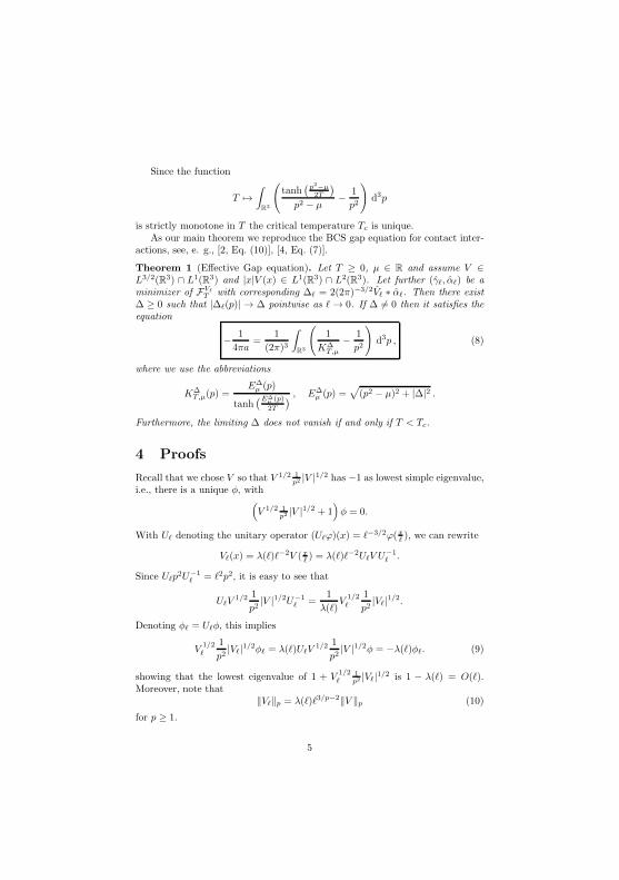
Since the function
T 7→∫
R3
(tanh
(p2−µ2T
)
p2 − µ− 1
p2
)d3p
is strictly monotone in T the critical temperature Tc is unique.As our main theorem we reproduce the BCS gap equation for contact inter-
actions, see, e. g., [2, Eq. (10)], [4, Eq. (7)].
Theorem 1 (Effective Gap equation). Let T ≥ 0, µ ∈ R and assume V ∈L3/2(R3) ∩ L1(R3) and |x|V (x) ∈ L1(R3) ∩ L2(R3). Let further (γℓ, αℓ) be aminimizer of FVℓ
T with corresponding ∆ℓ = 2(2π)−3/2Vℓ ∗ αℓ. Then there exist∆ ≥ 0 such that |∆ℓ(p)| → ∆ pointwise as ℓ → 0. If ∆ 6= 0 then it satisfies theequation
− 1
4πa=
1
(2π)3
∫
R3
(1
K∆T,µ
− 1
p2
)d3p , (8)
where we use the abbreviations
K∆T,µ(p) =
E∆µ (p)
tanh(E∆
µ (p)
2T
) , E∆µ (p) =
√(p2 − µ)2 + |∆|2 .
Furthermore, the limiting ∆ does not vanish if and only if T < Tc.
4 Proofs
Recall that we chose V so that V 1/2 1p2 |V |1/2 has −1 as lowest simple eigenvalue,
i.e., there is a unique φ, with(V 1/2 1
p2 |V |1/2 + 1)φ = 0.
With Uℓ denoting the unitary operator (Uℓϕ)(x) = ℓ−3/2ϕ(xℓ ), we can rewrite
Vℓ(x) = λ(ℓ)ℓ−2V (xℓ ) = λ(ℓ)ℓ−2UℓV U−1ℓ .
Since Uℓp2U−1
ℓ = ℓ2p2, it is easy to see that
UℓV1/2 1
p2|V |1/2U−1
ℓ =1
λ(ℓ)V
1/2ℓ
1
p2|Vℓ|1/2.
Denoting φℓ = Uℓφ, this implies
V1/2ℓ
1
p2|Vℓ|1/2φℓ = λ(ℓ)UℓV
1/2 1
p2|V |1/2φ = −λ(ℓ)φℓ. (9)
showing that the lowest eigenvalue of 1 + V1/2ℓ
1p2 |Vℓ|1/2 is 1 − λ(ℓ) = O(ℓ).
Moreover, note that‖Vℓ‖p = λ(ℓ)ℓ3/p−2‖V ‖p (10)
for p ≥ 1.
5

Remark 1. In [6, Appendix A.1], we show that the scattering length corre-sponding to the potential Vℓ, indeed, converges to the negative value
limℓ→0
a(Vℓ) = − 1
λ′(0)|〈|V |1/2|φ〉|2〈sgn(V )φ|φ〉 < 0.
In the next Lemma, we derive a lower bound for the BCS functional whichis uniform in ℓ. This will allow us to obtain limits for the order parameter ∆ℓ.
Lemma 1. There exists C1 > 0, independent of ℓ, such that
FVℓ
T (Γ) ≥ −C1 +1
2
∫
R3
(1 + p2)(γ − γ0)2 d3p+
1
2
∫
R3
|p|b|α|2 d3p, (11)
for 0 ≤ b < 1, where we denote γ0(p) =1
1+e(p2−µ)/T.
Proof. For details of the proof of this Lemma we refer to [6, Lemma 3]. The mainobservation in the proof is that we may express the difference FVℓ
T (Γ)−FVℓ
T (Γ0)as
FVℓ
T (Γ)− FVℓ
T (Γ0) =T
2H(Γ,Γ0) +
∫
R3
Vℓ(x)|α(x)|2 d3x,
where H(Γ,Γ0) is the relative entropy of Γ and Γ0. By means of [17, Lemma 3],which is an extension of [18, Theorem 1], giving a bound on the relative entropyone obtains
FVℓ
T (Γ)−FVℓ
T (Γ0) ≥⟨α∣∣p2 + Vℓ − µ
∣∣α⟩
+1
2
∫
R3
(1 + p2)(γ − γ0)2 d3p− C
for an appropriate constant C. By means of a Birman-Schwinger type argumentone can further show that
p2 + Vℓ ≥ |p|b − C1 ,
uniformly in ℓ for 0 ≤ b < 1 and an appropriate C1, which, together with theconstraint |α|2 ≤ 1, then implies the statement.
It was shown in [5, Theorem 1] that the functional FVℓ
T attains a minimizer(γℓ, αℓ) for each Vℓ. Lemma 1, with αℓ(p) ≤ 1, immediately tells us that theterms
∫
R3
(1 + |p|b)|αℓ(p)| d3p and
∫
R3
(1 + |p|2)(γℓ − γ0)2 d3p
are uniformly bounded in ℓ. Let us further mention the following useful relationsbetween ∆ℓ and the minimizer (γℓ, αℓ),
γℓ =1
2− 1
2
p2 − µ
K∆ℓ
T,µ
, ∆ℓ = 2K∆ℓ
T,µαℓ, (12)
6

which follow from the corresponding Euler-Lagrange equations. One immediateconsequence of these relations and Lemma 1 is the uniform boundedness of∫R3 γℓ(p)|p|b d3p, which implies
limR→∞
limℓ→0
∫
|p|2≥R
γℓ(p) d3p = 0. (13)
In the following lemma we show that, as ℓ → 0, pointwise limits for the mainquantities exist. To this aim we introduce the notation
m∆ℓµ (T ) =
1
(2π)3
∫
R3
(1
K∆ℓ
T,µ
− 1
p2
)d3p .
Lemma 2. Let (γℓ, αℓ) be a sequence of minimizers of FVℓ
T and ∆ℓ =2
(2π)3/2Vℓ∗
αℓ. Then there is a subsequence of ∆ℓ, which we continue to denote by ∆ℓ, anda ∆ ∈ R+ such that
(i) |∆ℓ(p)| converges pointwise to the constant function ∆ as ℓ → 0,
(ii) limℓ→0
m∆ℓµ (T ) = m∆
µ (T ).
We shall see later that it is not necessary to restrict to a subsequence, theresult holds in fact for the whole sequence.
Proof. (i) Set cℓ =1
(2π)3/2
∫R3 Vℓ(x)αℓ(x) d
3x. Then
|∆ℓ(p)− cℓ| ≤1
(2π)3/2
∫
R3
∣∣(e−ip·x − 1)Vℓ(x)αℓ(x)∣∣ d3x
≤ (2π)−3/2‖αℓ‖2(∫
R3
∣∣(e−ip·x − 1)Vℓ(x)∣∣2 d3x
)1/2
.
Now ‖αℓ‖2 is uniformly bounded in ℓ and | · |V ∈ L2(R3) by assumption, so
∫
R3
∣∣(e−ip·x − 1)Vℓ(x)∣∣2 d3x = ℓ−1λ(ℓ)2
∫
R3
∣∣(e−iℓp·x − 1)V (x)∣∣2 d3x
≤ ℓλ(ℓ)2|p|2∥∥ | · |V
∥∥22.
(14)
Hence, |∆ℓ(p) − cℓ| converges to zero pointwise. Since αℓ = −2(K∆ℓ
T,µ)−1∆ℓ is
uniformly bounded in L2, it is straightforward to see, using E∆ℓµ ≥ |∆ℓ|, that
the same holds for the sequence ∆ℓ/E∆ℓµ . This fact can now be used to show
that the sequence |cℓ| is a uniformly bounded. Assume on the contrary thatc = lim supℓ→0 |cℓ| = ∞. Then by dominated convergence
lim supℓ→0
∫
|p|≤R
|∆ℓ|2(p2 − µ)2 + |∆ℓ|2
d3p =
∫
|p|≤R
lim supℓ→0
1(p2−µ)2
|cℓ|2 + 1d3p =
4
3πR3.
(15)
7

However, the divergence of right side of Eq. (15) as R → ∞ contradicts theuniform boundedness of ∆ℓ/E
∆ℓµ in L2(R3). Hence c < ∞ and limℓ→0 |∆ℓ(p)| =
c for a suitable subsequence.
(ii) Obviously by (i) the integrand of m∆ℓµ (T ) converges pointwise to the inte-
grand of m∆µ (T ). By (12) we are able to rewrite the integrand as
1
K∆ℓ
T,µ(p)− 1
p2=
1
p2 − µ− 1
p2− 2γℓ(p)
p2 − µ. (16)
Using (13) we now conclude that
limR→∞
limℓ→0
∫
|p|2≥R
(1
K∆ℓ
T,µ(p)− 1
p2
)d3p = 0,
which together with the dominated convergence inside |p|2 ≤ R, implies thestatement of (ii).
Proposition 1. Let a = limℓ→0 a(Vℓ), then
limℓ→0
1
(2π)3
∫
R3
(1
K∆ℓ
T,µ
− 1
p2
)d3p = − 1
4πa. (17)
Proof. We again follow the proof of [6, Theorem 2]. Observe that with help ofthe second relation in (12) the BCS gap equation (4) for αℓ can be convenientlywritten in the form
(K∆ℓ
T,µ + Vℓ)αℓ = 0, with αℓ ∈ H1(R3) .
By means of the Birman–Schwinger principle one concludes that K∆ℓ
T,µ+Vℓ hav-
ing 0 as an eigenvalue is equivalent to V1/2ℓ
1
K∆ℓT,µ
|Vℓ|1/2 having −1 as eigenvalue.
We now rewrite V1/2ℓ
1
K∆ℓT,µ
|Vℓ|1/2 as
V1/2ℓ
1
K∆ℓ
T,µ
|Vℓ|1/2 = V1/2ℓ
1
p2|Vℓ|1/2 +m∆ℓ
µ (T )|V 1/2ℓ 〉〈|Vℓ|1/2|+Aµ,T,ℓ, (18)
where Aµ,T,ℓ is given in terms of the integral kernel
Aµ,T,ℓ(x, y) =Vℓ(x)
12 |Vℓ(y)|
12
(2π)3
∫
R3
(1
K∆ℓ
T,µ
− 1
p2
)(e−i(x−y)·p − 1) d3p , (19)
which can be estimated, e. g., by
|Aµ,T,ℓ(x, y)| ≤|Vℓ(x)|
12 |Vℓ(y)|
12
(2π)3
∫
R3
∣∣∣∣∣1
K∆ℓ
T,µ
− 1
p2
∣∣∣∣∣ (|x− y| |p|)1/2 d3p. (20)
8

Using the relation (16) as well as the uniform boundedness of∫R3 γℓ(p)|p|1/2 d3p
we are able to conclude that the integral
∫
R3
∣∣∣∣∣1
K∆ℓ
T,µ
− 1
p2
∣∣∣∣∣ |p|1/2 d3p =
∫
R3
∣∣∣∣1
p2 − µ− 1
p2− 2γℓ(p)
p2 − µ
∣∣∣∣ |p|1/2 d3p
is uniformly bounded in ℓ. We can thus bound the Hilbert-Schmidt norm ofAµ,T,ℓ by
‖Aµ,T,ℓ‖2 ≤ const ‖Vℓ| · |‖1/21 ‖Vℓ‖1/21 ≤ O(ℓ3/2) . (21)
We further proceed with equation (18). By construction, 1 + V1/2ℓ
1p2 |Vℓ|1/2
is invertible and thus can be factored out, i.e.,
1 + V1/2ℓ
1
K∆ℓ
T,µ
|Vℓ|1/2 =
(1 + V
1/2ℓ
1
p2|Vℓ|1/2
)×
×[1 + 1
1+V1/2ℓ
1p2
|Vℓ|1/2
(m∆ℓ
µ (T )|V 12
ℓ 〉〈|Vℓ|12 |+AT,µ,ℓ
)],
with the second term on the right hand side necessarily having an eigenvalue 0.With J = Vℓ(x)/|Vℓ(x)| and X = |Vℓ|1/2 1
p2 |Vℓ|1/2, we are able to rewrite
1
1 + V1/2ℓ
1p2 |Vℓ|1/2
=1
1 + JX= 1− JX1/2 1
1 +X1/2JX1/2X1/2 .
This allows us to bound
∥∥∥ 1
1 + V1/2ℓ
1p2 |Vℓ|1/2
∥∥∥ ≤ 1 + ‖X‖∥∥∥∥
1
1 +X1/2JX1/2
∥∥∥∥ ≤ O(ℓ−1),
where we have used that, due to the HLS-inequality, ‖X‖ ≤ C‖Vℓ‖3/2, as wellas the fact that 1+X1/2JX1/2 is self-adjoint with its lowest eigenvalue of orderO(ℓ). Indeed, X1/2JX1/2 has the same spectrum as JX . Hence,
∥∥∥ 1
1+V1/2ℓ
1p2
|Vℓ|1/2Aµ,T,ℓ
∥∥∥ ≤∥∥∥ 1
1+V1/2ℓ
1p2
|Vℓ|1/2
∥∥∥‖Aµ,T,ℓ‖ ≤ O(ℓ1/2).
Since1
1 + V1/2ℓ
1p2 |Vℓ|1/2
(m∆ℓ
µ (T )|V 1/2ℓ 〉〈|Vℓ|1/2|+AT,µ,ℓ
)
has an eigenvalue −1 and 1+ (1+V1/2ℓ
1p2 |Vℓ|1/2)−1Aµ,T,ℓ is invertible for small
enough ℓ, we can argue by factoring out the term 1+(1+V1/2ℓ
1p2 |Vℓ|1/2)−1Aµ,T,ℓ
that the rank one operator
m∆ℓµ (T )
(1 +
1
1 + V1/2ℓ
1p2 |Vℓ|1/2
Aµ,T,ℓ
)−11
1 + V1/2ℓ
1p2 |Vℓ|1/2
|V 1/2ℓ 〉〈|Vℓ|1/2|
9

has an eigenvalue −1, which, by taking the trace, implies
− 1 = m∆ℓµ (T )
⟨|Vℓ|1/2
∣∣∣∣∣
[1 + 1
1+V1/2ℓ
1p2
|Vℓ|1/2Aµ,T,ℓ
]−11
1+V1/2ℓ
1p2
|Vℓ|1/2
∣∣∣∣∣V1/2ℓ
⟩.
(22)With the aid of Eq. (5) and the resolvent identity, we can rewrite Eq. (22) as
4πa(Vℓ) +1
m∆ℓµ (T )
=⟨|Vℓ|1/2
∣∣∣ 1
1+V1/2ℓ
1p2
|Vℓ|1/2Aµ,T,ℓ
[1 + 1
1+V1/2ℓ
1p2
|Vℓ|1/2Aµ,T,ℓ
]−1
×
× 1
1+V1/2ℓ
1p2
|Vℓ|1/2
∣∣∣V 1/2ℓ
⟩,
(23)
where the right hand side is bounded by
‖Vℓ‖1∥∥∥ 1
1+V1/2ℓ
1p2
|Vℓ|1/2
∥∥∥∥∥∥ 1
1+V1/2ℓ
1p2
|Vℓ|1/2Aµ,T,ℓ
∥∥∥×
×∥∥∥[1 + 1
1+V1/2ℓ
1p2
|Vℓ|1/2Aµ,T,ℓ
]−1∥∥∥ ≤ O(ℓ1/2) .
This implies Eq. (17) and completes the proof.
With the aid of Lemma 2 and Proposition 1, we can now finish the proof ofTheorem 1.
Proof of Theorem 1. We know from Lemma 2 and Proposition 1 that |∆ℓ(p)|has a subsequence that converges to a constant function ∆, which satisfies theequation
− 1
4πa=
1
(2π)3
∫
R3
(1
K∆T,µ
− 1
p2
)d3p.
Since the solution |∆| of (8) is unique we obtain that the sequence |∆ℓ(p)|converges to the unique solution of (8). Furthermore, this shows that the limitof |∆ℓ| does not vanish in the case that T < Tc, and that the limit vanishes forT ≥ Tc.
References
[1] J. Bardeen, L. Cooper, J. Schrieffer, Phys. Rev. 108, 1175 (1957).
[2] A. J. Leggett, Diatomic molecules and cooper pairs, in Modern Trendsin the Theory of Condensed Matter , eds. A. Pekalski and J. Przystawa,Lecture Notes in Physics, Vol. 115 (Springer Berlin / Heidelberg, 1980) pp.13–27.
10

[3] P. Nozieres and S. Schmitt-Rink, Journal of Low Temperature Physics 59,195 (1985).
[4] M. Randeria, Crossover from BCS theory to Bose-Einstein condensation, inBose-Einstein Condensation, eds. A. Griffin, D. W. Snoke and S. Stringari(Cambridge University Press, July 1996), pp. 355–392.
[5] C. Hainzl, E. Hamza, R. Seiringer, J. P. Solovej, Comm. Math. Phys. 281,349 (2008).
[6] G. Braunlich, C. Hainzl, R. Seiringer, preprint arXiv/1305.5135.
[7] V. Bach, E. H. Lieb, J. P. Solovej, J. Statist. Phys. 76, 3 (1994).
[8] R. L. Frank, C. Hainzl, S. Naboko, R. Seiringer, J. Geom. Anal. 17, 559(2007).
[9] L. P. Gor’kov, ZH. Eksp. Teor. Fiz. 36, 1918 (1959).
[10] C. Hainzl and R. Seiringer, Lett. Math. Phys. 84, 99 (2008).
[11] S. Albeverio, F. Gesztesy, R. Høegh-Krohn, H. Holden, Solvable modelsin quantum mechanics, Texts and monographs in physics (Springer-VerlagNew York, 1988).
[12] M. Drechsler and W. Zwerger, Ann. Phys. 504, 15 (1992).
[13] P. Pieri and G. C. Strinati, Phys. Rev. Lett. 91, 030401 (2003).
[14] C. Hainzl and R. Seiringer, Lett. Math. Phys. 100, 119 (2012).
[15] C. Hainzl and B. Schlein, Journal of Functional Analysis 265, 399 (2013).
[16] G. Braunlich, C. Hainzl, R. Seiringer, Meth. Funct. Anal. Top. 19, 364(2013).
[17] R. L. Frank, C. Hainzl, R. Seiringer, J. P. Solovej, J. Amer. Math. Soc. 25,667 (2012).
[18] C. Hainzl, M. Lewin, R. Seiringer, Rev. Math. Phys. 20, 1283 (2008).
11

Appendix A Publications in the Thesis
A.1.3 Translation-invariant quasi-free states forfermionic systems and the BCS approximation
92
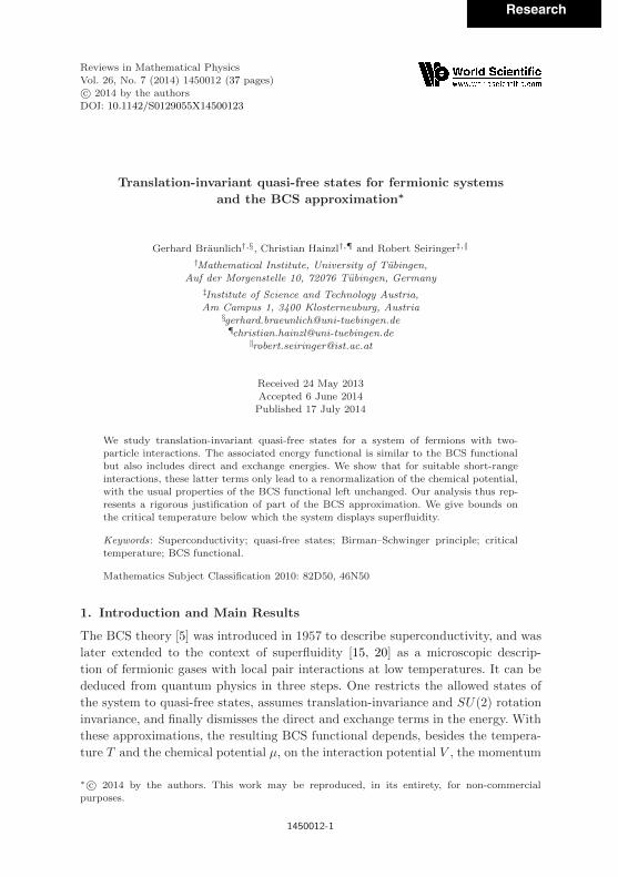
3rd Reading
July 15, 2014 15:42 WSPC/S0129-055X 148-RMP J070-1450012
Reviews in Mathematical PhysicsVol. 26, No. 7 (2014) 1450012 (37 pages)c© 2014 by the authorsDOI: 10.1142/S0129055X14500123
Translation-invariant quasi-free states for fermionic systems
and the BCS approximation∗
Gerhard Braunlich†,§, Christian Hainzl†,¶ and Robert Seiringer‡,‖
†Mathematical Institute, University of Tubingen,Auf der Morgenstelle 10, 72076 Tubingen, Germany
‡Institute of Science and Technology Austria,Am Campus 1, 3400 Klosterneuburg, Austria
§[email protected]¶[email protected]
Received 24 May 2013Accepted 6 June 2014Published 17 July 2014
We study translation-invariant quasi-free states for a system of fermions with two-particle interactions. The associated energy functional is similar to the BCS functionalbut also includes direct and exchange energies. We show that for suitable short-rangeinteractions, these latter terms only lead to a renormalization of the chemical potential,with the usual properties of the BCS functional left unchanged. Our analysis thus rep-resents a rigorous justification of part of the BCS approximation. We give bounds onthe critical temperature below which the system displays superfluidity.
Keywords: Superconductivity; quasi-free states; Birman–Schwinger principle; criticaltemperature; BCS functional.
Mathematics Subject Classification 2010: 82D50, 46N50
1. Introduction and Main Results
The BCS theory [5] was introduced in 1957 to describe superconductivity, and was
later extended to the context of superfluidity [15, 20] as a microscopic descrip-
tion of fermionic gases with local pair interactions at low temperatures. It can be
deduced from quantum physics in three steps. One restricts the allowed states of
the system to quasi-free states, assumes translation-invariance and SU(2) rotation
invariance, and finally dismisses the direct and exchange terms in the energy. With
these approximations, the resulting BCS functional depends, besides the tempera-
ture T and the chemical potential µ, on the interaction potential V , the momentum
∗ c© 2014 by the authors. This work may be reproduced, in its entirety, for non-commercialpurposes.
1450012-1

3rd Reading
July 15, 2014 15:42 WSPC/S0129-055X 148-RMP J070-1450012
G. Braunlich, C. Hainzl & R. Seiringer
distribution γ and the Cooper pair wave function α. A non-vanishing α implies a
macroscopic coherence of the particles involved, i.e. the formation of a condensate
of Cooper pairs. This motivates the characterization of a superfluid phase by the
existence of a minimizer of the BCS functional for which α = 0.
A rigorous treatment of the BCS functional was presented in [9, 14, 13, 7],
where the question was addressed for which interaction potentials V and at which
temperatures T a superfluid phase exists. In the present work, we focus on the
question to what extent it is justifiable to dismiss the direct and exchange terms in
the energy. A heuristic justification was given in [15, 16], where it was argued that
as long as the range of the interaction potential is suitably small, the only effect of
the direct and exchange terms is to renormalize the chemical potential.
In this paper we derive a gap equation for the extended theory with direct and
exchange terms and investigate the existence of non-trivial solutions for general
interaction potentials. We give a rigorous justification for dismissing the two terms
for potentials whose range is short compared to the scattering length a and the
Fermi wave length 2π√µ . The potentials are required to have a suitable repulsive core
to assure stability of the system. We show that, for small enough , the system
still can be described by the conventional BCS equation if the chemical potential
is renormalized appropriately. In the limit → 0, the spectral gap function ∆(p)
converges to a constant function and we recover the BCS equation in its form found
in the physics literature.
While we do not prove that for fixed, finite there exists a critical temperature
Tc such that superfluidity occurs if and only if T < Tc, we find bounds T+ and
T− such that T < T−
implies superfluidity and T > T+ excludes superfluidity.
Moreover, in the limit → 0 the two bounds converge to the same temperature,
lim→0 T− = lim→0 T
+ , which can be determined by the usual BCS gap equation.
The situation is illustrated in the following sketch.
We note that similar models as the one considered in our paper are sometimes
referred to as Bogoliubov–Hartree–Fock theory and have been studied previously
mainly with Newtonian interactions, modeling stars, and without the restriction to
1450012-2

3rd Reading
July 15, 2014 15:42 WSPC/S0129-055X 148-RMP J070-1450012
Translation-invariant quasi-free states for fermionic systems and the BCS approximation
translation-invariant states [3, 17, 10]. The proof of existence of a minimizer in [17]
turns out to be surprisingly difficult and even more strikingly, the appearance of
pairing is still open. It was confirmed numerically for the Newton model and also
for models with short range interaction in [18]. Hence the present work represents
the first proof of existence of pairing in a translation-invariant Bogoliubov–Hartree–
Fock model in the continuum. For the Hubbard model at half filling this was shown
earlier in [4].
1.1. The model
We consider a gas of spin 1/2 fermions in the thermodynamic limit at temperature
T ≥ 0 and chemical potential µ ∈ R. The particles interact via a local two-body
potential which we denote by V . We assume V to be reflection-symmetric, i.e.
V (−x) = V (x). The state of the system is described by two functions γ : R3 → R+
and α : R3 → C, with α(p) = α(−p), which are conveniently combined into a 2× 2
matrix
Γ(p) =
(γ(p) α(p)
α(p) 1− γ(−p)
), (1.1)
required to satisfy 0 ≤ Γ ≤ C2 at every point p ∈ R3. The function γ is interpreted
as the momentum distribution of the gas, while α (the inverse Fourier transform of
α) is the Cooper pair wave function. Note that there are no spin variables in Γ; the
full, spin dependent Cooper pair wave function is the product of α(x − y) with an
antisymmetric spin singlet.
The BCS-HF functional FVT , whose infimum over all states Γ describes the
negative of the pressure of the system, is given as
FVT (Γ) =
∫
R3
(p2 − µ)γ(p)d3p+
∫
R3
|α(x)|2V (x)d3x− TS(Γ)
−∫
R3
|γ(x)|2V (x)d3x+ 2γ(0)2∫
R3
V (x)d3x, (1.2)
where
S(Γ) = −∫
R3
TrC2(Γ(p) ln Γ(p))d3p
is the entropy of the state Γ. Here, γ and α denote the inverse Fourier transforms of γ
and α, respectively. The last two terms in (1.2) are referred to as the exchange term
and the direct term, respectively. The functional (1.2) can be obtained by restricting
the many-body problem on Fock space to translation-invariant and spin-rotation
invariant quasi-free states, see [9, Appendix A] and [4]. The factor 2 in the last term
in (1.2) originates from two possible orientations of the particle spin.
A normal state Γ0 is a minimizer of the functional (1.2) restricted to states with
α = 0. Any such minimizer can easily be shown to be of the form
γ0(p) =1
1 + eεγ0 (p)−µγ0
T
, (1.3)
1450012-3

3rd Reading
July 15, 2014 15:42 WSPC/S0129-055X 148-RMP J070-1450012
G. Braunlich, C. Hainzl & R. Seiringer
where we denote, for general γ,
εγ(p) = p2 − 2
(2π)3/2
∫
R3
(V (p− q)− V (0))γ(q)d3q, (1.4)
µγ = µ− 2
(2π)3/2V (0)
∫
R3
γ(p)d3p. (1.5)
Notice that Eq. (1.3) is an implicit relation with γ0 also appearing in the expression
on the right-hand side of (1.3) via (1.4) and (1.5). In the absence of the exchange
term, the normal state would be unique, but this is not necessarily the case here.
The system is said to be in a superfluid phase if and only if the minimum of FVT is
not attained at a normal state, and we call a normal state Γ0 unstable in this case.
1.2. Main results
Our first goal is to characterize the existence of a superfluid phase for a large class
of interaction potentials V . We first find sufficient conditions on V for (1.2) to have
a minimizer. These conditions are stated in the following proposition.
Proposition 1 (Existence of Minimizers). Let µ ∈ R, 0 ≤ T < ∞, and let
V ∈ L1(R3) ∩ L3/2(R3) be real-valued with ‖V ‖∞ ≤ 2V (0). Then FVT is bounded
from below and attains a minimizer (γ, α) on
D =
Γ of the form (1.1)
∣∣∣∣∣γ ∈ L1(R3, (1 + p2)d3p),
α ∈ H1(R3, d3x),0 ≤ Γ ≤ C2
.
Moreover, the function
∆(p) =2
(2π)3/2
∫
R3
V (p− q)α(q)d3q (1.6)
satisfies the BCS gap equation
1
(2π)3/2
∫
R3
V (p− q)∆(q)
Kγ,∆T,µ (q)
d3q = −∆(p). (1.7)
In (1.7), we have introduced the notation
Kγ,∆T,µ (p) =
Eγ,∆µ (p)
tanh
(Eγ,∆
µ (p)
2T
) , (1.8)
Eγ,∆µ (p) =
√(εγ(p)− µγ)2 + |∆(p)|2, (1.9)
with εγ and µγ defined in (1.4) and (1.5), respectively. For T = 0, (1.8) is interpreted
as Kγ,∆0,µ (p) = Eγ,∆
µ (p).
1450012-4
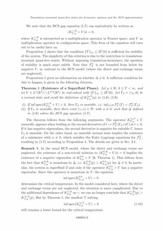
3rd Reading
July 15, 2014 15:42 WSPC/S0129-055X 148-RMP J070-1450012
Translation-invariant quasi-free states for fermionic systems and the BCS approximation
We note that the BCS gap equation (1.7) can equivalently be written as
(Kγ,∆T,µ + V )α = 0,
where Kγ,∆T,µ is interpreted as a multiplication operator in Fourier space, and V as
multiplication operator in configuration space. This form of the equation will turn
out to be useful later on.
Proposition 1 shows that the condition ‖V ‖∞ ≤ 2V (0) is sufficient for stability
of the system. The simplicity of this criterion is due to the restriction to translation-
invariant quasi-free states. Without imposing translation-invariance, the question
of stability is much more subtle. Note that FVT is not bounded from below for
negative V , in contrast to the BCS model (where the direct and exchange terms
are neglected).
Proposition 1 gives no information on whether ∆ = 0. A sufficient condition for
this to happen is given in the following theorem.
Theorem 1 (Existence of a Superfluid Phase). Let µ ∈ R, 0 ≤ T < ∞, and
let V ∈ L1(R3) ∩ L3/2(R3) be real-valued with ‖V ‖∞ ≤ 2V (0). Let Γ0 = (γ0, 0) be
a normal state and recall the definition of Kγ0,0T,µ (p) in (1.8)–(1.9).
(i) If inf spec(Kγ0,0T,µ + V ) < 0, then Γ0 is unstable, i.e. infΓ∈D FV
T (Γ) < FVT (Γ0).
(ii) If Γ0 is unstable, then there exist (γ, α) ∈ D, with α = 0, such that ∆ defined
in (1.6) solves the BCS gap equation (1.7).
The theorem follows from the following arguments. The operator Kγ0,0T,µ + V
naturally appears when looking at the second derivative of t → FVT (Γ0+tΓ) at t = 0.
If it has negative eigenvalues, the second derivative is negative for suitable Γ, hence
Γ0 is unstable. On the other hand, an unstable normal state implies the existence
of a minimizer with α = 0, which satisfies the Euler–Lagrange equations for FVT ,
resulting in (1.7) according to Proposition 1. The details are given in Sec. 2.1.
Remark 1. In the usual BCS model, where the direct and exchange terms are
neglected, the existence of a non-trivial solution to (K0,∆T,µ + V )α = 0 implies the
existence of a negative eigenvalue of K0,0T,µ + V [9, Theorem 1]. This follows from
the fact that K0,∆T,µ is monotone in ∆, i.e. K0,∆
T,µ (p) > K0,0T,µ(p) for ∆ = 0. In partic-
ular, the system is superfluid if and only if the operator K0,0T,µ + V has a negative
eigenvalue. Since this operator is monotone in T , the equation
inf spec(K0,0Tc,µ
+ V ) = 0
determines the critical temperature. In the model considered here, where the direct
and exchange terms are not neglected, the situation is more complicated. Due to
the additional dependence of Kγ,∆T,µ on γ, we can no longer conclude that Kγ,∆
T,µ (p) >
Kγ0,0T,µ (p). But by Theorem 1, the smallest T solving
inf spec(Kγ0,0T,µ + V ) = 0 (1.10)
still remains a lower bound for the critical temperature.
1450012-5

3rd Reading
July 15, 2014 15:42 WSPC/S0129-055X 148-RMP J070-1450012
G. Braunlich, C. Hainzl & R. Seiringer
Our main result concerns the case of short-range interaction potentials V , where
we can recover monotonicity in ∆, and hence conclude that (1.10) indeed defines
the correct critical temperature. More precisely, we shall consider a sequence of
potentials V>0 with → 0, which satisfies the following assumptions.
Remark 2. In the following, 1 is a small parameter, e.g., it suffices to consider
≤ 1.
Assumption 1.
(A1) V ∈ L1 ∩ L2.
(A2) The range of V is at most , i.e. suppV ⊆ B(0).
(A3) The scattering length a(V) is negative and does not vanish as → 0, i.e.
lim→0 a(V) = a < 0.
(A4) lim sup→0 ‖V‖1 <∞.
(A5) V(0) > 0 and lim→0 V(0) = V ≥ 0.
(A6) ‖V‖∞ ≤ 2V(0).
(A7) For small , ‖V‖2 ≤ C1−N for some C1 > 0 and N ∈ N.
(A8) ∃ 0 < b < 1 such that inf spec(p2+V−|p|b) > C2 > −∞ holds independently
of .
(A9) The operator 1+V1/2
1p2 |V|1/2 is invertible, and has an eigenvalue e of order
, with corresponding eigenvector φ. Moreover, (1 + V1/2
1p2 |V|1/2)−1(1 −
P) is uniformly bounded in , where P = 〈Jφ|φ〉−1|φ〉〈Jφ| and J =
sgn(V).
(A10) The eigenvector φ satisfies |〈φ| sgn(V)φ〉|−1〈|V|1/2||φ|〉 ≤ O(1/2) for
small .
Here we use the notation sgn(V ) = 1, V ≥ 0−1, V < 0 and V
1/2(x) = sgn(V )|V (x)|1/2.As discussed in [12], the scattering length of a real-valued potential V ∈ L1(R3) ∩L3/2(R3) is given by
a(V ) =1
4π
⟨|V |1/2
∣∣∣∣∣∣
1
1 + V 1/21
p2|V |1/2
V 1/2
⟩. (1.11)
Assumptions (A6)–(A10) are to some extent technical and are needed, among other
things, to guarantee that FV
T is bounded from below uniformly in . Our main
results presumably hold for a larger class of potentials with less restrictive assump-
tions, but to avoid additional complications in the proofs we do not aim here for
the greatest possible generality. Assumption 1 implies, in particular, that V con-
verges to a point interaction as → 0, and we refer to [6] for a general study of
point interactions arising as limits of short-range potentials of the form considered
here.
1450012-6

3rd Reading
July 15, 2014 15:42 WSPC/S0129-055X 148-RMP J070-1450012
Translation-invariant quasi-free states for fermionic systems and the BCS approximation
Remark 3. As an example for such a sequence of short-range potentials V we
have the following picture in mind:
The attractive part allows to adjust the scattering length. The repulsive core is
needed to guarantee stability, and can be used to adjust the L1 norm. If its range
is small compared to the range of the attractive part, i.e. ε , the scattering
length is essentially unaffected by the repulsive core. In Appendix A, we construct
an explicit example of such a sequence, satisfying all the assumptions (A1)–(A10).
As → 0, it approximates a contact potential, defined via suitable selfadjoint
extensions of −∆ on R3\0. Functions in its domain are known to diverge as |x|−1
for small x, hence decay like p−2 for large |p|. This suggests the validity of (A8) for
b < 1. Assumption (A9) is easy to show in case V is uniformly bounded in L3/2
(in which case V(0) = O()) but much harder to prove if lim→0 V(0) > 0. It is
possible to generalize (A9) and allow finitely many eigenvalues of 1+V1/2
1p2 |V|1/2
of order . For simplicity, we restrict to the case of only one eigenvalue of order ,
however.
For the remainder of this section, we assume that the sequence V satisfies (A1)–
(A10). We shall use the notation
µγ = µ− 2
(2π)3/2V(0)
∫
R3
γ(p)d3p
in analogy to (1.5).
Theorem 2 (Effective Gap Equation). Let T ≥ 0, µ ∈ R, and let (γ, α) be
a minimizer of FV
T with corresponding ∆ = 2(2π)−3/2V ∗ α. Then there exist
∆ ≥ 0 and γ : R3 → R+ such that |∆(p)| → ∆ pointwise, γ(p) → γ(p) pointwise
and µγ → µ as → 0, satisfying
µ = µ− 2V(2π)3/2
∫
R3
γ(p)d3p
γ(p) =1
2− p2 − µ
2K0,∆T,µ (p)
.
(1.12)
1450012-7

3rd Reading
July 15, 2014 15:42 WSPC/S0129-055X 148-RMP J070-1450012
G. Braunlich, C. Hainzl & R. Seiringer
If ∆ = 0 for a subsequence of ’s going to zero, then, in addition,
− 1
4πa=
1
(2π)3
∫
R3
(1
K0,∆T,µ
− 1
p2
)d3p. (1.13)
Recall that, according to our definitions (1.4)–(1.9),
K0,∆T,µ (p) =
E0,∆µ (p)
tanh
(E0,∆
µ (p)
2T
) , E0,∆µ (p) =
√(p2 − µ)2 + |∆|2.
Remark 4. If we consider potentials such that V(0) → 0, we obtain at the same
time that µγ → µ and consequently (1.13) becomes
− 1
4πa=
1
(2π)3
∫
R3
(1
K0,∆T,µ
− 1
p2
)d3p. (1.14)
Equation (1.14) is the form of the BCS gap equation one finds in the literature, see
for instance [15].
The effective gap equation (1.13) suggests to define the critical temperature
of the system via the solution of (1.13) for ∆ = 0, in which case γ is given by
(1 + ep2−µ
T )−1.
Definition 1 (Critical Temperature/Renormalized Chemical Potential).
Let µ > 0. The critical temperature Tc and the renormalized chemical potential µ
in the limit of a contact potential with scattering length a < 0 and lim→0 V(0) =
V ≥ 0 are implicitly given by the set of equations
− 1
4πa=
1
(2π)3
∫
R3
tanh
(p2 − µ
2Tc
)
p2 − µ− 1
p2
d3p,
µ = µ− 2V(2π)3/2
∫
R3
1
1 + ep2−µTc
d3p.
(1.15)
We will show existence and uniqueness of Tc and µ in Appendix B. Note that
it is essential that µ > 0. If µ ≤ 0, then µ ≤ 0 and hence the right side of the first
equation in (1.15) is always non-positive, hence there is no solution for a < 0. In
other words, Tc = 0 for µ ≤ 0.
Remark 5. In [13], the behavior of the first integral on the right-hand side of
(1.15) as Tc → 0 was examined. This allows one to deduce the asymptotic behavior
of Tc as a tends to zero, which equals
Tc = µ
(8
πeγ−2 + o(1)
)e
π2√
µa ,
1450012-8

3rd Reading
July 15, 2014 15:42 WSPC/S0129-055X 148-RMP J070-1450012
Translation-invariant quasi-free states for fermionic systems and the BCS approximation
with γ ≈ 0.577 denoting Euler’s constant. Similarly, one can study the asymptotic
behavior as µ→ 0.
Although this definition for Tc is only valid in the limit → 0, it serves to make
statements about upper and lower bounds on the critical temperature for small
(but non-zero) , as sketched in the figure on p. 2.
Theorem 3 (Bounds on Critical Temperature). Let µ ∈ R, T ≥ 0 and let
(γ0 , 0) be a normal state for FV
T .
(i) For T < Tc, there exists an 0(T ) > 0 such that for < 0(T ), inf spec(Kγ0 ,0
T,µ +
V) < 0. Consequently, the system is superfluid.
(ii) For T > Tc, there exists an 0(T ) > 0 such that for < 0(T ), FV
T is minimized
by a normal state. I.e. the system is not superfluid.
Theorem 3 shows that Definition 1 is indeed the correct definition of the critical
temperature in the limit → 0. In addition, it also shows that in this limit there
is actually equivalence of statements (i) and (ii) in Theorem 1. In particular, one
recovers the linear criterion for the existence of a superfluid phase valid in the usual
BCS model, as discussed in Remark 1.
2. Proofs
2.1. General potentials
In this section we prove Proposition 1 and Theorem 1. As a first step we show that
FVT is bounded from below and has a minimizer.
Lemma 1. Let V ∈ L1 ∩ L3/2, V (0) ≥ 0 and V (p) ≤ 2V (0) for all p ∈ R3. Then
FVT is bounded from below and there exists a minimizer Γ of FV
T (Γ).
Proof. The case without direct and exchange term was treated in [9, Proposition
2]. The Hartree–Fock part of the functional FVT gives the additional contribution
−∫
R3
|γ(x)|2V (x)d3x+ 2γ(0)2∫
R3
V (x)d3x =1
(2π)3/2
∫
R3
γ(2V (0)− V ) ∗ γd3p,
which is non-negative because of our assumption V (p) ≤ 2V (0). Hence, the same
lower bound as in the case without direct and exchange term applies.
To show the existence of a minimizer, it remains to check the weak lower semi-
continuity of FVT in Lq(R3) ×H1(R3, d3x) (note that γ ∈ L1(R3) ∩ L∞(R3)). The
exchange term
γ →∫
R3
V (x)|γ(x)|2d3x
is actually weakly continuous on H1(R3), see, e.g., [19, Theorem 11.4]. Since also
for any sequence γn converging to γ weakly, we have limn→∞∫R3 γnd
3p ≥∫R3 γd
3p,
the direct term is weakly lower semicontinuous. In the proof of [9, Proposition 2] it
1450012-9

3rd Reading
July 15, 2014 15:42 WSPC/S0129-055X 148-RMP J070-1450012
G. Braunlich, C. Hainzl & R. Seiringer
was shown that all other terms in FVT are weakly lower semicontinuous as well. As
a consequence, a minimizing sequence will actually converge to a minimizer.
Lemma 2. The Euler–Lagrange equations for a minimizer (γ, α) of FVT are of the
form
γ(p) =1
2− εγ(p)− µγ
2Kγ,∆T,µ (p)
(2.1)
α(p) =1
2∆(p)
tanh
(Eγ,∆
µ (p)
2T
)
Eγ,∆µ (p)
, (2.2)
where we used the abbreviations introduced in (1.4)–(1.9). In particular, the BCS
gap equation (1.7) holds.
Proof. The proof works similar to [9]. We sketch here an alternative, more concise
derivation, restricting our attention to T > 0 for simplicity. A minimizer Γ = (γ, α)
of FVT fulfills the inequality
0 ≤ d
dt
∣∣∣∣t=0
FVT (Γ + t(Γ− Γ)) (2.3)
for arbitrary Γ ∈ D. Here we may assume that Γ stays away from 0 and 1 by arguing
as in [9, Proof of Lemma 1]. A simple calculation using
S(Γ) = −∫
R3
TrC2 Γ lnΓd3p = −1
2
∫
R3
TrC2(Γ ln(Γ) + (1− Γ) ln(1− Γ))d3p
shows that
d
dt
∣∣∣∣t=0
FVT (Γ + t(Γ− Γ)) =
1
2
∫
R3
TrC2
[H∆(Γ− Γ) + T (Γ− Γ) ln
(Γ
1− Γ
)]d3p,
with
H∆ =
(εγ − µγ ∆
∆ −(εγ − µγ)
),
using the definition
∆ = 2(2π)−3/2V ∗ α.Here, TrC2 G denotes the trace of the 2× 2 matrix G(p) for fixed p. Separating the
terms containing no Γ and moving them to the left-hand side in (2.3), we obtain∫
R3
TrC2
(H∆
(Γ−
(0 0
0 1
))+ T Γ ln
(Γ
1− Γ
))d3p
≤∫
R3
TrC2
(H∆
(Γ−
(0 0
0 1
))+ T Γ ln
(Γ
1− Γ
))d3p.
1450012-10

3rd Reading
July 15, 2014 15:42 WSPC/S0129-055X 148-RMP J070-1450012
Translation-invariant quasi-free states for fermionic systems and the BCS approximation
Note that∫R3 TrC2(H∆Γ)d
3p is not finite but∫R3 TrC2
(H∆
(Γ−
(0 00 1
)))d3p is. Since
Γ was arbitrary, Γ also minimizes the linear functional
Γ →∫
R3
TrC2
(H∆
(Γ−
(0 0
0 1
))+ T Γ ln
(Γ
1− Γ
))d3p,
whose Euler–Lagrange equation is of the simple form
0 = H∆ + T ln
(Γ
1− Γ
), (2.4)
which is equivalent to
Γ =1
1 + e1T H∆
.
This in turn implies (2.1) and (2.2). Indeed,
Γ =1
1 + e1T H∆
=1
2− 1
2tanh
(1
2TH∆
).
For the simple reason that tanh(x)x is an even function and H2
∆ = [Eγ,∆µ ]2C2 ,
the expression simplifies to
Γ =1
2− 1
2H∆
tanh
(1
2TEγ,∆
µ
)
Eγ,∆µ
=1
2− 1
2Kγ,∆T,µ
H∆
=
1
2− εγ − µγ
2Kγ,∆T,µ
− ∆
2Kγ,∆T,µ
− ∆
2Kγ,∆T,µ
1
2+εγ − µγ
2Kγ,∆T,µ
.
Proof of Proposition 1. This is an immediate consequence of Lemmas 1 and 2.
Proof of Theorem 1. The proof works exactly as the analog steps in [9, Proof
of Theorem 1]. To see (i), note that 〈α, (Kγ0,0T,µ + V )α〉 is the second derivative of
FVT with respect to α at Γ = Γ0. For (ii), we use the fact that the gap equation
is a combination of the Euler–Lagrange equation (2.2) of the functional and the
definition of ∆.
2.2. Sequence of short-range potentials
In the following, we consider a sequence of potentials V satisfying the assumptions
(A1)–(A10) in Assumption 1. Since V converges to a contact potential, Lemma 1 is
not sufficient to prove that FV
T is uniformly bounded from below. To this aim, we
1450012-11

3rd Reading
July 15, 2014 15:42 WSPC/S0129-055X 148-RMP J070-1450012
G. Braunlich, C. Hainzl & R. Seiringer
have to use more subtle estimates involving bounds on the relative entropy obtained
in [8], and we heavily rely on assumption (A8).
Lemma 3. There exists C1 > 0, independent of , such that
FV
T (Γ) ≥ −C1 +1
2
∫
R3
(1 + p2)(γ − γ0)2d3p+
1
2
∫
R3
|p|b|α|2d3p, (2.5)
where we denote γ0(p) =1
1+e(p2−µ)/T.
Proof. We rewrite FV
T (Γ) as
FV
T (Γ) =1
2
∫
R3
TrC2
(H0
(Γ−
(0 0
0 1
)))d3p+
∫
R3
V(x)|α(x)|2d3x
− TS(Γ) +1
(2π)3/2
∫
R3
((2V(0)− V) ∗ γ)(p)γ(p)d3p,
where Γ = Γ(γ, α) and
H0 =
(p2 − µ 0
0 −(p2 − µ)
).
Since γ(p) ≥ 0 and, by assumption (A6), 2V(0) − V(p) ≥ 0, the combination
of direct plus exchange term is non-negative and it suffices to find a lower bound
for
FV
T (Γ) =1
2
∫
R3
TrC2
(H0
(Γ−
(0 0
0 1
)))d3p+
∫
R3
V(x)|α(x)|2d3x− TS(Γ).
We compare FV
T (Γ) to the value FV
T (Γ0), where Γ0 = 11+eH0/T . Their difference
equals
FV
T (Γ)− FV
T (Γ0) =1
2
∫
R3
TrC2(H0(Γ− Γ0))d3p− T (S(Γ)− S(Γ0))
+
∫
R3
V(x)|α(x)|2d3x.
Using H0 + T ln( Γ0
1−Γ0) = 0 in the trace and performing some simple algebraic
transformations, we may write
FV
T (Γ)− FV
T (Γ0) =T
2H(Γ,Γ0) +
∫
R3
V(x)|α(x)|2d3x,
where
H(Γ,Γ0) =
∫
R3
TrC2 [Γ(ln(Γ)− ln(Γ0)) + (1− Γ)(ln(1− Γ)− ln(1− Γ0))]d3p
1450012-12

3rd Reading
July 15, 2014 15:42 WSPC/S0129-055X 148-RMP J070-1450012
Translation-invariant quasi-free states for fermionic systems and the BCS approximation
denotes the relative entropy of Γ and Γ0. Lemma 3 in [8], which is an extension of
Theorem 1 in [11], implies the lower bound
T
2H(Γ,Γ0) ≥
1
2
∫
R3
TrC2
H0
tanh
(H0
2T
) (Γ− Γ0)2
d3p
=
∫
R3
K0,0T,µ(p)((γ(p)− γ0(p))
2 + |α(p)|2)d3p.
Hence we obtain
FV
T (Γ)− FV
T (Γ0) ≥ 〈α|K0,0T,µ + V|α〉 +
∫
R3
K0,0T,µ(p)(γ(p)− γ0(p))
2d3p.
In both terms, we can use K0,0T,µ ≥ p2 − µ, therefore
FV
T (Γ)− FV
T (Γ0) ≥ 〈α|p2 + V − µ|α〉+ 1
2
∫
R3
(1 + p2)(γ − γ0)2d3p
+
∫
R3
(p2
2− µ− 1
2
)(γ − γ0)
2d3p.
Using (γ − γ0)2 ≤ 1, we can bound
∫
R3
(p2
2− µ− 1
2
)(γ − γ0)
2d3p ≥ −∫
R3
[p2
2− µ− 1
2
]
−d3p,
where [t]− = max0,−t denote the negative part of a real number t. By assumption
(A8), inf spec(p2 + V − |p|b) is bounded by some number C independent of .
Thus∫
R3
(p2 + V − µ)|α|2d3p ≥∫
R3
(|p|b + C − µ)|α|2d3p
=1
2
∫
R3
|p|b|α|2d3p+∫
R3
( |p|b2
+ C − µ
)|α|2d3p.
With |α|2 ≤ 1, we conclude
∫
R3
( |p|b2
+ C − µ
)|α|2d3p ≥ −
∫
R3
[ |p|b2
− µ+ C
]
−d3p.
Our final lower bound is thus
FV
T (Γ) ≥ FV
T (Γ) ≥ −C1 +1
2
∫
R3
(1 + p2)(γ − γ0)2d3p+
1
2
∫
R3
|p|b|α|2d3p,
with
C1 = −FV
T (Γ0) +
∫
R3
[p2
2− µ− 1
2
]
−d3p+
∫
R3
[ |p|b2
− µ+ C
]
−d3p.
1450012-13

3rd Reading
July 15, 2014 15:42 WSPC/S0129-055X 148-RMP J070-1450012
G. Braunlich, C. Hainzl & R. Seiringer
Since FV
T (Γ0) does not depend on (the off-diagonal entries of Γ0 being 0) this
concludes the proof.
Lemma 4. If (γ, α) is a minimizer of FV
T , then∫R3 γ(p)|p|bd3p is uniformly
bounded in .
Proof. To simplify notation, we leave out the index . A minimizer (γ, α) of FVT
satisfies the Euler–Lagrange equation (2.1). Using the abbreviation
Kγ,∆T,µ =
Eγ,∆µ (p)
tanh
(Eγ,∆
µ (p)
2T
) ,
we may express (2.1) in the form
γ =1
2− 1
2
εγ − µγ
Kγ,∆T,µ
.
Adding and subtracting 12
Eγ,∆µ
Kγ,∆T,µ
= 12 tanh(
Eγ,∆µ (p)
2T ), we may write
γ =1
2
(1− tanh
(Eγ,∆
µ
2T
))+
1
2
Eγ,∆µ − (εγ − µγ)
Kγ,∆T,µ
(2.6)
=1
1 + eE
γ,∆µT
+1
2
|∆|2(Eγ,∆
µ + (εγ − µγ))Kγ,∆T,µ
.
Using the Euler–Lagrange equation ∆ = 2Kγ,∆T,µ α for α, we obtain
γ =1
1 + eE
γ,∆µT
+ 2|α|2Kγ,∆
T,µ
Eγ,∆µ + (εγ − µγ)
. (2.7)
Assumption (A6) implies that εγ − µγ ≥ p2 − µ. In particular, the contribution of
the first term is bounded by∫
R3
1
1 + eE
γ,∆µT
|p|bd3p ≤∫
R3
1
1 + ep2−µ
T
|p|bd3p
which is independent of . To treat the second term, we split the domain of integra-
tion R3 into two disjoint sets and show that the integral is uniformly bounded on
each subset. On the set B = p | tanh(p2−µ2T ) ≥ 2
3 we have that tanh( εγ−µγ
2T ) ≥ 23
and εγ − µγ ≥ 0. This implies that
|α|2Kγ,∆T,µ
Eγ,∆µ + (εγ − µγ)
≤ 3
2|α|2,
whose integral over B is bounded uniformly in by (2.5), even after multiplication
by |p|b. The complement Bc = p | tanh(p2−µ2T ) ≤ 2
3 of B is compact and thus also∫Bc γ(p)|p|bd3p is trivially bounded, because 0 ≤ γ ≤ 1.
1450012-14

3rd Reading
July 15, 2014 15:42 WSPC/S0129-055X 148-RMP J070-1450012
Translation-invariant quasi-free states for fermionic systems and the BCS approximation
In the following lemma, we show that, as → 0, pointwise limits for the main
quantities exist. In the case of ∆, observe that ∆(x) = 2V(x)α(x) is supported
in |x| ≤ . Heuristically, if the norm ‖∆‖1 stays finite, ∆ should converge to a
δ distribution and its Fourier transform ∆ to a constant function. While we do
not show that ‖∆‖1 stays finite, we can use assumption (A7) to at least show
that it cannot increase too fast as → 0, which will turn out to be sufficient. The
pointwise convergence γ(p) → γ(p) then follows from Lemma 4 together with the
Euler–Lagrange equation (2.1) for γ.
In the following, we use the definition
mγ,∆µ (T ) =
1
(2π)3
∫
R3
(1
Kγ,∆
T,µ
− 1
p2
)d3p.
Lemma 5. Let (γ, α) be a sequence of minimizers of FV
T and ∆ = 2(2π)−3/2V∗α. Then there are subsequences of γ and α, which we continue to denote by γand α, and γ ∈ L1(R3) ∩ L∞(R3), ∆ ∈ R+ such that
(i) |∆(p)| converges pointwise to the constant function ∆ as → 0,
(ii) lim→0
∫R3 γd
3p =∫R3 γd
3p,
(iii) lim→0 µγ = µγ , where µγ = µ− 2(2π)−3/2V
∫R3 γ(p)d
3p,
(iv) εγ(p) → p2 pointwise as → 0,
(v) γ(p) → γ(p) pointwise as → 0, and Eqs. (1.12) are satisfied for (γ, µγ ,∆),
(vi) lim→0mγ,∆µ (T ) = mγ,∆
µ (T ) = m0,∆µγ (T ).
We shall see later that it is not necessary to restrict to a subsequence, the result
holds in fact for the whole sequence.
Proof. (i) Lemma 3 and assumption (A7) imply that, with ∆ = 2Vα,
‖∆‖1 ≤ 2‖V‖2‖α‖2 ≤ C−N . (2.8)
The fact that ∆ is compactly supported in B(0) will allow us to argue that a
suitable subsequence of ∆(p) converges to a polynomial in p. Furthermore, the
fact that α = −2(Kγ,∆
T,µ )−1∆ is uniformly bounded in L2 forces the polynomial
to be a constant.
We denote by
P,N (p) =1
(2π)3/2
N∑
j=0
(−i)jj!
3∑
i1,...,ij=1
c(,j)i1,...,ij
pi1 · · · pij
the Nth order Taylor approximation of ∆(p) = (2π)−3/2∫R3 ∆(x)e
−ip·xd3x at
p = 0, with coefficients given by
c(,j)i1,...,ij
=
∫
R3
∆(x)xi1 · · ·xijd3x.
1450012-15

3rd Reading
July 15, 2014 15:42 WSPC/S0129-055X 148-RMP J070-1450012
G. Braunlich, C. Hainzl & R. Seiringer
Using that ∆ is supported in B(0) we may estimate the remainder term as
|∆(p)− P,N (p)| = 1
(2π)3/2
∣∣∣∣∣∣
∫
R3
∆(x)
e−ip·x −
N∑
j=0
(−ip · x)jj!
d3x
∣∣∣∣∣∣
≤ N+1
(2π)3/2‖∆‖1|p|N+1e|p|,
which goes to zero pointwise for → 0 by (2.8).
Now let c = max0≤j≤N max1≤i1,...,ij≤3|c(,j)i1,...,ij|. We want to show that c =
lim sup→0 c < ∞. If c = 0, we are done. If not, then there is a subsequence of
P,N (p)/c which converges pointwise to some polynomial P (p) of degree n ≤ N .
We now use the uniform boundedness of 2‖α‖2 = ‖ ∆
Kγ,∆T,µ
‖2 to conclude that P (p)
cannot be a polynomial of degree n ≥ 1, and that c is finite. We first rewrite 2α as
∆
Kγ,∆
T,µ
=∆
Eγ,∆µ
tanh(Eγ,∆µ /(2T )) =
∆
Eγ,∆µ
− ∆
Eγ,∆µ
2
1 + exp(Eγ,∆µ /T )
.
Using Eγ,∆µ ≥ εγ − µγ ≥ p2 − µ and |∆| ≤ Eγ,∆
µ , it is easy to see that the L2
norm of the second summand on the right-hand side is uniformly bounded in .
Furthermore, by assumption (A6) we have εγ − µγ ≤ p2 + ν for
ν = −µ+6
(2π)3/2sup>0
V(0)‖γ‖1,
which is finite due to assumption (A5) and Lemma 4. In particular,
Eγ,∆µ ≤
√(p2 + ν)2 + |∆|2.
Recall that ∆(p)/c converges pointwise to P (p), and that c = lim sup→0 c.
Assume, for the moment, that c <∞. Then, by dominated convergence,
lim sup→0
∫
|p|≤R
|∆|2(p2 + ν)2 + |∆|2
d3p =
∫
|p|≤R
|cP (p)|2(p2 + ν)2 + |cP (p)|2 d
3p (2.9)
for any R > 0. If c = ∞, the same holds, with the integrand replaced by 1. In
particular, if either c = ∞ or P is a polynomial of degree n ≥ 1, the right-hand side
of (2.9) diverges as R → ∞, contradicting the uniform boundedness of ∆/Eγ,∆µ
in L2(R3). We thus conclude that n = 0 and c < ∞, i.e. lim→0 ∆(p) = c for a
suitable subsequence.
(ii) The uniform bound (2.5) for FV
T implies that γ is uniformly bounded in L2.
Thus, there is a subsequence which converges weakly to some γ in L2. For that
subsequence, we have for arbitrary R > 0
lim→0
∫
BR(0)
γd3p =
∫
BR(0)
γd3p. (2.10)
1450012-16

3rd Reading
July 15, 2014 15:42 WSPC/S0129-055X 148-RMP J070-1450012
Translation-invariant quasi-free states for fermionic systems and the BCS approximation
In particular,
lim→0
∫
R3
γd3p ≥
∫
R3
γd3p.
Therefore, lim→0
∫R3 γd
3p =∫R3 γd
3p+ δ for an appropriate δ ≥ 0. Then
lim→0
∫
|p|≥R
γ(p)|p|bd3p ≥ Rb lim→0
∫
|p|≥R
γd3p
= Rb lim→0
[∫
R3
γd3p−
∫
|p|≤R
γd3p
]≥ δRb.
Since R can be arbitrarily large and the left-hand side is bounded, δ has to be 0.
(iii) This follows immediately from part (ii) together with assumption (A5).
(iv) Let D(p) = εγ(p)− p2. We compute
|D(p)| = 2(2π)−3/2|(V − V(0)) ∗ γ|
≤ 2
(2π)3
∫
R3
d3k
∫
R3
d3x|V(x)(e−i(p−k)·x − 1)|γ(k)
≤ 2‖V‖1(2π)3
∫
R3
γ(k) sup|x|≤
|e−i(p−k)·x − 1|d3k
≤ 2‖V‖1(2π)3
b(‖γ| · |b‖1 + ‖γ‖1|p|b), (2.11)
where we applied the fact that |eit − 1| ≤ |t|b for t ∈ R and 0 ≤ b ≤ 1, as well as
|p− k|b ≤ |p|b + |k|b. By Lemma 4, ‖γ| · |b‖1 is uniformly bounded in , hence this
concludes the proof.
(v) Recall the Euler–Lagrange equation (2.1) for γ, which states that
γ =1
2− 1
2
εγ(p)− µγ
Kγ,∆
T,µ (p).
We have just shown that the right-hand side converges pointwise to
γ(p) =1
2− 1
2
p2 − µγ
K0,∆T,µγ (p)
. (2.12)
Since γ is the weak limit of γ, it has to agree with the pointwise limit γ, i.e. γ = γ
almost everywhere. Therefore γ satisfies Eq. (1.12).
(vi) We have already shown that the integrand converges pointwise. Moreover,
assumption (A6) implies εγ − µγ ≥ p2 − µ and thus
Eγ,∆µ ≥ |εγ − µγ | ≥ εγ − µγ ≥ p2 − µ.
1450012-17

3rd Reading
July 15, 2014 15:42 WSPC/S0129-055X 148-RMP J070-1450012
G. Braunlich, C. Hainzl & R. Seiringer
Together with the fact that
κc(x) =
x
tanh(x), x ≥ 0
1, x ≤ 0
(2.13)
is monotone increasing, we obtain
− 1
p2≤ 1
Kγ,∆
T,µ (p)− 1
p2≤ 1
2Tκc
( |p2 − µ|2T
) − 1
p2.
In particular, by dominated convergence we have, for R > 0,
lim→0
∫
|p|2≤R
(1
Kγ,∆
T,µ
− 1
p2
)d3p =
∫
|p|2≤R
(1
Kγ,∆T,µ
− 1
p2
)d3p.
For the remaining domain of integration, i.e. |p|2 ≥ R, it is useful to rewrite the
Euler–Lagrange equation (2.1) to express the integrand in terms of γ,
1
Kγ,∆
T,µ
− 1
p2=
1
εγ − µγ− 1
p2− 2γεγ − µγ
. (2.14)
The uniform bound (2.5) from Lemma 3 implies that∫R3 γd
3p is uniformly bounded
in . Therefore∫
|p|2≥R
γεγ − µγ
d3p ≤∫
|p|2≥R
γp2 − µ
d3p ≤ 1
R− µ
∫
|p|2≥R
γd3p
vanishes in the limit R → ∞ (uniformly in ). Together with (2.14) and εγ − µγ ≥p2 − µ, this shows
limR→∞
∫
|p|2≥R
(1
Kγ,∆
T,µ
− 1
p2
)d3p = 0,
uniformly in and finishes the proof.
With the aid of Lemma 5, we can now give the following proof of Theorem 2.
Proof of Theorem 2. The convergence of |∆(p)|, µγ and γ(p) follows immedi-
ately from Lemma 5, at least for a suitable subsequence. To prove the validity of
(1.13), we follow a similar strategy as in [12, Lemma 1]. From Theorem 1 we know
that
(Kγ,∆
T,µ + V)α = 0, with α ∈ H1(R3),
and we assume that α is not identically zero. According to the Birman–Schwinger
principle, Kγ,∆
T,µ + V has 0 as eigenvalue if and only if
V1/2
1
Kγ,∆
T,µ
|V|1/2
has −1 as an eigenvalue.
1450012-18

3rd Reading
July 15, 2014 15:42 WSPC/S0129-055X 148-RMP J070-1450012
Translation-invariant quasi-free states for fermionic systems and the BCS approximation
We decompose V1/2
1
Kγ,∆T,µ
|V|1/2 as
V1/2
1
Kγ,∆
T,µ
|V|1/2 = V1/2
1
p2|V|1/2 +mγ,∆
µ (T )|V 1/2 〉〈|V|1/2|+Aµ,T,,
where
Aµ,T, = V1/2
(1
Kγ,∆
T,µ
− 1
p2
)|V|1/2 −mγ,∆
µ (T )|V 1/2 〉〈|V|1/2|.
By assumption (A9), 1 + V1/2
1p2 |V|1/2 is invertible. Hence we can write
1 + V1/2
1
Kγ,∆
T,µ
|V|1/2
=
(1 + V
1/2
1
p2|V|1/2
)
×
1 +
1
1 + V1/2
1
p2|V|1/2
(mγ,∆µ (T )|V 1/2
〉〈|V|1/2|+AT,µ,)
,
and conclude that the operator
1
1 + V1/2
1
p2|V|1/2
(mγ,∆µ (T )|V 1/2
〉〈|V|1/2|+AT,µ,)
has an eigenvalue −1.
We are going to show below that
lim→0
∥∥∥∥∥∥∥
1
1 + V1/2
1
p2|V|1/2
Aµ,T,
∥∥∥∥∥∥∥= 0. (2.15)
As a consequence, 1 + (1 + V1/2
1p2 |V|1/2)−1Aµ,T, is invertible for small , and we
can argue as above to conclude that the rank one operator
mγ,∆µ (T )
1 +
1
1 + V1/2
1
p2|V|1/2
Aµ,T,
−1
1
1 + V1/2
1
p2|V|1/2
|V 1/2 〉〈|V|1/2|
has an eigenvalue −1, i.e.
−1 = mγ,∆µ (T )
×
⟨|V|1/2
∣∣∣∣∣∣∣
1 +
1
1 + V1/2
1
p2|V|1/2
Aµ,T,
−11
1 + V1/2
1
p2|V|1/2
∣∣∣∣∣∣∣V
1/2
⟩.
(2.16)
1450012-19

3rd Reading
July 15, 2014 15:42 WSPC/S0129-055X 148-RMP J070-1450012
G. Braunlich, C. Hainzl & R. Seiringer
With the aid of (1.11) and the resolvent identity, we can rewrite (2.16) as
4πa(V) +1
mγ,∆µ (T )
=
⟨|V|1/2
∣∣∣∣∣∣∣
1
1 + V1/2
1
p2|V|1/2
Aµ,T,
×
1 +
1
1 + V1/2
1
p2|V|1/2
Aµ,T,
−11
1 + V1/2
1
p2|V|1/2
∣∣∣∣∣∣∣V
1/2
⟩. (2.17)
We are going to show below that the term on the right-hand side of (2.17) goes
to zero as → 0 and, as a consequence,
lim→0
mγ,∆µ (T ) = −lim
→0
1
4πa(V)= − 1
4πa. (2.18)
On the other hand, by Lemma 5 there is a subsequence of (γ, α) such that
lim→0
mγ,∆µ (T ) =
1
(2π)3
∫
R3
(1
K0,∆T,µ
− 1
p2
)d3p,
where ∆ is the pointwise limit of |∆(p)| and µ is the limit of µγ . This shows (1.13),
at least for a subsequence.
It remains to show (2.15) and (2.18). We start with the decomposition
1
1 + V1/2
1
p2|V|1/2
=1
eP +
1
1 + V1/2
1
p2|V|1/2
(1− P), (2.19)
where the second summand is uniformly bounded by assumption (A9). The integral
kernel of Aµ,T, is given by
Aµ,T,(x, y) =V(x)
12 |V(y)|
12
(2π)3
∫
R3
(1
Kγ,∆
T,µ
− 1
p2
)(e−i(x−y)·p − 1)d3p, (2.20)
which can be estimated as
|Aµ,T,(x, y)| ≤|V(x)| 12 |V(y)| 12
(2π)3
∫
R3
∣∣∣∣∣1
Kγ,∆
T,µ
− 1
p2
∣∣∣∣∣ (|x− y| |p|)qd3p (2.21)
for any 0 ≤ q ≤ 1. As in the proof of Lemma 5(vi), using the decomposition (2.14),
one can show that the integral∫
R3
∣∣∣∣∣1
Kγ,∆
T,µ
− 1
p2
∣∣∣∣∣ |p|qd3p
converges as → 0 and thus is uniformly bounded in for q < 1. With the aid of
assumption (A1), we can thus bound the Hilbert–Schmidt norm of Aµ,T, as
‖Aµ,T,‖2 ≤ const q‖V‖1. (2.22)
1450012-20

3rd Reading
July 15, 2014 15:42 WSPC/S0129-055X 148-RMP J070-1450012
Translation-invariant quasi-free states for fermionic systems and the BCS approximation
In particular, because of assumption (A4),∥∥∥∥∥∥∥
1
1 + V1/2
1
p2|V|1/2
(1− P)Aµ,T,
∥∥∥∥∥∥∥≤ O(q)
for small . It remains to show that the contribution of the first summand in (2.19)
to the norm in question vanishes as well. We have
‖PAµ,T,‖ =‖A∗
µ,T,Jφ‖|〈Jφ|φ〉|
.
By (2.21),
|(A∗µ,T,Jφ)(x)| ≤ Cq|V(x)|1/2
∫
R3
|V(y)|1/2|φ(y)|d3y,
and hence
‖PAµ,T,‖ ≤ const q1
|〈Jφ|φ〉|⟨|V|1/2
∣∣∣ |φ|⟩‖V‖1/21 . (2.23)
By (A10), we know that 〈|V|1/2||φ|〉|〈Jφ|φ〉| ≤ O(1/2). Since e = O() by assumption, we
arrive at ∥∥∥∥∥∥∥
1
1 + V1/2
1
p2|V|1/2
Aµ,T,
∥∥∥∥∥∥∥≤ O(q−1/2),
which vanishes by choosing 1/2 < q < 1.
To show (2.18), i.e. that the term on the right-hand side of (2.17) vanishes as
→ 0, we can again use the decomposition (2.19) to argue that∥∥∥∥∥∥∥
1 +
1
1 + V1/2
1
p2|V|1/2
Aµ,T,
−1
1
1 + V1/2
1
p2|V|1/2
|V 1/2 〉
∥∥∥∥∥∥∥≤ O(−1/2),
(2.24)
where we used (2.15) as well as assumptions (A4), (A9) and (A10). Moreover,∥∥∥∥∥∥∥A∗
µ,T,
1
1 + |V|1/21
p2V
1/2
||V|1/2〉∥∥∥∥∥∥∥
≤ O(q) +1
e‖PAµ,T,‖ ‖P ∗
||V|1/2〉‖ ≤ O(q) (2.25)
using (2.23). The last term in (2.17) thus is of order q−1/2, and vanishes as → 0
for any 1/2 < q < 1. This proves (2.18).
As a last step, we show that the limit points for µγ and |∆(p)|, and thus also
of γ(p), are unique. We use the fact that the limit points solve the two implicit
1450012-21

3rd Reading
July 15, 2014 15:42 WSPC/S0129-055X 148-RMP J070-1450012
G. Braunlich, C. Hainzl & R. Seiringer
equations (1.12) and (1.13), i.e.
F (µ,∆) = 0, G(µ,∆) = 0,
where
F (ν,∆) = ν − µ+V
(2π)3/2
∫
R3
(1− p2 − ν
K0,∆T,ν
)d3p,
G(ν,∆) =1
4πa+
1
(2π)3
∫
R3
(1
K0,∆T,ν
− 1
p2
)d3p.
It is straightforward to check that
∂νF > 0 ∂νG > 0
∂∆F > 0 ∂∆G < 0
(compare with similar computations in Appendix B). Hence the set where F van-
ishes defines a strictly decreasing curve R+ → R, while the analogous curve for
the zero-set of G is strictly increasing. Consequently, they can intersect at most
once.
This proves uniqueness under the assumptions that ∆ = 0 for a sequence of ’s
going to zero. In the opposite case, ∆ = 0 for small enough, hence ∆ = 0. The
uniqueness in this case follows as above, looking at the equation F (µ, 0) = 0. This
completes the proof of Theorem 2.
Remark 6. In case Kγ,∆
T,µ is reflection-symmetric in p, one can show that the
bound (2.22) holds also for q = 1. Indeed, in this case only the symmetric part of
e−i(x−y)·p − 1 contributes to the integral kernel of Aµ,T,, and hence
Aµ,T,(x, y) =V
12
(x)|V| 12 (y)(2π)3
∫
R3
(1
Kγ,∆
T,µ
− 1
p2
)(cos((x − y) · p)− 1)d3p.
It is easy to see, that∣∣∣∣∣
1
Kγ,∆
T,µ
− 1
p2
∣∣∣∣∣ ≤ const1
1 + p4+R(p),
such that∫
R3
|pR(p)|d3p
is uniformly bounded in . Indeed, if |p|2 > µ we have∣∣∣∣∣
1
Kγ,∆
T,µ
− 1
p2
∣∣∣∣∣ ≤1
p2 − µ− 1
p2=
1
p4 + 1
µ
1− 1 + µp2
p4 + 1
,
1450012-22
3rd Reading
July 15, 2014 15:42 WSPC/S0129-055X 148-RMP J070-1450012
Translation-invariant quasi-free states for fermionic systems and the BCS approximation
where on the compact set |p|2 ≤ µ, we just set R(p) = | 1
Kγ,∆T,µ
− 1p2 |. Since
∫
R3
1− cos(p · (x − y))
1 + p4d3p =
√2π2
1− e
− |x−y|√2
sin
( |x− y|√2
)
|x− y|/√2
≤ π2|x− y|,
we get
‖Aµ,T,‖2 ≤ const
[∫
R3
|V(x)||V(y)||x − y|2d3xd3y]1/2
≤ O()
in this case.
2.3. Critical temperature
In this section, we will prove Theorem 3. We start with the following observation.
Lemma 6. Let µ > 0, T < Tc, and let (γ0 , 0) be a family of normal states for FV
T .
Then
lim inf→0
mγ0 ,0
µ (T ) > − 1
4πa. (2.26)
Proof. By mimicking the proof of Lemma 5, we observe that (for a suitable sub-
sequence)
lim→0
mγ0 ,0
µ (T ) = m0,0µγ (T )
where µγ = µ− 2(2π)−3/2V∫R3 γ(p)d
3p and γ(p) = (1 + e(p2−µγ)/T )−1. It is shown
in Appendix B that m0,0µγ (T ) is a strictly decreasing function of T . At T = Tc, it
equals −1/(4πa) according to Definition 1, hence m0,0µγ (T ) > −1/(4πa) for T < Tc.
The first part of Theorem 3 then follows from the following lemma.
Lemma 7. Let (γ0 , 0) be a normal state of FV
T . Assume that lim→0mγ0 ,0
µ (T ) >
− 14πa . Then, for small enough , the linear operator K
γ0 ,0
T,µ + V has at least one
negative eigenvalue.
Proof. With the aid of the Birman–Schwinger principle, we will attribute the exis-
tence of an eigenvalue of Kγ0 ,0
T,µ + V below the essential spectrum to a solution of
a certain implicit equation. We then show the existence of such a solution, which
proves the existence of a negative eigenvalue.
Note that the infimum of the essential spectrum of Kγ0 ,0
T,µ +V is 2T . Let e < 2T .
According to the Birman–Schwinger principle, Kγ0 ,0
T,µ +V has an eigenvalue e if and
1450012-23

3rd Reading
July 15, 2014 15:42 WSPC/S0129-055X 148-RMP J070-1450012
G. Braunlich, C. Hainzl & R. Seiringer
only if
V1/2
1
Kγ0 ,0
T,µ − e|V|1/2 (2.27)
has an eigenvalue −1. As in the proof of Theorem 2, we decompose the operator
(2.27) as
V1/2
1
Kγ0 ,0
T,µ − e|V|1/2 = V
1/2
1
p2|V|1/2 +m
γ0
µ,e(T )|V 1/2 〉〈|V|1/2|+ Aµ,T,,e
where
mγ0
µ,e(T ) =1
(2π)3
∫
R3
1
Kγ0 ,0
T,µ − e− 1
p2
d3p. (2.28)
We claim that the remainder Aµ,T,,e is bounded above by O(q) in Hilbert–Schmidt
norm, for any 0 ≤ q < 1, uniformly in e for e ≤ 0. This will follow from the same
estimates as in the proof of Theorem 2 if we can show that
∫
R3
|p|q 1
Kγ0 ,0
T,µ − e− 1
Kγ0 ,0
T,µ
d3p
is uniformly bounded in for 0 ≤ q < 1. But since
1
Kγ0,0
T,µ − e− 1
Kγ0,0
T,µ
=e
Kγ0,0
T,µ (Kγ0,0
T,µ − e)
≤ e
(2T )21
κc
(p2 − µ
2T
)(κc
(p2 − µ
2T
)− e
2T
) ,
with κc defined in (2.13), this is indeed the case.
Again, the operator
1 + V1/2
1
p2|V|1/2 +Aµ,T,,e
=
(1 + V
1/2
1
p2|V|1/2
)1 +
1
1 + V1/2
1
p2|V|1/2
Aµ,T,,e
is invertible for small , by assumption (A9) and the fact that
lim→0
∥∥∥∥∥∥∥
1
1 + V1/2
1
p2|V|1/2
Aµ,T,,e
∥∥∥∥∥∥∥= 0, (2.29)
with the same argument as in the proof of Theorem 2. We conclude that Kγ0 ,0
T,µ +Vhas an eigenvalue e if and only if the rank one operator
mγ0
µ,e(T )
(1 + V
1/2
1
p2|V|1/2 +Aµ,T,,e
)−1
|V 1/2 〉〈|V|1/2|
1450012-24

3rd Reading
July 15, 2014 15:42 WSPC/S0129-055X 148-RMP J070-1450012
Translation-invariant quasi-free states for fermionic systems and the BCS approximation
has an eigenvalue −1, i.e. if
a,e =
⟨|V|1/2
∣∣∣∣∣∣∣
1
1 + V1/2
1
p2|V|1/2 +Aµ,T,,e
∣∣∣∣∣∣∣V
1/2
⟩= − 1
mγ0
µ,e(T ). (2.30)
We claim that, for small enough , the implicit equation (2.30) has a solution
e < 0, which implies the existence of a negative eigenvalue of Kγ0 ,0
T,µ + V. We first
argue that lim→0 a,e = 4πa. This follows from the same arguments as in (2.24)–
(2.25), in fact. Recall that, by assumption, lim→0mγ0 ,0
µ (T ) > − 14πa . Moreover the
integral mγ0
µ,e(T ) is monotone increasing in e and e → mγ0
µ,e(T ) maps (−∞, 0] onto
the interval (−∞,mγ0 ,0
µ (T )]. Since a,e depends continuously on e, there has to be
a solution e < 0 to (2.30) for small enough , and thus Kγ0 ,0
T,µ + V must have a
negative eigenvalue. This completes the proof.
We now give the proof of Theorem 3.
Proof of Theorem 3. Part (i) follows immediately from Lemmas 6 and 7. To
prove part (ii), we argue by contradiction. Suppose that T > Tc and that there
does not exist an 0(T ) such that for < 0(T ) all minimizers of FV
T are normal.
Then there exists a sequence of ’s going to zero and corresponding minimizers
(γ, α) with α = 0 and thus, by Theorem 2, Eqs. (1.12) and (1.13) hold in the
limit → 0. We claim that these equations do not have a solution for T > Tc, thus
providing the desired contradiction.
At the end of the proof of Theorem 2, we have already argued that the right-
hand side of (1.13) is monotone decreasing in ∆ and increasing in µ. Moreover, µ
is decreasing in ∆. In particular, we conclude from Eqs. (1.12) and (1.13) that
− 1
4πa≤ 1
(2π)3
∫
R3
tanh
(p2 − µ
2T
)
p2 − µ− 1
p2
d3p
with µ given by
µ = µ− 2V(2π)3/2
∫
R3
1
1 + ep2−µ
T
d3p.
According to our analysis in Appendix B, this implies T ≤ Tc, however.
Acknowledgments
We would like to thank Max Lein and Andreas Deuchert for valuable suggestions
and remarks. Partial financial support by the NSERC (R.S.) is gratefully acknowl-
edged.
1450012-25
3rd Reading
July 15, 2014 15:42 WSPC/S0129-055X 148-RMP J070-1450012
G. Braunlich, C. Hainzl & R. Seiringer
A. Example of a Sequence of Short-Range Potentials
In dimension d = 3, contact potentials are realized by a one-parameter family
−∆a of self-adjoint extensions of the Laplacian −∆|C∞0 (R3\0), indexed by the
scattering length a. Moreover, −∆a can be obtained as a norm resolvent limit
of short-range Hamiltonians of the form −∆ + V. This is presented in [2, 1] in
the case of 0 < lim→0 ‖V‖3/2 < ∞, and was extended in [6] to cases where
0 < lim→0 ‖V‖1 < ∞. In this appendix, we use an approach similar to [6] to
construct a sequence of potentials V converging to a contact potential. In particular,
we are interested in the case where the scattering length a(V) converges to a
negative value a < 0, and where all the assumptions in Assumption 1 are satisfied.
A.1. Example 1
As a first example, we follow [1, Chap. I.1.2-4]. We start with an arbitrary potential
V ∈ L1(R3) ∩ L2(R3), such that
(1) p2 + V (x) ≥ 0, and V has a simple zero-energy resonance, i.e. there is a simple
eigenvector φ ∈ L2(R3) with (V 1/2 1p2 |V |1/2 +1)φ = 0, and ψ(x) = 1
p2 |V |1/2φ ∈L2loc(R3),
(2) ‖V ‖∞ ≤ 2V (0).
Define V(x) = λ()−2V (x ), where λ(0) = 1, λ < 1 for all > 0 and 1−λ() = O().
The important point of this scaling is the following. Denote by U the unitary scaling
operator (Uϕ)(x) = −3/2ϕ(x ). By a simple calculation, one obtains the relation
UV1/2 1
p2|V |1/2U−1
=1
λ()V
1/2
1
p2|V|1/2,
such that, with φ = Uφ,
V1/2
1
p2|V|1/2φ = λ()UV
1/2 1
p2|V |1/2φ = −λ()φ. (A.1)
This shows that the lowest eigenvalue of 1 + V1/2
1p2 |V|1/2 is 1− λ() = O().
Moreover, by construction, V(p) = λ()V (p), ‖V‖3/2 = λ()‖V ‖3/2, and the
1-norm can be bounded as ‖V‖1 ≤ (43π)1/3λ()‖V ‖3/2, hence (A1), (A2) and
(A4)–(A7) hold.
The validity of assumption (A8) is a consequence of the following general fact.
Lemma 8. If ‖V‖3/2 is uniformly bounded, assumptions (A1) and (A9) imply
assumption (A8).
Proof. We look for C > 0 such that p2+V−|p|b+C is non-negative for all > 0.
By the Birman–Schwinger principle, this is the case if and only if
1 + V1/2
1
p2 − |p|b + C + E|V|1/2 = 1 + JX
C+E +RE
1450012-26

3rd Reading
July 15, 2014 15:42 WSPC/S0129-055X 148-RMP J070-1450012
Translation-invariant quasi-free states for fermionic systems and the BCS approximation
is invertible for all E > 0. Here J = 1, V ≥ 0
−1, V < 0, XE
= |V|1/2 1p2+E |V|1/2 and
RE = V
1/2
1
p2 − |p|b + C + E|V|1/2 − V
1/2
1
p2 + C + E|V|1/2.
By expanding in a Neumann series, we see that 1 + JXC+E +RE
has a bounded
inverse provided that
‖(1 + JXC+E )−1‖ ‖RE
‖ < 1. (A.2)
We first examine ‖(1 + JXE )−1‖. We have
1
1 + JXE
= 1− J(XE )1/2
1
1 + (XE )1/2J(XE
)1/2(XE
)1/2,
and thus ∥∥∥∥1
1 + JXE
∥∥∥∥ ≤ 1 + ‖XE ‖
∥∥∥∥1
1 + (XE )1/2J(XE
)1/2
∥∥∥∥ .
Using the fact that (4π|x − y|)−1e−√E|x−y| is the integral kernel of the opera-
tor 1p2+E for E ≥ 0, the Hardy–Littlewood–Sobolev inequality [19, Theorem 4.3]
implies that ‖XE ‖ ≤ ‖X0
‖2 ≤ c2‖V‖3/2. Moreover, ‖(1 + (XE )1/2J(X
E )1/2)−1‖
is the inverse of the eigenvalue of 1 + (XE )1/2J(X
E )1/2 with smallest mod-
ulus, and this latter operator is isospectral to 1 + JXE . We conclude that
‖(1 + (XE )1/2J(X
E )1/2)−1‖ ≤ e(E)
−1, where e(E) is the smallest eigenvalue
of 1 + JXE . The latter is bigger than e(0), which is of order O() by assumption
(A9). This shows that there is a constant c1 > 0 such that∥∥∥∥∥
1
1 + JXC+E
∥∥∥∥∥ ≤ c1−1
for small .
It remains to bound the operator RE , whose integral kernel is given by
RE (x, y) =
1
(2π)3V(x)
1/2|V(y)|1/2
×∫
R3
(1
p2 − |p|b + C + E− 1
p2 + C + E
)e−ip·(y−x)d3p.
The trace norm ‖RE ‖1 is bounded by
‖RE ‖1 ≤
4π
(2π)3‖V‖1
∫ ∞
0
pb
p2 − pb + C + E
p2
p2 + C + Edp.
By dominated convergence, the integral tends to 0 as C → ∞. By Holder’s inequal-
ity, ‖V‖1 ≤O(), so there exists a C such that ‖RE ‖<c−1
1 . This shows (A.2).
Next we show the validity of (A9). Let J = 1, V ≥ 0−1, V < 0, X = |V |1/2 1
p2 |V |1/2 and
P = 1〈Jφ|φ〉 |φ〉〈Jφ| the projection onto the eigenfunction φ corresponding to the zero
1450012-27

3rd Reading
July 15, 2014 15:42 WSPC/S0129-055X 148-RMP J070-1450012
G. Braunlich, C. Hainzl & R. Seiringer
eigenvalue of 1+V 1/2 1p2 |V |1/2 = 1+JX . Using the unitary scaling operator U we
also introduce the scaled versions φ = Uφ, J = UJU−1 and P = UPU
−1 , and
let X = λ()UXU−1 . Then 〈Jφ|φ〉 = 〈Jφ|φ〉 = −〈Xφ|φ〉 < 0 does not vanish,
since X = |V |1/2 1p2 |V |1/2 is a positive operator whose kernel does not contain φ.
Note that [JX,P ] = 0, which follows from
(1 + JX)P = 0
and
P (1 + JX) = JP ∗J(1 + JX) = JP ∗(1 + JX)∗J = J((1 + JX)P )∗J = 0.
We decompose 1 + JX as
1 + JX = (1 + JX)P + (1 + JX)(1 − P)
and examine the two parts separately. For the first summand, note that since
JXφ = −φ,(1 + JX)P = (1− λ())P.
Next, we study the operator JX(1 − P). The operator
T = 1 + JX(1− P ) = 1 + JX + P
has no zero eigenvalue. Indeed, if Tψ = 0, then
0 = (1 + JX + P )(P + (1 − P ))ψ = Pψ + (1− P )(1 + JX)ψ,
where we used that P commutes with 1 + JX . Projecting onto P and 1 − P ,
respectively, yields
0 = Pψ, 0 = (1− P )(1 + JX)ψ = (1 + JX)ψ,
which constrains ψ to be 0.
Due to the compactness of P + JX , eigenvalues of T can only accumulate at 1,
and hence T has a bounded inverse T−1. Now JX = λ()UJXU−1 , and we have
the decomposition
U−1 (1 + JX)U = 1 + λ()JX = (1 − λ())P + [1 + λ()(T − 1)](1− P )
with inverse
U−1
1
1 + JXU =
1
1− λ()P +
1
1− λ() + λ()T(1 − P ).
This shows that
1
1 + JX(1− P) = U
1
1− λ() + λ()T(1 − P )U−1
.
Since 0, and thus also a neighborhood of 0, is not in the spectrum of T , and λ() → 1
as → 0, we conclude that 11−λ()+λ()T is uniformly bounded for small . This yields
the uniform boundedness of 11+JX
(1− P).
1450012-28

3rd Reading
July 15, 2014 15:42 WSPC/S0129-055X 148-RMP J070-1450012
Translation-invariant quasi-free states for fermionic systems and the BCS approximation
In order to prove (A3) we decompose 11+JX
as
1
1 + JX=
1
1 + JXP +
1
1 + JX(1 − P) =
1
1− λ()P +
1
1 + JX(1− P).
We have just shown that the second summand is uniformly bounded in . This
allows us to calculate the limit → 0 of the scattering length a(V), which equals
4πa(V) =
⟨|V|1/2
∣∣∣∣∣∣∣
1
1 + V1/2
1
p2|V|1/2
V1/2
⟩
=1
1− λ()〈|V|1/2|PV
1/2 〉+
⟨|V|1/2
∣∣∣∣1
1 + JX(1− P)V
1/2
⟩.
Using the uniform boundedness of the second summand together with the fact that
‖V‖1 → 0 as → 0, we see that the second summand vanishes in the limit → 0.
Therefore
lim→0
4πa(V) = lim→0
1
1− λ()
|〈|V|1/2|φ〉|2〈Jφ|φ〉
= lim→0
λ()
1− λ()
|〈|V |1/2|φ〉|2〈Jφ|φ〉
= − 1
λ′(0)|〈|V |1/2|φ〉|2
〈Jφ|φ〉 .
We are left with demonstrating (A10). This is immediate, since
〈|V|1/2|φ〉 =√λ()1/2〈|V |1/2||φ|〉
and
〈φ|sgn(V)φ〉 = 〈φ|sgn(V )φ〉.
A.2. Example 2
We consider a sequence of potentials as suggested in [15], of the form
V = V + − V −
,V + (x) = (k+ )
2 χ|x|<ε(x),
V − (x) = (k− )
2 χε<|x|<(x),
k+ = k+ε−3/2
k− =
π
2− ω
− ε,
(A.3)
with ω > 0, k+ > 0 and 0 < ε < c2 with c < 2ω/π. The function χA(x) denotes
the characteristic function of the set A. (See the sketch on p. 7.) We shall show
that this sequence of potentials satisfies assumptions (A1)–(A10).
Assumptions (A1), (A2), (A4), (A5) and (A7) are in fact obvious, and V =
lim→0 V(0) =√2/π(k+)2/3.
1450012-29
3rd Reading
July 15, 2014 15:42 WSPC/S0129-055X 148-RMP J070-1450012
G. Braunlich, C. Hainzl & R. Seiringer
(A3) To calculate the scattering length a(V), we have to find the solution ψ of
−∆ψ + Vψ = 0, with lim|x|→∞ ψ(x) = 1. The scattering length then appears in
the asymptotics
ψ(x) ≈ 1− a(V)
|x|for large |x|. To solve the zero-energy scattering equation, we write ψ(x) =
u(|x|)|x|
with u(0) = 0. Then u solves the equation
−u′′ + Vu = 0.
For r ≥ the function u is of the form u(r) = c1r + c2. The normalization at
infinity requires c1 = 1, and ψ automatically has the desired asymptotics with
a(V) = −c2.In our example, the equation we have to solve is
−u′′ (r) + (k+ )2u(r) = 0, 0 ≤ r ≤ ε
−u′′ (r) − (k− )2u(r) = 0, ε ≤ r ≤
−u′′ (r) = 0, r ≥ ,
with the solution
u(r) =
A sinh(k+ r), 0 ≤ r ≤ ε
B1 cos(k− r) +B2 sin(k
− r), ε ≤ r ≤
r − a(V), r ≥ .
Continuity of u and u′ then requires
A sinh(k+ ε) = B1 cos(k− ε) +B2 sin(k
− ε)
Ak+ cosh(k+ ε) = −B1k− sin(k− ε) +B2k
− cos(k− ε)
and
B1 cos(k− ) + B2 sin(k
− ) = − a(V)
−B1k− sin(k− ) +B2k
− cos(k− ) = 1.
Solving for a(V) yields
a(V) = − 1
k−
k+ tan(k− (− ε)) + k− tanh(k+ ε)
k+ − k− tan(k− (− ε)) tanh(k+ ε)
. (A.4)
By Eq. (A.3), ( − ε)k− = π
2 − ω and k+ ε = k+ε−1/2 . Since we assume that
ε = O(2), we thus obtain as expression for the scattering length in the limit → 0
lim→0
a(V) = −lim→0
tan(π2− ω
)
k−= − 2
πω.
This shows the validity of (A3).
1450012-30

3rd Reading
July 15, 2014 15:42 WSPC/S0129-055X 148-RMP J070-1450012
Translation-invariant quasi-free states for fermionic systems and the BCS approximation
(A6) To verify assumption (A6), we have to compute the Fourier transform of
V, which equals
V(p) =
√2
π[ε3((k
+ )
2 + (k− )2)ς(|p|ε)− (k− )23 ς(|p|)],
with ς(x) = 1x3 (sin(x)−x cos(x)). Since |ς(p)| ≤ ς(0) = 1/3, one readily checks that
|V(p)| ≤ 2|V(0)| for small enough.
(A8) Our next goal is to verify assumption (A8). Let U(x) = π2
4 χ|x|≤1(x) and set
U(x) = −2U(x/). For λ() = (1−2ω
π
1−ε/)2, the potential W(x) = λ()U(x) agrees
with V − (x) on its support, so obviously −W(x) ≤ −V −
(x) ≤ V(x) holds. The
function U(x) is chosen such that p2 − U(x) has a zero energy resonance. Indeed,
ψ(x) =
sin
(π2|x|)/
|x|, |x| ≤ 1
1/|x|, |x| ≥ 1
∈ L2loc(R3)\L2(R3)
is a generalized eigenfunction of p2 −U and ψ(x) = ψ(x/) is a generalized eigen-
function of p2−U. Therefore, U1/2
1p2U
1/2 has the eigenvector U
1/2 ψ ∈ L2(R3) to
the eigenvalue 1.
Note that our condition on ε implies that λ() < 1− c for some constant c > 0
and small enough . Since V − ≤W, the largest eigenvalue of (V
− )1/2 1
p2 (V− )1/2 is
smaller or equal to λ(), i.e.∥∥∥∥(V
− )1/2
1
p2(V −
)1/2∥∥∥∥ ≤ λ() ≤ 1− c. (A.5)
Now choose C > 0 such that p2 − |p|b + C > 0 and define the operator
R = (V − )1/2
1
p2 − |p|b + C(V −
)1/2 − (V − )1/2
1
p2 + C(V −
)1/2.
Its trace norm equals
‖R‖1 =1
2π2‖V −
‖1∫ ∞
0
p2
p2 + C
pb
p2 − pb + Cdp,
which tends to zero as C → ∞ by monotone convergence. Since ‖V − ‖1 = O(),
there is a C such that ‖R‖ < c, proving that∥∥∥∥(V −
)1/21
p2 − |p|b + C(V −
)1/2∥∥∥∥ ≤
∥∥∥∥(V − )1/2
1
p2 + C(V −
)1/2∥∥∥∥+ ‖R‖
<
∥∥∥∥(V− )1/2
1
p2(V −
)1/2∥∥∥∥+ c ≤ 1,
where we have used (A.5) in the last step. By the Birman–Schwinger principle, this
shows that p2 − V − − |p|b + C ≥ 0, and hence also p2 + V − |p|b + C ≥ 0.
1450012-31

3rd Reading
July 15, 2014 15:42 WSPC/S0129-055X 148-RMP J070-1450012
G. Braunlich, C. Hainzl & R. Seiringer
(A9) Note that V1/2
1p2 |V|1/2 has an eigenvalue −λ−1 = 0 if and only if p2 +λV
has a zero-energy resonance. Equivalently, the scattering length a(λV) diverges.
According to our calculation (A.4), this happens for λ > 0 either satisfying
k+ = k− tan(√λk− (− ε)) tanh(
√λk+ ε)
or√λk− ( − ε) = mπ/2 for odd integer m. The smallest λ satisfying either of
these equations is λ = 1 + 4ω/π + O(2), hence the smallest eigenvalue of 1 +
V1/2
1p2 |V|1/2 is
e = 4ω/π +O(2).
We are left with showing that(1 + V
1/2
1
p2|V|1/2
)−1
(1 − P)
is uniformly bounded in . This follows directly from [6, Consequence 1]. For the
sake of completeness we repeat the argument here.
First, recall that φ denotes the eigenvector of 1 + V1/2
1p2 |V|1/2 to its small-
est eigenvalue e, and J = 1, V ≥ 0
−1, V < 0. We also introduce the notation X =
|V|1/2 1p2 |V|1/2 and X±
= |V ± |1/2 1
p2 |V ± |1/2.
We now pick some ψ ∈ L2(R3) and set
ϕ =
(1 + V
1/2
1
p2|V|1/2
)−1
(1− P)ψ =1
1 + JX(1− P)ψ
=1
J +XJ(1 − P)ψ. (A.6)
Below we are going to show that there exists a constant c > 0 such that for small
enough
〈ϕ|(1 −X− )ϕ〉 ≥ c‖ϕ‖2L2. (A.7)
In order to utilize this inequality we need the following lemma, which already
appeared in [6, Lemma 1].
Lemma 9. Let V = V+−V−, where V−, V+ ≥ 0 have disjoint support. Denote J = 1, V ≥ 0
−1, V < 0, X = |V |1/2 1
p2 |V |1/2 and X± = V1/2±
1p2 V
1/2± . Then for any φ ∈ L2(R3),
we have√2 ‖φ‖‖(J +X)φ‖ ≥ 〈φ|(X+ + 1−X−)φ〉. (A.8)
Proof. Decompose φ = φ+ +φ−, such that supp(φ−) ⊆ supp(V−) and supp(φ+)∩supp(V−) = ∅. By applying the Cauchy–Schwarz inequality, we have
‖(J +X)φ‖‖φ+‖ ≥ 〈φ+|(J +X)φ〉= 〈φ+|(1 +X+)φ+〉+ 〈φ+|V 1/2
+1p2 V
1/2− φ−〉,
1450012-32

3rd Reading
July 15, 2014 15:42 WSPC/S0129-055X 148-RMP J070-1450012
Translation-invariant quasi-free states for fermionic systems and the BCS approximation
‖(J +X)φ‖‖φ−‖ ≥ 〈(J +X)φ| − φ−〉
= 〈φ−|(1 −X−)φ−〉 − 〈φ+|V 1/2+
1p2 V
1/2− φ−〉.
We add the two inequalities and obtain
‖(J +X)φ‖(‖φ+‖+ ‖φ−‖) ≥ 〈φ+|(1 +X+)φ+〉+ 〈φ−|(1−X−)φ−〉
= 〈φ|(X+ + 1−X−)φ〉.
Finally, we use that ‖φ+‖+ ‖φ−‖ ≤√2‖φ‖, which completes the proof.
In combination with Lemma 9 the inequality (A.7) immediately yields√2‖ϕ‖‖(J +X)ϕ‖ ≥ 〈ϕ|(1 −X−
)ϕ〉 ≥ c‖ϕ‖2,
which further implies that
‖ψ‖ ≥ ‖J(1− P)ψ‖ = ‖(J +X)ϕ‖ ≥ c√2‖ϕ‖ =
c√2‖(1 + JX)
−1(1− P)ψ‖,
proving uniform boundedness of (1 + V1/2
1p2 |V|1/2)−1(1− P).
It remains to show the inequality (A.7). To this aim we denote by φ− the eigen-
vector corresponding to the smallest eigenvalue e− > 0 of 1−X− and by Pφ−
the
orthogonal projection onto φ− . The Birman–Schwinger operator X− corresponding
to the potential V − has only one eigenvalue close to 1. All other eigenvalues are
separated from 1 by a gap of order one. Hence there exists c1 > 0 such that
(1−X− )(1− Pφ−
) ≥ c1
and, therefore,
〈ϕ|(1 −X− )ϕ〉 ≥ c1〈ϕ|(1 − Pφ−
)ϕ〉+ e− 〈ϕ|Pφ−
ϕ〉
= c1‖ϕ‖2L2 + (e− − c1)〈ϕ|Pφ−ϕ〉.
With PJφ= |Jφ〉〈Jφ| being the orthogonal projection onto Jφ we can write
ϕ = (1 − PJφ)ϕ,
simply for the reason that, because of (A.6) and the fact that P commutes with
B,
PJφϕ = PJφ
(1 + JX)−1(1− P)ψ = PJφ
(1 − P)(1 + JX)−1ψ = 0.
Consequently,
|〈ϕ|Pφ−ϕ〉| = |〈ϕ|(1 − PJφ
)Pφ−ϕ〉| ≤ ‖ϕ‖2L2‖(1− PJφ
)Pφ−‖
= ‖ϕ‖2L2‖(1− PJφ)φ− ‖2 = ‖ϕ‖2L2‖(1− Pφ−
)Jφ‖2.
1450012-33

3rd Reading
July 15, 2014 15:42 WSPC/S0129-055X 148-RMP J070-1450012
G. Braunlich, C. Hainzl & R. Seiringer
To estimate ‖(1− Pφ−)Jφ‖, we apply Lemma 9 to φ and obtain
√2 e =
√2 ‖(J +X)φ‖ ≥ 〈φ|(1−X−
)φ〉= 〈Jφ|(1−X−
)Jφ〉 = e− |〈Jφ|φ− 〉|2
+ 〈(1 − Pφ−)Jφ|(1−X−
)(1 − Pφ−)Jφ〉
≥ c1‖(1− Pφ−)Jφ‖2.
This shows that ‖(1−Pφ−)Jφ‖ = O(1/2) and consequently (A.7) holds for small
enough .
(A10) By construction, 1 − (V − )1/2 1
p2 (V− )1/2 has no negative eigenvalues. By
applying Lemma 9 to φ, we obtain⟨φ
∣∣∣∣(V + )1/2
1
p2(V +
)1/2 φ
⟩≤
√2e and
⟨φ
∣∣∣∣(1− (V −
)1/21
p2(V −
)1/2)φ
⟩≤
√2e.
(A.9)
We claim that this implies
lim→0
〈Jφ|φ〉 = −1.
Indeed,
(J +X)φ = eJφ
and thus
(1− e)〈Jφ|φ〉 = −〈φ|Xφ〉= −〈φ|X+
φ〉 − 〈φ|X− φ〉
− 〈φ|(V − )1/2 1
p2 (V+ )1/2φ〉 − 〈φ|(V +
)1/2 1p2 (V
− )1/2φ〉.
Adding 1 on both sides yields
(1− e)〈(1 + J)φ|φ〉+ e = −〈φ|X+ φ〉+ 〈φ|(1−X−
)φ〉
− 〈φ|(V − )1/2 1
p2 (V+ )1/2φ〉
− 〈φ|(V + )1/2 1
p2 (V− )1/2φ〉.
By taking the absolute value, applying the Cauchy–Schwarz inequality and using
(A.9), we obtain
|〈(1 + J)φ|φ〉| ≤1
1− e
((1 + 2
√2)e + 2
√〈φ|X+
φ〉〈φ|X− φ〉
)
= O(e1/2 ). (A.10)
1450012-34

3rd Reading
July 15, 2014 15:42 WSPC/S0129-055X 148-RMP J070-1450012
Translation-invariant quasi-free states for fermionic systems and the BCS approximation
Finally, to bound 〈|V|1/2||φ|〉, we note that 〈|V − |1/2||φ|〉 ≤ ‖V −
‖1/21 =
O(1/2). For the analogous bound with V − replaced by V +
, we can again employ
Lemma 9, which implies that√2e ≥ 〈φ+ |X+
+ 1|φ+ 〉 ≥ ‖φ+ ‖22 (where φ+ =12 (1 + J)φ), hence 〈|V +
|1/2||φ|〉 ≤ ‖V + ‖1/21 ‖φ+ ‖2 ≤ O(1/2). This completes the
proof.
B. The Definition of Tc
In this appendix, we shall show that Eq. (1.15) define Tc and µ uniquely. To start,
let F : R× R+ → R2 be defined by its components
F1(ν, T ) =1
(2π)3
∫
R3
tanh
(p2 − ν
2T
)
p2 − ν− 1
p2
d3p (B.1)
and
F2(ν, T ) = ν +2V
(2π)3/2
∫
R3
1
1 + ep2−ν
T
d3p. (B.2)
We clearly have ∂F1/∂T < 0 and ∂F2/∂ν > 0 (since V ≥ 0 by assumption). By
dominated convergence, we may interchange the derivative with the integral and
compute
∂F1
∂ν=
1
(2π)3
∫
R3
κ′(p2 − ν
2T
)
κ
(p2 − ν
2T
)2 d3p, (B.3)
where κ(x) = x/tanh(x). If ν ≤ 0, this is positive, since κ′(t) ≥ 0 for t ≥ 0. If
ν > 0, on the other hand, we can integrate out the angular coordinates and change
variables to ±t = p2 − ν, respectively, to obtain
∂F1
∂ν=
1
4π2
∫ ∞
0
κ′(t
2T
)√ν + t
κ2(t
2T
) dt− 1
4π2
∫ ν
0
κ′(t
2T
)√ν − t
κ2(t
2T
) dt. (B.4)
Since√ν + t >
√ν − t, it is clear that this sum is positive, i.e. ∂F1/∂ν > 0.
We proceed similarly to show that ∂F2/∂T > 0. We have
∂F2
∂T=
V2T 2
1
(2π)3/2
∫
R3
p2 − ν
cosh
(p2 − ν
2T
)2 d3p
=V2T 2
1√2π
∫ ∞
0
t√t+ ν
cosh
(t
2T
)2 dt−∫ ν
0
t√ν − t
cosh
(t
2T
)2 dt
> 0. (B.5)
In particular, the Jacobian determinant of F is strictly positive.
1450012-35

3rd Reading
July 15, 2014 15:42 WSPC/S0129-055X 148-RMP J070-1450012
G. Braunlich, C. Hainzl & R. Seiringer
For fixed T , we have limν→−∞ F2(ν, T ) = −∞ and limν→∞ F2(ν, T ) = ∞. Hence
there is a unique solution νT of the equation F2(ν, T ) = µ, for any µ ∈ R, and νTis decreasing in T . Moreover, the function T → F1(νT , T ) is strictly decreasing,
and hence the equation F1(νT , T ) = λ has a unique solution for λ in its range. In
particular, Tc is a strictly decreasing function of λ = −1/(4πa), hence a strictly
decreasing function of a for a < 0.
For µ ≤ 0, one checks that limT→0 F1(νT , T ) ≤ 0, hence Tc = 0. For µ > 0,
however, limT→0 F1(νT , T ) = ∞, hence Tc > 0 for any a < 0.
References
[1] S. Albeverio, F. Gesztesy, R. Høegh-Krohn and H. Holden, Solvable Models in Quan-tum Mechanics, 2nd edn., With an appendix by Pavel Exner (AMS Chelsea Publish-ing, Providence, RI, 2005).
[2] S. Albeverio, F. Gesztesy and R. Høegh-Krohn, The low energy expansion in nonrel-ativistic scattering theory, Ann. Inst. H. Poincare 37 (1982) 1–28.
[3] V. Bach, J. Frohlich and L. Jonsson, Bogolubov–Hartree–Fock mean field theoryfor neutron stars and other systems with attractive interactions, J. Math. Phys. 50(2009) 102102.
[4] V. Bach, E. H. Lieb and J. P. Solovej, Generalized Hartree–Fock theory and theHubbard model, J. Stat. Phys. 76 (1994) 3–89.
[5] J. Bardeen, L. N. Cooper and J. R. Schrieffer, Theory of superconductivity, Phys.Rev. 108 (1957) 1175–1204.
[6] G. Braunlich, C. Hainzl and R. Seiringer, On contact interactions as limits of short-range potentials, Methods Funct. Anal. Topology 19(4) (2013) 364–375.
[7] R. L. Frank, C. Hainzl, S. Naboko and R. Seiringer, The critical temperature for theBCS equation at weak coupling, J. Geom. Anal. 17 (2007) 559–567.
[8] R. L. Frank, C. Hainzl, R. Seiringer and J. P. Solovej, Microscopic derivation ofGinzburg–Landau theory, J. Amer. Math. Soc. 25 (2012) 667–713.
[9] C. Hainzl, E. Hamza, R. Seiringer and J. P. Solovej, The BCS functional for generalpair interactions, Comm. Math. Phys. 281 (2008) 349–367.
[10] C. Hainzl, E. Lenzmann, M. Lewin and B. Schlein, On blowup for time-dependentgeneralized Hartree–Fock equations, Ann. Henri Poincare 11 (2010) 1023–1052.
[11] C. Hainzl, M. Lewin and R. Seiringer, A nonlinear model for relativistic electrons atpositive temperature, Rev. Math. Phys. 20 (2008) 1283–1307.
[12] C. Hainzl and R. Seiringer, The BCS critical temperature for potentials with negativescattering length, Lett. Math. Phys. 84 (2008) 99–107.
[13] C. Hainzl and R. Seiringer, Critical temperature and energy gap for the BCS equation,Phys. Rev. B 77 (2008) 184517.
[14] C. Hainzl and R. Seiringer, Spectral properties of the BCS gap equation of superflu-idity, in Mathematical Results in Quantum Mechanics (World Sci. Publ., Hackensack,NJ, 2008), pp. 117–136.
[15] A. J. Leggett, Diatomic molecules and cooper pairs, in Modern Trends in the The-ory of Condensed Matter, Lecture Notes in Physics, Vol. 115 (Springer, 1980),pp. 13–27.
[16] A. J. Leggett, Quantum Liquids: Bose Condensation and Cooper Pairing inCondensed-Matter Systems, Oxford Graduate Texts (OUP, Oxford, 2006).
[17] M. Lewin and E. Lenzmann, Minimizers for the Hartree–Fock–Bogoliubov theory ofneutron stars and white dwarfs, Duke Math. J. 152 (2010) 257–315.
1450012-36

3rd Reading
July 15, 2014 15:42 WSPC/S0129-055X 148-RMP J070-1450012
Translation-invariant quasi-free states for fermionic systems and the BCS approximation
[18] M. Lewin and S. Paul, A numerical perspective on Hartree–Fock–Bogoliubov theory,ESAIM Math. Model. Numer. Anal. 48 (2014) 53–86.
[19] E. H. Lieb and M. Loss, Analysis, 2nd edn. (American Mathematical Society, 2001).[20] P. Nozieres and S. Schmitt-Rink, Bose condensation in an attractive fermion gas:
From weak to strong coupling superconductivity, J. Low Temp. Phys. 59 (1985)195–211.
1450012-37

Appendix A Publications in the Thesis
A.2 Ready for submission manuscripts
A.2.1 The Bogolubov-Hartree-Fock theory forstrongly interacting fermions in the low densitylimit
130

The Bogolubov-Hartree-Fock theory for strongly interactingfermions in the low density limit
Gerhard Bräunlich1, Christian Hainzl1 and Robert Seiringer2
1Mathematical Institute, University of TübingenAuf der Morgenstelle 10, 72076 Tübingen, Germany
2Institute of Science and Technology AustriaAm Campus 1, 3400 Klosterneuburg, Austria
August 26, 2014
Abstract
1 Introduction
We consider a gas of fermions confined in an external macroscopic potential. The particles interactthrough a two-body potential V which admits a negative energy bound state. At low temperatures andlow particle densities, this leads to the formation of bosonic-like diatomic molecules, which can createa Bose-Einstein condensate (BEC). It was realized in the 80-ies [14, 17] that BCS-theory adequatelycan be applied to such types of tightly bound fermions. It was pointed out in [20, 5, 18, 19] that inthe low density limit the macroscopic variations in the pair density is well captured by the Gross-Pitaevskii (GP) equation. From a mathematical point of view, the emergence of the GP functionalin the low density limit was recently proven in [13] for the static case and the dynamical case wassubsequently treated in [11]. The assumption, that the two-body interaction potential allows for abound state plays a crucial role. In the case of weak coupling where the potential is not strong enoughto form a bound state, the pairing mechanism may still play a decisive role for a macroscopic coherentbehavior, however, the separation of paired particles can be much larger than the average particle
Figure 1: Fermions form bosonic-like diatomic molecules with its repulsive interaction represented byan effective scattering length g.
1
spacing. In fact this is the case in the usual BCS situation of superconductive materials or superfluidgases. Close to the critical temperature the macroscopic variation of the pairs is captured by theGinzburg-Landau equation as pointed out by Gorkov [8] soon after the introduction of BCS-theory,see also [4]. The first mathematical proof of the emergence of Ginzburg-Landau theory from BCStheory was recently given in [8, 7], which itself relied on earlier work on the BCS functional [9, 12, 6].
In the current paper, in contrast to the usual BCS-functional approach, our starting point is thefull BCS Hartree-Fock (BCS-HF) functional. In other words we include the direct and exchangeenergy terms. In the literature one also finds this functional under the name Bogolubov-Hartree-Fock (BHF) functional. In particular the inclusion of the density-density interaction adds additionaldifficulty with respect to the question of stability. To this aim we will restrict to systems with two-body potential V that, on the one hand, allows for a bound state and, on the other hand, does notspoil the stability of the system. This leads to a class of potentials which have a rather high repulsivecore and an attractive tail deep enough to trap a particle. This is consistent with the description oftypical interaction potentials in the physics literature [14].
We prove that the ground state anergy of such a BHF-functional (for obvious reasons we preferthe name BHF to BCS-HF) is to leading order given by −EbN/2h, which corresponds to the numberof fermion pairs times their internal binding energy. And, more important, the next to leading orderis given by the condensation energy of a repulsive Bose gas with each boson consisting of a fermionicpair. This energy is given by the Gross-Pitaevskii energy of a BEC. If EBHF(N,h) denotes theBHF-energy of N/h fermions, and EGP(N) describes the Gross-Pitaevskii energy of N bosons andparameter g this fact can be expressed as
EBHF(N,h) = −EbN
2h+ hEGP(g,N) +O(h3/2).
The small parameter h represents the relation between the macroscopic and macroscopic scale of thesystem. Notice the external field varies on the scale of order 1/h whereas the fermions via V varyon a scale of order one. Since we can imagine that the external potential convinces the particles in abox of order 1/h3 the particle density is Nh2, such that the parameter h also represents the squareroot of the particle density. In other words in the low density limit the fermions group together inpairs, such that the leading order in the energy is given by the number of pairs, N/2h times thebinding energy of one pair. The next to leading order is given by the energy of a repulsive bose-gasin an external macroscopic trap. In terms of the ground state of the BHF functional the result canbe expressed as follows. Its two particle wavefunction α, to leading order, has the form
α(x, y) = h−2α0
(x− yh
)ψ
(x+ y
2
),
where α0 is the Schrödinger ground state with energy −Eb, and ψ(x) solves the GP-equation andcaptures the density fluctuations of the pairs due to the external trap.
Our work is an extension of [13] in two directions. First, we include exchange and direct term,second we get rid of the periodic boundary terms in [13], whose proof heavily relies on the involvedestimates of [7], and third, we improve the error bounds. In fact our proof implies
EBHF(N,h) = −EbN
2h+ hEGP(gbcs, N) +O(h3/2),
where the gbcs denotes the corresponding parameter due to the BCS-functional and with the thecurrent proof using ideas of [11].
Moreover the work presents a first proof of the appearance of pairing in the ground state of aBogolubov-Hartree-Fock system. The ground state properties of the Bogoliubov-Hartree-Fock func-tional, in the context of Newtonian interaction was studied in Lenzmann-Lewin [15], see also [1]. Still
2

it could not be shown that the fermions in the ground state exhibit pairing. In fact, until now, theexistence of non-vanishing pairs has not yet been established analytically, but only numerically in[16]. In fact in the low density limit, which we are studying here, the ground state predominatelyconsists of pairs. We remark, that the direct and exchange term were already studied before in thecontext of the BCS functional in a the translation invariant model in [3].
2 Main Results
In BCS theory, the state of a fermionic system is encoded in a self-adjoint operator Γ ∈ L(L2(R3)⊕
L2(R3)), satisfying 0 ≤ Γ ≤ 1. In decomposed form, Γ is determined by two operators γ, α ∈
L(L2(R3)
)and reads
Γ =
(γ αα 1− γ
),
where γ is trace class and α is Hilbert-Schmidt and where we denote by γ, α the operators withkernels γ(x, y) and α(x, y) respectively.
Given an external potential W and an external vector potential A and a two-particle interactionpotential V , the corresponding BCS Hartree-Fock functional, which we denote with BHF functionalfor Bogolubov-Hartree-Fock, is given by
EBHF(Γ) = Tr([−i∇+A(x)]2 +W
)γ +
1
2
∫
R6
V (x− y)|α(x, y)|2 d3x d3y
− 1
2
∫
R6
|γ(x, y)|2V (x− y) d3x d3y +
∫
R6
γ(x, x)γ(y, y)V (x− y) d3x d3y.
(2.1)
A formal derivation of such an energy functional from Quantum mechanics is given in [9, Appendix].We study a system of fermions interacting by means of a two-body interaction V = V (x − y),
confined in an external macroscopic potential W = W (hx). I.e., the potential W lives on a scaleof order 1/h whereas V varies on a scale of order one. In other words 1/h represents the relationbetween the macroscopic and microscopic length scales. Let us remark that the trap W confines theparticles within a volume of order 1/h3. We assume now that the number of particles is of the orderof 1/h. Consequently the particle density ρ is of the order of h2. In that sense the limit of small hcorresponds to a low density limit. For simplicity, we neglect the magnetic field A.
Mathematically we are interested in the effect of weak external potentials, i.e., we replace W byh2W . Further, it is convenient to use macroscopic variables instead of microscopic ones, i.e., we definexh = hx, yh = hy, αh(x, y) = h−3α(xh ,
yh), γh(x, y) = h−3γ(xh ,
yh).
The resulting BHF functional is given by (now denoting the macroscopic quantities by x, y, γ, αin favor of xh, yh, γh, αh)
EBHF(Γ) = Tr(−h2∆ + h2W )γ +1
2
∫
R6
V(x− y
h
)|α(x, y)|2 d3x d3y
− 1
2
∫
R6
|γ(x, y)|2V(x− y
h
)d3x d3y +
∫
R6
γ(x, x)γ(y, y)V(x− y
h
)d3x d3y,
(2.2)
with corresponding ground state energy
EBHF(N,h) = infEBHF(Γ) | 0 ≤ Γ ≤ 1, Tr γ = N/h (2.3)
On the other hand, given ψ ∈ H1(R3) the GP functional is defined by
EGP(ψ) =
∫
R3
(1
4|∇ψ(x)|2 +W (x)|ψ(x)|2 + g|ψ(x)|4
)d3x, (2.4)
3
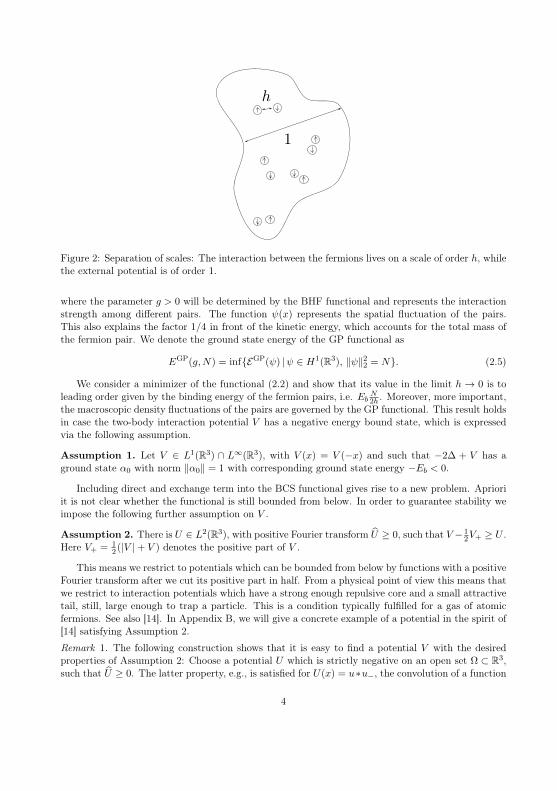
Figure 2: Separation of scales: The interaction between the fermions lives on a scale of order h, whilethe external potential is of order 1.
where the parameter g > 0 will be determined by the BHF functional and represents the interactionstrength among different pairs. The function ψ(x) represents the spatial fluctuation of the pairs.This also explains the factor 1/4 in front of the kinetic energy, which accounts for the total mass ofthe fermion pair. We denote the ground state energy of the GP functional as
EGP(g,N) = infEGP(ψ) |ψ ∈ H1(R3), ‖ψ‖22 = N. (2.5)
We consider a minimizer of the functional (2.2) and show that its value in the limit h → 0 is toleading order given by the binding energy of the fermion pairs, i.e. Eb N2h . Moreover, more important,the macroscopic density fluctuations of the pairs are governed by the GP functional. This result holdsin case the two-body interaction potential V has a negative energy bound state, which is expressedvia the following assumption.
Assumption 1. Let V ∈ L1(R3) ∩ L∞(R3), with V (x) = V (−x) and such that −2∆ + V has aground state α0 with norm ‖α0‖ = 1 with corresponding ground state energy −Eb < 0.
Including direct and exchange term into the BCS functional gives rise to a new problem. Aprioriit is not clear whether the functional is still bounded from below. In order to guarantee stability weimpose the following further assumption on V .
Assumption 2. There is U ∈ L2(R3), with positive Fourier transform U ≥ 0, such that V − 12V+ ≥ U .
Here V+ = 12(|V |+ V ) denotes the positive part of V .
This means we restrict to potentials which can be bounded from below by functions with a positiveFourier transform after we cut its positive part in half. From a physical point of view this means thatwe restrict to interaction potentials which have a strong enough repulsive core and a small attractivetail, still, large enough to trap a particle. This is a condition typically fulfilled for a gas of atomicfermions. See also [14]. In Appendix B, we will give a concrete example of a potential in the spirit of[14] satisfying Assumption 2.
Remark 1. The following construction shows that it is easy to find a potential V with the desiredproperties of Assumption 2: Choose a potential U which is strictly negative on an open set Ω ⊂ R3,such that U ≥ 0. The latter property, e.g., is satisfied for U(x) = u∗u−, the convolution of a function
4

u(x) with its reflection u−(x) = u(−x), since U = |u|2 ≥ 0. Now set V = 2U+ − U−. Obviously thisV fulfills Assumption 2. Finally, scale V according to V 7→ λV until the negative part is deep enoughto ensure binding.
With these assumptions we are ready to formulate our main theorem.
Theorem 1. Let W ∈ H1(R3) ∩ L∞(R3). Under Assumptions 1 and 2, we have for small h,
EBHF(N,h) = −Eb2
N
h+ hEGP(g,N) +O(h3/2), (2.6)
where g is given by
g =1
(2π)3
∫|α0(p)|4(2p2 + Eb) d3p− 1
2
∫
R3
|(α0 ∗ α0)(x)|2 V (x) d3x+
∫
R3
V (x) d3x.
Moreover, if Γ is an approximate minimizer of EBHF, in the sense that
EBHF(Γ) ≤ −Eb2
N
h+ h(EGP(g,N) + ε)
for some ε > 0, then the corresponding α can be decomposed as
α = αψ + ξ, ‖ξ‖22 ≤ O(h), (2.7)
where
αψ(x, y) = h−2ψ(x+ y
2
)α0
(x− yh
), (2.8)
and ψ is an approximate minimizer of EGP in the sense that
EGP(ψ) ≤ EGP(g,N) + ε+O(h1/2). (2.9)
Remark 2. In contrast to the usual BCS functional [11, Eq. (1.2)] and [13], the coupling constant g,where g only consists of the BCS term
gBCS =1
(2π)3
∫|α0(p)|4(2p2 + Eb) d3p
receives the additional contributions from direct and exchange energy
gdir =
∫
R3
V (x) d3x and gex = −1
2
∫
R3
|(α0 ∗ α0)(x)|2 V (x) d3x
respectively.
Remark 3. In [13] we proved the emergence of the Gross-Pitaevstii functional within the frameworkof the BCS functional, i.e., without direct and exchange terms. Of course, our current work wouldapply as well to the BCS-functional. Following the proof, one obtains the asymptotic statement
EBHF(N,h) = −Eb2
N
h+ hEGP(gBCS, N) +O(h3/2).
I.e., compared to [13] we improve the error bound, from O(h6/5) to O(h3/2). Further we get rid ofthe boundary condition and we significantly simplify the proof of [13], which relied on the involvedestimates of [7]. However, we remark that, for simplicity, we neglect the magnetic field A.
5

Remark 4. The proof of our current work relies on ideas of [11], where within the same setting ofour work, the BCS evolution equation was studied showing that the macroscopic fluctuations aregoverned by the time-dependent Gross-Pitaevskii equation. Starting point is the evolution equationtime evolution for the BCS state Γt which takes the form
ih2∂tΓt = [HΓt ,Γt], (2.10)
where the BCS Hamiltonian HΓt is given by
HΓt =
(−h2∆ + h2W V αtV αt h2∆− h2W
)
and where V αt ∈ L(L2(R3)
)is the operator with kernel V
((x − y)/h
)αt(x, y). If the energy of the
initial BCS state Γ0 is sufficiently close to the minimal energy, i.e., if
EBCS(Γ0) ≤ −Eb2
Tr(γ0) + Ch,
then, it is shown in [11], that the macroscopic fluctuations in the center-of-mass variable
ψt(X) =e−itEb/h
2
h
∫
R3
α0(r/h)αt(X + r/2, X − r/2) d3r
satisfies to leading order the time-dependent Gross-Pitaevskii equation
i∂tϕt = −1
2∆ϕt + 2Wϕt + 2gBCS|ϕt|2ϕt
with initial data ϕt=0 ≡ ψt=0. More precisely, it is shown that ψt is close to a ϕt, i.e.,
‖ψt − ϕt‖2 ≤ Ch1/2ec|t|
for some constants c, C > 0, with ϕt satisfying the GP-equation.A similar result would now hold as well in the case of the time-dependent BHF equation, which in
a different context was treated in [10]. By repeating the strategy of [11] and handling the exchangeand direct terms one may obtain the emergence of the time-dependent GP equation with parameterg.
3 Note on stability
Before giving a sketch of the proof we show how Assumption 2 gives rise to stability. In fact we showthat the assumption guarantees that the direct and exchange terms are non-negative. To this aim wefirst consider the exchange term and estimate
−∫
R6
|γ(x, y)|2V((x− y)/h
)d3x d3y ≥ −
∫
R6
|γ(x, y)|2V+
((x− y)/h
)d3x d3y
≥ −∫
R6
γ(x, x)γ(y, y)V+
((x− y)/h
)d3x d3y
6

replacing first V by its positive part V+ = 12(|V | + V ) and using |γ(x, y)|2 ≤ γ(x, x)γ(y, y). Hence,
we have for the sum of direct and exchange term
2
∫
R6
γ(x, x)γ(y, y)V((x− y)/h
)d3x d3y −
∫
R6
|γ(x, y)|2V((x− y)/h
)d3x d3y
≥ 2
∫
R6
γ(x, x)γ(y, y) (V − V+/2)((x− y)/h
)d3x d3y,
= 2
∫
R3
(ρ ∗ ρ−) (x) (V − V+/2) (x/h) d3x,
where we denote by ρ(x) = γ(x, x) the density and ρ−(x) = ρ(−x). By assumption, there is apotential U with
(V − 1
2V+
)≥ U and U(p) ≥ 0 for almost every p. Since ρ ≥ 0, the last term on the
right hand side is bounded below by
2
∫
R3
(ρ ∗ ρ−) (x)U(x/h) d3x = 2
∫
R3
|ρ|2(p)U(p) d3p ≥ 0,
showing the non-negativity of the direct and exchange energy terms.
4 Sketch of the proof of Theorem 1
We decompose the proof of Theorem 1 into an upper and a lower bound. The upper bound is donevia a trial argument. We define the trial state Γψ via the pair wavefunction
αψ(x, y) = ψ(x+ y
2
)α0
(x− yh
),
with α0 being the ground-state in the relative coordinates of the two particle system, i. e.,
(−2∆ + V )α0 = −Ebα0,
whereas ψ accounts for the macroscopic fluctuations in the center-of-mass coordinates. Since weexpect that the system in its ground state energy consists predominantly of pairs we define the oneparticle density γψ such that to leading order it is given by αψαψ, i.e., γψ = αψαψ + O(h). Recallthat the number of particles Tr γψ is of the order of 1/h, such that the error term of order O(h) is infact by a factor of h2 higher than the leading term. With the trial state Γψ at hand it is mainly atedious calculation to obtain the bound
EBHF(Γ) ≤ −Eb2N/h+ hEGP(ψ) +O(h2).
For the lower bound the first step consists of using energy estimates, see [7, 13, 11], in order toconclude that an approximate ground state Γ the corresponding two particle state α necessarily hasto be of the form α = αψ + ξ, with ξ being negligible compared to αψ, i.e., ‖ξ‖22 ≤ h2‖αψ‖2. Withthe apriori bound at hand we then show that ξ at most contributes a term of the order of o(h) to theenergy. Using now the estimates from the upper bound completes the proof of the Theorem.
In the following we give a more detailed sketch of the upper, respectively, lower bound.
7

4.1 Upper bound
We proceed in analogy to [11]. For the upper bound we use the trial state
Γψ =
(γψ αψαψ 1− γψ
)
with the definition
αψ(x, y) = h−2ψ(x+ y
2
)α0
(x− yh
),
γψ = αψαψ + (1 + Cψh)αψαψαψαψ
Tr γψ = N/h,
(4.1)
where the constant Cψ has to be chosen such that
Cψ h ≥ ‖2(1 + Cψ h)αψαψ + (1 + Cψ h)2(αψαψ)2‖∞
in order to guarantee 0 ≤ Γψ ≤ 1. We will see later, that a good choice for small h is
Cψ = C‖∇ψ‖22‖α0‖26
for appropriate C.In the limit of small h the GP energy-functional will emerge at the order of h from the BHF
functional EBHFh (Γψ). This appears as follows. If we first consider the kinetic energy term plus the
pairing term of EBHFh (Γψ) and subtract the total binding energy, −Eb
2Nh = −Eb
2 Tr γψ, we obtain
Tr(−h2∆
)γψ +
1
2
∫
R6
V(x− y
h
)|αψ(x, y)|2 d3x d3y + Eb
N
2h
= Tr(−h2∆ + Eb/2
)γψ +
1
2
∫
R6
V(x− y
h
)|αψ(x, y)|2 d3x d3y. (4.2)
If we first only consider the αψαψ contribution from (4.7) we can rewrite the corresponding term as∫
R3
⟨αψ(·, y),
[−h2∆x +
1
2V( · − y
h
)+Eb2
]αψ(·, y)
⟩d3y.
Since αψ(x, y) is symmetric we can replace ∆x by 12(∆x+∆y). In terms of center of massX = (x+y)/2
and relative coordinates r = x−y we can write ∆x+∆y = 12∆X +2∆r, such that in these coordinates
the term can be rewritten as
h−4
∫
R6
α0(r/h)ψ(X)
[−h2 1
4∆X − h2∆r +
1
2V (r/h) + Eb/2
]α0(r/h)ψ(X) d3X d3r
=h
4
∫
R3
|∇ψ(X)|2 d3X + h‖ψ‖22 〈α0, [−∆r + V/2 + Eb/2]α0〉 =h
4
∫
R3
|∇ψ(x)|2 d3x, (4.3)
using the ground-state property in the last equality and the normalization condition
h−3
∫
R3
|α0(r/h)|2 d3r = 1
in the first equality.
8

Second, we remark that the monomial term αψαψαψαψ of γψ in inserted into
Tr[−h2∆ + Eb/2]γψ
contributes to the quartic term∫R3 gbcs|ψ(x)|4 d3x term in the GP functional. The remaining part of
the∫R3 g|ψ(x)|4 d3x term is due to the contribution of the monomial αψαψ in the direct and exchange
energy. The estimation of these terms is straightforward but tedious and occupies the main part ofthe proof.
Further, it will be easy to show that
h2 TrWαψαψ = h−2
∫
R3
W (X + r/2)|ψ(X)|2|α0(r/h)|2 d3r = h
∫
R3
W (X)|ψ(X)|2 d3X +O(h2).
Consequently we obtain
EBHF(Γψ) + EbN
2h= hEGP(ψ) +O(h2). (4.4)
Finally, we remark that the constraint Tr γψ = N/h implies for ψ that
‖ψ‖22 = N(1−O(h2)).
Since, however, ∣∣EGP(ψ)− EGP([1 +O(h2)]ψ
)∣∣ ≤ O(h2)
we obtain the bound
inf0≤Γ≤1
Tr(γ)=N/h
EBHF(Γ) + EbN
2h≤ h inf
ψ∈H1(R3)‖ψ‖22=N
EGP(ψ) +O(h2), (4.5)
which is the content of Section 6.
Remark 5.
• Since the infimum of EBHF remains unchanged when restricting Γ to be a projector [2], thenatural choice for a trial state Γψ would be a projector, i.e. Γψ = Γ2
ψ. The operator γψwould then be determined by γψ = γ2
ψ + αψαψ. Following this approach, we would haveto deal with additional difficulties. To evaluate EBHF at this state, we first had to expandγψ = 1
2 −√
14 − αψαψ in terms of αψαψ. This would give rise to much more complicated
computations.
• Our actual choice for Γψ,
γψ = αψαψ + (1 + Cψ h)αψαψαψαψ
in fact consists of the first two terms of the expansion of γ = 12 −√
14 − αψαψ in terms of αψαψ.
It indeed satisfies 0 ≤ Γψ ≤ 1 for small enough h. This can be seen as follows. 0 ≤ Γψ ≤ 1 isequivalent to 0 ≤ Γψ(1 − Γψ). If γψ is of the special form (4.7) which is a function of αψαψ,the off diagonals of
Γψ(1− Γψ) =
(γψ − γ2
ψ − αψαψ αψγψ − γψαψγψαψ − αψγψ γψ − γψ2 − αψαψ
)
=
(γψ − γ2
ψ − αψαψ 0
0 γψ − γψ2 − αψαψ
)
9

vanish and thus the statement is equivalent to
γψ − γ2ψ − αψαψ ≥ 0. (4.6)
Plugging in the expression for γψ (4.6) is equivalent to
αψαψ(Cψ h− 2(1 + Cψ h)αψαψ − (1 + Cψ h)2(αψαψ)2
)αψαψ ≥ 0.
Using (see Corollary 1 below) ‖αψ‖∞ ≤ ‖αψ‖6 = h1/2C‖∇ψ‖2 ‖α0‖6, this inequality is suresatisfied for small enough h for the choice
Cψ = C‖∇ψ‖22‖α0‖26
4.2 Lower bound
From the upper bound we learn that for an approximate ground state Γ we can assume
EBHFh (Γ) ≤ −Eb
N
2h+O(h).
We will show in Lemma 4 by energy estimates, that the corresponding α necessarily has to be of theform
α(x, y) = αψ(x, y) + ξ(x, y) = h−2ψ(x+ y
2
)α0
(x− yh
)+ ξ(x, y)
for an appropriate ψ ∈ H1(R3), and ξ being negligible with respect to αψ, e.g.,
‖ξ‖22 ≤ O(h2)‖αψ‖22 ≤ O(h).
The function ψ is obtained by projecting α in the direction of α0 with respect to the relative coordi-nates, more precisely, with X = x+y
2 ,
ψ(X) =1
h
∫
R3
α0(r/h)α(X + r/2, X − r/2) d3r.
This allows us to define, similar to the upper bound,
Γψ =
(γψ αψαψ 1− γψ
)
with the definition
αψ(x, y) = h−2ψ(x+ y
2
)α0
(x− yh
),
γψ = αψαψ + (1 + Cψ h)αψαψαψαψ.(4.7)
Next we use the apriori bounds to show in Section 7 that the difference between EBHF(Γ) andEBHF(Γψ) is positive or at least of higher order than the contribution from the GP functional, i.e.,
EBHF(Γ) ≥ EBHF(Γψ)−O(h3/2). (4.8)
Using now our calculation (4.4) from the upper bound immediately implies
inf0≤Γ≤1
Tr(γ)=N/h
EBHF(Γ) + EbN
2h≥ h inf
ψ∈H1(R3)‖ψ‖22=N
EGP(ψ) +O(h3/2). (4.9)
Together with (4.5) this combines to (2.6).
10

4.3 Properties of approximate minimizers
Let us finally indicate how to prove (2.7), (2.8) and (2.9) under the assumption of the lower andupper bounds. Given an approximate minimizer Γ, for which we have by definition
EBHF(Γ) ≤ −Eb2
N
h+ h(EGP(g,N) + ε
),
the methods from the lower bound immediately apply and we obtain (2.7) and (2.8). To see (2.9),we combine (4.8) with (4.4), implying
|EGP(g,N) + ε− EGP(ψ)| ≤ O(h1/2).
5 Useful properties of the pair-wavefunction
In the following we derive some useful properties for the type of pair-wave function α which we willmeet throughout our proof. Recall that α0 was defined in Assumption 1 to be the normalized groundstate of −2∆ + V .
Lemma 1. Let α = αψ + ξ, with ψ ∈ H1(R3), ‖ψ‖22 = N , and ‖ξ‖22 ≤ O(h).
(i) For n ∈ 2N, there are appropriate constants C, such that
‖αψ‖nn ≤ Chn−3‖ψ‖nn ‖α0‖nn, (5.1a)
‖∇(x−y)αψ‖nn ≤ Ch−3‖ψ‖nn ‖∇α0‖nn, (5.1b)
where(∇(x−y)αψ)(x, y) = h−3ψ
((x+ y)/2
)(∇α0)
((x− y)/h
).
(ii) Let gBCS = (2π)3∫R3 |α0(p)|4(p2 + Eb/2) d3p. Then
Tr((−h2∆ + Eb/2)αψαψαψαψ
)= h gBCS‖ψ‖44 +O(h2). (5.2)
(iii) ‖αψαψ(·, ·)‖∞ = supx|αψαψ(x, x)| ≤ h−2‖α0‖23 ‖∇ψ‖22. (5.3)
(iv) Let σ be a Hilbert-Schmidt operator. Then
|σαψ(x, x)| ≤ h−1‖σ(·, x)‖2‖∇ψ‖2 ‖α0‖3. ∀x ∈ R3 (5.4)
Let us mention that we use the symbol ‖ · ‖p for the Lp-norm of functions as well as for theoperator norm in the corresponding Schatten class, since it is in general clear out of the context, if wetalk about a function or an operator. In that sense ‖σ(·, x)‖2 denotes the L2-norm of the function,corresponding to the first variable of its kernel. Whereas ‖σ‖2 denotes its Hilbert-Schmidt operator.
Proof of Lemma 1, Part I. We postpone the proof of (5.1a), (5.1b) and (5.2) to Part II in the Ap-pendix A. In order to see (5.3) we use Hölder
(αψαψ)(x, x) =
∫
R3
|αψ(x, y)|2 d3y = h−4
∫
R3
∣∣α0
((x− y)/h
)∣∣2 ∣∣ψ((x+ y)/2)
)∣∣2 d3y
≤ h−4‖α0(·/h)2‖3/2‖|ψ|2‖3 = h−2C‖α0‖23‖∇ψ‖22,
11

Finally, observe
|(σαψ)(x, x)| = h−2
∣∣∣∣∫
R6
σ(x, y)α0
((x− y)/h
)ψ((x+ y)/2
)d3y
∣∣∣∣≤ h−2‖σ(·, x)‖2‖α0(·/h)‖3‖ψ‖6 = h−1‖σ(·, x)‖2‖ψ‖6‖α0‖3,
using Hölder inequality in y, which implies (5.4)
Since γψ is to leading order equal to αψαψ, we obtain as a corollary that the norm of γψ is atmost O(h), meaning that the largest eigenvalue is of order h. However, let us remark, that theidea of Bardeen-Cooper-Schrieffer was that the Quantum mechanical two-particle density matrix isessentially given by
N
h|α〉〈α|, |α〉 =
αψ
N1/2/h1/2,
which means that the two particle density matrix has one large eigenvalue N/h.
Corollary 1. Let the assumptions be as in Lemma 1. Then
‖αψ‖44 ≤ hC(2π)3‖ψ‖2‖∇ψ‖32 ‖α0‖44, (5.5a)
‖αψ‖66 ≤ h3C‖∇ψ‖62 ‖α0‖66, (5.5b)
‖∇(x−y)αψ‖66 ≤ Ch−3‖∇ψ‖66 ‖∇α0‖66, (5.5c)
‖αψ‖∞ ≤ h1/2C‖∇ψ‖2 ‖α0‖6, (5.5d)
(αψαψαψαψ)(x, x) ≤ ‖αψ‖2∞(αψαψ)(x, x) ≤ O(h−1), (5.5e)
‖α‖∞ ≤ ‖αψ‖∞ + ‖ξ‖2 ≤ O(h1/2). (5.5f)
Let γψ defined as in (4.7). Then
‖γψ‖∞ ≤ ‖αψ‖2∞ + (1 + Cψ h)‖αψ‖4∞ ≤ O(h) (5.6a)
γψ(x, x) ≤ O(h−2). (5.6b)
Proof. The estimates (5.5a), (5.5b) and (5.5c) are a consequence of (5.1a) and (5.1b). In the case ofn = 6, we use the Sobolev inequality to have ‖ψ‖6 ≤ ‖∇ψ‖2 and in the case of n = 4, we use Lp
interpolation and the Sobolev inequality to conclude
‖ψ‖4 ≤ ‖ψ‖1/42 ‖ψ‖3/46 ≤ C‖ψ‖1/42 ‖∇ψ‖
3/42 .
Inequality (5.5d) follows immediately from ‖αψ‖∞ ≤ ‖αψ‖6 together with (5.5b), while inequal-ity (5.5f) is (5.5d) combined with the assumption ‖ξ‖2 ≤ O(h1/2).
Next observe that(αψαψαψαψ)(x, x) ≤ ‖αψαψ‖∞(αψαψ)(x, x).
Let us only show it on a more formal level using the physics notation of an integral kernel, i.e.,
(αψαψαψαψ)(x, x) = 〈x|αψαψαψαψ|x〉 ≤ ‖αψαψ‖∞〈x|αψαψ|x〉 ≤ ‖αψαψ‖∞(αψαψ)(x, x).
Consequently, using (4.7)
‖γψ‖∞ = ‖αψαψ + (1 + Cψ h)αψαψαψαψ‖∞ ≤ ‖αψ‖2∞ + (1 + Cψ h)‖αψ‖4∞.
12

6 Upper bound
As explained above, for any ψ ∈ H1(R3) we are going to define the trial state
Γψ =
(γψ αψαψ 1− γψ
), (6.1)
with
αψ(x, y) = h−2ψ(x+ y
2
)α0
(x− yh
), (6.2)
γψ = αψαψ + (1 + Cψ h)αψαψαψαψ, (6.3)
and the normalization conditionTr γψ = N/h.
Since, by definition,N/h = Tr γψ = ‖ψ‖22 + (1 + h)‖αψ‖44,
this implies ∣∣‖ψ‖22 −N∣∣ ≤ Ch‖ψ‖2H1 .
Hence, as an immediate consequence we are able to realize that in order to prove
inf0≤Γ≤1
Tr(γ)=N/h
EBHF(Γ) +Eb2
N
h≤ h inf
ψ∈H1(R3)‖ψ‖22=N
EGP(ψ) +O(h2). (6.4)
it suffices to show the following asymptotic expansion for our trial states.
Lemma 2. Assume Γψ to be of the form (6.1), then
EBHF(Γψ) +Eb2
N
h= hEGP(ψ) +O(h2). (6.5)
Proof. The remaining part of this section will be dedicated to proving (6.5). Recall the form of theBCS and GP functionals we see that Equation (6.5) can be decomposed in the following estimates
Tr(−h2∆ + Eb/2)γψ +1
2
∫
R6
V((x− y)/h)
)|αψ(x, y)|2 d3x d3y
= h
∫
R3
(1
4|∇ψ(x)|2 + gBCS|ψ(x)|4
)d3x+O(h2)
(6.6a)
Trh2Wγψ = h
∫
R3
W (x)|ψ(x)|2 d3x+O(h2) (6.6b)
− 1
2
∫
R6
|γψ(x, y)|2V(x− y
h
)d3x d3y = h gex
∫
R3
|ψ(x)|4 d3x+O(h2) (6.6c)∫
R6
γψ(x, x)γψ(y, y)V(x− y
h
)d3x d3y = h gdir
∫
R3
|ψ(x)|4 d3x+O(h2), (6.6d)
where the constants gBCS, gex, and gdir are given in Remark 2. These estimates will be proven in thefollowing subsections.
13

6.1 Kinetic and potential energy (Proof of (6.6a))
Using the definition of our trial state (6.3) and (6.2) as well the calculation in (4.3) we obtain
Tr(−h2∆ + Eb/2)γψ +1
2
∫
R6
|αψ(x, y)|2V(x− y
h
)d3x d3y
= Tr((−h2∆ + Eb/2
)(αψαψ + (1 + Cψ h)αψαψαψαψ)
)+
1
2
∫
R6
|αψ(x, y)|2V(x− y
h
)d3x d3y
=h
4
∫
R3
|∇ψ(x)|2 d3x+ h
∫
R3
gBCS|ψ(x)|4 d3x−O(h2),
where we used (5.2) in order to recover the |ψ|4-term from the contribution involving αψαψαψαψ.Hence we obtain (6.6a).
6.2 External potential (Proof of (6.6b))
With our definition (6.3) for γψ we have
Trh2Wγψ = h2 Tr(Wαψαψ) + (1 + Cψ h) Tr(h2Wαψαψαψαψ). (6.7)
By (5.5a) of Corollary 1, we know that the second term is of higher order, i.e.
Tr(h2Wαψαψαψαψ) ≤ h2‖W‖∞Tr(αψαψαψαψ) = O(h3).
In terms of integral kernels and using center-of-mass and relative coordinates for the expression (2.8)for αψ we can write
h2 Tr(Wαψαψ) = h2
∫
R6
W (x)|αψ(x, y)|2 d3x d3y = h−2
∫
R6
W (X + r/2)|ψ(X)|2|α0(r/h)|2 d3X d3r
= h
∫
R6
W (X)|ψ(X − hr/2)|2|α0(r)|2 d3X d3r,
in the last equality we performed a change of variables according to X + r/2→ X and r → hr.Next, we apply the fundamental theorem of calculus and obtain
h2 Tr(Wαψαψ) = h
∫
R6
W (X)|ψ(X)|2|α0(r)|2 d3X d3r
+ h
∫
R6
∫ 1
0W (X)
∂
∂τ|ψ(X − τhr/2)|2|α0(r)|2 dτ |α0(r)|2 d3X d3r.
Using Cauchy-Schwarz in X, the last term is bounded by∣∣∣∣h∫
R6
∫ 1
0W (X)<
(h r · ∇ψ(X − τhr/2)ψ(X − τhr/2)
)dτ |α0(r)|2 d3X d3r
∣∣∣∣
≤ h2‖W‖∞‖∇ψ‖2‖ψ‖2‖√| · |α0‖22.
This shows (6.6a).
14

6.3 Direct and exchange term (Proof of (6.6c) and (6.6d))
We first argue, that the leading order contribution of the direct and exchange terms stems fromreplacing γψ by αψαψ contributes to leading order of the direct and exchange terms. To see this, wesimply estimate the differences
∫
R6
|γψ(x, y)|2V((x− y)/h
)d3x d3y −
∫
R6
|(αψαψ)(x, y)|2V((x− y)/h
)d3x d3y (6.8a)
and∫
R6
γψ(x, x)γψ(y, y)V((x−y)/h
)d3x d3y−
∫
R6
(αψαψ)(x, x)(αψαψ)(y, y)V((x−y)/h
)d3x d3y. (6.8b)
Both expressions are can be reduced to the following form, whose proof is elementary.
Lemma 3. Let σ(x, y) and δ(x, y) be integral kernels of two positive trace class operators. If V (r) =V (−r), then
∣∣∣∣∫
R6
V (x− y) [(σ + δ)(x, x)(σ + δ)(y, y)− σ(x, x)σ(y, y)] d3x d3y
∣∣∣∣
≤ 2
∫
R6
|V (x− y)|(σ + δ)(x, x)δ(y, y) d3x d3y
(6.9a)
and∣∣∣∣∫
R6
V (x− y)[|(σ + δ)(x, y)|2 − |σ(x, y)|2
]d3x d3y
∣∣∣∣ ≤ 2
∫
R6
|V (x− y)|(σ + δ)(x, x)δ(y, y) d3x d3y.
(6.9b)
Proof. To show (6.9a), we simply use
(σ + δ)(x, x)(σ + δ)(y, y)− σ(x, x)σ(y, y)
= (σ + δ)(x, x)δ(y, y) + δ(x, x)σ(y, y)
≤ (σ + δ)(x, x)δ(y, y) + δ(x, x)(σ + δ)(y, y).
Under the integral on the left hand side of (6.9a), we use the symmetry V (x − y) = V (y − x) toobtain (6.9a).
For (6.9b) we follow a similar strategy and first split
V (x− y)[|(σ + δ)(x, y)|2 − |σ(x, y)|2
]
= V (x− y)[(σ + δ)(x, y)δ(x, y) + δ(x, y)σ(x, y)
]
≤ |V (x− y)| [|(σ + δ)(x, y)| |δ(x, y)|+ |δ(x, y)| |σ(x, y)|] .
Applying now to σ, δ, and σ + δ, that for positive trace class operators a its kernel satisfies
|a(x, y)| ≤√|a(x, x)|
√|a(y, y)|
and using Cauchy-Schwarz inequality we obtain the stated inequality.
15

By applying Lemma 3 to σ + δ = γψ and σ = αψαψ the differences (6.8a) and (6.8b) can bebounded by
(1 + Cψ h)
∫
R6
∣∣V((x− y)/h
)∣∣ γψ(x, x)(αψαψαψαψ)(y, y) d3x d3y
≤ (1 + Cψ h)‖γψ(·, ·)‖∞∫
R6
(αψαψαψαψ)(x, x)∣∣V((x− y)/h
)∣∣ d3x d3y
= (1 + Cψ h)h3‖V ‖1‖γψ(·, ·)‖∞Tr(αψαψαψαψ) ≤ O(h2),
(6.10)
where we used (5.6b).In order to recover the ‖ψ‖44 contribution we inspect the remaining parts of the direct and the
exchange term separately. We begin with the exchange term and write explicitly
− 1
2
∫
R6
|(αψαψ)(x, y)|2V((x− y)/h
)d3x d3y
= −1
2
∫
R12
αψ(x, z)αψ(z, y)αψ(x,w)αψ(w, y)V((x− y)/h
)d3x d3y d3z d3w.
Introducing new variables
X =x+ y
2, r = x− y, s = x− z, t = x− w,
the last expression becomes
− 1
2
∫
R6
|(αψαψ)(x, y)|2V((x− y)/h
)d3x d3y
= −h2
∫
R12
V (r)α0(s)α0(r − s)α0(t)α0(r − t)
× ψ(X + h(r − s)/2)ψ(X − hs/2)ψ(X − ht/2)ψ(X + h(r − t)/2) d3X d3r d3s d3t.
The result can be rewritten as
−1
2
∫
R6
|(αψαψ)(x, y)|2V((x− y)/h
)d3x d3y = −h
2
∫
R3
|ψ(X)|2 d3X
∫
R3
V (r)|(α0 ∗ α0)(r)|2 d3r +Aex
= h gex
∫
R3
|ψ(x)|4 d3x+Aex,
(6.11)
where
Aex = −h2
∫
R12
V (r)α0(s)α0(r − s)α0(t)α0(r − t)×
×∫ 1
0
d
dτ
(ψ(X + τh(r − s)/2)ψ(X − τhs/2)ψ(X − τht/2)ψ(X + τh(r − t)/2)
)dτ d3X d3r d3s d3t,
which is bounded by
|Aex| ≤ h2‖∇ψ‖2‖ψ‖36‖V (α0 ∗ α0)((| · |α0) ∗ α0)‖1 ≤ Ch2‖∇ψ‖42‖V ‖1‖α0‖32∥∥| · |α0
∥∥2,
16

using Hölder, Sobolev ‖ψ‖6 ≤ C‖∇ψ‖2, and Young’s inequality. This shows (6.6c). We continuewith the direct term. Its remaining part is given by
∫
R6
(αψαψ)(x, x)(αψαψ)(y, y)V((x− y)/h
)d3x d3y
=
∫
R6
|αψ(x, z)|2|αψ(y, w)|2V((x− y)/h
)d3x d3y d3w d3z
= h
∫
R12
V (r)|α0(s)|2|α0(t)|2|ψ(X + h(r − s)/2)|2|ψ(X − h(r + t)/2)|2 d3X d3r d3s d3t,
where we changed to the variables
X =x+ y
2, r = x− y, s = x− z, t = y − w.
The fundamental theorem of calculus leads to∫
R6
(αψαψ)(x, x)(αψαψ)(y, y)V((x− y)/h
)d3x d3y = h‖α0‖22
∫
R3
V (r) d3r
∫
R3
|ψ(X)|2 d3X +Adir
= h gdir
∫
R3
|ψ(x)|4 d3x+Adir,
(6.12)
where
Adir = h
∫
R12
V (r)|α0(s)|2|α0(t)|2×
×∫ 1
0
d
dτ
(|ψ(X + τh(r − s)/2)|2|ψ(X − τh(r + t)/2)|2
)dτ d3X d3r d3s d3t
is bounded by
|Adir| ≤ 4h2‖∇ψ‖2‖ψ‖36 ‖α0‖2(‖| · |V ‖1‖α0‖2 + ‖V ‖1‖
√| · |α0‖2
).
This shows (6.6d).
7 Lower bound
Our proof of the lower bound on EBHF(N,h) in Theorem 1 consists of two parts. As first step weobtain apriori bounds on approximate ground states.
Lemma 4 (Apriori bounds). Let Γ, with Tr γ = N/h, be a state satisfying
EBHF(Γ) ≤ −EbN
2h+ Ch
for some C > 0. There exists a function ψ ∈ H1(R3), with
ψ(X) =1
h
∫
R3
α0(r/h)α(X + r/2, X − r/2) d3r, (7.1)
such thatα(X + r/2, X − r/2) = α(X, r) = h−2ψ(X)α0(r/h) + ξ,
with ξ(X, r) = ξ(X + r/2, X − r/2), satisfy the bounds
17

Tr[(−h2∆ +
Eb2
)(γ − αα)]≤ O(h), (7.2a)
Tr(γ2) ≤ Tr(γ − αα) ≤ O(h), (7.2b)‖ψ‖2 ≤ O(1), (7.2c)‖∇ψ‖2 ≤ O(1), (7.2d)
‖ξ‖22 ≤ O(h), (7.2e)
‖∇X ξ‖2 ≤ O(h−1/2), (7.2f)
‖∇r ξ‖2 ≤ O(h−1/2), (7.2g)Tr(αααα) ≤ O(h). (7.2h)
Proof. According to Section 3 the sum of direct and exchange term is non-negative. Thus, we havethat
Ch ≥ EBHF(Γ) + EbN
2h
≥ Tr(−h2∆ + Eb/2)γ +1
2
∫
R6
V((x− y)/h
)|α(x, y)|2 d3x d3y − h2‖W‖∞Tr(γ).
We bring the term −h2‖W‖∞Tr(γ) = O(h) to the left hand side and combine it with Ch. Addingand subtracting an appropriate expression involving αα, we obtain
Ch ≥ Tr(−h2∆ + Eb/2)(γ − αα) + Tr(−h2∆ + Eb/2)αα+1
2
∫
R6
V((x− y)/h
)|α(x, y)|2 d3x d3y.
The two terms on the right hand side can be written in the form, and expressed via center-of-massand relative coordinates as∫
R3
⟨α(·, y),
[−h2∆x +
1
2V( · − y
h
)+Eb2
]α(·, y)
⟩d3y
=
⟨α0ψ + ξ,
[−h2 1
4∆X − h2∆r +
1
2V (r/h) +
Eb2
]α0ψ + ξ
⟩
L2(R6)
=h
4
∫
R3
|∇ψ(X)|2 d3X + ‖∇X ξ‖22 +
∫
R3
〈ξ(X, ·), (−h2∆ +1
2V (·/h) + Eb/2)ξ(X, ·)〉d3X,
(7.3)
where we used that the normalized α0 is the zero eigenvector to the operator −∆ + V/2 +Eb/2 andthe fact, that ξ(X, ·) is orthogonal to α0 for almost every X ∈ R3. This implies
Ch ≥ Tr(−h2∆+Eb/2)(γ−αα)+h
4‖∇ψ‖22+h2 ‖∇X ξ‖22+
∫
R3
〈ξ(X, ·), (−h2∆+1
2V (·/h)+Eb/2)ξ(X, ·)〉 d3X.
Since all terms on the right hand side are positive, and γ − γ2 ≥ αα we read off the estimates (7.2a),(7.2b), (7.2f), and (7.2d). To prove (7.2e) and (7.2g), we use the fact, that the operator −∆ + V/2has a spectral gap in between the ground state energy −Eb and the next higher eigenvalue. Hencethere is a κ > 0 and an ε > 0 such that
(1− ε)∆ + V/2 + Eb/2 ≥ κon the orthogonal complement of α0. In other words
∫
R3
〈ξ(X, ·), (−h2∆r +1
2V (·/h) + Eb/2)ξ(X, ·)〉d3X ≥ (1− ε)κ‖ξ‖22 + εh2‖∇r ξ‖22,
proving (7.2e) and (7.2g). The estimate (7.2c) for the L2 norm of ψ is obtained using the definitionψ and ‖α‖22 = Tr(γ − αα) + Tr γ = O(h). Namely
‖ψ‖22 = h−2
∫
R3
α0(r1/h)α(X, r2)α0(r2/h)α(X, r1) d3r1 d3r2 d3X
≤ h−2
∫
R3
|α0(r1/h)|2|α(X, r2)|2 d3r1 d3r2 d3X = h‖α‖22 = O(1),
(7.4)
18

where we used Cauchy-Schwarz with respect to the measure d3r1 d3r2. Finally, to see (7.2h), notethat in an analogous way
Tr(αααα) = Tr(γ2 − γ(γ − αα)− (γ − αα)γ + (γ − αα)2
)
≤ Tr(γ2) + Tr(γ − αα)2 + 2√
Tr(γ2) Tr(γ − αα)2 = O(h).
Observe, that we do not necessarily have ‖ψ‖22 = N . The norm deviates from N by a correctionof order h2,
∣∣‖ψ‖22 −N∣∣ = h |Tr(αψαψ)− Tr(γ)| ≤ h |Tr(αψαψ − αα)|+ hTr(γ − αα). (7.5)
By (7.2b) and (7.2e), the right hand side is of order O(h2).Now that we have recovered the function ψ(x) starting from an arbitrary approximate ground
state Γ, we are able to define a corresponding Γψ via
αψ(x, y) = h−2ψ(x+ y
2
)α0
(x− yh
)
and the definition (6.1). Observe that we are able to rescale ψ 7→ λψ, such that we can assume
Tr γψ = N/h.
The second step now consists of proving that for a lower bound we can replace EBHF(Γ) byEBHF(Γψ) up to higher order. Together with the calculations from the upper bound this implies thelower bound stated in Theorem 1.
Lemma 5. With Γ and Γψ defined as above, one has
EBHF(Γ) ≥ EBHF(Γψ)−O(h3/2). (7.6)
Proof. Recall the definition of the BHF-functional
EBHF(Γ) = Tr(−h2∆ + h2W )γ +1
2
∫
R6
V((x− y)/h
)|α(x, y)|2 d3x d3y (7.7)
− 1
2
∫
R6
|γ(x, y)|2V((x− y)/h
)d3x d3y +
∫
R6
γ(x, x)γ(y, y)V((x− y)/h
)d3x d3y. (7.8)
Assume for a moment that the following estimates hold.
Tr(−h2∆)γ +1
2
∫
R6
V((x− y)/h
)|α(x, y)|2 d3x d3y
≥ Tr(−h2∆)γψ +1
2
∫
R6
V((x− y)/h
)|αψ(x, y)|2 d3x d3y −O(h3/2)
(7.9a)
Trh2Wγ ≥ Trh2Wγψ −O(h2) (7.9b)
− 1
2
∫
R6
|γ(x, y)|2V((x− y)/h
)d3x d3y ≥ −1
2
∫
R6
|γψ(x, y)|2V((x− y)/h
)d3x d3y −O(h2) (7.9c)
∫
R6
γ(x, x)γ(y, y)V((x− y)/h
)d3x d3y ≥
∫
R6
γψ(x, x)γψ(y, y)V((x− y)/h
)d3x d3y −O(h3/2).
(7.9d)
Obviously these estimates immediately imply the statement of the Lemma.
The rest of the section will be dedicated to proving these estimates.
19

7.1 Kinetic and potential energy (Proof of (7.9a))
First of all, observe that since we chose γψ so that Tr γψ = N/h, we have
Tr(−h2∆)γ − Tr(−h2∆)γψ = Tr((−h2∆ + Eb/2)γ
)− Tr
((−h2∆ + Eb/2)γψ
).
We use the identity
γ = αα+ αααα+ (γ − αα− γ2)− (γ − αα)2 + γ(γ − αα) + (γ − αα)γ.
The strategy is to show, that all terms on the right hand side containing γ are non-negative, or atleast of order O(h2). Since (γ − αα− γ2) is a positive self-adjoint operator,
Tr((−h2∆ + Eb/2)(γ − αα− γ2)
)≥ 0.
The trace of the operator (−h2∆ + Eb/2)(γ − αα)2 is bounded by
Tr(−h2∆ + Eb/2)(γ − αα)2 = Tr(γ − αα)1/2(−h2∆ + Eb/2)1/2(−h2∆ + Eb/2)1/2(γ − αα)1/2(γ − αα)
≤ ‖γ − αα‖∞Tr(−h2∆ + Eb/2)(γ − αα) ≤ O(h2),
where we used (7.2a) and (7.2b). The traces of the terms γ(γ − αα) and (γ − αα)γ can be boundedby
Tr((−h2∆ + Eb/2)(γ − αα)γ
)≤ ‖[−h2∆ + Eb/2]1/2(γ − αα)‖2‖[−h2∆ + Eb/2]1/2γ‖2= Tr
((−h2∆ + Eb/2)(γ − αα)2
)1/2Tr((−h2∆ + Eb/2)γ2
)1/2
≤ O(h3/2),
using (7.2a) and
Tr((−h2∆ + Eb/2)γ2
)≤ Tr
((−h2∆ + Eb/2)(γ − αα− γ2)
)+ Tr
((−h2∆ + Eb/2)γ2
)
= Tr((−h2∆ + Eb/2)(γ − αα)γ
)≤ O(h).
As a result, we have
Tr((−h2∆ + Eb/2)γ
)≥ Tr
((−h2∆ + Eb/2)(αα+ αααα)
)+O(h3/2).
Next we redo the calculation in (7.3) in order to conclude
Tr((−h2∆ + Eb/2)αα
)+
1
2
∫
R6
V((x− y)/h
)|α(x, y)|2 d3x d3y
≥ Tr((−h2∆ + Eb/2)αψαψ
)+
1
2
∫
R6
V((x− y)/h
)|αψ(x, y)|2 d3x d3y.
(7.10)
Finally, we are going to show, that
Tr[(−h2∆ + Eb/2)αααα
]≥ Tr
[(−h2∆ + Eb/2)αψαψαψαψ
]+O(h2). (7.11)
Recalling the definition of γψ we see that this implies (7.9a). We are left with estimating the difference
Tr((−h2∆ + Eb/2)
[αααα− αψαψαψαψ
])= Tr
((−h2∆ + Eb/2)
[αααα− αψαααψ + αψ(αα− αψαψ)αψ
])
≥ Tr((−h2∆ + Eb/2)
[αψααξ + ξαααψ + αψ(αα− αψαψ)αψ
]),
20

where we dropped the contribution of the term Tr((−h2∆ + Eb/2)ξααξ
)≥ 0. Applying the Hölder
inequality for the term with Eb, we obtain
Tr(αψααξ + ξαααψ + αψ(αα− αψαψ)αψ
)
≤ 2‖αψ‖6‖α‖26‖ξ‖2 + ‖αψ‖26‖αα− αψαψ‖3/2 ≤ O(h2),(7.12)
where we used ‖α‖6 ≤ ‖αψ‖6 + ‖ξ‖6 ≤ ‖αψ‖6 + ‖ξ‖2 together with (7.2e) and (5.5b). The sameprocedure also holds for the term involving the Laplacian and we obtain
h2 Tr(∇[αψααξ + ξαααψ + αψ(αα− αψαψ)αψ
]∇)
≤ 2h2‖∇αψ‖6‖α‖26‖∇ξ‖2 + h2‖∇αψ‖26‖αα− αψαψ‖3/2.
Note that
‖∇αψ‖6 ≤1
2‖∇Xαψ‖6 + ‖∇rαψ‖6.
Using ‖∇Xαψ‖6 = ‖α∇ψ‖6 ≤ ‖α∇ψ‖2 = ‖∇ψ‖2h−1/2 and (5.5c), we conclude that
‖∇αψ‖6 = O(h−1/2).
The remaining factor can be bounded as follows.
‖αα− αψαψ‖3/2 = ‖αψξ + ξαψ + ξξ‖3/2 ≤ 2‖αψ‖6‖ξ‖2 + ‖ξ‖6‖ξ‖2 ≤ 2‖αψ‖6‖ξ‖2 + ‖ξ‖22 = O(h),
using (5.5b) and (7.2e). This shows that
h2|Tr(−∆
[αψααξ + ξαααψ + αψ(αα− αψαψ)αψ
])| ≤ O(h2)
Together with (7.12), this proves (7.11). Moreover, note that ‖ξααξ‖1 ≤ ‖αα‖3‖ξ‖23 ≤ ‖α‖26‖ξ‖22 ≤O(h2), using (5.5b) and (7.2e). This shows that
‖αααα− αψαψαψαψ‖1 ≤ O(h2), (7.13)
which we will need later.
7.2 External potential (Proof of (7.9b))
Using the form of γψ we evaluate
h2 TrW (γ − γψ) = h2 TrW (γ − αα) + h2 TrW (αα− αψαψ) + h2 TrW (αψαψαψαψ)
≥ −h2‖W‖∞[Tr(γ − αα) + ‖ξ‖22 + 2‖αψξ‖1 + Trαψαψαψαψ)
]≥ −O(h2), (7.14)
where we used (7.2b), the explicit form α = αψ + ξ, and ‖αψξ‖1 ≤ ‖αψ‖2‖ξ‖2 ≤ O(1), which shows(7.9b).
21

7.3 Direct and exchange term (Proof of (7.9c) and (7.9d))
We reduce the direct term and exchange term to expressions in α in favor of γ. We apply Lemma 3with σ = αα and δ = γ − αα to the differences
∫
R6
|γ(x, y)|2V((x− y)/h
)d3x d3y −
∫
R6
|(αα)(x, y)|2V((x− y)/h
)d3x d3y
and∫
R6
γ(x, x)γ(y, y)V((x− y)/h
)d3x d3y −
∫
R6
(αα)(x, x)(αα)(y, y)V((x− y)/h
)d3x d3y.
They are thus bounded by
2
∫
R6
∣∣V((x− y)/h
)(γ − αα)(x, x)γ(y, y)
∣∣ d3x d3y
≤ 2
∫
R6
∣∣V((x− y)/h
)(γ − αα)(x, x)(γ − αα)(y, y)
∣∣ d3x d3y (7.15a)
+ 2
∫
R6
∣∣V((x− y)/h
)(γ − αα)(x, x)(αα)(y, y)
∣∣ d3x d3y. (7.15b)
By (7.2b), remainder (7.15a) is bounded by∣∣∣∣∫
R6
(γ − αα)(x, x)(γ − αα)(y, y)V((x− y)/h
)d3x d3y
∣∣∣∣ ≤ [Tr(γ − αα)]2‖V ‖∞ = O(h2).
For (7.15b), we are going to use the decomposition α = αψ + ξ in order to show that∣∣∣∣∫
R6
(γ − αα)(x, x)(αα)(y, y)V((x− y)/h
)d3x d3y
∣∣∣∣ ≤ O(h3/2). (7.16)
Sinceαα = αψαψ + ξαψ + αψξ + ξξ
we have to bound four terms seperately. First, observe∣∣∣∣∫
R6
(γ − αα)(x, x)(ξξ)(y, y)V((x− y)/h
)d3x d3y
∣∣∣∣ ≤ ‖V ‖∞Tr(γ − αα) Tr(ξξ) ≤ O(h2).
Second,∣∣∣∣∫
R6
(γ − αα)(x, x)(αψαψ)(y, y)V((x− y)/h
)d3x d3y
∣∣∣∣≤ h3 Tr(γ − αα)‖(αψαψ)(·, ·)‖∞‖V ‖1 ≤ O(h2), (7.17)
where we used (5.3). For the remaining terms we use (5.4) with σ = ξ, and Young’s inequality to see∣∣∣∣∫
R6
(γ − αα)(x, x)(αψξ)(y, y)V((x− y)/h
)d3x d3y
∣∣∣∣
≤ h−1‖ψ‖6‖α0‖3∣∣∣∣∫
R9
(γ − αα)(x, x)‖ξ(·, y)‖2V((x− y)/h
)d3x d3y
∣∣∣∣≤ h−1‖α0‖3‖ψ‖6‖ξ‖2‖V (·/h)‖2 Tr(γ − αα) = h1/2‖α0‖3‖ψ‖6‖ξ‖2‖V ‖2 Tr(γ − αα) ≤ O(h2).
22

The only terms from the direct and exchange term contributing to the order h are∫
R6
(αα)(x, x)(αα)(y, y)V((x− y)/h
)d3x d3y and
∫
R6
|(αα)(x, y)|2V((x− y)/h
)d3x d3y
respectively. We reduce these integrals to expressions in αψ. In the case of the exchange term, thedifference is bounded by
1
2‖V ‖∞Tr(αααα− αψαψαψαψ).
Equation (7.13) implies, that this expression is of order O(h2).For the direct term we have to estimate the difference
∫
R6
(αα)(x, x)(αα)(y, y)V((x− y)/h
)d3x d3y −
∫
R6
(αψαψ)(x, x)(αψαψ)(y, y)V((x− y)/h
)d3x d3y
Plugging α = αψ + ξ in the difference yields 15 terms. However, due to symmetry, it suffices toestimate the following 5 terms. We begin the term with four ξ’s. Obviously
∫
R6
(ξξ)(x, x)(ξξ)(y, y)∣∣V((x− y)/h
)∣∣ d3x d3y ≤ ‖V ‖∞[
Tr(ξξ)]2 ≤ O(h2).
Second, using (5.3). we obtain
∫
R6
(ξξ)(x, x)(αψαψ)(y, y)∣∣V((x− y)/h
)∣∣ d3x d3y
≤ Tr(ξξ)‖(αψαψ)(·, ·)‖∞h3‖V ‖1 ≤ hTr(ξξ)‖V ‖1‖ψ‖24‖α0‖24 ≤ O(h2).
For the last three terms we invoke equation (5.4) from Lemma 1 with σ = ξ, and Youngs inequality,to evaluate
∫
R6
(ξαψ)(x, x)(αψαψ)(y, y) |V ((x− y)/h)| d3x d3y
≤ h−1‖α0‖3‖ψ‖6∫
R6
‖ξ(x, ·)‖2(αψαψ)(y, y) |V ((x− y)/h)| d3x d3y
≤ h−1‖α0‖3‖ψ‖6‖V (·/h)‖1‖ξ‖2‖αψαψ(·, ·)‖2.
The factor ‖αψαψ(·, ·)‖2 on the right hand side is of order O(h−1),
‖αψαψ(·, ·)‖22 =
∫
R9
|αψ(x, y)|2|αψ(x, z)|2 d3x d3y d3z
= h−8
∫
R9
|α0
((x− y)/h
)|2|α0
((x− z)/h
)|2|ψ
((x+ y)/2
)|2|ψ
((x+ z)/2
)|2 d3x d3y d3z.
Changing to the variables r = x− y, s = x− z and x and using Cauchy-Schwarz in x, we obtain
‖αψαψ(·, ·)‖22 = h−8
∫
R9
|α0
(r/h)|2|α0
(s/h)|2|ψ(x− r/2)|2|ψ(x− s/2)|2 d3x d3r d3s ≤ h−2‖α0‖22‖ψ‖44.
Therefore∫
R6
(ξαψ)(x, x)(αψαψ)(y, y) |V ((x− y)/h)| d3x d3y ≤ h‖α0‖3‖ψ‖6‖ψ‖24‖V ‖1‖ξ‖2 ≤ O(h3/2).
23

Again using equation (5.4) from Lemma 1 with σ = ξ, and Youngs inequality, we estimate theremaining terms
∫
R6
(ξξ)(x, x)(ξαψ)(y, y)∣∣V((x− y)/h
)∣∣ d3x d3y
≤ h−1‖α0‖3‖ψ‖6∫
R6
(ξξ)(x, x)‖ξ(y, ·)‖2 |V ((x− y)/h)| d3x d3y
≤ h−1‖α0‖3‖ψ‖6‖V (·/h)‖2‖ξ‖2 Tr(ξξ) ≤ O(h2)
and∫
R6
(ξαψ)(x, x)(ξαψ)(y, y)∣∣V((x− y)/h
)∣∣ d3x d3y
≤ h−2‖α0‖23‖ψ‖26∫
R6
‖ξ(x, ·)‖2‖ξ(y, ·)‖2 |V ((x− y)/h)| d3x d3y
≤ h−2‖α0‖23‖ψ‖26‖ξ‖22‖V (·/h)‖1 = h‖α0‖23‖ψ‖26 Tr ξξ‖V ‖1 ≤ O(h2).
A Proof of Lemma 1
Proof of Lemma 1, Part II. Recall, that by (4.7) αψ is defined by
αψ(x, y) = h−2ψ(x+ y
2
)α0
(x− yh
).
We first prove (5.1a) and (5.1b). In terms of the integral kernel ‖αψ‖nn is given by
Tr((αψαψ)n/2
)=
∫
R3n
αψ(x1, x2)αψ(x2, x3) · · ·αψ(xn−1, xn)αψ(xn, x1) d3x1 · · · d3xn. (A.1)
We switch to the following coordinates
X =1
n
n∑
k=1
xk
rk = xk+1 − xk, k = 1, . . . , n− 1.
(A.2)
It is easy to see, that the corresponding Jacobi determinant is equal to 1. Moreover we can recoverthe original coordinates via
x1 = X − 1
n
n−1∑
i=1
(n− i)ri,
xk+1 = xk + rk,
i.e.
xk = X + sk(r1, . . . , rn−1),
for some linear combinations sk of ri, which we do not need to know explicitly. We therefore obtainfor the integral in (A.1)
‖αψ‖nn = h−2n
∫
R3n
ψ(X + s1(r1, . . . , rn−1)
)· · ·ψ
(X + sn(r1, . . . , rn−1)
)×
× α0(r1/h) · · ·α0(rn/h) d3X d3r1 · · · d3rn−1,
24
where we introduced rn := −∑n−1k=1 rk. Scaling rk → hrk and using Hölder in the X variable, we
obtain
‖αψ‖nn ≤ hn−3‖ψ‖nn∫
R3(n−1)
∣∣∣α0(r1/h) · · ·α0(rn/h)∣∣∣ d3r1 · · · d3rn−1
= (2π)3/2(n−2)hn−3‖ψ‖nn ‖α0‖nn.
Just the same calculation with α0 replaced by ∇α0 yields (5.1b).Due to the symmetry αψ(x, y) = αψ(y, x), we have
Tr((∆xαψ)αψαψαψ
)= 〈αψαψαψ,∆xαψ〉L2(R6) = 〈αψαψαψ,
∆x + ∆y
2αψ〉L2(R6)
= 〈αψαψαψ,∆X/4 + ∆rαψ〉L2(R6)
= Tr((∆rαψ)αψαψαψ
)+
1
4Tr(∆Xαψ)αψαψαψ
),
where it is meant that r and X are the relative coordinates of the kernel of the αψ. Therefore usingthe coordinates (A.2), for which we have in the case of n = 4
x1 + x2
2= X − s x3 + x4
2= X + s s(r1, r2, r3) =
r1 + 2r2 + r3
4x2 + x3
2= X − t x1 + x4
2= X + t t(r1, r2, r3) =
r3 − r1
4
and changing variables according to rk → hrk, k = 1, 2, 3, we can write
Tr(−h2∆+Eb/2)αψαψαψαψ = h
∫
R12
ψ(X − hs)ψ(X − ht)ψ(X + hs)ψ(X + ht)
×[(−∆ + Eb/2)α0(r1)
]α0(r2)α0(r3)α0(−r1 − r2 − r3) d3X d3r1 d3r2 d3r3
− h2
4Tr((∆Xαψ)αψαψαψ
).
Expanding in h, this term has the form
h(2π)3‖ψ‖44∫
R3
|α0(p)|4(p2 + Eb/2) d3p+A1 h2 +A2 h
2,
where
A1 = −1
4Tr((∆Xαψ)αψαψαψ
),
A2 = h−1
∫
R12
∫ 1
0
d
dτ
(ψ(X − τhs)ψ(X − τht)ψ(X + τhs)ψ(X + τht)
)dτ
×[(−∆ + Eb/2)α0(r1)
]α0(r2)α0(r3)α0(−r1 − r2 − r3) d3X d3r1 d3r2 d3r3.
Using partial integration, we write A1 as
|A1| =1
4|Tr
((∆Xαψ)αψαψαψ
)|
=1
4|Tr(∇Xαψ∇Xαψαψαψ +∇Xαψαψ∇Xαψαψ +∇Xαψαψαψ∇Xαψ)|
≤ ‖∇Xαψ‖22‖αψαψ‖∞ + ... ≤ O(1),
25

due to (5.5d).To estimate A2, we write the τ derivative as gradients and apply the Hölder inequality in the X
integral with coefficient 2 for the ∇ψ factor and coefficient 6 for the remaining ψ factors. Moreover,we replace the Laplacian acting on α0 by V , using the fact, that (−∆ + Eb/2)α0 = V α0.
|A2| ≤1
2‖∇ψ‖2‖ψ‖36
∫
R9
(|s|+ |t|
)∣∣(V α0)(r1)α0(r2)α0(r3)α0(−r1 − r2 − r3)∣∣d3r1 d3r2 d3r3.
We now note that |s|+ |t| ≤ |r1 + r2 + r3|+ |r2|+ |r3| and apply Cauchy-Schwarz to the r2 integrationin the case of |r1 + r2 + r3| or |r2| and to the r3 integration in the case of |r3| to conclude
|A2| ≤3
2‖∇ψ‖2‖ψ‖36‖V α0‖1 ‖α0‖1 ‖α0‖2
∥∥| · |α0
∥∥2≤ O(1).
By the Sobolev inequality, we have ‖ψ‖36 ≤ C‖∇ψ‖32.
B Explicit example for a potential V for which EBHF is bounded frombelow
To explicitly give an example for a potential V satisfying Assumptions 1 and 2, we will use a moreconcrete minorant, namely a linear combination of Gaussians with appropriate coefficients. We willconsider
U(x) = A+ e− x2
σ2+ −A− e− x2
σ2− .
Then
U(p) = A+σ3+e−σ
2+p
2 −A−σ3−e−σ
2−p
2
and U(p) ≥ 0 whenever
σ− ≥ σ+
A+σ3+ ≥ A−σ3
−.(B.1)
Now consider a potential of the type
V = V + − V −, V+(x) = k2+ χ|x|<ε(x),
V−(x) = k2− χε<|x|<`(x).
(B.2)
with fixed k− and `, such that the simple potential well −k2− χ|x|<`(x) has a bound state, i.e.
k−` > π2 . We will see, that it is possible to find appropriate k+ and ε such that V has a minorant
V ≥ U with U ≥ 0. The condition for V having a bound state is (see for example [3][Appendix 2,(A9)]
k−(`− ε) ≥ arctan
(k+
k−
1
tanh(k+ε)
).
This is guaranteed by choosing ε such that k−(`− ε) ≥ π2 .
26

We take −U−(x) = −A− e− x2
σ2− as a minorant of V−, i.e. U− > V− with appropriate constants A− andσ−. In a next step, we choose A+ and σ+ such that (B.1) holds. Note, that scaling A+ 7→ λ−3A+ andσ+ 7→ λσ+ leaves (B.1) invariant. That is for every λ > 0, Uλ = Uλ+ − U− has non-negative Fourier
transform for Uλ+(x) = λ−3A+ e− x2
λ2σ2+ . We observe, that for x 6= 0 and λ → 0, Uλ+(x) convergespointwise to 0. We conclude, that there exists λ such that U = Uλ ≤ V−.
References
[1] Volker Bach, Jürg Fröhlich, and Lars Jonsson, Bogolubov-Hartree-Fock mean field theory forneutron stars and other systems with attractive interactions, J. Math. Phys. 50 (2009), no. 10,102102, 22. MR MR2573100
[2] Volker Bach, Elliott H. Lieb, and Jan Philip Solovej, Generalized Hartree-Fock theory and theHubbard model, 1993, arXiv:cond-mat/9312044v1.
[3] Gerhard Bräunlich, Christian Hainzl, and Robert Seiringer, Translation invariant quasi-free states for fermionic systems and the BCS approximation, ArXiv e-prints (2013),arXiv/1305.5135.
[4] P.G. De Gennes, Superconductivity of metals and alloys, Advanced Books Classics Series, West-view Press, 1999.
[5] M. Drechsler andWilhelm Zwerger, Crossover from BCS-superconductivity to Bose-condensation,Ann. Phys. 504 (1992), 15—-23.
[6] Rupert L. Frank, Christian Hainzl, Serguei Naboko, and Robert Seiringer, The critical temper-ature for the BCS equation at weak coupling, J. Geom. Anal. 17 (2007), no. 4, 559–567. MR2365659 (2008k:82147)
[7] Rupert L. Frank, Christian Hainzl, Robert Seiringer, and Jan Philip Solovej, Microscopic deriva-tion of the Ginzburg-Landau theory, J. Amer. Math. Soc. 25 (2008), 667–713.
[8] Lew Petrowitsch Gor’kov, Microscopic derivation of the Ginzburg - Landau equations in thetheory of superconductivity, ZH. Eksp. Teor. Fiz. 36 (1959), 1918–1923.
[9] Christian Hainzl, Eman Hamza, Robert Seiringer, and Jan Philip Solovej, The BCS functionalfor general pair interactions, Comm. Math. Phys. 281 (2008), no. 2, 349–367.
[10] Christian Hainzl, Enno Lenzmann, Mathieu Lewin, and Benjamin Schlein, On blowup for time-dependent generalized Hartree-Fock equations, Ann. Henri Poincaré 11 (2010), no. 6, 1023–1052.
27

[11] Christian Hainzl and Benjamin Schlein, Dynamics of Bose-Einstein condensates of fermion pairsin the low density limit of BCS theory, Journal of Functional Analysis 265 (2013), 399–423.
[12] Christian Hainzl and Robert Seiringer, Critical temperature and energy gap for the BCS equation,Phys. Rev. B 77 (2008), no. 18, 184517.
[13] , Low density limit of BCS theory and Bose-Einstein condensation of fermion pairs., Lett.Math. Phys. 100 (2012), no. 2, 119–138 (English).
[14] Anthony James Leggett, Diatomic molecules and Cooper pairs, Modern Trends in the Theory ofCondensed Matter (Andrzej Pekalski and Jerzy Przystawa, eds.), Lecture Notes in Physics, vol.115, Springer Berlin / Heidelberg, 1980, 10.1007/BFb0120125, pp. 13–27.
[15] Enno Lenzmann and Mathieu Lewin, Minimizers for the Hartree-Fock-Bogoliubov theory of neu-tron stars and white dwarfs, Duke Math. J. 152 (2010), no. 2, 257–315.
[16] Mathieu Lewin and Séverine Paul, A numerical perspective on Hartree-Fock-Bogoliubov theory,ESAIM: Mathematical Modelling and Numerical Analysis 48 (2014), 53–86.
[17] P. Noziéres and S. Schmitt-Rink, Bose condensation in an attractive fermion gas: From weakto strong coupling superconductivity, Journal of Low Temperature Physics 59 (1985), 195–211,10.1007/BF00683774.
[18] P. Pieri and G. C. Strinati, Derivation of the Gross-Pitaevskii equation for condensed bosonsfrom the Bogoliubov–de Gennes equations for superfluid fermions, Phys. Rev. Lett. 91 (2003),030401.
[19] Mohit Randeria, Crossover from BCS theory to Bose-Einstein condensation, Bose-Einstein Con-densation (Allan Griffin, D. W. Snoke, and S. Stringari, eds.), Cambridge University Press, July1996, pp. 355–392.
[20] C. A. R. Sá de Melo, Mohit Randeria, and Jan R. Engelbrecht, Crossover from bcs to bose su-perconductivity: Transition temperature and time-dependent ginzburg-landau theory, Phys. Rev.Lett. 71 (1993), 3202–3205.
28