master protective relaying system for education
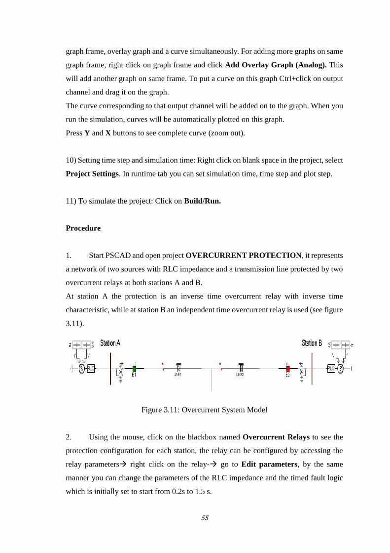
TRANSCRIPT
Registration Number:..…../2018
People’s Democratic Republic of AlgeriaMinistry of Higher Education and Scientific Research
University M’Hamed BOUGARA – Boumerdes
Institute of Electrical and Electronic Engineering
Department of Power and Control
Final Year Project Report Presented in Partial Fulfilment ofthe Requirements for the Degree of
MASTER
In Power Engineering
Option: Power Engineering
Title:
Presented by:
Adel ADROUCHE
Supervisor:
Pr. Hamid BENTARZI
Protective Relaying System forEducation

1

2
Abstract
A rapidly growing in power industry requires more reliable operation of power supply
that increases complexity of power systems. For attaining this aim new communication
solutions and an increased focus on protection may be needed. The power engineering
department at IGEE has proposed advanced power systems initiatives to better prepare
its students for the power industry field. One of these initiatives is the development of a
new laboratory curriculum that uses digital relays to reinforce the fundamental concepts
of power system protection. The simple relay protection lab planned at IGEE should
include a test bench with distance, over-current and differential relays, and a relay tester
that may be used for applying simulated waveforms to the relays.
This project proposes a laboratory protection system fulfilling this task. It presents
background on power system protection, modern relay technology, and relay testing, to
support the design and practical setup of the protective relaying system.
The report includes a theoretical part describing the components of power system
protection, their function, and attributes in order to understand better the importance of
power system protection. Three chapters covering the principles of protective relaying
functions relevant to the lab are included. They cover the theory of overcurrent,
differential and distance protection.
Modeling and simulation can help students to better understand how a relay reacts
during a fault or other non-fault disturbances. New design models of overcurrent and
differential relay have been implemented in PC using power system simulator PSCAD.
Proposals of lab assignments that can be performed in the protective relaying
laboratory are presented at the end, using the designed models and the protective
equipment available at the institute and donated for the purpose of this work.

3
Dedication
I dedicate this modest work
To my idolized Mother, my treasured Father
To my precious Sisters, Uncles, Aunts and Cousins
To every teacher who added something in me from childhood to this day
And to all those who offered me memorable moments

4
Acknowledgements
The completion of this work could not have been possible without the participation and
assistance of so many people whose names may not all be enumerated. Their
contributions are sincerely appreciated and gratefully acknowledged.
However, I would like to express appreciation and indebtedness particularly to the
following:
IGEE professor Hamid BENTARZI, project supervisor. I am very grateful to him for
encouraging me to take on this project. I owe him a very important debt for offering the
necessary background and knowledge I needed
Dr. BENTARZI’s continual encouragement and support made this project a joy to
work on.
IGEE professor Mohamed BOUCHAHDANE donated the equipment necessary for
achieving this work. I am deeply grateful for his support, patience, and motivation.
Thanks to his generosity, guidance and persistent help this work has been accomplished
in time. And without forgetting the power system protection courses taught by him that
helped me a lot in this project.
I would like also to show my greatest appreciation to the expert Mr. ABBACI
Mohamed for his support and contribution during time of need and for providing me with
all the information i needed, without his passionate participation, the results of this thesis
could not have been successfully conducted.
To all relatives, parents, family and others who in one way or another shared my
support, either morally, financially and physically. Thank you
5
Table of Contents
Abstract.............................................................................................................................2List of Tables....................................................................................................................7List of Figures...................................................................................................................8List of Abbreviation and Acronyms ...............................................................................10
Introduction ..................................................................................................................11
Chapter 1: Protection Student Laboratory................................................................121.1 Customer Needs Assessment....................................................................................121.2 Protective System ............................................................................................121.3 Protection Requirements..................................................................................131.4 Protection Equipment ......................................................................................13
1.4.1 Current and Voltage Transformers...............................................................141.4.2 Relays ...........................................................................................................141.4.3 Circuit Breakers ...........................................................................................141.4.4 Fuses.............................................................................................................151.4.5 Reclosers ......................................................................................................151.5 Protective Relays..........................................................................................15
1.5.1 Numerical Relay ..............................................................................................161.6 Conclusion .......................................................................................................17
Chapter 2: Protection Equipment Overview .............................................................182.1 Protection Equipment Introduction ..........................................................................182.2 SEL-221F Numerical Relay .....................................................................................182.3 The Universal Relay Test Set and Commissioning Tool CMC356 .........................192.4 Experiment 3....................................................................................................22
Chapter 03: Phase Overcurrent Protection ...............................................................233.1 Overcurrent Protection Overview....................................................................23
3.1.1 Instantaneous:...............................................................................................243.1.2 Definite Time Protection..............................................................................253.1.3 Inverse Definite Minimum Time (IDMT)....................................................263.1.4 Normal Inverse.............................................................................................273.1.5 Very Inverse .................................................................................................273.1.6 Extremely Inverse ........................................................................................273.1.7 Long Time Inverse .......................................................................................28
3.2 Application of Over Current Relay..................................................................283.3 Overcurrent Protection Model .........................................................................29
3.3.1 PSCAD.........................................................................................................293.4 Proposed Protection Model and Tools Required .........................................31
3.5 Laboratory Experiment 1 .................................................................................35
Chapter 4: Differential Protection ..............................................................................364.1 Differential Protection Overview.....................................................................36
6
4.1.1 Balanced Circulating Current System..........................................................364.2 Transformer Differential Protection (ANSI code 87 T) ..................................38
4.2.1 Differential Protection Scheme in A Power Transformer............................394.3 Transformer Differential Protection Model In PSCAD...................................41
4.3.1 Dual Slope Current Differential Relays .......................................................414.3.2 Front Panel Block Construction ...................................................................42
4.4 Laboratory Experiment 2: ................................................................................43
Chapter 5: Distance Protection ...................................................................................445.1 Introduction: .............................................................................................................445.2 Application of Distance Protection Relay .......................................................455.3 Principles of Distance Relays ..........................................................................455.4 Mho Distance Protection Overview.................................................................465.4.1 Zone 1 Protection.............................................................................................47
5.4.2 Zone 2 Protection .........................................................................................485.4.3 Zone 3 Protection .........................................................................................48
5.5 Laboratory Experiment 5 .................................................................................49
Conclusion .....................................................................................................................50References .....................................................................................................................51Appendices ....................................................................................................................53Appendix A: Experiment 1 ..........................................................................................53Appendix B: Experiment 2 ..........................................................................................61Appendix C: Experiment 3 ..........................................................................................68Appendix D: Experiment 4 ..........................................................................................77Appendix E: Experiment 5 ..........................................................................................90Appendix F ...................................................................................................................103
7
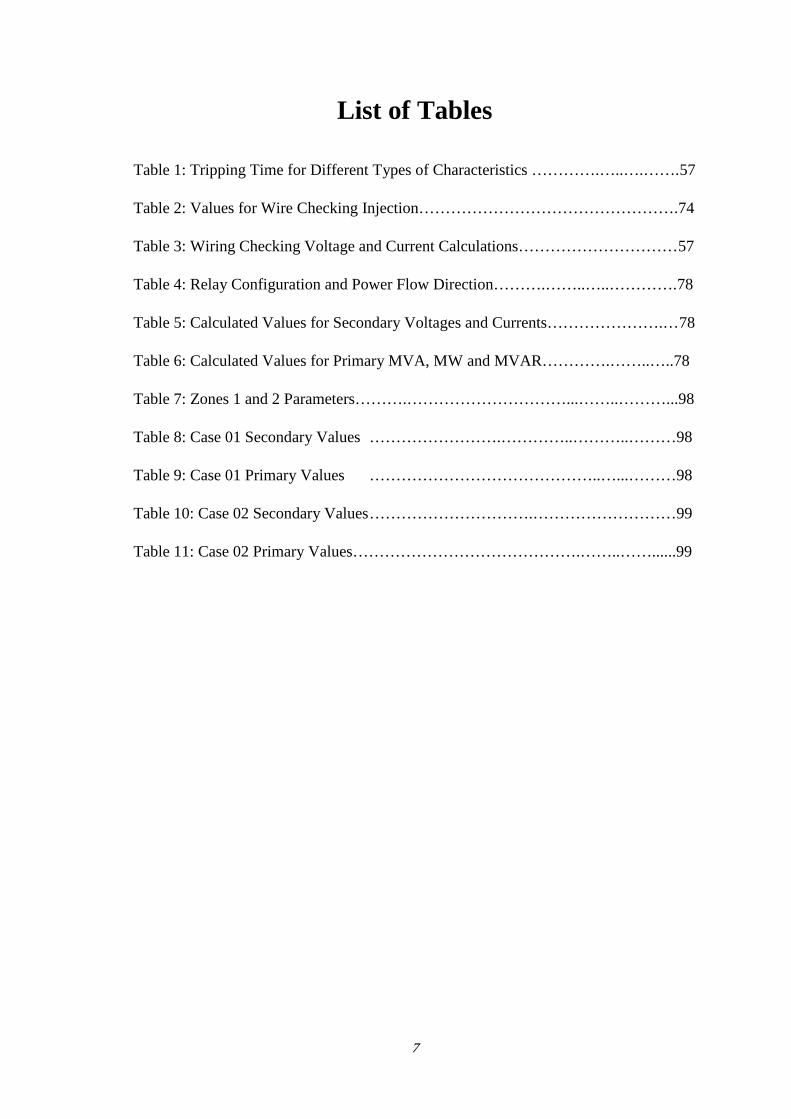
List of Tables
Table 1: Tripping Time for Different Types of Characteristics ………….…..….…….57
Table 2: Values for Wire Checking Injection………………………………………….74
Table 3: Wiring Checking Voltage and Current Calculations…………………………57
Table 4: Relay Configuration and Power Flow Direction……….……..…..………….78
Table 5: Calculated Values for Secondary Voltages and Currents………………….…78
Table 6: Calculated Values for Primary MVA, MW and MVAR………….……..…..78
Table 7: Zones 1 and 2 Parameters……….…………………………...……..………...98
Table 8: Case 01 Secondary Values …………………….…………..………..………98
Table 9: Case 01 Primary Values ……………………………………..…...………98
Table 10: Case 02 Secondary Values………………………….………………………99
Table 11: Case 02 Primary Values…………………………………….……..……......99
8
List of Figures
Figure 1.1: High Voltage Circuit Breaker from Siemens…………………….………..15Figure 1.2: SEL-T400L Numerical Relay…………………………………….……….16Figure 2.1: SEL-221F Numerical Distance Relay……………………….…….………19Figure 2.2: Front View of CMC356………………….…………………….……….…20Figure 2.3: Rear View of CMC356…………………….…………..………………….20Figure 2.4: SEL 221 Relay and Omicron CMC 356 Put Together in IGEE Lab……...21Figure 3.1: Time Versus Current Curve of Instantaneous Overcurrent Relay……..….24Figure 3.2: Independent Time Delay….…….…………………………………………25Figure 3.3: Times Versus Current Curve for IDMT Overcurrent Relay….………..….26Figure 3.4: IEC 60255 Characteristics of IDMT Relay…………….…………….……28Figure 3.5: The General Block Diagram of The Proposed Protection Scheme……..…31Figure 3.6: FFT Block…………………………………………………………………32Figure 3.7: Signal Sampling Block Diagram…………………………………………..32Figure 3.8: Overcurrent Relay Models………………..……………………………….33Figure 3.9: Conditioning and Relays Circuit Blackbox Diagram…………………..….33Figure 3.10: Overcurrent Protection Front Panel………………………………………34Figure 4.1: Block Diagram of Differential Protection…………………………………36Figure 4.2: Balanced Circulating Current System, External Fault (Stable)…………....37Figure 4.3: Balanced Circulating Current System, Internal Fault (Operate)…………..37Figure 4.4: Transformer Differential Protection Block Diagram…….……..…………38Figure 4.5: Schematic Diagram Of Differential Protection Scheme.………..….……..40Figure 4.6: Transformer Differential Protection Tripping Curve………………...……40Figure 4.7: Current Differential Relays Blocks……………….………….……………41Figure 4.8: Differential Protection Signal Processing Blackbox Diagram.…………....42Figure 4.9: Transformer Differential Protection System Model……………..………..42Figure 5.1: Typical Mho Distance Characteristic ..……………...…………………….46Figure 5.2: Zone 1 Mho Characteristic……….………………………………………..48Figure 5.3: Three-Zone MHO Characteristics……….………..……………………….49Figure 3.11: Overcurrent System Model ………………………………….…………..55Figure 3.12: Inverse Time Relay Parameters Window……..……………….…..……..56Figure 3.13: Independent Time Relay Parameters Window………………….…...…...56Figure 3.14: Phase Fault A-G Selection Window……………..………….……..……..57Figure 3.15: Moderately Inverse Characteristic Simulation Graphs…………………..58Figure 3.16: Standard Inverse Characteristic Simulation Graphs.………….…...……..58Figure 3.17: Very Inverse Characteristic Simulation Graphs …………..………59Figure 3.18: Extremely Inverse Characteristic Simulation Graphs…………………....59Figure 3.19: Long Time Backup Characteristic Simulation Graphs…………….….….60Figure 4.10: FFT Block In PSCAD …….……………………………………………..62Figure 4.11: Dual Slope Differential Relay in PSCAD And the Characteristic………62Figure 4.12: System Model……………………….……………………..……………..62Figure 4.13: Differential Relay Parameters Setting………….………….……………..64Figure 4.14: Phase Fault A-G Selection Window……………………………….……..65Figure 4.15: Internal Phase Fault A-G Simulation Result………………………..……65Figure 4.16: External Fault Transformer Protection System Model…….……….….…66Figure 4.17: External Phase Fault A-G Simulation Results……………….…………..67Figure 4.18: Internal and External Fault Comparison………………....….…………...67
9
Figure 2.5: Injection Test Set OMICRON CMC 356……………………………...…..70Figure 2.6: Quickset Main Window…………………….……………………………..71Figure 2.7: CMC 356 Communication Setup Window……………………………......72Figure 2.8: Front View of CMC 356 With Voltage and Current Outputs Connected...72Figure 2.9: Rear View of SEL 221F Relay with Voltage And Currents Inputs….…...73Figure 2.10: The Experimental Setup for Experiment 1………..…………….….…….73Figure 2.11: Test Execution Window…………………………………………….……74Figure 2.12: Communications Window…………………………….…..……….……..75Figure 2.13: Meter Command Report Window……………….……………..….……..76Figure 2.14: SEL 221 Settings Editor………………………………………………….80Figure 2.15: Send Modified Settings to SEL 221……………………………….….….80Figure 2.16: Communication Window……….……………….…..…….……….…….81Figure 2.17: Case 01 Values Injection Execution……………………………..………82Figure 2.18: Case 01 Meter Values……………………..…………………...….……..83Figure 2.19: Case 02 Values Injection Execution……………………………….…….84Figure 2.20: Case 02 Meter Values……………………………….……..……...……..85Figure 2.21: Case 03 Values Injection Execution……………………………….…….86Figure 2.22: Case 03 Meter Values……………………………………………………87Figure 2.23: Case 03 Values Injection Execution…………………………….….……88Figure 2.24: Case 04 Meter Values……………………………….……..…………….89Figure 5.4: Algiers Boumerdes Single Line Network Diagram……………………….90Figure 5.5: Experimental Setup of Experiment 5……………………………...………93Figure 5.6: Device Part Number Inserting………….………………….………………94Figure 5.7: Setting Line Parameters And Zones Reach………………………………..94Figure 5.8: Setting Zones Time Delays in Cycles…………………...………………...95Figure 5.9: QuickCMC Test Object Window………………….………………….…...96Figure 5.10: Voltage Levels Set on QuickCMC…………………………………….....96Figure 5.11: Distance Protection Parameters Set on Quick CMC……………..………97Figure 5.12: Case 1 Injections Window……………………….……………...………..99Figure 5.13: SEL 221 Tripping In Zone 1………………………………………..…..100Figure 5.14: Resetting the Relay…………………………….……….……………….100Figure 5.15: Case 2 Injections Window……………………….………….……….….101Figure 5.16: SEL 221 Tripping in Zone 1 for Case 02 Fault……………….….……..101
10
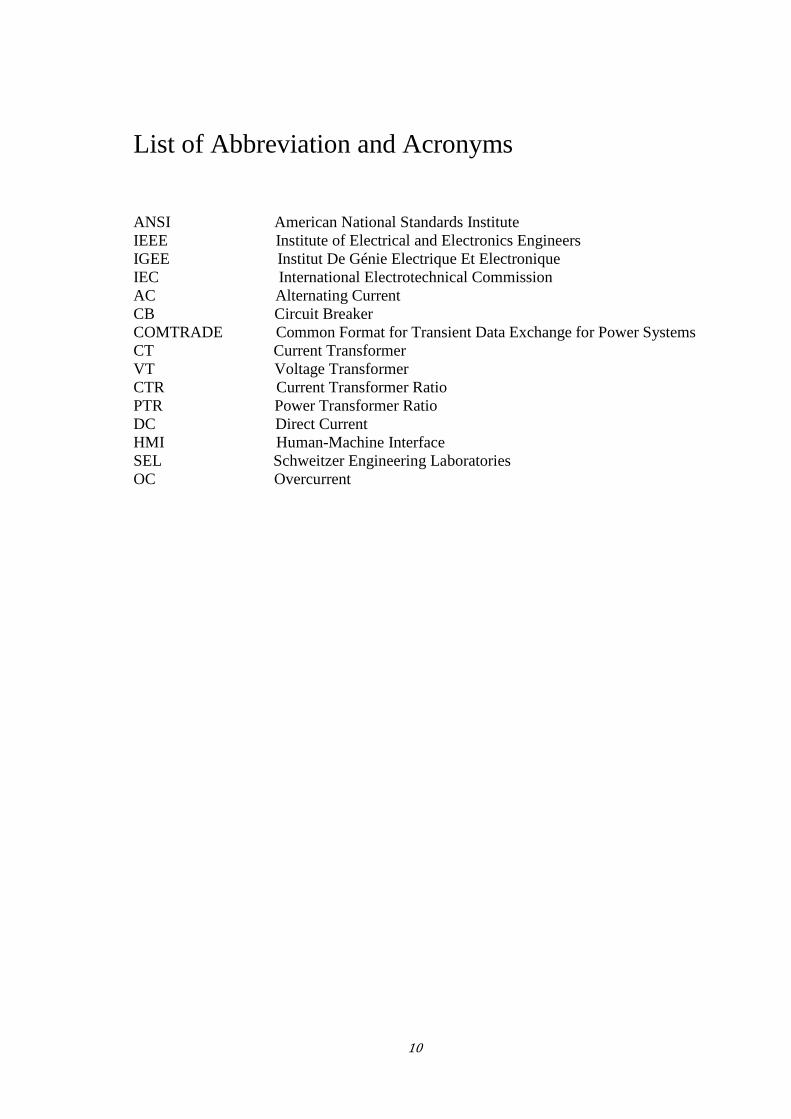
List of Abbreviation and Acronyms
ANSI American National Standards InstituteIEEE Institute of Electrical and Electronics EngineersIGEE Institut De Génie Electrique Et ElectroniqueIEC International Electrotechnical CommissionAC Alternating CurrentCB Circuit BreakerCOMTRADE Common Format for Transient Data Exchange for Power SystemsCT Current TransformerVT Voltage TransformerCTR Current Transformer RatioPTR Power Transformer RatioDC Direct CurrentHMI Human-Machine InterfaceSEL Schweitzer Engineering LaboratoriesOC Overcurrent
11
Introduction
Protective relays are becoming more advanced to keep up with more complex and
integrated power systems. The future of power systems is smart grids, meaning more
complex designs, with distributed generation, smart meters and continuous surveillance
to ensure optimal operation and power flow at every instant.
The electrical engineers of the future should be educated with this in mind. To
enlighten today’s and future students about protective relaying, a solid theoretical
background part is a fundamental first step. To complement the theory and to better the
understanding of the topic, a practical component, to understand how power system
protection works in real life, is vital. A protective relay lab can be the foundation of
such a practical, hands-on component.
Motivated by the growing demand from the power industry for engineering graduates
versed in power systems, as well as a need to provide continuing education opportunities
for power engineering students, the Institute of Electrical Engineering and Electronics at
Boumerdes University has for a future aim the redesign of its electrical engineering
power systems emphasis programs at both the BS and MS levels. The educational goals
of the lab are to provide students with hands-on experience with industry protection
equipment and software, enhance the classroom-based course curriculum, and acquaint
students with industry standards and design practices.
This project is to propose laboratory-scale microprocessor-based relay experiments
for students, illustrating the principles of real-time fault protection in radial and
bidirectional networks. Student learning outcomes include: applying the fundamental
principles of power system protection to detect faults in transformers and transmission
lines; comparing experimentally-derived results with expected theoretical circuit
performance through post-fault data analysis; developing experience in wiring common
circuit connections; understanding the relationship between a relay and a circuit breaker
in detecting and clearing faults. This work also lays a foundation for the future
development of a microgrid lab in the IGEE power engineering department.
12
Chapter 1: Protection Student Laboratory
1.1 Customer Needs Assessment
This project directly serves IGEE electrical engineering power students. It arose from the
expressed desire of power engineering department to introduce a power systems
protection teaching laboratory for graduate power engineering education utilizing
protective relaying equipment.
IGEE currently offers a graduate level power systems protection lecture course,
EE535 Instrumentation and Protection Systems, to which this project adds an
accompanying laboratory component. Curriculum resulting from this project should give
students hands-on experience applying the fundamentals of power system protection
through microprocessor-based relays. The following section describes the high-level
functionality of the proposed student laboratory experiments.
Power system protection rests at the heart of this project. Reference [9] defines the
protection as “the science, skill, and art of applying and setting relays or fuses, or both,
to provide maximum sensitivity to faults and undesirable conditions, but to avoid their
operation under all permissible or tolerable conditions”.
The stability of power system was and is still a major concern for electrical engineers,
each day; they try to design an ideal power system so it can face the different disturbances
that may affect its performances. But, no matter how well designed, faults will always
occur and these faults may represent a serious risk to both equipments and personnel.
Protective systems were developed so that the power system could operate in a safe
manner at all times.
1.2 Protective System
Protection System is a full arrangement of protective equipment and other devices that
are required to achieve a specified function based on a protection principle. Its main
function is to protect the whole electrical power system (generators, transformers,
13
reactors, lines…) from abnormal conditions such as short circuits, overloads and also
equipment failures. This is made by isolating the faulty section from the remaining living
system parts [1].
1.3 Protection Requirements
The protection scheme established for this system must recognize to eliminate fault
conditions but never interrupt normal circuit operation. This balance in discriminating
normal load from fault conditions requires considering the impacts to the system caused
by single-line-to-ground, double-line-to-ground, triple-line-to-ground, three-phase, and
line-to-line bolted faults. All relays used to detect these faults require coordination so
that a relay closer to a fault operates before any of the relays further upstream from the
fault location. In order to carry out its duties, protection must have the following qualities:
Selectivity: To detect and isolate the faulty part only.
Stability: To leave all healthy circuits intact to ensure continuity of the supply.
Sensitivity: To detect even the lowest fault, current or system abnormalities, and
to operate correctly before the fault causes irreparable damage.
Speed: To operate speedily when it is called upon to do so, thereby minimizing
damage to the surroundings and ensuring safety to equipment as well as to personnel.
To meet all of the above requirements, protection must be reliable which means it
must be:
Dependable: It must trip when called upon to do so.
Secure: It must not trip when it is not supposed to do [2].
1.4 Protection Equipment
Protection systems consist of components called protection devices. They are installed
and connected together with the aims of assets protection, and insurance of continued
supply of energy. In any protection system, six essential elements are distinguished.
14
1.4.1 Current and Voltage Transformers
Current and voltage transformers are continuously used to measure current and voltage
signals of the electrical system even under fault conditions. They step these signals down
to lower and safe levels so that the relay and other instruments hardware can support
them. Besides, they also isolate the relaying system from the primary high voltage system
and provide safety to both human being and equipment. The CTs available in the industry
can lower the current up to 5 A or 1A, while the voltage transformers lower the voltage
to 110V.
1.4.2 Relays
The measured values are converted into analog and/or digital signals and are made to
operate the relay. In most of the cases, the relays provide two functions, alarm and trip.
They give instructions to open the circuit surrounding the faulty part of the network under
faulty conditions. Relays perform also automatic operations, such as auto-reclosing and
system restart. Besides, they monitor the equipment which collects the system data for
post-event analysis.
1.4.3 Circuit Breakers
The opening of faulty circuits requires some time (in milliseconds), which for a common
day life could be insignificant. However, the circuit breakers used to isolate the faulty
circuits, are capable of carrying these fault currents until the fault is totally cleared [2].
They are expected to be switched ON with loads and capable of breaking a live circuit
under normal switching and fault conditions. The process is realized through the
instructions given by the monitoring devices like relays.
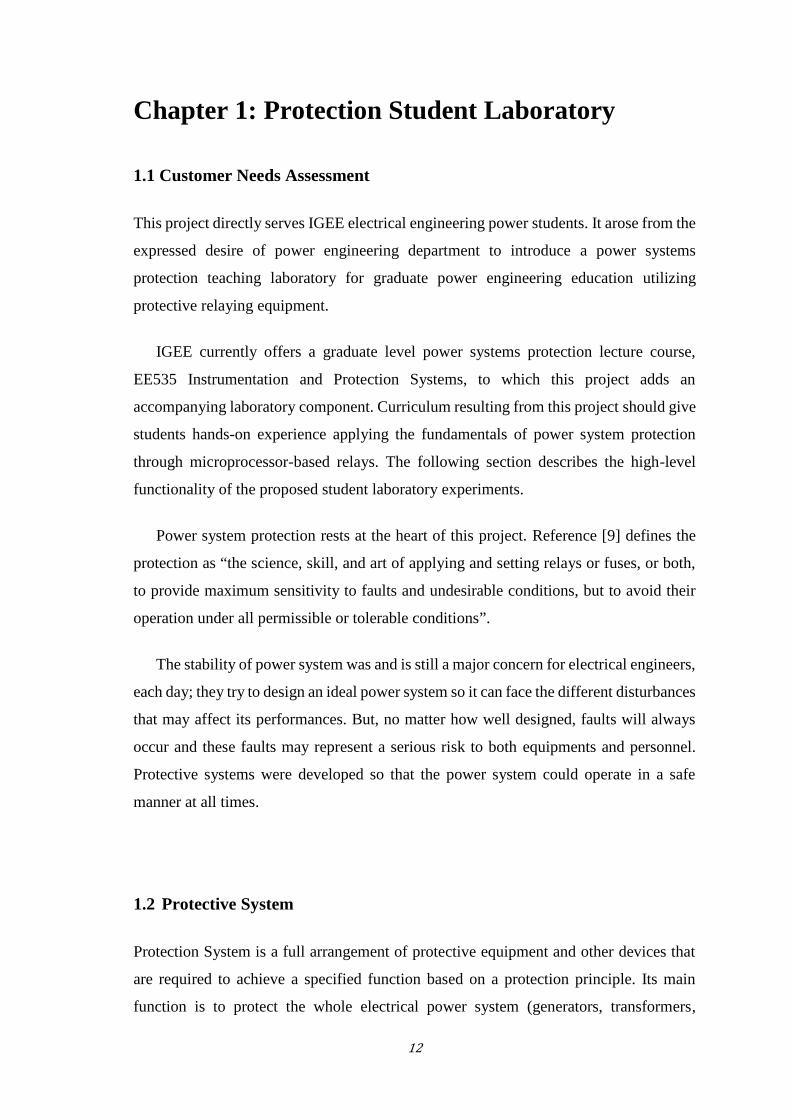
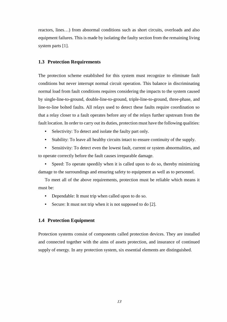
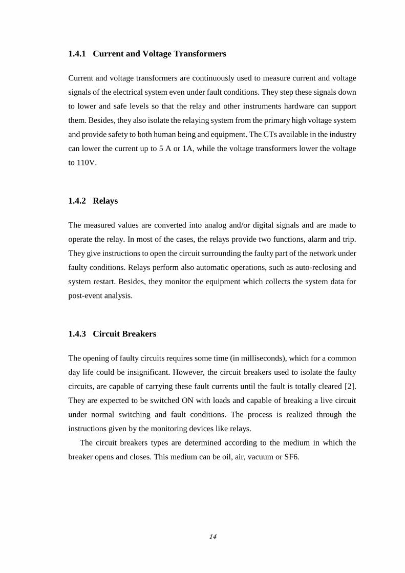
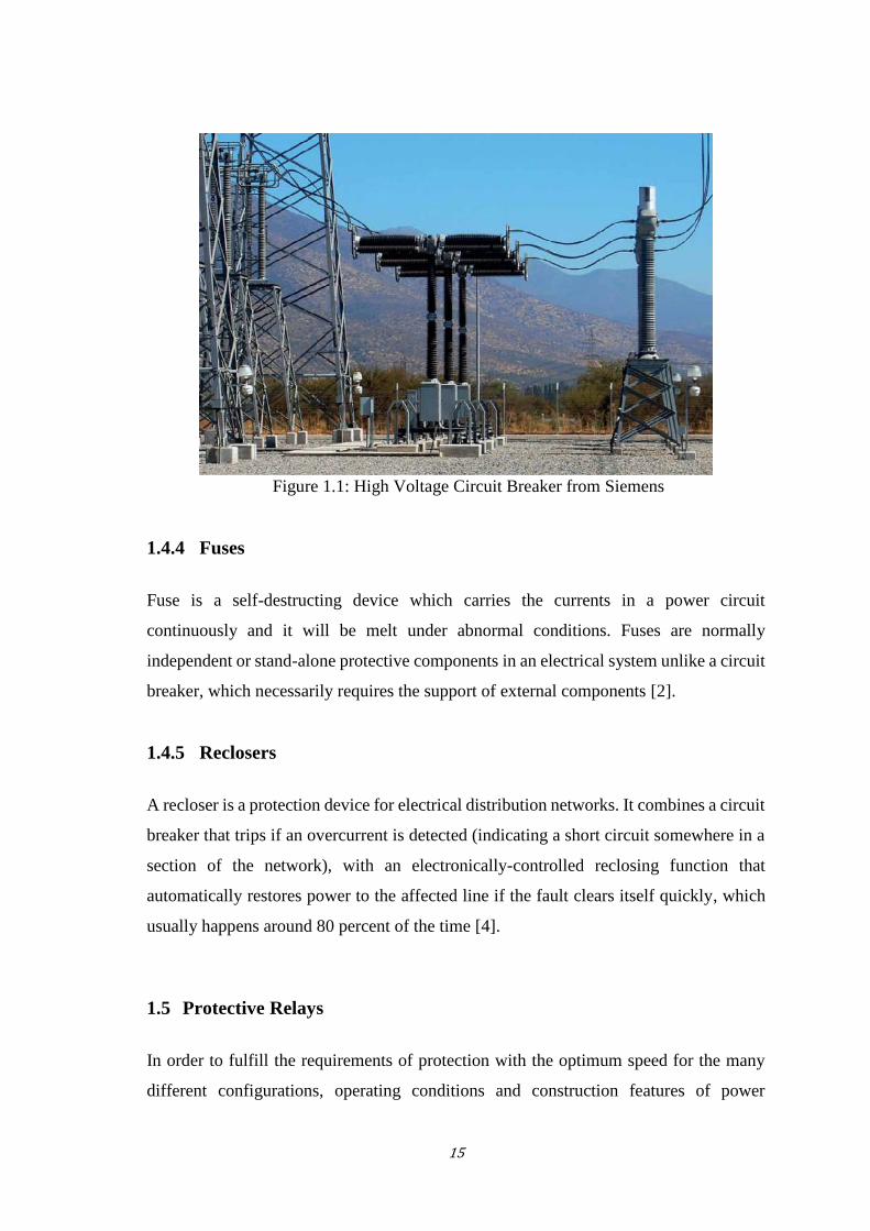
The circuit breakers types are determined according to the medium in which the
breaker opens and closes. This medium can be oil, air, vacuum or SF6.
15
Figure 1.1: High Voltage Circuit Breaker from Siemens
1.4.4 Fuses
Fuse is a self-destructing device which carries the currents in a power circuit
continuously and it will be melt under abnormal conditions. Fuses are normally
independent or stand-alone protective components in an electrical system unlike a circuit
breaker, which necessarily requires the support of external components [2].
1.4.5 Reclosers
A recloser is a protection device for electrical distribution networks. It combines a circuit
breaker that trips if an overcurrent is detected (indicating a short circuit somewhere in a
section of the network), with an electronically-controlled reclosing function that
automatically restores power to the affected line if the fault clears itself quickly, which
usually happens around 80 percent of the time [4].
1.5 Protective Relays
In order to fulfill the requirements of protection with the optimum speed for the many
different configurations, operating conditions and construction features of power
16
systems, it has been necessary to develop many types of relay that respond to various
functions of the power system quantities. For example, simple observation of the fault
current magnitude may be sufficient in some cases but measurement of power or
impedance may be necessary for others. Relays frequently measure complex functions
of the system quantities, which may only be readily expressible by mathematical or
graphical means.
Relays may be classified according to the technology used:
Electromechanical
Static
Digital
Numerical
The different types have varying capabilities, according to the limitations of the
technology used.
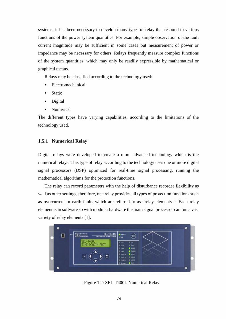
1.5.1 Numerical Relay
Digital relays were developed to create a more advanced technology which is the
numerical relays. This type of relay according to the technology uses one or more digital
signal processors (DSP) optimized for real-time signal processing, running the
mathematical algorithms for the protection functions.
The relay can record parameters with the help of disturbance recorder flexibility as
well as other settings, therefore, one relay provides all types of protection functions such
as overcurrent or earth faults which are referred to as “relay elements “. Each relay
element is in software so with modular hardware the main signal processor can run a vast
variety of relay elements [1].
Figure 1.2: SEL-T400L Numerical Relay

17
1.6 Conclusion
This chapter gives the reader a brief introduction to the protection system and its elements
including the importance of using numerical relays regarding their efficiency in
providing the protection requirements from selectivity, speed, sensitivity and so on,
which makes them the most appropriate relays for protecting human life and expensive
devices.

18
Chapter 2: Protection Equipment Overview
2.1 Protection Equipment Introduction
This project deals with the proposal of a new laboratory curriculum. This chapter
introduces the various devices that comprise the protection scheme throughout the
various project phases. Information on protection device capabilities and characteristics
have been obtained from the company’s product literature.
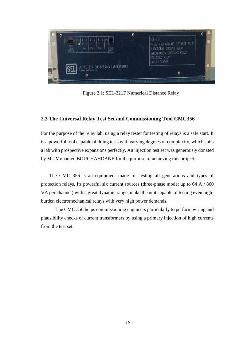
2.2 SEL-221F Numerical Relay
The SEL-221F Relay is a phase and ground distance relay with directional ground,
synchronism checking, reclosing and fault locator elements.
It is designed to protect transmission, sub-transmission and distribution lines for all
fault types. The following list outlines protective features, performance, and versatility
gained when applying this relay to the electrical installations:
• Three zones of phase and ground distance protection.
• A residual time-overcurrent element with selectable curves.
• Instantaneous residual overcurrent element.
• A negative-sequence polarization of ground directional elements.
• A versatile user-programmable logic for outputs and tripping.
• Programmable switch-onto-fault logic.
• Loss-of-potential detection logic.
• Programmable single-shot reclosing with synchronism check and voltage checking.
• Fault locating.
• Metering.
• EIA-232 serial communications ports for local and remote access.
• Automatic self-testing.
• Target indicators for faults and testing [14].
19
Figure 2.1: SEL-221F Numerical Distance Relay
2.3 The Universal Relay Test Set and Commissioning Tool CMC356
For the purpose of the relay lab, using a relay tester for testing of relays is a safe start. It
is a powerful tool capable of doing tests with varying degrees of complexity, which suits
a lab with prospective expansions perfectly. An injection test set was generously donated
by Mr. Mohamed BOUCHAHDANE for the purpose of achieving this project.
The CMC 356 is an equipment made for testing all generations and types of
protection relays. Its powerful six current sources (three-phase mode: up to 64 A / 860
VA per channel) with a great dynamic range, make the unit capable of testing even high-
burden electromechanical relays with very high power demands.
The CMC 356 helps commissioning engineers particularly to perform wiring and
plausibility checks of current transformers by using a primary injection of high currents
from the test set.
20
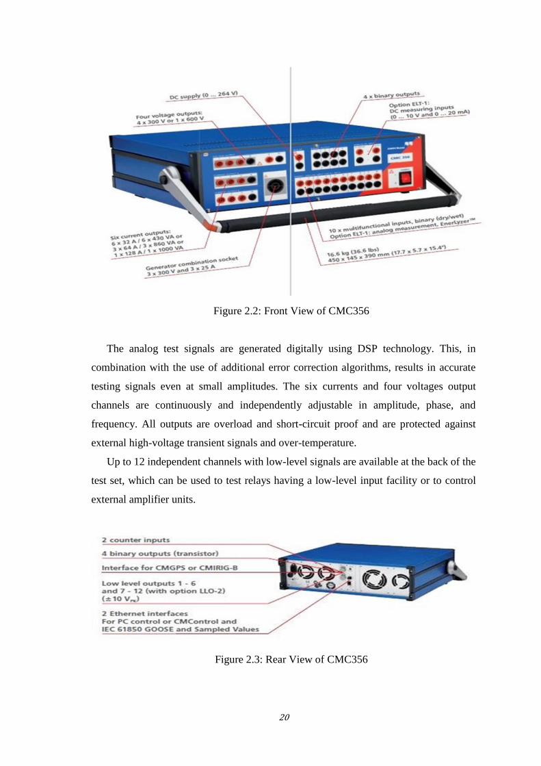
Figure 2.2: Front View of CMC356
The analog test signals are generated digitally using DSP technology. This, in
combination with the use of additional error correction algorithms, results in accurate
testing signals even at small amplitudes. The six currents and four voltages output
channels are continuously and independently adjustable in amplitude, phase, and
frequency. All outputs are overload and short-circuit proof and are protected against
external high-voltage transient signals and over-temperature.
Up to 12 independent channels with low-level signals are available at the back of the
test set, which can be used to test relays having a low-level input facility or to control
external amplifier units.
Figure 2.3: Rear View of CMC356
21
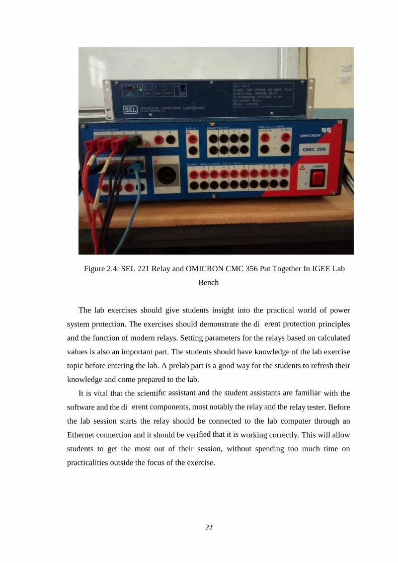
Figure 2.4: SEL 221 Relay and OMICRON CMC 356 Put Together In IGEE Lab
Bench
The lab exercises should give students insight into the practical world of power
system protection. The exercises should demonstrate the different protection principles
and the function of modern relays. Setting parameters for the relays based on calculated
values is also an important part. The students should have knowledge of the lab exercise
topic before entering the lab. A prelab part is a good way for the students to refresh their
knowledge and come prepared to the lab.
It is vital that the scientific assistant and the student assistants are familiar with the
software and the different components, most notably the relay and the relay tester. Before
the lab session starts the relay should be connected to the lab computer through an
Ethernet connection and it should be verified that it is working correctly. This will allow
students to get the most out of their session, without spending too much time on
practicalities outside the focus of the exercise.
22
2.4 Experiment 3
SEL-211F Basic Connections and Wiring Check Procedure
This exercise Introduces these equipments to students in a laboratory environment, it has
the aim of getting familiar with the SEL 221 relay and the OMICRON test set, this
experiment is an exercise of establishing wiring connection and software communication.
In the lab exercises, the students face a practical challenge; they are handed a relay, with
no cables connected, and have to use the manual and follow the procedure to figure how
to connect inputs and outputs. The lab manual guides its performer toward a safe and
correct wiring, at the same time, learning how to use the TestUniverse and AcSELerator
Quickset software, how to inject correct values and record the relay's results.
2.5 Experiments 4
SEL-211 Relay Configuration and Metering Check Procedure
Lab exercise 4 provides the students with insight on how to configure the relay, change
and set parameters relevant to the relay with a metering check procedure that resumes a
deeper understanding of the power flow in a power system. Experiments 3 and 4 are
shown in appendices C and D respectively.
When designing a university relay lab, it might be a good idea to build the lab
gradually, a strategic co-operation with Siemens Algeria and Schweitzer Engineering
Laboratories is under establishment for the donation of new relays for the benefit of IGEE
students, However, for the time being, the only available relay is a distance relay, a
protection laboratory should include the basic protection functions; overcurrent, distance
and differential protection; to cover this and replace the present lack of materials, a
desirable good start is to experiment with simulation models proposed and described in
the coming chapters.
23
Chapter 03: Phase Overcurrent Protection
As mentioned earlier, building the lab gradually is desirable. It is therefore important to
have a vision for the future expansions and use of the lab. The final outlook for the relay
lab may change as it develops. For the present being, in order to understand the functions
of relays, for a student of electrical protection, software relay models must be realized,
modeling of protective relays offer an economic and feasible alternative to studying the
performance of protective relays. This chapter introduces a new software model for
overcurrent protection to be introduced as the first experiment in protection laboratory.
3.1 Overcurrent Protection Overview
The function of this protection is to detect single-phase, two-phase or three-phase
overcurrents. Protection is activated when one, two or three of the currents concerned
rise above the specified setting threshold.
The overcurrent relay uses current inputs from a current transformer and compares
the measured values with the pre-set values. If the input current value exceeds the preset
value, the relay detects an overcurrent and issues a trip signal to the breaker which opens
its contact to disconnect the protected equipment.
When the relay detects a fault, the condition is called fault pickup. The relay can send
a trip signal instantaneously after picking up the fault in the case of instantaneous
overcurrent relays or it can wait for a specific time before issuing a trip signal in the case
of time overcurrent relays. This time delay is also known as the operation time of the
relay and is computed by the relay on the basis of the protection algorithm incorporated
in the microprocessor [7].
This protection can be time delayed and, in this case, will only be activated if the
current monitored rises above the setting threshold for a period of time at least equal to
the time delay selected. This delay can be an instantaneous, independent (definite) time
or inverse time delay.
24
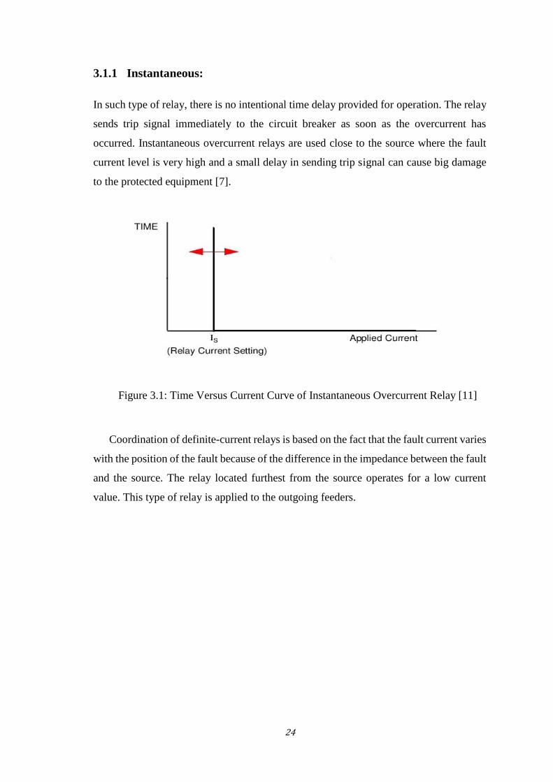
3.1.1 Instantaneous:
In such type of relay, there is no intentional time delay provided for operation. The relay
sends trip signal immediately to the circuit breaker as soon as the overcurrent has
occurred. Instantaneous overcurrent relays are used close to the source where the fault
current level is very high and a small delay in sending trip signal can cause big damage
to the protected equipment [7].
Figure 3.1: Time Versus Current Curve of Instantaneous Overcurrent Relay [11]
Coordination of definite-current relays is based on the fact that the fault current varies
with the position of the fault because of the difference in the impedance between the fault
and the source. The relay located furthest from the source operates for a low current
value. This type of relay is applied to the outgoing feeders.
25
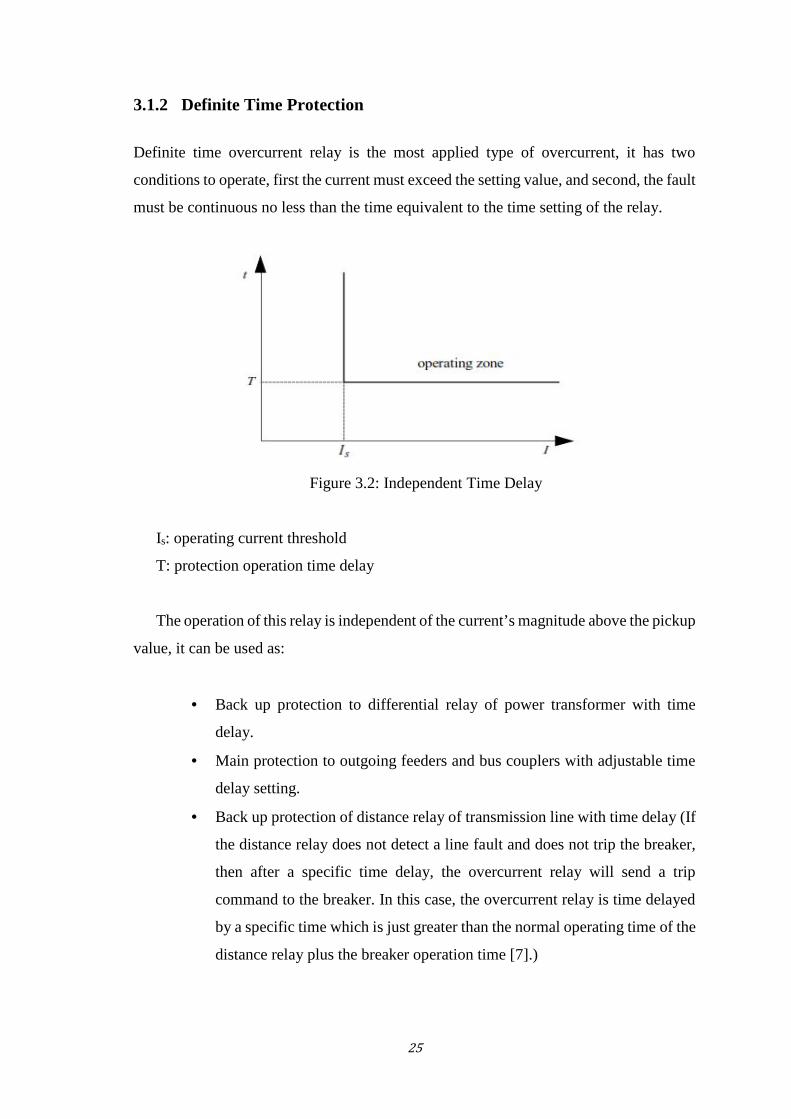
3.1.2 Definite Time Protection
Definite time overcurrent relay is the most applied type of overcurrent, it has two
conditions to operate, first the current must exceed the setting value, and second, the fault
must be continuous no less than the time equivalent to the time setting of the relay.
Figure 3.2: Independent Time Delay
Is: operating current threshold
T: protection operation time delay
The operation of this relay is independent of the current’s magnitude above the pickup
value, it can be used as:
Back up protection to differential relay of power transformer with time
delay.
Main protection to outgoing feeders and bus couplers with adjustable time
delay setting.
Back up protection of distance relay of transmission line with time delay (If
the distance relay does not detect a line fault and does not trip the breaker,
then after a specific time delay, the overcurrent relay will send a trip
command to the breaker. In this case, the overcurrent relay is time delayed
by a specific time which is just greater than the normal operating time of the
distance relay plus the breaker operation time [7].)
26
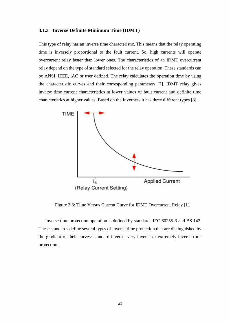
3.1.3 Inverse Definite Minimum Time (IDMT)
This type of relay has an inverse time characteristic. This means that the relay operating
time is inversely proportional to the fault current. So, high currents will operate
overcurrent relay faster than lower ones. The characteristics of an IDMT overcurrent
relay depend on the type of standard selected for the relay operation. These standards can
be ANSI, IEEE, lAC or user defined. The relay calculates the operation time by using
the characteristic curves and their corresponding parameters [7]. IDMT relay gives
inverse time current characteristics at lower values of fault current and definite time
characteristics at higher values. Based on the Inverness it has three different types [8].
Figure 3.3: Time Versus Current Curve for IDMT Overcurrent Relay [11]
Inverse time protection operation is defined by standards IEC 60255-3 and BS 142.
These standards define several types of inverse time protection that are distinguished by
the gradient of their curves: standard inverse, very inverse or extremely inverse time
protection.
27
3.1.4 Normal Inverse
This type is used when Fault Current is dependent on the generation of fault not fault
location and it has a relatively small change in time per unit of change of current. Its
operating time’s accuracy may range from 5 to 7.5% of the nominal operating time as
specified in the relevant norms. The uncertainty of the operating time and the necessary
operating time may require a grading margin of 0.4 to 0.5 seconds. Normal Inverse Time
Overcurrent Relay is used in utility and industrial circuits [8].
3.1.5 Very Inverse
Very inverse overcurrent relays are particularly suitable if there is a substantial reduction
of fault current as the distance from the power source increases, i.e. there is a substantial
increase in fault impedance. The grading margin may be reduced to a value in the range
from 0.3 to 0.4 seconds when they are used [8]. This type has more inverse characteristics
than that of IDMT. It can be used when the fault current is dependent on fault location.
3.1.6 Extremely Inverse
With this characteristic, the operation time is approximately inversely proportional to the
square of the applied current. This makes it suitable for the protection of distribution
feeder circuits in which the feeder is subjected to peak currents on switching in, as would
be the case on a power circuit supplying refrigerators, pumps, water heaters and so on,
which remain connected even after a prolonged interruption of supply. This type has
more inverse characteristics than that of IDMT and very inverse overcurrent relay [8]. It
is also used for the protection of alternators, transformers, expensive cables, the
protection of machines against overheating and when fault current is dependent on fault
location.
28
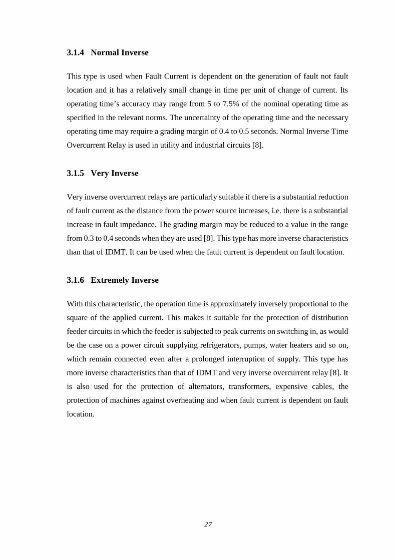
3.1.7 Long Time Inverse
The main application of long time overcurrent relays is as backup earth fault protection.
Figure 3.4: IEC 60255 Characteristics of IDMT Relay [1]
3.2 Application of Over Current Relay
Used against overloads and short circuits in stator windings of motors.
Used at power transformer locations for external fault back-up protection.
For ground backup protection on most lines having pilot relaying for primary
protection.
29
Distribution Protection: Overcurrent relaying is very well suited to distribution
system protection for the following reasons:
- It is basically simple and inexpensive.
- It is possible to use a set of two OC relays for protection against interphase faults
and a separate overcurrent relay for ground faults [8].
3.3 Overcurrent Protection Model
Relay models have been long used in a variety of tasks, such as designing new relaying
algorithms, optimizing relay settings. Electric power utilities use computer-based relay
models to confirm how the relay would perform during systems disturbances and normal
operating conditions and to make the necessary corrective adjustment on the relay
settings. It is seen, then, that for the better comprehension of a student to the overcurrent
relay, the implementation, simulation and testing is to be done on two steps, the first to
be a work on a model, the second is a hardware hands-on experiment.
The principles of operation and application procedures of overcurrent have been
presented above. The concept of a generalized numerical relay, whose structure is
constituted by the typical operational modules and functions of modern digital and
numerical relays, has been introduced.
For this purpose, an overcurrent protection design model is proposed in the coming
section. The proposed relay model and tools required are summarized into the flowchart
in figure 3.5. The design was performed on PSCAD software.
3.3.1 PSCAD
PSCAD (Power Systems Computer Aided Design) is a powerful and flexible graphical
user interface to the world-renowned, EMTDC (Electromagnetic Transient Simulation
Engine). PSCAD enables the user to schematically construct a circuit, run a simulation,
analyze the results, and manage the data in a completely integrated, graphical
environment. Online plotting functions, controls and meters are also included, enabling
the user to alter system parameters during a simulation run, and thereby view the effects
while the simulation is in progress.

30
Because this modeling is meant to be for laboratory learning purposes, PSCAD is the
appropriate tool for a simplified scheme for better and faster learning, this is due to the
fact that PSCAD comes complete with a library of pre-programmed and tested simulation
models, ranging from simple passive elements and control functions to more complex
models, such as electric machines and transmission lines and cables. If a required model
does not exist, PSCAD provides avenues for building custom models. For example,
custom models may be constructed by piecing together existing models to form a module,
or by constructing rudimentary models from scratch in a flexible design environment.
The following are some common models found in the PSCAD master library:
Resistors, inductors, capacitors.
Mutually coupled windings, such as transformers.
Frequency-dependent transmission lines and cables (including the most accurate
time-domain line model in the world).
Current and voltage sources.
Switches and breakers.
Protection and relaying.
Diodes, thyristors and GTOs.
Analog and digital control functions.
AC and DC machines, exciters, governors, stabilizers and inertial models.
Meters and measuring functions.
Generic DC and AC controls.
Wind source, turbines and governors.
31
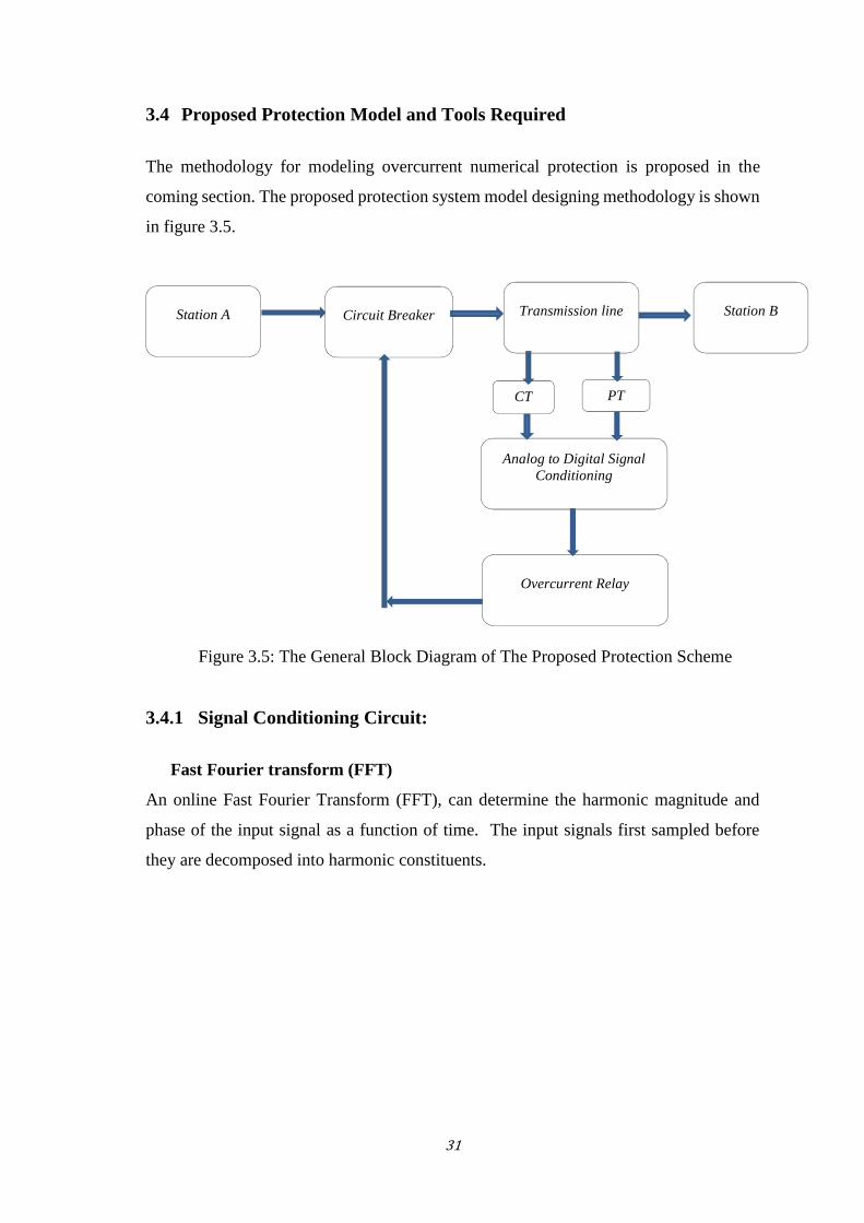
3.4 Proposed Protection Model and Tools Required
The methodology for modeling overcurrent numerical protection is proposed in the
coming section. The proposed protection system model designing methodology is shown
in figure 3.5.
Figure 3.5: The General Block Diagram of The Proposed Protection Scheme
3.4.1 Signal Conditioning Circuit:
Fast Fourier transform (FFT)
An online Fast Fourier Transform (FFT), can determine the harmonic magnitude and
phase of the input signal as a function of time. The input signals first sampled before
they are decomposed into harmonic constituents.
Station A Circuit Breaker Transmission line Station B
Overcurrent Relay
Analog to Digital SignalConditioning
CTsuppl
y
PT
32
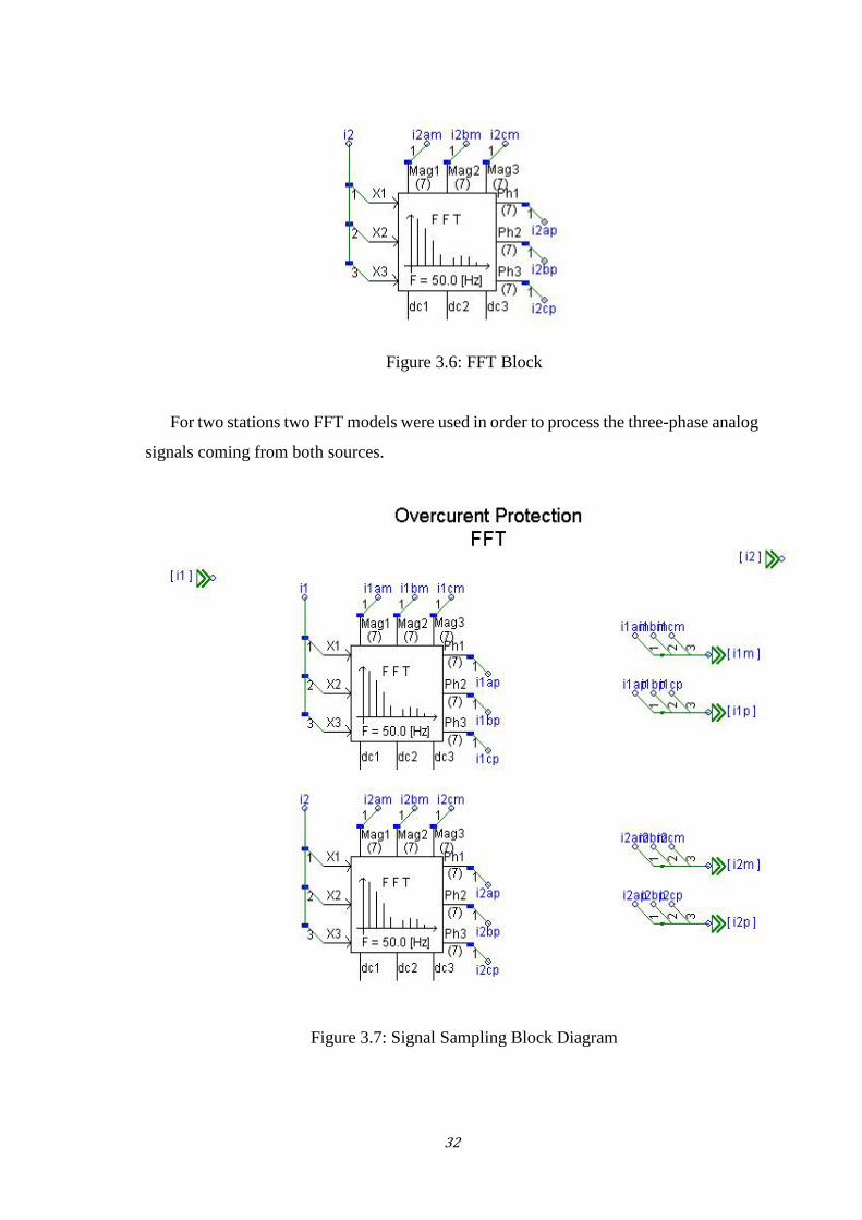
Figure 3.6: FFT Block
For two stations two FFT models were used in order to process the three-phase analog
signals coming from both sources.
Figure 3.7: Signal Sampling Block Diagram
33
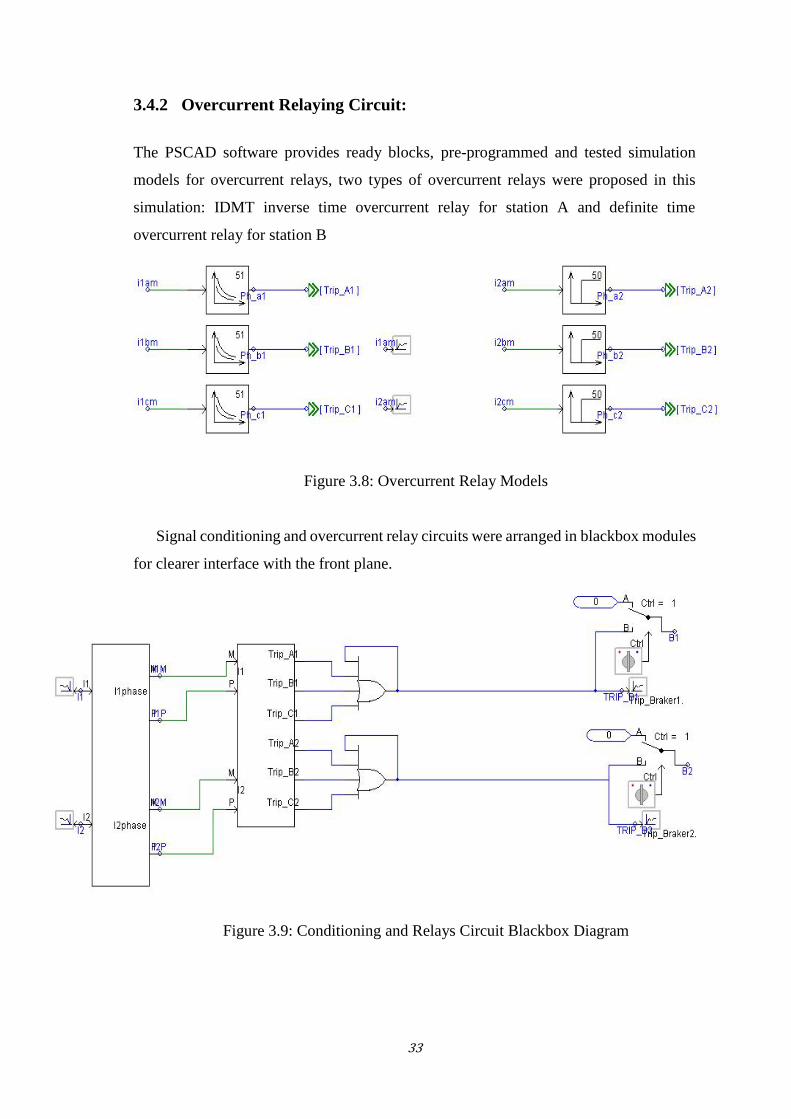
3.4.2 Overcurrent Relaying Circuit:
The PSCAD software provides ready blocks, pre-programmed and tested simulation
models for overcurrent relays, two types of overcurrent relays were proposed in this
simulation: IDMT inverse time overcurrent relay for station A and definite time
overcurrent relay for station B
Figure 3.8: Overcurrent Relay Models
Signal conditioning and overcurrent relay circuits were arranged in blackbox modules
for clearer interface with the front plane.
Figure 3.9: Conditioning and Relays Circuit Blackbox Diagram
34
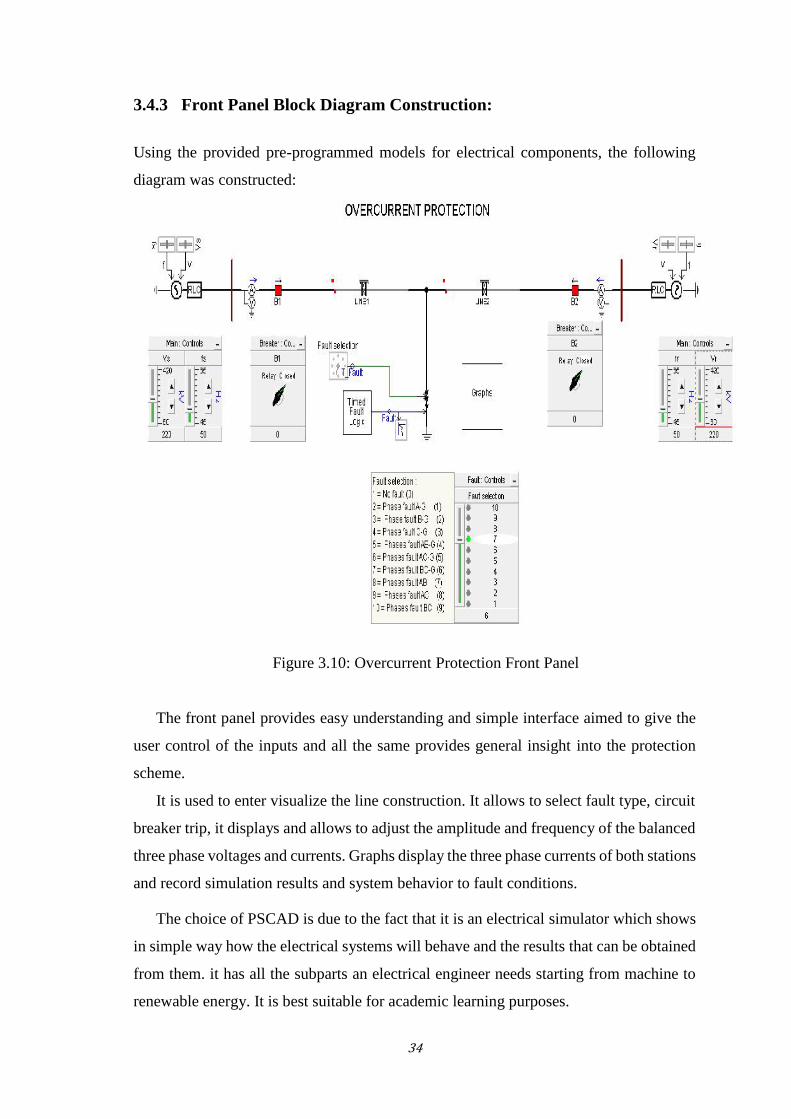
3.4.3 Front Panel Block Diagram Construction:
Using the provided pre-programmed models for electrical components, the following
diagram was constructed:
Figure 3.10: Overcurrent Protection Front Panel
The front panel provides easy understanding and simple interface aimed to give the
user control of the inputs and all the same provides general insight into the protection
scheme.
It is used to enter visualize the line construction. It allows to select fault type, circuit
breaker trip, it displays and allows to adjust the amplitude and frequency of the balanced
three phase voltages and currents. Graphs display the three phase currents of both stations
and record simulation results and system behavior to fault conditions.
The choice of PSCAD is due to the fact that it is an electrical simulator which shows
in simple way how the electrical systems will behave and the results that can be obtained
from them. it has all the subparts an electrical engineer needs starting from machine to
renewable energy. It is best suitable for academic learning purposes.

35
3.5 Laboratory Experiment 1
Found in appendix A, it is a laboratory exercise for students, designed to use the PSCAD
Simulator and the overcurrent protection model presented in the previous section. It
serves the goal of demonstrating and comparing the behavior of IDMT and independent
time overcurrent relay for different types of faults between interconnected systems.
36
Chapter 4: Differential Protection
4.1 Differential Protection Overview
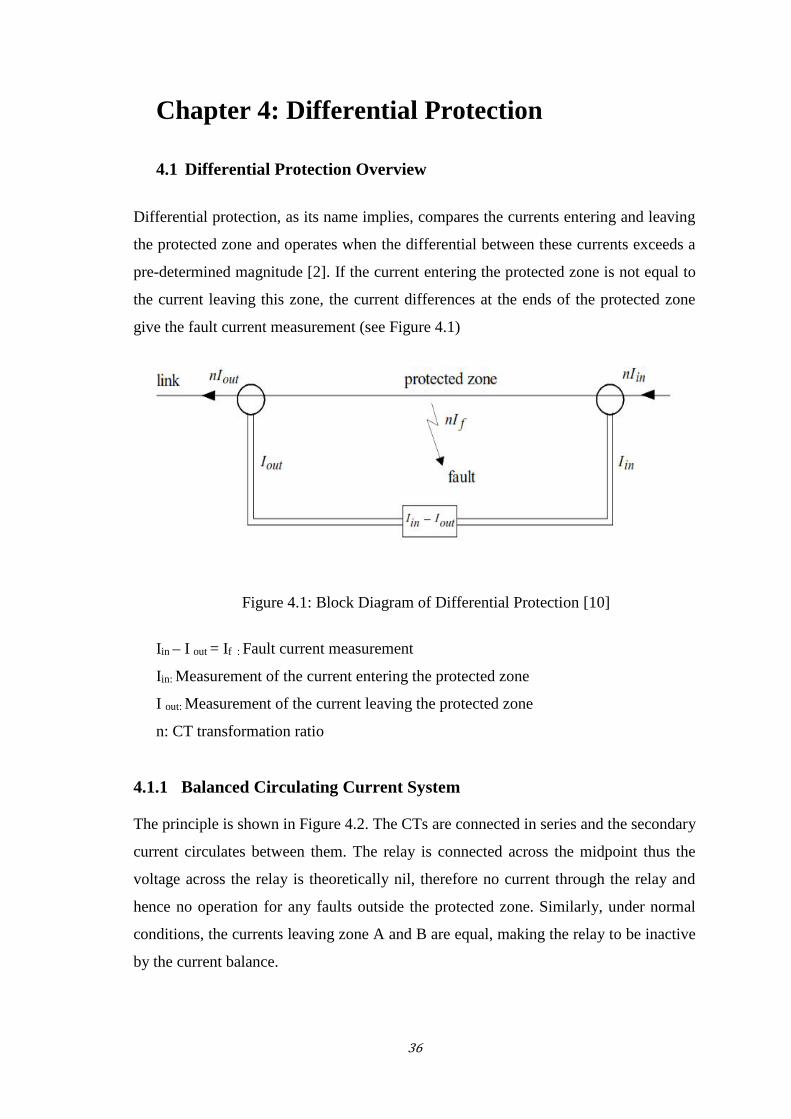
Differential protection, as its name implies, compares the currents entering and leaving
the protected zone and operates when the differential between these currents exceeds a
pre-determined magnitude [2]. If the current entering the protected zone is not equal to
the current leaving this zone, the current differences at the ends of the protected zone
give the fault current measurement (see Figure 4.1)
Figure 4.1: Block Diagram of Differential Protection [10]
Iin – I out = If : Fault current measurement
Iin: Measurement of the current entering the protected zone
I out: Measurement of the current leaving the protected zone
n: CT transformation ratio
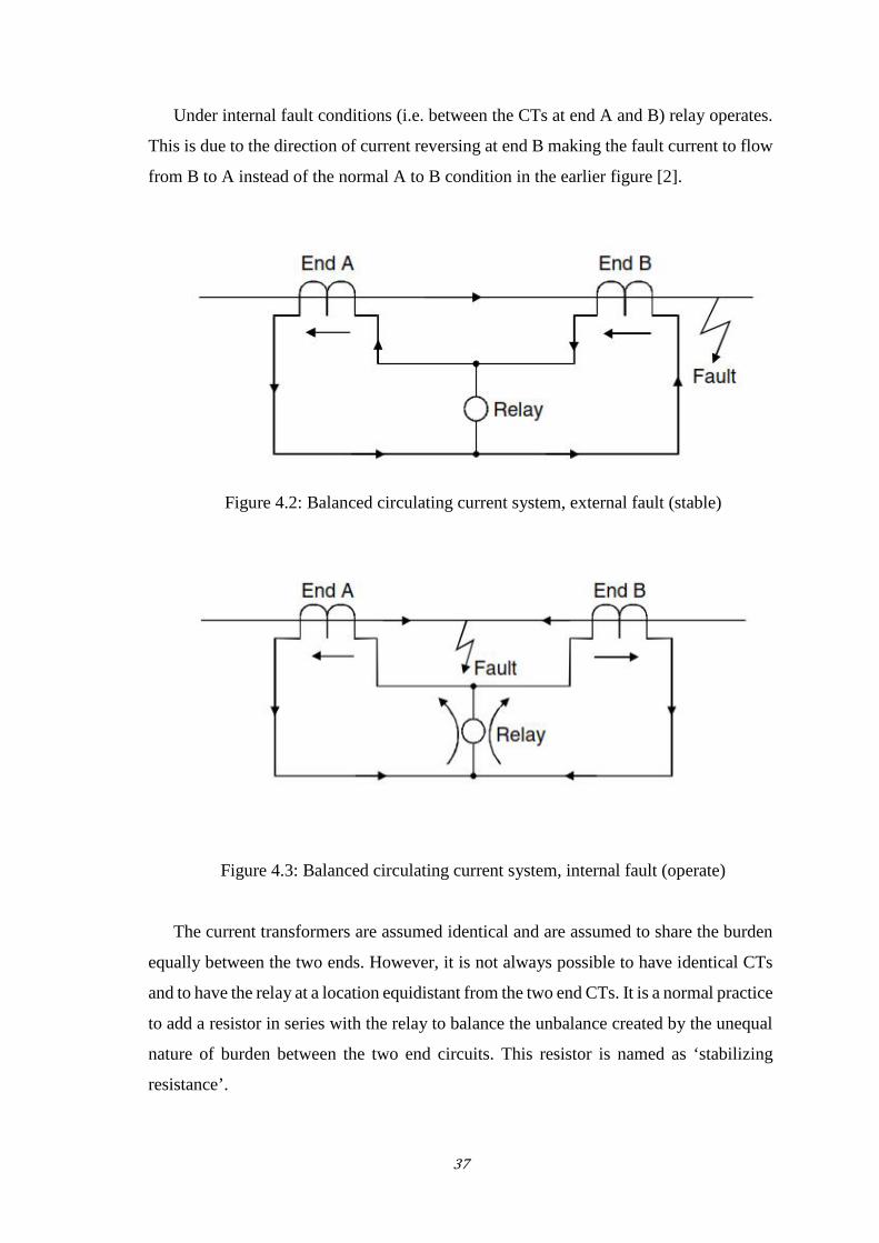
4.1.1 Balanced Circulating Current System
The principle is shown in Figure 4.2. The CTs are connected in series and the secondary
current circulates between them. The relay is connected across the midpoint thus the
voltage across the relay is theoretically nil, therefore no current through the relay and
hence no operation for any faults outside the protected zone. Similarly, under normal
conditions, the currents leaving zone A and B are equal, making the relay to be inactive
by the current balance.
37
Under internal fault conditions (i.e. between the CTs at end A and B) relay operates.
This is due to the direction of current reversing at end B making the fault current to flow
from B to A instead of the normal A to B condition in the earlier figure [2].
Figure 4.2: Balanced circulating current system, external fault (stable)
Figure 4.3: Balanced circulating current system, internal fault (operate)
The current transformers are assumed identical and are assumed to share the burden
equally between the two ends. However, it is not always possible to have identical CTs
and to have the relay at a location equidistant from the two end CTs. It is a normal practice
to add a resistor in series with the relay to balance the unbalance created by the unequal
nature of burden between the two end circuits. This resistor is named as ‘stabilizing
resistance’.
38
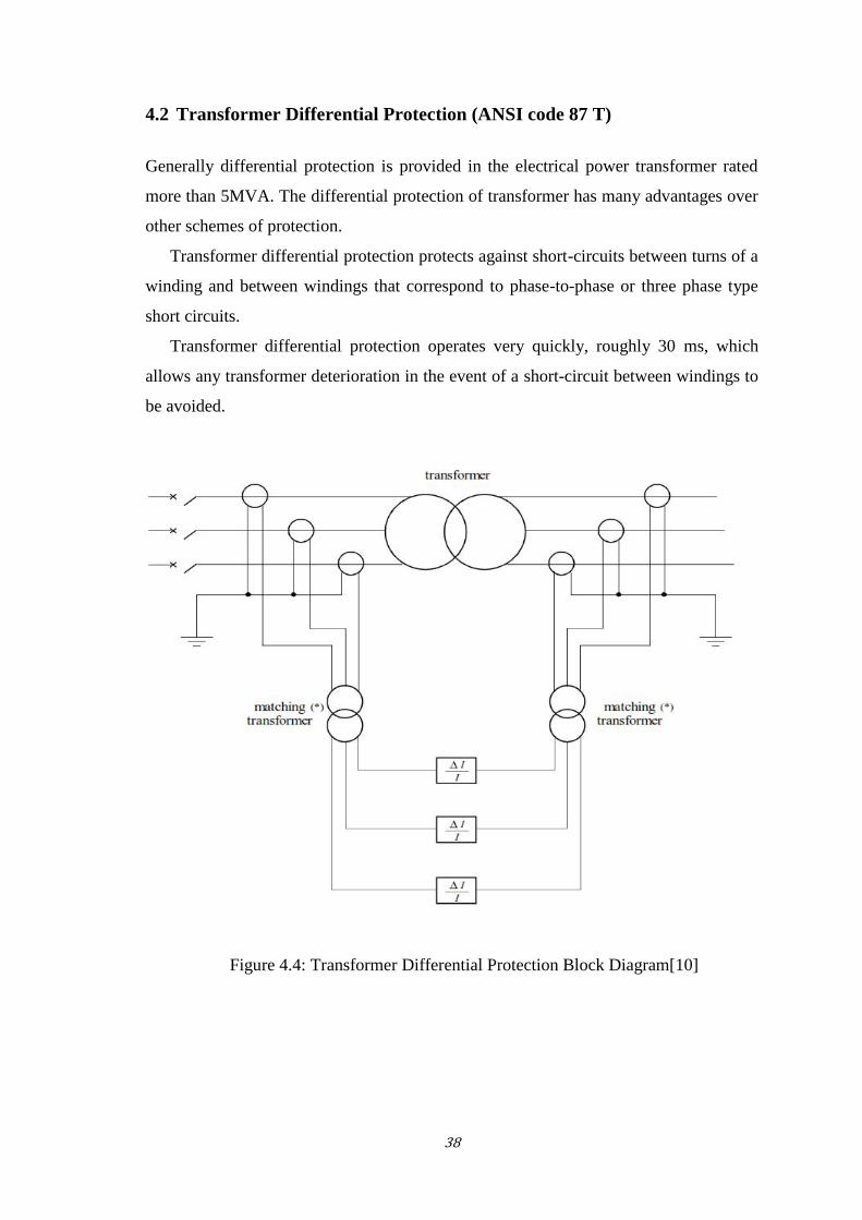
4.2 Transformer Differential Protection (ANSI code 87 T)
Generally differential protection is provided in the electrical power transformer rated
more than 5MVA. The differential protection of transformer has many advantages over
other schemes of protection.
Transformer differential protection protects against short-circuits between turns of a
winding and between windings that correspond to phase-to-phase or three phase type
short circuits.
Transformer differential protection operates very quickly, roughly 30 ms, which
allows any transformer deterioration in the event of a short-circuit between windings to
be avoided.
Figure 4.4: Transformer Differential Protection Block Diagram[10]

39
4.2.1 Differential Protection Scheme in A Power Transformer
The principle of differential protection scheme is one simple conceptual technique. The
differential relay actually compares between primary current and secondary current of
power transformer, if any unbalance found in between primary and secondary currents
the relay will actuate and inter trip both the primary and secondary circuit breaker of the
transformer.
Transformers cannot be differentially protected using high impedance differential
protection for phase-to-phase short-circuit due to the natural differential currents that
occur:
The transformer inrush currents. The operating speed required means that a time
delay longer than the duration of this current cannot be used (several tenths of a second).
The action of the on-load tap changer causes a differential current.
The characteristics of transformer differential protection are related to the
transformer specifications:
Transformation ratio between the current entering and the current leaving .
primary and secondary coupling method.
inrush current.
permanent magnetizing current [10].
In the case of the transformer which has primary rated current Ip and secondary
current Is. An installed CT of ratio Ip/1 A at the primary side and similarly, CT of ratio
Is/1 A at the secondary side of the transformer. The secondaries of these both CTs are
connected together in such a manner that secondary currents of both CTs will oppose
each other.
In other words, the secondaries of both CTs should be connected to the same current
coil of a differential relay in such an opposite manner that there will be no resultant
current in that coil in a normal working condition of the transformer. But if any major
fault occurs inside the transformer due to which the normal ratio of the transformer
disturbed then the secondary current of both transformers will not remain the same and
one resultant current will flow through the current coil of the differential relay, which
will actuate the relay and inter trip both the primary and secondary circuit breakers. To
correct phase shift of current because of star-delta connection of transformer winding in
40
the case of a three-phase transformer, the current transformer secondaries should be
connected in delta and star as shown in figure 4.5 [4].
Figure 4.5: Schematic Diagram of Differential Protection Scheme
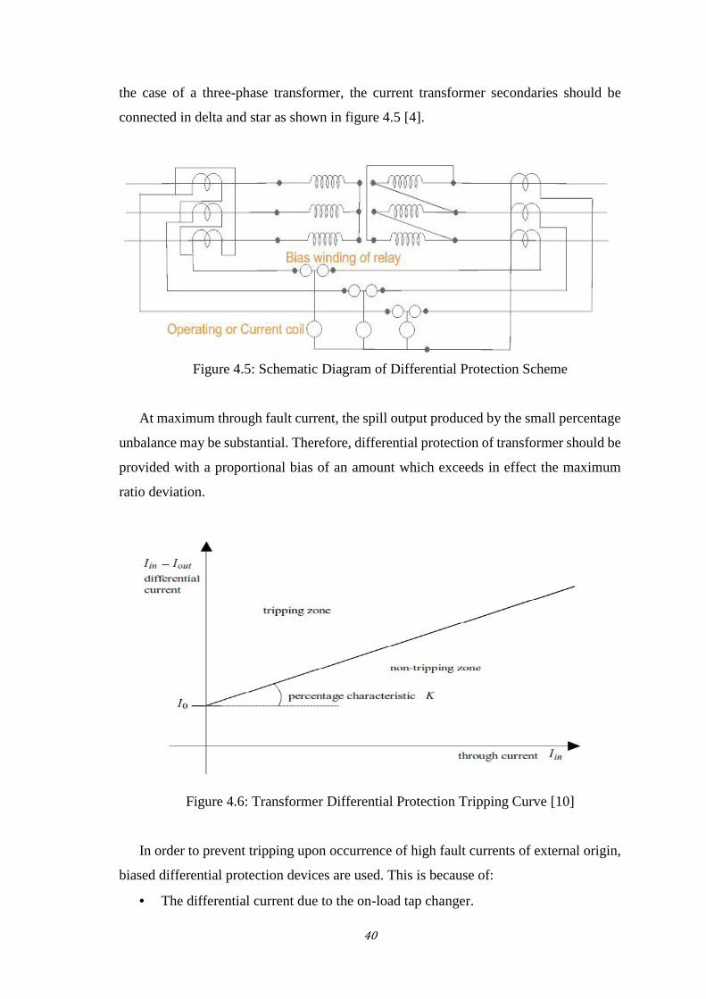
At maximum through fault current, the spill output produced by the small percentage
unbalance may be substantial. Therefore, differential protection of transformer should be
provided with a proportional bias of an amount which exceeds in effect the maximum
ratio deviation.
Figure 4.6: Transformer Differential Protection Tripping Curve [10]
In order to prevent tripping upon occurrence of high fault currents of external origin,
biased differential protection devices are used. This is because of:
The differential current due to the on-load tap changer.
41
The current transformer measurement errors, as for pilot wire differential
protection for cables or lines.
Protection is activated when − > (see figure 4.6).
4.3 Transformer Differential Protection Model In PSCAD
A transformer differential protection design model is proposed in the coming section for
a better understanding of the differential relay, simulation and testing is to be performed
on PSCAD software.
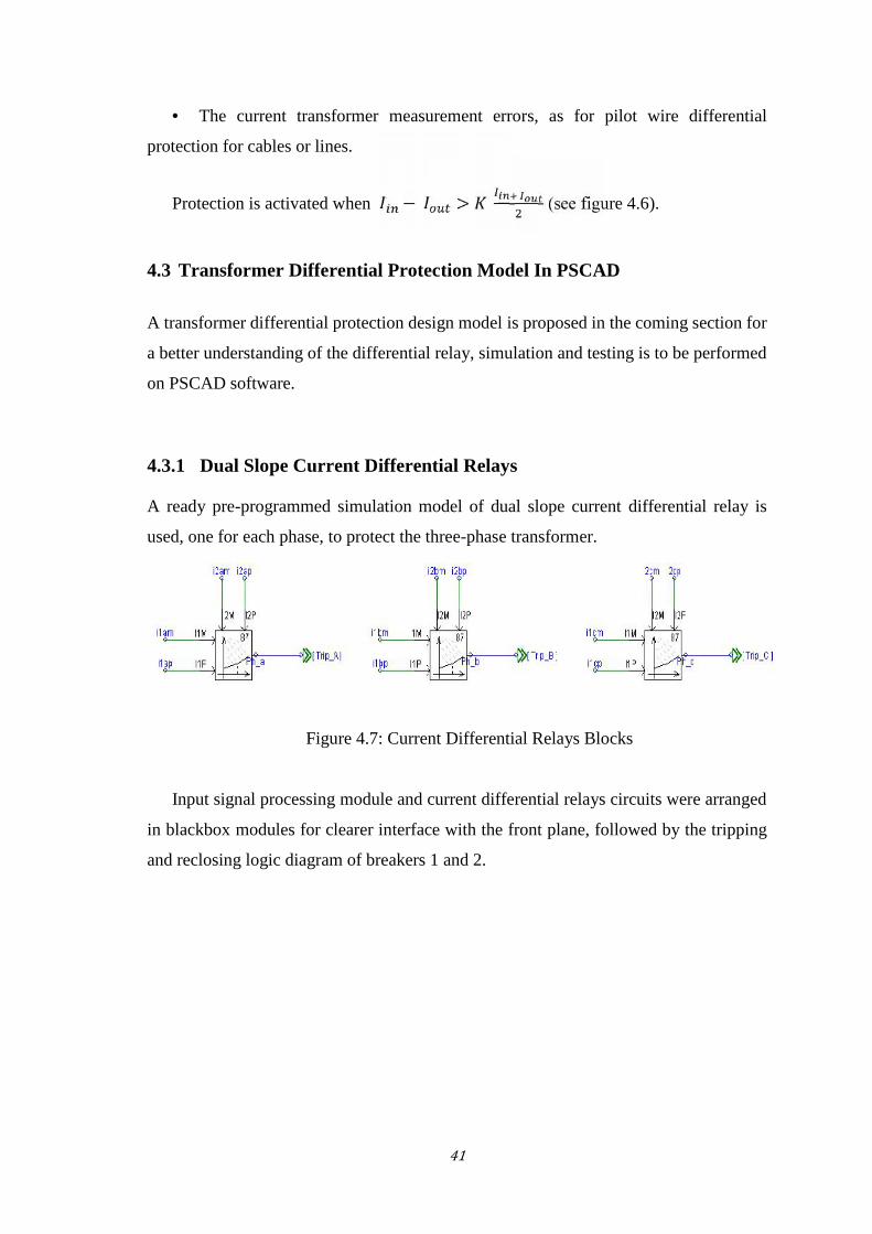
4.3.1 Dual Slope Current Differential Relays
A ready pre-programmed simulation model of dual slope current differential relay is
used, one for each phase, to protect the three-phase transformer.
Figure 4.7: Current Differential Relays Blocks
Input signal processing module and current differential relays circuits were arranged
in blackbox modules for clearer interface with the front plane, followed by the tripping
and reclosing logic diagram of breakers 1 and 2.
42
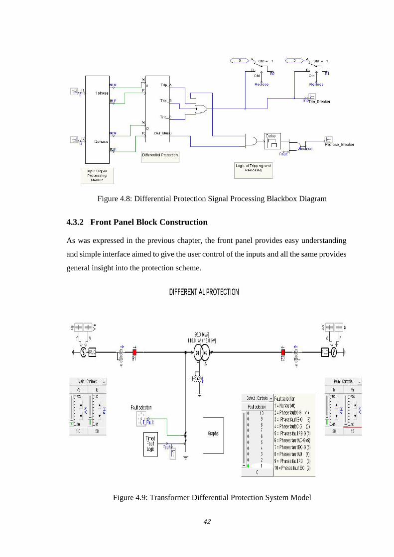
Figure 4.8: Differential Protection Signal Processing Blackbox Diagram
4.3.2 Front Panel Block Construction
As was expressed in the previous chapter, the front panel provides easy understanding
and simple interface aimed to give the user control of the inputs and all the same provides
general insight into the protection scheme.
Figure 4.9: Transformer Differential Protection System Model
43
This model consists of a Y-∆ 25MVA – 110kV/15kV three phase transformer
protected with dual slope differential relays that operates on two circuit breakers, Breaker
1 and breaker 2.
The control panels of the model allow to select fault type, it displays and adjusts the
amplitude and frequency of the balanced three phase voltages and currents.
Graphs display the three phase currents of both sides of the transformer and record
simulation results and system behavior to fault conditions.
.
4.4 Laboratory Experiment 2: Transformer Differential Protection
This laboratory experiment, found in Appendix B, carries the idea of selection of dual
slope differential relay parameters for various faulty conditions on the system. The
differential protection of power transformer is a unit protection scheme. The protective
scheme should operate only for the internal fault, and it must be insensitive for any fault
outside the zone of protection. That means the protection scheme should not operate for
any external through fault and the magnetizing inrush current due to energization of the
transformer under no load condition and also due to external fault removal.
Fast Fourier Transform technique is used to provide the operating quantity for the
dual slope differential relay. The simulation for Y-∆ connection of transformer is made
using PSCAD software.
44
Chapter 5: Distance Protection
5.1 Introduction:
Overcurrent protection scheme is a simple protection scheme, consequently, its accuracy
is not very high. It is comparatively cheap as non-directional protection does not require
VT. However, it is not suitable for protection of meshed transmission systems where
selectivity and sensitivity requirements are more stringent. Overcurrent protection is also
not a feasible option if fault current and load currents are comparable. Distance protection
scheme provides both 'higher' sensitivity and selectivity.
Distance protection provides more accurate as more information is used for decision
taking. It is a directional protection, i.e. it responds to the phase angle of current with
respect to voltage phasor. Distance protection is fast and accurate and ensures backup
protection. It is primarily used in transmission line protection. Also, it can be applied to
generator backup, loss of field and transformer protection.
Distance protection relay is the name given to the protection, whose action depends
on the distance of the feeding point to the fault. The time of operation of such protection
is a function of the ratio of voltage and current, i.e., impedance. This impedance between
the relay and the fault depends on the electrical distance between them. The principal
types of distance relays is impedance relays, reactance relays and the mho relays.
Distance protection relay principle differs from other forms of protection because their
performance does not depend on the magnitude of the current or voltage in the protective
circuit but it depends on the ratio of these two quantities [13].
The relay operates only when the ratio of voltage and current falls below a set value.
During the fault the magnitude of current increases and the voltage at the fault point
decreases. The ratio of the current and voltage is measured at the point of the current and
potential transformer. The voltage at potential transformer region depends on the distance
between the PT and the fault.
If the fault is nearer, measured voltage is lesser, and if the fault is farther, measured
voltage is more. Hence, assuming constant fault impedance each value of the ratio of
voltage and current measured from relay location comparable to the distance between the
relaying point and fault point along the line. Hence such protection is called the distance
protection or impedance protection.
45
Distance relays are used for both phase fault and ground fault protection, and they
provide higher speed for clearing the fault. It is also independent of changes in the
magnitude of the short circuits, current and hence they are not much affected by the
change in the generation capacity and the system configuration. Thus, they eliminate long
clearing times for the fault near the power sources required by overcurrent relay if used
for this purpose [13].
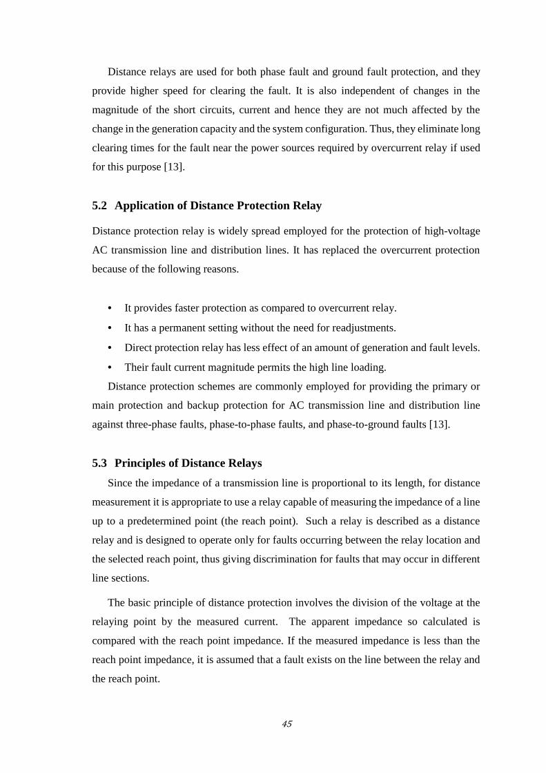
5.2 Application of Distance Protection Relay
Distance protection relay is widely spread employed for the protection of high-voltage
AC transmission line and distribution lines. It has replaced the overcurrent protection
because of the following reasons.
It provides faster protection as compared to overcurrent relay.
It has a permanent setting without the need for readjustments.
Direct protection relay has less effect of an amount of generation and fault levels.
Their fault current magnitude permits the high line loading.
Distance protection schemes are commonly employed for providing the primary or
main protection and backup protection for AC transmission line and distribution line
against three-phase faults, phase-to-phase faults, and phase-to-ground faults [13].
5.3 Principles of Distance Relays
Since the impedance of a transmission line is proportional to its length, for distance
measurement it is appropriate to use a relay capable of measuring the impedance of a line
up to a predetermined point (the reach point). Such a relay is described as a distance
relay and is designed to operate only for faults occurring between the relay location and
the selected reach point, thus giving discrimination for faults that may occur in different
line sections.
The basic principle of distance protection involves the division of the voltage at the
relaying point by the measured current. The apparent impedance so calculated is
compared with the reach point impedance. If the measured impedance is less than the
reach point impedance, it is assumed that a fault exists on the line between the relay and
the reach point.
46
The reach point of a relay is the point along the line impedance locus that is
intersected by the boundary characteristic of the relay. Since this is dependent on the
ratio of voltage and current and the phase angle between them, it may be plotted on an
R/X diagram. The loci of power system impedances as seen by the relay during faults,
power swings and load variations may be plotted on the same diagram and in this manner
the performance of the relay in the presence of system faults and disturbances may be
studied [1].
5.4 Mho Distance Protection Overview
Distance relays use voltage and current measurements to detect fault conditions. These
relays have fixed zones of protection that generally do not vary much in response to
changes in loading conditions, which allows them to employ higher sensitivity than
overcurrent relays in detecting faults [6].
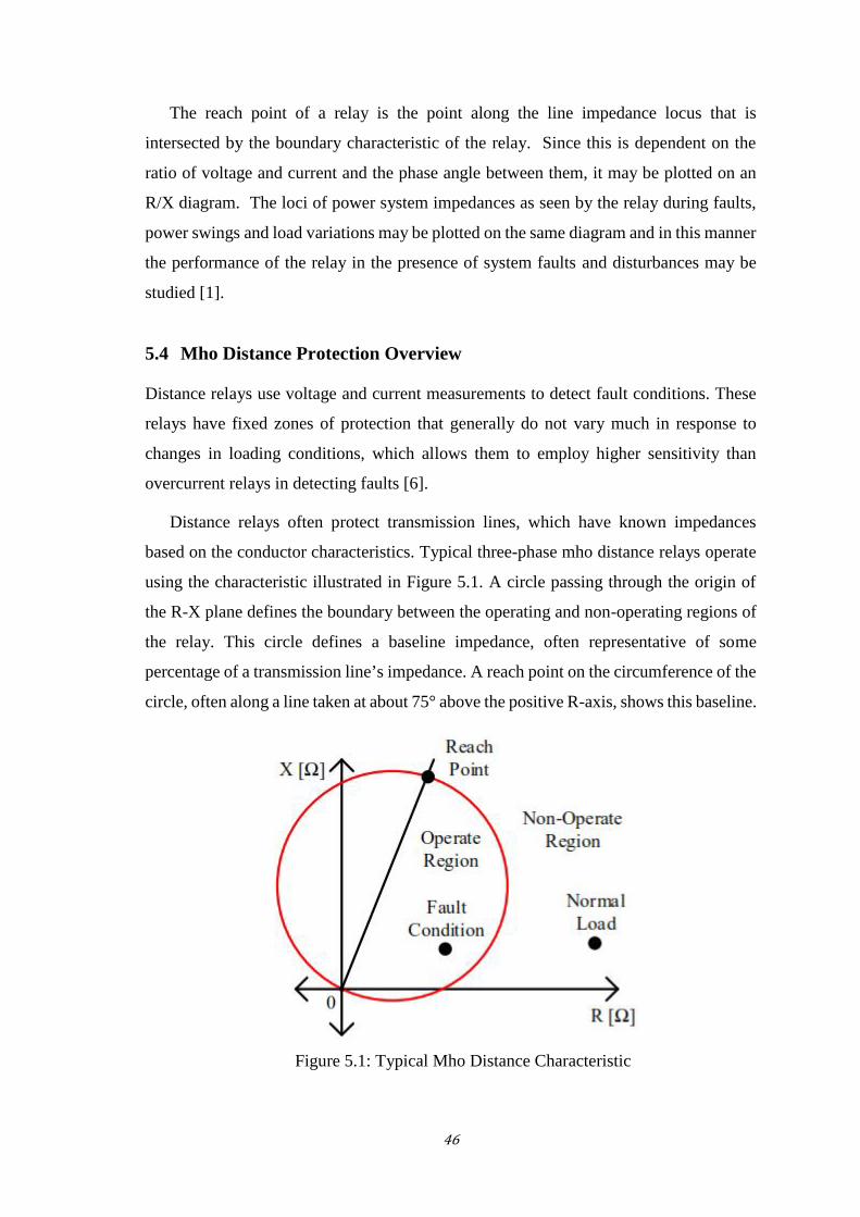
Distance relays often protect transmission lines, which have known impedances
based on the conductor characteristics. Typical three-phase mho distance relays operate
using the characteristic illustrated in Figure 5.1. A circle passing through the origin of
the R-X plane defines the boundary between the operating and non-operating regions of
the relay. This circle defines a baseline impedance, often representative of some
percentage of a transmission line’s impedance. A reach point on the circumference of the
circle, often along a line taken at about 75° above the positive R-axis, shows this baseline.
Figure 5.1: Typical Mho Distance Characteristic
47
Local ground faults cause decrease in voltage (closer to ground potential) and
increase in current (due to a reduced-impedance path available to ground). This condition
decreases the impedance measured by the relay and moves the operating point on the R-
X plane closer to the origin, the point of minimum impedance. Faults outside the defined
distance covered by the relay cause the impedance measured by the relay (based on the
measured voltage and current) to decrease, but not by enough to come inside the circle.
Faults inside the defined distance cause a greater drop in impedance, bringing the
operating point inside the circle. The larger impedance drop alerts the relay to the fault,
leading the relay to trip for the fault condition. Calculating impedance in this way allows
a distance relay to distinguish between internal and external faults.
Correct coordination of the distance relays is achieved by having an instantaneous
directional zone 1 protection and one or two more time-delayed zones. A transmission
line has a resistance and reactance proportional to its length, which also defines its own
characteristic angle. It can therefore be represented on an R/X diagram as shown in figure
5.1.
5.4.1 Zone 1 Protection
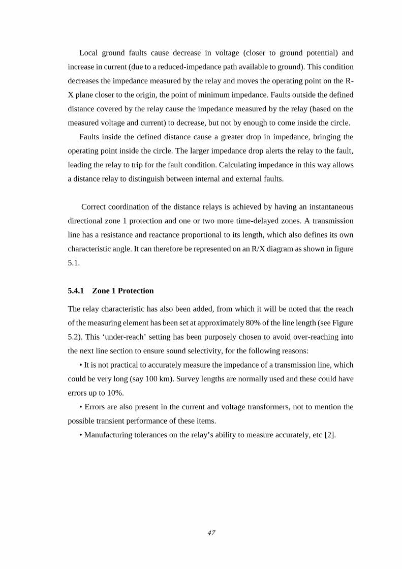
The relay characteristic has also been added, from which it will be noted that the reach
of the measuring element has been set at approximately 80% of the line length (see Figure
5.2). This ‘under-reach’ setting has been purposely chosen to avoid over-reaching into
the next line section to ensure sound selectivity, for the following reasons:
• It is not practical to accurately measure the impedance of a transmission line, which
could be very long (say 100 km). Survey lengths are normally used and these could have
errors up to 10%.
• Errors are also present in the current and voltage transformers, not to mention the
possible transient performance of these items.
• Manufacturing tolerances on the relay’s ability to measure accurately, etc [2].
48
Figure 5.2: Zone 1 Mho Characteristic
This measuring element is known as zone 1 of the distance relay and is instantaneous
in operation.
5.4.2 Zone 2 Protection
To cover the remaining 20% of the line length, a second measuring element can be fitted,
set to over-reach the line, but it must be time delayed by 0.5 s to provide the necessary
coordination with the downstream relay. This measuring element is known as zone 2. It
not only covers the remaining 20% of the line but also provides backup for the next line
section should this fail to trip for whatever reason.
5.4.3 Zone 3 Protection
A third zone is invariably added as a starter element and this takes the form of an offset
mho characteristic. This offset provides a closing-onto-fault feature, as the mho elements
may not operate for this condition due to the complete collapse of voltage for the nearby
fault. The short backward reach also provides local backup for a busbar fault.
The zone 3 element also has another very useful function. As a starter it can be used
to switch the zone 1 element to zone 2, reach after say 0.5 s, thereby saving the
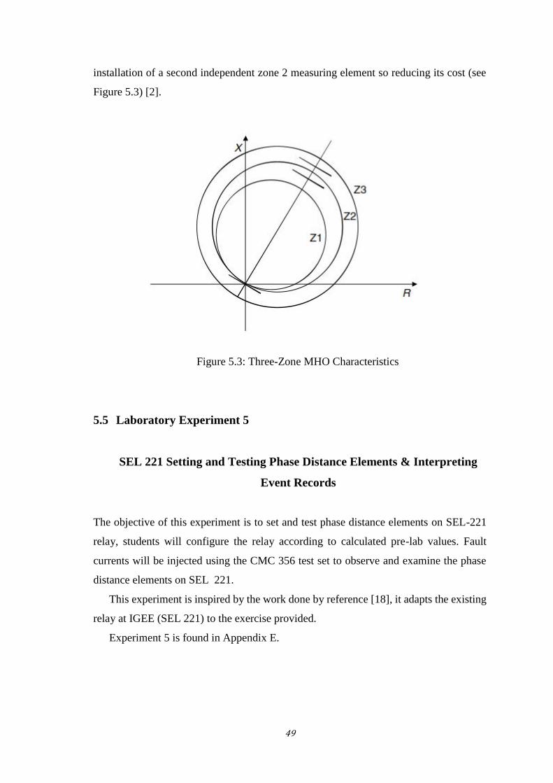
49
installation of a second independent zone 2 measuring element so reducing its cost (see
Figure 5.3) [2].
Figure 5.3: Three-Zone MHO Characteristics
5.5 Laboratory Experiment 5
SEL 221 Setting and Testing Phase Distance Elements & Interpreting
Event Records
The objective of this experiment is to set and test phase distance elements on SEL-221
relay, students will configure the relay according to calculated pre-lab values. Fault
currents will be injected using the CMC 356 test set to observe and examine the phase
distance elements on SEL 221.
This experiment is inspired by the work done by reference [18], it adapts the existing
relay at IGEE (SEL 221) to the exercise provided.
Experiment 5 is found in Appendix E.
50
Conclusion
A protective relaying laboratory consisting of modern relays is an essential component
to educate students in the field of power system protection. The relay lab should function
as an arena to demonstrate protection principles and practical challenges. Further
developing of the lab to include newer multifunctional relays is vital, as this is important
for the future of power system protection.
Certain challenges that occurred during this project correspond to relatively simple
misunderstandings in operating the equipment. For example, during a great period,
difficulties were encountered in extracting event reports from the SEL 221, this was due
to the fact that being an old version relay, it is not compatible with present software
available for users. Another is the availability of the relay tester at the institute which
could not be achieved without the charitable donation previously mentioned in chapter
2.
Students should be educated with knowledge of the possibilities within modern relay
technology. After graduation, they can contribute to a shift in protection strategies within
utility companies to meet the demands for power system protection in the future. Using
an injection test set as a testing tool for the relay lab is a good, versatile and flexible
solution. It is easy to use for the beginner, while having advanced features for the more
advanced user. A new relay tester should be acquired by IGEE, as well as new protective
relays to create opportunities for future senior projects and master’s theses.
Power system analysis software such as PSCAD and ETAP presents opportunities for
future groups to analyze transient and steady-state imbalances in the system, further work
can be done to create more ready models for the students to benefit from.
If utilized properly the relay lab can contribute to increased interest and knowledge
of power system protection among students at IGEE for many years to come. Educating
future engineers with this knowledge is important for the protection and reliability of
future power systems. If the lab is well maintained and expanded to keep up with trends
in the field it could last many years.
51
References
[1] “Network protection & automation guide”, [Stafford, England], Alstom Grid,2011.
[2] Hewitson, L., Brown, M. and Balakrishnan, R, “Practical power systems protection”.Oxford, Newnes/Elsevier, 2004.
[3] J. L. Blackburn and T. J. Domin, “Protection Fundamentals and Basic DesignPrinciples,” in Protective Relaying: Principles and Applications, 3rd ed., H. L.Willis and M. H. Rashid, Eds., Boca Raton, Florida: CRC Press, 2007.
[4] Electrical4u.com, Differential Protection of Transformer, Differential Relays, [online]Available at:https://www.electrical4u.com/differential-protection-of-transformer-differential-relays ,[Accessed 4 May 2018].
[5] Youtube, [online] Available at: https://www.youtube.com/watch?v=ZQgRzATOn6k
[6] H. J. Li and F. Calero, “Line and circuit protection,” in Protective relaying theoryand applications, W. A. Elmore, Ed, 1st ed, New York, NY: Marcel Dekker, 1994.
[7] Muhammad Shoaib Almas, Rujiroj Leelaruji,and Luigi Vanfrettio, “Over-currentrelay model implementation for real time simulation & Hardware-in-the-Loop (HIL)validation”, KTH, Elektriska energy system, 2012.
[8] [online] Available at: https://electricalnotes.wordpress.com/2013/01/01/types-of-over-current-relay, [Accessed 20 Apr. 2018].
[9] J. L. Blackburn and T. J. Domin, “Introduction and general philosophies,” inProtective Relaying: Principles and Applications, 3rd ed., H. L. Willis and M. H.Rashid,Eds., Boca Raton, Florida: CRC Press, 2007.
[10] Prévé, C., “Protection of electrical networks”, London: Wiley-Liss, 2006.
[11] [online] Available at:https://www.slideshare.net/ASWANTH6270/over-current-relays
[12] YouTube, (2018), (PSCAD) single line fault and circuit breaker, [online] Availableat: https://www.youtube.com/watch?v=Mi_rdqtlTRQ&t=188s [Accessed 29 May 2018].
[13] Circuit Globe, What is Distance Protection Relay? Description & its Application -Circuit Globe, [online] Available at: https://circuitglobe.com/distance-protection-relay.html [Accessed 29 May 2018].
52
[14] [online] Availlable at:https://www.bing.com/cr?IG=34F4272884C246E6AD631A200A06AD6D&CID=11325B291CA965CA010E57281D5464D9&rd=1&h=SVUamOAqUB4JZIjaX3OERiOcoc223o_FzrUZyqV7MPk&v=1&r=https%3a%2f%2fselinc.cachefly.net%2fassets%2fLiterature%2fProduct%2520Literature%2fData%2520Sheets%2f221F-121F_DS_20000104.pdf%3fv%3d20150812-085319&p=DevEx.LB.1,5070.1[Accessed 1 May 2018].
[15] YouTube. (2018), Transformer Differential Protection. [online] Available at:https://www.youtube.com/watch?v=ZQgRzATOn6k
[16] ELK412 - Distribution of Electrical Energy Lab. Notes v1.0, Overcurrent andGround Fault Protection, Spring 2012.
[17] Mayurdhvajsinh P. Gohil, Jinal Prajapati, Ankit Rabari, “Differential ProtectionOf Y-Y And Δ-Δ Connected Power Transformer”, International Journal of EngineeringDevelopment and Research, 2014.
[18] College of Engineering and Computer Science, “Smart Grid and ProtectionLaboratory, hands-on demo 1,2”, University of Tennessee at Chattanooga,2015
[19] The workhorse Universal Relay Testing and Commissioning, CMC 356Brochure, ENU.
53
Appendices
Appendix A
University of M’hamed BOUGARA BoumerdesInstitute of Electrical Engineering and ElectronicsControl and Power Department
Experiment # 1Overcurrent Protection Modeling Using PSCAD Simulator
Learning outcome
• To use and understand an overcurrent protection model in PSCAD power systemsimulator and gain an understanding of the impact of both IDMT and independent timeovercurrent relays on power system protection.
• To compare the different types of characteristics of inverse time overcurrentrelay.
Apparatus
PSCAD Simulator. Computer.
Background
Power system simulators are mathematical models of the electric system. They use an
iterative method to simultaneously solve a large matrix of complex numbers, which
numerically represent the power system for a set of initial conditions. They are often
accompanied by a graphical interface which allows the user to ‘see’ the numerical results
they produce.
Simple Guide to Using PSCAD/EMTDC
1) Launch PSCAD (student version) from Start Menu.
2) Creating a new project:
Click on File/New/Case: A new project entitled ‘noname’ appears in the left workspace
window, indicating that a new project is created.

54
3) Setting active project: In the workspace window, right click on the title of an inactive
project and select Set as active.
4) Saving active project: Click on File/Save Active Project. Select an appropriate folder
and save the project as ‘Lab1’ or any other name.
5) Adding components to a project: Double click on master library in left top workspace.
Navigate to the area containing desired component. Right click on component and select
Copy. Open the project where you wish to add the component (double click on ‘project
name’), right click over blank area and select Paste. (Note: There are many other ways
to add a component to a project)
6) Setting Properties: To set the properties double click on any component and change
the parameters.
At the top of the parameter dialog is a drop list, which contains list of all parameter dialog
pages. If only one page exists, then the drop list will be disabled. For e.g. if you double
click on resistor, it will ask for only resistance value.
7) Making connections between components: Click Wire Mode button in the main
toolbar. Move the mouse pointer onto the project page.
The mouse pointer will have turned into a pencil, which indicates you are in Wire mode.
To draw a wire, move the cursor to the node where you want the line to start and left
click. Move the cursor to where you want the line to end and right-click to complete the
wire. Multi-segment Wires may be built by continuing to left click at different points. To
turn off Wire Mode, press Esc key.
8) Measurement: To measure currents and voltages ammeter and voltmeter are provided
on the toolbar on the right. Ammeter should be connected in series.
To plot currents and voltages use output channel and data signal label on the toolbar.
The output channel parameter dialog gives title, unit, scale factor and min/max limits.
9) Adding a Graph Frame: Right click on the Output Channel component. Select
Input/Output Reference/Add Overlay Graph with Signal. This will create a new
55
graph frame, overlay graph and a curve simultaneously. For adding more graphs on same
graph frame, right click on graph frame and click Add Overlay Graph (Analog). This
will add another graph on same frame. To put a curve on this graph Ctrl+click on output
channel and drag it on the graph.
The curve corresponding to that output channel will be added on to the graph. When you
run the simulation, curves will be automatically plotted on this graph.
Press Y and X buttons to see complete curve (zoom out).
10) Setting time step and simulation time: Right click on blank space in the project, select
Project Settings. In runtime tab you can set simulation time, time step and plot step.
11) To simulate the project: Click on Build/Run.
Procedure
1. Start PSCAD and open project OVERCURRENT PROTECTION, it represents
a network of two sources with RLC impedance and a transmission line protected by two
overcurrent relays at both stations A and B.
At station A the protection is an inverse time overcurrent relay with inverse time
characteristic, while at station B an independent time overcurrent relay is used (see figure
3.11).
Figure 3.11: Overcurrent System Model
2. Using the mouse, click on the blackbox named Overcurrent Relays to see the
protection configuration for each station, the relay can be configured by accessing the
relay parameters right click on the relay- go to Edit parameters, by the same
manner you can change the parameters of the RLC impedance and the timed fault logic
which is initially set to start from 0.2s to 1.5 s.
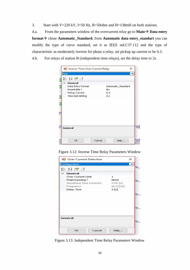
56
3. Start with V=220 kV, f=50 Hz, R=50ohm and H=138mH on both stations.
4.a. From the parameters window of the overcurrent relay go to Main Data entry
format chose Automatic_Standard, from Automatic data entry_standart you can
modify the type of curve standard, set it as IEEE std.C37.112 and the type of
characteristic as moderately inverse for phase a relay, set pickup up current to be 0.3.
4.b. For relays of station B (independent time relays), set the delay time to 2s.
Figure 3.12: Inverse Time Relay Parameters Window
Figure 3.13: Independent Time Relay Parameters Window
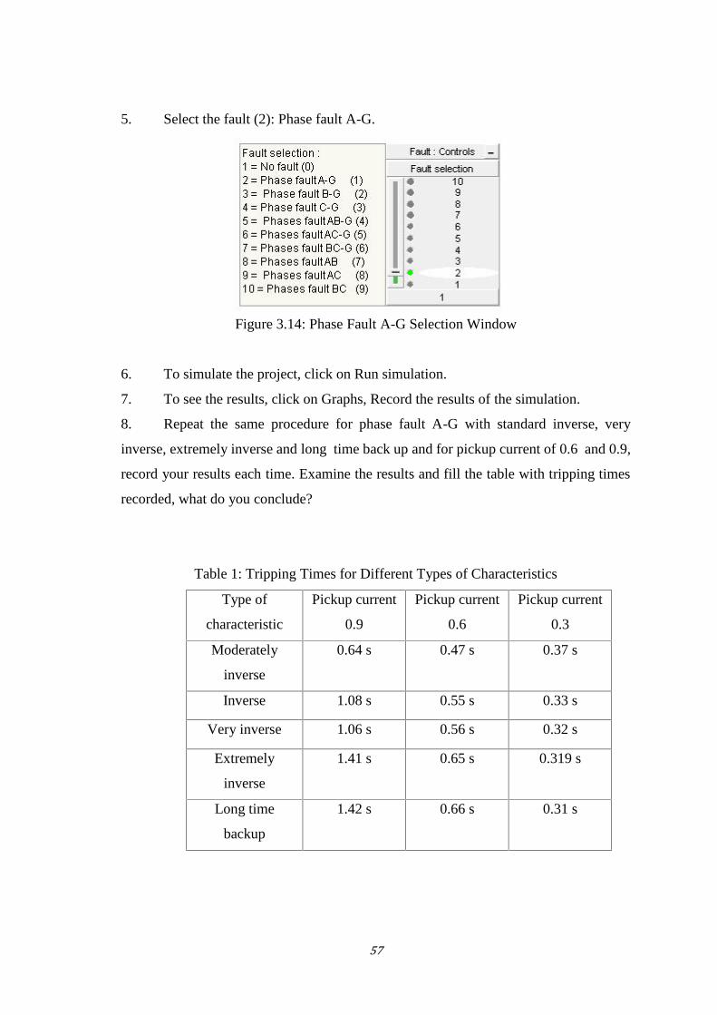
57
5. Select the fault (2): Phase fault A-G.
Figure 3.14: Phase Fault A-G Selection Window
6. To simulate the project, click on Run simulation.
7. To see the results, click on Graphs, Record the results of the simulation.
8. Repeat the same procedure for phase fault A-G with standard inverse, very
inverse, extremely inverse and long time back up and for pickup current of 0.6 and 0.9,
record your results each time. Examine the results and fill the table with tripping times
recorded, what do you conclude?
Table 1: Tripping Times for Different Types of Characteristics
Type of
characteristic
Pickup current
0.9
Pickup current
0.6
Pickup current
0.3
Moderately
inverse
0.64 s 0.47 s 0.37 s
Inverse 1.08 s 0.55 s 0.33 s
Very inverse 1.06 s 0.56 s 0.32 s
Extremely
inverse
1.41 s 0.65 s 0.319 s
Long time
backup
1.42 s 0.66 s 0.31 s
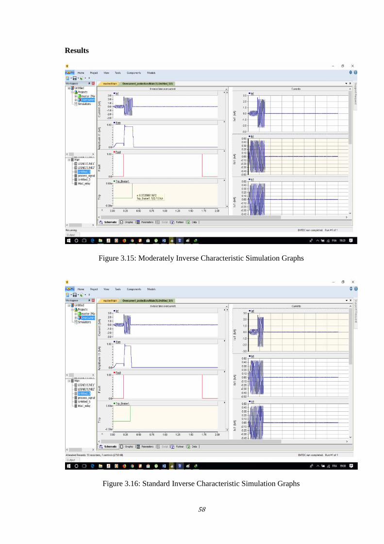
58
Results
Figure 3.15: Moderately Inverse Characteristic Simulation Graphs
Figure 3.16: Standard Inverse Characteristic Simulation Graphs
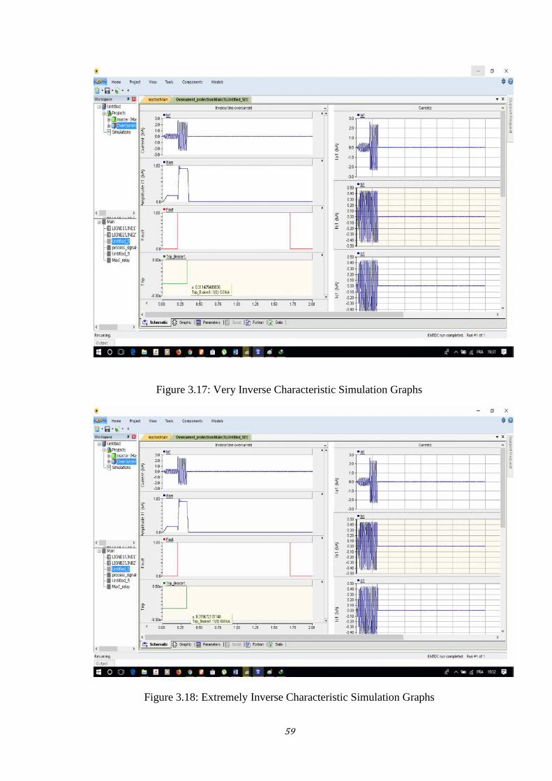
59
Figure 3.17: Very Inverse Characteristic Simulation Graphs
Figure 3.18: Extremely Inverse Characteristic Simulation Graphs
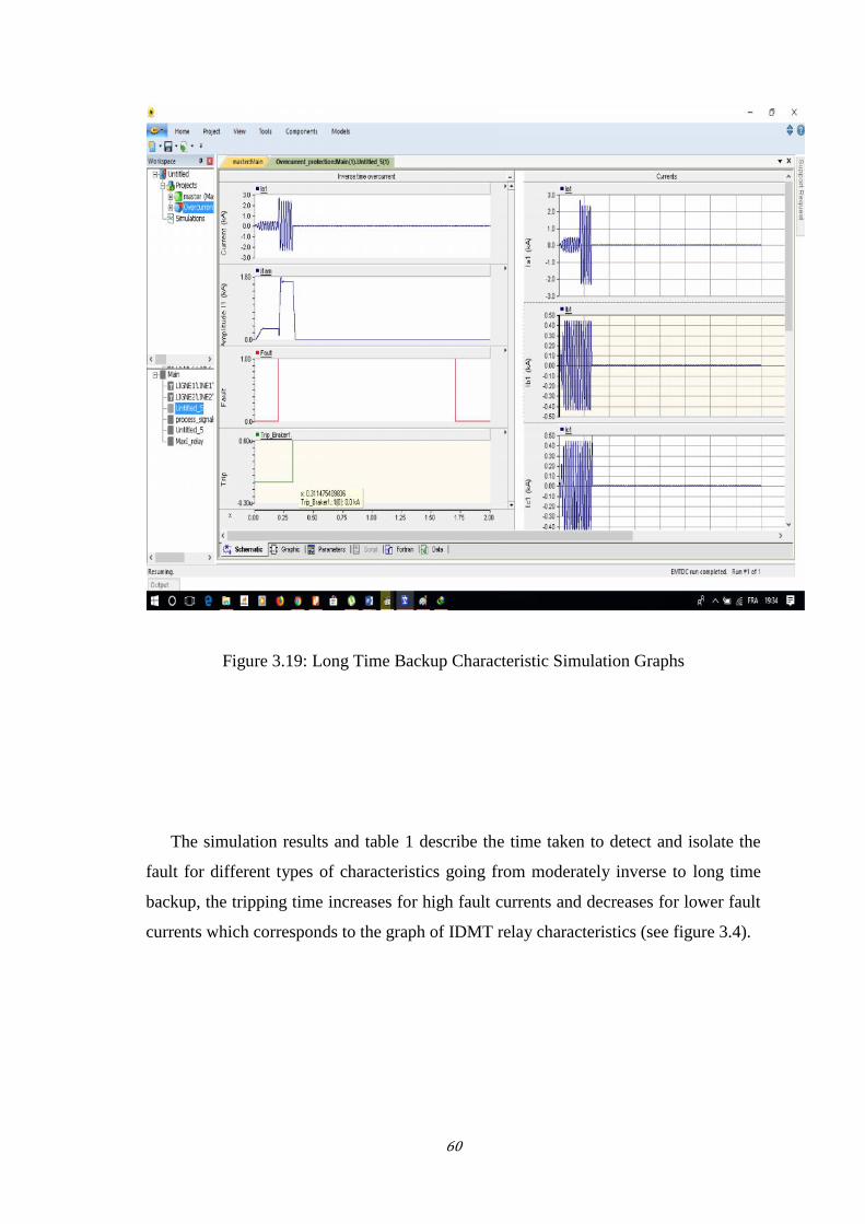
60
Figure 3.19: Long Time Backup Characteristic Simulation Graphs
The simulation results and table 1 describe the time taken to detect and isolate the
fault for different types of characteristics going from moderately inverse to long time
backup, the tripping time increases for high fault currents and decreases for lower fault
currents which corresponds to the graph of IDMT relay characteristics (see figure 3.4).
61
Appendix B
University of M’hamed BOUGARA BoumerdesInstitute of Electrical Engineering and ElectronicsControl and Power Department
Experiment #2Transformer Differential Protection
Learning Outcomes
To use and understand the differential protection scheme of power transformer.
To compare and study various faulty conditions on the system.
Background
The basic operating principle of differential protection is to calculate the difference
between the current entering and leaving the protected zone. There is a phenomenon that
occurred during removal of external through fault or due to energization of the
transformer under no load condition named magnetizing inrush current. The differential
protection scheme should remain insensitive for such magnetizing inrush current. The
differential relay should not operate for the external/through fault. The differential
protection of power transformer is a unit protection scheme. The protective scheme
should operate only for the internal fault, and it must be insensitive for any fault outside
the zone of protection.
The protection operates when the differential current exceeds the set bias threshold
value. For external faults, the differential current should be zero, but error caused by the
CT saturation and CT ration error leads to non-zero value. To prevent maloperation the
operating threshold is raised by increasing the relay setting [17].
Maloperation of the differential protection of power transformer may occur due to
Magnetizing inrush current, CT saturation and Through Fault Inrush. Among all these
three; magnetizing inrush results during excitation of Transformer under no load
condition. It can also come in to picture during the energization of parallelly connected
power transformer. For this setting of 4 relay parameter is very important: i.e.
(1) Differential Current Threshold: Is1
(2) Lower Percentage Bias Setting: K1
(3) Bias current threshold: Is2
(4) Higher Percentage bias setting: K2
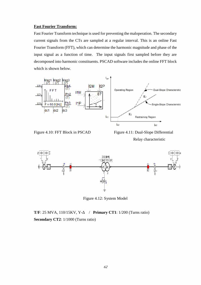
62
Fast Fourier Transform:
Fast Fourier Transform technique is used for preventing the maloperation. The secondary
current signals from the CTs are sampled at a regular interval. This is an online Fast
Fourier Transform (FFT), which can determine the harmonic magnitude and phase of the
input signal as a function of time. The input signals first sampled before they are
decomposed into harmonic constituents. PSCAD software includes the online FFT block
which is shown below.
Figure 4.10: FFT Block in PSCAD Figure 4.11: Dual-Slope Differential
Relay characteristic
Figure 4.12: System Model
T/F: 25 MVA, 110/15KV, Y-∆ / Primary CT1: 1/200 (Turns ratio)
Secondary CT2: 1/1000 (Turns ratio)
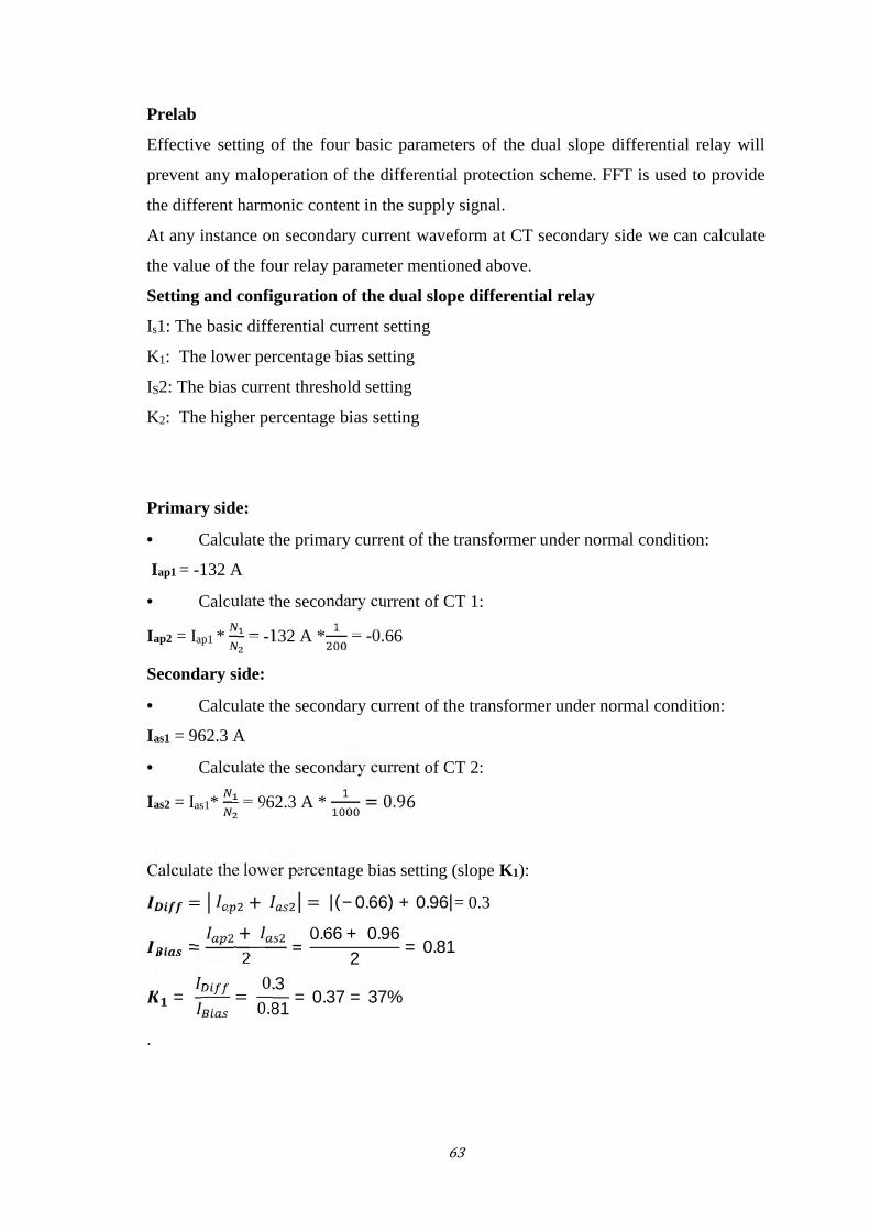
63
Prelab
Effective setting of the four basic parameters of the dual slope differential relay will
prevent any maloperation of the differential protection scheme. FFT is used to provide
the different harmonic content in the supply signal.
At any instance on secondary current waveform at CT secondary side we can calculate
the value of the four relay parameter mentioned above.
Setting and configuration of the dual slope differential relay
Is1: The basic differential current setting
K1: The lower percentage bias setting
IS2: The bias current threshold setting
K2: The higher percentage bias setting
Primary side:
Calculate the primary current of the transformer under normal condition:
Iap1 = -132 A
Calculate the secondary current of CT 1:
Iap2 = Iap1 * = -132 A * = -0.66
Secondary side:
Calculate the secondary current of the transformer under normal condition:
Ias1 = 962.3 A
Calculate the secondary current of CT 2:
Ias2 = Ias1* = 962.3 A * = 0.96Calculate the lower percentage bias setting (slope K1):= + = |(−0.66) + 0.96|= 0.3= +2 = 0.66 + 0.962 = 0.81
= = 0.30.81 = 0.37 = 37%.
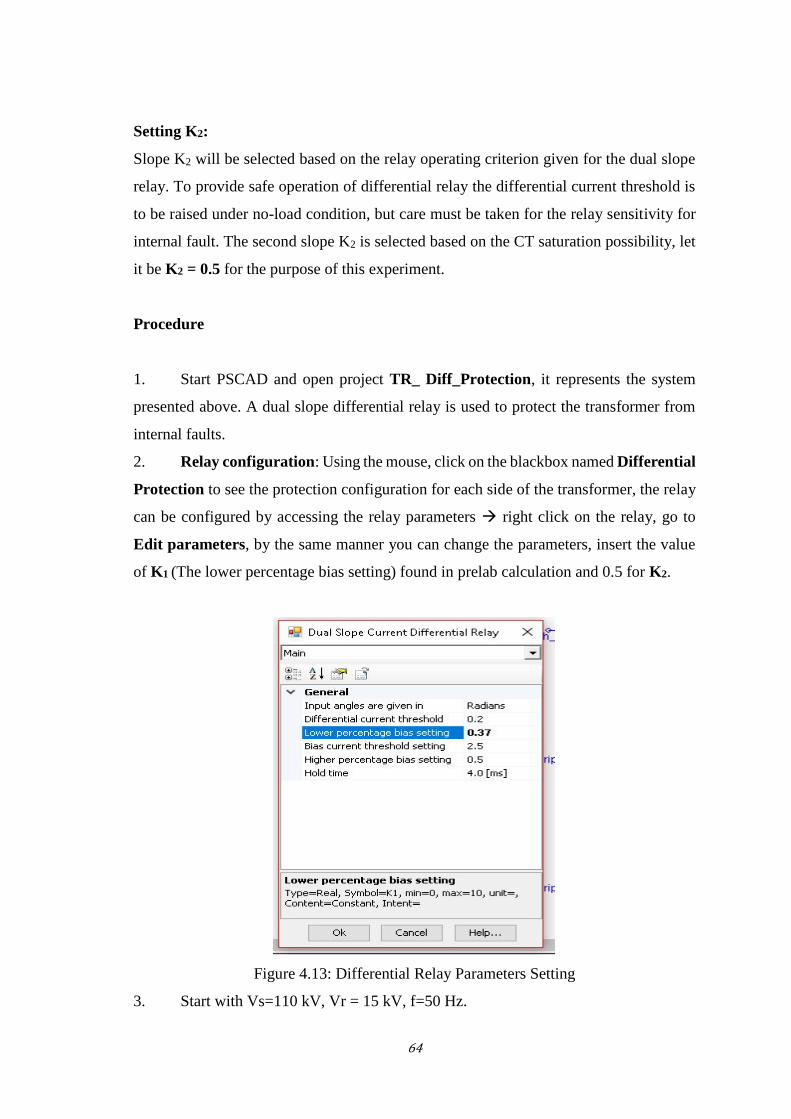
64
Setting K2:
Slope K2 will be selected based on the relay operating criterion given for the dual slope
relay. To provide safe operation of differential relay the differential current threshold is
to be raised under no-load condition, but care must be taken for the relay sensitivity for
internal fault. The second slope K2 is selected based on the CT saturation possibility, let
it be K2 = 0.5 for the purpose of this experiment.
Procedure
1. Start PSCAD and open project TR_ Diff_Protection, it represents the system
presented above. A dual slope differential relay is used to protect the transformer from
internal faults.
2. Relay configuration: Using the mouse, click on the blackbox named Differential
Protection to see the protection configuration for each side of the transformer, the relay
can be configured by accessing the relay parameters right click on the relay, go to
Edit parameters, by the same manner you can change the parameters, insert the value
of K1 (The lower percentage bias setting) found in prelab calculation and 0.5 for K2.
Figure 4.13: Differential Relay Parameters Setting
3. Start with Vs=110 kV, Vr = 15 kV, f=50 Hz.
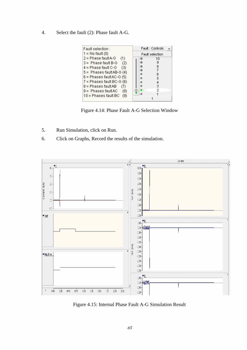
65
4. Select the fault (2): Phase fault A-G.
Figure 4.14: Phase Fault A-G Selection Window
5. Run Simulation, click on Run.
6. Click on Graphs, Record the results of the simulation.
Figure 4.15: Internal Phase Fault A-G Simulation Result
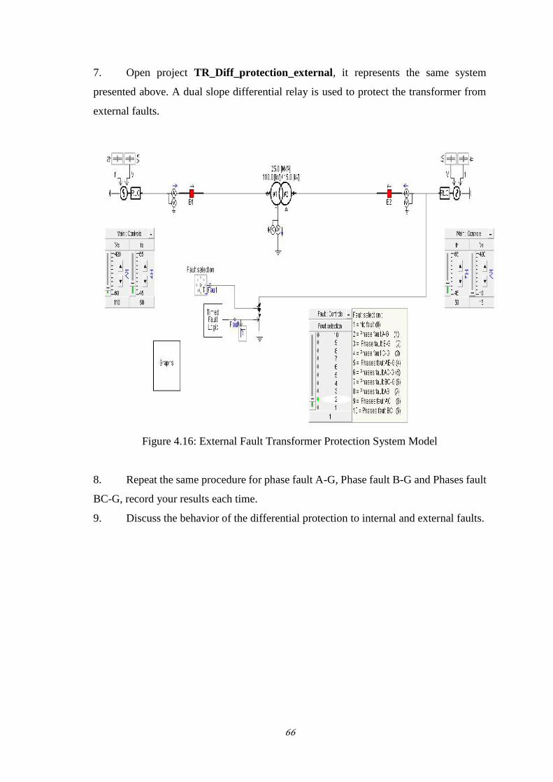
66
7. Open project TR_Diff_protection_external, it represents the same system
presented above. A dual slope differential relay is used to protect the transformer from
external faults.
Figure 4.16: External Fault Transformer Protection System Model
8. Repeat the same procedure for phase fault A-G, Phase fault B-G and Phases fault
BC-G, record your results each time.
9. Discuss the behavior of the differential protection to internal and external faults.
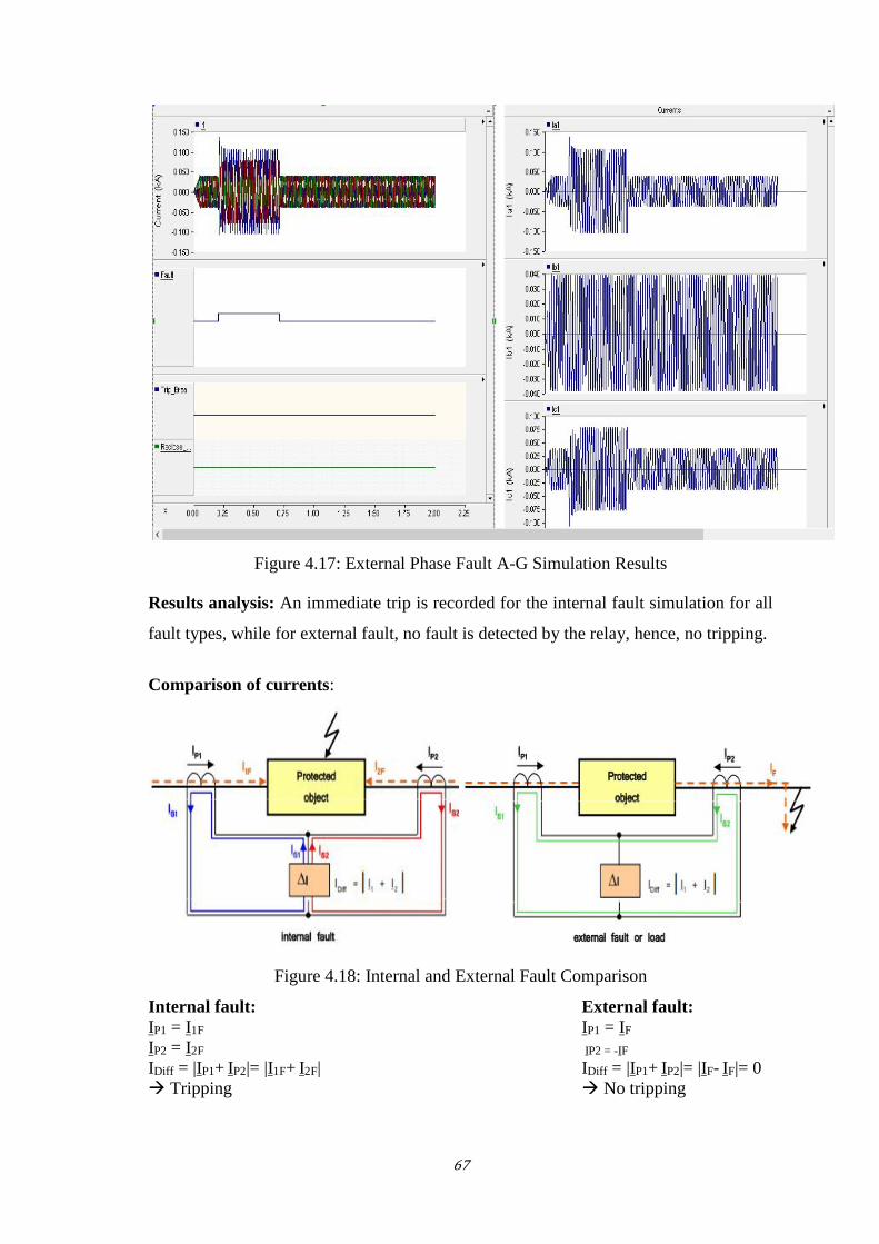
67
Figure 4.17: External Phase Fault A-G Simulation Results
Results analysis: An immediate trip is recorded for the internal fault simulation for all
fault types, while for external fault, no fault is detected by the relay, hence, no tripping.
Comparison of currents:
Figure 4.18: Internal and External Fault Comparison
Internal fault: External fault:IP1 = I1F IP1 = IF
IP2 = I2F IP2 = -IF
IDiff = |IP1+ IP2|= |I1F+ I2F| IDiff = |IP1+ IP2|= |IF- IF|= 0 Tripping No tripping
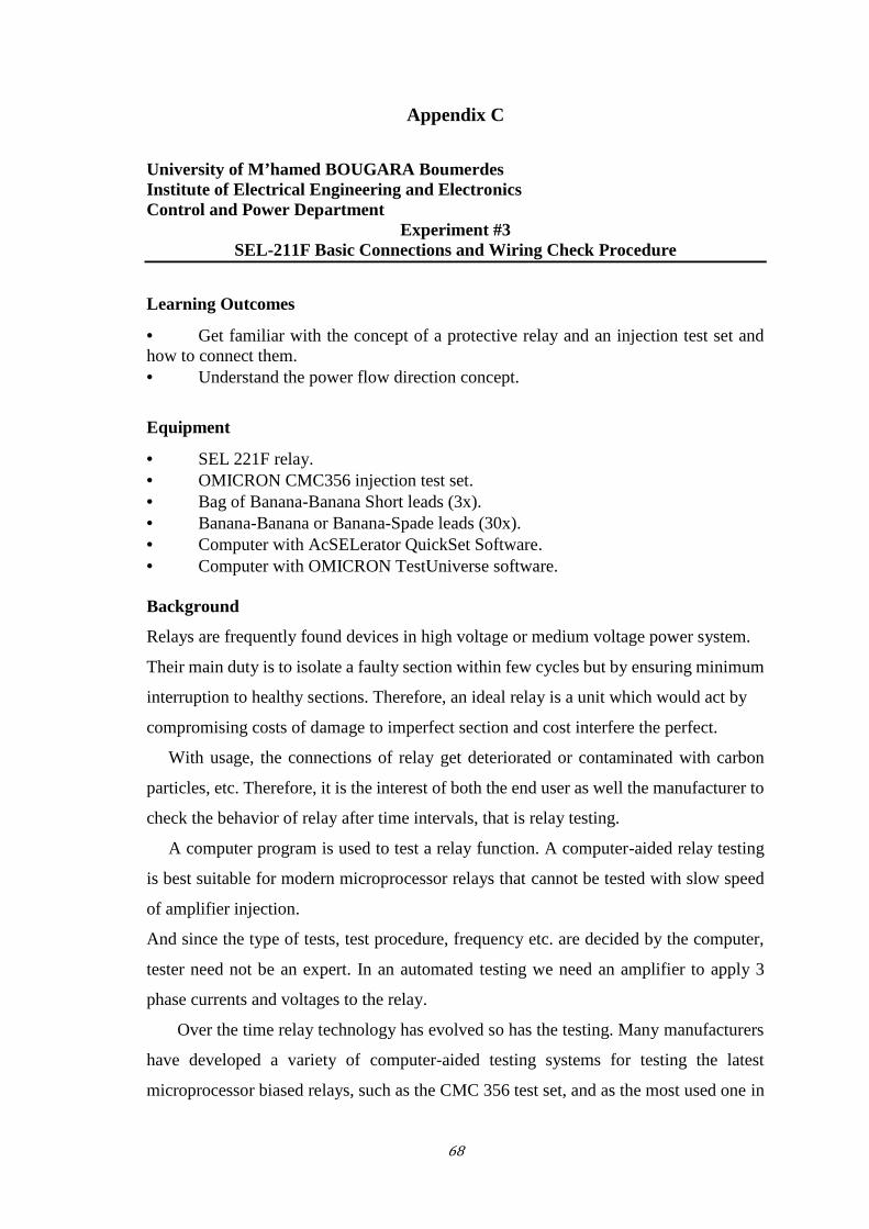
68
Appendix C
University of M’hamed BOUGARA BoumerdesInstitute of Electrical Engineering and ElectronicsControl and Power Department
Experiment #3SEL-211F Basic Connections and Wiring Check Procedure
Learning Outcomes
Get familiar with the concept of a protective relay and an injection test set andhow to connect them. Understand the power flow direction concept.
Equipment
SEL 221F relay. OMICRON CMC356 injection test set. Bag of Banana-Banana Short leads (3x). Banana-Banana or Banana-Spade leads (30x). Computer with AcSELerator QuickSet Software. Computer with OMICRON TestUniverse software.
Background
Relays are frequently found devices in high voltage or medium voltage power system.
Their main duty is to isolate a faulty section within few cycles but by ensuring minimum
interruption to healthy sections. Therefore, an ideal relay is a unit which would act by
compromising costs of damage to imperfect section and cost interfere the perfect.
With usage, the connections of relay get deteriorated or contaminated with carbon
particles, etc. Therefore, it is the interest of both the end user as well the manufacturer to
check the behavior of relay after time intervals, that is relay testing.
A computer program is used to test a relay function. A computer-aided relay testing
is best suitable for modern microprocessor relays that cannot be tested with slow speed
of amplifier injection.
And since the type of tests, test procedure, frequency etc. are decided by the computer,
tester need not be an expert. In an automated testing we need an amplifier to apply 3
phase currents and voltages to the relay.
Over the time relay technology has evolved so has the testing. Many manufacturers
have developed a variety of computer-aided testing systems for testing the latest
microprocessor biased relays, such as the CMC 356 test set, and as the most used one in
69
our country for its high accuracy and the ability of testing many relay functions in a single
module, moreover, it confirms to the IEC60255-151 measuring relay and protective
equipment standards.
Equipment Used
SEL 221 Relay
The SEL-221F is designed to protect transmission, sub-transmission, and distribution
lines for all fault types. The relay has three zones of phase-to-phase and phase-to-ground
mho distance elements with independent timers. Distance elements are polarized using
positive-sequence memory voltage.
SEL 221F generates an eleven-cycle event report after each fault, or upon command.
The report provides four cycles of pre-fault data and seven cycles of fault data. The data
includes voltages, currents, relay elements, and relay inputs and outputs. The report also
shows the calculated fault location, time and date of event, and relay settings. This
information simplifies post-fault analysis and improves understanding of protective
scheme operation.
OMICRON Test Set CMC 356
The OMICRON test set CMC 356 is a universal test set that is used all around the world
to test relays’ operation. The test set has six current and four voltage output channels
which are continuously and independently adjustable in amplitude, phase and frequency.
All outputs are overload and short-circuit proof and are protected against external high-
voltage transient signals and over-temperature. The test set also has digital 10 input and
4 output ports.
The analog test signals are generated digitally using DSP technology. This, in
combination with the use of additional error correction algorithms, results in accurate
testing signals even at small amplitudes.
The output channels are continuously and independently adjustable in amplitude,
phase and frequency. All outputs are overload and short-circuit proof and are protected
against external high-voltage transient signals and over-temperature. The signals injected
to the relay can be specified through the pc software Test Universe.
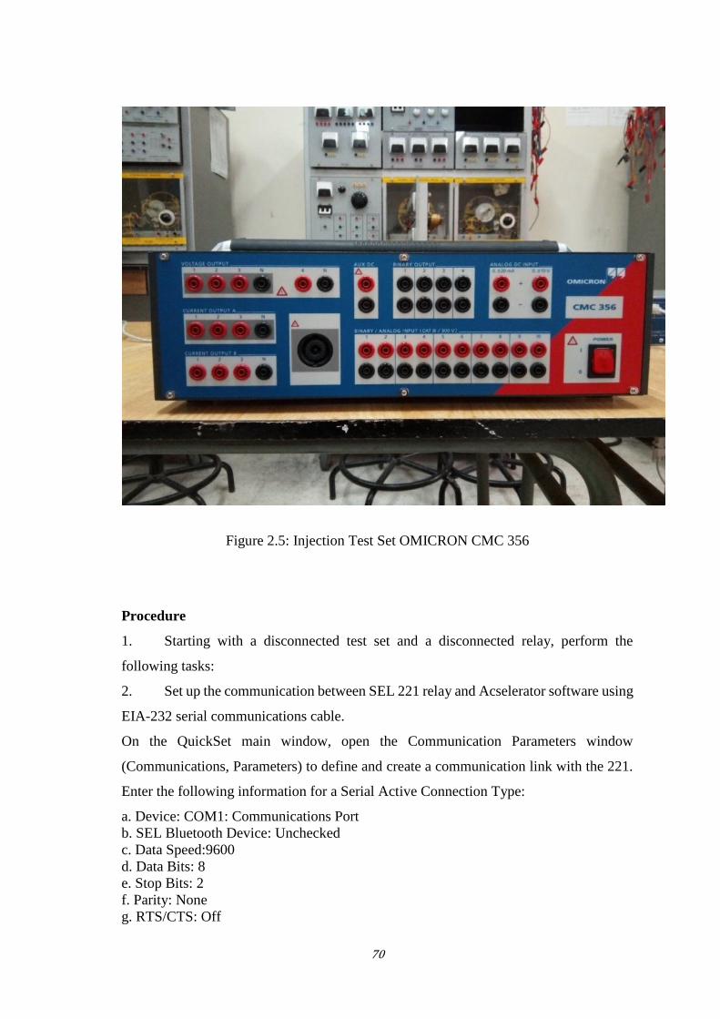
70
Figure 2.5: Injection Test Set OMICRON CMC 356
Procedure
1. Starting with a disconnected test set and a disconnected relay, perform the
following tasks:
2. Set up the communication between SEL 221 relay and Acselerator software using
EIA-232 serial communications cable.
On the QuickSet main window, open the Communication Parameters window
(Communications, Parameters) to define and create a communication link with the 221.
Enter the following information for a Serial Active Connection Type:
a. Device: COM1: Communications Portb. SEL Bluetooth Device: Uncheckedc. Data Speed:9600d. Data Bits: 8e. Stop Bits: 2f. Parity: Noneg. RTS/CTS: Off
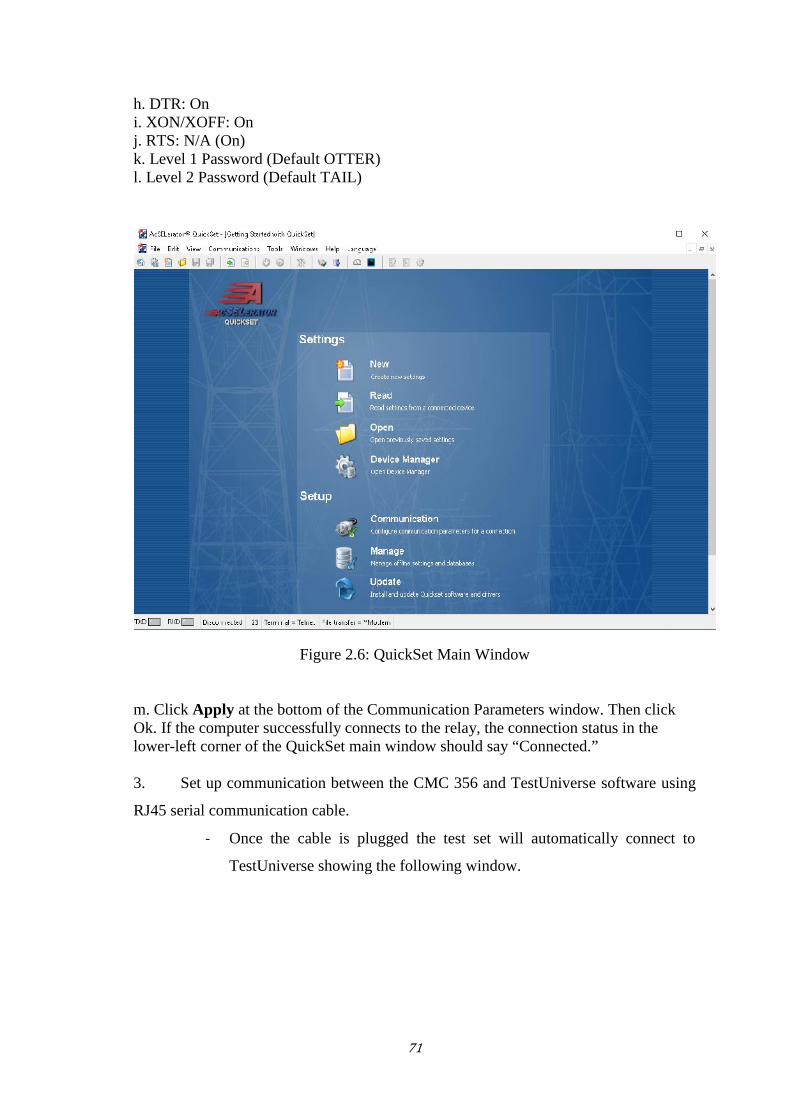
71
h. DTR: Oni. XON/XOFF: Onj. RTS: N/A (On)k. Level 1 Password (Default OTTER)l. Level 2 Password (Default TAIL)
Figure 2.6: QuickSet Main Window
m. Click Apply at the bottom of the Communication Parameters window. Then clickOk. If the computer successfully connects to the relay, the connection status in thelower-left corner of the QuickSet main window should say “Connected.”
3. Set up communication between the CMC 356 and TestUniverse software using
RJ45 serial communication cable.
- Once the cable is plugged the test set will automatically connect to
TestUniverse showing the following window.
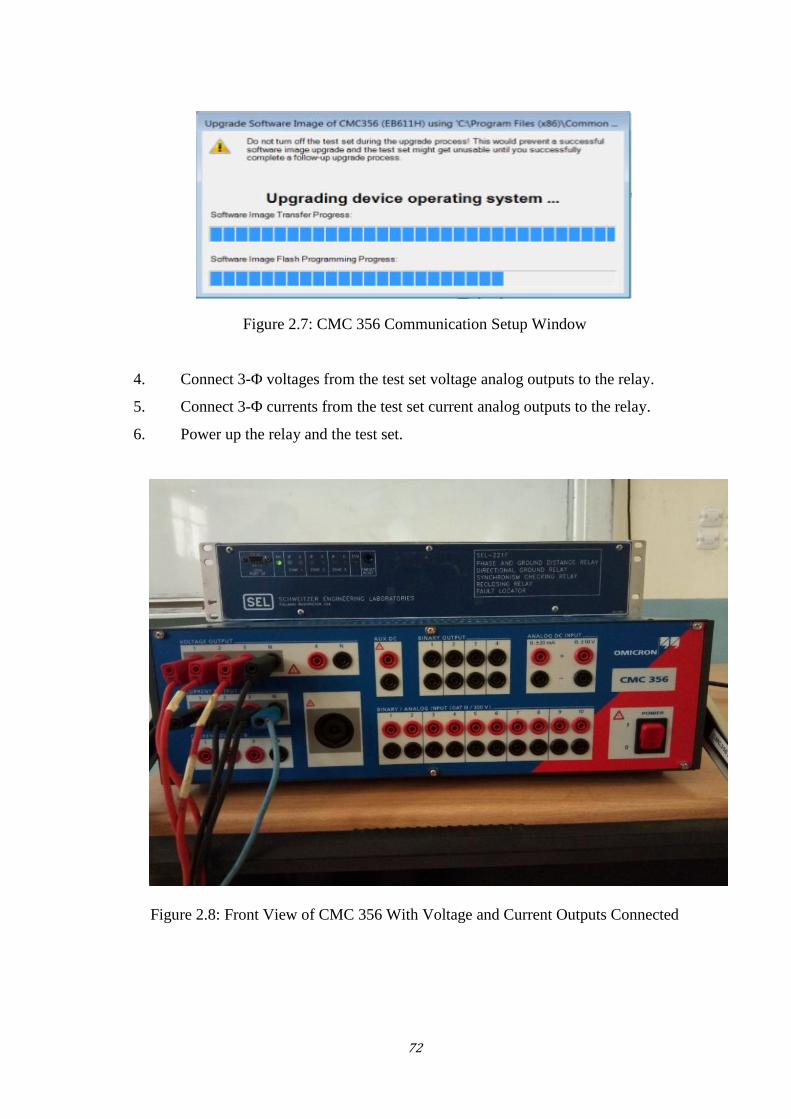
72
Figure 2.7: CMC 356 Communication Setup Window
4. Connect 3-Φ voltages from the test set voltage analog outputs to the relay.
5. Connect 3-Φ currents from the test set current analog outputs to the relay.
6. Power up the relay and the test set.
Figure 2.8: Front View of CMC 356 With Voltage and Current Outputs Connected
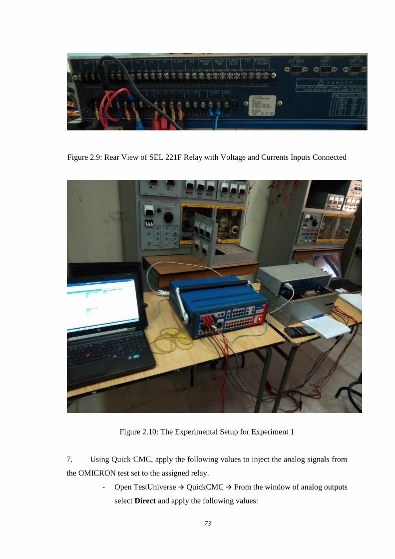
73
Figure 2.9: Rear View of SEL 221F Relay with Voltage and Currents Inputs Connected
Figure 2.10: The Experimental Setup for Experiment 1
7. Using Quick CMC, apply the following values to inject the analog signals from
the OMICRON test set to the assigned relay.
- Open TestUniverse QuickCMC From the window of analog outputs
select Direct and apply the following values:
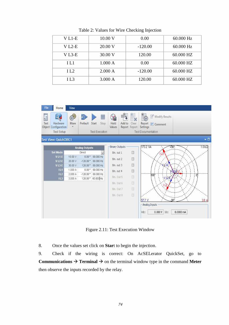
74
Table 2: Values for Wire Checking Injection
V L1-E 10.00 V 0.00 60.000 Hz
V L2-E 20.00 V -120.00 60.000 Hz
V L3-E 30.00 V 120.00 60.000 HZ
I L1 1.000 A 0.00 60.000 HZ
I L2 2.000 A -120.00 60.000 HZ
I L3 3.000 A 120.00 60.000 HZ
Figure 2.11: Test Execution Window
8. Once the values set click on Start to begin the injection.
9. Check if the wiring is correct: On AcSELerator QuickSet, go to
Communications Terminal on the terminal window type in the command Meter
then observe the inputs recorded by the relay.
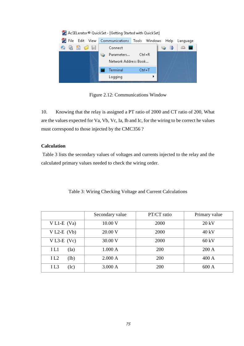
75
Figure 2.12: Communications Window
10. Knowing that the relay is assigned a PT ratio of 2000 and CT ratio of 200, What
are the values expected for Va, Vb, Vc, Ia, Ib and Ic, for the wiring to be correct he values
must correspond to those injected by the CMC356 ?
Calculation
Table 3 lists the secondary values of voltages and currents injected to the relay and the
calculated primary values needed to check the wiring order.
Table 3: Wiring Checking Voltage and Current Calculations
Secondary value PT/CT ratio Primary value
V L1-E (Va) 10.00 V 2000 20 kV
V L2-E (Vb) 20.00 V 2000 40 kV
V L3-E (Vc) 30.00 V 2000 60 kV
I L1 (Ia) 1.000 A 200 200 A
I L2 (Ib) 2.000 A 200 400 A
I L3 (Ic) 3.000 A 200 600 A
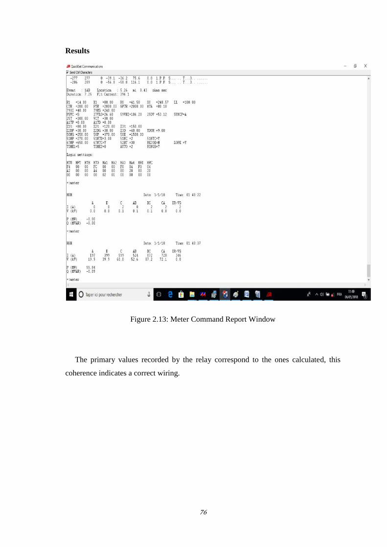
76
Results
Figure 2.13: Meter Command Report Window
The primary values recorded by the relay correspond to the ones calculated, this
coherence indicates a correct wiring.
77
Appendix DUniversity of M’hamed BOUGARA BoumerdesInstitute of Electrical Engineering and ElectronicsControl and Power Department
Experiment #4SEL-211 Relay Configuration and Metering Check Procedure
Learning Outcomes
Learn how to properly set SEL 221 relay and the test set.
Understand the power flow direction concept.
Equipment
SEL 221F relay OMICRON CMC356 injection test set Bag of Banana-Banana Short Leads (3x) * Banana-Banana or Banana-Spade Leads (30x) Computer with AcSELerator QuickSet Software Computer with OMICRON TestUniverse software
Prelab
1. Assume that the full load ratings of the transmission lines of Table 1 are equal to
their CTRs. For example, if the CTR is 3000/5, then the transmission line full loading is
3000A.
2. Use the given information as shown in Table 3, calculate the secondary phasor
values of the balanced three-phase systems as follows:
a. Va-N, Vb-N, Vc-N
b. Ia, Ib, Ic
3. Calculate the primary three phase values of S, MW, MVAR
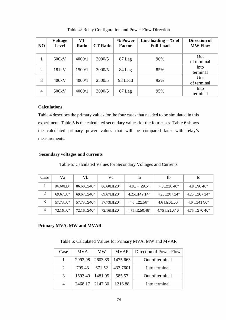
78
Table 4: Relay Configuration and Power Flow Direction
NOVoltageLevel
VTRatio CT Ratio
% PowerFactor
Line loading = % ofFull Load
Direction ofMW Flow
1 600kV 4000/1 3000/5 87 Lag 96%Out
of terminal
2 181kV 1500/1 3000/5 84 Lag 85%Into
terminal
3 400kV 4000/1 2500/5 93 Lead 92%Out
of terminal
4 500kV 4000/1 3000/5 87 Lag 95%Into
terminal
Calculations
Table 4 describes the primary values for the four cases that needed to be simulated in this
experiment. Table 5 is the calculated secondary values for the four cases. Table 6 shows
the calculated primary power values that will be compared later with relay’s
measurements.
Secondary voltages and currents
Table 5: Calculated Values for Secondary Voltages and Currents
Primary MVA, MW and MVAR
Table 6: Calculated Values for Primary MVA, MW and MVAR
Case MVA MW MVAR Direction of Power Flow
1 2992.98 2603.89 1475.663 Out of terminal
2 799.43 671.52 433.7601 Into terminal
3 1593.49 1481.95 585.57 Out of terminal
4 2468.17 2147.30 1216.88 Into terminal
Case Va Vb Vc Ia Ib Ic
1 86.60∠0° 86.60∠240° 86.60∠120° 4.8∠ − 29.5° 4.8∠210.46° 4.8 ∠90.46°2 69.67∠0° 69.67∠240° 69.67∠120° 4.25∠147.14° 4.25∠207.14° 4.25 ∠267.14°3 57.73∠0° 57.73∠240° 57.73∠120° 4.6 ∠21.56° 4.6 ∠261.56° 4.6 ∠141.56°4 72.16∠0° 72.16∠240° 72.16∠120° 4.75 ∠150.46° 4.75 ∠210.46° 4.75 ∠270.46°
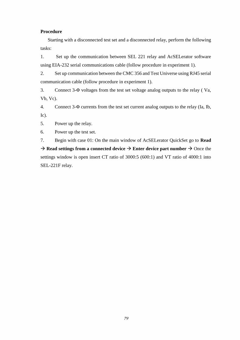
79
Procedure
Starting with a disconnected test set and a disconnected relay, perform the following
tasks:
1. Set up the communication between SEL 221 relay and AcSELerator software
using EIA-232 serial communications cable (follow procedure in experiment 1).
2. Set up communication between the CMC 356 and Test Universe using RJ45 serial
communication cable (follow procedure in experiment 1).
3. Connect 3-Φ voltages from the test set voltage analog outputs to the relay ( Va,
Vb, Vc).
4. Connect 3-Φ currents from the test set current analog outputs to the relay (Ia, Ib,
Ic).
5. Power up the relay.
6. Power up the test set.
7. Begin with case 01: On the main window of AcSELerator QuickSet go to Read
Read settings from a connected device Enter device part number Once the
settings window is open insert CT ratio of 3000:5 (600:1) and VT ratio of 4000:1 into
SEL-221F relay.
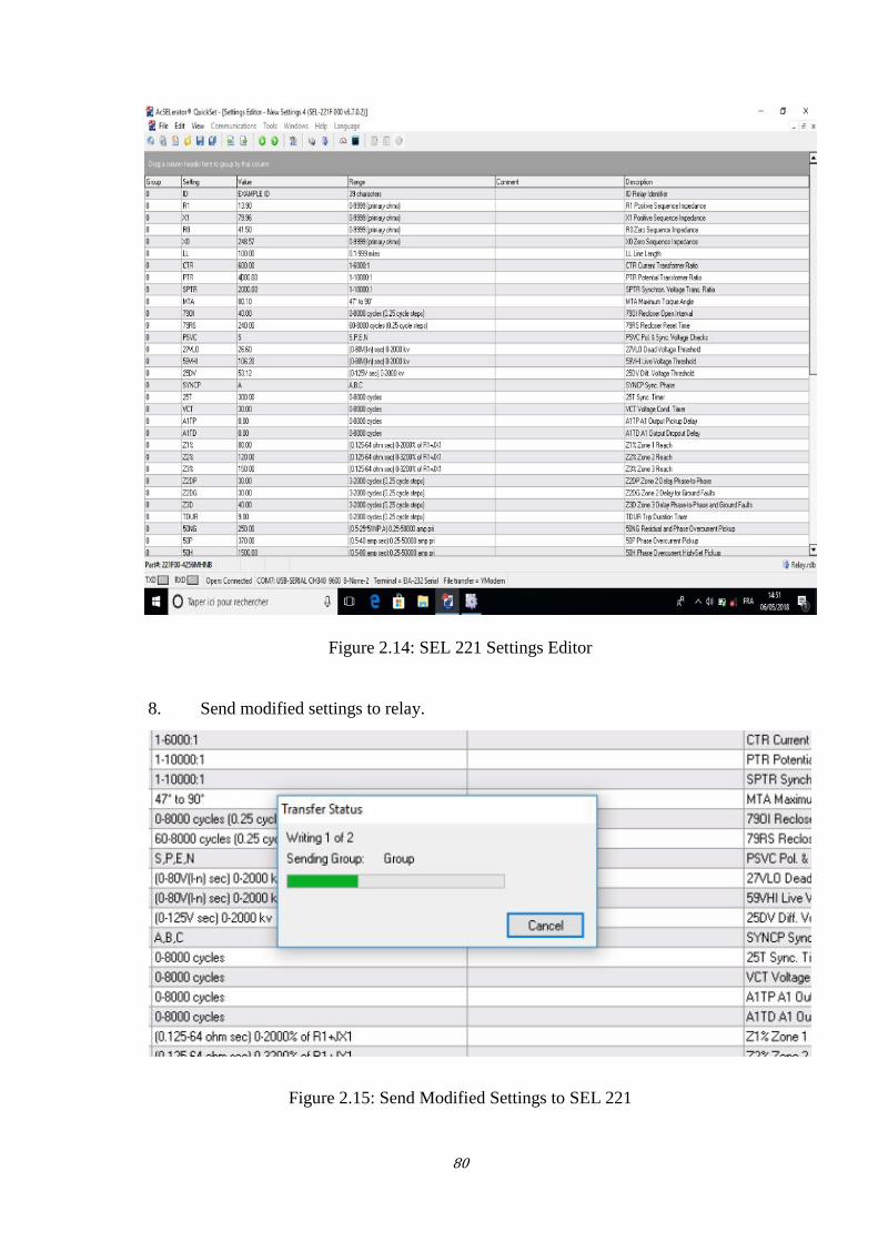
80
Figure 2.14: SEL 221 Settings Editor
8. Send modified settings to relay.
Figure 2.15: Send Modified Settings to SEL 221
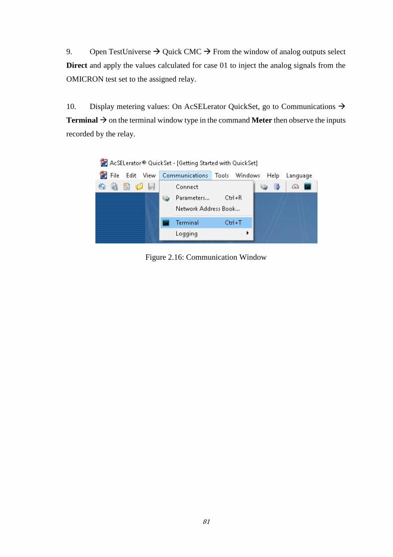
81
9. Open TestUniverse Quick CMC From the window of analog outputs select
Direct and apply the values calculated for case 01 to inject the analog signals from the
OMICRON test set to the assigned relay.
10. Display metering values: On AcSELerator QuickSet, go to Communications
Terminal on the terminal window type in the command Meter then observe the inputs
recorded by the relay.
Figure 2.16: Communication Window
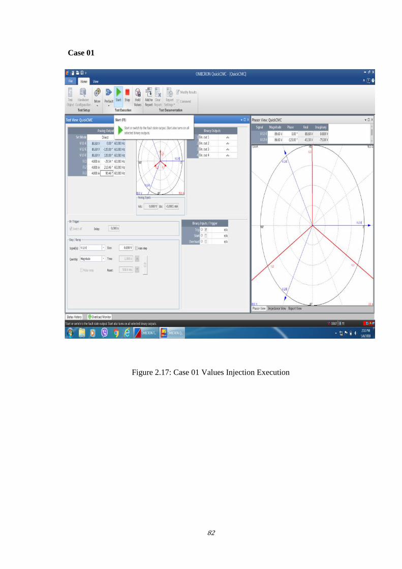
82
Case 01
Figure 2.17: Case 01 Values Injection Execution
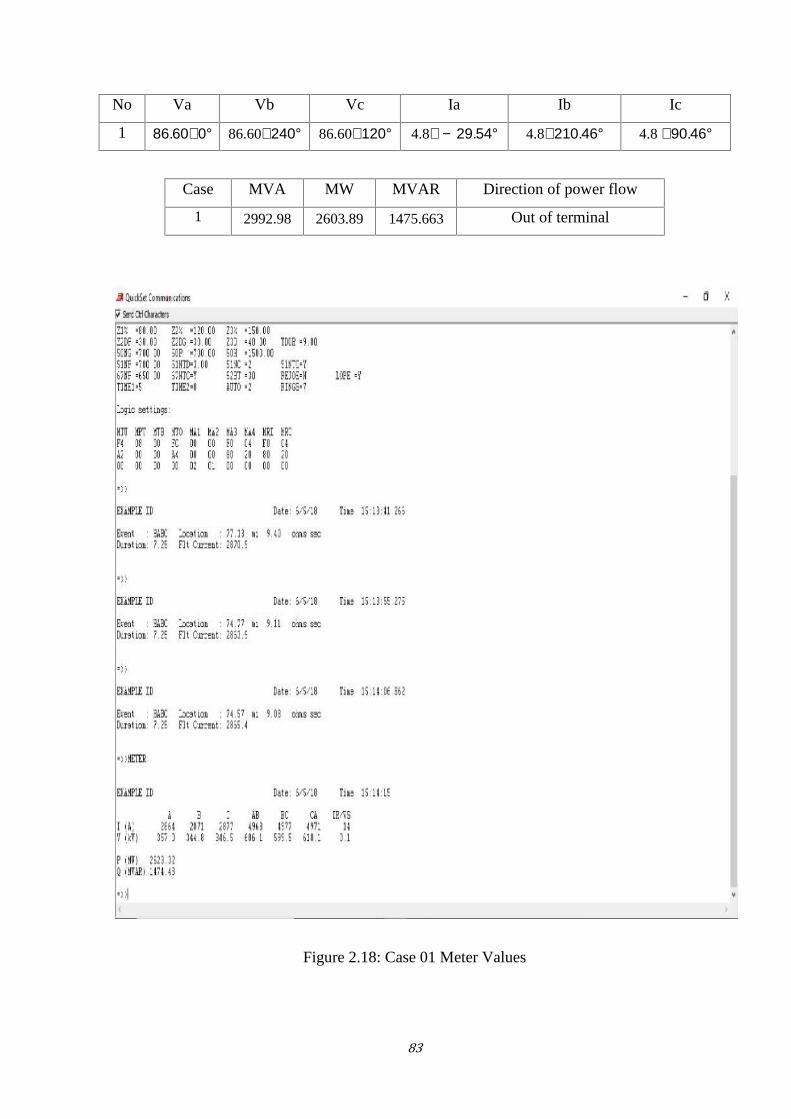
83
No Va Vb Vc Ia Ib Ic
1 86.60∠0° 86.60∠240° 86.60∠120° 4.8∠ − 29.54° 4.8∠210.46° 4.8 ∠90.46°Case MVA MW MVAR Direction of power flow
1 2992.98 2603.89 1475.663 Out of terminal
Figure 2.18: Case 01 Meter Values
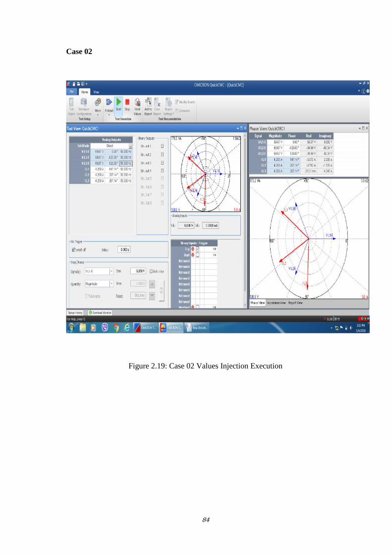
84
Case 02
Figure 2.19: Case 02 Values Injection Execution
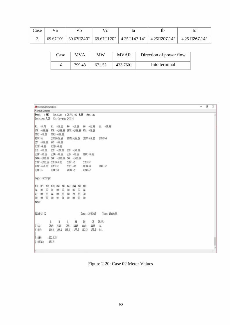
85
Case Va Vb Vc Ia Ib Ic
2 69.67∠0° 69.67∠240° 69.67∠120° 4.25∠147.14° 4.25∠207.14° 4.25 ∠267.14°Case MVA MW MVAR Direction of power flow
2 799.43 671.52 433.7601 Into terminal
Figure 2.20: Case 02 Meter Values
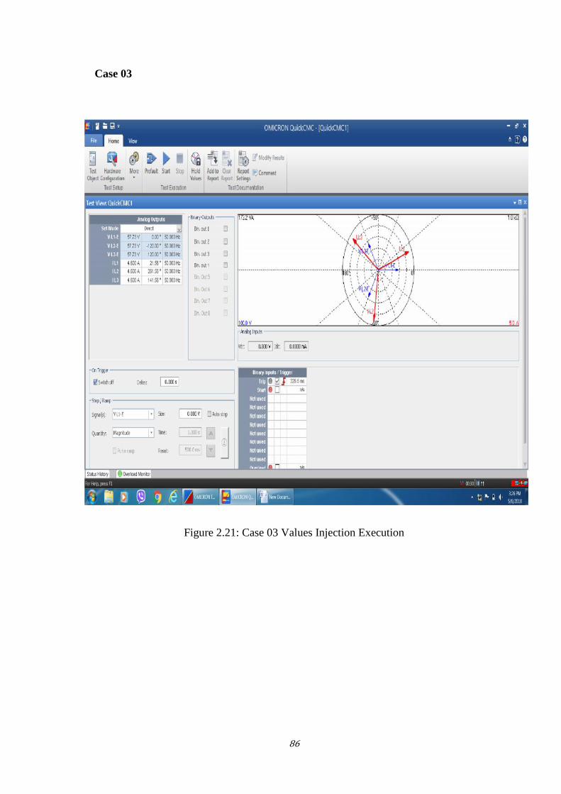
86
Case 03
Figure 2.21: Case 03 Values Injection Execution
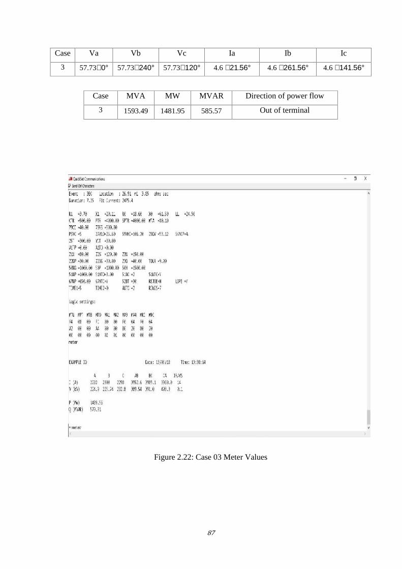
87
Case Va Vb Vc Ia Ib Ic
3 57.73∠0° 57.73∠240° 57.73∠120° 4.6 ∠21.56° 4.6 ∠261.56° 4.6 ∠141.56°Case MVA MW MVAR Direction of power flow
3 1593.49 1481.95 585.57 Out of terminal
Figure 2.22: Case 03 Meter Values
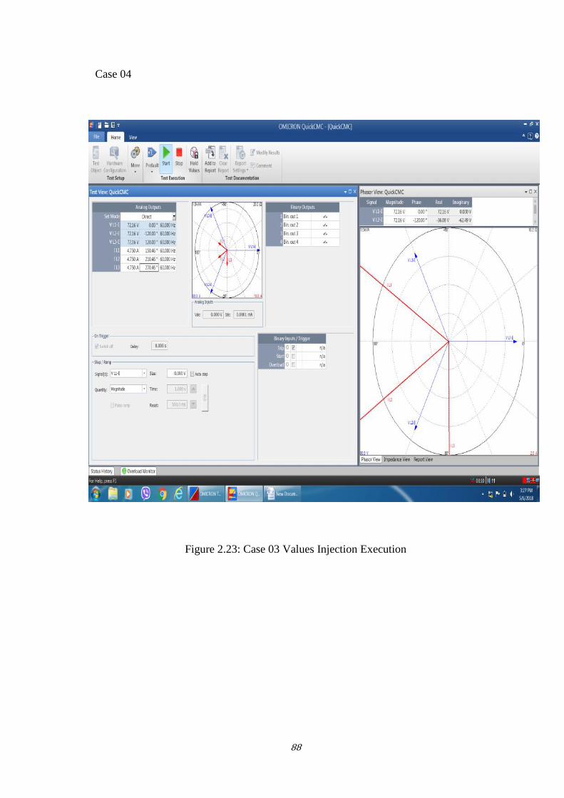
88
Case 04
Figure 2.23: Case 03 Values Injection Execution
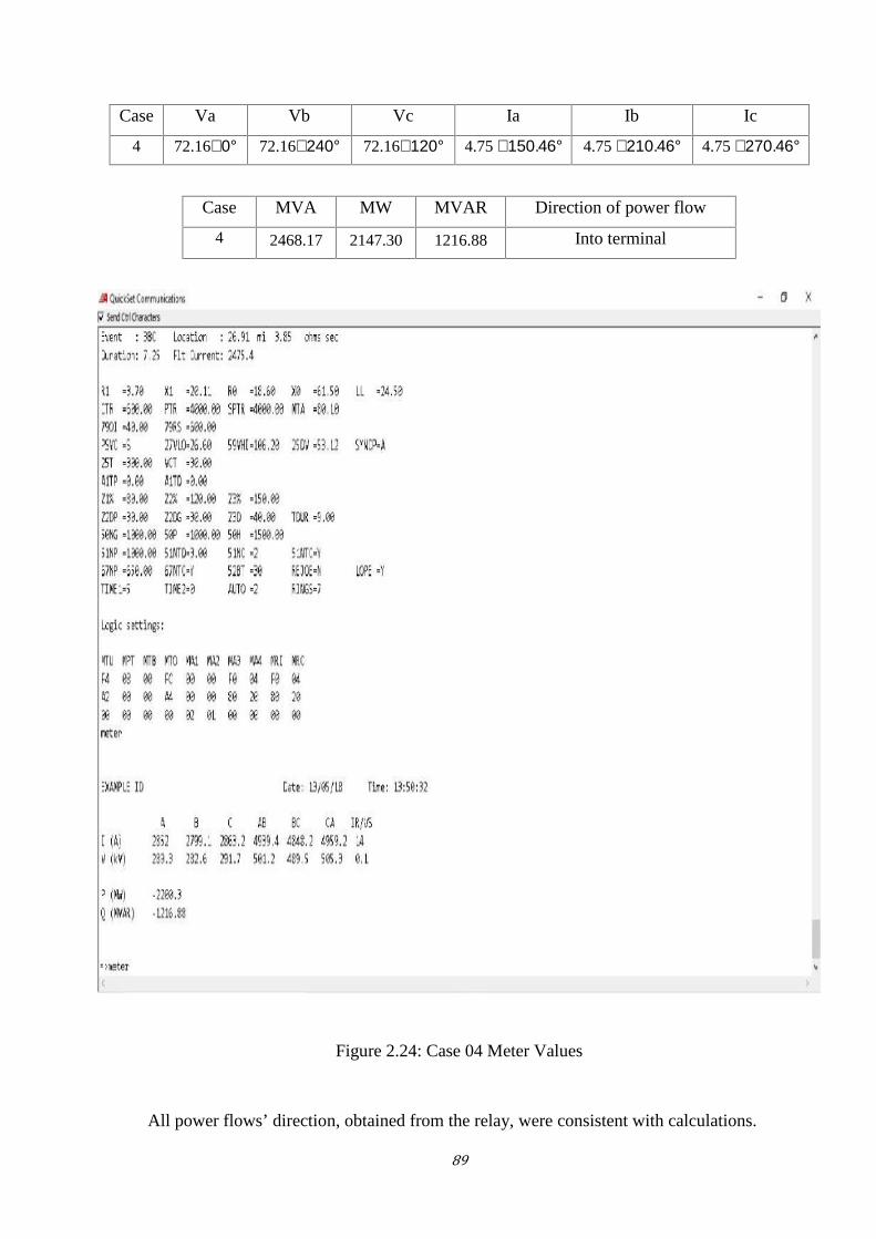
89
Case Va Vb Vc Ia Ib Ic
4 72.16∠0° 72.16∠240° 72.16∠120° 4.75 ∠150.46° 4.75 ∠210.46° 4.75 ∠270.46°Case MVA MW MVAR Direction of power flow
4 2468.17 2147.30 1216.88 Into terminal
Figure 2.24: Case 04 Meter Values
All power flows’ direction, obtained from the relay, were consistent with calculations.
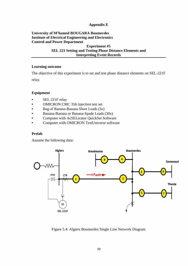
90
Appendix E
University of M’hamed BOUGARA BoumerdesInstitute of Electrical Engineering and ElectronicsControl and Power Department
Experiment #5SEL 221 Setting and Testing Phase Distance Elements and
Interpreting Event Records
Learning outcome
The objective of this experiment is to set and test phase distance elements on SEL-221F
relay.
Equipment
SEL 221F relay OMICRON CMC 356 injection test set Bag of Banana-Banana Short Leads (3x) Banana-Banana or Banana-Spade Leads (30x) Computer with AcSELerator QuickSet Software Computer with OMICRON TestUniverse software
Prelab
Assume the following data:
Figure 5.4: Algiers Boumerdes Single Line Network Diagram
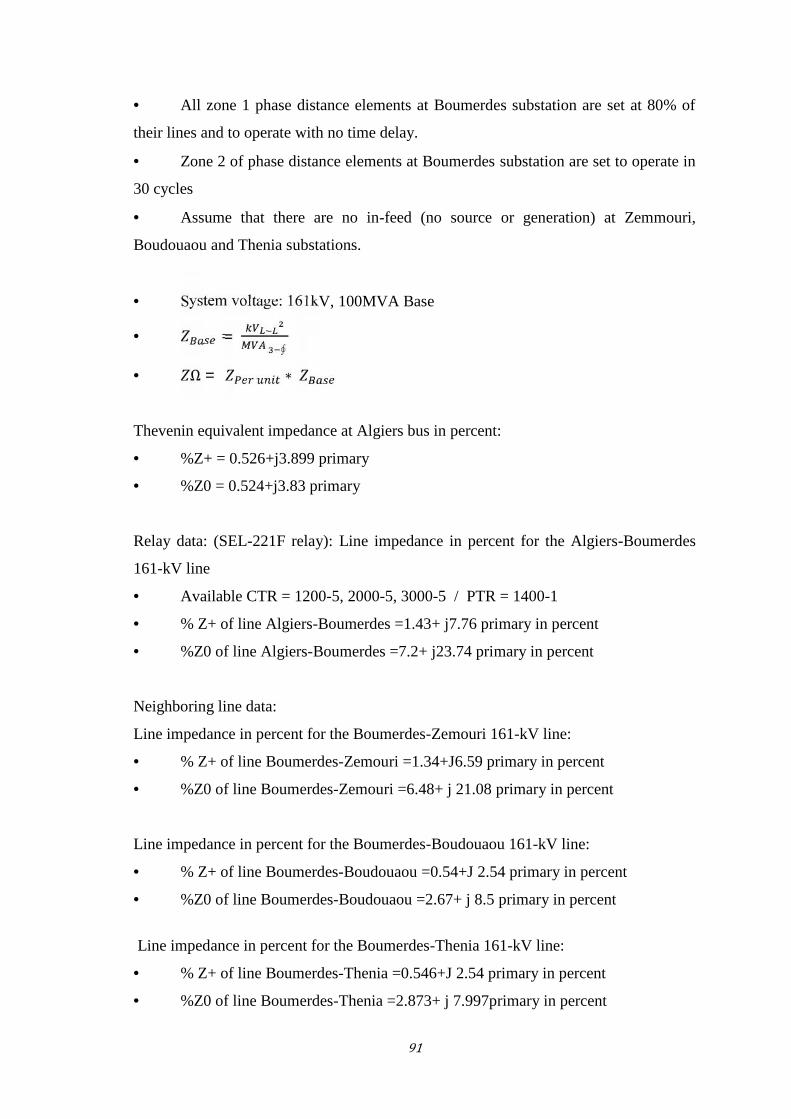
91
All zone 1 phase distance elements at Boumerdes substation are set at 80% of
their lines and to operate with no time delay.
Zone 2 of phase distance elements at Boumerdes substation are set to operate in
30 cycles
Assume that there are no in-feed (no source or generation) at Zemmouri,
Boudouaou and Thenia substations.
System voltage: 161kV, 100MVA Base
= ∮ Ω = ∗Thevenin equivalent impedance at Algiers bus in percent:
• %Z+ = 0.526+j3.899 primary
• %Z0 = 0.524+j3.83 primary
Relay data: (SEL-221F relay): Line impedance in percent for the Algiers-Boumerdes
161-kV line
• Available CTR = 1200-5, 2000-5, 3000-5 / PTR = 1400-1
• % Z+ of line Algiers-Boumerdes =1.43+ j7.76 primary in percent
• %Z0 of line Algiers-Boumerdes =7.2+ j23.74 primary in percent
Neighboring line data:
Line impedance in percent for the Boumerdes-Zemouri 161-kV line:
• % Z+ of line Boumerdes-Zemouri =1.34+J6.59 primary in percent
• %Z0 of line Boumerdes-Zemouri =6.48+ j 21.08 primary in percent
Line impedance in percent for the Boumerdes-Boudouaou 161-kV line:
• % Z+ of line Boumerdes-Boudouaou =0.54+J 2.54 primary in percent
• %Z0 of line Boumerdes-Boudouaou =2.67+ j 8.5 primary in percent
Line impedance in percent for the Boumerdes-Thenia 161-kV line:
• % Z+ of line Boumerdes-Thenia =0.546+J 2.54 primary in percent
• %Z0 of line Boumerdes-Thenia =2.873+ j 7.997primary in percent

92
Step 1
Calculate z1 and z2 mho phase distance elements for the relay at Algiers
substation that is used to protect the Algiers Boumerdes 164 kV line.
1. Calculate the following line data for line Algiers-Boumerdes 161-kV line:
a. Z+ line = _____________ primary ohms
b. Z0 line = _____________ primary ohms
c. Line length = 24.5 miles
2. Select an appropriate CTR to make sure that your secondary fault currents will
not exceed 12.5A for OMICRON test set.
3. Perform the following calculations:
a. Set the reach for zone 1 mho phase distance
b. Set an operating time for the Z1P element
c. Set the reach for zone 2 mho phase distance
d. Set an operating time for the Z2P element
4. Fill in the following data:
PrimaryOhms
SecondaryOhms
OperatingTime inCycles
SEL RelaySetting
Parameter
SEL RelayWord Bit
Z1P
Z2P
Step 2 : Test Z1 and Z2 Mho phase distance element
(Limit the test current to 12.5A or less)
1) Calculate the fault currents that the relay at Algiers substation sees for the following
faults:
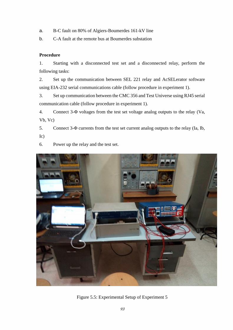
93
a. B-C fault on 80% of Algiers-Boumerdes 161-kV line
b. C-A fault at the remote bus at Boumerdes substation
Procedure
1. Starting with a disconnected test set and a disconnected relay, perform the
following tasks:
2. Set up the communication between SEL 221 relay and AcSELerator software
using EIA-232 serial communications cable (follow procedure in experiment 1).
3. Set up communication between the CMC 356 and Test Universe using RJ45 serial
communication cable (follow procedure in experiment 1).
4. Connect 3-Φ voltages from the test set voltage analog outputs to the relay (Va,
Vb, Vc)
5. Connect 3-Φ currents from the test set current analog outputs to the relay (Ia, Ib,
Ic)
6. Power up the relay and the test set.
Figure 5.5: Experimental Setup of Experiment 5
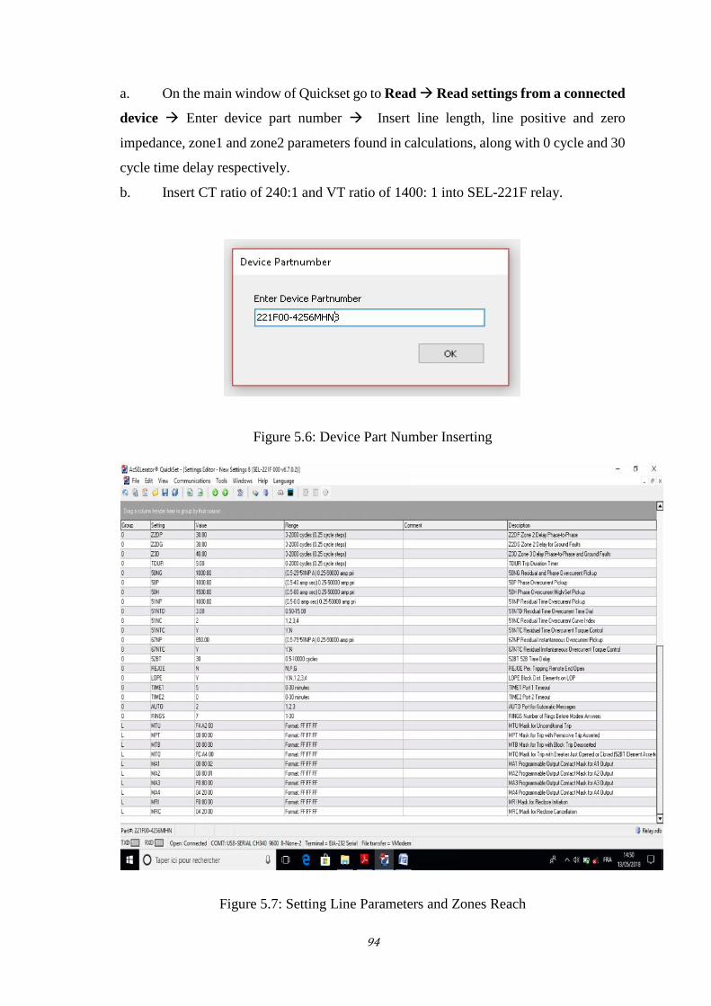
94
a. On the main window of Quickset go to ReadRead settings from a connected
device Enter device part number Insert line length, line positive and zero
impedance, zone1 and zone2 parameters found in calculations, along with 0 cycle and 30
cycle time delay respectively.
b. Insert CT ratio of 240:1 and VT ratio of 1400: 1 into SEL-221F relay.
Figure 5.6: Device Part Number Inserting
Figure 5.7: Setting Line Parameters and Zones Reach
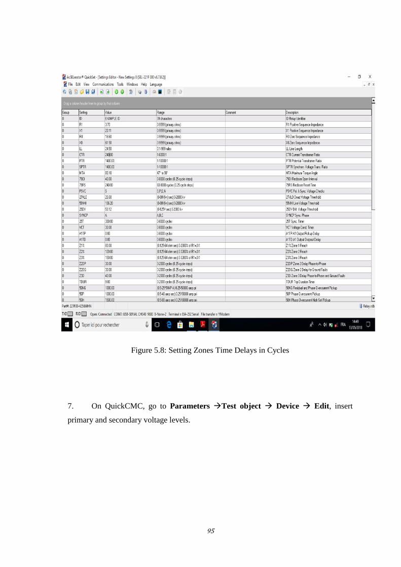
95
Figure 5.8: Setting Zones Time Delays in Cycles
7. On QuickCMC, go to Parameters Test object Device Edit, insert
primary and secondary voltage levels.
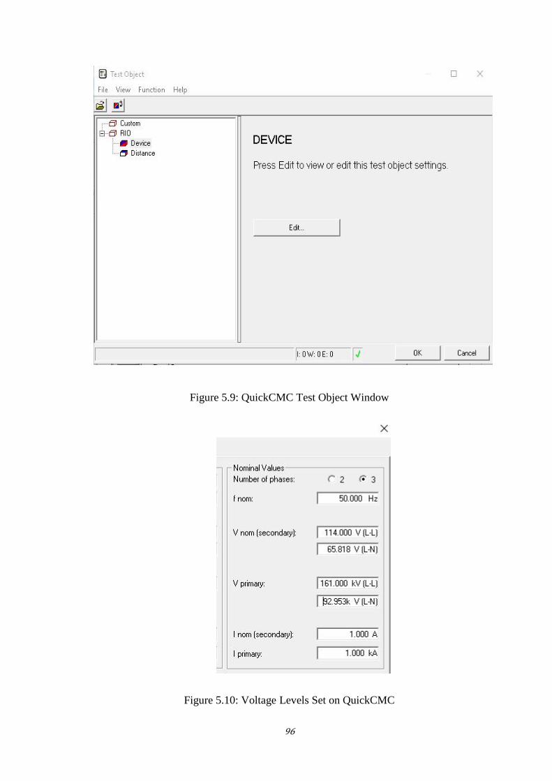
96
Figure 5.9: QuickCMC Test Object Window
Figure 5.10: Voltage Levels Set on QuickCMC
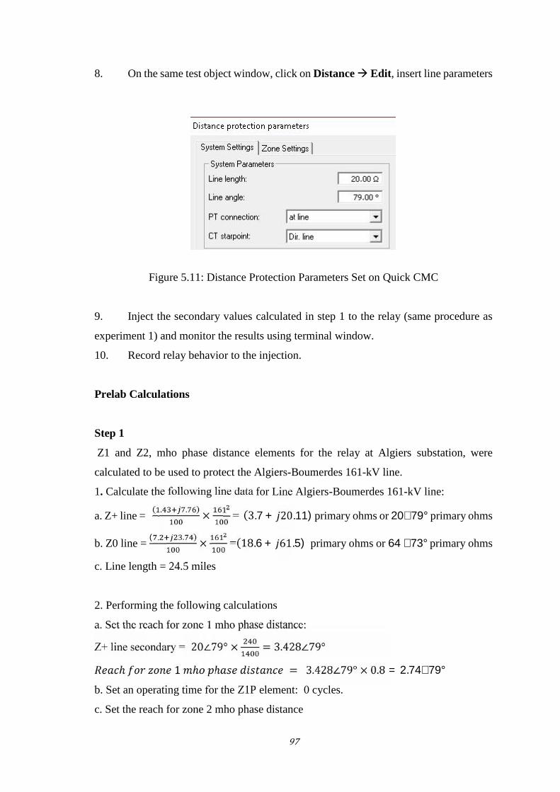
97
8. On the same test object window, click on Distance Edit, insert line parameters
Figure 5.11: Distance Protection Parameters Set on Quick CMC
9. Inject the secondary values calculated in step 1 to the relay (same procedure as
experiment 1) and monitor the results using terminal window.
10. Record relay behavior to the injection.
Prelab Calculations
Step 1
Z1 and Z2, mho phase distance elements for the relay at Algiers substation, were
calculated to be used to protect the Algiers-Boumerdes 161-kV line.
1. Calculate the following line data for Line Algiers-Boumerdes 161-kV line:
a. Z+ line =( . . ) × = (3.7 + 20.11) primary ohms or 20∠79° primary ohms
b. Z0 line =( . . ) × =(18.6 + 61.5) primary ohms or 64 ∠73° primary ohms
c. Line length = 24.5 miles
2. Performing the following calculations
a. Set the reach for zone 1 mho phase distance:
Z+ line secondary = 20∠79° × = 3.428∠79°ℎ 1 ℎ ℎ = 3.428∠79° × 0.8 = 2.74∠79°b. Set an operating time for the Z1P element: 0 cycles.
c. Set the reach for zone 2 mho phase distance
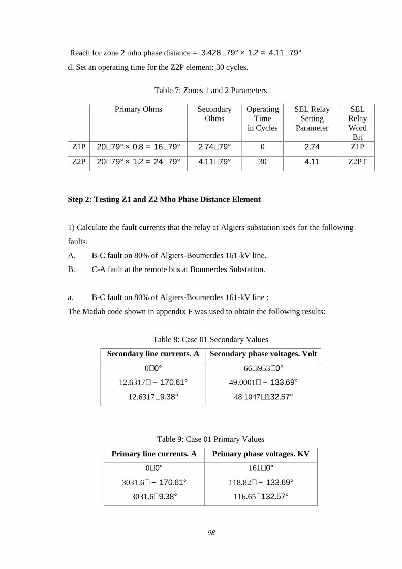
98
Reach for zone 2 mho phase distance = 3.428∠79° × 1.2 = 4.11∠79°d. Set an operating time for the Z2P element: 30 cycles.
Table 7: Zones 1 and 2 Parameters
Step 2: Testing Z1 and Z2 Mho Phase Distance Element
1) Calculate the fault currents that the relay at Algiers substation sees for the following
faults:
A. B-C fault on 80% of Algiers-Boumerdes 161-kV line.
B. C-A fault at the remote bus at Boumerdes Substation.
a. B-C fault on 80% of Algiers-Boumerdes 161-kV line :
The Matlab code shown in appendix F was used to obtain the following results:
Table 8: Case 01 Secondary Values
Secondary line currents. A Secondary phase voltages. Volt
0∠0°12.6317∠ − 170.61°
12.6317∠9.38°66.3953∠0°
49.0001∠ − 133.69°48.1047∠132.57°
Table 9: Case 01 Primary Values
Primary line currents. A Primary phase voltages. KV
0∠0°3031.6∠ − 170.61°
3031.6∠9.38°161∠0°
118.82∠ − 133.69°116.65∠132.57°
Primary Ohms SecondaryOhms
OperatingTime
in Cycles
SEL RelaySetting
Parameter
SELRelayWord
BitZ1P 20∠79° × 0.8 = 16∠79° 2.74∠79° 0 2.74 Z1P
Z2P 20∠79° × 1.2 = 24∠79° 4.11∠79° 30 4.11 Z2PT
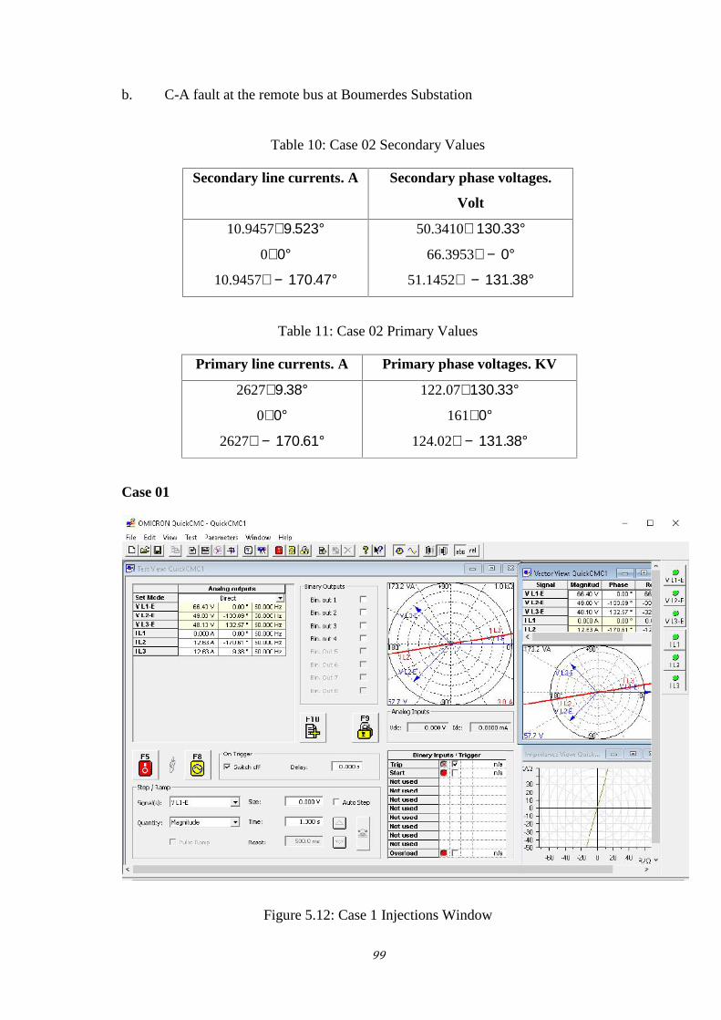
99
b. C-A fault at the remote bus at Boumerdes Substation
Table 10: Case 02 Secondary Values
Secondary line currents. A Secondary phase voltages.
Volt
10.9457∠9.523°0∠0°
10.9457∠ − 170.47°50.3410∠ 130.33°
66.3953∠ − 0°51.1452∠ − 131.38°
Table 11: Case 02 Primary Values
Primary line currents. A Primary phase voltages. KV
2627∠9.38°0∠0°
2627∠ − 170.61°122.07∠130.33°
161∠0°124.02∠ − 131.38°
Case 01
Figure 5.12: Case 1 Injections Window
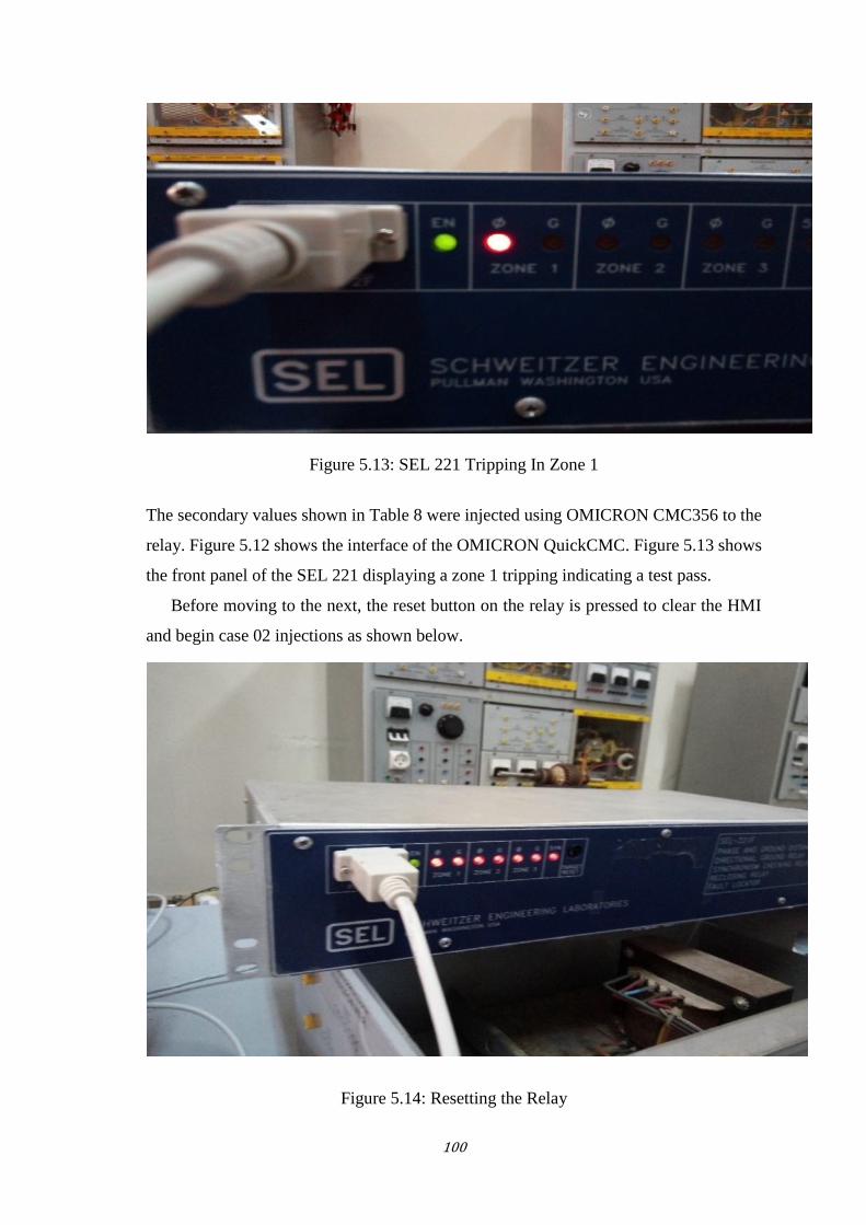
100
Figure 5.13: SEL 221 Tripping In Zone 1
The secondary values shown in Table 8 were injected using OMICRON CMC356 to the
relay. Figure 5.12 shows the interface of the OMICRON QuickCMC. Figure 5.13 shows
the front panel of the SEL 221 displaying a zone 1 tripping indicating a test pass.
Before moving to the next, the reset button on the relay is pressed to clear the HMI
and begin case 02 injections as shown below.
Figure 5.14: Resetting the Relay
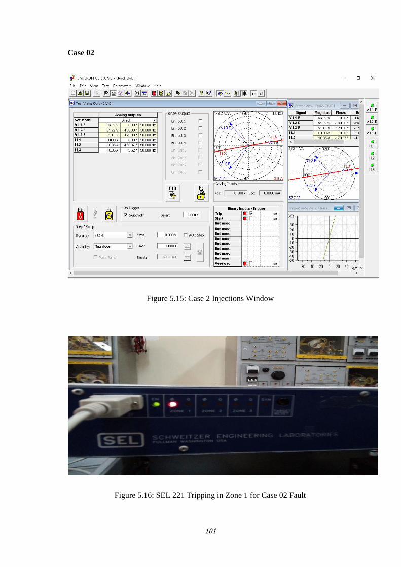
101
Case 02
Figure 5.15: Case 2 Injections Window
Figure 5.16: SEL 221 Tripping in Zone 1 for Case 02 Fault
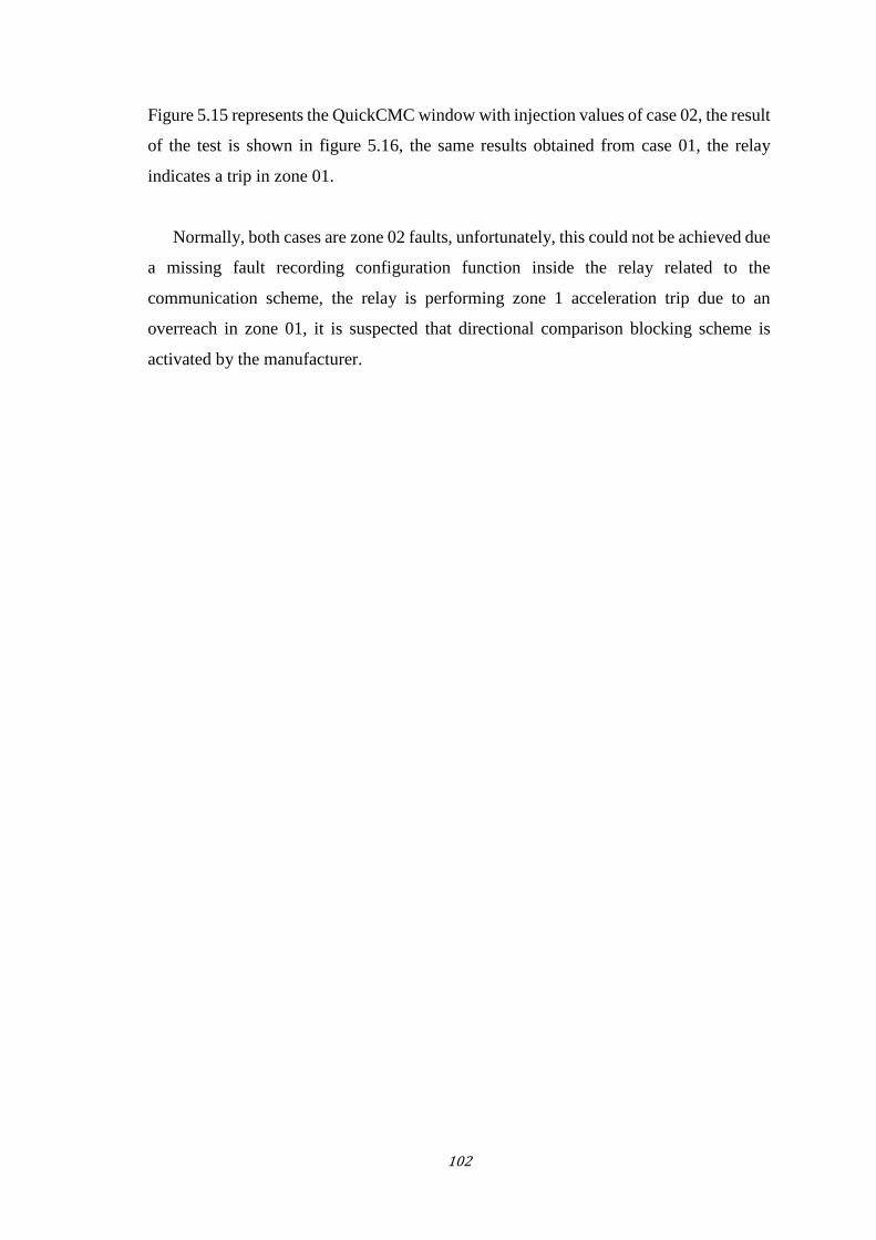
102
Figure 5.15 represents the QuickCMC window with injection values of case 02, the result
of the test is shown in figure 5.16, the same results obtained from case 01, the relay
indicates a trip in zone 01.
Normally, both cases are zone 02 faults, unfortunately, this could not be achieved due
a missing fault recording configuration function inside the relay related to the
communication scheme, the relay is performing zone 1 acceleration trip due to an
overreach in zone 01, it is suspected that directional comparison blocking scheme is
activated by the manufacturer.
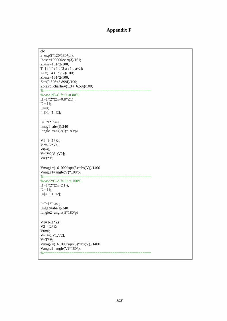
103
Appendix F
clca=exp(i*120/180*pi);Ibase=100000/sqrt(3)/161;Zbase=161^2/100;T=[1 1 1; 1 a^2 a ; 1 a a^2];Z1=(1.43+7.76i)/100;Zbase=161^2/100;Zs=(0.526+3.899i)/100;Zbravo_charlie=(1.34+6.59i)/100;%==================================================%case1:B-C fault at 80%.I1=1/(2*(Zs+0.8*Z1));I2=-I1;I0=0;I=[I0; I1; I2];
I=T*I*Ibase;Imag1=abs(I)/240Iangle1=angle(I)*180/pi
V1=1-I1*Zs;V2=-I2*Zs;V0=0;V=[V0;V1;V2];V=T*V;
Vmag1=(161000/sqrt(3)*abs(V))/1400Vangle1=angle(V)*180/pi%==================================================%case2:C-A fault at 100%.I1=1/(2*(Zs+Z1));I2=-I1;I=[I0; I1; I2];
I=T*I*Ibase;Imag2=abs(I)/240Iangle2=angle(I)*180/pi
V1=1-I1*Zs;V2=-I2*Zs;V0=0;V=[V0;V1;V2];V=T*V;Vmag2=(161000/sqrt(3)*abs(V))/1400Vangle2=angle(V)*180/pi%==================================================