Mapping malaria transmission in West and Central Africa

Armin Gemperli1, Nafomon Sogoba1,2, Etienne Fondjo3, Musawenkosi Mabaso1,4, Magaran Bagayoko5,

Olivier J. T. Briet1,6, Dan Anderegg1, Jens Liebe7, Tom Smith1 and Penelope Vounatsou1

1 Swiss Tropical Institute, Basel, Switzerland2 Malaria Research and Training Center, Faculte de Medicine de Pharmacie et d’Otondo-Stomatologie, Universite de Bamako, Bamako,

Mali3 Organisation de Coordination pour la lutte contre les Endemies en Afrique Centrale, Yaounde, Cameroon4 Malaria Research Programme, Medical Research Council of South Africa, Durban, South Africa5 World Health Organization Regional Office for Africa, Libreville, Gabon6 International Water Management Institute, Colombo, Sri Lanka7 Biological & Environmental Engineering, Cornell University, Ithaca, NY, USA

Summary We have produced maps of Plasmodium falciparum malaria transmission in West and Central Africa

using the Mapping Malaria Risk in Africa (MARA) database comprising all malaria prevalence surveys

in these regions that could be geolocated. The 1846 malaria surveys analysed were carried out during

different seasons, and were reported using different age groupings of the human population. To allow

comparison between these, we used the Garki malaria transmission model to convert the malaria

prevalence data at each of the 976 locations sampled to a single estimate of transmission intensity E,

making use of a seasonality model based on Normalized Difference Vegetation Index (NDVI),

temperature and rainfall data. We fitted a Bayesian geostatistical model to E using further environmental

covariates and applied Bayesian kriging to obtain smooth maps of E and hence of age-specific

prevalence. The product is the first detailed empirical map of variations in malaria transmission intensity

that includes Central Africa. It has been validated by expert opinion and in general confirms known

patterns of malaria transmission, providing a baseline against which interventions such as insecticide-

treated nets programmes and trends in drug resistance can be evaluated. There is considerable

geographical variation in the precision of the model estimates and, in some parts of West Africa, the

predictions differ substantially from those of other risk maps. The consequent uncertainties indicate

zones where further survey data are needed most urgently. Malaria risk maps based on compilations of

heterogeneous survey data are highly sensitive to the analytical methodology.

keywords entomological inoculation rate, kriging, malaria, markov chain monte carlo, parasite

prevalence, vectorial capacity

Introduction

Malaria is a major public health problem in sub-Saharan

Africa. The risk of infection has been linked to patterns of

morbidity and mortality caused by Plasmodium falciparum

which varies widely across the continent (Snow et al.

1998). Accurate risk maps, describing this variation, have

long been recognized as important tools for planning

malaria prevention and control, and for estimation of

disease burden. A number of malaria distribution maps are

available for Africa based on climatic and other environ-

mental predictors of malaria transmission (Craig et al.

1999; Snow et al. 1999; Rogers et al. 2002); however, they

make little or no use of the data from field surveys of

malaria prevalence, which form the largest body of

relevant information. Reliable empirical maps of the

geographical distribution of malaria are urgently needed

for accurate estimation of disease burden, to identify

geographical areas which should be prioritized in terms of

resource allocations and for assessing the progress of

intervention programmes.

The Mapping Malaria Risk in Africa (MARA) project is

a collaborative network of key African scientists and

institutions with the aim of providing empirical risk maps

of malaria in Africa (Snow et al. 1996). Initially, this

involved the development of continent-wide climate-based

theoretical models of climatic suitability (Craig et al.

1999) and the collection of parasite prevalence data to

Tropical Medicine and International Health doi:10.1111/j.1365-3156.2006.01640.x

volume 11 no 7 pp 1032–1046 july 2006

1032 ª 2006 Blackwell Publishing Ltd

validate and/or improve these models. The availability of

new remote sensing (RS) data sources, computerized

geographic information systems (GIS) and geostatistical

methods have provided unprecedented information and

capacity for development of malaria risk maps (Hay et al.

2000; Kitron 2000; Thomson & Connor 2000; Bergquist

2001; Diggle et al. 2002; Gemperli 2003). Subsequently,

several empirical risk maps have been produced using a

combination of the environmental and malaria data

collected as part of the MARA project at both country and

regional level in Kenya and West Africa (Omumbo et al.

1998; Snow et al. 1998; Kleinschmidt et al. 2000, 2001;

Gemperli et al. 2006), in each case, using the mapping

exercise to further develop methodology for empirical

mapping of malaria.

These maps make use of both the prevalence data and

relevant environmental data obtained from RS and GIS

databases. However, there are a number of limitations. In

particular, compilations of prevalence data comprise sur-

vey results from different seasons with non-standardized

and overlapping age groups of the population. This makes

it difficult to allow for seasonality and the age dependence

of the malaria prevalence (Gemperli et al. 2006). Most

analyses of MARA data have chosen a target age group

and discarded data for other age groups and for sites where

data for the target age group were not available. This

usually results in wasting large amounts of data and thus

weakening estimates of malaria transmission for some

geographical regions with sparse data.

Mathematical models of malaria transmission provide

an approach for converting a set of heterogeneous malar-

iological indices onto a common scale for mapping

purposes. For instance, the Garki model (Dietz et al. 1974)

is a dynamic compartment model which considers basic

characteristics of immunity to malaria and the dynamics of

the interactions among humans, mosquitoes and malaria.

Given entomological measures of transmission intensity as

input, the model predicts age-specific prevalence. Con-

versely, it can be used to predict transmission from age-

specific prevalence (Hagmann et al. 2003). Gemperli et al.

(2006) have used this model to convert the MARA

prevalence data from Mali to a measure of entomological

inoculation rates which in turn could be used for mapping

purposes. However, that analysis treated malaria trans-

mission as constant throughout the year; this leads to

biases in the estimation of transmission rates as the length

of transmission season varies between locations.

In this paper, we further analyse the West African

parasite prevalence data including Central Africa using

new methods. We produced age-specific maps of malaria

risk maps using an extension of the approach of Gemperli

et al. (2006) that allows for the seasonality in malaria

transmission between locations. We based our estimates of

seasonality on a seasonality map produced using tem-

perature, rainfall and the Normalized Difference Veget-

ation Index (NDVI), based on an augmented version of the

model of Tanser et al. (2000). Using both this seasonality

map and the Garki model, we estimated the transmission

intensity (E) for each location from the age-specific malaria

prevalence values. We fitted a Bayesian geostatistical model

on the E using a number of environmental and ecological

variables as covariates obtained from RS and GIS. We then

produced smooth maps of E for the whole of West and

Central Africa using Bayesian kriging. Finally, we back-

transformed this map to maps of age-specific malaria

prevalence by re-applying the Garki model.

Materials and methods

Datasets

Malaria data

The malaria prevalence data were extracted from the

version of the Mapping Malaria Risk in Africa (MARA/

ARMA) database available in mid-2002. In addition, we

included 2760 datapoints which were extracted by litera-

ture search in MEDLINE. The augmented database con-

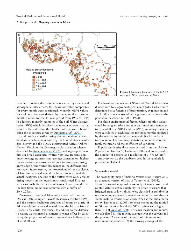
tained 7738 age-specific prevalences for West and Central

Africa, collected during 2371 surveys, carried out at 1220

distinct locations. In this analysis, we included only those

surveys conducted in rural regions after the year 1950 and

discarded data sampled at locations where we estimated no

transmission throughout the year. The final data set we

analysed was collected at 976 distinct locations over 1846

surveys and comprised 294 different (overlapping) age

categories (Figure 1).

Climatic, environmental and population data

The temperature and rainfall data were obtained from the

‘Topographic and Climate Data Base for Africa (1920–

1980)’ Version 1.1 by Hutchinson et al. (1996). It is based

on data collected by various research agencies at 1499

stations for temperature and at 6051 stations for rainfall,

between 1920 and 1980. These measures have been

averaged into monthly values for locations where data

have been collected for at least 5 years. Spatially predicted

values were then derived for a 0.05-degree spatial grid by

applying a thin-plate smoothing spline interpolation

(Hutchinson 1991).

Normalized Difference Vegetation Index extracted from

National Oceanic and Atmospheric Administration and

National Aeronautics and Space Administration (NOAA/

NASA) satellite data (Agbu & James 1994) were used as a

proxy of vegetation and soil wetness (Justice et al. 1985).

Tropical Medicine and International Health volume 11 no 7 pp 1032–1046 july 2006

A. Gemperli et al. Mapping malaria in Africa

ª 2006 Blackwell Publishing Ltd 1033

In order to reduce distortion effects caused by clouds and

atmospheric interference, the maximum value composites

for every month were considered. Monthly NDVI values

for each location were derived by averaging the maximum

monthly values for the 11-year period from 1985 to 1995.

In addition, monthly estimates of the Soil Water Storage

Index (SWS) which describes the amount of water that is

stored in the soil within the plant’s root zone were obtained

using the procedure given by Droogers et al. (2001).

Land use was classified using the land use/land cover

database which is maintained by the United States Geolo-

gical Survey and the NASA’s Distributed Active Archive

Center. We chose the 24-category classification scheme

described by Anderson et al. (1979) and regrouped them

into six broad categories (water, very low transmission,

under-average transmission, average transmission, higher-

than-average transmission and high transmission), using

knowledge of the vector abundance in the different land

use types. Subsequently, the proportions of the six classes

of land use were calculated for buffer areas around the

actual locations. The size of the buffers were calculated by

fitting models on the logarithmic-transformed E values

with various buffer sizes as predictors. It was found that

the best fitted model was achieved with a buffer of

20 · 20 km.

Permanent rivers and lakes were extracted from the

‘African Data Sampler’ (World Resources Institute 1995)

and the nearest Euclidean distances of points on a grid of

1-km resolution were calculated using the Idrisi software

(Clark Labs, Clark University). In addition to the distance-

to-water, we estimated a content-of-water effect by calcu-

lating the proportion of water contained in a buffered area

of 20 · 20 km.

Furthermore, the whole of West and Central Africa was

divided into four agro-ecological zones (AEZ) which were

determined as a function of precipitation, evaporation and

availability of water stored in the ground, according to the

procedure described in FAO (1978).

For those environmental factors where monthly values

could be assigned (the minimum and maximum tempera-

ture, rainfall, the NDVI and the SWS), summary statistics

were calculated at each location for those months predicted

by the seasonality model as being suitable for malaria

transmission. The summary statistics computed were the

total, the mean and the coefficient of variation.

Population density data were derived from the ‘African

Population Database’ (Deichman 1996) and correspond to

the number of persons at a resolution of 3.7 · 4.8 km2.

An overview on the databases used in the analysis is

provided in Table 1.

Seasonality model

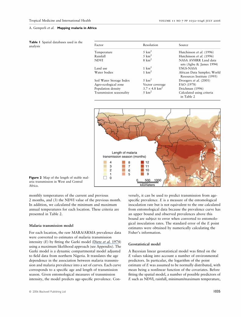
The seasonality map of malaria transmission (Figure 2) is

an amended version of that of Tanser et al. (2003).

Tanser’s original map makes use only of temperature and

rainfall data to define suitability. In order to ensure that

irrigated areas of low rainfall were classified as suitable for

transmission, we defined a region and month as suitable for

stable malaria transmission either when it met the criteria

set by Tanser et al. (2003), or those excluding the rainfall

of 60 mm criterion but if the NDVI values were higher

than 0.35 (Hay et al. 1998). For each location and month,

we calculated (1) the moving average over the current and

the previous 2 months of the mean of minimum and

maximum temperature, (2) the moving average of the

Malaria survey locationsPrevalence

> 0.8

< 0.2

0 500kilometers

1000

0.6 – 0.80.4 – 0.60.2 – 0.4

N

Figure 1 Sampling locations of the MARA

surveys in West and Central Africa.

Tropical Medicine and International Health volume 11 no 7 pp 1032–1046 july 2006

A. Gemperli et al. Mapping malaria in Africa

1034 ª 2006 Blackwell Publishing Ltd

monthly temperatures of the current and previous

2 months, and (3) the NDVI value of the previous month.

In addition, we calculated the minimum and maximum

annual temperatures for each location. These criteria are

presented in Table 2.

Malaria transmission model

For each location, the raw MARA/ARMA prevalence data

were converted to estimates of malaria transmission

intensity (E) by fitting the Garki model (Dietz et al. 1974)

using a maximum likelihood approach (see Appendix). The

Garki model is a dynamic compartmental model adjusted

to field data from northern Nigeria. It translates the age

dependence in the association between malaria transmis-

sion and malaria prevalence into a set of curves. Each curve

corresponds to a specific age and length of transmission

season. Given entomological measures of transmission

intensity, the model predicts age-specific prevalence. Con-

versely, it can be used to predict transmission from age-

specific prevalence. E is a measure of the entomological

inoculation rate but is not equivalent to the one calculated

from entomological data because the prevalence curve has

an upper bound and observed prevalences above this

bound are subject to error when converted to entomolo-

gical inoculation rates. The standard error of the E point

estimates were obtained by numerically calculating the

Fisher’s information.

Geostatistical model

A Bayesian linear geostatistical model was fitted on the

E values taking into account a number of environmental

predictors. In particular, the logarithm of the point

estimate of E was assumed to be normally distributed, with

mean being a nonlinear function of the covariates. Before

fitting the spatial model, a number of possible predictors of

E such as NDVI, rainfall, minimum/maximum temperature,

Length of malariatransmission season (months)

43210

5678 12

11109

0 500 1000kilometers

Figure 2 Map of the length of stable mal-aria transmission in West and Central

Africa.

Table 1 Spatial databases used in the

analysis Factor Resolution Source

Temperature 5 km2 Hutchinson et al. (1996)Rainfall 5 km2 Hutchinson et al. (1996)NDVI 8 km2 NASA AVHRR Land data

sets (Agbu & James 1994)

Land use 1 km2 USGS-NASA

Water bodies 1 km2 African Data Sampler; WorldResources Institute (1995)

Soil Water Storage Index 5 km2 Droogers et al. (2001)Agro-ecological zone Vector coverage FAO (1978)

Population density 3.7 · 4.8 km2 Deichman (1996)Transmission seasonality 5 km2 Calculated using criteria

in Table 2

Tropical Medicine and International Health volume 11 no 7 pp 1032–1046 july 2006

A. Gemperli et al. Mapping malaria in Africa

ª 2006 Blackwell Publishing Ltd 1035

SWS, distance from nearest water source, population

density, proportion of surface water, agro-ecological zone,

year of survey and length of transmission season were

screened univariately to select those which were statisti-

cally significantly related to E. Some of these covariates

were used earlier in spatial malaria risk models by

Thomson et al. (1999), Kleinschmidt et al. (2000, 2001)

and Diggle et al. (2002); however, the proportion of sur-

face water, land-use class, SWS and the climatic suitability

indicator were not considered in previous models.

We fitted various non-spatial models to identify the best

subset of predictors and their best (possibly nonlinear)

functional form based on the bias-corrected Akaike’s

information criterion (Hurvich & Tsai 1989), which was

used to assess model fit. The functional forms of predictors

which we screened include polynomials up to second order,

first-order interaction terms, logarithmic, inverse and

exponential forms with different parameterizations. Only

one parameter was found to enter the best model

nonlinearly. For ease of application, this parameter was

fixed at its optimal estimate to obtain a purely linear

model. This non-spatial analysis of the E value was carried

out using the SAS System (SAS Institute, Cary, NC).

In the Bayesian geostatistical model, the spatial depen-

dency among the log-E values Yj for locations j ¼ 1 … m

was modelled using the exponential correlation function

covðYj;YkÞ ¼ r2 exp�djk

q

� �for j 6¼ k

andvarðYjÞ ¼ r2 þ s2=wj;

where djk is the Euclidean distance between the locations of

observation Yj and Yk. wj is a weight introduced to account

for uncertainty in estimates derived from the Garki model

and equal to the reciprocal of the variance of the estimated

log E. The parameter r2 captures the variation attributable

to spatial dependency and s2 the remaining variation. The

decay of spatial variation as a function of the distance

between sample points is expressed by the parameter

q. Markov chain Monte Carlo was applied for model

fitting. Bayesian kriging was employed to produce a

smooth map of the E in West and Central Africa. The

software used for fitting the Bayesian models was written

by the authors in Fortran 95 (Compaq Visual Fortran v6.6)

using standard numerical libraries [The Numerical Algo-

rithms Group (NAG) Ltd.]. The smoothed E map was

back-transformed to age-specific maps of malaria risk in

children using the Garki model. Details on the spatial

Bayesian model and kriging are given in the Appendix.

Results

The univariate non-spatial analysis indicated that among

environmental factors the year of survey, NDVI, distance

from water, length of season, rainfall, SWS, agro-ecological

zone, andminimumandmaximumtemperaturewere related

to E. As described above, temporal variables such as NDVI,

rainfall and temperature, whose values change from month

to month, were summarized for each location by annual

total,mean and coefficient of variation (CV)over themonths

with stable transmission during the year. Univariate analysis

revealed that the mean leads to a better model fit than the

total and the CV. No statistically significant univariate

associationwas found between the logarithm ofE and either

the land use or population density.

The best fitting model included NDVI and length of

season on a logarithmic scale. The distance to water

entered the model scaled as an exponential function. The

scaling factor was chosen to optimize model fit. The

association with rainfall was best described by a reciprocal

transformation. The parameter estimates obtained after

Table 2 Criteria for suitability of stableP. falciparum malaria transmissionDescription Climatic effect Rule

Frost Minimum annual temperature 5 �CVector survival Mean monthly temperature* 19.5 �C + annual

standard deviationCatalyst month Annual maximum rainfall >80 mm

Availability of

breeding sites

NDVI� or rainfall� >0.35 or >60 mm

A month is suitable for transmission when all rules are fulfilled for the current month or for

the immediate preceding and following months. The table extends the seasonality model byTanser et al. (2003) by including the NDVI effect.

*Average of minimum and maximum temperature. Moving average from two previous

months and the current one.

�NDVI value from preceding month.�Moving average from two previous months and the current one.

Tropical Medicine and International Health volume 11 no 7 pp 1032–1046 july 2006

A. Gemperli et al. Mapping malaria in Africa

1036 ª 2006 Blackwell Publishing Ltd

fitting the spatial Bayesian model are presented in Table 3.

The results indicate a 0.3% increase in E every year.

Rainfall was also associated with transmission. The mini-

mum temperature, agro-ecological zone and the SWS index

were not retained in the multivariate model.

The interactions in the model capture the differences

in the effects of environmental factors on E in the

climatic zones. Some of these interactions which were

estimated by the model are graphically depicted in

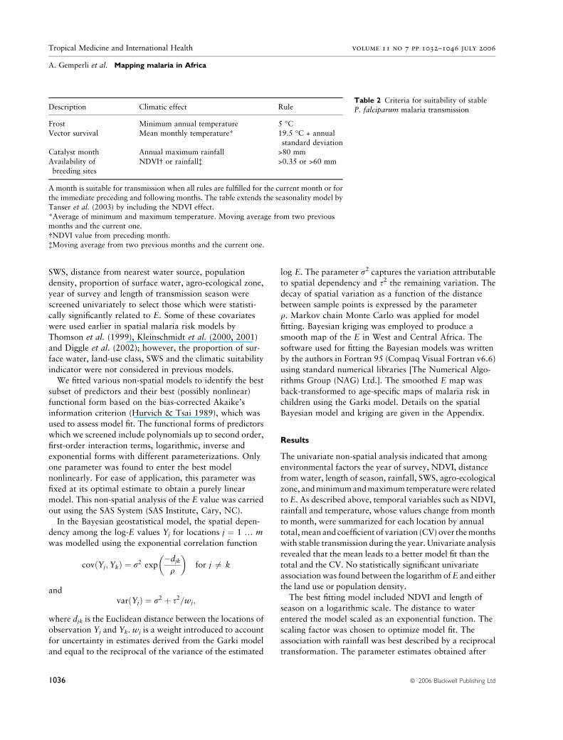
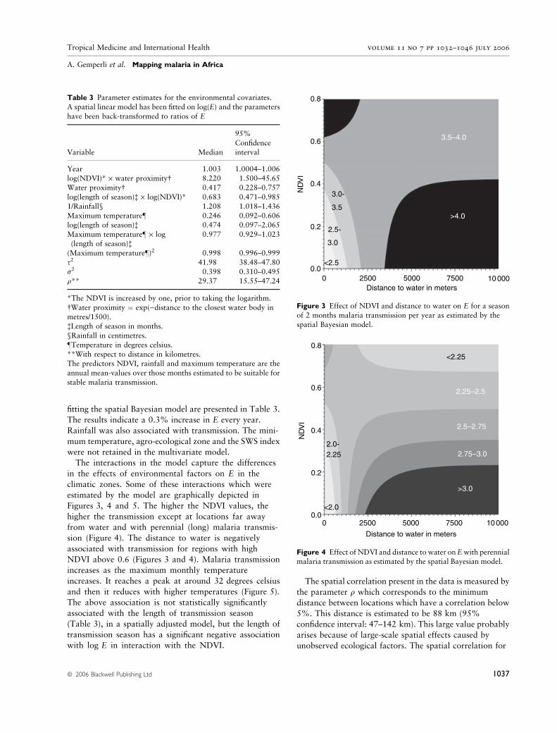
Figures 3, 4 and 5. The higher the NDVI values, the

higher the transmission except at locations far away

from water and with perennial (long) malaria transmis-

sion (Figure 4). The distance to water is negatively

associated with transmission for regions with high

NDVI above 0.6 (Figures 3 and 4). Malaria transmission

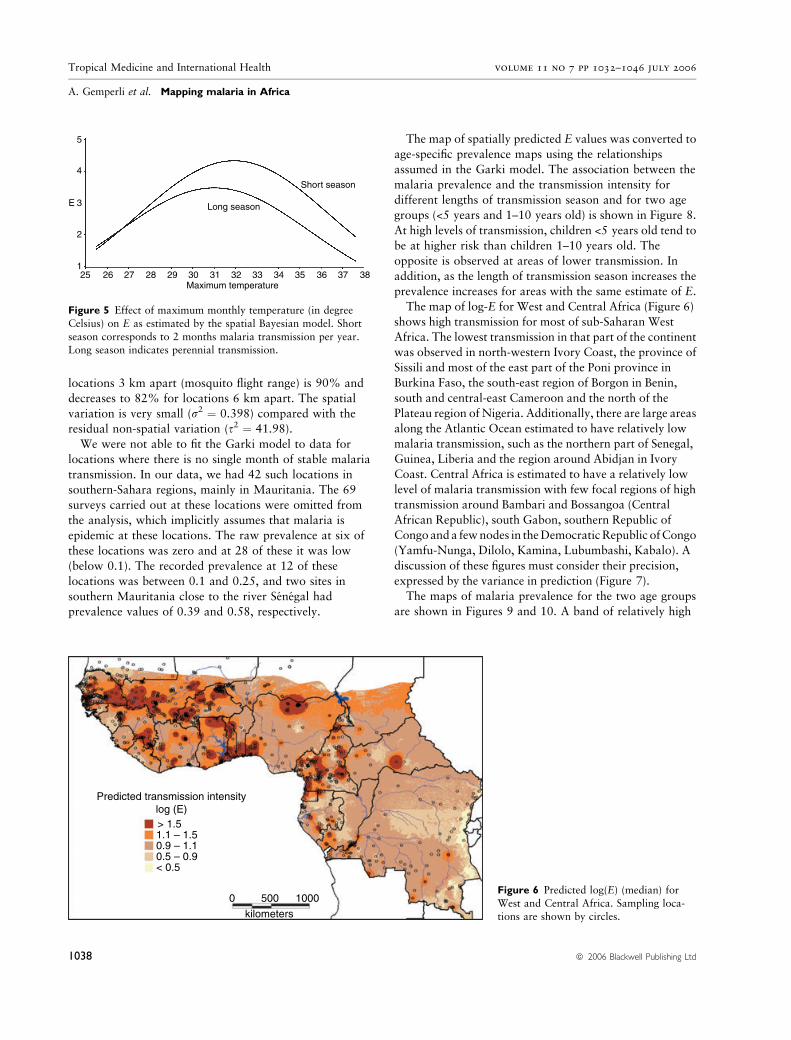
increases as the maximum monthly temperature

increases. It reaches a peak at around 32 degrees celsius

and then it reduces with higher temperatures (Figure 5).

The above association is not statistically significantly

associated with the length of transmission season

(Table 3), in a spatially adjusted model, but the length of

transmission season has a significant negative association

with log E in interaction with the NDVI.

The spatial correlation present in the data is measured by

the parameter q which corresponds to the minimum

distance between locations which have a correlation below

5%. This distance is estimated to be 88 km (95%

confidence interval: 47–142 km). This large value probably

arises because of large-scale spatial effects caused by

unobserved ecological factors. The spatial correlation for

0.8

0.6

0.4

0.2

ND

VI

0.00 2500 5000 7500

Distance to water in meters

3.5–4.0

>4.0

<2.5

3.0

2.5-

3.5

3.0-

10 000

Figure 3 Effect of NDVI and distance to water on E for a season

of 2 months malaria transmission per year as estimated by the

spatial Bayesian model.

0.8

0.6

0.4

0.2

ND

VI

0.00 2500 5000

Distance to water in meters

7500 10 000

<2.25

2.25–2.5

2.5–2.75

2.75–3.0

>3.0

2.252.0-

<2.0

Figure 4 Effect of NDVI and distance to water onEwith perennialmalaria transmission as estimated by the spatial Bayesian model.

Table 3 Parameter estimates for the environmental covariates.

A spatial linear model has been fitted on log(E) and the parameters

have been back-transformed to ratios of E

Variable Median

95%

Confidenceinterval

Year 1.003 1.0004–1.006log(NDVI)* · water proximity� 8.220 1.500–45.65

Water proximity� 0.417 0.228–0.757

log(length of season)� · log(NDVI)* 0.683 0.471–0.9851/Rainfall§ 1.208 1.018–1.436

Maximum temperature– 0.246 0.092–0.606

log(length of season)� 0.474 0.097–2.065

Maximum temperature– · log(length of season)�

0.977 0.929–1.023

(Maximum temperature–)2 0.998 0.996–0.999

s2 41.98 38.48–47.80

r2 0.398 0.310–0.495q** 29.37 15.55–47.24

*The NDVI is increased by one, prior to taking the logarithm.

�Water proximity ¼ exp()distance to the closest water body in

metres/1500).�Length of season in months.

§Rainfall in centimetres.

–Temperature in degrees celsius.

**With respect to distance in kilometres.The predictors NDVI, rainfall and maximum temperature are the

annual mean-values over those months estimated to be suitable for

stable malaria transmission.

Tropical Medicine and International Health volume 11 no 7 pp 1032–1046 july 2006

A. Gemperli et al. Mapping malaria in Africa

ª 2006 Blackwell Publishing Ltd 1037

locations 3 km apart (mosquito flight range) is 90% and

decreases to 82% for locations 6 km apart. The spatial

variation is very small (r2 ¼ 0.398) compared with the

residual non-spatial variation (s2 ¼ 41.98).

We were not able to fit the Garki model to data for

locations where there is no single month of stable malaria

transmission. In our data, we had 42 such locations in

southern-Sahara regions, mainly in Mauritania. The 69

surveys carried out at these locations were omitted from

the analysis, which implicitly assumes that malaria is

epidemic at these locations. The raw prevalence at six of

these locations was zero and at 28 of these it was low

(below 0.1). The recorded prevalence at 12 of these

locations was between 0.1 and 0.25, and two sites in

southern Mauritania close to the river Senegal had

prevalence values of 0.39 and 0.58, respectively.

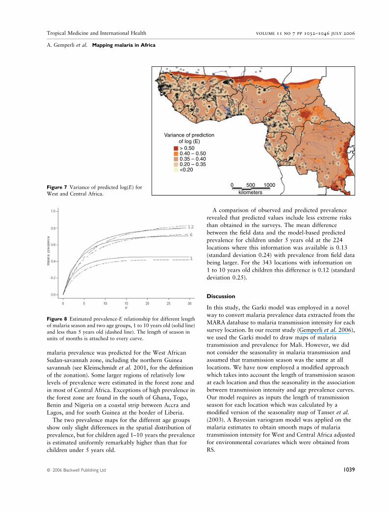
The map of spatially predicted E values was converted to

age-specific prevalence maps using the relationships

assumed in the Garki model. The association between the

malaria prevalence and the transmission intensity for

different lengths of transmission season and for two age

groups (<5 years and 1–10 years old) is shown in Figure 8.

At high levels of transmission, children <5 years old tend to

be at higher risk than children 1–10 years old. The

opposite is observed at areas of lower transmission. In

addition, as the length of transmission season increases the

prevalence increases for areas with the same estimate of E.

The map of log-E for West and Central Africa (Figure 6)

shows high transmission for most of sub-Saharan West

Africa. The lowest transmission in that part of the continent

was observed in north-western Ivory Coast, the province of

Sissili and most of the east part of the Poni province in

Burkina Faso, the south-east region of Borgon in Benin,

south and central-east Cameroon and the north of the

Plateau region of Nigeria. Additionally, there are large areas

along the Atlantic Ocean estimated to have relatively low

malaria transmission, such as the northern part of Senegal,

Guinea, Liberia and the region around Abidjan in Ivory

Coast. Central Africa is estimated to have a relatively low

level of malaria transmission with few focal regions of high

transmission around Bambari and Bossangoa (Central

African Republic), south Gabon, southern Republic of

Congoanda fewnodes in theDemocraticRepublic ofCongo

(Yamfu-Nunga, Dilolo, Kamina, Lubumbashi, Kabalo). A

discussion of these figures must consider their precision,

expressed by the variance in prediction (Figure 7).

The maps of malaria prevalence for the two age groups

are shown in Figures 9 and 10. A band of relatively high

5

4

3E

2

125 26 27 28 29 30 31 32 33 34 35 36 37 38

Long season

Maximum temperature

Short season

Figure 5 Effect of maximum monthly temperature (in degree

Celsius) on E as estimated by the spatial Bayesian model. Short

season corresponds to 2 months malaria transmission per year.Long season indicates perennial transmission.

Predicted transmission intensitylog (E)> 1.51.1 – 1.50.9 – 1.10.5 – 0.9< 0.5

0 500 1000

kilometers

Figure 6 Predicted log(E) (median) for

West and Central Africa. Sampling loca-tions are shown by circles.

Tropical Medicine and International Health volume 11 no 7 pp 1032–1046 july 2006

A. Gemperli et al. Mapping malaria in Africa

1038 ª 2006 Blackwell Publishing Ltd

malaria prevalence was predicted for the West African

Sudan-savannah zone, including the northern Guinea

savannah (see Kleinschmidt et al. 2001, for the definition

of the zonation). Some larger regions of relatively low

levels of prevalence were estimated in the forest zone and

in most of Central Africa. Exceptions of high prevalence in

the forest zone are found in the south of Ghana, Togo,

Benin and Nigeria on a coastal strip between Accra and

Lagos, and for south Guinea at the border of Liberia.

The two prevalence maps for the different age groups

show only slight differences in the spatial distribution of

prevalence, but for children aged 1–10 years the prevalence

is estimated uniformly remarkably higher than that for

children under 5 years old.

A comparison of observed and predicted prevalence

revealed that predicted values include less extreme risks

than obtained in the surveys. The mean difference

between the field data and the model-based predicted

prevalence for children under 5 years old at the 224

locations where this information was available is 0.13

(standard deviation 0.24) with prevalence from field data

being larger. For the 343 locations with information on

1 to 10 years old children this difference is 0.12 (standard

deviation 0.25).

Discussion

In this study, the Garki model was employed in a novel

way to convert malaria prevalence data extracted from the

MARA database to malaria transmission intensity for each

survey location. In our recent study (Gemperli et al. 2006),

we used the Garki model to draw maps of malaria

transmission and prevalence for Mali. However, we did

not consider the seasonality in malaria transmission and

assumed that transmission season was the same at all

locations. We have now employed a modified approach

which takes into account the length of transmission season

at each location and thus the seasonality in the association

between transmission intensity and age prevalence curves.

Our model requires as inputs the length of transmission

season for each location which was calculated by a

modified version of the seasonality map of Tanser et al.

(2003). A Bayesian variogram model was applied on the

malaria estimates to obtain smooth maps of malaria

transmission intensity for West and Central Africa adjusted

for environmental covariates which were obtained from

RS.

Variance of predictionof log (E)> 0.500.40 – 0.500.35 – 0.400.20 – 0.35<0.20

0 500 1000kilometers

Figure 7 Variance of predicted log(E) forWest and Central Africa.

Figure 8 Estimated prevalence-E relationship for different length

of malaria season and two age groups, 1 to 10 years old (solid line)

and less than 5 years old (dashed line). The length of season inunits of months is attached to every curve.

Tropical Medicine and International Health volume 11 no 7 pp 1032–1046 july 2006

A. Gemperli et al. Mapping malaria in Africa

ª 2006 Blackwell Publishing Ltd 1039

Seasonality in transmission is an important, but neglec-

ted, consideration in malaria mapping, both because the

season at which the data were collected may be important,

and because the malaria maps themselves may be season-

specific. At very high transmission levels, malaria preval-

ence is generally not very seasonal (Smith et al. 1993), but

at low transmission levels, surveys carried out in the dry

season generally have much lower prevalence than wet

season surveys. Many surveys are deliberately carried out

during the peak transmission season, and this introduces a

bias in the maps unless it is allowed for. Seasonality also

affects the relationship between prevalence and inoculation

rates, because when many inoculations occur over a short

period of time the proportion resulting in erythrocytic

infections is reduced (Beier et al. 1994; Charlwood et al.

1998). The Garki model adjusts automatically for this effect

when a seasonal input of vectorial capacity is assumed.

However, it would have been preferable to use a seasonality

model that predicted quantitative variation in transmission

between months, rather than simply classifying them into

months of transmission/no transmission. Moreover, there is

a clear need for empirical maps of seasonality based on

fitting models to local data on seasonality of either

entomological or clinical indices. Despite our attempt to

augment the seasonality map using NDVI data, it has

clearly failed to correctly assign areas of endemic trans-

mission in southern Mauritania, and probably also in other

areas where rivers flow north into dry zones.

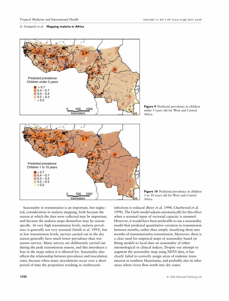
Predicted prevalenceChildren under 5 years

> 0.70.4 – 0.70.3 – 0.40.2 – 0.3< 0.2

0 500 1000kilometers

Figure 9 Predicted prevalence in children

under 5 years old for West and Central

Africa.

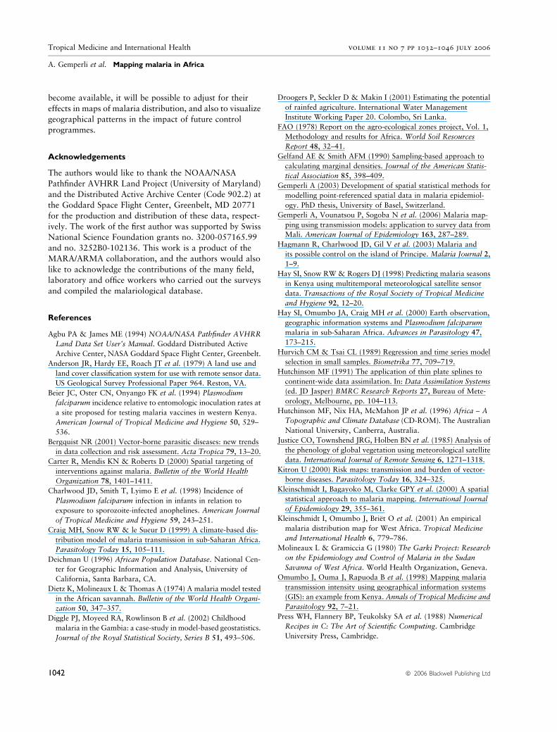
Predicted prevalenceChildren 1 to 10 years

0.4 – 0.70.3 – 0.40.2 – 0.3< 0.2

0 500 1000

kilometers

> 0.7

Figure 10 Predicted prevalence in children

1 to 10 years old for West and CentralAfrica.

Tropical Medicine and International Health volume 11 no 7 pp 1032–1046 july 2006

A. Gemperli et al. Mapping malaria in Africa

1040 ª 2006 Blackwell Publishing Ltd

The Garki model enabled us to convert malaria

prevalence data collected from surveys from non-stan-

dardized age categories of the population to an age-

independent transmission measure. Previous mapping

efforts attempted to overcome the problem of age-

adjustment by discarding inappropriate age-groups. This

resulted in a vast waste of available malaria data. The

model could then be further applied to obtain age-

specific prevalence. The mapping of outputs of malaria

transmission models provides a general framework to

derive malaria prevalence estimates for any desired age-

group. It can be also used to derive other measures of

transmission, different from the E, which are not

measured in the field. However, the Garki model was

developed on field data from the savannah zone of

Nigeria (Molineaux & Gramiccia 1980). It needs to be

verified how accurately it can be adapted for other

regions in West and Central Africa, with different

environmental conditions and malaria endemicity.

The Bayesian variogram modelling approach takes into

account the spatial dependence present in the data in a

flexible way. The method inherently calculates the stan-

dard error of the parameter estimates as well as the

prediction error without relying on approximations or

asymptotic results. Maps of the prediction error indicate

the confidence we can have on the model predictions for

the study area.

In a previous study to map malaria in West Africa,

Kleinschmidt et al. (2001) modelled interactions between

the environmental predictors and agro-ecological zones by

a separate analysis for each ecological zone. The resulting

map showed discontinuities around the borders of the

zones, which were further smoothed. This additional step

applied after kriging made inference on the prediction error

unfeasible. To avoid the separation into geographical

zones, we considered interaction amongst the environ-

mental predictors which capture space-varying functional

relationships between the predictors and malaria trans-

mission. This approach produces no discontinuities and

avoids arbitrary geographical partitioning. Our modelling

approach goes further beyond that of Kleinschmidt et al.

(2001), because we could include all survey information,

irrespective of their age group, and the Bayesian model

applied allowed correct adjustment for estimation uncer-

tainty and prediction error.

A comparison of our estimated malaria prevalence maps

with those produced by Kleinschmidt et al. (2001) for West

Africa reveals similar patterns, but the predicted prevalence

in our map shows fewer regions with prevalence above

70% or below 30%. Both maps identify the same areas

with high malaria prevalence (border of Senegal-Mali-

Guinea, north Ivory-Coast, Togo, north Nigeria, west

Cameroon) and with lower malaria prevalence (Guinea-

Bissau, south-east Burkina Faso, central Nigeria, and

central-north and north Cameroon). There are discrepan-

cies between the two maps in the region of central Nigeria

which the map of Kleinschmidt et al. (2001) shows to be a

high-risk area and in the border region between Burkina

Faso and Mali and in south Guinea which was found to be

a low-risk area by Kleinschmidt et al. (2001). Our map

estimates a much lower malaria prevalence for the whole

country of Ghana (with the exception of the coastal strip).

The two areas, Central Ghana and Central Nigeria, where

the two maps depict their largest differences are also the

regions where the sampling density is relatively low (see

Figure 1). More surveys in these two regions are needed to

assess the quality of the maps and help to improve them.

The models tend to underestimate high malaria risk as

revealed by comparing the observed with the predicted

prevalence data. This is because the prevalence curve

obtained from the Garki transmission model has an upper

bound so that it attributes observed prevalences above this

bound to sampling variation. The introduced bias is large

(0.13 for the <5-year olds; 0.12 for the 1–10-year olds)

suggesting further refinement of the Garki model.

Surveys conducted in urban areas were omitted in our

analysis. Thus, the produced maps may depict too high a

malaria estimate for large urban areas (especially in

Nigeria). In order to estimate the population at risk, based

on our malaria risk map, a separate prevalence estimate for

urban areas is required.

For low NDVI, an increase in malaria risk with

increasing distance to water was estimated (Figures 3 and

4). Kleinschmidt et al. (2000) found the same effect in an

analysis on malaria prevalence in Mali. In their work, the

malaria risk was estimated to be reduced to a level lower

than that measured close to water only for distances of

more than 40 km away from the nearest water body. While

vector abundance is supposed to be high closer to the

breeding sites (Carter et al. 2000), the negative association

between malaria infection and vector abundance is either

attributed to the propensity of people to use bednets

(Thomson et al. 1996) or the stimulated development of

immunity during early childhood in high-risk areas

(Thomas & Lindsay 2000).

The present analyses and maps demonstrate the feasi-

bility of using transmission model-based estimates for

mapping malaria risk across large areas of the African

continent taking into account different patterns of sea-

sonality. Further developments of this approach will

require transmission models with a stronger empirical base.

Realistic temporal components are needed in such models

to allow for nonlinear trends in malaria risk and for space–

time interactions. If spatial databases on control measures

Tropical Medicine and International Health volume 11 no 7 pp 1032–1046 july 2006

A. Gemperli et al. Mapping malaria in Africa

ª 2006 Blackwell Publishing Ltd 1041

become available, it will be possible to adjust for their

effects in maps of malaria distribution, and also to visualize

geographical patterns in the impact of future control

programmes.

Acknowledgements

The authors would like to thank the NOAA/NASA

Pathfinder AVHRR Land Project (University of Maryland)

and the Distributed Active Archive Center (Code 902.2) at

the Goddard Space Flight Center, Greenbelt, MD 20771

for the production and distribution of these data, respect-

ively. The work of the first author was supported by Swiss

National Science Foundation grants no. 3200-057165.99

and no. 3252B0-102136. This work is a product of the

MARA/ARMA collaboration, and the authors would also

like to acknowledge the contributions of the many field,

laboratory and office workers who carried out the surveys

and compiled the malariological database.

References

Agbu PA & James ME (1994) NOAA/NASA Pathfinder AVHRR

Land Data Set User’s Manual. Goddard Distributed Active

Archive Center, NASA Goddard Space Flight Center, Greenbelt.

Anderson JR, Hardy EE, Roach JT et al. (1979) A land use and

land cover classification system for use with remote sensor data.

US Geological Survey Professional Paper 964. Reston, VA.

Beier JC, Oster CN, Onyango FK et al. (1994) Plasmodium

falciparum incidence relative to entomologic inoculation rates at

a site proposed for testing malaria vaccines in western Kenya.

American Journal of Tropical Medicine and Hygiene 50, 529–

536.

Bergquist NR (2001) Vector-borne parasitic diseases: new trends

in data collection and risk assessment. Acta Tropica 79, 13–20.

Carter R, Mendis KN & Roberts D (2000) Spatial targeting of

interventions against malaria. Bulletin of the World Health

Organization 78, 1401–1411.

Charlwood JD, Smith T, Lyimo E et al. (1998) Incidence of

Plasmodium falciparum infection in infants in relation to

exposure to sporozoite-infected anophelines. American Journal

of Tropical Medicine and Hygiene 59, 243–251.

Craig MH, Snow RW & le Sueur D (1999) A climate-based dis-

tribution model of malaria transmission in sub-Saharan Africa.

Parasitology Today 15, 105–111.

Deichman U (1996) African Population Database. National Cen-

ter for Geographic Information and Analysis, University of

California, Santa Barbara, CA.

Dietz K, Molineaux L & Thomas A (1974) A malaria model tested

in the African savannah. Bulletin of the World Health Organi-

zation 50, 347–357.

Diggle PJ, Moyeed RA, Rowlinson B et al. (2002) Childhood

malaria in the Gambia: a case-study in model-based geostatistics.

Journal of the Royal Statistical Society, Series B 51, 493–506.

Droogers P, Seckler D & Makin I (2001) Estimating the potential

of rainfed agriculture. International Water Management

Institute Working Paper 20. Colombo, Sri Lanka.

FAO (1978) Report on the agro-ecological zones project, Vol. 1,

Methodology and results for Africa. World Soil Resources

Report 48, 32–41.

Gelfand AE & Smith AFM (1990) Sampling-based approach to

calculating marginal densities. Journal of the American Statis-

tical Association 85, 398–409.

Gemperli A (2003) Development of spatial statistical methods for

modelling point-referenced spatial data in malaria epidemiol-

ogy. PhD thesis, University of Basel, Switzerland.

Gemperli A, Vounatsou P, Sogoba N et al. (2006) Malaria map-

ping using transmission models: application to survey data from

Mali. American Journal of Epidemiology 163, 287–289.

Hagmann R, Charlwood JD, Gil V et al. (2003) Malaria and

its possible control on the island of Principe. Malaria Journal 2,

1–9.

Hay SI, Snow RW & Rogers DJ (1998) Predicting malaria seasons

in Kenya using multitemporal meteorological satellite sensor

data. Transactions of the Royal Society of Tropical Medicine

and Hygiene 92, 12–20.

Hay SI, Omumbo JA, Craig MH et al. (2000) Earth observation,

geographic information systems and Plasmodium falciparum

malaria in sub-Saharan Africa. Advances in Parasitology 47,

173–215.

Hurvich CM & Tsai CL (1989) Regression and time series model

selection in small samples. Biometrika 77, 709–719.

Hutchinson MF (1991) The application of thin plate splines to

continent-wide data assimilation. In: Data Assimilation Systems

(ed. JD Jasper) BMRC Research Reports 27, Bureau of Mete-

orology, Melbourne, pp. 104–113.

Hutchinson MF, Nix HA, McMahon JP et al. (1996) Africa – A

Topographic and Climate Database (CD-ROM). The Australian

National University, Canberra, Australia.

Justice CO, Townshend JRG, Holben BN et al. (1985) Analysis of

the phenology of global vegetation using meteorological satellite

data. International Journal of Remote Sensing 6, 1271–1318.

Kitron U (2000) Risk maps: transmission and burden of vector-

borne diseases. Parasitology Today 16, 324–325.

Kleinschmidt I, Bagayoko M, Clarke GPY et al. (2000) A spatial

statistical approach to malaria mapping. International Journal

of Epidemiology 29, 355–361.

Kleinschmidt I, Omumbo J, Briet O et al. (2001) An empirical

malaria distribution map for West Africa. Tropical Medicine

and International Health 6, 779–786.

Molineaux L & Gramiccia G (1980) The Garki Project: Research

on the Epidemiology and Control of Malaria in the Sudan

Savanna of West Africa. World Health Organization, Geneva.

Omumbo J, Ouma J, Rapuoda B et al. (1998) Mapping malaria

transmission intensity using geographical information systems

(GIS): an example from Kenya. Annals of Tropical Medicine and

Parasitology 92, 7–21.

Press WH, Flannery BP, Teukolsky SA et al. (1988) Numerical

Recipes in C: The Art of Scientific Computing. Cambridge

University Press, Cambridge.

Tropical Medicine and International Health volume 11 no 7 pp 1032–1046 july 2006

A. Gemperli et al. Mapping malaria in Africa

1042 ª 2006 Blackwell Publishing Ltd

Rogers DJ, Randolph SE, Snow RW et al. (2002) Satellite

imagery in the study and forecast of malaria. Nature 415,

710–715.

Smith T, Charlwood JD, Kihonda J et al. (1993) Absence of sea-

sonal variation in malaria parasitaemia in an area of intense

seasonal transmission. Acta Tropica 54, 55–72.

Snow RW, Marsh K & Le Sueur D (1996) The need for maps of

transmission intensity to guide malaria control in Africa. Para-

sitology Today 12, 455–457.

Snow RW, Gouws E, Omumbo J et al. (1998) Models to predict

the intensity of Plasmodium falciparum transmission: applica-

tions to the burden of disease in Kenya. Transactions of the

Royal Society of Tropical Medicine and Hygiene 92, 601–606.

Snow RW, Craig MH, Deichman U et al. (1999) A continental risk

map for malaria mortality among African children. Parasitology

Today 15, 99–104.

Tanser FC, Sharp B & Le Sueur D (2003) Potential effect of cli-

mate change on malaria transmission in Africa. Lancet 29,

1792–1798.

Thomas CJ & Lindsay SW (2000) Local-scale variation in malaria

infection amongst rural Gambian children estimated by satellite

remote sensing. Transactions of the Royal Society of Tropical

Medicine and Hygiene 94, 159–163.

Thomson MC & Connor SJ (2000) Environmental information

systems for the control of arthropod vectors of disease. Medical

Veterinary Entomology 14, 227–244.

Thomson M, Connor S, Bennet S et al. (1996) Geographical

perspectives on bednet use and malaria transmission in the

Gambia, West Africa. Social Science and Medicine 42,

101–112.

Thomson MC, Connor SJ & D’Alessandro U et al. (1999) Pre-

dicting malaria infection in Gambian children from satellite data

and bednet use surveys: the importance of spatial correlation in

the interpretation of results. American Journal of Tropical

Medicine and Hygiene 61, 2–8.

World Resources Institute (1995) African Data Sampler.

(CD-ROM) Edition I. World Resources Institute, Washington,

DC.16161616

Appendix : models

Garki model

The Garki model (Dietz et al. 1974) is a mathematical

model of malaria transmission which can be used to predict

age-specific malaria prevalence as a function of the vectorial

capacity C. C is defined to be the number of potentially

infective contacts induced by the mosquito population per

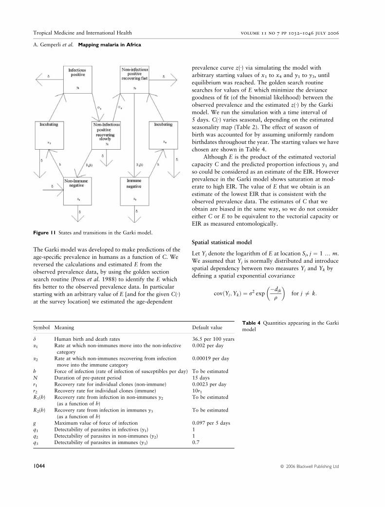
infectious person per day. The Garki model describes

transitions among seven categories of hosts distinguished by

their infection and immunological status (Figure 11). The

proportions x1 and x3, account for uninfected individuals,

and x2 and x4 are compartments with prepatent infections.

y1, y2 and y3, represent proportions of humans with blood-

stage infections. The model predicts the proportion of

human population at each age in each of the compartments.

It is defined by a set of linked difference equations that

specify the change in each of these proportions from one

time point to the next. Let D be the change in proportion

from one time point to the next one, i.e. Dx1 ¼x1(t + 1) ) x1(t), then the equations are defined as below:

Dx1 ¼ dþ y2R1ðhÞ � ðhþ dÞx1

Dx2 ¼ hx1 � ð1� dÞN þ hðt �NÞx1ðt �NÞ � dx2

Dx3 ¼ y3R2ðhÞ � ðhþ dÞx3

Dx4 ¼ hx3 � ð1� dÞN þ hðt �NÞx3ðt �NÞ � dx4

Dy1 ¼ ð1� dÞN þ hðt �NÞx1ðt �NÞ � ða1 þ dÞy1Dy2 ¼ a1y1 � ða2 þR1ðhÞ þ dÞy2Dy3 ¼ a2y2 � ð1� dÞN þ hðt �NÞx3ðt �NÞ � ðR2ðhÞ þ dÞy3

The meanings of the additional symbols are given in

Table 4. The time points to which the proportions and the

force of infection (h) refer to, are only indicated in the

above equations when they differ from t. h is the

probability per unit time, that a given susceptible indi-

vidual becomes infected. Here it is defined as a function

of C.

In order to account for seasonal variation, C is consid-

ered to depend on the month and its suitability for malaria

transmission, as estimated in Table 2. Each bite on an

infective individual will result in C new inoculations after

N days, where N is the duration of sporogony. Dependent

on the proportion of the population being infective, the E is

defined as

EðtÞ ¼ Cðt � NÞy1ðt � NÞ:

h(t) is assumed to be related to E(t) via

hðtÞ ¼ gð1� expð�EðtÞÞÞ;

which introduces an upper limit in the force of infection,

when E increases. g specifies this upper limit and is

interpreted as a parameter measuring host susceptibility.

The recovery rates R1 and R2 are defined as

R ¼ h

expðh=rÞ � 1;

where r is the recovery rate for a single-clone infection.

Non-immunes are assumed to recover at rate R1, calcu-

lated from this equation by setting r ¼ r1. Immunes

recover at rate R2, calculated by setting r ¼ r2 where

r2 > r1. q1, q2, and q3 are introduced to allow for

imperfect detection of parasitaemia in each of the three

infected classes y1, y2 and y3. Hence, the prevalence is

estimated by

zðtÞ ¼ q1y1ðtÞ þ q2y2ðtÞ þ q3y3ðtÞ:

Tropical Medicine and International Health volume 11 no 7 pp 1032–1046 july 2006

A. Gemperli et al. Mapping malaria in Africa

ª 2006 Blackwell Publishing Ltd 1043

The Garki model was developed to make predictions of the

age-specific prevalence in humans as a function of C. We

reversed the calculations and estimated E from the

observed prevalence data, by using the golden section

search routine (Press et al. 1988) to identify the E which

fits better to the observed prevalence data. In particular

starting with an arbitrary value of E [and for the given C(Æ)at the survey location] we estimated the age-dependent

prevalence curve z(Æ) via simulating the model with

arbitrary starting values of x1 to x4 and y1 to y3, until

equilibrium was reached. The golden search routine

searches for values of E which minimize the deviance

goodness of fit (of the binomial likelihood) between the

observed prevalence and the estimated z(Æ) by the Garki

model. We run the simulation with a time interval of

5 days. C(Æ) varies seasonal, depending on the estimated

seasonality map (Table 2). The effect of season of

birth was accounted for by assuming uniformly random

birthdates throughout the year. The starting values we have

chosen are shown in Table 4.

Although E is the product of the estimated vectorial

capacity C and the predicted proportion infectious y1 and

so could be considered as an estimate of the EIR. However

prevalence in the Garki model shows saturation at mod-

erate to high EIR. The value of E that we obtain is an

estimate of the lowest EIR that is consistent with the

observed prevalence data. The estimates of C that we

obtain are biased in the same way, so we do not consider

either C or E to be equivalent to the vectorial capacity or

EIR as measured entomologically.

Spatial statistical model

Let Yj denote the logarithm of E at location Sj, j ¼ 1 … m.

We assumed that Yj is normally distributed and introduce

spatial dependency between two measures Yj and Yk by

defining a spatial exponential covariance

covðYj;YkÞ ¼ r2 exp�djk

q

� �for j 6¼ k:

Table 4 Quantities appearing in the Garki

modelSymbol Meaning Default value

d Human birth and death rates 36.5 per 100 years

a1 Rate at which non-immunes move into the non-infectivecategory

0.002 per day

a2 Rate at which non-immunes recovering from infection

move into the immune category

0.00019 per day

h Force of infection (rate of infection of susceptibles per day) To be estimated

N Duration of pre-patent period 15 days

r1 Recovery rate for individual clones (non-immune) 0.0023 per day

r2 Recovery rate for individual clones (immune) 10r1R1(h) Recovery rate from infection in non-immunes y2

(as a function of h)To be estimated

R2(h) Recovery rate from infection in immunes y3(as a function of h)

To be estimated

g Maximum value of force of infection 0.097 per 5 days

q1 Detectability of parasites in infectives (y1) 1

q2 Detectability of parasites in non-immunes (y2) 1q3 Detectability of parasites in immunes (y3) 0.7

Figure 1118 States and transitions in the Garki model.

Tropical Medicine and International Health volume 11 no 7 pp 1032–1046 july 2006

A. Gemperli et al. Mapping malaria in Africa

1044 ª 2006 Blackwell Publishing Ltd

djk is the Euclidean distance that separates Yj and Yk, r2

quantifies the amount of spatially structured variation and

q the spatial dependency. A parameter s2 is introduced to

measure non-spatial variation at the origin and to add

extra variability to those values with imprecise estimates

from the Garki model. The variance in Yj is then given by

var(Yj) ¼ r2 + s2/wj, where wj is a weight, formed by the

reciprocal of the variance of the log-E estimate at location

sj from the Garki model. The mean of Yj is modelled via a

parametric function l(xj, b) of the covariates xj and a

parameter vector b.The model for Y ¼ (Y1, …, Ym)

t is written in matrix

notation as

Y � NðlðX; bÞ; r2RðqÞ þ s2WÞ:

ðRÞjk ¼ exp�djk

q

� �

and W is the weight matrix with elements Wjj ¼ 1/wj and

Wjk ¼ 0 for j „ k. The specification above holds if all m

locations are distinct. In case of n > m observations,

Y1, …, Yn at m distinct locations, an m · n incidence

matrix Z is formed with Zji ¼ 1 if observation i is observed

at location j and Zji ¼ 0 otherwise. Then

Y � NðlðX; bÞ; r2ZtRðqÞZþ s2ZtWZÞ:

The following prior distributions are adopted for the

parameters involved in the model:

b � Nð0; bbIÞ; r2 � IGðar2 ; br2Þ; s2 � IGðas2 ; bs2Þand q � Gðaq; bqÞ:

G(Æ) indicates the gamma and IG(Æ) the inverse-gamma

distribution. The hyperpriors are fixed to bb ¼ 100, ar2 ¼as2 ¼ 2.01, br2 ¼ bs2 ¼ 1.01 and aq ¼ bq ¼ 0.01. This

leads to a prior mean of one for all the covariance

parameters and a large variance of 100.

Parameters are estimated using Markov chain Monte

Carlo (MCMC) (Gelfand & Smith 1990). The joint

posterior distribution of the parameters is simulated using

Gibbs sampling, what requires to generate random

numbers from the conditional distribution of the

parameters individually. For l(X, b) linear, the conditionaldistribution of b is normal and easy to sample from. The

conditional distribution of the covariance parameters r2, s2

and q, are identified to have no standard forms and are

sampled using a random-walk Metropolis–Hastings

algorithm having a log-Gaussian proposal density with

mean equals the estimate from the previous iteration

and variance iteratively altered to reach an acceptance rate

of 0.4.

The log-E can be predicted at new locations s01, …, s0l,

once the spatial correlation between locations is estimated

and the environmental covariates Xnew at the new locations

are known. The algorithm for Bayesian kriging iteratively

draws independent values from the predictive distribution.

At iteration r, the algorithm starts by drawing values from

the joint posterior distribution of r2, s2 and q, which is

given empirically as the output of the Gibbs sampler

described above. The sampled values are used to form the

covariance matrix

RðrÞ ¼ r2ðrÞRðqðrÞÞ þ s2ðrÞW:

RðqðrÞÞjk ¼ exp�djk

qðrÞ

� �;

with djk the Euclidean distance between location sj and

location sk. There are three matrices formed this way. RðrÞold

is build by including only the old locations s1, …, sm, RðrÞnew

takes only new locations s01, …, s0l and RðrÞold�new describes

covariances between old and new locations. That is, the

m · l matrix ðRðrÞold�newÞjk includes locations s1, …, sm for j

and locations s01, …, s0l for k. For new locations, the

weights in the diagonal of W are set to one.

Subsequently, the parameter b(r) is drawn from its

posterior distribution to form the vector l(Xnew, b(r)).

Finally, a single vector from the predictive distribution of

Y0 is drawn from a multivariate normal with mean

lðXnew; bðrÞÞ þ RðrÞt

old�newRðrÞ�1old ðY � lðXold; b

ðrÞÞÞ

and variance

RðrÞnew � RðrÞt

old�newRðrÞ�1old RðrÞ

old�new:

The map with predicted log-E is back-transformed to age-

related prevalence by applying the relations estimated by

the Garki model. The back-transformation considers the

location-specific season-length.

Corresponding Author Armin Gemperli, Malaria Research Institute, Department of Molecular Microbiology and Immunology, Johns

Hopkins University Bloomberg School of Public Health, Baltimore, MD 21205, USA. Tel.: 410 614 7795; Fax: 410 955 0105; E-mail:

agemperl@jhsph.edu

Tropical Medicine and International Health volume 11 no 7 pp 1032–1046 july 2006

A. Gemperli et al. Mapping malaria in Africa

ª 2006 Blackwell Publishing Ltd 1045

Cartographie de la transmission de la malaria en Afrique de l’ouest et centrale

Nous avons produit des cartes de la transmission de la malaria a Plasmodium falciparum en Afrique de l’ouest et centrale en utilisant la base de donnees

MARA (Mapping malaria risk in Africa) qui contient toutes les etudes de prevalence de la malaria qui ont pu etre geo-localisees dans la region. Les 1846

etudes sur la malaria que nous avons analysees ont ete menees durant differentes saisons et ont ete rapportees en fonction de differents groupes d’age de

la population humaine. Afin de permettre la comparaison entre celles-ci, nous avons utilise le modele de transmission de la malaria de Garki pour

convertir les donnees de prevalence de la malaria dans chacune des 976 locations echantillonnees, en une seule estimation E de l’intensite de trans-

mission, en utilisant le modele saisonnier base sur l’Index Normalise de la Difference de Vegetation, la temperature et les donnees de pluviosite. Nous

avons applique a E le modele geostatistique bayesien en utilisant des variables supplementaires et avons applique le modele kriging bayesien pour

obtenir de cartes souples de E avec des prevalences age-specifiques. Le resultat obtenu est la premiere cartographie empirique detaillee des variations

dans l’intensite de la transmission de la malaria incluant l’Afrique centrale. Il a ete valide par des opinions d’experts et en general il confirme les profiles

connus de la transmission de la malaria, procurant des donnees de base a partir desquelles pourront etre evaluees des interventions telles que celles des

programmes aux moustiquaires impregnes d’insecticide ou les etudes sur les tendances de resistance aux medicaments. Il y a des variations geo-

graphiques considerables dans la precision des estimations sur modele et dans certaines parties de l’Afrique de l’ouest, les predictions different

substantiellement de celles provenant d’autres cartes de risque. Les incertitudes consequentes indiquent des zones pour lesquelles des donnees d’etudes

supplementaires sont plus urgemment necessaires. Les cartes de risque de la malaria, basees sur la compilation de donnees d’etudes heterogenes sont tres

sensibles a la methodologie d’analyse.

mots cles taux d’inoculation entomologique, kriging, malaria, chaıne Markov Monte Carlo, prevalence du parasite, capacite vectorielle

Mapeando la transmision de malaria en Africa del Este y Central

Hemos producido mapas con la transmision de malaria por Plasmodium falciparum en Africa del Este y Central, utilizando la base de datos MARA

(Mapping malaria risk in Africa - Mapeando el Riesgo de Malaria en Africa), que contiene todos aquellos estudios de prevalencia de malaria en estas

regiones que pudieron ser geoposicionados. Los 1,846 estudios de malaria analizados fueron realizados durante diferentes estaciones y reportados

utilizando diferentes estratificaciones por edad en las poblaciones humanas. Con el fin de poder compararlos, se utilizo el modelo de transmision de

malaria Garki para convertir los datos de prevalencia de cada una de las 976 localidades a un unico estimativo de intensidad de transmision E,

utilizando un modelo de estacionalidad basado en la diferencia normalizada de los ındices de vegetacion (NDVI), los datos de temperatura y pre-

cipitacion. Utilizando variables ambientales, ajustamos un modelo geoestadıstico Bayesiano a E y aplicamos un kriging Bayesiano para obtener mapas

suavizados de E y por lo tanto de prevalencia especıfica por edad. El resultado es el primer mapa empırico detallado de variaciones en la intensidad de

transmision de malaria que incluye Africa Central. Ha sido validado por opiniones expertas y en general confirma patrones conocidos de transmision de

malaria, aportando ası una lınea de base sobre la cual pueden evaluarse intervenciones tales como programas de redes mosquiteras impregnadas o

farmacovigilancia. Existe una variacion geografica considerable en la precision de los estimadores del modelo y en algunas partes de Africa del Este las

predicciones difieren sustancialmente de aquellas presentes en otros mapas de riesgo. Las incertidumbres resultantes indican zonas en las que se requiere

con mayor urgencia la obtencion datos adicionales. Los mapas de riesgo de malaria basados en recopilaciones de datos heterogeneos son altamente

sensibles a la metodologıa analıtica.

palabras clave tasa entomologica de inoculacion, kriging, malaria, cadena de Markov, Monte Carlo, prevalencia parasitologica, capacidad vectorial

Tropical Medicine and International Health volume 11 no 7 pp 1032–1046 july 2006

A. Gemperli et al. Mapping malaria in Africa

1046 ª 2006 Blackwell Publishing Ltd