macroeconomics annual 2006
TRANSCRIPT

Macroeconomics Annual
2006
National Bureau of Economic Research
NBER Macroeconomics Annual 2006edited by Daron Acemoglu, Kenneth Rogoff, and Michael Woodford
This 21st edition of the NBER Macroeconomics Annual treats many questions at thecutting edge of macroeconomics that are central to current policy debates. The firstfour papers and discussions focus on such current macroeconomic issues as howstructural-vector-autoregressions help identify sources of business cycle fluctuationsand the evolution of U.S. macroeconomic policies. The last two papers analyze the-oretical developments in optimal taxation policy and equilibrium yield curves.
Daron Acemoglu is Charles P. Kindleberger Professor of Applied Economics atMIT. Kenneth Rogoff is Thomas D. Cabot Professor of Public Policy and Professor ofEconomics at Harvard University. Michael Woodford is John Bates Clark Professorof Political Economy at Columbia University. All three are research associates of theNational Bureau of Economic Research.
Contents
Lawrence J. Christiano, Martin Eichenbaum, and Robert VigfussonASSESSING STRUCTURAL VARS(comments by Patrick J. Kehoe and Mark W. Watson)
Steven J. Davis, John Haltiwanger, Ron Jarmin, and Javier MirandaVOLATILITY AND DISPERSION IN BUSINESS GROWTH RATES: PUBLICLYTRADED VERSUS PRIVATELY HELD FIRMS(comments by Christopher Foote and Éva Nagypál)
Lars Ljungqvist and Thomas J. SargentDO TAXES EXPLAIN EUROPEAN EMPLOYMENT? INDIVISIBLE LABOR, HUMANCAPITAL, LOTTERIES, AND SAVINGS(comments by Olivier Blanchard and Edward C. Prescott)
Troy Davig and Eric M. LeeperFLUCTUATING MACRO POLICIES AND THE FISCAL THEORY(comments by Jordi Galí and Christopher Sims)
Mikhail Golosov, Aleh Tsyvinski, and Iván WerningNEW DYNAMIC PUBLIC FINANCE: A USER’S GUIDE(comments by Peter Diamond and Kenneth L. Judd)
Monika Piazzesi and Martin SchneiderEQUILIBRIUM YIELD CURVES(comments by Pierpaolo Benigno and John Y. Campbell)
The MIT PressMassachusetts Institute of TechnologyCambridge, Massachusetts 02142http://mitpress.mit.edu
978-0-262-51200-80-262-51200-9
Macroeconom
ics Annual 2006 V
olume 21
Acemglu_pb.qxd 5/21/07 3:59 PM Page 1

NBER Macroeconomics Annual 2006

NBER Macroeconomics Annual 2006
Daron Acemoglu, Kenneth Rogoff, and Michael Woodford, editors
The MIT PressCambridge, MassachusettsLondon, England
NBER/Macroeconomics Annual, Number 21, 2006
Published annually by The MIT Press, Cambridge, Massachusetts 02142.
© 2007 by the National Bureau of Economic Research and the Massachusetts Institute of Technology.
All rights reserved. No part of this book may be reproduced in any form by any elec-tronic or mechanical means (including photocopying, recording, or information storage and retrieval) without permission in writing from the publisher.
Standing orders/subscriptions are available. Inquiries, and changes to subscriptions and addresses should be addressed to Triliteral, Attention: Standing Orders, 100 Maple Ridge Drive, Cumberland, RI 02864, phone 1-800-366-6687 ext. 112 (U.S. and Canada), fax 1-800-406-9145 (U.S. and Canada).
In the United Kingdom, continental Europe, and the Middle East and Africa, send single copy and back volume orders to: The MIT Press, Ltd., Fitzroy House, 11 Chenies Street, London WC1E 7ET England, phone 44-020-7306-0603, fax 44-020-7306-0604, email [email protected], website http://mitpress.mit.edu.
In the United States and for all other countries, send single copy and back volume orders to: The MIT Press c/o Triliteral, 100 Maple Ridge Drive, Cumberland, RI 02864, phone 1-800-405-1619 (U.S. and Canada) or 401-658-4226, fax 1-800-406-9145 (U.S. and Canada) or 401-531-2801, email [email protected], website http://mitpress.mit.edu.
MIT Press books may be purchased at special quantity discounts for business or sales promotional use. For information, please email [email protected] or write to Special Sales Department, The MIT Press, 55 Hayward Street, Cambridge, MA 02142.
This book was set in Palatino and was printed and bound in the United States of America.
ISSN: 0889-3365ISBN-13: 978-0-262-01239-3 (hc.:alk.paper)—978-0-262-51200-8 (pbk.:alk.paper)ISBN-10: 0-262-01239-1 (hc.:alk.paper)—0-262-51200-9 (pbk.:alk.paper)
10 9 8 7 6 5 4 3 2 1

NBER Board of Directors by Affi liationOffi cersElizabeth E. Bailey, ChairmanJohn S. Clarkeson, Vice ChairmanMartin Feldstein, President and Chief Executive Offi cerSusan Colligan, Vice President for Administration and Budget and Corporate SecretaryRobert Mednick, TreasurerKelly Horak, Controller and Assistant Corporate SecretaryGerardine Johnson, Assistant Corporate Secretary
Directors at LargePeter C. AldrichElizabeth E. BaileyJohn H. BiggsJohn S. ClarkesonDon R. Conlan Kathleen B. CooperCharles H. DallaraGeorge C. Eads
Directors by University AppointmentGeorge Akerlof, California, BerkeleyJagdish Bhagwati, Columbia Ray C. Fair, YaleMichael J. Brennan, California, Los AngelesGlen G. Cain, WisconsinFranklin Fisher, Massachusetts Institute of TechnologySaul H. Hymans, Michigan
Directors by Appointment of Other OrganizationsRichard B. Berner, National Association for Business EconomicsGail D. Fosler, The Conference BoardMartin Gruber, American Finance Association Arthur B. Kennickell, American Statistical AssociationThea Lee, American Federation of Laborand Congress of Industrial OrganizationsWilliam W. Lewis, Committee for Economic Development
Directors EmeritiAndrew BrimmerCarl F. ChristGeorge HatsopoulosLawrence R. Klein
Jessica P. EinhornMartin FeldsteinRoger W. Ferguson, Jr.Jacob A. FrenkelJudith M. Gueron Robert S. HamadaKaren N. HornJudy C. Lewent
John Lipsky Laurence H. MeyerMichael H. MoskowAlicia H. MunnellRudolph A. OswaldRobert T. ParryMarina v. N. WhitmanMartin B. Zimmerman
Marjorie B. McElroy, DukeJoel Mokyr, NorthwesternAndrew Postlewaite, PennsylvaniaUwe E. Reinhardt, PrincetonNathan Rosenberg, StanfordCraig Swan, MinnesotaDavid B. Yoffi e, HarvardArnold Zellner (Director Emeritus), Chicago
Robert Mednick, American Institute of Certifi ed Public AccountantsAngelo Melino, Canadian Economics AssociationJeffrey M. Perloff, American Agricultural Economics AssociationJohn J. Siegfried, American Economic AssociationGavin Wright, Economic History Association
Franklin A. LindsayPaul W. McCrackenPeter G. Peterson
Richard N. RosettEli ShapiroArnold Zellner


Relation of the Directors to the Work and Publications of the NBER
1. The object of the NBER is to ascertain and present to the economics profession, and to the public more generally, important economic facts and their interpretation in a scientifi c manner without policy recom-mendations. The Board of Directors is charged with the responsibility of ensuring that the work of the NBER is carried on in strict conformity with this object.2. The President shall establish an internal review process to ensure that book manuscripts proposed for publication DO NOT contain policy recommendations. This shall apply both to the proceedings of conferences and to manuscripts by a single author or by one or more co-authors but shall not apply to authors of comments at NBER confer-ences who are not NBER affi liates.3. No book manuscript reporting research shall be published by the NBER until the President has sent to each member of the Board a notice that a manuscript is recommended for publication and that in the President’s opinion it is suitable for publication in accordance with the above principles of the NBER. Such notifi cation will include a table of contents and an abstract or summary of the manuscript’s content, a list of contributors if applicable, and a response form for use by Directors who desire a copy of the manuscript for review. Each manuscript shall contain a summary drawing attention to the nature and treatment of the problem studied and the main conclusions reached.4. No volume shall be published until forty-fi ve days have elapsed from the above notifi cation of intention to publish it. During this period a copy shall be sent to any Director requesting it, and if any Director objects to publication on the grounds that the manuscript con-tains policy recommendations, the objection will be presented to the author(s) or editor(s). In case of dispute, all members of the Board shall

Relation of the Directors to the Work and Publications of the NBERviii
be notifi ed, and the President shall appoint an ad hoc committee of the Board to decide the matter; thirty days additional shall be granted for this purpose.5. The President shall present annually to the Board a report describing the internal manuscript review process, any objections made by Direc-tors before publication or by anyone after publication, any disputes about such matters, and how they were handled. 6. Publications of the NBER issued for informational purposes con-cerning the work of the Bureau, or issued to inform the public of the activities at the Bureau, including but not limited to the NBER Digest and Reporter, shall be consistent with the object stated in paragraph 1. They shall contain a specifi c disclaimer noting that they have not passed through the review procedures required in this resolution. The Execu-tive Committee of the Board is charged with the review of all such pub-lications from time to time.7. NBER working papers and manuscripts distributed on the Bureau’s web site are not deemed to be publications for the purpose of this reso-lution, but they shall be consistent with the object stated in paragraph 1. Working papers shall contain a specifi c disclaimer noting that they have not passed through the review procedures required in this resolution. The NBER’s web site shall contain a similar disclaimer. The President shall establish an internal review process to ensure that the working papers and the web site do not contain policy recommendations, and shall report annually to the Board on this process and any concerns raised in connection with it.8. Unless otherwise determined by the Board or exempted by the terms of paragraphs 6 and 7, a copy of this resolution shall be printed in each NBER publication as described in paragraph 2 above.
Editorial xi Daron Acemoglu, Kenneth Rogoff, and Michael Woodford Abstracts xix
1 Assessing Structural VARs 1
Lawrence J. Christiano, Martin Eichenbaum, and Robert Vigfusson
Comments 73
Patrick J. Kehoe Mark W. Watson
Discussion 103
2 Volatility and Dispersion in Business Growth Rates: Publicly Traded versus Privately Held Firms 107
Steven J. Davis, John Haltiwanger, Ron Jarmin, and Javier Miranda
Comments 157
Christopher Foote Éva Nagypál
Discussion 177
3 Do Taxes Explain European Employment? Indivisible Labor, Human Capital, Lotteries, and Savings 181
Lars Ljungqvist and Thomas J. Sargent
Contents

Comments 225
Olivier Blanchard Edward C. Prescott
Discussion 243
4 Fluctuating Macro Policies and the Fiscal Theory 247
Troy Davig and Eric M. Leeper
Comments 299
Jordi Galí Christopher Sims
Discussion 313
5 New Dynamic Public Finance: A User’s Guide 317
Mikhail Golosov, Aleh Tsyvinski, and Iván Werning
Comments 365
Peter Diamond Kenneth L. Judd
Discussion 385
6 Equilibrium Yield Curves 389
Monika Piazzesi and Martin Schneider
Comments 443
Pierpaolo Benigno John Y. Campbell
Discussion 469
Contentsx

The twenty-fi rst edition of the NBER Macroeconomics Annual continues with its tradition of featuring debates central to current-day macroeco-nomic issues and analyses of important developments in macro-theory. A number of the papers in the twenty-fi rst edition revisit important debates from earlier editions. These include the debate on the role of structural vector-autoregressions (SVARs) in identifying sources of business cycle fl uctuations, the investigation of the trends in fi rm-level volatility and their implications for aggregate volatility, the debate on the causes of European unemployment, and the question of whether macro policy rules in the U.S. economy have changed over time. In addition, two papers explore new theoretical advances in optimal taxa-tion policy and new approaches to equilibrium yield curves. As has been the tradition in the NBER Macroeconomics Annual, each paper is discussed by two experts, who provide contrasting views and elabora-tions of the themes raised in the papers.
The fi rst paper in this edition is on structural vector-autoregression (SVARs) methodology, which has recently become a popular tech-nique in empirical macroeconomics. SVARs attempt to measure the dynamic responses of a range of macroeconomic variables to struc-tural disturbances (such as technology or preference shocks), while making few a priori assumptions about the correct structural relation-ships. This methodology is potentially useful since there is generally no widespread agreement on the exact structural forms to be imposed on the data to identify the role of various economic disturbances and the mechanisms of propagation. The SVAR approach has been widely used in the context of identifying the relative importance of technology and demand shocks and for uncovering the effects of monetary policy shocks, as well as in a range of other applications, such as studies of the impact of fi scal policy on the economy. Studies using SVAR meth-
Editorial
Daron Acemoglu, Kenneth Rogoff, and Michael Woodford
odology have had a considerable impact on business cycle research, for example, opening a lively debate on the role of technology shocks and how these propagate through the economy at business cycle frequen-cies. The NBER Macroeconomics Annual has already featured some of the infl uential work in this genre, starting with the paper by Matthew Shapiro and Mark W. Watson (1988) in volume 3, and more recently with the paper by Jordi Galí and Pau Rabanal (2004) in volume 19. We felt that it would be useful in this volume to have a broader discussion of the appropriate use and interpretation of SVARs.
The debate here may be viewed as an outgrowth of Ellen McGrat-tan’s (2004) comment on Galí and Rabanal (2004) in volume 19 of the NBER Macroeconomics Annual, where she argued that the application of the SVAR methodology to uncover the role of technology shocks can be highly misleading. A widely-discussed subsequent paper by V. V. Chari, Patrick J. Kehoe, and Ellen McGrattan (2005) extended this critique to argue that SVAR methodology in general is unreliable, since it depends on econometric specifi cations that are inevitably violated by dynamic stochastic general-equilibrium models. In “Assessing Structural VARs,” Lawrence J. Christiano, Martin Eichenbaum, and Robert Vigfusson assess these criticisms for applied work using SVAR methodology. Their focus is on whether the misspecifi cation involved in assuming a fi nite-order VAR to describe the joint dynamics of a set of aggregate time series is likely to lead to misleading inferences in practice. They explore this question in the context of two classes of dynamic equilibrium mod-els. Their conclusion is that SVARs are unlikely to lead to misleading conclusions, even when misspecifi ed. In particular, they fi nd that even with misspecifi ed SVARs, confi dence intervals for estimated impulse responses would correctly indicate the degree of sampling uncertainty in the estimates, and that the bias in the estimated responses is typically small relative to the width of the confi dence interval. They also show that biases in the estimated impulse responses resulting from SVARs with “long run” identifying restrictions (of the kind used by Galí and Rabanal, among others) are small and propose an alternative estimator that can further reduce biases in this case. Their conclusions suggest that when correctly used, SVARs can provide useful insight in the char-acter of aggregate fl uctuations.
Another area central to macroeconomic analysis of business cycle fl uctuations is whether and how the volatility of aggregate fl uctuations has changed over time. Important work in this area has already been featured in the NBER Macroeconomics Annual. James Stock and Mark
Acemoglu, Rogoff, and Woodfordxii
W. Watson (2002) in volume 17 have documented the large decline in aggregate volatility in the U.S. economy and investigated its causes, while a number of studies, including the NBER Macroeconomics Annual paper by Diego Comin and Thomas Philippon (2005), have documented that, somewhat paradoxically, the level of risk faced by individual fi rms appears to have increased during the same time span. The paper by Ste-ven J. Davis, John Haltiwanger, Ron Jarmin, and Javier Miranda, “Vola-tility and Dispersion in Business Growth Rates: Publicly Traded versus Privately Held Firms,” reconsiders the question of fi rm-level volatility using a new database, the Longitudinal Business Database (LBD) devel-oped by the U.S. Department of the Census. The LBD is an ideal dataset for this purpose since it provides annual data on employment at nearly fi ve million fi rms, covering all sectors of the U.S. economy and all geo-graphic areas. The coverage is thus much wider than that provided by COMPUSTAT, which has previously been used to investigate changes in fi rm-level volatility, but includes only publicly traded fi rms (only about 7,000 of the fi ve million fi rms in the LBD). Davis and co-authors fi nd the trend in fi rm-level volatility looks quite different when one uses the LBD instead of the COMPUSTAT database because of differences in the behavior of publicly-traded and private fi rms. There has indeed been a large increase in the volatility faced by publicly-traded fi rms, but this has been accompanied with an even larger decline in fi rm-level volatil-ity and cross-sectional dispersion of fi rm growth rates among private fi rms. Davis et al. show that this contrast between publicly-traded and private fi rms is present across different industries. They also document the role of selection in the increased volatility of publicly-traded fi rms, driven by the fact that recently-listed fi rms appear to be more volatile than those that have been listed for a longer period. These striking new fi ndings dramatically change our view of the structural changes in the U.S. economy, suggesting that recent advances in productivity have not been associated with as great an increase in risk (and risk-taking) at the fi rm level as some have argued.
Another topic of lively debate among macroeconomists in recent years has been the source of Western Europe’s persistent problem of high unemployment. This topic generated a large literature through-out the 1990s. It has received renewed interest partly because of Edward C. Prescott’s (2002) Ely Lecture, where he argued that the dif-ference between hours worked per capita in France and those in the United States could largely be explained by higher tax rates on labor income in France. Prescott based his conclusion on a calibration of a
xiiiEditorial
representative-household model in which tax revenues are used to fi nance government services that are perfect substitutes for private consumer expenditures. In their paper, “Do Taxes Explain European Employment? Indivisible Labor, Human Capital, Lotteries, and Sav-ings,” Lars Ljungqvist and Thomas J. Sargent reconsider Prescott’s analysis in a richer model, incorporating both unemployment and poten-tially incomplete markets. Incomplete markets are important, since they allow Ljungqvist and Sargent to develop a model of indivisible labor without employment lotteries. In this model, unemployed individuals have a negative income shock, and they can only protect themselves against this by “self-insurance”, i.e., by borrowing and lending at a risk-free interest rate. Their model also extends Prescott’s by allowing for human capital accumulation. They illustrate that the assumption of incomplete markets (and thus no full insurance against employment risk) is important and realistic, and document that full insurance against employment risk (as in Prescott’s baseline model) would in fact result in a radical under-prediction of work effort in Europe for the levels of unemployment benefi ts in effect in most of Western Europe. They also show that their model and Prescott’s do not have the same aggregate implications, notably with regard to the predicted effects of changes in the level of unemployment benefi ts. Ljungqvist and Sargent also sug-gest that a realistic calibration of their model would indicate that low unemployment is compatible with fairly high tax rates and that Western Europe’s more generous welfare policies are more likely to be the pri-mary explanation for higher unemployment than in the United States. Their model therefore not only contributes to the theoretical literature, but also suggests a provocative alternative vision for policy reform in Europe. Their contribution is thus likely to spark both future theoreti-cal work on the modeling of the labor market and unemployment and further debate on possible policy reforms in Western Europe.
An important question in empirical macroeconomic modeling is whether government policy is appropriately modeled by uniform, time-invariant systematic rules, perturbed by additive random errors, or whether the response coeffi cients that describe government policy should be modeled as varying over time as well. Proponents of the view that systematic policy has changed to an important extent over time often deal with this problem by splitting their sample, but esti-mate rational-expectations equilibria (REE) under the assumption of a uniform policy rule that is expected to last forever for each sub-period. Troy Davig and Eric M. Leeper, in “Fluctuating Macro Policies and
Acemoglu, Rogoff, and Woodfordxiv
the Fiscal Theory,” propose an alternative approach: estimation of a regime-switching model in which the response coeffi cients of the gov-ernment policy rules switch at random intervals among a fi nite number of recurrent possibilities, under the assumption that agents correctly understand the probability of these switches and their consequences for equilibrium dynamics. The estimated regime-switching model has different implications than a simple assumption of a REE for each inter-val over which the policy rules remain constant, for the anticipation of possible switching to another regime affects equilibrium dynamics under each of the individual regimes. First, the conditions for stability and determinacy of equilibrium are changed: even though, according to the authors’ estimates, the U.S. economy has spent some parts of the postwar period under monetary/fi scal regimes that would imply either explosive dynamics or the existence of stationary sunspot equi-libria if the regime in question were expected to persist indefi nitely, the estimated switching model is one with a determinate REE. Conse-quently they support the conclusion of Richard Clarida, Jordi Galí, and Mark Gertler (2000) that U.S. monetary policy switched from “passive” to “active” at the beginning of the 1980s. Nevertheless, their model does not confi rm the conclusion of the earlier authors that the U.S. economy was for that reason subject to instability due to self-fulfi lling expecta-tions in the 1970s. And second, they fi nd that even in periods in which fi scal policy is “passive” (or Ricardian), fi scal disturbances affect both infl ation and real activity (contrary to the principle of Ricardian equiva-lence), owing to the fact that the U.S. periodically reverts to an “active” fi scal policy regime under which taxes do not increase in response to increased public debt. This means that even clear evidence that tax rates respond to public debt in at least some periods in the way required to ensure intertemporal solvency does not mean that the fi scal theory of the price level is empirically unimportant; in the model of these authors, the mechanism emphasized in that literature affects equilib-rium dynamics (though to differing extents) both when fi scal policy is “passive” and when it is not.
One of the important developments in theoretical public fi nance in recent years has been a revival of interest in the optimal policy approach pioneered by James Mirrlees (1971). Mirrlees’ seminal paper showed how incentive and information problems can be the critical constraint on the structure of tax systems, and thus offered an attractive alterna-tive to the existing approach, pioneered by Frank Ramsey, which arbi-trarily assumed a given set of tax instruments (say, only proportional
xvEditorial
taxes on various categories of income). The Ramsey theory of optimal taxation was extended to dynamic settings starting in the late 1970s and has since become the basis for macroeconomists’ recommendations on optimal tax smoothing over the business cycle or on the desirability of taxing capital income. The renewed interest in Mirrleesian theory has prompted economists to reassess these macroeconomic questions using models in which constraints on the structure of taxes come from information and incentive compatibility constraints. This literature has already made important advances, but many of the contributions are theoretical and are cast in the context of relatively abstract models. In “New Dynamic Public Finance: A User’s Guide,” Mikhail Golosov, Aleh Tsyvinski, and Iván Werning survey this new literature and emphasize its implications for macroeconomics. They develop the major insights of the dynamic Mirrlees approach in the context of a two-period econ-omy. They give particular attention to the question of how capital and labor “wedges”—discrepancies between marginal rates of substitution and technological rates of transformation that might (but need not be) created by the presence of a distorting tax—should vary in response to aggregate shocks in a constrained-optimal allocation of resources. In addition to showing that a Mirrleesian approach to such questions may be possible (and insightful), the analysis highlights some notable differ-ences between the Mirrleesian results and those derived in the Ramsey theory. For example, a celebrated result of the representative-agent Ramsey theory is that tax rates on labor income should be smoothed, both across time and across states of the world; thus they should not vary in response to different levels of government purchases. The authors show that a similar result (with regard to the labor “wedge”) obtains under the Mirrleesian theory when uncertainty regarding indi-vidual agents’ skills is fully resolved in the fi rst period. However, when uncertainty about skills remains even in the second period, optimal labor “wedges” can vary with the realized shock to the level of govern-ment purchases. These results make it clear that a careful analysis of the constraints on tax policy that pays attention to the relevant kinds of heterogeneity in the population is necessary to draw reliable conclu-sions about the nature of optimal policy.
Another important growth area in macroeconomics in recent years has been the use of macroeconomic models to understand asset pric-ing; “macro fi nance” models of the term structure of interest rates have attracted particular interest. In “Equilibrium Yield Curves,” Monika Piazzesi and Martin Schneider consider the extent to which variations
Acemoglu, Rogoff, and Woodfordxvi
over time in the yield curve for U.S. bond prices are consistent with a representative-household model, and the extent to which these move-ments can be explained by the evolution of aggregate time series. Their theoretical model predicts the evolution of the prices of bonds of all maturities, given stochastic processes for infl ation and for aggregate consumption expenditure. A theoretical forecasting model (a VAR) is estimated for the joint dynamics of the latter two macro variables, and the authors then ask to what extent the yield-curve dynamics that would be implied by the theoretical bond-pricing model are similar to those actually observed over the sample period. Previous exercises of this kind have often failed even to correctly explain the average slope of the yield curve, fi nding a “bond premium puzzle” according to which the theoretical model implies that the average yields on longer-matu-rity bonds should be lower than average short rates of interest, whereas historically they have been higher. Piazzesi and Schneider solve this problem by proposing an alternative form of preferences (Epstein-Zin preferences), and documenting a dynamic relationship between infl a-tion and consumption growth of a kind that can generate a positive average term premium in the case of these preferences. Their model also successfully accounts for other important features of observed bond prices, such as the degree of serial correlation of both short and long yields. They then consider a more complex version of their model, in which agents must estimate the joint dynamics and infl ation and the aggregate consumption process, rather than being assumed to cor-rectly understand the data-generating process estimated by the authors (i.e., assumed to have rational expectations). The model with learning helps to explain shifts in the average shape of yield curves over time; for example, differences in the yield curve after 1980 are attributed to an increased subjective estimate of the degree of persistence of fl uctua-tions in infl ation after observing large and persistent swings in infl a-tion in the 1970s. These suggestive results are encouraging, both for the prospect of an eventual unifi ed explanation of aggregate fl uctuations and the evolution of asset prices, and for our ability to understand the role of expectation formation in macroeconomic dynamics.
The authors and the editors would like to take this opportunity to thank Martin Feldstein and the National Bureau of Economic Research for their continued support of the NBER Macroeconomics Annual and the associated conference. We would also like to thank the NBER confer-ence staff, especially Rob Shannon, for excellent logistical support; and the National Science Foundation for fi nancial assistance. Jon Steinsson
xviiEditorial
and Davin Chor did an excellent job as conference rapporteurs. We are also grateful to Lauren Fahey, Jane Trahan, and Helena Fitz-Patrick for assistance in editing and producing the manuscript.
References
Chari, V. V., Patrick J. Kehoe, and Ellen R. McGrattan. 2005. “A Critique of Structural VARs Using Real Business Cycle Theory.” Federal Reserve Bank of Minneapolis Working Paper no. 631.
Clarida, Richard, Jordi Galí, and Mark Gertler. 2000. “Monetary Policy Rules and Mac-roeconomic Stability: Evidence and Some Theory.” Quarterly Journal of Economics 115: 147–180.
Comin, Diego, and Thomas Philippon. 2005. “The Rise in Firm-Level Volatility: Causes and Consequences.” NBER Macroeconomics Annual 20: 167–227.
Galí, Jordi, and Pau Rabanal. 2004. “Technology Shocks and Aggregate Fluctuations: How Well Does the Real Business Cycle Model Fit Postwar U.S. Data?” NBER Macroeco-nomics Annual 19: 225–288.
McGrattan, Ellen R. 2004. “Comment.” NBER Macroeconomics Annual 19: 289–308.
Mirrlees, James A. 1971. “An Exploration in the Theory of Optimal Income Taxation.” Review of Economic Studies 38: 175–208.
Prescott, Edward C. 2002. “Prosperity and Depression.” American Economic Review 92: 1–15.
Shapiro, Matthew D., and Mark W. Watson. 1988. “Sources of Business Cycle Fluctua-tions.” NBER Macroeconomics Annual 3: 111–148.
Stock, James H., and Mark W. Watson. 2002. “Has the Business Cycle Changed and Why?” NBER Macroeconomics Annual 17: 159–228.
Acemoglu, Rogoff, and Woodfordxviii
1 Assessing Structural VARsLawrence J. Christiano, Martin Eichenbaum, and Robert Vigfusson
This paper analyzes the quality of VAR-based procedures for estimat-ing the response of the economy to a shock. We focus on two key issues. First, do VAR-based confi dence intervals accurately refl ect the actual degree of sampling uncertainty associated with impulse response func-tions? Second, what is the size of bias relative to confi dence intervals, and how do coverage rates of confi dence intervals compare with their nominal size? We address these questions using data generated from a series of estimated dynamic, stochastic general equilibrium models. We organize most of our analysis around a particular question that has attracted a great deal of attention in the literature: How do hours worked respond to an identifi ed shock? In all of our examples, as long as the variance in hours worked due to a given shock is above the remarkably low number of 1 percent, structural VARs perform well. This fi nding is true regardless of whether identifi cation is based on short-run or long-run restrictions. Confi dence intervals are wider in the case of long-run restrictions. Even so, long-run identifi ed VARs can be useful for dis-criminating among competing economic models.
2 Volatility and Dispersion in Business Growth Rates: Publicly Traded versus Privately Held FirmsSteven J. Davis, John Haltiwanger, Ron Jarmin, and Javier Miranda
We study the variability of business growth rates in the U.S. private sector from 1976 onwards. To carry out our study, we exploit the recently developed Longitudinal Business Database (LBD), which contains annual observations on employment and payroll for all U.S.
Abstracts
businesses. Our central fi nding is a large secular decline in the cross sectional dispersion of fi rm growth rates and in the average magni-tude of fi rm level volatility. Measured the same way as in other recent research, the employment-weighted mean volatility of fi rm growth rates has declined by more than 40 percent since 1982. This result stands in sharp contrast to previous fi ndings of rising volatility for pub-licly traded fi rms in COMPUSTAT data. We confi rm the rise in volatil-ity among publicly traded fi rms using the LBD, but we show that its impact is overwhelmed by declining volatility among privately held fi rms. This pattern holds in every major industry group. Employment shifts toward older businesses account for 27 percent or more of the volatility decline among privately held fi rms. Simple cohort effects that capture higher volatility among more recently listed fi rms account for most of the volatility rise among publicly traded fi rms.
3 Do Taxes Explain European Employment? Indivisible Labor, Human Capital, Lotteries, and SavingsLars Ljungqvist and Thomas J. Sargent
Adding generous government supplied benefi ts to Prescott’s (2002) model with employment lotteries and private consumption insurance causes employment to implode and prevents the model from matching outcomes observed in Europe. To understand the role of a “not-so-well-known aggregation theory” that Prescott uses to rationalize the high labor supply elasticity that underlies his fi nding that higher taxes on labor have depressed Europe relative to the United States, this paper compares aggregate outcomes for economies with two arrangements for coping with indivisible labor: (1) employment lotteries plus com-plete consumption insurance, and (2) individual consumption smooth-ing via borrowing and lending at a risk-free interest rate. The two arrangements support equivalent outcomes when human capital is not present; when it is present, allocations differ because households’ reli-ance on personal savings in the incomplete markets model constrains the “career choices” that are implicit in their human capital acquisi-tion plans relative to those that can be supported by lotteries and con-sumption insurance in the complete markets model. Nevertheless, the responses of aggregate outcomes to changes in tax rates are quantitatively similar across the two market structures. Thus, under both aggregation theories, the high disutility that Prescott assigns to labor is an impedi-
Abstractsxx

ment to explaining European nonemployment and benefi ts levels. Moreover, while the identities of the nonemployed under Prescott’s tax hypothesis differ between the two aggregation theories, they all seem counterfactual.
4 Fluctuating Macro Policies and The Fiscal TheoryTroy Davig and Eric M. Leeper
This paper estimates regime-switching rules for monetary policy and tax policy over the post-war period in the United States and imposes the estimated policy process on a calibrated dynamic stochastic general equilibrium model with nominal rigidities. Decision rules are locally unique and produce a rational expectations equilibrium in which (lump-sum) tax shocks always affect output and infl ation. Tax non-neu-tralities in the model arise solely through the mechanism articulated by the fi scal theory of the price level. The paper quantifi es that mechanism and fi nds it to be important in U.S. data, reconciling a popular class of monetary models with the evidence that tax shocks have substantial impacts. Because long-run policy behavior determines the qualitative nature of equilibrium, in a regime-switching environment more accu-rate qualitative inferences can be gleaned from full-sample information than by conditioning on policy regime.
5 New Dynamic Public Finance: A User’s GuideMikhail Golosov, Aleh Tsyvinski, and Iván Werning
This paper reviews recent advances in the theory of optimal policy in a dynamic Mirrlees setting, and contrasts this approach to the one based on the representative-agent Ramsey framework. We revisit three clas-sical issues and focus on insights and results that contrast with those from the Ramsey approach. In particular, we illustrate, using a simple two period economy, the implications for capital taxation, tax smooth-ing, and time inconsistency.
6 Equilibrium Yield CurvesMonika Piazzesi and Martin Schneider
This paper considers how the role of infl ation as a leading business-cycle indicator affects the pricing of nominal bonds. We examine a
xxiAbstracts

representative agent asset pricing model with recursive utility prefer-ences and exogenous consumption growth and infl ation. We solve for yields under various assumptions on the evolution of investor beliefs. If infl ation is bad news for consumption growth, the nominal yield curve slopes up. Moreover, the level of nominal interest rates and term spreads are high in times when infl ation news is harder to interpret. This is relevant for periods such as the early 1980s, when the joint dynamics of infl ation and growth was not well understood.
Abstractsxxii
1
Assessing Structural VARs
Lawrence J. Christiano, Northwestern University, the Federal Reserve Bank of Chicago, and NBERMartin Eichenbaum, Northwestern University, the Federal Reserve Bank of Chicago, and NBERRobert Vigfusson, Federal Reserve Board of Governors
1 Introduction
Sims’s seminal paper Macroeconomics and Reality (1980) argued that procedures based on vector autoregression (VAR) would be useful to macroeconomists interested in constructing and evaluating economic models. Given a minimal set of identifying assumptions, structural VARs allow one to estimate the dynamic effects of economic shocks. The estimated impulse response functions provide a natural way to choose the parameters of a structural model and to assess the empirical plausibility of alternative models.1
To be useful in practice, VAR-based procedures must have good sam-pling properties. In particular, they should accurately characterize the amount of information in the data about the effects of a shock to the economy. Also, they should accurately uncover the information that is there.
These considerations lead us to investigate two key issues. First, do VAR-based confi dence intervals accurately refl ect the actual degree of sampling uncertainty associated with impulse response functions? Sec-ond, what is the size of bias relative to confi dence intervals, and how do coverage rates of confi dence intervals compare with their nominal size?
We address these questions using data generated from a series of estimated dynamic, stochastic general equilibrium (DSGE) models. We consider real business cycle (RBC) models and the model in Altig, Chris-tiano, Eichenbaum, and Linde (2005) (hereafter, ACEL) that embodies real and nominal frictions. We organize most of our analysis around a particular question that has attracted a great deal of attention in the literature: How do hours worked respond to an identifi ed shock? In the case of the RBC model, we consider a neutral shock to technology. In
Christiano, Eichenbaum, and Vigfusson2
the ACEL model, we consider two types of technology shocks as well as a monetary policy shock.
We focus our analysis on an unavoidable specifi cation error that occurs when the data generating process is a DSGE model and the econometrician uses a VAR. In this case the true VAR is infi nite ordered, but the econometrician must use a VAR with a fi nite number of lags.
We fi nd that as long as the variance in hours worked due to a given shock is above the remarkably low number of 1 percent, VAR-based methods for recovering the response of hours to that shock have good sampling properties. Technology shocks account for a much larger frac-tion of the variance of hours worked in the ACEL model than in any of our estimated RBC models. Not surprisingly, inference about the effects of a technology shock on hours worked is much sharper when the ACEL model is the data generating mechanism.
Taken as a whole, our results support the view that structural VARs are a useful guide to constructing and evaluating DSGE models. Of course, as with any econometric procedure it is possible to fi nd exam-ples in which VAR-based procedures do not do well. Indeed, we pres-ent such an example based on an RBC model in which technology shocks account for less than 1 percent of the variance in hours worked. In this example, VAR-based methods work poorly in the sense that bias exceeds sampling uncertainty. Although instructive, the example is based on a model that fi ts the data poorly and so is unlikely to be of practical importance.
Having good sampling properties does not mean that structural VARs always deliver small confi dence intervals. Of course, it would be a Pyrrhic victory for structural VARs if the best one could say about them is that sampling uncertainty is always large and the econometrician will always know it. Fortunately, this is not the case. We describe examples in which structural VARs are useful for discriminating between com-peting economic models.
Researchers use two types of identifying restrictions in structural VARs. Blanchard and Quah (1989), Galí (1999), and others exploit the implications that many models have for the long-run effects of shocks.2 Other authors exploit short-run restrictions.3 It is useful to distinguish between these two types of identifying restrictions to summarize our results.
We fi nd that structural VARs perform remarkably well when identi-fi cation is based on short-run restrictions. For all the specifi cations that we consider, the sampling properties of impulse response estimators
3Assessing Structural VARs
are good and sampling uncertainty is small. This good performance obtains even when technology shocks account for as little as 0.5 per-cent of the variance in hours. Our results are comforting for the vast literature that has exploited short-run identifi cation schemes to iden-tify the dynamic effects of shocks to the economy. Of course, one can question the particular short-run identifying assumptions used in any given analysis. However, our results strongly support the view that if the relevant short-run assumptions are satisfi ed in the data generating process, then standard structural VAR procedures reliably uncover and identify the dynamic effects of shocks to the economy.
The main distinction between our short and long-run results is that the sampling uncertainty associated with estimated impulse response functions is substantially larger in the long-run case. In addition, we fi nd some evidence of bias when the fraction of the variance in hours worked that is accounted for by technology shocks is very small. How-ever, this bias is not large relative to sampling uncertainty as long as technology shocks account for at least 1 percent of the variance of hours worked. Still, the reason for this bias is interesting. We document that, when substantial bias exists, it stems from the fact that with long-run restrictions one requires an estimate of the sum of the VAR coeffi cients. The specifi cation error involved in using a fi nite-lag VAR is the reason that in some of our examples, the sum of VAR coeffi cients is diffi cult to estimate accurately. This diffi culty also explains why sampling uncer-tainty with long-run restrictions tends to be large.
The preceding observations led us to develop an alternative to the standard VAR-based estimator of impulse response functions. The only place the sum of the VAR coeffi cients appears in the standard strategy is in the computation of the zero-frequency spectral density of the data. Our alternative estimator avoids using the sum of the VAR coeffi cients by working with a nonparametric estimator of this spectral density. We fi nd that in cases when the standard VAR procedure entails some bias, our adjustment virtually eliminates the bias.
Our results are related to a literature that questions the ability of long-run identifi ed VARs to reliably estimate the dynamic response of macroeconomic variables to structural shocks. Perhaps the fi rst critique of this sort was provided by Sims (1972). Although his paper was writ-ten before the advent of VARs, it articulates why estimates of the sum of regression coeffi cients may be distorted when there is specifi cation error. Faust and Leeper (1997) and Pagan and Robertson (1998) make an important related critique of identifi cation strategies based on long-run

Christiano, Eichenbaum, and Vigfusson4
restrictions. More recently Erceg, Guerrieri, and Gust (2005) and Chari, Kehoe, and McGrattan (2005b) (henceforth, CKM) also examine the reliability of VAR-based inference using long-run identifying restric-tions.4 Our conclusions regarding the value of identifi ed VARs differ sharply from those recently reached by CKM. One parameterization of the RBC model that we consider is identical to the one considered by CKM. This parameterization is included for pedagogical purposes only, as it is overwhelmingly rejected by the data.
The remainder of the paper is organized as follows. Section 2 pres-ents the versions of the RBC models that we use in our analysis. Section 3 discusses our results for standard VAR-based estimators of impulse response functions. Section 4 analyzes the differences between short and long-run restrictions. Section 5 discusses the relation between our work and the recent critique of VARs offered by CKM. Section 6 sum-marizes the ACEL model and reports its implications for VARs. Section 7 contains concluding comments.
2 A Simple RBC Model
In this section, we display the RBC model that serves as one of the data generating processes in our analysis. In this model the only shock that affects labor productivity in the long-run is a shock to technology. This property lies at the core of the identifi cation strategy used by King et al. (1991), Galí (1999) and other researchers to identify the effects of a shock to technology. We also consider a variant of the model which rationalizes short run restrictions as a strategy for identifying a tech-nology shock. In this variant, agents choose hours worked before the technology shock is realized. We describe the conventional VAR-based strategies for estimating the dynamic effect on hours worked of a shock to technology. Finally, we discuss parameterizations of the RBC model that we use in our experiments.
2.1 The Model
The representative agent maximizes expected utility over per capita consumption, ct, and per capita hours worked, lt:
E clt
tt
t0
0
11 1 1
1( ( )) log
( )β γ ψσ
σ+ +
− −−
⎡
⎣⎢
⎤
⎦⎥
=
∞ −
∑ ,,

5Assessing Structural VARs
subject to the budget constraint:
ct + (1 + τx,t) it ≤ (1 – τl,t)wtlt + rtkt + Tt,
where
it = (1 + γ) kt+1 – (1 – δ)kt.
Here, kt denotes the per capita capital stock at the beginning of period t, wt is the wage rate, rt is the rental rate on capital, τx,t is an investment tax, τl,t is the tax rate on labor income, δ ∈ (0, 1) is the depreciation rate on capital, γ is the growth rate of the population, Tt represents lump-sum taxes and σ > 0 is a curvature parameter.
The representative competitive fi rm’s production function is:
yt = k αt (Ztlt)
1–α ,
where Zt is the time t state of technology and α ∈ (0, 1). The stochastic processes for the shocks are:
log zt = μz + σzε zt (1)
τl,t+1 = (1 – ρl)τl + ρlτl,t + σlεlt+1
τx,t+1 = (1 – ρx)τx + ρxτx,t + σxε xt+1,
where zt = Zt /Zt–1. In addition, ε zt , ε l
t, and ε xt are independently and
identically distributed (i.i.d.) random variables with mean zero and unit standard deviation. The parameters, σz, σl, and σx are non-negative scalars. The constant, μz, is the mean growth rate of technology, τl is the mean labor tax rate, and τx is the mean tax on capital. We restrict the autoregressive coeffi cients, ρl and ρx, to be less than unity in absolute value.
Finally, the resource constraint is:
ct + (1 + γ) kt+1 – (1 – δ)kt ≤ yt.
We consider two versions of the model, differentiated according to timing assumptions. In the standard or nonrecursive version, all time t decisions are taken after the realization of the time t shocks. This is the conventional assumption in the RBC literature. In the recursive version of the model the timing assumptions are as follows. First, τl,t is observed,
Christiano, Eichenbaum, and Vigfusson6
and then labor decisions are made. Second, the other shocks are real-ized and agents make their investment and consumption decisions.
2.2 Relation of the RBC Model to VARs
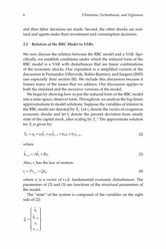
We now discuss the relation between the RBC model and a VAR. Spe-cifi cally, we establish conditions under which the reduced form of the RBC model is a VAR with disturbances that are linear combinations of the economic shocks. Our exposition is a simplifi ed version of the discussion in Fernandez-Villaverde, Rubio-Ramirez, and Sargent (2005) (see especially their section III). We include this discussion because it frames many of the issues that we address. Our discussion applies to both the standard and the recursive versions of the model.
We begin by showing how to put the reduced form of the RBC model into a state-space, observer form. Throughout, we analyze the log-linear approximations to model solutions. Suppose the variables of interest in the RBC model are denoted by Xt. Let st denote the vector of exogenous economic shocks and let kt denote the percent deviation from steady state of the capital stock, after scaling by Zt.
5 The approximate solution for Xt is given by:
X a a k a k b s b st t t t t= + + + +− −0 1 2 1 0 1 1ˆ ˆ , (2)
where
ˆ ˆ .k Ak Bst t t+ = +1 (3)
Also, st has the law of motion:
st = Pst–1 + Qεt, (4)
where εt is a vector of i.i.d. fundamental economic disturbances. The parameters of (2) and (3) are functions of the structural parameters of the model.
The “state” of the system is composed of the variables on the right side of (2):
ξt
t
t
t
t
k
k
s
s
=
⎛
⎝
⎜⎜⎜⎜⎜
⎞
⎠
⎟⎟⎟⎟⎟
−
−
ˆ
ˆ.1
1

7Assessing Structural VARs
The law of motion of the state is:
ξ ξ εt t tF D= +−1 , (5)
where F and D are constructed from A, B, Q, P. The econometrician observes the vector of variables, Yt. We assume Yt is equal to Xt plus iid measurement error, vt, which has diagonal variance-covariance, R. Then:
Yt = Hξt + vt. (6)
Here, H is defi ned so that Xt = Hξt, that is, relation (2) is satisfi ed. In (6) we abstract from the constant term. Hamilton (1994, section 13.4) shows how the system formed by (5) and (6) can be used to construct the exact Gaussian density function for a series of observations, Y1,…, YT . We use this approach when we estimate versions of the RBC model.
We now use (5) and (6) to establish conditions under which the reduced form representation for Xt implied by the RBC model is a VAR with dis-turbances that are linear combinations of the economic shocks. In this discussion, we set vt = 0, so that Xt = Yt. In addition, we assume that the number of elements in εt coincides with the number of elements in Yt.
We begin by substituting (5) into (6) to obtain:
Yt = HFξt–1 + Cεt, C ≡ HD.
Our assumption on the dimensions of Yt and εt implies that the matrix C is square. In addition, we assume C is invertible. Then:
εt = C–1Yt – C–1HFξt–1. (7)
Substituting (7) into (5), we obtain:
ξt = Mξt–1 + DC–1Yt,
where
M = [I – DC–1H]F. (8)
As long as the eigenvalues of M are less than unity in absolute value,
ξt = DC–1Yt + MDC–1Yt–1 + M2DC–1Yt–2 + … . (9)

Christiano, Eichenbaum, and Vigfusson8
Using (9) to substitute out for ξt –1 in (7), we obtain:
εt = C–1Yt – C–1HF[DC–1Yt–1 + MDC–1Yt–2 + M2DC–1Yt–3 + …],
or, after rearranging:
Yt = B1Yt–1 + B2Yt–2 + … + ut, (10)
where
ut = Cεt (11)
Bj = HFMj–1DC–1, j = 1, 2, … (12)
Expression (10) is an infi nite-order VAR, because ut is orthogonal to Yt–j, j ≥ 1.
Proposition 2.1. (Fernandez-Villaverde, Rubio-Ramirez, and Sargent) If C is invertible and the eigenvalues of M are less than unity in absolute value, then the RBC model implies:
• Yt has the infi nite-order VAR representation in (10)
• The linear one-step-ahead forecast error Yt given past Yt’s is ut, which is related to the economic disturbances by (11)
• The variance-covariance of ut is CC′• The sum of the VAR lag matrices is given by:
B B HF I M DCjj
( ) [ ] .11
1 1≡ = −=
∞− −∑
We will use the last of these results below.Relation (10) indicates why researchers interested in constructing
DSGE models fi nd it useful to analyze VARs. At the same time, this relationship clarifi es some of the potential pitfalls in the use of VARs. First, in practice the econometrician must work with fi nite lags. Sec-ond, the assumption that C is square and invertible may not be satis-fi ed. Whether C satisfi es these conditions depends on how Yt is defi ned. Third, signifi cant measurement errors may exist. Fourth, the matrix, M, may not have eigenvalues inside the unit circle. In this case, the eco-nomic shocks are not recoverable from the VAR disturbances.6 Implic-
9Assessing Structural VARs
itly, the econometrician who works with VARs assumes that these pitfalls are not quantitatively important.
2.3 VARs in Practice and the RBC Model
We are interested in the use of VARs as a way to estimate the response of Xt to economic shocks, i.e., elements of εt. In practice, macroeconomists use a version of (10) with fi nite lags, say q. A researcher can estimate B1, …, Bq and V = Eutu’t. To obtain the impulse response functions, how-ever, the researcher needs the Bi’s and the column of C corresponding to the shock in εt that is of interest. However, to compute the required col-umn of C requires additional identifying assumptions. In practice, two types of assumptions are used. Short-run assumptions take the form of direct restrictions on the matrix C. Long-run assumptions place indirect restrictions on C that stem from restrictions on the long-run response of Xt to a shock in an element of εt. In this section we use our RBC model to discuss these two types of assumptions and how they are imposed on VARs in practice.
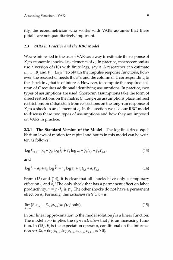
2.3.1 The Standard Version of the Model The log-linearized equi-librium laws of motion for capital and hours in this model can be writ-ten as follows:
log ˆ log ˆ log ,, ,k k zt k t z t l l t x x t+ = + + + +1 0γ γ γ γ τ γ τ (13)
and
log log ˆ log ., ,l a a k a z a at k t z t l l t x x t= + + + +0 τ τ (14)
From (13) and (14), it is clear that all shocks have only a temporary effect on lt and kt.
7 The only shock that has a permanent effect on labor productivity, at ≡ yt/lt, is ε z
t. The other shocks do not have a permanent effect on at. Formally, this exclusion restriction is:
lim[ ] ( ).j
t t j t t j tzE a E a f
→∞ + − +− =1 ε only (15)
In our linear approximation to the model solution f is a linear function. The model also implies the sign restriction that f is an increasing func-tion. In (15), Et is the expectation operator, conditional on the informa-tion set Ωt t s t s l t s x t sk z s= ≥− − − −(log ˆ , log , , ; )., ,τ τ 0
Christiano, Eichenbaum, and Vigfusson10
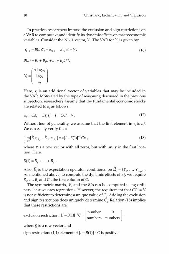
In practice, researchers impose the exclusion and sign restrictions on a VAR to compute ε z
t and identify its dynamic effects on macroeconomic variables. Consider the N × 1 vector, Yt. The VAR for Yt is given by:
Y B L Y u Eu u Vt t t t t+ += + ′ =1 1( ) , , (16)
B(L) ≡ B1 + B2L +… + BqLq–1,
Y
a
l
xt
t
t
t
=⎛
⎝
⎜⎜⎜
⎞
⎠
⎟⎟⎟
Δ loglog .
Here, xt is an additional vector of variables that may be included in the VAR. Motivated by the type of reasoning discussed in the previous subsection, researchers assume that the fundamental economic shocks are related to ut as follows:
u C E I CC Vt t t t= ′ = ′ =ε ε ε, , . (17)
Without loss of generality, we assume that the fi rst element in εt is εtz.
We can easily verify that:
lim[ ] [ ( )] ,j
t t j t t j tE a E a I B C→∞ + − +
−− = −� �1
11τ ε (18)
where τ is a row vector with all zeros, but with unity in the fi rst loca-tion. Here:
B(1) ≡ B1 + … + Bq.
Also, E~t is the expectation operator, conditional on Ω~t = {Yt, …, Yt–q+1}. As mentioned above, to compute the dynamic effects of ε z
t, we require B1, …, Bq and C1, the fi rst column of C.
The symmetric matrix, V, and the Bi’s can be computed using ordi-nary least squares regressions. However, the requirement that CC′ = V is not suffi cient to determine a unique value of C1. Adding the exclusion and sign restrictions does uniquely determine C1. Relation (18) implies that these restrictions are:
exclusion restriction: [ ( )] ,I B C− =⎡
⎣⎢
⎤
⎦⎥
−101 number
numbers numbers
where 0 is a row vector and
sign restriction: (1,1) element of [I – B(1)]–1 C is positive.

11Assessing Structural VARs
There are many matrices, C, that satisfy CC′ = V as well as the exclusion and sign restrictions. It is well-known that the fi rst column, C1, of each of these matrices is the same. We prove this result here, because elements of the proof will be useful to analyze our simulation results. Let
D ≡ [I – B(1)]–1 C.
Let SY(ω) denote the spectral density of Yt at frequency ω that is implied by the qth-order VAR. Then:
DD I B V I B SY′ = − − ′ =− −[ ( )] [ ( ) ] ( ).1 1 01 1 (19)
The exclusion restriction requires that D have a particular pattern of zeros:
D
d
D DN
N
= × × −
− ×
( )
( )
111 1 1 1
211 1
22
0
( ) ( )N N− × −
⎡
⎣
⎢⎢⎢
⎤
⎦
⎥⎥⎥1 1
so that
DDd d D
D d D D D D′ =
′′ + ′
⎡
⎣⎢⎢
⎤
⎦⎥11
211 21
21 11 21 21 22 22 ⎥⎥=
′⎡
⎣⎢⎢
⎤
⎦⎥⎥
S S
S SY Y
Y Y
11 21
21 22
0 0
0 0
( ) ( )
( ) ( ),
where
SS S
S SY
Y Y
Y Y
( )( ) ( )
( ) ( )ω
ω ω
ω ω≡
′⎡
⎣⎢⎢
⎤
⎦⎥⎥
11 21
21 22..
The exclusion restriction implies that
d S D S dY Y112 11
2121
110 0= =( ), ( )/ . (20)
There are two solutions to (20). The sign restriction
d11 > 0 (21)
selects one of the two solutions to (20). So, the fi rst column of D, D1, is uniquely determined. By our defi nition of C, we have
C1 = [I – B(1)]D1. (22)
We conclude that C1 is uniquely determined.
Christiano, Eichenbaum, and Vigfusson12
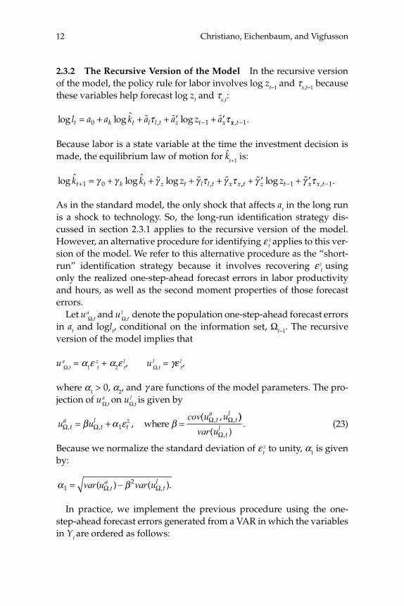
2.3.2 The Recursive Version of the Model In the recursive version of the model, the policy rule for labor involves log zt–1 and τx,t–1 because these variables help forecast log zt and τx,t:
log log ˆ log,l a a k a a z at k t l l t z t x= + + + ′ + ′−0 1� � �τ τ xx t, .−1
Because labor is a state variable at the time the investment decision is made, the equilibrium law of motion for kt+1 is:
log ˆ log ˆ log ,k k zt k t z t l l t x x+ = + + + +1 0γ γ γ γ τ γ τ� � � ,, ,log .t z t x x tz+ ′ + ′− −� �γ γ τ1 1
As in the standard model, the only shock that affects at in the long run is a shock to technology. So, the long-run identifi cation strategy dis-cussed in section 2.3.1 applies to the recursive version of the model. However, an alternative procedure for identifying ε t
z applies to this ver-
sion of the model. We refer to this alternative procedure as the “short-run” identifi cation strategy because it involves recovering ε z
t using only the realized one-step-ahead forecast errors in labor productivity and hours, as well as the second moment properties of those forecast errors.
Let u aΩ,t and u l
Ω,t denote the population one-step-ahead forecast errors
in at and loglt, conditional on the information set, Ωt–1. The recursive version of the model implies that
u aΩ,t = α1ε z
t + α2ε lt, u l
Ω,t = γε lt,
where α1 > 0, α2, and γ are functions of the model parameters. The pro-jection of u a
Ω,t on u lΩ,t is given by
u uu u
ta
tl
tz t
at
l
Ω ΩΩ Ω
, ,, ,,
( ,= + =β α ε β1 where
cov ))
( ).
,var u tlΩ
(23)
Because we normalize the standard deviation of ε tz to unity, α1 is given
by:
α β12= −var u var,t
a( Ω Ω) ( ).,u tl
In practice, we implement the previous procedure using the one-step-ahead forecast errors generated from a VAR in which the variables in Yt are ordered as follows:

13Assessing Structural VARs
Y
l
a
xt
t
t
t
=⎛
⎝
⎜⎜⎜
⎞
⎠
⎟⎟⎟
loglog .Δ
We write the vector of VAR one-step-ahead forecast errors, ut, as:
u
u
u
u
t
tl
ta
tx
=
⎛
⎝
⎜⎜⎜
⎞
⎠
⎟⎟⎟
.
We identify the technology shock with the second element in εt in (17). To compute the dynamic response of the variables in Yt to the technol-ogy shock we need B1, …, Bq in (16) and the second column, C2, of the matrix C, in (17). We obtain C2 in two steps. First, we identify the tech-nology shock using:
εα
βtz
ta
tlu u= −1
1ˆ( ˆ ),
where
ˆ ( , )( )
, ˆ ( ) ˆβ α β= = −cov
varvar var
u uu
uta
tl
tl t
a1
2 (( ).utl
The required variances and covariances are obtained from the estimate of V in (16). Second, we regress ut on ε z
t to obtain:8
C
u
u
u
l z
z
a z
z
x
2 =
cov
var
cov
var
cov
( , )( )
( , )( )
(
εε
εε,, )
( )
ˆ
ˆ(
εε
α
αz
zvar
c
⎛
⎝
⎜⎜⎜⎜⎜⎜⎜⎜
⎞
⎠
⎟⎟⎟⎟⎟⎟⎟⎟
=
0
11
1oov cov( , ) ˆ ( , ))
.u u u ut
xta
tx
tl−
⎛
⎝
⎜⎜⎜⎜
⎞
⎠
⎟⎟⎟⎟β
2.4 Parameterization of the Model
We consider different specifi cations of the RBC model that are distin-guished by the parameterization of the laws of motion of the exogenous shocks. In all specifi cations we assume, as in CKM, that:
β θ δ ψ γ= = = − − = =0 98 0 33 1 1 06 2 5 1 01 4 1 4. , . , ( . ) , . , ./ / 11 11 4/ − (24)
τ τ μ σx l z= = = − =0 3 0 242 1 016 1 11 4. , . , . , ./

Christiano, Eichenbaum, and Vigfusson14
2.4.1 Our MLE Parameterizations We estimate two versions of our model. In the two-shock maximum likelihood estimation (MLE) specifi cation we assume that σx = 0, so that there are two shocks, τl,t and log zt. We estimate the parameters ρl, σl, and σz, by maximizing the Gaussian like-lihood function of the vector, Xt = (Δlog yt, loglt)′, subject to (24).9 Our results are given by:
log . ,zt z tz= +μ ε0 00953
τ τ τ εl t l l t tl
, ,( . ) . . .= − + +−1 0 986 0 986 0 00561
The three-shock MLE specifi cation incorporates the investment tax shock, τx,t, into the model. We estimate the three-shock MLE version of the model by maximizing the Gaussian likelihood function of the vec-tor, Xt = (Δlog yt, loglt, Δlogit)′, subject to the parameter values in (24). The results are:
log zt = μz + 0.00968ε zt ,
τl,t = (1 – 0.9994)τl + 0.9994τl,t–1 + 0.00631ε lt,
τx,t = (1 – 0.9923)τx + 0.9923τx,t–1 + 0.00963ε xt .
The estimated values of ρx and ρl are close to unity. This fi nding is con-sistent with other research that also reports that shocks in estimated general equilibrium models exhibit high degrees of serial correlation.10
2.4.2 CKM Parameterizations The two-shock CKM specifi cation has two shocks, zt and τl,t. These shocks have the following time series rep-resentations:
log zt = μz + 0.0131ε tz ,
τl,t = (1 – 0.952)τl + 0.952τl,t–1 + 0.0136ε tl.
The three-shock CKM specifi cation adds an investment shock, τx,t, to the model, and has the following law of motion:
τx,t = (1 – 0.98)τx + 0.98τx,t–1 + 0.0123ε tx . (25)
As in our specifi cations, CKM obtain their parameter estimates using maximum likelihood methods. However, their estimates are very dif-
15Assessing Structural VARs
ferent from ours. For example, the variances of the shocks are larger in the two-shock CKM specifi cation than in our MLE specifi cation. Also, the ratio of σl
2 to σz2 is nearly three times larger in the two-shock CKM
specifi cation than in our two-shock MLE specifi cation. Section 2.5 dis-cusses the reasons for these differences.
2.5 The Importance of Technology Shocks for Hours Worked
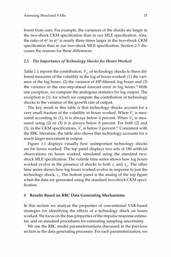
Table 1.1 reports the contribution, Vh, of technology shocks to three dif-ferent measures of the volatility in the log of hours worked: (1) the vari-ance of the log hours, (2) the variance of HP-fi ltered, log hours and (3) the variance in the one-step-ahead forecast error in log hours.11 With one exception, we compute the analogous statistics for log output. The exception is (1), for which we compute the contribution of technology shocks to the variance of the growth rate of output.
The key result in this table is that technology shocks account for a very small fraction of the volatility in hours worked. When Vh is mea-sured according to (1), it is always below 4 percent. When Vh is mea-sured using (2) or (3) it is always below 8 percent. For both (2) and (3), in the CKM specifi cations, Vh is below 2 percent.12 Consistent with the RBC literature, the table also shows that technology accounts for a much larger movement in output.
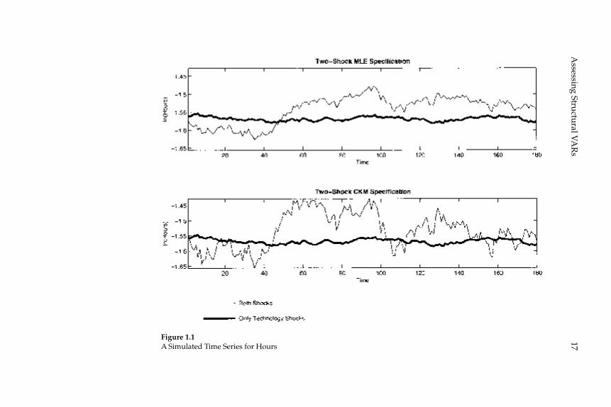
Figure 1.1 displays visually how unimportant technology shocks are for hours worked. The top panel displays two sets of 180 artifi cial observations on hours worked, simulated using the standard two-shock MLE specifi cation. The volatile time series shows how log hours worked evolve in the presence of shocks to both zt and τl,t. The other time series shows how log hours worked evolve in response to just the technology shock, zt. The bottom panel is the analog of the top fi gure when the data are generated using the standard two-shock CKM speci-fi cation.
3 Results Based on RBC Data Generating Mechanisms
In this section we analyze the properties of conventional VAR-based strategies for identifying the effects of a technology shock on hours worked. We focus on the bias properties of the impulse response estima-tor, and on standard procedures for estimating sampling uncertainty.
We use the RBC model parameterizations discussed in the previous section as the data generating processes. For each parameterization, we
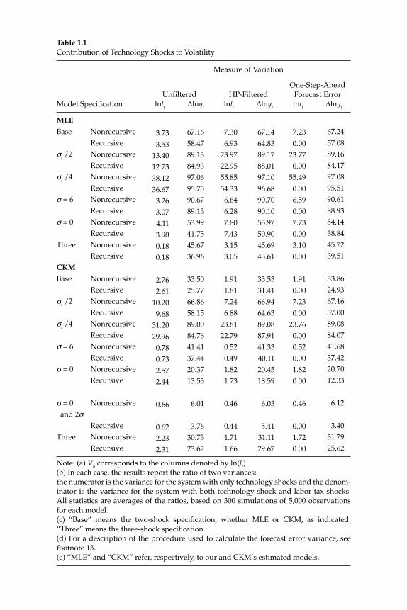
Table 1.1Contribution of Technology Shocks to Volatility
Model Specifi cation
Measure of Variation
Unfi lteredlnlt Δlnyt
HP-Filteredlnlt Δlnyt
One-Step-AheadForecast Errorlnlt Δlnyt
MLE Base Nonrecursive Recursiveσl /2 Nonrecursive Recursiveσl /4 Nonrecursive Recursiveσ = 6 Nonrecursive Recursiveσ = 0 Nonrecursive RecursiveThree Nonrecursive RecursiveCKM Base Nonrecursive Recursiveσl /2 Nonrecursive Recursiveσl /4 Nonrecursive Recursiveσ = 6 Nonrecursive Recursiveσ = 0 Nonrecursive Recursive
σ = 0 Nonrecursive and 2σl
RecursiveThree Nonrecursive Recursive
Note: (a) Vh corresponds to the columns denoted by ln(lt).(b) In each case, the results report the ratio of two variances: the numerator is the variance for the system with only technology shocks and the denom-inator is the variance for the system with both technology shock and labor tax shocks. All statistics are averages of the ratios, based on 300 simulations of 5,000 observations for each model.(c) “Base” means the two-shock specifi cation, whether MLE or CKM, as indicated. “Three” means the three-shock specifi cation.(d) For a description of the procedure used to calculate the forecast error variance, see footnote 13.(e) “MLE” and “CKM” refer, respectively, to our and CKM’s estimated models.
3.733.53
13.4012.7338.1236.673.263.074.113.900.180.18
2.762.61
10.209.68
31.2029.960.780.732.572.44
0.66
0.622.232.31
67.1658.4789.1384.9397.0695.7590.6789.1353.9941.7545.6736.96
33.5025.7766.8658.1589.0084.7641.4137.4420.3713.53
6.01
3.7630.7323.62
7.306.93
23.9722.9555.8554.336.646.287.807.433.153.05
1.911.817.246.88
23.8122.790.520.491.821.73
0.46
0.44 1.711.66
67.1464.8389.1788.0197.1096.6890.7090.1053.9750.9045.6943.61
33.5331.4166.9464.6389.0887.9141.3340.1120.4518.59
6.03
5.4131.1129.67
7.230.00
23.770.00
55.490.006.590.007.730.003.100.00
1.910.007.230.00
23.760.000.520.001.820.00
0.46
0.001.720.00
67.2457.0889.1684.1797.0895.5190.6188.9354.1438.8445.7239.51
33.8624.9367.1657.0089.0884.0741.6837.4220.7012.33
6.12
3.4031.7925.62
17A
ssessing Structural VA
Rs
Figure 1.1A Simulated Time Series for Hours
Christiano, Eichenbaum, and Vigfusson18
simulate 1,000 data sets of 180 observations each. The shocks ε zt, ε l
t, and possibly ε x
t, are drawn from i.i.d. standard normal distributions. For each artifi cial data set, we estimate a four-lag VAR. The average, across the 1,000 datasets, of the estimated impulse response functions, allows us to assess bias.
For each data set we also estimate two different confi dence intervals: a percentile-based confi dence interval and a standard-deviation based con-fi dence interval.13 We construct the intervals using the following bootstrap procedure. Using random draws from the fi tted VAR disturbances, we use the estimated four lag VAR to generate 200 synthetic data sets, each with 180 observations. For each of these 200 synthetic data sets we estimate a new VAR and impulse response function. For each artifi cial data set the percentile-based confi dence interval is defi ned as the top 2.5 percent and bottom 2.5 percent of the estimated coeffi cients in the dynamic response functions. The standard-deviation-based confi dence interval is defi ned as the estimated impulse response plus or minus two standard deviations where the standard deviations are calculated across the 200 simulated estimated coeffi cients in the dynamic response functions.
We assess the accuracy of the confi dence interval estimators in two ways. First, we compute the coverage rate for each type of confi dence interval. This rate is the fraction of times, across the 1,000 data sets sim-ulated from the economic model, that the confi dence interval contains the relevant true coeffi cient. If the confi dence intervals were perfectly accurate, the coverage rate would be 95 percent. Second, we provide an indication of the actual degree of sampling uncertainty in the VAR-based impulse response functions. In particular, we report centered 95 percent probability intervals for each lag in our impulse response func-tion estimators.14 If the confi dence intervals were perfectly accurate, they should on average coincide with the boundary of the 95 percent probability interval.
When we generate data from the two-shock MLE and CKM specifi ca-tions, we set Yt = (Δlogat, loglt)′. When we generate data from the three-shock MLE and CKM specifi cations, we set Yt = (Δlogat, loglt, logit/yt)′.
3.1 Short-Run Identifi cation
Results for the two- and three- Shock MLE Specifi cations
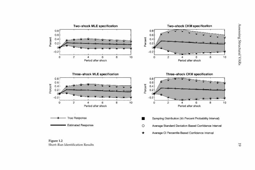
Figure 1.2 reports results generated from four different parameter-izations of the recursive version of the RBC model. In each panel, the
19A
ssessing Structural VA
Rs
Figure 1.2Short–Run Identifi cation Results
Christiano, Eichenbaum, and Vigfusson20
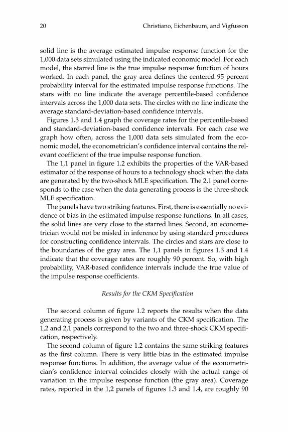
solid line is the average estimated impulse response function for the 1,000 data sets simulated using the indicated economic model. For each model, the starred line is the true impulse response function of hours worked. In each panel, the gray area defi nes the centered 95 percent probability interval for the estimated impulse response functions. The stars with no line indicate the average percentile-based confi dence intervals across the 1,000 data sets. The circles with no line indicate the average standard-deviation-based confi dence intervals.
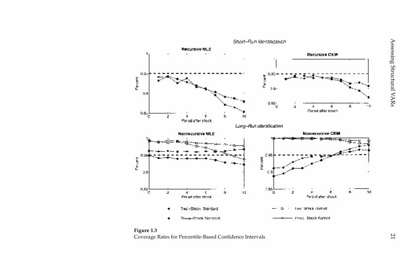
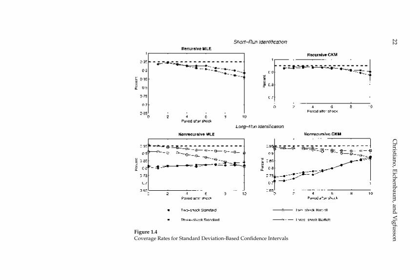
Figures 1.3 and 1.4 graph the coverage rates for the percentile-based and standard-deviation-based confi dence intervals. For each case we graph how often, across the 1,000 data sets simulated from the eco-nomic model, the econometrician’s confi dence interval contains the rel-evant coeffi cient of the true impulse response function.
The 1,1 panel in fi gure 1.2 exhibits the properties of the VAR-based estimator of the response of hours to a technology shock when the data are generated by the two-shock MLE specifi cation. The 2,1 panel corre-sponds to the case when the data generating process is the three-shock MLE specifi cation.
The panels have two striking features. First, there is essentially no evi-dence of bias in the estimated impulse response functions. In all cases, the solid lines are very close to the starred lines. Second, an econome-trician would not be misled in inference by using standard procedures for constructing confi dence intervals. The circles and stars are close to the boundaries of the gray area. The 1,1 panels in fi gures 1.3 and 1.4 indicate that the coverage rates are roughly 90 percent. So, with high probability, VAR-based confi dence intervals include the true value of the impulse response coeffi cients.
Results for the CKM Specifi cation
The second column of fi gure 1.2 reports the results when the data generating process is given by variants of the CKM specifi cation. The 1,2 and 2,1 panels correspond to the two and three-shock CKM specifi -cation, respectively.
The second column of fi gure 1.2 contains the same striking features as the fi rst column. There is very little bias in the estimated impulse response functions. In addition, the average value of the econometri-cian’s confi dence interval coincides closely with the actual range of variation in the impulse response function (the gray area). Coverage rates, reported in the 1,2 panels of fi gures 1.3 and 1.4, are roughly 90
21A
ssessing Structural VA
Rs
Figure 1.3Coverage Rates for Percentile-Based Confi dence Intervals
Christiano, E
ichenbaum, and
Vigfusson
22
Figure 1.4Coverage Rates for Standard Deviation-Based Confi dence Intervals

23Assessing Structural VARs
percent. These rates are consistent with the view that VAR-based proce-dures lead to reliable inference.
A comparison of the gray areas across the fi rst and second columns of fi gure 1.2, clearly indicates that more sampling uncertainty occurs when the data are generated from the CKM specifi cations than when they are generated from the MLE specifi cations (the gray areas are wider). VAR-based confi dence intervals detect this fact.
3.2 Long-run Identifi cation
Results for the two- and three- Shock MLE Specifi cations
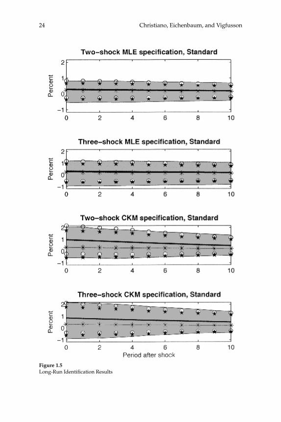
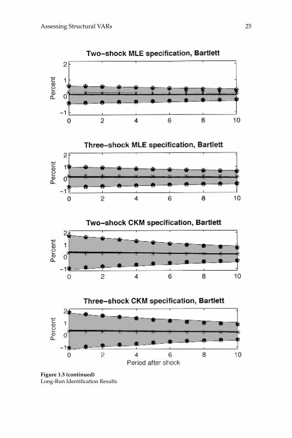
The fi rst and second rows of column 1 in fi gure 1.5 exhibit our results when the data are generated by the two- and three- shock MLE speci-fi cations. Once again there is virtually no bias in the estimated impulse response functions and inference is accurate. The coverage rates asso-ciated with the percentile-based confi dence intervals are very close to 95 percent (see fi gure 1.3). The coverage rates for the standard-devia-tion-based confi dence intervals are somewhat lower, roughly 80 per-cent (see fi gure 1.4). The difference in coverage rates can be seen in fi gure 1.5, which shows that the stars are shifted down slightly relative to the circles. Still, the circles and stars are very good indicators of the boundaries of the gray area, although not quite as good as in the analog cases in fi gure 1.2.
Comparing fi gures 1.2 and 1.5, we see that fi gure 1.5 reports more sampling uncertainty. That is, the gray areas are wider. Again, the cru-cial point is that the econometrician who computes standard confi dence intervals would detect the increase in sampling uncertainty.
Results for the CKM Specifi cation
The third and fourth rows of column 1 in fi gure 1.5 report results for the two- and three-shock CKM specifi cations. Consistent with results reported in CKM, there is substantial bias in the estimated dynamic response functions. For example, in the two-shock CKM specifi cation, the contemporaneous response of hours worked to a one-standard-deviation technology shock is 0.3 percent, while the mean estimated response is 0.97 percent. This bias stands in contrast to our other results.
Christiano, Eichenbaum, and Vigfusson24
Figure 1.5Long-Run Identifi cation Results
25Assessing Structural VARs
Figure 1.5 (continued)Long-Run Identifi cation Results
Christiano, Eichenbaum, and Vigfusson26
Is this bias big or problematic? In our view, bias cannot be evaluated without taking into account sampling uncertainty. Bias matters only to the extent that the econometrician is led to an incorrect inference. For example, suppose sampling uncertainty is large and the econometri-cian knows it. Then the econometrician would conclude that the data contain little information and, therefore, would not be misled. In this case, we say that bias is not large. In contrast, suppose sampling uncer-tainty is large, but the econometrician thinks it is small. Here, we would say bias is large.
We now turn to the sampling uncertainty in the CKM specifi cations. Figure 1.5 shows that the econometrician’s average confi dence interval is large relative to the bias. Interestingly, the percentile confi dence inter-vals (stars) are shifted down slightly relative to the standard-deviation-based confi dence intervals (circles). On average, the estimated impulse response function is not in the center of the percentile confi dence inter-val. This phenomenon often occurs in practice.15 Recall that we estimate a four lag VAR in each of our 1,000 synthetic data sets. For the purposes of the bootstrap, each of these VARs is treated as a true data generat-ing process. The asymmetric percentile confi dence intervals show that when data are generated by these VARs, VAR-based estimators of the impulse response function have a downward bias.
Figure 1.3 reveals that for the two- and three-shock CKM specifi ca-tions, percentile-based coverage rates are reasonably close to 95 per-cent. Figure 1.4 shows that the standard deviation based coverage rates are lower than the percentile-based coverage rates. However even these coverage rates are relatively high in that they exceed 70 percent.
In summary, the results for the MLE specifi cation differ from those of the CKM specifi cations in two interesting ways. First, sampling uncertainty is much larger with the CKM specifi cation. Second, the estimated responses are somewhat biased with the CKM specifi ca-tion. But the bias is small: It has no substantial effect on inference, at least as judged by coverage rates for the econometrician’s confi dence intervals.
3.3 Confi dence Intervals in the RBC Examples and a Situation in Which VAR-Based Procedures Go Awry
Here we show that the more important technology shocks are in the dynamics of hours worked, the easier it is for VARs to answer the

27Assessing Structural VARs
question, “how do hours worked respond to a technology shock.” We demonstrate this by considering alternative values of the innovation variance in the labor tax, σl, and by considering alternative values of σ, the utility parameter that controls the Frisch elasticity of labor supply.
Consider fi gure 1.6, which focuses on the long-run identifi cation schemes. The fi rst and second columns report results for the two-shock MLE and CKM specifi cations, respectively. For each specifi cation we redo our experiments, reducing σl by a half and then by a quarter. Table 1.1 shows that the importance of technology shocks rises as the stan-dard deviation of the labor tax shock falls. Figure 1.6 indicates that the magnitude of sampling uncertainty and the size of confi dence intervals fall as the relative importance of labor tax shocks falls.16
Figure 1.7 presents the results of a different set of experiments based on perturbations of the two-shock CKM specifi cation. The 1,1 and 2,1 panels show what happens when we vary the value of σ, the param-eter that controls the Frisch labor supply elasticity. In the 1,1 panel we set σ = 6, which corresponds to a Frisch elasticity of 0.63. In the 2,1 panel, we set σ = 0, which corresponds to a Frisch elasticity of infi n-ity. As the Frisch elasticity is increased, the fraction of the variance in hours worked due to technology shocks decreases (see table 1.1). The magnitude of bias and the size of confi dence intervals are larger for the higher Frisch elasticity case. In both cases the bias is still smaller than the sampling uncertainty.
We were determined to construct at least one example in which the VAR-based estimator of impulse response functions has bad proper-ties, i.e., bias is larger than sampling uncertainty. We display such an example in the 3,1 panel of fi gure 1.7. The data generating process is a version of the two-shock CKM model with an infi nite Frisch elasticity and double the standard deviation of the labor tax rate. Table 1.1 indi-cates that with this specifi cation, technology shocks account for a trivial fraction of the variance in hours worked. Of the three measures of Vh, two are 0.46 percent and the third is 0.66 percent. The 3,1 panel of fi gure 1.7 shows that the VAR-based procedure now has very bad properties: the true value of the impulse response function lies outside the aver-age value of both confi dence intervals that we consider. This example shows that constructing scenarios in which VAR-based procedures go awry is certainly possible. However, this example seems unlikely to be of practical signifi cance given the poor fi t to the data of this version of the model.
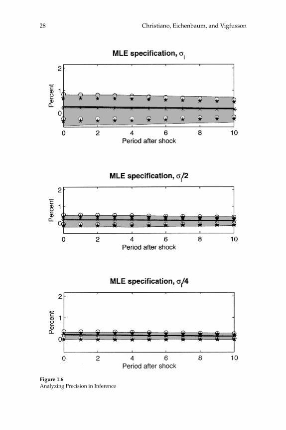
Christiano, Eichenbaum, and Vigfusson28
Figure 1.6Analyzing Precision in Inference
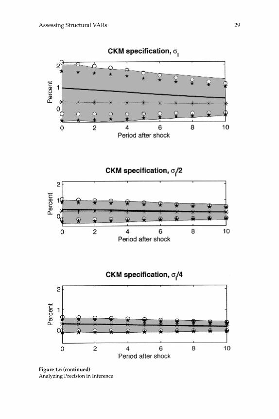
29Assessing Structural VARs
Figure 1.6 (continued)Analyzing Precision in Inference
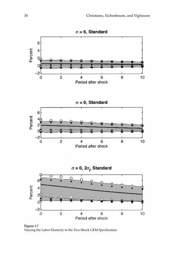
Christiano, Eichenbaum, and Vigfusson30
Figure 1.7Varying the Labor Elasticity in the Two-Shock CKM Specifi cation
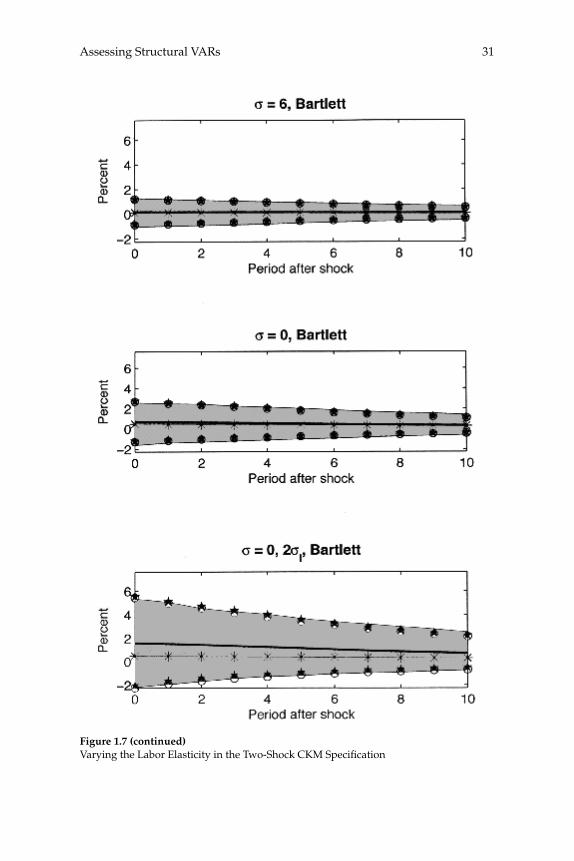
31Assessing Structural VARs
Figure 1.7 (continued)Varying the Labor Elasticity in the Two-Shock CKM Specifi cation
Christiano, Eichenbaum, and Vigfusson32
3.4 Are Long-Run Identifi cation Schemes Informative?
Up to now, we have focused on the RBC model as the data generating process. For empirically reasonable specifi cations of the RBC model, confi dence intervals associated with long-run identifi cation schemes are large. One might be tempted to conclude that VAR-based long-run identifi cation schemes are uninformative. Specifi cally, are the confi dence intervals so large that we can never discriminate between competing economic models? Erceg, Guerrieri, and Gust (2005) show that the answer to this question is “no.” They consider an RBC model similar to the one discussed above and a version of the sticky wage-price model developed by Christiano, Eichenbaum, and Evans (2005) in which hours worked fall after a positive technology shock. They then conduct a series of experiments to assess the ability of a long-run iden-tifi ed structural VAR to discriminate between the two models on the basis of the response of hours worked to a technology shock.
Using estimated versions of each of the economic models as a data generating process, they generate 10,000 synthetic data sets each with 180 observations. They then estimate a four-variable structural VAR on each synthetic data set and compute the dynamic response of hours worked to a technology shock using long-run identifi cation. Erceg, Guerrieri, and Gust (2005) report that the probability of fi nding an ini-tial decline in hours that persists for two quarters is much higher in the model with nominal rigidities than in the RBC model (93 percent versus 26 percent). So, if these are the only two models contemplated by the researcher, an empirical fi nding that hours worked decline after a positive innovation to technology will constitute compelling evidence in favor of the sticky wage-price model.
Erceg, Guerrieri, and Gust (2005) also report that the probability of fi nding an initial rise in hours that persists for two quarters is much higher in the RBC model than in the sticky wage-price model (71 per-cent versus 1 percent). So, an empirical fi nding that hours worked rises after a positive innovation to technology would constitute compel-ling evidence in favor of the RBC model versus the sticky wage-price alternative.
4 Contrasting Short- and Long-Run Restrictions
The previous section demonstrates that, in the examples we considered, when VARs are identifi ed using short-run restrictions, the conventional
33Assessing Structural VARs
estimator of impulse response functions is remarkably accurate. In con-trast, for some parameterizations of the data generating process, the conventional estimator of impulse response functions based on long-run identifying restrictions can exhibit noticeable bias. In this section we argue that the key difference between the two identifi cation strate-gies is that the long-run strategy requires an estimate of the sum of the VAR coeffi cients, B(1). This object is notoriously diffi cult to estimate accurately (see Sims 1972).
We consider a simple analytic expression related to one in Sims (1972). Our expression shows what an econometrician who fi ts a misspecifi ed, fi xed-lag, fi nite-order VAR would fi nd in population. Let B1, …, Bq, and V denote the parameters of the qth-order VAR fi t by the econometrician. Then:
ˆ min [ ( ) ˆ( )] (ˆ ,... ˆ
V V B e B e SB B
i iY
q
= + −− −
1
12π
ωω ω ))[ ( ) ˆ( )] ,B e B e di iω ω
π
πω− ′
−∫ (26)
where
B(L) = B1 + B2L + B3L2 + …,
ˆ( ) ˆ ˆ ... ˆ .B L B B L B L= + + +1 2 43
Here, B(e–iω) and B(e–iω) correspond to B(L) and B(L) with L replaced by e–iω.17 In (26), B and V are the parameters of the actual infi nite-ordered VAR representation of the data (see (10)), and SY(ω) is the associated spectral density at frequency ω.18 According to (26), estimation of a VAR approximately involves choosing VAR lag matrices to minimize a qua-dratic form in the difference between the estimated and true lag matri-ces. The quadratic form assigns greatest weight to the frequencies for which the spectral density is the greatest. If the econometrician’s VAR is correctly specifi ed, then B(e–iω) = B(e–iω) for all ω, and V = V, so that the estimator is consistent. If there is specifi cation error, then B(e–iω) ≠ B (e–iω) for some ω and V > V.19 In our context, specifi cation error exists because the true VAR implied by our data generating processes has q = ∞, but the econometrician uses a fi nite value of q.
To understand the implications of (26) for our analysis, it is useful to write in lag-operator form the estimated dynamic response of Yt to a shock in the fi rst element of εt
Y I L L Ct l t= + + +[ ...] ˆ ,,θ θ ε1 22
1 (27)
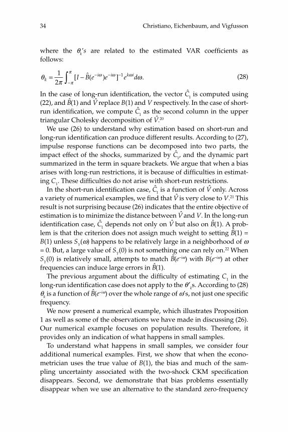
Christiano, Eichenbaum, and Vigfusson34
where the θk’s are related to the estimated VAR coeffi cients as follows:
θπ
ωω ω ω
π
πk
i i k iI B e e e d= − − − −
−∫1
21[ ˆ( ) ] . (28)
In the case of long-run identifi cation, the vector C1 is computed using (22), and B(1) and V replace B(1) and V respectively. In the case of short-run identifi cation, we compute C1 as the second column in the upper triangular Cholesky decomposition of V.20
We use (26) to understand why estimation based on short-run and long-run identifi cation can produce different results. According to (27), impulse response functions can be decomposed into two parts, the impact effect of the shocks, summarized by C1, and the dynamic part summarized in the term in square brackets. We argue that when a bias arises with long-run restrictions, it is because of diffi culties in estimat-ing C1. These diffi culties do not arise with short-run restrictions.
In the short-run identifi cation case, C1 is a function of V only. Across a variety of numerical examples, we fi nd that V is very close to V.21 This result is not surprising because (26) indicates that the entire objective of estimation is to minimize the distance between V and V. In the long-run identifi cation case, C1 depends not only on V but also on B(1). A prob-lem is that the criterion does not assign much weight to setting B(1) = B(1) unless SY(ω) happens to be relatively large in a neighborhood of ω = 0. But, a large value of SY(0) is not something one can rely on.22 When SY(0) is relatively small, attempts to match B(e–iω) with B(e–iω) at other frequencies can induce large errors in B(1).
The previous argument about the diffi culty of estimating C1 in the long-run identifi cation case does not apply to the θ′ks. According to (28) θk is a function of B(e–iω) over the whole range of ω’s, not just one specifi c frequency.
We now present a numerical example, which illustrates Proposition 1 as well as some of the observations we have made in discussing (26). Our numerical example focuses on population results. Therefore, it provides only an indication of what happens in small samples.
To understand what happens in small samples, we consider four additional numerical examples. First, we show that when the econo-metrician uses the true value of B(1), the bias and much of the sam-pling uncertainty associated with the two-shock CKM specifi cation disappears. Second, we demonstrate that bias problems essentially disappear when we use an alternative to the standard zero-frequency
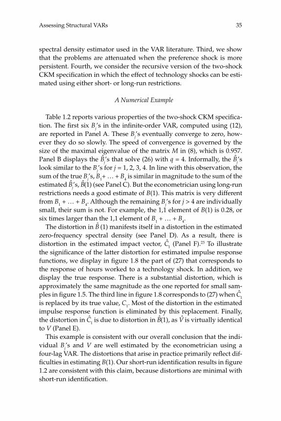
35Assessing Structural VARs
spectral density estimator used in the VAR literature. Third, we show that the problems are attenuated when the preference shock is more persistent. Fourth, we consider the recursive version of the two-shock CKM specifi cation in which the effect of technology shocks can be esti-mated using either short- or long-run restrictions.
A Numerical Example
Table 1.2 reports various properties of the two-shock CKM specifi ca-tion. The fi rst six Bj’s in the infi nite-order VAR, computed using (12), are reported in Panel A. These Bj’s eventually converge to zero, how-ever they do so slowly. The speed of convergence is governed by the size of the maximal eigenvalue of the matrix M in (8), which is 0.957. Panel B displays the Bj’s that solve (26) with q = 4. Informally, the Bj’s look similar to the Bj’s for j = 1, 2, 3, 4. In line with this observation, the sum of the true Bj’s, B1+ … + B4 is similar in magnitude to the sum of the estimated Bj’s, B(1) (see Panel C). But the econometrician using long-run restrictions needs a good estimate of B(1). This matrix is very different from B1 + … + B4. Although the remaining Bj’s for j > 4 are individually small, their sum is not. For example, the 1,1 element of B(1) is 0.28, or six times larger than the 1,1 element of B1 + … + B4.
The distortion in B (1) manifests itself in a distortion in the estimated zero-frequency spectral density (see Panel D). As a result, there is distortion in the estimated impact vector, C1 (Panel F).23 To illustrate the signifi cance of the latter distortion for estimated impulse response functions, we display in fi gure 1.8 the part of (27) that corresponds to the response of hours worked to a technology shock. In addition, we display the true response. There is a substantial distortion, which is approximately the same magnitude as the one reported for small sam-ples in fi gure 1.5. The third line in fi gure 1.8 corresponds to (27) when C1 is replaced by its true value, C1. Most of the distortion in the estimated impulse response function is eliminated by this replacement. Finally, the distortion in C1 is due to distortion in B(1), as V is virtually identical to V (Panel E).
This example is consistent with our overall conclusion that the indi-vidual Bj’s and V are well estimated by the econometrician using a four-lag VAR. The distortions that arise in practice primarily refl ect dif-fi culties in estimating B(1). Our short-run identifi cation results in fi gure 1.2 are consistent with this claim, because distortions are minimal with short-run identifi cation.

Christiano, Eichenbaum, and Vigfusson36
Table 1.2Properties of Two-Shock CKM Specifi cation
Panel A: First Six Lag Matrices in Infi nite-Order VAR Representation
B B1 20 013 0 041
0 0065 0 94
0 012 0 00=
⎡
⎣⎢
⎤
⎦⎥ =
−. .. .
,. .
00 0062 0 00
0 012 0 00
0 0059 0 003. .,
. .. .−
⎡
⎣⎢
⎤
⎦⎥ =
−−
B⎡⎡
⎣⎢
⎤
⎦⎥ ,
B B4 50 011 0 00
0 0056 0 00
0 011 0 0=
−−
⎡
⎣⎢
⎤
⎦⎥ =
−. .. .
,. . 00
0 0054 0 00
0 010 0 00
0 0051 0 06. .,
. .. .−
⎡
⎣⎢
⎤
⎦⎥ =
−−
B00
⎡
⎣⎢
⎤
⎦⎥
Panel B: Population Estimate of Four-lag VAR
ˆ . .. .
, ˆ . .B B1 2
0 017 0 043
0 0087 0 94
0 017 0=
⎡
⎣⎢
⎤
⎦⎥ =
− 000
0 0085 0 00
0 012 0 00
0 0059 03. ., ˆ . .
.−⎡
⎣⎢
⎤
⎦⎥ =
−−
B..
,00
⎡
⎣⎢
⎤
⎦⎥
ˆ . .. .
B40 0048 0 0088
0 0025 0 0045=
−−
⎡
⎣⎢
⎤
⎦⎥
Panel C: Actual and Estimated Sum of VAR Coeffi cients
ˆ( ). .. .
, ( ). .
B B10 055 0 032
0 14 0 941
0 28 0 0=
⎡
⎣⎢
⎤
⎦⎥ =
222
0 14 0 93
0 047 0 039
0 024 014
. .,
. .
. .⎡
⎣⎢
⎤
⎦⎥ ==Σ j jB
994
⎡
⎣⎢
⎤
⎦⎥
Panel D: Actual and Estimated Zero-Frequency Spectral Density
S SY Y( ). .. .
, ˆ (00 00017 0 00097
0 00097 0 120=
⎡
⎣⎢
⎤
⎦⎥ ))
. .. .
.=⎡
⎣⎢
⎤
⎦⎥
0 00012 0 0022
0 0022 0 13
Panel E: Actual and Estimated One-Step-Ahead Forecast Error Variance
V V= =−
− −⎡
⎣⎢
⎤
⎦⎥ˆ . .
. .0 00012 0 00015
0 00015 0 00053
Panel F: Actual and Estimated Impact Vector
C C1 10 00773
0 00317
0 00406
0 01208=
⎛⎝⎜
⎞⎠⎟
=⎛.
., ˆ .
.⎝⎝⎜⎞⎠⎟
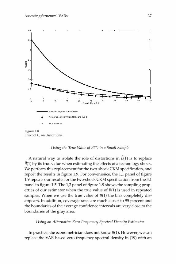
37Assessing Structural VARs
Using the True Value of B(1) in a Small Sample
A natural way to isolate the role of distortions in B(1) is to replace B(1) by its true value when estimating the effects of a technology shock. We perform this replacement for the two-shock CKM specifi cation, and report the results in fi gure 1.9. For convenience, the 1,1 panel of fi gure 1.9 repeats our results for the two-shock CKM specifi cation from the 3,1 panel in fi gure 1.5. The 1,2 panel of fi gure 1.9 shows the sampling prop-erties of our estimator when the true value of B(1) is used in repeated samples. When we use the true value of B(1) the bias completely dis-appears. In addition, coverage rates are much closer to 95 percent and the boundaries of the average confi dence intervals are very close to the boundaries of the gray area.
Using an Alternative Zero-Frequency Spectral Density Estimator
In practice, the econometrician does not know B(1). However, we can replace the VAR-based zero-frequency spectral density in (19) with an
Figure 1.8Effect of C1 on Distortions
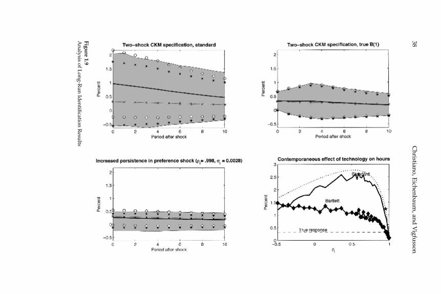
Christiano, E
ichenbaum, and
Vigfusson
38Figure 1.9
Analysis of L
ong-Run Id
entifi cation Results
39Assessing Structural VARs
alternative estimator of SY(0). Here, we consider the effects of using a standard Bartlett estimator:24
S g k C k g kkr
k r
k rY
k T
( ) ( ) ˆ ( ), ( ) ,(
01
0= = − ≤
⎧⎨⎪
⎩⎪=− >−−
−
∑1
1
)
T
(29)
where, after removing the sample mean from Yt:
ˆ ( ) .C kT
Y Yt t kt k
T
= ′−= +∑1
1
We use essentially all possible covariances in the data by choosing a large value of r, r = 150.25 In some respects, our modifi ed estimator is equivalent to running a VAR with longer lags.
We now assess the effect of our modifi ed long-run estimator. The fi rst two rows in fi gure 1.5 present results for cases in which the data generating mechanism corresponds to our two-and three-shock MLE specifi cations. Both the standard estimator (the left column) and our modifi ed estimator (the right column) exhibit little bias. In the case of the standard estimator, the econometrician’s estimator of standard errors understates somewhat the degree of sampling uncertainty asso-ciated with the impulse response functions. The modifi ed estimator reduces this discrepancy. Specifi cally, the circles and stars in the right column of fi gure 1.5 coincide closely with the boundary of the gray area. Coverage rates are reported in the 2,1 panels of fi gures 1.3 and 1.4. In fi gure 1.3, coverage rates now exceed 95 percent. The coverage rates in fi gure 1.4 are much improved relative to the standard case. Indeed, these rates are now close to 95 percent. Signifi cantly, the degree of sam-pling uncertainty associated with the modifi ed estimator is not greater than that associated with the standard estimator. In fact, in some cases, sampling uncertainty declines slightly.
The last two rows of column 1 in fi gure 1.5 display the results when the data generating process is a version of the CKM specifi cation. As shown in the second column, the bias is essentially eliminated by using the modifi ed estimator. Once again the circles and stars roughly coin-cide with the boundary of the gray area. Coverage rates for the per-centile-based confi dence intervals reported in fi gure 1.3 again have a tendency to exceed 95 percent (2,2 panel). As shown in the 2,2 panel of fi gure 1.4, coverage rates associated with the standard deviation based estimator are very close to 95 percent. There is a substantial improve-

Christiano, Eichenbaum, and Vigfusson40
ment over the coverage rates associated with the standard spectral den-sity estimator.
Figure 1.5 indicates that when the standard estimator works well, the modifi ed estimator also works well. When the standard estimator results in biases, the modifi ed estimator removes them. These fi ndings are consistent with the notion that the biases for the two CKM specifi ca-tions refl ect diffi culties in estimating the spectral density at frequency zero. Given our fi nding that V is an accurate estimator of V, we con-clude that the diffi culties in estimating the zero-frequency spectral den-sity in fact refl ect problems with B(1).
The second column of fi gure 1.7 shows how our modifi ed VAR-based estimator works when the data are generated by the various perturba-tions on the two-shock CKM specifi cation. In every case, bias is sub-stantially reduced.
Shifting Power to the Low Frequencies
Formula (26), suggests that, other things being equal, the more power there is near frequency zero, the less bias there is in B(1) and the better behaved is the estimated impulse response function to a technology shock. To pursue this observation we change the parameterization of the non-technology shock in the two-shock CKM specifi cation. We real-locate power toward frequency zero, holding the variance of the shock constant by increasing ρl to 0.998 and suitably lowering σl in (1). The results are reported in the 2,1 panel of fi gure 1.9. The bias associated with the two-shock CKM specifi cation almost completely disappears. This result is consistent with the notion that the bias problems with the two-shock CKM specifi cation stem from diffi culties in estimating B(1).
The previous result calls into question conjectures in the literature (see Erceg, Guerrieri, and Gust 2005). According to these conjectures, if there is more persistence in a non-technology shock, then the VAR will produce biased results because it will confuse the technology and non-technology shocks. Our result shows that this intuition is incom-plete, because it fails to take into account all of the factors mentioned in our discussion of (26). To show the effect of persistence, we consider a range of values of ρl to show that the impact of ρl on bias is in fact not monotone.
The 2,2 panel of fi gure 1.9 displays the econometrician’s estimator of the contemporaneous impact on hours worked of a technology shock against ρl. The dashed line indicates the true contemporaneous effect of
41Assessing Structural VARs
a technology shock on hours worked in the two-shock CKM specifi ca-tion. The dot-dashed line in the fi gure corresponds to the solution of (26), with q = 4, using the standard VAR-based estimator.26 The star in the fi gure indicates the value of ρl in the two-shock CKM specifi cation. In the neighborhood of this value of ρl, the distortion in the estimator falls sharply as ρl increases. Indeed, for ρl = 0.9999, essentially no dis-tortion occurs. For values of ρl in the region, (–0.5, 0.5), the distortion increases with increases in ρl.
The 2,2 panel of fi gure 1.9 also allows us to assess the value of our proposed modifi cation to the standard estimator. The line with dia-monds displays the modifi ed estimator of the contemporaneous impact on hours worked of a technology shock. When the standard estimator works well, that is, for large values of ρl the modifi ed and standard esti-mators produce similar results. However, when the standard estimator works poorly, e.g., for values of ρl near 0.5, our modifi ed estimator cuts the bias in half.
A potential shortcoming of the previous experiments is that persis-tent changes in τl,t do not necessarily induce very persistent changes in labor productivity. To assess the robustness of our results, we also con-sidered what happens when there are persistent changes in τx,t. These do have a persistent impact on labor productivity. In the two-shock CKM model, we set τl,t to a constant and allowed τx,t to be stochastic. We considered values of ρx in the range, [–0.5, 1], holding the variance of τx,t constant. We obtain results similar to those reported in the 2,2 panel of fi gure 1.9.
Short- and Long-Run Restrictions in a Recursive Model
We conclude this section by considering the recursive version of the two-shock CKM specifi cation. This specifi cation rationalizes estimat-ing the impact on hours worked of a shock to technology using either the short- or the long-run identifi cation strategy. We generate 1,000 data sets, each of length 180. On each synthetic data set, we estimate a four lag, bivariate VAR. Given this estimated VAR, we can estimate the effect of a technology shock using the short- and long-run identifi cation strategy. Figure 1.10 reports our results. For the long-run identifi cation strategy, there is substantial bias. In sharp contrast, there is no bias for the short-run identifi cation strategy. Because both procedures use the same estimated VAR parameters, the bias in the long-run identifi cation strategy is entirely attributable due to the use of B(1).
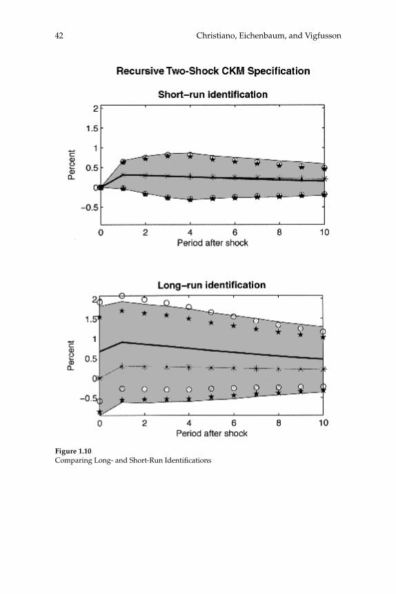
Christiano, Eichenbaum, and Vigfusson42
Figure 1.10Comparing Long- and Short-Run Identifi cations

43Assessing Structural VARs
5 Relation to Chari-Kehoe-McGrattan
In the preceding sections we argue that structural VAR-based proce-dures have good statistical properties. Our conclusions about the use-fulness of structural VARs stand in sharp contrast to the conclusions of CKM. These authors argue that, for plausibly parameterized RBC models, structural VARs lead to misleading results. They conclude that structural VARs are not useful for constructing and evaluating struc-tural economic models. In this section we present the reasons we dis-agree with CKM.
CKM’s Exotic Data Generating Processes
CKM’s critique of VARs is based on simulations using particular DSGE models estimated by maximum likelihood methods. Here, we argue that their key results are driven by assumptions about measurement error. CKM’s measurement error assumptions are overwhelmingly rejected in favor of alternatives under which their key results are overturned.
CKM adopt a state-observer setup to estimate their model. Defi ne:
Yt = (Δlogat, loglt, Δlogit, ΔlogGt)′,
where Gt denotes government spending plus net exports. CKM sup-pose that
Y X v Ev v Rt t t t t= + ′ =, , (30)
where R is diagonal, vt is a 4 × 1 vector of i.i.d. measurement errors and Xt is a 4 × 1 vector containing the model’s implications for the variables in Yt. The two-shock CKM specifi cation has only the shocks, τl,t and zt. CKM model government spending plus net exports as:
Gt = gt × Zt,
where gt is in principle an exogenous stochastic process. However, when CKM estimate the parameters of the technology and preferences processes, τl,t and zt, they set the variance of the government spending shock to zero, so that gt is a constant. As a result, CKM assume that
ΔlogGt = log zt + measurement error.
Christiano, Eichenbaum, and Vigfusson44
CKM fi x the elements on the diagonal of R exogenously to a “small number,” leading to the remarkable implication that government pur-chases plus net exports.
To demonstrate the sensitivity of CKM’s results to their specifi ca-tion of the magnitude of R, we consider the different assumptions that CKM make in different drafts of their paper. In the draft of May 2005, CKM (2005a) set the diagonal elements of R to 0.0001. In the draft of July 2005, CKM (2005b) set the ith diagonal element of R equal to 0.01 times the variance of the ith element of Yt.
The 1,1 and 2,1 panels in fi gure 1.11 report results corresponding to CKM’s two-shock specifi cations in the July and May drafts, respec-tively.27 These panels display the log likelihood value (see LLF) of these two models and their implications for VAR-based impulse response functions (the 1,1 panel is the same as the 3,1 panel in fi gure 1.5). Sur-prisingly, the log-likelihood of the July specifi cation is orders of magni-tude worse than that of the May specifi cation.
The 3,1 panel in fi gure 1.11 displays our results when the diagonal elements of R are included among the parameters being estimated.28 We refer to the resulting specifi cation as the “CKM free measurement error specifi cation.” First, both the May and the July specifi cations are rejected relative to the free measurement error specifi cation. The likeli-hood ratio statistic for testing the May and July specifi cations are 428 and 6,266, respectively. Under the null hypothesis that the May or July specifi cation is true, these statistics are realizations of a chi-square dis-tribution with four degrees of freedom. The evidence against CKM’s May or July specifi cations of measurement error is overwhelming.
Second, when the data generating process is the CKM free measure-ment error specifi cation, the VAR-based impulse response function is virtually unbiased (see the 3,1 panel in fi gure 1.11). We conclude that the bias in the two-shock CKM specifi cation is a direct consequence of CKM’s choice of the measurement error variance.
As noted above, CKM’s measurement error assumption has the implication that ΔlogGt is roughly equals to log zt. To investigate the role played by this peculiar implication, we delete ΔlogGt from Yt and re-estimate the system. We present the results in the right column of fi gure 1.11. In each panel of that column, we re-estimate the system in the same way as the corresponding panel in the left column, except that ΔlogGt is excluded from Yt. Comparing the 2,1 and 2,2 panels, we see that, with the May measurement error specifi cation, the bias disap-pears after relaxing CKM’s ΔlogGt = logzt assumption. Under the July
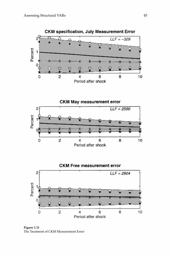
45Assessing Structural VARs
Figure 1.11The Treatment of CKM Measurement Error
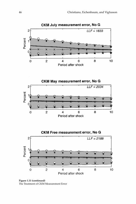
Christiano, Eichenbaum, and Vigfusson46
Figure 1.11 (continued)The Treatment of CKM Measurement Error
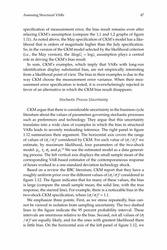
47Assessing Structural VARs
specifi cation of measurement error, the bias result remains even after relaxing CKM’s assumption (compare the 1,1 and 1,2 graphs of fi gure 1.11). As noted above, the May specifi cation of CKM’s model has a like-lihood that is orders of magnitude higher than the July specifi cation. So, in the version of the CKM model selected by the likelihood criterion (i.e., the May version), the ΔlogGt = logzt assumption plays a central role in driving the CKM’s bias result.
In sum, CKM’s examples, which imply that VARs with long-run identifi cation display substantial bias, are not empirically interesting from a likelihood point of view. The bias in their examples is due to the way CKM choose the measurement error variance. When their mea-surement error specifi cation is tested, it is overwhelmingly rejected in favor of an alternative in which the CKM bias result disappears.
Stochastic Process Uncertainty
CKM argue that there is considerable uncertainty in the business cycle literature about the values of parameters governing stochastic processes such as preferences and technology. They argue that this uncertainty translates into a wide class of examples in which the bias in structural VARs leads to severely misleading inference. The right panel in fi gure 1.12 summarizes their argument. The horizontal axis covers the range of values of (σl /σz)
2 considered by CKM. For each value of (σl /σz)2 we
estimate, by maximum likelihood, four parameters of the two-shock model: μz, τl, σl, and ρl.
29 We use the estimated model as a data generat-ing process. The left vertical axis displays the small sample mean of the corresponding VAR-based estimator of the contemporaneous response of hours worked to a one-standard deviation technology shock.
Based on a review the RBC literature, CKM report that they have a roughly uniform prior over the different values of (σl/σz)
2 considered in fi gure 1.12. The fi gure indicates that for many of these values, the bias is large (compare the small sample mean, the solid line, with the true response, the starred line). For example, there is a noticeable bias in the two-shock CKM specifi cation, where (σl/σz)
2 = 1.1.We emphasize three points. First, as we stress repeatedly, bias can-
not be viewed in isolation from sampling uncertainty. The two dashed lines in the fi gure indicate the 95 percent probability interval. These intervals are enormous relative to the bias. Second, not all values of (σl /σz)
2 are equally likely, and for the ones with greatest likelihood there is little bias. On the horizontal axis of the left panel of fi gure 1.12, we
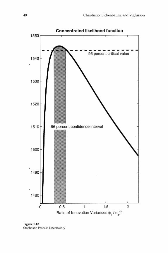
Christiano, Eichenbaum, and Vigfusson48
Figure 1.12Stochastic Process Uncertainty
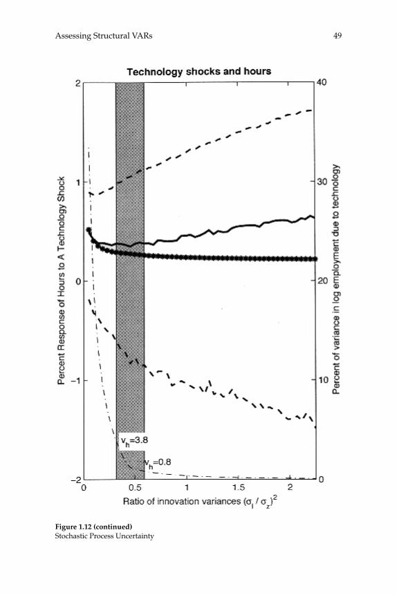
49Assessing Structural VARs
Figure 1.12 (continued)Stochastic Process Uncertainty
Christiano, Eichenbaum, and Vigfusson50
display the same range of values of (σl/σz)2 as in the right panel. On
the vertical axis we report the log-likelihood value of the associated model. The peak of this likelihood occurs close to the estimated value in the two-shock MLE specifi cation. Note how the log-likelihood value drops sharply as we consider values of (σl /σz)
2 away from the uncon-strained maximum likelihood estimate. The vertical bars in the fi gure indicate the 95 percent confi dence interval for (σl/σz)
2.30 Figure 1.12 reveals that the confi dence interval is very narrow relative to the range of values considered by CKM, and that within the interval, the bias is quite small.
Third, the right axis in the right panel of fi gure 1.12 plots Vh, the per-cent of the variance in log hours due to technology, as a function of (σl /σz)
2. The values of (σl/σz)2 for which there is a noticeable bias corre-
spond to model economies where Vh is less than 2 percent. Here, identi-fying the effects of a technology shock on hours worked is tantamount to looking for a needle in a haystack.
The Metric for Assessing the Performance of Structural VARs
CKM emphasize comparisons between the true dynamic response function in the data generating process and the response function that an econometrician would estimate using a four-lag VAR with an infi nite amount of data. In our own analysis in section 4, we fi nd population calculations with four lag VARs useful for some purposes. However, we do not view the probability limit of a four lag VAR as an interest-ing metric for measuring the usefulness of structural VARs. In practice econometricians do not have an infi nite amount of data. Even if they did, they would certainly not use a fi xed lag length. Econometricians determine lag length endogenously and, in a large sample, lag length would grow. If lag lengths grow at the appropriate rate with sample size, VAR-based estimators of impulse response functions are consis-tent. The interesting issue (to us) is how VAR-based procedures per-form in samples of the size that practitioners have at their disposal. This is why we focus on small sample properties like bias and sampling uncertainty.
Over-Differencing
The potential power of the CKM argument lies in showing that VAR-based procedures are misleading, even under circumstances when
51Assessing Structural VARs
everyone would agree that VARs should work well, namely when the econometrician commits no avoidable specifi cation error. The econo-metrician does, however, commit one unavoidable specifi cation error. The true VAR is infi nite ordered, but the econometrician assumes the VAR has a fi nite number of lags. CKM argue that this seemingly innoc-uous assumption is fatal for VAR analysis. We have argued that this conclusion is unwarranted.
CKM present other examples in which the econometrician commits an avoidable specifi cation error. Specifi cally, they study the conse-quences of over differencing hours worked. That is, the econometri-cian fi rst differences hours worked when hours worked are stationary.31 This error gives rise to bias in VAR-based impulse response functions that is large relative to sampling uncertainty. CKM argue that this bias is another reason not to use VARs.
However, the observation that avoidable specifi cation error is possi-ble in VAR analysis is not a problem for VARs per se. The possibility of specifi cation error is a potential pitfall for any type of empirical work. In any case, CKM’s analysis of the consequences of over differencing is not new. For example, Christiano, Eichenbaum, and Vigfusson (2003, hereafter, CEV) study a situation in which the true data generating pro-cess satisfi es two properties: Hours worked are stationary and they rise after a positive technology shock. CEV then consider an econometrician who does VAR-based long-run identifi cation when Yt in (16) contains the growth rate of hours rather than the log level of hours. CEV show that the econometrician would falsely conclude that hours worked fall after a positive technology shock. CEV do not conclude from this exer-cise that structural VARs are not useful. Rather, they develop a statis-tical procedure to help decide whether hours worked should be fi rst differenced or not.
CKM Ignore Short-Run Identifi cation Schemes
We argue that VAR-based short-run identifi cation schemes lead to remarkably accurate and precise inference. This result is of interest because the preponderance of the empirical literature on structural VARs explores the implications of short-run identifi cation schemes. CKM are silent on this literature. McGrattan (2006) dismisses short-run identifi cation schemes as “hokey.” One possible interpretation of this adjective is that McGrattan can easily imagine models in which the identifi cation scheme is incorrect. The problem with this interpretation

Christiano, Eichenbaum, and Vigfusson52
is that all models are a collection of strong identifying assumptions, all of which can be characterized as “hokey.” A second interpretation is that in McGrattan’s view, the type of zero restrictions typically used in short run identifi cation are not compatible with dynamic equilibrium theory. This view is simply incorrect (see Sims and Zha 2006). A third possible interpretation is that no one fi nds short-run identifying assumptions interesting. However, the results of short-run identifi cation schemes have had an enormous effect on the construction of dynamic, general equilibrium models. See Woodford (2003) for a summary in the context of monetary models.
Sensitivity of Some VAR Results to Data Choices
CKM argue that VARs are very sensitive to the choice of data. Spe-cifi cally, they review the papers by Francis and Ramey (2005), CEV, and Galí and Rabanal (2005), which use long-run VAR methods to estimate the response of hours worked to a positive technology shock. CKM note that these studies use different measures of per capita hours worked and output in the VAR analysis. The bottom panel of fi gure 1.13 displays the different measures of per capita hours worked that these studies use. Note how the low frequency properties of these series differ. The corresponding estimated impulse response functions and confi dence intervals are reported in the top panel. CKM view it as a defect in VAR methodology that the different measures of hours worked lead to dif-ferent estimated impulse response functions. We disagree. Empirical results should be sensitive to substantial changes in the data. A construc-tive response to the sensitivity in fi gure 1.13 is to carefully analyze the different measures of hours worked, see which is more appropriate, and perhaps construct a better measure. It is not constructive to dismiss an econometric technique that signals the need for better measurement.
CKM note that the principle differences in the hours data occur in the early part of the sample. According to CKM, when they drop these early observations they obtain different impulse response functions. However, as fi gure 1.13 shows, these impulse response functions are not signifi cantly different from each other.
6 A Model with Nominal Rigidities
In this section we use the model in ACEL to assess the accuracy of struc-tural VARs for estimating the dynamic response of hours worked to
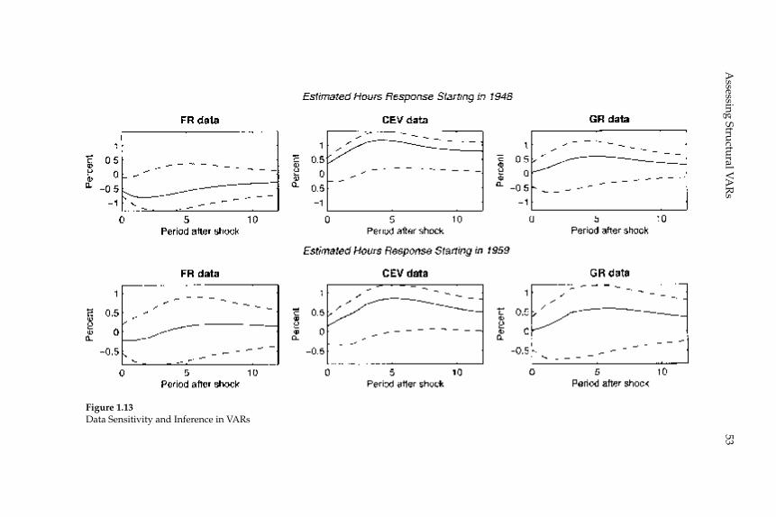
53A
ssessing Structural VA
Rs
Figure 1.13Data Sensitivity and Inference in VARs
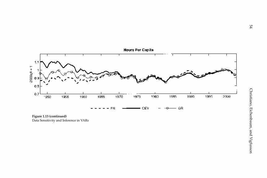
Christiano, E
ichenbaum, and
Vigfusson
54
Figure 1.13 (continued)Data Sensitivity and Inference in VARs

55Assessing Structural VARs
shocks. This model allows for nominal rigidities in prices and wages and has three shocks: a monetary policy shock, a neutral technology shock, and a capital-embodied technology shock. Both technology shocks affect labor productivity in the long run. However, the only shock in the model that affects the price of investment in the long run is the capital-embodied technology shock. We use the ACEL model to evaluate the ability of a VAR to uncover the response of hours worked to both types of technology shock and to the monetary policy shock. Our strategy for identifying the two technology shocks is similar to the one proposed by Fisher (2006). The model rationalizes a version of the short-run, recursive identifi cation strategy used by Christiano, Eichen-baum, and Evans (1999) to identify monetary shocks. This strategy cor-responds closely to the recursive procedure studied in section 2.3.2.
6.1 The Model
The details of the ACEL model, as well as the parameter estimates, are reported in Appendix A of the NBER Working Paper version of this paper. Here, we limit our discussion to what is necessary to clarify the nature of the shocks in the ACEL model. Final goods, Yt, are produced using a standard Dixit-Stiglitz aggregator of intermediate goods, yt(i), i ∈ (0, 1). To produce a unit of consumption goods, Ct, one unit of fi nal goods is required. To produce one unit of investment goods, It, ϒt
–1 units of fi nal goods are required. In equilibrium, ϒt
–1 is the price, in units of consumption goods, of an investment good. Let μϒ,t denote the growth rate of ϒt, let μϒ denote the nonstochastic steady state value of μϒ,t, and let μϒ,t denote the percent deviation of μϒ,t from its steady state value:
μ μμ μ
μϒ ϒϒ ϒ
ϒ
ϒϒ, ,
,, ˆ .tt
tt
t= =−
−1 (31)
The stochastic process for the growth rate of ϒt is:
ˆ ˆ , ., , ,μ ρ μ σ ε σμ μ μ μϒ ϒϒ ϒ ϒ ϒt t t= +−1 0> (32)
We refer to the i.i.d. unit variance random variable, εuϒ,t, as the capi-tal-embodied technology shock. ACEL assume that the intermediate good, yt(i), for i ∈ (0, 1) is produced using a Cobb-Douglas production function of capital and hours worked. This production function is per-turbed by a multiplicative, aggregate technology shock denoted by Zt. Let zt denote the growth rate of Zt, let z denote the nonstochastic steady
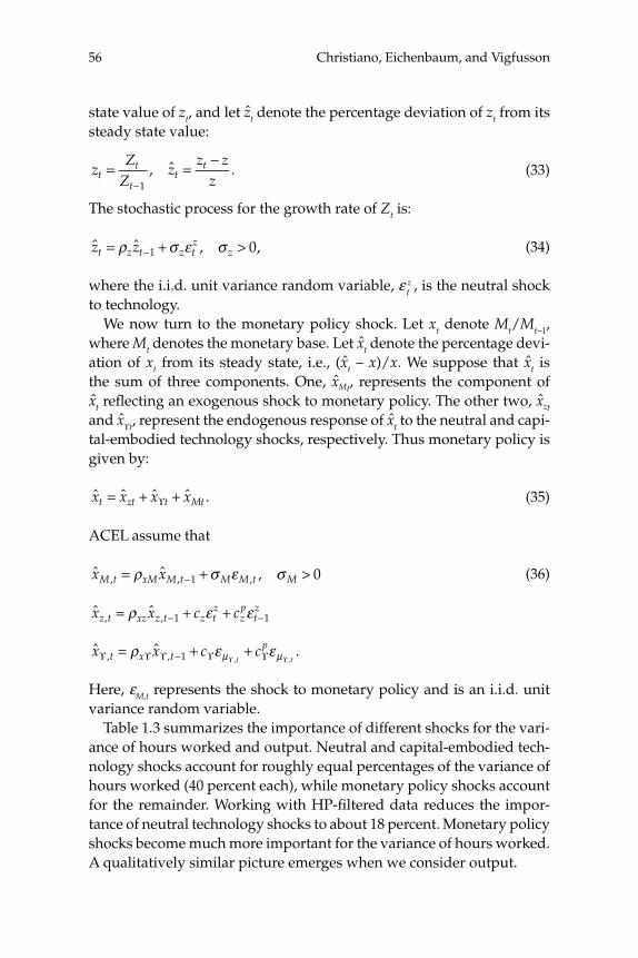
Christiano, Eichenbaum, and Vigfusson56
state value of zt, and let zt denote the percentage deviation of zt from its steady state value:
zZ
Zz
z zzt
t
tt
t= =−
−1, ˆ . (33)
The stochastic process for the growth rate of Zt is:
ˆ ˆ , ,z zt z t z tz
z= +−ρ σ ε σ1 0> (34)
where the i.i.d. unit variance random variable, ε tz , is the neutral shock
to technology.We now turn to the monetary policy shock. Let xt denote Mt/Mt–1,
where Mt denotes the monetary base. Let xt denote the percentage devi-ation of xt from its steady state, i.e., (xt – x)/x. We suppose that xt is the sum of three components. One, xMt, represents the component of xt refl ecting an exogenous shock to monetary policy. The other two, xzt and xϒt, represent the endogenous response of xt to the neutral and capi-tal-embodied technology shocks, respectively. Thus monetary policy is given by:
ˆ ˆ ˆ ˆ .x x x xt zt t Mt= + +ϒ (35)
ACEL assume that
ˆ ˆ ,, , ,x xM t xM M t M M t M= +−ρ σ ε σ1 0> (36)
ˆ ˆ, ,x x c cz t xz z t z tz
zp
tz= + +− −ρ ε ε1 1
ˆ ˆ ., , , ,x x c ct x t
pt tϒ ϒ ϒ ϒ ϒϒ ϒ
= + +−ρ ε εμ μ1
Here, εM,t represents the shock to monetary policy and is an i.i.d. unit variance random variable.
Table 1.3 summarizes the importance of different shocks for the vari-ance of hours worked and output. Neutral and capital-embodied tech-nology shocks account for roughly equal percentages of the variance of hours worked (40 percent each), while monetary policy shocks account for the remainder. Working with HP-fi ltered data reduces the impor-tance of neutral technology shocks to about 18 percent. Monetary policy shocks become much more important for the variance of hours worked. A qualitatively similar picture emerges when we consider output.

57Assessing Structural VARs
It is worth emphasizing that neutral technology shocks are much more important in hours worked in the ACEL model than in the RBC model. This fact plays an important role in determining the precision of VAR-based inference using long-run restrictions in the ACEL model.
6.2 Results
We use the ACEL model to simulate 1,000 data sets each with 180 obser-vations. We report results from two different VARs. In the fi rst VAR, we simultaneously estimate the dynamic effect on hours worked of a neu-tral technology shock and a capital-embodied technology shock. The variables in this VAR are:
Y
p
a
lt
It
t
t
=⎛
⎝
⎜⎜⎜
⎞
⎠
⎟⎟⎟
ΔΔ
lnln
ln,
where pIt denotes the price of capital in consumption units. The vari-able, ln (pIt), corresponds to ln (ϒ t
–1) in the model. As in Fisher (2006), we identify the dynamic effects on Yt of the two technology shocks, using a generalization of the strategy in section 2.3.1.32 The details are provided in Appendix B of the NBER Working Paper version of this paper.
The 1,1 panel of fi gure 1.14 displays our results using the standard VAR procedure to estimate the dynamic response of hours worked to a neutral technology shock. Several results are worth emphasizing. First, the estimator is essentially unbiased. Second, the econometrician’s estimator of sampling uncertainty is also reasonably unbiased. The
Table 1.3Percent Contribution of Shocks in the ACEL model to the Variation in Hours and in Output
Types of Shock
Monetary Neutral Capital-Statistic Policy Technology Embodied
Variance of logged hours 22.2 40.0 38.5
Variance of HP fi ltered logged hours 37.8 17.7 44.5
Variance of Δy 29.9 46.7 23.6
Variance of HP fi ltered logged output 31.9 32.3 36.1
Note: Results are average values based on 500 simulations of 3,100 observations each. ACEL: Altig Christiano, Eichenbaum, and Linde (2005).
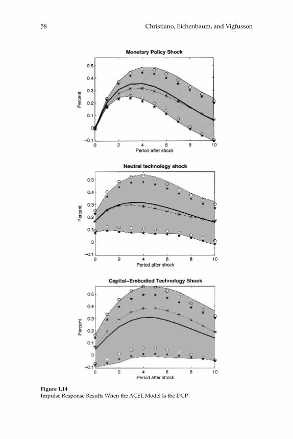
Christiano, Eichenbaum, and Vigfusson58
Figure 1.14Impulse Response Results When the ACEL Model Is the DGP
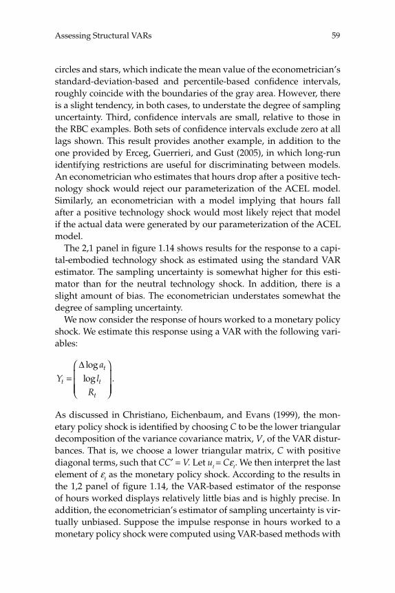
59Assessing Structural VARs
circles and stars, which indicate the mean value of the econometrician’s standard-deviation-based and percentile-based confi dence intervals, roughly coincide with the boundaries of the gray area. However, there is a slight tendency, in both cases, to understate the degree of sampling uncertainty. Third, confi dence intervals are small, relative to those in the RBC examples. Both sets of confi dence intervals exclude zero at all lags shown. This result provides another example, in addition to the one provided by Erceg, Guerrieri, and Gust (2005), in which long-run identifying restrictions are useful for discriminating between models. An econometrician who estimates that hours drop after a positive tech-nology shock would reject our parameterization of the ACEL model. Similarly, an econometrician with a model implying that hours fall after a positive technology shock would most likely reject that model if the actual data were generated by our parameterization of the ACEL model.
The 2,1 panel in fi gure 1.14 shows results for the response to a capi-tal-embodied technology shock as estimated using the standard VAR estimator. The sampling uncertainty is somewhat higher for this esti-mator than for the neutral technology shock. In addition, there is a slight amount of bias. The econometrician understates somewhat the degree of sampling uncertainty.
We now consider the response of hours worked to a monetary policy shock. We estimate this response using a VAR with the following vari-ables:
Y
a
l
Rt
t
t
t
=⎛
⎝
⎜⎜⎜
⎞
⎠
⎟⎟⎟
Δ loglog .
As discussed in Christiano, Eichenbaum, and Evans (1999), the mon-etary policy shock is identifi ed by choosing C to be the lower triangular decomposition of the variance covariance matrix, V, of the VAR distur-bances. That is, we choose a lower triangular matrix, C with positive diagonal terms, such that CC′ = V. Let ut = Cεt. We then interpret the last element of εt as the monetary policy shock. According to the results in the 1,2 panel of fi gure 1.14, the VAR-based estimator of the response of hours worked displays relatively little bias and is highly precise. In addition, the econometrician’s estimator of sampling uncertainty is vir-tually unbiased. Suppose the impulse response in hours worked to a monetary policy shock were computed using VAR-based methods with
Christiano, Eichenbaum, and Vigfusson60
data generated from this model. We conjecture that a model in which money is neutral, or in which a monetary expansion drives hours worked down, would be easy to reject.
7 Concluding Remarks
In this paper we study the ability of structural VARs to uncover the response of hours worked to a technology shock. We consider two classes of data generating processes. The fi rst class consists of a series of real business cycle models that we estimate using maximum like-lihood methods. The second class consists of the monetary model in ACEL. We fi nd that with short-run restrictions, structural VARs per-form remarkably well in all our examples. With long-run restrictions, structural VARs work well as long as technology shocks explain at least a very small portion of the variation in hours worked.
In a number of examples that we consider, VAR-based impulse response functions using long-run restrictions exhibit some bias. Even though these examples do not emerge from empirically plausible data generating processes, we fi nd them of interest. They allow us to diag-nose what can go wrong with long-run identifi cation schemes. Our diagnosis leads us to propose a modifi cation to the standard VAR-based procedure for estimating impulse response functions using long-run identifi cation. This procedure works well in our examples.
Finally, we fi nd that confi dence intervals with long-run identifi ca-tion schemes are substantially larger than those with short-run iden-tifi cation schemes. In all empirically plausible cases, the VARs deliver confi dence intervals that accurately refl ect the true degree of sampling uncertainty. We view this characteristic as a great virtue of VAR-based methods. When the data contain little information, the VAR will indi-cate the lack of information. To reduce large confi dence intervals the analyst must either impose additional identifying restrictions (i.e., use more theory) or obtain better data.
Acknowledgments
The fi rst two authors are grateful to the National Science Foundation for Financial Support. We thank Lars Hansen and our colleagues at the Fed-eral Reserve Bank of Chicago and the Board of Governors for useful com-ments at various stages of this project. The views in this paper are solely those of the authors and should not be interpreted as refl ecting the views of the Board of Governors of the Federal Reserve System or its staff.

61Assessing Structural VARs
Endnotes
1. See for example Sims (1989), Eichenbaum and Evans (1995), Rotemberg and Woodford (1997), Galí (1999), Francis and Ramey (2005), Christiano, Eichenbaum, and Evans (2005), and Del Negro, Schorfheide, Smets, and Wouters (2005).
2. See, for example, Basu, Fernald, and Kimball (2004), Christiano, Eichenbaum, and Vigfusson (2003, 2004), Fisher (2006), Francis and Ramey (2005), King, Plosser, Stock and Watson (1991), Shapiro and Watson (1988), and Vigfusson (2004). Francis, Owyang, and Roush (2005) pursue a related strategy to identify a technology shock as the shock that maximizes the forecast error variance share of labor productivity at a long but fi nite horizon.
3. This list is particularly long and includes at least Bernanke (1986), Bernanke and Blinder (1992), Bernanke and Mihov (1998), Blanchard and Perotti (2002), Blanchard and Watson (1986), Christiano and Eichenbaum (1992), Christiano, Eichenbaum, and Evans (2005), Cushman and Zha (1997), Eichenbaum and Evans (1995), Hamilton (1997), Rotem-berg and Woodford (1992), Sims (1986), and Sims and Zha (2006).
4. See also Fernandez-Villaverdez, Rubio-Ramirez, and Sargent (2005) who investigate the circumstances in which the economic shocks are recoverable from the VAR distur-bances. They provide a simple matrix algebra check to assess recoverability. They identify models in which the conditions are satisfi ed and other models in which they are not.
5. Let k~
t = kt/Zt–1. Then, k = (k~
t – k~
)/k~, where k
~ denotes the value of k
~t in nonstochastic
steady state.
6. For an early example, see Hansen and Sargent (1980, footnote 12). Sims and Zha (forth-coming) discuss the possibility that, although a given economic shock may not lie exactly in the space of current and past Yt, it may nevertheless be “close.” They discuss methods to detect this case.
7. Cooley and Dwyer (1998) argue that in the standard RBC model, if technology shocks have a unit root, then per capita hours worked will be difference stationary. This claim, which plays an important role in their analysis of VARs, is incorrect.
8. We implement the procedure for estimating C2 by computing CC′ = V, where C is the lower triangular Cholesky decomposition of V, and setting C2 equal to the second column of C.
9. We use the standard Kalman fi lter strategy discussed in Hamilton (1994, section 13.4). We remove the sample mean from Xt prior to estimation and set the measurement error in the Kalman fi lter system to zero, i.e., R = 0 in (6).
10. See, for example, Christiano (1988), Christiano et al. (2004), and Smets and Wouters (2003).
11. We compute forecast error variances based on a four lag VAR. The variables in the VAR depend on whether the calculations correspond to the two or three shock model. In the case of the two-shock model, the VAR has two variables, output growth and log hours. In the case of the three-shock model, the VAR has three variables: output growth, log hours and the log of the investment to output ratio. Computing Vh requires estimat-ing VARs in artifi cial data generated with all shocks, as well as in artifi cial data gener-ated with only the technology shock. In the latter case, the one-step ahead forecast error from the VAR is well defi ned, even though the VAR coeffi cients themselves are not well defi ned due to multicollinearity problems.

Christiano, Eichenbaum, and Vigfusson62
12. When we measure Vh according to (1), Vh drops from 3.73 in the two-shock MLE model to 0.18 in the three-shock MLE model. The analogous drop in Vh is an order of magnitude smaller when Vh is measured using (2) or (3). The reason for this difference is that ρl goes from 0.986 in the two-shock MLE model to 0.9994 in the three-shock MLE model. In the latter specifi cation there is a near-unit root in τl,t, which translates into a near-unit root in hours worked. As a result, the variance of hours worked becomes very large at the low frequencies. The near-unit root in τlt has less of an effect on hours worked at high and business cycle frequencies.
13. Sims and Zha (1999) refer to what we call the percentile-based confi dence interval as the “other-percentile bootstrap interval.” This procedure has been used in several studies, such as Blanchard and Quah (1989), Christiano, Eichenbaum, and Evans (1999), Francis and Ramey (2005), McGrattan (2006), and Runkle (1987). The standard-deviation based confi dence interval has been used by other researchers, such as Christiano, Eichenbaum, and Evans (2005), Galí (1999), and Galí and Rabanal (2005).
14. For each lag starting at the impact period, we ordered the 1,000 estimated impulse responses from smallest to largest. The lower and upper boundaries correspond to the 25th and the 975th impulses in this ordering.
15. An extreme example, in which the point estimates roughly coincide with one of the boundaries of the percentile-based confi dence interval, appears in Blanchard and Quah (1989).
16. As σl falls, the total volatility of hours worked falls, as does the relative importance of labor tax shocks. In principle, both effects contribute to the decline in sampling uncer-tainty.
17. The minimization in (26) is actually over the trace of the indicated integral. One inter-pretation of (26) is that it provides the probability limit of our estimators—what they would converge to as the sample size increases to infi nity. We do not adopt this interpre-tation, because in practice an econometrician would use a consistent lag-length selection method. The probability limit of our estimators corresponds to the true impulse response functions for all cases considered in this paper.
18. The derivation of this formula is straightforward. Write (10) in lag operator form as follows:
Yt = B(L)Yt–1 + ut,
where Eutu ′t = V. Let the fi tted disturbances associated with a particular parameteriza-tion, B(L), be denoted ut. Simple substitution implies:
ˆ [ ( ) ˆ( )] .u B L B L Y ut t t= − +−1
The two random variables on the right of the equality are orthogonal, so that the variance ut of is just the variance of the sum of the two:
var u var B L B L Y Vt t( ˆ ) ([ ( ) ˆ( )] ) .= − +−1
Expression (26) in the text follows immediately.
19. By V > V, we mean that V – V is a positive defi nite matrix.
20. In the earlier discussion it was convenient to adopt the normalization that the tech-nology shock is the second element of εt. Here, we adopt the same normalization as for the long-run identifi cation—namely, that the technology shock is the fi rst element of εt.

63Assessing Structural VARs
21. This result explains why lag-length selection methods, such as the Akaike criterion, almost never suggest values of q greater than four in artifi cial data sets of length 180, regardless of which of our data generating methods we used. These lag length selection methods focus on V.
22. Equation (26) shows that B(1) corresponds to only a single point in the integral. So other things equal, the estimation criterion assigns no weight at all to getting B(1) right. The reason B(1) is identifi ed in our setting is that the B(ω) functions we consider are con-tinuous at ω = 0.
23. A similar argument is presented in Ravenna (2005).
24. Christiano, Eichenbaum, and Vigfusson (2006) also consider the estimator proposed by Andrews and Monahan (1992).
25. The rule of always setting the bandwidth, r, equal to sample size does not yield a consistent estimator of the spectral density at frequency zero. We assume that as sample size is increased beyond T = 180, the bandwidth is increased suffi ciently slowly to achieve consistency.
26. Because (26) is a quadratic function, we solve the optimization problem by solving the linear fi rst-order conditions. These are the Yule-Walker equations, which rely on population second moments of the data. We obtain the population second moments by complex integration of the reduced form of the model used to generate the data, as sug-gested by Christiano (2002).
27. To ensure comparability of results we use CKM’s computer code and data, avail-able on Ellen McGrattan’s webpage. The algorithm used by CKM to form the estimation criterion is essentially the same as the one we used to estimate our models. The only difference is that CKM use an approximation to the Gaussian function by working with the steady state Kalman gain. We form the exact Gaussian density function, in which the Kalman gain varies over dates, as described in Hamilton (1994). We believe this differ-ence is inconsequential.
28. When generating the artifi cial data underlying the calculations in the 3,1 panel of fi gure 1.11, we set the measurement error to zero. (The same assumption was made for all the results reported here.) However, simulations that include the estimated measurement error produce results that are essentially the same.
29. We use CKM’s computer code and data to ensure comparability of results.
30. The bounds of this interval are the upper and lower values of (σl /σz)2 where twice the
difference of the log-likelihood from its maximal value equals the critical value associated with the relevant likelihood ratio test.
31. For technical reasons, CKM actually consider “quasi differencing” hours worked using a differencing parameter close to unity. In small samples this type of quasi differ-encing is virtually indistinguishable from fi rst differencing.
32. Our strategy differs somewhat from the one pursued in Fisher (2006), who applies a version of the instrumental variables strategy proposed by Shapiro and Watson (1988).
33. Similar specifi cations have been used by authors such as Sims (1994) and Schmitt-Grohé and Uribe (2004).
Christiano, Eichenbaum, and Vigfusson64
References
Altig, David, Lawrence Christiano, Martin Eichenbaum, and Jesper Linde. 2005. “Firm-Specifi c Capital, Nominal Rigidities, and the Business Cycle.” NBER Working Paper Series 11034. Cambridge, MA: National Bureau of Economic Research.
Andrews, Donald W. K., and J. Christopher Monahan. 1992. “An Improved Heteroske-dasticity and Autocorrelation Consistent Covariance Matrix Estimator.” Econometrica 60: 953–966.
Basu, Susanto, John G. Fernald, and Miles S. Kimball. 2006. “Are Technology Improve-ments Contractionary?” American Economic Review 96(5): 1418–1448.
Bernanke, Ben S. 1986. “Alternative Explanations of the Money-Income Correlation.” Carnegie Rochester Conference Series on Public Policy 25: 49–99.
Bernanke, Ben S., and Alan S. Blinder. 1992. “The Federal Funds Rate and the Channels of Monetary Transmission.” American Economic Review 82: 901–921.
Bernanke, Ben S., and Ilian Mihov. 1998. “Measuring Monetary Policy.” Quarterly Journal of Economics 113: 869–902.
Blanchard, Olivier, and Roberto Perotti. 2002. “An Empirical Characterization of the Dynamic Effects of Changes in Government Spending and Taxes on Output.” Quarterly Journal of Economics 117: 1329–1368.
Blanchard, Olivier, and Danny Quah. 1989. “The Dynamic Effects of Aggregate Demand and Supply Disturbances.” American Economic Review 79: 655–673.
Blanchard, Olivier, and Mark Watson. 1986. “Are Business Cycles All Alike?” In Robert Gordon, ed., Continuity and Change in the American Business Cycle. Chicago, IL: University of Chicago Press, 123–156.
Chari, V. V., Patrick J. Kehoe, and Ellen McGrattan. 2005a. “A Critique of Structural VARs Using Real Business Cycle Theory.” Working Paper Series 631. Minneapolis, MN: Federal Reserve Bank of Minneapolis, May.
Chari, V. V., Patrick J. Kehoe, and Ellen McGrattan. 2005b. “A Critique of Structural VARs Using Real Business Cycle Theory.” Working Paper Series 631. Minneapolis, MN: Federal Reserve Bank of Minneapolis, July.
Christiano, Lawrence J. 1988. “Why Does Inventory Investment Fluctuate So Much?” Journal of Monetary Economics 21: 247–280.
Christiano, Lawrence J. 2002. “Solving Dynamic Equilibrium Models by a Method of Undetermined Coeffi cients.” Computational Economics 20: 21–55.
Christiano, Lawrence J., and Martin Eichenbaum. 1992. “Identifi cation and the Liquidity Effect of a Monetary Policy Shock.” In Alex Cukierman, Zvi Hercowitz, and Leonardo Leiderman, eds., Political Economy, Growth, and Business Cycles. Cambridge, MA: MIT Press, 335–370.
Christiano, Lawrence J., Martin Eichenbaum, and Charles Evans. 1999. “Monetary Policy Shocks: What Have We Learned and to What End?” In John B.Taylor and Michael D. Woodford, eds., Handbook of Macroeconomics, Volume 1A, Amsterdam: Elsevier Science, 65–148.

65Assessing Structural VARs
Christiano, Lawrence J., Martin Eichenbaum, and Charles Evans. 2005. “Nominal Rigidi-ties and the Dynamic Effects of a Shock to Monetary Policy.” Journal of Political Economy 113: 1–45.
Christiano, Lawrence J., Martin Eichenbaum, and Robert Vigfusson. 2003. “What Hap-pens after a Technology Shock?” NBER Working Paper Series 9819. Cambridge, MA: National Bureau of Economic Research.
Christiano, Lawrence J., Martin Eichenbaum, and Robert Vigfusson. 2004. “The Response of Hours to a Technology Shock: Evidence Based on Direct Measures of Technology.” Journal of the European Economic Association 2: 381–395.
Christiano, Lawrence J., Martin Eichenbaum, and Robert Vigfusson. 2006. “Alternative Procedures for Estimating Vector Autoregressions Identifi ed with Long-Run Restric-tions.” Journal of the European Economic Association 4(2-3): 475–483.
Cooley, Thomas F., and Mark Dwyer. 1998. “Business Cycle Analysis without Much The-ory: A Look at Structural VARs.” Journal of Econometrics 83: 57–88.
Cushman, David O., and Tao Zha. 1997. “Identifying Monetary Policy in a Small Open Economy under Flexible Exchange Rates.” Journal of Monetary Economics 39: 433–448.
Del Negro, Marco, Frank Schorfheide, Frank Smets, and Raf Wouters. 2005. “On the Fit and Forecasting Performance of New Keynesian Models.” Unpublished paper, Univer-sity of Pennsylvania.
Eichenbaum, Martin, and Charles Evans. 1995. “Some Empirical Evidence on the Effects of Shocks to Monetary Policy on Exchange Rates.” Quarterly Journal of Economics 110: 975–1009.
Erceg, Christopher J., Luca Guerrieri, and Christopher Gust. 2005. “Can Long-Run Restrictions Identify Technology Shocks?” Journal of the European Economic Association 3: 1237–1278.
Erceg, Christopher J., Dale W. Henderson, and Andrew T. Levin. 2000. “Optimal Mon-etary Policy with Staggered Wage and Price Contracts.” Journal of Monetary Economics 46: 281–313.
Faust, Jon, and Eric Leeper. 1997. “When Do Long-Run Identifying Restrictions Give Reli-able Results?” Journal of Business and Economic Statistics 15: 345–353.
Fernandez-Villaverde, Jesus, Juan F. Rubio-Ramirez, and Thomas J. Sargent. 2005. “A, B, C’s (and D’s) for Understanding VARs.” Unpublished paper, New York University.
Fisher, Jonas. 2006. “The Dynamic Effects of Neutral and Investment-Specifi c Technology Shocks.” Journal of Political Economy 114(3): 413–451.
Francis, Neville, Michael T. Owyang, and Jennifer E. Roush. 2005. “A Flexible Finite-Hori-zon Identifi cation of Technology Shocks.” Working Paper Series 2005–024A. St. Louis: Federal Reserve Bank of St. Louis.
Francis, Neville, and Valerie A. Ramey. 2005. “Is the Technology-Driven Real Business Cycle Hypothesis Dead? Shocks and Aggregate Fluctuations Revisited.” Journal of Mon-etary Economics 52: 1379–1399.
Galí, Jordi. 1999. “Technology, Employment, and the Business Cycle: Do Technology Shocks Explain Aggregate Fluctuations?” American Economic Review 89: 249–271.
Christiano, Eichenbaum, and Vigfusson66
Galí, Jordi, and Pau Rabanal. 2005. “Technology Shocks and Aggregate Fluctuations: How Well Does the Real Business Cycle Model Fit Postwar U.S. Data?” In Mark Gertler and Kenneth Rogoff, eds., NBER Macroeconomics Annual 2004. Cambridge, MA: MIT Press.
Hamilton, James D. 1994. Time Series Analysis. Princeton, NJ: Princeton University Press.
Hamilton, James D. 1997. “Measuring the Liquidity Effect.” American Economic Review 87: 80–97.
Hansen, Lars, and Thomas Sargent. 1980. “Formulating and Estimating Dynamic Linear Rational Expectations Models.” Journal of Economic Dynamics and Control 2: 7–46.
King, Robert G., Charles I. Plosser, James H. Stock, and Mark W. Watson. 1991. “Stochas-tic Trends and Economic Fluctuations.” American Economic Review 81: 819–840.
McGrattan, Ellen. 2006. “A Critique of Structural VARs Using Business Cycle Theory.” Presentation at the annual meeting of the American Economic Association, Boston, Janu-ary 6–8. Available at <http://minneapolisfed.org/research/economists/mcgrattan/CEV/assa.htm>.
Pagan, Adrian R., and John C. Robertson. 1998. “Structural Models of the Liquidity Effect.” Review of Economics and Statistics 80: 202–217.
Ravenna, Federico. 2005. “Vector Autoregressions and Reduced Form Representations of Dynamic Stochastic General Equilibrium Models.” Unpublished manuscript.
Rotemberg, Julio J., and Michael Woodford. 1992. “Oligopolistic Pricing and the Effects of Aggregate Demand on Economic Activity.” Journal of Political Economy 100: 1153–1207.
Rotemberg, Julio J., and Michael Woodford. 1997. “An Optimization-Based Econometric Framework for the Evaluation of Monetary Policy.” In Ben S. Bernanke and Julio Rotem-berg, eds., NBER Macroeconomics Annual 1997. Cambridge, MA: MIT Press.
Runkle, David E. 1987. “Vector Autoregressions and Reality.” Journal of Business and Eco-nomic Statistics 5: 437–442.
Schmitt-Grohé, Stefanie, and Martin Uribe. 2004. “Optimal Fiscal and Monetary Policy under Sticky Prices.” Journal of Economic Theory 114: 198–230.
Shapiro, Matthew, and Mark Watson. 1988. “Sources of Business Cycle Fluctuations.” In Stanley Fischer, ed., NBER Macroeconomics Annual 1988. Cambridge, MA: MIT Press.
Sims, Christopher. 1972. “The Role of Approximate Prior Restrictions in Distributed Lag Estimation.” Journal of the American Statistical Association 67: 169–175.
Sims, Christopher. 1980. “Macroeconomics and Reality.” Econometrica 48: 1–48.
Sims, Christopher. 1986. “Are Forecasting Models Usable for Policy Analysis?” Federal Reserve Bank of Minneapolis, Quarterly Review 10: 2–16.
Sims, Christopher. 1989. “Models and Their Uses.” American Journal of Agricultural Eco-nomics 71: 489–494.
Sims, Christopher. 1994. “A Simple Model for Study of the Determination of the Price Level and the Interaction of Monetary and Fiscal Policy.” Economic Theory 4(3): 381–399.
Sims, Christopher, and Tao Zha. 1999. “Error Bands for Impulse Responses.” Econometrica 67: 1113–1155.
67Assessing Structural VARs
Sims, Christopher, and Tao Zha. 2006. “Does Monetary Policy Generate Recessions?” Macroeconomic Dynamics 10(2): 231–272.
Smets, Frank, and Raf Wouters. 2003. “An Estimated Dynamic Stochastic General Equilib-rium Model of the Euro Area.” Journal of the European Economic Association 1: 1123–1175.
Vigfusson, Robert J. 2004. “The Delayed Response to a Technology Shock: A Flexible Price Explanation.” International Finance Discussion Paper Series 2004–810. Washington, D.C.: Board of Governors of the Federal Reserve System.
Woodford, Michael M. 1996. “Control of the Public Debt: A Requirement for Price Stabil-ity?” NBER Working Paper Series no. 5684. Cambridge, MA.: National Bureau of Eco-nomic Research.
Woodford, Michael M. 2003. Interest and Prices: Foundations of a Theory of Monetary Policy. Princeton, NJ: Princeton University Press.
Appendix A A Model with Nominal Wage and Price Rigidities
This appendix describes the ACEL model used in section 6. The model econ-omy is composed of households, fi rms, and a monetary authority.
There is a continuum of households, indexed by j ∈ (0, 1). The jth household is a monopoly supplier of a differentiated labor service, and sets its wage sub-ject to Calvo-style wage frictions. In general, households earn different wage rates and work different amounts. A straightforward extension of arguments in Erceg, Henderson, and Levin (2000) and in Woodford (1996) establishes that in the presence of state contingent securities, households are homogeneous with respect to consumption and asset holdings. Our notation refl ects this result. The preferences of the jth household are given by:
E C bCh
tj l t
t t l Lj t
t
β ψ−+ + −
+
=
− −⎡
⎣⎢
⎤
⎦⎥log( ) ,
1 11
2
200
∞
∑ ,
where ψL ≥ 0 and E jt is the time t expectation operator, conditional on household
j’s time t information set. The variable, Ct, denotes time t consumption and hjt denotes time t hours worked. The household’s asset evolution equation is given by:
Mt+1 = Rt [Mt – Qt + (xt – 1)Mat ] + Aj,t + Qt + Wj,thj,t + Dt – (1 + η (Vt)) PtCt.
Here, Mt and Qt denote, respectively, the household’s stock of money, and cash balances at the beginning of period t. The variable Wj,t represents the nominal wage rate at time t. In addition Dt and Aj,t denote fi rm profi ts and the net cash infl ow from participating in state-contingent security markets at time t. The variable, xt, represents the gross growth rate of the economy-wide per capita
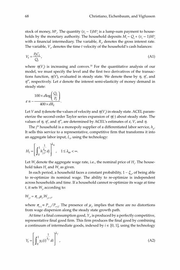
Christiano, Eichenbaum, and Vigfusson68
stock of money, Mat. The quantity (xt – 1)M a
t is a lump-sum payment to house-holds by the monetary authority. The household deposits Mt – Qt + (xt – 1)M a
t with a fi nancial intermediary. The variable, Rt, denotes the gross interest rate. The variable, Vt, denotes the time t velocity of the household’s cash balances:
VP CQtt t
t= , (A1)
where η(Vt) is increasing and convex.33 For the quantitative analysis of our model, we must specify the level and the fi rst two derivatives of the transac-tions function, η(V), evaluated in steady state. We denote these by η, η′, and η′′, respectively. Let ε denote the interest semi-elasticity of money demand in steady state:
ε ≡× ⎛
⎝⎜⎞⎠⎟
×−
100 logdQP
dR
t
t
t400.
Let V and η denote the values of velocity and η(Vt) in steady state. ACEL param-eterize the second-order Taylor series expansion of η(·) about steady state. The values of η, η′, and η′′, are determined by ACEL’s estimates of ε, V, and η.
The jth household is a monopoly supplier of a differentiated labor service, hjt. It sells this service to a representative, competitive fi rm that transforms it into an aggregate labor input, Lt, using the technology:
H h djt j t=⎡
⎣⎢⎢
⎤
⎦⎥⎥ ∞∫ , , .
1
0
11λ
λ
ωω
ω
λ≤ <
Let Wt denote the aggregate wage rate, i.e., the nominal price of Ht. The house-hold takes Ht and Wt as given.
In each period, a household faces a constant probability, 1 – ξw, of being able to re-optimize its nominal wage. The ability to re-optimize is independent across households and time. If a household cannot re-optimize its wage at time t, it sets Wjt according to:
Wj,t = πt–1μz*Wj,t–1,
where πt–1 ≡ Pt–1/Pt–2. The presence of μz* implies that there are no distortions
from wage dispersion along the steady state growth path.At time t a fi nal consumption good, Yt, is produced by a perfectly competitive,
representative fi nal good fi rm. This fi rm produces the fi nal good by combining a continuum of intermediate goods, indexed by i ∈ [0, 1], using the technology
Y y i dit tf
f
=⎡
⎣⎢⎢
⎤
⎦⎥⎥∫ ( ) ,
1
0
1 λ
λ
(A2)

69Assessing Structural VARs
where 1 ≤ λf < ∞ and yt(i) denotes the time t input of intermediate good i. The fi rm takes its output price, Pt, and its input prices, Pt(i), as given and beyond its control.
Intermediate good i is produced by a monopolist using the following tech-nology:
y i
K i Z h i z K i Z h
t
t t t t t t t
( )( ) ( ( )) ( ) (
=
α α αφ1− ∗− if (( ))i zt1
0
− ∗⎧⎨⎪
⎩⎪
α φ≥otherwise
(A3)
where 0 < α < 1. Here, ht(i) and Kt(i) denote time t labor and capital services used to produce the ith intermediate good. The variable Zt represents a time t shock to the technology for producing intermediate output. The growth rate of Zt, Zt /Zt –1, is denoted by μzt. The non-negative scalar, φ, parameterizes fi xed costs of production. To express the model in terms of a stochastic steady state, we fi nd it useful to defi ne the variable z*
t as:
z Zt t t∗ −= ϒ
αα1 , (A4)
where ϒt represents a time t shock to capital-embodied technology. The sto-chastic process generating Zt is defi ned by (33) and (34). The stochastic process generating ϒt is defi ned by (31) and (32).
Intermediate good fi rms hire labor in perfectly competitive factor markets at the wage rate, Wt. Profi ts are distributed to households at the end of each time period. We assume that the fi rm must borrow the wage bill in advance at the gross interest rate, Rt.
In each period, the ith intermediate goods fi rm faces a constant probability, 1 – ξp, of being able to re-optimize its nominal price. The ability to re-optimize prices is independent across fi rms and time. If fi rm i cannot re-optimize, it sets Pt(i) according to:
Pt(i) = πt–1Pt –1(i). (A5)
Let K–t(i) denote the physical stock of capital available to the ith fi rm at the beginning of period t. The services of capital, Kt(i) are related to stock of physi-cal capital, by:
K i u i K it t t( ) ( ) ( ).=
Here ut(i) is fi rm i′s capital utilization rate. The cost, in investment goods, of setting the utilization rate to ut(i) is a(ut(i)) K
–t(i), where a(⋅) is increasing and con-
vex. We assume that ut(i) = 1 in steady state and a(1) = 0. These two conditions determine the level and slope of a(⋅) in steady state. To implement our log-linear solution method, we must also specify a value for the curvature of a in steady state, σa = a′′(1) /a′(1) ≥ 0.
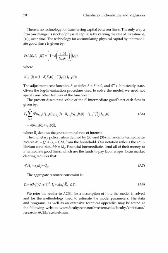
Christiano, Eichenbaum, and Vigfusson70
There is no technology for transferring capital between fi rms. The only way a fi rm can change its stock of physical capital is by varying the rate of investment, It(i) , over time. The technology for accumulating physical capital by intermedi-ate good fi rm i is given by:
F I i I i SI i
I it tt
t( ( ), ( ))
( )( )−
−= − ⎛
⎝⎜⎞⎠⎟
⎛
⎝⎜
⎞
⎠1
11 ⎟⎟ I it( ),
where
K i K i F I i I it t t t+ −= − +1 11( ) ( ) ( ) ( ( ), ( )).δ
The adjustment cost function, S, satisfi es S = S′ = 0, and S′′ > 0 in steady state. Given the log-linearization procedure used to solve the model, we need not specify any other features of the function S.
The present discounted value of the ith intermediate good’s net cash fl ow is given by:
E P i y i R W h i Ptj
t j t j t j t j t j t t jβ υ + + + + + +− −{ ( ) ( ) ( ) ϒtt j t jj
t j t j
I i
a u i K i
+−
+=
∞
+ +
∑+
1
0
[ ( )
( ( )) ( )]},,
(A6)
where Rt denotes the gross nominal rate of interest.The monetary policy rule is defi ned by (35) and (36). Financial intermediaries
receive Mt – Qt + (xt – 1)Mt from the household. Our notation refl ects the equi-librium condition, M a
t = Mt. Financial intermediaries lend all of their money to intermediate good fi rms, which use the funds to pay labor wages. Loan market clearing requires that:
WtHt = xtMt – Qt. (A7)
The aggregate resource constraint is:
( ( )) [ ( ) ] .1 1+ + + ≤−η V C I a u K Yt t t t t t tϒ (A8)
We refer the reader to ACEL for a description of how the model is solved and for the methodology used to estimate the model parameters. The data and programs, as well as an extensive technical appendix, may be found at the following website: www.faculty.econ.northwestern.edu/faculty/christiano/research/ACEL/acelweb.htm.
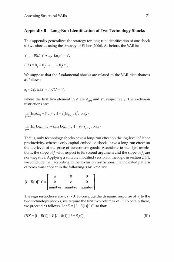
71Assessing Structural VARs
Appendix B Long-Run Identifi cation of Two Technology Shocks
This appendix generalizes the strategy for long-run identifi cation of one shock to two shocks, using the strategy of Fisher (2006). As before, the VAR is:
Yt+1 = B(L) Yt + ut, Eutu′t = V,
B(L) ≡ B1 + B2L + … + BqLq–1,
We suppose that the fundamental shocks are related to the VAR disturbances as follows:
ut = Cεt, Eεtε′t = I, CC′ = V,
where the fi rst two element in εt are εμϒ,t and ε tz, respectively. The exclusion
restrictions are:
lim[ ] ( , ,,j
t t j t t j z tzE a E a f
t→∞+ − +− =� �
1 ε εμϒonlyy)
lim[ log log ] (, , ,jt I t j t I t jE p E p f
→∞+ − +− =� �
1 ϒ ϒεμ tt
, only).
That is, only technology shocks have a long-run effect on the log-level of labor productivity, whereas only capital-embodied shocks have a long-run effect on the log-level of the price of investment goods. According to the sign restric-tions, the slope of fz with respect to its second argument and the slope of fϒ are non-negative. Applying a suitably modifi ed version of the logic in section 2.3.1, we conclude that, according to the exclusion restrictions, the indicated pattern of zeros must appear in the following 3 by 3 matrix:
[ ( )]I B C
a
b c− =⎡
⎣
⎢⎢⎢
⎤
⎦
−10 0
01
number number number
⎥⎥⎥⎥
The sign restrictions are a, c > 0. To compute the dynamic response of Yt to the two technology shocks, we require the fi rst two columns of C. To obtain these, we proceed as follows. Let D ≡ [I – B(1)]–1 C, so that:
DD′ = [I – B(1)]–1 V [I – B(1)′]–1 = SY(0) , (B1)

Christiano, Eichenbaum, and Vigfusson72
where, as before, SY(0) is the spectral density of Yt at frequency-zero, as implied by the estimated VAR. The exclusion restrictions require that D have the fol-lowing structure:
D
d
d d
d d d
=⎡
⎣
⎢⎢⎢
⎤
⎦
⎥⎥⎥
11
21 22
31 32 33
0 00 .
Here, the zero restrictions refl ect our exclusion restrictions, and the sign restric-tions require d11, d22 ≥ 0. Then,
DD
d d d d d
d d d d d d d′ = + +112
11 21 11 31
21 11 212
222
21 31 222 32
31 11 31 21 32 22 312
322
332
d
d d d d d d d d d+ + +
⎡
⎣
⎢⎢⎢⎢⎢
⎤
⎦
⎥⎥⎥⎥
=
S S S
S S
Y Y Y
Y Y
11 21 31
21 22
0 0 0
0
( ) ( ) ( )
( ) (00 0
0 0 0
32
31 32 33
) ( )
( ) ( ) ( )
S
S S S
Y
Y Y Y
⎡
⎣
⎢⎢⎢⎢
⎤
⎦
⎥⎥⎥⎥
and
d S d S d d S dY Y Y1111
2121
11 3131
110 0 0= = =( ), ( )/ , ( )/
ddS S S
Sd
SY Y Y
Y22
11 22 21 2
11 320 0 0
0= − =( ) ( ) ( ( ))
( ), YY Y YS S d
d
32 21 31112
22
0 0 0( ) ( ) ( )/.
−
The sign restrictions imply that the square roots should be positive. The fact that SY(0) is positive defi nite ensures that the square roots are real numbers. Finally, the fi rst two columns of C are calculated as follows:
C C I B D D1 2 1 21� �[ ] = − [ ][ ( )] ,
where Ci is the ith column of C and Di is the ith column of D, i = 1, 2.To construct our modifi ed VAR procedure, simply replace SY(0) in (B1) by
(29).
Comment
Patrick J. Kehoe, Federal Reserve Bank of Minneapolis, University of Minnesota, and NBER
1 Introduction
Most of the existing structural VAR (SVAR) literature argues that a use-ful way of advancing theory is to directly compare impulse responses from structural VARs run on the data to theoretical impulse responses from models. The crux of the Chari, Kehoe, and McGrattan (2006) (henceforth, CKM) critique of this common approach is that it compares the empirical impulse responses from the data to inappropriate objects in the model. We argue that logically, instead of being compared to the theoretical impulse responses, the empirical impulse responses should be compared to impulse responses from identical structural VARs run on data from the model of the same length as the actual data. We refer to this latter approach as the Sims-Cogley-Nason approach since it has been advocated by Sims (1989) and successfully applied by Cogley and Nason (1995).
CKM argue that in making the inappropriate comparison, the com-mon approach makes an error avoided by the Sims-Cogley-Nason approach. That error makes the common approach prone to various pitfalls, including small-sample bias and lag-truncation bias. For exam-ple, the data length may be so short that the researcher is forced to use a short lag length, and the estimated VAR may be a poor approximation to the model’s infi nite-order VAR. The Sims-Cogley-Nason approach avoids such problems because it treats the data from the U.S. economy and the model economy symmetrically.
On purely logical grounds, then, the Sims-Cogley-Nason approach seems to dominate the common approach.1 How well does the common approach do in practice using SVARs based on long-run restrictions on data from a real business cycle model? CKM show that for data of the
Kehoe74
relevant length, SVARs do miserably: The bias is large and SVARs are unable to distinguish between models of interest—unless technology shocks account for virtually all the fl uctuations in output.
Christiano, Eichenbaum, and Vigfusson (2006) (henceforth, CEV), perhaps the most prominent defenders of the common approach, seem to agree with CKM on the most important matters of substance. Indeed, since there seems to be no dispute that the Sims-Cogley-Nason approach dominates the common approach, there should be little dis-agreement over how future research in this area should be conducted. Likewise, there seems to be no dispute that when shocks other than technology play a sizable role in output fl uctuations, SVARs do mis-erably. The primary point of disagreement between CEV and CKM is thus a relatively minor one about the likely size of the errors in the past literature that uses the common approach. CEV argue that the errors are small because the evidence is overwhelming that in U.S. data, tech-nology shocks account for virtually all the fl uctuations in output. CKM point to both 20 years of business cycle research and simple statistics in the data that all lead to the opposite conclusion about technology shocks and, hence, to the opposite conclusion as to the size of the errors of the common approach.
CEV also venture beyond the confi nes of the CKM critique and ana-lyze SVARs with short-run restrictions. They focus on SVARs applied to monetary models which satisfy the same recursive identifying assump-tions as their SVARs. CEV argue that the error in this application of the common approach is small, and thus the technique can be used broadly to distinguish promising models from the rest. Here the pri-mary problem with their analysis is that it is subject to the Lucas and Stokey critique (Lucas and Stokey 1987): Only a tiny subset of existing monetary models in the literature actually satisfi es the recursive identi-fying assumptions. That subset does not include even, for example, the best-known monetary models of Lucas (1972, 1990). Yet the technique has been used to reject these and other such models. Clearly, comparing impulse responses from SVARs with a set of identifying assumptions to those from models which do not satisfy those assumptions is prob-lematic.
Notice that the Sims-Cogley-Nason approach is immune to the Lucas and Stokey critique. Under this approach, it is entirely coherent to compare impulse responses with a set of identifying assumptions to those from models which do not satisfy these assumptions. Under this approach, the impulse responses are simply statistics with possibly
75Comment
little economic interpretation. Now, those statistics may not be interpre-table as being close to the model’s theoretical response, but so what? When Kydland and Prescott (1982) compare variances, covariances, and cross-correlations in the model and the data, it does not matter whether these statistics have some deep economic interpretation.
Of course, it is not true that all statistics are equally desirable. What properties lead certain statistics to be more desirable than others? One important property is that the statistics vary across alternative models in such a way that, with samples of the lengths we have, they can be used to point with confi dence toward one class of models and away from another. (If no such statistics exist, then the data have little to say about the theories of interest.) A second desirable property is that the statistics depend on key features of theory and not on inessential aux-iliary assumptions. An important question for a serious assessment of the SVAR literature is, in what sense are the SVAR statistics more or less desirable than a host of other non–SVAR-related statistics? Regrettably, little or no work in the SVAR literature seems directed at this critical question.
To reiterate: The CKM critique does not apply to all SVAR analyses, only those that use the common approach rather than the Sims-Cog-ley-Nason approach. For most analyses, switching to that dominant approach would cost little—changing only a few lines of computer code and a few lines of text. By making such a switch, researchers using structural VARs can vastly enhance the role of VARs in guiding theory.
In these comments, I begin by carefully describing the difference between the common approach and the Sims-Cogley-Nason approach. Then I describe four issues of perceived disagreement between CKM and CEV about SVARs with long-run restrictions. Finally, in terms of CEV’s analysis with short-run restrictions, I describe two critiques which need to be addressed by researchers who steadfastly refuse to abandon the common approach.
2 Getting Precise
Let me begin with some notation with which I can make the CKM argu-ment precise.
The fi rst step in both SVAR approaches is to run a VAR with p lags on a data set {Yt}
Tt=1 and then apply the identifying assumptions to con-
struct the impulse response matrices Ai(p, T ) for i = 0, 1, … , where i denotes periods after the impact period and the notation emphasizes

Kehoe76
that the impulse responses depend on the lag length p and the sample size T. In applications using postwar U.S. data, it is common to set p = 4 and to have T = 180 or numbers similar to these, and I will denote the resulting matrices by A i
US(p = 4, T = 180).The common approach emphasizes the interpretation of these matri-
ces. For instance, in the standard example, the data consist of a measure of labor productivity and a measure of hours and the theoretical model has two shocks, technology and non-technology shocks. The fi rst col-umn of the impact matrix A 0
US(p = 4, T = 180) is interpreted as the impact effect of the technology shock on productivity and hours, while the sec-ond column is interpreted as the impact effect of the non-technology shock on productivity and hours. The subsequent matrices are simi-larly interpreted.
In contrast, CKM and Sims, Cogley, and Nason view these matri-ces as moments of the data that may be used in discriminating among models of interest.
Now suppose we have a quantitative economic model in which the impulse responses to the technology and non-technology shocks are the matrices Di(θ), i = 0, 1, … , where θ denotes the model parameters. The second step of the common approach compares
A iUS
(p = 4, T = 180) to Di(θ). (1)
Sometimes this comparison is informal and implicit, as in the work of Galí (1999), Francis and Ramey (2005), and Galí and Rabanal (2005), who fi nd that labor falls after a positive productivity shock and con-clude that real business cycles are dead. Sometimes this comparison is formal and explicit, as in the work of Altig et al. (2005), and is used to choose model parameters θ.
The second step of the Sims-Cogley-Nason approach is quite differ-ent. To understand this step, let A–i(p,T|θ) denote the mean of impulse responses found by applying the SVAR approach with p lags in the VAR to the many simulations of data of length T generated from the model with parameters θ. The second step of the Sims-Cogley-Nason approach compares
A p T A p TiUS
i( , ) ( , ).= = = =4 180 4 180 to θ (2)
At a conceptual level, we interpret the Sims-Cogley-Nason approach as advocating comparing the exact small-sample distribution of the esti-
77Comment
mator of the impulse responses with p = 4 and T = 180 to the estimated impulse response parameters. We view the simulations involved as a simple way to approximate that small-sample distribution. If it were feasible to analytically work out the small-sample distribution of the estimator, then so much the better.
CKM interpret (2) as the correct comparison, which is fi rmly grounded in (simulated) method-of-moments theory, and (1) as simply a mistake of the common approach.
The whole point of the CKM work is to quantify when and why these two comparisons will yield different answers, that is, when and why the two objects computed from the model, A–i (p = 4, T = 180|θ) and Di(θ), will differ. Part of CKM’s analysis focuses on the two-variable case with Yt(α) = (Δ (yt /lt), lt – α lt–1)′, where yt is the log of output, lt is the log of hours, and α ∈ [0, 1] is the quasi-differencing parameter. The specifi cation Yt(α) nests three cases of interest: α = 0, the level SVAR (LSVAR) case; α = 1, the differenced SVAR (DSVAR) case; and α = .99, the quasi-differenced SVAR (QDSVAR) case.
When θ is such that technology shocks do not account for the vast bulk of fl uctuations in output, LSVARs do miserably: The bias is large and the confi dence bands are so enormous that the technique is unable to distinguish among most classes of models of interest.
With such a θ, the DSVARs and QDSVARs also fare poorly: The bias is large enough to fl ip the sign of the impact coeffi cient of hours on a technology shock. While the confi dence bands are large, they don’t stop a researcher from rejecting that the simulated data came from a real business cycle model, even though they did. CKM think that this result suggests that researchers who have determined that real business cycle models are dead based on SVAR evidence may have come to that conclusion simply because they were not comparing the appropriate objects in the model and the data.
Note that, at least for the long-run restriction branch of the SVAR lit-terature, the issue is all about approximation error. If we had an infi nite sample of data from a model that satisfi es the identifying restrictions and we estimated a VAR with an infi nite number of lags, we would have (in the relevant sense of convergence)
A p T Di i( , ) ( )= ∞ = ∞ = θ (3)
for both the LSVAR and the QDSVAR cases, where, for simplicity, we have assumed that the identifying assumptions are suffi cient as well
Kehoe78
as necessary. (As we discuss below, Marcet (2005) shows why (3) holds even for the DSVAR case in which hours are “over-differenced.”)
With (1)–(3) in mind, note that A–i(p = 4, T = 4) – Di(θ) can be inter-preted as the error in the common approach relative to the Sims-Cogley-Nason approach. CKM decompose this error into
[ ( , ) ( , )] [ ( , )A p T A p T A p T Di i i i= = − = = ∞ + = = ∞ −4 180 4 4 (( )],θ
where the fi rst term is the Hurwicz-type small-sample bias and the sec-ond term is the lag-truncation bias. It turns out that for both the LSVAR case and the QDSVAR case, most of the error is coming from the lag-truncation bias. Intuitively, this truncation bias arises both because the p = 4 specifi cation forced terms to be zero that are not and because the OLS estimator adjusts the estimates of the included lags to com-pensate for those that have been excluded. CKM develop propositions that give intuition for when the error from the lag-truncation bias will be large.2
3 The Common Approach with Long-Run Restrictions
The SVAR literature with long-run restrictions, in general, and CEV, in particular, claim that the common approach is a state-of-the-art tech-nique which is a useful guide for theory. We disagree. Here I describe three specifi c points of disagreement relevant to CEV’s discussion of long-run restrictions and one point in which CEV seem to think there is disagreement where none really exists. My overall point here is that we all agree there exist circumstances under which the errors from using the common approach are small; however, as CKM have shown, these cir-cumstances are not general. Moreover, regardless of the circumstances, this approach is dominated by what we consider the state-of-the-art technique, the Sims-Cogley-Nason approach. This approach is at least as easy to use as the common approach, and it has the advantage of a fi rm logical and statistical foundation.
Consider now the four points.First, CEV argue that LSVARs are useful in guiding theory about fl uc-
tuations in the U.S. economy because in U.S. data, they say, technology shocks account for almost all of the fl uctuations in output. We argue that while some reasonable statistics do point to technology shocks playing an overwhelming role, a number of other sensible statistics, as well as much of the literature, strongly suggest that their role is modest.

79Comment
Second, CEV argue that even if technology shocks do not account for almost all of the fl uctuations in output, there is a new estimator of impulse responses that virtually eliminates the bias associated with the standard OLS estimator. We argue that while for some parameter values this new estimator improves on the OLS estimator, for others it does worse. In this sense, the new estimator does not solve all the prob-lems facing this literature.
Third, CEV ignore the DSVAR literature on the grounds, they say, that the DSVAR is misspecifi ed because it incorrectly differences hours. This misspecifi cation, they say, leads to incorrect estimates of impulse responses even with an infi nite amount of data. We argue that here, for all practical purposes, CEV are wrong about the DSVAR being mis-specifi ed. Instead the only error in the DSVAR literature is the same as in the LSVAR literature: Using the common approach rather than the Sims-Cogley-Nason approach.
Finally, I consider a point on which there is actually no disagreement. CEV argue that when more variables are added to an LSVAR, in special cases it can sometimes usefully distinguish between classes of models. CEV somehow seem to think we disagree here, but we do not. Indeed, part of the point of CKM is to provide a theorem as to when LSVARs can and cannot perform this function. We emphasize, however, that the “can” circumstances are somewhat narrow.
3.1 Do Technology Shocks Account for Virtually All of the Fluctuations in Output?
CKM show that if technology shocks account for virtually all of the fl uctuations in output, then the errors associated with the common approach are relatively small. Much of CEV’s work is devoted to argu-ing that the U.S. data defi nitively show that technology shocks account for the vast bulk of the movements in output and non-technology shocks, almost none. There is a vast literature on this subject, much of it contradicting that stand.
Let’s take a closer look at the issues at stake. Using the notation of CKM and ignoring means, we can write the stochastic processes for a technology shock, log Zt, and a non-technology shock, τlt, for both CEV and CKM, as
log Zt+1 = log Zt + log zt+1 (4)
τlt+1 = ρτlt + εlt+1, (5)
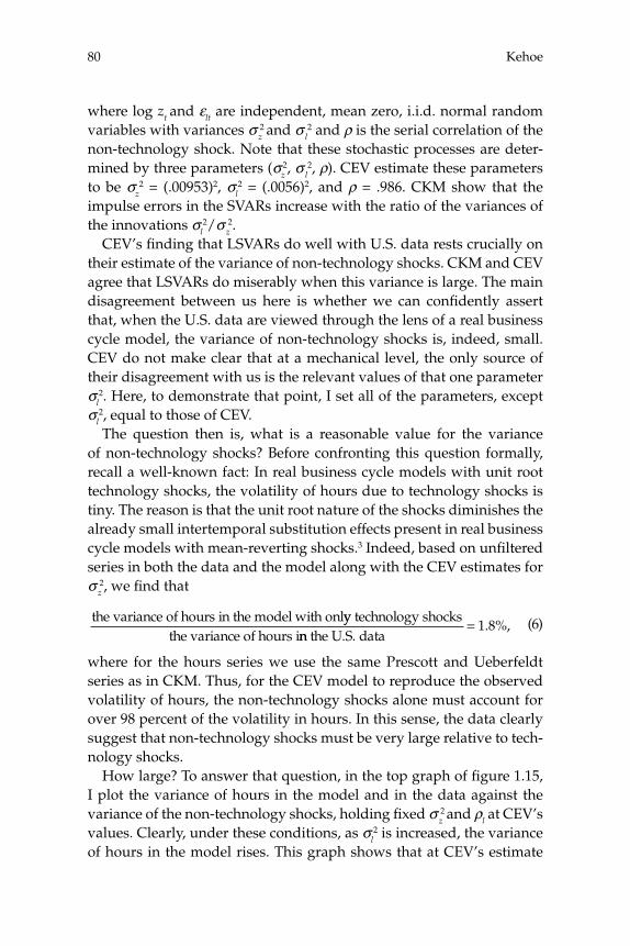
Kehoe80
where log zt and εlt are independent, mean zero, i.i.d. normal random variables with variances σ z
2 and σ l
2 and ρ is the serial correlation of the non-technology shock. Note that these stochastic processes are deter-mined by three parameters (σz
2, σ l2, ρ). CEV estimate these parameters
to be σz2 = (.00953)2, σl
2 = (.0056)2, and ρ = .986. CKM show that the impulse errors in the SVARs increase with the ratio of the variances of the innovations σl
2/σ z2.
CEV’s fi nding that LSVARs do well with U.S. data rests crucially on their estimate of the variance of non-technology shocks. CKM and CEV agree that LSVARs do miserably when this variance is large. The main disagreement between us here is whether we can confi dently assert that, when the U.S. data are viewed through the lens of a real business cycle model, the variance of non-technology shocks is, indeed, small. CEV do not make clear that at a mechanical level, the only source of their disagreement with us is the relevant values of that one parameter σl
2. Here, to demonstrate that point, I set all of the parameters, except σl
2, equal to those of CEV.The question then is, what is a reasonable value for the variance
of non-technology shocks? Before confronting this question formally, recall a well-known fact: In real business cycle models with unit root technology shocks, the volatility of hours due to technology shocks is tiny. The reason is that the unit root nature of the shocks diminishes the already small intertemporal substitution effects present in real business cycle models with mean-reverting shocks.3 Indeed, based on unfi ltered series in both the data and the model along with the CEV estimates for σ z
2, we fi nd that
the variance of hours in the model with onlyy technology shocksthe variance of hours inn the U.S. data
= 1 8. %, (6)
where for the hours series we use the same Prescott and Ueberfeldt series as in CKM. Thus, for the CEV model to reproduce the observed volatility of hours, the non-technology shocks alone must account for over 98 percent of the volatility in hours. In this sense, the data clearly suggest that non-technology shocks must be very large relative to tech-nology shocks.
How large? To answer that question, in the top graph of fi gure 1.15, I plot the variance of hours in the model and in the data against the variance of the non-technology shocks, holding fi xed σ z
2 and ρl at CEV’s
values. Clearly, under these conditions, as σl2 is increased, the variance
of hours in the model rises. This graph shows that at CEV’s estimate
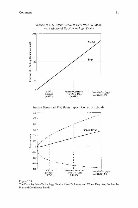
81Comment
Figure 1.15The Data Say Non-Technology Shocks Must Be Large, and When They Are, So Are the Bias and Confi dence Bands

Kehoe82
for σl2 (.00562), hours are only about a third as volatile in their model as
in the data. The graph also shows that for the model to account for the observed variability in hours, σl
2 must be substantially larger (about .00982).4
The bottom graph of fi gure 1.15 shows that when the parameter under dispute, σl
2, is chosen to reproduce CEV’s estimate, the bias is modest but the confi dence bands are large. When this parameter is cho-sen to reproduce the observed volatility of hours, the LSVAR does mis-erably: The bias is large and the confi dence bands are so enormous that the technique is unable to distinguish among most classes of models of interest.
I should be clear that we do not disagree that there exist some statis-tics, including some maximum likelihood statistics, that would lead to the conclusion that non-technology shocks are small. CKM fi nd that the maximum likelihood estimates are sensitive to the variables included in the observer equation, especially investment. Under some specifi ca-tions, the variance of non-technology shocks is large while in others it is small. The reason for this sensitivity is that a stripped-down model like ours cannot mimic well all of the comovements in U.S. data, so that it matters what features of the data the researcher wants to mimic. In such a circumstance, we think it makes sense to use a limited-information technique in which we can choose the moments we want the model to do well on.
Therefore, in designing a laboratory to test whether the SVAR meth-odology works, we asked, what would be some desirable features of the data for the model to reproduce? We came up with three answers, all of which contradict the condition necessary for SVARs to work well in practice; that is, all three suggest that non-technology shocks must be large.
One of our answers, which motivates the exercise just conducted, is that if the whole point of the procedure is to decompose the movements in hours, then the model should generate volatility in hours similar to that in the data. As CKM demonstrate, in the context of the CEV model, to do that the model needs large non-technology shocks.
A second answer is that the laboratory model should reproduce the key statistic that both started off the whole debate and is the main result in the long-run restriction SVAR literature: Galí’s (1999) initial drop in hours after a positive technology shock. CKM ask, holding fi xed the estimates of the variance of technology shocks and the persistence of
83Comment
non-technology shocks, what must be the variance of the non-technol-ogy shocks in order to reproduce Galí’s impact coeffi cient on hours? We fi nd that the variance of non-technology shocks must be large, large enough so that the SVARs do miserably in terms of bias and size of confi dence bands.
(Note here that under the Sims-Cogley-Nason approach, whether or not Galí’s DSVAR is misspecifi ed is irrelevant. Galí’s statistic is just a moment of the data that has happened to receive a lot of attention, with possibly no more interpretation than those in the standard Kydland and Prescott (1982) table of moments.)
A third answer to the question of reproducible features is that if the SVAR procedure works well, then the variance of the shocks should be consistent with the variance decompositions in the SVAR literature itself. Much of this literature, including Christiano, Eichenbaum, and Vigfusson (2003), attributes only a small fraction of the fl uctuations to technology shocks. As CKM show, with the parameters set to generate any of these statistics, the SVAR responses are badly biased and have enormous confi dence bands.
In sum, contrary to the argument of CEV, the U.S. data do not defi ni-tively show that technology shocks account for virtually all of the move-ments in output. Most of the literature agrees with us, including much of the previous work of CEV, both alone and in concert.
3.2 Does the Mixed OLS–Newey-West Estimator Uniformly Improve on OLS?
Perhaps the most interesting part of CEV’s work is their proposed estimator of impulse responses with long-run restrictions. They argue that this estimator, which splices the OLS estimator and a Newey and West (1987) estimator, “virtually eliminates the bias” (CEV 2006, p. 3) associated with the standard OLS estimator and thus makes the errors of their approach tiny. In this sense, CEV argue that it does not matter whether technology shocks account for almost all of the fl uc-tuations in output because their new estimator takes care of the bias problem.
We disagree. The results of Mertens (2006) show that actually the new estimator does not even uniformly improve on the standard OLS estimator. Unfortunately, the new estimator is thus not a comprehen-sive solution for the problems with long-run restrictions.
Kehoe84
To understand these issues, use the notation of Mertens (2006) to write the standard OLS estimator of the impact coeffi cient matrix A0 as
A I B Chol SOLSiOLS
iX
OLS0 0= −⎛
⎝⎜⎞⎠⎟
∑ ( ( ) ),
where BiOLS
denotes the regression coeffi cient matrices from the VAR and Chol(SX(0)OLS) denotes the Cholesky decomposition of the OLS esti-mate of the spectral density matrix SX(0)OLS of the variables in the VAR at frequency zero. Here
S I B I BXOLS
iOLS
i
OLSiOLS
i
( )01
= −⎛⎝⎜
⎞⎠⎟
−⎛⎝⎜
⎞∑ ∑−Ω
⎠⎠⎟−t 1
,
where ΩOLS is the OLS estimate of the covariance matrix of residuals from the VAR.
CEV propose replacing SX(0)OLS with a spectral density estimator along the lines of Newey and West (1987), with a Bartlett weighting scheme given by
Sk
bE X XX
NWT t t k
k b
b
( ) ,0 11
= −+
⎛⎝⎜
⎞⎠⎟ ′−
=−∑
where Xt is the data, T is the sample length, ET is the sample moments operator, and b is a truncation parameter.5
Figure 1.16, taken from Mertens (2006), displays the impact errors resulting from the use of the OLS estimator and the mixed OLS–Newey-West estimator, with four lags in the VAR, b = 150, T = 180, various val-ues of σl
2/σ z2, and the rest of the parameters set as in CEV. The fi gure
shows that when non-technology shocks are small, the CEV estimator has a larger bias than does the OLS estimator. As Mertens shows, if non-technology shocks are large enough, the positions eventually reverse. Clearly, the mixed OLS–Newey-West estimator is not uniformly better than the OLS estimator. (For more details, see Mertens (2006).)
3.3 Are DSVARs Misspecifi ed?
It is somewhat of a puzzle to me why, in their broad assessment of SVARs, CEV focus on the LSVAR literature, which does not have eco-
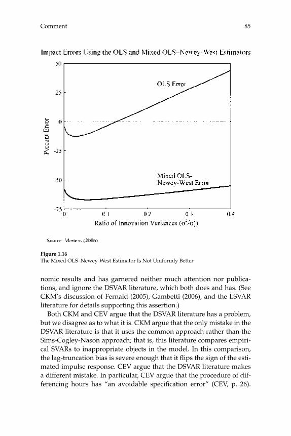
85Comment
nomic results and has garnered neither much attention nor publica-tions, and ignore the DSVAR literature, which both does and has. (See CKM’s discussion of Fernald (2005), Gambetti (2006), and the LSVAR literature for details supporting this assertion.)
Both CKM and CEV argue that the DSVAR literature has a problem, but we disagree as to what it is. CKM argue that the only mistake in the DSVAR literature is that it uses the common approach rather than the Sims-Cogley-Nason approach; that is, this literature compares empiri-cal SVARs to inappropriate objects in the model. In this comparison, the lag-truncation bias is severe enough that it fl ips the sign of the esti-mated impulse response. CEV argue that the DSVAR literature makes a different mistake. In particular, CEV argue that the procedure of dif-ferencing hours has “an avoidable specifi cation error” (CEV, p. 26).
Figure 1.16The Mixed OLS–Newey-West Estimator Is Not Uniformly Better

Kehoe86
They seem to conclude that, even with an infi nite amount of data, the DSVAR impulse responses will not coincide with the model’s impulse responses. We disagree: CKM address the issue of misspecifi cation directly and argue that the DSVAR procedure has no specifi cation error of importance.6
CKM argue this result in two steps. The fi rst step in our argument is that with a QDSVAR, with α close to 1, say, .99, Galí (1999) would have obtained impulse responses virtually indistinguishable from those he actually obtains in his DSVAR in which he sets α equal to 1. In this sense, for all practical purposes, we can think of Galí as having run a QDSVAR. The second step in our argument is that, for any α < 1 and a long enough data set, the QDSVAR will get exactly the right answer. That is, with the lag length chosen to be suitably increasing with sam-ple size, the sample impulse responses in the QDSVAR procedure will converge in the relevant sense to the model’s impulse response; that is, A–i (p = ∞, T = ∞) = Di(θ). In this precise sense, contrary to what CEV claim, this procedure has no specifi cation error of importance.
Marcet (2005) shows something subtler. He shows that with the DSVAR procedure in which α equals 1, the sample impulse responses from a procedure in which the lag length increases appropriately with sample size converge in the relevant sense to the model’s impulse response. Marcet notes that his Proposition 1 seems to directly contra-dict the, at least implicit, claims of Christiano, Eichenbaum, and Vigfus-son (2003).7
So, with large samples, researchers have no a priori reason to prefer the LSVAR procedure to the QDSVAR procedure, and with α close to 1 in samples of length typical to that in postwar data, the QDSVAR is indistinguishable from the DSVAR. Beyond that, small-sample issues do lead one specifi cation to be preferred. Quasi-differencing lessens the amount of Hurwicz-type small-sample bias in estimating the param-eters of a highly correlated series like per capita hours. Thus, at least a priori, the QDSVAR seems to be preferable to the LSVAR.
Nevertheless, the QDSVAR turns out to actually do worse than the LSVAR. When CKM decompose the mean impulse response error into small-sample bias and lag-truncation bias, we fi nd that even though the QDSVAR has smaller Hurwicz-type bias, it has a much larger lag-trun-cation bias for reasonable parameters; the QDSVAR does worse. That is a quantitative result, however. We are not sure that it holds in a large class of models with a wide variety of parameters.
87Comment
3.4 Does Adding More Variables to the SVARs Help?
CEV argue that, even though for a wide variety of circumstances, SVARs with long-run restrictions are uninformative, they can be infor-mative in special cases—for example, when more variables are added to an LSVAR. Contrary to the impression we get from CEV, there is no disagreement on this point. Indeed, part of the point of CKM is to prove analytically exactly what the special cases are.
A commonly cited example of an economy in which SVARs with long-run restrictions work well is Fisher’s (2006) model (see Fernandez-Villaverde, Rubio-Ramirez, and Sargent (2005)). CKM show that Fisher’s model is a special case of our Proposition 4, a case when LSVARs can be informative. In this sense, we obviously agree with CEV about the validity of our proposition. We do not think, however, that an approach that works only in special cases has much to offer researchers seeking a reliable, generally applicable tool.
4 The Common Approach with Short-Run Restrictions
The use of the common approach on SVARs with long-run restrictions thus has little to recommend it. What about using it on SVARs with short-run restrictions? CEV claim that with this type of SVAR, their approach is a state-of-the-art technique that is useful for guiding the-ory. They focus on short-run restrictions that are satisfi ed in models which satisfy certain timing assumptions, often referred to as recursive assumptions. CEV claim to show that when a model satisfi es such an assumption, SVARs with short-run restrictions perform remarkably well in small samples. And CEV imply that, because of this fi nding, this technique can be used broadly to distinguish promising models from the rest.
Since the CKM work has nothing to do with short-run restrictions, I have not studied the details of CEV’s claims about how well the short-run restrictions work in practice with small samples and therefore have nothing to disagree with on these small-sample claims. Never-theless, I do disagree with CEV’s main message with respect to short-run restrictions in this area. As other researchers do, CEV ignore two critiques which seem to be widely thought of as devastating for much of the literature that uses SVARs with short-run restrictions. These cri-tiques are of a theoretical nature, not about some problems with small
Kehoe88
samples. These critiques thus imply that, regardless of how well the short-run restrictions work with small samples, they are of little value in guiding the development of a broad class of monetary research. Hence, these critiques need to be addressed with a precise theoretical argument, not with some small-sample results.
The main critique of the SVAR literature with short-run restrictions is the Lucas and Stokey critique of Lucas and Stokey (1987). The point of this critique is that the particular class of short-run identifying assumptions made by CEV and related work in the short-run SVAR literature do not apply to a broad class of models and hence are of little use in guiding the development of a broad class of research.
The upshot of this critique is that some of the prominent researchers in the short-run SVAR literature have drastically overreached the con-clusions of their studies. The short-run identifying assumptions in their work apply to only a tiny subset of monetary models, but the SVAR results have been used to rule out models not in that tiny subset. This mismatch between assumptions and models is a serious problem for this work.
A simple way for researchers in the short-run literature using the common approach to inoculate themselves from the Lucas and Stokey critique is to include in an appendix a list of the papers in the existing literature that satisfy their proposed identifying assumptions. Unfor-tunately, for most of the identifying schemes that I have seen, that list would be extremely short and would exclude most of the famous mon-etary models that constitute the core of theoretical monetary econom-ics. If researchers are able to invent new identifying schemes for which this list is both broad and long, then this literature would have a much greater impact on guiding the development of monetary theory than it currently does. Doing so would constitute progress.
To understand my claim that the current literature is subject to the Lucas and Stokey critique, consider the recursiveness assumption itself. As Christiano, Eichenbaum, and Evans (1998, p. 68) explain, “The economic content of the recursiveness assumption is that the time t variables in the Fed’s information set do not respond to the time t real-izations of the monetary policy shock.” To see how this assumption might be satisfi ed in a model, note that if the monetary authority at time t sets its policy as a function of time t variables, including output, consumption, and investment, as it does in Christiano, Eichenbaum, and Evans (2005), then the model must have peculiar timing assump-tions in which, in a quarterly model, after a monetary shock is realized, private agents cannot adjust their output, consumption, and invest-

89Comment
ment decisions during the remainder of the quarter. Whether or not one agrees that this timing assumption is peculiar, it is irrefutable that this timing assumption is not satisfi ed in the primary models in the monetary literature. I illustrate this point in fi gure 1.17, which lists the typical classes of models studied in monetary economics. (Technically, for all the models in the large rectangle, the impulse responses from the SVAR procedure do not converge in the relevant sense to the impulse responses in the model, so that A
–i (p = ∞, T = ∞) ≠ Di(θ).)
As an illustration of the claim that some of the short-run litera-ture overreaches, consider the exposition by Christiano and Eichen-baum (1999) of the research agenda of the monetary SVAR literature. This exposition draws on the well-cited comprehensive survey by
Figure 1.17CEV’s Recursiveness Assumption Does Not Apply to Most Monetary Models(Representative Classes of Existing Monetary Models, Grouped Whether They Violate or Satisfy CEV’s Recursiveness Assumption)
Kehoe90
Christiano, Eichenbaum, and Evans (1998) of the short-run SVAR lit-erature, which is the clearest statement of the research agenda of the monetary SVAR literature that I could fi nd.
Christiano and Eichenbaum (1999) start with a summary of the so-called facts and a brief note that some identifying assumptions have been used to establish them:
In a series of papers, we have argued that the key consequences of a contrac-tionary monetary policy shock are as follows: (i) interest rates, unemployment and inventories rise; (ii) real wages fall, though by a small amount; (iii) the price level falls by a small amount, after a substantial delay; (iv) there is a per-sistent decline in profi ts and the growth rate of various monetary aggregates; (v) there is a hump-shaped decline in consumption and output; and (vi) the US exchange rate appreciates and there is an increase in the differential between US and foreign interest rates. See CEE [Christiano, Eichenbaum, and Evans] (1998) for a discussion of the literature and the role of identifying assumptions that lie at the core of these claims.
Christiano and Eichenbaum (1999) then go on to reject some models that, they say, are not consistent with those facts. In particular, based on their SVAR-established facts, they reject both Lucas’ (1972) island model and Lucas’ (1990) liquidity model. These claims are clearly overreaching. Since Lucas’ two models in particular do not satisfy the peculiar timing assumptions needed to justify the recursive identify-ing assumption in the SVAR, how is it logically coherent to reject those models based on the SVAR-established facts?
A potential objection to the Lucas and Stokey critique is that the SVAR literature is not overreaching because some of the models that violate the recursiveness assumption satisfy some other identifying assumptions that researchers have made, and for these other assump-tions, SVAR researchers have found similar qualitative patterns. The second main critique of the short-run literature, the Uhlig critique of Uhlig (2005), dismisses this objection. The Uhlig critique is that the atheoretical SVAR specifi cation searches are circular: “the literature just gets out what has been stuck in, albeit more polished and with num-bers attached” (Uhlig 2005, p. 383). Uhlig argues that the reason the other identifying assumptions fi nd similar answers is that the answers are essentially built into the search algorithm. Uhlig suggests that the algorithm used to fi nd some SVAR results is, perhaps unconsciously, to pick a pattern of qualitative results and then do an atheoretical search over patterns of zeros, lists of variables to include, and periods of time to study, so that the resulting SVAR impulse responses reproduce the

91Comment
desired qualitative results. If this description is accurate, then I am sym-pathetic with Uhlig’s conclusion that not much is to be learned from this branch of the short-run SVAR literature.
Note, again, that neither of these critiques would apply if, when comparing models and data, researchers simply followed the Sims-Cogley-Nason approach. Under that approach, the issue of whether the identifying assumptions of an SVAR hold in a model doesn’t come up. The impulse responses from the SVAR on the data simply defi ne some sample statistics that are coherently compared to the analogous statistics from the model. That is, now letting A i
US(p = 4, T = 180) and A–i (p = 4, T = 180|θ) denote the impulse responses obtained from an SVAR with short-run restrictions, using standard (simulated) method-of-moments logic, it makes perfect sense to compare these two even though A–i (p = ∞, T = ∞) ≠ Di(θ).
In sum, if the SVAR literature with short-run restrictions followed the research agenda advocated by Sims (1989) and applied by Cogley and Nason (1995), then it would be on fi rm statistical and logical grounds.
5 Concluding Remarks
Let me be clear about what I am advocating in practice. For research-ers willing to make a quantitative comparison between a model and the data, all I am advocating basically is changing several lines of computer code—replacing the theoretical impulse responses, Di(θ), with the more relevant empirical responses derived from applying the SVAR procedure to the model, A–i (p = 4, T = 180|θ), in the relevant spots where the com-parison between model and data is being made. For researchers who just want to run SVARs in the data and chat about what it means for a model, all I am advocating is a change in claims. Replace the claim about having robustly discovered what happens after a particular type of shock with a more precise claim about having documented what type of impulse responses should arise in a model when an SVAR with 4 lags and 180 observations is run on the data from it. Changing these several lines of code or text will vastly increase the intellectual impact of the approach.
It is puzzling to me that CEV and CKM seem to agree on two of the three key facts; yet we somehow disagree on their primary implication.
We agree on these two facts about the common approach:
• The common approach sometimes makes large errors relative to the Sims-Cogley-Nason approach. In particular, with long-run restrictions,
Kehoe92
SVARs do miserably unless technology shocks account for virtually all of the fl uctuations in output.
• The common approach sometimes excludes most models of interest while the Sims-Cogley-Nason approach does not. For example, with short-run restrictions, the recursive identifying assumptions apply to only a tiny subset of the existing monetary models.
We disagree on one signifi cant fact about interpreting the U.S. data:
• CEV argue that the evidence defi nitively implies that technology shocks account for virtually all of the fl uctuations in output. CKM argue that while one can fi nd statistics supporting this view, 20 years of macroeconomic research and some simple statistics show that shocks involving something other than technology play a sizable role in gener-ating fl uctuations in output and other variables.
And we disagree on the overriding implication of these facts:
• CEV argue that the common approach is a state-of-the-art technique that can be saved with a mechanical fi x and analyst restraint:
–For the long-run restriction branch of the SVAR literature, CEV argue that a mixed OLS–Newey-West estimator essentially elimi-nates the errors of the common approach.
–For the short-run restriction branch, CEV think that, in order to avoid the over-reaching of some of the recent work in the area, researchers should be much more careful to delineate exactly to which work they claim their analyses apply. (This view is implicit in their conference discussions of early drafts of CKM’s work.)
• CKM argue, to the contrary, that the common approach is not a state-of-the-art technique and that it should be abandoned in favor of one that is. The Sims-Cogley-Nason approach has fi rm statistical and theoretical foundations and thus avoids the type of statistical and logi-cal errors of the common approach.
Beyond the specifi cs of the debate between CEV and CKM, my bot-tom line is simple: Let’s stop worrying about the size of the errors in the old SVAR literature and instead start moving forward with the more promising Sims-Cogley-Nason approach that has potential to help us advance theory.
93Comment
Acknowledgments
This work is a response to the comments of Lawrence Christiano, Martin Eichenbaum, and Robert Vigfusson on the critique of struc-tural VARs with long-run restrictions by V. V. Chari, Patrick Kehoe, and Ellen McGrattan. For very helpful comments, the author thanks his coauthors as well as numerous others, including his coauthors, Tim Cogley, Jesus Fernandez-Villaverde, Bob Hall, Chris House, Narayana Kocherlakota, Ricardo Lagos, Monika Piazzesi, Juan Rubio-Ramirez, Tom Sargent, and Jim Stock. The author also thanks the NSF for fi nan-cial support and Kathy Rolfe and Joan Gieseke for excellent editorial assistance. Any views expressed here are those of the author and not necessarily those of the Federal Reserve Bank of Minneapolis or the Federal Reserve System.
Endnotes
1. The idea of the Sims-Cogley-Nason approach is to compare the exact small-sample distribution of the estimator from the model (with short lags) to the small-sample esti-mate (with short lags) from the data. This is a contrast to the common approach, which makes no attempt to deal with any of the issues that arise with a small sample. At a logi-cal level, as long as the small-sample distribution is approximated well, either by hand, which is exceedingly diffi cult, or by a computer, which is easy, the Sims-Cogley-Nason approach seems to clearly dominate the common approach.
2. Note that, at least for the environment considered by CKM, since the Hurwicz-type small-sample bias is small, the comparison of
AiUS(p = 4, T = 180) to A
–i (p = 4, T = ∞|θ)
would eliminate most of the error in the common approach and would allow the researcher to use standard asymptotic formulas. We view this comparison as a rough-and-ready approximation to the one in the Sims-Cogley-Nason approach.
3. This reasoning helps explain why the bulk of the real business cycle literature has not adopted the unit root specifi cation. In this sense, technically, the SVAR results really have little to say about this literature. But that point has already been forcefully made by McGrattan (2005).
4. Note that, as other parameters in the model shift, so does the size of σl2 needed
to produce a certain volatility in hours. In this sense, whether or not a certain value of σl
2 is small or not should be judged by whether or not the model with this parameter can produce the observed volatility of hours in the data.
5. The spectral density at frequency zero is defi ned as SX(0) = Σ∞k=–∞EXtX′t–k. The estima-
tor of Newey and West (1987) is a truncated version of this sum that replaces population moments with sample moments and weights these sample moments to ensure positive defi niteness.
Kehoe94
6. In an interesting recent paper, Dupaigne, Fève, and Matheron (2006) take a different approach to show that while the DSVAR performs poorly in the laboratory of an eco-nomic model, this poor performance has nothing to do with specifi cation error. These authors consider an economic model with nonstationary hours so that there is clearly no “avoidable specifi cation error” in the DSVAR. Nonetheless, they show that DSVARs per-form poorly in short samples for exactly the same reasons that DSVARs perform poorly in the CKM analysis. Dupaigne, Fève, and Matheron go on to show that the estimation pro-cedures of structural models based on the common approach—in which parameters are chosen to minimize the distance between the theoretical impulse responses and the SVAR impulse responses—lead to systematically biased estimates. These authors argue that the natural estimation procedure based on the Sims-Cogley-Nason approach resoundingly dominates the procedure based on the common approach.
7. Part of the disagreement in this regard may come from a failure to precisely distinguish between two types of noninvertibility problems. The type considered by Fernandez-Villaverde, Rubio-Ramirez, and Sargent (2005) are nontrivial and diffi cult to deal with without using a detailed economic theory. As Fernandez-Villaverde, Rubio-Ramirez, and Sargent (2005) discuss and Marcet (2005) and CKM show, however, the type of knife-edge invertibility issues that come from differencing a stationary series are much more trivial and are easy to deal with.
References
Altig, D., L. J. Christiano, M. Eichenbaum, and J. Linde. 2005. “Firm-Specifi c Capital, Nominal Rigidities, and the Business Cycle.” NBER Working Paper no. 11034. Cam-bridge, MA: National Bureau of Economic Research.
Barro, R. 1977. “Unanticipated Money Growth and Unemployment in the United States.” American Economic Review 67(2): 101–115.
Bernanke, B. S., M. Gertler, and S. Gilchrist. 1999. “The Financial Accelerator in a Quan-titative Business Cycle Framework.” In J. Taylor and M. Woodford, eds., Handbook of Macroeconomics, Vol. 1C. Amsterdam: North-Holland.
Chari, V. V., P. J. Kehoe, and E. R. McGrattan. 2002. “Can Sticky Price Models Gener-ate Volatile and Persistent Real Exchange Rates?” Review of Economic Studies 69(3): 533–563.
Chari, V. V., P. J. Kehoe, and E. R. McGrattan. 2006. “Are Structural VARs with Long-Run Restrictions Useful in Developing Business Cycle Theories?” Research Department Staff Report 364, Federal Reserve Bank of Minneapolis.
Christiano, L. J., and M. Eichenbaum. 1999. “The Research Agenda: Larry Christiano and Martin Eichenbaum Write about Their Current Research Program on the Monetary Transmission Mechanism.” EconomicDynamics Newsletter 1(1). Society for Economic Dynamics, available at <http://www.economicdynamics.org/>.
Christiano, L. J., M. Eichenbaum, and C. L. Evans. 1998. “Monetary Policy Shocks: What Have We Learned and to What End?” NBER Working Paper no. 6400. Cambridge, MA: National Bureau of Economic Research.
Christiano, L. J., M. Eichenbaum, and C. L. Evans. 2005. “Nominal Rigidities and the Dynamic Effects of a Shock to Monetary Policy.” Journal of Political Economy 113(1): 1–45.
95Comment
Christiano, L. J., M. Eichenbaum, and R. Vigfusson. 2003. “What Happens after a Technol-ogy Shock?” NBER Working Paper no. 9819. Cambridge, MA: National Bureau of Eco-nomic Research.
Christiano, L. J., M. Eichenbaum, and R. Vigfusson. 2006. “Assessing Structural VARs.” NBER Working Paper no. 12353. Cambridge, MA: National Bureau of Economic Research.
Cogley, T., and J. M. Nason. 1995. “Output Dynamics in Real-Business-Cycle Models.” American Economic Review 85(3): 492–511.
Cooley, T. F., and G. D. Hansen. 1989. “The Infl ation Tax in a Real Business Cycle Model.” American Economic Review 79(4): 733–748.
Dupaigne, M., P. Fève, and J. Matheron. 2006. “Avoiding Pitfalls in Using Structural VARs to Estimate Economic Models.” Banque de France. Mimeo.
Fernald, J. G. 2005. “Trend Breaks, Long-run Restrictions, and the Contractionary Effects of Technology Improvements.” Working Paper no. 2005-21. Federal Reserve Bank of San Francisco.
Fernandez-Villaverde, J., J. F. Rubio-Ramirez, and T. J. Sargent. 2005. “A, B, C’s (and D’s) for Understanding VARs.” NBER Technical Working Paper no. 0308. Cambridge, MA: National Bureau of Economic Research.
Fisher, J. D. M. 2006. “The Dynamic Effects of Neutral and Investment-Specifi c Technol-ogy Shocks.” Journal of Political Economy 114(3): 413–451.
Francis, N., and V. A. Ramey. 2005. “Is the Technology-Driven Real Business Cycle Hypothesis Dead? Shocks and Aggregate Fluctuations Revisited.” Journal of Monetary Economics 52(8): 1379–1399.
Fuerst, T. S. 1992. “Liquidity, Loanable Funds, and Real Activity.” Journal of Monetary Economics 29(1): 3–24.
Galí, J. 1999. “Technology, Employment, and the Business Cycle: Do Technology Shocks Explain Aggregate Fluctuations?” American Economic Review 89(1): 249–271.
Galí, J., and P. Rabanal. 2005. “Technology Shocks and Aggregate Fluctuations: How Well Does the Real Business Cycle Model Fit Postwar U.S. Data?” In M. Gertler and K. Rogoff, eds., NBER Macroeconomics Annual 2004. Cambridge, MA: MIT Press, 225–288.
Gambetti, L. 2006. “Technology Shocks and the Response of Hours Worked: Time-Vary-ing Dynamics Matter.” Universitat Pompeu Fabra. Mimeo.
Kydland, F. E., and E. C. Prescott. 1982. “Time to Build and Aggregate Fluctuations.” Econometrica 50(6): 1345–1370.
Lagos, R., and R. Wright. 2005. “A Unifi ed Framework for Monetary Theory and Policy Analysis.” Journal of Political Economy 113(3): 463–484.
Lucas, R. E., Jr. 1972. “Expectations and the Neutrality of Money.” Journal of Economic Theory 4(2): 103–124.
Lucas, R. E., Jr. 1990. “Liquidity and Interest Rates.” Journal of Economic Theory 50(2): 237–264.
Kehoe96
Lucas, R. E., Jr., and N. L. Stokey. 1987. “Money and Interest in a Cash-in-Advance Econ-omy.” Econometrica 55(3): 491–513.
Marcet, A. 2005. “Overdifferencing VAR’s Is OK.” Universitat Pompeu Fabra. Mimeo.
McGrattan, E. R. 2005. “Comment on Galí and Rabanal’s ‘Technology Shocks and Aggre-gate Fluctuations: How Well Does the RBC Model Fit Postwar U.S. Data?’ ” In M. Gertler and K. Rogoff, eds., NBER Macroeconomics Annual 2004. Cambridge, MA: MIT Press, 289–308.
Mertens, E. 2006. “Shocks to the Long Run: A Note on Mixing VAR Methods with Non-Parametric Methods.” Study Center Gerzensee. Mimeo.
Newey, W. K., and K. D. West. 1987. “A Simple, Positive Semi-Defi nite, Heteroskedastic-ity and Autocorrelation Consistent Covariance Matrix.” Econometrica 55(3): 703–708.
Rotemberg, J. J., and M. Woodford. 1997. “An Optimization-Based Econometric Frame-work for the Evaluation of Monetary Policy.” In B. S. Bernanke and J. J. Rotemberg, eds., NBER Macroeconomics Annual 1997. Cambridge, MA: MIT Press, 297–346.
Shi, Shouyong. 1997. “A Divisible Search Model of Fiat Money.” Econometrica 67(1): 75–102.
Sims, C. 1989. “Models and Their Uses.” American Journal of Agricultural Economics 71(2): 489–494.
Uhlig, H. 2005. “What Are the Effects of Monetary Policy on Output? Results from an Agnostic Identifi cation Procedure.” Journal of Monetary Economics 52(2): 381–419.
Yun, T. 1996. “Nominal Price Rigidity, Money Supply Endogeneity, and Business Cycles.” Journal of Monetary Economics 37(2): 345–370.
Comment
Mark W. Watson, Princeton University and NBER
1 Introduction
Sometimes structural VARs work. Sometimes they don’t. That is, in some situations SVARs can be used for reliable statistical inference about structural features of the economy, while in other situations SVARs pro-vide misleading inference. Whether or not a SVAR will work depends on the structure of the economy and on the particulars of the SVAR.
There are three situations in which a SVAR will not work. First, a SVAR will not work if it is based on faulty identifi cation restrictions. For example, VAR analysis based on an incorrect Wold causal ordering of the errors will lead to faulty inference. This is widely understood. Second, a SVAR will not work if the structural shocks under study can-not be recovered from current and past values of the variables used in the VAR. This is the “invertibility problem” discussed in the context of VARs in Hansen and Sargent (1991, 2007), Lippi and Reichlin (1994), and elsewhere. Third, a SVAR will not work when the data contain little information about key parameters. Said differently, a SVAR is a sys-tem of linear simultaneous equations and inference may be affected by unreliable or “weak” instruments.
The paper by Christiano, Eichenbaum, and Vigfusson (CEV) concerns the third problematic situation for SVARs. They use appropriately iden-tifi ed SVARs to study invertible model economies, thereby eliminating concerns about the fi rst two problems. In their model economies, they vary the numerical value of parameters, and this changes the amount of information in realizations from the models. This allows them to determine the validity of statistical inferences based on SVAR analy-sis for a range of the model’s parameter values. In the context of the models considered (a simple RBC model and a sticky-price variant), they determine a range of values for the model parameters for which
Watson98
SVARs provide reliable inference about the dynamic effect of technol-ogy shocks on employment, and a range of values of the model param-eters for which SVAR inference is unreliable. They argue that the U.S. economy is characterized by parameter values for which SVAR infer-ence is reliable for the purpose of determining the effect of technology shocks on employment.
While CEV provide a systematic numerical study of the question and provide some intuition for their results, it is interesting to push a little harder on the question of why their SVARs fail. Constructively, it is also interesting to ask whether, in the context of the models used by CEV, the reliability of a proposed SVAR can be diagnosed using standard sta-tistical procedures. The comment focuses on these two questions. The next section outlines a simplifi ed version of the CEV model, and the following section uses this simplifi ed model to explain why the SVAR worked for some parameter values, why it failed for others, and how (in principle at least) this could have been determined by a statistical test.
2 A Simplifi ed Version of the Simple RBC Model
The two-shock RBC model discussed in section 2 of CEV leads to the following equations for labor productivity, yt/lt, and employment, lt
Δln(yt/lt) = γy −α Δln(lt) + (1 − α)ln(zt) + αΔln(kt) (1)
ln(lt) = γl + alτl,t + azln(zt) + a~zln(zt−1) + akln(kt) (2)
where (2) includes both ln(zt) and ln(zt−1) to incorporate both the “Stan-dard” and “Recursive” form of the model used by CEV. The simpli-fi ed version of the model analyzed here suppressed the constant terms and the terms involving the capital stock. Constants play no role in the analysis; capital is more important because it affects the dynamics, but with one exception discussed below, has no important affect on the econometric features of the model that I will discuss.
Using CEV’s AR(1) specifi cation for τl,t, τl,t = ρlτl,t−1 + σlεtl, a straightfor-
ward calculation shows that, after eliminating the constants and capi-tal, (1)–(2) can be rewritten as the VAR
Δln(yt/lt) = β0ln(lt) + β1ln(lt−1) + ηt (3)
99Comment
ln(lt) = φln(lt−1) + γ1[Δln(yt−1/lt−1) − αΔln(lt−1)] (4)
+ γ2[Δln(yt−2/lt−2) − αΔln(lt−2)] + υt
where the VAR coeffi cients are β0 = −β1 = –α, φ = ρl, γ1 = (a~z − azρl) /(1 − α), and γ2= − a~z ρl/(1 − α); the VAR errors are ηt = (1 − α)σzε t
z and υt = alσlεt
l + azσzεt
z.
3 Estimation and Inference in the SVAR
CEV are interested in estimating the dynamic effect of the technol-ogy shock on employment. This would be easy if technology shocks were observed. They can be constructed from (3) (up to scale) from the observed data if the coeffi cients β0 and β1 were known. Thus, I will focus on estimating these coeffi cients. CEV discuss two restrictions that identify these coeffi cients: a short-run restriction and long-run restric-tion. I consider each in turn.
CEV’s “short-run” restriction is that az = 0 in (2). This implies that the VAR shock in the employment equation does not depend on the tech-nology shock. That is, υt = alσlεt
l in equation (4). This restriction implies that ln(lt) is uncorrelated with ηt in (3), so that the coeffi cients in (3) can be estimated by OLS. Standard theory shows that OLS performs well in regressions involving stationary variables. Consistent with this, CEV fi nd the SVARs perform well using this short-run restriction. (A closer look at the CEV results suggests some deterioration in the quality of SVAR for longer IRF lags. This is probably caused by the high persis-tence in lt (more on this below); with persistent regressors VAR impulse response estimators are nicely behaved (approximately normal) for short lags but have non-normal distributions at longer lags for reasons discussed in Sims, Stock, and Watson (1990).)
CEV’s “long-run” restriction is that long-run movements in Δln(yt/lt) come solely from the (scaled) productivity shock ηt. With |φ| < 1, this equivalent to the restriction that β0 = −β1 in (3). Imposing this restric-tion, (3) becomes
Δln(yt/lt) = βΔln(lt) + ηt (5)
where β = β0 = −β1. Equation (5) cannot be estimated by OLS because Δln(lt) is correlated with ηt. It can be estimated by instrumental vari-
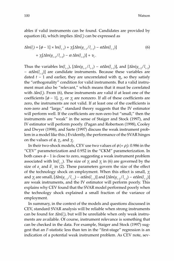
Watson100
ables if valid instruments can be found. Candidates are provided by equation (4), which implies Δln(lt) can be expressed as
Δln(lt) = [φ − 1] × ln(lt−1) + γ1[Δln(yt−1/lt−1) − αΔln(lt−1)] (6)
+ γ2[Δln(yt−2/lt−2) − α Δln(lt−2)] + υt .
Thus the variables ln(lt−1), [Δln(yt−1/lt−1) − αΔln(lt−1)], and [Δln(yt−2/lt−2) − αΔln(lt−2)] are candidate instruments. Because these variables are dated t − 1 and earlier, they are uncorrelated with ηt, so they satisfy the “orthogonality” condition for valid instruments. But a valid instru-ment must also be “relevant,” which means that it must be correlated with Δln(lt). From (6), these instruments are valid if at least one of the coeffi cients [φ − 1], γ1, or γ2 are nonzero. If all of these coeffi cients are zero, the instruments are not valid. If at least one of the coeffi cients is non-zero and “large,” standard theory suggests that the IV estimator will perform well. If the coeffi cients are non-zero but “small,” then the instruments are “weak” in the sense of Staiger and Stock (1997), and IV estimator will perform poorly. (Pagan and Robertson (1998), Cooley and Dwyer (1998), and Sarte (1997) discuss the weak instrument prob-lem in a model like this.) Evidently, the performance of the SVAR hinges on the values of φ, γ1, and γ2.
In their two-shock models, CEV use two values of φ (= ρl): 0.986 in the “CEV” parameterization and 0.952 in the “CKM” parameterization. In both cases φ − 1 is close to zero, suggesting a weak instrument problem associated with ln(lt−1). The size of γ1 and γ2 in (6) are governed by the size of az and a~z in (2). These parameters govern the size of the effect of the technology shock on employment. When this effect is small, γ1 and γ2 are small, [Δln(yt−1/lt−1) − αΔln(lt−1)] and [Δln(yt−2/lt−2) − αΔln(lt−2)] are weak instruments, and the IV estimator will perform poorly. This explains why CEV found that the SVAR model performed poorly when the technology shock explained a small fraction of the variance of employment.
In summary, in the context of the models and questions discussed in CEV, standard SVAR analysis will be reliable when strong instruments can be found for Δln(lt), but will be unreliable when only weak instru-ments are available. Of course, instrument relevance is something that can be checked in the data. For example, Staiger and Stock (1997) sug-gest that an F-statistic less than ten in the “fi rst-stage” regression is an indication of a potential weak instrument problem. As CEV note, sev-
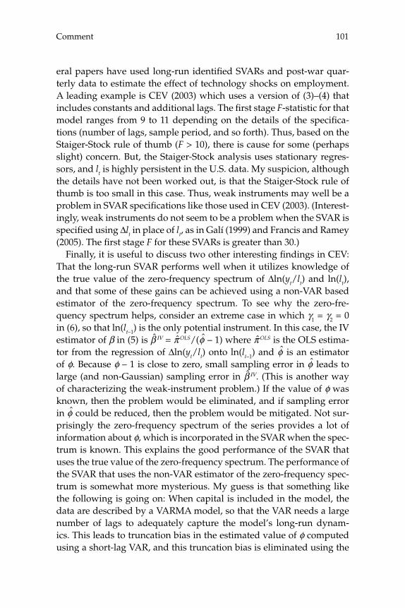
101Comment
eral papers have used long-run identifi ed SVARs and post-war quar-terly data to estimate the effect of technology shocks on employment. A leading example is CEV (2003) which uses a version of (3)–(4) that includes constants and additional lags. The fi rst stage F-statistic for that model ranges from 9 to 11 depending on the details of the specifi ca-tions (number of lags, sample period, and so forth). Thus, based on the Staiger-Stock rule of thumb (F > 10), there is cause for some (perhaps slight) concern. But, the Staiger-Stock analysis uses stationary regres-sors, and lt is highly persistent in the U.S. data. My suspicion, although the details have not been worked out, is that the Staiger-Stock rule of thumb is too small in this case. Thus, weak instruments may well be a problem in SVAR specifi cations like those used in CEV (2003). (Interest-ingly, weak instruments do not seem to be a problem when the SVAR is specifi ed using Δlt in place of lt, as in Galí (1999) and Francis and Ramey (2005). The fi rst stage F for these SVARs is greater than 30.)
Finally, it is useful to discuss two other interesting fi ndings in CEV: That the long-run SVAR performs well when it utilizes knowledge of the true value of the zero-frequency spectrum of Δln(yt/lt) and ln(lt), and that some of these gains can be achieved using a non-VAR based estimator of the zero-frequency spectrum. To see why the zero-fre-quency spectrum helps, consider an extreme case in which γ1 = γ2 = 0 in (6), so that ln(lt–1) is the only potential instrument. In this case, the IV estimator of β in (5) is β IV = π OLS/(φ – 1) where π OLS is the OLS estima-tor from the regression of Δln(yt/lt) onto ln(lt–1) and φ is an estimator of φ. Because φ – 1 is close to zero, small sampling error in φ leads to large (and non-Gaussian) sampling error in β IV. (This is another way of characterizing the weak-instrument problem.) If the value of φ was known, then the problem would be eliminated, and if sampling error in φ could be reduced, then the problem would be mitigated. Not sur-prisingly the zero-frequency spectrum of the series provides a lot of information about φ, which is incorporated in the SVAR when the spec-trum is known. This explains the good performance of the SVAR that uses the true value of the zero-frequency spectrum. The performance of the SVAR that uses the non-VAR estimator of the zero-frequency spec-trum is somewhat more mysterious. My guess is that something like the following is going on: When capital is included in the model, the data are described by a VARMA model, so that the VAR needs a large number of lags to adequately capture the model’s long-run dynam-ics. This leads to truncation bias in the estimated value of φ computed using a short-lag VAR, and this truncation bias is eliminated using the
Watson102
alternative estimator proposed by CEV. Analyzing the properties of this SVAR estimator would be interesting and non-standard because it relies on an inconsistent estimator of the zero-frequency spectrum. (The estimator used by CEV uses an untruncated Bartlett kernel.) Kiefer and Vogelsang (2002) and Müller (2005) discuss the usefulness of this incon-sistent estimator in other contexts.
References
Christiano, L. J., M. Eichenbaum, and R. Vigfusson. 2003. “What Happens After a Tech-nology Shock.” Manuscript, Northwestern University.
Cooley, T. F., and M. Dwyer. 1998. “Business Cycle Analysis Without Much Theory: A Look at Structual VARs.” Journal of Econometrics 83: 57–88.
Francis, N., and V. A. Ramey. 2005. “Is the Technology-Driven Real Business Cycle Hypothesis Dead? Shocks and Aggregrate Fluctuations Revisited.” Journal of Monetary Economics 52: 1379–1399.
Galí, Jordi. 1999. “Technology, Employment, and the Business Cycle: Do Technology Shocks Explain Aggregate Fluctuations?” American Economic Review 89: 249–271.
Hansen, L. P., and T. J. Sargent. 1991. “Two Diffi culties in Interpreting Vector Autoregres-sions.” In L. P. Hansen and T. J. Sargent, eds., Rational Expectations Econometrics: 77–120, Boulder, CO: Westview Press.
Hansen, L. P., and T. J. Sargent. 2007, forthcoming. Recursive Linear Models of Dynamic Economies. Princeton, NJ: Princeton University Press.
Kiefer, N., and T. Vogelsang. 2002. “Heteroskedasticity-Autocorrelation Robust Standard Errors Using the Bartlett Kernel Without Truncation.” Econometrica 70: 2093–2095.
Lippi, M., and L. Reichlin. 1994. “VAR Analysis, Nonfundamental Representations, Blashke Matrices.” Journal of Econometrics 63(1): 307–325.
Müller, U. K. 2005. “A Theory of Long-Run Variance Estimation.” Manuscript, Princeton University.
Pagan, A. R., and J. Robertson. 1998. “Structural Models of the Liquidity Effect.” Review of Economics and Statistics 80: 202–217.
Sarte, Pierre. 1997. “On the Identifi cation of Structural Vector Autoregressions.” Federal Reserve Bank of Richmond Economic Quarterly 83(3): 45–67.
Sims, C. A., J. H. Stock, and M. W. Watson. 1990. “Inference in Linear Time Series Models with Some Unit Roots” (with C. A. Sims and J. H. Stock). Econometrica 58(1).
Staiger, D., and J. H. Stock. 1997. “Instrumental Variable Regression with Weak Instru-ments.” Econometrica 65(3): 557–586.

Discussion
Lawrence Christiano responded to a number of points made by Ellen McGrattan in her presentation of Patrick Kehoe’s comment. First, he disagreed with the view that the appropriate way to conduct the line of research in which he and his coauthors were engaged was to run a VAR on the data from the model, and then run the same VAR on data from the actual economy, and compare the two. While he said that he was generally sympathetic to this approach, he thought that this was not the appropriate approach for the problem they were studying. In their case, they were trying to assess how well a VAR estimator is able to estimate a particular feature of a model, namely how hours respond to a productivity shock. He thought that for this sampling theory ques-tion, the approach they used was the appropriate one.
Christiano agreed with McGrattan that the conclusions of VAR anal-ysis using fi rst differenced data could be very misleading. He, however, felt that the fact that VARs are sensitive to fi rst differencing was not a reason to throw out VARs. He pointed out that many other statistical procedures, such as correlations, are sensitive to fi rst differencing, but this has not led economists to discard these other procedures.
Christiano then commented that it was true that in the context of RBC models, the VARs they estimate with long run restrictions tend to produce very large confi dence intervals. He said that this was due to the fact that sampling uncertainty is big in data coming from RBC models. He stressed that VARs are good in that they will correctly tell the researcher that the sampling uncertainty is large and that there is not much information in the data generated by the RBC model. Christiano then stressed that VARs work very well with short run restrictions and that the VAR literature that relies on short run restric-tions has had a large impact on how macroeconomists think about busi-ness cycles.
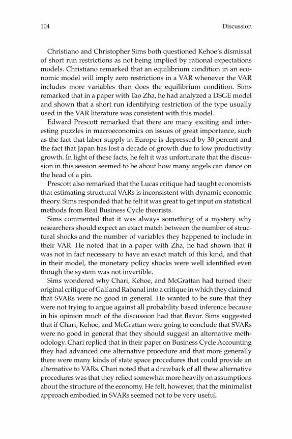
Discussion104
Christiano and Christopher Sims both questioned Kehoe’s dismissal of short run restrictions as not being implied by rational expectations models. Christiano remarked that an equilibrium condition in an eco-nomic model will imply zero restrictions in a VAR whenever the VAR includes more variables than does the equilibrium condition. Sims remarked that in a paper with Tao Zha, he had analyzed a DSGE model and shown that a short run identifying restriction of the type usually used in the VAR literature was consistent with this model.
Edward Prescott remarked that there are many exciting and inter-esting puzzles in macroeconomics on issues of great importance, such as the fact that labor supply in Europe is depressed by 30 percent and the fact that Japan has lost a decade of growth due to low productivity growth. In light of these facts, he felt it was unfortunate that the discus-sion in this session seemed to be about how many angels can dance on the head of a pin.
Prescott also remarked that the Lucas critique had taught economists that estimating structural VARs is inconsistent with dynamic economic theory. Sims responded that he felt it was great to get input on statistical methods from Real Business Cycle theorists.
Sims commented that it was always something of a mystery why researchers should expect an exact match between the number of struc-tural shocks and the number of variables they happened to include in their VAR. He noted that in a paper with Zha, he had shown that it was not in fact necessary to have an exact match of this kind, and that in their model, the monetary policy shocks were well identifi ed even though the system was not invertible.
Sims wondered why Chari, Kehoe, and McGrattan had turned their original critique of Galí and Rabanal into a critique in which they claimed that SVARs were no good in general. He wanted to be sure that they were not trying to argue against all probability based inference because in his opinion much of the discussion had that fl avor. Sims suggested that if Chari, Kehoe, and McGrattan were going to conclude that SVARs were no good in general that they should suggest an alternative meth-odology. Chari replied that in their paper on Business Cycle Accounting they had advanced one alternative procedure and that more generally there were many kinds of state space procedures that could provide an alternative to VARs. Chari noted that a drawback of all these alternative procedures was that they relied somewhat more heavily on assumptions about the structure of the economy. He felt, however, that the minimalist approach embodied in SVARs seemed not to be very useful.

105Discussion
Sims remarked that the weak instruments problem Mark Watson had discussed in his comment was easily dealt with by using likelihood based inference, even in the case when the instruments are highly auto-correlated.
Chari felt that the SVAR procedure as originally envisioned by Blanchard and Quah and later applied by many other authors was “totally cool stuff.” This opinion was based on the fact that the SVAR literature came up with strong, clear, and confi dent results that held the promise of allowing researchers to reject certain classes of models and focus on other classes. He then explained that all he, Kehoe, and McGrattan had wanted to do in their paper was to subject SVARs to a simple test. If they generated data from a model where they knew what the response of hours to a productivity shock was, would a SVAR be able to identify that the data came from the model? He noted that the examples in their paper did not raise questions about VARs in general, but rather only attempted to assess how good SVARs are at identify-ing whether data is generated from the particular model they specifi ed. Their fi ndings were that when demand shocks are important, then the SVAR does not perform particularly well.
Chari then remarked that different papers in the SVAR literature analyzing the same question had found very different results based on seemingly small differences in the variables being used. In reply, Martin Eichenbaum disagreed that the differences in the data were small. He furthermore noted that when the sample was restricted to a more recent sample period where the differences in the data were in fact small, the differences in results disappeared.

Volatility and Dispersion in Business Growth Rates: Publicly Traded versus Privately Held Firms
Steven J. Davis, University of Chicago, NBER, and American Enterprise InstituteJohn Haltiwanger, University of Maryland and NBERRon Jarmin, U.S. Census BureauJavier Miranda, U.S. Census Bureau
2
1 Introduction
We study the variability of business growth rates in the U.S. economy from 1976 onwards. To carry out our study, we exploit the recently developed Longitudinal Business Database (LBD) (Jarmin and Miranda 2002a), which contains annual observations on employment and pay-roll for all establishments and fi rms in the private sector. Compared to other longitudinal business databases for the United States, the LBD is unparalleled in its comprehensive coverage over an extended period of time. The underlying sources for the LBD are periodic business surveys conducted by the Census Bureau and federal government administra-tive records.1
Macroeconomists increasingly recognize the importance of inter-actions between aggregate economic performance and the volatility and heterogeneity of business level outcomes. Idiosyncratic shocks are central to modern theories of unemployment. Frictions in product, factor and credit markets that impede business responses to idiosyn-cratic shocks can raise unemployment, lower productivity and depress investment. Financial innovations that facilitate better risk sharing can simultaneously encourage risk taking and investment, amplify business level volatility, and promote growth. Several recent studies hypothesize a close connection between declining aggregate volatility and trends in business level volatility. These examples of interactions between busi-ness level and aggregate outcomes help motivate our empirical study. Our chief objective is to develop a robust set of facts about the magni-tude and evolution of business level volatility and the cross sectional dispersion of business growth rates in the U.S. economy.
Davis, Haltiwanger, Jarmin, and Miranda108
Previous empirical work in this area yields an unclear picture. Sev-eral recent studies fi nd a secular rise in average volatility among pub-licly traded fi rms. Examples include Campbell et al. (2001), Chaney, Gabaix, and Philippon (2002), Comin and Mulani (2006), and Comin and Philippon (2005). In fi gure 2.1, we replicate a key fi nding from the latter two studies. The fi gure shows that the average magnitudes of fi rm level volatility in the growth rates of sales and employment have roughly doubled since the early 1960s.2 In a different line of research, Davis, Faberman, and Haltiwanger (2006) and Faberman (2006) pro-duce evidence of a downward trend in the excess job reallocation rate, a measure of cross sectional dispersion in establishment growth rates.3 As seen in the top panel of fi gure 2.2, the quarterly excess job realloca-tion rate in the U.S. manufacturing sector fell from about 12 percent in the early 1960s to 8 percent by 2005. The shorter time series in the lower panel shows a decline in excess job reallocation for the U.S. private sec-tor from 16 percent or more in the early 1990s to less than 14 percent by 2005.4 The data underlying fi gure 2.2 are not restricted to publicly traded fi rms.
There is an unresolved tension between the evidence of rising fi rm level volatility and declining cross sectional dispersion in establishment growth rates. To appreciate the tension, consider a simple example in which all employers follow identical and independent autoregressive processes. Then an increase in the innovation variance of idiosyncratic shocks implies an increase in employer volatility and in the cross sec-tional dispersion of growth rates. Of course, it is possible to break the tight link between employer volatility and cross sectional dispersion in more complicated specifi cations. It is also possible that fi rm and estab-lishment growth processes have evolved along sharply different paths in recent decades. Yet another possibility is that the restriction to pub-licly traded businesses in previous studies paints a misleading picture of fi rm level volatility trends in the economy as a whole.5 A related pos-sibility is that the economic selection process governing entry into the set of publicly traded fi rms has changed over time in ways that affect measured trends in volatility.
In what follows, we explore each of these issues. We fi nd similar trends in cross sectional dispersion and fi rm level volatility, so the dif-ferent measures cannot account for the contrast between fi gures 2.1 and 2.2. Instead, the resolution turns mainly on the distinction between pub-licly traded and privately held businesses. For the private nonfarm sec-tor as a whole, both fi rm level volatility and cross sectional dispersion
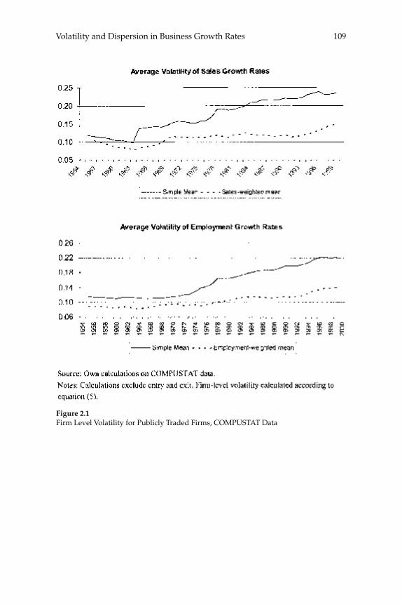
109Volatility and Dispersion in Business Growth Rates
Figure 2.1Firm Level Volatility for Publicly Traded Firms, COMPUSTAT Data
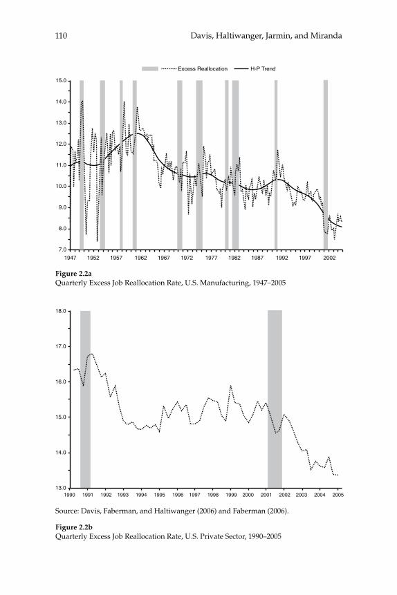
Davis, Haltiwanger, Jarmin, and Miranda110
Figure 2.2bQuarterly Excess Job Reallocation Rate, U.S. Private Sector, 1990–2005
Figure 2.2aQuarterly Excess Job Reallocation Rate, U.S. Manufacturing, 1947–2005
Source: Davis, Faberman, and Haltiwanger (2006) and Faberman (2006).
15.0
14.0
13.0
12.0
11.0
10.0
9.0
8.0
7.0
1947 1952 1957 1962 1967 1972 1977 1982 1987 1992 1997 2002
Excess Reallocation H-P Trend
18.0
17.0
16.0
15.0
14.0
13.01990 1991 1992 1993 1994 1995 1996 1997 1998 1999 2000 2001 2002 2003 2004 2005
111Volatility and Dispersion in Business Growth Rates
measures show large declines in recent decades. For publicly traded fi rms, we provide independent evidence that cross sectional dispersion and fi rm level volatility have risen during the period covered by the LBD. We also show, however, that this rise for publicly traded fi rms is overwhelmed by the dramatic decline among privately held fi rms, which account for more than two-thirds of private business employ-ment. Very similar results obtain when we treat establishments, rather than fi rms, as the unit of observation.
Two basic patterns hold across major industry groups. First, the vola-tility and dispersion of business growth rates are considerably greater for privately held fi rms. As of 1978, the average standard deviation of fi rm-level employment growth rates is 3.7 times larger for privately held than for publicly traded fi rms. This volatility ratio ranges from 2.3 in Services to 6.3 in Transportation and Public Utilities. Second, volatil-ity and dispersion decline sharply among privately held businesses in the period covered by the LBD, and they rise sharply among publicly traded fi rms. The overall private-public volatility ratio falls to 1.6 by 2001, and it drops sharply in every major industry group. We refer to this phenomenon as “volatility convergence.”
We also provide proximate explanations for these patterns. First, much of the decline in dispersion and volatility for the private sector as a whole, and for privately held fi rms in particular, refl ects a decline in (employment-weighted) business entry and exit rates. Second, the age distribution of employment among privately held fi rms shifted towards older businesses in the period covered by the LBD. Because volatility declines steeply with age, the shift toward older businesses brought about a decline in overall volatility. We estimate that 27 per-cent or more of the volatility decline among privately held fi rms refl ects the shift toward older businesses. Third, the evolution toward larger fi rms in certain industries, especially Retail Trade, accounts for about 10 percent of the volatility decline among nonfarm businesses during the period covered by the LBD.
Fourth, and perhaps most striking, changes over time in the number and character of newly listed fi rms played a major role in the volatil-ity rise among publicly traded fi rms and in the volatility convergence phenomenon. There was a large infl ux of newly listed fi rms after 1979, and newly listed fi rms are much more volatile than seasoned listings. Moreover, fi rms newly listed in the 1980s and 1990s exhibit much greater volatility than earlier cohorts. Indeed, simple cohort dummies for the year of fi rst listing in COMPUSTAT account for 67 percent of the

Davis, Haltiwanger, Jarmin, and Miranda112
volatility rise among publicly traded fi rms from 1978 to 2001, and they account for 90 percent of the smaller rise over the 1951–2004 period spanned by COMPUSTAT. Other evidence discussed below also points to important changes over time in the selection of fi rms that become public.
The paper proceeds as follows. Section 2 reviews the role of idiosyn-cratic shocks, producer heterogeneity and risk-taking in selected theo-ries of growth, fl uctuations and unemployment. Section 2 also identifi es several factors that infl uence business volatility and its connection to aggregate volatility. Section 3 describes our data and measurement pro-cedures. Section 4 presents our main empirical fi ndings on volatility and cross sectional dispersion in business outcomes. Section 5 explores various factors that help to amplify and explain our main fi ndings. Sec-tion 6 offers concluding remarks.
2 Conceptual Underpinnings and Theoretical Connections
Theories of growth and fl uctuations in the Schumpeterian mold envision a market economy constantly disturbed by technological and commer-cial innovations. Firms and workers differ in their capacities to create, adopt and respond to these innovations, so that winners and losers emerge as unavoidable by-products of economic progress. According to this view, an economy’s long-term growth rate depends on how well it facilitates and responds to the process of creative destruction (Aghion and Howitt 1998). Institutions and policies that impede restructuring and adjustment can mute the disruptive nature of factor reallocation—at the cost of lower productivity, depressed investment and, in some circumstances, persistently high unemployment (Caballero 2006).
Empirical evidence supports the Schumpeterian view in its broad outlines. Large-scale job reallocation is a pervasive feature of market economies (Davis and Haltiwanger 1999). The large job fl ows and high fi rm level volatility refl ect the restructuring, experimentation and adjustment processes at the heart of Schumpeterian theories. Empiri-cally, gross job fl ows are dominated by reallocation within narrowly defi ned sectors, even in countries that undergo massive structural transformations. Thus longitudinal fi rm and establishment data are essential for helping gauge the pace of restructuring and reallocation. Empirical studies also fi nd that excess job reallocation rates decline strongly during the early lifecycle of fi rms and establishments (Davis and Haltiwanger (1992), and Bartelsman, Haltiwanger, and Scarpetta
113Volatility and Dispersion in Business Growth Rates
(2004)). This fi nding indicates that experimentation and adjustment in the face of uncertainty about demand, technologies, costs, and manage-rial ability are especially pronounced among younger businesses.
A closely related empirical literature highlights the role of factor real-location in productivity growth. Over horizons of fi ve or ten years, the reallocation of inputs and outputs from less to more productive business units typically accounts for a sizable fraction of industry-level produc-tivity growth (Foster, Haltiwanger, and Krizan 2001). Several studies reviewed in Caballero (2006, chapter 2) provide evidence that trade barriers, entry barriers, impediments to labor mobility, and misdirected fi nancing can hamper effi cient factor reallocation and, as a result, retard restructuring and undermine productivity growth. In short, there are sound theoretical and empirical reasons to treat restructuring and fac-tor reallocation as key aspects of growth and fl uctuations. The busi-ness volatility and dispersion measures that we construct in this study capture the pace of restructuring and reallocation on important dimen-sions. In this respect, they are useful inputs into theories of growth and fl uctuations in the Schumpeterian mold.
Theories of unemployment based on search and matching frictions (Mortensen and Pissarides (1999) and Pissarides (2000)) rely on idiosyn-cratic shocks to drive job destruction and match dissolution. A greater intensity of idiosyncratic shocks in these models produces higher match dissolution rates and increased fl ows of workers into the unemploy-ment pool. The measures of employer volatility and dispersion that we consider provide empirical indicators for the intensity of idiosyncratic shocks. Evidence regarding trends in these indicators can serve as use-ful inputs into theoretical explanations for longer term movements in the rates of unemployment and match dissolution. These indicators also provide grist for empirical studies of how long term changes in idiosyncratic shock intensity affect unemployment.
Another class of theories stresses the impact of risk-sharing oppor-tunities on the willingness to undertake risky investments. Obstfeld (1994), for example, shows that better diversifi cation opportunities induce a portfolio shift by risk-averse investors toward riskier proj-ects with higher expected returns. Greater portfolio diversifi cation also weakens one motive for organizing production activity around large, internally diversifi ed fi rms. On both counts, improved opportunities for diversifi cation lead to more volatility and dispersion in producer outcomes. Empirical indicators of increased fi nancial diversifi cation include the rise of mutual funds and institutional investors, lower
Davis, Haltiwanger, Jarmin, and Miranda114
trading costs for fi nancial securities, higher stock market participation rates by households, and greater cross-border equity holdings. Moti-vated in part by these developments, Thesmar and Thoenig (2004) build a model whereby a bigger pool of portfolio investors encourages listed fi rms to adopt riskier business strategies with greater expected profi ts. More aggressive risk-taking by listed fi rms also leads unlisted fi rms to adopt riskier strategies in their model, raising fi rm level volatility throughout the economy.6 In the model of Acemoglu (2005), risk-taking by fi rms increases with aggregate capital accumulation, technical prog-ress and fi nancial development, so that fi rm volatility naturally rises with economic development. Acemoglu stresses that his model can deliver rising fi rm volatility accompanied by falling aggregate volatility.
In contrast, Koren and Tenreyro (2006) highlight a mechanism that generates declines in both aggregate and fi rm volatility as an economy develops. In their model, input variety rises naturally with economic development. As input variety expands, shocks to the productivity of specifi c varieties lead to less output volatility, provided that the correla-tion of variety-specifi c shocks is imperfect and not rising in the number of varieties. Koren and Tenreyro argue that this economic mechanism linking development to input variety helps to explain the negative rela-tionship between GDP per capita and the volatility of GDP growth rates across countries and over time within countries. Whether economic development ultimately dampens fi rm volatility through the impact of greater input variety or amplifi es it as a result of better opportunities for fi nancial diversifi cation is obviously an empirical question.
Another line of research stresses the role of competition in goods markets. Philippon (2003) considers a model with nominal rigidities that links goods-market competition to fi rm and aggregate volatility. In his model, greater competition in the form of a bigger substitution elasticity among consumption goods magnifi es the effects of idiosyn-cratic shocks on profi tability. As a result, greater competition leads to more fi rm volatility in sales growth rates and a higher frequency of price adjustments. In turn, more frequent price adjustments dampen the response to aggregate demand disturbances in a calibrated ver-sion of the model. Thus, insofar as aggregate demand shocks drive aggregate fl uctuations, Philippon’s model produces divergent trends in aggregate and fi rm volatility. Comin and Mulani (2005) argue that increased R&D-based competition leads to more fi rm volatility but weaker comovements and, hence, lower aggregate volatility. As Acemoglu (2005) points out, however, R&D investments can act to
115Volatility and Dispersion in Business Growth Rates
increase or decrease competitive intensity, and the link to aggregate volatility is also tenuous. Comin and Philippon (2005) point to deregu-lation as a source of greater goods-market competition and rising fi rm level volatility. While deregulation is likely to increase fi rm volatility in the short term, its longer term impact is less clear. For example, when regulatory restrictions hamper horizontal consolidation, deregulation can lead to an industry structure with fewer, larger fi rms. Horizon-tal consolidation is, in turn, a force for less fi rm level volatility. The removal of regulatory restrictions on branching and interstate banking accelerated this type of evolutionary pattern in the U.S. banking sector (Jayaratne and Strahan 1998).
Although much recent work focuses on the potential for better risk-sharing opportunities or greater goods-market competition to produce opposite trends in aggregate and fi rm level volatility, there is a simple mechanical reason to anticipate that micro and macro volatility will trend in the same direction. To see the argument, write the fi rm level growth rate as a linear function of K aggregate shocks that (potentially) affect all fi rms and an idiosyncratic shock, εi, that affects only fi rm i:
γ β εit ik kt itk
K
Z i N= + ==
∑ , , , ... .1
1 2 (1)
The aggregate growth rate is Σiαitγit, where αi is fi rm i’s share of aggregate activity. Assuming mutually uncorrelated shocks, equation (1) implies the following expressions for fi rm level and aggregate volatility:
Weighted Mean Firm Volatility = α σεiti
n
=∑
1tt it
i
n
ik ktk
K2
1
2 2
1
+⎡⎣⎢
⎤⎦⎥
= =∑ ∑α β σ (2)
Aggregate Volatility = +∑α σ α β σit iti
n
it ik k2 2 2 2
ttk
K
i
n2
1=∑∑ ⎡
⎣⎢
⎤⎦⎥ (3)
+⎡⎣⎢
⎤⎦⎥
=>∑∑2 2
1
α α β β σit jt ik jk ktk
K
j i
n
In light of the positive comovements that typify aggregate fl uctuations, we assume that the weighted cross-product of the β coeffi cients is posi-tive for each k.
Inspecting (2) and (3), we see that fi rm and aggregate volatility respond in the same direction to a change in any one of the shock vari-ances, provided that the fi rm shares αi and the shock response coeffi -cients βik are reasonably stable. In particular, a decline in the variability
Davis, Haltiwanger, Jarmin, and Miranda116
of aggregate shocks leads to a decline in both aggregate and fi rm vola-tility. Hence, insofar as the well-established secular decline in aggregate volatility refl ects a decline in the size or frequency of aggregate shocks, we anticipate a decline in average fi rm volatility as well. Another argu-ment stresses the importance of idiosyncratic shocks to large fi rms. Especially if σi is independent of size (αi) at the upper end of the fi rm size distribution, as in Gabaix’s (2005) granular theory of aggregate fl uc-tuations, trend changes in the idiosyncratic shock variance for, say, the 100 largest fi rms can be a powerful force that drives micro and macro volatility in the same direction. Of course, (2) and (3) do not require that aggregate and fi rm volatility trend in the same direction. A mix of positive and negative changes in the shock variances could drive micro and macro volatility measures in opposite directions, as could certain changes in the pattern of shock-response coeffi cients or the fi rm size distribution. Still, big trends in the opposite direction for micro and macro volatility strike us as an unlikely outcome.
Evolutions in market structure can also drive the trend in fi rm vola-tility, particularly in sectors that undergo sweeping transformations. Consider Retail Trade. The expansion of Wal-Mart, Target, Staples, Best Buy, Home Depot, Borders, and other national chains has propelled the entry of large retail outlets and displaced thousands of indepen-dent and smaller retail establishments and fi rms. Jarmin, Klimek, and Miranda (2005) report that the share of U.S. retail activity accounted for by single-establishment fi rms fell from 60 percent in 1967 to 39 per-cent in 1997. In its initial phase, this transformation involved high entry and exit rates, but over time the Retail Trade size distribution shifted towards larger establishments and much larger fi rms. Empirical stud-ies routinely fi nd a strong negative relationship between business size and volatility. Hence, we anticipate that the transformation of the retail sector led to a secular decline in the volatility and dispersion of growth rates among retail businesses.
One other key issue involves the impact of developments that expand business access to equity markets. Financial developments of this sort can profoundly alter the mix of publicly traded fi rms and drive volatil-ity trends among all listed fi rms that are unrepresentative of trends for seasoned listings and the economy as a whole. Some previous studies point strongly in that direction. For example, Fama and French (2004) report that the number of new lists (mostly IPOs) on major U.S. stock markets jumped from 156 per year in 1973–1979 to 549 per year in 1980–2001. Remarkably, about 10 percent of listed fi rms are new each year
117Volatility and Dispersion in Business Growth Rates
from 1980 to 2001. Fama and French also provide compelling evidence that new lists are much riskier than seasoned fi rms and increasingly so from 1980 to 2001. They conclude that the upsurge of new listings explains much of the trend increase in idiosyncratic stock return volatil-ity documented by Campbell et al. (2001). They also suggest that there was a decline in the cost of equity that allowed weaker fi rms and those with more distant payoffs to issue public equity. Fink et al. (2005) pro-vide additional evidence in support of these conclusions. Drawing on data from Jovanovic and Rousseau (2001), they report that fi rm age at IPO date (measured from its founding date or date of incorporation) fell dramatically from nearly 40 years old in the early 1960s to less than fi ve years old by the late 1990s. They fi nd that the positive trend in idio-syncratic risk is fully explained by the proportion of young fi rms in the market. After controlling for age and other measures of fi rm maturity (book-to-market, size, profi tability), they fi nd a negative trend in idio-syncratic risk. These studies imply that the selection process govern-ing entry into the set of publicly traded fi rms shifted dramatically after 1979, and that the shift continued to intensify through the late 1990s.
3 Data and Measurement
3.1 Source Data: The LBD and COMPUSTAT
The Longitudinal Business Database (LBD) is constructed from the Cen-sus Bureau’s Business Register of U.S. businesses with paid employees and enhanced with survey data collections. The LBD covers all sectors of the economy and all geographic areas and currently runs from 1976 to 2001. In recent years, it contains over six million establishment records and almost fi ve million fi rm records per year. Basic data items include employment, payroll, 4-digit SIC, employer identifi cation numbers, business name, and information about location.7 Identifi ers in the LBD fi les enable us to compute growth rate measures for establishments and fi rms.8 Firms in the LBD are defi ned based on operational control, and all establishments that are majority owned by the parent fi rm are included as part of the parent’s activity measures. We restrict attention in this study to nonfarm businesses in the private sector.
We also exploit COMPUSTAT data from 1950 to 2004.9 A unit of observation in COMPUSTAT is a publicly traded security identifi ed by a CUSIP. We exclude certain CUSIPs because they refl ect duplicate records for a particular fi rm, multiple security issues for the same fi rm,

Davis, Haltiwanger, Jarmin, and Miranda118
or because they do not correspond to fi rms in the usual sense. Duplicate entries for the same fi rm (refl ecting more than one 10-K fi ling in the same year) are few in number but can be quite large (more than 500,000 workers). We also exclude CUSIPs for American Depository Receipts (ADRs)—securities created by U.S. banks to permit U.S.-based trading of stocks listed on foreign exchanges. All together, we exclude approxi-mately 1,100 CUSIPs because of duplicates and ADRs. The presence of duplicates, ADRs and other features of COMPUSTAT imply the need for caution in measuring fi rm outcomes and in linking COMPUSTAT records to the LBD.
We use COMPUSTAT to supplement the LBD with information on whether fi rms are publicly traded. For this purpose, we created a bridge fi le that links LBD and COMPUSTAT records based on busi-ness taxpayer identifi cation numbers (EINs) and business name and address.10 Missing data on equity prices, sales and employment data for some COMPUSTAT records do not cause problems for our LBD-based analysis, because we rely on LBD employment data whether or not the COMPUSTAT data are missing. Our matching procedures also work when there are holes in the COMPUSTAT data. In particular, we clas-sify a fi rm in the LBD as publicly traded in a given year if it matches to a COMPUSTAT CUSIP by EIN or name and address, and if the CUSIP has non-missing equity price data in the same year or in years that bracket the given year.
Table 2.1 presents LBD and COMPUSTAT summary statistics for fi rm counts, employment and fi rm size in selected years. As of 2000, the LBD has almost fi ve million fi rms with positive employment in the nonfarm private sector, of which we identify more than 7,000 as publicly traded. Average LBD fi rm size in 2000 is about 18 employees, which is tiny compared to the average of 4,000 employees for publicly traded fi rms. Publicly traded fi rms account for a trivial fraction of all fi rms and less than one-third of nonfarm business employment during the period covered by the LBD. The highly skewed nature of the fi rm size distribution is also apparent in the enormous difference between average fi rm size and the employment-weighted mean fi rm size (the coworker mean). For example, the upper panel of table 2.1 reports a coworker mean of 92,604 employees at publicly traded fi rms in the LBD in 2000, roughly 23 times larger than the simple mean of fi rm size. The highly skewed nature of the fi rm size distribution implies the potential for equally weighted and size-weighted measures of business volatility and dispersion to behave in dissimilar ways.
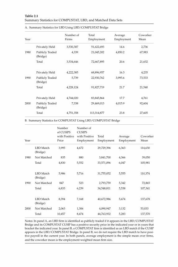
Table 2.1Summary Statistics for COMPUSTAT, LBD, and Matched Data Sets
A. Summary Statistics for LBD Using LBD/COMPUSTAT Bridge
1980
1990
2000
YearNumber of Firms
Total Employment
Average Employment
Coworker Mean
Privately Held
Publicly Traded (Bridge)
Total
Privately Held
Publicly Traded (Bridge)
Total
Privately Held
Publicly Traded (Bridge)
Total
3,530,307
4,339
3,534,646
4,222,385
5,739
4,228,124
4,744,020
7,338
4,751,358
51,622,693
21,045,202
72,667,895
68,896,957
22,930,762
91,827,719
83,845,864
29,469,013
113,314,877
14.6
4,850.2
20.6
16.3
3,995.6
21.7
17.7
4,015.9
23.8
2,736
67,983
21,632
4,235
73,533
21,540
4,761
92,604
27,605
B. Summary Statistics for COMPUSTAT Using LBD/COMPUSTAT Bridge
Year
Number of CUSIPS with Positive Price
Number of CUSIPS with Positive Employment
Total Employment
Average Employment
Coworker Mean
1980
1990
2000
LBD Match (Bridge)
Not Matched
Total
LBD Match (Bridge)
Not Matched
Total
LBD Match (Bridge)
Not Matched
Total
3,995
835
4,830
5,986
847
6,833
8,394
2,063
10,457
4,672
880
5,552
5,716
523
6,239
7,168
1,306
8,474
29,729,396
3,841,700
33,571,096
31,755,052
2,793,759
34,548,811
40,672,986
4,090,947
44,763,932
6,363
4,366
6,047
5,555
5,342
5,538
5,674
3,132
5,283
114,630
39,050
105,981
110,374
72,865
107,341
137,678
53,033
137,570
Notes: In panel A, an LBD fi rm is identifi ed as publicly traded if it appears in the LBD/COMPUSTAT Bridge and its COMPUSTAT CUSIP has a positive security price in the indicated year or in years that bracket the indicated year. In panel B, a COMPUSTAT fi rm is identifi ed as an LBD match if the CUSIP appears in the LBD/COMPUSTAT Bridge. In panel B, we do not require the LBD match to have posi-tive payroll in the current year. In both panels, average employment is the simple mean over fi rms, and the coworker mean is the employment-weighted mean fi rm size.
Davis, Haltiwanger, Jarmin, and Miranda120
Comparisons between the upper and lower panels of table 2.1 require some care, because the LBD and COMPUSTAT differ in how they defi ne a fi rm and in how key variables are measured. LBD employment refl ects the count of workers on the payroll during the pay period covering the 12th of March. The employment concept is all employees subject to U.S. payroll taxes. COMPUSTAT employment is the number of com-pany workers reported to shareholders. It may be an average number of employees during the year or a year-end fi gure. More important, it includes all employees of consolidated subsidiaries, domestic and for-eign. For this reason, discrepancies between the LBD and COMPUSTAT are likely to be greater for large multinationals and for foreign fi rms with U.S. operations (and listings on U.S. stock exchanges). Since the source data from annual reports can be incomplete, some COMPUS-TAT fi rms have missing employment even when the fi rm has positive sales and a positive market value.
With these cautions in mind, consider the lower panel of table 2.1 and its relationship to the upper panel. The lower panel provides informa-tion about the match rate in the LBD/COMPUSTAT Bridge. In 1990, for example, there are 6,239 CUSIPs with positive COMPUSTAT employ-ment. We match 5,716 of these CUSIPs to fi rms in the LBD, which amounts to 92 percent of COMPUSTAT fi rms with positive employ-ment and 92 percent of COMPUSTAT employment.11 It is instructive to compare total employment, average fi rm size and the coworker mean between the upper and lower panels of table 2.1 for the bridge cases. COMPUSTAT fi gures for these quantities exceed the corresponding LBD statistics by a very wide margin in all years. For example, among matched publicly traded fi rms in the Bridge fi le, the LBD employment fi gure (Panel A) is only 70.8 percent of COMPUSTAT employment (Panel B) in 1980, 72.2 percent in 1990, and 72.5 percent in 2000. These large discrepancies for matched cases refl ect signifi cant differences in the LBD and COMPUSTAT employment concepts, e.g., domestic ver-sus global operations. See the Data Appendix for additional compari-sons between the two data sources.
We can use the information reported in table 2.1 to construct an esti-mate for the percentage of nonfarm business employment in publicly traded fi rms. First, adjust the COMPUSTAT employment totals for “Not Matched” cases in Panel B by multiplying by the ratio of LBD-to-COMPUSTAT employment for matched cases. Second, add the adjusted COMPUSTAT employment fi gure for “Not Matched” cases
121Volatility and Dispersion in Business Growth Rates
to LBD employment for “Publicly Traded (Bridge)” cases in Panel A, and then divide the sum by LBD nonfarm business employment. The resulting estimates imply that publicly traded fi rms account for 32.7 percent of nonfarm business employment in 1980, 27.2 percent in 1990, and 28.6 percent in 2000.
To sum up, the LBD provides data from 1976 to 2001 on the universe of fi rms and establishments with at least one employee in the U.S. pri-vate sector. We identify publicly traded fi rms in the LBD using our COMPUSTAT/LBD Bridge. The empirical analysis below focuses on the LBD, but we also carry out several exercises using COMPUSTAT data.
3.2 Measuring Firm Growth, Volatility and Cross Sectional Dispersion
We focus on employment as our activity measure because of its ready availability in the LBD and COMPUSTAT. Recall from fi gure 2.1 that volatility trends for employment and sales growth rates are similar in COMPUSTAT data. We use a growth rate measure that accommodates entry and exit. In particular, our time-t growth rate measure for fi rm or establishment i is
γ itit it
it it
x xx x
=−
+−
−
1
1 2( )/. (4)
This growth rate measure has become standard in work on labor market fl ows, because it offers signifi cant advantages relative to log changes and growth rates calculated on initial employment. In particular, it yields measures that are symmetric about zero and bounded, affording an integrated treatment of births, deaths, and continuers. It also lends itself to consistent aggregation, and it is identical to log changes up to a second-order Taylor Series expansion. See Tornqvist, Vartia, and Vartia (1985) and the appendix to Davis, Haltiwanger, and Schuh (1996) for additional discussion.
To characterize the variability of business outcomes, we consider several measures of cross sectional dispersion in business growth rates and volatility in business growth rates. Our basic dispersion measure is the cross sectional standard deviation of the annual growth rates in (4), computed in an equal-weighted or size-weighted manner. Our basic volatility measure follows recent work by Comin and Mulani (2005,
Davis, Haltiwanger, Jarmin, and Miranda122
2006) and Comin and Philippon (2005), among others. They measure volatility for fi rm i at t by
σ γ γττ
it i t it= −⎡⎣⎢
⎤⎦⎥+
=−∑1
10 4
52
1 2
( ) ,,
/
(5)
where γ–it is the simple mean growth rate for i from t – 4 to t + 5. This measure requires ten consecutive observations on the fi rm’s growth rates; hence, short-lived fi rms and entry and exit are not cap-tured.12
Limiting the analysis to fi rms and establishments with ten consecu-tive years of positive activity is quite restrictive. Hence, we also con-sider a modifi ed volatility measure that incorporates entry and exit and short-lived business units. The modifi ed measure differs from the basic measure in two main respects. First, we weight the squared deviation at t for fi rm i in proportion to its size at t relative to its average size in the ten-year window from t – 4 to t + 5. Second, we apply a standard degrees-of-freedom correction to avoid the small-sample bias that oth-erwise arises for second moment estimates.13 We ignored this issue in the basic volatility measure, following standard practice, because the correction is the same for all fi rms and would simply scale up the vola-tility magnitude by (10/9). However, the correction matters when some fi rms have much shorter intervals of positive activity than others. The degrees-of-freedom correction also enables us to obtain unbiased esti-mates for average volatility near the LBD and COMPUSTAT sample end points, which truncate the available window for estimating fi rm level volatility.
Here are the details for constructing our modifi ed volatility measure. Let zit = .5(xit + xit–1) denote the size of fi rm i at time t, and let Pit denote the number of years from t – 4 to t + 5 for which zit > 0. Defi ne the scal-ing quantity,
K P zit it i t= +=−∑/ , ,ττ 4
5
and the rescaled weights, z it = Kitzit. By construction,
�z Pit it==−∑ .τ 4
5
The modifi ed fi rm volatility measure with degrees-of-freedom correc-tion is given by
123Volatility and Dispersion in Business Growth Rates
��
σ γ γττ
τit
i t
iti t it
wz
P=
−⎛⎝⎜
⎞⎠⎟
−++
=−∑ ,
,( )14
52⎡⎡
⎣⎢
⎤
⎦⎥
1/2
, (6)
where γ– wit is fi rm i’s size-weighted mean growth rate from t – 4 to t + 5,
using the zit as weights. We construct this measure for all businesses in year t with a positive value for zit. In other words, we compute (6) on the same set of fi rms as the contemporaneous dispersion measure.
The average magnitude of fi rm volatility at a point in time can be cal-culated using equal weights or weights proportional to business size. We prefer size-weighted volatility (and dispersion) measures for most purposes, but we also report some equal-weighted measures for com-parison to previous work. In the size-weighted measures, the weight for business i at t is proportional to zit.
Summing up, our dispersion measures refl ect year-to-year, between-fi rm variation in growth rates. Our volatility measures refl ect year-to-year, within-fi rm variation in growth rates. Some volatility measures restrict analysis to long-lived fi rms, but we also consider modifi ed volatility measures defi ned over the same fi rms as contemporaneous dispersion measures. Volatility and dispersion measures have differ-ent properties, and they highlight different aspects of business growth rate behavior. Still, they are closely related concepts. For example, if business growth rates are drawn from stochastic processes with con-temporaneously correlated movements in second moments, then the cross-sectional dispersion in business growth rates and the average vol-atility of business growth rates are likely to move together over longer periods of time.14
3.3 Firm Volatility—Robustness to the Bridge Cases
To assess whether our results are sensitive to the use of publicly traded fi rms in the LBD/COMPUSTAT Bridge, we compare fi rm volatility for the full COMPUSTAT to fi rm volatility for matched cases. We consider all CUSIPs that match to the LBD in any year during the LBD overlap from 1976 to 2001. Figure 2.3 displays the comparison. It shows that restricting attention to those publicly traded fi rms that we identify in the LBD/COMPUSTAT Bridge has no material effect on the volatility results. This result gives us confi dence that our LBD-based compari-sons below of publicly traded and privately held fi rms are not distorted by inadequacies in our matching algorithm.
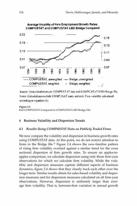
Davis, Haltiwanger, Jarmin, and Miranda124
4 Business Volatility and Dispersion Trends
4.1 Results Using COMPUSTAT Data on Publicly Traded Firms
We now compare the volatility and dispersion in business growth rates using COMPUSTAT data. At this point, we do not restrict attention to fi rms in the Bridge fi le.15 Figure 2.4 shows the now-familiar pattern of rising fi rm volatility overlaid against a similar trend for the cross sectional dispersion of fi rm growth rates. To ensure an apples-to-apples comparison, we calculate dispersion using only those fi rm-year observations for which we calculate fi rm volatility. While the vola-tility and dispersion measures capture different aspects of business dynamics, fi gure 2.4 shows that they closely track each other over the longer term. Similar results obtain for sales-based volatility and disper-sion measures and for dispersion measures calculated on all fi rm-year observations. However, dispersion is uniformly larger than aver-age fi rm volatility. That is, between-fi rm variation in annual growth
Figure 2.3Full COMPUSTAT Compared to COMPUSTAT-LBD Bridge File
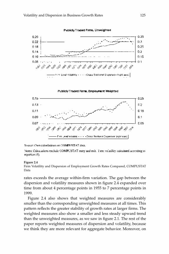
125Volatility and Dispersion in Business Growth Rates
rates exceeds the average within-fi rm variation. The gap between the dispersion and volatility measures shown in fi gure 2.4 expanded over time from about 4 percentage points in 1955 to 7 percentage points in 1999.
Figure 2.4 also shows that weighted measures are considerably smaller than the corresponding unweighted measures at all times. This pattern refl ects the greater stability of growth rates at larger fi rms. The weighted measures also show a smaller and less steady upward trend than the unweighted measures, as we saw in fi gure 2.1. The rest of the paper reports weighted measures of dispersion and volatility, because we think they are more relevant for aggregate behavior. Moreover, on
Figure 2.4Firm Volatility and Dispersion of Employment Growth Rates Compared, COMPUSTAT Data
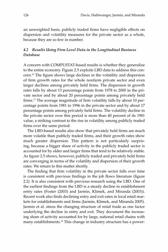
Davis, Haltiwanger, Jarmin, and Miranda126
an unweighted basis, publicly traded fi rms have negligible effects on dispersion and volatility measures for the private sector as a whole, because they are so few in number.
4.2 Results Using Firm Level Data in the Longitudinal Business Database
A concern with COMPUSTAT-based results is whether they generalize to the entire economy. Figure 2.5 exploits LBD data to address this con-cern.16 The fi gure shows large declines in the volatility and dispersion of fi rm growth rates for the whole nonfarm private sector and even larger declines among privately held fi rms. The dispersion in growth rates falls by about 13 percentage points from 1978 to 2000 in the pri-vate sector and by about 20 percentage points among privately held fi rms.17 The average magnitude of fi rm volatility falls by about 10 per-centage points from 1981 to 1996 in the private sector and by about 17 percentage points among privately held fi rms. The volatility decline in the private sector over this period is more than 40 percent of its 1981 value, a striking contrast to the rise in volatility among publicly traded fi rms over the same period.
The LBD-based results also show that privately held fi rms are much more volatile than publicly traded fi rms, and their growth rates show much greater dispersion. This pattern is not particularly surpris-ing, because a bigger share of activity in the publicly traded sector is accounted for by older and larger fi rms that tend to be relatively stable. As fi gure 2.5 shows, however, publicly traded and privately held fi rms are converging in terms of the volatility and dispersion of their growth rates. We return to this matter shortly.
The fi nding that fi rm volatility in the private sector falls over time is consistent with previous fi ndings in the job fl ows literature (fi gure 2.2). It is also consistent with previous research using the LBD. One of the earliest fi ndings from the LBD is a steady decline in establishment entry rates (Foster (2003) and Jarmin, Klimek, and Miranda (2003)). Recent work also fi nds declining entry and exit rates in local retail mar-kets for establishments and fi rms (Jarmin, Klimek, and Miranda 2005). Jarmin et al. stress the changing structure of retail trade as one factor underlying the decline in entry and exit. They document the increas-ing share of activity accounted for by large, national retail chains with many establishments.18 This change in industry structure has a power-
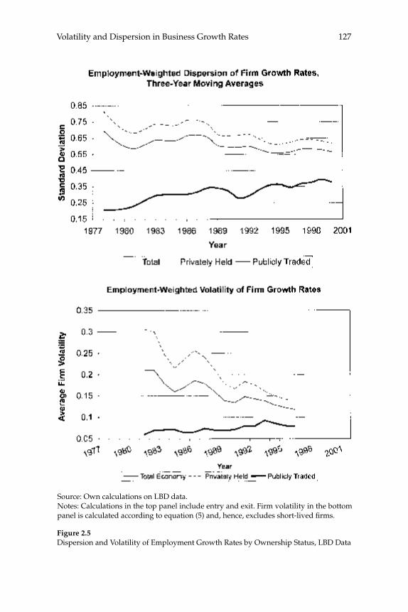
127Volatility and Dispersion in Business Growth Rates
Figure 2.5Dispersion and Volatility of Employment Growth Rates by Ownership Status, LBD Data
Source: Own calculations on LBD data. Notes: Calculations in the top panel include entry and exit. Firm volatility in the bottom panel is calculated according to equation (5) and, hence, excludes short-lived fi rms.

Davis, Haltiwanger, Jarmin, and Miranda128
ful effect, because entry and exit rates are substantially higher for small, single-unit fi rms than for large national chains. We return to the role of industry structure and business turnover in section 5.
All volatility series displayed thus far are based on equation (5) and limited to fi rms with at least ten consecutive observations. This selec-tion criterion is especially restrictive for privately held fi rms, most of which do not survive ten years. By and large, privately held fi rms are relatively volatile, and so are short-lived fi rms. If the objective is to examine the overall magnitude of fi rm volatility, then it is desirable to use datasets and statistics that capture the most volatile units in the economy. To do so, we now use LBD data to calculate modifi ed volatil-ity measures based on equation (6). Figure 2.6 shows the results for the employment-weighted modifi ed volatility measure. As before, volatil-ity is higher and falling for privately held business, lower and rising for publicly traded fi rms. Modifi ed volatility for privately held fi rms falls from 0.60 in 1977 to 0.42 in 2001, with the entire fall occurring after 1987. Modifi ed volatility for publicly traded fi rms rises from 0.16 in 1977 to 0.29 in 1999.
4.3 Volatility Convergence across Major Industry Groups
The most striking features of fi gures 2.5 and 2.6 are the opposite trends for publicly traded and privately held fi rms and the dramatic convergence in their volatility levels. Table 2.2 shows that these two features hold in every major industry group. Among publicly traded fi rms, modifi ed volatility rises for all industry groups, though by widely varying amounts. The biggest volatility gains among publicly traded fi rms occur in Transportation and Public Utilities, Wholesale, FIRE, and Services. Among privately held fi rms, the modifi ed volatility measure declines by 23 percent for FIRE and by 30 percent or more for all other industry groups. Overall volatility in the nonfarm business sector declines for every industry group, with drops of more than 30 percent in Construction, Wholesale, Retail, and Services. The volatil-ity convergence phenomenon is also present in every industry group. Between 1978 and 2001, the ratio of volatility among privately held fi rms to volatility among publicly traded fi rms fell from 3.2 to 1.7 in Manufacturing, from 6.3 to 1.8 in Transportation and Public Utilities, from 4.2 to 2.2 in Retail, from 3.3 to 1.3 in FIRE, and from 2.3 to 1.1 in Services.
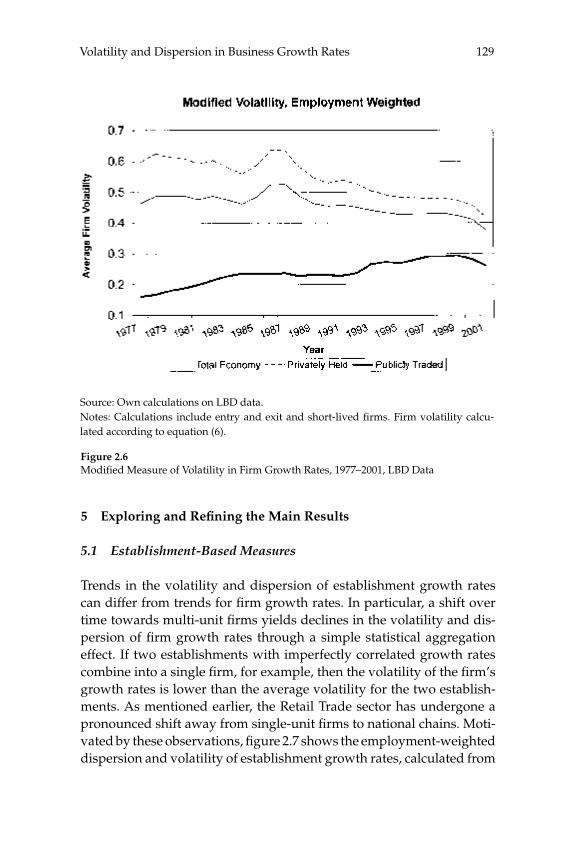
129Volatility and Dispersion in Business Growth Rates
5 Exploring and Refi ning the Main Results
5.1 Establishment-Based Measures
Trends in the volatility and dispersion of establishment growth rates can differ from trends for fi rm growth rates. In particular, a shift over time towards multi-unit fi rms yields declines in the volatility and dis-persion of fi rm growth rates through a simple statistical aggregation effect. If two establishments with imperfectly correlated growth rates combine into a single fi rm, for example, then the volatility of the fi rm’s growth rates is lower than the average volatility for the two establish-ments. As mentioned earlier, the Retail Trade sector has undergone a pronounced shift away from single-unit fi rms to national chains. Moti-vated by these observations, fi gure 2.7 shows the employment-weighted dispersion and volatility of establishment growth rates, calculated from
Figure 2.6Modifi ed Measure of Volatility in Firm Growth Rates, 1977–2001, LBD Data
Source: Own calculations on LBD data. Notes: Calculations include entry and exit and short-lived fi rms. Firm volatility calcu-lated according to equation (6).
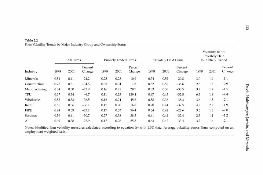
Davis, H
altiwanger, Jarm
in, and M
iranda
130
Table 2.2Firm Volatility Trends by Major Industry Group and Ownership Status
All Firms Publicly Traded Firms Privately Held Firms
Volatility Ratio: Privately Held
to Publicly Traded
Industry
Minerals
Construction
Manufacturing
TPU
Wholesale
Retail
FIRE
Services
All
1978
0.54
0.78
0.34
0.37
0.53
0.56
0.44
0.59
0.49
2001
0.41
0.51
0.30
0.34
0.33
0.36
0.39
0.41
0.38
PercentChange
–24.2
–34.5
–12.9
–6.7
–36.5
–36.1
–13.1
–30.7
–22.9
1978
0.25
0.33
0.16
0.11
0.16
0.17
0.17
0.27
0.17
2001
0.28
0.34
0.21
0.25
0.24
0.20
0.33
0.38
0.26
PercentChange
10.9
1.3
28.7
129.4
45.6
16.8
96.4
38.5
55.5
1978
0.74
0.82
0.53
0.67
0.58
0.70
0.54
0.61
0.63
2001
0.52
0.52
0.35
0.45
0.36
0.44
0.42
0.41
0.42
PercentChange
–29.8
–36.6
–33.5
–32.8
–38.3
–37.5
–22.6
–32.4
–33.4
1978
3.0
2.5
3.2
6.3
3.6
4.2
3.3
2.3
3.7
2001
1.9
1.5
1.7
1.8
1.5
2.2
1.3
1.1
1.6
PercentChange
–1.1
–0.9
–1.5
–4.4
–2.1
–1.9
–2.0
–1.2
–2.1
Notes: Modifi ed fi rm volatility measures calculated according to equation (6) with LBD data. Average volatility across fi rms computed on an employment-weighted basis.
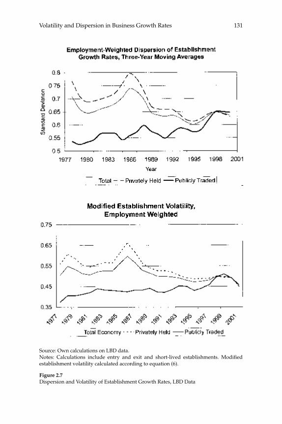
131Volatility and Dispersion in Business Growth Rates
Figure 2.7Dispersion and Volatility of Establishment Growth Rates, LBD Data
Source: Own calculations on LBD data. Notes: Calculations include entry and exit and short-lived establishments. Modifi ed establishment volatility calculated according to equation (6).
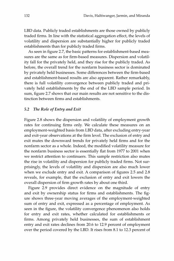
Davis, Haltiwanger, Jarmin, and Miranda132
LBD data. Publicly traded establishments are those owned by publicly traded fi rms. In line with the statistical aggregation effect, the levels of volatility and dispersion are substantially higher for publicly traded establishments than for publicly traded fi rms.
As seen in fi gure 2.7, the basic patterns for establishment-based mea-sures are the same as for fi rm-based measures. Dispersion and volatil-ity fall for the privately held, and they rise for the publicly traded. As before, the overall trend for the nonfarm business sector is dominated by privately held businesses. Some differences between the fi rm-based and establishment-based results are also apparent. Rather remarkably, there is full volatility convergence between publicly traded and pri-vately held establishments by the end of the LBD sample period. In sum, fi gure 2.7 shows that our main results are not sensitive to the dis-tinction between fi rms and establishments.
5.2 The Role of Entry and Exit
Figure 2.8 shows the dispersion and volatility of employment growth rates for continuing fi rms only. We calculate these measures on an employment-weighted basis from LBD data, after excluding entry-year and exit-year observations at the fi rm level. The exclusion of entry and exit mutes the downward trends for privately held fi rms and for the nonfarm sector as a whole. Indeed, the modifi ed volatility measure for the nonfarm business sector is essentially fl at from 1977 to 2001 when we restrict attention to continuers. This sample restriction also mutes the rise in volatility and dispersion for publicly traded fi rms. Not sur-prisingly, the levels of volatility and dispersion are also much lower when we exclude entry and exit. A comparison of fi gures 2.5 and 2.8 reveals, for example, that the exclusion of entry and exit lowers the overall dispersion of fi rm growth rates by about one third.
Figure 2.9 provides direct evidence on the magnitude of entry and exit by ownership status for fi rms and establishments. The fi g-ure shows three-year moving averages of the employment-weighted sum of entry and exit, expressed as a percentage of employment. As seen in the fi gure, the volatility convergence phenomenon also holds for entry and exit rates, whether calculated for establishments or fi rms. Among privately held businesses, the sum of establishment entry and exit rates declines from 20.6 to 12.9 percent of employment over the period covered by the LBD. It rises from 8.1 to 12.3 percent of
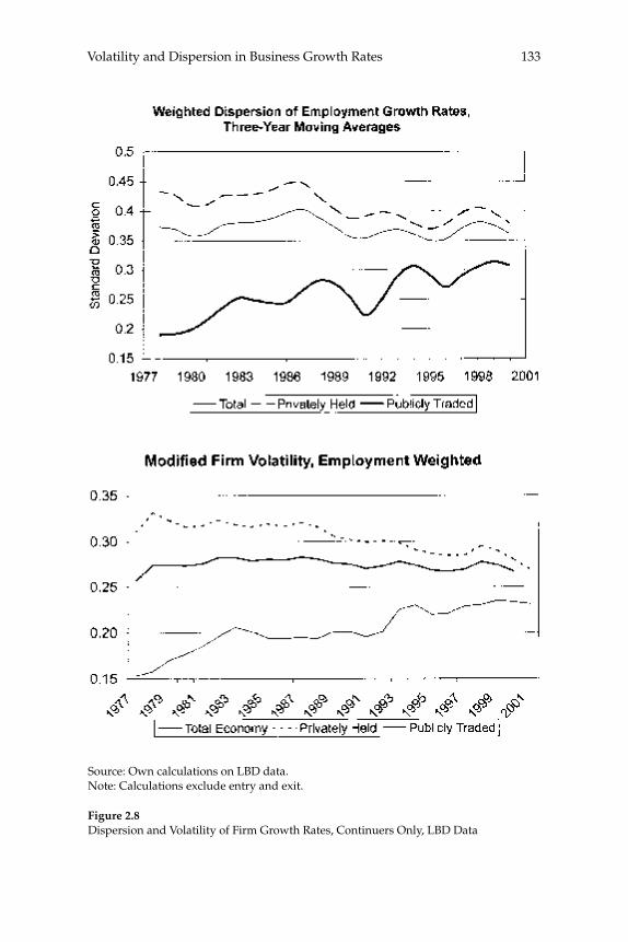
133Volatility and Dispersion in Business Growth Rates
Source: Own calculations on LBD data. Note: Calculations exclude entry and exit.
Figure 2.8Dispersion and Volatility of Firm Growth Rates, Continuers Only, LBD Data
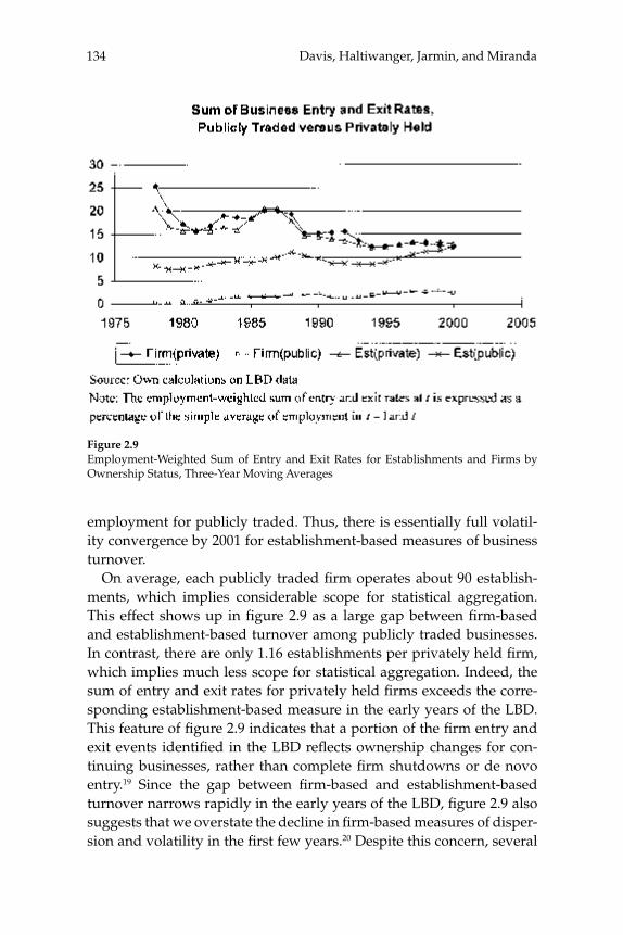
Davis, Haltiwanger, Jarmin, and Miranda134
employment for publicly traded. Thus, there is essentially full volatil-ity convergence by 2001 for establishment-based measures of business turnover.
On average, each publicly traded fi rm operates about 90 establish-ments, which implies considerable scope for statistical aggregation. This effect shows up in fi gure 2.9 as a large gap between fi rm-based and establishment-based turnover among publicly traded businesses. In contrast, there are only 1.16 establishments per privately held fi rm, which implies much less scope for statistical aggregation. Indeed, the sum of entry and exit rates for privately held fi rms exceeds the corre-sponding establishment-based measure in the early years of the LBD. This feature of fi gure 2.9 indicates that a portion of the fi rm entry and exit events identifi ed in the LBD refl ects ownership changes for con-tinuing businesses, rather than complete fi rm shutdowns or de novo entry.19 Since the gap between fi rm-based and establishment-based turnover narrows rapidly in the early years of the LBD, fi gure 2.9 also suggests that we overstate the decline in fi rm-based measures of disper-sion and volatility in the fi rst few years.20 Despite this concern, several
Figure 2.9Employment-Weighted Sum of Entry and Exit Rates for Establishments and Firms by Ownership Status, Three-Year Moving Averages
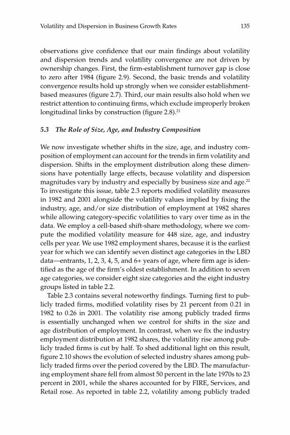
135Volatility and Dispersion in Business Growth Rates
observations give confi dence that our main fi ndings about volatility and dispersion trends and volatility convergence are not driven by ownership changes. First, the fi rm-establishment turnover gap is close to zero after 1984 (fi gure 2.9). Second, the basic trends and volatility convergence results hold up strongly when we consider establishment-based measures (fi gure 2.7). Third, our main results also hold when we restrict attention to continuing fi rms, which exclude improperly broken longitudinal links by construction (fi gure 2.8).21
5.3 The Role of Size, Age, and Industry Composition
We now investigate whether shifts in the size, age, and industry com-position of employment can account for the trends in fi rm volatility and dispersion. Shifts in the employment distribution along these dimen-sions have potentially large effects, because volatility and dispersion magnitudes vary by industry and especially by business size and age.22 To investigate this issue, table 2.3 reports modifi ed volatility measures in 1982 and 2001 alongside the volatility values implied by fi xing the industry, age, and/or size distribution of employment at 1982 shares while allowing category-specifi c volatilities to vary over time as in the data. We employ a cell-based shift-share methodology, where we com-pute the modifi ed volatility measure for 448 size, age, and industry cells per year. We use 1982 employment shares, because it is the earliest year for which we can identify seven distinct age categories in the LBD data—entrants, 1, 2, 3, 4, 5, and 6+ years of age, where fi rm age is iden-tifi ed as the age of the fi rm’s oldest establishment. In addition to seven age categories, we consider eight size categories and the eight industry groups listed in table 2.2.
Table 2.3 contains several noteworthy fi ndings. Turning fi rst to pub-licly traded fi rms, modifi ed volatility rises by 21 percent from 0.21 in 1982 to 0.26 in 2001. The volatility rise among publicly traded fi rms is essentially unchanged when we control for shifts in the size and age distribution of employment. In contrast, when we fi x the industry employment distribution at 1982 shares, the volatility rise among pub-licly traded fi rms is cut by half. To shed additional light on this result, fi gure 2.10 shows the evolution of selected industry shares among pub-licly traded fi rms over the period covered by the LBD. The manufactur-ing employment share fell from almost 50 percent in the late 1970s to 23 percent in 2001, while the shares accounted for by FIRE, Services, and Retail rose. As reported in table 2.2, volatility among publicly traded
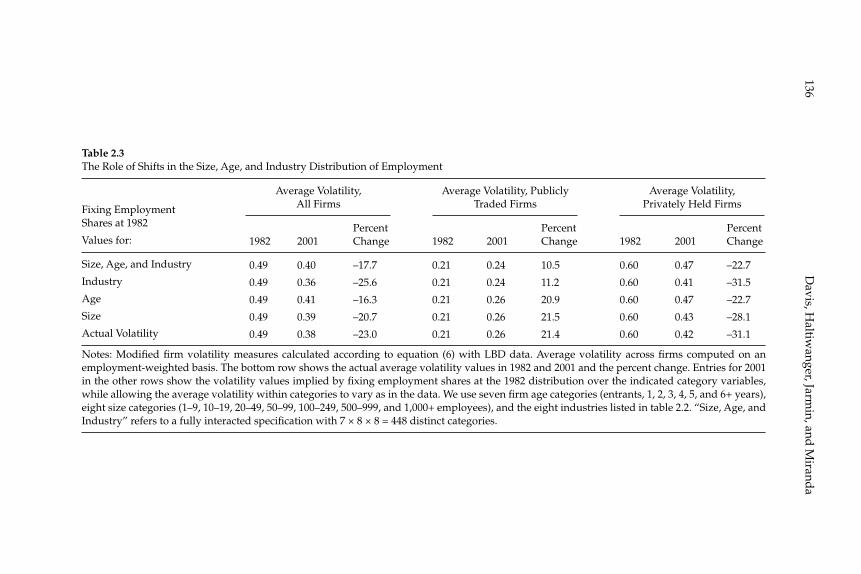
Davis, H
altiwanger, Jarm
in, and M
iranda
136
Table 2.3The Role of Shifts in the Size, Age, and Industry Distribution of Employment
Fixing Employment Shares at 1982
Values for:
Size, Age, and Industry
Industry
Age
Size
Actual Volatility
Average Volatility, All Firms
Average Volatility, Publicly Traded Firms
Average Volatility, Privately Held Firms
1982
0.49
0.49
0.49
0.49
0.49
2001
0.40
0.36
0.41
0.39
0.38
PercentChange
–17.7
–25.6
–16.3
–20.7
–23.0
1982
0.21
0.21
0.21
0.21
0.21
2001
0.24
0.24
0.26
0.26
0.26
PercentChange
10.5
11.2
20.9
21.5
21.4
1982
0.60
0.60
0.60
0.60
0.60
2001
0.47
0.41
0.47
0.43
0.42
PercentChange
–22.7
–31.5
–22.7
–28.1
–31.1
Notes: Modifi ed fi rm volatility measures calculated according to equation (6) with LBD data. Average volatility across fi rms computed on an employment-weighted basis. The bottom row shows the actual average volatility values in 1982 and 2001 and the percent change. Entries for 2001 in the other rows show the volatility values implied by fi xing employment shares at the 1982 distribution over the indicated category variables, while allowing the average volatility within categories to vary as in the data. We use seven fi rm age categories (entrants, 1, 2, 3, 4, 5, and 6+ years), eight size categories (1–9, 10–19, 20–49, 50–99, 100–249, 500–999, and 1,000+ employees), and the eight industries listed in table 2.2. “Size, Age, and Industry” refers to a fully interacted specifi cation with 7 × 8 × 8 = 448 distinct categories.
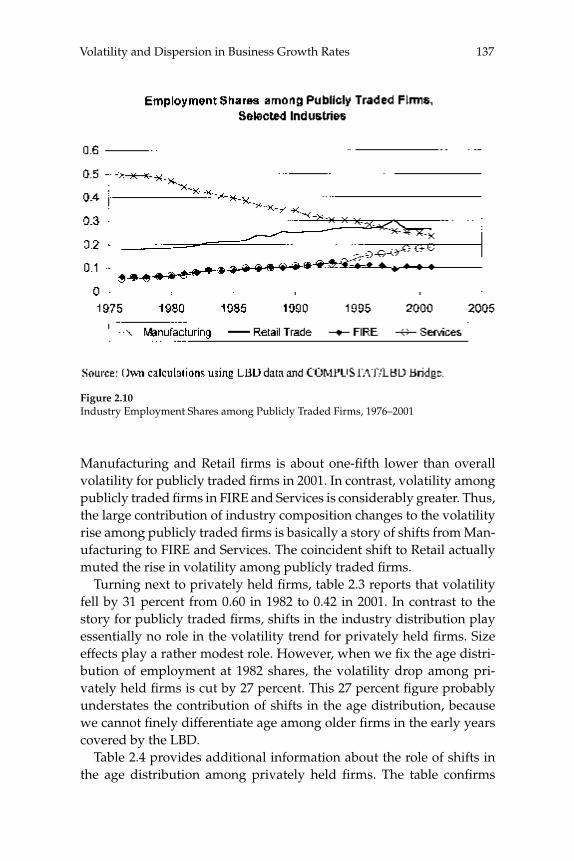
137Volatility and Dispersion in Business Growth Rates
Manufacturing and Retail fi rms is about one-fi fth lower than overall volatility for publicly traded fi rms in 2001. In contrast, volatility among publicly traded fi rms in FIRE and Services is considerably greater. Thus, the large contribution of industry composition changes to the volatility rise among publicly traded fi rms is basically a story of shifts from Man-ufacturing to FIRE and Services. The coincident shift to Retail actually muted the rise in volatility among publicly traded fi rms.
Turning next to privately held fi rms, table 2.3 reports that volatility fell by 31 percent from 0.60 in 1982 to 0.42 in 2001. In contrast to the story for publicly traded fi rms, shifts in the industry distribution play essentially no role in the volatility trend for privately held fi rms. Size effects play a rather modest role. However, when we fi x the age distri-bution of employment at 1982 shares, the volatility drop among pri-vately held fi rms is cut by 27 percent. This 27 percent fi gure probably understates the contribution of shifts in the age distribution, because we cannot fi nely differentiate age among older fi rms in the early years covered by the LBD.
Table 2.4 provides additional information about the role of shifts in the age distribution among privately held fi rms. The table confi rms
Figure 2.10Industry Employment Shares among Publicly Traded Firms, 1976–2001
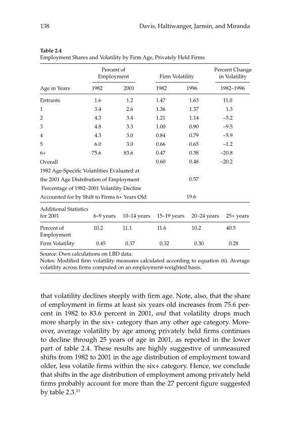
Davis, Haltiwanger, Jarmin, and Miranda138
that volatility declines steeply with fi rm age. Note, also, that the share of employment in fi rms at least six years old increases from 75.6 per-cent in 1982 to 83.6 percent in 2001, and that volatility drops much more sharply in the six+ category than any other age category. More-over, average volatility by age among privately held fi rms continues to decline through 25 years of age in 2001, as reported in the lower part of table 2.4. These results are highly suggestive of unmeasured shifts from 1982 to 2001 in the age distribution of employment toward older, less volatile fi rms within the six+ category. Hence, we conclude that shifts in the age distribution of employment among privately held fi rms probably account for more than the 27 percent fi gure suggested by table 2.3.23
Table 2.4Employment Shares and Volatility by Firm Age, Privately Held Firms
Percent of Employment Firm Volatility
Percent Change in Volatility
Age in Years
Entrants
1
2
3
4
5
6+
1982
1.6
3.4
4.3
4.8
4.3
6.0
75.6
2001
1.2
2.6
3.4
3.3
3.0
3.0
83.6
1982
1.47
1.36
1.21
1.00
0.84
0.66
0.47
0.60
1996
1.63
1.37
1.14
0.90
0.79
0.65
0.38
0.48
0.57
19.6
1982–1996
11.0
1.3
–5.2
–9.5
–5.9
–1.2
–20.8
–20.2Overall
1982 Age-Specifi c Volatilities Evaluated at
the 2001 Age Distribution of Employment
Percentage of 1982–2001 Volatility Decline
Accounted for by Shift to Firms 6+ Years Old
Additional Statistics for 2001
Percent of Employment
Firm Volatility
6–9 years
10.2
0.45
10–14 years
11.1
0.37
15–19 years
11.6
0.32
20–24 years
10.2
0.30
25+ years
40.5
0.28
Source: Own calculations on LBD data.Notes: Modifi ed fi rm volatility measures calculated according to equation (6). Average volatility across fi rms computed on an employment-weighted basis.

139Volatility and Dispersion in Business Growth Rates
Turning last to the results for all fi rms, table 2.3 implies that shifts in the age distribution of employment account for 29 percent of the volatility decline. Size effects alone account for 10 percent of the over-all volatility decline. In unreported results that use a fi ner size break-down, we fi nd that a shift toward larger fi rms accounts for 25 percent of the volatility decline in Retail Trade.24 These results are related to the decline in the employment-weighted entry and exit rates among privately held fi rms, documented in fi gure 2.9. Since older and larger fi rms have lower exit rates, a shift of employment toward these fi rms leads to lower rates of fi rm turnover. Lastly, table 2.3 implies that shifts in the industry mix of employment actually work against the overall volatility decline among nonfarm businesses.
5.3 Why the Rise in Volatility among Publicly Traded Firms?
As discussed in section 2, there was a large upsurge in the number of newly listed fi rms after 1979. Fama and French (2004), among oth-ers, provide evidence that new listings are riskier than seasoned pub-lic fi rms, and that they became increasingly risky relative to seasoned fi rms after 1979. These pieces of evidence point to a signifi cant change in the economic selection process governing entry into the set of pub-licly traded fi rms. They also suggest that much of the volatility and dispersion rise among publicly traded fi rms refl ects a large infl ux of more volatile fi rms in later cohorts.
We now investigate this issue, focusing on the modifi ed volatility concept for publicly traded fi rms. We rely on COMPUSTAT for this pur-pose, because it spans a much longer period than the LBD. The scope of COMPUSTAT expanded in certain years during our sample period, e.g., NASDAQ listings fi rst became available as part of COMPUSTAT in 1973. Since COMPUSTAT does not accurately identify fi rst listing year for fi rms that are added to COMPUSTAT because of changes in scope, we drop such fi rms from the data set for the present analysis.25 As before, we intentionally exclude entry-year and exit-year observa-tions in the COMPUSTAT data because listing and delisting typically do not refl ect the birth or shutdown of the fi rm.
Figure 2.11 plots modifi ed volatility time series for ten-year entry cohorts, defi ned by time of fi rst listing. Volatility appears to be some-what higher for the 1960s and 1970s cohort than earlier cohorts, and it is much higher still for the 1980s and 1990s cohorts.26 To help understand how these cohort effects infl uence the evolution of overall volatility

Davis, Haltiwanger, Jarmin, and Miranda140
among publicly traded fi rms, fi gure 2.12 displays cohort employment shares over the period covered by COMPUSTAT. This fi gure shows that cohort employment shares initially grow quite rapidly, and that this effect is especially strong for the 1990s cohort. By the latter part of the 1990s, fi rms that fi rst listed in the 1980s or 1990s account for about 40 percent of employment among publicly traded fi rms. Taken together, fi gures 2.11 and 2.12 suggest that cohort effects play a powerful role in the volatility rise among publicly traded fi rms.
Figure 2.13 quantifi es the contribution of cohort effects to the evolu-tion of volatility among publicly traded fi rms. For the sake of compari-son, the fi gure also provides information about the contribution of size, age, and industry effects. To construct fi gure 2.13, we fi rst fi t employ-ment-weighted regressions of fi rm volatility on year effects and other variables using COMPUSTAT data from 1951 to 2004. Our basic spec-ifi cation regresses fi rm volatility on year effects only. The fi tted year
Figure 2.11Modifi ed Volatility by Cohort among Publicly Traded Firms
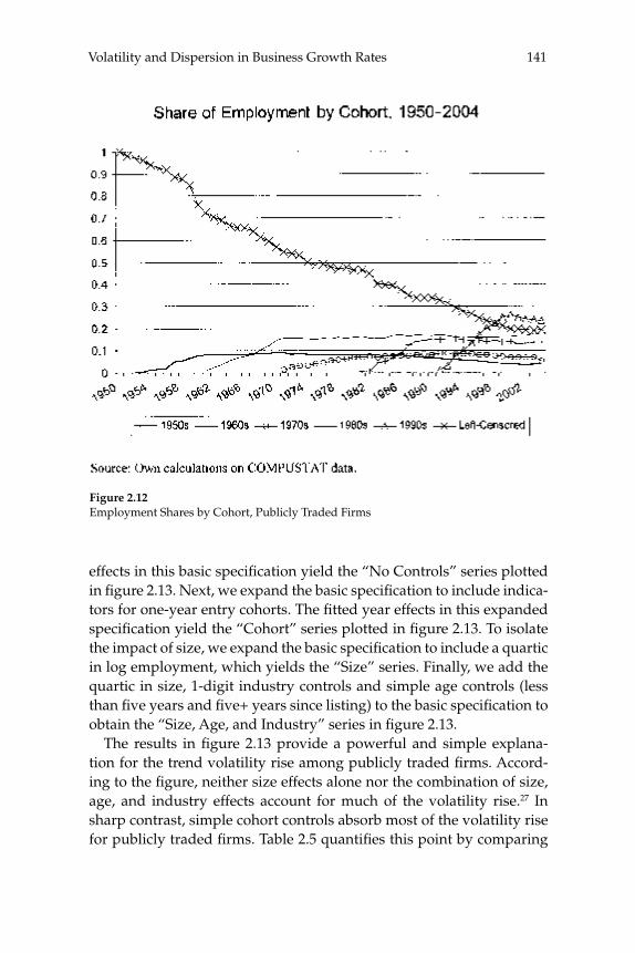
141Volatility and Dispersion in Business Growth Rates
effects in this basic specifi cation yield the “No Controls” series plotted in fi gure 2.13. Next, we expand the basic specifi cation to include indica-tors for one-year entry cohorts. The fi tted year effects in this expanded specifi cation yield the “Cohort” series plotted in fi gure 2.13. To isolate the impact of size, we expand the basic specifi cation to include a quartic in log employment, which yields the “Size” series. Finally, we add the quartic in size, 1-digit industry controls and simple age controls (less than fi ve years and fi ve+ years since listing) to the basic specifi cation to obtain the “Size, Age, and Industry” series in fi gure 2.13.
The results in fi gure 2.13 provide a powerful and simple explana-tion for the trend volatility rise among publicly traded fi rms. Accord-ing to the fi gure, neither size effects alone nor the combination of size, age, and industry effects account for much of the volatility rise.27 In sharp contrast, simple cohort controls absorb most of the volatility rise for publicly traded fi rms. Table 2.5 quantifi es this point by comparing
Figure 2.12Employment Shares by Cohort, Publicly Traded Firms
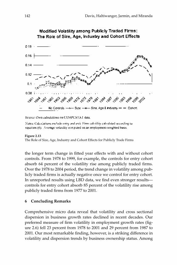
Davis, Haltiwanger, Jarmin, and Miranda142
the longer term change in fi tted year effects with and without cohort controls. From 1978 to 1999, for example, the controls for entry cohort absorb 64 percent of the volatility rise among publicly traded fi rms. Over the 1978 to 2004 period, the trend change in volatility among pub-licly traded fi rms is actually negative once we control for entry cohort. In unreported results using LBD data, we fi nd even stronger results—controls for entry cohort absorb 85 percent of the volatility rise among publicly traded fi rms from 1977 to 2001.
6 Concluding Remarks
Comprehensive micro data reveal that volatility and cross sectional dispersion in business growth rates declined in recent decades. Our preferred measure of fi rm volatility in employment growth rates (fi g-ure 2.6) fell 23 percent from 1978 to 2001 and 29 percent from 1987 to 2001. Our most remarkable fi nding, however, is a striking difference in volatility and dispersion trends by business ownership status. Among
Figure 2.13The Role of Size, Age, Industry and Cohort Effects for Publicly Trade Firms
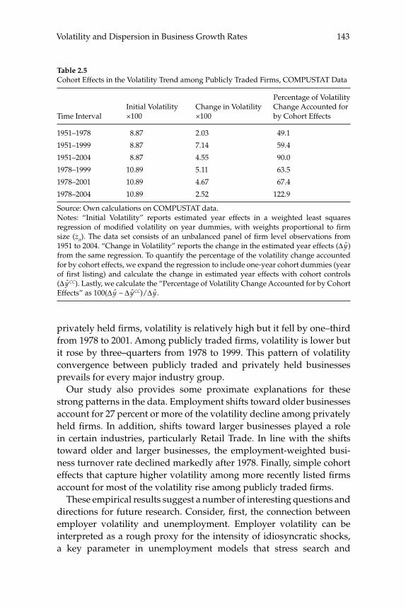
143Volatility and Dispersion in Business Growth Rates
privately held fi rms, volatility is relatively high but it fell by one–third from 1978 to 2001. Among publicly traded fi rms, volatility is lower but it rose by three–quarters from 1978 to 1999. This pattern of volatility convergence between publicly traded and privately held businesses prevails for every major industry group.
Our study also provides some proximate explanations for these strong patterns in the data. Employment shifts toward older businesses account for 27 percent or more of the volatility decline among privately held fi rms. In addition, shifts toward larger businesses played a role in certain industries, particularly Retail Trade. In line with the shifts toward older and larger businesses, the employment-weighted busi-ness turnover rate declined markedly after 1978. Finally, simple cohort effects that capture higher volatility among more recently listed fi rms account for most of the volatility rise among publicly traded fi rms.
These empirical results suggest a number of interesting questions and directions for future research. Consider, fi rst, the connection between employer volatility and unemployment. Employer volatility can be interpreted as a rough proxy for the intensity of idiosyncratic shocks, a key parameter in unemployment models that stress search and
Table 2.5Cohort Effects in the Volatility Trend among Publicly Traded Firms, COMPUSTAT Data
Time Interval
1951–1978
1951–1999
1951–2004
1978–1999
1978–2001
1978–2004
Initial Volatility×100
8.87
8.87
8.87
10.89
10.89
10.89
Change in Volatility×100
2.03
7.14
4.55
5.11
4.67
2.52
Percentage of Volatility Change Accounted for by Cohort Effects
49.1
59.4
90.0
63.5
67.4
122.9
Source: Own calculations on COMPUSTAT data.Notes: “Initial Volatility” reports estimated year effects in a weighted least squares regression of modifi ed volatility on year dummies, with weights proportional to fi rm size (zit). The data set consists of an unbalanced panel of fi rm level observations from 1951 to 2004. “Change in Volatility” reports the change in the estimated year effects (Δ y) from the same regression. To quantify the percentage of the volatility change accounted for by cohort effects, we expand the regression to include one-year cohort dummies (year of fi rst listing) and calculate the change in estimated year effects with cohort controls (Δ yCC). Lastly, we calculate the “Percentage of Volatility Change Accounted for by Cohort Effects” as 100(Δ y – Δ yCC)/Δ y .

Davis, Haltiwanger, Jarmin, and Miranda144
matching frictions. A lower intensity of idiosyncratic shocks in these models leads to less job loss, fewer workers fl owing through the unem-ployment pool, and less frictional unemployment. Motivated by these models, fi gure 2.14 plots our employment-weighted modifi ed volatility measure against annual averages of monthly unemployment infl ow and outfl ow rates. The fi gure suggests that secular declines in the intensity of idiosyncratic shocks contributed to large declines in unemployment fl ows and frictional unemployment in recent decades. More study is clearly needed to confi rm or disconfi rm this view, and there is surely a role for other factors such as the aging of the workforce after 1980.
Another major development in U.S. labor markets since the early 1980s is a large rise in wage and earnings inequality.28 One line of inter-pretation for this development stresses potential sources of increased wage and earnings fl exibility: declines in the real minimum wage, a diminished role for private sector unionism and collective bargaining, intensifi ed competitive pressures that undermined rigid compensation structures, the growth of employee leasing and temp workers, and the
Source: Figure 6 for volatility measure and the Current Population Survey.Notes: Unemployment fl ows are annual averages of monthly fl ows, expressed as a per-centage of the labor force.
Figure 2.14Firm Volatility Compared to Unemployment Infl ows and Outfl ows
145Volatility and Dispersion in Business Growth Rates
erosion of norms that had previously restrained wage differentials and prevented wage cuts. Greater wage (and hours) fl exibility can produce smaller fi rm level employment responses to idiosyncratic shocks and smaller aggregate employment responses to common shocks. So, in principle, greater wage fl exibility can provide a unifi ed explanation for the rise in wage and earnings inequality and the declines in aggregate volatility, fi rm volatility and unemployment fl ows. We mention the role of wage fl exibility because we think it merits investigation and may be a signifi cant part of the story, not because we believe that greater wage fl exibility or any single factor can explain all aspects of longer term developments in wage inequality, unemployment, fi rm volatility, and aggregate volatility.
The potential role of greater wage fl exibility is related to another question raised by our results. In particular, to what extent do trends in fi rm volatility refl ect a change in the size and frequency of shocks, and to what extent do they refl ect a change in shock response dynam-ics? One simple approach to this question is to fi t statistical models that allow for nonstationarity in the size and frequency of business level innovations and in the response dynamics to the innovations. Another approach is to identify specifi c shocks, quantify their magnitude, and investigate whether shock magnitudes and fi rm level responses to them have changed over time.
Several pieces of evidence point to a major shift in the selection pro-cess governing entry into the set of publicly traded fi rms. Figure 2.13 and table 2.5 above indicate that more than half of the volatility rise among publicly traded fi rms in recent decades refl ects an infl ux of more volatile fi rms in later cohorts. Other researchers fi nd that later cohorts of publicly traded fi rms are riskier in terms of equity return variabil-ity, profi t variability, time from IPO to profi tability, and business age at time of fi rst listing. The shift in the selection process for publicly traded fi rms is a major phenomenon, in our view, but it does not by itself explain the volatility convergence pattern we have documented or the overall downward trend in fi rm volatility and dispersion. To appreci-ate this point, consider a simple selection story that we sketch with the aid of fi gure 2.15. The fi gure shows a hypothetical density function for fi rm level risk and a risk threshold that separates publicly traded from privately held fi rms. This fi gure captures, in a highly stylized man-ner, the notion that publicly traded fi rms are less risky than privately held ones. Suppose that the risk threshold moves to the right, so that a riskier class of fi rms now goes public. This shift yields an increase in
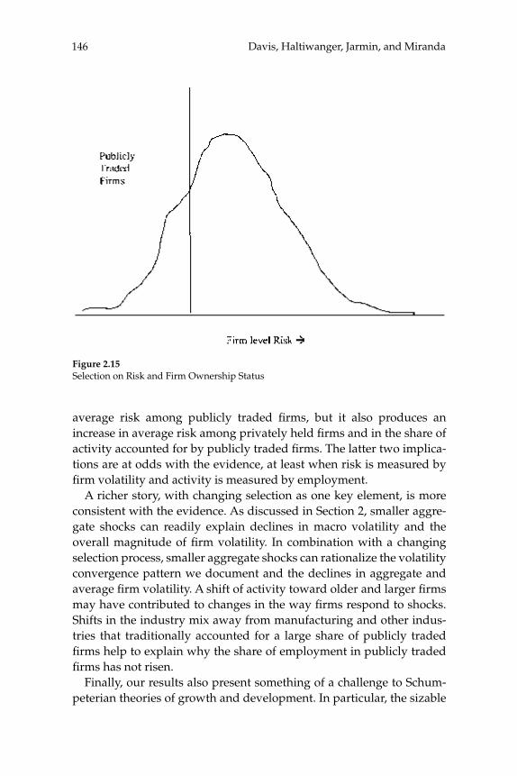
Davis, Haltiwanger, Jarmin, and Miranda146
average risk among publicly traded fi rms, but it also produces an increase in average risk among privately held fi rms and in the share of activity accounted for by publicly traded fi rms. The latter two implica-tions are at odds with the evidence, at least when risk is measured by fi rm volatility and activity is measured by employment.
A richer story, with changing selection as one key element, is more consistent with the evidence. As discussed in Section 2, smaller aggre-gate shocks can readily explain declines in macro volatility and the overall magnitude of fi rm volatility. In combination with a changing selection process, smaller aggregate shocks can rationalize the volatility convergence pattern we document and the declines in aggregate and average fi rm volatility. A shift of activity toward older and larger fi rms may have contributed to changes in the way fi rms respond to shocks. Shifts in the industry mix away from manufacturing and other indus-tries that traditionally accounted for a large share of publicly traded fi rms help to explain why the share of employment in publicly traded fi rms has not risen.
Finally, our results also present something of a challenge to Schum-peterian theories of growth and development. In particular, the sizable
Figure 2.15Selection on Risk and Firm Ownership Status
147Volatility and Dispersion in Business Growth Rates
decline in average fi rm volatility that we document coincided with a period of impressive productivity gains for the U.S. economy. This coin-cidence belies any close and simple positive relationship between pro-ductivity growth and the intensity of the creative destruction process, at least as measured by fi rm-based or establishment-based measures of volatility in employment growth rates. Perhaps there has been a large increase in the pace of restructuring, experimentation, and adjustment activities within fi rms. Another possibility is that a more intense cre-ative destruction process among publicly traded fi rms, partly facilitated by easier access to public equity by high-risk fi rms, has been suffi cient to generate the commercial innovations that fueled rapid productivity gains throughout the economy.
Acknowledgments
For many helpful comments on earlier drafts, we thank Chris Foote, Eva Nagypal, the editors, participants in the 2006 NBER Macroeconom-ics Annual Conference, the CEPR Conference on Firm Dynamics, the Ewing Marion Kauffman—Max Planck Conference on Entrepreneur-ship and Growth and seminars at the Brookings Institution, the Census Bureau, New York University, and the University of Chicago. We thank Marios Michaelides for excellent research assistance and the Kauffman Foundation for fi nancial support. The views expressed in the paper are those of the authors and do not necessarily represent those of the Cen-sus Bureau. The paper has been screened to ensure that it does not dis-close any confi dential information.
Endnotes
1. The LBD is confi dential under Titles 13 & 26 U.S.C. Research access to the LBD can be granted to non-Census staff for approved projects. See www.ces.census.gov for more information. COMPUSTAT, which provides information on publicly traded fi rms only, has been the primary data source for recent work on fi rm level volatility.
2. Firm level volatility is calculated from COMPUSTAT data as a moving ten-year win-dow on the standard deviation of fi rm level growth rates. See equation (5) in section 3.
3. Excess job reallocation equals the sum of gross job creation and destruction less the absolute value of net employment growth. Dividing excess reallocation by the level of employment yields a rate. One can show that the excess reallocation rate is equivalent to the employment-weighted mean absolute deviation of establishment growth rates about zero. See Davis, Haltiwanger, and Schuh (1996).
4. Job fl ow statistics for the whole private sector are from the BLS Business Employment Dynamics. They are unavailable prior to 1990.

Davis, Haltiwanger, Jarmin, and Miranda148
5. Acemoglu (2005), Eberly (2005), and Davis, Faberman, and Haltiwanger (2006) question whether sample selection colors the fi ndings in previous studies of fi rm level volatility.
6. French stock market reforms in the 1980s considerably broadened the shareholder base for French fi rms. Thesmar and Thoenig (2004) provide evidence that these reforms led to a rise in the volatility of sales growth rates among listed fi rms relative to unlisted ones. Their analysis sample contains about 5,600 French fi rms per year with more than 500 employees or 30 million Euros in annual sales, and that were never owned, entirely or in part, by the French state.
7. Sales data are available in the LBD from 1994. Sales data from the Economic Censuses are available every fi ve years for earlier years. More recent years in the LBD record indus-try on a NAICS basis.
8. See the data appendix regarding the construction of longitudinal links, which are criti-cal for our analysis.
9. Our COMPUSTAT data are from the same provider (WRDS) as in recent work by Comin and Mulani (2006), Comin and Philippon (2005), and others.
10. See McCue and Jarmin (2005) for details. We extend their methodology to include the whole period covered by the LBD.
11. If we require that matches have positive COMPUSTAT employment and positive LBD employment in 1990, then the number of matched CUSIPs drops from 5,716 to 5,035. However, this requirement is overly restrictive in light of our previous remarks about missing COMPUSTAT employment observations, the inclusion of employment from for-eign operations in COMPUSTAT, and timing differences between COMPUSTAT and the LBD. For instance, when we relax this requirement and instead allow CUSIPs with posi-tive sales, price or employment to match to LBD fi rms with positive employment, then the number of matches exceeds 5,700.
12. When we implement (5) using LBD data, we permit the fi rm to enter or exit at the beginning or end of the ten-year window. This is a small difference in measurement pro-cedures relative to Comin and Mulani (2005, 2006) and Comin and Philippon (2005). A more important difference is that our LBD-based calculations include the pre-public and post-public history of fi rms that are publicly traded at t but privately held before or after t. As a related point, we do not treat listing and de-listing in COMPUSTAT as fi rm entry and exit.
13. We thank Eva Nagypal for drawing our attention to this issue.
14. The shorter term response differs, however, as have verifi ed in unreported numerical simulations. For example, a one-time permanent increase in the variance of the distribu-tion of idiosyncratic shocks leads to a coincident permanent increase in the cross sectional dispersion of business growth rates, but it leads to a gradual rise in the average volatility that begins several years prior to the increase in the shock variance and continues for several years afterward.
15. But we do exclude observations with growth rates of 2 and –2, because COMPUSTAT listing and de-listing typically do not refl ect true entry and exit by fi rms. In the LBD-based analysis below, we include observations with growth rates of 2 and –2 (unless otherwise noted), because we can identify true entry and exit in the LBD.
16. A comparison between fi gures 2.4 and 2.5 reveals that the level of volatility among publicly traded fi rms is much greater in COMPUSTAT, perhaps because COMPUSTAT activity measures include the foreign operations of multinational fi rms.

149Volatility and Dispersion in Business Growth Rates
17. Recall that we use all fi rm-year observations with positive values of zit when comput-ing our basic dispersion measure. That is, we include all continuing, entering and exiting fi rms. Below, we consider the effects of restricting the analysis to continuing fi rms only.
18. Foster, Haltiwanger, and Krizan (2005) present related evidence using the Census of Retail Trade. They show that much of the increase in labor productivity in the 1990s in retail trade refl ects the entry of relatively productive establishments owned by large national chains and the exit of less productive establishments owned by single-unit fi rms. See, also, McKinsey Global Institute (2001).
19. While ownership changes can affect fi rm level longitudinal linkages in the LBD, they do not affect establishment level linkages. See the Data appendix for more discussion of linkage issues.
20. While not a trivial task, we can use the LBD to separately identify and measure fi rm ownership change, de novo entry and complete fi rm shutdown. In future work, we plan to explore this decomposition.
21. See the Data Appendix for details about the fi rm and establishment concepts used in the LBD and the construction of longitudinal links.
22. There is a vast literature on the relationship of business entry, exit, and growth rates to business size and age. See Dunne, Roberts, and Samuelson (1989), Sutton (1997), Caves (1998), Davis and Haltiwanger (1999), and Davis et al. (2005) for evidence, analysis, and extensive references to related research.
23. The precise contribution of shifts in the age distribution to the volatility decline among privately held fi rms depends on exactly how we carry out the decomposition. Table 2.3, which evaluates volatilities at the 1982 age distribution, implies that the age dis-tribution shift accounts for 27 percent of the volatility drop from 1982 to 2001. Table 2.4, which evaluates volatilities at the 2001 age distribution, reports that the age distribution shift accounts for 19.6 percent of the volatility drop. Both exercises are likely to understate the impact of shifts toward older privately held fi rms for reasons discussed in the text.
24. The fi ner size classifi cation breaks the 1,000+ category into 1000–2499, 2500–4999, 5000–9999, and 10,000+ categories.
25. In unreported results, this sample selection requirement has little impact on the over-all volatility trend in COMPUSTAT, but it does have an impact on the volatility trends for certain cohorts.
26. The modifi ed volatility series in fi gure 2.11 are employment weighted. We suppress the 1953 and 1954 values for the 1950s cohort, because they are calculated from only one or two fi rm level observations. In unreported results, the equal-weighted modifi ed volatility series show a stronger pattern of greater volatility for later cohorts. So does the employment-weighted basic volatility measure.
27. Industry effects play a substantially larger role in table 2.3 (LBD data) than in fi gure 2.13 (COMPUSTAT data). Unreported results show that much of the difference arises because of different sample periods. In particular, regardless of data set and whether we use a shift-share or regression-based method, industry effects play a substantially larger role from 1982 to 2001 than from 1977 to 2001. Differences between table 2.3 and fi gure 2.13 in method and data set play a smaller role.
28. See Autor, Katz, and Kearney (2005) for a recent contribution to this literature, a review of major competing hypotheses about the reasons for rising inequality and refer-ences to related research.

Davis, Haltiwanger, Jarmin, and Miranda150
29. We construct birth and death retiming weights from accurate data on the timing of births and deaths using a conditional logit model. The model includes controls for state, metro, and rural areas and job creation and destruction rates. The model is run separately by 2-digit SIC and for four different 5-year census cycles.
30. There are between 40,000 and 120,000 cases each year. Work by Davis et. al. (2005) shows that business transitions between employer and non-employer status explains some of these cases.
References
Acemoglu, Daron. 2005. “Comments on Comin and Philippon, The Rise in Firm level Volatility: Causes and Consequences.” NBER Macroeconomics Annual, 167–202.
Autor, David H., Lawrence F. Katz, and Melissa S. Kearney. 2005. “Trends in U.S. Wage Inequality: Re-Assessing the Revisionists.” NBER Working Paper no. 11627. Cambridge, MA: National Bureau of Economic Research.
Bartelsman, Eric, John Haltiwanger, and Stefano Scarpetta. 2004. “Microeconomic Evi-dence of Creative Destruction in Industrial and Development Countries.” Tinbergen Insti-tute Discussion Paper no. 2004-114/3. Amsterdam, Netherlands: Tinbergen Institute.
Caballero, Ricardo. 2006. The Macroeconomics of Specifi city and Restructuring. Cambridge, MA: The MIT Press, forthcoming.
Campbell, John Y., Martin Lettau, Burton Malkiel, and Y. Xu. 2001. “Have Idiosyncratic Stocks Become More Volatile? An Empirical Exploration of Idiosyncratic Risk.” Journal of Finance 56(1): 1–43.
Caves, Richard. 1998. “Industrial Organization and New Findings on the Turnover and Mobility of Firms.” Journal of Economic Literature 36(4): 1947–1982.
Chaney, Thomas, Xavier Gabaix, and Thomas Philippon. 2002. “Firm Volatility.” Unpub-lished paper, Massachusetts Institute of Technology.
Comin, Diego, and Sunil Mulani. 2005. “A Theory of Growth and Volatility at the Aggre-gate and Firm Level.” NBER Working Paper no. 11503. Cambridge, MA: National Bureau of Economic Research.
Comin, Diego, and S. Mulani. 2006. “Diverging Trends in Aggregate and Firm Volatility.” Review of Economics and Statistics 88(2): 374–383.
Comin, Diego, and Thomas Philippon. 2005. “The Rise in Firm level Volatility: Causes and Consequences.” NBER Macroeconomics Annual, 167–202.
Davis, Steven J., Jason Faberman, and John Haltiwanger. 2006. “The Flow Approach to Labor Market Analysis: New Data Sources and Micro-Macro Links.” Journal of Economic Perspectives 20(3): 3–26.
Davis, Steven J., and John Haltiwanger. 1992. “Gross Job Creation, Gross Job Destruction, and Employment Reallocation.” Quarterly Journal of Economics 107(3): 819–863.
Davis, Steven J., and John Haltiwanger. 1999. “Gross Job Flows.” In David Card and Orley Ashenfelter, eds., Handbook of Labor Economics. North-Holland.
151Volatility and Dispersion in Business Growth Rates
Davis, Steven J., and John Haltiwanger. 1999. “On the Driving Forces behind Cyclical Movements in Employment and Job Reallocation.” American Economic Review 89(5): 1234–1258.
Davis, Steven J., John Haltiwanger, Ron Jarmin, C. J. Krizan, Javier Miranda, Alfred Nucci, and Kristin Sandusky. 2005. “Measuring the Dynamics of Young and Small Busi-nesses: Integrating the Employer and Nonemployer Business Universes.” Unpublished paper, U.S Bureau of the Census.
Davis, Steven J., John C. Haltiwanger, and Scott Schuh. 1996. Job Creation and Destruction. MIT Press.
Dunne, Timothy, Mark Roberts, and Larry Samuelson. 1989. “Plant Turnover, and Gross Employment Flows in the U.S. Manufacturing Sector.” Journal of Labor Economics 7(1): 48–71.
Eberly, Janice. 2005. “Comments on Comin and Philippon, The Rise in Firm level Volatil-ity: Causes and Consequences.” NBER Macroeconomics Annual, 167–202.
Fama, Eugene F., and Kenneth R. French. 2004. “New Lists: Fundamentals and Survival Rates.” Journal of Financial Economics 73(2): 229–269.
Faberman, Jason. 2006. “Job Flows and the Recent Business Cycle: Not all ‘Recoveries’ are Created Equal.” BLS Working Paper no. 391. Washington, D.C.: Bureau of Labor Statistics.
Fink, Jason, Kristin Fink, Gustavo Grullon, and James Peter Weston. 2005. “IPO Vintage and the Rise of Idiosyncratic Risk.” Presented at the Seventh Annual Texas Finance Festi-val Paper. Available at <http://ssrn.com/abstract=661321>.
Foster, Lucia, John Haltiwanger, and C. J. Krizan. 2001. “Aggregate Productivity Growth: Lessons from Microeconomic Evidence.” In Edward Dean, Michael Harper, and Charles Hulten, eds., New Developments in Productivity Analysis. Chicago, IL: University of Chicago Press.
Foster, Lucia. 2003. “Establishment and Employment Dynamics in Appalachia: Evidence from the Longitudinal Business Database.” CES Working Paper no. 03-19. Washington, D.C.: Center for Economic Studies, Bureau of Census.
Foster, Lucia, John Haltiwanger, and C. J. Krizan. 2006. “Market Selection, Reallocation and Restructuring in the U.S. Retail Trade Sector in the 1990s.” Review of Economics and Statistics 88(4): 748–758.
Gabaix, Xavier. 2005. “The Granular Origins of Aggregate Fluctuations.” Unpublished paper, MIT. Cambridge, MA: Massachusetts Institute of Technology.
Jarmin, Ron, Shawn Klimek, and Javier Miranda. 2003. “Firm Entry and Exit in the U.S. Retail Sector.” CES Working Paper no. 04-17. Washington, D.C.: Center for Economic Studies, Bureau of Census.
Jarmin, Ron S., Shawn Klimek, and Javier Miranda. 2005. “The Role of Retail Chains: National, Regional and Industry Results.” CES Working Paper no. 05-30. Washington, D.C.: Center for Economic Studies, Bureau of Census.
Jarmin, Ron S., and Javier Miranda. 2002a. “The Longitudinal Business Database.” CES Working Paper no. 02-17. Washington, D.C.: Center for Economic Studies, Bureau of Census.
Davis, Haltiwanger, Jarmin, and Miranda152
Jarmin, Ron S., and Javier Miranda. 2002b. “Fixing Missed Reorganizations and Broken Links from Inactive Spells.” CES Technical Note 2002-06.
Jarmin, Ron S., and Javier Miranda. 2005. “Reassigning Incorrectly Timed MU Births and Deaths” CES Technical Note.
Jayaratne, Jith, and Philip E. Strahan. 1998. “Entry Restrictions, Industry Evolution and Dynamic Effi ciency: Evidence from Commercial Banking.” Journal of Law and Economics 41: 239–273.
Jovanovic, Boyan, and Peter L. Rousseau. 2001. “Why Wait? A Century of Life before IPO.” American Economic Review 91(2): 336–341.
Koren, Miklos, and Silvana Tenreyro. 2006. “Technological Diversifi cation.” Federal Reserve Bank of New York and London School of Economics.
McCue, Kristin, and Ron Jarmin. 2005. “Matching Compustat Data to the SSEL.” CES Technical Note. Washington, D.C.: Center for Economic Studies, Bureau of Census.
McKinsey Global Institute. 2001. “U.S. Productivity Growth, 1995–2000: Understanding the Contribution of Information Technology Relative to other Factors.” Washington, D.C.: McKinsey Global Institute.
Mortensen, Dale T., and Christopher A. Pissarides. 1999. “New Developments in Models of Search in the Labor Market.” In Orley Ashenfelter and David Card, eds., Handbook of Labor Economics, Volume 3, 2567–2627.
Obstfeld, M. 1994. “Risk-Taking, Global Diversifi cation, and Growth.” American Economic Review 84: 1310–1329.
Philippon, Thomas. 2003. “An Explanation for the Joint Evolution of Firm and Aggregate Volatility.” Unpublished paper, New York University.
Pissarides, Christopher. 2000. Equilibrium Unemployment Theory, second edition. Cam-bridge, MA: The MIT Press.
Sutton, John. 1997. “Gibrat’s Legacy.” Journal of Economic Literature 35(1): 40–59.
Thesmar, David, and Mathias Thoenig. 2004. “Financial Market Development and the Rise in Firm level Uncertainty.” Delta, unpublished paper. Paris, France: Delta.
Tornqvist, Leo, Pentti Vartia, and Yrjo Vartia. 1985. “How Should Relative Change Be Measured?” American Statistician 39(1): 43–46.
Data Appendix
A Additional Information about the LBD
This appendix discusses improvements to the LBD that aided the analysis in this paper. The LBD is comprised of longitudinally linked Business Register (BR) fi les. The BR is updated continuously and a snapshot is taken once a year after the incorporation of survey data collections. The resulting fi les contain

153Volatility and Dispersion in Business Growth Rates
a longitudinal establishment identifi er, the Permanent Plant Number (PPN). This identifi er is designed to remain unchanged throughout the life of the estab-lishment and regardless of reorganizations or ownership changes. However, there are known breaks in PPN linkages, and PPNs existed only for the man-ufacturing sector prior to 1982. Jarmin and Miranda (2002a) addressed these shortcomings in the BR fi les in creating the LBD. Their methodology employed existing numeric establishment identifi ers to the greatest extent possible to repair and construct longitudinal establishment links. They further enhanced the linkages using commercially available statistical name and address match-ing software.
Construction of the longitudinal establishment links is relatively straight-forward because they are one to one, and because establishments typically have well-defi ned physical locations. The construction of fi rm links requires additional work. Longitudinal linkages of fi rm identifi ers can be broken by the expansion of single location fi rms to multi establishment entities and by merger and acquisition (M&A) activity. We address the fi rst problem by assigning a unique fi rm identifi er to fi rms that expand from single to multiple establishments. This process is straightforward because we can track estab-lishments over time. The second problem is harder to resolve, because M&A activity can result in many-to-many matches, e.g., when a fi rm sells some estab-lishments and acquires others in the same period. We do not directly address this issue in the current paper, but we recognize that it would be interesting to explore the role of M&A activity in greater depth, and we plan to do so in future work.
The combination and reconciliation of administrative and survey data sources in the LBD lead to a more serious problem that we have addressed in the current analysis. Early versions of the LBD contain a number of incorrectly timed establishment births and deaths. To see how this timing problem arises, recall that the LBD is a longitudinally linked version of the Business Register. Although the primary unit of observation in the BR is a business establishment (physical location), administrative data are typically available at the taxpayer ID (EIN) level. As the vast majority of fi rms are single establishment entities, the EIN, fi rm, and establishment levels of aggregation all refer to the same busi-ness entity. Business births typically enter the BR from administrative sources. Outside of Economic Census years, however, the Census Bureau directly sur-veys only large births, as measured by payroll. In Economic Census years, all establishments of “known” multi location fi rms are directly surveyed. A subset of larger single location businesses are canvassed as well.
The Census Bureau separately identifi es the individual establishments of multi-establishment companies based on primary data collections from the Economic Census and certain annual surveys such as the Company Organiza-tion Survey and the Annual Survey of Manufacturers. Since a much larger por-
Davis, Haltiwanger, Jarmin, and Miranda154
tion of fi rms and establishments are surveyed in Economic Census years (years ending in “2” and “7”), the Economic Census becomes the primary vehicle by which the Census Bureau learns about establishment entry and exit for smaller multi-unit fi rms. This information is then incorporated into the LBD. The impli-cation is that the unadjusted LBD fi les show large spikes in establishment births and deaths for multi-unit fi rms in Economic Census years. Many of those births and deaths actually occurred in the previous four years.
We retime these incorrectly timed deaths and births following a two-phase methodology, described more fully in Jarmin and Miranda (2005). The fi rst phase uses fi rm level information contained in the LBD to identify the correct birth and death years for as many establishments as possible. The second phase adapts an algorithm developed by Davis, Haltiwanger, and Schuh (1996) to randomly assign a birth or death year for those cases that cannot be resolved in phase one. The randomization procedure is constrained so that the tempo-ral patterns of births and deaths for retimed cases match those for the accu-rately timed births and deaths that we observe directly in the data (single-unit births and establishment births in large multi-unit fi rms that are directly can-vassed).29
Finally, the LBD contains a substantial number of establishments that appear to become inactive for a period of time (Jarmin and Miranda 2002b). That is, the establishment is active in period t – 1 and t + 1 but not in period t.30 These gaps lead to possibly spurious startups and shutdowns. In this paper, we take a conservative approach by eliminating these establishment-year observations in the entry and exit computations. Our goal in doing so is to focus on true entry and exit.
B COMPUSTAT-LBD Employment Comparisons
The top panel in fi gure 2A.1 compares log employment levels between COM-PUSTAT and the LBD data sources for a matched set of publicly traded fi rms. The lower panel compares fi ve-year growth rates, calculated according to equa-tion (4). Here, we restrict attention to matched fi rms that have positive employ-ment in the LBD and COMPUSTAT. Much of the mass is concentrated along the 45 degree line in the top panel, but there are clearly many large discrepan-cies between the two data sources. The simple correlation of log employment levels is 0.89 on an unweighted basis and 0.83 on an employment-weighted basis. The standardized employment difference, measured as LBD employ-ment minus COMPUSTAT employment divided by the average of the two, has an unweighted median value of –13 percent and an unweighted mean of –26 percent . The weighted values are –25 percent for the median and –30 percent for the mean. The lower panel shows a weaker relationship for growth rates,

155Volatility and Dispersion in Business Growth Rates
with a correlation of 0.64 unweighted and 0.54 weighted. Lower values for the weighted correlations probably refl ect bigger discrepancies for multi-national fi rms with signifi cant global operations.
In short, the results in fi gure 2.1 indicate that COMPUSTAT measures of fi rm level activity contain considerable measurement error, if the goal is to measure the U.S. domestic operations of publicly traded fi rms. Despite the large COM-PUSTAT-LBD differences in employment levels and growth rates, the two data sources produce similar trends in fi rm volatility measures, as seen by compar-ing fi gures 2.4, 2.5, and 2.7.
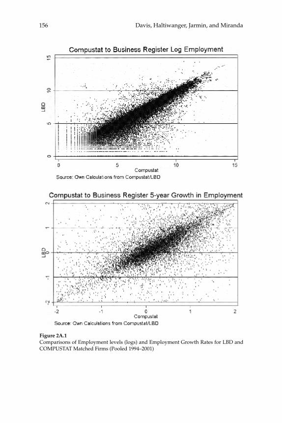
Davis, Haltiwanger, Jarmin, and Miranda156
Figure 2A.1Comparisons of Employment levels (logs) and Employment Growth Rates for LBD and COMPUSTAT Matched Firms (Pooled 1994–2001)

Comment
Christopher Foote, Federal Reserve Bank of Boston
Sixteen years ago, Steven Davis and John Haltiwanger’s paper for the NBER Macroeconomics Annual was among the fi rst to use fi rm-level data to study employment fl uctuations. The focus of the current paper, written with Ron Jarmin and Javier Miranda, is on a different piece of the employment picture. The authors argue that during the past two decades, employment levels at individual fi rms and establishments have become more stable. Their preferred measure of fi rm volatility for the U.S. private sector, displayed in fi gure 2.6, declines by about one-quarter from 1978 to 2001. I am confi dent that like Davis and Halti-wanger (1990), this thoughtful paper will infl uence both empirical and theoretical work long after its publication.
In this comment, I will explore three main themes, with the fi rst two involving measurement issues. I begin by developing some intuition for the author’s preferred volatility statistic. This intuition illustrates why their results are admittedly sensitive to the treatment of fi rm entry and exit. My second point involves the relationship between microeco-nomic volatility and business cycles. The paper does an excellent job of highlighting why this relationship is interesting; some theoretical mod-els predict that both types of volatility should decline as an economy develops, while other models claim that macro and micro volatility should move in opposite directions. My own view is that without tak-ing account of micro-level adjustment costs, setting down the stylized facts in this literature will be diffi cult. Finally, my third point is that it seems highly likely that some decrease in idiosyncratic volatility has indeed occurred, based on the results of this paper and some worker-based data cited in the paper. This decrease has no doubt contributed to the decline in the U.S. unemployment rate during the past two decades. As a result, the authors’ research agenda may prove integral to answer-
Foote158
ing a question on the minds of many policymakers: Why has the natu-ral rate of unemployment fallen so much?
1 Measuring Firm-level Volatility and Dispersion
Economists discuss employment volatility all the time. However, typi-cally the volatility occurs in some going concern, like an entire econ-omy, or a big, publicly traded fi rm. The authors’ data are distinguished by the inclusion of all fi rms in the United States (a monumental accom-plishment) and most of these fi rms are small, with high entry and exit rates. To probe these data, the authors apply some previous variance statistics and develop a new, preferred one, “modifi ed fi rm-level vola-tility” (equation 6). The new statistic allows data from even short-lived fi rms to contribute to overall volatility averages.
To gain some intuition for the modifi ed volatility statistic, I worked through some examples using simulated data from individual fi rms. Figure 2.16 presents data from one such fi rm. The fi rm is born with 100 employees in year 0. Employment (the solid line) remains constant at 100 until year 35, when it begins to cycle annually between 100 and 150 employees. Modifi ed volatility (the dotted line) starts out high at 0.63, refl ecting the high “growth rate” registered in the birth year (γ = 2). By year 5, the rolling standard deviation moves past this initial growth rate, so volatility falls to zero, as we would expect for a fi rm with constant employment. In period 30, modifi ed volatility begins to rise in anticipation of the cycling phase, because this statistic is a cen-tered standard deviation of past, current, and future γ ’s. During the cycling phase, the fi rm’s γ ’s (not shown) alternate between –0.4 and 0.4, and modifi ed volatility stabilizes to about 0.42.1
I would think that a fi rm that cycles annually between 100 and 150 employees would have a lot of jittery employees. If this level of volatil-ity refl ected the stability of employment in the United States, most of us would arrive at work each day fearing pink slips on our desks! Accord-ing to fi gure 2.6, however, employment-weighted modifi ed volatility in the U.S. private sector is greater than 0.4 almost every year from 1977 and 2001. The reason for this high measured volatility is entry and exit. Note that for our sample fi rm, the highest modifi ed volatility comes in the year immediately following its birth—thanks to the γ = 2 recorded in its initial year—even though employment is constant for the fi rm’s fi rst 35 years.
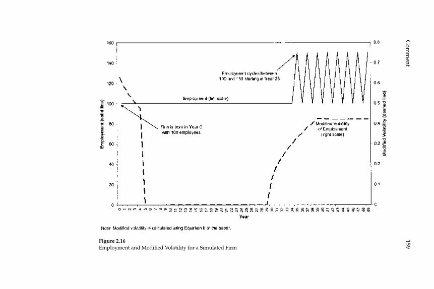
159C
omm
ent
Figure 2.16Employment and Modifi ed Volatility for a Simulated Firm
Foote160
Just as interesting is what happens when a fi rm is short-lived, so that it contributes both a birth and a death to the data. In these cases, the modifi ed volatility statistic may have problems distinguishing between short-lived fi rms that are truly volatile and those that are not. I calcu-lated modifi ed volatility for two simulated fi rms that each operated for four years. In one fi rm, the employment sequence was 100, 200, 300, 400, 0 while a second, less volatile fi rm had employment of 100, 100, 100, 100, 0. The modifi ed volatility statistic for the fi rst fi rm was indeed larger than that of the second, but not by much. In each year of the data, the fi rst fi rm’s modifi ed volatility was 1.19, but the stable fi rm’s statistic only marginally smaller, at 1.12. The likely reason for this similarity is that the γ ’s of 2 and –2 that bookend both of these fi rms’ histories are dominating their modifi ed volatility statistics, so that the statistic is unable to distinguish much difference in volatility between them.2
The implication of these simulations is that fl uctuations in the num-ber of births and deaths in the economy are likely to have a large impact on economywide volatility that may not accurately refl ect underlying theoretical concepts. Indeed, the authors’ fi gure 2.8 shows that exclud-ing births and deaths causes the average level of modifi ed volatility to decline by about one-third. More importantly for our purposes, the authors point out that the decline in volatility among privately held fi rms also becomes less pronounced, relative to their preferred fi gure 2.6. In fact, modifi ed volatility for the entire economy is essentially fl at over the sample period when entry and exit are left out.
The issue is just as important for the other variance statistic discussed by the authors, the cross-sectional distribution of γ ’s in any particular year. To make a trivial point, both an entry γ of 2 and an exit γ of –2 get larger in absolute value when they are squared for a calculation of cross-sectional standard deviation. But squaring shrinks the contribu-tion of fi rms with more modest growth rates (γ < 1). As a result, births and deaths of even small fi rms can have exceptionally large infl uences on the time-series pattern of cross-sectional dispersion. It is not hard to come up with examples in which the entry or exit decision of a tiny fi rm makes a big difference for employment-weighted dispersion in a sector that includes many large fi rms.3
The authors make a strong case that entry and exit should not be ignored when discussing idiosyncratic volatility, despite the associ-ated measurement diffi culties. When Wal-Mart enters a market and pushes out smaller, more volatile fi rms, employment volatility in the labor market declines in part because Wal-Mart is less likely to likely
161Comment
to go out of business than the stores it replaces. My concern is that I don’t have a good feel for the quantitative impact that entry and exit should have on measures of economywide volatility. There is no obvi-ous way to answer this question, given the diffi culty of translating the infi nite percentage changes in employment that occur upon entry and exit into some growth rate that can contribute to an economywide vol-atility average. The authors’ growth rate (γ ) equals 2 upon an entry, but why shouldn’t this number be 4? Or 1? By implication, how do we know that the author’s preferred fi gure 2.6 does a better job of inform-ing theoretical work on this topic than fi gure 2.8, where entry and exit are excluded?
2 Aggregate Shocks, Idiosyncratic Variance, and the Great Moderation
My second point is that the empirical separation of trends in aggregate vs. idiosyncratic volatility is likely more diffi cult that it would appear at fi rst glance. In recent years, there has been an explosion of theoretical work on fi rm-level volatility. Among other things, this work explores the implications of changes in research and development intensity, better diversifi cation through fi nancial markets, and a wider basket of potential inputs to production. This research also asks how changes in idiosyncratic volatility are likely to affect volatility at the aggregate level. For example, could microeconomic factors leading to higher or lower fi rm-level volatility help explain the Great Moderation in the U.S business cycle since the mid-1980s?
This research generally concerns the volatility of desired employ-ment at fi rms, but desired employment differs from the actual employ-ment we see in data when there are fi rm-level adjustment costs. One of the most important lessons we have learned from micro-level employ-ment data in the past two decades is that these costs should not be ignored. Changes in either employment or capital stocks on the micro level are usually much less frequent and much larger than we would expect under convex adjustment costs (or no costs at all). This pattern is typically explained by some non-convexity in adjustment costs, of which the simple (S,s) model is the best-known example.4
Non-convex adjustment costs draw a sharp distinction between the observed level of employment at fi rms and the desired level, with the latter denoting the employment level that would obtain if adjustment costs were momentarily suspended. In turn, the distinction between
Foote162
actual and desired employment makes it diffi cult to isolate aggregate shocks in the data. This is because only a few fi rms are likely to adjust actual employment when an aggregate shock occurs, even though the shock may affect desired employment at all fi rms in the same way. Think of a negative aggregate shock that reduces desired employment for all fi rms. In an (S,s) world, this shock will push some fi rms over the “reduce employment” boundary, so they will reduce employment a great deal. The other fi rms just move closer to this boundary, remaining inside the (S,s) inaction region.
What is more, the presence of non-convex adjustment costs can con-fuse the relationship between aggregate volatility and fi rm-level volatil-ity. Consider again the implications of a negative aggregate shock. The fact that some fi rms are pushed over the reduce-employment bound-ary shows up in the data as an increase in the dispersion of fi rm-level employment changes. After all, some fi rms have adjusted employment a great deal, while others have kept employment stable.
This empirical regularity is important for interpreting Davis and Haltiwanger’s 1990 paper, one of the fi rst to explore the relation-ship between aggregate and fi rm-level volatility. Using a dataset that included establishment-level data from the manufacturing industry alone, that paper found that the recessions of 1975 and 1982 were peri-ods of intense reallocation in the manufacturing sector, as measured (for example) by a measure of dispersion in the absolute value of employment changes at the microeconomic level This led them and a number of other 1990s authors to explore the possibility that recessions and interfi rm employment reallocation were theoretically linked, per-haps because recessions were in a time of low aggregate productivity (so that the opportunity costs of suspending production for reallocation fell in recessions). The recessions-as-reallocations theory suffered when confronted with other data, however. In other countries (Boeri 1996) or in non-manufacturing industries (Foote 1998), reallocation often looked procyclical, as the cross-sectional distribution of employment growth rate spread out in booms, not recessions. A simple explanation for this discrepancy is that an intense aggregate shock in any direction will cause measured microlevel dispersion to rise in an (S,s) world. If the data covers a period of intense positive shocks, microeconomic dispersion will look procyclical. If instead the most intense aggregate shocks are negative, then dispersion will look countercyclical.
Now consider the more recent lines of inquiry into micro and macro volatility. Section 2 of the paper states that there is a “simple mechani-
163Comment
cal reason to anticipate that micro and macro volatility will trend in the same direction.” I would elaborate on this statement, adding that under non-convex adjustment costs, there is a mechanical reason why a period of less-intense aggregate shocks will also be periods of lower idiosyncratic variation. So, theories that predict that micro and macro volatility trend in the same direction may be “vindicated” by the data, even if there is no underlying relationship between business cycles and idiosyncratic volatility in the desired employment of fi rms.
A unifying theme of my fi rst two points is that asking simple ques-tions of microeconomic data can be harder that it seems, due in part to the granular nature of employment change at the microeconomic level. Rather than curse our fate at having to deal with the associated measurement issues, I think we should instead be encouraged to con-tinue to develop empirical models that highlight distinctions between desired and actual employment. Those who would test recent theories on the relationship between aggregate and idiosyncratic volatility will undoubtedly fi nd these models useful.
3 Firm-level Idiosyncratic Variance and Workers Flows
Despite my concerns regarding measurement issues, I am quite com-fortable with the idea that some decline in idiosyncratic volatility has recently occurred. As the authors point out, their results dovetail nicely with worker-based data. Their fi gure 2.14 correlates fi rm-level volatil-ity with fl ows into and out of unemployment, with the latter two fl ows expressed as fractions of the labor force. I believe that the point can be made more forcefully by looking at the data in a different way. My fi gure 2.17 graphs the average monthly probability that an employed worker will separate into unemployment, as calculated by Robert Shimer. The data are quarterly averages of monthly rates from 1960:1 to 2004:4. Focusing on the separation rate is useful because this rate is closely related to reallocational intensity in search-and-matching mod-els of the labor market (Pissarides 2000, Chapter 1). The main feature of the graph is the low-frequency rise and fall in separations after 1970. Because the trend unemployment rate is essentially the ratio of the sep-aration rate to the sum of separation and fi nding rates, this movement in separations is a prime determinant of low-frequency movements in the overall unemployment rate as well.5
As the authors point out, one potential source for movements in sepa-rations is worker demographics. The peak year for baby boom births is
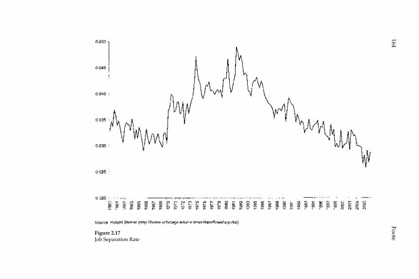
Foote164
Figure 2.17Job Separation Rate

165Comment
1957, so a lot of young people—with high separation rates—are enter-ing the labor market near the time when separations are highest. Yet movements in separations are probably too large to attribute to demo-graphics alone, as attempts to link recent trends in overall unemploy-ment solely to demographics have typically failed (Katz and Krueger 1999). Something else besides demographics must also be causing the separation rate to move, and, by extension, driving the trend in the overall unemployment rate. But what?
A great deal of ink has been spilled on sources of the recent decline in the natural unemployment rate, most of it focused on the question from the worker’s point of view. I think it likely that at least part of the answer will be found in fi rm-side data of the type that the authors employ. In light of this, the results in the paper’s table 2.2 are especially tantalizing. At least among privately held fi rms, declines in volatility from 1978 to 2001 are strikingly similar across industries, ranging from a low of 22.6 percent in Mining to 38.3 percent in Wholesale Trade. This similarity could rule out some explanations for declining volatility while supporting others.
4 Conclusion
The four authors of this paper are to be commended for the care in which they have constructed these data and the imagination they have used in analyzing them. As their research agenda develops, I would press them to clarify the measurement issues I have discussed as well as further explore the links between fi rm-side data to unemployment trends. Like many in both the policy and academic worlds, I will be interested to learn what they fi nd.
Endnotes
1. The volatility statistic would be of course be invariant to scaling the fi rm’s employment history by some constant factor, which would leave the sequence of γ ’s unchanged.
2. A fi rm in existence for only one year contributes two observations of 2.83 to modifi ed volatility, no matter what its size.
3. Consider an industry with ten fi rms. Nine of the fi rms have employment weights of 1,000 (that is average employment in t and t – 1 of 1,000), and their γ ’s are distributed between –0.02 and 0.02 (three with γ = –0.02, three with γ = 0.02, one with γ = –0.01, and two with γ = 0.01). The tenth fi rm has four employees, and either keeps employment con-stant (γ = 0, employment weight = 4) or drops employment to zero (γ = –2, employment weight = 2). If the tenth fi rm keeps employment constant, the employment weighted
Foote166
standard deviation of the ten fi rms will equal 0.0182. If the tenth fi rm exits, this statistic nearly doubles, to 0.0363.
4. In an (S,s) world, fi rms keep the deviation of desired-from-actual employment bounded, changing employment only when this deviation crosses either the “S” or “s” boundary. A generalization of the (S,s) model is the upward-sloping hazard model, which states that the probability (“hazard rate”) for employment adjustment rises as the devia-tion of desired-from-actual employments gets larger (Caballero, Engel, and Haltiwanger 1997). The (S,s) model is an extreme version of this framework, in which the hazard rate is 0 inside the (S,s) region and 1 outside of it. To my knowledge, there is little disagreement over whether non-convex adjustment costs are important at the micro level, although there is considerable disagreement over whether these non-convexities matter for macro-economic dynamics (Thomas (2002), Veracierto (2002)) as well as disputes over the pre-cise way in which micro-level models should be specifi ed and estimated (Cooper and Willis (2004), Cabellero and Engel (2004)).
5. Indeed, Shimer (2005) argues that business cycle variability in unemployment should be credited to the fi nding rate, not the separation rate, in contrast to previous research. It seems reasonable that lower frequency movements would then be driven in large part by the separation rate.
References
Boeri, Tito. 1996. “Is Job Turnover Countercylical?” Journal of Labor Economics 14: 603–625.
Cooper, Russell, and Jonathan L. Willis. 2004. “A Comment on the Economics of Labor Adjustment: Mind the Gap.” American Economic Review 94: 1223–1237.
Cabellero, Ricardo J., and Eduardo M. R. A. Engel. 2004. “A Comment on the Economics of Labor Adjustment: Mind the Gap: Reply.” American Economic Review 94: 1238–1244.
Caballero, Ricardo J., Eduardo M. R. A. Engel, and John Haltiwanger. 1997. “Aggregate Employment Dynamics: Building from Microeconomic Evidence.” American Economic Review 87: 115–137.
Davis, Steven J., and John Haltiwanger. 1990. “Gross Job Creation and Destruction: Micro-economic Evidence and Macroeconomic Implications.” NBER Macroeconomics Annual 1990, 123–168.
Foote, Christopher L. 1998. “Trend Employment Growth and the Bunching of Job Cre-ation and Destruction.” Quarterly Journal of Economics 113: 809–834.
Katz, Lawrence F., and Alan Krueger. 1999. “The High-Pressure U.S. Labor Market of the 1990s.” Brookings Papers on Economic Activity 1: 1–87.
Pissarides, Christopher A. 2000. Equilibrium Unemployment Theory. Cambridge, MA: MIT Press.
Shimer, Robert. 2005. “Reassessing the Ins and Outs of Unemployment.” University of Chicago manuscript.
Thomas, Julia K. 2002. “Is Lumpy Investment Relevant for the Business Cycle?” Journal of Political Economy 110: 508–534.
Veracierto, Marcelo K. 2002. “Plant-Level Irreversible Investment and Equilibrium Busi-ness Cycles.” American Economic Review 92: 181–197.
Comment
Éva Nagypál, Northwestern University
1 Introduction
The work of Davis, Haltiwanger, Jarmin, and Miranda (henceforth, DHJM) is a very informative piece of work that brings new and more comprehensive data to the active research area of business volatility. Just last year at the Macroeconomics Annual, Comin and Phillipon (henceforth, CP) were examining the change in business volatility that took place in recent decades and its relation to the change in aggre-gate volatility. DHJM confi rm the fi ndings of CP that the volatility of publicly-held fi rms increased recently, but show that the features of the COMPUSTAT data used by CP do not generalize to all fi rms, since there are important differences in the business volatility trend of publicly-traded versus privately-held fi rms.
To show just how exhaustive the LBD data DHJM use are, in table 2.6, I compare the employment numbers from the Current Employment Statistics, the Bureau of Labor Statistics’ most comprehensive survey of payroll employment in private nonfarm industries, for 1980, 1990, and 2000, with the employment numbers for the same segment of the econ-omy from the LBD. As can be seen, in all years, the LBD covers essen-tially all employment in private nonfarm industries, of which only a little over a quarter takes places in publicly-traded fi rms.
I view the DHJM piece as the beginning of an exciting new research program using the rich data available in the LBD. In my discussion, I would like to offer some suggestions as to how one might use these data to address questions that are at the core of macroeconomic research today. First, I discuss whether the distinction between publicly-traded versus privately-held businesses matters for macroeconomics and whether the LBD data are well-suited to study this distinction further. Second, I discuss the macroeconomic implications of the decline in
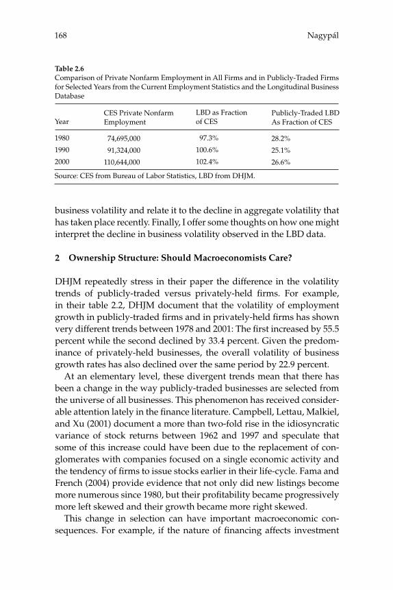
Nagypál168
business volatility and relate it to the decline in aggregate volatility that has taken place recently. Finally, I offer some thoughts on how one might interpret the decline in business volatility observed in the LBD data.
2 Ownership Structure: Should Macroeconomists Care?
DHJM repeatedly stress in their paper the difference in the volatility trends of publicly-traded versus privately-held fi rms. For example, in their table 2.2, DHJM document that the volatility of employment growth in publicly-traded fi rms and in privately-held fi rms has shown very different trends between 1978 and 2001: The fi rst increased by 55.5 percent while the second declined by 33.4 percent. Given the predom-inance of privately-held businesses, the overall volatility of business growth rates has also declined over the same period by 22.9 percent.
At an elementary level, these divergent trends mean that there has been a change in the way publicly-traded businesses are selected from the universe of all businesses. This phenomenon has received consider-able attention lately in the fi nance literature. Campbell, Lettau, Malkiel, and Xu (2001) document a more than two-fold rise in the idiosyncratic variance of stock returns between 1962 and 1997 and speculate that some of this increase could have been due to the replacement of con-glomerates with companies focused on a single economic activity and the tendency of fi rms to issue stocks earlier in their life-cycle. Fama and French (2004) provide evidence that not only did new listings become more numerous since 1980, but their profi tability became progressively more left skewed and their growth became more right skewed.
This change in selection can have important macroeconomic con-sequences. For example, if the nature of fi nancing affects investment
Table 2.6Comparison of Private Nonfarm Employment in All Firms and in Publicly-Traded Firms for Selected Years from the Current Employment Statistics and the Longitudinal Business Database
Year
1980
1990
2000
CES Private Nonfarm Employment
74,695,000
91,324,000
110,644,000
LBD as Fraction of CES
97.3%
100.6%
102.4%
Publicly-Traded LBD As Fraction of CES
28.2%
25.1%
26.6%
Source: CES from Bureau of Labor Statistics, LBD from DHJM.
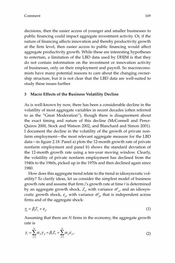
169Comment
decisions, then the easier access of younger and smaller businesses to public fi nancing could impact aggregate investment activity. Or, if the nature of fi nancing affects innovation and thereby productivity growth at the fi rm level, then easier access to public fi nancing would affect aggregate productivity growth. While these are interesting hypotheses to entertain, a limitation of the LBD data used by DHJM is that they do not contain information on the investment or innovation activity of businesses, only on their employment and payroll. So macroecono-mists have many potential reasons to care about the changing owner-ship structure, but it is not clear that the LBD data are well-suited to study these issues further.
3 Macro Effects of the Business Volatility Decline
As is well-known by now, there has been a considerable decline in the volatility of most aggregate variables in recent decades (often referred to as the “Great Moderation”), though there is disagreement about the exact timing and nature of this decline (McConnell and Perez-Quiros 2000, Stock and Watson 2002, and Blanchard and Simon 2001). I document the decline in the volatility of the growth of private non-farm employment—the most relevant aggregate measure for the LBD data—in fi gure 2.18. Panel a) plots the 12-month growth rate of private nonfarm employment and panel b) shows the standard deviation of the 12-month growth rate using a ten-year moving window. Clearly, the volatility of private nonfarm employment has declined from the 1940s to the 1960s, picked up in the 1970s and then declined again since 1980.
How does this aggregate trend relate to the trend in idiosyncratic vol-atility? To clarify ideas, let us consider the simplest model of business growth rate and assume that fi rm j’s growth rate at time t is determined by an aggregate growth shock, Zt, with variance σ 2
zt, and an idiosyn-cratic growth shock, εjt, with variance σ 2
ft, that is independent across fi rms and of the aggregate shock:
γjt = βtZt + εjt. (1)
Assuming that there are N fi rms in the economy, the aggregate growth rate is
γ α γ β α εt jt jt t t jt jtj
N
j
N
Z= = +==∑∑ ,
11 (2)
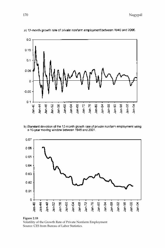
Nagypál170
Figure 2.18Volatility of the Growth Rate of Private Nonfarm EmploymentSource: CES from Bureau of Labor Statistics.
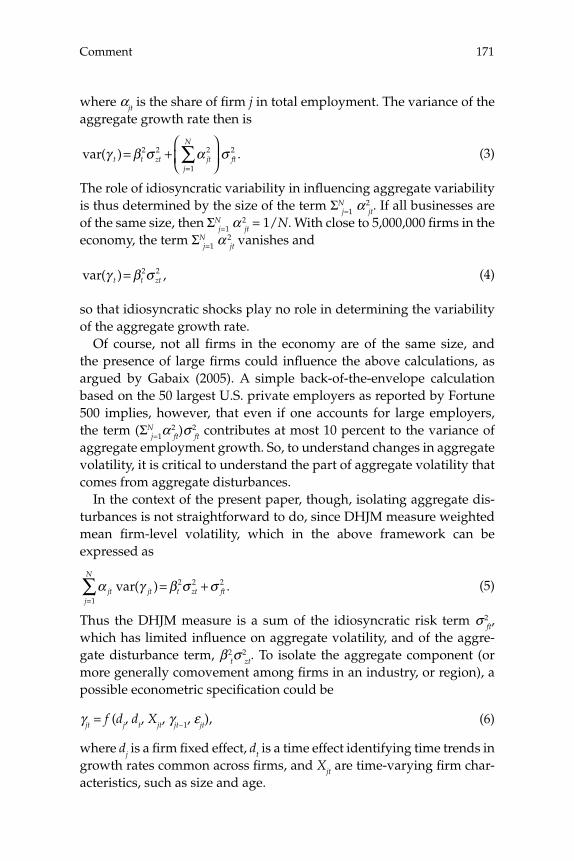
171Comment
where αjt is the share of fi rm j in total employment. The variance of the aggregate growth rate then is
var( ) .γ β σ α σt t zt jtj
N
ft= +⎛
⎝⎜⎞
⎠⎟=∑2 2 2
1
2 (3)
The role of idiosyncratic variability in infl uencing aggregate variability is thus determined by the size of the term ΣN
j=1 α 2jt. If all businesses are
of the same size, then ΣNj=1 α 2
jt = 1/N. With close to 5,000,000 fi rms in the economy, the term ΣN
j=1 α 2jt vanishes and
var( ) ,γ β σt t zt= 2 2 (4)
so that idiosyncratic shocks play no role in determining the variability of the aggregate growth rate.
Of course, not all fi rms in the economy are of the same size, and the presence of large fi rms could infl uence the above calculations, as argued by Gabaix (2005). A simple back-of-the-envelope calculation based on the 50 largest U.S. private employers as reported by Fortune 500 implies, however, that even if one accounts for large employers, the term (ΣN
j=1α 2ft)σ 2
ft contributes at most 10 percent to the variance of aggregate employment growth. So, to understand changes in aggregate volatility, it is critical to understand the part of aggregate volatility that comes from aggregate disturbances.
In the context of the present paper, though, isolating aggregate dis-turbances is not straightforward to do, since DHJM measure weighted mean fi rm-level volatility, which in the above framework can be expressed as
α γ β σ σjt jt t zt ftj
N
var( ) .= +=∑ 2 2 2
1
(5)
Thus the DHJM measure is a sum of the idiosyncratic risk term σ 2ft,
which has limited infl uence on aggregate volatility, and of the aggre-gate disturbance term, β 2
tσ 2zt. To isolate the aggregate component (or
more generally comovement among fi rms in an industry, or region), a possible econometric specifi cation could be
γjt = f (dj, dt, Xjt, γjt−1, εjt), (6)
where dj is a fi rm fi xed effect, dt is a time effect identifying time trends in growth rates common across fi rms, and Xjt are time-varying fi rm char-acteristics, such as size and age.
Nagypál172
With the rich data available in the LBD, by extracting a common component across different industries and studying its volatility, one could answer many interesting questions relating to the Great Modera-tion (GM). For example, was there a GM in all segments of economy? When did the GM start? Did it start at the same time in all segments of economy? Is the GM related to jobless recoveries as hypothesized by Koenders and Rogerson (2005)? Was the GM due to falling correlation between segments of the economy?
The last question of falling correlations among segments of the economy is all the more relevant, since not only could this account for the fall in aggregate volatility, but there is also evidence supporting its empirical validity. Assume that the aggregate growth shock, Zt, in the above framework is composed of two separate fundamental shocks (say, to different segments of the economy):
Zt = β1Z1t + β2Z2t. (7)
Then
σ β β β βzt t t tZ Z Z Z212
1 22
2 1 2 12= + +var( ) var ( ,covar 22t ), (8)
so a fall in the correlation of the two shocks would immediately imply a fall in the variance of the aggregate component.
The empirical relevance of this falling correlation is suggested by the fact that the correlation among the eight major private nonfarm sectors has fallen since the early 1980s, exactly the same period that aggregate volatility has fallen. To show this, in fi gure 2.19, I plot the average pair-wise correlation between the 12-month growth rate of employment in eight major private nonfarm sectors using a ten-year moving window, both weighted by sectoral employment and unweighted.
Of course, the most important outstanding question about the Great Moderation is whether it was due to a change in the size of the shocks, i.e., a result of smaller exogenous or policy shocks, or to a change in the transmission mechanism from shocks to outcomes that took place due to a shift from goods to services, to better inventory manage-ment, to innovations in fi nancial markets, or to a changing composition of the workforce. Putting this question into the context of the above simple model, did var(γt) decline because σ 2
zt declined or because βt declined?
With regards to this question, it is not immediately clear how the microdata of the LBD can help, since just as the aggregate data, they
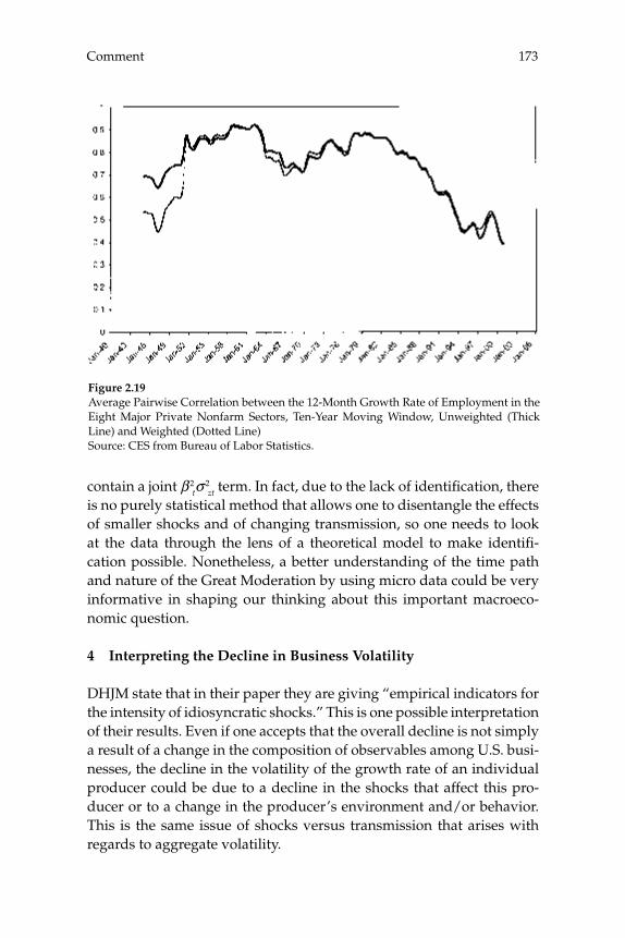
173Comment
contain a joint β 2tσ 2
zt term. In fact, due to the lack of identifi cation, there is no purely statistical method that allows one to disentangle the effects of smaller shocks and of changing transmission, so one needs to look at the data through the lens of a theoretical model to make identifi -cation possible. Nonetheless, a better understanding of the time path and nature of the Great Moderation by using micro data could be very informative in shaping our thinking about this important macroeco-nomic question.
4 Interpreting the Decline in Business Volatility
DHJM state that in their paper they are giving “empirical indicators for the intensity of idiosyncratic shocks.” This is one possible interpretation of their results. Even if one accepts that the overall decline is not simply a result of a change in the composition of observables among U.S. busi-nesses, the decline in the volatility of the growth rate of an individual producer could be due to a decline in the shocks that affect this pro-ducer or to a change in the producer’s environment and/or behavior. This is the same issue of shocks versus transmission that arises with regards to aggregate volatility.
Figure 2.19Average Pairwise Correlation between the 12-Month Growth Rate of Employment in the Eight Major Private Nonfarm Sectors, Ten-Year Moving Window, Unweighted (Thick Line) and Weighted (Dotted Line)Source: CES from Bureau of Labor Statistics.
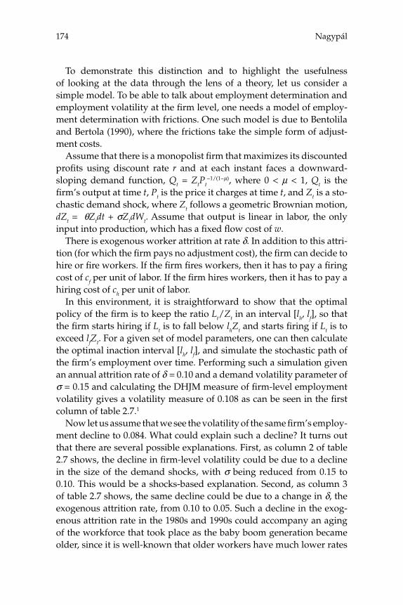
Nagypál174
To demonstrate this distinction and to highlight the usefulness of looking at the data through the lens of a theory, let us consider a simple model. To be able to talk about employment determination and employment volatility at the fi rm level, one needs a model of employ-ment determination with frictions. One such model is due to Bentolila and Bertola (1990), where the frictions take the simple form of adjust-ment costs.
Assume that there is a monopolist fi rm that maximizes its discounted profi ts using discount rate r and at each instant faces a downward-sloping demand function, Qt = ZtPt
−1/(1−μ), where 0 < μ < 1, Qt is the fi rm’s output at time t, Pt is the price it charges at time t, and Zt is a sto-chastic demand shock, where Zt follows a geometric Brownian motion, dZt = θZtdt + σZtdWt. Assume that output is linear in labor, the only input into production, which has a fi xed fl ow cost of w.
There is exogenous worker attrition at rate δ. In addition to this attri-tion (for which the fi rm pays no adjustment cost), the fi rm can decide to hire or fi re workers. If the fi rm fi res workers, then it has to pay a fi ring cost of cf per unit of labor. If the fi rm hires workers, then it has to pay a hiring cost of ch per unit of labor.
In this environment, it is straightforward to show that the optimal policy of the fi rm is to keep the ratio Lt/Zt in an interval [lh, lf], so that the fi rm starts hiring if Lt is to fall below lhZt and starts fi ring if Lt is to exceed lfZt. For a given set of model parameters, one can then calculate the optimal inaction interval [lh, lf], and simulate the stochastic path of the fi rm’s employment over time. Performing such a simulation given an annual attrition rate of δ = 0.10 and a demand volatility parameter of σ = 0.15 and calculating the DHJM measure of fi rm-level employment volatility gives a volatility measure of 0.108 as can be seen in the fi rst column of table 2.7.1
Now let us assume that we see the volatility of the same fi rm’s employ-ment decline to 0.084. What could explain such a decline? It turns out that there are several possible explanations. First, as column 2 of table 2.7 shows, the decline in fi rm-level volatility could be due to a decline in the size of the demand shocks, with σ being reduced from 0.15 to 0.10. This would be a shocks-based explanation. Second, as column 3 of table 2.7 shows, the same decline could be due to a change in δ, the exogenous attrition rate, from 0.10 to 0.05. Such a decline in the exog-enous attrition rate in the 1980s and 1990s could accompany an aging of the workforce that took place as the baby boom generation became older, since it is well-known that older workers have much lower rates
175Comment
of exogenous attrition than younger workers. This, of course, would be a transmission-based explanation, since here the change in the fi rm’s environment led to a decline in fi rm-level volatility.
So it is clear that the decline in fi rm-level volatility need not neces-sarily imply a reduction in the size of the shocks that the fi rm experi-ences, rather it could be due to other changes in the fi rm’s environment. The advantage of having an explicit model is that it can give us ways to disentangle the two possible reasons for the decline in volatility. In particular, in the above simple model, the two sources of the decline in fi rm-level volatility could be distinguished by looking at the aver-age time between adjustments of the fi rm’s workforce. In the case of smaller shocks, the average time to adjust declines, since now the fi rm faces less risk and is willing to take advantage even of small changes in demand (i.e., the region of inactivity shrinks). In the case of lower exogenous attrition due to the baby boomers getting older, the average time to adjust increases, since now the fi rm needs to do replacement hiring less often.
Of course, these simple calculations are only demonstrative, since they rely on an easily calculable partial-equilibrium model with some restrictive assumptions, but they demonstrate how one might use a the-oretical model to think about the rich data studied in DHJM. Campbell and Fisher (2004) develop a dynamic stochastic general equilibrium model with similar features.
5 Conclusions
To conclude, it is worth reiterating that the LBD contains great new data to study business dynamics and to guide our thinking about impor-tant macro questions. The paper by DHJM presents some very nice and thought-provoking fi ndings and is certainly only the beginning of
Table 2.7DHJM Volatility Measure and Adjustment Frequency for Different Parameter Specifi ca-tions in the Employment Determination Model with Adjustment Costs
DHJM volatility
Adjustment frequency
Benchmark Specifi cationδ = 0.10σ = 0.15
0.108
8.5 weeks
Smaller Shocks Hypothesisδ = 0.10σ = 0.10
0.084
6 weeks
Baby Boom Hypothesisδ = 0.05σ = 0.15
0.084
15.4 weeks
Nagypál176
an exciting new research program. The fi nding, in particular, that the volatility trends of all fi rms do not coincide with the volatility trends of publicly-held fi rms that have been studied in previous papers cer-tainly deserves attention, since it changes the basic stylized fact that the growing theoretical literature connecting business-level volatility with aggregate volatility must confront.
One interesting way to push this research agenda forward, especially in its relation to macroeconomics, is to bring more theory to the inter-pretation of data, since some important questions regarding the source of the decline in aggregate volatility are not possible to answer without it.
Endnote
1. The other parameters are set at annual values of r = 0.05, θ = 0.012, μ = 0.5, w = 1, cf = 0.5, and ch = 0.5. Details of the calculations and simulations are available upon request.
References
Bentolila, S., and G. Bertola. 1990. “Firing Costs and Labor Demand: How Bad Is Euro-sclerosis?” Review of Economic Studies 57: 381–402.
Blanchard, O., and J. Simon. 2001. “The Long and Large Decline in U.S. Output Volatil-ity.” Brookings Papers on Economic Activity: 135–164.
Campbell, J. R., and J. D. M. Fisher. 2004. “Idiosyncratic Risk and Aggregate Employment Dynamics.” Review of Economic Dynamics 7: 331–353.
Campbell, J. Y., M. Lettau, B. G. Malkiel, and Y. Xu. 2001. “Have Individual Stocks Become More Volatile? An Empirical Exploration of Idiosyncratic Risk.” Journal of Finance 56(1): 1–43.
Comin, D., and T. Philippon. 2005. “The Rise in Firm-Level Volatility: Causes and Con-sequences.” In M. Gertler and K. Rogoff, eds. NBER Macroeconomics Annual Volume 20, 167–202. Cambridge, MA: MIT Press.
Fama, E. F., and K. R. French. 2004. “New Lists: Fundamentals and Survival Rates.” Jour-nal of Financial Economics 73: 229–269.
Gabaix, X. 2005. “The Granular Origins of Aggregate Fluctuations.” Mimeo, MIT.
Koenders, K., and R. Rogerson. 2005. “Organizational Dynamics over the Business Cycle: A View on Jobless Recoveries.” Federal Reserve Bank of Saint Louis Review 87(4): 555–579.
McConnell, M., and G. Perez-Quiros. 2000. “Output Fluctuations in the United States: What Has Changed Since the Early 1980s?” American Economic Review 90(5): 1464–1476.
Stock, J. H., and M. W. Watson. 2002. “Has the Business Cycle Changed and Why?” In M. Gertler and K. Rogoff, eds., NBER Macroeconomics Annual Volume 17, 159–218. Cam-bridge, MA: MIT Press.
Discussion
Diego Comin began the discussion by raising several points. He noted that it was entirely possible for time series and cross-sectional measures of fi rm volatility to behave very differently. While the cross-sectional measures of volatility capture the dispersion of the distribution of fi rm growth, the time-series measures of volatility get at the changes in a fi rm’s position within this distribution. He mentioned that in work with Sunil Mulani, he had found that turnover had increased more in the COMPUSTAT sample. Using sales data rather than employment data, they furthermore found a decrease in the cross-sectional measure of volatility in the COMPUSTAT sample. Thomas Philippon remarked that similar trends vis-à-vis the convergence in cross-sectional volatility between private and publicly-traded fi rms had been observed in French data.
Comin noted that if the authors’ conclusions are correct, they are par-ticularly interesting because they help distinguish between different explanations that have been put forward regarding the upward trend in the volatility of public companies. In particular, he saw the authors’ evidence as supporting Schumpeterian models in which fi rms that do a disproportionate amount of R&D, such as public fi rms, experience larger increases in volatility. On the other hand, he saw the authors’ evi-dence as posing a challenge for models that stress fi nancial frictions.
Comin emphasized the importance of controlling for compositional change by including fi rm fi xed effects in the regressions. He noted that while the results could be driven by compositional change, in his own work on the COMPUSTAT sample, he had found that this was not the case. He noted that his results were also robust to the inclusion of age effects, size effects and to different weighting schemes, and said that he would like to see whether the results in the paper were robust to these effects as well.
Discussion178
Both Comin and Philippon noted that while the fi rms in the COMPU-STAT sample accounted for only about one-third of total U.S. employ-ment, they accounted for a much larger fraction of value added in the economy. This implied that the weights were very different if fi rms were weighted by sales rather than employment. John Haltiwanger agreed that it was important to look at measures of activity other than employment. He noted that the LBD data set was particularly good for the employment variable, whereas investigating other measures would require signifi cant additional work to construct these variables. Regarding entry and exit, Haltiwanger said that the results would not change signifi cantly if sales weights were used instead of employment weights.
Daron Acemoglu cautioned against implicitly adopting a steady-state view of the economy when thinking about fi rm volatility. He noted that the entry of a large retail fi rm like Wal-mart in a particular local mar-ket typically induces a spike in hiring and fi ring activity, and this non steady-state phenomenon should affect the interpretation given to the empirical results. He also suggested that monotonic selection of less risky fi rms into public listing was not necessarily a good assumption. In response to an improvement in fi nancial development, he argued that the most risky fi rms might seek and obtain a public listing since these fi rms have the biggest need for risk diversifi cation. This would imply that the pool of listed fi rms would contain both old, low-risk fi rms and young, high-risk fi rms. Steven Davis responded that while the logic of Acemoglu’s argument was correct, the quantitative force of this argument was not strong enough to explain the volatility conver-gence result.
Philippon said that he thought the take-away message from the paper was that economists need to think more about the decision of fi rms to go public. Two parameters he felt were particularly important in deter-mining which fi rms go public are the amount of risk and the amount of asymmetric information. Firms should be more likely to go public the more risky they are and the less they are plagued by asymmetric infor-mation, other things equal. Philippon emphasized that the asymmetric information in IPOs was a very large phenomenon which led to a large amount of underpricing. In order to explain the large increase in the fraction of fi rms that go public, he felt that it was important to examine closely the role of improved fi nancial intermediation, such as the rise of venture capital, in reducing asymmetric information problems. John

179Discussion
Haltiwanger agreed with Philippon’s point and said that the authors were actively working on integrating the information in the LBD with venture capital data. He noted that with the dataset they had created, they could study the prehistory of fi rms that go public.
Andrew Levin urged the authors to think about the possible causal links between the trends they observe in fi rm level volatility and the Great Moderation in macroeconomic volatility since the mid-1980s. He noted that the causation could go either way and that it was even pos-sible that there was no link. It seemed to him, however, that the authors were rather hesitant to draw any link between the Great Moderation and the trends in fi rm level volatility that they documented. Olivier Blanchard wondered whether the difference in volatility between public and private fi rms was primarily due to the larger size of public fi rms.
Responding to the discussants’ comments, Haltiwanger noted that it was reassuring that there were now multiple datasets for the U.S. based on different sources from which consistent empirical patterns have emerged. He said that they had emphasized the retail sector in the paper since they were better able to ascertain the reasonableness of their results for this sector than for some other sectors. He however emphasized the pervasiveness of their fi ndings across sectors. He noted that one potential explanation for the results was a shift in the economy towards larger national fi rms, but that many other explanations likely played a role.
Haltiwanger said that they were confi dent that the data showed a decline in entry and exit. He noted that in a large class of models with frictions, entry and exit played a very important role. He discussed work that he had done with Steven Davis and Jason Faberman showing that in the JOLTS data, the employment growth distribution has fat tails and that in light of this, entry and exit is particularly important.
Ron Jarmin rounded up the discussion by encouraging researchers to exploit the LBD dataset. He noted that research proposals could be submitted easily to the Census Bureau (via the Bureau’s website) for access to the dataset.

3
Do Taxes Explain European Employment? Indivisible Labor, Human Capital, Lotteries, and Savings
Lars Ljungqvist, Stockholm School of Economics and New York UniversityThomas J. Sargent, New York University and Hoover Institution
“The differences in the consumption and labor tax rates in France and the United States account for virtually all of the 30-percent difference in the labor input per working-age person. … if France modifi ed its intratemporal tax wedge so that its value was the same as the U.S. value, French welfare in consumption equiva-lents would increase by 19 percent.”
Prescott (2002, p. 13, p. 1)
“The Achilles’ Heel? Europe’s generous unemployment benefi ts…
German workers typically receive 70% of their take-home pay in the fi rst month of unemployment, and 62% in the 60th month, according to the Paris-based Organization for Economic Cooperation and Development. And the percent-ages are roughly similar for most of the Continent. In the U.S., by contrast, benefi ts plunge over time. Comparable U.S. workers receive 58% of their take-home pay in the fi rst month, but just 7% in the 60th month, the OECD says.”
Wall Street Journal (1998, p. R.17)
1 Introduction
Prescott (2002) used a growth model with a stand-in household and the assumption that the government transfers all tax revenues to the house-hold to argue that cross-country differences in taxes on labor account for cross-country differences in hours per capita. This paper examines the sensitivity of Prescott’s analysis to his assumptions about private risk sharing arrangements, labor markets, human capital acquisition, the government’s disposition of tax revenues, the absence of govern-ment supplied benefi ts to people who withdraw from work, and the high disutility of labor.1
Section 2 adds an important aspect of the European landscape that Prescott ignored: Government supplied non-employment benefi ts in
Ljungqvist and Sargent182
the form of a replacement ratio times foregone labor income. Martin (1996) documents that European governments offer benefi ts with high replacement rates and long durations. In our modifi cation of his model, a benefi t rate works just like Prescott’s labor-tax wedge (see the mul-tiplication of wedges that appears in our equation (4)). With the high disutility of labor set by Prescott, benefi t wedges of magnitudes esti-mated by Martin (1996) lead to depressions much deeper than Europe has experienced. This good news for Europe is bad news for the fi t of Prescott’s model. Prescott says that the high labor supply elasticity responsible for these outcomes comes from his use of a “not-so-well-known” aggregation theory due to Hansen (1985) and Rogerson (1988) that assumes indivisible labor, employment lotteries, and perfect pri-vate consumption insurance. How do Prescott’s conclusions, and the bad fi ts that result after we extend his analysis to include those gener-ous European inactivity benefi ts, depend on that aggregation theory?
Mulligan (2001) suggested that Hansen’s and Rogerson’s aggrega-tion theory is not necessary for Prescott’s results because by borrowing and lending a risk-free asset that bears a suffi ciently high interest rate, a worker can smooth consumption across alternating periods of work and nonwork.2 Section 3 formulates a version of Mulligan’s argument in a single-agent setting. We show that whether Mulligan’s time averag-ing leads to outcomes equivalent to Hansen’s and Rogerson’s depends on whether human capital is absent (here the answer is yes) or present (now the answer is no). Introducing a stylized human capital acquisi-tion technology like those of Shaw (1989) and Imai and Keane (2004) creates a nonconvexity over careers and allows a stand-in household to achieve allocations with employment lotteries that individuals cannot attain by time averaging.3 Furthermore, the employment lotteries and time-averaging models have different implications about the identi-ties of the nonemployed and disingenuously disabled or prematurely retired (at government expense) and how their consumption compares to those who are working.4 The models thus point in different direc-tions for microeconomic verifi cation. Nevertheless in the small open economy equilibrium setting of section 4, we show that the two market structures (“aggregation theories” in Prescott’s language) give rise to virtually identical responses of aggregate nonemployment to increases in tax rates on labor income. In both market structures, the high disu-tility of labor calibrated by Prescott, which we adopt and hold fi xed across the two market structures, delivers a high elasticity of aggregate nonemployment to after tax real wages (when the government trans-

183Indivisible Labor, Human Capital, Lotteries, and Savings
fers all tax revenues to the households). This fi nding is also confi rmed in the general equilibrium extension of Ljungqvist and Sargent (2006a), as summarized in section 5.
Why do generous government supplied benefi ts for nonemployment cause aggregate activity to implode in the model of section 2 and the employment lotteries model of Ljungqvist and Sargent (2006b)?5 After all, even when those government benefi ts are absent, these models already include perfect “nonemployment” or “inactivity” insurance in the employment lotteries model, and that causes no such problems. But this insurance is private and the stand-in household internalizes its costs. In contrast, government supplied inactivity benefi ts induce dis-tortions because households do not internalize their costs. As we shall see, in the models of this paper, the high disutility of labor and the resulting high labor supply elasticity that give labor taxes such potency in Prescott’s model also enhance the distortion in nonemployment that comes from government supplied benefi ts. They form a package.
Section 6 discusses what to make of the common aggregate outcomes that characterize the employment lottery and time-averaging mod-els presented in sections 3, 4, and 5. We describe how the aggregate outcomes conceal important differences in the lives of the individual workers whose actions underlie the aggregates and how those differ-ences would lead us in different directions when it comes to calibrating key parameters and seeking microeconomic verifi cation.
Section 7 reiterates why we answer “no” to the question asked in our title, then describes additional model features whose inclusion we think will explain the cross-country employment data.
2 Breakdown of Prescott’s Model with Government Supplied Benefi ts
2.1 The Model and Equilibrium Relationships
To explain international differences in hours worked, Prescott (2002) uses the standard growth model with a labor supply elasticity set high enough to make employment vary substantially over the business cycle. In this section, we describe how Prescott alludes to an employment lot-teries model to justify a representative household whose choices exhibit a high labor supply elasticity; how that high labor supply elasticity also makes Prescott’s representative household’s leisure choice very sensi-tive to government supplied benefi ts for those not working; and how Prescott’s assumption about what the government does with its tax
Ljungqvist and Sargent184
revenues disarms an income effect that would substantially affect out-comes. We point out that adding government benefi ts while retaining Prescott’s calibrated labor supply elasticity causes the fi t of the model to deteriorate substantially, creating the “puzzle” of why Europeans work so much.
Prescott’s stand-in household has preferences ordered by
β αtt
tt tN c h
=
∞
∑ + −0
1[log( ) log( )]. (1)
There is a Cobb-Douglas production function with capital share param-eter θ and fl at rate taxes τkt, τht, τct on earnings from capital and labor, and on consumption, respectively.
2.1.1 The Stand-in Household’s Budget Set with Benefi ts Prescott’s supply side analysis succeeds in explaining cross-country differences in hours while ignoring cross-country differences in government sup-plied benefi ts to people not working. To probe Prescott’s statement that he had expected “… the nature of the unemployment benefi ts sys-tem to be more important” (Prescott 2002, p. 9), we add publicly sup-plied inactivity benefi ts to Prescott’s model. Following Prescott, let pt be the time 0 price of a unit of consumption at time t, wt the pre-tax wage, Tt the government lump-sum transfer, δ the depreciation rate, and rt the pre-tax rental rate on capital, and let kt, ht, ct, respectively, be capital, hours, and consumption per person. Assume that population Nt+1 = ηNt, η > 0, and that there is a constant geometric gross rate of Harrod neutral technical progress of γ. We augment Prescott’s version of the stand-in household’s intertemporal budget constraint to include a contribution from government supplied inactivity benefi ts:
p N c k rt tt
ct t t t kt=
∞
+∑ + + − + − −0
11 1 1[( ) [ ( )( )]τ η δ τ kk
w h w h h T
t
ht t t ht t t( ) ( ) max{ , }− − − − − −1 1 0τ ρ τ tt ] ,≤ 0
(2)
where ρ(1 – τht)wt max{0, h– – ht} represents government benefi ts, which we intend to stand for a broad set of programs for rewarding people who are said to be disabled, prematurely retired, and unemployed. The stand-in household receives government supplied subsidies for time spent not working in the form of a replacement rate ρ ∈ [0, 1) times after tax earnings that it forgoes when it sets h < h
–. If the household’s hours
185Indivisible Labor, Human Capital, Lotteries, and Savings
fall short of h–, the government replaces a fraction ρ of the defi ciency of after-tax labor income relative to w(1 – τh) h
–. We suppose that param-eter values are such that the household chooses to supply labor ht in an amount strictly less than h–.
By using Abel’s summation formula, the terms in capital in (2) can be expressed as
p N k r k p Nt tt
t t kt t=
∞
+∑ − + − − = −0
1 0 01 1[ ( ( )( )) ] [η δ τ 11 1
1
0 0 0
1 1
+ − −
+ − +− −
( )( )]
( [ (
r k
p N p N
k
t t t t
δ τ
η rr k p N kt kt t Tt
t t T− − +→∞
=
∞
+∑ δ τ η)( )]) lim .11
1
The last term is zero by a no-Ponzi argument and a transversality con-dition; and a no arbitrage argument implies that the coeffi cients on kt under the summation sign should be zero,6 so that
pp
rt
tt kt
− = + − −1 1 1[ ( )( )]δ τ (3)
for t ≥ 1, with the value of the stand-in household’s initial capital being p0[1 + (r0 – δ)(1 – τk0)]N0k0. The marginal conditions for consumption imply pt–1/pt = ct /βct–1. In a steady state, ct = γ ct–1, so that pt–1/pt = γ/β. Substituting this into (3) and imposing τkt = τk gives Prescott’s equation (10):
ri
k
= +−
δτ1
,
where 1 + i = γ/β would be the gross interest rate on a tax-free one period bond in this economy.
2.1.2 An Altered h – c/y Relationship Prescott’s conclusion that cross-country differences in tax wedges account for cross-country differences in hours depends sensitively on how he treats the con-sumption-output ratio c/y. We follow Prescott (2002) and use the household’s fi rst-order conditions with respect to consumption and lei-sure, and also the constant labor share implied by the Cobb-Douglas production function, to derive an equilibrium relationship between h and c/y:
hc y
tt t ct
ht
= +−
+− −
⎡
⎣⎢
⎤
⎦⎥
−
11
11
11
1α
θττ ρ
/. (4)

Ljungqvist and Sargent186
When ρ = 0, this is the same as expression (12) in Prescott (2002, p. 7). Prescott called this an “equilibrium relationship” because the consump-tion-output ratio c/y is endogenous. In the spirit of Prescott (2004), we defi ne the intratemporal tax-benefi t wedge as
11
11
11
11
+− −
≡− −
ττ ρ τ ρ
ct
ht t
, (5)
which is a product of a benefi t rate and Prescott’s intratemporal tax wedge 1/(1 – τt) ≡ (1 + τct)/(1 – τht), where τt ≡ (τht + τct)/(1 + τct).
2.2 Why Do French People Work So Much?
We use the same parameter values that underlie Prescott’s computa-tions (2002, table 4) to construct our fi gure 3.1.7 We take the United States as the benchmark economy against which to measure the employment effects of taxes and benefi ts. Setting the effective marginal tax rate equal
Figure 3.1Employment Effects of Taxation and Social Insurance in Prescott’s (2002) Framework. Prescott’s calibration of the United States serves as the benchmark economy where the effective marginal tax rate on labor income is 40 percent and there is no social insurance (ρ = 0)

187Indivisible Labor, Human Capital, Lotteries, and Savings
to 40 percent for the United States, Prescott argues that the French effec-tive marginal tax rate is 20 percentage points higher than the American tax rate. Prescott confi nes himself to the back of fi gure 3.1, where the replacement rate is ρ = 0. There, a tax rate differential of 20 percent sends the employment index down to 0.73. So we have reproduced Prescott’s fi nding that this tax differential can indeed explain why France is depressed by 30 percent relative to the United States when we suppose along with Prescott that ρ = 0.
When we move forward from the back of fi gure 3.1, we see dra-matic effects of publicly provided benefi ts.8 At Prescott’s calibration of .2 for the French tax wedge differential relative to the United States, as we raise the social insurance replacement rate ρ above 0, employ-ment plummets. The model sets the employment index equal to 0.55, 0.41, and 0.25 when the replacement rate is equal to 0.30, 0.50, and 0.70, respectively. Of course, the French economy was not depressed by 45, 59, or 75 percent relative to the United States. With Prescott’s calibra-tion of the other parameters, setting the replacement rate ρ to one of the values reported by Martin (1996) makes the puzzle become: Why do French people work so much?
2.3 Government Expenditures, Income Effects of Taxes, and c/y
Prescott’s calibration of c/y is a big part of his supply side story. His treatment of government expenditures infl uences how he estimates c/y in the ρ = 0 version of his workhorse formula (4). Let g denote “govern-ment expenditures” that are not substitutes for private consumption and assume that g is a constant fraction ζ of tax revenues:
g = ζ [τcc + τhwh + τk(r – δ)k].
We assume that the government returns lump sum rebates of (1 – ζ) times its tax revenues to the stand-in household. The above formula for g, feasibility, and the formula for the equilibrium capital stock can be combined to yield the following formula for the equilibrium value of c/y:
c y
iih k
k/( )( ) ( )
( )=
− − + −+ −
⎛⎝⎜
⎞⎠⎟
+
1 1 11
1
θ ζτ θ ζττ δ
ζζτ c
. (6)

Ljungqvist and Sargent188
Under Prescott’s preferred value of ζ = 0, this formula simplifi es to
c yi
i k
/ ( )( )
,= − ++ −
⎛⎝⎜
⎞⎠⎟
11
θ θτ δ
(7)
which makes c/y independent of the intratemporal tax wedge (there remains an effect from capital taxation). But with ζ > 0, formula (6) activates income effects from the intratemporal wedge to c/y, income effects that Prescott’s ζ = 0 assumption disables.
Prescott (2002, p. 7) acknowledges that his assumption about c/y substantially affects outcomes:
“The assumption that the tax revenues are given back to households either as transfers or as goods and services matters. If these revenues are used for some public good or are squandered, private consumption will fall, and the tax wedge will have little consequence for labor supply. If, as I assume, it is used to fi nance substitutes for private consumption, such as highways, public schools, health care, parks, and police protection, then the ct/wt factor will not change when the intratemporal tax factor changes. In this case, changes in this tax fac-tor will have large consequences for labor supply.”
Prescott assumes not only that all public expenditures are substitutes for private consumption but also that the government allocates resources as effi ciently as when households choose for themselves.
Although the calculations in fi gure 3.1 accept Prescott’s (2002) assumption that “all [tax] receipts are distributed lump-sum back to the stand-in household,” it is worth noting that Prescott (2004) proceeded differently when he studied the time series evidence for the tax expla-nation of the European employment experience:
“All tax revenue except for that used to fi nance the pure public consumption is given back to the households either as transfer payments or in-kind. These transfers are lump sum, being independent of a household’s income. Most public expenditure are substitutes for private consumption in the G-7 countries. Here I will assume that they substitute on a one-to-one basis for private consumption with the exception of military expenditures. The goods and services in question consist mostly of publicly provided education, health care, protection services, and even judiciary services. My estimate of pure pub-lic consumption g is two times military’s share of employment times GDP.” Prescott (2004, p. 4)
The cross-country differences in c/y that result from that assumption contribute to the success that Prescott (2004) ascribes to the tax explana-tion of the European employment experience.
189Indivisible Labor, Human Capital, Lotteries, and Savings
Thus, as described by Ljungqvist (2005), Prescott’s (2004, table 2) time series analysis of the European employment experience rests on variations in both the tax wedge and the ratio c/y. For example, even in the 1970s, France and Germany had tax wedges 9 and 12 percentage points higher than the United States, respectively. Prescott fi ts French and German employment levels that are comparable to those in the United States in the 1970s only by plugging in c/y’s for the 1970s that were 8 percentage points lower in the two European countries than in the United States. Thus, a signifi cant qualifi cation applies to Prescott’s conclusion that “an important observation is that when European and U.S. tax rates were comparable, European and U.S. labor supplies were comparable.” We could instead say of the 1970s that while French and German tax rates already exceeded the U.S. rate by about half of the tax differential of 20 percentage points that were later to prevail during the 1990s, Prescott’s estimates of low c/y ratios for France and Germany in the 1970s allow the model to fi t the outcomes then. If it had not been for those low c/y ratios, the model would have predicted signifi cantly depressed employment levels during the 1970s instead of the observed outcomes in which both countries’ employment rates exceeded that in the United States.
2.4 Prescott’s Appeal to an Aggregation Theory
To justify the high labor supply elasticity that he attributes to the stand-in household, Prescott (2002, p. 4) refers to “some not-so-well-known aggregation theory behind the stand-in household utility function (1) (see Gary D. Hansen, 1985; Richard Rogerson, 1988; Andreas Hornstein and Prescott, 1993).” Hansen (1985) and Rogerson (1988) assume indi-visibilities in households’ choice sets for labor, like the models to be described in sections 3 and 4. Employment lotteries and complete con-sumption insurance markets imply a stand-in household that wants to maximize
β φ αtt
tt tN c h[ log( ) log( ˆ)],
=
∞
∑ + −0
1 (8)
where φt is a choice variable that represents the fraction of people working and the parameter h equals the indivisible number of hours supplied by each worker. This functional form obviously differs from (1). However, we understand Prescott’s point really to be that the

Ljungqvist and Sargent190
aggregation theory underlying (8) rationalizes his decision to use a value of α in (1) that gives a high labor supply elasticity.
Prescott (2006) assigns the same high importance to the aggregation theory underlying the stand-in household that he attaches to the aggre-gation theory behind the aggregate production function. He empha-sizes that both types of aggregation divorce essential properties of the aggregated function from the properties of the individual functions being aggregated:9
“Rogerson’s aggregation result is every bit as important as the one giving rise to the aggregate production function. In the case of production technology, the nature of the aggregate production function in the empirically interesting cases is very different from that of the individual production units being aggregated. The same is true for the aggregate or a stand-in household’s utility function in the empirically interesting case.”
2.4.1 Insensitivity of Results to Making Disutility Linear in LaborWe studied how Prescott’s (2002) results would be affected were we to adopt the Hansen-Rogerson objective function (8). That preference specifi cation implies the following equilibrium relationship for the fraction of employed households:
φ θα
τ ρτt
t t
ht
cth c y= − −
−− −
+1
1
1 11log( ˆ) /
( )( ). (9)
Because Prescott (2002) did not provide a complete account of his parameter settings, we also use the reported fi ndings of Prescott (2004) when calibrating the Hansen-Rogerson framework.10 Our computations indicate that the outcomes associated with preference specifi cations (1) and (8) are similar. As one would expect, because the Hansen-Rogerson framework has a more elastic labor supply, increases in the tax wedge lead to larger negative employment effects. But the differences across the two preference specifi cations are not too big in our general equilib-rium analysis. For example, a calculation from (9) that corresponds to Prescott’s calibration of France yields an employment effect that is 6.5 percentage points more depressed with the Hansen-Rogerson utility function (8) than with Prescott’s utility function (1).11
2.4.2 Are Employment Lotteries Necessary? A high labor supply elasticity is an important part of the reasoning that leads to Prescott’s interpretation of how cross-country differences in the intratemporal tax wedge can account for observed differences in employment rates. In

191Indivisible Labor, Human Capital, Lotteries, and Savings
the next two sections, we study employment lotteries in more depth with the aim of understanding whether the Hansen-Rogerson aggre-gation theory is necessary to justify Prescott’s approach or whether it would work just as well to use an alternative aggregation theory proposed by Mulligan (2001) that allows each individual to choose alternating spells of work and leisure. Our answer is that Mulligan’s aggregation theory will do just as well, though as we shall see, the presence of a human capital acquisition technology that features learn-ing by working affects many interesting details.12 In particular, we shall see that while the responses of aggregate nonemployment to labor taxes are similar, the two aggregation theories promote different views about the types of workers we should expect not to be working and when.
To economize on notation in the next two sections, we set benefi ts ρ = 0, with the understanding that were we to include a nonemployment benefi t like the one in this section, i.e., as an entitlement to compensa-tion for time not worked up to some threshold h–, ρ would continue to augment the tax wedge as in (5). Therefore, in our quest to understand how that high labor supply elasticity depends on the market structure, i.e., the aggregation theory, that underpins it, it suffi ces to focus on the ρ = 0 case. However, in section 6 we return to the issue of social insur-ance when discussing what to make out of the forces behind Prescott’s high aggregate labor supply elasticity.
3 Aggregation Theories: Time Averaging and Lotteries
In this section we show that without human capital, lotteries and time-averaging-with-savings give similar outcomes at the aggregate level, and in an ex-ante sense at the individual level too. In contrast, when work leads to human capital accumulation, lotteries give an allocation that differs from, and in terms of ex ante utility is superior to, the one attained with time averaging. But in section 4, we show that, despite these differences in outcomes when there is human capital, the responses of nonemployment to labor tax changes are quantitatively similar under both employment lotteries and time-averaging with incomplete mar-kets. Thus, we conclude that the Hansen-Rogerson aggregation theory that Prescott (2002) emphasizes is not really necessary for his quantita-tive results. The high value at which he calibrates the disutility of labor makes nonemployment just as sensitive to after tax real wages under time-averaging as it is with lotteries.

Ljungqvist and Sargent192
We study two arrangements that allow an individual to attain a smooth consumption path when he faces a zero-one labor supply indi-visibility at each moment. One arrangement was proposed by Hansen (1985) and Rogerson (1988), namely, an employment lottery supple-mented with perfect consumption insurance. Another arrangement was discussed by Jones (1988) and Mulligan (2001) and allows an indi-vidual who alternates between spells of work and leisure to achieve intertemporal consumption smoothing by engaging in risk-free bor-rowing and lending subject to a “natural” borrowing constraint.13 Sub-sections 3.1 and 3.2 describe a basic labor market participation decision and a static lottery model, respectively; while subsections 3.3 and 3.4 set forth dynamics models without and with lotteries, respectively, all in a physical environment purposefully set up so that all intertempo-ral tie-ins come from the presence of the employment indivisibility. In particular, in all of these subsections, there is no opportunity to acquire human capital. Although there is an indeterminacy in designing lotter-ies in the dynamic economy, comparable outcomes can emerge regard-less of the presence of lotteries in the dynamic environment.
Subsections 3.5 and 3.6 study the dynamic models without and with lotteries, respectively, in an environment that allows human capital acquisition. Now the outcomes from the two market structures differ. Relative to the lotteries arrangement, the isolated-individual intertem-poral smoothing model gives worse allocations: Depending on param-eter values, an individual consumes either too much or too little. The human capital acquisition technology confronts the ‘invisible hand’ or planner with a “mother of all indivisibilities” and, if lotteries are avail-able, causes the planner to preside over a dual labor market in which some people specialize in work and others in leisure. While this out-come mimics outcomes in Europe in the sense that a signifi cant fraction of workers seem to have withdrawn from labor market activity for long spells, it differs from what is going on in Europe because in the model such “careers” that specialize in leisure are not carried on at government expense, as many of them seem to be in Europe. Throughout this section, we set labor taxes to zero. Section 4 adds taxes to the analysis.
3.1 A Static Participation Decision Model
As a warmup, consider a setting in which a person chooses c ≥ 0 and n ∈ {0, 1} to maximize
u(c) – v(n) (10)

193Indivisible Labor, Human Capital, Lotteries, and Savings
subject to c ≤ wn where u is strictly concave, increasing, and twice con-tinuously differentiable and v is increasing, and, by a normalization, satisfi es v(0) = 0. The following equation determines a reservation wage w–:
u(0) – v(0) = u(w–) – v(1).
A person chooses to work if and only if w ≥ w–.In this and all the other models with indivisible labor that we pres-
ent below, v(0) and v(1) are the only relevant aspects of v. However, the curvature of u will be important.
3.2 A Static Lotteries Model
Each of a continuum of ex ante identical workers indexed by j ∈ [0, 1] has preferences ordered by (10). A planner (or stand-in house-hold) chooses an employment, consumption plan that respects nj ∈ {0, 1} and that maximizes
[ ( ) ( )] ( ) ( )u c v n dj u c dj v n djj j j j− = −∫ ∫∫ 0
1
0
1
0
11 (11)
subject to
c dj w n djj j≤ ∫∫ 0
1
0
1.
The planner assigns consumption c– to each individual j and adminis-ters a lottery that exposes each individual j to an identical probability φ = ∫0
1 njdj of working. Letting B = v(1), the planner chooses (c–, φ) to maximize
u(c–) – Bφ
subject to c– = wφ, a problem whose solution satisfi es the fi rst-order con-dition
u′(φw) = B/w (12)
that evidently determines the fraction φ of people working as a func-tion of the wage w, the utility of consumption u(⋅), and the disutility of work. Ex post, the utility of those who work is u(c–) – v(1) and of those
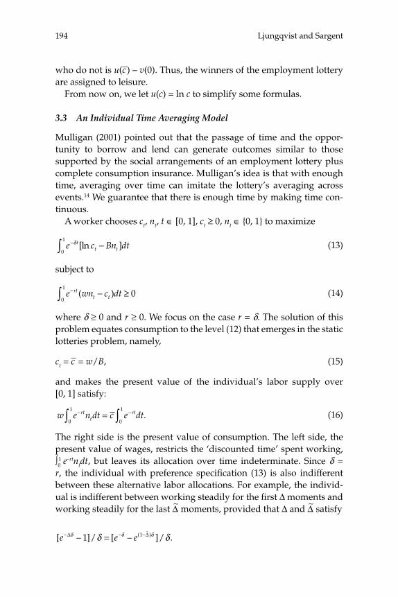
Ljungqvist and Sargent194
who do not is u(c–) – v(0). Thus, the winners of the employment lottery are assigned to leisure.
From now on, we let u(c) = ln c to simplify some formulas.
3.3 An Individual Time Averaging Model
Mulligan (2001) pointed out that the passage of time and the oppor-tunity to borrow and lend can generate outcomes similar to those supported by the social arrangements of an employment lottery plus complete consumption insurance. Mulligan’s idea is that with enough time, averaging over time can imitate the lottery’s averaging across events.14 We guarantee that there is enough time by making time con-tinuous.
A worker chooses ct, nt, t ∈ [0, 1], ct ≥ 0, nt ∈ {0, 1} to maximize
e c Bn dttt t
− −∫ δ [ln ]0
1 (13)
subject to
e wn c dtrtt t
− − ≥∫ ( ) 00
1 (14)
where δ ≥ 0 and r ≥ 0. We focus on the case r = δ. The solution of this problem equates consumption to the level (12) that emerges in the static lotteries problem, namely,
ct = c– = w/B, (15)
and makes the present value of the individual’s labor supply over [0, 1] satisfy:
w e n dt c e dtrtt
rt− −= ∫∫ .0
1
0
1 (16)
The right side is the present value of consumption. The left side, the present value of wages, restricts the ‘discounted time’ spent working, ∫0
1 e–rtntdt, but leaves its allocation over time indeterminate. Since δ = r, the individual with preference specifi cation (13) is also indifferent between these alternative labor allocations. For example, the individ-ual is indifferent between working steadily for the fi rst Δ moments and working steadily for the last Δ∼ moments, provided that Δ and Δ∼ satisfy
[ – ]/ [ – ]/ .– – ( – )e e eΔδ δ δδ δ1 1= Δ�

195Indivisible Labor, Human Capital, Lotteries, and Savings
Of course, many other employment patterns also work, including ones that “chatter” by having the worker rapidly move back and forth between employment and leisure.15
3.4 An Intertemporal Lotteries Model
Now consider a continuum j ∈ [0, 1] of ex ante identical workers like those in subsection 3.3. A planner chooses a consumption and employ-ment allocation ct
j ≥ 0, ntj ∈ {0, 1} to maximize
e c Bn dt djtt
jt
j− −∫∫ δ [ln ]0
1
0
1 (17)
subject to
e w n dj c dj dtrttj
tj− −⎡
⎣⎢⎤⎦⎥
≥∫∫∫ 0
1
0
1
0
10. (18)
Thus, the planner can borrow and lend at an instantaneous rate r. We again assume that r = δ. The planner solves this problem by setting ct
j = c–t for all j ∈ [0, 1] and φt = ∫01nt
jdj, exposing each household at time t to a lottery that sends him to work with probability φt. The planner chooses c–t and φt to maximize
e c B dtrtt t
− −∫ [ln ]φ0
1 (19)
subject to
e w c dtrtt t
− − ≥∫ [ ] .φ 00
1 (20)
This is obviously equivalent to problem (13)–(14). It follows that there are many intertemporal lottery patterns that support the optimal consump-tion allocation ct
j = w/B. Only the present value of time spent working is determined. Among the alternative types of lotteries that work are these:
1. One lottery before time 0: Before time 0, the planner can randomize over a constant fraction of people φ– who are assigned to work for every t ∈ [0, 1], and a fraction 1 – φ– who are asked to specialize in leisure, where φ– is chosen to satisfy the planner’s intertemporal budget constraint (20).
2. A lottery at each t: At each time t ∈ [0, 1], the planner can run a lottery that sends a time invariant fraction φ– to work and a fraction 1 – φ– to leisure.

Ljungqvist and Sargent196
3. Another lottery at each t: At each time t ∈ [0, 1], the planner can run a lottery that sends a fraction φt to work and 1 – φt to leisure at instant t, where φt is free to be any function that satisfi es the planner’s inter-temporal budget constraint (20). Only the present value of φt is deter-mined.
The indeterminacy among such lotteries evaporates in the next sec-tion when by adding human capital we confront people with career choices.
3.5 Time Averaging with Human Capital
We return to an isolated consumer who copes with the instantaneous labor supply indivisibility by borrowing and lending. We alter the consumer’s choice set in the model of subsection 3.3 by adding a very simple technology that describes how work experience promotes the accumulation of human capital. Where h ∈ (0, 1), the household’s bud-get constraint is now
e w h n c dtrtt t t
− − ≥∫ [ ( ) ]ψ 00
1 (21)
where
h n dst s
t= ∫0
(22)
ψ ( ).
hh h
H h ht
t
=<
> ≥
⎧⎨⎪
⎩⎪
1
1
if
if
�
� (23)
Two solutions interest us:
• A corner solution in which (h, B, H) are such that the person chooses to set ∫0
1ntdt < h. In this case, the model becomes equivalent with the model of subsection 3.3. The individual chooses to set
c– = wB–1 (24)
and to work a present value of time at a low skilled wage that is suf-fi cient to support this constant level of consumption.
• An interior solution for which (h, B, H) are such that the household chooses to set h < ∫0
1ntdt < 1; i.e., the household chooses to become high

197Indivisible Labor, Human Capital, Lotteries, and Savings
skilled but also to enjoy some leisure. In such an interior solution, con-sumption ct = c– will satisfy
c– = wHB–1. (25)
Time spent working when unskilled and skilled satisfy
c e dt w e n dt H e n dtrt rttL rt
tH− − −= +⎡
⎣⎢⎤⎦⎥∫∫ 0
1
00
1 1
∫∫ (26)
where
nn h h
tL t t=
= <⎧⎨⎪
⎩⎪
1 10
if andotherwise
�
, (27)
and
nn h h
tH t t=
= ≥⎧⎨⎪
⎩⎪
1 10
if andotherwise
�
. (28)
The fi rst term on the right side of (26) is the marginal product of a low productivity person times the present value of the time that a worker works when unskilled. The second term is the marginal product of a high productivity person times the present value of working time when skilled.
Backloading: When r = δ > 0 and (h, B, H) call for a solution that is interior in the sense that 1 > ∫0
1ntdt > h, the problem of maximizing (13) subject to (21) and (22) has the following solution. There exists an s that solves
c e dt w e dt H e dtrt rt rt
s hs
s h− − −
+
+= +⎡
⎣⎢⎤⎦⎥∫∫ �
�1
0
1
∫∫and such that the household sets nt = 0 for t < s and nt = 1 for t ≥ s. Thus, the household ‘back loads’ all of its work and takes leisure early. To understand why this is the solution, consider the disutility of work associated with this solution:
B B e dtrt
s= −∫ .
1 (29)
Starting from this allocation, consider a perturbation in which the household supplies some labor earlier and takes some leisure later, but keeps the disutility of labor fi xed at B–. Because of discounting, such a shift allows the household to work less total time over the interval [0, 1]

Ljungqvist and Sargent198
(i.e., ∫01ntdt would be smaller), but involves working a smaller proportion
of its time as a high skill worker. That would lower the present value of income associated with a given disutility of labor and so is subopti-mal.
3.6 Lotteries with Human Capital
Now suppose that a planner designs a consumption sharing plan and an intertemporal employment lottery to maximize (17) subject to
e w h n c dj dtrttj
tj
tj− − ≥∫∫ [ ( ) ]ψ 0
0
1
0
1 (30)
where each household j has the skill accumulation technology described in subsection 3.5.
A perturbation argument leads to the conclusion that the planner administers a life-time employment lottery once and for all before time 0 and assigns a fraction φ of people to work always (nt
j = 1 for all t ∈ [0, 1] for these unlucky people) and a fraction 1 – φ always to enjoy leisure (nt
j = 0 for all t ∈ [0, 1] for these lucky ones).16 The planner’s problem then becomes to choose c– and φ ∈ [0, 1] to maximize
(ln )c B e dtt− −∫φ δ
0
1
subject to
φw e dt H e dt c e dtrt rt
h
h rt− − −+⎡⎣⎢
⎤⎦⎥
≥∫∫ ∫�
�1
0 0
1. (31)
An interior solution sets φ to satisfy
c e r w e dt H e dtr rt rt
h
h[ ]/ .1
1
0− = +⎡
⎣⎢⎤⎦⎥
− − −∫∫φ �
�
(32)
Consumption c– satisfi es
c w B e e dt H e dtrt rt rt
h
h= ( ) +⎡
⎣⎢⎤⎦⎥
−−
− −∫ ∫∫0
1 1 1
0�
�
.. (33)
3.6.1 Comparison of Outcomes In the individual time averag-ing model of subsection 3.5, when (h, B, H) are such that the worker chooses the corner solution ∫0
1ntdt < h (i.e., he chooses not to acquire skills), consumption given by (24) is less than given in formula (33) for the lotteries economy. But when (h–, B, H) are such that the worker

199Indivisible Labor, Human Capital, Lotteries, and Savings
chooses an interior solution ∫01nt > h (i.e., he chooses to acquire skills),
his consumption level under time-averaging (25) exceeds that attained in (33) under lotteries. It follows that in the model with human capi-tal, lotteries signifi cantly change allocations relative to the individual time averaging model. In the presence of human capital, the lottery model supports an allocation with a higher ex ante utility than can be attained by having the individual alternate between work and leisure and smooth consumption by borrowing and lending. It does so by con-vexifying a “mother of all indivisibilities,” the decision to acquire skills over individual lifetimes.
4 Taxation under Time Averaging versus Lotteries
We add labor taxation and lump sum government transfers to the model of section 3 and regard it as describing a small open economy. The gov-ernment and the agents borrow and lend at the exogenous interest rate r. We continue to focus on the case r = δ. Furthermore, for expositional simplicity, we set r = δ = 0 so that the discounted times above now equal fractions of an individual’s time endowment over the unit interval. Let Φavg and Φlott denote the fraction of time spent working under time aver-aging and lotteries, respectively: Φavg = ∫0
1ntdt and Φlott = ∫01φtdt.
The government levies a tax rate τ on labor income and balances its budget over the unit interval of time by returning all tax revenues to the agents as equal per-capita lump sum transfers. Let T be the present value of all lump sum transfers to an agent.
4.1 Taxation without Human Capital
The results of sections 3.3 and 3.4 lead us to anticipate correctly that without human capital, taxation has identical effects on the aggregate labor supply under time averaging and lotteries, i.e., Φavg = Φlott = Φ. Specifi cally, the budget constraints in (14) and (18) become
( – ) – ,1 0τ w c TΦ + ≥ (34)
and, corresponding to our earlier fi rst-order condition (15) at an interior solution, the optimal consumption level under taxation satisfi es
c wB= ( – ) .–1 1τ (35)

Ljungqvist and Sargent200
After substituting (34) into (35) and invoking T = τ wΦ, the equilibrium labor supply is
Φ = min{(1 – τ) B–1, 1}, (36)
where we have explicitly included the possibility of a corner solution with Φ = 1.
Figure 3.2 depicts nonemployment, 1 – Φ, as a function of the tax rate, τ, and the preference parameter for the disutility of working, B.17
4.2 Taxation with Human Capital and Lotteries
It is easy to modify our earlier analysis of the model with lotteries and human capital to include taxes. With taxation and r = 0, the expressions for the budget constraint (31) and the optimality condition (33) at an interior solution in section 3.6 are modifi ed to become
( – ) [ ( – ) ] – ,1 1 0τ w h h H c Tlott� �
+ + ≥Φ (37)
and
c w h h H B= +( – ) [ ( – ) ] .–1 1 1τ� �
(38)
After substituting (37) in (38), and invoking T = τw[h + (1 – h)H]Φlott, the equilibrium labor supply is
Φlott = min{(1 – τ)B–1, 1}. (39)
Figure 3.3 illustrates an equilibrium outcome when the tax rate is such that the stand-in household chooses an interior solution to its labor supply.
4.3 Taxation with Human Capital and Time Averaging
Substantially more interesting possibilities emerge with time averag-ing. Depending on the parameterization and the tax rate, there are three constellations of outcomes: (1) for low tax rates, everyone chooses to become skilled, Φavg ∈ [h, 1]; (2) for somewhat higher tax rates, equi-libria have the property that a fraction of people choose to become skilled and the remainder choose to stay unskilled; and (3) for a highest range of tax rates, no one chooses to become skilled, Φavg ∈ (0, h). These outcomes are depicted in fi gures 3.4 and 3.5. In the middle region, the
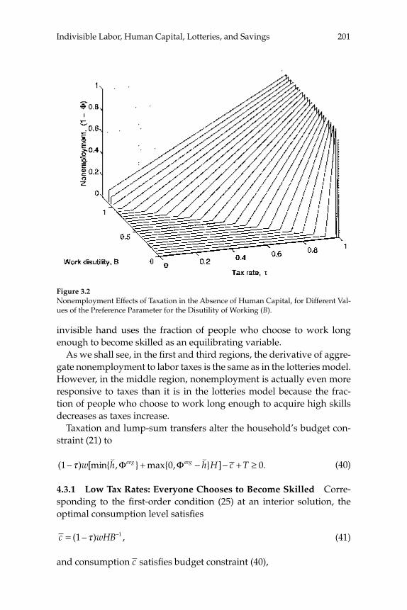
201Indivisible Labor, Human Capital, Lotteries, and Savings
invisible hand uses the fraction of people who choose to work long enough to become skilled as an equilibrating variable.
As we shall see, in the fi rst and third regions, the derivative of aggre-gate nonemployment to labor taxes is the same as in the lotteries model. However, in the middle region, nonemployment is actually even more responsive to taxes than it is in the lotteries model because the frac-tion of people who choose to work long enough to acquire high skills decreases as taxes increase.
Taxation and lump-sum transfers alter the household’s budget con-straint (21) to
( – ) [min{ , } max{ , – } ] – .1 0 0τ w h h H c Tavg avg� �
Φ Φ+ + ≥ (40)
4.3.1 Low Tax Rates: Everyone Chooses to Become Skilled Corre-sponding to the fi rst-order condition (25) at an interior solution, the optimal consumption level satisfi es
c wHB= ( – ) ,–1 1τ (41)
and consumption c– satisfi es budget constraint (40),
Figure 3.2Nonemployment Effects of Taxation in the Absence of Human Capital, for Different Val-ues of the Preference Parameter for the Disutility of Working (B).
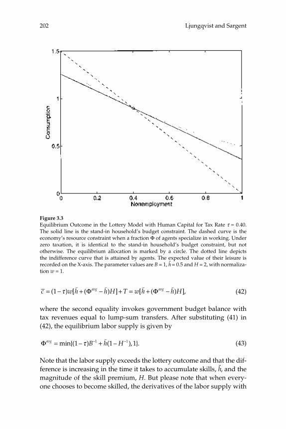
Ljungqvist and Sargent202
c w h h H T w h h Havg avg= + + = +( – ) [ ( – ) ] [ ( – ) ],1 τ� � � �
Φ Φ (42)
where the second equality invokes government budget balance with tax revenues equal to lump-sum transfers. After substituting (41) in (42), the equilibrium labor supply is given by
Φavg B h H= +min{( – ) ( – ), }.– –1 1 11 1τ�
(43)
Note that the labor supply exceeds the lottery outcome and that the dif-ference is increasing in the time it takes to accumulate skills, h, and the magnitude of the skill premium, H. But please note that when every-one chooses to become skilled, the derivatives of the labor supply with
Figure 3.3Equilibrium Outcome in the Lottery Model with Human Capital for Tax Rate τ = 0.40. The solid line is the stand-in household’s budget constraint. The dashed curve is the economy’s resource constraint when a fraction Φ of agents specialize in working. Under zero taxation, it is identical to the stand-in household’s budget constraint, but not otherwise. The equilibrium allocation is marked by a circle. The dotted line depicts the indifference curve that is attained by agents. The expected value of their leisure is recorded on the X-axis. The parameter values are B = 1, h = 0.5 and H = 2, with normaliza-tion w = 1.
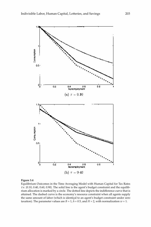
203Indivisible Labor, Human Capital, Lotteries, and Savings
Figure 3.4Equilibrium Outcomes in the Time Averaging Model with Human Capital for Tax Rates τ ∈ {0.10, 0.40, 0.60, 0.90}. The solid line is the agent’s budget constraint and the equilib-rium allocation is marked by a circle. The dotted line depicts the indifference curve that is attained. The dashed curve is the economy’s resource constraint when all agents supply the same amount of labor (which is identical to an agent’s budget constraint under zero taxation). The parameter values are B = 1, h = 0.5, and H = 2, with normalization w = 1.
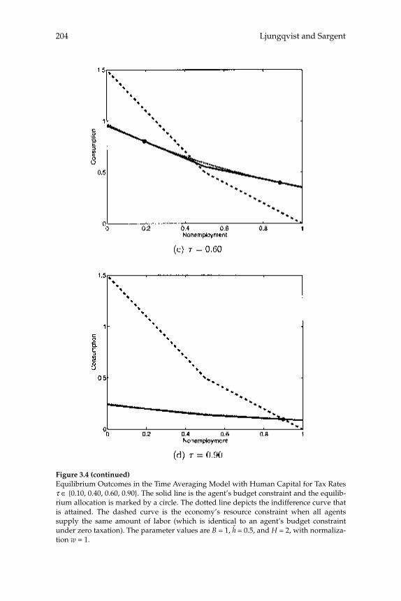
Ljungqvist and Sargent204
Figure 3.4 (continued)Equilibrium Outcomes in the Time Averaging Model with Human Capital for Tax Rates τ ∈ {0.10, 0.40, 0.60, 0.90}. The solid line is the agent’s budget constraint and the equilib-rium allocation is marked by a circle. The dotted line depicts the indifference curve that is attained. The dashed curve is the economy’s resource constraint when all agents supply the same amount of labor (which is identical to an agent’s budget constraint under zero taxation). The parameter values are B = 1, h = 0.5, and H = 2, with normaliza-tion w = 1.
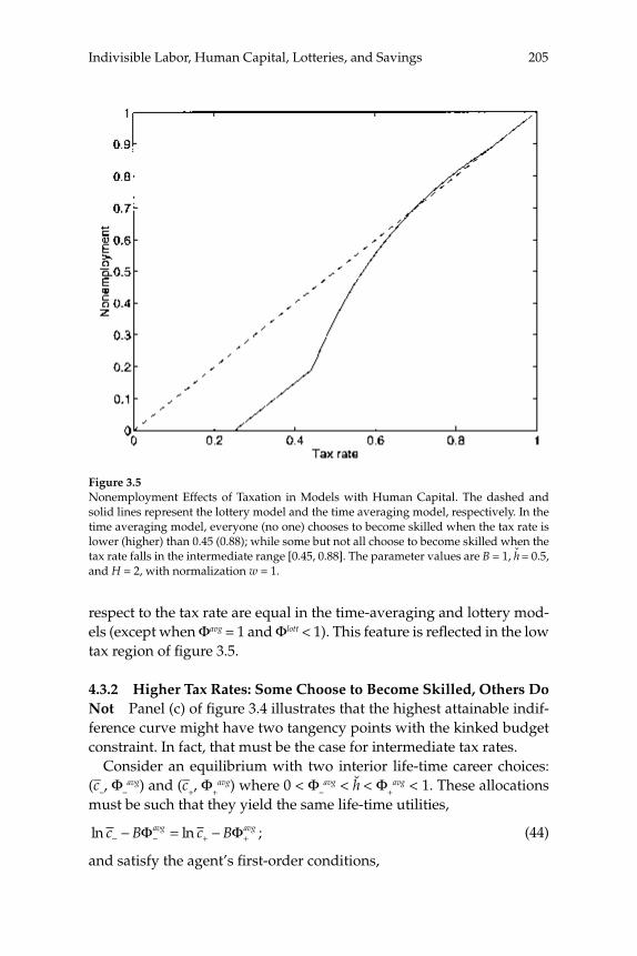
205Indivisible Labor, Human Capital, Lotteries, and Savings
respect to the tax rate are equal in the time-averaging and lottery mod-els (except when Φavg = 1 and Φlott < 1). This feature is refl ected in the low tax region of fi gure 3.5.
4.3.2 Higher Tax Rates: Some Choose to Become Skilled, Others Do Not Panel (c) of fi gure 3.4 illustrates that the highest attainable indif-ference curve might have two tangency points with the kinked budget constraint. In fact, that must be the case for intermediate tax rates.
Consider an equilibrium with two interior life-time career choices: (c––, Φ–
avg) and (c–+, Φ+avg) where 0 < Φ–
avg < h < Φ+avg < 1. These allocations
must be such that they yield the same life-time utilities,
ln ln ;c B c Bavg avg− − + +− = −Φ Φ (44)
and satisfy the agent’s fi rst-order conditions,
Figure 3.5Nonemployment Effects of Taxation in Models with Human Capital. The dashed and solid lines represent the lottery model and the time averaging model, respectively. In the time averaging model, everyone (no one) chooses to become skilled when the tax rate is lower (higher) than 0.45 (0.88); while some but not all choose to become skilled when the tax rate falls in the intermediate range [0.45, 0.88]. The parameter values are B = 1, h = 0.5, and H = 2, with normalization w = 1.

Ljungqvist and Sargent206
c wB−−= −( )1 1τ , (45)
c HwB+−= −( ) .1 1τ (46)
When evaluated at those allocations, the agent’s budget constraint must hold with equality,
c w Tavg− −= − +( ) ,1 τ Φ (47)
c w H h Tavg avg+ + += − + − − +( ) [ ( )( )] .1 1τ Φ Φ
� (48)
From (44) we get
ln ( );cc
B avg avg+
−+ −
⎛⎝⎜
⎞⎠⎟
= −Φ Φ (49)
(45) and (46) imply
cc
H+
−
= , (50)
c c wB H+ −−− = − −( ) ( );1 11τ (51)
while (47) and (48) yield an alternative expression for the consumption differential
c c w H havg avg avg+ − + − +− = − − + − −( ) [ ( )( )].1 1τ Φ Φ Φ
� (52)
From (51) and (52) we get
B H B havg avg avg( ) ( )[ ( )].Φ Φ Φ+ − +− = − − −1 1�
(53)
After substituting (50) and (53) into (49), we obtain an expression for the labor supply that does not depend on the tax rate,
Φ+−= + −
−avg B h
HB H
1
1
� ln( )
, (54)
and the value for Φ_avg can then be solved from (53),
Φ Φ− +−= −avg avg B H1 ln . (55)

207Indivisible Labor, Human Capital, Lotteries, and Savings
4.3.3 The Highest Tax Rates: No One Chooses to Become Skilled This equilibrium class looks just like the equilibrium without human capital that we studied in section 4.1.
5 Synopsis of a General Equilibrium Analysis
Ljungqvist and Sargent (2006a) extend our comparison of employment lotteries and time-averaging to a closed-economy stochastic general equilibrium setting that includes physical capital, stochastic skill accu-mulation, and aging. Relative to our models in sections 3 and 4, those extensions enhance heterogeneity among agents and create more dif-ferences in the identities of the nonemployed workers across the lotter-ies and time-averaging models.18
The models have stochastic transitions among three age groups, young, old, and retired workers. There is a stochastic skill accumula-tion technology between high and low skills that allows deterioration as well as enhancement of skills. Individuals save claims on capital that enters an economy-wide production function. There is a fl at rate tax on earnings from labor, which equal a wage times a skill level. An indivisi-blity in labor supply is convexifi ed either by employment lotteries or individual time-averaging.
The employment lotteries and time-averaging versions of the model share the same striking implication of the section 4 model that the quan-titative responses of aggregate nonemployment to labor tax increases are quantitatively similar, thus reconfi rming our fi ndings about the insen-sitivity of aggregate outcomes to the “aggregation theory.” However, there are substantial differences in the characteristics of those who work less as taxes increase in the lotteries and the time-averaging versions of the models. As taxes increase at low tax rates, the employment lotteries model assigns more and more old workers with low skills to specialize in leisure, while the equilibrium outcome in the time-averaging model is that more and more old workers with high skills stop working. At higher tax rates, as taxes increase, the employment lotteries model assigns more and more young workers with low skills to specialize in life-long lei-sure, while in the time-averaging model the outcome is that more young workers with high skills stop working. In the time-averaging model, a worker’s age, skill, and accumulated fi nancial assets interact with tax rates to determine when to retire. Thus, in the time-averaging model, labor tax rates work by affecting the when-to-retire margin.
Ljungqvist and Sargent208
We shall refer to some of these results again in subsection 6.5 when we come back to address the question “Do taxes explain European non-employment?”
6 Practical Implications of the Models
To summarize what to make of our theoretical fi ndings, this section (1) describes how it is impossible to include social insurance with the high benefi t levels observed in Europe while maintaining the high disutility of labor favored by Prescott; (2) summarizes what delivers that high labor supply elasticity in the lotteries and the time-averaging model; (3) compares calibration strategies for that disutility in the lotteries and time-averaging models without benefi ts; (4) criticizes some of the evi-dence Prescott used to justify setting a high disutility parameter; and (5) answers “no” to the question “Do taxes explain European nonem-ployment”?
6.1 Social Insurance Is Problematic
Prescott (2002, p. 9) summarized his fi ndings by saying: “I fi nd it remark-able that virtually all of the large difference in labor supply between France and the United States is due to differences in tax systems. I expected institutional constraints on the operation of labor markets and the nature of the nonemployment benefi t system to be more important.” Because generous social insurance is indeed a pervasive phenomenon in Europe, accounting for cross-country employment differences with any model that ignores it is naturally subject to the suspicion that one has miscast other parameters in order to fi t the employment observa-tions. Figure 3.1 confi rms that suspicion about the stand-in household model with complete markets and employment lotteries.19
Rogerson (2006a) adds social insurance to a stand-in household model and interprets it as a subsidy to leisure: “unemployment insur-ance programs, social security programs and traditional welfare pro-grams all involve a transfer of resources that is conditional on not engaging in market work and hence implicitly involve marginal subsi-dies to leisure.” We like Rogerson’s description especially as it pertains to Europe, but we question the way that he implicitly sets replacement rates for European social insurance programs. Referring to Prescott (2004), Rogerson calibrates the preference parameter α in the stand-in household’s utility function (1) so that h = 1/3 at the U.S. tax level, then

209Indivisible Labor, Human Capital, Lotteries, and Savings
assumes that h– = 1 in budget constraint (2). The replacement rate ρ is implicitly determined by his assumptions about government taxes and tax revenues. In a key calibration that provides an explanation for why hours of work in Continental Europe are only 2/3 of those in the United States, Rogerson assumed that both economies hand back lump-sum the tax revenues raised by the U.S. level of taxes, while the 20 percentage points incremental taxation in Continental Europe are used to fi nance the subsidy to leisure. A back-of-the-envelope calculation then yields a replacement rate of 15 percent.20 The low replacement rate that he cali-brates is much lower than the replacement rates estimated by Martin (1996), which are more than 50 percent. Figure 3.1 tells why Rogerson wants a low replacement rate.
When it comes to understanding cross-country differences in employ-ment and nonemployment, social insurance seems to be the Achilles’ heel of models that have a high labor supply elasticity. Nevertheless, let’s temporarily set aside the troublesome issue of social insurance and explore what our analysis in sections 3 and 4 has taught us about the forces behind Prescott’s high aggregate labor supply elasticity.
6.2 Time Averaging versus Lotteries
As reviewed in section 2.4, Prescott (2006) assigns great importance to Rogerson’s model of employment lotteries as a theory of aggrega-tion. But taking our cue from Mulligan (2001), we have shown that this aggregation theory is not necessary for Prescott’s results.21 In a model without human capital and no uncertainty, households can attain the same allocations by alternating between spells of employment and non-employment and relying on private savings to smooth consumption. This is good news for Prescott’s tax analysis because his assumption of complete markets with employment lotteries has been questioned and occasionally deemed incredible.
But the pertinence of the employment lotteries model for Prescott’s tax results reemerges when we add a human capital acquisition tech-nology. Like the choice of either working full-time or not at all in Rogerson’s (1988) static model, career choices in a dynamic model with human capital accumulation introduce a kind of indivisibility. The individual who accumulates human capital reaps the returns on that investment by working. By way of contrast, in an economy with employment lotteries and complete markets, the effi cient alloca-tion is one where some individuals pursue labor careers while others

Ljungqvist and Sargent210
specialize in providing leisure to the stand-in household. This is accom-plished through a grand lottery for newborn workers that grants the same ex ante utility to everyone but dooms the losers of the lottery to life-long labor careers.22
In the absence of employment lotteries, individuals are on one side or the other of the expected consumption-leisure tradeoff in the lottery economy. The individual consumes less if returns on human capital are too low to compensate him for bearing the disutility of supplying the labor needed to acquire human capital all by himself. The random assign-ment of labor in the lottery allocation implies a more favorable expected tradeoff that could very well justify human capital investments by the community. In contrast, an isolated individual works and consumes more only if returns on human capital are high enough to spur careers with human capital acquisition, because then his optimality condition will favor a longer working life as compared to the average labor supply in the lottery allocation that smooths the indivisibility of labor careers.
The different allocations supported by time averaging versus lotteries have implications for the employment effects of taxation. For example, if the equilibria without taxation are characterized by a corner solution with full employment, successive increases in taxation will fi rst reduce employment in the economy with employment lotteries while the labor supply in the economy with time averaging is more robust. The reason is that individuals who have accumulated human capital in the time-averaging economy view the investment as a sunk cost and are unwill-ing to surrender the returns on those sunk investments by shortening their careers. The lottery economy does not exhibit this feature because the lotteries have convexifi ed labor careers so that the losers pursue life-long careers and any substitution toward leisure shows up in the number of winners who specialize in leisure. However, if we suppose that individuals in the time-averaging economy do choose to shorten their careers in response to taxation, then the marginal employment effects of taxes are identical to those of the lottery economy (and even surpass those when taxes become so high that they compel some indi-viduals to give up on human capital accumulation altogether). Hence, how the disutility of working is calibrated is crucial for understanding how taxes affect those career choices.
6.3 Calibration of the Disutility of Working
In the fi rst business cycle model with Rogerson’s (1988) aggregation theory, Hansen (1985) took the calibration of a model with divisible

211Indivisible Labor, Human Capital, Lotteries, and Savings
labor as a starting point for calibrating the disutility of working. Spe-cifi cally, the model with divisible labor was calibrated to match “the observation that individuals spend 1/3 of their time engaged in market activities and 2/3 of their time in non-market activities.” After impos-ing the same steady-state hours of work across the models, Hansen arrived at a calibration for the disutility of working in the model with indivisible labor.
An alternative to matching the fraction of households’ total hours devoted to work is taken by Hopenhayn and Rogerson (1993), who calibrate the disutility of working to “produce an employment to pop-ulation ratio equal to .6.” For an economy with indivisible labor and employment lotteries, it would seem that the latter calibration target is the proper one. In any case, the two approaches share the important outcome that target observations imply calibrations to interior solu-tions for the stand-in household’s labor supply. We understand that those interior solutions defi ne what Prescott (2006, p. 221) refers to as “the empirically interesting cases.”
The model with employment lotteries prompts us to try to match snapshots of averages in the population. The time-averaging model tells us instead to focus on matching household outcomes over time. The labor services performed by individuals determine their dispos-able incomes and consumption rates in the time-averaging model, while they don’t in the stand-in household model because of the exten-sive state-contingent consumption insurance. Hence, it is important from the perspective of the time-averaging model to study the distribu-tion of labor supply across individuals while, in the stand-in household model, we can just sum up the labor supplied by all individuals and focus on aggregates.23 In our time-averaging model, taxes impact labor supply by shortening individuals’ labor careers. Besides the effects of differences in the subjective rate of discount and the market interest rate, the simple model has little to say about the timing of nonemploy-ment spells—front loading (“youth nonemployment”), back loading (“early retirement”) or intermittent shorter spells of nonemployment. However, as summarized in section 5, our numerical analysis of a related stochastic general equilibrium model with human capital accu-mulation in Ljungqvist and Sargent (2006a) suggests that taxes cause early retirement.
The model without employment lotteries raises the question: What should be the calibration target for the length of labor careers? Some might argue that the large number of people working until the legis-lated retirement age suggests a corner solution and the disutility of

Ljungqvist and Sargent212
working should be calibrated accordingly. Needless to say, such a cali-bration would mute the employment effects of taxation.24 Others might suggest that the employment effects of taxation manifest themselves largely as having one of two spouses in a household curtail his/her labor career. Hence, the disutility of working should be calibrated to refl ect household composition in the economy.
Much remains to be learned from explicit models of the family, such as the collective labor supply model of Chiappori (1992). However, one immediate implication of changing the perspective from models with a stand-in household to models of nuclear families without employ-ment lotteries is the additional empirical evidence that needs to be addressed before one can declare any theoretical success in explaining cross-country differences in employment. The evidence that we present below does not look particularly promising for the tax explanation of European nonemployment.
6.4 Prescott’s Evidence for a High Labor Supply Elasticity
Prescott (2006) emphasizes that a high labor supply elasticity is neces-sary to reproduce business cycles of the magnitude and nature observed. He says that compelling corroborating evidence for a high aggregate elasticity can be found in observations on employment and tax rates across countries and across time, as studied and modeled by Prescott (2004), who is particularly successful reproducing the observed differ-ences between France and Germany, on the one hand, and the United States, on the other. Given that French and German tax rates in table 3.1 increased by 10 and 7 percentage points, respectively, the aggregate labor supply elasticity must indeed be very high if tax changes are to explain the plummeting employment in these countries.25 In addition
Table 3.1Empirical Estimates of Tax Rates (Prescott 2004, Table 2) and Benefi t Dependency Rates in the Population Aged 15 to 64 (OECD 2003, Table 4.1)
Empirical Estimates of Tax Rates
Benefi t Dependency Rates in the Working-Age Population
United States
France
Germany
1970–74
0.40
0.49
0.52
1993–96
0.40
0.59
0.59
1980
0.168
0.139
0.152
1999
0.137
0.242
0.224
213Indivisible Labor, Human Capital, Lotteries, and Savings
to being an example of a successful application of the growth model with a stand-in household, Prescott interprets the theory’s ability to rationalize those outcomes as evidence for a high labor supply elastic-ity. The high labor supply elasticity is the key ingredient that makes real business cycle theory work and that also explains the dramatic fall in European employment.
Prescott suggests that one reason that earlier microeconomic stud-ies failed to fi nd a high labor supply elasticity is that they ignored human capital investments. He refers to a study of Imai and Keane (2004) for substantiation. Imai and Keane analyze how a human capital acquisition technology can reconcile a rather fl at life-cycle labor sup-ply path with a high labor supply elasticity, which they estimate to be 3.8. Prescott takes comfort in this high elasticity. But there is another implication that emerges with human capital accumulation and that is more troublesome for real business cycle theory. Specifi cally, the pres-ence of human capital weakens the link between the curvature param-eter on the disutility of working and the optimal response of workers with these preferences to fl uctuations in the wage rate. Imai and Keane (2004, fi gure 8) forcefully illustrate this with a computational experi-ment that imposes a temporary wage increase of 2 percent and fi nds that at age 20 a person with that 3.8 elasticity parameter would respond by increasing hours by only 0.6 percent. As Imai and Keane explain, the presence of human capital adds a term representing the continuation value to what had been an intratemporal marginal condition for moment t labor supply in models without human capital; the presence of this term means that the wage understates a worker’s value of time, espe-cially a young worker’s. The response of hours to a temporary wage jump increases with age, especially towards the end of a career. Hence, the inclusion of human capital investments in real business cycle mod-els might increase the aggregate labor supply elasticity but it would be at odds with the business-cycle fact that most variations in hours are borne by young rather than old workers.26 Once again, this highlights the new set of interesting issues that arise when we abandon Prescott’s aggregation theory and his stand-in household.
Although Imai and Keane (2004) offer no simulations of the employ-ment effects of taxation, their estimated model could conceivably support Prescott’s assertion of potent employment effects of taxes. Relevant for our analysis of the extensive margin in labor supply, the estimated age-hours path by Imai and Keane (2004, fi gure 3) predicts a sharp acceleration of retirement already at the age of 50. While we
Ljungqvist and Sargent214
have yet to observe the actual retirement of the cohort in their study, this prediction is clearly at odds with past data from the United States where retirement peaks have been recorded at the ages of 62 and 65. See, for example, the study of Rust and Phelan (1997), who attribute the observed past retirement behavior to the U.S. Social Security and Medi-care insurance systems—institutions that are not modeled by Imai and Keane (2004). Despite our skepticism of their forecast of an imminent early retirement boom in the United States, we fully agree with Imai and Keane’s emphasis on the importance of modeling human capi-tal accumulation when attempting to understand individuals’ labor supply.
6.5 Do Taxes Explain European Nonemployment?
Prescott’s (2002) explanation of today’s 30-percent difference in labor input per working-age person in France relative to the U.S. posits a tax differential of 20 percentage points. From a time series perspective, Prescott (2004) fi nds that his theory is especially successful in explain-ing changes over time for the two large Continental European coun-tries—France and Germany—that have increased their taxes by 10 and 7 percentage points, respectively, between the early 1970s and the mid-1990s when the U.S. tax rate remained constant (see table 3.1). But this means that half of today’s tax differential between France and Ger-many versus the United States was already in place in the early 1970s when hours worked were similar across these countries. As described in section 2.3, to explain why those already large early tax differen-tials did not lower European employment relative to the United States, Prescott estimated a French-German consumption-output ratio that was signifi cantly depressed relative to that of the United States. Hence, variation in consumption-output ratios over time and across countries, not explained by the theory, contributes substantially to the success of Prescott’s account. We have nothing to say about this exogenous factor and instead turn to discuss how we might go about seeking further evidence about the particular individuals that the theory predicts to be nonemployed.
In section 5, the lotteries and time averaging versions of the stochas-tic general equilibrium model with human capital accumulation have some deceptively appealing implications about nonemployment. In the lotteries model, the effi cient allocation prescribes making older workers who have had disadvantageous labor careers the fi rst to be furloughed
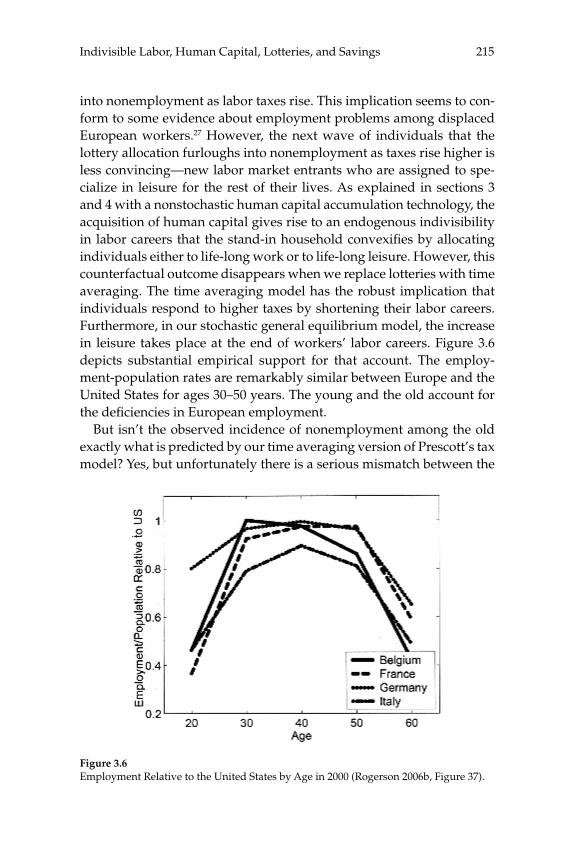
215Indivisible Labor, Human Capital, Lotteries, and Savings
into nonemployment as labor taxes rise. This implication seems to con-form to some evidence about employment problems among displaced European workers.27 However, the next wave of individuals that the lottery allocation furloughs into nonemployment as taxes rise higher is less convincing—new labor market entrants who are assigned to spe-cialize in leisure for the rest of their lives. As explained in sections 3 and 4 with a nonstochastic human capital accumulation technology, the acquisition of human capital gives rise to an endogenous indivisibility in labor careers that the stand-in household convexifi es by allocating individuals either to life-long work or to life-long leisure. However, this counterfactual outcome disappears when we replace lotteries with time averaging. The time averaging model has the robust implication that individuals respond to higher taxes by shortening their labor careers. Furthermore, in our stochastic general equilibrium model, the increase in leisure takes place at the end of workers’ labor careers. Figure 3.6 depicts substantial empirical support for that account. The employ-ment-population rates are remarkably similar between Europe and the United States for ages 30–50 years. The young and the old account for the defi ciencies in European employment.
But isn’t the observed incidence of nonemployment among the old exactly what is predicted by our time averaging version of Prescott’s tax model? Yes, but unfortunately there is a serious mismatch between the
Figure 3.6Employment Relative to the United States by Age in 2000 (Rogerson 2006b, Figure 37).
Ljungqvist and Sargent216
arrangement that the theory uses to pay for those “early retirements” and what actually prevails in Europe. The theory states erroneously that the workers fi nance their nonemployment with either private insur-ance (in the lotteries model) or private savings (in the time averaging model). But as is well known, the nonemployed in the welfare states of Europe are to a large extent fi nanced with government supplied ben-efi ts. Table 3.1 depicts how the benefi t dependency rate in the working-age population has changed between 1980 and 1999. The largest benefi t programs in 1999 were disability, unemployment, and early retirement. The European welfare states have created dual economies that divide households into those who are gainfully employed and those who are inactive and living on government supplied benefi ts. The OECD (2005, fi gure SS3.1) reports that in 2000 the number of persons living in house-holds with a working-age head where no one works accounted for 11.1 percent and 16.1 percent of the total population in France and Germany, respectively, versus only 4.9 percent in the United States.
While there are no government supplied inactivity benefi ts in Prescott’s (2002, 2004) model, it is important to recognize that the employment effects of taxes hinge critically on the government’s returning the tax revenues as lump sum transfers to the households. Those transfers are vast. Their sheer magnitude makes the cost of the progressive propos-als made by some interest groups, especially in Europe, who want the government to guarantee modest levels of a citizen’s income, or “basic income,” pale by comparison.28
7 Concluding Remarks
We answer “no” to the question “Do taxes explain European nonem-ployment?” When we modify Prescott’s model to incorporate the gen-erous social insurance that European governments offer their citizens to protect them from periods of nonemployment, the fi t of the model deteriorates. We conclude by sketching an alternative view of Euro-pean nonemployment and by emphasizing three basic messages of our analysis.
7.1 Our Alternative Vision
To explain cross-country differences in employment rates, we advocate using a model that includes the following features that are missing or different from the model in Prescott (2002): (1) a much lower disutility

217Indivisible Labor, Human Capital, Lotteries, and Savings
of labor than chosen by Prescott; (2) other activities like unemployment, disability, and old-age retirement in addition to the two activities, labor and leisure, that are included in Prescott’s model; (3) government-sup-plied inactivity benefi ts; and (4) tax revenues that are not handed back lump-sum but rather are used to fi nance public goods and inactivity benefi ts.
Feature (1) will obviously help make the alternative framework com-patible with feature (3), i.e., the fact that Europe has generous social insurance. Feature (4) will also help by reactivating the negative income effect of taxation that Prescott disarmed when he assumed that all tax revenues are handed back lump sum to households. Under our alterna-tive assumption, tax revenues are used to fi nance public good that are imperfect substitutes for private consumption and to pay for inactiv-ity benefi ts that, in an equilibrium, are conferred on “marginalized” groups of the population. In such an equilibrium, the high taxes of Europe provide little of private value to those who actually pay them because tax revenues either fi nance public goods or accrue to people who are marginalized and not working. Hence, the negative income effect of taxation would help to keep most people at work and stop them from planning to arrange employment lotteries with high odds of leisure (in the lottery model) or to accumulate private wealth with the thought of taking early retirement (in the time averaging model).
We have already used some of these proposed features in our research on the European employment experience. Because we are also interested in explaining observations pertaining to stocks and fl ows of workers searching for jobs, we have incorporated an additional feature: (5) a search or matching friction that impedes moving between labor and leisure. Ljungqvist and Sargent (2007) construct a McCall search model and Ljungqvist and Sargent (2006c) construct several matching models and a search-island model that are able to match many aspects of U.S. and European employment outcomes over the last half cen-tury.29 These models put the spotlight on cross-country differences in the generosity of government inactivity benefi ts, rather than on the tax rates emphasized by Prescott (2002).
7.2 Three Basic Messages
Since our paper contains a number of nuances and qualifi cations, it seems appropriate that we summarize the main lessons in three basic messages.
Ljungqvist and Sargent218
1. Employment lotteries are not necessary for Prescott’s (2002) conclusion about large employment effects of taxation. The aggregate employment effects of taxation are quite similar in the lotteries and time averaging models, even though the identities of the nonemployed differ. A high disutility of labor and returning tax revenues via lump sum transfers to households are the critical ingredients for obtaining Prescott’s large employment effects of taxation.
2. A model with a high disutility of labor is a non-starter for explaining employment outcomes in Europe with its generous social insurance. A force-ful illustration of that is our incorporation of government-supplied benefi ts in Prescott’s model in section 2 where employment literally implodes. Hence, it is also important to avoid a common mistake of not differentiating between private and social insurance when discussing possible real-world examples of employment-lottery equilibria.30
3. The tax explanation for European nonemployment has counterfactual impli-cations about the identities of the nonemployed and how they are fi nanced. Empirical observations support neither the lottery model when it allocates people to specialize either in labor or in leisure, nor the time averaging model when it asserts that the nonemployed in Europe are successful people who have amassed enough savings to afford early retirement. The notion that nonemployed Europeans are fi nanced with private consumption insurance or personal savings is utterly wrong.
We are not able to run large-scale policy experiment with real-world economies, but our models do invite us to entertain thought experi-ments. The following question comes to mind. Faced with its predica-ment of high nonemployment in the last 30 years, suppose that Europe had to choose either a reform that cuts labor tax rates to the levels of the United States or a reform that replaces its social insurance programs with U.S. style income support. Which reform would increase European employment the most? Using the stand-in household model, Prescott (2002) is on the record as suggesting that the solution to European non-employment is to cut labor tax rates. We lean the other way and suggest that reforming social insurance would go much farther in providing incentives for people to choose to work.
Acknowledgments
We thank Kenneth Rogoff for urging us to explain why we are skeptical about Prescott’s account of lower hours in Europe and prefer our own

219Indivisible Labor, Human Capital, Lotteries, and Savings
(Ljungqvist and Sargent 2007). We thank Matteo Pignatti and Demian Pouzo for excellent help with the computations and Daron Acemoglu, Olivier Blanchard, V. V. Chari, Patrick Kehoe, Narayana Kocherla-kota, Ellen McGrattan, Tomasz Piskorski, Edward C. Prescott, Richard Rogerson, Kenneth Rogoff, Robert Shimer, and Kjetil Storesletten for very helpful criticisms.
Endnotes
1. We confess to being biased readers of Prescott’s work because in Ljungqvist and Sar-gent (2007), we assert that it is better to account for cross-country differences in employ-ment rates by emphasizing cross-country differences in benefi ts rather than taxes.
2. Jones (1988, p. 13) anticipated Mulligan’s idea when he wrote: “A natural question to raise here is that if the time horizons we are considering are suffi ciently divisible, why cannot timing perform the same function as lotteries?” Jones showed that timing could replace lotteries for an example without discounting.
3. As emphasized by Imai and Keane (2004), when we add human capital, the marginal condition describing leisure-consumption tradeoffs acquires an additional term that mea-sures the effect of current work experience on the continuation value via the accumula-tion of human capital. From the vantage of models with human capital, the marginal condition in the model of section 2 is misspecifi ed, creating an apparent “wedge.” Manu-elli and Seshadri (2005) adapt the Ben-Porath model to generate cross-country differences in wealth. Their model features a different technology for accumulating human capital than the one in this paper.
4. Alesina et al. (2005) documented that the European defi cit in hours worked per capita relative to the United States can be decomposed into fewer hours in a normal work week, fewer weeks worked in a year, and fewer people employed. Our analysis focuses on the last component. The large number of nonemployed who are supported with government funds especially concerns European policy makers. Our analysis of indivisible labor says nothing about the other two components that refl ect the intensive rather than the exten-sive margin in labor supply.
5. For an early analysis of large employment effects of government supplied benefi ts in a time-averaging model, see Hansen and Imrohoroglu (1992).
6. For example, see Ljungqvist and Sargent (2004b, ch. 11).
7. Prescott’s (2002) calibration can be extracted from the numbers reported in his table 4 together with equilibrium relationship (4). In particular, we can deduce that α(ct/yt)/(1 – θ) ≈ 1.65.
8. In the spirit of Prescott’s (2002) analysis, lump sum transfers to households are adjusted to ensure government budget balance.
9. For an alternate view that emphasizes the differences between using lotteries as an aggregation theory for fi rms versus households, see Ljungqvist and Sargent (2004a).
10. Prescott (2002) uses a capital-share parameter θ = 0.3 but he reports on neither the parameter α nor the ratio c/y. On the basis of Prescott (2004, table 2), we proceed here with the value c/y = 0.75. We set h = 0.4 as implied by a work week length of 40 hours and

Ljungqvist and Sargent220
Prescott’s (2004) assertion that “on a per person basis a household has about 100 hours of productive time per week.” Given these parameter values, we can match the U.S. out-come in Prescott’s (2002) table 4 by choosing the utility of leisure parameter α = 1.64. (For comparison, our calibration of α = 1.64 for the utility function (8) is almost the same as the Prescott (2004) calibration of α = 1.54 in a study using utility function (1).)
11. Prescott (2002, p. 8) multiplies an average tax rate by 1.6 to obtain a marginal tax rate. That procedure fails to follow the recommendation of Mulligan (2001), who noted that because the social planner is considering variations in the extensive rather than the intensive margin, the average rather than the marginal tax rate is relevant in the Hansen-Rogerson framework.
12. Shaw (1989) and Imai and Keane (2004) are good examples of studies that econo-metrically estimate technologies by which work now builds human capital later.
13. The natural borrowing constraint is weak enough to make the loan market perfect. See Aiyagari (1994) and Ljungqvist and Sargent (2004b) for discussions of the natural borrowing constraint.
14. The individual time-averaging models in the following subsections can be viewed as adaptations of a model of occupational choice by Nosal and Rupert (2005).
15. Nosal and Rupert (2005) study cases in which r ≠ δ, so that consumption and working schedules are tilted toward either the beginning or the end of the interval [0, 1].
16. Consider a deviation from this allocation that withdraws a positive measure of work-ers, lets them enjoy a small positive measure of leisure, then makes up the defi ciency in output by assigning work to some of those who initially specialize in leisure. It can be verifi ed that this perturbation increases the ex ante disutility of work component of (17).
17. As noted above, we have excluded benefi ts from the present analysis with the under-standing that were we to include a nonemployment benefi t like the one in section 2, the replacement rate ρ would continue to augment the tax wedge and operate in similar ways as before. This can easily be seen in the model without human capital. Adding a benefi t term alters the budget constraint (34) to
(1 – τ)wΦ – c– + T + ρ(1 – τ)w(1 – Φ) ≥ 0
and makes the equilibrium labor supply become
Φ = min{(1 – τ)(1 – ρ)B–1, 1} (*)
instead of (36). Equation (*) becomes the counterpart to (9). From the life-cycle perspec-tive that is highlighted in the model with indivisible labor and time averaging, everyone who is at an interior solution is also at the margin for taking up those benefi ts (unless the individual worker is up against a ceiling like h
– in section 2).
18. For another time averaging version of a stochastic general equilibrium model that focuses on the extensive margin of labor supply, see Chang and Kim (2006). In their model, agents are infi nitely lived and, hence, the life-cycle dimension of careers is absent, but Chang and Kim enrich their analysis by studying two-person households.
19. Also see Ljungqvist and Sargent (2006b).
20. Hours of work in Continental Europe should be h = 2/9, since those hours are only 2/3 of the U.S. value h = 1/3. After multiplying the hours worked by the incremental tax rate of 0.2 that pays for the subsidy to leisure, and then dividing by the number of hours

221Indivisible Labor, Human Capital, Lotteries, and Savings
eligible for the subsidy (1 – h = 7/9), we arrive at a replacement rate on gross earnings of ρ(1 – τh) = 0.057. Hence, given the calibrated Continental European tax rate τh = 0.6, the replacement rate on net-of-tax earnings is ρ = 0.1425.
21. The published version of Prescott’s (2006) Nobel lecture contains an added section on “The Life Cycle and Labor Indivisibility” that shares features of our analysis in sec-tion 3.3. This analytical perspective raises new issues to be addressed and suggests new empirical facts to be explained. Hence, it is potentially an important addition to the origi-nal lecture, http://nobelprize.org/economics/laureates/2004/prescott-lecture.pdf.
22. We thank Richard Rogerson for alerting us to Grilli and Rogerson (1988) who also analyze human capital accumulation in a model with employment lotteries. The authors cite the story “The Lottery in Babylon” by the surrealist Jorge Luis Borges, in which an all-encompassing lottery dictates all activities in a fi ctional society. The Borges story either arouses skepticism about the real-world relevance of the analysis or exemplifi es that real-ity sometimes surpasses fi ction.
23. The theory of the stand-in household tells us to expect private transfers across indi-viduals: Some of them specialize in generating leisure and others in providing for con-sumption goods. Shiller’s (2003) vision for a new fi nancial order in the 21st century with privately provided livelihood insurance and inequality insurance prevails in the stand-in household model.
24. Carneiro and Heckman (2003, p. 196) argue that “[i]n a modern society, in which human capital is a larger component of wealth than is land, a proportional tax on human capital is like a nondistorting Henry George tax as long as labor supply responses are negligible. Estimated intertemporal labor supply elasticities are small, and welfare effects from labor supply adjustment are negligible. . . . Taxes on human capital should be increased, whereas taxes on capital should be decreased, to promote wage growth and effi ciency.”
25. Prescott (2006, p. 225) offers a misleading summary of his earlier study (Prescott 2004) when he states that France and Germany “increased their marginal effective tax rate from 40 percent in the early 1970s to 60 percent today.” Below we reiterate the fact that the actual tax increases were only half of that size and hence, half of the tax differential versus the United States was already in place in the early 1970s.
26. See e.g. Gomme et al. (2004).
27. See e.g. Burda and Mertens (2001).
28. As defi ned by Guy Standing (2004) at the International Labor Offi ce in Geneva, “a basic income is an income unconditionally granted to everybody on an individual basis ... regardless of gender, age, work status, marital status, household status or any other perceived distinguishing feature of individuals.” The idea is partially to protect citi-zens from the vagaries of the market economy by providing a basic income that can be supplemented with market activities, if so desired. Some proponents argue that such a reform can be fi nanced largely by reallocating spending from other government pro-grams and expenditures. In the world of Prescott’s (2002) analysis of European employ-ment, there is no reason either to advocate or to oppose such a reform: It would have no impact on the equilibrium, since one kind of government lump-sum transfer would just replace another in the stand-in household’s budget constraint.
29. However, Ljungqvist and Sargent (2006b) show that it is diffi cult to get an employ-ment-lotteries model with a high disutility attached to labor to match the observations. One failure of that framework is especially informative. Even though the assumed pref-
Ljungqvist and Sargent222
erence specifi cation (8) is consistent with a constant labor supply when wages increase along a balanced growth path, our modeling of a human capital accumulation technology disrupts that cancellation of the income and substitution effects. We fi nd that the labor supply responds strongly when there is rapid obsolescence of human capital following instances of involuntary job dissolutions. In the laissez-faire economy, the employment-population ratio converges rapidly to its maximum because of a negative income effect, while even with a modest replacement rate in its social insurance system, the welfare state experiences a sharply falling employment-population ratio because of a substitution effect. The high labor supply elasticity in that framework is evidently at work.
30. For a recent example, see Mulligan (2001) who slips by including social insurance in his list of real-world counterparts to the consumption insurance arrangements in the employment-lottery model: “the sharing of resources by husbands and wives, sick pay, disability insurance, and intergenerational transfers (both public and private).” As we have shown, it is a mistake to think that government-supplied nonemployment insur-ance helps to implement an optimal allocation either by completing markets or by substi-tuting for private insurance in the employment lottery framework.
References
Aiyagari, Rao S. 1994. “Uninsured Idiosyncratic Risk and Aggregate Saving.” Quarterly Journal of Economics 109(3): 659–684.
Alesina, Alberto, Edward Glaeser, and Bruce Sacerdote. 2005. “Work and Leisure in the U.S. and Europe: Why so Different?” In Mark Gertler and Kenneth Rogoff, eds., NBER Macroeconomics Annual. Cambridge MA: MIT Press.
Burda, Michael C., and Antje Mertens. 2001. “Estimating Wage Losses of Displaced Work-ers in Germany.” Labour Economics 8: 15–41.
Carneiro, Pedro, and James J. Heckman. 2003. “Human Capital Policy.” In Benjamin Friedman, ed., Inequality in America: What Role for Human Capital Policies? 77–239. Cam-bridge, MA: MIT Press.
Chang, Yongsung, and Sun-Bin Kim. 2006. “From Individual to Aggregate Labor Supply: A Quantitative Analysis Based on a Heterogeneous Agent Macroeconomy.” International Economic Review 47: 1–27.
Chiappori, Pierre-Andre. 1992. “Collective Labor Supply and Welfare.” Journal of Political Economy 100: 437–467.
Gomme, Paul, Richard Rogerson, Peter Rupert, and Randall Wright. 2004. “The Business Cycle and the Life Cycle.” In Mark Gertler and Kenneth Rogoff, eds., NBER Macroeconom-ics Annual. Cambridge MA: MIT Press.
Grilli, Vittorio, and Richard Rogerson. 1988. “Indivisible Labor, Experience, and Inter-temporal Allocations.” Yale Univerity and Stanford University.
Hansen, Gary D. 1985. “Indivisible Labor and the Business Cycle.” Journal of Monetary Economics 16: 309–327.
Hansen, Gary D., and Ayse Imrohoroglu. 1992. “The Role of Unemployment Insurance in an Economy with Liquidity Constraints and Moral Hazard.” Journal of Political Economy 100(1): 118–142.
223Indivisible Labor, Human Capital, Lotteries, and Savings
Hopenhayn, Hugo, and Richard Rogerson. 1993. “Job Turnover and Policy Evaluation: A General Equilibrium Analysis.” Journal of Political Economy 101: 915–938.
Hornstein, Andreas, and Edward C. Prescott. 1993. “The Firm and the Plant in General Equilibrium Theory.” In R. Becker, M. Boldrin, R. Jones and W. Thomson, eds., General Equilibrium, Growth and Trade II: The Legacy of Lionel McKenzie, 393–410. London: Aca-demic Press.
Imai, Susumu, and Michael P. Keane. 2004. “Intertemporal Labor Supply and Human Capital Accumulation.” International Economic Review 45: 601–641.
Jones, Larry. 1988. “A Note on the Joint Occurrence of Insurance and Gambling.” Kellogg Graduate School of Management, Northwestern University.
Ljungqvist, Lars. 2005. “Comment.” In Mark Gertler and Kenneth Rogoff, eds., NBER Macroeconomics Annual. Cambridge MA: MIT Press.
Ljungqvist, Lars, and Thomas J. Sargent. 2004a. “Lotteries for Consumers Versus Lotter-ies for Firms.” In Timothy J. Kehoe, T.N. Srinivasan, and John Whalley, eds., Frontiers in Applied General Equilibrium Modeling. Cambridge, UK: Cambridge University Press.
Ljungqvist, Lars, and Thomas J. Sargent. 2004b. Recursive Macroeconomic Theory, Second Edition. Cambridge, Mass.: MIT Press.
Ljungqvist, Lars, and Thomas J. Sargent. 2006a. “Taxation and Equilibrium Career Choices.” Stockholm School of Economics and New York University.
Ljungqvist, Lars, and Thomas J. Sargent. 2006b. “Understanding European Unemploy-ment with a Representative Family Model.” Stockholm School of Economics and New York University.
Ljungqvist, Lars, and Thomas J. Sargent. 2006c. “Understanding European Unemploy-ment with Matching and Search-Island Models.” Stockholm School of Economics and New York University.
Ljungqvist, Lars, and Thomas J. Sargent. 2007. “Two Questions about European Unem-ployment.” Stockholm School of Economics and New York University.
Manuelli, Rodolfo, and Ananth Seshadri. 2005. “Human Capital and the Wealth of Nations.” Department of Economics, University of Wisconsin.
Martin, John P. 1996. “Measures of Replacement Rates for the Purpose of International Comparisons: A Note.” OECD Economic Studies 26: 99–115.
Mulligan, Casey B. 2001. “Aggregate Implications of Indivisible Labor.” Advances in Mac-roeconomics 1(1).
Nosal, Ed, and Peter Rupert. 2005. “How Amenities affect Job and Wage Choices over the Life Cycle.” Forthcoming in Review of Economic Dynamics.
OECD. 2003. Employment Outlook. Paris.
OECD. 2005. Society at a Glance: OECD Social Indicators. Paris.
Prescott, Edward C. 2002. “Prosperity and Depression.” American Economic Review 92: 1–15.
Prescott, Edward C. 2004. “Why Do Americans Work So Much More Than Europeans?” Federal Reserve Bank of Minneapolis Quarterly Review 28: 2–13.

Ljungqvist and Sargent224
Prescott, Edward C. 2006. “Nobel Lecture: The Transformation of Macroeconomic Policy and Research.” Journal of Political Economy 114(2): 203–235.
Rogerson, Richard. 1988. “Indivisible Labor, Lotteries, and Equilibrium.” Journal of Mon-etary Economics 21: 3–16.
Rogerson, Richard. 2006a. “Taxation and Market Work: Is Scandinavia an Outlier?” Forth-coming in Economic Theory.
Rogerson, Richard. 2006b. “Understanding Differences in Hours Worked.” Review of Eco-nomic Dynamics 9: 365–409.
Rust, John, and Christopher Phelan. 1997. “How Social Security and Medicare Affect Retirement Behavior In a World of Incomplete Markets.” Econometrica 65(4): 781–831.
Shaw, Kathryn L. 1989. “Life-Cycle Labor Supply with Human Capital Accumulation.” International Economic Review 30: 431–456.
Shiller, Robert J. 2003. The New Financial Order: Risk in the 21st Century. Princeton and Oxford: Princeton University Press.
Standing, Guy. 2004. “About Time: Basic Income Security as a Right.” In G. Standing, ed., Promoting Income Security as a Right: Europe and North America. London: Wimbledon, Anthem Press.
Wall Street Journal. 1998. “The Corporate Challenge – The Achilles’ Heel? Europe’s Gener-ous Unemployment Benefi ts Could Be the Weak Link in Monetary Union.” New York, NY: September 28, page R.17.
Comment
Olivier Blanchard, Massachusetts Institute of Technology and NBER
1 Introduction
There are two ways to read the paper by Ljungqvist and Sargent (and these two ways are refl ected in the two parts of the title): First, as a response to Prescott’s argument about labor supply and taxes; Second, as an exploration of the implications of heterogeneity for aggregate labor supply. While the fi rst clearly provided the motivation for the paper, I believe the second is likely to prove the more important con-tribution.
First a bit of background. In a now famous paper, Prescott (2004) pre-sented yet another example of what he sees as the power of the rep-resentative agent neo-classical model to explain facts. Relying on the preferences already used in the RBC model, he argued that the model naturally explained differences in hours worked in the United States and Europe. The difference, he argued, was exactly what one would expect, given labor and consumption taxes.
Just as for his claim that the neo-classical model could fully explain fl uctuations, this argument has generated controversy and further research. There are many ways to disagree with Prescott. First, one may question the assumptions about individual preferences and taxes. Sec-ond, one may want to question the representative agent assumption, and explore the implications of various types of heterogeneity. Third, one may want to introduce distinctions between various types of non-market work, from leisure, to home work, to job search.
The focus of LS is partly on the fi rst, and mostly on the second. As a discussant, I am tempted to take up both the original Prescott argument as well as the LS response and contribution. I shall do a bit of both, starting with an issue not taken by LS, namely the assumptions about preferences.
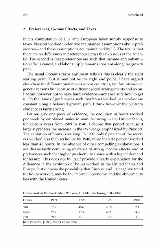
Blanchard226
2 Preferences, Income Effects, and Taxes
In his computation of U.S. and European labor supply response to taxes, Prescott worked under two maintained assumptions about pref-erences—and these assumptions are maintained by LS. The fi rst is that there are no differences in preferences across the two sides of the Atlan-tic. The second is that preferences are such that income and substitu-tion effects cancel, and labor supply remains constant along the growth path.
The usual Occam’s razor argument tells us this is clearly the right starting point. But it may not be the right end point. I have argued elsewhere for different preferences across countries, not for intrinsic or genetic reasons but because of different social arrangements and so on. I admit however not to have hard evidence—nor am I sure how to get it. On the issue of preferences such that hours worked per worker are constant along a balanced growth path, I think however the contrary evidence is fairly strong.
Let me give one piece of evidence, the evolution of hours worked per week by employed males in manufacturing in the United States, for various years from 1909 to 1940. I choose that period because it largely predates the increase in the tax wedge emphasized by Prescott. The evolution of hours is striking. In 1909, only 8 percent of the work-ers worked less than 48 hours; by 1940, more than 92 percent worked less than 48 hours. In the absence of other compelling explanations, I see this as fairly convincing evidence of strong income effects, and of preferences such that higher productivity comes with a higher demand for leisure. This does not by itself provide a ready explanation for the difference in the evolution of hours worked in the United States and Europe, but it opens the possibility that Europe, and its negative trend for hours worked, may be the “normal” economy, and the abnormality lies with the United States.
Hours Worked Per Week, Male Workers, U.S. Manufacturing, 1909–1940
Hours 1909 1919 1929 1940
≤48 7.9 48.6 46.0 92.1
49-59 52.9 39.3 46.5 4.9
≥60 39.2 12.1 7.5 3.0
John Pencavel [1986], from Census data.

227Comment
3 Heterogeneity and Labor Supply
The representative agent version of the Prescott model focuses on the labor supply choice at the intensive margin, i.e., how many hours to work. It is clear that individuals also make a choice at the extensive margin, i.e., whether to work or not.
As soon as one recognizes this second choice, things become more complicated and endogenous heterogeneity arises. People now have different work histories, thus different asset levels, and by implica-tion different reservation wages. This heterogeneity in turn affects the response of aggregate labor supply to taxes.
There are two ways of, in effect, avoiding the issue. The fi rst is to rely on the fi ction of very large households, who can fully diversify individ-ual labor income risk—an approach typically followed in New Keynes-ian models—or, equivalently, allow for work lotteries combined with insurance—the approach followed by RBC models. The second is to assume linear utility, so wealth does not affect the reservation wage, the approach followed in Diamond-Mortensen-Pissarides (DMP) models. Either approach works in getting us out of the diffi culty and deliver-ing a tractable characterization of labor supply; but, from a descriptive viewpoint, neither is appealing.
It is clearly worthwhile to tackle the complexity head on, i.e., to see how much agents can self insure through asset accumulation and decu-mulation, and then derive the implications for individual and aggre-gate labor supply. This is what LS start to do. In doing so, they can potentially answer two types of questions: The effect of taxes on labor supply; and how the answer differs from those obtained under the shortcuts described above, either the assumption of a representative agent and variations at the intensive margin, or variations at the exten-sive margin with full insurance cum lotteries.
Much of the LS paper is spent comparing the equivalence—or lack of—between insurance cum lotteries, and self insurance through asset decumulation and accumulation. Given Prescott’s rationalization, it is again a natural starting point. And knowing when the two are equiva-lent is obviously useful (just as knowing when Ricardian equivalence holds). It is clear however that the distance between the two is likely to be substantial in practice. Human capital accumulation through work, which LS focus on as the source of non-equivalence, would not have been my starting point (I suspect the motivation was internal, coming from the earlier work by LS on European unemployment, in which skill

Blanchard228
acquisition and skill loss play an important role). I would have focused instead on the implications of fi nite horizons, of the life cycle, and of the fact that workers face substantial uncertainty, both about income when employed, and about employment. The evidence is that workers can smooth only a limited proportion of their idiosyncratic labor income risk. I read for example the papers by Heathcote et al. (2004) and by Blundell et al. (2003) as suggesting that they are able to insure about half of the permanent changes in their labor income.
LS however give us a clear agenda (and take the fi rst few steps in a model which was originally part of the paper presented at the confer-ence, and is now developed in LS 2006a): Write down a model in which workers self insure through asset accumulation and decumulation. Fit the facts about labor supply, consumption, and saving across the life cycle (extending to labor supply the work of Gourinchas and Parker (2002) on consumption). Then, look at the effect of an increase in labor taxes.
There are many interesting issues to explore here. Let me just men-tion one. In this paper and the general equilibrium extension (2006a), LS look at decisions to work or not work in a model without labor market frictions, so all non work is voluntary. But in the presence of frictions, the layoff rate and the exit rate from unemployment affects asset accu-mulation, which in turn affect the reservation wage, and the decision to quit or to look for a job if unemployed. In other words, layoffs affect asset accumulation, which in turn affects quits. This in turn affects the effects of the tax rate on aggregate labor supply; these implications are both complex and extremely relevant to the issue at hand.
4 Heterogeneity. Back to the Comparison between the United States and Europe
LS point to the importance of heterogeneity in understanding the effects of taxes on labor supply, in characterizing both whose decision is affected, and what the overall effect on labor supply is likely to be. While their model is admittedly only a rough beta version, it is tempt-ing to speculate as to whether it or later versions will fi t some of the aspects of the disaggregated data.
First, let me again give some background. The fi rst basic fact about relative labor market evolutions in Europe versus the United States is that there has been a steady decline in hours worked per capita in
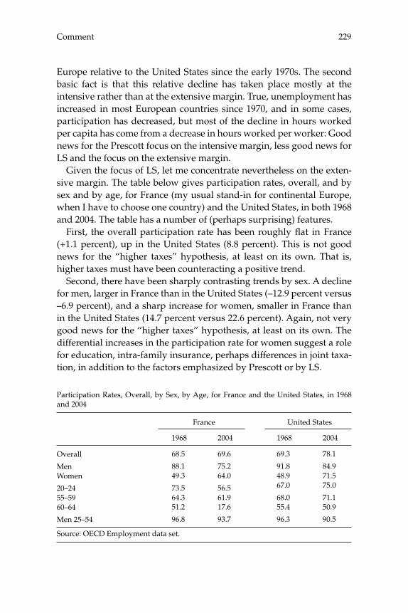
229Comment
Europe relative to the United States since the early 1970s. The second basic fact is that this relative decline has taken place mostly at the intensive rather than at the extensive margin. True, unemployment has increased in most European countries since 1970, and in some cases, participation has decreased, but most of the decline in hours worked per capita has come from a decrease in hours worked per worker: Good news for the Prescott focus on the intensive margin, less good news for LS and the focus on the extensive margin.
Given the focus of LS, let me concentrate nevertheless on the exten-sive margin. The table below gives participation rates, overall, and by sex and by age, for France (my usual stand-in for continental Europe, when I have to choose one country) and the United States, in both 1968 and 2004. The table has a number of (perhaps surprising) features.
First, the overall participation rate has been roughly fl at in France (+1.1 percent), up in the United States (8.8 percent). This is not good news for the “higher taxes” hypothesis, at least on its own. That is, higher taxes must have been counteracting a positive trend.
Second, there have been sharply contrasting trends by sex. A decline for men, larger in France than in the United States (–12.9 percent versus –6.9 percent), and a sharp increase for women, smaller in France than in the United States (14.7 percent versus 22.6 percent). Again, not very good news for the “higher taxes” hypothesis, at least on its own. The differential increases in the participation rate for women suggest a role for education, intra-family insurance, perhaps differences in joint taxa-tion, in addition to the factors emphasized by Prescott or by LS.
Participation Rates, Overall, by Sex, by Age, for France and the United States, in 1968 and 2004
France United States
Overall
MenWomen
20–2455–5960–64
Men 25–54
1968
68.5
88.149.3
73.564.351.2
96.8
2004
69.6
75.264.0
56.561.917.6
93.7
1968
69.3
91.848.967.0
68.055.4
96.3
2004
78.1
84.971.575.0
71.150.9
90.5
Source: OECD Employment data set.

Blanchard230
Third, much of the difference comes from the sharp drop in the par-ticipation rate of older workers (60–64) in France, from 51.2 percent in 1968 to 17.6 percent in 2004. This sharp increase in early retirement would appear to be good news for LS: In their simple model with human capital, as well as in their more fl eshed out version (LS 2006a), most of the effect of an increase in the tax rate is through early retire-ment: Those workers who have accumulated substantial assets decide that work is no longer attractive, and take early retirement. But the news is less good than it looks: Most of the early retirements in France (and elsewhere in Europe) are due to a high implicit tax rate on work after age 55, a dimension of taxation neither LS nor Prescott look at. Jon Gruber and David Wise (1998) have constructed a so called “tax force” index, equal to the sum of the tax rates on working one more year, from age 55 to 69. The value of the index is equal to 1.6 for the United States, 7.3 for France. And the index correlates extremely well across countries with participation rates for the 55–64 age group.
5 Non Work: Leisure versus Unemployment
Neither Prescott nor LS make an explicit distinction between unem-ployment and leisure. This leads to some uneasiness, for example, in the way LS formalize unemployment benefi ts as paid for all non-work. True, most countries have social assistance programs even for those out of the labor force, but these programs are typically much less generous than social insurance programs.
It is becoming increasingly clear (at least to me) that, to fully under-stand European labor market evolutions, looking just at unemploy-ment, or lumping home work, unemployment, and leisure into “non work,” cannot do justice to the facts: Unemployment has increased and, in many countries, is higher than in the United States. Hours worked per worker have decreased, and are nearly everywhere lower than in the United States. We have little solid evidence about the evolution of home work over time, but today’s numbers suggest that home work is higher in Europe than in the United States (Freeman and Schettkat 2005, and Burda et al. 2006).
Why does it matter? Because payroll taxes, income taxes, consump-tion taxes, and unemployment benefi ts affect these different margins of choice differently. Let me end with a few examples.
When looking at the effect of the tax wedge on the choice between market work and leisure, the issue is how much of the substitution effect is cancelled by the income effect. When looking at the effect of the same
231Comment
tax wedge on the choice between market work and home work, the income effect plays a much smaller role. If home work and market work are close substitutes, a small increase in the tax wedge may lead to a large shift from market to home work, with little or no income effect.
The effect of the tax wedge on unemployment may be very different from its effect on leisure. What happens depends very much on the fric-tions that generate unemployment.
In many models, where unemployment serves the role of a discipline device, an increase in the tax wedge is likely to increase unemploy-ment. In an effi ciency wage model where shirking is unobservable, an increase in payroll taxes decreases the after-tax wage that fi rms can pay, decreasing the utility cost of being laid off at a given unemployment rate: This in turn leads to an increase in equilibrium unemployment. Very much the same logic applies to fl ow/bargaining models: The reduction in the after-tax wage that fi rms can pay requires an increase in unemployment, so as to get workers to accept the lower real wage.
The effect may however go the other way. Think of a model of search unemployment, where workers have the choice between searching for jobs or taking leisure. Then, the effects of an increase in the tax wedge will have the same qualitative effect on unemployment and employ-ment. Anything which makes work less attractive will also make search less attractive, and thus leads to lower search effort, to lower unem-ployment.
We have a long way to go in understanding the effects of taxes on labor supply, especially in markets with frictions. We must thank Prescott for the challenge, and LS for taking us a bit further along.
Acknowledgment
I thank Ivan Werning for discussions.
References
Blundell, Richard, L. Pistaferri, and I. Preston. 2003. “Consumption Inequality and Partial Insurance.” Mimeo, UCL.
Burda, M., D. Hammermesh, and P. Weil. 2006. “Different but Equal: Total Work, Gender, and Social Norms in the EU and US Time Use.” Mimeo, Humboldt University.
Freeman, Richard, and R. Schettkat. 2005. “Marketization of Household Production and the EU-US Gap in Work.” Economic Policy 20: 6–50.
Heathcote, Jonathan, K. Storesletten, and G. Violante. 2004. “The Macroeconomic Impli-cations of Rising Wage Inequality in the United States.” Mimeo, NYU.

Blanchard232
Gourinchas, Pierre Olivier, and J. Parker. 2002. “Consumption over the Life-Cycle.” Econometrica 70(1): 47–89.
Gruber, Jon, and D. Wise. 1998. “Social Security and Retirement: An International Com-parison.” AER 88(2): 158–163.
Pencavel, John. 1986. “Labor Supply of Men: A Survey.” In O. Ashenfelter and R. Layard, eds., Handbook of Labor Economics Volume 1. North Holland, 3–102.
Prescott, Edward. 2004. “Why Do Americans Work So Much More than Europeans?” Fed-eral Reserve Bank of Minneapolis Quarterly Review 28(1): 2–13.
Comments
Edward C. Prescott, Arizona State University, Federal Reserve Bank of Minneapolis, and NBER
1 Introduction
The authors obscure the important contribution of their paper by argu-ing that the reason employment is so low in the big continental Euro-pean countries relative to other advanced industrial countries is that these European countries have big government transfers that are con-ditional on recipients not working. They challenge my conclusion that most of these employment differences as well as the change over time in these differences for the European countries are the result of differ-ences in tax rates. Policies that affect the budget constraint are tax poli-cies. Thus, the authors and I agree that the reason for this difference in employment is primarily due to differences in tax systems.
The authors do not carry out a quantitative general equilibrium anal-ysis using a model that is restricted to be consistent with the national account statistics. As shown in section 2, the tax-and-transfer system that I considered and a payment-not-to-work system have identical implications for employment if transfers as a percentage of the product of labor are held fi xed. For a model calibrated to reasonable govern-ment transfers, the European employment is as predicted by the life cycle labor supply model with labor indivisibilities.
The obscured and important contribution of their paper is the ini-tiation of an important research program, a program that already has begun to bear fruit. This research program is to derive the implications of labor indivisibility for lifetime labor supply. In the simplest version of the theory, with people having access to costless borrowing and lending markets, what gets determined is the fraction of the periods of an individual’s lifetime that an individual works and the fraction of the population working at each point in time. This theory matches with the observation that differences in the fraction of periods of lifetimes

Prescott234
worked account for the huge difference in market hours between the big continental European countries and the employment rates of the other major advanced industrial countries. With labor indivisibilities, labor supply is proportional to the employment rate. This is why I often use the term employment rate rather than labor supply.
The theory predicts how many periods that an individual works in his or her lifetime, but not when. The term period is key in this state-ment, so what is a period must be addressed. A year is far too long to be a period. Hours worked per year per employed person is low in Europe relative to the United States. This difference is mostly in the weeks worked per employed person and not in hours worked per week. This is what the theory predicts. Europeans have more weeks of vacation, sick days, and holidays than do Americans. This leads me to defi ne a period to be a week or even a day.
The OECD (2004) reports that the average number of weeks worked per year by full-time employees accounts for about 40 percent of the difference in European and U.S. labor supply. The other 60 percent of the difference is accounted for by differences in the number of years of employment over lifetimes. Full-time European employees work 40 weeks a year, while their American counterparts work 46 weeks a year on average.
Most of the remaining 60 percent difference is the fraction of potential working life that individuals are employed. Within the working life, the employment rate differences are for those over 55 years of age and for those under 25. Employment rates for those between 25 and 55 are close in the United States and Europe (see Rogerson 2006, fi gure 37).
The authors introduce occupational skill investment, and its impli-cations are just what their theory predicts. With this feature of real-ity introduced, there is a working period whose length is determined given the tax system. The theory does not say when this working period begins and ends, just how long it is. Thus, the above observations are what the theory predicts, with some people beginning a little later, or equivalently retiring a little later, than others. This assumes a costless borrowing and lending market and no borrowing constraints.
The Ljungqvist and Sargent research program is important for the following reason. As the population ages and people enjoy a longer and healthier retirement, life cycle labor supply theory is needed to evaluate alternative schemes for fi nancing retirement consumption. Some coun-tries such as Australia and Singapore have adopted systems that force savings. Others such as Finland have recently restructured their public pension systems to encourage later retirement. Will the new Finnish
235Comment
system just result in people shifting in their lifetime when they work and not increasing the number of lifetime working hours? This is an important question for the Finns, and a life cycle labor supply theory is needed to answer the question.
2 Consequences of Alternative Tax Systems for Employment
I now show how the tax system affects the employment rate. I consider the effects of policies that tax labor income at rate τe and tax consump-tion at rate τc and which make lump-sum transfers to employed of ψ and lump-sum transfers to those not employed of b + ψ. If b = 0, this is the tax system used in Prescott (2004). If b > 0, there are the Ljungqvist and Sargent payments for not working.
The model used has the Ljungqvist and Sargent life cycle structure with labor indivisibilities. The nature of preferences and the household consumption possibility set are such that the margin of adjustment is the employment rate and not hours per period per employed person.1 I deal with the case that the parameters are such that in equilibrium not all are employed at any instance. This is the empirically interesting case. Further, for simplicity the equilibrium interest rate is zero, which requires no growth in the product of labor and a zero discount rate. There is no capital accumulation. Generalizing the result to environ-ments for which the interest rate is positive and which have uncertainty is straightforward. Preferences are
(log )c v e dt−∫ 0
1
for an individual born at time t = 0 and with a lifetime normalized to 1. The disutility of working v is positive. Above c:[0,1]→ℜ+ is the path of consumption and e:[0,1]→{0,1} is the path of employment. Thus, c and e are functions of time, but they will become scalars. Variable c is the rate of consumption which is constant over time. Variable e is the fraction of lifetime worked and is the integral of the e(t) function. In the general equilibrium context, e is the employment rate. All people are identical and their measure is 1.
The budget constraint has taxes on labor income at rate τe, taxes on consumption at rate τc, transfers b when not employed, and lump-sum transfers ψ independent of employment state. An individual’s budget constraint is
( ) ( ) ( ) .1 1 1+ = − + − +τ τ ψc ec e w e b

Prescott236
The government has a balanced budget, so
total transfers = + = +e b e w ce cψ τ τ .
An employed person produces one unit of the consumption good, so wage w = 1. Market clearing requires c = e.
Equilibrium e is given by
eb
ve
c
=− −
+1
1τ
τ( ).
The parameter v is calibrated to the observations e = 0.60 when b = 0, τc = .12, and τe = .33, which are approximate U.S. values. The calibrated v is 0.997.
Of importance is the fact that the employment rate is proportional to
11− −
+τ
τe
c
b( )
.
What enters this formula for the employment rate is the sum of τe and b. From an accounting perspective, τe and b are different. From an eco-nomic perspective, they are the same.
We introduce the tax rate estimates using the Prescott (2004) meth-odology. There are no payments for not working. Table 3.2 reports the results of two tax systems. These are essentially the tax parameters used in Prescott (2005) and the results obtained using a dynastic model of households. A key number in table 3.2 is that with the European tax rates, a huge fraction of product is transfer by the government. This fraction is 0.80, a number that is ridiculously high.
Table 3.2
Tax Systems Considered in Prescott (2005)
Policy Parameters United States Europe
τc 0.12 0.30
τe 0.33 0.50
b 0.00 0.00
ψ + b 0.27 0.45
Equilibrium Values
e 0.60 0.39
Transfers relative to product 0.45 0.80
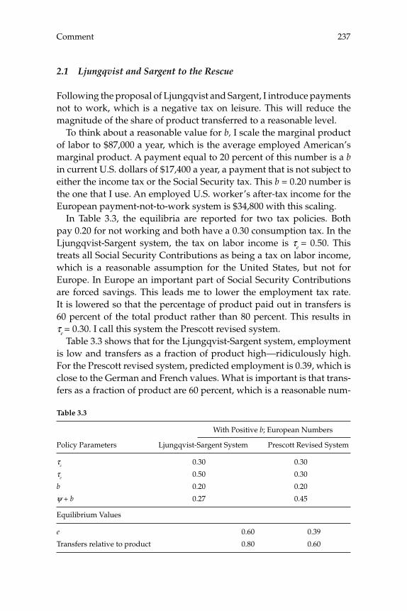
237Comment
2.1 Ljungqvist and Sargent to the Rescue
Following the proposal of Ljungqvist and Sargent, I introduce payments not to work, which is a negative tax on leisure. This will reduce the magnitude of the share of product transferred to a reasonable level.
To think about a reasonable value for b, I scale the marginal product of labor to $87,000 a year, which is the average employed American’s marginal product. A payment equal to 20 percent of this number is a b in current U.S. dollars of $17,400 a year, a payment that is not subject to either the income tax or the Social Security tax. This b = 0.20 number is the one that I use. An employed U.S. worker’s after-tax income for the European payment-not-to-work system is $34,800 with this scaling.
In Table 3.3, the equilibria are reported for two tax policies. Both pay 0.20 for not working and both have a 0.30 consumption tax. In the Ljungqvist-Sargent system, the tax on labor income is τe = 0.50. This treats all Social Security Contributions as being a tax on labor income, which is a reasonable assumption for the United States, but not for Europe. In Europe an important part of Social Security Contributions are forced savings. This leads me to lower the employment tax rate. It is lowered so that the percentage of product paid out in transfers is 60 percent of the total product rather than 80 percent. This results in τe = 0.30. I call this system the Prescott revised system.
Table 3.3 shows that for the Ljungqvist-Sargent system, employment is low and transfers as a fraction of product high—ridiculously high. For the Prescott revised system, predicted employment is 0.39, which is close to the German and French values. What is important is that trans-fers as a fraction of product are 60 percent, which is a reasonable num-
Table 3.3
With Positive b; European Numbers
Policy Parameters Ljungqvist-Sargent System Prescott Revised System
τc 0.30 0.30
τe 0.50 0.30
b 0.20 0.20
ψ + b 0.27 0.45
Equilibrium Values
e 0.60 0.39
Transfers relative to product 0.80 0.60

Prescott238
ber. Thus, I stick with my statement that the difference in European and American employment rates is primarily due to differences in tax rates. It is an implication of the Ljungqvist and Sargent life cycle labor supply theory with indivisibilities.
3 A Red Herring
A claim of the Ljungqvist and Sargent paper is that it is differences in “benefi ts” and not differences in “tax rates” that account for the cur-rent low European labor supply relative to other advanced industrial economies. Benefi ts and tax rates are put in quotes because from the perspective of the budget constraint, there is no distinction. Being paid not to work is a negative tax on nonmarket time. The authors and I agree that the big difference in Western European labor supply and that of other advanced industrial countries is due to differences in tax sys-tems. We also agree that the big reduction in European labor supply between the early 1970s and the early 1990s is due to a change in their tax system.
Another point is how to treat pensions paid by the state. The U.S. Social Security retirement system, which is fi nanced by 10.6 percent of the 12.4 percent FICA tax, is on margin to a fi rst approximation a tax-and-transfer system. In Europe, however, pensions paid by government are in signifi cant part based upon earnings. Thus, they are a hybrid of a savings system, which does not depress employment, and a trans-fer system, which does depress employment. One implication is that the marginal effective labor income tax rate that I estimated for Europe is too high. Ljungqvist and Sargent provide an additional tax factor, namely payments not to work, that depresses employment.
4 Two Comments
4.1 Human Capital Investment
The authors point out that the intertemporal budget constraint does not get around the problem of achieving an effi cient allocation without enforceable lottery or sunspot contracts. A consequence of this inabil-ity is that human capital investment will be lower per employed per-son. The issues concerning the consequences of tax systems for relative employment rates, however, are not affected, and the authors do not claim that it is affected.
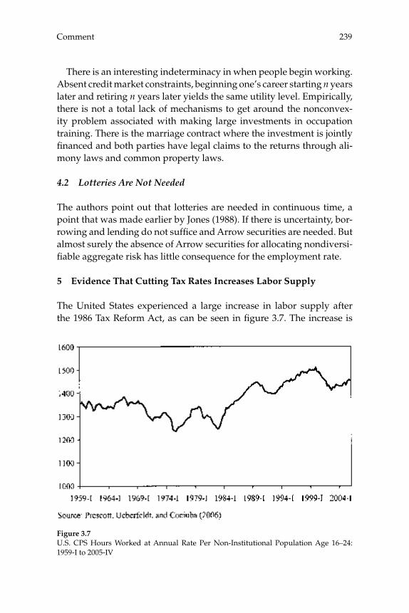
239Comment
There is an interesting indeterminacy in when people begin working. Absent credit market constraints, beginning one’s career starting n years later and retiring n years later yields the same utility level. Empirically, there is not a total lack of mechanisms to get around the nonconvex-ity problem associated with making large investments in occupation training. There is the marriage contract where the investment is jointly fi nanced and both parties have legal claims to the returns through ali-mony laws and common property laws.
4.2 Lotteries Are Not Needed
The authors point out that lotteries are needed in continuous time, a point that was made earlier by Jones (1988). If there is uncertainty, bor-rowing and lending do not suffi ce and Arrow securities are needed. But almost surely the absence of Arrow securities for allocating nondiversi-fi able aggregate risk has little consequence for the employment rate.
5 Evidence That Cutting Tax Rates Increases Labor Supply
The United States experienced a large increase in labor supply after the 1986 Tax Reform Act, as can be seen in fi gure 3.7. The increase is
Figure 3.7U.S. CPS Hours Worked at Annual Rate Per Non-Institutional Population Age 16–24: 1959-I to 2005-IV
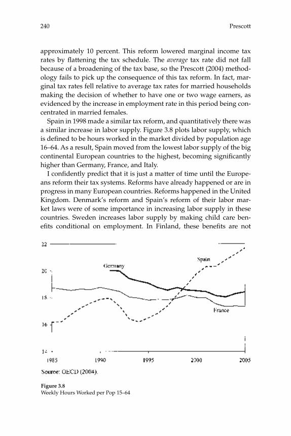
Prescott240
approximately 10 percent. This reform lowered marginal income tax rates by fl attening the tax schedule. The average tax rate did not fall because of a broadening of the tax base, so the Prescott (2004) method-ology fails to pick up the consequence of this tax reform. In fact, mar-ginal tax rates fell relative to average tax rates for married households making the decision of whether to have one or two wage earners, as evidenced by the increase in employment rate in this period being con-centrated in married females.
Spain in 1998 made a similar tax reform, and quantitatively there was a similar increase in labor supply. Figure 3.8 plots labor supply, which is defi ned to be hours worked in the market divided by population age 16–64. As a result, Spain moved from the lowest labor supply of the big continental European countries to the highest, becoming signifi cantly higher than Germany, France, and Italy.
I confi dently predict that it is just a matter of time until the Europe-ans reform their tax systems. Reforms have already happened or are in progress in many European countries. Reforms happened in the United Kingdom. Denmark’s reform and Spain’s reform of their labor mar-ket laws were of some importance in increasing labor supply in these countries. Sweden increases labor supply by making child care ben-efi ts conditional on employment. In Finland, these benefi ts are not
Figure 3.8Weekly Hours Worked per Pop 15–64
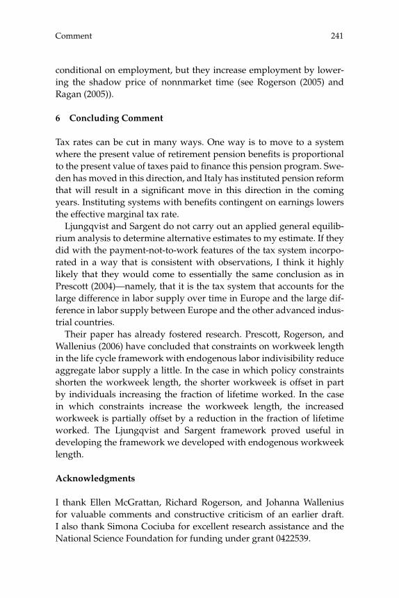
241Comment
conditional on employment, but they increase employment by lower-ing the shadow price of nonnmarket time (see Rogerson (2005) and Ragan (2005)).
6 Concluding Comment
Tax rates can be cut in many ways. One way is to move to a system where the present value of retirement pension benefi ts is proportional to the present value of taxes paid to fi nance this pension program. Swe-den has moved in this direction, and Italy has instituted pension reform that will result in a signifi cant move in this direction in the coming years. Instituting systems with benefi ts contingent on earnings lowers the effective marginal tax rate.
Ljungqvist and Sargent do not carry out an applied general equilib-rium analysis to determine alternative estimates to my estimate. If they did with the payment-not-to-work features of the tax system incorpo-rated in a way that is consistent with observations, I think it highly likely that they would come to essentially the same conclusion as in Prescott (2004)—namely, that it is the tax system that accounts for the large difference in labor supply over time in Europe and the large dif-ference in labor supply between Europe and the other advanced indus-trial countries.
Their paper has already fostered research. Prescott, Rogerson, and Wallenius (2006) have concluded that constraints on workweek length in the life cycle framework with endogenous labor indivisibility reduce aggregate labor supply a little. In the case in which policy constraints shorten the workweek length, the shorter workweek is offset in part by individuals increasing the fraction of lifetime worked. In the case in which constraints increase the workweek length, the increased workweek is partially offset by a reduction in the fraction of lifetime worked. The Ljungqvist and Sargent framework proved useful in developing the framework we developed with endogenous workweek length.
Acknowledgments
I thank Ellen McGrattan, Richard Rogerson, and Johanna Wallenius for valuable comments and constructive criticism of an earlier draft. I also thank Simona Cociuba for excellent research assistance and the National Science Foundation for funding under grant 0422539.
Prescott242
Endnote
1. See Prescott, Rogerson, and Wallenius (2006) for why the latter margin is not used.
References
Jones, Larry E. 1988. “A Note on the Joint Occurrence of Insurance and Gambling.” Mimeo, Kellogg Graduate School of Management, Northwestern University.
OECD. 2004. OECD Employment Outlook, 2004. Paris: Organisation for Economic Co-operation and Development.
Prescott, Edward C. 2004. “Why Do Americans Work So Much More Than Europeans?” Federal Reserve Bank of Minneapolis Quarterly Review 28: 2–13.
Prescott, Edward C., Richard Rogerson, and Johanna Wallenius. 2006. “Lifetime Aggregate Labor Supply with Endogenous Workweek Length.” Mimeo, Arizona State University.
Prescott, Edward C., Alexander Ueberfeldt, and Simona E. Cociuba. 2006. “U.S. Hours and Productivity Behavior Using CPS Hours Worked Data: 1959-I to 2005-IV.” Federal Reserve Bank of Minneapolis Research Memorandum.
Ragan, Kelly S. 2005. “Taxes, Transfers and Time Use: Fiscal Policy in a Household Pro-duction Model.” Mimeo, University of Chicago.
Rogerson, Richard. 2005. “Taxes and Market Work: Is Scandinavia an Outlier?” Mimeo, Arizona State University.
Rogerson, Richard. 2006. “Understanding Differences in Hours Worked.” Review of Eco-nomic Dynamics 9(3): 365–409.
Discussion
Lars Ljungqvist began the discussion by pointing out that in the indi-visible labor model, it is the average tax wedges that infl uence worker behavior rather than the marginal tax wedges. Nevertheless, as long as differences in countries’ average tax wedges are similar to those in mar-ginal tax wedges, this distinction is not important for the quantitative analysis of differences in countries’ aggregate employment, hence, their disagreement with Edward Prescott over whether the issue of average versus marginal tax rates was consequential. On the other hand, he said that they did disagree with Prescott’s view of the intertemporal evi-dence on tax wedges. According to Prescott’s own earlier study, half of the French and German tax differentials versus the United States were already in place in the early 1970s and thus, there have been neither large tax hikes nor, for that matter, large benefi t hikes that coincide with the large rise in European nonemployment over the subsequent quarter century.
Robert Gordon disagreed with Olivier Blanchard’s characterization of the decline in hours per capita in Europe. He noted that if one looked at the entire period since 1960, only 1/3 of the decline in hours per capita was due to a decline in hours per employee. The remaining 2/3 was due to a declining labor force participation rate and an increase in the unemployment rate, of which each of these factors accounted for roughly 1/3. Gordon then noted that since 1995, employment in Europe relative to the United States had actually stopped falling and begun to turn around. He noted that two alternative explanations for this turnaround—which the data could not distinguish between—were the productivity slowdown in Europe and labor market reforms.
Gordon remarked that he did not see how a generalized payroll tax explanation like the one put forth by Edward Prescott could explain the age distribution of the employment rate and labor force participation

Discussion244
rate in Europe relative to the U.S, where Europe tails off at the begin-ning and at the end while its prime age ratios to the United States are very close to 100 percent. He noted that specifi c features of the tax sys-tem in Europe that created incentives for early retirement might explain the tailing off at the end, and other specifi c features relating to higher education might explain the difference for young workers. But he said he did not see how a general tax story could explain this pattern.
Daron Acemoglu remarked that the paper highlighted the need for more work on the role of the family in macroeconomics. In particular, he felt there was a need to think more about the relative roles played by the government and the family in providing social insurance and transfers to unemployed youth in Europe. In addition, Acemoglu noted that it would be interesting to extend the type of model studied in the paper to explore more fully tax and transfer schemes where the treat-ment of all agents is not equal and where selective redistribution is undertaken.
Andrew Levin questioned whether tax and transfer policies such as unemployment benefi ts could reasonably be thought of as exogenous, especially in the long run. He remarked that the model in the paper was promising in dealing with this issue, since it took seriously the fact that there exist multiple generations of agents with different levels of human capital that interact in a world with incomplete insurance markets. He felt that these elements made it possible to endogenize policy decisions by introducing voting and thinking about what policies the median voter would choose. He speculated that such a model could explain how apparently small differences in initial conditions between the United States and Europe could lead to very different social choices.
V. V. Chari remarked that our ignorance about what the correct dis-aggregated model is makes it diffi cult to know whether the stand-in household formulation is a misleading abstraction or not. He noted that the authors’ conclusion that the presence of young people poses a problem for the stand-in household model was perhaps overstated as their disaggregated model ignored certain possibilities of insurance that exist in the real world. In particular, he felt that intra-family insur-ance in the real world might alleviate some of these problems.
John Haltiwanger liked the focus on career paths in the paper, add-ing that there was a lot to be learned about career paths from looking at new data sets that follow workers and fi rms together. He noted that for the United States, there is evidence of diverse patterns: Some workers
245Discussion
do well by matching early to a fi rm, staying with that fi rm and building a career within the fi rm. Other workers build a career by changing jobs several times in the fi rst ten to 15 years of their career. He noted that a worker’s ability to build a career in this second way depended heavily on labor market fl exibility. He felt that the data showed that labor mar-ket fl exibility had really paid off for the United States in this regard.
Éva Nagypál followed up on the discussion about the age distribution of differences in hours worked between Europe and the United States by noting that a similar pattern also shows up in studies of the variation of hours over time in the United States. In particular, just as young and old workers explain the bulk of the difference between hours worked in Europe and the United States, these same groups account for most of the variation of hours worked over the business cycle in the United States.
Thomas Sargent remarked that there was a tension running through the discussion, one that he believed had been running through much of macroeconomics for the last 20 years. The fi rst source of tension was whether macroeconomists should import parameter estimates from microeconomic studies or whether macroeconomic evidence alone should be used to infer those parameters because the specifi cations of those micro studies were too incompatible with the structures of the macro models. Another tension in Sargent’s view was about whether heterogeneity is important for macroeconomics. Sargent noted that a key factor determining whether heterogeneity is important is how extensively the presence of incentive and enforcement problems inhibit how people can share risks across states and over time. Macro analy-ses like Prescott’s that stress a stand-in household are betting that het-erogeneity can be downplayed for understanding how fi scal policies impinge on macroeconomic outcomes.
Responding to Edward Prescott’s discussion, Sargent agreed with Prescott that once plausible benefi t replacement rates are included in Prescott’s model along with the high tax rates that Prescott had origi-nally estimated for Europe, the model fails to explain labor supply in Western Europe. He noted that a key reason for this is that he and Ljungqvist had insisted on playing by Prescott’s rules in the paper being discussed, meaning that they accepted without question the high labor supply elasticity implied by the high disutility that Prescott set for leisure. Sargent then said that in his 1998 JPE paper with Ljungqvist, they advocated a different framework lacking a stand-in-household. In

Discussion246
that framework, there are incomplete markets and it matters a great deal which agents receive labor inactivity benefi ts from the govern-ment. That JPE model captures the situation in which a small fraction of people has been living at the government’s expense for a long period of time rather than working. Sargent said that seemed to him to provide a good snapshot of several important European countries.
Fluctuating Macro Policies and the Fiscal Theory
Troy Davig, Federal Reserve Bank of Kansas CityEric M. Leeper, Indiana University and NBER
4
1 Introduction
A popular approach to analyzing macroeconomic policy posits simple policy rules and characterizes how alternative policy specifi cations perform in dynamic stochastic general equilibrium models. This line of work has shown that simple rules seem to explain observed policy choices quite well and that those rules produce desirable outcomes in popular classes of dynamic monetary models. Most of the work makes convenient assumptions that allow monetary and fi scal rules to be studied separately. Because these assumptions are questionable, it has long been known that the resulting conclusions could be misleading. Recent work, particularly the fi scal theory of the price level, empha-sizes that assumptions about how monetary and fi scal policies interact can be important.
Research on policy interactions has spawned a number of results that have become part of the standard reasoning about macroeconomic policy: (1) an active monetary policy that raises the nominal interest rate more than one-for-one with infl ation—the “Taylor principle”—is necessary for stability of the economy (Taylor 1993); (2) the Taylor principle delivers good economic performance in widely used models (Rotemberg and Woodford 1997, Schmitt-Grohé and Uribe 2006); (3) high and variable infl ation rates may be due to failure of central banks to obey the Taylor principle, leaving the price level undetermined and subject to self-fulfi lling expectations (Clarida, Galí, and Gertler 2000, Lubik and Schorfheide 2004); (4) the combination of active monetary policy and passive tax policy insulates the economy from aggregate demand disturbances, such as those arising from tax-debt policies (Leeper 1991).
Davig and Leeper248
As with earlier work that focused on monetary or fi scal rules sepa-rately, the derivation of these results rests on a number of assumptions of convenience that simplify the nature of monetary and fi scal policy interactions. The authors usually note that different sets of equally plausible assumptions may lead to qualitatively different outcomes. For example, there is now a growing literature providing counter-examples to the desirability of the Taylor principle (Benhabib and Farmer 2000, Benhabib, Schmitt-Grohé, and Uribe 2001a, b, 2002, Zanna 2003).
Perhaps the least plausible assumption in this work is that policy regime is fi xed. This implies that agents always expect the current policy regime to last forever; regime change, if it occurs, comes as a complete surprise. A major branch of the applied side of the literature consists of identifying periods of different policy regimes (Taylor 1999a, 2000, Clarida, Galí, and Gertler 2000, Auerbach 2002, Lubik and Schorfheide 2004, Sala 2004, Favero and Monacelli 2005). But, as Cooley, LeRoy, and Raymon (1984) argue, it makes little sense to assume policy mak-ers are contemplating regime change when agents put zero probability on this event. Despite the empirical evidence and Cooley, LeRoy, and Raymon’s compelling logic, there is little modeling of environments where recurring regime change is stochastic and the objects that change are the rules governing how policy authorities respond to the economy.1
Davig and Leeper (2006b) show the consequences of regime switch-ing for determinacy of equilibrium in a simpler context in which lump-sum taxes passively adjust to satisfy the government budget constraint. When coeffi cients of a Taylor (1993) rule evolve stochastically, the region of determinacy for bounded solutions can expand dramatically relative to a constant-parameter specifi cation. That paper also shows in analytically tractable environments that cross-regime spillovers can change the impacts of exogenous disturbances in quantitatively impor-tant ways.
This paper extends Davig and Leeper’s (2006b) analysis to con-sider fi scal as well as monetary regime switching. It aims to bring the applied and theoretical lines of this literature closer together by study-ing a model with a simple, but empirically plausible, specifi cation of regime changes. We estimate Markov-switching rules for monetary and fi scal policy. Monetary policy obeys a Taylor rule that makes the nomi-nal interest rate depend on infl ation and the output gap; fi scal policy adjusts taxes as a function of government debt and other variables. All the parameters of the rules, including the error variances, evolve according to a Markov process. After imposing the estimated policy
249Fluctuating Macro Policies and the Fiscal Theory
process on a conventional calibrated dynamic stochastic general equi-librium (DSGE) model with nominal rigidities, we compute a solution that is a function of the minimum set of state variables and provide an interpretation of post-war macro policies.
There are fi ve main fi ndings.First, the estimates uncover periods of active monetary/passive fi scal
behavior, the policy mix typically assumed to prevail in monetary stud-ies; there are also episodes of passive monetary/active fi scal behavior, the mix associated with the fi scal theory of the price level.2 Remain-ing periods combine passive monetary with passive fi scal policy or active monetary with active fi scal behavior. Identifi cation of estimated switching policy rules is corroborated by connecting estimated regime changes to narrative accounts of policy behavior.
Second, post-war U.S. data can be modeled as a locally unique equilibrium: Necessary and suffi cient conditions for a solution to the optimum problem in a DSGE model are satisfi ed. While our empirical results are largely consistent with existing estimates from fi xed-regime models, we avoid the necessary implication of those models that the economy lurched unexpectedly among periods of indeterminacy (pas-sive/passive), non-existence of equilibrium (active/active), or unique equilibria with completely different characteristics (active monetary/passive fi scal or passive monetary/active fi scal) (see, for example, Clar-ida, Galí, and Gertler 2000, Lubik and Schorfheide 2004, or Sala 2004 for such interpretations). Instead, in a regime switching setup those peri-ods are merely alternative realizations of the state vector over which agents’ decision rules are defi ned. Consequently, in a switching model the policy episodes have strikingly different implications. For exam-ple, an empirical fi nding that over some sub-period monetary policy has been active and fi scal policy has been passive is perfectly consis-tent with there being important impacts from (lump-sum) tax shocks. A fi nding that both monetary and fi scal behaviors have been passive need not imply the equilibrium is indeterminate. And the economy can temporarily experience active/active policies without dire economic consequences.
Third, the fi scal theory of the price level is always operative. Shocks to (lump-sum) taxes always affect aggregate demand, even when the rules in place at a given moment would suggest that Ricardian equiv-alence should hold if regime were fi xed. The fi scal theory is operat-ing whenever economic agents believe it is possible for fi scal policy to become active. Then a cut in current taxes, fi nanced by sales of nominal
Davig and Leeper250
government debt, does not generate an expectation that future taxes will rise by at least enough to service the new debt. The tax reduction leaves households feeling wealthier, at initial prices and interest rates, and they perceive they can raise their consumption paths.3 When nomi-nal rigidities are present, the expansion in demand for goods raises out-put and infl ation. Davig, Leeper, and Chung (2004) show analytically that in a related regime-switching environment, a unique bounded equilibrium exists; in that equilibrium, the fi scal theory is always at work, as long as agents believe there is a positive probability of moving to a regime with active fi scal policy.
Fourth, the fi scal theory mechanism is quantitatively signifi cant in U.S. data, according to the model.4 Through that mechanism alone, a surprise transitory tax cut of $1 raises the discounted present value of output in the long run by between 76 cents and $1.02, depending on which policy regime the simulation conditions. A temporary tax cut of 2 percent of output increases the long-run price level by between 1.2 percent and 6.7 percent, conditional on remaining in a given monetary-fi scal regime. Similar impacts arise from an anticipated cut in taxes. Stochastic simulations that draw from the estimated distribution for policy regime imply that the 80th percentile for the output multiplier ranges from 43 cents to $1.36 after six years, while a tax cut of 2 per-cent of output raises the price level between 0.53 to 2.27 percent after six years. These numbers suggest the fi scal theory mechanism may be quite potent in U.S. data, helping to reconcile a popular class of DSGE models for monetary policy with the empirical evidence that tax distur-bances have important “demand-side” impacts (Blanchard and Perotti 2002, Mountford and Uhlig 2005, and Perotti 2004).
Fifth, viewing time series as generated by recurring regime change alters how those time series should be interpreted. Many estimates of policy rules use a priori information about policy behavior in order to condition on sub-samples in which a particular regime prevailed. This procedure can obtain accurate estimates of policy parameters and the impacts of policy disturbances. But embedding the estimated rules in fi xed-regime DSGE models can lead to seriously misleading qualitative inferences when a regime-switching environment generates the data. Because long-run policy behavior determines the qualitative features of data, more accurate inferences can be gleaned from full-sample infor-mation than by conditioning on regime.
Taken together, the paper’s fi ndings lead to a fundamental reassess-ment of results (1)–(4) that guide macro policy research. The fi ndings
251Fluctuating Macro Policies and the Fiscal Theory
also lead us to argue that to understand macroeconomic policy effects, it is essential to model policy regimes (or rules) as governed by a stochas-tic process over which agents form expectations. This argument puts on the table a new interpretation of macro policies and their impacts.5
1.1 Why Recurring Regime Change?
Because this paper models regime change as recurring, some motiva-tion for this modeling assumption is necessary.
Eugene Steuerle (2006), a close observer of U.S. fi scal policy, charac-terizes pendulum swings (or regime changes) in policy behavior as aris-ing from two political views toward fi scal policy: The “bargain lunch” view, by which politicians try to make tax cuts or expenditure increases appear to be costless, and the “green eye-shade” view, by which deci-sion makers are ever-wary of the balance-sheet requirements associ-ated with fi scal choices. For our purposes, the “bargain lunch” view treats tax decisions as independent of the state of government debt, while the “green eye-shade” view makes taxes rise with increases in government debt. This perspective is echoed in the popular press. In response to rising federal government budget defi cits, New York Times columnist David Brooks writes: “But what can’t last won’t last. Before too long, some new sort of leader is going to arise. . . . He’s going to rail against a country that cannot control its appetites (Brooks 2005).” Even-tually, when fi scal conditions deteriorate suffi ciently, regime change will occur.
More dramatic recurring changes in both monetary and fi scal poli-cies occur between wartime and peacetime. During wars—at least World War Two and the Korean War—spending rises rapidly with no immediate adjustment in taxes, while monetary policy supports debt fi nancing by keeping bond prices high (Ohanian 1997, Woodford 2001). This combination of active fi scal policy and passive monetary policy tends to be reversed after the fi scal needs of the war have passed.
Some observers—including several participants at the conference—want to believe that since the appointment of Paul Volcker to be chair-man of the Federal Reserve in 1979, U.S. monetary policy has been in an absorbing state with active policy. We don’t share this sanguine view. Central bank governor appointments are political decisions, subject to the vagaries of the political process. The appointment of Volcker and subsequently of Alan Greenspan and Ben Bernanke did not grow out of institutional reform or legislative change designed to achieve and instill

Davig and Leeper252
low and stable infl ation. Indeed, leading up to Bernanke’s appointment, several less-qualifi ed candidates’ names were fl oated. A different set of political realities at the time might well have produced a very different nominee whose policies exhibit appreciably less continuity.
Implicit in these examples is the notion that some regime changes are endogenous responses to the state of the economy—high infl ation leading to the appointment of infl ation-fi ghting central bank gover-nors—and some changes are exogenous—wartime fi scal fi nancing. But even endogenous changes have an important exogenous (political) component: Why wasn’t an infl ation hawk appointed Fed chairman earlier in the 1970s, when infl ation had already reached double digits? This paper assumes policy regimes evolve exogenously, leaving endog-enous change to future work.6
2 Identifi cation and Estimation of Policy Rules
We seek empirical characterizations of policy behavior that use simple rules of the kind appearing in the policy literature, but allow for recur-ring changes in regime. Monetary and tax regimes can switch indepen-dently of each other. This section reports maximum likelihood estimates of policy rules whose parameters evolve according to a hidden Markov chain, as in Hamilton (1989) and Kim and Nelson (1999).
Estimates of simple interest rate rules for monetary policy and tax rules for fi scal policy are plagued by identifi cation problems because other omnipresent equilibrium conditions involve similar variables. An empirical relationship that links a short-term nominal interest rate to infl ation and some measure of output might be capturing monetary policy behavior or it might simply refl ect the correlations that a Fisher equation induces among the nominal rate, the real rate, and expected infl ation. Similarly, a regression of taxes on lagged debt might describe how fi scal authorities raise taxes in response to increases in govern-ment indebtedness or it might arise from the positive correlation that the government budget constraint creates between the value of debt and expected future primary surpluses.
These problems are particularly acute in single-equation regressions that assume policy follows simple rules with constant coeffi cients: nothing distinguishes a “policy rule” from some other equilibrium con-dition. Positing that policy behavior shifts discretely, as we do in our estimated policy rules and in the subsequent theory, can help to dis-tinguish policy behavior from the other equilibrium conditions, which
253Fluctuating Macro Policies and the Fiscal Theory
would not be expected to exhibit time variation that coincides with policy shifts.7 A key step in identifying regime-switching policy rules corroborates the timing and nature of estimated regime changes with extra-sample evidence from other studies of policy behavior. This sec-tion also reports that evidence.
2.1 Specifi cations
For monetary policy, we estimate a standard Taylor (1993) specifi ca-tion, which Rotemberg and Woodford (1999) have shown is nearly opti-mal in the class of models we consider in section 3. The rule makes the nominal interest rate, rt, depend only on infl ation, πt, and the output gap, yt:
r S S S y St tM
tM
t y tM
t r tM
tr= + + +α α π α σ επ0( ) ( ) ( ) ( ) , (1)
where StM is the monetary policy regime and ε r
t ~ N(0, σ 2r). Regime
evolves according to a Markov chain with transition matrix PM. r and π are net rates. We allow for four states, with the parameters restricted to take only two sets of values, while the variance may take four different values. PM is a 4 × 4 matrix.8
Unlike monetary policy, there is no widely accepted specifi cation for fi scal policy.9 We model some of the complexity of tax policy with a rule that allows for the revenue impacts of automatic stabilizers, some degree of pay-as-you-go spending, and a response to the state of gov-ernment indebtedness. The rule links revenues net of transfer payments, τt, to current government purchases, gt, the output gap, and lagged debt held by the public, bt–1. The specifi cation is:
τ γ γ γ γt tF
b tF
t y tF
t g tF
tS S b S y S g= + + + +−0 1( ) ( ) ( ) ( ) σσ εττ( ) ,St
Ft (2)
where StF is the fi scal policy regime, which obeys a Markov chain with
transition matrix PF, for the two fi scal states, and ε τt ~ N(0, σ 2
τ). Both (1) and (2) allow for heteroskedastic errors, which Sims and Zha (2006) emphasize are essential for fi tting U.S. time series.
Let St = (StM, St
F) denote the joint monetary/fi scal policy state. The joint distribution of policy regimes evolves according to a Markov chain with transition matrix P = PM ⊗ PF, whose typical element is pij = Pr[St = j|St–1 = i], where Σjpij = 1. With independent switching, the joint policy process has eight states.
Davig and Leeper254
2.2 Estimation Results
We use quarterly U.S. data from 1948:2 to 2004:1. To obtain estimates of (1) that resemble those from the Taylor rule literature, we defi ne πt to be the infl ation rate over the past four quarters. Similarly, estimates of (2) use the average debt-output ratio over the previous four quarters as a measure of bt–1.
The nominal interest rate is the three-month Treasury bill rate in the secondary market. Infl ation is the log difference in the GDP defl ator. The output gap is the log deviation of real GDP from the Congressional Budget Offi ce’s measure of potential real GDP. All fi scal variables are for the federal government only. τ is federal tax receipts net of total federal transfer payments as a share of GDP, b is the Federal Reserve Bank of Dallas’ market value of gross marketable federal debt held by the public as a share of GDP, and g is federal government consumption plus investment expenditures as a share of GDP. All variables are con-verted to quarterly values.
Parameter estimates are reported in tables 4.1 and 4.2 (standard errors in parentheses) and estimated transition matrices are in table 4.3.10
Associated with each set of monetary policy parameters is a high- and a low-variance state.11 Monetary policy behavior breaks into peri-ods when it responds strongly to infl ation (active policy) and periods when it does not (passive policy). In the active, volatile periods, the standard deviation is 3.7 times higher than in the active, docile periods; in passive periods, the standard deviations differ by a factor of seven. Passive regimes respond twice as strongly to the output gap, which is consistent with the Fed paying relatively less attention to infl ation sta-bilization. There are also important differences in duration of regime. Active regimes last about 15 quarters each, on average, while the dura-tion of the docile passive regime is over 22 quarters; the volatile passive regime is most transient, with a duration of 11.6 quarters.
Tax policies fl uctuate between responding by more than the quar-terly real interest rate to debt (passive) and responding negatively to debt (active). The active policy is what one would expect over the busi-ness cycle, with revenues and debt covarying negatively. Active policy reacts strongly to government spending, though by less than one-to-one, while passive policy reacts more weakly. In both regimes taxes rise systematically and strongly with the output gap, as one would expect from built-in stabilizers in the tax system. A stronger response to output
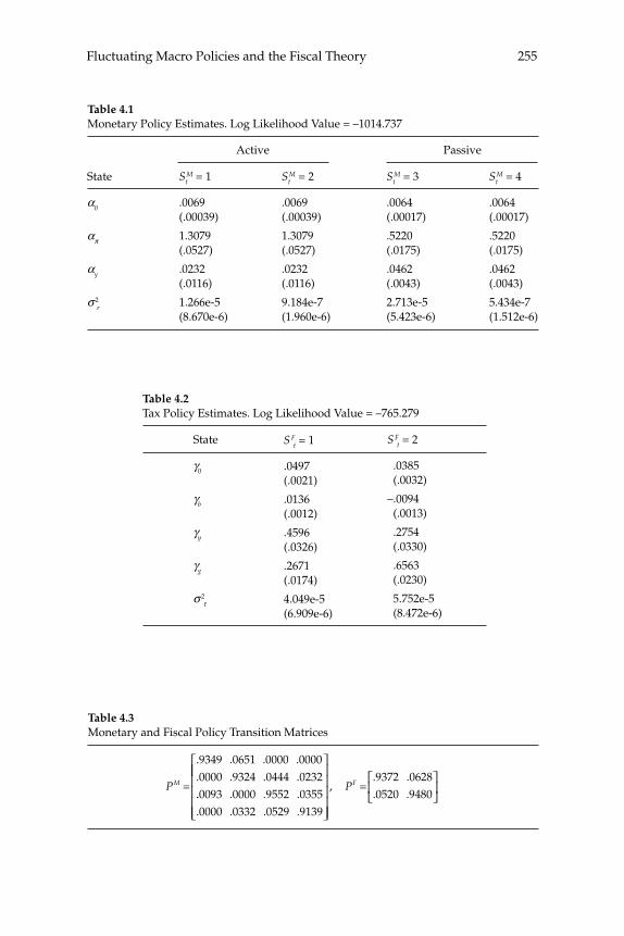
255Fluctuating Macro Policies and the Fiscal Theory
Table 4.1Monetary Policy Estimates. Log Likelihood Value = –1014.737
Active Passive
State
α0
απ
αy
σ 2r
StM = 1
.0069(.00039)
1.3079(.0527)
.0232(.0116)
1.266e-5(8.670e-6)
StM = 2
.0069(.00039)
1.3079(.0527)
.0232(.0116)
9.184e-7(1.960e-6)
StM = 3
.0064(.00017)
.5220(.0175)
.0462(.0043)
2.713e-5(5.423e-6)
StM = 4
.0064(.00017)
.5220(.0175)
.0462(.0043)
5.434e-7(1.512e-6)
Table 4.2Tax Policy Estimates. Log Likelihood Value = –765.279
State
γ0
γb
γy
γg
σ 2τ
S Ft = 1
.0497(.0021)
.0136(.0012)
.4596(.0326)
.2671(.0174)
4.049e-5(6.909e-6)
S Ft = 2
.0385 (.0032)
–.0094 (.0013)
.2754 (.0330)
.6563 (.0230)
5.752e-5 (8.472e-6)
Table 4.3Monetary and Fiscal Policy Transition Matrices
PM =
. . . .
. . . .9349 0651 0000 00000000 9324 0444 0232.. . . .. . . .0093 0000 9552 03550000 0332 0529 9139
⎡
⎣
⎢⎢⎢⎢⎢⎢
⎤
⎦
⎥⎥⎥⎥⎥
=⎡
⎣⎢
⎤
⎦⎥,
. .
. .PF
9372 06280520 9480
Davig and Leeper256
under passive policy is consistent with active policy pursuing counter-cyclical objectives more vigorously.
2.3 Plausibility of Estimates
We consider several checks on the plausibility of the estimated rules. First, are the estimates reasonable on a priori grounds? We think they are, as the rules fl uctuate between theoretically interpretable regimes. Monetary policy fl uctuates between periods when it is active, satisfy-ing the Taylor principle (απ > 1), and periods when it is passive (απ < 1). Passive tax policy responds to debt by a coeffi cient that exceeds most estimates of the quarterly real interest rate (and by more than the cali-brated real rate in the DSGE model below), while active tax policy low-ers taxes when debt is high.
Second, how well do the estimated equations track the actual paths of the interest rate and taxes? We use the estimates of equations (1) and (2), weighted by the estimated regime probabilities, to predict the time paths of the short-term nominal interest rate, r, and the ratio of tax revenues to output, τ, treating all explanatory variables as evolving exogenously. The predicted—using smoothed and fi ltered probabili-ties—and actual paths of r and τ appear in fi gures 4.1 and 4.2. These fi ts are easily comparable to those reported by, for example, Taylor (1999a) for monetary policy.12 The interest-rate equation goes off track in the 1950s, suggesting that period might constitute a third distinct regime, but in three-regime specifi cations the response of policy to output was negative. The tax rule tracks the revenue-output ratio extremely well, except in the last year or so when revenues dropped precipitously.
2.4 Corroborating Evidence: Individual Policy Processes
A third check on the plausibility of the estimates, which is a critical step in identifying policy behavior, asks whether the periods estimated to be active and passive correspond with narrative accounts of policy his-tory.13 The estimated marginal probabilities of the monetary and fi scal states are plotted in fi gures 4.3 and 4.4. All probabilities reported are at time t, conditional on information available at t – 1.
Figure 4.3 reports that, except for a brief active period in 1959–60, monetary policy was passive from 1948 until the Fed changed oper-ating procedures in October 1979 and policy became active. Mone-tary policy was consistently active except immediately after the two
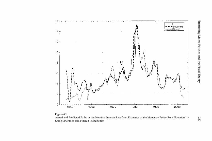
257Fluctuating M
acro Policies and the Fiscal T
heory
Figure 4.1Actual and Predicted Paths of the Nominal Interest Rate from Estimates of the Monetary Policy Rule, Equation (1) Using Smoothed and Filtered Probabilities
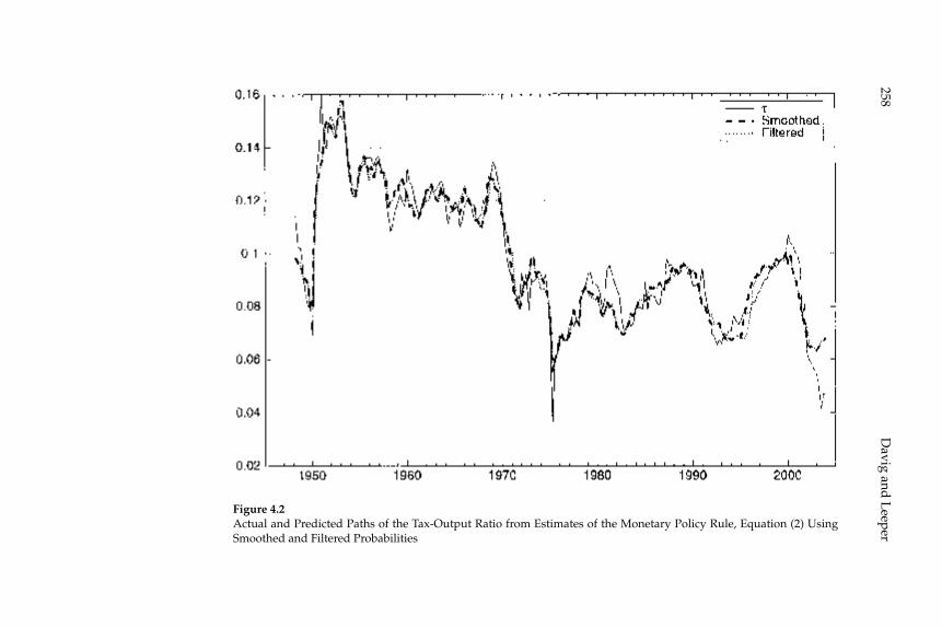
Davig and
Leeper
258
Figure 4.2Actual and Predicted Paths of the Tax-Output Ratio from Estimates of the Monetary Policy Rule, Equation (2) Using Smoothed and Filtered Probabilities
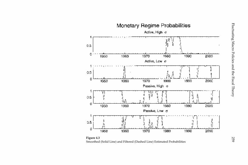
259Fluctuating M
acro Policies and the Fiscal T
heory
Figure 4.3Smoothed (Solid Line) and Filtered (Dashed Line) Estimated Probabilities
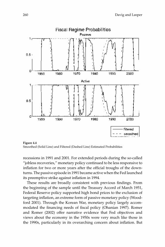
Davig and Leeper260
recessions in 1991 and 2001. For extended periods during the so-called “jobless recoveries,” monetary policy continued to be less responsive to infl ation for two or more years after the offi cial troughs of the down-turns. The passive episode in 1991 became active when the Fed launched its preemptive strike against infl ation in 1994.
These results are broadly consistent with previous fi ndings. From the beginning of the sample until the Treasury Accord of March 1951, Federal Reserve policy supported high bond prices to the exclusion of targeting infl ation, an extreme form of passive monetary policy (Wood-ford 2001). Through the Korean War, monetary policy largely accom-modated the fi nancing needs of fi scal policy (Ohanian 1997). Romer and Romer (2002) offer narrative evidence that Fed objectives and views about the economy in the 1950s were very much like those in the 1990s, particularly in its overarching concern about infl ation. But
Figure 4.4Smoothed (Solid Line) and Filtered (Dashed Line) Estimated Probabilities
261Fluctuating Macro Policies and the Fiscal Theory
Romer and Romer (2002, p. 123) quote Chairman William McChesney Martin’s congressional testimony, in which he explained that “the 1957–58 recession was a direct result of letting infl ation get substan-tially ahead of us.” The Romers also mention that FOMC “members felt they had not reacted soon enough in 1955 [to offset the burst of infl ation]” (p. 122). To buttress their narrative case, the Romers estimate a forward-looking Taylor rule from 1952:1–1958:4. They conclude that policy was active: The response of the interest rate to infl ation was 1.178 with a standard error of 0.876. Our estimate of this response coeffi cient in passive regimes is 0.522, which is less than one standard error below the Romers’ point estimate. The Fed might well have intended to be vigilant against infl ation, but it appears not to have acted to prevent the 1955 infl ation. The brief burst of active monetary policy late in 1959 and early in 1960 is consistent with the Romers’ (2002) fi nding that the Fed raised the real interest rate in this period to combat infl ation. From 1960–1979, monetary policy responded weakly to infl ation, while since the mid-1980s the Fed has reacted strongly to infl ation, a pattern found in many studies (Taylor 1999a, Clarida, Galí, and Gertler 2000, Romer and Romer 2002, and Lubik and Schorfheide 2004).
The estimates of passive monetary policy behavior following the 1991 and 2001 recessions are likely to confl ict with some readers’ pri-ors. Other evidence, however, corroborates the estimates. As early as March 1993, after the federal funds rate had been at 3 percent for sev-eral months, during policy deliberations Governors Angell, LaWare, and Mullins expressed concern that the Fed was keeping the rate low for too long. Angell warned that “our progress to get infl ation down low enough so it [isn’t a factor affecting] any business decision is now in jeopardy” (p. 30) (Board of Governors of the Federal Reserve System 1993a). At that March FOMC meeting, Governors Angell and Lindsey dissented on the vote to maintain the funds rate at 3 percent. Six months later, Mullins analogized 1993 to the 1970s as another “period in which perhaps short rates weren’t appropriately set to track infl ation” (p. 11) (Board of Governors of the Federal Reserve System 1993b).
More recently, close observers of the Fed have expressed similar concerns, citing the rapid growth in liquidity in 2003 and 2004 and the exceptionally low real interest rates since 2001 (Unsigned 2005a, b). Financial economists list unusually low interest rates as an impor-tant factor behind the spectacular growth in household and corporate debt in recent years (Unsigned 2002 and Roach 2004). These senti-ments about monetary policy behavior in the early 1990s and 2000s are
Davig and Leeper262
consistent with our estimates that the Fed responded only weakly to infl ation in those periods.
Estimates of the tax rule in (2) reveal substantially more regime insta-bility than for monetary policy. Over the post-war period, there were 12 fi scal regime changes, with tax policy spending 55 percent of the time in the active regime. Figure 4.4 shows that the model associates tax policy with regimes that accord well with narrative histories. Fiscal policy was active in the beginning of the sample. Despite an extremely high level of debt from World War Two expenditures, Congress overrode President Truman’s veto in early 1948 and cut taxes. Although, as Stein (1996) recounts the history, legislators argued that cutting taxes would reduce the debt, the debt-GDP ratio rose while revenues as a share of GDP fell. In 1950 and 1951 policy became passive, as taxes were increased and excess profi ts taxes were extended into 1953 to fi nance the Korean War, consistent with the budget-balancing goals of both the Truman and the Eisenhower Administrations. From the mid-50s, through the Kennedy tax cut of 1964, and into the second half of the 1960s, fi scal policy was active, paying little attention to debt. There followed a period of about 15 years when fi scal policy fl uctuated in its degree of concern about debt relative to economic conditions.
President Carter cut taxes to stimulate the economy in early 1979, ini-tiating a period of active fi scal policy that extended through the Reagan Administration’s Economic Recovery Plan of 1981. By the mid-1980s, the probability of passive tax policy increased as legislation was passed in 1982 and 1984 to raise revenues in response to the rapidly increas-ing debt-output ratio. Following President Clinton’s tax hike in 1993, fi scal policy switched to being passive through the 2001 tax cut. Presi-dent Bush’s tax reductions in 2002 and 2003 made fi scal policy active again.14
Favero and Monacelli (2005) estimate switching regressions similar to (1) and (2) and also fi nd that monetary policy was passive from 1961 to 1979. In contrast to our results, they do not detect any tendency to return to passive policy following the 1991 and 2001 recessions, though they estimate one regime, which occurs in 1985:2–2000:4 and 2002:2–2002:4, in which the monetary policy response to infl ation is exactly unity. Their estimates of fi scal policy are not directly comparable to ours because Favero and Monacelli use the net-of-interest defi cit as the policy variable, which confounds spending and tax policies. Like us, they fi nd that fi scal policy is more unstable than monetary policy.15 Our fi ndings are also consistent with the time-varying monetary policy
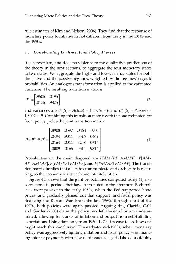
263Fluctuating Macro Policies and the Fiscal Theory
rule estimates of Kim and Nelson (2006). They fi nd that the response of monetary policy to infl ation is not different from unity in the 1970s and the 1990s.
2.5 Corroborating Evidence: Joint Policy Process
It is convenient, and does no violence to the qualitative predictions of the theory in the next sections, to aggregate the four monetary states to two states. We aggregate the high- and low-variance states for both the active and the passive regimes, weighted by the regimes’ ergodic probabilities. An analogous transformation is applied to the estimated variances. The resulting transition matrix is
PM =⎡
⎣⎢
⎤
⎦⎥
. .
. .9505 04950175 9825
(3)
and variances are σ 2r(St = Active) = 4.0576e – 6 and σ 2
r (St = Passive) = 1.8002e – 5. Combining this transition matrix with the one estimated for fi scal policy yields the joint transition matrix
P P PM F= ⊗ =
. . . .
. . .8908 0597 0464 00310494 9011 0026 ... . . .. . . .
04690164 0011 9208 06170009 0166 0511 93314
⎡
⎣
⎢⎢⎢⎢
⎤
⎦
⎥⎥⎥⎥
(4)
Probabilities on the main diagonal are P[AM/PF|AM/PF], P[AM/AF|AM/AF], P[PM/PF|PM/PF], and P[PM/AF|PM/AF]. The transi-tion matrix implies that all states communicate and each state is recur-ring, so the economy visits each one infi nitely often.
Figure 4.5 shows that the joint probabilities computed using (4) also correspond to periods that have been noted in the literature. Both pol-icies were passive in the early 1950s, when the Fed supported bond prices (and gradually phased out that support) and fi scal policy was fi nancing the Korean War. From the late 1960s through most of the 1970s, both policies were again passive. Arguing this, Clarida, Galí, and Gertler (2000) claim the policy mix left the equilibrium undeter-mined, allowing for bursts of infl ation and output from self-fulfi lling expectations. Using data only from 1960–1979, it is easy to see how one might reach this conclusion. The early-to-mid-1980s, when monetary policy was aggressively fi ghting infl ation and fi scal policy was fi nanc-ing interest payments with new debt issuances, gets labeled as doubly
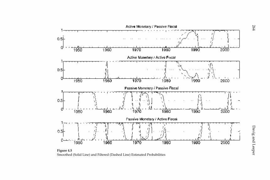
Davig and
Leeper
264
Figure 4.5Smoothed (Solid Line) and Filtered (Dashed Line) Estimated Probabilities

265Fluctuating Macro Policies and the Fiscal Theory
active policies. Finally, the mid-1980s on is largely a period of active monetary and passive fi scal policies, as most models of monetary pol-icy assume (for example, the papers in Bryant, Hooper, and Mann 1993 and Taylor 1999b).
Taken together, the marginal and joint probabilities paint a picture of post-war monetary and fi scal policies that is broadly consistent with both narrative accounts and fi xed-regime policy rule estimates.
A fi nal check on the plausibility of the estimates asks if the policies make economic sense when they are embedded in a conventional DSGE model. Sections 6 and 7 answer this question in detail.
3 A Model with Nominal Rigidities
We employ a conventional model with monopolistic competition and sticky prices in goods markets, extended to include lump-sum taxes and nominal government debt.16 Although the model is standard, because we intend to solve it in its full nonlinear form, it is worthwhile briefl y reviewing the specifi cation.
3.1 Households
The representative household chooses {Ct, Nt, Mt, Bt} to maximize
EC N M P
ti t i t i t i t iβ
σχ
ηδ
σ η κ+−
++
+ +−
−−
++
1 1 1
1 1 1( / )
−−⎡
⎣⎢
⎤
⎦⎥
=
∞
∑ κi 0
(5)
with 0 < β < 1, σ > 0, η > 0, κ > 0, χ > 0, and δ > 0.17 Ct is a composite con-sumption good that combines the demand for the differentiated goods, cjt, using a Dixit and Stiglitz (1977) aggregator:
C c djt jt=⎡
⎣⎢
⎤
⎦⎥ >
− −
∫θ
θ
θθ
θ1
0
1 1
1, . (6)
The household chooses cjt to minimize expenditure on the continuum of goods indexed by the unit interval, leading to the demand functions for each good j
cp
PCjt
jt
tt=
⎛⎝⎜
⎞⎠⎟
−θ
, (7)
where Pt ≡ [∫ 10pjt
1–θ dj]1/1–θ is the aggregate price level at t.

Davig and Leeper266
The household’s budget constraint is
CMP
E QBP
WP
Ntt
tt t t
t
tt
t
tt+ +
⎛⎝⎜
⎞⎠⎟
+ ≤⎛⎝⎜
⎞⎠⎟
++, 1 τ MMP
BP
t
t
t
tt
− −+ +1 1 Π , (8)
where τt is lump-sum taxes/transfers from the government to the household, Bt is one-period nominal bonds, Qt,t+1 is the stochastic dis-count factor for the price at t of one dollar at t + 1, and Πt is profi ts from the fi rm, which the household owns. The household maximizes (5) sub-ject to (8) to yield the fi rst-order conditions
χη
σNC
WP
t
t
t
t− = (9)
QC
CP
Pt tt
t
t
t, .+
+ +
=⎛⎝⎜
⎞⎠⎟1
1 1
βσ
(10)
If 1 + rt denotes the risk-free gross nominal interest rate between t and t + 1, then absence of arbitrage implies the equilibrium condition
[Et(Qt,t+1)]–1 = 1 + rt, (11)
so the fi rst-order conditions imply that real money balances may be written as
MP
rr
Ct
t
t
tt=
+⎛
⎝⎜⎞
⎠⎟
−
δκ
κ
σ κ
1
1/
/ . (12)
The government demands goods in the same proportion that house-holds do, so the government’s demand is gjt = (pjt/Pt)
–θGt, where Gt = [∫ 1
0 gjtθ–1/θ dj]θ/θ–1.
Necessary and suffi cient conditions for household optimization are that (9)–(12) hold at all dates and that households exhaust their intertemporal budget constraints. The latter condition is equivalent to requiring that the present value of households’ planned expenditure is fi nite and that wealth accumulation satisfi es the transversality condi-tion (Woodford 2001):
lim ,,T t t TT
T
E qAP→∞
⎡
⎣⎢
⎤
⎦⎥ = 0 (13)
where At = Bt + Mt and qt,t+1 = Qt,t+1Pt+1/Pt.

267Fluctuating Macro Policies and the Fiscal Theory
3.2 Firms
A continuum of monopolistically competitive fi rms produce goods using labor. Production of good j is
yjt = ZNjt, (14)
where Z is aggregate technology, common across fi rms and taken to be constant.
Aggregating consumers’ and government’s demand, fi rm j faces the demand curve
yp
PYjt
jt
tt=
⎛⎝⎜
⎞⎠⎟
−θ
, (15)
where Yt is defi ned by
Ct + Gt = Yt. (16)
Equating supply and demand for individual goods,
ZNp
PYjt
jt
tt=
⎛⎝⎜
⎞⎠⎟
−θ
. (17)
Following Calvo (1983), a fraction 1 – ϕ fi rms are permitted to adjust their prices each period, while the fraction ϕ are not permitted to adjust. If fi rms are permitted to adjust at t, they choose a new optimal price, p*
t, to maximize the expected discounted sum of profi ts given by
E qpP
pPt
it t i
t
t it i
t
t i
ϕθ
,
* *
++
−
++
⎛⎝⎜
⎞⎠⎟
−⎛⎝⎜
⎞⎠
1
Ψ ⎟⎟⎡
⎣⎢⎢
⎤
⎦⎥⎥
−
=
∞
+∑θ
it iY
0
, (18)
where the real profi t fl ow of fi rm j at period t, Πjt = (pjt/Pt)1–θYt – (Wt/Pt)Njt,
has been rewritten using (17). Ψt is real marginal cost, defi ned as
Ψtt
t
WZP
= . (19)
The fi rst-order condition that determines pt* can be written as
pP
E Y GPPt
t
ti
t i t it i
t*
( ) ( )=
−⎛
⎝⎜⎞
⎠⎟
−⎛
+ +− +
θθ
ϕβ σ
1⎝⎝⎜
⎞⎠⎟
−
+ +=
∞
+ +− +
∑θ
σϕβ
Ψt i t ii
ti
t i t it
Y
E Y GP
0
( ) ( ) ii
tt i
i PY
⎛⎝⎜
⎞⎠⎟
−
+=
∞
∑θ 1
0
, (20)

Davig and Leeper268
which we denote by
pP
KK
t
t
t
t
*
,=−
⎛
⎝⎜⎞
⎠⎟θ
θ 11
2
(21)
where the numerator and the denominator have recursive representa-tions:
K Y G Y E KPPt t t t t t tt
t1 1 1
1= − +⎛⎝⎜
⎞⎠⎟
−+
+( ) σθ
ϕβΨ (22)
and
K Y G Y E KPPt t t t t tt
t2 2 1
1
1
= − +⎛⎝⎜
⎞⎠⎟
−+
+
−
( ) .σθ
ϕβ (23)
Solving (21) for pt* and using the result in the aggregate price index,
Pt1–θ = (1 – ϕ)( pt
*)1–θ + ϕP 1–θt–1, yields
πϕ
ϕϕ
μθθ
tt
t
KK
−−
= −− ⎛
⎝⎜⎞⎠⎟
1 1
2
11 1
, (24)
where μ ≡ θ/(θ – 1) is the markup.We assume that individual labor services may be aggregated linearly
to produce aggregate labor, Nt = ∫ 10Njtdj. Linear aggregation of individ-
ual market clearing conditions implies ZNt = ΔtYt, where Δt is a measure of relative price dispersion defi ned by
Δtjt
t
p
Pdj=
⎛⎝⎜
⎞⎠⎟∫
−
0
1θ
. (25)
Now the aggregate production function is given by
YZ
Ntt
t=Δ
. (26)
It is natural to defi ne aggregate profi ts as the sum of individual fi rm profi ts, Πt = ∫ 1
0Πjtdj. Integrating over fi rms’ profi ts and combining the household’s and the government’s budget constraints yields the aggre-gate resource constraint
ZN C G
tt t tΔ= + . (27)

269Fluctuating Macro Policies and the Fiscal Theory
From the defi nitions of price dispersion and the aggregate price index, relative price dispersion evolves according to
Δ Δtt
tt t
pP
= −⎛⎝⎜
⎞⎠⎟
+−
−( ) ,*
1 1ϕ ϕπθ
θ (28)
where πt = Pt/Pt–1.Following Woodford (2003), we defi ne potential output, Y p
t, to be the equilibrium level of output that would be realized if prices were per-fectly fl exible. Potential output, then, emerges from the model when ϕ = 0, so all fi rms can adjust prices every period. The output gap, yt, is defi ned as yt = Yt – Y p
t. In this model, with disturbances only to mon-etary policy and to lump-sum taxes, Y p
t ≡ 1.
3.3 Policy Specifi cation
Monetary and tax policies follow (1) and (2), with error terms that are standard normal and i.i.d. The processes for {Gt, τt, Mt, Bt} must satisfy the government budget identity
GM M
PE Q
BP
BPt t
t t
tt t t
t
t
t
t
= +−
+⎛⎝⎜
⎞⎠⎟
−−+
−τ 11
1, . (29)
given M–1 > 0 and (1 + r–1)B–1. Government spending is assumed to be a constant share of output.
3.4 Information Assumptions
Although in the empirical estimates in section 2 regime is a state vari-able hidden from the econometrician, we do not confront agents in the model with an inference problem. Instead, we assume agents observe at least current and past policy shocks and regimes. Under conventional information assumptions, the model is solved assuming that private agents base their decisions at date t on the information set Ωt = {ε r
t–j, ε τ
t–j, SMt–j, S
Ft–j, j ≥ 0} plus the initial conditions (M–1, (1 + r–1)B–1). This con-
ventional information structure enables us to quantify the impacts of unanticipated changes in taxes. We also seek to quantify the effects of anticipated changes in taxes. Those effects are computed by endowing agents with foreknowledge of tax disturbances, so the model is solved using the expanded information set Ω *
t = Ωt ∪ {ετt+1}.
18
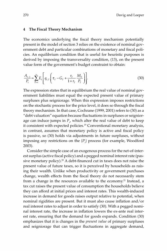
Davig and Leeper270
4 The Fiscal Theory Mechanism
The economics underlying the fi scal theory mechanism potentially present in the model of section 3 relies on the existence of nominal gov-ernment debt and particular combinations of monetary and fi scal poli-cies. An equilibrium condition that is useful for heuristic purposes is derived by imposing the transversality condition, (13), on the present value form of the government’s budget constraint to obtain:
AP
E q Gr
rMP
t
tt t T T T
T
T
T
T
− = − ++
⎛
⎝⎜⎞
⎠⎟⎡
⎣⎢⎢
⎤
⎦⎥⎥
1
1, τTT t=
∞
∑ . (30)
The expression states that in equilibrium the real value of nominal gov-ernment liabilities must equal the expected present value of primary surpluses plus seigniorage. When this expression imposes restrictions on the stochastic process for the price level, it does so through the fi scal theory mechanism. In that case, Cochrane (1999, 2001) refers to (30) as a “debt valuation” equation because fl uctuations in surpluses or seignior-age can induce jumps in Pt, which alter the real value of debt to keep it consistent with expected policies.19 Conventional monetary analysis, in contrast, assumes that monetary policy is active and fi scal policy is passive, so (30) holds via adjustments in future surpluses, without imposing any restrictions on the {Pt} process (for example, Woodford 2003).
Consider the simple case of an exogenous process for the net-of-inter-est surplus (active fi scal policy) and a pegged nominal interest rate (pas-sive monetary policy).20 A debt-fi nanced cut in taxes does not raise the present value of future taxes, so it is perceived by households as rais-ing their wealth. Unlike when productivity or government purchases change, wealth effects from the fi scal theory do not necessarily stem from a change in the resources available to the economy.21 Instead, a tax cut raises the present value of consumption the households believe they can afford at initial prices and interest rates. This wealth-induced increase in demand for goods raises output relative to potential, when nominal rigidities are present. But it must also cause infl ation and/or real interest rates to adjust in order to satisfy (30). With a pegged nomi-nal interest rate, the increase in infl ation lowers the ex-ante real inter-est rate, ensuring that the demand for goods expands. Condition (30) emphasizes that it is changes in the present value of primary surpluses and seigniorage that can trigger fl uctuations in aggregate demand,
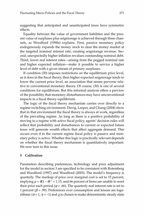
271Fluctuating Macro Policies and the Fiscal Theory
suggesting that anticipated and unanticipated taxes have symmetric effects.
Equality between the value of government liabilities and the pres-ent value of surpluses plus seigniorage is achieved through three chan-nels, as Woodford (1998a) explains. First, passive monetary policy endogenously expands the money stock to clear the money market at the targeted nominal interest rate, creating seigniorage revenue. Sec-ond, unexpectedly higher infl ation revalues outstanding nominal debt. Third, lower real interest rates—arising from the pegged nominal rate and higher expected infl ation—make it possible to service a higher level of debt with a given stream of primary surpluses.
If condition (30) imposes restrictions on the equilibrium price level, as it does in the fi scal theory, then higher expected seigniorage tends to lower the current price level, an association that seems perverse rela-tive to conventional monetary theory. Of course, (30) is one of several conditions for equilibrium. But this informal analysis offers a preview of the possibility that monetary disturbances may have unconventional impacts in a fi scal theory equilibrium.
The logic of the fi scal theory mechanism carries over directly to a regime-switching environment. Davig, Leeper, and Chung (2004) show that in that environment the fi scal theory is always at work, regardless of the prevailing regime. As long as there is a positive probability of moving to a regime with active fi scal policy, agents’ decision rules will refl ect that probability and disturbances to current or expected future taxes will generate wealth effects that affect aggregate demand. This occurs even if in the current regime fi scal policy is passive and mon-etary policy is active. Whether this logic is practically relevant depends on whether the fi scal theory mechanism is quantitatively important. We now turn to this issue.
5 Calibration
Parameters describing preferences, technology and price adjustment for the model in section 3 are specifi ed to be consistent with Rotemberg and Woodford (1997) and Woodford (2003). The model’s frequency is quarterly. The markup of price over marginal cost is set to 15 percent, implying μ = θ(1 – θ)–1 = 1.15, and 66 percent of fi rms are unable to reset their price each period (ϕ = .66). The quarterly real interest rate is set to 1 percent (β = .99). Preferences over consumption and leisure are loga-rithmic (σ = 1, η = –1) and χ is chosen to make deterministic steady state
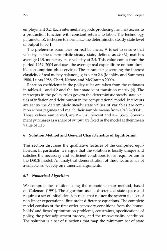
Davig and Leeper272
employment 0.2. Each intermediate goods producing fi rm has access to a production function with constant returns to labor. The technology parameter, Z, is chosen to normalize the deterministic steady state level of output to be 1.
The preference parameter on real balances, δ, is set to ensure that velocity in the deterministic steady state, defi ned as cP/M, matches average U.S. monetary base velocity at 2.4. This value comes from the period 1959–2004 and uses the average real expenditure on non-dura-ble consumption plus services. The parameter governing the interest elasticity of real money balances, κ, is set to 2.6 (Mankiw and Summers 1986, Lucas 1988, Chari, Kehoe, and McGrattan 2000).
Reaction coeffi cients in the policy rules are taken from the estimates in tables 4.1 and 4.2 and the four-state joint transition matrix (4). The intercepts in the policy rules govern the deterministic steady state val-ues of infl ation and debt-output in the computational model. Intercepts are set so the deterministic steady state values of variables are com-mon across regimes and match their sample means from 1948:2–2004:1. Those values, annualized, are π = 3.43 percent and b = .3525. Govern-ment purchases as a share of output are fi xed in the model at their mean value of .115.
6 Solution Method and General Characteristics of Equilibrium
This section discusses the qualitative features of the computed equi-librium. In particular, we argue that the solution is locally unique and satisfi es the necessary and suffi cient conditions for an equilibrium in the DSGE model. An analytical demonstration of these features is not available, so we rely on numerical arguments.
6.1 Numerical Algorithm
We compute the solution using the monotone map method, based on Coleman (1991). The algorithm uses a discretized state space and requires a set of initial decision rules that reduce the system to a set of non-linear expectational fi rst-order difference equations. The complete model consists of the fi rst-order necessary conditions from the house-holds’ and fi rms’ optimization problems, constraints, specifi cations of policy, the price adjustment process, and the transversality condition. The solution is a set of functions that map the minimum set of state
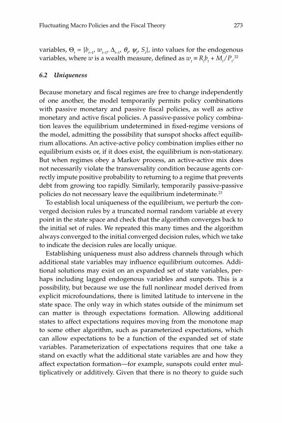
273Fluctuating Macro Policies and the Fiscal Theory
variables, Θt = {bt–1, wt–1, Δt–1, θt, ψt, St}, into values for the endogenous variables, where w is a wealth measure, defi ned as wt ≡ Rtbt + Mt/Pt.
22
6.2 Uniqueness
Because monetary and fi scal regimes are free to change independently of one another, the model temporarily permits policy combinations with passive monetary and passive fi scal policies, as well as active monetary and active fi scal policies. A passive-passive policy combina-tion leaves the equilibrium undetermined in fi xed-regime versions of the model, admitting the possibility that sunspot shocks affect equilib-rium allocations. An active-active policy combination implies either no equilibrium exists or, if it does exist, the equilibrium is non-stationary. But when regimes obey a Markov process, an active-active mix does not necessarily violate the transversality condition because agents cor-rectly impute positive probability to returning to a regime that prevents debt from growing too rapidly. Similarly, temporarily passive-passive policies do not necessary leave the equilibrium indeterminate.23
To establish local uniqueness of the equilibrium, we perturb the con-verged decision rules by a truncated normal random variable at every point in the state space and check that the algorithm converges back to the initial set of rules. We repeated this many times and the algorithm always converged to the initial converged decision rules, which we take to indicate the decision rules are locally unique.
Establishing uniqueness must also address channels through which additional state variables may infl uence equilibrium outcomes. Addi-tional solutions may exist on an expanded set of state variables, per-haps including lagged endogenous variables and sunpots. This is a possibility, but because we use the full nonlinear model derived from explicit microfoundations, there is limited latitude to intervene in the state space. The only way in which states outside of the minimum set can matter is through expectations formation. Allowing additional states to affect expectations requires moving from the monotone map to some other algorithm, such as parameterized expectations, which can allow expectations to be a function of the expanded set of state variables. Parameterization of expectations requires that one take a stand on exactly what the additional state variables are and how they affect expectation formation—for example, sunspots could enter mul-tiplicatively or additively. Given that there is no theory to guide such
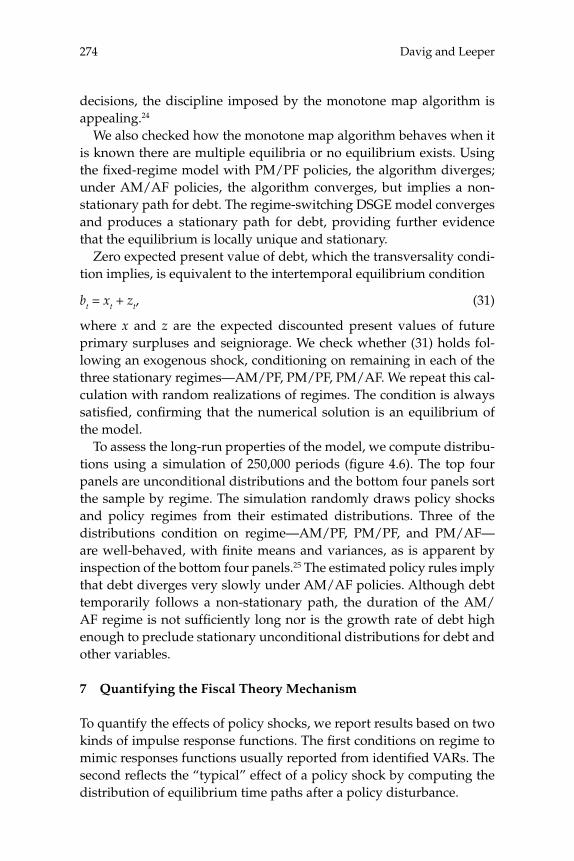
Davig and Leeper274
decisions, the discipline imposed by the monotone map algorithm is appealing.24
We also checked how the monotone map algorithm behaves when it is known there are multiple equilibria or no equilibrium exists. Using the fi xed-regime model with PM/PF policies, the algorithm diverges; under AM/AF policies, the algorithm converges, but implies a non-stationary path for debt. The regime-switching DSGE model converges and produces a stationary path for debt, providing further evidence that the equilibrium is locally unique and stationary.
Zero expected present value of debt, which the transversality condi-tion implies, is equivalent to the intertemporal equilibrium condition
bt = xt + zt, (31)
where x and z are the expected discounted present values of future primary surpluses and seigniorage. We check whether (31) holds fol-lowing an exogenous shock, conditioning on remaining in each of the three stationary regimes—AM/PF, PM/PF, PM/AF. We repeat this cal-culation with random realizations of regimes. The condition is always satisfi ed, confi rming that the numerical solution is an equilibrium of the model.
To assess the long-run properties of the model, we compute distribu-tions using a simulation of 250,000 periods (fi gure 4.6). The top four panels are unconditional distributions and the bottom four panels sort the sample by regime. The simulation randomly draws policy shocks and policy regimes from their estimated distributions. Three of the distributions condition on regime—AM/PF, PM/PF, and PM/AF—are well-behaved, with fi nite means and variances, as is apparent by inspection of the bottom four panels.25 The estimated policy rules imply that debt diverges very slowly under AM/AF policies. Although debt temporarily follows a non-stationary path, the duration of the AM/AF regime is not suffi ciently long nor is the growth rate of debt high enough to preclude stationary unconditional distributions for debt and other variables.
7 Quantifying the Fiscal Theory Mechanism
To quantify the effects of policy shocks, we report results based on two kinds of impulse response functions. The fi rst conditions on regime to mimic responses functions usually reported from identifi ed VARs. The second refl ects the “typical” effect of a policy shock by computing the distribution of equilibrium time paths after a policy disturbance.
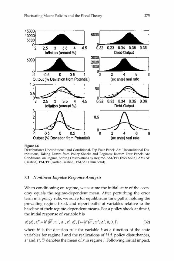
275Fluctuating Macro Policies and the Fiscal Theory
7.1 Nonlinear Impulse Response Analysis
When conditioning on regime, we assume the initial state of the econ-omy equals the regime-dependent mean. After perturbing the error term in a policy rule, we solve for equilibrium time paths, holding the prevailing regime fi xed, and report paths of variables relative to the baseline of their regime-dependent means. For a policy shock at time t, the initial response of variable k is
φ ε ε ε ετ τtk
tr
tk J J J
tr
tk Jh b w J h b w( , ) ( , , , , , ) ( ,= −Δ JJ J J, , , , ),Δ 0 0 (32)
where hk is the decision rule for variable k as a function of the state variables for regime J and the realizations of i.i.d. policy disturbances, ε t
r and ε tτ . x–J denotes the mean of x in regime J. Following initial impact,
Figure 4.6Distributions: Unconditional and Conditional. Top Four Panels Are Unconditional Dis-tributions, Taking Draws from Policy Shocks and Regimes; Bottom Four Panels Are Conditional on Regime, Sorting Observations by Regime. AM/PF (Thick Solid), AM/AF (Dashed), PM/PF (Dotted-Dashed), PM/AF (Thin Solid)
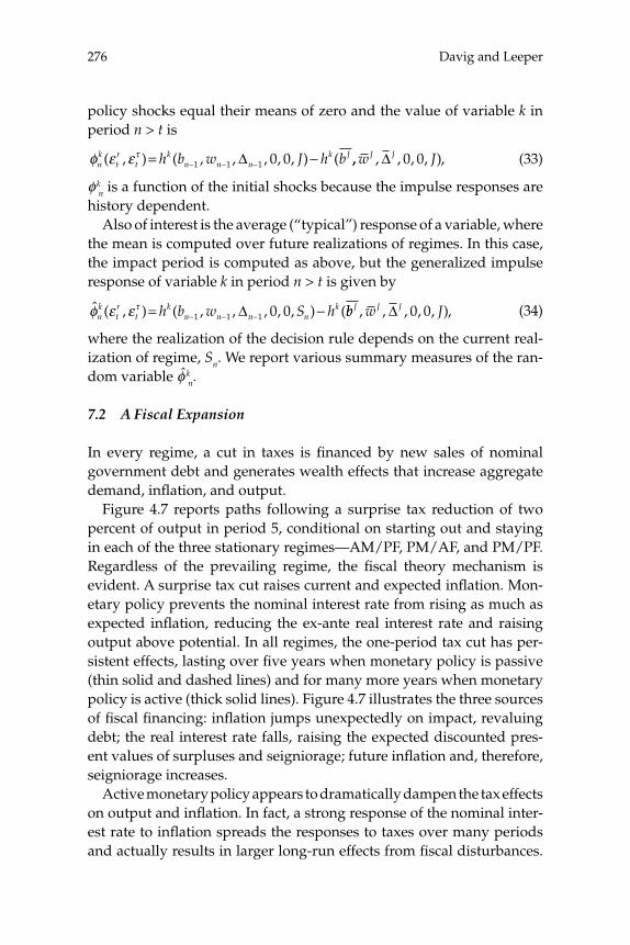
Davig and Leeper276
policy shocks equal their means of zero and the value of variable k in period n > t is
φ ε ετnk
tr
tk
n n nk Jh b w J h b( , ) ( , , , , , ) (= −− − −1 1 1 0 0Δ ,, , , , , ),w JJ JΔ 0 0 (33)
φ kn is a function of the initial shocks because the impulse responses are
history dependent.Also of interest is the average (“typical”) response of a variable, where
the mean is computed over future realizations of regimes. In this case, the impact period is computed as above, but the generalized impulse response of variable k in period n > t is given by
ˆ ( , ) ( , , , , , ) (φ ε ετnk
tr
tk
n n n nkh b w S h= −− − −1 1 1 0 0Δ bb w JJ J J, , , , , ),Δ 0 0 (34)
where the realization of the decision rule depends on the current real-ization of regime, Sn. We report various summary measures of the ran-dom variable φ k
n.
7.2 A Fiscal Expansion
In every regime, a cut in taxes is fi nanced by new sales of nominal government debt and generates wealth effects that increase aggregate demand, infl ation, and output.
Figure 4.7 reports paths following a surprise tax reduction of two percent of output in period 5, conditional on starting out and staying in each of the three stationary regimes—AM/PF, PM/AF, and PM/PF. Regardless of the prevailing regime, the fi scal theory mechanism is evident. A surprise tax cut raises current and expected infl ation. Mon-etary policy prevents the nominal interest rate from rising as much as expected infl ation, reducing the ex-ante real interest rate and raising output above potential. In all regimes, the one-period tax cut has per-sistent effects, lasting over fi ve years when monetary policy is passive (thin solid and dashed lines) and for many more years when monetary policy is active (thick solid lines). Figure 4.7 illustrates the three sources of fi scal fi nancing: infl ation jumps unexpectedly on impact, revaluing debt; the real interest rate falls, raising the expected discounted pres-ent values of surpluses and seigniorage; future infl ation and, therefore, seigniorage increases.
Active monetary policy appears to dramatically dampen the tax effects on output and infl ation. In fact, a strong response of the nominal inter-est rate to infl ation spreads the responses to taxes over many periods and actually results in larger long-run effects from fi scal disturbances.
277Fluctuating Macro Policies and the Fiscal Theory
In a fi xed-regime model, the Taylor principle creates explosive infl a-tion dynamics following an i.i.d. shock, so it may seem anomalous that the infl ation process is stationary in the AM/PF regime. Davig, Leeper, and Chung (2004) show, in an endowment version of this model, that an AM/PF regime creates wealth effects that make the forecast error in infl ation serially correlated, depending negatively on past infl ation and positively on past real debt. These surprises in infl ation are a key feature of the fi scal theory mechanism, as they serve to revalue debt. Through the Taylor principle, higher πt raises rt, which increases future debt service. Because regimes can switch, agents expect some debt ser-vice to be met with future seigniorage. But the paths in fi gure 4.7 con-dition on remaining in the AM/PF regime, so taxes are unexpectedly high, which reduces aggregate demand and stabilizes infl ation.
Generalized impulse response functions bring out the role that the evolution of regime plays in affecting economic agents’ expectations and choices. Dynamic impacts of policy disturbances display impor-tant differences from their counterparts in fi gure 4.7. For the three
Figure 4.7Responses to an i.i.d. Tax Cut of 2 Percent of Output, Conditional on Remaining in the Prevailing Regime
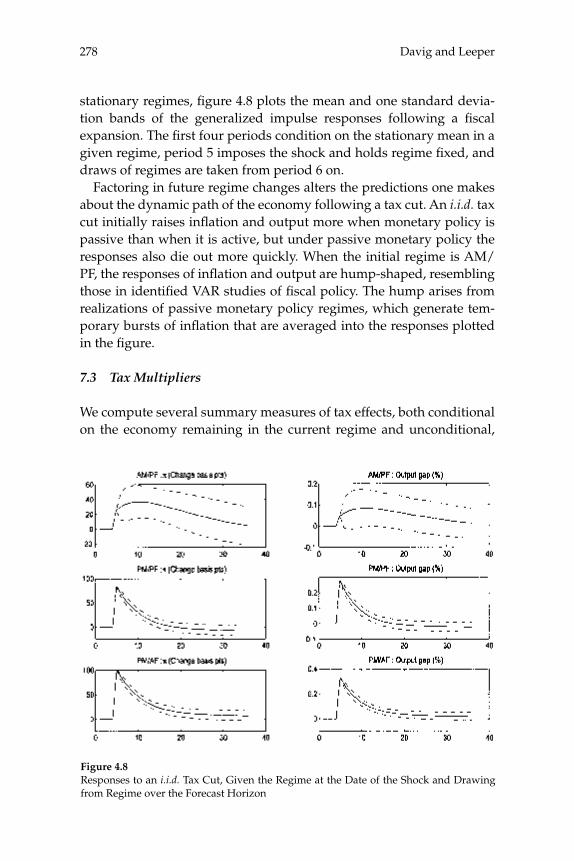
Davig and Leeper278
stationary regimes, fi gure 4.8 plots the mean and one standard devia-tion bands of the generalized impulse responses following a fi scal expansion. The fi rst four periods condition on the stationary mean in a given regime, period 5 imposes the shock and holds regime fi xed, and draws of regimes are taken from period 6 on.
Factoring in future regime changes alters the predictions one makes about the dynamic path of the economy following a tax cut. An i.i.d. tax cut initially raises infl ation and output more when monetary policy is passive than when it is active, but under passive monetary policy the responses also die out more quickly. When the initial regime is AM/PF, the responses of infl ation and output are hump-shaped, resembling those in identifi ed VAR studies of fi scal policy. The hump arises from realizations of passive monetary policy regimes, which generate tem-porary bursts of infl ation that are averaged into the responses plotted in the fi gure.
7.3 Tax Multipliers
We compute several summary measures of tax effects, both conditional on the economy remaining in the current regime and unconditional,
Figure 4.8Responses to an i.i.d. Tax Cut, Given the Regime at the Date of the Shock and Drawing from Regime over the Forecast Horizon
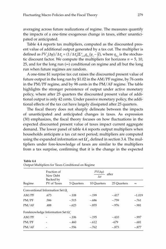
279Fluctuating Macro Policies and the Fiscal Theory
averaging across future realizations of regime. The measures quantify the impacts of a one-time exogenous change in taxes, either unantici-pated or anticipated.
Table 4.4 reports tax multipliers, computed as the discounted pres-ent value of additional output generated by a tax cut. The multiplier is defi ned as PVn(Δy)/Δτ0 = (1/Δτ0)Σ
ns=0q0,s(ys – y–), where q0,s is the stochas-
tic discount factor. We compute the multipliers for horizons n = 5, 10, 25, and for the long run (∞) conditional on regime and all but the long run when future regimes are random.
A one-time $1 surprise tax cut raises the discounted present value of future output in the long run by $1.02 in the AM/PF regime, by 76 cents in the PM/PF regime, and by 98 cents in the PM/AF regime. The table highlights the stronger persistence of output under active monetary policy, where after 25 quarters the discounted present value of addi-tional output is only 42 cents. Under passive monetary policy, the addi-tional effects of the tax cut have largely dissipated after 25 quarters.
The fi scal theory does not sharply delineate between the impacts of unanticipated and anticipated changes in taxes. As expression (30) emphasizes, the fi scal theory focuses on how fl uctuations in the expected discounted present value of taxes impact current aggregate demand. The lower panel of table 4.4 reports output multipliers when households anticipate a tax cut next period; multipliers are computed using the expanded information set Ω *
t, defi ned in section 3.4. The mul-tipliers under fore-knowledge of taxes are similar to the multipliers from a tax surprise, confi rming that it is the change in the expected
Table 4.4Output Multipliers for Taxes Conditional on Regime
Regime
Conventional Information Set Ωt
AM/PF
PM/PF
PM/AF
Foreknowledge Information Set Ω t*
AM/PF
PM/PF
PM/AF
Fraction of New Debt Backed by PV of Taxes
.673
.586
.488
-
-
-
5 Quarters
–.108
–.515
–.623
–.106
–.460
–.556
10 Quarters
–.199
–.686
–.855
–.195
–.612
–.762
25 Quarters
–.417
–.759
–.976
–.410
–679
–.873
∞
–1.019
–.761
–.981
–.997
–.681
–.877
afterPV(Δy)
Δτ
Davig and Leeper280
discounted present value of primary surpluses that is central to the fi s-cal theory mechanism.
Table 4.4 shows the proportion of the marginal addition to debt aris-ing from a tax cut that is backed by an increase in discounted primary surpluses. Under an AM/PF policy, two-thirds of new debt is backed by discounted primary surpluses, in contrast to fi xed-regime models, where the proportion is 100 percent. The proportions under PM/PF and PM/AF are 59 percent and 49 percent. Consequently, the PM/AF regime experiences the strongest wealth effect on impact from a tax cut, as fi gure 4.7 makes apparent. Much of this adjustment arises from the lower real interest rates that are used to discount future surpluses and seigniorage.
In the model, it is highly unusual for policy regime to remain unchanged, as the calculations in table 4.4 assume. Typically, after a policy disturbance, regimes evolve according to their estimated transi-tion matrices. Table 4.5 reports 80th percentile ranges for the tax multi-pliers, computed from 10,000 draws of regimes, using the generalized impulse response function defi ned in (34). At the 80th percentile, a $1 tax cut raises the discounted present value of output from 76 cents to $1.36 after six years, depending on the initial regime.
Table 4.6 reports the price level effects of a one-period tax shock, con-ditional on regime. In the long run, a transitory tax cut of 2 percent of output raises the price level by 6.7 percent under AM/PF policies. At a little over 1 percent, the long-run price effects are substantially smaller when monetary policy is passive. At shorter horizons, taxes have larger price effects when monetary policy is passive than when it is active. Table 4.7 records typical price level impacts, accounting for possible future regimes. These impacts can be substantial, with the price level more than 2 percent higher six years after the tax cut. Uncertainty about realizations of future regimes creates a wide range of possible output and price level impacts from tax changes, as tables 4.5 and 4.7 attest.26
7.4 Quantitative Sensitivity to Policy Process
In this model, tax shocks matter as long as fi scal policy can be active some of the time and agents’ expectations incorporate this belief. Figure 4.9 shows the immediate impact of a tax shock (positive or negative) on output and infl ation as the percentage of time policy spends in the AM/PF regime varies from 0 percent to 100 percent. This impact effect
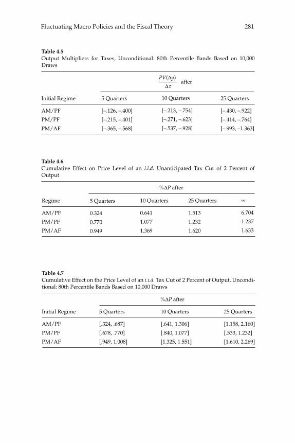
281Fluctuating Macro Policies and the Fiscal Theory
afterPV(Δy)
Δτ
Table 4.5Output Multipliers for Taxes, Unconditional: 80th Percentile Bands Based on 10,000 Draws
Initial Regime
AM/PF
PM/PF
PM/AF
5 Quarters
[–.126, –.400]
[–.215, –.401]
[–.365, –.568]
10 Quarters
[–.213, –.754]
[–.271, –.623]
[–.537, –.928]
25 Quarters
[–.430, –.922]
[–.414, –.764]
[–.993, –1.363]
%ΔP after
Table 4.6Cumulative Effect on Price Level of an i.i.d. Unanticipated Tax Cut of 2 Percent of Output
Regime
AM/PF
PM/PF
PM/AF
5 Quarters
0.324
0.770
0.949
10 Quarters
0.641
1.077
1.369
25 Quarters
1.513
1.232
1.620
∞
6.704
1.237
1.633
%ΔP after
Table 4.7Cumulative Effect on the Price Level of an i.i.d. Tax Cut of 2 Percent of Output, Uncondi-tional: 80th Percentile Bands Based on 10,000 Draws
Initial Regime
AM/PF
PM/PF
PM/AF
5 Quarters
[.324, .687]
[.678, .770]
[.949, 1.008]
10 Quarters
[.641, 1.306]
[.840, 1.077]
[1.325, 1.551]
25 Quarters
[1.158, 2.160]
[.533, 1.232]
[1.610, 2.269]
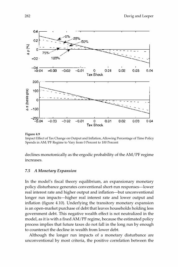
Davig and Leeper282
Figure 4.9Impact Effect of Tax Change on Output and Infl ation, Allowing Percentage of Time Policy Spends in AM/PF Regime to Vary from 0 Percent to 100 Percent
declines monotonically as the ergodic probability of the AM/PF regime increases.
7.5 A Monetary Expansion
In the model’s fi scal theory equilibrium, an expansionary monetary policy disturbance generates conventional short-run responses—lower real interest rate and higher output and infl ation—but unconventional longer run impacts—higher real interest rate and lower output and infl ation (fi gure 4.10). Underlying the transitory monetary expansion is an open-market purchase of debt that leaves households holding less government debt. This negative wealth effect is not neutralized in the model, as it is with a fi xed AM/PF regime, because the estimated policy process implies that future taxes do not fall in the long run by enough to counteract the decline in wealth from lower debt.
Although the longer run impacts of a monetary disturbance are unconventional by most criteria, the positive correlation between the
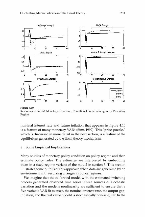
283Fluctuating Macro Policies and the Fiscal Theory
nominal interest rate and future infl ation that appears in fi gure 4.10 is a feature of many monetary VARs (Sims 1992). This “price puzzle,” which is discussed in more detail in the next section, is a feature of the equilibrium generated by the fi scal theory mechanism.
8 Some Empirical Implications
Many studies of monetary policy condition on policy regime and then estimate policy rules. The estimates are interpreted by embedding them in a fi xed-regime variant of the model in section 3. This section illustrates some pitfalls of this approach when data are generated by an environment with recurring changes in policy regimes.
We imagine that the calibrated model with the estimated switching process generated observed time series. Three sources of stochastic variation and the model’s nonlinearity are suffi cient to ensure that a fi ve-variable VAR fi t to taxes, the nominal interest rate, the output gap, infl ation, and the real value of debt is stochastically non-singular. In the
Figure 4.10Responses to an i.i.d. Monetary Expansion, Conditional on Remaining in the Prevailing Regime
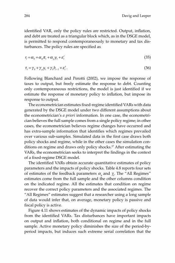
Davig and Leeper284
identifi ed VAR, only the policy rules are restricted. Output, infl ation, and debt are treated as a triangular block which, as in the DSGE model, is permitted to respond contemporaneously to monetary and tax dis-turbances. The policy rules are specifi ed as
r yt t y t tr= + + +α α π α επ0 (35)
τ γ γ γ ετt y t b t ty b= + + +−0 1 . (36)
Following Blanchard and Perotti (2002), we impose the response of taxes to output, but freely estimate the response to debt. Counting only contemporaneous restrictions, the model is just identifi ed if we estimate the response of monetary policy to infl ation, but impose its response to output.
The econometrician estimates fi xed-regime identifi ed VARs with data generated by the DSGE model under two different assumptions about the econometrician’s a priori information. In one case, the econometri-cian believes the full sample comes from a single policy regime; in other cases, the econometrician believes regime changes have occurred and has extra-sample information that identifi es which regimes prevailed over various sub-samples. Simulated data in the fi rst case draws both policy shocks and regime, while in the other cases the simulation con-ditions on regime and draws only policy shocks.27 After estimating the VARs, the econometrician seeks to interpret the fi ndings in the context of a fi xed-regime DSGE model.
The identifi ed VARs obtain accurate quantitative estimates of policy parameters and the impacts of policy shocks. Table 4.8 reports four sets of estimates of the feedback parameters απ and γb. The “All Regimes” estimates come from the full sample and the other columns condition on the indicated regime. All the estimates that condition on regime recover the correct policy parameters and the associated regimes. The “All Regimes” estimates suggest that a researcher using a long sample of data would infer that, on average, monetary policy is passive and fi scal policy is active.
Figure 4.11 shows estimates of the dynamic impacts of policy shocks from the identifi ed VARs. Tax disturbances have important impacts on output and infl ation, both conditional on regime and in the full sample. Active monetary policy diminishes the size of the period-by-period impacts, but induces such extreme serial correlation that the
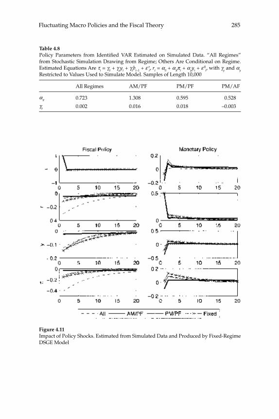
285Fluctuating Macro Policies and the Fiscal Theory
Table 4.8Policy Parameters from Identifi ed VAR Estimated on Simulated Data. “All Regimes” from Stochastic Simulation Drawing from Regime; Others Are Conditional on Regime. Estimated Equations Are τt = γ0 + γyyt + γbbt–1 + ε τ
t, rt = α0 + αππt + αyyt + ε Rt, with γy and αy
Restricted to Values Used to Simulate Model. Samples of Length 10,000
απ
γb
All Regimes
0.723
0.002
AM/PF
1.308
0.016
PM/PF
0.595
0.018
PM/AF
0.528
–0.003
Figure 4.11Impact of Policy Shocks. Estimated from Simulated Data and Produced by Fixed-Regime DSGE Model
Davig and Leeper286
total impacts are substantial. Monetary contractions have conventional short-run effects (lower output and infl ation), but unconventional longer run effects (higher output and infl ation), owing to the result-ing wealth effects engendered by the fi scal theory mechanism. The rise in future infl ation resembles the price puzzle Sims (1992) discovered in monetary VARs. That puzzle is more pronounced when monetary policy is passive, consistent with Hanson’s (2004) fi ndings that in U.S. data the puzzle is more severe in samples that include data before 1979, a period that section 2 labels passive monetary policy. Both the param-eter estimates and the impulse response functions the econometrician obtains are quantitatively consistent with those in the switching model underlying the simulated data (given that the econometrician knows αy and γy a priori).
Connecting these quantitative results to fi xed-regime theories can lead to qualitatively misleading inferences. Clarida, Galí, and Gertler (2000) and Lubik and Schorfheide (2004) use different econometric methods, but both condition on monetary policy regime and both conclude that since the early 1980s, U.S. monetary policy has been active, while from 1960–1979, monetary policy was passive. Both sets of authors maintain the assumption that fi scal policy was passive throughout, leading in their fi xed-regime DSGE models to Ricardian equivalence in the recent sub-sample and indeterminacy in the earlier sub-sample. The results for AM/PF (thick solid lines) in fi gure 4.11 are diffi cult to reconcile with Ricardian equivalence. Similarly, in the sub-sample where the esti-mated rules imply PM/PF (thin solid lines), the econometrician would infer the equilibrium is indeterminate and be compelled to interpret the policy impacts as arising from correlations between sunspot shocks and policy shocks. But the simulated data were generated by locally unique decision rules.
Employing the full sample, the econometrician estimates the policy impacts shown by dashed lines in fi gure 4.11. Moreover, using the “All Regimes” parameter estimates in a fi xed-regime version of the model in section 3, produces the policy impacts represented by lines in the fi gure punctuated with x’s. In contrast to the estimates that condi-tion on regime, the full sample estimates deliver qualitatively correct inferences about policy effects. Correct qualitative inferences require nailing down the correct long-run behavior of policy. That long-run behavior is better gleaned from a long sample that includes the pos-
287Fluctuating Macro Policies and the Fiscal Theory
sible realizations of regimes than from sub-samples that condition on regime.28
9 Concluding Remarks
Existing work on policy rules is based on a logical inconsistency: It assumes regime cannot change and then proceeds to analyze the impli-cations of alternative regimes. This paper takes a step toward resolv-ing this inconsistency. A simple and plausible empirical specifi cation of regime change fi nds that U.S. monetary and fi scal policies have fl uctuated among active and passive rules. Treating that evidence of regime change in an internally consistent manner can signifi cantly alter interpretations of the historical period and of monetary and fi scal poli-cies more generally. Both the empirical specifi cation and the economic model are very simple, leaving much room for improving fi t to data. This is an important area for continued research.
This paper has not addressed why policy regimes change. This is a hard question, but it is the same hard question that can be asked of any model with a stochastic component to policy behavior. Although Sims (1987) offers a rationale for why optimal policy might include a compo-nent that is random to private agents, there is certainly no consensus on this issue. Lack of consensus, however, does not undermine the utility of simply postulating the existence of policy shocks and then tracing out their infl uence in data and in models. In this paper, we have followed the convention of assuming some part of policy behavior is random.
Under the working hypothesis of recurring regime change, this paper shows that when estimated Markov-switching rules for monetary and tax policies are embedded in a DSGE model calibrated to U.S. data, lump-sum taxes have quantitatively important effects on aggregate demand, output, and infl ation. In the model, tax non-neutralities arise because the estimates imply that agents always place positive probabil-ity mass on an active fi scal regime in the future, a belief that makes the fi scal theory of the price level operative.
Of course, the fi scal theory is not the only source of tax non-neutrali-ties in actual data. A full accounting of tax effects requires introducing some of the panoply of reasons offered for why taxes might be non-neutral—distortions, life-cycle considerations, and so forth. In any case, the quantitative predictions of this paper strongly suggest that the fi scal
Davig and Leeper288
theory mechanism should be added to the list of usual suspects for the breakdown of Ricardian equivalence.
Acknowledgments
We thank Daron Acemoglu, Hess Chung, Jon Faust, Jordi Galí, Dave Gordon, Ross Levine, Jim Nason, Jürgen von Hagen, Chris Sims, Mike Woodford, Tack Yun, Tao Zha, and seminar participants at the Federal Reserve Board, the ECB, and the NBER Macro Annual meeting for com-ments. Leeper acknowledges support from NSF Grant SES-0452599. The views expressed herein are solely those of the authors and do not necessarily refl ect the views of the Federal Reserve Bank of Kansas City or the Federal Reserve System.
Endnotes
1. Some work considers recurring regime switching in exogenous processes, including exogenously evolving policy variables (Andolfatto and Gomme 2003, Davig 2003, 2004, Leeper and Zha 2003, and Schorfheide 2005). There have also been efforts to incorporate one-time regime changes into general equilibrium models of the fi scal theory (Sims 1997, Woodford 1998b, Loyo 1999, Mackowiak 2006, Daniel 2003, and Weil 2003).
2. We apply the terminology in Leeper (1991). Active monetary policy arises when the response of the nominal interest rate is more than one-for-one to infl ation and passive monetary policy occurs when that response is less than one-for-one. Analogously, passive fi scal policy occurs when the response of taxes to debt exceeds the real interest rate and active fi scal policy occurs when taxes do not respond suffi ciently to debt to cover real inter-est payments. In many models, a unique bounded equilibrium requires one active and one passive policy.
3. See Leeper (1991), Woodford (1994, 1995), Sims (1994), and Cochrane (1999, 2001).
4. Cochrane (1999) interprets U.S. infl ation in light of the fi scal theory and Woodford (2001) points to particular historical episodes when the fi scal theory might have been relevant.
5. The table is pretty full. Included among purely monetary interpretations are narra-tives (DeLong 1997, Mayer 1998, and Romer and Romer 2004), fi xed regime (Orphanides 2003a), permanent regime change (Clarida, Galí, and Gertler 2000, and Lubik and Schor-fheide 2004), adaptive learning (Cogley and Sargent 2005b, 2002, Primiceri 2006, and Sargent, Williams, and Zha 2006), model uncertainty (Cogley and Sargent 2005a), and regime-switching identifi ed VARs (Sims and Zha 2006). Work that integrates monetary and fi scal policy includes Leeper and Sims (1994), Romer and Romer (1994), and Sala (2004).
6. Davig and Leeper (2006a) examine the implications of making monetary policy regime change endogenous, maintaining the assumption that fi scal policy is perpetually passive.

289Fluctuating Macro Policies and the Fiscal Theory
7. See Beyer and Farmer (2005) for a related discussion.
8. Ireland (2004), Leeper and Zha (2001), Leeper and Roush (2003), and Sims and Zha (2006) argue that allowing money growth to enter the monetary policy rule is important for identifying policy behavior. To keep to a specifi cation that is comparable to the Taylor rule literature, we exclude money growth.
9. Examples of estimated fi scal rules include Bohn (1998), Taylor (2000), Fatas and Mihov (2001), Auerbach (2003), Cohen and Follette (2003), Ballabriga and Martinez-Mongay (2005), and Claeys (2004).
10. To follow existing empirical work on simple policy rules, the paper does not estimate the rules as parts of a fully specifi ed model. We are reassured in doing this by the model-based estimates of Ireland (2004) and Lubik and Schorfheide (2004), which are very close to single-equation estimates of Taylor rules. It is noteworthy, though, that in an identifi ed switching VAR, Sims and Zha (2006) conclude that monetary policy was consistently active since 1960; they do not consider fi scal behavior and their switching specifi cation is more restricted than ours along some dimensions, but less restricted along others (see endnote 8).
11. We include a dummy variable to absorb the variability in interest rates induced by credit controls in the second and third quarters of 1980. See Schreft (1990) for a detailed account of those controls.
12. Orphanides (2003b) argues that the poor U.S. infl ation performance from 1965–1979 was due to a strong policy response to poor estimates of the output gap available at the time, rather than a weak response to infl ation. Using real-time data on the gap and infl a-tion, he claims the fi t of a conventional Taylor rule specifi cation is much improved when real-time data are used rather recent vintage data. Orphanides (2003a) extends this argu-ment to the 1950s. The fi t of our switching regression for monetary policy is far superior to Orphanides’s over the 1960:2–1966:4 period, yet our results label this as a period of passive monetary policy.
13. This draws on Pechman (1987), Poterba (1994), Stein (1996), Steuerle (2002), Romer and Romer (2004), and Yang (2006).
14. The negative response of taxes to debt in the active fi scal regime might be regarded as perverse. A negative correlation arises naturally over the business cycle, as recessions automatically lower revenues and raise debt. Two active fi scal regimes, the late 1940s and 1973:4–1975:1, almost exactly coincide with the cycle. But there are extended periods of active behavior, which include but do not coincide with recessions (1955:4–1965:2 and 1978:4–1984:3). There are also instances in which recessions occur during periods of pas-sive fi scal policy (1990:3-1991:1 and 2001:1-2001:4). Taken together these results suggest that the tax rule does more than simply identify active regimes with economic down-turns.
15. Favero and Monacelli (2005) estimate that through 2002, fi scal policy was active in 1961:1–1974:3, 1975:3–1995:1, and 2001:3–2002:4 and passive otherwise. Our estimates fi nd more periods of passive behavior.
16. Detailed expositions appear in Yun (1996, 2005), Woodford (2003), and Schmitt-Grohé and Uribe (2006).
17. The constant relative risk aversion preferences over real money balances rule out Obstfeld and Rogoff’s (1983) speculative hyperinfl ations.
Davig and Leeper290
18. See Leeper (1989) and Yang (2005) for further discussion of the implications of fi scal foresight.
19. In the model all debt matures in one period. Cochrane (2001) emphasizes that with long-maturity debt, the infl ation consequences of a fi scal expansion can be pushed into the future.
20. This policy mix does not impose a boundary condition on the infl ation process, but it does impose a boundary condition on the real debt process. With nominal liabilities predetermined, the price level is uniquely determined. This is the canonical fi scal theory specifi cation (see Woodford 2001 or Gordon and Leeper 2006).
21. Taking a price-theoretic view of the fi scal theory with tax distortions, Leeper and Yun (2006) refer to this as the “asset revaluation effect,” as distinct from conventional “wealth” and “substitution” effects.
22. Details appear in Appendix A.
23. Davig and Leeper (2006b) provide a detailed analytical proof of determinacy for bounded solutions under doubly passive monetary and fi scal policies in a linear model with regime switching in monetary policy.
24. In the monotone map algorithm, it is possible to allow additional state variables to enter expectations. However, allowing expectations formation to depend on an expanded state vector does not produce a solution that differs from the locally unique solution.
25. Francq and Zakoian (2001) show that Markov-switching processes can have explo-sive regimes, yet the entire stochastic process can be stable. Davig (2005) shows that a properly restricted Markov-switching process for discounted debt can have an explosive regime, yet satisfy the transversality condition for debt.
26. Appendix B considers an alternative specifi cation of the policy process that increases the duration of the active monetary policy regime by labeling as active the periods after the recessions in 1991 and 2001, which section 2 estimated as passive monetary policy. This reduces the quantitative impacts of tax shocks, though the fi scal theory mechanism remains important.
27. But the data are generated by decision rules based on the “true” regime-switching process.
28. Unless there is compelling evidence that agents believe the prevailing regime is per-manent.
References
Andolfatto, D., and P. Gomme. 2003. “Monetary Policy Regimes and Beliefs.” Interna-tional Economic Review 44(1): 1–30.
Auerbach, A. J. 2002. “Is There a Role for Discretionary Fiscal Policy?” In Rethinking Sta-bilization Policy: Proceedings of a Symposium Sponsored by the Federal Reserve Bank of Kansas City, pp. 109–150.
Auerbach, A. J. 2003. “Fiscal Policy, Past and Present.” Brookings Papers on Economic Activ-ity (1): 75–122.
Ballabriga, F. C., and C. Martinez-Mongay. 2005. “Sustainability of EU Public Finances.” European Commission Economic Papers no. 225.
291Fluctuating Macro Policies and the Fiscal Theory
Benhabib, J., and R. E. A. Farmer. 2000. “The Monetary Transmission Mechanism.” Review of Economic Dynamics 3(2): 523–550.
Benhabib, J., S. Schmitt-Grohé, and M. Uribe. 2001a. “Monetary Policy and Multiple Equi-libria.” American Economic Review 91(1): 167–186.
Benhabib, J., S. Schmitt-Grohé, and M. Uribe. 2001b. “The Perils of Taylor Rules.” Journal of Economic Theory 96(1-2): 40–69.
Benhabib, J., S. Schmitt-Grohé, and M. Uribe. 2002. “Avoiding Liquidity Traps.” Journal of Political Economy 110(3): 535–563.
Beyer, A., and R. E. A. Farmer. 2005. “Identifying the Monetary Transmission Mechanism using Structural Breaks.” Manuscript, UCLA.
Blanchard, O. J., and R. Perotti. 2002. “An Empirical Characterization of the Dynamic Effects of Changes in Government Spending and Taxes on Output.” Quarterly Journal of Economics 117(4): 1329–1368.
Board of Governors of the Federal Reserve System. 1993a. “Transcript of Federal Open Market Committee.” March 23.
Board of Governors of the Federal Reserve System. 1993b. “Transcript of Federal Open Market Committee.” September 23.
Bohn, H. 1998. “The Behavior of U.S. Public Debt and Defi cits.” Quarterly Journal of Eco-nomics 113(3): 949–963.
Brooks, D. 2005. “In the Midst of Budget Decadence, a Leader Will Arise.” The New York Times, February 19.
Bryant, R. C., P. Hooper, and C. L. Mann, eds. 1993. Evaluating Policy Regimes: New Research in Empirical Macroeconomics. Washington, D.C.: The Brookings Institution.
Calvo, G. A. 1983. “Staggered Prices in a Utility Maxmimizing Model.” Journal of Mon-etary Economics 12(3): 383–398.
Chari, V. V., P. J. Kehoe, and E. R. McGrattan. 2000. “Sticky Price Models of the Business Cycle: Can the Contract Multiplier Solve the Persistence Problem?” Econometrica 68(5): 1151–1179.
Claeys, P. 2004. “Monetary and Budget Policy Interaction: An Empirical Analysis of Fiscal Policy Rules, Stabilisation Policies and Policy Interaction in Monetary Union.” Manu-script, European University Institute.
Clarida, R., J. Galí, and M. Gertler. 2000. “Monetary Policy Rules and Macroeconomic Stability: Evidence and Some Theory.” Quarterly Journal of Economics 115(1): 147–180.
Cochrane, J. H. 1999. “A Frictionless View of U.S. Infl ation.” In B. S. Bernanke, and J. J. Rotemberg, eds., NBER Macroeconomics Annual 1998, 323–384. Cambridge, MA: MIT Press.
Cochrane, J. H. 2001. “Long Term Debt and Optimal Policy in the Fiscal Theory of the Price Level.” Econometrica 69(1): 69–116.
Cogley, T., and T. J. Sargent. 2002. “Evolving Post-World War II U.S. Infl ation Dynamics.” In B. S. Bernanke, and J. J. Rotemberg, eds., NBER Macroeconomics Annual 2001. Cam-bridge, MA: MIT Press.
Davig and Leeper292
Cogley, T., and T. J. Sargent. 2005a. “The Conquest of U.S. Infl ation: Learning and Robust-ness to Model Uncertainty.” Review of Economic Dynamics 8(2): 528–563.
Cogley, T., and T. J. Sargent. 2005b. “Drifts and Volatilities: Monetary Policies and Out-comes in the Post WWII U.S.” Review of Economic Dynamics 8(2): 262–302.
Cohen, D., and G. Follette. 2003. “Forecasting Exogenous Fiscal Variables in the United States.” Finance and Economics Discussion Series, 2003–59, Federal Reserve Board.
Coleman, II, W. J. 1991. “Equilibrium in a Production Economy with an Income Tax.” Econometrica 59(4): 1091–1104.
Cooley, T. F., S. F. LeRoy, and N. Raymon. 1984. “Econometric Policy Evaluation: Note.” American Economic Review 74(3): 467–470.
Daniel, B. C. 2003 “Fiscal Policy, Price Surprises, and Infl ation.” Manuscript, SUNY Albany.
Davig, T. 2003. “Regime-Switching Fiscal Policy in General Equilibrium.” Manuscript, The College of William and Mary.
Davig, T. 2004. “Regime-Switching Debt and Taxation.” Journal of Monetary Economics 51(4): 837–859.
Davig, T. 2005. “Periodically Expanding Discounted Debt: A Threat to Fiscal Policy Sus-tainability?” Journal of Applied Econometrics 20(7): 829–840.
Davig, T., and E. M. Leeper. 2006a. “Endogenous Monetary Policy Regime Change.” In L. Reichlin and K. D. West, eds., NBER International Seminar on Macroeconomics 2006, forthcoming. Cambridge, MA: MIT Press.
Davig, T., and E. M. Leeper. 2006b. “Generalizing the Taylor Principle.” American Eco-nomic Review, forthcoming. NBER Working Paper no. 11874. Cambridge, MA: National Bureau of Economic Research.
Davig, T., E. M. Leeper, and H. Chung. 2004. “Monetary and Fiscal Policy Switching.” Journal of Money, Credit and Banking, forthcoming. NBER Working Paper no. 10362. Cam-bridge, MA: National Bureau of Economic Research.
DeLong, B. J. 1997. “America’s Peacetime Infl ation: The 1970s.” In C. D. Romer, and D. H. Romer, eds., Reducing Infl ation: Motivation and Strategy, 247–276. Chicago, IL: University of Chicago Press.
Dixit, A. K., and J. E. Stiglitz. 1977. “Monopolistic Competition and Optimum Product Diversity.” American Economic Review 67(3): 297–308.
Fatas, A., and I. Mihov. 2001. “Politica Fiscal y Ciclos Economicos: Una Investigacion Empirica. (Fiscal Policy and the Business Cycle: An Empirical Analysis.)” Moneda y Credito (212): 167–205.
Favero, C. A., and T. Monacelli. 2005. “Fiscal Policy Rules and Regime (In)Stability: Evi-dence from the U.S.” IGIER Working Paper no. 282, January.
Francq, C., and J.-M. Zakoian. 2001. “Stationarity of Multivariate Markov-Switching ARMA Models.” Journal of Econometrics. 102: 339–364.
Gordon, D. B., and E. M. Leeper. 2006. “The Price Level, The Quantity Theory of Money, and the Fiscal Theory of the Price Level.” Scottish Journal of Political Economy 53(1): 4–27.
293Fluctuating Macro Policies and the Fiscal Theory
Hamilton, J. D. 1989. “A New Approach to the Economic Analysis of Nonstationary Time Series and the Business Cycle.” Econometrica 57(2): 357–384.
Hanson, M. S. 2004. “The ‘Price Puzzle’ Reconsidered.” Journal of Monetary Economics 51(7): 1385–1413.
Ireland, P. N. 2004. “Money’s Role in the Monetary Business Cycle.” Journal of Money, Credit and Banking 36(6): 969–983.
Kim, C-J, and C. R. Nelson. 1999 State-Space Models with Regime Switching. Cambridge, MA: MIT Press.
Kim, C-J, and C. R. Nelson. 2006. “Estimation of a Forward-Looking Monetary Policy Rule: A Time-Varying Parameter Model using Ex-Post Data.” Journal of Monetary Econom-ics 53(8): 1949–1966.
Leeper, E. M. 1989. “Policy Rules, Information, and Fiscal Effects in a ‘Ricardian’ Model.” Federal Reserve Board, International Finance Discussion Paper no. 360.
Leeper, E. M. 1991. “Equilibria Under ‘Active’ and ‘Passive’ Monetary and Fiscal Poli-cies.” Journal of Monetary Economics 27(1): 129–147.
Leeper, E. M., and J. E. Roush. 2003. “Putting ’M’ Back in Monetary Policy.” Journal of Money, Credit, and Banking 35(6, Part 2): 1217–1256.
Leeper, E. M., and C. A. Sims. 1994. “Toward a Modern Macroeconomic Model Usable for Policy Analysis.” In S. Fischer, and J. J. Rotemberg, eds., NBER Macroeconomics Annual 1994, 81–118. Cambridge, MA: MIT Press.
Leeper, E. M., and T. Yun. 2006. “The Fiscal Theory of the Price Level: Background and Beyond.” International Tax and Public Finance 13(4): 373–409.
Leeper, E. M., and T. Zha. 2001. “Assessing Simple Policy Rules: A View from a Complete Macro Model.” Federal Reserve Bank of St. Louis Review 83(July/August), 83–110.
Leeper, E. M., and T. Zha. 2003. “Modest Policy Interventions.” Journal of Monetary Eco-nomics 50(8): 1673–1700.
Loyo, E. 1999. “Tight Money Paradox on the Loose: A Fiscalist Hyperinfl ation.” Manu-script, Harvard University.
Lubik, T. A., and F. Schorfheide. 2004. “Testing for Indeterminacy: An Application to U.S. Monetary Policy.” American Economic Review 94(1): 190–217.
Lucas, Jr., R. E. 1988. “Money Demand in the United States: A Quantitative Review.” Carnegie-Rochester Conference Series on Public Policy 29: 137–168.
Mackowiak, B. 2006. “Macroeconomic Regime Switching and Speculative Attacks.” Jour-nal of Economic Dynamics and Control, forthcoming.
Mankiw, N. G., and L. H. Summers. 1986. “Money Demand and the Effects of Fiscal Poli-cies.” Journal of Money, Credit, and Banking 18(4): 415–429.
Mayer, T. 1998. Monetary Policy and the Great Infl ation in the United States. Cheltenham, U.K.: Edward Elgar.
Mountford, A., and H. Uhlig. 2005. “What Are the Effects of Fiscal Policy Shocks?” SFB 649 Discussion Paper no. 2005-039, Humbolt University.
Davig and Leeper294
Obstfeld, M., and K. Rogoff. 1983. “Speculative Hyperinfl ations in Maximizing Models: Can We Rule Them Out?” Journal of Political Economy 91(August): 675–687.
Ohanian, L. E. 1997. “The Macroeconomic Effects of War Finance in the United States: World War II and the Korean War.” American Economic Review 87(1): 23–40.
Orphanides, A. 2003a. “Historical Monetary Policy Analysis and the Taylor Rule.” Journal of Monetary Economics 50(5): 983–1022.
Orphanides, A. 2003b. “The Quest for Prosperity without Infl ation.” Journal of Monetary Economics 50(3): 633–663.
Pechman, J. A. 1987. Federal Tax Policy. Washington, D.C.: The Brookings Institution, fi fth edn.
Perotti, R. 2004. “Estimating the Effects of Fiscal Policy in OECD Countries.” IGIER Work-ing Paper no. 276.
Poterba, J. M. 1994. “Federal Budget Policy in the 1980s.” In M. Feldstein, ed., American Economic Policy in the 1980s, 235–270. Chicago, IL: University of Chicago Press.
Primiceri, G. 2006. “Why Infl ation Rose and Fell: Policymakers’ Beliefs and US Postwar Stabilization Policy.” Quarterly Journal of Economics 121(3): 867–901.
Roach, S. 2004. “The Asset Economy.” Morgan Stanley Online.
Romer, C. D., and D. Romer. 1994. “What Ends Recessions?” In S. Fischer, and J. J. Rotem-berg, eds., NBER Macroeconomics Annual 1994, 13–57. Cambridge, MA: MIT Press.
Romer, C. D., and D. H. Romer. 2002. “A Rehabilitation of Monetary Policy in the 1950s.” American Economic Review 92(2): 121–127.
Romer, C. D., and D. H. Romer. 2004. “Choosing the Federal Reserve Chair: Lessons from History.” Journal of Economic Perspectives 18(1): 129–162.
Rotemberg, J. J., and M. Woodford. 1997. “An Optimization-Based Econometric Frame-work for the Evaluation of Monetary Policy.” In B. S. Bernanke, and J. J. Rotemberg, eds., NBER Macroeconomics Annual 1997, 297–346. Cambridge, MA: MIT Press.
Rotemberg, J. J., and M. Woodford. 1999. “Interest Rate Rules in an Estimated Sticky Price Model.” In J. B. Taylor, ed., Monetary Policy Rules, 57–119. Chicago, IL: University of Chi-cago Press.
Sala, L. 2004. “The Fiscal Theory of the Price Level: Identifying Restrictions and Empirical Evidence.” IGIER Working Paper no. 257.
Sargent, T. J., N. Williams, and T. Zha. 2006. “Shocks and Government Beliefs: The Rise and Fall of American Infl ation.” American Economic Review 96(4): 1193–1224.
Schmitt-Grohé, S., and M. Uribe. 2006. “Optimal Simple and Implementable Monetary and Fiscal Rules.” Journal of Monetary Economics, forthcoming.
Schorfheide, F. 2005. “Learning and Monetary Policy Shifts.” Review of Economic Dynamics 8(2): 392–419.
Schreft, S. L. 1990. “Credit Controls: 1990.” Federal Reserve Bank of Richmond Economic Review 76(6): 25–55.
295Fluctuating Macro Policies and the Fiscal Theory
Sims, C. A. 1987. “A Rational Expectations Framework for Short-Run Policy Analysis.” In W. A. Barnett, and K. J. Singleton, eds., New Approaches to Monetary Economics, 293–308. Cambridge, UK: Cambridge University Press.
Sims, C. A. 1992. “Interpreting the Macroeconomic Time Series Facts: The Effects of Mon-etary Policy.” European Economic Review 36: 975–1000.
Sims, C. A. 1994. “A Simple Model for Study of the Determination of the Price Level and the Interaction of Monetary and Fiscal Policy.” Economic Theory 4(3): 381–399.
Sims, C. A. 1997. “Fiscal Foundations of Price Stability in Open Economies.” Manuscript, Yale University.
Sims, C. A., and T. Zha. 2006. “Were There Regime Switches in US Monetary Policy?” American Economic Review 96(1): 54–81.
Stein, H. 1996. The Fiscal Revolution in America. Washington, D.C.: AEI Press, second revised edn.
Steuerle, C. E. 2002. “Tax Policy from 1990 to 2001.” In J. Frankel, and P. Orszag, eds., American Economic Policy in the 1990s, 139–169. Cambridge, MA: MIT Press.
Steuerle, C. E. 2006. “Fiscal Policy from Kennedy to Reagan to G. W. Bush.” In R. W. Kopcke, G. M. B. Tootell, and R. K. Triest, eds., The Macroeconomics of Fiscal Policy, 119–142. Cambridge, MA: MIT Press.
Taylor, J. B. 1993. “Discretion versus Policy Rules in Practice.” Carnegie-Rochester Confer-ence Series on Public Policy 39: 195–214.
Taylor, J. B. 1999a. “An Historical Analysis of Monetary Policy Rules.” In J. B. Taylor, ed., Monetary Policy Rules, 319–341. Chicago, IL: University of Chicago Press.
Taylor, J. B., ed. 1999b. Monetary Policy Rules. Chicago, IL: University of Chicago Press.
Taylor, J. B. 2000. “Reassessing Discretionary Fiscal Policy.” Journal of Economic Perspec-tives 14(3): 21–36.
Unsigned. 2002. “Dicing with Debt.” The Economist, (January 24).
Unsigned. 2005a. “Saturated.” The Economist, (February 26).
Unsigned. 2005b. “Still Gushing Forth.” The Economist, (February 3).
Weil, P. 2003. “Refl ections on the Fiscal Theory of the Price Level.” Manuscript, ECARES.
Woodford, M. 1994. “Monetary Policy and Price Level Determinacy in a Cash-in-Advance Economy.” Economic Theory 4(3): 345–380.
Woodford, M. 1995. “Price-Level Determinacy Without Control of a Monetary Aggre-gate.” Carnegie-Rochester Conference Series on Public Policy 43: 1–46.
Woodford, M. 1998a. “Control of the Public Debt: A Requirement for Price Stability?” In G. Calvo, and M. King, eds., The Debt Burden and Its Consequences for Monetary Policy, 117–154. New York: St. Martin’s Press.
Woodford, M. 1998b. “Public Debt and the Price Level.” Manuscript, Princeton Univer-sity.
Davig and Leeper296
Woodford, M. 2001. “Fiscal Requirements for Price Stability.” Journal of Money, Credit, and Banking 33(3): 669–728.
Woodford, M. 2003. Interest and Prices: Foundations of a Theory of Monetary Policy. Princ-eton, NJ: Princeton University Press.
Yang, S-C. S. 2005. “Quantifying Tax Effects Under Policy Foresight.” Journal of Monetary Economics 52(8): 1557–1568.
Yang, S-C. S. 2006. “Tentative Evidence of Tax Foresight.” Economic Letters, forthcoming.
Yun, T. 1996. “Nominal Price Rigidity, Money Supply Endogeneity, and Business Cycles.” Journal of Monetary Economics 37(April): 345–370.
Yun, T. 2005. “Optimal Monetary Policy with Relative Price Distortions.” American Eco-nomic Review 95(1): 89–108.
Zanna, L. F. 2003. “Interest Rate Rules and Multiple Equilibria in the Small Open Econ-omy.” Federal Reserve Board IFDP No. 785.
Appendix A Solution Method
Implementation of the algorithm begins by conjecturing an initial set of rules, which we take to be the solution from the model’s fi xed-regime counterpart. Specifi cally, we take the solutions from the fi xed-regime model with AM/PF and PM/AF policies as the initial rules for the corresponding regimes in the non-synchronous switching model. For the AM/AF and PM/PF regimes there are no stationary, unique fi xed-regime counterparts, so we use the solution from the PM/AF fi xed-regime model to initialize the algorithm. To ensure the solution is not sensitive to initial conditions, we also use the solution from the AM/PF regime and weighted averages of the two.
Taking the initial rules for labor, hN(Θt) = Nt, and the functions determining the fi rm’s optimal pricing decision, hK1(Θt) = K1,t and hK2(Θt) = K2,t, we fi nd values using a nonlinear equation solver for Nt, K1,t, K2,t such that
C R E ht t t tC
t−
+ +−=σ σβ π[ ( ( )) ],1 1Θ (37)
K C E ht t t tK
t11
11
,ˆ ( ),= +−
+σ ϕβΨ Θ (38)
K C E ht t tK
t21
12
,ˆ ( ),= +−
+σ ϕβ Θ (39)
where hC(Θt) = (A/Δt)hN(Θt) – g. Given Nt, K1,t, K2,t, we compute the endogenous
variables. Note that Δt, bt and wt = Rtbt + Mt/Pt are states at t + 1. Gauss-Hermite integration is used over possible values for ε r
t+1, ε τt+1, and St+1, yielding values
for Et[πt+1C–σt+1], EtK1,t+1, EtK2,t+1, which reduces the above system to three equa-
tions in three unknowns. The (net) nominal interest rate is restricted to always be positive.
When solving the above system, the state vector and the decision rules are taken as given. The system is solved for every set of state variables defi ned
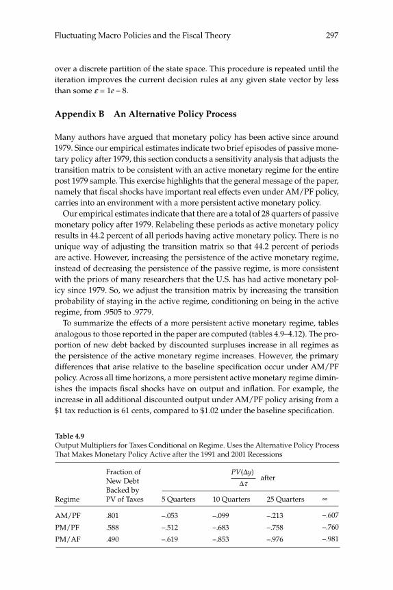
297Fluctuating Macro Policies and the Fiscal Theory
over a discrete partition of the state space. This procedure is repeated until the iteration improves the current decision rules at any given state vector by less than some ε = 1e – 8.
Appendix B An Alternative Policy Process
Many authors have argued that monetary policy has been active since around 1979. Since our empirical estimates indicate two brief episodes of passive mone-tary policy after 1979, this section conducts a sensitivity analysis that adjusts the transition matrix to be consistent with an active monetary regime for the entire post 1979 sample. This exercise highlights that the general message of the paper, namely that fi scal shocks have important real effects even under AM/PF policy, carries into an environment with a more persistent active monetary policy.
Our empirical estimates indicate that there are a total of 28 quarters of passive monetary policy after 1979. Relabeling these periods as active monetary policy results in 44.2 percent of all periods having active monetary policy. There is no unique way of adjusting the transition matrix so that 44.2 percent of periods are active. However, increasing the persistence of the active monetary regime, instead of decreasing the persistence of the passive regime, is more consistent with the priors of many researchers that the U.S. has had active monetary pol-icy since 1979. So, we adjust the transition matrix by increasing the transition probability of staying in the active regime, conditioning on being in the active regime, from .9505 to .9779.
To summarize the effects of a more persistent active monetary regime, tables analogous to those reported in the paper are computed (tables 4.9–4.12). The pro-portion of new debt backed by discounted surpluses increase in all regimes as the persistence of the active monetary regime increases. However, the primary differences that arise relative to the baseline specifi cation occur under AM/PF policy. Across all time horizons, a more persistent active monetary regime dimin-ishes the impacts fi scal shocks have on output and infl ation. For example, the increase in all additional discounted output under AM/PF policy arising from a $1 tax reduction is 61 cents, compared to $1.02 under the baseline specifi cation.
afterPV(Δy)
Δτ
Table 4.9Output Multipliers for Taxes Conditional on Regime. Uses the Alternative Policy Process That Makes Monetary Policy Active after the 1991 and 2001 Recessions
Regime
AM/PF
PM/PF
PM/AF
Fraction of New Debt Backed by PV of Taxes
.801
.588
.490
5 Quarters
–.053
–.512
–.619
10 Quarters
–.099
–.683
–.853
25 Quarters
–.213
–.758
–.976
∞
–.607
–.760
–.981
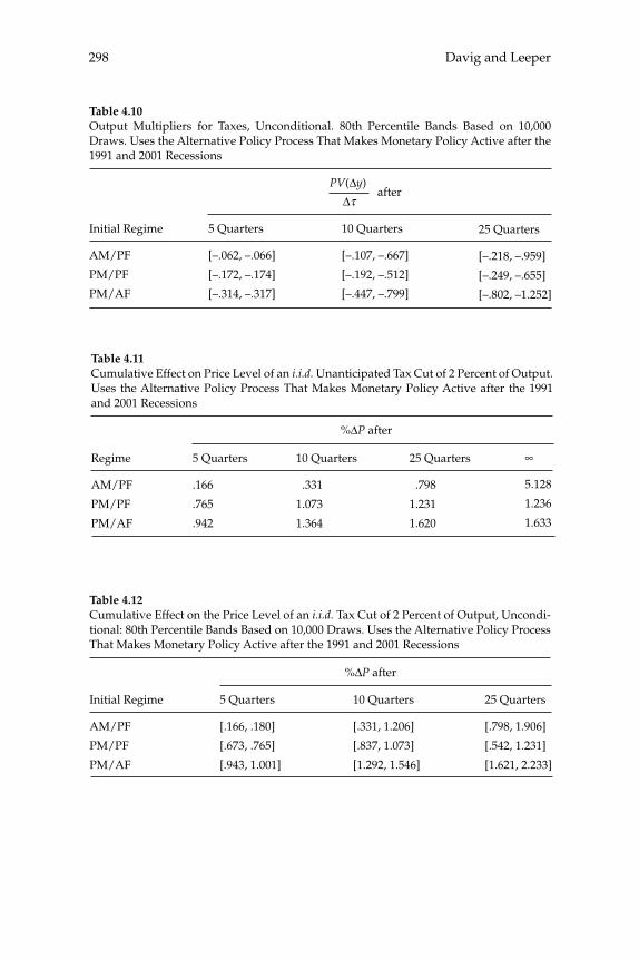
Davig and Leeper298
afterPV(Δy)
Δτ
Table 4.10Output Multipliers for Taxes, Unconditional. 80th Percentile Bands Based on 10,000 Draws. Uses the Alternative Policy Process That Makes Monetary Policy Active after the 1991 and 2001 Recessions
Initial Regime
AM/PF
PM/PF
PM/AF
5 Quarters
[–.062, –.066]
[–.172, –.174]
[–.314, –.317]
10 Quarters
[–.107, –.667]
[–.192, –.512]
[–.447, –.799]
25 Quarters
[–.218, –.959]
[–.249, –.655]
[–.802, –1.252]
Table 4.11Cumulative Effect on Price Level of an i.i.d. Unanticipated Tax Cut of 2 Percent of Output. Uses the Alternative Policy Process That Makes Monetary Policy Active after the 1991 and 2001 Recessions
Regime
AM/PF
PM/PF
PM/AF
5 Quarters
.166
.765
.942
10 Quarters
.331
1.073
1.364
25 Quarters
.798
1.231
1.620
∞
5.128
1.236
1.633
%ΔP after
%ΔP after
Table 4.12Cumulative Effect on the Price Level of an i.i.d. Tax Cut of 2 Percent of Output, Uncondi-tional: 80th Percentile Bands Based on 10,000 Draws. Uses the Alternative Policy Process That Makes Monetary Policy Active after the 1991 and 2001 Recessions
Initial Regime
AM/PF
PM/PF
PM/AF
5 Quarters
[.166, .180]
[.673, .765]
[.943, 1.001]
10 Quarters
[.331, 1.206]
[.837, 1.073]
[1.292, 1.546]
25 Quarters
[.798, 1.906]
[.542, 1.231]
[1.621, 2.233]
Comment
Jordi Galí, Centre de Recerca en Economia Internacional (CREI) and NBER
1 Introduction
In their contribution to the present volume, Davig and Leeper (hence-forth, DL) study the implications of variations over time in policy rules. More specifi cally, they analyze the equilibrium effects of exogenous random switches in the coeffi cients of monetary and fi scal policy rules, embedded in an otherwise conventional dynamic optimizing model with staggered price setting. Their motivation for the exercise is an empirical one: They estimate a Markov switching model for the two policy rules and fi nd evidence of recurring changes in those coeffi cients. Most interestingly, the estimated changes in the policy rules involve “qualitative” changes in the nature of the regime in place, i.e., they imply a shift from an “active” to a “passive” monetary policy (or vice versa), as well as analogous (but not necessarily synchronous) shifts in the fi scal policy rule. When DL embed their estimated monetary and fi scal Markov switching processes in a calibrated new Keynesian model and analyze the implied equilibrium properties, they uncover a num-ber of interesting results, some of which are summarized below.
Before we turn to some specifi cs of their analysis, I think it is impor-tant to stress the central, more general message of the DL exercise: Once we accept the possibility of a change in the policy regime (and the recog-nition of that possibility by agents in the model as a logical implication of the rational expectations assumption), a conventional fi xed-regime equilibrium analysis, i.e., one that treats the regime in place as if it were to persist forever, may be highly misleading. The fact that the fi xed-regime assumption is common-place in the macroeconomics literature is somewhat paradoxical, since one of the main stated objectives for the development of current generation of microfounded DSGE models was precisely to analyze the implications of policy regime changes.

Galí300
That general message of the DL paper is illustrated by some of their results. Here are, in my opinion, the most signifi cant ones:
• An equilibrium may exist and be unique even under a “doubly pas-sive” or a “doubly active” policy regime, i.e., regimes which would imply, respectively, an indeterminate equilibrium or the non-existence of a stationary equilibrium, when modeled “as if” they were perma-nent. Thus, for instance, the empirical violation of the Taylor principle in the pre-Volcker era detected by several authors (including DL in the present paper) does not necessarily imply that the equilibrium in that period was indeterminate or subject to potential sunspot fl uctuations, even if fi scal policy was simultaneously passive.
• Fiscal defi cits resulting from changes in lump-sum taxes may be nonneutral, even under a passive fi scal policy regime. In other words, and using the authors’ language, the mechanisms underlying the fi scal the-ory of the price level may be effective (to a lesser or greater degree) at all times. Equivalently, Ricardian equivalence may not hold even if the conditions under which it has been shown to hold (in a fi xed-regime world) are operating in any given period.
• The dynamic effects of any shock that occurs when a given regime is in place are not invariant to the characteristics (or the likelihood) of other possible future regimes. It follows that the use of estimated impulse responses for the purposes of calibration of “fi xed regime models” may be unwarranted, even if those impulse responses are estimated using data from a “stable regime” period.
All of those fi ndings share a common feature, which DL refer to as cross-regime spillovers: The equilibrium properties of an economy under any given regime are “contaminated” by the characteristics of the other possible regimes and by the probability distribution describing the shifts in regime. In other words, once we admit that policy regimes are subject to change, a description of the current policy regime is not suf-fi cient to characterize the equilibrium dynamics of the economy under that regime. One needs to know all possible regimes and the probabil-ity distribution describing the shifts among regimes over time.
Given the forward-looking nature of the models involved, combined with the assumption of rational expectations, that result may not be that surprising after all. But the fact that such a result is not surprising does not mean that it is not important or useful. In some sense it takes the logic of the Lucas’ critique to a higher level: The properties of the

301Comment
equilibrium are shown to be a function of the “meta-regime” in place. As far as I know, DL are the fi rst to analyze this phenomenon explicitly in the context of a modern, quantitative macro model.
The rest of this comment raises two caveats on DL’s paper. The fi rst has to do with the approach followed in analyzing the uniqueness of the equilibrium. The second deals with the empirical relevance of the assumption of recurring regimes.
2 Determinacy Analysis
One of the most striking fi ndings in DL’s paper is the claimed coex-istence of a unique stationary equilibrium with periods characterized by “doubly passive” and “doubly active” policies. Unfortunately, as the authors themselves acknowledge, no formal proof of that claim is provided in the paper. Instead, it is based on the convergence of a numerical algorithm that searches for decision rules consistent with equilibrium conditions. The postulated rules contain a minimum set of state variables as arguments, but that set does not allow for “redun-dant” state variables, including sunspots. It is thus not obvious that the mere convergence of the algorithm to a set of decision rules guaran-tees that those rules are the only ones consistent with equilibrium. The authors’ fi nding of algorithm divergence when solving for the equi-librium under a fi xed PM/PM regime known to imply indeterminacy offers some comfort, but is no defi nitive proof.
An alternative approach, pursued by the authors in a companion paper in the context of a simpler model (Davig and Leeper 2005), involves log-linearizing the equilibrium conditions and determining whether the resulting Markov-switching model satisfi es the analytical conditions for stationarity established in the relevant literature (see, e.g., Francq and Zaqoïan 2001). Let me illustrate that analytical approach (as well as a potential caveat) using a simple univariate example.
Suppose that the condition describing the equilibrium behavior of variable xt is given by the expectational difference equation
Et{xt+1} = φt xt (1)
where coeffi cient φt is possibly time-varying and where, for simplicity, we ignore the presence of a fundamental driving force. A stationary solution to the above equation always exists, and is given by xt = 0 for all t. The condition for uniqueness of that stationary solution for the case of a constant AR coeffi cient (φt = φ for all t) is well known:
Galí302
The above solution is the only one that remains in an arbitrarily small neighborhood of the steady state whenever |φ| ≥ 1. If instead we have |φ| < 1 we have an additional set of stationary solutions of the form
xt+1 = φxt + ξt+1
where {ξt} is an arbitrary random process (a “sunspot”) satisfying the martingale-difference property Et{ξt+1} = 0 for all t.
If we assume instead a Markov process for the AR coeffi cient φt things change considerably. For the sake of concreteness, let us assume a two-state process φt ∈ {φL, φH} where 0 < φL < 1 < φH and where the transition matrix is given by
Pp p
p pL L
H H
≡−
−⎡
⎣⎢
⎤
⎦⎥
11
.
Any potential sunspot solution to (1) takes the form
xt+1 = φt xt + ξt+1 (2)
where Et{ξt+1} = 0. Furthermore, and under our assumptions, that solu-tion is generally taken to be an admissible equilibrium if it is stationary. Francq and Zaqoïan (2001) derive necessary and suffi cient conditions for stationarity of Markov-switching ARMA processes of which (2) is a particularly simple case. Their condition implies that (2) may be non-stationary even if φL < 1 (i.e., even if solution (2) would be stationary in the case of a fi xed regime with φt = φL for all t). Roughly speaking, this will be the case whenever φH is suffi ciently larger than one and when the system spends enough time under the φH regime. In that case, solu-tion xt = 0 for all t will be the only stationary solution even if φt recur-rently takes a value less than one.
The previous result corresponds to DL’s claim that their model’s equilibrium may be locally unique even if, recurrently, a regime char-acterized by passive monetary policy and passive fi scal policy becomes effective. Their fi nding thus seems consistent with analytical results from the literature on Markov-switching processes. One would feel more confi dent about DL’s uniqueness result if the latter was cross-checked using the analytical conditions derived in that literature.
That confi dence may, however, be unwarranted in light of the fi nd-ings of a recent paper by Farmer, Waggoner, and Zha (2006; FWZ, henceforth). FWZ show that a regime-switching expectational differ-ence equation may have a multiplicity of solutions as long as one of
303Comment
the recurrent regimes implies such a multiplicity when considered in isolation, and as long as the economy operates under that regime a suffi ciently large fraction of time. That result holds independently of the value taken by φH. For the particular case of the simple univariate model (1) above, the FWZ solution takes the form
xt = 0 if φt = φH > 1 (3)
xp
xtL
Lt t t L= + = <−
φ γ φ φif1 1
where {γt} is an arbitrary exogenous martingale-difference process. Notice that {xt} reverts back to the steady state recurrently, with probability one as long as pH < 1. Furthermore, as shown by FWZ the assumption |φL| < √pL is suffi cient to guarantee stationarity of the global solution. Hence multiplicity of stationary equilibria appears to arise for a broad range of parameter values, as long as a regime with φL < 1 emerges recurrently. Whether a version of the FMZ result carries over (at least locally) to a non-linear model, like the one considered by DL in the present paper is not clear. If it did, one of the key fi ndings of the DL paper, which cur-rently relies exclusively on the convergence of a numerical algorithm, would unfortunately turn out to be wrong.
How can one reconcile the FMZ fi nding with the possibility, under certain conditions, of a unique equilibrium, as implied by the Francq and Zaqoïan (2001) result discussed above? My conjecture is that the analysis in the latter paper (and in the related literature) requires that the error term in the regime-switching process (2) is truly exogenous (as assumed in conventional ARMA models). By contrast, the FMZ solu-tion (3) implies
ξ φ φ φt t t t Hx= − = >− −1 1 1if
ξ φ φ γ φ φtL
Lt t t t Lp
x= −⎛⎝⎜
⎞⎠⎟
+ = <− −1 1 1if
Notice that the previous {ξt} process satisfi es the martingale differ-ence property Et{ξt+1} = 0, but it is not exogenous, depending instead on lagged values of φt and xt, as well as on the exogenous sunspot shock γt. Note that this kind of solution is not allowed for by DL’s solu-tion method, and it is also inconsistent with regime-switching models driven by exogenous shocks.
Galí304
3 Empirical Relevance
In the introduction to their paper, DL point to the assumption of a fi xed policy regime commonly made in modern analyses of fi scal and monetary policy as possibly being the least plausible among the many assumptions underlying that literature. In spite of that, there are many reasons for the prevalence of that assumption: It is convenient, it has a long tradition in economic theory (e.g., in the literature on the effects of capital income taxation), it allows for comparative dynamics exercises, and it facilitates the evaluation of a model’s predictions. DL’s analysis, however, emphasizes an important shortcoming of the fi xed-regime fi ction: The fact that it assumes away the possibility of cross-regime spillovers.
Of course, one may fi nd DL’s case for an explicit modeling of the possibility of regime changes fully persuasive without necessarily sym-pathizing with the specifi c model of regime changes postulated in the paper. i.e., one characterized by exogenous, recurrent switches between a fi nite number of policy regimes. Given that any two different policy regimes are likely to be rankable in terms of their desirability, it is hard to understand why policymakers would periodically switch to the least desirable of those regimes. Furthermore, the exogenous nature of those switches represents a renewed emphasis on policy randomization, away from the emphasis on the endogenous component of policy found in the recent literature.
While few economists would question the empirical relevance of regime change, I conjecture that most would view non-recurrent changes as more likely. Two examples of relevant non-recurrent regime changes come to mind:
• Anticipated “permanent” regime changes: including a stabilization program aimed at ending high infl ation, or the abandonment of an unsustainable exchange rate peg
• A gradual variation in the policy regime, resulting either from learn-ing (in an unchanged environment) or from adjustment of optimal responses to changes in the environment.
Any rational expectations model that incorporates the possibility of regime changes of that kind is likely to display the central property of DL’s model, namely, the presence of cross-regime spillovers, without having to rely on the less plausible notion of recurrence.
305Comment
4 Concluding Comments
DL’s paper is ambitious and important. Taking it seriously leads to questioning some results previously thought of as well established (e.g., the need to satisfy the Taylor principle in order to guarantee a unique equilibrium). Unfortunately, one key result in the paper (the global uniqueness of the equilibrium in DL’s calibrated model) has not yet been established in a rigorous way. That notwithstanding, the importance of cross-regime spillovers emphasized by the authors is somewhat orthogonal to the issue of indeterminacy and is likely to be relevant even in the context of switches among regimes which, when considered in isolation, are associated with a unique equilibrium. Simi-larly, the signifi cance of those cross-regime spillovers does not hinge on the questionable Markov switching formalism adopted to charac-terize regime change in the present paper. In my opinion, much of the value added in DL’s paper and the signifi cance of their contribution lies in providing a useful illustrative model of the potential importance of cross-regime spillovers, rather than a model that one should take seri-ously as a description of post-war U.S. fl uctuations and its sources.
Acknowledgments
I am grateful to Roger Farmer and Tao Zha for their comments.
References
Davig, T., and E. Leeper. 2005. “Generalizing the Taylor Principle.” NBER Working Paper no. 11874. Cambridge, MA: National Bureau of Economic Research.
Farmer, R., D. Waggoner, and T. Zha. 2006. “Indeterminacy in a Forward-Looking Regime Switching Model.” Unpublished manuscript.
Francq, C., and J-M Zaqoïan. 2001. “Stationarity of Multivariate Markov-Switching Mod-els.” Journal of Econometrics 102: 339–364.

Comment
Christopher Sims, Princeton University and NBER
1 Introduction
This is an important and thought-provoking paper. Its basic idea, that long–run fi scal considerations are central to understanding price and, in a sticky-price world, output fl uctuations, is surely correct. In fact it is the ability of fi scal policy to create a temporary imbalance between the value of government liabilities at current prices and their backing by future tax commitments that is the fundamental source of any impact of fi scal policy on demand. We see in political rhetoric and popular dis-cussion that the extent to which current tax and spending policies are thought appropriately to respond to the amount of outstanding debt or defi cits changes over time, and we need to account for this in our thinking about monetary and fi scal policy. The paper estimates a model of time-varying fi scal and monetary policy and embeds it in a cali-brated equilibrium model to demonstrate that the estimated effects are important.
The paper makes some dubious assumptions, though, and leaves some important questions open.
2 Money, Simultaneity
In a recent paper (2006) Tao Zha and I fi nd no evidence of passive mon-etary policy over the same period studied here by Davig and Leeper. As Davig and Leeper point out, we allow monetary policy change along dimensions that are in some ways more restrictive than the Davig and Leeper setup. However in one important way we are less restrictive: We allow the policy reaction function to include a monetary aggre-gate. Why is this important? The general form of the “Taylor princi-ple” is that the sum of coeffi cients on percentage changes in all nominal
Sims308
variables, not just infl ation, on the right-hand side of the reaction func-tion must exceed one. If the true reaction function has an important role for M, but we omit it, other nominal variables are drafted to serve as error-ridden proxies for it. That their coeffi cients then sum to less than one is unsurprising. Also, as Davig and Leeper point out, reaction func-tion estimation is rife with simultaneity issues. Distinguishing between reaction functions and the Fisher equation can be diffi cult. Money in the reaction function can help make the distinction from the Fisher rela-tion, but it leaves us still with a simultaneity issue because we need to avoid contamination with the money demand equation. This paper follows much of the literature in assuming away simultaneity bias in a specifi cation without money. Despite the interesting story-telling this allows, I am not convinced.
A similar issue arises with fi scal policy. Davig and Leeper separate government’s revenue net of transfers from its purchases, but only in the sense that they enter purchases on the right hand side of a revenue equation, treating it as exogenous. Political rhetoric in the 1980s and again this century has emphasized controlling debt and defi cits by con-trolling expenditures. Not all of the effort to control expenditures has focused on transfer payments. The estimates show the coeffi cient on purchases in the fi scal equation increasing sharply when the coeffi cient on debt drops. We really can’t be sure what is going on here without more careful treatment of dynamics and recognition that purchases are themselves likely to be responsive to debt and defi cits.
The paper argues that regime switches can help with identifi cation. This is true in principle, but it depends on the maintained assumption that we know something about when regimes switched, or in which equations switches were likely to have occurred. The paper simply assumes that what coeffi cient changes have occurred have been in the policy behavior equations and that there are no simultaneity problems that would lead to parameter change in the private sector being con-founded with instability in the policy rule. The infl ation of the 1970s and high interest rates of the 1980s led to rapid fi nancial innovation and deregulation of the mortgage market. That these developments changed the private sector’s reaction to monetary policy actions seems at least as likely as that the Federal Reserve realized only in 1980 that it was responsible for controlling infl ation.
The paper is a technical accomplishment that should provide a basis for further research, but the complexity of the task it sets itself forces a very ascetic specifi cation for the policy rules. This is quarterly data,
309Comment
yet the policy rules are entirely contemporaneous, except for a one-quarter lag on real debt in the fi scal equation and the use of four-quarter averages for debt and infl ation. It is well documented that vari-ances of disturbances changed over this period. If the model specifi ca-tion has overly restrictive dynamics or lists of variables, the shifting disturbance variances will result in shifting specifi cation error magni-tudes and an illusion of parameter change.
3 Fit
It ought to be standard in empirical work to check the fi t of the estimated model. There is only one way to do this—construct an alternative model, usually taken to be a less restricted model, and compare the two models’ abilities to explain the data. This amounts to calculating Bayesian poste-rior odds on the models, or some approximation thereto. In many recent papers in the literature this has been done by using reduced form BVARs as standards of fi t. We do not see any such check of fi t in this paper. It is likely, because the specifi cation has necessarily been so tightly param-eterized, that the model does not fi t as well as a BVAR. But we would like to know what the gap is. The paper shows plots of actual data vs. one-step ahead model predictions. While this kind of plot is common in the literature, it is uninformative. Close, in the eyeball sense, tracking of serially correlated data like those in fi gures 4.1 and 4.2 is easily achieved with naive no-change forecasts. The paper assures us that the plots shown are “easily comparable” to those achieved in an earlier paper by Taylor, but we are given no direct evidence of this, even in the form of root mean squared error. We are not even told how the predictive accu-racy of this model compares to that of a naive no-change forecast.
4 Existence and Uniqueness
Farmer, Waggoner, and Zha (2006) discuss existence and uniqueness in linear regime-switching models, pointing out that in such models it is possible for the class of probability-one bounded solutions with bounded inputs and the class of stationary, bounded expectation solu-tions under bounded inputs to be different. This is not true in purely linear models with no regime-switching. In the paper at hand, Davig and Leeper compute directly a set of nonlinear decision rules that con-stitute a stationary solution to their model, and argue from numerical results that it is at least locally, and probably globally, unique.
Sims310
The paper does not claim to have proved that its solutions are unique, however, and this is an important gap. There is no argument based on economic behavior to choose between almost surely bounded and bounded-in-expectation solutions in linear models. In a fully specifi ed general equilibrium model such paths may or may not be ruled out by considering feasibility or transversality conditions.1 Davig and Leeper show us how conclusions about the effects of monetary and fi scal pol-icy are affected by regime switching in one equilibrium of their model. But if the equilibrium is not unique, these results are not really a pre-diction of their model. The model would in that case imply that other results are also possible, and it could be these that matter for actual applications.
Often uniqueness problems arise because there are equilibria in which agents pay attention to an expanded state vector, so that elements of this vector matter to the solution, even though there are also equilib-ria in which they don’t matter. In particular, indeterminacy of the time path of prices often involves dependence of current prices or infl ation on past prices or infl ation, even though there are equilibria in which there is no such dependence. Sometimes such equilbria are pruned off by appeal to McCallum’s “minimum state vector” solution. There is no justifi cation within models for this way of eliminating solutions. In some classes of models it can be claimed that the MSV is “learnable,” while other solutions are not. But this rests on assuming that learning is by least-squares dynamic regressions. Agents would be quite irrational to use such learning rules if they believed that the explosive solutions the MSV solution rules out in these cases were in fact possible. In an economy with a history of high infl ation episodes, agents may “learn” that once infl ation starts rising, one should extrapolate accelerating infl ation, rather than projecting future infl ation as an average of the past. Such agents will quickly “learn” explosive equilibria. DL solve their model with an hypothesized state vector, which may well be a “minimum” state vector, but have not proved that there are no other equilibria with additional nominal history-dependence.
5 Long Rates
The paper refers to a point that has been emphasized by Cochrane, but has been noted in a number of FTPL papers: If the government has long as well as short debt, it can change the real value of outstanding nomi-nal debt without changing the price level. The idea is that, if expected
311Comment
future primary surpluses rise, the resulting defl ationary impact, as agents try to trade real goods for nominal government liabilities, can be offset by a decline in nominal rates, because this increases the mar-ket value of long debt. The model in this paper does not include this mechanism, and this could be important.
6 Endogenous Switching
Most people who think that policy changed dramatically and perma-nently in late 1979 in the United States believe that it did so because infl ation appeared to be running out of control, not because an indepen-dently evolving switching process happened to call for a change at that date. Davig and Leeper note that this could be important and that they don’t allow for it. But for fi tting data and estimating regime parameters, this may matter less than you’d think. There are a rather small number of estimated policy regime transitions. If we were to allow endogenous switching, our estimates of how the parameters of the transition prob-ability matrix P depend on the state would necessarily be imprecise, and thus would have little impact on estimates of regimes.
In this paper the assumption of exogenous regime switching may have a big impact not on estimates of regimes but on calculations of impulse responses in the equilibrium model. For example, we may believe (as the paper in fact suggests, informally) that if real debt gets high enough, an active fi scal policy becomes a very high probability, because of political economy bounds on tax rates. It is one of the lessons of the paper that beliefs about what will happen in fairly remote con-tingencies in the fairly distant future can affect the way the economy behaves today. It would be interesting to see how sensitive this paper’s exercises with the equilibrium model might be to modifying the policy rules so that they coincide with those estimated near the model steady state, but tend endogenously to switch toward active fi scal policy at high levels of debt and/or toward active monetary policy at high levels of infl ation and low debt. Estimation of such a specifi cation would be very diffi cult, but solving such an amended model using the methods of this paper appears feasible.
7 Conclusion
This paper has made some by and large well chosen simplifying assumptions in order to take a fi rst step in a diffi cult area. The results
Sims312
are interesting. While the simplifying assumptions mean we should treat the substantive conclusions cautiously, the possibility of relaxing some of those assumptions opens up research possibilities.
Endnote
1. Simple examples of stable and unstable paths that are and are not equilibria in mon-etary/fi scal models are worked out in Sims (1994).
References
Farmer , R. E. A., D. F. Waggoner,and T. Zha. 2006. “Indeterminacy in a Forward Looking Regime Switching Model.” Discussion paper, Federal Reserve Bank of Atlanta.
Sims, C. A. 1994. “A Simple Model for Study of the Determination of the Price Level and the Interaction of Monetary and Fiscal Policy.” Economic Theory 4: 381–399.
Sims, C. A., and T. Zha. 2006. “Were There Regime Switches in US Monetary Policy?” American Economic Review 96(1): 54–81.
Discussion
Andrew Levin remarked that the results of the paper implied that Alan Greenspan’s policy in 2002–2003 was essentially the same as the policy of William G. Miller in 1977–1978. Levin felt that most observers would agree that this was implausible and that this illustrated a pitfall in the recurring regime setup employed by the authors.
Levin remarked that he was sympathetic to the main message of the paper that the possibility of an active fi scal regime matters even dur-ing periods when the fi scal regime is passive. Levin noted the parallel between this result and the Peso Problem literature. He took the exam-ple of Sweden, New Zealand, and Canada, all of which have been in an infl ation targeting regime for about 15 years and anticipate that they will continue to target infl ation for the next 15 years. He noted that it is nevertheless possible that one of these countries will experience a war or some other type of crisis that leads it to switch to an active fi scal policy and perhaps even a passive monetary policy. He felt that it was important to study how this type of Peso Problem affects price determi-nation and the real economy today.
Greg Mankiw remarked that while this paper was an exercise in positive economics, he felt that it might point the way towards a new way of doing normative economics. He noted that ever since the Lucas critique, there has been a disconnect between academics who think in terms of policy rules and policy makers who think in terms of discre-tionary actions. He felt that this type of analysis had the potential to bridge the gap between these two world views. He suggested that pol-icy makers might perhaps be thought of as deciding whether to switch regimes with the knowledge that down the road a subsequent policy maker might switch back.
Michael Woodford remarked on the assumption made by the authors that policy regime switches were exogenous. He said that one type of

Discussion314
regime switch where this was perhaps a plausible assumption was the change in regime that often accompanied the switch between peace time and war time. He noted that war time has been associated with policies that might best be characterized by the active fi scal-passive monetary regime while peace time regimes were better described by the passive fi scal-active monetary regime. He then noted that if this description was realistic and a researcher wanted to analyze the behav-ior of infl ation and output during war time, then assuming that the war time regime was permanent would be seriously misleading. The analy-sis of the paper showed how to avoid making such an assumption.
Martin Eichenbaum followed up on Woodford’s comment by citing work by Ramey and Shapiro where they seek to identify exogenous military events that lead to large changes in government purchases. He noted that the response of the U.S. government after 9/11 was very dif-ferent from the typical response found by Ramey and Shapiro to a large military event. He felt that this suggested that there existed at least two war time fi scal regimes.
Robert Gordon agreed that the fi scal regimes in different wars were different. He noted that during WWI, the price level in all the major combatant countries doubled or tripled, yet no countries had employed price controls. He contrasted this with the experience during WWII when price controls had been put on right away, allowing government debt to become a free variable. He cited John Kenneth Galbraith’s argu-ment that the rationale for price controls during a war was that the sole goal in wartime was the maximization of production and that this was made possible by fi scal defi cits. He then noted that the experience dur-ing the Korean War had been very different from either of the World Wars. Taxes had been raised before the government started spending and the United States never ran big defi cits during that war. He sug-gested that each of these regimes represented learning from the past one with different outcomes.
Daron Acemoglu asked whether the features of the data that led the authors to estimate frequent regime changes could be due to non-lin-earities. He remarked that if the answer was “yes,” then the conclu-sions of the previous literature about determinacy of equilibria should be questioned much more severely since they would then be an artifact of assuming a linear policy rule rather than more general policy rules. Eric Leeper responded that he felt this issue was a serious one and that the answer was an open issue.
315Discussion
Robert Gordon underlined Christopher Sims’ caution about explosive infl ation. He remarked that when a country has a history of explosive infl ation, like Argentina and Brazil, it is unreasonable to expect expec-tations to be formed with autoregressions. He suggested that in these countries, agents look to the behavior of the fi scal authorities when they form expectations about infl ation. He said that when Argentina tried to peg its currency to the dollar, its state and local governments were spending money without restraint. He felt that astute observers realized that Argentina could not possibly continue to peg to the dollar for long, and indeed that regime collapsed.
Leeper took exception to Jordi Galí’s comment that recurrence of regimes was implausible. He emphasized that the argument that tax cuts are the best way to retire debt just keeps coming back. He further-more felt there was no reason to think that this argument would not continue to come back, suggesting that recurrence was plausible for fi scal regimes. He argued that economists have essentially no under-standing of what determines fi scal policy and that this justifi ed to some extent their treatment of regime switches as being exogenous.
Regarding monetary policy, Leeper felt that the notion that the Fed-eral Reserve was in an absorbing state had become an article of faith among economists. He suggested that we had dodged a bullet in Ben Bernanke’s appointment as Chairman of the Fed, but that there would be many more bullets to dodge in order to stay in that absorbing state. He thought it was possible that the probability of going back to a passive monetary policy was not as high as their estimates suggested, but that this probability was certainly not zero and it was misleading to assume that it was zero as much work in the recent literature has done.


New Dynamic Public Finance: A User’s Guide
Mikhail Golosov, MIT and NBERAleh Tsyvinski, Harvard University and NBERIván Werning, MIT and NBER
5
1 Introduction
New Dynamic Public Finance is a recent literature that extends the static Mirrlees [1971] framework to dynamic settings.1 The approach addresses a broader set of issues in optimal policy than its static counterpart, while not relying on exogenously specifi ed tax instruments as in the represen-tative-agent Ramsey approach often used in macroeconomics.
In this paper we show that this alternative approach can be used to revisit three issues that have been extensively explored within repre-sentative-agent Ramsey setups. We show that this alternative approach delivers insights and results that contrast with those from the Ramsey approach. First, it is optimal to introduce a positive distortion in savings that implicitly discourages savings (Diamond and Mirrlees 1978, Rog-erson 1985, Golosov, Kocherlakota, and Tsyvinski 2003). This contrasts with the Chamley-Judd (Judd 1985, Chamley 1986) result, obtained in Ramsey settings, that capital should go untaxed in the long run.2 Second, when workers’ skills evolve stochastically due to shocks that are not publicly observable, their labor income tax rates are affected by aggregate shocks: Perfect tax smoothing, as in Ramsey models (Barro 1979, Lucas and Stokey 1983, Judd 1989, Kingston 1991, Zhu 1992, Chari, Christiano, and Kehoe 1994), may not be optimal with uncertain and evolving skills.3 In contrast, it is optimal to smooth labor distortions when skills are heterogenous but constant or affected by shocks that are publicly observable (Werning 2007). Finally, the nature of the time-consistency problem is very different from that arising within Ramsey setups. The problem is, essentially, about learning and using acquired information, rather than taxing sunk capital: A benevolent government is tempted to exploit information collected in the past. Indeed, capital is not directly at the root of the problem, in that even if the government
Golosov, Tsyvinski, and Werning318
controlled all capital accumulation in the economy—or in an economy without capital—a time-consistency problem arises.
1.1 User’s Guide
We call this paper “a user’s guide” because our main goal is to pro-vide the reader with an overview of three implications of the dynamic Mirrlees literature that differ from those of Ramsey’s. Our workhorse model is a two-period economy that allows for aggregate uncertainty regarding government purchases or rates of returns on savings, as well as idiosyncratic uncertainty regarding workers’ productivity. The model is fl exible enough to illustrate some key results in the litera-ture. Moreover, its tractability allows us to explore some new issues. We aim to comprehensively explore the structure of distortions and its dependence on parameters within our dynamic Mirrleesian economy. Papers by Albanesi and Sleet (2006), Golosov and Tsyvinski (2006a) and Kocherlakota (2005) include some similar exercises, but our sim-ple model allows us to undertake a more comprehensive exploration.4 Although some of our analysis is based on numerical simulations, our focus is qualitative: We do not seek defi nitive quantitative answers from our numerical exercises, rather our goal is to illustrate qualitative features and provide a feel for their quantitative importance.
The presence of private information regarding skills and the stochas-tic evolution of skills introduces distortions in the marginal decisions of agents. We focus attention on two such wedges. The fi rst wedge is a consumption-labor wedge (or, simply, a labor wedge) that measures the difference between the marginal rate of substitution and trans-formation between consumption and labor. The second wedge is the intertemporal (or capital) wedge, defi ned as the difference between the expected marginal rate of substitution of consumption between peri-ods and the return on savings. In this paper, our focus is distinctively on these wedges—which are sometimes termed “implicit marginal tax rates”—rather than on explicit tax systems that implement them. How-ever, we do devote a section to discussing the latter.
1.2 Ramsey and Mirrlees Approaches
The representative-agent Ramsey model has been extensively used by macroeconomists to study optimal policy problems in dynamic set-

319New Dynamic Public Finance: A User’s Guide
tings.5 Examples of particular interest to macroeconomists include: the smoothing of taxes and debt management over the business cycle, the taxation of capital in the long run, monetary policy, and a variety of time inconsistency problems.
This approach studies the problem of choosing taxes within a given set of available tax instruments. Usually, to avoid the fi rst-best, it is assumed that taxation must be proportional. Lump-sum taxation, in particular, is prohibited. A benevolent government then sets taxes to fi nance its expenditures and maximize the representative agent’s util-ity. If, instead, lump-sum taxes were allowed, then the unconstrained fi rst-best optimum would be achieved. One criticism of the Ramsey approach is that the main goal of the government is to mimic lump-sum taxes with an imperfect set of instruments. However, very little is usu-ally said about why tax instruments are restricted or why they take a particular form. Thus, as has been previously recognized, the represen-tative-agent Ramsey model does not provide a theoretical foundation for distortionary taxation. Distortions are simply assumed and their overall level is largely determined exogenously by the need to fi nance some given level of government spending.
The Mirrlees approach to optimal taxation is built on a different foun-dation. Rather than starting with an exogenously restricted set of tax instruments, Mirrlees’s (1971) starting point is an informational friction that endogenizes the feasible tax instruments. The crucial ingredient is to model workers as heterogenous with respect to their skills or pro-ductivity. Importantly, workers’ skills and work effort are not directly observed by the government. This private information creates a trade-off between insurance (or redistribution) and incentives. Even when tax instruments are not constrained, distortions arise from the solution to the planning problem.
Since tax instruments are not restricted, without heterogeneity the fi rst-best would be attainable. That is, if everyone shared the same skill level then a simple lump-sum tax—that is, an income tax with no slope—could be optimally imposed. The planning problem is then equivalent to the fi rst-best problem of maximizing utility subject only to the economy’s resource constraints. This extreme case emphasizes the more general point that a key determinant of distortions is the desire to redistribute or insure workers with respect to their skills. As a result, the level of taxation is affected by the distribution of skills and risk aversion, among other things.
Golosov, Tsyvinski, and Werning320
1.3 Numerical Results
We now summarize the main fi ndings from our numerical simulations. We begin with the case without aggregate uncertainty.
We found that the main determinants for the size of the labor wedge are agents’ skills, the probability with which skill shocks occurs, risk aversion, and the elasticity of labor supply. Specifi cally, we found that the labor wedges in the fi rst period, or for those in the second period not suffering the adverse shock, are largely unaffected by the size or probability of the adverse shock; these parameters affect these agents only indirectly through the ex-ante incentive compatibility constraints. Higher risk aversion leads to higher labor wedges because it creates a higher desire to redistribute or insure agents. As for the elasticity of labor supply, we fi nd two opposing effects on the labor wedge: A lower elasticity leads to smaller welfare losses from redistribution but also leads to less pre-tax income inequality, for a given distribution of skills, making redistribution less desirable.
Turning to the capital wedge, we fi nd that two key determinants for its size are the size of the adverse future shock and its probability. A higher elasticity of labor may decrease the savings wedge if it decreases the desire to redistribute. More signifi cantly, we derive some novel pre-dictions for capital wedges when preferences over consumption and labor are nonseparable. The theoretical results in dynamic Mirrleesian models have been derived by assuming additively-separable utility between consumption and labor. In particular, the derivation of the Inverse Euler optimality condition, which ensures a positive capital wedge, relies on this separability assumption. Little is known about the solution of the optimal problem when preferences are not separable. Here we partially fi ll this gap with our numerical explorations. The main fi nding of the model with a nonseparable utility function is that the capital wedge may be negative. We show that the sign of the wedge depends on whether consumption and labor are complements or sub-stitutes in the utility function, as well as on whether skills are expected to trend up or down.
We now describe the cases with aggregate uncertainty. Most of our numerical fi ndings are novel here, since aggregate shocks have remained almost unexplored within the Mirrleesian approach.6
When it comes to aggregate shocks, an important insight from repre-sentative-agent Ramsey models is that tax rates on labor income should be smoothed across time (Barro 1979) and aggregate states of nature
321New Dynamic Public Finance: A User’s Guide
(Lucas and Stokey 1983).7 As shown by Werning (2007), this notion does not depend on the representative-agent assumption, as it extends to economies with heterogenous agents subject to linear or nonlinear taxa-tion. Thus, in our setup perfect tax smoothing obtains as long as all idio-syncratic uncertainty regarding skills is resolved in the fi rst period.
In our numerical exercises we also consider the case where idiosyn-cratic uncertainty persists into the second period. We fi nd that labor wedges then vary across aggregate shocks. Thus, perfect tax smooth-ing—where the wedges for each skill type are perfectly invariant to aggregate states—does not hold. Tax rates vary because individual skill shocks and aggregate shocks are linked through the incentive con-straints. Interestingly, aggregate shocks do not increase or decrease tax rates uniformly. In particular, we fi nd that a positive aggregate shock (from a higher return on savings or a lower government expenditure) lowers the spread between labor wedges across skill types in the sec-ond period.
2 An Overview of the Literature
The dynamic Mirrleesian literature builds on the seminal work by Mirrlees (1971), Diamond and Mirrlees (1978), Atkinson and Stiglitz (1976) and Stiglitz (1987).8,9 These authors laid down the foundation for analyzing optimal non-linear taxation with heterogeneous agents and private information. Many of the more recent results build on the insights fi rst developed in those papers. The New Dynamic Public Finance literature extends previous models by focusing on the stochastic evolution of skills and aggregate shocks. Thus, relative to the repre-sentative agent Ramsey approach, commonly pursued by macroecon-omists, it places greater emphasis on individual heterogeneity and uncertainty; whereas, relative to traditional work in public fi nance it places uncertainty, at the aggregate and individual level, at the fore-front of the analysis.
Werning (2002) and Golosov, Kocherlakota, and Tsyvinski (2003) incorporated Mirrleesian framework into the standard neoclassical growth model. Werning (2002) derived the conditions for the optimal-ity of smoothing labor income taxes over time and across states. Build-ing on the work of Diamond and Mirrlees (1978) and Rogerson (1985), Golosov et al. (2003) showed that it is optimal to distort savings in a general class of economies where skills of agents evolve stochastically over time. Kocherlakota (2005) extended this result to an economy with
Golosov, Tsyvinski, and Werning322
aggregate shocks. We discuss these results in section 4. Werning (2002), Shimer and Werning (2005), and Abraham and Pavoni (2003) study optimal taxation when capital is not observable and its rate of return is not taxed. da Costa and Werning (2002), Golosov and Tsyvinski (2006b), and da Costa (2005) consider economies where individual borrowing and lending are not observable so that non-linear distortions of savings are not feasible, but the government may still uniformly infl uence the rate of return by taxing the observable capital stock.
Unlike the taxation of savings, less work has been done in studying optimal labor wedges in the presence of stochastic skills shocks. Batta-glini and Coate (2005) show that if the utility of consumption is linear, labor taxes of all agents asymptotically converge to zero. Risk neutral-ity, however, is crucial to this result. Section 5 of this paper explores dynamic behavior of labor wedges for risk averse agents in our two-period economy.
Due to space constraints we limit our analysis in the main body of the paper only to capital and labor taxation. At this point we briefl y mention recent work on other aspects of tax policy. Farhi and Werning (2007) analyze estate taxation in a dynastic model with dynamic private information. They show that estate taxes should be progressive: Richer parents should face a higher marginal tax rate on bequests. This result is a consequence of the optimality of mean reversion in consumption across generations, which tempers the intergenerational transmission of welfare. Rich parents must face lower net rates of return on their transfers so that they revert downward towards the mean, while poor parents require the opposite to revert upwards. Albanesi (2006) con-siders optimal taxation of entrepreneurs. In her setup an entrepreneur exerts unobservable effort that affects the rate of return of the project. She shows that the optimal intertemporal wedge for the entrepreneurs can be either positive or negative. da Costa and Werning (2005) study a monetary model with heterogeneous agents with privately observed skills, where they prove the optimality of the Friedman rule, that the optimal infl ationary tax is zero.
The analysis of optimal taxation in response to aggregate shocks has traditionally been studied in the macro-oriented Ramsey literature. Wer-ning (2002, 2007) reevaluated the results on tax smoothing in a model with private information regarding heterogeneous skills. In his setup, all idiosyncratic uncertainty after the initial period is due to unobserv-able shock. In Section 6, for the two period economy introduced in this paper, we explore the extent of tax smoothing in response to aggregate
323New Dynamic Public Finance: A User’s Guide
shocks when unobservable idiosyncratic shocks are also present in the second period.
Some papers, for example Albanesi and Sleet (2006), Kocherlakota (2005), and Golosov and Tsyvinski (2006a), consider implementing optimal allocations by the government using tax policy. Those analyses assume that no private markets exist to insure idiosyncratic risks and agents are able to smooth consumption over time by saving at a mar-ket interest rate. Prescott and Townsend (1984) show that the fi rst wel-fare theorem holds in economies with unrestricted private markets and the effi cient wedges can be implemented privately without any gov-ernment intervention. When markets are very effi cient, distortionary taxes are redundant. However, if some of the fi nancial transactions are not observable, the competitive equilibrium is no longer constrained effi cient. Applying this insight, Golosov and Tsyvinski (2006b) and Albanesi (2006) explore the implications of unobservability in fi nancial markets on optimal tax interventions. We discuss some of these issues in section 4.
In step with theoretical advances, several authors have carried out quantitative analyses of the size of the distortion and welfare gains from improving tax policy. For example, Albanesi and Sleet (2006) study the size of the capital and labor wedges in a dynamic economy. However they are able to conduct their analyses only for the illustrative case of i.i.d. shocks to skills. Moving to the other side of the spectrum, with permanent disability shocks, Golosov and Tsyvinski (2006a) show that the welfare gains from improving disability insurance system might be large. Recent work by Farhi and Werning (2006a) develops a general method for computing the welfare gains from partial reforms, starting from any initial incentive compatible allocations with fl exible skill pro-cesses, that introduce optimal savings distortions.
All the papers discussed above assume that the government has full commitment power. The more information is revealed by agents about their types, the stronger is the incentive of the government to deviate from the originally promised tax sequences. This motivated several authors to study optimal taxation in environments where the govern-ment cannot commit. Optimal taxation without commitment is techni-cally a much more challenging problem since the simplest versions of the Revelation Principle do not hold in such an environment. One of the early contributors was Roberts (1984) who studies an economy where individuals have constant skills which are private information. Bisin and Rampini (2006) study a two period version of this problem. Sleet

Golosov, Tsyvinski, and Werning324
and Yeltekin (2005) and Acemoglu, Golosov, and Tsyvinski (2006) show conditions under which even the simplest versions of the Revelation Principle can be applied along the equilibrium path. We discuss these issues in section 4.
3 A Two-Period Mirrleesian Economy
In this section we introduce a two-period Mirrleesian economy with uncertainty.
3.1 Preferences
There is a continuum of workers that are alive in both periods and max-imize their expected utility
E[u(c1) + v(n1) + β(u(c2) + v(n2))],
where ct represents consumption and nt is a measure of work effort.With two periods, the most relevant interpretation of our model is
that the fi rst period represents relatively young workers, say those aged 20–45, while the second period represents relatively older workers and retired individuals, say, those older than 45.10
3.2 Skills
Following Mirrlees (1971), workers are, at any time, heterogenous with respect to their skills, and these skills are privately observed by workers. The output y produced by a worker with skill θ and work effort n is given by the product, effective labor: y = θn. The distribution of skills is independent across workers.
For computational reasons, we work with a fi nite number of skill types in both periods. Let the skill realizations for the fi rst period be θ1(i) for i = 1, 2, . . . ,N1 and denote by π1(i) their ex ante probability dis-tribution, equivalent to the ex post distribution in the population. In the second period the skill becomes θ2(i, j) for j = 1, 2, . . . ,N2(i) where π2(
j|i) is the conditional probability distribution for skill type j in the second period, given skill type i in the fi rst period.
3.3 Technology
We assume production is linear in effi ciency units of labor supplied by workers. In addition, there is a linear savings technology.
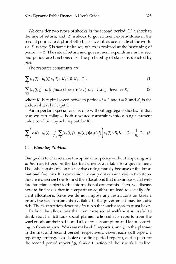
325New Dynamic Public Finance: A User’s Guide
We consider two types of shocks in the second period: (1) a shock to the rate of return; and (2) a shock to government expenditures in the second period. To capture both shocks we introduce a state of the world s ∈ S, where S is some fi nite set, which is realized at the beginning of period t = 2. The rate of return and government expenditure in the sec-ond period are functions of s. The probability of state s is denoted by μ(s).
The resource constraints are
( ( ) ( )) ( ) ,c i y i i K R K Gi
1 1 1 2 1 1 1− + ≤ −∑ π (1)
( ( , ) ( , )) ( | ) ( ) ( ),
c i j y i j j i i R s K Gi j
2 2 2 1 2 2− ≤ −∑ π π 22 ( ), ,s s Sforall ∈ (2)
where K2 is capital saved between periods t = 1 and t = 2, and K1 is the endowed level of capital.
An important special case is one without aggregate shocks. In that case we can collapse both resource constraints into a single present value condition by solving out for K2:
c i y iR
c i j y i j i jij
( ) ( ) [ ( , ) ( , )] ( , )− + −⎛
⎝∑1
22 2 2
1 π⎜⎜⎞
⎠⎟≤ − −∑ π 1 1 1 1
22
1( ) .i R K G
RG
i (3)
3.4 Planning Problem
Our goal is to characterize the optimal tax policy without imposing any ad hoc restrictions on the tax instruments available to a government. The only constraints on taxes arise endogenously because of the infor-mational frictions. It is convenient to carry out our analysis in two steps. First, we describe how to fi nd the allocations that maximize social wel-fare function subject to the informational constraints. Then, we discuss how to fi nd taxes that in competitive equilibrium lead to socially effi -cient allocations. Since we do not impose any restrictions on taxes a priori, the tax instruments available to the government may be quite rich. The next section describes features that such a system must have.
To fi nd the allocations that maximize social welfare it is useful to think about a fi ctitious social planner who collects reports from the workers about their skills and allocates consumption and labor accord-ing to those reports. Workers make skill reports ir and jr to the planner in the fi rst and second period, respectively. Given each skill type i, a reporting strategy is a choice of a fi rst-period report ir and a plan for the second period report jr(j, s) as a function of the true skill realiza-
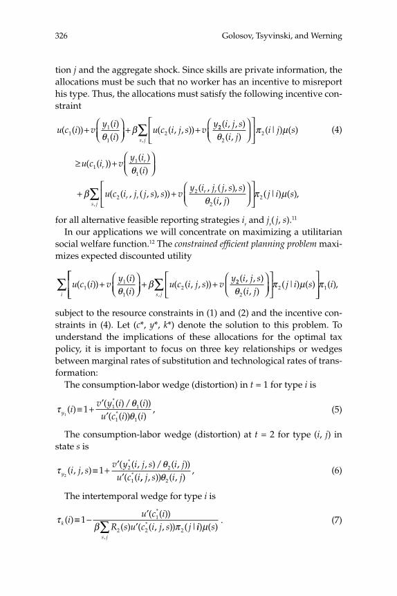
Golosov, Tsyvinski, and Werning326
tion j and the aggregate shock. Since skills are private information, the allocations must be such that no worker has an incentive to misreport his type. Thus, the allocations must satisfy the following incentive con-straint
u c i vy i
iu c i j s v
y( ( ))
( )( )
( ( , , ))11
12+
⎛⎝⎜
⎞⎠⎟+ +
θβ 22
22
( , , )( , )
( | ) ( ),
i j si j
i j ss j θ
π μ⎛⎝⎜
⎞⎠⎟
⎡
⎣⎢
⎤
⎦⎥∑ (4)
≥ +⎛⎝⎜
⎞⎠⎟
u c i vy i
irr( ( ))
( )( )1
1
1θ
+ +βθ
u c i j j s s vy i j j s s
ir rr r( ( , ( , ), ))
( , ( , ), )(2
2
2 ,, )( | ) ( ),
, jj i s
s j
⎛⎝⎜
⎞⎠⎟
⎡
⎣⎢
⎤
⎦⎥∑ π μ2
for all alternative feasible reporting strategies ir and jr( j, s).11
In our applications we will concentrate on maximizing a utilitarian social welfare function.12 The constrained effi cient planning problem maxi-mizes expected discounted utility
u c i vy i
iu c i j s v
y( ( ))
( )( )
( ( , , ))11
12+
⎛⎝⎜
⎞⎠⎟+ +
θβ 22
22
( , , )( , )
( | ) ( ),
i j si j
j i ss j θ
π μ⎛⎝⎜
⎞⎠⎟
⎡
⎣⎢
⎤
⎦⎥∑
⎡⎡
⎣⎢⎢
⎤
⎦⎥⎥
∑i
iπ 1( ),
subject to the resource constraints in (1) and (2) and the incentive con-straints in (4). Let (c*, y*, k*) denote the solution to this problem. To understand the implications of these allocations for the optimal tax policy, it is important to focus on three key relationships or wedges between marginal rates of substitution and technological rates of trans-formation:
The consumption-labor wedge (distortion) in t = 1 for type i is
τ θθy i
v y i iu c i i1
1 1 1
1 1
( )( ( )/ ( ))
( ( )) ( ),
*
*≡ +′′
(5)
The consumption-labor wedge (distortion) at t = 2 for type (i, j) in state s is
τ θy i j s
v y i j s i ju c i2
1 2 2
1
( , , )( ( , , )/ ( , ))
( (
*
*≡ +′′ ,, , )) ( , )
,j s i jθ2
(6)
The intertemporal wedge for type i is
τβ πk i
u c iR s u c i j s j
( )( ( ))
( ) ( ( , , )) ( |
*
*≡ − ′′
1 1
2 2 2 ii ss j
) ( ),
μ∑ . (7)

327New Dynamic Public Finance: A User’s Guide
Note that in the absence of government interventions all the wedges are equal to zero.
4 Theoretical Results and Discussion
In this section we review some aspects of the solution to the planning problem that can be derived theoretically. In the next sections we illus-trate these features in our numerical explorations.
4.1 Capital Wedges
We now characterize the intertemporal distortion, or implicit tax on capital. We fi rst work with an important benchmark in which there are no skill shocks in the second period. That is, all idiosyncratic uncer-tainty is resolved in the fi rst period. For this case we recover Atkinson and Stiglitz ’s (1976) classical uniform taxation result, implying no inter-temporal consumption distortion: Capital should not be taxed. Then, with shocks in the second period we obtain an Inverse Euler Equation, which implies a positive intertemporal wedge (Diamond and Mirrlees 1978, Golosov, Kocherlakota, and Tsyvinski 2003).
4.1.1 Benchmark: Constant Types and a Zero Capital Wedge In this section, we consider a benchmark case in which the skills of agents are fi xed over time and there is no aggregate uncertainty. Specifi cally, assume that N2(i) = 1, ∀i, and that θ1(i) = θ2(i, j) = θ(i). In this case the constrained effi cient problem simplifi es to:
max ( ( ))( )( )
( ( ))(
u c i vy i
iu c i v
y i1
12
2+⎛⎝⎜
⎞⎠⎟+ +
θ))
( )( )
θπ
ii
i
⎛⎝⎜
⎞⎠⎟
⎡
⎣⎢
⎤
⎦⎥∑ 1
subject to the incentive compatibility constraint that ∀i ∈ {1, ...,N1}, and ir ∈ {1, ...,N1}:
u c i vy i
iu c i v
y i( ( ))
( )( )
( ( ))( )
11
22+
⎛⎝⎜
⎞⎠⎟+ +
θβ
θ(( )( ( ))
iu c ir
⎛⎝⎜
⎞⎠⎟
⎡
⎣⎢
⎤
⎦⎥≥ 1
+⎛⎝⎜
⎞⎠⎟+ +
⎛⎝
vy i
iu c i v
y ii
rr
r12
2( )( )
( ( ))( )( )θ
βθ⎜⎜
⎞⎠⎟
⎡
⎣⎢
⎤
⎦⎥ ,
and subject to the feasibility constraint,

Golosov, Tsyvinski, and Werning328
c i y iR
c i y i i Ri
1 12
2 2 1
1( ) ( ) ( ( ) ( )) ( )− + −
⎡
⎣⎢
⎤
⎦⎥ ≤∑ π 11 1 1
22
1k G
RG− − .
We can now prove a variant of a classic Atkinson and Stiglitz (1976) uniform commodity taxation theorem which states that the marginal rate of substitution should be equated across goods and equated to the marginal rate of transformation.
To see this note that only the value of total utility from consumption u(c1) + βu(c2) enters the objective and incentive constraints. It follows that for any total utility coming from consumption u(c1(i)) + βu(c2(i)) it must be that resources c1(i) + (1/R2)c2(i) are minimized, since the resource constraint cannot be slack. The next proposition then follows immediately.
Proposition 1 Assume that the types of agents are constant. A constrained effi cient allocation satisfi es
u′(c1(i)) = βR2u′(c2(i)) ∀i
Note that if β = R2 then c1(i) = c2(i). Indeed, in this case the optimal allocation is simply a repetition of the optimal one in a static version of the model.
4.1.2 Inverse Euler Equation and Positive Capital Taxation We now return to the general case with stochastic types and derive a necessary condition for optimality: The Inverse Euler Equation. This optimality condition implies a positive marginal intertemporal wedge.
We consider variations around any incentive compatible allocation. The argument is similar to the one we used to derive Atkinson and Stiglitz’s (1976) result. In particular, it shares the property that for any realization of i in the fi rst period we shall minimize the resource cost of delivering the remaining utility from consumption.
Fix any fi rst period realization i. We then increase second period util-ity u(c2(i, j)) in a parallel way across second period realizations j. That is defi ne u(c2(i, j; Δ)) ≡ u(c2(i, j)) + Δ for some small Δ. To compensate, we decrease utility in the fi rst period by βΔ. That is, defi ne u(c1(i; Δ)) ≡ u(c1(i)) − βΔ for small Δ.
The crucial point is that such variations do not affect the objective function and incentive constraints in the planning problem. Only the resource constraint is affected. Hence, for the original allocation to be optimal it must be that Δ = 0 minimizes the resources expended

329New Dynamic Public Finance: A User’s Guide
� �c iR
c i j j ij
12
2
1( ; ) ( , ; ) ( | )Δ Δ+ ∑ π
= − + +− −u u c iR
u u c i j j i11
2
12
1( ( ( )) ) ( ( ( , )) ) ( |β πΔ Δ ))
j∑
for all i. The fi rst order condition for this problem evaluated at Δ = 0 then yields the Inverse Euler equation summarized in the next proposi-tion, due originally to Diamond and Mirrlees (1978) and extended to an arbitrary process for skill shocks by Golosov, Kocherlakota, and Tsyvinski (2003).
Proposition 2 A constrained effi cient allocation satisfi es an Inverse Euler Equation:
1 1 1
1 2 22′
=′∑u c i R u c i j
j ij( ( )) ( ( , ))
( | ).β
π (8)
If there is no uncertainty in second period consumption, given the fi rst period shock, the condition becomes
1 1 1
1 2 21 2 2′
=′
⇒ ′ = ′u c R u c
u c R u c( ) ( )
( ) ( ),β
β (9)
which is the standard Euler equation that must hold for a consumer who optimizes savings without distortions.
Whenever consumption remains stochastic, the standard Euler equa-tion must be distorted. This result follows directly by applying Jensen’s inequality to the reciprocal function “1/x” in equation (8).13
Proposition 3 Suppose that for some i, there exists j such that 0 < π(j|i) < 1 and that c2(i, j) is not independent of j. Then the constrained effi cient alloca-tion satisfi es:
′ < ′ ⇒ >∑u c i R u c i j j i ikj
( ( )) ( ( , )) ( | ) ( ) .1 2 2 2 0β π τ
The intuition for this intertemporal wedge is that implicit savings affect the incentives to work. Specifi cally, consider an agent who is con-templating a deviation. Such an agent prefers to implicitly save more than the agent who is planning to tell the truth. An intertemporal wedge worsens the return to such deviation.
The Inverse Euler Equation can be extended to the case of aggregate uncertainty (Kocherlakota 2005). At the optimum
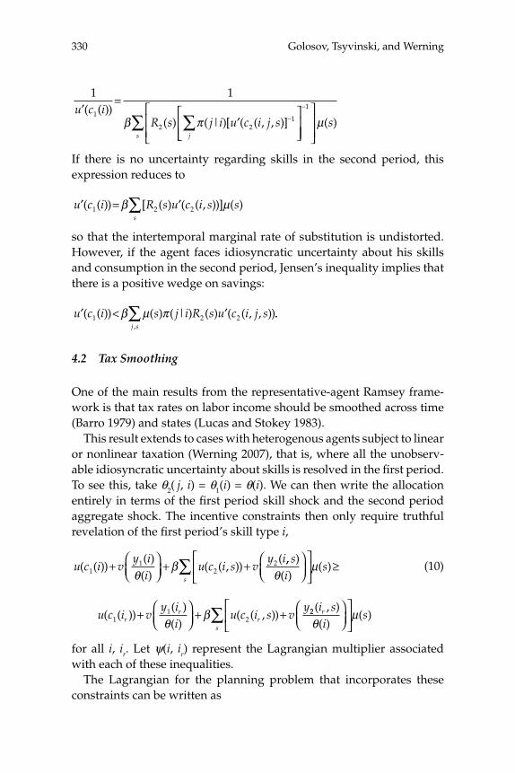
Golosov, Tsyvinski, and Werning330
1 1
1
2 21
′=
′⎡ −∑
u c iR s j i u c i j s
j
( ( ))( ) ( | )[ ( ( , , )]β π
⎣⎣⎢⎢
⎤
⎦⎥⎥
⎡
⎣⎢⎢
⎤
⎦⎥⎥
−
∑1
μ( )ss
If there is no uncertainty regarding skills in the second period, this expression reduces to
′ = ′∑u c i R s u c i s ss
( ( )) [ ( ) ( ( , ))] ( )1 2 2β μ
so that the intertemporal marginal rate of substitution is undistorted. However, if the agent faces idiosyncratic uncertainty about his skills and consumption in the second period, Jensen’s inequality implies that there is a positive wedge on savings:
′ < ′∑u c i s j i R s u c i j sj s
( ( )) ( ) ( | ) ( ) ( ( , , )),
1 2 2β μ π ..
4.2 Tax Smoothing
One of the main results from the representative-agent Ramsey frame-work is that tax rates on labor income should be smoothed across time (Barro 1979) and states (Lucas and Stokey 1983).
This result extends to cases with heterogenous agents subject to linear or nonlinear taxation (Werning 2007), that is, where all the unobserv-able idiosyncratic uncertainty about skills is resolved in the fi rst period. To see this, take θ2(
j, i) = θ1(i) = θ(i). We can then write the allocation entirely in terms of the fi rst period skill shock and the second period aggregate shock. The incentive constraints then only require truthful revelation of the fi rst period’s skill type i,
u c i vy i
iu c i s v
y i( ( ))
( )( )
( ( , ))(
11
22+
⎛⎝⎜
⎞⎠⎟+ +
θβ ,, )
( )( )
si
ss θ
μ⎛⎝⎜
⎞⎠⎟
⎡
⎣⎢
⎤
⎦⎥ ≥∑ (10)
u c i vy i
iu c i s v
yr
rr( ( ))
( )( )
( ( , ))11
2+⎛⎝⎜
⎞⎠⎟+ +
θβ 22 ( , )
( )( )
i si
sr
s θμ⎛
⎝⎜⎞⎠⎟
⎡
⎣⎢
⎤
⎦⎥∑
for all i, ir. Let ψ(i, ir) represent the Lagrangian multiplier associated with each of these inequalities.
The Lagrangian for the planning problem that incorporates these constraints can be written as
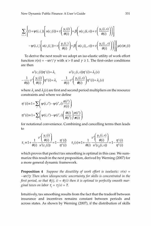
331New Dynamic Public Finance: A User’s Guide
( ( , )) ( ( ))( )( )
( (1 11
2+ +⎛⎝⎜
⎞⎠⎟+ψ
θβi i u c i v
y ii
u cr ii s vy i s
i, ))
( , )( )
+⎛⎝⎜
⎞⎠⎟
⎛⎝⎜
⎞⎠⎟
⎡
⎣⎢⎢
⎤
⎦⎥⎥
⎧⎨⎪
⎩2
θ⎪⎪∑i i sr, ,
− +⎛⎝⎜
⎞⎠⎟+ψ
θβ( , ) ( ( ))
( )( )
( (i i u c i vy i
iu c ir r
r1
12 rr
rs vy i s
i, ))
( , )( )
+⎛⎝⎜
⎞⎠⎟
⎛⎝⎜
⎞⎠⎟
⎡
⎣⎢⎢
⎤
⎦⎥⎥
⎫⎬⎪2
θ ⎭⎭⎪μ π( ) ( )s i1
To derive the next result we adopt an iso-elastic utility of work effort function v(n) = −κnγ/γ with κ > 0 and γ ≥ 1. The fi rst-order conditions are then
′ = ′ =
−
u c i i u c i s i sc c( ( )) ( ) ( ( , )) ( ) ( )
(
1 1 2 2
1
η λ η λ
θ iiv
y ii
ii
vy i sy
)( )( )
( )( )
( , )′⎛⎝⎜
⎞⎠⎟
= − ′11
21θ
η λθ θθ
η λ( )
( ) ( )i
i sy⎛⎝⎜
⎞⎠⎟
= 2
where λ1 and λ2(s) are fi rst and second period multipliers on the resource constraints and where we defi ne
η ψ ψ ππ
c
i
i i i i iii
( ) ( , ) ( , )( )( )
≡ + ′ − ′ ′⎛⎝⎜
⎞⎠⎟′
∑1
η ψ ψ θθ
πy i i i i iii
i( ) ( , ) ( , )
( )( )
( )≡ + ′ − ′′
⎛⎝⎜
⎞⎠⎟
′1
ππ( )ii
⎛⎝⎜
⎞⎠⎟′
∑for notational convenience. Combining and cancelling terms then leads to
τθ
θ η1
1
1
11
1≡ +′⎛⎝⎜
⎞⎠⎟
′= −
( )
( )( )
( ( ))(
i
vy i
iu c i
ic ))( )
( )( )
( , )( )
(ητ
θθ
y is
i
vy i s
iu c2
2
11≡ +
′⎛⎝⎜
⎞⎠⎟
′ 22
1( , ))
( )( )i sii
c
y= − ηη
which proves that perfect tax smoothing is optimal in this case. We sum-marize this result in the next proposition, derived by Werning (2007) for a more general dynamic framework.
Proposition 4 Suppose the disutility of work effort is isoelastic: v(n) = −κnγ/γ. Then when idiosyncratic uncertainty for skills is concentrated in the fi rst period, so that θ2(j, i) = θ1(i) then it is optimal to perfectly smooth mar-ginal taxes on labor τ1 = τ2(s) = τ–.
Intuitively, tax smoothing results from the fact that the tradeoff between insurance and incentives remains constant between periods and across states. As shown by Werning (2007), if the distribution of skills
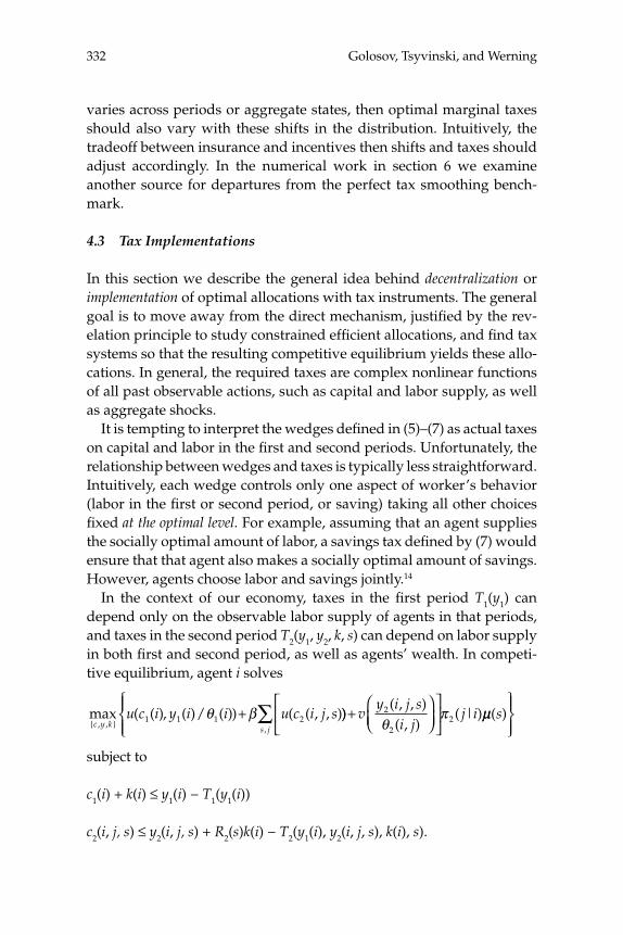
Golosov, Tsyvinski, and Werning332
varies across periods or aggregate states, then optimal marginal taxes should also vary with these shifts in the distribution. Intuitively, the tradeoff between insurance and incentives then shifts and taxes should adjust accordingly. In the numerical work in section 6 we examine another source for departures from the perfect tax smoothing bench-mark.
4.3 Tax Implementations
In this section we describe the general idea behind decentralization or implementation of optimal allocations with tax instruments. The general goal is to move away from the direct mechanism, justifi ed by the rev-elation principle to study constrained effi cient allocations, and fi nd tax systems so that the resulting competitive equilibrium yields these allo-cations. In general, the required taxes are complex nonlinear functions of all past observable actions, such as capital and labor supply, as well as aggregate shocks.
It is tempting to interpret the wedges defi ned in (5)–(7) as actual taxes on capital and labor in the fi rst and second periods. Unfortunately, the relationship between wedges and taxes is typically less straightforward. Intuitively, each wedge controls only one aspect of worker’s behavior (labor in the fi rst or second period, or saving) taking all other choices fi xed at the optimal level. For example, assuming that an agent supplies the socially optimal amount of labor, a savings tax defi ned by (7) would ensure that that agent also makes a socially optimal amount of savings. However, agents choose labor and savings jointly.14
In the context of our economy, taxes in the fi rst period T1(y1) can depend only on the observable labor supply of agents in that periods, and taxes in the second period T2(y1, y2, k, s) can depend on labor supply in both fi rst and second period, as well as agents’ wealth. In competi-tive equilibrium, agent i solves
max ( ( ), ( )/ ( )) ( ( , , ){ , , }c y k
u c i y i i u c i j s1 1 1 2θ β+ ))( , , )( , )
( | ),
+⎛⎝⎜
⎞⎠⎟
⎡
⎣⎢
⎤
⎦⎥∑ v
y i j si j
j is j
2
22θ
π μμ( )s⎧⎨⎪
⎩⎪
⎫⎬⎪
⎭⎪
subject to
c1(i) + k(i) ≤ y1(i) − T1(y1(i))
c2(i, j, s) ≤ y2(i, j, s) + R2(s)k(i) − T2(y1(i), y2(i, j, s), k(i), s).
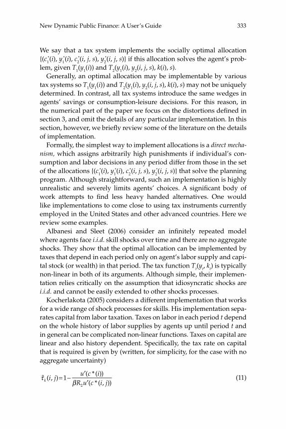
333New Dynamic Public Finance: A User’s Guide
We say that a tax system implements the socially optimal allocation {(c1
*(i), y1*(i), c2
*(i, j, s), y2*(i, j, s)} if this allocation solves the agent’s prob-
lem, given T1(y1(i)) and T2(y1(i), y2(i, j, s), k(i), s).Generally, an optimal allocation may be implementable by various
tax systems so T1(y1(i)) and T2(y1(i), y2(i, j, s), k(i), s) may not be uniquely determined. In contrast, all tax systems introduce the same wedges in agents’ savings or consumption-leisure decisions. For this reason, in the numerical part of the paper we focus on the distortions defi ned in section 3, and omit the details of any particular implementation. In this section, however, we briefl y review some of the literature on the details of implementation.
Formally, the simplest way to implement allocations is a direct mecha-nism, which assigns arbitrarily high punishments if individual’s con-sumption and labor decisions in any period differ from those in the set of the allocations {(c1
*(i), y1*(i), c2
*(i, j, s), y2*(i, j, s)} that solve the planning
program. Although straightforward, such an implementation is highly unrealistic and severely limits agents’ choices. A signifi cant body of work attempts to fi nd less heavy handed alternatives. One would like implementations to come close to using tax instruments currently employed in the United States and other advanced countries. Here we review some examples.
Albanesi and Sleet (2006) consider an infi nitely repeated model where agents face i.i.d. skill shocks over time and there are no aggregate shocks. They show that the optimal allocation can be implemented by taxes that depend in each period only on agent’s labor supply and capi-tal stock (or wealth) in that period. The tax function Tt(yt, kt) is typically non-linear in both of its arguments. Although simple, their implemen-tation relies critically on the assumption that idiosyncratic shocks are i.i.d. and cannot be easily extended to other shocks processes.
Kocherlakota (2005) considers a different implementation that works for a wide range of shock processes for skills. His implementation sepa-rates capital from labor taxation. Taxes on labor in each period t depend on the whole history of labor supplies by agents up until period t and in general can be complicated non-linear functions. Taxes on capital are linear and also history dependent. Specifi cally, the tax rate on capital that is required is given by (written, for simplicity, for the case with no aggregate uncertainty)
�τβk i j
u c iR u c i j
( , )( * ( ))( * ( , ))
= − ′′
12
(11)
Golosov, Tsyvinski, and Werning334
Incidentally, an implication of this implementation is that, at the opti-mum, taxes on capital average out to zero and raise no revenue. That is, the conditional average over j for τk(i, j) given by equation (11) is zero when the Inverse Euler equation (8) holds. At fi rst glance, a zero average tax rate may appear to be at odds with the positive intertempo-ral wedge τk(i) defi ned by equation (7) found in Proposition 3, but it is not: Savings are discouraged by this implementation. The key point is that the tax is not deterministic, but random. As a result, although the average net return on savings is unaffected by the tax, the net return R2(s)(1 − τk (i, j, s)) is made risky. Indeed, since net returns are negatively related to consumption, see equation (11), there is a risk-premium com-ponent (in the language of fi nancial economics) to the expected return. This tax implementation makes saving strictly less attractive, just as the positive intertemporal wedge τk suggests.
In some applications the number of shocks that agents face is small and, with a certain structure, that allows for simple decentralizations. Golosov and Tsyvinski (2006a) study a model of disability insurance, where the only uncertainty agents face is whether, and when, they receive a permanent shock that makes them unable to work. In this scenario, the optimal allocation can be implemented by paying disabil-ity benefi ts to agents who have assets below a specifi ed threshold, i.e., asset testing the benefi ts.
4.4 Time Inconsistency
In this section we argue that the dynamic Mirrlees literature and Ramsey literature are both prone to time-consistency problems. However, the nature of time inconsistency is very different in those two approaches.
An example that clarifi es the notion of time inconsistency in Ramsey models is taxation of capital. The Chamley-Judd (Judd 1985, Chamley 1986) result states that capital should be taxed at zero in the long run. One of the main assumptions underlying this result is that a govern-ment can commit to a sequence of capital taxes. However, a benevolent government would choose to deviate from the prescribed sequence of taxes. The reason is that, once capital is accumulated, it is sunk, and taxing capital is no longer distortionary. A benevolent government would choose high capital taxes once capital is accumulated. The rea-soning above motivates the analysis of time consistent policy as a game between a policy maker (government) and a continuum of economic agents (consumers).15

335New Dynamic Public Finance: A User’s Guide
To highlight problems that arise when we depart from the benchmark of a benevolent planner with full commitment, it is useful to start with Roberts’ (1984) example economy, where, similar to Mirrlees (1971), risk-averse individuals are subject to unobserved shocks affecting the marginal disutility of labor supply. But unlike the benchmark Mirrlees model, the economy is repeated T times, with individuals having per-fectly persistent types. Under full commitment, a benevolent planner would choose the same allocation at every date, which coincides with the optimal solution of the static model. However, a benevolent gov-ernment without full commitment cannot refrain from exploiting the information that it has collected at previous dates to achieve better risk sharing ex post. This turns the optimal taxation problem into a dynamic game between the government and the citizens. Roberts showed that as discounting disappears and T → ∞, the unique sequential equilib-rium of this game involves the highly ineffi cient outcome in which all types declare to be the worst type at all dates, supply the lowest level of labor and receive the lowest level of consumption. This example shows the potential ineffi ciencies that can arise once we depart from the case of full commitment, even with benevolent governments. The nature of time inconsistency in dynamic Mirrlees problems is, therefore, very dif-ferent from that in a Ramsey model. In the dynamic Mirrlees model the inability of a social planner not to exploit information it learns about agents’ types is a central issues in designing optimal policy without commitment. A recent paper by Bisin and Rampini (2006) considers the problem of mechanism design without commitment in a two-period setting. They show how the presence of anonymous markets acts as an additional constraint on the government, ameliorating the commitment problem.
Acemoglu, Golosov, and Tsyvinski (2006) depart from Roberts’ (1984) framework and consider, instead of a fi nite-horizon economy, an infi -nite-horizon economy. This enables them to use punishment strategies against the government to construct a sustainable mechanism, defi ned as an equilibrium tax-transfer program that is both incentive compatible for the citizens and for the government (i.e., it satisfi es a sustainabil-ity constraint for the government). The (best) sustainable mechanism implies that if the government deviates from the implicit agreement, citizens switch to supplying zero labor, implicitly punishing the gov-ernment. The infi nite-horizon setup enables them to prove that a ver-sion of the revelation principle, truthful revelation along the equilibrium path, applies and is a useful tool of analysis for this class of dynamic
Golosov, Tsyvinski, and Werning336
incentive problems with self-interested mechanism designers and with-out commitment.16 The fact that the truthful revelation principle applies only along the equilibrium path is important, since it is actions off the equilibrium path that place restrictions on what type of mechanisms are allowed (these are encapsulated in the sustainability constraints). This enables them to construct sustainable mechanisms with the rev-elation principle along the equilibrium path, to analyze more general environments, and to characterize the limiting behavior of distortions and taxes.
4.5 The Government’s Role As Insurance Provider
In the previous discussion we assumed that a government is the sole provider of insurance. However, in many circumstances, markets can provide insurance against shocks that agents experience. The presence of competitive insurance markets may signifi cantly change optimal policy prescriptions regarding the desirability and extent of taxation and social insurance policies.
We assumed that individual asset trades and, therefore, agents’ con-sumption, are publicly observable. In that case, following Prescott and Townsend (1984), Golosov and Tsyvinski (2006b) show that allocations provided by competitive markets are constrained effi cient and the fi rst welfare theorem holds. The competitive nature of insurance markets, even in the presence of private information, can provide optimal insur-ance as long as consumption and output are publicly observable. Note that individual insurance contracts, between agents and fi rms, would feature the same wedges as the social planning problem we studied, providing another motivation for focusing on wedges, rather than taxes that implement them.
In this paper we do not model explicitly reasons why private insur-ance markets may provide the ineffi cient level of insurance. Arnott and Stiglitz (1986, 1990), Greenwald and Stiglitz (1986), and Golosov and Tsyvinski (2006b) explore why markets may fail in the presence of asymmetric information.
5 Numerical Exercises
We now turn to numerical exercises with baseline parameters and per-form several comparative-static experiments. The exercises we conduct strike a balance between fl exibility and tractability. The two period

337New Dynamic Public Finance: A User’s Guide
setting is fl exible enough to illustrate the key theoretical results and explore a few new ones. At the same time, it is simple enough that a complete solution of the optimal allocation is possible. In contrast, most work on Mirrleesian models has focused on either partial theoretical characterizations of the optimum, e.g., showing that the intertempo-ral wedge is positive (Golosov, Kocherlakota, and Tsyvinski, 2003) or on numerical characterizations for a particular skills processes, e.g., i.i.d. skills in Albanesi and Sleet (2006) or absorbing disability shocks in Golosov and Tsyvinski (2006a). In a recent paper, Farhi and Werning (2006a) take a different approach, by studying partial tax reforms—that fully capture the savings distortions implied by the Inverse Euler equa-tion. The problem remains tractable even with empirically relevant skill processes.
5.1 Parameterization
When selecting parameters it is important to keep the following neutral-ity result in mind. With logarithmic utility, if productivity and govern-ment expenditures are scaled up within a period then: (1) the allocation for consumption is scaled by the same factor; (2) the allocation of labor is unaffected; and (3) marginal taxes rates are unaffected. This result is relevant for thinking about balanced growth in an extension of the model to an infi nite horizon. It is also convenient in that it allows us to normalize, without any loss of generality, the second period shock for our numerical explorations.
We now discuss how we choose parameters for the benchmark exam-ple. We use the following baseline parameters. We fi rst consider the case with no aggregate uncertainty. Assume that there is no discounting and that the rate of return on savings is equal to the discount factor: R = β = 1.
We choose the skill distribution as follows. In the fi rst period, skills are distributed uniformly. Individual skills in the fi rst period, θ1(i), are equally spaced in the interval [θ1, θ
–1]. The probability of the realiza-
tion of each skill is equal to π1(i) = 1/N1 for all i. We choose baseline parameters to be θ1 = 0.1, θ–1 = 1, and N1 = 50. Here, a relatively large number of skills allows us to closely approximate a continuous distri-bution of skills. In the second period, an agent can receive a skill shock. For computational tractability, we assume that there are only two pos-sible shocks to an agent’s skill in the second period, N2(i) = 2 for all i. Skill shocks take the form of a proportional increase θ2(i, 1) = α1θ1(i) or
Golosov, Tsyvinski, and Werning338
proportional decrease θ2(i, 2) = α2θ1(i). For the baseline case, we set α1 = 1, and α2 = 1/2. This means that an agent in the second period can only receive an adverse shock α2. We also assume that there is uncertainty about realization of skills and set π2(1|i) = π2(2|i) = 1/2. The agent learns his skill in the second period only at time t = 2. We chose the above parameterization of skills to allow a stark characterization of the main forces determining the optimum.17
We choose the utility function to be power utility. The utility of con-sumption is u(c) = c1−σ/(1 − σ). As our baseline we take σ = 1, so that u(c) = log(c). The utility of labor is given by v(l) = −lγ; as our benchmark we set γ = 2.
We use the following conventions in the fi gures below:
1. The horizontal axis displays the fi rst period skill type i = 1, 2, . . . , 50;
2. The wedges (distortions) in the optimal solutions are labeled as fol-lows:
(a) “Distortion t = 1” is the consumption-labor wedge in period 1: τy1
;
(b) “Distortion high t = 2” is the consumption-labor wedge in period 2 for an agent with a high skill shock: τy2
(i, 1);
(c) “Distortion low t = 2” is the consumption-labor wedge in period 2 for an agent with a low skill shock: τy2
(i, 2);
(d) “Distortion capital” is the intertemporal (capital) wedge: τk(i).
5.2 Characterizing the Benchmark Case
In this section, we describe the numerical characterization of the opti-mal allocation. Suppose fi rst that there were no informational friction and agents’ skills were observable. Then the solution to the optimal program would feature full insurance. The agent’s consumption would be equalized across realizations of shocks. Labor of agents would be increasing with their type. It is obvious that when skills are unobserv-able the unconstrained optimal allocation is not incentive compatible, as an agent with a higher skill would always prefer to claim to be of a lower type to receive the same consumption but work less. The optimal allocation with unobservable types balances two objectives of the social planner: Providing insurance and respecting incentive compatibility constraints.

339New Dynamic Public Finance: A User’s Guide
The optimal allocation for the benchmark case with unobservable types is shown in fi gure 5.1 and fi gure 5.2. There is no bunching in either period: Agents of different skills are allocated different consump-tion and labor bundles.
First note that there is a signifi cant deviation from the case of perfect insurance: agents’ consumption increases with type, and consumption in the second period for an agent who claims to have a high shock is higher than that of an agent with the low shock. The intuition for this pattern of consumption is as follows. It is optimal for an agent with a higher skill to provide a higher amount of effective labor. One way to make provision of higher effective labor incentive compatible for an agent is to allocate a larger amount of consumption to him. Another way to reward an agent for higher effort is to increase his continuation value, i.e., allocate a higher amount of expected future consumption for such an agent.
We now turn our attention to the wedges in the constrained effi cient allocation. In the unconstrained optimum with observable types, all wedges are equal to zero. We plot optimal wedges for the benchmark case in fi gure 5.3.
We see that the wedges are positive, indicating a signifi cant depar-ture from the case of perfect insurance. We notice that the consumption-labor wedge is equal to zero for the highest skill type in the fi rst period and for the high realization of the skill shock in the second period: τy1
(θ–1) = τy2
(θ–1,1) = 0. This result confi rms a familiar “no distortion at
the top” result due to Mirrlees (1971) which states that in a static con-text the consumption-labor decision of an agent with the highest skill is undistorted in the optimal allocation. The result that we obtain here is somewhat novel as we consider an economy with stochastically evolv-ing skills, for which the “no distortion at the top” result have not yet been proven analytically.
We also see that the labor wedges at the bottom {τy1(θ1), τy2
(θ1, 1), τy2
(θ1, 2)} are strictly positive. A common result in the literature is that with a continuum of types, the tax rate at the bottom is zero if bunching types is not optimal. In our case, there is no bunching, but this result does not literally apply because we work with a discrete distribution of types.
We see that the intertemporal wedge is low for agents with low skills θ1 in the fi rst period yet is quite high for agents with high skills. The rea-son is that it turns out that lower skilled workers are quite well insured: Their consumption is not very volatile in the second period. It follows
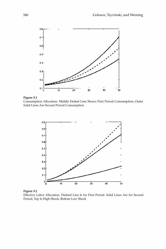
Golosov, Tsyvinski, and Werning340
Figure 5.1Consumption Allocation. Middle Dotted Line Shows First Period Consumption; Outer Solid Lines Are Second Period Consumption
Figure 5.2Effective Labor Allocation. Dashed Line Is for First Period. Solid Lines Are for Second Period, Top Is High Shock, Bottom Low Shock
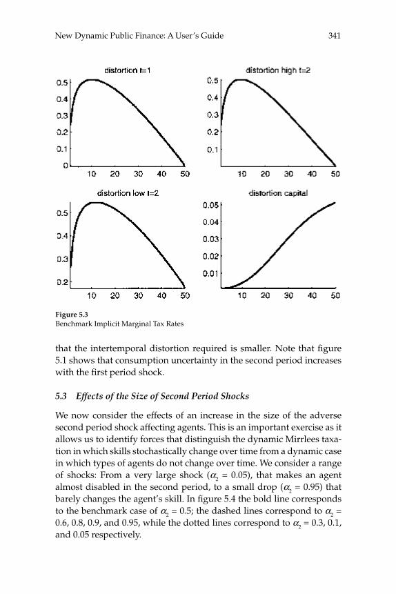
341New Dynamic Public Finance: A User’s Guide
that the intertemporal distortion required is smaller. Note that fi gure 5.1 shows that consumption uncertainty in the second period increases with the fi rst period shock.
5.3 Effects of the Size of Second Period Shocks
We now consider the effects of an increase in the size of the adverse second period shock affecting agents. This is an important exercise as it allows us to identify forces that distinguish the dynamic Mirrlees taxa-tion in which skills stochastically change over time from a dynamic case in which types of agents do not change over time. We consider a range of shocks: From a very large shock (α2 = 0.05), that makes an agent almost disabled in the second period, to a small drop (α2 = 0.95) that barely changes the agent’s skill. In fi gure 5.4 the bold line corresponds to the benchmark case of α2 = 0.5; the dashed lines correspond to α2 = 0.6, 0.8, 0.9, and 0.95, while the dotted lines correspond to α2 = 0.3, 0.1, and 0.05 respectively.
Figure 5.3Benchmark Implicit Marginal Tax Rates
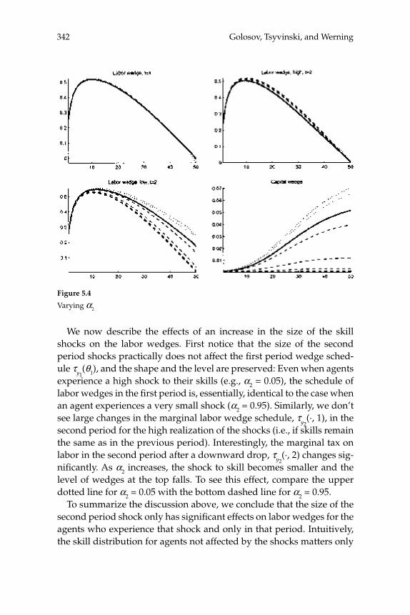
Golosov, Tsyvinski, and Werning342
We now describe the effects of an increase in the size of the skill shocks on the labor wedges. First notice that the size of the second period shocks practically does not affect the fi rst period wedge sched-ule τy1
(θ1), and the shape and the level are preserved: Even when agents experience a high shock to their skills (e.g., α2 = 0.05), the schedule of labor wedges in the fi rst period is, essentially, identical to the case when an agent experiences a very small shock (α2 = 0.95). Similarly, we don’t see large changes in the marginal labor wedge schedule, τy2
(·, 1), in the second period for the high realization of the shocks (i.e., if skills remain the same as in the previous period). Interestingly, the marginal tax on labor in the second period after a downward drop, τy2
(·, 2) changes sig-nifi cantly. As α2 increases, the shock to skill becomes smaller and the level of wedges at the top falls. To see this effect, compare the upper dotted line for α2 = 0.05 with the bottom dashed line for α2 = 0.95.
To summarize the discussion above, we conclude that the size of the second period shock only has signifi cant effects on labor wedges for the agents who experience that shock and only in that period. Intuitively, the skill distribution for agents not affected by the shocks matters only
Figure 5.4
Varying α2

343New Dynamic Public Finance: A User’s Guide
indirectly, and, therefore, the labor wedge for those agents is affected only to a small degree.
We now proceed to characterize the effects of the size of shocks on the capital wedge. The intertemporal wedge becomes smaller and fl at-ter when α2 increases—compare, for example, the lower curve associ-ated with α2 = 0.95 to the highest curve associated with α2 = 0.05. The reason is that consumption becomes less volatile in the second period when the skill drop is smaller. The inverse Euler equation then implies a smaller distortion. The intuition for this result is simple. If there were no skill shocks in the second period (α2 = 1) then, as we discussed above, the capital wedge is equal to zero. The higher is the wedge in the sec-ond period, the further away from the case of constant skills we are, therefore, the distortion increases. Also note that low α2 (large shocks in the second period) signifi cantly steepens the capital wedge profi le.
We conclude that the shape and size of the capital wedge responds signifi cantly to the size of the shocks that an agent may experience in the future.
5.4 Effects of the Probability of Second Period Shocks and Uncertainty
We now consider the effects of changing the probability of the adverse second period shock. This exercise is of interest because it allows us to investigate the effects of uncertainty about future skill realizations on the size and shape of wedges.
In fi gure 5.5, we show in bold the benchmark case where π2(2|·) = 0.5; dashed line correspond to π2(2|·) = 0.7 and 0.9 while the dotted lines correspond to π2(2|·) = 0.3 and 0.1, respectively.
We fi rst notice that the effects of the change in the probability of the adverse shock on labor wedge are similar to the case of increase in size of the adverse shock. That is, as the probability π2(2|·) of a drop in skills rises, the informational friction increases and so does the labor wedge.
For the intertemporal wedge there is an additional effect of chang-ing the probability of the adverse skill shock. The wedge is the highest when uncertainty about skills is the highest: At the symmetric baseline case with π2(2|·) = 0.5. Intuitively, the reason is that the uncertainty about next period’s skill is maximized at π2(2|·) = 0.5. It is uncertainty about future skills, rather than the level of next period’s skill shock, that matters for the size of the capital wedge.
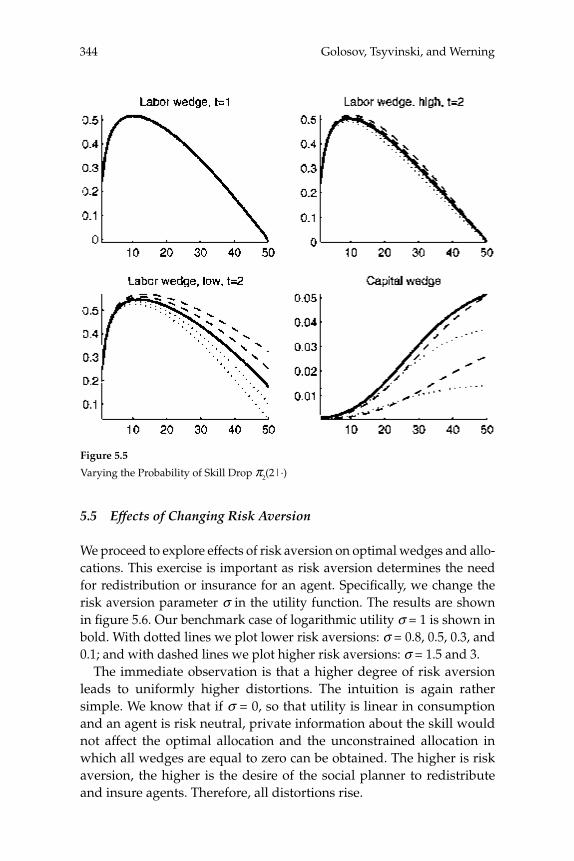
Golosov, Tsyvinski, and Werning344
5.5 Effects of Changing Risk Aversion
We proceed to explore effects of risk aversion on optimal wedges and allo-cations. This exercise is important as risk aversion determines the need for redistribution or insurance for an agent. Specifi cally, we change the risk aversion parameter σ in the utility function. The results are shown in fi gure 5.6. Our benchmark case of logarithmic utility σ = 1 is shown in bold. With dotted lines we plot lower risk aversions: σ = 0.8, 0.5, 0.3, and 0.1; and with dashed lines we plot higher risk aversions: σ = 1.5 and 3.
The immediate observation is that a higher degree of risk aversion leads to uniformly higher distortions. The intuition is again rather simple. We know that if σ = 0, so that utility is linear in consumption and an agent is risk neutral, private information about the skill would not affect the optimal allocation and the unconstrained allocation in which all wedges are equal to zero can be obtained. The higher is risk aversion, the higher is the desire of the social planner to redistribute and insure agents. Therefore, all distortions rise.
Figure 5.5
Varying the Probability of Skill Drop π2(2|·)
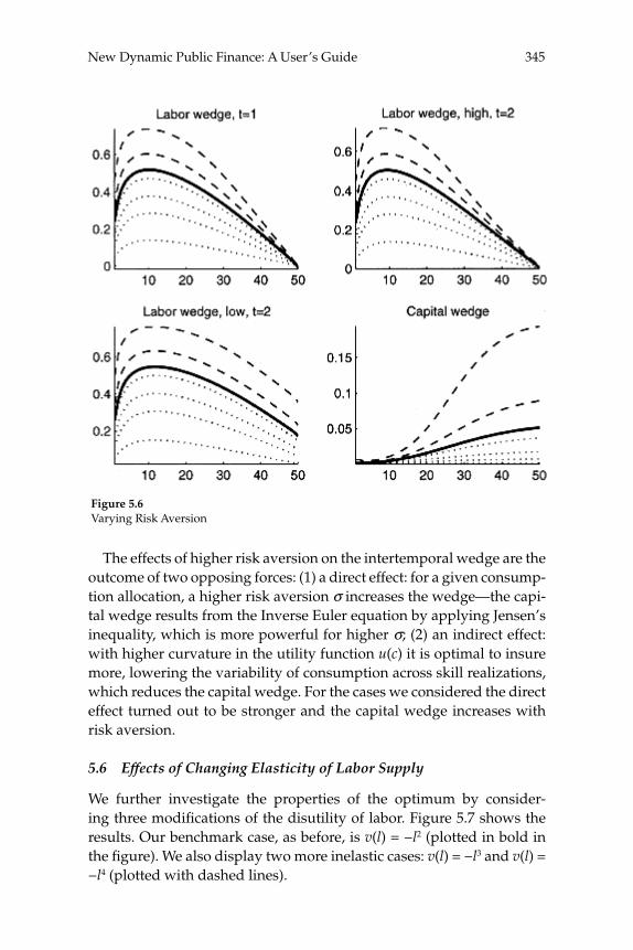
345New Dynamic Public Finance: A User’s Guide
The effects of higher risk aversion on the intertemporal wedge are the outcome of two opposing forces: (1) a direct effect: for a given consump-tion allocation, a higher risk aversion σ increases the wedge—the capi-tal wedge results from the Inverse Euler equation by applying Jensen’s inequality, which is more powerful for higher σ; (2) an indirect effect: with higher curvature in the utility function u(c) it is optimal to insure more, lowering the variability of consumption across skill realizations, which reduces the capital wedge. For the cases we considered the direct effect turned out to be stronger and the capital wedge increases with risk aversion.
5.6 Effects of Changing Elasticity of Labor Supply
We further investigate the properties of the optimum by consider-ing three modifi cations of the disutility of labor. Figure 5.7 shows the results. Our benchmark case, as before, is v(l) = −l2 (plotted in bold in the fi gure). We also display two more inelastic cases: v(l) = −l3 and v(l) = −l4 (plotted with dashed lines).
Figure 5.6Varying Risk Aversion
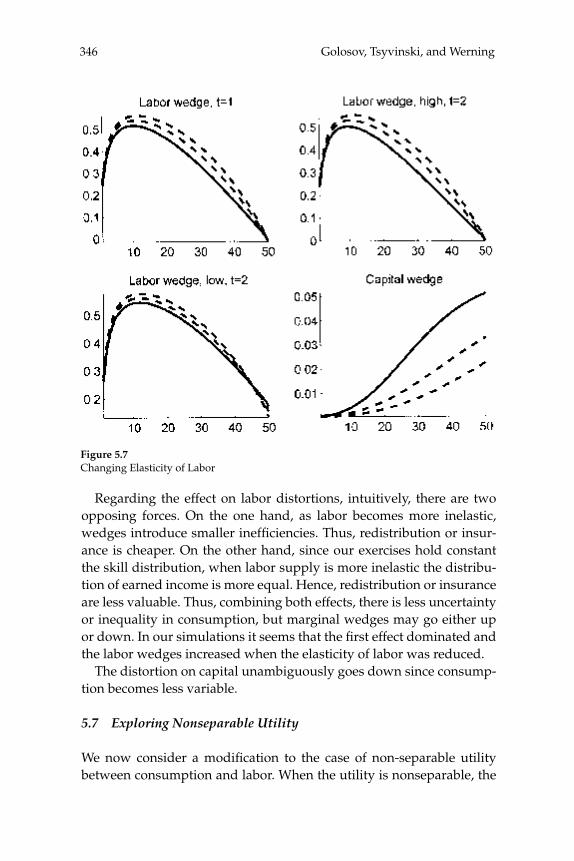
Golosov, Tsyvinski, and Werning346
Regarding the effect on labor distortions, intuitively, there are two opposing forces. On the one hand, as labor becomes more inelastic, wedges introduce smaller ineffi ciencies. Thus, redistribution or insur-ance is cheaper. On the other hand, since our exercises hold constant the skill distribution, when labor supply is more inelastic the distribu-tion of earned income is more equal. Hence, redistribution or insurance are less valuable. Thus, combining both effects, there is less uncertainty or inequality in consumption, but marginal wedges may go either up or down. In our simulations it seems that the fi rst effect dominated and the labor wedges increased when the elasticity of labor was reduced.
The distortion on capital unambiguously goes down since consump-tion becomes less variable.
5.7 Exploring Nonseparable Utility
We now consider a modifi cation to the case of non-separable utility between consumption and labor. When the utility is nonseparable, the
Figure 5.7Changing Elasticity of Labor
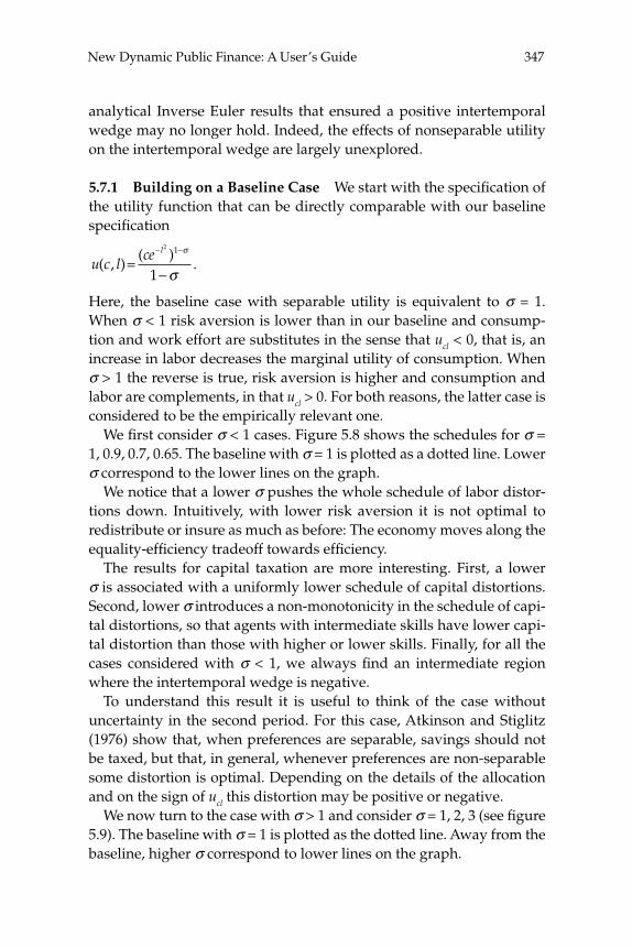
347New Dynamic Public Finance: A User’s Guide
analytical Inverse Euler results that ensured a positive intertemporal wedge may no longer hold. Indeed, the effects of nonseparable utility on the intertemporal wedge are largely unexplored.
5.7.1 Building on a Baseline Case We start with the specifi cation of the utility function that can be directly comparable with our baseline specifi cation
u c lce l
( , )( )
.=−
− −2 1
1
σ
σ
Here, the baseline case with separable utility is equivalent to σ = 1. When σ < 1 risk aversion is lower than in our baseline and consump-tion and work effort are substitutes in the sense that ucl < 0, that is, an increase in labor decreases the marginal utility of consumption. When σ > 1 the reverse is true, risk aversion is higher and consumption and labor are complements, in that ucl > 0. For both reasons, the latter case is considered to be the empirically relevant one.
We fi rst consider σ < 1 cases. Figure 5.8 shows the schedules for σ = 1, 0.9, 0.7, 0.65. The baseline with σ = 1 is plotted as a dotted line. Lower σ correspond to the lower lines on the graph.
We notice that a lower σ pushes the whole schedule of labor distor-tions down. Intuitively, with lower risk aversion it is not optimal to redistribute or insure as much as before: The economy moves along the equality-effi ciency tradeoff towards effi ciency.
The results for capital taxation are more interesting. First, a lower σ is associated with a uniformly lower schedule of capital distortions. Second, lower σ introduces a non-monotonicity in the schedule of capi-tal distortions, so that agents with intermediate skills have lower capi-tal distortion than those with higher or lower skills. Finally, for all the cases considered with σ < 1, we always fi nd an intermediate region where the intertemporal wedge is negative.
To understand this result it is useful to think of the case without uncertainty in the second period. For this case, Atkinson and Stiglitz (1976) show that, when preferences are separable, savings should not be taxed, but that, in general, whenever preferences are non-separable some distortion is optimal. Depending on the details of the allocation and on the sign of ucl this distortion may be positive or negative.
We now turn to the case with σ > 1 and consider σ = 1, 2, 3 (see fi gure 5.9). The baseline with σ = 1 is plotted as the dotted line. Away from the baseline, higher σ correspond to lower lines on the graph.
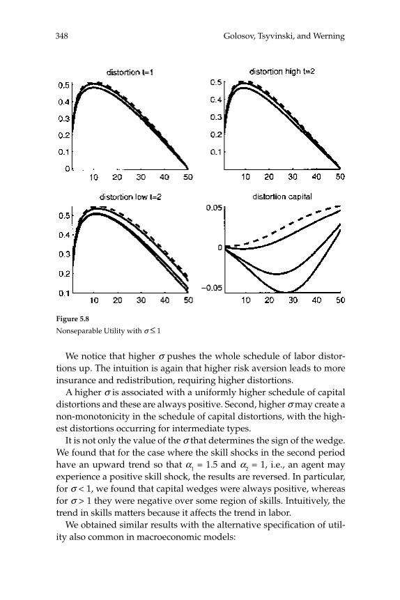
Golosov, Tsyvinski, and Werning348
We notice that higher σ pushes the whole schedule of labor distor-tions up. The intuition is again that higher risk aversion leads to more insurance and redistribution, requiring higher distortions.
A higher σ is associated with a uniformly higher schedule of capital distortions and these are always positive. Second, higher σ may create a non-monotonicity in the schedule of capital distortions, with the high-est distortions occurring for intermediate types.
It is not only the value of the σ that determines the sign of the wedge. We found that for the case where the skill shocks in the second period have an upward trend so that α1 = 1.5 and α2 = 1, i.e., an agent may experience a positive skill shock, the results are reversed. In particular, for σ < 1, we found that capital wedges were always positive, whereas for σ > 1 they were negative over some region of skills. Intuitively, the trend in skills matters because it affects the trend in labor.
We obtained similar results with the alternative specifi cation of util-ity also common in macroeconomic models:
Figure 5.8
Nonseparable Utility with σ ≤ 1
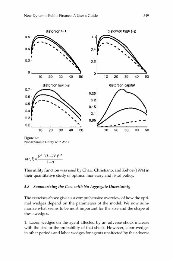
349New Dynamic Public Finance: A User’s Guide
u c lc L l
( , )( ( ) )
.=−−
− −1 1
1
γ γ σ
σ
This utility function was used by Chari, Christiano, and Kehoe (1994) in their quantitative study of optimal monetary and fi scal policy.
5.8 Summarizing the Case with No Aggregate Uncertainty
The exercises above give us a comprehensive overview of how the opti-mal wedges depend on the parameters of the model. We now sum-marize what seems to be most important for the size and the shape of these wedges.
1. Labor wedges on the agent affected by an adverse shock increase with the size or the probability of that shock. However, labor wedges in other periods and labor wedges for agents unaffected by the adverse
Figure 5.9Nonseparable Utility with σ ≥ 1
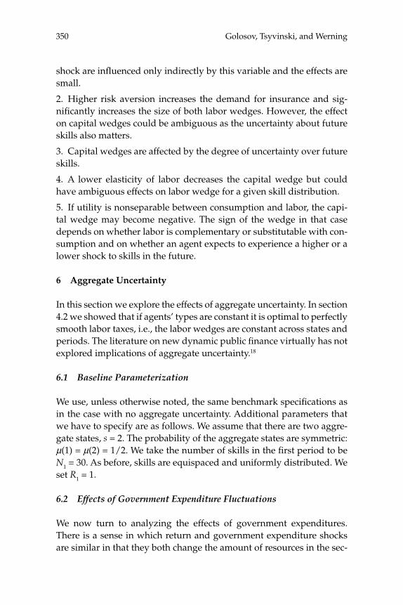
Golosov, Tsyvinski, and Werning350
shock are infl uenced only indirectly by this variable and the effects are small.
2. Higher risk aversion increases the demand for insurance and sig-nifi cantly increases the size of both labor wedges. However, the effect on capital wedges could be ambiguous as the uncertainty about future skills also matters.
3. Capital wedges are affected by the degree of uncertainty over future skills.
4. A lower elasticity of labor decreases the capital wedge but could have ambiguous effects on labor wedge for a given skill distribution.
5. If utility is nonseparable between consumption and labor, the capi-tal wedge may become negative. The sign of the wedge in that case depends on whether labor is complementary or substitutable with con-sumption and on whether an agent expects to experience a higher or a lower shock to skills in the future.
6 Aggregate Uncertainty
In this section we explore the effects of aggregate uncertainty. In section 4.2 we showed that if agents’ types are constant it is optimal to perfectly smooth labor taxes, i.e., the labor wedges are constant across states and periods. The literature on new dynamic public fi nance virtually has not explored implications of aggregate uncertainty.18
6.1 Baseline Parameterization
We use, unless otherwise noted, the same benchmark specifi cations as in the case with no aggregate uncertainty. Additional parameters that we have to specify are as follows. We assume that there are two aggre-gate states, s = 2. The probability of the aggregate states are symmetric: μ(1) = μ(2) = 1/2. We take the number of skills in the fi rst period to be N1 = 30. As before, skills are equispaced and uniformly distributed. We set R1 = 1.
6.2 Effects of Government Expenditure Fluctuations
We now turn to analyzing the effects of government expenditures. There is a sense in which return and government expenditure shocks are similar in that they both change the amount of resources in the sec-
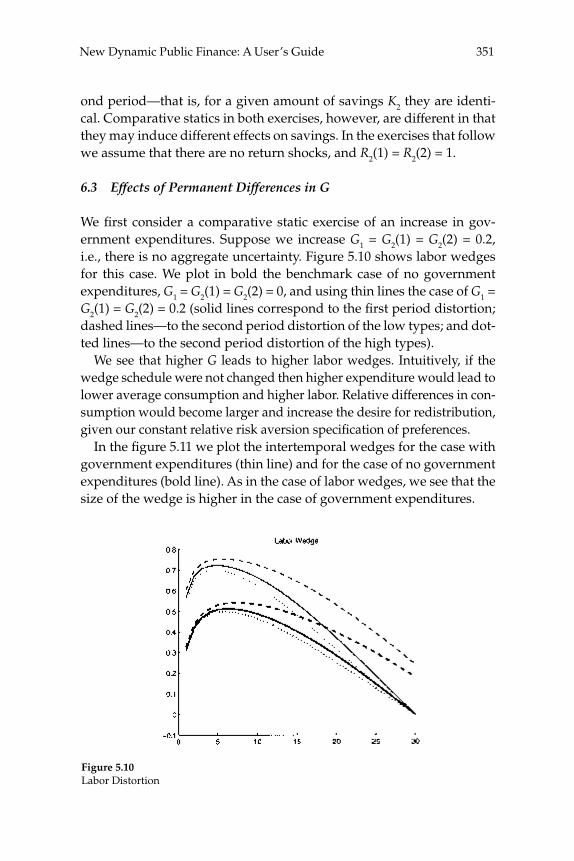
351New Dynamic Public Finance: A User’s Guide
ond period—that is, for a given amount of savings K2 they are identi-cal. Comparative statics in both exercises, however, are different in that they may induce different effects on savings. In the exercises that follow we assume that there are no return shocks, and R2(1) = R2(2) = 1.
6.3 Effects of Permanent Differences in G
We fi rst consider a comparative static exercise of an increase in gov-ernment expenditures. Suppose we increase G1 = G2(1) = G2(2) = 0.2, i.e., there is no aggregate uncertainty. Figure 5.10 shows labor wedges for this case. We plot in bold the benchmark case of no government expenditures, G1 = G2(1) = G2(2) = 0, and using thin lines the case of G1 = G2(1) = G2(2) = 0.2 (solid lines correspond to the fi rst period distortion; dashed lines—to the second period distortion of the low types; and dot-ted lines—to the second period distortion of the high types).
We see that higher G leads to higher labor wedges. Intuitively, if the wedge schedule were not changed then higher expenditure would lead to lower average consumption and higher labor. Relative differences in con-sumption would become larger and increase the desire for redistribution, given our constant relative risk aversion specifi cation of preferences.
In the fi gure 5.11 we plot the intertemporal wedges for the case with government expenditures (thin line) and for the case of no government expenditures (bold line). As in the case of labor wedges, we see that the size of the wedge is higher in the case of government expenditures.
Figure 5.10Labor Distortion
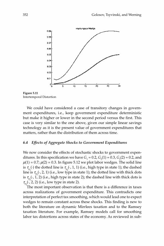
Golosov, Tsyvinski, and Werning352
We could have considered a case of transitory changes in govern-ment expenditures, i.e., keep government expenditure deterministic but make it higher or lower in the second period versus the fi rst. This case is very similar to the one above, given our simple linear savings technology as it is the present value of government expenditures that matters, rather than the distribution of them across time.
6.4 Effects of Aggregate Shocks to Government Expenditures
We now consider the effects of stochastic shocks to government expen-ditures. In this specifi cation we have G1 = 0.2, G2(1) = 0.3, G2(2) = 0.2, and μ(1) = 0.7; μ(2) = 0.3. In fi gure 5.12 we plot labor wedges. The solid line is τy1
(·) the dotted line is τy2(·, 1, 1) (i.e., high type in state 1); the dashed
line is τy2(·, 2, 1) (i.e., low type in state 1); the dotted line with thick dots
is τy2(·, 1, 2) (i.e., high type in state 2); the dashed line with thick dots is
τy2(·, 2, 2) (i.e., low type in state 2).The most important observation is that there is a difference in taxes
across realizations of government expenditure. This contradicts one interpretation of perfect tax smoothing, which would lead one to expect wedges to remain constant across these shocks. This fi nding is new to both the literature on dynamic Mirrlees taxation and to the Ramsey taxation literature. For example, Ramsey models call for smoothing labor tax distortions across states of the economy. As reviewed in sub-
Figure 5.11Intertemporal Distortion
353New Dynamic Public Finance: A User’s Guide
section 4.2, without unobservable idiosyncratic shocks, tax smoothing also obtains in a Mirrleesian model.
Interestingly, the distortions do not move in the same direction for the low and high types. This is in contrast to the comparative static exercise in fi gure 5.10, where lower government expenditure leads to lower taxes overall. Here, instead, the spread between the distortions on the low and high types becomes smaller when government expen-ditures are low. Our intuition is that when government expenditure is low, resources are more abundant. As a consequence, the contribu-tion to output from labor, the source of inequality becomes relatively smaller. Thus, insuring the new skill shocks becomes less valuable. The economy then behaves closer to the benchmark where there are no new skill shocks, where perfect tax smoothing obtains.
We now turn to fi gure 5.13, which shows the intertemporal distor-tion. In that fi gure, the upper (dashed) line is μ1 = 0.7, the solid line is μ1 = 0.5 and the lower (dotted) line is μ1 = 0.3.
We see that intertemporal wedge becomes higher with higher μ1.
6.5 Effects of Rate of Return Shocks
In this section we consider the effects of shocks to returns. We consider a case in which R2(1) = 1 and R2(2) = 4. In fi gure 5.14 we plot labor distortions. We plot labor wedges as follows. The solid line is τy1
(·) the
Figure 5.12Shocks to Government Expenditure
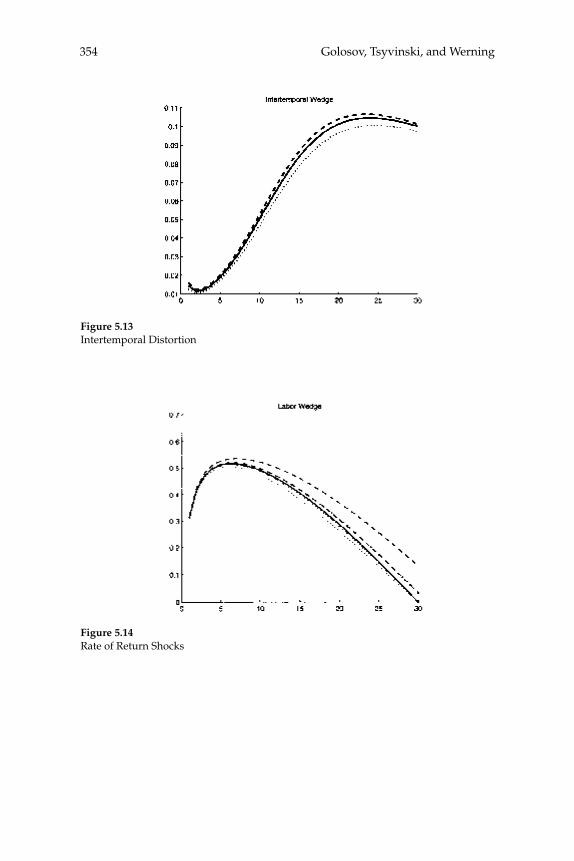
Golosov, Tsyvinski, and Werning354
Figure 5.13Intertemporal Distortion
Figure 5.14Rate of Return Shocks
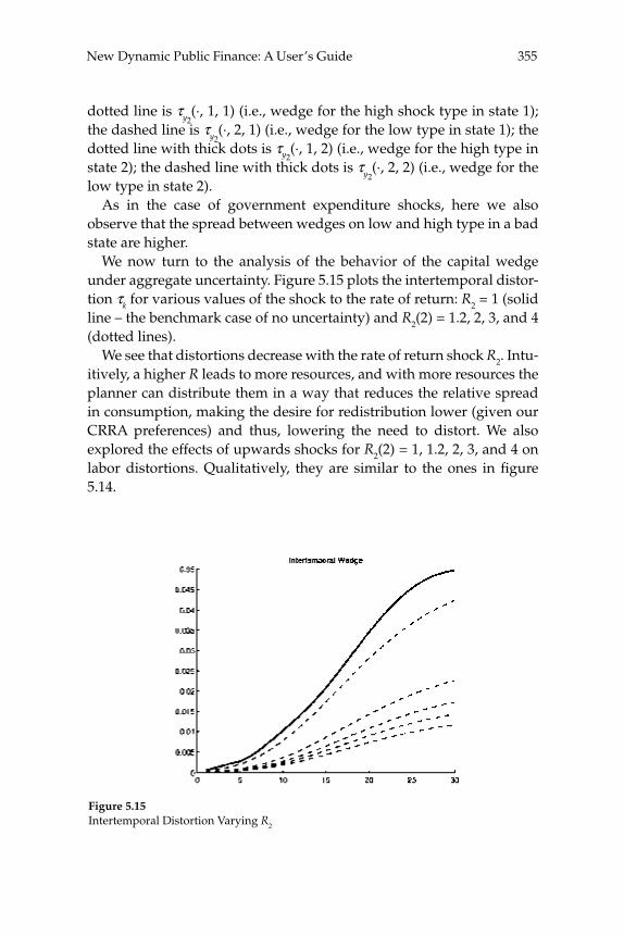
355New Dynamic Public Finance: A User’s Guide
dotted line is τy2(·, 1, 1) (i.e., wedge for the high shock type in state 1);
the dashed line is τy2(·, 2, 1) (i.e., wedge for the low type in state 1); the
dotted line with thick dots is τy2(·, 1, 2) (i.e., wedge for the high type in
state 2); the dashed line with thick dots is τy2(·, 2, 2) (i.e., wedge for the
low type in state 2).As in the case of government expenditure shocks, here we also
observe that the spread between wedges on low and high type in a bad state are higher.
We now turn to the analysis of the behavior of the capital wedge under aggregate uncertainty. Figure 5.15 plots the intertemporal distor-tion τk for various values of the shock to the rate of return: R2 = 1 (solid line – the benchmark case of no uncertainty) and R2(2) = 1.2, 2, 3, and 4 (dotted lines).
We see that distortions decrease with the rate of return shock R2. Intu-itively, a higher R leads to more resources, and with more resources the planner can distribute them in a way that reduces the relative spread in consumption, making the desire for redistribution lower (given our CRRA preferences) and thus, lowering the need to distort. We also explored the effects of upwards shocks for R2(2) = 1, 1.2, 2, 3, and 4 on labor distortions. Qualitatively, they are similar to the ones in fi gure 5.14.
Figure 5.15Intertemporal Distortion Varying R2
Golosov, Tsyvinski, and Werning356
6.6 Summary
We can now summarize the main implications of our analysis. There are two main points to take away from this section: (1) aggregate shocks lead to labor wedges differing across shocks, and (2) a positive aggre-gate shock (either a higher return on savings or lower realization of government expenditures) leads to lower capital wedges and to a lower spread between labor wedges.
7 Concluding Remarks
In this paper we reviewed some main results from the recent New Dynamic Public Finance literature. We also provided some novel explo-rations in the determinants of capital and labor wedges, and how these wedges respond to aggregate shocks.
We also argued that this approach not only provides a workable alternative to Ramsey models, but that it also comes with several sig-nifi cant advantages over its predecessor. First, while Ramsey models have provided several insights into optimal policy, their well-under-stood limitation regarding the ad hoc nature of tax instruments, may make interpreting their prescriptions problematic. In contrast, the main premise of the Mirrleesian approach is to model heterogeneity or uncer-tainty—creating a desire for insurance or redistribution—and an infor-mational friction that prevents the fi rst-best allocation and determines the set of feasible tax instruments endogenously. In particular, although a simple non-discriminatory lump-sum tax component is never ruled out, the optimum features distortions because these improve redistri-bution and insurance. Second, we also argued that this approach has novel implications for the type of dynamic policy issues that macro-economists have been interested in: capital taxation, smoothing of labor income taxes, and the nature of the time-consistency problem. In addi-tion, some new issues may arise directly from the focus on richer tax instruments—such as the progressivity of taxation.
In what follows we outline what we think are largely unresolved questions that we hope are explored in future research.
One remaining challenge is the quantitative exploration of the theory using calibrated models that can capture some empirically relevant fea-tures of skill dynamics—such as those studied in, for example, Stores-letten, Telmer, and Yaron (2004). The main diffi culty is that it is currently not tractable to solve multiple-period models with such a rich structure

357New Dynamic Public Finance: A User’s Guide
for skill shocks. Most current studies impose simplifying assumptions that provide illustrative insights, but remain unsuitable for quantitative purposes. One recent route around this problem is provided by Farhi and Werning (2006a) who study tax reforms in a dynamic Mirrleesian setting to evaluate the gains from distorting savings and provide a simple method which remains tractable even with rich skill processes. There is also some early progress in analyzing dynamic Mirrlees models with persistent shocks using a fi rst-order approach in Kapicka (2005).
A quantitative analysis could also be used to address and evalu-ate the importance of a common challenge against the New Dynamic Public Finance literature: that it delivers tax systems that are “too complicated.” For example, one could compare the level of welfare obtained with the fully optimal scheme to that which is attained when some elements of the tax system are simplifi ed. For example, it may be interesting to compute the welfare losses from a tax code close to the one in the United States and other countries, or other systems with limited history dependence.
A related route is to take insights into the nature of optimal taxation from Mirrleesian models and incorporate them in a simplifi ed fashion in Ramsey-style models, augmented with heterogeneity and idiosyn-cratic uncertainty regarding skills. The work by Conesa and Krueger (2005) and Smyth (2005) may be interpreted as a step in this direction. These papers compute the optimal tax schedule in a model where the tax function is arbitrarily restricted but fl exibly parameterized to allow for wide range of shapes, including progressive taxation. Work along these lines, using state-of-the-art computational models, could explore other tax features, such as certain differential treatments of capital and labor income, or some forms of history dependence.
Another quantitative direction for research is to consider the implica-tions of the new approach for classic macroeconomic questions, such as the conduct of fi scal policy over the business cycle. We only perfuncto-rily touched on this topic, but there is much more to be done to consider many of the issues that macroeconomists studied in the Ramsey tradi-tions. Ideally, one could derive a rich set of quantitative predictions, similar in spirit to the quantitative Ramsey analysis in Chari, Chris-tiano, and Kehoe (1994).
The main reason we stress the potential value of quantitative work is as follows. In our view, the approach to optimal taxation pioneered by Mirrlees (1971) and Atkinson and Stiglitz (1976) was seen as extremely promising in the ‘70s and early ‘80s, but received relatively less applied
Golosov, Tsyvinski, and Werning358
interest later. One common explanation for this is that the approach made quantitative and applied work diffi cult and demanding. We hope that, this time around, the recent surge in interest, combined with the more advanced quantitative techniques and computing power avail-able today, may soon create enough progress to make solving realistic quantitative models feasible. Recent quantitative work is promising in this regard (e.g., Golosov and Tsyvinski 2006a, Farhi and Werning 2006a), but more is needed.
Another direction for future research is to relax the assumption of mechanisms operated by benevolent social planners. A relevant ques-tion in this context is whether the normative insights of the dynamic Mirrlees literature apply to the positive real-world situations where politicians care about reelection, self-enrichment or their own individ-ual biases, and cannot commit to sequences of future policies. A related question is under what conditions markets can be better than optimal mechanisms. The potential misuse of resources and information by the government may make mechanisms less desirable relative to markets. Certain allocations resulting from anonymous market transactions can-not be achieved via centralized mechanisms. Nevertheless, centralized mechanisms may be preferable to anonymous markets because of the additional insurance they provide to risk-averse agents. Acemoglu, Golosov, and Tsyvinski (2006) approach these questions with a model that combines private information regarding individual skill types with the incentive problems associated with self-interested rulers.
Finally, we close by emphasizing that the New Dynamic Public Finance approach can be used to analyze a large variety of new topics, rarely explored within Ramsey settings. For instance, one recent line of research focuses on intergenerational issues. Phelan (2005) and Farhi and Werning (2007) consider how intergenerational incentives should be structured, while Farhi and Werning (2006b) and Farhi, Kocherla-kota, and Werning (2005) derive implications for optimal estate taxa-tion. This is just one example of how this approach promises more than just new answers to old questions, but also leads to new insights for a large set of unexplored questions.
Acknowledgments
For comments and suggestions we thank Daron Acemoglu, V. V. Chari, Peter Diamond, Kenneth Judd, James Mirrlees, and Michael Woodford.

359New Dynamic Public Finance: A User’s Guide
Endnotes
1. However, see Diamond and Mirrlees (1978, 1986, 1995) for early work with dynamic economies with private information.
2. Judd (1999) extends the analysis to cover cases where no steady state may exist.
3. Aiyagari et al. (2002) and Werning (2005) study tax-smoothing of labor income taxes when markets are incomplete. Farhi (2005) studies capital income taxation and owner-ship in this context.
4. See also Diamond, Helms, and Mirrlees (1980) for an early quantitative study of mod-els in which taxes are not linear.
5. A few papers have departed from the representative-agent setting. For example, the analysis of optimal capital taxation in Judd (1985) allowed some forms of heterogeneity.
6. One exception is Werning (2005a) who studies tax smoothing and capital taxation in a model with heterogeneous agents subject to aggregate shocks. Another one is Kocherla-kota (2005) who extends the inverse Euler equation to the case of aggregate uncertainty and includes a numerical illustration of the optimum with two skill types.
7. See also Kingston (1991) and Zhu (1992) for perfect tax smoothing results within a representative agent Ramsey economy with proportional taxation.
8. See also Brito et al. (1991).
9. See Kocherlakota (2006) for another review of the literature.
10. It is straightforward to extend the model by allowing the third period to explicitly distinguish retired individuals from older workers. Indeed, if we assume no labor deci-sion in the third period, nothing is lost by ignoring it and lumping consumption into the second period, as we implicitly do here.
11. The Revelation Principle guarantees that the best allocations can always be achieved by a mechanism where workers make reports about their types to the planner.
12. See Diamond (1998) and Tuomala (1990) for how the choice of the welfare function affects optimal taxes in static framework.
13. That is, we use that E[1/x] > 1/E[x] when Var(x) > 0, where x in our case is the marginal utility u′(c2(i, j)).
14. For example, if an agent considers changing her labor, then, in general, she also con-siders changing her savings. Golosov and Tsyvinski (2006a), Kocherlakota (2005) and Albanesi and Sleet (2006) showed that such double deviations would give an agent a higher utility than the utility from the socially optimal allocations, and therefore the optimal tax system must be enriched with additional elements in order to implement the optimal allocations.
15. A formalization of such a game and an equilibrium concept, sustainable equilibrium, is due to Chari and Kehoe (1990). They formulate a general equilibrium infi nite horizon model in which private agents are competitive, and the government maximizes the wel-fare of the agents. Benhabib and Rustichini (1997), Klein, Krusell, and Rios–Rull (2005), Phelan and Stacchetti (2001), and Fernandez-Villaverde and Tsyvinski (2004) solve for equilibria in an infi nitely lived agent version of the Ramsey model of capital taxation.

Golosov, Tsyvinski, and Werning360
16. See also Sleet and Yeltekin (2005) who prove similar result when agents’ shocks fol-low an i.i.d. process and the government is benevolent.
17. The assumption of uniformity of distribution of skills is not innocuous. Saez (2001), provides a calibrated example of distribution of skills. Diamond (1998) also uses Pareto distribution of skills. Here, we abstract from the effects of varying the skill distribution.
18. Two notable exceptions are Kocherlakota (2005) and Werning (2005a).
19. We thank Ken Judd for pointing this to us.
References
Abraham, Arpad, and Nicola Pavoni. 2003. “Effi cient Allocations with Moral Hazard and Hidden Borrowing and Lending.” Mimeo, University College London.
Acemoglu, Daron, Mikhail Golosov, and Aleh Tsyvinski. 2006. “Markets versus Govern-ments: Political Economy of Mechanisms.” Mimeo, MIT.
Aiyagari, S. Rao, Albert Marcet, Thomas J. Sargent, and Juha Seppälä. 2002. “Optimal Taxation without State-Contingent Debt.” Journal of Political Economy 110(6): 1220–1254.
Albanesi, Stefania. 2006. “Optimal Taxation of Entrepreneurial Capital under Private Information.” Mimeo, Columbia University.
Albanesi, Stefania, and Christoper Sleet. 2006. “Dynamic Optimal Taxation with Private Information.” Review of Economic Studies 73: 1–30.
Arnott, Richard, and Joseph Stiglitz. 1990. “The Welfare Economics of Moral Hazard.” In H. Louberge, ed., Information and Insurance: Essays in Memory of Karl H. Borch, 91–121. Norwell, MA: Kluwer.
Arnott, Richard, and Joseph E. Stiglitz. 1986. “Moral Hazard and Optimal Commodity Taxation.” Journal of Public Economics 29: 1–24.
Atkinson, Anthony B., and Joseph E. Stiglitz. 1976. “The Design of Tax Structure: Direct vs. Indirect Taxation.” Journal of Public Economics 6: 55–75.
Barro, Robert. 1979. “On the Determination of the Public Debt.” Journal of Political Econ-omy 87(5): 940–971.
Battaglini, Marco, and Stephen Coate. 2005. “Pareto Effi cient Taxation with Stochastic Abilities.” Mimeo, Cornell and Princeton.
Benhabib, Jess, and Aldo Rustichini. 1997. “Optimal Taxes without Commitment.” Journal of Economic Theory 77: 231–259.
Bisin, Alberto, and Adriano Rampini. 2006. “Markets as Benefi cial Constraints on the Government.” Journal of Public Economics 90(4-5): 601–629.
Brito, Dagobert L., Jonathan H. Hamilton, Steven M. Slutsky, and Joseph E. Stiglitz. 1991. “Dynamic Optimal Income Taxation with Government Commitment.” Journal of Public Economics 44(1): 15–35.
Chamley, Christophe. 1986. “Optimal Taxation of Capital in General Equilibrium.” Econo-metrica 54: 607–622.

361New Dynamic Public Finance: A User’s Guide
Chari, V. V., and Patrick Kehoe. 1990. “Sustainable Plans.” Journal of Political Economy 94: 783–802.
Chari, V. V., Lawrence J. Christiano, and Patrick Kehoe. 1994. “Optimal Fiscal Policy in a Business Cycle Model.” Journal of Political Economy 102(4): 617–652.
Conesa, Juan Carlos, and Dirk Krueger. 2005. “On the Optimal Progressivity of the Income Tax Code.” Journal of Monetary Economics 53(7): 1425–1450.
da Costa, Carlos. 2005. “Yet Another Reason to Tax Goods.” Mimeo, Getulio Vargas Foun-dation.
da Costa, Carlos, and Iván Werning. 2002. “Commodity Taxation and Social Insurance.” Mimeo, MIT.
da Costa, Carlos, and Iván Werning. 2005. “On the Optimality of the Friedman Rule with Heterogeneous Agents and Nonlinear Income Taxation.” MIT Working Paper. Cam-bridge, MA: MIT.
Diamond, Peter A., L. J. Helms, and James A. Mirrlees. 1980. “Optimal Taxation in a Sto-chastic Economy.” Journal of Public Economics 14: 1–29.
Diamond, Peter A. 1998. “Optimal Income Taxation: An Example with a U-Shaped Pat-tern of Optimal Marginal Tax Rates.” American Economic Review 88(1): 83–95.
Diamond, Peter A., and James A. Mirrlees. 1978. “A Model of Social Insurance with Vari-able Retirement.” Journal of Public Economics 10(3): 295–336.
Diamond, Peter A., and James A. Mirrlees. 1986. “Payroll-Tax Financed Social Insurance with Variable Retirement.” Scandinavian Journal of Economics 88(1): 25–50.
Diamond, Peter A., and James A. Mirrlees. 1995. “Social Insurance with Variable Retire-ment and Private Saving.” Mimeo, MIT.
Farhi, Emmanuel. 2005. “Capital Taxation and Ownership when Markets Are Incom-plete.” Mimeo, MIT.
Farhi, Emmanuel, and Iván Werning. 2006a. “Capital Taxation: Quantitative Implications of the Inverse Euler Equation.” Mimeo, MIT.
Farhi, Emmanuel, and Iván Werning. 2006b. “Progressive Estate Taxation.” Mimeo, MIT.
Farhi, Emmanuel, and Iván Werning. 2007. “Inequality and Social Discounting.” Journal of Political Economy, forthcoming.
Farhi, Emmanuel, Narayana Kocherlakota, and Iván Werning. 2005. “Estate Taxes and Estate Subsidies.” Work in Progress, MIT.
Fernandez-Villaverde, Jesus, and Aleh Tsyvinski. 2004. “Optimal Fiscal Policy in a Busi-ness Cycle Model without Commitment.” Mimeo, Harvard University.
Golosov, Mikhail, and Aleh Tsyvinski. 2006a. “Designing Optimal Disability Insurance: A Case for Asset Testing.” Journal of Political Economy 114(2): 257–279.
Golosov, Mikhail, and Aleh Tsyvinski. 2006b. “Optimal Taxation with Endogenous Insur-ance Markets.” Quarterly Journal of Economics, forthcoming.
Golosov, Mikhail, Narayana Kocherlakota, and Aleh Tsyvinski. 2003. “Optimal Indirect and Capital Taxation.” Review of Economic Studies 70(3): 569–587.
Golosov, Tsyvinski, and Werning362
Greenwald, Bruce C., and Joseph E. Stiglitz. 1986. “Externalities in Economies with Imper-fect Information and Incomplete Markets.” Quarterly Journal of Economics 101: 229–264.
Judd, Kenneth L. 1985. “Redistributive Taxation in a Perfect Foresight Model.” Journal of Public Economics 28: 59–83.
Judd, Kenneth L. 1989. “Optimal Taxation in Dynamic Stochastic Economies: Theory and Evidence.” Mimeo, Stanford University.
Judd, Kenneth L. 1999. “Optimal Taxation and Spending in General Competitive Growth Models.” Journal of Public Economics 71(1): 1–26.
Kapicka, Marek. 2005. “Effi cient Allocations in Dynamic Private Information Economies with Persistent Shocks: A First Order Approach.” Mimeo, University of California-Santa Barbara.
Kingston, Geoffrey. 1991. “Should Marginal Tax Rates be Equalized Through Time?” Quarterly Journal of Economics 106(3): 911–24.
Klein, Paul, Per Krusell, and Jose-Victor Rios-Rull. 2005. “Time-Consistent Public Expen-ditures.” Mimeo, University of Pennsylvania.
Kocherlakota, Narayana R. 2005. “Zero Expected Wealth Taxes: A Mirrlees Approach to Dynamic Optimal Taxation.” Econometrica 73(5): 1587–1621.
Kocherlakota, Narayana. 2006. “Advances in Dynamic Optimal Taxation.” In Advances in Economics and Econometrics, Theory and Applications Ninth World Congress, Volume I, 269–299. (New York, NY: Cambridge Univ. Press).
Lucas, Robert E., Jr., and Nancy L. Stokey. 1983. “Optimal Fiscal and Monetary Policy in an Economy without Capital.” Journal of Monetary Economics 12: 55–93.
Mirrlees, James A. 1971. “An Exploration in the Theory of Optimum Income Taxation.” Review of Economic Studies 38(2): 175–208.
Phelan, Christopher. 2005. “Opportunity and Social Mobility.” Federal Reserve Bank of Minneapolis, Research Department Staff Report 323.
Phelan, Christopher, and Ennio Stacchetti. 2001. “Sequential Equilibria in a Ramsey Tax Model.” Econometrica 69(6): 1491–1518.
Prescott, Edward C., and Robert Townsend. 1984. “Pareto Optima and Competitive Equi-libria with Adverse Selection and Moral Hazard.” Econometrica 52: 21–45.
Roberts, Kevin. 1984. “Theoretical Limits to Redistribution.” Review of Economic Studies 51: 177–195.
Rogerson, William P. 1985. “Repeated Moral Hazard.” Econometrica 53(1): 69–76.
Saez, Emmanuel. 2001. “Using Elasticities to Derive Optimal Income Tax Rates.” Review of Economic Studies 68(1): 205–229
Shimer, Robert, and Iván Werning. 2005. “Liquidity and Insurance for the Unemployed.” Mimeo, MIT.
Sleet, Christopher, and Sevin Yeltekin. 2005. “Credible Social Insurance.” Mimeo, Carnegie-Mellon University.
Smyth, S. 2005. “A Balancing Act: Optimal Nonlinear Taxation of Labor and Capital in Overlapping Generation Economies.” Mimeo, Harvard University.
363New Dynamic Public Finance: A User’s Guide
Stiglitz, Joseph. 1987. “Pareto Effi cient and Optimal Taxation and the New New Wel-fare Economics.” In A. Auerbach and M. Feldstein, eds, Handbook on Public Economics 991–1042. North Holland: Elsevier Science Publishers.
Storesletten, Kjetil, Chris I. Telmer, and Amir Yaron. 2004. “Cyclical Dynamics in Idiosyn-cratic Labor Market Risk.” Journal of Political Economy 112(3): 695–717.
Tuomala, Matti. 1990. Optimal Income Taxation and Redistribution. Oxford University Press, Clarendon Press.
Werning, Iván. 2002. “Optimal Dynamic Taxation.” PhD Dissertation, University of Chicago.
Werning, Iván. 2005. “Tax Smoothing with Incomplete Markets.” Mimeo, MIT.
Werning, Iván. 2007. “Optimal Fiscal Policy with Redistribution.” Quarterly Journal of Eco-nomics, forthcoming.
Zhu, Xiaodong. 1992. “Optimal Fiscal Policy in a Stochastic Growth Model.” Journal of Economic Theory 58: 250–89.
Appendix: Numerical Approach
In this appendix we describe the details of the numerical computations that we performed in this paper. The major conceptual diffi culty with computing this class of models is that there are a large number of incentive constraints, and there is no result analogous to static models that guarantee that only local incentive compatibility constraints can bind to reduce them. Our computational strategy in this regard is as follows:
1. We start with solving several examples in which we impose all of the IC con-straints. This step gives us a conjecture on what kind of constraints may bind.2. We then impose constraints that include deviations that bind in step 1. In fact, we include a larger set that also includes constraints in the neighborhood (of reporting strategies) to the ones that bind.
3. Finally, once the optimum is computed we check that no other constraints bind.
This approach is very much like the active set approach in constrained opti-mization: one begins with a set of constraints that are likely to be the binding ones, one then solves the smaller problems, checking all constraints, and add-ing the constraints that are violated in the set of constraints that are considered for the next round (and possibly dropping some of those that were not binding) and repeat the procedure.19


Comment
Peter Diamond, Massachusetts Institute of Technology and NBER
1 Introduction
This interesting and stimulating paper (referred to as GTW) discusses four issues: when capital should not be taxed, when labor taxes should be constant over time and states of nature, the sources of concern about limited government commitment, and the methodology of modeling for tax analysis. And it contains calculated examples. I will touch on three of these issues, leaving out the complex issue of how policy feasi-bility and desirability are infl uenced by the nature of the political pro-cess in democratic states. In the macro tradition, the analysis focuses on settings with stochastic shocks. To bring a public economics perspec-tive, I will consider the fi rst two issues in deterministic models with heterogeneous populations. Then I will consider a stochastic model to add to the intuition about taxing savings. For clarity of presentation, I work with models with only two types of workers and assume that the binding incentive compatibility constraint is that type-A not imitate type-B. I do not consider suffi cient conditions for this pattern of con-straints to be correct.
2 Taxing Savings
Atkinson-Stiglitz (1976) showed that in the presence of optimal non-linear earnings taxes, it was not optimal to also use distorting linear consumption taxes, provided that all consumer preferences are sepa-rable between goods and labor and all consumers have the same sub-utility function of consumption. Laroque (2005) and Kaplow (2006) have extended this result, showing that with the same preference assumptions, in the presence of any income tax function that gives rise to an equilibrium, if there are distorting consumer taxes, then a move
Diamond366
to nondistorting consumer taxes can be done along with a permutation of the income tax that leaves every consumer with the same utility and the same labor supply, while the government collects more revenue. If labor supply is smooth with uniform transfers to all consumers (no jumps in labor supply), then this revenue gain can be used to make a Pareto improvement.
GTW explore this issue by solving a social welfare optimization with quantities as control variables and incentive compatibility constraints as well as a resource constraint or constraints (if there is uncertainty about aggregate resources). Then, they compare the MRS between fi rst- and second-period consumptions at the optimal allocation to the MRT. The comparison allows calculation of the “wedge” between them, refl ecting implicit marginal taxation of savings. They consider two other wedges—between consumption and earnings in each of the two periods, refl ecting the implicit marginal taxation of earnings. They compare these two labor wedges to fi nd conditions where earnings are marginally taxed the same in both periods. These labor wedges are also examined with aggregate uncertainty about the resource constraint in order to compare wedges across states of nature. The comparison of labor wedges across periods is really a fourth wedge—between earn-ings in the two periods. That is, in this four-good model there are two separate own rates of interest—in earnings and in spending.
The Atkinson-Stiglitz condition for non-use of distorting consump-tion taxes has naturally received a great deal of attention, particularly with the interpretation of present and future consumption goods and so the taxation of savings. That is, under these assumptions, using the vocabulary of GTW, there is no wedge between MRS and MRT for consumptions in different periods. With no wedge for intertemporal consumption, unless the implicit marginal taxation of earnings is con-stant over time, there is a nonzero wedge between earnings in different periods. Below I will offer a simple example of an optimal model with no wedge in intertemporal consumption but a wedge in intertemporal earnings, that is, non-constant marginal taxation of earnings.
Despite the great interest in the Atkinson-Stiglitz result, there remain arguments in favor of taxing savings with nonlinear earnings taxes. One obvious argument would be that preferences do not exhibit the sepa-rability between consumption and labor used in the theorem. Then the Corlett-Hague (1953) style analysis in a 3-good model (current work, current consumption, and future consumption) can examine whether a move towards taxing savings or towards subsidizing savings raises
367Comment
welfare. But we do not know much about the relevant cross-elasticities, although the commonly-used assumptions of atemporal and intertem-poral separability strike me as implausible.
Another argument for taxing savings, one that is based closely on empirical observations, is due to Saez (2002). He argues that there is a positive correlation between labor skill level (wage rate) and the savings rate. In a two-period certainty setting with additive preferences, this is consistent with those with higher earnings abilities having less discount of future consumption. In terms of the conditions of the Atkinson-Sti-glitz theorem, Saez preserves separability but drops the assumption that the subutility function of consumption is the same for everyone. I begin my formal analysis (echoing Diamond, 2003) by showing this result in a two-types model with labor only in the fi rst period, illustrat-ing the Atkinson-Stiglitz result at the same time.
Consider the following social welfare function optimization. Assume full nonlinear taxation, and two types of households, with the only binding incentive compatibility constraint being type A considering imitating type B. I do not analyze suffi cient conditions for this to be the only binding constraint.
Maximizec,y π β θi ii
u c i u c i v y i i( [ ( )] [ ( )] [ ( )/ ( )])1 2 1 1+ −∑
subject to:
G c i R c i y iii
+ + − ≤∑ −π ( ( ) ( ) ( ))11
2 1 0 (1)
u[c1(A)] + βAu[c2(A)] − v[y1(A)/θ1(A)] ≥
u[c1(B)] + βAu[c2(B)] − v[y1(B)/θ1(A)]
with notation
cj(i) consumption in period j of household iyj(i) earnings in period j of household iθj(i) skill in period j of household iπi number of workers of type iβi discount factor of household iR 1 plus the return to capitalG government expendituresλ, ψ LaGrange multipliers

Diamond368
This problem has the FOCs for consumption levels:
(πA + ψ) u′[c1(A)] = λπA (2)
(πA + ψ) βAu′[c2(A)] = λπAR−1 (3)
(πB − ψ) u′[c1(B)] = λπB (4)
(πBβB − ψβA) u′[c2(B)] = λπBR−1 (5)
Taking the ratio of FOCs for A, there is no tax on savings on the high type:
′′
=u c Au c A
RA[ ( )][ ( )]
.1
2β (6)
This is the familiar no-marginal-taxation condition at the very top of the earnings distribution.
Now let us turn to type B. Taking the ratio of FOCs we have
( ) [ ( )]
[ ( )].
π ψ
π ψ ββ
βB
BA
B
Bu c B
u c BR
− ′
−⎛⎝⎜
⎞⎠⎟
′=1
2
(7)
The plausible case is that high earners have a lower discount of future consumption, βA < βB , resulting (with πB − ψ > 0) in
′′
u c Bu c B
RB[ ( )][ ( )]
.1
2< β (8)
That is, type-B would save if that were possible at zero taxation of savings, so there is implicit marginal taxation of savings. If and only if βA = βB does this imply no taxation of savings for type B. Saez does his analysis with linear taxation of savings and concludes that since higher earners have higher savings rates, taxing savings is part of the optimum.
The GTW exploration of the taxation of savings focuses on uncer-tainty about future earnings as a source of the desirability of taxation of savings. It is true that people are uncertain about future earnings. It is also true that people differ in discount rates. The case for not taxing savings does not survive either issue with plausible character-izations.
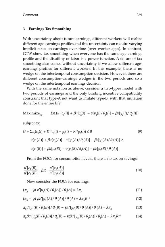
369Comment
3 Earnings Tax Smoothing
With uncertainty about future earnings, different workers will realize different age-earnings profi les and this uncertainty can require varying implicit taxes on earnings over time (over worker ages). In contrast, GTW show tax smoothing when everyone has the same age-earnings profi le and the disutility of labor is a power function. A failure of tax smoothing also comes without uncertainty if we allow different age-earnings profi les for different workers. In this example, there is no wedge on the intertemporal consumption decision. However, there are different consumption-earnings wedges in the two periods and so a wedge on the intertemporal earnings decision.
With the same notation as above, consider a two-types model with two periods of earnings and the only binding incentive compatibility constraint that type-A not want to imitate type-B, with that imitation done for the entire life.
Maximizec,y Σπi (u [c1(i)] + βu[c2(i)] − v[y1(i)/θ1(i)] − βv[y2(i)/θ2(i)])
subject to:
G + Σπi(c1(i) + R−1c2(i) − y1(i) − R−1y2(i)) ≤ 0 (9)
u[c1(A)] + βu[c2(A)] − v[y1(A)/θ1(A)] − βv[y2(A)/θ2(A)] ≥
u[c1(B)] + βu[c2(B)] − v[y1(B)/θ1(A)] − βv[y2(B)/θ2(A)]
From the FOCs for consumption levels, there is no tax on savings:
′′
= = ′′
u c Bu c B
Ru c Au c A
[ ( )][ ( )]
[ ( )][ ( )]
1
2
1
2β (10)
Now consider the FOCs for earnings:
(πA + ψ) v′[y1(A)/θ1(A)]/θ1(A) = λπA (11)
(πA + ψ) βv′[y2 (A)/θ2(A)]/θ2(A) = λπAR−1 (12)
πBv′[y1(B)/θ1(B)]/θ1(B) − ψv′[y1(B)/θ1(A)]/θ1(A) = λπB (13)
πBβv′[y2(B)/θ2(B)]/θ2(B) − ψβv′[y2(B)/θ2(A)]/θ2(A) = λπBR−1 (14)

Diamond370
Taking a ratio of FOCs, there is no intertemporal earnings wedge for the high type, consistent with no-marginal-taxation of the highest type on all margins:
′′
=v y A A Av y A A A
[ ( )/ ( )]/ ( )[ ( )/ ( )/ ( )
1 1 1
2 2 2
θ θθ θ
βRR (15)
Turning to type B, let us defi ne Δ as the wedge:
′′
+v y B B Bv y B B B
[ ( )/ ( )]/ ( )[ ( )/ ( )]/ ( )
1 1 1
2 2 2
θ θθ θ
ΔΔ = βR (16)
If Δ is negative, then the fi rst period marginal disutility of earning is larger than the discounted second period marginal disutility.
From the ratio of FOCs the sign of Δ depends on the difference in intertemporal MRS for type B and for type A if imitating type B:
Δ =′ − ′π θ θ ψ θBv y B B B v y B A[ ( )/ ( )]/ ( ) [ ( )/ ( )]/1 1 1 1 1 θθ
π θ θ ψ θ1
2 2 2 2 2
( )[ ( )/ ( )]/ ( ) [ ( )/ (
Av y B B B v y BB ′ − ′ AA A)]/ ( )θ2
(17)
[ ( )/ ( )]/ ( )[ ( )/ ( )]
−′′
v y B B Bv y B B
1 1 1
2 2
θ θθ // ( )θ2 B
with
π ψ θθ
θθB
v y B Av y B B
BA
−′′[ ( )/ ( )][ ( )/ ( )]
( )(
2 2
2 2
2
2 )) > 0
and
ψ > 0,
the sign of Δ is the same as that of
′′
−′v y B A
v y B BBA
v[ ( )/ ( )][ ( )/ ( )]
( )( )
2 2
2 2
2
2
θθ
θθ
[[ ( )/ ( )][ ( )/ ( )]
( )( )
.y B A
v y B BBA
1 1
1 1
1
1
θθ
θθ′
(18)
If v′[z] = zα, then the sign of Δ is the same as that of
( ( )/ ( ))( ( )/ ( ))
( )( )
( (y B A
y B BBA
y2 2
2 2
2
2
1θθ
θθ
α
α −BB A
y B BBA
)/ ( ))( ( )/ ( ))
( )( )
θθ
θθ
α
α1
1 1
1
1 (19)
or, simplifying, that of
θθ
θθ
α α2
2
11
1
1( )( )
( )( )
.BA
BA
⎛⎝⎜
⎞⎠⎟
− ⎛⎝⎜
⎞⎠⎟
+ + (20)
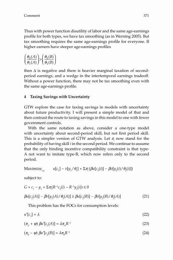
371Comment
Thus with power function disutility of labor and the same age-earnings profi le for both types, we have tax smoothing (as in Werning 2005). But tax smoothing requires the same age-earnings profi le for everyone. If higher earners have steeper age-earnings profi les
θθ
θθ
2
1
2
1
( )( )
( )( )
AA
BB
⎛⎝⎜
⎞⎠⎟
>⎛⎝⎜
⎞⎠⎟
then Δ is negative and there is heavier marginal taxation of second-period earnings, and a wedge in the intertemporal earnings tradeoff. Without a power function, there may not be tax smoothing even with the same age-earnings profi le.
4 Taxing Savings with Uncertainty
GTW explore the case for taxing savings in models with uncertainty about future productivity. I will present a simple model of that and then contrast the route to taxing savings in this model to one with fewer government controls.
With the same notation as above, consider a one-type model with uncertainty about second-period skill, but not fi rst period skill. This is a simpler version of GTW analysis. Let πi now stand for the probability of having skill i in the second period. We continue to assume that the only binding incentive compatibility constraint is that type-A not want to imitate type-B, which now refers only to the second period.
Maximizec,y u[c1] − v[y1/θ1] + Σπi (βu[c2(i)] − βv[y2(i)/θ2(i)])
subject to:
G + c1 − y1 + Σπi(R−1c2(i) − R−1y2(i)) ≤ 0
βu[c2(A)] − βv[y2(A)/θ2(A)] ≥ βu[c2(B)] − βv[y2(B)/θ2(A)] (21)
This problem has the FOCs for consumption levels:
u′[c1] = λ (22)
(πA + ψ) βu′[c2(A)] = λπAR−1 (23)
(πB − ψ) βu′[c2(B)] = λπBR−1 (24)
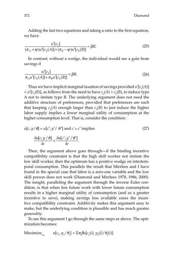
Diamond372
Adding the last two equations and taking a ratio to the fi rst equation, we have
′+ ′ + − ′
=u cu c A u c B
RA B
[ ]( ) [ ( )] ( ) [ ( )]
.1
2 2π ψ π ψβ (25)
In contrast, without a wedge, the individual would see a gain from savings if
′′ + ′
u cu c A u c B
RA B
[ ][ ( )] [ ( )]
.1
2 2π πβ< (26)
Thus we have implicit marginal taxation of savings provided u′[c2(A)] < u′[c2(B)], as follows from the need to have c2(A) > c2(B), to induce type A not to imitate type B. The underlying argument does not need the additive structure of preferences, provided that preferences are such that keeping c2(A) enough larger than c2(B) to just induce the higher labor supply implies a lower marginal utility of consumption at the higher consumption level. That is, consider the condition:
u[c, y/θ] = u[c′, y′/ θ ′] and c > c′ implies (27)
∂
∂∂ ′ ′ ′
∂u c y
cu c y
c[ , / ] [ , / ]
.θ θ
<
Then, the argument above goes through—if the binding incentive compatibility constraint is that the high skill worker not imitate the low skill worker, then the optimum has a positive wedge on intertem-poral consumption. This parallels the result that Mirrlees and I have found in the special case that labor is a zero-one variable and the low skill person does not work (Diamond and Mirrlees 1978, 1986, 2000). The insight, paralleling the argument through the inverse Euler con-dition, is that when less future work with lower future consumption results in a higher marginal utility of consumption (and so a greater incentive to save), making savings less available eases the incen-tive compatibility constraint. Additivity makes this argument easy to make, but the underlying condition is plausible and has much greater generality.
To see this argument I go through the same steps as above. The opti-mization becomes:
Maximizec,y u[c1, y1/θ1] + Σπiβu[c2(i), y2(i)/θ2(i)]

373Comment
subject to:
G + c1 − y1 + Σπi(R−1c2(i) − R−1y2(i)) ≤ 0 (28)
βu[c2(A), y2(A)/θ2(A)] ≥ βu[c2(B), y2(B)/θ2(A)]
This problem has the FOCs for consumption levels:
uc[c1, y1/θ1] = λ (29)
(πA + ψ) βuc[c2(A), y2(A)/θ2(A)] = λπAR−1 (30)
πBβuc[c2(B), y2(B)/θ2(B)] − ψβuc[c2(B, y2(B)/θ2(A))] = λπBR−1 (31)
Adding the last two equations and taking a ratio to the fi rst equation, we have
u c yu c A y A A u
c
A c B
[ , / ]( ) [ ( ), ( )/ ( )]
1 1 1
2 2 2
θπ ψ θ π+ + cc cc B y B B u c B y B A[ ( ), ( )/ ( )] [ ( ), ( )/ ( )2 2 2 2 2 2θ ψ θ− ]] = βR
(32)
In contrast, without a wedge, the individual would see a gain from savings if
u c yu c A y A A u c
c
A c B c
[ , / ][ ( ), ( )/ ( )] [
1 1 1
2 2 2 2
θπ θ π+ (( ), ( )/ ( )]
.B y B B
R2 2θ
β< (33)
Thus the sign of the wedge depends on the sign of
ψ(uc [c2(A), y2(A)/θ2(A)] − uc[c2(B), y2(B)/θ2(A)]), (34)
which is signed by the condition above. Thus in a setting where every-one is the same in the fi rst period, a plausible condition is suffi cient for a positive intertemporal consumption wedge. The insight, paralleling the argument through the inverse Euler condition, is that with this condition, less future work and lower future consumption will result in a higher marginal utility of consumption and a greater incentive to save (unless the condition is not satisfi ed and the impact of hours worked on the mar-ginal utility of consumption overcomes the higher level of consumption). Easing the incentive compatibility constraint then comes from making the return to saving smaller. Additivity makes this argument easy to make, but the underlying argument has much greater generality.
GTW explore a class of nonseparable period utility functions in their numerical results. They work with the utility function u[c, y/θ] = (ce–(y/θ)2)1–σ/(1 – σ). And they have many fi rst-period productivity
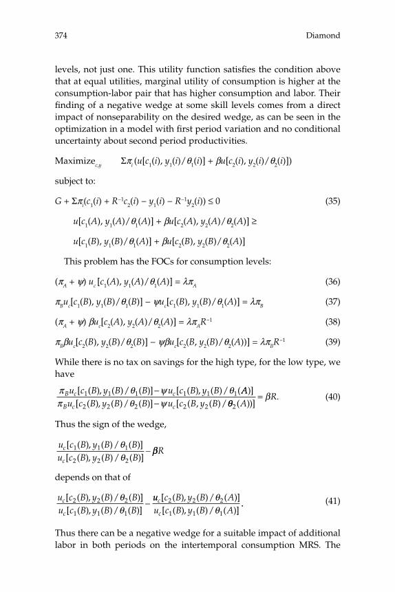
Diamond374
levels, not just one. This utility function satisfi es the condition above that at equal utilities, marginal utility of consumption is higher at the consumption-labor pair that has higher consumption and labor. Their fi nding of a negative wedge at some skill levels comes from a direct impact of nonseparability on the desired wedge, as can be seen in the optimization in a model with fi rst period variation and no conditional uncertainty about second period productivities.
Maximizec,y Σπi (u[c1(i), y1(i)/θ1(i)] + βu[c2(i), y2(i)/θ2(i)])
subject to:
G + Σπi(c1(i) + R−1c2(i) − y1(i) − R−1y2(i)) ≤ 0 (35)
u[c1(A), y1(A)/θ1(A)] + βu[c2(A), y2(A)/θ2(A)] ≥
u[c1(B), y1(B)/θ1(A)] + βu[c2(B), y2(B)/θ2(A)]
This problem has the FOCs for consumption levels:
(πA + ψ) uc [c1(A), y1(A)/θ1(A)] = λπA (36)
πBuc[c1(B), y1(B)/θ1(B)] − ψuc[c1(B), y1(B)/θ1(A)] = λπB (37)
(πA + ψ) βuc[c2(A), y2(A)/θ2(A)] = λπAR−1 (38)
πBβuc[c2(B), y2(B)/θ2(B)] − ψβuc[c2(B, y2(B)/θ2(A))] = λπBR−1 (39)
While there is no tax on savings for the high type, for the low type, we have
π θ ψ θB c cu c B y B B u c B y B[ ( ), ( )/ ( )] [ ( ), ( )/ (1 1 1 1 1 1− AAu c B y B B u c B y BB c c
)][ ( ), ( )/ ( )] [ ( , ( )/π θ ψ2 2 2 2 2− θθ
β2( ))]
.A
R= (40)
Thus the sign of the wedge,
u c B y B Bu c B y B B
c
c
[ ( ), ( )/ ( )][ ( ), ( )/ ( )]
1 1 1
2 2 2
θθ
− ββR
depends on that of
u c B y B Bu c B y B B
c
c
[ ( ), ( )/ ( )][ ( ), ( )/ ( )]
2 2 2
1 1 1
θθ
−uu c B y B Au c B y B A
c
c
[ ( ), ( )/ ( )][ ( ), ( )/ ( )]
2 2 2
1 1 1
θθ
.. (41)
Thus there can be a negative wedge for a suitable impact of additional labor in both periods on the intertemporal consumption MRS. The
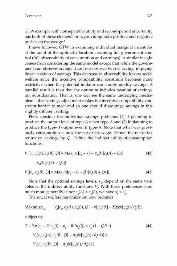
375Comment
GTW example with nonseparable utility and second-period uncertainty has both of these elements in it, providing both positive and negative pushes on the wedge.1
I have followed GTW in examining individual marginal incentives at the point of the optimal allocation assuming full government con-trol (full observability of consumption and earnings). A similar insight comes from considering the same model except that while the govern-ment can observe savings it can not observe who is saving, implying linear taxation of savings. This decrease in observability lowers social welfare since the incentive compatibility constraint becomes more restrictive when the potential imitator can simply modify savings. A parallel result is then that the optimum includes taxation of savings, not subsidization. That is, one can see the same underlying mecha-nism—that savings adjustment makes the incentive compatibility con-straint harder to meet and so one should discourage savings in this slightly different setting.
First, consider the individual savings problems (1) if planning to produce the output level of type-A when type-A and (2) if planning to produce the type-B output even if type-A. Note that what was previ-ously consumption is now the net-of-tax wage. Denote the net-of-tax return on savings by Q. Defi ne the indirect utility-of-consumption functions:
VA[c1, c2(A), c2(B), Q] ≡ Maxs{u [c1 − s] + πAβu[c2(A) + Qs] (42)
+ πBβu[c2(B) + Qs]}
VB[c1, c2(B), Q] ≡ Maxs{u[c1 − s] + βu[c2(B) + Qs]}. (43)
Note that the optimal savings levels, s*i, depend on the same vari-
ables as the indirect utility functions Vi. With these preferences (and much more generally) since c2(A) > c2(B), we have sB
* > sA*.
The social welfare maximization now becomes
Maximizec,y VA[c1, c2(A), c2(B), Q] − v[y1/θ1] − Σπiβv[y2(i)/θ2(i)]
subject to:
G + Σπi(c1 + R−1c2(i) − y1 − R−1y2(i)) ≤ sA* (1 − QR−1) (44)
VA[c1, c2(A), c2(B), Q] − πAβv[y2(A)/θ2(A)] ≥
VB[c1, c2(B), Q] − πAβv[y2(B)/θ2(A)]
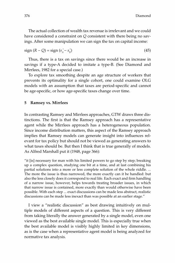
Diamond376
The actual collection of wealth tax revenue is irrelevant and we could have considered a constraint on Q consistent with there being no sav-ings. After some manipulation we can sign the tax on capital income:
sign (R − Q) = sign (sA* − sB
*) (45)
Thus, there is a tax on savings since there would be an increase in savings if a type-A decided to imitate a type-B. (See Diamond and Mirrlees, 1982 for a special case.)
To explore tax smoothing despite an age structure of workers that prevents its optimality for a single cohort, one could examine OLG models with an assumption that taxes are period-specifi c and cannot be age-specifi c, or how age-specifi c taxes change over time.
5 Ramsey vs. Mirrlees
In contrasting Ramsey and Mirrlees approaches, GTW draws three dis-tinctions. The fi rst is that the Ramsey approach has a representative agent while the Mirrlees approach has a heterogeneous population. Since income distribution matters, this aspect of the Ramsey approach implies that Ramsey models can generate insight into infl uences rel-evant for tax policy but should not be viewed as generating answers to what taxes should be. But then I think that is true generally of models. As Alfred Marshall put it (1948, page 366):
“it [is] necessary for man with his limited powers to go step by step; breaking up a complex question, studying one bit at a time, and at last combining his partial solutions into a more or less complete solution of the whole riddle. ... The more the issue is thus narrowed, the more exactly can it be handled: but also the less closely does it correspond to real life. Each exact and fi rm handling of a narrow issue, however, helps towards treating broader issues, in which that narrow issue is contained, more exactly than would otherwise have been possible. With each step ... exact discussions can be made less abstract, realistic discussions can be made less inexact than was possible at an earlier stage.”
I view a “realistic discussion” as best drawing intuitively on mul-tiple models of different aspects of a question. This is very different from taking literally the answer generated by a single model, even one viewed as the best available single model. This is especially true when the best available model is visibly highly limited in key dimensions, as is the case when a representative agent model is being analyzed for normative tax analysis.

377Comment
A second distinction they draw is between linear taxes and nonlinear taxes. Since some taxes are linear in practice, it seems worthwhile to analyze how to set linear taxes as well. Since it is often the case that linear taxes operate in the presence of nonlinear ones, it is important to learn about that interaction. But not all linear taxes are in a setting where there are nonlinear taxes, making a separate analysis also worth-while. In Massachusetts it is not constitutional to have progressive tax-ation of a single kind of income, apart from an exempt amount. Some would love to see the same restriction in the U.S. constitution. More generally, political economy considerations may call for restrictions in the taxes considered. I wonder if the very minor distinctions in income taxation by age of the worker in current U.S. law are not a refl ection of the diffi culty in setting so many tax parameters as would be needed with different income taxes for each age of a worker (or pairs of ages for a working couple). Or maybe this is just the lag of practice behind theory—as we saw in the roughly two decade lag in the United States in collecting tolls only one way on some bridges and tunnels.
The third distinction drawn by GTW is between a given, restricted set of tax tools, referred to as an ad hoc restriction, and deriving the set of tax tools from an underlying technology, asymmetric informa-tion in the Mirrlees case. I think this distinction is overdrawn. First, if we assume that for some transactions asymmetric information extends to the parties engaged in transactions, then taxation of a transaction might vary with the size of the transaction but cannot vary with the presence of other transactions. Then, nonlinear taxation based on total earnings is not feasible. Assuming that without this constraint there would be higher taxation of larger transactions, and that such taxation can be prevented by repeated transactions, then we are left with linear taxation, derived, not assumed. Second, there is the issue of admin-istrative costs, which are assumed to be zero for observables in the Mirrlees model. We can recast asymmetric information as assuming that the administrative cost is infi nite for what are otherwise labeled non-observables. This can be a helpful recasting. We could track the identity for each purchase of gasoline the way we do each payment of earnings. But that would be expensive (but becoming less so, par-ticularly if we do not allow purchases for cash). If expensive enough, gasoline purchase should be subject to linear taxes, as they are. Hav-ing a more basic model (deriving what tax structure might otherwise be assumed) is not necessarily a virtue if the basic model has critical incompleteness.

Diamond378
In GTW there are two periods with a stochastic change in worker skill between the two periods. This allows taxes to be set differently in each period. But if skills evolve more rapidly than taxes are set (because of administrative costs, perhaps) then the modeling needs to recognize an explosion of types depending on all the stochastic realizations of opportunities that might occur within a year. Plausibly we are in the same basic position as with the assumption of a complete set of markets—no one can list all the states that might occur. So we can not envision trading on all of them, even apart from the cost in today’s resources of preparing in this way for distant and/or low probability events, which would not be worthwhile. Just as incomplete markets are a reality, so too incomplete use of incentives is a reality. I see no reason to believe that assuming such a reality is necessarily worse than deriving it when trying to model something as complex as tax policy.
6 Concluding Remarks
It is good to have macroeconomists looking at the same issues as public fi nance economists. In the spirit of encouraging further comple-mentary analysis, let me say that there is a great deal of current inter-est in annuities and taxation. This might appeal to macroeconomists as well. After all, as Benjamin Franklin wrote (in a letter to M. Leroy, 1789):
“Our Constitution is in actual operation; everything appears to promise that it will last; but in this world nothing is certain but death and taxes.”
Acknowledgments
I am indebted to Iván Werning for very clarifying comments, and to the National Science Foundation for fi nancial support under grant SES 0239 080.
Endnote
1. Nonseparability over time in the utility of consumption is also plausible. Mirrlees and I (1986) explored an extreme (Leontieff) case of intertemporal nonseparability and (2000) a standard-of-living model.
379Comment
References
Atkinson, A. B., and J. E. Stiglitz. 1976. “The Design of Tax Structure: Direct versus Indi-rect Taxation.” Journal of Public Economics 6: 55–75.
Corlett, W. J., and D. C. Hague. 1953. “Complementarity and the Excess Burden of Taxa-tion.” Review of Economic Studies 21(1): 21–30.
Diamond, P. 2003. “Taxation, Incomplete Markets, and Social Security.” Cambridge, MA: MIT Press.
Diamond, P., and J. Mirrlees. 1978. “A Model of Social Insurance with Variable Retire-ment.” Journal of Public Economics 10: 295–336.
Diamond, P., and J. Mirrlees. 1986. “Payroll-Tax Financed Social Insurance with Variable Retirement.” Scandinavian Journal of Economics 88(1): 25–50.
Diamond, P., and J. Mirrlees. 2000. “Adjusting One’s Standard of Living: Two Period Models.” In P. J. Hammond and G. D. Myles, eds., Incentives, Organization, and Public Eco-nomics, Papers in Honour of Sir James Mirrlees. Oxford: Oxford University Press.
Diamond, P., and J. Mirrlees. 1982. “Social Insurance with Variable Retirement and Pri-vate Saving.” MIT Working Paper no. 296. 1995, unpublished. Forthcoming in Journal of Public Economics.
Kaplow, L. 2006. “On the Undesirability of Commodity Taxation Even When IncomeTax-ation Is Not Optimal.” Journal of Public Economics 90: 1235.
Laroque, G. 2005. “Indirect Taxation is Superfl uous under Separability and Taste Homo-geneity: A Simple Proof.” Economics Letters 87: 141–144.
Marshall, A. 1948. Principles of Economics, eighth edition. New York: The Macmillan Com-pany.
Saez, E. 2002. “The Desirability of Commodity Taxation under Non-Linear Income Taxa-tion and Heterogeneous Tastes.” Journal of Public Economics 83: 217–230.
Werning, I. 2005. “Tax Smoothing with Redistribution.” Federal Reserve Bank of Min-neapolis, Staff Report 365.


Comment
Kenneth L. Judd, Hoover Institution and NBER
Professors Golosov, Tsyvinski, and Werning have given us an excel-lent overview of recent work applying the Mirrlees (1971) approach for income taxation to questions in the theory of taxation of dynamic and stochastic environments. I am delighted to see this renewed interest in optimal taxation problems. The work discussed in this paper shows us that there is great value in this effort and also how much is left to be done.
My comments will focus on three issues. First, I will comment on the relationship between this work and the earlier literature. Second, I want to discuss a possibly heretical interpretation of Mirrlees work. Third, I will discuss the problems facing future work.
This literature has worked to emphasize the difference between the dynamic Mirrlees literature and the Ramsey literature. In particular, these papers often interpret any difference between a marginal rate of substitution and the corresponding marginal rate of transformation as a tax. However, the dynamic Mirrlees approach is not strictly compa-rable to the Ramsey approach. In the Ramsey approach, as executed in, for example, Atkinson and Stiglitz (1976), Diamond and Mirrlees (1971), and Judd (1985, 1999) assume that a full set of private markets exist and that prices are determined competitively. Even Mirrlees (1971) assumes that workers are paid their marginal product, implicitly assuming that there is no market power in labor markets. In these analyses, taxes are then chosen to distort market outcome so as to accomplish a realloca-tion of resources desired by the government. In the dynamic Mirrlees approach outlined in this paper, there are no private markets for insur-ance and government policy is used for both conventional purposes of raising revenue for government expenditures and redistribution, as well as to replace, or at least offer a substitute for, the missing private markets.

Judd382
This point is acknowledged in this paper. The authors are often care-ful to refer to distortions as wedges, staying away from the question of what they signify. Section 4.5 correctly argues that in many cases pri-vate markets will attain a constrained Pareto allocation, and that these private outcomes will have many of the same wedges often called taxes in the dynamic Mirrlees literature. If the government does not enjoy an advantage in either transaction costs or information, then no govern-ment policy can attain a Pareto superior allocation.
This does not mean that the dynamic Mirrlees approach as executed so far has no value. The point here is that we should do as Mirrlees did, assume that private markets work, and then fi nd the policy that best achieves the goal taking into account the presence of a private market. I suspect that this is a much more diffi cult problem, explaining why this path has not been taken, but the insights in the work summarized in this paper will help us tackle the more complex problem.
This paper makes the common assertion that Mirrlees endogenized the tax instruments by basing his analysis on an informational friction; more specifi cally, Mirrlees assumed that the government could observe income but could not observe either hours or wages. This is argued to be superior to “starting with an exogenously restricted set of tax instruments.” I disagree with this characterization of Mirrlees (1971). In fact, wages and hours are not only observable but are often used by the government. Many workers punch a time clock, recording when a worker begins his work and when he fi nishes, and his income is the product of the measured hours and a wage rate known to both worker and employer. If wages and hours could not be observed then we could have neither minimum wage laws nor laws regarding overtime pay.
Of course, wages and hours would be diffi cult to measure for many individuals, and impossible for some occupations such as profes-sors. However, ignoring the wage and hours information that could be obtained cheaply is particularly odd in any analysis, such as Mir-rlees (1971), where the objective is to shift money to the poor since they are the ones more likely to have jobs with easily observed wages and hours.
For these reasons, I do not view Mirrlees’ analysis as an explanation why we have income taxation instead of, say, lump sum taxes. We do not need information economics to understand why taxes need to be different for people with different abilities to pay. The key accomplish-ment in Mirrlees (1971) is that he did not restrict the functional form of the tax policy. He made the exogenous assumption that taxes depended
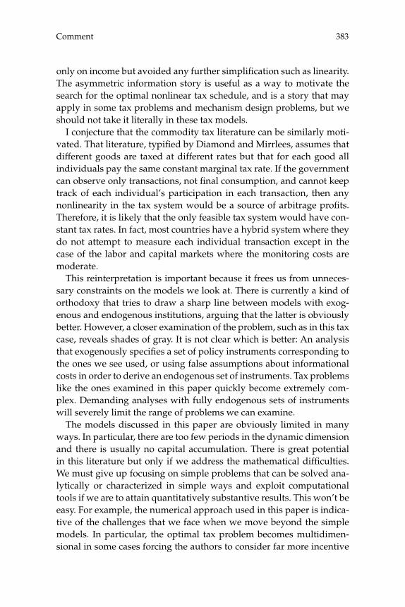
383Comment
only on income but avoided any further simplifi cation such as linearity. The asymmetric information story is useful as a way to motivate the search for the optimal nonlinear tax schedule, and is a story that may apply in some tax problems and mechanism design problems, but we should not take it literally in these tax models.
I conjecture that the commodity tax literature can be similarly moti-vated. That literature, typifi ed by Diamond and Mirrlees, assumes that different goods are taxed at different rates but that for each good all individuals pay the same constant marginal tax rate. If the government can observe only transactions, not fi nal consumption, and cannot keep track of each individual’s participation in each transaction, then any nonlinearity in the tax system would be a source of arbitrage profi ts. Therefore, it is likely that the only feasible tax system would have con-stant tax rates. In fact, most countries have a hybrid system where they do not attempt to measure each individual transaction except in the case of the labor and capital markets where the monitoring costs are moderate.
This reinterpretation is important because it frees us from unneces-sary constraints on the models we look at. There is currently a kind of orthodoxy that tries to draw a sharp line between models with exog-enous and endogenous institutions, arguing that the latter is obviously better. However, a closer examination of the problem, such as in this tax case, reveals shades of gray. It is not clear which is better: An analysis that exogenously specifi es a set of policy instruments corresponding to the ones we see used, or using false assumptions about informational costs in order to derive an endogenous set of instruments. Tax problems like the ones examined in this paper quickly become extremely com-plex. Demanding analyses with fully endogenous sets of instruments will severely limit the range of problems we can examine.
The models discussed in this paper are obviously limited in many ways. In particular, there are too few periods in the dynamic dimension and there is usually no capital accumulation. There is great potential in this literature but only if we address the mathematical diffi culties. We must give up focusing on simple problems that can be solved ana-lytically or characterized in simple ways and exploit computational tools if we are to attain quantitatively substantive results. This won’t be easy. For example, the numerical approach used in this paper is indica-tive of the challenges that we face when we move beyond the simple models. In particular, the optimal tax problem becomes multidimen-sional in some cases forcing the authors to consider far more incentive
Judd384
constraints than is necessary in the usual one-dimensional models. This is because the single-crossing property that is heavily exploited in the one-dimensional literature has no analogue for even two-dimensional problems. Therefore, if there are N types of taxpayers, we need to exam-ine N2 incentive constraints instead of N.
Judd and Su (2006) have examined this problem in more complex cases and fi nd cases far more challenging than the ones in this paper, and argue that the multidimensional optimal tax problem is generally far more diffi cult. They show that the solution to an optimal taxation problem will generally not satisfy the linear independence constraint qualifi cation, a fact that greatly increases the diffi culty of solving these problems numerically. Fortunately, the last decade has seen many advances in the fi eld of mathematical programming with equilibrium constraints which can be applied to these problems.
Again, I congratulate the authors for their “users guide” to an approach that can potentially provide major insights into the design of rational public policy and encourage other young researchers to follow their lead.
References
Atkinson, A. B., and J. E. Stiglitz. 1976. “The Design of Tax Structure: Direct vs. Indirect Taxation.” Journal of Public Economics 6: 55–75.
Diamond, Peter, and James A. Mirrlees. 1971. “Optimal Taxation and Public Production.” American Economic Review 61: 8–27, 175–208.
Judd, Kenneth L. 1985. “Redistributive Taxation in a Perfect Foresight Model.” Journal of Public Economics 28: 59–83.
Judd, Kenneth L. 1999. “Optimal Taxation and Spending in General Competitive Growth Models.” Journal of Public Economics 71(1): 1–26.
Judd, Kenneth L., and Che-Lin Su. 2006. “Optimal Income Taxation with Multidimen-sional Taxpayer Types.” Hoover Institution Working Paper.
Mirrlees, James A. 1971. “An Exploration in the Theory of Optimum Income Taxation.” Review of Economic Studies 38(2): 175–208.
Discussion
Iván Werning began by saying that he agreed with most of what the discussants had said. He noted that part of the discussants’ comments had focused on bringing new issues to the table. He and his coauthors felt that this was exactly what was nice about their approach to the tax problem, namely that it could address issues that could not have been addressed before using the traditional Ramsey approach. Werning observed that their approach provided scope for making normative assessments on the effects of policies related to unemployment, com-plementing the positive analysis from the previous day’s discussion on unemployment in Europe.
Werning agreed that the optimal tax systems that emerge from the class of models they studied were in some cases quite complex. With respect to this issue, he felt that there was room for a middle ground. In their view, it was essential to bring heterogeneity and skill shocks into the models. In such models, it turned out to be convenient analytically to start by studying the case where the government is only restricted by the informational friction and not in addition by restrictions on the set of tax instruments. He suggested that restrictions on tax instruments should be considered, but only after the basic models were well under-stood. He also noted that in some cases, the tax systems that emerged from their approach were reasonably simple, citing recent work on disability insurance by Mikhail Golosov and Aleh Tsyvinski as well as work by himself and Robert Shimer.
Golosov said that they were sympathetic to Kenneth Judd’s comment that it was important to think about the interaction of private market arrangements and government policies. He said that this was the reason why they had deliberately used the term “wedges” rather than taxes in the paper. However, he emphasized that there are many circumstances
Discussion386
where even if markets are perfectly functioning they would fail to yield effi cient outcomes due to externalities.
Greg Mankiw asked Peter Diamond what the evidence was for the statement he had made that high type people are more patient. Dia-mond responded that the assumptions on preferences that are made in these models imply that high skilled people have higher earnings and that people who discount the future less heavily have higher sav-ings rates. Given this, he said, the statement follows from the empiri-cal correlation between savings rates and earnings. Mankiw responded that this correlation may be due to consumption smoothing. Diamond thought that it was unreasonable to think that consumption smoothing explained the entire correlation.
James Poterba remarked that the paper had potential implications for the design of the tax period. He observed that many people had argued in favor of a lifetime income tax. He noted that such a tax seemed to dilute the information on what happens period by period. Poterba asked if the paper was pushing in the opposite direction by advocating that the government should exploit high frequency information. Werning responded that some of their results were supportive of tax smooth-ing but that temporary shocks to individuals generally did move the optimal tax system away from a completely smooth tax. He conjectured that it might be possible that a lifetime income tax accompanied with side programs like unemployment insurance to deal with temporary shocks might be close to what the theory suggests is optimal.
Kenneth Rogoff remarked that the discussants had emphasized the importance of knowing how robust the results of the paper were along several dimensions. He noted that another important dimension to generalize the model was the international dimension. Rogoff felt that this was especially important in the context of a world in which both fi nancial and human capital were increasingly mobile.
Daron Acemoglu remarked that the Mirrlees approach to optimal tax-ation was not so much in the business of writing exact models that could make precise predictions, but rather concerned with understanding general principles. He felt that the real power of the Mirrlees approach was that it was making an explicit effort to understand what the con-straints on taxes are. He noted that even though the Ramsey approach often yielded nice insights, the question about why lump sum taxes were ruled out always remained. He noted that in the dynamic setting, lump sum taxes sneak in through the back door in that the optimal tax mimics a lump sum tax. Golosov agreed with Acemoglu’s assessment.

387Discussion
Peter Diamond said that while Werning had stressed the role of shocks and Kenneth Judd had talked about insurance markets, his own comments stressed the role of predictable differences between people. He emphasized that there were many predictable differences between people and that in these cases what insurance markets cannot do comes to the fore. He noted that the conclusions of optimal tax theory were likely to change once it was taken into account that the adjustments made by workers in response to shocks are in practice not always smooth in the number of hours worked. Diamond also remarked that it was important to recognize incompleteness when analyzing taxes. In the context of taxes, he thought it was unrealistic to think that policies could be contingent on a full set of types. However, he thought it was important to know what the optimal policy would be if policies could be contingent on a full set of types as a fi rst step to thinking about what to do with fewer powers.

6
Equilibrium Yield Curves
Monika Piazzesi, University of ChicagoMartin Schneider, New York University and Federal Reserve Bank of Minneapolis
1 Introduction
The main theme of this paper is that investors dislike surprise infl a-tion not only because it lowers the payoff on nominal bonds, but also because it is bad news for future consumption growth. The fact that nominal bonds pay off little precisely when the outlook on the future worsens makes them unattractive assets to hold. The premium that risk averse investors seek as compensation for infl ation risk should thus depend on the extent to which infl ation is perceived as a carrier of bad news.
One implication is that the nominal yield curve slopes upward: Long bonds pay off even less than short bonds when infl ation, and hence bad news, arrives. Therefore, long bonds command a term spread over short bonds. Moreover, the level of interest rates and term spreads should increase in times when infl ation news is harder to inter-pret. This is relevant for periods such as the early 1980s, when the joint dynamics of infl ation and growth had just become less well under-stood.
We study the effect of infl ation as bad news in a simple representa-tive agent asset pricing model with two key ingredients. First, investor preferences are described by recursive utility. One attractive feature of this preference specifi cation is that—in contrast to the standard time-separable expected utility model—it does not imply indifference to the temporal distribution of risk. In particular, it allows investors to prefer a less persistent consumption stream to a more persistent stream, even if overall risk of the two streams is the same. In our context, aversion to persistence generates a heightened concern with news about the future and makes investors particularly dislike assets that pay off little when bad news arrives.
Piazzesi and Schneider390
The second ingredient of the model is a description of how inves-tor beliefs about consumption and infl ation evolve over time. Inves-tor beliefs determine to what extent infl ation is perceived to carry bad news at a particular point in time. We consider various specifi cations, some of which take into account structural change in the relationship between consumption growth and infl ation over the postwar period in the United States. Given investor beliefs about these two fundamentals, we determine interest rates implied by the model from the intertempo-ral Euler equation.
We perform two broad classes of model exercises. First, we consider stationary rational expectations versions of the model. Here we begin by estimating a stochastic process for U.S. consumption growth and infl ation over the entire postwar period. We assume that investor beliefs are the conditionals of this process, and derive the properties of the model-implied yield curve. The estimated process in this benchmark exercise has constant conditional variances. As a result, all asset price volatility derives from changes in investors’ conditional expectations. In particular, the dynamics of yields are entirely driven by movements in expected consumption growth and infl ation.
The benchmark model captures a number of features of observed yields. Both model implied and observed yields contain a sizeable low frequency component (period > eight years) that is strongly correlated with infl ation. At business cycle frequencies (between one and a half and eight years), both the short rate and the term spread are driven by the business cycle component of infl ation, which covaries positively with the former and negatively with the latter. Both a high short rate and a low term spread forecast recessions, that is, times of low con-sumption growth. Finally, average yields are increasing, and yield vola-tility is decreasing, in the maturity of the bond.
The fact that the model implies an upward-sloping nominal yield curve depends critically on both preferences and the distribu-tion of fundamentals. In the standard expected utility case, an asset commands a premium over another asset only when its payoff cova-ries more with consumption growth. Persistence of consumption growth and infl ation then implies a downward sloping yield curve. When investors exhibit aversion to persistence, an asset commands a premium also when its payoff covaries more with news about future consumption growth. The estimated process implies that infl ation brings bad news. The implied correlation between growth and infl a-tion is critical; if infl ation and consumption growth were independent,
391Equilibrium Yield Curves
the yield curve would slope downward even if investors were averse to persistence.
The role of infl ation as bad news suggests that other indicators of future growth might matter for term premia. Moreover, one might expect the arrival of other news about growth or infl ation to make yields more volatile than they are in our benchmark model. In a second exercise, we maintain the rational expectations assumption, but model investors’ information set more explicitly by exploiting information contained in yields themselves. In particular, we begin by estimating an unrestricted stochastic process for consumption growth, infl ation, the short rate, and the term spread. We then derive model-implied yields given the information set described by this stochastic process.
The resulting model-implied yields are very similar to those from our benchmark. It follows that, viewed through the lens of our consump-tion-based asset pricing model, infl ation itself is the key predictor of future consumption, infl ation, and yields that generates interest rate volatility. Conditional on our model, we can rule out the possibility that other variables—such as investors’ perception of a long run infl a-tion target, or information inferred from other asset prices—generates volatility in yields. Indeed, if observed yields had been generated by a version of our model in which investors price bonds using better infor-mation than we modelers have, our exercise would have recovered that information from yields.
We also explore the role of infl ation as bad news in a class of mod-els that accommodate investor concern with structural change. Here we construct investor beliefs by sequentially estimating the stochas-tic process for fundamentals. We use a constant gain adaptive learn-ing scheme where the estimation for date t places higher weight on more recent observations. The investor belief for date t is taken to be the conditional of the process estimated with data up to date t. We then compute a sample of model-implied yields from the Euler equations, using a different investor belief for each date. We apply this model to consider changes in yield curve dynamics, especially around the mon-etary policy experiment.
It has been suggested that long interest rates were high in the early 1980s because investors at the time were only slowly adjusting their infl ation expectations downward. In the context of our model, this is not a plausible story. Indeed, it is hard to write down a sensible adap-tive learning scheme in which the best forecast of future infl ation is not close to current infl ation. Since infl ation fell much more quickly in
Piazzesi and Schneider392
the early 1980s than nominal interest rates, our learning schemes do not generate much inertia in infl ation expectations. At the same time, survey expectations of infl ation also fell relatively quickly in the early 1980s, along with actual infl ation and the forecasts in our model.
We conclude that learning can help in understanding changes in the yield curve only if it entails changes in subjective uncertainty that have fi rst order effects on asset prices. In a fi nal exercise, we explore one scenario where this happens. In addition to sequential estimation, we introduce parameter uncertainty which implies that investors cannot easily distinguish permanent and transitory movements in infl ation. With patient investors who are averse to persistence, changes in uncer-tainty then have large effects on interest rates and term spreads. In par-ticular, the uncertainty generated by the monetary policy experiment leads to sluggish behavior in interest rates, especially at the long end of the yield curve, in the early 1980s.
A by-product of our analysis is a decomposition into real and nominal interest rates, where the former are driven by expected consumption growth, whereas the latter also move with changes in expected infl a-tion. Importantly, infl ation as an indicator of future growth affects both nominal and real interest rates. Loosely speaking, our model says that yields in the 1970s and early 1980s were driven by nominal shocks—infl ation surprises—that affect nominal and real rates in opposite direc-tions. Here an infl ation surprise lowers real rates because it is bad news for future consumption growth. In contrast, prior to the 1970s, and again more recently, there were more real shocks—surprises in consumption growth—that make nominal and real interest rates move together.
Our model also predicts a downward sloping real yield curve. In con-trast to long nominal bonds, long indexed bonds pay off when future real interest rates—and hence future expected consumption growth—are low, thus providing insurance against bad times. Coupled with per-sistence in growth, this generates a downward sloping real yield curve in an expected utility model. The effect is reinforced when investors are averse to persistence. Unfortunately, the available data series on U.S. indexed bonds, which is short and comes from a period of relatively low interest rates, makes it diffi cult to accurately measure average long indexed yields. However, evidence from the United Kingdom suggests that average term spreads are positive for nominal, but negative for indexed bonds.
The paper is organized as follows. Section 2 presents the model, motivates our use of recursive utility, and outlines the yield computa-
393Equilibrium Yield Curves
tions. Section 3 reports results from the benchmark rational expecta-tions version of the model. Section 4 maintains the rational expectations assumption, but allows for more conditioning information. Section 5 introduces learning. Section 6 reviews related literature. Appendix A collects our estimation results. Appendix B presents summary statistics about real rate data from the United States and the United Kingdom. A separate Appendix C which is downloadable from our websites con-tains results with alternative data defi nitions, evidence from infl ation surveys, as well as more detailed derivations.
2 Model
We consider an endowment economy with a representative investor. The endowment—denoted {Ct} since it is calibrated to aggregate con-sumption—and infl ation {πt} are given exogenously. Equilibrium prices adjust such that the agent is happy to consume the endowment. In the remainder of this section, we defi ne preferences and explain how yields are computed.
2.1 Preferences
We describe preferences using the recursive utility model proposed by Epstein and Zin (1989) and Weil (1989), which allows for a constant coef-fi cient of relative risk aversion that can differ from the reciprocal of the intertemporal elasticity of substitution (IES). This class of preferences is now common in the consumption-based asset pricing literature. Camp-bell (1993, 1996) derives approximate loglinear pricing formulas (that are exact if the IES is one) to characterize premia and the price volatility of equity and real bonds. Duffi e, Schroeder, and Skiadas (1997) derive closed-form solutions for bond prices in a continuous time version of the model. Restoy and Weil (1998) show how to interpret the pricing kernel in terms of a concern with news about future consumption. For our computations, we assume a unitary IES and homoskedastic lognor-mal shocks, which allow us to use a linear recursion for utility derived by Hansen, Heaton, and Li (2005).
We fi x a fi nite horizon T and a discount factor β > 0. The time t utility Vt of a consumption stream {Ct} is defi ned recursively by V C Vt t t t
t t= −+
11
α αCE ( ) , (1)
Piazzesi and Schneider394
with VT+1 = 0. Here the certainty equivalent CEt imposes constant rela-tive risk aversion with coeffi cient γ,
CEt t t tV E V( ) ( ) ,/( )+ +
− −=1 11 1 1γ γ
and the sequence of weights αt is given by
α β βtj
j
T tj
j
T
: .==
−
=
−
∑ ∑1 0
1
(2)
If β < 1, the weight αt on continuation utility converges to β as the hori-zon becomes large. If γ = 1, the model reduces to standard logarith-mic utility. More generally, the risk aversion coeffi cient can be larger or smaller than one, the (inverse of the) intertemporal elasticity of substi-tution.
2.1.1 Discussion Recursive preferences avoid the implication of the time-separable expected utility model that decision makers are indiffer-ent to the temporal distribution of risk. A standard example, reviewed by Duffi e and Epstein (1992), considers a choice at some date zero between two risky consumption plans A and B. Both plans promise contingent consumption for the next 100 periods. Under both plans, consumption in a given period can be either high or low, with the out-come determined by the toss of a fair coin. However, the consumption stream promised by plan A is determined by repeated coin tosses: If the toss in period t is heads, consumption in t is high, otherwise consump-tion in t is low. In contrast, the consumption stream promised by plan B is determined by a once and for all coin toss at date 1: if this toss is heads, consumption is high for the next 100 periods, otherwise, consumption is low for the next 100 periods.
Intuitively, plan A looks less risky than plan B. Under plan B, all eggs are in one basket, whereas plan A is more diversifi ed. If all payoffs were realized at the same time, risk aversion would imply a preference for plan A. However, if the payoffs arrive at different dates, the standard time-separable expected utility model implies indifference between A and B. This holds regardless of risk aversion and of how little time elapses between the different dates. The reason is that the time-sepa-rable model evaluates risks at different dates in isolation. From the per-spective of time zero, random consumption at any given date—viewed in isolation—does have the same risk (measured, for example, by the variance.) What the standard model misses is that the risk is distributed
395Equilibrium Yield Curves
differently over time for the two plans: Plan A looks less risky since the consumption stream it promises is less persistent.
According to the preferences (1), the plans A and B are ranked dif-ferently if the coeffi cient of relative risk aversion γ is not equal to one. In particular, γ > 1 implies that the agent is averse to the persistence induced by the initial shock that characterizes plan B and therefore pre-fers A. This is the case we consider in this paper. When γ < 1, the agent likes the persistence and prefers B.
Another attractive property of the utility specifi cation (1) is that the motives that govern consumption smoothing over different states of nature and consumption smoothing over time are allowed to differ. For example, an agent with recursive utility and γ > 1 would not prefer an erratic deterministic consumption stream A to a constant stream B. Indeed, there is no reason to assume why the two smoothing motives should be tied together like in the power utility case, where the risk aversion coeffi cient γ is the reciprocal of the elasticity of intertempo-ral substitution. After all, the notion of smoothing over different states even makes sense in a static economy with uncertainty, while smooth-ing over time is well defi ned in a dynamic but deterministic economy.
We specify a (long) fi nite horizon T because we want to allow for high discount factors, β > 1. There is no a priori reason to rule out this case. The usual justifi cation for low discount factors is introspection: When faced with a constant consumption stream, many people would prefer to shift some consumption into the present. While this introspec-tive argument makes sense in the stochastic environment in which we actually live—where we may die before we get to consume, and so we want to consume while we still can—it is not clear whether the argu-ment should apply to discounting in a deterministic environment with some known horizon (which is the case for which the discount factor β is designed.)
2.1.2 Pricing Kernel We divide equation (1) by current consumption to get
VC
VC
CC
t
tt
t
t
t
t
t
=⎛⎝⎜
⎞⎠⎟
+
+
+CE 1
1
1
α
.
Taking logarithms, denoted throughout by small letters, we obtain the recursion
v c v c ct t t t t t t− = − ++ + +α ln [exp( )].CE 1 1 1Δ
Piazzesi and Schneider396
Assuming that the variables are conditionally normal, we get
v c E v c c vt t t t t t t t t− = − + + −+ + +α α γ( ) ( )var (1 1 1
12
1Δ tt+1). (3)
Solving the recursion forward and using our assumption that the agent’s beliefs are homoskedastic, we can express the log ratio of con-tinuation utility to consumption as an infi nite sum of expected dis-counted future consumption growth,
v c E ct t t i ti
T t
t i− = ++=
−
+ +∑α , ( )10
1Δ constant. (4)
For β < 1 and T = ∞, the weights on expected future consumption growth are simply αt,i = β ι. Even for large fi nite T, equation (4) can be viewed as a sum of expected consumption growth with weights that are independent of the forecasting horizon 1 + i.
For fi nite T, the weights αt,i are given by
α β βt ij
j i
T tj
j
T t
, : ,==
−
=
−
∑ ∑0
so that αt,1 = αt. For β > 1, the weights on expected future consumption growth are decreasing and concave in the forecast horizon i. For large T, they remain equal to one for many periods. If consumption growth reverts to its mean—that is, Et(Δct+1+i) converges to the unconditional mean of consumption growth as i becomes large—then the log ratio of continuation utility is approximately given by the infi nite-horizon undiscounted sum of expected consumption growth.
Payoffs denominated in units of consumption are valued by the real pricing kernel
MCC
VVt
t
t
t
t t+
+
−
+
+
−
=⎛⎝⎜
⎞⎠⎟
⎛⎝⎜
⎞⎠⎟1
1
1
1
1
1
βγ
CE ( ). (5)
The random variable Mt+1 represents the date t prices of contingent claims that pay off in t + 1. In particular, the price of a contingent claim that pays off one unit if some event in t + 1 occurs is equal to the expected value of the pricing kernel conditional on the event, multi-plied by the probability of the event. In a representative agent model, the pricing kernel is large over events in which the agent will feel bad: Claims written on such events are particularly expensive.
397Equilibrium Yield Curves
Again using normality, we obtain the log real pricing kernel
m c Et t t t t+ + + += − − − − − −1 1 1 1112
1ln ( )( ( )) ( )β γ υ υ γΔ 221var ( )t tυ + (6)
ln ( ) (,= − − − −+ +=
− −
+∑β γ αΔc Et t ii
T t
t1 10
1
11 EE ct t i)Δ + +1
( ) var ( ),− − + + + +=
−12
1 21 1 1
0
γ αt t i t t ii
T
E cΔtt−
∑⎛
⎝⎜⎞
⎠⎟1
.
The logarithmic expected utility model (the case γ = 1) describes “bad events” in terms of future realized consumption growth—the agent feels bad when consumption growth is low. This effect is represented by the fi rst term in the pricing kernel. Recursive utility introduces a new term that refl ects a concern with the temporal distribution of risk. In the case we consider, γ > 1, the agent fears downward revisions in consumption expectations. More generally, a source of risk is not only refl ected in asset prices if it makes consumption more volatile, as in the standard model, but it can also affect prices if it affects only the temporal distribution of risk, for example if it makes consumption growth more persistent.
Finally, we defi ne the log nominal pricing kernel, that we use below to value payoffs denominated in dollars:
m mt t t+ + += −1 1 1$ .π (7)
2.2 Nominal and Real Yield Curves
The agent’s Euler equation for a real bond that pays one unit of con-sumption n periods later determines its time-t price Pt
(n) as the expected
value of its payoff tomorrow weighted by the real pricing kernel:
P E P M E Mtn
t tn
t t ti
n( ) ( ) .= ( ) =
⎛
⎝⎜⎞
⎠⎟+−
+ +=
∏11
1 11
(8)
This recursion starts with the one-period bond at Pt(1) = Et[Mt+1] Under
normality, we get in logs
p E p m p mtn
t tn
t t tn( ) ( ) ( )( ) var (= + + ++
−+ +
−1
11 1
112 tt+1) (9)
var=⎛
⎝⎜⎞
⎠⎟+
⎛
⎝⎜+
=+
=∑ ∑E m mt t ii
n
t t ii
n
1 1
12
⎞⎞
⎠⎟.
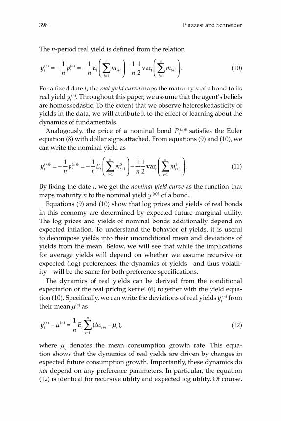
Piazzesi and Schneider398
The n-period real yield is defi ned from the relation
yn
pn
E mnt
ntn
t t ii
n( ) ( ) var= − = −
⎛
⎝⎜⎞
⎠⎟−+
=∑1 1 1 1
21tt t i
i
n
m +=∑⎛
⎝⎜⎞
⎠⎟1
. (10)
For a fi xed date t, the real yield curve maps the maturity n of a bond to its real yield yt
(n). Throughout this paper, we assume that the agent’s beliefs are homoskedastic. To the extent that we observe heteroskedasticity of yields in the data, we will attribute it to the effect of learning about the dynamics of fundamentals.
Analogously, the price of a nominal bond Pt(n)$ satisfi es the Euler
equation (8) with dollar signs attached. From equations (9) and (10), we can write the nominal yield as
yn
pn
E mnt
ntn
t ti
n( )$ ( )$ $= − = −
⎛
⎝⎜⎞
⎠⎟−+
=∑1 1 1 1
211
vvar .$t t
i
n
m +=∑⎛
⎝⎜⎞
⎠⎟1
1
(11)
By fi xing the date t, we get the nominal yield curve as the function that maps maturity n to the nominal yield yt
(n)$ of a bond.Equations (9) and (10) show that log prices and yields of real bonds
in this economy are determined by expected future marginal utility. The log prices and yields of nominal bonds additionally depend on expected infl ation. To understand the behavior of yields, it is useful to decompose yields into their unconditional mean and deviations of yields from the mean. Below, we will see that while the implications for average yields will depend on whether we assume recursive or expected (log) preferences, the dynamics of yields—and thus volatil-ity—will be the same for both preference specifi cations.
The dynamics of real yields can be derived from the conditional expectation of the real pricing kernel (6) together with the yield equa-tion (10). Specifi cally, we can write the deviations of real yields yt
(n) from their mean μ(n) as
yn
E ctn n
t t i ci
n( ) ( ) ( ),− = −+
=∑μ μ1
1
Δ (12)
where μc denotes the mean consumption growth rate. This equa-tion shows that the dynamics of real yields are driven by changes in expected future consumption growth. Importantly, these dynamics do not depend on any preference parameters. In particular, the equation (12) is identical for recursive utility and expected log utility. Of course,
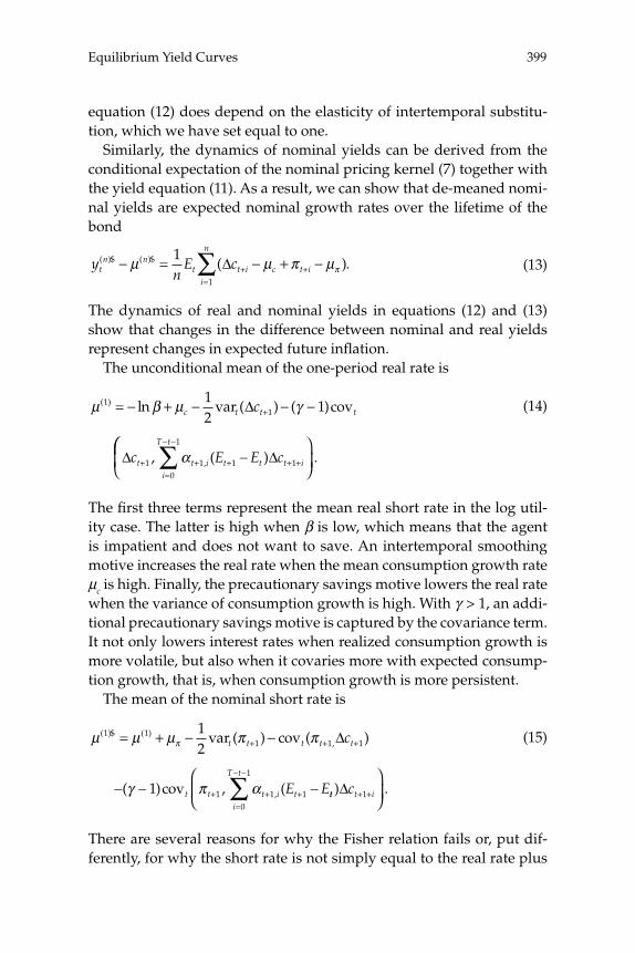
399Equilibrium Yield Curves
equation (12) does depend on the elasticity of intertemporal substitu-tion, which we have set equal to one.
Similarly, the dynamics of nominal yields can be derived from the conditional expectation of the nominal pricing kernel (7) together with the yield equation (11). As a result, we can show that de-meaned nomi-nal yields are expected nominal growth rates over the lifetime of the bond
yn
E ctn n
t t i c t ii
n( )$ ( )$ ( ).− = − + −+ +
=∑μ μ π μπ
1
1
Δ (13)
The dynamics of real and nominal yields in equations (12) and (13) show that changes in the difference between nominal and real yields represent changes in expected future infl ation.
The unconditional mean of the one-period real rate is
μ β μ γ( ) ln var ( ) ( )cov11
12
1= − + − − −+c t t tcΔ (14)
, ( ),Δ Δc E E ct t i t t t ii
T t
+ + + + +=
− −
−∑1 1 1 10
1
α⎛⎛
⎝⎜⎞
⎠⎟.
The fi rst three terms represent the mean real short rate in the log util-ity case. The latter is high when β is low, which means that the agent is impatient and does not want to save. An intertemporal smoothing motive increases the real rate when the mean consumption growth rate μc is high. Finally, the precautionary savings motive lowers the real rate when the variance of consumption growth is high. With γ > 1, an addi-tional precautionary savings motive is captured by the covariance term. It not only lowers interest rates when realized consumption growth is more volatile, but also when it covaries more with expected consump-tion growth, that is, when consumption growth is more persistent.
The mean of the nominal short rate is
μ μ μ π ππ( )$ ( )
,var ( ) cov ( )1 11 1 1
12
= + − −+ + +t t t t tcΔ (15)
( )cov , (,− − −+ +=
− −
+∑γ π α1 1 10
1
1t t t ii
T t
tE Ett t ic) .Δ + +
⎛
⎝⎜⎞
⎠⎟1
There are several reasons for why the Fisher relation fails or, put dif-ferently, for why the short rate is not simply equal to the real rate plus

Piazzesi and Schneider400
expected infl ation. First, the variance of infl ation enters due to Jensen’s inequality. Second, the covariance of consumption growth and infl a-tion represents an infl ation risk premium. Intuitively, nominal bonds—including those with short maturity—are risky assets. The real payoff from nominal bonds is low in times of surprise infl ation. If the covari-ance between infl ation and consumption is negative, nominal bonds are unattractive assets, because they have low real payoffs in bad times. In other words, nominal bonds do not provide a hedge against times of low consumption growth. Investors thus demand higher nominal yields as compensation for holding nominal bonds. Recursive utility introduces an additional reason why nominal bonds may be unattract-ive for investors: Their payoffs are low in times with bad news about future consumption growth. These bonds may thus not provide a hedge against times with bad news about the future.
We defi ne rx(n)t+1 = p(
tn+–1 1)
– p(n)t – yt
(1) as the return on buying an n-period real bond at time t for pt
(n) and selling it at time t + 1 for p(tn+–1 1) in excess of
the short rate. Based on equation (9), the expected excess return is
E rx m E mt tn
t t t t ii
n
+ + + + +=
−
( ) = −⎛
⎝⎜ ∑1 1 1 11
1( ) cov ,
⎞⎞
⎠⎟− +
−12 1
1var ( ).( )t t
np (16)
The covariance term on the right-hand size is the risk premium, while the variance term is due to Jensen’s inequality. Expected excess returns are constant whenever conditional variances are constant, as in our benchmark belief specifi cation. With learning, however, the conditional probabilities that are used to evaluate the conditional covariances in equation (16) will be derived from different beliefs each period. As a result, expected excess returns will vary overtime.
The risk premium on real bonds is positive when the pricing ker-nel and long bond prices are negatively correlated. This correlation is determined by the autocorrelation of marginal utility. The risk premium is positive if marginal utility is negatively correlated with expected changes in future marginal utility. In this case, long bonds are less attractive than short bonds, because their payoffs tend to be low in bad times (when marginal utility is high). The same equation also holds for nominal bonds after we attach dollar signs everywhere. Here, the sign of the risk premium also depends on the correlation between (nomi-nal) bond prices and infl ation. Over long enough samples, the average excess return on an n-period bond is approximately equal to the aver-

401Equilibrium Yield Curves
age spread between the n-period yield and the short rate.1 This means that the yield curve is on average upward sloping if the right-hand side of equation (16) is positive on average.
In our model, expected changes in marginal utility depend on expected future consumption growth. The expected excess return (16) can therefore be rewritten as
E rx m E ct tn
t t t t ii
n
( ) cov ,( )+ + + + +
=
−
=⎛
⎝⎜ ∑1 1 1 11
1
Δ⎞⎞
⎠⎟− +
−12 1
1var ( ).( )t t
np (17)
Real term premia are thus driven by the covariance of marginal utility with expected con-sumption growth. The expected excess return equa-tion (16) for an n-period nominal bond becomes
E rx m E ct tn
t t t t i t ii
( ) cov ,( )$ $+ + + + + + += +1 1 1 1 1Δ π
==
−
+−∑⎛
⎝⎜⎞
⎠⎟−
1
1
111
2
n
t tnpvar ( ).( )$ (18)
This equation shows that nominal term premia are driven by the cova-riance of the nominal pricing kernel with expected nominal growth.
3 Benchmark
In this section, we derive investor beliefs from a state space system for consumption growth and infl ation that is estimated with data from the entire postwar sample. The conditional probabilities that we use to evaluate the agent’s Euler equation, and thus to compute yields, come from this estimated system.
3.1 Data
We measure aggregate consumption growth with quarterly NIPA data on nondurables and services and construct the corresponding price index to measure infl ation. We assume that population growth is constant. The data on bond yields with maturities one year and lon-ger are from the CRSP Fama-Bliss discount bond fi les. These fi les are available for the sample 1952:2–2005:4. The short (1-quarter) yield is from the CRSP Fama riskfree rate fi le. These data, our MATLAB pro-grams, and Appendix C which contains additional results based on alternative infl ation and population series can be downloaded from our websites.
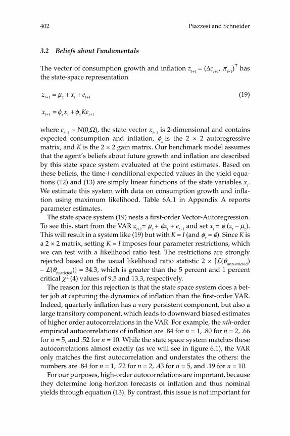
Piazzesi and Schneider402
3.2 Beliefs about Fundamentals
The vector of consumption growth and infl ation zt+1 = (Δct+1, πτ+1)T has
the state-space representation
z x et z t t+ += + +1 1μ (19)
x x Ket x t x t+ += +1 1φ φ
where et+1 ~ N(0,Ω), the state vector xt+1 is 2-dimensional and contains expected consumption and infl ation, φx is the 2 × 2 autoregressive matrix, and K is the 2 × 2 gain matrix. Our benchmark model assumes that the agent’s beliefs about future growth and infl ation are described by this state space system evaluated at the point estimates. Based on these beliefs, the time-t conditional expected values in the yield equa-tions (12) and (13) are simply linear functions of the state variables xt. We estimate this system with data on consumption growth and infl a-tion using maximum likelihood. Table 6A.1 in Appendix A reports parameter estimates.
The state space system (19) nests a fi rst-order Vector-Autoregression. To see this, start from the VAR zt+1= μz + φzt + et+1 and set xt = φ (zt – μz). This will result in a system like (19) but with K = I (and φx = φ). Since K is a 2 × 2 matrix, setting K = I imposes four parameter restrictions, which we can test with a likelihood ratio test. The restrictions are strongly rejected based on the usual likelihood ratio statistic 2 × [L(θunrestricted) – L(θrestricted)] = 34.3, which is greater than the 5 percent and 1 percent critical χ 2 (4) values of 9.5 and 13.3, respectively.
The reason for this rejection is that the state space system does a bet-ter job at capturing the dynamics of infl ation than the fi rst-order VAR. Indeed, quarterly infl ation has a very persistent component, but also a large transitory component, which leads to downward biased estimates of higher order autocorrelations in the VAR. For example, the nth-order empirical autocorrelations of infl ation are .84 for n = 1, .80 for n = 2, .66 for n = 5, and .52 for n = 10. While the state space system matches these autocorrelations almost exactly (as we will see in fi gure 6.1), the VAR only matches the fi rst autocorrelation and understates the others: the numbers are .84 for n = 1, .72 for n = 2, .43 for n = 5, and .19 for n = 10.
For our purposes, high-order autocorrelations are important, because they determine long-horizon forecasts of infl ation and thus nominal yields through equation (13). By contrast, this issue is not important for
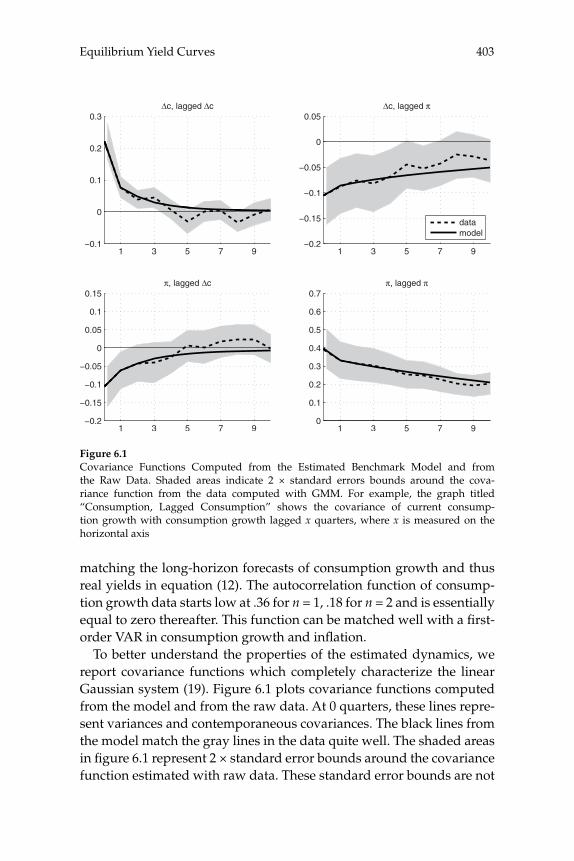
403Equilibrium Yield Curves
matching the long-horizon forecasts of consumption growth and thus real yields in equation (12). The autocorrelation function of consump-tion growth data starts low at .36 for n = 1, .18 for n = 2 and is essentially equal to zero thereafter. This function can be matched well with a fi rst-order VAR in consumption growth and infl ation.
To better understand the properties of the estimated dynamics, we report covariance functions which completely characterize the linear Gaussian system (19). Figure 6.1 plots covariance functions computed from the model and from the raw data. At 0 quarters, these lines repre-sent variances and contemporaneous covariances. The black lines from the model match the gray lines in the data quite well. The shaded areas in fi gure 6.1 represent 2 × standard error bounds around the covariance function estimated with raw data. These standard error bounds are not
Figure 6.1Covariance Functions Computed from the Estimated Benchmark Model and from the Raw Data. Shaded areas indicate 2 × standard errors bounds around the cova-riance function from the data computed with GMM. For example, the graph titled “Consumption, Lagged Consumption” shows the covariance of current consump-tion growth with consumption growth lagged x quarters, where x is measured on the horizontal axis
1 3 5 7 9−0.1
0
0.1
0.2
0.3Δc, lagged Δc
1 3 5 7 9−0.2
−0.15
−0.1
−0.05
0
0.05Δc, lagged π
datamodel
1 3 5 7 9−0.2
−0.15
−0.1
−0.05
0
0.05
0.1
0.15π, lagged Δc
1 3 5 7 90
0.1
0.2
0.3
0.4
0.5
0.6
0.7π, lagged π
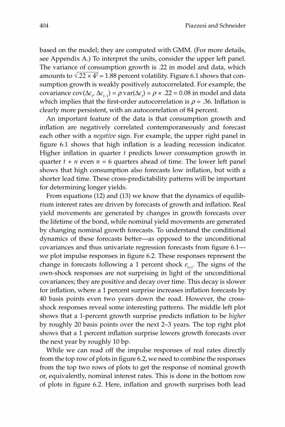
Piazzesi and Schneider404
based on the model; they are computed with GMM. (For more details, see Appendix A.) To interpret the units, consider the upper left panel. The variance of consumption growth is .22 in model and data, which amounts to √.22 × 42 = 1.88 percent volatility. Figure 6.1 shows that con-sumption growth is weakly positively autocorrelated. For example, the covariance cov(Δct, Δct–1) = ρ var(Δct) = ρ × .22 = 0.08 in model and data which implies that the fi rst-order autocorrelation is ρ = .36. Infl ation is clearly more persistent, with an autocorrelation of 84 percent.
An important feature of the data is that consumption growth and infl ation are negatively correlated contemporaneously and forecast each other with a negative sign. For example, the upper right panel in fi gure 6.1 shows that high infl ation is a leading recession indicator. Higher infl ation in quarter t predicts lower consumption growth in quarter t + n even n = 6 quarters ahead of time. The lower left panel shows that high consumption also forecasts low infl ation, but with a shorter lead time. These cross-predictability patterns will be important for determining longer yields.
From equations (12) and (13) we know that the dynamics of equilib-rium interest rates are driven by forecasts of growth and infl ation. Real yield movements are generated by changes in growth forecasts over the lifetime of the bond, while nominal yield movements are generated by changing nominal growth forecasts. To understand the conditional dynamics of these forecasts better—as opposed to the unconditional covariances and thus univariate regression forecasts from fi gure 6.1—we plot impulse responses in fi gure 6.2. These responses represent the change in forecasts following a 1 percent shock et+1. The signs of the own-shock responses are not surprising in light of the unconditional covariances; they are positive and decay over time. This decay is slower for infl ation, where a 1 percent surprise increases infl ation forecasts by 40 basis points even two years down the road. However, the cross-shock responses reveal some interesting patterns. The middle left plot shows that a 1-percent growth surprise predicts infl ation to be higher by roughly 20 basis points over the next 2–3 years. The top right plot shows that a 1 percent infl ation surprise lowers growth forecasts over the next year by roughly 10 bp.
While we can read off the impulse responses of real rates directly from the top row of plots in fi gure 6.2, we need to combine the responses from the top two rows of plots to get the response of nominal growth or, equivalently, nominal interest rates. This is done in the bottom row of plots in fi gure 6.2. Here, infl ation and growth surprises both lead
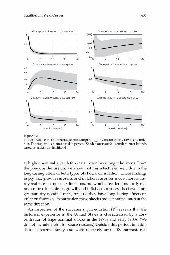
405Equilibrium Yield Curves
to higher nominal growth forecasts—even over longer horizons. From the previous discussion, we know that this effect is entirely due to the long-lasting effect of both types of shocks on infl ation. These fi ndings imply that growth surprises and infl ation surprises move short-matu-rity real rates in opposite directions, but won’t affect long-maturity real rates much. In contrast, growth and infl ation surprises affect even lon-ger-maturity nominal rates, because they have long-lasting effects on infl ation forecasts. In particular, these shocks move nominal rates in the same direction.
An inspection of the surprises et+1 in equation (19) reveals that the historical experience in the United States is characterized by a con-centration of large nominal shocks in the 1970s and early 1980s. (We do not include a plot for space reasons.) Outside this period, infl ation shocks occurred rarely and were relatively small. By contrast, real
Figure 6.2Impulse Responses to 1 Percentage Point Surprises et+1 in Consumption Growth and Infl a-tion. The responses are measured in percent. Shaded areas are 2 × standard error bounds based on maximum likelihood
0 5 10 15 20
0
0.5
1Change in Δc forecast to Δc surprise
0 5 10 15 20−0.2
−0.15
−0.1
−0.05
0
0.05Change in Δc forecast to π surprise
0 5 10 15 200
0.1
0.2
0.3
0.4Change in π forecast to Δc surprise
0 5 10 15 200
0.5
1Change in π forecast to π surprise
0 5 10 15 200
0.5
1
time (in quarters)
Change in Δc+π forecast to Δc surprise
0 5 10 15 200
0.5
1
time (in quarters)
Change in Δc+π forcast to π surprise
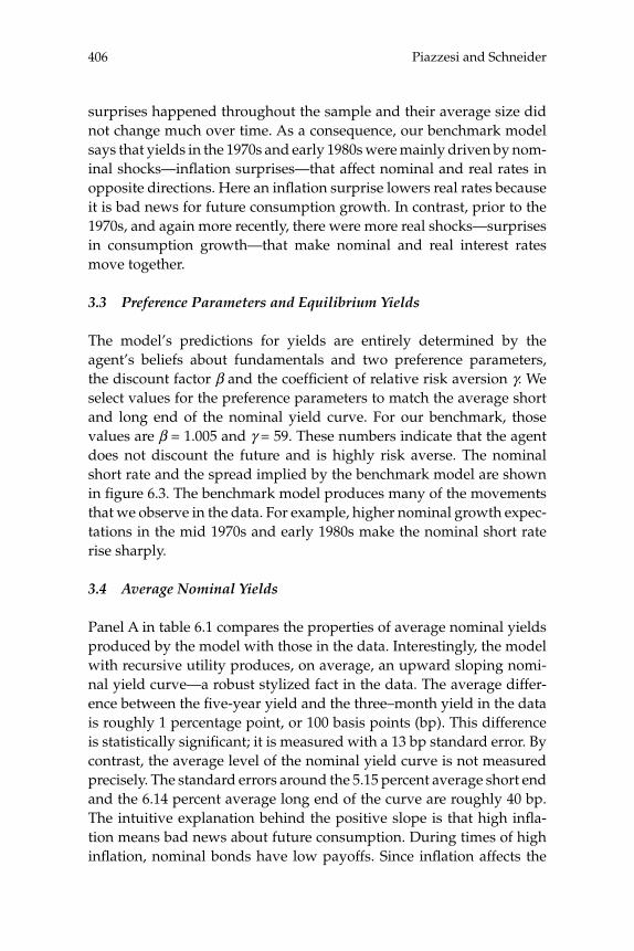
Piazzesi and Schneider406
surprises happened throughout the sample and their average size did not change much over time. As a consequence, our benchmark model says that yields in the 1970s and early 1980s were mainly driven by nom-inal shocks—infl ation surprises—that affect nominal and real rates in opposite directions. Here an infl ation surprise lowers real rates because it is bad news for future consumption growth. In contrast, prior to the 1970s, and again more recently, there were more real shocks—surprises in consumption growth—that make nominal and real interest rates move together.
3.3 Preference Parameters and Equilibrium Yields
The model’s predictions for yields are entirely determined by the agent’s beliefs about fundamentals and two preference parameters, the discount factor β and the coeffi cient of relative risk aversion γ. We select values for the preference parameters to match the average short and long end of the nominal yield curve. For our benchmark, those values are β = 1.005 and γ = 59. These numbers indicate that the agent does not discount the future and is highly risk averse. The nominal short rate and the spread implied by the benchmark model are shown in fi gure 6.3. The benchmark model produces many of the movements that we observe in the data. For example, higher nominal growth expec-tations in the mid 1970s and early 1980s make the nominal short rate rise sharply.
3.4 Average Nominal Yields
Panel A in table 6.1 compares the properties of average nominal yields produced by the model with those in the data. Interestingly, the model with recursive utility produces, on average, an upward sloping nomi-nal yield curve—a robust stylized fact in the data. The average differ-ence between the fi ve-year yield and the three–month yield in the data is roughly 1 percentage point, or 100 basis points (bp). This difference is statistically signifi cant; it is measured with a 13 bp standard error. By contrast, the average level of the nominal yield curve is not measured precisely. The standard errors around the 5.15 percent average short end and the 6.14 percent average long end of the curve are roughly 40 bp. The intuitive explanation behind the positive slope is that high infl a-tion means bad news about future consumption. During times of high infl ation, nominal bonds have low payoffs. Since infl ation affects the
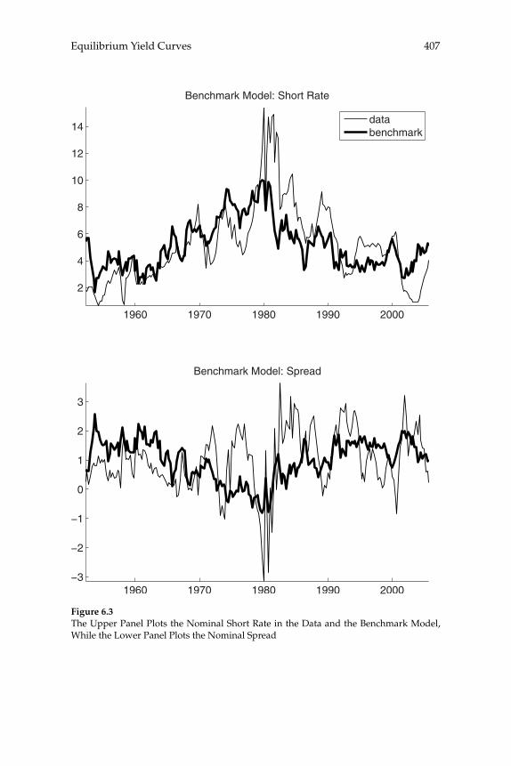
407Equilibrium Yield Curves
Figure 6.3The Upper Panel Plots the Nominal Short Rate in the Data and the Benchmark Model, While the Lower Panel Plots the Nominal Spread
1960 1970 1980 1990 2000
2
4
6
8
10
12
14
Benchmark Model: Short Rate
databenchmark
1960 1970 1980 1990 2000−3
−2
−1
0
1
2
3
Benchmark Model: Spread
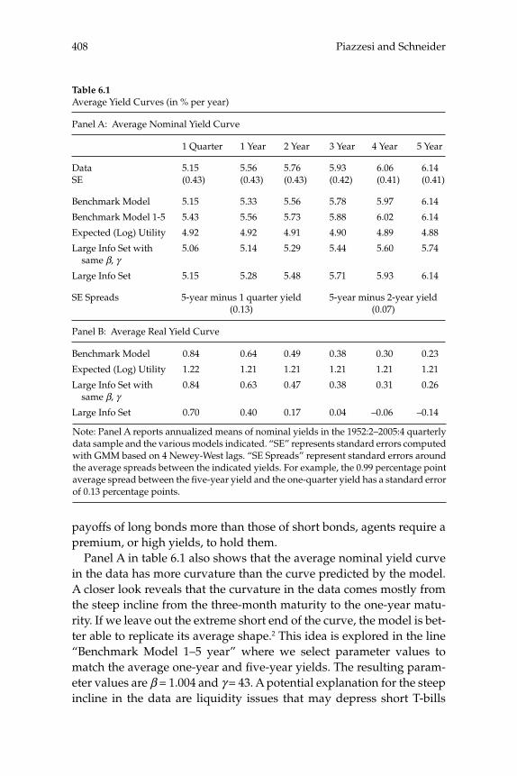
Piazzesi and Schneider408
payoffs of long bonds more than those of short bonds, agents require a premium, or high yields, to hold them.
Panel A in table 6.1 also shows that the average nominal yield curve in the data has more curvature than the curve predicted by the model. A closer look reveals that the curvature in the data comes mostly from the steep incline from the three-month maturity to the one-year matu-rity. If we leave out the extreme short end of the curve, the model is bet-ter able to replicate its average shape.2 This idea is explored in the line “Benchmark Model 1–5 year” where we select parameter values to match the average one-year and fi ve-year yields. The resulting param-eter values are β = 1.004 and γ = 43. A potential explanation for the steep incline in the data are liquidity issues that may depress short T-bills
Table 6.1Average Yield Curves (in % per year)
Panel A: Average Nominal Yield Curve
DataSE
Benchmark Model
Benchmark Model 1-5
Expected (Log) Utility
Large Info Set with same β, γLarge Info Set
SE Spreads
1 Quarter
5.15(0.43)
5.15
5.43
4.92
5.06
5.15
1 Year
5.56(0.43)
5.33
5.56
4.92
5.14
5.28
2 Year
5.76(0.43)
5.56
5.73
4.91
5.29
5.48
3 Year
5.93(0.42)
5.78
5.88
4.90
5.44
5.71
4 Year
6.06 (0.41)
5.97
6.02
4.89
5.60
5.93
5 Year
6.14 (0.41)
6.14
6.14
4.88
5.74
6.14
5-year minus 1 quarter yield(0.13)
5-year minus 2-year yield(0.07)
Panel B: Average Real Yield Curve
Benchmark Model
Expected (Log) Utility
Large Info Set with same β, γLarge Info Set
0.84
1.22
0.84
0.70
0.64
1.21
0.63
0.40
0.49
1.21
0.47
0.17
0.38
1.21
0.38
0.04
0.30
1.21
0.31
–0.06
0.23
1.21
0.26
–0.14
Note: Panel A reports annualized means of nominal yields in the 1952:2–2005:4 quarterly data sample and the various models indicated. “SE” represents standard errors computed with GMM based on 4 Newey-West lags. “SE Spreads” represent standard errors around the average spreads between the indicated yields. For example, the 0.99 percentage point average spread between the fi ve-year yield and the one-quarter yield has a standard error of 0.13 percentage points.
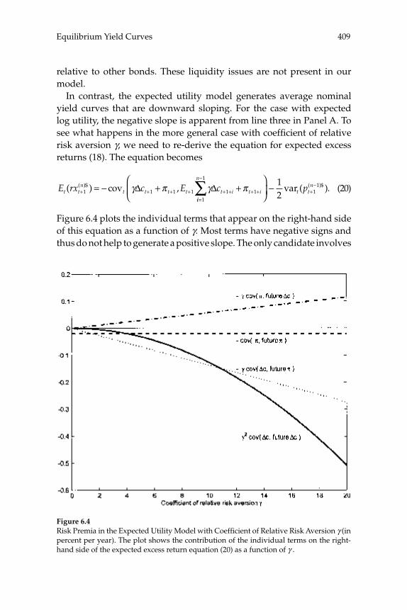
409Equilibrium Yield Curves
relative to other bonds. These liquidity issues are not present in our model.
In contrast, the expected utility model generates average nominal yield curves that are downward sloping. For the case with expected log utility, the negative slope is apparent from line three in Panel A. To see what happens in the more general case with coeffi cient of relative risk aversion γ, we need to re-derive the equation for expected excess returns (18). The equation becomes
E rx c E ct tn
t t t t t i( ) cov ,( )$+ + + + + += − +1 1 1 1 1γ π γΔ Δ
ii
n
t i t tnp
=
−
+ + +−∑ +
⎛
⎝⎜⎞
⎠⎟−
1
1
1 111
2π var ( ).( )$ (20)
Figure 6.4 plots the individual terms that appear on the right-hand side of this equation as a function of γ. Most terms have negative signs and thus do not help to generate a positive slope. The only candidate involves
Figure 6.4Risk Premia in the Expected Utility Model with Coeffi cient of Relative Risk Aversion γ (in percent per year). The plot shows the contribution of the individual terms on the right-hand side of the expected excess return equation (20) as a function of γ .
Piazzesi and Schneider410
the covariance between infl ation and expected future consumption growth, covt (πt+1, Et+1Σ
ni–=11γΔct+1+i). This term is positive, because of the
minus sign in equation (20) and the fact that positive infl ation surprises forecast lower future consumption growth. With a higher γ, the impor-tance of this term goes up. However, as we increase γ, the persistence of consumption growth becomes more and more important, and the real yield curve becomes steeply downward sloping. Since this effect is quadratic in γ, it even leads to a downward-sloping nominal curve. The intuitive explanation is that long real bonds have high payoffs precisely when current and future expected consumption growth is low. This makes them attractive assets to hold and so the real yield curve slopes down. When γ is high, this effect dominates also for nominal bonds.
3.5 Average Real Yields
At the preference parameters we report, the benchmark model also pro-duces a downward sloping real yield curve. The short real rate is already low, .84 percent, while long real rates are an additional .60 percentage point lower. It is diffi cult to assess the plausibility of this property of the model without a long sample on real yields for the United States. In the United Kingdom, where indexed bonds have been trading for a long time, the real yield curve seems to be downward sloping. Table 6B.3 reports statistics for these bonds. For the early sample (January 1983–November 1995), these numbers are taken from table 1 in Evans (1998). For the period after that (December 1995–March 2006), we use data from the Bank of England website. Relatedly, table 1 in Barr and Campbell (1997) documents that average excess returns on real bonds in the UK are negative.
In the United States, indexed bonds, so-called TIPS, have started trading only recently, in 1997. During this time period, the TIPS curve has been mostly upward sloping. For example, mutual funds that hold TIPS—such as the Vanguard Infl ation-Protected Securities Fund—have earned substantial returns, especially during the early years. Based on the raw TIPS data, J. Huston McCulloch has constructed real yield curves. Table 6B.4 in Appendix B documents that the average real yield curve in these data is upward sloping. The average real short rate is .8 percent, while the average fi ve-year yield is 2.2 percent.
These statistics have to be interpreted with appropriate caution. First, the short sample for which we have TIPS data and, more importantly, the low risk of infl ation during this short sample make it diffi cult to
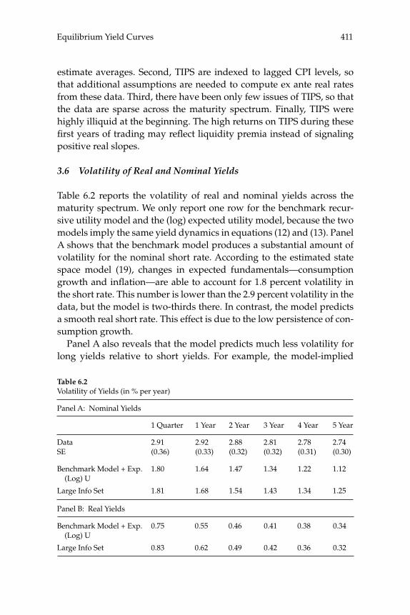
411Equilibrium Yield Curves
estimate averages. Second, TIPS are indexed to lagged CPI levels, so that additional assumptions are needed to compute ex ante real rates from these data. Third, there have been only few issues of TIPS, so that the data are sparse across the maturity spectrum. Finally, TIPS were highly illiquid at the beginning. The high returns on TIPS during these fi rst years of trading may refl ect liquidity premia instead of signaling positive real slopes.
3.6 Volatility of Real and Nominal Yields
Table 6.2 reports the volatility of real and nominal yields across the maturity spectrum. We only report one row for the benchmark recur-sive utility model and the (log) expected utility model, because the two models imply the same yield dynamics in equations (12) and (13). Panel A shows that the benchmark model produces a substantial amount of volatility for the nominal short rate. According to the estimated state space model (19), changes in expected fundamentals—consumption growth and infl ation—are able to account for 1.8 percent volatility in the short rate. This number is lower than the 2.9 percent volatility in the data, but the model is two-thirds there. In contrast, the model predicts a smooth real short rate. This effect is due to the low persistence of con-sumption growth.
Panel A also reveals that the model predicts much less volatility for long yields relative to short yields. For example, the model-implied
Table 6.2Volatility of Yields (in % per year)
Panel A: Nominal Yields
DataSE
Benchmark Model + Exp. (Log) U
Large Info Set
1 Quarter
2.91(0.36)
1.80
1.81
1 Year
2.92(0.33)
1.64
1.68
2 Year
2.88(0.32)
1.47
1.54
3 Year
2.81(0.32)
1.34
1.43
4 Year
2.78(0.31)
1.22
1.34
5 Year
2.74(0.30)
1.12
1.25
Panel B: Real Yields
Benchmark Model + Exp. (Log) U
Large Info Set
0.75
0.83
0.55
0.62
0.46
0.49
0.41
0.42
0.38
0.36
0.34
0.32

Piazzesi and Schneider412
fi ve-year yield has a volatility of 1.1 percent, while the fi ve-year yield in the data has a volatility of 2.7 percent. While the volatility curve in the data is also downward sloping, the slope of this curve is less pro-nounced than in the model. This relationship between the volatility of long yields relative to the volatility of short yields is the excess vola-tility puzzle. This puzzle goes back to Shiller (1979) who documents that long yields derived from the expectations hypothesis are not vola-tile enough. According to the expectations hypothesis, long yields are conditional expected values of future short rates. It turns out that the persistence of the short rate is not high enough to generate enough volatility for long yields. Shiller’s argument applies to our benchmark specifi cation, because risk premia in equation (17) are constant, and the expectations hypothesis holds. Below, we will show that our specifi ca-tion with learning produces more volatility for long yields.
Panel B shows that the volatility curve of real bonds also slopes down. Tables 6B.3 and 6B.4 in Appendix B show that this feature is also present in the UK indexed yield data and the McCullogh real yields for the United States.
3.7 Frequency Decompositions and the Monetary Experiment
To better understand the properties of the model, we use a band-pass fi lter to estimate trend and cyclical components of yields. The fi lters iso-late business-cycle fl uctuations in yields that persist for periods between one and a half and eight years from those that persist longer than eight years. Figure 6.5 plots the various estimated components. The top left panel shows the low frequency components of the model-implied short rate as well as the observed short rate and infl ation. The plots show that the model captures the fact that the low frequency component in nomi-nal yields is strongly correlated with infl ation. At these low frequencies, the main difference between model and data is the experience of the mid 1980s. When infl ation started to come down at the end of the 1970s, nominal yields stayed high well into the 1980s. According to bench-mark beliefs—which are estimated over the whole data sample and which ignore parameter uncertainty—infl ation forecasts came down as soon as infl ation started to decline. The basic mechanism behind these changes in infl ation expectations is persistence; since infl ation is close to a random walk, infl ation forecasts for next quarter are close to this quarter’s value of infl ation. As a consequence, infl ation forecasts in the early 1980s fell dramatically, right after infl ation went down. In
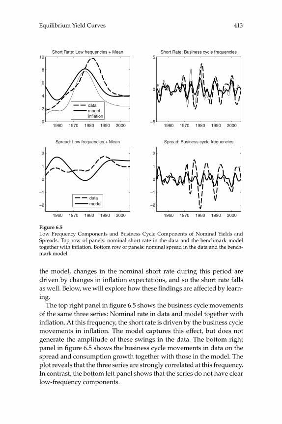
413Equilibrium Yield Curves
the model, changes in the nominal short rate during this period are driven by changes in infl ation expectations, and so the short rate falls as well. Below, we will explore how these fi ndings are affected by learn-ing.
The top right panel in fi gure 6.5 shows the business cycle movements of the same three series: Nominal rate in data and model together with infl ation. At this frequency, the short rate is driven by the business cycle movements in infl ation. The model captures this effect, but does not generate the amplitude of these swings in the data. The bottom right panel in fi gure 6.5 shows the business cycle movements in data on the spread and consumption growth together with those in the model. The plot reveals that the three series are strongly correlated at this frequency. In contrast, the bottom left panel shows that the series do not have clear low-frequency components.
1960 1970 1980 1990 20000
2
4
6
8
10Short Rate: Low frequencies + Mean
datamodelinflation
1960 1970 1980 1990 2000−5
0
5Short Rate: Business cycle frequencies
1960 1970 1980 1990 2000
−2
−1
0
1
2
Spread: Low frequencies + Mean
datamodel
1960 1970 1980 1990 2000
−2
−1
0
1
2
Spread: Business cycle frequencies
Figure 6.5Low Frequency Components and Business Cycle Components of Nominal Yields and Spreads. Top row of panels: nominal short rate in the data and the benchmark model together with infl ation. Bottom row of panels: nominal spread in the data and the bench-mark model
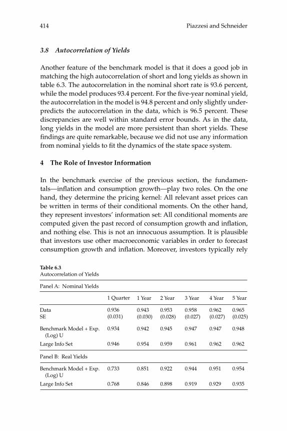
Piazzesi and Schneider414
3.8 Autocorrelation of Yields
Another feature of the benchmark model is that it does a good job in matching the high autocorrelation of short and long yields as shown in table 6.3. The autocorrelation in the nominal short rate is 93.6 percent, while the model produces 93.4 percent. For the fi ve-year nominal yield, the autocorrelation in the model is 94.8 percent and only slightly under-predicts the autocorrelation in the data, which is 96.5 percent. These discrepancies are well within standard error bounds. As in the data, long yields in the model are more persistent than short yields. These fi ndings are quite remarkable, because we did not use any information from nominal yields to fi t the dynamics of the state space system.
4 The Role of Investor Information
In the benchmark exercise of the previous section, the fundamen-tals—infl ation and consumption growth—play two roles. On the one hand, they determine the pricing kernel: All relevant asset prices can be written in terms of their conditional moments. On the other hand, they represent investors’ information set: All conditional moments are computed given the past record of consumption growth and infl ation, and nothing else. This is not an innocuous assumption. It is plausible that investors use other macroeconomic variables in order to forecast consumption growth and infl ation. Moreover, investors typically rely
Table 6.3Autocorrelation of Yields
Panel A: Nominal Yields
DataSE
Benchmark Model + Exp. (Log) U
Large Info Set
1 Quarter
0.936(0.031)
0.934
0.946
1 Year
0.943(0.030)
0.942
0.954
2 Year
0.953(0.028)
0.945
0.959
3 Year
0.958(0.027)
0.947
0.961
4 Year
0.962(0.027)
0.947
0.962
5 Year
0.965(0.025)
0.948
0.962
Panel B: Real Yields
Benchmark Model + Exp. (Log) U
Large Info Set
0.733
0.768
0.851
0.846
0.922
0.898
0.944
0.919
0.951
0.929
0.954
0.935
415Equilibrium Yield Curves
on sources of information that do not come readily packaged as statis-tics, such as their knowledge of institutional changes or future mon-etary policy.
In this section, we extend the model to accommodate a larger inves-tor information set. In particular, we use yields themselves to model agents’ information. We proceed in two steps. First, we estimate an unrestricted state space system of the type (19) that contains not only consumption growth and infl ation, but also the short rate and the yield spread. At this stage, we ignore the fact that the model itself places restrictions on the joint dynamics of these variables—the only purpose of the estimation is to construct agents’ information set. The second step of the exercise is then the same as in the benchmark case: We com-pute model-implied yields and compare them to the yields in the data.
The motivation for this particular way of modeling investor infor-mation comes from the theoretical model itself. If the data were in fact generated by a model economy in which yields are equal to investors’ expectations of consumption growth and infl ation, our approach would perfectly recover all investor information relevant for the analysis of the yield curve. To illustrate, suppose that the short rate is given by
yt(1)$ = Et[Δct+1 + πt+1|It] + constant,
where It is the investor information set, which contains past consump-tion growth, infl ation, and yields, but perhaps also other variables that we do not know about.
Suppose further that our unrestricted estimation delivers the true joint distribution of Δct+1, πt+1,yt
(1)$ and yt(20)$. The sequence of model-
implied short rates computed in the second step of our exercise, is then, up to a constant,
E c c y yt t tt[ |( , , , ) ].( )$ ( )$Δ Δ+ + =+1 1
1 201π πτ τ τ τ τ
The law of iterated expectations implies that this sequence should exactly recover the data yt
$(1). A similar argument holds for the yield spread. The series of model-implied yield changes would thus be identical to yield changes in the data. In other words, if the benchmark model replicates observed yield changes for some information struc-ture under rational expectations, then it will generate observed yield changes also under the particular information structure we consider here.
The joint model of fundamentals and yields takes the same general form as the system (19), except that it allows for four state variables and
Piazzesi and Schneider416
four observables, which implies that 42 parameters must be estimated. Table 6A.2 in Appendix A contains these parameter estimates. Figure 6.6 compares the autocovariance functions of the four observables in the data and for the estimated model. A fi rst order state space structure appears to do a reasonable job in capturing the joint dynamics of funda-mentals and yields. According to these estimated dynamics, low short rates and high spreads predict lower consumption growth. Moreover, high short rates and low spreads predict high infl ation rates. The key question for our model is whether these real and nominal growth pre-dictions arise from additional information contained in yields.
When we compute the model-implied short rate and term spread with a “Large Info Set”, they look very much like those from the bench-mark. Figure 6.7 plots these series, together with the data and the benchmark results. Summary statistics on model-implied yields from this “Large Info Set” model are also included in tables 6.1 and 6.2. Inter-estingly, average nominal yields in table 6.1 based on a “Large Info Set” are somewhat lower than in the benchmark, when we evaluate the two models at the same preference parameter values. The intuitive explana-tion is that more information lowers risk in the model. Line 5 of table 6.1 rephrases this fi nding: If we want to match the average slope of the nominal yield curve with a “Large Info Set,” we need to rely on more risk aversion, γ = 85 instead of the benchmark value of γ = 59, and a similar discount factor β = 1.005. Nevertheless, the results are overall very similar to the benchmark case. We conclude that not much is lost by restricting the investor information set to contain only past infl ation and consumption growth.
The key point from this exercise is that the short rate and the yield spread do not contain much more information about future consump-tion growth and infl ation than is already contained current and past consumption growth and infl ation. Another way to see this is to run regressions of future real and nominal growth rates on current val-ues of the four variables Δct, πt, yt
(1)$, and yt(20)$. In the one-step ahead
real growth regression, the coeffi cient on consumption growth is .26 with a t-statistic of 4.2 and the coeffi cient on infl ation is –.11 with a t-statistic of –1.85. (These t-statistics are based on Newey-West standard errors.) The coeffi cients on yields are not signifi cant and also economi-cally tiny, around 0.0015. The R2 in this regression is 16 percent. In four-step ahead and eight-step ahead growth regressions, infl ation becomes more important, but yields remain insignifi cant. In the one-step ahead nominal growth regression, we fi nd the same pattern. The coeffi cient
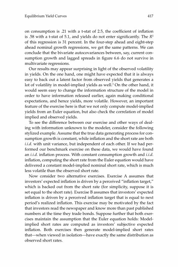
417Equilibrium Yield Curves
on consumption is .21 with a t-stat of 2.5, the coeffi cient of infl ation is .58 with a t-stat of 5.1, and yields do not enter signifi cantly. The R2 of this regression is 31 percent. In the four-step ahead and eight-step ahead nominal growth regressions, we get the same patterns. We can conclude that the bivariate autocovariances between, say, current con-sumption growth and lagged spreads in fi gure 6.6 do not survive in multivariate regressions.
Our results may appear surprising in light of the observed volatility in yields. On the one hand, one might have expected that it is always easy to back out a latent factor from observed yields that generates a lot of volatility in model-implied yields as well.3 On the other hand, it would seem easy to change the information structure of the model in order to have information released earlier, again making conditional expectations, and hence yields, more volatile. However, an important feature of the exercise here is that we not only compute model-implied yields from an Euler equation, but also check the correlation of model implied and observed yields.
To see the difference between our exercise and other ways of deal-ing with information unknown to the modeler, consider the following stylized example. Assume that the true data generating process for con-sumption growth is constant, while infl ation and the short rate are both i.i.d. with unit variance, but independent of each other. If we had per-formed our benchmark exercise on these data, we would have found an i.i.d. infl ation process. With constant consumption growth and i.i.d. infl ation, computing the short rate from the Euler equation would have delivered a constant model-implied nominal short rate, which is much less volatile than the observed short rate.
Now consider two alternative exercises. Exercise A assumes that investors’ expected infl ation is driven by a perceived “infl ation target,” which is backed out from the short rate (for simplicity, suppose it is set equal to the short rate). Exercise B assumes that investors’ expected infl ation is driven by a perceived infl ation target that is equal to next period’s realized infl ation. This exercise may be motivated by the fact that investors read the newspaper and know more than past published numbers at the time they trade bonds. Suppose further that both exer-cises maintain the assumption that the Euler equation holds: Model-implied short rates are computed as investors’ subjective expected infl ation. Both exercises then generate model-implied short rates that—when viewed in isolation—have exactly the same distribution as observed short rates.
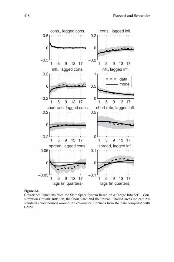
Piazzesi and Schneider418
1 5 9 13 17−0.5
0
0.5cons., lagged cons.
1 5 9 13 17−0.2
0
0.2cons., lagged infl.
1 5 9 13 17−0.2
0
0.2infl., lagged cons.
1 5 9 13 170
0.5
1infl., lagged infl.
datamodel
1 5 9 13 17−0.2
0
0.2short rate, lagged cons.
1 5 9 13 170
0.5short rate, lagged infl.
1 5 9 13 17−0.05
0
0.05spread, lagged cons.
lags (in quarters)1 5 9 13 17
−0.1
0
0.1spread, lagged infl.
lags (in quarters)
Figure 6.6Covariance Functions from the State Space System Based on a “Large Info Set”—Con-sumption Growth, Infl ation, the Short Rate, and the Spread. Shaded areas indicate 2 × standard errors bounds around the covariance functions from the data computed with GMM
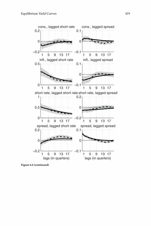
419Equilibrium Yield Curves
Figure 6.6 (continued)
1 5 9 13 17−0.2
0
0.2cons., lagged short rate
1 5 9 13 17−0.1
0
0.1cons., lagged spread
1 5 9 13 170
0.5infl., lagged short rate
1 5 9 13 17−0.1
0
0.1infl., lagged spread
1 5 9 13 170
0.5
1short rate, lagged short rate
1 5 9 13 17−0.2
0
0.2short rate, lagged spread
1 5 9 13 17−0.2
0
0.2spread, lagged short rate
lags (in quarters)1 5 9 13 17
−0.1
0
0.1spread, lagged spread
lags (in quarters)
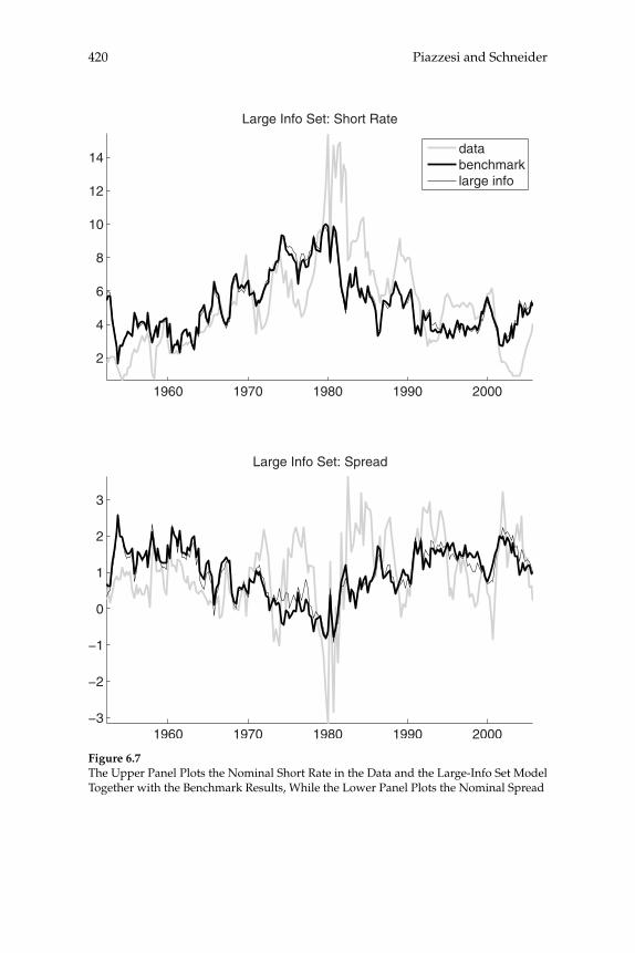
Piazzesi and Schneider420
1960 1970 1980 1990 2000
2
4
6
8
10
12
14
Large Info Set: Short Rate
databenchmarklarge info
1960 1970 1980 1990 2000−3
−2
−1
0
1
2
3
Large Info Set: Spread
Figure 6.7The Upper Panel Plots the Nominal Short Rate in the Data and the Large-Info Set Model Together with the Benchmark Results, While the Lower Panel Plots the Nominal Spread
421Equilibrium Yield Curves
In spite of their success in generating volatility, both exercises miss key aspects of the joint distribution of infl ation and the short rate. In Exercise A, model-implied expected infl ation is independent of actual infl ation one period ahead, which is inconsistent with rational expecta-tions. This happens because the infl ation target is backed out from the short rate, which here moves in the data for reasons that have nothing to do with infl ation or infl ation expectations. In Exercise B, the model implied short rate is perfectly correlated with infl ation one period ahead, while these variables are independent in the data.
The exercise of this section avoids the problems of either Exercise A or B. If the fi rst step estimation had been done using the example data, we would have found independence of infl ation and the short rate. As a result, the model-implied short rate based on the estimated informa-tion set would be exactly the same as in the benchmark case. The model would thus again imply constant short rates. We would thus have cor-rectly inferred that yields do not contain information about future infl a-tion and consumption growth, than is contained in the fundamentals themselves. As a result, any model economy where the Euler equation holds and beliefs are formed via rational expectations produces model-implied yields that are less volatile than observed yields.
5 Learning
In the benchmark exercise of section 3, investor beliefs about funda-mentals are assumed to be conditional probabilities of a process that was estimated using all data through 2005. This approach has three a priori unattractive properties. First, it ignores the fact that investors in, say, 1980 only had access to data up to 1980. Second, it assumes that agents believed in the same stationary model throughout the postwar period. This is problematic given that the 1970s are often viewed as a period of structural change. Indeed, the decade witnessed the fi rst ever peacetime infl ation in the United States, the breakdown of leading mac-roeconomic models, as well as signifi cant innovation in bond markets. Third, the benchmark beliefs were based on point estimates of the forc-ing process, ignoring the fact that the parameters of the process itself are not estimated with perfect precision, and investors know this.
In this section, we construct a sequence of investor beliefs that do not suffer from the above drawbacks. We maintain the hypothesis that, at every date t, investors form beliefs based on a state space system of the form (19). However, we re-estimate the system for every date t using
Piazzesi and Schneider422
only data up to date t. To accommodate investor concern with struc-tural change, we maximize a modifi ed likelihood function that puts more weight on more recent observations. To model investor concern with parameter uncertainty, we combine the state space dynamics with a Bayesian learning scheme about mean fundamentals.
5.1 Beliefs
Formally, beliefs for date t are constructed in three steps. We fi rst remove the mean from the fundamentals zt = (Δct,πt)
T. Let υ ∈ (0,1) denote a “forget factor” that defi nes a sequence of geometrically declining sam-ple weights. The weighted sample mean for date t is
ˆ ( ) .μ υ υzi
i
ti
t ii
t
t z=⎛
⎝⎜⎞
⎠⎟=
− −
−=
−
∑ ∑0
1 1
0
1
(21)
The sequences of estimated means for consumption growth and infl a-tion pick up the low frequency components in fundamentals.
5.1.1 Adaptive Learning In a second step, we estimate the state space system (19) using data up to date t by minimizing the criterion
− Ω + − −=
−
− − −∑12 0
1
1υ μi
i
t
t i z t iz t x[logdet ( ˆ ( ) ) ΩΩ−− − −− −1
1( ˆ ( ) )]z t xt i z t iμ (22)
starting at x0 = 0. Maximum likelihood estimation amounts to the spe-cial case υ = 1; it minimizes the equally weighted sum of squared in-sample forecast errors. In contrast, the criterion (22) penalizes recent forecast errors more heavily than those in the distant past. Ljung and Soderstrom (1987) and Sargent (1993) advocate this approach to adap-tive learning in situations where the dynamics of a process may change over time.
The forget factor υ determines how quickly past data are down-weighted. For most of our results, we use υ = .99, which implies that the data point from 17 years ago receives about one–half the weight of the most recent data point. To allow an initial sample for the estimation, the fi rst belief is constructed for 1965:1. The analysis of yields in this section will thus be restricted to the period since 1965. As in the benchmark case, the estimation step not only delivers estimates for the matrices φx, K, and Ω, but also estimates for the sequence of states (xτ )
tτ =1, starting
from x0 = 0. In particular, we obtain an estimate of the current state xt
T
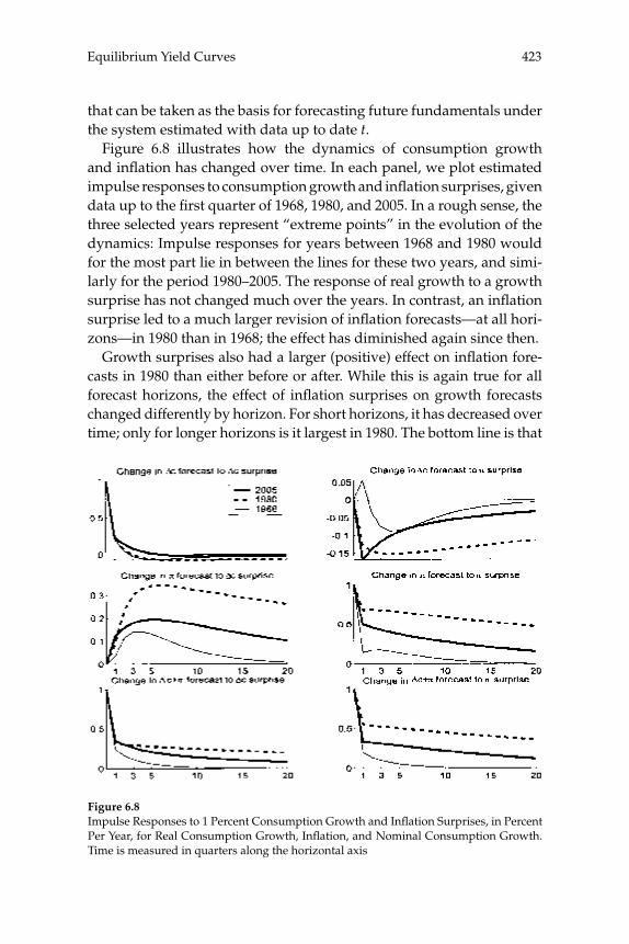
423Equilibrium Yield Curves
that can be taken as the basis for forecasting future fundamentals under the system estimated with data up to date t.
Figure 6.8 illustrates how the dynamics of consumption growth and infl ation has changed over time. In each panel, we plot estimated impulse responses to consumption growth and infl ation surprises, given data up to the fi rst quarter of 1968, 1980, and 2005. In a rough sense, the three selected years represent “extreme points” in the evolution of the dynamics: Impulse responses for years between 1968 and 1980 would for the most part lie in between the lines for these two years, and simi-larly for the period 1980–2005. The response of real growth to a growth surprise has not changed much over the years. In contrast, an infl ation surprise led to a much larger revision of infl ation forecasts—at all hori-zons—in 1980 than in 1968; the effect has diminished again since then.
Growth surprises also had a larger (positive) effect on infl ation fore-casts in 1980 than either before or after. While this is again true for all forecast horizons, the effect of infl ation surprises on growth forecasts changed differently by horizon. For short horizons, it has decreased over time; only for longer horizons is it largest in 1980. The bottom line is that
Figure 6.8Impulse Responses to 1 Percent Consumption Growth and Infl ation Surprises, in Percent Per Year, for Real Consumption Growth, Infl ation, and Nominal Consumption Growth. Time is measured in quarters along the horizontal axis
Piazzesi and Schneider424
both the persistence of infl ation and its role as an indicator of bad times became temporarily stronger during the great infl ation of the 1970s.
Performing the estimation step for every date t delivers not only sequences of parameter estimates, but also estimates of the current state xt. Computing conditional distributions given xt date by date produces a sequence of investor beliefs. The subjective belief at date t determines investors’ evaluation of future utility and asset payoffs at date t. We thus use this belief below to calculate expectations of the pricing kernel, that is, yields, for date t. In contrast to the benchmark approach, the exercise of this section does not impose any direct restriction on beliefs across different dates; for example, it does not require that all beliefs are conditionals of the same probability over sequences of data. The updat-ing of beliefs is thus implicit in the sequential estimation.
The model also does not impose a direct link between investor beliefs and some “true data generating process,” as the benchmark approach does by imposing rational expectations. The belief at date t captures investors’ subjective distribution over fundamentals at date t. It is con-strained only by past observations (via the estimation step), and not by our (the modelers’) knowledge of what happened later. At the same time, our approach does impose structural knowledge on the part of investors: Their theory of asset prices is based on the representative agent preferences that we use.
5.1.2 Parameter Uncertainty The third step in our construction of beliefs introduces parameter uncertainty. Here we focus exclusively on uncertainty about the estimated means. Our goal is to capture the intuition that, in times of structural change, it becomes more diffi cult to distinguish permanent and transitory changes in the economy. We thus assume that, as of date t, the investor views both the true mean μz and the current persistent (but transitory) component xt as random. The dis-tribution of zt can be represented by a system with four state variables:
z x ezτ τ τμ+ += + +1 1 ,
μφ
μφτ τ
z
x
z
xx
I
x Ke+
⎛⎝⎜
⎞⎠⎟
=⎛⎝⎜
⎞⎠⎟
⎛⎝⎜
⎞⎠⎟
+1
2 00
0 ττ +
⎛⎝⎜
⎞⎠⎟1
. (23)
The matrices φx, K, and Ω are assumed to be known and are taken from the date t estimation step.
In order to describe investors’ perception of risk, it is helpful to rewrite (23) so that investors—conditional expectations—rather than the unob-

425Equilibrium Yield Curves
servables μz and x—are the state variables. Let μz(τ) and xτ denote inves-tors’ expectations of μz and xτ, respectively, given their initial knowledge at date t as well as data up to date τ. We can rewrite (23) as
z x ezτ τ τμ τ+ += ( ) + +1 1ˆ ˆ ˆ ,
ˆ
ˆ
ˆ ( )ˆ
μ τφ
μ τ
τ
z
x
z
x
I
x
+( )⎛
⎝⎜⎞
⎠⎟=
⎛⎝⎜
⎞⎠⎟+
1 001
2
ττ
μτ
τφ τ
⎛
⎝⎜⎞
⎠⎟+
+( )+( )
⎛
⎝⎜
⎞
⎠⎟ +
K
Ke
x z
1
1 1ˆ , (24)
where eτ+1 is investors’ one step ahead forecast error of the data zr+1.
The matrices Kμ(τ + 1) and Kz(τ + 1) can be derived by applying Bayes’ Rule. They vary over time, because the learning process is nonstation-ary. Early on, the investor expects to adjust his estimate of, say, mean infl ation, a lot in response to an infl ation shock. As time goes by, the estimate of the mean converges, and the matrix Kμ converges to zero, while the matrix Kz reverts to the matrix K from (19).
To complete the description of investors’ belief, it remains to specify the initial distribution of μz and xt at date t. We assume that these vari-ables are jointly normally distributed, with the mean of μz given by the point estimate (21) and the mean of xt given by its point estimate from the date t estimation step. To specify the variance, we fi rst compute the weighted sum of squares
Σzi
i
ti
t i zi
t
t z t( ) ( ˆ ( ))=⎛
⎝⎜⎞
⎠⎟−
=
− −
−=
−
∑υ υ μ0
1 1
0
11
∑ − −⎛
⎝⎜⎞
⎠⎟( ˆ ( )) .z tt i zμ (25)
This provides a measure of overall uncertainty that the investor has recently experienced. We then compute the variance of the estimates (μz (t), xt) under the assumption that the system (24) was initialized at some date t – n, at a variance of Σz(t) for μz(t – n) and a variance of zero for xt–n.
The idea here is to have investors’ relative date t uncertainty about μz and x depend not only on the total variance in recent history, cap-tured by Σz(t), but also by the nature of recent dynamics, captured by the estimation step. For example, it should have been easier to dis-entangle temporary and permanent movements in infl ation from the data if infl ation has been less persistent recently. The above procedure captures such effects. Indeed, the main source of variation in investor beliefs for this exercise comes from the way the estimated dynamics of fi gure 6.8 change the probability that an infl ation surprise signals a permanent change in infl ation. The patterns for yields we report below remain essentially intact if we initialize beliefs at the same variance Σz
T
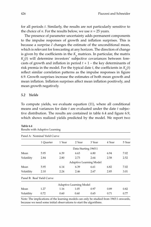
Piazzesi and Schneider426
for all periods t. Similarly, the results are not particularly sensitive to the choice of n. For the results below, we use n = 25 years.
The presence of parameter uncertainty adds permanent components to the impulse responses of growth and infl ation surprises. This is because a surprise e changes the estimate of the unconditional mean, which is relevant for forecasting at any horizon. The direction of change is given by the coeffi cients in the Kμ matrices. In particular, the matrix Kμ(t) will determine investors’ subjective covariances between fore-casts of growth and infl ation in period t + 1 – the key determinants of risk premia in the model. For the typical date t, the coeffi cients in Kμ(t) refl ect similar correlation patterns as the impulse responses in fi gure 6.9. Growth surprises increase the estimates of both mean growth and mean infl ation. Infl ation surprises affect mean infl ation positively, and mean growth negatively.
5.2 Yields
To compute yields, we evaluate equation (11), where all conditional means and variances for date t are evaluated under the date t subjec-tive distribution. The results are contained in table 6.4 and fi gure 6.9, which shows realized yields predicted by the model. We report two
Table 6.4Results with Adaptive Learning
Panel A: Nominal Yield Curve
Data Starting 1965:1
Adaptive Learning Model
Panel B: Real Yield Curve
Adaptive Learning ModelMean
Volatility
1.27
0.72
1.16
0.60
1.05
0.60
0.97
0.65
0.89
0.71
0.82
0.77
Mean
Volatility
Mean
Volatility
1 Quarter
5.95
2.84
5.95
2.10
1 Year
6.39
2.80
6.14
2.24
2 Year
6.63
2.73
6.39
2.46
3 Year
6.80
2.64
6.61
2.67
4 Year
6.94
2.58
6.82
2.85
5 Year
7.02
2.52
7.02
3.01
Note: The implications of the learning models can only be studied from 1965:1 onwards, because we need some initial observations to start the algorithms.

427Equilibrium Yield Curves
types of results. The results in table 6.4 allow only for adaptive learn-ing, without parameter uncertainty. For this case, we select the prefer-ence parameters so that the model matches the mean short rate and term spread, as for the previous exercises. Model-implied yields from an example with parameter uncertainty are presented in fi gure 6.9.
Implementing the case of parameter uncertainty for patient investors (β ≥ 1) requires us to choose a third parameter, the planning horizon T. To see why, consider how continuation utility (4) enters the pricing kernel (6). Utility next quarter depends on next quarter’s forecasts of future consumption growth, up to the planning horizon. As discussed above, the case of parameter uncertainty adds a permanent compo-nent to the impulse response of, say, an infl ation surprise: An infl ation surprise next quarter will lower expected consumption growth for all quarters up to the planning horizon. The “utility surprise” vt+1 – Etvt+1 therefore depends on the length of the planning horizon. Intuitively, an investor who lives longer and cares more strongly about the future, is more affected by the outcomes of future learning.4
It follows that, for patient investors with a long planning horizon, the effect of risk on utility can be as large (or larger) as the effect of mean consumption growth and infl ation. Since parameter uncertainty becomes the main driver of risk premia in this case, the planning hori-zon and the risk aversion coeffi cient have similar effects on the model results. For the results below, we use T = 25000 years and γ = 4, together with β = 1. At these parameter values, the model has interesting impli-cations for the behavior of the short rate and spread during the mon-etary experiment.
5.2.1 Adaptive Learning The short rate in the economy with adap-tive learning (not shown) behaves similarly to that in the benchmark model as long as there is little turbulence—the 1960s and early 1970s, and the 1990s. However, the model generates signifi cantly higher short rates during the monetary experiment and also somewhat higher rates during the mid–1980s. The new movements are brought about by changes in the dynamics. In particular, the investor’s subjective covari-ance between infl ation and future expected consumption increased a lot around 1980. This development was not just due to infl ation vola-tility: The correlation between infl ation and future consumption also increased. As the stagfl ation experience of the 1970s made its way into the beliefs of adaptive learners, our basic “infl ation as bad news” mech-anism was thus reinforced.
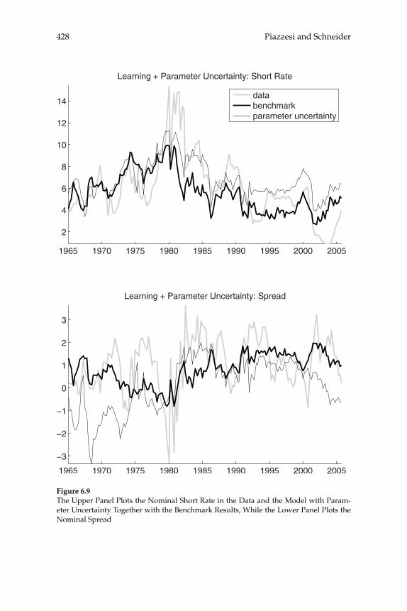
Piazzesi and Schneider428
1965 1970 1975 1980 1985 1990 1995 2000 2005
2
4
6
8
10
12
14
Learning + Parameter Uncertainty: Short Rate
databenchmarkparameter uncertainty
1965 1970 1975 1980 1985 1990 1995 2000 2005
−3
−2
−1
0
1
2
3
Learning + Parameter Uncertainty: Spread
Figure 6.9The Upper Panel Plots the Nominal Short Rate in the Data and the Model with Param-eter Uncertainty Together with the Benchmark Results, While the Lower Panel Plots the Nominal Spread

429Equilibrium Yield Curves
Since infl ation became such an important carrier of bad news, the 1980s not only increased the infl ation premium on short bonds in the adaptive learning economy, but also introduced large spikes in the term spread. In the data, the high short rates of 1980 were accompanied by historically low term spreads. In contrast, the adaptive learning model generates a large term spread, for the same reason as it generates high short rates. Apart from this outlier, the model economy does exhibit a low frequency trend in the spread, with higher spreads after the 1980s than before.
Model implied yields from the adaptive learning economy are remark-ably similar to the benchmark model immediately after the monetary experiment ended. The reason is that infl ation forecasts from both mod-els drop immediately as infl ation itself comes down. This result is quite robust to alternative specifi cations of the learning scheme, obtained for example by changing the forget rate or switching from geometric downweighting to a rolling window approach. We conclude that learn-ing does not induce inertia in infl ation forecasts; that can explain why interest rates remained high in the early 1980s.
5.2.2 Parameter Uncertainty The results with parameter uncertainty also look very different in the early 1980s compared to other years. The short rate tracks the benchmark until the late 1970s. However, it then peaks at a higher rate in 1981 and it remains high thereafter. Parameter uncertainty thus generates the sluggish adjustment of yields at the end of the monetary experiment. The economy with parameter uncertainty also exhibits a transition of the spread from negative values in the late 1970s to historically high values throughout the fi rst half of the 1980s. A similar transition took place in the data. Towards the end of the sam-ple, yields and spreads come down again; especially for the latter, the decline is more pronounced than in the data.5
Importantly, this is not due to sluggish infl ation expectations: By design, infl ation forecasts are the same in the adaptive learning and the parameter uncertainty exercises. Instead, the role of infl ation as bad news is here enhanced by the diffi culty investors face in disentangling permanent from transitory moves in infl ation. The increase in param-eter uncertainty through the 1970s implies that, in the early 1980s, there is a greater chance that an infl ation surprise signals a permanent shift in infl ation that would generate bad news. Since the (subjective) means of infl ation and consumption growth are also negatively correlated, the
Piazzesi and Schneider430
infl ation surprise would generate permanent bad news. For a patient investor, we obtain large movements in risk premia.
6 Related Literature
The literature on the term structure of interest rates is vast. In addition to a substantial body of work that documents the behavior of short and long interest rates and summarizes it using statistical and arbitrage-free models, there are literatures on consumption based asset pricing mod-els, as well as models of monetary policy and the business cycle that have implications for yields. There is also a growing set of papers that documents the importance of structural change in the behavior of inter-est rates and the macroeconomy. We discuss these groups of papers in turn.
6.1 Statistical and Arbitrage-Free Models
Average nominal yields are increasing and concave in maturity. Excess returns on nominal bonds are positive on average and also increasing in maturity. They are also predictable using interest rate information (Fama and Bliss 1987, Campbell and Shiller 1991). The latter fact con-tradicts the expectations hypothesis, which says that long rates are simply averages of expected future short rates, up to a constant. The expectations hypothesis also leads to an “excess volatility puzzle” for long bond prices, which is similar to the excess volatility of stock prices: Under rational expectations, one cannot reconcile the high volatility of nominal rates with observed persistence in short rates (Shiller 1979). A related literature documents “excess sensitivity” of long rates to par-ticular shocks, such as macroeconomic announcements (Gurkaynak, Sack, and Swanson 2005).
Another stylized fact is that nominal yields of all maturities are highly correlated. Litterman and Scheinkman (1991) have shown that a few principal components explain much of the variation in yields. For example, in our quarterly postwar panel data, 99.8 percent of the variation is explained by the fi rst and second principal components. Here the elephant in the room is the fi rst component, which alone cap-tures 98.2 percent of this variation and stands for the “level” of the yield curve. The second component represents changes the “slope” of the curve, while the third principal component represents “curvature” changes.
431Equilibrium Yield Curves
This fact has motivated a large literature on arbitrage-free models of the term structure. The goal here is to summarize the dynamics of the entire yield curve using a few unobservable factors. Recent work in this area explores the statistical relationship between term structure factors and macroeconomic variables. For example, the arbitrage-free model in Ang, Piazzesi, and Wei (2006) captures the role of the term spread as a leading indicator documented by the predictive regressions sur-veyed in Stock and Watson (1999). In this work, the only cross-equation restrictions on the joint distribution of macro variables and yields come from the absence of arbitrage.
In the present paper, our focus is on cross-equation restrictions induced by Euler equations, which directly link yields to conditional moments of macroeconomic variables. In particular, we focus on prop-erties of the short rate and a single yield spread and use these to link the level and slope of the yield curve to infl ation and the business cycle. The rational expectations exercises in sections 3 and 4 also impose the expectations hypothesis through our assumptions on preferences and the distribution of shocks. While this implies that the model econo-mies do not exhibit predictability and excess volatility of long yields, they are useful for understanding the macro underpinnings of average yields as well as the volatility of the level factor, which accounts in turn for the lion’s share of yield volatility. The learning exercises in section 5 do generate predictability in yields because of time variation in per-ceived risk.
6.2 Consumption-Based Asset Pricing Models
The representative agent asset pricing approach we follow in this paper takes the distribution of consumption growth and infl ation as exog-enous and then derives yields from Euler equations. Early applications assumed power utility. Campbell (1986) shows analytically that posi-tive serial correlation in consumption growth and infl ation leads to downward sloping yield curves. In particular, term spreads on long indexed bonds are negative because such bonds provide insurance against times of low expected consumption growth. Backus, Gregory, and Zin (1989) document a “bond premium puzzle”: Average returns of long bonds in excess of the short rate are negative and small for coef-fi cients of relative risk aversion below ten. Boudoukh (1993) considers a model with power utility where the joint distribution of consumption growth and infl ation is driven by a heteroskedastic VAR. Again, term

Piazzesi and Schneider432
premia are small and negative. The latter two papers also show that heteroskedasticity in consumption growth and infl ation, respectively, is not strong enough to generate as much predictability in excess bond returns as is present in the data. Chapman (1997) documents that ex-post real rates and consumption growth are highly correlated, at least outside the monetary policy experiment.
Our results show that the standard result of negative nominal term spreads is overturned with recursive utility if infl ation brings bad news. The form of recursive utility preferences proposed by Epstein and Zin (1989) and Weil (1989) has become a common tool for describ-ing investors’ attitudes towards risk and intertemporal substitution. Campbell (1999) provides a textbook exposition. An attractive feature of these preferences is that they produce plausible quantity implica-tions in business cycle models even for high values of the coeffi cient of relative risk aversion, as demonstrated by Tallarini (2000). Bansal and Yaron (2004) show that a model with recursive utility can also generate a high equity premium and a low risk free rate if consumption growth contains a small, but highly persistent, component. They argue that, even though empirical autocovariances of consumption growth do not reveal such a component, it is hard to refute its presence given the large transitory movements in consumption growth.
Our benchmark rational expectations exercise postulates a consump-tion process parameterized by our maximum likelihood point esti-mates. As a result, the autocovariances of consumption growth in our model are close to their empirical counterparts. The effects we derive are mostly due to the forecastability of consumption growth by infl a-tion, again suggested by our point estimates. Our learning exercise with parameter uncertainty plays off the fact that permanent and persistent transitory components can be hard to distinguish.
The literature has also considered utility specifi cations in which current marginal utility depends on a mean-reverting state variable. In habit formation models as well as in Abel’s (1999) model of “catch-ing up with the Joneses,” marginal utility not only depends on current consumption but also on consumption growth which is mean revert-ing. The presence of a mean-reverting state variable in marginal utility tends to generate an upward sloping yield curve: It implies that bond prices (expected changes in marginal utility) are negatively correlated with marginal utility itself. Since bonds thus pay off little precisely in times of need (when marginal utility is high), they command a pre-mium. Quantitative analysis of models of habit formation and catching
433Equilibrium Yield Curves
up with the Joneses showed that short real interest rates become very volatile when the models are calibrated to match the equity premium.
Campbell and Cochrane (1995) introduce a model in which marginal utility is driven by a weighted average of past innovations to aggre-gate consumption, where the weight on each innovation is positively related to the level of the marginal utility. With this feature, low current marginal utility need not imply extremely high bond prices, since the anticipation of less volatile weighted innovations in the future discour-ages precautionary savings and lowers bond prices. In their quantitative application, Campbell and Cochrane focus on equity and short bonds, and pick the weight function so that the real riskless rate is constant and the term structure is fl at. Wachter (2006) instead picks the weight func-tion to match features of the short rate dynamics. In a model driven by i.i.d. consumption growth and an estimated infl ation process, she shows that this approach accounts for several aspects of yield behavior, while retaining the results for equity from the Campbell-Cochrane model.6
6.3 Monetary and Business Cycle Models
The consumption based asset pricing approach we follow in this paper assumes a stochastic trend in consumption. In contrast, studies in the business cycle literature often detrend real variables, including con-sumption, in a fi rst step and then compare detrended data to model equilibria in which the level of consumption is stationary. This dis-tinction is important for the analysis of interest rates, since the pricing kernel (6), derived from the Euler equation, behaves very differently if consumption is stationary in levels or trend stationary (Labadie 1994).7 Alvarez and Jermann (2005) have shown that a permanent component must account for a large fraction of the variability of state prices if there are assets that have large premia over long–term bonds, as is the case in the data. A stochastic trend in consumption directly induces a large permanent component in real state prices.
Recently various authors have examined the term-structure impli-cations of New Keynesian models. The “macro side” of these models restricts the joint distribution of output, infl ation and the short nominal interest rate through an Euler equation—typically allowing for an effect of past output on current marginal utility as well as a taste shock—, a Phillips curve and a policy reaction function for the central bank. Lon-ger yields are then linked to the short rate via an exogenous pricing kernel (Rudebusch and Wu 2005, Beechey 2005) or directly through

Piazzesi and Schneider434
the pricing kernel implied by the Euler equation (Bekaert, Cho, and Moreno 2005, Hordahl, Tristani, and Vestin 2005, Ravenna and Seppala 2005). Our model differs from these studies in that it does not put theo-retical restrictions on the distribution of the macro variables and does not allow for taste shocks.
Our model assumes frictionless goods and asset markets. In partic-ular, there are no frictions associated with the exchange of goods for assets, which can help generate an upward sloping yield curve. For example, Bansal and Coleman (1996) derive a liquidity premium on long bonds in a model where short bonds are easier to use for transac-tions purposes. Alvarez, Atkeson, and Kehoe (1999) show that money injections contribute to an upward sloping real yield curve in a lim-ited participation model of money. This is because money injections generate mean reversion in the level of consumption of bond market participants. Seppala (2004) studies the real yield curve in a model with heterogeneous agents and limited commitment. He shows that incom-plete risk sharing helps to avoid a bond premium puzzle.
6.4 Learning
Our learning exercise builds on a growing literature that employs adaptive learning algorithms to describe agent beliefs. This literature is surveyed by Evans and Honkapohja (2001). Empirical applications to the joint dynamics of infl ation and real variables include Sargent (1999) and Marcet and Nicolini (2003). Carceles-Poveda and Giannit-sarou (2006) consider a Lucas asset pricing model where agents learn adaptively about aspects of the price function. In these studies, learn-ing often concerns structural parameters that affect the determination of endogenous variables. In our setup, investors learn only about the (reduced form) dynamics of exogenous fundamentals; they have full structural knowledge of the price function. Another feature of many adaptive learning applications is that standard errors on the re-esti-mated parameters are not taken into account by agents. In our model, standard errors are used to construct subjective variances around the parameters and investors’ anticipation of future learning is an impor-tant determinant of risk premia.
Learning has been applied to the analysis of the term structure by Fuhrer (1996), Kozicki and Tinsley (2001), and Cogley (2005). In these papers, the expectations hypothesis holds under investors’ subjective belief, as it does in our model. Fuhrer’s work is closest to ours in that
435Equilibrium Yield Curves
he also considers the relationship between macrovariables and yields, using an adaptive learning scheme. However, the link between yields and macroeconomic variables in his model is given by a policy reaction function with changing coeffi cients, rather than by an Euler equation as in our setting. His paper argues that changing policy coeffi cients induce expectations about short rates that generate inertia in long rates in the 1980s. In other words, inertia is due to changing conditional means. This is different from our results, where interest rates are tied to expected consumption growth and infl ation. This is why, in the context of our model, changes in conditional variances are more important.
Kozicki and Tinsley (2001) and Cogley (2005) use different learning models to show that the expectations hypothesis may seem to fail in the data even if it holds under investors’ subjective belief. Kozicki and Tinsley consider an adaptive learning scheme, while Cogley derives beliefs from a Bayesian VAR with time-varying parameters for yields, imposing the expectations hypothesis. Regime-switching models of interest rates deal with some of the same stylized facts on structural change as learning models. (For a survey, see Singleton 2006.) A key property is that they allow for time variation in conditional variances. Since this is helpful to capture the joint movements of infl ation and the short rate, regime switching is a prominent feature of statistical models that construct ex ante real rates from infl ation and nominal yield data. Veronesi and Yared (2001) consider an equilibrium model of the term structure with regime switching and power utility.
7 Conclusion
We see at least two interesting tasks for future research. The fi rst is to understand better the sources of yield volatility at business cycle fre-quencies. While some of the models presented in this paper exhibit sub-stantial volatility, and do quite well on low frequency movements in interest rate levels, none of them exhibits as much volatility at business cycle frequencies as we fi nd in the data, especially for the yield spread. One natural extension of our benchmark rational expectations model is to capture nonlinear features of the infl ation process through regime switching or other devices that allow conditional heteroskedasticity. In addition to generating more volatility, this might have interesting implications for the predictability of excess long bond returns. To eval-uate rational expectations models, the analysis in section 4—where we

Piazzesi and Schneider436
capture investors’ information using asset prices in a fi rst step before computing model implied yields—provides a way to evaluate many different information structures at the same time.
A second task is to develop further models in which changes in uncer-tainty have fi rst order effects on interest rates. We have provided one example of such a model and have shown that it holds some promise for understanding why interest rates were high in the 1980s, although infl ation expectations were low. However, more work is needed to rec-oncile the learning process with interest rates during other periods, and to integrate it more tightly with survey expectations. To this end, the tractable approach to learning that we consider in section 5—com-bining adaptive learning and parameter uncertainty—is less involved than a full Bayesian learning setup, but can nevertheless capture both agents’ understanding of the future dynamics of fundamentals and agents’ confi dence in how well they understand these dynamics.
Endnotes
1. To see this, we can write the excess return as
p p y ny n ytn
tn
t tn
tn
+−
+−− − = − −1
1 11
11( ) ( ) ( ) ( ) ( )( ) −− = − − − −+−y y y n y yt t
nt t
ntn( ) ( ) ( ) ( ) ( )( )( ).1 1
111
For large n and a long enough sample, the difference between the average (n – 1)-period yield and the average n-period yield is zero.
2. We are grateful to John Campbell for this suggestion.
3. Indeed, the quarterly variation in bond yields is well explained using a statistical fac-tor model with only two latent factors, or principal components. Intuitively, the lion share of the movements in nominal yields is up/down movements across the curve. The fi rst principal component of yields captures these so-called “level” movements which explain 98.22 percent of the total variation in yields. An additional 1.58 percent of the movements in yields is captured by the second principal component, which represents movements in the slope of the curve. Together, “level” and “slope” explain almost all, 99.80 percent, of the variation in yields.
4. This effect is not present without parameter uncertainty, because the random com-ponent of future consumption growth forecasts then converges to zero with the forecast horizon. Therefore, as long as the planning horizon is long enough, it does not matter for the utility surprise even if β > 1.
5. The parameter uncertainty model also generates low spreads at the beginning of the sample. As for the adaptive learning model, the behavior in this period is driven in part by the fact that the samples used in the sequential estimation are as yet rather short.
6. The New Keynesian model of Bekaert, Cho, and Moreno (2005) assumes “catching up with the Joneses” together with a taste shock to marginal utility. This is another way to reconcile the behavior of yields with a habit formation model.
437Equilibrium Yield Curves
7. In particular, if consumption reverts to its mean, “good” shocks that increase con-sumption lead to lower expected consumption growth and hence lower real interest rates and higher real bond prices. This is exactly the opposite of the effect discussed in section 2, where “good” shocks that increase consumption growth leads to higher expected con-sumption growth and hence higher real interest rates and lower bond prices.
References
Abel, A. B. 1999. “Risk Premia and Term Premia in General Equilibrium.” Journal of Mon-etary Economics 43: 3–33.
Alvarez, F., and U. Jermann. 2005. “Using Asset Prices to Measure the Persistence of the Marginal Utility of Wealth.” Econometrica 73(6): 1977–2016.
Alvarez, F., A. Atkeson, and P. J. Kehoe. 2005. “Time-Varying Risk, Interest Rates and Exchange Rates in General Equilibrium.” Federal Reserve Bank of Minneapolis Working Paper no. 627.
Alvarez, F., A. Atkeson, and P. J. Kehoe. 1999. “Money and Interest Rates with Endoge-neously Segmented Markets.” NBER Working Paper no. 7060. Cambridge, MA: National Bureau of Economic Research.
Ang, A., M. Piazzesi, and M. Wei. 2006. “What Does the Yield Curve tell us about GDP Growth?” Journal of Econometrics 131: 359–403.
Backus, D., A. Gregory, and S. Zin. 1989. “Risk Premiums in the Term Structure: Evidence from Artifi cial Economies.” Journal of Monetary Economics 24: 371–399.
Bansal, R., and W. J. Coleman II. 1996. “A Monetary Explanation of the Equity Premium, Term Premium, and Riskfree Rate Puzzles.” Journal of Political Economy 104: 1135–1171.
Bansal, R., and A. Yaron. 2004. “Risks for the Long Run: A Potential Resolution of Asset Pricing Puzzles.” Journal of Finance 59: 1481–1509.
Barr, D. G., and J. Y. Campbell. 1997. “Infl ation, Real Interest Rates, and the Bond Market: A Study of UK Nominal and Index-Linked Government Bond Prices.” Journal of Monetary Economics 39: 361–383.
Beechey, M. 2005. “Excess Sensitivity and Volatility of Long Interest Rates: The Role of Limited Information in Bond Markets.” Working Paper. Berkeley, CA: UC Berkeley.
Bekaert G., S. Cho, and A. Moreno. 2005. “New-Keynsian Macroeconomics and the Term Structure.” NBER Working Paper no. 11340. Cambridge, MA: National Bureau of Eco-nomic Research.
Boudoukh J. 1993. “An Equilibrium Model of Nominal Bond Prices with Infl ation-Output Correlation and Stochastic Volatility.” Journal of Money, Credit, and Banking 25: 636–665.
Campbell, J. Y. 1986. “Bond and Stock Returns in a Simple Exchange Model.” Quarterly Journal of Economics 101(4): 785–803.
Campbell, J. Y. 1993. “Intertemporal Asset Pricing without Consumption Data.” American Economic Review 83: 487–512.
Campbell, J. Y. 1996. “Understanding Risk and Return.” Journal of Political Economy 104: 298–345.
Piazzesi and Schneider438
Campbell, J. Y. 1999. “Asset Prices, Consumption, and the Business Cycle.” In J. Taylor and M. Woodford, eds., Handbook of Macroeconomics 1(19): 1231–1303.
Campbell, J. Y., and J. H. Cochrane. 1995. “By Force of Habit: A Consumption-Based Explanation of Aggregate Stock Market Behavior.” NBER Working Paper no. 4995. Cam-bridge, MA: National Bureau of Economic Research.
Campbell, J. Y., and R. J. Shiller. 1991. “Yield Spreads and Interest Rate Movements: A Bird’s Eye View.” Review of Economic Studies 58: 495–514.
Carceles-Poveda, E., and C. Giannitsarou. 2006. “Asset Pricing with Adaptive Learning.” Working Paper. University of Cambridge.
Chapman, D. 1997. “The Cyclical Properties of Consumption Growth and the Real Term Structure.” Journal of Monetary Economics 39: 145–172.
Cogley, T. 2005. “Changing Beliefs and the Term Structure of Interest Rates: Cross-Equa-tion Restrictions with Drifting Parameters.” Review of Economic Dynamics 8: 420–451.
Duffi e, D., and L. Epstein. 1992. “Stochastic Differential Utility.” Econometrica 60(2): 353–394.
Duffi e, D., M. Schroeder, and C. Skiadas. 1997. “A Term Structure Model with Preferences for the Timing of Resolution of Uncertainty.” Economic Theory 9: 3–22.
Epstein, L., and S. Zin. 1989. “Substitution, Risk Aversion and the Temporal Behavior of Consumption and Asset Returns: A Theoretical Framework.” Econometrica 57: 937–969.
Evans, M. D. 1998. “Real Rates, Expected Infl ation, and Infl ation Risk Premia.” Journal of Finance 53(1): 187–218.
Evans, G. W., and S. Honkapohja. 2001. Learning and Expectations in Macroeconomics. Princeton University Press, Princeton, NJ.
Fama, E. F., and R. R. Bliss. 1987. “The Information in Long-Maturity Forward Rates.” American Economic Review 77: 680–692.
Fuhrer, J. 1996. “Monetary Policy Shifts and Long-Term Interest Rates.” Quarterly Journal of Economics 111(4): 1183–1209.
Gurkaynak, R., B. Sack, and E. Swanson. 2005. “The Sensitivity of Long-Term Interest Rates to Economic News: Evidence and Implications for Macroeconomic Models.” Ameri-can Economic Review 95(1): 425–436.
Hansen, L. P., J. C. Heaton, and N. Li. 2005. “Consumption strikes back? Measuring Long Run Risk.” Working Paper. Chicago: University of Chicago.
Hordahl, P., O. Tristani, and D. Vestin. 2005. “The Yield Curve and Macroeconomic Dynamics.” Working Paper. European Central Bank.
Kozicki, S., and P. A. Tinsley. 2001. “Shifting Endpoints in the Term Structure of Interest Rates.” Journal of Monetary Economics 47: 613–652.
Labadie, P. 1994. “The Term Structure of Interest Rates over the Business Cycle.” Journal of Economic Dynamics and Control 18(3-4): 671–697.
Litterman, R., and J. Scheinkman. 1991. “Common factors affecting bond returns.” Journal of Fixed Income 1, 54–61.
439Equilibrium Yield Curves
Ljung, L., and T. Soderstrom. 1987. “Theory and Practice of Recursive Identifi cation.” Cam-bridge, MA: MIT Press.
Marcet, A., and J. P. Nicolini. 2003. “Recurrent Hyperinfl ations and Learning.” American Economic Review 93(5): 1476–1498.
Ravenna, F. , and J. Seppala. 2005. “Monetary Policy and Rejections of the Expectations.” Working Paper, University of Illinois.
Restoy, F., and P. Weil. 1998. “Approximate Equilibrium Asset Prices.” NBER Working Paper no. 6611. Cambridge, MA: National Bureau of Economic Research.
Rudebusch, G., and T. Wu. 2005. “A Macro-Finance Model of the Term Structure, Mon-etary Policy and the Economy.” Working Paper. San Francisco: Federal Reserve Bank of San Francisco.
Sargent, T. J. 1993. “Bounded Rationality in Macroeconomics” Oxford: Oxford University Press.
Sargent, T. J. 1999. “The Conquest of American Infl ation.” Princeton, NJ: Princeton Univer-sity Press.
Seppala, J. 2004. “The Term Structure of Real Interest Rates: Theory and Evidence from UK Index-linked Bonds.” Journal of Monetary Economics 51: 1509–1549.
Shiller, R. 1979. “The Volatility of Long-Term Interest Rates and Expectations Models of the Term Structure.” Journal of Political Economy 87(6): 1190–1219.
Sims, C., and T. Zha. “Were there Regime Switches in U.S. Monetary Policy?” Working Paper. Princeton, NJ: Princeton University.
Singleton, K. J. 2006. “Empirical Dynamic Asset Pricing.” Princeton, NJ: Princeton Univer-sity Press.
Stock, J. H., and M. Watson. 1999. “Business Cycle Fluctuations in U.S. Macroeconomic Time Series.” In J. Taylor and M. Woodford, eds., Handbook of Macroeconomics 1: 3–61.
Tallarini, T. D. 2000. “Risk-sensitive Real Business Cycles.” Journal of Monetary Economics 45: 507–532.
Veronesi, P., and F. Yared. 2001. “Short and Long Horizon Term and Infl ation Risk Premia in the U.S. Term Structure.” Working Paper. Chicago: University of Chicago.
Wachter, J. 2006. “A Consumption-Based Model of the Term Structure of Interest Rates.” Journal of Financial Economics 79: 365–399.
Weil, P. 1989. “The Equity Premium Puzzle and the Risk-Free Rate Puzzle.” Journal of Monetary Economics 24: 401–421.
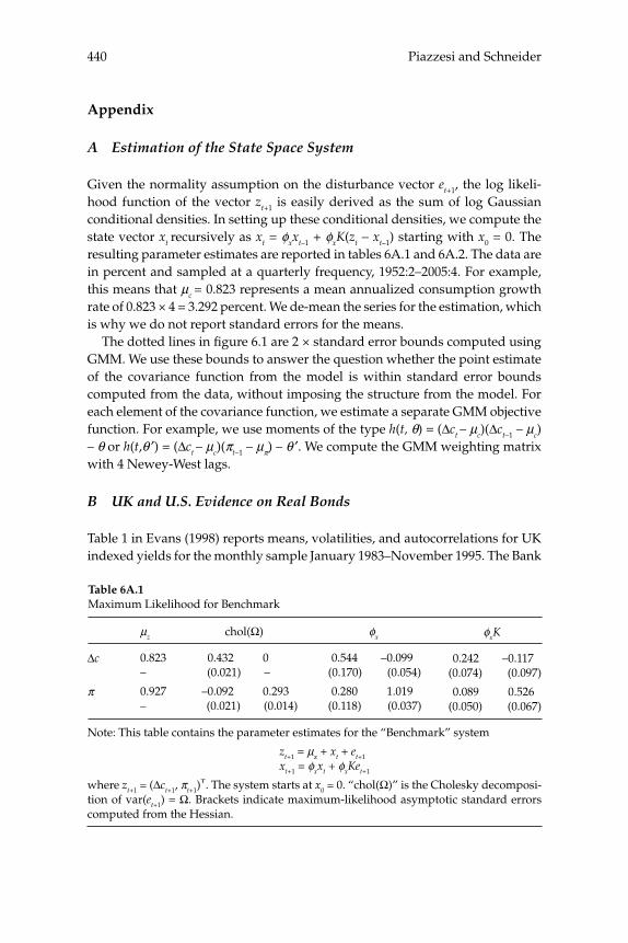
Piazzesi and Schneider440
Appendix
A Estimation of the State Space System
Given the normality assumption on the disturbance vector et+1, the log likeli-hood function of the vector zt+1 is easily derived as the sum of log Gaussian conditional densities. In setting up these conditional densities, we compute the state vector xt recursively as xt = φxxt–1 + φxK(zt – xt–1) starting with x0 = 0. The resulting parameter estimates are reported in tables 6A.1 and 6A.2. The data are in percent and sampled at a quarterly frequency, 1952:2–2005:4. For example, this means that μc = 0.823 represents a mean annualized consumption growth rate of 0.823 × 4 = 3.292 percent. We de-mean the series for the estimation, which is why we do not report standard errors for the means.
The dotted lines in fi gure 6.1 are 2 × standard error bounds computed using GMM. We use these bounds to answer the question whether the point estimate of the covariance function from the model is within standard error bounds computed from the data, without imposing the structure from the model. For each element of the covariance function, we estimate a separate GMM objective function. For example, we use moments of the type h(t, θ) = (Δct – μc)(Δct–1 – μc) – θ or h(t,θ ′) = (Δct – μc)(πt–1 – μπ) – θ ′. We compute the GMM weighting matrix with 4 Newey-West lags.
B UK and U.S. Evidence on Real Bonds
Table 1 in Evans (1998) reports means, volatilities, and autocorrelations for UK indexed yields for the monthly sample January 1983–November 1995. The Bank
Table 6A.1Maximum Likelihood for Benchmark
Δc
π
μz
0.823–
0.927–
chol(Ω)
0.432 0 (0.021) –
–0.092 0.293 (0.021) (0.014)
φx
0.544 –0.099(0.170) (0.054)
0.280 1.019(0.118) (0.037)
φxK
0.242 –0.117(0.074) (0.097)
0.089 0.526(0.050) (0.067)
Note: This table contains the parameter estimates for the “Benchmark” system
zt+1 = μz + xt + et+1
xt+1 = φxxt + φxKet+1
where zt+1 = (Δct+1, πt+1)T. The system starts at x0 = 0. “chol(Ω)” is the Cholesky decomposi-
tion of var(et+1) = Ω. Brackets indicate maximum-likelihood asymptotic standard errors computed from the Hessian.
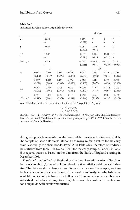
441Equilibrium Yield Curves
of England posts its own interpolated real yield curves from UK indexed yields. The sample of these data starts later and has many missing values for the early years, especially for short bonds. Panel A in table 6B.3. therefore reproduces the statistics from table 1 in Evans (1998) for the early sample. Panel B in table 6B.3 reports statistics based on the data from the Bank of England starting in December 1995.
The data from the Bank of England can be downloaded in various fi les from the website http://www.bankofengland.co.uk/statistics/yieldcurve/index.htm. The data are daily observations. To construct a monthly sample, we take the last observation from each month. The shortest maturity for which data are available consistently is two and a half years. There are a few observations on individual maturities missing. We extrapolate these observations from observa-tions on yields with similar maturities.
Table 6A.2Maximum Likelihood for Large Info Set Model
Δc
π
y(1)$
y(20)$ – y(1)$
μz
0.823–
0.927–
1.287–
0.248–
0.422 (0.021)
–0.082 (0.020)
0.031 (0.016)
–0.013 (0.011)
0 –
0.288 (0.014)
0.045 (0.016)
–0.017 (0.011)
0 –
0 –
0.234 (0.011)
–0.112 (0.010)
0–
0–
0–
0.119(0.006)
chol(Ω)
Δc
π
y(1)$
y(20)$ – y(1)$
0.604 (0.156)
–0.057 (0.070)
–0.008 (0.047)
0.151 (0.115)
0.256 (0.109)
1.042 (0.048)
–0.027 (0.032)
–0.030 (0.081)
0.139 (0.096)
0.126 (0.043)
0.906 (0.030)
–0.022 (0.074)
–0.096 (0.073)
–0.036 (0.028)
0.023 (0.019)
0.883 (0.049)
0.243 (0.083)
–0.075 (0.107)
–0.239 (0.192)
0.090 (0.246)
0.070 (0.052)
0.440 (0.076)
0.142 (0.113)
–0.195 (0.165)
0.119 (0.041)
0.098 (0.056)
0.7701 (0.093)
0.286 (0.137)
–0.088 (0.029)
–0.098 (0.039)
0.043 (0.064)
0.548 (0.101)
Note: This table contains the parameter estimates for the “Large Info Set” system
zt+1 = μz + xt + et+1
xt+1 = φxxt + φxKet+1
where zt+1 = (Δct+1, πt+1, y(1)t+1, y
(20)$ – y(1)$)T. The system starts at x0 = 0. “chol(Ω)” is the Cholesky decompo-sition of var(et+1) = Ω. The data are in percent and sampled quarterly, 1952:2 to 2005:4. Standard errors are computed from the Hessian.
φx φxK
t+1 t+1
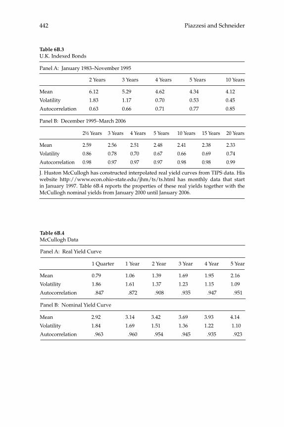
Piazzesi and Schneider442
Table 6B.3U.K. Indexed Bonds
Panel A: January 1983–November 1995
Mean
Volatility
Autocorrelation
2 Years
6.12
1.83
0.63
3 Years
5.29
1.17
0.66
4 Years
4.62
0.70
0.71
5 Years
4.34
0.53
0.77
10 Years
4.12
0.45
0.85
Panel B: December 1995–March 2006
Mean
Volatility
Autocorrelation
2½ Years
2.59
0.86
0.98
3 Years
2.56
0.78
0.97
4 Years
2.51
0.70
0.97
5 Years
2.48
0.67
0.97
10 Years
2.41
0.66
0.98
15 Years
2.38
0.69
0.98
20 Years
2.33
0.74
0.99
J. Huston McCullogh has constructed interpolated real yield curves from TIPS data. His website http://www.econ.ohio-state.edu/jhm/ts/ts.html has monthly data that start in January 1997. Table 6B.4 reports the properties of these real yields together with the McCullogh nominal yields from January 2000 until January 2006.
Table 6B.4McCullogh Data
Panel A: Real Yield Curve
Mean
Volatility
Autocorrelation
1 Quarter
0.79
1.86
.847
1 Year
1.06
1.61
.872
2 Year
1.39
1.37
.908
3 Year
1.69
1.23
.935
4 Year
1.95
1.15
.947
5 Year
2.16
1.09
.951
Panel B: Nominal Yield Curve
Mean
Volatility
Autocorrelation
2.92
1.84
.963
3.14
1.69
.960
3.42
1.51
.954
3.69
1.36
.945
3.93
1.22
.935
4.14
1.10
.923
Comment
Pierpaolo Benigno, New York University
1 Introduction
Section 1 of this discussion reviews the analysis of Piazzesi and Sch-neider (2006) (hereinafter PS). Section 2 analyzes alternative preference specifi cations. Section 3 derives term-structure implications using stan-dard preferences but with a fractional integrated process for the infl a-tion rate. Section 4 concludes pointing out some statistical evidence on term-structure data that needs to be further analyzed.
No-arbitrage theory is based on the existence of some discount fac-tor Mt+1, between generic periods t and t + 1, such that the return Rj
t+1 of a generic asset j, between the same periods, satisfi es the following moment condition
Et[Rjt+1Mt+1] = 1. (1)
For a zero-coupon bond the return is given by the change between peri-ods in the price of the bond. Let Pn,t denote the price at time t of a nomi-nal bond with n-periods to maturity, (1) can be written as
EP
PMt
n t
n tt
− ++
⎡
⎣⎢⎢
⎤
⎦⎥⎥
=1 11 1,
,
.
Since the price of a zero-coupon bond at maturity is equal to 1, i.e, P0,t = 1, it is possible to write the price of a bond with n-periods to maturity as
Pn,t = Et[Mt+1Mt+2Mt+3…Mt+n].
The yield to maturity on a bond with n-periods to maturity is defi ned as
yn
Pn t n t, ,ln .≡ − 1
Benigno444
The theory of the term structure is nothing more than a theory of the stochastic discount factor. To have a model of the term structure that represents the data, it is necessary to specify a process {Mt}. This is the approach used in most of the term-structure literature in fi nance (see, among others, Dai and Singleton 2003).
PS disentangle the problem using two steps. First, they specify the consumption preferences of some agent in the economy and derive the nominal stochastic discount factor based on these preferences. Prefer-ences depend on macro variables, and consequently, so will the sto-chastic discount factor. Second, they estimate processes for the macro variables that make up the stochastic discount factor. In doing so, they are able to specify a process for the stochastic discount factor to have a model of the term structure that can be compared to the actual data.
Special to this procedure is that it is able to provide explanations regarding whether macro variables are important in driving term struc-ture and whether preferences assumed in macro models are consistent with fi nancial data.
Their fi rst step consists of specifying preferences using a general family of isoelastic utility derived from the work of Kreps and Porteus (1978) and Epstein and Zin (1989). These preferences do not confuse behavior toward risk with that of intertemporal substitution as in the standard expected utility model. This makes it possible to distinguish the intertemporal elasticity of substitution from the risk-aversion coef-fi cient.1 PS fi x the intertemporal elasticity of substitution to a unitary value which, together with other assumptions, has the advantage of implying a linear-affi ne model of the term structure. Utility at time t given by Vt is defi ned recursively as
V C E Vt t t t= −+− −11
11
1β γ γ β{[ ] }
where γ is the risk-aversion coeffi cient and β is the intertemporal dis-count factor.2
An important implication of the work of Tallarini (2000) is that risk aversion can be set as high as needed without signifi cantly affecting the relative variabilities and simultaneous movements of aggregate quan-tity variables in a business-cycle model.
Under this preference specifi cation the nominal stochastic discount factor is given by
MCC
V
E Vt
t
t
t
t t
++
−
+−
=⎛⎝⎜
⎞⎠⎟
⎛
⎝⎜⎜
⎞
⎠−1
1
1
11
11
βγ γ[ ]
⎟⎟⎟
−
+
1
1
γ
PP
t
t
(2)
445Comment
while its log implies
m c E Et t t t tj
j+ + + +
−
=
∞
= − − − − − ∑1 1 1 11
1
1ln ( )( )β π γ βΔ ΔΔct j+ +1 (3)
− −⎛
⎝⎜
⎞
⎠⎟+
−+ +
=
∞
∑12
1 21
11
1
( )γ βVart tj
t jj
E cΔ
where lower-case variables denote the log of the respective uppercase variable; and πt is the infl ation rate defi ned as πt = ln Pt /ln Pt–1.
It is possible to make predictions about the term structure simply by specifying the processes for consumption growth and infl ation since the stochastic discount factor depends only on these two variables. Let z′t = [Δctπt], PS estimate a process for zt of the form
zt+1 = μz + xt + et+1, (4)
xt+1 = φxxt + φxKet+1. (5)
Matrices and vectors are presented in their paper and the variance-covariance matrix of the innovation et is given by Ω. One of the main fi ndings of PS is that this two-step procedure is successful in refl ecting statistical properties of the yield curve, especially for the average yield curve.
This discussion will fi rst analyze the implications of alternative preference specifi cations given the estimated process and then moves to analyze an alternative process given standard preference specifi cations.
2 Preferences
2.1 What Is Preventing the Standard Expected Utility Model from Working?
Under the standard isoelastic expected utility model with preferences given by
U EC
t tT t
T t
t=−
−
=
∞ −
∑βρ
ρ1
1,
the nominal stochastic discount factor is
MCC
PPt
t
t
t
t+
+−
+
=⎛⎝⎜
⎞⎠⎟1
1
1
βρ
, (6)
Benigno446
where ρ is the risk-aversion coeffi cient which now coincides with the inverse of the intertemporal elasticity of substitution. In this case, the price of a bond with n-periods to maturity can be written as
P ECC
PPn t t
n t n
t
t
t n, .= ⎛
⎝⎜⎞⎠⎟
⎡
⎣⎢⎢
⎤
⎦⎥⎥
+−
+
βρ
This price can be relatively low either when future prices or consump-tions are expected to be relatively high. Under these conditions future marginal utility of nominal income is low. Agents dislike assets that pay when they do not need extra nominal income. The prices of these assets will be relatively low and agents require a premium to hold them. Fol-lowing this line of reasoning, nothing should prevent standard pref-erences from reproducing, at least, the upward-sloping average yield curve dictated by the data. However, this is not the case under the esti-mated processes (4) and (5).
The fi rst problem one can expect to face when working with standard preferences is in matching moments of the short-term interest rate i1,t. This is given by
i E c E ct t t t t t t1 1 1
2
1212, ln var va= − + + − −+ + +β ρ π ρΔ Δ rrt tπ +1
− + +ρ πcov ( , )t t tcΔ 1 1
which implies an unconditional mean
μ β ρμ μ ρ σ σ ρσπ π π1
22 2
212
= − + + − − −ln .c c c (7)
When the values of the parameters β and ρ, along with the vector of means µz and the variance-covariance matrix Ω from the estimated sys-tem (4) and (5) are known, it is possible to calculate a value for the unconditional mean. The estimated variance-covariance matrix does not play a large role in (7) since its magnitude is negligible compared to the means. According to the data μc = 3.29 percent and μπ = 3.70 percent. In order for the unconditional mean of the short-term rate μ1 = 5.15 per-cent to refl ect the data, either β should be greater than one or ρ, the risk-aversion coeffi cient, should be less than one. If β is not allowed to be greater than one and is set arbitrarily at 0.999, then ρ should be 0.32.3
This means that when the fi rst point of the model average yield curve corresponds to the data, all the parameters are already tied down, mak-ing it harder for the model to match other facts as the upward-sloping
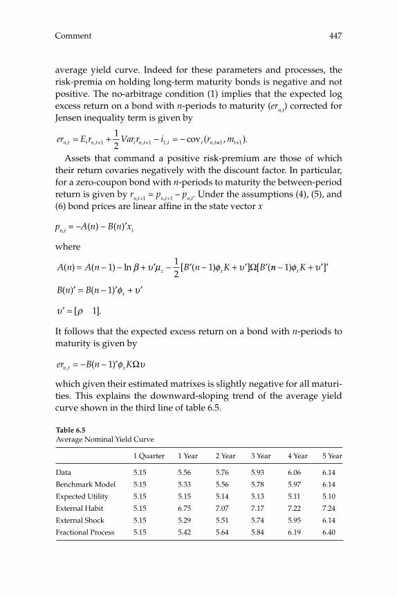
447Comment
average yield curve. Indeed for these parameters and processes, the risk-premia on holding long-term maturity bonds is negative and not positive. The no-arbitrage condition (1) implies that the expected log excess return on a bond with n-periods to maturity (ern,t) corrected for Jensen inequality term is given by
er E r Var r i rn t t n t t n t t t n t, , , , ,cov (= + − = −+ +1 1 1
12 ++ +1 1, ).mt
Assets that command a positive risk-premium are those of which their return covaries negatively with the discount factor. In particular, for a zero-coupon bond with n-periods to maturity the between-period return is given by rn,t+1 = pn,t+1 – pn,t. Under the assumptions (4), (5), and (6) bond prices are linear affi ne in the state vector x
pn,t = –A(n) – B(n)′xt
where
A n A n B n K Bz x( ) ( ) ln [ ( ) ] [ (= − − + ′ − ′ − + ′ ′112
1β υ μ φ υ Ω nn Kx− + ′ ′1) ]φ υ
B n B n x( ) ( )′ = − ′ + ′1 φ υ
′ =υ ρ[ ]. 1
It follows that the expected excess return on a bond with n-periods to maturity is given by
er B n Kn t x, ( )= − − ′1 φ υΩ
which given their estimated matrixes is slightly negative for all maturi-ties. This explains the downward-sloping trend of the average yield curve shown in the third line of table 6.5.
Table 6.5Average Nominal Yield Curve
Data
Benchmark Model
Expected Utility
External Habit
External Shock
Fractional Process
1 Quarter
5.15
5.15
5.15
5.15
5.15
5.15
1 Year
5.56
5.33
5.15
6.75
5.29
5.42
2 Year
5.76
5.56
5.14
7.07
5.51
5.64
3 Year
5.93
5.78
5.13
7.17
5.74
5.84
4 Year
6.06
5.97
5.11
7.22
5.95
6.19
5 Year
6.14
6.14
5.10
7.24
6.14
6.40
Benigno448
The preference specifi cation (3) used by PS adds an extra factor to standard preferences that allows for greater fl exibility. Under these preferences, the prices of the bonds with different maturities are still linear-affi ne, but
A n A n i e Z Z ez( ) ( ) ln ( )= − − + ′ + − ′ ′ +112
1 21 1β μ γ Ω
− ′ − + ′ + − ′ ′ − + ′ + −12
1 1 1 11[ ( ) ( ) ] [ ( ) ( )B n i e Z B n iγ γΩ ′′ ′e Z1 ]
and
B(n)′ = B(n – 1)′φx + i′
with
′ ≡ ′ ≡i e[ ] [ ]1 1 1 01
Z I I Kx x≡ + − −β φ β φ( ) .1
The expected excess return is given by
er B n K i B n K Z en t x x, ( ) ( ) ( )= − − ′ − − − ′ ′1 1 1 1φ γ φΩ Ω
which shows an additional term that helps to generate a positive risk premium. This new term is multiplied by the risk-aversion coeffi cient, which can be freely moved to produce an upward-sloping average yield curve, as shown in the second line of table 6.5.4
As discussed in Cochrane (2006), drawing empirical facts from fi nan-cial data using a stochastic discount factor based on consumer prefer-ences requires that additional factors be added to the standard expected utility model. I will now investigate the implications for the yield curve of traditional extensions to standard preferences which have been used to explain the equity-premium puzzle.
2.2 Habit Model As in Abel (1990)
Consider the model proposed by Abel (1990) in which the utility func-tion is given by
U EC
Ct tT t
T t
Tj
T
=⎛⎝⎜
⎞⎠⎟
−
=
∞
−
−
∑β θ
ρ
1
1
where the utility fl ow does not only depend on individual consump-tion, but on consumption relative to past aggregate consumption. This
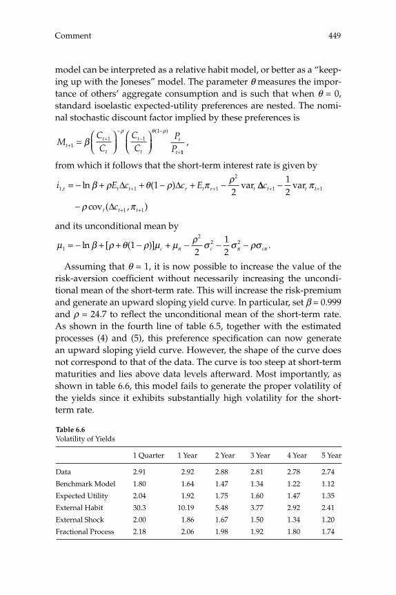
449Comment
model can be interpreted as a relative habit model, or better as a “keep-ing up with the Joneses” model. The parameter θ measures the impor-tance of others’ aggregate consumption and is such that when θ = 0, standard isoelastic expected-utility preferences are nested. The nomi-nal stochastic discount factor implied by these preferences is
MCC
CC
PPt
t
t
t
t
t
t+
+−
−−
+
=⎛⎝⎜
⎞⎠⎟
⎛⎝⎜
⎞⎠⎟1
1 11
βρ θ ρ( )
11
,
from which it follows that the short-term interest rate is given by
i E c c Et t t r t r t1 1 1
2
12, ln ( ) var= − + + − + −+ +β ρ θ ρ π ρΔ Δ ΔΔct t t+ +−1 1
12
var π
− + +ρ πcov ( , )t t tcΔ 1 1
and its unconditional mean by
μ β ρ θ ρ μ μ ρ σ σ ρσπ π π1
22 21
212
= − + + − + − − −ln [ ( )] .c c c
Assuming that θ = 1, it is now possible to increase the value of the risk-aversion coeffi cient without necessarily increasing the uncondi-tional mean of the short-term rate. This will increase the risk-premium and generate an upward sloping yield curve. In particular, set β = 0.999 and ρ = 24.7 to refl ect the unconditional mean of the short-term rate. As shown in the fourth line of table 6.5, together with the estimated processes (4) and (5), this preference specifi cation can now generate an upward sloping yield curve. However, the shape of the curve does not correspond to that of the data. The curve is too steep at short-term maturities and lies above data levels afterward. Most importantly, as shown in table 6.6, this model fails to generate the proper volatility of the yields since it exhibits substantially high volatility for the short-term rate.
Table 6.6Volatility of Yields
Data
Benchmark Model
Expected Utility
External Habit
External Shock
Fractional Process
1 Quarter
2.91
1.80
2.04
30.3
2.00
2.18
1 Year
2.92
1.64
1.92
10.19
1.86
2.06
2 Year
2.88
1.47
1.75
5.48
1.67
1.98
3 Year
2.81
1.34
1.60
3.77
1.50
1.92
4 Year
2.78
1.22
1.47
2.92
1.34
1.80
5 Year
2.74
1.12
1.35
2.41
1.20
1.74

Benigno450
2.3 External Shock As in Gallmeyer et al. (2005)
To explore the implications of a more sophisticated model of habit as presented by Gallmeyer, Hollifi eld, and Zin (2005), which falls under the class of habit models discussed in Campbell and Cochrane (1999), consider a utility fl ow of the form
U EC
Qt tT t
T t
TT=
−−
=
∞ −
∑βρ
ρ1
1
where Qt is a preference shock that follows a martingale, i.e., Et(Qt+1/Qt) = 1. In this case, the nominal stochastic discount factor is given by
MCC
PPt
t
t
t
t
t
t+
+−
+
+
=⎛⎝⎜
⎞⎠⎟
⎛⎝⎜
⎞⎠⎟1
1 1
1
βρ
.
The shock Qt is modelled in a way that
− = − ++ + +Δ Δ Δ Δ Δq c c E c ct c t t t t c t1 1 121
2( )( ) ( ) varφ φ tt tcΔ +1 ,
where, as previously, lower-case letters denote logarithms and φc is a parameter. It follows that the nominal stochastic discount factor can be written as
M kCC
CC
Pt t
t
t
t
t
tc t
++
−
−
−
=⎛⎝⎜
⎞⎠⎟
⎛⎝⎜
⎞⎠⎟
+
11
1
1
βρ φ ξ
PPt+1
, (8)
where
ξt+1 = (Δct+1 – EtΔct+1)
captures unexpected surprises in consumption at time t + 1 and
kt ≡ exp{1/2(φcΔct)2vartΔct+1}.
Past consumption matters as it did in the standard habit model, but now its weight depends on the magnitude of the unexpected consump-tion surprises.
This preference specifi cation, together with the processes (4) and (5), generates an affi ne linear yield curve, in which risk-premia are now time varying.
As shown in table 6.5, this model is more successful in producing an upward-sloping yield curve and toward this aspect of the data per-forms as well as the benchmark model of PS. In particular the param-
451Comment
eter β is set equal to 0.9999 while φc = –11250. The latter number is not large since ξt+1 is very small. The standard deviation over the sample of φcξt+1—which is the variable what matters in (8)—is 36. Note the simi-larities between these preferences and the ones used in PS. Both add an additional martingale to the stochastic discount factor. This additional term can be interpreted as a distortion in the initial probability mea-sure as in the risk-sensitive control literature (see Hansen and Sargent 2006).
3 Processes for Consumption and Infl ation
In the previous section, the estimated processes for consumption and infl ation were maintained as those in the specifi cation of PS. It was shown that in order to match an upward sloping average yield curve, the standard isoelastic expected utility model had to be modifi ed to include additional terms. However, the models discussed thus far have all failed to properly represent one important aspect of the data regard-ing the volatility of the yields, as shown in table 6.6. Every model has implied a progressively decreasing trend, even though the volatility of the yields over the full sample of data does not actually decrease with longer maturities. This result greatly depends on the estimation of the processes (4) and (5). The estimation is performed on demeaned data, which imposes stationarity on the variables infl uencing the stochastic discount factor. As discussed in Backus and Zin (1993), when the state vector is stationary, the volatility of the yields with longer maturities converge to zero. Since the data does not show this pattern, this indi-cates some nonstationarity in the factors infl uencing the yield curve for at least some part of the sample.
An obvious candidate of this nonstationary behavior is the infl ation-rate process. Firstly, because if a raw unit-root test is performed on the data taken from 1952 to 19xy where xy is above 70, a unit root cannot be rejected for some years. Also because recent literatures on infl ation forecasting discussed in Mayoral and Gadea (2005) have argued that infl ation processes for many OECD countries can be described well by fractionally-integrated processes. This class of processes implies longer memory and as discussed in Backus and Zin (1993) can generate a non-decreasing volatility of yields.
A careful multivariate fractional integration approach to consump-tion and infl ation is out of this discussion’s scope. Yet, I will explore the implication of a fractionally integrated process for infl ation and show
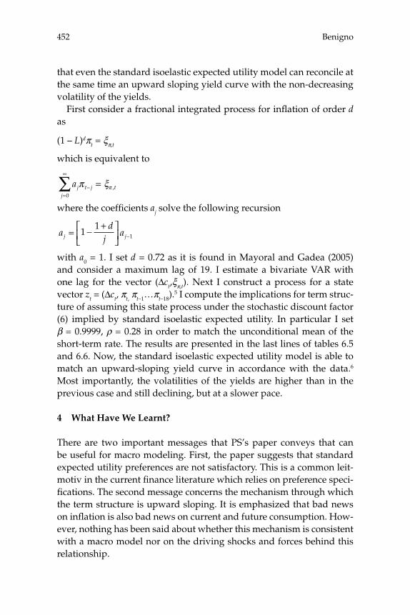
Benigno452
that even the standard isoelastic expected utility model can reconcile at the same time an upward sloping yield curve with the non-decreasing volatility of the yields.
First consider a fractional integrated process for infl ation of order d as
(1 – L)dπt = ξπ,t
which is equivalent to
aj t jj
tπ ξπ−=
∞
=∑0
,
where the coeffi cients aj solve the following recursion
ad
jaj j= − +⎡
⎣⎢
⎤⎦⎥ −1
11
with a0 = 1. I set d = 0.72 as it is found in Mayoral and Gadea (2005) and consider a maximum lag of 19. I estimate a bivariate VAR with one lag for the vector (Δct,ξπ,t). Next I construct a process for a state vector zt = (Δct, πt, πt–1…πt–18).
5 I compute the implications for term struc-ture of assuming this state process under the stochastic discount factor (6) implied by standard isoelastic expected utility. In particular I set β = 0.9999, ρ = 0.28 in order to match the unconditional mean of the short-term rate. The results are presented in the last lines of tables 6.5 and 6.6. Now, the standard isoelastic expected utility model is able to match an upward-sloping yield curve in accordance with the data.6 Most importantly, the volatilities of the yields are higher than in the previous case and still declining, but at a slower pace.
4 What Have We Learnt?
There are two important messages that PS’s paper conveys that can be useful for macro modeling. First, the paper suggests that standard expected utility preferences are not satisfactory. This is a common leit-motiv in the current fi nance literature which relies on preference speci-fi cations. The second message concerns the mechanism through which the term structure is upward sloping. It is emphasized that bad news on infl ation is also bad news on current and future consumption. How-ever, nothing has been said about whether this mechanism is consistent with a macro model nor on the driving shocks and forces behind this relationship.
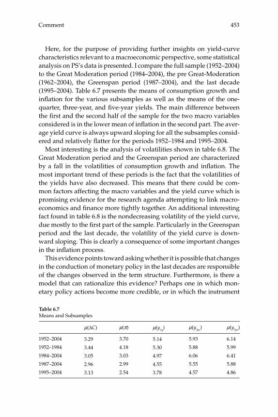
453Comment
Here, for the purpose of providing further insights on yield-curve characteristics relevant to a macroeconomic perspective, some statistical analysis on PS’s data is presented. I compare the full sample (1952–2004) to the Great Moderation period (1984–2004), the pre Great-Moderation (1962–2004), the Greenspan period (1987–2004), and the last decade (1995–2004). Table 6.7 presents the means of consumption growth and infl ation for the various subsamples as well as the means of the one-quarter, three-year, and fi ve-year yields. The main difference between the fi rst and the second half of the sample for the two macro variables considered is in the lower mean of infl ation in the second part. The aver-age yield curve is always upward sloping for all the subsamples consid-ered and relatively fl atter for the periods 1952–1984 and 1995–2004.
Most interesting is the analysis of volatilities shown in table 6.8. The Great Moderation period and the Greenspan period are characterized by a fall in the volatilities of consumption growth and infl ation. The most important trend of these periods is the fact that the volatilities of the yields have also decreased. This means that there could be com-mon factors affecting the macro variables and the yield curve which is promising evidence for the research agenda attempting to link macro-economics and fi nance more tightly together. An additional interesting fact found in table 6.8 is the nondecreasing volatility of the yield curve, due mostly to the fi rst part of the sample. Particularly in the Greenspan period and the last decade, the volatility of the yield curve is down-ward sloping. This is clearly a consequence of some important changes in the infl ation process.
This evidence points toward asking whether it is possible that changes in the conduction of monetary policy in the last decades are responsible of the changes observed in the term structure. Furthermore, is there a model that can rationalize this evidence? Perhaps one in which mon-etary policy actions become more credible, or in which the instrument
Table 6.7Means and Subsamples
1952–2004
1952–1984
1984–2004
1987–2004
1995–2004
μ(ΔC)
3.29
3.44
3.05
2.96
3.13
μ(π)
3.70
4.18
3.03
2.99
2.54
μ(y1q)
5.14
5.30
4.97
4.55
3.78
μ(y3yr)
5.93
5.88
6.06
5.55
4.57
μ(y5yr)
6.14
5.99
6.41
5.88
4.86
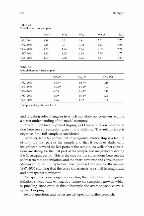
Benigno454
and targeting rules change or in which monetary policymakers acquire a better understanding of the model economy.
PS’s intuition for an upward sloping yield curve relies on the correla-tion between consumption growth and infl ation. This relationship is negative if the full sample is considered.
However, table 6.9 shows that this negative relationship is a feature of only the fi rst part of the sample and that it becomes statistically insignifi cant toward the last parts of the sample. As well, other correla-tions are strong for the fi rst part of the sample and insignifi cant during the Greenspan period. This is the case for the correlations between the short-term rate and infl ation, and the short-term rate and consumption. Moreover fi gure 6.10 replicates their fi gure 6.1 but just for the sample 1987–2005 showing that the cross covariances are small in magnitude and perhaps not signifi cant.
Perhaps, this is no longer supporting their intuition that negative infl ation shocks lead to negative future consumption growth which is puzzling since even in this subsample the average yield curve is upward sloping.
Several questions and issues are left open for further research.
Table 6.8Volatility and Subsamples
1952–2004
1952–1984
1984–2004
1987–2004
1995–2004
σ(ΔC)
1.88
2.18
1.29
1.30
1.09
σ(π)
2.51
3.01
1.24
1.25
0.98
σ(y1q)
2.91
3.30
2.26
2.03
1.76
σ(y3yr)
2.81
3.13
2.32
1.89
1.51
σ(y5yr)
2.73
3.06
2.24
1.75
1.27
Table 6.9Correlations and Subsamples
1952–2004
1952–1984
1984–2004
1987–2004
1995–2004
c(ΔC,π)
–0.35**
–0.44**
–0.13
–0.19
–0.06
c(y1q, π)
0.67**
0.74**
0.43**
0.44**
–0.12
c(y1q, ΔC)
–0.15**
–0.27
0.10
0.00
0.26
**=1 percent signifi cance level
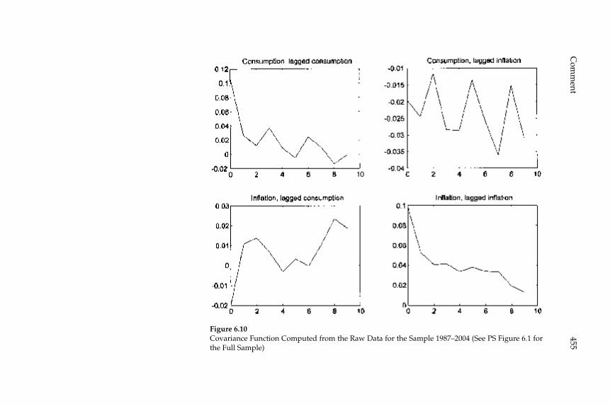
455C
omm
ent
Figure 6.10Covariance Function Computed from the Raw Data for the Sample 1987–2004 (See PS Figure 6.1 for the Full Sample)
Benigno456
Acknowledgments
I am grateful for helpful comments and discussions to David Backus, Sydney Ludvigson, Giorgio Primiceri, Tom Sargent, Mike Woodford. I thank Laura Petramala for research assistance.
Endnotes
1. This is not the fi rst paper to use this kind of preferences to study term-structure impli-cations, but the fi rst to take it seriously to the data. See among others Campbell (1999), Campbell and Viceira (2002), Restoy and Weil (2004).
2. I am assuming an infi nite horizon economy differently from PS fi nite-horizon model.
3. Standard procedures require fi rst to set ρ and then derive β but this would violate the upper bound on β. PS fi nite-horizon model allows for β being greater than the unitary value. The fact that by raising the risk-aversion coeffi cient the mean of the short-rate increases is the mirror image of the equity premium puzzle. This is the risk-free rate puzzle, see Weil (1989).
4. The second line of table 6.5 reports the results of the fi nite-horizon model of PS. Note that in the infi nite-horizon case to generate a positive risk premium it is suffi cient to assume a value of γ above two, but to match the risk-premium of the data γ should be 59. A high risk-aversion coeffi cient also reduces the unconditional mean of the short rate helping to reduce the value of β needed to match the fi rst point of the average yield curve.
5. To further simplify the analysis, I keep only the signifi cant coeffi cients from the VAR estimates.
6. The result that the standard expected utility model can be also successful in generating a positive risk-premium is in some way consistent with PS learning experiment in which the estimation procedure can account for possible breaks in the consumption and infl a-tion processes. Indeed, in their fi nal example of section 5, they need a parameter of risk aversion γ = 4 which is close to imply the standard expected utility model.
References
Abel, Andrew. 1990. “Asset Prices under Habit Formation and Catching Up with the Joneses.”American Economic Review 80: 38–42.
Backus, David, and Stanley Zin. 1993. “Long-memory Infl ation Uncertainty: Evidence from the Term Structure of Interest Rates.” Journal of Money, Credit and Banking 25: 681–700.
Campbell, John. 1999. “Asset Prices, Consumption, and the Business Cycle.” In John Taylor and Michael Woodford, eds., Handbook of Macroeconomics Vol. 1. North-Holland, Amsterdam.
Campbell, John, and John Cochrane. 1999. “By Force of Habit: A Consumption-Based Expla-nation of Aggregate Stock Market Behavior.” Journal of Political Economy 107: 205–251.
457Comment
Campbell, John, and Luis Viceira. 2002. Strategic Asset Allocation. New York: Oxford Uni-versity Press.
Cochrane, John. 2006. “Financial Markets and the Real Economy.” Unpublished manu-script, GSB Chicago University.
Dai, Qiang, and Kenneth Singleton. 2003. “Term Structure Dynamics in Theory and Real-ity.” Review of Financial Studies 16(3): 631–678.
Epstein, Larry G., and Stanley E. Zin. 1989. “Substitution, Risk Aversion, and the Tempo-ral Behavior of Consumption and Asset Returns: A Theoretical Framework.” Econometrica 57(4): 937–969.
Gallmeyer, Michael, Burton Hollifi eld, and Stanley Zin. 2005. “Taylor Rules, McCallum Rules, and the Term Structure of Interest Rates.” Journal of Monetary Economics 52(5): 921–950.
Hansen, Lars, and Thomas Sargent. 2006. Robustness. Unpublished manuscript, Univ. of Chicago and New York University.
Kreps, David M., and Evan L. Porteus. 1978. “Temporal Resolution of Uncertainty and Dynamic Choice Theory.” Econometrica 46(1): 185–200.
Mayoral, Laura, and Lola Gadea. 2005. “The Persistence of Infl ation in OECD Countries.” The International Journal of Central Banking 4.
Restoy, Fernando, and Philippe Weil. 2004. “Approximate Equilibrium Asset Prices.” Unpublished manuscript, ULB.
Tallarini, T. D. 2000. “Risk-Sensitive Real Business Cycle.” Journal of Monetary Economics 45: 507–532.
Weil, Philippe. 1989. “The Equity Premium Puzzle and the Risk-Free Rate Puzzle.” Jour-nal of Monetary Economics 24: 401–421.

Comment
John Y. Campbell, Harvard University and NBER
Are government bonds risky assets? This deceptively simple question raises fundamental issues in macroeconomics and fi nance. To begin, assume that the bonds are infl ation-indexed or infl ation is determin-istic. Over a short holding period, long-term government bonds have volatile returns whereas short-term Treasury bills have a known return. Over a long holding period, however, Treasury bills must be rolled over at unknown future interest rates, while long-term bonds deliver a known return. Unsurprisingly, then, normative models of portfolio choice imply that highly conservative short-term investors living off their fi nancial wealth should hold Treasury bills, but conservative long-term investors should hold long-term infl ation-indexed bonds (Camp-bell and Viceira 2001).1
General equilibrium asset pricing theory approaches this question from a somewhat different angle. In a general equilibrium asset pricing model, a risky asset is one whose return covaries negatively with the stochastic discount factor (SDF); such an asset will command a positive risk premium over a short-term safe asset. The SDF may be estimated empirically, or may be derived from assumptions about the tastes and endowment of a representative investor. Similarly, the covariance of bond returns with the SDF may be estimated from historical data, or may be derived from assumptions about the endowment process.
Two simple examples of this approach set the stage for the more sophisticated logic employed by Monika Piazzesi and Martin Sch-neider. First, the Capital Asset Pricing Model (CAPM) assumes that the SDF is a negative linear function of the return on a broad stock index. According to the CAPM, government bonds are risky assets if they have a positive beta with the stock market. Empirical estimates of bond betas were close to zero in the 1960s, positive in the 1970s and 1980s,
Campbell460
and appear to have turned negative during the last fi ve to ten years (Campbell and Ammer 1993, Viceira 2006).
Second, a consumption-based asset pricing model with power util-ity implies that the SDF is a negative linear function of consumption growth. In this framework, government bonds are risky assets if their returns covary positively with consumption growth. Since bond prices rise when interest rates fall, bonds are risky assets if interest rates fall in response to consumption growth. Campbell (1986) points out that in a real model, this requires positive consumption shocks to drive down real interest rates; but because equilibrium real interest rates are posi-tively related to expected future consumption growth, this is possible only if positive consumption shocks drive down expected future con-sumption growth, that is, if consumption growth is negatively autocor-related. In the presence of persistent shocks to consumption growth, by contrast, consumption growth is positively autocorrelated. In this case long-term bonds are hedges against prolonged slow growth and thus are desirable assets with negative risk premia.
Randomness in infl ation further complicates the analysis for long-term nominal bonds. The real payoffs on long-term nominal bonds are uncertain and are negatively related to infl ation. If shocks to infl ation are positively correlated with the SDF, nominal bonds become risky assets that command positive risk premia.
The paper by Piazzesi and Schneider (PS) extends this analysis by more carefully modeling the effects of infl ation on bond prices. PS assume that a representative investor has not power utility, but the more general utility function described by Epstein and Zin (1989, 1991). This utility function allows the coeffi cient of relative risk aversion γ and the elasticity of intertemporal substitution (EIS) ψ to be separate free parameters, whereas power utility restricts one to be the reciprocal of the other. With power utility, increasing risk aversion to explain the high equity premium forces the EIS to be very low, and this can have problematic implications for the dynamic behavior of interest rates and consumption. Epstein-Zin utility allows one to avoid this problem. In order to derive closed-form solutions, PS assume that the EIS equals one, implying that the consumption-wealth ratio is constant over time. In this discussion, I instead use the approximate loglinear solutions I have proposed in earlier work (Campbell 1993), and treat the EIS as a free parameter.
Like PS, I will assume joint lognormality and homoskedasticity of asset returns and consumption. With this assumption, the Epstein-Zin

461Comment
Euler equation implies that the risk premium on any asset i over the short-term safe asset is
RP r ri t i t f ti ic
iw≡ − + = + −+ +E [ ] ( ) ., ,1 1
2
21
σ θ σψ
θ σ (1)
The risk premium is defi ned to be the expected excess log return on the asset plus one-half its variance to correct for Jensen’s Inequality. The preference parameter θ ≡ (1 – γ)/(1 – 1/ψ); in the power utility case, γ = 1/ψ and θ = 1. According to this formula, the risk premium on any asset is a weighted average of two conditional covariances, the con-sumption covariance σic (scaled by the reciprocal of the EIS) which gets full weight in the power utility case, and the wealth covariance σiw.
It is tempting to treat the consumption covariance and wealth covari-ance as two separate quantities, but this ignores the fact that consump-tion and wealth are linked by the intertemporal budget constraint and by a time-series Euler equation. By using these additional equations, one can substitute either consumption (Campbell 1993) or wealth (Restoy and Weil 1998) out of the formula for the risk premium. The fi rst approach explains the risk premium using covariances with the current market return and with news about future market returns; this might be called “CAPM+”, as it generalizes the insight about risk that was fi rst formalized in the CAPM. The second approach explains the risk premium using covariances with current consumption growth and with news about future consumption growth; this might be called the “CCAPM+”, as it generalizes the insight about risk that is contained in the consumption-based CAPM with power utility.
PS use the CCAPM+ approach, which can be written as
RPi ic ig= + −⎛⎝⎜
⎞⎠⎟
γσ γψ
σ1
, (2)
σ ig i t t i t tr r g≡ −+ + +Cov E( , ),, ,1 1 1� (3)
and
�g ct t tj
t jj
+ + + +=
∞
≡ − ∑1 1 11
( ) .E E ρ Δ (4)
The letter g is used here as a mnemonic for consumption growth. The risk premium on any asset is the coeffi cient of risk aversion γ times the covariance of that asset with consumption growth, plus (γ – 1/ψ) times the covariance of the asset with revisions in expected future
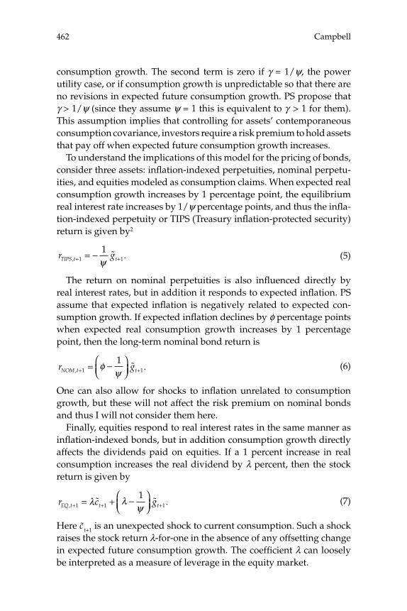
Campbell462
consumption growth. The second term is zero if γ = 1/ψ, the power utility case, or if consumption growth is unpredictable so that there are no revisions in expected future consumption growth. PS propose that γ > 1/ψ (since they assume ψ = 1 this is equivalent to γ > 1 for them). This assumption implies that controlling for assets’ contemporaneous consumption covariance, investors require a risk premium to hold assets that pay off when expected future consumption growth increases.
To understand the implications of this model for the pricing of bonds, consider three assets: infl ation-indexed perpetuities, nominal perpetu-ities, and equities modeled as consumption claims. When expected real consumption growth increases by 1 percentage point, the equilibrium real interest rate increases by 1/ψ percentage points, and thus the infl a-tion-indexed perpetuity or TIPS (Treasury infl ation-protected security) return is given by2
r gTIPS t t, .+ += −1 1
1ψ
� (5)
The return on nominal perpetuities is also infl uenced directly by real interest rates, but in addition it responds to expected infl ation. PS assume that expected infl ation is negatively related to expected con-sumption growth. If expected infl ation declines by φ percentage points when expected real consumption growth increases by 1 percentage point, then the long-term nominal bond return is
r gNOM t t, .+ += −⎛⎝⎜
⎞⎠⎟1 1
1φψ
� (6)
One can also allow for shocks to infl ation unrelated to consumption growth, but these will not affect the risk premium on nominal bonds and thus I will not consider them here.
Finally, equities respond to real interest rates in the same manner as infl ation-indexed bonds, but in addition consumption growth directly affects the dividends paid on equities. If a 1 percent increase in real consumption increases the real dividend by λ percent, then the stock return is given by
r c gEQ t t t, .+ + += + −⎛⎝⎜
⎞⎠⎟1 1 1
1λ λ
ψ� � (7)
Here c t+1 is an unexpected shock to current consumption. Such a shock raises the stock return λ-for-one in the absence of any offsetting change in expected future consumption growth. The coeffi cient λ can loosely be interpreted as a measure of leverage in the equity market.
463Comment
Now we are in a position to solve for the implied risk premia on real bonds, nominal bonds, and equities. Combining (2) with (5) gives
RPTIPS cg g= −⎛⎝⎜
⎞⎠⎟
+ −⎛⎝⎜
⎞⎠⎟
−⎛⎝⎜
⎞⎠⎟
γψ
σ γψ ψ
σ1 1 1 2 .. (8)
With power utility, only the fi rst term is nonzero. This term is described by Campbell (1986); persistent consumption growth implies a positive covariance between current consumption growth shocks and expected future consumption growth, and hence a negative real term premium. The second term is also negative under the plausible assumption that γ > 1/ψ, and its sign does not depend on the persistence of the con-sumption process. Hence this model generates a strong prediction that the real term premium is negative.
Combining (2) with (6) gives
RPNOM cg g= −⎛⎝⎜
⎞⎠⎟
+ −⎛⎝⎜
⎞⎠⎟
−⎛⎝⎜
⎞⎠⎟
γ φψ
σ γψ
φψ
σ1 1 1 22 . (9)
If the infl ation effect is large enough, φ > 1/ψ, nominal bonds can have positive risk premia even when real bonds have negative premia. The reason is that good news about expected future consumption reduces expected infl ation, and thus causes nominal interest rates to decline and nominal bond prices to increase. Nominal bonds become procycli-cal, risky assets even though real bonds are countercyclical assets that hedge against weak economic growth.
Combining (2) with (7) gives a more complicated expression for the equity premium,
RPEQ cg g= −⎛⎝⎜
⎞⎠⎟
+ −⎛⎝⎜
⎞⎠⎟
−⎛⎝⎜
⎞⎠⎟
γ λψ
σ γψ
λψ
σ1 1 1 2 ++ + −⎛
⎝⎜⎞⎠⎟
γλσ γψ
λσc cg2 1
. (10)
This is also positive and larger than the nominal bond premium if equity leverage λ is high.
Finally, the covariance between real bond returns and equity returns is
Covt TIPS t EQ t gr r( , ), ,+ + = − −⎛⎝⎜
⎞⎠⎟
+1 121 1
ψλ
ψσ λσ ccg
⎡
⎣⎢
⎤
⎦⎥ , (11)
which is negative when equity leverage is high, whereas the covariance between nominal bond returns and stock returns is
Cov ( +1t EQ tr rNOM,t , ), + = −⎛⎝⎜
⎞⎠⎟
−⎛⎝⎜
⎞⎠⎟1
1 1φψ
λψ
σσ λσg cg2 +
⎡
⎣⎢
⎤
⎦⎥ , (12)
Campbell464
which is positive when equity leverage and the infl ation sensitivity of nominal bonds are both high.
Summarizing, PS argue that infl ation is negatively related to the long-run prospects for consumption growth. Thus nominal bonds, whose real payoffs are negatively related to infl ation, are more similar to equi-ties, whose dividends respond positively to consumption, than they are to infl ation-indexed bonds. And stock returns correlate negatively with infl ation, despite the fact that stocks are real assets, because the real economy drives infl ation.3
This story has several testable implications. First, equations (5) and (6) imply that lagged returns on infl ation-indexed bonds should pre-dict negative consumption growth whereas lagged returns on nominal bonds should predict positive consumption growth. Second, equations (8) and (9) imply that infl ation-indexed bonds should have negative term premia and nominal bonds should have positive term premia. Third, equations (11) and (12) imply that infl ation-indexed bonds should have negative betas with stocks whereas nominal bonds should have positive betas.
Evidence on these implications is fragmentary, and it is particularly diffi cult to test the implications for infl ation-indexed bonds because these bonds have only been issued relatively recently. The UK, for exam-ple, fi rst issued infl ation-indexed gilts (UK government bonds) in the early 1980s, and the United States followed suit in the late 1990s. How-ever a piece of evidence in support of the fi rst implication, for nominal bonds, is that nominal yield spreads predict future real consumption growth positively. This is relevant because yield spreads tend to widen when nominal interest rates are falling and bond prices are rising. Table 12A in Campbell (2003) reports positive and often statistically signifi -cant coeffi cients in regressions of real consumption growth on nominal yield spreads in postwar data from a number of developed economies (Australia, Canada, France, Germany, Italy, the Netherlands, Sweden, Switzerland, the UK, and the United States). The major exception to the pattern is Japan, where the estimated relationship is negative although statistically insignifi cant. Longer-term annual data from Sweden, the UK, and the United States are less supportive of this implication, with negative and statistically signifi cant coeffi cients for Sweden and the UK and insignifi cant coeffi cients for the United States.
Turning to the second implication, there is ample evidence that term premia on nominal bonds are typically positive (see for example Camp-
465Comment
bell, Lo, and MacKinlay 1997, Chapter 10, for a textbook exposition). It is much harder to judge the sign of term premia on infl ation-indexed bonds, because average returns on these bonds are dominated by unex-pected movements in real interest rates over short periods of time. Barr and Campbell (1997) fi nd that UK infl ation-indexed gilts deliv-ered negative average excess returns over short-term bills during the period 1985–1994, but real interest rates rose at the end of this period with the forced departure of the UK from the European exchange rate mechanism; Roll (2004) fi nds that TIPS delivered extremely high posi-tive average excess returns over Treasury bills during the period 1999–2003, but real interest rates declined dramatically during this period. An alternative method for assessing the sign of bond risk premia is to look at the average slope of the yield curve. This is diffi cult to do when relatively few short-term TIPS are outstanding, but Roll (2004) fi nds that the TIPS yield curve has been upward-sloping.
A complication in judging the sign of risk premia on long-term bonds is that short-term Treasury bills may have liquidity properties that are not captured by consumption-based asset pricing models. If investors have a liquidity motive for holding Treasury bills, the yields on these bills may be lower in equilibrium than the yields on TIPS, but this is not valid evidence against the PS asset pricing model. PS take a good fi rst step to handle this issue by calibrating their model to the nominal yield curve at maturities of one year and greater.
Finally, let us consider the third implication of the PS model. Recent movements in U.S. real interest rates suggest that TIPS do indeed have negative betas with the stock market, as real rates and TIPS yields fell dramatically during the period of stock market weakness in the early 2000s. Lai (2006) presents similar evidence for other developed coun-tries that have issued infl ation-indexed bonds. Interestingly, however, nominal bonds have also had very low or even negative betas in recent years. Viceira (2006) uses a rolling three-month window of daily data to estimate the beta of nominal Treasury bonds with an aggregate U.S. stock market index over the period 1962–2003. He fi nds that the beta was close to zero in the 1960s, modestly positive in the 1970s, very large and positive in the 1980s and mid-1990s, but has been negative for much of the 2000s. Such instability suggests that the parameters of the PS model may have changed over time.
What forces might change the parameters of the PS model? One straightforward possibility is that infl ation stabilization by Federal
Campbell466
Reserve chairmen Paul Volcker and Alan Greenspan has reduced the size of the coeffi cient φ and has made nominal bonds more like infl ation-indexed bonds. Campbell and Viceira (2001) fi nd evidence in favor of this effect. A second possibility, emphasized by PS, is that investors were uncertain about the infl ation process in the 1980s and this parameter uncertainty led them to price nominal bonds as if the coeffi cient φ were large. As parameter uncertainty has gradually dimin-ished, nominal bonds have started to behave more like real bonds.
A third possibility is that the correlation between infl ation and the real economy has varied over time. In a new Keynesian model, for example, the economy will have a stable Phillips curve when infl ation expectations are stable and the economy is hit by demand shocks; in such a regime, infl ation will be procyclical and the coeffi cient φ will be small or nega-tive. The Phillips curve will be unstable if the economy is hit by shocks to infl ation expectations or aggregate supply; in this regime, infl ation will be countercyclical and the coeffi cient φ will be positive. The classic example of the fi rst regime is the defl ationary experience of Japan in the 1990s, while the classic example of the second is the stagfl ationary expe-rience of the United States in the 1970s. Perhaps nominal bonds covaried positively with stocks in the 1980s because investors feared stagfl ation and acted as if φ were positive; perhaps they covaried negatively with stocks in the early 2000s because investors feared defl ation and acted as if φ were negative. This idea could also be used to explain variation in the predictive power of nominal yield spreads for consumption growth across countries and sample periods (Campbell 2003, Table 12A). For example, nominal yield spreads might predict consumption growth negatively in Japan because φ was negative during Japan’s defl ationary 1990s. A full exploration of these effects is well beyond the scope of this discussion, but is a promising area for future research.
The literature on consumption-based bond pricing is surprisingly small, given the vast amount of attention given to consumption-based models of equity markets. Monika Piazzesi and Martin Schneider’s paper is therefore most welcome. It makes excellent use of the Epstein-Zin framework to explain the offsetting effects of infl ation and real interest rate risk on nominal bond prices. Future work should build on this contribution by testing jointly the implications of the model for bond and equity returns, exploring changes over time in the volatility of infl ation and its correlation with real variables, and deriving implica-tions for normative models of portfolio choice.
467Comment
Endnotes
1. The dangers of short-term safe investments for long-term investors were highlighted by the steep decline in short-term interest rates that took place during 2000–03. A July 2003 Wall Street Journal article described the effects of this on retirees in Florida who had invested in bank CD’s. The article is titled “As Fed Cuts Rates, Retirees are Forced to Pinch Pennies”, and begins:
“For Ruth Putnam, an 86-year-old widow in a small retirement community here, the con-sequences of the Federal Reserve’s continuing interest-rate cuts are painfully clear: She’s selling her English Rose china collection, piece by piece. Mrs. Putnam relies on interest income to make ends meet—and her investments are earning only a fraction of what they did when she retired 24 years ago. ‘I don’t know what else I could do’, she says.”
2. A more careful derivation of this expression can be found in Campbell (2003), equation (34) on p. 839.
3. Fama and Schwert (1977) and other authors in the late 1970s noted a negative correla-tion between infl ation and stock returns. Geske and Roll (1983) attributed this to a nega-tive effect of real economic growth on infl ation. The PS model is similar in spirit.
References
Barr, David G., and John Y. Campbell. 1997. “Infl ation, Real Interest Rates, and the Bond Market: A Study of UK Nominal and Index-Linked Government Bond Prices.” Journal of Monetary Economics 39: 361–383.
Campbell, John Y. 1986. “Bond and Stock Returns in a Simple Exchange Model.” Quar-terly Journal of Economics 101:785–804.
Campbell, John Y. 1993. “Intertemporal Asset Pricing without Consumption Data.” Amer-ican Economic Review 83: 487–512.
Campbell, John Y. 2003. “Consumption-Based Asset Pricing.” In George Constantinides, Milton Harris, and Rene Stulz eds., Handbook of the Economics of Finance Vol. IB. North-Holland, Amsterdam.
Campbell, John Y., and John M. Ammer. 1993. “What Moves the Stock and Bond Markets? A Variance Decomposition for Long-Term Asset Returns.” Journal of Finance 48: 3–37.
Campbell, John Y., Andrew W. Lo, and A. Craig MacKinlay. 1997. The Econometrics of Financial Markets. Princeton, NJ: Princeton University Press.
Campbell, John Y., and Luis M. Viceira. 2001. “Who Should Buy Long-Term Bonds?” American Economic Review 91: 99–127.
Epstein, Lawrence, and Stanley Zin. 1989. “Substitution, Risk Aversion, and the Temporal Behavior of Consumption and Asset Returns: A Theoretical Framework.” Econometrica 57: 937–69.
Epstein, Lawrence, and Stanley Zin. 1991. “Substitution, Risk Aversion, and the Tempo-ral Behavior of Consumption and Asset Returns: An Empirical Investigation.” Journal of Political Economy 99: 263–286.

Campbell468
Fama, Eugene F., and G. William Schwert. 1977. “Asset Returns and Infl ation.” Journal of Financial Economics 5: 115–146.
Geske, Robert, and Richard Roll. 1983. “The Fiscal and Monetary Linkage Between Stock Returns and Infl ation.” Journal of Finance 38: 1–33.
Lai, Jonathan Ye-Kong. 2006. “A Study of Infl ation-Indexed Debt: Risk Measurement, Return Prediction, and Infl ation Forecasting.” Unpublished senior thesis, Harvard Uni-versity.
Restoy, Fernando, and Philippe Weil. 1998. “Approximate Equilibrium Asset Prices.” NBER Working Paper No. 6611. Cambridge, MA: National Bureau of Economic Research.
Roll, Richard. 2004. “Empirical TIPS.” Financial Analysts Journal 60(1): 31–53.
Viceira, Luis M. 2006. “Bond Risk, Bond Return Volatility, and the Term Structure of Inter-est Rates.” Unpublished paper, Harvard Business School.

Discussion
Martin Schneider began by responding to the discussants’ comments. He said he did not view the Epstein-Zin-Weil framework as a tool to get an additional free parameter. Rather he viewed this framework as making it possible for researchers to make more realistic assumptions about preferences toward the temporal distribution of risk. He noted that in the standard separable expected utility model, agents are indif-ferent about the temporal distribution of risk. He felt that this was a very implausible feature of the standard model.
Schneider noted that existing results showed that it is possible to rationalize virtually any set of asset prices by adding certain features to the model. He emphasized that in light of this, the crucial question facing researchers was where to get guidance about which features to add to the model. In this paper, they had chosen to seek guidance about the subjective beliefs of investors by using a sequential estima-tion and learning scheme in which the investors’ beliefs were estimated from the fundamentals without reference to asset prices. He noted that this approach helped them account for the apparent nonstationarity of infl ation over the sample period and delivered the result that infl ation carried a particularly high risk premium in the early 1980s when there was a strong association between infl ation and future consumption growth.
Monika Piazzesi noted that in the appendix to the paper, they had updated the results of David Barr and John Campbell on the negative excess returns on UK indexed bonds. Expanding the sample to the pres-ent, they confi rmed Barr and Campbell’s results. Piazzesi then pointed out that the evidence they presented in the appendix for U.S. TIPS pointed the other way. Given how short the sample period for the U.S. TIPS was, she felt that the evidence from the UK was more suggestive.

Discussion470
Thomas Philippon pointed out that long-term bonds are risky if and only if an increase in the short rate is associated with bad news. He explained that the price of long-term bonds goes down when the short rate rises. So, if increases in the short rate are associated with bad news, then long-term bonds are risky, and the reverse is true as well. He then noted that from a macro perspective, this meant that whether or not long-term bonds are risky depends on the sources of the shocks that hit the economy. In response to a positive demand shock, the Fed will increase the short rate and long-term bonds will therefore be a hedge. However, in the case of a supply shock, a negative shock will lead the Fed to raise the short rate. In this case, long-term bonds are risky. He therefore concluded that in a world that is dominated by demand shocks, the yield curve should be downward sloping while it should be upward sloping in a world dominated by supply shocks. Further-more, the observed average slope of the yield curve over any particular period should indicate how worried investors were during this period about demand versus supply shocks. He felt that these observations were consistent with Piazzesi and Schneider’s evidence in the learning part of their paper.
Philippon remarked that the recent literature on the term structure had shown that in order to fi t the variation in risk premiums and the slope of the yield curve, it was important to introduce fi scal policy into the model. He noted that this literature showed that the relative price of short-term and long-term bonds depends on the budget defi cit. Xavier Gabaix suggested that a good place to seek evidence on the slope of the yield curve was in data on UK bonds from the 19th century.
Christopher Sims remarked that the learning model used in the paper assumed that agents used a constant gain updating rule to learn about fi rst moments. He pointed out that recent work by Martin Weitzman suggested that an alternative model of learning, where agents perform Bayesian updating about distributions of posteriors and are uncertain about variances, had huge effects on the evolution of risk premiums. He felt that it would be interesting if the authors could incorporate these features into their analysis.
Greg Mankiw remarked that John Campbell’s chart about the changes in betas for bonds over time made him think back to Davig and Leeper’s paper about changing regimes for monetary and fi scal policy. Mankiw noted that in Davig and Leeper’s model the risk premiums for bonds depend on which monetary and perhaps fi scal regime is in effect. He said that this suggested that there might be strong synergies between
471Discussion
macroeconomics and fi nance in using high frequency data on fi nancial assets to estimate risk premiums in order to infer the monetary and fi s-cal regime.
Michael Woodford followed up on Mankiw’s comment by adding that one important difference in the different regimes that Davig and Leeper provided evidence for was the connection between the real interest rate and infl ation. He noted that the difference between the two monetary policy regimes in that paper was that in one regime short-term real rates fall with infl ation, while in the other regime they rise with infl ation. This implied that the sign of the correlation between consumption growth and infl ation was different in the two regimes.
Xavier Gabaix felt that the success of the learning model in the paper was very exciting. He thought that it was a way of reconciling the behavioral perspective about macroeconomics with more traditional perspectives. He argued that this type of analysis could be fruitful in understanding other important macroeconomic phenomena such as the equity premium puzzle, and that perhaps some years in the future it would be possible to match the large swings in the equity premium and the slope of the yield curve over the different decades of the 20th century. He felt that this modeling approach was particularly prom-ising because it actually rang true that such learning had occurred in response to large events such as the Great Depression, the Great Infl a-tion, and the Great Moderation.
Daron Acemoglu wondered whether the model was able to fi t the shape of the yield curve over different subsamples. He noted that the evidence suggested that the relationship between consumption growth and infl ation was different over different subsamples and that given this, the model implied that the shape of the yield curve should also change. Schneider responded that the paper reported fi gures with the yield spread implied by the model. These fi gures showed that the yield spread implied by the model was high in the early 1980s and low towards the end of the sample period.
Acemoglu asked whether the authors thought it mattered why infl a-tion predicts consumption growth. He noted that old style models sug-gested that unanticipated infl ation is good for output, while this paper argues that high infl ation predicts low consumption in the future. Sch-neider responded that they had completely abstracted from structural relationships between macroeconomic variables in the paper. He said that the only behavioral equation in the model was the consumption Euler equation and that their analysis was therefore consistent with

Discussion472
many different structural models that would give rise to the particu-lar distribution of consumption and infl ation that they found in the data. He then noted that a consequence of their approach was that they were not able to answer some interesting questions about what types of models could give rise to their empirical results. Piazzesi agreed that adding more structure to the model was a very interesting way to aug-ment their analysis.