lq-moments for statistical analysis of extreme events

Journal of Modern Applied Statistical Methods Copyright © 2007 JMASM, Inc. May, 2007, Vol. 6, No. 1, 228-238 1538 – 9472/07/$95.00

228

LQ-Moments for Statistical Analysis of Extreme Events

Ani Shabri Abdul Aziz Jemain

Universiti Teknologi Malaysia Universiti Kebangsaan Malaysia

Statistical analysis of extremes is conducted for predicting large return periods events. LQ-moments that are based on linear combinations are reviewed for characterizing the upper quantiles of distributions and larger events in data. The LQ-moments method is presented based on a new quick estimator using five points quantiles and the weighted kernel estimator to estimate the parameters of the generalized extreme value (GEV) distribution. Monte Carlo methods illustrate the performance of LQ-moments in fitting the GEV distribution to both GEV and non-GEV samples. The proposed estimators of the GEV distribution were compared with conventional L-moments and LQ-moments based on linear interpolation quantiles for various sample sizes and return periods. The results indicate that the new method has generally good performance and makes it an attractive option for estimating quantiles in the GEV distribution. Key words: LQ-moments, L-moments, quick estimator, generalized extreme value, weighted kernel.

Introduction

Statistical analysis of extremes is often interested for predicting large return period events. Thus, the more relevant analysis is the upper quantiles of the distributions and the extreme sample events (Wang, 1997). The method of classical moments (MOM) is mostly used because of its relative ease of application but it is generally not as efficient as the maximum likelihood (ML) method estimates and it is too sensitive to the upper quantiles of distributions (Vogel & Fennessey, 1993).

The ML method is the most important method because it leads to efficient parameter estimators with Gaussian asymptotic Ani Shabri is a Lecturer at the Department of Mathematics. His research interests are the analysis of flood frequency and time series. Email address: [email protected]. Abdul Abdul Aziz Jemain is Professor in the School of Mathematical Science. His researcher interests include multivariate method, social science, flood frequency analysis and multi-criteria decision making. Email address: [email protected].

distributions. However, this method sometimes under-estimates and so causes large bias and variance of extreme upper quantile and does not always work well in small samples (Park, 2005).

The L-moments (LMOM), certain linear functions of the expectations of order statistics, were introduced and comprehensively reviewed by Hosking (1990). Hosking (1990) presented the LMOM estimators for some common distributions and demonstrates that in some cases, the LMOM method may give even better fit than ML method. Hosking and Wallis (1997) illustrated that LMOM are efficient in estimating parameters of a wide range of distributions. In general, the bias of small sample estimates of higher-order LMOM is fairly small as compared to traditional moment estimates. This method has become a standard procedure in hydrology for estimating the parameters of certain statistical distributions. The LMOM have found wide applications in such fields of applied research as civil engineering, meteorology, hydrology, quality control and engineering (Sankarasubramanian & Srinivasan, 1999; Karvanen, 2005). Mudolkar and Hutson (1998) extended LMOM to new moment like entitiles called LQ-moments (LQMOM). The LQMOM are constructed by using functional defining the quick estimators, such as the median, trimean or Gastwirth, in places of expectations in LMOM.

SHABRI & JEMAIN 229

The LQMOM that are based on the quick estimators, namely the trimean and the linear interpolation quantile estimator are used to fit a GEV to observed flood frequencies. They found the LQMOM are often easier to compute than LMOM, and in general behave similarly to the LMOM. In this article, LQMOM that are based on the trimean and the linear interpolation quantile (LIQ) estimator are reviewed for characterizing the upper part of distributions and larger events in data. The objective of this article is to revisit the LQMOM, presents the LQMOM method based on the new quick estimator using five-points quantiles and the weighted kernel estimator (WK5) to estimate the parameters of the generalized extreme value (GEV) distribution. Estimation of the GEV distribution by using LQMOM is formulated. The performance of the LQMOM based on the new estimator is compared to LMOM and LIQ methods, by using both GEV and non-GEV simulated sample data. Definition of LQ-Moment

Let nXXX ,...,, 21 be a random sample from a continuous distribution function ).(F with quantile function )()( 1 uFuQ −= , and let

nnnn XXX ::2:1 ... ≤≤≤ denote the corresponding order statistics. Hosking (1990) defined the thr L-moment rλ as

( ) ,...2,1,)(1

11 1

0: =⎟⎟

⎠

⎞⎜⎜⎝

⎛ −−=λ ∑

−

=− rXE

kr

r

r

krkr

kr

(1) Mudholkar and Hutson (1998) suggested a robust modification in which the mean of the distribution of rkrX :− in (1) is replaced by its median or some others population location measure. In particular, they defined the thr LQ-moments rξ as

,...2,1,)(1

)1(1 1

0:, =τ⎟⎟

⎠

⎞⎜⎜⎝

⎛ −−=ξ ∑

−

=−α rX

kr

r

r

krkrp

kr

(2)

where )( :, rkrp X −ατ is a quick measure of the location of the sampling distribution of the order

rkrX :− . They introduced ατ ,p based on a three-points quantiles of the sample calculated from the order statistics and defined as

r k:r

r k:r

r k:r

p, r k:r

X

X

X

(X )

pQ ( )

(1 2p)Q (1/ 2)

pQ (1 )

−

−

−

α −τ

= α

+ −

+ − α

(3)

where 2/10,2/10 ≤≤≤α≤ p . ατ ,p is called the median for 1,0 =α=p , the trimean for

4/1,4/1 =α=p and Gastwirth for 3/1,3.0 =α=p .

The quick measures of location ατ ,p for five-points quantiles is defined as

r k:r

r k:r

r k:r

r k:r

r k:r

p, r k:r

X

X

X

X

X

(X )

pQ ( )

pQ (5 )

(1 4p)Q (1/ 2)

pQ (1 5 )

pQ (1 )

−

−

−

−

−

α −τ

= α

+ α

+ −

+ − α

+ − α

(4) where 1.00 ≤α≤ and 4/10 ≤≤ p .

The first four LQ-moments of the random variable X are defined as )(,1 Xp ατ=ξ , (5) )]()([ 2:1,2:2,2

12 XX pp αα τ−τ=ξ , (6)

)]()(2)([ 3:1,3:2,3:3,3

13 XXX ppp ααα τ+τ−τ=ξ ,

(7)

1

4 p, 4:4 p, 3:44

p, 2:4 p, 1:4

[ (X ) 3 (X )

3 (X ) (X )]α α

α α

ξ = τ − τ

+ τ − τ

(8)

LQ-MOMENTS FOR STATISTICAL ANALYSIS OF EXTREME EVENTS

230

The skewness and kurtosis based upon the ratios of LQ-moments to be called LQ skewness and LQ kurtosis are given respectively by 233 / ξξ=η (9) and

244 / ξξ=η (10) Estimation of LQ-moments

For samples of size n, the thr sample LQ-moment rξ is given by

,...2,1,)(ˆ1

)1(1ˆ1

0:, =τ⎟⎟

⎠

⎞⎜⎜⎝

⎛ −−=ξ ∑

−

=−α rX

kr

r

r

krkrp

kr

(11) where the quick estimator ( )rkrp X :,ˆ −ατ of the location of the order statistic rkrX :− for five-points quantiles is given by

p, r k:r

1 1r k:r r k:r

1r k:r

1r k:r

1r k:r

ˆ (X )

pQ[B ( )] pQ[B (5 )]

(1 4p)Q[B (1/ 2)]

pQ[B (1 5 )]

pQ[B (1 )]

α −

− −− −

−−

−−

−−

τ

= α + α

+ −

+ − α

+ − α

(12) where )(1

: α−− rkrB is the quantile of a beta random

variable with parameter kr − and 1+k , and (.)Q denotes the quantile estimator. The sample

LQ skewness and LQ kurtosis are given respectively by 233

ˆ/ˆˆ ξξ=η (13) and

244ˆ/ˆˆ ξξ=η (14)

The Quantile Estimator

David and Nagaraja (2003), Sheather and Marron (1990), Huang and Brill (1999) and Huang (2001) discussed several quantile estimators for estimating the values of the population quantile. In this study, only the linear interpolation quantile estimator and the weighted kernel quantile estimator are presented.

The Linear Interpolation Quantile Estimator

Mudholkar and Hutson (1998) proposed the simplest quantile function estimator based on the linear interpolation (LIQ). This quantiles is used commonly in statistical packages such as MINITAB, SAS, IMSL and S-PLUS. The LIQ estimator is given by [ ] [ ] nunnun XXuQ :1':')1()( +ε+ε−= 10 << u (15) where [ ]unun '' −=ε and .1' += nn The Weighted Kernel Quantile Estimator

A popular class of L quantile estimators is called kernel quantile estimators has been widely applied (Sheather & Marron, 1990; Huang & Brill, 1999; Huang, 2001). The L quantile estimators is given by

( )

ni

n

i

ni

nih XdtutKuQ :

1

/

/1

)()( ∑ ∫= − ⎥

⎥⎦

⎤

⎢⎢⎣

⎡−=

(16) where K is a density function symmetric about 0 and )/()/1()( hKhKh •=• (17) The approximation of the L quantile estimator is called as the weighted kernel quantile estimator (WKQ) is given by

ni

n

i

i

jnjh XuwKnuQ :

1 1,

1)( ∑ ∑= =

−

⎥⎥⎦

⎤

⎢⎢⎣

⎡⎟⎟⎠

⎞⎜⎜⎝

⎛−= , 10 << u

(18) where

⎪⎩

⎪⎨

⎧

−=

=⎟⎠⎞⎜

⎝⎛ −

=−

−−

.1,...,3,2,

,,1,1

)1(1

)1(2

21

,ni

niw

nn

nnn

ni

(19)

SHABRI & JEMAIN 231

2/1]/)1([ nuuh −= (20) and )2/1exp()2()( 22/1 ttK −π= − is the Gaussian Kernel. Generalized Extreme Value

The generalized extreme value (GEV) distribution has been used widely and importantly in the modeling of extreme events in several areas including hydrology, meteorology, finance and insurance, and reliability engineering (Park, 2005). It was recommended for at-site flood frequency analysis in the United Kingdom, for rainfall frequency and for sea waves in the United States. Many studies in regional frequency have used the GEV distribution (Hosking et al., 1985b; Chowdhury et al., 1991). In practice, it has been used to model a wide variety of natural extremes, including floods, rainfall, wind speeds, and wave height. Mathematically, the GEV distribution is very attractive because its inverse has a closed form, and parameters are easily estimated by LMOM (Martin & Stedinger, 2000). The GEV distribution has cumulative distribution function (CDF)

⎪⎭

⎪⎬⎫

⎪⎩

⎪⎨⎧

⎥⎦

⎤⎢⎣

⎡⎟⎠⎞

⎜⎝⎛

σμ−−−=

kxkxF

/1

1exp)( 0≠k

⎭⎬⎫

⎩⎨⎧

⎥⎦⎤

⎢⎣⎡

σμ−−−= )(expexp x 0=k

(21) where ∞<≤σ+μ xk/ for 0<k and

kx /σ+μ≤<∞− for 0>k . Here, μ , σ , and k are location, scale, and shape parameters, respectively. Quantiles function of GEV distribution are given in terms of the parameters and the cumulative probability F by )()( 0 FQFQ σ+μ= where

kFFQ k /])log(1[)(0 −−= 0≠k ))ln(ln( F−−= 0=k (22) L-Moments of GEV Distribution

The LMOM estimators for GEV distribution (Martins & Stedinger, 2000) are

29544.28590.7ˆ cck += , )3log(/)2log()ˆ3/(2 3 −τ+=c ,

(23)

)ˆ1()21(

ˆˆˆ

ˆ2

k

kk +Γ−

λ=α

−,

)}ˆ1(1{ˆˆˆˆ 1 kk

+Γ−α−λ=μ

(24) .

The k̂ function is a very good approximation for k̂ in the range (-0.5, 0.5). The LMOM estimators 321

ˆ,ˆ,ˆ λλλ and 233ˆˆˆ λλ=τ were

obtained by using an unbiased estimator of the first three probability weighted moment (PWM) defined as

)1/()]1()1(1[ ++Γ+−α+μ=β − rkrk

kr . (25)

The unbiased estimator of rβ is

∑= −−−

−−−−=n

inir X

rnnnnriiiib

1:))...(2)(1(

))...(3)(2)(1(

,...2,1,0=r (26) where the niX : are the ordered observations from a sample of size and

01 β=λ , 012 2 β−β=λ , and 0123 66 β+β−β=λ . (27)

The LQ moments of GEV Distribution

The LQ-moment estimators for the GEV distribution behave similarly to the L-moments.


232

From equations (5)-(9) and equation (22), the first three LQ-moments of the GEV distribution for the quick estimator based on five-points quantiles can be written as 1ξ = )( 1:1, Xt p ασ+μ (28) )]()([ 2:1,2:2,2

12 XtXt pp αα −σ=ξ (29)

)]()(2)([ 3:1,3:2,3:3,3

13 XtXtXt ppp ααα +−σ=ξ

(30)

)]()([

)]()(2)([

2:1,2:2,21

3:1,3:2,3:3,31

3 XtXtXtXtXt

pp

ppp

αα

ααα

−+−

=η

(31) where

p, r k:r

1 10 r k:r 0 r k:r

10 r k:r

1 10 r k:r 0 r k:r

t (X )

pQ [B ( )] pQ [B (5 )]

(1 4p)Q [B (1/ 2)]

pQ [B (1 5 )] pQ [B (1 )]

α −

− −− −

−−

− −− −

= α + α

+ −

+ − α + − α

(32) and

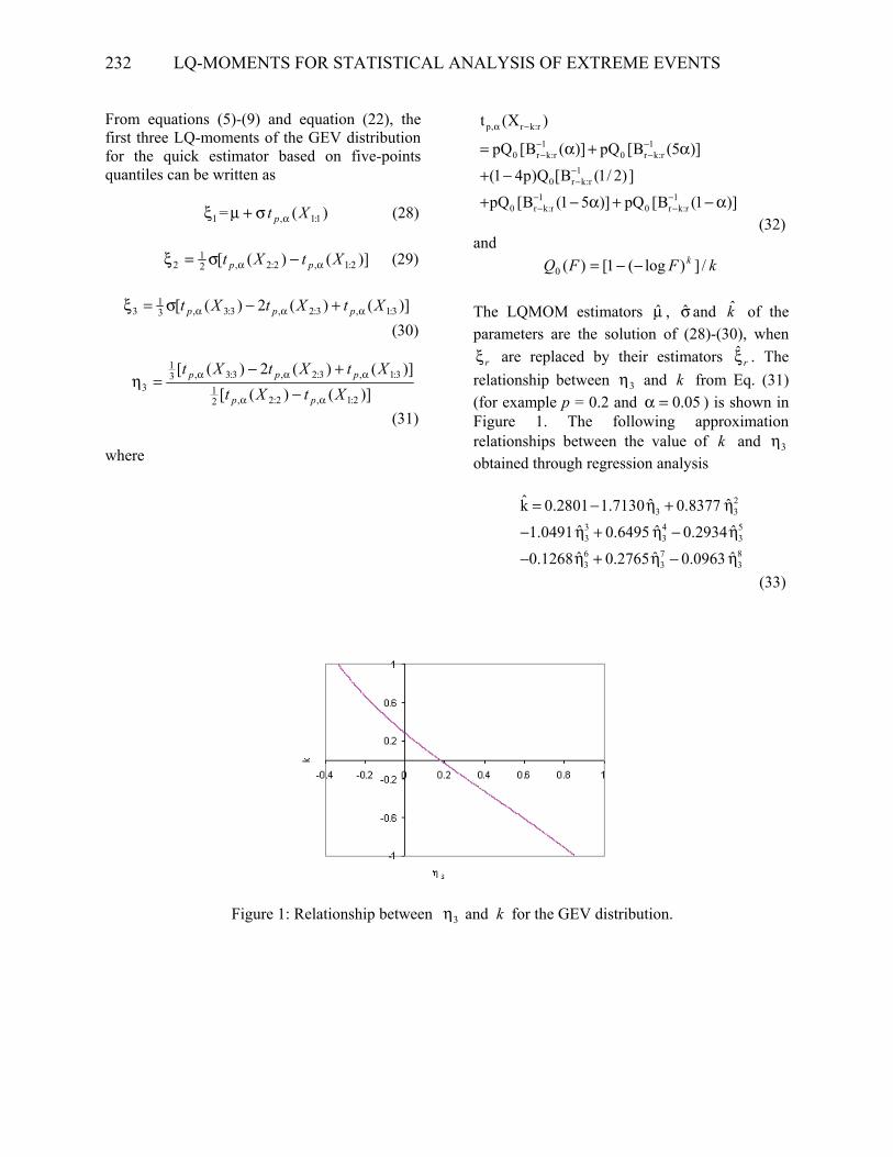
kFFQ k /])log(1[)(0 −−= The LQMOM estimators μ̂ , σ̂ and k̂ of the parameters are the solution of (28)-(30), when

rξ are replaced by their estimators rξ̂ . The relationship between 3η and k from Eq. (31) (for example p = 0.2 and 05.0=α ) is shown in Figure 1. The following approximation relationships between the value of k and 3η obtained through regression analysis

23 3

3 4 53 3 3

6 7 83 3 3

ˆ ˆ ˆk 0.2801 1.7130 0.8377ˆ ˆ ˆ1.0491 0.6495 0.2934ˆ ˆ ˆ0.1268 0.2765 0.0963

= − η + η

− η + η − η

− η + η − η

(33)

Figure 1: Relationship between 3η and k for the GEV distribution.

SHABRI & JEMAIN 233

The k̂ function is a very good approximation for k̂ in the range [-1.0, 1.0] and 3η̂ in the

range [-0.336, 0.854]. Once the value of k̂ is obtained, σ̂ and μ̂ can be estimated successively from Equation (29) and (28) as

)](ˆ)(ˆ[

ˆ2ˆ2:1,2:2,

2

XtXt pp αα −ξ

=σ (34)

)(ˆˆˆˆ 1:1.1 Xt p ασ−ξ=μ (35)

Monte Carlo Simulations

Monte Carlo simulations have been carried out to investigate the effect of LQ-moments based on WK5 with p = 0.2 and

05.0=α on the high quantiles estimation. Simulation Study For Parent Distribution Function Known

It is still useful to look at how estimation is affected by various methods when the distribution function is known, although the true underlying distribution function is never known in practice. In this study, the GEV

distribution is used to generate GEV samples. Monte Carlo simulations were performed for sample sizes 15, 25, 50 and 100, and parameters of GEV are 0=μ and 1=σ with different values of k between –0.4 and 0.4. The samples are fitted by the GEV distribution function using the method of LMOM, LIQ, and WK5.

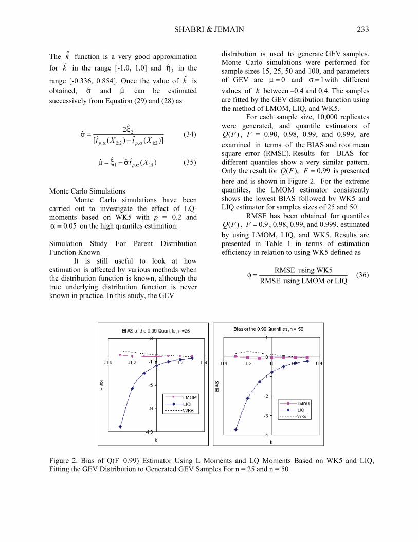
For each sample size, 10,000 replicates were generated, and quantile estimators of

)(FQ , F = 0.90, 0.98, 0.99, and 0.999, are examined in terms of the BIAS and root mean square error (RMSE). Results for BIAS for different quantiles show a very similar pattern. Only the result for ),(FQ 99.0=F is presented here and is shown in Figure 2. For the extreme quantiles, the LMOM estimator consistently shows the lowest BIAS followed by WK5 and LIQ estimator for samples sizes of 25 and 50.

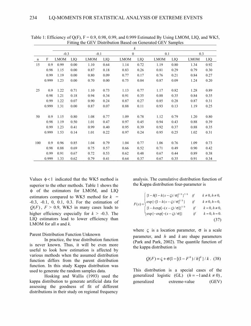
RMSE has been obtained for quantiles )(FQ , 9.0=F , 0.98, 0.99, and 0.999, estimated

by using LMOM, LIQ, and WK5. Results are presented in Table 1 in terms of estimation efficiency in relation to using WK5 defined as

LIQor LMOM using RMSE

WK5using RMSE=φ (36)

Figure 2. Bias of Q(F=0.99) Estimator Using L Moments and LQ Moments Based on WK5 and LIQ, Fitting the GEV Distribution to Generated GEV Samples For n = 25 and n = 50


234

Values 1<φ indicated that the WK5 method is superior to the other methods. Table 1 shows the φ of the estimators for LMOM, and LIQ estimators compared to WK5 method for k = -0.3, -0.1, 0, 0.1, 0.3. For the estimation of

)(FQ , F > 0.9, WK5 in many cases leads to higher efficiency especially for k > -0.3. The LIQ estimators lead to lower efficiency than LMOM for all n and k. Parent Distribution Function Unknown

In practice, the true distribution function is never known. Thus, it will be even more useful to look how estimation is affected by various methods when the assumed distribution function differs from the parent distribution function. In this study Kappa distribution was used to generate the random samples data. Hosking and Wallis (1993) used the kappa distribution to generate artificial data for assessing the goodness of fit of different distributions in their study on regional frequency

analysis. The cumulative distribution function of the Kappa distribution four-parameter is

⎪⎪

⎩

⎪⎪

⎨

⎧

==σς−−−≠=σς−−−

=≠σς−−−

≠≠σς−−−

=

.0,0]}/)(exp[exp{,0,0]}/)(exp[1{

,0,0}]/)(1[exp{

,0,0}]/)(1[1{

)(/1

/1

/1/1

hkifxhkifxh

hkifxk

hkifxkh

xFh

k

hk

(37) where ς is a location parameter, σ is a scale parameter, and h and k are shape parameters (Park and Park, 2002). The quantile function of the kappa distribution is khFFQ kh /}]/)1[(1{)( −−σ+ς= . (38) This distribution is a special cases of the generalized logistic (GL) )0 and 1( ≠−= kh , generalized extreme-value (GEV)

Table 1: Efficiency of Q(F), F = 0.9, 0.98, 0.99, and 0.999 Estimated By Using LMOM, LIQ, and WK5, Fitting the GEV Distribution Based on Generated GEV Samples

k -0.3 -0.1 0 0.1 0.3

n F LMOM LIQ LMOM LIQ LMOM LIQ LMOM LIQ LMOM LIQ 15 0.9 0.99 0.00 1.10 0.64 1.14 0.72 1.19 0.80 1.34 0.92 0.98 1.15 0.00 0.87 0.18 0.83 0.26 0.81 0.29 0.79 0.30 0.99 1.19 0.00 0.80 0.09 0.77 0.17 0.76 0.21 0.84 0.27 0.999 1.23 0.00 0.70 0.00 0.75 0.04 0.87 0.09 1.24 0.20

25 0.9 1.22 0.71 1.10 0.73 1.13 0.77 1.17 0.82 1.28 0.89 0.98 1.21 0.18 0.94 0.34 0.91 0.35 0.88 0.35 0.84 0.35 0.99 1.22 0.07 0.90 0.24 0.87 0.27 0.85 0.28 0.87 0.31 0.999 1.31 0.00 0.87 0.07 0.88 0.11 0.93 0.13 1.19 0.25

50 0.9 1.15 0.80 1.08 0.77 1.09 0.78 1.12 0.79 1.20 0.80 0.98 1.19 0.50 1.01 0.47 0.97 0.45 0.94 0.43 0.88 0.39 0.99 1.23 0.41 0.99 0.40 0.95 0.39 0.92 0.37 0.88 0.35 0.999 1.53 0.14 1.01 0.22 0.97 0.24 0.95 0.25 1.02 0.31

100 0.9 0.96 0.85 1.04 0.79 1.04 0.77 1.06 0.76 1.09 0.73 0.98 0.88 0.69 0.75 0.57 0.66 0.52 0.71 0.49 0.90 0.42 0.99 0.91 0.67 0.72 0.53 0.62 0.48 0.67 0.44 0.89 0.38 0.999 1.33 0.62 0.79 0.41 0.64 0.37 0.67 0.35 0.91 0.34

SHABRI & JEMAIN 235

)0 and 0( ≠= kh , generalized Pareto (GP) )0 and 1( ≠= kh , Gumbel (EV1)

)0 and 0( == kh , uniform (U) )1 and1( == kh and exponential (EXP) )1 and0( == kh distributions (Sing et al, 2002).

In order to evaluate the performance of the four-parameter estimation methods for GEV distribution, different parameters of kappa distribution were considered for simulation with values of the shape parameter ),( kh were set

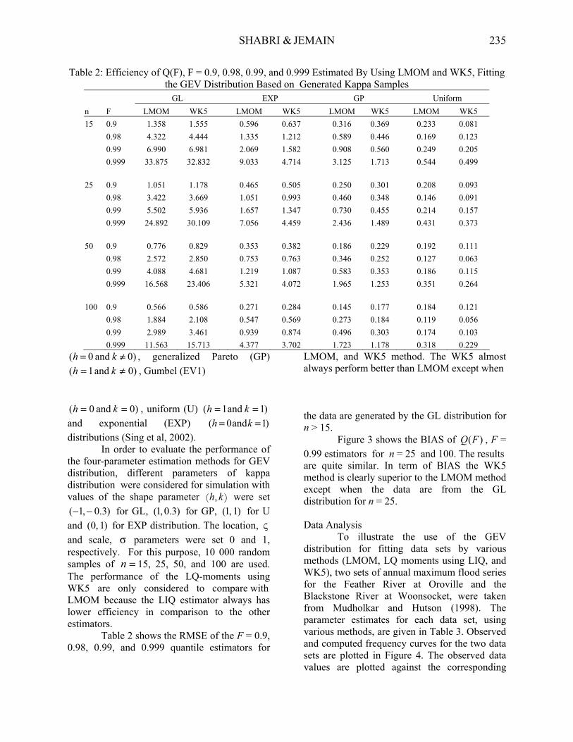
)3.0,1( −− for GL, )3.0,1( for GP, )1,1( for U and )1,0( for EXP distribution. The location, ς and scale, σ parameters were set 0 and 1, respectively. For this purpose, 10 000 random samples of =n 15, 25, 50, and 100 are used. The performance of the LQ-moments using WK5 are only considered to compare with LMOM because the LIQ estimator always has lower efficiency in comparison to the other estimators. Table 2 shows the RMSE of the F = 0.9, 0.98, 0.99, and 0.999 quantile estimators for

LMOM, and WK5 method. The WK5 almost always perform better than LMOM except when the data are generated by the GL distribution for n > 15.

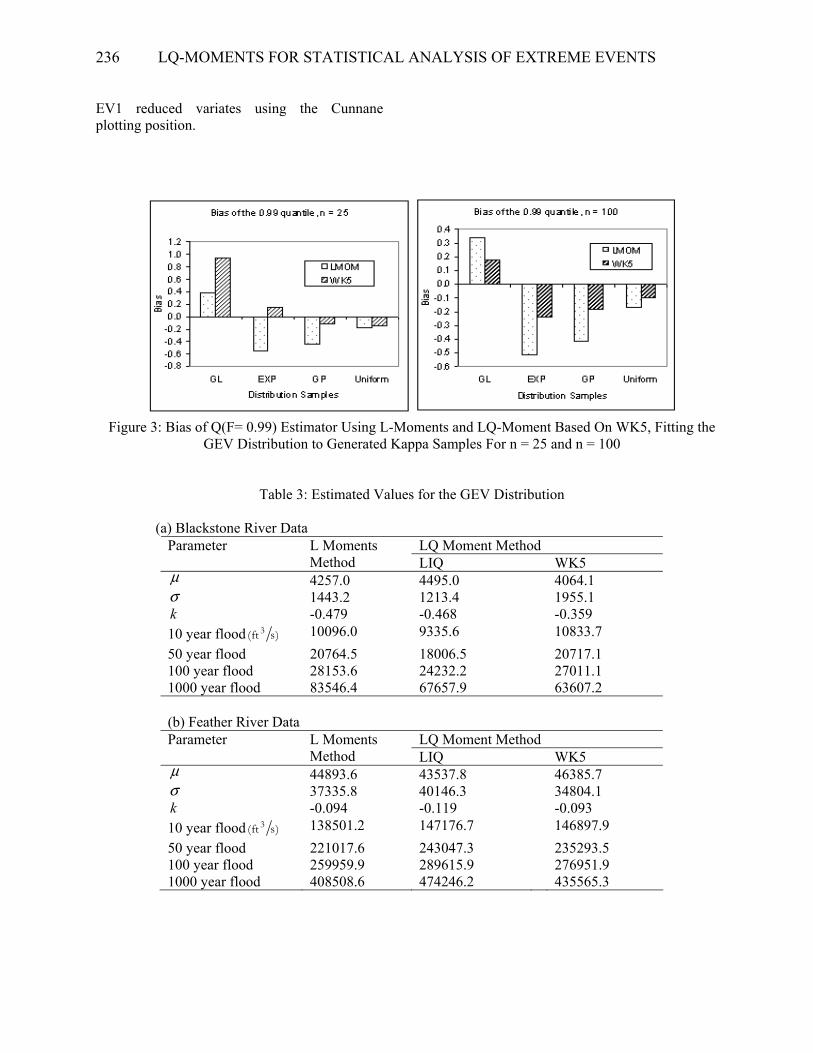
Figure 3 shows the BIAS of )(FQ , F = 0.99 estimators for n = 25 and 100. The results are quite similar. In term of BIAS the WK5 method is clearly superior to the LMOM method except when the data are from the GL distribution for n = 25. Data Analysis

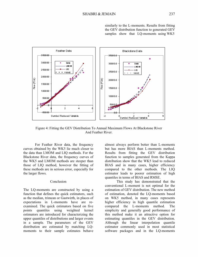
To illustrate the use of the GEV distribution for fitting data sets by various methods (LMOM, LQ moments using LIQ, and WK5), two sets of annual maximum flood series for the Feather River at Oroville and the Blackstone River at Woonsocket, were taken from Mudholkar and Hutson (1998). The parameter estimates for each data set, using various methods, are given in Table 3. Observed and computed frequency curves for the two data sets are plotted in Figure 4. The observed data values are plotted against the corresponding

Table 2: Efficiency of Q(F), F = 0.9, 0.98, 0.99, and 0.999 Estimated By Using LMOM and WK5, Fitting the GEV Distribution Based on Generated Kappa Samples

GL EXP GP Uniform n F LMOM WK5 LMOM WK5 LMOM WK5 LMOM WK5 15 0.9 1.358 1.555 0.596 0.637 0.316 0.369 0.233 0.081 0.98 4.322 4.444 1.335 1.212 0.589 0.446 0.169 0.123 0.99 6.990 6.981 2.069 1.582 0.908 0.560 0.249 0.205 0.999 33.875 32.832 9.033 4.714 3.125 1.713 0.544 0.499 25 0.9 1.051 1.178 0.465 0.505 0.250 0.301 0.208 0.093 0.98 3.422 3.669 1.051 0.993 0.460 0.348 0.146 0.091 0.99 5.502 5.936 1.657 1.347 0.730 0.455 0.214 0.157 0.999 24.892 30.109 7.056 4.459 2.436 1.489 0.431 0.373 50 0.9 0.776 0.829 0.353 0.382 0.186 0.229 0.192 0.111 0.98 2.572 2.850 0.753 0.763 0.346 0.252 0.127 0.063 0.99 4.088 4.681 1.219 1.087 0.583 0.353 0.186 0.115 0.999 16.568 23.406 5.321 4.072 1.965 1.253 0.351 0.264 100 0.9 0.566 0.586 0.271 0.284 0.145 0.177 0.184 0.121 0.98 1.884 2.108 0.547 0.569 0.273 0.184 0.119 0.056 0.99 2.989 3.461 0.939 0.874 0.496 0.303 0.174 0.103 0.999 11.563 15.713 4.377 3.702 1.723 1.178 0.318 0.229


236

EV1 reduced variates using the Cunnane plotting position.

Figure 3: Bias of Q(F= 0.99) Estimator Using L-Moments and LQ-Moment Based On WK5, Fitting the

GEV Distribution to Generated Kappa Samples For n = 25 and n = 100

Table 3: Estimated Values for the GEV Distribution (a) Blackstone River Data

LQ Moment Method Parameter L Moments Method LIQ WK5

μ 4257.0 4495.0 4064.1 σ 1443.2 1213.4 1955.1 k -0.479 -0.468 -0.359 10 year flood )sft( 3 10096.0 9335.6 10833.7 50 year flood 20764.5 18006.5 20717.1 100 year flood 28153.6 24232.2 27011.1 1000 year flood 83546.4 67657.9 63607.2 (b) Feather River Data

LQ Moment Method Parameter L Moments Method LIQ WK5

μ 44893.6 43537.8 46385.7 σ 37335.8 40146.3 34804.1 k -0.094 -0.119 -0.093 10 year flood )sft( 3 138501.2 147176.7 146897.9 50 year flood 221017.6 243047.3 235293.5 100 year flood 259959.9 289615.9 276951.9 1000 year flood 408508.6 474246.2 435565.3

SHABRI & JEMAIN 237

For Feather River data, the frequency

curves obtained by the WK5 lie much closer to the data than LMOM and LIQ methods. For the Blackstone River data, the frequency curves of the WK5 and LMOM methods are steeper than those of LIQ method, however the fitting of these methods are in serious error, especially for the larger flows.

Conclusion The LQ-moments are constructed by using a function that defines the quick estimators, such as the median, trimean or Gastwirth, in places of expectations in L-moments have are re-examined. The quick estimators based on five points quantiles using weighted kernel estimators are introduced for characterizing the upper quantiles of distributions and larger events in a sample. The parameters of the GEV distribution are estimated by matching LQ-moments to their sample estimates behave

similarly to the L-moments. Results from fitting the GEV distribution function to generated GEV samples show that LQ-moments using WK5

almost always perform better than L-moments but has more BIAS than L-moments method. Results from fitting the GEV distribution function to samples generated from the Kappa distribution show that the WK5 lead to reduced BIAS and in many cases, higher efficiency compared to the other methods. The LIQ estimator leads to poorer estimation of high quantiles in terms of BIAS and RMSE. This study has demonstrated that the conventional L-moment is not optimal for the estimation of GEV distribution. The new method of estimation, denoted the LQ-moments based on WK5 method, in many cases represents higher efficiency in high quantile estimation compared the L-moments method. The simplicity and generally good performance of this method make it an attractive option for estimating quantiles in the GEV distribution. Although the linear interpolation quantile estimator commonly used in most statistical software packages and in the LQ-moments

Figure 4: Fitting the GEV Distribution To Annual Maximum Flows At Blackstone River And Feather River.


238

method, but it does not perform as good as the WK5 in estimating the parameters of the GEV distribution.

References

Chowdhury, J. U., Stedinger, J. R., Lu, L. H. (1991). Goodness of fit tests for regional generalized extreme value flood distribution. Water Resources Research. 27(7), 1765-1776.

David, H. A. & Nagaraja, H. N. (2003). Order Statistic. New York: Wiley.

Hosking, J. R. M. (1990). L-moments: Analysis and Estimation of Distribution Using Liner Combinations of Order Statistics. Journal of the Royal Statistical Society, Series B. 52, 105-124.

Hosking, J. R. M. & Wallis, J. R. (1993). Some statistics useful in regional frequency analysis. Water Resources Research. 29(2), 271-281.

Hosking, J. R. M. & Wallis, J. R. (1997). Regional Frequency Analysis: An approach based on L-Moments Cambridge: Cambridge University Press.

Hosking, J. R. M., Wallis, J. R., & Wood, E. F. (1985a). Estimation of the generalized extreme-value distribution by the method of probability weighted moments. Technometrics, 27(3), 251-261.

Huang, M. L., Brill, P. (1999). A Level Crossing Quantile Estimation Method. Statistics & Probability Letters, 45, 111-119.

Huang, M. L. (2001). On a Distribution-Free Quantile Estimator. Computational Statistics & Data Analysis, 37, 477-486.

Karvane, J. (2006). Estimation of quantile mixtures via L-moments and trimmed L-moments. Computational Statistics & Data Analysis, 51, 947-959.

Martins, E. S., Stedinger, J. R. (2000). Generalized Maximum-Likelihood Generalized Extreme-Value Quantile Estimators for Hydrologic Data. Water Resources Research, 36(3), 737-744.

Mudholkar, G. S. & Hutson, A. D. (1998). LQ moments: Analogs of L-Moments. Journal of Statistical Planning and Inference, 71, 191-208.

Park, J. S. (2006). A Simulation-Based Hyperparameter Selection for Quantile Estimation of the Generalized Extreme Value Distribution. Mathematics and Computers in Simulation, 70(4), 366-376.

Park, J. S. & Park, B. J. (2002). Maximum Likelihood Estimation of the Four-Parameter Kappa Distribution Using The Penalty Method. Computers and Geosciences, 28, 65-68.

Sankarasubramanian, A. & Srinivasan K. (1999). Investigation and Comparison of Sampling Properties of L-Moments and Conventional Moments. Journal of Hydrology, 218, 13-24.

Sheather, S. J. & Marron, J. S. (1990). Kernel Quantile Estimators. Journal of the American Statistical Association, 85, 410-416.

Vogel, R. M. & Fennessey, N. M. (1993). L-Moment diagrams should replace product moment diagrams. Water Resources Research, 29(6), 1745-1752.

Wang, Q. J. (1997). LH moments for statistical analysis of extreme events. Water Resources Research, 33(12), 2841-2848.

lq-moments for statistical analysis of extreme events

Documents