“LOW VOLATILITY ANOMALY IN THE INDIAN EQUITY

MARKET”

by

Ayush Banerjee (A008)

Bachelor of Science in Economics, 2013-2016

Submitted in complete fulfilment of the requirements for the degree of

BSc. Economics

28th March, 2016

SARLA ANIL MODI SCHOOL OF ECONOMICS, NMIMS (MUMBAI)

ACKNOWLEDGEMENTS

I would sincerely like to thank my mentor, Professor Hemal Khandwala. His

feedback, patience and understanding aided me in completing this paper.

I would earnestly like to thank my batch mate Dheer Patel for helping me streamline

and expedite my calculation process in Microsoft Excel 2010.

Lastly, I would like to thank my friends and family for their support.

1 | P a g e

CONTENTS

No.

Topic Page no.

Abstract 31 Introduction 4-62

2.12.22.3

Literature Review -Traditional Portfolio TheoryEmpirical Findings of Low Volatility AnomalyReasons for Low Volatility Anomaly

7-117710

33.13.23.33.4

Need for StudyFormulating 3 tests for exploring Low Volatility AnomalyUsing CAGR instead of Monthly Average ReturnsRationale behind Choice of frequencyObjectives of the study

12-1512131415

44.14.24.3

MethodologySamplingData CollectionFramework of Analysis

16-18161617

55.15.25.3

Results and AnalysisTest 1Test 2Test 3

19-23192022

66.16.26.3

Reasons for low volatility anomaly in the Indian equity marketWhat accounts for anomaly?Limits to ArbitrageUndervaluation of Stocks

24-26242426

77.17.2

ConclusionScope for further studyLimitations

272829

8 References 30-31

2 | P a g e

ABSTRACT

Modern portfolio theory postulates that risk and return move in tandem. However, new

literature has explored the linkages between risk and return and shown that one need not

invest in high volatility stocks to earn commensurate returns. A low volatility portfolio yields

higher returns than a high volatility portfolio. This phenomenon has been termed as low

volatility anomaly. However, such empirical work has been done predominantly in the

developed markets of USA and Europe. This paper documents the prevalence of low

volatility anomaly in the Indian equity market with standard deviation being a measure of

volatility. To check for this phenomenon, a test for monthly average returns, portfolio values

and Sharpe ratio values is conducted respectively with a time frame of 15 years. It is found

that the portfolio experiencing the least amount of volatility yields a higher return in absolute

and risk adjusted terms than the portfolio which experiences the maximum amount of

volatility. The reasons for the prevalence of this phenomenon in the Indian equity market are

ascertained to be the limitations to arbitrage opportunities and the presence of undervalued

stocks in the low volatility segment.

3 | P a g e

I. INTRODUCTION

The generalized notion while making investments in the equity markets is that if an

investor has to assume greater risks, he/she must be compensated with higher returns. In an

efficient market, investors can expect above average returns only when they are willing to

take above average risks by investing in volatile stocks (volatility being a measure of risk).

However, there is evidence that this founding principle of modern finance has not

always held up in practice. Investors attempt to minimize risk and maximize returns from a

given investment in a portfolio. This has given rise to the theory of low volatility anomaly in

the equity market which challenges the underlying assumption that risk and reward move in

tandem. High volatility stocks have not always generated commensurately higher returns than

low volatile stocks when analysed from the perspective of formulating a high volatility and

low volatility portfolio.

Given the sizeable Indian equity market which is the 11th largest in the world, it is

imperative to check for the phenomenon of low volatility anomaly herein. The main idea of

this paper is summarized in the following 2 points:

This study seeks to explore the low volatility anomaly in the Indian equity market and

check if the corresponding low volatility portfolio delivers higher returns than the

high volatility portfolio. The performance of the portfolios is measured in terms of

monthly average returns, portfolio value over 15 years, CAGR return and the Sharpe

Ratio trend. The above 3 tests are carried out to check for consistency in results.

This study seeks to determine if the draw down effect is prevalent in the Indian equity

market. This effect refers to the phenomenon where in a bear market the low portfolio

is least hit and subsequently generates higher absolute and risk adjusted returns,

whereas a high volatile portfolio suffers a huge drawdown as the stock prices

4 | P a g e

plummet. This will determine if investing in a low volatility portfolio can lead to

stronger preservation of capital.

To examine the phenomenon of low volatility anomaly, there are 2 investment strategies:

1. Low volatility portfolio investing- Segregates the stocks into low volatile portfolios

and high volatile portfolios with standard deviation as the explanatory variable.

2. Minimum Variance investing- Takes in to account the correlations of individual

stocks and optimally diversifies a portfolio so as to generate the highest expected

return for a given level of standard deviation (risk).

In a nutshell the investment decision is predicated upon the volatility of stock prices or the

variability of stock prices with a market index (which is a benchmark figure).

Choice of investment strategy and rationale

This study employs ‘the low volatility investing method’ to explore the phenomenon

of low volatility anomaly in the Indian equity market. This method is better as it overcomes

the bias in the market cap weighted portfolios, wherein a few stocks which are dominant,

consequently subdue the returns of a smaller but fundamentally strong company. The strategy

allocates equal weights to all stocks in the portfolio.

This paper is organized as follows:

Section II summarizes the earlier research done in examining low volatility anomaly.

In this section you will find an overview of Markowitz risk-return theory, how it was

refuted by Fama and French, empirical findings of authors confirming the prevalence

of low volatility anomaly in different markets and the reasons for a low volatility

portfolio performing better than the high volatility portfolio.

Section III discusses the need for this study in the Indian context, critique and further

developments on erstwhile research in this domain and the objectives of this study.

5 | P a g e

Section IV discusses the methodology of calculating average returns, portfolio

values and plotting the Sharpe Ratio trend. The time horizon, important formulae and

necessary frequencies for measurement are mentioned here.

Section V provides the corresponding results and provides an analysis of the

performance of the low volatility portfolio vis-à-vis the high volatility portfolio.

Section VI explores the reasons for investors to purchase highly volatile stocks

despite the prevalence of low volatility anomaly in the Indian equity market.

Section VII draws conclusion from the results and analysis, provides the limitations

of the study and mentions the scope for further research.

6 | P a g e

II. LITERATURE REVIEW

2.1 Traditional Portfolio Theory

According to the modern portfolio theory formulated by Harry Markowitz (1952),

there is a direct relationship between risk and return. In an efficient market, an investor needs

to assume higher risk in order to earn higher returns. Taking the stock market as an example,

risky stocks with higher standard deviation are expected to give higher returns than “safe”

stocks (stocks with low standard deviation). Jack Treynor (1961), William Sharpe (1964),

John Lintner (1965) and Jan Mossin (1966) carried forward the work of Harry Markowitz by

formulating the Capital Asset Pricing Model (CAPM). They key tenet of this model is that for

investors to accept risk, they must be compensated with higher returns. This model gave rise

to the term beta which measures the volatility of a stock price in comparison to the market

portfolio. Essentially, a high beta stock is categorized as a high volatility stock and is

therefore expected to generate higher returns for the investor.

The Sharp Linter Black (SLB) Model hypothesized that the market portfolio is the

tangency portfolio. The risk premium of an asset (over and above the risk free rate) is a

function of beta, stipulating that it is the only explanatory variable for predicting expected

return on a stock. Adding an asset which has a low correlation with the market portfolio will

reduce the overall risk of the portfolio and generate relatively higher payoffs in a bear market

than a portfolio which is highly correlated to the market.

2.2 Empirical findings of low volatility anomaly

However, Fama and French (1992) investigated the stocks listed on NASDAQ from

the period 1963-1990 and found that book to market-equity and firm size captures the effect

of expected returns on a particular stock. The size effect is robust and smaller stocks have

higher expected returns whereas companies with higher book to market equity generate

higher returns.

7 | P a g e

Akdeniz, Ayodgan and Salih (2000) confirmed the empirical findings of Fama and

French. An analysis of cross sectional variations across stocks in the Turkish Stock Market

from the period 1992-1998 concluded that the cross sectional returns vary directly with book

to market equity and inversely with firm size. Thus, as opposed to what the SLB model

hypothesizes, beta is not the only explanatory variable which impacts expected stock returns.

The underlying assumptions of the CAPM were investigated by Black (1972). It was

found that the CAPM model does not hold true if the assumption of borrowing/lending any

amount at the risk free rate of interest is relaxed. Analysing the US stock returns at different

levels of beta from the period 1926-1966, the average portfolio returns is not consistent with

the equation Ri = Rf +beta(Rm-Rf). The expected returns on stocks at low levels of beta were

higher as opposed to what the equation would imply. Moreover, Black goes on to challenge

another assumption which states that short positions in riskless assets are allowed contending

that there are restrictions on borrowing due to which the outcomes of the CAPM model

would change. Accounting for such a fact reveals that low beta stocks yet again yield higher

average returns than high beta stocks.

There were empirical findings which confirmed Black (1972)’s findings. Robert

Haguen challenged the traditional theory in his paper “On the Evidence supporting the

existence of risk premium in the Capital Markets”. Empirical findings confirmed that risk

does not necessarily generate a special reward for the investors in the form of higher returns.

Over the long run, stock portfolios with relatively lesser variance in monthly average returns

have given greater average returns than their riskier counterparts. With reference to the

CAPM model, a low volatility portfolio posted superior returns compared to the supposedly

efficient market portfolio.

Recently, Roger Clarke, Harvin De Silva and Steven Thorley (2006) found that a

minimum variance portfolio derived from the 1000 largest US stocks from the time period

8 | P a g e

1968-2005 delivered higher average returns than the efficient market portfolio. The

minimum variance portfolio gave an average of 6.5% over the T-bill with standard deviation

=11.7% whereas the market index gave an average return of 5% over the T-bill with standard

deviation=15.4%.

Taking into consideration the phenomenon of low volatility anomaly, low volatility

investing can be a strategy adopted to generate higher risk adjusted returns than the market

portfolio. In terms of the time period taken to reap the benefits of such a strategy, State Street

(2009) points out that in circumstances of strong market rallies, the low volatility portfolio

will lag the equity market. Moreover, when the market sees a downward trend, the low

volatility portfolio will lag behind again and it is at that time that the investor will be

protected from a sharp decline in stock prices (as his/her portfolio stocks will see a relatively

lesser decline in value).The sector wise breakdown of a low volatility portfolio is different

from that of a broad market (index). For example, in USA a low volatility portfolio would

typically comprise of utilities and consumer staples, whereas a market index would consist of

IT and consumer discretionary stocks. Thus investors, adopting this strategy, given the

phenomenon of low volatility anomaly should be prepared to accept sustained periods of

underperformance.

From a global perspective, looking at the equity markets across the world, Biltz et al

(2007) analysed the average stock returns in the FTSE World Development Index and found

that stocks with low historical volatility exhibit higher risk adjusted returns, both in terms of

Sharpe ratio and CAPM beta.

In context to the Indian equity market, Rambhia (2012) employs the Low Volatility

investment strategy to explore the existence of low volatility anomaly in the Indian equity

market. Using an 11 year period (from 2000-2011), stocks in the index are segregated into

high and low volatility portfolios on the basis of standard deviation on a monthly basis. The

9 | P a g e

average arithmetic monthly returns of each portfolio are computed and compared. It is

ascertained that in the Indian equity market, a low volatility portfolio gives not only higher

absolute returns, but higher risk adjusted returns as well when compared to a high volatility

portfolio. Jindal Kiran (2006) and Sarma (2004) analysed the stock returns across various

indices in the Indian equity market in order test for the presence of seasonality. It was

ascertained that the Indian equity market experiences a monthly effect as well as semi-

monthly effect. There was no detection of a day effect.

Joshipura (2014) constructs a high volatility and low volatility portfolio using the

CNX 200 index (from the year 2001-2013) and finds the same results, wherein a low

volatility portfolio outperforms the high volatility portfolio in terms of absolute returns and

risk adjusted returns. He further analyses the behaviour of high volatility and low volatility

portfolio by computing their Sharpe ratio respectively. Results show that low volatility

portfolio in the Indian equity market from the time period 2001 to 2013 has a Sharpe ratio

value=0.19 whereas the high volatility portfolio has a Sharpe ratio value= -0.102.

2.3 Reasons for low volatility anomaly

An essential question that arises with the prevalence of low volatility anomaly is that

why are people still investing in high volatility portfolios? Firstly, Binsbergen, Brandt and

Koijen (2008) look at the behaviour of asset managers and infer that they are profit

maximizing and are always looking to outperform the bull market rather than the bear

market. The investment approach is decentralized and thus the chief investment officer’s

decision to allocate funds to high beta stocks is incontrovertible.

Secondly, Black(1993) postulates that the main reasons for low low volatility

anomaly is the borrowing restrictions on short selling and leverage, given the fact that

leverage is required to take full advantage of low beta stocks. Thirdly, due to the restrictions

on borrowing (Baker, Bradley and Wurgler 2011), the possibility of carrying out an arbitrage

10 | P a g e

transaction between low beta- high alpha stocks and high beta- low alpha stocks gets

eliminated.

Lastly, Boyer, Mitton and Vorkink, (2010) attributed the occurrence of low volatility

anomaly to behavioural biases amongst investors who are looking for lottery like payoffs.

Volatility is considered to be a proxy for skewness. High volatility individual stocks which

are positively skewed are preferred by investors.

11 | P a g e

III. NEED FOR THE STUDY

3.1 Formulating 3 tests for exploring low volatility anomaly

Given the occurrence of low volatility anomaly and the fact that CAPM equation R i =

Rf +beta(Rm-Rf) does not justify it, proof for this phenomenon is essential to formulate and

test with empirical evidence.

In this domain of research, there remain a few fundamental questions which haven’t

been answered comprehensively. These are as follows:

Is there a model which explains the high returns of low volatile stocks?

When does the low volatility portfolio begin to outperform the high volatility

portfolio?

There is no justification for the time frequency used i.e average “monthly” returns. Is

it a suitable measure?

This study seeks to answer the above questions and give a clearer picture of low

volatility anomaly in the Indian context.

Taking in to cognizance the earlier research done, calculating the average returns of

each portfolio over 10-15 years is merely conclusive proof that low volatility anomaly exists

in the Indian equity market. Investors are concerned about how much their wealth will

appreciate if they put their capital in a low volatility portfolio vis-a-vis a high volatility

portfolio. Moreover, since the study seeks to estimate the returns and draw conclusions in

terms of how much risk is assumed to generate a given amount of return in a portfolio, risk

adjusted returns of a low volatility portfolio vis-a-vis a high volatility portfolio needs to be

calculated. Thus there is a need to calculate not only the average returns of each portfolio, but

also the portfolio values and Sharpe ratio values of the high and low volatility portfolio.

The phenomenon of low volatility anomaly exists if there are favourable results across

the 3 tests. The first test will ascertain if the portfolio with the least volatility (“LV” portfolio)

12 | P a g e

delivers higher returns than the portfolio with the maximum amount of volatility (“HV”

portfolio). The second test will estimate the terminal portfolio values of the LV and HV

portfolio and check if a given sum amount invested in a LV appreciates to a higher value than

the HV portfolio. Lastly, the annual risk adjusted returns will be calculated for the LV and

HV portfolio using the Sharpe ratio. Thus, this study seeks to analyse the notion of low

volatility anomaly from a broader perspective and provide more conclusive and consistent

results.

3.2 Using Compounded Annual Growth Rate instead of Average Returns

Another drawback of erstwhile research is that there is no justification for using

“arithmetic average” returns. In fact using a simple arithmetic average is not an adequate

measure of your stock returns. When looking at annual investment returns, if you lose money

in a particular year, you have that much less capital to generate returns in the following year

and vice versa. This study employs the compounded annual compounded growth rate

(CAGR) to check for the existence of low volatility anomaly. However, the 1st test does

measure the low volatility anomaly using monthly average returns as a preliminary check to

determine the composition of stocks in each portfolio which will be used to estimate the more

pertinent portfolio values and CAGR of the HV and LV portfolio.

CAGR helps to measure the average growth of an investment over a variable period of

time. Given the market volatility, the year-to-year growth will keep fluctuating and hence it

may become difficult to interpret. CAGR herein resolves this issue by calculating the average

growth rate of a single investment. It is superior to the concept of average returns as it

considers the assumption that an investment is compounded over time. While measuring

CAGR returns it is imperative to determine your look back period and holding period. The

look back period serves as the basis on how you select your portfolio. In this study the look

back period is 2 years. Hence the portfolio is selected by analysing the measure of risk over

13 | P a g e

the past 2 years. The holding period refers to the amount of time for which the portfolio is

held before it is sold off. The value at the end of the holding period is known as the portfolio

value. The holding period in this study is 1 year.

Jegadeesh and Titman prove conclusively that stock prices overreact to information

which is why a 3-12 month contrarian strategy yields abnormal returns. This overreaction to

prices is also present in the Indian equity market and is confirmed by Dr. Shalini Agarwal in

her thesis “Prior Return Effect in Indian Stock Market Using High Frequency Data”.

Moreover, picking stocks based on price movements in the last 1 year may lead to a selection

bias and overlook the fact that there are stocks which don’t perform well for a year given the

underlying problems of the company (say a long gestation period faced by an infrastructure

company or a renewable energy company paying off its debt in a year). Thus there is need to

test the performance of portfolios with a look back period greater than 1 year. Secondly, De

Bondt and Thaler show that stocks with a holding period equal to or greater than 1 year that

performed poorly in the previous years achieve higher returns than the stocks that performed

well over the same period. Hence, the need to test the performance of portfolios with a

holding period of 1 year in the Indian equity market. Amalgamating the above notions by

Jegadeesh and Titman and De Bondt and thaler, portfolios are being selected based on a look

back period of 2 years and are being held for a period of 1 year (holding period). This notion

is being tested in the Indian equity as it is the target segment of this paper. Since this paper is

focussing on risk due to volatility in the Indian equity market, portfolios are formed on the

basis of standard deviation measured over 2 years.

3.3 Rationale behind choice of frequency

There have been different frequencies(daily, weekly, monthly, quarterly and even 3

years in case of Blitz (2007)) used to measure stock returns and standard deviation, but no

14 | P a g e

justification as to why it has been used. Which frequency should ideally be used all the time

in the context of the Indian equity market is still unknown.

This paper measures average monthly returns as it is most suited for analysing the

performance of portfolios over a long period of time (15 years is the time horizon in this

study). The reason why a daily or weekly return is not being used is that it is too short a time

period to gauge over returns due to information trade. The HV stocks are likely to perform

significantly better than LV portfolio in one day or a week. Such fluctuations in a day or over

a week are essentially why such stocks are characterised as HV stocks. Moreover, with a lot

more number of data points, finding out a trend becomes relatively more difficult. The

purpose over here is to see how certain portfolios perform over a longer period of time of 10-

15 years and not project a massive rise or downfall by focussing on price level shifts on daily

or weekly basis.

In a nutshell, I acknowledge the fact that research has been done previously on this

topic, but the methodology employed is restricted and there is no justification for the

parameters of measurement. This study seeks to provide more conclusive proof by

consolidating the results from 3 tests and explaining at each step the rationale behind using

every parameter ( as explained already the reasons for using CAGR, 2 years as look back

period and 1 year as holding period).

3.4 Objectives of the study

1. To construct high and low volatility portfolios in the Indian equity market.

2. To calculate the risk and return of high and low volatility portfolios in terms of

arithmetic mean and CAGR return.

3. To check for the existence of low volatility anomaly wherein the low volatility

portfolio has a higher portfolio value than the high volatility portfolio.

4. Determine the reasons for low volatility anomaly, if at all the notion holds true.

15 | P a g e

IV. METHODOLOGY:

4.1 Sampling

The sampling for this study consists of the constituent stocks of the S&P CNX 500

index. The rationale for such sampling is that CNX500 index represents about 95% of the

free float market capitalisation on the NSE as of 28th March, 2016. It therefore is an adequate

representation of the entire Indian equity market. Moreover, it avoids the problem of small

and illiquid stocks dominating the results.

4.2 Data Collection

Adjusted monthly closing prices1 of all the stocks in the CNX 500 index was collected

from the Prowess Database. The time horizon chosen for the purpose of this analysis is April,

2000 to March, 2015. The reason this time period has been chosen is because it covers a

significant number of events which brought about a change in the Indian equity market. It

includes the strong Bull run from 2004-2008, the global meltdown in 2008-2009, the

Eurozone crisis and the rise in oil prices in 2014-2015.

Of the companies present in the index, those which did not meet the following criteria

were excluded:

1. Stocks replaced during the period and not present in the index now.

2. Stocks for which 24 months of historical data was not available as a result of which

volatility could not be calculated.

1 Stock price is adjusted for stock splits, dividends/distributions, etc. which facilitates calculation of return without any difficulty i.e.if current price of a stock is Rs. 100, the company has just gone ex bonus with bonus of 1:1, which means price before the bonus may be say Rs.200. Now if we go by absolute price then in that case the last month closing price may be somewhere around Rs. 200 and this month closing price is around Rs.100, which means negative returns. However, that may not be true as the stock has gone ex-bonus and therefore the price should be adjusted backwards to half of the price prevailing before the bonus of 1:1 to make it comparable of price now.

16 | P a g e

4.3 Framework of Analysis

The following procedures of risk and volatility estimation have been employed:

1. Portfolio formation-The stocks were categorized into portfolios of low volatility and

high volatility. In order to do this, the monthly returns of stocks were calculated using

the formula: (p1-p0/p0), where p1 is the current month’s closing price and p0 is the

previous month’s closing price. The average returns for a period of 24 months and the

standard deviation of these returns over 24 months was calculated to arrive at a return

and risk (volatility) value for the stock. Therefore, the starting point is April, 2002

wherein the return value will be the average return from 1st April, 2000 to 31st

March,2002 (24 months) and the volatility value will be the standard deviation of

these 24 data points (indicating returns). Similarly, for May, 2002 the return and

volatility value will be from 1st May, 2000 to 31st April, 2002. The portfolio for each

month (starting from April, 2002) is calculated by taking the standard deviation of all

the stocks in a given month and arranging them in ascending order with the first stock

having the least standard deviation and the last stock in the list having the maximum

standard deviation. The average return of the stock for that month is placed next to it

respectively. Portfolios are then formed by taking the top 10% of the stocks in this list

and placing it in portfolio 1 known as “P1”-the portfolio of stocks with the least

standard deviation. The next 10% of the stocks are placed in “P2”. The average

standard deviation and average return for each portfolio is calculated. This gives a list

of 10 portfolios, its standard deviation and the average return for each time period.

Finally, the aggregate return and standard deviation for each portfolio across all time

periods is calculated.

2. CAGR calculation- For the purpose of CAGR calculation, the look back period is 2

years whereas the holding period is 1 year. So the first purchase of shares is made on

17 | P a g e

1st April, 2002 and it is sold on 31st March, 2003. The next purchase will be made on

1st April, 2003 and sold on 31st March, 20042. For the purpose of comparative

analysis, there are 2 cases simulated. In the first case, a sum of Rs.100000 is invested

in the LV portfolio and in the second case a sum of Rs.100000 is invested in the HV

portfolio. The principal amount of Rs.100000 and the subsequent portfolio value at

the end of each period is divided equally among the stocks in the LV and HV

portfolio assuming that the investor is indifferent to investing in accordance to market

capitalisation based weightage or investing according to equal allocation to each

stock. Once the terminal value of the HV and LV portfolio is known, CAGR return is

calculated using the following formula:

3. Sharpe Ratio- the Sharpe ratio values for the portfolio with the highest volatility and

lowest volatility is calculated and plotted against each other to observe the

performance in risk adjusted terms. The risk free rate is taken as the 10 year yield on

the government bond.

2 This is a simulation to measure the performance from one point in the year. With a change in the starting point of purchase, the results are likely to differ in absolute values but the overall conclusion remains the same that the LV portfolio generates a higher return than the HV portfolio

18 | P a g e

V RESULTS AND ANALYSIS

5.1 TEST (1)-Does the LV portfolio deliver higher monthly average returns than the

HV portfolio?

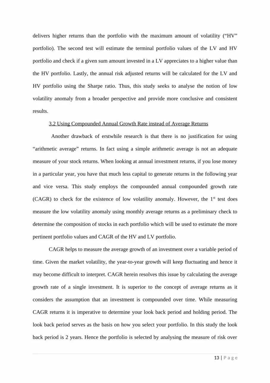
Chart 1 delineates the monthly returns of the 10 portfolios when measured in terms of

simple arithmetic average. P1 is the portfolio with the lowest standard deviation and hence

sees the least amount of volatility. P10 is the portfolio with the maximum amount of

volatility. P1 delivers an average return of 1.72% whereas the P10 delivers an average return

of 1.68%. Table 1 summarizes the portfolio returns and the volatility of monthly returns.

Portfolio 1 experiences a 7.04% volatility in its monthly returns and yields an average

monthly return of 1.73% whereas portfolio 9 and 10 experience a monthly volatility of

17.15% and 21.66% , but yield a lower monthly average return of 1.67%(P9) and 1.68%

(P10). This is evidence for the presence of low volatility anomaly in the Indian equity market

given that the low volatility portfolio generates a higher return than the high volatility

portfolio.

(Lowest Volatility) (Highest Volatility)

CHART 1: Average Returns of the 10 portfolios

19 | P a g e

PortfolioNumber 1 2 3 4 5 6 7 8 9 10

AverageMonthly Returns (%)

1.73 1.61 1.47 1.56 1.54 1.62 1.65 1.57 1.68 1.67

VolatilityOf Returns (%)

7.04 8.83 9.97 10.97 11.92 12.89 13.93 15.29 17.15 21.66

Table 1-Average Monthly returns and volatility of monthly returns

5.2 TEST (2)-Does the LV portfolio yield a higher portfolio value and CAGR return

than the HV portfolio?

Employing CAGR as the measure of returns, Chart 2 delineates the trend of the LV

portfolio (portfolio with the least standard deviation) and the HV portfolio (portfolio with the

highest standard deviation) over the analysis period. This is the set of primary results used to

confirm the presence of low volatility anomaly in the Indian equity market and its associated

arguments.

The purpose of calculating portfolio values at the end of each period and subsequently

calculating the CAGR is to ascertain as to when the LV portfolio begins to perform better

than the HV portfolio consistently. From 2012 onwards, the LV portfolio yields a higher

value than the HV portfolio. The summary results of the portfolio values and the CAGR are

given in Table 2.

20 | P a g e

Chart 2: Trend of portfolio value

In the time period 2008-2009, the HV portfolio was the worst hit. The graph shows a

steep fall in case of the HV portfolio. However, the LV portfolio sees a moderate decline in

portfolio value. From this trend we can infer that during a bear run the LV portfolio provides

a cushioning effect with a moderate decline in portfolio value. Thus it is better to stay

invested in a LV portfolio. Undoubtedly, the HV portfolio does experiences an equally

significant increase in value during a bull run but over a longer period of time the value of the

LV portfolio steadily increases and eventually performs better than the HV portfolio.

Portfolio Opening value1st April, 2002

Terminal Value (approx.)31st March, 2015

CAGR Return (%)

Low Volatility (LV) 100000 1312609 18.82

High Volatility (HV) 100000 1217736 17.23

Table 2: Terminal portfolio value and CAGR of HV and LV portfolio

With reference to the companies listed in the CNX 500, a time horizon of 15 years, a

look back period of 2 years (in terms of standard deviation) and a holding period of 1 year,

21 | P a g e

there exists low volatility anomaly. The low volatility portfolio performs consistently better

than the high volatility portfolio after 2011. The LV portfolio gives a compounded annual

growth rate of 18.82% whereas the HV portfolio yields a return of 17.23%. Thus low

volatility anomaly does exist in the Indian equity market with the LV portfolio giving a

higher return than the HV portfolio.

With an initial investment of Rs.100000 the low risk (volatility) portfolio achieves a

higher terminal value than the high volatility portfolio. Moreover, the low-risk portfolios’

paths to their higher rupee values have been much smoother than those of the high-risk

portfolios

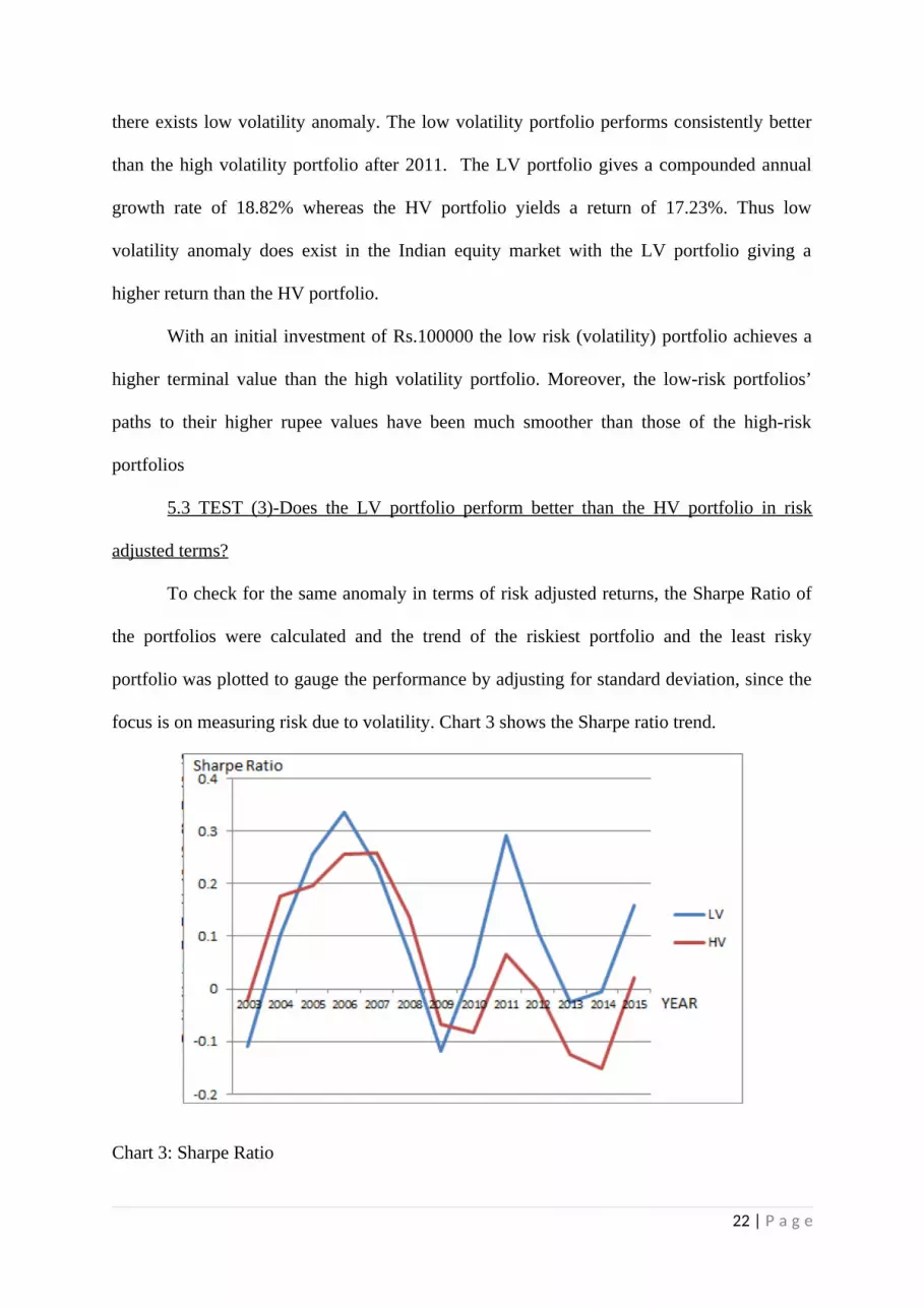
5.3 TEST (3)-Does the LV portfolio perform better than the HV portfolio in risk

adjusted terms?

To check for the same anomaly in terms of risk adjusted returns, the Sharpe Ratio of

the portfolios were calculated and the trend of the riskiest portfolio and the least risky

portfolio was plotted to gauge the performance by adjusting for standard deviation, since the

focus is on measuring risk due to volatility. Chart 3 shows the Sharpe ratio trend.

Chart 3: Sharpe Ratio

22 | P a g e

The Sharpe Ratio trend shows that the HV portfolio has marginally performed better

than the LV portfolio from 2003-2004 and 2007-2008. Otherwise, in terms of risk adjusted

returns, the LV has yielded higher returns. From 2010 onwards, the LV portfolio has

consistently outperformed the HV portfolio.

23 | P a g e

VI REASONS FOR LOW VOLATILITY ANOMALY IN THE

INDIAN EQUITY MARKET

6.1 What accounts for increase in volatility?

There are structural factors which contribute to volatility extremes. In India, new

investment instruments have emerged and technological developments have taken place over

the last 15 years. An investor/trader can now buy and sell shares using his laptop. A broker

need not be contacted anymore. With the introduction of broadband/2G/3G facilities in the

internet domain, information is available more and more instantaneously. Thus there has been

an improvement in the access to information and the ability to react to it by conveniently

buying/selling stocks.

Similarly, growth in investment instruments such as ETF’s has enabled investors to

execute large reallocations. The first ETF was introduced in India in the year 2001. This

instrument gave exposure to a basket of securities like an index fund and could be traded in

any quantity like a stock. The total “Assets under Management” in the ETF’s segment in

India is more than $800million dollars and it continues to grow. Sudden shifts in allocation

due to events that warrant trading action are possible to a greater extent with the advent of

ETF’s in India.

6.2 Limitations to arbitrage in the Indian equity market

Based on the findings of Kahneman and Traversky, Boyer, Mitton and Vorkink

(2010), investors have a behavioural bias towards stocks with high expected payoffs with low

probability. High volatility stocks have a positively skewed distribution with several

instances of small losses and a few large gains. Assuming that investors have a psychological

demand for highly volatile stocks, the more pertinent economic question that remains

unexplored in the Indian equity market is why don’t institutional investors capitalize on this

low risk-high return anomaly?

24 | P a g e

Various brokerage houses in India (eg. Kotak Securities) offer arbitrage funds as an

investment instrument for investors with low risk appetite. Such funds seek to benefit from

the mispricing in different segments of the stock market. If such funds seek to make gains on

a LV/HV stock, there are limitations which prohibit such stocks from realizing their true

value in the short run.

In the Indian market, the most commonly used arbitrage is ‘Buy stock - sell future’.

Such an arbitrage opportunity arises when the price of a stock (in the stock/cash/spot market)

trades at a large discount to the price of its future contract (in the futures/derivatives

segment). Thus, one can buy the stock from the cash market at lower price and sell its futures

contract at a higher price, the profit being the difference between the futures price and cash

price. On or before the expiry date (last Thursday of every month), the difference between the

spot and futures price narrows. The position is then reversed to book the profit. However,

following are the limitations:

1. The availability of arbitrage opportunities in the market is limited with only 265

stocks trading in the derivatives market.

2. A prolonged bear run poses an opportunity crunch for arbitrage funds as the future

prices of stocks could trade at discounts to their spot price. The arbitrage strategy of buy

stock - sell future will not work in this case.

3. Arbitrage funds are also affected by lower liquidity in the spot/future segment.

Future contracts are always traded in lots i.e. one lot of a future contract of a particular stock

comprises of multiple shares. If the market is illiquid, there is a chance that the fund manager

may not be able to buy/sell the desired number of shares at the given price. This affects the

funds overall performance.

This can be considered to be one of the reasons as to why LV stocks do not see a significant

rise in their prices in the short run. Although, HV stocks face the same problem, they still see

25 | P a g e

a lot of upward and downward movements because of the trades in the stock market.

Essentially, LV stocks see volatility neither in the derivatives market nor in the stock market,

but the HV stocks sees volatility in the stock market. Thus LV stocks are restricted from

realizing their true value in the short run.

6.3 Low volatility of undervalued stocks

An undervalued stock will typically be found in the low volatility segment. Such stocks are

unidentified for their potential fundamental value and see lesser momentum on a day-to-day

basis caused by the activities of traders. These stocks are loosely coupled with market

movements implying a low beta value. This implies that the risk in such stocks is less

attributed to the market (systematic risk) and more attributed to the firm specific risk (non-

systematic risk). Their price movements are less correlated with market movements. Thus in

the long run as these stocks see an appreciation in their value, it is correlated more with the

firm’s inherent performance. This can be seen as an indicator of good management practices

which is a key requirement to sustain a steady performance in the long run.

26 | P a g e

VII CONCLUSION

The findings of this study are consistent with the global market and it shows evidence

for the presence of low volatility anomaly. In the Indian equity market, a portfolio with least

amount of risk in terms of standard deviation performs better than the portfolio with the

highest amount of risk in the long run. The low volatility portfolio yields an 18.82% return

(CAGR) whereas the high volatility portfolio yields a 17.22% return (CAGR). One needs to

be patient to reap the benefits over time. Moreover, not only does the low volatility portfolio

deliver higher absolute returns, but it also gives higher risk adjusted returns. This is inferred

from observing the Sharpe ratio trend. In addition, during a bear run, the LV portfolio suffers

a smaller drawdown than the HV portfolio. Thus investing in a LV portfolio provides a

stronger preservation of capital.

These results clearly negate the popularly held assumption that one needs to assume

high risk to get higher returns. There is greater scope for profitability in the low volatility

portfolio over the long run. The more time you give to your investments, the more you are

able to accelerate the growth of your investment. Drawing inference from the legends of

Value investing like Warren Buffet, one needs to pick good businesses of durable moat and

be extremely disciplined to hold on to the portfolio for a long period of time.

27 | P a g e

7.1 SCOPE FOR FURTHER STUDY

There is ample scope for further research in the domain of this topic within the Indian

context. Some of the points which can be further analyzed are:

1. Does the phenomenon of low volatility anomaly exist across multiple indices in the

Indian equity market?

2. What happens to the portfolio values if the look back period and holding period are

rebalanced?

3. To what extent do the terminal values differ if money is invested in the LV and HV

portfolio on the basis of market capitalization of each stock in the portfolio (as against

equal allocation done in this paper)?

28 | P a g e

7.2 LIMITATIONS

This study uses standard deviation as a measure of volatility. However, volatility is only one

factor affecting the risk of a stock. A stable past performance does not necessarily guarantee

future stability. Thus one cannot use the results of this paper to simply invest in a portfolio

with least standard deviation. The results are pointing out the fact that you don’t necessarily

have to invest in riskier securities to receive higher returns. Most importantly, you need to be

patient and hold on to your portfolio for a long period of time to benefit in the long run.

While calculating the portfolio values, the simulation process made each purchase on 1st April

of every year up to 2014 and the stocks were sold off at the end of every 1 year( to adjust for

the change in the stocks ) on 31st March. This study does not account for the fact that

investments aren’t made on such a fixed schedule. As a matter of fact, the purchases can be

made in any of the month other than April and consequently the returns and standard

deviation of each portfolio are going to differ (although the phenomenon of low volatility

anomaly will still be prevalent).

Buying and selling of stocks involves transaction costs such as brokerage fees and payment

of taxes as well. Given that different brokerage houses charges charge separate fees and that

tax is only charged when there is a capital gain, these costs haven’t been accounted for.

Incorporating the fees and taxes paid, the net return will be lower than what is estimated in

this study.

29 | P a g e

REFERENCES

Akdeniz, L. (2000). Cross Section of Stock Returns in ISE.

Arnold, M. (2014). How to think about low volatility investing.

Baker, M. (2013). The Low Beta Anomaly: A Decomposition into Micro and Macro Effects.

Baker, M. (2014). The Low volatility anomaly Tradeoff of Leverage*.

Black, F. (1972). Capital Market Equilibrium with Restricted Borrowing.

Blitz, D. (2007). The Volatility Effect: Lower Risk without Lower Return. ERIM REPORT

SERIES.

Clarke, R. (2012). Minimum-Variance Portfolio Composition. Journal Of Portfolio

Management.

Dev, S. (2012). Testing of Risk Anomalies in Indian Equity Market.

FAMA, E. (1992). The Cross Section of Expected Stock Returns. The Journal Of Finance.

French, K. (1987). Expected Stock Returns and Volatility. Journal Of Financial Economics.

Garg, A. (2010). Seasonal Anomalies in Stock Returns. Journal Of Management Science.

Haguen, R. (1972). On The Evidence Supporting The Existence Of Risk Premium In The

Capital Markets.

Haguen, R. (2012). Low Risk Stocks Outperform within All Observable Markets of the

World.

Joshipura, N. (2014). Low volatility anomaly - Empirical Evidence from Indian Stock

Market.

30 | P a g e

Kinniry, F. (2010). Best Practices for Rebalancing Portfolios. Vanguard Research.

Li, X. (2014). The Limits to Arbitrage and the Low-Volatility Anomaly. The Financial

Analysts Journal.

Markowitz, H. (1952). Portfolio Selection. The Journal Of Finance.

Rambhia, R. (2012). Exploring Risk Anomlay in Indian Equity Market.

Ramos, E. (2013). Finding opportunities through the low volatility anomaly. Investment

Perspectives.

Soe, A. (2012). THE LOW-VOLATILITY EFFECT: A COMPREHENSIVE LOOK. S&P

DOW JONE INDICES.

Volkan, N. (2003). Cross Section of Expected Stock Returns on ISE.

31 | P a g e