Loss Aversion Index Recovery in The CrossSection of Subjective Well Being and Happiness

On Income

G. Charles-CadoganUniversity of Cape Town

andInstitute for Innovation and Technology Management

Ted Rogers School of Management, Ryerson University

Seminar presentation:Department of Economics & EconometricsFaculty of Economics and Financial Sciences

University of JohannesburgOctober 1, 2015

Outline

Overview of subjective well being (SWB) as alternative to GDP

Review of emerging research on behavioural welfare economics andasymmetric effects of loss aversion to decline in SWB

Microfoundations for econometric theory and recovery of lossaversion to decline in SWB

Econometric estimation and testing for impact of loss aversion onSWB cross sectional regressions

Conclusion and summary: A loss aversion index can be recovered andtested from published papers using simple recovered ratio procedures.Extant cross-sectional models are misspecifed due to simultaneitybias, and they overestimate the impact of economic growth on SWB.Loss aversion identifies clientele effects in SWB that explainoptimism in poor countries. We propose an econometric theory tosolve the simultaneity bias problem.

A typology of subjective well being

Preference satisfaction. The freedom and resources to meet onesown wants and desires;

Objective lists or basic needs. The fulfilment of a fixed set ofmaterial, psychological and social needs, which are identifiedexogenously;

Flourishing or eudaimonic. The realization of ones potential, alongdimensions such as autonomy, personal growth, or positiverelatedness;

Hedonic or affective. Synonymous with positive affect balance, arelative predominance of positive moods and feelings;

Evaluative or cognitive. The individuals own assessment of his orher life according to some positive criterion.

Source: [MacKerron, 2012, p. 706]

Motivation for study

☛ Subjective well being (SWB)Many applied papers report empirical associations betweenhappiness and other variables. Few papers treat happiness economicsin relation to its origins, definitions, theory, and methods[MacKerron, 2012].Happiness–A self reported measure of SWB from surveys.SWB measures features of individuals perceptions of their experiences,not their utility as economists typically conceive of it[Kahneman and Krueger, 2005].Life satisfaction depends on relative income compared to socialreference group and weather! [Feddersen et al., 2015].Those perceptions are a more accurate gauge of actual feelings if theyare reported closer to the time of, and in direct reference to, the actualexperience.

☛ Happiness-income paradox [Easterlin, 1974, p. 113]:An increase in national income per capita does not increase the overalllevel of happiness in the economy.People compare themselves to their neighbours or some aspiration orreference level other than per capita income alone.

Explosive growth in research on economics of happiness

Source: [MacKerron, 2012, Fig. 1, p. 706]

Number of EconLit Journal Articles with Titles Including the Terms’Happiness’, ’Wellbeing’, ’Well-being’ or ’Life Satisfaction’, by YearThe series plotted with filled circles excludes articles from the Journal of

Happiness Studies.

Life satisfaction concave in relative income

Source: [Stevenson and Wolfers, 2008]

Predicted by [Veblen, 1899, Duesenberry, 1949, Easterlin, 1974]

Life satisfaction gap for education

0-0.5 0.5 1.0 1.5 2.0 2.5

Tertiary – secondary LS gap Tertiary – primary LS gap

IrelandSwedenNorway

DenmarkCzech Republic

IcelandGermany

United KingdomNew Zealand

CanadaUnited States

NetherlandsTurkeyJapan

SwitzerlandOECD average

ItalySlovak Republic

AustriaLuxembourg

ChileFrance

EstoniaAustralia

Russian FederationBrazil

BelgiumGreecePoland

South KoreaFinland

IsraelHungary

ChinaSlovenia

IndiaIndonesia

SpainSouth Africa

Portugal

Source: OECD (2013), OECD Guidelines on Measuring Subjective Well–being, OECDPublishing.

Some policy implications of misspecified SWB models

Longitudinal studies that fail to account for loss aversion mayoverestimate the positive effects of income on SWB.

Such failure could carry important policy implications regardingraising individual and national income and well-being. [Boyce, 2010].

Income inequality implies that as reference income increases, lossaversion within relatively low income groups may cause them to seekgreater access to credit and subprime loans in order to maintainwell-being–thereby reducing public welfare. [Treeck, 2014].

Loss aversion implies that instead of overall economic growthnational agenda should focus on closing income inequality gaps inorder to increase SWB.

SWB as predictor of social unrest I–Arab Spring

30

25

20

15

10

5

0

7 000

6 500

6 000

5 500

5 000

4 500

2005 2006 2007 2008 2009 2010

%

5 158

4 762

5 508

5 904

6 114

6 367

Thriving (left scale) GDP per capita (PPP) (right scale)

US dollars

25%29%

13% 13%12%

Source: OECD (2013), OECD Guidelines on Measuring Subjective

Well-being. SWB data for Egypt are from Gallup. GDP per capita (PPP)estimates are from the International Monetary Fund’s World EconomicOutlook Database. The “Arab Spring” occurred in February 2011 overperceptions of worsening living conditions despite rising GDP per capita.

SWB as predictor of social unrest II–Greece

Source: Jan-Emmanuel DeNeve (2015) LSE EUROPP Blog

Real GDP in Greece grew by more than 50% between 1981 and 2008,while SWB grew 510% overall (most of it between 1998-2008). GreatRecession of 2008 erased all prior gains. The pain of recession cut deeperthan the negative growth numbers would indicate.

What is loss aversion?

The loss aversion concept was introduced in[Kahneman and Tversky, 1979] original prospect theory (OPT)behavioural challenge to [Von Neumann and Morgenstern, 1953]neoclassical expected utility theory (EUT). It characterizes the “lossesloom larger than gains” phenomenon observed in experiments.Skewed S-shaped value function v (x): concave over gains and convexand steeper over losses relative to a reference point. A genericparametrization is v (x) = vg (x)I{x>0} − vℓ(−x)I{x<0} with referencepoint 0 and sub-value functions vg , vℓ over gain and loss domain.[Charles-Cadogan, 2015d] shows that this was anticipated in[Bernoulli, 1738].Gain seeking is reflected by 0 < λ < 1. This can occur if the concaveportion of the function is steeper than the convex portion or the curve isconcave over loss and convex and steeper over gains.There is no settled formula for loss aversion index. However, most are

“ratio scaled”. Two popular formulae are: λ =vℓ(−1)

vg (1)and

λ =v ′ℓ(0−)

v ′g (0+). See [Wakker, 2010] for a review. [Charles-Cadogan, 2015b]

proves that the loss aversion index is unmeasureable under[Tversky and Kahneman, 1992] CPT but measurable under EUT.

Myopic loss aversion (MLA) to decline in SWB

Loss aversion redux: Anticipated losses have a greater influenceon choice and predicted feelings about an outcome than anticipatedgains of the same magnitude [Boyce et al., 2013]. It is the tendencyfor individuals to be more sensitive to reductions in their levels ofwell-being than to increases [Benartzi and Thaler, 1995].

Myopia is characterized by short term evaluation. For example,deviation from optimal consumption plans [Stroz, 1956];consumption tracking income [Shea, 1995].

Myopic loss aversion (MLA) is characterized by loss aversion overshort evaluation periods [Benartzi and Thaler, 1995].

Myopic loss aversion to decline in SWB was identified in[Vendrik and Woltje, 2007] but the MLA index not estimated.

Literature on loss aversion and subjective well being

There are several emergent papers on the subject of loss aversion todecline in SWB. None of them estimate a MLA index directly.

The most comprehensive study so far is by [De Neve et al., 2015]who used millions of observations for data at the international level.

➵ Implied MLA index in range [1.5, 6.31] wherein measures of lifesatisfaction are more sensitive to negative economic growth comparedto positive economic growth.

➵ MLA implicates growth policy and our understanding of the long-runrelationship between GDP and subjective well-being.

[Boyce et al., 2013] implied MLA index of 2.2 and 2.6

[Di Tella et al., 2010] implied MLA index 4.0, 5.0

[Vendrik and Woltje, 2007] implied MLA index 1.31

[Charles-Cadogan, 2015a] directly estimated a time series of MLAindexes for the relative income hypothesis concentrated in the range[1.27, 7.79].

Research questions posed

☛ Assuming that self reported (as opposed to elicited) ratings on one’slife satisfaction in a single item in a survey are admissible measures ofutility, we try to answer the following questions under rubric ofrelative income and subjective well being:

Is loss aversion to decline in happiness estimable?

If so, are extant cross sectional models of SWB misspecified by virtueof analysts failure to explicitly include a loss aversion index parameterin their specifications?

What would the econometric theory for embedding and recoveringthe MLA index in SWB regressions look like?

Are wealthier people more loss averse to a decline in their happinesscompared to poorer people?

Is the myopic loss aversion index for decline in happiness identifiable inextant cross-sectional regressions on SWB?

The robust ratio of slopes formula for MLA index

[Tversky and Kahneman, 1992] introduced a robust ratio of slopesformula for MLA via stochastic choice.

Subjects were presented with two simple lotteries L1 =(a, 12 ; b, 12

)

and L2 =(c , 12 ; x , 12

). Vizly, for L1, probability of loss of amount a is

12 and probability of gain of amount b is 1

2 and similarly for L2.

Value of x which subjects chose to establish equivalence betweenlotteries, i.e., L1 ∼ L2, was noted for a, b, c combination.

The ratio λθ =x−bc−a was used as a robust estimator of MLA

[Tversky and Kahneman, 1992, p. 310] noted that “when thepossible loss is increased by k the compensating gain must beincreased by about 2k. So λθ is a ratio of the slope of gains overthe slope of losses.

[Duesenberry, 1949] implicit consumption function

Assume Yt = Ct + St

St

Yt= α0 + α1

Yt

Mt, Mt = max

0<s<t{Ys}, α0 > 0, α1 > 0

⇒ Ct

Yt= 1− α0 − α1

Yt

Mt

Yt > Mt ⇒ income gainYt

Mt= 1+ gG

t

Yt = Mt ⇒ reference incomeYt

Mt= 1

Yt < Mt ⇒ income lossYt

Mt= 1− gL

t

where Ct , St , Yt is consumption, savings, income, resp; gLt > 0 and

gGt > 0 are pseudo-growth rates of income, and α1 is a savings ratefactor. In discrete time we use Mt−1 instead of Mt . For application weuse a sliding window of length w , i.e., Mw

t = maxt−w<s<t{Ys} torepresent standard of living.

Reference Dependent Consumption With Loss Aversion

CDt =

C rt + ∆bCD

t if gain in income

C rt if reference income

C rt − λ∆bCD

t , λ > 0 if loss of income

∆bCDt = −α1g

Gt Yt , λt =

gLt

gGt

, C rt = a(d)Yt a(d) = 1− α0 − α1

C rt is reference consumption, and a(d) is consumption factor

Identifying restriction for MLAλt |gL

t |gGt

= 1

If consumption response to income changes is symmetric, thenλt = 1

If it is asymmetric such that |gLt | = k and gG

t = 2k , then λt = 2 asin the Tversky-Kahneman compensating gain hypothesis.

λt is a myopic loss aversion index motivated by Tversky-Kahnemanrobust ratio method which we embed in our model.Source: [Charles-Cadogan, 2015a].

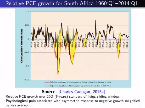
Relative PCE growth for South Africa 1960:Q1–2014:Q1

-0.15

-0.1

-0.05

0

0.05

0.1

19

65

/01

19

66

/04

19

68

/03

19

70

/02

19

72

/01

19

73

/04

19

75

/03

19

77

/02

19

79

/01

19

80

/04

19

82

/03

19

84

/02

19

86

/01

19

87

/04

19

89

/03

19

91

/02

19

93

/01

19

94

/04

19

96

/03

19

98

/02

20

00

/01

20

01

/04

20

03

/03

20

05

/02

20

07

/01

20

08

/04

20

10

/03

20

12

/02

20

14

/01

Consum

pti

on G

row

th R

ate

ZA Rolling 5yrs Impact of Loss Aversion to Decline in Growth of Standard of Living

ZA (Semidurable) Personal Consumption Expenditure Growth Rate in 2010 Prices

Source: [Charles-Cadogan, 2015a]Relative PCE growth over 20Q (5-years) standard of living sliding window.Psychological pain associated with asymmetric response to negative growth magnifiedby loss aversion.

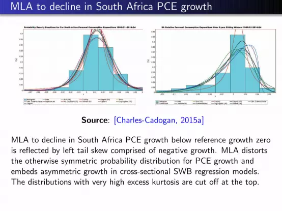
MLA to decline in South Africa PCE growth

Source: [Charles-Cadogan, 2015a]

MLA to decline in South Africa PCE growth below reference growth zerois reflected by left tail skew comprised of negative growth. MLA distortsthe otherwise symmetric probability distribution for PCE growth andembeds asymmetric growth in cross-sectional SWB regression models.The distributions with very high excess kurtosis are cut off at the top.

Local regression estimator for MLA index

Gains Losses

O

Microfoundations of cross-sectional regression model with asymmetricgrowth in an ǫ-neighbourhood Bǫ(xr ) of the reference point xr .

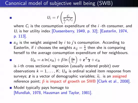
Canonical model of subjective well being (SWB)

Ui = f

(Ci

∑j

αijCj

)

where Ci is the consumption expenditure of the i -th consumer, andUi is her utility index [Duesenberry, 1949, p. 32]; [Easterlin, 1974,p. 113].

αij is the weight assigned by i to j ’s consumption. According toEasterlin, if i chooses the weights αij =

1n then she is comparing

herself to the average consumption expenditure of her neighbours.

Uik = α ln(xik) + β ln(xikxi ·

)+ zTγγγ + ǫik

is i -th cross sectional regression (usually ordered probit) overobservations k = 1, . . . ,K ; Uik is ordinal scaled item response fromsurveys; zzz is a vector of demographic variables; xi · is an assignedreference point; β is impact of growth on SWB [Clark et al., 2008].

Model typically pays homage to[Mundlak, 1978, Hausman and Taylor, 1981].

Clientele Effects Of Economic Growth On SWB

The relative impact of a unit change in average economic growth (g ) on average SWB(U) under neoclassical (Neo) and behavioural economics (BE) theory:

Neoi =

(∂Ui ./∂gGi . )

(∂Ui ./∂gLi . )

=β/gG

i .

β/gLi .

=gLi .

gGi .

BEi =(∂Ui ./∂gG

i . )

(∂Ui ./∂gLi . )

=βG /gG

i .

βL/gLi .

=βG

βL

gLi .

gGi .

=1

λi

(gLi .

gGi .

)2

If gGi . = gL

i . , then Neoi = 1 and BEi = 1/λi .

Under Neoi the impact of a unit increase in economic growth is offset by a unit

decrease in economic growth.

Under BEi the impact of a unit change in economic growth is asymmetric. Thegain in SWB for a unit increase in economic growth is a fraction of the loss inSWB for a unit decrease in economic growth.

Gain seeking in low income countries, i.e., 0 < λi < 1 magnifies SWB by afactor much greater than that for higher income countries characterized by lossaversion, i.e., λi > 1. Thus, risk attitudes provide a theoretical explanation forwhy low income countries are more optimistic than high income countries.Cf. [Humphrey and Verschoor, 2004, Graham, 2008].

Recovery of MLA index in 2SLS procedure for βRewrite canonical regression asUik = α ln(xik) + βGg

Gik I{xik>xi ·} − βLg

LikI{xik<xi ·} + zTγγγ + ǫik , ǫ ∼

(0, σ2ǫ ), H0 : βG = βL = β vs Ha : H0 not true

Incorporate the identifying restriction for MLAgLik = λgG

ik + ηik , ηik ∼ (0, σ2η ), k = 1, . . . ,K

Theoretical first stage regression yields gLik = λgG

ik

Estimation of second stage regression yieldsUik = α ln(xik) + βGg

Gik I{xik>xi ·} − θgL

ikI{xik<xi ·} + zT γγγwhere λ =

θ

βG

Run auxiliary regression ǫi · = βLηi ·I{xik<xi ·} + νi ·, νi · ∼ (0, σ2ν )

from stages 1 and 2

βL =

∑i ǫi ·ηi ·I{xik<xi ·}∑i η2

i ·I{xik<xi ·}βL is asymptotically consistent and efficient [White, 2001, p. 144] soλ is a conservative [under] estimate of λ.

Canonical model overestimates impact of growth on SWB

yyy = Xααα + Zβββ + ǫǫǫ, Z =[gggG gggL

], βββ =

[βG βL

]T

ηηη = Zφφφ, φφφ = [−λ 1]T , ǫǫǫ = βLηηη + νννMX = I − X (XTX )−1XT , MZ = I − Z (ZTZ )−1ZT

ααα =(XTMZX

)−1XTMZyyy

βG =(gggGT

MXgggG)−1

gggGTMXyyyI{gggG>000}

βL =

(φφφTZTZ φφφ

)−1φφφTZ ǫǫǫ embeds MLA theory for λ,

βL =(gggLTMXggg

L)−1

gggLTMXyyyI{gggL<000} no MLA theory,

V(βL

)= E

[(βL − βL

)2]=(φφφTZTZφφφ

)−1σ2

ν

V(βL

)= E

[(βL − βL

)2]=(gggLTMXggg

L)−1

σ2ǫ I{gggL<000}

V(βL

)=(gggLTgggL + λ2gggGT

gggG)−1

σ2ν

< V (βL) =(gggLTgggL−gggLTX (XTX )−1XTgggL

)−1σ2

ǫ I{gggL<000}

=⇒ βL < βL a.s. in Hilbert space L2(R) or weakly in R

Geometry of identifying restriction for MLA

O

45o

[Tversky and Kahneman, 1992] compensating gain hypothesis posits:“when the possible loss is increased by k the compensating gain must beincreased by about [λ]k”. This is equivalent totan(ψ(λ)) = λ‖gG‖ ⋆ ‖gL‖−1 = 1. The vector of losses dominates thespace and permeates the corresponding regressions.

Recovery Theorem for MLA index for SWBTHEOREM. Under regularity conditions for least squares write the canonical SWB regressionunder H0 = βG = βL = β and Ha : βG = β and βL = θ, β 6= θ

yyy = Xδδδ + ǫ, so that δδδ =(XT X

)−1XTyyy ,

where X = [x zzzT gggGTgggLT ] =

[X : Z

]is the design matrix with transposed (T ) row

vectors in bold, yyy is a vector of utility scores (ordinal or otherwise),

δδδ = [α γγγ β θ]T

is the vector of parameters to be estimated; ǫ ∼ (0, σ2ǫ III n) where III n is the n× n identity matrix;√

n(

δδδ − δδδ)−→d

(000, ΣΣΣδ) where ΣΣΣδ is the variance-covariance matrix of δδδ given by

ΣΣΣδ = σ2ǫ

(XT X

)−1=

(XTX XTZZTX ZTZ

)−1

=(⋆ ⋆

⋆ ΣΣΣ(θ, β)

)

where ⋆ denotes sub-matrices for parameters that are not of interest. And σ2θ , σ2

β , σ2θβ are the

variance and covariance components of the sub-matrix of interest ΣΣΣ(θ, β) =

[σ2

θ σθβ

σθβ σ2β

]and

[θβ

]∼ N

([θβ

], ΣΣΣ(θ, β)

). We claim that limn P

λn = limn Pθn

βn

= λ and the asymptotic

distribution √n( ˆλn − λ) −→

dN

(0,

σ2θ − 2λσθβ + λ2σ2

β

β2

)

exist provided |β| > 0. By definition σθβ = 0.

Variance stabilizing transform forλn

√n( ˆλn − λ) −→

dN

(0,

σ2θ −2λσθβ+λ2σ2

β

β2

), σθβ = 0

Confound: Asymptotic variance λn depends on λA variance stabilizing transformation is needed to eliminate thevariance confound [Bar-Lev and Enis, 1990].The computed variance stabilizing transformation (VST) is

g(λ) =σ

σ∗β

ln

(tan

(π

4+

ψ

2

))

tan(ψ) =λσ∗

β

σ∗θ

, tan

(ψ

2

)=

λσ∗β

σ∗θ + τ(λ)

√n(g(λn

)− g(λ)

)−→d

N(0, σ2) where σ2 = τ2(λ)g ′2(λ),

τ2(λ) = σ∗2θ + λ2σ∗2

β , and σ∗θ = σθ/β, σ∗

β = σβ/β

g(λ) is related to the distribution function F (u) = 12 +

1π arctan(u)

for a Cauchy density function of type f (u) = [π(1+ u2)]−1. So the

VST is α-stable i.e., f (λ; σ∗2β , σ∗2

θ ) = 2(1+ λ2σ∗2

β σ∗−2θ

)−1

Sample distribution of MLA index

Figure : Empirical distributionof US MLA index

0 5 10 15 20 25 30 350

0.05

0.1

0.15

0.2

0.25

0.3

0.35

Reference dependent MLA USA

Cauch

y t

ransfo

rm w

ith m

edia

n=

2.2

5

Figure : Theoretical Levydistribution

The empirical US MLA index was fitted by interpolation from a method of moments estimatorapplied to US real income and nondurable consumption data in [Charles-Cadogan, 2015c]. Thetheoretical Levy distribution is

f (x ;µ, c) =

√c

2π(x − µ)−3/2 exp

(−c(2(x − µ)−1)

)

with measure of location µ and scale parameter c for tail efffects.

Levy scale parameter and asymmetric growth exposure

Assign the standard deviations of growth exposure to the abstractnorms, i.e., ‖gL‖ = σ∗

θ , ‖gG ‖ = σ∗β

Let c = σ∗β /σ∗

θ be a scale parameter induced by the norms forgrowth exposure.

Levy density now has the form f (x) = (c√2π)

−1x−

32 exp(−2x)

when measure of location µ = 0.

If tan(ψ(λ)) = λ‖gG‖ ⋆ ‖gL‖−1 = 1, then λ = 1/c and λ = 2when c = 1/2.

The scale parameter c for the Levy density is informative aboutthe MLA index asymmetric growth exposure under Ha.

f (λ; σ∗2β , σ∗2

θ ) = 2(1+ λ2c2

)−1

Exact test for identifying MLA index restriction

Theorem

The exact test for the myopic loss aversion (MLA) index identifying

restriction is given by

Z =

4

(λ2

λ2H0

− ln(

σνσǫ

)− 1

)

√2

∼ N (0, 1)

where Z is a standard normal random variable, λ is the observed or

estimated MLA index, λH0= ‖gggL‖/‖gGgGgG ‖ is the given MLA index under

the null, and ‖gG ‖ and ‖gL‖ are suitable normed vectors of gains and

losses in growth, respectively.

Remarks. The test statistic is derived from the LR statistic−2 ln ϑ = -2 ln(V ( ˆβL)/V (βL)) ∼ χ2

1 where χ21 ∼ (1, 2), and

Z =(χ21 − 1

)/√2. It is based on H0 : βG = βL = β and

Ha : βG = β and βL = θ, β 6= θ. A correction factor 3√2 was used for

consistency under the null, and σν < σǫ by definition.

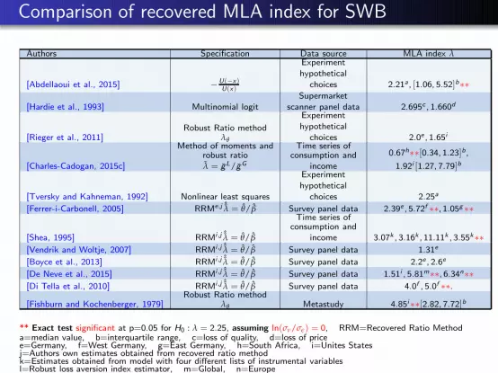
Comparison of recovered MLA index for SWB

Authors Specification Data source MLA index λ

[Abdellaoui et al., 2015] − U(−x)U(x)

Experiment

hypothetical

choices 2.21a, [1.06, 5.52]b∗∗

[Hardie et al., 1993] Multinomial logit

Supermarket

scanner panel data 2.695c , 1.660d

[Rieger et al., 2011]Robust Ratio method

λθ

Experiment

hypothetical

choices 2.0e , 1.65i

[Charles-Cadogan, 2015c]

Method of moments androbust ratioλ = gL/gG

Time series ofconsumption and

income

0.67h∗∗[0.34, 1.23]b,1.92i [1.27, 7.79]b

[Tversky and Kahneman, 1992] Nonlinear least squares

Experiment

hypothetical

choices 2.25a

[Ferrer-i-Carbonell, 2005] RRMe,j ˆλ = θ/β Survey panel data 2.39e , 5.72f ∗∗, 1.05g ∗∗

[Shea, 1995] RRMi ,j ˆλ = θ/β

Time series ofconsumption and

income 3.07k , 3.16k , 11.11k , 3.55k∗∗[Vendrik and Woltje, 2007] RRMi ,j ˆλ = θ/β Survey panel data 1.31e

[Boyce et al., 2013] RRMi ,j ˆλ = θ/β Survey panel data 2.2e , 2.6e

[De Neve et al., 2015] RRMi ,j ˆλ = θ/β Survey panel data 1.51i , 5.81m∗∗, 6.34n∗∗[Di Tella et al., 2010] RRMi ,j ˆλ = θ/β Survey panel data 4.0f , 5.0f ∗∗.

[Fishburn and Kochenberger, 1979]Robust Ratio method

λθ Metastudy 4.85i ∗∗[2.82, 7.72]b

** Exact test significant at p=0.05 for H0 : λ = 2.25, assuming ln(σν/σǫ) = 0, RRM=Recovered Ratio Methoda=median value, b=interquartile range, c=loss of quality, d=loss of pricee=Germany, f=West Germany, g=East Germany, h=South Africa, i=Unites Statesj=Authors own estimates obtained from recovered ratio methodk=Estimates obtained from model with four different lists of instrumental variablesl=Robust loss aversion index estimator, m=Global, n=Europe

Distribution of MLA index by data source

0 2 4 6 8 10 12

1

2

3

4

5

6

7

8

9

10

11

Myopic loss aversion index

Metastudy

Time series of consumption and

income

Survey panel data

Experiment-hypothetical choices

Supermarket scanner panel data

2.25

Conclusion

☛ Theory shows that the canonical SWB regression model overestimatesthe impact of growth on SWB by failing to control for MLA.

☛ The recovery theorem for MLA index for decline in SWB introducedhere is new to the literature.

☛ Application of the theorem to published results produced admissibleMLA index estimates.

☛ The α-stable feature of the recovered MLA index estimatorcomplicates statistical inference but establishes a relation betweentail thickness and asymmetric exposure of SWB to income growth.

☛ Further research on econometric theory of myopic loss aversion todecline in SWB is needed to:

derive sharp bounds for recovered MLA index estimatorcharacterize the geometry of MLA index in gain loss space

References I

Abdellaoui, M., Bleichrodt, H., l’Haridon, O., and van Dolder, D. (2015).Measuring loss aversion under risk and uncertainty: A new method and a critical test ofprospect theory.Working paper. Available at http://ssrn.com/abstract=2318352.

Bar-Lev, S. K. and Enis, P. (1990).The Contruction of Classes of Variance Stailizing Transformations.Statistics and Probability Letters, 10:95–100.

Benartzi, S. and Thaler, R. E. (1995).

Myopic Loss Aversion And The Equity Premium Puzzle.Quarterly Journal of Economics, 110(1):73–92.

Bernoulli, D. (1738).

Specimen Theoriae Novae de Mensura Sortis.Commentarii Academiae Scientiarum Imperialis Petropolitanae, 5:175–192.English translation (1954): Exposition of a new theory on the measurement of risk.Econometrica, 22(1):23-?36.

Boyce, C. J. (2010).

Understanding fixed effects in human well-being.Journal of Economic Psychology, 31(1):1 – 16.

References II

Boyce, C. J., Wood, A. M., Banks, J., Clark, A. E., and Brown, G. D. A. (2013).Money, Well-Being, and Loss Aversion: Does an Income Loss Have a Greater Effect onWell-Being Than an Equivalent Income Gain?Psychological Science, 24(12):2557–2562.

Charles-Cadogan, G. (2015a).Asymptotic Theory Of Myopic Loss Aversion: Applications To Intolerance for Decline inStandard Of Living and Asset Pricing.In Proceedings of Midwest Econometric Group–Econometric Theory and Methods.Research Division, Federal Reserve Bank of St. Louis.25th Annual Meeting of the Midwest Econometrics Group, 2015.

Charles-Cadogan, G. (2015b).Expected Utility Theory and Inner and Outer Measures of Loss Aversion.Working Paper.

Charles-Cadogan, G. (2015c).Myopic Loss Aversion and Intolerance for Decline in Standard of Living.Working Paper.

Charles-Cadogan, G. (2015d).

Prospect Theory’s Cognitive Error About Bernoullis Utility Function.AER Bulletin Peer Reviewed Working Paper Series.

References III

Clark, A. E., Frijters, P., and Shields, M. A. (2008).Relative Income, Happiness, and Utility: An Explanation for the Easterlin Paradox andOther Puzzles.Journal of Economic Literature, 46(1):95–144.

De Neve, J.-E., Ward, G. W., De Keulenaer, F., Van Landeghem, B., Kavetsos, G., and

Norton, M. I. (2015).The Asymmetric Experience of Positive and Negative Economic Growth: Global EvidenceUsing Subjective Well-Being Data.Technical report, Institute for the Study of Labor.IZA Discussion Paper No. 8914.

Di Tella, R., Haisken-De New, J., and MacCulloch, R. (2010).Happiness adaptation to income and to status in an individual panel.Journal of Economic Behavior & Organization, 76(3):834 – 852.

Duesenberry, J. S. (1949).

Income, Saving, and The Theory of Consumer Behavior.Harvard University Press, Cambridge, MA.4th Printing, 1962.

Easterlin, R. A. (1974).

Does economic growth improve the human lot? Some empirical evidence.In David, P. and Reder, M. W., editors, Nations and Households in Economic Growth:Essays in Honor of Moses Abramowitz, pages 89–125. Academic Press, New York, NY.

References IV

Feddersen, J., Metcalfe, R., and Wooden, M. (2015).Subjective wellbeing: why weather matters.Journal of the Royal Statistical Society: Series A (Statistics in Society).In press.

Ferrer-i-Carbonell, A. (2005).

Income and well-being: An empirical analysis of the comparison income effect.Journal of Public Economics, 89(5):997–1019.

Fishburn, P. C. and Kochenberger, G. A. (1979).Two-Piece Von Neumann-Morgenstern Utility Functions.Decision Sciences, 10(4):503–518.

Graham, C. (2008).Optimism and Poverty in Africa: Adaptation or A means of Survival.Brookings Brief.Washington, DC: Brookings Institute. Available athttp://www.brookings.edu/research/papers/2006/10/globaleconomics-graham.

Hardie, B. G. S., Johnson, E. J., and Fader, P. S. (1993).Modeling loss aversion and reference dependence effects on brand choice.Marketing Science, 12(4):378–394.

References V

Hausman, J. A. and Taylor, W. E. (1981).Panel data and unobservable individual effects.Econometrica, 49(6):1377–1398.

Humphrey, S. J. and Verschoor, A. (2004).The Probability Weighting Function: Experimental Evidence From Uganda, India andEthopia.Economics Letters, 84:419–425.

Kahneman, D. and Krueger, A. B. (2005).Developments in The Mesurement of Subjective Well Being.Journal of Economic Perspectives, 20(1):3–24.

Kahneman, D. and Tversky, A. (1979).Prospect Theory: An Analysis of Decisions Under Risk.Econometrica, 47(2):263–291.

MacKerron, G. (2012).

Happiness Economics From 35000 Feet.Journal of Economic Surveys, 26(4):705–735.

Mundlak, Y. (1978).

On the pooling of time series and cross section data.Econometrica, 46(1):69–85.

References VI

Rieger, M. O., Wang, M., and Hens, T. (2011).

Prospect theory around the world.NHH Dept. of Finance & Management Science Discussion Paper No. 2011/19.

Shea, J. (1995).Myopia, Liquidity Constraints, and Aggregate Consumption: A Simple Test.Journal of Money, Credit and Banking, 27(3):798–805.

Stevenson, B. and Wolfers, J. (2008).Economic Growth and Subjective Well-Being: Reassessing the Easterlin Paradox.Brookings Papers on Economic Activity.

Stroz, R. H. (1956).

Myopia and Inconsistency in Dynamic Utility Maximization.Review of Economic Studies, 23(3):165–180.

Treeck, T. (2014).Did inequality cause the us financial crisis?Journal of Economic Surveys, 28(3):421–448.

Tversky, A. and Kahneman, D. (1992).Advances in Prospect Theory: Cumulative Representation of Uncertainty.Journal of Risk and Uncertainty, 5:297–323.

References VII

Veblen, T. (1899).

The Theory Of The Leisure Class: An Economic Study In The Evolution Of Institutions.The Macmillan Company.

Vendrik, M. C. and Woltje, G. B. (2007).Happiness and loss aversion: Is utility concave or convex in relative income?Journal of Public Economics, 91(78):1423 – 1448.

Von Neumann, J. and Morgenstern, O. (1953).

Theory of Games and Economic Behavior.Princeton University Press, Princeton, NJ, 3rd edition.

Wakker, P. P. (2010).

Prospect Theory for Risk and Ambiguity.Cambridge University Press, New York, N. Y.

White, H. (2001).Asymptotic Theory for Econometricans.Academic Press, San Diego, CA, 2nd revised edition.