localization and heegaard floer homology kristen hendricks
TRANSCRIPT

Localization and Heegaard Floer Homology
Kristen Hendricks
Submitted in partial fulfillment of the
requirements for the degree
of Doctor of Philosophy
in the Graduate School of Arts and Sciences
COLUMBIA UNIVERSITY
2013

c⃝2013
Kristen Hendricks
All Rights Reserved

ABSTRACT
Localization and Heegaard Floer Homology
Kristen Hendricks
In this thesis we use Seidel-Smith localization for Lagrangian Floer cohomology to study
invariants of cyclic branched covers of three-manifolds and symmetry groups of knots by con-
structing localization spectral sequences in Heegaard Floer homology.
Our first application is to double branched covers of knots and links in the three-sphere.
Given a link K in S3, let Σ(K) be the double branched cover of S3 over L. We show that there
is a spectral sequence whose E1 page is HFK (Σ(K), K)⊗H∗(Tn)⊗ Z2((θ)) and whose E∞
page is isomorphic to HFK (S3, K) ⊗ H∗(Tn) ⊗ Z2((θ)), as Z2((θ))-modules. As a conse-
quence, we deduce a rank inequality between the knot Floer homologies HFK (Σ(K), K) and
HFK (S3, K). We also prove the analogous theorem for link Floer homology. This result was
recently published by Algebraic & Geometric Topology [18].
Our second application is to doubly-periodic knots in the three-sphere. A knot K ⊂ S3 is q-
periodic if there is a Zq-action preserving K whose fixed set is an unknot U . The quotient of K
under the action is a second knotK. We construct equivariant Heegaard diagrams for q-periodic
knots, and show that Murasugi’s classical condition on the Alexander polynomials of periodic
knots is a quick consequence of these diagrams. For K a two-periodic knot, we show that there
is a spectral sequence whose E1 page is HFL(S3, K ∪ U)⊗H∗(T2n+1)⊗ Z2((θ)) and whose
E∞ pages is isomorphic to HFL(S3, K ∪ U)⊗H∗(Tn)⊗ Z2((θ)), as Z2((θ))-modules, and a
related spectral sequence whoseE1 page is HFK (S3, K)⊗H∗(T2n+1)⊗H∗(S0))⊗Z2((θ)) and
whose E∞ page is isomorphic to HFK (S3, K)⊗H∗(Tn)⊗H∗(S0))⊗ Z2((θ)). We use these
spectral sequences to recover a lower bound of Edmonds on the genus of K, orginally proved
using minimal surface theory, along with a weak version of a fibredness result of Edmonds and

Livingston. These results may also be found in the preprint [17].

Table of Contents
1 Introduction 1
1.1 Double Branched Covers of Links in the Three-Sphere . . . . . . . . . . . . . 2
1.2 Periodic Knots . . . . . . . . . . . . . . . . . . . . . . . . . . . . . . . . . . 4
1.3 Further generalization of the main theorem . . . . . . . . . . . . . . . . . . . . 7
1.4 Seidel–Smith Localization: A Key Technical Tool . . . . . . . . . . . . . . . . 8
2 Background on Heegaard Floer Homology 9
2.1 Link Floer homology, the multivariable Alexander polynomial, and the Thurston
norm . . . . . . . . . . . . . . . . . . . . . . . . . . . . . . . . . . . . . . . . 20
2.2 Link Floer homology and fibredness . . . . . . . . . . . . . . . . . . . . . . . 23
3 Equivariant Heegaard Diagrams 24
3.1 Heegaard Diagrams for Branched Double Covers of Links . . . . . . . . . . . 25
3.2 Heegaard Diagrams for Periodic Knots and Proofs of Edmonds’ and Mura-
sugi’s Conditions . . . . . . . . . . . . . . . . . . . . . . . . . . . . . . . . . 30
3.3 Essential properties of Heegaard diagrams compatible with involutions . . . . . 44
4 Spectral Sequences for Lagrangian Floer Cohomology 46
4.1 Interpretation in the context of Heegaard Floer homology . . . . . . . . . . . . 57
5 Geometry of Symmetric Products 62
5.1 Symplectic Geometry of Symmectric Products of Punctured Heegaard Surfaces 62
i

5.2 Homotopy Type and Cohomology of Symmetric Products of Punctured Hee-
gaard Surfaces . . . . . . . . . . . . . . . . . . . . . . . . . . . . . . . . . . . 66
6 Important Constructions from K-Theory 71
7 The Existence of Stable Normal Trivializations 78
8 Sample Computations for Two-Periodic Knots 87
Bibliography 104
Appendix I: Holomorphic Embeddings 108
ii

List of Figures
1 A doubly-periodic diagram for the trefoil, and its quotient knot (an unknot)
under the Z2 action. . . . . . . . . . . . . . . . . . . . . . . . . . . . . . . . . 5
2 A Heegaard diagram on the sphere derived from a two-bridge presentation of
the trefoil. . . . . . . . . . . . . . . . . . . . . . . . . . . . . . . . . . . . . . 30
3 An equivariant Heegaard diagram D for the trefoil together with the unknotted
axis, and its quotient Heegaard diagram D for the Hopf link. . . . . . . . . . . 32
4 The arrangement of α and β curves D. Note that if wi is on the component Kj
of L, zk is either zi+1 or znj. . . . . . . . . . . . . . . . . . . . . . . . . . . . 45
5 The periodic domain Pi = Ei − Fi has Maslov index zero. . . . . . . . . . . . 81
6 An equivariant Heegaard diagram for the unknot together with an axis (i.e. a
Hopf link), and its quotient Heegaard diagram (another Hopf link). . . . . . . . 88
7 Alexander gradings and differentials for CFL(D) (left) and CFK (D) (right). . 89
8 Alexander gradings and differentials of CFL(D) (left) and CFK (D) (right). . . 89
9 Intersection points in D. . . . . . . . . . . . . . . . . . . . . . . . . . . . . . 90
10 Intersection points of α and β curves in D. . . . . . . . . . . . . . . . . . . . . 91
11 Alexander gradings and differentials of CFL(D) (left) and CFK (D) (right). . . 91
12 Alexander A1 and A2 gradings of the generators of CFL(D). These generate
the E0 page of the link Floer homology spectral sequence. . . . . . . . . . . . 92
13 The homology HFL(D). These elements generate theE1 page of the link Floer
spectral sequence as a Z2((θ)) module. . . . . . . . . . . . . . . . . . . . . . . 93iii

14 Generators for the E2 = E∞ page of the link Floer spectral sequence for D as
a Z2((θ))-module. . . . . . . . . . . . . . . . . . . . . . . . . . . . . . . . . . 94
15 Alexander A1 gradings of elements of CFK (D). These elements generate the
E0 page of the link Floer spectral sequence as a Z2((θ)) module. . . . . . . . . 95
16 The homology HFK (D), which is HFK (31)⊗ V1 ⊗W . These elements gen-
erate the E1 page of the knot Floer homology spectral sequence of D as a
Z2((q))-module. . . . . . . . . . . . . . . . . . . . . . . . . . . . . . . . . . . 95
17 Generators for the E2 page of the knot Floer spectral sequence associated to D
as a Z2((q)) module. . . . . . . . . . . . . . . . . . . . . . . . . . . . . . . . 96
18 Generators for the E3 = E∞ page of the knot Floer spectral sequence associ-
ated to D. . . . . . . . . . . . . . . . . . . . . . . . . . . . . . . . . . . . . . 97
19 The chain complex CFL(D) in Alexander grading A1 = −72, and the chain
complex CFK (D) in Alexander grading A1 = −5. Dashed arrows denote
differentials appearing only in the latter. . . . . . . . . . . . . . . . . . . . . . 97
20 The chain complex CFL(D) in Alexander grading A1 = −52, and the chain
complex CFK (D) in Alexander grading A1 = −4. Dashed arrows denote
differentials appearing only in the latter. . . . . . . . . . . . . . . . . . . . . . 98
21 The chain complex CFL(D) in Alexander grading A1 = −32, and the chain
complex CFK (D) in Alexander grading A1 = −3. Dashed arrows denote
differentials appearing only in the latter. . . . . . . . . . . . . . . . . . . . . . 98
22 The chain complex CFL(D) in Alexander grading A1 = −12, and the chain
complex CFK (D) in Alexander grading A1 = −2. Dashed arrows denote
differentials appearing only in the latter. . . . . . . . . . . . . . . . . . . . . . 99
23 The chain complex CFL(D) in Alexander grading A1 =12, and the chain com-
plex CFK (D) in Alexander grading A1 = −1. Dashed arrows denote differ-
entials appearing only in the latter. . . . . . . . . . . . . . . . . . . . . . . . . 100
iv

24 The chain complex CFL(D) in Alexander grading A1 =32, and the chain com-
plex CFK (D) in Alexander grading A1 = 0. Dashed arrows denote differen-
tials appearing only in the latter. . . . . . . . . . . . . . . . . . . . . . . . . . 100
25 The chain complex CFL(D) in Alexander grading A1 =52, and the chain com-
plex CFK (D) in Alexander grading A1 = 1. Dashed arrows denote differen-
tials appearing only in the latter. . . . . . . . . . . . . . . . . . . . . . . . . . 100
v

Acknowledgements
To begin, I am deeply indebted to my advisers Robert Lipshitz and Peter Ozsvath for their
invaluable guidance. They proposed fascinating problems to study, provided endless helpful
advice, and constantly directed, encouraged, and challenged me in my research. From the
very start of my time in graduate school, they made me feel like a part of the mathematical
community by inviting me to conferences and seminars and introducing me to their colleagues.
I am particularly grateful to Peter for his invariably helpful perspective and for immediately
including me in the vibrant atmosphere of collaboration he fosters among his descendants, and
to Robert for always making himself extremely available to me to discuss my research and other
aspects of my graduate career, and reading drafts of my writing. I look forward to continuing
to learn from them in the years to come.
Thanks to Dusa McDuff, Walter Neumann, and Zoltan Szabo for their interest interest in
my progress, for agreeing to be on my thesis committee, and for their helpful comments and
questions.
It has been a joy to be involved with the low-dimensional and symplectic topology com-
munity at Columbia University and beyond. I am very grateful to my colleagues and teachers
for innumerable helpful discussions. Special thanks go to Mohammed Abouzaid, Jon Bloom,
Andre Carneiro, Corrin Clarkson, Andrew Fanoe, Allison Gilmore, Elizabeth Goodman, Eli
Grigsby, Jonathan Hanselman, Matt Hedden, Jen Hom, Peter Horn, Paul Kirk, Adam Knapp,
Adam Levine, Joan Licata, Tye Lidman, Chuck Livingston, Ciprian Manolescu, Paul Melvin,
Yi Ni, Ina Petkova, Dan Ramras, Sucharit Sarkar, Dylan Thurston, and Rumen Zarev.
vi

I was introduced to Heegaard Floer homology during the Mathematical Sciences Reseach
Institute’s Spring 2010 program in knot homology theories; I remain very grateful to the insti-
tute for a stimulating program in an idyllic setting, and to the mathematicians in attendance,
who were uniformly extremely generous with their time and knowledge. Thanks also to the
NSF for its support (grant DMS-0739392).
I thank my classmates at Columbia – Daniel Disegni, Alex Ellis, Zachary Maddock, Thomas
Nyberg, Xuanyu Pan, Qi You, Wang Ye Kai, Xue Hang, and Zhou Fan – for their camararderie
and their insights into other areas of mathematics, and wish them all the best in their future
pursuits. I also appreciate the knowledge and friendship offered by other mathematicians out-
side my field, including notably Alison Miller, Anna Puskas, Michael Von Korff, and Elena
Yudovina.
I owe my introduction to abstract mathematics to Tom Coates, from whom I had the priv-
ilege of taking Math 25 in the 2008-2009 academic year. The class opened my eyes to the
beauty of abstract mathematics. I am also grateful to my undergraduate professors Elizabeth
Denne, Veronique Godin, and Andreea Nicoara for encouraging and equipping me to pursue a
career in mathematics.
I thank my parents, Susan and Joe Hendricks, my sister Katie Hendricks, and the rest of
my family for their enthusiasm, encouragement, patience with explanations of abstract mathe-
matics, and enormous logistical support. Particular thanks is due to my mother for forbidding
me to drive to MSRI through an ice storm at night. Thanks also to David Kowarsky for love,
support, and many cups of tea.
And finally, thanks to friends far and near, for filling my time in graduate school with
beautiful arts and innumerable pleasant hours.
vii

For Doris Sperlich, Deforest Piper, and Michael McLaren.
viii

CHAPTER 1. INTRODUCTION 1
Chapter 1
Introduction
The study of cyclic group actions on low-dimensional manifolds is a source of many important
constructions in low-dimensional topology and knot theory. One example of classical and
continuing interest is cyclic branched covers of knots in the three-sphere; another notable case
is periodic knots, knots in the three-sphere which are preserved by a Zq action whose fixed set
is an unknot disjoint from the knot. In this thesis we study these two examples by applying a
modern version of classical localization spectral sequences to invariants from gauge theory and
symplectic topology.
Localization is a technique for studying actions of a compact Lie group G on a finite-
dimensional CW complex X which was introduced by Armand Borel [5, 4] and elaborated by
Michael Atiyah, Raoul Bott, Graeme Segal, and Daniel Quillen in the 1960s [1, 35, 3]. When
G = Zp, their work gives a reformulation of work done by Paul Smith in 1938 [42]. In the
simplest setting, given a Z2–action τ on X with fixed set X inv, we obtain an action τ# on
C∗(X;Z2). Consider the spectral sequence of the double complex (C∗(X;Z2) ⊗ Z2[[θ]], ∂ +
(1 + τ#)θ), which has E1 page H∗(X;Z2) ⊗ Z2[[θ]] and the final page is the equivariant
cohomology H∗Z2(X). There is then a localization map
H∗Z2(X) → H∗(X inv;Z2)⊗ Z2[[θ]]
which becomes an isomorphism after tensoring with θ−1. This implies a dimension inequality

CHAPTER 1. INTRODUCTION 2
between H∗(X;Z2) and H∗(X inv;Z2).
Lagrangian Floer cohomology was introduced by Floer [9, 10, 11] in 1988 to study classical
problems in differential and symplectic geometry and Hamiltonian dynamics. It studies the
geometry of two Lagrangian submanifolds in a symplectic manifold M by applying Morse
theoretic techniques to its symplectic action functional. The theory deals with moduli spaces
of holomorphic curves in M with boundary on the Lagrangians L0 and L1; it is by no means
obvious that a finite group action onM that preserves L0 and L1 should give rise to an analog of
Smith localization for the Lagrangian Floer cohomology. In 2010, Paul Seidel and Ivan Smith
drew on parallels between a Morse theory proof of classical localization and the Lagrangian
Floer construction to establish a bundle-theoretic condition, which they called stable normal
trivialization, under which a symplectic Z2–action on M preserving the Lagrangians induces a
localization spectral sequence for Floer cohomology.
Heegaard Floer link homology is an invariant of a nulhomologous linkL in a three-manifold
Y due to Peter Ozsvath and Zoltan Szabo [29], and independently in the case of knots to Jacob
Rasmussen [36] which associates to (Y, L) a multigraded Z2-vector space HFL(Y, L). Among
its other properties, the link Floer homology of a link L in the three-sphere categorifies the
multivariable Alexander polynomial of the link [32] and detects the the Thurston norm of the
link complement [33] (or the genus in the case of a knot [28]), and fibredness [13, 25].
Link Floer homology is computed as a slight variation on Lagrangian Floer cohomology.
In this thesis, we use Seidel and Smith’s localization result to study the interaction of Heegaard
Floer homology and two branched covering constructions, branched double covers of links and
periodic knots.
1.1 Double Branched Covers of Links in the Three-Sphere
Our first application is a comparison between the link Floer homology of a link in the three-
sphere and of the lift of the link in its double branched cover. If L is a knot in S3, let Σ(L)
be the double branched cover of S3 over L. The preimage of L under the branched cover map

CHAPTER 1. INTRODUCTION 3
π : Σ(L) → S3 is a nullhomologous link L in Σ(L). The relationship between the knot Floer
homology groups HFK (S3, L) and HFK (Σ(L), L) has been investigated by Grigsby [14] and
Levine [19, 20].
We prove the following theorem, conjectured by Levine [20, Conjecture 4.5] after being
proved in the case of two-bridge knots by Grigsby [14, Theorem 4.3]. Let n be the bridge
number of L, or equivalently the minimum number of pairs of basepoints on some Heegaard
diagram D for (Y, L) whose underlying surface is S2. Let D be a double branched cover of D
which is an n-pointed Heegaard diagram for (Σ(L), L). (We will introduce this construction
more explicitly in Chapter 3). We will work with a variant of knot Floer homology, HFL(D),
which is dependent on n and equal to HFL(Y, L)⊗ V ⊗(n−1). Here V is a a dimension 2 vector
space with several possible gradings, which we will discuss further in Chapter 2.
Theorem 1.1.1. There is a spectral sequence whose E1 page is (HFL(Σ(L), L)⊗ V ⊗(n−1))⊗
Z2((θ)) and whose E∞ page is isomorphic to (HFL(S3, L)⊗ V ⊗(n−1))⊗ Z2((θ)) as Z2((θ))-
modules.
Here Z2((θ)) denotes the ring Z2[[θ]][θ−1] of Laurent series in the variable θ. In particular,
we have the following rank inequality.
Corollary 1.1.2. Given L a link in S3 and Σ(L) the double branched cover of S3 over L, the
following rank inequality holds:
rk(HFL(S3, L)) ≤ rk(HFL(Σ(L), L)).
Link Floer homology admits two gradings, the Maslov or homological grading and the
Alexander multi-grading. We will see that the spectral sequence of Theorem 1.1.1 is generated
by a double complex whose two differentials each preserve the Alexander gradings on the
basepoint-dependent invariant HFK (D), inducing a splitting of the spectral sequence along
relative Alexander multi-gradings which the isomorphism of Theorem 1.1.1 fails to disrupt.
Link Floer homology also splits along the spinc structures s of Y , such that we have
HFK (Y, L) = ⊕sHFK (Y, L, s).

CHAPTER 1. INTRODUCTION 4
The extra factors of V in HFK (D) respect this splitting, such that
HFK (D, s) = HFK (Y, L, s)⊗ V ⊗(n−1).
The differentials on the spectral sequence of Theorem 1.1.1 interchange conjugate spinc struc-
tures on Σ(L). In the event that H1(Σ(L)) has no two-torsion – which is automatic if L is in
fact a knot – these differentials preserve a single canonical spinc structure s0 on Σ(L), which is
moreover the only spinc structure to survive to theE∞ page of the spectral sequence. Therefore
we can sharpen Corollary 1.1.2 to the following.
Corollary 1.1.3. Given a link L in S3 such that H1(Σ(L)) has no two-torsion, let s0 be the
canonical spinc structure on its double branched cover Σ(L). Then we have the rank inequality
rk(HFK (Σ(L), L, s0)
)≥ rk
(HFK (S3, L)
).
In the case that L = K is a knot, we also have the following.
Corollary 1.1.4. Given a knot K in S3 and s0 the canonical spinc structure on its double
branched cover Σ(K), let F be a Seifert surface for K and F its lift to Σ(K). Then there is a
rank inequality
rk(HFK (D, s0, i)
)≥ rk
(HFK (D, i)
)for i any Alexander grading, with Alexander gradings on the left computed relative to F . In
particular, for g the top Alexander grading such that HFK (Σ(K), K, s0, i) is nonzero, this is
an inequality of the hat invariant:
rk(HFK (Σ(K), K, s0, g)
)≥ rk
(HFK (S3, K, g)
).
1.2 Periodic Knots
Our second application is to periodic knots in the three-sphere. We say K ⊂ S3 is a periodic
knot if there is a Zq-action on (S3, K) which preserves K and whose fixed set is an unknot U

CHAPTER 1. INTRODUCTION 5
Figure 1: A doubly-periodic diagram for the trefoil, and its quotient knot (an unknot) under the
Z2 action.
disjoint from K. Let τ be a generator for the action. An important special case is τ 2 = 1, in
which case K is said to be doubly-periodic.
The quotient of (S3, K) under the group action is a second knot (S3, K) such that the map
(S3, K) → (S3, K) is an q-fold branched cover over U . The knot K is said to be the q-fold
quotient knot of K.
We will first construct Heegaard diagrams for (S3, K∪U) which are preserved by the action
of Zq and whose quotients under the action are Heegaard diagrams for (S3, K). These periodic
Heegaard diagrams will allow us to give a simple Heegaard Floer reproof of one of Murasugi’s
conditions for the Alexander polynomial of a periodic knot in the case that q = pr for some
prime p. Let λ = ℓk(K, U) = ℓk(K,U).
Theorem 1.2.1. [24, Corollary 1] ∆K(t) ≡ t±i(1 + t+ · · ·+ tλ−1)q−1(∆K(t))q modulo p.
Restricting to the case that K is doubly periodic, we will proceed to prove the following
localization theorem.
Theorem 1.2.2. There is an integer n1 less than half the number of crossings of a periodic
diagram D for K such that there is a spectral sequence whose E1 page is(HFL(S3, K ∪ U)⊗ V ⊗(2n1−1)
)⊗ Z2((θ))

CHAPTER 1. INTRODUCTION 6
and whose E∞ page is isomorphic to(HFL(S3, K ∪ U)⊗ V ⊗(n1−1)
)⊗ Z2((θ))
as Z2((θ))-modules.
We shall see that this spectral sequence splits along the Alexander multigradings of the
theory HFL(S3, K ∪ U) ⊗ V ⊗(2n1−1), which will have a simple relationship to the Alexander
multigrading of HFL(S3, K ∪ U)⊗ V ⊗(n1−1).
We may also reduce the spectral sequence of Theorem 1.2.2 to contain only the information
of knot Floer homology of K and K. Below, V and W are both two-dimensional vector spaces
over F2, which will later be distinguished by their gradings.
Theorem 1.2.3. There is an integer n1 less than half the number of crossings of a periodic
diagram D for K such that there is a spectral sequence whose E1 page is(HFK (S3, K)⊗ V ⊗(2n1−1) ⊗W
)⊗ Z2((θ))
and whose E∞ page is isomorphic to(HFK (S3, K)⊗ V ⊗(n1−1) ⊗W
)⊗ Z2((θ))
as Z2((θ))–modules.
This spectral sequence splits along Alexander gradings of HFK (S3, K)⊗ V ⊗(2n1−1) ⊗W ,
which are related to the Alexander gradings of HFK (S3, K) ⊗ V ⊗(n1−1) ⊗W by division by
two and an overall grading shift. Analysis of the behavior of this grading yields a reproof of a
classical result, proven by Alan Edmonds using minimal surface theory.
Corollary 1.2.4. [7, Theorem 4] Let K be a doubly-periodic knot in S3 and K be its quotient
knot. Then
g(K) ≥ 2g(K) +λ− 1
2.
We also observe from the spectral sequence a proof of the following corollary.

CHAPTER 1. INTRODUCTION 7
Corollary 1.2.5. Let K be a doubly-periodic knot in S3 and K its quotient knot. If Edmonds’
condition is sharp and K is fibered, K is fibered.
This is a weaker version of a theorem proved by Livingston and Edmonds (which does not
follow from the work in this thesis).
Theorem 1.2.6. [8, Prop. 6.1] Let K be a doubly-periodic knot in S3 and K its quotient knot.
If K is fibered, K is fibered.
1.3 Further generalization of the main theorem
In order to provide proofs Theorems 1.1.1, 1.2.2, and 1.2.3, we will in fact prove a slightly
more general statement concerning Heegaard diagrams on the sphere and their branched double
covers. As we will see in Chapter 2, given a Heegaard diagram for a link L in a three manifold
Y , we may compute a theory HFLL′(D) for any sublink L′, equal to HFL(Y, L′) tensored with
an appropriate number of copies of a two-dimensional vector space Z2 with varying gradings.
Let L be a link in S3 and let L′, L′′ be two (possibly overlapping) sublinks. Let D be a
Heegaard diagram on the sphere for a link L ⊂ S3. (We will define Heegaard diagrams in
Chapter 2.) Let D be a Heegaard diagram for the branched double cover (Σ(L′), L) for the lift
L to the branched double cover Σ(L′) of S3 over L′. We impose some mild conditions on the
arrangement of curves in D to ensure that D and D are a localizable diagram pair. (For a full
description of these conditions, see Definition 3.3.1.) Let L′′ be the lift of L′′ in Σ(L′).
Theorem 1.3.1. There is a spectral sequence with E1 page HFLL′′(D)⊗Z2((θ)) and with E∞
page Z2((θ))-isomorphic to HFLL′′(D).
In particular, specializing to L = L′ implies that the rank inequality of Corollary 1.1.2
applies not only to the ranks of HFL(Σ(L), L) and HFL(S3, L) but also, for any sublink L′′ of
L, to the ranks of HFL(Σ(L), L′′) and HFL(S3, L′′).

CHAPTER 1. INTRODUCTION 8
This reformulation was partly motivated by a question asked by Kent Baker. While it is
possible to describe the behaviour of the Alexander grading under an arbitrary spectral se-
quence for localizable Heegaard diagrams, the general form is somewhat complicated and has
no immediate applications, so we omit it here.
1.4 Seidel–Smith Localization: A Key Technical Tool
Our strategy for proving Theorems 1.1.1, 1.2.2, and 1.2.3 rests on a result of Seidel and Smith
concerning equivariant Floer cohomology. Let M be an exact symplectic manifold, convex at
infinity, containing exact Lagrangians L0 and L1 and equipped with an involution τ preserving
(M,L0, L1). Let (M inv, Linv0 , Linv
1 ) be the submanifolds of each space fixed by τ . Then under
certain stringent conditions on the normal bundle N(M inv) of M inv in M , there is a rank
inequality between the Floer cohomology HF (L0, L1) of the two Lagrangians L0 and L1 in
M and the Floer cohomology HF (Linv0 , Linv
1 ) of Linv0 and Linv
1 in M inv. More precisely, they
consider the normal bundle N(M inv) to M inv in M and its pullback Υ(M inv) to M inv × [0, 1].
We ask that M satisfy a K-theoretic condition called stable normal triviality relative to two
Lagrangian subbundles over Linv0 ×{0} and Linv
1 ×{1}. Seidel and Smith prove the following.
Theorem 1.4.1. [40, Section 3f] If Υ(M inv) carries a stable normal trivialization, there is a
spectral sequence whose E1 page is HF (L0, L1)⊗Z2((θ)) and whose E∞ page is isomorphic
to HF (Linv0 , Linv
1 )⊗ Z2((θ)) as Z2((θ)) modules.
In particular, there is the following useful corollary.
Corollary 1.4.2. [40, Thm 1] If Υ(M inv) carries a stable normal trivialization, the Floer
theoretic version of the Smith inequality holds:
rk(HF (L0, L1)) ≥ rk(HF (Linv0 , Linv
1 )).

CHAPTER 2. BACKGROUND ON HEEGAARD FLOER HOMOLOGY 9
Chapter 2
Background on Heegaard Floer Homology
We pause to recall the construction of the link Floer homology of a nulhomologous link L in a
three-manifold Y , first defined by Ozsvath and Szabo in [32]. All work is done over F2.
2.0.1 Heegaard diagrams and admissibility
Definition 2.0.3. A multipointed Heegaard diagram D = (S,α,β,w, z) consists of the fol-
lowing data.
• An oriented surface S of genus g.
• Two sets of basepoints w = (w1, · · · , wn) and z = (z1, · · · , zn) on S.
• Two sets of closed embedded curves α = {α1, · · · , αg+n−1} and β = {β1, · · · , βg+n−1}
on S such that each of α and β spans a g-dimensional subspace of H1(S), αi∩αj = ∅ =
βi ∩ βj for i = j, each αi and βj intersect transversely, and each component of S − ∪αiand of S − ∪βi contains exactly one point of w and one point of z.
We use D to obtain an oriented 3-manifold Y by attaching two-handles to S × I along
the curves αi × {0} and βi × {1} and filling in 2n three-balls to close the resulting manifold.
This yields a handlebody decomposition Y = Hα ∪S Hβ of Y . The Heegaard diagram D
furthermore determines a knot or link in Y : connect the z basepoints to the w basepoints in

CHAPTER 2. BACKGROUND ON HEEGAARD FLOER HOMOLOGY 10
the complement of the curves αi, push these arcs into the handlebody Hα, then connect the w
basepoints to the z basepoints in the complement of the curves βi and push these arcs into the
Hβ handlebody.
Conversely, given a pair (Y, L), we may produce a Heegaard diagram D for (Y,K) via the
following strategy. Let f : (Y, L) → [0, 3] be a self-indexing Morse function with n critical
points each of index zero and index three, and g + n − 1 critical points each of index one and
index two. Furthermore, insist that L is a union of flowlines between critical points of index
zero and index three, and passes once through each such critical point. Then S = f−1(32) is a
surface of genus g. Draw α curves at the intersection of S with the ascending manifolds of the
critical points of index one, and β curves at the intersection of S with the descending manifolds
of the critical points of index two. Finally, let the w basepoints be the intersection of flowlines
in L from index zero critical points to index three critical points, and the z basepoints be the
intersection of flowlines in L from index three critical points to index zero critical points. This
produces a D = (S,α,β,w, z) satisfying the conditions of Definiton 2.0.3.
We insist on numbering our basepoints such that if L = K1 ∪ · · · ∪Kℓ, there are nj pairs
of basepoints on Kj , and there are integers 0 = k0 < k1 < · · · < kℓ = n with kj − kj−1 = nj
such that wkj−1+1, · · · , wkj , zkj−1+1, · · · , zkj are the basepoints on Kj . (While this notation
may seem cumbersome in the abstract, its primary relevance to our examples will be in the
case of a two-component link L = K1 ∪K2 with n1 pairs of basepoints on K1 and one pair of
basepoint on K2, so it will not be too terrible in practice.)
There is an important collection of two-chains on the surface S on which we shall impose
one more technical condition.
Definition 2.0.4. A periodic domain is a 2-chain P on S\{w} whose boundary may be ex-
pressed as a linear combination of the α and β curves.
Note that this definition agrees with the convention of [32, Definition 3.4], in which the
set of periodic domains is the set of 2-chains with boundary a linear combination of α and β
curves which contain the components of S − α − β containing a point in {w} algebraically

CHAPTER 2. BACKGROUND ON HEEGAARD FLOER HOMOLOGY 11
zero times. The set of periodic domains on S is in bijection with Zb2(Y )+n−1 = H2(Y#(S1 ×
S2)#(n−1)). If we additionally puncture the surface S by removing the basepoints {z}, the
remaining periodic domains are in bijection with H2(Y − L) ∼= Zb2(Y )+ℓ−1, where ℓ is the
number of components of the link. We say that D is weakly admissible if every periodic
domain on S has both positive and negative local multiplicities, and require that any Heegaard
diagram we use to compute link Floer homology have this property. Note that we may always
find a self-indexing Morse function f : (Y, L) → [0, 3] such that the Heegaard diagram derived
from f is weakly admissible.
2.0.2 Symmetric products and generators
The construction of the link Floer homology HFL(Y, L) makes use of the symmetric prod-
uct Symg+n−1(S), whose points are all unordered (g + n − 1)-tuples of points in S. This
space is the quotient of (S)g+n−1 by the action of the symmetric group Sg+n−1 permuting the
factors of (S)g+n−1, and its holomorphic structure is defined by insisting that the quotient map
(S)g+n−1 → Symg+n−1(S) be holomorphic. In particular, if j is a complex structure on S, there
is a natural complex structure Symg+n−1(j) on the symmetric product. There are two trans-
versely intersecting submanifolds of Symg+n−1(S) of especial interest, namely the two totally
real embedded tori Tα = α1 × · · · × αg+n−1 and Tβ = β1 × · · · × βg+n−1. The chain complex
CFL(D) for knot Floer homology is generated by the finite set of intersection points of Tα and
Tβ. More concretely, a generator of CFL(D) is a point x = (x1 · · ·xg+n−1) ∈ Symg+n−1(S)
such that if we regard x as a set of g+n−1 points on the surface S, each α or β curve contains
a single xi.
2.0.3 Absolute and relative spinc structures associated to generators
Before continuing to discuss the differential on CFL(D), we pause to recall Turaev’s interpre-
tation of relative spinc structures on three-manifolds [44]. If Y is a closed, oriented 3-manifold,
we say that two nowhere-vanishing vector fields v and v′ on Y are homologous if v and v′ are

CHAPTER 2. BACKGROUND ON HEEGAARD FLOER HOMOLOGY 12
homotopic (through nowhere vanishing vector fields) on the complement of some ball B ⊂ V .
The set of equivalence classes of such vector fields is a copy of Spinc(Y ), and an affine copy
of H2(Y ).
Following Ozsvath and Szabo [32], we can extend this notion to relative spinc structures.
Let (N, ∂N) be a manifold with toroidal boundary T1∪· · ·Tℓ. The boundary of a torus contains,
up to homotopy, a canonical nowhere-vanishing vector field. Therefore we consider nowhere-
vanishing vector fields v on N which restrict to the canonical vector field on each boundary
component of N . In this case vector fields v and v′ are homologous if they are homotopic
on N − B for B a ball in N◦. The set of such homotopy classes is the set of relative spinc
structures, and is an affine space for the relative homology H2(N, ∂N). This space is denoted
Spinc(N, ∂N).
There is an action of conjugation of relative spinc structures induced by multiplying a
nowhere-vanishing vector field v by −1. This yields a map
Spinc(N, ∂N) → Spinc(N, ∂N)
s → j(s)
Ordinarily if s is an absolute spinc structure on a three-manifold Y without boundary, we write
the conjugate spinc structure as j(s) = s. Moreover, if v is a nowhere-vanishing vector field
on N with canonical restriction to the toroidal boundary ∂N , the restriction of the field of two-
planes v⊥ has a canonical trivialization along ∂N . Therefore there is a well-defined notion of
the relative first Chern class c1(s) of a relative spinc structure. It follows that c1(j(s)) = −c1(s).
In the case that L = K is a knot, a relative spinc structure on Y −K, ∂(Y −K) can equiv-
alently be regarded as an absolute spinc structure on Y0(K). (If Y is not a integer homology
sphere, this may first require a choice of longitude of K.)
To each generator of CFL(D), we associate a relative spinc structure as follows. If D is
constructed from a self-indexing Morse function f : (Y 3, L) → [0, 3] as in Subsection 2.0.1,
an intersection point x corresponds to a (g+n− 1)-tuple of flowlines connecting all index one

CHAPTER 2. BACKGROUND ON HEEGAARD FLOER HOMOLOGY 13
and index two critical points. Let γx be the union of these gradient flowlines, and γw be the
union of gradient flowlines passing through each wi ⊂ w. Then the γx ∪ γw is a collection of
arcs with boundary all the critical points of f . Since each component connects critical points
of opposite parities, we can modify the gradient vector field of f in a small neighborhood of
γx ∪ γw to obtain a nowhere-vanishing vector field v on Y . We denote the associated relative
spinc structure sw(x). This construction can be shown to be well-defined [32, Section 3.3].
Finally, before moving on, observe that if D is a Heegaard diagram for (Y, L), then there is
an identification H1(Y − L) ∼= H1(S−{w,z})⟨[α1],···[αgn−1],[β1],··· ,[βg+n−1]⟩
∼= H1(Symg+n−1(S\{w,z}))
H1(Tα)⊕H1(Tβ). Under this
identification the set Spinc(N, ∂N) is canonically identified with the set of homotopy classes
of paths P(Tα,Tβ). We will discuss the homology and cohomology of punctured symmetric
products at greater length in Chapter 5.
2.0.4 Whitney disks and the Maslov index
In its original form, link Floer homology is computed as follows: let x,y be two intersection
points in CFL(D). We consider the set π2(x,y) of Whitney disks, that is, the set of homotopy
classes of topological disks ϕ : D → Symg+n−1(S) from the unit disk in the complex plane to
our symmetric product such that ϕ(−i) = x, ϕ(i) = y and ϕ maps the portion of the boundary
of the unit disk with positive real part into Tα and the portion with negative real part into Tβ.
The most common method of studying such maps ϕ is to use the following familiar construction
of Ozsvath and Szabo to associate to any homotopy class of Whitney disks in π(x, y) a domain
in S. There is a (g + n− 1)-fold branched cover
S × Symg+n−2(S) → Symg+n−1(S)
The pullback of this branched cover along ϕ is a (g + n− 1)-fold branched cover of B1(0)
which we shall denote Σ(B1(0)). Consider the induced map on Σ(B1(0)) formed by projecting

CHAPTER 2. BACKGROUND ON HEEGAARD FLOER HOMOLOGY 14
the total space of this fibration to S.
Σ(B1(0)) //
��
S × Symg+n−2(S) //
��
S
B1(0)ϕ // Symg+n−1(S)
We associate to ϕ the image of this projection counted with multiplicities; to wit, we let
D = ΣaiDi whereDi are the closures of the components of S−∪αi−∪βi and ai is the algebraic
multiplicity of the intersection of the holomorphic submanifold Vxi = {xi} × Symg+n−2(S)
with ϕ(B1(0)) for any interior point xi ofDi. The boundary ofD consists of α arcs from points
of x to points of y and β arcs from points of y to points of x. If Di contains a basepoint zj ,
then we introduce some additional notation by letting ai = nzi(ϕ) be the algebraic intersection
number of zi × Symg+n−2(S) with the image of ϕ.
Given ϕ ∈ π2(x,x), we define the Maslov index as follows. Recall that a Whitney disk
ϕ : D → Symg+n−1(S) maps the portion of the boundary of the unit disk D in the right
half of the complex plane C = {u + iv : u, v ∈ R} to a loop in Tα and the portion of the
boundary in the left half to Tβ. Choose a constant trivialization of the orientable real vector
bundle ϕ∗(T (Tα)) over ∂D|v≥0. We may tensor this real trivialization with C and extend to
a complex trivialization of ϕ∗(T (Symg+n−1(S)) by pushing across the disk linearly. Relative
to this trivialization, the real bundle ϕ∗(T (Tβ)) over ∂D|v≥0 induces a loop of real subspaces
of Cg+n−1 = ϕ∗(TSymg+n−1(S)). The winding number of this loop is the Maslov index of
the map ϕ. Notice that we could also have used ϕ∗(J(T (Tα))) and ϕ∗(T (Tβ), where J is the
complex structure on the vector bundle TSymg+n−1(S), and obtained the same number.
The Maslov index µ(ϕ) can equivalently be computed using the associated domain ΣaiDi
in a formula of Lipshitz’s [21, Proposition 4.2]. For each domain Di, let e(Di) be the Euler
measure of Di. In particular, if Di has 2k corners, e(Di) = 1− k2. Let px(D) be the sum of the
average of the multiplicities of D at the four corners of each point in x and likewise for py(D).
Then the Maslov index is
µ(ϕ) =∑
aie(Di) + px(D) + py(D). (2.0.1)

CHAPTER 2. BACKGROUND ON HEEGAARD FLOER HOMOLOGY 15
In the case that [ϕ] ∈ π2(x,x) is a domain from x to itself, and therefore a periodic domain,
we have the following alternate interpretation of the Maslov index. Because ϕ(i) = ϕ(−i),
we see that ϕ sends ∂D|v≥0 to a loop in Tα and ∂Dv≤0 to a loop in Tβ. Therefore we may
replace ϕ by a map ϕ : S2 × I → Symg+n−1(S) which maps S1 × {1} to Tα and S1 × {0} to
Tβ. We then consider the complex pullback bundle E = ϕ∗(T (Symg+n−1(S)) to S2 × I and
the totally real subbundles ϕ|∗S1×{1}(T (Tα)) of ES1×{1} and ϕ|∗S1×{0}(T (Tβ)) of E|S1×{0}. The
Maslov index is still calculated by trivializing ϕ|∗S1×{1}(T (Tα)), complexifying, and computing
the winding number of the loop of real-half dimensional subspaces in Cg+n−1 represented by
ϕ|∗S1×{0}(T (Tβ)) with respect to the trivialization. This number classifies the bundle in the
following way: complex vector bundles over the annulus whose restriction to the boundary
of the annulus carries a canonical real subbundle are in bijection with maps [(S1 × I, ∂(S1 ×
I)), (BU,BO)] = ⟨(S1 × I, ∂(S1 × I)), (BU,BO)⟩ ∼= Z, where the map to Z is the Maslov
index µ(ϕ) = µ(ϕ) [23, Theorem C.3.7].
Now let us look at the bundle E over S1 × I and its real subbundles over the boundary
components of S1 × I from a slightly different perspective. The real bundles ϕ|∗S1×{1}(T (Tα))
and ϕ|∗S1×{0}(T (Tβ)) are orientable, hence trivializable over the circle, so we may choose real
trivializations and tensor with C to obtain a complex trivialization of E|∂(S1×I). We can now
regard E as a relative vector bundle Erel over (S1 × I, ∂(S1 × I)), and consider its relative
first Chern class c1(E|rel). Equivalently, we may use this trivialization to construct a vector
bundle E over (S1 × I)/∂(S1 × I) ∼= S2 such that the pullback q∗(E) along the quotient map
is E. Then c1(E) is the relative first Chern class c1(E|rel) under the identification H1(S2) ≃
H1(S1 × I, ∂(S1 × I)). Moreover, isomorphism classes of vector bundles over S2 are in
bijection with homotopy classes of maps [S2, BU ] ∼= ⟨S2, BU⟩ = π2(BU) ∼= Z, where the
identification with Z is via the first Chern class. Using the homotopy long exact sequence of
the pair (BU,BO), we observe the following relationship between µ and c1.
π2(BU) //
c1��
π2(BU,BO) //
µ
��
π1(BO)
��Z ×2 // Z // Z2

CHAPTER 2. BACKGROUND ON HEEGAARD FLOER HOMOLOGY 16
Therefore the Maslov index µ(ϕ) is twice the relative first Chern class c1(E|rel).
2.0.5 Differentials and gradings on CFL(D)
We now have the tools we need to define a differential and gradings on the Heegaard Floer
complex CFl(D). The differential ∂ on CFL(D) counts the dimension of the moduli spaces of
pseudo-holomorphic curves of Maslov index one in π2(x,y).
∂(x) =∑
y∈Tα∩Tβ
∑ϕ∈π2(x,y):µ(ϕ)=1nwi (ϕ)=0nzj (ϕ)=0
#
(M(ϕ)
R
)y
Ozsvath and Szabo have shown [29] that this is a well-defined differential. Indeed, once we
show that the homology of CFL(D) with respect to ∂ can be seen as a Floer cohomology
theory, this will be a special case of the well-definedness of the differential of Definition 4.0.5.
The complex CFL(D) carries a (relative, for our purposes) homological grading called the
Maslov grading M(x) which takes values in Z. Suppose x and y are connected by a Whitney
disk ϕ. Then the relative Maslov grading is determined by
M(x)−M(y) = µ(ϕ)− 2∑i
nwi(ϕ).
The complex also carries an additional Alexander multigrading A = (A1, · · · , Aℓ). This
multigrading takes values in an affine lattice H over H1(S3 − L;Z) ∼= H1(L). Recall that
H1(S3 − L;Z) ∼= Zℓ generated by the homology classes of meridians µj of the component
knots Kj of L. Define the lattice H to consist of elements
ℓ∑i=1
Ai[µi]
where Ai ∈ Q satisfies the property that 2Ai + ℓk(Ki, L−Ki) is an even integer. That is, the
vector A records the coefficients of an element in H with respect to to the basis consisting of
the homology classes of the meridians µi. To compute the relative Alexander multigrading in
the most elementary way, recall that the basepoints wkj−1+1, · · · , wkj , zkj−1+1, · · · , zkj lie on

CHAPTER 2. BACKGROUND ON HEEGAARD FLOER HOMOLOGY 17
Kj (with the convention that k0 = 0). Then once again if ϕ is a Whitney disk connecting x and
y,
Aj(x)− Aj(y) =
kj∑i=kj−1+1
nzi(ϕ)−kj∑
i=kj−1+1
nwi(ϕ).
We can also see the relative Alexander multigrading geometrically. Let x,y ∈ Tα ∩ Tβ, we
find paths
a : [0, 1] → Tα and b : [0, 1] → Tβ
such that ∂a = ∂b = x−y. (For example, a∪ b may be the boundary of a Whitney disk ϕ from
y to x.) View these paths as as one-chains on S\{w, z}. Since attaching one- and two-handles
to the α and β curves on S and filling in three-balls at the basepoints yields Y , we obtain a
trivial one-cycle in Y . Indeed, a domain D on D is the shadow of a Whitney disk if and only if
its boundary, viewed as a cycle on S, descends to a trivial cycle on Y . However, if we attach α
and β circles to S\{w, z} (and no three balls) we obtain the manifold Y − L and a one cycle
ϵ(x,y) in Y − L.
ϵw,z : (Tα ∩ Tβ)× (Tα ∩ Tβ) → H1(Y − L;Z)
We obtain the following lemma (which has only been very slightly adjusted from the original
to account for the possibility of multiple pairs of basepoints on a link component).
Lemma 2.0.5. [32, Lemma 3.10] An oriented ℓ-component link L in Y induces a map∏H1(Y − L) → Zℓ
where∏
i(γ) is the linking number of γ with the ith component Ki of L. In particular, for
x,y ∈ Tα ∩ Tβ and ϕ ∈ π2(x,y), we have
∏i
(ϵw,z(x,y)) =
ni∑ni−1+1
nzj(ϕ)−ni∑
ni−1+1
nzj(ϕ).

CHAPTER 2. BACKGROUND ON HEEGAARD FLOER HOMOLOGY 18
Proof. The proof is nearly identical to the original: ϕ induces a nulhomology of ϵ(x,y), which
meets the ith component Ki of L with intersection number∑n1
ni−1nzi(ϕ)−
∑n1
ni−1nwi
(ϕ).
To construct the absolute Alexander grading when Y is an integer homology sphere, we
must be slightly more subtle. Recall that to every generator x in CFL(D) there is associated a
relative spinc structure sw(x). For each component Ki of the link L = K1 ∪ · · · ∪Kℓ, let µi be
a meridian of Ki. Then the Absolute grading of x is given by
c1 (sw(x)) +ℓ∑i=1
PD[µi] = 2ℓ∑i=1
Ai(x)PD[µi]
In the case that L = K is a knot, up to a choice of Seifert surface F for K we may pin down
the Alexander grading in a more direct geometric way. Let Y0(K) be the manifold obtained
by zero-surgery along the preferred longitude of K induced by F and s be the spinc structure
obtained by extending the relative spinc structure associated to x over Y0(K). Then if F is the
closed surface resulting from capping off F in Y0(K), A(x) = ⟨c1(s), [F ]⟩. Of course, if Y is
an integer homology sphere, this construction does not depend on the choice of F .
Formulas for the absolute Maslov grading may be found in [31, Theorem 3.3], but will not
be needed here.
The differential ∂ lowers the Maslov grading by one and preserves spinc structures on Y
and the Alexander multigrading (or equivalently relative spinc structures on Y −νL). Therefore
CFL(D) splits along spinc structures on Y and along the Alexander multigrading.
The homology of CFL(D) with respect to the differential ∂ is very nearly the link Floer
homology of (Y, L). There is, however, a slight subtlety having to do with the number of pairs
of basepoints zi and wi on D. Let Vi be a vector space over F2 with generators in gradings
(M,A) = (0,0) and (M, (A1, · · · , Aj, · · · , Aℓ)) = (−1, (0, · · · ,−1, · · · , 0)), with the −1 in
the jth component. As before, let Kj carry nj pairs of basepoints.
Definition 2.0.6. The homology of the complex CFL(D) with respect to the differential ∂ is
HFL(D) = HFL((Y, L))⊗ V⊗(n1−1)1 ⊗ · · · ⊗ V
⊗(nℓ−1)ℓ .

CHAPTER 2. BACKGROUND ON HEEGAARD FLOER HOMOLOGY 19
For the rest of this chapter, let us concentrate purely on the case that Y = S3, and discuss
the relationship of the Alexander multigrading to various knot invariants and to basic spectral
sequences between the Heegaard Floer homology of links and their sublinks more carefully.
To begin, the theory HFL(S3, L) is symmetric with respect to the Alexander multigrading as
follows. Let HFLd(S3, L,A) be the summand of the link Floer homology of L in Alexander
multigrading A and Maslov grading d.
Proposition 2.0.7. [32, Proposition 8.2] There is an isomorphism
HFLd(Y, L,A) ∼= HFLd−∑Ai(Y, L,−A).
In particular, ignoring Maslov gradings, we see that the link Floer homology is symmetric
in each of its Alexander gradings.
2.0.6 Computations and grading for sublinks
Let D be a Heegaard diagram for (Y 3, L), where L = K1 ∪ · · ·Kℓ. Let us consider one
addition differential on the complex CFL(D). Suppose that in addition to the disks we counted
previously, we also include disks passing over z basepoints on the component Ki of L. In other
words, consider the differential ∂Kjdefined as follows.
∂Kj(x) =
∑y∈Tα∩Tβ
∑ϕ∈π2(x,y):µ(ϕ)=1nwi (ϕ)=0
nzj (ϕ)=0 if zi /∈Kj
#
(M(ϕ)
R
)y
This has the effect of discounting the contribution of the component Kj to the link Floer
homology, but of maintaining the effect of an extra nj pairs of basepoints on the Heegaard
surface. We denote the result of the computation HFLL−Kj(D). Ergo we have the following
proposition. Let W be a two-dimensional vector space over F2 with summands in gradings
(M, (A1, · · · , Aj, · · · , Aℓ)) = (0, (0, ..., 0)) and (M, (A1, ...Aj, ...Aℓ)) = (−1, (0, ..., 0)).
Proposition 2.0.8. [32, Proposition 7.2] The homology of the complex CFL(D) with respect to
the differential ∂Kjis isomorphic to HFL(Y, L−Kj)⊗V ⊗(n1−1)
1 ⊗· · ·⊗W⊗nj⊗· · ·⊗V ⊗(nℓ−1)ℓ .

CHAPTER 2. BACKGROUND ON HEEGAARD FLOER HOMOLOGY 20
We may think of Proposition 2.0.8 as the assertion that there is a spectral sequence from the
Zℓ graded theory HFL(Y 3, L) to the Zℓ−1 graded theory HFL(Y 3, L −Kj) by computing all
differentials that change the kjth entry of the Zℓ multigrading. This spectral sequence comes
with an overall shift in relative Alexander gradings, which is computed by considering fillings
of relative spinc structures on Y −L to relative spinc structures on Y − (L−Kj). The generally
slightly complicated formula admits a simple expression in the case of two-component links in
the three-sphere, which is the only case of interest to this thesis.
Lemma 2.0.9. [32, Lemma 3.13] Let L = K1 ∪K2, and λ = ℓk(K1, K2). Then suppose D is
a Heegaard diagram for (S3, L), and x ∈ CFL(D). If (A1(x), A2(x)) = (i, j) in the complex
CFL(D) with differential ∂, then in the complex CFK (D) with differential ∂K2 , the Alexander
grading of x is A1(x) = i− λ2.
That is, forgetting one component of a two-component link has the effect of shifting Alexan-
der gradings of the other component downward by λ2. The proof comes from an analysis of
filling relative spinc structures; the effect of extending a relative spinc structure s on S3 − νL
to S3 − ν(L−Kj) is to shift the Chern class c1(s) by the Poincare dual of the homology class
of Kj in S3 − ν(L−Kj). For a two-component link this is a shift by the linking number.
We can of course repeat this construction an arbitrary number of times, obtaining a theory
for any sublink of L in Y , at the cost of more factors of W .
2.1 Link Floer homology, the multivariable Alexander poly-
nomial, and the Thurston norm
For this section, we work only with links L ⊂ S3. Recall that the multivariable Alexander
polynomial of an oriented link L = K1 ∪ · · · ∪ Kℓ is a polynomial invariant ∆L(t1, · · · , tℓ)
with one variable for each component of the link. A full construction can be found in [38,
Section 7.I]. While its relationship to the Alexander polynomials of the component knots is in

CHAPTER 2. BACKGROUND ON HEEGAARD FLOER HOMOLOGY 21
general slightly complicated, in the case of a two-component L = K1 ∪K2 Murasugi proved
the following using Fox calculus.
Lemma 2.1.1. [24, Proposition 4.1] Let L = K1∪K2 be an oriented two-component link with
ℓk(K1, K2) = λ. If ∆L(t1, t2) is the multivariable Alexander polynomial of L and ∆K1(t1) is
the ordinary Alexander polynomial of K1, then
∆L(t1, 1) = (1 + t+ t2 + · · ·+ tλ−1)∆K1(t)
The Euler characteristic of link Floer homology encodes the multivariable Alexander poly-
nomial of the link as follows.
Proposition 2.1.2. [32, Theorem 1.3] If L is an oriented link,and B is a basis for HFL(S3, L),
∑[x]∈B
(−1)M(x)tA1(x)1 · · · tAℓ(x)
ℓ =
(∏ℓ
i=1(t12i − t
− 12
i ))∆L(t1, · · · , tℓ) ℓ > 1
∆L(t1) ℓ = 1
Link Floer homology also categorifies the Thurston seminorm of the link complement. Let
us recall the definition of the Thurston seminorm on a three manifold with boundary.
Definition 2.1.3. Let γ ∈ H2(M,∂M). The Thurston seminorm x(γ) is
x(γ) = inf{−χ(S)}
where S is any embedded surface in (M,∂M) with [S] = γ.
An important special case occurs when M is the complement of a link L = K1 ∪ · · · ∪Kℓ,
that is, M = S3−νK1−· · ·−νKℓ. Then H2(M,∂M) ∼= H1(L), and computing the Thurston
seminorm of the element of H2(M,∂M) corresponding to [∑aiKi] ∈ H1(L) is a matter of
computing the minimal Euler characteristic of an embedded surface F whose intersection with
a meridian µi of Ki is ai for each i. In particular, x([Ki]) is the minimal Euler characteristic
of surface F with boundary one longitude of Ki and an arbitrary number of meridians of the
components of L. (For practical purposes, one may consider taking a Seifert surface F for
Ki and puncturing F wherever it intersects some other component of L. However, take note

CHAPTER 2. BACKGROUND ON HEEGAARD FLOER HOMOLOGY 22
that puncturing a minimal Seifert surface for Ki does not necessarily result in a Thurston-norm
minimizing surface.) When L is a knot, this determines the minimal Euler characteristic of
a Seifert surface for the knot, and thus determines the genus of the knot. Because H1(L) ∼=
H1(S3 − νL), we commonly refer to the element of H2(M,∂M) which spans Ki as the dual
to the homology class of meridian µi of Ki.
Thurston showed [43] that the Thurston seminorm extends to an R-valued function of
H2(S3 − ν(L)) ∼= H2(S
3, L):
xL : H2(S3, L;R) → R.
Link Floer homology yields a related function. Recall that H ⊂ H2(S3, L;R) ∼= H1(L;R)
is the affine lattice of real second cohomology classes h =∑Ai[µi] for which HFL(S3, L,A)
is defined. We have
y : H1(S3 − L;R) → R
which is defined by
y(γ) = max{∑Ai[µi]∈H⊂H1(L;R):HFL(L,A)=0}|⟨
∑Ai [µi], γ⟩|.
The categorification considers the case of links with no trivial components, that is, unknot-
ted components unlinked with the rest of the link.
Proposition 2.1.4. [33, Thm 1.1] Let L be an oriented link with no trivial components. Given
γ ∈ H1(S3 −L;R), the link Floer homology groups determine the Thurston norm of L via the
relationship
xL(PD[γ]) +ℓ∑i=1
|⟨γ, µi⟩| = 2y(γ).
Here µi is the homology class of the meridian for the ith component of L in H1(S3−L;R),
and therefore |⟨h, µi⟩| is the absolute value of the Kronecker pairing of h with µi.

CHAPTER 2. BACKGROUND ON HEEGAARD FLOER HOMOLOGY 23
We will primarily evaluate this equality on the dual classes to the meridians µi themselves.
As above, we will continue to use xL([Ki]) for the Thurston norm of the dual to µi. In the
case that K is a knot, so that xK([K]) = 2g(K) − 1, Proposition 2.1.4 reduces to the familiar
theorem of [28, Theorem 1.2] that the top Alexander grading i for which HFK (S3, K, i) is
nontrivial is the genus of the knot. In general, observe that if we evaluate on µi, we obtain
xL([Ki]) + 1 = 2y(µi). In other words, the total breadth of the Ai Alexander grading in the
link Floer homology is the Thurston norm of the dual to Ki plus one.
2.2 Link Floer homology and fibredness
Before leaving the realm of link Floer homology background, we will require one further result
concerning the knot Floer homology of fibred knots.
Proposition 2.2.1. [25, Thm 1.1], [13, Thm 1.4] Let K be a knot, and g(K) its genus. Then K
is fibered if and only if HFK (S3, K, g(K)) = Z2.
The forward direction (that ifK is fibred, then the knot Floer homology in the top nontrivial
Alexander grading is Z2) is due to Ozsvath and Szabo [30, Theorem 1.1], whereas the other
direction was proved by Ghiggini [13] in the case g = 1 and Ni [25] in the general case.
We are now ready to consider Heegaard diagrams that respect various possible group ac-
tions on a three-manifold.

CHAPTER 3. EQUIVARIANT HEEGAARD DIAGRAMS 24
Chapter 3
Equivariant Heegaard Diagrams
In this section we discuss the construction of Heegaard diagrams compatible with various group
actions, and make some basic observations concerning their link Floer homology. In Section
3.1 we construct equivariant Heegaard diagrams for double branched covers of links in the
three-sphere. Assuming Theorem 1.1.1, we then prove Corollaries 1.1.2, 1.1.3, and 1.1.4.
In Section 3.2 we construct equivariant Heegaard digrams for periodic knots, and show how
Theorem 1.2.1 can be derived from these diagrams. Assuming Theorems 1.2.2 and 1.2.3, we
then show how Corollaries 1.2.4 and 1.2.5 follow.
Some lemmas in this chapter are true of the equivariant Heegaard diagrams developed in
both Section 3.1 and Section 3.2. Since we hope for each of these sections to be independently
comprehensible, we have stated appropriate versions twice, although in most cases only proved
one. Note of this has been made when it occurs in the text.
At the end of this chapter we list the characteristics shared by all of the pairs Heegaard
diagrams constructed in this chapter which are compatible with involutions on a three-manifold
pair (Y, L). We call any Heegaard diagram pair with all of these characteristics localizable. In
the chapters that follow we draw on this list to prove lemmas concerning the behavior of any
localizable pair of Heegaard diagrams.

CHAPTER 3. EQUIVARIANT HEEGAARD DIAGRAMS 25
3.1 Heegaard Diagrams for Branched Double Covers of Links
Let L be a link in S3. Consider the double branched cover Σ(L) of the three-sphere over L;
that is, the unique manifold with an involution τ : Σ(L) → Σ(L) such that the quotient of
Σ(L) by the action of τ is S3, and such that if π : Σ(L) → S3 is the quotient map, π−1(L) is
exactly the set of fixed points of τ . One way of constructing this manifold is to choose a Seifert
surface F of L and remove a tubular neighborhood F × (−1, 1) from S3. We then take two
copies of S3\(F × (−1, 1)) and identify the positive side of the boundary in the one copy with
the negative side in the other.
Recall that the first homology of Σ(L) is of order |∆L(−1)|, that is, the ordinary (nonmul-
tivariable) Alexander polynomial of the link evaluated on −1. Alternately, this number is the
absolute value of the multivariable Alexander polynomial of the link evaluated on (−1, ...,−1),
then multiplied by (−112 − (−1)−
12 ). Here zero corresponds to a cyclic group of infinite order.
Moreover, analysis of transfer maps shows that in general if γ ∈ H1(Σ(L)), then γ + τ ∗γ = 0.
Therefore in general τ ∗ acts on H1 as multiplication by −1.
Let us know consider relationships between Heegaard diagrams for (S3, L) and the double
branched cover (Σ(L), L). Suppose f : (Y, L) → [0, 3] is a self-indexing Morse function with
respect to which L is a collection of flowlines between critical points of index zero and index
three. Let D be the Heegaard surface for (Y, L) constructed from f . That is, D consists of the
surface S = f−1(32), curves α = {α1, ..., αg+n−1} at the intersection of the ascending manifolds
of critical points of index one with S, curves β = {β1, ..., βg+n−1} at the intersection of the
descending manifolds of critical points of index two with S, and basepoints w = (w1, ..., wn)
(resp. z = (z1, ..., zn)) at the negatively (resp. positively) oriented points of S ∪ K. Now
consider the map f = f ◦ π, which is also self-indexing Morse since π is proper. From f
we obtain a Heegaard diagram D for (Σ(L), L) which has surface S = π|−1S (S), the branched
double cover of S over the basepoints {w, z}. Moreover, each αi lifts to two closed curves α1i
and α2i , each of which is the attaching circle of a one-handle in Σ(L), and similarly for the β
curves and two-handles. Let α = (α11, α
21, · · · , α1
g+n−1, α2g+n−1) and likewise for β. Let w, z

CHAPTER 3. EQUIVARIANT HEEGAARD DIAGRAMS 26
be the lifts of the basepoints w, z to D. Then we have the following lemma.
Lemma 3.1.1. If D = (S,α,β,w, z) is a weakly admissible Heegaard surface for (S3, L),
then D = (Σ(S), α, β, w, z) is a weakly admissible Heegaard surface for (Σ(L), L).
Proof. The only thing left to check is admissibility. Yet if there is a two-chain F in Σ(S) with
boundary some collection of the curves in α and β with only positive (or only negative) local
multiplicities, then π(F ) is a two-chain in S with boundary some of the curves in α and β with
only positive (or negative) local multiplicities. Hence D is weakly admissible if D is.
The generators of CFL(D) have been studied by Grigsby [14] and Levine [19]; we give a
quick sketch of their proofs of the following lemmas before proceeding to discuss the Heegaard
diagrams we will use to prove Seidel–Smith localization for double branched covers of links.
Lemma 3.1.2. [19, Lemma 3.1] Let s ∈ CFL(D), thought of as an 2n − 2-tuple of points on
S with one point on each αki and one on each βki for k = 1, 2. Consider its projection π(s)
to 2n − 2 points on D. There is a (not canonical) way to write π(s) as s1 ∪ s2 a union of
generators in CFL(D).
The proof of this lemma is the direct analog of the more general proof of Lemma 3.2.3 in
Section 3.2, so we refer the reader there. We will also need the following basic lemma.
Lemma 3.1.3. The map τ# on CFL(D) induced by the involution τ on D preserves Alexander
and Maslov gradings.
Again, this is analogous to a more general case dealt with in Section 3.2; we refer the reader
to Lemma 3.2.1 for the structure of the proof.
Of particular interest are the generators of the form x = π−1(x) in CFK (D); that is, the
generators which consist of all lifts of the points of a generator x in CFK (D). These points
are exactly the invariant set of the induced involution τ# on CFK (D).
Lemma 3.1.4. [14, Propn 3.2] All generators of CFL(D) of the form x = π−1(x) are in
the same spinc structure, hereafter denoted s0 and called the canonical spinc structure on the
double branched cover.

CHAPTER 3. EQUIVARIANT HEEGAARD DIAGRAMS 27
Proof. Given two such generators x and y, let γx,y be a one-cycle in S connecting x and y
chosen as in Chapter 2 and γx,y be any lift to Σ(S). Then γx,y + τ#(γx,y) is a suitable one-
cycle running from x to y. Moreover, since τ# acts by multiplication by -1 on H1(Σ(Y )) ∼=H1(Σ(S))
⟨[α11],[α
21)],··· ,[β1
g+n−1],[β2g+n−1)]⟩
, the image ϵ(x, y) of γx,y + τ#(γx,y) in H1(Σ(Y )) is trivial.
At this juncture we pause to discuss the action of the induced involution τ# on spinc struc-
tures on HFL(Σ(L), L). The spinc structures on Σ(L) are an affine copy of H2(Σ(L)) ∼=
H1(Σ(L)); setting s0 = 0 removes the ambiguity of the identification between the set of spinc
structures on Σ(L) and H2(Σ(L)). Moreover, we shall see that for suitable choice of Hee-
gaard diagram D, including both the spherical bridge diagrams used later in this section and
the toroidal grid diagrams of [19], and additionally any D which is nice in the sense of [39], τ#
is a chain map. The induced involution τ ∗ acts by multiplication by −1 on the first homology
of Σ(L), as does conjugation of spinc structures on H1(Σ(L)). Ergo τ ∗(s) = s. Thus the action
of τ on D induces an isomorphism
HFL(Σ(L), L, s) ∼= HFL(Σ(L), L, s).
In particular, the action of τ on CFL(D) can preserve only spinc structures which are their
own conjugates. In the case that H1(Σ(L)) has no two-torsion the only spinc structure with
this property is s0. Notice that this is always the case if L = K is a knot, since |H1(Σ(K))|
is cyclic of odd order. However, if H1(Σ(L)) contains two-torsion, there may be other spinc
structures preserved by the involution.
In the case of a knot, we may also fix precisely the relationship between the Alexander grad-
ings in CFK (D) and CFK (D). Any choice of Seifert surface for a knot in a three-manifold
gives rise to an absolute Alexander grading for HFK (Y,K). Let F be a Seifert surface for K
and F be its lift to a Seifert surface for K.
Lemma 3.1.5. If the projection π(s) of a generator s in CFL(D) breaks up as a union s1 ∪ s2,
the Alexander grading of s computed relative to F is the average of the Alexander gradings of
s1 and s2.

CHAPTER 3. EQUIVARIANT HEEGAARD DIAGRAMS 28
We refer the reader to [19, Lemma 3.4] for a lovely proof of this lemma.
We are now ready to consider the equivariant link Floer homology of a double branched
cover of S3 over a link. Let π : (Σ(L), L) → (Y, L) be the branched double cover map and
τ : Σ(L) → Σ(L) be the involution interchanging the two not necessarily distinct preimages
of a point x ∈ Y . Assume that for our particular Heegaard diagram D, the map τ# is a chain
map on CFL(D).
The spectral sequence derived from the double complex
0 //
��
CFK i+1(D)
∂��
1+τ# // CFK i+1(D)
∂��
1+τ# // CFK i+1(D) · · ·
∂��
0 //
��
CFK i(D)
∂��
1+τ# // CFK i(D)
∂��
1+τ# // CFK i(D) · · ·
∂��
0 // CFK i−1(D)1+τ# // CFK i−1(D)
1+τ# // CFK i−1(D) · · ·
has been a source of interest for some time; a popular conjecture has been that its E∞ page is
isomorphic modulo torsion to HFK (D) ⊗ Z2[[θ]]. We will show a similar statement, namely
Theorem 1.1.1, for a closely related spectral sequence. The E1 page of this spectral sequence
(after computing the homology of the vertical differentials) is (HFK (D)⊗ V ⊗(n−1))⊗Z2[[θ]],
and an application of Theorem 1.4.1 for Lagrangian Floer cohomology will show that after
tensoring with Z2((θ)), the E∞ page of the spectral sequence is isomorphic to (HFK (D) ⊗
V ⊗(n−1))⊗ Z2((θ)).
Let us now explain how Corollaries 1.1.3 and 1.1.4 follow from Theorem 1.1.1. The spec-
tral sequence arising from the double complex above clearly splits along Alexander gradings
and pairs of conjugate spinc structures, since ∂ and τ preserve both. Our spectral sequence is
not identical to the one described above; in particular, it may induce a different action τ ∗ on
the complex HFL(D). However, we will see that the splitting of the sequence is preserved
for geometric reasons. Therefore all spinc structures which are not their own conjugate vanish
precisely at the E2 page of the spectral sequence.
Moreover, the application of the localization maps of Theorem 1.4.1 in the case of Hee-

CHAPTER 3. EQUIVARIANT HEEGAARD DIAGRAMS 29
gaard Floer homology will be defined by counting holomorphic disks in an appropriate sym-
metric product punctured along the divisors Vwi, Vzi and by multiplications and divisions by
θ. Therefore the Alexander grading on HFK (D) is preserved by the isomorphism of Theorem
1.1.1 [40, Section 2c]. Ergo it is interesting to consider not only the full spectral sequence but
also its restriction to CFK (Σ(K), K, s0,A) for any Alexander grading A.
In order to apply 1.4.1 to the case of (S3, L) and its double branched cover (Σ(L), L)
we will require a Heegaard diagram D for (S3, L) lying on the sphere S2. Choose a bridge
presentation of L in S2; that is, a diagram of L in S2 = R2 ∪ {∞} such that there are a finite
number of line segments b1, · · · , bn in the image of L in the plane with the property that at
every crossing in L the overcrossing arc is a portion of the bi and neither of the undercrossing
arcs are. Distribute basepoints w = (w1, · · · , wn) and z = (z1, · · · , zn) along the image of
L in the bridge presentation at the endpoints of the line segments bi such that as one moves
along the component Ki of L of L starting with wni−1+1 in the direction of the orientation,
beginning with an arc which is not one of the bi, these basepoints are encountered in the order
zni−1+1, wni−1+1, · · · , zni, wni
. For 1 ≤ i ≤ n − 1, let αi be a closed curve in the plane
encircling the arc of L which contains none of the bridges bj and has endpoints zi and wi; let βi
be a closed curve in the plane encircling whichever bridge bj has an endpoint wi. Both sets of
curves will be oriented counterclockwise with respect to their interiors in the plane S2\{zn}.
We deduce a rank inequality between HFK (Σ(L), L, s0) and HFK (S3, L). But since each
of these Heegaard diagrams contains n pairs of basepoints, we obtain the rank inequality in
Corollary 1.1.2. Moreover, our previous remarks concerning the splitting of the spectral se-
quence along spinc structures and Alexander gradings will then imply Corollaries 1.1.3 and
1.1.4.

CHAPTER 3. EQUIVARIANT HEEGAARD DIAGRAMS 30
z1 w1 w2 z2
α1
β1
Figure 2: A Heegaard diagram on the sphere derived from a two-bridge presentation of the
trefoil.
3.2 Heegaard Diagrams for Periodic Knots and Proofs of
Edmonds’ and Murasugi’s Conditions
Let K ⊂ S3 be an oriented q-periodic knot andK its quotient knot. We will begin by construct-
ing a Heegaard diagram for (S3, K ∪U) which is preserved by the action of Zq on (S3, K ∪U)
and whose quotient under this action is a Heegaard diagram for (S3, K ∪ U).
3.2.1 Equivariant diagrams and Murasugi’s Condition
As in Section 3.1, we work with Heegaaard diagrams for (S3, K∪U) on the sphere S2. Regard
S3 as R3 ∪ {∞} and arrange K such that the unknotted axis of periodicity U is the z-axis
together with the point at infinity. Then the projection of K to the xy-plane together with the
point at infinity is a periodic diagram E for K. Taking the quotient of (S3, K) by the action
of Zq and similarly projecting to the xy-plane together with the point at infinity produces a

CHAPTER 3. EQUIVARIANT HEEGAARD DIAGRAMS 31
quotient diagram E for K.
Construct a Heegaard diagram for K ∪ U as follows: Begin with the diagram E on S2 =
R2 ∪ {∞}. Place a basepoint w0 at ∞ and z0 at 0; these will be the sole basepoints on U .
(This is a slight departure from the notation of Chapter 2; it will be more convenient to have
the indexing start at w0 rather than w1 for the diagrams we construct.) Arrange basepoints
z1, w1, · · · , zn1 , wn1 on K such that traversing K in the chosen orientation, one passes through
the basepoints in that order. Moreover, we insist that while travelling from zi to wi one passes
only through undercrossings and travelling from wi to zi+1 or from wn1 to z1 one passes only
through overcrossings. In other words, we choose basepoints so as to make E into a bridge
diagram for K. Notice that n1 is at most the number of crossings on the diagram E, or half the
number of crossings on E. Encircle the portion of the knot running from zi to wi with a curve
αi, oriented counterclockwise in the complement of w0. Similarly, encircle the portion of the
knot running from wi to zi+1 (or from wn1 to z1) with a curve βi, oriented counterclockwise
in the complement of w0. Notice that both αi and βi run counterclockwise around wi, and
moreover for each i, S2\{αi, βi} has four components: one each containing zi, wi, and zi+1,
and one containing all other basepoints. This yields a Heegaard diagram D = (S2,α,β,w, z)
for (S3, K ∪ U).
We may now take the branched double cover of D over z0 and w0 to produce a Heegaard
diagram D for (S3, K∪U) compatible with E. This diagram has basepointsw0 and z0 forU and
basepoints z11 , w11, · · · , z1n1
, w1n1, z21 , · · · , w2
n1, · · · , zq1, · · · , wqn1
arranged in that order along the
oriented knot K. Each adjacent pair zai and wai is encircled by αai a lift of αi, and each adjacent
pair wai and zai+1 is encircled by βai a lift of βi. (Pairs wan1and za+1
1 , as well as wqn1and z11 , are
encircled by lifts βan1of βn1 .) This yields a diagram D = (S2, α, β, w, z) with qn1 each of α
and β curves and qn1 + 1 pairs of basepoints.
Our next goal will be to investigate the behavior of the relative Maslov and (particularly)
Alexander gradings of generators of CFK (D) and CFK (D). We begin with two relatively
simple lemmas. As before, let τ be the involution on (S3, K) (and on D). Let τ# be the
induced involution on CFK (D).

CHAPTER 3. EQUIVARIANT HEEGAARD DIAGRAMS 32
Figure 3: An equivariant Heegaard diagram D for the trefoil together with the unknotted axis,
and its quotient Heegaard diagram D for the Hopf link.
α11
β11
β21
α21
z0z11
w 11
w 21
z21
α1
β1
z0w1
z1
Lemma 3.2.1. The induced map τ# preserves Alexander and Maslov gradings.
Proof. Let s ∈ CFK (D). Choose a generator x ∈ CFK (D), and let x = π−1(x), such
that x is a generator in CFK (D) which is invariant under τ#. Choose a Whitney disk ϕ in
π2(s, x) and let D be its shadow on D. Then τ ◦ ϕ is a Whitney disk in π2(τ(s), x) with
shadow τ(D). Furthermore, since w0 and z0 are fixed by the involution, nz0(D) = nz0(D)
and nw0(D) = nw0(τ(D)), whereas since the remaining basepoints are interchanged by the
involution, we have∑n1
i=0 nzi(D) =∑n1
i=0 nzi(τ(D)) and∑n1
i=0 nwi(D) =
∑n1
i=0 nwi(τ(D)).
These equalities imply that M(x)−M(s) =M(x)−M(τ#(s)), and similarly for A1 and A2.
Therefore s and τ#s are in identical gradings.
Lemma 3.2.2. Let ϕ ∈ π2(x,y) be a Whitney disk between generators x and y in CFK (D)
with Maslov index µ(ϕ), with shadow the domainD on D. There is a Whitney disk ϕ ∈ π2(x, y)
with shadow the domain π−1(D) on D, and µ(ϕ) = qµ(ϕ)− (q − 1)(nz0(ϕ) + nw0(ϕ)).
Proof. The boundary of the lift π−1(D) is trivial as a one cycle in S3, implying that π−1(D) is
the shadow of a Whitney disk ϕ ∈ π2(x, y). We will compare the Maslov index of ϕ with the

CHAPTER 3. EQUIVARIANT HEEGAARD DIAGRAMS 33
Maslov index of ϕ using the formula 2.0.1. As in that formula, we will write D as a sum of the
closures of the components of S2 −α− β. Say there are m such components, and label them
as follows. There are two domains in S2 − α − β which contain a branch point. Let these be
D1 containing z0 and D2 containing w0. Let the shadow of ϕ be a1D1 + a2D2 +∑m
i=3 aiDi.
Then the Maslov index of ϕ is
µ(ϕ) =∑i
aie(Di) + px(D) + py(D)
Let us now consider applying the same formula to π−1(D) =∑
i aiπ−1(Di). For i ≥ 3,
the lift π−1(Dj) of Dj consists of q copies of Di, and by additivity of the Euler measure
we see that e(Di) = qe(Di). For i = 1, 2, let 2ki be the number of corners of Di. Then
π−1(Di) = Di is a single component of S2 − α − β with 2qki corners and Euler measure
e(Di) = 1 − qki2
= q(e(Di)) − (q − 1). Notice, furthermore, that px(D) = qpx(D) and
py(D) = qpy(D). Therefore we compute
µ(ϕ) =∑i
aie(π−1(Di)) + px(D) + py(D)
= a1e(D1) + a2e(D2) + qm∑i=3
e(Di) + qpx(D) + qpy(D)
= a1(qe(D1)− (q − 1)) + a2(qe(D2)− (q − 1)) + qm∑i=3
e(Di) + qpx(D) + qpy(D)
= qµ(ϕ)− (q − 1)(k1 + k2).
Since k1 + k2 is exactly nz0(D) + nw0(D) the total algebraic intersection of ϕ with the
branch points, this proves the result.
We can now construct the relationship between the Alexander gradings of the generators
of CFL(D) and CFL(D). For the case of a q-periodic knot, we will look only at the relative
gradings; later in the particular case of a doubly-periodic knot we will fix the absolute gradings
using symmetries of link Floer homology. Let π : D → D be the restriction of the branched
covering map (S3, K ∪U) → (S3, K ∪U). We have the following, which is analogous to [19,
Lemma 3.1].

CHAPTER 3. EQUIVARIANT HEEGAARD DIAGRAMS 34
Lemma 3.2.3. Let s ∈ CFL(D), thought of as an qn1-tuple of points on S2 with one point on
each αki and one on each βki . Consider its projection π(s) to qn1 points on D. There is a (not
at all canonical) way to write π(s) as s1 ∪ s2 ∪ · · · ∪ sq a union of generators in CFL(D).
The proof of this lemma (pointed out by Adam Levine) is an application of the following
combinatorial result of Hall [15]. Let A be a set, and {Ai}mi=1 be a collection of finite subsets
(a version also exists for infinitely many Ai). A system of distinct representatives is a choice of
elements ji ∈ Ai for each i such that ji1 = ji2 if i1 = i2. Hall’s theorem gives conditions under
which a system of distinct representatives exists.
Theorem 3.2.4. [15, Theorem 1] Let {Ai}mi=1 be finitely many subsets of a setA. Then a system
of distinct representatives exists if and only if, for any 1 ≤ s ≤ m and 1 < i1 < ... < is < m,
Ai1 ∪ ... ∪ Ais contains at least s elements.
Using this, we may prove Lemma 3.2.3
Proof of Lemma 3.2.3. Let A = {1, ..., q}. For 1 ≤ i ≤ n1, let Ai be a set of integers j, with
1 ≤ j ≤ n1, such that each j appears once in Ai for every point of π(s) ∩ (αi ∩ βj). That is,
the sets Ai record how many intersection points on αi also lie on βj . Notice that there are q
elements in each Ai, and each j appears exactly q times in⨿
iAi. We claim the sets Ai satisfy
the condition of Hall’s theorem. For given 1 ≤ i1 ≤ ... ≤ im ≤ n1, the disjoint union⨿m
k=1Aik
contains qm elements, and therefore must contain at least m different integers j. Therefore∪mk=1Aik contains at least m elements. Hence we can choose a set of distinct representatives ji
inAi. There is a generator s1 consisting of points in π(s) on αi∩βji . Remove these points from
π(s) (and the individual ji from the sets Ai, producing new sets A′i) and repeat the argument,
now with q − 1 elements in each A′i and q − 1 appearances of each symbol j in
⨿iA
′i. After q
repetetions, we have broken s into s1 ∪ ...∪ sq, where each si is a generator for CFL(D). This
choice of partition is not at all unique.
We can start by determining the relative Alexander gradings of generators of CFL(D)
which are invariant under the action of Zq on D; that is, exactly those generators which are
total lifts of generators in CFL(D) under the projection map π.

CHAPTER 3. EQUIVARIANT HEEGAARD DIAGRAMS 35
Lemma 3.2.5. Let x,y ∈ Tα ∩ Tβ and x, y be their total lifts in Tα ∩ Tβ. Then
A1(y)− A1(x) = q (A1(y)− A1(x))
A2(y)− A2(x) = A2(y)− A2(x).
Proof. Let D be a domain from x to y on D. Then π−1(D) = D is a domain from x to y on D.
Since z0 and w0 are branch points of π, we see that nz0(D) = nz0(D) and nw0(D) = nw0(D).
Therefore
A2(x)− A2(y) = nz0(D)− nw0(D)
= nz0(D)− nw0(D)
= A2(x)− A2(y)
However, for i = 0, each of zi and wi basepoints on D has q preimages in D. Moreover
nzji(D) = nzi(D) for all 1 ≤ i ≤ n1 and 1 ≤ j ≤ q, and similarly for wji , so we compute as
follows.
A1(x)− A1(y) =
n1∑i=1
q∑j=1
nzji(D)−
n1∑i=1
q∑j=1
nwji(D)
= q
(n1∑i=1
nzi(D)−n1∑i=1
nwi(D)
)= q (A1(x)− A1(y))
Finally, we can use this fact to compute the relative Alexander gradings in CFL(D).
Lemma 3.2.6. Let s, r be generators of CFL(D), whose projection to D can be written as
π∗(s) = s1 ∪ · · · ∪ sq and r = r1 ∪ · · · ∪ rq. Then the relative Alexander gradings between s
and r is described by
A1(s)− A1(r) =
q∑j=1
(A1(sj)− A1(rj))
A2(s)− A2(r) =1
q
(q∑j=1
(A1(sj)− A1(rj))
).

CHAPTER 3. EQUIVARIANT HEEGAARD DIAGRAMS 36
Proof. The proof is quite similar to the first half of the argument of [19, Proposition 3.4]. As
in Chapter 2, choose paths a : [0, 1] → Tα, b : [0, 1] → Tβ, with ∂a = ∂b = s − r. Then let
ϵ(s, r) = a−b be a one-cycle inH1(S3−(K∪U);Z). Consider the projection π∗(ϵ(s, r)) to D.
The restriction of this one-cycle to any α or β curve consists of q possibly overlapping arcs. By
adding copies of the α or β circle if necessary, we may arrange that these arcs connect a point
in sj to a point in rj. That is, modulo α and β curves, which have linking number zero with the
knot, π∗ϵ(s, r) ≡ ϵ(r1, s1) · · · ϵ(rq, sq). Notice also that ℓk (π∗ϵ(s, r), K) = ℓk(ϵ(s, r), K
),
whereas ℓk (π∗ϵ(s, r), U) = qℓk (ϵ(s, r), U). Therefore we compute
A1(r)− A1(s) = ℓk(ϵ(s, r), K
)= ℓk(π∗(ϵ(s, r)), K)
=
q∑j=1
ℓk (ϵ (sj, rj) , K)
=∑
A1(r)− A1(s)
and moreover
A2(r)− A2(s) = ℓk (ϵ(s, r), U)
=1
qℓk (π∗(ϵ(s, r)), U)
=1
q
(q∑j=1
(ℓk(ϵ(sj, rj), U)
)
=1
q
(q∑j=1
(A1(rj)− A1(sj))
)
We may now give a proof of Theorem 1.2.1.
Proof of Theorem 1.2.1. Let K be a periodic knot with period q = pr for some prime p, and
K be its quotient knot, and let λ = ℓk(K, U) = ℓk(K,U). Choose a periodic diagram D for
(S3, K ∪ U) and its quotient diagram D for (S3, K ∪ U) as outlined above.
Consider the Euler characteristic of CFL(D) computed modulo p. Let s be a generator in
CFL(D). Either s = y = π−1(y) for some y ∈ CFL(D), and thus s is invariant under the

CHAPTER 3. EQUIVARIANT HEEGAARD DIAGRAMS 37
action of τ , or the order of the orbit of s under the action of τ is a multiple of p. Since the action
preserves the Alexander and Maslov gradings, modulo p the terms of the Euler characteristic of
CFL(D) corresponding to noninvariant generators sum to zero. Moreover, there is a one-to-one
correspondence between generators y of CFL(D) and their total lifts π−1(y) = s in CFL(D).
This correspondence preserves relative Alexander A2-gradings, and multiplies Alexander
A1-gradings by a factor of q. We also claim that it preserves the parity of relative Maslov
gradings if p is odd. In particular, any two generators x and y of CFL(D) are joined by a
domain D which does not pass over w0. Let D be the lift of this domain. Then the Maslov
index µ(D) is equal to qµ(D)− (q − 1)nz0(D) by Lemma 3.2.2, and we have
M(x)−M(y) = µ(D)− 2n∑i=1
(nw1
i(D) + · · ·+ nwq
i(D)
)= qµ(D)− (q − 1)nz0(D)− 2q
n∑i=1
nwi(D)
≡ µ(D)− 2n∑i=1
nwi(D) mod 2
≡M(x)−M(y) mod 2
Here we have used the assumption that p, and therefore q, is odd, and q− 1 is even. Ergo if
p is odd, (−1)M(x) = ±(−1)M(x) where the choice of sign is the same for all generators x of
CFL(D). (If p = 2 the sign is of course immaterial.)
Therefore, we capture the following equality.
χ(CFL(D))(t1, t2).= χ(CFL(D))(tq1, t2) mod p
Here .= denotes equivalence up to an overall factor of ±ti11 ti22 .
However, χ(CFL(D)) is χ(HFL(D)) and similarly χ(CFL(D)) is χ(HFL(D)). Hence we
may express the Euler characteristics of the chain complexes as the multivariable Alexander
polynomials of L = K ∪U and L = K ∪U multiplied by appropriate powers of (1− t−11 ) and
(1 − t−12 ) according to the number of basepoints on each component of each link. Therefore

CHAPTER 3. EQUIVARIANT HEEGAARD DIAGRAMS 38
the equality above reduces to
∆L(t1, t2)(1− t−11 )qn(1− t−1
2 ).= ∆L(t
q1, t2)(1− (t−1
1 )q)n(1− t−12 ) mod p
∆L(t1, t2)(1− t−11 )qn
.= ∆L(t
q1, t2)(1− (t−1
1 )q)n mod p.
Recalling that q is a power of p, and that therefore (a + b)q ≡ aq + bq mod p, we may reduce
farther.
∆L(t1, t2)(1− t−11 )qn
.= ∆L(t
q1, t2)(1− t−1
1 )qn mod p
∆L(t1, t2).= ∆L(t
q1, t2) mod p
We now set t2 = 1. By Lemma 2.1.1, this reduces the equality above to
∆K(t1)(1 + t1 + · · ·+ tλ−11 )
.= ∆K(t
q1)(1 + tq1 + (tq1)
2 + · · ·+ ((t1)q)λ−1 mod p.
Again using the fact that q is a power of p, we produce
∆K(t1)(1 + t1 + · · ·+ tλ−11 )
.= (∆K(t1))
q(1 + t1 + t21 + · · ·+ t(λ−1)1 )q mod p
∆K(t1).= (∆K(t1))
q(1 + t+ · · ·+ tλ−1)q−1 mod p.
This last is Murasugi’s condition.
3.2.2 Spectral sequences for doubly-periodic knots and Edmonds’ Con-
dition
From now on we restrict ourselves entirely to the case of K a doubly-periodic knot. Moreover,
we insist that K be oriented such that ℓk(K, U) = λ is positive. Notice also that λ is necessarily
odd; otherwise K would be disconnected. We proceed to explain how Corollary 1.2.4 follows
from Theorem 1.2.3. Consider the map τ# : CFL(D) → CFL(D) induced by the involution
τ on D. In principle, we would like to consider the spectral sequence induced by a double

CHAPTER 3. EQUIVARIANT HEEGAARD DIAGRAMS 39
complex of the following form.
∂��
∂��
∂��
0 // CFLi+1(D)1+τ# //
∂��
CFLi+1(D)1+τ# //
∂��
CFLi+1(D)1+τ# //
∂��
0 // CFLi(D)1+τ# //
∂��
CFLi(D)1+τ# //
∂��
CFLi(D)1+τ# //
∂��
0 // CFLi−1(D)1+τ# //
∂
��
CFLi−1(D)1+τ# //
∂
��
CFLi−1(D)1+τ# //
∂
��
However, as in Section 3.1, we will need to replace(CFL(D)∂
)with a chain homotopy
equivalent complex with the same invariant generators but possibly different noninvariant gen-
erators, and τ# with a new involution (τ#)′, which has the same fixed set but is not necessarily
chain homotopy equivalent. This then is the spectral sequence of 1.2.2. We will see that the
map (τ#)′ still preserves Alexander gradings. Computing vertical differentials first, we find
that the E1 page of the spectral sequence is HFL(D) ⊗ Z2[[θ]]. We will see that after tensor-
ing with θ−1, the E∞ page is Z2((θ))-isomorphic to HFL(D) ⊗ Z2((θ)) under a map which
preserves both relative Alexander gradings. Therefore the spectral sequence splits along the
relative grading (A1, A2).
The knot Floer homology spectral sequence of Theorem 1.2.3 arises from a similar double
complex. Recall that for a link L = K1∪· · ·∪Kℓ, the differential ∂Kjcorresponds to forgetting
the component Kj of the link. Therefore for the link L = K ∪ U , let ∂U be the differential
corresponding to forgetting the componentU ofL. Again, we would hope to consider a spectral

CHAPTER 3. EQUIVARIANT HEEGAARD DIAGRAMS 40
sequence of the following form.
∂U��
∂U��
∂U��
0 // CFLi+1(D)1+τ# //
∂U��
CFLi+1(D)1+τ# //
∂U��
CFLi+1(D)1+τ# //
∂U��
0 // CFLi(D)1+τ# //
∂U��
CFLi(D)1+τ# //
∂U��
CFLi(D)1+τ# //
∂U��
0 // CFLi−1(D)1+τ# //
∂U
��
CFLi−1(D)1+τ# //
∂U
��
CFLi−1(D)1+τ# //
∂U
��
However, we will again need to replace(CFL(D)∂U
)with a chain homotopy equivalent
complex with the same invariant generators but possibly different noninvariant generators, and
τ# with a new involution (τ#)′′, which has the same fixed set but is not necessarily chain
homotopy equivalent. This then is the spectral sequence of 1.2.3. Once again, although (τ#)′′
may not be chain homotopic to τ#, it does preserve the Alexander grading A1, as does ∂U .
Therefore the spectral sequence splits along (relative) Alexander gradings with respect to the
knots K and K.
Let us consider how we might fix the relationship between the absolute Alexander gradings
of HFL(D) and HFL(D) in the link Floer spectral sequence. Let xL([K]) be the Thurston
seminorm of the class dual to [K] inH2(S3−ν(L), ∂(S3−ν(L))) and xL([K]) be the Thurston
seminorm of the class dual to [K] in H2(S3 − ν(L), ∂(S3 − ν(L))). Notice that if F is a
Thurston-norm minimizing surface for the class dual to [K] of Euler characteristic χ(F ) =
−xL([K]), then the preimage F = π−1(F ) under the ordinary double cover π : S3 − ν(L) →
S3 − ν(L) is an embedded surface representing the class dual to [K] in H2(S3 − ν(L), ∂(S3 −
ν(L))), and χ(F ) = 2χ(F ). Hence xL([K]) ≤ 2xL([K]).
However, recall that xL([K]) + 1 is exactly the breadth of the Alexander A1 grading in
HFL(S3, L), and therefore that the breadth of theA1 grading in HFL(D) is xL([K])+1+(n1−
1) = xL([K])+n1. Similarly, the breadth of the A1 grading in HFL(S3, L) is xL([K])+1, and

CHAPTER 3. EQUIVARIANT HEEGAARD DIAGRAMS 41
therefore the total breadth of the A1 grading in HFL(D) is xL([K])+1+2n1−1 = xL([K])+
2n1. Moreover, we have seen that in the spectral sequence from E1 = HFL(D) ⊗ Z2((θ)) to
E∞ ∼= HFL(D) ⊗ Z2((θ)), the relative A1 grading of two elements on the E1 page is twice
the relative A1 grading of their residues on the E∞ page. Therefore the total breadth of the A1
grading on the E1 page of the spectral sequence is at least twice the breadth of the A1 grading
on the last page of the spectral sequence. We thus have the inequality
xL([K]) + 2n1 ≥ 2xL([K]) + 2n1
≥ 2(xL([K]) + n1)
i.e. xL([K]) ≥ 2xL([K]).
Consequently we see directly from the spectral sequence that
xL([K]) = 2xL([K]).
This implies that the breadth of the A1 grading on the E1 page is exactly twice the breadth of
the A1 grading on the E∞ page. Therefore the breadth of the A1 grading cannot decrease over
the course of the spectral sequence. A similar argument, sans the factors of two, shows that
xL([U ]) = xL([U ]) and that the breadths of the Alexander A2 grading of the E1 and E∞ pages
of the spectral sequence are the same. Therefore the breadth of the A2 grading does not change
either over the course of the spectral sequence.
In particular, the top A1 grading in HFL(D) is sent to the top A1 grading in HFL(D).
However, by the symmetry of HFL and the determination of the breadth of the A1 grading
by the Thurston norm, the top A1 grading of HFL(D) is the same as the top A1 grading of
HFL(S3, L), which is A1 =xL([K])+1
2= 2xL(K)+1
2. Similarly, the top A1 grading of HFL(D)
is the top A1 grading of HFL(S3, L), to wit, A1 = xL([K])+12
. Therefore the spectral sequence
carries the A1 Alexander grading 2xL([K])+12
on the E1 page to the A1 grading xL([K])+12
on the
E∞ page. Therefore in general the A1 grading 2xL([K])+12
+ 2a on the E1 page is sent to the
A1 grading xL([K])+12
+ a for any integer a. Notice that xL([K]) is an even number: suppose
F is a Thurston-seminorm minimizing surface for K in S3 − L of genus g′ with geometric

CHAPTER 3. EQUIVARIANT HEEGAARD DIAGRAMS 42
intersection number #(F ∩ U) = Λ. Since the algebraic intersection number λ is odd, so is
Λ. Then xL([K]) = 1 − 2g′ − Λ is even. Therefore xL([K])2
is an integer, and we can take
a = xL([K])2
to see that the A1 grading 12
on the E1 page is sent to the A1 grading 12
on the E∞
page.
A parallel but simpler argument for the A2 gradings shows that the A2 grading b on the
E1 page is sent precisely to the A2 grading b on the E∞ page, using the fact that relative A2
gradings of elements on the E1 page that survive in the spectral sequence are preserved rather
than doubled on the E∞ page.
Remark 3.2.7. The observations that xL([K]) = 2xL([K]) and xL([U ]) = xL([U ]) are a spe-
cial case of Gabai’s theorem [12, Corollary 6.13] that the Thurston norm is multiplicative for
ordinary finite covers. Indeed, by appealing to Gabai’s theorem (or by constructing a Zp analog
of Seidel and Smith’s localization spectral sequence) we could similarly fix the relationship
between the absolute gradings of HFL(D) and HFL(D) for p-periodic knots.
Remark 3.2.8. The reader may wonder at the asymmetry in the construction that causes the
A1 gradings 12
and 12
to correspond, but not the gradings −12
and −12. This is the result of the
convention that the two summands of the vector space V1 have A1 gradings 0 and −1.
This serves to illustrate the important role of the vector space V1 in the existence of the
spectral sequence; the breadth of the A1 grading in HFL(S3, L) is one less than twice the
breadth of the A1 grading in HFL(S3, L), a trouble which is corrected for by increasing the
breadth upstairs by 2n1 − 1 and the breadth downstairs by n1 − 1. While one might hope
to produce a spectral sequence in which n1 = 1, it seems impossible to produce a link Floer
homology spectral sequence for doubly periodic knots which does not involve at least one copy
of V1 on the E1 page.
We summarize the discussion above in the following two lemmas.
Lemma 3.2.9. The spectral sequence from E1 = HFL(D) ⊗ Z2((θ)) to E∞ ∼= HFL(D) ⊗
Z2((θ)) splits along Alexander gradings. For a ∈ Z, b ∈ Z + 12, the sequences sends the
gradings (A1, A2) = (12+ 2a, b) on the E1 page to the gradings (A1, A2) = (1
2+ a, b) on the

CHAPTER 3. EQUIVARIANT HEEGAARD DIAGRAMS 43
E∞ page and kills all other gradings. In particular there is a rank inequality
rk
(HFL
(D,(1
2+ 2a, b
)))≥ rk
(HFL
(D,(1
2+ a, b
))).
By Lemma 2.0.9, computing the knot Floer homology complex using ∂U yields a downward
shift in Alexander gradings by ℓk(K,U)2
on the E1 page and ℓk(K,U)2
on the E∞ page. Since both
of these numbers are λ2, we obtain an overall downward shift of λ
2between that link and knot
Floer homology spectral sequences, leading to the following lemma.
Lemma 3.2.10. The spectral sequence from E1 = HFK (D)⊗ Z2((θ)) to E∞ ∼= HFK (D)⊗
Z2((θ)) splits along the Alexander grading. For a ∈ Z, the sequences sends the gradings
A1 = 1−λ2
+ 2a on the E1 page to the gradings A1 = (1−λ2
+ a) on the E∞ page and kills all
other gradings. In particular there is a rank inequality
rk
(HFK
(D, 2a+ 1− λ
2
))≥ rk
(HFK
(D, a+ 1− λ
2
)).
Having fixed the Alexander gradings in the spectral sequence, we may provide a proof of
Corollary 1.2.4 (Edmonds’ Condition) from 1.2.3.
Proof of Corollary 1.2.4. Once again, let V1 denote a two-dimensional vector space over F2
whose two sets of gradings (M, (A1, A2)) are (0, (0, 0)) and (−1, (−1, 0)), and likewise let
W be a two-dimensional vector space over F2 whose two sets of gradings (M, (A1, A2)) are
(0, (0, 0)) and (−1, (0, 0)). By Theorem 1.2.3, there is a spectral sequence whose E1 page is
HFK (S3, K) ⊗ V ⊗n1−11 ⊗W ⊗ Z2((θ)) to a theory whose E∞ page is Z((θ))-isomorphic to
HFK (S3, K)⊗ V ⊗2n1−11 ⊗W ⊗Z2((θ)). Moreover, this spectral sequence splits along the A1
grading, and by Lemma 3.2.10 the subgroup of the E1 page in A1 grading 1−λ2
+ 2a is carried
to the subgroup of the E∞ page in grading 1−λ2
+ a. Moreover, the top A1 grading on the E1
page is g(K) and the top A1 grading on the E∞ page is g(K). Since there must be something
on the E1 page in the A1 grading which converges to the A1 grading g(K) on the E∞ page, we
have the following inequality.
g(K)− 1− λ
2≥ 2
(g(K)− 1− λ
2
)i.e. g(K) ≥ 2g(K) +
λ− 1
2

CHAPTER 3. EQUIVARIANT HEEGAARD DIAGRAMS 44
Finally, let us prove Corollary 1.2.5.
Proof of Corollary 1.2.5. Suppose Edmonds’ condition is sharp, that is, that g(K) = 2g(K) +
λ−12
. Recall that the spectral sequence from E1 ∼= HFK (D) ⊗ Z2((θ)) to E∞ ∼= HFK (D) ⊗
Z2((θ)) in general sends the Alexander grading 2a + 1−λ2
to the Alexander grading a + 1−λ2
.
Therefore it sends the Alexander grading g(K) = 2g(K) + λ−12
= 2(g(K) + λ−1
2
)+ 1−λ
2to
the Alexander grading g(K). That is, sharpness of Edmonds’ condition exactly says that the
top Alexander grading on the E1 page is not killed in the spectral sequence.
Suppose now that K is fibered. Then the top Alexander grading of HFK (D)⊗ Z2((θ)) =
(HFK (S3, L)⊗V⊗(2n1−1)1 ⊗W )⊗Z2((θ)) has rank two as a Z2((θ)) module. (The knot Floer
homology of fibered knots is monic in the top Alexander grading by the forward direction of
Lemma 2.2.1 , and the factor of W doubles the number of entries in each Alexander grading.)
Since this Alexander grading is not killed in the spectral sequence, the top Alexander grading
of HFK (D) ⊗ Z2((θ)) = HFK (S3, L) ⊗ V⊗(n1−1)1 ⊗W ) ⊗ Z2((θ)) also has rank two as a
Z2((θ))-module. Therefore K is also fibered.
Remark 3.2.11. The converse of Corollary 1.2.5, that when Edmonds’ condition is sharp, the
quotient knot K being fibered implies K is fibered, is false. Consider the following coun-
terexample: the knot K = 10144 is doubly periodic with quotient knot K = 31, the trefoil.
The linking number λ = ℓk(K, U) = 1. Since g(10144) = 2 and g(31) = 1, we see that
g(K) = 2 = 2g(K) + λ−12
. Therefore Edmonds’ condition is sharp. However, the trefoil is
fibered, whereas 10144 is not.
3.3 Essential properties of Heegaard diagrams compatible
with involutions
We pause for a moment to note important similarities between the Heegaard diagrams we have
constructed for double branched covers of links and those we have constructed for doubly-
periodic knots. That is, we consider all of the cases above involving an involution on a Heegaard

CHAPTER 3. EQUIVARIANT HEEGAARD DIAGRAMS 45
wizi zk
α i βi
Figure 4: The arrangement of α and β curves D. Note that if wi is on the component Kj of L,
zk is either zi+1 or znj.
diagram.
Definition 3.3.1. We say that a pair of multipointed Heegaard diagrams (D, D) is localizable
if
1. The diagram D = (S2,α,β,w, z} is a Heegaard diagram on the two-sphere for a link
(S3, L).
2. The diagram D = (Σ(S2), α, β, w, z) is the branched double cover of D over a subset
A of {w, z} consisting of m pairs of basepoints, such that Σ(S2) has genus m − 1 and
D carries 2n−m pairs of basepoints and 2n each of α and β curves.
3. If Ki is a component of L and any basepoint on Ki is in A, then all basepoints on Ki are
in A.
4. On the diagram D, the closed curves αi and βi are always arranged as shown in Figure
3.3. In particular, one component of S2−αi−βi is a bigon containing only the basepoint
wi. Note that Condition (4) implies that in this picture, either both zi and zk are branch
points or neither is.
Notice that in Section 3.1, the basepoints on the diagram D we constructed were labelled
(w1, ...wn), with wn the single w–basepoint not encircled by an α or β curve as in Figure .
However, in Section 3.2 the w–basepoints are (w0, ..., wn1), with w0 the single basepoint not
circled by an α and β curve as in the Figure, and n1 = n − 1. For the sake of consistency in
the chapters that follow, particularly Chapter 5, we will take indices modulo n; that is, we will
let “w0” indicate w0 or wn as appropriate.

CHAPTER 4. SPECTRAL SEQUENCES FOR LAGRANGIAN FLOER COHOMOLOGY 46
Chapter 4
Spectral Sequences for Lagrangian Floer
Cohomology
Floer cohomology is an invariant for Lagrangian submanifolds in a symplectic manifold in-
troduced by Floer [9, 10, 11]. Many versions of the theory exist; in this section we briefly
introduce Seidel and Smith’s setting for Floer cohomology before stating the hypotheses and
results of their main theorem for equivariant Floer cohomology. Let M be a manifold equipped
with an exact symplectic form ω = dθ and a compatible almost complex structure J . Let L0
and L1 be two exact Lagrangian submanifolds of M . For our purposes we can restrict to the
case that L0 and L1 intersect transversely.
Definition 4.0.2. The Floer chain complex CF (L0, L1) is an abelian group with generators the
finite set of points L0 ∩ L1.
The differential d on CF (L0, L1) counts holomorphic disks whose boundary lies in L0∪L1
which run from x− to x+. More precisely, we choose J = Jt a time-dependent perturbation of

CHAPTER 4. SPECTRAL SEQUENCES FOR LAGRANGIAN FLOER COHOMOLOGY 47
J and let M(x−, x+) be the moduli space of Floer trajectories u of the following form.
u : R× [0, 1] →M
u(s, 0) ∈ L0, u(s, 1) ∈ L1
∂su+ Jt(u)∂t(u) = 0
lims→±∞
= x±
This moduli space carries a natural action by R corresponding to translation on the coordinate
s; we let the quotient by this action be M(x−, x+) = M(x−,x+)R the set of unparametrized
holomorphic curves from x− to x+.
Before formally defining the differential on CF (L0, L1), we need to impose one further
technical condition on M to ensure both that there are only finitely many equivalence classes
of holomorphic curves between any two intersection points x+, x− ∈ L0∩L1 and that the image
of any holomorphic curve u : R× [0, 1] →M is contained in some compact set in M . We say
ϕ : M → R is exhausting if it is smooth, proper, and bounded below. We consider the one-form
dC(ϕ) = dϕ ◦ J and the two-form ωϕ = −ddC(ϕ). We say that ϕ is J-convex or plurisubhar-
monic if ωϕ is compatible with the complex structure on M , that is, if ωϕ(Jv, Jw) = ωϕ(v, w)
and ωϕ(v, Jv) > 0 for all v ∈ TM . This ensures that ωϕ is a symplectic form on M . (The term
plurisubharmonic indicates that the restriction of ϕ to any holomorphic curve in M is subhar-
monic, hence satisfies the maximum modulus principle.) A noncompact symplectic manifold
M with this structure is called convex at infinity. If ωϕ is in fact the symplectic form ω on M ,
then M is said to be strictly convex at infinity.
We use an index condition to determine which strips u count for the differential. Given any
u ∈ M(x−, x+), we can associate to u a Fredholm operator DJu : W1u → W0
u from W1u =
{X ∈ W 1,p(u∗TM) : X(·, 0) ∈ u∗TL0, X(·, 1) ∈ u∗TL1} to W 0u . (Here p > 2 is a fixed real
number.) This operator describes the linearization of Floer’s equation, ∂su + Jt(u)∂t(u) = 0,
near u. We say that J is regular if DJu is surjective for all finite energy holomorphic strips u.

CHAPTER 4. SPECTRAL SEQUENCES FOR LAGRANGIAN FLOER COHOMOLOGY 48
Lemma 4.0.3. If M is an exact symplectic manifold with a compatible almost convex structure
J which is convex at infinity and L0, L1 are exact Lagrangian submanifolds also convex at
infinity, then a generic choice of J perturbing J is regular.
Floer’s original proof of this result [9, Propn 2.1] and Oh’s revision [26, Propn 3.2] were
for compact manifolds, but, as observed in [23, Section 9.2] and indeed by Sikorav [41] in
his review of Floer’s paper [9], the proof carries through identically for noncompact manifolds
which are convex at infinity. Choose such a generic regular J. We let M1(x−, x+) be the set
of trajectories u in M(x−, x+) such that the Fredholm index of DJu = 1.
Lemma 4.0.4. [9, Lemma 3.2] If J is regular, M1(x−, x+) is a smooth, compact 1-manifold
such that #M1(x−, x+) = nx−x+ is finite. Moreover, for any x−, x+ ∈ CF (L0, L1), the sum∑x∈CF (L0,L1)
nx−xnxx+
is zero modulo two.
Therefore we make the following definition.
Definition 4.0.5. [9, Defn 3.2] The Floer cohomology HF (L0, L1) is the homology of the
chain complex CF (L0, L1) with respect to the differential
δ(x−) =∑
x+∈CF (L0,L1)
#M1(x−, x+)x+ (4.0.1)
with respect to a regular family of almost complex structures J perturbing J .
Now suppose thatM carries a symplectic involution τ preserving (M,L0, L1) and the forms
ω and θ. Let the submanifold of M fixed by τ be M inv, and similarly for Linvi for i = 0, 1. We
can define the Borel (or equivariant) cohomology of (M,L0, L1) with respect to this involu-
tion. Seidel and Smith give a geometric description of the cochain complexes used to produce
equivariant Floer cohomology; we’ll content ourselves with an algebraic description, referring
the reader to their paper [40, Section 3] for further geometric detail. Notice that the usual Floer
chain complex CF (L0, L1) carries an induced involution τ# which takes an intersection point

CHAPTER 4. SPECTRAL SEQUENCES FOR LAGRANGIAN FLOER COHOMOLOGY 49
x ∈ L0 ∩ L1 to the intersection point τ(x) ∈ L0 ∩ L1. This map τ# is not a chain map with
respect to a generic family of complex structures on M . However, suppose that we are in the
nice case that we can find a suitable family of complex structures J on M such that τ# com-
mutes with the differential on CF (L0, L1). (Part of Seidel and Smith’s use of their technical
conditions on the bundle Υ(M inv) is to establish that, after an equivariant isotopy of L0 and L1
fixing the invariant sets, such a J exists [40, Lemma 19]. Such an isotopy can have the effect
of changing what action is induced on HF (L0, L1) by τ#, an issue which we will address in
Section 4.1.) Then CF (L0, L1) is a chain complex over F2[Z2] = F2[τ#]/⟨(τ#)2 = 1⟩. Indeed,
(1 + τ#)2 = 0, so there is a chain complex
0 → CF (L0, L1)1+τ# // CF (L0, L1)
1+τ# // CF (L0, L1) · · ·
Definition 4.0.6. If CF (L0, L1) is the Floer chain complex and τ# is a chain map with respect
to the complex structure on M , HF borel(L0, L1) is the homology of the complex CF (L0, L1)⊗
Z2[[θ]] with respect to the differential δ + (1 + τ#)θ.
Therefore the double complex
0 → CF (L0, L1)
δ
��1+τ# // CF (L0, L1)
1+τ# //
δ
��CF (L0, L1) · · ·
δ
��
induces a spectral sequence whose first page is HF (L0, L1) ⊗ Z2[[θ]] and which converges to
HF borel(L0, L1).
There is another more algebraic method of generating this complex. We may begin by
considering the Floer homology complex on L0 and L1, which is constructed identically to
the cohomology complex except in counting holomorphic strips u of Maslov index 1 with
u(s, 0) ∈ L1 and u(s, 1) ∈ L0; that is, it is equal to the Floer cohomology HF (L1, L0). Let
nx−x+ be the number of such Floer trajectories after quotienting by the translation action on R.
Let d be the Floer homology differential on CF (L1, L0). If J is a time-dependent perturbation
of J which is regular for Floer cohomology, it is also regular for Floer homology. Moreover,
notice that CF (L1, L0) carries an involution τ# = τ#, also not generically a chain map.
The following relationship between the two theories is well-known.

CHAPTER 4. SPECTRAL SEQUENCES FOR LAGRANGIAN FLOER COHOMOLOGY 50
Lemma 4.0.7. The Floer cohomology complex CF (L0, L1) is canonically isomorphic to the
complex HomZ2(CF (L1, L0),Z2) with the dual differential d† as chain complexes.
Proof. Since the group CF (L0, L1) = CF (L1, L0) has a canonical set of generators in the
intersection points of L0 and L1, the group Hom(CF (L1, L0),Z2) is canonically isomorphic
to CF (L0, L1) as abelian groups. (Indeed, in some moral sense the space of maps ought to be
the chain complex for Floer cohomology.) It remains to be shown that d† = δ. First observe
that nx−x+ = nx+x−: if u : R × [0, 1] → M is a Floer trajectory of index 1 from x− to x+
which counts for the differential δ, then v : R× [0, 1] → M defined by v(s, t) = u(−s, 1− t)
is a Floer trajectory from x+ to x− which counts for the differential δ. Let x be an intersection
point of L0 and L1, and x∗ its dual in Hom(CF (L1, L0),Z2). Then if y is another intersection
point, we have
⟨d†x∗, y⟩ = ⟨x∗, dy∗⟩
= ⟨x∗,∑
z∈L1∩L0
nyzz⟩
= nyx
= nxy
So y∗ appears in d†x∗ with coefficient nxy. Since y appears in δx with coefficient nxy, the two
chain complexes are isomorphic, as promised.
A similar argument applies to CF (L1, L0) and HomZ2(CF (L0, L1),Z2). In particular, if J
is a perturbation of J with respect to which τ# is a chain map, there is a chain map (τ#)† on
HomZ2(CF (L0, L1),Z2) which is identified with τ# with respect to the isomorphism. Ergo τ#
is also a chain map with respect to J.
This leads to a more algebraic definition of equivariant Floer cohomology.
Lemma 4.0.8. The equivariant Floer cohomology HF borel(L0, L1) is isomorphic to
ExtF2[Z2](CF (L1, L0),F2).

CHAPTER 4. SPECTRAL SEQUENCES FOR LAGRANGIAN FLOER COHOMOLOGY 51
Here we regard F2 as the trivial module over F2[Z2].
Proof. We will show that the double complex that computes ExtF2[Z2](CF (L1, L0),F2) is iso-
morphic to the double complex from which our spectral sequence arises. Consider the follow-
ing free resolution of F2 over F2[Z2].
· · ·1+τ#// F2[Z2]
1+τ# // F2[Z2] // 0
We may obtain a free resolution of CF (L1, L0) by tensoring it with the chain complex
above over F2. This produces a double complex
· · ·1⊗(1+τ#)
// CF (L1, L0)⊗F2 F2[Z2]1⊗(1+τ#)
//
d ''CF (L1, L0)⊗F2 F2[Z2] //
d ''0
To compute ExtF2[Z2](CF (L0, L1),F2), we must take the homology of the double complex
HomF2[Z2](CF (L1, L0)⊗Z2 F2[Z2],F2) with respect to the duals of the maps d and 1 + τ#.
However, suppose ϕ ∈ HomF2[Z2](CF (L1, L0)⊗F2 F2[Z2],F2). Then since ϕ is equivariant
with respect to the action of τ# on CF (L1, L0) ⊗F2 F2[Z2], we see ϕ(x ⊗ τ#) = ϕ(τ#x ⊗ 1),
that is, ϕ is determined by its behavior as a F2-linear map on CF (L1, L0) ⊗ {1}. Hence there
is a canonical isomorphism
HomF2[Z2](CF (L1, L0)⊗F2 F2[Z2],F2) ∼= HomF2(CF (L1, L0),F2)
Since this isomorphism is natural, we can compute ExtF2[Z2](CF (L1, L0),F2) from the
double complex below.
· · ·(1+τ#)†
// HomF2(CF (L1, L0),F2)(1+τ#)†
//
d†
��HomF2(CF (L1, L0),F2)
d†
�� (1+τ#)†// 0
We saw in the proof of Lemma 4.0.8 that d† = δ; moreover, since τ# and τ# are in point
of fact the same map on the generators of CF (L0, L1), (τ#)† = τ#. Therefore this is precisely
the double complex we used to define equivariant Floer cohomology.

CHAPTER 4. SPECTRAL SEQUENCES FOR LAGRANGIAN FLOER COHOMOLOGY 52
Seidel and Smith’s result concerns the existence of a localization map from HF borel(L0, L1)
to HF (Linv0 , Linv
1 ), where the second space is the Floer cohomology of the two Lagrangians Linv0
and Linv1 in M inv. The main goal is to produce a family of τ -invariant complex structures on M
such that, for u : R× [0, 1] →M inv, the index of the operator DJu of u with respect to J in M
differs from the index of the operator DJinv of u with respect to Jinv in M inv by a constant.
Consider the normal bundleN(M inv) toM inv inM and its Lagrangian subbundlesN(Linvi )
the normal bundles to each Linvi in Li. The construction requires one additional degree of free-
dom, achieved by pulling back the bundle N(M inv) along the projection map M inv × [0, 1] →
M inv. Call this pullback Υ(M inv). This bundle is constant with respect to the interval [0, 1].
Its restriction to each M inv × {t} is a copy of N(M inv) which will occasionally, by a slight
abuse of notation, be called N(M inv) × {t}; similarly, for i = 0, 1 the copy of N(Linvi ) above
Linvi × {t} will be referred to as N(Linv
i )× {t}.
We make a note here of the correspondence between our notation and Seidel and Smith’s
original usage. Our bundle Υ(M inv) is their TManti; while our N(Linv0 ) × {0} is their TLinv
0
and our N(Linv1 ) × {1} is their TLanti
1 . (The name TLanti1 is also used for the bundle that we
denote N(Linv1 )× {0}, using the obvious isomorphism between the bundles.)
We are now ready to introduce the notion of a stable normal trivialization of Υ(M inv). We
denote the trivial bundleX×Cn → X by Cn, whenever the base spaceX is clear from context,
and similarly for Rn.
Definition 4.0.9. [40, Defn 18] A stable normal trivialization of the vector bundle Υ(M inv)
over M inv × [0, 1] consists of the following data.
• A stable trivialization of unitary vector bundles ϕ : Υ(M inv)⊕CK → Ckanti+K for some
K.
• A Lagrangian subbundle Λ0 ⊂ (Υ(M inv))|[0,1]×Linv0
such that Λ0|{0}×Linv0
= (N(Linv0 ) ×
{0})⊕ RK and ϕ(Λ0|{1}×Linv0) = Rkanti+K .

CHAPTER 4. SPECTRAL SEQUENCES FOR LAGRANGIAN FLOER COHOMOLOGY 53
• A Lagrangian subbundle Λ1 ⊂ (Υ(M inv))|[0,1]×Linv1
such that Λ1|{0}×Linv1
= (N(Linv1 ) ×
{0})⊕ RK and ϕ(Λ1|{1}×Linv1) = iRkanti+K .
The crucial theorem of [40], proved through extensive geometric analysis and comparison
with the Morse theoretic case, is as follows.
Theorem 4.0.10. [40, Thm 20] If Υ(M inv) carries a stable normal trivialization, then after an
equivariant isotopy which replaces L0 and L1 with L0 and L1, HF borel(L0, L1) is well-defined
and there are localization maps
∆(m) : HF borel(L0, L1) → HF (Linv0 , Linv
1 )[[θ]]
defined for m >> 0 and satisfying ∆(m+1) = θ∆(m). Moreover, after tensoring over Z2[[θ]]
with Z2((θ)) these maps are isomorphisms.
This implies Theorem 1.4.1. Because the localization maps are well-behaved with respect
to the Z2((θ)) module structures, we also deduce Corollary 1.4.2. Notice while the isotopy
of L0 and L1 to L0 and L1 does not change the first page of the spectral sequence (that is,
HF (L0, L1) ∼= HF (L0, L1), it may change the action τ ∗ of the involution τ on HF (L0, L1).
That is, τ ∗ is not necessarily the map induced by the map τ# on the original complex. This in
general makes the higher differentials of the spectral sequence difficult to compute.
When checking that a stable normal trivialization exists, we can in fact dispense with the
symplectic structure and work on the level of the complex normal bundle Υ(M inv) with its
totally real subbundles NLinv0 × {1} and J(NLinv
1 × {1}). The following lemma is mentioned
in [40, Section 3d]; we give a detailed proof here.
Lemma 4.0.11. The existence of a stable normal trivialization of (M,L0, L1) is implied by the
existence of a nullhomotopy of the map
(M × [0, 1], (L0 × {0}) ∪ (L1 × {1})) → (BU,BO)
which classifies the complex normal bundle Υ(M inv) = NM inv × [0, 1] and its totally real
subbundles NLinv0 × {0} over Linv
0 × {0} and J(NLinv1 × {1}) over Linv
1 × {1}.

CHAPTER 4. SPECTRAL SEQUENCES FOR LAGRANGIAN FLOER COHOMOLOGY 54
Proof. This is largely the statement that we can dispense with the symplectic structure involved
in a stable normal trivialization and argue purely in terms of complex vector bundles. Recall
that any symplectic vector bundle can be equipped with a compatible complex structure which
is unique up to homotopy, and any complex vector bundle similarly admits a symplectifica-
tion. Moreover, two symplectic vector bundles are isomorphic if and only if their underlying
complex vector bundles are isomorphic, and isomorphisms of symplectic vector bundles map
Lagrangian subbundles to Lagrangian subbundles [22, Theorem 2.62]. Let ωM be the natural
symplectic structure on N(M inv) coming from the symplectic structure on TM .
Suppose that g : N(M inv) → BU is a classifying map of N(M inv) thought of as a unitary
vector bundle, so that the image of g lies inside BUkanti . Let ζkanti : EUkanti → BUkanti be
the complex kanti-dimensional universal bundle, and similarly let ηkanti : EOkanti → BOkanti
be the real kanti-dimensional universal bundle. Equip EUkanti with a symplectic structure ωζ
such that ηkanti ⊂ ζkanti is a Lagrangian subbundle. Then the bundles (N(M inv), ωM) and
(N(M inv), g∗(ωζ)) are isomorphic (indeed, equal) as complex vector bundles, so there is a sym-
plectic vector bundle isomorphism χ : (N(M inv), ωM) → (N(M inv), g∗(ωζ)). This extends to
a symplectic vector bundle isomorphism χ : (Υ(M inv), ωM) → (Υ(M inv), g∗(ωζ) = f∗(ωM)),
where in both cases the symplectic forms are the pullbacks of the original symplectic forms on
N(M inv) to Υ(M inv), and therefore constant with respect to the interval [0, 1], as is the map χ.
From now on, we assume that we have first applied an isomorphism of this form to Υ(M inv) so
that the map g : Υ(M inv) → BU is in fact a symplectic classifying map. We can if necessary
precompose the resulting stable normal trivialization with χ.
Consider a nullhomotopy H of f .
H :(M inv × [0, 1], Linv
0 × {0} ∪ Linv1 × {1}
)× [0, 1] → (BU,BO)
(x, t, s) 7→ hs(x, t)
Here the map h0 is equal to f and the map h1 is constant.
SinceM inv is homotopy equivalent to a compact subspace of itself, we may assume there is
someK > 0 such that if s = kanti+K, the image ofH lies inside (BUs, BOs). Let ζs : EUs →

CHAPTER 4. SPECTRAL SEQUENCES FOR LAGRANGIAN FLOER COHOMOLOGY 55
BUs be the complex s-dimensional universal bundle with subbundle ηs : EOs → BOs the real
s-dimensional universal bundle. Then the pullbacks of ζs and ηs along h1 and h0 are certain
bundles of great interest to our investigation.
h∗0(ζs) = (Υ(M inv)⊕ CK , h∗0ωζ)
h∗1(ζs) = (Cs, h∗1ωζ)
(h0|Linv0 ×{0})
∗(ηs) = (N(Linv0 )× {0})⊕ RK
(h0|Linv1 ×{1})
∗(ηs) = (J(N(Linv1 ))× {1})⊕ RK
(h1|Linvi ×{i})
∗(ηs) = Rs for i = 0, 1
For clarity’s sake it should be borne in mind that RK and Rs refer to the canonical real
subspaces in CK and Cs.
Since H is a nullhomotopy, it induces a stable trivialization ψ of Υ(M inv). Write an arbi-
trary vector in Υ(M inv) as (x, t, v) where (x, t) ∈M inv × [0, 1] and v is an element of the fiber
over (x, t).
ψ : Υ(M inv)⊕ CK = h∗0(ζs)∼−→ h∗1(ζs) = Cs
(x, t, v) 7→ ψ(x, t, v)
The restrictions of ψ to (N(Linv0 ) × {0}) ⊕ RK and to (J(N(Linv
1 ) × {1})) ⊕ RK are real
stable trivializations of these two bundles.
ψ|(N(Linv0 ×{0})⊕RK) : (N(Linv
0 )× {0})⊕ RK → Rs
ψ|(J(N(Linv1 )×{1})⊕RK) : (J(N(Linv
1 ))× {1})⊕ RK → Rs
Since Υ(M inv) is the pullback of N(M inv) to M inv × [0, 1], the map h0 = f is constant with
respect to the interval [0, 1]. That is, h0(x, t1) = h0(x, t2) for all x ∈ M inv and t1, t2 ∈ [0, 1].
Then each ψt = ψ|M inv×{t} is a stable trivialization of N(M inv) × {t} = N(M inv). More
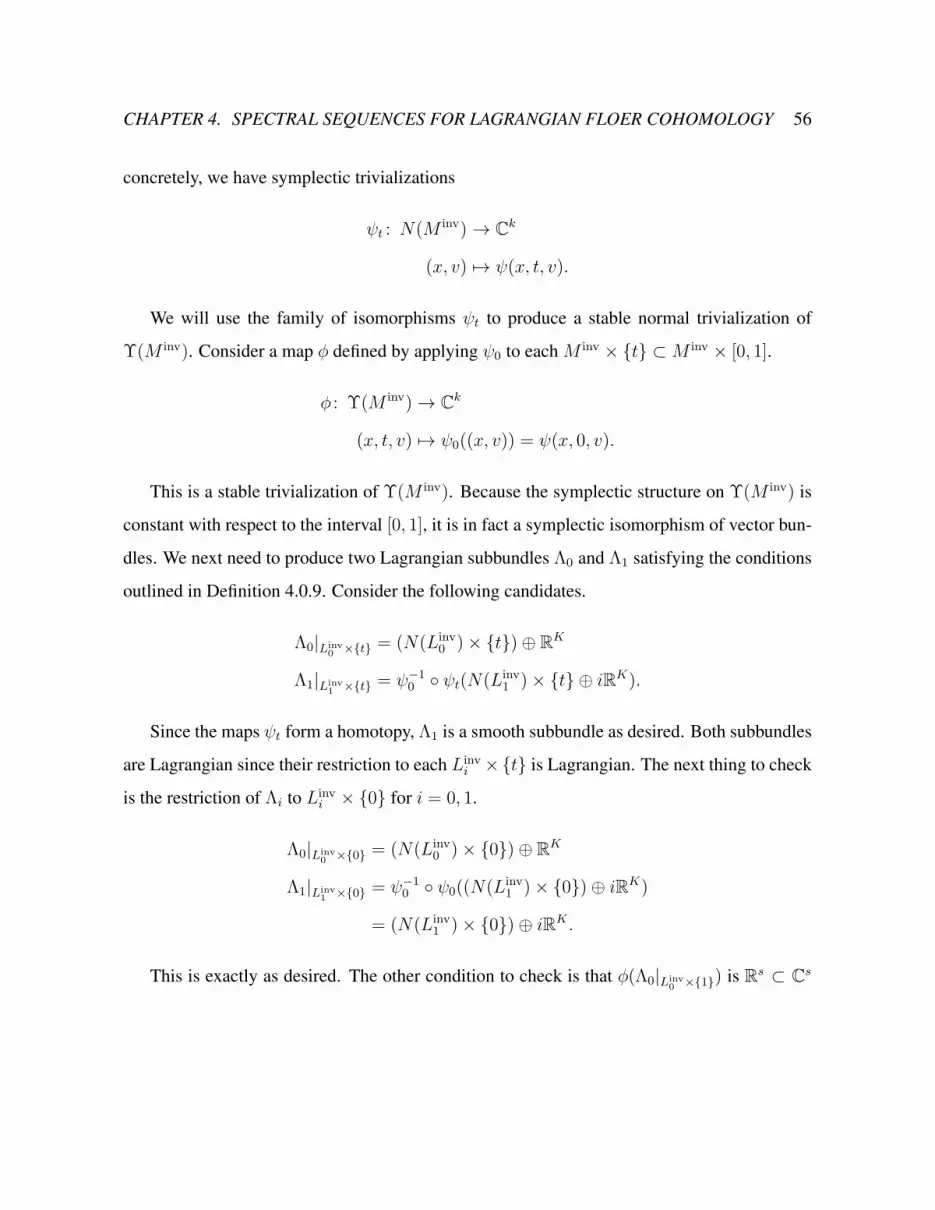
CHAPTER 4. SPECTRAL SEQUENCES FOR LAGRANGIAN FLOER COHOMOLOGY 56
concretely, we have symplectic trivializations
ψt : N(M inv) → Ck
(x, v) 7→ ψ(x, t, v).
We will use the family of isomorphisms ψt to produce a stable normal trivialization of
Υ(M inv). Consider a map ϕ defined by applying ψ0 to each M inv × {t} ⊂M inv × [0, 1].
ϕ : Υ(M inv) → Ck
(x, t, v) 7→ ψ0((x, v)) = ψ(x, 0, v).
This is a stable trivialization of Υ(M inv). Because the symplectic structure on Υ(M inv) is
constant with respect to the interval [0, 1], it is in fact a symplectic isomorphism of vector bun-
dles. We next need to produce two Lagrangian subbundles Λ0 and Λ1 satisfying the conditions
outlined in Definition 4.0.9. Consider the following candidates.
Λ0|Linv0 ×{t} = (N(Linv
0 )× {t})⊕ RK
Λ1|Linv1 ×{t} = ψ−1
0 ◦ ψt(N(Linv1 )× {t} ⊕ iRK).
Since the maps ψt form a homotopy, Λ1 is a smooth subbundle as desired. Both subbundles
are Lagrangian since their restriction to each Linvi ×{t} is Lagrangian. The next thing to check
is the restriction of Λi to Linvi × {0} for i = 0, 1.
Λ0|Linv0 ×{0} = (N(Linv
0 )× {0})⊕ RK
Λ1|Linv1 ×{0} = ψ−1
0 ◦ ψ0((N(Linv1 )× {0})⊕ iRK)
= (N(Linv1 )× {0})⊕ iRK .
This is exactly as desired. The other condition to check is that ϕ(Λ0|Linv0 ×{1}) is Rs ⊂ Cs

CHAPTER 4. SPECTRAL SEQUENCES FOR LAGRANGIAN FLOER COHOMOLOGY 57
and ϕ(Λ1|Linv1 ×{1}) is iRs ⊂ Cs.
ϕ(Λ0|Linv0 ×{1}) = ψ0((N(Linv
0 )× {0})⊕ RK)
= ψ((N(Linv0 )× {0})⊕ RK)
= Rs
ϕ(Λ1|Linv1 ×{1}) = ψ0(ψ
−10 ◦ ψ1((N(Linv
1 )× {0})⊕ iRK)
= ψ1(J(J((N(Linv1 )× {0})⊕ iRK)))
= J(ψ1(J(N(Linv1 )× {0})⊕ Rk))
= i(Rs)
Ergo the stable trivialization ϕ of Υ(M inv) together with the subbundles Λ0 and Λ1 constitutes
a stable normal trivialization of Υ(M inv).
4.1 Interpretation in the context of Heegaard Floer homol-
ogy
Let D = (S2,α,β,w, z) and D = (Σ(S2), α, β, w, z) be a pair of Heegaard diagrams which
is localizable in the sense of Definition 3.3.1. Given x a point on D, let x1, x2 be its two (not
necessarily distinct) lifts to D in some order. There is a natural map
ι : Symn−1(S2) → Sym2n−2(Σ(S2))
(x1 · · ·xn−1) 7→ (x11x21 · · ·x1n−1x
2n−1).
This map is a holomorphic embedding; for a proof, see Appendix 1. Moreover, consider the
induced involution on Sym2n−2(Σ(S2)), which through a slight abuse of notation we will also
call τ . The fixed set of τ is exactly our embedded copy of Symn−1(S2); moreover, τ preserves
the two tori Tα and Tβ, with fixed sets T invα = Tα and T inv
β= Tβ.
Perutz has shown that for an arbitrary Heegaard diagram D = (S,α,β,w, z), there is a
symplectic form ω on Symg+n−1(S) which is compatible with the complex structure induced

CHAPTER 4. SPECTRAL SEQUENCES FOR LAGRANGIAN FLOER COHOMOLOGY 58
by a complex structure on S, and with respect to which the submanifolds Tα and Tβ are in
fact Lagrangian and the various Heegaard Floer homology theories are their Lagrangian Floer
cohomologies [34, Thm 1.2]. In particular, the knot Floer homology is the Floer cohomology
of these two tori in the ambient space Symg+n−1(S\{z,w}), where the removal of the base-
points accounts for the restriction that holomorphic curves not be permitted to intersect the
submanifolds Vwiand Vzj of the symmetric product.
Proposition 4.1.1. There is a symplectic structure on Symg−n−1(S\{w, z}) with respect to
which the submanifolds Tα and Tβ are Lagrangian and
HFL(D) ∼= HFL((Y, L))⊗ V⊗(n1−1)1 ⊗ · · · ⊗ V
⊗(nℓ−1)ℓ
∼= HF (Tβ,Tα).
This is essentially Theorem 1.2 of [34]; the proof is identical save for trivial notation ad-
justments for Heegaard diagrams with multiple basepoints. From now on we will work with
this method of computing knot Floer homology; in Chapter 5 we will show that the symplectic
form produced by Perutz’s construction meets the requirements of Seidel and Smith’s theorem.
Let us now consider the application of Theorem 4.0.10 to double branched covers of links
in the three sphere and to periodic knots. We begin with the case that D and D are Heegaard
diagrams for (S3, L) and the double branched cover (Σ(L), L) as in Section 3.1. We make the
following suggestive choices of notation.
M1 = Sym2n−2(Σ(S2)\{w, z}) M inv1 = Symn−1(S2\{w, z})
L0 = Tβ Linv0 = Tβ
L1 = Tα Linv1 = Tα
Then the following is immediate from the definitions.
Lemma 4.1.2. With respect to our choice of symplectic manifold M and Lagrangians L0 and
L1, we have the following Floer cohomology groups.
HF (L0, L1) = HF (Tβ,Tα) = HFL(Σ(L), L)⊗ V ⊗n1−1 ⊗ · · · ⊗ V ⊗nℓ−1.
HF (Linv0 , Linv
1 ) = HF (Tβ,Tα) = HFL(S3, L)⊗ V ⊗n1−1 ⊗ · · · ⊗ V ⊗nℓ−1.

CHAPTER 4. SPECTRAL SEQUENCES FOR LAGRANGIAN FLOER COHOMOLOGY 59
Similarly, given Heegaard diagrams D and D as in 3.2.1 for a periodic knot together with
an unknotted axis and its quotient knot, we consider the spaces
M2 = Sym2n1(S2\{w, z− z0}) M inv2 = Symn1(S2\{w, z− z0})
M3 = Sym2n1(S2\{w, z}) M inv3 = Symn1(S2\{w, z})
Recall, for clarity’s sake, that the total number of basepoints on the periodic Heegaard diagram
D is n = n1 + 1. Here again the Lagrangians and their invariant sets are as follows.
L0 = Tβ Linv0 = Tβ
L1 = Tα Linv1 = Tα
The following is immediate from the definitions.
Lemma 4.1.3. With respect to our choice of symplectic manifolds Mi for i = 1, 2 and La-
grangians L0 and L1, we have the following Floer cohomology groups.
In M2,
HF (L0, L1) = HF (Tβ,Tα) = HFL(S3, K ∪ U)⊗ V ⊗(2n1−1).
HF (Linv0 , Linv
1 ) = HF (Tβ,Tα) = HFL(S3, K ∪ U)⊗ V ⊗(n1−1).
In M3,
HF (L0, L1) = HF (Tβ,Tα) = HFK (S3, K)⊗ V ⊗(2n1−1) ⊗W.
HF (Linv0 , Linv
1 ) = HF (Tβ,Tα) = HFK (S3, K)⊗ V ⊗(n1−1) ⊗W.
Observe that in all cases we work with a symmetric products of Heegaard surfaces D and D
which have been punctured along some subset {r} of {w, z} containing {w}. It will therefore
suffice to show the following two lemmas.
Lemma 4.1.4. Let D and D be a localizable Heegaard diagram pair, and {r} be a subset of
{w, z}. Then if we set
M = Sym2n−2(Σ(S2)\{r}) M inv = Symn−1(S2\{r})

CHAPTER 4. SPECTRAL SEQUENCES FOR LAGRANGIAN FLOER COHOMOLOGY 60
with the Lagrangians
L0 = Tβ Linv0 = Tβ
L1 = Tα Linv1 = Tα
we may equip M with an exact symplectic form ω with respect to which Li is exact for i = 0, 1
and τ is a symplectic involution. In addition we may giveM an ω-compatible complex structure
j which is convex at infinity.
To show that such a manifold M necessarily satisfies the conditions of Lemma 4.0.11 it
suffices to check that a slightly larger manifold M0 does.
Lemma 4.1.5. Let D and D be a localizable Heegaard diagram pair, and let
M0 = Sym2n−2(Σ(S2)\{w}) M inv0 = Symn−1(S2\{w})
with the Lagrangians
L0 = Tβ Linv0 = Tβ
L1 = Tα Linv1 = Tα
Then (M0, L0, L1) satisfies the conditions of Lemma 4.0.11.
Since a relative trivialization of the complex relative normal bundle on the level of Lemma
4.0.11 descends to any full-dimensional submanifold of M0 which contains the Lagrangians
L0 and L1, we immediately have the following theorem.
Theorem 4.1.6. Each of the trios (M1, L0, L1), (M2, L0, L1), and (M3, L0, L1) carries a stable
normal trivialization.
In combination with the symplectic geometry conditions checked in Chapter 5, this implies
Theorems 1.1.1, 1.2.2, and 1.2.3.
In some moral sense, this is the correct level of generality: the most important feature of
our punctured Heegaard diagram D is that no periodic domain has nonzero index, and in all our

CHAPTER 4. SPECTRAL SEQUENCES FOR LAGRANGIAN FLOER COHOMOLOGY 61
examples {w} (or {z}) is the smallest set of points at which we may puncture S2 and produce a
diagram for which this property holds. Moreover, M inv0 conveniently deformation retracts onto
each of Tα and Tβ, making certain cohomology computations in Chapters 5 and 7 cleaner than
they might otherwise be.
We have yet to address one important issue promised in Chapter 3. Since the involution
τ ∗ on HFL(D) may not be induced by the involution τ# on CFL(D) arising in the obvious
way from the Heegaard diagram, why is our claim that τ ∗ preserves spinc structures valid? To
see this, recall that a spinc structure is a homotopy class of paths between Tα and Tβ. As
we perform an equivariant isotopy of the Lagrangians Tα and Tβ, such homotopy classes are
preserved, as is which pairs of homotopy classes are exchanged under the involution τ on M .
Since our final choice of complex structure for M is equivariant, the action of τ determines
conjugacy of spinc structures, which is therefore also preserved. The argument for Alexander
gradings – which are equivalent to relative spinc structures on Y 3 − νL by Subsection 2.0.5
proceeds similarly.
An important note is that the localization map of Theorem 4.0.10 is entirely constructed
by counting pseudoholomorphic disks of varying index and by multiplication and division by
powers of θ. In particular, the localization isomorphism preserves the Alexander multigrading
on the E∞ page, because no flowlines can pass over the missing basepoint divisors. In general,
however, we should expect that these isomorphisms will not preserve the data of the Maslov
grading.

CHAPTER 5. GEOMETRY OF SYMMETRIC PRODUCTS 62
Chapter 5
The Geometry of Symmetric Products of
Punctured Heegaard Surfaces
In this chapter we consider the geometry of a symmetric product of a punctured Heegaard
diagram.
5.1 Symplectic Geometry of Symmectric Products of Punc-
tured Heegaard Surfaces
It remains to be verified that given a pair of Heegaard diagrams D and D which are localizable
in the sense of Definition 3.3.1 and a set of punctures r on D such that {w} ⊂ {r} ⊂ {w, z},
the manifold M = Sym2n−2(Σ(S)\{r}) satisfies the basic symplectic structural requirements
of Seidel and Smith’s theory. To wit, we must see that M can be equipped with a triple (j, ω, θ)
such that ω = dθ, the tori Tα and Tβ are exact Lagrangians, the involution τ on M is symplec-
tic, and moreover the complex structure j is convex at infinity.
Recall that D is a Heegaard diagram with underlying surface S2. Let f be an exhausting
function on S2\{r} as follows. Identify S2\{w0} with C, and let x = u + iv be a complex

CHAPTER 5. GEOMETRY OF SYMMETRIC PRODUCTS 63
number.
f : S2\{r} → R
x 7→ C|x|2 +∑
rj∈{r−w0}
1
|x− rj|2
Here C > 0 is a constant determined as follows. The exact symplectic form associated to
f is
ωf = −ddC(f) =
4C +∑
rj∈{r−w0}
4
|x− ri|4
du ∧ dv.
The α and β curves on S2 are certainly Lagrangian with respect to the symplectic form ωf ,
but we require them to moreover be exact; that is, we wish to ensure that∫αj−dC(f) = 0 for
all αj on S2\{r}. We choose C large enough that the integral∫αj−dCf > 0 for 1 ≤ j ≤ n−1,
and similarly for each βj . Then we may isotope the α and β curves inward toward the punctures
w (around which the curves are oriented counterclockwise) until we have a new, isotopic set of
curves for which∫αj−dCf = 0 =
∫αj−dCf . Hence we have arranged that the α and β curves
are exact Lagrangians with respect to ωf .
We now lift f to an exhausting function f on Σ(S2)\{r}. Our previous manipulations of
the α and β curves ensure that each αkj and βkj , where k = 1, 2 is exact with respect to the
symplectic form induced by f .
On the product space (Σ(S2)\{r})2n−2 there is a corresponding exhausting function defined
as follows. Let pm be the projection of the product to its mth factor, and let f = f ◦ p1 + · · ·+
f ◦ p2n−2. Notice that Sym2n−2(j)-convexity, properness, and boundedness of f follow from
the corresponding properties of f . The symplectic form we obtain from f is ωf = ωf ⊗ 1 · · ·⊗
1 + 1⊗ ωf ⊗ 1⊗ · · · ⊗ 1 + · · ·+ 1⊗ · · · ⊗ ωf . Therefore any of the (2n− 2)! lifts of Tα and
Tβ is an exact Lagrangian submanifold with respect to ωf .
Finally, consider the symmetric product Sym2n−2(Σ(S2)\{r}). There is a (possibly singu-

CHAPTER 5. GEOMETRY OF SYMMETRIC PRODUCTS 64
lar) continuous function
ψ : Sym2n−2(Σ(S2)\{r}) → R
(x1 · · ·x2n−2) 7→∑
σ∈S2n−2
f(xσ(1), · · · , xσ(2n−2))
which is smooth outside a neighborhood of {(x1 · · · x2n−2) ∈ Sym2n−2(Σ(S2)\{r}) : xk =
xj for some k = j}, the fat diagonal. Perutz observes [34] that this function is strictly plurisub-
harmonic in the sense of non-smooth functions, that is, that the two-current −ddCψ is strictly
positive. This gives us a continuous exhausting function on Sym2n−2(Σ(S2)\{r}). We may
apply the following lemma of Richberg [37], quoted in [6, Lemma 3.10].
Lemma 5.1.1. Let ψ be a continuous J-convex function on an integrable complex manifold V .
Then for every positive function h : V → R+, there exists a smooth J-convex function ψ′ such
that |ψ(x)− ψ′(x)| < h(x). If ϕ is already smooth on a neighborhood of a compact subset A,
then we can achieve ϕ = ϕ′ on A.
In particular, we may take h : Sym2n−2(Σ(S2)\{r}) → R+ to be a constant function
h(x) = ϵ, and apply the lemma to our map ψ and h. We produce ψ′ : Sym2n−2(Σ(S2\{r}) →
R such that |ψ′(x) − ψ(x)| < ϵ and ψ′ is smooth and Sym2n−2(j)-convex. Moreover, since ψ
is bounded below and proper, ψ′ is also, since the two real valued functions differ by at most ϵ.
Therefore ψ′ is an exhausting function on M , and M is convex at infinity.
We have yet to produce an appropriate symplectic form onM , which we will do using work
of Perutz [34]. We begin with a definition.
Definition 5.1.2. [34, Defn 7.3] Let X be a complex manifold with complex structure J . A
Kahler cocycle on X is a collection (Uk, ϕk)k∈K , where (Uk)k∈K is an open cover of X and
ϕk : Uk → R is an upper semicontinuous function such that
• ϕk is strictly plurisubharmonic
• ϕk − ϕℓ is pluriharmonic

CHAPTER 5. GEOMETRY OF SYMMETRIC PRODUCTS 65
If a Kahler cocycle (Uk, ϕk)k∈K is smooth then we can associate to it the symplectic form ω
which is −ddCϕk on each Uk. Notice, for example, that a Kahler cocycle can consist of a single
smooth plurisubharmonic function on all of X , as in the case of the smooth Kahler cocycle
((Σ(S2)\{r})2n−2, f) on (Σ(S2)\{r})2n−2 and the singular Kahler cocycle (M,ψ) on M .
Perutz proves the following technical result.
Lemma 5.1.3. [34, Lemma 7.4] Let (Uk, ϕk) be a continuous Kahler cocycle on a complex
manifold X . Suppose that X = X1 ∪ X2 such that X1 and X2 are open and the functions
ϕk|Uk∩X1 are smooth. Then there exists a continuous function
χ : X → R, Supp(χ) ⊂ X2
and a locally finite refinement
Vℓ ⊂ Uk(ℓ)
such that the family (Vℓ, ϕk(ℓ)|Vℓ + χ|Vℓ) is a smooth Kahler cocycle.
Notice that if (Uk, ϕk) happened to be the Kahler cocycle associated to a single J-convex
function ϕ on X , then (Vℓ, ϕℓ(k)|Vℓ + χ|Vℓ) is the Kahler cocycle associated to the smooth
plurisubharmonic function ϕ+ χ.
In our case we take X to be Sym2n−2(Σ(S)\{r}), X1 to be the complement of the main
diagonal in this symmetric product, and X2 to be a small neighborhood of the main diagonal
with no intersection with Tα and Tβ. Then the function ψ : Sym2n−2(Σ(S2)\{r}) → R admits
a smoothing to a Sym2n−2(j)-convex function ψ + χ : Sym2n−2(Σ(S2)\{r}) → R which is
equal to ψ away from a neighborhood of the large diagonal. The symplectic form ωϕ+χ is exact
and compatible with the complex structure on M .
Finally, on Tα the map χi is identically 0 and ψi = (2n−2)!fi|α11×α2
1×··· .×α1n−1×α2
n−1. There-
fore ωψ+χ|Tα= 0 and dC(ψi + χi)|Tα
= (2k)!dC(f)|α11×···×α2
n−1is exact. Ergo Tα is an exact
Lagrangian in the exact symplectic manifold M , and similarly Tβ is as well.
The reader may at this point be alarmed that we have failed to check that τ is a sym-
plectic involution. We amend this by replacing ωψ+χ by ω = 12(ωψ+χ + τ ∗ωψ+χ). Since τ

CHAPTER 5. GEOMETRY OF SYMMETRIC PRODUCTS 66
is a holomorphic involution, the exact form ω is Sym2n−2(j)-compatible and nondegenerate.
Moreover, since τ preserves Tα and Tβ, it is still the case that these two submanifolds are exact
Lagrangians with respect to ω. This ω is our final choice of symplectic form on M .
5.2 Homotopy Type and Cohomology of Symmetric Prod-
ucts of Punctured Heegaard Surfaces
Recall that to prove the existence of a stable normal trivialization for the triples (M,L0, L1)
introduced in Section 4.1, it suffices to prove that given a localizable Heegaard diagram pair
D and D, the standard triple (M0, L0, L1) carries a stable normal trivialization. Here M0 =
Sym2n−2(Σ(S)\{w}), and correspondingly M inv0 = Symn−1(S2\{w}).
Let us now proceed to discuss the homotopy type and cohomology of M inv0 , building up
the structure we will use in the proof that this manifold satisfies the complex conditions which
imply the existence of a stable normal trivialization.
We claim M inv0 deformation retracts onto each of Tα and Tβ. To check this, we use a
lemma whose proof essentially follows an argument of Ong [27].
Lemma 5.2.1. The rth symmetric product of a wedge of k circles ∨ki=1S1i deformation retracts
onto the r-skeleton of the k torus∏k
i=1 S1i , where each circle is given a CW structure consisting
of the wedge point and a single one-cell, and the torus has the natural product CW structure.
Proof. Let σ1, · · · , σr be the first r elementary symmetric functions of r variables x1, · · · , xr,
such that
σj(x1, · · · , xr) =∑
1≤i1<···<ij≤r
xi1 · · ·xij .
There is a well-known biholomorphism between Symr(C) and Cr by evaluating each of the
functions σj for 1 ≤ j ≤ r on an unordered set of complex numbers x1, · · · , xr. This has the
effect of mapping to the ordered coefficients of the monic polynomial with roots x1, · · · , xr,

CHAPTER 5. GEOMETRY OF SYMMETRIC PRODUCTS 67
multiplied by an alternating sign.
ϕ : Symr(C) → Cr (5.2.1)
(x1 · · ·xr) 7→ (σ1(x1, · · · , xr), · · · , σr(x1, · · · , xr)).
Under the map ϕ the submanifold Symr(C∗) is carried to Cr−1 × C∗. We can use this map
to construct the following homotopy equivalence between S1 and Symr(S1) for any r.
Symr(S1) �� // Symr(C∗)
ϕ|Symr(C∗) // Cr−1 × C∗ // C∗ // S1
Here the first inclusion map is a homotopy equivalence and the final two maps are deforma-
tion retractions. The total map carries (eiθ1 · · · eiθr) ∈ Symr(S1) to σr((eiθ1 , · · · , eiθr)), which
is exactly the product of the entries, ei(θ1+···+θr). Ergo the total map from Symr(S1) to S1 which
multiplies the entries of an unordered r-tuple of points on the circle is a homotopy equivalence.
Indeed, since this homotopy equivalence can be regarded as a retract from Symr(S1) to its
subspace Ar = {(eiθ1eiθ2 · · · eiθr) : θ2 = · · · = θr = 0} = S1 × {1}r−1, there must be a
deformation retraction F r from Symr(S1) to this subspace.
It will be useful to be slightly more careful concerning our choice of deformation retraction.
Suppose Symr−1(S1) is regarded as a subspace Symr−1×{1} of Symr(S1) via the embedding
(eiθ1 · · · eiθr−1) 7→ ((eiθ1 · · · eiθr−1ei0). Then both Symr(S1) and Symr−1(S1) × {1} deforma-
tion retract onto the subspace Ar in Symr(S1), implying that the relative homotopy groups
πi(Symr(S1), Symr−1(S1) × {1}) are trivial. Hence since all the spaces involved carry CW
structures induced by the CW structure on S1 and the inclusion Symr−1(S1) ↪→ Symr(S1) is
cellular, there is a deformation retraction F r,0 from Symr(S1) to Symr−1(S1)×{1}, which can
be taken to run on a time interval [0, 1r−1
]. By similar logic for r ≥ k ≥ 2, there is a deforma-
tion retraction F r,r−k from Symk(S1) × {1}r−k to Symk−1(S1) × {1}r−k+1 whose time input
can be taken to be [ r−kr−1
, r−k+1r−1
]. If we take F r to be the map Symr(S1) × [0, 1] → Symr(S1)
which is F r,r−k on [ r−kr−1
, r−k+1r−1
], then F r is a deformation retraction from Symr(S1) to Ar =
Sym1(S1)× {1}r−1 which preserves each of the subspaces Symk × {1}r−k.
We can now deal with the symmetric product of a wedge of circles. To keep track of which

CHAPTER 5. GEOMETRY OF SYMMETRIC PRODUCTS 68
points originate in which circle, label the circles S11 , · · · , S1
m and refer to points eiθj on S1j . Take
the wedge point to be the basepoint 1 = ei0 on each circle.
Regard the space Symr(∨mi=1 S
1i ) as the canonical subspace Symr(
∨mi=1 S
1i )×{1}r(m−1) of
Symrm(∨mi=1 S
1i ). Any point in Symr(
∨mi=1 S
1i )×{1}r(m−1) may be split uniquely into a point
in Symr(S11)×Symr(S1
2)×· · ·×Symr(S1m), as there are at most r terms from any circle S1
i in
an mr-tuple in Symr(∨mi=1 S
1i )× {1}r(m−1). Consider applying F r : Symr(S1
1)× [0, 1] to this
submanifold; that is, consider the following map.
F r1 : Symr(S1
1)× Symr(S12)× · · · × Symr(S1
m)× [0, 1] →
Symr(S11)× Symr(S1
2)× · · · × Symr(S1m)
((eiθ11 · · · eiθr1 ), · · · , (eiθ1m · · · eiθrm ))× [0, 1] 7→
(F r(eiθ11 · · · eiθr1 , t), · · · , (eiθ1m · · · eiθrm )).
Because F r never increases the number of nonbasepoint terms in (eiθ11 · · · eiθr1 ), the map
F r1 preserves the subspace Symr(
∨mi=1 S
1i ) × {1}r(m−1) in Symr(S1
1) × Symr(S12) × · · · ×
Symr(S1m). Ergo F r
1 is a deformation retraction from Symr(∨mi=1 S
1i ) to the subspace of r-
tuples in Symr(∨mi=1 S
1i ) of which at most one entry is a nonbasepoint point on S1
1 . Running
this procedure on each factor of Symr(S11)×Symr(S1
2)×· · ·×Symr(S1m) produces a deforma-
tion retraction from Symr(∨mi=1 S
1i ) to the subspace of r-tuples in this space containing only
one nontrivial point of each S1j for 1 ≤ j ≤ r. So we have the following homotopy equivalence.
Symr(m∨i=1
S1i ) ≃ {(eiθ11 , · · · , eiθmm )} ⊂ S1
1 × · · · × S1m : at most r θi are nonzero}
If r > m, this space is all of S11 × · · · × S1
m = (S1)m. If r < m, this space is exactly∪I=|r|(S
1)I ⊂ (S1)m.
We will apply this observation to M inv0 . In S2, let νi : [0, 1] → S2 be a small closed curve
around wi for 1 ≤ i ≤ n, such that νi is oriented counterclockwise in the complement of w0.
Then
H1(S2\{z}) = Z⟨ν1, · · · , νn−1⟩.

CHAPTER 5. GEOMETRY OF SYMMETRIC PRODUCTS 69
Now S2\{w} deformation retracts onto a wedge of n − 1 circles ∨n−1i=1 ν
′i, where ν ′i is a closed
curve homotopic to νi which passes once through the origin. Ergo M inv0 = Symn−1(S2\{w})
deformation retracts onto the symmetric product of ∨n−1i=1 ν
′i, which in turn deformation retracts
onto the product∏n−1
i=1 ν′i. However, this product is homotopy equivalent to
∏n−1i=1 νi, and indeed
to∏n−1
i=1 αi and to∏n
i=1 βi. We conclude that M inv0 has the homotopy type of an n − 1-torus
and in particular admits a deformation retraction onto each of Tα and Tβ.
We will require a concrete description of the cohomology rings of M inv0 , Tα, and Tβ for
the computations of Chapter 7, so we pause to supply one now. Consider the one cycles
νi : [0, 1] →M inv
t 7→ (νi(t)x0 · · ·x0)
where x0 is any choice of basepoint. The [νi] form a basis for H1(Minv). Ergo, letting [νi]
denote the dual of νi, we have
H1(M inv) = Z⟨[ν1], · · · , [νn−1]⟩
Hk(M inv) =∧kH1(M inv)
Similarly, we can write down the homology of the tori Tα and Tβ. Through a slight abuse of
notation, let us insist that we have parametrizations αi : [0, 1] → S2 running counterclockwise
in S2\{w0} and βi running clockwise. The first homology of Tα is generated by one-cycles
αi : [0, 1] → α1 × · · · × αn−1
t 7→ (y1, · · · , yi−1, αi(t), yi+1, · · · , yn−1)
where yj = αj(0), and thus the cohomology of this torus is
H1(Tα) = Z⟨[α1], · · · , [αn−1]⟩
Hk(Tα) =∧kH1(Tα)

CHAPTER 5. GEOMETRY OF SYMMETRIC PRODUCTS 70
We apply analagous naming conventions to Tβ, obtaining
H1(Tβ) = Z⟨[β1], · · · , [βn−1]⟩
Hk(Tβ) =∧kH1(Tβ)
Moreover, observe that under the map on homology induced by inclusion ι : X ↪→ M inv ×
[0, 1], both [αi] and of [βi] are sent to [νi]. Therefore the map ι∗ on cohomology Hk(M inv ×
[0, 1]) → Hk(X) is precisely the diagonal map, with
∧mj=1 [νij ] 7→
∧mj=1 [αij ] +
∧mj=1 [βij ]
Corollary 5.2.2. The relative cohomology H∗(M inv0 × [0, 1], X) is the cohomology of the torus
(S1)n−1, and in particular is torsion-free.
Proof. Consider the long exact sequence
· · ·Hm−1(X) // Hm(M inv0 × [0, 1], X)
q∗ // Hm(M inv0 ) ι∗ // Hm(X) · · ·
Taking into account that the obvious isomorphism between H∗(Tα) and H∗(Tβ) respects
our labelling of the cohomology classes, ι∗ is the diagonal map, and in particular an injection.
When m ≥ 2 we have the following short exact sequences.
0 → Hm−1(M inv0 × [0, 1]) ι∗ //// Hm−1(X) // Hm(M inv
0 × [0, 1], X) → 0
∧m−1j=1 [νij ]
� //∧m−1j=1 [αij ] +
∧m−1j=1 [βij ]
Ergo for m ≥ 2, Hm(M inv0 × [0, 1], X) ∼= Hm−1(Tα) ∼= Hm−1(Tβ). (We will have occasion to
be careful about the generators in Chapter 7.) The same result follows for H1(M inv0 × [0, 1], X)
trivially.

CHAPTER 6. IMPORTANT CONSTRUCTIONS FROM K-THEORY 71
Chapter 6
Important Constructions from K-Theory
Central to our argument that the triples (M,L0, L1) introduced in Section 4.1 admit stable
normal trivializations will be several useful results from complex K-theory, most trivial but
one rather less so. A detailed treatment of the subject, along with proofs of all results up to
Proposition 6.0.10, may be found in [16].
Let V be a complex vector bundle over a base space X , which for purposes of this paper
we take to be a compact Hausdorff topological space. We let VectCn(X) denote the set of
isomorphism classes of n-dimensional vector bundles over X . This is a monoid under the
direct sum of vector bundles. For any n, as before we refer to the trivial complex vector bundle
of degree n overX simply as Cn. Then there is an equivalence relation ≈S on VectCn(X) defined
as follows: given V,W two n-dimensional vector bundles over X , we say that V ≈S W if and
only if there is some m such that V ⊕ Cm ∼= W ⊕ Cm. The two vector bundles V and W
are said to be stably isomorphic. This relation respects the direct sums and tensor products
of vector bundles, such that the set of equivalence classes of bundles under ≈S inherits two
abelian laws of composition [V ]S + [W ]S = [V ⊕W ]S and [V ]S × [W ]S = [V ⊗W ]S . This set
of equivalence classes may be given the structure of a ring by formally adjoining the inverse of
each element under the direct sum. More precisely, we set
K0(X) = {[V ]S − [W ]S : [V ]S, [W ]S are equivalence classes with respect to ≈S}.

CHAPTER 6. IMPORTANT CONSTRUCTIONS FROM K-THEORY 72
Commonly [V ]S − [C0]S will be written simply as [V ]S and its additive inverse [C0]S − [V ]S
simply as −[V ]S .
Lemma 6.0.3. K0(X) is a ring with respect to the operations [V ]S + [W ]S = [V ⊕W ]S and
[V ]S × [W ]S = [V ⊗W ]S .
There is also a reduced form of this ring K(X) constructed as follows. Let ∼ be a second
equivalence relation on∪n∈N VectCn such that V ∼ W if there is some m1,m2 such that V ⊕
Cm1 ∼= W ⊕ Cm2 . In this case one can show that the set of equivalence classes with respect
to ∼ contains additive inverses without adjoining any additional elements. Let the equivalence
class of a vector bundle V with respect to ∼ be [V ].
Lemma 6.0.4. K0(X) is a ring with respect to the operations [V ] + [W ] = [V ⊕ W ] and
[V ]× [W ] = [V ⊗W ].
Then K0(X) ∼= K0(X) ⊕ Z. In both cases a vector bundle in the same equivalence class
as Cm is said to be stably trivial. Notice as a most basic case that for {x0} a one point space
K0(x0) = Z and K0(x0) = 0.
Given a continuous map f : X → Y , the corresponding map f∗ : VectCn(Y ) → VectCn(X)
which maps a vector bundle V over Y to its pullback f ∗(V ) descends to maps f ∗ : K0(Y ) →
K0(Y ) and f ∗ : K0(Y ) → K0(X). Recalling that if maps f, g : X → Y are homotopic
then f ∗(V ) and g∗(V ) the two pullbacks of a bundle V over Y are isomorphic, we see that
homotopic maps f and g induce the same maps f∗ = g∗ on K0(Y ) and K0(Y ). In particular,
we have the following lemma.
Lemma 6.0.5. If f : X1 → X2 is a homotopy equivalence with homotopy inverse g : X2 →
X1, the induced map f ∗ : K0(X2) → K0(X1) is an isomorphism with inverse g∗. The same is
true of the reduced theory.
We will use this lemma to deal with the minor problem that M inv is not actually compact.
The three spaces whose K-theory will be of interest to us are M inv × [0, 1], its subspace X =
Linv0 ×{0}∪Linv
1 ×{1}, and the quotient space M inv/X . The space X is a disjoint union of two

CHAPTER 6. IMPORTANT CONSTRUCTIONS FROM K-THEORY 73
tori, hence compact. We have seen previously that M inv deformation retracts onto a compact
subspace homeomorphic to the n − 1 skeleton of (S1)2n−1. For purposes of dealing with
K0(M inv) let us choose a slightly different deformation retraction. Let Y = (∪αi)∪(∪βi).
Then let F : (S2\{w, z})×[0, 1] → S2\{w, z} be a deformation retraction from the punctured
sphere to the union of Y and all components of S2\Y not containing any point of {w, z}. This
is a compact subspace of the punctured sphere; let it be Z. Then F induces a deformation
retraction Symn−1(F ) of M inv = Symn−1(S2\{w, z}) onto the compact set Symn−1(Z), so
we can legitimately refer to the K-theory of M inv by identifying it with K0(Symn−1(Z)).
Notice further that F is the identity on Y × I , so the induced deformation retraction from M inv
preserves X ⊂ Symn−1(Y ). Therefore we may produce a deformation retract Symn−1(F )
from M inv/X to Symn−1(Z)/X , and Symn−1(Z)/X is compact Hausdorff. So we identify the
K-groups ofM inv/X with those of Symn−1(Z)/X , and from now on make no further reference
to this technical subtlety.
The relationship between homotopy classes of maps and pullbacks of vector bundles in
fact gives us the following deeper proposition, which follows from the theorem that any n-
dimensional complex vector bundle overX is a pullback of the canonical n-dimensional bundle
over the Grassmanian Gn(C∞) along some homotopy class of maps X → Gn(C∞).
Proposition 6.0.6. K0(X) ∼= [X,BU ]
Here BU is the classifying space of the infinite unitary group.
We extend our definition of K0(X) as follows. Let K−i(X) = K0(Σi(X)), where Σ(X)
is (for this section only) the reduced suspension of X . Then we have the following.
Proposition 6.0.7. (The Bott Periodicity Theorem) K0(X) ∼= K0(Σ2(X)).
We use this two-periodicity to define Ki(X) for positive i. Now notice that K0(X) =
K0(X+), where X+ denotes the one-point compactification of X (when X is compact, this
will mean X together with a point at infinity). In particular, K1(X) = K0(Σ(X)). Then the
groups Ki(X) are also doubly-periodic.

CHAPTER 6. IMPORTANT CONSTRUCTIONS FROM K-THEORY 74
With Ki(X) now defined for all i ∈ Z, we are ready for the following proposition, which
deals with K∗(X) = ∪iKi(X) merely as a collection of abelian groups and (momentarily)
ignores their ring structure.
Proposition 6.0.8. The groupsKi(X) form a generalized cohomology theory on compact topo-
logical spaces. Likewise, the groups Ki(X) form a reduced cohomology theory.
A relevant note is that if {x0} is a one point space, we have
Ki({x0}) =
Z if i even
0 if i odd .
One consequence of this structure on the K-theory of a space is that there is a notion of
the relative K-theory of a compact space X and a closed subspace Y . We let K0(X, Y ) be
the ring of isomorphism classes of vector bundles over X which restrict to a trival bundle over
Y . Equivalently, K0(X, Y ) ∼= K0(X/Y ); notice that if X is compact Hausdorff and Y is a
closed subspace, X/Y is compact Hausdorff, so this statement makes sense. With respect to
this construction, the long exact sequence of a pair (X, x0) consisting of a space X together
with a basepoint x0 becomes a long exact sequence relating the groups Ki(X) and Ki(X).
· · · Ki(X) → Ki(X) → Ki(x0) → Ki−1(X) · · ·
For our purposes, the crucial results from K-theory will be those relating K∗(X) to the
rational cohomology H(X;Q) of X . The exact sequence above, and the corresponding exact
sequence on the reduced and unreduced rational cohomology of X , will allow us to move
between maps on K∗(X) and K∗(X) with relative ease.
Recall that the Chern classes of a vector bundle V over a space X are a set of natural
characteristic classes ci(V ) ∈ H2i(X). The total Chern class of an n-dimensional vector bundle
V is c(V ) = c0(V ) + c1(V ) + · · · + cn(X). If X has the structure of a complex manifold, as
do most spaces of interest to us, we will often use c(X) to refer to the total Chern class of the
tangent bundle TX of X . The Chern classes may be used to produce a ring homomorphism
K0(X) ∪K1(X) → H∗(X;Q).

CHAPTER 6. IMPORTANT CONSTRUCTIONS FROM K-THEORY 75
Let σj(x1, · · · , xk) be the elementary symmetric functions on k elements as in Chapter 5.
Then we assert the existence of a new set of polynomials s(x1, · · · , xk) with the following
properties.
Lemma 6.0.9. There exists a unique set of polynomials sj(x1, · · · , xk) with the property that
sj(σ1(x1, · · · , xk), · · · , σk(x1, · · · , xk)) = xj1 + · · ·+ xjk.
The polynomials sj are defined recursively in terms of the elementary symmetric functions
and the si of lower degree by the following relation.
sj = σ1sj−1 − σ2sj−2 + · · ·+ (−1)j−2σj−2s2 + (−1)j−1σj−1s1
We can now define the Chern character of a vector bundle.
ch : K0(X) → Heven(X;Q)
[V ]S 7→ n+∑j>0
sk(c1(V ), · · · , ck(V ))/k!
While this is the quickest way to produce this definition, it is not clear that it is necessarily
the most intuitive. To clarify: this definition is explicitly chosen so that if L is a line bundle over
X and the total Chern class of L is 1 + c1(L), then ch(L) = 1 + c1(L) +c1(L)2
2!+ c1(L)3
3!+ · · · ,
the “exponential” of the total Chern class of L. As the map ch was intended to be a ring
isomorphism on K0(X), we next require that for a product of line bundles L1 ⊗L2 ⊗ · · · ⊗Lk
over X we have ch(L1 ⊗ · · · ⊗ Lk) = ch(L1) · · · ch(Lk). A computation leads to the formula
above.
The Chern character descends to a reduced map ch : K0(X) → Heven(X;Q). We may also
consider the Chern character of vector bundles on Σ(X), which yields the following map into
the odd cohomology of X .
ch : K1(X) = K0(Σ(X)) → Heven(Σ(X);Q) ∼= Hodd(X;Q)
Similarly, we define ch : K1(X) → Hodd(X;Q). We then have the following extremely
useful result.

CHAPTER 6. IMPORTANT CONSTRUCTIONS FROM K-THEORY 76
Proposition 6.0.10. The Chern character induces a rational isomorphism
ch : K0(X) ∪K1(X)⊗Q → H∗(X;Q).
In particular, the rank of K0(X) ∪K1(X) is equal to the rank of H∗(X). The analogous
statement holds for ch and the two reduced theories.
The proof of this proposition takes Bott periodicity as a base case and is laid out in [16,
Thm 4.5].
We will last need a K-theoretic statement about relationship between the torsion of H∗(X)
and K∗(X). As it is a rather high-powered result, we’ll say a few words about the proof,
which relies on the Atiyah-Hirzebruch spectral sequence, a device for computing an arbitrary
cohomology theory first described by its eponymous introducers in [2].
Proposition 6.0.11. Let hn(X) be any cohomology theory. Then there is a spectral sequence
which converges to hn(X) whose E2 page is given by
E2i,j = H i(X;hj({pt}).
In the particular case of the cohomology theory K∗(X) this spectral sequence collapses
rationally, leading to a useful statement concerning the torsion groups of K∗(X).
Proposition 6.0.12. [2, Section 2.5] Let X be a compact Hausdorff space. If H i(X;Z) is
torsion-free for all i and finitely generated, then K0(X) ∪ K1(X) is torsion-free of the same
rank.
Proof. Recall that if {x0} is a one-point space then Kq(x0) is Z for q even and 0 for q odd.
Since unreduced K-theory is a cohomology theory, Proposition 6.0.11 gives first and second
quadrant spectral sequence converging to K∗(X) whose E2 page has entries
E2p,q = Hp(X;Kq({x0})) =
Hp(X) if q is even
0 if q is odd.

CHAPTER 6. IMPORTANT CONSTRUCTIONS FROM K-THEORY 77
The rank of Ki(X) is the sum∑
p+q=i rk(E∞p,q). Moreover, the ranks of the corresponding
entries on the E2 page of the spectral sequence sum to∑
p+q=i rk(E2p,q) =
∑p≡n mod 2H
p(X).
By Proposition 6.0.10, the rank of Ki(X) and the total rank of the integer cohomology groups
of degree the same parity as i are equal, so∑
p+q=i rk(E∞p,q) =
∑p+q=i rk(E
2p,q). As rk(E∞
p,q) ≤
rk(E2p,q) for all p, q, we see that in fact this is an equality for all pairs (p, q).
Now notice that every entry on the E2 page of this spectral sequence is free abelian. Sup-
pose E∞p,q has a nontrivial torsion subgroup for some fixed p, q such that q is even. Then there
must be some first Erp,q such that r > 2 with this property. Because Er
p,q is a quotient of a
subgroup of the free abelian group Er−1p,q , if it contains a torsion subgroup it must have lower
rank than Erp,q, implying that E∞
p,q has strictly lower rank than E2p,q. We have seen that this
never happens. Therefore the E∞ page of our spectral sequence is torsion-free, implying that
K∗(X), which is filtered by the entries on the E∞ page, is also free abelian.
This argument, which is similar to the original proof of [2, Section 2.5] was suggested by
Dan Ramras.
Our proof that (M inv, Linv0 , L
inv1 ) carries a stable normal trivialization will contain as a crucial
step a proof that H∗(M inv/(Linv0 ×{0}∪Linv
1 ×{1})) is torsion-free, and thus that the K-theory
of this space must likewise be free abelian.

CHAPTER 7. THE EXISTENCE OF STABLE NORMAL TRIVIALIZATIONS 78
Chapter 7
The Existence of Stable Normal
Trivializations
Recall that in Chapter 5, we took D, D to be a localizable pair of Heegaard diagrams in the
sense of 3.3.1, and {r} to be a subset of the basepoints {w, z} on D containing {w}. We then
let {r} be the lift of {r} on D. We saw that the triple (M,L0, L1), where M is the symmet-
ric product of D punctured along {r} and L0, L1 are the Lagrangians Tβ, Tα, satisfies the
symplectic geometry conditions of Seidel–Smith localization. We now proceed to check that
(M inv, Linv0 , Linv
1 ) fulfills the complex conditions that, by Lemma 4.0.11, imply the existence
of a stable normal trivialization. In fact it suffices to check this fact for the case that the set of
punctures is {r} is equal to {w}. As in Section 5.2, let us refer to the manifold generated in
this particular case as M0. Then the complex relative trivialization we produce then restricts to
a relative trivialization on the submanifold M of M0 generated by considering any larger set
{r}.
Proposition 7.0.13. Consider the complex manifold M0 = Sym2n−1(Σ(S2)\{w}) together
with its totally real submanifolds L0 = Tβ and L1 = Tα, and the holomorphic involution τ
which preverves L0 and L1. The map
(M inv0 × [0, 1], (L0 × {0}) ∪ (L1 × {1})) → (BU,BO)

CHAPTER 7. THE EXISTENCE OF STABLE NORMAL TRIVIALIZATIONS 79
which classifies the pullback Υ(M inv0 ) = N(M inv
0 ) × [0, 1] of the complex normal bundle of
M inv0 together with the totally real subbundlesNLinv
0 ×{0} over Linv0 ×{0} and J(NLinv
1 )×{1}
over Linv1 × {1} is nulhomotopic.
As a first step, we must establish the complex triviality of NM inv0 (and thus of Υ(M inv
0 ))
and the real triviality of NLinvi for i = 1, 2.
Lemma 7.0.14. The complex bundle NM inv0 is stably trivial.
Proof. The inclusion map ι1 : (S2\{w}) ↪→ S2 is nulhomotopic. Therefore the induced in-
clusion Symn−1(ι1) : Symn−1(S2\{w}) ↪→ Symn−1(S2) is also nulhomotopic. The normal
bundle of M inv0 = Symn−1(S2\{w}) in M0 = Sym2n−2(Σ(S2)\{w}) is exactly the restriction
of the normal bundle to Symn−1(S2) in Sym2n−2(Σ(S2)) along the inclusion map Symn−1(ι1).
As the map Symn−1(ι1) is nulhomotopic, NM inv0 is stably trivial.
We must also show that the real normal bundles of the invariant Lagrangians are trivial.
Lemma 7.0.15. N(Linvi ) is trivial for i = 0, 1.
Proof. Recall that L1 = Tα ⊂ Sym2n−2(Σ(S2)\{w}) is the totally real torus α11 × α2
1 × · · · ×
α1n−1 × α2
n−1. Thus the tangent bundle TL1 = T (α11)× T (α2
1)× · · · × T (α1n−1)× T (α2
n−1) is
the trivial real tangent bundle to (S1)2n−2. The invariant set Linv1 = i(Tα) = i(α1×· · ·×αn−1)
is embedded in L1 via
i|Tα : Tα ↪→ Tα
(x1, · · · , xn−1) 7→ (x11, x21, · · · , x1n−1, x
2n−1).
We conclude that
T (Linv1 ) = i∗(T (Tα)) = {(v11, v21, · · · , vn−1, v
2n−1) : (v1, v2, · · · , vn−1) ∈ T (Tα)} ⊂ TL1
N(Linv1 ) = {(v11,−v21), · · · , v1n−1,−v2n−1) : (v1, · · · , vn−1) ∈ T (Tα}) ⊂ TL1.
The point is that T (Linv1 ) ≃ T ((S1)n−1) is trivial, and there is an isomorphism
T (Linv1 ) → N(Linv
1 )
(v11, v21, · · · , v1n−1, v
2n−1) 7→ (v11,−v21, · · · , v1n−1,−v2n−1).

CHAPTER 7. THE EXISTENCE OF STABLE NORMAL TRIVIALIZATIONS 80
Triviality of N(Linv0 ) is proven analogously.
We now turn to the question of relative triviality. Let X = (L0 × {0}) ∪ (L1 × {1}) as
in Chapter 5. Choose preferred trivializations of the totally real bundles NLinv0 × {0} and
J(NLinv1 )×{1} and tensor with C to extend to a preferred trivialization of the complex bundle
Υ(M inv0 )|X . We use this trivialization to pull back [Υ(M inv
0 )] ∈ K0(M inv0 × [0, 1]) to a relative
bundle [Υ(M inv0 )]rel ∈ K0((M inv
0 ×[0, 1])/X). Because the reduced cohomology, and therefore
the reduced K-theory, of (M inv0 × [0, 1])/X have no torsion, to verify triviality of the relative
bundle, it suffices to show that the Chern classes of [Υ(M inv0 )]rel are trivial.
Remark 7.0.16. It may be helpful to draw attention to a minor problem of notation: in earlier
sections, K is a doubly periodic knot, but also in the present section K0(B) is the reduced
K-theory of the topological space B. We hope this will not occasion confusion.
Fundamentally, the argument for relative triviality rests on the fact that each of the n − 1
linearly independent periodic domains in S2\{w} has Maslov index zero. Therefore, we pause
here to recall the notation of Section 3.3. Let xi be the single positive intersection point in
αi ∩ βi and yi the negative intersection point. Let Fi be the closure of the component of
S − αi − βi containing zi and Ei be the closure of the component of S − αi − βi containing
another basepoint zk for some k. Then Pi = Ei − Fi is a periodic domain of index zero on D
with boundary βi − αi. Finally, let γi be the union of the arc of αi running from xi to yi and
the arc of βi running from xi to yi. In particular, this specifies that γi has no intersection with
any α or β curves other than αi and βi, and moreover the component of S − γi which does not
contain w0 contains only a single basepoint wi. See Figure 5 for an illustration of the domain
Pi.
The structure of the argument is as follows: for each even k such that 1 ≤ k ≤ 2n− 2, we
will use the periodic domains Pi to produce a set of k-chains {WI} in (M inv0 × [0, 1], X) whose
relative homology classes generate the kth homology of Hk(Minv0 × [0, 1], X). We will then
show that the restriction of Υ(M inv0 )|rel to each WI is trivial as a relative vector bundle, and that
therefore ⟨ck(Υ(M inv0 )|rel), [WI]⟩ = 0. Since the [WI] generate Hk(M
inv0 × [0, 1], X), we will

CHAPTER 7. THE EXISTENCE OF STABLE NORMAL TRIVIALIZATIONS 81
Figure 5: The periodic domain Pi = Ei − Fi has Maslov index zero.
wizi zkFi E i
α i βix i
have proven that ck(Υ(M inv0 )|rel) is identically zero.
More specifically, we will describe the chains WI as a subset of a product of two-chains
Yi in (S2\{w}) × [0, 1] such that the projection to S2\{w} is the periodic domain Pi and the
Yi are pairwise disjoint. We will then show that the restriction of the bundle Υ(M inv0 )|rel to
WI also breaks up as the restriction of a product of relative bundles Υ(Yi) over the Yi which
are known to be trivial through Maslov index arguments. Let us begin by constructing these
manifolds Yi.
For 1 ≤ i ≤ n− 1, let Yi be a subspace of S2 × [0, 1] with the following properties:
• Yi is topologically S1 × [0, 1], and Yi ∩ (S2 × {t}) is S1 for all t.
• The boundary of Yi is βi × {0} − αi × {1}.
• The projection of Yi to the punctured sphere is a copy of the periodic domain Pi.
• Yi ∩ Yj = ∅ if i = j.
• If xi is the point of positive intersection of αi and βi, {xi} × [0, 1] ⊂ Yi.
The 2-chains Yi are constructed as follows: for t ∈ [0, 12], choose a linear homotopy Ht
from βi to γi inside the domain Ei which fixes βi ∩ γi. Let the intersection of Yi with S2 × {t}
be the embedded circleHt(βi)×{t}. Similarly, for t ∈ [12, 1], choose a linear homotopy Jt from
γi to αi inside the domain Fi which fixes αi ∩ γi, and let the intersection of Yi with S2 × {t}
be Jt(γi).

CHAPTER 7. THE EXISTENCE OF STABLE NORMAL TRIVIALIZATIONS 82
Observe that this description of Yi has the following properties: first, Yi is contained in
(S2\{w}) × [0, 1] as promised. Second, Yi contains the line segment {xi} × [0, 1]. Third, the
intersection of Yi with (αi∪βi)× (0, 1) is entirely contained in the cylinder γi× (0, 1). Finally,
the projection of Yi ∩ (S2 × [0, 12]) to S2 lies entirely “inside” βi - that is, on the component
of S2\βi not containing w0 - implying that the sets Yi ∩ (S2 × [0, 12]) are pairwise disjoint.
Similarly, the projection of Yi ∩ (S2 × [12, 1]) to S2 lies entirely “inside” αi, and therefore the
sets Yi ∩ (S2 × [12, 1]) are pairwise disjoint. Ergo the Yi are pairwise disjoint.
We are now ready to define the complex line bundles Υ(Yi). Recall from Section 4.1 that
there is a holomorphic embedding
ι : M inv0 = Symn−1(Σ(S2)\{w}) → Symn−1(S2\{w}) =M0
(x1...xn−1) 7→ (x11x21...x
1n−1x
2n−1).
Similarly, we have a holomorphic embedding
ι′ : (S2\{w}) → Sym2(Σ(S2)\{w})
x 7→ (x1x2)
which takes a point x on S2\{w} to the unordered pair consisting of its two (not necessarily
distinct) lifts on Σ(S2)\{w} under the projection map π : (Σ(S2)\{w}) → (S2\{w}). Notice
that for each 1 ≤ i ≤ n − 1, ι′(αi) ⊂ α1i × α2
i and ι′(βi) ⊂ β1i × β2
i . Let N(S2\{w}) be
the normal bundle to S2\{w} in the second symmetric product Sym2(Σ(S2)\{w}). This is a
complex line bundle over a punctured sphere, hence trivial. For each 1 ≤ i ≤ n−1, let Nαi be
the real normal bundle to αi in α1i ×α2
i and Nβi be the real normal bundle to βi in β1i ×β2
i . An
argument similar to that of Lemma 7.0.15 shows that Nαi and Nβi are trivial real line bundles
for all i.
Consider the pullback of the normal bundleN(S2\{w}) to (S2\{w})×[0, 1]. The complex
line bundle over Yi that interests us is the restriction of this pullback to Yi, which we shall by
analogy denote Υ(Yi). That is, Υ(Yi) = (N(S2\{w}) × [0, 1])|Yi . This complex line bundle
has totally real subbundles J(Nαi×{1}) over αi×{1} and Nβi×{0} over βi×{0}. Choose

CHAPTER 7. THE EXISTENCE OF STABLE NORMAL TRIVIALIZATIONS 83
preferred real trivializations of these real line bundles, and extend to a complex trivialization
of Υ(Yi)|(βi×{0})∪(αi×{1}) by tensoring with C. For convenience, let this subspace (βi × {0}) ∪
(αi × {1}) be Xi.
Lemma 7.0.17. For 1 ≤ i ≤ n−1, given any preferred trivialization of Υ(Yi)|Xias a complex
vector bundle, the relative vector bundle Υ(Yi)|rel over (Yi, Xi) is stably trivial.
Proof. Let ιi be the inclusion of Yi into (S2\{w})×[0, 1], and p be the projection of (S2\{w})×
[0, 1] to S2\{w}. Then the image of p ◦ ιi(Yi) is the periodic domain Pi.
Consider the commutative diagram below. The top horizontal inclusion of S2\{w} into
Symn−1(S2\{w}) is defined by mapping a point x to (xx1...xi...xn−1), where again each xj
is the positively oriented point in αj ∪ βj . The bottom inclusion of Sym2(Σ(S2)\{w}) into
Sym2n−2(Σ(S2)\{w}) sends an unordered pair (xy) to (xyx1ix2i ...x
1i x
2i ...x
1n−1x
2n−1).
Yip◦ιi //
&&LLLLL
LLLLLL
L S2\{w} ↪� _
ι′
��
// Symn−1(S2\{w})� _
ι
��Sym2(S2\{w}) ↪ // Sym2n−1(S2\{w})
Consider the map ϕ : Yi → Symn−1(S2\{w}) given by composition along the top row
of the diagram. This is a topological annulus representing the periodic domain Pi. Since Pi
has Maslov index zero, by the discussion in Chapter 2, the first Chern class of the pullback
of the complex tangent bundle TSymn−1(S2\{w}) to Yi relative to the complexification of
the pullbacks of the real tangent bundles J(T (Tα)) to one component of the boundary of Yi
and T (Tβ) to the other is zero. However, the pullback ϕ∗(TSymn−1(S2\{w})) of the tangent
bundle of the total symmetric product to Yi is exactly (p ◦ ι)∗(T (S2\{w})⊕Cn−2), where the
factors of C are the restriction of the tangent bundle of the punctured sphere to the points xj
such that j = i. Moreover, (p ◦ ι)∗(T (S2\{w})) is precisely the restriction of the pullback
bundle p∗(T (S2\{w})) = T ((S2\{w}) × [0, 1]) over (S2\{w}) × [0, 1] to the subspace Yi.
Therefore ϕ∗(TSymn−1(S2\{w})) = T ((S\{w})× [0, 1])|Yi ⊕ Cn−2.
Similarly, the pullback ϕ∗(J(T (Tα))) to the boundary component αi × {1} ⊂ Yi is (p ◦
ιi)∗(J(T (αi)⊕Rn−1−1)), where the factors of R are the canonical real subspace of the tangent

CHAPTER 7. THE EXISTENCE OF STABLE NORMAL TRIVIALIZATIONS 84
bundle to the punctured sphere at the points xj for j = i. The pullback of this bundle to
αi×{1} ⊂ Yi is J((T (αi)×{1})⊕Rn−1−1). A similar argument shows that ϕ∗(J(T (Tβ))) is
(T (βi)×{0})⊕Rn−2. Therefore we have seen that the complex vector bundle T ((S2\{w})×
[0, 1])|Yi ⊕Cn−2 relative to the complexification of its totally real subbundles (T (βi)× {0})⊕
Rn−2 over βi × {0} and J((T (αi)× {1})⊕ Rn−2) over αi × {1} has relative first Chern class
zero. Hence the same is true of the complex line bundle T ((S2\{w}) × [0, 1])|Yi relative to
the complexification of its totally real subbundles J(T (αi)× {1}) and T (βi)× {0}. As this is
a line bundle, triviality of the first relative Chern class suffices to show stable triviality of the
relative vector bundle.
Now consider the map ϕ = ι ◦ ϕ from Yi to Sym2n−2(Σ(S2)\{w}) given by any path
through the diagram from Yi to Sym2n−2(Σ(S2)\{w}). This is a topological annulus rep-
resenting the periodic domain π−1(Pi) in D, which also has Maslov index zero because of
our insistence that either both z basepoints in the image of Pi are branch points or neither is.
Therefore the pullback along ϕ of the complex tangent bundle T (Sym2n−2(Σ(S2)\{w})) to Yi
relative to complexifications of pullbacks of the totally real subbundles J(T (Tα)) and T (Tβ)
to αi×{1} and βi×{0} has trivial relative first Chern class. However, once again the pullback
of this relative bundle along the inclusion map Sym2(Σ(S2)\{w}) ↪→ Sym2n−2(Σ(S2)\{w})
decomposes into a much smaller tangent bundle together with a trivial summand. Observe that
ϕ∗(T (Sym2n−2(Σ(S2)\{w})) is (ι′ ◦(p◦ ιi))∗(T (Sym2(Σ(S2)\{w}))⊕C2n−4)). Pulling back
along the inclusion map ι′, we see that this bundle breaks up as T (S2\{w})⊕N(Σ(S2)\{w})⊕
C2n−4 over Σ(S2)\{w}, and that therefore its ultimate pullback to Yi is T ((Σ(S2)\{w}) ×
[0, 1])⊕Υ(Yi)⊕ C2n−4.
Similarly, the pullback along ϕ of J(T (Tα)) to αi × {1} is precisely J(Tαi × {1}) ⊕
J(Nαi × {1}) ⊕ J(R2n−4). Finally, the pullback along ϕ of T (Tβ) to βi × {0} is (Tβi ×
{0})⊕ (Nβi ×{0})⊕R2n−4. Dropping the trivial summands, we conclude that the first relative
Chern class of T ((S2\{w}) × [0, 1]) ⊕ Υ(Yi) relative to complexifications of the totally real
subbundle (Tβi × {0}) ⊕ (Nβi × {0}) over βi × {0} and the totally real subbundle J(Tαi ×
{1}) ⊕ J(Nαi × {1}) over αi × {1} has relative first Chern class zero. This, combined with

CHAPTER 7. THE EXISTENCE OF STABLE NORMAL TRIVIALIZATIONS 85
our previous conclusions concerning relative triviality of T ((S2\{w})× [0, 1]) with respect to
its subbundles Tβi×{1} over βi×{1} and J(Tαi×{0}) over αi×{0}, implies that Υ(Yi) has
relative first Chern class zero with respect to complexifications of its subbundles Nβi × {0}
and J(Nα1 × {1}), as promised.
We are now ready to construct generators for Hk(Minv0 × [0, 1], X), and use them to prove
that the relative Chern classes of [Υ(M inv0 )] are identically zero. Recall that for k > 1 there are
short exact sequences on homology
0 // Hk+1(Minv0 × [0, 1], X) // Hk(Tβ)⊕Hk(Tα)
ι∗ // Hk(Minv0 ) // 0.
As in Section 5.2, for k > 1, the degree k + 1 homology Hk+1(Minv0 × [0, 1], X) is the
kernel of the map (ι∗). Let us take a closer look at generators for this group. We have seen that
the kernel of ι∗ is Z⟨∧kj=1[βij ]⊕−
∧kj=1[αij ] : 1 ≤ i1 < · · · < ik ≤ n− 1⟩. Therefore for each
I = (i1, ..., ik) such that 1 ≤ i1 < · · · < ik ≤ n−1, there is a (k+1)-chain WI in M inv0 × [0, 1]
whose boundary is∏k
j=1 βij −∏k
j=1 αij . We will describe this chain in terms of the two-chains
Yi.
Construct the k chain WI as follows. Let WI be topologically (S1)k × [0, 1], and insist
that the intersection of WI with M inv0 × {t} is the product
∏kj=1 Yij ∩ (S2\{w}) ×
∏i/∈I{xi}.
Since the intersection of each Yij with (S2\{w})× {t} is a circle for each t, this says that the
intersection of WI with M inv0 × {t} is a k-torus for all t.
Notice that for all t, WI ∩ (M inv0 × {t}) is a subset of the product
∏ni=1(Yi ∩ ((S2{w}) ×
[0, 1]). (Recall here that the line segments {xi} × [0, 1] are subsets of Yi for each i.) Since the
Yi are pairwise disjoint, eachWI∩(M inv0 ×{t}) is a submanifold ofM inv
0 = Symn−1(S2\{w})
and is disjoint from the fat diagonal. Furthermore, since WI is homeomorphic to (S1)k × [0, 1]
and ∂WI is∏k
j=1 βij −∏k
j=1 αij , we see that the collection {WI : 1 ≤ i1 < · · · < ik ≤ n− 1}
generates Hk(M inv0 × [0, 1], X).
Let us consider the restriction of Υ(M inv0 ) to WI for some particular I. We pick preferred
trivializations ofN(L0)×{0}) = N(Tβ)×{0} and J(N(L1)×{1}) = J(N(Tα)×{1}) which

CHAPTER 7. THE EXISTENCE OF STABLE NORMAL TRIVIALIZATIONS 86
are products of preferred trivializations of the real subbundlesN(βi)×{0} and J(N(αi)×{1})
in Υ(Yi).
Because Wi ∩ (M inv0 × {t}) lies entirely off the fat diagonal for each t, the restriction of
Υ(M inv0 ) to each Wi also decomposes as a product bundle. In other words, regard Wi as a
subset of the abstract product∏n−1
i=1 Yi (which is not a submanifold of M inv0 × [0, 1]). Then
Υ(M inv0 )|WI
is the restriction of the product bundle (∏
Υ(Yi))|WI. Therefore, since each Υ(Yi)
admits a trivialization with respect to a choice of trivialization of the bundle restricted to αi and
βi, we conclude that Υ(M inv0 )|WI
is trivializable with respect to preferred trivializations of the
bundle over Tβ × {0} and J(Tα × {1}).
Remark 7.0.18. We could as easily have shown that (Sym2k(Σ(S2)\{z}),Tβ, Tα) has a stable
normal trivialization. In the case of double branched covers this would produce a spectral
sequence from HF (Σ(L)) ⊗W⊗n−1 to HF (S3) ⊗W⊗n−1. The author is not presently aware
of any interesting applications of this fact.

CHAPTER 8. SAMPLE COMPUTATIONS FOR TWO-PERIODIC KNOTS 87
Chapter 8
Sample Computations for Two-Periodic
Knots
In this section we produce some examples of the behavior of the spectral sequences of The-
orems 1.2.2 and 1.2.3. We present the cases of the unknot and the trefoil as doubly-periodic
knots. In general, it is difficult to show that the Seidel-Smith action on HFL(D) agrees with the
action induced by the map τ# on CFL(D) derived from the Heegaard diagram, and therefore
difficult to compute the higher differentials in the spectral sequence. However, in these simple
examples the higher differentials are entirely constrained by the homological grading, so the
spectral sequences we compute here are in fact the same as the Seidel-Smith spectral sequence.
To simplify matters, we will compute all spectral sequences using appropriate chain com-
plexes tensored with Z2((θ)), instead of tensoring with Z2[[θ]] and later further tensoring the
E∞ page with θ−1. Then the E1 page of each spectral sequence is a free module with genera-
tors the link Floer or knot Floer homology of our doubly periodic knot, and the E∞ page is a
free module over Z((θ)) with generators the link or knot Floer homology of the quotient. (The
only information we lose by this change is that the E∞ page is not the Borel Heegaard Floer
link or knot homology, but rather the Borel homology tensored with θ−1.)

CHAPTER 8. SAMPLE COMPUTATIONS FOR TWO-PERIODIC KNOTS 88
Figure 6: An equivariant Heegaard diagram for the unknot together with an axis (i.e. a Hopf
link), and its quotient Heegaard diagram (another Hopf link).
w11
w21
z11z21z0
w0 a1
b1
a2
b2
e1
c1
e2
c2
z0
w0
w1
z1
a
b
c
e
8.0.1 The case of the Unknot
In the simplest possible case, let K be an unknot, and K its quotient knot, a second unknot.
Consider the diagram D for K ∪ U on the sphere S2 = C2 in which K is the unit circle with
basepoints w0, z0 on U and basepoints w1, z1 on K such that w0 lies at ∞, z0 lies at 0, w1 lies
at i, and z1 lies at −i. Supply a single α1 and β1 as in Figure 6 coherently with a clockwise
orientation of K.
Label the intersection points a, b, c, e vertically down the diagram as in the figure. (Since
we plan to discuss the differentials di in the spectral sequence, we will not also use d to label
any intersection points.) There are no differentials that count for HFL(D) – which is exactly
the link Floer homology of the Hopf link with positive linking number – and three differentials
that count for HFK (D) = HFK (S3, K) ⊗ W . See the table of Figure 7 for the Alexander
gradings of these entries.
Now lift to a diagram D for the same Hopf link, which has basepoints w0, z0 on the axis
U and w11, w
21, z
11 , z
21 on the lifted unknot K. These basepoints lie on S2 = C ∪ {∞} as fol-
lows: w0 and z0 lie at 0 and ∞ as previously, and w11, w
21, z
11 , z
21 lie at i,−i, 1,−1 respectively.
There are two curves α11 and α2
1 encircling the pairs w11, z
11 and w2
1, z21 , and two curves β1
1
and β21 encircling pairs z21 , w
11 and z11 , w
21. The intersection points a, b, c, e lift to eight points

CHAPTER 8. SAMPLE COMPUTATIONS FOR TWO-PERIODIC KNOTS 89
Figure 7: Alexander gradings and differentials for CFL(D) (left) and CFK (D) (right).
b a
c e
−1
2
1
2
1
2
−1
2
A2
A1
b a
c e
− 1 0A1
Figure 8: Alexander gradings and differentials of CFL(D) (left) and CFK (D) (right).
A2
A1 −3
2−1
2
1
2
1
2
−1
2
b1b2
c1c2
a1a2
e1e2
b1a2 a1b2
c1e2 e1c2
A1 − 2 − 1 0
b1b2
c1c2
a1a2
e1e2
b1a2 a1b2
c1e2 e1c2
a1, a2, b1, b2, c1, c2, e1, e2 on the diagram in ∪(αi1 ∩ βj1). (The numbering of each pair is arbi-
trarily determined by insisting that ai lie on αi1, and so on.) The complex CFL(D) has eight
generators, whose Alexander gradings are laid out in the left table of Figure 8; there are no
differentials that count for the theory HFL(D) = HFL(S3, K ∪ U) ⊗ V1. Allowing differen-
tials that pass over the basepoint z0, we obtain the complex of the right table Figure 8 which
computes HFK (D) = HFK (S3, K)⊗ V1 ⊗W .
First, consider the spectral sequence for link Floer homology derived from the double com-
plex (CFL(D⊗Z2, ∂+(1+τ#)θ). Since ∂ = 0 on this complex, the only nontrivial differential
occurs on the E1 page and is exactly d1 = 1 + τ#. Therefore the E2 page of the spectral se-
quence is Z2((θ))⟨a1a2, b1b2, c1c2, e1e2⟩, which is isomorphic to HFL(S3, K ∪ U) ⊗ Z2((θ)),
as expected.
Next, consider the spectral sequence of the double complex (CFK (D ⊗ Z2, ∂U + (1 +
τ#)θ). We have the complex of Figure 8; the E1 page of the spectral sequence is equal to
Z2⟨[a1a2], [e1e2], [a1b2 + b1a2], [c1e2]⟩ ⊗ Z2((θ)). Bearing in mind that [c1e2] = [c2e1], we see
that τ ∗ is the identity on each of these four elements, and therefore the E2 page of the spectral

CHAPTER 8. SAMPLE COMPUTATIONS FOR TWO-PERIODIC KNOTS 90
sequence is the same as the E1 page. Since the differential d2 must raise the Maslov grading
by two, the only possible nontrivial differential on the E2 page is d2([c1e2]θn). Let us compute
this differential. On the chain level, we have (1 + τ#)(c1e2) = (c1e2 + c2e1). We observe that
c1e2 + c2e1 = ∂(a1b2), so
d2([c1e2]θn) = [(1 + τ#)(a1b2)]θn+1
= [a1b2 + a2b1]θn+2
Therefore the E3 page of this spectral sequence is exactly Z2((θ))⟨[a1a2], [e1e2]⟩, which is
isomorphic to(HFK (S3, K)⊗W
)⊗ Z2((θ)) as promised, and unchanged thereafter.
8.0.2 The case of the trefoil
Let us now compute some of the spectral sequence for the trefoil as a doubly-periodic knot
with quotient the unknot, using the Heegaard diagrams D and D of Figure 3. Recall that D is
a Heegaard diagram for a link L in S3 consisting of two unknots with linking number λ = 3
and D is a Heegaard diagram for a link L in S3 consisting of the left-handed trefoil and the
unknotted axis also with linking number λ = 3. We label the twelve intersection points of α1
and β1 in D as shown in Figure 9, and lift to twenty-four intersection points in D in Figure 10.
The Alexander gradings and differentials of CFL(D) and CFK (D) are laid out in the tables of
Figure 11.
There are no differentials on CFL(D), so HFL(D) = HFL(S3, L) has the twelve genera-
tors and gradings of Figure 9. From the remainder of that diagram, we observe that the group
Figure 9: Intersection points in D.
z1
w1
a b
hij
gf
k
ec
ml

CHAPTER 8. SAMPLE COMPUTATIONS FOR TWO-PERIODIC KNOTS 91
Figure 10: Intersection points of α and β curves in D.
z0z11
w11
a1 b1
h1i 1j 1
g1f 1
k 11
e1c1
m 1
w21
z21
h2 i 2 j 2k 2 2
m 2
a2b2c2e2
f 2g2
l
l
Figure 11: Alexander gradings and differentials of CFL(D) (left) and CFK (D) (right).
A2
A1 − 32
− 12
12
32
32
12
− 12
− 32
m
a
k
c
b
i
f j
e
h
g
A1 − 3 − 2 − 1 0
m
a
k
c
b
i
f j
e
h
g
ll
HFK (D) = HFK (S3, U)⊗W is Z2⟨[a], [m]⟩.
Now consider the seventy-two generators of CFL(D), whose Alexander A1 and A2 grad-
ings are laid out in Figure 12. It so happens that D is a nice diagram in the sense of Sarkar and
Wang [39], although the equivariant diagrams for periodic knots introduced in Section 3.2 are
not in general, so we may compute HFL(D) with relative ease. The chain complexes in each
Alexander A1 grading are shown in Figures 19, 20, 21, 22, 23, 24 and 25 at the close of this
section. These convention for these figures is as follows: the generators shown are those in the
A1 grading of CFL(D), which are also the generators of the A1− 32
grading of CFK (D). Solid
arrows denote differentials that count for the differential ∂ and thus exist in both complexes,
whereas dashed arrows denote differentials corresponding to disks with nontrivial intersection
with the divisor Vz0 = {z0} × Sym2n1(S2). Therefore dashed differentials only count for the
knot Floer complex (CFK (D), ∂U).
The link Floer homology spectral sequence associated to D arises from the double complex
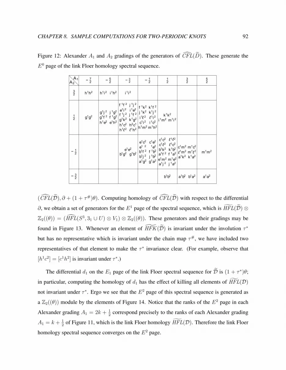
CHAPTER 8. SAMPLE COMPUTATIONS FOR TWO-PERIODIC KNOTS 92
Figure 12: Alexander A1 and A2 gradings of the generators of CFL(D). These generate the
E0 page of the link Floer homology spectral sequence.
A2A1 − 7
2
h1h2
g1g2
− 52
h1i 2 i 1h2
g1j 2 j 1g2
g1f 2 f 1g2
h1e2 e1h2
12
32
f 1f 2 j 1j 2
e1i 2 i 1e2
f 1j 2 j 1f 2
g1k2 k1g2
h1c2 h2c1
h1 2 1h2
− 32
i 1i 2
e1c2 c1e2
e1 2 1e2
b1f 2 f 1b2
b1j 2 j 1b2
a1g2 g1a2
− 12
− 12
e1e2
b1g2 g1b2
f 1k2 k1f 2
j 1k2 k1j 2
i 1 2 1i 2
c1i 2 i 1c2
h1m2 m1h2
12
32
52
m1m2
k1k2
i 1m2 m1i 2
c1m2 m1c2
1m2 m1 2
a1k2 k1a2
− 32 a1a2a1b2 b1a2b1b2
b1k2 k1b2
a1f 2 f 1a2
c1c2 1 2
c1 2 1c2
e1m2 m1e2
a1j 2 j 1a2
l l
l l
l l
l
ll
l
(CFL(D), ∂ + (1 + τ#)θ). Computing homology of CFL(D) with respect to the differential
∂, we obtain a set of generators for the E1 page of the spectral sequence, which is HFL(D)⊗
Z2((θ)) = (HFL(S3, 31 ∪ U) ⊗ V1) ⊗ Z2((θ)). These generators and their gradings may be
found in Figure 13. Whenever an element of HFK (D) is invariant under the involution τ ∗
but has no representative which is invariant under the chain map τ#, we have included two
representatives of that element to make the τ ∗ invariance clear. (For example, observe that
[h1c2] = [c1h2] is invariant under τ ∗.)
The differential d1 on the E1 page of the link Floer spectral sequence for D is (1 + τ ∗)θ;
in particular, computing the homology of d1 has the effect of killing all elements of HFL(D)
not invariant under τ ∗. Ergo we see that the E2 page of this spectral sequence is generated as
a Z2((θ)) module by the elements of Figure 14. Notice that the ranks of the E2 page in each
Alexander grading A1 = 2k + 12
correspond precisely to the ranks of each Alexander grading
A1 = k + 12
of Figure 11, which is the link Floer homology HFL(D). Therefore the link Floer
homology spectral sequence converges on the E2 page.

CHAPTER 8. SAMPLE COMPUTATIONS FOR TWO-PERIODIC KNOTS 93
Figure 13: The homology HFL(D). These elements generate the E1 page of the link Floer
spectral sequence as a Z2((θ)) module.
A2
A1 − 72
[h1h2]
[g1g2]
− 52
[h1i 2] [i 1h2]
[g1j 2 + f 1g2]
[j 1g2 + g1f 2]12
32
[f 1f 2 + k1g2+
g1k2 + j 1j 2]
[h1c2] = [c1h2]
− 32
[i 1i 2]
[a1g2] [g1a2]
− 12
− 12
[b1g2 + g1b2]
[c1i 2][i 1c2]
12
32
52
[m1m2]
[i 1m2] = [m1i 2]
[c1m2 + m1 2]
[m1c2 + 1m2]
− 32
[a1a2][a1b2] [b1a2][b1b2]
[a1f 2] = [f 1a2]
[c1c2 + e1m2+
m1e2 + 1 2]
llll
We now turn our attention to the knot Floer homology spectral sequence for D, which arises
from the double complex (CFK (D)⊗Z2((θ)), ∂U + (1+ τ#)θ)). The Alexander A1 gradings
of the seventy-two generators in CFK (D) are laid out in Figure 15. Notice that these gradings
are exactly the A1 gradings of CFL(D) shifted downward by ℓk(31,U)2
= 32. These elements
generate the E0 page of the link Floer spectral sequence as a Z2((θ)) module.
As before, the chain complexes in each Alexander grading may be found in Figures Fig-
ures 19, 20, 21, 22, 23, 24 and 25. Computing the homology of these complexes, we obtain
HFK (D) = HFK (31)⊗V1⊗W , whose generators are described in Figure 16. These elements
generate the E1 page of the knot Floer homology spectral sequence of D as a Z2((q))-module.
Once again, homology classes which are equivalent under the induced involution τ ∗ but have
no representative which is invariant under the chain map τ# have been included with two
equivalent descriptions to emphasize their invariance.
The differential d1 = (1 + τ ∗)θ on the E1 page of the spectral sequence has the effect of

CHAPTER 8. SAMPLE COMPUTATIONS FOR TWO-PERIODIC KNOTS 94
Figure 14: Generators for the E2 = E∞ page of the link Floer spectral sequence for D as a
Z2((θ))-module.
A2A1 − 7
2
[h1h2]
[g1g2]
− 52
12
32
[f 1f 2 + k1g2+
g1k2 + j 1j 2]
[h1c2] = [c1h2]
− 32
[i 1i 2]
− 12
− 12
[b1g2 + g1b2]
12
32
52
[m1m2]
[i 1m2] = [m1i 2]
− 32
[b1b2]
[a1f 2] = [f 1a2]
[c1c2 + e1m2+
m1e2 + 1 2]
[a1a2]
1
ll

CHAPTER 8. SAMPLE COMPUTATIONS FOR TWO-PERIODIC KNOTS 95
Figure 15: Alexander A1 gradings of elements of CFK (D). These elements generate the E0
page of the link Floer spectral sequence as a Z2((θ)) module.
A1 − 5
h1h2
g1g2
− 4
h1i 2 i 1h2
g1j 2 j 1g2
g1f 2 f 1g2
h1e2 e1h2
f 1f 2 j 1j 2
e1i 2 i 1e2
f 1j 2 j 1f 2
g1k2 k1g2
h1c2 h2c1
h1 2 1h2
− 3
i 1i 2
e1c2 c1e2
e1 2 1e2
b1f 2 f 1b2
b1j 2 j 1b2
a1g2 g1a2
− 2
e1e2
b1g2 g1b2
f 1k2 k1f 2
j 1k2 k1j 2
i 1 2 1i 2
c1i 2 i 1c2
h1m2 m1h2
− 1 0 1
m1m2
k1k2
i 1m2 m1i 2
c1m2 m1c2
1m2 m1 2
a1k2 k1a2
a1a2a1b2 b1a2b1b2
b1k2 k1b2
a1f 2 f 1a2
c1c2 1 2
c1 2 1c2
e1m2 m1e2
a1j 2 j 1a2
ll
l
l l
l
l
l
l
Figure 16: The homology HFK (D), which is HFK (31) ⊗ V1 ⊗W . These elements generate
the E1 page of the knot Floer homology spectral sequence of D as a Z2((q))-module.
A1 − 5 − 4 − 3
[a1g2] = [g1a2]
− 2
[h1m2 + m1h2]
− 1 0 1
[m1m2]
[i 1m2 + m1e2]
[m1i 2 + e1m2]
[ 1m2 + m1c2]
[m1 2 + c1m2]
[a1a2][a1b2] [b1a2]
[a1f 2] [f 1a2]l
l

CHAPTER 8. SAMPLE COMPUTATIONS FOR TWO-PERIODIC KNOTS 96
Figure 17: Generators for the E2 page of the knot Floer spectral sequence associated to D as a
Z2((q)) module.
A1 − 5 − 4 − 3
[a1g2] = [g1a2]
− 2
[h1m2 + m1h2]
− 1 0 1
[m1m2]
[a1a2]
eliminating all elements of HFK (D) which are not invariant under the action of τ ∗. Computing
homology with respect to d1 yields the set of generators of Figure 17.
The knot Floer spectral sequence stabilizes on the E2 page in every Alexander grading
except A1 = −2. There is a single nontrivial d2 differential which behaves similarly to the
nontrivial d2 differential we earlier saw in the case of the unknot as a doubly-periodic knot.
In particular: consider d2([a1g2]). We compute this differential as follows: first, apply 1 + τ#
to a1g2, obtaining (a1g2 + g1a2)θ. Next, we choose an element whose boundary under ∂U
is (a1g2 + g1a2)θ; one such is (h1m2)θ. Then d2([a1g2]) = [1 + τ#(h1m2)]θ = [h1m2 +
m1h2]θ2. Moreover, we then have d2([a1g2]θn) = [h1m2 + m1h2]θn+2 in general. Therefore
the Alexander grading −2 vanishes on the E3 page of the knot Floer spectral sequence, and the
E3 = E∞ page is isomorphic to HFK (D) after an appropriate shift and rescaling in Alexander
A1 gradings. Generators for this page of the knot Floer spectral sequence appear in Figure 18.
Notice that for the left-handed trefoil considered as a two-periodic knot, Edmonds’ condi-
tion is sharp: g(31) = 1 = 2(0) + 3−12
= 2g(U) + λ−12
. We also see here the realization of

CHAPTER 8. SAMPLE COMPUTATIONS FOR TWO-PERIODIC KNOTS 97
Figure 18: Generators for the E3 = E∞ page of the knot Floer spectral sequence associated to
D.
A1 − 5 − 4 − 3 − 2 − 1 0 1
[m1m2]
[a1a2]
Figure 19: The chain complex CFL(D) in Alexander gradingA1 = −72, and the chain complex
CFK (D) in Alexander grading A1 = −5. Dashed arrows denote differentials appearing only
in the latter.
h1h2
g1g2
Corollary 1.2.5: the left-handed trefoil is fibred, and the highest nontrivial Alexander grading
in HFK (D), namely A1 = 1 has rank two. The two generators in this Alexander grading,
[a1a2] and [m1m2], are preserved over the course of the spectral sequence and become the two
generators of HFK (D) in grading A1 = 0 under the isomorphism between the E∞ page of the
knot Floer spectral sequence and HFK (D). Then the highest nontrivial Alexander grading of
HFK (D), A1 = 0, also has rank two, corresponding to the unknot being a fibred knot.

CHAPTER 8. SAMPLE COMPUTATIONS FOR TWO-PERIODIC KNOTS 98
Figure 20: The chain complex CFL(D) in Alexander gradingA1 = −52, and the chain complex
CFK (D) in Alexander grading A1 = −4. Dashed arrows denote differentials appearing only
in the latter.
h1i 2
g1j 2 f 1g2
e1h2
i 1h2
g1f 2 j 1g2
h1e2
Figure 21: The chain complex CFL(D) in Alexander gradingA1 = −32, and the chain complex
CFK (D) in Alexander grading A1 = −3. Dashed arrows denote differentials appearing only
in the latter.
i 1i 2
k1g2 g1k2f 1f 2 j 1j 2
e1e2c1h2h1c2 1h2 h1 2
g1b2 b1g2
e1i 2 i 1e2
f 1j 2 j 1f 2

CHAPTER 8. SAMPLE COMPUTATIONS FOR TWO-PERIODIC KNOTS 99
Figure 22: The chain complex CFL(D) in Alexander gradingA1 = −12, and the chain complex
CFK (D) in Alexander grading A1 = −2. Dashed arrows denote differentials appearing only
in the latter.k1j2
f1k2
k1f2
j1k2
h1m2
m1h2
1e2
e12
1i2
c1i2
e1c2
i12
i1c2
c1e2
b1j2
j1b2
a1g2
f1b2
g1a2
b1f2
ll
ll

CHAPTER 8. SAMPLE COMPUTATIONS FOR TWO-PERIODIC KNOTS 100
Figure 23: The chain complex CFL(D) in Alexander grading A1 = 12, and the chain complex
CFK (D) in Alexander grading A1 = −1. Dashed arrows denote differentials appearing only
in the latter.
k1k2
i 1m2 m1i 2e1m2c1c2 m1e2 1 2
b1b2a1f 2f 1a2 a1j 2 j 1a2
c1 2 1c2
b1k2 k1b2
l l
l l
Figure 24: The chain complex CFL(D) in Alexander grading A1 = 32, and the chain complex
CFK (D) in Alexander grading A1 = 0. Dashed arrows denote differentials appearing only in
the latter.
1m2 m1c2 c1m2 m1 2
a1b2 k1a2 a1k2 b1a2
l l
Figure 25: The chain complex CFL(D) in Alexander grading A1 = 52, and the chain complex
CFK (D) in Alexander grading A1 = 1. Dashed arrows denote differentials appearing only in
the latter.

BIBLIOGRAPHY 101
Bibliography
[1] M. F. Atiyah and R. Bott, The moment map and equivariant cohomology, Topology 23(1984), no. 1, 1–28. MR 721448 (85e:58041)
[2] M. F. Atiyah and F. Hirzebruch, Vector bundles and homogeneous spaces, Proc. Sympos.Pure Math., Vol. III, American Mathematical Society, Providence, R.I., 1961, pp. 7–38.MR 0139181 (25 #2617)
[3] Michael Atiyah and Graeme Segal, On equivariant Euler characteristics, J. Geom. Phys.6 (1989), no. 4, 671–677. MR 1076708 (92c:19005)
[4] Armand Borel, Nouvelle demonstration d’un theoreme de P. A. Smith, Comment. Math.Helv. 29 (1955), 27–39. MR 0066649 (16,611b)
[5] , Seminar on transformation groups, With contributions by G. Bredon, E. E.Floyd, D. Montgomery, R. Palais. Annals of Mathematics Studies, No. 46, PrincetonUniversity Press, Princeton, N.J., 1960. MR 0116341 (22 #7129)
[6] Kai Cieleback and Yakov Eliashberg, From Stein to Weinstein and back, 1991,http://math.stanford.edu/ eliash/Public/stein-final.pdf.
[7] Allan L. Edmonds, Least area Seifert surfaces and periodic knots, Topology Appl. 18(1984), no. 2-3, 109–113. MR 769284 (86c:57005)
[8] Allan L. Edmonds and Charles Livingston, Group actions on fibered three-manifolds,Comment. Math. Helv. 58 (1983), no. 4, 529–542. MR 728451 (85k:57037)
[9] Andreas Floer, Morse theory for Lagrangian intersections, J. Differential Geom. 28(1988), no. 3, 513–547. MR 965228 (90f:58058)
[10] , A relative Morse index for the symplectic action, Comm. Pure Appl. Math. 41(1988), no. 4, 393–407. MR 933228 (89f:58055)
[11] , The unregularized gradient flow of the symplectic action, Comm. Pure Appl.Math. 41 (1988), no. 6, 775–813. MR 948771 (89g:58065)

BIBLIOGRAPHY 102
[12] David Gabai, Foliations and the topology of 3-manifolds, J. Differential Geom. 18 (1983),no. 3, 445–503. MR 723813 (86a:57009)
[13] Paolo Ghiggini, Knot Floer homology detects genus-one fibred knots, Amer. J. Math. 130(2008), no. 5, 1151–1169. MR 2450204 (2010f:57013)
[14] J. Elisenda Grigsby, Knot Floer homology in cyclic branched covers, Algebr. Geom.Topol. 6 (2006), 1355–1398. MR 2253451 (2008a:57033)
[15] Philip Hall, On representatives of subsets, J. London Math. Soc. s1-10 (1935), no. 1,26–30.
[16] Allen Hatcher, Vector bundles & k-theory, 2009.
[17] Kristen Hendricks, Localization and the link Floer homology of doubly-periodic knots,(2012), http://arxiv.org/pdf/1206.5989.pdf.
[18] , A rank inequality for the knot Floer homology of double branched covers, Alge-braic I& Geometric Topology 12 (2012), 2127–2178.
[19] Adam Simon Levine, Computing knot Floer homology in cyclic branched covers, Algebr.Geom. Topol. 8 (2008), no. 2, 1163–1190. MR 2443111 (2009i:57029)
[20] , Applications of Heegaard Floer homology to knot and link concordance, Pro-Quest LLC, Ann Arbor, MI, 2010, Thesis (Ph.D.)–Columbia University. MR 2794779
[21] Robert Lipshitz, A cylindrical reformulation of Heegaard Floer homology, Geom. Topol.10 (2006), 955–1097. MR 2240908 (2007h:57040)
[22] Dusa McDuff and Dietmar Salamon, Introduction to symplectic topology, Oxford Math-ematical Monographs, The Clarendon Press Oxford University Press, New York, 1995,Oxford Science Publications. MR 1373431 (97b:58062)
[23] , J-holomorphic curves and symplectic topology, American Mathematical Soci-ety Colloquium Publications, vol. 52, American Mathematical Society, Providence, RI,2004. MR 2045629 (2004m:53154)
[24] Kunio Murasugi, On periodic knots, Comment. Math. Helv. 46 (1971), 162–174. MR0292060 (45 #1148)
[25] Yi Ni, Knot Floer homology detects fibred knots, Invent. Math. 170 (2007), no. 3, 577–608. MR 2357503 (2008j:57053)

BIBLIOGRAPHY 103
[26] Yong-Geun Oh, Floer cohomology of Lagrangian intersections and pseudo-holomorphicdisks. I, Comm. Pure Appl. Math. 46 (1993), no. 7, 949–993. MR 1223659 (95d:58029a)
[27] Boon W. Ong, The homotopy type of the symmetric products of bouquets of circles, Inter-nat. J. Math. 14 (2003), no. 5, 489–497. MR 1993792 (2004g:55010)
[28] Peter Ozsvath and Zoltan Szabo, Holomorphic disks and genus bounds, Geom. Topol. 8(2004), 311–334. MR 2023281 (2004m:57024)
[29] , Holomorphic disks and knot invariants, Adv. Math. 186 (2004), no. 1, 58–116.MR 2065507 (2005e:57044)
[30] , Heegaard Floer homology and contact structures, Duke Math. J. 129 (2005),no. 1, 39–61. MR 2153455 (2006b:57043)
[31] , Lectures on Heegaard Floer homology, Floer homology, gauge theory, and low-dimensional topology, Clay Math. Proc., vol. 5, Amer. Math. Soc., Providence, RI, 2006,pp. 29–70. MR 2249248 (2007g:57053)
[32] , Holomorphic disks, link invariants and the multi-variable Alexander polynomial,Algebr. Geom. Topol. 8 (2008), no. 2, 615–692. MR 2443092 (2010h:57023)
[33] , Link Floer homology and the Thurston norm, J. Amer. Math. Soc. 21 (2008),no. 3, 671–709. MR 2393424 (2009a:57050)
[34] Timothy Perutz, Hamiltonian handleslides for Heegaard Floer homology, Proceedings ofGokova Geometry-Topology Conference 2007, Gokova Geometry/Topology Conference(GGT), Gokova, 2008, pp. 15–35. MR 2509747 (2010m:57048)
[35] Daniel Quillen, The spectrum of an equivariant cohomology ring. I, II, Ann. of Math. (2)94 (1971), 549–572; ibid. (2) 94 (1971), 573–602. MR 0298694 (45 #7743)
[36] Jacob Andrew Rasmussen, Floer homology and knot complements, ProQuest LLC, AnnArbor, MI, 2003, Thesis (Ph.D.)–Harvard University. MR 2704683
[37] Rolf Richberg, Stetige streng pseudokonvexe Funktionen, Math. Ann. 175 (1968), 257–286. MR 0222334 (36 #5386)
[38] Dale Rolfsen, Knots and links, Mathematics Lecture Series, vol. 7, Publish or Perish Inc.,Houston, TX, 1990, Corrected reprint of the 1976 original. MR 1277811 (95c:57018)
[39] Sucharit Sarkar and Jiajun Wang, An algorithm for computing some Heegaard Floer ho-mologies, Ann. of Math. (2) 171 (2010), no. 2, 1213–1236. MR 2630063

BIBLIOGRAPHY 104
[40] Paul Seidel and Ivan Smith, Localization for involutions in Floer cohomology, Geom.Funct. Anal. 20 (2010), no. 6, 1464–1501. MR 2739000
[41] Jean-Claude Sikorav, Review of Morse theory for Lagrangian intersections, MathematicalReviews, http://www.ams.org/mathscinet/pdf/965228.pdf.
[42] P. A. Smith, Transformations of finite period, Ann. of Math. (2) 39 (1938), no. 1, 127–164.MR 1503393
[43] William P. Thurston, A norm for the homology of 3-manifolds, Mem. Amer. Math. Soc.59 (1986), no. 339, i–vi and 99–130. MR 823443 (88h:57014)
[44] Vladimir Turaev, Torsions of 3-manifolds, Invariants of knots and 3-manifolds (Kyoto,2001), Geom. Topol. Monogr., vol. 4, Geom. Topol. Publ., Coventry, 2002, pp. 295–302.MR 2002617 (2004g:57035)

APPENDIX 1: HOLOMORPHIC EMBEDDINGS 105
Appendix 1: Holomorphic Embeddings
Since the proof that the map
h : Symn−1(S2) → Sym2n−2(Σ(S2))
(x1 · · · xn−1) 7→ (x11x21 · · ·x1n−1x
2n−1)
is holomorphic is a computation on charts in the symmetric product, we place it here so as notto disrupt the flow of the preceding chapters.
We claim h is continuous; indeed, holomorphic. Let x = (x1 · · ·xn−1) be a point inSymn−1(S2). Collect repeated points, so that x has the form (y1, · · · , y1, · · · , yℓ, · · · , yℓ) withn − 1 total entries but ℓ unique entries. Moreover, if A ⊂ {w, z} is the set of branch pointsof the double branched cover, list points which are not in A first, so that y1, · · · , ys /∈ A andys+1, · · · , yℓ ∈ A for some s.
First consider yi such that 1 ≤ i ≤ s, so that yi is not a branch point of the double cover.Then let yji be a lift of yi for j = 1, 2. There is a neighborhood Ui of yi which admits home-omorphic lifts to neighborhoods U j
i of yji such that (π|Uji)−1 : Ui → U j
i is holomorphic.Moreover, we may pick Ui sufficiently small such that there is a chart fi : Ui → D, where D isthe unit disk in the complex plane, and corresponding charts f ji = fi ◦ π : U j
i → D. In totalthis gives local biholomorphisms between Ui and U j
i expressed on charts as follows.
U ji� �
(π|Uji
)−1
//
fi��
U ji
fji��
D Id // D
Similarly, there is a neighborhood τ(Ui) of the second lift τ(yi) of yi which is homeomor-phic to Ui via (π|τ(Ui
)−1 and has a chart τ(fi) : τ(Ui) → D.
Now suppose s+1 ≤ i ≤ ℓ, so that yi is a branch point for the double branched cover map.Then there is a chart fi : Ui → D around yi and a chart gi : π−1(Ui) → D with respect to which

APPENDIX 1: HOLOMORPHIC EMBEDDINGS 106
fi ◦ π ◦ (gi)−1 is x 7→ x2.
π−1(Ui)
gi��
π|π−1(Ui) // Ui
fi��
D x 7→x2 // DIn particular, if y ∈ Ui and fi(y) = x ∈ D, then if y1 and y2 are the two lifts of y in π−1(Ui),
then gi(y1) and gi(y2) are√x and −
√x in some order.
We will insist that all of our choices of neighborhoods Ui about each yi on which we choosecharts be made such that if i1 = i2, then Ui1 ∩ Ui2 = ∅, by shrinking if necessary. This in turnimplies that U1
1 , U21 ), · · · , U1
s , U2s ), π
−1(Us+1), · · · , π−1(Uℓ) are all pairwise disjoint.
We are now ready to discuss the map h. Recall that we began with a point x = (x1 · · ·xn−1)
= (y1 · · · y1y2 · · · y2 · · · yℓ · · · yℓ) in Symn−1(S2). Let ki be the number of times yi appears in x.Then x is contained in the open neighborhood Symk1(U1)×· · ·×Symkℓ(Uℓ). Here the productnotation arises due to our unwavering insistence that the Ui be pairwise disjoint. Moreover, wesee h(x) = (x11x
21 · · ·x1n−1x
2n−1) is contained in the analogous open neighborhood
s∏i=1
(Symki(U1i )× Symki(U2
i ))×ℓ∏
i=s+1
Sym2ki(π−1(Ui)).
We see that locally the map h is a product of maps of two forms. If 1 ≤ i ≤ s, we havemaps hi of the form
hi : Symki(Ui) → Symki(U1
i )× Symki(U2i )
(z1 · · · zki) 7→ ((z11 · · · z1n−1), (z21 · · · z2ki))
where z1i is the lift of zi in U1i and similarly for U2
i , If however s+1 ≤ i ≤ ℓ, we have maps hiof the form
hi : Symki(Ui) → Sym2ki(π−1(Ui))
(z1 · · · zki) 7→ (z11z21 · · · z1kiz
2ki)
Our goal is to show hi is holomorphic in each of these cases. We begin with the first case,in which xi is not a branch point of the double branch covering. In this case hi carries a point(z1 · · · zki) in Symki(Ui) to the product of its lifts (z11 · · · z1ki) in Symki(U1
i ) and (z21 · · · z2ki) inSymki(U2
i ). Ergo hi = Symki((π|U1i)−1)×Symki((π|U2
i)−1). We already know how to express
this map in terms of the biholomorphisms Symki(fi) : Symki(Ui) → Symki(Dki) and thecorresponding maps Symki(f1
i ) on Symki(U1i ) and Symki(f 2
i )) on U2i .

APPENDIX 1: HOLOMORPHIC EMBEDDINGS 107
Symki(Ui)hi=Sym((π|
U1i)−1)×Symki ((π|
U2i)−1)
//
Symki (fi)��
Symki(U1i )× Symki(U2
i ))
Symki (f1i )×Symki (f2i )��
Symki(D) Id×Id // Symki(D)× Symki(D)
We see ji is holomorphic. For the second case we will need to be slightly more subtle,producing actual charts for Symki(Ui) and Sym2ki(π−1(Ui)). We can assign Symki(Uj) ∼=Symki(D) a holomorphic chart using the familiar biholomorphism (5.2.1) which maps a point(r1 · · · rki) in Symki(D) to the ki elementary symmetric functions of its coordinates in D. Let’ssee what this produces in our particular case. Let ϕki(D) ⊂ Cki be the image of Symki(D)under the map (5.2.1) from Symki(C) → Cki , and similarly for ϕ2ki(D).
Symki(Ui)hi //
Symki (fi)��
Sym2ki(π−1(Ui))
Sym2ki (gi)��
Symki(D)ϕki��
// Sym2ki(D)ϕ2ki��
ϕki(D) // ϕ2ki(D)
Let (z1 · · · zki) be an arbitary point of Ui, so that hi(z1 · · · zki) = (z11z21 · · · z1kiz
2ki). Then the
middle horizontal map takes (r1 · · · rki) = (fi(z1) · · · fi(zki)) to (gi(z11)gi(z
21) · · · gi(z1ki)gi(z
2ki)),
which is exactly (√r1−
√r1 · · ·
√rki−
√rki). Taking symmetric functions of both sides reveals
that the bottom horizontal map is expressed in coordinates as below.
ϕki(D) → ϕ2ki(D)(σ1(r1, · · · , rki), · · · , σki(r1, · · · , rki)) 7→ (σ1(
√r1,−
√r1, · · · ,
√rki ,−
√rki), · · · ,
σ2ki(√r1,−
√r1, · · · ,
√rki ,−
√rki))
Let’s consider the symmetric functions σj of a set of complex roots and their opposites, towit (a1, · · · , a2ki) = (
√r1,−
√r1, · · · ,
√rki ,−
√rki). Recall from Chapter 6 that the functions
σj are defined to be the sums
σj(a1, a2, · · · , a2ki) =∑
1≤i1<···<ij≤2ki
ai1 · · · aij .
If the set of indices (i1, · · · , ij) ⊂ (i1, · · · , i2k) contains only one of i2t−1 and i2t for anyr, then there is a set of indices (i′1, · · · , i′j) identical to (i1, · · · , ij) except that either i2t isreplaced with i2t−1 or vice versa. Moreover ai1 · · · aij = −a′i′1 · · · ai′j , so these two terms cancel

APPENDIX 1: HOLOMORPHIC EMBEDDINGS 108
each other out in the sum which comprises σj . Therefore σj(a1, · · · , a2ki) is a sum of termsai1 · · · aij for sets 1 ≤ i1 < · · · < ij < 1 which contain either both i2t−1 and i2t or neither, forevery 1 ≤ t ≤ j
2. In particular, σj(
√r1,−
√r1, · · · ,
√rki ,−
√rki) = 0 for j odd. When j is
even we may make the following computation.
σj(a1,−a1, · · · , ak,−ak) =∑
1≤i1<···<ij≤ki
a2i1−1a2i1 · · · a2ij−1a2ij
=∑
1≤i1<···<ij≤ki
(√ri1)(−
√ri1) · · · (
√rij)(−
√rij)
=∑
1≤i1<···<ij≤ki
(−1)jri1 · · · rij
= (−1)jσj(r1, · · · , rki)
So the bottom horizontal map in the diagram above is of the form
ϕki(D) → ϕ2ki(D)(σ1(r1, · · · , rki), · · · , σki(r1, · · · , rki)) 7→
(0,−σ1(r1, · · · , rki), 0, · · · , (−1)kiσki(r1, · · · , rki))
This is holomorphic, implying that hi is as well. Since all the maps hi are holomorphisms,and h is locally the product h1 × · · · × hℓ, h is holomorphic.