Citation: Cortes-Aguilar, T.A.;

Cantoral-Ceballos, J.A.;

Tovar-Arriaga, A. Link Quality

Estimation for Wireless ANDON

Towers Based on Deep Learning

Models. Sensors 2022, 22, 6383.

https://doi.org/10.3390/s22176383

Academic Editors: Kelvin K.L. Wong,

Dhanjoo N. Ghista, Andrew W.H. Ip

and Wenjun (Chris) Zhang

Received: 13 July 2022

Accepted: 17 August 2022

Published: 24 August 2022

Publisher’s Note: MDPI stays neutral

with regard to jurisdictional claims in

published maps and institutional affil-

iations.

Copyright: © 2022 by the authors.

Licensee MDPI, Basel, Switzerland.

This article is an open access article

distributed under the terms and

conditions of the Creative Commons

Attribution (CC BY) license (https://

creativecommons.org/licenses/by/

4.0/).

sensors

Article

Link Quality Estimation for Wireless ANDON Towers Based onDeep Learning ModelsTeth Azrael Cortes-Aguilar 1,*, Jose Antonio Cantoral-Ceballos 2,* and Adriana Tovar-Arriaga 3

1 Centro de Tecnologia Avanzada, CIATEQ A.C., Jalisco 45131, Mexico2 Tecnologico de Monterrey, School of Engineering and Sciences, Monterrey 64849, Mexico3 Instituto Tecnologico Jose Mario Molina Pasquel y Henriquez, Jalisco 45019, Mexico* Correspondence: teth.cortes@zapopan.tecmm.edu.mx (T.A.C.-A.); joseantonio.cantoral@tec.mx (J.A.C.-C.)

Abstract: Data reliability is of paramount importance for decision-making processes in the industry,and for this, having quality links for wireless sensor networks plays a vital role. Process and machinemonitoring can be carried out through ANDON towers with wireless transmission and machinelearning algorithms that predict link quality (LQE) to save time, hence reducing expenses by earlyfailure detection and problem prevention. Indeed, alarm signals used in conjunction with LQEclassification models represent a novel paradigm for ANDON towers, allowing low-cost remotesensing within industrial environments. In this research, we propose a deep learning model, suitablefor implementation in small workshops with limited computational resources. As part of our work,we collected a novel dataset from a realistic experimental scenario with actual industrial machinery,similar to that commonly found in industrial applications. Then, we carried out extensive dataanalyses using a variety of machine learning models, each with a methodical search process to adjusthyper-parameters, achieving results from common features such as payload, distance, power, and biterror rate not previously reported in the state of the art. We achieved an accuracy of 99.3% on the testdataset with very little use of computational resources.

Keywords: wireless sensor network; link quality estimation; deep learning; failure detection

1. Introduction

ANDON tower lamps have evolved from simple alarm systems with visual signals inthe traditional factory towards a wireless sensor network (WSN) at the heart of Industry 4.0capable of remotely identifying machine status whilst getting information about the work-shop productivity [1,2]. The alarm signals for ANDON tower lamps are established by theinternational standard IEC 60073:2002 [3] in which the red code sends a fault or emergencystop message, the amber code sends a warning signal for operation in an abnormal processcondition or machine setup, and the green code indicates a normal operation signal, whilstthe blue and white codes represent user-defined signals. These types of systems are readilyavailable on the market, such as NH-3FV2W from the company Patlite [4], TL70 fromBanner Engineering Corp. [5], and SmartMonitor by Werma Signaltechnik [6].

In the industry, the information generated by WSN such as wireless ANDON towersystems is of paramount relevance because it allows for on-time error correction, applyingcontainment measures and preventing different problems not possible to anticipate in atraditional industry. The reliability of such information is even more relevant in Industry4.0 since it is used for different automation processes aided by the existence of intelligent,autonomous, and collaborative machines that communicate with each other in real-timeto perform actions based on the environment data [7]. In this regard, machine learningmodels such as deep neural networks (DNNs) have made remarkable progress that mayhave a big impact in the industry with highly reliable analytical solutions [8].

Sensors 2022, 22, 6383. https://doi.org/10.3390/s22176383 https://www.mdpi.com/journal/sensors

Sensors 2022, 22, 6383 2 of 16

1.1. Application of Machine Learning in the Industry

Deep learning (DL) is a subset of ML methods that aim to model data with complexarchitectures that combine different non-linear transformations. The fundamental compo-nents of DL models are artificial neural networks (ANNs), which combine to form DNNs.These techniques have enabled significant progress in the fields of image processing [9,10],pattern recognition [11] including facial recognition [12], speech recognition [13], computervision [14], automated language processing [15], text classification [16], and recently, in thelink quality estimation for a WSN. The fundamental characteristic of a DNN is the inte-gration of multiple sequential layers, each made of multiple artificial neurons that requireproper initialization and optimization algorithms for optimal performance. The right choiceof DNN architecture can lead to results with outstanding performance compared to othermethods [17]. In addition, the application of a multilayer ANN was shown to achieve betterperformance in pattern recognition in complex and highly variable environments [18].Within the industrial sector, the multilayer perceptron (MLP) architecture is the one withthe highest number of application cases partly due to its simplicity, which allows its im-plementation in devices with limited computational resources, such as those commonlyfound in the industry in developing countries [19]. The MLP has a basic architecture, whereeach unit or neuron in one layer is linked to all units in the next layer (fully connected) buthas no link with neurons in the same layer. The number of hidden layers, the number ofneurons in each layer, and the activation function define the architecture of the MLP model.

The DL paradigm has been used successfully in classification problems; however,neural networks with many layers are sensitive to weight initialization and prematurelearning stoppage as the gradient values decrease towards small values, the phenomenonwhich is known as the vanishing gradient problem [20]. To ameliorate this problem, wemay use the rectified linear unit (ReLU) activation function which has a maximum gradientvalue of 1, without saturating, allowing the network to continue learning. For this reason, inthe present paper, the ReLU function was used as the activation function of the MLP model.

With the continuous increase in device connectivity and computing capabilities ofdigital systems, some industries have succeeded in incorporating new methods based onartificial intelligence (AI). Hence, data provided by a wide variety of sensors are used todetect and prevent a possible failure or breakdown, especially via machine and processsupervision systems. Indeed, failure detection is critical in the industry because it allowsdetermining if it is necessary to stop a process and carry out maintenance actions [21].Márquez-Vera et al. [22] use a DL model with long short-term memory (LSTM) in a fail-ure detection case. They reported that the neural network was more sensitive to hyper-parameters such as batch size or the learning rate regarding the number of layers, whichincreased until no improvement was found.

1.2. Motivation

In today’s industry, the ANDON tower works as a sensor node in the WSN that sendsan alarm signal without information about data reliability. After a comprehensive literaturesurvey, we found that this alarm signal in conjunction with link quality classification hasnot been used in applications for wireless ANDON towers in the industry. In this paper,we propose a novel application for a deep neural network model based on a multilayer per-ceptron (MLP) to predict the link quality estimation (LQE) and consequently, the reliabilityof the information used for decision making in the workshop. In addition, the LQE canalso be used to improve WSN performance.

The packet reception rate (PRR) was used to define the LQE classes, and 10,000 datapoints were gathered from a realistic experimental scenario using actual industrial machin-ery. Using these data, we carried out comprehensive experimentation comparing differentmachine learning (ML) models, including random forest (RF), support vector machines(SVM), K-nearest neighbors (KNN), gradient boosting (GB), and MLP, which displayedthe best performance from all the models, achieving an accuracy >99% on the test datasetafter a thorough hyper-parameter tuning. In order to choose the most suitable learning rate,

Sensors 2022, 22, 6383 3 of 16

we carried out extensive random searches in the range of 3 × 10−8 ≤ LR ≤ 3 × 10−2 untilfinding that an LR = 2.95 × 10−5 achieved the best performance in the training and valida-tion sets. In spite of the model’s simplicity, MLP achieved high precision in classificationtasks, making it the ideal model for our industrial application due to its low computationalrequirements both for training and inference.

The remainder of this paper is organized as follows. Section 2 presents a review ofprevious work related to our research. Then, Section 3 refers to materials and methodsand describes the hardware, MLP model, and dataset, and Section 4 shows the resultsand comparison to other machine learning models. Finally, Sections 5 and 6 present thediscussion and conclusions, respectively.

2. Related Work

Machine monitoring plays an important role in the industry due to its effects onproduction quality and production cost. It can be divided into two types, machine conditionmonitoring and machine process monitoring. The first one refers to the monitoring ofmachine components, such as gears and bearings, and the second one refers to monitoringworkpieces and tools. The first step in machine monitoring is signal acquisition, forexample: vibration, temperature, cutting force, product labelling, and others. In thiscontext, WSNs are the key to achieving advanced automated systems by turning traditionalmachines into modern machines. The synergy between WSN and machine learning allowsintelligent decision making and LQE estimation with efficient computational time and highaccuracy [23].

The propagation environment of radio frequency signals can change in space and timeand affect the quality of the link in WSN. Consequently, to achieve reliable and error-freetransmission, the transceiver’s parameters must be adjusted depending on the best LQEestimate. Over the last few years, machine learning algorithms have been used to estimateLQE due to their ability to process and learn from large amounts of data, which can begathered from various scenarios and technologies [24].

The link quality metrics for LQE algorithms fall mainly into three categories: software,hardware, and scores [25]. The software LQE metrics such as packet reception rate (PRR),required number of packet retransmissions (RNP), and expected transmission count (EXT)are calculated using the transmission variables. The PRR measurement is the ratio of thenumber of packets successfully received to the number of packets transmitted within a timewindow, but PRR-based algorithms are not sensitive to rapid fluctuations in link quality [26].The RNP measurement is the average number of packet transmissions and retransmissionsrequired before a successful reception; nonetheless, it is unstable and it cannot estimatepacket delivery for asymmetric links successfully [27]. The EXT measurement refers to thenumber of transmissions required to send a complete packet; however, its implementationoften fails in congested networks [28].

The hardware LQE metrics such as received signal strength indicator (RSSI), link qual-ity indicator (LQI), and signal to noise ratio (SNR) are acquired from the transceivers. TheRSSI is the measurement of the intensity of the signal present in the receiver that evaluatesthe quality of the link via supervised learning algorithms, and it classifies the quality ofa link as high or low for a given routing protocol. However, the RSSI indicates only thepower of the received signal at the receiver, and it does not provide an accurate measurethat considers the affectation due to noise. The LQI measurement is a characterizationof the strength or quality of a received packet according to the IEEE 802.15.4 standard;however, the algorithms based on LQI have three disadvantages:

1. The variance of the LQI increases significantly as the quality of the link degrades;2. There is no consensus among transceiver manufacturers on how to calculate LQI;3. It is only useful for transceivers that work with the IEEE 802.15.4 standard [29].

The SNR metric is the difference, in decibels, between the received signal strength andthe floor noise. Despite algorithms based on SNR measurement being easy to implement,

Sensors 2022, 22, 6383 4 of 16

these are not suitable for random SNR behaviors, and these are unable to provide anaccurate description of link quality [30].

The score algorithms to calculate the LQE metric use various input parameters; forexample, Luo et al. [31] used SNR, LQI, and RSSI of up and down links in a neural networkarchitecture of seven stacked layers to extract information from the asymmetric charac-teristics of the input data. Then, the classification was made by an SVM algorithm. Thisalgorithm is focused for bidirectional communications and it is not suitable for unidirec-tional communications, such as the application presented here.

The use of physics and software metrics such as SNR, RSSI or PRR allows calculatingthe instantaneous LQE parameter without considering its historical trend. In a recentresearch, He and Shu [32] proposed an LQE deep forest algorithm that estimates the PRRfrom the input of the mean of LQI, RSSI, and SNR metrics and stability parameters CVLQI,CVRSSI, and CVSNR that the authors calculated as the standard deviation divided by themean. Abdel-Nasser et al. [33] predicted the LQE using long short-term memory (LSTM)and gated recurrent units (GRUs). However, the implementation of these algorithms hasthe disadvantage of needing large amounts of historical data for networks that are alreadyin operation.

Contribution

The most widely used methods to predict the link quality of WSN use input metricsacquired from the transceiver such as RSSI, LQI, and SNR or metrics calculated by softwaresuch as PRR, RNP, and EXT. Other algorithms seek to improve prediction accuracy usingmany metrics, historical data, and statistical trends. However, despite the reported success-ful results, some of these metrics cannot be easily acquired from the transceiver or are notreadily available. In addition, the quality of a link can also be affected by other factors suchas the distance from the transmitter to the receiver, the transmission rate, the data payload,the transmitter’s power, and the presence of noise and interference, as well as the randompresence of obstacles and objects that can attenuate, reflect, or scatter the radio frequencysignal, consequently increasing the bit error rate (BER).

For complex industrial environments, the application of a DNN classification algo-rithm is a better choice to predict LQE than other traditional methods based on statisticalmodels and fuzzy logic [34,35]. Moreover, the MLP model proposed in this paper com-pared to other machine learning models can help adjust the best WSN parameters, suchas distance, transmission rate, power, and data payload in the transceiver. In addition,our work differs significantly from the current state of the art because, at the moment,there is no industrial solution to predict the LQE and the associated information reliabilitywith alarm signals produced by modern wireless ANDON towers. The application ofthis technology will further the digitalization and evolution from a traditional factory to asmart factory within the Industry 4.0 model, particularly in developing countries, wherethe incorporation of new technology is slow and difficult.

3. Materials and Methods

In a WSN with a star network topology, communications occur between two types ofdevices, a coordinator node that manages those with the lower nodes, and the lower nodesthat transmit the signal from the sensors to the coordinator node, as shown in Figure 1.

To describe our industrial WSN setup, this section is divided into seven parts; thefirst one describes the transceiver used in the ANDON tower that works as a sensornode; the second one describes the characteristics of the computer equipment used forthe programming of the MLP model; the third one describes the experimental scenariowhere data were collected; the fourth one addresses the neuronal network’s features, i.e.,the model’s input variables; the fifth one is the LQE classification based on PRR, i.e., themodel’s output variables; the sixth describes the dataset structure; and the seventh oneexplains the MLP model structure.

Sensors 2022, 22, 6383 5 of 16

Sensors 2022, 22, x FOR PEER REVIEW 5 of 16

3. Materials and Methods In a WSN with a star network topology, communications occur between two types

of devices, a coordinator node that manages those with the lower nodes, and the lower nodes that transmit the signal from the sensors to the coordinator node, as shown in Figure 1.

To describe our industrial WSN setup, this section is divided into seven parts; the first one describes the transceiver used in the ANDON tower that works as a sensor node; the second one describes the characteristics of the computer equipment used for the programming of the MLP model; the third one describes the experimental scenario where data were collected; the fourth one addresses the neuronal network’s features, i.e., the model´s input variables; the fifth one is the LQE classification based on PRR, i.e., the model´s output variables; the sixth describes the dataset structure; and the seventh one explains the MLP model structure.

Figure 1. Experimental scenario, workshop TecMM, Zapopan, México.

3.1. Transceiver The ANDON tower uses the low-cost NRF24L01 [36] transceiver to send the

experimental data from the sensor node to the coordinator node, with a computer connected to the coordinator node to store the data in a CSV file. The transceiver works in the 2.4 GHz free band and allows setting the transmission power at −18 dBm, −12 dBm, −6 dBm, and 0 dBm. The transmission rate setting options are 250 kbps, 1 Mbps, and 2 Mbps. The transceiver uses the SPI protocol for communication with the ANDON tower microcontroller. Its maximum range is 30 m, which is sufficient for the maximum distance in our experimental scenario of 16 m. The communication tests were realized by sending a payload of 2, 4, 8, 16, and 32 bytes.

3.2. Computer Hardware and Software The MLP classification model was developed using the PyTorch library [37] and ran

on a GPU, whilst the other ML models were developed using the SkLearn library [38]. All the models were trained on a standard laptop equipped with INTEL core i7 CPU, 8GB of RAM, and an NVIDIA GEFORCE 940MX graphics card. PyTorch is a library developed by Meta (formerly Facebook) that facilitates the construction of deep learning projects through models coded in Python. For the scientific community, PyTorch has become an outstanding deep learning tool due to its accessibility, ease of use, and wide range of applications [37].

3.3. Experimental Scenario The main challenge to implement a wireless ANDON tower for industrial

monitoring and control systems is satisfying reliability and performance requirements,

Figure 1. Experimental scenario, workshop TecMM, Zapopan, México.

3.1. Transceiver

The ANDON tower uses the low-cost NRF24L01 [36] transceiver to send the experi-mental data from the sensor node to the coordinator node, with a computer connected tothe coordinator node to store the data in a CSV file. The transceiver works in the 2.4 GHzfree band and allows setting the transmission power at −18 dBm, −12 dBm, −6 dBm,and 0 dBm. The transmission rate setting options are 250 kbps, 1 Mbps, and 2 Mbps.The transceiver uses the SPI protocol for communication with the ANDON tower micro-controller. Its maximum range is 30 m, which is sufficient for the maximum distance inour experimental scenario of 16 m. The communication tests were realized by sending apayload of 2, 4, 8, 16, and 32 bytes.

3.2. Computer Hardware and Software

The MLP classification model was developed using the PyTorch library [37] and ranon a GPU, whilst the other ML models were developed using the SkLearn library [38]. Allthe models were trained on a standard laptop equipped with INTEL core i7 CPU, 8GB ofRAM, and an NVIDIA GEFORCE 940MX graphics card. PyTorch is a library developed byMeta (formerly Facebook) that facilitates the construction of deep learning projects throughmodels coded in Python. For the scientific community, PyTorch has become an outstandingdeep learning tool due to its accessibility, ease of use, and wide range of applications [37].

3.3. Experimental Scenario

The main challenge to implement a wireless ANDON tower for industrial monitoringand control systems is satisfying reliability and performance requirements, where someaccepted indicators for the reliability of the physical layer in each node are the quality of thewireless link, based on PRR and BER [39]. Figure 1 shows the experimental scenario wherethe communication tests of the ANDON towers were carried out and where experimentaldata were acquired. The ANDON tower worked as the sensor node in the WSN, with itstransceiver programmed to send 100 test data packets to the receiver node that worked asthe coordinator node. The receiver node calculated the PRR from the correctly receivedpackets. Data were saved in a computer connected to the coordinator node. The receiver-coordinator node was placed in a fixed position in the workshop, while the location of thesensor-transmitter node was changed according to the distances selected for the experiment.A star topology was used in the network.

3.4. Neuronal Network’s Features

Our classification model to predict the LQE was trained on an original dataset withthe following features: the transmission rate x1, the transmitter power x2, the distance

Sensors 2022, 22, 6383 6 of 16

from the transmitter to the receiver x3, the payload x4, and the bit error rate x5. Table 1shows statistical information of the input data. The data rate, power, and payload werecollected from the transceiver configuration. Distance data were collected by locating thesensor node at different positions in the experimental scenario and the bit error rate (BER)was calculated with (1), where f = 8n is the length of the packet in bits, and n is the datapayload [40].

BER = 1 − PRR( f−1) (1)

Table 1. Statistical information of the input data.

Ratex1

Powerx2

Distancex3

Payloadx4

BERx5

count 10 k 10 k 10 k 10 k 10 kmean 1101.9 kbps 272.9 mW 8.9 m 13.9 bytes 0.0144std 699.2 kbps 376.7 mW 4.4 m 11.4 bytes 0.0328min 250 kbps 15.85 mW 1 m 2 bytes 0.0max 2 Mbps 1000 mW 16 m 32 bytes 0.470

3.5. LQE Classification Based on PRR

The PRR measurement is used as a classification parameter in the LQE predictionmodel [31–35]. In the experimental scenario presented in Figure 1, the transmitting nodeperiodically sent 100 test packets to the receiver node that calculated PRR. The LQE wasrelated to the rate of packets received successfully. Forecast categories were divided accord-ing to (2). We considered that a PRR smaller than 0.89 is not acceptable for our industrialapplication; 2500 random samples were collected for each of the four LQE categories.

y = f(PRR) = f (x) =

1, Best PRR = 12, Good 0.96 < PRR ≤ 0.993, Common 0.89 < PRR ≤ 0.964, Bad PRR ≤ 0.89

(2)

Figures 2–5 show the scatterplots of the experimental measurements for distance,transmission rate, power, and data payload against BER. The LQE classification is denotedby numbers in the scatterplots, where the best subset is denoted by number 1, good bynumber 2, common by number 3, and bad by number 4, as explained in (2). The BERobservation range in the scatterplots was chosen to identify the four forecast categories,and we can see that the BER mean value was low because experimental data were gatheredwith low noise working conditions, i.e., from (1), we can see that BER = 0 when PRR = 1.The scatterplot in Figure 2 shows that BER decreased with distance. In Figure 3, we did notsee a strong relationship between transmission rate and the BER variable; however, forecastcategories 1 and 2 had low BER values. On the other hand, increasing the transceiver’spower improved the quality of transmission with better BER values, i.e., more data packetswithout errors arrive at the receiver, whilst data from categories 1 and 2 tended to havelower BER values, as shown in Figure 4. For the NRF24L01 transceiver, a high payloadincreased the transmission quality, and finally, Figure 5 shows a clear division betweenforecast categories. We selected values of rate, payload, and power based on the NRF24L01transceiver characteristics.

Sensors 2022, 22, 6383 7 of 16

Sensors 2022, 22, x FOR PEER REVIEW 7 of 16

we did not see a strong relationship between transmission rate and the BER variable; however, forecast categories 1 and 2 had low BER values. On the other hand, increasing the transceiver’s power improved the quality of transmission with better BER values, i.e., more data packets without errors arrive at the receiver, whilst data from categories 1 and 2 tended to have lower BER values, as shown in Figure 4. For the NRF24L01 transceiver, a high payload increased the transmission quality, and finally, Figure 5 shows a clear division between forecast categories. We selected values of rate, payload, and power based on the NRF24L01 transceiver characteristics.

Figure 2. Scatterplot of distance against BER.

Figure 3. Scatterplot of transmission rate against BER.

Figure 4. Scatterplot of transmission power against BER.

Figure 2. Scatterplot of distance against BER.

Sensors 2022, 22, x FOR PEER REVIEW 7 of 16

we did not see a strong relationship between transmission rate and the BER variable; however, forecast categories 1 and 2 had low BER values. On the other hand, increasing the transceiver’s power improved the quality of transmission with better BER values, i.e., more data packets without errors arrive at the receiver, whilst data from categories 1 and 2 tended to have lower BER values, as shown in Figure 4. For the NRF24L01 transceiver, a high payload increased the transmission quality, and finally, Figure 5 shows a clear division between forecast categories. We selected values of rate, payload, and power based on the NRF24L01 transceiver characteristics.

Figure 2. Scatterplot of distance against BER.

Figure 3. Scatterplot of transmission rate against BER.

Figure 4. Scatterplot of transmission power against BER.

Figure 3. Scatterplot of transmission rate against BER.

Sensors 2022, 22, x FOR PEER REVIEW 7 of 16

we did not see a strong relationship between transmission rate and the BER variable; however, forecast categories 1 and 2 had low BER values. On the other hand, increasing the transceiver’s power improved the quality of transmission with better BER values, i.e., more data packets without errors arrive at the receiver, whilst data from categories 1 and 2 tended to have lower BER values, as shown in Figure 4. For the NRF24L01 transceiver, a high payload increased the transmission quality, and finally, Figure 5 shows a clear division between forecast categories. We selected values of rate, payload, and power based on the NRF24L01 transceiver characteristics.

Figure 2. Scatterplot of distance against BER.

Figure 3. Scatterplot of transmission rate against BER.

Figure 4. Scatterplot of transmission power against BER. Figure 4. Scatterplot of transmission power against BER.

Sensors 2022, 22, x FOR PEER REVIEW 8 of 16

Figure 5. Scatterplot of payload against BER.

3.6. Dataset From the experimental raw data, we selected 10,000 random data. In order to avoid

the problem of class imbalance [35], 2500 random samples were selected for each of the four LQE categories. Then, 80% of the dataset was used for training, 10% for validation, and 10% for testing. A mini-batch size of 2048 data points was chosen with a random shuffling method.

Figure 6 shows the dataset´s structure. The input variables data rate, power, and payload depend on the transceiver’s setting options, in contrast to the distance and BER that depend on experimental measurements.

Figure 6. Dataset structure from CSV file.

3.7. Estimation Model The multilayer perceptron is one of the most established deep learning models for

non-linear classification and regression. These architectures are frequently used in the industry to model systems and predict phenomena due to their ease of implementation with relatively low computational requirements for training compared to other more complex methods [41]. In addition, an MLP is a suitable option for small workshops in developing countries such as Mexico, where computational resources are limited and commonly older than 10 years. The MLP estimation model proposed in the present paper has three hidden layers, as shown in Figure 7, with the ReLU as the activation function to avoid the vanishing gradient problem. The inputs to our MLP model were the transmission rate, the transmitter power, the distance from the transmitter to the receiver, the payload, and the bit error rate.

Figure 5. Scatterplot of payload against BER.

Sensors 2022, 22, 6383 8 of 16

3.6. Dataset

From the experimental raw data, we selected 10,000 random data. In order to avoid theproblem of class imbalance [35], 2500 random samples were selected for each of the four LQEcategories. Then, 80% of the dataset was used for training, 10% for validation, and 10% fortesting. A mini-batch size of 2048 data points was chosen with a random shuffling method.

Figure 6 shows the dataset’s structure. The input variables data rate, power, andpayload depend on the transceiver’s setting options, in contrast to the distance and BERthat depend on experimental measurements.

Sensors 2022, 22, x FOR PEER REVIEW 8 of 16

Figure 5. Scatterplot of payload against BER.

3.6. Dataset From the experimental raw data, we selected 10,000 random data. In order to avoid

the problem of class imbalance [35], 2500 random samples were selected for each of the four LQE categories. Then, 80% of the dataset was used for training, 10% for validation, and 10% for testing. A mini-batch size of 2048 data points was chosen with a random shuffling method.

Figure 6 shows the dataset´s structure. The input variables data rate, power, and payload depend on the transceiver’s setting options, in contrast to the distance and BER that depend on experimental measurements.

Figure 6. Dataset structure from CSV file.

3.7. Estimation Model The multilayer perceptron is one of the most established deep learning models for

non-linear classification and regression. These architectures are frequently used in the industry to model systems and predict phenomena due to their ease of implementation with relatively low computational requirements for training compared to other more complex methods [41]. In addition, an MLP is a suitable option for small workshops in developing countries such as Mexico, where computational resources are limited and commonly older than 10 years. The MLP estimation model proposed in the present paper has three hidden layers, as shown in Figure 7, with the ReLU as the activation function to avoid the vanishing gradient problem. The inputs to our MLP model were the transmission rate, the transmitter power, the distance from the transmitter to the receiver, the payload, and the bit error rate.

Figure 6. Dataset structure from CSV file.

3.7. Estimation Model

The multilayer perceptron is one of the most established deep learning models fornon-linear classification and regression. These architectures are frequently used in theindustry to model systems and predict phenomena due to their ease of implementation withrelatively low computational requirements for training compared to other more complexmethods [41]. In addition, an MLP is a suitable option for small workshops in developingcountries such as Mexico, where computational resources are limited and commonly olderthan 10 years. The MLP estimation model proposed in the present paper has three hiddenlayers, as shown in Figure 7, with the ReLU as the activation function to avoid the vanishinggradient problem. The inputs to our MLP model were the transmission rate, the transmitterpower, the distance from the transmitter to the receiver, the payload, and the bit error rate.

Sensors 2022, 22, x FOR PEER REVIEW 9 of 16

Figure 7. The MLP model structure.

In order to select the most suitable learning rate, we realized two random searches. The first search was performed in a broad range of 3 × 10−8≤ LR ≤ 3 × 10−2 for 5000 epochs, as shown in Figure 8, where we found the best LR=1.65× 10−5; then, we repeated the process within a finer range of 1.55 × 10−5 ≤ LR ≤ 3 × 10−5; this time, the model was trained for 10,000 epochs (Figure 9). In the first search, we used the confusion matrix to evaluate the model (Figure 8), and in the second search, we used the metric of accuracy against epochs (Figure 10). The accuracy metric was calculated by (3) where TP indicates true positives and TN indicates true negatives. 𝐴𝑐𝑐𝑢𝑟𝑎𝑐𝑦 = 𝑇𝑃 + 𝑇𝑁𝑇𝑜𝑡𝑎𝑙 (3)

Figure 7. The MLP model structure.

Sensors 2022, 22, 6383 9 of 16

In order to select the most suitable learning rate, we realized two random searches. Thefirst search was performed in a broad range of 3 × 10−8 ≤ LR ≤ 3 × 10−2 for 5000 epochs,as shown in Figure 8, where we found the best LR = 1.65 × 10−5; then, we repeated theprocess within a finer range of 1.55 × 10−5 ≤ LR ≤ 3 × 10−5; this time, the model wastrained for 10,000 epochs (Figure 9). In the first search, we used the confusion matrix toevaluate the model (Figure 8), and in the second search, we used the metric of accuracyagainst epochs (Figure 10). The accuracy metric was calculated by (3) where TP indicatestrue positives and TN indicates true negatives.

Accuracy =TP + TN

Total(3)

Sensors 2022, 22, x FOR PEER REVIEW 10 of 16

Figure 8. Confusion matrix for first search learning rate tuning.

Figure 9. Accuracy score for training dataset with MLP model during first learning rate search.

Figure 8. Confusion matrix for first search learning rate tuning.

Sensors 2022, 22, 6383 10 of 16

Sensors 2022, 22, x FOR PEER REVIEW 10 of 16

Figure 8. Confusion matrix for first search learning rate tuning.

Figure 9. Accuracy score for training dataset with MLP model during first learning rate search. Figure 9. Accuracy score for training dataset with MLP model during first learning rate search.

Sensors 2022, 22, x FOR PEER REVIEW 11 of 16

Figure 10. Accuracy score for training dataset with MLP model during second learning rate search.

4. Results In this section, we present the results of the tuning process of the MLP model (see

Table 2) and the comparison against other machine learning models such as SVM, RF, KNN, and GB. Experiments on the proposed dataset demonstrated satisfactory results. In order to find the best hyper-parameters, the performance of the model was evaluated by searching LR values, i.e., (a) LR = 3 × 10−8, (b) LR = 1.65 × 10−7, (c) LR = 3 × 10−7, (d) LR = 1.65 × 10−6, (e) LR = 3 × 10−6, and (f) LR = 1.65 × 10−5, as shown in Figure 9. We can see that the MLP model showed strong performance for a value of LR = 1.65 × 10−5, achieving an accuracy of 0.996 for the training dataset.

Table 2. Search of learning rate and accuracy score for training data.

Search Epochs Learning Rate Training Accuracy

Firs

t Tun

ing

5000 3.00 × 10−8 0.465 5000 1.65 × 10−7 0.473 5000 3.00 × 10−7 0.564 5000 1.65 × 10−6 0.800 5000 3.00 × 10−6 0.920 5000 1.65 × 10−5 0.996

Seco

nd T

unin

g 10,000 1.55 × 10−5 0.993 10,000 1.75 × 10−5 0.994 10,000 1.85 × 10−5 0.996 10,000 2.05 × 10−5 0.997 10,000 2.80 × 10−5 0.999 10,000 2.95 × 10−5 1.000

Although the previous results were reasonable, we carried out a second search for a finer learning rate tuning in the range of 1.55 × 10−5 ≤ LR ≤ 3 × 10−5. The MLP model achieved an accuracy of 0.993 with LR = 1.55 × 10−5; nonetheless, increasing the learning rate to LR = 2.95 × 10−5 led to an accuracy equal to 1 for the training data and 0.998 for the validation set (Figure 11). Figure 12 shows that the MLP model with LR = 2.95 × 10−5 presented neither underfitting nor overfitting issues.

Figure 10. Accuracy score for training dataset with MLP model during second learning rate search.

4. Results

In this section, we present the results of the tuning process of the MLP model (see Table 2)and the comparison against other machine learning models such as SVM, RF, KNN, andGB. Experiments on the proposed dataset demonstrated satisfactory results. In order to findthe best hyper-parameters, the performance of the model was evaluated by searching LRvalues, i.e., (a) LR = 3 × 10−8, (b) LR = 1.65 × 10−7, (c) LR = 3 × 10−7, (d) LR = 1.65 × 10−6,(e) LR = 3 × 10−6, and (f) LR = 1.65 × 10−5, as shown in Figure 9. We can see that the MLPmodel showed strong performance for a value of LR = 1.65 × 10−5, achieving an accuracyof 0.996 for the training dataset.

Sensors 2022, 22, 6383 11 of 16

Table 2. Search of learning rate and accuracy score for training data.

Search Epochs Learning Rate Training Accuracy

First Tuning

5000 3.00 × 10−8 0.4655000 1.65 × 10−7 0.4735000 3.00 × 10−7 0.5645000 1.65 × 10−6 0.8005000 3.00 × 10−6 0.9205000 1.65 × 10−5 0.996

Second Tuning

10,000 1.55 × 10−5 0.99310,000 1.75 × 10−5 0.99410,000 1.85 × 10−5 0.99610,000 2.05 × 10−5 0.99710,000 2.80 × 10−5 0.99910,000 2.95 × 10−5 1.000

Although the previous results were reasonable, we carried out a second search for afiner learning rate tuning in the range of 1.55 × 10−5 ≤ LR ≤ 3 × 10−5. The MLP modelachieved an accuracy of 0.993 with LR = 1.55 × 10−5; nonetheless, increasing the learningrate to LR = 2.95 × 10−5 led to an accuracy equal to 1 for the training data and 0.998 forthe validation set (Figure 11). Figure 12 shows that the MLP model with LR = 2.95 × 10−5

presented neither underfitting nor overfitting issues.

Sensors 2022, 22, x FOR PEER REVIEW 12 of 16

Figure 11. Accuracy vs. epochs for training and validation data with LR = 2.95 × 10−5.

Figure 12. Loss function vs. epochs for training and validation data with LR = 2.95 × 10−5.

Comparison with Other Machine Learning Models In this section, we present comparative experimental results to demonstrate the

validity and effectiveness of the proposed MLP model over other ML alternatives. The random forest (RF) classifier was tuned with a depth of 3 and 100 estimators, keeping default values for other parameters. From the experimentation, we noticed that although increasing the maximum depth of the tree improved the model’s accuracy, it was still below than the accuracy of other models. Then, we tried with a support vector machine (SVM) classifier with a hinge loss function and trained for 2000 iterations; here, we noted that an increase in the number of iterations did not lead to better accuracy. We also tested a K-nearest neighbors (KNN) model, where we found that k = 3 led to the best results, since larger values of k led to lower accuracies. The next model we tried was a gradient boosting (GB) classifier, which built an additive model that led to very good results. To achieve this, it was tuned with 100 estimators and a maximum depth of 3. The best accuracy was achieved with a learning rate of 0.0125, with higher learning rates leading to underfitting. Figure 13 to Figure 14 show the comparison between the proposed model and the other machine learning alternatives all coded using the SkLearn library [37]. From this experimentation, we concluded the following:

1. The MLP model had the best performance for the training, validation, and test sets, as shown in Figures 13 and 14.

Figure 11. Accuracy vs. epochs for training and validation data with LR = 2.95 × 10−5.

Sensors 2022, 22, x FOR PEER REVIEW 12 of 16

Figure 11. Accuracy vs. epochs for training and validation data with LR = 2.95 × 10−5.

Figure 12. Loss function vs. epochs for training and validation data with LR = 2.95 × 10−5.

Comparison with Other Machine Learning Models In this section, we present comparative experimental results to demonstrate the

validity and effectiveness of the proposed MLP model over other ML alternatives. The random forest (RF) classifier was tuned with a depth of 3 and 100 estimators, keeping default values for other parameters. From the experimentation, we noticed that although increasing the maximum depth of the tree improved the model’s accuracy, it was still below than the accuracy of other models. Then, we tried with a support vector machine (SVM) classifier with a hinge loss function and trained for 2000 iterations; here, we noted that an increase in the number of iterations did not lead to better accuracy. We also tested a K-nearest neighbors (KNN) model, where we found that k = 3 led to the best results, since larger values of k led to lower accuracies. The next model we tried was a gradient boosting (GB) classifier, which built an additive model that led to very good results. To achieve this, it was tuned with 100 estimators and a maximum depth of 3. The best accuracy was achieved with a learning rate of 0.0125, with higher learning rates leading to underfitting. Figure 13 to Figure 14 show the comparison between the proposed model and the other machine learning alternatives all coded using the SkLearn library [37]. From this experimentation, we concluded the following:

1. The MLP model had the best performance for the training, validation, and test sets, as shown in Figures 13 and 14.

Figure 12. Loss function vs. epochs for training and validation data with LR = 2.95 × 10−5.

Sensors 2022, 22, 6383 12 of 16

Comparison with Other Machine Learning Models

In this section, we present comparative experimental results to demonstrate the valid-ity and effectiveness of the proposed MLP model over other ML alternatives. The randomforest (RF) classifier was tuned with a depth of 3 and 100 estimators, keeping default valuesfor other parameters. From the experimentation, we noticed that although increasing themaximum depth of the tree improved the model’s accuracy, it was still below than theaccuracy of other models. Then, we tried with a support vector machine (SVM) classifierwith a hinge loss function and trained for 2000 iterations; here, we noted that an increasein the number of iterations did not lead to better accuracy. We also tested a K-nearestneighbors (KNN) model, where we found that k = 3 led to the best results, since largervalues of k led to lower accuracies. The next model we tried was a gradient boosting(GB) classifier, which built an additive model that led to very good results. To achievethis, it was tuned with 100 estimators and a maximum depth of 3. The best accuracy wasachieved with a learning rate of 0.0125, with higher learning rates leading to underfitting.Figures 13 and 15 show the comparison between the proposed model and the other machinelearning alternatives all coded using the SkLearn library [37]. From this experimentation,we concluded the following:

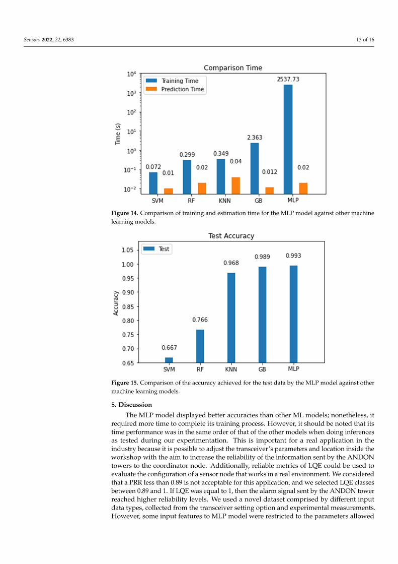
1. The MLP model had the best performance for the training, validation, and test sets, asshown in Figures 13 and 15.

2. Although the MLP achieved the best results, the GB model achieved an accuracy only0.4% lower than that achieved by the MLP.

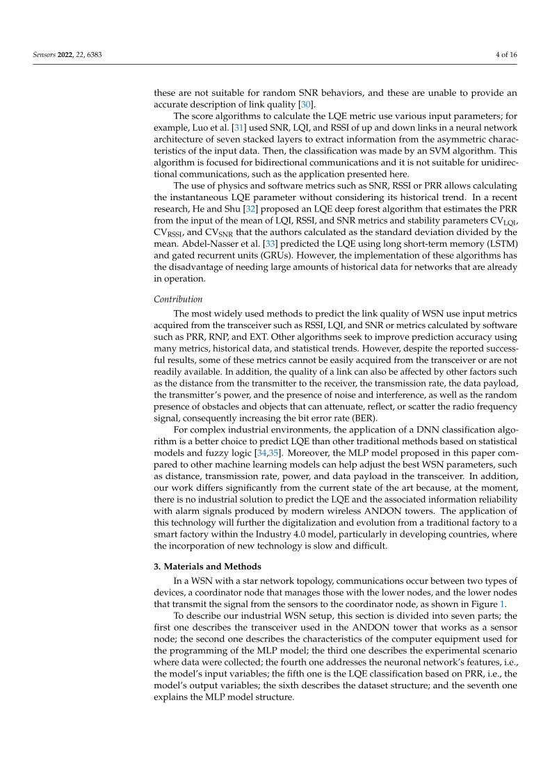
3. The MLP model required more time to complete the training stage than other simplermodels; nonetheless, once trained, the time it took to make the estimation with thetest data was very brief, approximately 0.02 s, as shown in Figure 14.

4. We demonstrated that the MLP model can be implemented with limited computa-tional resources and with data gathered from a low-cost transceiver. Despite thesedisadvantages, the MLP model was capable of making accurate estimations. In addi-tion, for industries in developing countries, the application of these technologies canhelp the transition into Industry 4.0.

Sensors 2022, 22, x FOR PEER REVIEW 13 of 16

2. Although the MLP achieved the best results, the GB model achieved an accuracy only 0.4% lower than that achieved by the MLP.

3. The MLP model required more time to complete the training stage than other simpler models; nonetheless, once trained, the time it took to make the estimation with the test data was very brief, approximately 0.02 s, as shown in Figure 15.

4. We demonstrated that the MLP model can be implemented with limited computational resources and with data gathered from a low-cost transceiver. Despite these disadvantages, the MLP model was capable of making accurate estimations. In addition, for industries in developing countries, the application of these technologies can help the transition into Industry 4.0.

Figure 13. Comparison of the accuracy achieved for the training and validation data by the MLP model against other machine learning models.

Figure 14. Comparison of the accuracy achieved for the test data by the MLP model against other machine learning models.

Figure 13. Comparison of the accuracy achieved for the training and validation data by the MLPmodel against other machine learning models.

Sensors 2022, 22, 6383 13 of 16Sensors 2022, 22, x FOR PEER REVIEW 14 of 16

Figure 15. Comparison of training and estimation time for the MLP model against other machine learning models.

5. Discussion The MLP model displayed better accuracies than other ML models; nonetheless, it

required more time to complete its training process. However, it should be noted that its time performance was in the same order of that of the other models when doing inferences as tested during our experimentation. This is important for a real application in the industry because it is possible to adjust the transceiver´s parameters and location inside the workshop with the aim to increase the reliability of the information sent by the ANDON towers to the coordinator node. Additionally, reliable metrics of LQE could be used to evaluate the configuration of a sensor node that works in a real environment. We considered that a PRR less than 0.89 is not acceptable for this application, and we selected LQE classes between 0.89 and 1. If LQE was equal to 1, then the alarm signal sent by the ANDON tower reached higher reliability levels. We used a novel dataset comprised by different input data types, collected from the transceiver setting option and experimental measurements. However, some input features to MLP model were restricted to the parameters allowed by the transceiver and physical constraints of our setup. As a future work, we suggest collecting more data from larger distances and payload measurements.

The alarm signal used in conjunction with LQE is a novel application for wireless ANDON towers, with the potential to ameliorate problems faced by factories located in developing countries through the incorporation of new technology during transition into the Industry 4.0 paradigm.

6. Conclusions In the industry, the information of alarm signal in conjunction with the LQE class is

relevant and represents a new approach to evaluate data´s reliability. In this paper, we proposed a novel application of a deep learning MLP model for the estimation of the LQE metric for a WSN integrated by ANDON towers that sends wireless information about alarm signals or about the operational status of a workshop’s machinery.

The random dataset was gathered from a realistic experimental scenario and split into 80% for training, 10% for validation, and 10% for testing. In order to find the best learning rate parameter, we realized a methodical tuning process for the MLP model and noted that a learning rate of LR = 2.95 × 10−5 achieved an accuracy of 99.8% for validation data without overfitting the training set.

The MLP model achieved an accuracy of 99.3% for test data and showed better performance than other machine learning models such as SVM, RF, KNN, and GB. Despite the MLP training time, its time to carry out estimations was in the order of ms, i.e., the

Figure 14. Comparison of training and estimation time for the MLP model against other machinelearning models.

Sensors 2022, 22, x FOR PEER REVIEW 13 of 16

2. Although the MLP achieved the best results, the GB model achieved an accuracy only 0.4% lower than that achieved by the MLP.

3. The MLP model required more time to complete the training stage than other simpler models; nonetheless, once trained, the time it took to make the estimation with the test data was very brief, approximately 0.02 s, as shown in Figure 15.

4. We demonstrated that the MLP model can be implemented with limited computational resources and with data gathered from a low-cost transceiver. Despite these disadvantages, the MLP model was capable of making accurate estimations. In addition, for industries in developing countries, the application of these technologies can help the transition into Industry 4.0.

Figure 13. Comparison of the accuracy achieved for the training and validation data by the MLP model against other machine learning models.

Figure 14. Comparison of the accuracy achieved for the test data by the MLP model against other machine learning models.

Figure 15. Comparison of the accuracy achieved for the test data by the MLP model against othermachine learning models.

5. Discussion

The MLP model displayed better accuracies than other ML models; nonetheless, itrequired more time to complete its training process. However, it should be noted that itstime performance was in the same order of that of the other models when doing inferencesas tested during our experimentation. This is important for a real application in theindustry because it is possible to adjust the transceiver’s parameters and location inside theworkshop with the aim to increase the reliability of the information sent by the ANDONtowers to the coordinator node. Additionally, reliable metrics of LQE could be used toevaluate the configuration of a sensor node that works in a real environment. We consideredthat a PRR less than 0.89 is not acceptable for this application, and we selected LQE classesbetween 0.89 and 1. If LQE was equal to 1, then the alarm signal sent by the ANDON towerreached higher reliability levels. We used a novel dataset comprised by different inputdata types, collected from the transceiver setting option and experimental measurements.However, some input features to MLP model were restricted to the parameters allowed

Sensors 2022, 22, 6383 14 of 16

by the transceiver and physical constraints of our setup. As a future work, we suggestcollecting more data from larger distances and payload measurements.

The alarm signal used in conjunction with LQE is a novel application for wirelessANDON towers, with the potential to ameliorate problems faced by factories located indeveloping countries through the incorporation of new technology during transition intothe Industry 4.0 paradigm.

6. Conclusions

In the industry, the information of alarm signal in conjunction with the LQE class isrelevant and represents a new approach to evaluate data’s reliability. In this paper, weproposed a novel application of a deep learning MLP model for the estimation of the LQEmetric for a WSN integrated by ANDON towers that sends wireless information aboutalarm signals or about the operational status of a workshop’s machinery.

The random dataset was gathered from a realistic experimental scenario and split into80% for training, 10% for validation, and 10% for testing. In order to find the best learningrate parameter, we realized a methodical tuning process for the MLP model and notedthat a learning rate of LR = 2.95 × 10−5 achieved an accuracy of 99.8% for validation datawithout overfitting the training set.

The MLP model achieved an accuracy of 99.3% for test data and showed betterperformance than other machine learning models such as SVM, RF, KNN, and GB. Despitethe MLP training time, its time to carry out estimations was in the order of ms, i.e., thesame order as that of the other models. From our research and experimentations, we couldsee that despite its simplicity, the MLP is a suitable model for workshops in developingcountries with limited computational resources.

Author Contributions: Conceptualization, T.A.C.-A.; methodology, T.A.C.-A.; software, T.A.C.-A.;validation, J.A.C.-C.; formal analysis, T.A.C.-A.; investigation, T.A.C.-A.; resources, A.T.-A.; datacuration, T.A.C.-A. and A.T.-A.; writing—original draft preparation, T.A.C.-A.; writing—review andediting, T.A.C.-A. and J.A.C.-C.; visualization, T.A.C.-A.; supervision, J.A.C.-C.; project adminis-tration, T.A.C.-A.; funding acquisition, A.T.-A. All authors have read and agreed to the publishedversion of the manuscript.

Funding: This work was supported by El Consejo Nacional de Ciencia y Tecnología de MexicoCONACYT and CIATEQ under research project “Modelo de confiabilidad para una red de sensoresinalámbricos para su implementación en la manufactura inteligente”.

Institutional Review Board Statement: Not applicable.

Informed Consent Statement: Not applicable.

Data Availability Statement: The dataset used for this research is publicly available at:https://ieee-dataport.org/documents/wireless-andon-tower-nrf24l01 (accessed on 9 March 2022).

Acknowledgments: This article was partially produced thanks to the support of the Instituto Tec-nológico José Mario Molina Pasquel y Henriquez, Unidad Académica Zapopan, Tecnológico Nacionalde Mexico TecNM and Advanced Technology Center CIATEQ.

Conflicts of Interest: The authors declare no conflict of interest.

References1. Lei, G.; Lu, G.; Sang, Y. Design of wireless Andon system based on ZigBee. In Proceedings of the 2015 8th International Conference

on Biomedical Engineering and Informatics, Shenyang, China, 14–16 October 2015. [CrossRef]2. Bonavolonta, F.; Tedesco, A.; Moriello, R.S.L.; Tufano, A. Enabling wireless technologies for industry 4.0: State of the art.

In Proceedings of the 2017 IEEE International Workshop on Measurement and Networking, Naples, Italy, 27–29 September 2017.[CrossRef]

3. International Electrotechnical Comm. IEC 60073 International Standard. Available online: www.iec.ch (accessed on 14 May 2021).4. PATLITE Corporation. Signal Tower. Available online: www.patlite.com (accessed on 14 May 2021).5. Banner Engineering Corp. Tower Lights. Available online: www.bannerengineering.com (accessed on 15 May 2021).6. WERMA Signaltechnik GmbH. SmartMONITOR. Available online: www.werma.com (accessed on 16 May 2021).

Sensors 2022, 22, 6383 15 of 16

7. Webert, H.; Döß, T.; Kaupp, L.; Simons, S. Fault Handling in Industry 4.0: Definition, Process and Applications. Sensors 2022, 22, 2205.[CrossRef] [PubMed]

8. Beysolow, T., II. Introduction to Deep Learning Using R; Apress: San Francisco, CA, USA, 2017.9. Kim, J.S.; Lee, D.M. A Deep Learning Module Design for Workspace Identification in Manufacturing Industry. In Proceedings of the

2021 International Conference on Artificial Intelligence in Information and Communication, Jeju Island, Korea, 13–16 April 2021.[CrossRef]

10. Messali, Z.; Saad Saoud, S.; Lamreche, A. Covid-19 Images and Video Denoising Algorithms Based on Convolutional NeuralNetwork CNNs. Alger. J. Signals Syst. 2021, 6, 122–129. [CrossRef]

11. Rustam, F.; Reshi, A.A.; Ashraf, I.; Mehmood, A.; Ullah, S.; Khan, D.M.; Choi, G.S. Sensor-Based Human Activity RecognitionUsing Deep Stacked Multilayered Perceptron Model. IEEE Access 2020, 8, 218898–218910. [CrossRef]

12. Bisogni, C.; Castiglione, A.; Hossain, S.; Narducci, F.; Umer, S. Impact of Deep Learning Approaches on Facial ExpressionRecognition in Healthcare Industries. IEEE Trans. Ind. Inform. 2022, 18, 5619–5627. [CrossRef]

13. Mukhamadiyev, A.; Khujayarov, I.; Djuraev, O.; Cho, J. Automatic Speech Recognition Method Based on Deep LearningApproaches for Uzbek Language. Sensors 2022, 22, 3683. [CrossRef]

14. Ozdemir, R.; Koc, M. A Quality Control Application on a Smart Factory Prototype Using Deep Learning Methods. In Pro-ceedings of the 2019 IEEE 14th International Conference on Computer Sciences and Information Technologies, Lviv, Ukraine,17–20 September 2019. [CrossRef]

15. Senarathne, P.; Silva, M.; Methmini, A.; Kavinda, D.; Thelijjagoda, S. Automate Traditional Interviewing Process Using NaturalLanguage Processing and Machine Learning. In Proceedings of the 2021 6th International Conference for Convergence inTechnology, Pune, India, 2–4 April 2021. [CrossRef]

16. Akhter, M.P.; Jiangbin, Z.; Naqvi, I.R.; Abdelmajeed, M.; Mehmood, A.; Sadiq, M.T. Document-Level Text Classification UsingSingle-Layer Multisize Filters Convolutional Neural Network. IEEE Access 2020, 8, 42689–42707. [CrossRef]

17. Morales-Gamboa, R. Mentes en la orilla: Presente y futuro de la inteligencia artificial. Revista Digital Universitaria UNAM. 2020.Available online: https://doi.org/10.22201/codeic.16076079e.2020.v21n1.a8 (accessed on 15 July 2021).

18. Zhang, L. A Pattern-Recognition-Based Ensemble Data Imputation Framework for Sensors from Building Energy Systems. Sensors2020, 20, 5947. [CrossRef]

19. De Araújo, R.P.; De Freitas, V.C.G.; De Lima, G.F.; Salazar, A.O.; Neto, A.D.D.; Maitelli, A.L. Pipeline Inspection Gauge’s VelocitySimulation Based on Pressure Differential Using Artificial Neural Networks. Sensors 2018, 18, 3072. [CrossRef]

20. Nair, V.; Hinton, G.E. Rectified linear units improve restricted boltzmann machines. In Proceedings of the 27th InternationalConference on International Conference on Machine Learning, Haifa, Israel, 21–24 June 2010. [CrossRef]

21. Liu, C.; Tang, D.; Zhu, H.; Nie, Q. A Novel Predictive Maintenance Method Based on Deep Adversarial Learning in the IntelligentManufacturing System. IEEE Access 2021, 9, 49557–49575. [CrossRef]

22. Márquez-Vera, M.A.; López-Ortega, O.; Ramos-Velasco, L.E.; Ortega-Mendoza, R.M.; Fernández-Neri, B.J.; Zúñiga-Peña, N.S.Diagnóstico de fallas mediante una LSTM y una red elástica. Rev. Iberoam. Autom. Inf. Ind. 2021, 18, 160–171. [CrossRef]

23. Ahmad, M.I.; Yusof, Y.; Daud, E.; Latiff, K.; Kadir, A.Z.A.; Saif, Y. Machine monitoring system: A decade in review. Int. J. Adv.Manuf. Technol. 2020, 108, 3645–3659. [CrossRef]

24. Cerar, G.; Yetgin, H.; Mohorcic, M.; Fortuna, C. Machine Learning for Wireless Link Quality Estimation: A Survey. IEEE Commun.Surv. Tutor. 2021, 23, 696–728. [CrossRef]

25. Sun, W.; Lu, W.; Li, Q.; Chen, L.; Mu, D.; Yuan, X. WNN-LQE: Wavelet-Neural-Network-Based Link Quality Estimation for SmartGrid WSNs. IEEE Access 2017, 5, 12788–12797. [CrossRef]

26. Woo, A.; Culler, D. Evaluation of Efficient Link Reliability Estimators for Low-Power Wireless Networks; EECS at UC Berkeley; EECSDepartment, University of California: Berkeley, CA, USA, 2003; Available online: https://www2.eecs.berkeley.edu/Pubs/TechRpts/2003/6239.html (accessed on 15 July 2021).

27. Cerpa, A.; Wong, J.L.; Potkonjak, M.; Estrin, D. Temporal properties of low power wireless links: Modeling and implications onmulti-hop routing. In Proceedings of the 6th ACM international symposium on Mobile ad hoc networking and computing, NewYork, NY, USA, 25–27 May 2005. [CrossRef]

28. Gomez, C.; Boix, A.; Paradells, J. Impact of LQI-Based Routing Metrics on the Performance of a One-to-One Routing Protocol forIEEE 802.15.4 Multihop Networks. J. Wirel. Commun. Netw. 2010, 2010, 205407. [CrossRef]

29. Qin, F.; Dai, X.; Mitchell, J.E. Effective-SNR estimation for wireless sensor network using Kalman filter. Ad Hoc Netw. 2013, 11,944–958. [CrossRef]

30. Farkas, K.; Hossmann, T.; Legendre, F.; Plattner, B.; Das, S.K. Link quality prediction in mesh networks. Comput. Commun. 2008,31, 1497–1512. [CrossRef]

31. Luo, X.; Liu, L.; Shu, J.; Al-Kali, M. Link Quality Estimation Method for Wireless Sensor Networks Based on Stacked Autoencoder.IEEE Access 2019, 7, 21572–21583. [CrossRef]

32. He, M.; Shu, J. A Link Quality Estimation Method for Wireless Sensor Networks Based on Deep Forest. IEEE Access 2021, 9,2564–2575. [CrossRef]

33. Abdel-Nasser, M.; Mahmoud, K.; Omer, O.A.; Lehtonen, M.; Puig, D. Link quality prediction in wireless community networksusing deep recurrent neural networks. Alex. Eng. J. 2020, 59, 3531–3543. [CrossRef]

Sensors 2022, 22, 6383 16 of 16

34. Cerar, G.; Yetgin, H.; Mohorcic, M.; Fortuna, C. On Designing a Machine Learning Based Wireless Link Quality Classifier.In Proceedings of the 2020 IEEE 31st Annual International Symposium on Personal, Indoor and Mobile Radio Communications,London, UK, 31 August–3 September 2020. [CrossRef]

35. Kulin, M.; Kazaz, T.; De Poorter, E.; Moerman, I. A Survey on Machine Learning-Based Performance Improvement of WirelessNetworks: PHY, MAC and Network Layer. Electronics 2021, 10, 318. [CrossRef]

36. Semiconductor, N. NRF24L01 Data Sheet. Available online: https://www.nordicsemi.com/ (accessed on 14 May 2021).37. Stevens, E.; Antiga, L.; Viehmann, T.; Chintala, S. Deep Learning with PyTorch; Manning Publications Co.: Shelter Island, NY, USA, 2020.38. Pedregosa, F.; Varoquaux, G.; Gramfort, A.; Michel, V.; Thirion, B.; Grisel, O.; Blondel, M.; Prettenhofer, P.; Weiss, R.; Dubourg, V.; et al.

Scikit-learn: Machine Learning in Python. J. Mach. Learn. Res. 2011, 12, 2825–2830.39. Sun, W.; Yuan, X.; Wang, J.; Li, Q.; Chen, L.; Mu, D. End-to-End Data Delivery Reliability Model for Estimating and Optimizing

the Link Quality of Industrial WSNs. IEEE Trans. Autom. Sci. Eng. 2018, 15, 1127–1137. [CrossRef]40. Shih-Lin, W.; Yu-Chee, T. Wireless Ad Hoc Networking; Auerbach Publications: New York, NY, USA, 2007.41. Boutaba, R.; Salahuddin, M.A.; Limam, N.; Ayoubi, S.; Shahriar, N.; Estrada-Solano, F.; Caicedo, O.M. A comprehensive survey on

machine learning for networking: Evolution, applications and research opportunities. J. Internet Serv. Appl. 2018, 9, 16. [CrossRef]