linear algebra solution manual edition 8
TRANSCRIPT
Chapter 1
Linear Equations and Matrices
Section 1.1, p. 8
2. x = 1, y = 2, z = −2. 4. No solution.
6. x = 13 + 10z, y = −8 − 8z, z = any real number.
8. No solution.
10. x = 2, y = −1.
12. No solution.
14. x = −1, y = 2, z = −2.
16. (c) Yes. (d) Yes.
18. x = 2, y = 1, z = 0.
20. There is no such value of r.
22. Zero, infinitely many, zero.
24. 1.5 tons of regular and 2.5 tons of special plastic.
26. 20 tons of 2-minute developer and a total of 40 tons of 6-minute and 9-minute developer.
28. $7000, $14,000, $3000.
T.1. The same numbers sj satisfy the system when the pth equation is written in place of the qth equationand vice versa.
T.2. If s1, s2, . . . , sn is a solution to (2), then the ith equation of (2) is satisfied: ai1s1+ai2s2+· · ·+ainsn =bi. Then for any r �= 0, rai1s1 + rai2s2 + · · ·+ rainsn = rbi. Hence s1, s2, . . . , sn is a solution to thenew system. Conversely, for any solution s′1, s
′2, . . . , s
′n to the new system, rai1s
′1+· · ·+rains′n = rbi,
and dividing both sides by nonzero r we see that s′1, . . . , s′n must be a solution to the original linear
system.
T.3. If s1, s2, . . . , sn is a solution to (2), then the pth and qth equations are satisfied:
ap1s1 + · · · apn = bp
aq1s1 + · · · aqn = bq.
2 Chapter 1
Thus, for any real number r,
(ap1 + raq1)s1 + · · · + (apn + raqn)sn = bp + rbq
and so s1, . . . , sn is a solution to the new system. Conversely, any solution to the new system is alsoa solution to the original system (2).
T.4. Yes; x = 0, y = 0 is a solution for any values of a, b, c, and d.
Section 1.2, p. 19
2. a = 3, b = 1, c = 8, d = −2.
4. (a) C + E = E + C =
⎡⎣5 −5 84 2 95 3 4
⎤⎦. (b) Impossible. (c)[7 −70 1
].
(d)
⎡⎣ −9 3 −9−12 −3 −15−6 −3 −9
⎤⎦. (e)
⎡⎣ 0 10 −98 −1 −2
−5 −4 3
⎤⎦. (f) Impossible.
6. (a) AT =
⎡⎣1 22 13 4
⎤⎦, (AT )T =[1 2 32 1 4
]. (b)
⎡⎣ 5 4 5−5 2 3
8 9 4
⎤⎦. (c)[−6 1011 17
].
(d)[0 −44 0
]. (e)
⎡⎣3 46 39 10
⎤⎦. (f)[
17 2−16 6
].
8. Yes: 2[1 00 1
]+ 1
[1 00 0
]=
[3 00 2
].
10.
⎡⎣λ − 1 −2 −3−6 λ + 2 −3−5 −2 λ − 4
⎤⎦.
12. (a)[0 01 1
]. (b)
[1 11 0
]. (c)
[1 10 1
]. (d)
[0 10 1
]. (e)
[1 10 1
].
14. v =[0 0 0 0
].
T.1. Let A and B each be diagonal n×n matrices. Let C = A + B, cij = aij + bij . For i �= j, aij and bij
are each 0, so cij = 0. Thus C is diagonal. If D = A − B, dij = aij − bij , then dij = 0. ThereforeD is diagonal.
T.2. Following the notation in the solution of T.1 above, let A and B be scalar matrices, so that aij = 0and bij = 0 for i �= j, and aii = a, bii = b. If C = A + B and D = A − B, then by Exercise T.1, Cand D are diagonal matrices. Moreover, cii = aii + bii = a + b and dii = aii − bii = a − b, so C andD are scalar matrices.
T.3. (a)
⎡⎣ 0 b − c c − ec − b 0 0e − c 0 0
⎤⎦. (b)
⎡⎣ 2a c + b e + cb + c 2d 2ec + e 2e 2f
⎤⎦. (c) Same as (b).
T.4. Let A =[aij
]and C =
[cij
], so cij = kaij . If kaij = 0, then either k = 0 or aij = 0 for all i, j.
T.5. (a) Let A =[aij
]and B =
[bij
]be upper triangular matrices, and let C = A + B. Then for i > j,
cij = aij + bij = 0 + 0 = 0, and thus C is upper triangular. Similarly, if D = A − B, then fori > j, dij = aij − bij = 0 − 0 = 0, so D is upper triangular.
Section 1.2 3
(b) Proof is similar to that for (a).
(c) Let A =[aij
]be both upper and lower triangular. Then aij = 0 for i > j and for i < j. Thus,
A is a diagonal matrix.
T.6. (a) Let A =[aij
]be upper triangular, so that aij = 0 for i > j. Since AT =
[aT
ij
], where aT
ij = aji,we have aT
ij = 0 for j > i, or aTij = 0 for i < j. Hence AT is lower triangular.
(b) Proof is similar to that for (a).
T.7. To justify this answer, let A =[aij
]be an n × n matrix. Then AT =
[aji
]. Thus, the (i, i)th entry
of A − AT is aii − aii = 0. Therefore, all entries on the main diagonal of A − AT are 0.
T.8. Let x =
⎡⎢⎢⎢⎣x1
x2
...xn
⎤⎥⎥⎥⎦ be an n-vector. Then
x + 0 =
⎡⎢⎢⎢⎣x1
x2
...xn
⎤⎥⎥⎥⎦ +
⎡⎢⎢⎢⎣00...0
⎤⎥⎥⎥⎦ =
⎡⎢⎢⎢⎣x1 + 0x2 + 0
...xn + 0
⎤⎥⎥⎥⎦ =
⎡⎢⎢⎢⎣x1
x2
...xn
⎤⎥⎥⎥⎦ = x.
T.9.[00
],[10
],[01
],[11
]; four.
T.10.
⎡⎣000
⎤⎦,
⎡⎣001
⎤⎦,
⎡⎣010
⎤⎦,
⎡⎣011
⎤⎦,
⎡⎣100
⎤⎦,
⎡⎣101
⎤⎦,
⎡⎣110
⎤⎦,
⎡⎣111
⎤⎦; eight
T.11.
⎡⎢⎢⎣0000
⎤⎥⎥⎦,
⎡⎢⎢⎣0001
⎤⎥⎥⎦,
⎡⎢⎢⎣0010
⎤⎥⎥⎦,
⎡⎢⎢⎣0011
⎤⎥⎥⎦,
⎡⎢⎢⎣0100
⎤⎥⎥⎦,
⎡⎢⎢⎣0101
⎤⎥⎥⎦,
⎡⎢⎢⎣0110
⎤⎥⎥⎦,
⎡⎢⎢⎣0111
⎤⎥⎥⎦,
⎡⎢⎢⎣1000
⎤⎥⎥⎦,
⎡⎢⎢⎣1001
⎤⎥⎥⎦,
⎡⎢⎢⎣1010
⎤⎥⎥⎦,
⎡⎢⎢⎣1011
⎤⎥⎥⎦,
⎡⎢⎢⎣1100
⎤⎥⎥⎦,
⎡⎢⎢⎣1101
⎤⎥⎥⎦,
⎡⎢⎢⎣1110
⎤⎥⎥⎦,
⎡⎢⎢⎣1111
⎤⎥⎥⎦; sixteen
T.12. Thirty two; 2n.
T.13.[0 00 0
],
[0 00 1
],
[0 10 0
],
[0 10 1
],
[0 01 0
],
[0 01 1
],
[0 11 0
],
[0 11 1
],
[1 00 0
],
[1 00 1
],
[1 10 0
],
[1 10 1
],[
1 01 0
],[1 01 1
],[1 11 0
],[1 11 1
]; sixteen
T.14. 29 = 512.
T.15. 2n2.
T.16. A =
⎡⎣1 1 00 1 00 1 1
⎤⎦ so B = A is such that A + B =
⎡⎣0 0 00 0 00 0 0
⎤⎦.
T.17. A =
⎡⎣1 1 00 1 00 1 1
⎤⎦; if B =
⎡⎣0 0 11 0 11 0 0
⎤⎦, then A + B =
⎡⎣1 1 11 1 11 1 1
⎤⎦.
T.18. (a) B =
⎡⎣1 11 11 1
⎤⎦ since A + B =
⎡⎣0 11 00 0
⎤⎦.
4 Chapter 1
(b) Yes; C + B =
⎡⎣0 01 10 1
⎤⎦.
(c) Let B be a bit matrix of all 1s. A + B will be a matrix that reverses each state of A.
ML.1. Once you have entered matrices A and B you can use the commands given below to see the itemsrequested in parts (a) and (b).
(a) Commands: A(2,3), B(3,2), B(1,2)
(b) For row1(A) use command A(1,:)
For col3(A) use command A(:,3)
For row2(B) use command B(2,:)
(In this context the colon means ‘all.’)
(c) Matrix B in format long is
8.00000000000000 0.666666666666670.00497512437811 −3.200000000000000.00000100000000 4.33333333333333
ML.2. (a) Use command size(H)
(b) Just type H
(c) Type format rat, then H. (To return to decimal format display type format.)
(d) Type H(:,1:3)
(e) Type H(4:5,:)
Section 1.3, p. 34
2. (a) 4. (b) 0. (c) 1. (d) 1.
4. 1
6. x = 65 , y = 12
5 .
8. (a)[26 4234 54
]. (b) Same as (a). (c)
[−7 −12 18
4 6 −8
].
(d) Same as (c). (e)[
4 8 −12−1 6 −7
].
10. DI2 = I2D = D.
12.[0 00 0
].
14. (a)
⎡⎢⎢⎣1
140
13
⎤⎥⎥⎦. (b)
⎡⎢⎢⎣0
183
13
⎤⎥⎥⎦.
16. col1(AB) = 1
⎡⎣123
⎤⎦ + 3
⎡⎣−240
⎤⎦ + 2
⎡⎣−13
−2
⎤⎦; col2(AB) = −1
⎡⎣123
⎤⎦ + 2
⎡⎣−240
⎤⎦ + 4
⎡⎣−13
−2
⎤⎦.
Section 1.3 5
18.[−2 2 3
3 5 −1
]⎡⎣342
⎤⎦.
20. −2x − y + 4w = 5−3x + 2y + 7z + 8w = 3
x + 2w = 43x + z + 3w = 6.
22. (a)
⎡⎢⎢⎣3 −1 22 1 00 1 34 0 −1
⎤⎥⎥⎦. (b)
⎡⎢⎢⎣3 −1 22 1 00 1 34 0 −1
⎤⎥⎥⎦⎡⎣x
yz
⎤⎦ =
⎡⎢⎢⎣4274
⎤⎥⎥⎦. (c)
⎡⎢⎢⎣3 −1 2 42 1 0 20 1 3 74 0 −1 4
⎤⎥⎥⎦.
24. (a)[1 2 02 5 3
]⎡⎣xyz
⎤⎦ =[11
]. (b)
⎡⎣1 2 11 1 22 0 2
⎤⎦⎡⎣xyz
⎤⎦ =
⎡⎣000
⎤⎦.
26. (a) Can say nothing. (b) Can say nothing.
28. There are infinitely many choices. For example, r = 1, s = 0; or r = 0, s = 2; or r = 10, s = −18.
30. A =
⎡⎢⎢⎢⎢⎣2 × 2 2 × 2 2 × 1
2 × 2 2 × 2 2 × 1
2 × 2 2 × 2 2 × 1
⎤⎥⎥⎥⎥⎦ and B =
⎡⎢⎢⎢⎣2 × 2 2 × 3
2 × 2 2 × 3
1 × 2 1 × 3
⎤⎥⎥⎥⎦.
A =
⎡⎣3 × 3 3 × 2
3 × 3 3 × 2
⎤⎦ and B =
⎡⎣3 × 3 3 × 2
2 × 3 2 × 2
⎤⎦.
AB =
⎡⎢⎢⎢⎢⎢⎢⎣21 48 41 48 4018 26 34 33 524 26 42 47 1628 38 54 70 3533 33 56 74 4234 37 58 79 54
⎤⎥⎥⎥⎥⎥⎥⎦32. For each product P or Q, the daily cost of pollution control at plant X or at plant Y .
34. (a) $103,400. (b) $16,050.
36. (a) 1. (b) 0.
38. x = 0 or x = 1.
40. AB =
⎡⎣1 0 01 1 01 0 1
⎤⎦, BA =
⎡⎣0 1 01 0 01 1 1
⎤⎦.
T.1. (a) No. If x = (x1, x2, . . . , xn), then x ·x = x21 + x2
2 + · · · + x2n ≥ 0.
(b) x = 0.
T.2. Let a = (a1, a2, . . . , an), b = (b1, b2, . . . , bn), and c = (c1, c2, . . . , cn). Then
(a) a ·b =n∑
i=1
aibi and b ·a =n∑
i=1
biai, so a ·b = b ·a.
6 Chapter 1
(b) (a + b) · c =n∑
i=1
(ai + bi)ci =n∑
i=1
aici +n∑
i=1
bici = a · c + b · c.
(c) (ka) ·b =n∑
i=1
(kai)bi = k
n∑i=1
aibi = k(a ·b).
T.3. Let A =[aij
]be m × p and B =
[bij
]be p × n.
(a) Let the ith row of A consist entirely of zeros, so aik = 0 for k = 1, 2, . . . , p. Then the (i, j)entry in AB is
p∑k=1
aikbkj = 0 for j = 1, 2, . . . , n.
(b) Let the jth column of B consist entirely of zeros, so bkj = 0 for k = 1, 2, . . . , p. Then again the(i, j) entry of AB is 0 for i = 1, 2, . . . , m.
T.4. Let A and B be diagonal matrices, so aij = 0 and bij = 0 for i �= j. Let C = AB. Then, if C =[cij
],
we have
cij =n∑
k=1
aikbkj . (1.1)
For i �= j and any value of k, either k �= i and so aik = 0, or k �= j and so bkj = 0. Thus each termin the summation (1.1) equals 0, and so also cij = 0. This holds for every i, j such that i �= j, so Cis a diagonal matrix.
T.5. Let A and B be scalar matrices, so that aij = a and bij = b for all i = j. If C = AB, then byExercise T.4, cij = 0 for i �= j, and cii = a · b = aii · bii = c, so C is a scalar matrix.
T.6. Let A =[aij
]and B =
[bij
]be upper triangular matrices.
(a) Let C = AB, cij =∑
aikbkj . If i > j, then for each k, either k > j (and so bkj = 0), or elsek ≤ j < i (and so aik = 0). Thus cij = 0.
(b) Proof similar to that for (a).
T.7. Yes. If A =[aij
]and B =
[bij
]are diagonal matrices, then C =
[cij
]is diagonal by Exercise T.4.
Moreover, cii = aiibii. Similarly, if D = BA, then dii = biiaii. Thus, C = D.
T.8. (a) Let a =[a1 a2 · · · an
]and B =
[bij
]. Then
aB =[
a1b11 + a2b21 + · · · + anbn1 a1b12 + a2b22 + · · · + anbn2 · · ·a1b1p + a2b2p + · · · + anbnp
]= a1
[b11 b12 · · · b1p
]+ a2
[b21 b22 · · · b2p
]+ · · · + an
[bn1 bn2 · · · bnp
].
(b) 1[2 1 −4
]− 2
[−3 −2 3
]+ 3
[4 5 −2
].
T.9. (a) The jth column of AB is ⎡⎢⎢⎢⎢⎢⎢⎢⎢⎢⎢⎢⎣
∑k
a1kbkj∑k
a2kbkj
...∑k
amkbkj
⎤⎥⎥⎥⎥⎥⎥⎥⎥⎥⎥⎥⎦.
Section 1.3 7
(b) The ith row of AB is [∑k
aikbk1
∑k
aikbk2 · · ·∑
k
aikbkn
].
T.10. The i, ith element of the matrix AAT isn∑
k=1
aikaTki =
n∑k=1
aikaik =n∑
k=1
(aik)2.
Thus if AAT = O, then each sum of squaresn∑
k=1
(aik)2 equals zero, which implies aik = 0 for each i
and k. Thus A = O.
T.11. (a)n∑
i=1
(ri + si)ai = (r1 + s1)a1 + (r2 + s2)a2 + · · · + (rn + sn)an
= r1a1 + s1a1 + r2a2 + s2a2 + · · · + rnan + snan
= (r1a1 + r2a2 + · · · + rnan) + (s1a1 + s2a2 + · · · + snan) =n∑
i=1
riai +n∑
i=1
siai
(b)n∑
i=1
c(riai) = cr1a1 + cr2a2 + · · · + crnan = c(r1a1 + r2a2 + · · · + rnan) = c
n∑i=1
riai.
T.12.n∑
i=1
m∑j=1
aij = (a11 + a12 + · · · + a1m) + (a21 + a22 + · · · + a2m) + · · · + (an1 + an2 + · · · + anm)
= (a11 + a21 + · · · + an1) + (a12 + a22 + · · · + an2) + · · · + (a1m + a2m + · · · + anm)
=m∑
j=1
n∑i=1
aij .
T.13. (a) True.n∑
i=1
(ai + 1) =n∑
i=1
ai +n∑
i=1
1 =n∑
i=1
ai + n.
(b) True.n∑
i=1
m∑j=1
1 =n∑
i=1
⎛⎝ m∑j=1
1
⎞⎠ =n∑
i=1
m = mn.
(c) True.
⎡⎣ n∑i=1
ai
⎤⎦⎡⎣ m∑j=1
bj
⎤⎦ = a1
m∑j=1
bj + a2
m∑j=1
bj + · · · + an
m∑j=1
bj
= (a1 + a2 + · · · + an)m∑
j=1
bj
=n∑
i=1
ai
m∑j=1
bj =m∑
j=1
n∑i=1
aibj
T.14. (a) If u =
⎡⎢⎢⎢⎣u1
u2
...un
⎤⎥⎥⎥⎦ and v =
⎡⎢⎢⎢⎣v1
v2
...vn
⎤⎥⎥⎥⎦, then
u ·v =n∑
i=1
uivi =[u1 u2 · · · un
]⎡⎢⎢⎢⎣
v1
v2
...vn
⎤⎥⎥⎥⎦ = uT v.
8 Chapter 1
(b) If u =[u1 u2 · · · un
]and v =
[v1 v2 · · · vn
], then
u ·v =n∑
i=1
uivi =[u1 u2 · · · un
]⎡⎢⎢⎢⎣
v1
v2
...vn
⎤⎥⎥⎥⎦ = uvT .
(c) If u =[u1 u2 · · · un
]and v =
⎡⎢⎢⎢⎣v1
v2
...vn
⎤⎥⎥⎥⎦, then
u ·v =n∑
i=1
uivi = uv.
ML1.1 (a) A ∗∗∗ Cans =
4.5000 2.2500 3.7500
1.5833 0.9167 1.5000
0.9667 0.5833 0.9500
(b) A ∗∗∗ B??? Error using ===> ∗Inner matrix dimensions must agree.
(c) A+++ C′′′
ans =5.0000 1.5000
1.5833 2.2500
2.4500 3.1667
(d) B ∗∗∗ A−−− C′′′ ∗∗∗ A??? Error using ===> ∗Inner matrix dimensions must agree.
(e) (((2 ∗∗∗ C−−− 6 ∗∗∗ A′′′) ∗∗∗ B′′′
??? Error using ===> ∗Inner matrix dimensions must agree.
(f) A ∗∗∗ C−−− C ∗∗∗ A??? Error using ===> −−−Inner matrix dimensions must agree.
(g) A ∗∗∗ A′′′ +++ A′′′ ∗∗∗ Cans =
18.2500 7.4583 12.2833
7.4583 5.7361 8.9208
12.2833 8.9208 14.1303
ML.2. aug =2 4 6 −122 −3 −4 15
3 4 5 −8
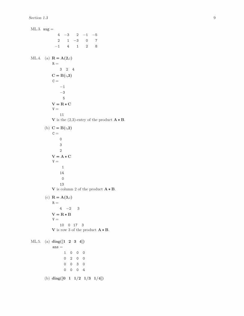
Section 1.3 9
ML.3. aug =4 −3 2 −1 −52 1 −3 0 7
−1 4 1 2 8
ML.4. (a) R === A(2,:)R =
3 2 4
C === B(:,3)C =
−1−35
V === R ∗∗∗ CV =
11V is the (2,3)-entry of the product A ∗∗∗ B.
(b) C === B(:,2)C =
0
3
2
V === A ∗∗∗ CV =
1
14
0
13V is column 2 of the product A ∗∗∗ B.
(c) R === A(3,:)R =
4 −2 3
V === R ∗∗∗ BV =
10 0 17 3V is row 3 of the product A ∗∗∗ B.
ML.5. (a) diag([1 2 3 4])ans =
1 0 0 0
0 2 0 0
0 0 3 0
0 0 0 4
(b) diag([0 1 1/2 1/3 1/4])
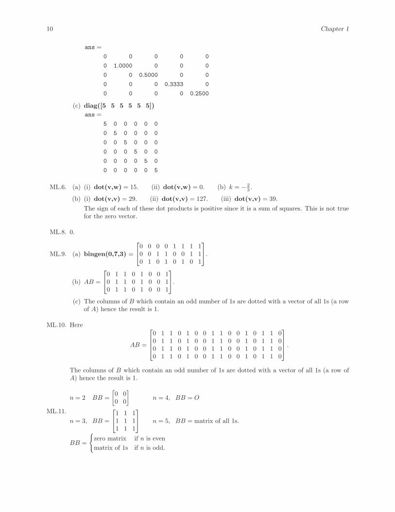
10 Chapter 1
ans =0 0 0 0 0
0 1.0000 0 0 0
0 0 0.5000 0 0
0 0 0 0.3333 0
0 0 0 0 0.2500
(c) diag([5 5 5 5 5 5])ans =
5 0 0 0 0 0
0 5 0 0 0 0
0 0 5 0 0 0
0 0 0 5 0 0
0 0 0 0 5 0
0 0 0 0 0 5
ML.6. (a) (i) dot(v,w) = 15. (ii) dot(v,w) = 0. (b) k = − 23 .
(b) (i) dot(v,v) = 29. (ii) dot(v,v) = 127. (iii) dot(v,v) = 39.The sign of each of these dot products is positive since it is a sum of squares. This is not truefor the zero vector.
ML.8. 0.
ML.9. (a) bingen(0,7,3) =
⎡⎣0 0 0 0 1 1 1 10 0 1 1 0 0 1 10 1 0 1 0 1 0 1
⎤⎦.
(b) AB =
⎡⎣0 1 1 0 1 0 0 10 1 1 0 1 0 0 10 1 1 0 1 0 0 1
⎤⎦.
(c) The columns of B which contain an odd number of 1s are dotted with a vector of all 1s (a rowof A) hence the result is 1.
ML.10. Here
AB =
⎡⎢⎢⎣0 1 1 0 1 0 0 1 1 0 0 1 0 1 1 00 1 1 0 1 0 0 1 1 0 0 1 0 1 1 00 1 1 0 1 0 0 1 1 0 0 1 0 1 1 00 1 1 0 1 0 0 1 1 0 0 1 0 1 1 0
⎤⎥⎥⎦ .
The columns of B which contain an odd number of 1s are dotted with a vector of all 1s (a row ofA) hence the result is 1.
ML.11.
n = 2 BB =[0 00 0
]n = 4, BB = O
n = 3, BB =
⎡⎣1 1 11 1 11 1 1
⎤⎦ n = 5, BB = matrix of all 1s.
BB =
{zero matrix if n is evenmatrix of 1s if n is odd.
Section 1.4 11
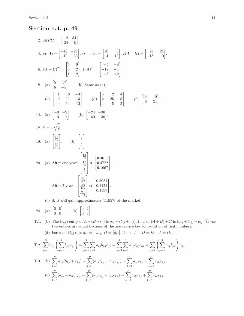
Section 1.4, p. 49
2. A(BC) =[−2 3424 −9
].
4. r(sA) =[−48 −24−12 36
], (r + s)A =
[16 84 −12
], r(A + B) =
[24 24
−18 0
].
6. (A + B)T =
⎡⎣5 05 21 2
⎤⎦, (rA)T =
⎡⎣ −4 −8−12 −4−8 12
⎤⎦.
8. (a)[5 176 −5
]. (b) Same as (a).
(c)
⎡⎣ 1 18 −40 11 −3
−9 14 −12
⎤⎦. (d)
⎡⎣5 2 42 25 −54 −5 5
⎤⎦. (e)[14 88 21
].
14. (a)[−3 −2
4 1
]. (b)
[−24 −30
60 36
].
16. k = ±√
16
18. (a)
⎡⎣ 1645
2945
⎤⎦. (b)
⎡⎣ 38
58
⎤⎦.
20. (a) After one year:
⎡⎢⎢⎢⎣1336
1736
16
⎤⎥⎥⎥⎦ ≈
⎡⎣0.36110.47220.1667
⎤⎦.
After 2 years:
⎡⎢⎢⎢⎣43108
191432
23144
⎤⎥⎥⎥⎦ ≈
⎡⎣0.39810.44210.1597
⎤⎦.
(c) S. It will gain approximately 11.95% of the market.
24. (a)[0 00 0
]. (b)
[0 10 1
].
T.1. (b) The (i, j) entry of A+(B +C) is aij +(bij + cij), that of (A+B)+C is (aij + bij)+ cij . Thesetwo entries are equal because of the associative law for addition of real numbers.
(d) For each (i, j) let dij = −aij , D =[dij
]. Then A + D = D + A = O.
T.2.3∑
p=1
aip
(4∑
q=1
bpqcqj
)=
3∑p=1
4∑q=1
aipbpqcqj =4∑
q=1
3∑p=1
aipbpqcqj =4∑
q=1
(3∑
p=1
aipbpq
)cqj .
T.3. (b)p∑
k=1
aik(bkj + ckj) =p∑
k=1
(aikbkj + aikckj) =p∑
k=1
aikbkj +p∑
k=1
aikckj
(c)p∑
k=1
(aik + bik)ckj =p∑
k=1
(aikckj + bikckj) =p∑
k=1
aikckj +p∑
k=1
bikckj .
12 Chapter 1
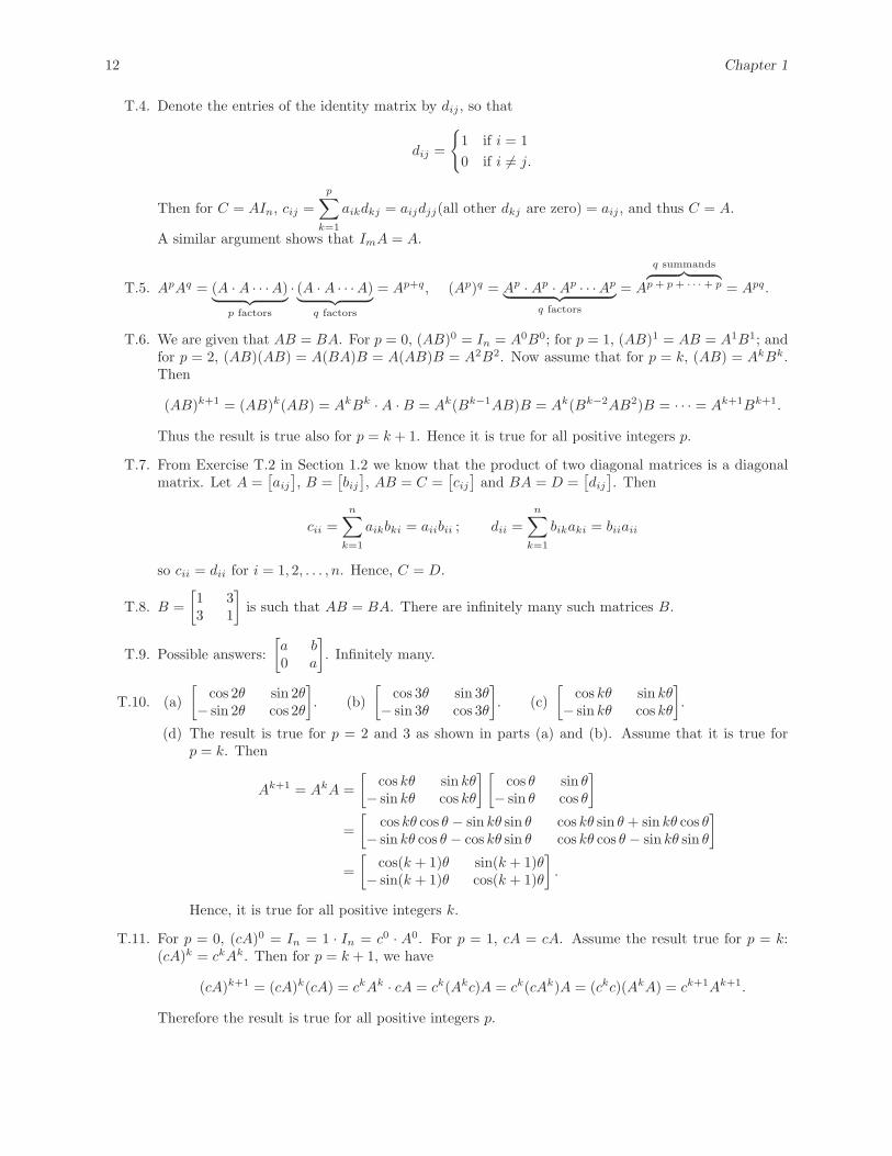
T.4. Denote the entries of the identity matrix by dij , so that
dij =
{1 if i = 10 if i �= j.
Then for C = AIn, cij =p∑
k=1
aikdkj = aijdjj(all other dkj are zero) = aij , and thus C = A.
A similar argument shows that ImA = A.
T.5. ApAq = (A · A · · ·A)︸ ︷︷ ︸p factors
· (A · A · · ·A)︸ ︷︷ ︸q factors
= Ap+q, (Ap)q = Ap · Ap · Ap · · ·Ap︸ ︷︷ ︸q factors
= A
q summands︷ ︸︸ ︷p + p + · · · + p = Apq.
T.6. We are given that AB = BA. For p = 0, (AB)0 = In = A0B0; for p = 1, (AB)1 = AB = A1B1; andfor p = 2, (AB)(AB) = A(BA)B = A(AB)B = A2B2. Now assume that for p = k, (AB) = AkBk.Then
(AB)k+1 = (AB)k(AB) = AkBk · A · B = Ak(Bk−1AB)B = Ak(Bk−2AB2)B = · · · = Ak+1Bk+1.
Thus the result is true also for p = k + 1. Hence it is true for all positive integers p.
T.7. From Exercise T.2 in Section 1.2 we know that the product of two diagonal matrices is a diagonalmatrix. Let A =
[aij
], B =
[bij
], AB = C =
[cij
]and BA = D =
[dij
]. Then
cii =n∑
k=1
aikbki = aiibii ; dii =n∑
k=1
bikaki = biiaii
so cii = dii for i = 1, 2, . . . , n. Hence, C = D.
T.8. B =[1 33 1
]is such that AB = BA. There are infinitely many such matrices B.
T.9. Possible answers:[a b0 a
]. Infinitely many.
T.10. (a)[
cos 2θ sin 2θ− sin 2θ cos 2θ
]. (b)
[cos 3θ sin 3θ
− sin 3θ cos 3θ
]. (c)
[cos kθ sin kθ
− sin kθ cos kθ
].
(d) The result is true for p = 2 and 3 as shown in parts (a) and (b). Assume that it is true forp = k. Then
Ak+1 = AkA =[
cos kθ sin kθ− sin kθ cos kθ
] [cos θ sin θ
− sin θ cos θ
]=
[cos kθ cos θ − sin kθ sin θ cos kθ sin θ + sin kθ cos θ
− sin kθ cos θ − cos kθ sin θ cos kθ cos θ − sin kθ sin θ
]=
[cos(k + 1)θ sin(k + 1)θ
− sin(k + 1)θ cos(k + 1)θ
].
Hence, it is true for all positive integers k.
T.11. For p = 0, (cA)0 = In = 1 · In = c0 · A0. For p = 1, cA = cA. Assume the result true for p = k:(cA)k = ckAk. Then for p = k + 1, we have
(cA)k+1 = (cA)k(cA) = ckAk · cA = ck(Akc)A = ck(cAk)A = (ckc)(AkA) = ck+1Ak+1.
Therefore the result is true for all positive integers p.
Section 1.4 13
T.12. (a) For A =[aij
], the (i, j) element of r(sA) is r(saij), that of (rs)A is (rs)aij , and these are equal
by the associative law for multiplication of real numbers.
(b) The (i, j) element of (r + s)A is (r + s)aij , that of rA + sA is raij + saij , and these are equalby the distributive law of real numbers.
(c) r(aij + bij) = raij + rbij .
(d)p∑
k=1
aik(rbkj) = r
p∑k=1
aikbkj =p∑
k=1
(raik)bkj .
T.13. (−1)aij = −aij (see Exercise T.1.).
T.14. (a) The i, jth element of (AT )T is the j, ith element of AT , which is the i, jth element of A.
(b) The i, jth element of (A + B)T is cji, where cij = aij + bij . Thus cji = aji + bji. Hence(A + B)T = AT + BT .
(c) The i, jth element of (rA)T is the j, ith element of rA, that is, raji. Thus (rA)T = rAT .
T.15. Let A =[aij
]and B =
[bij
]. Then A−B =
[cij
], where cij = aij − bij . Then (A−B)T =
[cTij
], so
cTij = cji = aji − bji = aT
ij − bTij = the i, jth entry in AT − BT .
T.16. (a) We have A2 = AA, so (A2)T = (AA)T = AT AT = (AT )2.
(b) From part (a), (A3)T = (A2A)T = AT (A2)T = AT (AT )2 = (AT )3.
(c) The result is true for p = 2 and 3 as shown in parts (a) and (b). Assume that it is true forp = k. Then
(Ak+1)T = (AAk)T = (Ak)T AT = (AT )kAT = (AT )k+1.
Hence, it is true for k = 4, 5, . . . .
T.17. If A is symmetric, then AT = A. Thus aji = aij for all i and j. Conversely, if aji = aij for all i andj, then AT = A and A is symmetric.
T.18. Both “A is symmetric” and “AT is symmetric” are logically equivalent to “aji = aij for all i and j.”
T.19. If Ax = 0 for all n × 1 matrices x, then Aej = 0, j = 1, 2, . . . , n, where ej = column j of In. Butthen
Aej =
⎡⎢⎢⎢⎣a1j
a2j
...anj
⎤⎥⎥⎥⎦ = 0.
Hence column j of A is equal to 0 for each j and it follows that A = O.
T.20. If Ax = x for all n × 1 matrices x, then Aej = ej , where ej = column j of In. Since
Aej =
⎡⎢⎢⎢⎣a1j
a2j
...anj
⎤⎥⎥⎥⎦ = ej ,
it follows that aij = 1 if i = j and 0 otherwise. Hence A = In.
14 Chapter 1
T.21. Given that AAT = O, we have that each entry of AAT is zero. In particular then, each diagonalentry of AAT is zero. Hence
0 = rowi(A) · coli(AT ) =[ai1 ai2 · · · ain
]⎡⎢⎢⎢⎣
ai1
ai2
...ain
⎤⎥⎥⎥⎦ =n∑
j=1
(aij)2.
(Recall that coli(AT ) is rowi(A) written in column form.) A sum of squares is zero only if eachmember of the sum is zero, hence ai1 = ai2 = · · · = ain = 0, which means that rowi(A) consists ofall zeros. The previous argument holds for each diagonal entry, hence each row of A contains allzeros. Thus it follows that A = O.
T.22. Suppose that A is a symmetric matrix. By Exercise T.16(c) we have (Ak)T = (AT )k = Ak so Ak issymmetric for k = 2, 3, . . . .
T.23. (a) (A + B)T = AT + BT = A + B, so A + B is symmetric.
(b) Suppose that AB is symmetric. Then
(AB)T = AB
BT AT = AB [Thm. 1.4(c)]BA = AB (A and B are each symmetric)
Thus A and B commute. Conversely, if A and B commute, then (AB)T = AB and AB issymmetric.
T.24. Suppose A is skew symmetric. Then the j, ith element of A equals −aij . That is, aij = −aji.
T.25. Let A = rIn. Then (rIn)T = −rIn so rIn = −rIn. Hence, r = −r, which implies that r = 0. Thatis, A = O.
T.26. (AAT )T = (AT )T AT [Thm. 1.4(c)]= AAT [Thm. 1.4(a)]
Thus AAT is symmetric. A similar argument applies to AT A.
T.27. (a) (A + AT )T = AT + (AT )T = AT + A = A + AT .
(b) (A − AT )T = AT − (AT )T = AT − A = −(A − AT ).
T.28. Let
S = 12 (A + AT ) and K = 1
2 (A − AT ).
Then S is symmetric and K is skew symmetric, by Exercise T.15, and S+K = 12 (A+AT +A−AT ) =
12 (2A) = A. Conversely, suppose A = S + K is any decomposition of A into the sum of a symmetricand skew symmetric matrix. Then
AT = (S + K)T = ST + KT = S − K,
A + AT = (S + K) + (S − K) = 2S, =⇒ S = 12 (A + AT ),
A − AT = (S + K) − (S − K) = 2K, =⇒ K = 12 (A − AT ).
T.29. If the diagonal entries of A are r, then since r = r · 1, A = rIn.
T.30. In =[dij
], where dij =
{1 if i = j
0 if i �= j.Then dji =
{1 if i = j
0 if i �= j.Thus IT
n = I.
Section 1.4 15
T.31. Suppose r �= 0. The i, jth entry of rA is raij . Since r �= 0, aij = 0 for all i and j. Thus A = O.
T.32. Let u and v be two (distinct) solutions to the linear system Ax = b, and consider w = ru + sv forr + s = 1. Then w is a solution to the system since
Aw = A(ru + sv) = r(Au) + s(Av) = rb + sb = (r + s)b = b.
If b = 0, then at least one of u, v must be nonzero, say u, and then the infinitely many matricesru, r a real number, constitute solutions.
If b �= 0, then u and v cannot be nontrivial multiples of each other. (If v = tu, t �= 1, thenAv = tb �= b = Au, a contradiction.) Thus if ru + sv = r′u + s′v for some r, s, r′, s′, then
(r − r′)u = (s′ − s)v,
whence r = r′ and s = s′. Therefore the matrices w = ru + sv are distinct as r ranges over realnumbers and s = 1 − r.
T.33. Suppose A =[a bc d
]satisfies AB = BA for any 2 × 2 matrix B. Choosing B =
[1 00 0
]we get
[a bc d
] [1 00 0
]=
[1 00 0
] [a bc d
]and
[a 0c 0
]=
[a b0 0
]
which implies b = c = 0. Thus A =[a 00 d
]is diagonal. Next choosing B =
[0 10 0
]we get
[0 a0 0
]=
[0 d0 0
],
or a = d. Thus A =[a 00 a
]is a scalar matrix.
T.34. Skew symmetric. To show this, let A be a skew symmetric matrix. Then AT = −A. Therefore(AT )T = A = −AT . Hence AT is skew symmetric.
T.35. A symmetric matrix. To show this, let A1, . . . , An be symmetric matrices and let c1, . . . , cn bescalars. Then AT
1 = A1, . . . , ATn = An. Therefore
(c1A1 + · · · + cnAn)T = (c1A1)T + · · · + (cnAn)T
= c1AT1 + · · · + cnAT
n
= c1A1 + · · · + cnAn.
Hence the linear combination c1A1 + · · · + cnAn is symmetric.
T.36. A scalar matrix. To show this, let A1, . . . , An be scalar matrices and let r1, . . . , rn be scalars. ThenAi = ciIn for scalars c1, . . . , cn. Therefore
r1A1 + · · · + rnAn = r1(c1I1) + · · · + rn(cnIn) = (r1c1 + · · · + rncn)In
which is the scalar matrix whose diagonal entries are all equal to r1c1 + · · · + rncn.
T.37. Let A =[aij
], B =
[bij
], and C = AB. Then
cij =p∑
k=1i �=k
aikbkj + aiibij = rbij .
16 Chapter 1
T.38. For any m × n bit matrix A + A =[entij(A) + entij(A)
]. Since entij(A) = 0 or 1 and 0 + 0 = 0,
1 + 1 = 0, we have A + A = O; hence −A = A.
T.39. Let A =[a bc d
]be a bit matrix. Then
A2 = O provided[a2 + bc ab + bdac + dc bc + d2
]=
[0 00 0
].
Hence (a + d)b = 0 and (a + d)c = 0.
Case b = 0. Then a2 = 0 =⇒ a = 0 and d2 = 0 =⇒ d = 0. Hence c = 0 or 1. So
A =[0 00 0
]or A =
[0 01 0
].
Case c = 0. Then a2 = 0 =⇒ a = 0 and d2 = 0 =⇒ d = 0. Hence b = 0 or 1. So
A =[0 00 0
]or A =
[0 10 0
].
Case a + d = 0
(i) a = d = 0 =⇒ bc = 0 so b = 0, c = 0 or 1, or b = 1, c = 0. So
A =[0 00 0
],
[0 01 0
],
[0 10 0
].
(ii) a = d = 1 =⇒ bc + 1 = 0 =⇒ bc = 1 =⇒ b = c = 1. So
A =[1 11 1
].
T.40. Let A =[a bc d
]be a bit matrix. Then
A2 = I2 provided[a2 + bc ab + bdac + dc bc + d2
]=
[1 00 1
].
Hence (a + d)b = 0 and (a + d)c = 0.
Case b = 0 =⇒ a2 = 0 =⇒ a = 0 and d2 = 0 =⇒ d = 0. Hence c = 0 or 1. But we also musthave bc = 1 =⇒ c = 1 and b = 1. So
A =[0 11 0
].
Case c = 0 =⇒ a2 = 0 =⇒ a = 0 and d2 = 0 =⇒ d = 0. Hence b = 0 or 1. But we also musthave bc = 1 =⇒ b = 1 and c = 1. So
A =[0 11 0
].
Case a + d = 0
(i) a = d = 0 =⇒ bc = 1 =⇒ b = c = 1. So
A =[0 11 0
].
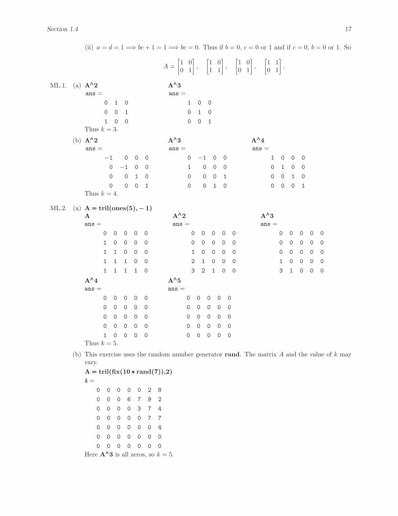
Section 1.4 17
(ii) a = d = 1 =⇒ bc + 1 = 1 =⇒ bc = 0. Thus if b = 0, c = 0 or 1 and if c = 0, b = 0 or 1. So
A =[1 00 1
],
[1 01 1
],
[1 00 1
],
[1 10 1
].
ML.1. (a) A∧∧∧2ans =
0 1 0
0 0 1
1 0 0
A∧∧∧3ans =
1 0 0
0 1 0
0 0 1Thus k = 3.
(b) A∧∧∧2ans =
−1 0 0 0
0 −1 0 0
0 0 1 0
0 0 0 1
A∧∧∧3ans =
0 −1 0 0
1 0 0 0
0 0 0 1
0 0 1 0
A∧∧∧4ans =
1 0 0 0
0 1 0 0
0 0 1 0
0 0 0 1Thus k = 4.
ML.2. (a) A === tril(ones(5),−−− 1)Aans =
0 0 0 0 0
1 0 0 0 0
1 1 0 0 0
1 1 1 0 0
1 1 1 1 0
A∧∧∧2ans =
0 0 0 0 0
0 0 0 0 0
1 0 0 0 0
2 1 0 0 0
3 2 1 0 0
A∧∧∧3ans =
0 0 0 0 0
0 0 0 0 0
0 0 0 0 0
1 0 0 0 0
3 1 0 0 0
A∧∧∧4ans =
0 0 0 0 0
0 0 0 0 0
0 0 0 0 0
0 0 0 0 0
1 0 0 0 0
A∧∧∧5ans =
0 0 0 0 0
0 0 0 0 0
0 0 0 0 0
0 0 0 0 0
0 0 0 0 0Thus k = 5.
(b) This exercise uses the random number generator rand. The matrix A and the value of k mayvary.A === tril(fix(10 ∗∗∗ rand(7)),2)A =
0 0 0 0 0 2 8
0 0 0 6 7 9 2
0 0 0 0 3 7 4
0 0 0 0 0 7 7
0 0 0 0 0 0 4
0 0 0 0 0 0 0
0 0 0 0 0 0 0
Here A∧∧∧3 is all zeros, so k = 5.
18 Chapter 1
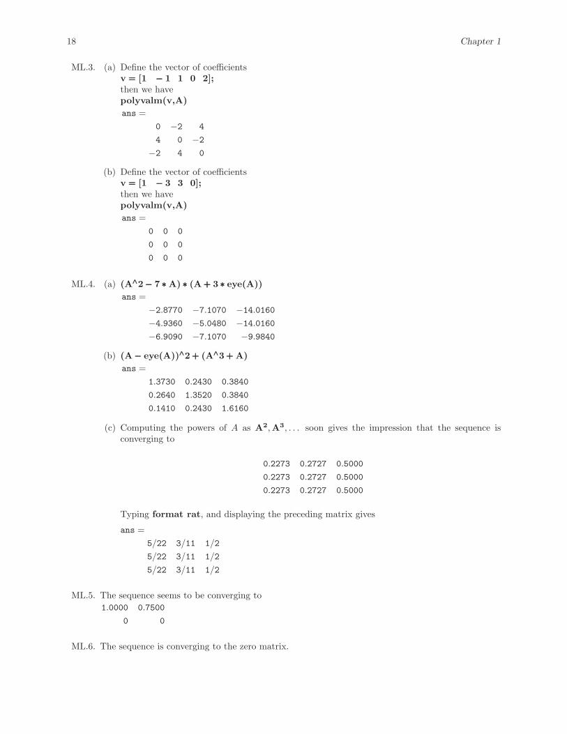
ML.3. (a) Define the vector of coefficientsv === [1 −−− 1 1 0 2];then we havepolyvalm(v,A)ans =
0 −2 4
4 0 −2−2 4 0
(b) Define the vector of coefficientsv === [1 −−− 3 3 0];then we havepolyvalm(v,A)ans =
0 0 0
0 0 0
0 0 0
ML.4. (a) (A∧∧∧2−−− 7 ∗∗∗ A) ∗∗∗ (A+++ 3 ∗∗∗ eye(A))ans =
−2.8770 −7.1070 −14.0160−4.9360 −5.0480 −14.0160−6.9090 −7.1070 −9.9840
(b) (A−−− eye(A))∧∧∧2+++ (A∧∧∧3+++ A)ans =
1.3730 0.2430 0.3840
0.2640 1.3520 0.3840
0.1410 0.2430 1.6160
(c) Computing the powers of A as A2,A3, . . . soon gives the impression that the sequence isconverging to
0.2273 0.2727 0.5000
0.2273 0.2727 0.5000
0.2273 0.2727 0.5000
Typing format rat, and displaying the preceding matrix gives
ans =5/22 3/11 1/2
5/22 3/11 1/2
5/22 3/11 1/2
ML.5. The sequence seems to be converging to1.0000 0.7500
0 0
ML.6. The sequence is converging to the zero matrix.
Section 1.5 19
ML.7. (a) A′′′ ∗∗∗ Aans =
2 −3 −1−3 9 2
−1 2 6
A ∗∗∗ A′′′
ans =6 −1 −3
−1 6 4
−3 4 5
AT A and AAT are not equal.
(b) B === A+++ A′′′
B =2 −3 1
−3 2 4
1 4 2
C === A−−− A′′′
C =0 −1 1
1 0 0
−1 0 0
Just observe that B = BT and that CT = −C.
(c) B+++ Cans =
2 −4 2
−2 2 4
0 4 2We see that B + C = 2A.
ML.8. (a) Use command B = binrand(3,3). The results will vary.
(b) B + B = O, B + B + B = B.
(c) If n is even, the result is O; otherwise it is B.
ML.9. k = 4.
ML.10. k = 4.
ML.11. k = 8.
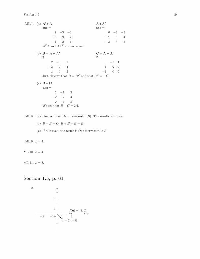
Section 1.5, p. 61
2. y
x
(1, )
3
1
−1−3
(3, 0)
31
−2u =
f(u) =
O
20 Chapter 1
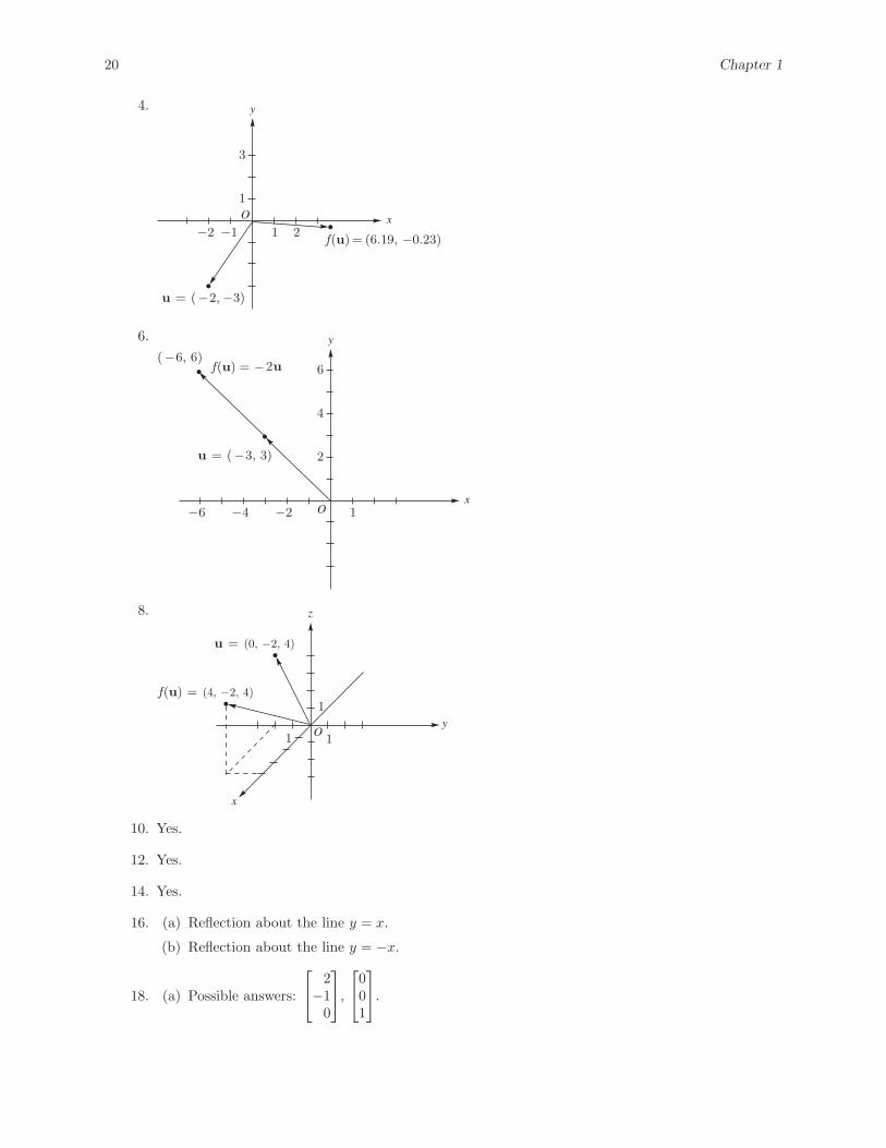
4. y
x
3
1
−1−2 21
u =
f(u)
( 2, 3)− −
= (6.19, −0.23)
O
6. y
x
2
4
6
−2−4−6 1
u =
f(u)
( 3, 3)−
= − u2( 6, 6)−
O
8.
y
x
1
1
u =
f(u) =
z
(0, −2, 4)
(4, −2, 4)
1O
10. Yes.
12. Yes.
14. Yes.
16. (a) Reflection about the line y = x.
(b) Reflection about the line y = −x.
18. (a) Possible answers:
⎡⎣ 2−1
0
⎤⎦,
⎡⎣001
⎤⎦.
Section 1.6 21
(b) Possible answers:
⎡⎣044
⎤⎦,
⎡⎣120
⎤⎦.
T.1. (a) f(u + v) = A(u + v) = Au + Av = f(u) + f(v).
(b) f(cu) = A(cu) = c(Au) = cf(u).
(c) f(cu + dv) = A(cu + dv) = A(cu) + A(cv) = c(Au) + d(Av) = cf(u) + df(v).
T.2. For any real numbers c and d, we have
f(cu+dv) = A(cu+dv) = A(cu)+A(dv) = c(Au)+d(Av) = cf(u)+df(v) = c0+d0 = 0+0 = 0.
T.3. (a) O(u) =
⎡⎢⎣0 · · · 0...
0 · · · 0
⎤⎥⎦⎡⎢⎣u1
...un
⎤⎥⎦ =
⎡⎢⎣0...0
⎤⎥⎦ = 0.
(b) I(u) =
⎡⎢⎣1 0 · · · 0...
0 0 · · · 1
⎤⎥⎦⎡⎢⎣u1
...un
⎤⎥⎦ =
⎡⎢⎣u1
...un
⎤⎥⎦ = u.
Section 1.6, p. 85
2. Neither.
4. Neither.
6. Neither.
8. Neither.
10. (a)
⎡⎣ 2 0 4 2−1 3 1 1
3 −2 5 6
⎤⎦.
(b)
⎡⎣ 2 0 4 2−12 8 −20 −24−1 3 1 1
⎤⎦.
(c)
⎡⎣ 0 6 6 43 −2 5 6
−1 3 1 1
⎤⎦.
12. Possible answers:
(a)
⎡⎣ 4 3 7 52 0 1 4
−2 4 −2 6
⎤⎦.
(b)
⎡⎣ 3 5 6 8−4 8 −4 12
2 0 1 4
⎤⎦.
(c)
⎡⎣ 4 3 7 5−1 2 −1 3
0 4 −1 10
⎤⎦.
22 Chapter 1
14.
⎡⎢⎢⎢⎢⎢⎢⎣1 −2 0 20 1 −1 10 0 1 − 2
7
0 0 0 10 0 0 0
⎤⎥⎥⎥⎥⎥⎥⎦.
16.
⎡⎢⎢⎢⎢⎣1 −2 1 4 −30 1 − 2
3 − 73
103
0 0 0 0 00 0 0 0 0
⎤⎥⎥⎥⎥⎦.
18. (a) No. (b) Yes. (c) Yes. (d) No.
20. (a) x = 1, y = 2, z = −2. (b) No solution. (c) x = 1, y = 1, z = 0.
(d) x = 0, y = 0, z = 0.
22. (a) x = 1 − 25r, y = −1 + 1
5r, z = r. (b) x = 1 − r, y = 3 + r, z = 2 − r, w = r. (c) Nosolution.
(d) x = 0, y = 0, z = 0.
24. (a) a = ±√
3. (b) a �= ±√
3. (c) None.
26. (a) a = −3. (b) a �= ±3. (c) a = 3.
28. (a) x = r, y = −2r, z = r, r = any real number. (b) x = 1, y = 2, z = 2.
30. (a) No solution. (b) x = 1 − r, y = 2 + r, z = −1 + r, r = any real number.
32. x = −2 + r, y = 2 − 2r, z = r, where r is any real number.
34. c − b − a = 0
36.
⎡⎣ 1−1
2
⎤⎦,
⎡⎣ 02
−2
⎤⎦.
38. x = 5r, y = 6r, z = r, r = any nonzero real number.
40. −a + b − c = 0.
42. x =[rr
], r �= 0.
44. x =
⎡⎢⎢⎢⎣− 1
2r
12r
r
⎤⎥⎥⎥⎦, r �= 0.
46. x =
⎡⎢⎢⎢⎢⎢⎢⎣196
− 5930
1730
0
⎤⎥⎥⎥⎥⎥⎥⎦ +
⎡⎢⎢⎢⎢⎢⎢⎣− 1
3r
215r
1915r
r
⎤⎥⎥⎥⎥⎥⎥⎦.
48. y = 252 x2 − 61
2 x + 23.
Section 1.6 23
50. y = 23x3 + 4
3x2 − 23x + 2
3 .
52. 60 in deluxe binding. If r is the number in bookclub binding, then r is an integer which must satisfy0 ≤ r ≤ 90 and then the number of paperbacks is 180 − 2r.
54. 32x2 − x + 1
2 .
56. (a)
⎡⎣101
⎤⎦. (b)
⎡⎣010
⎤⎦.
58. (a) Inconsistent.
(b)
⎡⎢⎢⎣0000
⎤⎥⎥⎦,
⎡⎢⎢⎣0110
⎤⎥⎥⎦,
⎡⎢⎢⎣1101
⎤⎥⎥⎦,
⎡⎢⎢⎣1011
⎤⎥⎥⎦.
T.1. Suppose the leading one of the ith row occurs in the jth column. Since leading ones of rowsi + 1, i + 2, . . . are to the right of that of the ith row, and in any nonzero row, the leading one is thefirst nonzero element, all entries in the jth column below the ith row must be zero.
T.2. (a) A is row equivalent to itself: the sequence of operations is the empty sequence.
(b) Each elementary row operation of types (a), (b) or (c) has a corresponding inverse operation ofthe same type which “undoes” the effect of the original operation. For example, the inverse ofthe operations “add d times row r of A to row s of A” is “add −d times row r of A to row s ofA.” Since B is assumed row equivalent to A, there is a sequence of elementary row operationswhich gets from A to B. Take those operations in the reverse order, and for each operation doits inverse, and that takes B to A. Thus A is row equivalent to B.
(c) Follow the operations which take A to B with those which take B to C.
T.3. The sequence of elementary row operations which takes A to B, when applied to the augmentedmatrix
[A 0
], yields the augmented matrix
[B 0
]. Thus both systems have the same solutions,
by Theorem 1.7.
T.4. A linear system whose augmented matrix has the row[0 0 0 · · · 0 1
](1.2)
can have no solution: that row corresponds to the unsolvable equation 0x1 + 0x2 + · · · + 0xn = 1.If the augmented matrix of Ax = b is row equivalent to a matrix with the row (1.2) above, then byTheorem 1.7, Ax = b can have no solution.
Conversely, assume Ax = b has no solution. Its augmented matrix is row equivalent to some matrix[C D
]in reduced row echelon form. If
[C D
]does not contain the row (1.2) then it has at most
m nonzero rows, and the leading entries of those nonzero rows all correspond to unknowns of thesystem. After assigning values to the free variables — the variables not corresponding to leadingentries of rows — one gets a solution to the system by solving for the values of the leading entryvariables. This contradicts the assumption that the system had no solution.
T.5. If ad − bc = 0, the two rows of
A =[a bc d
]are multiples of one another:
c[a b
]=
[ac bc
]and a
[c d
]=
[ac ad
]and bc = ad.
24 Chapter 1
Any elementary row operation applied to A will produce a matrix with rows that are multiplesof each other. In particular, elementary row operations cannot produce I2, and so I2 is not rowequivalent to A. If ad − bc �= 0, then a and c are not both 0. Suppose a �= 0.
a b 1 0 Multiply the first row by 1a , and add (−c) times
the first row to the second row.
c d 0 1
1b
a
1a
0 Multiply the second row by aad−bc .
0 d − bc
a− c
a1
1b
a
1a
0 Add(− b
a
)times the second row to the first row.
0 1−c
ad − bc
1ad − bc
1 0d
ad − bc
−b
ad − bc
0 1−c
ad − bc
a
ad − bc
T.6. (a) Since a(kb) − b(ka) = 0, it follows from Exercise T.5 that A is not row equivalent to I2.
(b) Suppose that A =[0 0a b
]. Since 0 · b − 0 · c = 0, it follows from Exercise T.5 that A is not
row equivalent to I2.
T.7. For any angle θ, cos θ and sin θ are not both zero. Assume that cos θ �= 0 and proceed as follows.The row operation 1
cos θ times row 1 gives⎡⎢⎢⎣ 1sin θ
cos θ
− sin θ cos θ
⎤⎥⎥⎦ .
Applying row operation sin θ times row 1 added to row 2 we obtain⎡⎢⎢⎢⎢⎣1
sin θ
cos θ
0 cos θ +sin2 θ
cos θ
⎤⎥⎥⎥⎥⎦ .
Simplifying the (2, 2)-entry we have
cos θ +sin2 θ
cos θ=
cos2 θ + sin2 θ
cos θ=
1cos θ
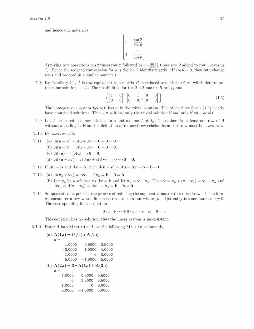
Section 1.6 25
and hence our matrix is ⎡⎢⎢⎢⎢⎣1
sin θ
cos θ
01
cos θ
⎤⎥⎥⎥⎥⎦ .
Applying row operations cos θ times row 2 followed by(− sin θ
cos θ
)times row 2 added to row 1 gives us
I2. Hence the reduced row echelon form is the 2× 2 identity matrix. (If cos θ = 0, then interchangerows and proceed in a similar manner.)
T.8. By Corollary 1.1, A is row equivalent to a matrix B in reduced row echelon form which determinesthe same solutions as A. The possibilities for the 2 × 2 matrix B are I2 and{[
1 00 0
],
[0 10 0
],
[0 00 0
]}. (1.3)
The homogeneous system I2x = 0 has only the trivial solution. The other three forms (1.3) clearlyhave nontrivial solutions. Thus Ax = 0 has only the trivial solution if and only if ad − bc �= 0.
T.9. Let A be in reduced row echelon form and assume A �= In. Thus there is at least one row of Awithout a leading 1. From the definition of reduced row echelon form, this row must be a zero row.
T.10. By Exercise T.8.
T.11. (a) A(u + v) = Au + Av = 0 + 0 = 0.(b) A(u − v) = Au − Av = 0 − 0 = 0.(c) A(ru) = r(Au) = r0 = 0.(d) A(ru + sv) = r(Au) + s(Av) = r0 + s0 = 0.
T.12. If Au = b and Av = b, then A(u − v) = Au − Av = b − b = 0.
T.13. (a) A(xp + xh) = Axp + Axh = b + 0 = b.(b) Let xp be a solution to Ax = b and let xh = x − xp. Then x = xp + (x − xp) = xp + xh and
Axh = A(x − xp) = Ax − Axp = b − b = 0.
T.14. Suppose at some point in the process of reducing the augmented matrix to reduced row echelon formwe encounter a row whose first n entries are zero but whose (n + 1)st entry is some number c �= 0.The corresponding linear equation is
0 · x1 + · · · + 0 · xn = c or 0 = c.
This equation has no solution, thus the linear system is inconsistent.
ML.1. Enter A into Matlab and use the following Matlab commands.
(a) A(1,:) === (1/4) ∗∗∗ A(1,:)A =
1.0000 0.5000 0.5000−3.0000 1.0000 4.00001.0000 0 3.00005.0000 −1.0000 5.0000
(b) A(2,:) === 3 ∗∗∗ A(1,:) +++ A(2,:)A =
1.0000 0.5000 0.50000 2.5000 5.5000
1.0000 0 3.00005.0000 −1.0000 5.0000
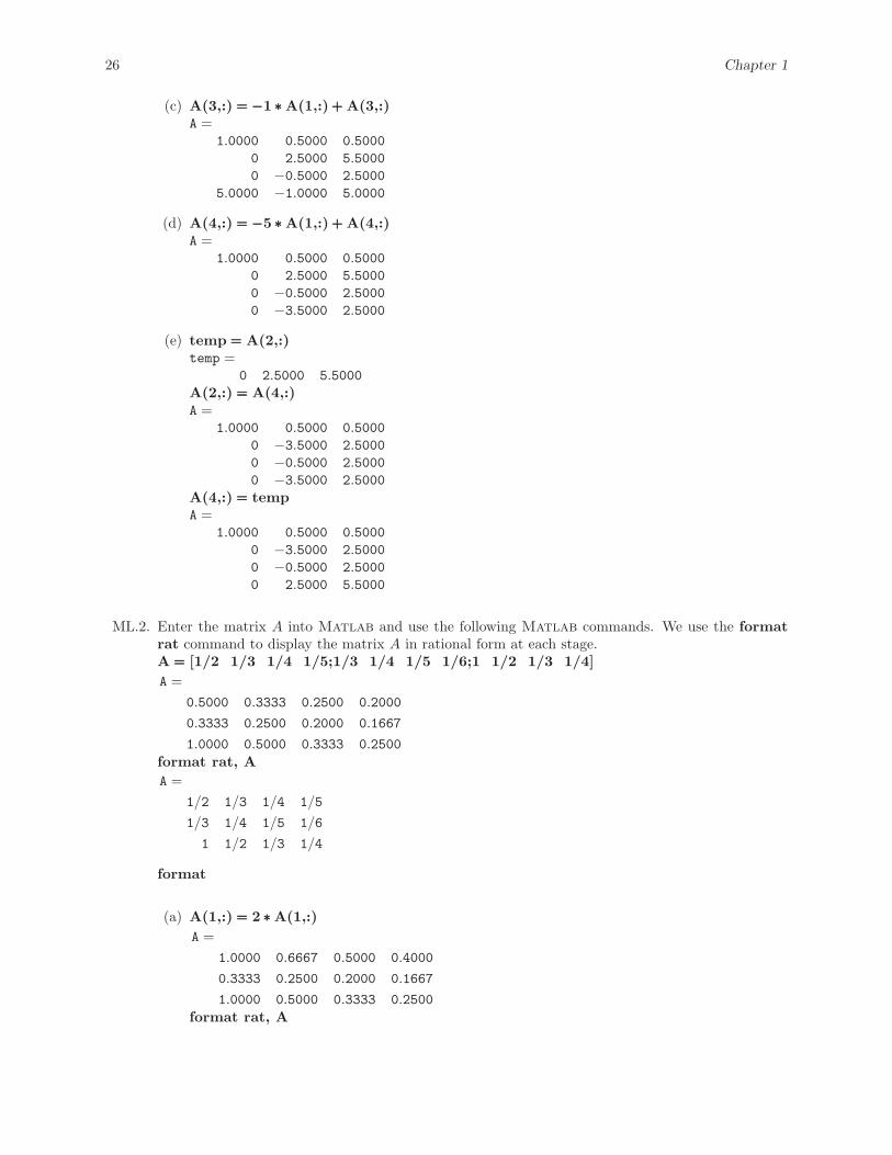
26 Chapter 1
(c) A(3,:) === −−−1 ∗∗∗ A(1,:) +++ A(3,:)A =
1.0000 0.5000 0.50000 2.5000 5.50000 −0.5000 2.5000
5.0000 −1.0000 5.0000
(d) A(4,:) === −−−5 ∗∗∗ A(1,:) +++ A(4,:)A =
1.0000 0.5000 0.50000 2.5000 5.50000 −0.5000 2.50000 −3.5000 2.5000
(e) temp === A(2,:)temp =
0 2.5000 5.5000A(2,:) === A(4,:)A =
1.0000 0.5000 0.50000 −3.5000 2.50000 −0.5000 2.50000 −3.5000 2.5000
A(4,:) === tempA =
1.0000 0.5000 0.50000 −3.5000 2.50000 −0.5000 2.50000 2.5000 5.5000
ML.2. Enter the matrix A into Matlab and use the following Matlab commands. We use the formatrat command to display the matrix A in rational form at each stage.A === [1/2 1/3 1/4 1/5;1/3 1/4 1/5 1/6;1 1/2 1/3 1/4]A =
0.5000 0.3333 0.2500 0.2000
0.3333 0.2500 0.2000 0.1667
1.0000 0.5000 0.3333 0.2500format rat, AA =
1/2 1/3 1/4 1/5
1/3 1/4 1/5 1/6
1 1/2 1/3 1/4
format
(a) A(1,:) === 2 ∗∗∗ A(1,:)A =
1.0000 0.6667 0.5000 0.4000
0.3333 0.2500 0.2000 0.1667
1.0000 0.5000 0.3333 0.2500format rat, A
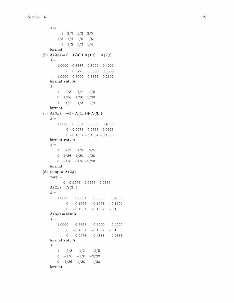
Section 1.6 27
A =1 2/3 1/2 2/5
1/3 1/4 1/5 1/6
1 1/2 1/3 1/4
format(b) A(2,:) === (−−− 1/3) ∗∗∗ A(1,:) +++ A(2,:)
A =1.0000 0.6667 0.5000 0.4000
0 0.0278 0.0333 0.0333
1.0000 0.5000 0.3333 0.2500format rat, AA =
1 2/3 1/2 2/5
0 1/36 1/30 1/30
1 1/2 1/3 1/4
format(c) A(3,:) === −−−1 ∗∗∗ A(1,:) +++ A(3,:)
A =1.0000 0.6667 0.5000 0.4000
0 0.0278 0.0333 0.0333
0 −0.1667 −0.1667 −0.1500format rat, AA =
1 2/3 1/2 2/5
0 1/36 1/30 1/30
0 −1/6 −1/6 −3/20format
(d) temp === A(2,:)temp =
0 0.0278 0.0333 0.0333A(2,:) === A(3,:)A =
1.0000 0.6667 0.5000 0.4000
0 −0.1667 −0.1667 −0.15000 −0.1667 −0.1667 −0.1500
A(3,:) === tempA =
1.0000 0.6667 0.5000 0.4000
0 −0.1667 −0.1667 −0.15000 0.0278 0.0333 0.0333
format rat, AA =
1 2/3 1/2 2/5
0 −1/6 −1/6 −3/200 1/36 1/30 1/30
format
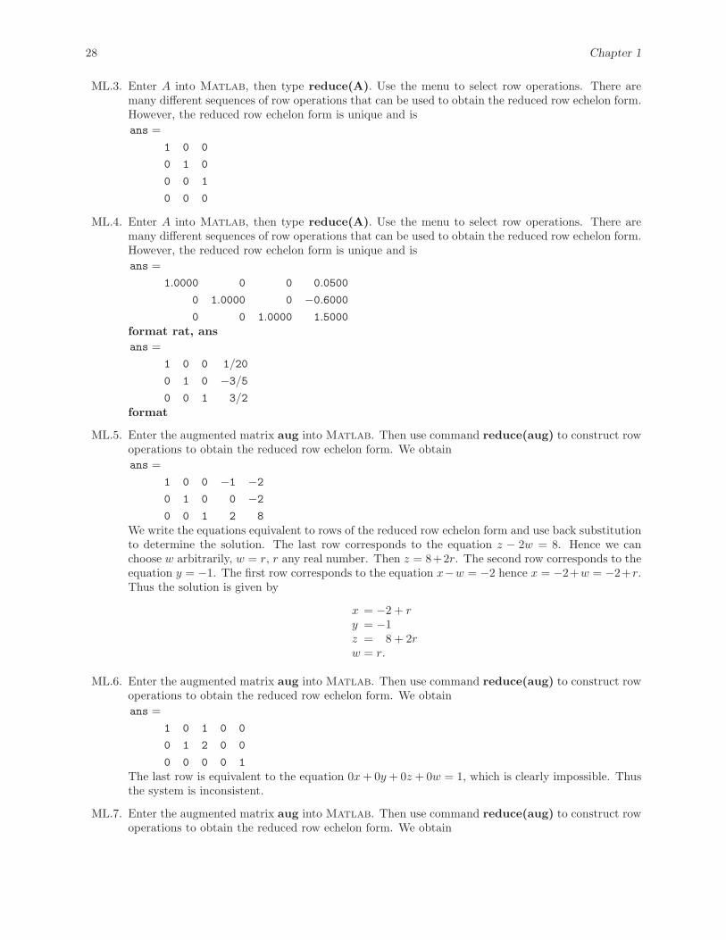
28 Chapter 1
ML.3. Enter A into Matlab, then type reduce(A). Use the menu to select row operations. There aremany different sequences of row operations that can be used to obtain the reduced row echelon form.However, the reduced row echelon form is unique and isans =
1 0 0
0 1 0
0 0 1
0 0 0
ML.4. Enter A into Matlab, then type reduce(A). Use the menu to select row operations. There aremany different sequences of row operations that can be used to obtain the reduced row echelon form.However, the reduced row echelon form is unique and isans =
1.0000 0 0 0.0500
0 1.0000 0 −0.60000 0 1.0000 1.5000
format rat, ansans =
1 0 0 1/20
0 1 0 −3/50 0 1 3/2
format
ML.5. Enter the augmented matrix aug into Matlab. Then use command reduce(aug) to construct rowoperations to obtain the reduced row echelon form. We obtainans =
1 0 0 −1 −20 1 0 0 −20 0 1 2 8
We write the equations equivalent to rows of the reduced row echelon form and use back substitutionto determine the solution. The last row corresponds to the equation z − 2w = 8. Hence we canchoose w arbitrarily, w = r, r any real number. Then z = 8+2r. The second row corresponds to theequation y = −1. The first row corresponds to the equation x−w = −2 hence x = −2+w = −2+r.Thus the solution is given by
x = −2 + ry = −1z = 8 + 2rw = r.
ML.6. Enter the augmented matrix aug into Matlab. Then use command reduce(aug) to construct rowoperations to obtain the reduced row echelon form. We obtainans =
1 0 1 0 0
0 1 2 0 0
0 0 0 0 1The last row is equivalent to the equation 0x + 0y + 0z + 0w = 1, which is clearly impossible. Thusthe system is inconsistent.
ML.7. Enter the augmented matrix aug into Matlab. Then use command reduce(aug) to construct rowoperations to obtain the reduced row echelon form. We obtain
Section 1.6 29
ans =1 0 0 0
0 1 0 0
0 0 1 0
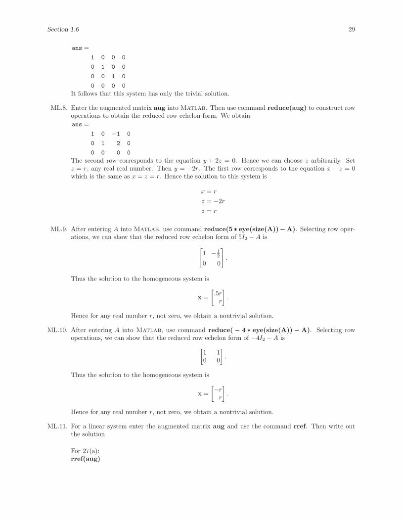
0 0 0 0It follows that this system has only the trivial solution.
ML.8. Enter the augmented matrix aug into Matlab. Then use command reduce(aug) to construct rowoperations to obtain the reduced row echelon form. We obtainans =
1 0 −1 0
0 1 2 0
0 0 0 0The second row corresponds to the equation y + 2z = 0. Hence we can choose z arbitrarily. Setz = r, any real real number. Then y = −2r. The first row corresponds to the equation x − z = 0which is the same as x = z = r. Hence the solution to this system is
x = r
z = −2r
z = r
ML.9. After entering A into Matlab, use command reduce(5 ∗∗∗ eye(size(A))−−− A). Selecting row oper-ations, we can show that the reduced row echelon form of 5I2 − A is[
1 − 12
0 0
].
Thus the solution to the homogeneous system is
x =[.5r
r
].
Hence for any real number r, not zero, we obtain a nontrivial solution.
ML.10. After entering A into Matlab, use command reduce( −−− 4 ∗∗∗ eye(size(A)) −−− A). Selecting rowoperations, we can show that the reduced row echelon form of −4I2 − A is[
1 10 0
].
Thus the solution to the homogeneous system is
x =[−r
r
].
Hence for any real number r, not zero, we obtain a nontrivial solution.
ML.11. For a linear system enter the augmented matrix aug and use the command rref. Then write outthe solution
For 27(a):rref(aug)
30 Chapter 1
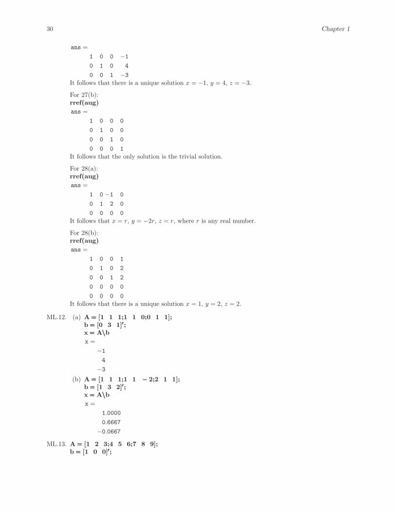
ans =1 0 0 −10 1 0 4
0 0 1 −3It follows that there is a unique solution x = −1, y = 4, z = −3.
For 27(b):rref(aug)ans =
1 0 0 0
0 1 0 0
0 0 1 0
0 0 0 1It follows that the only solution is the trivial solution.
For 28(a):rref(aug)ans =
1 0 −1 0
0 1 2 0
0 0 0 0It follows that x = r, y = −2r, z = r, where r is any real number.
For 28(b):rref(aug)ans =
1 0 0 1
0 1 0 2
0 0 1 2
0 0 0 0
0 0 0 0It follows that there is a unique solution x = 1, y = 2, z = 2.
ML.12. (a) A === [1 1 1;1 1 0;0 1 1];b === [0 3 1]′′′;x === A\\\bx =
−14
−3(b) A === [1 1 1;1 1 −−− 2;2 1 1];
b === [1 3 2]′′′;x === A\\\bx =
1.0000
0.6667
−0.0667
ML.13. A === [1 2 3;4 5 6;7 8 9];b === [1 0 0]′′′;
Section 1.7 31
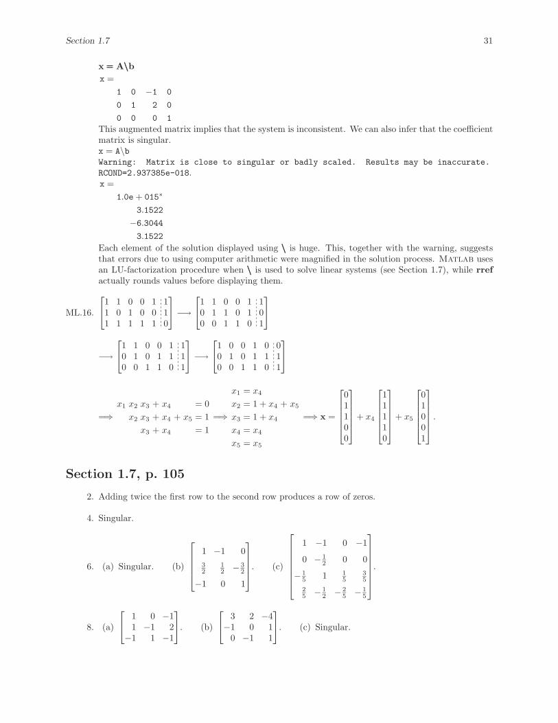
x === A\\\bx =
1 0 −1 0
0 1 2 0
0 0 0 1This augmented matrix implies that the system is inconsistent. We can also infer that the coefficientmatrix is singular.x = A\bWarning: Matrix is close to singular or badly scaled. Results may be inaccurate.RCOND=2.937385e-018.x =
1.0e + 015∗
3.1522
−6.30443.1522
Each element of the solution displayed using \\\ is huge. This, together with the warning, suggeststhat errors due to using computer arithmetic were magnified in the solution process. Matlab usesan LU-factorization procedure when \\\ is used to solve linear systems (see Section 1.7), while rrefactually rounds values before displaying them.
ML.16.
⎡⎣1 1 0 0 1 11 0 1 0 0 11 1 1 1 1 0
⎤⎦ −→
⎡⎣1 1 0 0 1 10 1 1 0 1 00 0 1 1 0 1
⎤⎦
−→
⎡⎣1 1 0 0 1 10 1 0 1 1 10 0 1 1 0 1
⎤⎦ −→
⎡⎣1 0 0 1 0 00 1 0 1 1 10 0 1 1 0 1
⎤⎦
=⇒x1 x2 x3 + x4 = 0
x2 x3 + x4 + x5 = 1x3 + x4 = 1
=⇒
x1 = x4
x2 = 1 + x4 + x5
x3 = 1 + x4
x4 = x4
x5 = x5
=⇒ x =
⎡⎢⎢⎢⎢⎣01100
⎤⎥⎥⎥⎥⎦ + x4
⎡⎢⎢⎢⎢⎣11110
⎤⎥⎥⎥⎥⎦ + x5
⎡⎢⎢⎢⎢⎣01001
⎤⎥⎥⎥⎥⎦ .
Section 1.7, p. 105
2. Adding twice the first row to the second row produces a row of zeros.
4. Singular.
6. (a) Singular. (b)
⎡⎢⎢⎢⎣1 −1 032
12 − 3
2
−1 0 1
⎤⎥⎥⎥⎦. (c)
⎡⎢⎢⎢⎢⎢⎢⎣1 −1 0 −1
0 − 12 0 0
− 15 1 1
535
25 − 1
2 − 25 − 1
5
⎤⎥⎥⎥⎥⎥⎥⎦.
8. (a)
⎡⎣ 1 0 −11 −1 2
−1 1 −1
⎤⎦. (b)
⎡⎣ 3 2 −4−1 0 1
0 −1 1
⎤⎦. (c) Singular.
32 Chapter 1
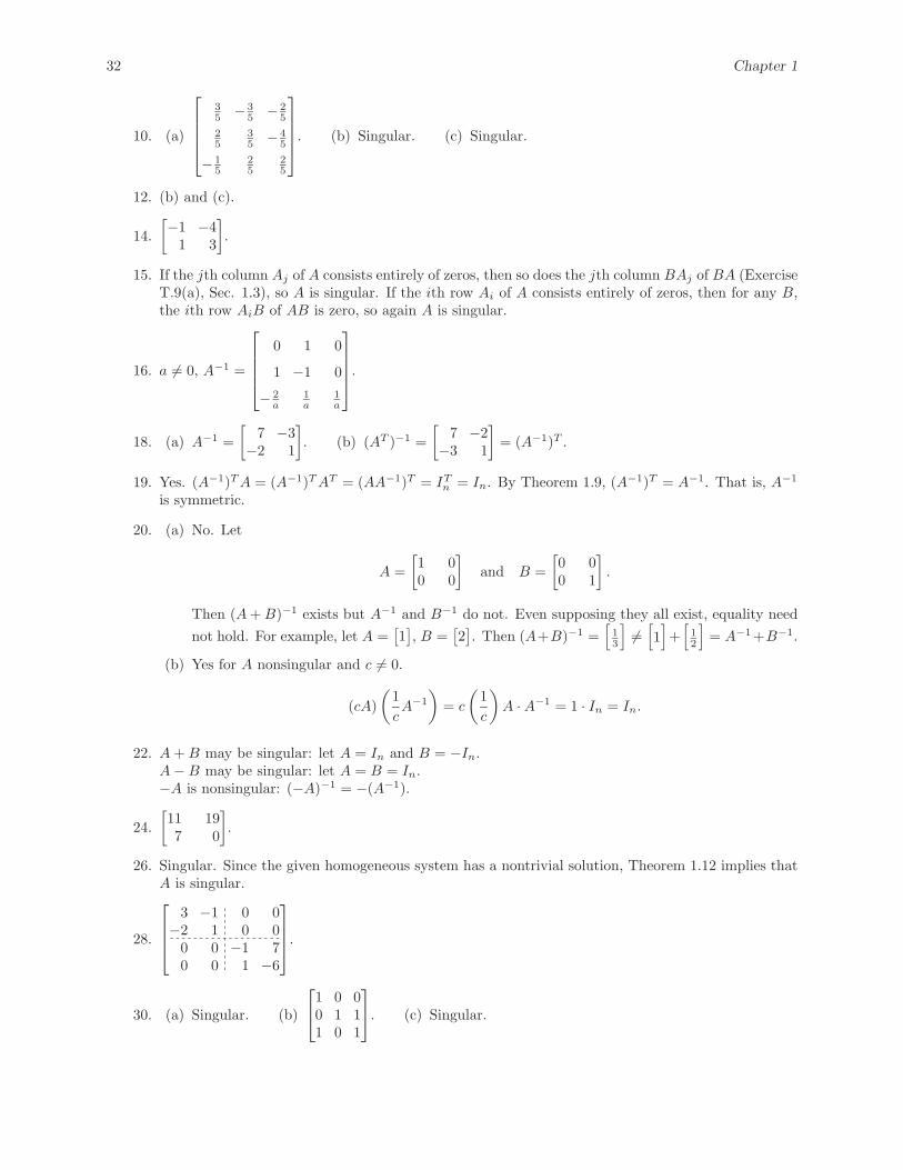
10. (a)
⎡⎢⎢⎢⎣35 − 3
5 − 25
25
35 − 4
5
− 15
25
25
⎤⎥⎥⎥⎦. (b) Singular. (c) Singular.
12. (b) and (c).
14.[−1 −4
1 3
].
15. If the jth column Aj of A consists entirely of zeros, then so does the jth column BAj of BA (ExerciseT.9(a), Sec. 1.3), so A is singular. If the ith row Ai of A consists entirely of zeros, then for any B,the ith row AiB of AB is zero, so again A is singular.
16. a �= 0, A−1 =
⎡⎢⎢⎢⎣0 1 0
1 −1 0
− 2a
1a
1a
⎤⎥⎥⎥⎦.
18. (a) A−1 =[
7 −3−2 1
]. (b) (AT )−1 =
[7 −2
−3 1
]= (A−1)T .
19. Yes. (A−1)T A = (A−1)T AT = (AA−1)T = ITn = In. By Theorem 1.9, (A−1)T = A−1. That is, A−1
is symmetric.
20. (a) No. Let
A =[1 00 0
]and B =
[0 00 1
].
Then (A + B)−1 exists but A−1 and B−1 do not. Even supposing they all exist, equality neednot hold. For example, let A =
[1], B =
[2]. Then (A+B)−1 =
[13
]�=
[1]+
[12
]= A−1+B−1.
(b) Yes for A nonsingular and c �= 0.
(cA)(
1cA−1
)= c
(1c
)A · A−1 = 1 · In = In.
22. A + B may be singular: let A = In and B = −In.A − B may be singular: let A = B = In.−A is nonsingular: (−A)−1 = −(A−1).
24.[11 197 0
].
26. Singular. Since the given homogeneous system has a nontrivial solution, Theorem 1.12 implies thatA is singular.
28.
⎡⎢⎢⎣3 −1 0 0
−2 1 0 00 0 −1 70 0 1 −6
⎤⎥⎥⎦.
30. (a) Singular. (b)
⎡⎣1 0 00 1 11 0 1
⎤⎦. (c) Singular.
Section 1.7 33
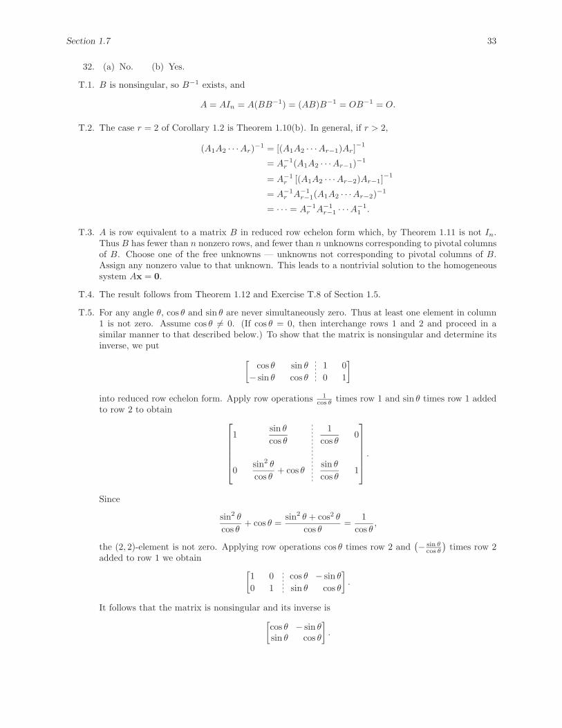
32. (a) No. (b) Yes.
T.1. B is nonsingular, so B−1 exists, and
A = AIn = A(BB−1) = (AB)B−1 = OB−1 = O.
T.2. The case r = 2 of Corollary 1.2 is Theorem 1.10(b). In general, if r > 2,
(A1A2 · · ·Ar)−1 = [(A1A2 · · ·Ar−1)Ar]−1
= A−1r (A1A2 · · ·Ar−1)−1
= A−1r [(A1A2 · · ·Ar−2)Ar−1]
−1
= A−1r A−1
r−1(A1A2 · · ·Ar−2)−1
= · · · = A−1r A−1
r−1 · · ·A−11 .
T.3. A is row equivalent to a matrix B in reduced row echelon form which, by Theorem 1.11 is not In.Thus B has fewer than n nonzero rows, and fewer than n unknowns corresponding to pivotal columnsof B. Choose one of the free unknowns — unknowns not corresponding to pivotal columns of B.Assign any nonzero value to that unknown. This leads to a nontrivial solution to the homogeneoussystem Ax = 0.
T.4. The result follows from Theorem 1.12 and Exercise T.8 of Section 1.5.
T.5. For any angle θ, cos θ and sin θ are never simultaneously zero. Thus at least one element in column1 is not zero. Assume cos θ �= 0. (If cos θ = 0, then interchange rows 1 and 2 and proceed in asimilar manner to that described below.) To show that the matrix is nonsingular and determine itsinverse, we put [
cos θ sin θ 1 0− sin θ cos θ 0 1
]into reduced row echelon form. Apply row operations 1
cos θ times row 1 and sin θ times row 1 addedto row 2 to obtain ⎡⎢⎢⎢⎢⎢⎣
1sin θ
cos θ
1cos θ
0
0sin2 θ
cos θ+ cos θ
sin θ
cos θ1
⎤⎥⎥⎥⎥⎥⎦ .
Since
sin2 θ
cos θ+ cos θ =
sin2 θ + cos2 θ
cos θ=
1cos θ
,
the (2, 2)-element is not zero. Applying row operations cos θ times row 2 and(− sin θ
cos θ
)times row 2
added to row 1 we obtain [1 0 cos θ − sin θ
0 1 sin θ cos θ
].
It follows that the matrix is nonsingular and its inverse is[cos θ − sin θsin θ cos θ
].
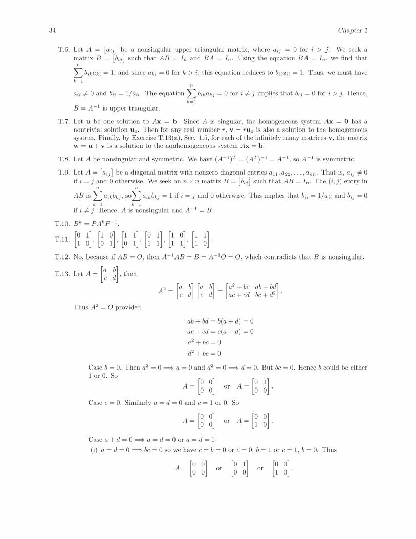
34 Chapter 1
T.6. Let A =[aij
]be a nonsingular upper triangular matrix, where aij = 0 for i > j. We seek a
matrix B =[bij
]such that AB = In and BA = In. Using the equation BA = In, we find that
n∑k=1
bikaki = 1, and since aki = 0 for k > i, this equation reduces to biiaii = 1. Thus, we must have
aii �= 0 and bii = 1/aii. The equationn∑
k=1
bikakj = 0 for i �= j implies that bij = 0 for i > j. Hence,
B = A−1 is upper triangular.
T.7. Let u be one solution to Ax = b. Since A is singular, the homogeneous system Ax = 0 has anontrivial solution u0. Then for any real number r, v = ru0 is also a solution to the homogeneoussystem. Finally, by Exercise T.13(a), Sec. 1.5, for each of the infinitely many matrices v, the matrixw = u + v is a solution to the nonhomogeneous system Ax = b.
T.8. Let A be nonsingular and symmetric. We have (A−1)T = (AT )−1 = A−1, so A−1 is symmetric.
T.9. Let A =[aij
]be a diagonal matrix with nonzero diagonal entries a11, a22, . . . , ann. That is, aij �= 0
if i = j and 0 otherwise. We seek an n× n matrix B =[bij
]such that AB = In. The (i, j) entry in
AB isn∑
k=1
aikbkj , son∑
k=1
aikbkj = 1 if i = j and 0 otherwise. This implies that bii = 1/aii and bij = 0
if i �= j. Hence, A is nonsingular and A−1 = B.
T.10. Bk = PAkP−1.
T.11.[0 11 0
],[1 00 1
],[1 10 1
],[0 11 1
],[1 01 1
],[1 11 0
].
T.12. No, because if AB = O, then A−1AB = B = A−1O = O, which contradicts that B is nonsingular.
T.13. Let A =[a bc d
], then
A2 =[a bc d
] [a bc d
]=
[a2 + bc ab + bdac + cd bc + d2
].
Thus A2 = O provided
ab + bd = b(a + d) = 0ac + cd = c(a + d) = 0
a2 + bc = 0
d2 + bc = 0
Case b = 0. Then a2 = 0 =⇒ a = 0 and d2 = 0 =⇒ d = 0. But bc = 0. Hence b could be either1 or 0. So
A =[0 00 0
]or A =
[0 10 0
].
Case c = 0. Similarly a = d = 0 and c = 1 or 0. So
A =[0 00 0
]or A =
[0 01 0
].
Case a + d = 0 =⇒ a = d = 0 or a = d = 1
(i) a = d = 0 =⇒ bc = 0 so we have c = b = 0 or c = 0, b = 1 or c = 1, b = 0. Thus
A =[0 00 0
]or
[0 10 0
]or
[0 01 0
].
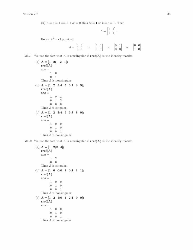
Section 1.7 35
(ii) a = d = 1 =⇒ 1 + bc = 0 thus bc = 1 so b = c = 1. Then
A =[1 11 1
].
Hence A2 = O provided
A =[0 00 0
]or
[1 11 1
]or
[0 10 0
]or
[0 01 0
].
ML.1. We use the fact that A is nonsingular if rref(A) is the identity matrix.
(a) A === [1 2;−−− 2 1];rref(A)ans =
1 00 1
Thus A is nonsingular.(b) A === [1 2 3;4 5 6;7 8 9];
rref(A)ans =
1 0 −10 1 20 0 0
Thus A is singular.(c) A === [1 2 3;4 5 6;7 8 0];
rref(A)ans =
1 0 00 1 00 0 1
Thus A is nonsingular.
ML.2. We use the fact that A is nonsingular if rref(A) is the identity matrix.
(a) A === [1 2;2 4];rref(A)ans =
1 20 0
Thus A is singular.(b) A === [1 0 0;0 1 0;1 1 1];
rref(A)ans =
1 0 00 1 00 0 1
Thus A is nonsingular.(c) A === [1 2 1;0 1 2;1 0 0];
rref(A)ans =
1 0 00 1 00 0 1
Thus A is nonsingular.
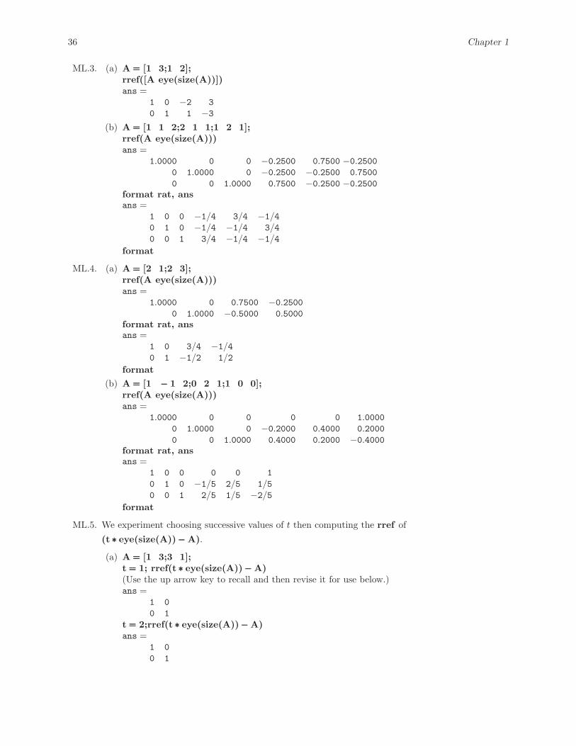
36 Chapter 1
ML.3. (a) A === [1 3;1 2];rref([A eye(size(A))])ans =
1 0 −2 30 1 1 −3
(b) A === [1 1 2;2 1 1;1 2 1];rref(A eye(size(A)))ans =
1.0000 0 0 −0.2500 0.7500 −0.25000 1.0000 0 −0.2500 −0.2500 0.75000 0 1.0000 0.7500 −0.2500 −0.2500
format rat, ansans =
1 0 0 −1/4 3/4 −1/40 1 0 −1/4 −1/4 3/40 0 1 3/4 −1/4 −1/4
format
ML.4. (a) A === [2 1;2 3];rref(A eye(size(A)))ans =
1.0000 0 0.7500 −0.25000 1.0000 −0.5000 0.5000
format rat, ansans =
1 0 3/4 −1/40 1 −1/2 1/2
format(b) A === [1 −−− 1 2;0 2 1;1 0 0];
rref(A eye(size(A)))ans =
1.0000 0 0 0 0 1.00000 1.0000 0 −0.2000 0.4000 0.20000 0 1.0000 0.4000 0.2000 −0.4000
format rat, ansans =
1 0 0 0 0 10 1 0 −1/5 2/5 1/50 0 1 2/5 1/5 −2/5
format
ML.5. We experiment choosing successive values of t then computing the rref of
(t ∗∗∗ eye(size(A))−−− A).
(a) A === [1 3;3 1];t === 1; rref(t ∗∗∗ eye(size(A))−−− A)(Use the up arrow key to recall and then revise it for use below.)ans =
1 00 1
t === 2;rref(t ∗∗∗ eye(size(A))−−− A)ans =
1 00 1

Section 1.8 37
t === 3;rref(t ∗∗∗ eye(size(A))−−− A)ans =
1 00 1
t === 4;rref(t ∗∗∗ eye(size(A))−−− A)ans =
1 −10 0
Thus t = 4.
(b) A === [4 1 2;1 4 1;0 0 −−− 4];t === 1;rref(t ∗∗∗ eye(size(A))−−− A)ans =
1 0 00 1 00 0 1
t === 2;rref(t ∗∗∗ eye(size(A))−−− A)ans =
1 0 00 1 00 0 1
t === 3;rref(t ∗∗∗ eye(size(A))−−− A)ans =
1 1 00 0 10 0 0
Thus t = 3.
ML.8. (a) Nonsingular. (b) Singular.
ML.9.
⎡⎣1 0 00 1 00 0 1
⎤⎦ and
⎡⎣1 1 10 1 10 0 1
⎤⎦ have inverses, but there are others.
⎡⎣1 0 10 1 10 1 1
⎤⎦ and
⎡⎣0 0 00 1 11 0 1
⎤⎦ do not have inverses, but there are others.
Section 1.8, p. 113
2. x =
⎡⎣ 0−2
3
⎤⎦. 4. x =
⎡⎢⎢⎣2
−105
⎤⎥⎥⎦.
6. L =
⎡⎣ 1 0 04 1 0
−5 3 1
⎤⎦, U =
⎡⎣−3 1 −20 6 20 0 −4
⎤⎦, x =
⎡⎣−34
−1
⎤⎦.
8. L =
⎡⎢⎢⎣1 0 0 06 1 0 0
−1 2 1 0−2 3 2 1
⎤⎥⎥⎦, U =
⎡⎢⎢⎣−5 4 0 1
0 3 2 10 0 −4 10 0 0 −2
⎤⎥⎥⎦, x =
⎡⎢⎢⎣1
−25
−4
⎤⎥⎥⎦.
38 Chapter 1
10. L =
⎡⎢⎢⎣1 0 0 0
0.2 1 0 0−0.4 0.8 1 0
2 −1.2 −0.4 1
⎤⎥⎥⎦, U =
⎡⎢⎢⎣4 1 0.25 − 0.50 0.4 1.2 −2.50 0 − 0.85 20 0 0 −2.5
⎤⎥⎥⎦, x =
⎡⎢⎢⎣−1.5
4.22.6−2
⎤⎥⎥⎦.
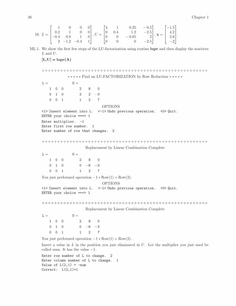
ML.1. We show the first few steps of the LU-factorization using routine lupr and then display the matricesL and U .
[L,U] === lupr(A)
++++++++++++++++++++++++++++++++++++++++++++++++++++++
∗ ∗ ∗ ∗ ∗ Find an LU-FACTORIZATION by Row Reduction ∗ ∗ ∗ ∗ ∗L =
1 0 0
0 1 0
0 0 1
U =2 8 0
2 2 −31 2 7
OPTIONS<1> Insert element into L. <-1> Undo previous operation. <0> Quit.ENTER your choice ===> 1
Enter multiplier. -1Enter first row number. 1Enter number of row that changes. 2
++++++++++++++++++++++++++++++++++++++++++++++++++++++
Replacement by Linear Combination Complete
L =1 0 0
0 1 0
0 0 1
U =2 8 0
0 −6 −31 2 7
You just performed operation −1 ∗ Row(1) + Row(2).
OPTIONS<1> Insert element into L. <-1> Undo previous operation. <0> Quit.ENTER your choice ===> 1
++++++++++++++++++++++++++++++++++++++++++++++++++++++
Replacement by Linear Combination Complete
L =1 0 0
0 1 0
0 0 1
U =2 8 0
0 −6 −31 2 7
You just performed operation −1 ∗ Row(1) + Row(2).
Insert a value in L in the position you just eliminated in U . Let the multiplier you just used becalled num. It has the value −1.
Enter row number of L to change. 2Enter column number of L to change. 1Value of L(2,1) = -numCorrect: L(2,1)=1
Section 1.8 39
++++++++++++++++++++++++++++++++++++++++++++++++++++++
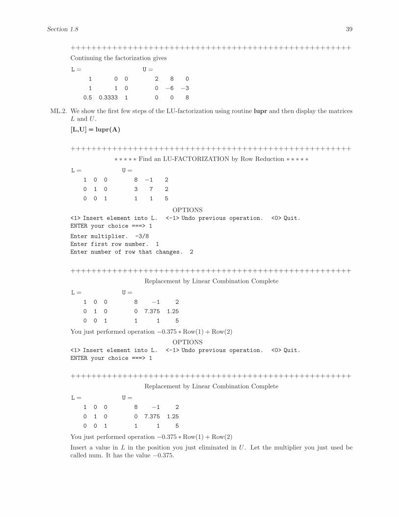
Continuing the factorization gives
L =1 0 0
1 1 0
0.5 0.3333 1
U =2 8 0
0 −6 −30 0 8
ML.2. We show the first few steps of the LU-factorization using routine lupr and then display the matricesL and U .
[L,U] === lupr(A)
++++++++++++++++++++++++++++++++++++++++++++++++++++++
∗ ∗ ∗ ∗ ∗ Find an LU-FACTORIZATION by Row Reduction ∗ ∗ ∗ ∗ ∗L =
1 0 0
0 1 0
0 0 1
U =8 −1 2
3 7 2
1 1 5
OPTIONS<1> Insert element into L. <-1> Undo previous operation. <0> Quit.ENTER your choice ===> 1
Enter multiplier. -3/8Enter first row number. 1Enter number of row that changes. 2
++++++++++++++++++++++++++++++++++++++++++++++++++++++
Replacement by Linear Combination Complete
L =1 0 0
0 1 0
0 0 1
U =8 −1 2
0 7.375 1.25
1 1 5
You just performed operation −0.375 ∗ Row(1) + Row(2)
OPTIONS<1> Insert element into L. <-1> Undo previous operation. <0> Quit.ENTER your choice ===> 1
++++++++++++++++++++++++++++++++++++++++++++++++++++++
Replacement by Linear Combination Complete
L =1 0 0
0 1 0
0 0 1
U =8 −1 2
0 7.375 1.25
1 1 5
You just performed operation −0.375 ∗ Row(1) + Row(2)
Insert a value in L in the position you just eliminated in U . Let the multiplier you just used becalled num. It has the value −0.375.
40 Chapter 1
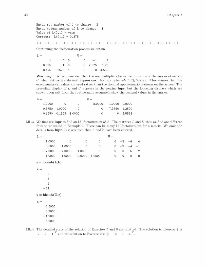
Enter row number of L to change. 2Enter column number of L to change. 1Value of L(2,1) = -numCorrect: L(2,1) = 0.375
++++++++++++++++++++++++++++++++++++++++++++++++++++++
Continuing the factorization process we obtain
L =1 0 0
0.375 1 0
0.125 0.1525 1
U =8 −1 2
0 7.375 1.25
0 0 4.559
Warning: It is recommended that the row multipliers be written in terms of the entries of matrixU when entries are decimal expressions. For example, −U(3, 2)/U(2, 2). This assures that theexact numerical values are used rather than the decimal approximations shown on the screen. Thepreceding display of L and U appears in the routine lupr, but the following displays which areshown upon exit from the routine more accurately show the decimal values in the entries.
L =1.0000 0 0
0.3750 1.0000 0
0.1250 0.1525 1.0000
U =8.0000 −1.0000 2.0000
0 7.3750 1.2500
0 0 4.5593
ML.3. We first use lupr to find an LU-factorization of A. The matrices L and U that we find are differentfrom those stated in Example 2. There can be many LU-factorizations for a matrix. We omit thedetails from lupr. It is assumed that A and b have been entered.
L =1.0000 0 0 0
0.5000 1.0000 0 0
−2.0000 −2.0000 1.0000 0
−1.0000 1.0000 −2.0000 1.0000
U =6 −2 −4 4
0 −2 −4 −10 0 5 −20 0 0 8
z === forsub(L,b)
z =2
−52
−32
x === bksub(U,z)
x =4.5000
6.9000
−1.2000−4.0000
ML.4. The detailed steps of the solution of Exercises 7 and 8 are omitted. The solution to Exercise 7 is[2 −2 −1
]T and the solution to Exercise 8 is[1 −2 5 −4
]T .
Supplementary Exercises 41
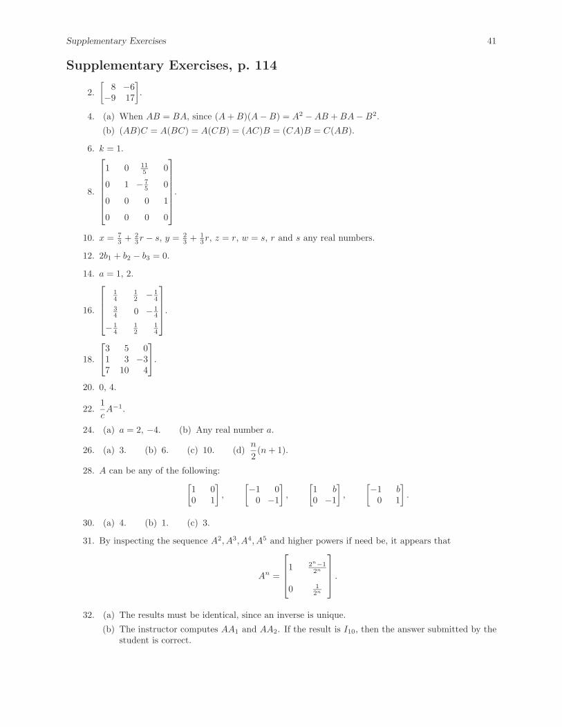
Supplementary Exercises, p. 114
2.[
8 −6−9 17
].
4. (a) When AB = BA, since (A + B)(A − B) = A2 − AB + BA − B2.
(b) (AB)C = A(BC) = A(CB) = (AC)B = (CA)B = C(AB).
6. k = 1.
8.
⎡⎢⎢⎢⎢⎢⎢⎣1 0 11
5 0
0 1 − 75 0
0 0 0 1
0 0 0 0
⎤⎥⎥⎥⎥⎥⎥⎦.
10. x = 73 + 2
3r − s, y = 23 + 1
3r, z = r, w = s, r and s any real numbers.
12. 2b1 + b2 − b3 = 0.
14. a = 1, 2.
16.
⎡⎢⎢⎢⎣14
12 − 1
4
34 0 − 1
4
− 14
12
14
⎤⎥⎥⎥⎦.
18.
⎡⎣3 5 01 3 −37 10 4
⎤⎦.
20. 0, 4.
22.1cA−1.
24. (a) a = 2, −4. (b) Any real number a.
26. (a) 3. (b) 6. (c) 10. (d)n
2(n + 1).
28. A can be any of the following:[1 00 1
],
[−1 0
0 −1
],
[1 b0 −1
],
[−1 b
0 1
].
30. (a) 4. (b) 1. (c) 3.
31. By inspecting the sequence A2, A3, A4, A5 and higher powers if need be, it appears that
An =
⎡⎢⎢⎣1 2n−12n
0 12n
⎤⎥⎥⎦ .
32. (a) The results must be identical, since an inverse is unique.
(b) The instructor computes AA1 and AA2. If the result is I10, then the answer submitted by thestudent is correct.
42 Chapter 1
34. L =
⎡⎣ 1 0 03 1 0
−3 2 1
⎤⎦, U =
⎡⎣2 2 30 −1 −20 0 3
⎤⎦, x =
⎡⎣ 1−1−2
⎤⎦.
T.1. (a) Tr(cA) =n∑
i=1
caii = c
n∑i=1
aii = cTr(A).
(b) Tr(A + B) =n∑
i=1
(aii + bii) =n∑
i=1
aii +n∑
i=1
bii = Tr(A) + Tr(B).
(c) Let AB = C =[cij
]. Then
Tr(AB) = Tr(C) =n∑
i=1
cii =n∑
i=1
n∑k=1
aikbki =n∑
k=1
n∑i=1
bkiaik = Tr(BA).
(d) Tr(AT ) =n∑
i=1
aii = Tr(A).
(e) Tr(AT A) is the sum of the diagonal entries of AT A. The ith diagonal entry of AT A isn∑
j=1
a2ji,
so
Tr(AT A) =n∑
i=1
⎡⎣ n∑j=1
a2ji
⎤⎦ = sum of the squares of all entries of A.
Hence, Tr(AT A) ≥ 0.
T.2. From part (e) of Exercise T.1.,
Tr(AT A) =n∑
i=1
⎡⎣ n∑j=1
a2ji
⎤⎦ .
Thus, if Tr(AT A) = 0, then aji = 0 for all i, j, that is, A = O.
T.3. If Ax = Bx for all n × 1 matrices x, then Aej = Bej , j = 1, 2, . . . , n, where ej = column j of In.But then
Aej =
⎡⎢⎢⎢⎣a1j
a2j
...anj
⎤⎥⎥⎥⎦ = Bej =
⎡⎢⎢⎢⎣b1j
b2j
...bnj
⎤⎥⎥⎥⎦ .
Hence column j of A = column j of B for each j and it follows that A = B.
T.4. We have Tr(AB − BA) = Tr(AB) − Tr(BA) = 0, while
Tr([
1 00 1
])= 2.
T.5. Suppose that A is skew symmetric, so AT = −A. Then (Ak)T = (AT )k = (−A)k = −Ak if k is apositive odd integer, so Ak is skew symmetric.
Supplementary Exercises 43
T.6. If A is skew symmetric then AT = −A. Note that xT Ax is a scalar, thus (xT Ax)T = xT Ax. Thatis,
xT Ax = (xT Ax)T = xT AT x = −(xT Ax).
The only scalar equal to its negative is zero. Hence xT Ax = 0 for all x.
T.7. If A is symmetric and upper (lower) triangular, then aij = aji and aij = 0 for j > i (j < i). Thus,aij = 0, i �= j, so A is diagonal.
T.8. Assume that A is upper triangular. If A is nonsingular then A is row equivalent to In. Since A isupper triangular this can occur only if aii �= 0 because in the reduction process we must performthe row operations (1/aii) · (ith row of A). The steps are reversible.
T.9. Suppose that A �= O but row equivalent to O. Then in the reduction process some row operationmust have transformed a nonzero matrix into the zero matrix. However, considering the types ofrow operations this is impossible. Thus A = O. The converse follows immediately.
T.10. Let A and B be row equivalent n× n matrices. Then there exists a finite number of row operationswhich when applied to A yield B and vice versa. If B is nonsingular, then B is row equivalent toIn. Thus A is also row equivalent to In, hence A is nonsingular. We repeat the argument with Aand B interchanged to prove the converse.
T.11. Assume that B is singular. Then by Theorem 1.13 there exists x �= 0 such that Bx = 0. Then(AB)x = A0 = 0, which means that the homogeneous system (AB)x = 0 has a nontrivial solution.Theorem 1.13 implies that AB is singular, but this is a contradiction. Suppose now that A is singularand B is nonsingular. Then there exists a y �= 0 such that Ay = 0. Since B is nonsingular we canfind x �= 0 such that y = Bx (x = B−1y). Then 0 = Ay = (AB)x, which again implies that AB issingular, a contradiction.
T.12. If A is skew symmetric, AT = −A. Thus aii = −aii, so aii = 0.
T.13. If AT = −A and A−1 exists, then
(A−1)T = (AT )−1 = (−A)−1 = −A−1.
Hence A−1 is skew symmetric.
T.14. (a) I2n = In and O2 = O.
(b) One such matrix is[0 00 1
].
(c) If A2 = A and A−1 exists, then A−1(A2) = A−1A. Simplifying gives A = In.
T.15. (a) Let A be nilpotent. If A were nonsingular, then products of A with itself are also nonsingular.But Ak = O, hence Ak is singular. Thus A must be singular.
(b) A2 =
⎡⎣0 0 10 0 00 0 0
⎤⎦, A3 = O.
(c) k = 1, A = O; In − A = In; (In − A)−1 = In.k = 2, A2 = O; (In − A)(In + A) = In − A2 = In; (In − A)−1 = In + A.k = 3, A3 = O; (In − A)(In + A + A2) = In − A3 = In; (In − A)−1 = In + A + A2, etc.
T.16. We have that A2 = A and B2 = B.
(a) (AB)2 = ABAB = A(BA)B = A(AB)B (since AB = BA)= A2B2 = AB (since A and B are idempotent)
44 Chapter 1
(b) (AT )2 = AT AT = (AA)T (by the properties of the transpose)= (A2)T = AT (since A is idempotent)
(c) If A and B are n × n and idempotent, then A + B need not be idempotent., For example, let
A =[1 10 0
]and B =
[0 01 1
].
Both A and B are idempotent and C = A + B =[1 11 1
]. However, C2 =
[2 22 2
]�= C.
T.17. Let
A =[
0 a−a 0
]and B =
[0 b
−b 0
].
Then A and B are skew symmetric and
AB =[−ab 00 −ab
]which is diagonal. The result is not true for n > 2. For example, let
A =
⎡⎣ 0 1 2−1 0 3−2 −3 0
⎤⎦ .
Then
A2 =
⎡⎣ 5 6 −36 10 2
−3 2 13
⎤⎦ .
T.18. Assume that A is nonsingular. Then A−1 exists. Hence we can multiply Ax = b by A−1 on the lefton both sides obtaining
A−1(Ax) = A−1b or Inx = x = A−1b.
Thus Ax = b has a unique solution. Assume that Ax = b has a unique solution for every b. SinceAx = 0 has solution x = 0, Theorem 1.13 implies that A is nonsingular.
T.19. (a) xyT =
⎡⎣ 4 5 68 10 12
12 15 18
⎤⎦. (b) xyT =
⎡⎢⎢⎣−1 0 3 5−2 0 6 10−1 0 3 5−2 0 6 10
⎤⎥⎥⎦.
T.20. It is not true that xyT must be equal to yxT . For example, let
x =[12
]and y =
[45
].
Then
xyT =[4 58 10
]and yxT =
[4 85 10
].
T.21. Tr(xyT ) = x1y1 + x2y2 + · · · + xnyn = xT y. (See discussion preceding Exercises T.19–T.22.)
Supplementary Exercises 45
T.22. The outer product of x and y can be written in the form
xyT =
⎡⎢⎢⎢⎢⎢⎢⎣x1
[y1 y2 · · · yn
]x2
[y1 y2 · · · yn
]...
xn
[y1 y2 · · · yn
]
⎤⎥⎥⎥⎥⎥⎥⎦If either x = 0 or y = 0, then xyT = On. Thus assume that there is at least one nonzero componentin x, say xi, and at least one nonzero component in y, say yj . Then 1
xiRowi(xyT ) makes the ith row
exactly yT . Since all the other rows are multiples of yT , row operations of the form (−xk)Ri + Rp,for p �= i can be performed to zero out everything but the ith row. It follows that either xyT is rowequivalent to On or to a matrix with n − 1 zero rows.
T.23. (a) HT = (In − 2wwT )T = ITn − 2(wwT )T = In − 2(wT )T wT = In − 2wwT = H.
(b) HHT = HH = (In − 2wwT )(In − 2wwT )= In − 4wwT + 4wwT wwT
= In − 4wwT + 4w(wT w)wT
= In − 4wwT + 4w(In)wT = In
Thus, HT = H−1.
T.24. Let B =[a bc d
]. Then
[2 0
−1 1
] [a bc d
]=
[a bc d
] [2 0
−1 1
]=⇒
[2a 2b
−a + c −b + d
]=
[2a − b b2c − d d
]
which yields a = r, b = 0, d = s, c = d − a = s − r. Thus, B =[
r 0s − r s
].