arX

iv:h

ep-p

h/02

0922

8v2

9 D

ec 2

002

UdeM-GPP-TH-02-107

IMSc-2002/09/33

Lepton Polarization and Forward-Backward

Asymmetries in b → sτ+τ−

Wafia Bensalam a,1, David London a,2, Nita Sinha b,3, Rahul Sinha b,4

a: Laboratoire Rene J.-A. Levesque, Universite de Montreal,

C.P. 6128, succ. centre-ville, Montreal, QC, Canada H3C 3J7

b: Institute of Mathematical Sciences, Taramani, Chennai 600113, India

(July 24, 2013)

Abstract

We study the spin polarizations of both τ leptons in the decay b → sτ+τ−. In addi-tion to the polarization asymmetries involving a single τ , we construct asymmetriesfor the case where both polarizations are simultaneously measured. We also studyforward-backward asymmetries with polarized τ ’s. We find that a large number ofasymmetries are predicted to be large, >∼ 10%. This permits the measurement of allWilson coefficients and the b-quark mass, thus allowing the standard model (SM) tobe exhaustively tested. Furthermore, there are many unique signals for the presenceof new physics. For example, asymmetries involving triple-product correlations arepredicted to be tiny within the SM, O(10−2). Their observation would be a clearsignal of new physics.

1wafia@lps.umontreal.ca2london@lps.umontreal.ca3nita@imsc.res.in4sinha@imsc.res.in

1 Introduction

There has been a great deal of theoretical work examining the decay b → sℓ+ℓ−, bothat the inclusive and exclusive level [1]. As usual, the hope is that, through precisionmeasurements of this decay, one will find evidence for the presence of physics beyondthe standard model (SM). Indeed, this decay mode has been extensively studied invarious models of new physics [2].

Some years ago, it was noted that the measurement of the polarization of thefinal-state τ− in the inclusive decay b → Xsτ

+τ− can provide important informationabout the Wilson coefficients of the underlying effective Hamiltonian [3, 4, 5]. Withinthe SM, this inclusive decay is described in terms of five theoretical parameters: thefour Wilson coefficients (C7, C10 and real and imaginary parts of C9), and the massof the b-quark, mb. In principle, all of these theoretical parameters can be completelydetermined using measurements of the three τ− polarization asymmetries, the total(unpolarized) rate, and the forward-backward (FB) asymmetry.

In practice, however, the SM τ− polarization asymmetry along the normal com-ponent is expected to be O(10−2) [6], and is therefore probably too small to bemeasured. This situation can be remedied to some extent if, in addition to thepolarization asymmetries of the τ−, we also consider similar asymmetries for the τ+

[7]. This adds one more independent observable. However, even if the sizeable polar-ization asymmetries of both τ+ and τ− can be separately measured, there are onlyas many measurements as there are unknowns, so that there are no redundant mea-surements to provide crosschecks for the SM. Furthermore, this program requiresthat the flavor of the b-quark be tagged: in an untagged sample, there are onlyfour observables, since the measurement of the FB asymmetry requires tagging. Itwill therefore be very difficult to rigorously test the SM if only single τ -polarizationmeasurements are made in b → Xsτ

+τ−.In this paper, we try to construct the maximum possible number of independent

observables. This is achieved by considering the situation in which both τ+ andτ− polarizations are simultaneously measured. As we will see, a variety of newasymmetries can be constructed in this case. We compute the polarization andforward-backward asymmetries for both singly-polarized and doubly-polarized final-state leptons. A large number of these new asymmetries do not require the taggingof the b-quark. (Note that, in an untagged sample, while the FB asymmetry forunpolarized leptons vanishes, some of the FB asymmetries for polarized leptons arenonvanishing.) On the other hand, if b-tagging is possible, the measurement of thesenew asymmetries provides even more information. The polarized FB asymmetries aswell as the double-spin polarization asymmetries all depend in different ways on theWilson coefficients, so that these coefficients can be obtained in many different ways.This redundancy provides a huge number of crosschecks, and allows the SM to beexhaustively tested. An interesting consequence of the large number of observables,is that mb can be extracted. If the phenomenologically-obtained value of mb were to

1

agree with theoretical estimates [8], this would be an important step in confirmingour understanding of QCD,

In our calculations we consider only contributions from SM operators. However,using arguments based on CPT invariance and the properties of the SM operatorsunder C, P and T, we derive relations between these observables which are cleantests of new physics. Some of these tests rely on the fact that within the SM thereare negligible CP-violating contributions to the decay mode being considered. Ourphilosophy is to test for the presence of new physics (NP) without considering thedetailed structure of the various operators that can contribute to NP. Should a signalfor NP be seen, the consideration of specific NP operators would help in determiningthe nature of NP contributions (for example, see Ref. [7]).

We begin in Sec. 2 with a discussion of the calculation of |M|2, where M isthe amplitude for b → sτ+τ− (the results of the calculation of M are complicated,and are presented in the Appendix). The polarization asymmetries and forward-backward asymmetries are examined in Secs. 3 and 4, respectively. We discuss theseasymmetry measurements within a variety of scenarios in Sec. 5. We conclude inSec. 6.

In total, we numerically evaluate the differential decay rate and 31 asymmetriesas a function of the invariant lepton mass. Note that it will be extremely difficultto measure asymmetries smaller than 10%, as they would require ∼ 1010 B mesonsfor a 3σ signal (not including efficiencies for spin-polarization measurements and fortagging). We therefore consider only asymmetries larger than 10% as measurable. Ifone can only measure an individual τ+ or τ− spin, but cannot tag the flavor of the b-quark, then there are only two sizeable observables. If b-tagging can be done and onecan measure the spin of the τ+ or τ−, this increases to 6 measurable asymmetries.However, if the polarizations of both the τ -leptons can be measured and flavortagging of the b is possible, we find that nine of the asymmetries constructed hereare large in the SM. Including the decay rate, this leads to 10 sizeable observables,which allows for a redundant test of the SM.

In addition, we find that the violation of certain SM asymmetry relations areclean tests of NP. Some of these relations are violated only in the presence of CP-violating NP. A large numbers of these asymmetries are O(10−2) in the SM, so thatthe observation of larger asymmetries would be signals of NP. Certain combinationsof these asymmetries are identically zero in the SM, and hence are litmus tests ofNP.

2

2 |M|2 for b → sτ+τ−

We begin by considering the calculation of |M|2 for b → sτ+τ−. Including QCDcorrections, the effective Hamiltonian describing the decay b → sτ+τ− [9] leads tothe matrix element

M = T9 + T10 + T7 , (1)

where

T9 =αGF√

2πCeff

9 VtbV∗ts

[sLγµbL

][τ−γµτ+

], (2)

T10 =αGF√

2πC10VtbV

∗ts

[sLγµbL

][τ−γµγ5τ

+], (3)

T7 =αGF√

2πCeff

7 VtbV∗ts

[−2imb

q2

] [sLσµνq

νbR

][τ−γµτ+

]. (4)

In the above, q is the momentum transferred to the lepton pair, and we have ne-glected the s-quark mass. The Wilson coefficients Ci are evaluated perturbativelyat the electroweak scale and then evolved down to the renormalization scale µ. Thecoefficients Ceff

7 and C10 are real, and take the values

Ceff7 = −0.315 , C10 = −4.642 (5)

in the leading-logarithm approximation [5]. On the other hand, the coefficient Ceff9

is complex, and its value is a function of s ≡ q2/m2b : Ceff

9 (µ) ≡ C9(µ) + Y (µ, s),where the function Y (µ, s) contains the one-loop contributions of the four-quark

operators [3, 9]. An additional contribution to Ceff9 arises from the long-distance

effects associated with real cc resonances in the intermediate states [10]. Thus,within the SM, the decay b → sτ+τ− is described by four Wilson coefficients for agiven value of s: Ceff

7 , C10, Re(Ceff9 ) and Im(Ceff

9 ).Because the expressions in |M|2 are complicated, we present the actual results of

this calculation in the Appendix. Note that the polarization and forward-backwardasymmetries, which will be discussed in subsequent sections, are calculated as func-tions of the terms of |M|2. Also, some signals of new physics are derived using theC, P and T properties of the terms at the |M|2 level.

There is one point which is worth mentioning here. In the calculation of |M|2,there are terms which involve the imaginary pieces of the Wilson coefficients [e.g. the

Im(Ceff9 C∗

10) term in Eq. (53)]. These are the coefficients of terms like ǫµαβφ pµsp

α−sβ

−pφ+

in |M|2, which give rise to triple-product correlations (e.g. ~p− · (~p+ ×~s−)). Naively,these triple products appear to violate time-reversal symmetry (T) and so, by theCPT theorem, should also be signals of CP violation. However, all the amplitudesin Eq. (1) have the same weak phase (neglecting the small u-quark contribution inthe loop), so that their interference cannot give rise to CP violation. Thus, thereappears to be an inconsistency.

3

What is happening is the following: a triple product is not a true T-violatingsignal, since the action of T exchanges the initial and final states. Because of this,triple-product correlations can be faked by the presence of strong phases, even ifthere is no CP violation. This is the situation which arises here – nonzero strongphases of the Wilson coefficients can lead to triple products. Usually, it is CP viola-tion which interests us, and we wish to eliminate such fake signals. However, in thiscase, we are interested in measuring the imaginary parts of the Wilson coefficientsin order to test the SM, so that these fake signals will be quite useful.

3 Polarization Asymmetries

In the computation of the various polarization asymmetries we choose a frame ofreference in which the leptons move back to back along the z-axis, with the τ−

moving in the direction +z. The s-quark then goes in the same direction as theb-quark, with the s-quark making an angle θ with the τ−. Our specific choices forthe 4-momenta components are as follows:

pµ

τ− = {√

P 2 + m2τ , 0, 0, P} ,

pµ

τ+ = {√

P 2 + m2τ , 0, 0,−P} ,

pµs = {K, 0, K sin θ, K cos θ} ,

pµb = {

√K2 + m2

b , 0, K sin θ, K cos θ}. (6)

Using the above calculation of |M|2, we can compute the decay rate for unpo-larized leptons by summing over the lepton spins and integrating over the angularvariables. As a function of the invariant mass of the lepton pair, this decay rate isgiven by

(dΓ(s)

ds

)

unpol

=G2

F m5b

192 π3

α2

4 π2|Vtb V ∗

ts|2 (1 − s)2

√

1 − 4 mτ2

s∆ , (7)

where mτ ≡ mτ/mb, and

∆ =(12 Re(Ceff

7 Ceff∗

9 ) +4 |Ceff

7 |2 (2 + s)

s

) (1 +

2 m2τ

s

)(8)

+(|Ceff9 |2 + |C10|2)

(1 + 2 s +

2 (1 − s) m2τ

s

)+ 6 (|Ceff

9 |2 − |C10|2) m2τ .

This agrees with the earlier results [3, 4, 5, 9, 11] in the appropriate limits.We now consider the possibility that the polarizations of the final-state leptons

can be measured. The spins of the τ± are defined in their rest frames to be:

sµ

τ− ={0, s−x , s−y , s−z

}, sµ

τ+ ={0, s+

x , s+y , s+

z

}. (9)

4

One can obtain the spins of the τ± in the frame of Eq. (6) straightforwardly byperforming a Lorentz boost:

sµ

τ− =

P

mτ

s−z , s−x , s−y ,

√P 2 + m2

τ

mτ

s−z

, sµ

τ+ =

−P

mτ

s+z , s+

x , s+y ,

√P 2 + m2

τ

mτ

s+z

.

(10)We now define differential decay rate as a function of the spin directions of the

τ±, s+ and s−, where s+ and s− are unit vectors in the τ± rest frames. This is givenby

dΓ(s+, s−, s)

ds=

1

4

(dΓ(s)

ds

)

unpol

[

1 +

(

P−x s−x + P−

y s−y + P−z s−z

+ P+x s+

x + P+y s+

y + P+z s+

z

)

+

(

Pxx s+x s−x + Pxy s+

x s−y + Pxz s+x s−z + Pyx s+

y s−x + Pyy s+y s−y

+ Pyz s+y s−z + Pzx s+

z s−x + Pzy s+z s−y + Pzz s+

z s−z

)]

, (11)

where the single-lepton polarization asymmetries P∓i (i = x, y, z) are obtained by

evaluating

P−i =

[dΓ(s−=i, s+=i)

ds+ dΓ(s−=i, s+=−i)

ds

]−[

dΓ(s−=−i, s+=i)ds

+ dΓ(s−=−i, s+=−i)ds

]

[dΓ(s−=i, s+=i)

ds+ dΓ(s−=i, s+=−i)

ds

]+[

dΓ(s−=−i, s+=i)ds

+ dΓ(s−=−i, s+=−i)ds

] ,

P+i =

[dΓ(s−=i, s+=i)

ds+ dΓ(s−=−i, s+=i)

ds

]−[

dΓ(s−=i, s+=−i)ds

+ dΓ(s−=−i, s+=−i)ds

]

[dΓ(s−=i, s+=i)

ds+ dΓ(s−=−i, s+=i)

ds

]+[

dΓ(s−=i, s+=−i)ds

+ dΓ(s−=−i, s+=−i)ds

] .(12)

Similarly, the double spin asymmetries Pij can be obtained:

Pij =

[dΓ(s+=i,s−=j)

ds− dΓ(s+=i,s−=−j)

ds

]−[

dΓ(s+=−i,s−=j)ds

− dΓ(s+=−i,s−=−j)ds

]

[dΓ(s+=i,s−=j)

ds+ dΓ(s+=i,s−=−j)

ds

]+[

dΓ(s+=−i,s−=j)ds

+ dΓ(s+=−i,s−=−j)ds

] , (13)

where i and j are unit vectors along the i and j directions. Note that both P±i and

Pij depend also on s. However, the explicit dependence on s has been suppressedfor simplicity of notation.

Before presenting explicit expressions for these quantities, it is useful to make thefollowing remark. With our choice of 4-momenta [Eq. (6)], the decay takes place inthe yz plane. Therefore, the only vectors which can have x components are the spinss+ and s−. This implies that the only scalar product which involves x components

5

is the dot product of two spins. Thus, any term that has only one component of spinalong x (i.e. Px, Pxy and Pxz) must come from a triple-product correlation. Thisholds even in the presence of new physics. It is therefore these quantities whichprobe the imaginary parts of the products of Wilson coefficients.

The P’s take the form

P+x =

−3 π

2√

s∆

(2 Im(Ceff

7 C∗10) + Im(Ceff

9 C∗10) s

)mτ

√

1 − 4 m2τ

s(14)

P+y =

3 π

2√

s∆

(4 |Ceff7 |2s

+ 2 Re(Ceff7 C∗

10) + 4 Re(Ceff7 Ceff∗

9 )

+ Re(Ceff9 C∗

10) + |Ceff9 |2 s

)mτ (15)

P+z =

2

∆

(6 Re(Ceff

7 C∗10) + Re(Ceff

9 C∗10) (1 + 2 s)

)√

1 − 4 m2τ

s(16)

P−x = P+

x (17)

P−y =

3 π

2√

s∆

(4 |Ceff7 |2s

− 2 Re(Ceff7 C∗

10) + 4 Re(Ceff7 Ceff∗

9 )

− Re(Ceff9 C∗

10) + |Ceff9 |2 s

)mτ (18)

P−z = P+

z (19)

Pxx =1

∆

(

24 Re(Ceff7 Ceff∗

9 )m2

τ

s+ 4 |Ceff

7 |2((−1 + s) s + 2 (2 + s) m2

τ

)

s2

+(|Ceff9 |2 − |C10|2)

((1 − s)s + 2 (1 + 2 s)m2

τ

)

s

)

(20)

Pyx =−2

∆Im(Ceff

9 C∗10) (1 − s)

√

1 − 4 m2τ

s(21)

Pzx =−3 π

2√

s∆

(2 Im(Ceff

7 C∗10) + Im(Ceff

9 C∗10))mτ (22)

Pxy = Pyx (23)

Pyy =1

∆

(24 Re(Ceff

7 Ceff∗

9 ) m2τ

s− 4 (|Ceff

9 |2 + |C10|2)(1 − s) m2

τ

s(24)

+(|Ceff9 |2 − |C10|2) ((−1 + s) +

6 m2τ

s)

+4 |Ceff

7 |2((1 − s) s + 2 (2 + s) m2

τ

)

s2

)

(25)

Pzy =3 π

2√

s∆

(2 Re(Ceff

7 C∗10) − |C10|2 + Re(Ceff

9 C∗10) s

)mτ

√

1 − 4 m2τ

s(26)

Pxz = −Pzx (27)

6

Pyz =3 π

2√

s∆

(2 Re(Ceff

7 C∗10) + |C10|2 + Re(Ceff

9 C∗10) s

)mτ

√

1 − 4 m2τ

s(28)

Pzz =1

∆

(

12 Re(Ceff7 Ceff∗

9 )(1 − 2 m2

τ

s

)+

4 |Ceff7 |2 (2 + s)

(1 − 2 m2

τ

s

)

s(29)

+(|Ceff9 |2 + |C10|2)

(1 + 2 s − 6 (1 + s) m2

τ

s

)

+2 (|Ceff

9 |2 − |C10|2) (2 + s) m2τ

s

)

. (30)

0.04

-0.6

-0.4

-0.2

0

0

0.01

0.02

0.03

0.7 0.8 0.9 1 Sz

0.2

0.7 0.8 0.9 1

-0.4

-0.2

0

0.2

0.4

0.6

0.8

0.7 0.8 0.9 1

*�Y

*ZY

Sz

Sz

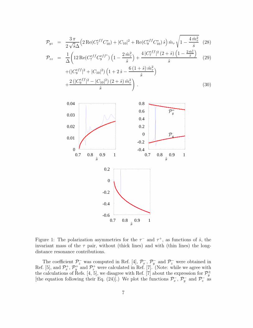
Figure 1: The polarization asymmetries for the τ− and τ+, as functions of s, theinvariant mass of the τ pair, without (thick lines) and with (thin lines) the long-distance resonance contributions.

The coefficient P−z was computed in Ref. [4], P−

x , P−y and P−

z were obtained inRef. [5], and P+

x , P+y and P+

z were calculated in Ref. [7]. (Note: while we agree withthe calculations of Refs. [4, 5], we disagree with Ref. [7] about the expression for P±

y

[the equation following their Eq. (24)].) We plot the functions P−x , P−

y and P−z as

7

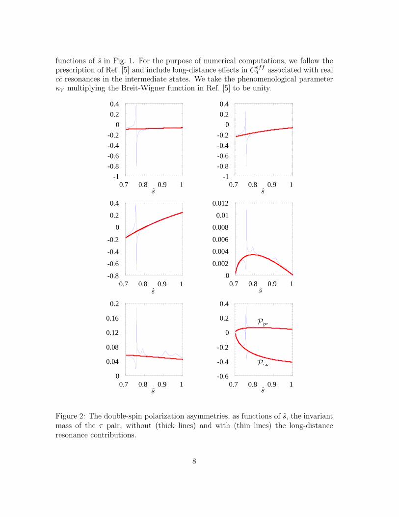
functions of s in Fig. 1. For the purpose of numerical computations, we follow theprescription of Ref. [5] and include long-distance effects in Ceff

9 associated with realcc resonances in the intermediate states. We take the phenomenological parameterκV multiplying the Breit-Wigner function in Ref. [5] to be unity.

-1

-0.8

-0.6

-0.4

-0.2

0

0.2

0.4

0.7 0.8 0.9 1

-1

-0.8

-0.6

-0.4

-0.2

0

0.2

0.4

0.7 0.8 0.9 1 Sz Sz

-0.8

-0.6

-0.4

-0.2

0

0.2

0.4

0.7 0.8 0.9 1 Sz

0

0.002

0.004

0.006

0.008

0.01

0.012

0.7 0.8 0.9 1

Sz

0.04

0.08

0.12

0.16

0.2

0.7 0.8 0.9 1

Sz

0 -0.6

-0.4

-0.2

0

0.2

0.4

0.7 0.8 0.9 1

*ZY

*YZ

Sz

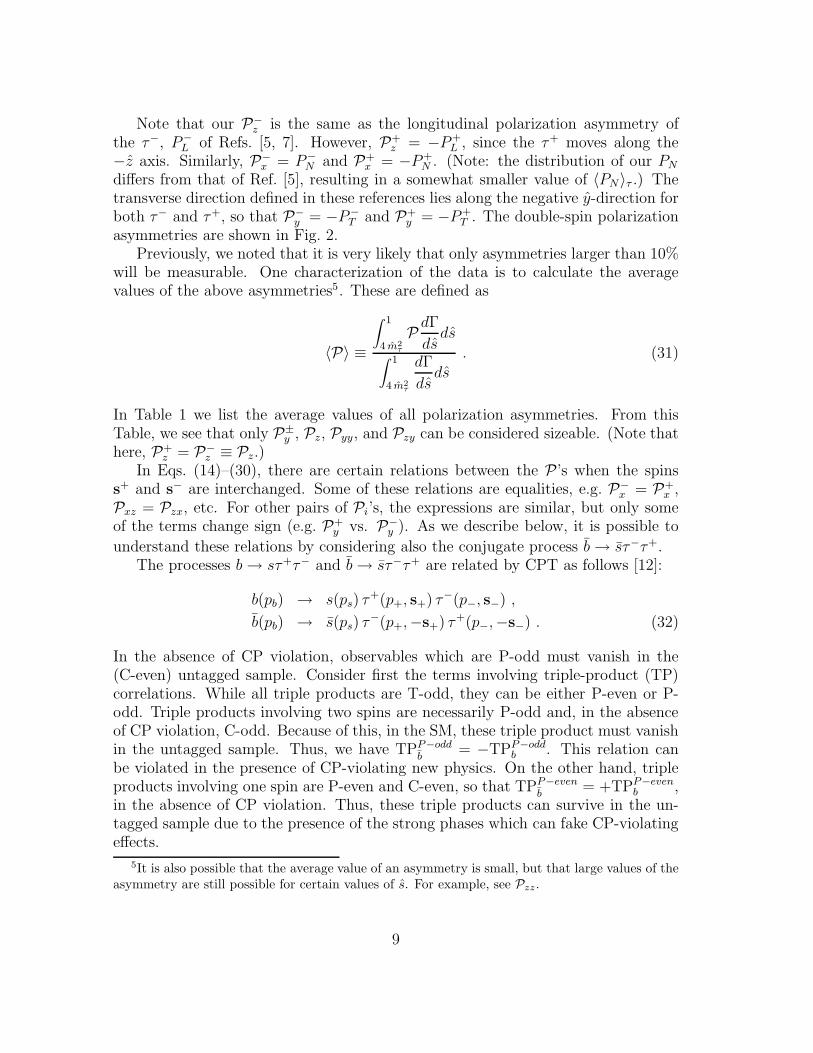
Figure 2: The double-spin polarization asymmetries, as functions of s, the invariantmass of the τ pair, without (thick lines) and with (thin lines) the long-distanceresonance contributions.

8

Note that our P−z is the same as the longitudinal polarization asymmetry of

the τ−, P−L of Refs. [5, 7]. However, P+

z = −P+L , since the τ+ moves along the

−z axis. Similarly, P−x = P−

N and P+x = −P+

N . (Note: the distribution of our PN

differs from that of Ref. [5], resulting in a somewhat smaller value of 〈PN〉τ .) Thetransverse direction defined in these references lies along the negative y-direction forboth τ− and τ+, so that P−

y = −P−T and P+

y = −P+T . The double-spin polarization

asymmetries are shown in Fig. 2.Previously, we noted that it is very likely that only asymmetries larger than 10%

will be measurable. One characterization of the data is to calculate the averagevalues of the above asymmetries5. These are defined as

〈P〉 ≡

∫ 1

4 m2τ

P dΓ

dsds

∫ 1

4 m2τ

dΓ

dsds

. (31)

In Table 1 we list the average values of all polarization asymmetries. From thisTable, we see that only P±

y , Pz, Pyy, and Pzy can be considered sizeable. (Note thathere, P+

z = P−z ≡ Pz.)

In Eqs. (14)–(30), there are certain relations between the P’s when the spinss+ and s− are interchanged. Some of these relations are equalities, e.g. P−

x = P+x ,

Pxz = Pzx, etc. For other pairs of Pi’s, the expressions are similar, but only someof the terms change sign (e.g. P+

y vs. P−y ). As we describe below, it is possible to

understand these relations by considering also the conjugate process b → sτ−τ+.The processes b → sτ+τ− and b → sτ−τ+ are related by CPT as follows [12]:

b(pb) → s(ps) τ+(p+, s+) τ−(p−, s−) ,

b(pb) → s(ps) τ−(p+,−s+) τ+(p−,−s−) . (32)

In the absence of CP violation, observables which are P-odd must vanish in the(C-even) untagged sample. Consider first the terms involving triple-product (TP)correlations. While all triple products are T-odd, they can be either P-even or P-odd. Triple products involving two spins are necessarily P-odd and, in the absenceof CP violation, C-odd. Because of this, in the SM, these triple product must vanishin the untagged sample. Thus, we have TPP−odd

b= −TPP−odd

b . This relation canbe violated in the presence of CP-violating new physics. On the other hand, tripleproducts involving one spin are P-even and C-even, so that TPP−even

b= +TPP−even

b ,in the absence of CP violation. Thus, these triple products can survive in the un-tagged sample due to the presence of the strong phases which can fake CP-violatingeffects.

5It is also possible that the average value of an asymmetry is small, but that large values of the

asymmetry are still possible for certain values of s. For example, see Pzz.

9

〈P−x 〉 = 〈P+

x 〉 1.413 × 10−2

〈P−y 〉 0.723

〈P−z 〉 = 〈P+

z 〉 −0.336

〈P+y 〉 −0.164

〈Pxx〉 −8.658 × 10−2

〈Pyx〉 = 〈Pxy〉 2.868 × 10−3

〈Pzx〉 = −〈Pxz〉 5.322 × 10−2

〈Pyy〉 −0.168

〈Pzy〉 −0.281

〈Pyz〉 5.717 × 10−2

〈Pzz〉 −1.1254 × 10−2

Table 1: Numerical values of the various averaged spin-polarization asymmetrieswithout including the long-distance resonance contributions. We use mb = 4.24GeV [8]. The corresponding branching ratio is BR(B → Xsτ

+τ−) = 1.192 × 10−7.

We now apply these observations to P+x and P−

x , which involve a single spin. Asnoted earlier, terms with a single spin along x must come only from a triple-productcorrelation. The general triple-product term giving these quantities can be writtenas ǫαβµρ pα

b pβs (a pµ

+sρ+ + b pµ

−sρ−), where a and b are arbitrary coefficients. For the

conjugate process [Eq. (32)], the corresponding term is −ǫαβµρ pαb pβ

+(a pµ−sρ

−+b pµ+sρ

+).Since TPP−even

b= +TPP−even

b , this implies that a = −b (in the absence of CPviolation). Using the 4-vectors of Eq. (6), it is then straightforward to show thatthis results in P+

x = +P−x . Note that this will hold even in the presence of CP-

conserving New Physics.Similarly, the two-spin triple products, which contribute to the pairs {Pyx,Pxy}

and {Pzx,Pxz}, are proportional to ǫαβµρ pαs pβ

b sµ−sρ

+. In the absence of CP violation,the CP-odd combination of Pyx and Pxy (and of Pzx and Pxz) will vanish in anuntagged sample. Again, a simple calculation then shows that this implies thatPyx = +Pxy and Pzx = −Pxz.

For the other terms that do not contain triple products, and are hence always T-even, one can understand the relationship between the P’s in a similar fashion. For

10

example, consider P+y and P−

y . Since only dot products of various momenta and one

spin are involved, the coefficients of both terms |Ceff7 |2 [Eq. (54)] and Re(Ceff

7 C∗10)

[Eq. (56)] are T-even and P-odd. However, the |Ceff7 |2 term “ps · (s−+s+)” switches

sign under CPT for the conjugate process, while the Re(Ceff7 C∗

10) term “ps·(s+−s−)”has the same sign for the conjugate process. Since these terms are P-odd and C-odd(in the absence of CP violation), they must vanish in an untagged sample. This

explains the relative sign difference between the |Ceff7 |2 and Re(Ceff

7 C∗10) terms in

P+y and P−

y . This argument may be extended to all terms contributing to variousPi’s. In particular, in the SM, P+

z = +P−z . On the other hand, in presence of New

Physics, while the additional terms must still be T-even and P-odd, they could beeven or odd under CPT, implying that the relation between P+

z and P−z could differ.

Of course, the above discussion assumes that there is no CP violation in b →sτ+τ−, which is the case in the SM, to a good approximation. On the other hand, ifnew CP-violating physics contributes to this decay, this gives us several clear tests forits presence. For example, any violation of the relation P+

x = P−x (or P−

L + P+L = 0)

is a smoking-gun signal of such new physics.

4 Forward-Backward Asymmetries

One observable which does not depend on the polarization of the final-state leptonsis the forward-backward (FB) asymmetry. In the frame of reference described inEq. (6), the forward-backward asymmetry is given by

AFB(s) =

∫ 1

0

d2Γ

ds d cos θd cos θ −

∫ 0

−1

d2Γ

ds d cos θd cos θ

∫ 1

0

d2Γ

ds d cos θd cos θ +

∫ 0

−1

d2Γ

ds d cos θd cos θ

=3

∆

(2 Re(Ceff

7 C∗10) + s Re(Ceff

9 C∗10))√

1 − 4 m2τ

s. (33)

This agrees with the result of Ref. [5] (and that of Ref. [11] when mτ is neglected).Note that the FB asymmetry is of opposite sign for the CP-conjugate process b →sτ+τ−, so that Ab

FB + AbFB = 0. Thus, in order to measure the unpolarized FB

asymmetry, it will be necessary to tag the flavor of the decaying b-quark.If the polarization of the final-state leptons can be measured, then, in addition to

the polarization asymmetries discussed in the previous section, one can also extractforward-backward asymmetries of the polarized leptons. While the unpolarized FBasymmetry of Eq. (33) requires b-tagging, some of the polarized FB asymmetriesare non-vanishing even in an untagged sample.

We can extract the forward-backward asymmetries corresponding to various po-

11

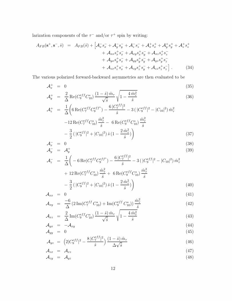
larization components of the τ− and/or τ+ spin by writing:

AFB(s+, s−, s) = AFB(s) +[A−

x s−x + A−y s−y + A−

z s−z + A+x s+

x + A+y s+

y + A+z s+

z

+ Axxs+x s−x + Axys

+x s−y + Axzs

+x s−z

+ Ayxs+y s−x + Ayys

+y s−y + Ayzs

+y s−z

+ Azxs+z s−x + Azys

+z s−y + Azzs

+z s−z

]. (34)

The various polarized forward-backward asymmetries are then evaluated to be

A+x = 0 (35)

A+y =

2

∆Re(Ceff

9 C∗10)

(1 − s) mτ√s

√

1 − 4 m2τ

s(36)

A+z =

1

∆

(

6 Re(Ceff7 Ceff∗

9 ) − 6 |Ceff7 |2s

− 3 ( |Ceff9 |2 − |C10|2) m2

τ

−12 Re(Ceff7 C∗

10)m2

τ

s− 6 Re(Ceff

9 C∗10)

m2τ

s

− 3

2( |Ceff

9 |2 + |C10|2) s (1 − 2 m2τ

s)

)

(37)

A−x = 0 (38)

A−y = A+

y (39)

A−z =

1

∆

(

− 6 Re(Ceff7 Ceff∗

9 ) − 6 |Ceff7 |2s

− 3 ( |Ceff9 |2 − |C10|2) m2

τ

+ 12 Re(Ceff7 C∗

10)m2

τ

s+ 6 Re(Ceff

9 C∗10)

m2τ

s

− 3

2( |Ceff

9 |2 + |C10|2) s (1 − 2 m2τ

s)

)

(40)

Axx = 0 (41)

Axy =−6

∆(2 Im(Ceff

7 C∗10) + Im(Ceff

9 C∗10))

m2τ

s(42)

Axz =2

∆Im(Ceff

9 C∗10)

(1 − s) mτ√s

√

1 − 4 m2τ

s(43)

Ayx = −Axy (44)

Ayy = 0 (45)

Ayz =(2|Ceff

9 |2 − 8 |Ceff7 |2s

) (1 − s) mτ

∆√

s(46)

Azx = Axz (47)

Azy = Ayz (48)

12

Azz =−3

∆(2 Re(Ceff

7 C∗10) + Re(Ceff

9 C∗10) s)

√

1 − 4 m2τ

s. (49)

Note that, in the SM, it turns out that AFB = −Azz.

-0.02

-0.015

-0.01

-0.005

0

0.005

0.01

0.7 0.8 0.9 1

-0.5

-0.4

-0.3

-0.2

-0.1

0

0.1

0.7 0.8 0.9 1

SzSz

�ZZ

��Z

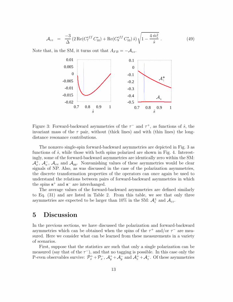
Figure 3: Forward-backward asymmetries of the τ− and τ+, as functions of s, theinvariant mass of the τ pair, without (thick lines) and with (thin lines) the long-distance resonance contributions.

The nonzero single-spin forward-backward asymmetries are depicted in Fig. 3 asfunctions of s, while those with both spins polarized are shown in Fig. 4. Interest-ingly, some of the forward-backward asymmetries are identically zero within the SM:A+

x , A−x , Axx and Ayy. Nonvanishing values of these asymmetries would be clear

signals of NP. Also, as was discussed in the case of the polarization asymmetries,the discrete transformation properties of the operators can once again be used tounderstand the relations between pairs of forward-backward asymmetries in whichthe spins s+ and s− are interchanged.

The average values of the forward-backward asymmetries are defined similarlyto Eq. (31) and are listed in Table 2. From this table, we see that only threeasymmetries are expected to be larger than 10% in the SM: A±

z and Azz.

5 Discussion

In the previous sections, we have discussed the polarization and forward-backwardasymmetries which can be obtained when the spins of the τ+ and/or τ− are mea-sured. Here we consider what can be learned from these measurements in a varietyof scenarios.

First, suppose that the statistics are such that only a single polarization can bemeasured (say that of the τ−), and that no tagging is possible. In this case only theP-even observables survive: P+

x +P−x , A+

y +A−y and A+

z +A−z . Of these asymmetries

13

0

0.02

0.04

0.06

0.08

0.1

0.12

0.7 0.8 0.9 1

-0.006

-0.005

-0.004

-0.003

-0.002

-0.001

0

0.7 0.8 0.9 1

SzSz

0

0.02

0.04

0.06

0.08

0.7 0.8 0.9 1

Sz

-0.1

-0.05

0

0.05

0.1

0.15

0.2

0.25

0.3

0.7 0.8 0.9 1

Sz

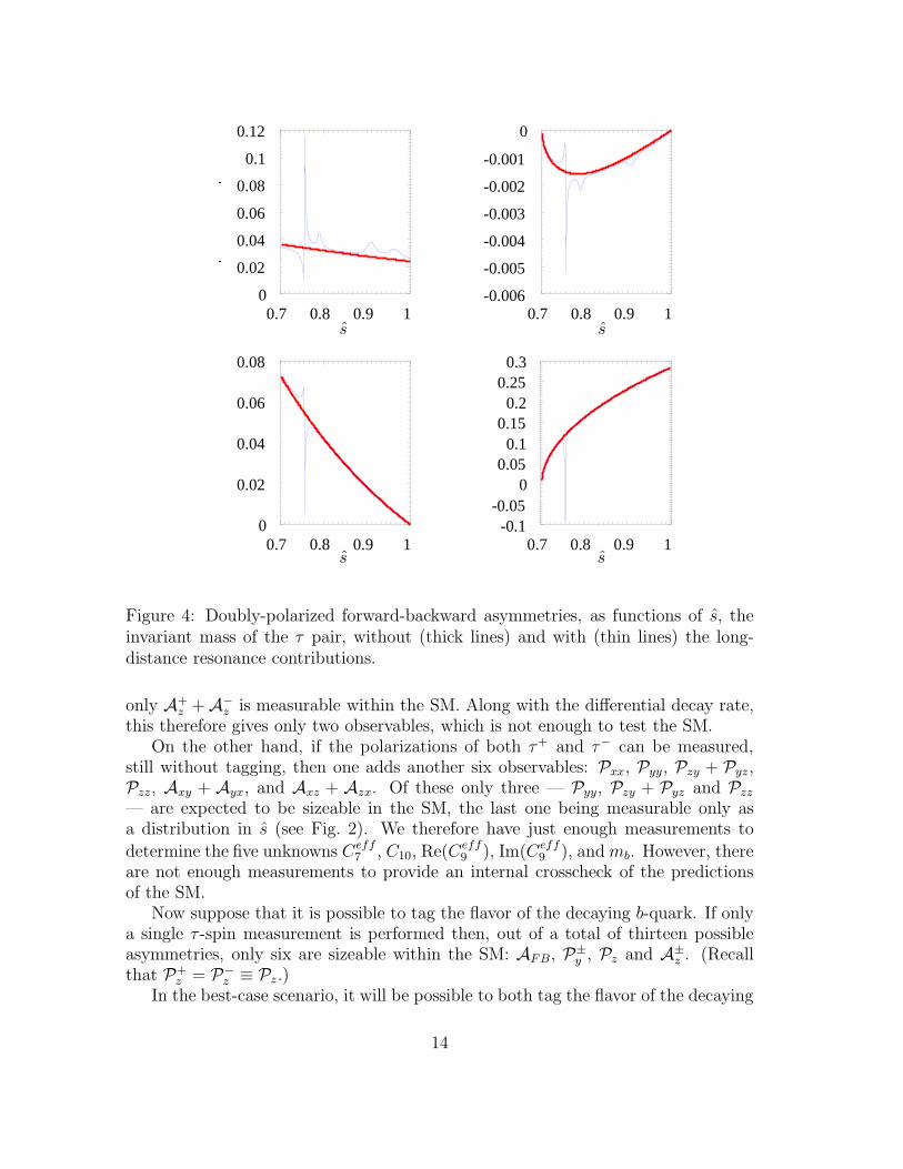
Figure 4: Doubly-polarized forward-backward asymmetries, as functions of s, theinvariant mass of the τ pair, without (thick lines) and with (thin lines) the long-distance resonance contributions.

only A+z + A−

z is measurable within the SM. Along with the differential decay rate,this therefore gives only two observables, which is not enough to test the SM.

On the other hand, if the polarizations of both τ+ and τ− can be measured,still without tagging, then one adds another six observables: Pxx, Pyy, Pzy + Pyz,Pzz, Axy + Ayx, and Axz + Azx. Of these only three — Pyy, Pzy + Pyz and Pzz

— are expected to be sizeable in the SM, the last one being measurable only asa distribution in s (see Fig. 2). We therefore have just enough measurements to

determine the five unknowns Ceff7 , C10, Re(Ceff

9 ), Im(Ceff9 ), and mb. However, there

are not enough measurements to provide an internal crosscheck of the predictionsof the SM.

Now suppose that it is possible to tag the flavor of the decaying b-quark. If onlya single τ -spin measurement is performed then, out of a total of thirteen possibleasymmetries, only six are sizeable within the SM: AFB, P±

y , Pz and A±z . (Recall

that P+z = P−

z ≡ Pz.)In the best-case scenario, it will be possible to both tag the flavor of the decaying

14

〈A+y 〉 = 〈A−

y 〉 −1.302 × 10−2

〈A+z 〉 −0.148

〈A−z 〉 −0.490

〈Axy〉 = −〈Ayx〉 3.184 × 10−2

〈Axz〉 = 〈Azx〉 −1.347 × 10−3

〈Ayz〉 = 〈Azy〉 4.298 × 10−2

〈Azz〉 0.154

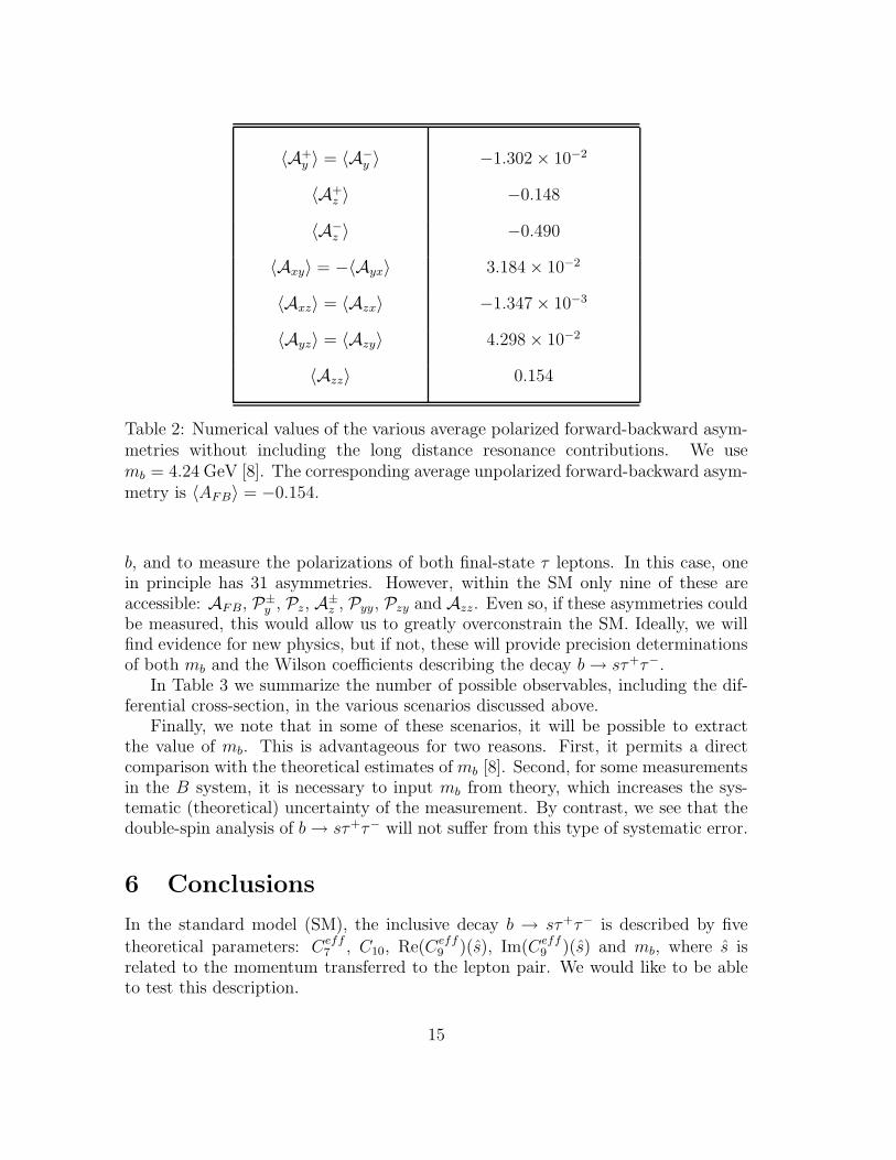
Table 2: Numerical values of the various average polarized forward-backward asym-metries without including the long distance resonance contributions. We usemb = 4.24 GeV [8]. The corresponding average unpolarized forward-backward asym-metry is 〈AFB〉 = −0.154.

b, and to measure the polarizations of both final-state τ leptons. In this case, onein principle has 31 asymmetries. However, within the SM only nine of these areaccessible: AFB, P±

y , Pz, A±z , Pyy, Pzy and Azz. Even so, if these asymmetries could

be measured, this would allow us to greatly overconstrain the SM. Ideally, we willfind evidence for new physics, but if not, these will provide precision determinationsof both mb and the Wilson coefficients describing the decay b → sτ+τ−.

In Table 3 we summarize the number of possible observables, including the dif-ferential cross-section, in the various scenarios discussed above.

Finally, we note that in some of these scenarios, it will be possible to extractthe value of mb. This is advantageous for two reasons. First, it permits a directcomparison with the theoretical estimates of mb [8]. Second, for some measurementsin the B system, it is necessary to input mb from theory, which increases the sys-tematic (theoretical) uncertainty of the measurement. By contrast, we see that thedouble-spin analysis of b → sτ+τ− will not suffer from this type of systematic error.

6 Conclusions

In the standard model (SM), the inclusive decay b → sτ+τ− is described by five

theoretical parameters: Ceff7 , C10, Re(Ceff

9 )(s), Im(Ceff9 )(s) and mb, where s is

related to the momentum transferred to the lepton pair. We would like to be ableto test this description.

15

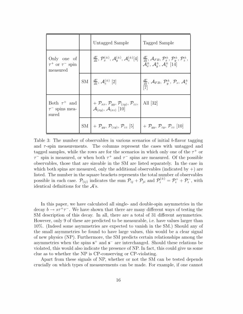
Untagged Sample Tagged Sample

Only one ofτ+ or τ− spinmeasured

dΓds

, P(±)x , A(±)

y , A(±)z [4] dΓ

ds, AFB, P±

x , P±y , P±

z ,A±

x , A±y , A±

z [14]

SM dΓds

, A(±)z [2] dΓ

ds, AFB, P±

y , Pz, A±z

[7]

Both τ+ andτ− spins mea-sured

+ Pxx, Pyy, P(zy), Pzz,A(xy), A(xz) [10]

All [32]

SM + Pyy, P(zy), Pzz [5] + Pyy, Pzy, Pzz [10]

Table 3: The number of observables in various scenarios of initial b-flavor taggingand τ -spin measurements. The columns represent the cases with untagged andtagged samples, while the rows are for the scenarios in which only one of the τ+ orτ− spin is measured, or when both τ+ and τ− spins are measured. Of the possibleobservables, those that are sizeable in the SM are listed separately. In the case inwhich both spins are measured, only the additional observables (indicated by +) arelisted. The number in the square brackets represents the total number of observablespossible in each case. P(ij) indicates the sum Pij + Pji and P(±)

i = P+i + P−

i , withidentical definitions for the A’s.

In this paper, we have calculated all single- and double-spin asymmetries in thedecay b → sτ+τ−. We have shown that there are many different ways of testing theSM description of this decay. In all, there are a total of 31 different asymmetries.However, only 9 of these are predicted to be measurable, i.e. have values larger than10%. (Indeed some asymmetries are expected to vanish in the SM.) Should any ofthe small asymmetries be found to have large values, this would be a clear signalof new physics (NP). Furthermore, the SM predicts certain relationships among theasymmetries when the spins s+ and s− are interchanged. Should these relations beviolated, this would also indicate the presence of NP. In fact, this could give us someclue as to whether the NP is CP-conserving or CP-violating.

Apart from these signals of NP, whether or not the SM can be tested dependscrucially on which types of measurements can be made. For example, if one cannot

16

perform b-tagging, and can measure only a single individual τ spin, then there areonly two sizeable observables. This is not enough to test the SM. On the other hand,if one can measure both τ spins, but cannot tag the flavor of the b, then there area total of five measurable observables. This is enough to determine the theoreticalunknowns, but does not provide the necessary redundancy to test the SM.

On the other hand, if one can perform b-tagging, but can only measure a singleτ spin, then there are 7 sizeable observables. This can provide a redundant test ofthe SM. The optimal scenario is if b-tagging is possible, and one can measure thepolarizations of both the τ+ and τ−. In this case, there are a total of 10 independentmeasurements, which would greatly overconstrain the SM. If new physics is notfound, this would precisely determine the five theoretical parameters.

Note that testing the SM implies that the quantity mb will be extracted fromthe experimental data. This will allow us to compare the experimental value of mb

with the theoretical estimates of this same quantity. Furthermore, as the measure-ments do not rely on theoretical input, the systematic error will be correspondinglyreduced.

Acknowledgements: N.S. and R.S. thank D.L. for the hospitality of the Universitede Montreal, where part of this work was done. The work of D.L. was financially sup-ported by NSERC of Canada. The work of Nita Sinha was supported by a project ofthe Department of Science and Technology, India, under the young scientist scheme.

7 Appendix

In this Appendix, we calculate the square of the amplitude in Eq. (1), keeping thespins of both final-state leptons. We define pb, ps, p+ and p− to be the momentaof the b-quark, s-quark, τ+ and τ−, respectively, with q = pb − ps = p+ + p−. Thespins of the τ+ and τ− are denoted by s+ and s−, respectively. We have

|M|2 = |T9|2 + |T10|2 + |T7|2 + 2Re(T †

9T10

)+ 2Re

(T †

9T7

)+ 2Re

(T †

10T7

). (50)

Summing over the s-quark spin and averaging over the b-quark spin, We find

1

2

∑

b,s spins

|T9|2 =α2G2

F

π2|VtbV

∗ts|2|Ceff

9 |2

×{

(m2b − q2)

2

(

−p− · s+ p+ · s− +q2

2s+ · s− + m2

τ (1 − s+ · s−)

)

+(1 − s+ · s−) (pb · p+ ps · p− + ps · p+ pb · p−)

−q2

2[pb · s+ ps · s− + ps · s+ pb · s−]

+s+ · p− [pb · p+ ps · s− + ps · p+ pb · s−]

17

+s− · p+ [pb · p− ps · s+ + ps · p− pb · s+]

+mτ

[ps · (p+ + p−) pb · (s+ + s−)

−pb · (p+ + p−) ps · (s+ + s−)]}

, (51)

1

2

∑

b,s spins

|T10|2 =α2G2

F

π2|VtbV

∗ts|2|C10|2

×{

−(m2b − q2)

2

(

−p− · s+ p+ · s− +q2

2s+ · s− + m2

τ (1 − s+ · s−)

)

+(1 + s+ · s−) (pb · p+ ps · p− + ps · p+ pb · p−)

−(

2m2τ −

q2

2

)

[pb · s+ ps · s− + ps · s+ pb · s−]

−s+ · p− [pb · p+ ps · s− + ps · p+ pb · s−]

−s− · p+ [pb · p− ps · s+ + ps · p− pb · s+]

−mτ

[ps · (p+ − p−) pb · (s+ − s−)

−pb · (p+ − p−) ps · (s+ − s−)]}

, (52)

∑

b,s spins

Re[T †

9T10

]=

α2G2F

π2|VtbV

∗ts|2

×{

2Re(Ceff9 C∗

10)[m2

τ [ps · s− pb · s+ − pb · s− ps · s+]

−q2

2(ps · p− − ps · p+)

+mτ [pb · p+ ps · s− + ps · p+ pb · s−−pb · p− ps · s+ − ps · p− pb · s+]

]

+Im(Ceff9 C∗

10)ǫµαβφ

[[2mτ + (ps + pb) · s+

]pµ

s pα−sβ

−pφ+

−[2mτ + (ps + pb) · s−

]pµ

spα+sβ

+pφ−

−(ps + pb) · p+ pµsp

α−sβ

−sφ+ + (ps + pb) · p− pµ

s pα+sβ

+sφ−

+(p− − p+) · ps pµ−pα

+sβ+sφ

−

]}

, (53)

18

1

2

∑

b,s spins

|T7|2 =α2G2

F

π2|VtbV

∗ts|2

m2b

q4|C7|2

×{

4m2bmτ

[ps · (p+ + p−) q · (s− + s+) − q2 ps · (s− + s+)

]

+2m2τm

2b(m

2b − q2)[(1 − s+ · s−] + q2m2

b(m2b − q2)

−2q2[2[ps · p− pb · p+ + ps · p+ pb · p−] − q2 pb · ps

][(1 − s+ · s−]

−4q2[s+ · p−[ps · s− pb · p+ + pb · s− ps · p+]

+s− · p+[ps · p− pb · s+ + pb · p− ps · s+]]

+2q2(m2b − q2) s+ · p− s− · p+

+2q4[ps · s− pb · s+ + pb · s− ps · s+]

}

, (54)

∑

b,s spins

Re[T †

9T7

]=

α2G2F

π2|VtbV

∗ts|2

m2b

q2

×{

Re(Ceff9 c∗7)

[(m2

b − q2)[q2 + 2m2τ − 2m2

τ s+ · s−]

−4mτ [pb · (p+ + p−) ps · (s+ + s−)

−ps · (p+ + p−) pb · (s+ + s−)]]}

, (55)

∑

b,s spins

Re[T †

10T7

]=

α2G2F

π2|VtbV

∗ts|2

m2b

q2

×{

− 2Re(C10Ceff∗

7 )[− mτ (m

2b − q2)

2[p+ · s− − p− · s+]

+q2[ps · p− − ps · p+] − 2m2τ [ps · s− p− · s+ − p+ · s− ps · s+]

+mτ q2ps · (s+ − s−) + mτ ps · (p− − p+)(s− · p+ + s+ · p−)]

−4Im(C10Ceff∗

7 )ǫαβµρ

[− mτ pα

s pβ+sµ

+pρb + mτ pα

s pβ−sµ

−pρb

+m2τ sα

−pβs sµ

+pρb

]}

. (56)

In the above, we have used the convention ǫ0123 = +1. Note that, as mentioned inSec. 2, Ceff

7 and C10 are expected to be real; only Ceff9 is complex. However, in

19

the expressions above, for completeness we have included both real and imaginarypieces of all Wilson coefficients.

References

[1] W. S. Hou, R. S. Willey and A. Soni, Phys. Rev. Lett. 58, 1608 (1987) [Erratum-ibid. 60, 2337 (1988)]; N. G. Deshpande and J. Trampetic, Phys. Rev. Lett.60, 2583 (1988); A. Ali, T. Mannel and T. Morozumi, Phys. Lett. B 273, 505(1991); A. F. Falk, M. E. Luke and M. J. Savage, Phys. Rev. D 49, 3367 (1994);A. Ali, G. F. Giudice and T. Mannel, Zeit. Phys. C67, 417 (1995); C. Greub,A. Ioannisian and D. Wyler, Phys. Lett. B 346, 149 (1995); J. L. Hewett, Phys.Rev. D53, 4964 (1996); F. Kruger and L. M. Sehgal, Phys. Lett. 380B, 199(1996); A. Ali, G. Hiller, L. T. Handoko and T. Morozumi, Phys. Rev. D 55,4105 (1997); C. S. Kim, T. Morozumi and A. I. Sanda, Phys. Rev. D 56, 7240(1997); T. M. Aliev, C. S. Kim and M. Savci, Phys. Lett. B 441, 410 (1998);C. Q. Geng and C. P. Kao, Phys. Rev. D 57, 4479 (1998); S. Fukae, C. S. Kim,T. Morozumi and T. Yoshikawa, Phys. Rev. D 59, 074013 (1999); Y. G. Kim,P. Ko and J. S. Lee, Nucl. Phys. B 544, 64 (1999); S. Fukae, C. S. Kim andT. Yoshikawa, Phys. Rev. D61, 074015 (2000); M. Zhong, Y. L. Wu andW. Y. Wang, arXiv:hep-ph/0206013; A. Ghinculov, T. Hurth, G. Isidori andY. P. Yao, arXiv:hep-ph/0208088; H. M. Asatrian, K. Bieri, C. Greub andA. Hovhannisyan, arXiv:hep-ph/0209006.

[2] P. L. Cho, M. Misiak and D. Wyler, Phys. Rev. D 54, 3329 (1996); Y. Gross-man, Z. Ligeti and E. Nardi, Phys. Rev. D 55, 2768 (1997); J. L. Hewett andJ. D. Wells, Phys. Rev. D 55, 5549 (1997); T. Goto, Y. Okada, Y. Shimizuand M. Tanaka, Phys. Rev. D 55, 4273 (1997) [Erratum-ibid. D 66, 019901(2002)]; L. T. Handoko, Nuovo Cim. A 111, 95 (1998); J. H. Jang, Y. G. Kimand J. S. Lee, Phys. Rev. D 58, 035006 (1998); T. G. Rizzo, Phys. Rev. D 58,114014 (1998); S. Rai Choudhury, A. Gupta and N. Gaur, Phys. Rev. D 60,115004 (1999); C.-S. Huang and S. H. Zhu, Phys. Rev. D 61, 015011 (2000)[Erratum-ibid. D 61, 119903 (2000)].

[3] A. Ali, G. F. Giudice and T. Mannel, Ref. [1].

[4] J. L. Hewett, Ref. [1].

[5] F. Kruger and L. M. Sehgal, Ref. [1].

[6] Refs. [5] and [7] give 〈PN〉τ = 0.05 and 〈PN〉τ = 0.02, respectively. The authorsof Ref. [7] cut out resonances below the Ψ′, which increases the asymmetry,while the authors of Ref. [5] have used a cut of ±30 MeV for the Ψ′ resonances.As we show later in the paper, we find 〈PN〉τ = 0.014.

20

[7] S. Fukae, C. S. Kim and T. Yoshikawa, Ref. [1].

[8] A.X. El-Khadra and M. Luke, hep-ph/0208114.

[9] B. Grinstein, M. J. Savage and M. B. Wise, Nucl. Phys. B319, 271 (1989);A. J. Buras and M. Munz, Phys. Rev. D52, 186 (1995); M. Misiak, Nucl. Phys.B 393, 23 (1993) [Erratum-ibid. B 439, 461 (1995)].

[10] C. S. Lim, T. Morozumi and A. I. Sanda, Phys. Lett. 218B, 343 (1989); N. G.Deshpande, J. Trampetic and K. Panose, Phys. Rev. D39, 1461 (1989); P. J.O’Donnell, M. Sutherland and H. K. K. Tung, Phys. Rev. D46, 4091 (1992);P. J. O’Donnell and H. K. K. Tung, Phys. Rev. D43, R2067 (1991); F. Krugerand L. M. Sehgal, Ref. [1].

[11] A. Ali, T. Mannel and T. Morozumi, Ref. [1].

[12] Particle Physics and Introduction to Field Theory, by T. D. Lee, HarwoodAcademic Publishers (1981).

21