leapfrog geo user manual
TRANSCRIPT

User Manualfor Leapfrog Geo version 5.0

© 2019 Seequent Limited (“Seequent”). All rights reserved. Unauthorised use, reproduction, or disclosure isprohibited. Seequent assumes no responsibility for errors or omissions in this document. LEAPFROG, SEEQUENT and
are trade marks owned by Seequent. All other product and company names are trade marks or registered trade
marks of their respective holders. Use of these trade marks in this document does not imply any ownership of thesetrade marks or any affiliation or endorsement by the holders of these trade marks.
ContentsGetting Started 1
Signing In to Leapfrog Geowith Seequent ID 1
Graphics and Drivers 2
Switching to High-PerformanceGraphics 3
Running the Graphics Test 4
The Leapfrog Geo Projects Tab 6
Recording Reference Codes 7
Managing Leapfrog Geo Projects 7
Saving Projects 8
Saving Zipped Copies of Projects 8
Saving Backup Copies of Projects 8
Compacting Projects 8
Upgrading Projects 9
Converting Leapfrog Hydro Projects 9
What is Implicit Modelling? 10
What are the Advantages of Implicit Modelling? 10
Implicit Modelling Makes Assumptions Explicit 11
Best Practices 11
An Overview of Leapfrog Geo 13
Keyboard Shortcuts in theMain Window 14
The Project Tree 16
Organising Objects in the Project Tree 19
Subfolders 19
Copying Objects 20
Renaming Objects 20
Finding Objects 21
Deleting Objects 21
Sharing Objects 22
Object Properties 22
Comments 23
Object Processing 24
Controlling Processing 25
Prioritising Objects 26
Freezing Objects 28
Correcting Errors 29
© 2019 Seequent Limited
ii | Leapfrog Geo User Manual
Project Tree Keyboard Shortcuts 29
The 3D Scene 31
Locating an Object from the Scene 34
Clicking in the Scene 35
Clicking in the Shape List 36
Slicing Through the Data 37
Slicer Properties 38
Object SliceMode 39
Slicer Shortcuts 39
Measuring in the Scene 40
Determining a Location 41
TheMoving Plane 42
The Ruler 43
Working With Split Views 45
Visualising Data 49
ColourOptions 51
Single Colour Display 52
CategoryColourmaps 53
Numeric Colourmaps 53
ContinuousColourmaps 55
Discrete Colourmaps 58
Importing Colour Gradients 61
Importing and Exporting Colourmaps 62
Opacity 63
Property Buttons 63
Legends 64
SliceMode 64
Filtering Data Using Queries 64
Filtering Data Using Values and Categories 65
Drawing in the Scene 66
TheDrawing Toolbar 67
Drawing Hotkeys 68
Drawing 3D Lines 69
Drawing 2D Lines 72
Polyline Properties 72
Tangents and Ribbons 73
Drawing Points 74
© 2019 Seequent Limited
Contents | iii
Organising YourWorkspace 77
Detaching Tabs 77
Detaching and Minimising the Project Tree 78
Organising the Scene View Tab 78
Interpolant Functions 80
The Spheroidal Interpolant Function 80
Total Sill 81
Nugget 82
Nugget to Total Sill Ratio 82
Base Range 82
Alpha 84
Drift 85
Accuracy 87
The Linear Interpolant Function 87
Total Sill and Base Range 89
Nugget 89
Drift 89
Accuracy 90
Central Integration 91
Connecting to Central 91
Connecting Via Seequent ID 91
Manual Setup 92
The Central Projects Tab 93
Central Settings 94
Viewing a Project’s History 95
Locking Branches 96
Project Included 97
Project Stages 97
Annotations and Attachments 97
Sharing Projects 98
Downloading a Local Copy of a Project 99
Publishing to Central 99
Unfinished Publish Events 100
Selecting Objects 100
Setting the Project Workflow Stage 101
Including the Project 101
Adding Revision Information 101
© 2019 Seequent Limited
iv | Leapfrog Geo User Manual
Preparing the Package 101
Uploading the Package 101
New Central Projects 102
Creating a New Central Project 102
Adding a Project to Central 103
Troubleshooting Connectivity Issues 103
Settings 104
Display and Navigation Settings 104
3D Acceleration Mode 104
Font Size 105
Z Axis Scale 105
Rotation Settings 106
Camera Settings 106
Overlay Settings 107
Screen Grid Settings 107
Axis Lines Settings 107
OtherOverlay Settings 107
Colour Scheme 107
Lighting Settings 108
Processing Settings 109
User Interface Settings 109
Show Tree Lines 109
Show Save Scene Button 109
Upload to View 109
Tab Position 110
Central Settings 110
Usage Policy Settings 111
Network Settings 112
Help Settings 112
Reporting a Problem 112
Getting Support 113
Checking Connectivitywith Leapfrog Start 113
Supplying Your Licence Details 113
Data Types 115
Working with Data Tables 116
Identifying Errors in Data Tables 117
Exporting Data Errors 118
© 2019 Seequent Limited
Contents | v
Correcting Data Errors in Leapfrog Geo 119
Replacing Values in a Column 120
Common Errors and How to Fix Them 121
Duplicate Points Error (Points Tables) 122
Duplicate Hole ID Error 122
Hole ID Not in Collar Table Error 123
Collar MaxDepth Error 123
Invalid MaxDepth Error 124
FromDepth Exceeds ToDepth Error 124
Overlapping Segments Error 125
No Samples for CollarsWarning 125
No Surveys for CollarWarning 126
Wedges Found Warning 126
Handling Special Values 126
Boundaries 128
The Clipping Boundary 128
Object Extents 131
Extending a Surface 132
Query Filters 134
Creating a NewQuery Filter 135
Leapfrog GeoQuery Syntax 136
Building a Query 137
Advanced Queries 138
Defining a Topography 138
Topography FromElevation Grid 139
Topography FromSurfaces, Points or GIS Vector Data 139
Fixed Elevation Topography 140
Adding Height Data to the Topography 140
Changing Topography Settings 141
Changing the Size of the Topography 141
Topography Resolution 142
Applying a Trend to the Topography 142
TopographyDisplayOptions 142
Projecting Collars onto the Topography 143
GIS Data, Maps and Images 144
Displaying GIS Data 144
CustomTopography Views 144
© 2019 Seequent Limited

vi | Leapfrog Geo User Manual
Importing Vector Data 146
Importing a MapInfo Batch File 147
Importing Data froman ESRI Geodatabase 148
Reloading GIS Data 149
Reloading Points, Lines and Polygons 149
Reloading an ESRI Database 149
Importing a Map or Image 150
Manual Georeferencing 151
Automatic Georeferencing 152
Exporting a Georeferenced Image 152
Setting Elevation for GIS Objects and Images 152
Creating a New GIS Line 153
Drawing a New GIS Line 154
Creating a New GIS Line from Intersecting Meshes 154
Exporting GIS Data 155
Drillhole Data 156
Displaying Drillholes 157
Displaying Drillholes as Lines or Cylinders 158
Hiding Lithologies 160
Displaying a Legend 160
Changing Colourmaps 161
Viewing Multiple Interval Tables 161
Selecting fromMultiple Columns 161
Displaying Interval Data in the Scene 162
Displaying Drillhole Graphs 163
Viewing Drillhole Data Table Statistics 165
Importing Drillhole Data 165
Expected Drillhole Data Tables and Columns 166
The Collar Table 166
The Survey Table 167
The Screens Table 167
Interval Tables 167
Selecting Files 168
Working Through the Data 169
Selecting theODBC Data Source 172
Selecting Tables 172
Connecting to an acQuire Database 174
© 2019 Seequent Limited
Contents | vii
Smart Refresh 175
Saving a Selection 175
Appending Drillholes 175
Importing Interval Tables 176
Importing Columns 176
Importing Screens 177
Importing Point ValuesDown Drillholes 177
Importing LAS PointsDown Drillholes 177
LAS File Mapping 178
LAS File Inconsistencies 178
Importing Downhole Structural Data 179
Drillhole Desurveying Options 179
The Spherical Arc Approximation Algorithm 180
The Balanced Tangent Algorithm 181
The Raw Tangent Algorithm 181
Processing Drillhole Data 182
CategoryComposites 183
Converting Ignored Segments 184
Filtering Short Segments 186
Viewing CategoryComposite Statistics 187
Economic Composites 188
Creating an Economic Composite 189
Selecting Values 189
Handling Missing Intervals and High Grades 190
Selecting a Dilution Rule 190
Setting the Cut-Off Grade 190
Two-PassCompositing 190
Using True Thickness 191
The Compositing Process and Parameters 191
Viewing Compositing Results 196
Majority Composites 198
Viewing Majority Composite Statistics 200
Numeric Composites 201
Creating a Numeric Composite 201
Compositing in the Entire Drillhole 202
Compositing in a Subset of Codes 204
Using Intervals FromAnother Table 205
© 2019 Seequent Limited
viii | Leapfrog Geo User Manual
Viewing Numeric Composite Statistics 205
Compositing Comparison 207
Compositing Interval Lengths 208
Grouping Lithologies 208
Automatic LithologyGroups 212
Splitting Lithologies 213
Interval Selection 216
Overlaid LithologyColumn 219
CategoryColumn fromNumeric Data 220
Back-Flagging Drillhole Data 221
Comparing Modelled Values to Drilling Lithologies 222
Comparing Drilling Lithologies toModelled Values 225
Refining the Geological Model to Improve Correlation Statistics 226
Merged Drillhole Data Tables 226
Core Photo Links 227
The ALS CoreViewer Interface 229
Setting Up the ALS CoreViewer Interface 229
Using the ALS Interface 230
Removing the ALS Link 231
The Coreshed Core Photo Interface 231
Setting Up the Coreshed Interface 231
Using the Coreshed Interface 232
Removing the Coreshed Link 233
The ImagoCore Photo Interface 233
Setting Up the Imago Interface 233
Using the Imago Interface 234
Removing the Imago Link 235
Reloading Drillhole Data 235
Exporting Drillhole Data 235
Exporting All Drillhole Data 236
Exporting a Single Drillhole Data Table 237
PointsData 238
Importing PointsData 238
Selecting theODBC Data Source 239
Reloading PointsData 239
Appending PointsData 239
Importing a Column 239
© 2019 Seequent Limited
Contents | ix
Setting Elevation for Points 240
Evaluating PointsData 240
Displaying Points 240
Viewing Points Table Statistics 242
Exporting PointsData 242
Exporting Intrusion Values 242
Exporting Interval Midpoints 243
Extracting Points fromDrillhole Data 243
Extracting Contact Points fromDrillhole Data 244
Extracting Intrusion Values fromDrillhole Data 245
Intrusion Point Generation Parameters 246
Extracting Interval Midpoints fromDrillhole Data 247
Creating Guide Points 248
Grids of Points 249
Creating a Grid of Points 249
Evaluating a Grid of Points 251
Statistics for a Grid of Points 251
Exporting a Grid of Points 251
Categorising Points 252
Geophysical Data 255
2D Grids 255
ASEG_DFN Files 256
UBC Grids 256
Importing a UBC Grid 256
Evaluating UBC Grids 256
Mapping Category Evaluations 257
Exporting a UBC Grid 257
GOCADModels 258
Structural Data 259
Creating New Planar Structural Data Tables 259
Importing Planar Structural Data 261
Selecting theODBC Data Source 262
Importing Lineations 262
Displaying Structural Data 263
Viewing Statistics on Structural Data 266
BinghamAnalysis 266
Fisher Statistics 267
© 2019 Seequent Limited
x | Leapfrog Geo User Manual
Assigning Structural Data to Categories 267
Editing theOrientation of Planar Structural Data 269
Declustering Planar Structural Data 269
Setting Elevation for Structural Data 271
Estimating Planar Structural Data 271
Meshes 271
Cleaning Up a Mesh 272
Importing a Mesh 274
Mesheswith Textures 274
Textured OBJ Meshes 275
Textured Vulcan Meshes 275
Reloading a Mesh 275
Displaying Surfaces 275
Draping an Image on a Mesh 276
Importing Meshes fromCentral 276
Importing Central Meshes 277
Updating Out-of-DateMeshes 279
Exporting Meshes 279
Exporting a SingleMesh 280
Exporting Multiple Meshes from theMeshes Folder 283
Exporting Multiple Meshes fromModels 284
Modifying Surfaces 285
Surface Resolution in Leapfrog Geo 285
Adding Data to Surfaces 287
Honouring Surface Contacts 288
Global Trends 291
Structural Trends 293
Creating a Structural Trend 293
Displaying a Structural Trend 295
Applying a Structural Trend 296
Editing Surfaceswith Polylines 297
Editing Surfaceswith Structural Data 299
Non-EditableMeshes 299
Mesh from theMoving Plane 300
Combining Meshes 300
Clipping a Volume 301
Clipping a Mesh 301
© 2019 Seequent Limited

Contents | xi
Merging 2DMeshes 302
Extracting Mesh Parts 303
Interpolated Meshes 303
Creating an Interpolated Mesh 304
Refining an Interpolated Mesh 305
Surface Resolution Settings 305
Snap Settings 305
OtherOptions 306
2D Interpolant Meshes 306
Offset Meshes 307
Triangulated Meshes 309
Elevation Grids 310
Importing an Elevation Grid 311
Exporting an Elevation Grid 312
ThicknessGrids 312
Polylines 314
Creating Polylines 314
Displaying Polylines 314
Sharing and Unsharing Polylines 315
Importing Polylines 316
Reloading Polylines 317
Exporting Polylines 317
Geochemical Data 319
Sending Data to ioGAS 320
Opening the Data in ioGAS 321
Sending a New Data Column Back to Leapfrog Geo 322
Importing ioGAS Data 323
Importing ioGAS Data as Points 324
Importing ioGAS Data as Intervals 324
Open Mining Format (OMF) Export and Import 324
OMF Export 325
OMF Import 326
Analysing Data 327
Statistics 327
Table of Statistics 328
Scatter Plots 332
Q-QPlots 334
© 2019 Seequent Limited
xii | Leapfrog Geo User Manual
Box Plots 335
Univariate Graphs 336
Drillhole Correlation Tool 338
Selecting Collars 338
The Correlation Set Window 340
Navigating in the Correlation Set Window 342
Correlation Column Layouts 342
Managing Styles 343
Interpretation Tables 343
Assigning Lithologies 344
Modifying the Interpretation Table 345
Stereonets 348
Creating a Stereonet 348
Displaying the Stereonet in the 3D Scene 349
Plot Options 350
Data DisplayOptions 350
Viewing Stereonet Statistics 354
Selecting Data in the Stereonet 354
Using the SceneWindowwith the Stereonet 359
Exporting a Stereonet 359
Form Interpolants 360
Creating a Form Interpolant 360
Setting a Trend 361
Adding Isosurfaces 362
The Form Interpolant in the Project Tree 362
Form Interpolant Statistics 363
Planning Drillholes 364
Adding Planned Drillholes 364
Planning Options 368
Drilling Prognoses 368
Exporting Planned Drillholes 369
Export Parameters 369
Export as Interval Table 369
Importing Planned Drillholes 369
Modelling 371
Evaluations 371
Assigning Attributes to Volumes 372
© 2019 Seequent Limited
Contents | xiii
Geological Models 374
Creating a New Geological Model 374
The Base Lithology 374
Surface Resolution 375
Model Extents 375
TheGeological Model in the Project Tree 376
Geological Model Display 376
Copying a Geological Model 377
Creating a Static Copy of a Geological Model 377
Geological Model Volumes and Surfaces Export Options 377
Extracting Model Volumes 378
Editing a Geological Model 379
Changing theQuery Filter 380
Surface Generation Options 381
VolumeGeneration Options 382
Surface Resolution for a Geological Model 382
Modifying a Geological Model’s Boundary 383
Creating Extents for a Geological Model 384
Extent Froma Polyline 384
Extent FromGIS Vector Data 385
Extent FromPoints 386
Extent FromStructural Data 386
Extent Froma Surface 388
Extent FromDistance to Points 388
Extent Froma Distance Function 389
Base FromLithologyContacts 390
Changing an Extent’s Settings 391
Surface Resolution 391
Contact Honouring 392
Applying a Trend 392
Adding Data to an Extent 393
Editing an Extent with a Polyline 393
Editing an Extent with Structural Data 393
Removing an Extent froma Geological Model 394
Model Lithologies 395
Faulted Models 396
The Fault System 397
© 2019 Seequent Limited
xiv | Leapfrog Geo User Manual
Fault Interactions 398
Activating the Fault System 399
Copying the Surface Chronology to an Empty Fault Block 399
Faulted Model DisplayOptions 400
Editing Faults 400
Surfacing Options for Faults 400
Boundary Filtering 401
Snapping to Data 401
Changing Fault Inputs 402
Replacing Fault Inputswith a SingleMesh 402
Adding Data to the Fault 403
Snap Settings for Individual Inputs 403
Boundary Filtering Settings for Individual Inputs 403
Applying a Trend to a Fault 403
Contact Surfaces 404
Contact Surfaces in the Surface Chronology 404
Contact Surfaces Types 407
Deposit and Erosion Contact Surfaces 408
Intrusion Contact Surfaces 409
Vein Contact Surfaces 411
Younging Direction 412
Deposits and Erosions 412
Creating Deposits and Erosions 413
Deposits and Erosions From the Base Lithology 413
Deposits and Erosions FromOther LithologyContacts 416
Deposits and Erosions FromOther Data 417
Deposits/Erosions in the Project Tree 419
Refining Deposits and Erosions 419
Surfacing Options for Deposits and Erosions 420
Boundary Filtering 420
Snapping to Data 420
Setting the Surface Resolution 421
Applying a Trend to a Deposit/Erosion 421
Intrusions 421
Creating Intrusions 422
Intrusions fromLithologyContacts 422
Intrusions fromOther Data 423
© 2019 Seequent Limited
Contents | xv
Intrusions in the Project Tree 425
Displaying Intrusion Points 425
Refining Intrusions 426
Surfacing Options for Intrusions 426
Boundary Filtering 426
Snapping to Data 427
Surface Resolution 427
Applying a Trend to an Intrusion 428
Clipping Values for Intrusions 429
Interpolation Settings 429
Veins 430
Creating Veins 430
Veins FromLithologyContacts 430
Veins FromOther Data 431
Veins in the Project Tree 432
Displaying Veins 433
Refining Veins 433
Surfacing Options for Veins 433
Boundary Filtering 433
Snapping to Data 434
Surface Resolution 434
Vein Thickness 434
Vein Pinch Out 435
The Vein Reference Surface 436
Adding Data to the Reference Surface 437
Using a Planar Reference Surface 438
The Vein Boundary 438
Adding a Polyline to the Vein Boundary 439
Adjusting the Vein Boundary Plane 439
Editing Vein Segments 440
Vein Segment Orientation 440
Vein Systems 440
Creating a Vein System 442
Adding Veins to the Vein System 442
Editing the Veins 442
Changing Vein SystemLithology Settings 442
Setting Vein Interactions 443
© 2019 Seequent Limited
xvi | Leapfrog Geo User Manual
Stratigraphic Sequences 445
Creating a Stratigraphic Sequence 446
Boundary Filtering 448
Snapping to Data 448
Surface Stiffness 449
Editing the Stratigraphic Sequence 449
Correcting Pinch-Out Errors 449
Surfacing Options 450
Applying a Trend 450
Editing Individual Surfaces 450
Contact Honouring and Boundary Filtering for Individual Surfaces 451
Adding Data to Individual Surfaces 451
Editing Surface Contacts 451
Offset Surfaces 451
Creating an Offset Surface 453
TheOffset Surface in the Project Tree 454
Refining an Offset Surface 454
Changing Surfacing Options for an Offset Surface 454
Boundary Filtering 455
Snapping to Data 455
Surface Resolution 456
Smoothing 456
Changing Offset Limits 456
Changing to a Constant Offset 456
Changing to an Offset to Points 457
Changing the ReferenceMesh 457
Editing the ReferenceMesh 457
Structural Surfaces 457
Creating a Structural Surface 458
The Structural Surface in the Project Tree 459
Refining a Structural Surface 459
Surfacing Options for a Structural Surface 460
Setting the Surface Resolution 460
Boundary Filtering 460
Snapping to Input Data 460
Non-Contact Structural Inputs Settings 461
Applying a Trend to a Structural Surface 461
© 2019 Seequent Limited

Contents | xvii
Value Clipping 461
The Surface Chronology 462
Refined Models 463
Editing the Sub-Model 465
Numeric Models 467
Importing a VariogramModel 468
Copying a Numeric Model 468
Creating a Static Copy of a Numeric Model 468
Exporting Numeric Model Volumes and Surfaces 469
Exporting Numeric Model Midpoints 469
RBF Interpolants 469
Creating an RBF Interpolant 470
ValuesUsed 470
Applying a Query Filter 471
Applying a Surface Filter 471
The Interpolant Boundary 471
Compositing Options 471
General Interpolant Properties 472
The RBF Interpolant in the Project Tree 472
Interpolant Display 473
RBF Interpolant Statistics 473
Modifying an RBF Interpolant’s Boundarywith Lateral Extents 473
Creating Lateral Extents 474
Extent froma Polyline 474
Extent fromGIS Vector Data 475
Extent fromPoints 476
Extent fromStructural Data 476
Extent froma Surface 477
Extent fromDistance to Points 477
Extent froma Distance Function 478
Changing a Lateral Extent’s Settings 479
Surface Resolution 479
Contact Honouring 479
Applying a Trend 480
Adding Data to an Extent 481
Editing an Extent with a Polyline 481
Editing an Extent with Structural Data 481
© 2019 Seequent Limited
xviii | Leapfrog Geo User Manual
Removing an Extent froman Interpolant 481
Changing the Settings for an RBF Interpolant 482
Adjusting the ValuesUsed 482
Adding a Contour Polyline 483
Adding Points 484
Compositing Parameters for an RBF Interpolant 484
Adjusting the Interpolant Boundary 485
Clipping and Transforming Values for an RBF Interpolant 486
Changing the Trend for an RBF Interpolant 487
Using a Global Trend 487
Using a Structural Trend 488
Adjusting Interpolation Parameters 490
Output Settings for an RBF Interpolant 491
Multi-Domained RBF Interpolants 491
Creating a Multi-Domained RBF Interpolant 492
Compositing and Filtering the ValuesUsed 493
Selecting Domains 494
Clipping and Transforming Values 494
Setting the Trend 494
Interpolation Parameters 494
Output Options 494
TheMulti-Domained RBF Interpolant in the Project Tree 496
Interpolant and Sub-Interpolant Display 496
Sub-Interpolant Statistics 497
Indicator RBF Interpolants 497
Creating an Indicator RBF Interpolant 498
Selecting the ValuesUsed 498
Setting the Cut Off 498
Applying a Query Filter 499
Applying a Surface Filter 499
The Interpolant Boundary 499
Compositing Options 499
General Interpolant Properties 500
The Indicator RBF Interpolant in the Project Tree 500
Indicator RBF Interpolant Display 501
Indicator RBF Interpolant Statistics 502
Editing an Indicator RBF Interpolant 502
© 2019 Seequent Limited
Contents | xix
Adjusting the ValuesUsed 503
Adding a Contour Polyline 503
Adding Points 505
Compositing Parameters for an Indicator RBF Interpolant 506
Adjusting the Interpolant Boundary 507
The Cut-Off Value 508
Changing the Trend for an Indicator RBF Interpolant 508
Adjusting Interpolation Parameters 509
Indicator RBF Interpolant Surfacing and VolumeOptions 509
Distance Functions 510
Creating a Distance Function 511
Setting the Boundary 513
Setting a Trend 513
Adding Buffers 513
TheNew Distance Function in the Project Tree 514
Combined Models 515
Creating a Combined Model 515
The Combined Model in the Project Tree 516
Editing a Combined Model 517
Displaying a Combined Model 517
Creating a Static Copy of a Combined Model 517
Combined Model Export 517
FlowModels 518
MODFLOWModels 518
Creating a MODFLOWModel 519
Horizontal Grid Spacing 520
Vertical Grid Layering 521
Editing a MODFLOWModel 523
Importing a MODFLOWModel 525
MODFLOW Evaluations 526
Assigning an Evaluation for Export 526
Combined Evaluations 526
MODFLOWHydrological Properties 527
Setting Hydrological Properties 528
ZoneNumbers 530
MODFLOWModel Display 530
Grid DisplayOptions 531
© 2019 Seequent Limited
xx | Leapfrog Geo User Manual
Viewing Block Information 532
Head Values and MT3D Concentrations 532
Generating a Head ValueMesh 533
MODFLOWModel Export 533
As a MODFLOW File 534
For Groundwater Vistas 534
As a Groundwater VistasUpdate 534
FEFLOWModels 534
FEFLOWModel Display 535
Displaying a 3DModel 537
Displaying a 2DModel 538
Viewing Block Information 539
Importing a FEFLOWGrid 539
Creating a 2D FEFLOWModel 540
BoundaryOptions 541
Element Size 542
Adding Features to the Grid 542
Creating a 3D FEFLOWModel 544
FEFLOW Evaluations 546
Assigning an Evaluation for Export 546
Combined Evaluations 547
FEFLOWMaterial Types 547
FEFLOWModel Export 549
BlockModels 550
Importing a BlockModel 550
Importing an Isatis BlockModel 550
Importing a BlockModel in CSV Format 551
Creating a BlockModel 552
Displaying a BlockModel 553
Viewing BlockModel Statistics 554
Table of Statistics 554
Exporting BlockModels 556
Exporting BlockModels in CSV Format 556
Selecting FromEvaluated Items 557
Setting Row Filtering Options 557
Setting Numeric Precision 557
Setting StatusCode Text Sequences 557
© 2019 Seequent Limited
Contents | xxi
Selecting the Character Set 558
Exporting BlockModels in Isatis Format 558
Selecting FromEvaluated Items 558
Setting StatusCode Text Sequences 558
Selecting the Character Set 559
Exporting BlockModels in Datamine Format 559
Selecting FromEvaluated Items 559
Setting Row Filtering Options 559
Setting StatusCode Text Sequences 559
Selecting the Character Set 560
Renaming Items 560
Exporting BlockModels in Surpac Format 560
Selecting FromEvaluated Items 560
Setting Row Filtering Options 561
Setting Numeric Precision 561
Setting StatusCode Text Sequences 561
Selecting the Character Set 561
Sub-Blocked Models 562
Creating a Sub-Blocked Model 562
Model Extents and Rotation 562
TheGrid Pattern 563
Triggers and Evaluations 565
Sub-Blocked Model Statistics 565
Sub-Blocked Model Export 566
Exporting Sub-Blocked Models in CSV Format 566
Selecting FromEvaluated Items 567
Setting Row Filtering Options 567
Setting Numeric Precision 567
Setting StatusCode Text Sequences 567
Selecting the Character Set 568
Exporting Sub-Blocked Models in Datamine Format 568
Selecting FromEvaluated Items 568
Setting Row Filtering Options 568
Setting StatusCode Text Sequences 569
Selecting the Character Set 569
Renaming Items 569
UBC Grids 570
© 2019 Seequent Limited
xxii | Leapfrog Geo User Manual
Importing a UBC Grid 570
Evaluating UBC Grids 570
Mapping Category Evaluations 570
Exporting a UBC Grid 571
Leapfrog Edge 572
Best Practices 572
Expertise is a Prerequisite 572
TheGeology is Fundamental 572
Analyse the Data First 572
Domaining 573
VariogramHypothesis and Experimentation, Analysis 573
Estimation Functions 573
BlockModelling 573
Data Analysis 574
Domained Estimations 575
Creating a Domained Estimation 575
Defining the Domain 576
Selecting Values 577
Setting Compositing Options 577
Boundary Validation 578
Filtering During Boundary Analysis 580
TheDomained Estimation in the Project Tree 581
Viewing Statistics 583
Copying a Domained Estimation 584
The Ellipsoid Widget 585
Display and Editing Modes 585
ChangeMovement Handles 587
Change LookDirection 589
Changing Controls in Edit Mode 589
Variography and Estimators 591
Experimental Variography and VariogramModels 591
The VariogramModel Window 593
VariogramModel Controls 595
Linear, Spherical and Spheroidal Model Options 596
Normalised Y Axis 596
Direction 597
Experimental Controls 597
© 2019 Seequent Limited
Contents | xxiii
Experimental VariogramParameters 600
Capping 601
Defining the Search Space 601
Radial Plot Parameters 603
Orienting CustomVariograms 604
Changing VariogramDisplay 604
TheDownhole Variogram 605
Axis Aligned Variograms 607
CustomVariograms 610
TransformVariography 611
Standard Estimators 615
Inverse Distance Estimators 616
Nearest Neighbour Estimators 618
Kriging Estimators 619
Kriging Attributes 622
RBF Estimators 624
Sample Geometries 626
Creating a New Declustering Object 626
General Settings 628
Outputs 629
The Declustering Object in the Project Tree 629
Applying a Declustering Object 630
Combined Estimators 630
Creating a Combined Estimator 631
Adding Estimators to a Combined Estimator 631
Evaluating a Combined Estimator 633
Viewing Statistics 639
Copying a Combined Estimator 640
Variable Orientations 640
Visualisation Options for Variable Orientations 641
Creating Variable Orientations 642
Selecting the Inputs 643
Setting the Global Plunge 647
Setting Visualisation Options 649
The Variable Orientation in the Project Tree 650
Applying a Variable Orientation 651
Exporting Rotations 652
© 2019 Seequent Limited
xxiv | Leapfrog Geo User Manual
BlockModel Evaluations 656
Visualising Sample Geometries and Estimators 656
Calculations and Filters on BlockModels 658
The CalculationsWindow 658
Creating a New Calculation or Filter 660
Variables 660
Numeric Calculations 661
Category Calculations 661
Filters 661
Understanding Errors Reported in the Errors Pane 661
Building Calculations and Filters 663
Examples of Variables 664
Example of a Numeric Calculation 664
Example of a Filter 665
Example of a Category Calculation 665
Null Values 667
Catalogue of Metadata, Syntax and Functions 669
Existing Items 670
Metadata 670
Evaluations 671
Variables, Calculations and Filters 672
Syntax and Functions 673
Statements 674
Basic Operators 675
Complex Comparisons 679
Invalid Values 680
Mathematics 682
Limits and Rounding 684
Text 686
Unit Conversion 690
Validation and Reporting 694
Block Estimate Interrogation 694
Grade TonnageGraphs 697
Swath Plots 702
Resource Reports 707
Presentation 711
Uploading to View 711
© 2019 Seequent Limited
Contents | xxv
Signing in to View 714
Uploading to View 715
Uploading the 3D View 715
Uploading Saved Scenes 716
Troubleshooting Connectivity Issues 716
Sections 717
Evaluating on Sections 717
Exporting Sections 717
Exporting Section Layouts 718
Creating Cross Sections 719
Importing Cross Sections 721
Fence Sections 722
Serial Sections 723
Setting the Base Section 723
Setting theOffset Sections 724
The Serial Section in the Project Tree 725
Displaying a Serial Section 725
Exporting a Serial Section 726
Section Layouts 727
Setting Up the Section 728
Creating New Section Layouts 729
Copying Section Layouts 730
Working With the Section Layout Editor 731
Changing Page Properties 732
Changing the Basic Section Properties 733
Organising Objects on the Section 737
Adding and Styling Models 738
Adding Styling Drillholes and Planned Drillholes 744
Adding and Styling Surfaces 748
Adding and Styling Lines 749
Setting Up the Legend 750
Adding and Organising Annotations 754
Displaying a Title 755
Displaying a Title Block 756
Displaying a Scale Bar and Location Information 757
Text Boxes 759
Images 760
© 2019 Seequent Limited

xxvi | Leapfrog Geo User Manual
Rendered Images 761
Background Rendering 763
Saved Scenes 763
Saving Scenes 764
Exporting Scenes 764
Linking to Scene Files 765
Movies 766
Contour Lines 767
Creating Contour Lines 767
Exporting GIS Contours 767
© 2019 Seequent Limited

Getting Started
Once Leapfrog Geo is installed, there are some first steps to carry out before you begin workingwith projects. This topic describes those first steps and then provides an overview of LeapfrogGeo project files. This topic is divided into:
l Signing In to Leapfrog Geo with Seequent ID
l Graphics and Drivers
l The Leapfrog Geo Projects Tab
l Recording Reference Codes
l Managing Leapfrog Geo Projects
Once you have carried out these first steps, see An Overview of Leapfrog Geo for a briefdescription of the different parts of the Leapfrog Geomain window. Formore detailedinformation on using the controls in the different parts of themain window, see the followingtopics:
l The Project Tree
l The 3D Scene
l Visualising Data
l Drawing in the Scene
l Organising Your Workspace
Signing In to Leapfrog Geo with Seequent IDTo use Leapfrog Geo, you need a Seequent ID and the correct permissions.
If you do not have a Seequent ID, you can sign up for one by launching Leapfrog Geo andclicking theRegister button.
To find out more about different permissions, visit the Flexible Leapfrog SoftwareSubscription Options page.
Once you have a Seequent ID and the correct permissions, launch Leapfrog Geo, enter yourdetails and click the button to sign in.
In the next window, you can:
l Select your group, if your organisation has a number of different groups.
l Select what extensions you wish to use. Some Leapfrog Geo features are only available withan extension.
l Select how long you wish to check out a seat, if your organisation is set up to check out seatson a day-by-day basis.
Select your options, then click theGet Started button.
© 2019 Seequent Limited
2 | User Manual
Signing in to Leapfrog Geo also signs you in to View, so you can upload scenes to View.
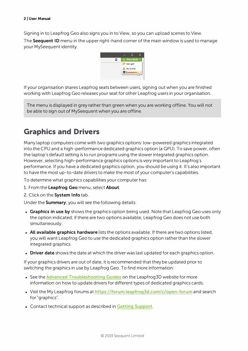
The Seequent IDmenu in the upper right-hand corner of themain window is used tomanageyourMySeequent identity.
If your organisation shares Leapfrog seats between users, signing out when you are finishedworking with Leapfrog Geo releases your seat for other Leapfrog users in your organisation.
Themenu is displayed in grey rather than green when you are working offline. You will notbe able to sign out of MySeequent when you are offline.
Graphics and DriversMany laptop computers comewith two graphics options: low-powered graphics integratedinto the CPU and a high-performance dedicated graphics option (a GPU). To save power, oftenthe laptop’s default setting is to run programsusing the slower integrated graphics option.However, selecting high-performance graphics options is very important to Leapfrog’sperformance. If you have a dedicated graphics option, you should be using it. It’s also importantto have themost up-to-date drivers tomake themost of your computer’s capabilities.
To determinewhat graphics capabilities your computer has:
1. From the Leapfrog Geomenu, select About.
2. Click on the System Info tab.
Under the Summary, you will see the following details:
l Graphics in use by shows the graphics option being used. Note that Leapfrog Geo uses onlythe option indicated; if there are two options available, Leapfrog Geo does not use bothsimultaneously.
l All available graphics hardware lists the options available. If there are two options listed,you will want Leapfrog Geo to use the dedicated graphics option rather than the slowerintegrated graphics.
l Driver date shows the date at which the driver was last updated for each graphics option.
If your graphics drivers are out of date, it is recommended that they be updated prior toswitching the graphics in use by Leapfrog Geo. To find more information:
l See the Advanced Troubleshooting Guides on the Leapfrog3Dwebsite formoreinformation on how to update drivers for different types of dedicated graphics cards.
l Visit theMy Leapfrog forums at https://forum.leapfrog3d.com/c/open-forum and searchfor “graphics”.
l Contact technical support as described in Getting Support.
© 2019 Seequent Limited
Switching to High-Performance Graphics | 3
Switching to High-Performance Graphics
If you havemore than one graphics option available, ensure you are using the dedicatedgraphics capabilities to get themost out of Leapfrog Geo. The steps below apply to an NVIDIAdriver and may be slightly different for other brands. Instructions for other brands can be foundon the driver’s or laptop manufacturer’swebsite.
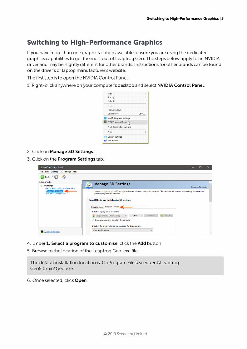
The first step is to open the NVIDIA Control Panel.
1. Right-click anywhere on your computer’s desktop and selectNVIDIA Control Panel.
2. Click on Manage 3D Settings.
3. Click on the Program Settings tab.
4. Under 1. Select a program to customise, click the Add button.
5. Browse to the location of the Leapfrog Geo .exe file.
The default installation location is: C:\ProgramFiles\Seequent\LeapfrogGeo5.0\bin\Geo.exe.
6. Once selected, clickOpen.
© 2019 Seequent Limited
4 | User Manual
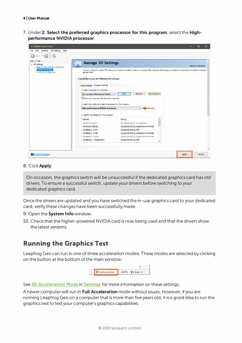
7. Under 2. Select the preferred graphics processor for this program, select theHigh-performance NVIDIA processor.
8. ClickApply.
On occasion, the graphics switch will be unsuccessful if the dedicated graphics card has olddrivers. To ensure a successful switch, update your drivers before switching to yourdedicated graphics card.
Once the drivers are updated and you have switched the in-use graphics card to your dedicatedcard, verify these changes have been successfullymade.
9. Open the System Infowindow.
10. Check that the higher-powered NVIDIA card is now being used and that the drivers showthe latest versions.
Running the Graphics Test
Leapfrog Geo can run in one of three acceleration modes. Thesemodes are selected by clickingon the button at the bottomof themain window:
See 3D Acceleration Mode in Settings formore information on these settings.
A newer computer will run in Full Accelerationmodewithout issues. However, if you arerunning Leapfrog Geo on a computer that ismore than five years old, it is a good idea to run thegraphics test to test your computer’s graphics capabilities.
© 2019 Seequent Limited
Running the Graphics Test | 5
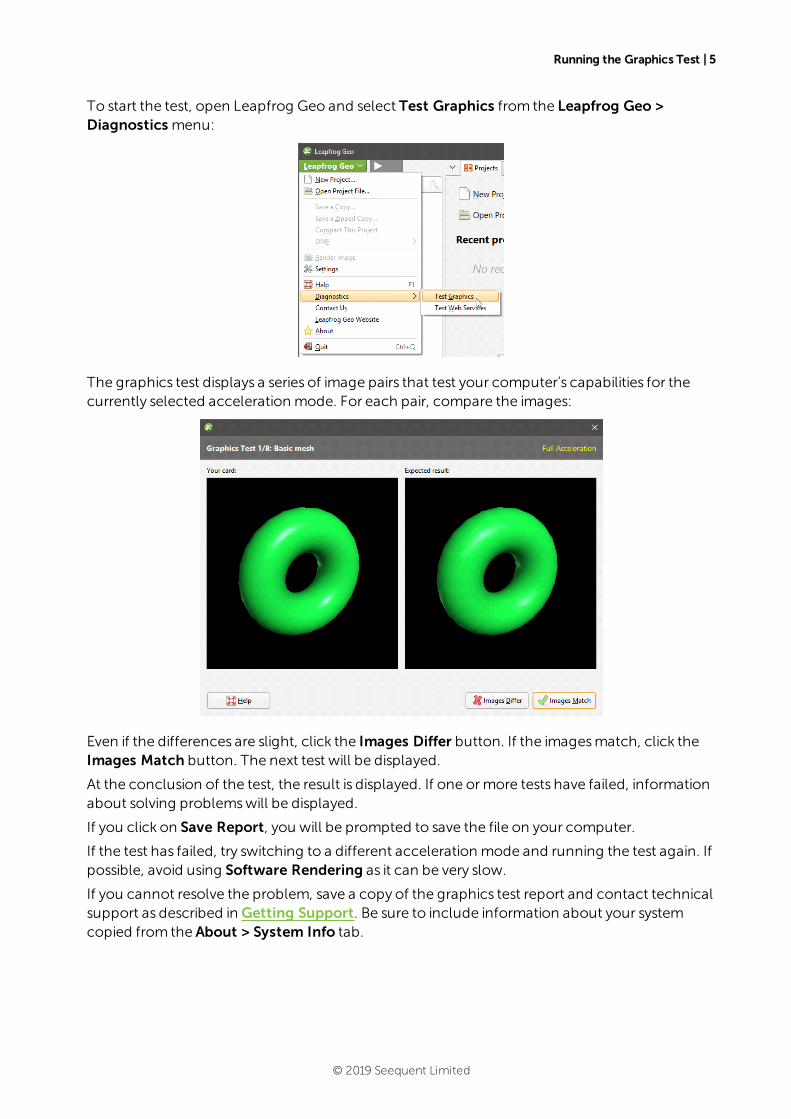
To start the test, open Leapfrog Geo and select Test Graphics from the Leapfrog Geo >Diagnostics menu:
The graphics test displays a series of image pairs that test your computer’s capabilities for thecurrently selected acceleration mode. For each pair, compare the images:
Even if the differences are slight, click the Images Differ button. If the imagesmatch, click theImages Match button. The next test will be displayed.
At the conclusion of the test, the result is displayed. If one ormore tests have failed, informationabout solving problemswill be displayed.
If you click on Save Report, you will be prompted to save the file on your computer.
If the test has failed, try switching to a different acceleration mode and running the test again. Ifpossible, avoid using Software Rendering as it can be very slow.
If you cannot resolve the problem, save a copy of the graphics test report and contact technicalsupport as described in Getting Support. Be sure to include information about your systemcopied from the About > System Info tab.
© 2019 Seequent Limited
6 | User Manual
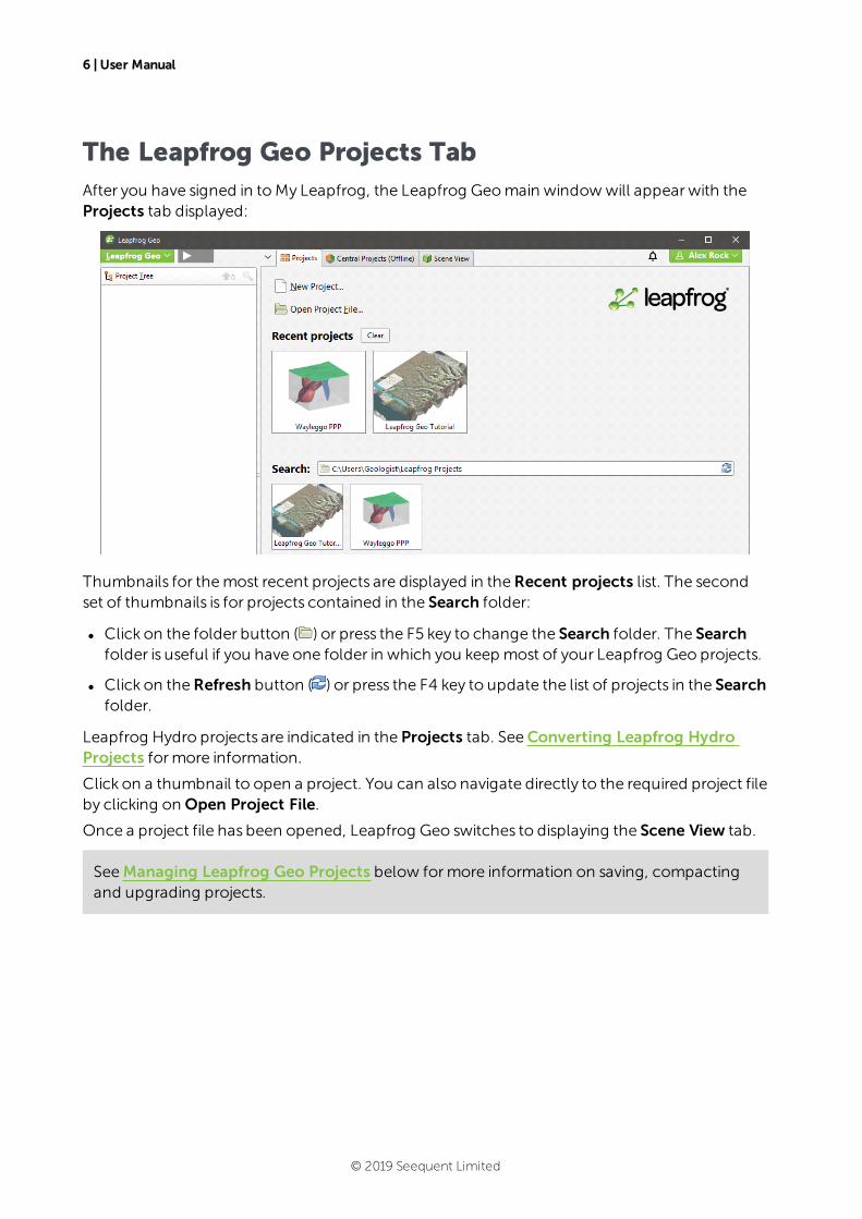
The Leapfrog Geo Projects TabAfter you have signed in toMy Leapfrog, the Leapfrog Geomain windowwill appear with theProjects tab displayed:
Thumbnails for themost recent projects are displayed in theRecent projects list. The secondset of thumbnails is for projects contained in the Search folder:
l Click on the folder button ( ) or press the F5 key to change the Search folder. The Searchfolder is useful if you have one folder in which you keep most of your Leapfrog Geo projects.
l Click on theRefresh button ( ) or press the F4 key to update the list of projects in the Searchfolder.
Leapfrog Hydro projects are indicated in the Projects tab. SeeConverting Leapfrog HydroProjects formore information.
Click on a thumbnail to open a project. You can also navigate directly to the required project fileby clicking on Open Project File.
Once a project file has been opened, Leapfrog Geo switches to displaying the Scene View tab.
SeeManaging Leapfrog Geo Projects below formore information on saving, compactingand upgrading projects.
© 2019 Seequent Limited
Recording Reference Codes | 7
Recording Reference CodesYou can enter a reference code to trackwork on specific projects. The time associated witheach reference code is included in yourmonthly usage report.
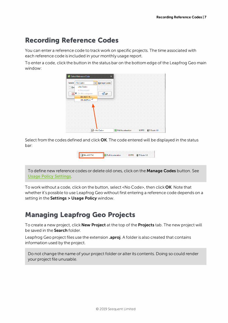
To enter a code, click the button in the status bar on the bottomedge of the Leapfrog Geomainwindow:
Select from the codes defined and clickOK. The code entered will be displayed in the statusbar:
To define new reference codes or delete old ones, click on theManage Codes button. SeeUsage Policy Settings.
Toworkwithout a code, click on the button, select <NoCode>, then clickOK. Note thatwhether it’s possible to use Leapfrog Geowithout first entering a reference code dependson asetting in the Settings > Usage Policy window.
Managing Leapfrog Geo ProjectsTo create a new project, clickNew Project at the top of the Projects tab. The new project willbe saved in the Search folder.
Leapfrog Geo project files use the extension .aproj. A folder is also created that containsinformation used by the project.
Do not change the name of your project folder or alter its contents. Doing so could renderyour project file unusable.
© 2019 Seequent Limited
8 | User Manual
A .lock file is created when a project is opened. The .lock file protects the project frombeingmoved while the project is open and frombeing opened by another instance of Leapfrog Geo,which can happen when projects are saved on shared network drives.
If processing and display of objects in your project is too slow and your project is stored on anetwork drive or on a USB drive, considermoving your project onto a local drive. LeapfrogGeo is optimised for working off your local hard drive, and working fromnetwork drives andUSB drives risks corrupting the project.
Saving Projects
Leapfrog Geo automatically saves an open project each time a processing task has beencompleted or settings have changed. Projects are also saved when they are closed so that scenesettings can be restored when the project is next opened.
Saving Zipped Copies of Projects
You can save a zipped copy of a project by selecting Save A Zipped Copy from the LeapfrogGeomenu. You will be prompted to choose a name and location for the zipped project. ClickSave to create the zip file.
Saving Backup Copies of Projects
You can save a backup copy of a project by selecting Save A Copy from the Leapfrog Geomenu. You will be prompted to choose a new name and location for the saved project. ClickOKto create the new project file. Leapfrog Geowill save a copy of the project in the locationselected.
Once the backup copy is saved, you can open and use it from the Projects tab. Otherwise,you can keep working in the original copy of the project.
Compacting Projects
When you delete objects froma project file, Leapfrog Geo retains those objects but notes thatthey are no longer used. Over time, the project file will grow in size and data stored in thedatabasemay become fragmented.
Compacting a project removes these unused objects and any unused space from the database.When you compact a project, Leapfrog Geowill close the project and back it up beforecompacting it. Depending on the size of the project, compacting it may take several minutes.Leapfrog Geowill then reopen the project.
To compact a project, selectCompact This Project from the Leapfrog Geomenu. You will beasked to confirm your choice.
© 2019 Seequent Limited
Upgrading Projects | 9
Upgrading Projects
When you open a project that was last saved in an earlier version of Leapfrog Geo, you may beprompted to upgrade the project. A list of affected objectswill be displayed. For large projectswith many objects that need to be reprocessed, the upgrade processmay take some time.
It is a good idea to back up the project before opening it. Tick the Back up the project beforeupgrading button, then clickUpgrade and Open. Navigate to the folder in which to save thebackup and click Save.
For large projectswith many objects, upgrading without backing up the project is notrecommended.
Converting Leapfrog Hydro Projects
Leapfrog Hydro projects can be converted to Leapfrog Geo projects. However, the process isone-way, and projects opened in Leapfrog Geo can no longer be opened in Leapfrog Hydro.
When you open a Leapfrog Hydro project, you will be prompted to save a backup beforeconverting the project.
It is strongly recommended that you back up the project before converting it.
© 2019 Seequent Limited
10 | User Manual
What is Implicit Modelling?Implicit modelling is a game-changing innovation in geological modelling.
Traditionally, geological models are produced using a manual drawing process. Sections aredefined, and lithologies, faults and veins are drawn on the sections. Lines are then drawn toconnect surfaces acrossmultiple sections. Modelling geology in thismanner is time-consumingand inflexible as it is difficult to update themodel whenmore data becomes available. Earlyassumptions that later are proved incorrect could shape a model in a way that is never correctedbecause of the effort involved in starting over. Instead of using their knowledge to revealimportant information about the study site, geologists spend significant proportions of theirtime engaged in mechanical drawing.
Implicit modelling, on the other hand, allows geologists to spend more time thinking about thegeology. Implicit modelling eliminates the laborious legwork by using mathematical tools toderive themodel from the data. Amathematical construct is built that can be used to visualisedifferent aspects of the data in 3D. Leapfrog Geo uses FastRBF™, a mathematical algorithmdeveloped from radial basis functions. FastRBF uses the data and parameters supplied by thegeologist to derive any one of a number of variables to bemodelled. Discrete variables such aslithologies can be used to construct surfaces, aswell as continuous variables such as oregrades.
Instead of presenting a model constructed from rigid geometric constructs, the visualisationsecho the natural forms found in reality.
What are the Advantages of Implicit Modelling?
Implicit models are easy to keep up-to-date with the latest data. New drillhole data can quicklybe integrated, instead of taking weeks or longermanuallymodifying themodel.
Implicit modelling allows several alternative hypothetical models to be produced from the data,quickly and easily. New data that affects themodel, even in very significant or fundamentalways, can be assimilated and integrated with little effort. Models can be built rapidly, whichmeans that a range of geological interpretations can be continually tested.
Because less effort is involved in creating a model, more time is available to spend onunderstanding the geology and studying more complex details such as faulting, stratigraphicsequences, trends and veins. Themodel can be developed to reflect reality to a greater degreeof precision than was previously possible.
Geological risk is reduced whenmodelling is done implicitly. With traditional modelling, theeffort involved means that the first model developed may be held to as the ground truth,despitemounting evidence that may discredit it. Instead, implicit modelling supports anapproach that follows the proven scientific method, developing hypothetical models,experimenting to find new data to corroborate or discredit models and, ultimately, allowing thebest model to be revealed. A geologist can experiment with alternative parameters at the limitsof what is geologically reasonable to determine if there is any significant variation in theresulting models, which can then bracket themodel with conceptual error bars. Geostatisticalanalysis can be conducted to identifywhat models are themost valid.
© 2019 Seequent Limited
Implicit Modelling Makes Assumptions Explicit | 11
It is easy to change yourmind whenmodelling implicitly. Perhapsmodels have been produceddemonstrating isometric shells enclosing specific grades of ore. Commodity price changes thenmake it desirable to recreate themodel using alternative ore grade values. If themodel hadbeen produced manually, doing sowould not be practical. But with implicit modelling, the easeof generating a newmodel with new interpolation parametersmeans this valuable businessinformation can be readily produced.
New questions can be answered more easily. Amodel tends to answer one question or class ofquestionswell, and new questions require newmodels. If a model takesmonths to produce,those new questionsmay remain forever unanswered. If it can be produced with only days orhoursworth of effort, valuable insights can be gained that could provide critical business value.
Implicit Modelling Makes Assumptions Explicit
Often, there is insufficient information in the data alone. For instance, drillhole data maywellneed to be supplemented with known details about the geology. When a geologist isconstructing a model using traditional techniques, they use their knowledge of the geology tomake decisions about themodel as it is constructed. This is something the geologist will doautomatically, which irretrievably conflatesmeasured data with hypothesised data, hiding awaysubjective assumptions that have influenced the development of themodel.
Implicit modelling, however, keeps themeasured data separate from interpretations. Thegeologist can use polylines and structural disks to interpret the data without equating them tomeasured data. Implicit modelling makes assumptions explicit; there is a clear separationbetween hard data and user-introduced interpretations.
Implicit modelling and the presentation of a selection of models communicating differentaspects of the geology provide new tools a geologist can use to communicate withprofessionals in other parts of the business.
On a purely business level, specialist staff can be putting their skills to use in productive,valuable geological modelling, rather than drawing lines on sections ad infinitum.
Implicit models aremore repeatable and, therefore, more auditable, because they are derivedfromactual data and explicitly communicated geological interpretations, with selectedparametric variables as inputs and processed using a mathematical algorithm.
The only thing implied in implicit modelling is the unknown value between two known values.Everything else is explicit. For this reason, it is best to refer to traditional modelling techniques as‘traditional modelling’ rather than ‘explicit modelling’, assuming that it should be labelled with aname that is the inverse of ‘implicit modelling’. Implicit modelling ismuchmore explicit thantraditional modelling.
Best Practices
l Analyse data. Analyse your data using drillhole interpretation and data visualisation tools.Use 3D visualisation to look for errors in the data set.
l Stay focussed. Produce a model that answers a specific question or addresses a specificproblem. Don’t unnecessarilymodel all the data available just because it is there. When anew question is asked, produce a model that answers that question using the necessary data.
© 2019 Seequent Limited
12 | User Manual
l Experiment and explore. Produce variations of the samemodel, or even models, using quitedifferent fundamental assumptions. Plan drillholes that will help reveal what model fits bestand then discard models that are inconsistent with new data.
l Understand risk. Model using a range of input parameters and assumptions to understandthe level of geologic risk.
l Share. Discuss and explore alternatives.
l Adapt. Previously, the effort of production and review of traditional modelsmeant that thereis reluctance to rebuild a model when new data becomes available soon aftermodelcompletion. However, with implicit modelling, you should integrate new data and refine themodel as soon as the new data is available. The revised model could indicate that plannedactivities should be redirected as expensive resourceswould bewasted persisting with theoriginal plan, for little return.
l Evaluate and review. Don’t assume that because it’s easy to generate a model that you havequickly produced the right model. Understanding the geology is vital for validating themodel and producing something that is geologically reasonable.
© 2019 Seequent Limited
An Overview of Leapfrog Geo | 13
An Overview of Leapfrog GeoThis topic provides an overview of the different parts of the Leapfrog Geomain window. Formore detailed information on using the controls in the different parts of themain window, seethe following topics:
l The Project Tree
l The 3D Scene
l Visualising Data
l Drawing in the Scene
l Organising Your Workspace
If you are new to Leapfrog Geo, it is a good idea to go through the tutorials, which introducebasic concepts. The tutorials take two to four hours to complete and will get you to the pointwhere you can start processing your own data. To download the tutorials, visithttp://help.leapfrog3d.com/Geo/5.0/en-GB/Content/tutorials.htm.
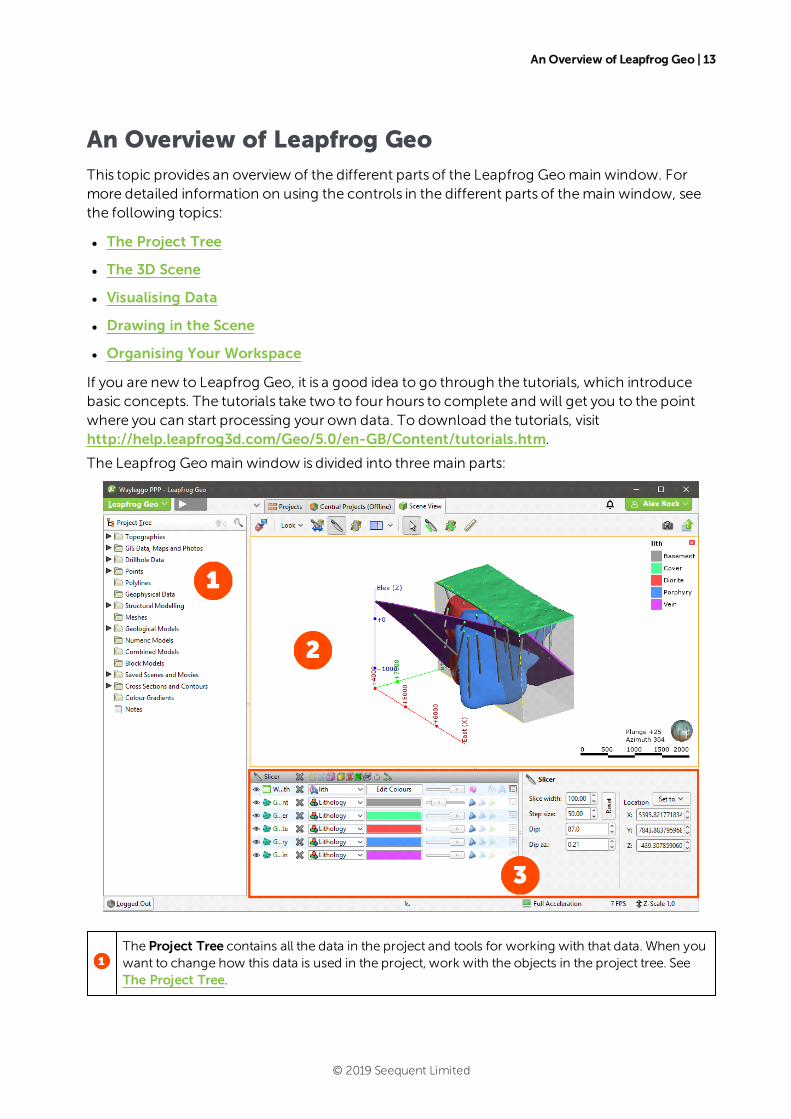
The Leapfrog Geomain window is divided into threemain parts:
The Project Tree contains all the data in the project and tools for working with that data. When youwant to change how this data is used in the project, work with the objects in the project tree. SeeThe Project Tree.
© 2019 Seequent Limited
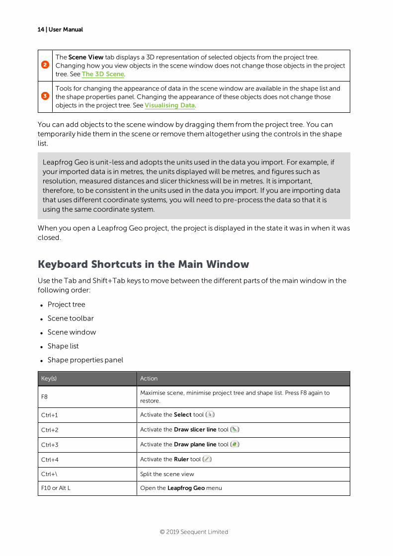
14 | User Manual
The Scene View tab displays a 3D representation of selected objects from the project tree.Changing how you view objects in the scenewindow does not change those objects in the projecttree. See The 3D Scene.
Tools for changing the appearance of data in the scenewindow are available in the shape list andthe shape properties panel. Changing the appearance of these objects does not change thoseobjects in the project tree. See Visualising Data.
You can add objects to the scenewindow by dragging them from the project tree. You cantemporarily hide them in the scene or remove themaltogether using the controls in the shapelist.
Leapfrog Geo is unit-less and adopts the units used in the data you import. For example, ifyour imported data is in metres, the units displayed will bemetres, and figures such asresolution, measured distances and slicer thicknesswill be in metres. It is important,therefore, to be consistent in the units used in the data you import. If you are importing datathat uses different coordinate systems, you will need to pre-process the data so that it isusing the same coordinate system.
When you open a Leapfrog Geo project, the project is displayed in the state it was in when it wasclosed.
Keyboard Shortcuts in the Main Window
Use the Tab and Shift+Tab keys tomove between the different parts of themain window in thefollowing order:
l Project tree
l Scene toolbar
l Scenewindow
l Shape list
l Shape properties panel
Key(s) Action
F8Maximise scene, minimise project tree and shape list. Press F8 again torestore.
Ctrl+1 Activate the Select tool ( )
Ctrl+2 Activate the Draw slicer line tool ( )
Ctrl+3 Activate the Draw plane line tool ( )
Ctrl+4 Activate the Ruler tool ( )
Ctrl+\ Split the scene view
F10 or Alt L Open the Leapfrog Geomenu
© 2019 Seequent Limited

Keyboard Shortcuts in the Main Window | 15
Key(s) Action
F11 Open the Seequent ID menu
F1 Open Leapfrog Geo help
Ctrl+Q Quit Leapfrog Geo
© 2019 Seequent Limited
16 | User Manual
The Project Tree
The series of folders in the project tree are used to organise objects such as datasets, maps andimages into categories. These folders also provide tools that let you import information into theproject and generatemodels. Right-click on each folder to view the actions you can performusing that folder.
This topic provides an introduction toworking with the project tree. It is divided into:
l Organising Objects in the Project Tree
l Object Properties
l Comments
l Object Processing
l Project Tree Keyboard Shortcuts
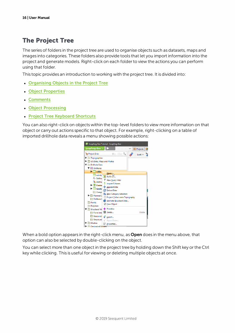
You can also right-click on objectswithin the top-level folders to viewmore information on thatobject or carry out actions specific to that object. For example, right-clicking on a table ofimported drillhole data reveals a menu showing possible actions:
When a bold option appears in the right-clickmenu, asOpen does in themenu above, thatoption can also be selected by double-clicking on the object.
You can select more than one object in the project tree by holding down the Shift key or the Ctrlkeywhile clicking. This is useful for viewing or deleting multiple objects at once.
© 2019 Seequent Limited
The Project Tree | 17
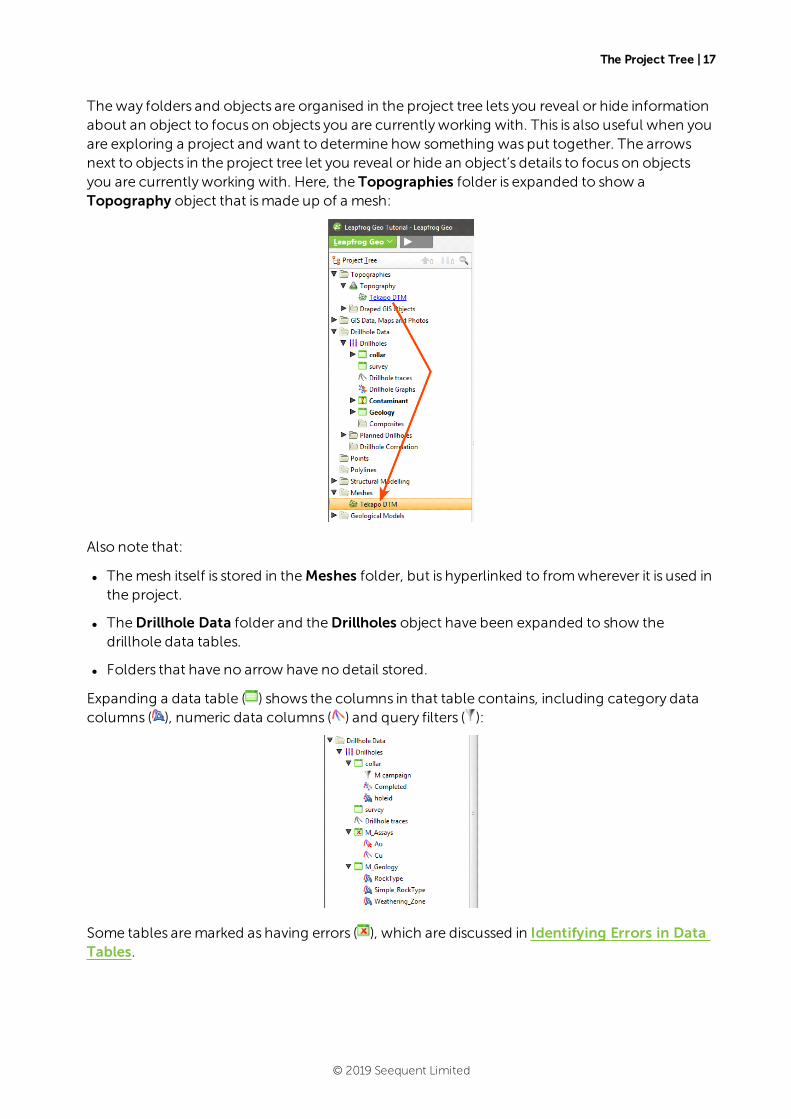
Theway folders and objects are organised in the project tree lets you reveal or hide informationabout an object to focus on objects you are currentlyworking with. This is also useful when youare exploring a project and want to determine how something was put together. The arrowsnext to objects in the project tree let you reveal or hide an object’s details to focus on objectsyou are currentlyworking with. Here, the Topographies folder is expanded to show aTopography object that ismade up of a mesh:
Also note that:
l Themesh itself is stored in theMeshes folder, but is hyperlinked to fromwherever it is used inthe project.
l TheDrillhole Data folder and theDrillholes object have been expanded to show thedrillhole data tables.
l Folders that have no arrow have no detail stored.
Expanding a data table ( ) shows the columns in that table contains, including category datacolumns ( ), numeric data columns ( ) and query filters ( ):
Some tables aremarked as having errors ( ), which are discussed in Identifying Errors in DataTables.
© 2019 Seequent Limited
18 | User Manual
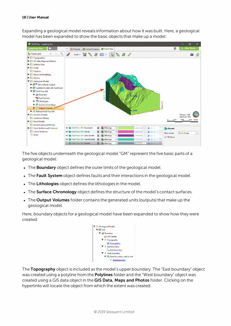
Expanding a geological model reveals information about how it was built. Here, a geologicalmodel has been expanded to show the basic objects that make up a model:
The five objects underneath the geological model “GM” represent the five basic parts of ageological model:
l The Boundary object defines the outer limits of the geological model.
l The Fault Systemobject defines faults and their interactions in the geological model.
l The Lithologies object defines the lithologies in themodel.
l The Surface Chronology object defines the structure of themodel’s contact surfaces.
l TheOutput Volumes folder contains the generated units (outputs) that make up thegeological model.
Here, boundary objects for a geological model have been expanded to show how theywerecreated:
The Topography object is included as themodel’s upper boundary. The “East boundary” objectwas created using a polyline from the Polylines folder and the “West boundary” object wascreated using a GIS data object in theGIS Data, Maps and Photos folder. Clicking on thehyperlinkswill locate the object fromwhich the extent was created.
© 2019 Seequent Limited
Organising Objects in the Project Tree | 19
Organising Objects in the Project Tree
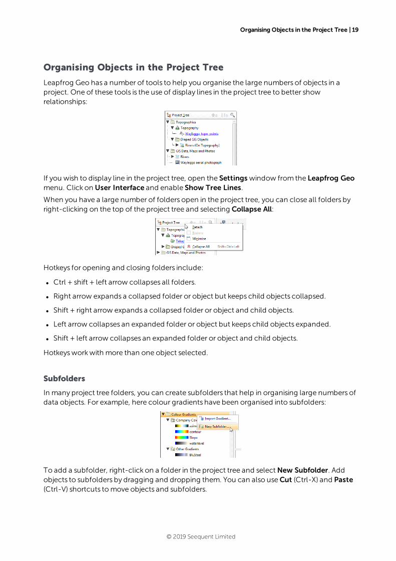
Leapfrog Geo has a number of tools to help you organise the large numbers of objects in aproject. One of these tools is the use of display lines in the project tree to better showrelationships:
If you wish to display line in the project tree, open the Settings window from the Leapfrog Geomenu. Click on User Interface and enable Show Tree Lines.
When you have a large number of folders open in the project tree, you can close all folders byright-clicking on the top of the project tree and selecting Collapse All:
Hotkeys for opening and closing folders include:
l Ctrl + shift + left arrow collapses all folders.
l Right arrow expands a collapsed folder or object but keeps child objects collapsed.
l Shift + right arrow expands a collapsed folder or object and child objects.
l Left arrow collapses an expanded folder or object but keeps child objects expanded.
l Shift + left arrow collapses an expanded folder or object and child objects.
Hotkeysworkwith more than one object selected.
Subfolders
In many project tree folders, you can create subfolders that help in organising large numbers ofdata objects. For example, here colour gradients have been organised into subfolders:
To add a subfolder, right-click on a folder in the project tree and selectNew Subfolder. Addobjects to subfolders by dragging and dropping them. You can also useCut (Ctrl-X) and Paste(Ctrl-V) shortcuts tomove objects and subfolders.
© 2019 Seequent Limited

20 | User Manual
Subfolders can be renamed, moved and deleted, but cannot bemoved to other top-levelfolders.
Subfolders have the same right-click commands as their parent folder, which means you canimport or create new data objects inside the subfolder rather than in the parent folder. You canalso add comments to folders to aid in keeping data organised:
You can view all objects in the subfolder by dragging the folder into the scene or by right-clicking on the subfolder and selecting View All.
When lists of objects are displayed, the subfolder organisation will be reflected in the list. Forexample, when creating an interpolant, the list of data objects that can be interpolated isdisplayed organised by subfolder:
Subfolders cannot be created in theDrillhole Data folder, although they can be created in theComposites and Planned Drillholes folders.
Copying Objects
Many objects in the project tree can be copied. Right-click on an object and selectCopy. Youwill be prompted to enter a name for the object’s copy.
The copied object is not linked to the original object. However, if the original object is linked toother objects in the project, the copywill also be linked to those objects.
Renaming Objects
When an object is created in Leapfrog Geo, it is given a default name. It is a good idea to giveobjects in Leapfrog Geo names that will help you distinguish them fromother objects, as largeprojectswith complicated modelswill contain many objects.
© 2019 Seequent Limited
Finding Objects | 21
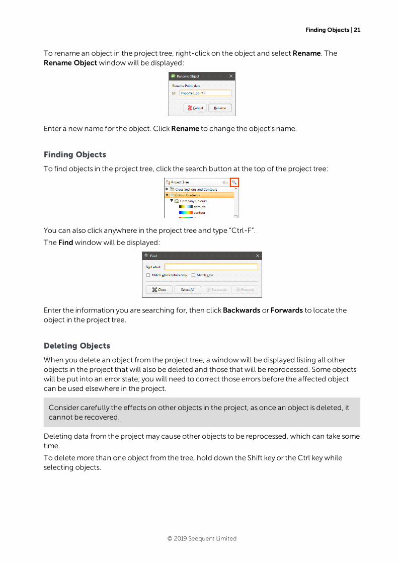
To rename an object in the project tree, right-click on the object and select Rename. TheRename Object windowwill be displayed:
Enter a new name for the object. ClickRename to change the object’s name.
Finding Objects
To find objects in the project tree, click the search button at the top of the project tree:
You can also click anywhere in the project tree and type “Ctrl-F”.
The Findwindowwill be displayed:
Enter the information you are searching for, then clickBackwards or Forwards to locate theobject in the project tree.
Deleting Objects
When you delete an object from the project tree, a windowwill be displayed listing all otherobjects in the project that will also be deleted and those that will be reprocessed. Some objectswill be put into an error state; you will need to correct those errors before the affected objectcan be used elsewhere in the project.
Consider carefully the effects on other objects in the project, as once an object is deleted, itcannot be recovered.
Deleting data from the project may cause other objects to be reprocessed, which can take sometime.
To deletemore than one object from the tree, hold down the Shift key or the Ctrl keywhileselecting objects.
© 2019 Seequent Limited
22 | User Manual
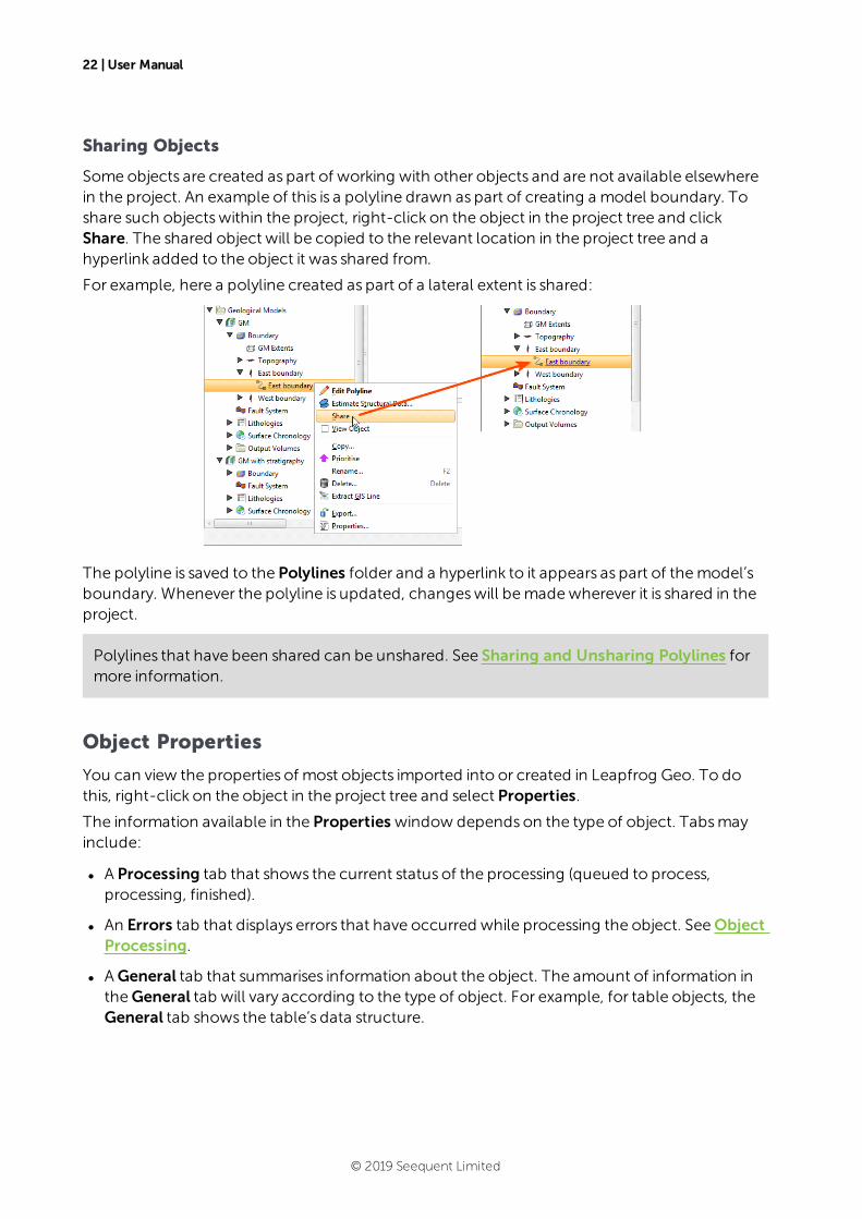
Sharing Objects
Some objects are created as part of working with other objects and are not available elsewherein the project. An example of this is a polyline drawn as part of creating a model boundary. Toshare such objectswithin the project, right-click on the object in the project tree and clickShare. The shared object will be copied to the relevant location in the project tree and ahyperlink added to the object it was shared from.
For example, here a polyline created as part of a lateral extent is shared:
The polyline is saved to the Polylines folder and a hyperlink to it appears as part of themodel’sboundary. Whenever the polyline is updated, changeswill bemadewherever it is shared in theproject.
Polylines that have been shared can be unshared. See Sharing and Unsharing Polylines formore information.
Object Properties
You can view the properties of most objects imported into or created in Leapfrog Geo. To dothis, right-click on the object in the project tree and select Properties.
The information available in the Properties window dependson the type of object. Tabsmayinclude:
l A Processing tab that shows the current status of the processing (queued to process,processing, finished).
l An Errors tab that displays errors that have occurred while processing the object. SeeObjectProcessing.
l AGeneral tab that summarises information about the object. The amount of information intheGeneral tab will vary according to the type of object. For example, for table objects, theGeneral tab shows the table’s data structure.
© 2019 Seequent Limited
Comments | 23
l A Statistics tab that shows statistics for some types of interpolants.
l For RBF interpolants, seeRBF Interpolant Statistics.
l Formulti-domained RBF interpolants, see Sub-Interpolant Statistics.
l For indicator RBF interpolants, see Indicator RBF Interpolant Statistics.
Comments
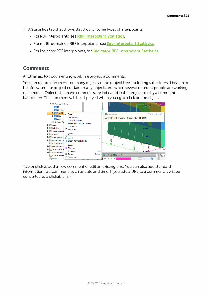
Another aid to documenting work in a project is comments.
You can record comments on many objects in the project tree, including subfolders. This can behelpful when the project containsmany objects and when several different people are workingon a model. Objects that have comments are indicated in the project tree by a commentballoon ( ). The comment will be displayed when you right-click on the object:
Tab or click to add a new comment or edit an existing one. You can also add standardinformation to a comment, such as date and time. If you add a URL to a comment, it will beconverted to a clickable link.
© 2019 Seequent Limited
24 | User Manual
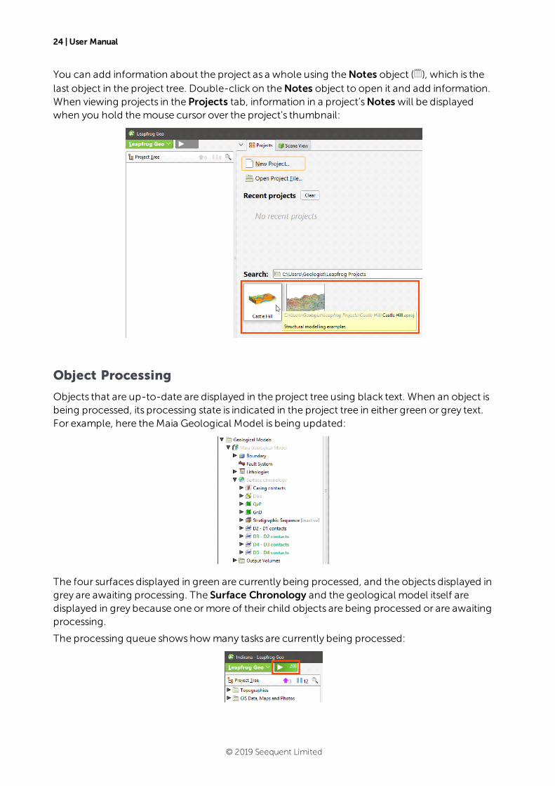
You can add information about the project as a whole using theNotes object ( ), which is thelast object in the project tree. Double-click on theNotes object to open it and add information.When viewing projects in the Projects tab, information in a project’sNotes will be displayedwhen you hold themouse cursor over the project’s thumbnail:
Object Processing
Objects that are up-to-date are displayed in the project tree using black text. When an object isbeing processed, its processing state is indicated in the project tree in either green or grey text.For example, here theMaia Geological Model is being updated:
The four surfaces displayed in green are currently being processed, and the objects displayed ingrey are awaiting processing. The Surface Chronology and the geological model itself aredisplayed in grey because one ormore of their child objects are being processed or are awaitingprocessing.
The processing queue showshowmany tasks are currently being processed:
© 2019 Seequent Limited
Controlling Processing | 25
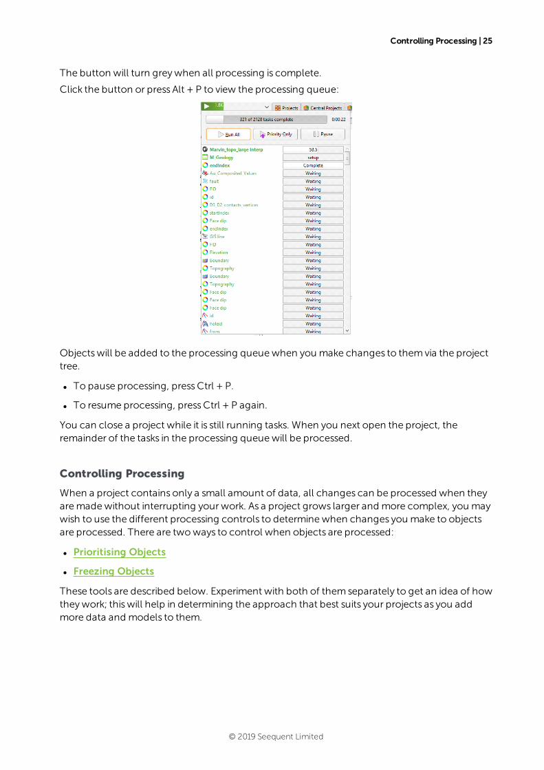
The button will turn greywhen all processing is complete.
Click the button or press Alt + P to view the processing queue:
Objectswill be added to the processing queuewhen you make changes to themvia the projecttree.
l To pause processing, pressCtrl + P.
l To resume processing, pressCtrl + P again.
You can close a project while it is still running tasks. When you next open the project, theremainder of the tasks in the processing queuewill be processed.
Controlling Processing
When a project contains only a small amount of data, all changes can be processed when theyaremadewithout interrupting yourwork. As a project grows larger and more complex, you maywish to use the different processing controls to determinewhen changes you make to objectsare processed. There are twoways to control when objects are processed:
l Prioritising Objects
l Freezing Objects
These tools are described below. Experiment with both of themseparately to get an idea of howtheywork; thiswill help in determining the approach that best suits your projects as you addmore data and models to them.
© 2019 Seequent Limited
26 | User Manual
The project treemay also contain restricted objects:
Restricted objectswere created using features only available in extensions. You can displayrestricted objects in the scene and change how they are displayed, but you cannot makechanges to the objects themselves or export them. When changes aremade to objects thatare inputs to restricted objects, the restricted objectswill not be processed. Instead, theywillremain in the processing queuemarked as “frozen”.
Contact Customer Support as described in Getting Support formore information aboutextensions.
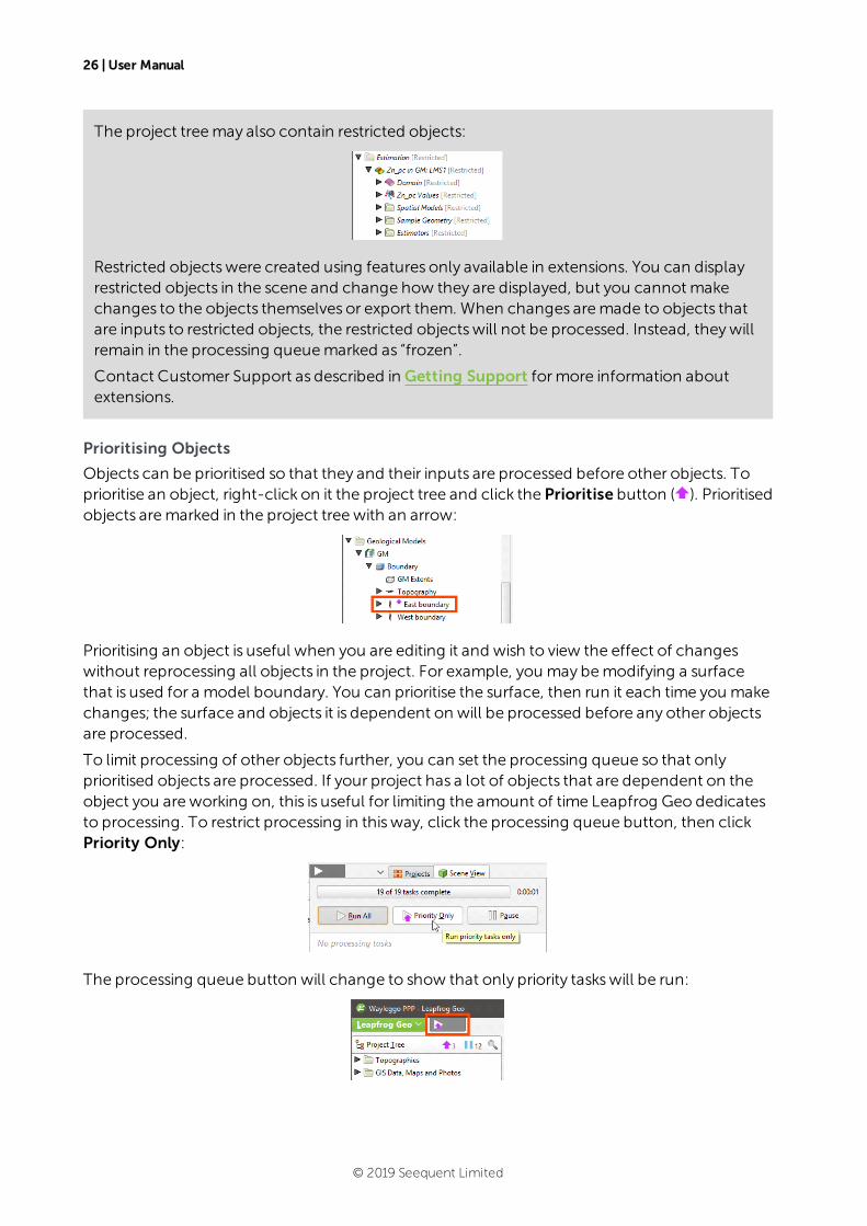
Prioritising Objects
Objects can be prioritised so that they and their inputs are processed before other objects. Toprioritise an object, right-click on it the project tree and click the Prioritise button ( ). Prioritisedobjects aremarked in the project tree with an arrow:
Prioritising an object is useful when you are editing it and wish to view the effect of changeswithout reprocessing all objects in the project. For example, you may bemodifying a surfacethat is used for a model boundary. You can prioritise the surface, then run it each time you makechanges; the surface and objects it is dependent on will be processed before any other objectsare processed.
To limit processing of other objects further, you can set the processing queue so that onlyprioritised objects are processed. If your project has a lot of objects that are dependent on theobject you are working on, this is useful for limiting the amount of time Leapfrog Geo dedicatesto processing. To restrict processing in thisway, click the processing queue button, then clickPriority Only:
The processing queue button will change to show that only priority taskswill be run:
© 2019 Seequent Limited
Prioritising Objects | 27
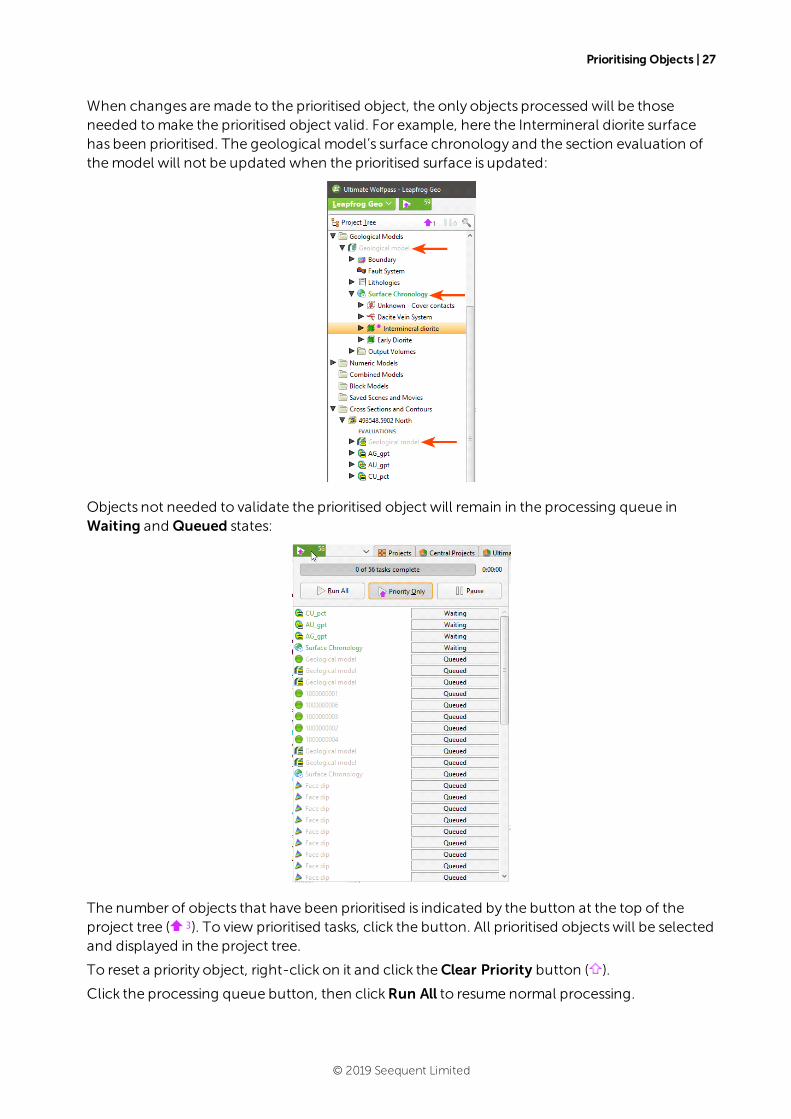
When changes aremade to the prioritised object, the only objects processed will be thoseneeded tomake the prioritised object valid. For example, here the Intermineral diorite surfacehas been prioritised. The geological model’s surface chronology and the section evaluation ofthemodel will not be updated when the prioritised surface is updated:
Objects not needed to validate the prioritised object will remain in the processing queue inWaiting and Queued states:
The number of objects that have been prioritised is indicated by the button at the top of theproject tree ( ). To view prioritised tasks, click the button. All prioritised objectswill be selectedand displayed in the project tree.
To reset a priority object, right-click on it and click theClear Priority button ( ).
Click the processing queue button, then clickRun All to resume normal processing.
© 2019 Seequent Limited
28 | User Manual
Freezing Objects
Objects can also be frozen so that theywill not be processed, which is a useful way of workingon one object without having all linked objects reprocess upon each change. For example, youmaywish tomodify a surface in a geological model, in which case you can freeze all objectsother than the surface.
You can display frozen objects in the scene, change how they are displayed and export them,but you cannot make changes to the objects themselves.
Some objects become frozen because they are restricted objects created using features onlyavailable in extensions. Frozen restricted objects can only be unfrozen if you switch to usingthe relevant extension.
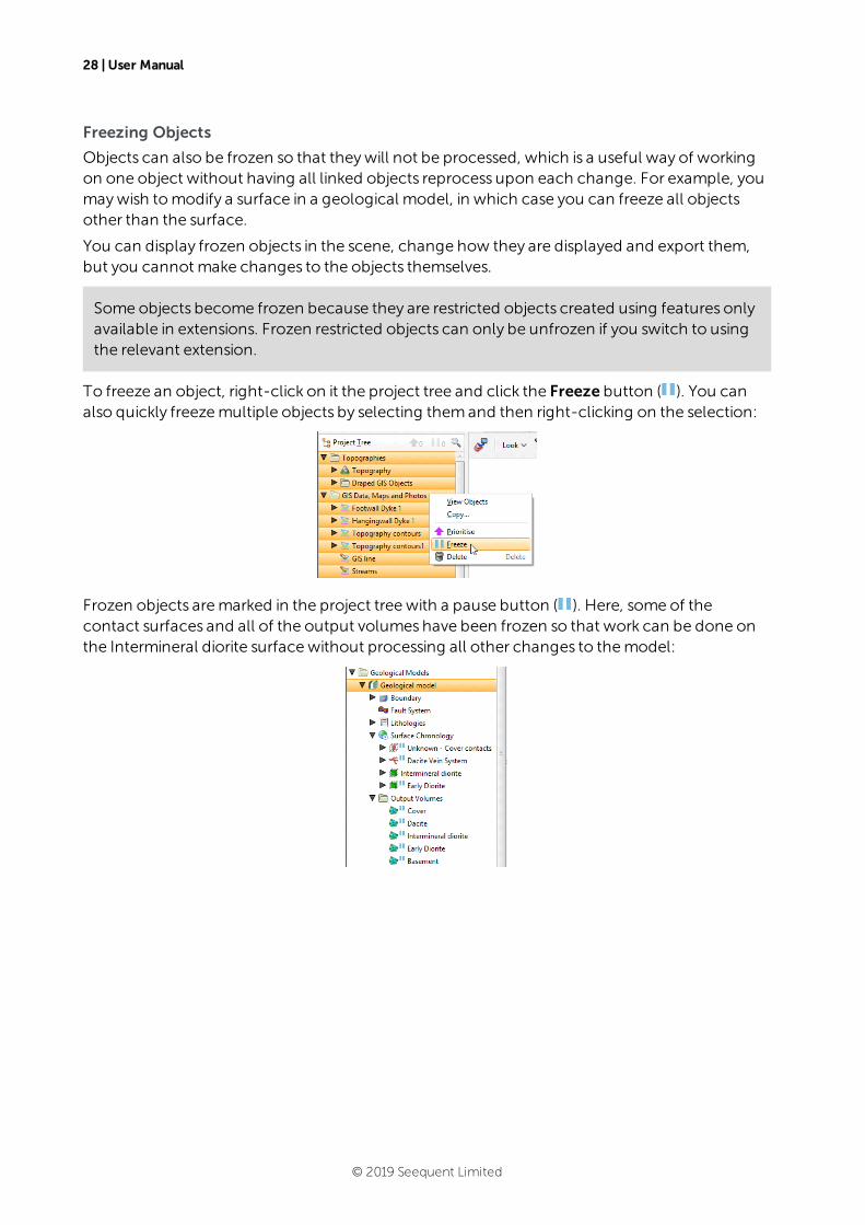
To freeze an object, right-click on it the project tree and click the Freeze button ( ). You canalso quickly freezemultiple objects by selecting themand then right-clicking on the selection:
Frozen objects aremarked in the project tree with a pause button ( ). Here, some of thecontact surfaces and all of the output volumes have been frozen so that work can be done onthe Intermineral diorite surfacewithout processing all other changes to themodel:
© 2019 Seequent Limited
Correcting Errors | 29
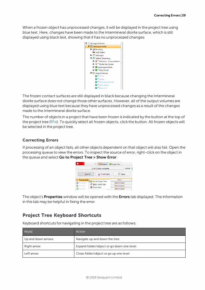
When a frozen object has unprocessed changes, it will be displayed in the project tree usingblue text. Here, changes have been made to the Intermineral diorite surface, which is stilldisplayed using black text, showing that it has no unprocessed changes:
The frozen contact surfaces are still displayed in black because changing the Intermineraldiorite surface does not change those other surfaces. However, all of the output volumes aredisplayed using blue text because they have unprocessed changes as a result of the changesmade to the Intermineral diorite surface.
The number of objects in a project that have been frozen is indicated by the button at the top ofthe project tree ( ). To quickly select all frozen objects, click the button. All frozen objectswillbe selected in the project tree.
Correcting Errors
If processing of an object fails, all other objects dependent on that object will also fail. Open theprocessing queue to view the errors. To inspect the source of error, right-click on the object inthe queue and selectGo to Project Tree > Show Error:
The object’sProperties windowwill be opened with the Errors tab displayed. The informationin this tab may be helpful in fixing the error.
Project Tree Keyboard Shortcuts
Keyboard shortcuts for navigating in the project tree are as follows:
Key(s) Action
Up and down arrows Navigate up and down the tree
Right arrow Expand folder/object or go down one level
Left arrow Close folder/object or go up one level
© 2019 Seequent Limited

30 | User Manual
Key(s) Action
Ctrl+shift+left arrow Close all folders/objects
Shift+right arrow Expand the selected folder/object and any objects in it
Shift+left arrow Close the selected folder/object and any objects in it
Ctrl+A and Ctrl+/ Selects all folders and objects
Ctrl+F Search for objects
Enter The equivalent of double-clicking on an object
Ctrl-X Cut an object or subfolder. Use with Ctrl-V tomove objects and subfolders.
Ctrl-V Paste an object or subfolder
Some actions are not available until data has been imported into the project.
© 2019 Seequent Limited
The 3D Scene | 31
The 3D Scene
This topic describes how to interact with the 3D scene. It is divided into:
l Locating an Object from the Scene
l Slicing Through the Data
l Measuring in the Scene
l Working With Split Views
How to change theway objects are displayed in the scene is described in a separate topic,Visualising Data.
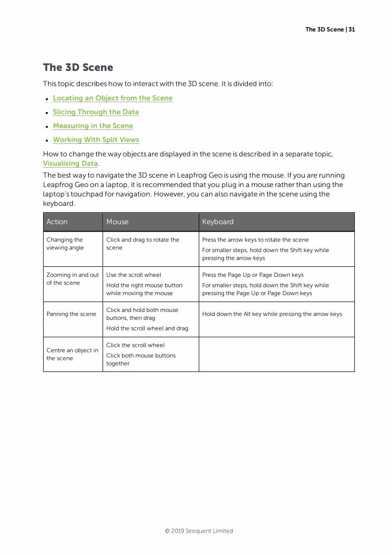
The best way to navigate the 3D scene in Leapfrog Geo is using themouse. If you are runningLeapfrog Geo on a laptop, it is recommended that you plug in a mouse rather than using thelaptop’s touchpad for navigation. However, you can also navigate in the scene using thekeyboard.
Action Mouse Keyboard
Changing theviewing angle
Click and drag to rotate thescene
Press the arrow keys to rotate the scene
For smaller steps, hold down the Shift key whilepressing the arrow keys
Zooming in and outof the scene
Use the scroll wheel
Hold the right mouse buttonwhile moving the mouse
Press the Page Up or Page Down keys
For smaller steps, hold down the Shift key whilepressing the Page Up or Page Down keys
Panning the sceneClick and hold both mousebuttons, then drag
Hold the scroll wheel and drag
Hold down the Alt key while pressing the arrow keys
Centre an object inthe scene
Click the scroll wheel
Click both mouse buttonstogether
© 2019 Seequent Limited
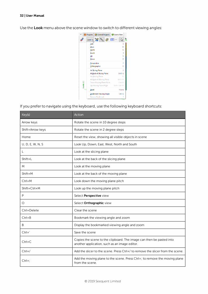
32 | User Manual
Use the Lookmenu above the scenewindow to switch to different viewing angles:
If you prefer to navigate using the keyboard, use the following keyboard shortcuts:
Key(s) Action
Arrow keys Rotate the scene in 10 degree steps
Shift+Arrow keys Rotate the scene in 2 degree steps
Home Reset the view, showing all visible objects in scene
U, D, E, W, N, S Look Up, Down, East, West, North and South
L Look at the slicing plane
Shift+L Look at the back of the slicing plane
M Look at the moving plane
Shift+M Look at the back of the moving plane
Ctrl+M Look down the moving plane pitch
Shift+Ctrl+M Look up the moving plane pitch
P Select Perspective view
O Select Orthographic view
Ctrl+Delete Clear the scene
Ctrl+B Bookmark the viewing angle and zoom
B Display the bookmarked viewing angle and zoom
Ctrl+’ Save the scene
Ctrl+CCopies the scene to the clipboard. The image can then be pasted intoanother application, such as an image editor.
Ctrl+/ Add the slicer to the scene. Press Ctrl+/ to remove the slicer from the scene.
Ctrl+;Add the moving plane to the scene. Press Ctrl+; to remove the moving planefrom the scene.
© 2019 Seequent Limited

The 3D Scene | 33
The current viewing angle and scale are displayed in the lower right-hand corner of the scenewindow:
You can change how the viewing angle and scale are displayed in theOverlays tab of theSettings window.
You can save the current viewing angle as a bookmark by selecting Bookmark Viewing Anglefrom the Lookmenu or by pressing Ctrl+B. Restore the bookmark by selecting Look > RestoreBookmark or by pressing B.
Only one viewing angle bookmark can be saved. The bookmark is not saved when LeapfrogGeo is shut down.
The scenewindow displays a 3D representation of selected data from the project tree. You canadd objects from the project tree to the scene in twoways:
l Click on the object and drag it into the scene. Hold down the Shift key or the Ctrl keywhileclicking to select multiple items, then add them to the scene.
l Right-click on the object and tick the View Object box.
Dragging objects into the scenewindowmay be blocked by other applications on yourcomputer. For example, if you are sharing a screen using Skype, you will not be able to dragobjects into the scene.
© 2019 Seequent Limited
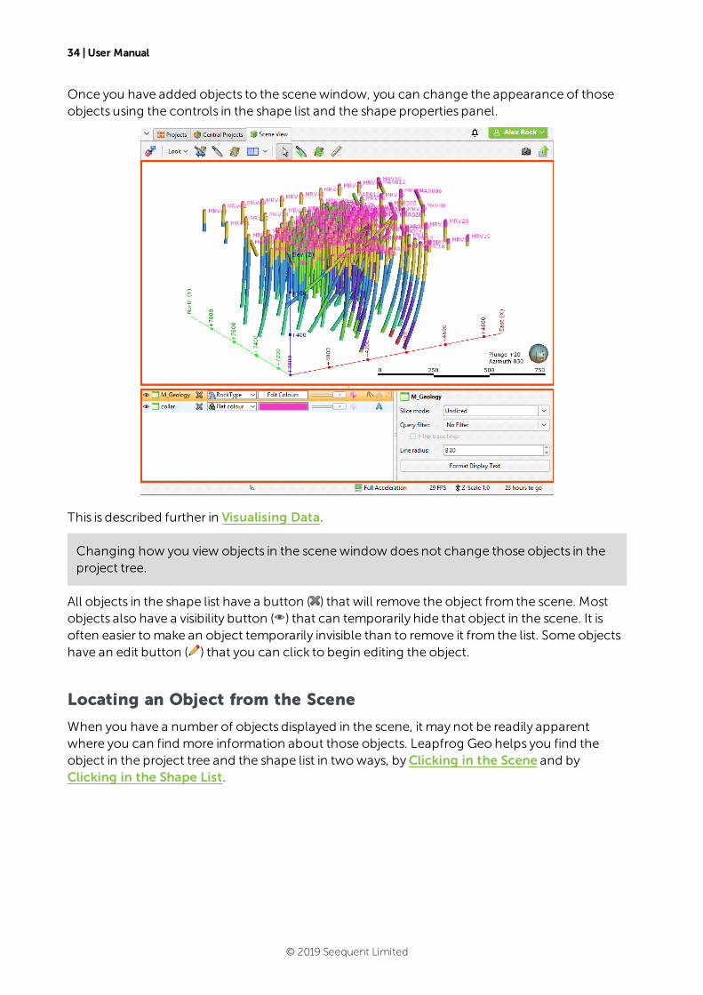
34 | User Manual
Once you have added objects to the scenewindow, you can change the appearance of thoseobjects using the controls in the shape list and the shape properties panel.
This is described further in Visualising Data.
Changing how you view objects in the scenewindow does not change those objects in theproject tree.
All objects in the shape list have a button ( ) that will remove the object from the scene. Mostobjects also have a visibility button ( ) that can temporarily hide that object in the scene. It isoften easier tomake an object temporarily invisible than to remove it from the list. Some objectshave an edit button ( ) that you can click to begin editing the object.
Locating an Object from the Scene
When you have a number of objects displayed in the scene, it may not be readily apparentwhere you can find more information about those objects. Leapfrog Geo helps you find theobject in the project tree and the shape list in twoways, byClicking in the Scene and byClicking in the Shape List.
© 2019 Seequent Limited

Clicking in the Scene | 35
Clicking in the Scene
Clicking on an object in the scene displays a window that contains a summary of the data and,formany objects, a link to the corresponding data in the project tree. For example, here drillholedata is displayed in the scene and clicking on a segment displays the corresponding data:
Note that clicking on an object in the scene also selects it in the shape list.
© 2019 Seequent Limited
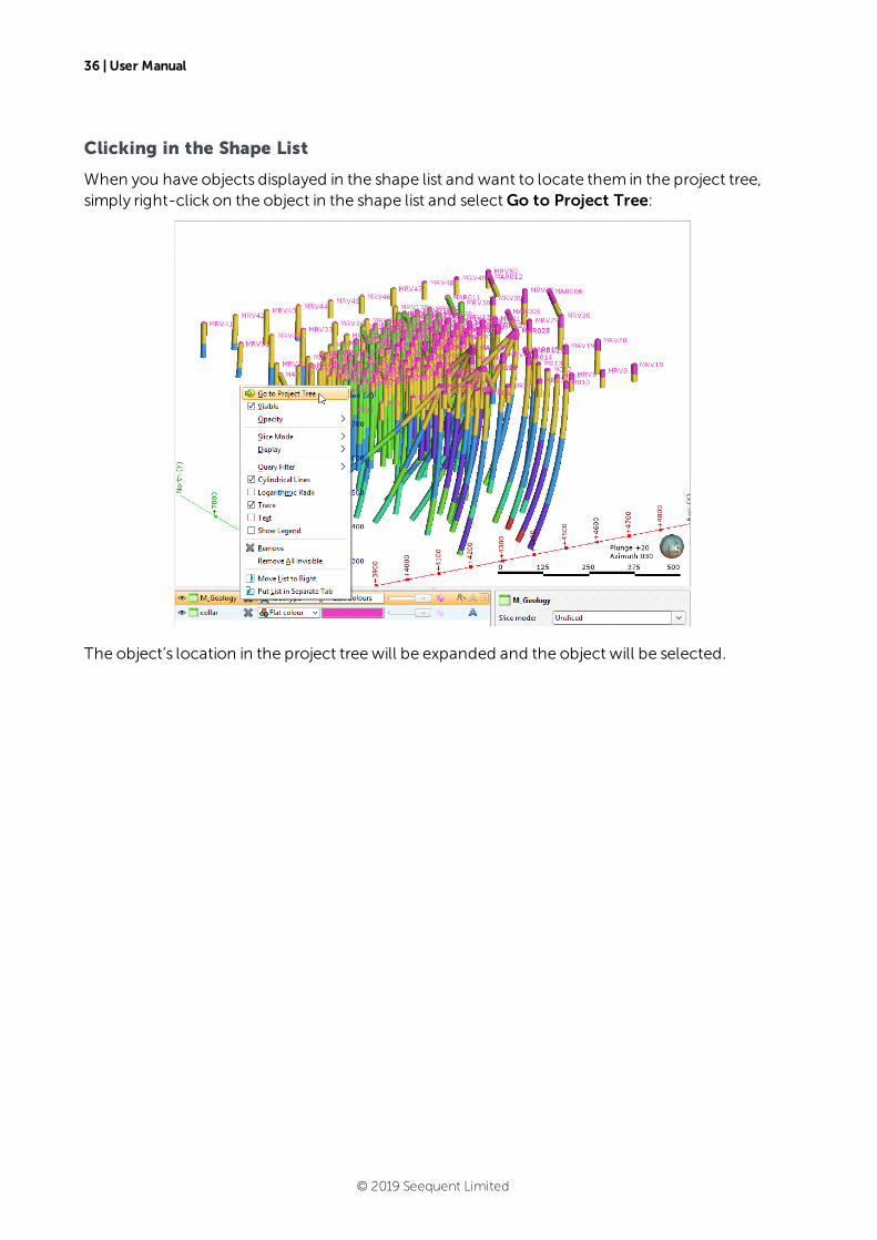
36 | User Manual
Clicking in the Shape List
When you have objects displayed in the shape list and want to locate them in the project tree,simply right-click on the object in the shape list and selectGo to Project Tree:
The object’s location in the project tree will be expanded and the object will be selected.
© 2019 Seequent Limited
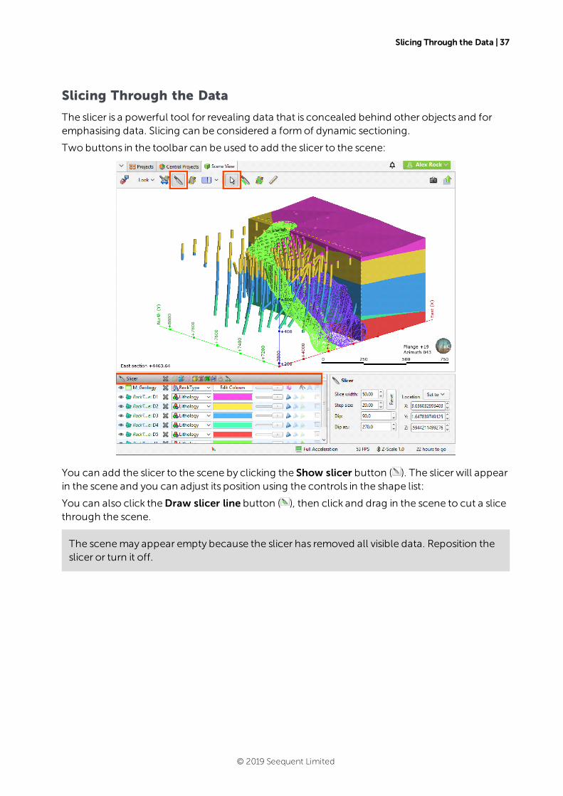
Slicing Through the Data | 37
Slicing Through the Data
The slicer is a powerful tool for revealing data that is concealed behind other objects and foremphasising data. Slicing can be considered a formof dynamic sectioning.
Two buttons in the toolbar can be used to add the slicer to the scene:
You can add the slicer to the scene by clicking the Show slicer button ( ). The slicer will appearin the scene and you can adjust its position using the controls in the shape list:
You can also click theDraw slicer line button ( ), then click and drag in the scene to cut a slicethrough the scene.
The scenemay appear empty because the slicer has removed all visible data. Reposition theslicer or turn it off.
© 2019 Seequent Limited
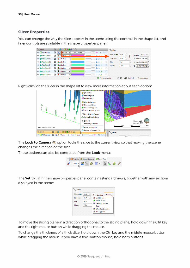
38 | User Manual
Slicer Properties
You can change theway the slice appears in the scene using the controls in the shape list, andfiner controls are available in the shape properties panel:
Right-click on the slicer in the shape list to viewmore information about each option:
The Lock to Camera ( ) option locks the slice to the current view so that moving the scenechanges the direction of the slice.
These options can also be controlled from the Lookmenu:
The Set to list in the shape properties panel contains standard views, together with any sectionsdisplayed in the scene:
Tomove the slicing plane in a direction orthogonal to the slicing plane, hold down the Ctrl keyand the right mouse button while dragging themouse.
To change the thickness of a thick slice, hold down the Ctrl key and themiddlemouse buttonwhile dragging themouse. If you have a two-button mouse, hold both buttons.
© 2019 Seequent Limited
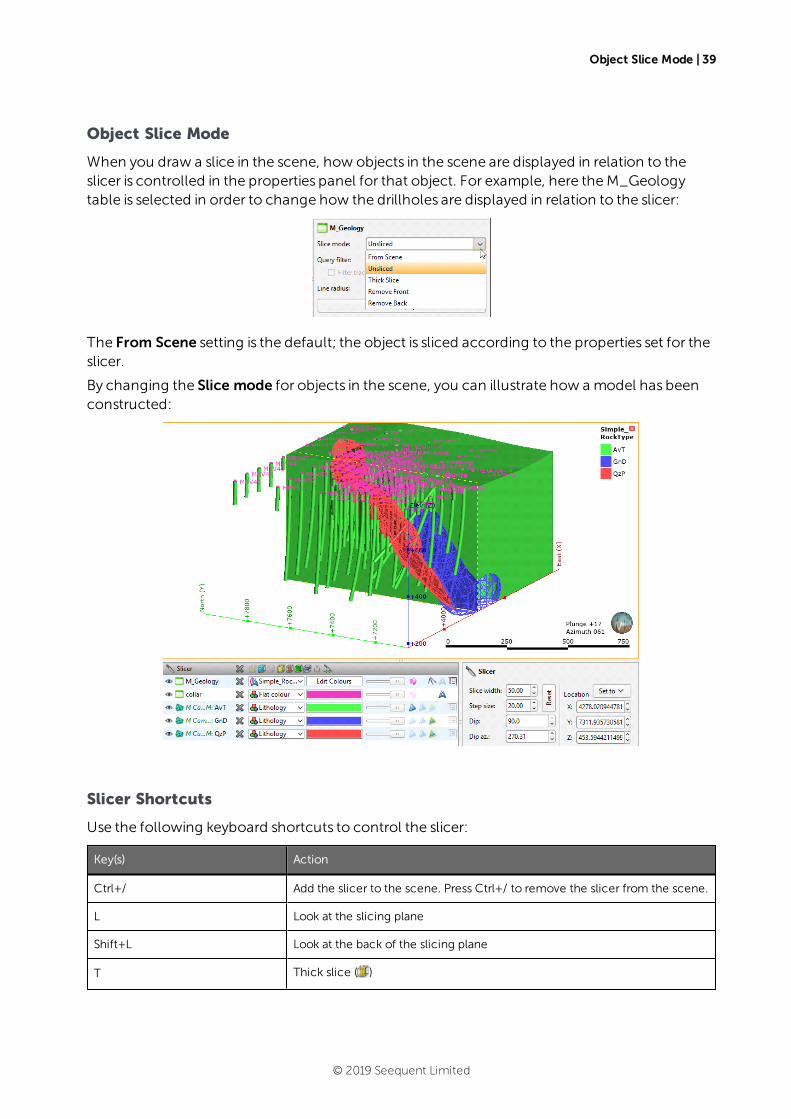
Object Slice Mode | 39
Object Slice Mode
When you draw a slice in the scene, how objects in the scene are displayed in relation to theslicer is controlled in the properties panel for that object. For example, here theM_Geologytable is selected in order to change how the drillholes are displayed in relation to the slicer:
The From Scene setting is the default; the object is sliced according to the properties set for theslicer.
By changing the Slice mode for objects in the scene, you can illustrate how a model has beenconstructed:
Slicer Shortcuts
Use the following keyboard shortcuts to control the slicer:
Key(s) Action
Ctrl+/ Add the slicer to the scene. Press Ctrl+/ to remove the slicer from the scene.
L Look at the slicing plane
Shift+L Look at the back of the slicing plane
T Thick slice ( )
© 2019 Seequent Limited
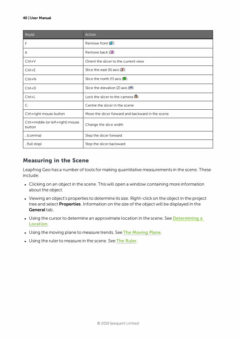
40 | User Manual
Key(s) Action
F Remove front ( )
K Remove back ( )
Ctrl+V Orient the slicer to the current view
Ctrl+E Slice the east (X) axis ( )
Ctrl+N Slice the north (Y) axis ( )
Ctrl+D Slice the elevation (Z) axis ( )
Ctrl+L Lock the slicer to the camera ( )
C Centre the slicer in the scene
Ctrl+right mouse button Move the slicer forward and backward in the scene
Ctrl+middle (or left+right) mousebutton
Change the slice width
, (comma) Step the slicer forward
. (full stop) Step the slicer backward
Measuring in the Scene
Leapfrog Geo has a number of tools formaking quantitativemeasurements in the scene. Theseinclude:
l Clicking on an object in the scene. Thiswill open a window containing more informationabout the object.
l Viewing an object’s properties to determine its size. Right-click on the object in the projecttree and select Properties. Information on the size of the object will be displayed in theGeneral tab.
l Using the cursor to determine an approximate location in the scene. SeeDetermining aLocation.
l Using themoving plane tomeasure trends. See The Moving Plane.
l Using the ruler tomeasure in the scene. See The Ruler.
© 2019 Seequent Limited
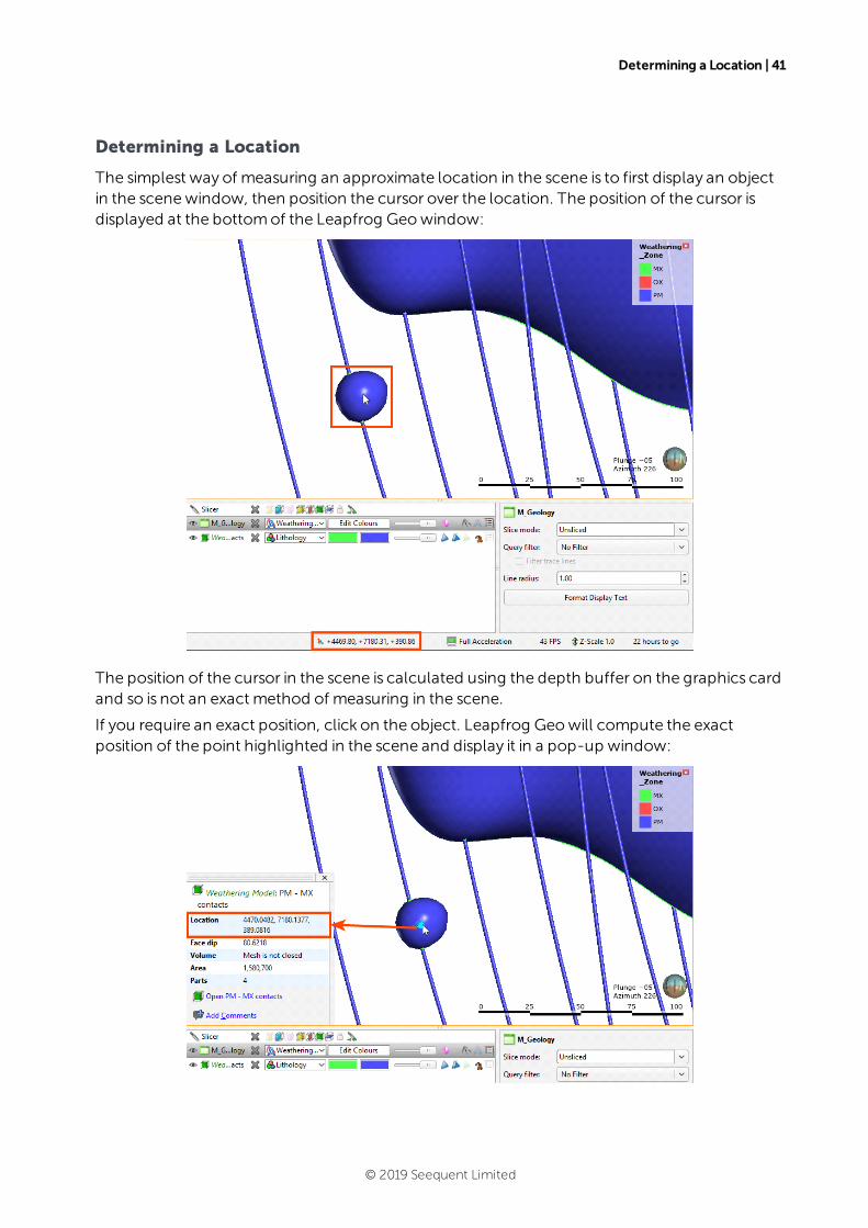
Determining a Location | 41
Determining a Location
The simplest way of measuring an approximate location in the scene is to first display an objectin the scenewindow, then position the cursor over the location. The position of the cursor isdisplayed at the bottomof the Leapfrog Geowindow:
The position of the cursor in the scene is calculated using the depth buffer on the graphics cardand so is not an exact method of measuring in the scene.
If you require an exact position, click on the object. Leapfrog Geowill compute the exactposition of the point highlighted in the scene and display it in a pop-up window:
© 2019 Seequent Limited
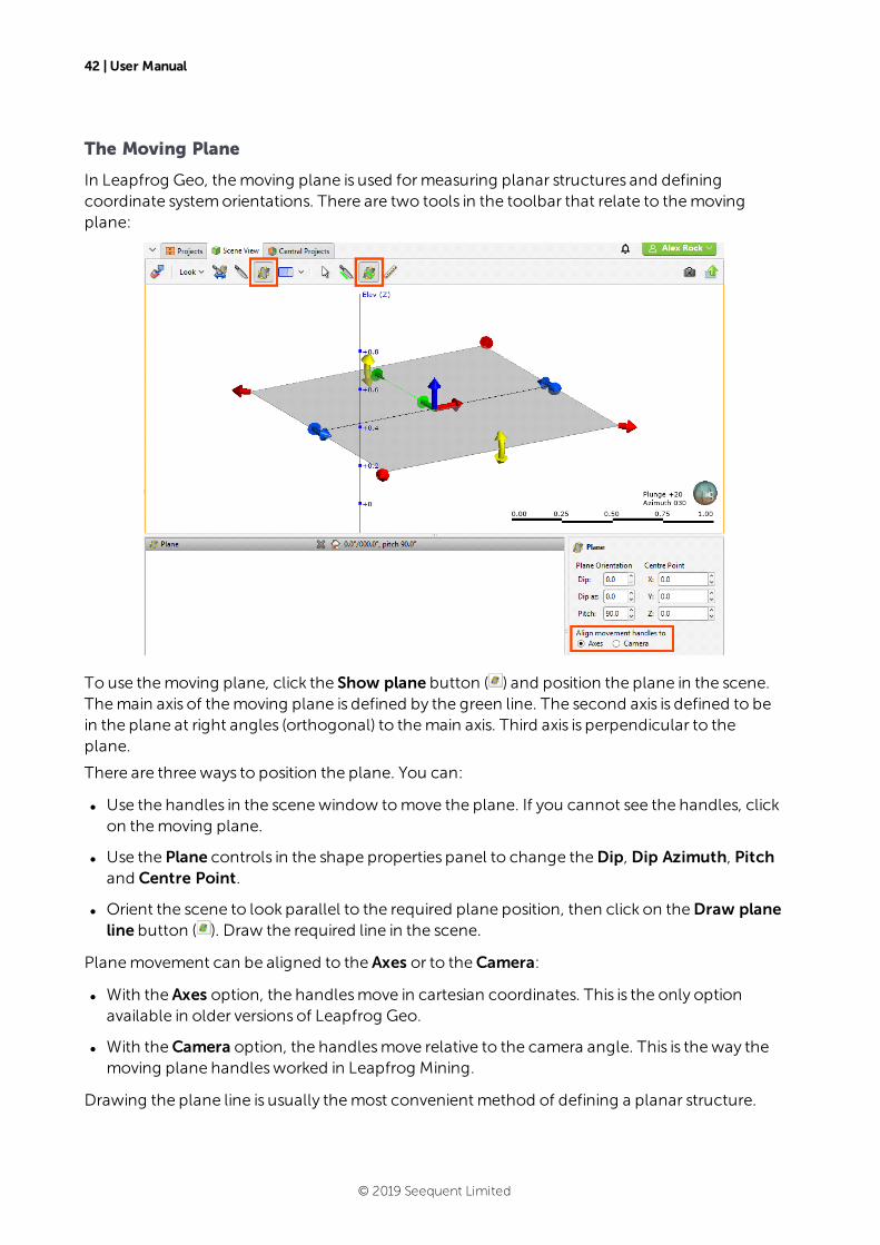
42 | User Manual
The Moving Plane
In Leapfrog Geo, themoving plane is used formeasuring planar structures and definingcoordinate systemorientations. There are two tools in the toolbar that relate to themovingplane:
To use themoving plane, click the Show plane button ( ) and position the plane in the scene.Themain axis of themoving plane is defined by the green line. The second axis is defined to bein the plane at right angles (orthogonal) to themain axis. Third axis is perpendicular to theplane.
There are threeways to position the plane. You can:
l Use the handles in the scenewindow tomove the plane. If you cannot see the handles, clickon themoving plane.
l Use the Plane controls in the shape properties panel to change theDip, Dip Azimuth, Pitchand Centre Point.
l Orient the scene to look parallel to the required plane position, then click on theDraw planeline button ( ). Draw the required line in the scene.
Planemovement can be aligned to the Axes or to theCamera:
l With the Axes option, the handlesmove in cartesian coordinates. This is the only optionavailable in older versions of Leapfrog Geo.
l With theCamera option, the handlesmove relative to the camera angle. This is theway themoving plane handlesworked in Leapfrog Mining.
Drawing the plane line is usually themost convenient method of defining a planar structure.
© 2019 Seequent Limited
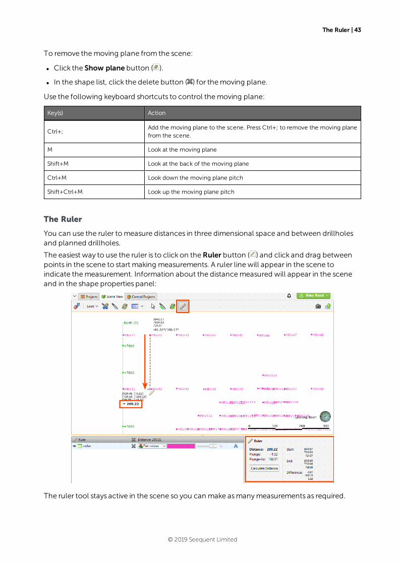
The Ruler | 43
To remove themoving plane from the scene:
l Click the Show plane button ( ).
l In the shape list, click the delete button ( ) for themoving plane.
Use the following keyboard shortcuts to control themoving plane:
Key(s) Action
Ctrl+;Add the moving plane to the scene. Press Ctrl+; to remove the moving planefrom the scene.
M Look at the moving plane
Shift+M Look at the back of the moving plane
Ctrl+M Look down the moving plane pitch
Shift+Ctrl+M Look up the moving plane pitch
The Ruler
You can use the ruler tomeasure distances in three dimensional space and between drillholesand planned drillholes.
The easiest way to use the ruler is to click on theRuler button ( ) and click and drag betweenpoints in the scene to start making measurements. A ruler line will appear in the scene toindicate themeasurement. Information about the distancemeasured will appear in the sceneand in the shape properties panel:
The ruler tool stays active in the scene so you can make asmanymeasurements as required.
© 2019 Seequent Limited
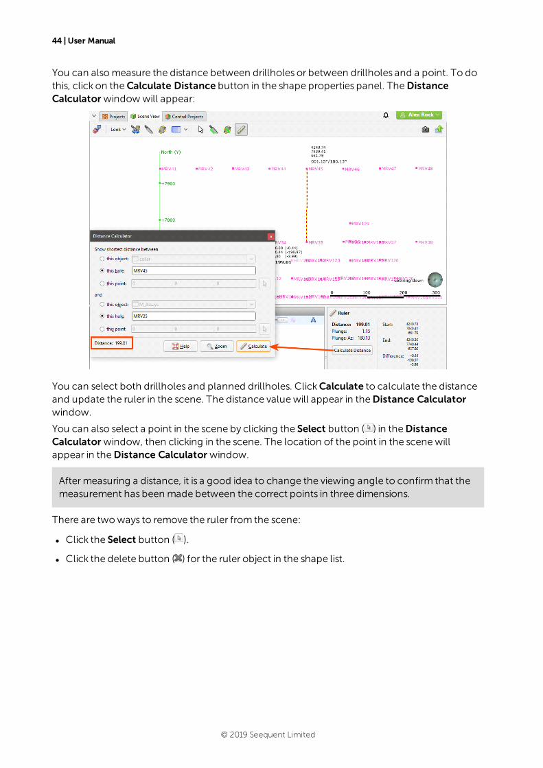
44 | User Manual
You can alsomeasure the distance between drillholes or between drillholes and a point. To dothis, click on theCalculate Distance button in the shape properties panel. TheDistanceCalculator windowwill appear:
You can select both drillholes and planned drillholes. ClickCalculate to calculate the distanceand update the ruler in the scene. The distance valuewill appear in theDistance Calculatorwindow.
You can also select a point in the scene by clicking the Select button ( ) in theDistanceCalculator window, then clicking in the scene. The location of the point in the scenewillappear in theDistance Calculator window.
Aftermeasuring a distance, it is a good idea to change the viewing angle to confirm that themeasurement has been made between the correct points in three dimensions.
There are twoways to remove the ruler from the scene:
l Click the Select button ( ).
l Click the delete button ( ) for the ruler object in the shape list.
© 2019 Seequent Limited
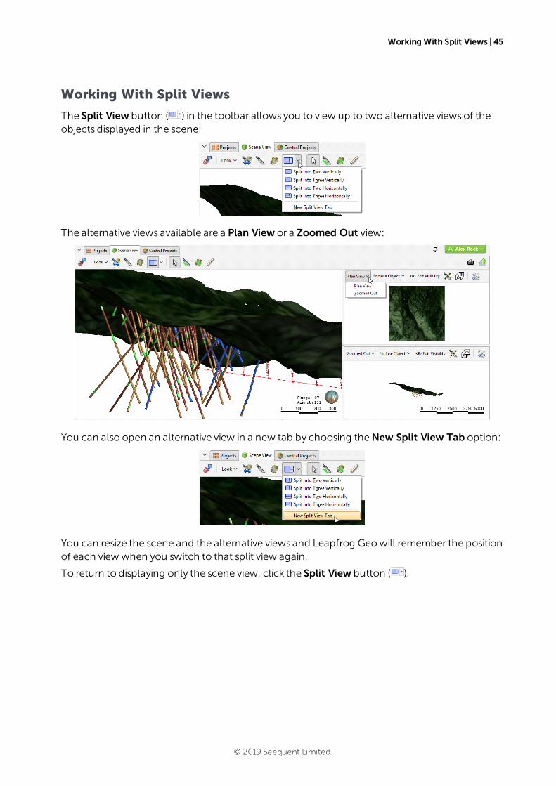
Working With Split Views | 45
Working With Split Views
The Split View button ( ) in the toolbar allows you to view up to two alternative viewsof theobjects displayed in the scene:
The alternative views available are a Plan View or a Zoomed Out view:
You can also open an alternative view in a new tab by choosing theNew Split View Tab option:
You can resize the scene and the alternative views and Leapfrog Geowill remember the positionof each view when you switch to that split view again.
To return to displaying only the scene view, click the Split View button ( ).
© 2019 Seequent Limited
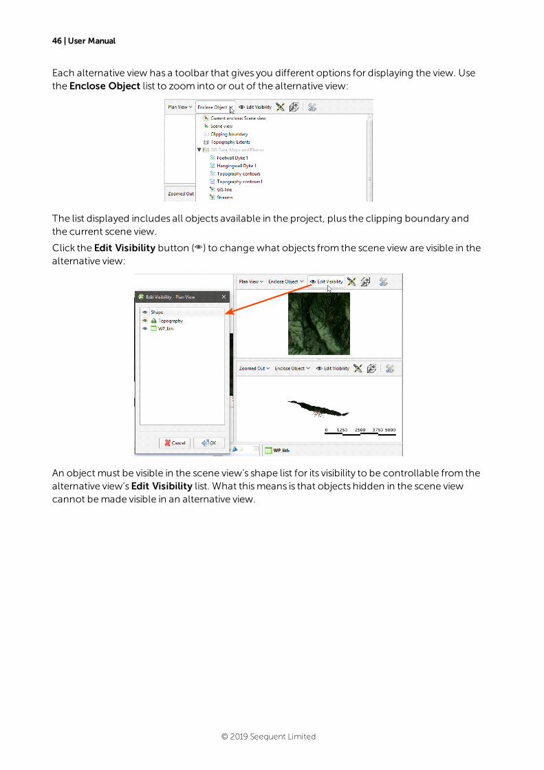
46 | User Manual
Each alternative view has a toolbar that gives you different options for displaying the view. Usethe Enclose Object list to zoom into or out of the alternative view:
The list displayed includes all objects available in the project, plus the clipping boundary andthe current scene view.
Click the Edit Visibility button ( ) to changewhat objects from the scene view are visible in thealternative view:
An object must be visible in the scene view’s shape list for its visibility to be controllable from thealternative view’sEdit Visibility list. What thismeans is that objects hidden in the scene viewcannot bemade visible in an alternative view.
© 2019 Seequent Limited
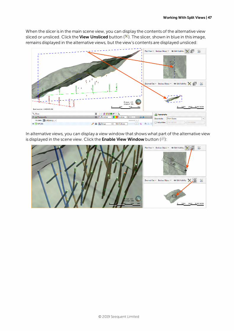
Working With Split Views | 47
When the slicer is in themain scene view, you can display the contents of the alternative viewsliced or unsliced. Click the View Unsliced button ( ). The slicer, shown in blue in this image,remains displayed in the alternative views, but the view’s contents are displayed unsliced:
In alternative views, you can display a view window that showswhat part of the alternative viewis displayed in the scene view. Click the Enable View Window button ( ):
© 2019 Seequent Limited

48 | User Manual
Each alternative view has a Settings button ( ) that lets you changewhat overlays are displayedfor that view. The alternative view can use the scene view settings, or you can customise thedisplay of the screen grid, axis lines and scale bar:
© 2019 Seequent Limited

Visualising Data | 49
Visualising Data
Visualising data is an important part of interpreting and refining data and making modellingdecisions. This topic describes the tools available for changing how data objects are displayed inthe scene. It is divided into:
l Colour Options
l Opacity
l Property Buttons
l Legends
l Slice Mode
l Filtering Data Using Queries
l Filtering Data Using Values and Categories
Tools for visualising data are accessed via the shape list and the shape properties panel:
The tools available depend on the type of object being displayed.
Changing how you view objects in the scenewindow does not change those objects in theproject tree.
© 2019 Seequent Limited
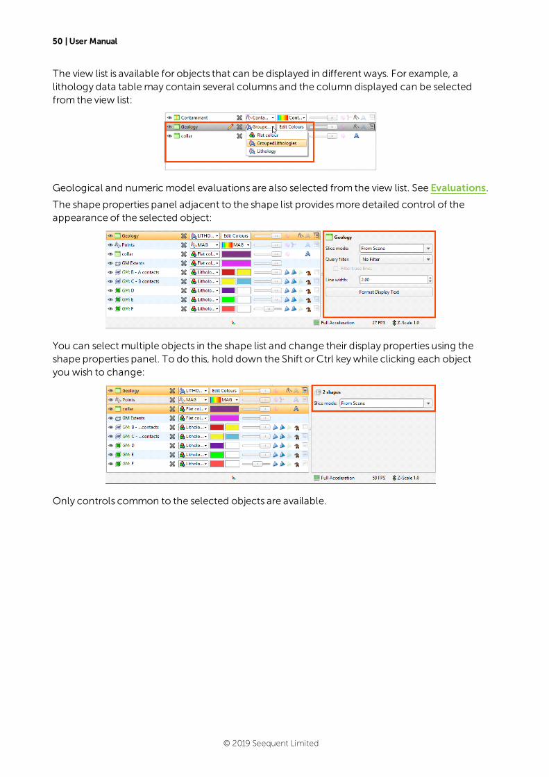
50 | User Manual
The view list is available for objects that can be displayed in different ways. For example, alithology data tablemay contain several columns and the column displayed can be selectedfrom the view list:
Geological and numericmodel evaluations are also selected from the view list. See Evaluations.
The shape properties panel adjacent to the shape list providesmore detailed control of theappearance of the selected object:
You can select multiple objects in the shape list and change their display properties using theshape properties panel. To do this, hold down the Shift or Ctrl keywhile clicking each objectyou wish to change:
Only controls common to the selected objects are available.
© 2019 Seequent Limited
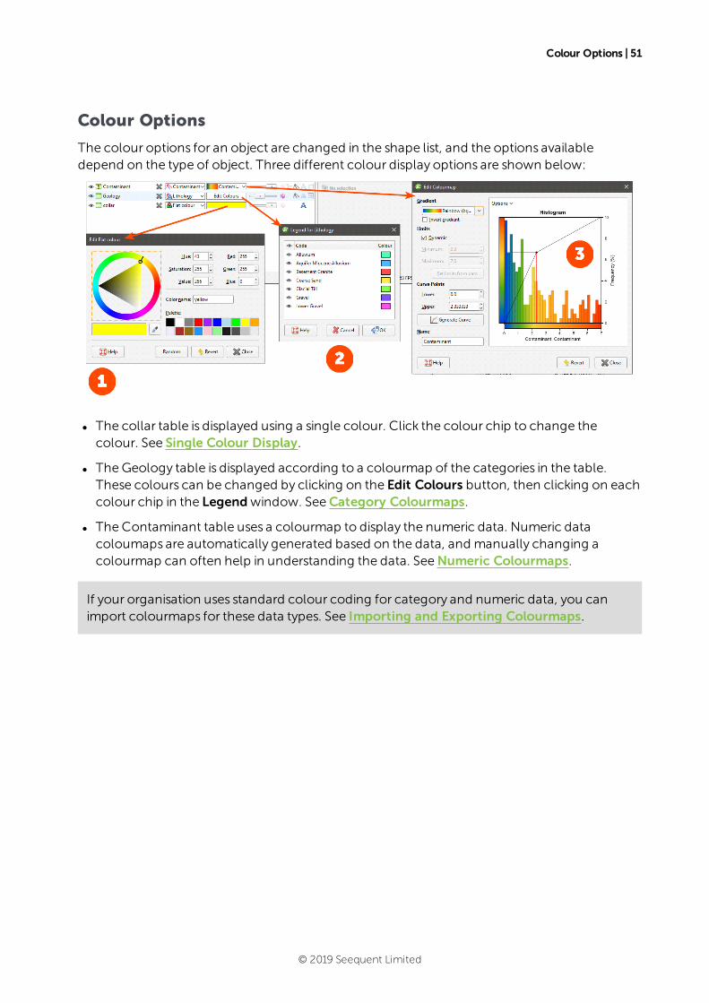
Colour Options | 51
Colour Options
The colour options for an object are changed in the shape list, and the options availabledepend on the type of object. Three different colour display options are shown below:
l The collar table is displayed using a single colour. Click the colour chip to change thecolour. See Single Colour Display.
l TheGeology table is displayed according to a colourmap of the categories in the table.These colours can be changed by clicking on the Edit Colours button, then clicking on eachcolour chip in the Legendwindow. SeeCategory Colourmaps.
l The Contaminant table uses a colourmap to display the numeric data. Numeric datacoloumaps are automatically generated based on the data, and manually changing acolourmap can often help in understanding the data. SeeNumeric Colourmaps.
If your organisation uses standard colour coding for category and numeric data, you canimport colourmaps for these data types. See Importing and Exporting Colourmaps.
© 2019 Seequent Limited
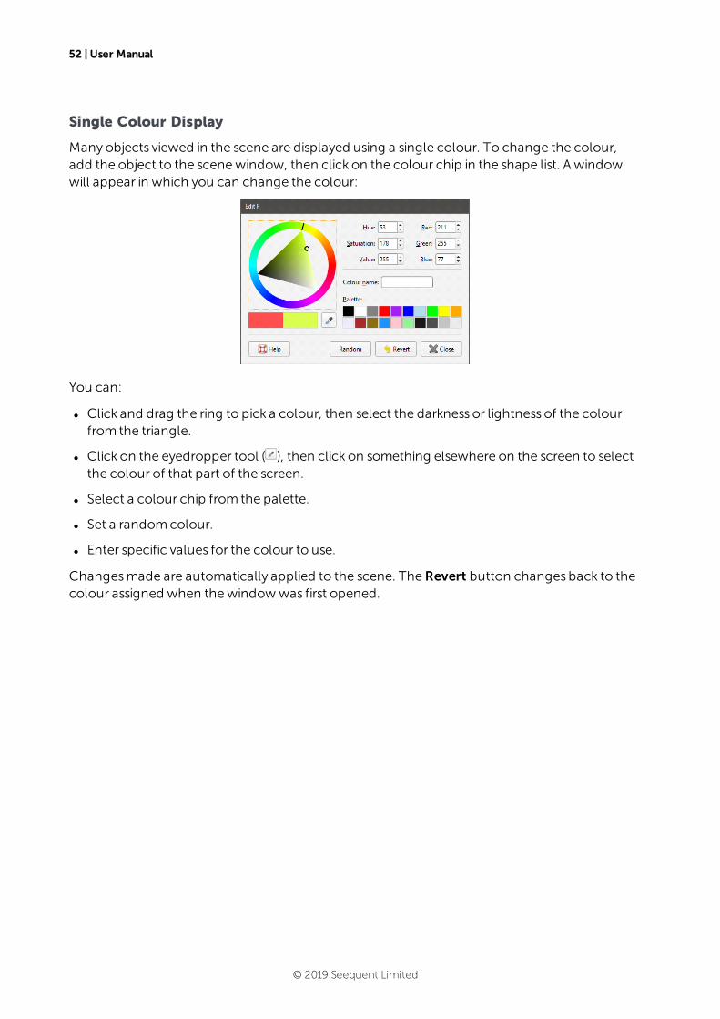
52 | User Manual
Single Colour Display
Many objects viewed in the scene are displayed using a single colour. To change the colour,add the object to the scenewindow, then click on the colour chip in the shape list. A windowwill appear in which you can change the colour:
You can:
l Click and drag the ring to pick a colour, then select the darkness or lightness of the colourfrom the triangle.
l Click on the eyedropper tool ( ), then click on something elsewhere on the screen to selectthe colour of that part of the screen.
l Select a colour chip from the palette.
l Set a randomcolour.
l Enter specific values for the colour to use.
Changesmade are automatically applied to the scene. TheRevert button changes back to thecolour assigned when thewindowwas first opened.
© 2019 Seequent Limited
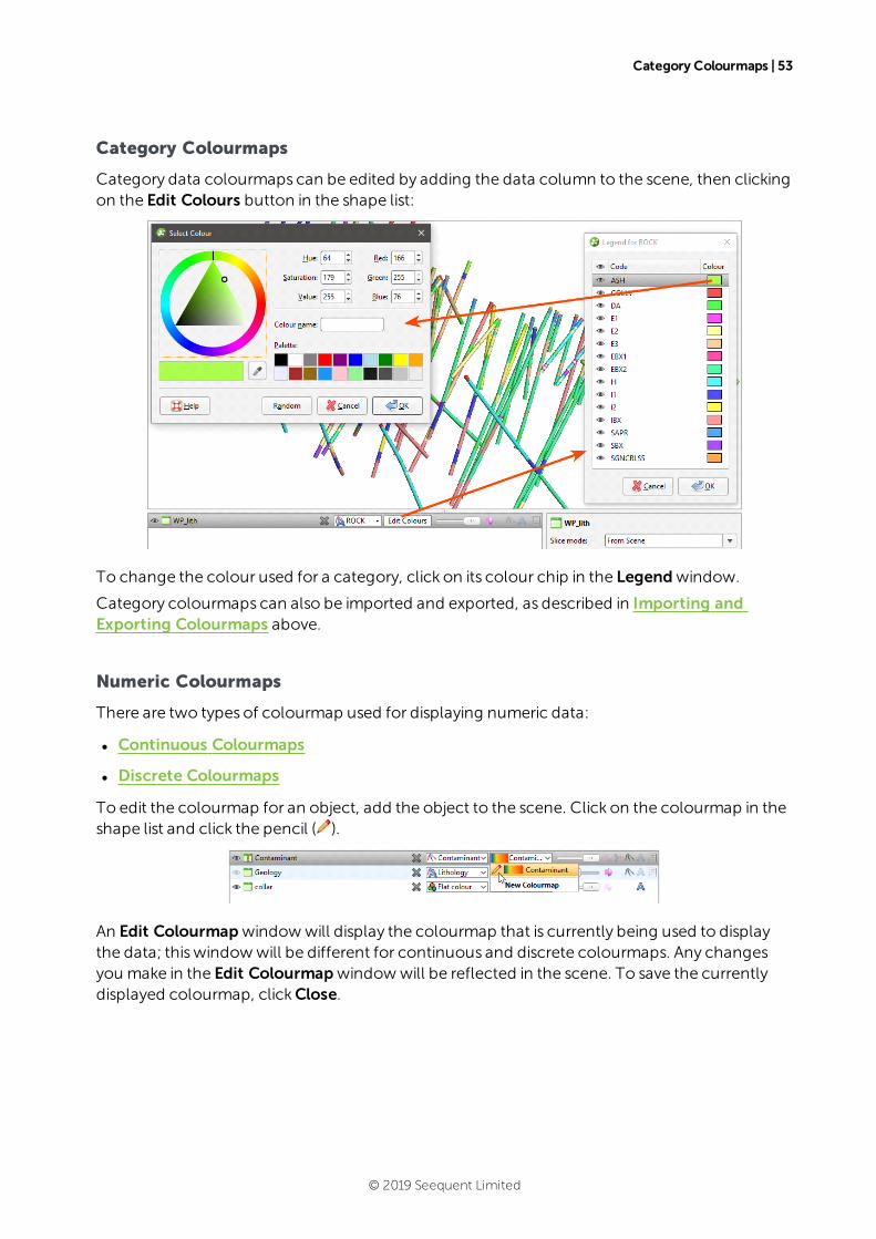
Category Colourmaps | 53
Category Colourmaps
Category data colourmaps can be edited by adding the data column to the scene, then clickingon the Edit Colours button in the shape list:
To change the colour used for a category, click on its colour chip in the Legendwindow.
Category colourmaps can also be imported and exported, as described in Importing andExporting Colourmaps above.
Numeric Colourmaps
There are two types of colourmap used for displaying numeric data:
l Continuous Colourmaps
l Discrete Colourmaps
To edit the colourmap for an object, add the object to the scene. Click on the colourmap in theshape list and click the pencil ( ).
An Edit Colourmapwindowwill display the colourmap that is currently being used to displaythe data; thiswindowwill be different for continuous and discrete colourmaps. Any changesyou make in the Edit Colourmapwindowwill be reflected in the scene. To save the currentlydisplayed colourmap, clickClose.
© 2019 Seequent Limited
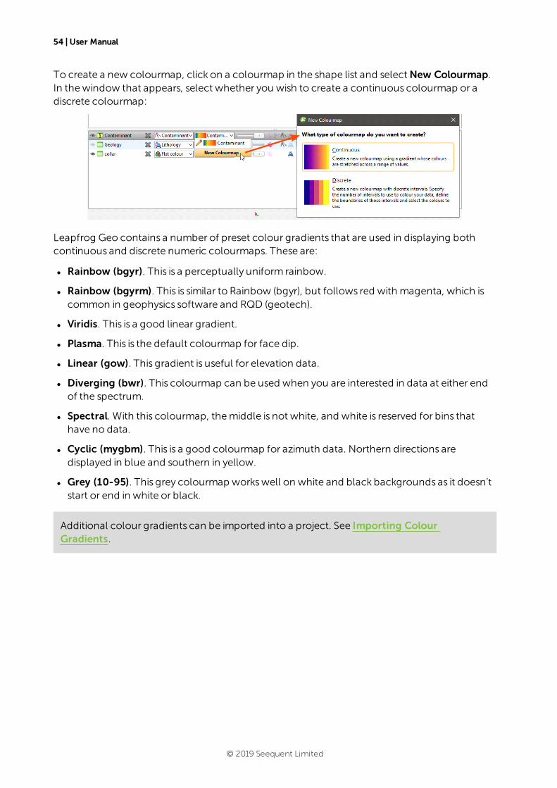
54 | User Manual
To create a new colourmap, click on a colourmap in the shape list and selectNew Colourmap.In thewindow that appears, select whether you wish to create a continuous colourmap or adiscrete colourmap:
Leapfrog Geo contains a number of preset colour gradients that are used in displaying bothcontinuous and discrete numeric colourmaps. These are:
l Rainbow (bgyr). This is a perceptually uniform rainbow.
l Rainbow (bgyrm). This is similar to Rainbow (bgyr), but follows red with magenta, which iscommon in geophysics software and RQD (geotech).
l Viridis. This is a good linear gradient.
l Plasma. This is the default colourmap for face dip.
l Linear (gow). This gradient is useful for elevation data.
l Diverging (bwr). This colourmap can be used when you are interested in data at either endof the spectrum.
l Spectral. With this colourmap, themiddle is not white, and white is reserved for bins thathave no data.
l Cyclic (mygbm). This is a good colourmap for azimuth data. Northern directions aredisplayed in blue and southern in yellow.
l Grey (10-95). This grey colourmap workswell on white and black backgrounds as it doesn’tstart or end in white or black.
Additional colour gradients can be imported into a project. See Importing ColourGradients.
© 2019 Seequent Limited
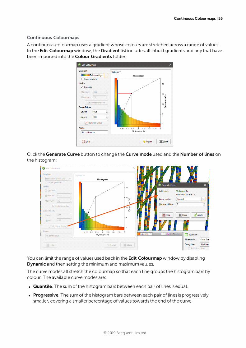
Continuous Colourmaps | 55
Continuous Colourmaps
A continuous colourmap uses a gradient whose colours are stretched across a range of values.In the Edit Colourmapwindow, theGradient list includes all inbuilt gradients and any that havebeen imported into theColour Gradients folder.
Click theGenerate Curve button to change theCurve mode used and theNumber of lines onthe histogram:
You can limit the range of values used back in the Edit Colourmapwindow by disablingDynamic and then setting theminimumand maximumvalues.
The curvemodes all stretch the colourmap so that each line groups the histogrambars bycolour. The available curvemodes are:
l Quantile. The sumof the histogrambars between each pair of lines is equal.
l Progressive. The sumof the histogrambars between each pair of lines is progressivelysmaller, covering a smaller percentage of values towards the end of the curve.
© 2019 Seequent Limited

56 | User Manual
l Progressive Double. This is similar to Progressive, but the effect is emphasised by increasingthe percentage difference between lines.
l Logarithmic Intervals. This stretches the colours using a logarithmic transform, which maybe preferred for data with a wide range of values.
Experiment with the different settings and clickApply to see the effects of changes. To edit thecurve points on the histogram, close theGenerate Curvewindow:
Note that if you usemore than 10 lines in generating the curve, you will not be able to edit thecurve points on the histogram:
© 2019 Seequent Limited

Continuous Colourmaps | 57
You can change the Bin Width in theOptions menu:
EnableHistogram of the Log to see the value distribution with a log scale X-axis. You can alsoview a Cumulative distribution function for the values, with or without a log scale X-axis.
If the numeric data column for which the colourmap is defined has been produced fromotherdata sources in the project, you will be able to select whether to display the Local Values or thevalues from the Parent Data. For example, for a numeric data column that is part of a mergedtable, you can display the values fromonly themerged table or from the parent table:
If theDynamic option is enabled, the gradient will be updated when the data is updated, suchaswhen drillhole data is appended. If the option is disabled, the valuesmanually set for theMinimum and Maximum limitswill control the lower and upper boundsof the colourmap.Reducing the range of the upper and lower bounds is useful if the bulk of the data points havevalues in a rangemuch smaller than the overall range of the data. This is common in skeweddata.
The Set limits from data button automatically adjusts theMinimum and Maximum Limitvalues so that the colourmap would follow the actual data distribution of the input data. Thevalues that lie outside the Limits are coloured with the last colour at the relevant end of thecolourmap.
© 2019 Seequent Limited
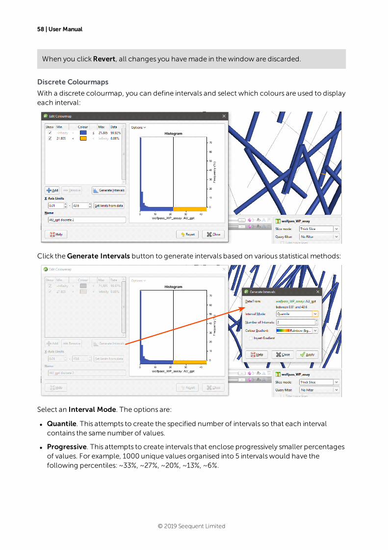
58 | User Manual
When you clickRevert, all changes you havemade in thewindow are discarded.
Discrete Colourmaps
With a discrete colourmap, you can define intervals and select which colours are used to displayeach interval:
Click theGenerate Intervals button to generate intervals based on various statistical methods:
Select an Interval Mode. The options are:
l Quantile. This attempts to create the specified number of intervals so that each intervalcontains the same number of values.
l Progressive. This attempts to create intervals that enclose progressively smaller percentagesof values. For example, 1000 unique values organised into 5 intervalswould have thefollowing percentiles: ~33%, ~27%, ~20%, ~13%, ~6%.
© 2019 Seequent Limited
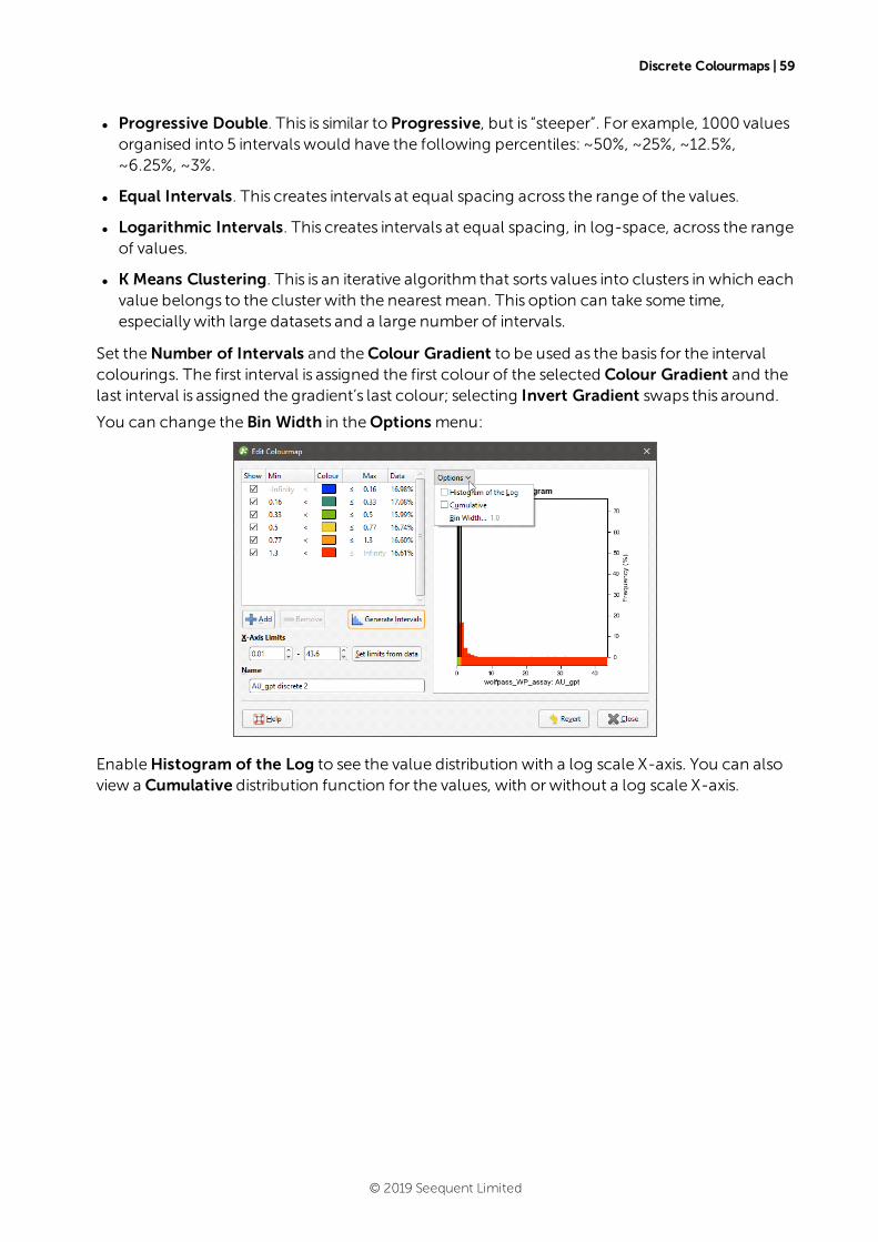
Discrete Colourmaps | 59
l Progressive Double. This is similar to Progressive, but is “steeper”. For example, 1000 valuesorganised into 5 intervalswould have the following percentiles: ~50%, ~25%, ~12.5%,~6.25%, ~3%.
l Equal Intervals. This creates intervals at equal spacing across the range of the values.
l Logarithmic Intervals. This creates intervals at equal spacing, in log-space, across the rangeof values.
l K Means Clustering. This is an iterative algorithm that sorts values into clusters in which eachvalue belongs to the cluster with the nearest mean. This option can take some time,especially with large datasets and a large number of intervals.
Set theNumber of Intervals and theColour Gradient to be used as the basis for the intervalcolourings. The first interval is assigned the first colour of the selected Colour Gradient and thelast interval is assigned the gradient’s last colour; selecting Invert Gradient swaps this around.
You can change the Bin Width in theOptions menu:
EnableHistogram of the Log to see the value distribution with a log scale X-axis. You can alsoview a Cumulative distribution function for the values, with or without a log scale X-axis.
© 2019 Seequent Limited

60 | User Manual
If the numeric data column for which the colourmap is defined has been produced fromotherdata sources in the project, you will be able to select whether to display the Local Values or thevalues from the Parent Data. For example, for a numeric data column that is part of a mergedtable, you can display the values fromonly themerged table or from the parent table:
The Set limits from data button automatically adjusts the X-Axis Limits so that the colourmapwould follow the actual data distribution of the input data.
Experiment with the different settings and clickApply to see the effects of changes.
You can also add intervalsmanually by clicking the Add button. For example, if you create adiscrete colourmap to show the different stages of a drilling campaign, the initial colourmapcontains only two intervals:
© 2019 Seequent Limited
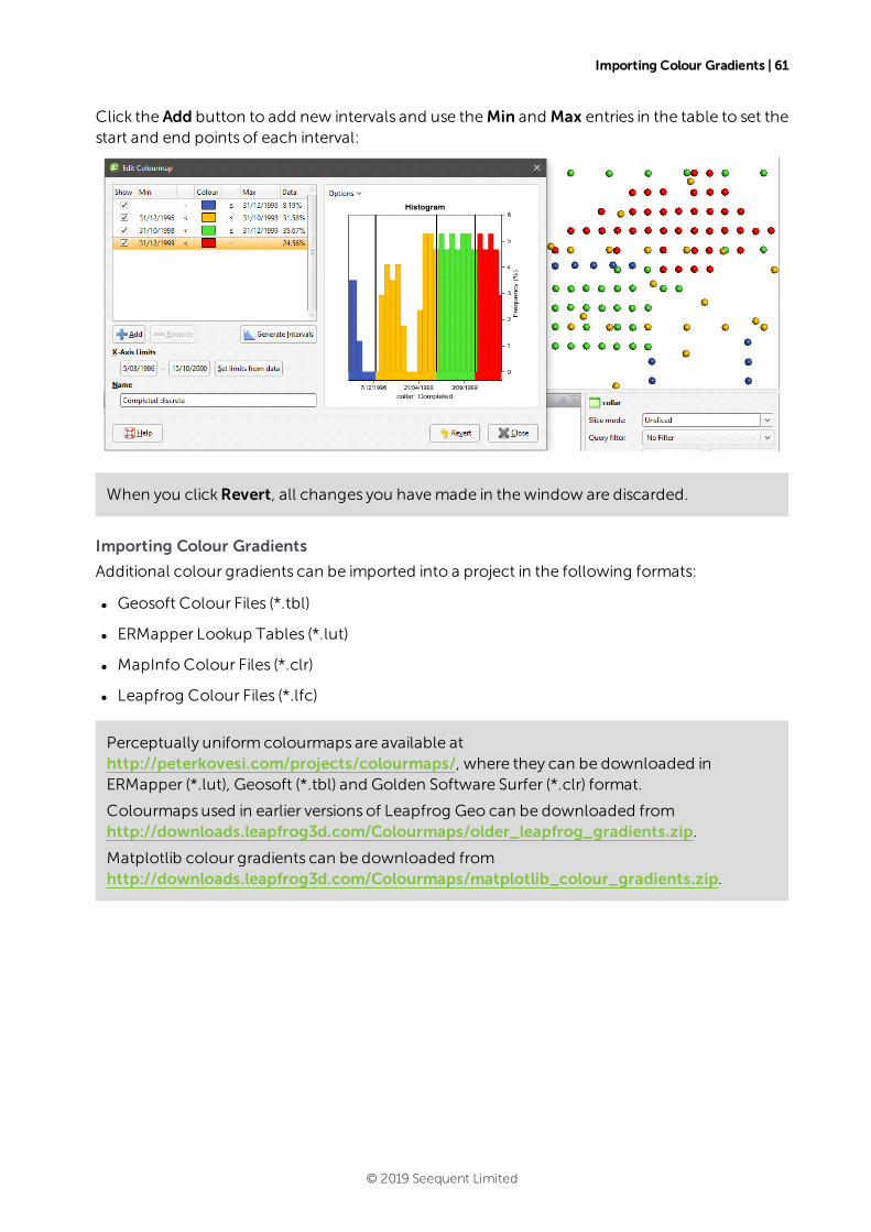
Importing Colour Gradients | 61
Click the Add button to add new intervals and use theMin and Max entries in the table to set thestart and end points of each interval:
When you clickRevert, all changes you havemade in thewindow are discarded.
Importing Colour Gradients
Additional colour gradients can be imported into a project in the following formats:
l Geosoft Colour Files (*.tbl)
l ERMapper Lookup Tables (*.lut)
l MapInfo Colour Files (*.clr)
l Leapfrog Colour Files (*.lfc)
Perceptually uniformcolourmaps are available athttp://peterkovesi.com/projects/colourmaps/, where they can be downloaded inERMapper (*.lut), Geosoft (*.tbl) and Golden Software Surfer (*.clr) format.
Colourmaps used in earlier versions of Leapfrog Geo can be downloaded fromhttp://downloads.leapfrog3d.com/Colourmaps/older_leapfrog_gradients.zip.
Matplotlib colour gradients can be downloaded fromhttp://downloads.leapfrog3d.com/Colourmaps/matplotlib_colour_gradients.zip.
© 2019 Seequent Limited
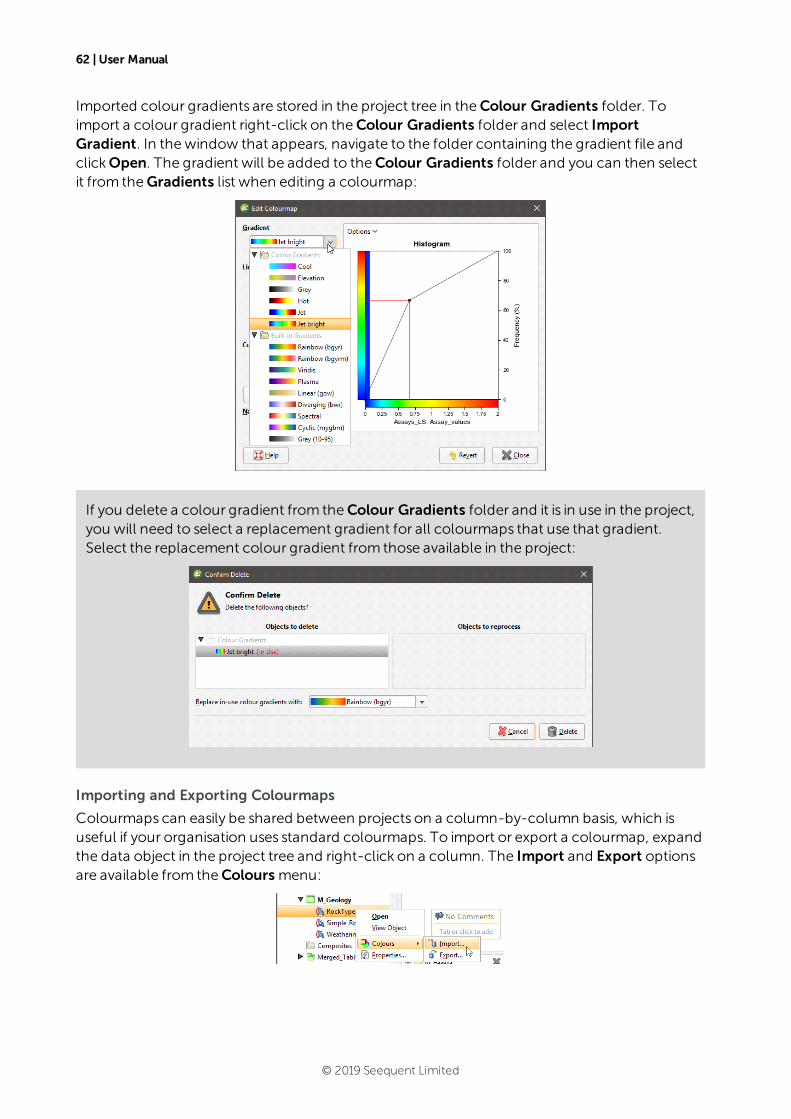
62 | User Manual
Imported colour gradients are stored in the project tree in theColour Gradients folder. Toimport a colour gradient right-click on theColour Gradients folder and select ImportGradient. In thewindow that appears, navigate to the folder containing the gradient file andclickOpen. The gradient will be added to theColour Gradients folder and you can then selectit from theGradients list when editing a colourmap:
If you delete a colour gradient from theColour Gradients folder and it is in use in the project,you will need to select a replacement gradient for all colourmaps that use that gradient.Select the replacement colour gradient from those available in the project:
Importing and Exporting Colourmaps
Colourmaps can easily be shared between projects on a column-by-column basis, which isuseful if your organisation uses standard colourmaps. To import or export a colourmap, expandthe data object in the project tree and right-click on a column. The Import and Export optionsare available from theColours menu:
© 2019 Seequent Limited
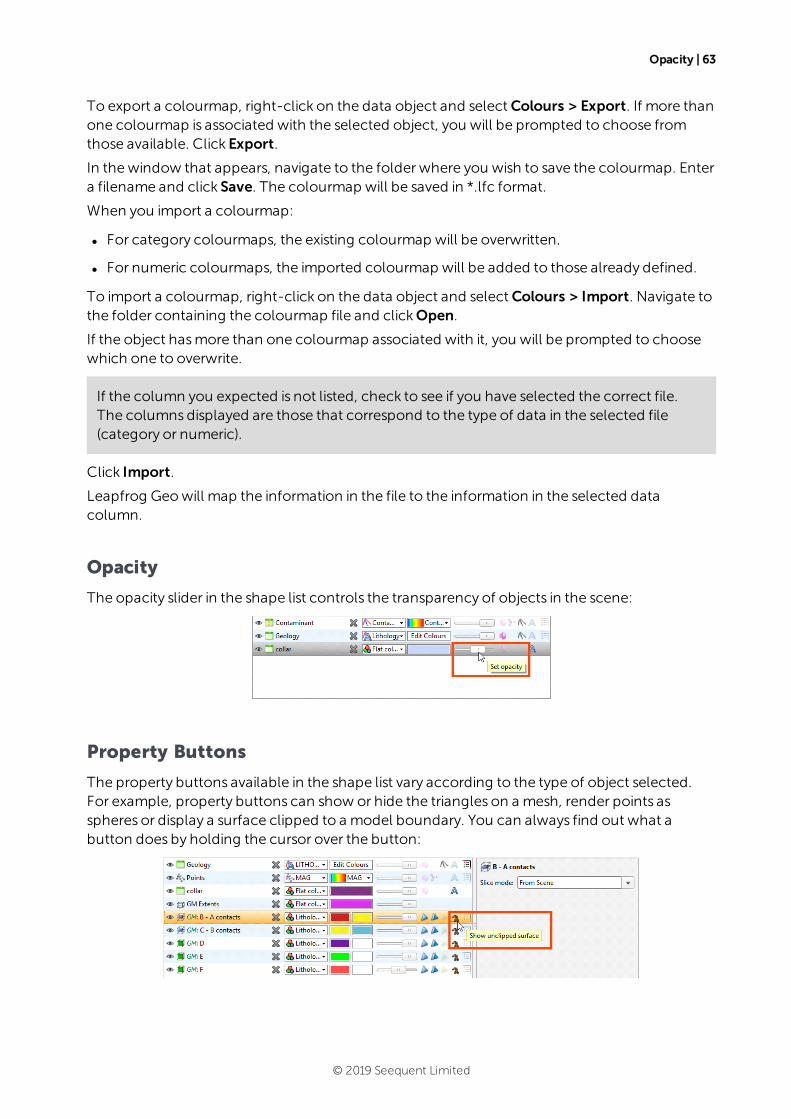
Opacity | 63
To export a colourmap, right-click on the data object and selectColours > Export. If more thanone colourmap is associated with the selected object, you will be prompted to choose fromthose available. Click Export.
In thewindow that appears, navigate to the folder where you wish to save the colourmap. Entera filename and click Save. The colourmap will be saved in *.lfc format.
When you import a colourmap:
l For category colourmaps, the existing colourmap will be overwritten.
l For numeric colourmaps, the imported colourmap will be added to those already defined.
To import a colourmap, right-click on the data object and selectColours > Import. Navigate tothe folder containing the colourmap file and clickOpen.
If the object hasmore than one colourmap associated with it, you will be prompted to choosewhich one to overwrite.
If the column you expected is not listed, check to see if you have selected the correct file.The columnsdisplayed are those that correspond to the type of data in the selected file(category or numeric).
Click Import.
Leapfrog Geowill map the information in the file to the information in the selected datacolumn.
Opacity
The opacity slider in the shape list controls the transparency of objects in the scene:
Property Buttons
The property buttons available in the shape list vary according to the type of object selected.For example, property buttons can show or hide the triangles on a mesh, render points asspheres or display a surface clipped to a model boundary. You can always find out what abutton does by holding the cursor over the button:
© 2019 Seequent Limited
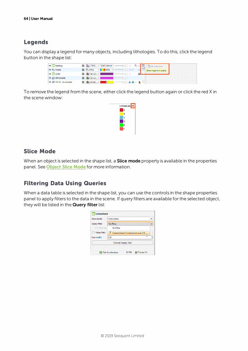
64 | User Manual
Legends
You can display a legend formany objects, including lithologies. To do this, click the legendbutton in the shape list:
To remove the legend from the scene, either click the legend button again or click the red X inthe scenewindow:
Slice Mode
When an object is selected in the shape list, a Slice mode property is available in the propertiespanel. SeeObject Slice Mode formore information.
Filtering Data Using Queries
When a data table is selected in the shape list, you can use the controls in the shape propertiespanel to apply filters to the data in the scene. If query filters are available for the selected object,theywill be listed in theQuery filter list:
© 2019 Seequent Limited
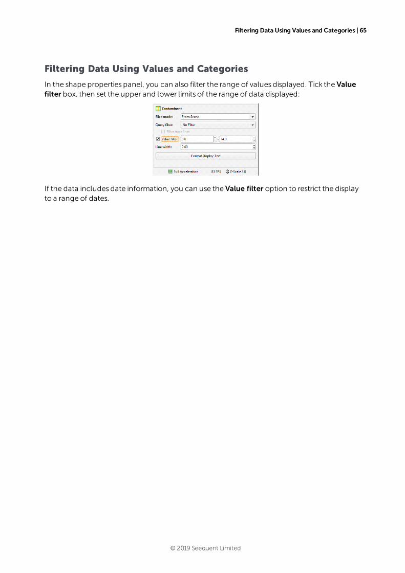
Filtering Data Using Values and Categories | 65
Filtering Data Using Values and Categories
In the shape properties panel, you can also filter the range of values displayed. Tick the Valuefilter box, then set the upper and lower limits of the range of data displayed:
If the data includes date information, you can use the Value filter option to restrict the displayto a range of dates.
© 2019 Seequent Limited
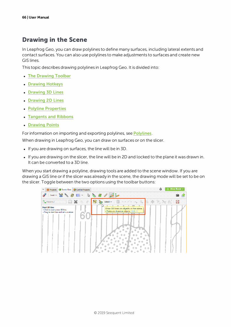
66 | User Manual
Drawing in the Scene
In Leapfrog Geo, you can draw polylines to definemany surfaces, including lateral extents andcontact surfaces. You can also use polylines tomake adjustments to surfaces and create newGIS lines.
This topic describes drawing polylines in Leapfrog Geo. It is divided into:
l The Drawing Toolbar
l Drawing Hotkeys
l Drawing 3D Lines
l Drawing 2D Lines
l Polyline Properties
l Tangents and Ribbons
l Drawing Points
For information on importing and exporting polylines, see Polylines.
When drawing in Leapfrog Geo, you can draw on surfaces or on the slicer.
l If you are drawing on surfaces, the line will be in 3D.
l If you are drawing on the slicer, the line will be in 2D and locked to the plane it was drawn in.It can be converted to a 3D line.
When you start drawing a polyline, drawing tools are added to the scenewindow. If you aredrawing a GIS line or if the slicer was already in the scene, the drawing modewill be set to be onthe slicer. Toggle between the two options using the toolbar buttons:
© 2019 Seequent Limited
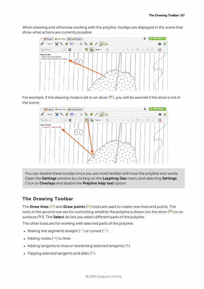
The Drawing Toolbar | 67
When drawing and otherwise working with the polyline, tooltips are displayed in the scene thatshowwhat actions are currently possible:
For example, if the drawing mode is set to on slicer ( ), you will be warned if the slicer is not inthe scene:
You can disable these tooltips once you aremore familiar with how the polyline tool works.Open the Settings window by clicking on the Leapfrog Geomenu and selecting Settings.Click on Overlays and disable the Polyline help text option.
The Drawing Toolbar
TheDraw lines ( ) and Draw points ( ) tools are used to create new lines and points. Thetools in the second row are for controlling whether the polyline is drawn (on the slicer ( ) or onsurfaces ( )). The Select list lets you select different parts of the polyline.
The other tools are for working with selected parts of the polyline:
l Making line segments straight ( ) or curved ( )
l Adding nodes ( ) to lines
l Adding tangents to lines or reorienting selected tangents ( )
l Flipping selected tangents and disks ( )
© 2019 Seequent Limited
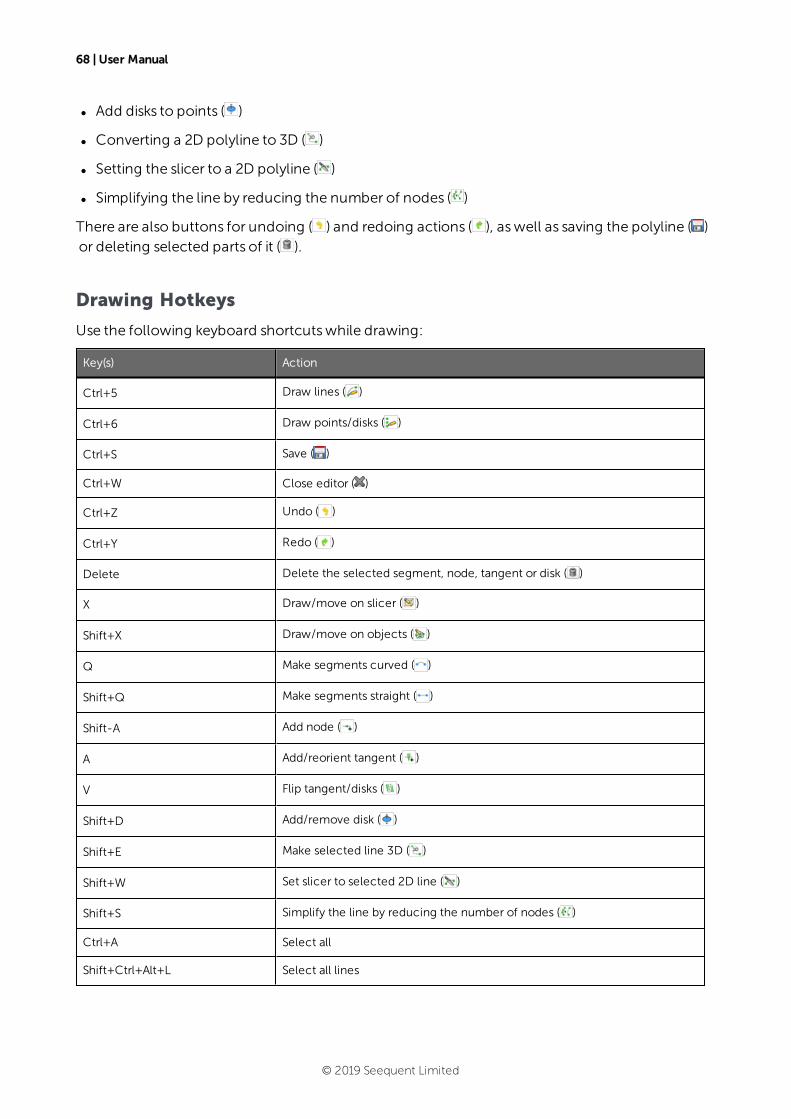
68 | User Manual
l Add disks to points ( )
l Converting a 2D polyline to 3D ( )
l Setting the slicer to a 2D polyline ( )
l Simplifying the line by reducing the number of nodes ( )
There are also buttons for undoing ( ) and redoing actions ( ), aswell as saving the polyline ( )or deleting selected parts of it ( ).
Drawing Hotkeys
Use the following keyboard shortcutswhile drawing:
Key(s) Action
Ctrl+5 Draw lines ( )
Ctrl+6 Draw points/disks ( )
Ctrl+S Save ( )
Ctrl+W Close editor ( )
Ctrl+Z Undo ( )
Ctrl+Y Redo ( )
Delete Delete the selected segment, node, tangent or disk ( )
X Draw/move on slicer ( )
Shift+X Draw/move on objects ( )
Q Make segments curved ( )
Shift+Q Make segments straight ( )
Shift-A Add node ( )
A Add/reorient tangent ( )
V Flip tangent/disks ( )
Shift+D Add/remove disk ( )
Shift+E Make selected line 3D ( )
Shift+W Set slicer to selected 2D line ( )
Shift+S Simplify the line by reducing the number of nodes ( )
Ctrl+A Select all
Shift+Ctrl+Alt+L Select all lines
© 2019 Seequent Limited

Drawing 3D Lines | 69
Key(s) Action
Shift+Ctrl+Alt+T Select all tangents
Shift+Ctrl+Alt+P Select all points without disks
Shift+Ctrl+Alt+D Select all points with disks
Drawing 3D Lines
Polylines aremade up of nodes, which are added where you click in the scene using theDrawlines ( ) tool. This is a 3D polyline, which is indicated in the scene by the dashed line:
Click to select a node and drag tomove it in the scene parallel to the screen. If you hold downthe Ctrl keywhilemoving the node, it will snap onto surfaces in the scene.
When drillhole segments are in the scene, the polyline tool will snap to the end of nearbyintervals.
When you click to add a node, dragging themouse before releasing the button lets you controlthe curvature:
© 2019 Seequent Limited
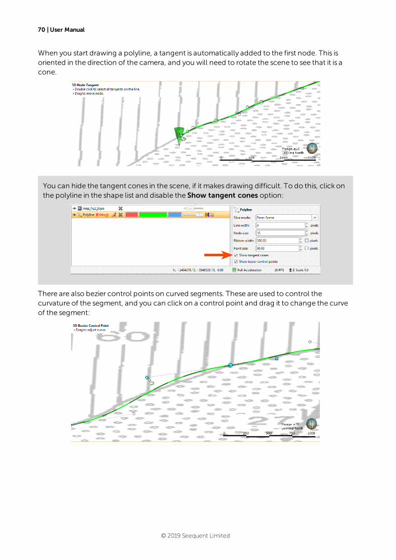
70 | User Manual
When you start drawing a polyline, a tangent is automatically added to the first node. This isoriented in the direction of the camera, and you will need to rotate the scene to see that it is acone.
You can hide the tangent cones in the scene, if it makes drawing difficult. To do this, click onthe polyline in the shape list and disable the Show tangent cones option:
There are also bezier control points on curved segments. These are used to control thecurvature of the segment, and you can click on a control point and drag it to change the curveof the segment:
© 2019 Seequent Limited
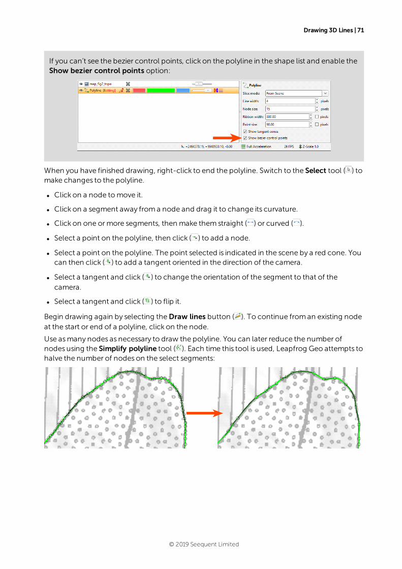
Drawing 3D Lines | 71
If you can’t see the bezier control points, click on the polyline in the shape list and enable theShow bezier control points option:
When you have finished drawing, right-click to end the polyline. Switch to the Select tool ( ) tomake changes to the polyline.
l Click on a node tomove it.
l Click on a segment away froma node and drag it to change its curvature.
l Click on one ormore segments, then make themstraight ( ) or curved ( ).
l Select a point on the polyline, then click ( ) to add a node.
l Select a point on the polyline. The point selected is indicated in the scene by a red cone. Youcan then click ( ) to add a tangent oriented in the direction of the camera.
l Select a tangent and click ( ) to change the orientation of the segment to that of thecamera.
l Select a tangent and click ( ) to flip it.
Begin drawing again by selecting theDraw lines button ( ). To continue froman existing nodeat the start or end of a polyline, click on the node.
Use asmany nodes as necessary to draw the polyline. You can later reduce the number ofnodes using the Simplify polyline tool ( ). Each time this tool is used, Leapfrog Geo attempts tohalve the number of nodes on the select segments:
© 2019 Seequent Limited
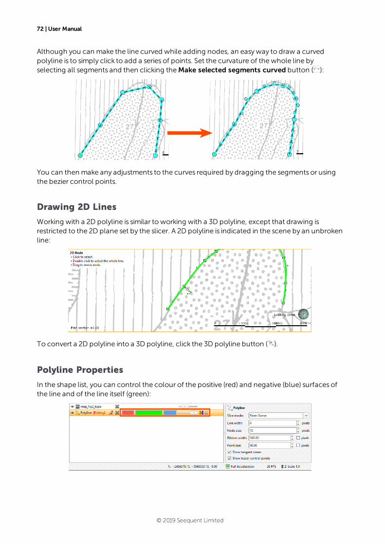
72 | User Manual
Although you can make the line curved while adding nodes, an easyway to draw a curvedpolyline is to simply click to add a series of points. Set the curvature of thewhole line byselecting all segments and then clicking theMake selected segments curved button ( ):
You can then make any adjustments to the curves required by dragging the segments or usingthe bezier control points.
Drawing 2D Lines
Working with a 2D polyline is similar to working with a 3D polyline, except that drawing isrestricted to the 2D plane set by the slicer. A 2D polyline is indicated in the scene by an unbrokenline:
To convert a 2D polyline into a 3D polyline, click the 3D polyline button ( ).
Polyline Properties
In the shape list, you can control the colour of the positive (red) and negative (blue) surfaces ofthe line and of the line itself (green):
© 2019 Seequent Limited

Tangents and Ribbons | 73
For contact surfaces, the colour of the positive and negative sides of a ribbon will bedetermined by the lithologies or categories assigned to either side of the surface.
With the controls in the properties panel, you can change the size of different parts of thepolyline tomakeworking with the polyline easier.
ForRibbon width and Point size, the setting is, by default, in pixels, but both can be displayedin real-world size, which maymake editing the polyline easier in some circumstances.
You can also choosewhether or not to show tangent cones and bezier control points.
Tangents and Ribbons
The Surface ribbon ( ) and Normal ribbon ( ) help you to determine the orientation of thepolyline in the scene. The surface ribbon reflects the orientation of the polyline and the normalribbon is perpendicular to the surface ribbon.
For example, click on the Surface ribbon button ( ) to determinewhich side of the polyline ispositive (red) and which side is negative (blue):
If you are having trouble seeing the ribbons, you can change their size using theRibbon widthcontrol in the properties panel.
When you first draw a polyline, it has only one tangent, located at the first node and oriented inthe direction of the camera. You can add more nodes by clicking at a point along the polylineand then clicking the Tangent button ( ). A tangent is added to the polyline, which is updated
© 2019 Seequent Limited
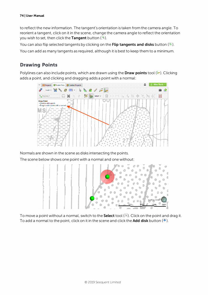
74 | User Manual
to reflect the new information. The tangent’s orientation is taken from the camera angle. Toreorient a tangent, click on it in the scene, change the camera angle to reflect the orientationyou wish to set, then click the Tangent button ( ).
You can also flip selected tangents by clicking on the Flip tangents and disks button ( ).
You can add asmany tangents as required, although it is best to keep them to a minimum.
Drawing Points
Polylines can also include points, which are drawn using theDraw points tool ( ). Clickingadds a point, and clicking and dragging adds a point with a normal:
Normals are shown in the scene as disks intersecting the points.
The scene below showsone point with a normal and onewithout:
Tomove a point without a normal, switch to the Select tool ( ). Click on the point and drag it.To add a normal to the point, click on it in the scene and click the Add disk button ( ).
© 2019 Seequent Limited
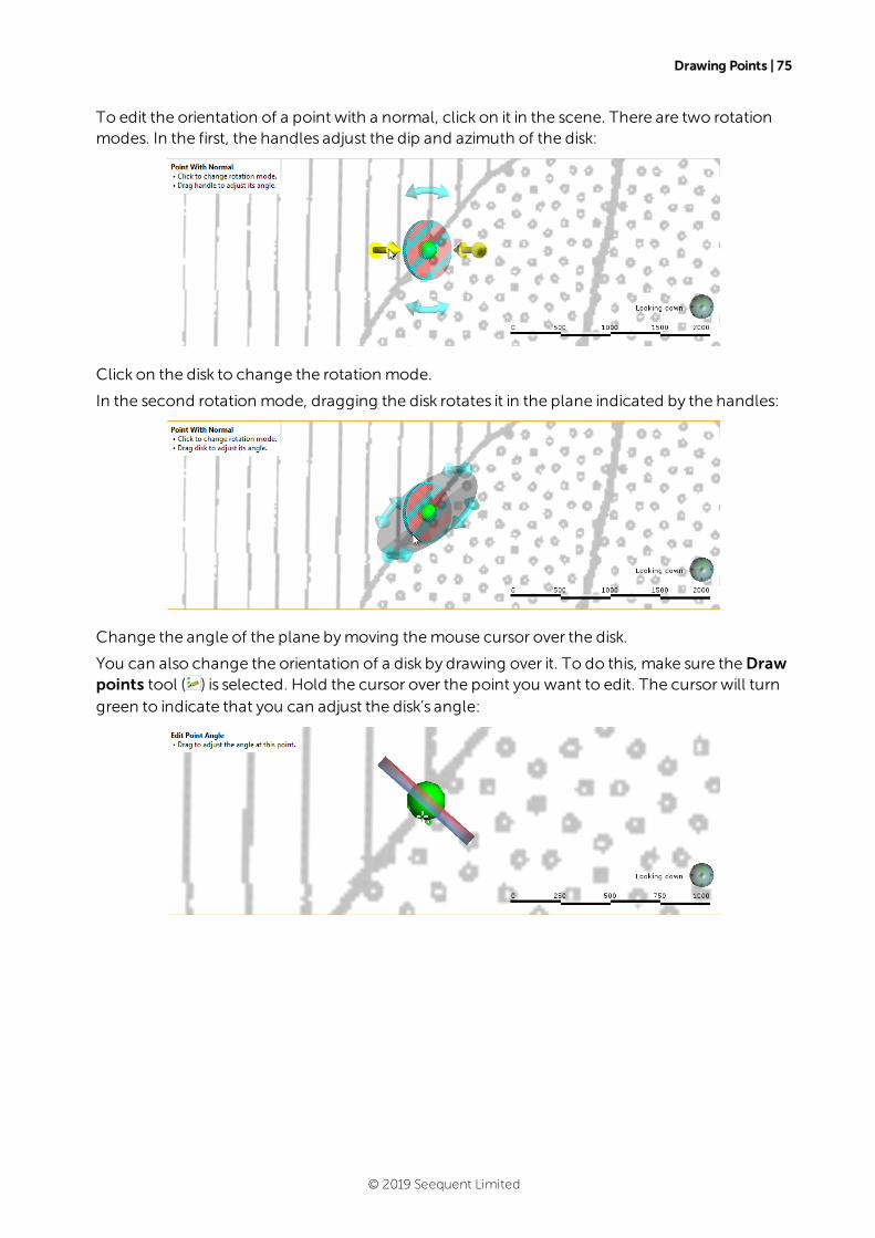
Drawing Points | 75
To edit the orientation of a point with a normal, click on it in the scene. There are two rotationmodes. In the first, the handles adjust the dip and azimuth of the disk:
Click on the disk to change the rotation mode.
In the second rotation mode, dragging the disk rotates it in the plane indicated by the handles:
Change the angle of the plane bymoving themouse cursor over the disk.
You can also change the orientation of a disk by drawing over it. To do this, make sure theDrawpoints tool ( ) is selected. Hold the cursor over the point you want to edit. The cursor will turngreen to indicate that you can adjust the disk’s angle:
© 2019 Seequent Limited
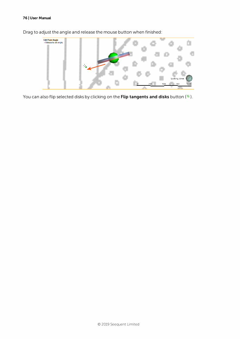
76 | User Manual
Drag to adjust the angle and release themouse button when finished:
You can also flip selected disks by clicking on the Flip tangents and disks button ( ).
© 2019 Seequent Limited
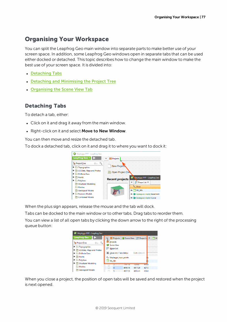
Organising Your Workspace | 77
Organising Your Workspace
You can split the Leapfrog Geomain window into separate parts tomake better use of yourscreen space. In addition, some Leapfrog Geowindowsopen in separate tabs that can be usedeither docked or detached. This topic describes how to change themain window tomake thebest use of your screen space. It is divided into:
l Detaching Tabs
l Detaching and Minimising the Project Tree
l Organising the Scene View Tab
Detaching Tabs
To detach a tab, either:
l Click on it and drag it away from themain window.
l Right-click on it and selectMove to New Window.
You can then move and resize the detached tab.
To dock a detached tab, click on it and drag it to where you want to dock it:
When the plus sign appears, release themouse and the tab will dock.
Tabs can be docked to themain window or to other tabs. Drag tabs to reorder them.
You can view a list of all open tabs by clicking the down arrow to the right of the processingqueue button:
When you close a project, the position of open tabswill be saved and restored when the projectis next opened.
© 2019 Seequent Limited
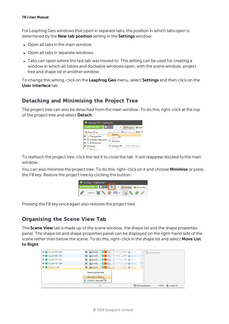
78 | User Manual
For Leapfrog Geowindows that open in separate tabs, the position in which tabs open isdetermined by theNew tab position setting in the Settings window:
l Open all tabs in themain window.
l Open all tabs in separate windows.
l Tabs can open where the last tab wasmoved to. This setting can be used for creating awindow in which all tables and dockable windowsopen, with the scenewindow, projecttree and shape list in another window.
To change this setting, click on the Leapfrog Geomenu, select Settings and then click on theUser Interface tab.
Detaching and Minimising the Project Tree
The project tree can also be detached from themain window. To do this, right-click at the topof the project tree and selectDetach:
To reattach the project tree, click the red X to close the tab. It will reappear docked to themainwindow.
You can alsominimise the project tree. To do this, right-click on it and chooseMinimise or pressthe F8 key. Restore the project tree by clicking the button:
Pressing the F8 key once again also restores the project tree.
Organising the Scene View Tab
The Scene View tab ismade up of the scenewindow, the shape list and the shape propertiespanel. The shape list and shape properties panel can be displayed on the right-hand side of thescene rather than below the scene. To do this, right-click in the shape list and selectMove Listto Right:
© 2019 Seequent Limited
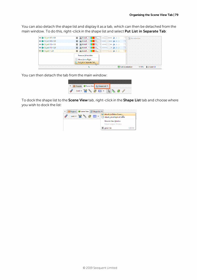
Organising the Scene View Tab | 79
You can also detach the shape list and display it as a tab, which can then be detached from themain window. To do this, right-click in the shape list and select Put List in Separate Tab:
You can then detach the tab from themain window:
To dock the shape list to the Scene View tab, right-click in the Shape List tab and choosewhereyou wish to dock the list:
© 2019 Seequent Limited
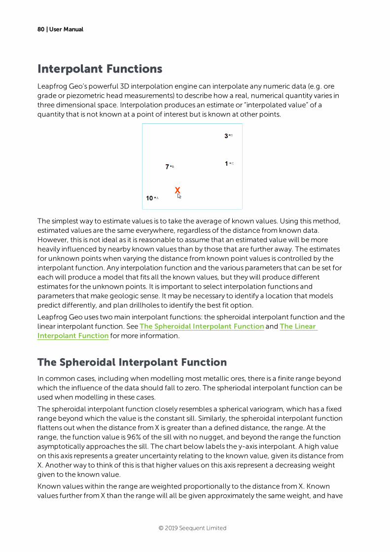
80 | User Manual
Interpolant FunctionsLeapfrog Geo’s powerful 3D interpolation engine can interpolate any numeric data (e.g. oregrade or piezometric head measurements) to describe how a real, numerical quantity varies inthree dimensional space. Interpolation produces an estimate or “interpolated value” of aquantity that is not known at a point of interest but is known at other points.
The simplest way to estimate values is to take the average of known values. Using thismethod,estimated values are the same everywhere, regardless of the distance fromknown data.However, this is not ideal as it is reasonable to assume that an estimated valuewill bemoreheavily influenced by nearby known values than by those that are further away. The estimatesfor unknown pointswhen varying the distance fromknown point values is controlled by theinterpolant function. Any interpolation function and the various parameters that can be set foreach will produce a model that fits all the known values, but theywill produce differentestimates for the unknown points. It is important to select interpolation functions andparameters that make geologic sense. It may be necessary to identify a location that modelspredict differently, and plan drillholes to identify the best fit option.
Leapfrog Geo uses twomain interpolant functions: the spheroidal interpolant function and thelinear interpolant function. See The Spheroidal Interpolant Function and The LinearInterpolant Function formore information.
The Spheroidal Interpolant Function
In common cases, including whenmodelling most metallic ores, there is a finite range beyondwhich the influence of the data should fall to zero. The spheriodal interpolant function can beused whenmodelling in these cases.
The spheroidal interpolant function closely resembles a spherical variogram, which has a fixedrange beyond which the value is the constant sill. Similarly, the spheroidal interpolant functionflattens out when the distance fromX is greater than a defined distance, the range. At therange, the function value is 96% of the sill with no nugget, and beyond the range the functionasymptotically approaches the sill. The chart below labels the y-axis interpolant. A high valueon this axis represents a greater uncertainty relating to the known value, given its distance fromX. Another way to think of this is that higher values on this axis represent a decreasing weightgiven to the known value.
Known valueswithin the range are weighted proportionally to the distance fromX. Knownvalues further fromX than the rangewill all be given approximately the sameweight, and have
© 2019 Seequent Limited
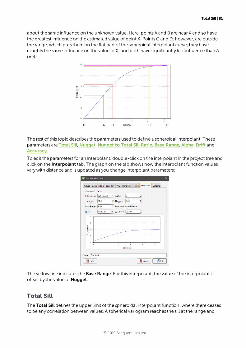
Total Sill | 81
about the same influence on the unknown value. Here, points A and B are near X and so havethe greatest influence on the estimated value of point X. PointsC and D, however, are outsidethe range, which puts themon the flat part of the spheroidal interpolant curve; they haveroughly the same influence on the value of X, and both have significantly less influence than Aor B:
The rest of this topic describes the parameters used to define a spheroidal interpolant. Theseparameters are Total Sill, Nugget, Nugget to Total Sill Ratio, Base Range, Alpha, Drift andAccuracy.
To edit the parameters for an interpolant, double-click on the interpolant in the project tree andclick on the Interpolant tab. The graph on the tab showshow the interpolant function valuesvarywith distance and is updated as you change interpolant parameters:
The yellow line indicates the Base Range. For this interpolant, the value of the interpolant isoffset by the value of Nugget.
Total Sill
The Total Sill defines the upper limit of the spheroidal interpolant function, where there ceasesto be any correlation between values. A spherical variogram reaches the sill at the range and
© 2019 Seequent Limited
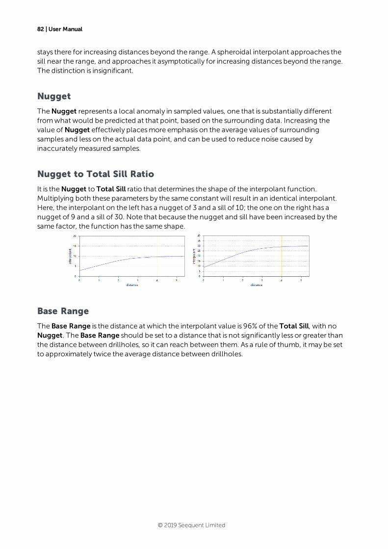
82 | User Manual
stays there for increasing distances beyond the range. A spheroidal interpolant approaches thesill near the range, and approaches it asymptotically for increasing distances beyond the range.The distinction is insignificant.
Nugget
TheNugget represents a local anomaly in sampled values, one that is substantially differentfromwhat would be predicted at that point, based on the surrounding data. Increasing thevalue of Nugget effectively placesmore emphasis on the average values of surroundingsamples and less on the actual data point, and can be used to reduce noise caused byinaccuratelymeasured samples.
Nugget to Total Sill Ratio
It is theNugget to Total Sill ratio that determines the shape of the interpolant function.Multiplying both these parameters by the same constant will result in an identical interpolant.Here, the interpolant on the left has a nugget of 3 and a sill of 10; the one on the right has anugget of 9 and a sill of 30. Note that because the nugget and sill have been increased by thesame factor, the function has the same shape.
Base Range
The Base Range is the distance at which the interpolant value is 96% of the Total Sill, with noNugget. The Base Range should be set to a distance that is not significantly less or greater thanthe distance between drillholes, so it can reach between them. As a rule of thumb, it may be setto approximately twice the average distance between drillholes.
© 2019 Seequent Limited
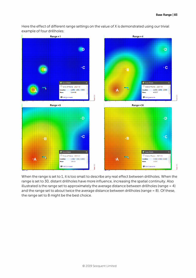
Base Range | 83
Here the effect of different range settings on the value of X is demonstrated using our trivialexample of four drillholes:
When the range is set to 1, it is too small to describe any real effect between drillholes. When therange is set to 30, distant drillholes havemore influence, increasing the spatial continuity. Alsoillustrated is the range set to approximately the average distance between drillholes (range = 4)and the range set to about twice the average distance between drillholes (range = 8). Of these,the range set to 8might be the best choice.
© 2019 Seequent Limited
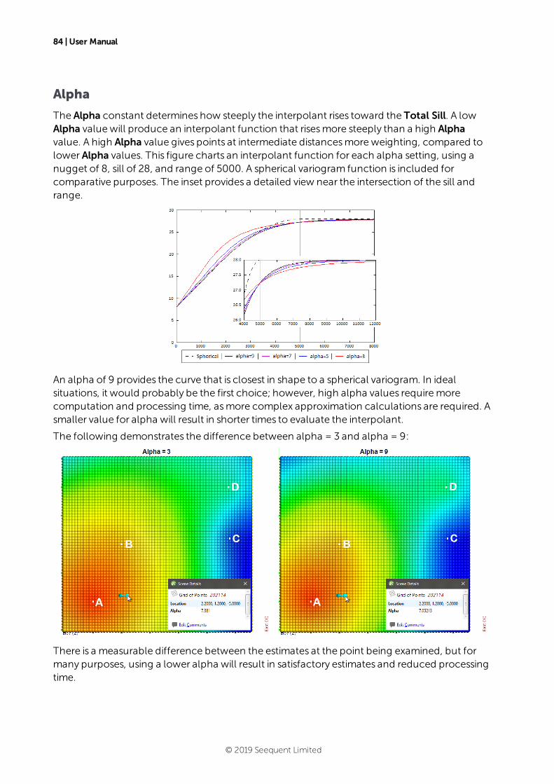
84 | User Manual
Alpha
The Alpha constant determines how steeply the interpolant rises toward the Total Sill. A lowAlpha valuewill produce an interpolant function that risesmore steeply than a high Alphavalue. A high Alpha value gives points at intermediate distancesmoreweighting, compared tolowerAlpha values. This figure charts an interpolant function for each alpha setting, using anugget of 8, sill of 28, and range of 5000. A spherical variogram function is included forcomparative purposes. The inset provides a detailed view near the intersection of the sill andrange.
An alpha of 9 provides the curve that is closest in shape to a spherical variogram. In idealsituations, it would probably be the first choice; however, high alpha values requiremorecomputation and processing time, asmore complex approximation calculations are required. Asmaller value for alpha will result in shorter times to evaluate the interpolant.
The following demonstrates the difference between alpha = 3 and alpha = 9:
There is a measurable difference between the estimates at the point being examined, but formany purposes, using a lower alpha will result in satisfactory estimates and reduced processingtime.
© 2019 Seequent Limited
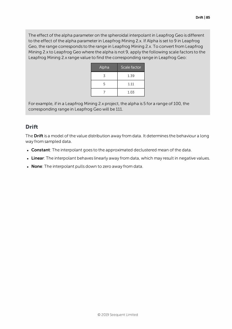
Drift | 85
The effect of the alpha parameter on the spheroidal interpolant in Leapfrog Geo is differentto the effect of the alpha parameter in Leapfrog Mining 2.x. If Alpha is set to 9 in LeapfrogGeo, the range corresponds to the range in Leapfrog Mining 2.x. To convert fromLeapfrogMining 2.x to Leapfrog Geowhere the alpha is not 9, apply the following scale factors to theLeapfrog Mining 2.x range value to find the corresponding range in Leapfrog Geo:
Alpha Scale factor
3 1.39
5 1.11
7 1.03
For example, if in a Leapfrog Mining 2.x project, the alpha is 5 for a range of 100, thecorresponding range in Leapfrog Geowill be 111.
Drift
TheDrift is a model of the value distribution away fromdata. It determines the behaviour a longway from sampled data.
l Constant: The interpolant goes to the approximated declustered mean of the data.
l Linear: The interpolant behaves linearly away fromdata, which may result in negative values.
l None: The interpolant pulls down to zero away fromdata.
© 2019 Seequent Limited
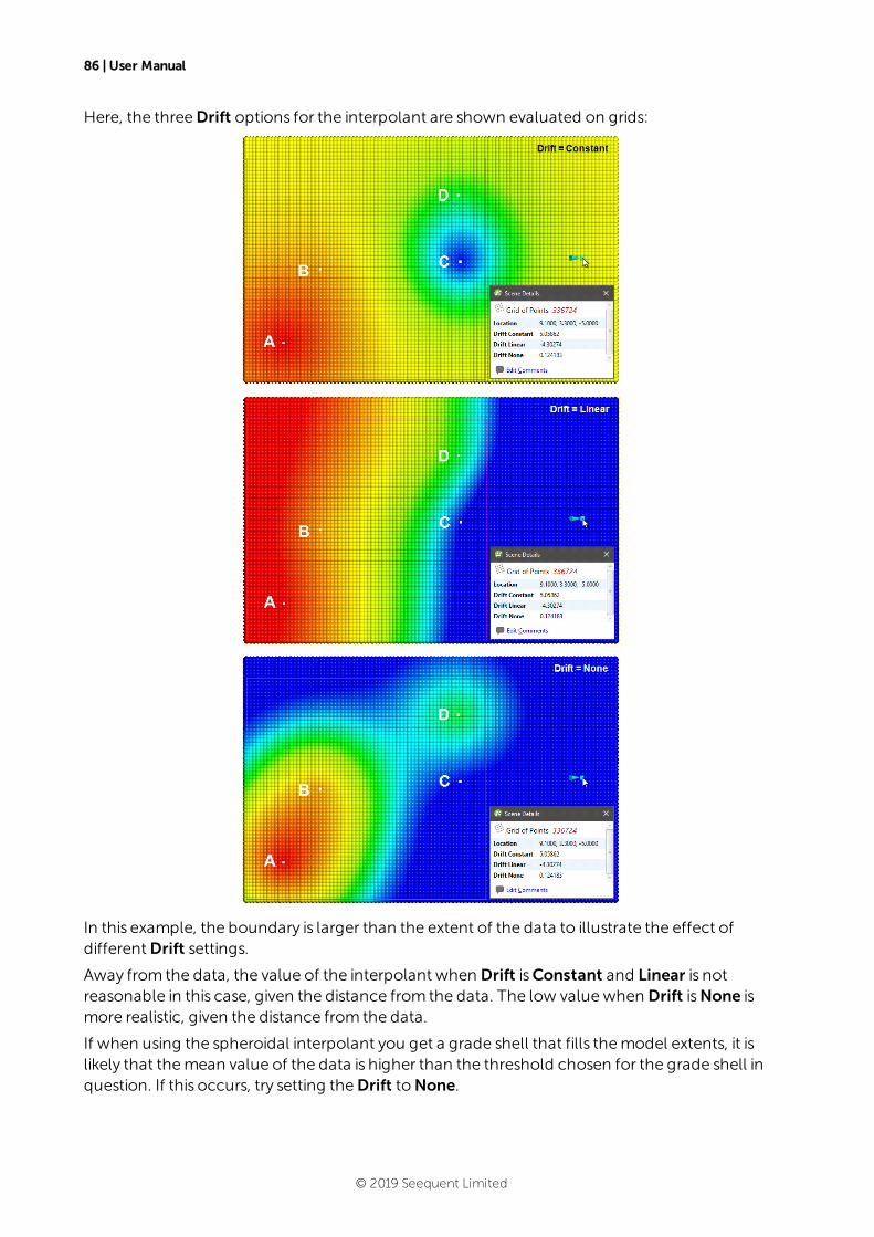
86 | User Manual
Here, the threeDrift options for the interpolant are shown evaluated on grids:
In this example, the boundary is larger than the extent of the data to illustrate the effect ofdifferentDrift settings.
Away from the data, the value of the interpolant when Drift isConstant and Linear is notreasonable in this case, given the distance from the data. The low valuewhen Drift isNone ismore realistic, given the distance from the data.
If when using the spheroidal interpolant you get a grade shell that fills themodel extents, it islikely that themean value of the data is higher than the threshold chosen for the grade shell inquestion. If this occurs, try setting theDrift toNone.
© 2019 Seequent Limited
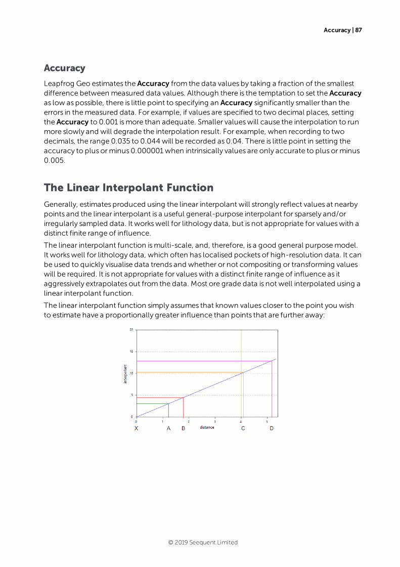
Accuracy | 87
Accuracy
Leapfrog Geo estimates the Accuracy from the data values by taking a fraction of the smallestdifference betweenmeasured data values. Although there is the temptation to set the Accuracyas low as possible, there is little point to specifying an Accuracy significantly smaller than theerrors in themeasured data. For example, if values are specified to two decimal places, settingthe Accuracy to 0.001 ismore than adequate. Smaller valueswill cause the interpolation to runmore slowly and will degrade the interpolation result. For example, when recording to twodecimals, the range 0.035 to 0.044 will be recorded as 0.04. There is little point in setting theaccuracy to plus orminus 0.000001 when intrinsically values are only accurate to plus orminus0.005.
The Linear Interpolant Function
Generally, estimates produced using the linear interpolant will strongly reflect values at nearbypoints and the linear interpolant is a useful general-purpose interpolant for sparsely and/orirregularly sampled data. It workswell for lithology data, but is not appropriate for valueswith adistinct finite range of influence.
The linear interpolant function ismulti-scale, and, therefore, is a good general purposemodel.It workswell for lithology data, which often has localised pockets of high-resolution data. It canbe used to quickly visualise data trends and whether or not compositing or transforming valueswill be required. It is not appropriate for valueswith a distinct finite range of influence as itaggressively extrapolates out from the data. Most ore grade data is not well interpolated using alinear interpolant function.
The linear interpolant function simply assumes that known values closer to the point you wishto estimate have a proportionally greater influence than points that are further away:
© 2019 Seequent Limited
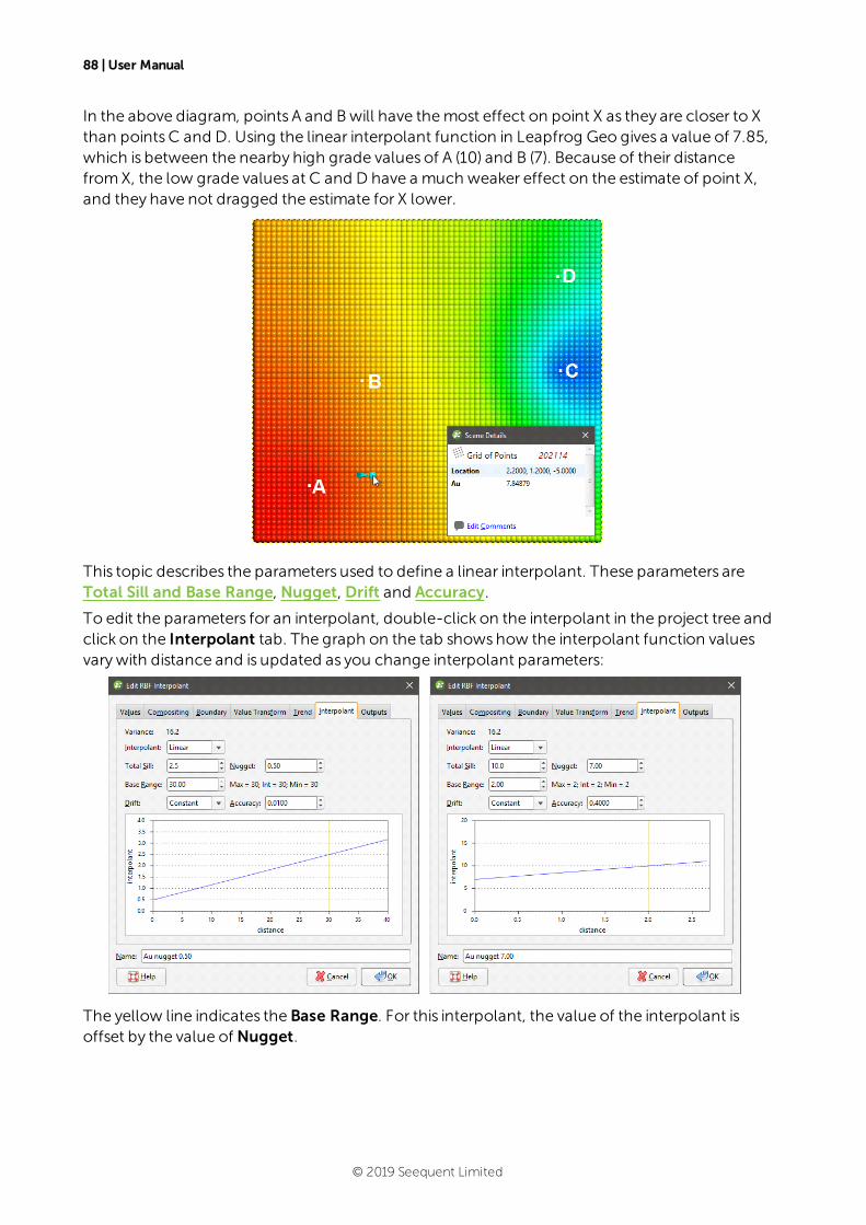
88 | User Manual
In the above diagram, points A and Bwill have themost effect on point X as they are closer to Xthan pointsC and D. Using the linear interpolant function in Leapfrog Geo gives a value of 7.85,which is between the nearby high grade values of A (10) and B (7). Because of their distancefromX, the low grade values at C and D have a much weaker effect on the estimate of point X,and they have not dragged the estimate for X lower.
This topic describes the parameters used to define a linear interpolant. These parameters areTotal Sill and Base Range, Nugget, Drift and Accuracy.
To edit the parameters for an interpolant, double-click on the interpolant in the project tree andclick on the Interpolant tab. The graph on the tab showshow the interpolant function valuesvarywith distance and is updated as you change interpolant parameters:
The yellow line indicates the Base Range. For this interpolant, the value of the interpolant isoffset by the value of Nugget.
© 2019 Seequent Limited

Total Sill and Base Range | 89
Total Sill and Base Range
A linear interpolant has no sill or range in the traditional sense. Instead, the Total Sill and BaseRange set the slope of the interpolant. The Base Range is the distance at which the interpolantvalue is the Total Sill. The two parameters sill and range are used instead of a single gradientparameter to permit switching between linear and spheroidal interpolant functionswithout alsomanipulating these settings.
Nugget
TheNugget represents a local anomaly in values, one that is substantially different fromwhatwould be predicted at that point based on the surrounding data. Increasing the value ofNugget effectively placesmore emphasis on the average values of surrounding samples andless on the actual data point, and can be used to reduce noise caused by inaccuratelymeasuredsamples.
Drift
TheDrift is a model of the value distribution away fromdata. It determines the behaviour a longway from sampled data.
l Constant: The interpolant goes to the approximated declustered mean of the data.
l Linear: The interpolant behaves linearly away fromdata, which may result in negative values.
© 2019 Seequent Limited
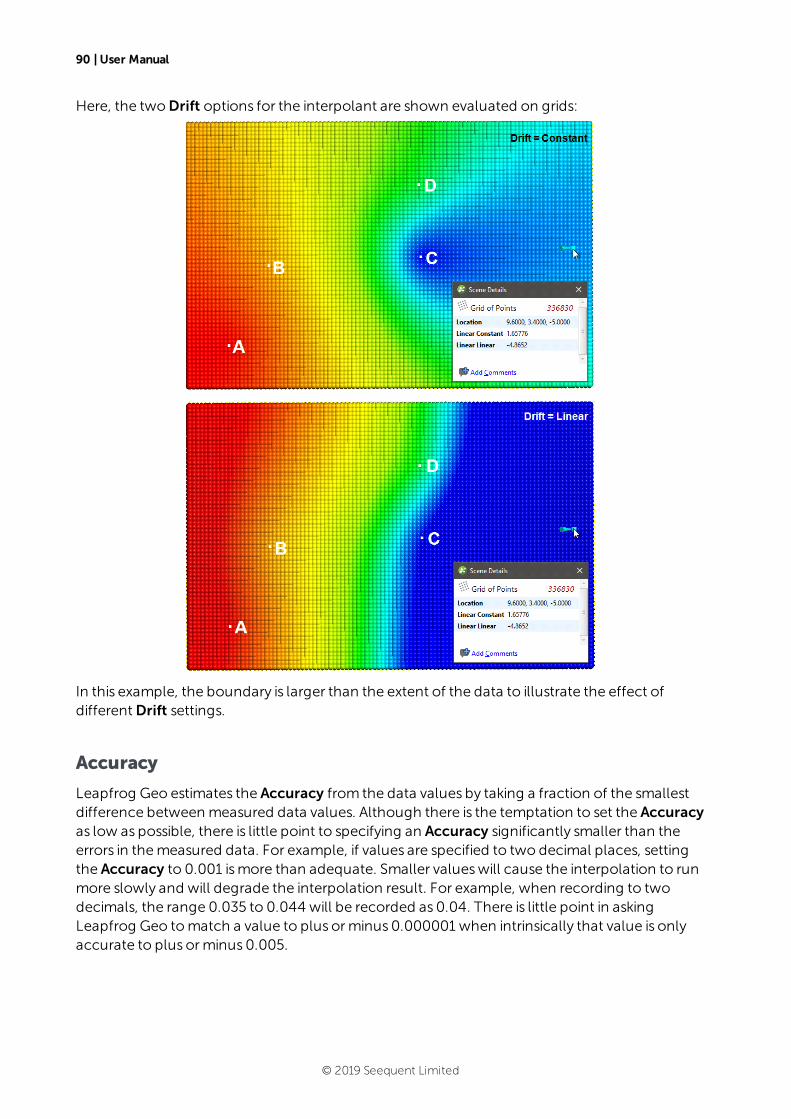
90 | User Manual
Here, the twoDrift options for the interpolant are shown evaluated on grids:
In this example, the boundary is larger than the extent of the data to illustrate the effect ofdifferentDrift settings.
Accuracy
Leapfrog Geo estimates the Accuracy from the data values by taking a fraction of the smallestdifference betweenmeasured data values. Although there is the temptation to set the Accuracyas low as possible, there is little point to specifying an Accuracy significantly smaller than theerrors in themeasured data. For example, if values are specified to two decimal places, settingthe Accuracy to 0.001 ismore than adequate. Smaller valueswill cause the interpolation to runmore slowly and will degrade the interpolation result. For example, when recording to twodecimals, the range 0.035 to 0.044 will be recorded as 0.04. There is little point in askingLeapfrog Geo tomatch a value to plus orminus 0.000001 when intrinsically that value is onlyaccurate to plus orminus 0.005.
© 2019 Seequent Limited

Central Integration | 91
Central IntegrationCentral’s integration with Leapfrog Geo lets you work in different project revisions, publishmodels to the server, view documents and annotations and reply to annotations. Projectsshared within Central can be downloaded and worked on locally in Leapfrog Geo. When youhave finished working on a project, select the objects you wish to publish to Central and addnotes about the revision. New projects can be added to Central by building them fromscratchor by uploading an existing project.
This topic describes how to set up and workwith Central fromwithin Leapfrog Geo. It is dividedinto:
l Connecting to Central
l The Central Projects Tab
l Central Settings
l Viewing a Project’s History
l Sharing Projects
l Downloading a Local Copy of a Project
l Publishing to Central
l New Central Projects
l Troubleshooting Connectivity Issues
To learn more about Central, see theCentral 3.0 help or theCentral 2.2 help.
Connecting to Central
Seequent is in the process of transitioning to using Seequent ID to connect to Central.
l If your organisation is using Central 3.0, you will need to connecting using Seequent ID. SeeConnecting Via Seequent ID.
l If your organisation has not yet upgraded to Central 3.0, you will need to connect manuallyusing the information provided by your administrator. SeeManual Setup.
Connecting Via Seequent ID
If you connect to Central using your Seequent ID, open the Settings window by clicking on theLeapfrog Geomenu. SelectCentral and tick the box to Enable Central integration. ACentralProjects tab will appear in themain window. Next, enable theUse Seequent ID option.
© 2019 Seequent Limited
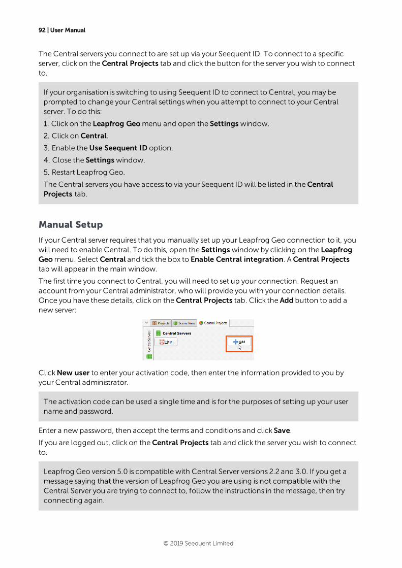
92 | User Manual
The Central servers you connect to are set up via your Seequent ID. To connect to a specificserver, click on theCentral Projects tab and click the button for the server you wish to connectto.
If your organisation is switching to using Seequent ID to connect to Central, you may beprompted to change your Central settingswhen you attempt to connect to your Centralserver. To do this:
1. Click on the Leapfrog Geomenu and open the Settings window.
2. Click on Central.
3. Enable theUse Seequent ID option.
4. Close the Settings window.
5. Restart Leapfrog Geo.
The Central servers you have access to via your Seequent ID will be listed in theCentralProjects tab.
Manual Setup
If your Central server requires that you manually set up your Leapfrog Geo connection to it, youwill need to enable Central. To do this, open the Settings window by clicking on the LeapfrogGeomenu. SelectCentral and tick the box to Enable Central integration. ACentral Projectstab will appear in themain window.
The first time you connect to Central, you will need to set up your connection. Request anaccount fromyour Central administrator, whowill provide you with your connection details.Once you have these details, click on theCentral Projects tab. Click the Add button to add anew server:
ClickNew user to enter your activation code, then enter the information provided to you byyour Central administrator.
The activation code can be used a single time and is for the purposes of setting up your username and password.
Enter a new password, then accept the terms and conditions and click Save.
If you are logged out, click on theCentral Projects tab and click the server you wish to connectto.
Leapfrog Geo version 5.0 is compatible with Central Server versions 2.2 and 3.0. If you get amessage saying that the version of Leapfrog Geo you are using is not compatible with theCentral Server you are trying to connect to, follow the instructions in themessage, then tryconnecting again.
© 2019 Seequent Limited
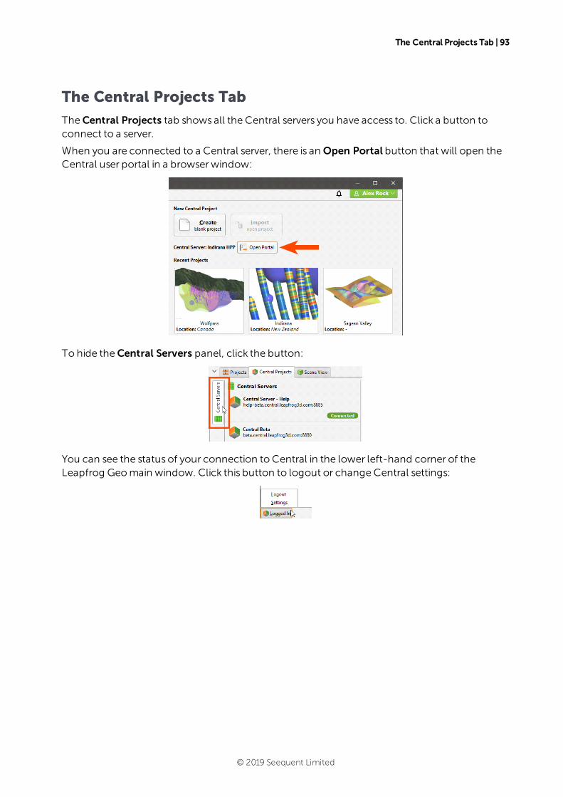
The Central Projects Tab | 93
The Central Projects Tab
TheCentral Projects tab shows all the Central servers you have access to. Click a button toconnect to a server.
When you are connected to a Central server, there is an Open Portal button that will open theCentral user portal in a browser window:
To hide theCentral Servers panel, click the button:
You can see the status of your connection to Central in the lower left-hand corner of theLeapfrog Geomain window. Click this button to logout or change Central settings:
© 2019 Seequent Limited
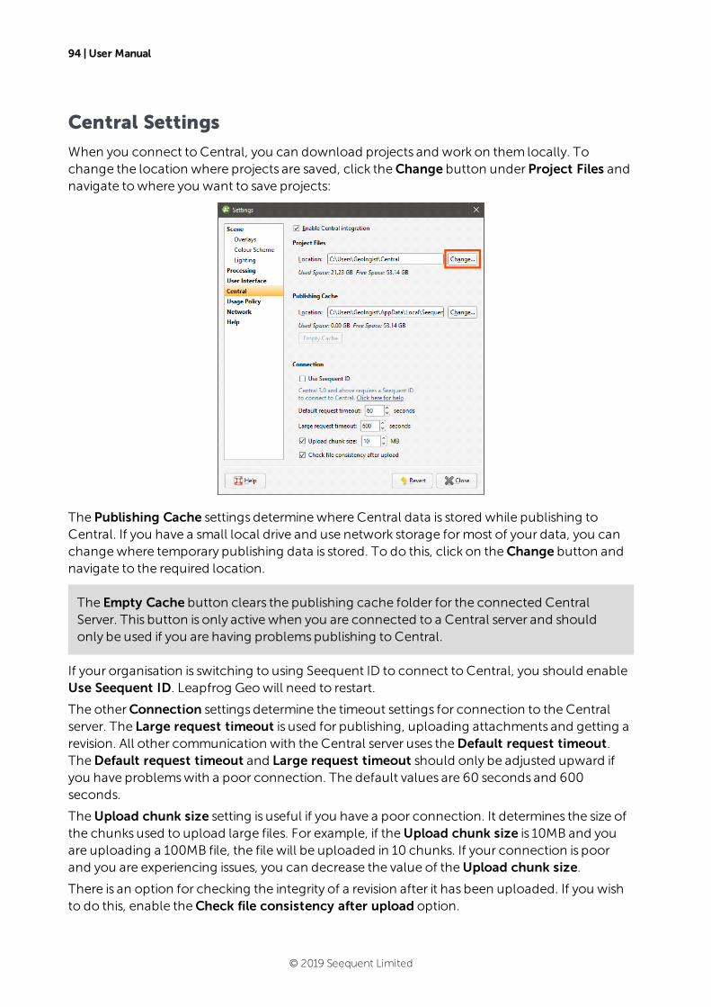
94 | User Manual
Central Settings
When you connect to Central, you can download projects and work on them locally. Tochange the location where projects are saved, click theChange button under Project Files andnavigate towhere you want to save projects:
The Publishing Cache settings determinewhere Central data is stored while publishing toCentral. If you have a small local drive and use network storage formost of your data, you canchangewhere temporary publishing data is stored. To do this, click on theChange button andnavigate to the required location.
The Empty Cache button clears the publishing cache folder for the connected CentralServer. This button is only active when you are connected to a Central server and shouldonly be used if you are having problemspublishing to Central.
If your organisation is switching to using Seequent ID to connect to Central, you should enableUse Seequent ID. Leapfrog Geowill need to restart.
The otherConnection settings determine the timeout settings for connection to the Centralserver. The Large request timeout is used for publishing, uploading attachments and getting arevision. All other communication with the Central server uses theDefault request timeout.TheDefault request timeout and Large request timeout should only be adjusted upward ifyou have problemswith a poor connection. The default values are 60 seconds and 600seconds.
TheUpload chunk size setting is useful if you have a poor connection. It determines the size ofthe chunks used to upload large files. For example, if theUpload chunk size is 10MB and youare uploading a 100MB file, the file will be uploaded in 10 chunks. If your connection is poorand you are experiencing issues, you can decrease the value of theUpload chunk size.
There is an option for checking the integrity of a revision after it has been uploaded. If you wishto do this, enable theCheck file consistency after upload option.
© 2019 Seequent Limited
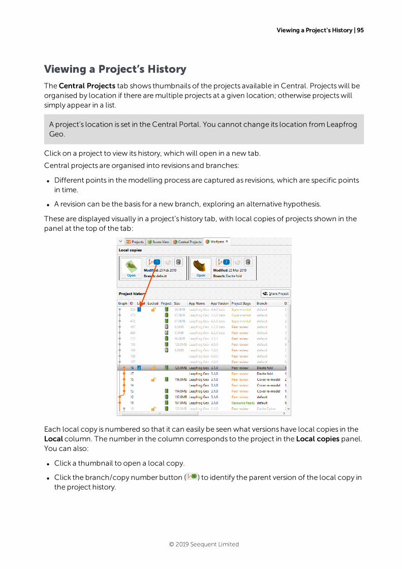
Viewing a Project’s History | 95
Viewing a Project’s History
TheCentral Projects tab shows thumbnails of the projects available in Central. Projectswill beorganised by location if there aremultiple projects at a given location; otherwise projectswillsimply appear in a list.
A project’s location is set in the Central Portal. You cannot change its location fromLeapfrogGeo.
Click on a project to view its history, which will open in a new tab.
Central projects are organised into revisions and branches:
l Different points in themodelling process are captured as revisions, which are specific pointsin time.
l A revision can be the basis for a new branch, exploring an alternative hypothesis.
These are displayed visually in a project’s history tab, with local copies of projects shown in thepanel at the top of the tab:
Each local copy is numbered so that it can easily be seen what versions have local copies in theLocal column. The number in the column corresponds to the project in the Local copies panel.You can also:
l Click a thumbnail to open a local copy.
l Click the branch/copy number button ( ) to identify the parent version of the local copy inthe project history.
© 2019 Seequent Limited
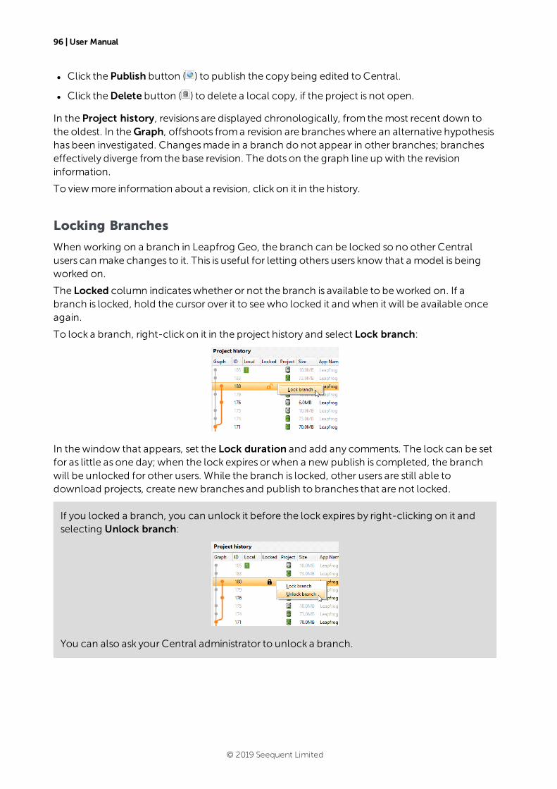
96 | User Manual
l Click the Publish button ( ) to publish the copy being edited to Central.
l Click theDelete button ( ) to delete a local copy, if the project is not open.
In the Project history, revisions are displayed chronologically, from themost recent down tothe oldest. In theGraph, offshoots froma revision are brancheswhere an alternative hypothesishas been investigated. Changesmade in a branch do not appear in other branches; brancheseffectively diverge from the base revision. The dots on the graph line up with the revisioninformation.
To viewmore information about a revision, click on it in the history.
Locking Branches
When working on a branch in Leapfrog Geo, the branch can be locked so no other Centralusers can make changes to it. This is useful for letting others users know that a model is beingworked on.
The Locked column indicateswhether or not the branch is available to beworked on. If abranch is locked, hold the cursor over it to seewho locked it and when it will be available onceagain.
To lock a branch, right-click on it in the project history and select Lock branch:
In thewindow that appears, set the Lock duration and add any comments. The lock can be setfor as little as one day; when the lock expires or when a new publish is completed, the branchwill be unlocked for other users. While the branch is locked, other users are still able todownload projects, create new branches and publish to branches that are not locked.
If you locked a branch, you can unlock it before the lock expires by right-clicking on it andselecting Unlock branch:
You can also ask your Central administrator to unlock a branch.
© 2019 Seequent Limited
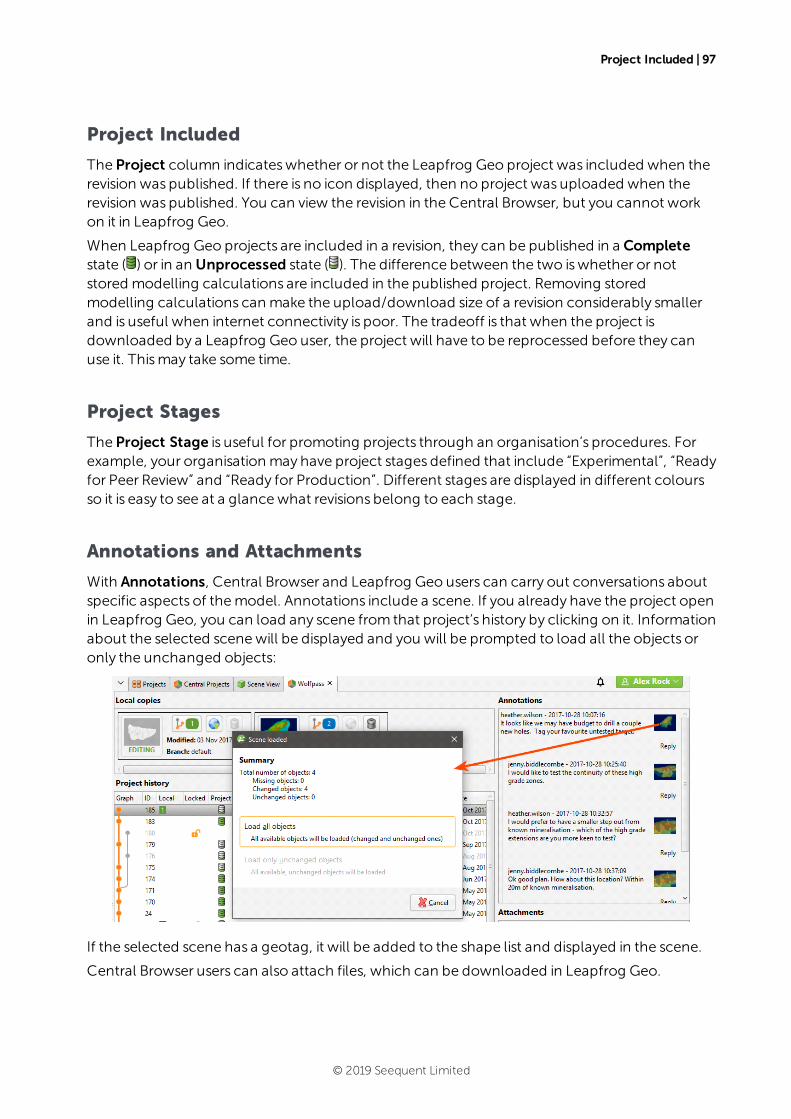
Project Included | 97
Project Included
The Project column indicateswhether or not the Leapfrog Geo project was included when therevision was published. If there is no icon displayed, then no project was uploaded when therevision was published. You can view the revision in the Central Browser, but you cannot workon it in Leapfrog Geo.
When Leapfrog Geo projects are included in a revision, they can be published in a Completestate ( ) or in an Unprocessed state ( ). The difference between the two iswhether or notstored modelling calculations are included in the published project. Removing storedmodelling calculations can make the upload/download size of a revision considerably smallerand is useful when internet connectivity is poor. The tradeoff is that when the project isdownloaded by a Leapfrog Geo user, the project will have to be reprocessed before they canuse it. Thismay take some time.
Project Stages
The Project Stage is useful for promoting projects through an organisation’s procedures. Forexample, your organisation may have project stages defined that include “Experimental”, “Readyfor Peer Review” and “Ready for Production”. Different stages are displayed in different coloursso it is easy to see at a glancewhat revisions belong to each stage.
Annotations and Attachments
With Annotations, Central Browser and Leapfrog Geo users can carry out conversations aboutspecific aspects of themodel. Annotations include a scene. If you already have the project openin Leapfrog Geo, you can load any scene from that project’s history by clicking on it. Informationabout the selected scenewill be displayed and you will be prompted to load all the objects oronly the unchanged objects:
If the selected scene has a geotag, it will be added to the shape list and displayed in the scene.
Central Browser users can also attach files, which can be downloaded in Leapfrog Geo.
© 2019 Seequent Limited
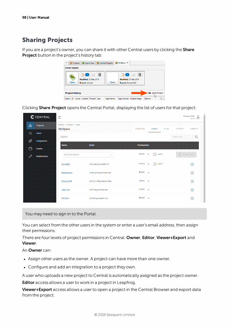
98 | User Manual
Sharing Projects
If you are a project’s owner, you can share it with other Central users by clicking the ShareProject button in the project’s history tab:
Clicking Share Project opens the Central Portal, displaying the list of users for that project:
You may need to sign in to the Portal.
You can select from the other users in the systemor enter a user’s email address, then assigntheir permissions.
There are four levels of project permissions in Central:Owner, Editor, Viewer+Export andViewer.
An Owner can:
l Assign other users as the owner. A project can havemore than one owner.
l Configure and add an integration to a project they own.
A user who uploads a new project to Central is automatically assigned as the project owner.
Editor access allows a user towork in a project in Leapfrog.
Viewer+Export access allows a user to open a project in the Central Browser and export datafrom the project.
© 2019 Seequent Limited
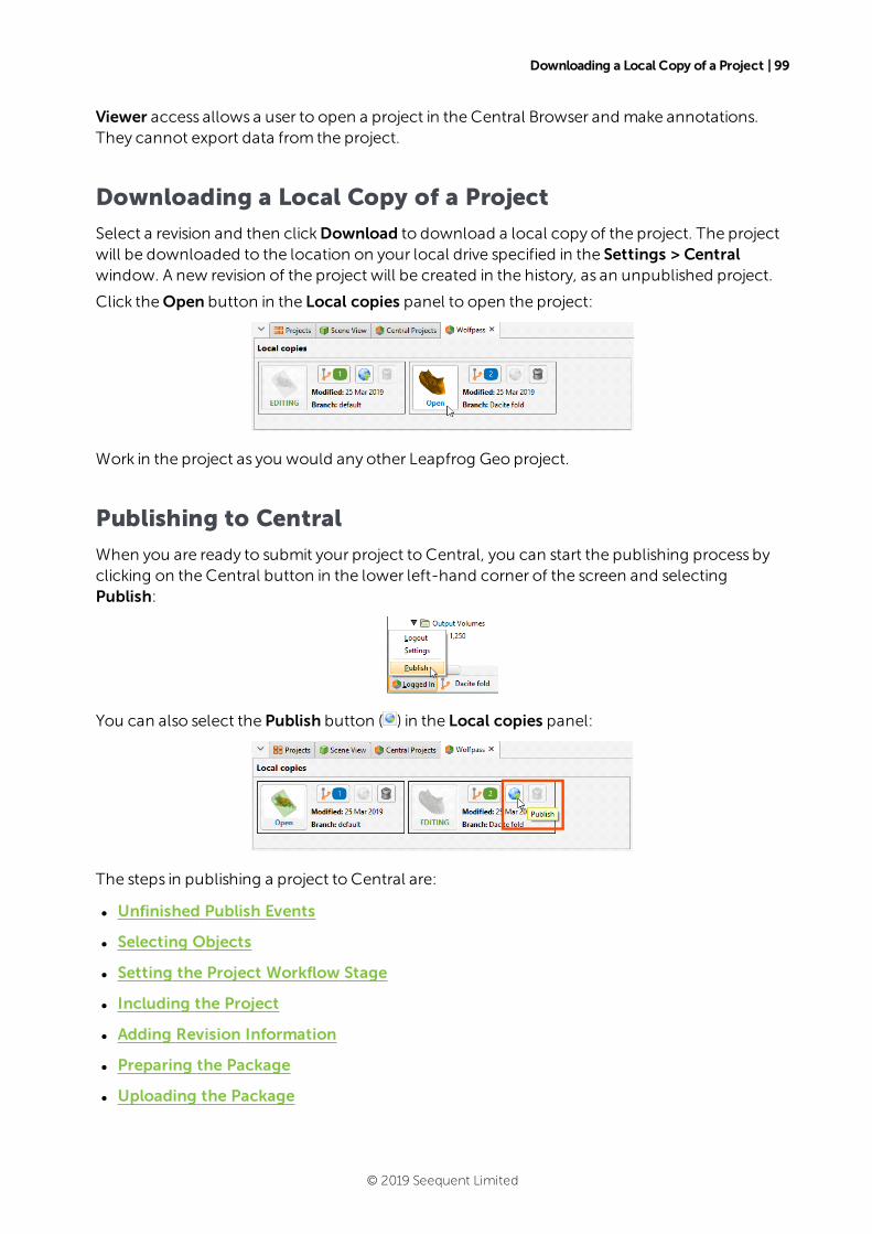
Downloading a Local Copy of a Project | 99
Viewer access allows a user to open a project in the Central Browser and make annotations.They cannot export data from the project.
Downloading a Local Copy of a Project
Select a revision and then clickDownload to download a local copy of the project. The projectwill be downloaded to the location on your local drive specified in the Settings > Centralwindow. A new revision of the project will be created in the history, as an unpublished project.
Click theOpen button in the Local copies panel to open the project:
Work in the project as you would any other Leapfrog Geo project.
Publishing to Central
When you are ready to submit your project to Central, you can start the publishing process byclicking on the Central button in the lower left-hand corner of the screen and selectingPublish:
You can also select the Publish button ( ) in the Local copies panel:
The steps in publishing a project to Central are:
l Unfinished Publish Events
l Selecting Objects
l Setting the Project Workflow Stage
l Including the Project
l Adding Revision Information
l Preparing the Package
l Uploading the Package
© 2019 Seequent Limited

100 | User Manual
Unfinished Publish Events
When you clickPublish, you may receive a message saying there is an unfinished publish event:
This occurswhen a previous publish event was interrupted. Choose from the options presented.
If the publish event was abandoned, it can be removed via the Central Portal.
Selecting Objects
Select the objects you wish to publish from those available in the project:
Although sub-blocked models can be published to Central, the dip will not be included.
ClickNext to choose options for how the project will be uploaded.
© 2019 Seequent Limited

Setting the Project Workflow Stage | 101
Setting the Project Workflow Stage
Project stages are useful for advancing projects through an organisation’s processes. If theproject is ready to bemoved on to a different stage, select a different Project Workflow Stagefrom the list.
Project stages can later be changed in the Central Browser.
Including the Project
Select whether or not to include the Leapfrog Geo project. There are three options:
l No. The Leapfrog Geo project will not be published. Other Central userswill not be able todownload the project and work on it in Leapfrog Geo. Theywill, however, be able to reviewthe published objects and their history in the Central Browser.
l Complete.This option publishes the complete Leapfrog Geo project, including storedmodelling calculations. Other Central userswill be able to download the project and workon it in Leapfrog Geowithout reprocessing the project.
l Unprocessed. An unprocessed project has a smaller upload/download size because storedmodelling calculations are removed. When an unprocessed project is downloaded again, allof themodelling calculationswill need to be reprocessed from the underlying data. OtherCentral userswill be able to download the project and work on it in Leapfrog Geo.Depending on the size of the project, reprocessing may take some time.
ClickNext.
Adding Revision Information
Enter information about the new revision. If you want to create a new branch, click theNewBranch button and enter a name for the branch.
Once you branch froma timeline, you cannot merge back into it. There’s no reason,however, that you can’t keep working in a branch and start considering that themainbranch, if that’s the conclusion you and your team reach.
Preparing the Package
ClickNext to begin the processes of packaging the project for publication.
Uploading the Package
Once the project has been packaged, there are two options for starting the upload:
l If you want the upload to begin automatically once the package has been prepared, tick theAuto upload box.
© 2019 Seequent Limited

102 | User Manual
l If you want the option to cancel the upload once it has been packaged, leave the Autoupload box unticked. Once the project has been packaged, clickPublish to upload theproject to Central.
If for some reason you need to stop the upload, click on the Central button in the lower left-hand corner of the screen and select Stop Upload:
You can resume the upload by clicking Publish in the project history. You will be prompted toresume the unfinished publish event, as described in Unfinished Publish Events above.
If the upload is interrupted because the connection to the server is lost, you will be prompted tofinish the publish event the next time you log in to Central.
If you exit Leapfrog Geowhile a publish event is in progress, you will be warned that a publishevent is in progress. You can:
l Cancel exiting Leapfrog Geo, in which case the publish event will continue.
l Confirm that you wish to exit Leapfrog Geo. The next time you connect to this Central serveror publish from this project or fromanother project on the same server, you will be promptedto the resume the interrupted publish event. You can complete the interrupted publishevent, if you wish, or ignore it.
New Central Projects
There are two options for putting a project into Central:
l Create a new Central project.
l Put an existing project into Central.
Creating a New Central Project
Use this option to create a new Leapfrog Geo project and put it into Central. In theCentralProjects tab, clickCreate blank project. Enter a name for the project and clickOK. A newLeapfrog Geo project will be created and saved in the location on your local drive specified inthe Settings > Centralwindow.
Work in the project as you would any other Leapfrog Geo project. When you are ready topublish the project to Central, click on the Central button in the lower left-hand corner of thescreen and select Publish:
© 2019 Seequent Limited

Adding a Project to Central | 103
Adding a Project to Central
Use this option to add an existing project to Central.
Open the project you wish to import, then in theCentral Projects tab, click Import openproject. Enter a new name for the project, if you wish, then clickOK. The project will be openedand copied to the location on your local drive specified in the Settings > Centralwindow.
Work in the project as you would any other Leapfrog Geo project. When you are ready topublish the project to Central, click on the Central button in the lower left-hand corner of thescreen and select Publish.
Troubleshooting Connectivity Issues
Leapfrog Start checks to see if your networkwill support the connection of Leapfrog web-based services to your desktop applications. If you are having trouble with your connection toCentral, seeChecking Connectivity with Leapfrog Start.
© 2019 Seequent Limited
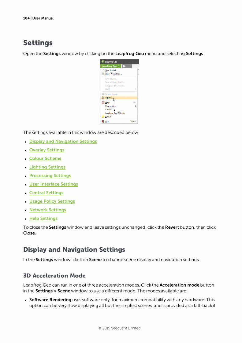
104 | User Manual
SettingsOpen the Settings window by clicking on the Leapfrog Geomenu and selecting Settings:
The settings available in thiswindow are described below:
l Display and Navigation Settings
l Overlay Settings
l Colour Scheme
l Lighting Settings
l Processing Settings
l User Interface Settings
l Central Settings
l Usage Policy Settings
l Network Settings
l Help Settings
To close the Settings window and leave settings unchanged, click theRevert button, then clickClose.
Display and Navigation Settings
In the Settings window, click on Scene to change scene display and navigation settings.
3D Acceleration Mode
Leapfrog Geo can run in one of three acceleration modes. Click the Acceleration mode buttonin the Settings > Scenewindow to use a different mode. Themodes available are:
l Software Rendering uses software only, formaximumcompatibility with any hardware. Thisoption can be very slow displaying all but the simplest scenes, and is provided as a fall-back if
© 2019 Seequent Limited
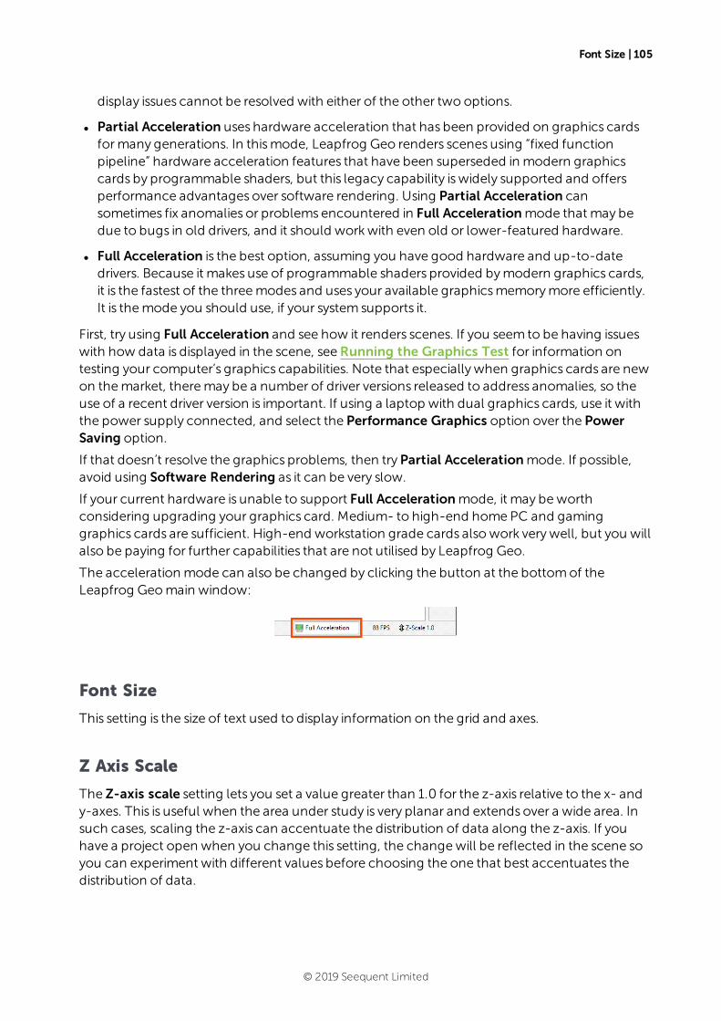
Font Size | 105
display issues cannot be resolved with either of the other two options.
l Partial Acceleration uses hardware acceleration that has been provided on graphics cardsformany generations. In thismode, Leapfrog Geo renders scenes using “fixed functionpipeline” hardware acceleration features that have been superseded in modern graphicscards by programmable shaders, but this legacy capability iswidely supported and offersperformance advantages over software rendering. Using Partial Acceleration cansometimes fix anomalies or problems encountered in Full Accelerationmode that may bedue to bugs in old drivers, and it should workwith even old or lower-featured hardware.
l Full Acceleration is the best option, assuming you have good hardware and up-to-datedrivers. Because it makes use of programmable shaders provided bymodern graphics cards,it is the fastest of the threemodes and uses your available graphicsmemorymore efficiently.It is themode you should use, if your system supports it.
First, try using Full Acceleration and see how it renders scenes. If you seem to be having issueswith how data is displayed in the scene, seeRunning the Graphics Test for information ontesting your computer’s graphics capabilities. Note that especially when graphics cards are newon themarket, theremay be a number of driver versions released to address anomalies, so theuse of a recent driver version is important. If using a laptop with dual graphics cards, use it withthe power supply connected, and select the Performance Graphics option over the PowerSaving option.
If that doesn’t resolve the graphics problems, then tryPartial Accelerationmode. If possible,avoid using Software Rendering as it can be very slow.
If your current hardware is unable to support Full Accelerationmode, it may beworthconsidering upgrading your graphics card. Medium- to high-end home PC and gaminggraphics cards are sufficient. High-end workstation grade cards alsowork verywell, but you willalso be paying for further capabilities that are not utilised by Leapfrog Geo.
The acceleration mode can also be changed by clicking the button at the bottomof theLeapfrog Geomain window:
Font Size
This setting is the size of text used to display information on the grid and axes.
Z Axis Scale
The Z-axis scale setting lets you set a value greater than 1.0 for the z-axis relative to the x- andy-axes. This is useful when the area under study is very planar and extends over a wide area. Insuch cases, scaling the z-axis can accentuate the distribution of data along the z-axis. If youhave a project open when you change this setting, the changewill be reflected in the scene soyou can experiment with different values before choosing the one that best accentuates thedistribution of data.
© 2019 Seequent Limited
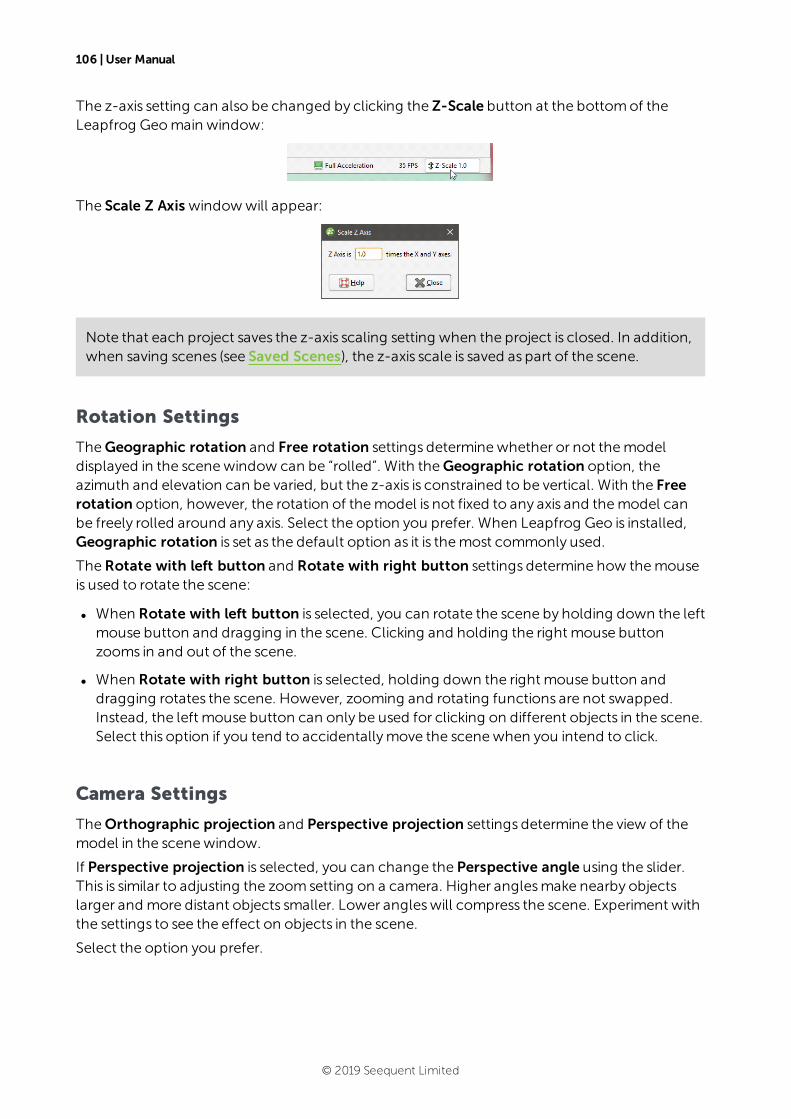
106 | User Manual
The z-axis setting can also be changed by clicking the Z-Scale button at the bottomof theLeapfrog Geomain window:
The Scale Z Axis windowwill appear:
Note that each project saves the z-axis scaling setting when the project is closed. In addition,when saving scenes (see Saved Scenes), the z-axis scale is saved as part of the scene.
Rotation Settings
TheGeographic rotation and Free rotation settings determinewhether or not themodeldisplayed in the scenewindow can be “rolled”. With theGeographic rotation option, theazimuth and elevation can be varied, but the z-axis is constrained to be vertical. With the Freerotation option, however, the rotation of themodel is not fixed to any axis and themodel canbe freely rolled around any axis. Select the option you prefer. When Leapfrog Geo is installed,Geographic rotation is set as the default option as it is themost commonly used.
TheRotate with left button and Rotate with right button settings determine how themouseis used to rotate the scene:
l When Rotate with left button is selected, you can rotate the scene by holding down the leftmouse button and dragging in the scene. Clicking and holding the right mouse buttonzooms in and out of the scene.
l When Rotate with right button is selected, holding down the right mouse button anddragging rotates the scene. However, zooming and rotating functions are not swapped.Instead, the left mouse button can only be used for clicking on different objects in the scene.Select this option if you tend to accidentallymove the scenewhen you intend to click.
Camera Settings
TheOrthographic projection and Perspective projection settings determine the view of themodel in the scenewindow.
If Perspective projection is selected, you can change the Perspective angle using the slider.This is similar to adjusting the zoomsetting on a camera. Higher anglesmake nearby objectslarger and more distant objects smaller. Lower angleswill compress the scene. Experiment withthe settings to see the effect on objects in the scene.
Select the option you prefer.
© 2019 Seequent Limited

Overlay Settings | 107
Overlay Settings
In the Settings window, click on Scene > Overlays to changewhat objects are included in thescene.
Changes you make to these settings are automatically updated in the scene so you can easilyexperiment to seewhat overlays you prefer.
Select Revert to return to the settings in placewhen the Settings windowwas first opened.
Screen Grid Settings
The Show screen grid setting determineswhether or not the screen grid is displayed. Select theoption you prefer. The Loose Spacing, Normal Spacing and Fine Spacing options determinethe spacing of the grid.
Axis Lines Settings
The Axis Lines settings determine how X-Y-Z coordinates are displayed in the scene. When axislines are enabled, the axes indicate the extent of data currently displayed in the scene.
l Enable Show axis lines to display the east (red), north (green) and elevation (blue) axis lines.
l Enable Put numbers on axes to display scale ticks along the grid. These are automaticallyadjusted to fit the extent of the data and the current zoomsetting.
l Enable Show whole box to display the axis lines as a box that encloses the current data set.
Other Overlay Settings
The scale bar, compass ball and viewing angle text are the navigation aids in the lower right-hand corner of the scenewindow.
When the slicer is in the scene and the slice is aligned with the x-, y- or z-axis, text describing theslicer position can be displayed in the lower left-hand corner if the scene. To do this, enabledthe Slicer position text option.
When drawing polylines, tooltips are displayed. If you do not wish to view these tooltips, untickthe box for Polyline help text.
Colour Scheme
In the Settings window, click on Scene > Colour Scheme to change the colour scheme used inthe scene. The options that can be changed include:
l The background colour used in the Scene View tab
l The colour and width used to display drillhole traces
© 2019 Seequent Limited

108 | User Manual
l The colour and width of mesh edges, together with thewidth of the line used when a meshis sliced and the highlight colour used whenmesh parts are selected in the scene
l The colours used for displaying the x, y and z axes
l Grid line width, style and colour
l Axes box line width, style and colour
l Slicer edgewidth, style and colour
Leapfrog Geo is installed with three colours schemes:Default, Black Background and WhiteBackground. The scheme selected in the Schemes list will be used for all new Leapfrog Geoprojects and for existing projectswhen they are next opened.
l Experiment with the settings to see how they affect the scenewindow. The scenewill beupdated as you make changes.
l Select Revert to return to the settings in placewhen the Settings windowwas first opened.
l To create a new scheme, click on an existing scheme. This is the scheme that will be used asa basis for defining the new scheme. Next, click theNew Scheme button and change itssettings.
l Click Factory Reset to revert to the colour schemesdefined when Leapfrog Geowas firstinstalled.
Clicking on Factory Reset to revert to the original colour schemesdeletes any customcolour schemes.
Lighting Settings
In the Settings window, click on Scene > Lighting to change how visual effects are displayed inthe scenewindow. You may be able to use these settings to emphasise significance in the datadisplayed in the scene.
l The Ambient level setting determines the overall brightness of the scene.
l The Specular brightness and Specular shininess settings determine how light appears tofall on the surfaces in the scene. The Specular brightness setting has a stronger effect whenSpecular shininess is soft.
You can have up to four light sources defined for a project. By default, two light sources aredefined.
Changesmade to these settings are automatically applied to the scene.
l ClickRevert to return to the settings in placewhen the Settings windowwas first opened.
l Click Factory Reset to revert to the lighting sources and settings defined when LeapfrogGeowas first installed.
© 2019 Seequent Limited
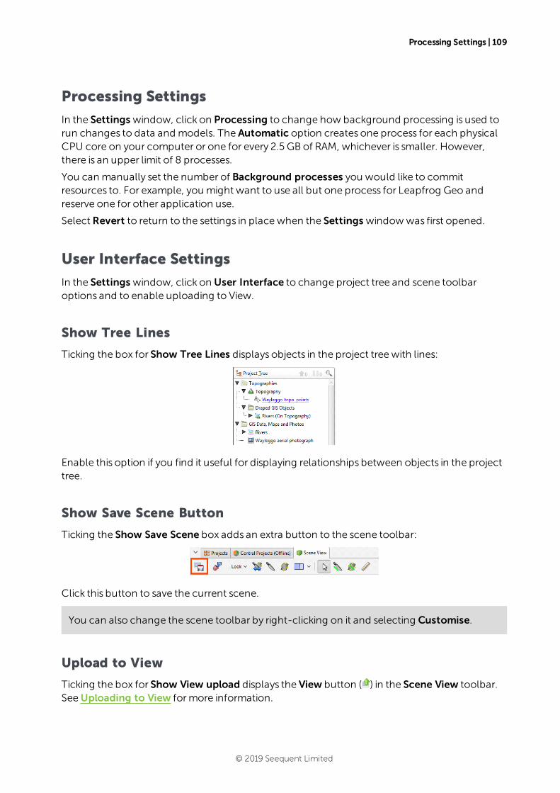
Processing Settings | 109
Processing Settings
In the Settings window, click on Processing to change how background processing is used torun changes to data and models. The Automatic option creates one process for each physicalCPU core on your computer or one for every 2.5 GB of RAM, whichever is smaller. However,there is an upper limit of 8 processes.
You can manually set the number of Background processes you would like to commitresources to. For example, you might want to use all but one process for Leapfrog Geo andreserve one for other application use.
Select Revert to return to the settings in placewhen the Settings windowwas first opened.
User Interface Settings
In the Settings window, click on User Interface to change project tree and scene toolbaroptions and to enable uploading to View.
Show Tree Lines
Ticking the box for Show Tree Lines displays objects in the project tree with lines:
Enable this option if you find it useful for displaying relationships between objects in the projecttree.
Show Save Scene Button
Ticking the Show Save Scene box adds an extra button to the scene toolbar:
Click this button to save the current scene.
You can also change the scene toolbar by right-clicking on it and selecting Customise.
Upload to View
Ticking the box for Show View upload displays the View button ( ) in the Scene View toolbar.SeeUploading to View formore information.
© 2019 Seequent Limited
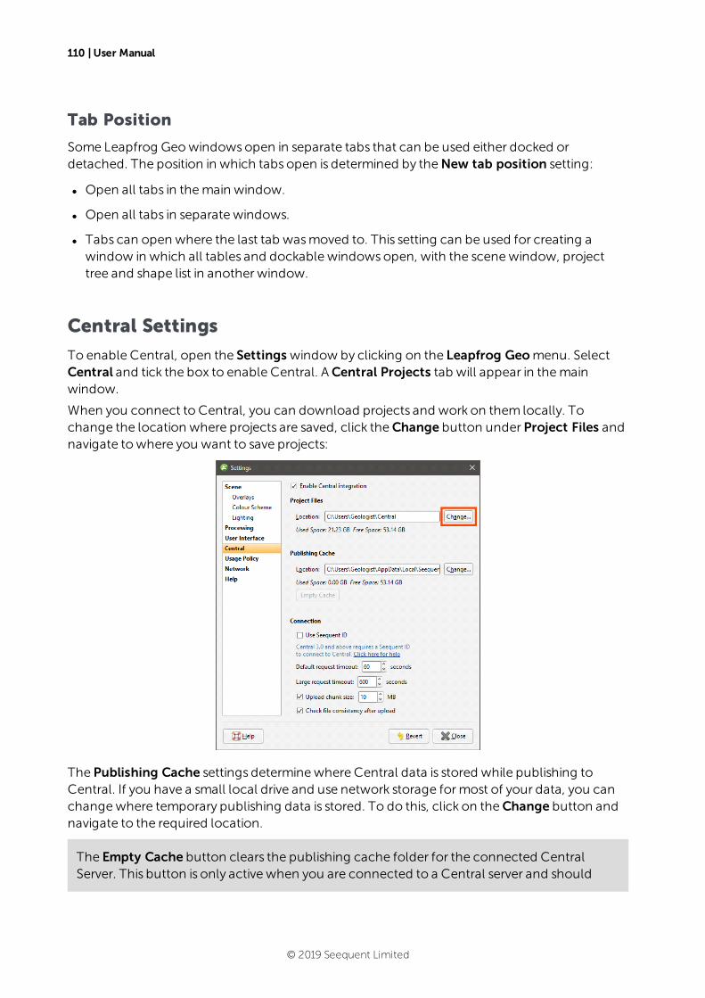
110 | User Manual
Tab Position
Some Leapfrog Geowindowsopen in separate tabs that can be used either docked ordetached. The position in which tabs open is determined by theNew tab position setting:
l Open all tabs in themain window.
l Open all tabs in separate windows.
l Tabs can open where the last tab wasmoved to. This setting can be used for creating awindow in which all tables and dockable windowsopen, with the scenewindow, projecttree and shape list in another window.
Central Settings
To enable Central, open the Settings window by clicking on the Leapfrog Geomenu. SelectCentral and tick the box to enable Central. ACentral Projects tab will appear in themainwindow.
When you connect to Central, you can download projects and work on them locally. Tochange the location where projects are saved, click theChange button under Project Files andnavigate towhere you want to save projects:
The Publishing Cache settings determinewhere Central data is stored while publishing toCentral. If you have a small local drive and use network storage formost of your data, you canchangewhere temporary publishing data is stored. To do this, click on theChange button andnavigate to the required location.
The Empty Cache button clears the publishing cache folder for the connected CentralServer. This button is only active when you are connected to a Central server and should
© 2019 Seequent Limited

Usage Policy Settings | 111
only be used if you are having problemspublishing to Central.
TheConnection settings determine how you connect to the Central server.
Seequent is in the process of transitioning to using Seequent ID to connect to Central. TheUseSeequent ID setting determineswhether your connections to Central are automaticallyconfigured via your Seequent ID or whether you need tomanually set up connections toCentral servers.
l If your organisation is using Central 3.0, you will need to connecting using Seequent ID.Enable this setting.
l If your organisation has not yet upgraded to Central 3.0, you will need to connect manuallyusing the information provided by your administrator. Leave this setting disabled.
You will be prompted to restart when you change this setting.
The Large request timeout is used for publishing, uploading attachments and getting arevision. All other communication with the Central server uses theDefault request timeout.TheDefault request timeout and Large request timeout should only be adjusted upward ifyou have problemswith a poor connection. The default values are 60 seconds and 600seconds.
TheUpload chunk size setting is useful if you have a poor connection. It determines the size ofthe chunks used to upload large files. For example, if theUpload chunk size is 10MB and youare uploading a 100MB file, the file will be uploaded in 10 chunks. If your connection is poorand you are experiencing issues, you can decrease the value of theUpload chunk size.
There is an option for checking the integrity of a revision after it has been uploaded. If you wishto do this, enable theCheck file consistency after upload option.
SeeCentral Integration formore information on using Central.
Usage Policy Settings
When the Idle time-out setting is enabled, Leapfrog Geowill prompt you after a period ofinactivity. Follow the instructions in themessage displayed.
Leapfrog Geo can use reference codes to trackwork on specific projects. The number of daysassociated with each reference code is included in your organisation’smonthly usage report. Inthe Settings > Usage Policy window, you can define reference codes on a per-project or per-computer basis. Click the Add New Code button to add a code for either the computer or thecurrently open project.
The other two settings can be used to ensure that you are regularly prompted to update thereference code.
l Prompt at project start up ensures that a prompt is displayed for selecting a reference codewhenever a project is opened or a new project is created.
l Always required ensures that Leapfrog Geo is not used without a reference code beingselected. <NoCode> is not an option.
© 2019 Seequent Limited
112 | User Manual
Network Settings
If your organisation uses a proxy server to connect to the internet, you can set this up in theSettings > Networkwindow.
If you choose the Autodetect proxy server option, Leapfrog Geowill detect the authenticationtype, server address and port; there are no further settings for you to change.
If Autodetect proxy server does not work or if you need to switch between proxy servers indifferent network environments, choose theManually configure proxy server option andenter the information provided by your IT department. The advanced settings are optional andyou should only change them from the default values if you have been instructed to do so byyour IT department.
You can manually configuremore than one proxy server. Click theNew button to add a newprofile and enter the required settings. When you want to swap fromone proxy server toanother, simply select a Profile from those already defined.
If you havemultiple Seequent products running on your computer, you only need to configurenetwork proxy settings once. Once you have, for example, configured the proxy for LeapfrogGeo, the same settingswill be used for the Central Browser.
Help Settings
If you are working on a slow connection, you can download a copy of the help that can besaved to your hard drive. To do this:
l Click here to download a copy of the help.
l Once you have downloaded a copy of the help and installed it, select Settings from theLeapfrog Geomenu.
l Click on theHelp tab and then select Local folder.
Leapfrog Geo help is updated at each release. If you are using a downloaded copy, you willneed to download a new copy each time you update Leapfrog Geo.
Reporting a ProblemIf Leapfrog Geo encounters an error, the Leapfrog Geo Problemwindowwill be displayed.Enter asmuch information as you can about the problem, then click Send.
© 2019 Seequent Limited

Getting Support | 113
Getting SupportTechnical support is available by visiting http://www.leapfrog3d.com/contact/support.
Checking Connectivity with Leapfrog Start
Leapfrog Start checks to see if your networkwill support the connection of Leapfrog web-based services to your desktop applications.
To run Leapfrog Start, either click the Test Web Services button in the Settings > Networkwindow or click on the Leapfrog Geomenu and selectDiagnostics > Test Web Services:
Supplying Your Licence Details
When contacting technical support, please include your licence number and a full descriptionof the problemor query, including any information provided in systemerrormessages.
You can access your licence information by selecting About from the Leapfrog Geomenu:
© 2019 Seequent Limited

114 | User Manual
You may also be asked to provide a copy of the log files. To find out where these are stored,select About from the Leapfrog Geomenu, then click on the System Info. tab. Click on the linkto open the folder that contains the log files:
© 2019 Seequent Limited
Data Types
Leapfrog Geo has tools for importing, creating and working with many different types of data,including:
l GIS Data, Maps and Images
l Drillhole Data
l Points Data
l Geophysical Data
l Structural Data
l Meshes
l Polylines
l Geochemical Data
Leapfrog Geo is unit-less and adopts the units used in the data you import. For example, ifyour imported data is in metres, the units displayed will bemetres, and figures such asresolution, measured distances and slicer thicknesswill be in metres. It is important,therefore, to be consistent in the units used in the data you import. If you are importing datathat uses different coordinate systems, you will need to pre-process the data so that it isusing the same coordinate system.
The rest of this topic describes how to open, edit and correct errors in data tables in LeapfrogGeo. It is divided into:
l Working with Data Tables
l Identifying Errors in Data Tables
l Exporting Data Errors
l Correcting Data Errors in Leapfrog Geo
l Common Errors and How to Fix Them
l Handling Special Values
© 2019 Seequent Limited
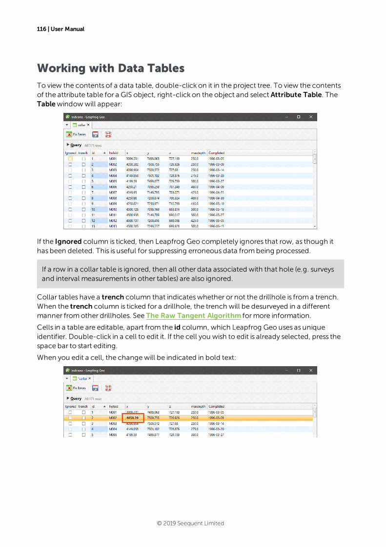
116 | User Manual
Working with Data TablesTo view the contents of a data table, double-click on it in the project tree. To view the contentsof the attribute table for a GIS object, right-click on the object and select Attribute Table. TheTablewindowwill appear:
If the Ignored column is ticked, then Leapfrog Geo completely ignores that row, as though ithas been deleted. This is useful for suppressing erroneous data frombeing processed.
If a row in a collar table is ignored, then all other data associated with that hole (e.g. surveysand interval measurements in other tables) are also ignored.
Collar tables have a trench column that indicateswhether or not the drillhole is froma trench.When the trench column is ticked for a drillhole, the trench will be desurveyed in a differentmanner fromother drillholes. See The Raw Tangent Algorithm formore information.
Cells in a table are editable, apart from the id column, which Leapfrog Geo uses as uniqueidentifier. Double-click in a cell to edit it. If the cell you wish to edit is already selected, press thespace bar to start editing.
When you edit a cell, the changewill be indicated in bold text:
© 2019 Seequent Limited
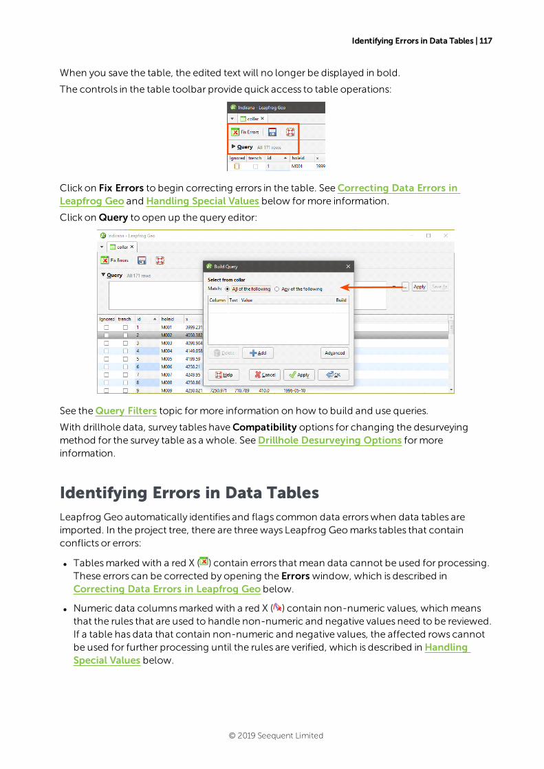
Identifying Errors in Data Tables | 117
When you save the table, the edited text will no longer be displayed in bold.
The controls in the table toolbar provide quick access to table operations:
Click on Fix Errors to begin correcting errors in the table. SeeCorrecting Data Errors inLeapfrog Geo and Handling Special Values below formore information.
Click on Query to open up the query editor:
See theQuery Filters topic formore information on how to build and use queries.
With drillhole data, survey tables haveCompatibility options for changing the desurveyingmethod for the survey table as a whole. SeeDrillhole Desurveying Options formoreinformation.
Identifying Errors in Data TablesLeapfrog Geo automatically identifies and flags common data errorswhen data tables areimported. In the project tree, there are threeways Leapfrog Geomarks tables that containconflicts or errors:
l Tablesmarked with a red X ( ) contain errors that mean data cannot be used for processing.These errors can be corrected by opening the Errors window, which is described inCorrecting Data Errors in Leapfrog Geo below.
l Numeric data columnsmarked with a red X ( ) contain non-numeric values, which meansthat the rules that are used to handle non-numeric and negative values need to be reviewed.If a table has data that contain non-numeric and negative values, the affected rows cannotbe used for further processing until the rules are verified, which is described in HandlingSpecial Values below.
© 2019 Seequent Limited
118 | User Manual
l Tablesmarked with a yellow exclamation mark ( ) contain warnings. Affected rows can beused for further processing, but the information in thewarning can indicate that the datarequires further attention. For example, if a warning indicates there is data missing for adrillhole defined in the collar table, it may be that a drillhole has been duplicated or that notall required data files have been loaded. Warnings are listed along with table errors in theErrors window.
Until errors are corrected, the rows that contain those errors are excluded for all processing thatuses the table, including viewing in the scene. For example, if the ID for a collar positioncontains an invalid coordinate, that collar will not be displayed in the scene as its location is notknown. Likewise, any processing will ignore data associated with this drillhole.
It isworth correcting errors as soon as possible, as correcting them later can result in significantrecomputation time.
When a table contains errors and warnings, only the errorswill be apparent in the projecttree view. However, all errors and warnings relevant to a particular table will be displayed intheDatabase Errors window.
There are two approaches to correcting errors in data:
l Correct the data in the primary source. Export the errors as described in Exporting DataErrors below. Then, when the errors have been corrected, reload the drillhole data asdescribed in Reloading Drillhole Data.
l Correct the data in Leapfrog Geo. If you need a record of corrected errors, first export theerrors as described in Exporting Data Errors below. Then correct errors as described inCorrecting Data Errors in Leapfrog Geo.
Exporting Data Errors
If you need a record of corrected errors, first export the errors. Thismust be done first, asonce errors have been corrected in Leapfrog Geo, they cannot be exported, as they nolonger exist.
For individual drillhole tables, points tables and structural data tables, export the errors by right-clicking on the table and selecting Export Errors. Choose a location where the file will be savedand click Save.
© 2019 Seequent Limited
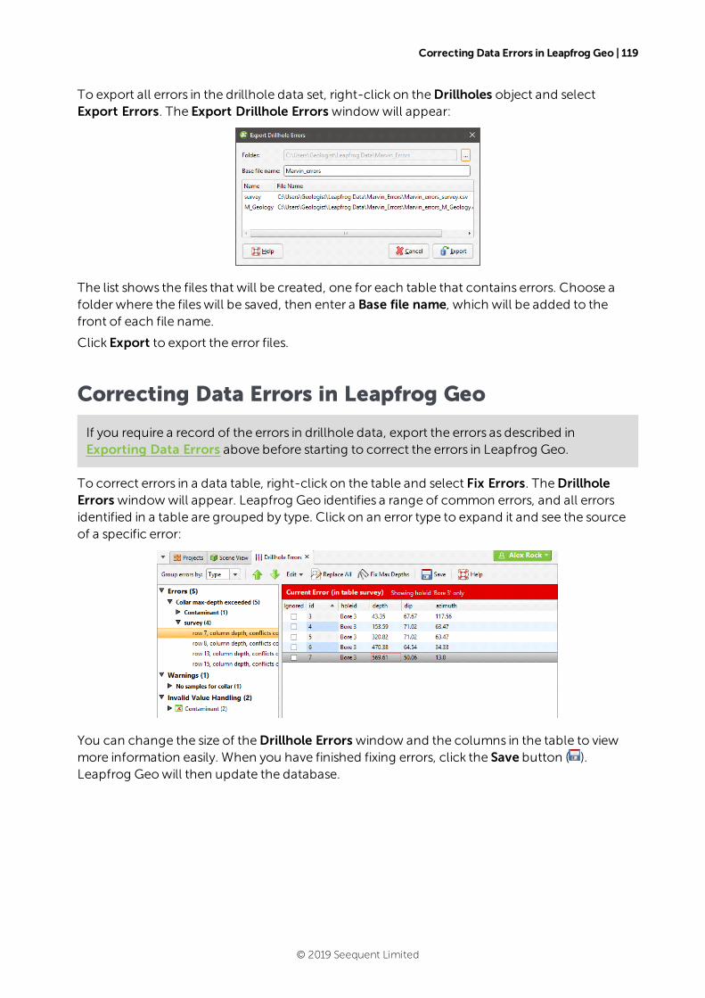
Correcting Data Errors in Leapfrog Geo | 119
To export all errors in the drillhole data set, right-click on theDrillholes object and selectExport Errors. The Export Drillhole Errors windowwill appear:
The list shows the files that will be created, one for each table that contains errors. Choose afolder where the fileswill be saved, then enter a Base file name, which will be added to thefront of each file name.
Click Export to export the error files.
Correcting Data Errors in Leapfrog Geo
If you require a record of the errors in drillhole data, export the errors as described inExporting Data Errors above before starting to correct the errors in Leapfrog Geo.
To correct errors in a data table, right-click on the table and select Fix Errors. TheDrillholeErrors windowwill appear. Leapfrog Geo identifies a range of common errors, and all errorsidentified in a table are grouped by type. Click on an error type to expand it and see the sourceof a specific error:
You can change the size of theDrillhole Errors window and the columns in the table to viewmore information easily. When you have finished fixing errors, click the Save button ( ).Leapfrog Geowill then update the database.
© 2019 Seequent Limited
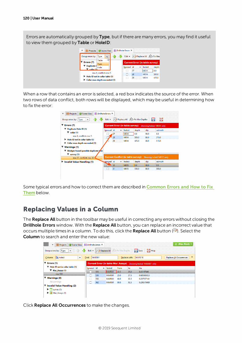
120 | User Manual
Errors are automatically grouped by Type, but if there aremany errors, you may find it usefulto view themgrouped by Table orHoleID:
When a row that contains an error is selected, a red box indicates the source of the error. Whentwo rowsof data conflict, both rowswill be displayed, which may be useful in determining howto fix the error:
Some typical errors and how to correct themare described in Common Errors and How to FixThem below.
Replacing Values in a Column
TheReplace All button in the toolbarmay be useful in correcting any errorswithout closing theDrillhole Errors window. With theReplace All button, you can replace an incorrect value thatoccursmultiple times in a column. To do this, click theReplace All button ( ). Select theColumn to search and enter the new value:
ClickReplace All Occurrences tomake the changes.
© 2019 Seequent Limited
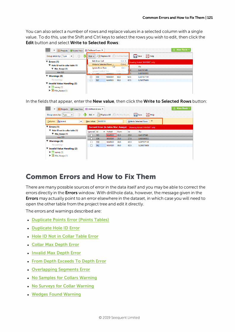
Common Errors and How to Fix Them | 121
You can also select a number of rows and replace values in a selected column with a singlevalue. To do this, use the Shift and Ctrl keys to select the rows you wish to edit, then click theEdit button and selectWrite to Selected Rows:
In the fields that appear, enter theNew value, then click theWrite to Selected Rows button:
Common Errors and How to Fix ThemThere aremany possible sources of error in the data itself and you may be able to correct theerrors directly in the Errors window. With drillhole data, however, themessage given in theErrors may actually point to an error elsewhere in the dataset, in which case you will need toopen the other table from the project tree and edit it directly.
The errors and warnings described are:
l Duplicate Points Error (Points Tables)
l Duplicate Hole ID Error
l Hole ID Not in Collar Table Error
l Collar Max Depth Error
l Invalid Max Depth Error
l From Depth Exceeds To Depth Error
l Overlapping Segments Error
l No Samples for Collars Warning
l No Surveys for Collar Warning
l Wedges Found Warning
© 2019 Seequent Limited
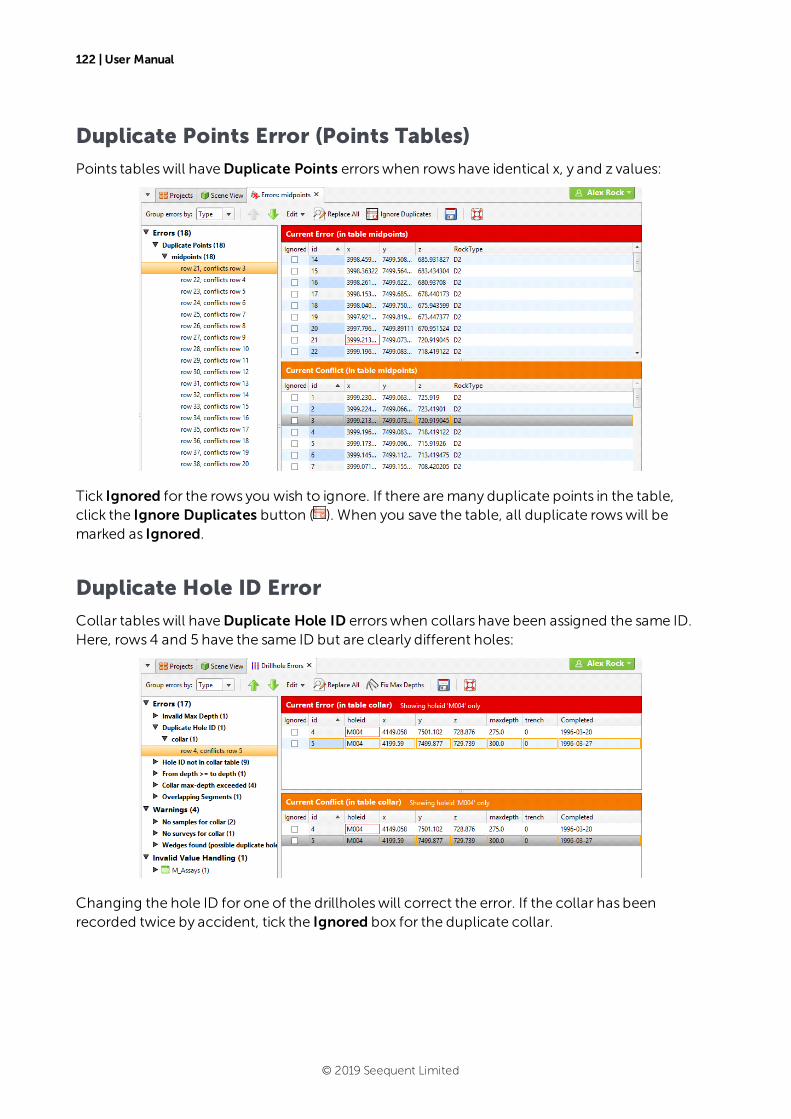
122 | User Manual
Duplicate Points Error (Points Tables)
Points tableswill haveDuplicate Points errorswhen rowshave identical x, y and z values:
Tick Ignored for the rows you wish to ignore. If there aremany duplicate points in the table,click the Ignore Duplicates button ( ). When you save the table, all duplicate rowswill bemarked as Ignored.
Duplicate Hole ID Error
Collar tableswill haveDuplicate Hole ID errorswhen collars have been assigned the same ID.Here, rows4 and 5 have the same ID but are clearly different holes:
Changing the hole ID for one of the drillholeswill correct the error. If the collar has beenrecorded twice by accident, tick the Ignored box for the duplicate collar.
© 2019 Seequent Limited
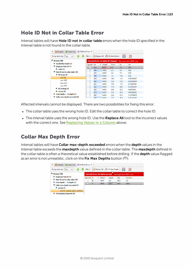
Hole ID Not in Collar Table Error | 123
Hole ID Not in Collar Table Error
Interval tableswill haveHole ID not in collar table errorswhen the hole ID specified in theinterval table is not found in the collar table.
Affected intervals cannot be displayed. There are two possibilities for fixing this error:
l The collar table uses thewrong hole ID. Edit the collar table to correct the hole ID.
l The interval table uses thewrong hole ID. Use theReplace All tool to the incorrect valueswith the correct one. SeeReplacing Values in a Column above.
Collar Max Depth Error
Interval tableswill haveCollar max-depth exceeded errorswhen the depth values in theinterval table exceeds themaxdepth value defined in the collar table. Themaxdepth defined inthe collar table is often a theoretical value established before drilling. If the depth value flaggedas an error is not unrealistic, click on the Fix Max Depths button ( ):
© 2019 Seequent Limited
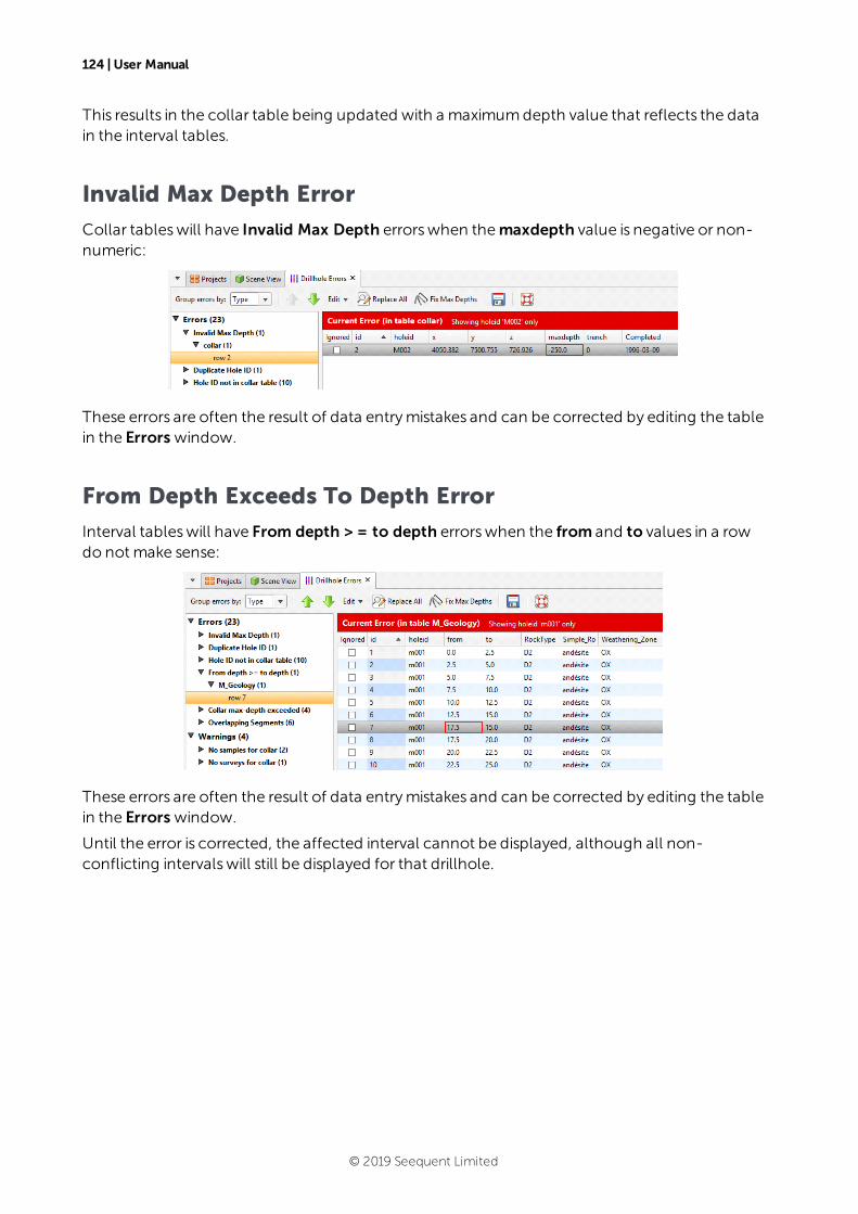
124 | User Manual
This results in the collar table being updated with a maximumdepth value that reflects the datain the interval tables.
Invalid Max Depth Error
Collar tableswill have Invalid Max Depth errorswhen themaxdepth value is negative or non-numeric:
These errors are often the result of data entrymistakes and can be corrected by editing the tablein the Errors window.
From Depth Exceeds To Depth Error
Interval tableswill have From depth > = to depth errorswhen the from and to values in a rowdo not make sense:
These errors are often the result of data entrymistakes and can be corrected by editing the tablein the Errors window.
Until the error is corrected, the affected interval cannot be displayed, although all non-conflicting intervalswill still be displayed for that drillhole.
© 2019 Seequent Limited

Overlapping Segments Error | 125
Overlapping Segments Error
Interval tableswill haveOverlapping Segments errorswhen intervals are in the same place forthe same hole or when two holes are in the same place. Here, row 12 overlaps row 13 and theerror can be corrected in theDrillhole Errors window by entering the correct to value for row12:
If an interval has been defined twice, click Ignored for one of the rows. Until the error iscorrected, the affected intervals cannot be displayed, although all non-conflicting intervalswillstill be displayed for that drillhole.
No Samples for Collars Warning
Interval tableswill haveNo values for Hole IDwarningswhen there are no values in the intervaltable that correspond to a collar defined in the collar table. In this example, a hole called M090has been defined in the collar table, but there is no data for it in theM_Assays table.
© 2019 Seequent Limited
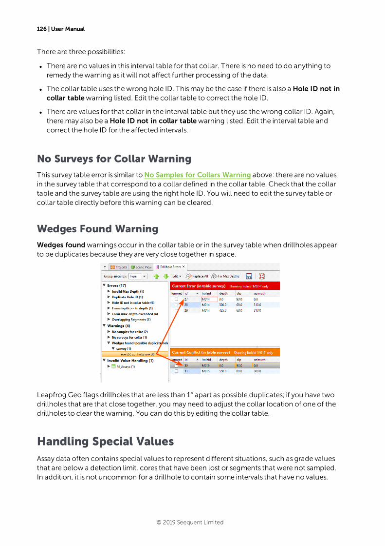
126 | User Manual
There are three possibilities:
l There are no values in this interval table for that collar. There is no need to do anything toremedy thewarning as it will not affect further processing of the data.
l The collar table uses thewrong hole ID. Thismay be the case if there is also a Hole ID not incollar tablewarning listed. Edit the collar table to correct the hole ID.
l There are values for that collar in the interval table but they use thewrong collar ID. Again,theremay also be a Hole ID not in collar tablewarning listed. Edit the interval table andcorrect the hole ID for the affected intervals.
No Surveys for Collar Warning
This survey table error is similar toNo Samples for Collars Warning above: there are no valuesin the survey table that correspond to a collar defined in the collar table. Check that the collartable and the survey table are using the right hole ID. You will need to edit the survey table orcollar table directly before thiswarning can be cleared.
Wedges Found Warning
Wedges foundwarnings occur in the collar table or in the survey table when drillholes appearto be duplicates because they are very close together in space.
Leapfrog Geo flags drillholes that are less than 1° apart as possible duplicates; if you have twodrillholes that are that close together, you may need to adjust the collar location of one of thedrillholes to clear thewarning. You can do this by editing the collar table.
Handling Special ValuesAssay data often contains special values to represent different situations, such as grade valuesthat are below a detection limit, cores that have been lost or segments that were not sampled.In addition, it is not uncommon for a drillhole to contain some intervals that have no values.
© 2019 Seequent Limited
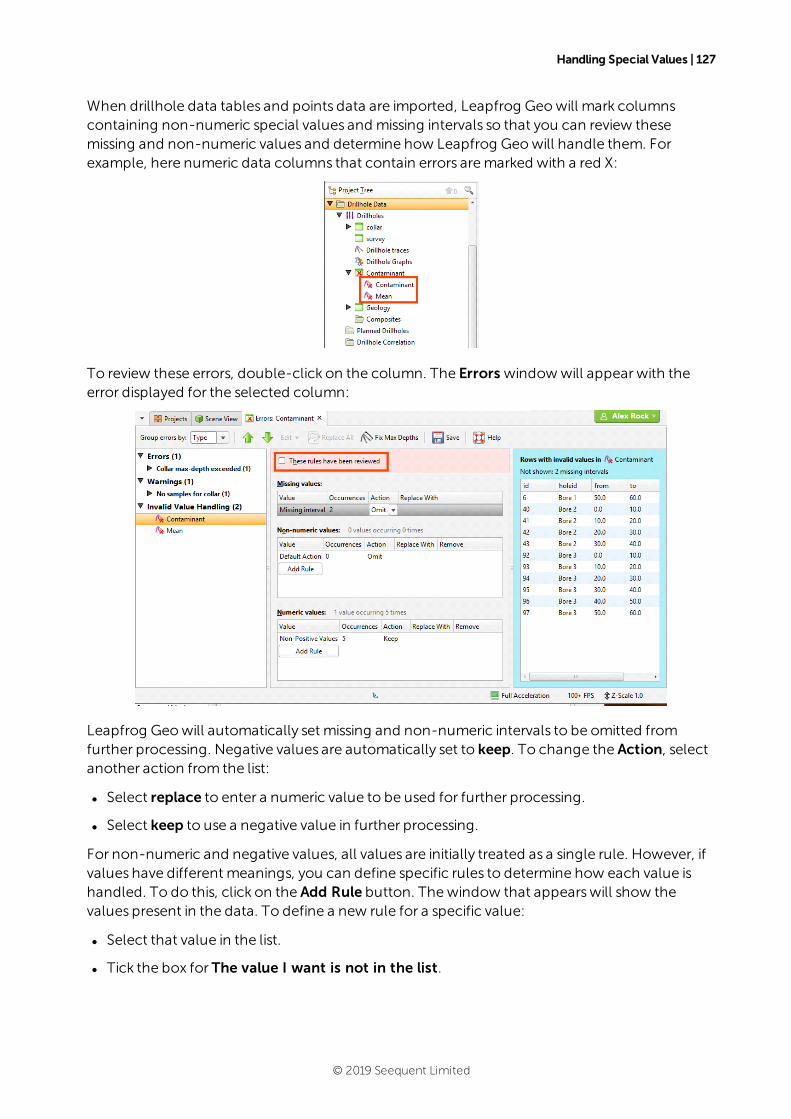
Handling Special Values | 127
When drillhole data tables and points data are imported, Leapfrog Geowill mark columnscontaining non-numeric special values and missing intervals so that you can review thesemissing and non-numeric values and determine how Leapfrog Geowill handle them. Forexample, here numeric data columns that contain errors aremarked with a red X:
To review these errors, double-click on the column. The Errors windowwill appear with theerror displayed for the selected column:
Leapfrog Geowill automatically set missing and non-numeric intervals to be omitted fromfurther processing. Negative values are automatically set to keep. To change the Action, selectanother action from the list:
l Select replace to enter a numeric value to be used for further processing.
l Select keep to use a negative value in further processing.
For non-numeric and negative values, all values are initially treated as a single rule. However, ifvalues have different meanings, you can define specific rules to determine how each value ishandled. To do this, click on the Add Rule button. Thewindow that appearswill show thevalues present in the data. To define a new rule for a specific value:
l Select that value in the list.
l Tick the box for The value I want is not in the list.
© 2019 Seequent Limited

128 | User Manual
l Enter the Value.
l ClickOK.
In the Invalid Value Handlingwindow, the valuewill be listed separately and you can choosethe Action to apply.
Once you have reviewed the rules that will be applied to the column, tick the These rules havebeen reviewed box and clickOK. The ruleswill be applied and used in further processing.
When you open a data table, the original valueswill be displayed. In all further processing ofthat data, the assigned special valueswill be used.
BoundariesThis topic discusses boundaries in Leapfrog Geo. It is divided into:
l The Clipping Boundary
l Object Extents
l Extending a Surface
A newly-created project has only a basic set of X-Y-Z coordinates, and the coordinate systemused by the project is determined by the data imported to the project. It is not necessary tospecifywhat coordinate system is used; however, it is necessary to ensure that data you importinto the project uses the same coordinate system.
Often the best way to set the coordinates for the project as a whole is to import a map or aerialphoto. Adding georeference data to a map will set the location of themap in three-dimensionalspace and set the coordinates for the project. See Importing a Map or Image formoreinformation.
An important consideration in defining the project space is setting the clipping boundary. SeeThe Clipping Boundary.
It is not necessary to define a topography tomodel in Leapfrog Geo, but a defined topographycan be used as an upper boundary for all models built in the project. SeeDefining aTopography.
Part of creating many objects in Leapfrog Geo is defining the basic rectangular boundary thatdefines the object’s extents. SeeObject Extents.
You can modify the extents of geological models and interpolants using surfaces created fromdifferent types of data. SeeModifying a Geological Model’s Boundary and Modifying an RBFInterpolant’s Boundary with Lateral Extents.
The Clipping Boundary
An important consideration in defining the project space is setting the clipping boundary.
The default clipping boundary in a new project file encompasses everything in the project andgrows asmore data is added to the project. It is not necessary to set the clipping boundary.However, the clipping boundary defines the limits of the X-Y coordinates for the region in which
© 2019 Seequent Limited
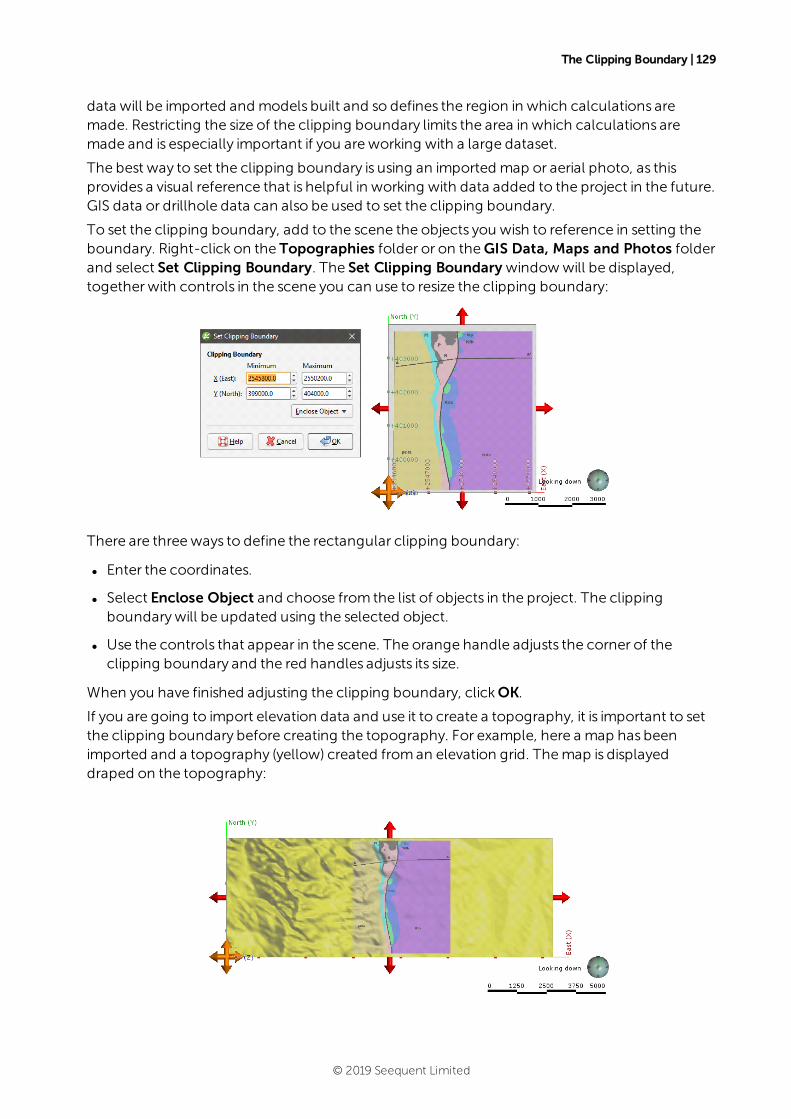
The Clipping Boundary | 129
data will be imported and models built and so defines the region in which calculations aremade. Restricting the size of the clipping boundary limits the area in which calculations aremade and is especially important if you are working with a large dataset.
The best way to set the clipping boundary is using an imported map or aerial photo, as thisprovides a visual reference that is helpful in working with data added to the project in the future.GIS data or drillhole data can also be used to set the clipping boundary.
To set the clipping boundary, add to the scene the objects you wish to reference in setting theboundary. Right-click on the Topographies folder or on theGIS Data, Maps and Photos folderand select Set Clipping Boundary. The Set Clipping Boundary windowwill be displayed,together with controls in the scene you can use to resize the clipping boundary:
There are threeways to define the rectangular clipping boundary:
l Enter the coordinates.
l Select Enclose Object and choose from the list of objects in the project. The clippingboundarywill be updated using the selected object.
l Use the controls that appear in the scene. The orange handle adjusts the corner of theclipping boundary and the red handles adjusts its size.
When you have finished adjusting the clipping boundary, clickOK.
If you are going to import elevation data and use it to create a topography, it is important to setthe clipping boundary before creating the topography. For example, here a map has beenimported and a topography (yellow) created froman elevation grid. Themap is displayeddraped on the topography:
© 2019 Seequent Limited

130 | User Manual
The red arrows and orange handle show the clipping boundary, which has been allowed toexpand to encompass all data imported to the project. Because the topographywas createdbefore the clipping boundarywas set, all the data in the imported elevation grid has been usedand the resulting topography is larger than might be practical. Clearly, if the intention is tomodel within the area on themap, the clipping boundary should be limited to the regionindicated by themap.
If themap is the only object in the project, it can easily be used to set the clipping boundary byselecting <Everything> from the Enclose Object list:
This results in a clipping boundary that is limited to the extents of themap:
© 2019 Seequent Limited

Object Extents | 131
Once the clipping boundary has been set, further data imported into the project will be clippedto it. For example, importing the elevation grid and using it to create a topography only after theclipping boundary has been set to themap extentswill result in a topography (with themapdraped) that looks like this:
Once the clipping boundary has been set, a good next step is defining the topography. SeeDefining a Topography.
Object Extents
Part of creating many objects in Leapfrog Geo is defining the basic rectangular boundary thatdefines the object’s extents. There are generally two options for defining an object’s extents:
l The first option is to define extents that are independent of other objects in the project. Youcan do this by entering coordinates or adjusting controls in the scene to set the size andshape of the extents. The new object’s extents are fixed to the specified size. This is a goodchoice if, for example, you are building a geological model froma map and wish to definethemodel extents based on information on themap.
l The second option is to define extents based on other objects in the project. This is done byselecting the other object from the Enclose Object list that appears in many Leapfrog Geoscreens.
For both methods, the new object’s extents are fixed to the selected size. Using the EncloseObject list does not link the two objects; it is simply using the X-Y-Z coordinates of theoriginal object as the basis for the new extents.
© 2019 Seequent Limited
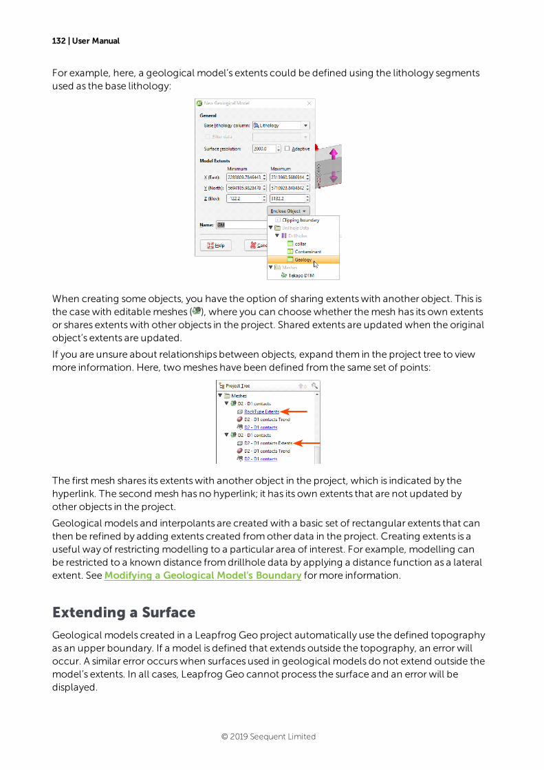
132 | User Manual
For example, here, a geological model’s extents could be defined using the lithology segmentsused as the base lithology:
When creating some objects, you have the option of sharing extentswith another object. This isthe casewith editablemeshes ( ), where you can choosewhether themesh has its own extentsor shares extentswith other objects in the project. Shared extents are updated when the originalobject’s extents are updated.
If you are unsure about relationships between objects, expand them in the project tree to viewmore information. Here, twomeshes have been defined from the same set of points:
The first mesh shares its extentswith another object in the project, which is indicated by thehyperlink. The second mesh has no hyperlink; it has its own extents that are not updated byother objects in the project.
Geological models and interpolants are created with a basic set of rectangular extents that canthen be refined by adding extents created fromother data in the project. Creating extents is auseful way of restricting modelling to a particular area of interest. For example, modelling canbe restricted to a known distance fromdrillhole data by applying a distance function as a lateralextent. SeeModifying a Geological Model’s Boundary formore information.
Extending a Surface
Geological models created in a Leapfrog Geo project automatically use the defined topographyas an upper boundary. If a model is defined that extends outside the topography, an error willoccur. A similar error occurswhen surfaces used in geological models do not extend outside themodel’s extents. In all cases, Leapfrog Geo cannot process the surface and an error will bedisplayed.
© 2019 Seequent Limited
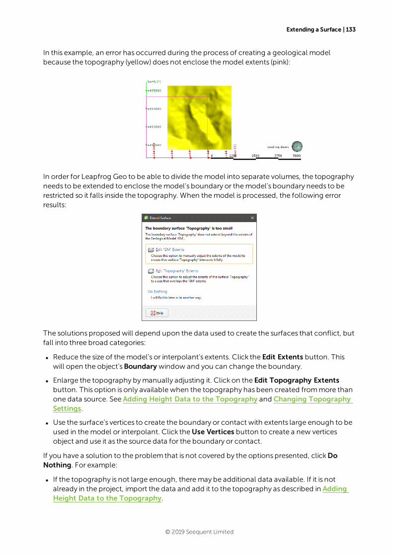
Extending a Surface | 133
In this example, an error has occurred during the process of creating a geological modelbecause the topography (yellow) does not enclose themodel extents (pink):
In order for Leapfrog Geo to be able to divide themodel into separate volumes, the topographyneeds to be extended to enclose themodel’s boundary or themodel’s boundary needs to berestricted so it falls inside the topography. When themodel is processed, the following errorresults:
The solutions proposed will depend upon the data used to create the surfaces that conflict, butfall into three broad categories:
l Reduce the size of themodel’s or interpolant’s extents. Click the Edit Extents button. Thiswill open the object’sBoundary window and you can change the boundary.
l Enlarge the topography bymanually adjusting it. Click on the Edit Topography Extentsbutton. This option is only available when the topography has been created frommore thanone data source. See Adding Height Data to the Topography and Changing TopographySettings.
l Use the surface’s vertices to create the boundary or contact with extents large enough to beused in themodel or interpolant. Click theUse Vertices button to create a new verticesobject and use it as the source data for the boundary or contact.
If you have a solution to the problem that is not covered by the options presented, clickDoNothing. For example:
l If the topography is not large enough, theremay be additional data available. If it is notalready in the project, import the data and add it to the topography as described in AddingHeight Data to the Topography.
© 2019 Seequent Limited
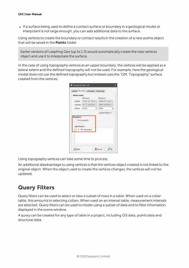
134 | User Manual
l If a surface being used to define a contact surface or boundary in a geological model orinterpolant is not large enough, you can add additional data to the surface.
Using vertices to create the boundary or contact results in the creation of a new points objectthat will be saved in the Points folder.
Earlier versions of Leapfrog Geo (up to 1.3) would automatically create the new verticesobject and use it to interpolate the surface.
In the case of using topography vertices as an upper boundary, the verticeswill be applied as alateral extent and the defined topographywill not be used. For example, here the geologicalmodel does not use the defined topography but instead uses the “GM: Topography” surfacecreated from the vertices:
Using topography vertices can take some time to process.
An additional disadvantage to using vertices is that the vertices object created is not linked to theoriginal object. When the object used to create the vertices changes, the verticeswill not beupdated.
Query FiltersQuery filters can be used to select or view a subset of rows in a table. When used on a collartable, this amounts to selecting collars. When used on an interval table, measurement intervalsare selected. Query filters can be used tomodel using a subset of data and to filter informationdisplayed in the scenewindow.
A query can be created for any type of table in a project, including GIS data, points data andstructural data.
© 2019 Seequent Limited

Creating a New Query Filter | 135
When a query filter has been defined for an object and the object is displayed in the scene, thequery filter can be applied by clicking on the object in the shape list and selecting the query filterin the shape properties panel:
For a drillhole data table, this displays only the data selected by the filter. The trace linesremain displayed in the scene. To filter trace lines, tick the Filter trace lines box:
Query filters defined for collar tables are available to all other drillhole data tables.
Creating a New Query Filter
To create a query filter, right-click on the required table in the project tree and selectNewQuery Filter. TheQuery Filter windowwill appear:
Type the required criteria into theQuery box, using the query syntax described below. PressCtrl-Enter for a new line in longer queries. Click the ... button formore advanced query buildingoptions, which are described in Building a Query and Advanced Queries below.
© 2019 Seequent Limited
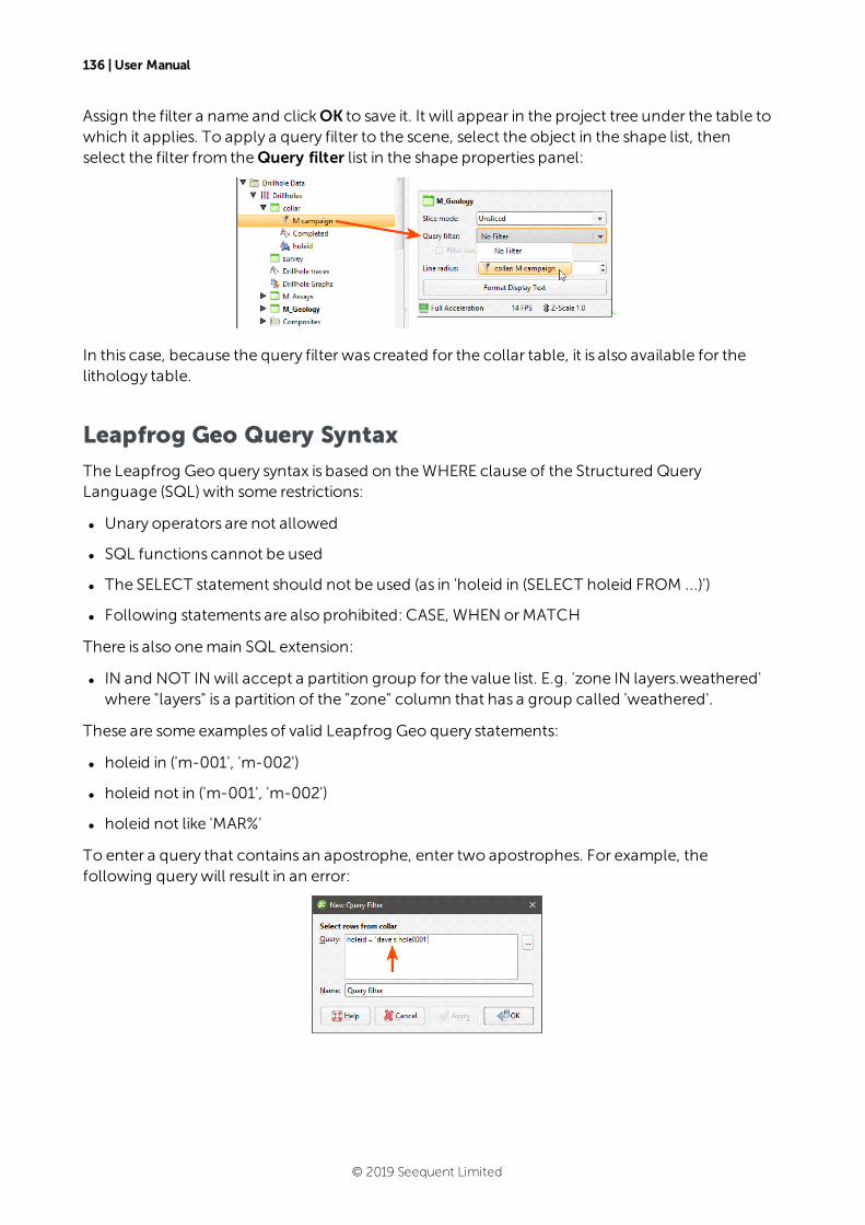
136 | User Manual
Assign the filter a name and clickOK to save it. It will appear in the project tree under the table towhich it applies. To apply a query filter to the scene, select the object in the shape list, thenselect the filter from theQuery filter list in the shape properties panel:
In this case, because the query filter was created for the collar table, it is also available for thelithology table.
Leapfrog Geo Query Syntax
The Leapfrog Geo query syntax is based on theWHERE clause of the Structured QueryLanguage (SQL) with some restrictions:
l Unary operators are not allowed
l SQL functions cannot be used
l The SELECT statement should not be used (as in 'holeid in (SELECT holeid FROM ...)')
l Following statements are also prohibited: CASE, WHEN orMATCH
There is also onemain SQL extension:
l IN and NOT INwill accept a partition group for the value list. E.g. 'zone IN layers.weathered'where "layers" is a partition of the "zone" column that has a group called 'weathered'.
These are some examples of valid Leapfrog Geo query statements:
l holeid in ('m-001', 'm-002')
l holeid not in ('m-001', 'm-002')
l holeid not like 'MAR%'
To enter a query that contains an apostrophe, enter two apostrophes. For example, thefollowing querywill result in an error:
© 2019 Seequent Limited

Building a Query | 137
Adding the second apostrophe results in a valid query:
TheQuery box allows the following shortcut queries:
l Typing a single word will match all hole-ids starting with that string. For example, typing"MAR" is a shortcut for "holeid like 'MAR%'"
l Typing a comma-separated list of wordswill match all hole-ids that exactlymatch the givenwords. For example typing "M001, M002" is a shortcut for "holeid in ('M001', 'M002')".
Building a Query
Many common queries can be built using the Build Query window:
Thiswindow aims to be easy to use rather than comprehensive in its support for the fullLeapfrog Geo query syntax. Formore advanced queries, click on the Advanced button. SeeAdvanced Queries formore information.
To add a criteria, clickColumn to view a list of columns available in the table. Select a Test andenter a Value. What can be entered for the Value dependson the type of column and testselected.
Quotes are not required around text values entered in the value column as they are in SQL.Leapfrog Geowill add quotes and brackets to the value "MX, PM" tomake a valid SQL list ofstrings "('MX', 'PM')" when the query is saved.
Click on the Apply button to apply to query to the context in which the dialog wasopened.
Use theDelete button to delete the criteria in the selected row and the Add button to add ablank row.
© 2019 Seequent Limited
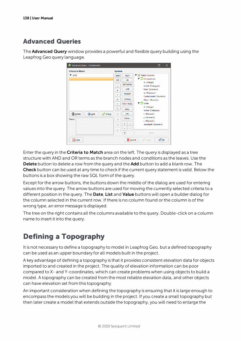
138 | User Manual
Advanced Queries
The Advanced Query window provides a powerful and flexible query building using theLeapfrog Geo query language.
Enter the query in theCriteria to Match area on the left. The query is displayed as a treestructure with AND and OR terms as the branch nodes and conditions as the leaves. Use theDelete button to delete a row from the query and the Add button to add a blank row. TheCheck button can be used at any time to check if the current query statement is valid. Below thebuttons is a box showing the raw SQL formof the query.
Except for the arrow buttons, the buttons down themiddle of the dialog are used for enteringvalues into the query. The arrow buttons are used formoving the currently selected criteria to adifferent position in the query. TheDate, List and Value buttonswill open a builder dialog forthe column selected in the current row. If there is no column found or the column is of thewrong type, an errormessage is displayed.
The tree on the right contains all the columns available to the query. Double-click on a columnname to insert it into the query.
Defining a TopographyIt is not necessary to define a topography tomodel in Leapfrog Geo, but a defined topographycan be used as an upper boundary for all models built in the project.
A key advantage of defining a topography is that it provides consistent elevation data for objectsimported to and created in the project. The quality of elevation information can be poorcompared to X- and Y-coordinates, which can create problemswhen using objects to build amodel. A topography can be created from themost reliable elevation data, and other objectscan have elevation set from this topography.
An important consideration when defining the topography is ensuring that it is large enough toencompass themodels you will be building in the project. If you create a small topography butthen later create a model that extends outside the topography, you will need to enlarge the
© 2019 Seequent Limited
Topography From Elevation Grid | 139
topography, which can result in considerable reprocessing of all objects in the project that usethe topography as a boundary. See Extending a Surface formore information.
This topic describes creating and working with a topography. It is divided into:
l Topography From Elevation Grid
l Topography From Surfaces, Points or GIS Vector Data
l Fixed Elevation Topography
l Adding Height Data to the Topography
l Changing Topography Settings
l Topography Display Options
l Projecting Collars onto the Topography
The topography can be created froman imported elevation grid, points data, surfaces and GISdata. It is not necessary to decide on a single source of information, as information can becombined, and you can add and remove data as required.
Once defined, you can export the topography as a mesh or as an elevation grid. See:
l Exporting Meshes
l Exporting an Elevation Grid
Topography From Elevation Grid
There are twoways to create the topography froman elevation grid:
l Right-click on the Topographies folder and selectNew Topography > Import ElevationGrid. Import the grid as described in Importing an Elevation Grid.
l Import the grid using theMeshes folder and then right-click on the Topographies folderand selectNew Topography > From Surface.
Enter a name for the topography and clickOK. A hyperlink to the elevation grid will appear inthe Topographies folder under the defined topography.
Once the topography has been defined, additional height data can be added by right-clicking on the topography and selecting from the options available. See See "AddingHeight Data to the Topography" formore information.
Topography From Surfaces, Points or GIS Vector Data
To create the topography froma surface, points or GIS data, first import the data into theproject.
l Import surfaces into theMeshes folder.
l Import drillhole data into the project or points data into the Points folder.
l Import GIS vector data into theGIS Data, Maps and Photos folder.
© 2019 Seequent Limited
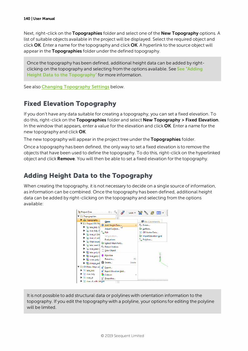
140 | User Manual
Next, right-click on the Topographies folder and select one of theNew Topography options. Alist of suitable objects available in the project will be displayed. Select the required object andclickOK. Enter a name for the topography and clickOK. A hyperlink to the source object willappear in the Topographies folder under the defined topography.
Once the topography has been defined, additional height data can be added by right-clicking on the topography and selecting from the options available. See See "AddingHeight Data to the Topography" formore information.
See alsoChanging Topography Settings below.
Fixed Elevation Topography
If you don’t have any data suitable for creating a topography, you can set a fixed elevation. Todo this, right-click on the Topographies folder and selectNew Topography > Fixed Elevation.In thewindow that appears, enter a value for the elevation and clickOK. Enter a name for thenew topography and clickOK.
The new topographywill appear in the project tree under the Topographies folder.
Once a topography has been defined, the onlyway to set a fixed elevation is to remove theobjects that have been used to define the topography. To do this, right-click on the hyperlinkedobject and clickRemove. You will then be able to set a fixed elevation for the topography.
Adding Height Data to the Topography
When creating the topography, it is not necessary to decide on a single source of information,as information can be combined. Once the topography has been defined, additional heightdata can be added by right-clicking on the topography and selecting from the optionsavailable:
It is not possible to add structural data or polylineswith orientation information to thetopography. If you edit the topographywith a polyline, your options for editing the polylinewill be limited.
© 2019 Seequent Limited

Changing Topography Settings | 141
For points, surfaces and GIS vector data, you will be prompted to select from the data sourcesavailable in the project. For an elevation grid, see Importing an Elevation Grid.
All data objects used to define the topographywill appear under the topography, hyperlinkedto their parent objects:
When you have added data to the topography, you may need to enlarge the topographyextents. SeeChanging Topography Settings below.
To remove data objects from the topography, either:
l Delete the object from the topography. To do this, right-click on the hyperlinked object andclickRemove.
l Delete the object from the project. If you choose this option, consider carefully the effectson other objects in the project, as once an object is deleted, it cannot be recovered.
When the topography is defined frommultiple objects, you can set the resolution of thetopography by double-clicking on it. SeeChanging Topography Settings below.
Changing Topography Settings
When the topography is created frompoints or GIS data or when the topography is created bycombining data, you can change its boundary and resolution and apply a trend. To do this,double-click on the topography in the project tree. The Edit Topography windowwill appear:
Changing the Size of the Topography
In theGeneral tab, you can change the topography extents. Use the controls in the scene orenter the required values in the Bounding Box fields.
© 2019 Seequent Limited
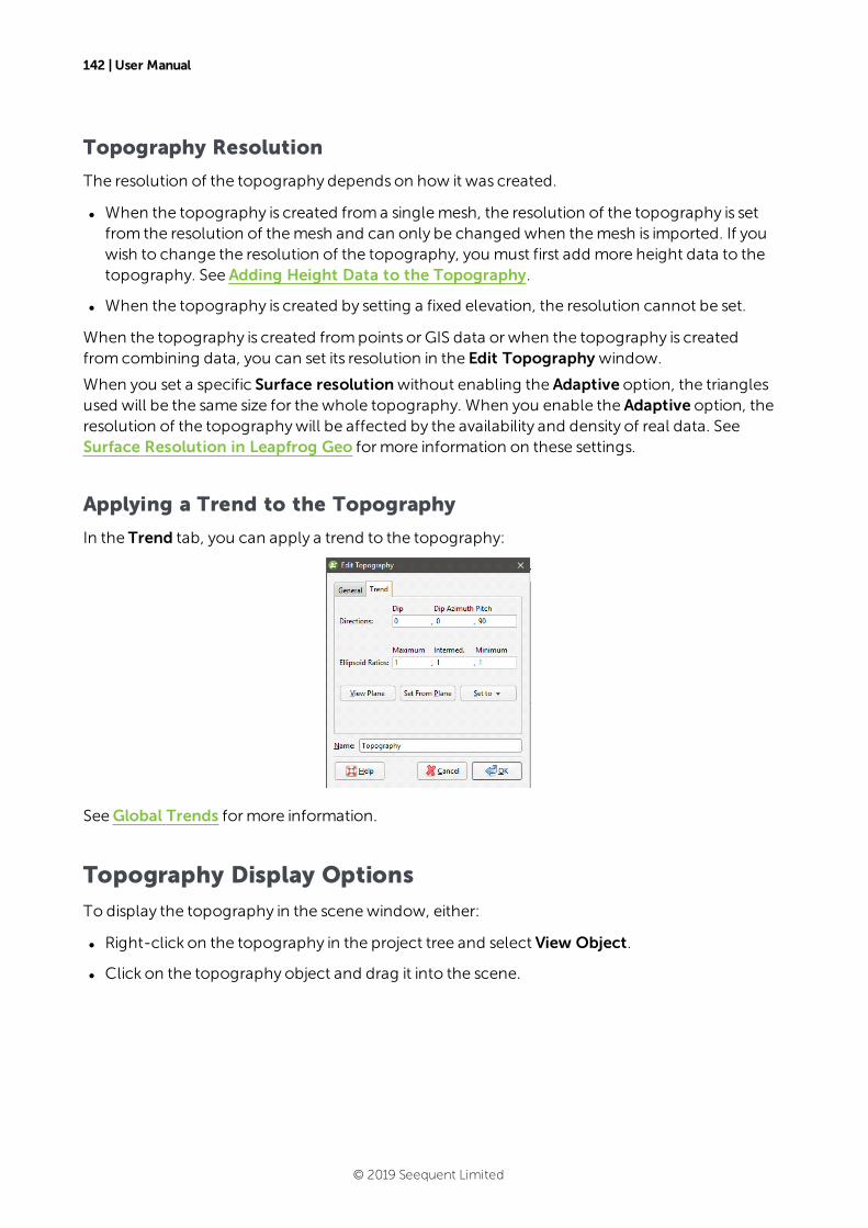
142 | User Manual
Topography Resolution
The resolution of the topography dependson how it was created.
l When the topography is created froma singlemesh, the resolution of the topography is setfrom the resolution of themesh and can only be changed when themesh is imported. If youwish to change the resolution of the topography, you must first add more height data to thetopography. See Adding Height Data to the Topography.
l When the topography is created by setting a fixed elevation, the resolution cannot be set.
When the topography is created frompoints or GIS data or when the topography is createdfromcombining data, you can set its resolution in the Edit Topography window.
When you set a specific Surface resolutionwithout enabling the Adaptive option, the trianglesused will be the same size for thewhole topography. When you enable the Adaptive option, theresolution of the topographywill be affected by the availability and density of real data. SeeSurface Resolution in Leapfrog Geo formore information on these settings.
Applying a Trend to the Topography
In the Trend tab, you can apply a trend to the topography:
SeeGlobal Trends formore information.
Topography Display Options
To display the topography in the scenewindow, either:
l Right-click on the topography in the project tree and select View Object.
l Click on the topography object and drag it into the scene.
© 2019 Seequent Limited
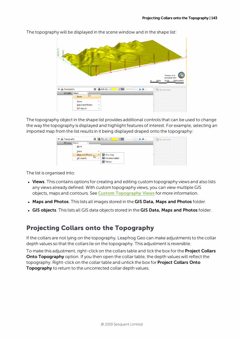
Projecting Collars onto the Topography | 143
The topographywill be displayed in the scenewindow and in the shape list:
The topography object in the shape list provides additional controls that can be used to changetheway the topography is displayed and highlight features of interest. For example, selecting animported map from the list results in it being displayed draped onto the topography:
The list is organised into:
l Views. This contains options for creating and editing custom topography views and also listsany views already defined. With custom topography views, you can viewmultiple GISobjects, maps and contours. SeeCustom Topography Views formore information.
l Maps and Photos. This lists all images stored in theGIS Data, Maps and Photos folder.
l GIS objects. This lists all GIS data objects stored in theGIS Data, Maps and Photos folder.
Projecting Collars onto the Topography
If the collars are not lying on the topography, Leapfrog Geo can make adjustments to the collardepth values so that the collars lie on the topography. This adjustment is reversible.
Tomake this adjustment, right-click on the collars table and tick the box for the Project CollarsOnto Topography option. If you then open the collar table, the depth valueswill reflect thetopography. Right-click on the collar table and untick the box for Project Collars OntoTopography to return to the uncorrected collar depth values.
© 2019 Seequent Limited
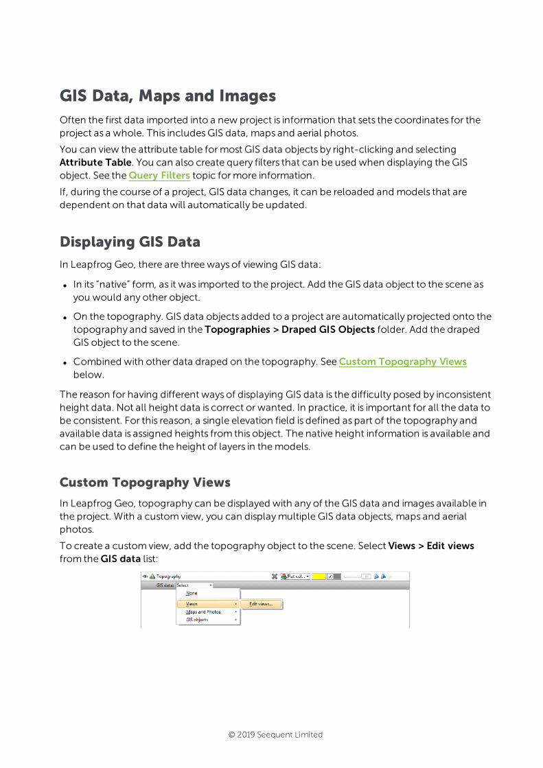
GIS Data, Maps and ImagesOften the first data imported into a new project is information that sets the coordinates for theproject as a whole. This includesGIS data, maps and aerial photos.
You can view the attribute table formost GIS data objects by right-clicking and selectingAttribute Table. You can also create query filters that can be used when displaying the GISobject. See theQuery Filters topic formore information.
If, during the course of a project, GIS data changes, it can be reloaded and models that aredependent on that data will automatically be updated.
Displaying GIS Data
In Leapfrog Geo, there are threeways of viewing GIS data:
l In its “native” form, as it was imported to the project. Add the GIS data object to the scene asyou would any other object.
l On the topography. GIS data objects added to a project are automatically projected onto thetopography and saved in the Topographies > Draped GIS Objects folder. Add the drapedGIS object to the scene.
l Combined with other data draped on the topography. SeeCustom Topography Viewsbelow.
The reason for having different ways of displaying GIS data is the difficulty posed by inconsistentheight data. Not all height data is correct or wanted. In practice, it is important for all the data tobe consistent. For this reason, a single elevation field is defined as part of the topography andavailable data is assigned heights from this object. The native height information is available andcan be used to define the height of layers in themodels.
Custom Topography Views
In Leapfrog Geo, topography can be displayed with any of the GIS data and images available inthe project. With a customview, you can displaymultiple GIS data objects, maps and aerialphotos.
To create a customview, add the topography object to the scene. Select Views > Edit viewsfrom theGIS data list:
© 2019 Seequent Limited
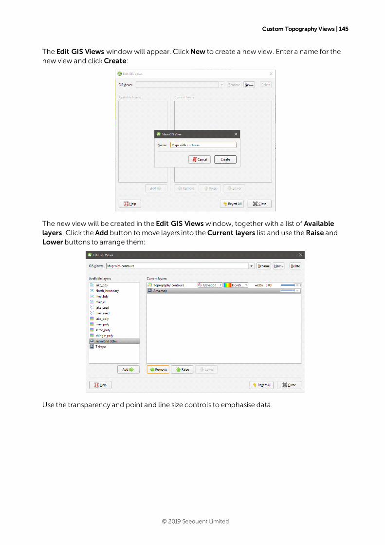
Custom Topography Views | 145
The Edit GIS Views windowwill appear. ClickNew to create a new view. Enter a name for thenew view and clickCreate:
The new view will be created in the Edit GIS Views window, together with a list of Availablelayers. Click the Add button tomove layers into theCurrent layers list and use theRaise andLower buttons to arrange them:
Use the transparency and point and line size controls to emphasise data.
© 2019 Seequent Limited

146 | User Manual
ClickClose. The topographywill be displayed in the scenewith the new view applied:
Importing Vector Data
Vector data formats Leapfrog Geo supports include:
l Shape Files (*.shp)
l MapInfo Files (*.tab, *.mif)
l ESRI Personal GeoDatabase Files (*.mdb, *.accdb)
You can also import data fromMapInfo and ESRI databases. See Importing a MapInfoBatch File and Importing Data from an ESRI Geodatabase formore information.
To import vector data, right-click on theGIS Data, Maps and Photos folder and select ImportVector Data. Navigate to the folder that contains the GIS data and select the file. You can selectmultiple files using the Shift and Ctrl keys.
ClickOpen to begin importing the data.
If you are importing a single file, the Import GIS Vector Datawindowwill show a summary ofthe data in the selected file:
You can choosewhat field in the data to use for the Elevation Field from the list.
© 2019 Seequent Limited

Importing a MapInfo Batch File | 147
If you are importing multiple files, all files being imported are listed in the Import GIS VectorDatawindow and no summary of each file is displayed:
Data is automatically clipped to the clipping boundary, but you can change how the data isfiltered to suit any bounding box that exists in the project. If you do not wish to clip the data,untick the Filter data box.
ClickOK to add the data to the project. The object or objectswill appear in the project treeunder theGIS Data, Maps and Photos folder. If a topography has been defined for the project,the imported GIS data objectswill automatically be projected onto the topography and saved inthe Topographies > Draped GIS Objects folder.
You can then view an object’s attributes by right-clicking on it and selecting Attribute Table.
When importing files, you may be prompted to select whether or not to filter elevation data.If you wish to use another data source for your elevation data, select Filter data. Forexample, if you import a GIS line that has suspect elevation data, you can discard theelevation data and set the elevation from the topography, as described in Setting Elevationfor GIS Objects and Images.
If data changes outside the project, it can be reloaded as described in Reloading GIS Data.
Importing a MapInfo Batch File
You can import a collection of GIS data exported fromMapInfo. TheMapInfo file can includepoints, lines, polygons, images and elevation grids.
To import GIS data in thisway, right-click on theGIS Data, Maps and Photos folder and selectBatch Import > from MapInfo. In thewindow that appears, navigate to the folder that containstheMapInfo batch file, which is an XML file. ClickOpen.
© 2019 Seequent Limited

148 | User Manual
The data that can be imported will be displayed and you can select which files to import:
You can select multiple files using the Shift and Ctrl keys.
Data is automatically clipped to the clipping boundary, but you can change how the data isfiltered to suit any bounding box that exists in the project. If you do not wish to clip the data,untick the Filter data box.
ClickOK to import the selected files, which will be added to theGIS Data, Maps and Photosfolder as a group ( ), with the exception of elevation grids, which will be added to theMeshesfolder.
Points, lines and polygons can be reloaded on an individual basis, which is described inReloading GIS Data.
Importing Data from an ESRI Geodatabase
You can import points, lines and polygons froman ESRI geodatabase. However, the import ofraster data is not supported.
To import GIS points, lines and polygons in thisway, right-click on theGIS Data, Maps andPhotos folder and select Batch Import > from ESRI Geodatabase. In thewindow that appears,navigate to the folder that contains the database and clickOpen.
Leapfrog Geo imports uncompressed ESRI geodatabases.
© 2019 Seequent Limited
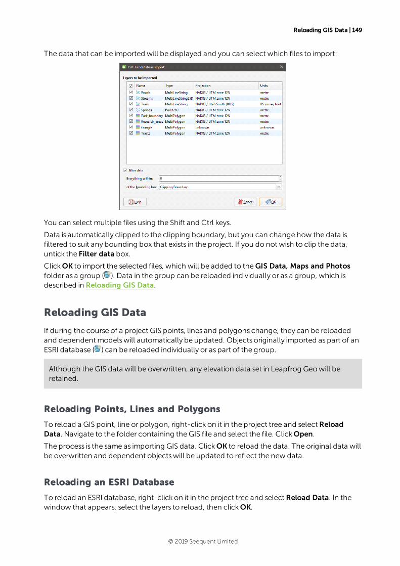
Reloading GIS Data | 149
The data that can be imported will be displayed and you can select which files to import:
You can select multiple files using the Shift and Ctrl keys.
Data is automatically clipped to the clipping boundary, but you can change how the data isfiltered to suit any bounding box that exists in the project. If you do not wish to clip the data,untick the Filter data box.
ClickOK to import the selected files, which will be added to theGIS Data, Maps and Photosfolder as a group ( ). Data in the group can be reloaded individually or as a group, which isdescribed in Reloading GIS Data.
Reloading GIS Data
If during the course of a project GIS points, lines and polygons change, they can be reloadedand dependent modelswill automatically be updated. Objects originally imported as part of anESRI database ( ) can be reloaded individually or as part of the group.
Although the GIS data will be overwritten, any elevation data set in Leapfrog Geowill beretained.
Reloading Points, Lines and Polygons
To reload a GIS point, line or polygon, right-click on it in the project tree and select ReloadData. Navigate to the folder containing the GIS file and select the file. ClickOpen.
The process is the same as importing GIS data. ClickOK to reload the data. The original data willbe overwritten and dependent objectswill be updated to reflect the new data.
Reloading an ESRI Database
To reload an ESRI database, right-click on it in the project tree and select Reload Data. In thewindow that appears, select the layers to reload, then clickOK.
© 2019 Seequent Limited
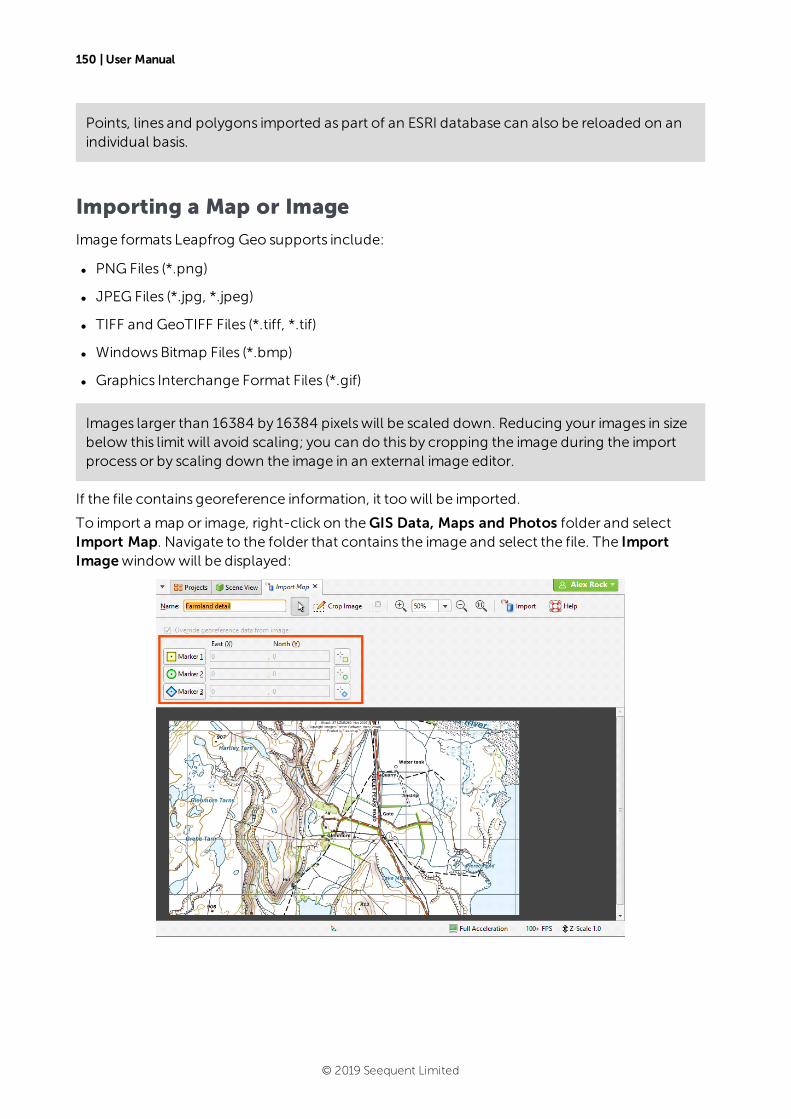
150 | User Manual
Points, lines and polygons imported as part of an ESRI database can also be reloaded on anindividual basis.
Importing a Map or Image
Image formats Leapfrog Geo supports include:
l PNG Files (*.png)
l JPEG Files (*.jpg, *.jpeg)
l TIFF and GeoTIFF Files (*.tiff, *.tif)
l WindowsBitmap Files (*.bmp)
l Graphics Interchange Format Files (*.gif)
Images larger than 16384 by 16384 pixelswill be scaled down. Reducing your images in sizebelow this limit will avoid scaling; you can do this by cropping the image during the importprocess or by scaling down the image in an external image editor.
If the file contains georeference information, it toowill be imported.
To import a map or image, right-click on theGIS Data, Maps and Photos folder and selectImport Map. Navigate to the folder that contains the image and select the file. The ImportImagewindowwill be displayed:
© 2019 Seequent Limited
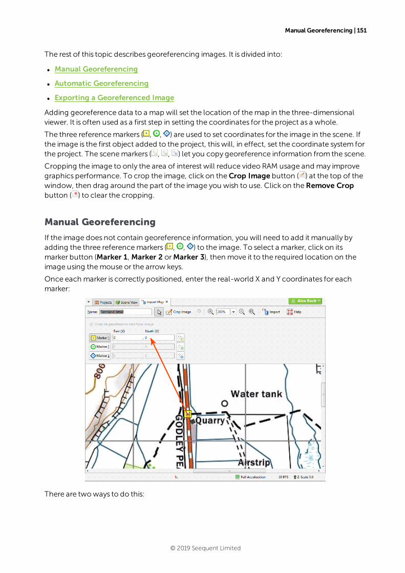
Manual Georeferencing | 151
The rest of this topic describes georeferencing images. It is divided into:
l Manual Georeferencing
l Automatic Georeferencing
l Exporting a Georeferenced Image
Adding georeference data to a map will set the location of themap in the three-dimensionalviewer. It is often used as a first step in setting the coordinates for the project as a whole.
The three referencemarkers ( , , ) are used to set coordinates for the image in the scene. Ifthe image is the first object added to the project, thiswill, in effect, set the coordinate system forthe project. The scenemarkers ( , , ) let you copy georeference information from the scene.
Cropping the image to only the area of interest will reduce video RAM usage and may improvegraphics performance. To crop the image, click on theCrop Image button ( ) at the top of thewindow, then drag around the part of the image you wish to use. Click on theRemove Cropbutton ( ) to clear the cropping.
Manual Georeferencing
If the image does not contain georeference information, you will need to add it manually byadding the three referencemarkers ( , , ) to the image. To select a marker, click on itsmarker button (Marker 1, Marker 2 orMarker 3), then move it to the required location on theimage using themouse or the arrow keys.
Once each marker is correctly positioned, enter the real-world X and Y coordinates for eachmarker:
There are twoways to do this:
© 2019 Seequent Limited
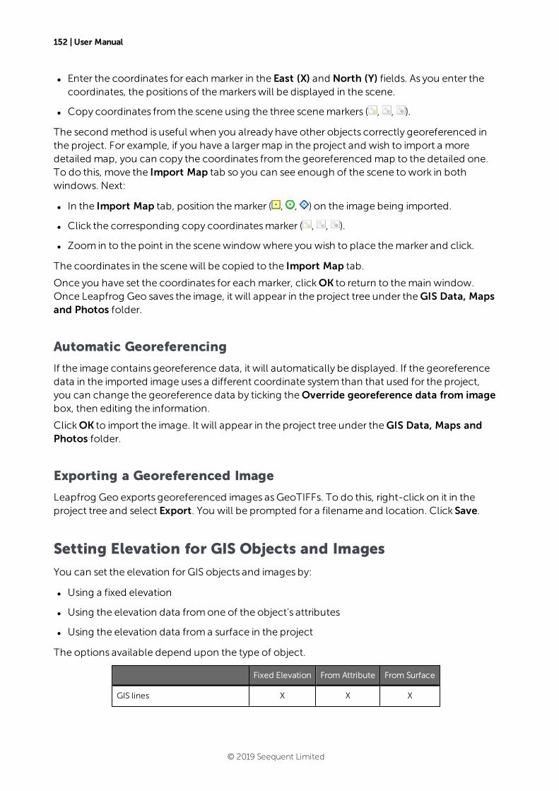
152 | User Manual
l Enter the coordinates for each marker in the East (X) and North (Y) fields. As you enter thecoordinates, the positions of themarkerswill be displayed in the scene.
l Copy coordinates from the scene using the three scenemarkers ( , , ).
The second method is useful when you already have other objects correctly georeferenced inthe project. For example, if you have a largermap in the project and wish to import a moredetailed map, you can copy the coordinates from the georeferenced map to the detailed one.To do this, move the Import Map tab so you can see enough of the scene towork in bothwindows. Next:
l In the Import Map tab, position themarker ( , , ) on the image being imported.
l Click the corresponding copy coordinatesmarker ( , , ).
l Zoom in to the point in the scenewindowwhere you wish to place themarker and click.
The coordinates in the scenewill be copied to the Import Map tab.
Once you have set the coordinates for each marker, clickOK to return to themain window.Once Leapfrog Geo saves the image, it will appear in the project tree under theGIS Data, Mapsand Photos folder.
Automatic Georeferencing
If the image contains georeference data, it will automatically be displayed. If the georeferencedata in the imported image uses a different coordinate system than that used for the project,you can change the georeference data by ticking theOverride georeference data from imagebox, then editing the information.
ClickOK to import the image. It will appear in the project tree under theGIS Data, Maps andPhotos folder.
Exporting a Georeferenced Image
Leapfrog Geo exports georeferenced images asGeoTIFFs. To do this, right-click on it in theproject tree and select Export. You will be prompted for a filename and location. Click Save.
Setting Elevation for GIS Objects and Images
You can set the elevation for GIS objects and images by:
l Using a fixed elevation
l Using the elevation data fromone of the object’s attributes
l Using the elevation data froma surface in the project
The options available depend upon the type of object.
Fixed Elevation From Attribute From Surface
GIS lines X X X
© 2019 Seequent Limited
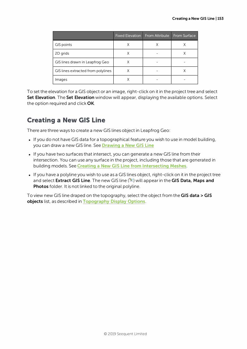
Creating a New GIS Line | 153
Fixed Elevation From Attribute From Surface
GIS points X X X
2D grids X - X
GIS lines drawn in Leapfrog Geo X - -
GIS lines extracted from polylines X - X
Images X - -
To set the elevation for a GIS object or an image, right-click on it in the project tree and selectSet Elevation. The Set Elevationwindowwill appear, displaying the available options. Selectthe option required and clickOK.
Creating a New GIS Line
There are threeways to create a new GIS lines object in Leapfrog Geo:
l If you do not have GIS data for a topographical feature you wish to use in model building,you can draw a new GIS line. SeeDrawing a New GIS Line
l If you have two surfaces that intersect, you can generate a new GIS line from theirintersection. You can use any surface in the project, including those that are generated inbuilding models. SeeCreating a New GIS Line from Intersecting Meshes.
l If you have a polyline you wish to use as a GIS lines object, right-click on it in the project treeand select Extract GIS Line. The new GIS line ( ) will appear in theGIS Data, Maps andPhotos folder. It is not linked to the original polyline.
To view new GIS line draped on the topography, select the object from theGIS data > GISobjects list, as described in Topography Display Options.
© 2019 Seequent Limited
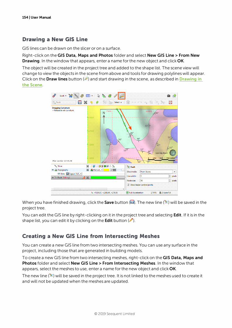
154 | User Manual
Drawing a New GIS Line
GIS lines can be drawn on the slicer or on a surface.
Right-click on theGIS Data, Maps and Photos folder and selectNew GIS Line > From NewDrawing. In thewindow that appears, enter a name for the new object and clickOK.
The object will be created in the project tree and added to the shape list. The scene view willchange to view the objects in the scene fromabove and tools for drawing polylineswill appear.Click on theDraw lines button ( ) and start drawing in the scene, as described in Drawing inthe Scene.
When you have finished drawing, click the Save button ( ). The new line ( ) will be saved in theproject tree.
You can edit the GIS line by right-clicking on it in the project tree and selecting Edit. If it is in theshape list, you can edit it by clicking on the Edit button ( ).
Creating a New GIS Line from Intersecting Meshes
You can create a new GIS line from two intersecting meshes. You can use any surface in theproject, including those that are generated in building models.
To create a new GIS line from two intersecting meshes, right-click on theGIS Data, Maps andPhotos folder and selectNew GIS Line > From Intersecting Meshes. In thewindow thatappears, select themeshes to use, enter a name for the new object and clickOK.
The new line ( ) will be saved in the project tree. It is not linked to themeshes used to create itand will not be updated when themeshes are updated.
© 2019 Seequent Limited
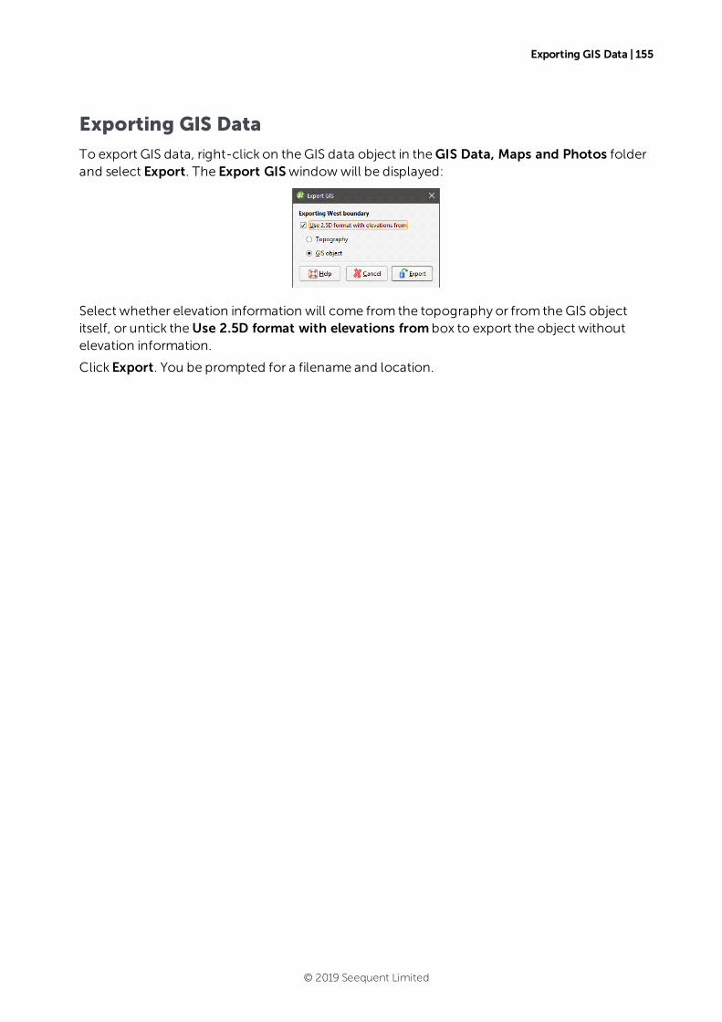
Exporting GIS Data | 155
Exporting GIS Data
To export GIS data, right-click on the GIS data object in theGIS Data, Maps and Photos folderand select Export. The Export GISwindowwill be displayed:
Select whether elevation information will come from the topography or from theGIS objectitself, or untick theUse 2.5D format with elevations from box to export the object withoutelevation information.
Click Export. You be prompted for a filename and location.
© 2019 Seequent Limited

Drillhole Data | 156
Drillhole DataDrillhole data forms the basis for creating models in Leapfrog Geo. Because drillhole data oftencontains errors that reduce the reliability of a model, Leapfrog Geo has tools that help you toidentify and correct errors and workwith the data.
Drillhole data defines the physical 3D shape of drillholes. It ismade up of:
l A collar table, containing information on the location of the drillhole.
l A survey table, containing information that describes the deviation of each drillhole.
l At least one interval table, containing information onmeasurements such as lithology, dateor any numeric or textual values. An interval tablemust also include collar IDs thatcorrespond to those in the collar table and sample start and end depth.
If you have the Hydrogeology extension, a screens table can also be imported.
When a project is first created, the only options available via theDrillhole Data folder are forimporting data. See Importing Drillhole Data formore information on these options.
Once data has been added to the project, a Drillholes object will be created that serves as acontainer for the tables imported:
You can open each table by double-clicking on the table ( ). The table will be displayed andyou can make changes. SeeWorking with Data Tables. When there are errors in the data, therelevant table will bemarked with a red X ( ). SeeCorrecting Data Errors in Leapfrog Geo formore information on fixing drillhole data errors.
Leapfrog Geo also has tools for creating new lithology data columns fromexisting columns inorder to solve problemswith the drillhole data. See Processing Drillhole Data formoreinformation.
To delete a lithology or numeric data table, right-click on the table in the project tree andselectDelete. You will be asked to confirm your choice.
When you right-click on the drillhole or collar table object in the project tree and selectDelete, the resulting action will also remove all lithology and numeric data tables from theproject. You will be asked to confirm your choice.
© 2019 Seequent Limited
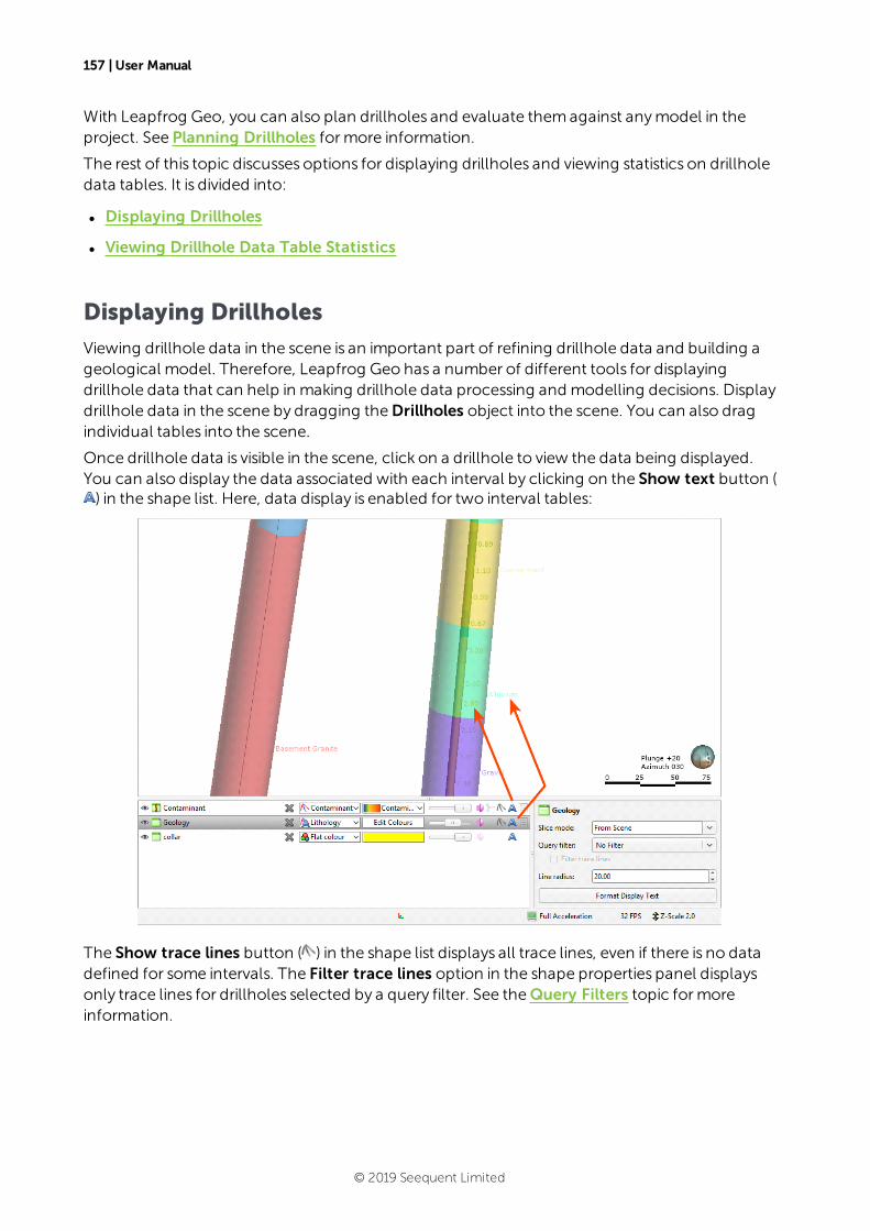
157 | User Manual
With Leapfrog Geo, you can also plan drillholes and evaluate themagainst anymodel in theproject. See Planning Drillholes formore information.
The rest of this topic discusses options for displaying drillholes and viewing statistics on drillholedata tables. It is divided into:
l Displaying Drillholes
l Viewing Drillhole Data Table Statistics
Displaying Drillholes
Viewing drillhole data in the scene is an important part of refining drillhole data and building ageological model. Therefore, Leapfrog Geo has a number of different tools for displayingdrillhole data that can help in making drillhole data processing and modelling decisions. Displaydrillhole data in the scene by dragging theDrillholes object into the scene. You can also dragindividual tables into the scene.
Once drillhole data is visible in the scene, click on a drillhole to view the data being displayed.You can also display the data associated with each interval by clicking on the Show text button () in the shape list. Here, data display is enabled for two interval tables:
The Show trace lines button ( ) in the shape list displays all trace lines, even if there is no datadefined for some intervals. The Filter trace lines option in the shape properties panel displaysonly trace lines for drillholes selected by a query filter. See theQuery Filters topic formoreinformation.
© 2019 Seequent Limited
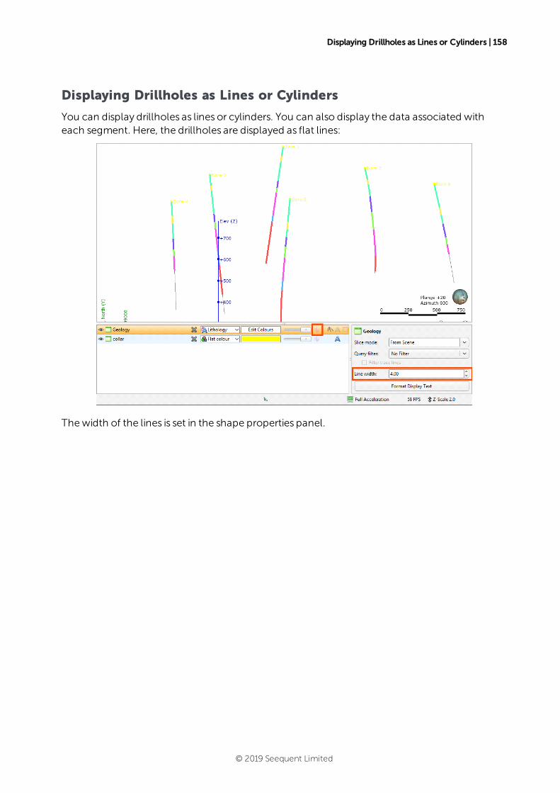
Displaying Drillholes as Lines or Cylinders | 158
Displaying Drillholes as Lines or Cylinders
You can display drillholes as lines or cylinders. You can also display the data associated witheach segment. Here, the drillholes are displayed as flat lines:
Thewidth of the lines is set in the shape properties panel.
© 2019 Seequent Limited

159 | User Manual
When theMake lines solid button ( ) is enabled, the drillhole data is displayed as cylinders andthe property that can be controlled is the Line radius:
When numeric data is displayed, there is an additional option, to use a data column in the tablefor the cylinder radius:
When the log button ( ) is enabled, the log of values is used for the radius.
© 2019 Seequent Limited
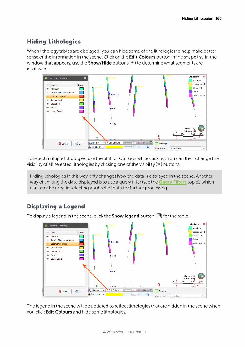
Hiding Lithologies | 160
Hiding Lithologies
When lithology tables are displayed, you can hide some of the lithologies to help make bettersense of the information in the scene. Click on the Edit Colours button in the shape list. In thewindow that appears, use the Show/Hide buttons ( ) to determinewhat segments aredisplayed:
To select multiple lithologies, use the Shift or Ctrl keyswhile clicking. You can then change thevisibility of all selected lithologies by clicking one of the visibility ( ) buttons.
Hiding lithologies in thisway only changes how the data is displayed in the scene. Anotherway of limiting the data displayed is to use a query filter (see theQuery Filters topic), whichcan later be used in selecting a subset of data for further processing.
Displaying a Legend
To display a legend in the scene, click the Show legend button ( ) for the table:
The legend in the scenewill be updated to reflect lithologies that are hidden in the scenewhenyou click Edit Colours and hide some lithologies.
© 2019 Seequent Limited
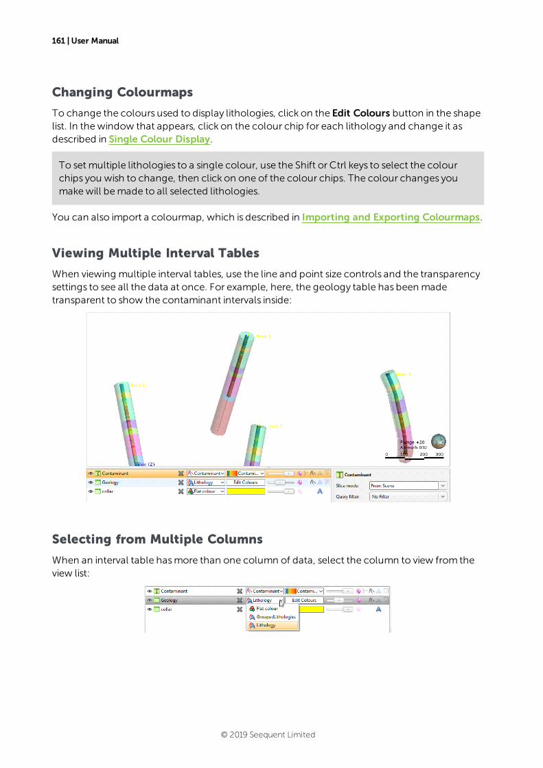
161 | User Manual
Changing Colourmaps
To change the colours used to display lithologies, click on the Edit Colours button in the shapelist. In thewindow that appears, click on the colour chip for each lithology and change it asdescribed in Single Colour Display.
To set multiple lithologies to a single colour, use the Shift or Ctrl keys to select the colourchips you wish to change, then click on one of the colour chips. The colour changes youmakewill bemade to all selected lithologies.
You can also import a colourmap, which is described in Importing and Exporting Colourmaps.
Viewing Multiple Interval Tables
When viewing multiple interval tables, use the line and point size controls and the transparencysettings to see all the data at once. For example, here, the geology table has been madetransparent to show the contaminant intervals inside:
Selecting from Multiple Columns
When an interval table hasmore than one column of data, select the column to view from theview list:
© 2019 Seequent Limited
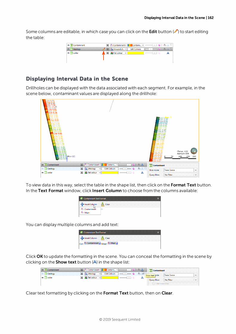
Displaying Interval Data in the Scene | 162
Some columns are editable, in which case you can click on the Edit button ( ) to start editingthe table:
Displaying Interval Data in the Scene
Drillholes can be displayed with the data associated with each segment. For example, in thescene below, contaminant values are displayed along the drillhole:
To view data in thisway, select the table in the shape list, then click on the Format Text button.In the Text Format window, click Insert Column to choose from the columns available:
You can displaymultiple columns and add text:
ClickOK to update the formatting in the scene. You can conceal the formatting in the scene byclicking on the Show text button ( ) in the shape list:
Clear text formatting by clicking on the Format Text button, then on Clear.
© 2019 Seequent Limited
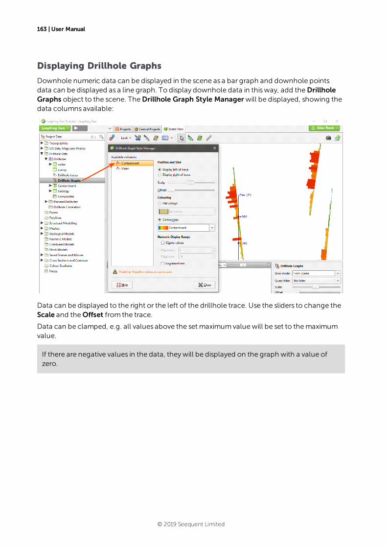
163 | User Manual
Displaying Drillhole Graphs
Downhole numeric data can be displayed in the scene as a bar graph and downhole pointsdata can be displayed as a line graph. To display downhole data in thisway, add theDrillholeGraphs object to the scene. TheDrillhole Graph Style Manager will be displayed, showing thedata columns available:
Data can be displayed to the right or the left of the drillhole trace. Use the sliders to change theScale and theOffset from the trace.
Data can be clamped, e.g. all values above the set maximumvaluewill be set to themaximumvalue.
If there are negative values in the data, theywill be displayed on the graph with a value ofzero.
© 2019 Seequent Limited
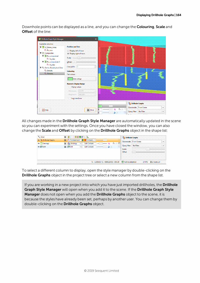
Displaying Drillhole Graphs | 164
Downhole points can be displayed as a line, and you can change theColouring, Scale andOffset of the line:
All changesmade in theDrillhole Graph Style Manager are automatically updated in the sceneso you can experiment with the settings. Once you have closed thewindow, you can alsochange the Scale and Offset by clicking on theDrillhole Graphs object in the shape list:
To select a different column to display, open the stylemanager by double-clicking on theDrillhole Graphs object in the project tree or select a new column from the shape list.
If you are working in a new project intowhich you have just imported drillholes, theDrillholeGraph Style Manager will open when you add it to the scene. If theDrillhole Graph StyleManager does not open when you add theDrillhole Graphs object to the scene, it isbecause the styles have already been set, perhaps by another user. You can change thembydouble-clicking on theDrillhole Graphs object.
© 2019 Seequent Limited
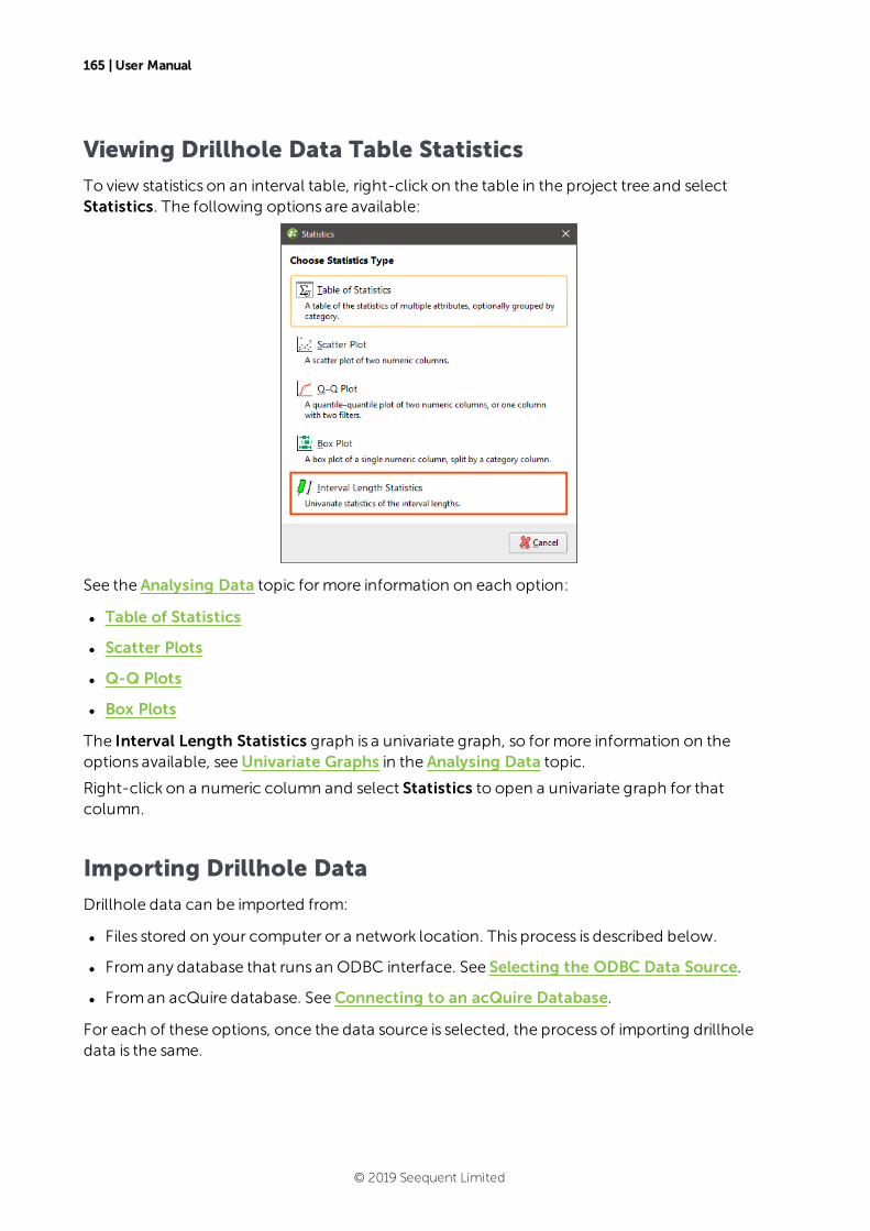
165 | User Manual
Viewing Drillhole Data Table Statistics
To view statistics on an interval table, right-click on the table in the project tree and selectStatistics. The following options are available:
See the Analysing Data topic formore information on each option:
l Table of Statistics
l Scatter Plots
l Q-Q Plots
l Box Plots
The Interval Length Statistics graph is a univariate graph, so formore information on theoptions available, seeUnivariate Graphs in the Analysing Data topic.
Right-click on a numeric column and select Statistics to open a univariate graph for thatcolumn.
Importing Drillhole Data
Drillhole data can be imported from:
l Files stored on your computer or a network location. This process is described below.
l Fromany database that runs an ODBC interface. See Selecting the ODBC Data Source.
l Froman acQuire database. SeeConnecting to an acQuire Database.
For each of these options, once the data source is selected, the process of importing drillholedata is the same.
© 2019 Seequent Limited
Expected Drillhole Data Tables and Columns | 166
The rest of this topic discusses the data format required and the steps for importing drillholedata. It is divided into:
l Expected Drillhole Data Tables and Columns
l Selecting Files
l Working Through the Data
Expected Drillhole Data Tables and Columns
Leapfrog Geo expects drillhole data that is stored in a collar table, a survey table and at leastone interval table. A screens table can be imported if you have the Hydrogeology extension.
The following formats are supported:
l CSV Text File (*.csv)
l ASCII Text File (*.asc)
l Plain Text Files (*.txt)
l Data Files (*.dat)
l TSV Text Files (*.tsv)
The Collar Table
The collar table should contain five columns:
l A drillhole identifier
l The location of the drillhole in X, Y and Z coordinates
l Themaximumdepth of the drillhole
A collar table can also contain a trench column, and collarsmarked as trencheswill bedesurveyed in a manner different fromother drillholes. SeeDrillhole Desurveying Options formore information.
Leapfrog Geo expects a 0 for a normal hole and a 1 for a trench. If there is no trench columnin the collar table, Leapfrog Geowill create one.
The drillhole ID is used to associate data in different tableswith a single drillhole. The ID for adrillholemust be identical in all tables in order for data to be associated with that drillhole.Inconsistencies in theway drillholes are identified are common sources of errors.
Themaximumdepth column is optional. If it is present, is used to validate the data imported forthe interval tables. Themaximumdepth specified is often a planned quantity, whereas theinterval table records actual measurements. For this reason, Leapfrog Geo has an option forfixing themaximumdepth value in the collar table tomatch the data in an interval table.
If maximumdepth information is not included in a collar file, Leapfrog Geowill determine itfrom themaximumdepth sampled as indicated by data in the interval tables.
© 2019 Seequent Limited
167 | User Manual
The Survey Table
For the survey table, Leapfrog Geo expects a minimumof four columns:
l A drillhole identifier
l Depth, dip and azimuth values
By default, Leapfrog Geo assumes that negative dip values point up. If this is not the case, ticktheNegative survey dip points down option.
SeeDrillhole Desurveying Options formore information on the drillhole desurveyingalgorithmsused in Leapfrog Geo.
The Screens Table
A screens table can only be imported if you have the Hydrogeology extension.
For the screens table, Leapfrog Geo expects a minimumof four columns:
l A drillhole identifier
l Start/fromand end/to depths
l A value column
Interval Tables
For interval tables, Leapfrog Geo expects, at minimum, four columns:
l A drillhole identifier
l Start/fromand end/to depths
l A column of measurements
If a drillhole ID in an interval table does not correspond to one in the collar table, the table canstill be imported but the interval table will contain errors.
Supported column types are:
l Lithology columns containing lithologic data, which can be used for geological modelling.
l Numeric columns containing numeric values, which can be used for interpolating data.
l Category columns, which is text representing categories such as company, geologist, ormineralisation.
l Text columns containing text data that is not categorical, such as comments. Text columnsare not validated when imported.
l Date columns containing date data. Customdate and timestamps formats are supported.
l URL columns. Use the prefix file:/// to link to local files.
© 2019 Seequent Limited

Selecting Files | 168
When an interval table is displayed in the scene and an interval is selected, clicking on a link inthe URL column will open the link. This is a useful way of linking to, for example, data files orcore photo images fromwithin Leapfrog Geo:
Selecting Files
To import drillhole data, right-click on theDrillhole Data folder and select Import Drillholes.The Import Drillhole Datawindowwill appear:
For theCollar, click on the Browse button to locate the collar file.
When a collar file is added to the Import Drillhole Datawindow, Leapfrog Geowill look forinterval tableswith names such as “lithology” or “geology” in the same location and will addthem to the Interval Tables list. If an interval table file is not automatically added to the list,clickAdd and browse for the required file.
If you have the Hydrogeology extension, you can also add any screens to import by clicking onthe Screens – Browse button.
© 2019 Seequent Limited
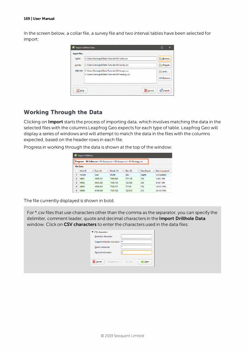
169 | User Manual
In the screen below, a collar file, a survey file and two interval tables have been selected forimport:
Working Through the Data
Clicking on Import starts the process of importing data, which involvesmatching the data in theselected fileswith the columns Leapfrog Geo expects for each type of table. Leapfrog Geowilldisplay a series of windows and will attempt tomatch the data in the fileswith the columnsexpected, based on the header rows in each file.
Progress in working through the data is shown at the top of thewindow:
The file currently displayed is shown in bold.
For *.csv files that use characters other than the comma as the separator, you can specify thedelimiter, comment leader, quote and decimal characters in the Import Drillhole Datawindow. Click on CSV characters to enter the characters used in the data files:
© 2019 Seequent Limited
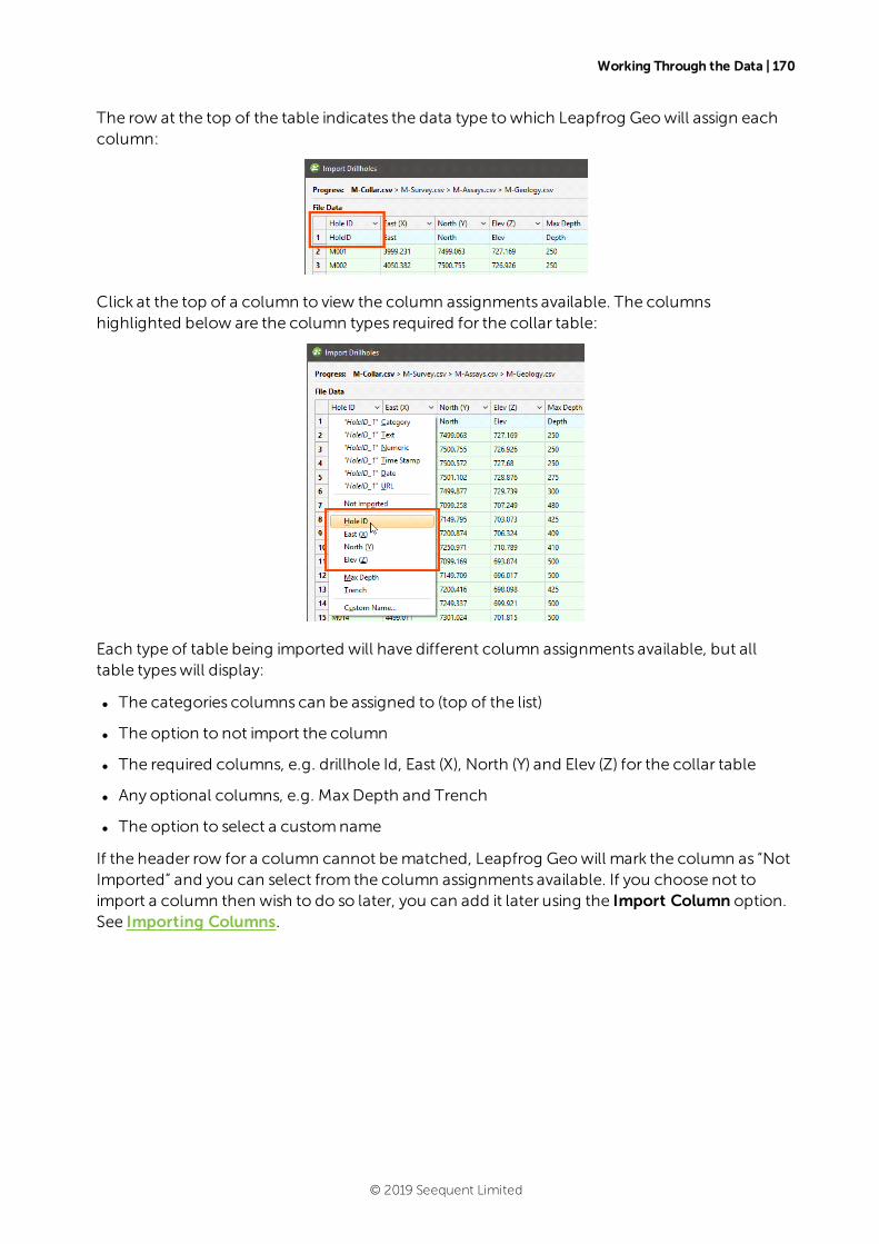
Working Through the Data | 170
The row at the top of the table indicates the data type towhich Leapfrog Geowill assign eachcolumn:
Click at the top of a column to view the column assignments available. The columnshighlighted below are the column types required for the collar table:
Each type of table being imported will have different column assignments available, but alltable typeswill display:
l The categories columns can be assigned to (top of the list)
l The option to not import the column
l The required columns, e.g. drillhole Id, East (X), North (Y) and Elev (Z) for the collar table
l Any optional columns, e.g. Max Depth and Trench
l The option to select a customname
If the header row for a column cannot bematched, Leapfrog Geowill mark the column as “NotImported” and you can select from the column assignments available. If you choose not toimport a column then wish to do so later, you can add it later using the Import Column option.See Importing Columns.
© 2019 Seequent Limited
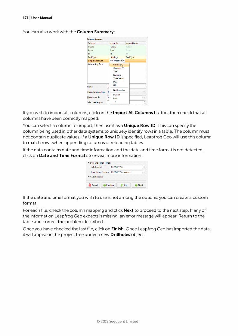
171 | User Manual
You can alsoworkwith theColumn Summary:
If you wish to import all columns, click on the Import All Columns button, then check that allcolumnshave been correctlymapped.
You can select a column for import, then use it as a Unique Row ID. This can specify thecolumn being used in other data systems to uniquely identify rows in a table. The columnmustnot contain duplicate values. If a Unique Row ID is specified, Leapfrog Geowill use this columntomatch rowswhen appending columnsor reloading tables.
If the data contains date and time information and the date and time format is not detected,click on Date and Time Formats to reveal more information:
If the date and time format you wish to use is not among the options, you can create a customformat.
For each file, check the columnmapping and clickNext to proceed to the next step. If any ofthe information Leapfrog Geo expects ismissing, an errormessagewill appear. Return to thetable and correct the problemdescribed.
Once you have checked the last file, click on Finish. Once Leapfrog Geo has imported the data,it will appear in the project tree under a new Drillholes object.
© 2019 Seequent Limited
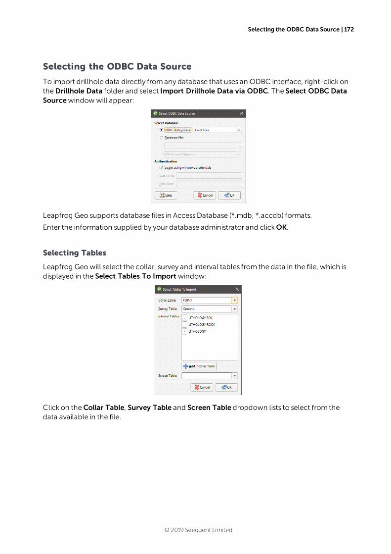
Selecting the ODBC Data Source | 172
Selecting the ODBC Data Source
To import drillhole data directly fromany database that uses an ODBC interface, right-click ontheDrillhole Data folder and select Import Drillhole Data via ODBC. The Select ODBC DataSourcewindowwill appear:
Leapfrog Geo supports database files in AccessDatabase (*.mdb, *.accdb) formats.
Enter the information supplied by your database administrator and clickOK.
Selecting Tables
Leapfrog Geowill select the collar, survey and interval tables from the data in the file, which isdisplayed in the Select Tables To Import window:
Click on theCollar Table, Survey Table and Screen Table dropdown lists to select from thedata available in the file.
© 2019 Seequent Limited
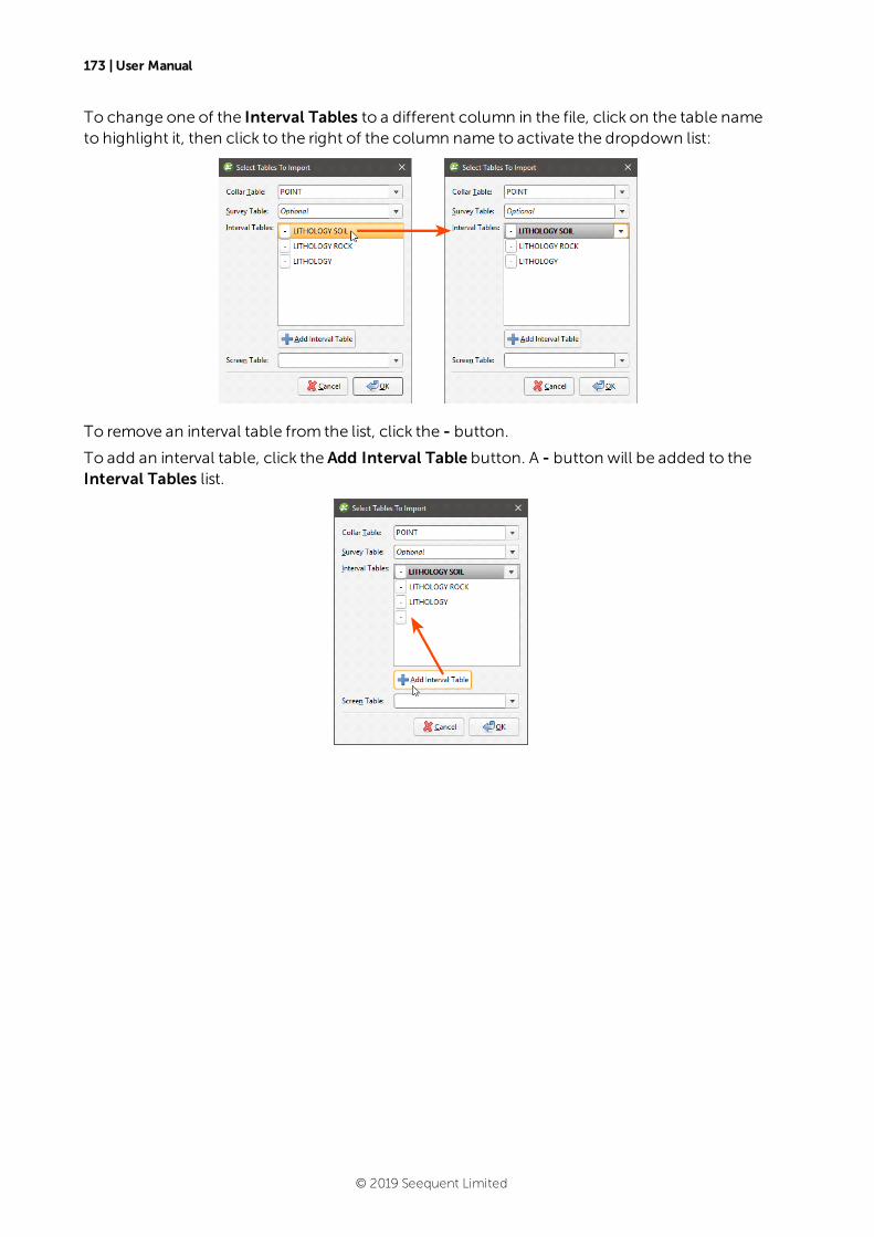
173 | User Manual
To change one of the Interval Tables to a different column in the file, click on the table nameto highlight it, then click to the right of the column name to activate the dropdown list:
To remove an interval table from the list, click the - button.
To add an interval table, click the Add Interval Table button. A - button will be added to theInterval Tables list.
© 2019 Seequent Limited
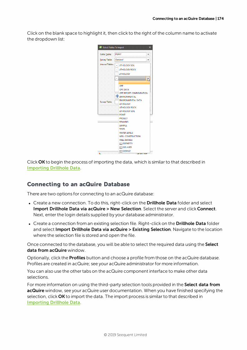
Connecting to an acQuire Database | 174
Click on the blank space to highlight it, then click to the right of the column name to activatethe dropdown list:
ClickOK to begin the process of importing the data, which is similar to that described inImporting Drillhole Data.
Connecting to an acQuire Database
There are two options for connecting to an acQuire database:
l Create a new connection. To do this, right-click on theDrillhole Data folder and selectImport Drillhole Data via acQuire > New Selection. Select the server and clickConnect.Next, enter the login details supplied by your database administrator.
l Create a connection froman existing selection file. Right-click on theDrillhole Data folderand select Import Drillhole Data via acQuire > Existing Selection. Navigate to the locationwhere the selection file is stored and open the file.
Once connected to the database, you will be able to select the required data using the Selectdata from acQuirewindow.
Optionally, click the Profiles button and choose a profile from those on the acQuire database.Profiles are created in acQuire; see your acQuire administrator formore information.
You can also use the other tabs on the acQuire component interface tomake other dataselections.
Formore information on using the third-party selection tools provided in the Select data fromacQuirewindow, see your acQuire user documentation. When you have finished specifying theselection, clickOK to import the data. The import process is similar to that described inImporting Drillhole Data.
© 2019 Seequent Limited
175 | User Manual
Once the drillhole data has been loaded, you can:
l Import additional interval tables. See Importing Interval Tables.
l Update the drillhole data with new data from the acQuire database. See Smart Refresh.
l Reload drillhole data. SeeReloading Drillhole Data.
Smart Refresh
Smart Refresh obtains the latest drillhole data from the acQuire databasewithout reloadingthe entire contents of the database. This reduces the amount of data transfer required andspeeds data updated. If any data relating to a drillhole has changed, thewhole drillhole isupdated. Any new drillholes in the database can be added.
Right-click on theDrillholes object in the project tree and select Smart Refresh. The Selectdata from acQuirewindowwill appear.
If the current data selection settings include data changes, you can clickOK and the updateddata will be imported. You may also chose tomodify the data selection settings, which mayappend further data when you clickOK.
Saving a Selection
Saving a selection saves the current acQuire database selection to file for future reuse. You canuse a selection to import the same set of drillhole data in new Leapfrog Geo projects.
To save an acQuire selection, right-click on theDrillholes object in the project tree and selectSave Selection. You will be prompted for a filename and location.
Appending Drillholes
If drillhole data is stored in multiple files or new drillhole data is available, you can import otherfiles into the project and add them to the existing drillhole data. To do this, right-click on theDrillholes object and select Append Drillholes.
Append drillhole data when you have new drillholes or wish to add extra length to existingdrillholes. If you wish to refresh drillhole data, overwriting all existing drillhole data, use theReload Drillholes option.
The Append Drillholes windowwill be displayed. Appending drillhole data is similar toimporting the original data (see Importing Drillhole Data):
l If the drillhole data was loaded froma file on your computer or a network location, you willbe asked to specify the file locations. Step through the files, checking theColumn Summaryfor each file to ensure that the correct information will be imported, then click Finish to addthe new files.
l If the interval table is stored in an ODBC database, you will be prompted to connect to thedatabase. See Selecting the ODBC Data Source.
© 2019 Seequent Limited

Importing Interval Tables | 176
l If your drillhole data is stored in an acQuire database, you will be prompted to connect to thedatabase. SeeConnecting to an acQuire Database.
Importing Interval Tables
Interval tables that have not been imported during the drillhole data import process can beadded to the project at any time. To add an interval table, right-click on theDrillholes object inthe project tree and select from the options available:
l If the interval table is stored in a file on your computer or a network location, select ImportFrom File > Interval Values. Leapfrog Geowill ask you to specify the file location, and thenwill display the data in the file in the Import Intervalwindow.
l If the interval table is stored in an ODBC database, select Import From ODBC > IntervalValues. You will be prompted to select the data source. See Selecting the ODBC DataSource.
l If your drillhole data is stored in an acQuire database, select Import From acQuire > IntervalValues. SeeConnecting to an acQuire Database.
Columns required are:
l A drillhole identifier
l Start/fromand end/to depths
l A column of measurements
See Expected Drillhole Data Tables and Columns formore information on the supportedcolumn types.
Select the required columns and assign the data type for each column. Click Finish to importthe file, which will appear under theDrillholes object.
Importing Columns
Columnsof an interval table that have not been imported during the drillhole data import orthat are stored in a separate file can be added to the table at any time. To do this, right-click onthe interval table in the project tree and selectNew Column > Import Column.
Importing a column is similar to importing interval tables themselves. Leapfrog Geowill ask youto specify the file location, and then will display the data in the file in the Add Column To Tablewindow. Select asmany columns to import as required and assign the appropriate data type.Before finishing, check theColumn Summary to ensure that the correct information will beimported.
It is not necessary to re-import any columns that are already part of the project. The drillhole IDand To and Fromdata columns, however, will be used to check the validity of the new columnagainst existing data. Any rows that do not match will not be imported.
Click Finish to import the new column.
© 2019 Seequent Limited
177 | User Manual
Importing Screens
This feature is only available with the Hydrogeology extension. See Flow Models formoreinformation.
Screens that have not been imported during the drillhole data import process can be added tothe project at any time. To do this, right-click on theDrillholes object in the project tree andselect Import From File > Screens or Import From ODBC > Screens.
When importing froma file, Leapfrog Geowill ask you to specify the file location, and then willdisplay the data in the file in the Import Screenwindow.
When importing fromODBC, you will first be prompted to select the data source. See Selectingthe ODBC Data Source.
Columns required are:
l A drillhole identifier
l Start/fromand end/to depths
l A value column
Select the required columns and assign the data type for each column. Click Finish to importthe file, which will appear under theDrillholes object.
A Leapfrog Geo project can have only one screens table.
Importing Point Values Down Drillholes
To import a set of points on drillholes, right-click on theDrillholes object in the project tree andselect Import From File > Point Values or Import From ODBC > Point Values.
When importing froma file, Leapfrog Geowill ask you to specify the file location and then willdisplay the data in the file in the Import Depth Points window.
When importing fromODBC, you will first be prompted to select the data source. See Selectingthe ODBC Data Source.
Columns required are:
l A drillhole identifier
l Depth
Select the required columns and assign the data type for each column. Click Finish to importthe file, which will appear under theDrillholes object.
Importing LAS Points Down Drillholes
Leapfrog Geo imports LAS points down drillholes in LAS 1.2 and LAS 2.0 formats. An importedset of LAS files appears as one object with its associated data columnsplus a LAS Drillholesfolder that contains a filter for each drillhole. Importing the data preserves themetadata fromthe LAS files, which can be viewed in the Properties window for the LAS points object and in theProperties window for each drillhole.
© 2019 Seequent Limited

LAS File Mapping | 178
To import LAS points down drillholes, right-click on theDrillholes object and select ImportFrom File > LAS Data. Select the files you wish to import and clickOpen.
Next, the Import LAS Datawindowwill appear. The data displayed in thiswindow is combinedfrom the selected files, with blank and invalid values indicated by “nan”. For example, if adrillhole file does not contain columns that are included in other drillhole files, thosemissingcolumnswill bemarked as “nan”.
Leapfrog Geo expects drillhole ID and Depth columns and will attempt tomatch the data in thefileswith the expected format. Select the columns to import, then click Finish. The fileswill beadded to the project tree as part of theDrillholes object, as described above.
To view LAS points, add the LAS points object ( ) to the scene. You can also display individualdrillholes by adding their filters to the scene.
LAS File Mapping
The Properties window for LAS Drillholes includes a LAS Mapping tab that showswhat datafiles have been used for the selected drillhole:
This is useful when data for a drillhole originates in different files.
LAS File Inconsistencies
When importing LAS files, inconsistencies in the files are handled as follows:
l If there are two fileswith the same curve values at the same depth, the duplicate valueswillbe added to the existing column and flagged as overlapping segments. SeeCorrecting DataErrors in Leapfrog Geo formore information about correcting drillhole data errors.
l If there aremore than two fileswith the same curve values at the same depth, Leapfrog Geowill not be able to import the files. Note the conflicting files shown in the errormessage andreimport the files, leaving the conflicting files out.
l If there aremultiple logs of the same name in the files, Leapfrog Geowill not be able toimport the data. Edit the LAS file header outside of Leapfrog Geo to change the names.
© 2019 Seequent Limited
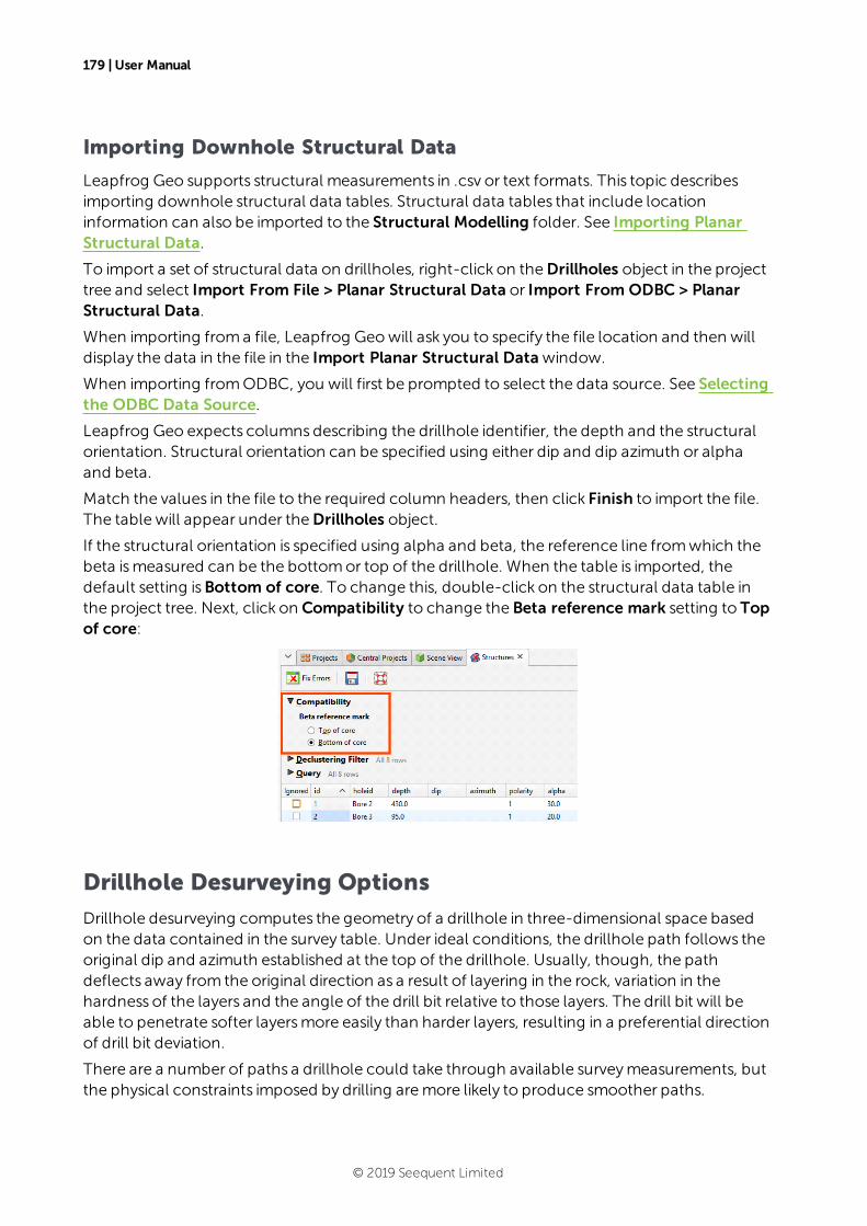
179 | User Manual
Importing Downhole Structural Data
Leapfrog Geo supports structural measurements in .csv or text formats. This topic describesimporting downhole structural data tables. Structural data tables that include locationinformation can also be imported to the Structural Modelling folder. See Importing PlanarStructural Data.
To import a set of structural data on drillholes, right-click on theDrillholes object in the projecttree and select Import From File > Planar Structural Data or Import From ODBC > PlanarStructural Data.
When importing froma file, Leapfrog Geowill ask you to specify the file location and then willdisplay the data in the file in the Import Planar Structural Datawindow.
When importing fromODBC, you will first be prompted to select the data source. See Selectingthe ODBC Data Source.
Leapfrog Geo expects columnsdescribing the drillhole identifier, the depth and the structuralorientation. Structural orientation can be specified using either dip and dip azimuth or alphaand beta.
Match the values in the file to the required column headers, then click Finish to import the file.The table will appear under theDrillholes object.
If the structural orientation is specified using alpha and beta, the reference line fromwhich thebeta ismeasured can be the bottomor top of the drillhole. When the table is imported, thedefault setting isBottom of core. To change this, double-click on the structural data table inthe project tree. Next, click on Compatibility to change the Beta reference mark setting to Topof core:
Drillhole Desurveying Options
Drillhole desurveying computes the geometry of a drillhole in three-dimensional space basedon the data contained in the survey table. Under ideal conditions, the drillhole path follows theoriginal dip and azimuth established at the top of the drillhole. Usually, though, the pathdeflects away from the original direction as a result of layering in the rock, variation in thehardness of the layers and the angle of the drill bit relative to those layers. The drill bit will beable to penetrate softer layersmore easily than harder layers, resulting in a preferential directionof drill bit deviation.
There are a number of paths a drillhole could take through available surveymeasurements, butthe physical constraints imposed by drilling aremore likely to produce smoother paths.
© 2019 Seequent Limited

The Spherical Arc Approximation Algorithm | 180
Selecting the desurveying method that gives the best likely approximation of the actual path ofthe drillhole will ensure that subsequent modelling is as accurate as possible.
Leapfrog Geo implements three algorithms for desurveying drillholes:
l The Spherical Arc Approximation Algorithm
l The Raw Tangent Algorithm
l The Balanced Tangent Algorithm
These options are described in more detail below.
Another factor that affects how drillholes are desurveyed is how dip values are handled. Whenthe survey table is imported, Leapfrog Geo sets theNegative survey dip points down valueaccording to the data in the imported table. When themajority of the dip data in the table ispositive, Leapfrog Geo assumes all these drillholeswill point down and leaves the field Negativesurvey dip points down disabled. Whenmost of the values are negative, the field is enabled.This field can be changed by double-clicking on the survey table to open it and then clicking onCompatibility to show the table’s desurveying settings:
If you are going to change the automatically set value of Negative survey dip points down,consider carefully the implications if there is a mix of drillholes pointing down and up.
The otherCompatibility setting relates to the algorithmused in desurveying the drillholes.
The Spherical Arc Approximation Algorithm
The default algorithmused in Leapfrog Geo is spherical arc approximation, which is sometimesreferred to as theminimumcurvature algorithm. Downhole distances are desurveyed exactly asdistances along a circular arc:
© 2019 Seequent Limited
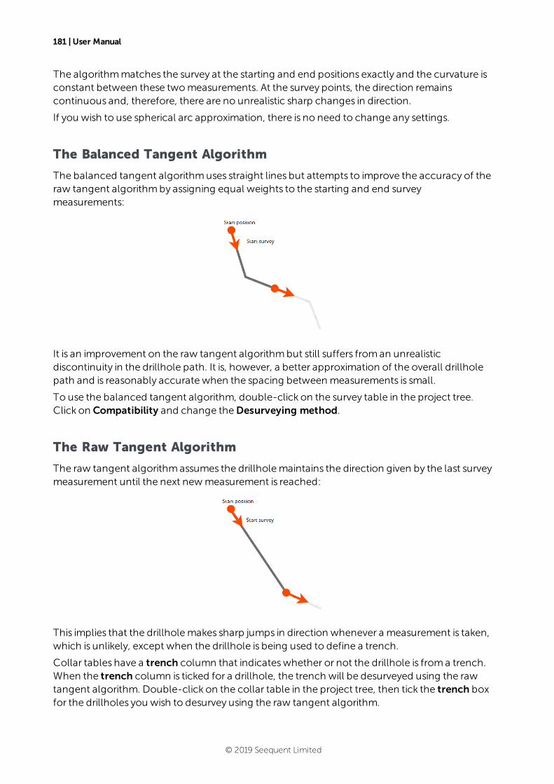
181 | User Manual
The algorithmmatches the survey at the starting and end positions exactly and the curvature isconstant between these twomeasurements. At the survey points, the direction remainscontinuous and, therefore, there are no unrealistic sharp changes in direction.
If you wish to use spherical arc approximation, there is no need to change any settings.
The Balanced Tangent Algorithm
The balanced tangent algorithmuses straight lines but attempts to improve the accuracy of theraw tangent algorithmby assigning equal weights to the starting and end surveymeasurements:
It is an improvement on the raw tangent algorithmbut still suffers froman unrealisticdiscontinuity in the drillhole path. It is, however, a better approximation of the overall drillholepath and is reasonably accurate when the spacing betweenmeasurements is small.
To use the balanced tangent algorithm, double-click on the survey table in the project tree.Click on Compatibility and change theDesurveying method.
The Raw Tangent Algorithm
The raw tangent algorithmassumes the drillholemaintains the direction given by the last surveymeasurement until the next newmeasurement is reached:
This implies that the drillholemakes sharp jumps in direction whenever a measurement is taken,which is unlikely, except when the drillhole is being used to define a trench.
Collar tables have a trench column that indicateswhether or not the drillhole is froma trench.When the trench column is ticked for a drillhole, the trench will be desurveyed using the rawtangent algorithm. Double-click on the collar table in the project tree, then tick the trench boxfor the drillholes you wish to desurvey using the raw tangent algorithm.
© 2019 Seequent Limited
Processing Drillhole Data | 182
Processing Drillhole Data
Once imported and corrected, drillhole data usually requires further processing before anymodels are built. Use the techniques described in Displaying Drillholes and DrillholeCorrelation Tool to aid in making decisions on what further processing is required.
Often, selecting a small portion of intervals can be achieved using a query filter (see theQueryFilters topic). In some cases, however, you maywish to composite data to focus on a single unit.Theremay also be issueswith how drillhole data has been recorded; for example, two unitshave been catalogued as one, or a single unit may be divided intomultiple units.
Leapfrog Geo has a number of tools for processing drillhole data, including:
l Category Composites. Sometimes unit boundaries are poorly defined, with fragments ofother lithologieswithin the lithology of interest. This can result in very small segments nearthe edges of the lithology of interest. Modelling the fine detail is not always necessary, and socompositing can be used to smooth these boundaries.
l Economic Composites. Economic compositing classifies assay data into “ore” and “waste”categories, taking into account grade thresholds, mining dimensions and allowable internaldilution. The result is an interval table with a column of ore/waste category data and acolumn of composited interval values, plus some additional columns showing the length,linear grade, included dilution length and included dilution grade.
l Majority Composites. Category data can be composited into interval lengths fromanothertable or into fixed interval lengths. The compositing is based on a majority percentagewhereeach interval is assigned a category based on the category that makes up the highestpercentage of the new interval.
l Numeric Composites. Compositing numeric data takes unevenly-spaced drillhole data andturns it into regularly-spaced data, which is then interpolated. Numeric data can becomposited along the entire drillhole or in selected regions. You can also set thecompositing length from the base interval table.
l Grouping Lithologies. The group lithologies tool lets you define a new unit to which existingunits are added. For example, a sandstone deposit might appear in an interval table aspoorly-sorted and well-sorted units. The group lithologies tool lets you group both unitsinto a single sandstone unit.
l Splitting Lithologies. Lithology unitsmay be incorrectly grouped, which can becomeapparent when you display drillholes in the scene. The split lithologies tool lets you createnew units by selecting from intervals displayed in the scene.
l Interval Selection. If the lithologies in a column are poorly sorted, you can display thecolumn in the scene and use the interval selection tool to workwith all the segments andsort them into new units.
l Overlaid Lithology Column. You may have two versions of an interval column, one thatcontains draft data and one that contains the final version. The final version may containgaps, which can be filled in using the draft version. The overlaid lithology tool lets youcombine the two columns to create a new column.
© 2019 Seequent Limited

183 | User Manual
l Category Column from Numeric Data. When you have numeric data you wish to usewiththe lithology and categorymodelling tools, you can convert the numeric data to a categorycolumn.
l Back-Flagging Drillhole Data. Evaluating geological models on drillholes creates a newlithology table containing the lithologies from the selected model.
Each of these tools creates a new interval table or creates a new column in an existing intervaltable, preserving the original data. New tables and columns can be used as the basis for newmodels in the project and can be incorporated into existing models using From Other Contactsoptions. When a new table is created, you can view it in the scene along with the original tableto see the differences between the processed and the unprocessed data.
If you are working with columns in different interval tables, you can create a newmerged tablethat includes columns from these different tables. Columns created in Leapfrog Geo can beincluded in a merged table. SeeMerged Drillhole Data Tables.
Category Composites
Sometimes unit boundaries are poorly defined, with fragments of other lithologieswithin thelithology of interest. This can result in very small segments near the edges of the lithology ofinterest. Modelling the fine detail is not always necessary, and so compositing can be used tosmooth these boundaries.
In Leapfrog Geo, you can composite category data in twoways:
l Composite the drillhole data directly. This creates a new interval table that can be used tobuild models, and changesmade to the table will be reflected in all models based on thattable. This process is described below.
l Composite the points used to create an object.
© 2019 Seequent Limited
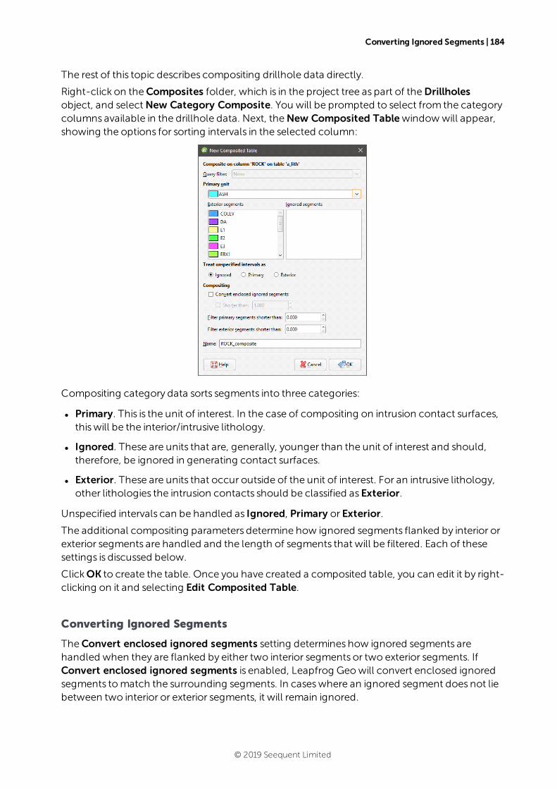
Converting Ignored Segments | 184
The rest of this topic describes compositing drillhole data directly.
Right-click on theComposites folder, which is in the project tree as part of theDrillholesobject, and selectNew Category Composite. You will be prompted to select from the categorycolumns available in the drillhole data. Next, theNew Composited Tablewindowwill appear,showing the options for sorting intervals in the selected column:
Compositing category data sorts segments into three categories:
l Primary. This is the unit of interest. In the case of compositing on intrusion contact surfaces,thiswill be the interior/intrusive lithology.
l Ignored. These are units that are, generally, younger than the unit of interest and should,therefore, be ignored in generating contact surfaces.
l Exterior. These are units that occur outside of the unit of interest. For an intrusive lithology,other lithologies the intrusion contacts should be classified asExterior.
Unspecified intervals can be handled as Ignored, Primary or Exterior.
The additional compositing parameters determine how ignored segments flanked by interior orexterior segments are handled and the length of segments that will be filtered. Each of thesesettings is discussed below.
ClickOK to create the table. Once you have created a composited table, you can edit it by right-clicking on it and selecting Edit Composited Table.
Converting Ignored Segments
TheConvert enclosed ignored segments setting determines how ignored segments arehandled when they are flanked by either two interior segments or two exterior segments. IfConvert enclosed ignored segments is enabled, Leapfrog Geowill convert enclosed ignoredsegments tomatch the surrounding segments. In caseswhere an ignored segment does not liebetween two interior or exterior segments, it will remain ignored.
© 2019 Seequent Limited
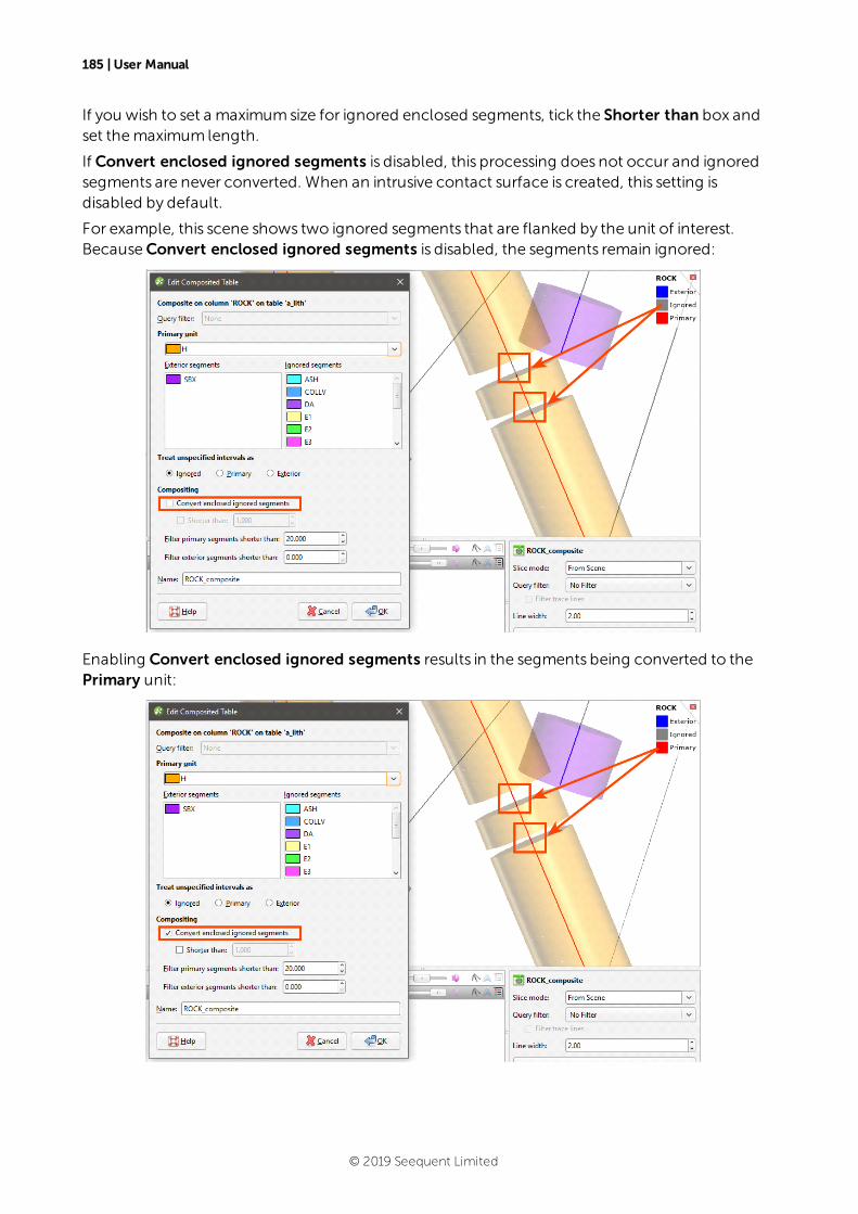
185 | User Manual
If you wish to set a maximumsize for ignored enclosed segments, tick the Shorter than box andset themaximum length.
If Convert enclosed ignored segments is disabled, this processing does not occur and ignoredsegments are never converted. When an intrusive contact surface is created, this setting isdisabled by default.
For example, this scene shows two ignored segments that are flanked by the unit of interest.BecauseConvert enclosed ignored segments is disabled, the segments remain ignored:
Enabling Convert enclosed ignored segments results in the segments being converted to thePrimary unit:
© 2019 Seequent Limited
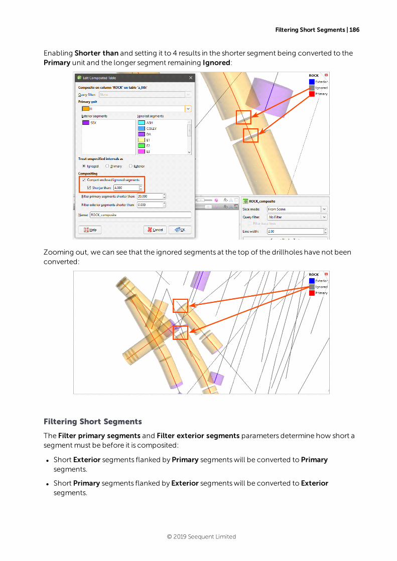
Filtering Short Segments | 186
Enabling Shorter than and setting it to 4 results in the shorter segment being converted to thePrimary unit and the longer segment remaining Ignored:
Zooming out, we can see that the ignored segments at the top of the drillholes have not beenconverted:
Filtering Short Segments
The Filter primary segments and Filter exterior segments parameters determine how short asegment must be before it is composited:
l Short Exterior segments flanked byPrimary segmentswill be converted to Primarysegments.
l Short Primary segments flanked by Exterior segmentswill be converted to Exteriorsegments.
© 2019 Seequent Limited
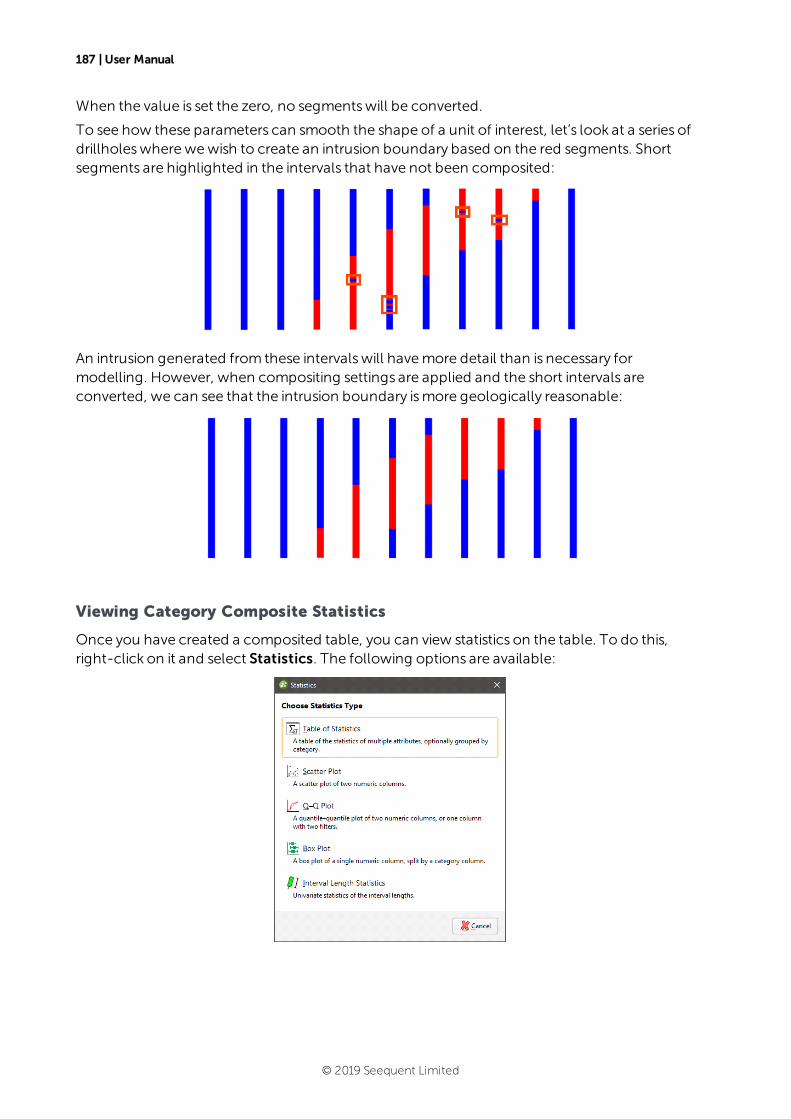
187 | User Manual
When the value is set the zero, no segmentswill be converted.
To see how these parameters can smooth the shape of a unit of interest, let’s look at a series ofdrillholeswherewewish to create an intrusion boundary based on the red segments. Shortsegments are highlighted in the intervals that have not been composited:
An intrusion generated from these intervalswill havemore detail than is necessary formodelling. However, when compositing settings are applied and the short intervals areconverted, we can see that the intrusion boundary ismore geologically reasonable:
Viewing Category Composite Statistics
Once you have created a composited table, you can view statistics on the table. To do this,right-click on it and select Statistics. The following options are available:
© 2019 Seequent Limited

Economic Composites | 188
See the Analysing Data topic formore information on each option:
l Table of Statistics
l Scatter Plots
l Q-Q Plots
l Box Plots
The Interval Length Statistics graph is a univariate graph, so formore information on theoptions available, seeUnivariate Graphs in the Analysing Data topic.
Economic Composites
Economic compositing classifies assay data into “ore” and “waste” categories, taking intoaccount grade thresholds, mining dimensions and allowable internal dilution. The result is aninterval table with a column of ore/waste category data and a column of composited intervalvalues, plus some additional columns showing the length, linear grade, included dilutionlength, included dilution grade and the percentage of the composite that is based onmissing(and then filled) interval data.
Economic compositing is primarily an input into themodelling of geometry rather than themodelling of grade. Whereas numeric compositing transforms variable length assay intervalsinto consistent intervalswith a common support length, economic composite intervals can beof any length, with the composited lengths always coinciding with the end of an assay interval.One common use for economic compositing is to generate a reasonablemineralised envelopefrom “ore” intervals, which has the benefit of being built on both mineability parameters andcut-off grade.
Economic compositing is based on a set cut-off grade, such that values that are greater than orequal to the cut-off value are considered “Ore” and values below are considered “Waste”.Adjacent intervals on the same side of the cut-off grade are concatenated, producing a series ofalternating ore and waste segments. The alternating waste and ore segments are thencomposited, with the segments being considered for incremental addition to an ore compositesequentially down each drillhole. Although the compositing process produces both ore andwaste composites, it only attempts to build ore composites. Waste composites are producedwhen a composite fails tomeet the constraints required for an ore composite, or as initial or finalsegments.
The rest of this topic describes creating and working with economic composites. It is dividedinto:
l Creating an Economic Composite
l Selecting Values
l Handling Missing Intervals and High Grades
l Selecting a Dilution Rule
l Setting the Cut-Off Grade
l Two-Pass Compositing
l Using True Thickness
© 2019 Seequent Limited
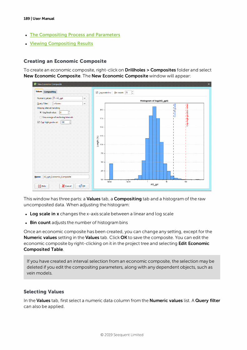
189 | User Manual
l The Compositing Process and Parameters
l Viewing Compositing Results
Creating an Economic Composite
To create an economic composite, right-click on Drillholes > Composites folder and selectNew Economic Composite. TheNew Economic Compositewindowwill appear:
Thiswindow has three parts: a Values tab, a Compositing tab and a histogramof the rawuncomposited data. When adjusting the histogram:
l Log scale in x changes the x-axis scale between a linear and log scale
l Bin count adjusts the number of histogrambins
Once an economic composite has been created, you can change any setting, except for theNumeric values setting in the Values tab. ClickOK to save the composite. You can edit theeconomic composite by right-clicking on it in the project tree and selecting Edit EconomicComposited Table.
If you have created an interval selection froman economic composite, the selection may bedeleted if you edit the compositing parameters, along with any dependent objects, such asvein models.
Selecting Values
In the Values tab, first select a numeric data column from theNumeric values list. AQuery filtercan also be applied.
© 2019 Seequent Limited
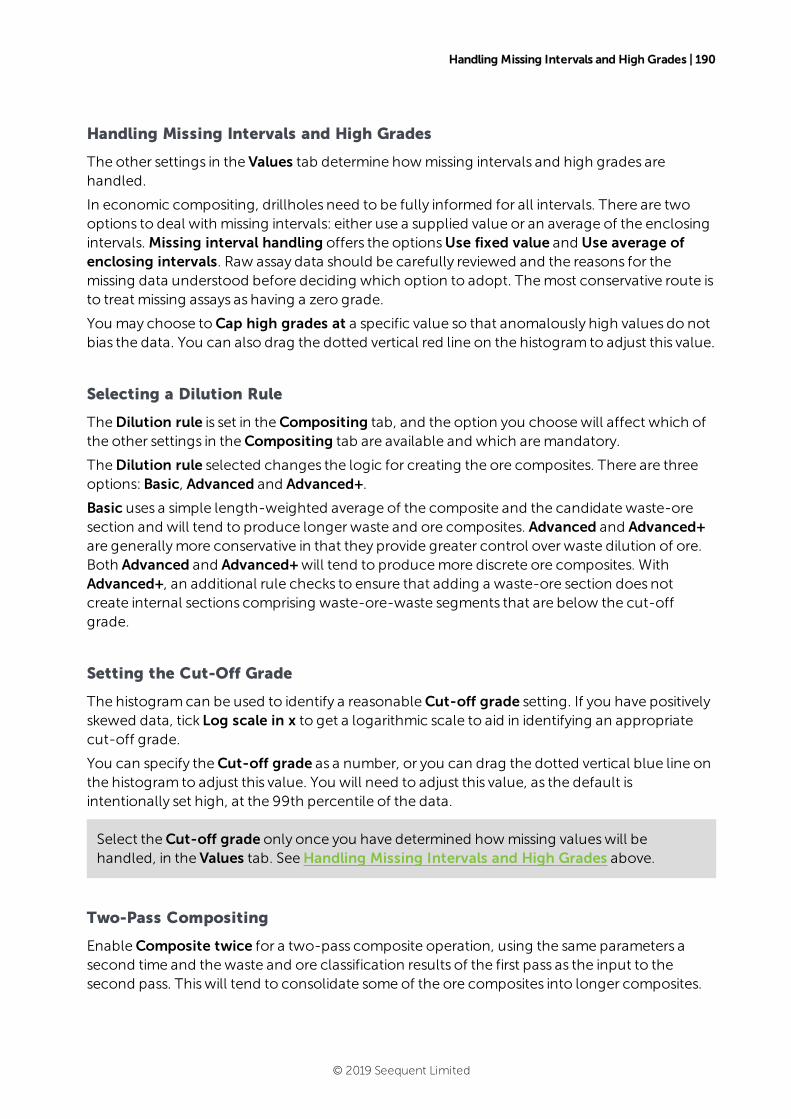
Handling Missing Intervals and High Grades | 190
Handling Missing Intervals and High Grades
The other settings in the Values tab determine howmissing intervals and high grades arehandled.
In economic compositing, drillholes need to be fully informed for all intervals. There are twooptions to deal with missing intervals: either use a supplied value or an average of the enclosingintervals. Missing interval handling offers the optionsUse fixed value and Use average ofenclosing intervals. Raw assay data should be carefully reviewed and the reasons for themissing data understood before deciding which option to adopt. Themost conservative route isto treat missing assays as having a zero grade.
You may choose toCap high grades at a specific value so that anomalously high values do notbias the data. You can also drag the dotted vertical red line on the histogram to adjust this value.
Selecting a Dilution Rule
TheDilution rule is set in theCompositing tab, and the option you choosewill affect which ofthe other settings in theCompositing tab are available and which aremandatory.
TheDilution rule selected changes the logic for creating the ore composites. There are threeoptions:Basic, Advanced and Advanced+.
Basic uses a simple length-weighted average of the composite and the candidate waste-oresection and will tend to produce longerwaste and ore composites. Advanced and Advanced+are generallymore conservative in that they provide greater control over waste dilution of ore.Both Advanced and Advanced+will tend to producemore discrete ore composites. WithAdvanced+, an additional rule checks to ensure that adding a waste-ore section does notcreate internal sections comprising waste-ore-waste segments that are below the cut-offgrade.
Setting the Cut-Off Grade
The histogramcan be used to identify a reasonableCut-off grade setting. If you have positivelyskewed data, tick Log scale in x to get a logarithmic scale to aid in identifying an appropriatecut-off grade.
You can specify theCut-off grade as a number, or you can drag the dotted vertical blue line onthe histogram to adjust this value. You will need to adjust this value, as the default isintentionally set high, at the 99th percentile of the data.
Select theCut-off grade only once you have determined howmissing valueswill behandled, in the Values tab. SeeHandling Missing Intervals and High Grades above.
Two-Pass Compositing
EnableComposite twice for a two-pass composite operation, using the same parameters asecond time and thewaste and ore classification results of the first pass as the input to thesecond pass. Thiswill tend to consolidate some of the ore composites into longer composites.
© 2019 Seequent Limited
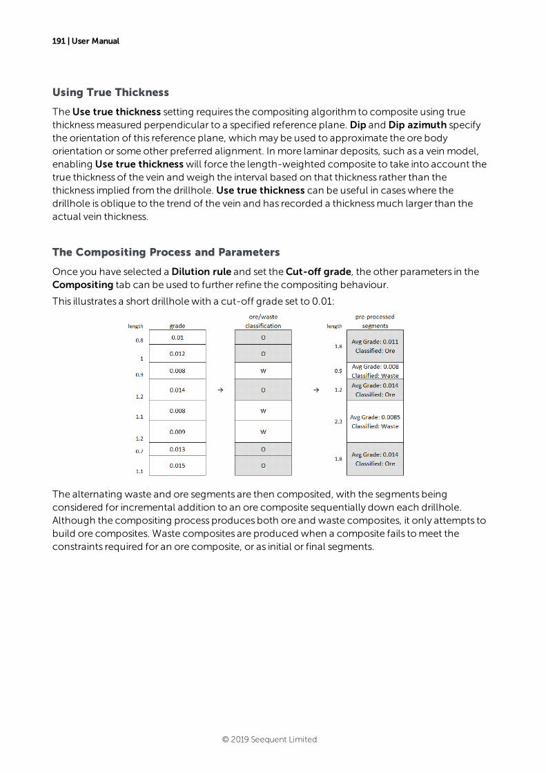
191 | User Manual
Using True Thickness
TheUse true thickness setting requires the compositing algorithm to composite using truethicknessmeasured perpendicular to a specified reference plane. Dip and Dip azimuth specifythe orientation of this reference plane, which may be used to approximate the ore bodyorientation or some other preferred alignment. In more laminar deposits, such as a vein model,enabling Use true thickness will force the length-weighted composite to take into account thetrue thickness of the vein and weigh the interval based on that thickness rather than thethickness implied from the drillhole. Use true thickness can be useful in caseswhere thedrillhole is oblique to the trend of the vein and has recorded a thicknessmuch larger than theactual vein thickness.
The Compositing Process and Parameters
Once you have selected a Dilution rule and set theCut-off grade, the other parameters in theCompositing tab can be used to further refine the compositing behaviour.
This illustrates a short drillhole with a cut-off grade set to 0.01:
The alternating waste and ore segments are then composited, with the segments beingconsidered for incremental addition to an ore composite sequentially down each drillhole.Although the compositing process produces both ore and waste composites, it only attempts tobuild ore composites. Waste composites are produced when a composite fails tomeet theconstraints required for an ore composite, or as initial or final segments.
© 2019 Seequent Limited
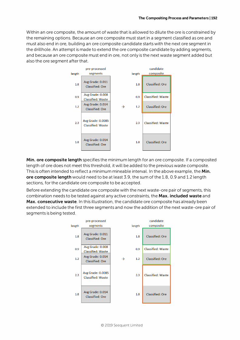
The Compositing Process and Parameters | 192
Within an ore composite, the amount of waste that is allowed to dilute the ore is constrained bythe remaining options. Because an ore compositemust start in a segment classified as ore andmust also end in ore, building an ore composite candidate startswith the next ore segment inthe drillhole. An attempt ismade to extend the ore composite candidate by adding segments,and because an ore compositemust end in ore, not only is the next waste segment added butalso the ore segment after that.
Min. ore composite length specifies theminimum length for an ore composite. If a compositedlength of ore does not meet this threshold, it will be added to the previouswaste composite.This is often intended to reflect a minimummineable interval. In the above example, theMin.ore composite lengthwould need to be at least 3.9, the sumof the 1.8, 0.9 and 1.2 lengthsections, for the candidate ore composite to be accepted.
Before extending the candidate ore composite with the next waste-ore pair of segments, thiscombination needs to be tested against any active constraints, theMax. included waste andMax. consecutive waste. In this illustration, the candidate ore composite has already beenextended to include the first three segments and now the addition of the next waste-ore pair ofsegments is being tested.
© 2019 Seequent Limited
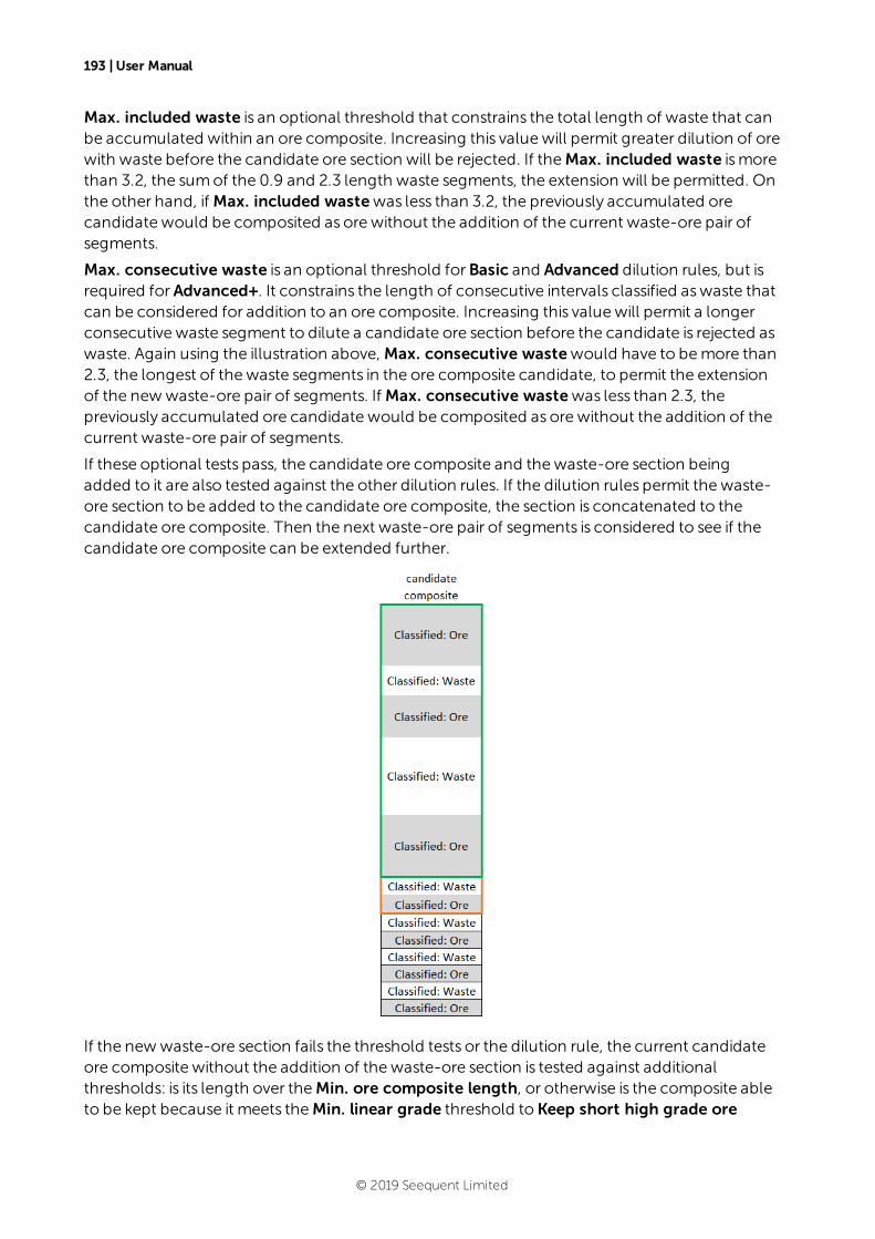
193 | User Manual
Max. included waste is an optional threshold that constrains the total length of waste that canbe accumulated within an ore composite. Increasing this valuewill permit greater dilution of orewith waste before the candidate ore section will be rejected. If theMax. included waste ismorethan 3.2, the sumof the 0.9 and 2.3 length waste segments, the extension will be permitted. Onthe other hand, if Max. included wastewas less than 3.2, the previously accumulated orecandidate would be composited as ore without the addition of the current waste-ore pair ofsegments.
Max. consecutive waste is an optional threshold forBasic and Advanced dilution rules, but isrequired forAdvanced+. It constrains the length of consecutive intervals classified aswaste thatcan be considered for addition to an ore composite. Increasing this valuewill permit a longerconsecutive waste segment to dilute a candidate ore section before the candidate is rejected aswaste. Again using the illustration above, Max. consecutive wastewould have to bemore than2.3, the longest of thewaste segments in the ore composite candidate, to permit the extensionof the newwaste-ore pair of segments. If Max. consecutive wastewas less than 2.3, thepreviously accumulated ore candidate would be composited as ore without the addition of thecurrent waste-ore pair of segments.
If these optional tests pass, the candidate ore composite and thewaste-ore section beingadded to it are also tested against the other dilution rules. If the dilution rules permit thewaste-ore section to be added to the candidate ore composite, the section is concatenated to thecandidate ore composite. Then the next waste-ore pair of segments is considered to see if thecandidate ore composite can be extended further.
If the newwaste-ore section fails the threshold tests or the dilution rule, the current candidateore composite without the addition of thewaste-ore section is tested against additionalthresholds: is its length over theMin. ore composite length, or otherwise is the composite ableto be kept because it meets theMin. linear grade threshold to Keep short high grade ore
© 2019 Seequent Limited

The Compositing Process and Parameters | 194
composites? Keep short high grade ore composites is an option that allowsore compositesshorter than theMin. ore composite length, provided theMin. linear grade is exceeded. Lineargrade is the length * grade. This allows a short length of high economic valuematerial to beclassified as ore and identified. If the current candidate ore composite can meet one of thesethresholds, the ore composite is added to the composite table, thewaste segment of thecurrent waste-ore segment is considered a candidate waste composite, and the ore segment isused to start a new candidate ore composite. If any of these requirements for keeping thecandidate ore composite are not met, the candidate ore composite fails, so thewholecandidate composite is considered a waste composite instead of ore, and is added to anypreceding candidate waste composite, along with the next waste segment in the drillhole.Compositing resumeswith the next ore segment in the drillhole.
© 2019 Seequent Limited

195 | User Manual
Min. waste composite length does not apply to the Basic dilution rule, but is an option forAdvanced and Advanced+. It specifies the preferred minimum length of waste composite. Thisis applied after initial compositing to anywaste composite that is bounded on both sides by ore.Waste composites are expanded into the surrounding ore composites by re-classifying ofadjacent intervals aswaste until theMin. waste composite length is satisfied, in such a way thatloss from the ore composites isminimised. The expansion of thewaste composite is not appliedif it would affect other configured ore requirements such asMin. ore composite length.
In the above illustration, the centre column depicts the initial status of composites prior toassessment against a Min. waste composite length of 20. Because thewaste composite in thecentre with a grade of 10.280 only has a length of 6, thiswaste composite will be expanded,taking segments off the surrounding ore composites. The original segments can be seen in theleft column. Thewaste-ore pair of segments above thewaste composite are added to it, andthe ore-waste pair of segments below it. This gives a length for the expanded waste compositeof 16. Given a Min. ore composite length of 5, the expansion stops, as the ore composite abovethe expanded waste composite has only a single ore segment in it, and if the ore-waste segmentpair below was added to the expanded waste composite thiswould create an ore compositeshorter than theMin. ore composite length.
© 2019 Seequent Limited
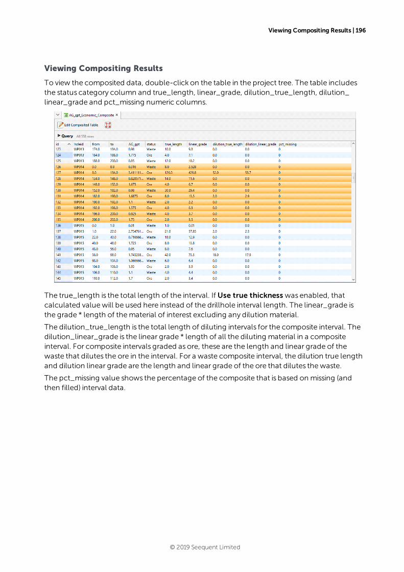
Viewing Compositing Results | 196
Viewing Compositing Results
To view the composited data, double-click on the table in the project tree. The table includesthe status category column and true_length, linear_grade, dilution_true_length, dilution_linear_grade and pct_missing numeric columns.
The true_length is the total length of the interval. If Use true thickness was enabled, thatcalculated valuewill be used here instead of the drillhole interval length. The linear_grade isthe grade * length of thematerial of interest excluding any dilution material.
The dilution_true_length is the total length of diluting intervals for the composite interval. Thedilution_linear_grade is the linear grade * length of all the diluting material in a compositeinterval. For composite intervals graded as ore, these are the length and linear grade of thewaste that dilutes the ore in the interval. For a waste composite interval, the dilution true lengthand dilution linear grade are the length and linear grade of the ore that dilutes thewaste.
The pct_missing value shows the percentage of the composite that is based onmissing (andthen filled) interval data.
© 2019 Seequent Limited

197 | User Manual
It is useful to use the drillhole correlation tool to visualise the resulting composited data. Here anew drillhole correlation has been created with a single selected collar (highlighted in the tableabove), with the source numeric column dragged in from the assay folder, along with the datacolumns from the economic composite.
To learn more about how to use the drillhole correlation tool, seeDrillhole Correlation Tool.
© 2019 Seequent Limited
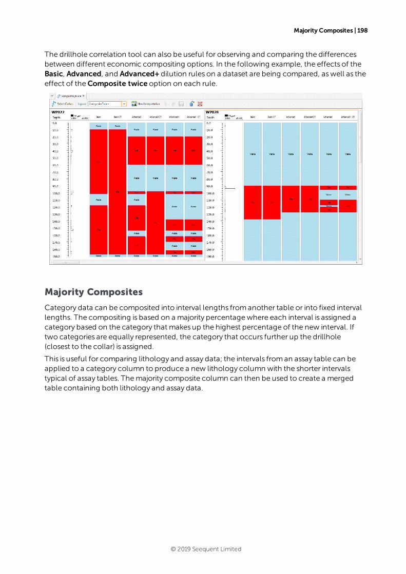
Majority Composites | 198
The drillhole correlation tool can also be useful for observing and comparing the differencesbetween different economic compositing options. In the following example, the effects of theBasic, Advanced, and Advanced+ dilution rules on a dataset are being compared, aswell as theeffect of theComposite twice option on each rule.
Majority Composites
Category data can be composited into interval lengths fromanother table or into fixed intervallengths. The compositing is based on a majority percentagewhere each interval is assigned acategory based on the category that makes up the highest percentage of the new interval. Iftwo categories are equally represented, the category that occurs further up the drillhole(closest to the collar) is assigned.
This is useful for comparing lithology and assay data; the intervals froman assay table can beapplied to a category column to produce a new lithology column with the shorter intervalstypical of assay tables. Themajority composite column can then be used to create a mergedtable containing both lithology and assay data.
© 2019 Seequent Limited
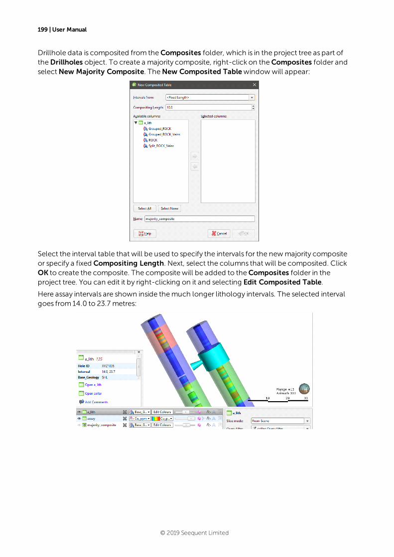
199 | User Manual
Drillhole data is composited from theComposites folder, which is in the project tree as part oftheDrillholes object. To create a majority composite, right-click on theComposites folder andselectNew Majority Composite. TheNew Composited Tablewindowwill appear:
Select the interval table that will be used to specify the intervals for the newmajority compositeor specify a fixed Compositing Length. Next, select the columns that will be composited. ClickOK to create the composite. The composite will be added to theComposites folder in theproject tree. You can edit it by right-clicking on it and selecting Edit Composited Table.
Here assay intervals are shown inside themuch longer lithology intervals. The selected intervalgoes from14.0 to 23.7 metres:
© 2019 Seequent Limited
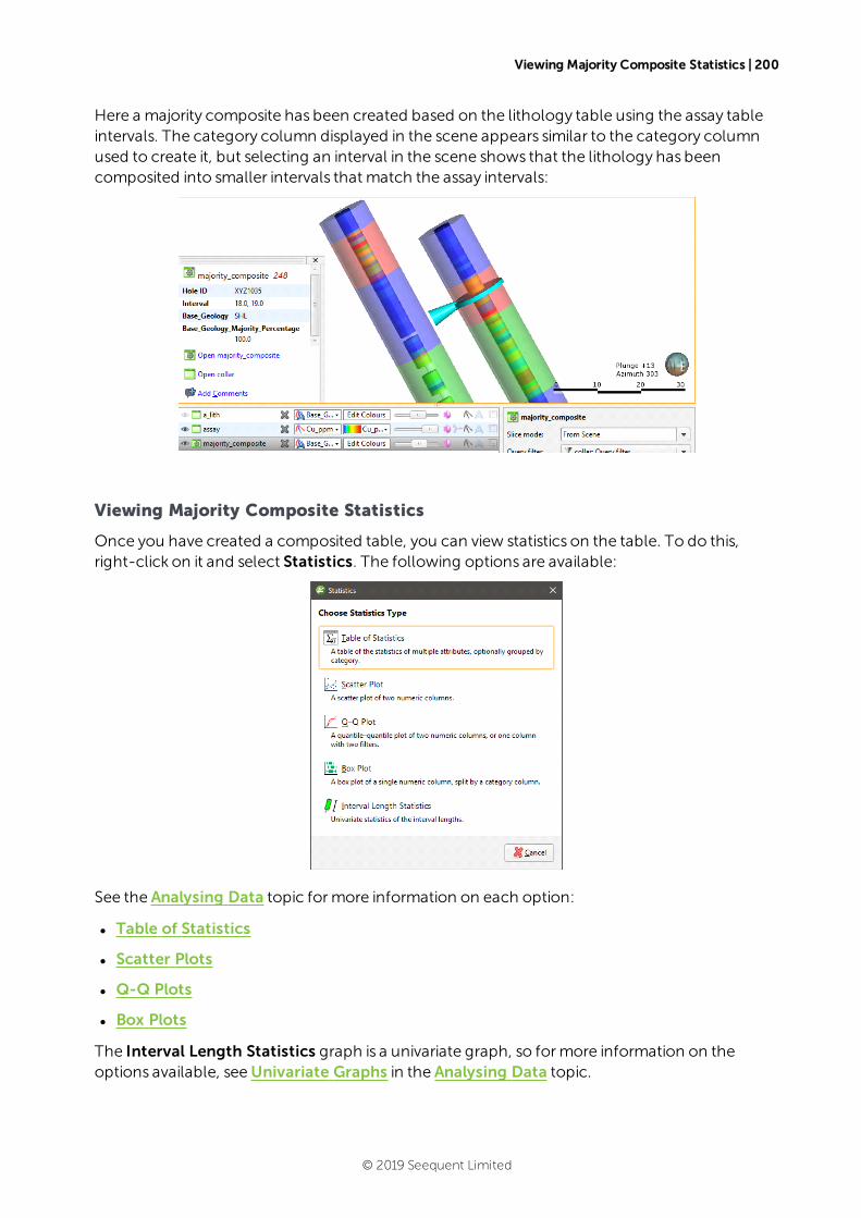
Viewing Majority Composite Statistics | 200
Here a majority composite has been created based on the lithology table using the assay tableintervals. The category column displayed in the scene appears similar to the category columnused to create it, but selecting an interval in the scene shows that the lithology has beencomposited into smaller intervals that match the assay intervals:
Viewing Majority Composite Statistics
Once you have created a composited table, you can view statistics on the table. To do this,right-click on it and select Statistics. The following options are available:
See the Analysing Data topic formore information on each option:
l Table of Statistics
l Scatter Plots
l Q-Q Plots
l Box Plots
The Interval Length Statistics graph is a univariate graph, so formore information on theoptions available, seeUnivariate Graphs in the Analysing Data topic.
© 2019 Seequent Limited
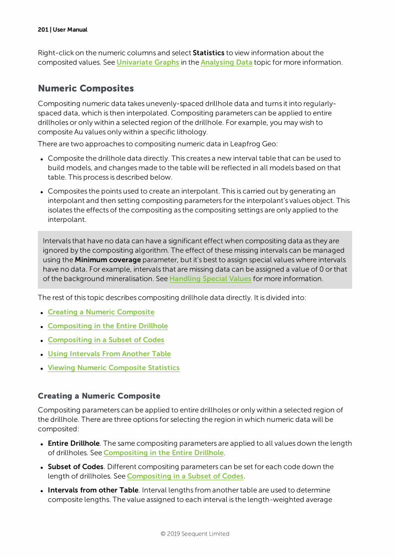
201 | User Manual
Right-click on the numeric columns and select Statistics to view information about thecomposited values. SeeUnivariate Graphs in the Analysing Data topic formore information.
Numeric Composites
Compositing numeric data takes unevenly-spaced drillhole data and turns it into regularly-spaced data, which is then interpolated. Compositing parameters can be applied to entiredrillholes or onlywithin a selected region of the drillhole. For example, you maywish tocomposite Au values onlywithin a specific lithology.
There are two approaches to compositing numeric data in Leapfrog Geo:
l Composite the drillhole data directly. This creates a new interval table that can be used tobuild models, and changesmade to the table will be reflected in all models based on thattable. This process is described below.
l Composites the points used to create an interpolant. This is carried out by generating aninterpolant and then setting compositing parameters for the interpolant’s values object. Thisisolates the effects of the compositing as the compositing settings are only applied to theinterpolant.
Intervals that have no data can have a significant effect when compositing data as they areignored by the compositing algorithm. The effect of thesemissing intervals can bemanagedusing theMinimum coverage parameter, but it’s best to assign special valueswhere intervalshave no data. For example, intervals that aremissing data can be assigned a value of 0 or thatof the background mineralisation. SeeHandling Special Values formore information.
The rest of this topic describes compositing drillhole data directly. It is divided into:
l Creating a Numeric Composite
l Compositing in the Entire Drillhole
l Compositing in a Subset of Codes
l Using Intervals From Another Table
l Viewing Numeric Composite Statistics
Creating a Numeric Composite
Compositing parameters can be applied to entire drillholes or onlywithin a selected region ofthe drillhole. There are three options for selecting the region in which numeric data will becomposited:
l Entire Drillhole. The same compositing parameters are applied to all values down the lengthof drillholes. SeeCompositing in the Entire Drillhole.
l Subset of Codes. Different compositing parameters can be set for each code down thelength of drillholes. SeeCompositing in a Subset of Codes.
l Intervals from other Table. Interval lengths fromanother table are used to determinecomposite lengths. The value assigned to each interval is the length-weighted average
© 2019 Seequent Limited
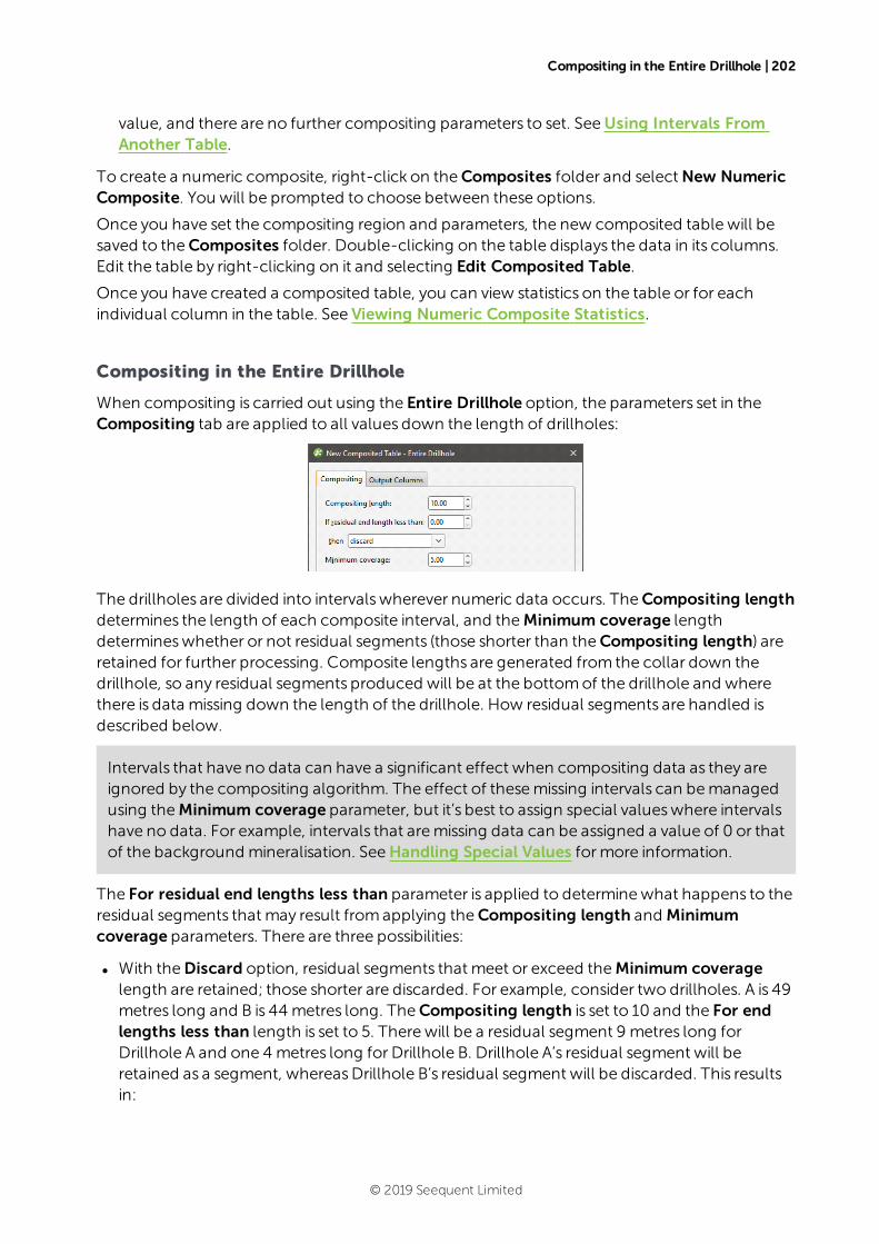
Compositing in the Entire Drillhole | 202
value, and there are no further compositing parameters to set. SeeUsing Intervals FromAnother Table.
To create a numeric composite, right-click on theComposites folder and selectNew NumericComposite. You will be prompted to choose between these options.
Once you have set the compositing region and parameters, the new composited table will besaved to theComposites folder. Double-clicking on the table displays the data in its columns.Edit the table by right-clicking on it and selecting Edit Composited Table.
Once you have created a composited table, you can view statistics on the table or for eachindividual column in the table. See Viewing Numeric Composite Statistics.
Compositing in the Entire Drillhole
When compositing is carried out using the Entire Drillhole option, the parameters set in theCompositing tab are applied to all values down the length of drillholes:
The drillholes are divided into intervalswherever numeric data occurs. TheCompositing lengthdetermines the length of each composite interval, and theMinimum coverage lengthdetermineswhether or not residual segments (those shorter than theCompositing length) areretained for further processing. Composite lengths are generated from the collar down thedrillhole, so any residual segments produced will be at the bottomof the drillhole and wherethere is data missing down the length of the drillhole. How residual segments are handled isdescribed below.
Intervals that have no data can have a significant effect when compositing data as they areignored by the compositing algorithm. The effect of thesemissing intervals can bemanagedusing theMinimum coverage parameter, but it’s best to assign special valueswhere intervalshave no data. For example, intervals that aremissing data can be assigned a value of 0 or thatof the background mineralisation. SeeHandling Special Values formore information.
The For residual end lengths less than parameter is applied to determinewhat happens to theresidual segments that may result fromapplying theCompositing length and Minimumcoverage parameters. There are three possibilities:
l With theDiscard option, residual segments that meet or exceed theMinimum coveragelength are retained; those shorter are discarded. For example, consider two drillholes. A is 49metres long and B is 44 metres long. TheCompositing length is set to 10 and the For endlengths less than length is set to 5. There will be a residual segment 9 metres long forDrillhole A and one 4metres long for Drillhole B. Drillhole A’s residual segment will beretained as a segment, whereasDrillhole B’s residual segment will be discarded. This resultsin:
© 2019 Seequent Limited
203 | User Manual
l Drillhole A: 10m, 10m, 10m, 10m, 9m (residual length >Minimum coverage length so the9msegment is kept)
l Drillhole B: 10m, 10m, 10m, 10m (residual length <Minimum coverage length so the 4msegment is discarded)
l With the Add to previous interval option, theMinimum coverage length is automaticallyset to zero. Residual segments longer than the For end lengths less than value are retainedas separate segments; those shorter are added to the previous interval. For our two drillholes,when theCompositing length is 10, there will be a residual segment 9 metres long forDrillhole A and one 4metres long for Drillhole B. When For end lengths less than is set to 5,Drillhole A’s residual segment will be retained as a segment, whereasDrillhole B’s residualsegment will be added to the previous interval. This results in:
l Drillhole A: 10m, 10m, 10m, 10m, 9m (residual length > For end lengths less than lengthso the 9m length is kept as a separate segment)
l Drillhole B: 10m, 10m, 10m, 14m (residual length < For end lengths less than length sothe 4msegment is added to the previous interval)
l With theDistribute equally throughout drillhole option, theMinimum coverageparameter is automatically set to zero. Residual segments longer than the For end lengthsless than value are retained as separate segments; those shorter will have their lengthdistributed among the other intervals. For our two drillholes, Drillhole A’s residual segmentwill be retained as an individual segment, whereasDrillhole B’s residual segment will have itslength distributed among the rest of the intervals. The segments for each compositeddrillhole will be:
l Drillhole A: 10m, 10m, 10m, 10m, 9m (residual length > For end lengths less than lengthso the 9msegment is kept as a separate segment)
l Drillhole B: 11m, 11m, 11m, 11m (residual length < For end lengths less than length so the4m length is distributed among the other intervals)
Composite values are calculated for each composite interval. This is simply the length-weighted average of all numeric drillhole data that fallswithin the composite interval.
Composite points are generated at the centre of each composite interval from the compositevalues.
Once you have set the compositing parameters, click on theOutput Columns tab to selectfrom the available columnsof numeric data. ClickOK to create the table.
© 2019 Seequent Limited
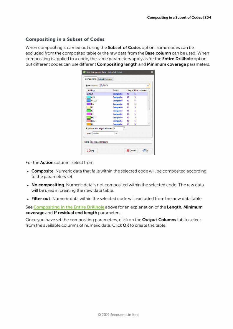
Compositing in a Subset of Codes | 204
Compositing in a Subset of Codes
When compositing is carried out using the Subset of Codes option, some codes can beexcluded from the composited table or the raw data from the Base column can be used. Whencompositing is applied to a code, the same parameters apply as for the Entire Drillhole option,but different codes can use differentCompositing length and Minimum coverage parameters.
For the Action column, select from:
l Composite. Numeric data that fallswithin the selected codewill be composited accordingto the parameters set.
l No compositing. Numeric data is not composited within the selected code. The raw datawill be used in creating the new data table.
l Filter out. Numeric data within the selected codewill excluded from the new data table.
SeeCompositing in the Entire Drillhole above for an explanation of the Length, Minimumcoverage and If residual end length parameters.
Once you have set the compositing parameters, click on theOutput Columns tab to selectfrom the available columnsof numeric data. ClickOK to create the table.
© 2019 Seequent Limited
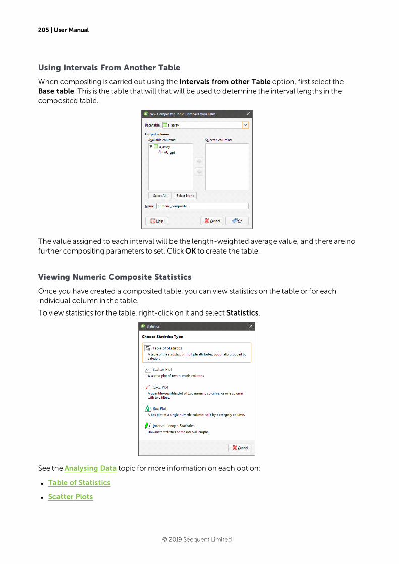
205 | User Manual
Using Intervals From Another Table
When compositing is carried out using the Intervals from other Table option, first select theBase table. This is the table that will that will be used to determine the interval lengths in thecomposited table.
The value assigned to each interval will be the length-weighted average value, and there are nofurther compositing parameters to set. ClickOK to create the table.
Viewing Numeric Composite Statistics
Once you have created a composited table, you can view statistics on the table or for eachindividual column in the table.
To view statistics for the table, right-click on it and select Statistics.
See the Analysing Data topic formore information on each option:
l Table of Statistics
l Scatter Plots
© 2019 Seequent Limited
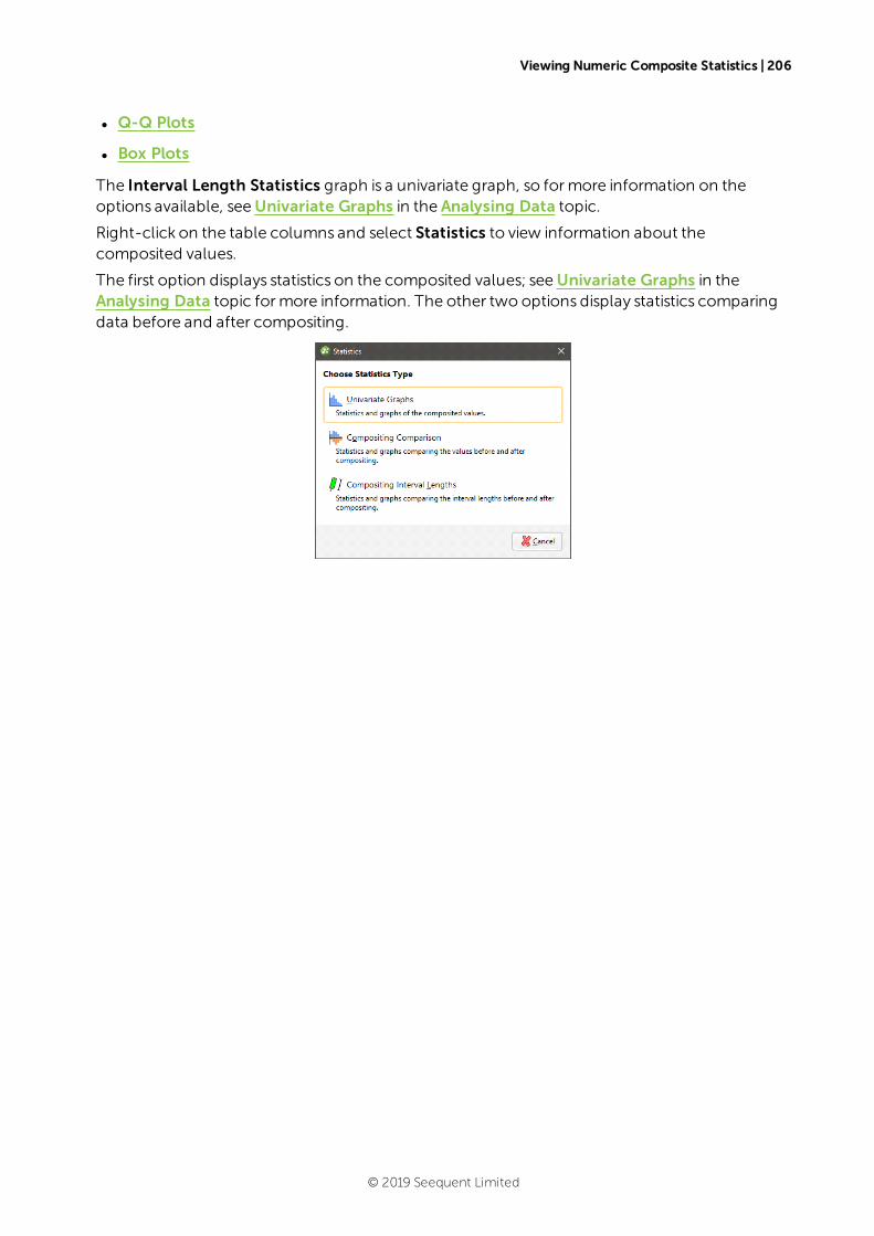
Viewing Numeric Composite Statistics | 206
l Q-Q Plots
l Box Plots
The Interval Length Statistics graph is a univariate graph, so formore information on theoptions available, seeUnivariate Graphs in the Analysing Data topic.
Right-click on the table columns and select Statistics to view information about thecomposited values.
The first option displays statistics on the composited values; seeUnivariate Graphs in theAnalysing Data topic formore information. The other two options display statistics comparingdata before and after compositing.
© 2019 Seequent Limited
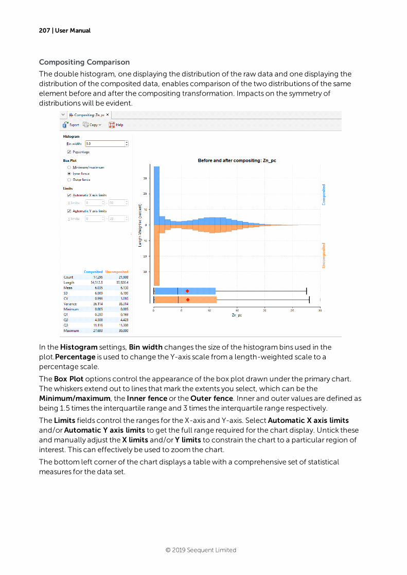
207 | User Manual
Compositing Comparison
The double histogram, one displaying the distribution of the raw data and one displaying thedistribution of the composited data, enables comparison of the two distributions of the sameelement before and after the compositing transformation. Impacts on the symmetry ofdistributionswill be evident.
In theHistogram settings, Bin width changes the size of the histogrambins used in theplot.Percentage is used to change the Y-axis scale froma length-weighted scale to apercentage scale.
The Box Plot options control the appearance of the box plot drawn under the primary chart.Thewhiskers extend out to lines that mark the extents you select, which can be theMinimum/maximum, the Inner fence or theOuter fence. Inner and outer values are defined asbeing 1.5 times the interquartile range and 3 times the interquartile range respectively.
The Limits fields control the ranges for the X-axis and Y-axis. Select Automatic X axis limitsand/orAutomatic Y axis limits to get the full range required for the chart display. Untick theseand manually adjust the X limits and/or Y limits to constrain the chart to a particular region ofinterest. This can effectively be used to zoom the chart.
The bottom left corner of the chart displays a table with a comprehensive set of statisticalmeasures for the data set.
© 2019 Seequent Limited
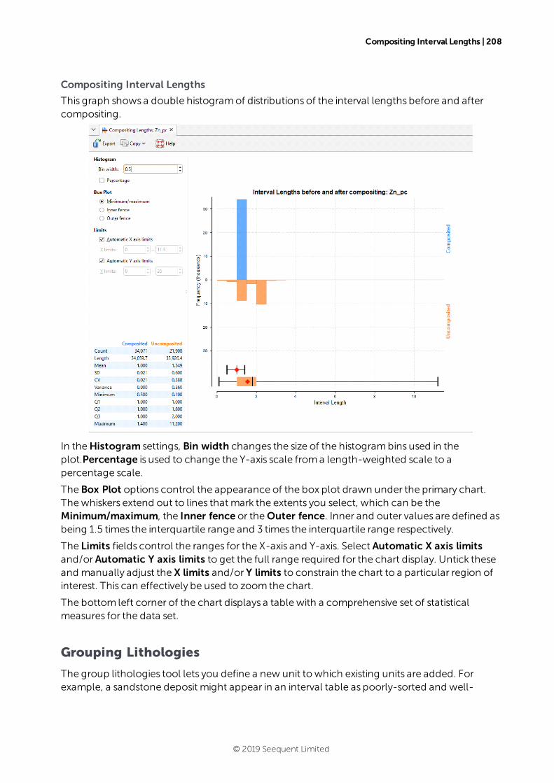
Compositing Interval Lengths | 208
Compositing Interval Lengths
This graph shows a double histogramof distributions of the interval lengths before and aftercompositing.
In theHistogram settings, Bin width changes the size of the histogrambins used in theplot.Percentage is used to change the Y-axis scale froma length-weighted scale to apercentage scale.
The Box Plot options control the appearance of the box plot drawn under the primary chart.Thewhiskers extend out to lines that mark the extents you select, which can be theMinimum/maximum, the Inner fence or theOuter fence. Inner and outer values are defined asbeing 1.5 times the interquartile range and 3 times the interquartile range respectively.
The Limits fields control the ranges for the X-axis and Y-axis. Select Automatic X axis limitsand/orAutomatic Y axis limits to get the full range required for the chart display. Untick theseand manually adjust the X limits and/or Y limits to constrain the chart to a particular region ofinterest. This can effectively be used to zoom the chart.
The bottom left corner of the chart displays a table with a comprehensive set of statisticalmeasures for the data set.
Grouping Lithologies
The group lithologies tool lets you define a new unit to which existing units are added. Forexample, a sandstone deposit might appear in an interval table as poorly-sorted and well-
© 2019 Seequent Limited
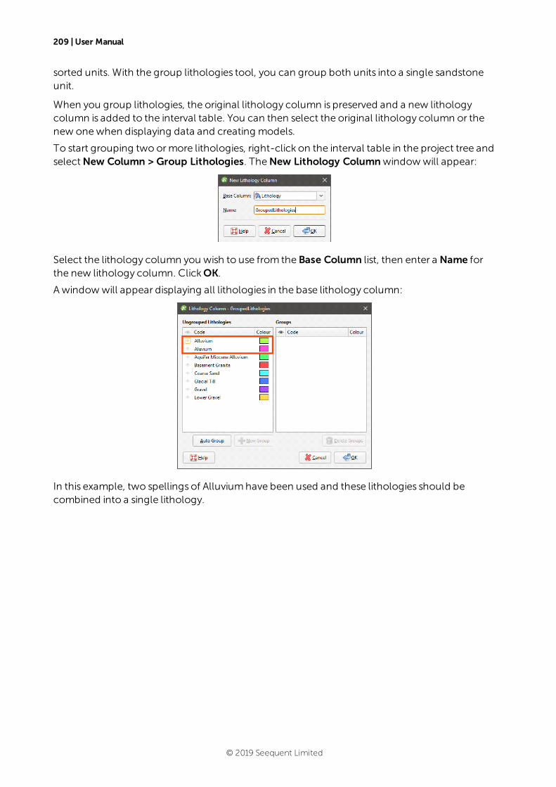
209 | User Manual
sorted units. With the group lithologies tool, you can group both units into a single sandstoneunit.
When you group lithologies, the original lithology column is preserved and a new lithologycolumn is added to the interval table. You can then select the original lithology column or thenew onewhen displaying data and creating models.
To start grouping two ormore lithologies, right-click on the interval table in the project tree andselectNew Column > Group Lithologies. TheNew Lithology Columnwindowwill appear:
Select the lithology column you wish to use from the Base Column list, then enter a Name forthe new lithology column. ClickOK.
A windowwill appear displaying all lithologies in the base lithology column:
In this example, two spellings of Alluviumhave been used and these lithologies should becombined into a single lithology.
© 2019 Seequent Limited
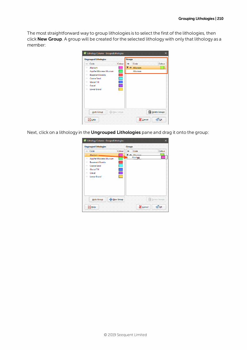
Grouping Lithologies | 210
Themost straightforward way to group lithologies is to select the first of the lithologies, thenclickNew Group. A group will be created for the selected lithologywith only that lithology as amember:
Next, click on a lithology in theUngrouped Lithologies pane and drag it onto the group:
© 2019 Seequent Limited

211 | User Manual
Grouping lithologies creates a new lithology column and any lithologies left in theUngrouped Lithologies panewill be excluded from the new column. For this reason, onceyou have grouped the required lithologies, move all remaining lithologies to theGroupspane by clicking on each lithology, then on theNew Group button. Thiswill make eachremaining lithology a new group with a singlemember:
When you are finished, clickOK to create the new lithology column. It will appear in the projecttree as an additional lithology column in the interval table.
Select the new column from the shape list to display it:
Click on the Edit button ( ) to start editing the selected column.
The other way to group lithologies is to let Leapfrog Geo create the lithology groups.
© 2019 Seequent Limited
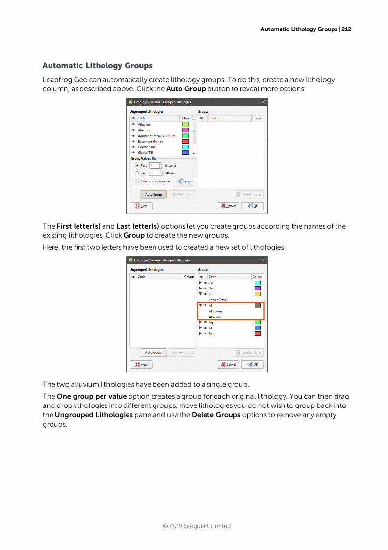
Automatic Lithology Groups | 212
Automatic Lithology Groups
Leapfrog Geo can automatically create lithology groups. To do this, create a new lithologycolumn, as described above. Click the Auto Group button to reveal more options:
The First letter(s) and Last letter(s) options let you create groups according the namesof theexisting lithologies. ClickGroup to create the new groups.
Here, the first two letters have been used to created a new set of lithologies:
The two alluvium lithologies have been added to a single group.
TheOne group per value option creates a group for each original lithology. You can then dragand drop lithologies into different groups, move lithologies you do not wish to group back intotheUngrouped Lithologies pane and use theDelete Groups options to remove any emptygroups.
© 2019 Seequent Limited
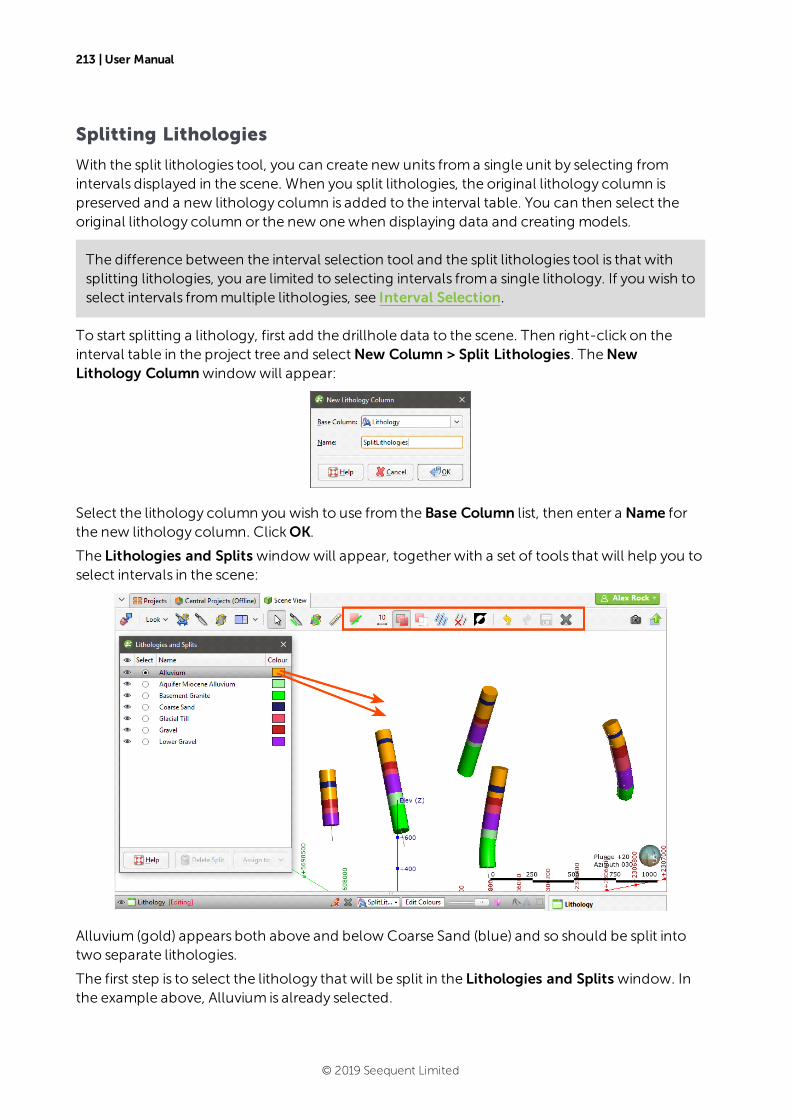
213 | User Manual
Splitting Lithologies
With the split lithologies tool, you can create new units froma single unit by selecting fromintervals displayed in the scene. When you split lithologies, the original lithology column ispreserved and a new lithology column is added to the interval table. You can then select theoriginal lithology column or the new onewhen displaying data and creating models.
The difference between the interval selection tool and the split lithologies tool is that withsplitting lithologies, you are limited to selecting intervals froma single lithology. If you wish toselect intervals frommultiple lithologies, see Interval Selection.
To start splitting a lithology, first add the drillhole data to the scene. Then right-click on theinterval table in the project tree and selectNew Column > Split Lithologies. TheNewLithology Columnwindowwill appear:
Select the lithology column you wish to use from the Base Column list, then enter a Name forthe new lithology column. ClickOK.
The Lithologies and Splits windowwill appear, together with a set of tools that will help you toselect intervals in the scene:
Alluvium (gold) appears both above and below Coarse Sand (blue) and so should be split intotwo separate lithologies.
The first step is to select the lithology that will be split in the Lithologies and Splits window. Inthe example above, Alluvium is already selected.
© 2019 Seequent Limited
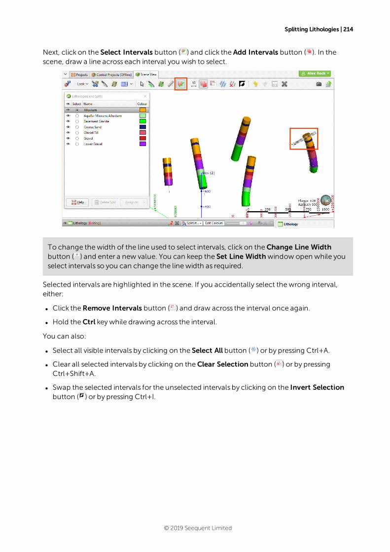
Splitting Lithologies | 214
Next, click on the Select Intervals button ( ) and click the Add Intervals button ( ). In thescene, draw a line across each interval you wish to select.
To change thewidth of the line used to select intervals, click on theChange Line Widthbutton ( ) and enter a new value. You can keep the Set Line Widthwindow open while youselect intervals so you can change the line width as required.
Selected intervals are highlighted in the scene. If you accidentally select thewrong interval,either:
l Click theRemove Intervals button ( ) and draw across the interval once again.
l Hold theCtrl keywhile drawing across the interval.
You can also:
l Select all visible intervals by clicking on the Select All button ( ) or by pressing Ctrl+A.
l Clear all selected intervals by clicking on theClear Selection button ( ) or by pressingCtrl+Shift+A.
l Swap the selected intervals for the unselected intervals by clicking on the Invert Selectionbutton ( ) or by pressing Ctrl+I.
© 2019 Seequent Limited
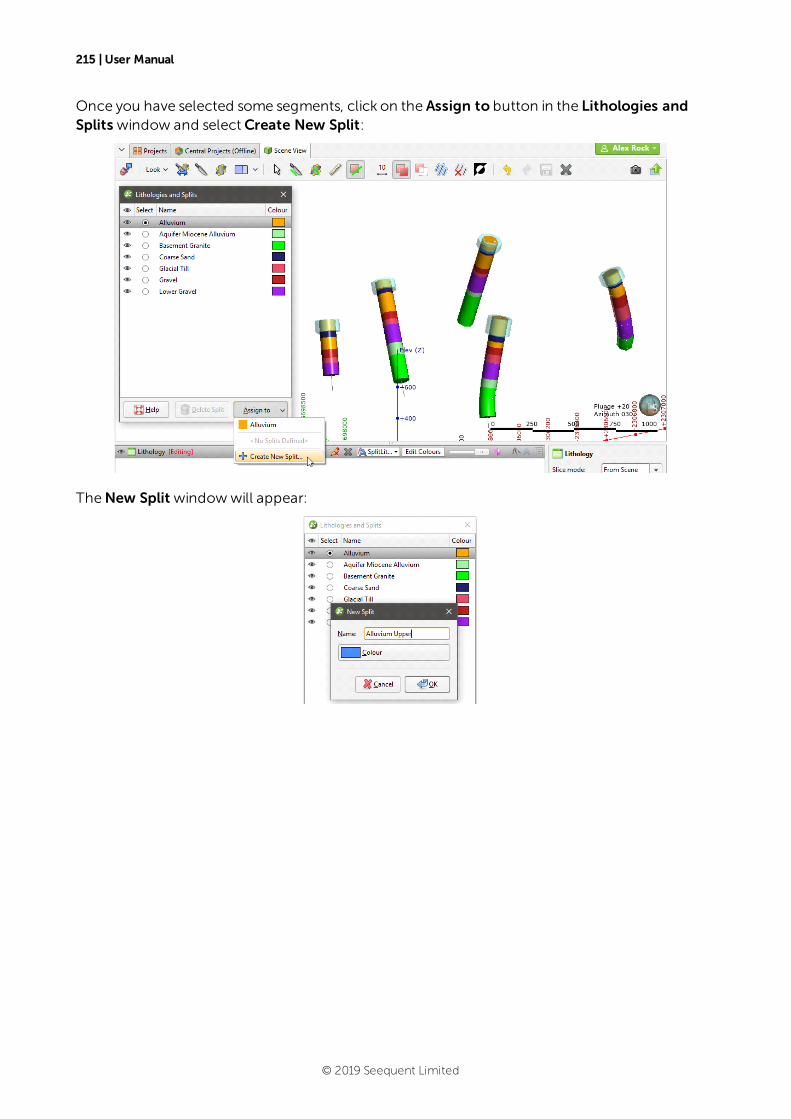
215 | User Manual
Once you have selected some segments, click on the Assign to button in the Lithologies andSplits window and selectCreate New Split:
TheNew Split windowwill appear:
© 2019 Seequent Limited
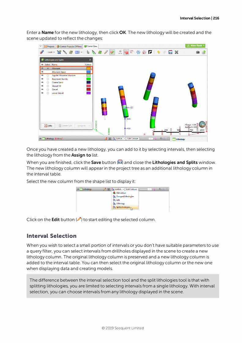
Interval Selection | 216
Enter a Name for the new lithology, then clickOK. The new lithologywill be created and thescene updated to reflect the changes:
Once you have created a new lithology, you can add to it by selecting intervals, then selectingthe lithology from the Assign to list.
When you are finished, click the Save button ( ) and close the Lithologies and Splits window.The new lithology column will appear in the project tree as an additional lithology column inthe interval table.
Select the new column from the shape list to display it:
Click on the Edit button ( ) to start editing the selected column.
Interval Selection
When you wish to select a small portion of intervals or you don’t have suitable parameters to usea query filter, you can select intervals fromdrillholes displayed in the scene to create a newlithology column. The original lithology column is preserved and a new lithology column isadded to the interval table. You can then select the original lithology column or the new onewhen displaying data and creating models.
The difference between the interval selection tool and the split lithologies tool is that withsplitting lithologies, you are limited to selecting intervals froma single lithology. With intervalselection, you can choose intervals fromany lithology displayed in the scene.
© 2019 Seequent Limited
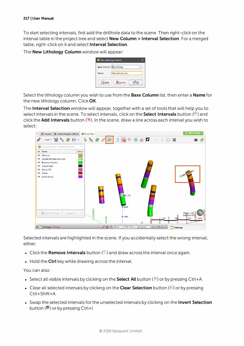
217 | User Manual
To start selecting intervals, first add the drillhole data to the scene. Then right-click on theinterval table in the project tree and selectNew Column > Interval Selection. For a mergedtable, right-click on it and select Interval Selection.
TheNew Lithology Columnwindowwill appear:
Select the lithology column you wish to use from the Base Column list, then enter a Name forthe new lithology column. ClickOK.
The Interval Selectionwindowwill appear, together with a set of tools that will help you toselect intervals in the scene. To select intervals, click on the Select Intervals button ( ) andclick the Add Intervals button ( ). In the scene, draw a line across each interval you wish toselect:
Selected intervals are highlighted in the scene. If you accidentally select thewrong interval,either:
l Click theRemove Intervals button ( ) and draw across the interval once again.
l Hold theCtrl keywhile drawing across the interval.
You can also:
l Select all visible intervals by clicking on the Select All button ( ) or by pressing Ctrl+A.
l Clear all selected intervals by clicking on theClear Selection button ( ) or by pressingCtrl+Shift+A.
l Swap the selected intervals for the unselected intervals by clicking on the Invert Selectionbutton ( ) or by pressing Ctrl+I.
© 2019 Seequent Limited
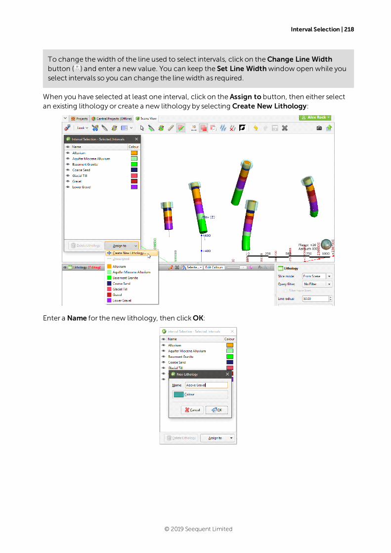
Interval Selection | 218
To change thewidth of the line used to select intervals, click on theChange Line Widthbutton ( ) and enter a new value. You can keep the Set Line Widthwindow open while youselect intervals so you can change the line width as required.
When you have selected at least one interval, click on the Assign to button, then either selectan existing lithology or create a new lithology by selecting Create New Lithology:
Enter a Name for the new lithology, then clickOK:
© 2019 Seequent Limited
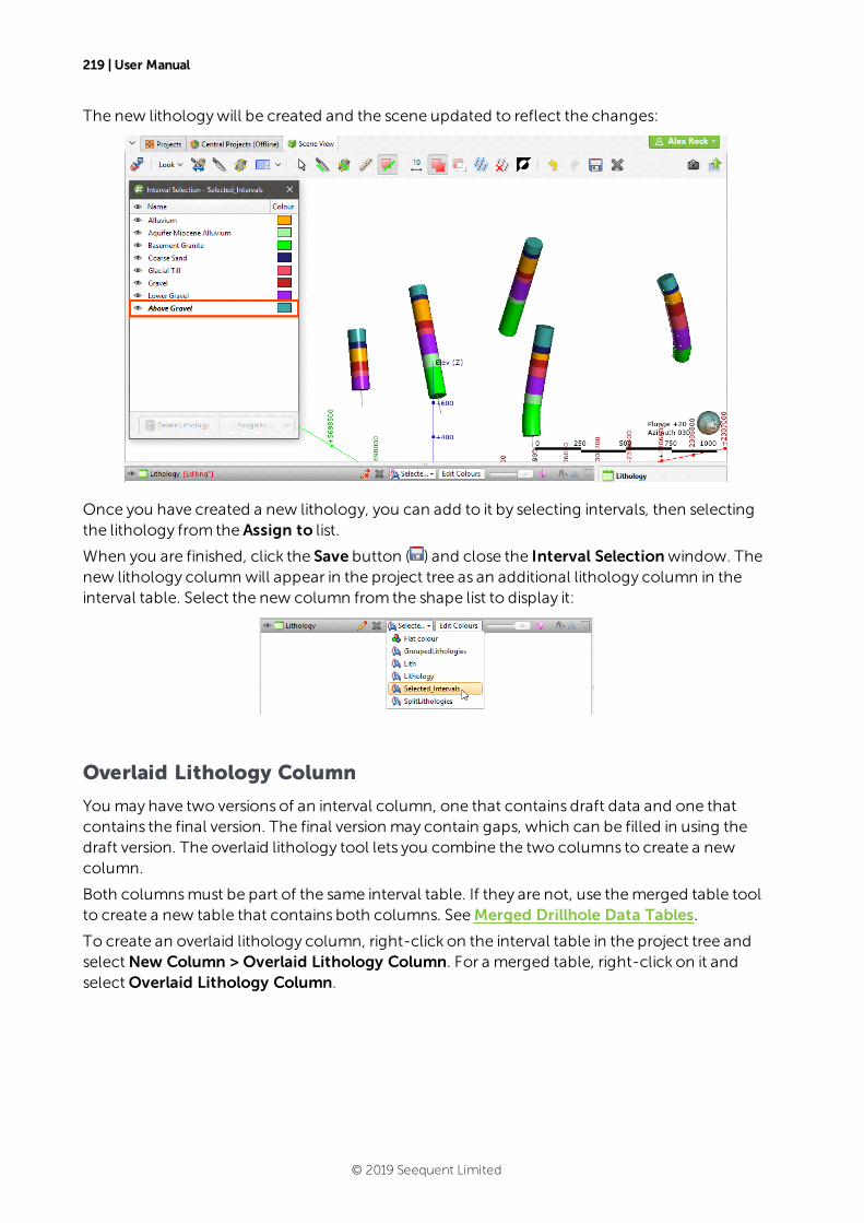
219 | User Manual
The new lithologywill be created and the scene updated to reflect the changes:
Once you have created a new lithology, you can add to it by selecting intervals, then selectingthe lithology from the Assign to list.
When you are finished, click the Save button ( ) and close the Interval Selectionwindow. Thenew lithology column will appear in the project tree as an additional lithology column in theinterval table. Select the new column from the shape list to display it:
Overlaid Lithology Column
You may have two versions of an interval column, one that contains draft data and one thatcontains the final version. The final version may contain gaps, which can be filled in using thedraft version. The overlaid lithology tool lets you combine the two columns to create a newcolumn.
Both columnsmust be part of the same interval table. If they are not, use themerged table toolto create a new table that contains both columns. SeeMerged Drillhole Data Tables.
To create an overlaid lithology column, right-click on the interval table in the project tree andselectNew Column > Overlaid Lithology Column. For a merged table, right-click on it andselectOverlaid Lithology Column.
© 2019 Seequent Limited
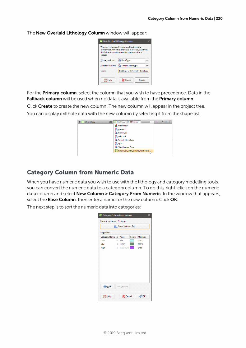
Category Column from Numeric Data | 220
TheNew Overlaid Lithology Columnwindowwill appear:
For the Primary column, select the column that you wish to have precedence. Data in theFallback columnwill be used when no data is available from the Primary column.
ClickCreate to create the new column. The new column will appear in the project tree.
You can display drillhole data with the new column by selecting it from the shape list:
Category Column from Numeric Data
When you have numeric data you wish to usewith the lithology and categorymodelling tools,you can convert the numeric data to a category column. To do this, right-click on the numericdata column and selectNew Column > Category From Numeric. In thewindow that appears,select the Base Column, then enter a name for the new column. ClickOK.
The next step is to sort the numeric data into categories:
© 2019 Seequent Limited
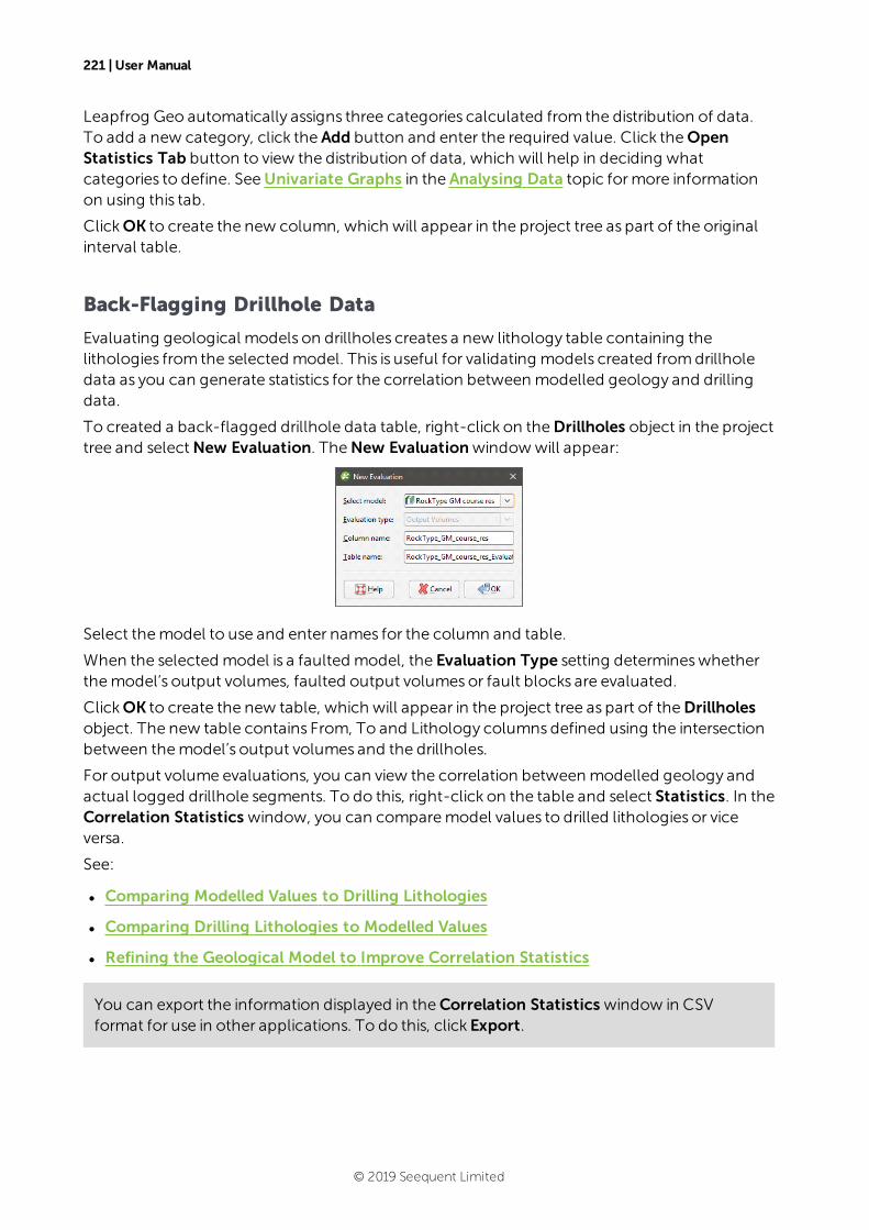
221 | User Manual
Leapfrog Geo automatically assigns three categories calculated from the distribution of data.To add a new category, click the Add button and enter the required value. Click theOpenStatistics Tab button to view the distribution of data, which will help in deciding whatcategories to define. SeeUnivariate Graphs in the Analysing Data topic formore informationon using this tab.
ClickOK to create the new column, which will appear in the project tree as part of the originalinterval table.
Back-Flagging Drillhole Data
Evaluating geological models on drillholes creates a new lithology table containing thelithologies from the selected model. This is useful for validating models created fromdrillholedata as you can generate statistics for the correlation betweenmodelled geology and drillingdata.
To created a back-flagged drillhole data table, right-click on theDrillholes object in the projecttree and selectNew Evaluation. TheNew Evaluationwindowwill appear:
Select themodel to use and enter names for the column and table.
When the selected model is a faulted model, the Evaluation Type setting determineswhetherthemodel’s output volumes, faulted output volumesor fault blocks are evaluated.
ClickOK to create the new table, which will appear in the project tree as part of theDrillholesobject. The new table contains From, To and Lithology columnsdefined using the intersectionbetween themodel’s output volumes and the drillholes.
For output volume evaluations, you can view the correlation betweenmodelled geology andactual logged drillhole segments. To do this, right-click on the table and select Statistics. In theCorrelation Statistics window, you can comparemodel values to drilled lithologies or viceversa.
See:
l Comparing Modelled Values to Drilling Lithologies
l Comparing Drilling Lithologies to Modelled Values
l Refining the Geological Model to Improve Correlation Statistics
You can export the information displayed in theCorrelation Statistics window in CSVformat for use in other applications. To do this, click Export.
© 2019 Seequent Limited
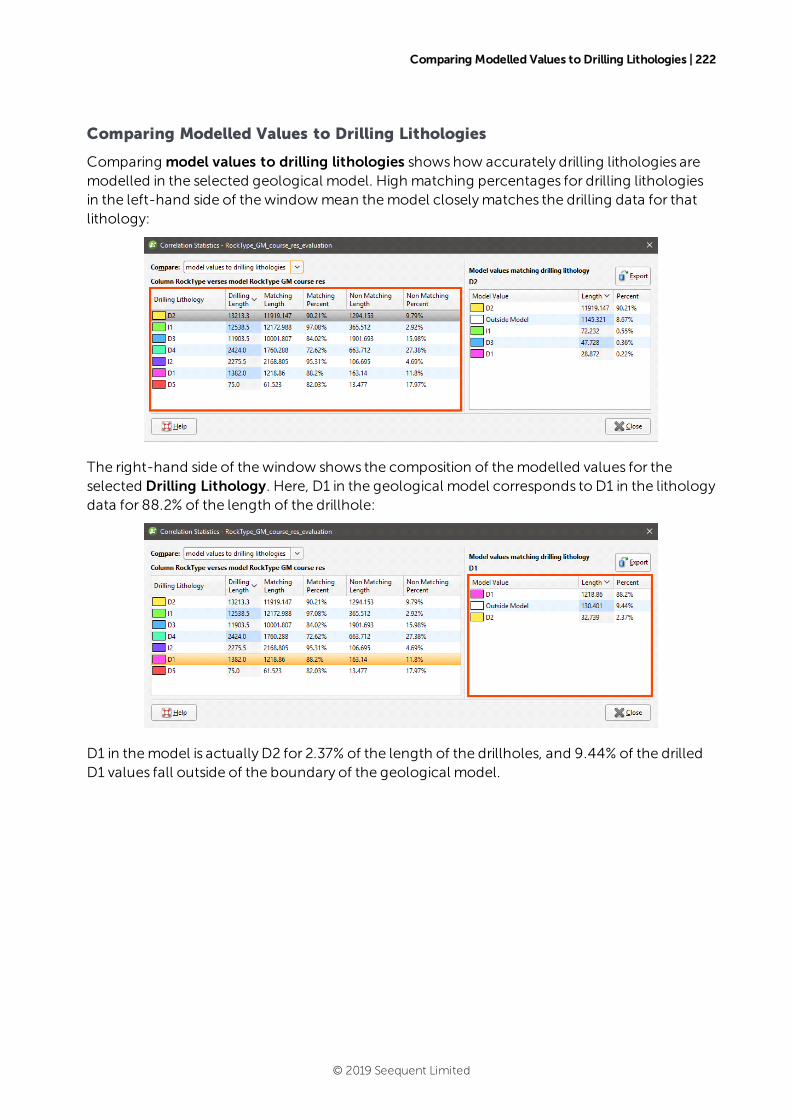
Comparing Modelled Values to Drilling Lithologies | 222
Comparing Modelled Values to Drilling Lithologies
Comparing model values to drilling lithologies showshow accurately drilling lithologies aremodelled in the selected geological model. High matching percentages for drilling lithologiesin the left-hand side of thewindowmean themodel closelymatches the drilling data for thatlithology:
The right-hand side of thewindow shows the composition of themodelled values for theselected Drilling Lithology. Here, D1 in the geological model corresponds to D1 in the lithologydata for 88.2% of the length of the drillhole:
D1 in themodel is actually D2 for 2.37% of the length of the drillholes, and 9.44% of the drilledD1 values fall outside of the boundary of the geological model.
© 2019 Seequent Limited
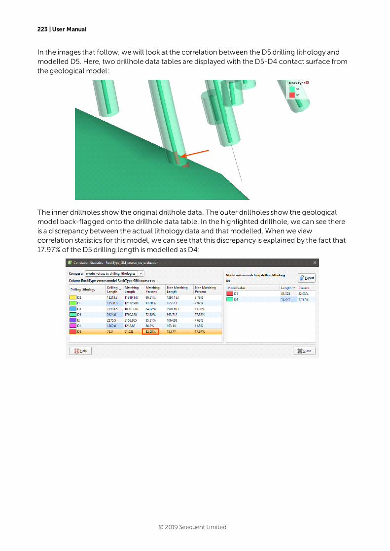
223 | User Manual
In the images that follow, wewill look at the correlation between the D5 drilling lithology andmodelled D5. Here, two drillhole data tables are displayed with the D5-D4 contact surface fromthe geological model:
The inner drillholes show the original drillhole data. The outer drillholes show the geologicalmodel back-flagged onto the drillhole data table. In the highlighted drillhole, we can see thereis a discrepancy between the actual lithology data and that modelled. When we viewcorrelation statistics for thismodel, we can see that this discrepancy is explained by the fact that17.97% of the D5 drilling length ismodelled asD4:
© 2019 Seequent Limited
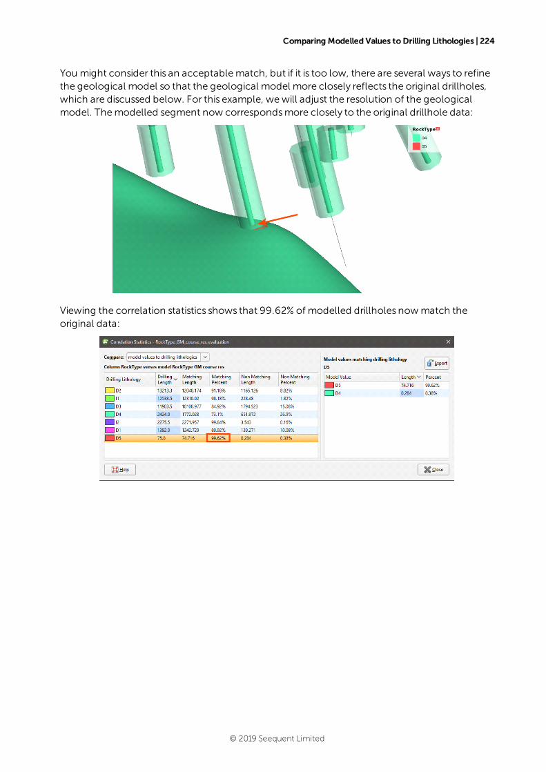
Comparing Modelled Values to Drilling Lithologies | 224
You might consider this an acceptablematch, but if it is too low, there are several ways to refinethe geological model so that the geological model more closely reflects the original drillholes,which are discussed below. For this example, wewill adjust the resolution of the geologicalmodel. Themodelled segment now correspondsmore closely to the original drillhole data:
Viewing the correlation statistics shows that 99.62% of modelled drillholes nowmatch theoriginal data:
© 2019 Seequent Limited
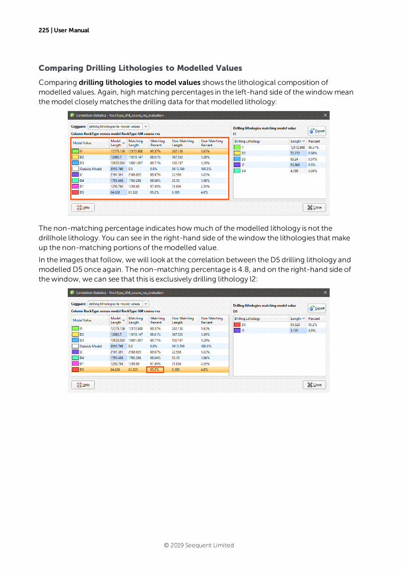
225 | User Manual
Comparing Drilling Lithologies to Modelled Values
Comparing drilling lithologies to model values shows the lithological composition ofmodelled values. Again, high matching percentages in the left-hand side of thewindowmeanthemodel closelymatches the drilling data for that modelled lithology:
The non-matching percentage indicates howmuch of themodelled lithology is not thedrillhole lithology. You can see in the right-hand side of thewindow the lithologies that makeup the non-matching portions of themodelled value.
In the images that follow, wewill look at the correlation between the D5 drilling lithology andmodelled D5 once again. The non-matching percentage is 4.8, and on the right-hand side ofthewindow, we can see that this is exclusively drilling lithology I2:
© 2019 Seequent Limited
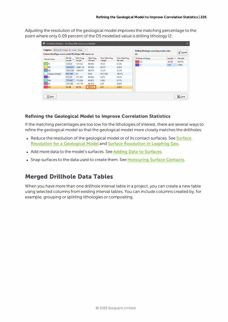
Refining the Geological Model to Improve Correlation Statistics | 226
Adjusting the resolution of the geological model improves thematching percentage to thepoint where only 0.09 percent of the D5modelled value is drilling lithology I2:
Refining the Geological Model to Improve Correlation Statistics
If thematching percentages are too low for the lithologies of interest, there are several ways torefine the geological model so that the geological model more closelymatches the drillholes:
l Reduce the resolution of the geological model or of its contact surfaces. See SurfaceResolution for a Geological Model and Surface Resolution in Leapfrog Geo.
l Add more data to themodel’s surfaces. See Adding Data to Surfaces.
l Snap surfaces to the data used to create them. SeeHonouring Surface Contacts.
Merged Drillhole Data Tables
When you havemore than one drillhole interval table in a project, you can create a new tableusing selected columns fromexisting interval tables. You can include columns created by, forexample, grouping or splitting lithologies or compositing.
© 2019 Seequent Limited
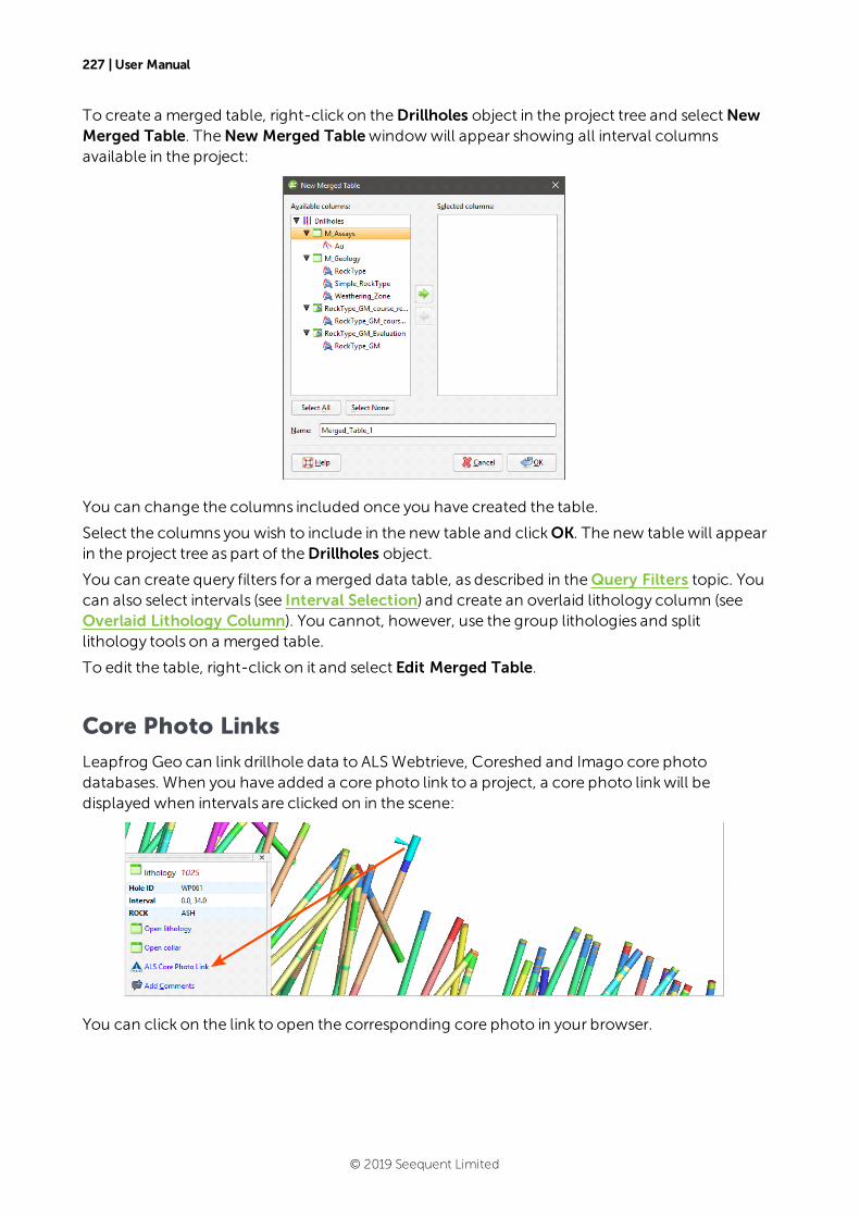
227 | User Manual
To create a merged table, right-click on theDrillholes object in the project tree and selectNewMerged Table. TheNew Merged Tablewindowwill appear showing all interval columnsavailable in the project:
You can change the columns included once you have created the table.
Select the columns you wish to include in the new table and clickOK. The new table will appearin the project tree as part of theDrillholes object.
You can create query filters for a merged data table, as described in theQuery Filters topic. Youcan also select intervals (see Interval Selection) and create an overlaid lithology column (seeOverlaid Lithology Column). You cannot, however, use the group lithologies and splitlithology tools on a merged table.
To edit the table, right-click on it and select Edit Merged Table.
Core Photo Links
Leapfrog Geo can link drillhole data to ALSWebtrieve, Coreshed and Imago core photodatabases. When you have added a core photo link to a project, a core photo linkwill bedisplayed when intervals are clicked on in the scene:
You can click on the link to open the corresponding core photo in your browser.
© 2019 Seequent Limited
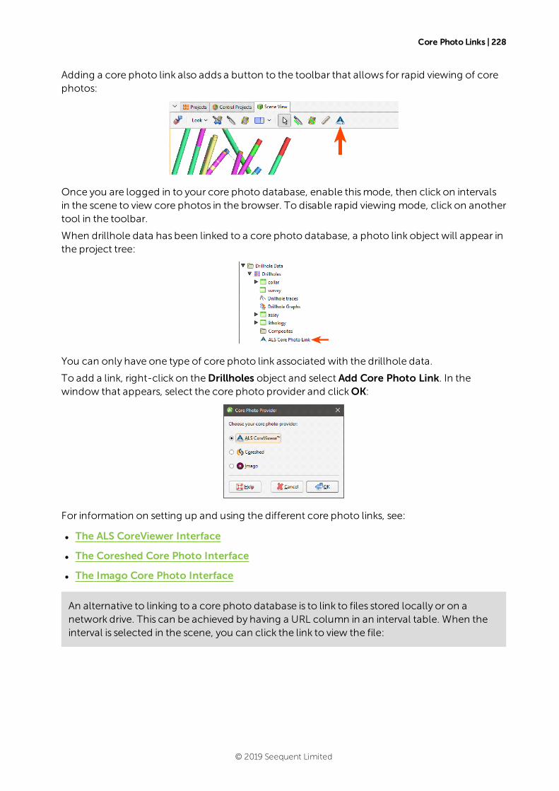
Core Photo Links | 228
Adding a core photo link also adds a button to the toolbar that allows for rapid viewing of corephotos:
Once you are logged in to your core photo database, enable thismode, then click on intervalsin the scene to view core photos in the browser. To disable rapid viewing mode, click on anothertool in the toolbar.
When drillhole data has been linked to a core photo database, a photo link object will appear inthe project tree:
You can only have one type of core photo link associated with the drillhole data.
To add a link, right-click on theDrillholes object and select Add Core Photo Link. In thewindow that appears, select the core photo provider and clickOK:
For information on setting up and using the different core photo links, see:
l The ALS CoreViewer Interface
l The Coreshed Core Photo Interface
l The Imago Core Photo Interface
An alternative to linking to a core photo database is to link to files stored locally or on anetwork drive. This can be achieved by having a URL column in an interval table. When theinterval is selected in the scene, you can click the link to view the file:
© 2019 Seequent Limited

229 | User Manual
Use the prefix file:/// to link to local files.
The ALS CoreViewer Interface
This topic describes how to set up and use the ALS core photo interface. It is divided into:
l Setting Up the ALS CoreViewer Interface
l Using the ALS Interface
l Removing the ALS Link
Setting Up the ALS CoreViewer Interface
Before you can view core photos, you must first set up the ALS CoreViewer interface. To set upthe interface between Leapfrog Geo and the ALS database, right-click on theDrillholes objectand select Add Core Photo Link. In thewindow that appears, select ALS CoreViewer and clickOK. The ALS Core Photo Settings windowwill appear. The Project Name is required to set upthe link, although the Encryption Key is optional.
ForApplication depths measured in, ensure that the units used for depth match in LeapfrogGeo and ALS.
ForOpen selection in new browser, choosewhether each core photowill be opened in aseparate browserWindow or Tab.
© 2019 Seequent Limited
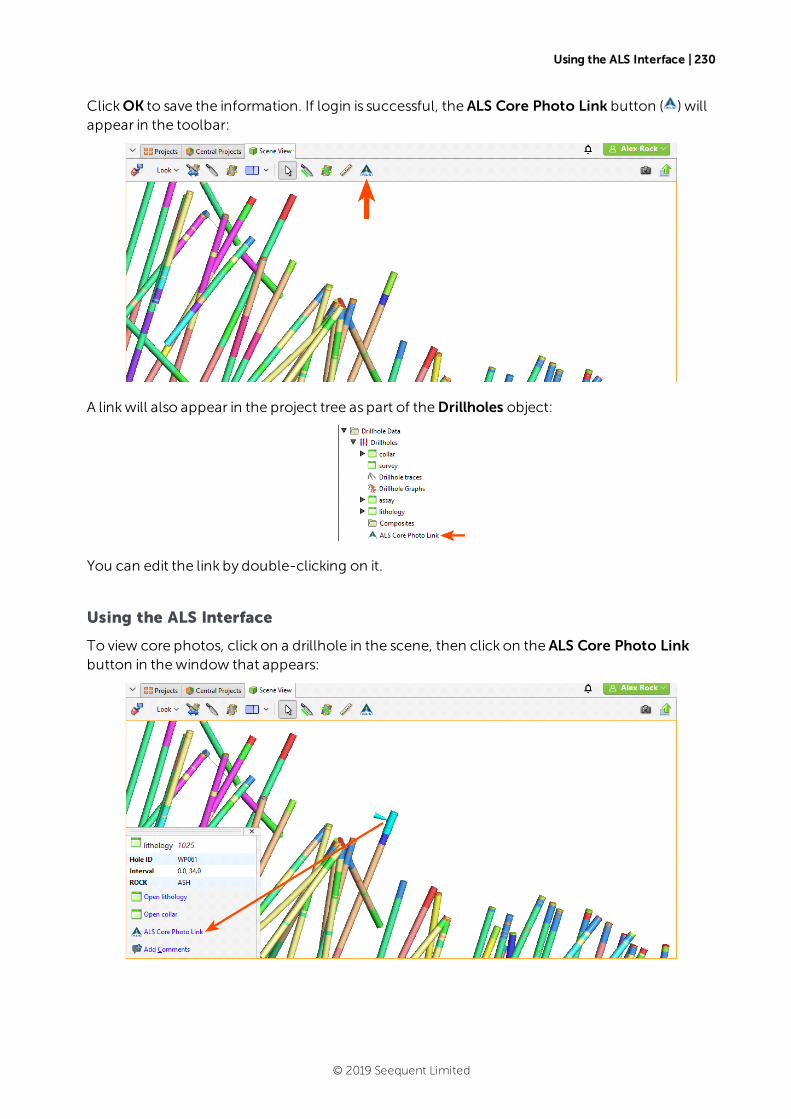
Using the ALS Interface | 230
ClickOK to save the information. If login is successful, the ALS Core Photo Link button ( ) willappear in the toolbar:
A linkwill also appear in the project tree as part of theDrillholes object:
You can edit the link by double-clicking on it.
Using the ALS Interface
To view core photos, click on a drillhole in the scene, then click on the ALS Core Photo Linkbutton in thewindow that appears:
© 2019 Seequent Limited

231 | User Manual
Your browser will be launched and you will be prompted to log in to the ALS database. EntertheUser Name and Password, which are case-sensitive. Remember to allow the browser tosave the details so that you will not be prompted to log in each time you wish to view a photo.
Your browser settingsmay require that you install a plugin ormake changes to settings inorder to view core photos. If you are not able to access the ALS database fromLeapfrog Geoand have ensured your Project Name, Encryption Key, User Name and Password havebeen entered correctly, contact Customer Support as described in Getting Support.
The ALS Core Photo Link button ( ) in the toolbar allows you to view core photos in yourbrowser in rapid succession. To do this, first make sure you are already logged into the database.Then click on the ALS Core Photo Link button ( ) to enable the rapid viewing mode. Each timeyou click on an interval in the scene, the core photo linkwill open in your browser.
Position your browser window alongside the Leapfrog Geo scenewindow to view drillholedata in Leapfrog Geo alongside the core photo data.
To disable rapid viewing mode, click on another tool in the toolbar.
Removing the ALS Link
To remove the ALS link, right-click on it in the project tree and selectDelete.
The Coreshed Core Photo Interface
This topic describes how to set up and use the Coreshed core photo interface. It is divided into:
l Setting Up the Coreshed Interface
l Using the Coreshed Interface
l Removing the Coreshed Link
Setting Up the Coreshed Interface
Before you can view core photos, you must first set up the Coreshed interface. To do this, right-click on theDrillholes object and select Add Core Photo Link. In thewindow that appears,selectCoreshed and clickOK. TheCoreshed Photo Settings windowwill appear. Enter theinformation required and select whether each core photowill be opened in a separate browserWindow or Tab.
© 2019 Seequent Limited
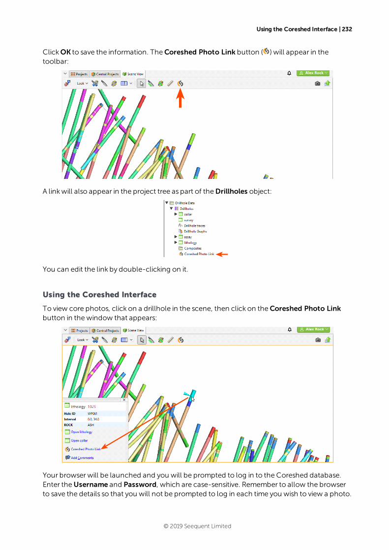
Using the Coreshed Interface | 232
ClickOK to save the information. TheCoreshed Photo Link button ( ) will appear in thetoolbar:
A linkwill also appear in the project tree as part of theDrillholes object:
You can edit the link by double-clicking on it.
Using the Coreshed Interface
To view core photos, click on a drillhole in the scene, then click on theCoreshed Photo Linkbutton in thewindow that appears:
Your browser will be launched and you will be prompted to log in to the Coreshed database.Enter theUsername and Password, which are case-sensitive. Remember to allow the browserto save the details so that you will not be prompted to log in each time you wish to view a photo.
© 2019 Seequent Limited

233 | User Manual
Your browser settingsmay require that you install a plugin ormake changes to settings inorder to view core photos. If you are not able to access the Coreshed database fromLeapfrog Geo and have ensured yourUsername and Password have been entered correctly,contact Customer Support as described in Getting Support.
TheCoreshed Photo Link button ( ) in the toolbar allows you to view core photos in yourbrowser in rapid succession. To do this, first make sure you are already logged into the database.Then click on theCoreshed Photo Link button ( ) to enable the rapid viewing mode. Eachtime you click on an interval in the scene, the core photo linkwill open in your browser.
Position your browser window alongside the Leapfrog Geo scenewindow to view drillholedata in Leapfrog Geo alongside the core photo data.
To disable rapid viewing mode, click on another tool in the toolbar.
Removing the Coreshed Link
To remove the Coreshed link, right-click on it in the project tree and selectDelete.
The Imago Core Photo Interface
This topic describes how to set up and use the Imago core photo interface. It is divided into:
l Setting Up the Imago Interface
l Using the Imago Interface
l Removing the Imago Link
Setting Up the Imago Interface
Before you can view core photos, you must first set up the link between Leapfrog Geo and theImago database. To do this, right-click on theDrillholes object and select Add Core PhotoLink. In thewindow that appears, select Imago and clickOK. The Imago Settings windowwillappear. Select whether each core photowill be opened in a separate browserWindow or Tab.All other parameters are optional.
© 2019 Seequent Limited
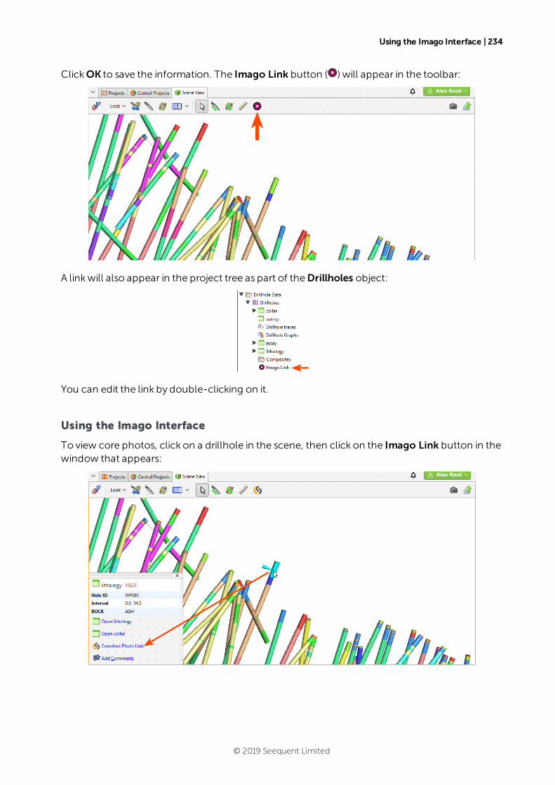
Using the Imago Interface | 234
ClickOK to save the information. The Imago Link button ( ) will appear in the toolbar:
A linkwill also appear in the project tree as part of theDrillholes object:
You can edit the link by double-clicking on it.
Using the Imago Interface
To view core photos, click on a drillhole in the scene, then click on the Imago Link button in thewindow that appears:
© 2019 Seequent Limited
235 | User Manual
Your browser will be launched and you will be prompted to log in to the Imago database.Remember to allow the browser to save the details so that you will not be prompted to log ineach time you wish to view a photo.
The Imago Link button ( ) in the toolbar allows you to view core photos in your browser inrapid succession. To do this, first make sure you are already logged into the database. Then clickon the Imago Link button ( ) to enable the rapid viewing mode. Each time you click on aninterval in the scene, the core photo linkwill open in your browser.
Position your browser window alongside the Leapfrog Geo scenewindow to view drillholedata in Leapfrog Geo alongside the core photo data.
To disable rapid viewing mode, click on another tool in the toolbar.
Removing the Imago Link
To remove the Imago link, right-click on it in the project tree and selectDelete.
Reloading Drillhole Data
Reloading data is necessarywhen the imported data ismodified externally. All drillhole data canbe reloaded by right-clicking on theDrillholes object and selecting Reload Drillholes. If youonly need to reload a single table, right-click on that table and select Reload Data.
Reloading drillhole data overwrites all existing drillhole data. If you have data you wish toadd to the project without overwriting existing data, use the Append Drillholes option.
The process is similar to that for importing drillhole data:
l If the drillhole data was loaded froma file on your computer or a network location, you willbe prompted to specify the file locations.
l If the interval table is stored in an ODBC database, you will be prompted to connect to thedatabase. See Selecting the ODBC Data Source.
l If your drillhole data is stored in an acQuire database, you will be prompted to connect to thedatabase. SeeConnecting to an acQuire Database.
When you reload data, Leapfrog Geo retains the table structure and refreshes the datacontained in the tables. This ensures that you do not need to reassign the data type for eachcolumn and select the columns to be imported.
Exporting Drillhole Data
Changesmade to the drillhole data in Leapfrog Geo only affect the Leapfrog Geo database,not the original data files. You can export Leapfrog Geo drillhole data, which is useful if youwish to keep a copy of drillhole data outside the project.
© 2019 Seequent Limited
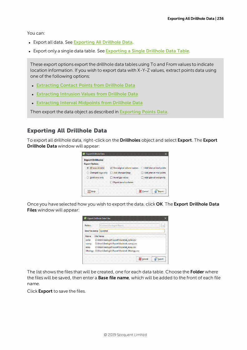
Exporting All Drillhole Data | 236
You can:
l Export all data. See Exporting All Drillhole Data.
l Export only a single data table. See Exporting a Single Drillhole Data Table.
These export options export the drillhole data tables using To and Fromvalues to indicatelocation information. If you wish to export data with X-Y-Z values, extract points data usingone of the following options:
l Extracting Contact Points from Drillhole Data
l Extracting Intrusion Values from Drillhole Data
l Extracting Interval Midpoints from Drillhole Data
Then export the data object as described in Exporting Points Data.
Exporting All Drillhole Data
To export all drillhole data, right-click on theDrillholes object and select Export. The ExportDrillhole Datawindowwill appear:
Once you have selected how you wish to export the data, clickOK. The Export Drillhole DataFiles windowwill appear:
The list shows the files that will be created, one for each data table. Choose the Folder wherethe fileswill be saved, then enter a Base file name, which will be added to the front of each filename.
Click Export to save the files.
© 2019 Seequent Limited
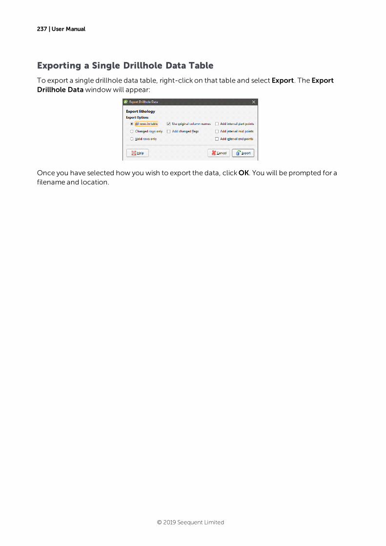
237 | User Manual
Exporting a Single Drillhole Data Table
To export a single drillhole data table, right-click on that table and select Export. The ExportDrillhole Datawindowwill appear:
Once you have selected how you wish to export the data, clickOK. You will be prompted for afilename and location.
© 2019 Seequent Limited
Points DataPoints are sets of X-Y-Z coordinates, with or without associated values. In Leapfrog Geo, pointsare used to define surfaces and for interpolation. You can use the Points folder to:
l Import points data
l Extract contact points, intrusion values and interval midpoints fromdrillhole data
l Create guide points
l Create grids of points that can be evaluated against geological and numericmodels andexported for use in othermodelling
The rest of this topic describes importing and exporting points, setting elevation for points andevaluating points. It is divided into:
l Importing Points Data
l Reloading Points Data
l Appending Points Data
l Importing a Column
l Setting Elevation for Points
l Evaluating Points Data
l Displaying Points
l Viewing Points Table Statistics
l Exporting Points Data
Importing Points Data
Leapfrog Geo supports the following file types for points data:
l CSV files (*.csv)
l ASCII text files (*.asc)
l DXF files (*.dxf)
l Leapfrog Geo 3D Point Data files (*.pl3, *.ara)
Points data can be imported from:
l Files stored on your computer or a network location. Right-click on the Points folder andselect Import Points. You will be prompted to select a file.
l Fromany database that runs an ODBC interface. Right-click on the Points folder and selectImport Points via ODBC. See Selecting the ODBC Data Source below.
For each of these options, once the data source is selected, the process of importing the data isthe same.
© 2019 Seequent Limited
239 | User Manual
When importing a file that hasmultiple features, you will be prompted to select which ones toimport. You can also choose to:
l Import the features as separate objects. Each feature will appear in the project tree as aseparate object.
l Flatten all features into one object. Leapfrog Geowill treat all features as a single object.
Once imported, the file will be added to the Points folder. If there are errors in the data, theerrors can be corrected as described in Correcting Data Errors in Leapfrog Geo.
To view the imported data, double-click on the object that has been added to the Points folder.
Once points data has been imported to the project, it can bemodified and evaluated againstgeological models, numericmodels and estimators, as described in Evaluating Points Data.
Selecting the ODBC Data Source
When importing points data froman ODBC database, you will need to specify theODBC datasource. Enter the information supplied by your database administrator and clickOK.
Once the data source is selected, the import process is similar to that described above.
Reloading Points Data
Reloading data is necessarywhen the imported data ismodified externally. Points data can bereloaded by right-clicking on the table and selecting Reload Data.
Reloading points data overwrites all data in the existing table. If you have data you wish toadd to the project without overwriting existing data, use the Append Data option.
The process is similar to that for importing the original table.
Appending Points Data
If points data is stored in multiple files, you can import these files into the project and add themto existing points data. To do this, right-click on the object you wish to append and selectAppend Data. You will be prompted to select a file.
Next, the Import Tables For Appendingwindowwill be displayed.
Check the data to ensure that the correct information will be imported, then click Finish to addthe new file.
Importing a Column
Columnsof points data that were not imported when the original data was imported or that arestored in a separate file can be added to the table at any time. To do this, right-click on thepoints table in the project tree and select Import Column.
The process is similar to importing the original table; select the file and map the columns youwish to import.
© 2019 Seequent Limited
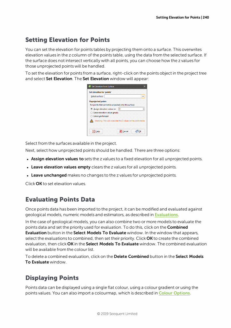
Setting Elevation for Points | 240
Setting Elevation for Points
You can set the elevation for points tables by projecting themonto a surface. This overwriteselevation values in the z column of the points table, using the data from the selected surface. Ifthe surface does not intersect vertically with all points, you can choose how the z values forthose unprojected pointswill be handled.
To set the elevation for points froma surface, right-click on the points object in the project treeand select Set Elevation. The Set Elevationwindowwill appear:
Select from the surfaces available in the project.
Next, select how unprojected points should be handled. There are three options:
l Assign elevation values to sets the z values to a fixed elevation for all unprojected points.
l Leave elevation values empty clears the z values for all unprojected points.
l Leave unchangedmakes no changes to the z values for unprojected points.
ClickOK to set elevation values.
Evaluating Points Data
Once points data has been imported to the project, it can bemodified and evaluated againstgeological models, numericmodels and estimators, as described in Evaluations.
In the case of geological models, you can also combine two ormoremodels to evaluate thepoints data and set the priority used for evaluation. To do this, click on theCombinedEvaluation button in the Select Models To Evaluatewindow. In thewindow that appears,select the evaluations to combined, then set their priority. ClickOK to create the combinedevaluation, then clickOK in the Select Models To Evaluatewindow. The combined evaluationwill be available from the colour list.
To delete a combined evaluation, click on theDelete Combined button in the Select ModelsTo Evaluatewindow.
Displaying Points
Points data can be displayed using a single flat colour, using a colour gradient or using thepoints values. You can also import a colourmap, which is described in Colour Options.
© 2019 Seequent Limited
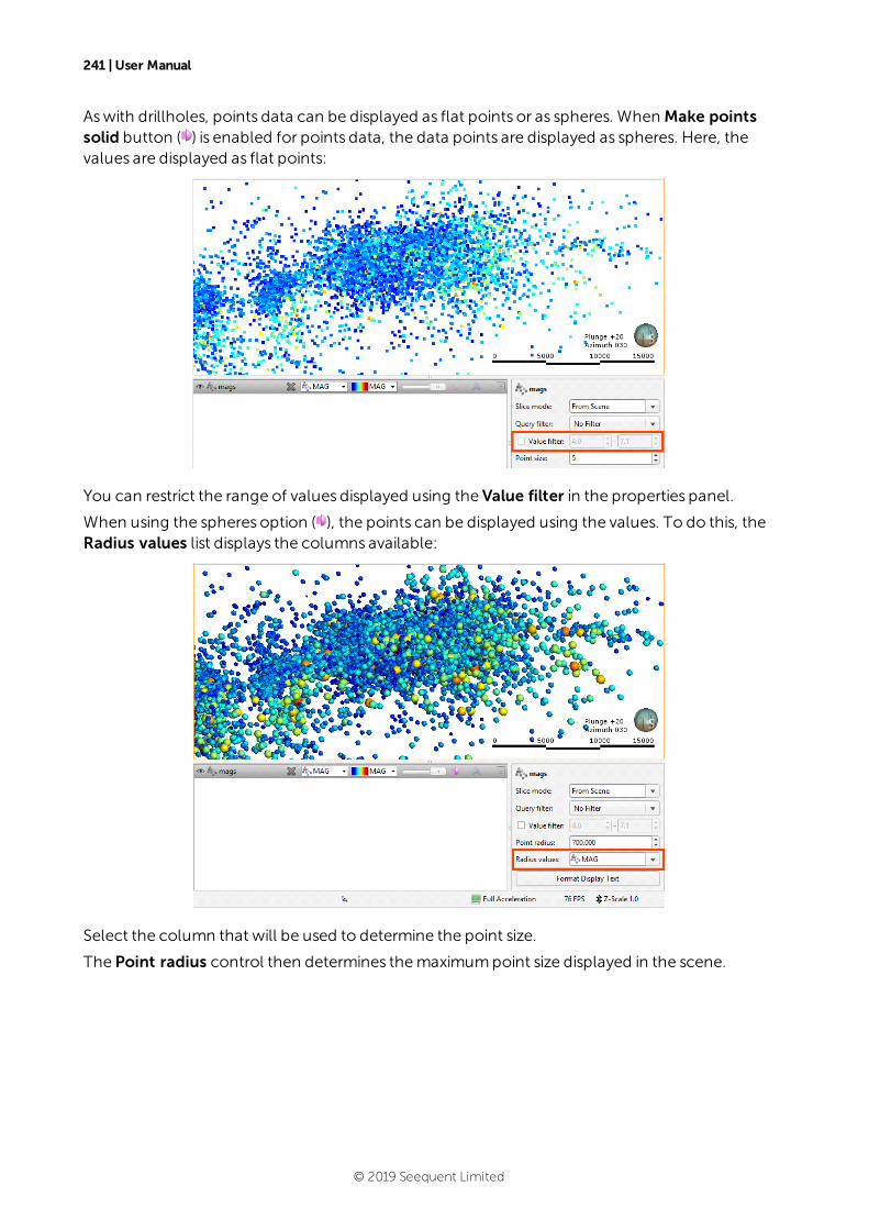
241 | User Manual
Aswith drillholes, points data can be displayed as flat points or as spheres. When Make pointssolid button ( ) is enabled for points data, the data points are displayed as spheres. Here, thevalues are displayed as flat points:
You can restrict the range of values displayed using the Value filter in the properties panel.
When using the spheres option ( ), the points can be displayed using the values. To do this, theRadius values list displays the columns available:
Select the column that will be used to determine the point size.
The Point radius control then determines themaximumpoint size displayed in the scene.
© 2019 Seequent Limited
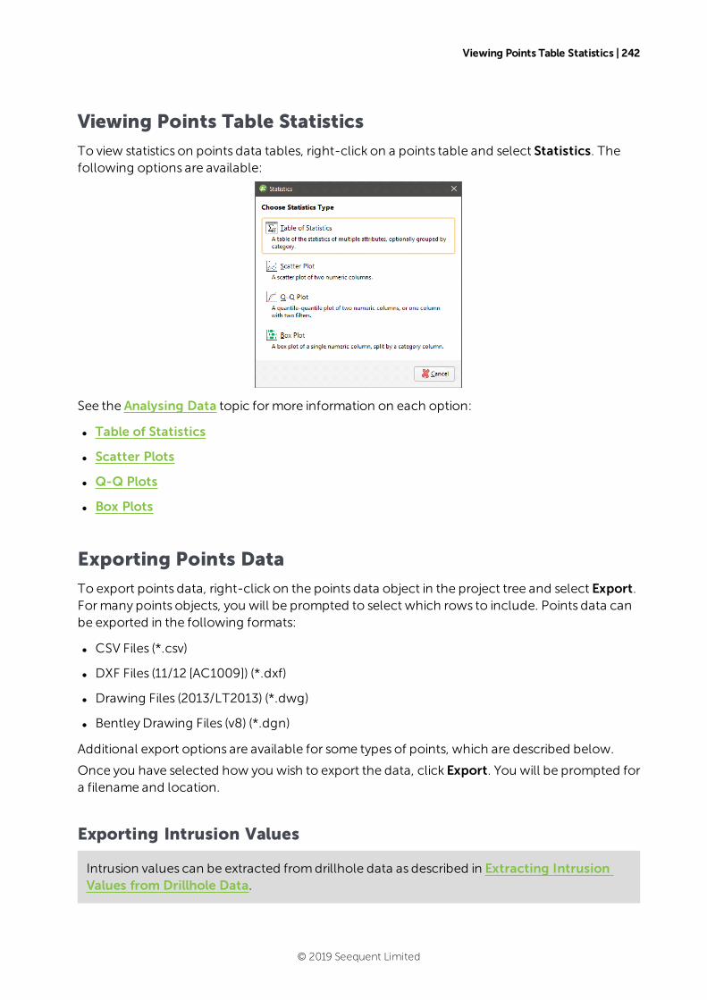
Viewing Points Table Statistics | 242
Viewing Points Table Statistics
To view statistics on points data tables, right-click on a points table and select Statistics. Thefollowing options are available:
See the Analysing Data topic formore information on each option:
l Table of Statistics
l Scatter Plots
l Q-Q Plots
l Box Plots
Exporting Points Data
To export points data, right-click on the points data object in the project tree and select Export.Formany points objects, you will be prompted to select which rows to include. Points data canbe exported in the following formats:
l CSV Files (*.csv)
l DXF Files (11/12 [AC1009]) (*.dxf)
l Drawing Files (2013/LT2013) (*.dwg)
l BentleyDrawing Files (v8) (*.dgn)
Additional export options are available for some types of points, which are described below.
Once you have selected how you wish to export the data, click Export. You will be prompted fora filename and location.
Exporting Intrusion Values
Intrusion values can be extracted fromdrillhole data as described in Extracting IntrusionValues from Drillhole Data.
© 2019 Seequent Limited
243 | User Manual
There are two options for exporting intrusion values:
l Export only the contact points. To do this, right-click on the intrusion values object andselect Export. If you choose this option, you can export the points in CSV format (*.csv), DXFformat (*.dxf) or DWG format (*.dwg).
l Export all the points used in creating an intrusion. To do this, right-click on the intrusionvalues object and select Export Volume Points. If you choose this option, you can onlyexport the points in CSV format (*.csv).
In both cases, you will be prompted for a filename and location.
Exporting Interval Midpoints
Interval midpoints can be extracted fromdrillhole data, which is described in ExtractingInterval Midpoints from Drillhole Data. You can also export midpoints directly froman RBFinterpolant, which is described in Exporting Numeric Model Midpoints.
To export interval midpoints, right-click on the points data object in the project tree and selectExport. Interval midpoints can be exported in the following formats:
l CSV text file (*.csv)
l Snowden Supervisor CSV file (*.csv)
l Isatis 3D points file (*.asc)
The values exported are themidpoints of each segment, the X-Y-Z values and the hole ID. TheSnowden Supervisor and Isatis 3D points formats also include the interval length.
In each case, you will be prompted for a filename and location.
Extracting Points from Drillhole Data
This topic describes extracting different types of points from imported drillhole data. It is dividedinto:
l Extracting Contact Points from Drillhole Data
l Extracting Intrusion Values from Drillhole Data
l Extracting Interval Midpoints from Drillhole Data
If you wish to save and export points data with X-Y-Z information, use these options, thenright-click on the data object to export the data as described in Exporting Points Data.
© 2019 Seequent Limited
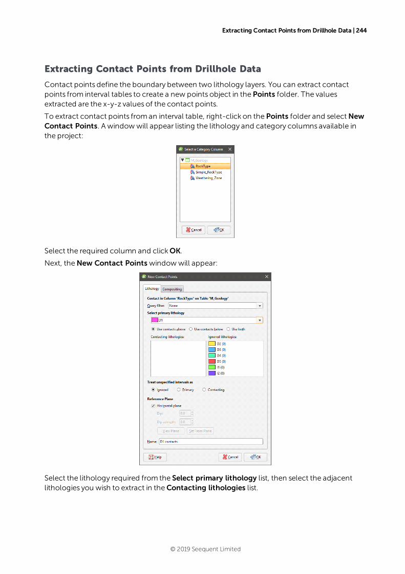
Extracting Contact Points from Drillhole Data | 244
Extracting Contact Points from Drillhole Data
Contact points define the boundary between two lithology layers. You can extract contactpoints from interval tables to create a new points object in the Points folder. The valuesextracted are the x-y-z values of the contact points.
To extract contact points froman interval table, right-click on the Points folder and selectNewContact Points. A windowwill appear listing the lithology and category columns available inthe project:
Select the required column and clickOK.
Next, theNew Contact Points windowwill appear:
Select the lithology required from the Select primary lithology list, then select the adjacentlithologies you wish to extract in theContacting lithologies list.
© 2019 Seequent Limited

245 | User Manual
Unspecified intervals are intervals that have no data. By default, unspecified intervals areignored when creating new contact points, but you can also treat themas the primary lithologyor as contacting lithologies.
For complex geologies, the up and down directions for the surfacemay not be clear. If this is thecase, untick theHorizontal Plane box. A reference planewill appear in the scene, with the up-facing surface labelled A and the downward-facing surface labelled B:
Controlling the position of the reference plane is similar to controlling the position of themoving plane:
l Use the handles in the scenewindow tomove the plane.
l Set theDip and Dip Azimuth values in theNew Contact Points window. The referenceplanewill be updated in the scene.
Once the reference plane is correctly oriented, click the Set From Plane button.
A reference plane set for contact points in the Points folder will be applied wherever thecontact points are used.
ClickOK to create the points, which will appear in the project tree under the Points folder. Toedit the points, double-click on them.
Extracted contact points can be exported as described in Exporting Points Data.
Extracting Intrusion Values from Drillhole Data
You can extract intrusion points from interval tables to create a new points object in the Pointsfolder.
To extract intrusion values froman interval table, right-click on the Points folder and selectNew Intrusion Values. A windowwill appear listing the lithology and category columnsavailable in the project:
Select the required column and clickOK.
© 2019 Seequent Limited

Intrusion Point Generation Parameters | 246
Next, theNew Intrusionwindowwill appear:
Select the intrusion lithology, then move any younger lithologies to the Ignore list.
Unspecified intervals are intervals that have no data. By default, unspecified intervals areignored when extracting intrusion values, but you can also treat themas the interior lithology oras exterior lithologies.
The settings in theCompositing tab are described in Category Composites.
ClickOK to create the new points object, which will appear in the project tree under the Pointsfolder. To edit the points, double-click on the points object ( ) in the project tree. See IntrusionPoint Generation Parameters below.
When you view the intrusion points in the scene, you can display only the contact points or allthe points used determining the extrusion values. To display all points, click on the points objectin the shape list and tick the box for Show volume points:
Extracted intrusion points and values can be exported as described in Exporting Points Data.
Intrusion Point Generation Parameters
To change theway intrusion values are generated, double-click on the points object ( ) in theproject tree:
The Edit Intrusionwindowwill appear, displaying the Point Generation tab.
© 2019 Seequent Limited
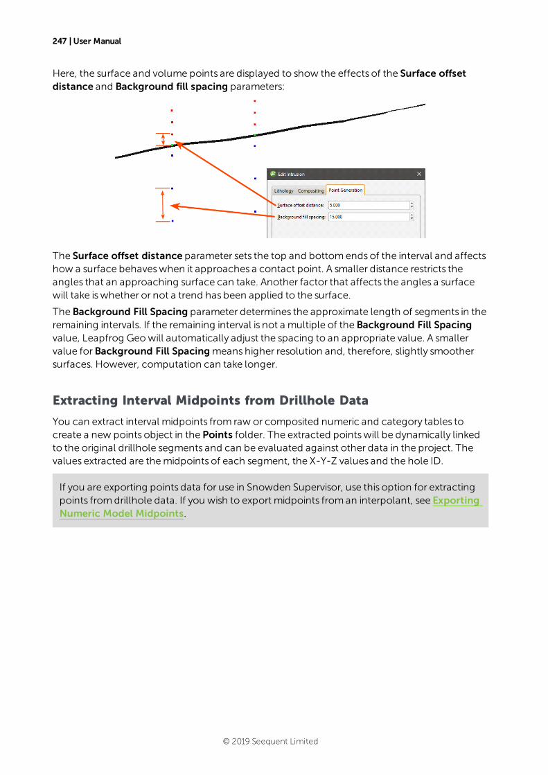
247 | User Manual
Here, the surface and volume points are displayed to show the effects of the Surface offsetdistance and Background fill spacing parameters:
The Surface offset distance parameter sets the top and bottomendsof the interval and affectshow a surface behaveswhen it approaches a contact point. A smaller distance restricts theangles that an approaching surface can take. Another factor that affects the angles a surfacewill take iswhether or not a trend has been applied to the surface.
The Background Fill Spacing parameter determines the approximate length of segments in theremaining intervals. If the remaining interval is not a multiple of the Background Fill Spacingvalue, Leapfrog Geowill automatically adjust the spacing to an appropriate value. A smallervalue forBackground Fill Spacingmeans higher resolution and, therefore, slightly smoothersurfaces. However, computation can take longer.
Extracting Interval Midpoints from Drillhole Data
You can extract interval midpoints from raw or composited numeric and category tables tocreate a new points object in the Points folder. The extracted pointswill be dynamically linkedto the original drillhole segments and can be evaluated against other data in the project. Thevalues extracted are themidpoints of each segment, the X-Y-Z values and the hole ID.
If you are exporting points data for use in Snowden Supervisor, use this option for extractingpoints fromdrillhole data. If you wish to export midpoints froman interpolant, see ExportingNumeric Model Midpoints.
© 2019 Seequent Limited
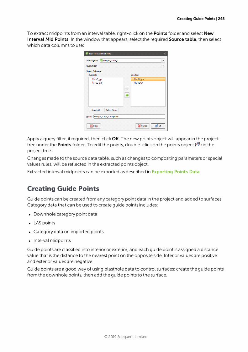
Creating Guide Points | 248
To extract midpoints froman interval table, right-click on the Points folder and selectNewInterval Mid Points. In thewindow that appears, select the required Source table, then selectwhich data columns to use:
Apply a query filter, if required, then clickOK. The new points object will appear in the projecttree under the Points folder. To edit the points, double-click on the points object ( ) in theproject tree.
Changesmade to the source data table, such as changes to compositing parameters or specialvalues rules, will be reflected in the extracted points object.
Extracted interval midpoints can be exported as described in Exporting Points Data.
Creating Guide Points
Guide points can be created fromany category point data in the project and added to surfaces.Category data that can be used to create guide points includes:
l Downhole category point data
l LAS points
l Category data on imported points
l Interval midpoints
Guide points are classified into interior or exterior, and each guide point is assigned a distancevalue that is the distance to the nearest point on the opposite side. Interior values are positiveand exterior values are negative.
Guide points are a good way of using blasthole data to control surfaces: create the guide pointsfrom the downhole points, then add the guide points to the surface.
© 2019 Seequent Limited
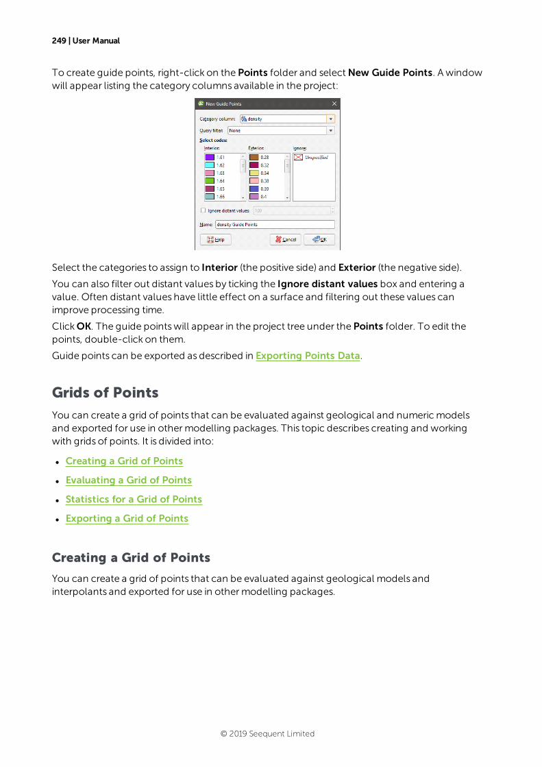
249 | User Manual
To create guide points, right-click on the Points folder and selectNew Guide Points. A windowwill appear listing the category columns available in the project:
Select the categories to assign to Interior (the positive side) and Exterior (the negative side).
You can also filter out distant values by ticking the Ignore distant values box and entering avalue. Often distant values have little effect on a surface and filtering out these values canimprove processing time.
ClickOK. The guide pointswill appear in the project tree under the Points folder. To edit thepoints, double-click on them.
Guide points can be exported as described in Exporting Points Data.
Grids of Points
You can create a grid of points that can be evaluated against geological and numericmodelsand exported for use in othermodelling packages. This topic describes creating and workingwith grids of points. It is divided into:
l Creating a Grid of Points
l Evaluating a Grid of Points
l Statistics for a Grid of Points
l Exporting a Grid of Points
Creating a Grid of Points
You can create a grid of points that can be evaluated against geological models andinterpolants and exported for use in othermodelling packages.
© 2019 Seequent Limited
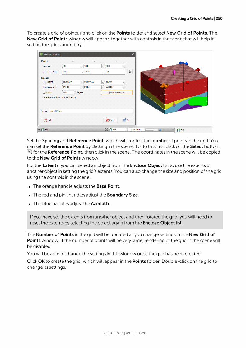
Creating a Grid of Points | 250
To create a grid of points, right-click on the Points folder and selectNew Grid of Points. TheNew Grid of Points windowwill appear, together with controls in the scene that will help insetting the grid’s boundary:
Set the Spacing and Reference Point, which will control the number of points in the grid. Youcan set theReference Point by clicking in the scene. To do this, first click on the Select button () for theReference Point, then click in the scene. The coordinates in the scenewill be copied
to theNew Grid of Points window.
For the Extents, you can select an object from the Enclose Object list to use the extents ofanother object in setting the grid’s extents. You can also change the size and position of the gridusing the controls in the scene:
l The orange handle adjusts the Base Point.
l The red and pink handles adjust the Boundary Size.
l The blue handles adjust the Azimuth.
If you have set the extents fromanother object and then rotated the grid, you will need toreset the extents by selecting the object again from the Enclose Object list.
TheNumber of Points in the grid will be updated as you change settings in theNew Grid ofPoints window. If the number of pointswill be very large, rendering of the grid in the scenewillbe disabled.
You will be able to change the settings in thiswindow once the grid has been created.
ClickOK to create the grid, which will appear in the Points folder. Double-click on the grid tochange its settings.
© 2019 Seequent Limited
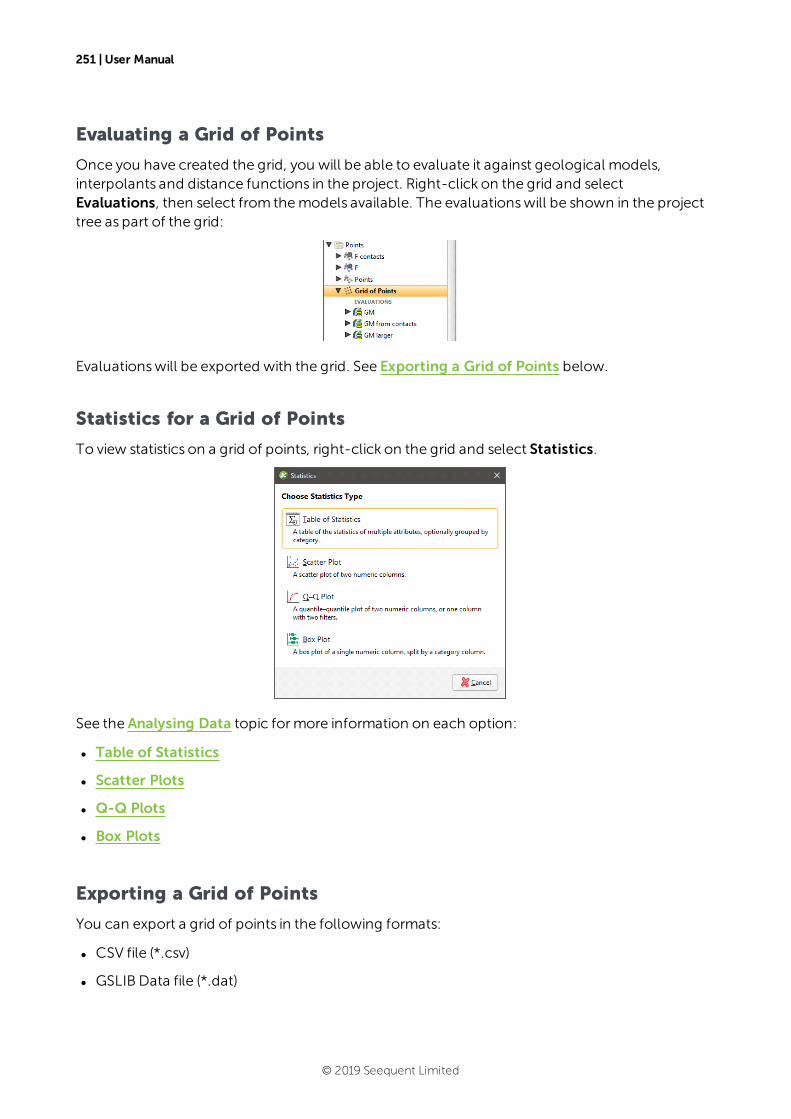
251 | User Manual
Evaluating a Grid of Points
Once you have created the grid, you will be able to evaluate it against geological models,interpolants and distance functions in the project. Right-click on the grid and selectEvaluations, then select from themodels available. The evaluationswill be shown in the projecttree as part of the grid:
Evaluationswill be exported with the grid. See Exporting a Grid of Points below.
Statistics for a Grid of Points
To view statistics on a grid of points, right-click on the grid and select Statistics.
See the Analysing Data topic formore information on each option:
l Table of Statistics
l Scatter Plots
l Q-Q Plots
l Box Plots
Exporting a Grid of Points
You can export a grid of points in the following formats:
l CSV file (*.csv)
l GSLIB Data file (*.dat)
© 2019 Seequent Limited
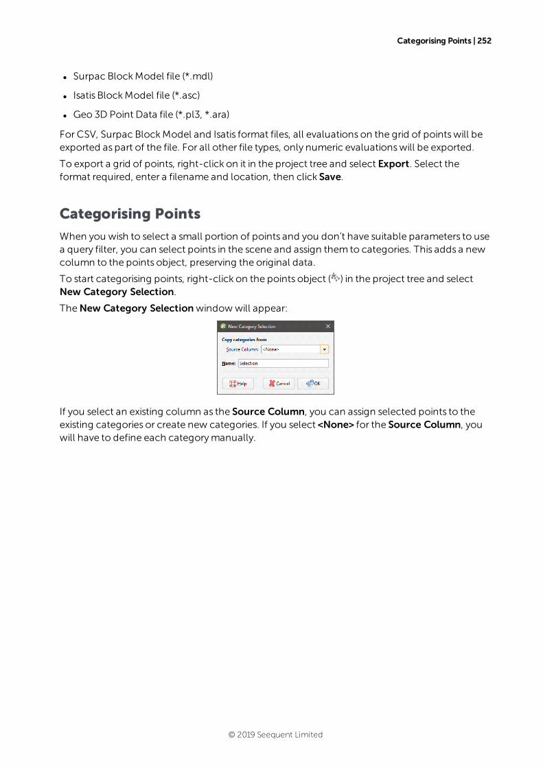
Categorising Points | 252
l Surpac BlockModel file (*.mdl)
l Isatis BlockModel file (*.asc)
l Geo 3D Point Data file (*.pl3, *.ara)
For CSV, Surpac BlockModel and Isatis format files, all evaluations on the grid of pointswill beexported as part of the file. For all other file types, only numeric evaluationswill be exported.
To export a grid of points, right-click on it in the project tree and select Export. Select theformat required, enter a filename and location, then click Save.
Categorising Points
When you wish to select a small portion of points and you don’t have suitable parameters to usea query filter, you can select points in the scene and assign them to categories. This adds a newcolumn to the points object, preserving the original data.
To start categorising points, right-click on the points object ( ) in the project tree and selectNew Category Selection.
TheNew Category Selectionwindowwill appear:
If you select an existing column as the Source Column, you can assign selected points to theexisting categories or create new categories. If you select <None> for the Source Column, youwill have to define each categorymanually.
© 2019 Seequent Limited

253 | User Manual
When you clickOK, the points object will be added to the scene, along with a set of tools forselecting points. To select points, click on the Select Points button ( ) and click the Add Pointsbutton ( ). In the scene, draw a line across each point you wish to select:
Selected points are highlighted in the scene. If you accidentally select thewrong point, either:
l Click theRemove Points button ( ) and draw across the point once again.
l Hold theCtrl keywhile drawing across the point.
You can also:
l Select all visible points by clicking on the Select All button ( ) or by pressing Ctrl+A.
l Clear all selected points by clicking on theClear Selection button ( ) or by pressingCtrl+Shift+A.
l Swap the selected points for the unselected points by clicking on the Invert Selectionbutton ( ) or by pressing Ctrl+I.
To change thewidth of the line used to select points, click on theChange Line Widthbutton ( ) and enter a new value. You can keep the Set Line Widthwindow open while youselect points so you can change the line width as required.
© 2019 Seequent Limited
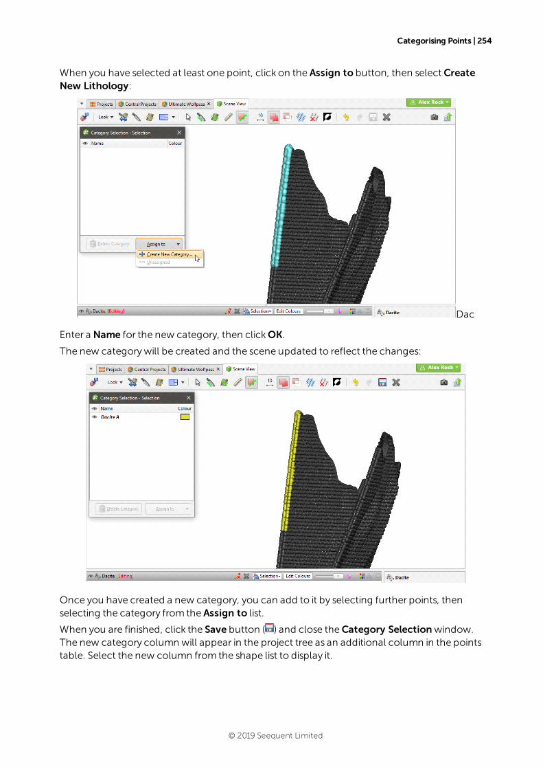
Categorising Points | 254
When you have selected at least one point, click on the Assign to button, then selectCreateNew Lithology:
Dac
Enter a Name for the new category, then clickOK.
The new categorywill be created and the scene updated to reflect the changes:
Once you have created a new category, you can add to it by selecting further points, thenselecting the category from the Assign to list.
When you are finished, click the Save button ( ) and close theCategory Selectionwindow.The new category column will appear in the project tree as an additional column in the pointstable. Select the new column from the shape list to display it.
© 2019 Seequent Limited
Geophysical DataThe types of geophysical data that can be imported into Leapfrog Geo are:
l 2D Grids
l ASEG_DFN Files
l UBC Grids
l GOCAD Models
2D Grids
Leapfrog Geo imports the following 2D grid formats:
l Arc/Info ASCII Grid (*.asc, *.txt)
l Arco/Info BinaryGrid (*.adf)
l Digital Elevation Model (*.dem)
l Intergraph ERDAS ERMapper 2D Grid (*.ers)
l ESRI .hdr Labelled Image (*.img, *.bil)
l SRTM .hgt (*.hgt)
l Surfer ASCII or BinaryGrid (*.grd)
l Grid eXchange File (*.gxf)
l Geosoft Grid (*.grd)
MapInfo files can be imported into theGIS Data, Maps and Photos folder. 2D grids in thesefileswill be saved into the into theGIS Data, Maps and Photos folder. See Importing aMapInfo Batch File formore information.
To import a 2D grid, right-click on either theGeophysical Data folder and select Import 2DGrid. Navigate to the folder that contains grid and select the file. ClickOpen to begin importingthe data.
The Import 2D Gridwindowwill appear, displaying the grid and each of the bands available.Select the data type for each band and set the georeference information, if necessary. SeeImporting a Map or Image for information on georeferencing imported files.
Once the grid has been imported, you can set its elevation, which is described in SettingElevation for GIS Objects and Images.
© 2019 Seequent Limited

ASEG_DFN Files | 256
When you display the grid in the scene, select the imported bands from the shape list:
Grids can be displayed as points ( ) or as cells and the values filtered, as described in DisplayingPoints.
ASEG_DFN Files
Leapfrog Geo imports ASEG_DFN points in *.dfn format. To import an ASEG_DFN file, right-click on theGeophysical Data folder and select Import ASEG_DFN. Leapfrog Geowill ask youto specify the file location. ClickOpen to import the file. In thewindow that appears, enter aname for the file, then clickOK. Next set the X, Y and Z coordinates and clickOK. If you select nocolumn for the Z coordinates, all Z valueswill be set to zero.
The file will appear in theGeophysical Data folder.
UBC Grids
Leapfrog Geo importsUBC grids in *.msh format, together with numeric values in propertiesfiles in *.gra, *.sus, *.mag and *.den formats. UBC grids can be evaluated against geological andnumericmodels, which can then be exported with the grid.
Importing a UBC Grid
To import a UBC grid, right-click on theGeophysical Data folder and select Import UBCModel. In thewindow that appears, clickBrowse to locate the file to be imported. ClickAdd toadd any properties file, although these are not required.
For any properties file, click the Inactive Value field tomark cells as inactive. Doing so does notchange the data but ensures that cellswith the inactive value can be hidden when the grid isdisplayed in the scene. If you do not set this valuewhen importing the grid, you can set it later bydouble-clicking on the grid in the project tree.
Click Import. The grid will appear in theGeophysical Data folder.
Evaluating UBC Grids
UBC grids can be evaluated against geological and numericmodels as described inEvaluations. However, UBC grids cannot be evaluated against fault blocks and mutli-domained RBF interpolants, although they can be evaluated against the parent geologicalmodel and the parent numericmodel.
© 2019 Seequent Limited
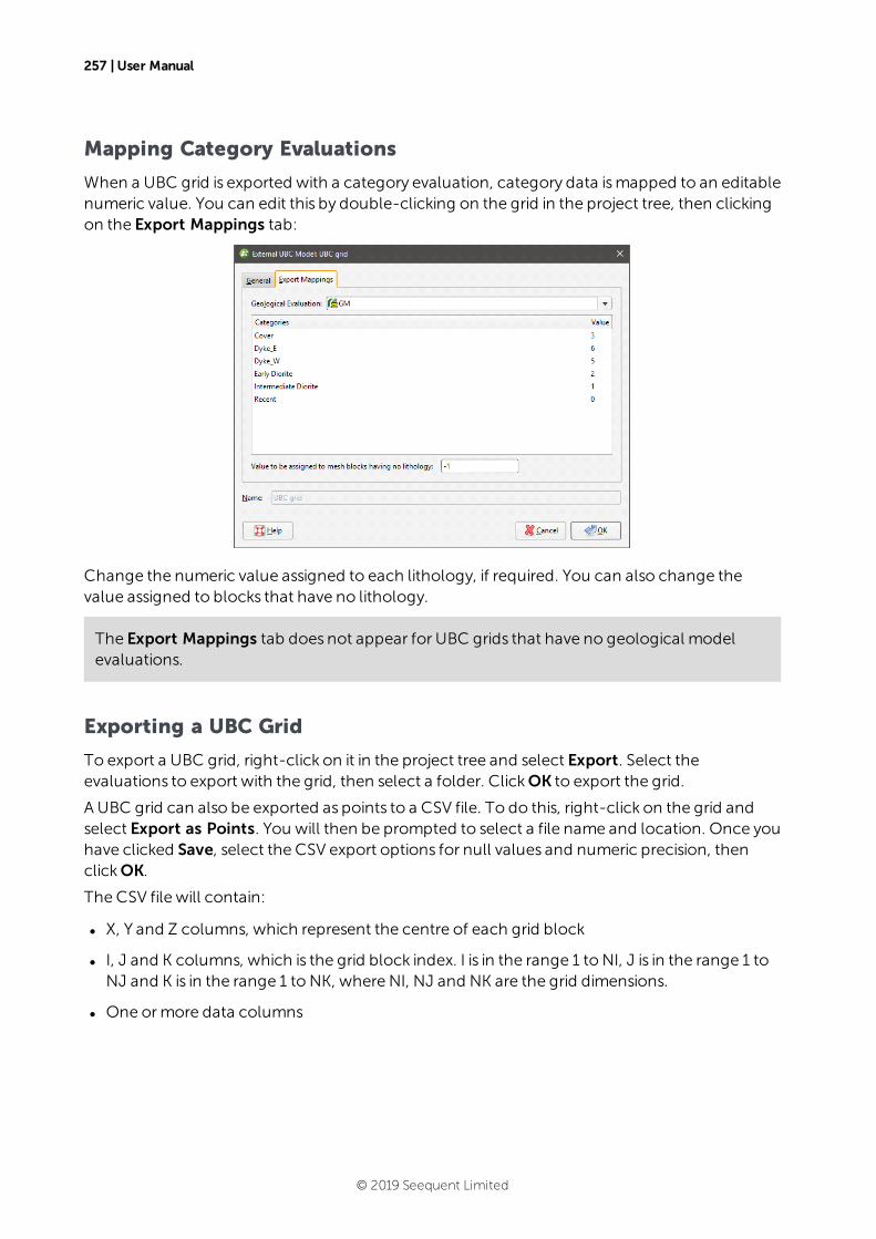
257 | User Manual
Mapping Category Evaluations
When a UBC grid is exported with a category evaluation, category data ismapped to an editablenumeric value. You can edit this by double-clicking on the grid in the project tree, then clickingon the Export Mappings tab:
Change the numeric value assigned to each lithology, if required. You can also change thevalue assigned to blocks that have no lithology.
The Export Mappings tab does not appear for UBC grids that have no geological modelevaluations.
Exporting a UBC Grid
To export a UBC grid, right-click on it in the project tree and select Export. Select theevaluations to export with the grid, then select a folder. ClickOK to export the grid.
A UBC grid can also be exported as points to a CSV file. To do this, right-click on the grid andselect Export as Points. You will then be prompted to select a file name and location. Once youhave clicked Save, select the CSV export options for null values and numeric precision, thenclickOK.
The CSV file will contain:
l X, Y and Z columns, which represent the centre of each grid block
l I, J and K columns, which is the grid block index. I is in the range 1 to NI, J is in the range 1 toNJ and K is in the range 1 to NK, where NI, NJ and NK are the grid dimensions.
l One ormore data columns
© 2019 Seequent Limited

GOCAD Models | 258
GOCAD Models
To import a GOCADmodel, right-click on theGeophysical Data folder and select ImportGOCAD Model. Leapfrog Geowill ask you to specify the file location. ClickOpen to import thefile.
In thewindow that appears, set the Subsample Rate and enter a Name for themodel. ClickOKto import themodel, which will appear under theGeophysical Data folder.
You can then evaluate geological models, interpolants and distance functions in the project onthemodel. In the case of geological models, you can also combine two ormoremodels toevaluate on themodel. To evaluate a model, right-click on themodel object in the project treeand select Evaluations. See Evaluations formore information.
A GOCADmodel can be exported as points to a CSV file. To do this, right-click on the grid andselect Export as Points. You will then be prompted to select a file name and location. Once youhave clicked Save, select the CSV export options for null values and numeric precision, thenclickOK.
The CSV file will contain:
l X, Y and Z columns, which represent the centre of each grid block
l I, J and K columns, which is the grid block index. I is in the range 1 to NI, J is in the range 1 toNJ and K is in the range 1 to NK, where NI, NJ and NK are the grid dimensions.
l One ormore data columns
© 2019 Seequent Limited
Structural DataIn Leapfrog Geo, you can create and edit planar structural data tables directly or fromotherobjects in the project. Structural data can also be used to create and edit many surfaces.Downhole planar structural data and lineations can also be imported, although structural dataimported in thisway cannot be edited.
This topic describes how toworkwith structural data in Leapfrog Geo. It covers:
l Creating New Planar Structural Data Tables
l Importing Planar Structural Data
l Importing Lineations
l Displaying Structural Data
l Viewing Statistics on Structural Data
l Assigning Structural Data to Categories
l Editing the Orientation of Planar Structural Data
l Declustering Planar Structural Data
l Setting Elevation for Structural Data
l Estimating Planar Structural Data
See Stereonets and Form Interpolants for information on tools for analysing structural data.
Leapfrog Geo calculates strike using the American right-hand rule; when looking in the strikedirection, the plane should dip to the right.
Creating New Planar Structural Data Tables
There are twoways to create a new planar structural data table in Leapfrog Geo:
l Create a new table as part of creating or editing another object. See Editing Surfaces withStructural Data.
l Create a new table using the Structural Modelling folder. Use this techniquewhen, forexample, you are creating structural data points froma map or image. Right-click on theStructural Modelling folder and selectNew Planar Structural Data. In thewindow thatappears, enter a name for the new table and clickOK.
Before creating the new data table, add themap, image or data object you wish towork from tothe scene and orient the scene for drawing the new data points.
© 2019 Seequent Limited
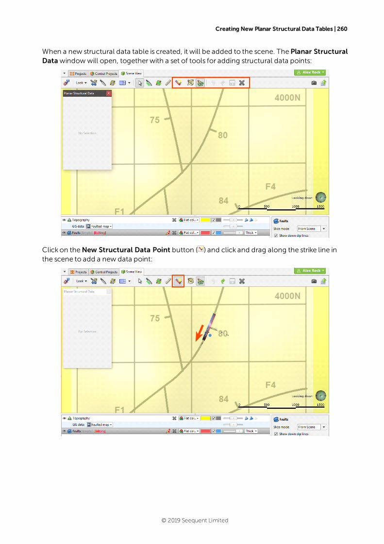
Creating New Planar Structural Data Tables | 260
When a new structural data table is created, it will be added to the scene. The Planar StructuralDatawindowwill open, together with a set of tools for adding structural data points:
Click on theNew Structural Data Point button ( ) and click and drag along the strike line inthe scene to add a new data point:
© 2019 Seequent Limited
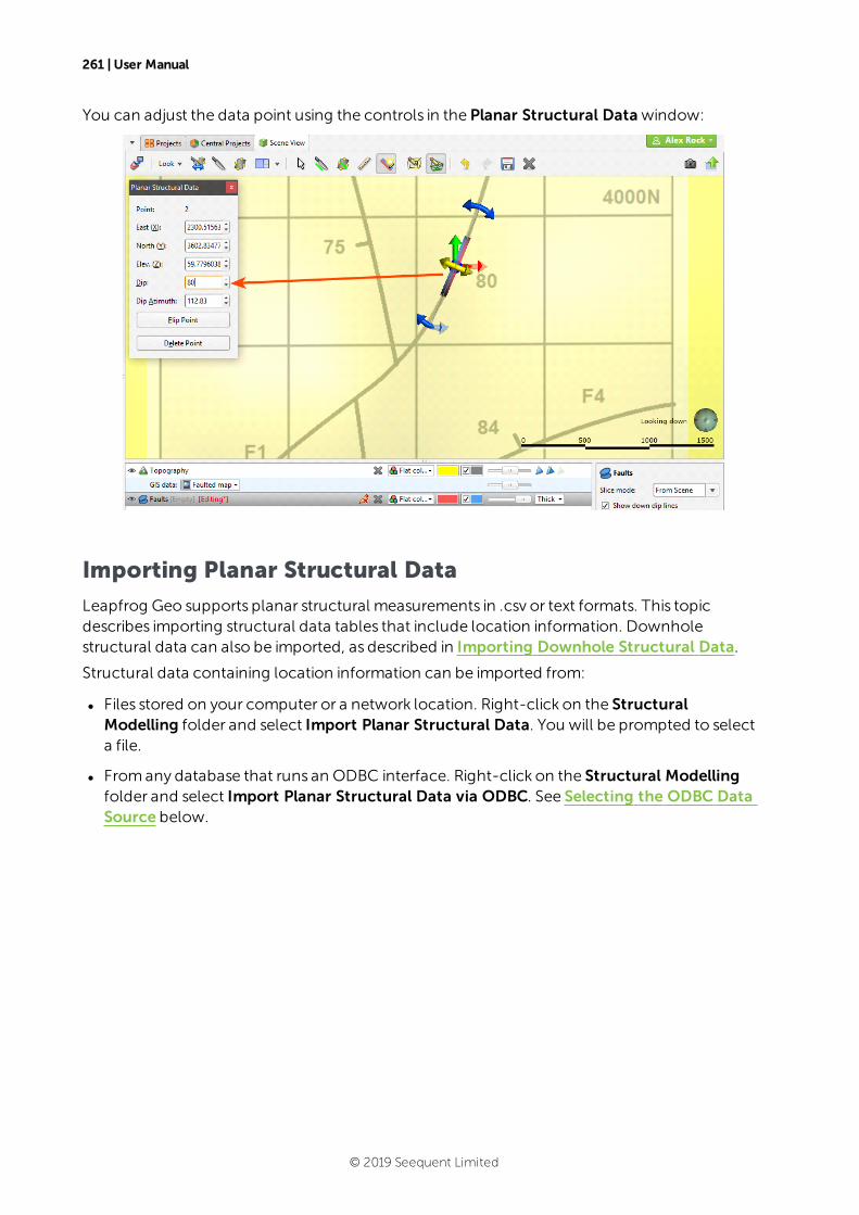
261 | User Manual
You can adjust the data point using the controls in the Planar Structural Datawindow:
Importing Planar Structural Data
Leapfrog Geo supports planar structural measurements in .csv or text formats. This topicdescribes importing structural data tables that include location information. Downholestructural data can also be imported, as described in Importing Downhole Structural Data.
Structural data containing location information can be imported from:
l Files stored on your computer or a network location. Right-click on the StructuralModelling folder and select Import Planar Structural Data. You will be prompted to selecta file.
l Fromany database that runs an ODBC interface. Right-click on the Structural Modellingfolder and select Import Planar Structural Data via ODBC. See Selecting the ODBC DataSource below.
© 2019 Seequent Limited
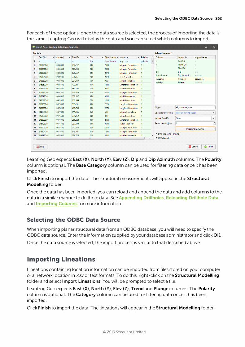
Selecting the ODBC Data Source | 262
For each of these options, once the data source is selected, the process of importing the data isthe same. Leapfrog Geowill display the data and you can select which columns to import:
Leapfrog Geo expectsEast (X), North (Y), Elev (Z), Dip and Dip Azimuth columns. The Polaritycolumn is optional. The Base Category column can be used for filtering data once it has beenimported.
Click Finish to import the data. The structural measurementswill appear in the StructuralModelling folder.
Once the data has been imported, you can reload and append the data and add columns to thedata in a similarmanner to drillhole data. See Appending Drillholes, Reloading Drillhole Dataand Importing Columns formore information.
Selecting the ODBC Data Source
When importing planar structural data froman ODBC database, you will need to specify theODBC data source. Enter the information supplied by your database administrator and clickOK.
Once the data source is selected, the import process is similar to that described above.
Importing Lineations
Lineations containing location information can be imported from files stored on your computeror a network location in .csv or text formats. To do this, right-click on the Structural Modellingfolder and select Import Lineations. You will be prompted to select a file.
Leapfrog Geo expectsEast (X), North (Y), Elev (Z), Trend and Plunge columns. The Polaritycolumn is optional. TheCategory column can be used for filtering data once it has beenimported.
Click Finish to import the data. The lineationswill appear in the Structural Modelling folder.
© 2019 Seequent Limited
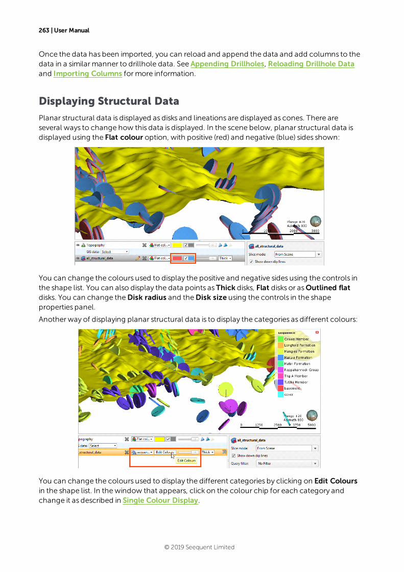
263 | User Manual
Once the data has been imported, you can reload and append the data and add columns to thedata in a similarmanner to drillhole data. See Appending Drillholes, Reloading Drillhole Dataand Importing Columns formore information.
Displaying Structural Data
Planar structural data is displayed as disks and lineations are displayed as cones. There areseveral ways to change how this data is displayed. In the scene below, planar structural data isdisplayed using the Flat colour option, with positive (red) and negative (blue) sides shown:
You can change the colours used to display the positive and negative sides using the controls inthe shape list. You can also display the data points asThick disks, Flat disks or asOutlined flatdisks. You can change theDisk radius and theDisk size using the controls in the shapeproperties panel.
Another way of displaying planar structural data is to display the categories as different colours:
You can change the colours used to display the different categories by clicking on Edit Coloursin the shape list. In thewindow that appears, click on the colour chip for each category andchange it as described in Single Colour Display.
© 2019 Seequent Limited

Displaying Structural Data | 264
To set multiple categories to a single colour, use the Shift or Ctrl keys to select the colourchips you wish to change, then click on one of the colour chips. The colour changes youmakewill bemade to all selected categories.
The categories displayed can also be filtered by other columns in the data table, as described inFiltering Data Using Values and Categories.
In the scene below, lineations are displayed using the Flat colour option in green:
Click the colour chip to change the colour used to display the cones in the shape list or selectone of the table’s columns:
© 2019 Seequent Limited
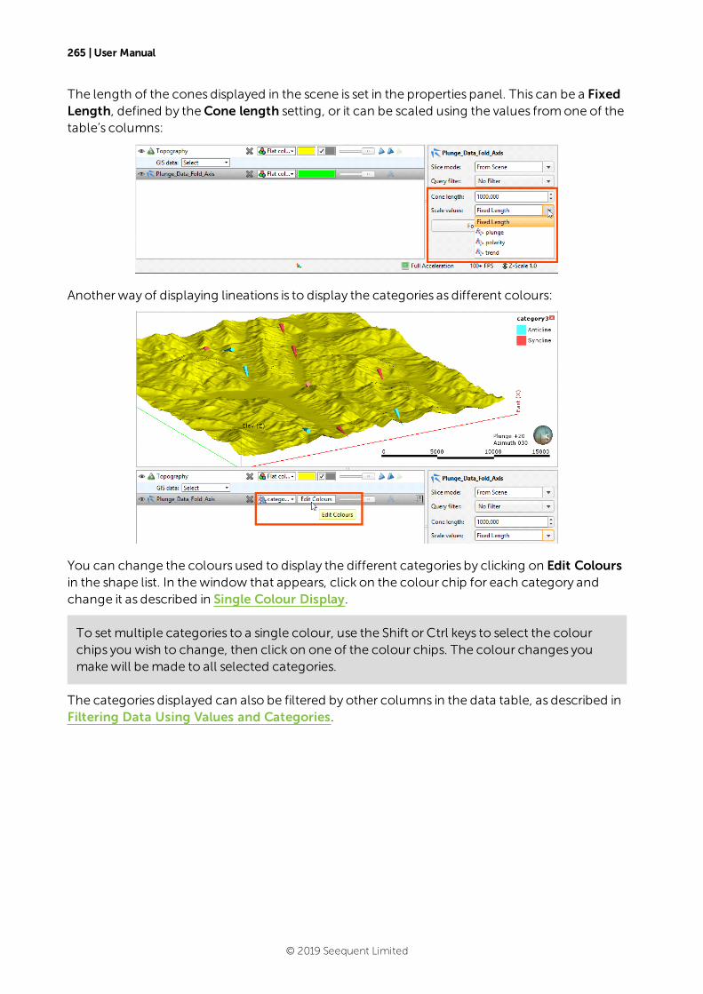
265 | User Manual
The length of the cones displayed in the scene is set in the properties panel. This can be a FixedLength, defined by theCone length setting, or it can be scaled using the values fromone of thetable’s columns:
Another way of displaying lineations is to display the categories as different colours:
You can change the colours used to display the different categories by clicking on Edit Coloursin the shape list. In thewindow that appears, click on the colour chip for each category andchange it as described in Single Colour Display.
To set multiple categories to a single colour, use the Shift or Ctrl keys to select the colourchips you wish to change, then click on one of the colour chips. The colour changes youmakewill bemade to all selected categories.
The categories displayed can also be filtered by other columns in the data table, as described inFiltering Data Using Values and Categories.
© 2019 Seequent Limited
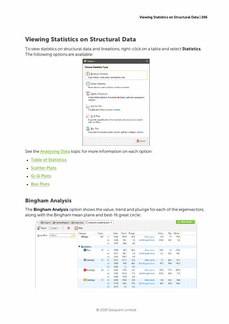
Viewing Statistics on Structural Data | 266
Viewing Statistics on Structural Data
To view statistics on structural data and lineations, right-click on a table and select Statistics.The following options are available:
See the Analysing Data topic formore information on each option:
l Table of Statistics
l Scatter Plots
l Q-Q Plots
l Box Plots
Bingham Analysis
The Bingham Analysis option shows the value, trend and plunge for each of the eigenvectors,along with the Binghammean plane and best-fit great circle:
© 2019 Seequent Limited
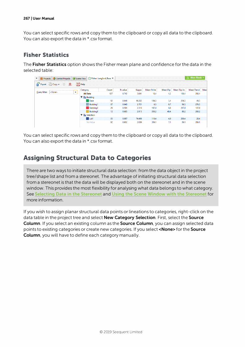
267 | User Manual
You can select specific rows and copy them to the clipboard or copy all data to the clipboard.You can also export the data in *.csv format.
Fisher Statistics
The Fisher Statistics option shows the Fishermean plane and confidence for the data in theselected table:
You can select specific rows and copy them to the clipboard or copy all data to the clipboard.You can also export the data in *.csv format.
Assigning Structural Data to Categories
There are twoways to initiate structural data selection: from the data object in the projecttree/shape list and froma stereonet. The advantage of initiating structural data selectionfroma stereonet is that the data will be displayed both on the stereonet and in the scenewindow. This provides themost flexibility for analysing what data belongs towhat category.See Selecting Data in the Stereonet and Using the Scene Window with the Stereonet formore information.
If you wish to assign planar structural data points or lineations to categories, right-click on thedata table in the project tree and selectNew Category Selection. First, select the SourceColumn. If you select an existing column as the Source Column, you can assign selected datapoints to existing categories or create new categories. If you select <None> for the SourceColumn, you will have to define each categorymanually.
© 2019 Seequent Limited

Assigning Structural Data to Categories | 268
Select points by clicking on the Select points tool ( ), then drawing over those points in thescene:
Once you have selected points, you can assign them to existing categories or create new ones.To create a new category, click on the Assign to > Create New Category button:
Enter a name for the new category and clickOK.
When you have finished selecting points and adding them to categories, close theCategorySelectionwindow to close the editor.
© 2019 Seequent Limited

269 | User Manual
Editing the Orientation of Planar Structural Data
If you need to edit the orientation of planar structural data points, you can do so in twoways:
l Edit the data in the table directly by double-clicking on the structural data table in theproject tree. SeeWorking with Data Tables.
l Edit the structural data orientation in the scene.
To edit the structural data in the scene, right-click on the table in the project tree and select EditOrientation in Scene. If the table is displayed in the scene, in the shape list, click on the Editbutton ( ). The Planar Structural Datawindowwill appear in the scene, together withcontrols for editing the data points. To edit a data point, click on it. Information about theselected point will be displayed in the Planar Structural Datawindow, together with controls inthe scene you can use to adjust the point:
You can also add new data points in the samemanner described in Creating New PlanarStructural Data Tables.
Declustering Planar Structural Data
If a planar structural data table containsmultiple duplicate or near-duplicatemeasurements,you can create a declustered structural data set that will make the table easier to workwith.Declustering is intended toworkwith large, machine-collected data sets rather than smallersets that might be edited manually.
Declustering preserves the original data table and creates the set as a “filter” by applying twoparameters: the Spatial search radius and the Angular tolerance.
l The Spatial search radius determines the size of the declustering space. All points inside theSpatial search radius are compared searching for duplicates.
© 2019 Seequent Limited
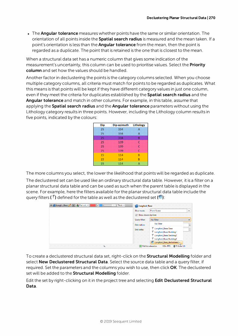
Declustering Planar Structural Data | 270
l The Angular tolerancemeasureswhether points have the same or similar orientation. Theorientation of all points inside the Spatial search radius ismeasured and themean taken. If apoint’s orientation is less than the Angular tolerance from themean, then the point isregarded as a duplicate. The point that is retained is the one that is closest to themean.
When a structural data set has a numeric column that gives some indication of themeasurement’s uncertainty, this column can be used to prioritise values. Select the Prioritycolumn and set how the values should be handled.
Another factor in declustering the points is the category columns selected. When you choosemultiple category columns, all criteria must match for points to be regarded as duplicates. Whatthismeans is that pointswill be kept if they have different category values in just one column,even if theymeet the criteria for duplicates established by the Spatial search radius and theAngular tolerance and match in other columns. For example, in this table, assume thatapplying the Spatial search radius and the Angular tolerance parameterswithout using theLithology category results in three points. However, including the Lithology column results infive points, indicated by the colours:
Themore columns you select, the lower the likelihood that pointswill be regarded as duplicate.
The declustered set can be used like an ordinary structural data table. However, it is a filter on aplanar structural data table and can be used as such when the parent table is displayed in thescene. For example, here the filters available for the planar structural data table include thequery filters ( ) defined for the table aswell as the declustered set ( ):
To create a declustered structural data set, right-click on the Structural Modelling folder andselectNew Declustered Structural Data. Select the source data table and a query filter, ifrequired. Set the parameters and the columns you wish to use, then clickOK. The declusteredset will be added to the Structural Modelling folder.
Edit the set by right-clicking on it in the project tree and selecting Edit Declustered StructuralData.
© 2019 Seequent Limited
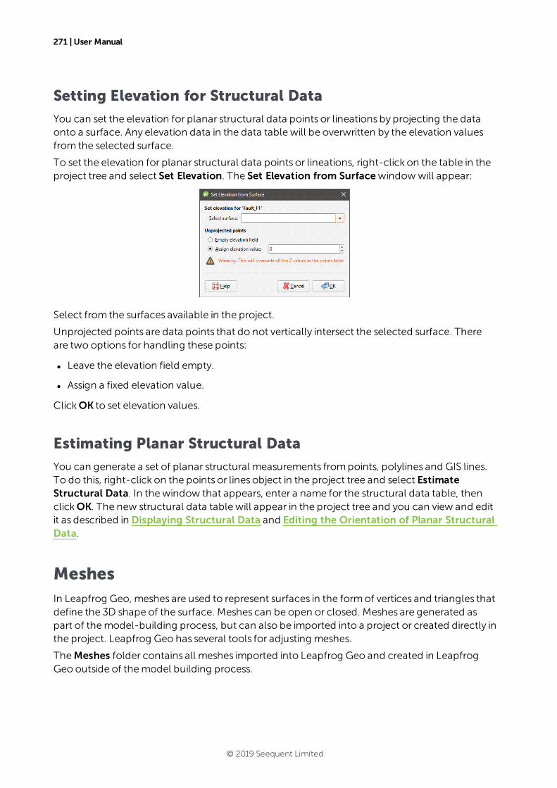
271 | User Manual
Setting Elevation for Structural Data
You can set the elevation for planar structural data points or lineations by projecting the dataonto a surface. Any elevation data in the data table will be overwritten by the elevation valuesfrom the selected surface.
To set the elevation for planar structural data points or lineations, right-click on the table in theproject tree and select Set Elevation. The Set Elevation from Surfacewindowwill appear:
Select from the surfaces available in the project.
Unprojected points are data points that do not vertically intersect the selected surface. Thereare two options for handling these points:
l Leave the elevation field empty.
l Assign a fixed elevation value.
ClickOK to set elevation values.
Estimating Planar Structural Data
You can generate a set of planar structural measurements frompoints, polylines and GIS lines.To do this, right-click on the points or lines object in the project tree and select EstimateStructural Data. In thewindow that appears, enter a name for the structural data table, thenclickOK. The new structural data table will appear in the project tree and you can view and editit as described in Displaying Structural Data and Editing the Orientation of Planar StructuralData.
MeshesIn Leapfrog Geo, meshes are used to represent surfaces in the formof vertices and triangles thatdefine the 3D shape of the surface. Meshes can be open or closed. Meshes are generated aspart of themodel-building process, but can also be imported into a project or created directly inthe project. Leapfrog Geo has several tools for adjusting meshes.
TheMeshes folder contains all meshes imported into Leapfrog Geo and created in LeapfrogGeo outside of themodel building process.
© 2019 Seequent Limited

Cleaning Up a Mesh | 272
Two types of meshes are stored in theMeshes folder:
l Non-editablemeshes ( ) aremeshes imported into Leapfrog Geo and meshes created inLeapfrog Geo from themoving plane, Meshes > Mesh Operations tools and by extractingmesh parts fromother surfaces in the project.
l Editablemeshes ( ) are created in Leapfrog Geo fromdata objects such as points data, GISdata and polylines. Editablemeshes can be refined by adding more data. Editablemeshescan be interpolated meshes (using FastRBF) or triangulated meshes (using Delaunaytriangulation). Interpolated meshes can also be created from structural data and valuesobjects.
The rest of this topic is divided into:
l Cleaning Up a Mesh
l Importing a Mesh
l Reloading a Mesh
l Displaying Surfaces
l Importing Meshes from Central
l Exporting Meshes
Cleaning Up a Mesh
There are several options for cleaning up a mesh that can be applied tomeshes imported intoLeapfrog Geo and to non-editablemeshes created in Leapfrog Geo.
To clean up a mesh, double-click on themesh in theMeshes folder or right-click on themeshand selectOpen. TheCleanup Meshwindowwill be displayed:
TheCleanup Meshwindowwill also be displayed when you import meshes.
The first option, Combine identical vertices, is intended for snapping caseswhere verticesoccupy the exact same point in space. When enabled, vertices that have the exact samecoordinateswill bemerged.
© 2019 Seequent Limited
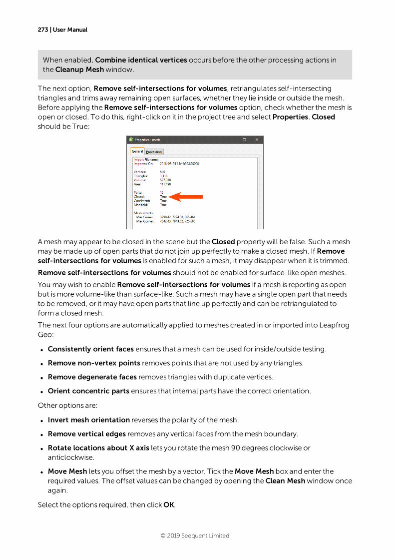
273 | User Manual
When enabled, Combine identical vertices occurs before the other processing actions intheCleanup Meshwindow.
The next option, Remove self-intersections for volumes, retriangulates self-intersectingtriangles and trims away remaining open surfaces, whether they lie inside or outside themesh.Before applying theRemove self-intersections for volumes option, checkwhether themesh isopen or closed. To do this, right-click on it in the project tree and select Properties. Closedshould be True:
Amesh may appear to be closed in the scene but theClosed propertywill be false. Such a meshmay bemade up of open parts that do not join up perfectly tomake a closed mesh. If Removeself-intersections for volumes is enabled for such a mesh, it may disappear when it is trimmed.
Remove self-intersections for volumes should not be enabled for surface-like open meshes.
You maywish to enableRemove self-intersections for volumes if a mesh is reporting as openbut ismore volume-like than surface-like. Such a mesh may have a single open part that needsto be removed, or it may have open parts that line up perfectly and can be retriangulated toforma closed mesh.
The next four options are automatically applied tomeshes created in or imported into LeapfrogGeo:
l Consistently orient faces ensures that a mesh can be used for inside/outside testing.
l Remove non-vertex points removes points that are not used by any triangles.
l Remove degenerate faces removes triangleswith duplicate vertices.
l Orient concentric parts ensures that internal parts have the correct orientation.
Other options are:
l Invert mesh orientation reverses the polarity of themesh.
l Remove vertical edges removes any vertical faces from themesh boundary.
l Rotate locations about X axis lets you rotate themesh 90 degrees clockwise oranticlockwise.
l Move Mesh lets you offset themesh by a vector. Tick theMove Mesh box and enter therequired values. The offset values can be changed by opening theClean Meshwindow onceagain.
Select the options required, then clickOK.
© 2019 Seequent Limited
Importing a Mesh | 274
Themesh will be added to the project tree under theMeshes folder.
Importing a Mesh
Mesh formats Leapfrog Geo supports include:
l Leapfrog Geo Attribute BinaryMesh Formats (*.msh, *.ara)
l Datamine Files (*.asc, *.dm)
l DXF Polyface Files (11/12 [AC1009]) (*.dxf)
l GemcomFiles (*.tri)
l AliasWavefront Object Files (*.obj)
l Surpac DTM Files (*.dtm)
l GOCAD Files (*.ts)
l Leapfrog Model Files (*.lfm)
l Micromine Files (*.dat)
l BentleyDrawing Files (v8) (*.dgn)
l AutoCAD Drawing Files (2013/LT2013) (*.dwg)
l Vulcan Files (*.00t) (with Maptek Link)
If you have theMaptek Link extension, you can also import meshes in VULCAN .00t format.Contact Customer Support as described in Getting Support formore information about theMaptek Link extension.
Once a mesh has been imported to the project, you can evaluate it against any interpolant ordistance function in the project. See Evaluations formore information.
To import a mesh, right-click on theMeshes folder and select Import Mesh. Navigate to thefolder that contains themesh file and select the file. You can select multiple files using the Shiftand Ctrl keys. ClickOpen to import the file.
TheCleanup Meshwindowwill be displayed. SeeCleaning Up a Mesh. Select the optionsrequired, then clickOK.
Themesh will be added to the project tree under theMeshes folder.
Meshes with Textures
Leapfrog Geo can import OBJ mesheswith textures. If you have theMaptek Link extension, youcan also import Vulcan mesheswith textures.
© 2019 Seequent Limited
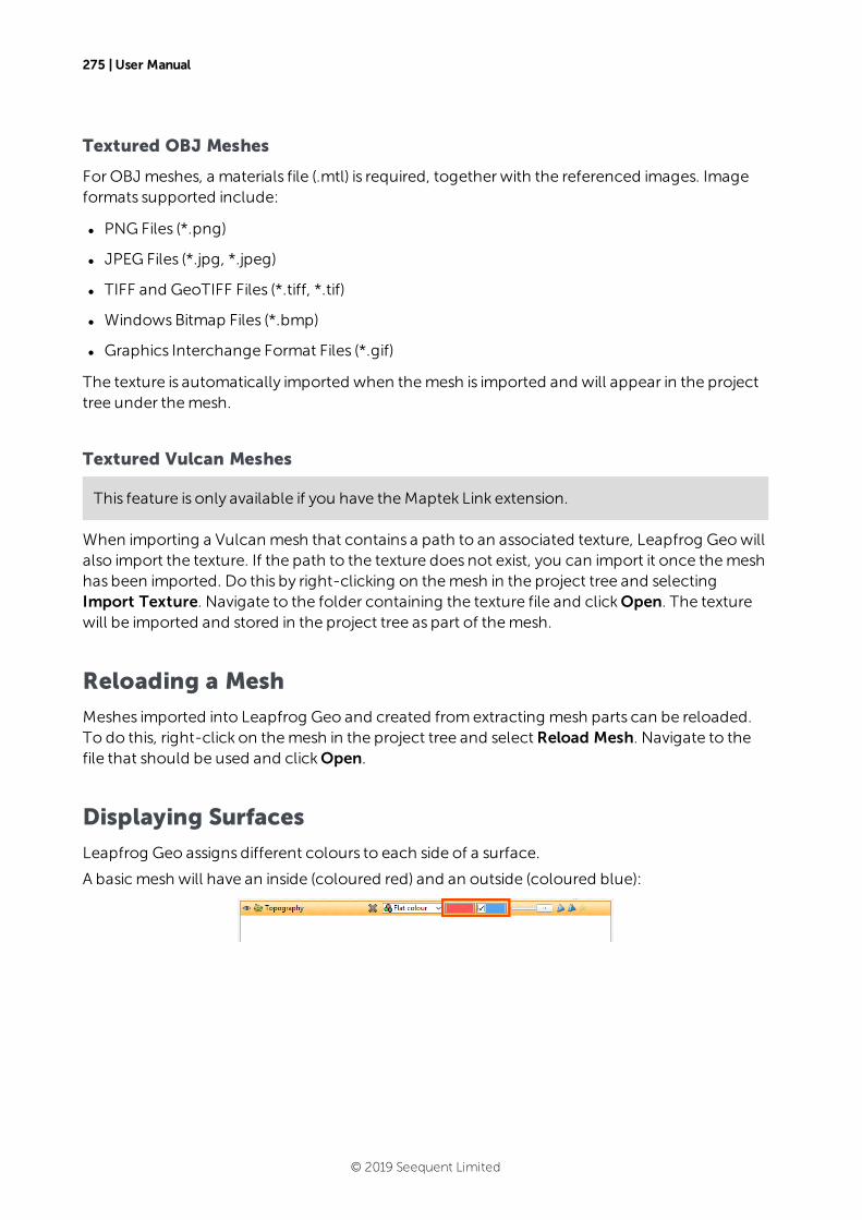
275 | User Manual
Textured OBJ Meshes
ForOBJ meshes, a materials file (.mtl) is required, together with the referenced images. Imageformats supported include:
l PNG Files (*.png)
l JPEG Files (*.jpg, *.jpeg)
l TIFF and GeoTIFF Files (*.tiff, *.tif)
l WindowsBitmap Files (*.bmp)
l Graphics Interchange Format Files (*.gif)
The texture is automatically imported when themesh is imported and will appear in the projecttree under themesh.
Textured Vulcan Meshes
This feature is only available if you have theMaptek Link extension.
When importing a Vulcan mesh that contains a path to an associated texture, Leapfrog Geowillalso import the texture. If the path to the texture does not exist, you can import it once themeshhas been imported. Do this by right-clicking on themesh in the project tree and selectingImport Texture. Navigate to the folder containing the texture file and clickOpen. The texturewill be imported and stored in the project tree as part of themesh.
Reloading a Mesh
Meshes imported into Leapfrog Geo and created fromextracting mesh parts can be reloaded.To do this, right-click on themesh in the project tree and select Reload Mesh. Navigate to thefile that should be used and clickOpen.
Displaying Surfaces
Leapfrog Geo assigns different colours to each side of a surface.
A basicmesh will have an inside (coloured red) and an outside (coloured blue):
© 2019 Seequent Limited
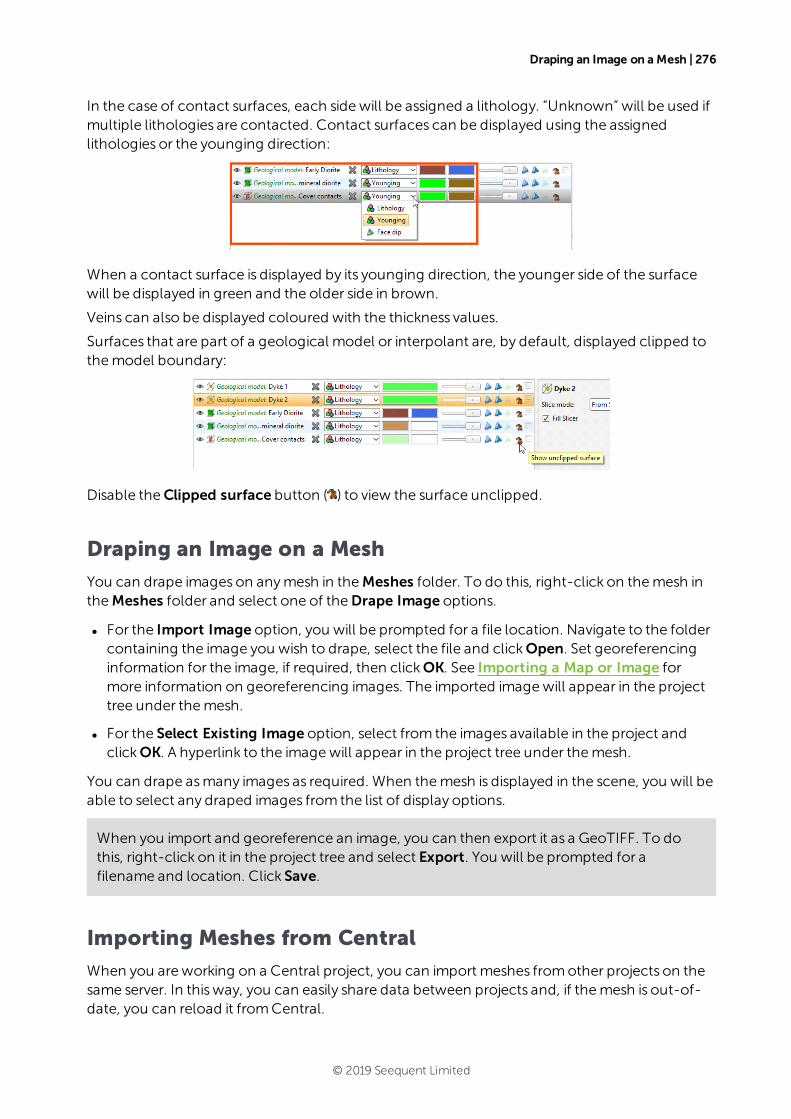
Draping an Image on a Mesh | 276
In the case of contact surfaces, each sidewill be assigned a lithology. “Unknown” will be used ifmultiple lithologies are contacted. Contact surfaces can be displayed using the assignedlithologies or the younging direction:
When a contact surface is displayed by its younging direction, the younger side of the surfacewill be displayed in green and the older side in brown.
Veins can also be displayed coloured with the thickness values.
Surfaces that are part of a geological model or interpolant are, by default, displayed clipped tothemodel boundary:
Disable theClipped surface button ( ) to view the surface unclipped.
Draping an Image on a Mesh
You can drape images on anymesh in theMeshes folder. To do this, right-click on themesh intheMeshes folder and select one of theDrape Image options.
l For the Import Image option, you will be prompted for a file location. Navigate to the foldercontaining the image you wish to drape, select the file and clickOpen. Set georeferencinginformation for the image, if required, then clickOK. See Importing a Map or Image formore information on georeferencing images. The imported imagewill appear in the projecttree under themesh.
l For the Select Existing Image option, select from the images available in the project andclickOK. A hyperlink to the imagewill appear in the project tree under themesh.
You can drape asmany images as required. When themesh is displayed in the scene, you will beable to select any draped images from the list of display options.
When you import and georeference an image, you can then export it as a GeoTIFF. To dothis, right-click on it in the project tree and select Export. You will be prompted for afilename and location. Click Save.
Importing Meshes from Central
When you are working on a Central project, you can import meshes fromother projects on thesame server. In thisway, you can easily share data between projects and, if themesh is out-of-date, you can reload it fromCentral.
© 2019 Seequent Limited
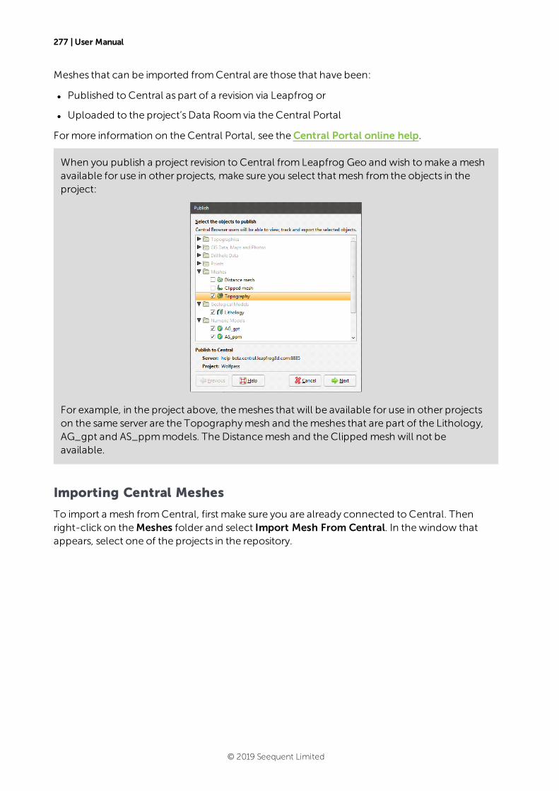
277 | User Manual
Meshes that can be imported fromCentral are those that have been:
l Published to Central as part of a revision via Leapfrog or
l Uploaded to the project’s Data Roomvia the Central Portal
Formore information on the Central Portal, see theCentral Portal online help.
When you publish a project revision to Central fromLeapfrog Geo and wish tomake a meshavailable for use in other projects, make sure you select that mesh from the objects in theproject:
For example, in the project above, themeshes that will be available for use in other projectson the same server are the Topographymesh and themeshes that are part of the Lithology,AG_gpt and AS_ppmmodels. The Distancemesh and the Clipped mesh will not beavailable.
Importing Central Meshes
To import a mesh fromCentral, first make sure you are already connected to Central. Thenright-click on theMeshes folder and select Import Mesh From Central. In thewindow thatappears, select one of the projects in the repository.
© 2019 Seequent Limited
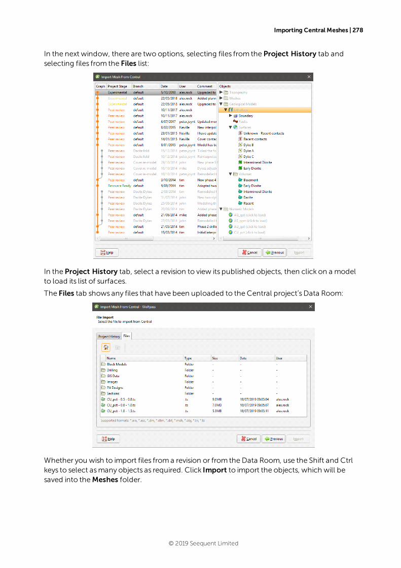
Importing Central Meshes | 278
In the next window, there are two options, selecting files from the Project History tab andselecting files from the Files list:
In the Project History tab, select a revision to view its published objects, then click on a modelto load its list of surfaces.
The Files tab shows any files that have been uploaded to the Central project’s Data Room:
Whether you wish to import files froma revision or from the Data Room, use the Shift and Ctrlkeys to select asmany objects as required. Click Import to import the objects, which will besaved into theMeshes folder.
© 2019 Seequent Limited
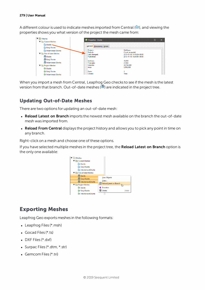
279 | User Manual
A different colour is used to indicatemeshes imported fromCentral ( ), and viewing theproperties shows you what version of the project themesh came from:
When you import a mesh fromCentral, Leapfrog Geo checks to see if themesh is the latestversion from that branch. Out-of-datemeshes ( ) are indicated in the project tree.
Updating Out-of-Date Meshes
There are two options for updating an out-of-datemesh:
l Reload Latest on Branch imports the newest mesh available on the branch the out-of-datemesh was imported from.
l Reload From Central displays the project history and allows you to pick any point in time onany branch.
Right-click on a mesh and choose one of these options.
If you have selected multiplemeshes in the project tree, theReload Latest on Branch option isthe only one available:
Exporting Meshes
Leapfrog Geo exportsmeshes in the following formats:
l Leapfrog Files (*.msh)
l Gocad Files (*.ts)
l DXF Files (*.dxf)
l Surpac Files (*.dtm, *.str)
l GemcomFiles (*.tri)
© 2019 Seequent Limited
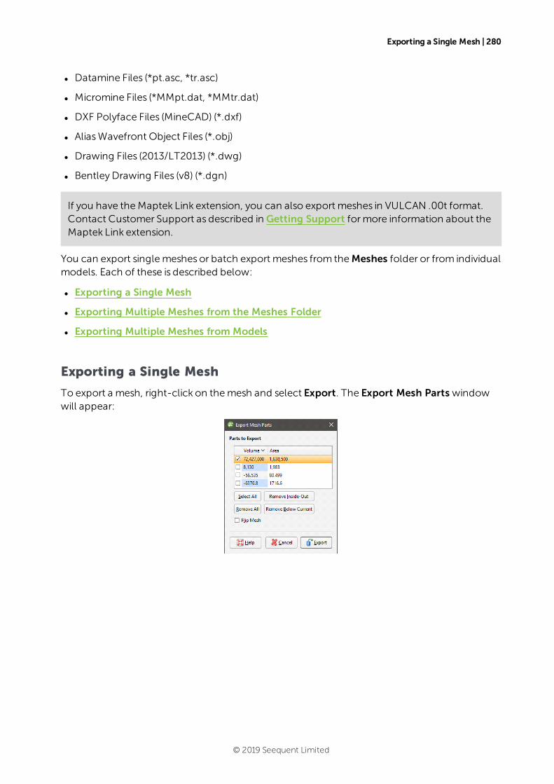
Exporting a Single Mesh | 280
l Datamine Files (*pt.asc, *tr.asc)
l Micromine Files (*MMpt.dat, *MMtr.dat)
l DXF Polyface Files (MineCAD) (*.dxf)
l AliasWavefront Object Files (*.obj)
l Drawing Files (2013/LT2013) (*.dwg)
l BentleyDrawing Files (v8) (*.dgn)
If you have theMaptek Link extension, you can also export meshes in VULCAN .00t format.Contact Customer Support as described in Getting Support formore information about theMaptek Link extension.
You can export singlemeshes or batch export meshes from theMeshes folder or from individualmodels. Each of these is described below:
l Exporting a Single Mesh
l Exporting Multiple Meshes from the Meshes Folder
l Exporting Multiple Meshes from Models
Exporting a Single Mesh
To export a mesh, right-click on themesh and select Export. The Export Mesh Parts windowwill appear:
© 2019 Seequent Limited

281 | User Manual
An Export clipped mesh option is available formeshes that are clipped to a boundary:
If the quality of themesh produced is not acceptable, clip themesh as described in Clippinga Mesh, then export themesh.
Select the Parts to Export, then clickOK. You will be prompted for a filename and location.
When exporting a mesh that hasmultiple parts, you can distinguish between the different partsby clicking on them in the Export Mesh Parts window. Here, themesh was added to the scenebefore the Export Mesh Parts windowwasopened. Clicking on a mesh part in the list selectsthat part in the scene:
© 2019 Seequent Limited
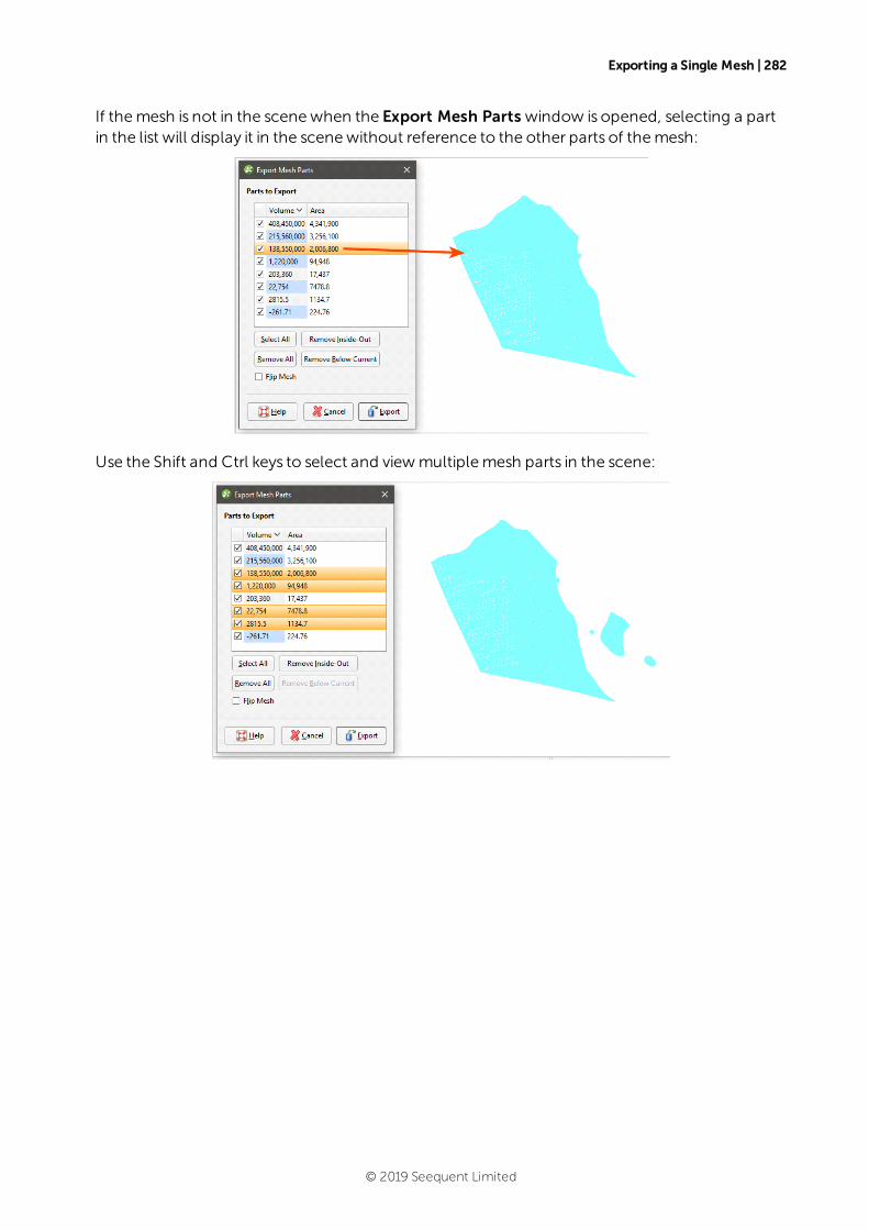
Exporting a Single Mesh | 282
If themesh is not in the scenewhen the Export Mesh Parts window is opened, selecting a partin the list will display it in the scenewithout reference to the other parts of themesh:
Use the Shift and Ctrl keys to select and viewmultiplemesh parts in the scene:
© 2019 Seequent Limited
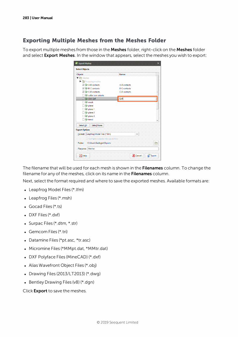
283 | User Manual
Exporting Multiple Meshes from the Meshes Folder
To export multiplemeshes from those in theMeshes folder, right-click on theMeshes folderand select Export Meshes. In thewindow that appears, select themeshes you wish to export:
The filename that will be used for each mesh is shown in the Filenames column. To change thefilename for any of themeshes, click on its name in the Filenames column.
Next, select the format required and where to save the exported meshes. Available formats are:
l Leapfrog Model Files (*.lfm)
l Leapfrog Files (*.msh)
l Gocad Files (*.ts)
l DXF Files (*.dxf)
l Surpac Files (*.dtm, *.str)
l GemcomFiles (*.tri)
l Datamine Files (*pt.asc, *tr.asc)
l Micromine Files (*MMpt.dat, *MMtr.dat)
l DXF Polyface Files (MineCAD) (*.dxf)
l AliasWavefront Object Files (*.obj)
l Drawing Files (2013/LT2013) (*.dwg)
l BentleyDrawing Files (v8) (*.dgn)
Click Export to save themeshes.
© 2019 Seequent Limited
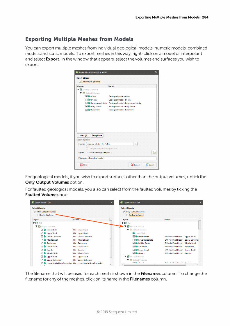
Exporting Multiple Meshes from Models | 284
Exporting Multiple Meshes from Models
You can export multiplemeshes from individual geological models, numericmodels, combinedmodels and staticmodels. To export meshes in thisway, right-click on a model or interpolantand select Export. In thewindow that appears, select the volumes and surfaces you wish toexport:
For geological models, if you wish to export surfaces other than the output volumes, untick theOnly Output Volumes option.
For faulted geological models, you also can select from the faulted volumes by ticking theFaulted Volumes box:
The filename that will be used for each mesh is shown in the Filenames column. To change thefilename for any of themeshes, click on its name in the Filenames column.
© 2019 Seequent Limited

285 | User Manual
Next, select the format required and where to save the exported meshes. Available formats are:
l Leapfrog Model Files (*.lfm)
l Leapfrog Files (*.msh)
l Gocad Files (*.ts)
l DXF Files (*.dxf)
l Surpac Files (*.dtm, *.str)
l GemcomFiles (*.tri)
l Datamine Files (*pt.asc, *tr.asc)
l Micromine Files (*MMpt.dat, *MMtr.dat)
l DXF Polyface Files (MineCAD) (*.dxf)
l AliasWavefront Object Files (*.obj)
l Drawing Files (2013/LT2013) (*.dwg)
l BentleyDrawing Files (v8) (*.dgn)
For any of the export options other than Leapfrog Model Files format, you can save themeshesas a zip file.
The Leapfrog Model File format exports a single *.lfm file. If the file is imported into theMeshes folder, each output volumewill appear as a singlemesh.
Click Export to save themeshes.
Modifying Surfaces
This topic describes aspects of modifying surfaces in Leapfrog Geo. It is divided into:
l Surface Resolution in Leapfrog Geo
l Adding Data to Surfaces
l Honouring Surface Contacts
l Global Trends
l Structural Trends
l Editing Surfaces with Polylines
l Editing Surfaces with Structural Data
Surface Resolution in Leapfrog Geo
In Leapfrog Geo, meshes are used to represent surfaces in the formof vertices and triangles thatdefine the 3D shape of the surface. The resolution of a surface is controlled by the size of thetriangles used to create a surface. A lower surface resolution valuemeans smaller triangles and,
© 2019 Seequent Limited
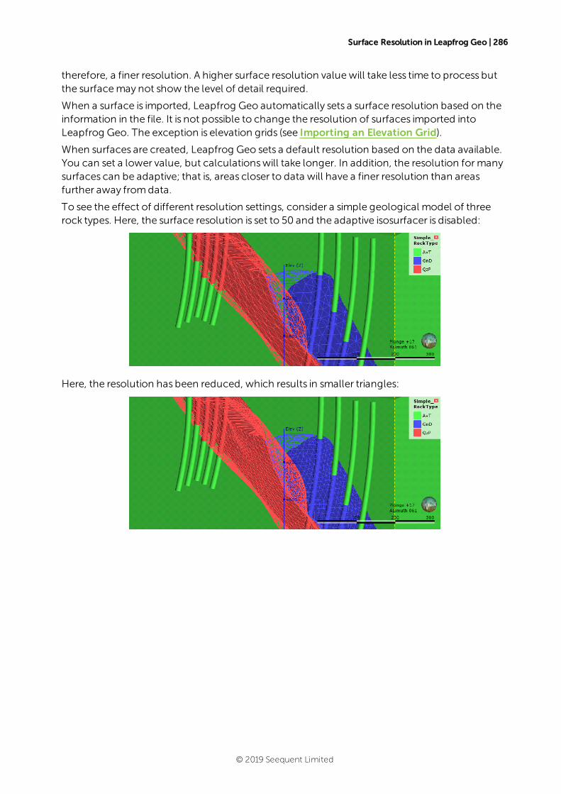
Surface Resolution in Leapfrog Geo | 286
therefore, a finer resolution. A higher surface resolution valuewill take less time to process butthe surfacemay not show the level of detail required.
When a surface is imported, Leapfrog Geo automatically sets a surface resolution based on theinformation in the file. It is not possible to change the resolution of surfaces imported intoLeapfrog Geo. The exception is elevation grids (see Importing an Elevation Grid).
When surfaces are created, Leapfrog Geo sets a default resolution based on the data available.You can set a lower value, but calculationswill take longer. In addition, the resolution formanysurfaces can be adaptive; that is, areas closer to data will have a finer resolution than areasfurther away fromdata.
To see the effect of different resolution settings, consider a simple geological model of threerock types. Here, the surface resolution is set to 50 and the adaptive isosurfacer is disabled:
Here, the resolution has been reduced, which results in smaller triangles:
© 2019 Seequent Limited
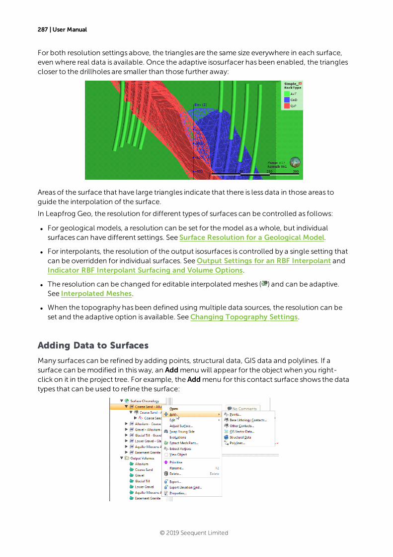
287 | User Manual
For both resolution settings above, the triangles are the same size everywhere in each surface,even where real data is available. Once the adaptive isosurfacer has been enabled, the trianglescloser to the drillholes are smaller than those further away:
Areas of the surface that have large triangles indicate that there is less data in those areas toguide the interpolation of the surface.
In Leapfrog Geo, the resolution for different types of surfaces can be controlled as follows:
l For geological models, a resolution can be set for themodel as a whole, but individualsurfaces can have different settings. See Surface Resolution for a Geological Model.
l For interpolants, the resolution of the output isosurfaces is controlled by a single setting thatcan be overridden for individual surfaces. SeeOutput Settings for an RBF Interpolant andIndicator RBF Interpolant Surfacing and Volume Options.
l The resolution can be changed for editable interpolated meshes ( ) and can be adaptive.See Interpolated Meshes.
l When the topography has been defined using multiple data sources, the resolution can beset and the adaptive option is available. SeeChanging Topography Settings.
Adding Data to Surfaces
Many surfaces can be refined by adding points, structural data, GIS data and polylines. If asurface can bemodified in thisway, an Addmenu will appear for the object when you right-click on it in the project tree. For example, the Addmenu for this contact surface shows the datatypes that can be used to refine the surface:
© 2019 Seequent Limited
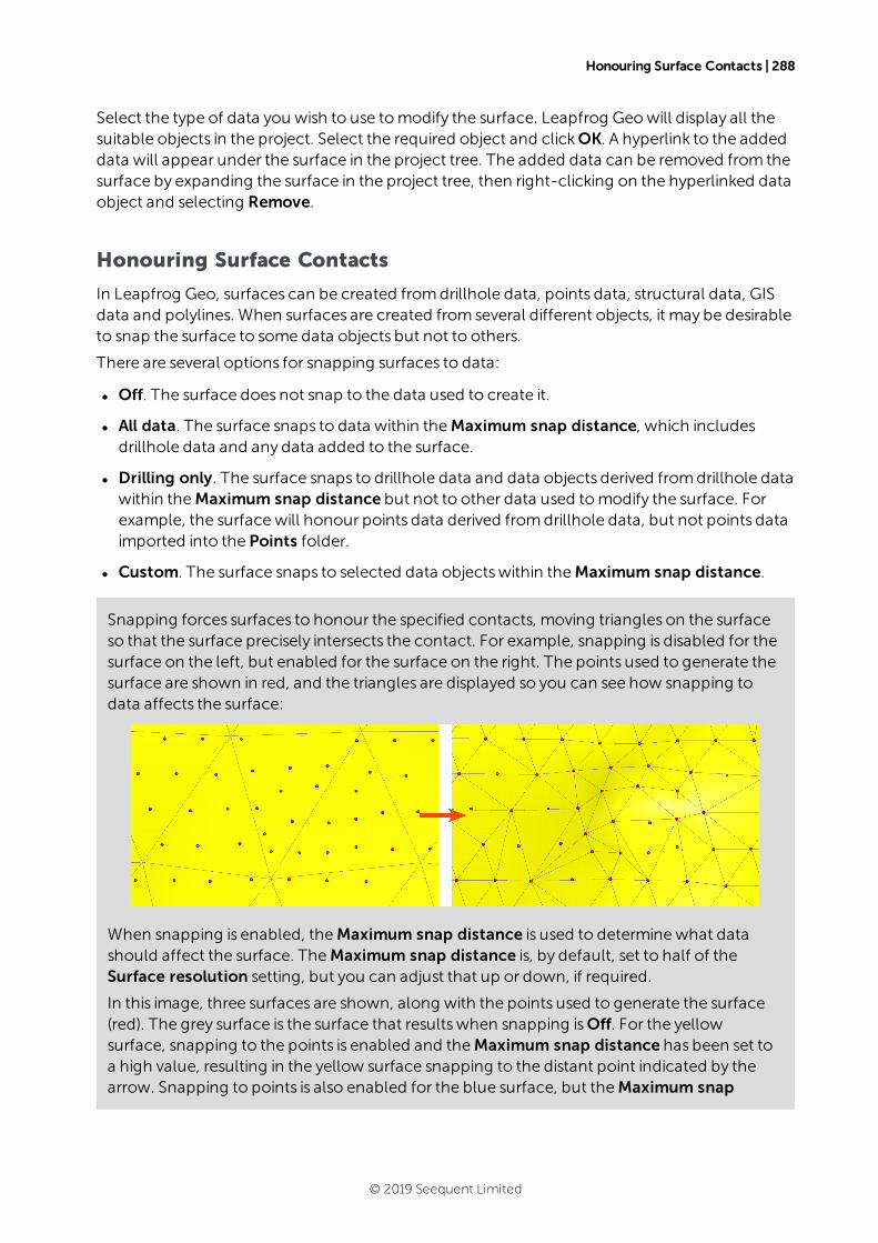
Honouring Surface Contacts | 288
Select the type of data you wish to use tomodify the surface. Leapfrog Geowill display all thesuitable objects in the project. Select the required object and clickOK. A hyperlink to the addeddata will appear under the surface in the project tree. The added data can be removed from thesurface by expanding the surface in the project tree, then right-clicking on the hyperlinked dataobject and selecting Remove.
Honouring Surface Contacts
In Leapfrog Geo, surfaces can be created fromdrillhole data, points data, structural data, GISdata and polylines. When surfaces are created from several different objects, it may be desirableto snap the surface to some data objects but not to others.
There are several options for snapping surfaces to data:
l Off. The surface does not snap to the data used to create it.
l All data. The surface snaps to data within theMaximum snap distance, which includesdrillhole data and any data added to the surface.
l Drilling only. The surface snaps to drillhole data and data objects derived fromdrillhole datawithin theMaximum snap distance but not to other data used tomodify the surface. Forexample, the surfacewill honour points data derived fromdrillhole data, but not points dataimported into the Points folder.
l Custom. The surface snaps to selected data objectswithin theMaximum snap distance.
Snapping forces surfaces to honour the specified contacts, moving triangles on the surfaceso that the surface precisely intersects the contact. For example, snapping is disabled for thesurface on the left, but enabled for the surface on the right. The points used to generate thesurface are shown in red, and the triangles are displayed so you can see how snapping todata affects the surface:
When snapping is enabled, theMaximum snap distance is used to determinewhat datashould affect the surface. TheMaximum snap distance is, by default, set to half of theSurface resolution setting, but you can adjust that up or down, if required.
In this image, three surfaces are shown, along with the points used to generate the surface(red). The grey surface is the surface that resultswhen snapping isOff. For the yellowsurface, snapping to the points is enabled and theMaximum snap distance has been set toa high value, resulting in the yellow surface snapping to the distant point indicated by thearrow. Snapping to points is also enabled for the blue surface, but theMaximum snap
© 2019 Seequent Limited
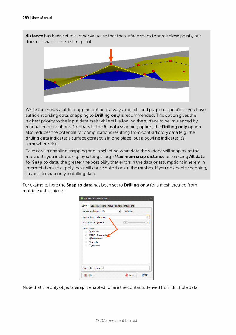
289 | User Manual
distance has been set to a lower value, so that the surface snaps to some close points, butdoes not snap to the distant point.
While themost suitable snapping option is always project- and purpose-specific, if you havesufficient drilling data, snapping toDrilling only is recommended. This option gives thehighest priority to the input data itself while still allowing the surface to be influenced bymanual interpretations. Contrary to the All data snapping option, theDrilling only optionalso reduces the potential for complications resulting fromcontradictory data (e.g. thedrilling data indicates a surface contact is in one place, but a polyline indicates it’ssomewhere else).
Take care in enabling snapping and in selecting what data the surfacewill snap to, as themore data you include, e.g. by setting a largeMaximum snap distance or selecting All datafor Snap to data, the greater the possibility that errors in the data or assumptions inherent ininterpretations (e.g. polylines) will cause distortions in themeshes. If you do enable snapping,it is best to snap only to drilling data.
For example, here the Snap to data has been set toDrilling only for a mesh created frommultiple data objects:
Note that the only objects Snap is enabled for are the contacts derived fromdrillhole data.
© 2019 Seequent Limited
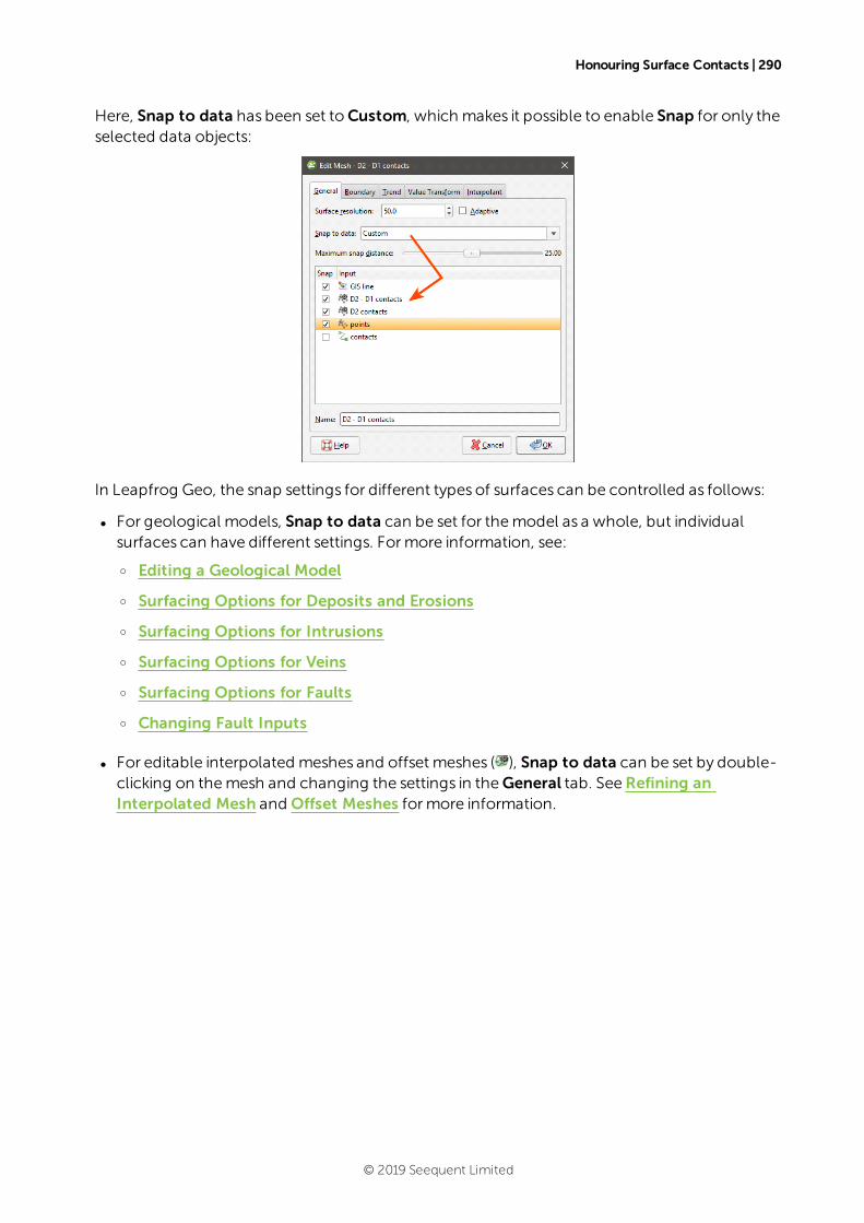
Honouring Surface Contacts | 290
Here, Snap to data has been set toCustom, which makes it possible to enable Snap for only theselected data objects:
In Leapfrog Geo, the snap settings for different types of surfaces can be controlled as follows:
l For geological models, Snap to data can be set for themodel as a whole, but individualsurfaces can have different settings. Formore information, see:
o Editing a Geological Model
o Surfacing Options for Deposits and Erosions
o Surfacing Options for Intrusions
o Surfacing Options for Veins
o Surfacing Options for Faults
o Changing Fault Inputs
l For editable interpolated meshes and offset meshes ( ), Snap to data can be set by double-clicking on themesh and changing the settings in theGeneral tab. SeeRefining anInterpolated Mesh and Offset Meshes formore information.
© 2019 Seequent Limited
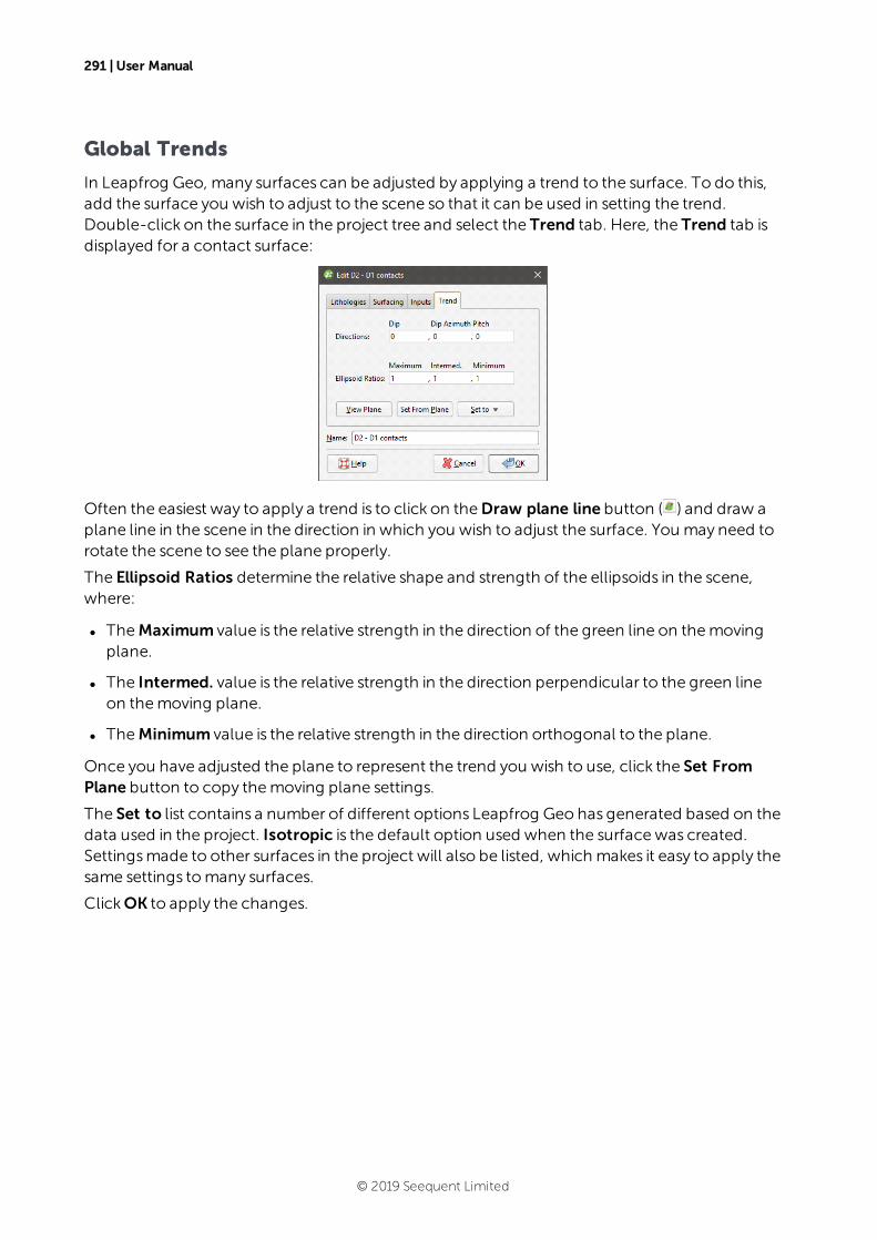
291 | User Manual
Global Trends
In Leapfrog Geo, many surfaces can be adjusted by applying a trend to the surface. To do this,add the surface you wish to adjust to the scene so that it can be used in setting the trend.Double-click on the surface in the project tree and select the Trend tab. Here, the Trend tab isdisplayed for a contact surface:
Often the easiest way to apply a trend is to click on theDraw plane line button ( ) and draw aplane line in the scene in the direction in which you wish to adjust the surface. You may need torotate the scene to see the plane properly.
The Ellipsoid Ratios determine the relative shape and strength of the ellipsoids in the scene,where:
l TheMaximum value is the relative strength in the direction of the green line on themovingplane.
l The Intermed. value is the relative strength in the direction perpendicular to the green lineon themoving plane.
l TheMinimum value is the relative strength in the direction orthogonal to the plane.
Once you have adjusted the plane to represent the trend you wish to use, click the Set FromPlane button to copy themoving plane settings.
The Set to list contains a number of different options Leapfrog Geo has generated based on thedata used in the project. Isotropic is the default option used when the surfacewas created.Settingsmade to other surfaces in the project will also be listed, which makes it easy to apply thesame settings tomany surfaces.
ClickOK to apply the changes.
© 2019 Seequent Limited

Global Trends | 292
How themoving plane can be used to adjust a surface in thismanner is illustrated by thefollowing intrusive contact surface:
The intrusion surface has two bodies that are not connected, and we can apply a trend toconnect the two parts. Here, the intrusion surface has been hidden in the scene and the scenerotated to line up theQzP segments. A plane line can then be drawn through theQzPsegments:
Using the plane settings to adjust the surface results in the two parts of the intrusion joining up:
© 2019 Seequent Limited
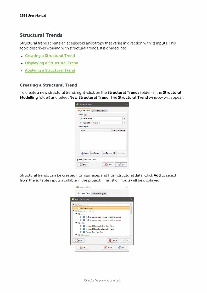
293 | User Manual
Structural Trends
Structural trends create a flat ellipsoid anisotropy that varies in direction with its inputs. Thistopic describesworking with structural trends. It is divided into:
l Creating a Structural Trend
l Displaying a Structural Trend
l Applying a Structural Trend
Creating a Structural Trend
To create a new structural trend, right-click on the Structural Trends folder (in the StructuralModelling folder) and selectNew Structural Trend. The Structural Trendwindowwill appear:
Structural trends can be created from surfaces and from structural data. ClickAdd to selectfrom the suitable inputs available in the project. The list of inputswill be displayed:
© 2019 Seequent Limited
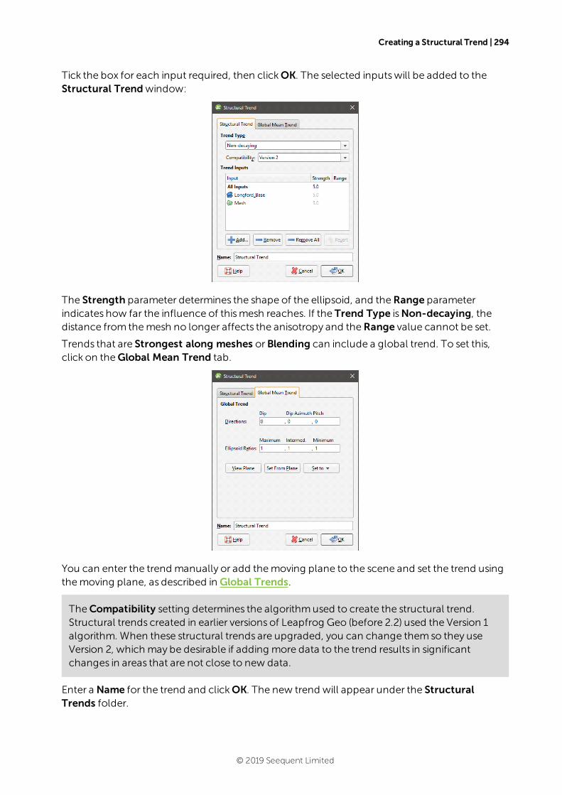
Creating a Structural Trend | 294
Tick the box for each input required, then clickOK. The selected inputswill be added to theStructural Trendwindow:
The Strength parameter determines the shape of the ellipsoid, and theRange parameterindicates how far the influence of thismesh reaches. If the Trend Type isNon-decaying, thedistance from themesh no longer affects the anisotropy and theRange value cannot be set.
Trends that are Strongest along meshes orBlending can include a global trend. To set this,click on theGlobal Mean Trend tab.
You can enter the trend manually or add themoving plane to the scene and set the trend usingthemoving plane, as described in Global Trends.
TheCompatibility setting determines the algorithmused to create the structural trend.Structural trends created in earlier versions of Leapfrog Geo (before 2.2) used the Version 1algorithm. When these structural trends are upgraded, you can change themso they useVersion 2, which may be desirable if adding more data to the trend results in significantchanges in areas that are not close to new data.
Enter a Name for the trend and clickOK. The new trend will appear under the StructuralTrends folder.
© 2019 Seequent Limited
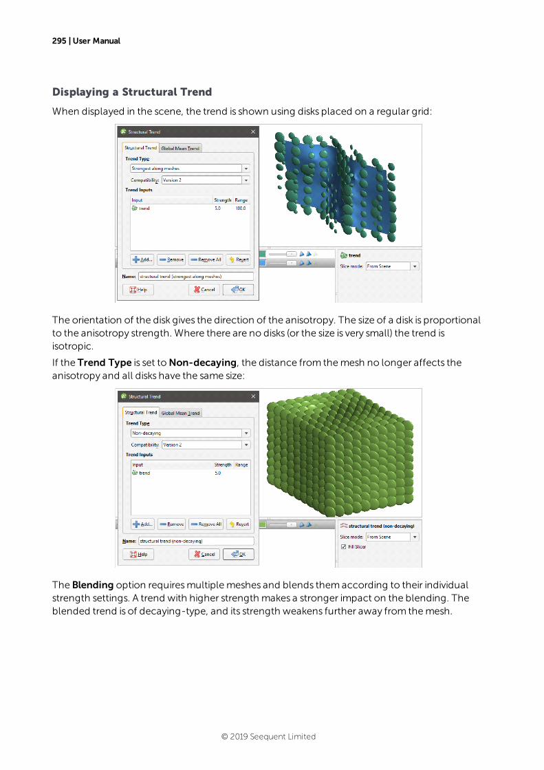
295 | User Manual
Displaying a Structural Trend
When displayed in the scene, the trend is shown using disks placed on a regular grid:
The orientation of the disk gives the direction of the anisotropy. The size of a disk is proportionalto the anisotropy strength. Where there are no disks (or the size is very small) the trend isisotropic.
If the Trend Type is set toNon-decaying, the distance from themesh no longer affects theanisotropy and all disks have the same size:
The Blending option requiresmultiplemeshes and blends themaccording to their individualstrength settings. A trend with higher strength makes a stronger impact on the blending. Theblended trend is of decaying-type, and its strength weakens further away from themesh.
© 2019 Seequent Limited
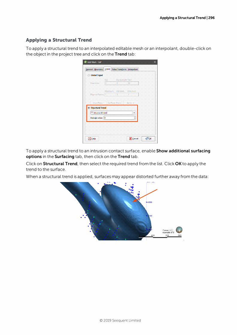
Applying a Structural Trend | 296
Applying a Structural Trend
To apply a structural trend to an interpolated editablemesh or an interpolant, double-click onthe object in the project tree and click on the Trend tab:
To apply a structural trend to an intrusion contact surface, enable Show additional surfacingoptions in the Surfacing tab, then click on the Trend tab.
Click on Structural Trend, then select the required trend from the list. ClickOK to apply thetrend to the surface.
When a structural trend is applied, surfacesmay appear distorted further away from the data:
© 2019 Seequent Limited
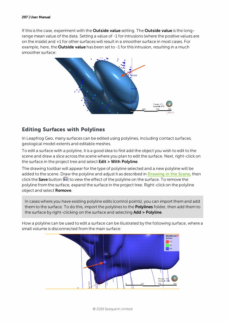
297 | User Manual
If this is the case, experiment with theOutside value setting. TheOutside value is the long-rangemean value of the data. Setting a value of -1 for intrusions (where the positive values areon the inside) and +1 for other surfaceswill result in a smoother surface in most cases. Forexample, here, theOutside value has been set to -1 for this intrusion, resulting in a muchsmoother surface:
Editing Surfaces with Polylines
In Leapfrog Geo, many surfaces can be edited using polylines, including contact surfaces,geological model extents and editablemeshes.
To edit a surfacewith a polyline, it is a good idea to first add the object you wish to edit to thescene and draw a slice across the scenewhere you plan to edit the surface. Next, right-click onthe surface in the project tree and select Edit > With Polyline.
The drawing toolbar will appear for the type of polyline selected and a new polyline will beadded to the scene. Draw the polyline and adjust it as described in Drawing in the Scene, thenclick the Save button ( ) to view the effect of the polyline on the surface. To remove thepolyline from the surface, expand the surface in the project tree. Right-click on the polylineobject and select Remove.
In caseswhere you have existing polyline edits (control points), you can import themand addthem to the surface. To do this, import the polylines to the Polylines folder, then add them tothe surface by right-clicking on the surface and selecting Add > Polyline.
How a polyline can be used to edit a surface can be illustrated by the following surface, where asmall volume is disconnected from themain surface:
© 2019 Seequent Limited
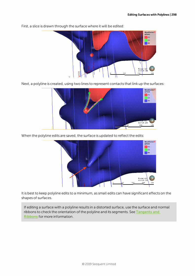
Editing Surfaces with Polylines | 298
First, a slice is drawn through the surfacewhere it will be edited:
Next, a polyline is created, using two lines to represent contacts that link up the surfaces:
When the polyline edits are saved, the surface is updated to reflect the edits:
It is best to keep polyline edits to a minimum, as small edits can have significant effects on theshapes of surfaces.
If editing a surfacewith a polyline results in a distorted surface, use the surface and normalribbons to check the orientation of the polyline and its segments. See Tangents andRibbons formore information.
© 2019 Seequent Limited
299 | User Manual
When you save the polyline, the object will be updated to reflect the additional points. Thepolyline will be added to the project tree as part of the object that was edited. You can edit thepolyline by double-clicking on it or by right-clicking and selecting Edit Polyline.
Editing Surfaces with Structural Data
In Leapfrog Geo, many surfaces can be edited using planar structural data points drawn in thescene. Surfaces that can be edited in thisway include contact surfaces, model extents andinterpolated editablemeshes. There are twoways to do this:
l If you have a structural data table created in or imported into Leapfrog Geo that you want touse to adjust the surface, right-click on the surface in the project tree and select Add >Structural Data. You will be prompted to select from the structural data tables available inthe project.
l If you want to create structural data points to use to adjust the surface, right-click on thesurface in the project tree and select Edit > With Structural Data.
To edit a surfacewith structural data using the second option, it is a good idea to first add theobject you wish to edit to the scene. Next, right-click on the surface in the project tree andselect the Edit > With Structural Data option.
The structural data toolbar will appear and a new structural data object will be added to thescene. Draw the structural data points and adjust themas described in Creating New PlanarStructural Data Tables, then click the Save button ( ) to view the effect on the surface.Structural data tables created in thisway cannot be used by other objects in the project until thetable has been shared. To do this, right-click on the table in the project tree and select Share.The structural data table will be saved to the Structural Modelling folder.
To remove the structural data from the surface, expand the surface in the project tree. Right-click on the structural data object and select Remove.
Non-Editable Meshes
Leapfrog Geo provides you with several tools for creating non-editablemeshes:
l Mesh from the Moving Plane
l Combining Meshes
l Clipping a Volume
l Clipping a Mesh
l Merging 2D Meshes
l Extracting Mesh Parts
These tools produce non-editablemeshes ( ).
© 2019 Seequent Limited
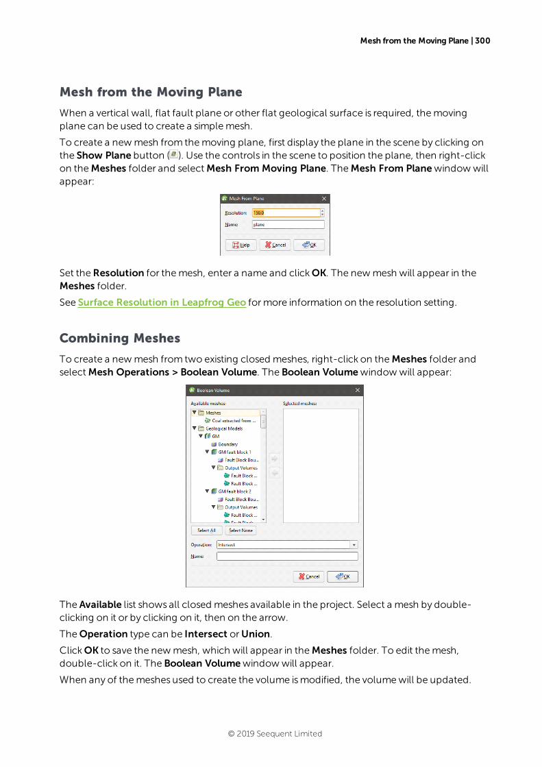
Mesh from the Moving Plane | 300
Mesh from the Moving Plane
When a vertical wall, flat fault plane or other flat geological surface is required, themovingplane can be used to create a simplemesh.
To create a newmesh from themoving plane, first display the plane in the scene by clicking onthe Show Plane button ( ). Use the controls in the scene to position the plane, then right-clickon theMeshes folder and selectMesh From Moving Plane. TheMesh From Planewindowwillappear:
Set theResolution for themesh, enter a name and clickOK. The newmesh will appear in theMeshes folder.
See Surface Resolution in Leapfrog Geo formore information on the resolution setting.
Combining Meshes
To create a newmesh from two existing closed meshes, right-click on theMeshes folder andselectMesh Operations > Boolean Volume. The Boolean Volumewindowwill appear:
The Available list shows all closed meshes available in the project. Select a mesh by double-clicking on it or by clicking on it, then on the arrow.
TheOperation type can be Intersect orUnion.
ClickOK to save the newmesh, which will appear in theMeshes folder. To edit themesh,double-click on it. The Boolean Volumewindowwill appear.
When any of themeshes used to create the volume ismodified, the volumewill be updated.
© 2019 Seequent Limited
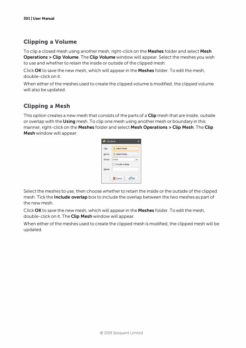
301 | User Manual
Clipping a Volume
To clip a closed mesh using anothermesh, right-click on theMeshes folder and selectMeshOperations > Clip Volume. TheClip Volumewindowwill appear. Select themeshes you wishto use and whether to retain the inside or outside of the clipped mesh.
ClickOK to save the newmesh, which will appear in theMeshes folder. To edit themesh,double-click on it.
When either of themeshes used to create the clipped volume ismodified, the clipped volumewill also be updated.
Clipping a Mesh
This option creates a newmesh that consists of the parts of a Clipmesh that are inside, outsideor overlap with theUsingmesh. To clip onemesh using anothermesh or boundary in thismanner, right-click on theMeshes folder and selectMesh Operations > Clip Mesh. TheClipMeshwindowwill appear:
Select themeshes to use, then choosewhether to retain the inside or the outside of the clippedmesh. Tick the Include overlap box to include the overlap between the twomeshes as part ofthe newmesh.
ClickOK to save the newmesh, which will appear in theMeshes folder. To edit themesh,double-click on it. TheClip Meshwindowwill appear.
When either of themeshes used to create the clipped mesh ismodified, the clipped mesh will beupdated.
© 2019 Seequent Limited
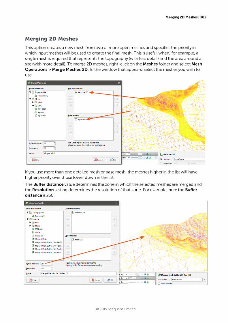
Merging 2D Meshes | 302
Merging 2D Meshes
This option creates a newmesh from two ormore open meshes and specifies the priority inwhich input mesheswill be used to create the final mesh. This is useful when, for example, asinglemesh is required that represents the topography (with less detail) and the area around asite (with more detail). Tomerge 2Dmeshes, right-click on theMeshes folder and selectMeshOperations > Merge Meshes 2D. In thewindow that appears, select themeshes you wish touse.
If you usemore than one detailed mesh or basemesh, themeshes higher in the list will havehigher priority over those lower down in the list.
The Buffer distance value determines the zone in which the selected meshes aremerged andtheResolution setting determines the resolution of that zone. For example, here the Bufferdistance is 250:
© 2019 Seequent Limited
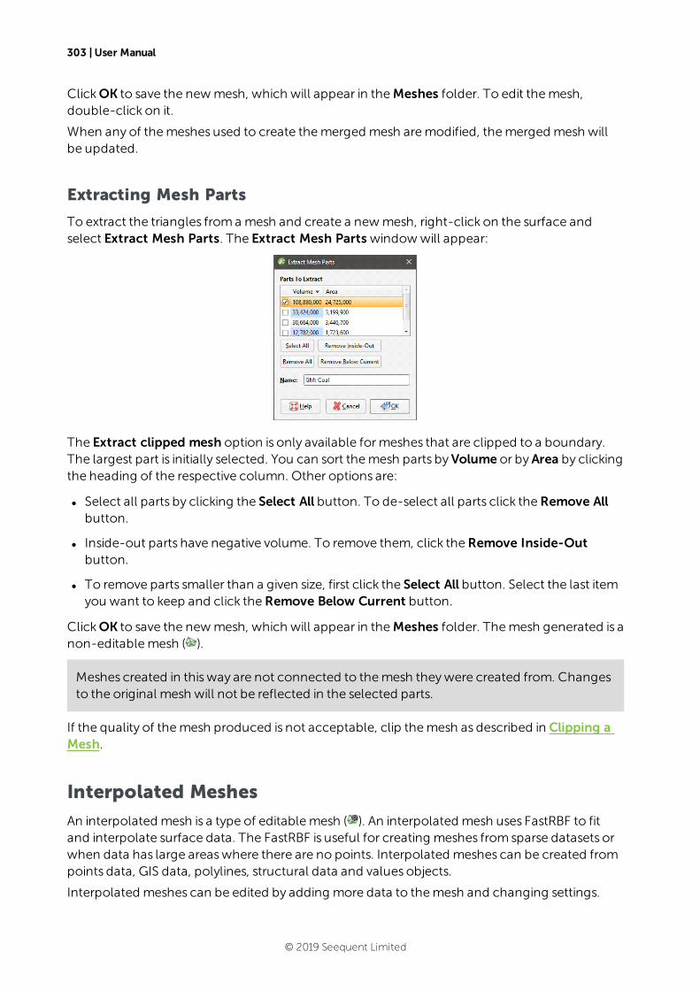
303 | User Manual
ClickOK to save the newmesh, which will appear in theMeshes folder. To edit themesh,double-click on it.
When any of themeshes used to create themerged mesh aremodified, themerged mesh willbe updated.
Extracting Mesh Parts
To extract the triangles froma mesh and create a newmesh, right-click on the surface andselect Extract Mesh Parts. The Extract Mesh Parts windowwill appear:
The Extract clipped mesh option is only available formeshes that are clipped to a boundary.The largest part is initially selected. You can sort themesh parts byVolume or byArea by clickingthe heading of the respective column. Other options are:
l Select all parts by clicking the Select All button. To de-select all parts click theRemove Allbutton.
l Inside-out parts have negative volume. To remove them, click theRemove Inside-Outbutton.
l To remove parts smaller than a given size, first click the Select All button. Select the last itemyou want to keep and click theRemove Below Current button.
ClickOK to save the newmesh, which will appear in theMeshes folder. Themesh generated is anon-editablemesh ( ).
Meshes created in thisway are not connected to themesh theywere created from. Changesto the original mesh will not be reflected in the selected parts.
If the quality of themesh produced is not acceptable, clip themesh as described in Clipping aMesh.
Interpolated Meshes
An interpolated mesh is a type of editablemesh ( ). An interpolated mesh uses FastRBF to fitand interpolate surface data. The FastRBF is useful for creating meshes from sparse datasets orwhen data has large areaswhere there are no points. Interpolated meshes can be created frompoints data, GIS data, polylines, structural data and values objects.
Interpolated meshes can be edited by adding more data to themesh and changing settings.
© 2019 Seequent Limited
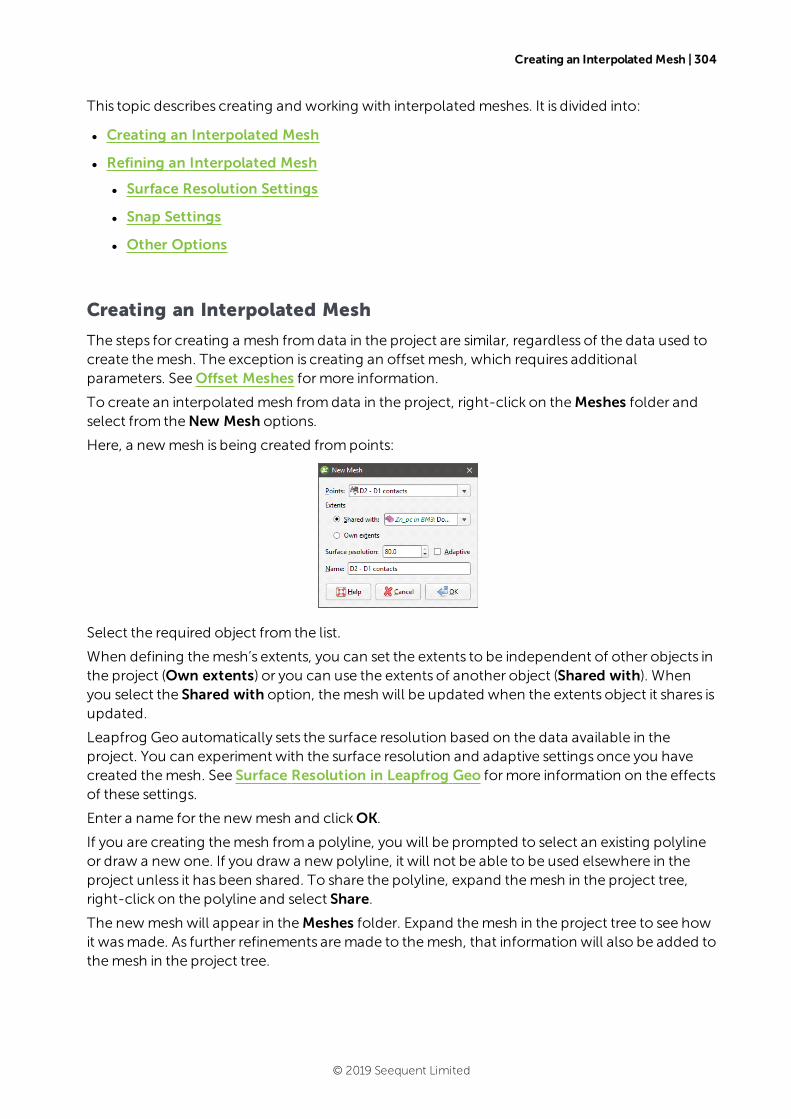
Creating an Interpolated Mesh | 304
This topic describes creating and working with interpolated meshes. It is divided into:
l Creating an Interpolated Mesh
l Refining an Interpolated Mesh
l Surface Resolution Settings
l Snap Settings
l Other Options
Creating an Interpolated Mesh
The steps for creating a mesh fromdata in the project are similar, regardless of the data used tocreate themesh. The exception is creating an offset mesh, which requires additionalparameters. SeeOffset Meshes formore information.
To create an interpolated mesh fromdata in the project, right-click on theMeshes folder andselect from theNew Mesh options.
Here, a newmesh is being created frompoints:
Select the required object from the list.
When defining themesh’s extents, you can set the extents to be independent of other objects inthe project (Own extents) or you can use the extents of another object (Shared with). Whenyou select the Shared with option, themesh will be updated when the extents object it shares isupdated.
Leapfrog Geo automatically sets the surface resolution based on the data available in theproject. You can experiment with the surface resolution and adaptive settings once you havecreated themesh. See Surface Resolution in Leapfrog Geo formore information on the effectsof these settings.
Enter a name for the newmesh and clickOK.
If you are creating themesh froma polyline, you will be prompted to select an existing polylineor draw a new one. If you draw a new polyline, it will not be able to be used elsewhere in theproject unless it has been shared. To share the polyline, expand themesh in the project tree,right-click on the polyline and select Share.
The newmesh will appear in theMeshes folder. Expand themesh in the project tree to see howit wasmade. As further refinements aremade to themesh, that information will also be added tothemesh in the project tree.
© 2019 Seequent Limited
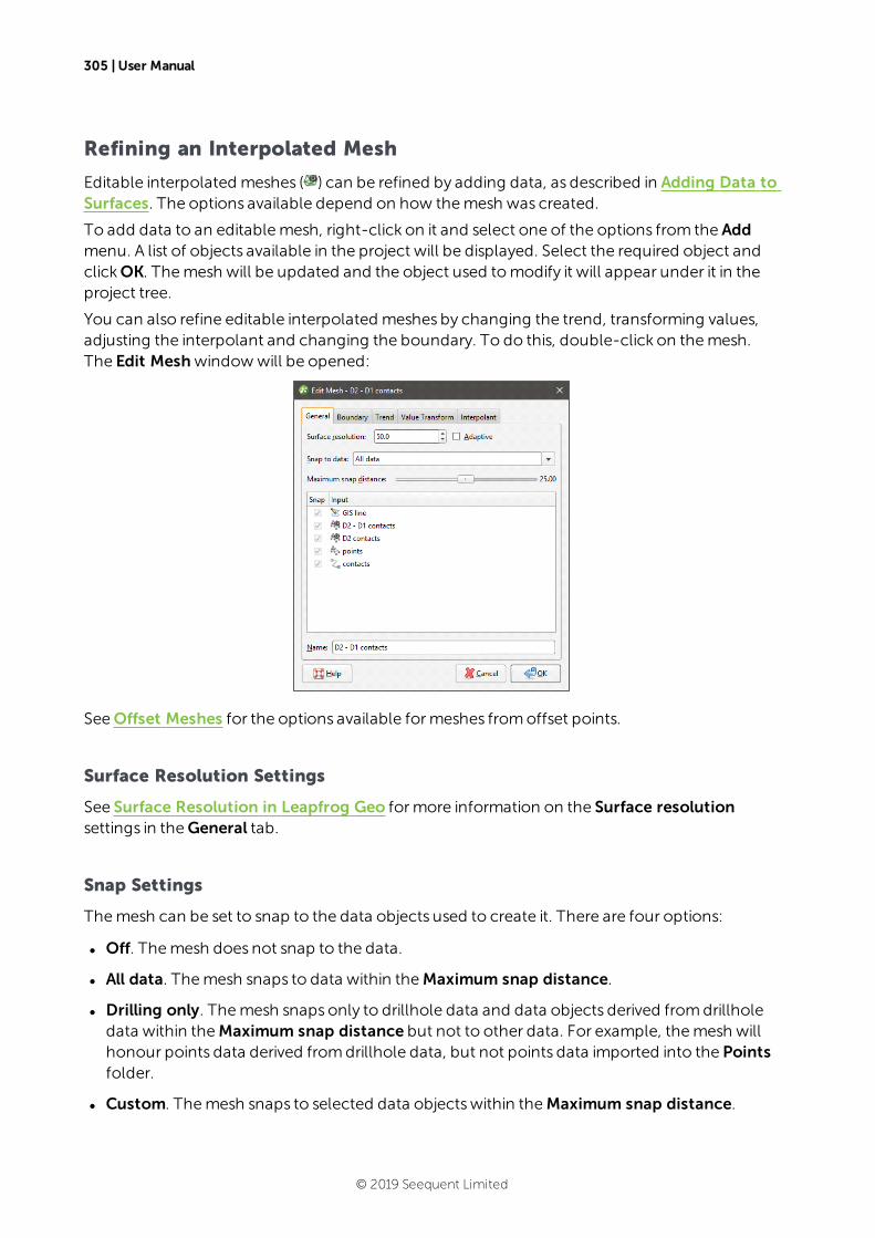
305 | User Manual
Refining an Interpolated Mesh
Editable interpolated meshes ( ) can be refined by adding data, as described in Adding Data toSurfaces. The options available depend on how themesh was created.
To add data to an editablemesh, right-click on it and select one of the options from the Addmenu. A list of objects available in the project will be displayed. Select the required object andclickOK. Themesh will be updated and the object used tomodify it will appear under it in theproject tree.
You can also refine editable interpolated meshes by changing the trend, transforming values,adjusting the interpolant and changing the boundary. To do this, double-click on themesh.The Edit Meshwindowwill be opened:
SeeOffset Meshes for the options available formeshes fromoffset points.
Surface Resolution Settings
See Surface Resolution in Leapfrog Geo formore information on the Surface resolutionsettings in theGeneral tab.
Snap Settings
Themesh can be set to snap to the data objects used to create it. There are four options:
l Off. Themesh does not snap to the data.
l All data. Themesh snaps to data within theMaximum snap distance.
l Drilling only. Themesh snaps only to drillhole data and data objects derived fromdrillholedata within theMaximum snap distance but not to other data. For example, themesh willhonour points data derived fromdrillhole data, but not points data imported into the Pointsfolder.
l Custom. Themesh snaps to selected data objectswithin theMaximum snap distance.
© 2019 Seequent Limited
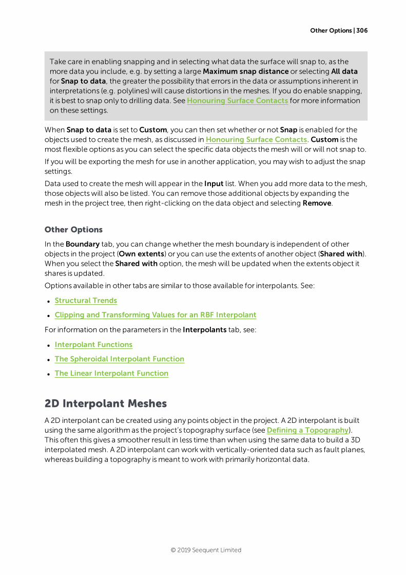
Other Options | 306
Take care in enabling snapping and in selecting what data the surfacewill snap to, as themore data you include, e.g. by setting a largeMaximum snap distance or selecting All datafor Snap to data, the greater the possibility that errors in the data or assumptions inherent ininterpretations (e.g. polylines) will cause distortions in themeshes. If you do enable snapping,it is best to snap only to drilling data. SeeHonouring Surface Contacts formore informationon these settings.
When Snap to data is set toCustom, you can then set whether or not Snap is enabled for theobjects used to create themesh, as discussed in Honouring Surface Contacts. Custom is themost flexible options as you can select the specific data objects themesh will or will not snap to.
If you will be exporting themesh for use in another application, you maywish to adjust the snapsettings.
Data used to create themesh will appear in the Input list. When you add more data to themesh,those objectswill also be listed. You can remove those additional objects by expanding themesh in the project tree, then right-clicking on the data object and selecting Remove.
Other Options
In the Boundary tab, you can changewhether themesh boundary is independent of otherobjects in the project (Own extents) or you can use the extents of another object (Shared with).When you select the Shared with option, themesh will be updated when the extents object itshares is updated.
Options available in other tabs are similar to those available for interpolants. See:
l Structural Trends
l Clipping and Transforming Values for an RBF Interpolant
For information on the parameters in the Interpolants tab, see:
l Interpolant Functions
l The Spheroidal Interpolant Function
l The Linear Interpolant Function
2D Interpolant Meshes
A 2D interpolant can be created using any points object in the project. A 2D interpolant is builtusing the same algorithmas the project’s topography surface (seeDefining a Topography).This often this gives a smoother result in less time than when using the same data to build a 3Dinterpolated mesh. A 2D interpolant can workwith vertically-oriented data such as fault planes,whereas building a topography ismeant toworkwith primarily horizontal data.
© 2019 Seequent Limited
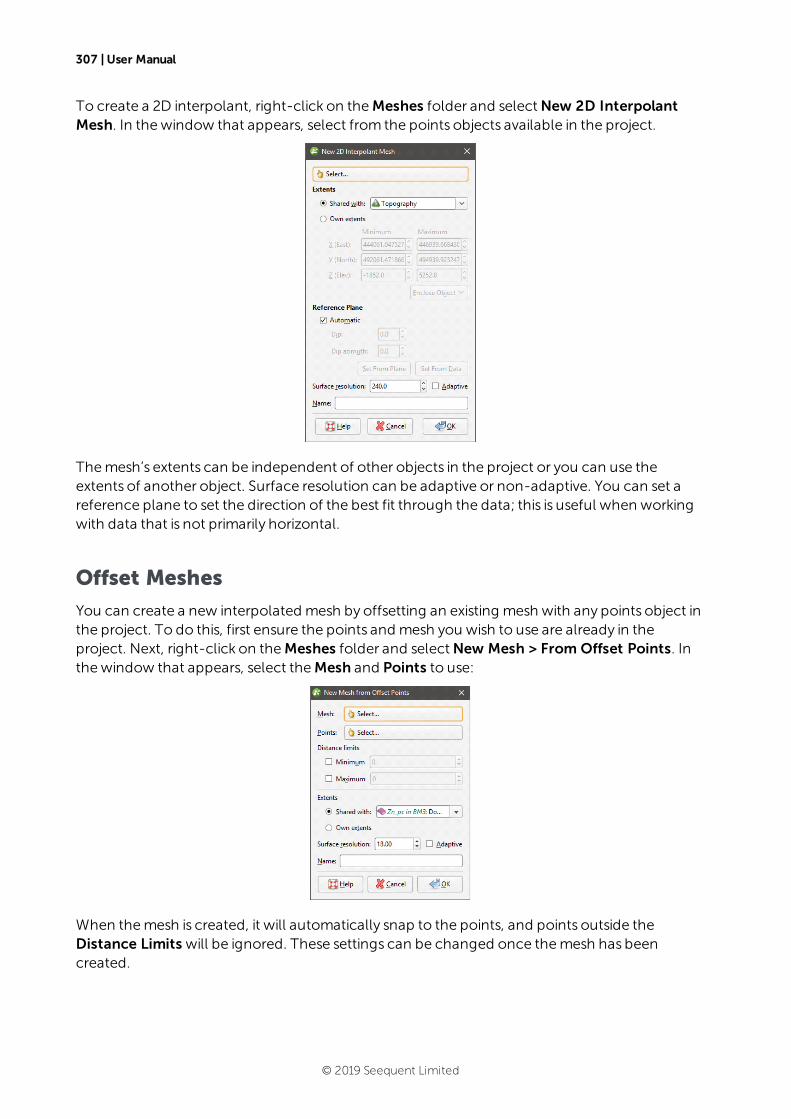
307 | User Manual
To create a 2D interpolant, right-click on theMeshes folder and selectNew 2D InterpolantMesh. In thewindow that appears, select from the points objects available in the project.
Themesh’s extents can be independent of other objects in the project or you can use theextents of another object. Surface resolution can be adaptive or non-adaptive. You can set areference plane to set the direction of the best fit through the data; this is useful when workingwith data that is not primarily horizontal.
Offset Meshes
You can create a new interpolated mesh by offsetting an existing mesh with any points object inthe project. To do this, first ensure the points and mesh you wish to use are already in theproject. Next, right-click on theMeshes folder and selectNew Mesh > From Offset Points. Inthewindow that appears, select theMesh and Points to use:
When themesh is created, it will automatically snap to the points, and points outside theDistance Limits will be ignored. These settings can be changed once themesh has beencreated.
© 2019 Seequent Limited
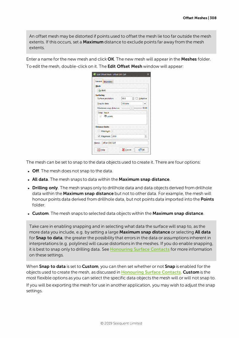
Offset Meshes | 308
An offset mesh may be distorted if points used to offset themesh lie too far outside themeshextents. If this occurs, set a Maximum distance to exclude points far away from themeshextents.
Enter a name for the newmesh and clickOK. The newmesh will appear in theMeshes folder.
To edit themesh, double-click on it. The Edit Offset Meshwindowwill appear:
Themesh can be set to snap to the data objects used to create it. There are four options:
l Off. Themesh does not snap to the data.
l All data. Themesh snaps to data within theMaximum snap distance.
l Drilling only. Themesh snaps only to drillhole data and data objects derived fromdrillholedata within theMaximum snap distance but not to other data. For example, themesh willhonour points data derived fromdrillhole data, but not points data imported into the Pointsfolder.
l Custom. Themesh snaps to selected data objectswithin theMaximum snap distance.
Take care in enabling snapping and in selecting what data the surfacewill snap to, as themore data you include, e.g. by setting a largeMaximum snap distance or selecting All datafor Snap to data, the greater the possibility that errors in the data or assumptions inherent ininterpretations (e.g. polylines) will cause distortions in themeshes. If you do enable snapping,it is best to snap only to drilling data. SeeHonouring Surface Contacts formore informationon these settings.
When Snap to data is set toCustom, you can then set whether or not Snap is enabled for theobjects used to create themesh, as discussed in Honouring Surface Contacts. Custom is themost flexible options as you can select the specific data objects themesh will or will not snap to.
If you will be exporting themesh for use in another application, you maywish to adjust the snapsettings.
© 2019 Seequent Limited
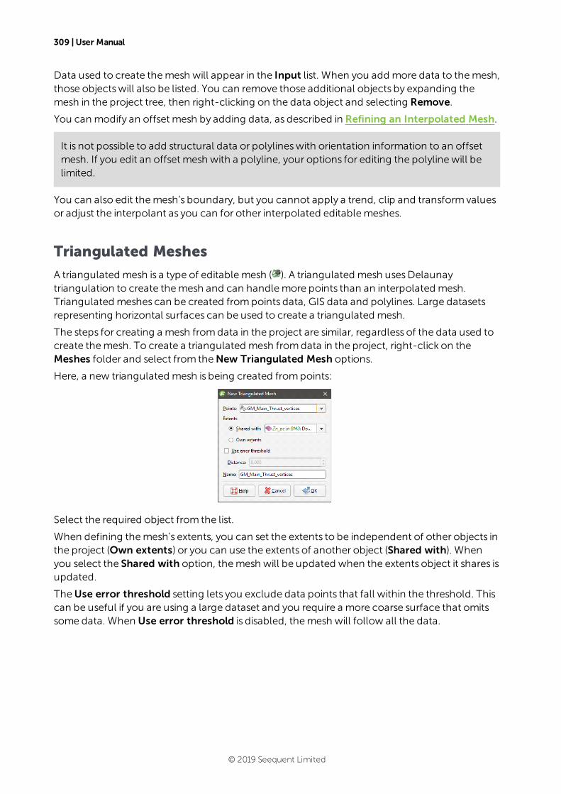
309 | User Manual
Data used to create themesh will appear in the Input list. When you add more data to themesh,those objectswill also be listed. You can remove those additional objects by expanding themesh in the project tree, then right-clicking on the data object and selecting Remove.
You can modify an offset mesh by adding data, as described in Refining an Interpolated Mesh.
It is not possible to add structural data or polylineswith orientation information to an offsetmesh. If you edit an offset mesh with a polyline, your options for editing the polyline will belimited.
You can also edit themesh’s boundary, but you cannot apply a trend, clip and transformvaluesor adjust the interpolant as you can for other interpolated editablemeshes.
Triangulated Meshes
A triangulated mesh is a type of editablemesh ( ). A triangulated mesh usesDelaunaytriangulation to create themesh and can handlemore points than an interpolated mesh.Triangulated meshes can be created frompoints data, GIS data and polylines. Large datasetsrepresenting horizontal surfaces can be used to create a triangulated mesh.
The steps for creating a mesh fromdata in the project are similar, regardless of the data used tocreate themesh. To create a triangulated mesh fromdata in the project, right-click on theMeshes folder and select from theNew Triangulated Mesh options.
Here, a new triangulated mesh is being created frompoints:
Select the required object from the list.
When defining themesh’s extents, you can set the extents to be independent of other objects inthe project (Own extents) or you can use the extents of another object (Shared with). Whenyou select the Shared with option, themesh will be updated when the extents object it shares isupdated.
TheUse error threshold setting lets you exclude data points that fall within the threshold. Thiscan be useful if you are using a large dataset and you require a more coarse surface that omitssome data. When Use error threshold is disabled, themesh will follow all the data.
© 2019 Seequent Limited
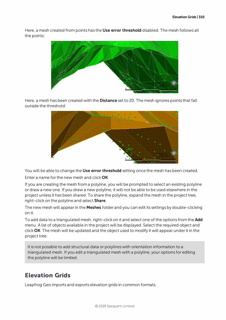
Elevation Grids | 310
Here, a mesh created frompoints has theUse error threshold disabled. Themesh follows allthe points:
Here, a mesh has been created with theDistance set to 20. Themesh ignores points that falloutside the threshold:
You will be able to change theUse error threshold setting once themesh has been created.
Enter a name for the newmesh and clickOK.
If you are creating themesh froma polyline, you will be prompted to select an existing polylineor draw a new one. If you draw a new polyline, it will not be able to be used elsewhere in theproject unless it has been shared. To share the polyline, expand themesh in the project tree,right-click on the polyline and select Share.
The newmesh will appear in theMeshes folder and you can edit its settings by double-clickingon it.
To add data to a triangulated mesh, right-click on it and select one of the options from the Addmenu. A list of objects available in the project will be displayed. Select the required object andclickOK. Themesh will be updated and the object used tomodify it will appear under it in theproject tree.
It is not possible to add structural data or polylineswith orientation information to atriangulated mesh. If you edit a triangulated mesh with a polyline, your options for editingthe polyline will be limited.
Elevation Grids
Leapfrog Geo imports and exports elevation grids in common formats.
© 2019 Seequent Limited
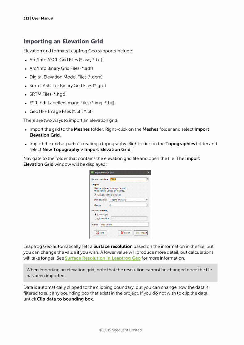
311 | User Manual
Importing an Elevation Grid
Elevation grid formats Leapfrog Geo supports include:
l Arc/Info ASCII Grid Files (*.asc, *.txt)
l Arc/Info BinaryGrid Files (*.adf)
l Digital Elevation Model Files (*.dem)
l Surfer ASCII or BinaryGrid Files (*.grd)
l SRTM Files (*.hgt)
l ESRI.hdr Labelled Image Files (*.img, *.bil)
l GeoTIFF Image Files (*.tiff, *.tif)
There are twoways to import an elevation grid:
l Import the grid to theMeshes folder. Right-click on theMeshes folder and select ImportElevation Grid.
l Import the grid as part of creating a topography. Right-click on the Topographies folder andselectNew Topography > Import Elevation Grid.
Navigate to the folder that contains the elevation grid file and open the file. The ImportElevation Gridwindowwill be displayed:
Leapfrog Geo automatically sets a Surface resolution based on the information in the file, butyou can change the value if you wish. A lower valuewill producemore detail, but calculationswill take longer. See Surface Resolution in Leapfrog Geo formore information.
When importing an elevation grid, note that the resolution cannot be changed once the filehas been imported.
Data is automatically clipped to the clipping boundary, but you can change how the data isfiltered to suit any bounding box that exists in the project. If you do not wish to clip the data,untickClip data to bounding box.
© 2019 Seequent Limited
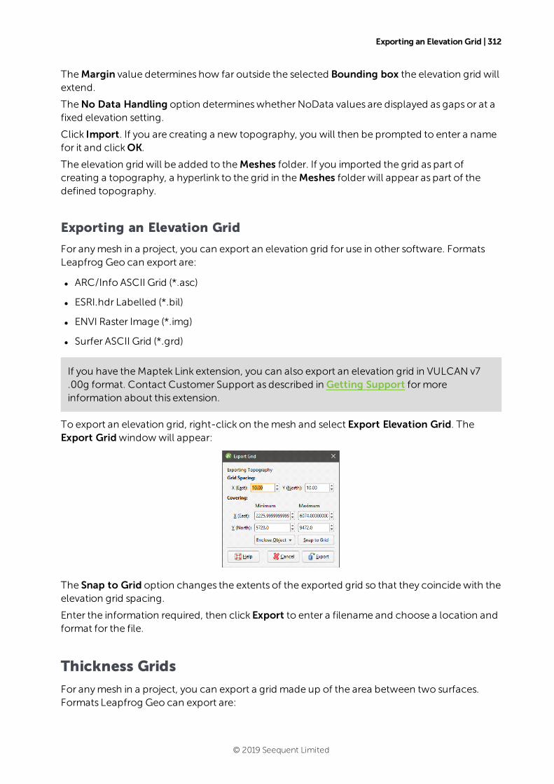
Exporting an Elevation Grid | 312
TheMargin value determines how far outside the selected Bounding box the elevation grid willextend.
TheNo Data Handling option determineswhether NoData values are displayed as gaps or at afixed elevation setting.
Click Import. If you are creating a new topography, you will then be prompted to enter a namefor it and clickOK.
The elevation grid will be added to theMeshes folder. If you imported the grid as part ofcreating a topography, a hyperlink to the grid in theMeshes folder will appear as part of thedefined topography.
Exporting an Elevation Grid
For anymesh in a project, you can export an elevation grid for use in other software. FormatsLeapfrog Geo can export are:
l ARC/Info ASCII Grid (*.asc)
l ESRI.hdr Labelled (*.bil)
l ENVI Raster Image (*.img)
l Surfer ASCII Grid (*.grd)
If you have theMaptek Link extension, you can also export an elevation grid in VULCAN v7.00g format. Contact Customer Support as described in Getting Support formoreinformation about this extension.
To export an elevation grid, right-click on themesh and select Export Elevation Grid. TheExport Gridwindowwill appear:
The Snap to Grid option changes the extents of the exported grid so that they coincidewith theelevation grid spacing.
Enter the information required, then click Export to enter a filename and choose a location andformat for the file.
Thickness Grids
For anymesh in a project, you can export a grid made up of the area between two surfaces.Formats Leapfrog Geo can export are:
© 2019 Seequent Limited
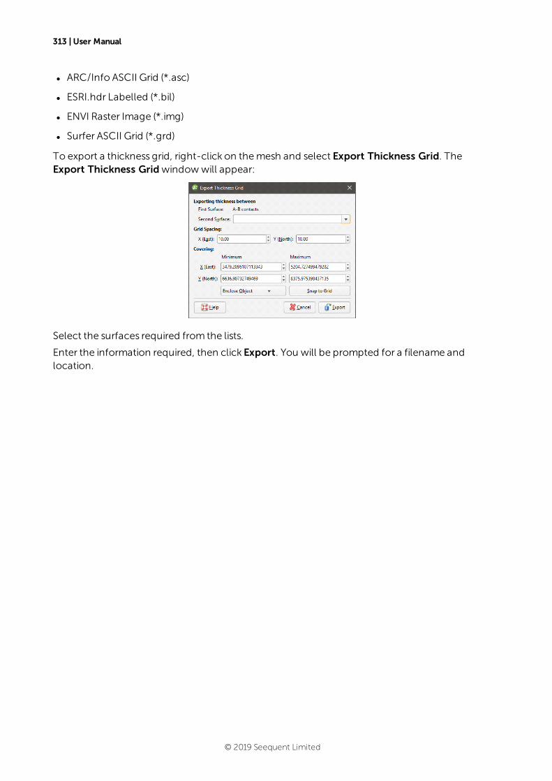
313 | User Manual
l ARC/Info ASCII Grid (*.asc)
l ESRI.hdr Labelled (*.bil)
l ENVI Raster Image (*.img)
l Surfer ASCII Grid (*.grd)
To export a thickness grid, right-click on themesh and select Export Thickness Grid. TheExport Thickness Gridwindowwill appear:
Select the surfaces required from the lists.
Enter the information required, then click Export. You will be prompted for a filename andlocation.
© 2019 Seequent Limited
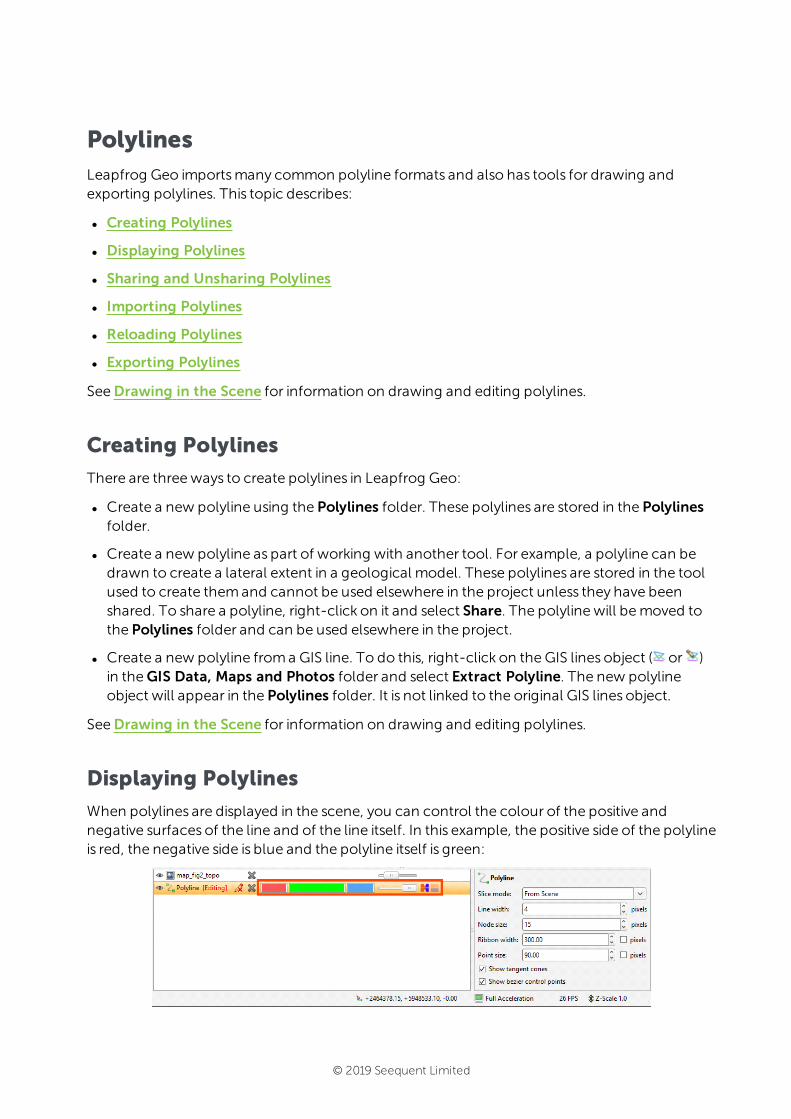
PolylinesLeapfrog Geo importsmany common polyline formats and also has tools for drawing andexporting polylines. This topic describes:
l Creating Polylines
l Displaying Polylines
l Sharing and Unsharing Polylines
l Importing Polylines
l Reloading Polylines
l Exporting Polylines
SeeDrawing in the Scene for information on drawing and editing polylines.
Creating Polylines
There are threeways to create polylines in Leapfrog Geo:
l Create a new polyline using the Polylines folder. These polylines are stored in the Polylinesfolder.
l Create a new polyline as part of working with another tool. For example, a polyline can bedrawn to create a lateral extent in a geological model. These polylines are stored in the toolused to create themand cannot be used elsewhere in the project unless they have beenshared. To share a polyline, right-click on it and select Share. The polyline will bemoved tothe Polylines folder and can be used elsewhere in the project.
l Create a new polyline froma GIS line. To do this, right-click on the GIS lines object ( or )in theGIS Data, Maps and Photos folder and select Extract Polyline. The new polylineobject will appear in the Polylines folder. It is not linked to the original GIS lines object.
SeeDrawing in the Scene for information on drawing and editing polylines.
Displaying Polylines
When polylines are displayed in the scene, you can control the colour of the positive andnegative surfaces of the line and of the line itself. In this example, the positive side of the polylineis red, the negative side is blue and the polyline itself is green:
© 2019 Seequent Limited

315 | User Manual
For contact surfaces, the colour of the positive and negative sides of a ribbon will bedetermined by the lithologies or categories assigned to either side of the surface.
With theNode size and Point size controls in the properties panel, you can change the size ofnodes and points in the scene tomakeworking with the polyline easier.
Polylines have a Surface ribbon( ) and Normal ribbon( ) to help you to determine theorientation of the polyline in the scene. The surface ribbon reflects the orientation of thepolyline and the normal ribbon is perpendicular to the surface ribbon. For example, click on theSurface ribbon button ( ) to determinewhich side of the polyline is positive (red) and whichside is negative (blue):
If you are having trouble seeing the ribbons, you can change their size using theRibbon widthcontrol in the properties panel.
Other aspects of polyline display are useful when creating and editing polylines. SeeDrawing inthe Scene.
Sharing and Unsharing Polylines
Some polylines are created as part of working with other objects and are not availableelsewhere in the project. An example of this is a polyline drawn as part of creating a modelboundary. To share the polyline, right-click on the object in the project tree and click Share.The shared polyline will be copied to the relevant location in the project tree and a hyperlinkadded to the object it was shared from.
© 2019 Seequent Limited
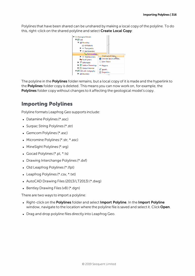
Importing Polylines | 316
Polylines that have been shared can be unshared bymaking a local copy of the polyline. To dothis, right-click on the shared polyline and selectCreate Local Copy:
The polyline in the Polylines folder remains, but a local copy of it ismade and the hyperlink tothe Polylines folder copy is deleted. Thismeans you can nowwork on, for example, thePolylines folder copywithout changes to it affecting the geological model’s copy.
Importing Polylines
Polyline formats Leapfrog Geo supports include:
l Datamine Polylines (*.asc)
l Surpac String Polylines (*.str)
l GemcomPolylines (*.asc)
l Micromine Polylines (*.str, *.asc)
l MineSight Polylines (*.srg)
l Gocad Polylines (*.pl, *.ts)
l Drawing Interchange Polylines (*.dxf)
l Old Leapfrog Polylines (*.lfpl)
l Leapfrog Polylines (*.csv, *.txt)
l AutoCAD Drawing Files (2013/LT2013) (*.dwg)
l BentleyDrawing Files (v8) (*.dgn)
There are twoways to import a polyline:
l Right-click on the Polylines folder and select Import Polyline. In the Import Polylinewindow, navigate to the location where the polyline file is saved and select it. ClickOpen.
l Drag and drop polyline files directly into Leapfrog Geo.
© 2019 Seequent Limited
317 | User Manual
If the polyline file is in Leapfrog, Gocad or DXF formats, the importing will start immediately. Forall other formats, the Polyline Import windowwill appear. If the polyline file is in one of thestandard formats listed above, the default settings can be used. Click Import to finish theprocess. If, however, you wish to specify polyline import parameters, two pieces of informationare required:
l The columns the polyline vertex coordinates are in
l How the polyline sections are separated in the file
Select the vertex coordinate columnsby clicking on the heading at the top of a column andselecting one of East (X), North (Y) or Elev (Z) from the list.
When importing a file that hasmultiple features, you will be prompted to select which ones toimport. You can also choose to:
l Import the features as separate objects. Each feature will appear in the project tree as aseparate object.
l Flatten all features into one object. Leapfrog Geowill treat all features as a single object.
The polyline will be imported and added to the project tree under the Polylines folder.
SeeDrawing in the Scene for information on drawing and editing polylines.
Reloading Polylines
Reloading data is necessarywhen the imported data ismodified externally. To reload a polyline,right-click on it in the project tree and select Reload Data.
Reloading a polyline overwrites any changes you havemade to the polyline. Any dependentobjectswill be updated, which can take some time.
Select the file to be reloaded and clickOpen. The polyline will be updated, aswill anydependent objects.
Exporting Polylines
Export a polyline by right-clicking on it and selecting Export. Leapfrog Geo exports polylines inthe following formats:
l Leapfrog Polylines (*.lfpl)
l Leapfrog Polylines (*.csv)
l Drawing Interchange Polylines (*.dxf)
l Surpac String Polylines (*.str)
l Gocad Polylines (*.pl, *.ts)
l MineSight Polylines (*.srg)
l Datamine Polylines (*.asc)
© 2019 Seequent Limited

Exporting Polylines | 318
l Micromine Polylines (*.str, *.asc)
l Drawing File (2013/LT2013) (*.dwg)
l BentleyDrawing Files (v8) (*.dgn)
© 2019 Seequent Limited

Geochemical Data
TheGeochemistry folder and related features are only available with the Geochemistryextension. Contact Customer Support as described in Getting Support formore informationabout this extension.
With theGeochemistry folder, you can establish a live link to ioGAS and visualise geochemicaldata in real time. You can also transfer data between Leapfrog Geo and ioGAS, including datatowhich query filters have been applied.
This topic describes how to connect to ioGAS and transfer data between ioGAS and LeapfrogGeo. It is divided into:
l Sending Data to ioGAS
l Importing ioGAS Data
To connect to ioGAS, make sure ioGAS is running. Next, right-click on the ioGAS object in theproject tree and selectConnect:
Once the connection is established, any dataset open in ioGAS will be available from the ioGASobject and can be displayed in the Leapfrog Geo scenewindow:
The status of the connection to ioGAS is indicated in Leapfrog Geo, and the data file open inioGAS appears in theGeochemistry folder (e.g. demo.gas).
You can view the data in Leapfrog Geo by adding the ioGAS data object to the scene. Whenattributes are changed in ioGAS, the displaywill be updated in Leapfrog Geo. You can also:
l Send fromand to data columns across the ioGAS link, analyse the data in ioGAS and importcalculated columns as interval tables. This data can then be used formodelling in LeapfrogGeo. See Sending Data to ioGAS.
l Import ioGAS data into Leapfrog Geo as points or intervals. See Importing ioGAS Data.
© 2019 Seequent Limited
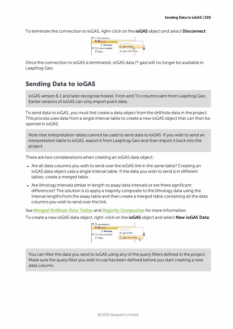
Sending Data to ioGAS | 320
To terminate the connection to ioGAS, right-click on the ioGAS object and selectDisconnect:
Once the connection to ioGAS is terminated, ioGAS data (*.gas) will no longer be available inLeapfrog Geo.
Sending Data to ioGAS
ioGAS version 6.1 and later recognise holeid, Fromand To columns sent fromLeapfrog Geo.Earlier versions of ioGAS can only import point data.
To send data to ioGAS, you must first create a data object from the drillhole data in the project.This process uses data froma single interval table to create a new ioGAS object that can then beopened in ioGAS.
Note that interpretation tables cannot be used to send data to ioGAS. If you wish to send aninterpretation table to ioGAS, export it fromLeapfrog Geo and then import it back into theproject.
There are two considerationswhen creating an ioGAS data object:
l Are all data columns you wish to send over the ioGAS link in the same table? Creating anioGAS data object uses a single interval table. If the data you wish to send is in differenttables, create a merged table.
l Are lithology intervals similar in length to assay data intervals or are there significantdifferences? The solution is to apply a majority composite to the lithology data using theinterval lengths from the assay table and then create a merged table containing all the datacolumns you wish to send over the link.
SeeMerged Drillhole Data Tables and Majority Composites formore information.
To create a new ioGAS data object, right-click on the ioGAS object and selectNew ioGAS Data:
You can filter the data you send to ioGAS using any of the query filters defined in the project.Make sure the query filter you wish to use has been defined before you start creating a newdata column.
© 2019 Seequent Limited
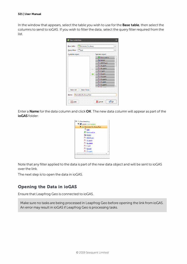
321 | User Manual
In thewindow that appears, select the table you wish to use for the Base table, then select thecolumns to send to ioGAS. If you wish to filter the data, select the query filter required from thelist.
Enter a Name for the data column and clickOK. The new data column will appear as part of theioGAS folder:
Note that any filter applied to the data is part of the new data object and will be sent to ioGASover the link.
The next step is to open the data in ioGAS.
Opening the Data in ioGAS
Ensure that Leapfrog Geo is connected to ioGAS.
Make sure no tasks are being processed in Leapfrog Geo before opening the link from ioGAS.An errormay result in ioGAS if Leapfrog Geo is processing tasks.
© 2019 Seequent Limited
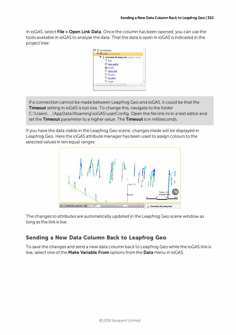
Sending a New Data Column Back to Leapfrog Geo | 322
In ioGAS, select File > Open Link Data. Once the column has been opened, you can use thetools available in ioGAS to analyse the data. That the data is open in ioGAS is indicated in theproject tree:
If a connection cannot bemade between Leapfrog Geo and ioGAS, it could be that theTimeout setting in ioGAS is too low. To change this, navigate to the folderC:\Users\....\AppData\Roaming\ioGAS\userConfig. Open the file link.ini in a text editor andset the Timeout parameter to a higher value. The Timeout is in milliseconds.
If you have the data visible in the Leapfrog Geo scene, changesmadewill be displayed inLeapfrog Geo. Here the ioGAS attributemanager has been used to assign colours to theselected values in ten equal ranges:
The changes to attributes are automatically updated in the Leapfrog Geo scenewindow aslong as the link is live.
Sending a New Data Column Back to Leapfrog Geo
To save the changes and send a new data column back to Leapfrog Geowhile the ioGAS link islive, select one of theMake Variable Fromoptions from theDatamenu in ioGAS.
© 2019 Seequent Limited
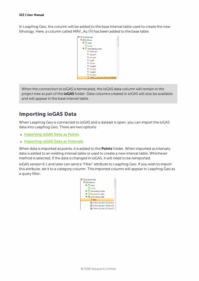
323 | User Manual
In Leapfrog Geo, the column will be added to the base interval table used to create the newlithology. Here, a column called MRV_Au ( ) has been added to the base table:
When the connection to ioGAS is terminated, the ioGAS data column will remain in theproject tree as part of the ioGAS folder. Data columns created in ioGAS will also be availableand will appear in the base interval table.
Importing ioGAS Data
When Leapfrog Geo is connected to ioGAS and a dataset is open, you can import the ioGASdata into Leapfrog Geo. There are two options:
l Importing ioGAS Data as Points
l Importing ioGAS Data as Intervals
When data is imported as points, it is added to the Points folder. When imported as intervals,data is added to an existing interval table or used to create a new interval table. Whichevermethod is selected, if the data is changed in ioGAS, it will need to be reimported.
ioGAS version 6.1 and later can send a “Filter” attribute to Leapfrog Geo. If you wish to importthis attribute, set it to a category column. This imported column will appear in Leapfrog Geo asa query filter:
© 2019 Seequent Limited
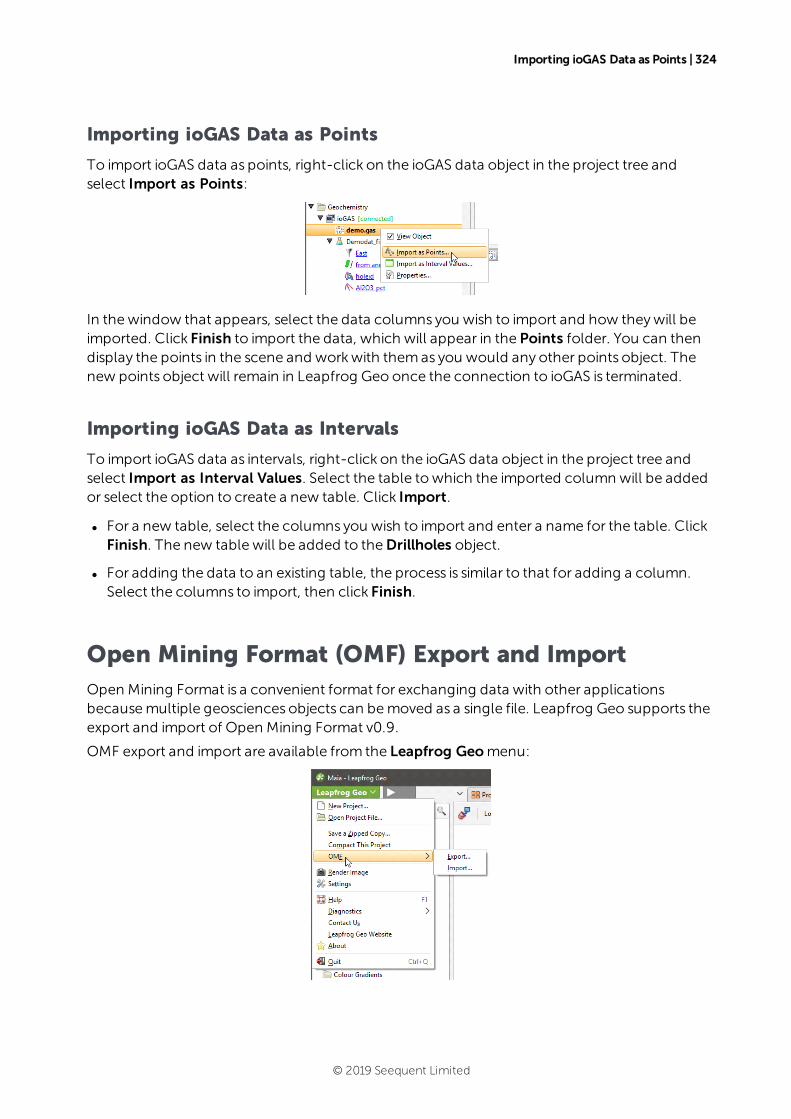
Importing ioGAS Data as Points | 324
Importing ioGAS Data as Points
To import ioGAS data as points, right-click on the ioGAS data object in the project tree andselect Import as Points:
In thewindow that appears, select the data columns you wish to import and how theywill beimported. Click Finish to import the data, which will appear in the Points folder. You can thendisplay the points in the scene and workwith themas you would any other points object. Thenew points object will remain in Leapfrog Geo once the connection to ioGAS is terminated.
Importing ioGAS Data as Intervals
To import ioGAS data as intervals, right-click on the ioGAS data object in the project tree andselect Import as Interval Values. Select the table towhich the imported column will be addedor select the option to create a new table. Click Import.
l For a new table, select the columns you wish to import and enter a name for the table. ClickFinish. The new table will be added to theDrillholes object.
l For adding the data to an existing table, the process is similar to that for adding a column.Select the columns to import, then click Finish.
Open Mining Format (OMF) Export and ImportOpen Mining Format is a convenient format for exchanging data with other applicationsbecausemultiple geosciences objects can bemoved as a single file. Leapfrog Geo supports theexport and import of Open Mining Format v0.9.
OMF export and import are available from the Leapfrog Geomenu:
© 2019 Seequent Limited
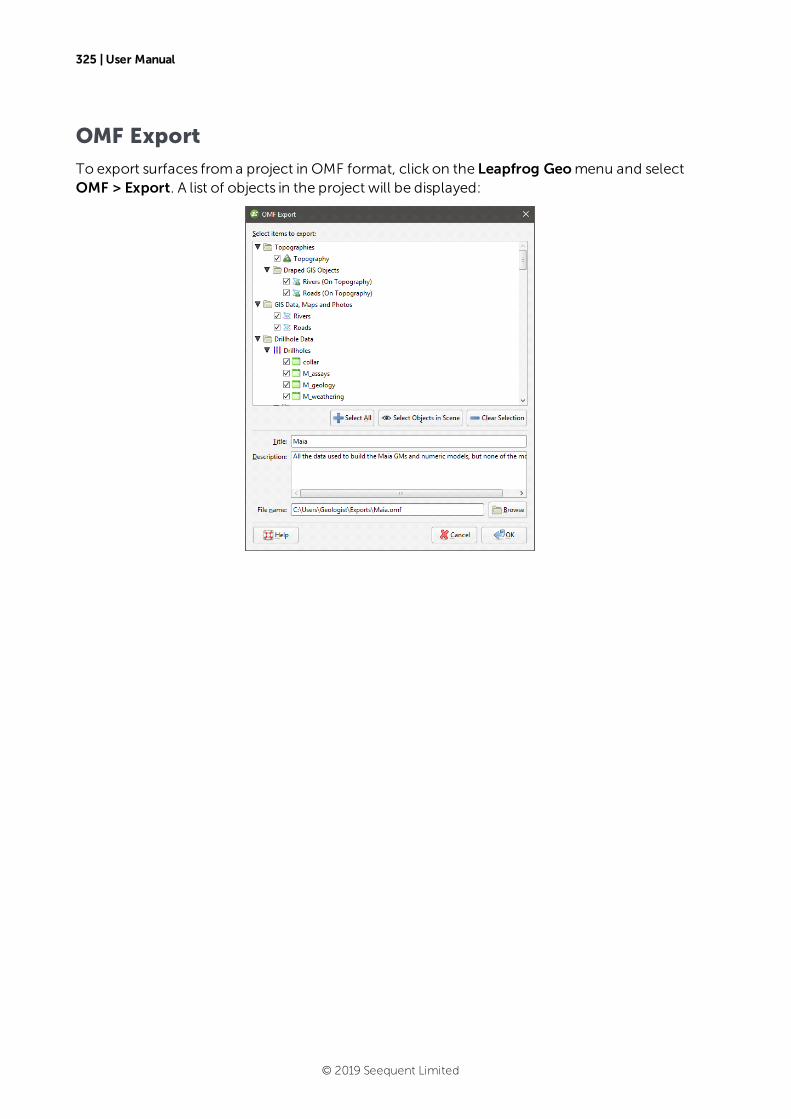
325 | User Manual
OMF Export
To export surfaces froma project in OMF format, click on the Leapfrog Geomenu and selectOMF > Export. A list of objects in the project will be displayed:
© 2019 Seequent Limited

OMF Import | 326
Select the objects you wish to export, then specify the file name and the folder where it will besaved. ClickOK to export the file.
Exporting the filemay take some time if you have selected a large number of objects.
OMF Import
To import data froman OMF file, click on the Leapfrog Geomenu and selectOMF > Import. Inthewindow that appears, select the file you wish to import and clickOpen. The objects in thefile will be displayed:
Select the objects you wish to import and clickOK. Selected objectswill be imported and addedto the project tree. GIS data will be added to theGIS Data, Maps and Photos folder and points,meshes and blockmodelswill be added to their respective folders.
© 2019 Seequent Limited
Analysing Data
Leapfrog Geo has a number of tools that help you to analyse your data.
l Themost basic information about an object is contained in the object’sProperties window,which is specific to the type of object. Right-click on the object in the project tree and selectProperties. SeeObject Properties in the The Project Tree topic formore information.
l Viewing statistical information about objects helps you to analyse your data. This is describedfurther below.
l Visualising data using the shape list and the shape properties panel is an important part ofinterpreting and refining data and making modelling decisions. The tools available dependon the type of object being displayed, and many objects can be displayed evaluated on otherobjects.
l Stereonets are useful for visualising structural data and identifying trends in 2D. Errors incategorisation of structural data can also become apparent when the data is viewed on astereonet.
l Form interpolants are useful for visualising structural data and identifying broad trends in 3D.The form interpolant’smeshes can then be used to control other surfaces in the project.
l With the drillhole correlation tool, you can view and compare selected drillholes in a 2Dview. You can then create interpretation tables in which you can assign and adjust intervalsand create new intervals. Interpretation tables are like any other interval table in a projectand can be used to createmodels.
l You can plan drillholes, view prognoses formodels in the project and export planneddrillholes in .csv format. Leapfrog Geo can also import planned drillholes.
The rest of this topic describes the different statistics visualisations available in Leapfrog Geo.
StatisticsThe statistics options available in Leapfrog Geo depend on the type of object. Commonstatistics visualisations are described below:
l Table of Statistics
l Scatter Plots
l Q-Q Plots
l Box Plots
l Univariate Graphs
Variations of these are described relative to the data objects for which they are relevant.
Leapfrog Geo uses fixed 25%/75% quartiles.
© 2019 Seequent Limited
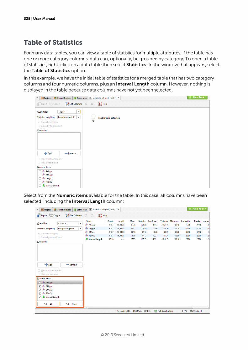
328 | User Manual
Table of Statistics
Formany data tables, you can view a table of statistics formultiple attributes. If the table hasone ormore category columns, data can, optionally, be grouped by category. To open a tableof statistics, right-click on a data table then select Statistics. In thewindow that appears, selectthe Table of Statistics option.
In this example, we have the initial table of statistics for a merged table that has two categorycolumns and four numeric columns, plus an Interval Length column. However, nothing isdisplayed in the table because data columnshave not yet been selected.
Select from theNumeric items available for the table. In this case, all columnshave beenselected, including the Interval Length column:
© 2019 Seequent Limited
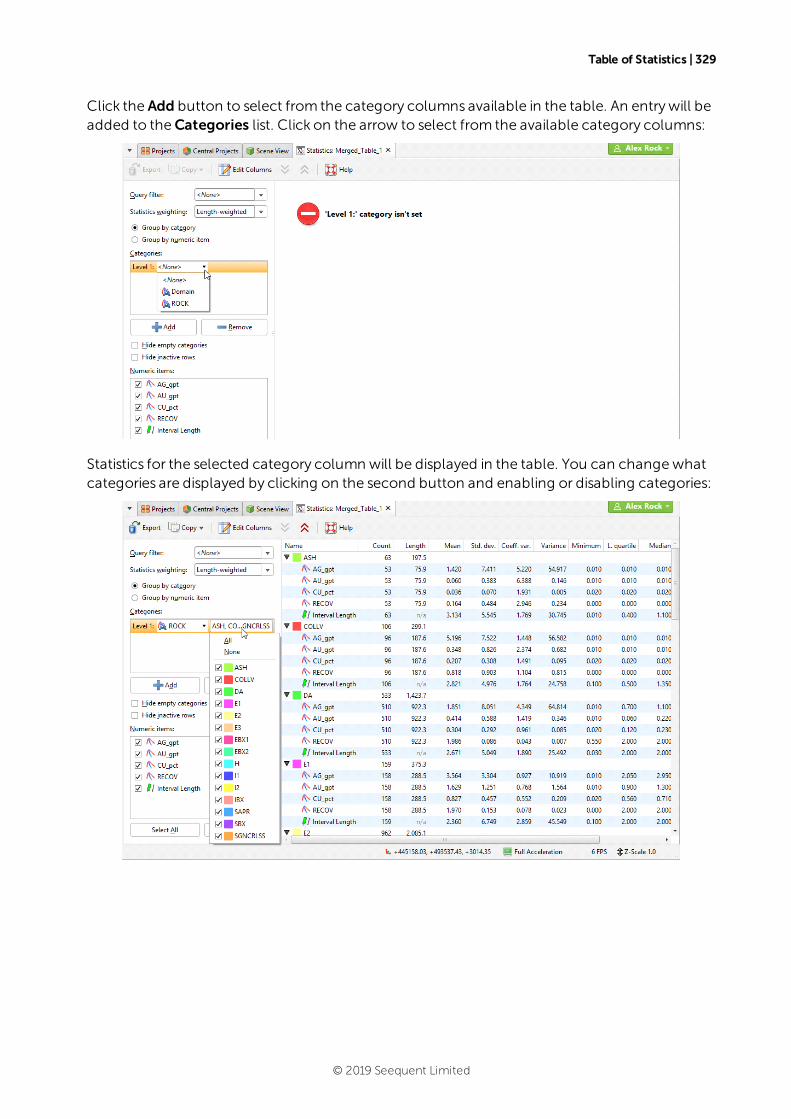
Table of Statistics | 329
Click the Add button to select from the category columns available in the table. An entrywill beadded to theCategories list. Click on the arrow to select from the available category columns:
Statistics for the selected category column will be displayed in the table. You can changewhatcategories are displayed by clicking on the second button and enabling or disabling categories:
© 2019 Seequent Limited

330 | User Manual
If there ismore than one category column, you can set lower levels. Here there are twocategory columnsdisplayed in the table, “ROCK” and “Domain”:
You can hide empty categories (thosewith a count of zero) and inactive rowsusing the optionsbelow theCategories list:
© 2019 Seequent Limited

Table of Statistics | 331
Group by category and Group by numeric item provide further options for the tableorganisation. Here theGroup by numeric itemoption has been selected:
You can filter the data using anyQuery filter defined for the data table. Statistics for intervaltables can be unweighted orweighted by interval length.
Change the columnsdisplayed in the table by clicking on the Edit Columns button:
Once you have set up a table of statistics on a particular table, its settingswill be saved so youcan easily review the statistics and export the table using the same settings.
To export the table in CSV format, click on the Export button in the toolbar ( ).
Other controls in thiswindow are as follows:
l The arrow buttons at the top of thewindow ( and ) allow you to quickly expand orcollapse the rows.
© 2019 Seequent Limited
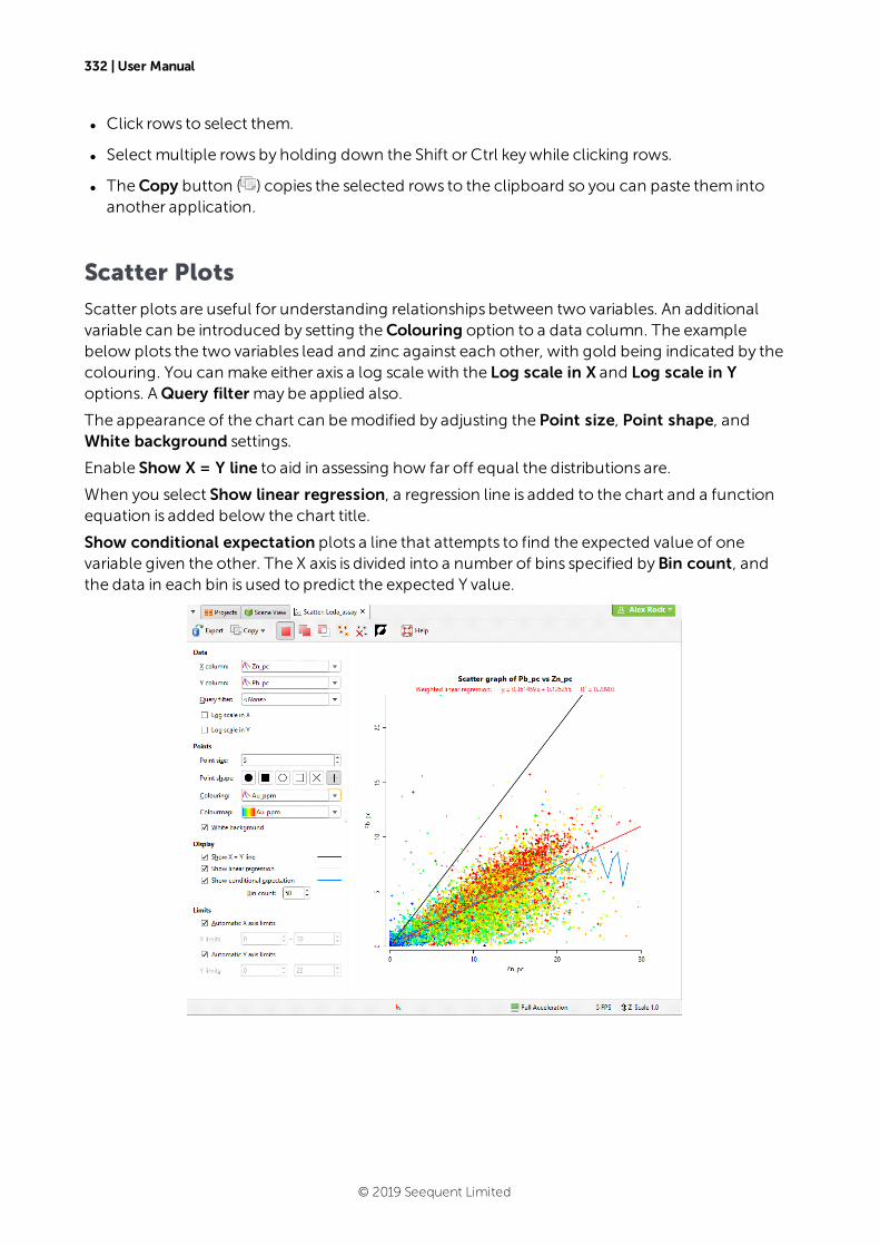
332 | User Manual
l Click rows to select them.
l Select multiple rowsby holding down the Shift or Ctrl keywhile clicking rows.
l TheCopy button ( ) copies the selected rows to the clipboard so you can paste them intoanother application.
Scatter Plots
Scatter plots are useful for understanding relationships between two variables. An additionalvariable can be introduced by setting theColouring option to a data column. The examplebelow plots the two variables lead and zinc against each other, with gold being indicated by thecolouring. You can make either axis a log scale with the Log scale in X and Log scale in Yoptions. AQuery filter may be applied also.
The appearance of the chart can bemodified by adjusting the Point size, Point shape, andWhite background settings.
Enable Show X = Y line to aid in assessing how far off equal the distributions are.
When you select Show linear regression, a regression line is added to the chart and a functionequation is added below the chart title.
Show conditional expectation plots a line that attempts to find the expected value of onevariable given the other. The X axis is divided into a number of bins specified byBin count, andthe data in each bin is used to predict the expected Y value.
© 2019 Seequent Limited
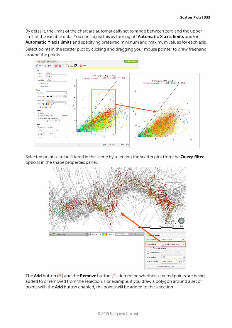
Scatter Plots | 333
By default, the limits of the chart are automatically set to range between zero and the upperlimit of the variable data. You can adjust this by turning off Automatic X axis limits and/orAutomatic Y axis limits and specifying preferred minimumand maximumvalues for each axis.
Select points in the scatter plot by clicking and dragging yourmouse pointer to draw freehandaround the points.
Selected points can be filtered in the scene by selecting the scatter plot from theQuery filteroptions in the shape properties panel.
The Add button ( ) and theRemove button ( ) determinewhether selected points are beingadded to or removed from the selection. For example, if you draw a polygon around a set ofpointswith the Add button enabled, the pointswill be added to the selection.
© 2019 Seequent Limited
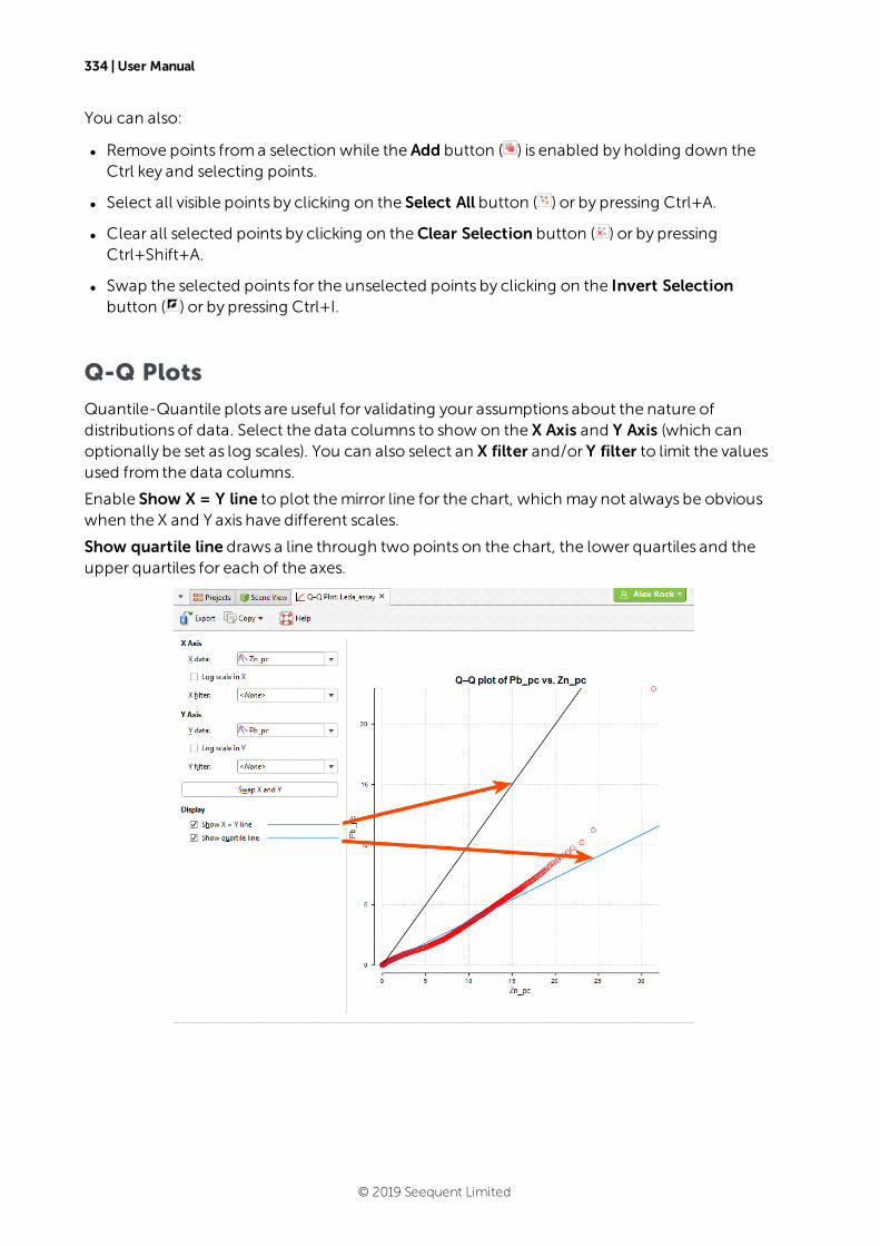
334 | User Manual
You can also:
l Remove points froma selection while the Add button ( ) is enabled by holding down theCtrl key and selecting points.
l Select all visible points by clicking on the Select All button ( ) or by pressing Ctrl+A.
l Clear all selected points by clicking on theClear Selection button ( ) or by pressingCtrl+Shift+A.
l Swap the selected points for the unselected points by clicking on the Invert Selectionbutton ( ) or by pressing Ctrl+I.
Q-Q Plots
Quantile-Quantile plots are useful for validating your assumptions about the nature ofdistributions of data. Select the data columns to show on the X Axis and Y Axis (which canoptionally be set as log scales). You can also select an X filter and/or Y filter to limit the valuesused from the data columns.
Enable Show X = Y line to plot themirror line for the chart, which may not always be obviouswhen the X and Y axis have different scales.
Show quartile line draws a line through two points on the chart, the lower quartiles and theupper quartiles for each of the axes.
© 2019 Seequent Limited
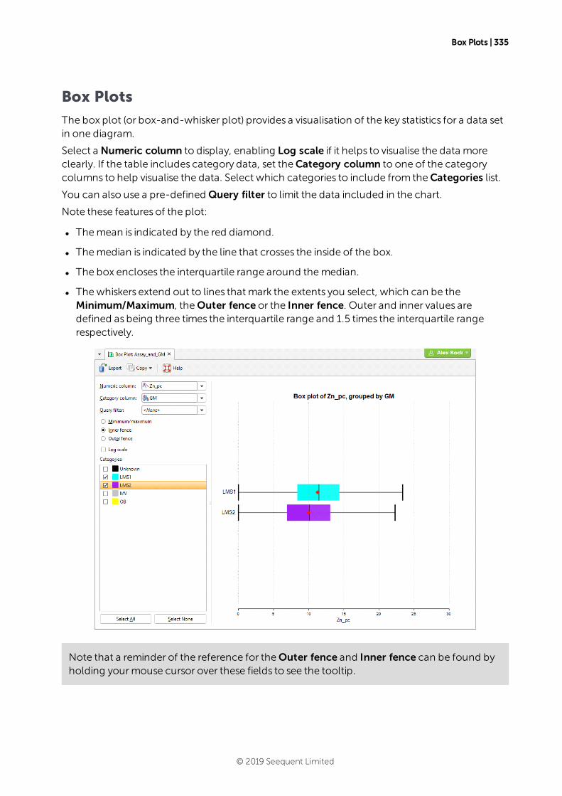
Box Plots | 335
Box Plots
The box plot (or box-and-whisker plot) provides a visualisation of the key statistics for a data setin one diagram.
Select a Numeric column to display, enabling Log scale if it helps to visualise the data moreclearly. If the table includes category data, set theCategory column to one of the categorycolumns to help visualise the data. Select which categories to include from theCategories list.
You can also use a pre-defined Query filter to limit the data included in the chart.
Note these features of the plot:
l Themean is indicated by the red diamond.
l Themedian is indicated by the line that crosses the inside of the box.
l The box encloses the interquartile range around themedian.
l Thewhiskers extend out to lines that mark the extents you select, which can be theMinimum/Maximum, theOuter fence or the Inner fence. Outer and inner values aredefined as being three times the interquartile range and 1.5 times the interquartile rangerespectively.
Note that a reminder of the reference for theOuter fence and Inner fence can be found byholding yourmouse cursor over these fields to see the tooltip.
© 2019 Seequent Limited
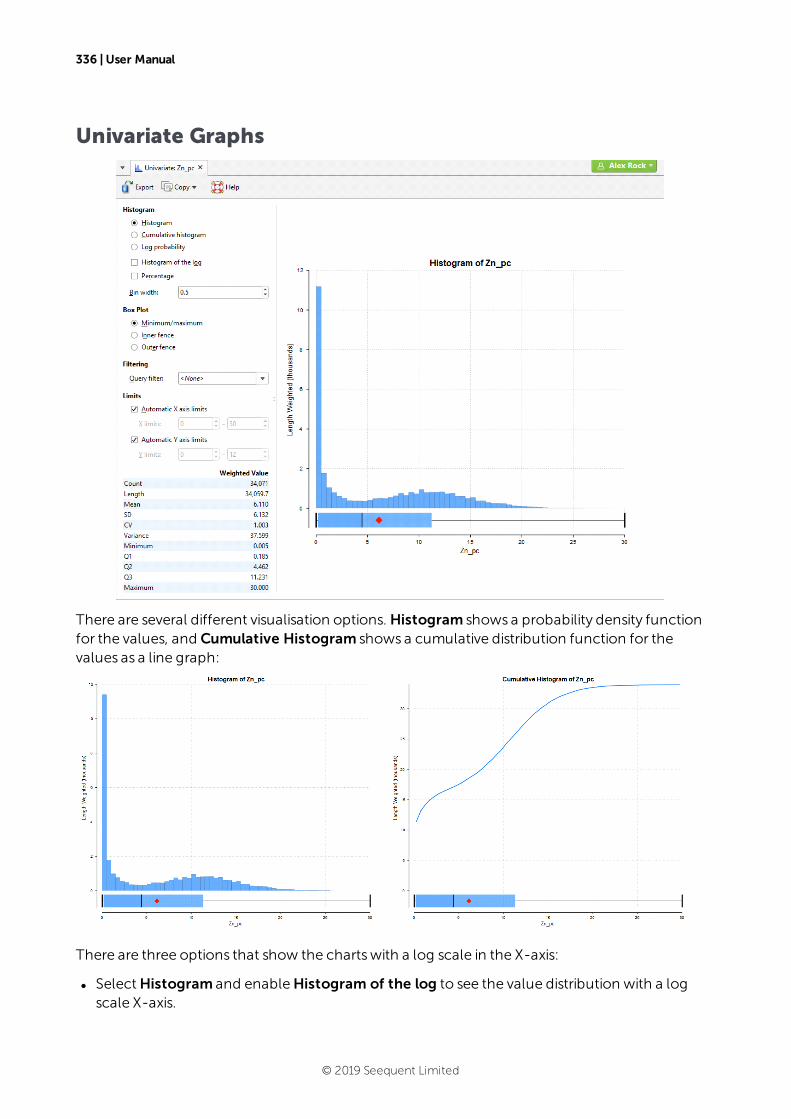
336 | User Manual
Univariate Graphs
There are several different visualisation options. Histogram shows a probability density functionfor the values, and Cumulative Histogram shows a cumulative distribution function for thevalues as a line graph:
There are three options that show the chartswith a log scale in the X-axis:
l SelectHistogram and enableHistogram of the log to see the value distribution with a logscale X-axis.
© 2019 Seequent Limited
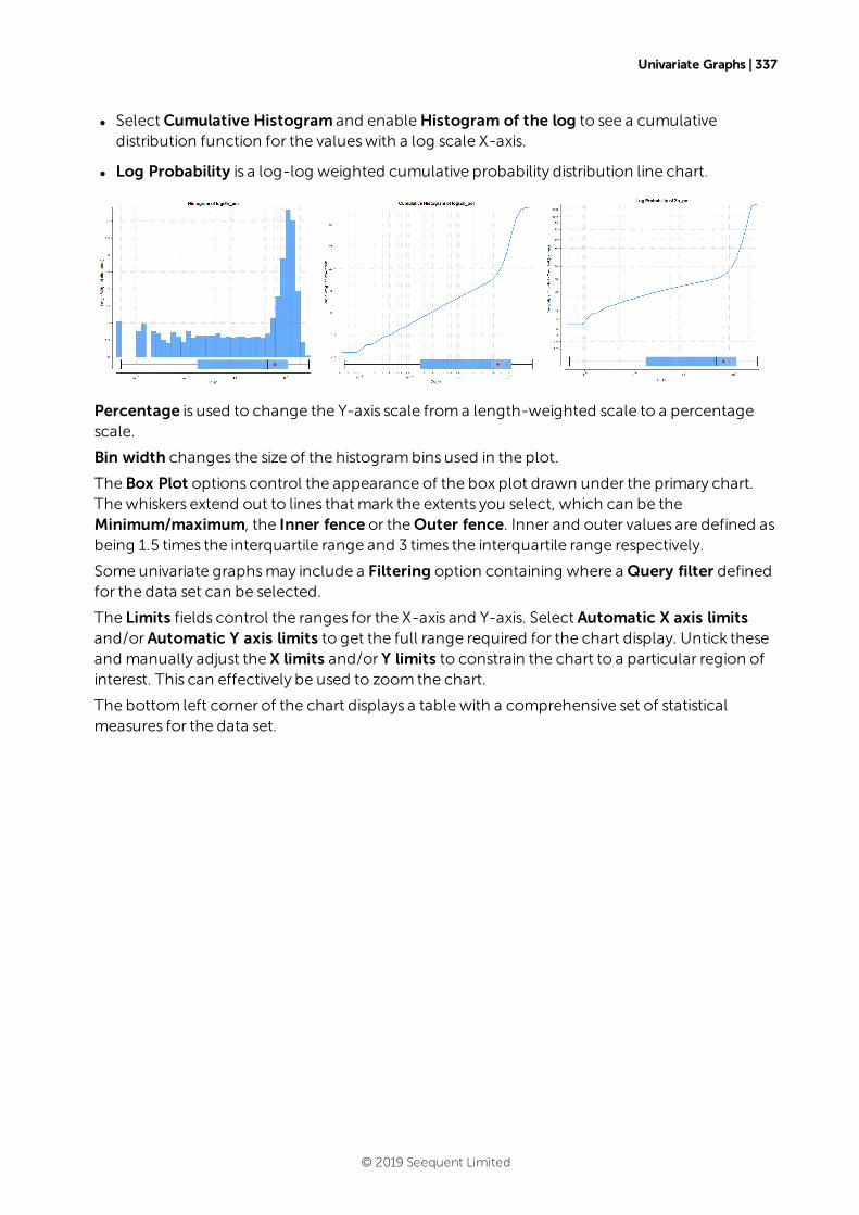
Univariate Graphs | 337
l SelectCumulative Histogram and enableHistogram of the log to see a cumulativedistribution function for the valueswith a log scale X-axis.
l Log Probability is a log-log weighted cumulative probability distribution line chart.
Percentage is used to change the Y-axis scale froma length-weighted scale to a percentagescale.
Bin width changes the size of the histogrambins used in the plot.
The Box Plot options control the appearance of the box plot drawn under the primary chart.Thewhiskers extend out to lines that mark the extents you select, which can be theMinimum/maximum, the Inner fence or theOuter fence. Inner and outer values are defined asbeing 1.5 times the interquartile range and 3 times the interquartile range respectively.
Some univariate graphsmay include a Filtering option containing where a Query filter definedfor the data set can be selected.
The Limits fields control the ranges for the X-axis and Y-axis. Select Automatic X axis limitsand/orAutomatic Y axis limits to get the full range required for the chart display. Untick theseand manually adjust the X limits and/or Y limits to constrain the chart to a particular region ofinterest. This can effectively be used to zoom the chart.
The bottom left corner of the chart displays a table with a comprehensive set of statisticalmeasures for the data set.
© 2019 Seequent Limited
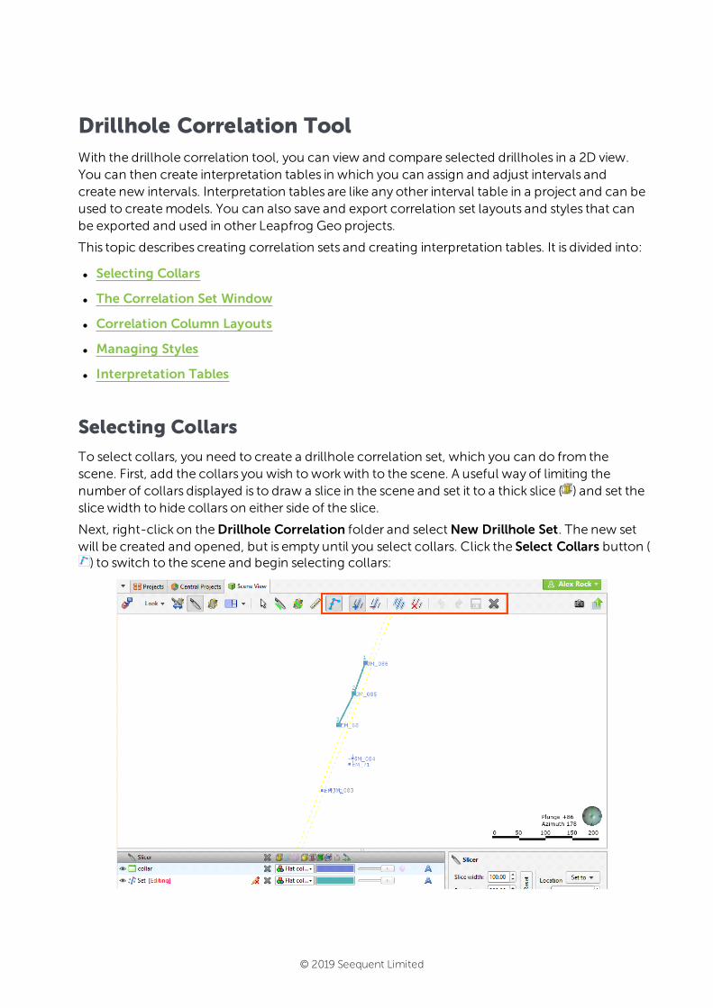
Drillhole Correlation ToolWith the drillhole correlation tool, you can view and compare selected drillholes in a 2D view.You can then create interpretation tables in which you can assign and adjust intervals andcreate new intervals. Interpretation tables are like any other interval table in a project and can beused to createmodels. You can also save and export correlation set layouts and styles that canbe exported and used in other Leapfrog Geo projects.
This topic describes creating correlation sets and creating interpretation tables. It is divided into:
l Selecting Collars
l The Correlation Set Window
l Correlation Column Layouts
l Managing Styles
l Interpretation Tables
Selecting Collars
To select collars, you need to create a drillhole correlation set, which you can do from thescene. First, add the collars you wish toworkwith to the scene. A useful way of limiting thenumber of collars displayed is to draw a slice in the scene and set it to a thick slice ( ) and set theslice width to hide collars on either side of the slice.
Next, right-click on theDrillhole Correlation folder and selectNew Drillhole Set. The new setwill be created and opened, but is empty until you select collars. Click the Select Collars button () to switch to the scene and begin selecting collars:
© 2019 Seequent Limited
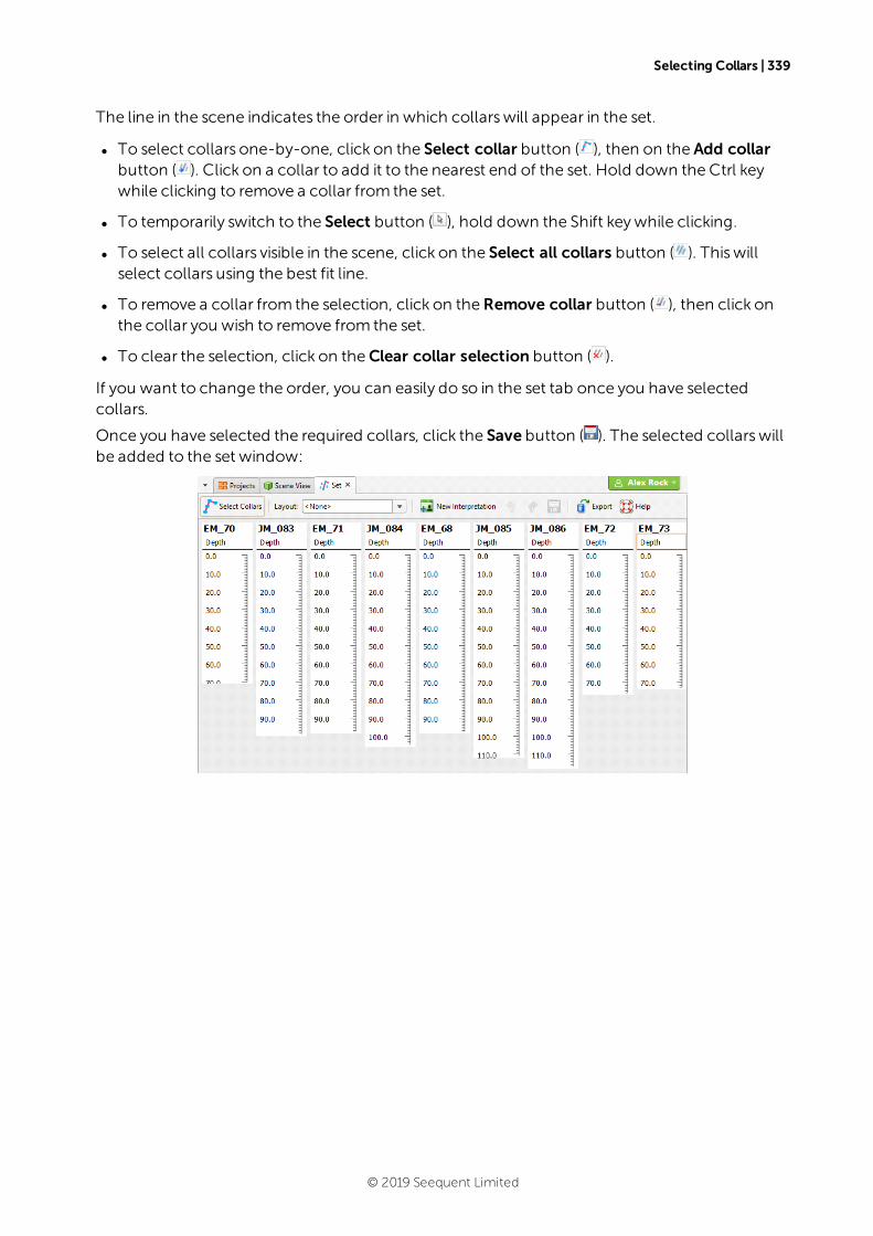
Selecting Collars | 339
The line in the scene indicates the order in which collarswill appear in the set.
l To select collars one-by-one, click on the Select collar button ( ), then on the Add collarbutton ( ). Click on a collar to add it to the nearest end of the set. Hold down the Ctrl keywhile clicking to remove a collar from the set.
l To temporarily switch to the Select button ( ), hold down the Shift keywhile clicking.
l To select all collars visible in the scene, click on the Select all collars button ( ). Thiswillselect collars using the best fit line.
l To remove a collar from the selection, click on theRemove collar button ( ), then click onthe collar you wish to remove from the set.
l To clear the selection, click on theClear collar selection button ( ).
If you want to change the order, you can easily do so in the set tab once you have selectedcollars.
Once you have selected the required collars, click the Save button ( ). The selected collarswillbe added to the set window:
© 2019 Seequent Limited
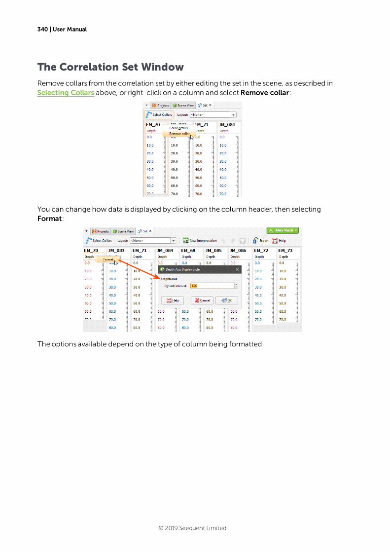
340 | User Manual
The Correlation Set Window
Remove collars from the correlation set by either editing the set in the scene, as described inSelecting Collars above, or right-click on a column and select Remove collar:
You can change how data is displayed by clicking on the column header, then selectingFormat:
The options available depend on the type of column being formatted.
© 2019 Seequent Limited
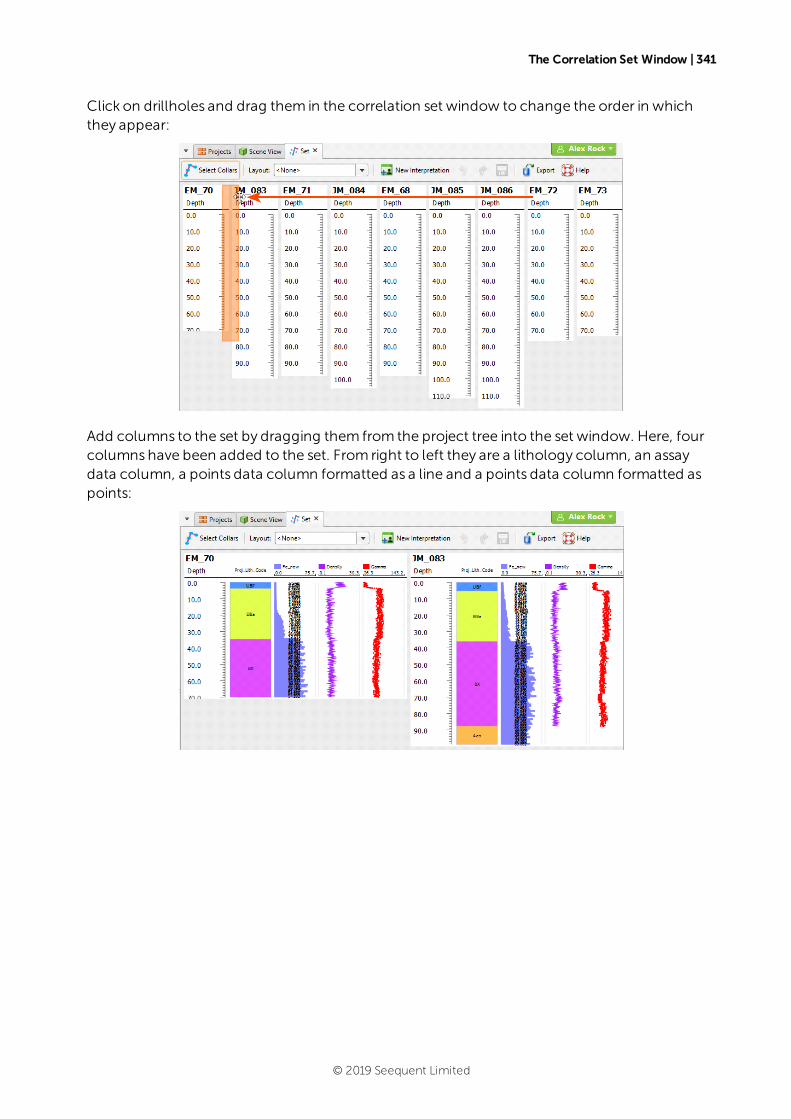
The Correlation Set Window | 341
Click on drillholes and drag them in the correlation set window to change the order in whichthey appear:
Add columns to the set by dragging them from the project tree into the set window. Here, fourcolumnshave been added to the set. From right to left they are a lithology column, an assaydata column, a points data column formatted as a line and a points data column formatted aspoints:
© 2019 Seequent Limited
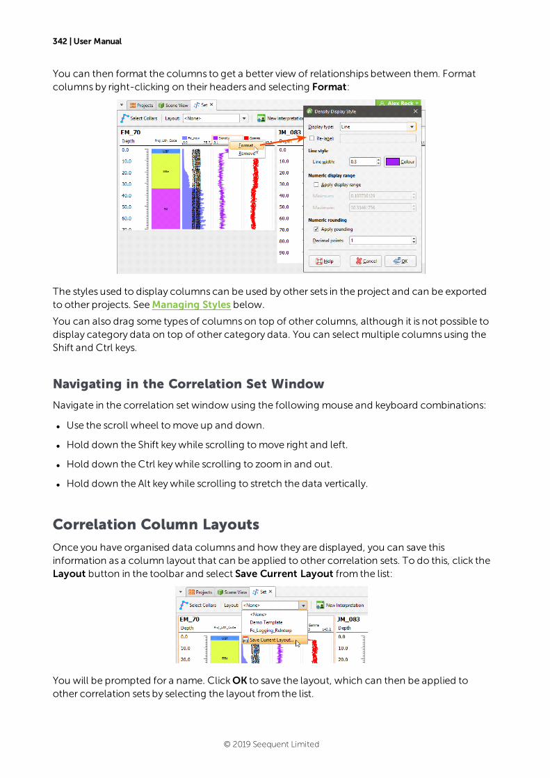
342 | User Manual
You can then format the columns to get a better view of relationships between them. Formatcolumnsby right-clicking on their headers and selecting Format:
The styles used to display columns can be used by other sets in the project and can be exportedto other projects. SeeManaging Styles below.
You can also drag some types of columnson top of other columns, although it is not possible todisplay category data on top of other category data. You can select multiple columnsusing theShift and Ctrl keys.
Navigating in the Correlation Set Window
Navigate in the correlation set window using the following mouse and keyboard combinations:
l Use the scroll wheel tomove up and down.
l Hold down the Shift keywhile scrolling tomove right and left.
l Hold down the Ctrl keywhile scrolling to zoom in and out.
l Hold down the Alt keywhile scrolling to stretch the data vertically.
Correlation Column Layouts
Once you have organised data columns and how they are displayed, you can save thisinformation as a column layout that can be applied to other correlation sets. To do this, click theLayout button in the toolbar and select Save Current Layout from the list:
You will be prompted for a name. ClickOK to save the layout, which can then be applied toother correlation sets by selecting the layout from the list.
© 2019 Seequent Limited
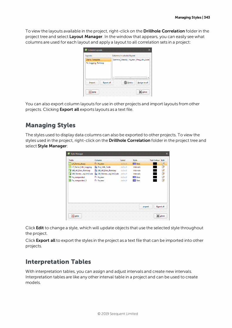
Managing Styles | 343
To view the layouts available in the project, right-click on theDrillhole Correlation folder in theproject tree and select Layout Manager. In thewindow that appears, you can easily seewhatcolumns are used for each layout and apply a layout to all correlation sets in a project:
You can also export column layouts for use in other projects and import layouts fromotherprojects. Clicking Export all exports layouts as a text file.
Managing Styles
The styles used to display data columns can also be exported to other projects. To view thestyles used in the project, right-click on theDrillhole Correlation folder in the project tree andselect Style Manager:
Click Edit to change a style, which will update objects that use the selected style throughoutthe project.
Click Export all to export the styles in the project as a text file that can be imported into otherprojects.
Interpretation Tables
With interpretation tables, you can assign and adjust intervals and create new intervals.Interpretation tables are like any other interval table in a project and can be used to createmodels.
© 2019 Seequent Limited
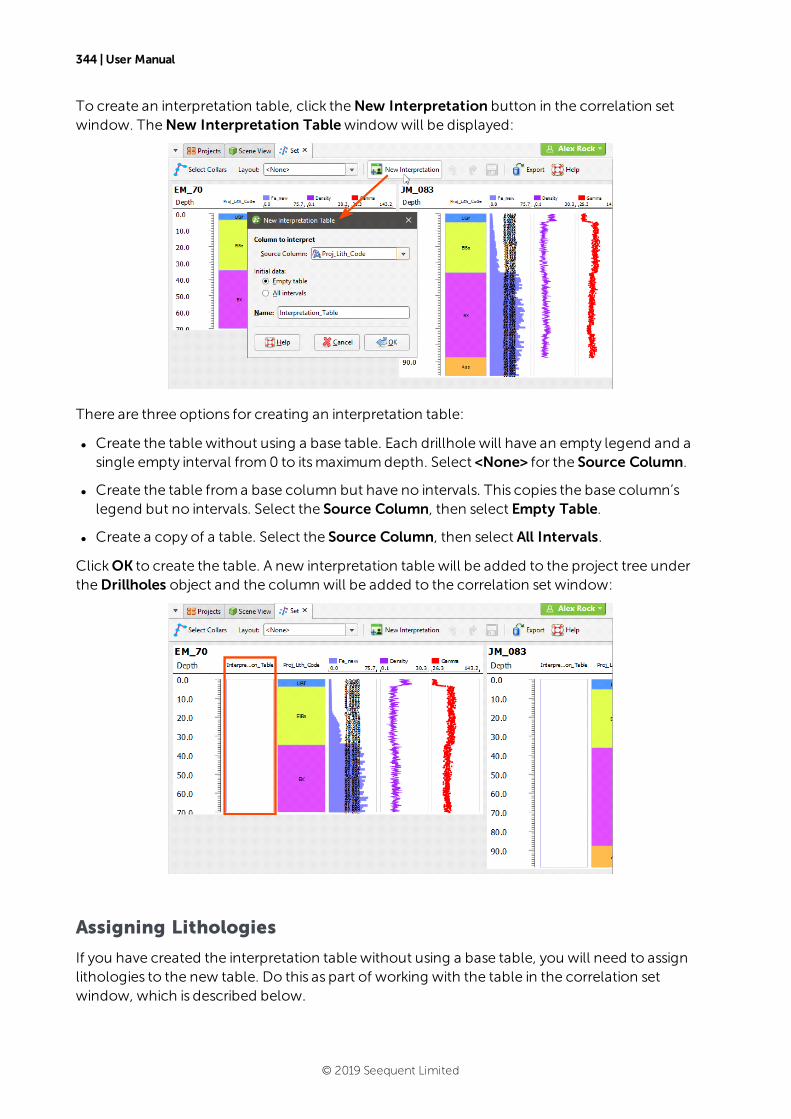
344 | User Manual
To create an interpretation table, click theNew Interpretation button in the correlation setwindow. TheNew Interpretation Tablewindowwill be displayed:
There are three options for creating an interpretation table:
l Create the table without using a base table. Each drillhole will have an empty legend and asingle empty interval from0 to itsmaximumdepth. Select <None> for the Source Column.
l Create the table froma base column but have no intervals. This copies the base column’slegend but no intervals. Select the Source Column, then select Empty Table.
l Create a copy of a table. Select the Source Column, then select All Intervals.
ClickOK to create the table. A new interpretation table will be added to the project tree undertheDrillholes object and the column will be added to the correlation set window:
Assigning Lithologies
If you have created the interpretation table without using a base table, you will need to assignlithologies to the new table. Do this as part of working with the table in the correlation setwindow, which is described below.
© 2019 Seequent Limited
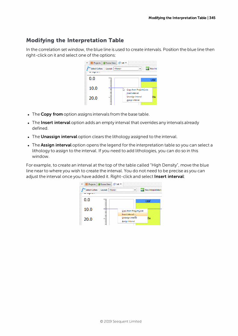
Modifying the Interpretation Table | 345
Modifying the Interpretation Table
In the correlation set window, the blue line is used to create intervals. Position the blue line thenright-click on it and select one of the options:
l TheCopy fromoption assigns intervals from the base table.
l The Insert interval option adds an empty interval that overrides any intervals alreadydefined.
l TheUnassign interval option clears the lithology assigned to the interval.
l The Assign interval option opens the legend for the interpretation table so you can select alithology to assign to the interval. If you need to add lithologies, you can do so in thiswindow.
For example, to create an interval at the top of the table called “High Density”, move the blueline near towhere you wish to create the interval. You do not need to be precise as you canadjust the interval once you have added it. Right-click and select Insert interval:
© 2019 Seequent Limited
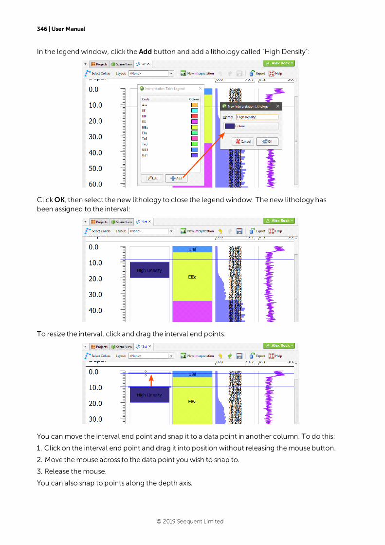
346 | User Manual
In the legend window, click the Add button and add a lithology called “High Density”:
ClickOK, then select the new lithology to close the legend window. The new lithology hasbeen assigned to the interval:
To resize the interval, click and drag the interval end points:
You can move the interval end point and snap it to a data point in another column. To do this:
1. Click on the interval end point and drag it into position without releasing themouse button.
2. Move themouse across to the data point you wish to snap to.
3. Release themouse.
You can also snap to points along the depth axis.
© 2019 Seequent Limited

Modifying the Interpretation Table | 347
Continuemaking changes to the interpretation table, using theUndo button to step backwardsif necessary. Save changes to update the table.
© 2019 Seequent Limited
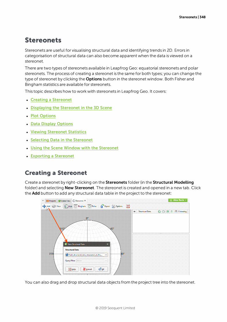
Stereonets | 348
StereonetsStereonets are useful for visualising structural data and identifying trends in 2D. Errors incategorisation of structural data can also become apparent when the data is viewed on astereonet.
There are two types of stereonets available in Leapfrog Geo: equatorial stereonets and polarstereonets. The process of creating a stereonet is the same for both types; you can change thetype of stereonet by clicking theOptions button in the stereonet window. Both Fisher andBinghamstatistics are available for stereonets.
This topic describes how toworkwith stereonets in Leapfrog Geo. It covers:
l Creating a Stereonet
l Displaying the Stereonet in the 3D Scene
l Plot Options
l Data Display Options
l Viewing Stereonet Statistics
l Selecting Data in the Stereonet
l Using the Scene Window with the Stereonet
l Exporting a Stereonet
Creating a Stereonet
Create a stereonet by right-clicking on the Stereonets folder (in the Structural Modellingfolder) and selecting New Stereonet. The stereonet is created and opened in a new tab. Clickthe Add button to add any structural data table in the project to the stereonet:
You can also drag and drop structural data objects from the project tree into the stereonet.
© 2019 Seequent Limited
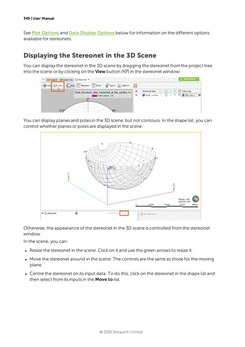
349 | User Manual
See Plot Options and Data Display Options below for information on the different optionsavailable for stereonets.
Displaying the Stereonet in the 3D Scene
You can display the stereonet in the 3D scene by dragging the stereonet from the project treeinto the scene or by clicking on the View button ( ) in the stereonet window:
You can display planes and poles in the 3D scene, but not contours. In the shape list, you cancontrol whether planes or poles are displayed in the scene:
Otherwise, the appearance of the stereonet in the 3D scene is controlled from the stereonetwindow.
In the scene, you can:
l Resize the stereonet in the scene. Click on it and use the green arrows to resize it.
l Move the stereonet around in the scene. The controls are the same as those for themovingplane.
l Centre the stereonet on its input data. To do this, click on the stereonet in the shape list andthen select from its inputs in theMove to list.
© 2019 Seequent Limited
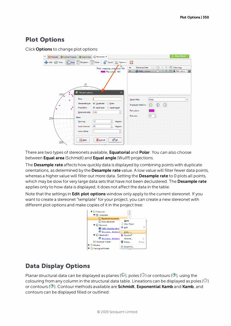
Plot Options | 350
Plot Options
ClickOptions to change plot options:
There are two types of stereonets available, Equatorial and Polar. You can also choosebetween Equal area (Schmidt) and Equal angle (Wulff) projections.
TheDesample rate affects how quickly data is displayed by combining pointswith duplicateorientations, as determined by theDesample rate value. A low valuewill filter fewer data points,whereas a higher valuewill filter out more data. Setting theDesample rate to 0 plots all points,which may be slow for very large data sets that have not been declustered. TheDesample rateapplies only to how data is displayed; it does not affect the data in the table.
Note that the settings in Edit plot options window only apply to the current stereonet. If youwant to create a stereonet “template” for your project, you can create a new stereonet withdifferent plot options and make copies of it in the project tree:
Data Display Options
Planar structural data can be displayed as planes ( ), poles ( ) or contours ( ), using thecolouring fromany column in the structural data table. Lineations can be displayed as poles ( )or contours ( ). Contourmethods available are Schmidt, Exponential Kamb and Kamb, andcontours can be displayed filled or outlined.
© 2019 Seequent Limited

351 | User Manual
Click on a line or pole to view information about the data point:
The information displayed includeswhether or not there are duplicates of the selected datapoint in the data set.
© 2019 Seequent Limited
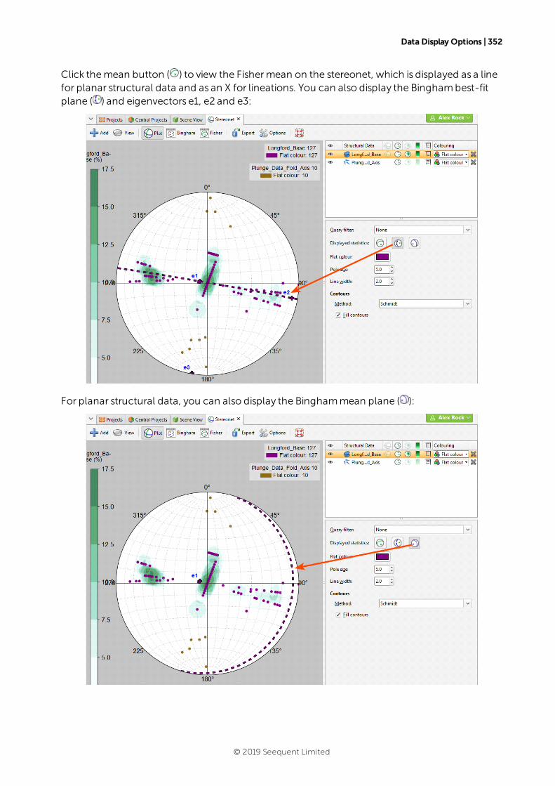
Data Display Options | 352
Click themean button ( ) to view the Fishermean on the stereonet, which is displayed as a linefor planar structural data and as an X for lineations. You can also display the Binghambest-fitplane ( ) and eigenvectors e1, e2 and e3:
For planar structural data, you can also display the Binghammean plane ( ):
© 2019 Seequent Limited
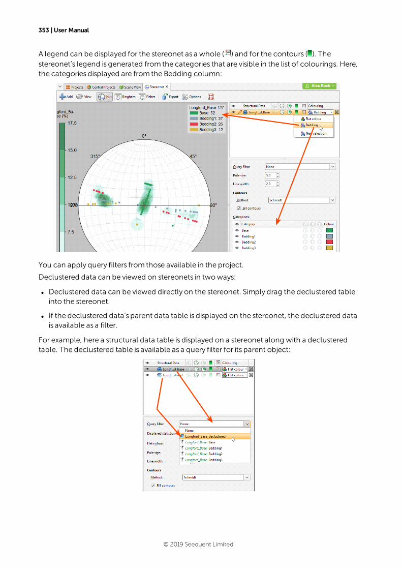
353 | User Manual
A legend can be displayed for the stereonet as a whole ( ) and for the contours ( ). Thestereonet’s legend is generated from the categories that are visible in the list of colourings. Here,the categories displayed are from the Bedding column:
You can apply query filters from those available in the project.
Declustered data can be viewed on stereonets in twoways:
l Declustered data can be viewed directly on the stereonet. Simply drag the declustered tableinto the stereonet.
l If the declustered data’s parent data table is displayed on the stereonet, the declustered datais available as a filter.
For example, here a structural data table is displayed on a stereonet along with a declusteredtable. The declustered table is available as a query filter for its parent object:
© 2019 Seequent Limited
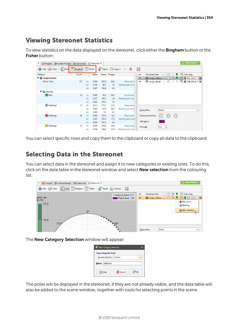
Viewing Stereonet Statistics | 354
Viewing Stereonet Statistics
To view statistics on the data displayed on the stereonet, click either the Bingham button or theFisher button:
You can select specific rows and copy them to the clipboard or copy all data to the clipboard.
Selecting Data in the Stereonet
You can select data in the stereonet and assign it to new categories or existing ones. To do this,click on the data table in the stereonet window and selectNew selection from the colouringlist:
TheNew Category Selectionwindowwill appear:
The poleswill be displayed in the stereonet, if they are not already visible, and the data table willalso be added to the scenewindow, together with tools for selecting points in the scene.
© 2019 Seequent Limited
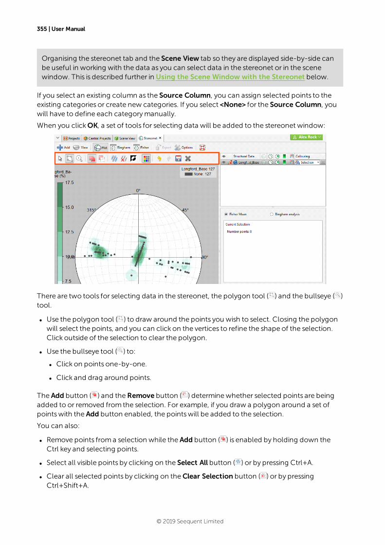
355 | User Manual
Organising the stereonet tab and the Scene View tab so they are displayed side-by-side canbe useful in working with the data as you can select data in the stereonet or in the scenewindow. This is described further in Using the Scene Window with the Stereonet below.
If you select an existing column as the Source Column, you can assign selected points to theexisting categories or create new categories. If you select <None> for the Source Column, youwill have to define each categorymanually.
When you clickOK, a set of tools for selecting data will be added to the stereonet window:
There are two tools for selecting data in the stereonet, the polygon tool ( ) and the bullseye ( )tool.
l Use the polygon tool ( ) to draw around the points you wish to select. Closing the polygonwill select the points, and you can click on the vertices to refine the shape of the selection.Click outside of the selection to clear the polygon.
l Use the bullseye tool ( ) to:
l Click on points one-by-one.
l Click and drag around points.
The Add button ( ) and theRemove button ( ) determinewhether selected points are beingadded to or removed from the selection. For example, if you draw a polygon around a set ofpointswith the Add button enabled, the pointswill be added to the selection.
You can also:
l Remove points froma selection while the Add button ( ) is enabled by holding down theCtrl key and selecting points.
l Select all visible points by clicking on the Select All button ( ) or by pressing Ctrl+A.
l Clear all selected points by clicking on theClear Selection button ( ) or by pressingCtrl+Shift+A.
© 2019 Seequent Limited
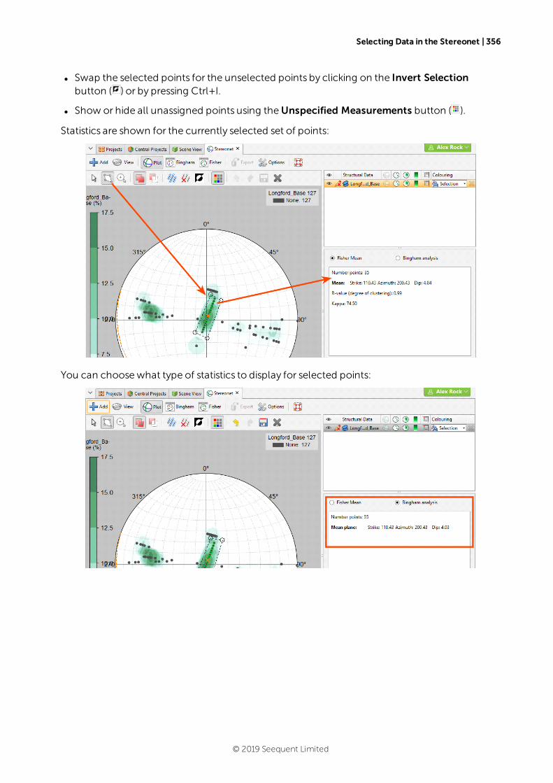
Selecting Data in the Stereonet | 356
l Swap the selected points for the unselected points by clicking on the Invert Selectionbutton ( ) or by pressing Ctrl+I.
l Show or hide all unassigned points using theUnspecified Measurements button ( ).
Statistics are shown for the currently selected set of points:
You can choosewhat type of statistics to display for selected points:
© 2019 Seequent Limited
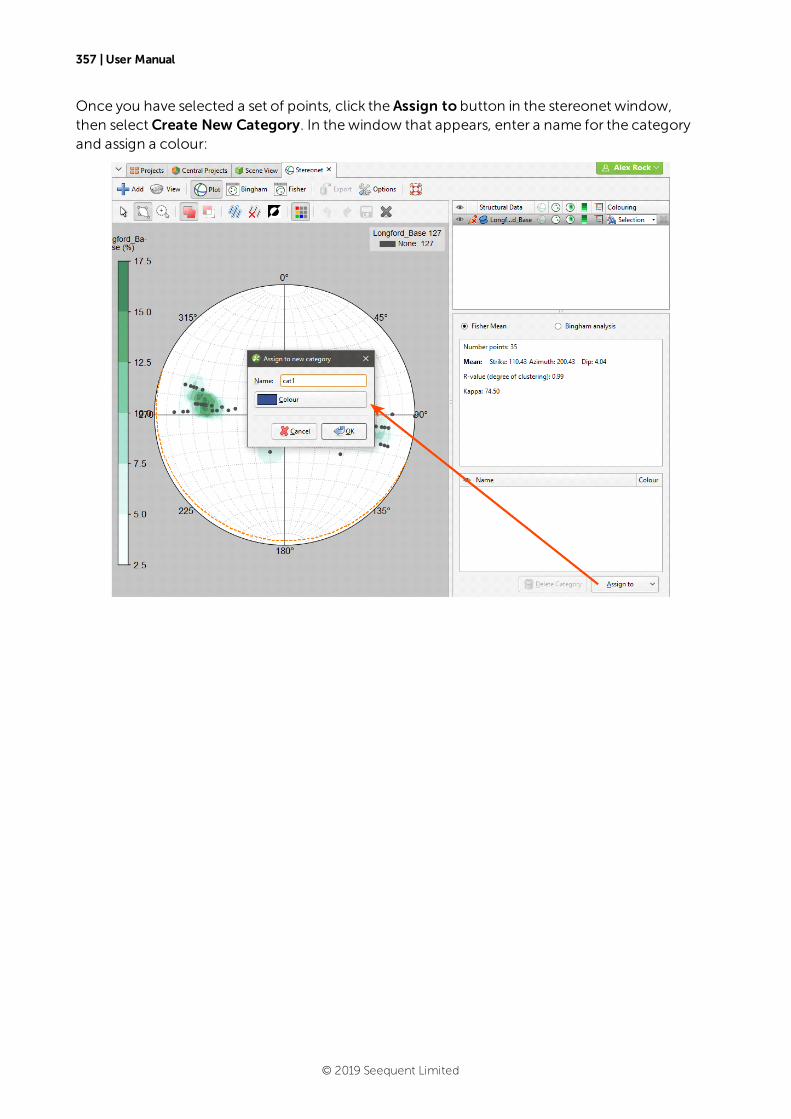
357 | User Manual
Once you have selected a set of points, click the Assign to button in the stereonet window,then selectCreate New Category. In thewindow that appears, enter a name for the categoryand assign a colour:
© 2019 Seequent Limited
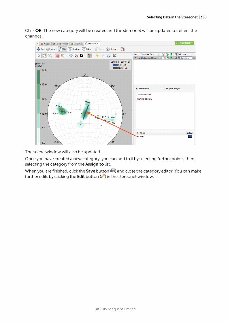
Selecting Data in the Stereonet | 358
ClickOK. The new categorywill be created and the stereonet will be updated to reflect thechanges:
The scenewindowwill also be updated.
Once you have created a new category, you can add to it by selecting further points, thenselecting the category from the Assign to list.
When you are finished, click the Save button ( ) and close the category editor. You can makefurther edits by clicking the Edit button ( ) in the stereonet window.
© 2019 Seequent Limited
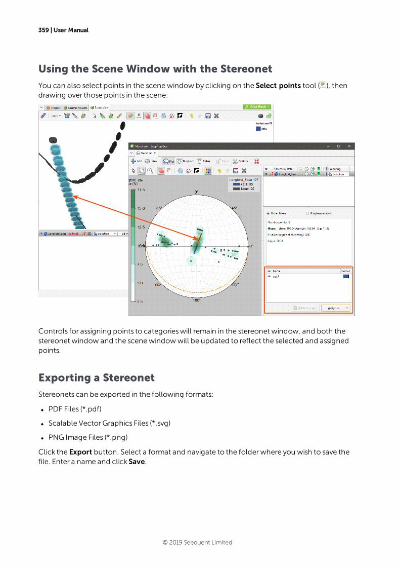
359 | User Manual
Using the Scene Window with the Stereonet
You can also select points in the scenewindow by clicking on the Select points tool ( ), thendrawing over those points in the scene:
Controls for assigning points to categorieswill remain in the stereonet window, and both thestereonet window and the scenewindowwill be updated to reflect the selected and assignedpoints.
Exporting a Stereonet
Stereonets can be exported in the following formats:
l PDF Files (*.pdf)
l Scalable Vector Graphics Files (*.svg)
l PNG Image Files (*.png)
Click the Export button. Select a format and navigate to the folder where you wish to save thefile. Enter a name and click Save.
© 2019 Seequent Limited
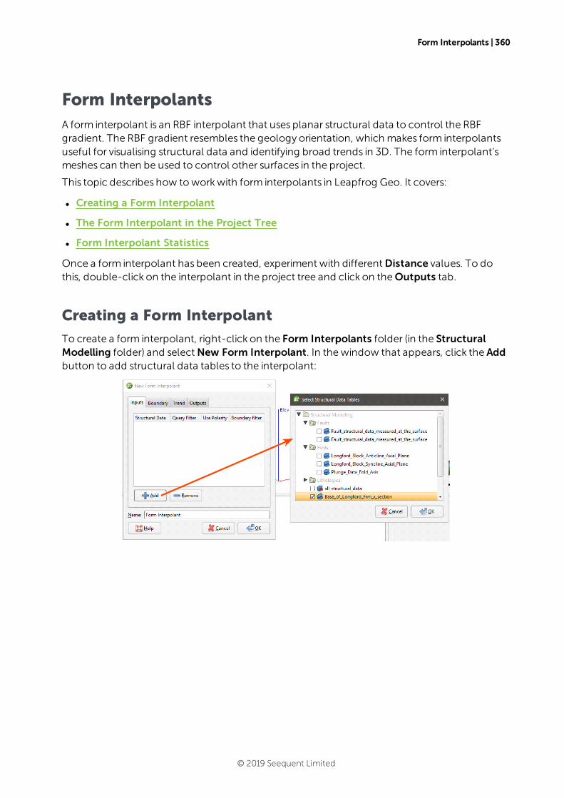
Form Interpolants | 360
Form InterpolantsA form interpolant is an RBF interpolant that uses planar structural data to control the RBFgradient. The RBF gradient resembles the geology orientation, which makes form interpolantsuseful for visualising structural data and identifying broad trends in 3D. The form interpolant’smeshes can then be used to control other surfaces in the project.
This topic describes how toworkwith form interpolants in Leapfrog Geo. It covers:
l Creating a Form Interpolant
l The Form Interpolant in the Project Tree
l Form Interpolant Statistics
Once a form interpolant has been created, experiment with differentDistance values. To dothis, double-click on the interpolant in the project tree and click on theOutputs tab.
Creating a Form Interpolant
To create a form interpolant, right-click on the Form Interpolants folder (in the StructuralModelling folder) and selectNew Form Interpolant. In thewindow that appears, click the Addbutton to add structural data tables to the interpolant:
© 2019 Seequent Limited

361 | User Manual
Data can be filtered using the query filters defined for the selected structural data tables:
Once you have created the interpolant, you can easily add and remove structural data tablesand change the filtering.
When generating the form interpolant, you can use the tangents and polarity or only thetangents. To use both, leave theUse Polarity box ticked. To use only the tangents, untick thebox.
The Boundary filter setting determines how data is handled when it lies outside theinterpolant’s boundary:
l Boundary filter enabled. The interpolant is only influenced by the data that falls inside theboundary.
l Boundary filter disabled. The interpolant is influenced by the data both inside and outsidethe boundary.
Setting a Trend
In the Trend tab, you can set a trend using themoving plane or by entering the required values.You can also use the Set to list to choose different options used in the project. Isotropic is thedefault option used when the function is created.
The Ellipsoid Ratios determine the relative shape and strength of the ellipsoids in the scene,where:
l TheMaximum value is the relative strength in the direction of the green line on themovingplane.
l The Intermed. value is the relative strength in the direction perpendicular to the green lineon themoving plane.
l TheMinimum value is the relative strength in the direction orthogonal to the plane.
© 2019 Seequent Limited

Adding Isosurfaces | 362
Adding Isosurfaces
The isosurfaces generated for the form interpolant are determined by the settings in theOutputs tab. If you wish to add more isosurfaces to the interpolant, click the Add button andenter the required Iso Value. Click on an isosurface and then on theRemove button to delete it.
TheDefault resolution setting is used for all new isosurfaces.
The Form Interpolant in the Project Tree
In the project tree, the form interpolant contains objects that represent different parts of theinterpolant:
l The Extents object represents the interpolant’s boundary settings, from the Boundary tab.
l The Trend object describes the trend applied in the interpolant. SeeGlobal Trends formoreinformation.
l The structural data object ( ) contains a link to the data used in generating the interpolant.See Form Interpolant Statistics formore information.
l The Isosurfaces folder contains the isosurfaces defined in theOutputs tab.
To display the form interpolant:
l Drag the interpolant into the scene.
l Right-click on the interpolant and select View Isosurfaces.
© 2019 Seequent Limited
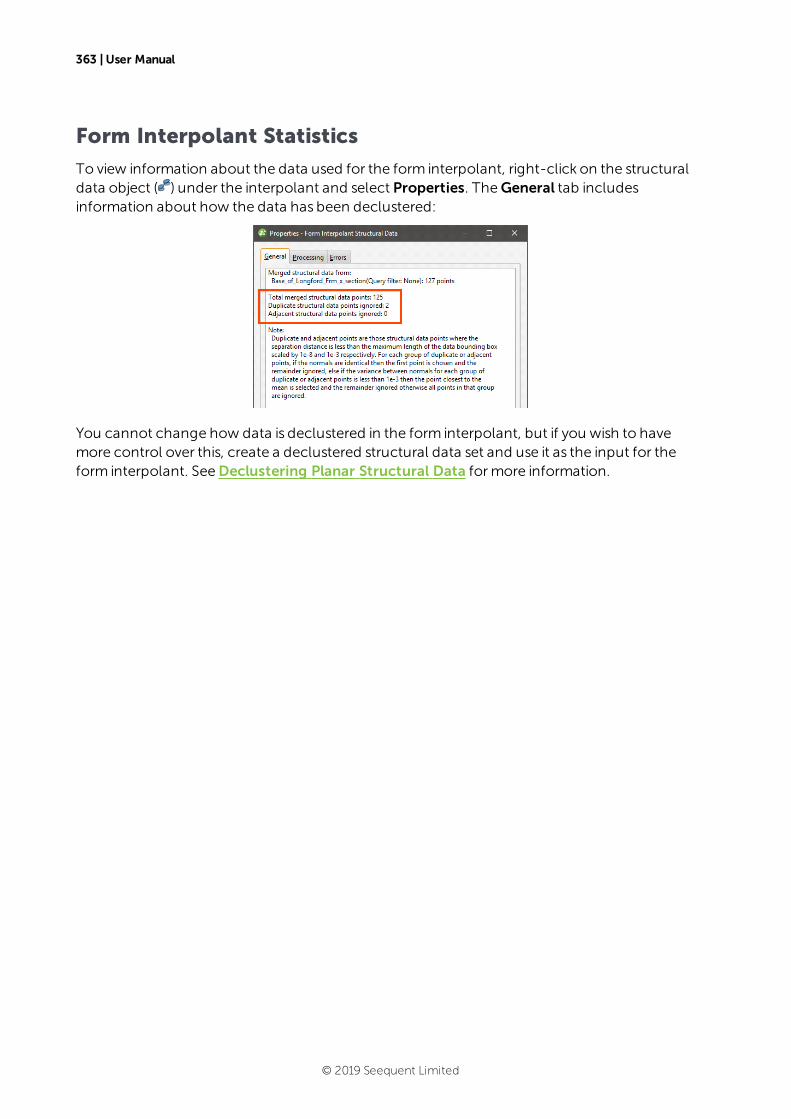
363 | User Manual
Form Interpolant Statistics
To view information about the data used for the form interpolant, right-click on the structuraldata object ( ) under the interpolant and select Properties. TheGeneral tab includesinformation about how the data has been declustered:
You cannot change how data is declustered in the form interpolant, but if you wish to havemore control over this, create a declustered structural data set and use it as the input for theform interpolant. SeeDeclustering Planar Structural Data formore information.
© 2019 Seequent Limited
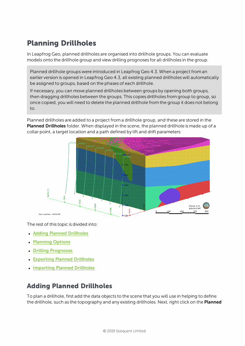
Planning DrillholesIn Leapfrog Geo, planned drillholes are organised into drillhole groups. You can evaluatemodels onto the drillhole group and view drilling prognoses for all drillholes in the group.
Planned drillhole groupswere introduced in Leapfrog Geo 4.3. When a project fromanearlier version is opened in Leapfrog Geo 4.3, all existing planned drillholeswill automaticallybe assigned to groups, based on the phases of each drillhole.
If necessary, you can move planned drillholes between groups by opening both groups,then dragging drillholes between the groups. This copies drillholes fromgroup to group, soonce copied, you will need to delete the planned drillhole from the group it does not belongto.
Planned drillholes are added to a project froma drillhole group, and these are stored in thePlanned Drillholes folder. When displayed in the scene, the planned drillhole ismade up of acollar point, a target location and a path defined by lift and drift parameters:
The rest of this topic is divided into:
l Adding Planned Drillholes
l Planning Options
l Drilling Prognoses
l Exporting Planned Drillholes
l Importing Planned Drillholes
Adding Planned Drillholes
To plan a drillhole, first add the data objects to the scene that you will use in helping to definethe drillhole, such as the topography and any existing drillholes. Next, right click on the Planned
© 2019 Seequent Limited

365 | User Manual
Drillholes folder and selectNew Group. In thewindow that appears, you can define basicinformation about the group, including the Prefix used for each drillhole added to the group:
Start defining drillholes by clicking the Add Drillhole button.
You can changewhetherCollar or Target is selected when thiswindow is opened byclicking on theDefaults button. See Planning Options below.
A name is automatically generated for the new planned drillhole based on the Prefix definedfor the group.
There are threeways to define the drillhole collar or target:
l Click in the scene to set the collar or target location. First, click on the Select button ( ) fortheCollar or Target, then click in the scene to define theCollar or Target. The drillhole willappear in the scene and you can adjust the coordinates using the controls in theDrillhole
© 2019 Seequent Limited
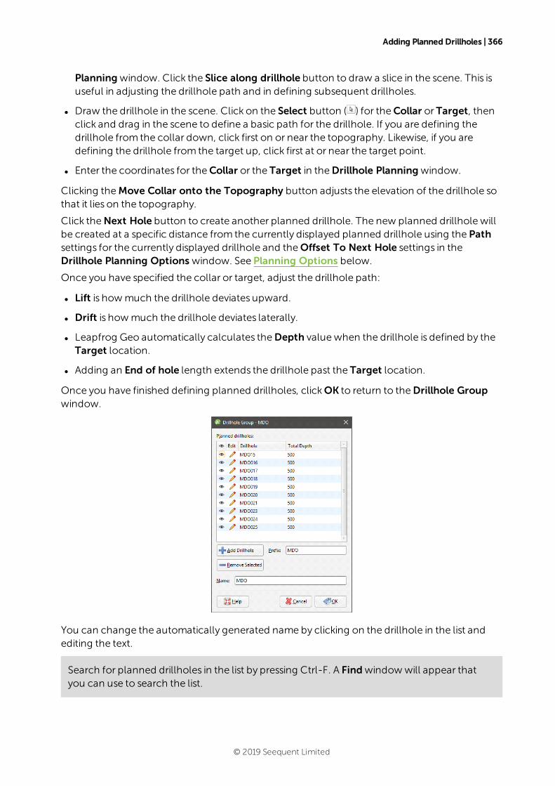
Adding Planned Drillholes | 366
Planningwindow. Click the Slice along drillhole button to draw a slice in the scene. This isuseful in adjusting the drillhole path and in defining subsequent drillholes.
l Draw the drillhole in the scene. Click on the Select button ( ) for theCollar or Target, thenclick and drag in the scene to define a basic path for the drillhole. If you are defining thedrillhole from the collar down, click first on or near the topography. Likewise, if you aredefining the drillhole from the target up, click first at or near the target point.
l Enter the coordinates for theCollar or the Target in theDrillhole Planningwindow.
Clicking theMove Collar onto the Topography button adjusts the elevation of the drillhole sothat it lies on the topography.
Click theNext Hole button to create another planned drillhole. The new planned drillhole willbe created at a specific distance from the currently displayed planned drillhole using the Pathsettings for the currently displayed drillhole and theOffset To Next Hole settings in theDrillhole Planning Options window. See Planning Options below.
Once you have specified the collar or target, adjust the drillhole path:
l Lift is howmuch the drillhole deviates upward.
l Drift is howmuch the drillhole deviates laterally.
l Leapfrog Geo automatically calculates theDepth valuewhen the drillhole is defined by theTarget location.
l Adding an End of hole length extends the drillhole past the Target location.
Once you have finished defining planned drillholes, clickOK to return to theDrillhole Groupwindow.
You can change the automatically generated name by clicking on the drillhole in the list andediting the text.
Search for planned drillholes in the list by pressing Ctrl-F. A Findwindowwill appear thatyou can use to search the list.
© 2019 Seequent Limited
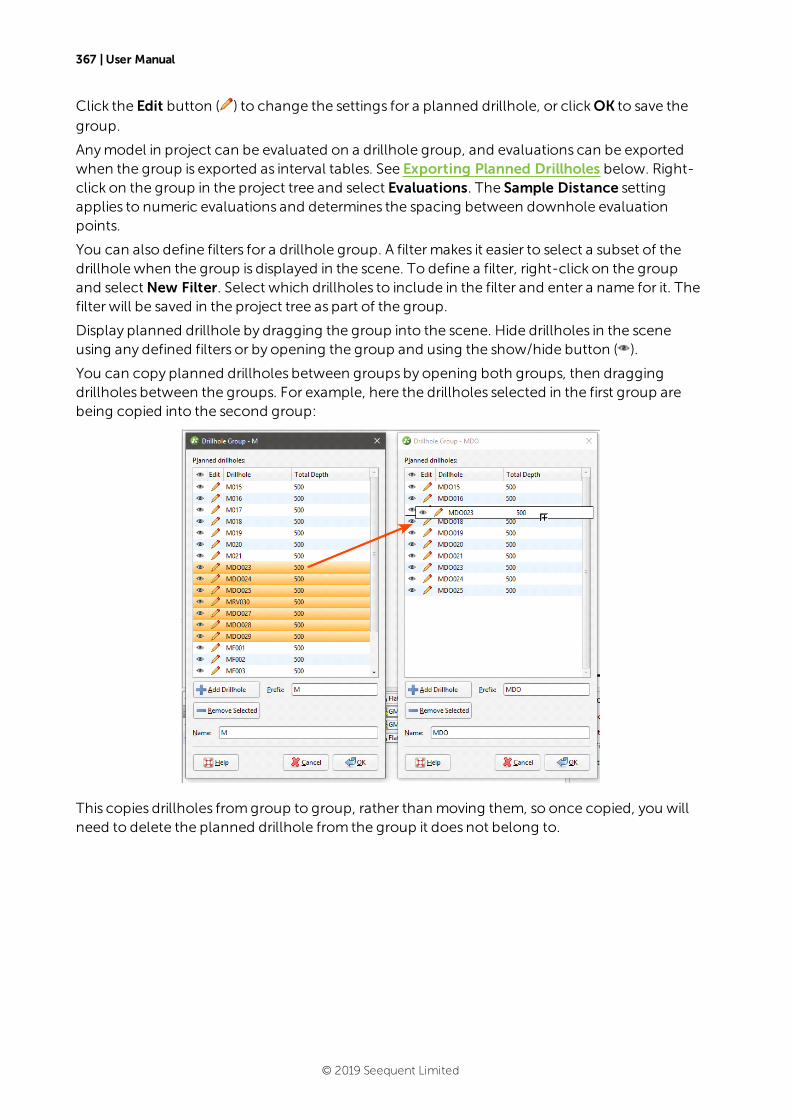
367 | User Manual
Click the Edit button ( ) to change the settings for a planned drillhole, or clickOK to save thegroup.
Anymodel in project can be evaluated on a drillhole group, and evaluations can be exportedwhen the group is exported as interval tables. See Exporting Planned Drillholes below. Right-click on the group in the project tree and select Evaluations. The Sample Distance settingapplies to numeric evaluations and determines the spacing between downhole evaluationpoints.
You can also define filters for a drillhole group. A filtermakes it easier to select a subset of thedrillhole when the group is displayed in the scene. To define a filter, right-click on the groupand selectNew Filter. Select which drillholes to include in the filter and enter a name for it. Thefilter will be saved in the project tree as part of the group.
Display planned drillhole by dragging the group into the scene. Hide drillholes in the sceneusing any defined filters or by opening the group and using the show/hide button ( ).
You can copy planned drillholes between groups by opening both groups, then draggingdrillholes between the groups. For example, here the drillholes selected in the first group arebeing copied into the second group:
This copies drillholes fromgroup to group, rather than moving them, so once copied, you willneed to delete the planned drillhole from the group it does not belong to.
© 2019 Seequent Limited

Planning Options | 368
Planning Options
Drillhole planning options are set on a per-project basis. To change drillhole planning options,right-click on the Planned Drillholes folder or on a drillhole group and select Edit PlannedDrillholes Defaults. TheDrillhole Planning Options windowwill appear:
Select whether new planned drillholes are specified by theCollar or by the Target.
TheOffset To Next Hole values applywhen defining multiple drillholes in theDrillholePlanningwindow.
Enter the information required and clickOK. The new settingswill be applied to the next newplanned drillhole added to the project.
Drilling Prognoses
Planned drillholes can be evaluated against anymodel in the project. To view drilling prognosesfor a drillhole, right-click on a drillhole group in the project tree and selectDrilling Prognoses.TheDrilling Prognoses tab will appear:
The dropdown list contains all evaluations on the drillhole group, along with a MergedIntervals option that combines the information fromall evaluations. You can copy theinformation displayed to your computer’s clipboard by selecting rows, then clicking theCopybutton ( ). The information in the selected rowswill be copied as tab delimited text, which canbe copied into a spreadsheet application such as Excel.
© 2019 Seequent Limited

369 | User Manual
Exporting Planned Drillholes
There are twoways to export planned drillholes: export their parameters or export intervaltables that contain the drillholes.
Export Parameters
Exporting planned drillhole parameters exports the drillholes as a *.csv file. To exportparameters for planned drillholes, right-click on a drillhole group and select ExportParameters. In thewindow that appears, select the drillholes you want to export. The totallength will be updated as you add or remove drillholes.
In Leapfrog Geo, positive dip points down for planned drillholes. To invert the dip for exportedplanned drillholes so that negative dip points down, tick the box for Invert dip on export.
Click Export. Navigate towhere you wish to save the file, then click Save.
Export as Interval Table
To export planned drillholes as an interval table, right-click on a drillhole group and selectExport as Interval Table. Select the evaluations you wish to include, then click Export. In theExport Planned Drillholes window, the files that will be created are listed, one each for thecollar and survey table and one for each selected evaluation. Change the Base file name, ifrequired, choose a folder in which to save the files, then click Export to save the files.
Importing Planned Drillholes
Leapfrog Geo imports planned drillholes from files in CSV format. The columns expected are:
l A drillhole identifier
l X-Y-Z coordinates for the planned drillhole
l Azimuth
l Dip
l Lift rate
l Drift rate
l Distance
l Extension
l Target Depth
l Comment
© 2019 Seequent Limited

Importing Planned Drillholes | 370
When importing planned drillholes, you can import them into a new group or into an existinggroup. To import planned drillholes, right-click on the Planned Drillholes folder or on a groupand select Import Planned Drillholes. If the IDs in the file are already in the project, you will beprompted to resolve the conflict:
You can:
l Rename the imported drillholes. Leapfrog Geowill automatically assign new names andimport the planned drillholes.
l Exclude planned drillholes that already exist in the project. Planned drillholeswill only beimported if they have an identifier that does not already exist in the project.
l Replace existing planned drillholeswith the imported drillholes. Use this option if you areimporting information previously exported from the project and subsequently updated in anexternal application.
ClickOK to process the file.
If there are no conflicts, the planned drillholeswill be added to the project.
© 2019 Seequent Limited
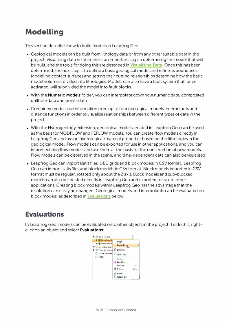
Modelling
This section describes how to build models in Leapfrog Geo.
l Geological models can be built from lithology data or fromany other suitable data in theproject. Visualising data in the scene is an important step in determining themodel that willbe built, and the tools for doing this are described in Visualising Data. Once this has beendetermined, the next step is to define a basic geological model and refine its boundaries.Modelling contact surfaces and setting their cutting relationships determine how the basicmodel volume is divided into lithologies. Models can also have a fault system that, onceactivated, will subdivided themodel into fault blocks.
l With theNumeric Models folder, you can interpolate downhole numeric data, compositeddrillhole data and points data.
l Combined models use information fromup to four geological models, interpolants anddistance functions in order to visualise relationships between different types of data in theproject.
l With the Hydrogeology extension, geological models created in Leapfrog Geo can be usedas the basis forMODFLOW and FEFLOWmodels. You can create flowmodels directly inLeapfrog Geo and assign hydrological/material properties based on the lithologies in thegeological model. Flowmodels can be exported for use in other applications, and you canimport existing flowmodels and use themas the basis for the construction of newmodels.Flowmodels can be displayed in the scene, and time-dependent data can also be visualised.
l Leapfrog Geo can import Isatis files, UBC grids and blockmodels in CSV format. LeapfrogGeo can import Isatis files and blockmodels in CSV format. Blockmodels imported in CSVformat must be regular, rotated only about the Z axis. Blockmodels and sub-blockedmodels can also be created directly in Leapfrog Geo and exported for use in otherapplications. Creating blockmodelswithin Leapfrog Geo has the advantage that theresolution can easily be changed. Geological models and interpolants can be evaluated onblockmodels, as described in Evaluations below.
EvaluationsIn Leapfrog Geo, models can be evaluated onto other objects in the project. To do this, right-click on an object and select Evaluations:
© 2019 Seequent Limited
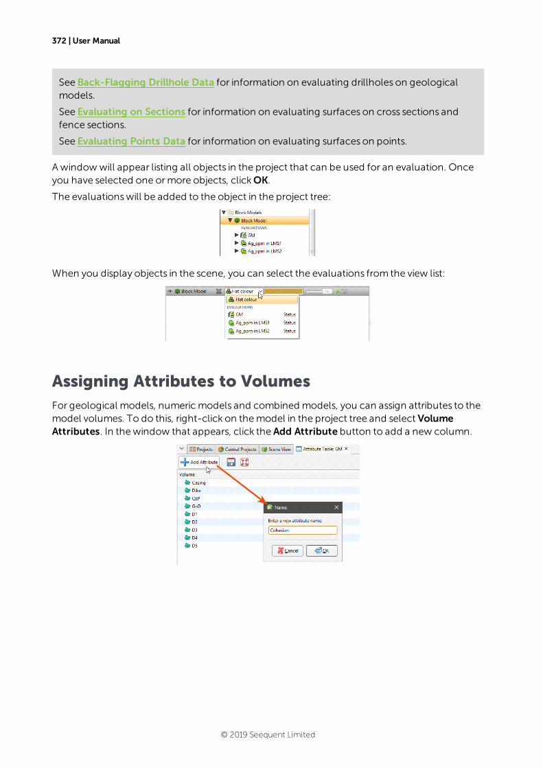
372 | User Manual
See Back-Flagging Drillhole Data for information on evaluating drillholes on geologicalmodels.
See Evaluating on Sections for information on evaluating surfaces on cross sections andfence sections.
See Evaluating Points Data for information on evaluating surfaces on points.
A windowwill appear listing all objects in the project that can be used for an evaluation. Onceyou have selected one ormore objects, clickOK.
The evaluationswill be added to the object in the project tree:
When you display objects in the scene, you can select the evaluations from the view list:
Assigning Attributes to VolumesFor geological models, numericmodels and combined models, you can assign attributes to themodel volumes. To do this, right-click on themodel in the project tree and select VolumeAttributes. In thewindow that appears, click the Add Attribute button to add a new column.
© 2019 Seequent Limited
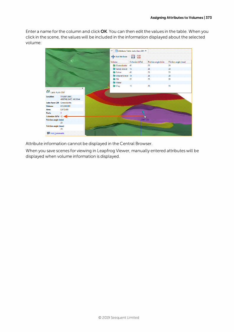
Assigning Attributes to Volumes | 373
Enter a name for the column and clickOK. You can then edit the values in the table. When youclick in the scene, the valueswill be included in the information displayed about the selectedvolume:
Attribute information cannot be displayed in the Central Browser.
When you save scenes for viewing in Leapfrog Viewer, manually entered attributeswill bedisplayed when volume information is displayed.
© 2019 Seequent Limited

Geological ModelsThemodel building process involves several key steps:
l Creating the project and setting up themodelling environment
l Importing drillhole data and correcting errors
l Importing other required data
l Visualising the data in the scene and inspecting it tomake sense of themodel that will bebuilt. It is at this stage that you might create new drillhole data columns to select data thatwill be the basis of geological models.
l Creating a basic GM, then refining its boundary and defining a fault system
l Modelling the contact surfaces
l Setting the cutting relationships between the different contact surfaces and generatingvolumes
A fault systemcan also be defined that divides the geological model into subunits in which theinternal structure can be defined independent of the other subunits in themodel. This isdescribed in Faulted Models.
The rest of this topic describes the process of creating a geological model. It is divided into:
l Creating a New Geological Model
l The Geological Model in the Project Tree
l Geological Model Display
l Copying a Geological Model
l Creating a Static Copy of a Geological Model
l Geological Model Volumes and Surfaces Export Options
l Extracting Model Volumes
A geological model can be created using only a basic set of parameters. The only parameterthat cannot be changed once themodel has been created is the base lithology.
Creating a New Geological Model
To create a new geological model, right-click on theGeological Models folder and selectNewGeological Model. TheNew Geological Modelwindowwill open, together with a set ofcontrols in the scene that help in defining themodel extents.
The Base Lithology
Select the drillhole data column that will be used as the basis of a model from the BaseLithology Column list. If you do not wish to use lithology data as the basis for themodel, select<None>. Thismay be the case if, for example, you want to build a model frompoints data or
© 2019 Seequent Limited
Surface Resolution | 375
froman imported map. If you select <None>, you will need tomanually define the lithologiesthat will bemodelled.
If more than one column of lithology data is available for creating models, be sure to choosethe correct one as it cannot be changed once the initial model has been created. If aftercreating and modifying themodel, you find you need tomodify the drillhole data, resultingin a new lithology column, you can use that new column to create contact surfaces usingOther Contacts options.
You can also filter the drillhole data used to build the geological model using query filters. Todo so, select the required query filter from the Filter data list. Once themodel has been created,you can remove the filter or select a different filter.
Surface Resolution
The surface resolution setting Leapfrog Geo automatically uses as the default is based on thedata available in the project. Set the surface resolution for themodel as a whole and choosewhether or not the resolution will be adaptive. See Surface Resolution in Leapfrog Geo formore information on the effects of these settings.
Later, while refining themodel, you can change the resolution of each surface and enable ordisable adaptive resolution. See Surface Resolution for a Geological Model.
Model Extents
A geological model is initially created with a basic rectangular set of extents aligned with thesouth/north and east/west axes. You can define themodel’s extents in threeways:
l Enter the coordinates.
l Select Enclose Object and choose from the list of objects in the project. If themodel is basedon drillhole data, select the lithology segments from the Enclose Object list.
l Use the controls that appear in the scene. The orange handle adjusts the centre of the planeand the red handles adjust the size.
SeeObject Extents formore information.
Enter a Name for themodel that describes the purpose of themodel. ThisNamewill be used innaming the objects that will be added to themodel. ClickOK to create the newmodel. The newgeological model will be created and added to theGeological Models folder.
See Editing a Geological Model for information on how to change the basic settings for themodel.
© 2019 Seequent Limited
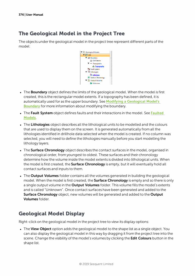
376 | User Manual
The Geological Model in the Project Tree
The objects under the geological model in the project tree represent different parts of themodel:
l The Boundary object defines the limits of the geological model. When themodel is firstcreated, this is the rectangularmodel extents. If a topography has been defined, it isautomatically used for as the upper boundary. SeeModifying a Geological Model’sBoundary formore information about modifying the boundary.
l The Fault Systemobject defines faults and their interactions in themodel. See FaultedModels.
l The Lithologies object describes all the lithological units to bemodelled and the coloursthat are used to display themon the screen. It is generated automatically fromall thelithologies identified in drillhole data selected when themodel is created. If no column wasselected, you will need to define the lithologiesmanually before you start modelling thelithology layers.
l The Surface Chronology object describes the contact surfaces in themodel, organised inchronological order, fromyoungest to oldest. These surfaces and their chronologydetermine how the volume inside themodel extents is divided into lithological units. Whenthemodel is first created, the Surface Chronology is empty, but it will eventually hold allcontact surfaces and inputs to them.
l TheOutput Volumes folder contains all the volumes generated in building the geologicalmodel. When themodel is first created, the Surface Chronology is empty and so there is onlya single output volume in theOutput Volumes folder. This volume fills themodel’s extentsand is called “Unknown”. Once contact surfaces have been generated and added to theSurface Chronology object, new volumeswill be generated and added to theOutputVolumes folder.
Geological Model Display
Right-click on the geological model in the project tree to view its display options:
l The View Object option adds the geological model to the shape list as a single object. Youcan also display the geological model in thisway by dragging it from the project tree into thescene. Change the visibility of themodel’s volumes by clicking the Edit Colours button in theshape list.
© 2019 Seequent Limited
Copying a Geological Model | 377
l The View Output Volumes option adds themodel to the scene as a series of outputvolumes. It is the equivalent of dragging theOutput Volumes folder into the scene. Changethe visibility of themodel’s volumes individually.
l The View Surface Chronology option displays the surfaces that are used to divided up themodel.
l The View Fault Block Boundaries option is only available when a fault systemhas beendefined and enabled for themodel. Selecting View Fault Block Boundaries displays thefault blockswithout displaying the lithology layers.
Copying a Geological Model
Creating a copy of a geological model is a useful way of experimenting with changes to amodel.
To copy a geological model, right-click on it in the project tree and selectCopy. Enter a namefor the copy of themodel and clickOK. The copywill be added to the project tree.
Creating a Static Copy of a Geological Model
Creating a static copy preserves a snapshot of a geological model that does not change, evenwhen changes aremade to the data on which the original model was dependent. This is auseful way of storing historical models and comparing models. Static copies can be exportedfromLeapfrog Geo, as described in Geological Model Volumes and Surfaces Export Optionsbelow.
To create a static copy of a geological model, right-click on it in the project tree and selectStatic Copy. Enter a name for the copy of themodel and clickOK. The copywill be added totheGeological Models folder.
In the project tree, the static copy ( ) ismade up of a Legend object ( ), the output volumes ( )and all surfaces created in building themodel.
Staticmodels created in versions of Leapfrog Geo before 2.2 copied only the output volumesand the legend, and the staticmodel appeared in the shape list only as a single line. Whenthese staticmodels are upgraded and displayed in the scene, the individual output volumeswill be added to the shape list.
To view the date a static copywas created, right-click on it in the project tree and selectProperties. The date the copywas created is shown in theGeneral tab.
Geological Model Volumes and Surfaces Export Options
There are three options for exporting a geological model’s output volumes and surfaces. Theseare:
l Export an output volume or a surface as a mesh. Right-click on it in the project tree and clickExport. You will be prompted for a file name and location. See Exporting a Single Mesh.
© 2019 Seequent Limited
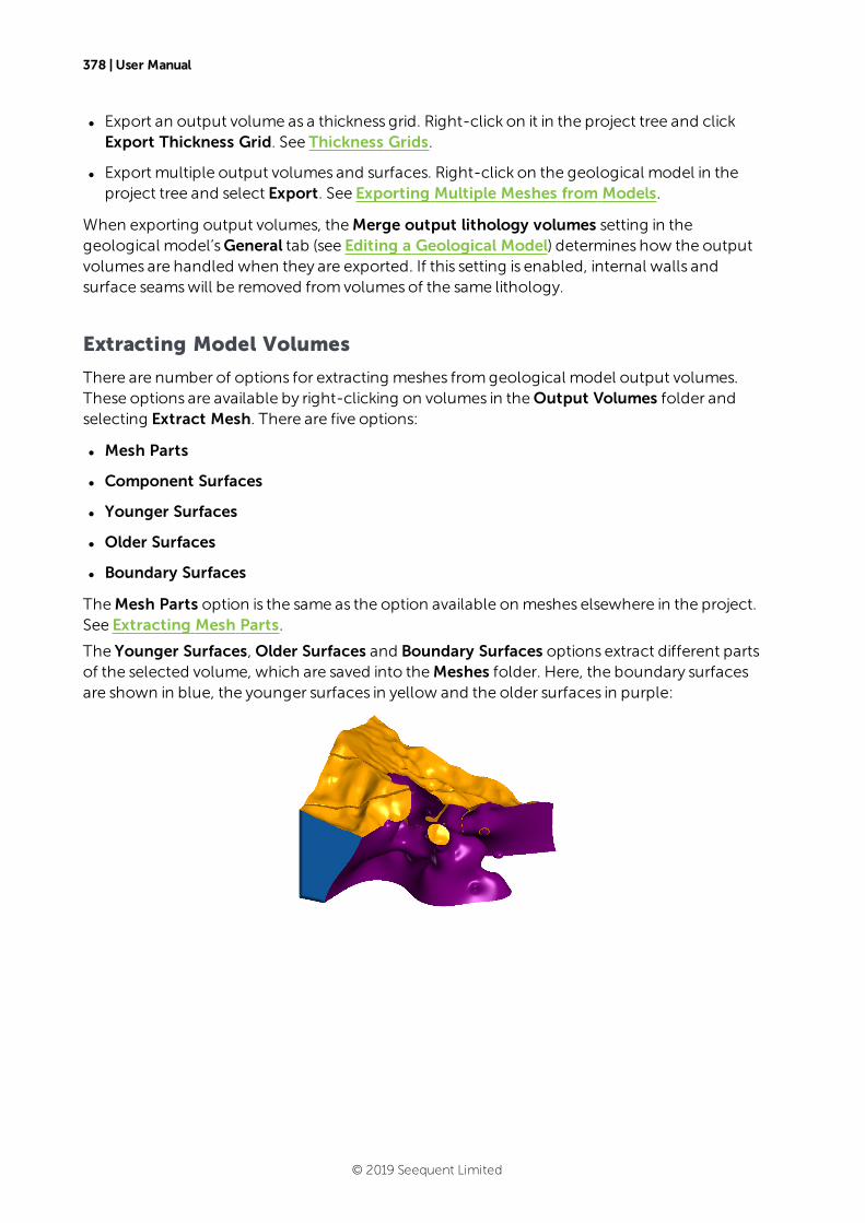
378 | User Manual
l Export an output volume as a thickness grid. Right-click on it in the project tree and clickExport Thickness Grid. See Thickness Grids.
l Export multiple output volumes and surfaces. Right-click on the geological model in theproject tree and select Export. See Exporting Multiple Meshes from Models.
When exporting output volumes, theMerge output lithology volumes setting in thegeological model’sGeneral tab (see Editing a Geological Model) determines how the outputvolumes are handled when they are exported. If this setting is enabled, internal walls andsurface seamswill be removed fromvolumesof the same lithology.
Extracting Model Volumes
There are number of options for extracting meshes fromgeological model output volumes.These options are available by right-clicking on volumes in theOutput Volumes folder andselecting Extract Mesh. There are five options:
l Mesh Parts
l Component Surfaces
l Younger Surfaces
l Older Surfaces
l Boundary Surfaces
TheMesh Parts option is the same as the option available on meshes elsewhere in the project.See Extracting Mesh Parts.
The Younger Surfaces, Older Surfaces and Boundary Surfaces options extract different partsof the selected volume, which are saved into theMeshes folder. Here, the boundary surfacesare shown in blue, the younger surfaces in yellow and the older surfaces in purple:
© 2019 Seequent Limited
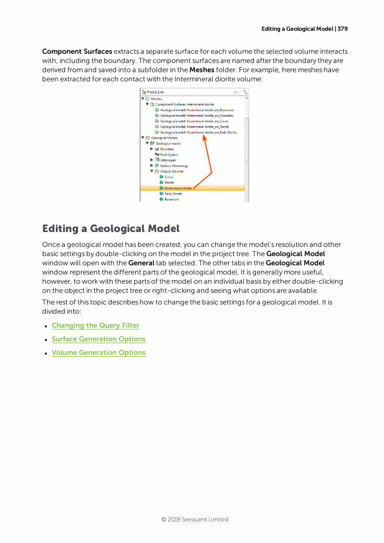
Editing a Geological Model | 379
Component Surfaces extracts a separate surface for each volume the selected volume interactswith, including the boundary. The component surfaces are named after the boundary they arederived fromand saved into a subfolder in theMeshes folder. For example, heremeshes havebeen extracted for each contact with the Intermineral diorite volume:
Editing a Geological Model
Once a geological model has been created, you can change themodel’s resolution and otherbasic settings by double-clicking on themodel in the project tree. TheGeological Modelwindowwill open with theGeneral tab selected. The other tabs in theGeological Modelwindow represent the different parts of the geological model. It is generallymore useful,however, to workwith these parts of themodel on an individual basis by either double-clickingon the object in the project tree or right-clicking and seeing what options are available.
The rest of this topic describes how to change the basic settings for a geological model. It isdivided into:
l Changing the Query Filter
l Surface Generation Options
l Volume Generation Options
© 2019 Seequent Limited
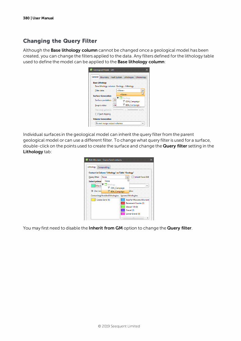
380 | User Manual
Changing the Query Filter
Although the Base lithology column cannot be changed once a geological model has beencreated, you can change the filters applied to the data. Any filters defined for the lithology tableused to define themodel can be applied to the Base lithology column:
Individual surfaces in the geological model can inherit the query filter from the parentgeological model or can use a different filter. To changewhat query filter is used for a surface,double-click on the points used to create the surface and change theQuery filter setting in theLithology tab:
You may first need to disable the Inherit from GM option to change theQuery filter.
© 2019 Seequent Limited
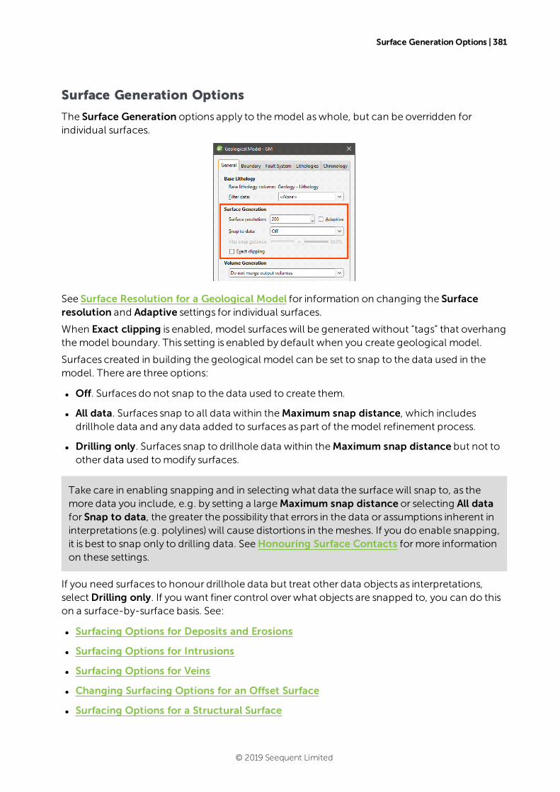
Surface Generation Options | 381
Surface Generation Options
The Surface Generation options apply to themodel aswhole, but can be overridden forindividual surfaces.
See Surface Resolution for a Geological Model for information on changing the Surfaceresolution and Adaptive settings for individual surfaces.
When Exact clipping is enabled, model surfaceswill be generated without “tags” that overhangthemodel boundary. This setting is enabled by default when you create geological model.
Surfaces created in building the geological model can be set to snap to the data used in themodel. There are three options:
l Off. Surfaces do not snap to the data used to create them.
l All data. Surfaces snap to all data within theMaximum snap distance, which includesdrillhole data and any data added to surfaces as part of themodel refinement process.
l Drilling only. Surfaces snap to drillhole data within theMaximum snap distance but not toother data used tomodify surfaces.
Take care in enabling snapping and in selecting what data the surfacewill snap to, as themore data you include, e.g. by setting a largeMaximum snap distance or selecting All datafor Snap to data, the greater the possibility that errors in the data or assumptions inherent ininterpretations (e.g. polylines) will cause distortions in themeshes. If you do enable snapping,it is best to snap only to drilling data. SeeHonouring Surface Contacts formore informationon these settings.
If you need surfaces to honour drillhole data but treat other data objects as interpretations,selectDrilling only. If you want finer control over what objects are snapped to, you can do thison a surface-by-surface basis. See:
l Surfacing Options for Deposits and Erosions
l Surfacing Options for Intrusions
l Surfacing Options for Veins
l Changing Surfacing Options for an Offset Surface
l Surfacing Options for a Structural Surface
© 2019 Seequent Limited
382 | User Manual
Volume Generation Options
TheMerge output volumes setting determineswhether or not output volumesof the samelithology aremerged when the volumes are exported. If Merge output volumes is set to Fast orRobust, internal walls and surface seamswill be removed fromvolumesof the same lithology.Either option is suitable when you are using output volumes as extents for othermodels.
The difference between Fast and Robust is the algorithmused:
l Fast removes back-to-back triangles before generating output volumes. This option wasnew in Leapfrog Geo version 4.0 and is the default option selected when a geological modelis created.
l Robust is theMerge output lithology volumes option fromversions of Leapfrog Geo before4.0. Robust uses the volume cutter, which trackswhere the triangles originated and is,therefore, a slow option for building output volumes.
If there are issueswith surfaces exported to othermodelling packages using theDo not mergeoutput volumes setting, try the Fast setting. If there are still issues, try theRobust setting.
When projects created in earlier versions of Leapfrog Geo are opened in Leapfrog Geo 5.0,the Volume Generation setting for any existing geological modelswill not be changed.
Surface Resolution for a Geological Model
When you create a geological model (seeCreating a New Geological Model), the surfaceresolution is set for themodel as a whole. When surfaces and boundaries are created as part ofthemodel-building process, their resolution is inherited from the geological model:
l For deposit and erosion contact surfaces, stratigraphic sequences and model boundaries,the resolution is the same as the geological model.
l For intrusion contact surfaces, the resolution is half that set for the geological model.
l For vein contact surfaces, the resolution is the same as the geological model, but theAdaptive option does not apply.
You can change the resolution and enable or disable the adaptive isosurfacer on a surface-by-surface basis. This is useful if you want to build a detailed model of some lithologieswithoutincreasing processing time for other volumes.
© 2019 Seequent Limited
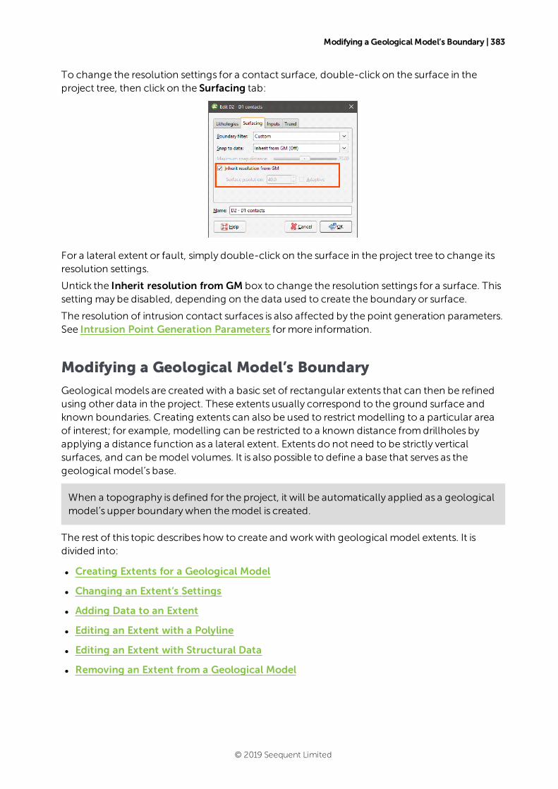
Modifying a Geological Model’s Boundary | 383
To change the resolution settings for a contact surface, double-click on the surface in theproject tree, then click on the Surfacing tab:
For a lateral extent or fault, simply double-click on the surface in the project tree to change itsresolution settings.
Untick the Inherit resolution from GM box to change the resolution settings for a surface. Thissetting may be disabled, depending on the data used to create the boundary or surface.
The resolution of intrusion contact surfaces is also affected by the point generation parameters.See Intrusion Point Generation Parameters formore information.
Modifying a Geological Model’s Boundary
Geological models are created with a basic set of rectangular extents that can then be refinedusing other data in the project. These extents usually correspond to the ground surface andknown boundaries. Creating extents can also be used to restrict modelling to a particular areaof interest; for example, modelling can be restricted to a known distance fromdrillholes byapplying a distance function as a lateral extent. Extents do not need to be strictly verticalsurfaces, and can bemodel volumes. It is also possible to define a base that serves as thegeological model’s base.
When a topography is defined for the project, it will be automatically applied as a geologicalmodel’s upper boundarywhen themodel is created.
The rest of this topic describes how to create and workwith geological model extents. It isdivided into:
l Creating Extents for a Geological Model
l Changing an Extent’s Settings
l Adding Data to an Extent
l Editing an Extent with a Polyline
l Editing an Extent with Structural Data
l Removing an Extent from a Geological Model
© 2019 Seequent Limited
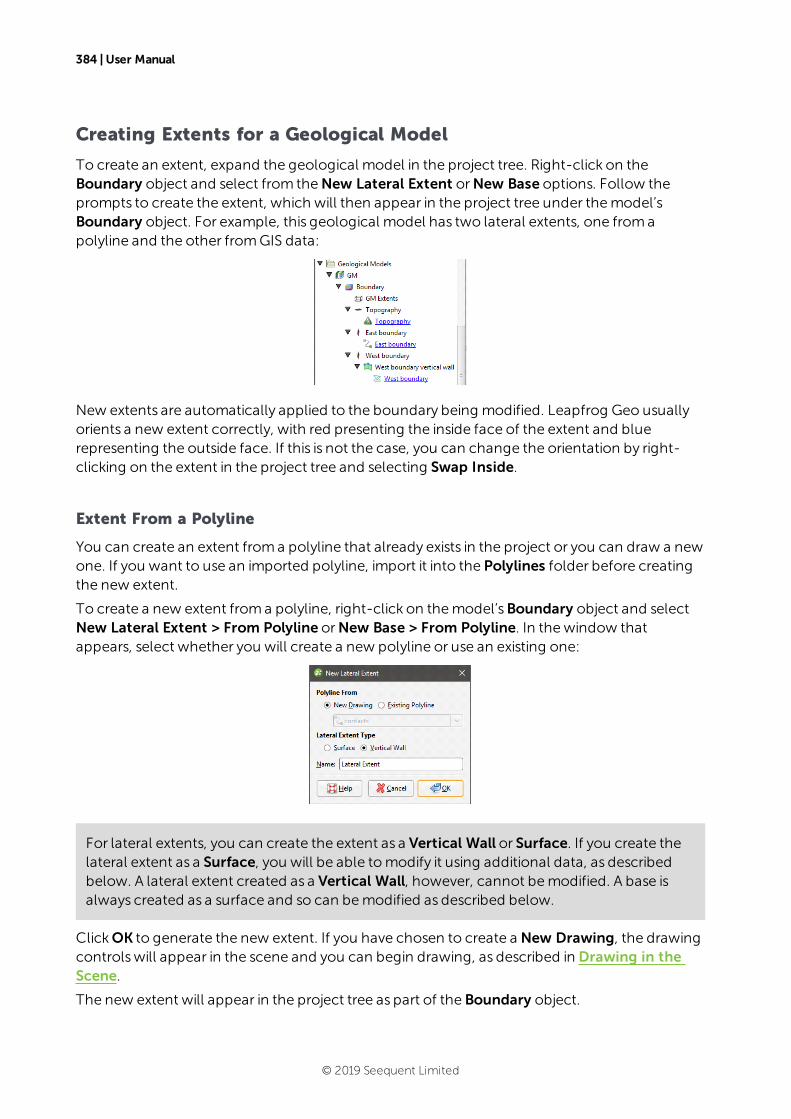
384 | User Manual
Creating Extents for a Geological Model
To create an extent, expand the geological model in the project tree. Right-click on theBoundary object and select from theNew Lateral Extent orNew Base options. Follow theprompts to create the extent, which will then appear in the project tree under themodel’sBoundary object. For example, this geological model has two lateral extents, one fromapolyline and the other fromGIS data:
New extents are automatically applied to the boundary being modified. Leapfrog Geo usuallyorients a new extent correctly, with red presenting the inside face of the extent and bluerepresenting the outside face. If this is not the case, you can change the orientation by right-clicking on the extent in the project tree and selecting Swap Inside.
Extent From a Polyline
You can create an extent froma polyline that already exists in the project or you can draw a newone. If you want to use an imported polyline, import it into the Polylines folder before creatingthe new extent.
To create a new extent froma polyline, right-click on themodel’sBoundary object and selectNew Lateral Extent > From Polyline orNew Base > From Polyline. In thewindow thatappears, select whether you will create a new polyline or use an existing one:
For lateral extents, you can create the extent as a Vertical Wall or Surface. If you create thelateral extent as a Surface, you will be able tomodify it using additional data, as describedbelow. A lateral extent created as a Vertical Wall, however, cannot bemodified. A base isalways created as a surface and so can bemodified as described below.
ClickOK to generate the new extent. If you have chosen to create a New Drawing, the drawingcontrolswill appear in the scene and you can begin drawing, as described in Drawing in theScene.
The new extent will appear in the project tree as part of the Boundary object.
© 2019 Seequent Limited
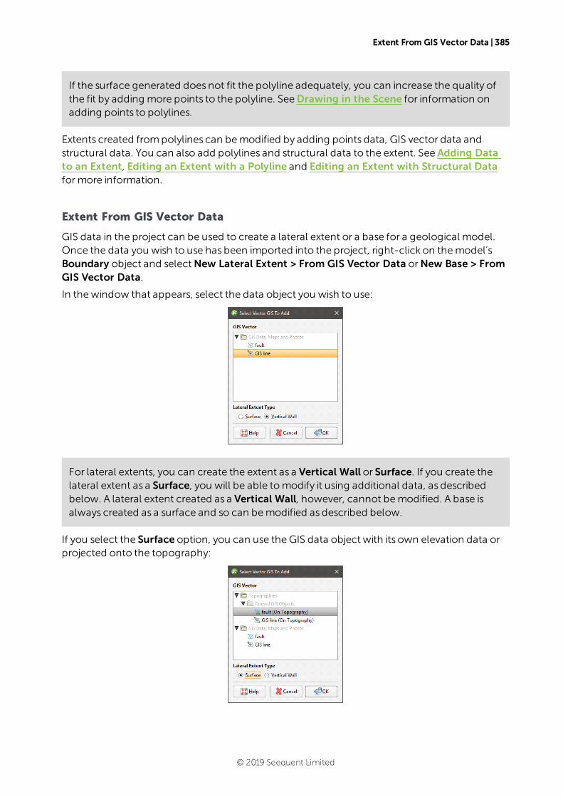
Extent From GIS Vector Data | 385
If the surface generated does not fit the polyline adequately, you can increase the quality ofthe fit by adding more points to the polyline. SeeDrawing in the Scene for information onadding points to polylines.
Extents created frompolylines can bemodified by adding points data, GIS vector data andstructural data. You can also add polylines and structural data to the extent. See Adding Datato an Extent, Editing an Extent with a Polyline and Editing an Extent with Structural Dataformore information.
Extent From GIS Vector Data
GIS data in the project can be used to create a lateral extent or a base for a geological model.Once the data you wish to use has been imported into the project, right-click on themodel’sBoundary object and selectNew Lateral Extent > From GIS Vector Data orNew Base > FromGIS Vector Data.
In thewindow that appears, select the data object you wish to use:
For lateral extents, you can create the extent as a Vertical Wall or Surface. If you create thelateral extent as a Surface, you will be able tomodify it using additional data, as describedbelow. A lateral extent created as a Vertical Wall, however, cannot bemodified. A base isalways created as a surface and so can bemodified as described below.
If you select the Surface option, you can use the GIS data object with its own elevation data orprojected onto the topography:
© 2019 Seequent Limited
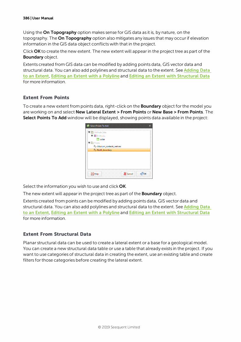
386 | User Manual
Using theOn Topography option makes sense for GIS data as it is, by nature, on thetopography. TheOn Topography option alsomitigates any issues that may occur if elevationinformation in the GIS data object conflictswith that in the project.
ClickOK to create the new extent. The new extent will appear in the project tree as part of theBoundary object.
Extents created fromGIS data can bemodified by adding points data, GIS vector data andstructural data. You can also add polylines and structural data to the extent. See Adding Datato an Extent, Editing an Extent with a Polyline and Editing an Extent with Structural Dataformore information.
Extent From Points
To create a new extent frompoints data, right-click on the Boundary object for themodel youare working on and selectNew Lateral Extent > From Points orNew Base > From Points. TheSelect Points To Addwindowwill be displayed, showing points data available in the project:
Select the information you wish to use and clickOK.
The new extent will appear in the project tree as part of the Boundary object.
Extents created frompoints can bemodified by adding points data, GIS vector data andstructural data. You can also add polylines and structural data to the extent. See Adding Datato an Extent, Editing an Extent with a Polyline and Editing an Extent with Structural Dataformore information.
Extent From Structural Data
Planar structural data can be used to create a lateral extent or a base for a geological model.You can create a new structural data table or use a table that already exists in the project. If youwant to use categories of structural data in creating the extent, use an existing table and createfilters for those categories before creating the lateral extent.
© 2019 Seequent Limited
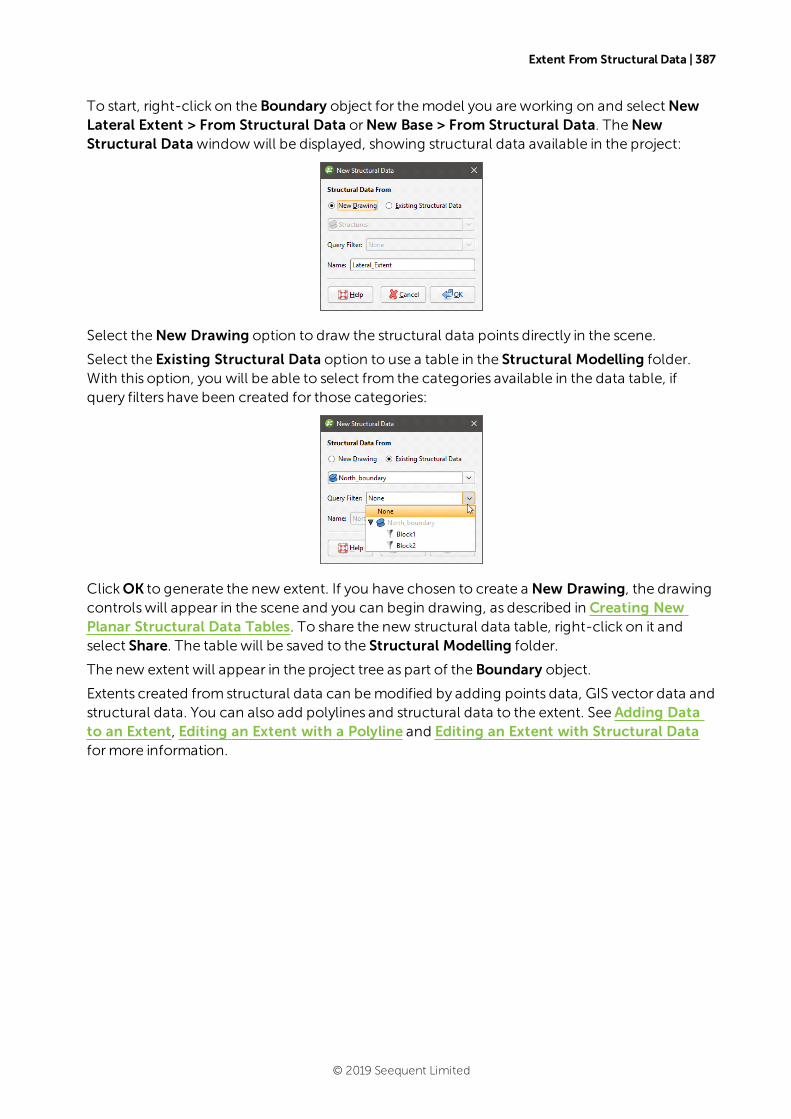
Extent From Structural Data | 387
To start, right-click on the Boundary object for themodel you are working on and selectNewLateral Extent > From Structural Data orNew Base > From Structural Data. TheNewStructural Datawindowwill be displayed, showing structural data available in the project:
Select theNew Drawing option to draw the structural data points directly in the scene.
Select the Existing Structural Data option to use a table in the Structural Modelling folder.With this option, you will be able to select from the categories available in the data table, ifquery filters have been created for those categories:
ClickOK to generate the new extent. If you have chosen to create a New Drawing, the drawingcontrolswill appear in the scene and you can begin drawing, as described in Creating NewPlanar Structural Data Tables. To share the new structural data table, right-click on it andselect Share. The table will be saved to the Structural Modelling folder.
The new extent will appear in the project tree as part of the Boundary object.
Extents created from structural data can bemodified by adding points data, GIS vector data andstructural data. You can also add polylines and structural data to the extent. See Adding Datato an Extent, Editing an Extent with a Polyline and Editing an Extent with Structural Dataformore information.
© 2019 Seequent Limited
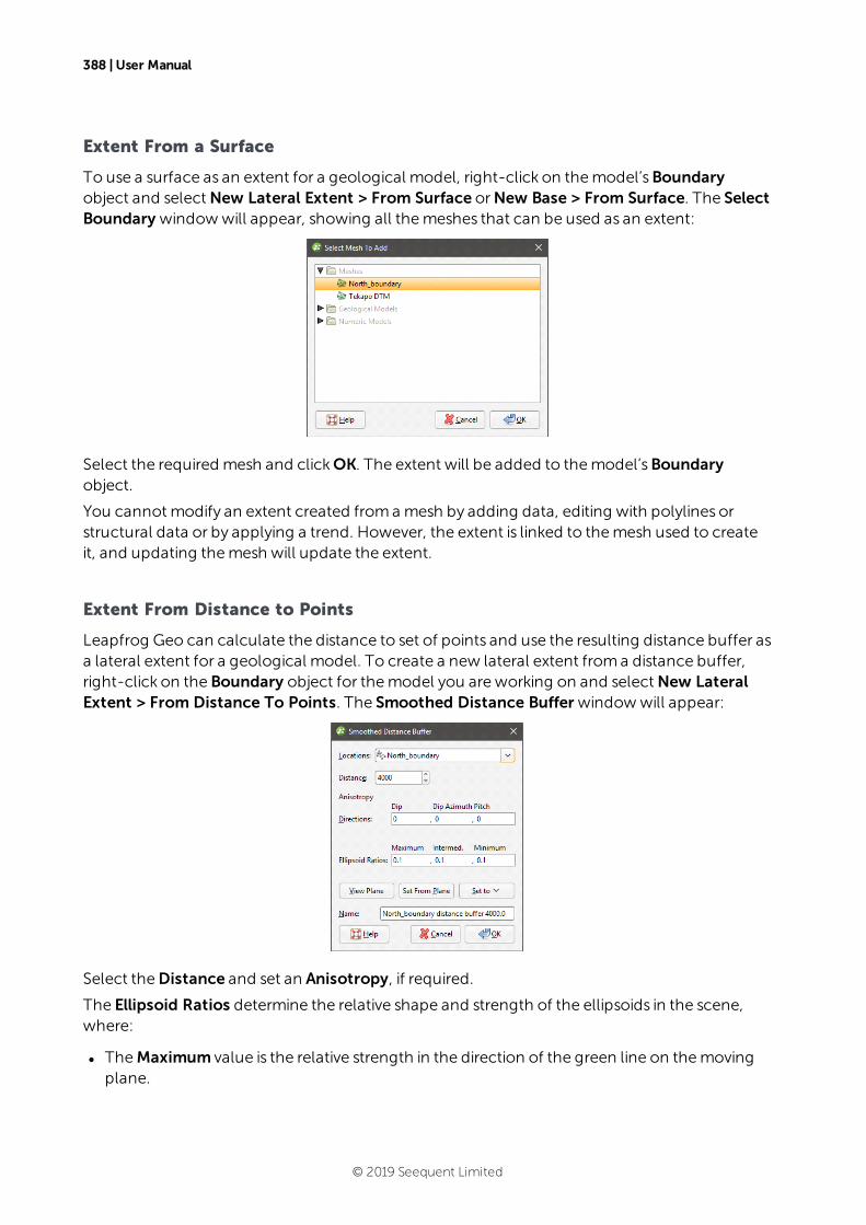
388 | User Manual
Extent From a Surface
To use a surface as an extent for a geological model, right-click on themodel’sBoundaryobject and selectNew Lateral Extent > From Surface orNew Base > From Surface. The SelectBoundary windowwill appear, showing all themeshes that can be used as an extent:
Select the required mesh and clickOK. The extent will be added to themodel’sBoundaryobject.
You cannot modify an extent created froma mesh by adding data, editing with polylines orstructural data or by applying a trend. However, the extent is linked to themesh used to createit, and updating themesh will update the extent.
Extent From Distance to Points
Leapfrog Geo can calculate the distance to set of points and use the resulting distance buffer asa lateral extent for a geological model. To create a new lateral extent froma distance buffer,right-click on the Boundary object for themodel you are working on and selectNew LateralExtent > From Distance To Points. The Smoothed Distance Buffer windowwill appear:
Select theDistance and set an Anisotropy, if required.
The Ellipsoid Ratios determine the relative shape and strength of the ellipsoids in the scene,where:
l TheMaximum value is the relative strength in the direction of the green line on themovingplane.
© 2019 Seequent Limited
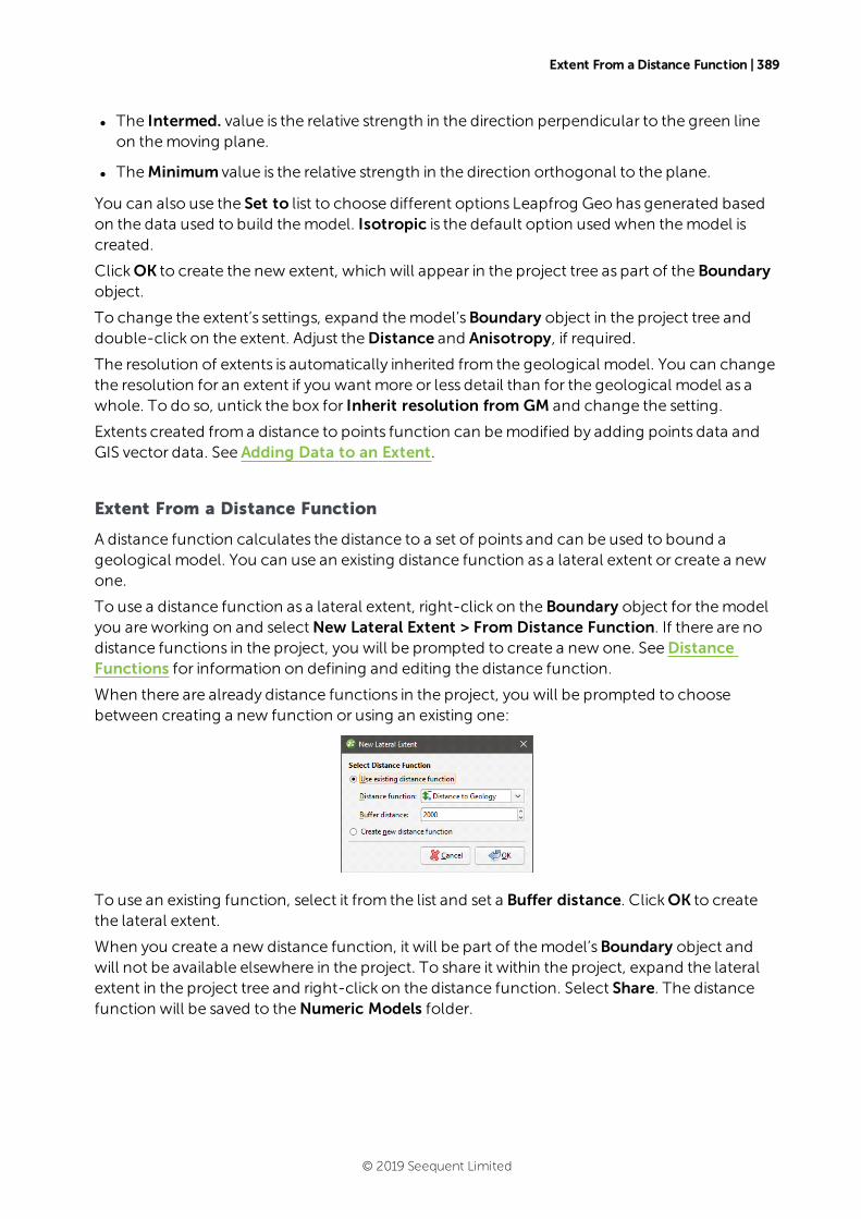
Extent From a Distance Function | 389
l The Intermed. value is the relative strength in the direction perpendicular to the green lineon themoving plane.
l TheMinimum value is the relative strength in the direction orthogonal to the plane.
You can also use the Set to list to choose different options Leapfrog Geo has generated basedon the data used to build themodel. Isotropic is the default option used when themodel iscreated.
ClickOK to create the new extent, which will appear in the project tree as part of the Boundaryobject.
To change the extent’s settings, expand themodel’sBoundary object in the project tree anddouble-click on the extent. Adjust theDistance and Anisotropy, if required.
The resolution of extents is automatically inherited from the geological model. You can changethe resolution for an extent if you want more or less detail than for the geological model as awhole. To do so, untick the box for Inherit resolution from GM and change the setting.
Extents created froma distance to points function can bemodified by adding points data andGIS vector data. See Adding Data to an Extent.
Extent From a Distance Function
A distance function calculates the distance to a set of points and can be used to bound ageological model. You can use an existing distance function as a lateral extent or create a newone.
To use a distance function as a lateral extent, right-click on the Boundary object for themodelyou are working on and selectNew Lateral Extent > From Distance Function. If there are nodistance functions in the project, you will be prompted to create a new one. SeeDistanceFunctions for information on defining and editing the distance function.
When there are already distance functions in the project, you will be prompted to choosebetween creating a new function or using an existing one:
To use an existing function, select it from the list and set a Buffer distance. ClickOK to createthe lateral extent.
When you create a new distance function, it will be part of themodel’sBoundary object andwill not be available elsewhere in the project. To share it within the project, expand the lateralextent in the project tree and right-click on the distance function. Select Share. The distancefunction will be saved to theNumeric Models folder.
© 2019 Seequent Limited

390 | User Manual
To change the extent’s settings, expand themodel’sBoundary object in the project tree anddouble-click on the extent. The Edit Distance Buffer windowwill appear.
The resolution of extents is automatically inherited from the geological model. You can changethe resolution for an extent if you want more or less detail than for the geological model as awhole. To do so, untick the box for Inherit resolution from GM and change the setting.
Base From Lithology Contacts
To create a base from lithlogy contacts, right-click on the Boundary object and select eitherNew Base > From Base Lithology orNew Base > From Other Contacts.
The only difference in the twomethods is that when creating a base fromother contacts,you must first select the lithology column from those available in the project.
When defining the base, select the primary lithology and the contacts to use:
© 2019 Seequent Limited
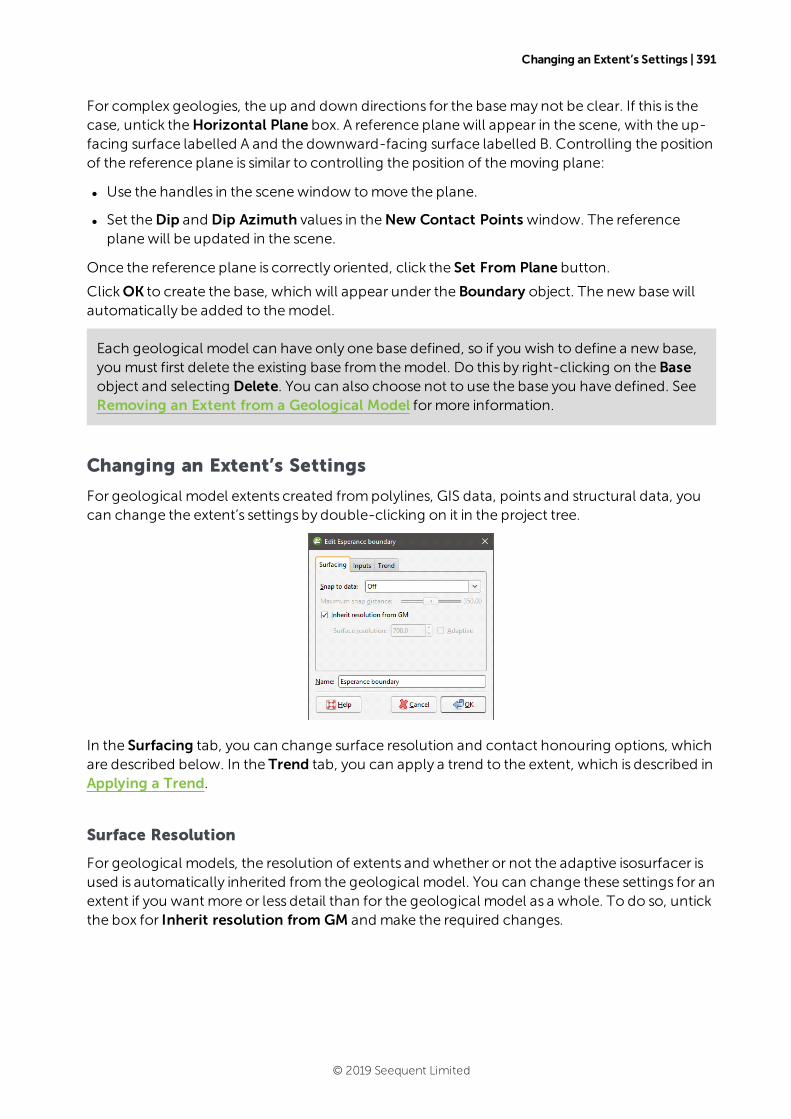
Changing an Extent’s Settings | 391
For complex geologies, the up and down directions for the basemay not be clear. If this is thecase, untick theHorizontal Plane box. A reference planewill appear in the scene, with the up-facing surface labelled A and the downward-facing surface labelled B. Controlling the positionof the reference plane is similar to controlling the position of themoving plane:
l Use the handles in the scenewindow tomove the plane.
l Set theDip and Dip Azimuth values in theNew Contact Points window. The referenceplanewill be updated in the scene.
Once the reference plane is correctly oriented, click the Set From Plane button.
ClickOK to create the base, which will appear under the Boundary object. The new basewillautomatically be added to themodel.
Each geological model can have only one base defined, so if you wish to define a new base,you must first delete the existing base from themodel. Do this by right-clicking on the Baseobject and selecting Delete. You can also choose not to use the base you have defined. SeeRemoving an Extent from a Geological Model formore information.
Changing an Extent’s Settings
For geological model extents created frompolylines, GIS data, points and structural data, youcan change the extent’s settings by double-clicking on it in the project tree.
In the Surfacing tab, you can change surface resolution and contact honouring options, whichare described below. In the Trend tab, you can apply a trend to the extent, which is described inApplying a Trend.
Surface Resolution
For geological models, the resolution of extents and whether or not the adaptive isosurfacer isused is automatically inherited from the geological model. You can change these settings for anextent if you want more or less detail than for the geological model as a whole. To do so, untickthe box for Inherit resolution from GM and make the required changes.
© 2019 Seequent Limited
392 | User Manual
Contact Honouring
Often, surfaces should honour drillhole data and treat data objects such as polylines and GISdata as interpretations. For extents, the Snap to data setting in the Surfacing tab determineswhether or not the extent honours the data used to create it. Options are:
l Off. The extent does not snap to the data used to create it. This is the default setting.
l All data. The extent snaps to all data within theMaximum snap distance, which includesdrillhole data and any data added to the extent.
l Drilling only. The extent snaps to drillhole data and data objects derived fromdrillhole datawithin theMaximum snap distance, but not to other data used tomodify the extent. Forexample, the extent will honour points data derived fromdrillhole data, but not points dataimported into the Points folder.
l Custom. The extent snaps to the data objects indicated in the Inputs tab that are within theMaximum snap distance.
Take care in enabling snapping and in selecting what data the surfacewill snap to, as themore data you include, e.g. by setting a largeMaximum snap distance or selecting All datafor Snap to data, the greater the possibility that errors in the data or assumptions inherent ininterpretations (e.g. polylines) will cause distortions in themeshes. If you do enable snapping,it is best to snap only to drilling data. SeeHonouring Surface Contacts formore informationon these settings.
The snap setting for the geological model will be used if Snap to data is set to Inherit from GM.
Whatever the setting, you can seewhat objects are snapped to by clicking on the Inputs tab.
If you need the extent to honour drillhole data but treat other data objects as interpretations,selectDrilling only. To honour some data objectswhile treating others as interpretations, selectCustom, then click on the Inputs tab to enable snapping for individual objects.
Applying a Trend
You can adjust an extent created frompolylines, GIS data, points and structural data byapplying a trend to it. To do this, add the extent to the scene. Next, double-click on the extent inthe project tree and click the Trend tab.
Often the easiest way to apply a trend is to click on theDraw plane line button ( ) and draw aplane line in the scene in the direction in which you wish to adjust the surface. You may need torotate the scene to see the plane properly.
The Ellipsoid Ratios determine the relative shape and strength of the ellipsoids in the scene,where:
l TheMaximum value is the relative strength in the direction of the green line on themovingplane.
l The Intermed. value is the relative strength in the direction perpendicular to the green line
© 2019 Seequent Limited
Adding Data to an Extent | 393
on themoving plane.
l TheMinimum value is the relative strength in the direction orthogonal to the plane.
Once you have adjusted the plane to represent the trend you wish to use, click the Set FromPlane button to copy themoving plane settings.
The Set to list contains a number of different options Leapfrog Geo has generated based on thedata used in the project. Isotropic is the default option used when the extent was created.Settingsmade to other surfaces in the project will also be listed, which makes it easy to apply thesame settings tomany surfaces.
ClickOK to apply the changes.
SeeGlobal Trends formore information.
Adding Data to an Extent
Extents created frompolylines, GIS data, points and structural data can bemodified by addingpoints data objects, GIS vector data and structural data. Extents created froma distance topoints function can bemodified by adding points data and GIS vector data. To add data to anextent, right-click on the extent in the project tree and select the data type you wish to use fromthe Addmenu.
l Points data. Select from the points data objects available in the project and clickOK.
l GIS vector data. Select from theGIS vector data available in the project and clickOK.
l Structural data. Select from the structural data tables available in the project. If the selectedtable has query filters defined, you can apply one of these filters by selecting the requiredquery from the list. ClickOK to add the selected data to the extent. An alternative to addingan existing structural data table to an extent is to edit the extent with structural data. This isdescribed in Editing an Extent with Structural Data below.
You can also add a polyline that already exists in the project. To do this, right-click on the extentin the project tree and select Add > Polyline. You will be prompted to choose from the polylinesin the Polylines folder.
Editing an Extent with a Polyline
You can edit an extent using a polyline, which is described in Editing Surfaces with Polylines. Apolyline used to edit an extent will be added to the project tree as part of the extent. To edit thepolyline, right-click on it and select Edit Polyline or add it to the scene and click the Edit button () in the shape list. If you wish to remove the polyline from the extent, right-click on it in the
project tree and selectDelete orRemove.
To add an existing polyline to a geological model extent, use the Add > Polyline option.
Editing an Extent with Structural Data
You can edit an extent using structural data, which is described in Editing Surfaces withStructural Data. A structural data table will be added to the project tree as part of the extent.To edit the table, right-click on it and select Edit In Scene or add it to the scene and click the
© 2019 Seequent Limited
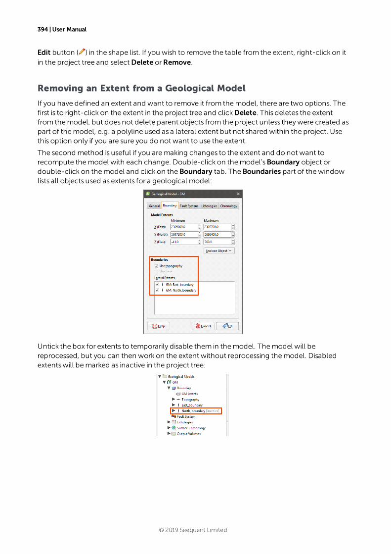
394 | User Manual
Edit button ( ) in the shape list. If you wish to remove the table from the extent, right-click on itin the project tree and selectDelete orRemove.
Removing an Extent from a Geological Model
If you have defined an extent and want to remove it from themodel, there are two options. Thefirst is to right-click on the extent in the project tree and clickDelete. This deletes the extentfrom themodel, but does not delete parent objects from the project unless theywere created aspart of themodel, e.g. a polyline used as a lateral extent but not shared within the project. Usethis option only if you are sure you do not want to use the extent.
The second method is useful if you aremaking changes to the extent and do not want torecompute themodel with each change. Double-click on themodel’sBoundary object ordouble-click on themodel and click on the Boundary tab. The Boundaries part of thewindowlists all objects used as extents for a geological model:
Untick the box for extents to temporarily disable them in themodel. Themodel will bereprocessed, but you can then work on the extent without reprocessing themodel. Disabledextentswill bemarked as inactive in the project tree:
© 2019 Seequent Limited
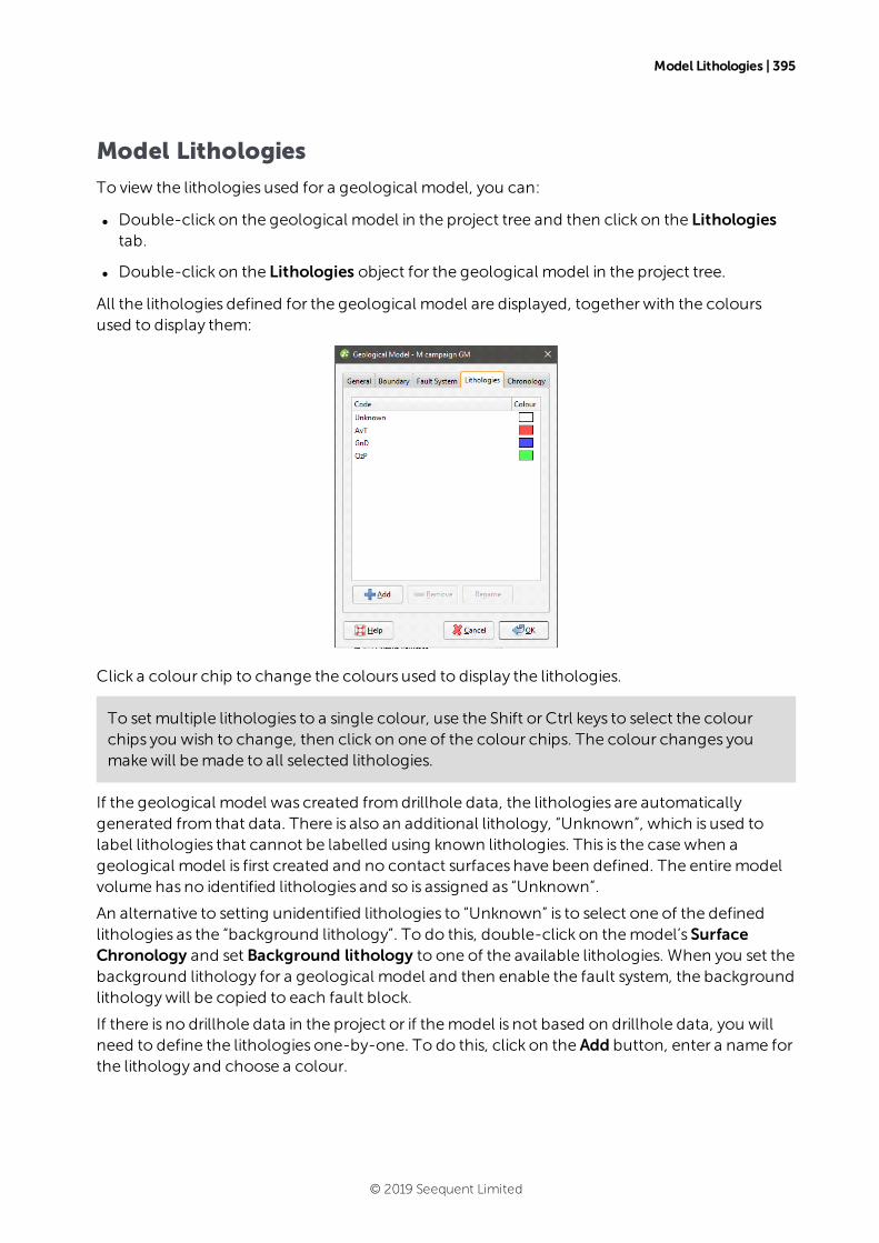
Model Lithologies | 395
Model Lithologies
To view the lithologies used for a geological model, you can:
l Double-click on the geological model in the project tree and then click on the Lithologiestab.
l Double-click on the Lithologies object for the geological model in the project tree.
All the lithologies defined for the geological model are displayed, together with the coloursused to display them:
Click a colour chip to change the colours used to display the lithologies.
To set multiple lithologies to a single colour, use the Shift or Ctrl keys to select the colourchips you wish to change, then click on one of the colour chips. The colour changes youmakewill bemade to all selected lithologies.
If the geological model was created fromdrillhole data, the lithologies are automaticallygenerated from that data. There is also an additional lithology, “Unknown”, which is used tolabel lithologies that cannot be labelled using known lithologies. This is the casewhen ageological model is first created and no contact surfaces have been defined. The entiremodelvolume has no identified lithologies and so is assigned as “Unknown”.
An alternative to setting unidentified lithologies to “Unknown” is to select one of the definedlithologies as the “background lithology”. To do this, double-click on themodel’s SurfaceChronology and set Background lithology to one of the available lithologies. When you set thebackground lithology for a geological model and then enable the fault system, the backgroundlithologywill be copied to each fault block.
If there is no drillhole data in the project or if themodel is not based on drillhole data, you willneed to define the lithologies one-by-one. To do this, click on the Add button, enter a name forthe lithology and choose a colour.
© 2019 Seequent Limited
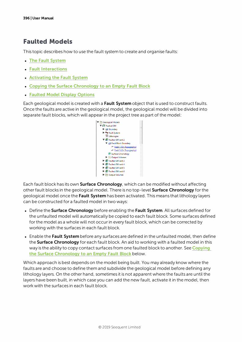
396 | User Manual
Faulted Models
This topic describes how to use the fault system to create and organise faults:
l The Fault System
l Fault Interactions
l Activating the Fault System
l Copying the Surface Chronology to an Empty Fault Block
l Faulted Model Display Options
Each geological model is created with a Fault Systemobject that is used to construct faults.Once the faults are active in the geological model, the geological model will be divided intoseparate fault blocks, which will appear in the project tree as part of themodel:
Each fault block has its own Surface Chronology, which can bemodified without affectingother fault blocks in the geological model. There is no top-level Surface Chronology for thegeological model once the Fault Systemhas been activated. Thismeans that lithology layerscan be constructed for a faulted model in twoways:
l Define the Surface Chronology before enabling the Fault System. All surfaces defined forthe unfaulted model will automatically be copied to each fault block. Some surfaces definedfor themodel as a whole will not occur in every fault block, which can be corrected byworking with the surfaces in each fault block.
l Enable the Fault System before any surfaces are defined in the unfaulted model, then definethe Surface Chronology for each fault block. An aid toworking with a faulted model in thisway is the ability to copy contact surfaces fromone faulted block to another. SeeCopyingthe Surface Chronology to an Empty Fault Block below.
Which approach is best dependson themodel being built. You may already knowwhere thefaults are and choose to define themand subdivide the geological model before defining anylithology layers. On the other hand, sometimes it is not apparent where the faults are until thelayers have been built, in which case you can add the new fault, activate it in themodel, thenworkwith the surfaces in each fault block.
© 2019 Seequent Limited
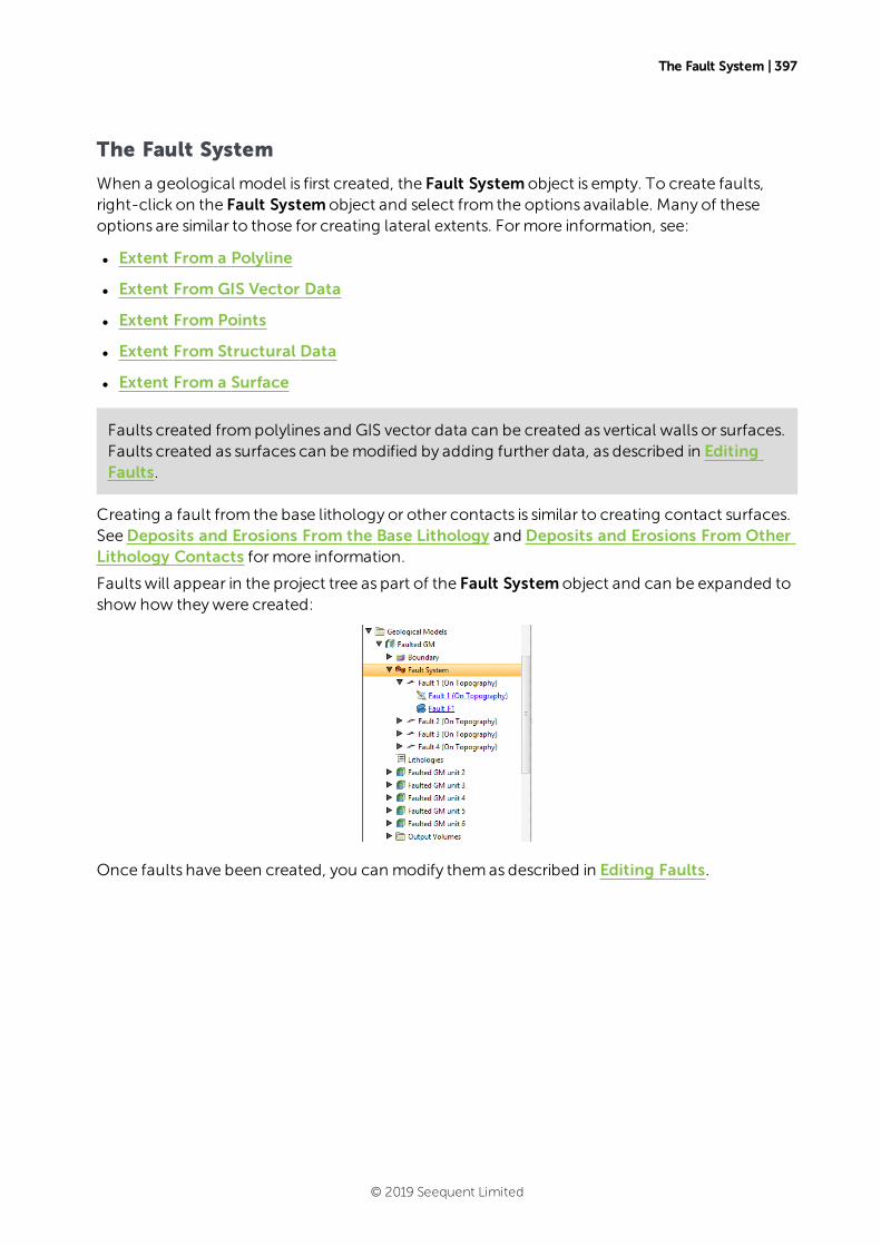
The Fault System | 397
The Fault System
When a geological model is first created, the Fault Systemobject is empty. To create faults,right-click on the Fault Systemobject and select from the options available. Many of theseoptions are similar to those for creating lateral extents. Formore information, see:
l Extent From a Polyline
l Extent From GIS Vector Data
l Extent From Points
l Extent From Structural Data
l Extent From a Surface
Faults created frompolylines and GIS vector data can be created as vertical walls or surfaces.Faults created as surfaces can bemodified by adding further data, as described in EditingFaults.
Creating a fault from the base lithology or other contacts is similar to creating contact surfaces.SeeDeposits and Erosions From the Base Lithology and Deposits and Erosions From OtherLithology Contacts formore information.
Faultswill appear in the project tree as part of the Fault Systemobject and can be expanded toshow how theywere created:
Once faults have been created, you can modify themas described in Editing Faults.
© 2019 Seequent Limited

398 | User Manual
Fault Interactions
Once all the faults required have been created, you can start defining the interactions betweenthe faults by double-clicking on the Fault Systemobject. TheGeological Modelwill be openedwith the Fault System tab displayed:
To add an interaction, click on a fault, then click the Add button. Select the Interaction Typeand set how the faults interact:
© 2019 Seequent Limited
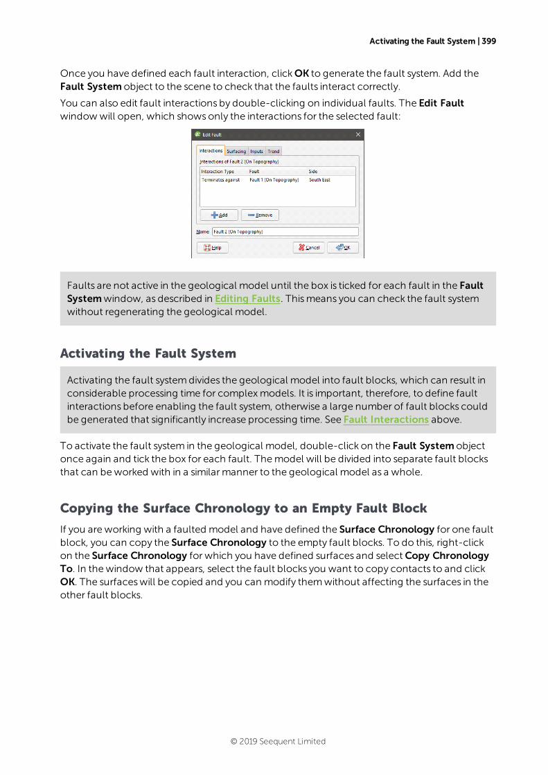
Activating the Fault System | 399
Once you have defined each fault interaction, clickOK to generate the fault system. Add theFault Systemobject to the scene to check that the faults interact correctly.
You can also edit fault interactions by double-clicking on individual faults. The Edit Faultwindowwill open, which showsonly the interactions for the selected fault:
Faults are not active in the geological model until the box is ticked for each fault in the FaultSystemwindow, as described in Editing Faults. Thismeans you can check the fault systemwithout regenerating the geological model.
Activating the Fault System
Activating the fault systemdivides the geological model into fault blocks, which can result inconsiderable processing time for complexmodels. It is important, therefore, to define faultinteractions before enabling the fault system, otherwise a large number of fault blocks couldbe generated that significantly increase processing time. See Fault Interactions above.
To activate the fault system in the geological model, double-click on the Fault Systemobjectonce again and tick the box for each fault. Themodel will be divided into separate fault blocksthat can beworked with in a similarmanner to the geological model as a whole.
Copying the Surface Chronology to an Empty Fault Block
If you are working with a faulted model and have defined the Surface Chronology for one faultblock, you can copy the Surface Chronology to the empty fault blocks. To do this, right-clickon the Surface Chronology for which you have defined surfaces and selectCopy ChronologyTo. In thewindow that appears, select the fault blocks you want to copy contacts to and clickOK. The surfaceswill be copied and you can modify themwithout affecting the surfaces in theother fault blocks.
© 2019 Seequent Limited
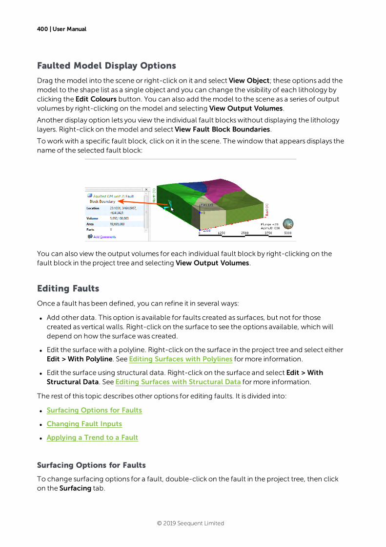
400 | User Manual
Faulted Model Display Options
Drag themodel into the scene or right-click on it and select View Object; these options add themodel to the shape list as a single object and you can change the visibility of each lithology byclicking the Edit Colours button. You can also add themodel to the scene as a series of outputvolumes by right-clicking on themodel and selecting View Output Volumes.
Another display option lets you view the individual fault blockswithout displaying the lithologylayers. Right-click on themodel and select View Fault Block Boundaries.
Toworkwith a specific fault block, click on it in the scene. Thewindow that appears displays thename of the selected fault block:
You can also view the output volumes for each individual fault block by right-clicking on thefault block in the project tree and selecting View Output Volumes.
Editing Faults
Once a fault has been defined, you can refine it in several ways:
l Add other data. This option is available for faults created as surfaces, but not for thosecreated as vertical walls. Right-click on the surface to see the options available, which willdepend on how the surfacewas created.
l Edit the surfacewith a polyline. Right-click on the surface in the project tree and select eitherEdit > With Polyline. See Editing Surfaces with Polylines formore information.
l Edit the surface using structural data. Right-click on the surface and select Edit > WithStructural Data. See Editing Surfaces with Structural Data formore information.
The rest of this topic describes other options for editing faults. It is divided into:
l Surfacing Options for Faults
l Changing Fault Inputs
l Applying a Trend to a Fault
Surfacing Options for Faults
To change surfacing options for a fault, double-click on the fault in the project tree, then clickon the Surfacing tab.
© 2019 Seequent Limited
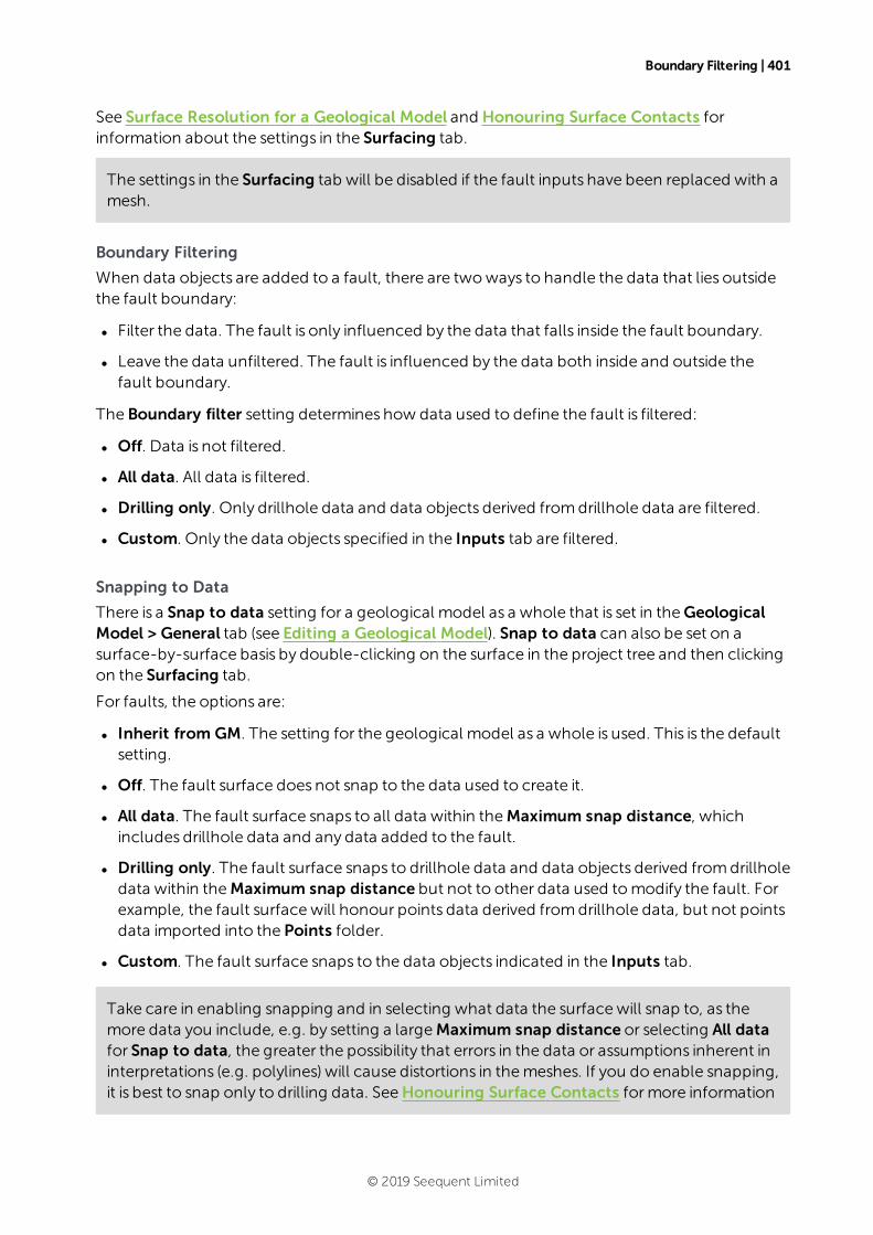
Boundary Filtering | 401
See Surface Resolution for a Geological Model and Honouring Surface Contacts forinformation about the settings in the Surfacing tab.
The settings in the Surfacing tab will be disabled if the fault inputs have been replaced with amesh.
Boundary Filtering
When data objects are added to a fault, there are twoways to handle the data that lies outsidethe fault boundary:
l Filter the data. The fault is only influenced by the data that falls inside the fault boundary.
l Leave the data unfiltered. The fault is influenced by the data both inside and outside thefault boundary.
The Boundary filter setting determines how data used to define the fault is filtered:
l Off. Data is not filtered.
l All data. All data is filtered.
l Drilling only. Only drillhole data and data objects derived fromdrillhole data are filtered.
l Custom. Only the data objects specified in the Inputs tab are filtered.
Snapping to Data
There is a Snap to data setting for a geological model as a whole that is set in theGeologicalModel > General tab (see Editing a Geological Model). Snap to data can also be set on asurface-by-surface basis by double-clicking on the surface in the project tree and then clickingon the Surfacing tab.
For faults, the options are:
l Inherit from GM. The setting for the geological model as a whole is used. This is the defaultsetting.
l Off. The fault surface does not snap to the data used to create it.
l All data. The fault surface snaps to all data within theMaximum snap distance, whichincludes drillhole data and any data added to the fault.
l Drilling only. The fault surface snaps to drillhole data and data objects derived fromdrillholedata within theMaximum snap distance but not to other data used tomodify the fault. Forexample, the fault surfacewill honour points data derived fromdrillhole data, but not pointsdata imported into the Points folder.
l Custom. The fault surface snaps to the data objects indicated in the Inputs tab.
Take care in enabling snapping and in selecting what data the surfacewill snap to, as themore data you include, e.g. by setting a largeMaximum snap distance or selecting All datafor Snap to data, the greater the possibility that errors in the data or assumptions inherent ininterpretations (e.g. polylines) will cause distortions in themeshes. If you do enable snapping,it is best to snap only to drilling data. SeeHonouring Surface Contacts formore information
© 2019 Seequent Limited

402 | User Manual
on these settings.
If you need the fault surface to honour drillhole data but treat other data objects asinterpretations, selectDrilling only. To honour some data objectswhile treating others asinterpretations, selectCustom, then click on the Inputs tab to enable snapping for individualobjects.
Changing Fault Inputs
For faults, the Inputs tab shows all the data objects used to create the fault and whether theSnap and Boundary filter options are enabled for each object used to define the fault. If aninput has any query filters defined, you can select one in thiswindow.
You can also replace the fault’s inputswith a singlemesh or add more data to the fault.
Replacing Fault Inputs with a Single Mesh
To replace the fault inputswith a singlemesh, click on theMesh option, then select from themeshes available in the project.
When you select a singlemesh to define the fault, all other inputs listed in the Inputs tab will
© 2019 Seequent Limited

Adding Data to the Fault | 403
be removed from the fault. This can result in objects being deleted from the project. Forexample, if the fault has been edited using a polyline, the polyline will be deleted when theinputs are replaced with themesh. If you wish to retain such inputs, be sure to share theobject before changing the inputs. See Sharing Objects formore information.
The snap and boundary filtering controls in the Surfacing tab will be disabled as the settingsfrom the geological model will be used. The settings in the Trend tab will also be disabled as it isnot possible to set a trend for a fault defined froma mesh.
Adding Data to the Fault
To add more data to the fault, click on the Select Objects button, then select from the suitableobjects available in the project.
Snap Settings for Individual Inputs
The Snap setting determineswhether or not the faults surface honours a particular data object.Often, surfaces should honour drillhole data and treat data objects such as polylines and GISdata as interpretations, as discussed in Honouring Surface Contacts. To change snap settingsfor a fault, click on the Surfacing tab and set Snap to data toCustom. You will then be able tochange Snap settings in the Inputs tab.
Boundary Filtering Settings for Individual Inputs
When data objects are added to a fault, there are twoways to handle the data that lies outsidethe fault boundary:
l Filter the data. The fault is only influenced by the data that falls inside the fault boundary.
l Leave the data unfiltered. The fault is influenced by the data both inside and outside thefault boundary.
To change the Boundary filter settings for each object used to define a fault, click on theSurfacing tab and set Boundary filter toCustom. You will then be able to change Boundaryfilter settings in the Inputs tab.
Applying a Trend to a Fault
To apply a trend to a fault, either:
l Double-click on the fault in the project tree, then click on the Trend tab.
l Right-click on the fault in the project tree and select Adjust Surface. This opens the EditFault windowwith the Trend tab displayed.
SeeGlobal Trends for information on using the controls in this tab.
The settings in the Trend tab will be disabled if the fault inputs have been replaced with amesh.
© 2019 Seequent Limited

404 | User Manual
Contact Surfaces
Defining the internal structure of a geological model involves generating contact surfaces thatcorrespond to the boundaries between lithological units, refining the contact surfaces,arranging them in chronological order and then using the surfaces and the chronological orderto divide the geological model into units. The Surface Chronology object represents thecollection of contact surfaces and defines how they interact to produce the volumesof thegeological model. Factors that influence the interaction of contact surfaceswith the volumesof the geological model are:
l The order of the contact surfaces in the Surface Chronology. SeeContact Surfaces in theSurface Chronology.
l The type of contact surface. SeeContact Surfaces Types formore information.
l The orientation of the older and younger sides of the surface. See Younging Direction.
The remainder of this topic describes how the different types of contact surface interact and willhelp you in deciding how tomodel different units. For specific information on creating thedifferent types of contact surfaces, see:
l Deposits and Erosions
l Intrusions
l Veins
l Vein Systems
l Stratigraphic Sequences
Contact Surfaces in the Surface Chronology
When a geological model is first created, it is simply a volume that is assigned the backgroundlithology. This background lithology is initially “Unknown”, as although themodel haslithologies defined, Leapfrog Geo cannot determinewhat lithology to use for the backgroundlithology.
© 2019 Seequent Limited
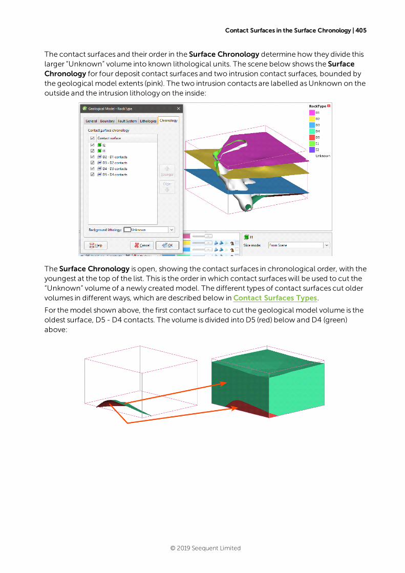
Contact Surfaces in the Surface Chronology | 405
The contact surfaces and their order in the Surface Chronology determine how they divide thislarger “Unknown” volume into known lithological units. The scene below shows the SurfaceChronology for four deposit contact surfaces and two intrusion contact surfaces, bounded bythe geological model extents (pink). The two intrusion contacts are labelled asUnknown on theoutside and the intrusion lithology on the inside:
The Surface Chronology is open, showing the contact surfaces in chronological order, with theyoungest at the top of the list. This is the order in which contact surfaceswill be used to cut the“Unknown” volume of a newly created model. The different types of contact surfaces cut oldervolumes in different ways, which are described below in Contact Surfaces Types.
For themodel shown above, the first contact surface to cut the geological model volume is theoldest surface, D5 -D4 contacts. The volume is divided into D5 (red) below and D4 (green)above:
© 2019 Seequent Limited
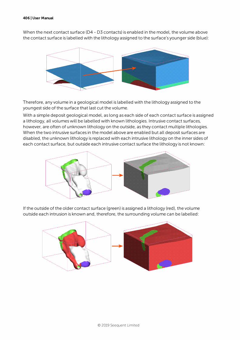
406 | User Manual
When the next contact surface (D4 -D3 contacts) is enabled in themodel, the volume abovethe contact surface is labelled with the lithology assigned to the surface’s younger side (blue):
Therefore, any volume in a geological model is labelled with the lithology assigned to theyoungest side of the surface that last cut the volume.
With a simple deposit geological model, as long as each side of each contact surface is assigneda lithology, all volumeswill be labelled with known lithologies. Intrusive contact surfaces,however, are often of unknown lithology on the outside, as they contact multiple lithologies.When the two intrusive surfaces in themodel above are enabled but all deposit surfaces aredisabled, the unknown lithology is replaced with each intrusive lithology on the inner sides ofeach contact surface, but outside each intrusive contact surface the lithology is not known:
If the outside of the older contact surface (green) is assigned a lithology (red), the volumeoutside each intrusion is known and, therefore, the surrounding volume can be labelled:
© 2019 Seequent Limited
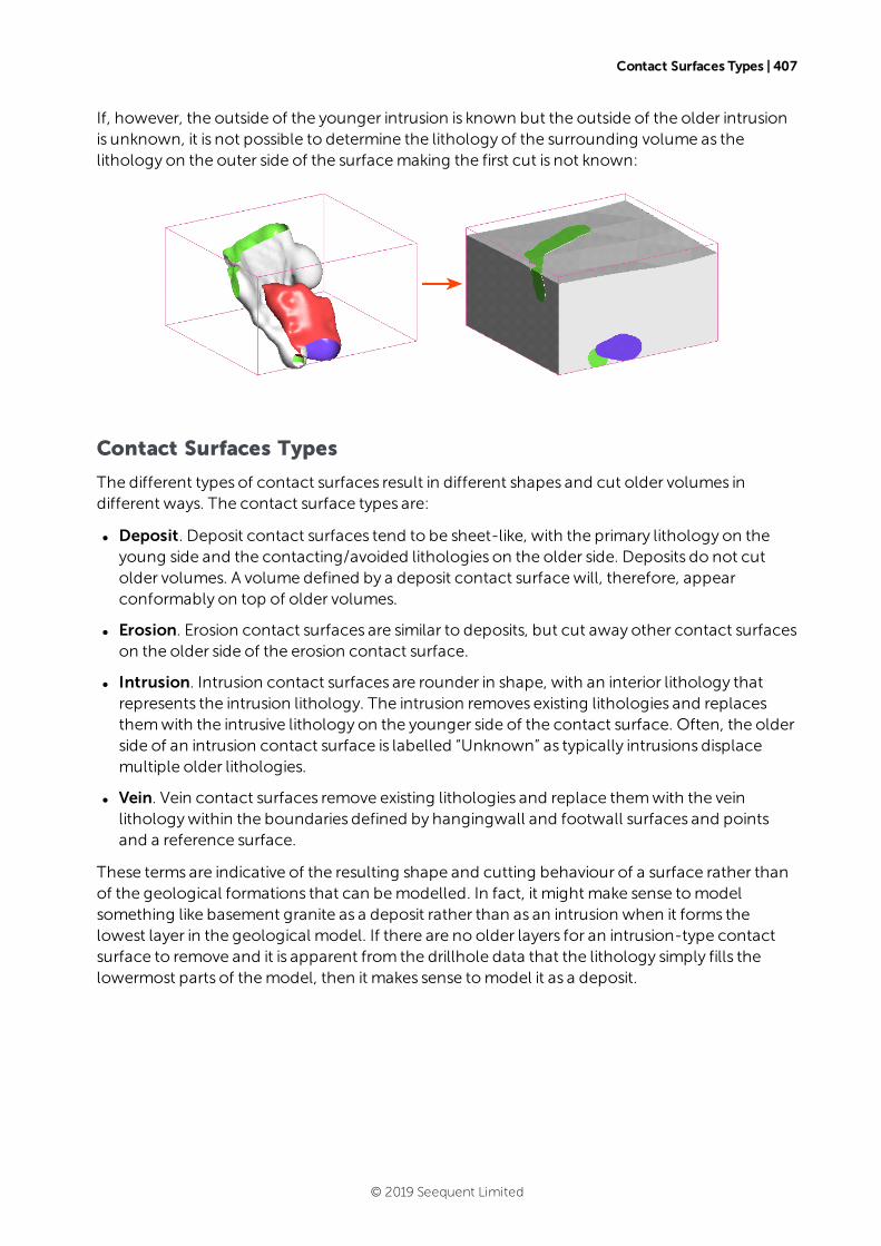
Contact Surfaces Types | 407
If, however, the outside of the younger intrusion is known but the outside of the older intrusionis unknown, it is not possible to determine the lithology of the surrounding volume as thelithology on the outer side of the surfacemaking the first cut is not known:
Contact Surfaces Types
The different types of contact surfaces result in different shapes and cut older volumes indifferent ways. The contact surface types are:
l Deposit. Deposit contact surfaces tend to be sheet-like, with the primary lithology on theyoung side and the contacting/avoided lithologies on the older side. Deposits do not cutolder volumes. A volume defined by a deposit contact surfacewill, therefore, appearconformably on top of older volumes.
l Erosion. Erosion contact surfaces are similar to deposits, but cut away other contact surfaceson the older side of the erosion contact surface.
l Intrusion. Intrusion contact surfaces are rounder in shape, with an interior lithology thatrepresents the intrusion lithology. The intrusion removes existing lithologies and replacesthemwith the intrusive lithology on the younger side of the contact surface. Often, the olderside of an intrusion contact surface is labelled “Unknown” as typically intrusions displacemultiple older lithologies.
l Vein. Vein contact surfaces remove existing lithologies and replace themwith the veinlithologywithin the boundaries defined by hangingwall and footwall surfaces and pointsand a reference surface.
These terms are indicative of the resulting shape and cutting behaviour of a surface rather thanof the geological formations that can bemodelled. In fact, it might make sense tomodelsomething like basement granite as a deposit rather than as an intrusion when it forms thelowest layer in the geological model. If there are no older layers for an intrusion-type contactsurface to remove and it is apparent from the drillhole data that the lithology simply fills thelowermost parts of themodel, then it makes sense tomodel it as a deposit.
© 2019 Seequent Limited
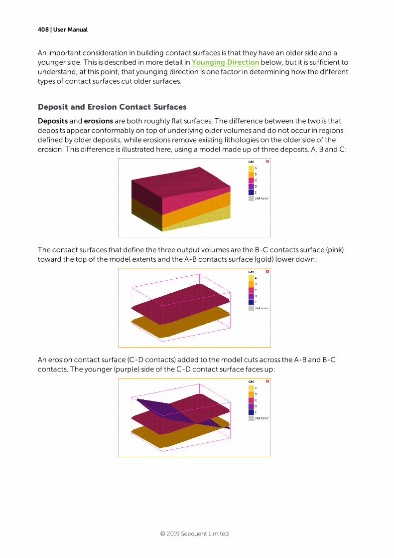
408 | User Manual
An important consideration in building contact surfaces is that they have an older side and ayounger side. This is described in more detail in Younging Direction below, but it is sufficient tounderstand, at this point, that younging direction is one factor in determining how the differenttypes of contact surfaces cut older surfaces.
Deposit and Erosion Contact Surfaces
Deposits and erosions are both roughly flat surfaces. The difference between the two is thatdeposits appear conformably on top of underlying older volumes and do not occur in regionsdefined by older deposits, while erosions remove existing lithologies on the older side of theerosion. This difference is illustrated here, using a model made up of three deposits, A, B and C:
The contact surfaces that define the three output volumes are the B-C contacts surface (pink)toward the top of themodel extents and the A-B contacts surface (gold) lower down:
An erosion contact surface (C-D contacts) added to themodel cuts across the A-B and B-Ccontacts. The younger (purple) side of the C-D contact surface faces up:
© 2019 Seequent Limited
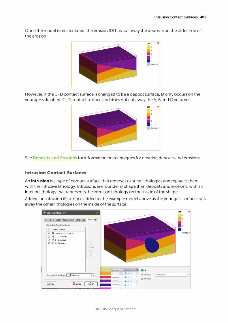
Intrusion Contact Surfaces | 409
Once themodel is recalculated, the erosion (D) has cut away the deposits on the older side ofthe erosion:
However, if the C-D contact surface is changed to be a deposit surface, D only occurs on theyounger side of the C-D contact surface and does not cut away the A, B and C volumes:
SeeDeposits and Erosions for information on techniques for creating deposits and erosions.
Intrusion Contact Surfaces
An intrusion is a type of contact surface that removes existing lithologies and replaces themwith the intrusive lithology. Intrusions are rounder in shape than deposits and erosions, with aninterior lithology that represents the intrusion lithology on the inside of the shape.
Adding an intrusion (E) surface added to the examplemodel above as the youngest surface cutsaway the other lithologies on the inside of the surface:
© 2019 Seequent Limited
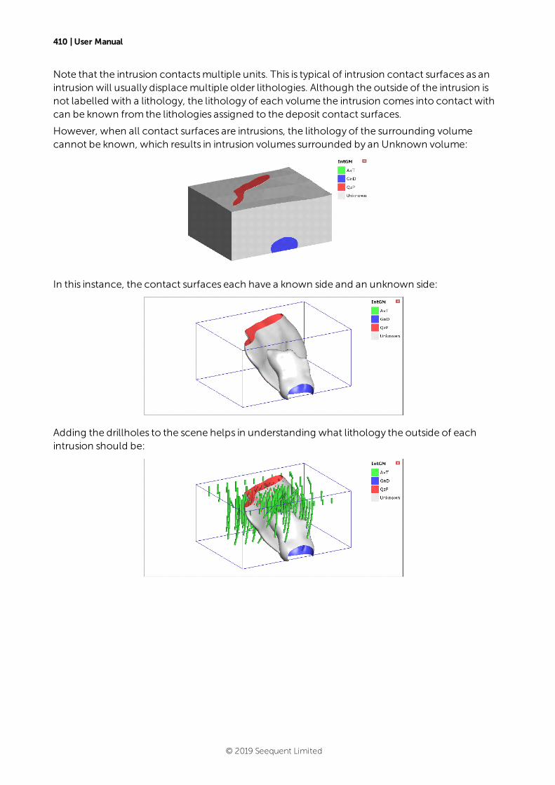
410 | User Manual
Note that the intrusion contactsmultiple units. This is typical of intrusion contact surfaces as anintrusion will usually displacemultiple older lithologies. Although the outside of the intrusion isnot labelled with a lithology, the lithology of each volume the intrusion comes into contact withcan be known from the lithologies assigned to the deposit contact surfaces.
However, when all contact surfaces are intrusions, the lithology of the surrounding volumecannot be known, which results in intrusion volumes surrounded by an Unknown volume:
In this instance, the contact surfaces each have a known side and an unknown side:
Adding the drillholes to the scene helps in understanding what lithology the outside of eachintrusion should be:
© 2019 Seequent Limited
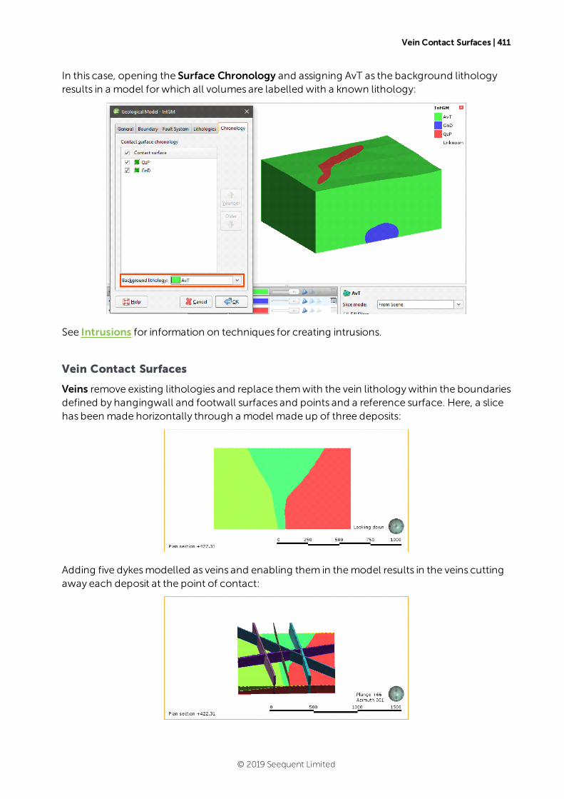
Vein Contact Surfaces | 411
In this case, opening the Surface Chronology and assigning AvT as the background lithologyresults in a model for which all volumes are labelled with a known lithology:
See Intrusions for information on techniques for creating intrusions.
Vein Contact Surfaces
Veins remove existing lithologies and replace themwith the vein lithologywithin the boundariesdefined by hangingwall and footwall surfaces and points and a reference surface. Here, a slicehas been made horizontally through a model made up of three deposits:
Adding five dykesmodelled as veins and enabling them in themodel results in the veins cuttingaway each deposit at the point of contact:
© 2019 Seequent Limited
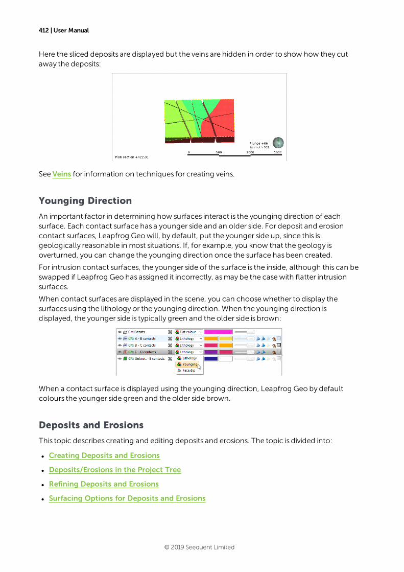
412 | User Manual
Here the sliced deposits are displayed but the veins are hidden in order to show how they cutaway the deposits:
See Veins for information on techniques for creating veins.
Younging Direction
An important factor in determining how surfaces interact is the younging direction of eachsurface. Each contact surface has a younger side and an older side. For deposit and erosioncontact surfaces, Leapfrog Geowill, by default, put the younger side up, since this isgeologically reasonable in most situations. If, for example, you know that the geology isoverturned, you can change the younging direction once the surface has been created.
For intrusion contact surfaces, the younger side of the surface is the inside, although this can beswapped if Leapfrog Geo has assigned it incorrectly, asmay be the casewith flatter intrusionsurfaces.
When contact surfaces are displayed in the scene, you can choosewhether to display thesurfaces using the lithology or the younging direction. When the younging direction isdisplayed, the younger side is typically green and the older side is brown:
When a contact surface is displayed using the younging direction, Leapfrog Geo by defaultcolours the younger side green and the older side brown.
Deposits and Erosions
This topic describes creating and editing deposits and erosions. The topic is divided into:
l Creating Deposits and Erosions
l Deposits/Erosions in the Project Tree
l Refining Deposits and Erosions
l Surfacing Options for Deposits and Erosions
© 2019 Seequent Limited
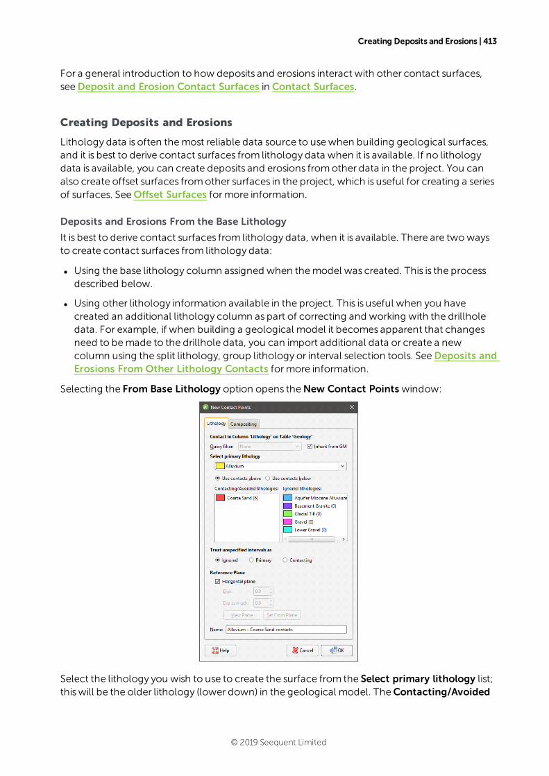
Creating Deposits and Erosions | 413
For a general introduction to how deposits and erosions interact with other contact surfaces,seeDeposit and Erosion Contact Surfaces in Contact Surfaces.
Creating Deposits and Erosions
Lithology data is often themost reliable data source to usewhen building geological surfaces,and it is best to derive contact surfaces from lithology data when it is available. If no lithologydata is available, you can create deposits and erosions fromother data in the project. You canalso create offset surfaces fromother surfaces in the project, which is useful for creating a seriesof surfaces. SeeOffset Surfaces formore information.
Deposits and Erosions From the Base Lithology
It is best to derive contact surfaces from lithology data, when it is available. There are twowaysto create contact surfaces from lithology data:
l Using the base lithology column assigned when themodel was created. This is the processdescribed below.
l Using other lithology information available in the project. This is useful when you havecreated an additional lithology column as part of correcting and working with the drillholedata. For example, if when building a geological model it becomes apparent that changesneed to bemade to the drillhole data, you can import additional data or create a newcolumn using the split lithology, group lithology or interval selection tools. SeeDeposits andErosions From Other Lithology Contacts formore information.
Selecting the From Base Lithology option opens theNew Contact Points window:
Select the lithology you wish to use to create the surface from the Select primary lithology list;thiswill be the older lithology (lower down) in the geological model. TheContacting/Avoided
© 2019 Seequent Limited
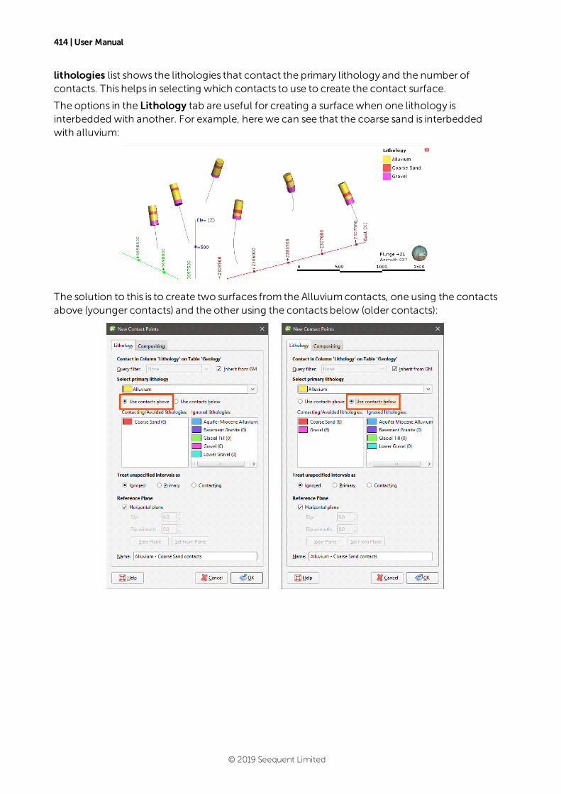
414 | User Manual
lithologies list shows the lithologies that contact the primary lithology and the number ofcontacts. This helps in selecting which contacts to use to create the contact surface.
The options in the Lithology tab are useful for creating a surfacewhen one lithology isinterbedded with another. For example, here we can see that the coarse sand is interbeddedwith alluvium:
The solution to this is to create two surfaces from the Alluviumcontacts, one using the contactsabove (younger contacts) and the other using the contacts below (older contacts):
© 2019 Seequent Limited
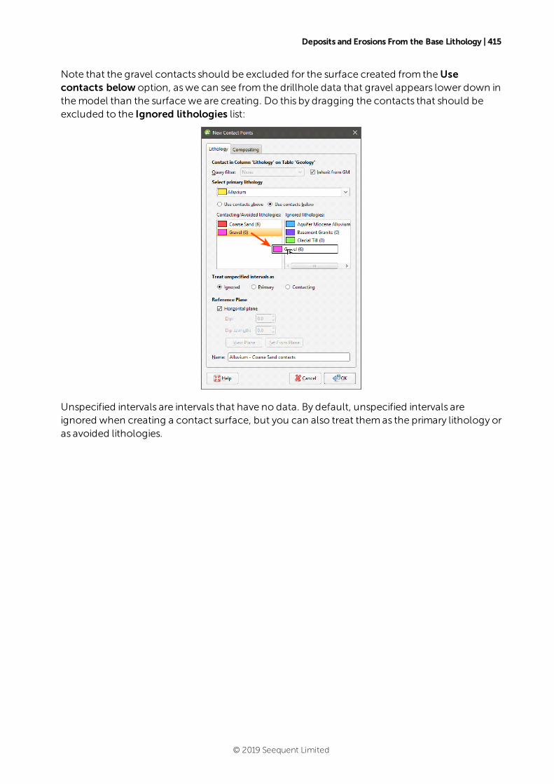
Deposits and Erosions From the Base Lithology | 415
Note that the gravel contacts should be excluded for the surface created from theUsecontacts below option, aswe can see from the drillhole data that gravel appears lower down inthemodel than the surfacewe are creating. Do this by dragging the contacts that should beexcluded to the Ignored lithologies list:
Unspecified intervals are intervals that have no data. By default, unspecified intervals areignored when creating a contact surface, but you can also treat themas the primary lithology oras avoided lithologies.
© 2019 Seequent Limited
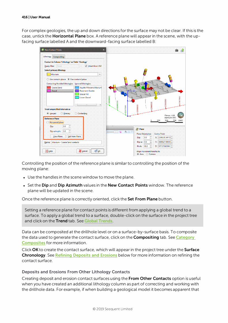
416 | User Manual
For complex geologies, the up and down directions for the surfacemay not be clear. If this is thecase, untick theHorizontal Plane box. A reference planewill appear in the scene, with the up-facing surface labelled A and the downward-facing surface labelled B:
Controlling the position of the reference plane is similar to controlling the position of themoving plane:
l Use the handles in the scenewindow tomove the plane.
l Set theDip and Dip Azimuth values in theNew Contact Points window. The referenceplanewill be updated in the scene.
Once the reference plane is correctly oriented, click the Set From Plane button.
Setting a reference plane for contact points is different fromapplying a global trend to asurface. To apply a global trend to a surface, double-click on the surface in the project treeand click on the Trend tab. SeeGlobal Trends.
Data can be composited at the drillhole level or on a surface-by-surface basis. To compositethe data used to generate the contact surface, click on theCompositing tab. SeeCategoryComposites formore information.
ClickOK to create the contact surface, which will appear in the project tree under the SurfaceChronology. SeeRefining Deposits and Erosions below formore information on refining thecontact surface.
Deposits and Erosions From Other Lithology Contacts
Creating deposit and erosion contact surfaces using the From Other Contacts option is usefulwhen you have created an additional lithology column as part of correcting and working withthe drillhole data. For example, if when building a geological model it becomes apparent that
© 2019 Seequent Limited
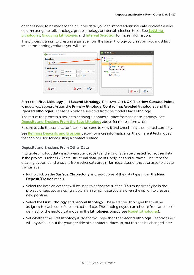
Deposits and Erosions From Other Data | 417
changes need to bemade to the drillhole data, you can import additional data or create a newcolumn using the split lithology, group lithology or interval selection tools. See SplittingLithologies, Grouping Lithologies and Interval Selection formore information.
The process is similar to creating a surface from the base lithology column, but you must firstselect the lithology column you will use:
Select the First Lithology and Second Lithology, if known. ClickOK. TheNew Contact Pointswindowwill appear. Assign the Primary lithology, Contacting/Avoided lithologies and theIgnored lithologies. These can only be selected from themodel’s base lithology.
The rest of the process is similar to defining a contact surface from the base lithology. SeeDeposits and Erosions From the Base Lithology above formore information.
Be sure to add the contact surface to the scene to view it and check that it is oriented correctly.
SeeRefining Deposits and Erosions below formore information on the different techniquesthat can be used for adjusting a contact surface.
Deposits and Erosions From Other Data
If suitable lithology data is not available, deposits and erosions can be created fromother datain the project, such asGIS data, structural data, points, polylines and surfaces. The steps forcreating deposits and erosions fromother data are similar, regardless of the data used to createthe surface:
l Right-click on the Surface Chronology and select one of the data types from theNewDeposit/Erosionmenu.
l Select the data object that will be used to define the surface. Thismust already be in theproject, unless you are using a polyline, in which case you are given the option to create anew polyline.
l Select the First lithology and Second lithology. These are the lithologies that will beassigned to each side of the contact surface. The lithologies you can choose fromare thosedefined for the geological model in the Lithologies object (seeModel Lithologies).
l Set whether the First lithology is older or younger than the Second lithology. Leapfrog Geowill, by default, put the younger side of a contact surface up, but this can be changed later.
© 2019 Seequent Limited

418 | User Manual
Here, a points data object is being used to create a deposit:
For polylines, you first set the lithologies and the younging order:
ClickOK tomove on to the next step:
You can draw the polyline in the scene directly by selecting theNew Drawing option. You canalso use any polyline in the project by selecting the Existing Polyline option. You can thenselect the required polyline from the list.
The new contact surfacewill appear in the project tree under the Surface Chronology. Add thecontact surface to the scene to view it and check that it is oriented correctly.
Expand the surface in the project tree to see how it wasmade. Here, a number of surfaces havebeen created using different types of data:
If creating a surface froma new polyline, the polyline will not be able to be used elsewhere inthe project unless it has been shared. To share the polyline, expand the contact surface in theproject tree, right-click on the polyline and select Share. The polyline will then be availableelsewhere in the project.
© 2019 Seequent Limited
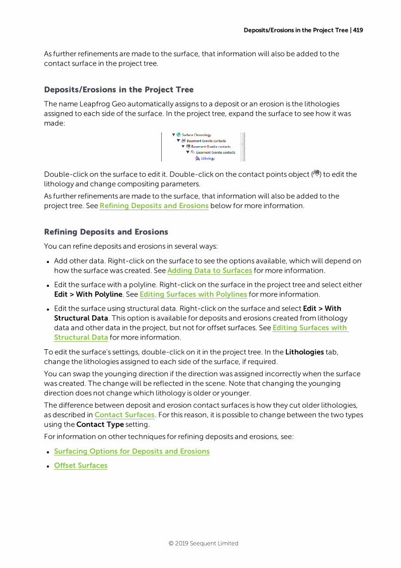
Deposits/Erosions in the Project Tree | 419
As further refinements aremade to the surface, that information will also be added to thecontact surface in the project tree.
Deposits/Erosions in the Project Tree
The name Leapfrog Geo automatically assigns to a deposit or an erosion is the lithologiesassigned to each side of the surface. In the project tree, expand the surface to see how it wasmade:
Double-click on the surface to edit it. Double-click on the contact points object ( ) to edit thelithology and change compositing parameters.
As further refinements aremade to the surface, that information will also be added to theproject tree. SeeRefining Deposits and Erosions below formore information.
Refining Deposits and Erosions
You can refine deposits and erosions in several ways:
l Add other data. Right-click on the surface to see the options available, which will depend onhow the surfacewas created. See Adding Data to Surfaces formore information.
l Edit the surfacewith a polyline. Right-click on the surface in the project tree and select eitherEdit > With Polyline. See Editing Surfaces with Polylines formore information.
l Edit the surface using structural data. Right-click on the surface and select Edit > WithStructural Data. This option is available for deposits and erosions created from lithologydata and other data in the project, but not for offset surfaces. See Editing Surfaces withStructural Data formore information.
To edit the surface’s settings, double-click on it in the project tree. In the Lithologies tab,change the lithologies assigned to each side of the surface, if required.
You can swap the younging direction if the direction was assigned incorrectlywhen the surfacewas created. The changewill be reflected in the scene. Note that changing the youngingdirection does not changewhich lithology is older or younger.
The difference between deposit and erosion contact surfaces is how they cut older lithologies,as described in Contact Surfaces. For this reason, it is possible to change between the two typesusing theContact Type setting.
For information on other techniques for refining deposits and erosions, see:
l Surfacing Options for Deposits and Erosions
l Offset Surfaces
© 2019 Seequent Limited
420 | User Manual
Surfacing Options for Deposits and Erosions
Surfacing options for deposits and erosions can be changed by double-clicking on the surfacein the project tree and then clicking on the Surfacing tab. There are additional settings relatedto boundary filtering and snapping to data in the Inputs tab.
Boundary Filtering
When data objects are added to a surface, there are twoways to handle the data that liesoutside the surface’s boundary:
l Filter the data. The surface is only influenced by the data that falls inside the surface’sboundary.
l Leave the data unfiltered. The surface is influenced by the data both inside and outside thesurface’s boundary.
The Boundary filter setting determines how data used to define the surface is filtered:
l Off. Data is not filtered.
l All data. All data is filtered.
l Drilling only. Only drillhole data and data objects derived fromdrillhole data are filtered.
l Custom. Only the data objects specified in the Inputs tab are filtered.
Snapping to Data
Often, surfaces should honour drillhole data and treat data objects such as polylines and GISdata as interpretations. SeeHonouring Surface Contacts.
There is a Snap to data setting for a geological model as a whole that is set in theGeologicalModel > General tab (see Editing a Geological Model). Snap to data can also be set on asurface-by-surface basis by double-clicking on the surface in the project tree and then clickingon the Surfacing tab.
For individual contact surfaces, the options are:
l Inherit from GM. The setting for the geological model as a whole is used. This is the defaultsetting.
l Off. Surfaces do not snap to the data used to create them.
l All data. Surfaces snap to all data within theMaximum snap distance, which includesdrillhole data and any data added to the surfaces.
l Drilling only. Surfaces snap to drillhole data and data objects derived fromdrillhole datawithin theMaximum snap distance but not to other data used tomodify the surfaces.
l Custom. Surfaces snap to the data objects indicated in the Inputs tab for each surface.
Take care in enabling snapping and in selecting what data the surfacewill snap to, as themore data you include, e.g. by setting a largeMaximum snap distance or selecting All datafor Snap to data, the greater the possibility that errors in the data or assumptions inherent in
© 2019 Seequent Limited
Setting the Surface Resolution | 421
interpretations (e.g. polylines) will cause distortions in themeshes. If you do enable snapping,it is best to snap only to drilling data. SeeHonouring Surface Contacts formore informationon these settings.
If you need a surface to honour drillhole data but treat other data objects as interpretations,selectDrilling only. To honour some data objectswhile treating others as interpretations, selectCustom, then click on the Inputs tab to enable snapping for individual objects.
Setting the Surface Resolution
See Surface Resolution for a Geological Model for information about the surface resolutionsettings in the Surfacing tab.
Applying a Trend to a Deposit/Erosion
There are twoways to change the trend for a deposit or an erosion:
l Right-click on the surface in the project tree and select Adjust Surface.
l Double-click on the surface in the project tree and then click on the Trend tab.
SeeGlobal Trends formore information.
Intrusions
This topic describes creating and editing intrusions. The topic is divided into:
l Creating Intrusions
l Intrusions in the Project Tree
l Displaying Intrusion Points
l Refining Intrusions
l Surfacing Options for Intrusions
l Applying a Trend to an Intrusion
l Clipping Values for Intrusions
l Interpolation Settings
© 2019 Seequent Limited
422 | User Manual
For a general introduction to how intrusions interact with other contact surfaces, see IntrusionContact Surfaces in Contact Surfaces.
Creating Intrusions
Lithology data is often themost reliable data source to usewhen building geological surfaces,and it is best to derive contact surfaces from lithology data when it is available. If no lithologydata is available, you can create intrusions fromother data in the project.
One thing to keep in mind for all intrusion contact surfaces is that an intrusion removes all theexisting material on the younger side of the contact surface. Therefore:
l An intrusion should always have the younger side of its surface labelled with the intrudedmaterial. This is called the “interior lithology”.
l The older side will typically be labelled “Unknown” as an intrusion will usually displacemultiple older lithologies. This is called the “exterior lithology”.
Intrusions from Lithology Contacts
Lithology data is often themost reliable data source to usewhen building geological surfaces,and it is best to derive contact surfaces from lithology data when it is available. There are twoways to create intrusions from lithology data:
l Using the base lithology column assigned when themodel was created.
l Using other lithology information available in the project. This is useful when you havecreated an additional lithology column as part of correcting and working with the drillholedata. For example, if when building a geological model it becomes apparent that changesneed to bemade to the drillhole data, you can import additional data or create a newcolumn using the split lithology, group lithology or interval selection tools.
To create a new intrusion from lithology contacts, right-click on the Surface Chronologyobject and select eitherNew Intrusion > From Base Lithology orNew Intrusion > From OtherContacts. The only difference in the twomethods is that when creating an intrusion fromothercontacts, you must first select the lithology column from those available in the project andspecify the First lithology and the Second lithology.
© 2019 Seequent Limited
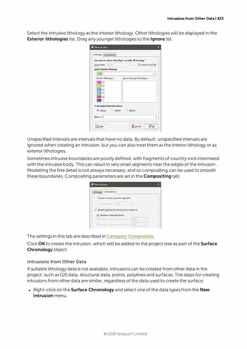
Intrusions from Other Data | 423
Select the intrusive lithology as the interior lithology. Other lithologieswill be displayed in theExterior lithologies list. Drag any younger lithologies to the Ignore list.
Unspecified intervals are intervals that have no data. By default, unspecified intervals areignored when creating an intrusion, but you can also treat themas the interior lithology or asexterior lithologies.
Sometimes intrusive boundaries are poorly defined, with fragments of country rock intermixedwith the intrusive body. This can result in very small segments near the edges of the intrusion.Modelling the fine detail is not always necessary, and so compositing can be used to smooththese boundaries. Compositing parameters are set in theCompositing tab:
The settings in this tab are described in Category Composites.
ClickOK to create the intrusion, which will be added to the project tree as part of the SurfaceChronology object.
Intrusions from Other Data
If suitable lithology data is not available, intrusions can be created fromother data in theproject, such asGIS data, structural data, points, polylines and surfaces. The steps for creatingintrusions fromother data are similar, regardless of the data used to create the surface:
l Right-click on the Surface Chronology and select one of the data types from theNewIntrusionmenu.
© 2019 Seequent Limited
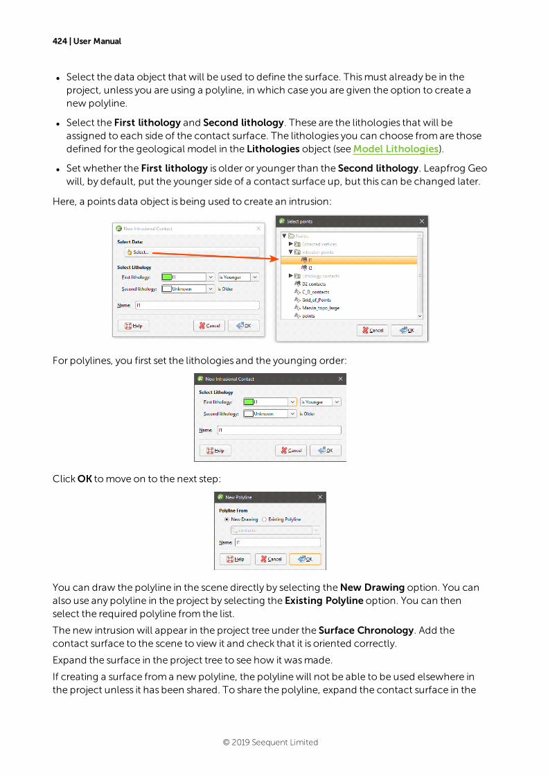
424 | User Manual
l Select the data object that will be used to define the surface. Thismust already be in theproject, unless you are using a polyline, in which case you are given the option to create anew polyline.
l Select the First lithology and Second lithology. These are the lithologies that will beassigned to each side of the contact surface. The lithologies you can choose fromare thosedefined for the geological model in the Lithologies object (seeModel Lithologies).
l Set whether the First lithology is older or younger than the Second lithology. Leapfrog Geowill, by default, put the younger side of a contact surface up, but this can be changed later.
Here, a points data object is being used to create an intrusion:
For polylines, you first set the lithologies and the younging order:
ClickOK tomove on to the next step:
You can draw the polyline in the scene directly by selecting theNew Drawing option. You canalso use any polyline in the project by selecting the Existing Polyline option. You can thenselect the required polyline from the list.
The new intrusion will appear in the project tree under the Surface Chronology. Add thecontact surface to the scene to view it and check that it is oriented correctly.
Expand the surface in the project tree to see how it wasmade.
If creating a surface froma new polyline, the polyline will not be able to be used elsewhere inthe project unless it has been shared. To share the polyline, expand the contact surface in the
© 2019 Seequent Limited

Intrusions in the Project Tree | 425
project tree, right-click on the polyline and select Share. The polyline will then be availableelsewhere in the project.
As further refinements aremade to the surface, that information will also be added to thecontact surface in the project tree.
Intrusions in the Project Tree
The name Leapfrog Geo automatically assigns to an intrusion is the name of the intrusivelithology. In the project tee, expand the intrusion to see how it wasmade:
Double-click on the intrusion to edit it. Double-click on the points object ( ) to edit theintrusion lithology, change compositing parameters and change point generation options.
As further refinements aremade to the surface, that information will also be added to theproject tree. SeeRefining Intrusions below formore information.
Displaying Intrusion Points
When you view the intrusion points in the scene, you can display only the contact points or allthe points used in creating the intrusion. To display all points, click on the points object ( ) inthe shape list and tick the box for Show volume points. Here, only the contact points aredisplayed:
© 2019 Seequent Limited
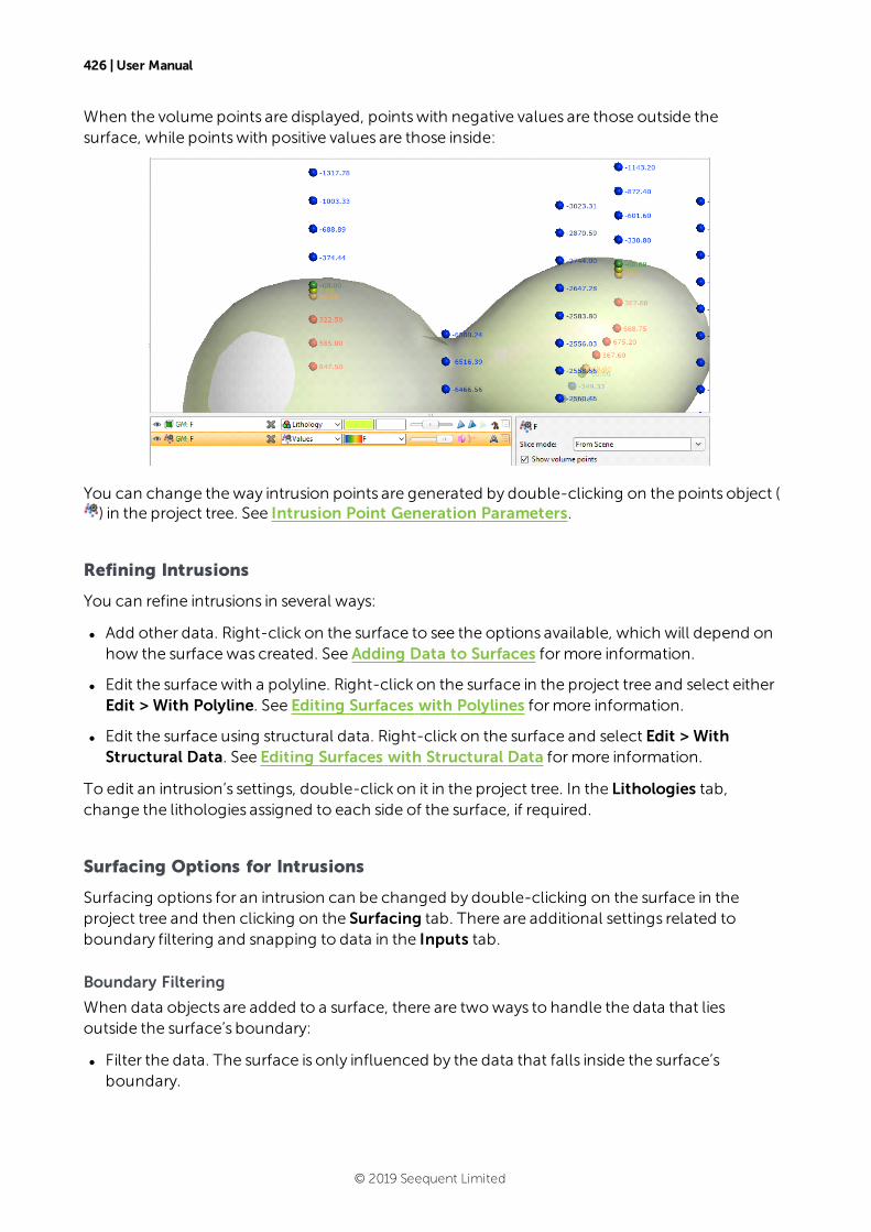
426 | User Manual
When the volume points are displayed, pointswith negative values are those outside thesurface, while pointswith positive values are those inside:
You can change theway intrusion points are generated by double-clicking on the points object () in the project tree. See Intrusion Point Generation Parameters.
Refining Intrusions
You can refine intrusions in several ways:
l Add other data. Right-click on the surface to see the options available, which will depend onhow the surfacewas created. See Adding Data to Surfaces formore information.
l Edit the surfacewith a polyline. Right-click on the surface in the project tree and select eitherEdit > With Polyline. See Editing Surfaces with Polylines formore information.
l Edit the surface using structural data. Right-click on the surface and select Edit > WithStructural Data. See Editing Surfaces with Structural Data formore information.
To edit an intrusion’s settings, double-click on it in the project tree. In the Lithologies tab,change the lithologies assigned to each side of the surface, if required.
Surfacing Options for Intrusions
Surfacing options for an intrusion can be changed by double-clicking on the surface in theproject tree and then clicking on the Surfacing tab. There are additional settings related toboundary filtering and snapping to data in the Inputs tab.
Boundary Filtering
When data objects are added to a surface, there are twoways to handle the data that liesoutside the surface’s boundary:
l Filter the data. The surface is only influenced by the data that falls inside the surface’sboundary.
© 2019 Seequent Limited
Snapping to Data | 427
l Leave the data unfiltered. The surface is influenced by the data both inside and outside thesurface’s boundary.
The boundary of an intrusion can be the geological model boundary or a fault block boundary.
The Boundary filter setting determines how data used to define the surface is filtered:
l Off. Data is not filtered.
l All data. All data is filtered.
l Drilling only. Only drillhole data and data objects derived fromdrillhole data are filtered.
l Custom. Only the data objects specified in the Inputs tab are filtered.
Snapping to Data
Often, surfaces should honour drillhole data and treat data objects such as polylines and GISdata as interpretations, as discussed in Honouring Surface Contacts.
There is a Snap to data setting for a geological model as a whole that is set in theGeologicalModel > General tab (see Editing a Geological Model). Snap to data can also be set on asurface-by-surface basis by double-clicking on the surface in the project tree and then clickingon the Surfacing tab.
For individual contact surfaces, the options are:
l Inherit from GM. The setting for the geological model as a whole is used. This is the defaultsetting.
l Off. Surfaces do not snap to the data used to create them.
l All data. Surfaces snap to all data within theMaximum snap distance, which includesdrillhole data and any data added to the surfaces.
l Drilling only. Surfaces snap to drillhole data and data objects derived fromdrillhole datawithin theMaximum snap distance but not to other data used tomodify the surfaces.
l Custom. Surfaces snap to the data objects indicated in the Inputs tab for each surface.
Take care in enabling snapping and in selecting what data the surfacewill snap to, as themore data you include, e.g. by setting a largeMaximum snap distance or selecting All datafor Snap to data, the greater the possibility that errors in the data or assumptions inherent ininterpretations (e.g. polylines) will cause distortions in themeshes. If you do enable snapping,it is best to snap only to drilling data. SeeHonouring Surface Contacts formore informationon these settings.
If you need a surface to honour drillhole data but treat other data objects as interpretations,selectDrilling only. To honour some data objectswhile treating others as interpretations, selectCustom, then click on the Inputs tab to enable snapping for individual objects.
Surface Resolution
See Surface Resolution for a Geological Model for information about the surface resolutionsettings in the Surfacing tab.
© 2019 Seequent Limited
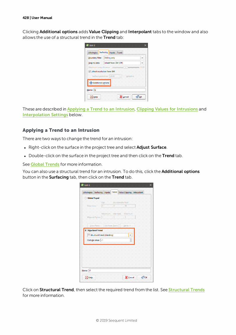
428 | User Manual
Clicking Additional options addsValue Clipping and Interpolant tabs to thewindow and alsoallows the use of a structural trend in the Trend tab:
These are described in Applying a Trend to an Intrusion, Clipping Values for Intrusions andInterpolation Settings below.
Applying a Trend to an Intrusion
There are twoways to change the trend for an intrusion:
l Right-click on the surface in the project tree and select Adjust Surface.
l Double-click on the surface in the project tree and then click on the Trend tab.
SeeGlobal Trends formore information.
You can also use a structural trend for an intrusion. To do this, click the Additional optionsbutton in the Surfacing tab, then click on the Trend tab.
Click on Structural Trend, then select the required trend from the list. See Structural Trendsformore information.
© 2019 Seequent Limited
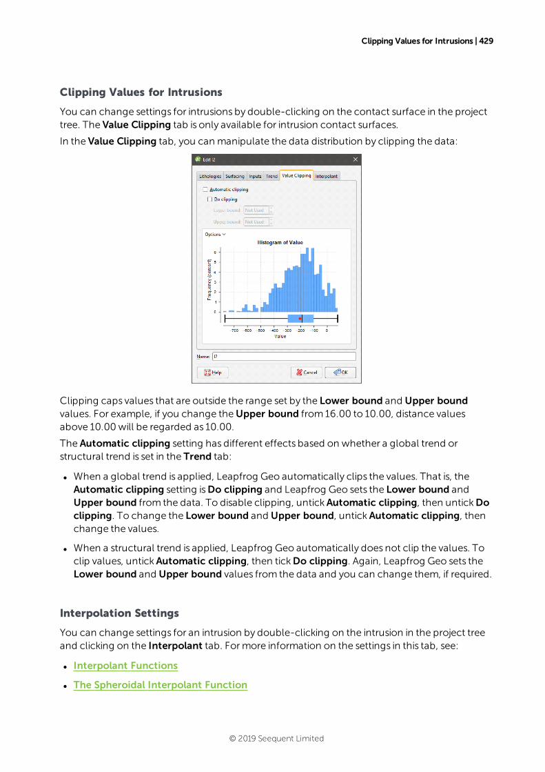
Clipping Values for Intrusions | 429
Clipping Values for Intrusions
You can change settings for intrusions by double-clicking on the contact surface in the projecttree. The Value Clipping tab is only available for intrusion contact surfaces.
In the Value Clipping tab, you can manipulate the data distribution by clipping the data:
Clipping caps values that are outside the range set by the Lower bound and Upper boundvalues. For example, if you change theUpper bound from16.00 to 10.00, distance valuesabove 10.00will be regarded as 10.00.
The Automatic clipping setting has different effects based on whether a global trend orstructural trend is set in the Trend tab:
l When a global trend is applied, Leapfrog Geo automatically clips the values. That is, theAutomatic clipping setting isDo clipping and Leapfrog Geo sets the Lower bound andUpper bound from the data. To disable clipping, untickAutomatic clipping, then untickDoclipping. To change the Lower bound and Upper bound, untickAutomatic clipping, thenchange the values.
l When a structural trend is applied, Leapfrog Geo automatically does not clip the values. Toclip values, untickAutomatic clipping, then tickDo clipping. Again, Leapfrog Geo sets theLower bound and Upper bound values from the data and you can change them, if required.
Interpolation Settings
You can change settings for an intrusion by double-clicking on the intrusion in the project treeand clicking on the Interpolant tab. Formore information on the settings in this tab, see:
l Interpolant Functions
l The Spheroidal Interpolant Function
© 2019 Seequent Limited
430 | User Manual
l The Linear Interpolant Function
Veins
This topic describes creating and editing veins. It is divided into:
l Creating Veins
l Veins in the Project Tree
l Displaying Veins
l Refining Veins
l Surfacing Options for Veins
l The Vein Reference Surface
l The Vein Boundary
l Editing Vein Segments
For a general introduction to how veins interact with other contact surfaces, see Vein ContactSurfaces in Contact Surfaces.
A vein is a type of contact surface that removes existing lithologies and replaces themwith thevein lithologywithin the boundaries defined by hangingwall and footwall surfaces constructedfrom selected input data. A reference surface is defined that is the best fit for the hangingwalland footwall surfaces. The reference surface can be curved or planar.
Creating Veins
Options for creating veins are:
l From lithology data, using the base lithology used to define the geological model or othercontacts available in the project. See Veins From Lithology Contacts below.
l FromGIS vector data, point data and polylines. See Veins From Other Data below.
l Creating a vein system. This results in a single lithology that represents all the veins in amodel. Veins and their interactions are defined within the vein system. See Vein Systems.
Veins From Lithology Contacts
To create a new vein from lithology contacts, right-click on the Surface Chronology object andselect eitherNew Vein > From Base Lithology orNew Vein > From Other Contacts. The onlydifference in the twomethods is that when creating a vein fromother contacts, you must firstselect the lithology column from those available in the project and specify the Vein lithologyand Outside lithology.
© 2019 Seequent Limited
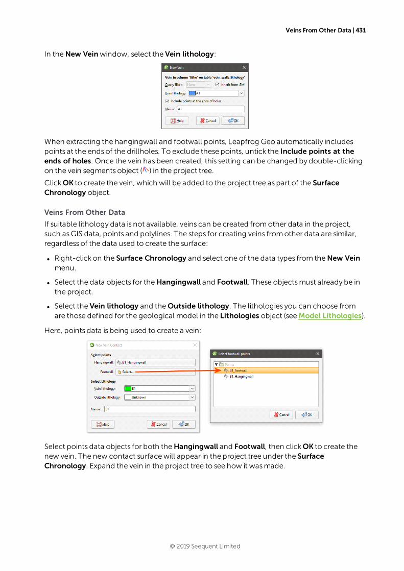
Veins From Other Data | 431
In theNew Veinwindow, select the Vein lithology:
When extracting the hangingwall and footwall points, Leapfrog Geo automatically includespoints at the ends of the drillholes. To exclude these points, untick the Include points at theends of holes. Once the vein has been created, this setting can be changed by double-clickingon the vein segments object ( ) in the project tree.
ClickOK to create the vein, which will be added to the project tree as part of the SurfaceChronology object.
Veins From Other Data
If suitable lithology data is not available, veins can be created fromother data in the project,such asGIS data, points and polylines. The steps for creating veins fromother data are similar,regardless of the data used to create the surface:
l Right-click on the Surface Chronology and select one of the data types from theNew Veinmenu.
l Select the data objects for theHangingwall and Footwall. These objectsmust already be inthe project.
l Select the Vein lithology and theOutside lithology. The lithologies you can choose fromare those defined for the geological model in the Lithologies object (seeModel Lithologies).
Here, points data is being used to create a vein:
Select points data objects for both theHangingwall and Footwall, then clickOK to create thenew vein. The new contact surfacewill appear in the project tree under the SurfaceChronology. Expand the vein in the project tree to see how it wasmade.
© 2019 Seequent Limited
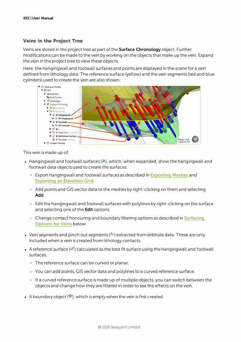
432 | User Manual
Veins in the Project Tree
Veins are stored in the project tree as part of the Surface Chronology object. Furthermodifications can bemade to the vein byworking on the objects that make up the vein. Expandthe vein in the project tree to view these objects.
Here, the hangingwall and footwall surfaces and points are displayed in the scene for a veindefined from lithology data. The reference surface (yellow) and the vein segments (red and bluecylinders) used to create the vein are also shown:
This vein ismade up of:
l Hangingwall and footwall surfaces ( ), which, when expanded, show the hangingwall andfootwall data objects used to create the surfaces.
o Export hangingwall and footwall surfaces as described in Exporting Meshes andExporting an Elevation Grid.
o Add points and GIS vector data to themeshes by right-clicking on themand selectingAdd.
o Edit the hangingwall and footwall surfaceswith polylines by right-clicking on the surfaceand selecting one of the Edit options.
o Change contact honouring and boundary filtering options as described in SurfacingOptions for Veins below.
l Vein segments and pinch out segments ( ) extracted fromdrillhole data. These are onlyincluded when a vein is created from lithology contacts.
l A reference surface ( ) calculated as the best fit surface using the hangingwall and footwallsurfaces.
o The reference surface can be curved or planar.
o You can add points, GIS vector data and polylines to a curved reference surface.
o If a curved reference surface ismade up of multiple objects, you can switch between theobjects and change how they are filtered in order to see the effects on the vein.
l A boundary object ( ), which is emptywhen the vein is first created.
© 2019 Seequent Limited
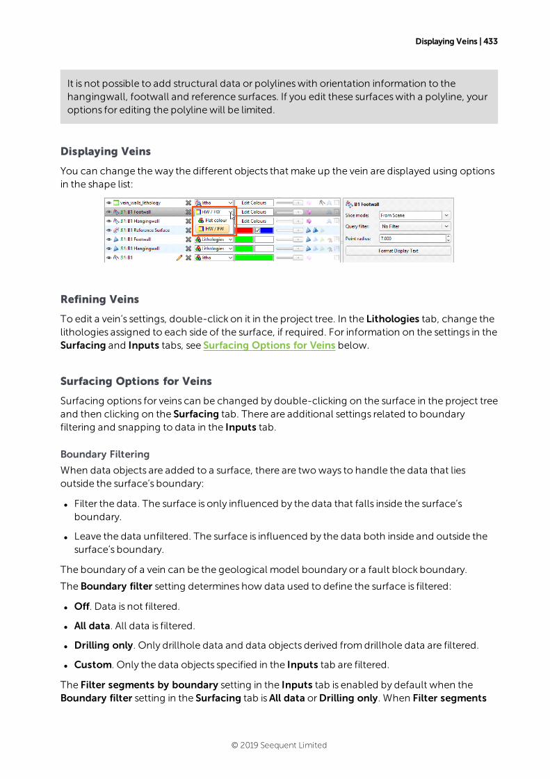
Displaying Veins | 433
It is not possible to add structural data or polylineswith orientation information to thehangingwall, footwall and reference surfaces. If you edit these surfaceswith a polyline, youroptions for editing the polyline will be limited.
Displaying Veins
You can change theway the different objects that make up the vein are displayed using optionsin the shape list:
Refining Veins
To edit a vein’s settings, double-click on it in the project tree. In the Lithologies tab, change thelithologies assigned to each side of the surface, if required. For information on the settings in theSurfacing and Inputs tabs, see Surfacing Options for Veins below.
Surfacing Options for Veins
Surfacing options for veins can be changed by double-clicking on the surface in the project treeand then clicking on the Surfacing tab. There are additional settings related to boundaryfiltering and snapping to data in the Inputs tab.
Boundary Filtering
When data objects are added to a surface, there are twoways to handle the data that liesoutside the surface’s boundary:
l Filter the data. The surface is only influenced by the data that falls inside the surface’sboundary.
l Leave the data unfiltered. The surface is influenced by the data both inside and outside thesurface’s boundary.
The boundary of a vein can be the geological model boundary or a fault block boundary.
The Boundary filter setting determines how data used to define the surface is filtered:
l Off. Data is not filtered.
l All data. All data is filtered.
l Drilling only. Only drillhole data and data objects derived fromdrillhole data are filtered.
l Custom. Only the data objects specified in the Inputs tab are filtered.
The Filter segments by boundary setting in the Inputs tab is enabled by default when theBoundary filter setting in the Surfacing tab isAll data orDrilling only. When Filter segments
© 2019 Seequent Limited

434 | User Manual
by boundary is enabled, the vein surfacewill only be influenced by the segments that fallsinside the vein boundary.
Snapping to Data
Often, surfaces should honour drillhole data and treat data objects such as polylines and GISdata as interpretations, as discussed in Honouring Surface Contacts.
There is a Snap to data setting for a geological model as a whole that is set in theGeologicalModel > General tab (see Editing a Geological Model). Snap to data can also be set on asurface-by-surface basis by double-clicking on the surface in the project tree and then clickingon the Surfacing tab.
For individual contact surfaces, the options are:
l Inherit from GM. The setting for the geological model as a whole is used. This is the defaultsetting.
l Off. Surfaces do not snap to the data used to create them.
l All data. Surfaces snap to all data within theMaximum snap distance, which includesdrillhole data and any data added to the surfaces.
l Drilling only. Surfaces snap to drillhole data and data objects derived fromdrillhole datawithin theMaximum snap distance but not to other data used tomodify the surfaces.
l Custom. Surfaces snap to the data objects indicated in the Inputs tab for each surface.
Take care in enabling snapping and in selecting what data the surfacewill snap to, as themore data you include, e.g. by setting a largeMaximum snap distance or selecting All datafor Snap to data, the greater the possibility that errors in the data or assumptions inherent ininterpretations (e.g. polylines) will cause distortions in themeshes. If you do enable snapping,it is best to snap only to drilling data. SeeHonouring Surface Contacts formore informationon these settings.
If you need a surface to honour drillhole data but treat other data objects as interpretations,selectDrilling only. To honour some data objectswhile treating others as interpretations, selectCustom, then click on the Inputs tab to enable snapping for individual objects.
Surface Resolution
Note that although you can change the Surface resolution for a vein, the Adaptive option isnot available, even when the resolution for the geological model is set to be Adaptive.
Vein Thickness
Veins have two thickness settings that force the vein tomaintain a minimumormaximumthickness. If footwall and hangingwall points are in pairs, it is not usually necessary to set theMinimum thickness orMaximum thickness.
l If the vein intersects itself, set theMinimum thickness to a value that is less than theminimumdistance between any two contact points.
l If the vein widens out toward the edges of the geological model set theMaximum thicknessto a value that limits the effects of long segments.
© 2019 Seequent Limited

Vein Pinch Out | 435
If the Pinch out option is enabled, you will not be able to set theMinimum thickness.
If you set theMaximum thickness and Pinch out, the Pinch out is applied before theMaximumthickness.
Note that if Snap to data is enabled, snapping occurs after the vein thickness has beencalculated. If it appears that the vein surface is not honouring the thickness setting, checkwhat data the surface is snapping to.
Vein Pinch Out
Vein walls can be set to pinch out where drillhole data indicates they do not occur. This isachieved by creating ‘outside’ intervals on drillholes that do not have an interior vein segment.These intervals are then flipped with respect to interior vein intervals, which, in effect means thefootwall and hangingwall orientation has the opposite sense to the nearest interior intervals.This forces the hangingwall and footwall surfaces to cross, thereby pinching out.
The Pinch out option is disabled when a vein is first created. To enable it, double-click on thevein in the project tree and click on the Surfacing tab. Tick the box for Pinch out. ClickOK toprocess the changes. The vein will be updated and pinch out points ( ) will be added to thevein in the project tree.
For this vein, the surface occurs even where the vein lithology (green cylinders) does not occurand terminates at the boundary of the geological model:
When the vein is set to pinch out, it tapers out where the vein lithology does not occur:
© 2019 Seequent Limited
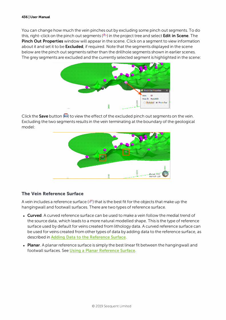
436 | User Manual
You can change howmuch the vein pinches out by excluding some pinch out segments. To dothis, right-click on the pinch out segments ( ) in the project tree and select Edit in Scene. ThePinch Out Properties windowwill appear in the scene. Click on a segment to view informationabout it and set it to be Excluded, if required. Note that the segments displayed in the scenebelow are the pinch out segments rather than the drillhole segments shown in earlier scenes.The grey segments are excluded and the currently selected segment is highlighted in the scene:
Click the Save button ( ) to view the effect of the excluded pinch out segments on the vein.Excluding the two segments results in the vein terminating at the boundary of the geologicalmodel:
The Vein Reference Surface
A vein includes a reference surface ( ) that is the best fit for the objects that make up thehangingwall and footwall surfaces. There are two types of reference surface.
l Curved. A curved reference surface can be used tomake a vein follow themedial trend ofthe source data, which leads to a more natural modelled shape. This is the type of referencesurface used by default for veins created from lithology data. A curved reference surface canbe used for veins created fromother types of data by adding data to the reference surface, asdescribed in Adding Data to the Reference Surface.
l Planar. A planar reference surface is simply the best linear fit between the hangingwall andfootwall surfaces. SeeUsing a Planar Reference Surface.
© 2019 Seequent Limited
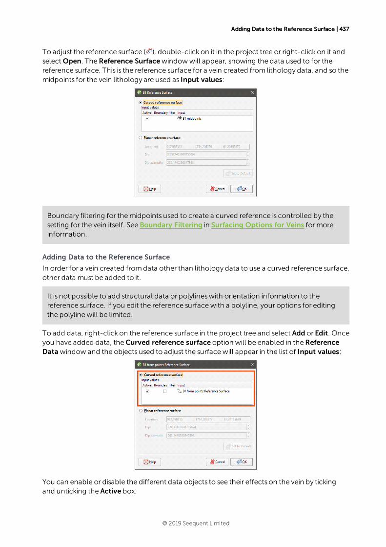
Adding Data to the Reference Surface | 437
To adjust the reference surface ( ), double-click on it in the project tree or right-click on it andselectOpen. TheReference Surfacewindowwill appear, showing the data used to for thereference surface. This is the reference surface for a vein created from lithology data, and so themidpoints for the vein lithology are used as Input values:
Boundary filtering for themidpoints used to create a curved reference is controlled by thesetting for the vein itself. See Boundary Filtering in Surfacing Options for Veins formoreinformation.
Adding Data to the Reference Surface
In order for a vein created fromdata other than lithology data to use a curved reference surface,other data must be added to it.
It is not possible to add structural data or polylineswith orientation information to thereference surface. If you edit the reference surfacewith a polyline, your options for editingthe polyline will be limited.
To add data, right-click on the reference surface in the project tree and select Add or Edit. Onceyou have added data, theCurved reference surface option will be enabled in theReferenceDatawindow and the objects used to adjust the surfacewill appear in the list of Input values:
You can enable or disable the different data objects to see their effects on the vein by tickingand unticking the Active box.
© 2019 Seequent Limited
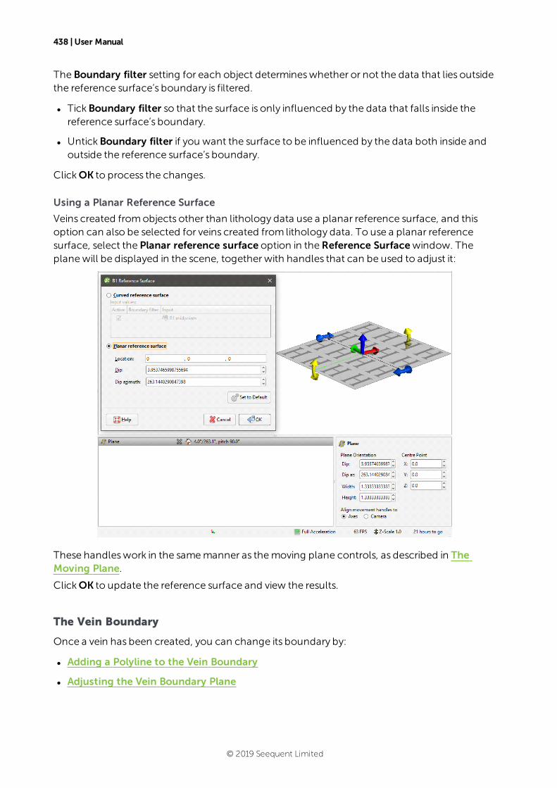
438 | User Manual
The Boundary filter setting for each object determineswhether or not the data that lies outsidethe reference surface’s boundary is filtered.
l TickBoundary filter so that the surface is only influenced by the data that falls inside thereference surface’s boundary.
l UntickBoundary filter if you want the surface to be influenced by the data both inside andoutside the reference surface’s boundary.
ClickOK to process the changes.
Using a Planar Reference Surface
Veins created fromobjects other than lithology data use a planar reference surface, and thisoption can also be selected for veins created from lithology data. To use a planar referencesurface, select the Planar reference surface option in theReference Surfacewindow. Theplanewill be displayed in the scene, together with handles that can be used to adjust it:
These handleswork in the samemanner as themoving plane controls, as described in TheMoving Plane.
ClickOK to update the reference surface and view the results.
The Vein Boundary
Once a vein has been created, you can change its boundary by:
l Adding a Polyline to the Vein Boundary
l Adjusting the Vein Boundary Plane
© 2019 Seequent Limited
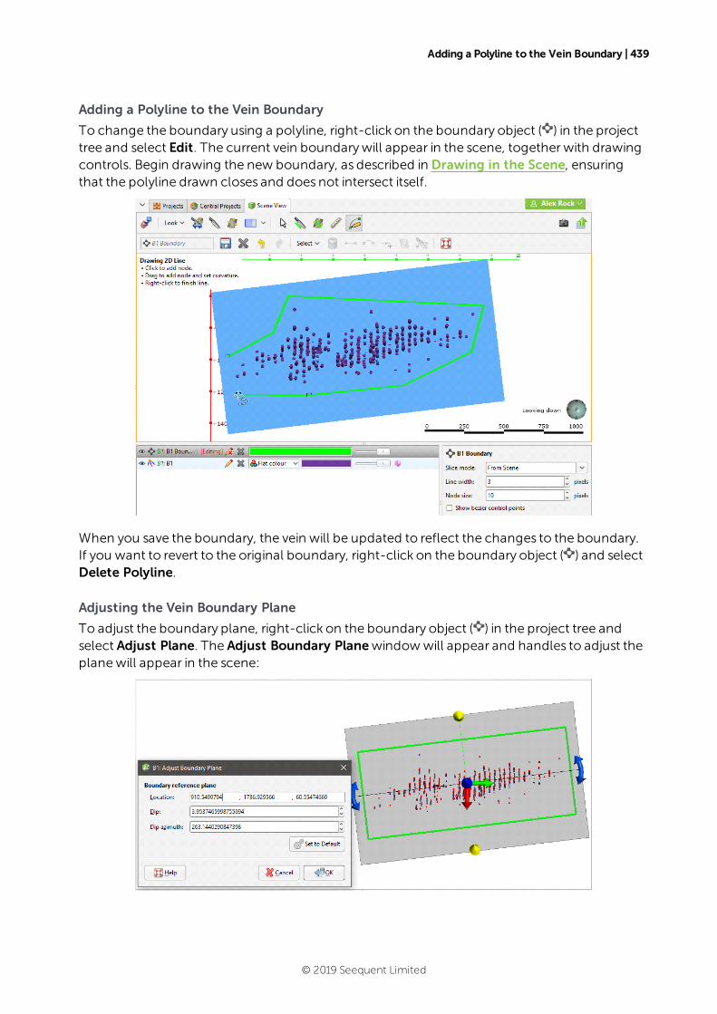
Adding a Polyline to the Vein Boundary | 439
Adding a Polyline to the Vein Boundary
To change the boundary using a polyline, right-click on the boundary object ( ) in the projecttree and select Edit. The current vein boundarywill appear in the scene, together with drawingcontrols. Begin drawing the new boundary, as described in Drawing in the Scene, ensuringthat the polyline drawn closes and does not intersect itself.
When you save the boundary, the vein will be updated to reflect the changes to the boundary.If you want to revert to the original boundary, right-click on the boundary object ( ) and selectDelete Polyline.
Adjusting the Vein Boundary Plane
To adjust the boundary plane, right-click on the boundary object ( ) in the project tree andselect Adjust Plane. The Adjust Boundary Planewindowwill appear and handles to adjust theplanewill appear in the scene:
© 2019 Seequent Limited
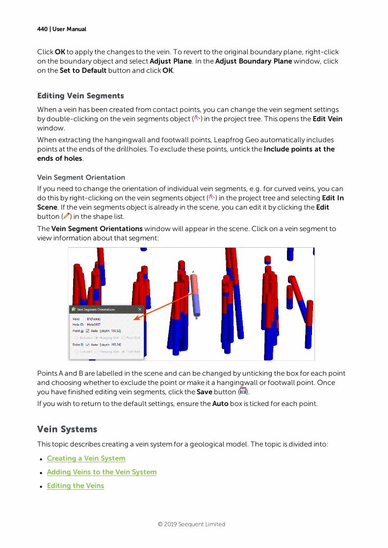
440 | User Manual
ClickOK to apply the changes to the vein. To revert to the original boundary plane, right-clickon the boundary object and select Adjust Plane. In the Adjust Boundary Planewindow, clickon the Set to Default button and clickOK.
Editing Vein Segments
When a vein has been created fromcontact points, you can change the vein segment settingsby double-clicking on the vein segments object ( ) in the project tree. This opens the Edit Veinwindow.
When extracting the hangingwall and footwall points, Leapfrog Geo automatically includespoints at the ends of the drillholes. To exclude these points, untick the Include points at theends of holes.
Vein Segment Orientation
If you need to change the orientation of individual vein segments, e.g. for curved veins, you cando this by right-clicking on the vein segments object ( ) in the project tree and selecting Edit InScene. If the vein segments object is already in the scene, you can edit it by clicking the Editbutton ( ) in the shape list.
The Vein Segment Orientations windowwill appear in the scene. Click on a vein segment toview information about that segment:
Points A and B are labelled in the scene and can be changed by unticking the box for each pointand choosing whether to exclude the point ormake it a hangingwall or footwall point. Onceyou have finished editing vein segments, click the Save button ( ).
If you wish to return to the default settings, ensure the Auto box is ticked for each point.
Vein Systems
This topic describes creating a vein system for a geological model. The topic is divided into:
l Creating a Vein System
l Adding Veins to the Vein System
l Editing the Veins
© 2019 Seequent Limited
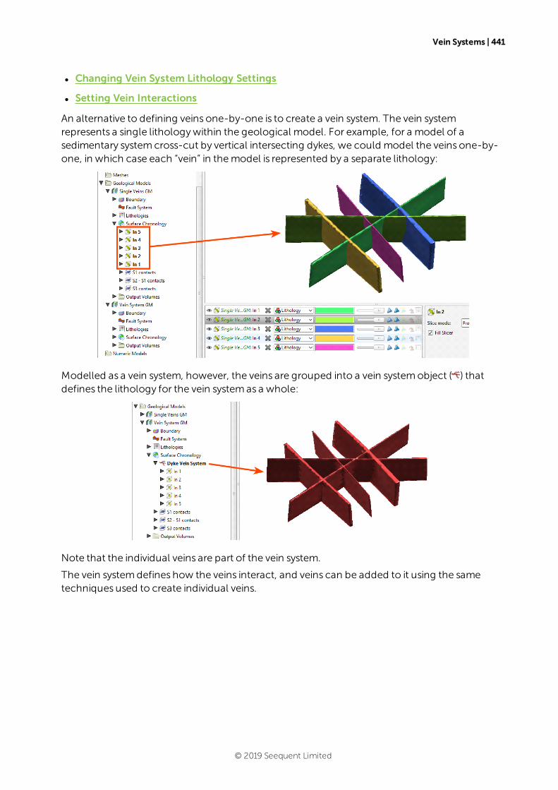
Vein Systems | 441
l Changing Vein System Lithology Settings
l Setting Vein Interactions
An alternative to defining veins one-by-one is to create a vein system. The vein systemrepresents a single lithologywithin the geological model. For example, for a model of asedimentary systemcross-cut by vertical intersecting dykes, we could model the veins one-by-one, in which case each “vein” in themodel is represented by a separate lithology:
Modelled as a vein system, however, the veins are grouped into a vein systemobject ( ) thatdefines the lithology for the vein systemas a whole:
Note that the individual veins are part of the vein system.
The vein systemdefines how the veins interact, and veins can be added to it using the sametechniques used to create individual veins.
© 2019 Seequent Limited
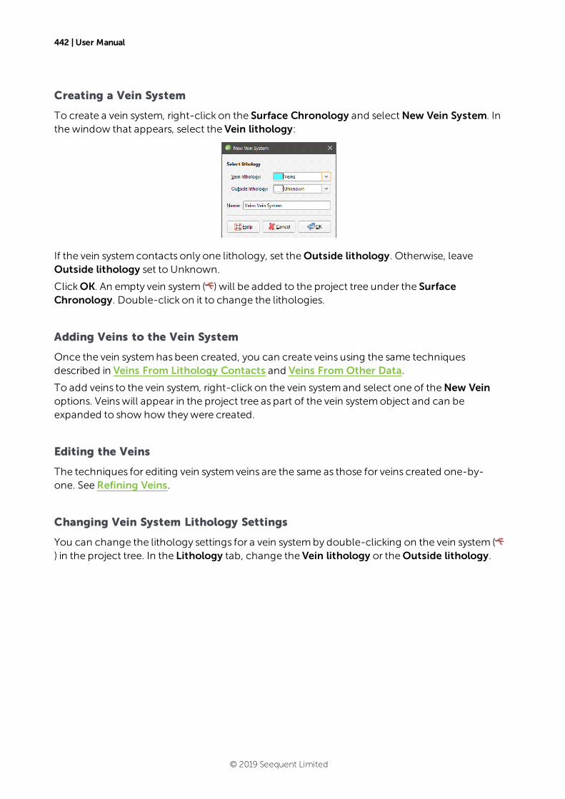
442 | User Manual
Creating a Vein System
To create a vein system, right-click on the Surface Chronology and selectNew Vein System. Inthewindow that appears, select the Vein lithology:
If the vein systemcontacts only one lithology, set theOutside lithology. Otherwise, leaveOutside lithology set to Unknown.
ClickOK. An empty vein system ( ) will be added to the project tree under the SurfaceChronology. Double-click on it to change the lithologies.
Adding Veins to the Vein System
Once the vein systemhas been created, you can create veins using the same techniquesdescribed in Veins From Lithology Contacts and Veins From Other Data.
To add veins to the vein system, right-click on the vein systemand select one of theNew Veinoptions. Veinswill appear in the project tree as part of the vein systemobject and can beexpanded to show how theywere created.
Editing the Veins
The techniques for editing vein systemveins are the same as those for veins created one-by-one. SeeRefining Veins.
Changing Vein System Lithology Settings
You can change the lithology settings for a vein systemby double-clicking on the vein system () in the project tree. In the Lithology tab, change the Vein lithology or theOutside lithology.
© 2019 Seequent Limited
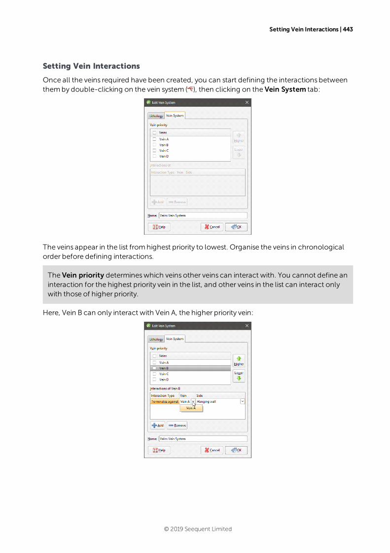
Setting Vein Interactions | 443
Setting Vein Interactions
Once all the veins required have been created, you can start defining the interactions betweenthemby double-clicking on the vein system ( ), then clicking on the Vein System tab:
The veins appear in the list fromhighest priority to lowest. Organise the veins in chronologicalorder before defining interactions.
The Vein priority determineswhich veins other veins can interact with. You cannot define aninteraction for the highest priority vein in the list, and other veins in the list can interact onlywith those of higher priority.
Here, Vein B can only interact with Vein A, the higher priority vein:
© 2019 Seequent Limited

444 | User Manual
The lowest priority vein, Vein D, can interact with all the other veins in the system:
To define an interaction, click on a vein, then click the Add button. Add an interaction for eachvein and then set the Side on which they interact.
© 2019 Seequent Limited
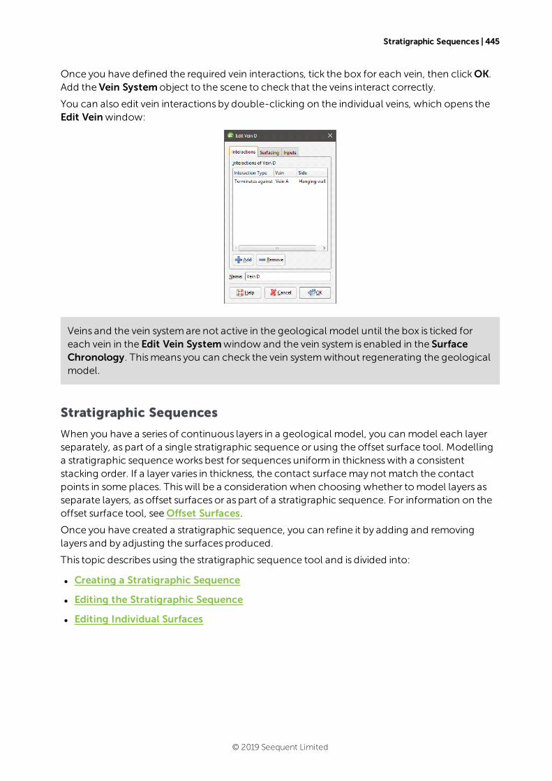
Stratigraphic Sequences | 445
Once you have defined the required vein interactions, tick the box for each vein, then clickOK.Add the Vein Systemobject to the scene to check that the veins interact correctly.
You can also edit vein interactions by double-clicking on the individual veins, which opens theEdit Veinwindow:
Veins and the vein systemare not active in the geological model until the box is ticked foreach vein in the Edit Vein Systemwindow and the vein system is enabled in the SurfaceChronology. Thismeans you can check the vein systemwithout regenerating the geologicalmodel.
Stratigraphic Sequences
When you have a series of continuous layers in a geological model, you can model each layerseparately, as part of a single stratigraphic sequence or using the offset surface tool. Modellinga stratigraphic sequenceworks best for sequences uniform in thicknesswith a consistentstacking order. If a layer varies in thickness, the contact surfacemay not match the contactpoints in some places. Thiswill be a consideration when choosing whether tomodel layers asseparate layers, as offset surfaces or as part of a stratigraphic sequence. For information on theoffset surface tool, seeOffset Surfaces.
Once you have created a stratigraphic sequence, you can refine it by adding and removinglayers and by adjusting the surfaces produced.
This topic describes using the stratigraphic sequence tool and is divided into:
l Creating a Stratigraphic Sequence
l Editing the Stratigraphic Sequence
l Editing Individual Surfaces
© 2019 Seequent Limited
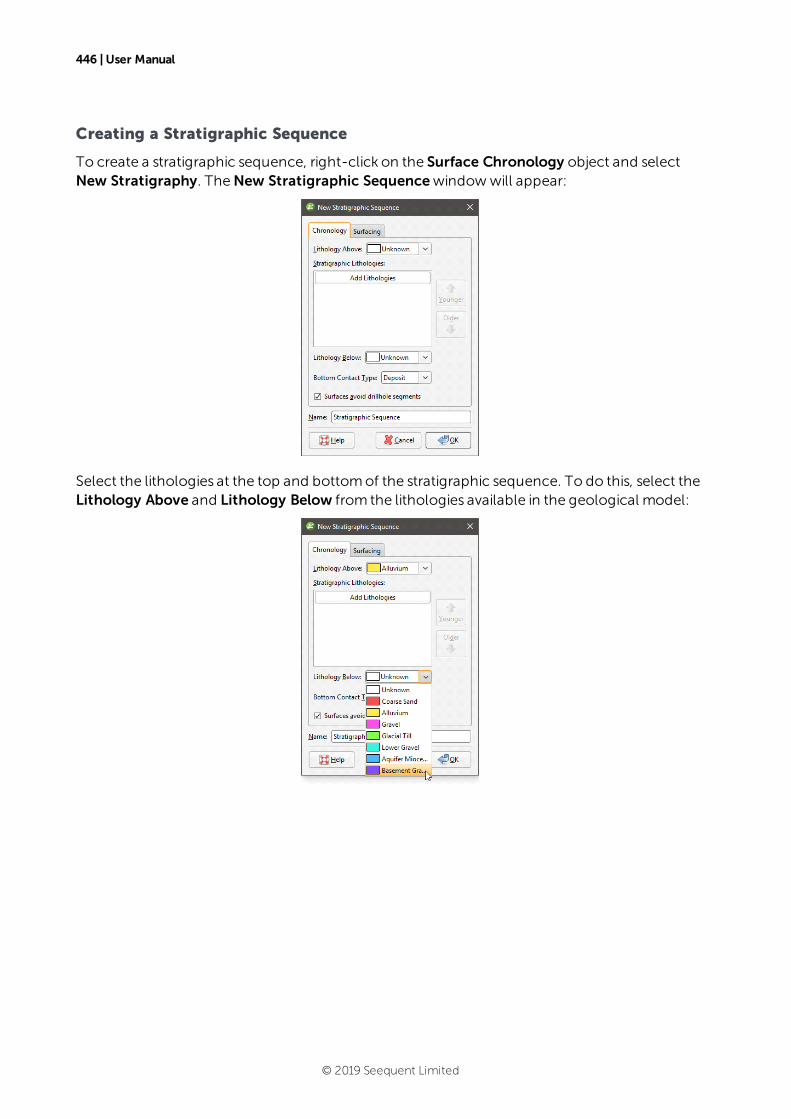
446 | User Manual
Creating a Stratigraphic Sequence
To create a stratigraphic sequence, right-click on the Surface Chronology object and selectNew Stratigraphy. TheNew Stratigraphic Sequencewindowwill appear:
Select the lithologies at the top and bottomof the stratigraphic sequence. To do this, select theLithology Above and Lithology Below from the lithologies available in the geological model:
© 2019 Seequent Limited
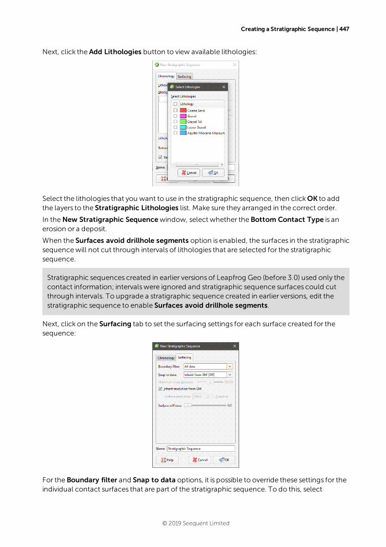
Creating a Stratigraphic Sequence | 447
Next, click the Add Lithologies button to view available lithologies:
Select the lithologies that you want to use in the stratigraphic sequence, then clickOK to addthe layers to the Stratigraphic Lithologies list. Make sure they arranged in the correct order.
In theNew Stratigraphic Sequencewindow, select whether the Bottom Contact Type is anerosion or a deposit.
When the Surfaces avoid drillhole segments option is enabled, the surfaces in the stratigraphicsequencewill not cut through intervals of lithologies that are selected for the stratigraphicsequence.
Stratigraphic sequences created in earlier versions of Leapfrog Geo (before 3.0) used only thecontact information; intervalswere ignored and stratigraphic sequence surfaces could cutthrough intervals. To upgrade a stratigraphic sequence created in earlier versions, edit thestratigraphic sequence to enable Surfaces avoid drillhole segments.
Next, click on the Surfacing tab to set the surfacing settings for each surface created for thesequence:
For the Boundary filter and Snap to data options, it is possible to override these settings for theindividual contact surfaces that are part of the stratigraphic sequence. To do this, select
© 2019 Seequent Limited
448 | User Manual
Custom. Once the stratigraphic sequence has been created, expand it in the project tree anddouble-click on each surface to change its surfacing options, as described in ContactHonouring and Boundary Filtering for Individual Surfaces below.
Boundary Filtering
When data objects are added to a surface, there are twoways to handle the data that liesoutside the surface’s boundary:
l Filter the data. The surface is only influenced by the data that falls inside the surface’sboundary.
l Leave the data unfiltered. The surface is influenced by the data both inside and outside thesurface’s boundary.
The Boundary filter setting determines how data used to define the surface is filtered:
l Off. Data is not filtered.
l All data. All data is filtered.
l Drilling only. Only drillhole data and data objects derived fromdrillhole data are filtered.
l Custom. Only the data objects specified in the Inputs tab are filtered.
All contact surfaces that make up a stratigraphic sequencewill inherit the Boundary filtersetting from the stratigraphy unlessBoundary filter is set toCustom.
Snapping to Data
There is a Snap to data setting for a geological model as a whole that is set in theGeologicalModel > General tab (see Editing a Geological Model). Snap to data can also be set on asurface-by-surface basis by double-clicking on the surface in the project tree and then clickingon the Surfacing tab.
For a stratigraphic sequence, the options are:
l Inherit from GM. The setting for the geological model as a whole is used. This is the defaultsetting.
l Off. Surfaces do not snap to the data used to create them.
l All data. Surfaces snap to all data within theMaximum snap distance, which includesdrillhole data and any data added to the surfaces.
l Drilling only. Surfaces snap to drillhole data and data objects derived fromdrillhole datawithin theMaximum snap distance but not to other data used tomodify the surfaces.
l Custom. Surfaces snap to the data objects indicated in the Inputs tab for each surface.
Take care in enabling snapping and in selecting what data the surfacewill snap to, as themore data you include, e.g. by setting a largeMaximum snap distance or selecting All datafor Snap to data, the greater the possibility that errors in the data or assumptions inherent ininterpretations (e.g. polylines) will cause distortions in themeshes. If you do enable snapping,it is best to snap only to drilling data. SeeHonouring Surface Contacts formore informationon these settings.
© 2019 Seequent Limited
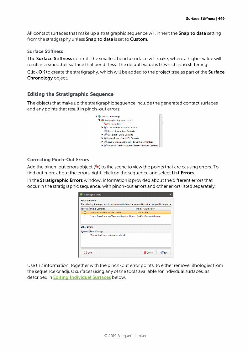
Surface Stiffness | 449
All contact surfaces that make up a stratigraphic sequencewill inherit the Snap to data settingfrom the stratigraphy unless Snap to data is set toCustom.
Surface Stiffness
The Surface Stiffness controls the smallest bend a surfacewill make, where a higher valuewillresult in a smoother surface that bends less. The default value is 0, which is no stiffening.
ClickOK to create the stratigraphy, which will be added to the project tree as part of the SurfaceChronology object.
Editing the Stratigraphic Sequence
The objects that make up the stratigraphic sequence include the generated contact surfacesand any points that result in pinch-out errors:
Correcting Pinch-Out Errors
Add the pinch-out errors object ( ) to the scene to view the points that are causing errors. Tofind out more about the errors, right-click on the sequence and select List Errors.
In the Stratigraphic Errors window, information is provided about the different errors thatoccur in the stratigraphic sequence, with pinch-out errors and other errors listed separately:
Use this information, together with the pinch-out error points, to either remove lithologies fromthe sequence or adjust surfaces using any of the tools available for individual surfaces, asdescribed in Editing Individual Surfaces below.
© 2019 Seequent Limited

450 | User Manual
Remove lithologies from the sequence by double-clicking on the sequence in the project tree,then reorganising the lithologies in theChronology tab. For example, here, the pinch-out errorsshown in thewindow above have been corrected by removing the affected surfaces from thesequence and changing the Lithology Above and Lithology Below:
You can also ignore an error by ticking the Ignored box in the Stratigraphic Errors window.
Surfacing Options
To change a stratigraphic sequence’s surfacing options, double-click on the sequence in theproject tree and click on the Surfacing tab. See Boundary Filtering and Snapping to Dataabove formore information on the settings in this tab. Note that boundary filtering and snapsettings can also be set for the individual surfaces that make up the stratigraphic sequence,which is described in Contact Honouring and Boundary Filtering for Individual Surfacesbelow.
Applying a Trend
To apply a global trend to a stratigraphic sequence either right-click on it in the project tree andselect Adjust Surface or double-click on the stratigraphic sequence and then click on theTrend tab. You can then apply a trend to the surface as described in Global Trends.
Editing Individual Surfaces
Individual surfaces that make up a stratigraphic sequence can bemodified by:
l Contact Honouring and Boundary Filtering for Individual Surfaces
l Adding Data to Individual Surfaces
l Editing Surface Contacts
© 2019 Seequent Limited
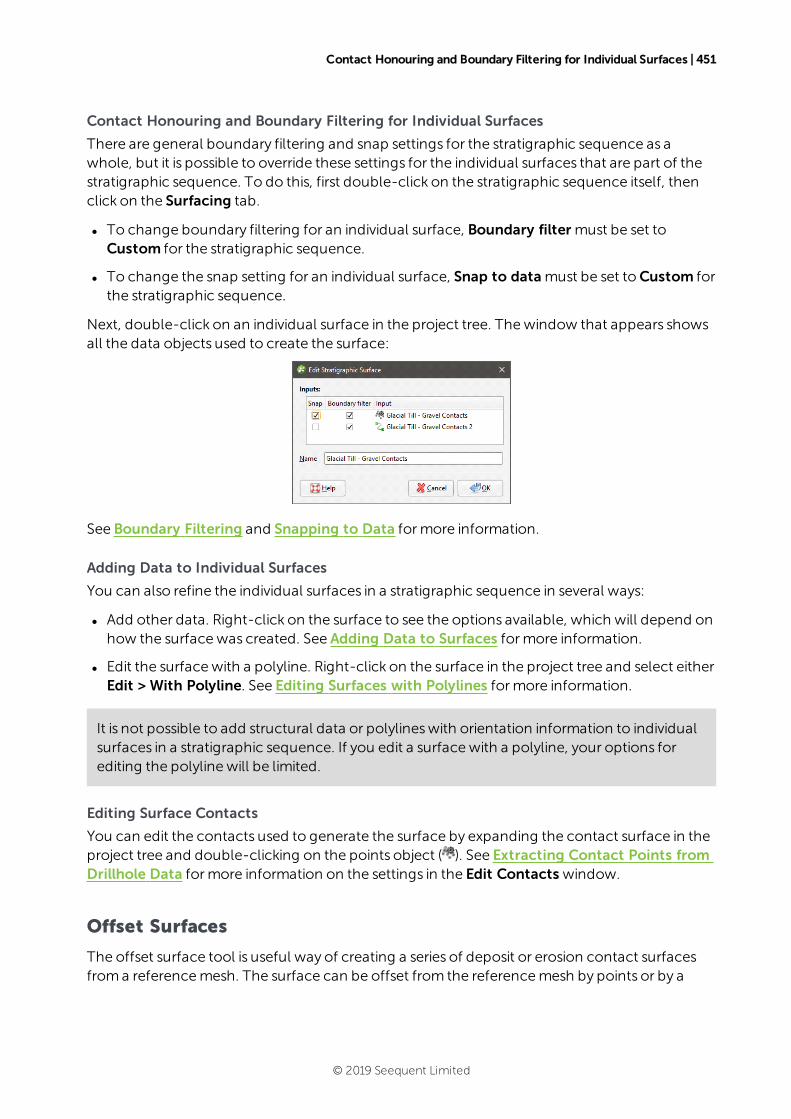
Contact Honouring and Boundary Filtering for Individual Surfaces | 451
Contact Honouring and Boundary Filtering for Individual Surfaces
There are general boundary filtering and snap settings for the stratigraphic sequence as awhole, but it is possible to override these settings for the individual surfaces that are part of thestratigraphic sequence. To do this, first double-click on the stratigraphic sequence itself, thenclick on the Surfacing tab.
l To change boundary filtering for an individual surface, Boundary filter must be set toCustom for the stratigraphic sequence.
l To change the snap setting for an individual surface, Snap to datamust be set toCustom forthe stratigraphic sequence.
Next, double-click on an individual surface in the project tree. Thewindow that appears showsall the data objects used to create the surface:
See Boundary Filtering and Snapping to Data formore information.
Adding Data to Individual Surfaces
You can also refine the individual surfaces in a stratigraphic sequence in several ways:
l Add other data. Right-click on the surface to see the options available, which will depend onhow the surfacewas created. See Adding Data to Surfaces formore information.
l Edit the surfacewith a polyline. Right-click on the surface in the project tree and select eitherEdit > With Polyline. See Editing Surfaces with Polylines formore information.
It is not possible to add structural data or polylineswith orientation information to individualsurfaces in a stratigraphic sequence. If you edit a surfacewith a polyline, your options forediting the polyline will be limited.
Editing Surface Contacts
You can edit the contacts used to generate the surface by expanding the contact surface in theproject tree and double-clicking on the points object ( ). See Extracting Contact Points fromDrillhole Data formore information on the settings in the Edit Contacts window.
Offset Surfaces
The offset surface tool is useful way of creating a series of deposit or erosion contact surfacesfroma referencemesh. The surface can be offset from the referencemesh by points or by a
© 2019 Seequent Limited
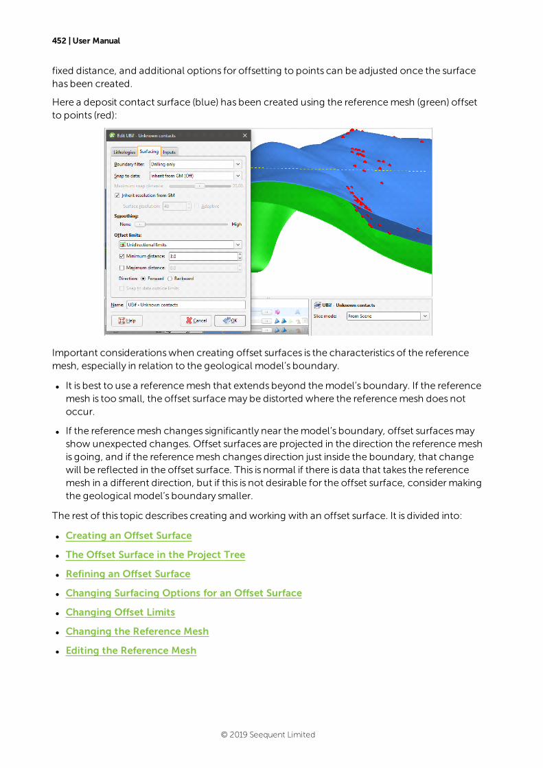
452 | User Manual
fixed distance, and additional options for offsetting to points can be adjusted once the surfacehas been created.
Here a deposit contact surface (blue) has been created using the referencemesh (green) offsetto points (red):
Important considerationswhen creating offset surfaces is the characteristics of the referencemesh, especially in relation to the geological model’s boundary.
l It is best to use a referencemesh that extends beyond themodel’s boundary. If the referencemesh is too small, the offset surfacemay be distorted where the referencemesh does notoccur.
l If the referencemesh changes significantly near themodel’s boundary, offset surfacesmayshow unexpected changes. Offset surfaces are projected in the direction the referencemeshis going, and if the referencemesh changes direction just inside the boundary, that changewill be reflected in the offset surface. This is normal if there is data that takes the referencemesh in a different direction, but if this is not desirable for the offset surface, considermakingthe geological model’s boundary smaller.
The rest of this topic describes creating and working with an offset surface. It is divided into:
l Creating an Offset Surface
l The Offset Surface in the Project Tree
l Refining an Offset Surface
l Changing Surfacing Options for an Offset Surface
l Changing Offset Limits
l Changing the Reference Mesh
l Editing the Reference Mesh
© 2019 Seequent Limited
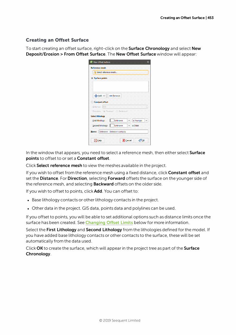
Creating an Offset Surface | 453
Creating an Offset Surface
To start creating an offset surface, right-click on the Surface Chronology and selectNewDeposit/Erosion > From Offset Surface. TheNew Offset Surfacewindowwill appear:
In thewindow that appears, you need to select a referencemesh, then either select Surfacepoints to offset to or set a Constant offset.
Click Select reference mesh to view themeshes available in the project.
If you wish to offset from the referencemesh using a fixed distance, clickConstant offset andset theDistance. ForDirection, selecting Forward offsets the surface on the younger side ofthe referencemesh, and selecting Backward offsets on the older side.
If you wish to offset to points, clickAdd. You can offset to:
l Base lithology contacts or other lithology contacts in the project.
l Other data in the project. GIS data, points data and polylines can be used.
If you offset to points, you will be able to set additional options such as distance limits once thesurface has been created. SeeChanging Offset Limits below formore information.
Select the First Lithology and Second Lithology from the lithologies defined for themodel. Ifyou have added base lithology contacts or other contacts to the surface, thesewill be setautomatically from the data used.
ClickOK to create the surface, which will appear in the project tree as part of the SurfaceChronology.
© 2019 Seequent Limited
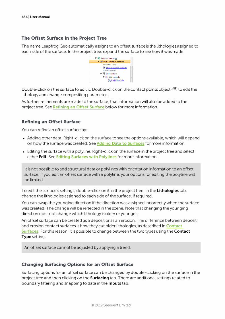
454 | User Manual
The Offset Surface in the Project Tree
The name Leapfrog Geo automatically assigns to an offset surface is the lithologies assigned toeach side of the surface. In the project tree, expand the surface to see how it wasmade:
Double-click on the surface to edit it. Double-click on the contact points object ( ) to edit thelithology and change compositing parameters.
As further refinements aremade to the surface, that information will also be added to theproject tree. SeeRefining an Offset Surface below formore information.
Refining an Offset Surface
You can refine an offset surface by:
l Adding other data. Right-click on the surface to see the options available, which will dependon how the surfacewas created. See Adding Data to Surfaces formore information.
l Editing the surfacewith a polyline. Right-click on the surface in the project tree and selecteither Edit. See Editing Surfaces with Polylines formore information.
It is not possible to add structural data or polylineswith orientation information to an offsetsurface. If you edit an offset surfacewith a polyline, your options for editing the polyline willbe limited.
To edit the surface’s settings, double-click on it in the project tree. In the Lithologies tab,change the lithologies assigned to each side of the surface, if required.
You can swap the younging direction if the direction was assigned incorrectlywhen the surfacewas created. The changewill be reflected in the scene. Note that changing the youngingdirection does not changewhich lithology is older or younger.
An offset surface can be created as a deposit or as an erosion. The difference between depositand erosion contact surfaces is how they cut older lithologies, as described in ContactSurfaces. For this reason, it is possible to change between the two types using theContactType setting.
An offset surface cannot be adjusted by applying a trend.
Changing Surfacing Options for an Offset Surface
Surfacing options for an offset surface can be changed by double-clicking on the surface in theproject tree and then clicking on the Surfacing tab. There are additional settings related toboundary filtering and snapping to data in the Inputs tab.
© 2019 Seequent Limited
Boundary Filtering | 455
Boundary Filtering
When data objects are added to a surface, there are twoways to handle the data that liesoutside the surface’s boundary:
l Filter the data. The surface is only influenced by the data that falls inside the surface’sboundary.
l Leave the data unfiltered. The surface is influenced by the data both inside and outside thesurface’s boundary.
The Boundary filter setting determines how data used to define the surface is filtered:
l Off. Data is not filtered.
l All data. All data is filtered.
l Drilling only. Only drillhole data and data objects derived fromdrillhole data are filtered.
l Custom. Only the data objects specified in the Inputs tab are filtered.
Snapping to Data
Often, surfaces should honour drillhole data and treat data objects such as polylines and GISdata as interpretations, as discussed in Honouring Surface Contacts.
There is a Snap to data setting for a geological model as a whole that is set in theGeologicalModel > General tab (see Editing a Geological Model). Snap to data can also be set on asurface-by-surface basis by double-clicking on the surface in the project tree and then clickingon the Surfacing tab.
For individual contact surfaces, the options are:
l Inherit from GM. The setting for the geological model as a whole is used. This is the defaultsetting.
l Off. Surfaces do not snap to the data used to create them.
l All data. Surfaces snap to all data within theMaximum snap distance, which includesdrillhole data and any data added to the surfaces.
l Drilling only. Surfaces snap to drillhole data and data objects derived fromdrillhole datawithin theMaximum snap distance but not to other data used tomodify the surfaces.
l Custom. Surfaces snap to the data objects indicated in the Inputs tab for each surface.
Take care in enabling snapping and in selecting what data the surfacewill snap to, as themore data you include, e.g. by setting a largeMaximum snap distance or selecting All datafor Snap to data, the greater the possibility that errors in the data or assumptions inherent ininterpretations (e.g. polylines) will cause distortions in themeshes. If you do enable snapping,it is best to snap only to drilling data. SeeHonouring Surface Contacts formore informationon these settings.
If you need a surface to honour drillhole data but treat other data objects as interpretations,selectDrilling only. To honour some data objectswhile treating others as interpretations, selectCustom, then click on the Inputs tab to enable snapping for individual objects.
© 2019 Seequent Limited
456 | User Manual
There is also a snap setting that can be used when offset limits are used. This option is discussedin Changing Offset Limits below.
Surface Resolution
The surface resolution for an offset surface can be inherited from the geological model or it canbe set specifically for the surface. To change the surface resolution for an offset surface,double-click on the surface in the project tree and then click on the Surfacing tab. See SurfaceResolution for a Geological Model for information about the surface resolution settings in theSurfacing tab.
Smoothing
The Smoothing parameter in the Surfacing tab can be used for all offset types other thanConstant. If your reference surface is highly curved, you may see distortions in the offsetsurface. If this is the case, set Smoothing to a higher value.
Increasing the Smoothing parameter will generally result in faster processing when offsetting tolarge distances. If you are finding that processing time is excessively long for an offset surface,consider increasing Smoothing. In some situations, however, increasing Smoothing canexaggerate imperfections in the reference surface.
If you are offsetting by a small distance and processing is taking longer than expected, considersetting Smoothing toNone.
Changing Offset Limits
There are four options forOffset limits in the Surfacing tab. Three relate to offsetting to pointsand the fourth to offsetting to a fixed distance from the referencemesh.
l TheNone option is the default setting used when a surface is created as an offset to points.No distance limits are used in creating the offset surface, and it simply follows the pointsused.
l TheUnidirectional limits option allows you to set distance limits in one direction. Pointsoutside the limitswill be disregarded.
l The Bidirectional limits option allows you to set distance limits in both directions, and pointsoutside these limits are disregarded. This setting is useful formodelling folded surfaces suchas veins.
l TheConstant offset option offsets the surface to a fixed distance from the referencemesh.
The Forward direction is the younger side of the referencemesh.
If the Snap to data outside limits setting is enabled, the surfacewill honour data, even if it isoutside the distance limits. This option will be greyed out if Snap to data is off.
Changing to a Constant Offset
To use a constant offset rather than points, select theConstant offset option and set theDistance and Direction to offset the surface. Selecting Forward offsets the surface on theyounger side of the referencemesh, whereas selecting Backward offsets on the older side.
If you created a surface as an offset to points and switch to using a constant offset, the pointsadded to the surfacewhen it was created will be disabled.
© 2019 Seequent Limited
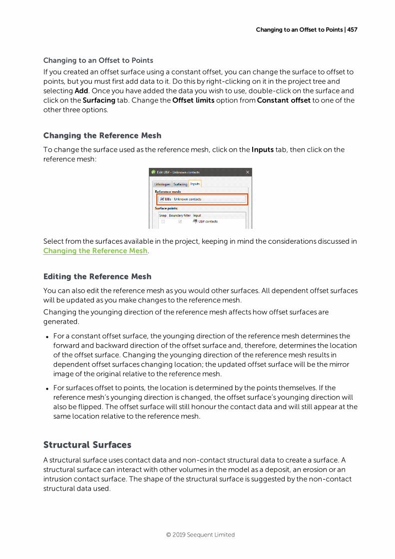
Changing to an Offset to Points | 457
Changing to an Offset to Points
If you created an offset surface using a constant offset, you can change the surface to offset topoints, but you must first add data to it. Do this by right-clicking on it in the project tree andselecting Add. Once you have added the data you wish to use, double-click on the surface andclick on the Surfacing tab. Change theOffset limits option fromConstant offset to one of theother three options.
Changing the Reference Mesh
To change the surface used as the referencemesh, click on the Inputs tab, then click on thereferencemesh:
Select from the surfaces available in the project, keeping in mind the considerations discussed inChanging the Reference Mesh.
Editing the Reference Mesh
You can also edit the referencemesh as you would other surfaces. All dependent offset surfaceswill be updated as you make changes to the referencemesh.
Changing the younging direction of the referencemesh affects how offset surfaces aregenerated.
l For a constant offset surface, the younging direction of the referencemesh determines theforward and backward direction of the offset surface and, therefore, determines the locationof the offset surface. Changing the younging direction of the referencemesh results independent offset surfaces changing location; the updated offset surfacewill be themirrorimage of the original relative to the referencemesh.
l For surfaces offset to points, the location is determined by the points themselves. If thereferencemesh’s younging direction is changed, the offset surface’s younging direction willalso be flipped. The offset surfacewill still honour the contact data and will still appear at thesame location relative to the referencemesh.
Structural Surfaces
A structural surface uses contact data and non-contact structural data to create a surface. Astructural surface can interact with other volumes in themodel as a deposit, an erosion or anintrusion contact surface. The shape of the structural surface is suggested by the non-contactstructural data used.
© 2019 Seequent Limited
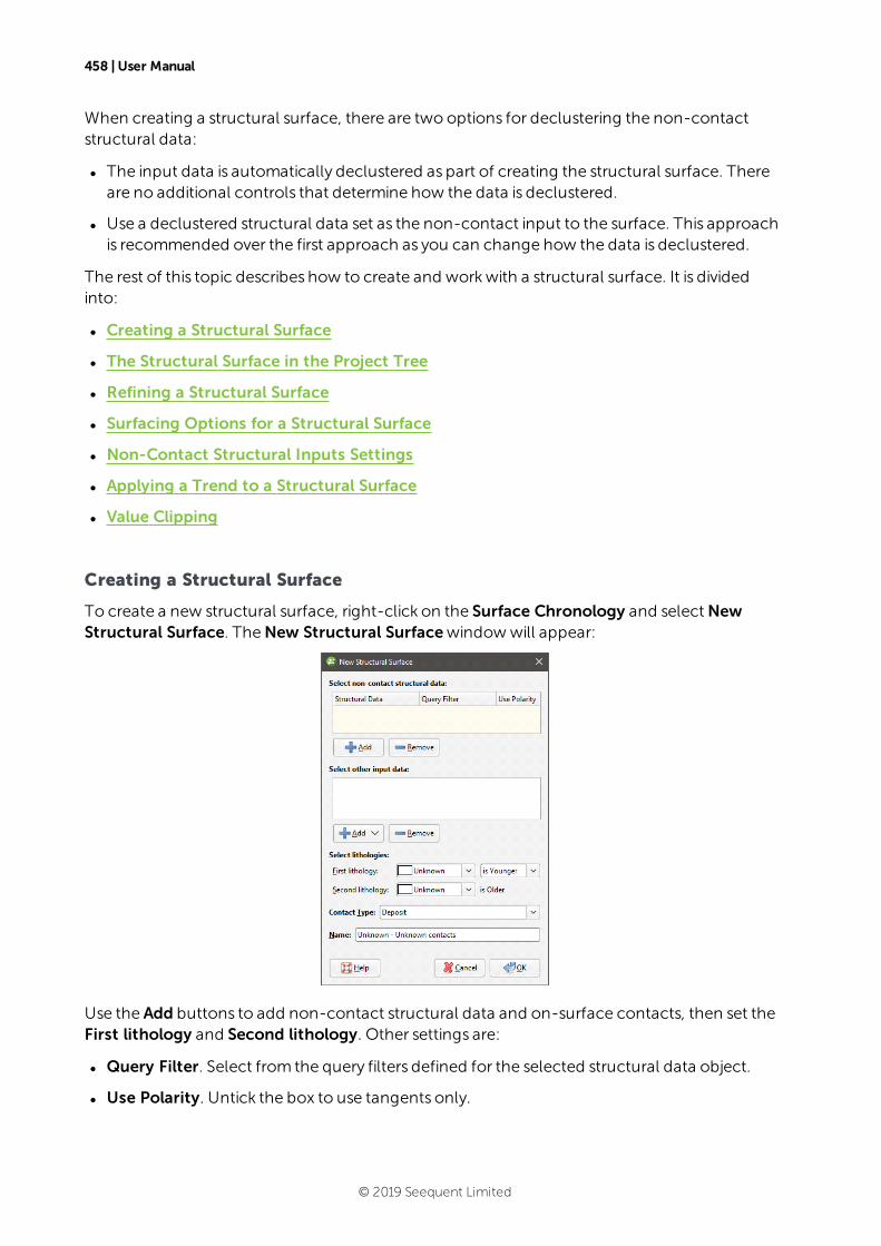
458 | User Manual
When creating a structural surface, there are two options for declustering the non-contactstructural data:
l The input data is automatically declustered as part of creating the structural surface. Thereare no additional controls that determine how the data is declustered.
l Use a declustered structural data set as the non-contact input to the surface. This approachis recommended over the first approach as you can change how the data is declustered.
The rest of this topic describes how to create and workwith a structural surface. It is dividedinto:
l Creating a Structural Surface
l The Structural Surface in the Project Tree
l Refining a Structural Surface
l Surfacing Options for a Structural Surface
l Non-Contact Structural Inputs Settings
l Applying a Trend to a Structural Surface
l Value Clipping
Creating a Structural Surface
To create a new structural surface, right-click on the Surface Chronology and selectNewStructural Surface. TheNew Structural Surfacewindowwill appear:
Use the Add buttons to add non-contact structural data and on-surface contacts, then set theFirst lithology and Second lithology. Other settings are:
l Query Filter. Select from the query filters defined for the selected structural data object.
l Use Polarity. Untick the box to use tangents only.
© 2019 Seequent Limited

The Structural Surface in the Project Tree | 459
l Contact Type. Structural surfaces can be deposit, erosion or intrusion contacts. The samealgorithm is used for each setting; the only difference is in how the surface interactswithother surfaces.
The Structural Surface in the Project Tree
The name Leapfrog Geo automatically assigns to a structural surface is the lithologies assignedto each side of the surface. In the project tree, expand the surface to see how it wasmade:
As further refinements aremade to the surface, that information will also be added to theproject tree. SeeRefining a Structural Surface below formore information.
To add more non-contact structural data to the surface, right-click on it in the project treeand select Add > Structural Data. In thewindow that appears, tick the box forNon-contactStructural Data:
Refining a Structural Surface
You can refine structural surfaces in several ways:
l Add other data. Right-click on the surface to see the options available, which will depend onhow the surfacewas created. See Adding Data to Surfaces formore information.
l Edit the surfacewith a polyline. Right-click on the surface in the project tree and select eitherEdit > With Polyline. See Editing Surfaces with Polylines formore information.
l Edit the surface using structural data. Right-click on the surface and select Edit > WithStructural Data. See Editing Surfaces with Structural Data formore information.
To edit the surface’s settings, double-click on it in the project tree. In the Lithologies tab,change the lithologies assigned to each side of the surface, if required.
You can swap the younging direction if the direction was assigned incorrectlywhen the surfacewas created. The changewill be reflected in the scene. Note that changing the youngingdirection does not changewhich lithology is older or younger.
© 2019 Seequent Limited
460 | User Manual
TheContact Type setting determines how the structural surface interactswith otherlithologies, as described in Contact Surfaces. A structural surface can be a deposit, erosion orintrusion contact surface.
For information on other techniques for refining structural surfaces, see Surfacing Options fora Structural Surface below.
Surfacing Options for a Structural Surface
Surfacing options for a structural surface are accessed by double-clicking on the surface in theproject tree and clicking on the Surfacing tab. There are additional settings related to boundaryfiltering and snapping to data in the Inputs tab.
Setting the Surface Resolution
See Surface Resolution for a Geological Model for information about the surface resolutionsettings in the Surfacing tab.
Boundary Filtering
When data objects are added to a surface, there are twoways to handle the data that liesoutside the surface’s boundary:
l Filter the data. The surface is only influenced by the data that falls inside the surface’sboundary.
l Leave the data unfiltered. The surface is influenced by the data both inside and outside thesurface’s boundary.
The boundary of a structural surface can be the geological model boundary or a fault blockboundary.
The Boundary filter setting determines how data used to define the surface is filtered:
l Off. Data is not filtered.
l All data. All data is filtered.
l Drilling only. Only drillhole data and data objects derived fromdrillhole data are filtered.
l Custom. Only the data objects specified in the Inputs tab are filtered.
Snapping to Input Data
Often, surfaces should honour drillhole data and treat data objects such as polylines and GISdata as interpretations. SeeHonouring Surface Contacts.
There is a Snap to data setting for a geological model as a whole that is set in theGeologicalModel > General tab (see Editing a Geological Model). Snap to data can also be set on asurface-by-surface basis by double-clicking on the surface in the project tree and then clickingon the Surfacing tab.
For individual contact surfaces, the options are:
l Inherit from GM. The setting for the geological model as a whole is used. This is the defaultsetting.
© 2019 Seequent Limited
Non-Contact Structural Inputs Settings | 461
l Off. Surfaces do not snap to the data used to create them.
l All data. Surfaces snap to all data within theMaximum snap distance, which includesdrillhole data and any data added to the surfaces.
l Drilling only. Surfaces snap to drillhole data and data objects derived fromdrillhole datawithin theMaximum snap distance but not to other data used tomodify the surfaces.
l Custom. Surfaces snap to the data objects indicated in the Inputs tab for each surface.
Take care in enabling snapping and in selecting what data the surfacewill snap to, as themore data you include, e.g. by setting a largeMaximum snap distance or selecting All datafor Snap to data, the greater the possibility that errors in the data or assumptions inherent ininterpretations (e.g. polylines) will cause distortions in themeshes. If you do enable snapping,it is best to snap only to drilling data. SeeHonouring Surface Contacts formore informationon these settings.
If you need a surface to honour drillhole data but treat other data objects as interpretations,selectDrilling only. To honour some data objectswhile treating others as interpretations, selectCustom, then click on the Inputs tab to enable snapping for individual objects.
Non-Contact Structural Inputs Settings
For the non-contact structural inputs, you can:
l Change theQuery Filter setting. Select from the query filters defined for the selectedstructural data object.
l Change theUse Polarity setting. Untick the box to use tangents only.
l Change the Boundary filter setting, if the Boundary filter setting in the Surfacing tab is settoCustom.
Applying a Trend to a Structural Surface
There are twoways to change the trend for a structural surface:
l Right-click on the surface in the project tree and select Adjust Surface.
l Double-click on the surface in the project tree and then click on the Trend tab.
SeeGlobal Trends formore information.
Value Clipping
In the Value Clipping tab, you can manipulate the data distribution by clipping the data.Clipping caps values that are outside the range set by the Lower bound and Upper boundvalues. For example, if you change theUpper bound from16.00 to 10.00, distance valuesabove 10.00will be regarded as 10.00.
© 2019 Seequent Limited
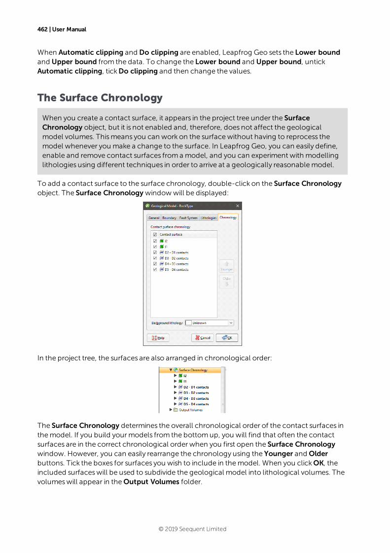
462 | User Manual
When Automatic clipping and Do clipping are enabled, Leapfrog Geo sets the Lower boundand Upper bound from the data. To change the Lower bound and Upper bound, untickAutomatic clipping, tickDo clipping and then change the values.
The Surface Chronology
When you create a contact surface, it appears in the project tree under the SurfaceChronology object, but it is not enabled and, therefore, does not affect the geologicalmodel volumes. Thismeans you can work on the surfacewithout having to reprocess themodel whenever you make a change to the surface. In Leapfrog Geo, you can easily define,enable and remove contact surfaces froma model, and you can experiment with modellinglithologies using different techniques in order to arrive at a geologically reasonablemodel.
To add a contact surface to the surface chronology, double-click on the Surface Chronologyobject. The Surface Chronology windowwill be displayed:
In the project tree, the surfaces are also arranged in chronological order:
The Surface Chronology determines the overall chronological order of the contact surfaces inthemodel. If you build yourmodels from the bottomup, you will find that often the contactsurfaces are in the correct chronological order when you first open the Surface Chronologywindow. However, you can easily rearrange the chronology using the Younger and Olderbuttons. Tick the boxes for surfaces you wish to include in themodel. When you clickOK, theincluded surfaceswill be used to subdivide the geological model into lithological volumes. Thevolumeswill appear in theOutput Volumes folder.
© 2019 Seequent Limited
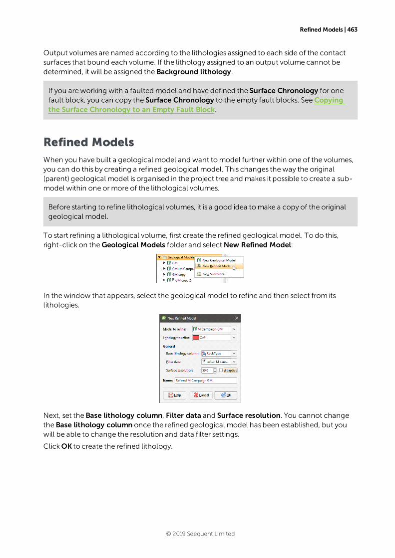
Refined Models | 463
Output volumes are named according to the lithologies assigned to each side of the contactsurfaces that bound each volume. If the lithology assigned to an output volume cannot bedetermined, it will be assigned the Background lithology.
If you are working with a faulted model and have defined the Surface Chronology for onefault block, you can copy the Surface Chronology to the empty fault blocks. SeeCopyingthe Surface Chronology to an Empty Fault Block.
Refined ModelsWhen you have built a geological model and want tomodel further within one of the volumes,you can do this by creating a refined geological model. This changes theway the original(parent) geological model is organised in the project tree and makes it possible to create a sub-model within one ormore of the lithological volumes.
Before starting to refine lithological volumes, it is a good idea tomake a copy of the originalgeological model.
To start refining a lithological volume, first create the refined geological model. To do this,right-click on theGeological Models folder and selectNew Refined Model:
In thewindow that appears, select the geological model to refine and then select from itslithologies.
Next, set the Base lithology column, Filter data and Surface resolution. You cannot changethe Base lithology column once the refined geological model has been established, but youwill be able to change the resolution and data filter settings.
ClickOK to create the refined lithology.
© 2019 Seequent Limited
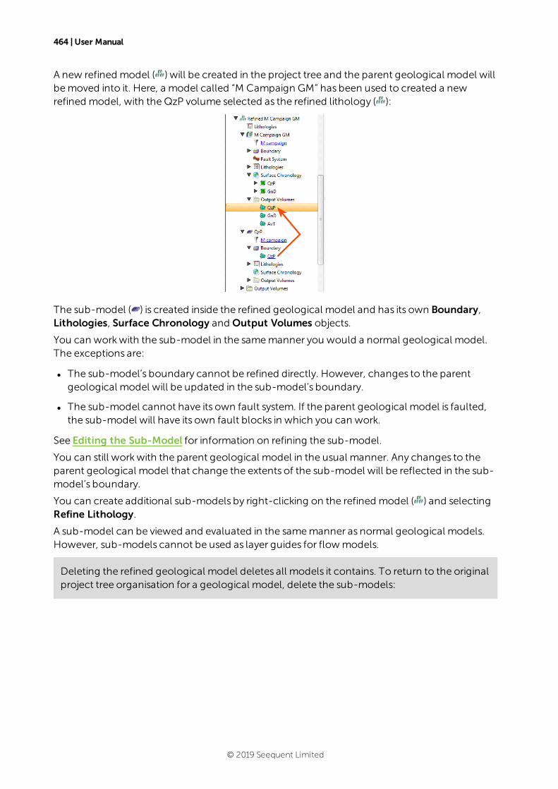
464 | User Manual
A new refined model ( ) will be created in the project tree and the parent geological model willbemoved into it. Here, a model called “M Campaign GM” has been used to created a newrefined model, with theQzP volume selected as the refined lithology ( ):
The sub-model ( ) is created inside the refined geological model and has its own Boundary,Lithologies, Surface Chronology and Output Volumes objects.
You can workwith the sub-model in the samemanner you would a normal geological model.The exceptions are:
l The sub-model’s boundary cannot be refined directly. However, changes to the parentgeological model will be updated in the sub-model’s boundary.
l The sub-model cannot have its own fault system. If the parent geological model is faulted,the sub-model will have its own fault blocks in which you can work.
See Editing the Sub-Model for information on refining the sub-model.
You can still workwith the parent geological model in the usual manner. Any changes to theparent geological model that change the extents of the sub-model will be reflected in the sub-model’s boundary.
You can create additional sub-models by right-clicking on the refined model ( ) and selectingRefine Lithology.
A sub-model can be viewed and evaluated in the samemanner as normal geological models.However, sub-models cannot be used as layer guides for flowmodels.
Deleting the refined geological model deletes all models it contains. To return to the originalproject tree organisation for a geological model, delete the sub-models:
© 2019 Seequent Limited
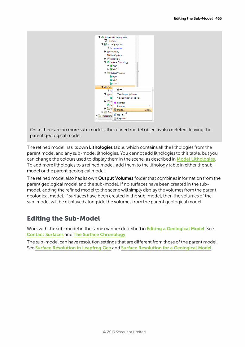
Editing the Sub-Model | 465
Once there are nomore sub-models, the refined model object is also deleted, leaving theparent geological model.
The refined model has its own Lithologies table, which contains all the lithologies from theparent model and any sub-model lithologies. You cannot add lithologies to this table, but youcan change the colours used to display them in the scene, as described in Model Lithologies.To add more lithologies to a refined model, add them to the lithology table in either the sub-model or the parent geological model.
The refined model also has its own Output Volumes folder that combines information from theparent geological model and the sub-model. If no surfaces have been created in the sub-model, adding the refined model to the scenewill simply display the volumes from the parentgeological model. If surfaces have been created in the sub-model, then the volumesof thesub-model will be displayed alongside the volumes from the parent geological model.
Editing the Sub-Model
Workwith the sub-model in the samemanner described in Editing a Geological Model. SeeContact Surfaces and The Surface Chronology.
The sub-model can have resolution settings that are different from those of the parent model.See Surface Resolution in Leapfrog Geo and Surface Resolution for a Geological Model.
© 2019 Seequent Limited
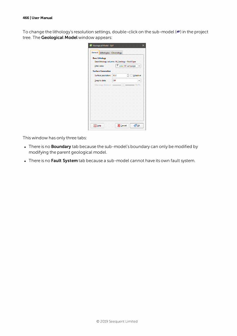
466 | User Manual
To change the lithology’s resolution settings, double-click on the sub-model ( ) in the projecttree. TheGeological Modelwindow appears:
Thiswindow has only three tabs:
l There is no Boundary tab because the sub-model’s boundary can only bemodified bymodifying the parent geological model.
l There is no Fault System tab because a sub-model cannot have its own fault system.
© 2019 Seequent Limited
Numeric ModelsThe FastRBF algorithmemploys interpolation functions to estimate values fromknown data.From these estimated values, geological surfaces are constructed as part of themodel-buildingprocess.
With theNumeric Models folder, you can create numericmodels and change their parameters.
l An RBF interpolant describes a physical quantity that varies continuously in space. An RBFinterpolant can be used tomodel, for example, grade distribution, with isosurface values setto represent both minimumconcentrations of interest and regions of high value. SeeRBFInterpolants.
l Amulti-domained RBF interpolant is an RBF interpolant that has a number of individual sub-interpolants that are bounded by the fault blocks or output volumesof a selected geologicalmodel. Changes to all sub-interpolants can bemade by editing the parent interpolant, whilesub-interpolants can be edited to account for local influences on the values used, the trendand interpolation parameters. SeeMulti-Domained RBF Interpolants.
l An indicator RBF interpolant calculates the likelihood that valueswill fall above and below aspecific threshold. An indicator RBF interpolant can be used to produce a volume insidewhich furthermodelling is carried out. For example, you can create an indicator RBFinterpolant for grade values above a certain threshold, and then use the inside volume as alateral extent for anothermodel. See Indicator RBF Interpolants.
l A distance function calculates the distance to a set of points. Aswith an indicator RBFinterpolant, a distance function is useful for restricting processing to a specific region. To dothis, create a distance function, select the objects to use, then add at least one buffer. Youcan then use one of the distance function’s isosurfaces as a lateral extent for anothermodel.SeeDistance Functions.
Values that can be interpolated include downhole numeric data, composited drillhole data andpoints data. See Interpolant Functions for a general introduction to interpolation.
The rest of this topic describes:
l Importing a Variogram Model
l Copying a Numeric Model
l Creating a Static Copy of a Numeric Model
l Exporting Numeric Model Volumes and Surfaces
l Exporting Numeric Model Midpoints
© 2019 Seequent Limited
468 | User Manual
Importing a Variogram Model
Leapfrog Geo can import spheroidal variogrammodels exported fromSnowden Supervisor.The settings that can be imported are:
l The anisotropy settings in the Trend tab
l TheNugget, Total Sill, Base Range and Alpha settings in the Interpolant tab
To import a variogrammodel, first create an interpolant. Next, right-click on the interpolant andselect Import Variogram Parameters. In thewindow that appears, navigate to the folder thatcontains the XML file and select it. ClickOpen. The interpolant will be updated with theparameters in the XML file.
The imported variogrammodel overwrites the parameters in the interpolant, which cannotbe undone. If you wish to save the original settings, make a copy of the interpolant beforeimporting the new parameters.
Once the interpolant has been updated, you can edit it further by double-clicking on theinterpolant in the project tree.
Copying a Numeric Model
Creating a copy of a numericmodel is a useful way of experimenting with changes to a model.
To copy a numericmodel, right-click on it in the project tree and selectCopy. Enter a name forthe copy of themodel and clickOK. The copywill be added to the project tree.
Creating a Static Copy of a Numeric Model
Creating a static copy preserves a snapshot of a numericmodel that does not change, evenwhen changes aremade to the data on which the original model was dependent. This is auseful way of storing historical models and comparing models. Static copies can be exportedfromLeapfrog Geo, as described in Exporting Numeric Model Volumes and Surfaces below.
To create a static copy of a numericmodel, right-click on it in the project tree and select StaticCopy. Enter a name for the copy of the numericmodel and clickOK. The copywill be added totheNumeric Models folder.
The objects that make up a static copy of a numericmodel depend on the type of model:
l For an RBF interpolant, a static copy ismade up of a Legend object, a Boundary object, andall isosurfaces and output volumes created in building themodel.
l For a multi-domained RBF interpolant, a static copy ismade up of a Legend object, aBoundary object, and the output volumes created in building themodel. There are alsostatic copies of the sub-interpolants, which are the same as static copies of RBF interpolants.
l For an indicator RBF interpolant, a static copy ismade up of a Legend object, a Boundaryobject, themodel’s isosurface and the output volumes.
© 2019 Seequent Limited
Exporting Numeric Model Volumes and Surfaces | 469
Staticmodels created in versions of Leapfrog Geo before 2.2 copied only the output volumesand the legend, and the staticmodel appeared in the shape list only as a single line. Whenthese staticmodels are upgraded and displayed in the scene, the individual output volumeswill be added to the shape list.
To view the date a static copywas created, right-click on it in the project tree and selectProperties. The date the copywas created is in theGeneral tab.
Exporting Numeric Model Volumes and Surfaces
There are three options for exporting a numericmodel’s output volumes and surfaces. Theseare:
l Export an output volume or a surface as a mesh. Right-click on it in the project tree and clickExport. You will be prompted for a file name and location. See Exporting a Single Mesh.
l Export an output volume as a thickness grid. Right-click on it in the project tree and clickExport Thickness Grid. See Thickness Grids.
l Export multiple output volumes and surfaces. Right-click on the interpolant in the projecttree and select Export. See Exporting Multiple Meshes from Models.
Exporting Numeric Model Midpoints
To export interval midpoints froma numericmodel, right-click on themodel’s values object ( )and select Export. Interval midpoints can be exported in the following formats:
l CSV text file (*.csv)
l DXF file (*.dxf)
l Snowden Supervisor CSV file (*.csv)
l Isatis 3D points file (*.asc)
l Drawing Files (2013/LT2013) (*.dwg)
The values exported are themidpoints of each segment, the X-Y-Z values and the hole ID. TheSnowden Supervisor and Isatis 3D points formats also include the interval length, when themodel has been created fromdrillhole data.
In each case, you will be prompted for a filename and location.
You can extract interval midpoints fromdrillhole data and then export them from the Pointsfolder. See Extracting Interval Midpoints from Drillhole Data formore information.
RBF Interpolants
If the data is both regularly and adequately sampled, different RBF interpolantswill producesimilar results. In practice, however, it is rarely the case that data is so abundant and input is
© 2019 Seequent Limited
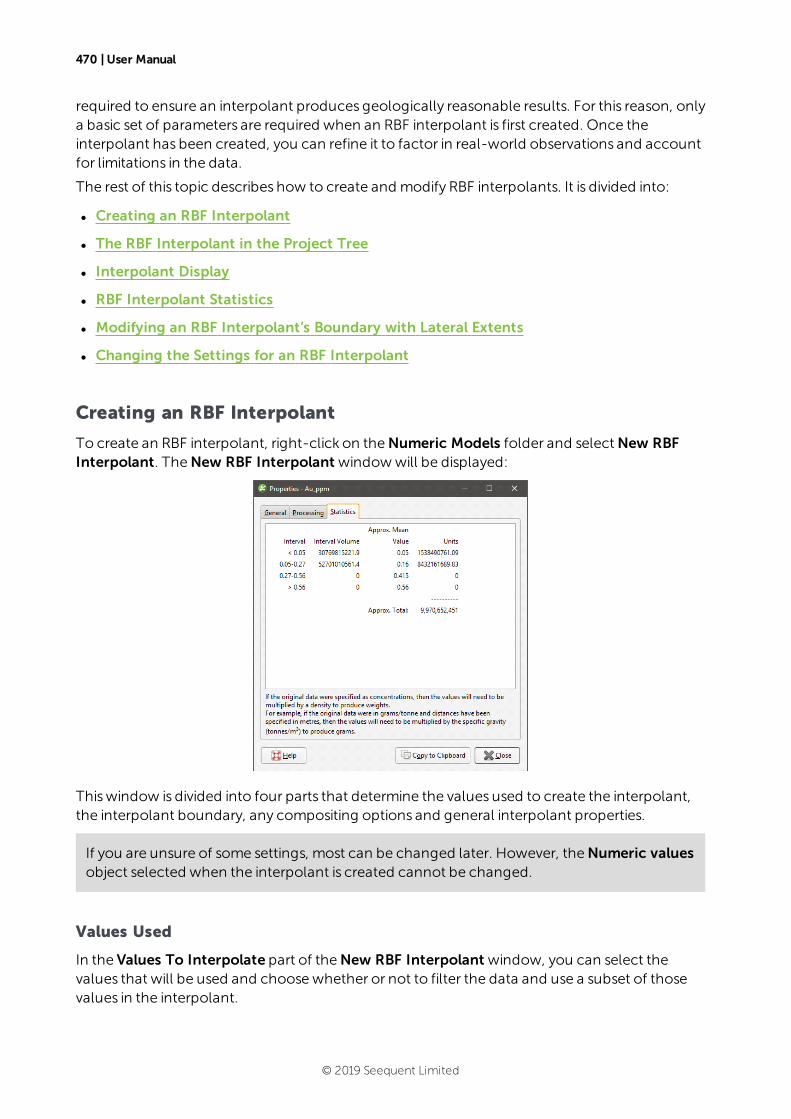
470 | User Manual
required to ensure an interpolant produces geologically reasonable results. For this reason, onlya basic set of parameters are required when an RBF interpolant is first created. Once theinterpolant has been created, you can refine it to factor in real-world observations and accountfor limitations in the data.
The rest of this topic describes how to create and modify RBF interpolants. It is divided into:
l Creating an RBF Interpolant
l The RBF Interpolant in the Project Tree
l Interpolant Display
l RBF Interpolant Statistics
l Modifying an RBF Interpolant’s Boundary with Lateral Extents
l Changing the Settings for an RBF Interpolant
Creating an RBF Interpolant
To create an RBF interpolant, right-click on theNumeric Models folder and selectNew RBFInterpolant. TheNew RBF Interpolant windowwill be displayed:
Thiswindow is divided into four parts that determine the values used to create the interpolant,the interpolant boundary, any compositing options and general interpolant properties.
If you are unsure of some settings, most can be changed later. However, theNumeric valuesobject selected when the interpolant is created cannot be changed.
Values Used
In the Values To Interpolate part of theNew RBF Interpolant window, you can select thevalues that will be used and choosewhether or not to filter the data and use a subset of thosevalues in the interpolant.
© 2019 Seequent Limited
Applying a Query Filter | 471
You can build an interpolant fromeither:
l Numeric data contained in imported drillhole data.
l Points data imported into the Points folder.
All suitable data in the project is available from theNumeric values list.
Applying a Query Filter
If you have defined a query filter and wish to use it to create the interpolant, select the filter fromtheQuery filter list. Once the interpolant has been created, you can remove the filter or select adifferent filter.
Applying a Surface Filter
All available data can be used to generate the interpolant or the data can be filtered so that onlythe data that iswithin the interpolant boundary or another boundary in the project influencesthe interpolant. The Surface Filter option is enabled by default, but if you wish to use all data inthe project, untick the box for Surface Filter. Otherwise, you can select the InterpolantBoundary or another boundary in the project.
You can use both theQuery Filter option and the Surface Filter option together.
The Interpolant Boundary
There are several ways to set the Interpolant Boundary:
l Enter values to set a Custom boundary.
l Use the controls in the scene to set theCustom boundary dimensions.
l Select another object in the project from the Enclose Object list, which could be thenumeric values object being interpolated. The extents for that object will be used as the basisfor theCustom boundary dimensions.
l Select another object in the project to use as the Interpolant Boundary. Click the Existingmodel boundary or volume option and select the required object from the list.
Once the interpolant has been created, you can furthermodify its boundary. SeeModifying anRBF Interpolant’s Boundary with Lateral Extents and Adjusting the Interpolant Boundarybelow.
Compositing Options
When numeric values fromdrillhole data are used to create an interpolant, there are twoapproaches to compositing that data:
l Composite the drillhole data, then use the composited values to create an interpolant. If youselect composited values to create an interpolant, compositing optionswill be disabled.
l Use drillhole data that hasn’t been composited to create an interpolant, then applycompositing settings to the interpolated values. If you are interpolating values that have notbeen composited and do not have specificCompositing values in mind, you maywish toleave this option blank as it can be changed once themodel has been created.
© 2019 Seequent Limited
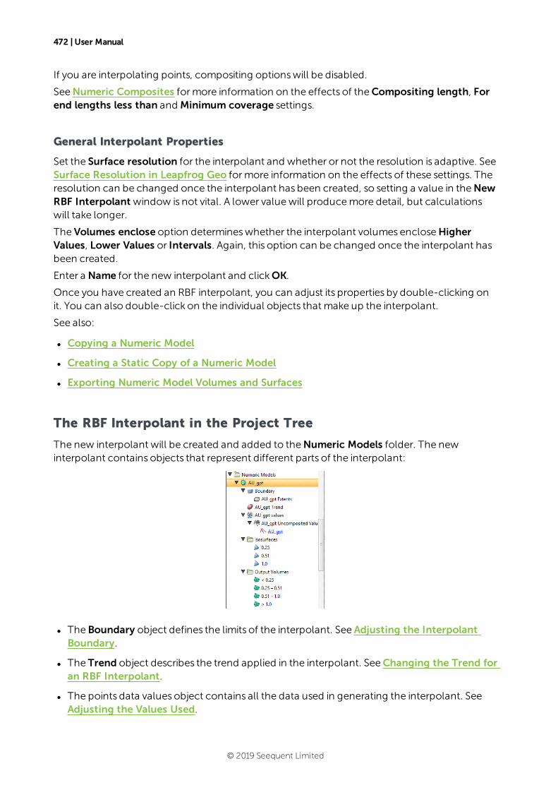
472 | User Manual
If you are interpolating points, compositing optionswill be disabled.
SeeNumeric Composites formore information on the effects of theCompositing length, Forend lengths less than and Minimum coverage settings.
General Interpolant Properties
Set the Surface resolution for the interpolant and whether or not the resolution is adaptive. SeeSurface Resolution in Leapfrog Geo formore information on the effects of these settings. Theresolution can be changed once the interpolant has been created, so setting a value in theNewRBF Interpolant window is not vital. A lower valuewill producemore detail, but calculationswill take longer.
The Volumes enclose option determineswhether the interpolant volumes encloseHigherValues, Lower Values or Intervals. Again, this option can be changed once the interpolant hasbeen created.
Enter a Name for the new interpolant and clickOK.
Once you have created an RBF interpolant, you can adjust its properties by double-clicking onit. You can also double-click on the individual objects that make up the interpolant.
See also:
l Copying a Numeric Model
l Creating a Static Copy of a Numeric Model
l Exporting Numeric Model Volumes and Surfaces
The RBF Interpolant in the Project Tree
The new interpolant will be created and added to theNumeric Models folder. The newinterpolant contains objects that represent different parts of the interpolant:
l The Boundary object defines the limits of the interpolant. See Adjusting the InterpolantBoundary.
l The Trend object describes the trend applied in the interpolant. SeeChanging the Trend foran RBF Interpolant.
l The points data values object contains all the data used in generating the interpolant. SeeAdjusting the Values Used.
© 2019 Seequent Limited
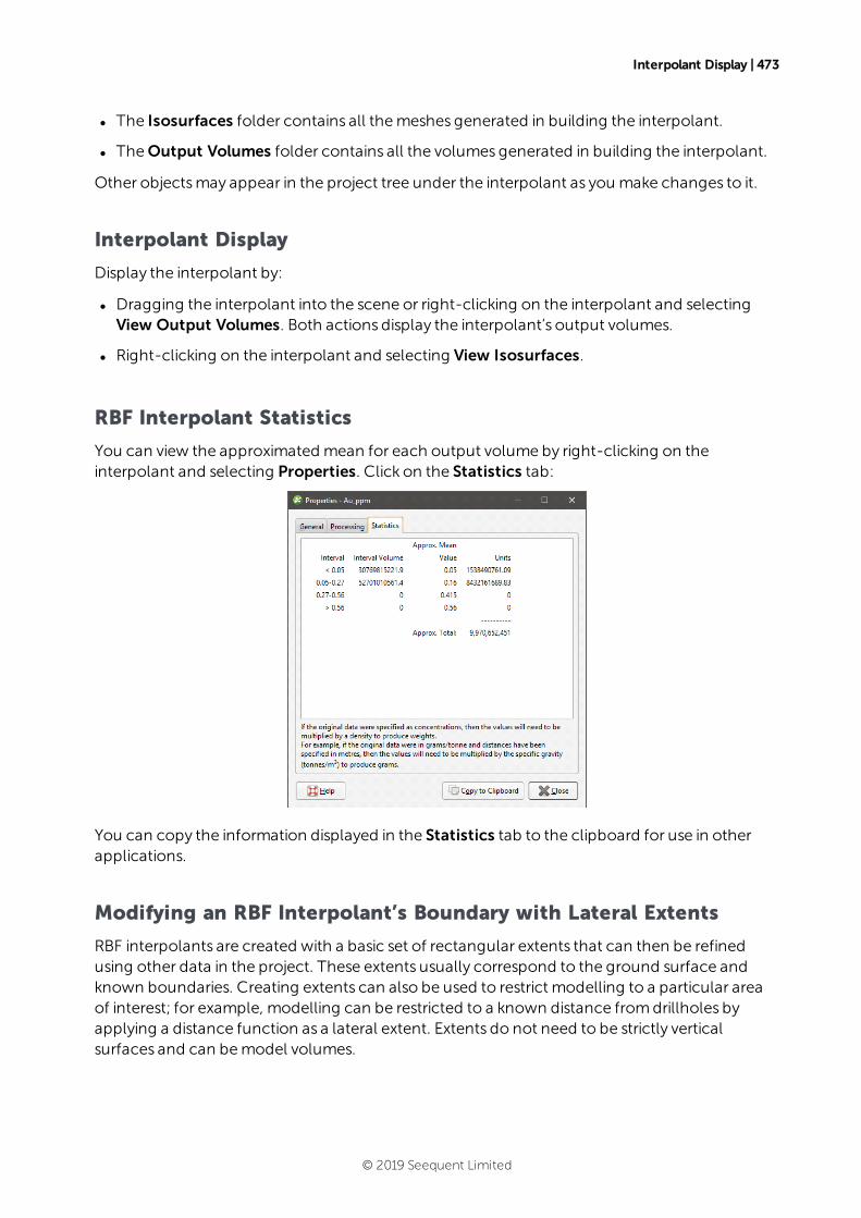
Interpolant Display | 473
l The Isosurfaces folder contains all themeshes generated in building the interpolant.
l TheOutput Volumes folder contains all the volumes generated in building the interpolant.
Other objectsmay appear in the project tree under the interpolant as you make changes to it.
Interpolant Display
Display the interpolant by:
l Dragging the interpolant into the scene or right-clicking on the interpolant and selectingView Output Volumes. Both actions display the interpolant’s output volumes.
l Right-clicking on the interpolant and selecting View Isosurfaces.
RBF Interpolant Statistics
You can view the approximated mean for each output volume by right-clicking on theinterpolant and selecting Properties. Click on the Statistics tab:
You can copy the information displayed in the Statistics tab to the clipboard for use in otherapplications.
Modifying an RBF Interpolant’s Boundary with Lateral Extents
RBF interpolants are created with a basic set of rectangular extents that can then be refinedusing other data in the project. These extents usually correspond to the ground surface andknown boundaries. Creating extents can also be used to restrict modelling to a particular areaof interest; for example, modelling can be restricted to a known distance fromdrillholes byapplying a distance function as a lateral extent. Extents do not need to be strictly verticalsurfaces and can bemodel volumes.
© 2019 Seequent Limited
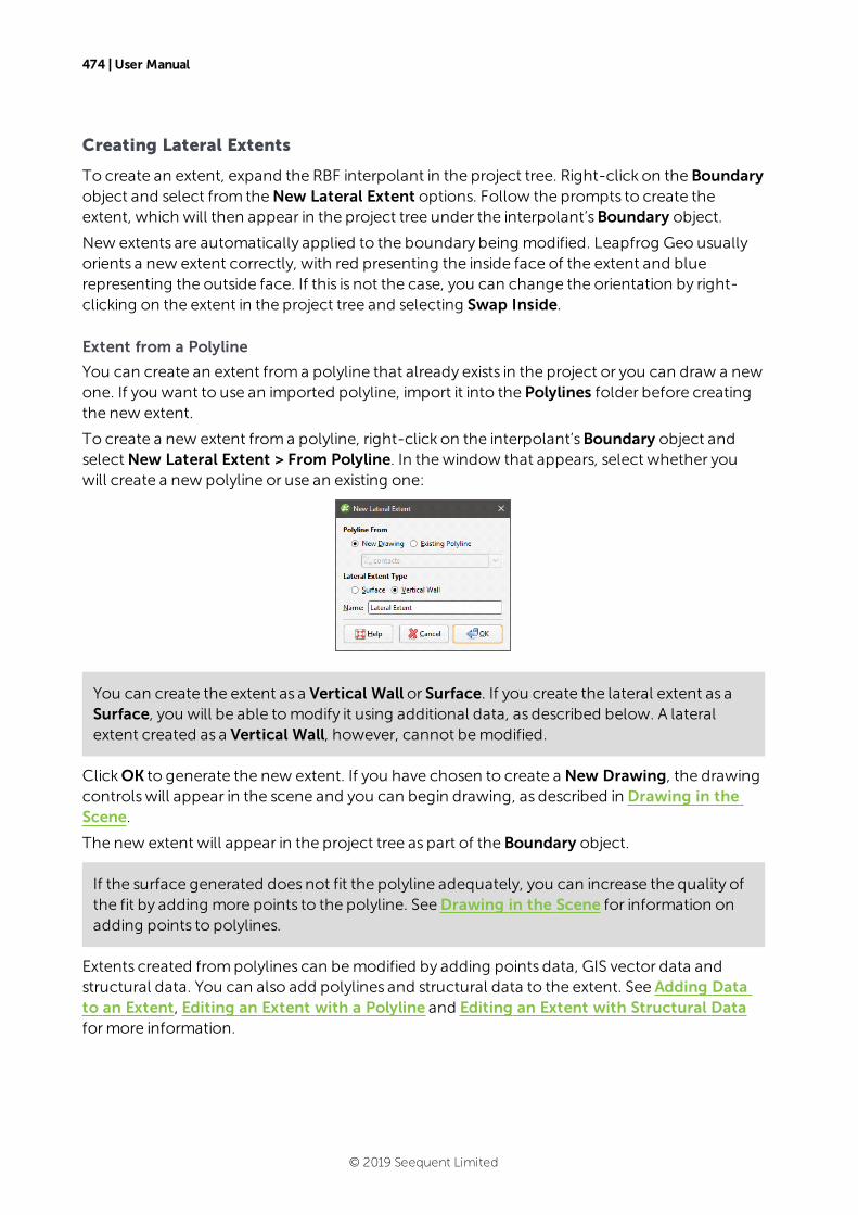
474 | User Manual
Creating Lateral Extents
To create an extent, expand the RBF interpolant in the project tree. Right-click on the Boundaryobject and select from theNew Lateral Extent options. Follow the prompts to create theextent, which will then appear in the project tree under the interpolant’sBoundary object.
New extents are automatically applied to the boundary being modified. Leapfrog Geo usuallyorients a new extent correctly, with red presenting the inside face of the extent and bluerepresenting the outside face. If this is not the case, you can change the orientation by right-clicking on the extent in the project tree and selecting Swap Inside.
Extent from a Polyline
You can create an extent froma polyline that already exists in the project or you can draw a newone. If you want to use an imported polyline, import it into the Polylines folder before creatingthe new extent.
To create a new extent froma polyline, right-click on the interpolant’sBoundary object andselectNew Lateral Extent > From Polyline. In thewindow that appears, select whether youwill create a new polyline or use an existing one:
You can create the extent as a Vertical Wall or Surface. If you create the lateral extent as aSurface, you will be able tomodify it using additional data, as described below. A lateralextent created as a Vertical Wall, however, cannot bemodified.
ClickOK to generate the new extent. If you have chosen to create a New Drawing, the drawingcontrolswill appear in the scene and you can begin drawing, as described in Drawing in theScene.
The new extent will appear in the project tree as part of the Boundary object.
If the surface generated does not fit the polyline adequately, you can increase the quality ofthe fit by adding more points to the polyline. SeeDrawing in the Scene for information onadding points to polylines.
Extents created frompolylines can bemodified by adding points data, GIS vector data andstructural data. You can also add polylines and structural data to the extent. See Adding Datato an Extent, Editing an Extent with a Polyline and Editing an Extent with Structural Dataformore information.
© 2019 Seequent Limited
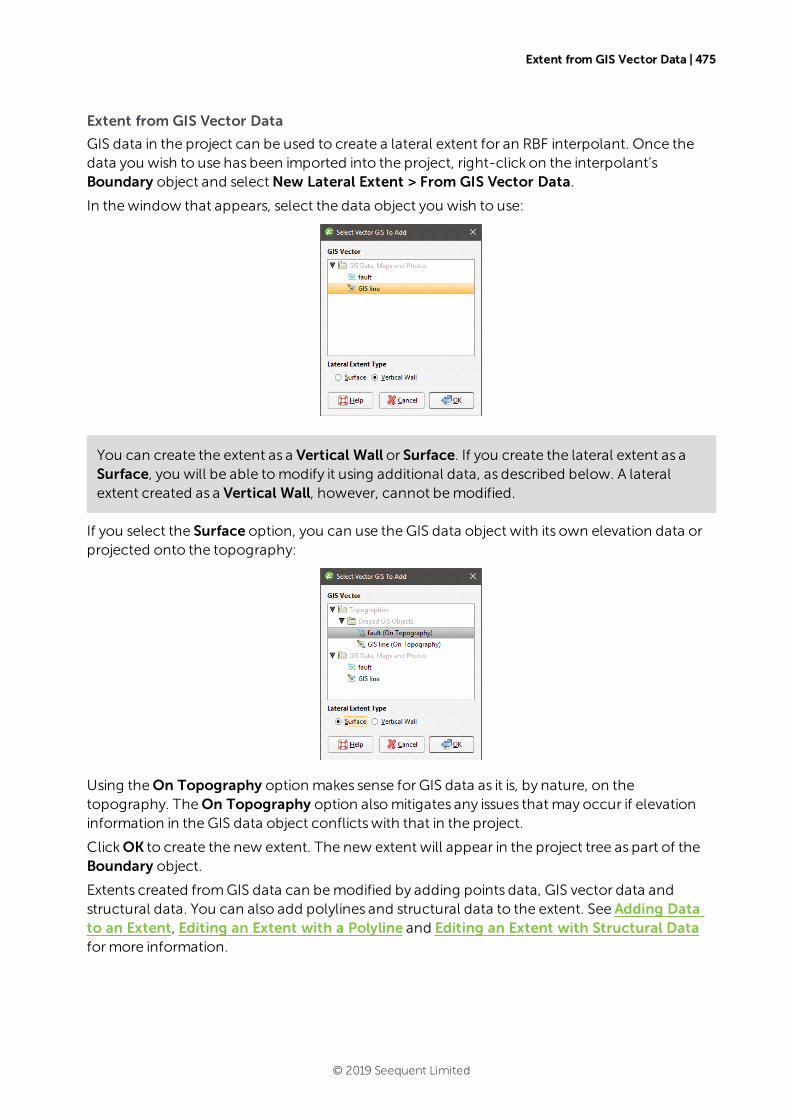
Extent from GIS Vector Data | 475
Extent from GIS Vector Data
GIS data in the project can be used to create a lateral extent for an RBF interpolant. Once thedata you wish to use has been imported into the project, right-click on the interpolant’sBoundary object and selectNew Lateral Extent > From GIS Vector Data.
In thewindow that appears, select the data object you wish to use:
You can create the extent as a Vertical Wall or Surface. If you create the lateral extent as aSurface, you will be able tomodify it using additional data, as described below. A lateralextent created as a Vertical Wall, however, cannot bemodified.
If you select the Surface option, you can use the GIS data object with its own elevation data orprojected onto the topography:
Using theOn Topography option makes sense for GIS data as it is, by nature, on thetopography. TheOn Topography option alsomitigates any issues that may occur if elevationinformation in the GIS data object conflictswith that in the project.
ClickOK to create the new extent. The new extent will appear in the project tree as part of theBoundary object.
Extents created fromGIS data can bemodified by adding points data, GIS vector data andstructural data. You can also add polylines and structural data to the extent. See Adding Datato an Extent, Editing an Extent with a Polyline and Editing an Extent with Structural Dataformore information.
© 2019 Seequent Limited
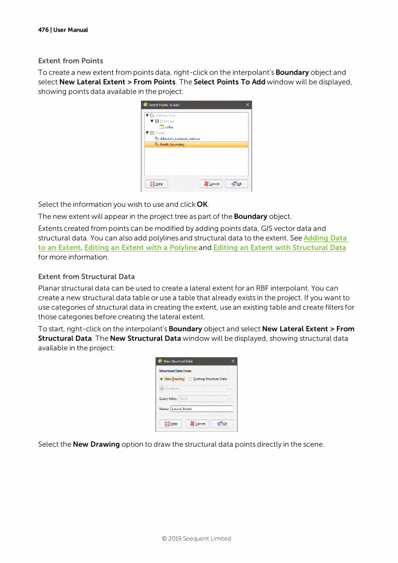
476 | User Manual
Extent from Points
To create a new extent frompoints data, right-click on the interpolant’sBoundary object andselectNew Lateral Extent > From Points. The Select Points To Addwindowwill be displayed,showing points data available in the project:
Select the information you wish to use and clickOK.
The new extent will appear in the project tree as part of the Boundary object.
Extents created frompoints can bemodified by adding points data, GIS vector data andstructural data. You can also add polylines and structural data to the extent. See Adding Datato an Extent, Editing an Extent with a Polyline and Editing an Extent with Structural Dataformore information.
Extent from Structural Data
Planar structural data can be used to create a lateral extent for an RBF interpolant. You cancreate a new structural data table or use a table that already exists in the project. If you want touse categories of structural data in creating the extent, use an existing table and create filters forthose categories before creating the lateral extent.
To start, right-click on the interpolant’sBoundary object and selectNew Lateral Extent > FromStructural Data. TheNew Structural Datawindowwill be displayed, showing structural dataavailable in the project:
Select theNew Drawing option to draw the structural data points directly in the scene.
© 2019 Seequent Limited
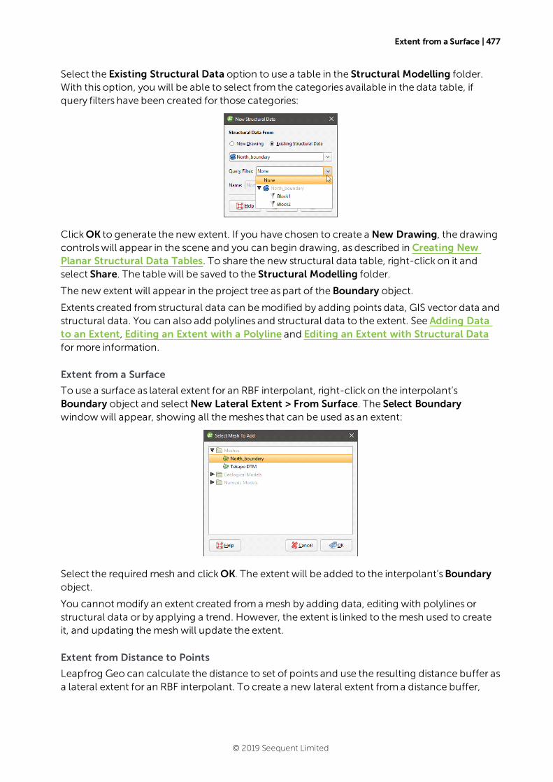
Extent from a Surface | 477
Select the Existing Structural Data option to use a table in the Structural Modelling folder.With this option, you will be able to select from the categories available in the data table, ifquery filters have been created for those categories:
ClickOK to generate the new extent. If you have chosen to create a New Drawing, the drawingcontrolswill appear in the scene and you can begin drawing, as described in Creating NewPlanar Structural Data Tables. To share the new structural data table, right-click on it andselect Share. The table will be saved to the Structural Modelling folder.
The new extent will appear in the project tree as part of the Boundary object.
Extents created from structural data can bemodified by adding points data, GIS vector data andstructural data. You can also add polylines and structural data to the extent. See Adding Datato an Extent, Editing an Extent with a Polyline and Editing an Extent with Structural Dataformore information.
Extent from a Surface
To use a surface as lateral extent for an RBF interpolant, right-click on the interpolant’sBoundary object and selectNew Lateral Extent > From Surface. The Select Boundarywindowwill appear, showing all themeshes that can be used as an extent:
Select the required mesh and clickOK. The extent will be added to the interpolant’sBoundaryobject.
You cannot modify an extent created froma mesh by adding data, editing with polylines orstructural data or by applying a trend. However, the extent is linked to themesh used to createit, and updating themesh will update the extent.
Extent from Distance to Points
Leapfrog Geo can calculate the distance to set of points and use the resulting distance buffer asa lateral extent for an RBF interpolant. To create a new lateral extent froma distance buffer,
© 2019 Seequent Limited
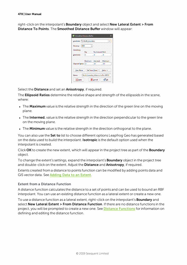
478 | User Manual
right-click on the interpolant’sBoundary object and selectNew Lateral Extent > FromDistance To Points. The Smoothed Distance Buffer windowwill appear:
Select theDistance and set an Anisotropy, if required.
The Ellipsoid Ratios determine the relative shape and strength of the ellipsoids in the scene,where:
l TheMaximum value is the relative strength in the direction of the green line on themovingplane.
l The Intermed. value is the relative strength in the direction perpendicular to the green lineon themoving plane.
l TheMinimum value is the relative strength in the direction orthogonal to the plane.
You can also use the Set to list to choose different options Leapfrog Geo has generated basedon the data used to build the interpolant. Isotropic is the default option used when theinterpolant is created.
ClickOK to create the new extent, which will appear in the project tree as part of the Boundaryobject.
To change the extent’s settings, expand the interpolant’sBoundary object in the project treeand double-click on the extent. Adjust theDistance and Anisotropy, if required.
Extents created froma distance to points function can bemodified by adding points data andGIS vector data. See Adding Data to an Extent.
Extent from a Distance Function
A distance function calculates the distance to a set of points and can be used to bound an RBFinterpolant. You can use an existing distance function as a lateral extent or create a new one.
To use a distance function as a lateral extent, right-click on the interpolant’sBoundary andselectNew Lateral Extent > From Distance Function. If there are no distance functions in theproject, you will be prompted to create a new one. SeeDistance Functions for information ondefining and editing the distance function.
© 2019 Seequent Limited
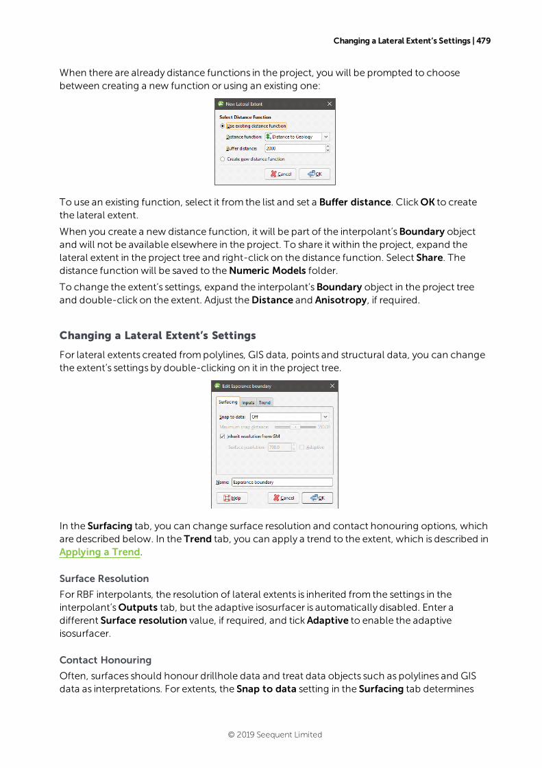
Changing a Lateral Extent’s Settings | 479
When there are already distance functions in the project, you will be prompted to choosebetween creating a new function or using an existing one:
To use an existing function, select it from the list and set a Buffer distance. ClickOK to createthe lateral extent.
When you create a new distance function, it will be part of the interpolant’sBoundary objectand will not be available elsewhere in the project. To share it within the project, expand thelateral extent in the project tree and right-click on the distance function. Select Share. Thedistance function will be saved to theNumeric Models folder.
To change the extent’s settings, expand the interpolant’sBoundary object in the project treeand double-click on the extent. Adjust theDistance and Anisotropy, if required.
Changing a Lateral Extent’s Settings
For lateral extents created frompolylines, GIS data, points and structural data, you can changethe extent’s settings by double-clicking on it in the project tree.
In the Surfacing tab, you can change surface resolution and contact honouring options, whichare described below. In the Trend tab, you can apply a trend to the extent, which is described inApplying a Trend.
Surface Resolution
For RBF interpolants, the resolution of lateral extents is inherited from the settings in theinterpolant’sOutputs tab, but the adaptive isosurfacer is automatically disabled. Enter adifferent Surface resolution value, if required, and tickAdaptive to enable the adaptiveisosurfacer.
Contact Honouring
Often, surfaces should honour drillhole data and treat data objects such as polylines and GISdata as interpretations. For extents, the Snap to data setting in the Surfacing tab determines
© 2019 Seequent Limited
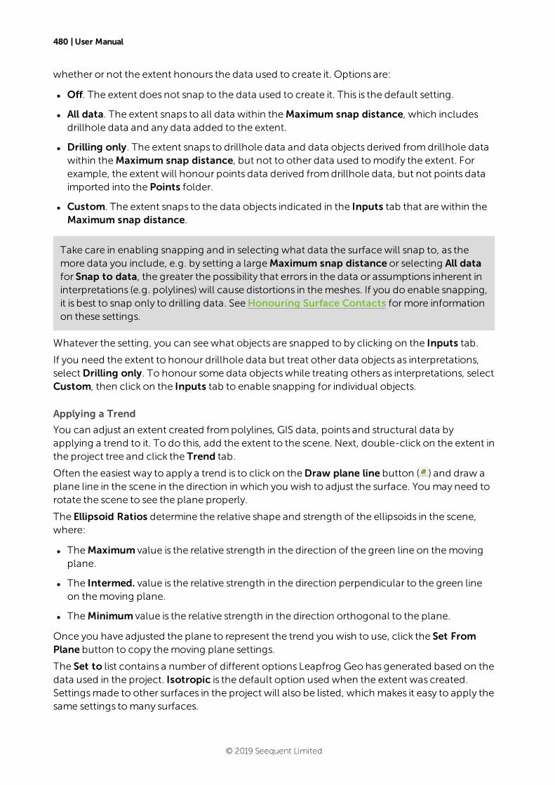
480 | User Manual
whether or not the extent honours the data used to create it. Options are:
l Off. The extent does not snap to the data used to create it. This is the default setting.
l All data. The extent snaps to all data within theMaximum snap distance, which includesdrillhole data and any data added to the extent.
l Drilling only. The extent snaps to drillhole data and data objects derived fromdrillhole datawithin theMaximum snap distance, but not to other data used tomodify the extent. Forexample, the extent will honour points data derived fromdrillhole data, but not points dataimported into the Points folder.
l Custom. The extent snaps to the data objects indicated in the Inputs tab that are within theMaximum snap distance.
Take care in enabling snapping and in selecting what data the surfacewill snap to, as themore data you include, e.g. by setting a largeMaximum snap distance or selecting All datafor Snap to data, the greater the possibility that errors in the data or assumptions inherent ininterpretations (e.g. polylines) will cause distortions in themeshes. If you do enable snapping,it is best to snap only to drilling data. SeeHonouring Surface Contacts formore informationon these settings.
Whatever the setting, you can seewhat objects are snapped to by clicking on the Inputs tab.
If you need the extent to honour drillhole data but treat other data objects as interpretations,selectDrilling only. To honour some data objectswhile treating others as interpretations, selectCustom, then click on the Inputs tab to enable snapping for individual objects.
Applying a Trend
You can adjust an extent created frompolylines, GIS data, points and structural data byapplying a trend to it. To do this, add the extent to the scene. Next, double-click on the extent inthe project tree and click the Trend tab.
Often the easiest way to apply a trend is to click on theDraw plane line button ( ) and draw aplane line in the scene in the direction in which you wish to adjust the surface. You may need torotate the scene to see the plane properly.
The Ellipsoid Ratios determine the relative shape and strength of the ellipsoids in the scene,where:
l TheMaximum value is the relative strength in the direction of the green line on themovingplane.
l The Intermed. value is the relative strength in the direction perpendicular to the green lineon themoving plane.
l TheMinimum value is the relative strength in the direction orthogonal to the plane.
Once you have adjusted the plane to represent the trend you wish to use, click the Set FromPlane button to copy themoving plane settings.
The Set to list contains a number of different options Leapfrog Geo has generated based on thedata used in the project. Isotropic is the default option used when the extent was created.Settingsmade to other surfaces in the project will also be listed, which makes it easy to apply thesame settings tomany surfaces.
© 2019 Seequent Limited
Adding Data to an Extent | 481
ClickOK to apply the changes.
SeeGlobal Trends formore information.
Adding Data to an Extent
Extents created frompolylines, GIS data, points and structural data can bemodified by addingpoints data objects, GIS vector data and structural data. Extents created froma distance topoints function can bemodified by adding points data and GIS vector data. To add data to anextent, right-click on the extent in the project tree and select the data type you wish to use fromthe Addmenu.
l Points data. Select from the points data objects available in the project and clickOK.
l GIS vector data. Select from theGIS vector data available in the project and clickOK.
l Structural data. Select from the structural data tables available in the project. If the selectedtable has query filters defined, you can apply one of these filters by ticking Use query filterand then selecting the required filter from the list. ClickOK to add the selected data to theextent. An alternative to adding an existing structural data table to an extent is to edit theextent with structural data. This is described in Editing an Extent with Structural Databelow.
You can also add a polyline that already exists in the project. To do this, right-click on the extentin the project tree and select Add > Polyline. You will be prompted to choose from the polylinesin the Polylines folder.
Editing an Extent with a Polyline
You can edit an extent using a polyline, which is described in Editing Surfaces with Polylines. Apolyline used to edit an extent will be added to the project tree as part of the extent. To edit thepolyline, right-click on it and select Edit Polyline or add it to the scene and click the Edit button () in the shape list. If you wish to remove the polyline from the extent, right-click on it in the
project tree and selectDelete orRemove.
To add an existing polyline to a lateral extent, use the Add > Polyline option.
Editing an Extent with Structural Data
You can edit an extent using structural data, which is described in Editing Surfaces withStructural Data. A structural data table will be added to the project tree as part of the extent.To edit the table, right-click on it and select Edit In Scene or add it to the scene and click theEdit button ( ) in the shape list. If you wish to remove the table from the extent, right-click on itin the project tree and selectDelete orRemove.
Removing an Extent from an Interpolant
If you have defined an extent and want to remove it from the interpolant, there are two options.The first is to right-click on the extent in the project tree and clickDelete. This deletes the extentfrom the interpolant, but does not delete parent objects from the project unless theywere
© 2019 Seequent Limited
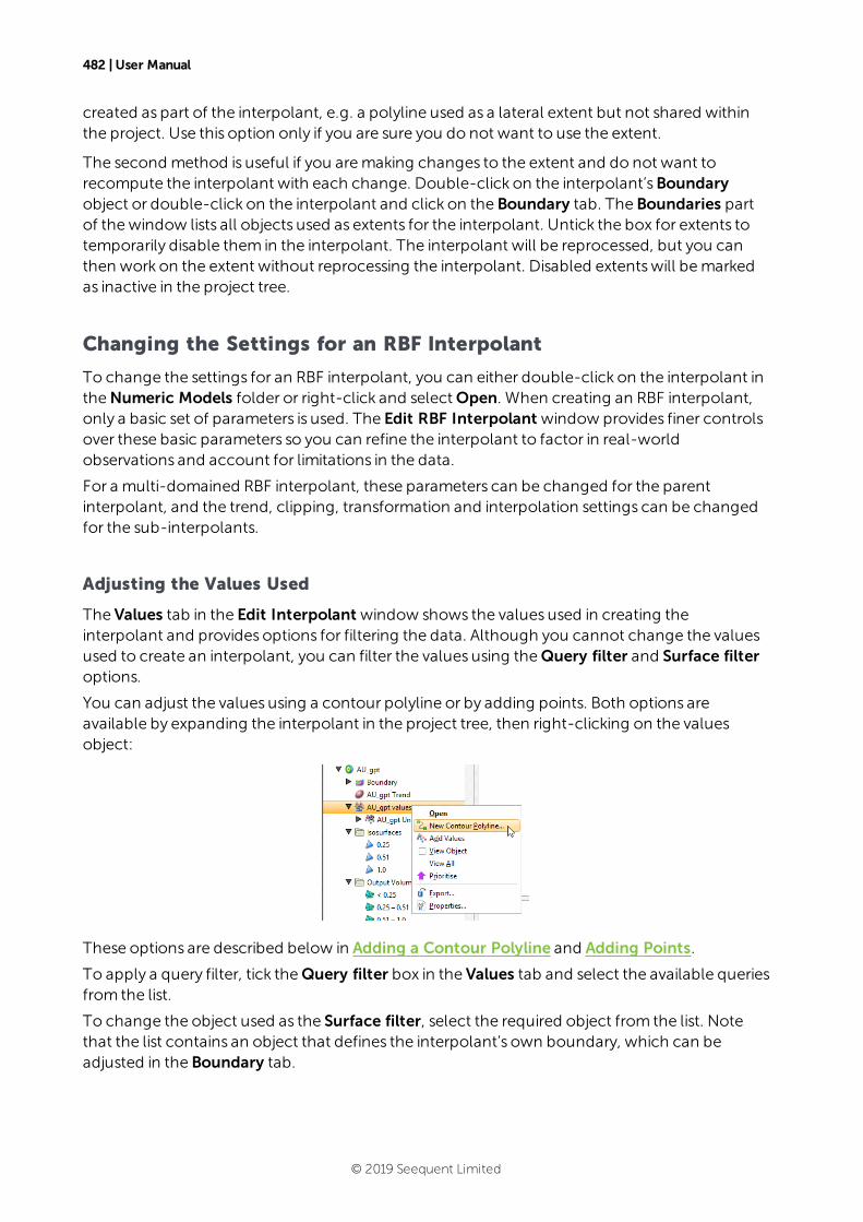
482 | User Manual
created as part of the interpolant, e.g. a polyline used as a lateral extent but not shared withinthe project. Use this option only if you are sure you do not want to use the extent.
The second method is useful if you aremaking changes to the extent and do not want torecompute the interpolant with each change. Double-click on the interpolant’sBoundaryobject or double-click on the interpolant and click on the Boundary tab. The Boundaries partof thewindow lists all objects used as extents for the interpolant. Untick the box for extents totemporarily disable them in the interpolant. The interpolant will be reprocessed, but you canthen work on the extent without reprocessing the interpolant. Disabled extentswill bemarkedas inactive in the project tree.
Changing the Settings for an RBF Interpolant
To change the settings for an RBF interpolant, you can either double-click on the interpolant intheNumeric Models folder or right-click and selectOpen. When creating an RBF interpolant,only a basic set of parameters is used. The Edit RBF Interpolant window provides finer controlsover these basic parameters so you can refine the interpolant to factor in real-worldobservations and account for limitations in the data.
For a multi-domained RBF interpolant, these parameters can be changed for the parentinterpolant, and the trend, clipping, transformation and interpolation settings can be changedfor the sub-interpolants.
Adjusting the Values Used
The Values tab in the Edit Interpolant window shows the values used in creating theinterpolant and provides options for filtering the data. Although you cannot change the valuesused to create an interpolant, you can filter the values using theQuery filter and Surface filteroptions.
You can adjust the values using a contour polyline or by adding points. Both options areavailable by expanding the interpolant in the project tree, then right-clicking on the valuesobject:
These options are described below in Adding a Contour Polyline and Adding Points.
To apply a query filter, tick theQuery filter box in the Values tab and select the available queriesfrom the list.
To change the object used as the Surface filter, select the required object from the list. Notethat the list contains an object that defines the interpolant’s own boundary, which can beadjusted in the Boundary tab.
© 2019 Seequent Limited
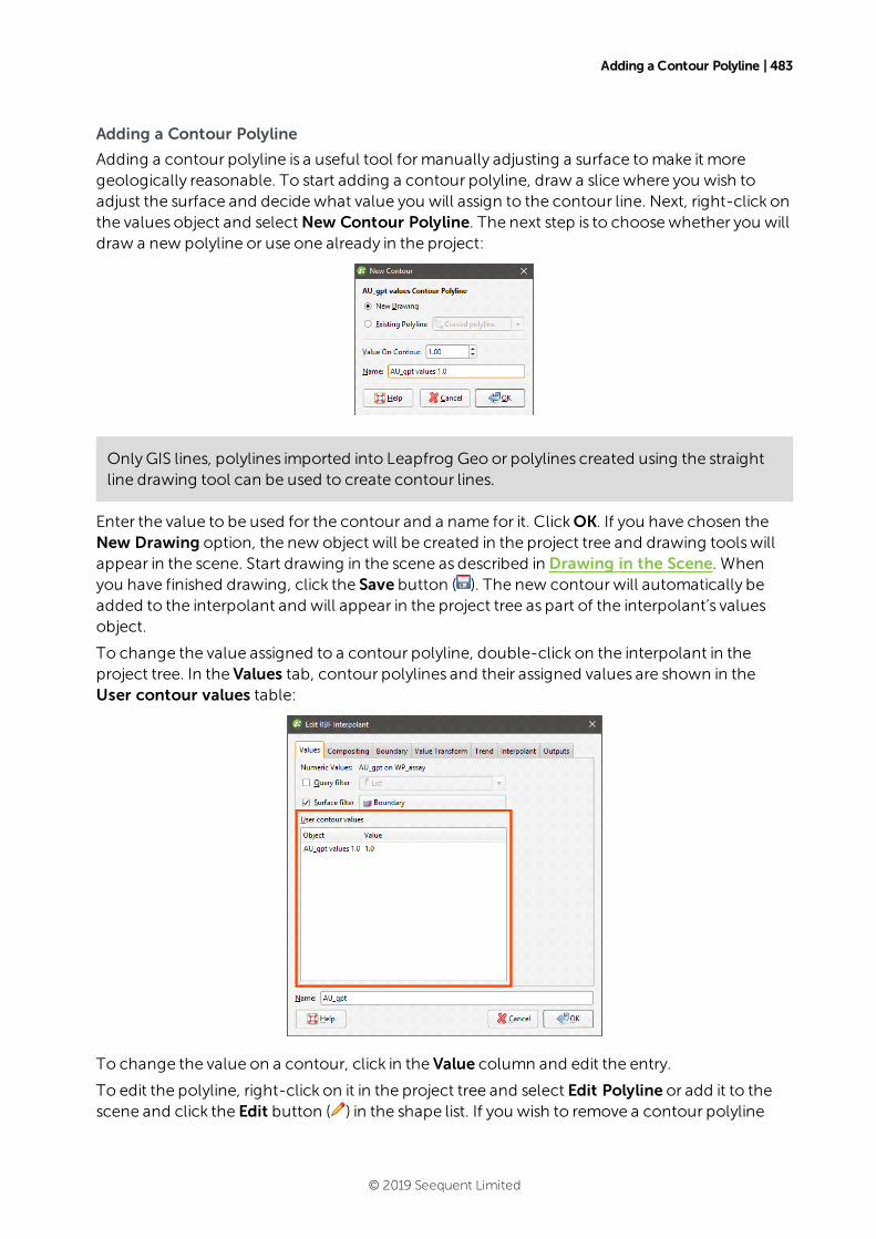
Adding a Contour Polyline | 483
Adding a Contour Polyline
Adding a contour polyline is a useful tool formanually adjusting a surface tomake it moregeologically reasonable. To start adding a contour polyline, draw a slice where you wish toadjust the surface and decidewhat value you will assign to the contour line. Next, right-click onthe values object and selectNew Contour Polyline. The next step is to choosewhether you willdraw a new polyline or use one already in the project:
OnlyGIS lines, polylines imported into Leapfrog Geo or polylines created using the straightline drawing tool can be used to create contour lines.
Enter the value to be used for the contour and a name for it. ClickOK. If you have chosen theNew Drawing option, the new object will be created in the project tree and drawing toolswillappear in the scene. Start drawing in the scene as described in Drawing in the Scene. Whenyou have finished drawing, click the Save button ( ). The new contourwill automatically beadded to the interpolant and will appear in the project tree as part of the interpolant’s valuesobject.
To change the value assigned to a contour polyline, double-click on the interpolant in theproject tree. In the Values tab, contour polylines and their assigned values are shown in theUser contour values table:
To change the value on a contour, click in the Value column and edit the entry.
To edit the polyline, right-click on it in the project tree and select Edit Polyline or add it to thescene and click the Edit button ( ) in the shape list. If you wish to remove a contour polyline
© 2019 Seequent Limited
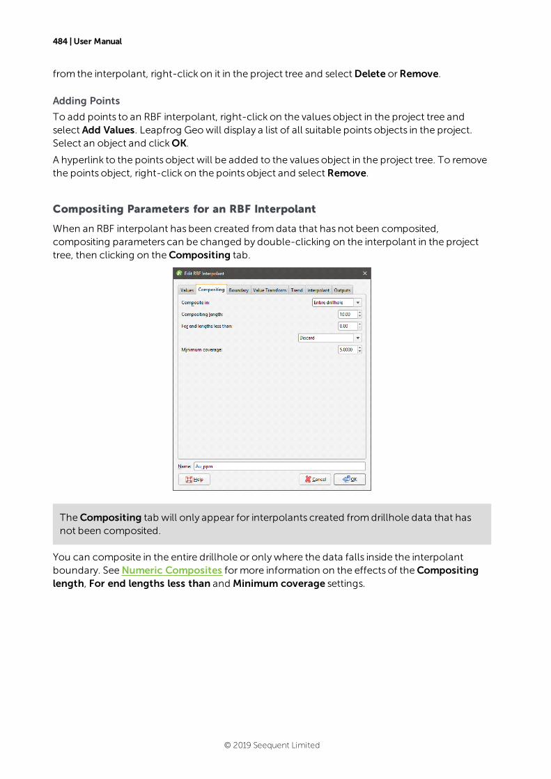
484 | User Manual
from the interpolant, right-click on it in the project tree and selectDelete orRemove.
Adding Points
To add points to an RBF interpolant, right-click on the values object in the project tree andselect Add Values. Leapfrog Geowill display a list of all suitable points objects in the project.Select an object and clickOK.
A hyperlink to the points object will be added to the values object in the project tree. To removethe points object, right-click on the points object and select Remove.
Compositing Parameters for an RBF Interpolant
When an RBF interpolant has been created fromdata that has not been composited,compositing parameters can be changed by double-clicking on the interpolant in the projecttree, then clicking on theCompositing tab.
TheCompositing tab will only appear for interpolants created fromdrillhole data that hasnot been composited.
You can composite in the entire drillhole or onlywhere the data falls inside the interpolantboundary. SeeNumeric Composites formore information on the effects of theCompositinglength, For end lengths less than and Minimum coverage settings.
© 2019 Seequent Limited
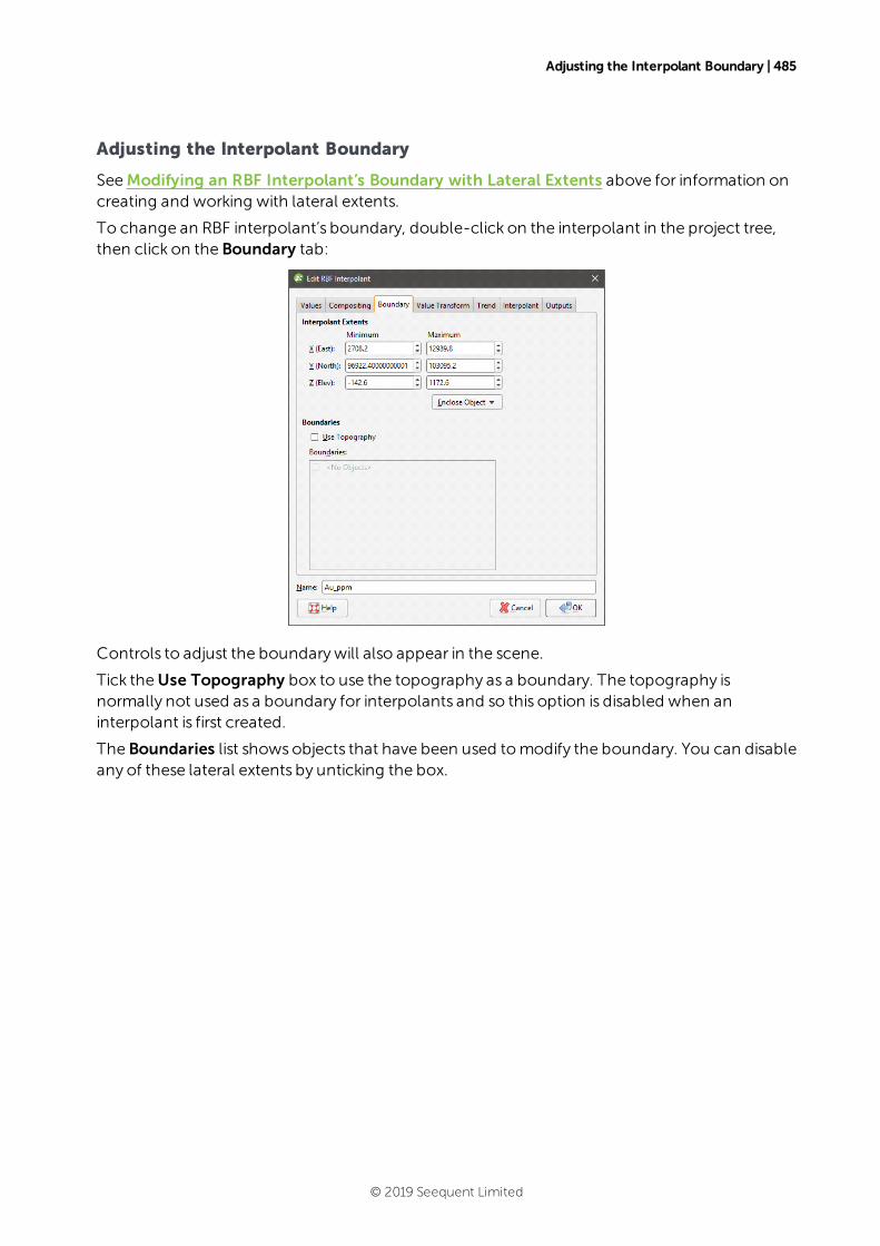
Adjusting the Interpolant Boundary | 485
Adjusting the Interpolant Boundary
SeeModifying an RBF Interpolant’s Boundary with Lateral Extents above for information oncreating and working with lateral extents.
To change an RBF interpolant’s boundary, double-click on the interpolant in the project tree,then click on the Boundary tab:
Controls to adjust the boundarywill also appear in the scene.
Tick theUse Topography box to use the topography as a boundary. The topography isnormally not used as a boundary for interpolants and so this option is disabled when aninterpolant is first created.
The Boundaries list showsobjects that have been used tomodify the boundary. You can disableany of these lateral extents by unticking the box.
© 2019 Seequent Limited
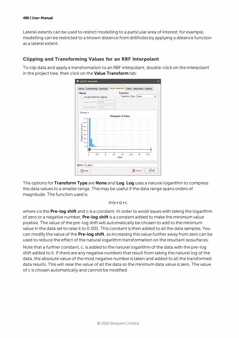
486 | User Manual
Lateral extents can be used to restrict modelling to a particular area of interest; for example,modelling can be restricted to a known distance fromdrillholes by applying a distance functionas a lateral extent.
Clipping and Transforming Values for an RBF Interpolant
To clip data and apply a transformation to an RBF interpolant, double-click on the interpolantin the project tree, then click on the Value Transform tab:
The options for Transform Type areNone and Log. Log uses a natural logarithm to compressthe data values to a smaller range. Thismay be useful if the data range spans orders ofmagnitude. The function used is:
ln(x+s)+c
where s is the Pre-log shift and c is a constant. In order to avoid issueswith taking the logarithmof zero or a negative number, Pre-log shift is a constant added tomake theminimumvaluepositive. The value of the pre-log shift will automatically be chosen to add to theminimumvalue in the data set to raise it to 0.001. This constant is then added to all the data samples. Youcan modify the value of the Pre-log shift, as increasing this value further away fromzero can beused to reduce the effect of the natural logarithm transformation on the resultant isosurfaces.
Note that a further constant, c, is added to the natural logarithmof the data with the pre-logshift added to it. If there are any negative numbers that result from taking the natural log of thedata, the absolute value of themost negative number is taken and added to all the transformeddata results. Thiswill raise the value of all the data so theminimumdata value is zero. The valueof c is chosen automatically and cannot bemodified.
© 2019 Seequent Limited
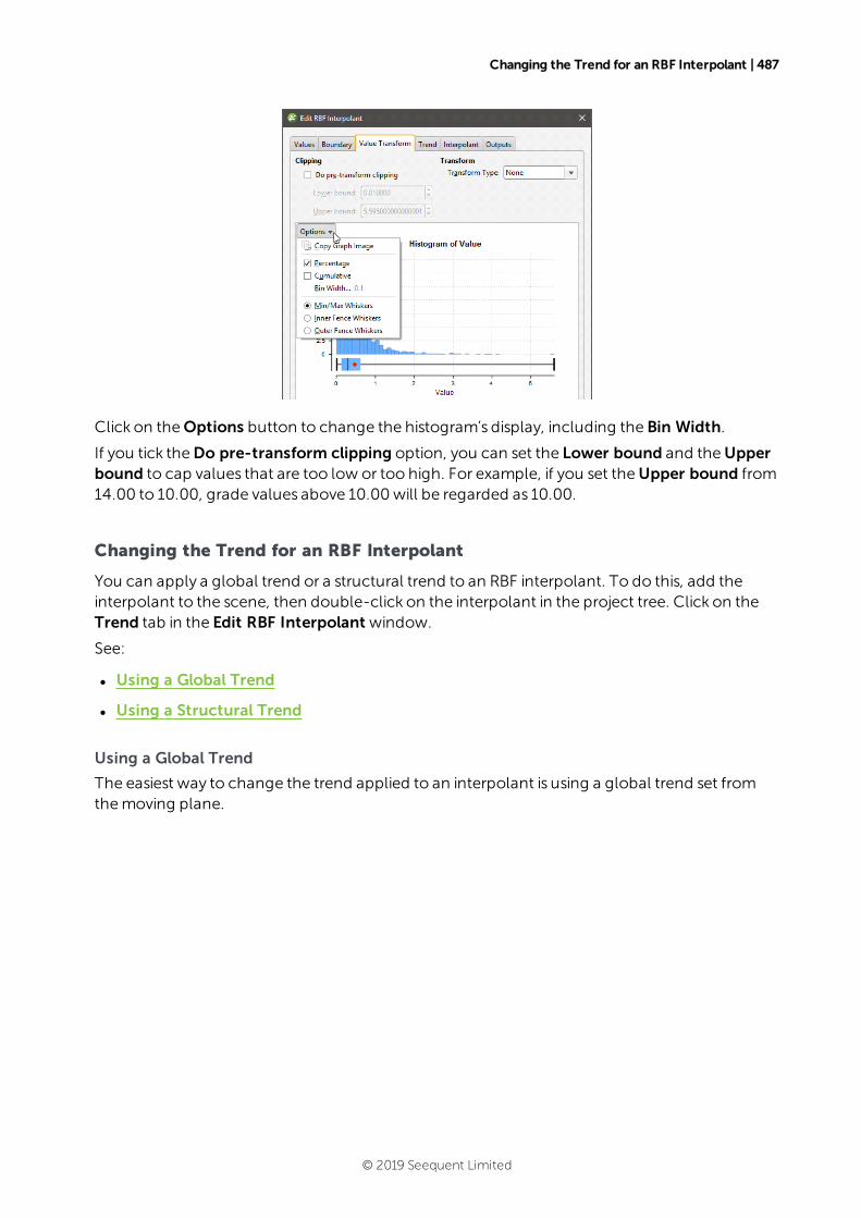
Changing the Trend for an RBF Interpolant | 487
Click on theOptions button to change the histogram’s display, including the Bin Width.
If you tick theDo pre-transform clipping option, you can set the Lower bound and theUpperbound to cap values that are too low or too high. For example, if you set theUpper bound from14.00 to 10.00, grade values above 10.00will be regarded as 10.00.
Changing the Trend for an RBF Interpolant
You can apply a global trend or a structural trend to an RBF interpolant. To do this, add theinterpolant to the scene, then double-click on the interpolant in the project tree. Click on theTrend tab in the Edit RBF Interpolant window.
See:
l Using a Global Trend
l Using a Structural Trend
Using a Global Trend
The easiest way to change the trend applied to an interpolant is using a global trend set fromthemoving plane.
© 2019 Seequent Limited
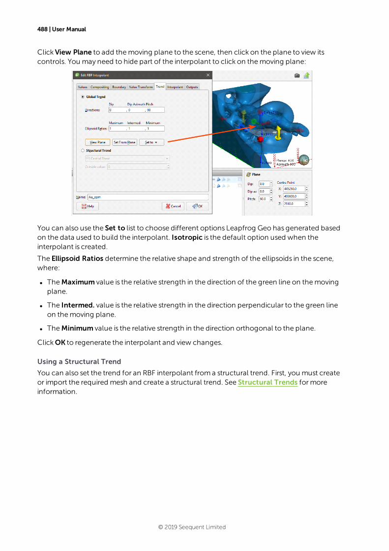
488 | User Manual
ClickView Plane to add themoving plane to the scene, then click on the plane to view itscontrols. You may need to hide part of the interpolant to click on themoving plane:
You can also use the Set to list to choose different options Leapfrog Geo has generated basedon the data used to build the interpolant. Isotropic is the default option used when theinterpolant is created.
The Ellipsoid Ratios determine the relative shape and strength of the ellipsoids in the scene,where:
l TheMaximum value is the relative strength in the direction of the green line on themovingplane.
l The Intermed. value is the relative strength in the direction perpendicular to the green lineon themoving plane.
l TheMinimum value is the relative strength in the direction orthogonal to the plane.
ClickOK to regenerate the interpolant and view changes.
Using a Structural Trend
You can also set the trend for an RBF interpolant froma structural trend. First, you must createor import the required mesh and create a structural trend. See Structural Trends formoreinformation.
© 2019 Seequent Limited
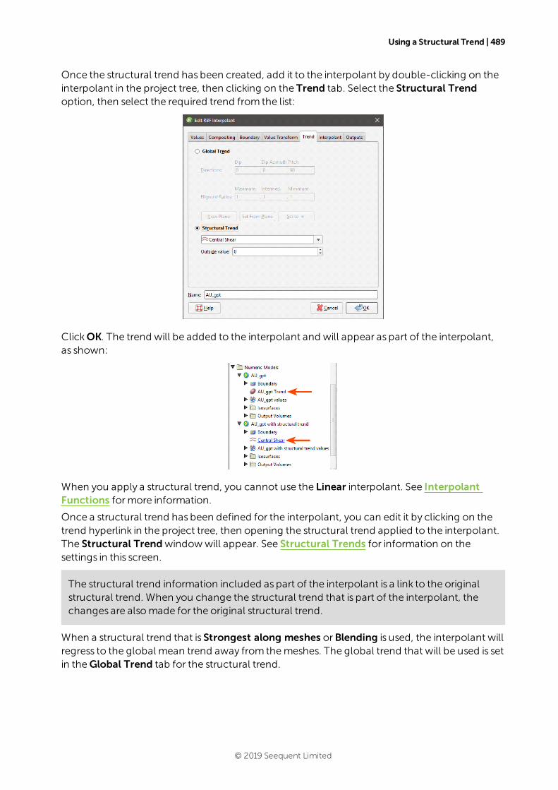
Using a Structural Trend | 489
Once the structural trend has been created, add it to the interpolant by double-clicking on theinterpolant in the project tree, then clicking on the Trend tab. Select the Structural Trendoption, then select the required trend from the list:
ClickOK. The trend will be added to the interpolant and will appear as part of the interpolant,as shown:
When you apply a structural trend, you cannot use the Linear interpolant. See InterpolantFunctions formore information.
Once a structural trend has been defined for the interpolant, you can edit it by clicking on thetrend hyperlink in the project tree, then opening the structural trend applied to the interpolant.The Structural Trendwindowwill appear. See Structural Trends for information on thesettings in this screen.
The structural trend information included as part of the interpolant is a link to the originalstructural trend. When you change the structural trend that is part of the interpolant, thechanges are alsomade for the original structural trend.
When a structural trend that is Strongest along meshes orBlending is used, the interpolant willregress to the global mean trend away from themeshes. The global trend that will be used is setin theGlobal Trend tab for the structural trend.
© 2019 Seequent Limited
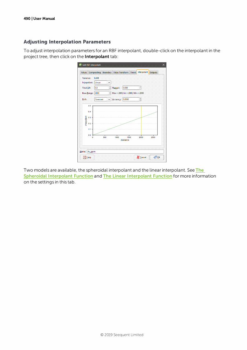
490 | User Manual
Adjusting Interpolation Parameters
To adjust interpolation parameters for an RBF interpolant, double-click on the interpolant in theproject tree, then click on the Interpolant tab:
Twomodels are available, the spheroidal interpolant and the linear interpolant. See TheSpheroidal Interpolant Function and The Linear Interpolant Function formore informationon the settings in this tab.
© 2019 Seequent Limited

Output Settings for an RBF Interpolant | 491
Output Settings for an RBF Interpolant
You can change the parameters used to generate RBF interpolant outputs by double-clickingon the interpolant, then clicking on theOutputs tab.
The Evaluation limits applywhen interpolants are evaluated against other objects in theproject. When the limits are enabled, all values outside the limitswill be set to theMinimum andMaximum.
When Exact clipping is enabled, the interpolant isosurfacewill be generated without “tags” thatoverhang the interpolant boundary. This setting is enabled by default when you create aninterpolant.
To add a new isosurface, click the Add button and enter the required value. To delete anisosurface, click on it in the list, then click theRemove button. You can also change the coloursused to display the isosurfaces by clicking on the colour chips.
If you find that grade shells are overlapping, the resolution may be too coarse. SetDefaultresolution to a lower value or enable adaptive resolution in theOutputs tab. See SurfaceResolution in Leapfrog Geo.
Multi-Domained RBF Interpolants
This topic describes creating and editing multi-domained RBF interpolants:
l Creating a Multi-Domained RBF Interpolant
l Compositing and Filtering the Values Used
l Selecting Domains
l Clipping and Transforming Values
© 2019 Seequent Limited
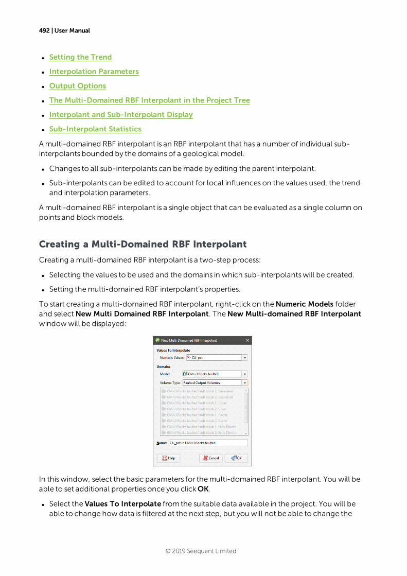
492 | User Manual
l Setting the Trend
l Interpolation Parameters
l Output Options
l The Multi-Domained RBF Interpolant in the Project Tree
l Interpolant and Sub-Interpolant Display
l Sub-Interpolant Statistics
Amulti-domained RBF interpolant is an RBF interpolant that has a number of individual sub-interpolants bounded by the domains of a geological model.
l Changes to all sub-interpolants can bemade by editing the parent interpolant.
l Sub-interpolants can be edited to account for local influences on the values used, the trendand interpolation parameters.
Amulti-domained RBF interpolant is a single object that can be evaluated as a single column onpoints and blockmodels.
Creating a Multi-Domained RBF Interpolant
Creating a multi-domained RBF interpolant is a two-step process:
l Selecting the values to be used and the domains in which sub-interpolantswill be created.
l Setting themulti-domained RBF interpolant’s properties.
To start creating a multi-domained RBF interpolant, right-click on theNumeric Models folderand selectNew Multi Domained RBF Interpolant. TheNew Multi-domained RBF Interpolantwindowwill be displayed:
In thiswindow, select the basic parameters for themulti-domained RBF interpolant. You will beable to set additional properties once you clickOK.
l Select the Values To Interpolate from the suitable data available in the project. You will beable to change how data is filtered at the next step, but you will not be able to change the
© 2019 Seequent Limited
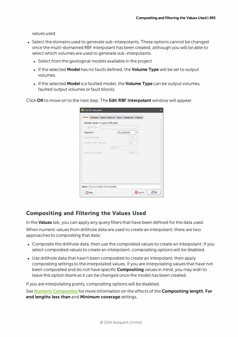
Compositing and Filtering the Values Used | 493
values used.
l Select the domains used to generate sub-interpolants. These options cannot be changedonce themulti-domained RBF interpolant has been created, although you will be able toselect which volumes are used to generate sub-interpolants.
l Select from the geological models available in the project.
l If the selected Model has no faults defined, the Volume Typewill be set to outputvolumes.
l If the selected Model is a faulted model, the Volume Type can be output volumes,faulted output volumesor fault blocks.
ClickOK tomove on to the next step. The Edit RBF Interpolant windowwill appear:
Compositing and Filtering the Values Used
In the Values tab, you can apply any query filters that have been defined for the data used.
When numeric values fromdrillhole data are used to create an interpolant, there are twoapproaches to compositing that data:
l Composite the drillhole data, then use the composited values to create an interpolant. If youselect composited values to create an interpolant, compositing optionswill be disabled.
l Use drillhole data that hasn’t been composited to create an interpolant, then applycompositing settings to the interpolated values. If you are interpolating values that have notbeen composited and do not have specificCompositing values in mind, you maywish toleave this option blank as it can be changed once themodel has been created.
If you are interpolating points, compositing optionswill be disabled.
SeeNumeric Composites formore information on the effects of theCompositing length, Forend lengths less than and Minimum coverage settings.
© 2019 Seequent Limited
494 | User Manual
Selecting Domains
In theDomains tab, you can select the volumes in which sub-interpolantswill be generated.You cannot, however, change the geological model or the types of volumes used.
Clipping and Transforming Values
In the Value Transform tab, clip data and apply a transformation, if required. SeeClipping andTransforming Values for an RBF Interpolant formore information about the settings in thistab.
You will be able to change the Value Transform settings for individual sub-interpolants oncethe parent interpolant has been created.
Setting the Trend
In the Trend tab, you can apply a global or structural trend to the interpolant. SeeChangingthe Trend for an RBF Interpolant formore information about these options.
You will be able to change the Trend settings for the interpolant and individual sub-interpolants once the parent interpolant has been created.
Interpolation Parameters
In the Interpolant tab, you can change interpolation parameters. See Adjusting InterpolationParameters formore information about these options.
You will be able to change the Interpolant settings or import variogramparameters for theinterpolant and individual sub-interpolants once the parent interpolant has been created.
Output Options
In theOutputs tab, you can change the parameters used to generate interpolant outputs.
The Evaluation limits applywhen interpolants are evaluated against other objects in theproject. When the limits are enabled, all values outside the limitswill be set to theMinimum andMaximum.
Set theDefault resolution for the interpolant and whether or not the resolution is adaptive. SeeSurface Resolution in Leapfrog Geo formore information on the effects of these settings. Theresolution can be changed once the interpolant has been created, so setting a valuewhencreating the parent interpolant is not vital. A lower valuewill producemore detail, butcalculationswill take longer.
When Exact clipping is enabled, the interpolant isosurfacewill be generated without “tags” thatoverhang the interpolant boundary. This setting is enabled by default when you create aninterpolant.
To add a new isosurface, click the Add button and enter the required value. To delete anisosurface, click on it in the list, then click theRemove button. You can also change the coloursused to display the isosurfaces by clicking on the colour chips.
© 2019 Seequent Limited
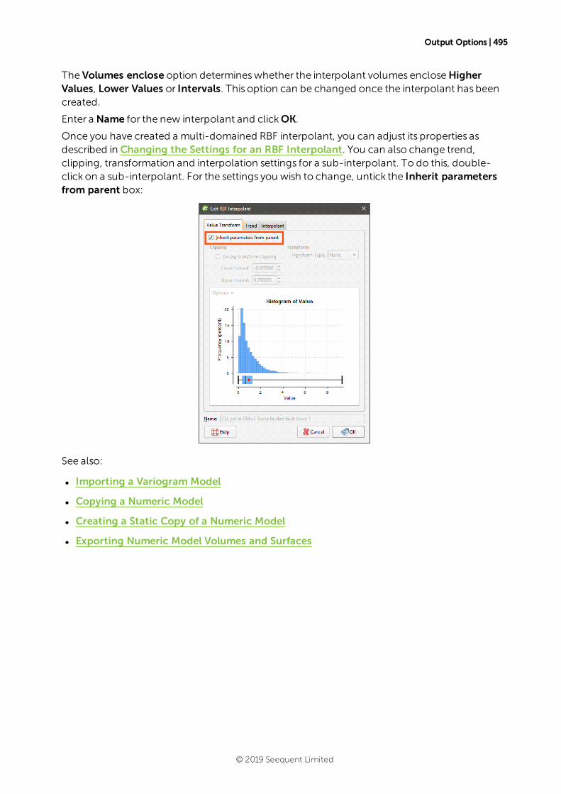
Output Options | 495
The Volumes enclose option determineswhether the interpolant volumes encloseHigherValues, Lower Values or Intervals. This option can be changed once the interpolant has beencreated.
Enter a Name for the new interpolant and clickOK.
Once you have created a multi-domained RBF interpolant, you can adjust its properties asdescribed in Changing the Settings for an RBF Interpolant. You can also change trend,clipping, transformation and interpolation settings for a sub-interpolant. To do this, double-click on a sub-interpolant. For the settings you wish to change, untick the Inherit parametersfrom parent box:
See also:
l Importing a Variogram Model
l Copying a Numeric Model
l Creating a Static Copy of a Numeric Model
l Exporting Numeric Model Volumes and Surfaces
© 2019 Seequent Limited
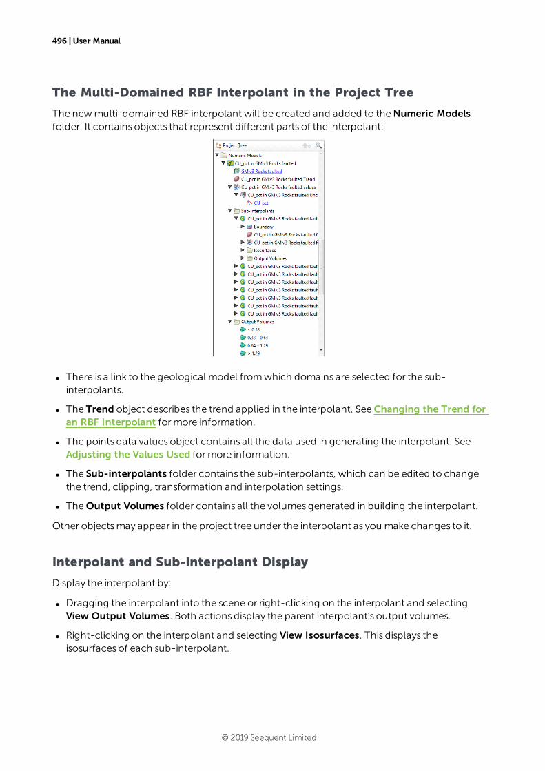
496 | User Manual
The Multi-Domained RBF Interpolant in the Project Tree
The newmulti-domained RBF interpolant will be created and added to theNumeric Modelsfolder. It contains objects that represent different parts of the interpolant:
l There is a link to the geological model fromwhich domains are selected for the sub-interpolants.
l The Trend object describes the trend applied in the interpolant. SeeChanging the Trend foran RBF Interpolant formore information.
l The points data values object contains all the data used in generating the interpolant. SeeAdjusting the Values Used formore information.
l The Sub-interpolants folder contains the sub-interpolants, which can be edited to changethe trend, clipping, transformation and interpolation settings.
l TheOutput Volumes folder contains all the volumes generated in building the interpolant.
Other objectsmay appear in the project tree under the interpolant as you make changes to it.
Interpolant and Sub-Interpolant Display
Display the interpolant by:
l Dragging the interpolant into the scene or right-clicking on the interpolant and selectingView Output Volumes. Both actions display the parent interpolant’s output volumes.
l Right-clicking on the interpolant and selecting View Isosurfaces. This displays theisosurfaces of each sub-interpolant.
© 2019 Seequent Limited
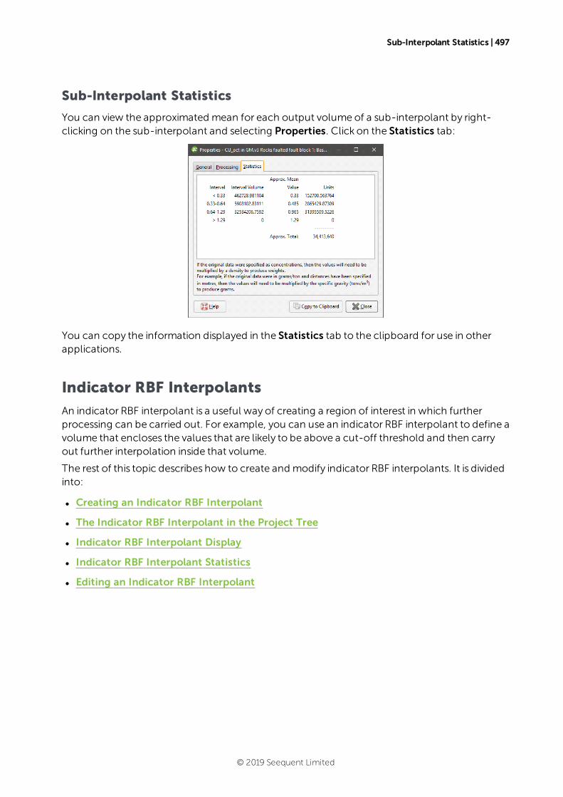
Sub-Interpolant Statistics | 497
Sub-Interpolant Statistics
You can view the approximated mean for each output volume of a sub-interpolant by right-clicking on the sub-interpolant and selecting Properties. Click on the Statistics tab:
You can copy the information displayed in the Statistics tab to the clipboard for use in otherapplications.
Indicator RBF Interpolants
An indicator RBF interpolant is a useful way of creating a region of interest in which furtherprocessing can be carried out. For example, you can use an indicator RBF interpolant to define avolume that encloses the values that are likely to be above a cut-off threshold and then carryout further interpolation inside that volume.
The rest of this topic describes how to create and modify indicator RBF interpolants. It is dividedinto:
l Creating an Indicator RBF Interpolant
l The Indicator RBF Interpolant in the Project Tree
l Indicator RBF Interpolant Display
l Indicator RBF Interpolant Statistics
l Editing an Indicator RBF Interpolant
© 2019 Seequent Limited
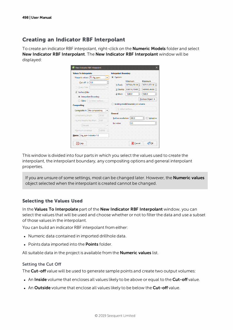
498 | User Manual
Creating an Indicator RBF Interpolant
To create an indicator RBF interpolant, right-click on theNumeric Models folder and selectNew Indicator RBF Interpolant. TheNew Indicator RBF Interpolant windowwill bedisplayed:
Thiswindow is divided into four parts in which you select the values used to create theinterpolant, the interpolant boundary, any compositing options and general interpolantproperties.
If you are unsure of some settings, most can be changed later. However, theNumeric valuesobject selected when the interpolant is created cannot be changed.
Selecting the Values Used
In the Values To Interpolate part of theNew Indicator RBF Interpolant window, you canselect the values that will be used and choosewhether or not to filter the data and use a subsetof those values in the interpolant.
You can build an indicator RBF interpolant fromeither:
l Numeric data contained in imported drillhole data.
l Points data imported into the Points folder.
All suitable data in the project is available from theNumeric values list.
Setting the Cut Off
TheCut-off valuewill be used to generate sample points and create two output volumes:
l An Inside volume that encloses all values likely to be above or equal to theCut-off value.
l An Outside volume that enclose all values likely to be below theCut-off value.
© 2019 Seequent Limited
Applying a Query Filter | 499
If you are unsure of whatCut-off value to use, you can view statistics on the distribution of thedata and change theCut-off value once the interpolant has been created.
You can change the namesof the Inside and Outside volumesonce the interpolant hasbeen created.
Applying a Query Filter
If you have defined a query filter and wish to use it to create the interpolant, select the filter fromtheQuery filter list. Once themodel has been created, you can remove the filter or select adifferent filter.
Applying a Surface Filter
All available data can be used to generate the interpolant or the data can be filtered so that onlythe data that iswithin the interpolant boundary or another boundary in the project influencesthe interpolant. The Surface Filter option is enabled by default, but if you wish to use all data inthe project, untick the box for Surface Filter. Otherwise, you can select the InterpolantBoundary or another boundary in the project.
You can use both theQuery Filter option and the Surface Filter option together.
The Interpolant Boundary
There are several ways to set the Interpolant Boundary:
l Enter values to set a Custom boundary.
l Use the controls in the scene to set theCustom boundary dimensions.
l Select another object in the project from the Enclose Object list, which could be thenumeric values object being interpolated. The extents for that object will be used as the basisfor theCustom boundary dimensions.
l Select another object in the project to use as the Interpolant Boundary. Click the Existingmodel boundary or volume option and select the required object from the list.
Once the interpolant has been created, you can furthermodify its boundary. SeeModifying anRBF Interpolant’s Boundary with Lateral Extents and Adjusting the Interpolant Boundary intheRBF Interpolants topic formore information.
Compositing Options
When numeric values fromdrillhole data are used to create an interpolant, there are twoapproaches to compositing that data:
l Composite the drillhole data, then use the composited values to create an interpolant. If youselect composited values to create an interpolant, compositing optionswill be disabled.
l Use drillhole data that hasn’t been composited to create an interpolant, then applycompositing settings to the interpolated values. If you are interpolating values that have notbeen composited and do not have specificCompositing values in mind, you maywish toleave this option blank as it can be changed once themodel has been created.
© 2019 Seequent Limited
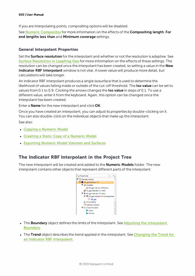
500 | User Manual
If you are interpolating points, compositing optionswill be disabled.
SeeNumeric Composites formore information on the effects of theCompositing length, Forend lengths less than and Minimum coverage settings.
General Interpolant Properties
Set the Surface resolution for the interpolant and whether or not the resolution is adaptive. SeeSurface Resolution in Leapfrog Geo formore information on the effects of these settings. Theresolution can be changed once the interpolant has been created, so setting a value in theNewIndicator RBF Interpolant window is not vital. A lower valuewill producemore detail, butcalculationswill take longer.
An indicator RBF interpolant produces a single isosurface that is used to determine thelikelihood of values falling inside or outside of the cut-off threshold. The Iso value can be set tovalues from0.1 to 0.9. Clicking the arrows changes the Iso value in steps of 0.1. To use adifferent value, enter it from the keyboard. Again, this option can be changed once theinterpolant has been created.
Enter a Name for the new interpolant and clickOK.
Once you have created an interpolant, you can adjust its properties by double-clicking on it.You can also double-click on the individual objects that make up the interpolant.
See also:
l Copying a Numeric Model
l Creating a Static Copy of a Numeric Model
l Exporting Numeric Model Volumes and Surfaces
The Indicator RBF Interpolant in the Project Tree
The new interpolant will be created and added to theNumeric Models folder. The newinterpolant contains other objects that represent different parts of the interpolant:
l The Boundary object defines the limits of the interpolant. See Adjusting the InterpolantBoundary.
l The Trend object describes the trend applied in the interpolant. SeeChanging the Trend foran Indicator RBF Interpolant.
© 2019 Seequent Limited
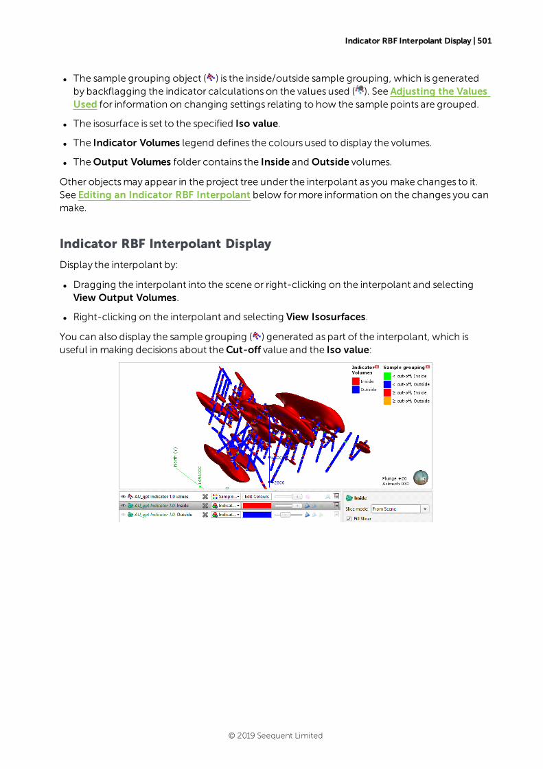
Indicator RBF Interpolant Display | 501
l The sample grouping object ( ) is the inside/outside sample grouping, which is generatedby backflagging the indicator calculations on the values used ( ). See Adjusting the ValuesUsed for information on changing settings relating to how the sample points are grouped.
l The isosurface is set to the specified Iso value.
l The Indicator Volumes legend defines the colours used to display the volumes.
l TheOutput Volumes folder contains the Inside and Outside volumes.
Other objectsmay appear in the project tree under the interpolant as you make changes to it.See Editing an Indicator RBF Interpolant below formore information on the changes you canmake.
Indicator RBF Interpolant Display
Display the interpolant by:
l Dragging the interpolant into the scene or right-clicking on the interpolant and selectingView Output Volumes.
l Right-clicking on the interpolant and selecting View Isosurfaces.
You can also display the sample grouping ( ) generated as part of the interpolant, which isuseful in making decisions about theCut-off value and the Iso value:
© 2019 Seequent Limited

502 | User Manual
Indicator RBF Interpolant Statistics
You can view the statistics for the indicator RBF interpolant by right-clicking on the interpolantand selecting Statistics. Use the information available to adjust the cut-off value and otherinterpolant properties:
You can copy the information displayed in the Statistics tab to the clipboard for use in otherapplications.
Editing an Indicator RBF Interpolant
To edit an indicator RBF interpolant, you can either double-click on the interpolant in theNumeric Models folder or right-click and selectOpen. Thewindow that appears is divided intotabs that let you change the different objects that make up the interpolant. Many of the optionsare the same for RBF and multi-domained RBF interpolants.
When creating an indicator RBF interpolant, only a basic set of parameters is used. The EditIndicator RBF Interpolant windowsprovide finer controls over these basic parameters so youcan refine the interpolant to factor in real-world observations and account for limitations in thedata.
l Adjusting the Values Used
l Compositing Parameters for an Indicator RBF Interpolant
l Adjusting the Interpolant Boundary
l The Cut-Off Value
l Changing the Trend for an Indicator RBF Interpolant
l Adjusting Interpolation Parameters
l Indicator RBF Interpolant Surfacing and Volume Options
© 2019 Seequent Limited
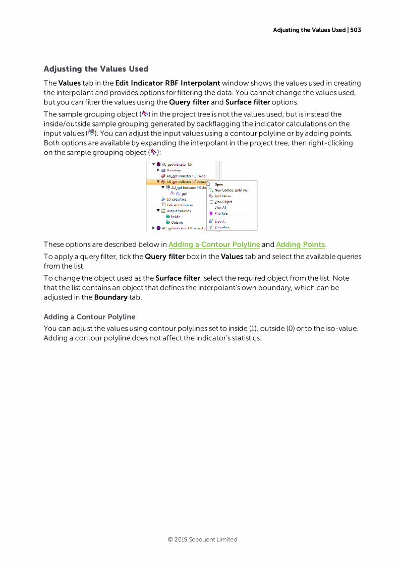
Adjusting the Values Used | 503
Adjusting the Values Used
The Values tab in the Edit Indicator RBF Interpolant window shows the values used in creatingthe interpolant and provides options for filtering the data. You cannot change the values used,but you can filter the values using theQuery filter and Surface filter options.
The sample grouping object ( ) in the project tree is not the values used, but is instead theinside/outside sample grouping generated by backflagging the indicator calculations on theinput values ( ). You can adjust the input values using a contour polyline or by adding points.Both options are available by expanding the interpolant in the project tree, then right-clickingon the sample grouping object ( ):
These options are described below in Adding a Contour Polyline and Adding Points.
To apply a query filter, tick theQuery filter box in the Values tab and select the available queriesfrom the list.
To change the object used as the Surface filter, select the required object from the list. Notethat the list contains an object that defines the interpolant’s own boundary, which can beadjusted in the Boundary tab.
Adding a Contour Polyline
You can adjust the values using contour polylines set to inside (1), outside (0) or to the iso-value.Adding a contour polyline does not affect the indicator’s statistics.
© 2019 Seequent Limited
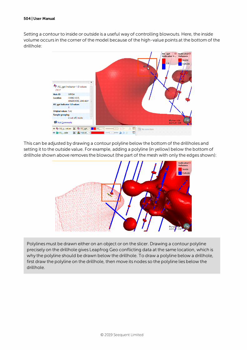
504 | User Manual
Setting a contour to inside or outside is a useful way of controlling blowouts. Here, the insidevolume occurs in the corner of themodel because of the high-value points at the bottomof thedrillhole:
This can be adjusted by drawing a contour polyline below the bottomof the drillholes andsetting it to the outside value. For example, adding a polyline (in yellow) below the bottomofdrillhole shown above removes the blowout (the part of themesh with only the edges shown):
Polylinesmust be drawn either on an object or on the slicer. Drawing a contour polylineprecisely on the drillhole gives Leapfrog Geo conflicting data at the same location, which iswhy the polyline should be drawn below the drillhole. To draw a polyline below a drillhole,first draw the polyline on the drillhole, then move its nodes so the polyline lies below thedrillhole.
© 2019 Seequent Limited
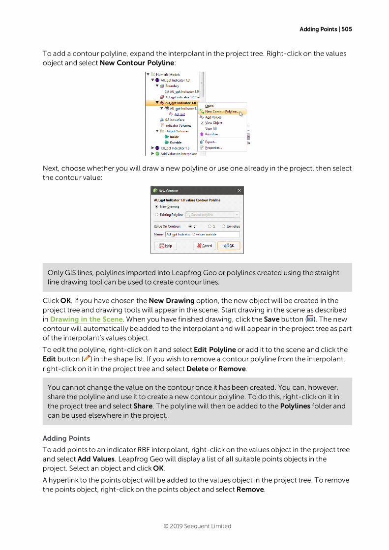
Adding Points | 505
To add a contour polyline, expand the interpolant in the project tree. Right-click on the valuesobject and selectNew Contour Polyline:
Next, choosewhether you will draw a new polyline or use one already in the project, then selectthe contour value:
OnlyGIS lines, polylines imported into Leapfrog Geo or polylines created using the straightline drawing tool can be used to create contour lines.
ClickOK. If you have chosen theNew Drawing option, the new object will be created in theproject tree and drawing toolswill appear in the scene. Start drawing in the scene as describedin Drawing in the Scene. When you have finished drawing, click the Save button ( ). The newcontourwill automatically be added to the interpolant and will appear in the project tree as partof the interpolant’s values object.
To edit the polyline, right-click on it and select Edit Polyline or add it to the scene and click theEdit button ( ) in the shape list. If you wish to remove a contour polyline from the interpolant,right-click on it in the project tree and selectDelete orRemove.
You cannot change the value on the contour once it has been created. You can, however,share the polyline and use it to create a new contour polyline. To do this, right-click on it inthe project tree and select Share. The polyline will then be added to the Polylines folder andcan be used elsewhere in the project.
Adding Points
To add points to an indicator RBF interpolant, right-click on the values object in the project treeand select Add Values. Leapfrog Geowill display a list of all suitable points objects in theproject. Select an object and clickOK.
A hyperlink to the points object will be added to the values object in the project tree. To removethe points object, right-click on the points object and select Remove.
© 2019 Seequent Limited
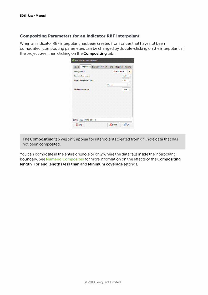
506 | User Manual
Compositing Parameters for an Indicator RBF Interpolant
When an indicator RBF interpolant has been created fromvalues that have not beencomposited, compositing parameters can be changed by double-clicking on the interpolant inthe project tree, then clicking on theCompositing tab.
TheCompositing tab will only appear for interpolants created fromdrillhole data that hasnot been composited.
You can composite in the entire drillhole or onlywhere the data falls inside the interpolantboundary. SeeNumeric Composites formore information on the effects of theCompositinglength, For end lengths less than and Minimum coverage settings.
© 2019 Seequent Limited
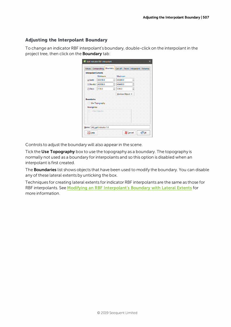
Adjusting the Interpolant Boundary | 507
Adjusting the Interpolant Boundary
To change an indicator RBF interpolant’s boundary, double-click on the interpolant in theproject tree, then click on the Boundary tab:
Controls to adjust the boundarywill also appear in the scene.
Tick theUse Topography box to use the topography as a boundary. The topography isnormally not used as a boundary for interpolants and so this option is disabled when aninterpolant is first created.
The Boundaries list showsobjects that have been used tomodify the boundary. You can disableany of these lateral extents by unticking the box.
Techniques for creating lateral extents for indicator RBF interpolants are the same as those forRBF interpolants. SeeModifying an RBF Interpolant’s Boundary with Lateral Extents formore information.
© 2019 Seequent Limited
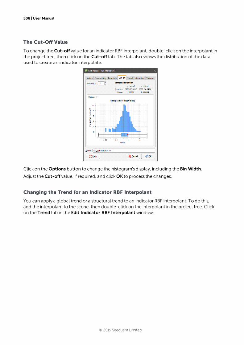
508 | User Manual
The Cut-Off Value
To change theCut-off value for an indicator RBF interpolant, double-click on the interpolant inthe project tree, then click on theCut-off tab. The tab also shows the distribution of the dataused to create an indicator interpolate:
Click on theOptions button to change the histogram’s display, including the Bin Width.
Adjust theCut-off value, if required, and clickOK to process the changes.
Changing the Trend for an Indicator RBF Interpolant
You can apply a global trend or a structural trend to an indicator RBF interpolant. To do this,add the interpolant to the scene, then double-click on the interpolant in the project tree. Clickon the Trend tab in the Edit Indicator RBF Interpolant window.
© 2019 Seequent Limited
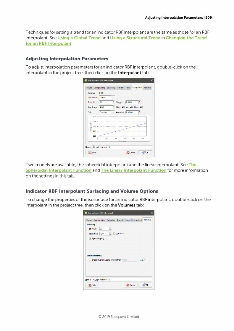
Adjusting Interpolation Parameters | 509
Techniques for setting a trend for an indicator RBF interpolant are the same as those for an RBFinterpolant. SeeUsing a Global Trend and Using a Structural Trend in Changing the Trendfor an RBF Interpolant.
Adjusting Interpolation Parameters
To adjust interpolation parameters for an indicator RBF interpolant, double-click on theinterpolant in the project tree, then click on the Interpolant tab:
Twomodels are available, the spheroidal interpolant and the linear interpolant. See TheSpheroidal Interpolant Function and The Linear Interpolant Function formore informationon the settings in this tab.
Indicator RBF Interpolant Surfacing and Volume Options
To change the properties of the isosurface for an indicator RBF interpolant, double-click on theinterpolant in the project tree, then click on the Volumes tab:
© 2019 Seequent Limited
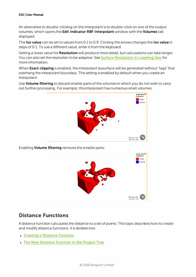
510 | User Manual
An alternative to double-clicking on the interpolant is to double-click on one of the outputvolumes, which opens the Edit Indicator RBF Interpolant windowwith the Volumes tabdisplayed.
The Iso value can be set to values from0.1 to 0.9. Clicking the arrows changes the Iso value insteps of 0.1. To use a different value, enter it from the keyboard.
Setting a lower value forResolutionwill producemore detail, but calculations can take longer.You can also set the resolution to be adaptive. See Surface Resolution in Leapfrog Geo formore information.
When Exact clipping is enabled, the interpolant isosurfacewill be generated without “tags” thatoverhang the interpolant boundary. This setting is enabled by default when you create aninterpolant.
Use Volume filtering to discard smaller parts of the volumes in which you do not wish to carryout further processing. For example, this interpolant has numerous small volumes:
Enabling Volume filtering removes the smaller parts:
Distance Functions
A distance function calculates the distance to a set of points. This topic describes how to createand modify distance functions. It is divided into:
l Creating a Distance Function
l The New Distance Function in the Project Tree
© 2019 Seequent Limited
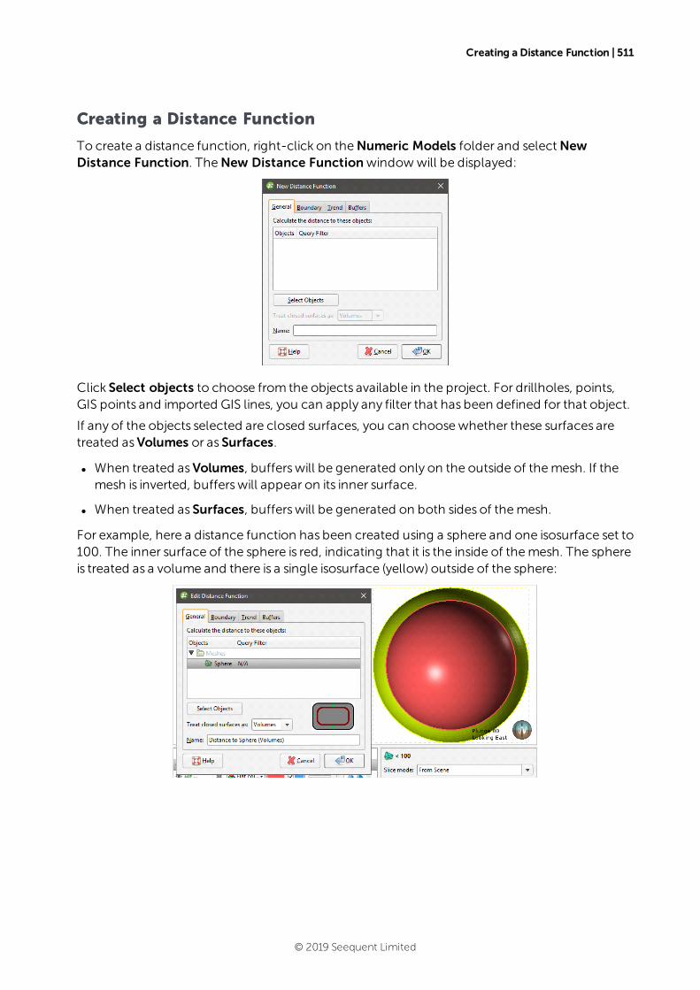
Creating a Distance Function | 511
Creating a Distance Function
To create a distance function, right-click on theNumeric Models folder and selectNewDistance Function. TheNew Distance Functionwindowwill be displayed:
Click Select objects to choose from the objects available in the project. For drillholes, points,GIS points and imported GIS lines, you can apply any filter that has been defined for that object.
If any of the objects selected are closed surfaces, you can choosewhether these surfaces aretreated asVolumes or as Surfaces.
l When treated asVolumes, bufferswill be generated only on the outside of themesh. If themesh is inverted, bufferswill appear on its inner surface.
l When treated as Surfaces, bufferswill be generated on both sides of themesh.
For example, here a distance function has been created using a sphere and one isosurface set to100. The inner surface of the sphere is red, indicating that it is the inside of themesh. The sphereis treated as a volume and there is a single isosurface (yellow) outside of the sphere:
© 2019 Seequent Limited
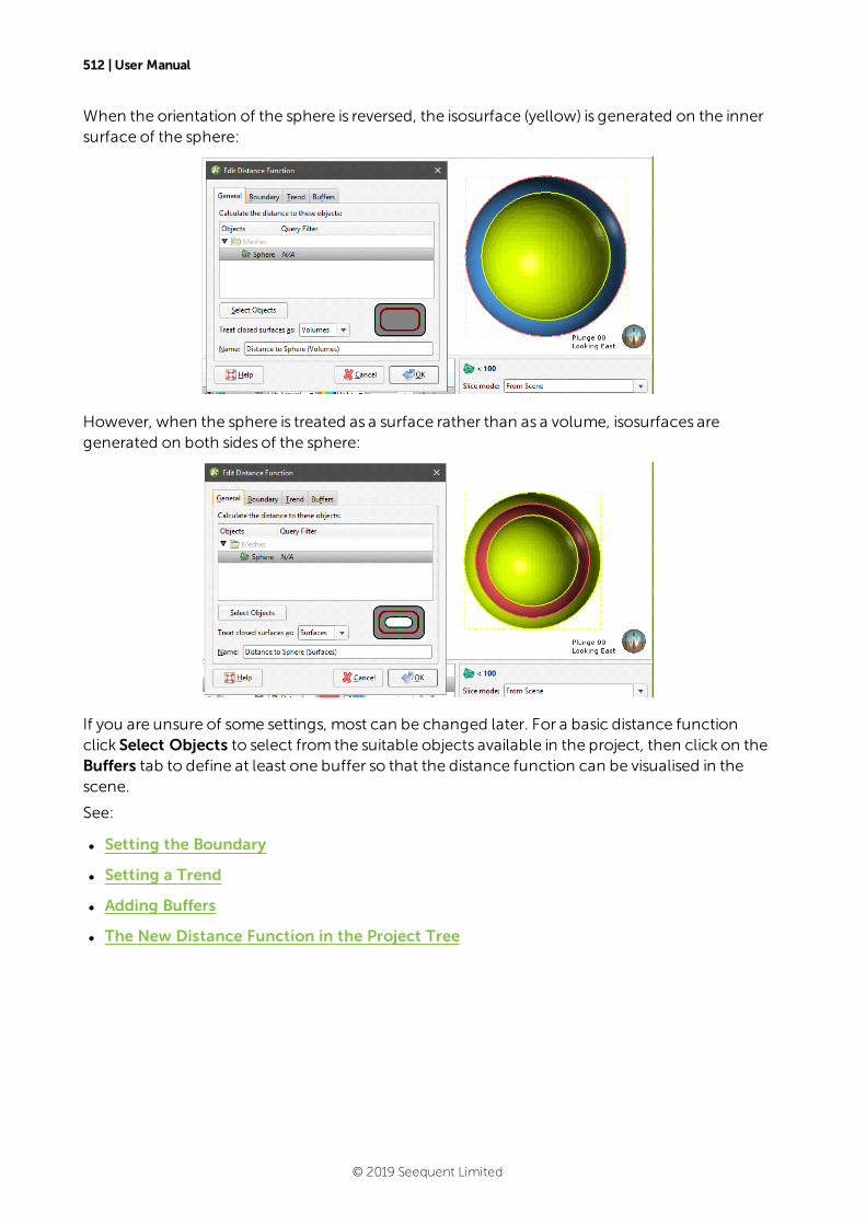
512 | User Manual
When the orientation of the sphere is reversed, the isosurface (yellow) is generated on the innersurface of the sphere:
However, when the sphere is treated as a surface rather than as a volume, isosurfaces aregenerated on both sides of the sphere:
If you are unsure of some settings, most can be changed later. For a basic distance functionclick Select Objects to select from the suitable objects available in the project, then click on theBuffers tab to define at least one buffer so that the distance function can be visualised in thescene.
See:
l Setting the Boundary
l Setting a Trend
l Adding Buffers
l The New Distance Function in the Project Tree
© 2019 Seequent Limited
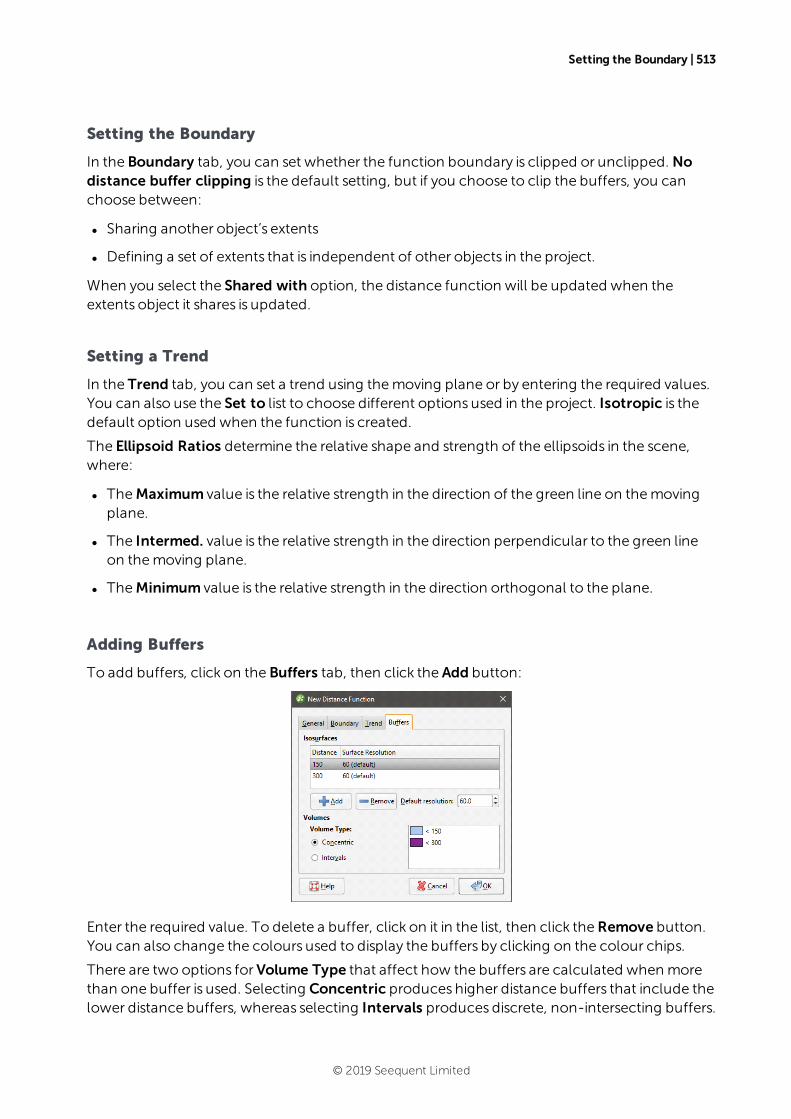
Setting the Boundary | 513
Setting the Boundary
In the Boundary tab, you can set whether the function boundary is clipped or unclipped. Nodistance buffer clipping is the default setting, but if you choose to clip the buffers, you canchoose between:
l Sharing another object’s extents
l Defining a set of extents that is independent of other objects in the project.
When you select the Shared with option, the distance function will be updated when theextents object it shares is updated.
Setting a Trend
In the Trend tab, you can set a trend using themoving plane or by entering the required values.You can also use the Set to list to choose different options used in the project. Isotropic is thedefault option used when the function is created.
The Ellipsoid Ratios determine the relative shape and strength of the ellipsoids in the scene,where:
l TheMaximum value is the relative strength in the direction of the green line on themovingplane.
l The Intermed. value is the relative strength in the direction perpendicular to the green lineon themoving plane.
l TheMinimum value is the relative strength in the direction orthogonal to the plane.
Adding Buffers
To add buffers, click on the Buffers tab, then click the Add button:
Enter the required value. To delete a buffer, click on it in the list, then click theRemove button.You can also change the colours used to display the buffers by clicking on the colour chips.
There are two options forVolume Type that affect how the buffers are calculated whenmorethan one buffer is used. Selecting Concentric produces higher distance buffers that include thelower distance buffers, whereas selecting Intervals produces discrete, non-intersecting buffers.
© 2019 Seequent Limited

514 | User Manual
TheDefault resolution setting is used for all new buffers and for existing buffers that use thedefault resolution.
The New Distance Function in the Project Tree
ClickOK to create the distance function, which will be added to theNumeric Models folder.The new distance function contains objects representing different parts of the function, whichcan be expanded to show the inputs to each part of the function:
l The Trend object that describes the trend applied.
l Hyperlinks to objects used for the distance function.
l An Isosurfaces folder that contains all themeshes generated in building the distancefunction.
l An Output Volumes folder that contains all the distance buffermeshes.
Other objectsmay appear in the project tree under the function as you make changes to it.
Display the function by dragging it into the scene or by right-clicking on it and selecting ViewBuffers.
Once you have created a distance function, you can adjust its properties by double-clicking onit. You can also double-click on the individual objects that make up the function.
© 2019 Seequent Limited
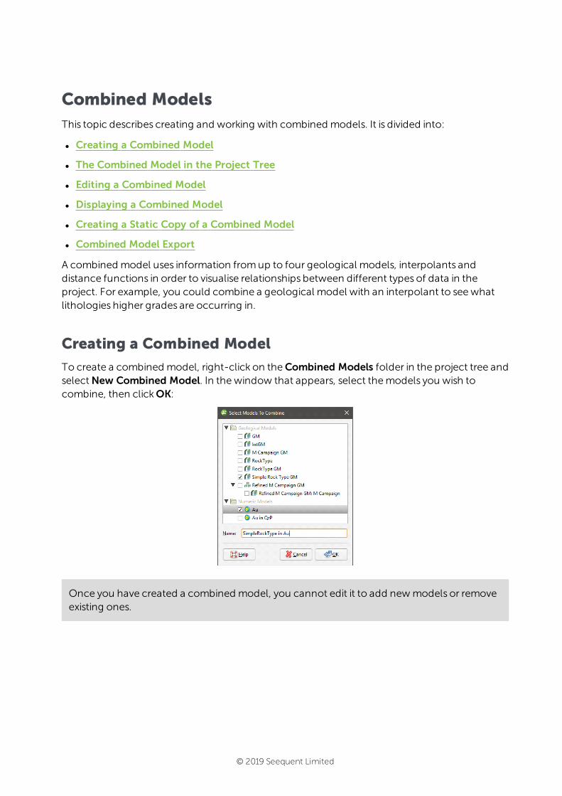
Combined ModelsThis topic describes creating and working with combined models. It is divided into:
l Creating a Combined Model
l The Combined Model in the Project Tree
l Editing a Combined Model
l Displaying a Combined Model
l Creating a Static Copy of a Combined Model
l Combined Model Export
A combined model uses information fromup to four geological models, interpolants anddistance functions in order to visualise relationships between different types of data in theproject. For example, you could combine a geological model with an interpolant to seewhatlithologies higher grades are occurring in.
Creating a Combined Model
To create a combined model, right-click on theCombined Models folder in the project tree andselectNew Combined Model. In thewindow that appears, select themodels you wish tocombine, then clickOK:
Once you have created a combined model, you cannot edit it to add newmodels or removeexisting ones.
© 2019 Seequent Limited
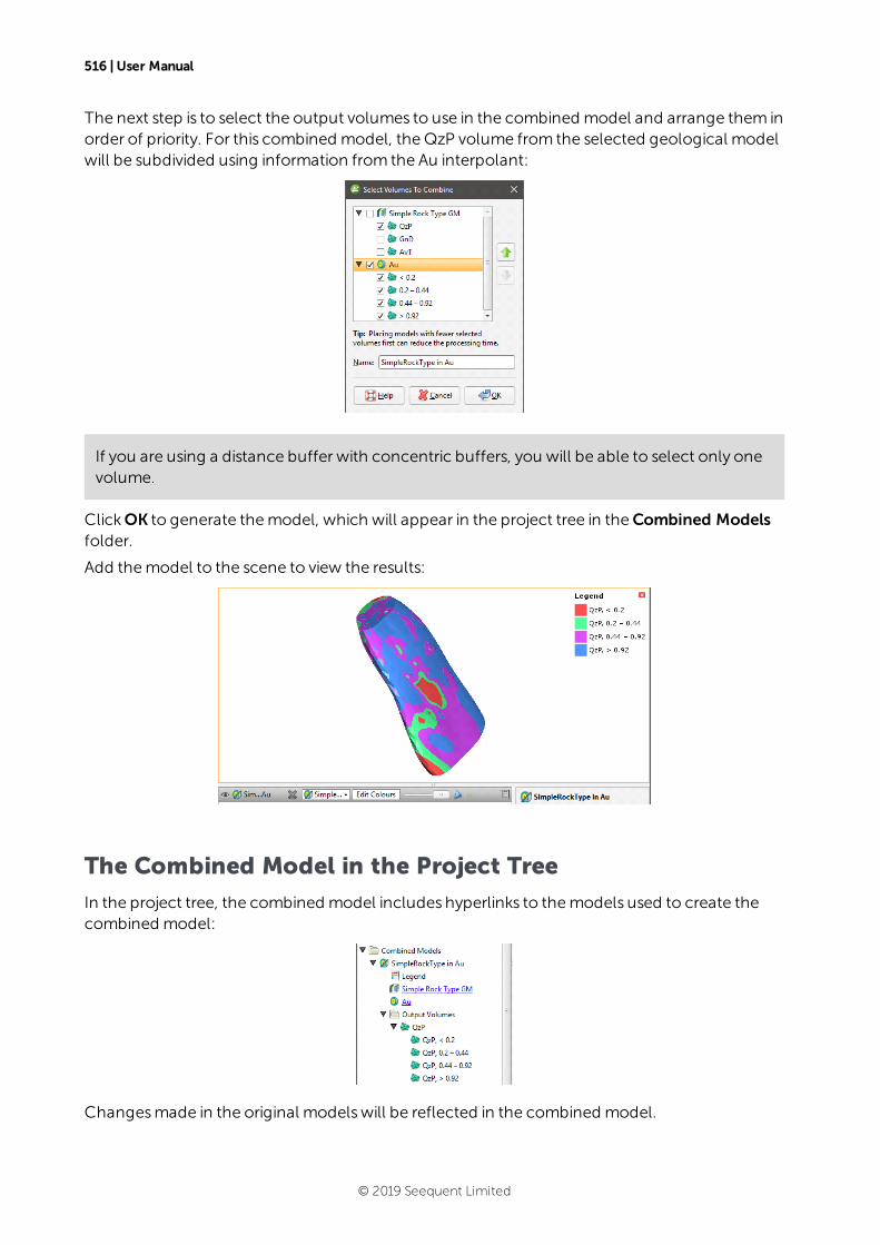
516 | User Manual
The next step is to select the output volumes to use in the combined model and arrange them inorder of priority. For this combined model, theQzP volume from the selected geological modelwill be subdivided using information from the Au interpolant:
If you are using a distance buffer with concentric buffers, you will be able to select only onevolume.
ClickOK to generate themodel, which will appear in the project tree in theCombined Modelsfolder.
Add themodel to the scene to view the results:
The Combined Model in the Project Tree
In the project tree, the combined model includes hyperlinks to themodels used to create thecombined model:
Changesmade in the original modelswill be reflected in the combined model.
© 2019 Seequent Limited
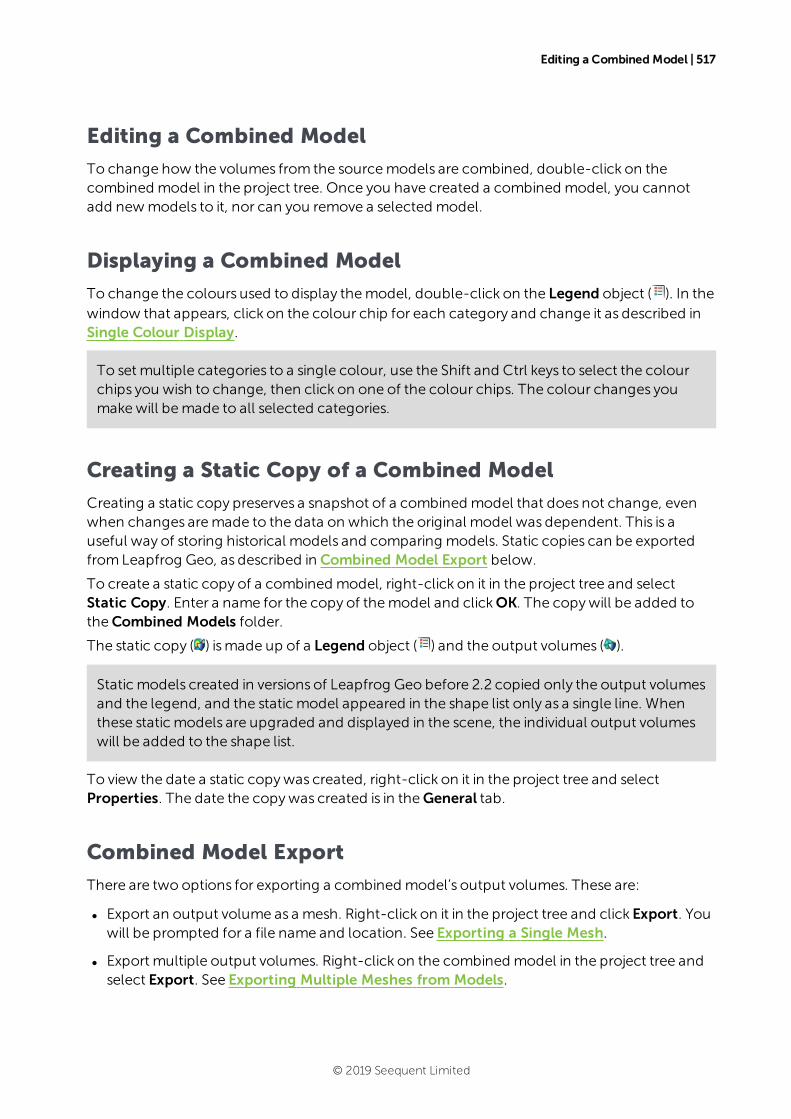
Editing a Combined Model | 517
Editing a Combined Model
To change how the volumes from the sourcemodels are combined, double-click on thecombined model in the project tree. Once you have created a combined model, you cannotadd newmodels to it, nor can you remove a selected model.
Displaying a Combined Model
To change the colours used to display themodel, double-click on the Legend object ( ). In thewindow that appears, click on the colour chip for each category and change it as described inSingle Colour Display.
To set multiple categories to a single colour, use the Shift and Ctrl keys to select the colourchips you wish to change, then click on one of the colour chips. The colour changes youmakewill bemade to all selected categories.
Creating a Static Copy of a Combined Model
Creating a static copy preserves a snapshot of a combined model that does not change, evenwhen changes aremade to the data on which the original model was dependent. This is auseful way of storing historical models and comparing models. Static copies can be exportedfromLeapfrog Geo, as described in Combined Model Export below.
To create a static copy of a combined model, right-click on it in the project tree and selectStatic Copy. Enter a name for the copy of themodel and clickOK. The copywill be added totheCombined Models folder.
The static copy ( ) ismade up of a Legend object ( ) and the output volumes ( ).
Staticmodels created in versions of Leapfrog Geo before 2.2 copied only the output volumesand the legend, and the staticmodel appeared in the shape list only as a single line. Whenthese staticmodels are upgraded and displayed in the scene, the individual output volumeswill be added to the shape list.
To view the date a static copywas created, right-click on it in the project tree and selectProperties. The date the copywas created is in theGeneral tab.
Combined Model Export
There are two options for exporting a combined model’s output volumes. These are:
l Export an output volume as a mesh. Right-click on it in the project tree and click Export. Youwill be prompted for a file name and location. See Exporting a Single Mesh.
l Export multiple output volumes. Right-click on the combined model in the project tree andselect Export. See Exporting Multiple Meshes from Models.
© 2019 Seequent Limited
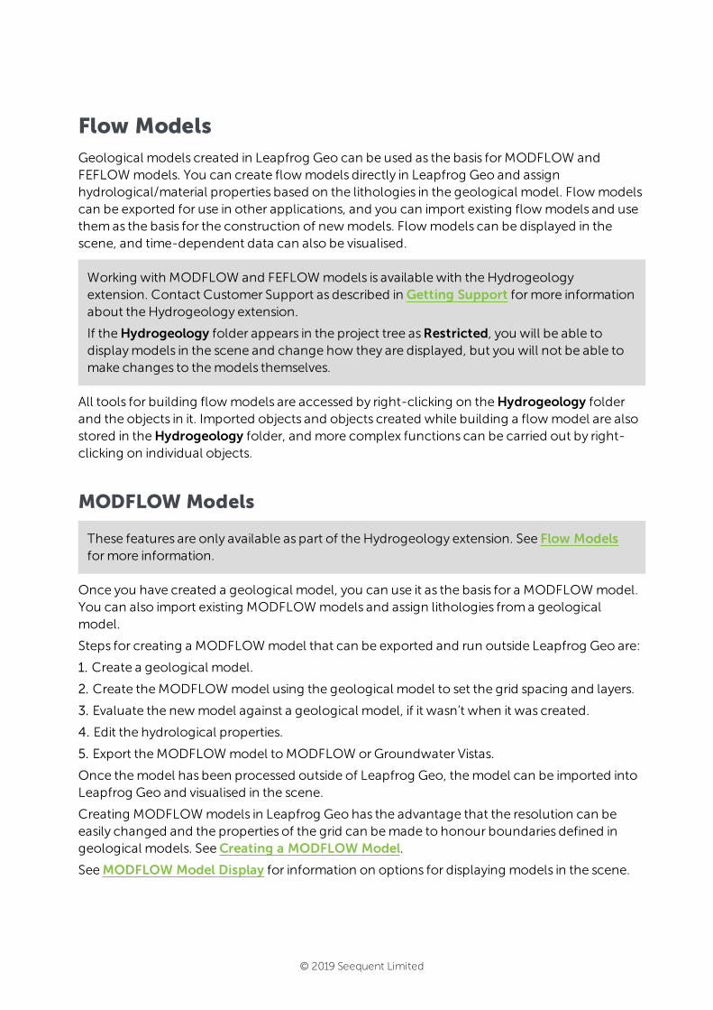
Flow ModelsGeological models created in Leapfrog Geo can be used as the basis forMODFLOW andFEFLOWmodels. You can create flowmodels directly in Leapfrog Geo and assignhydrological/material properties based on the lithologies in the geological model. Flowmodelscan be exported for use in other applications, and you can import existing flowmodels and usethemas the basis for the construction of newmodels. Flowmodels can be displayed in thescene, and time-dependent data can also be visualised.
Working with MODFLOW and FEFLOWmodels is available with the Hydrogeologyextension. Contact Customer Support as described in Getting Support formore informationabout the Hydrogeology extension.
If theHydrogeology folder appears in the project tree asRestricted, you will be able todisplaymodels in the scene and change how they are displayed, but you will not be able tomake changes to themodels themselves.
All tools for building flowmodels are accessed by right-clicking on theHydrogeology folderand the objects in it. Imported objects and objects created while building a flowmodel are alsostored in theHydrogeology folder, and more complex functions can be carried out by right-clicking on individual objects.
MODFLOW Models
These features are only available as part of the Hydrogeology extension. See Flow Modelsformore information.
Once you have created a geological model, you can use it as the basis for a MODFLOWmodel.You can also import existing MODFLOWmodels and assign lithologies froma geologicalmodel.
Steps for creating a MODFLOWmodel that can be exported and run outside Leapfrog Geo are:
1. Create a geological model.
2. Create theMODFLOWmodel using the geological model to set the grid spacing and layers.
3. Evaluate the newmodel against a geological model, if it wasn’t when it was created.
4. Edit the hydrological properties.
5. Export theMODFLOWmodel toMODFLOW orGroundwater Vistas.
Once themodel has been processed outside of Leapfrog Geo, themodel can be imported intoLeapfrog Geo and visualised in the scene.
Creating MODFLOWmodels in Leapfrog Geo has the advantage that the resolution can beeasily changed and the properties of the grid can bemade to honour boundaries defined ingeological models. SeeCreating a MODFLOW Model.
SeeMODFLOW Model Display for information on options for displaying models in the scene.
© 2019 Seequent Limited
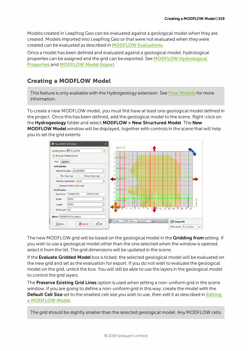
Creating a MODFLOW Model | 519
Models created in Leapfrog Geo can be evaluated against a geological model when they arecreated. Models imported into Leapfrog Geo or that were not evaluated when theywerecreated can be evaluated as described in MODFLOW Evaluations.
Once a model has been defined and evaluated against a geological model, hydrologicalproperties can be assigned and the grid can be exported. SeeMODFLOW HydrologicalProperties and MODFLOW Model Export.
Creating a MODFLOW Model
This feature is only available with the Hydrogeology extension. See Flow Models formoreinformation.
To create a newMODFLOWmodel, you must first have at least one geological model defined inthe project. Once this has been defined, add the geological model to the scene. Right-click ontheHydrogeology folder and selectMODFLOW > New Structured Model. TheNewMODFLOW Modelwindowwill be displayed, together with controls in the scene that will helpyou to set the grid extents:
The newMODFLOW grid will be based on the geological model in theGridding from setting. Ifyou wish to use a geological model other than the one selected when thewindow is opened,select it from the list. The grid dimensionswill be updated in the scene.
If the Evaluate Gridded Model box is ticked, the selected geological model will be evaluated onthe new grid and set as the evaluation for export. If you do not wish to evaluate the geologicalmodel on the grid, untick the box. You will still be able to use the layers in the geological modelto control the grid layers.
The Preserve Existing Grid Lines option is used when setting a non-uniformgrid in the scenewindow. If you are going to define a non-uniformgrid in thisway, create themodel with theDefault Cell Size set to the smallest cell size you wish to use, then edit it as described in Editinga MODFLOW Model.
The grid should be slightly smaller than the selected geological model. AnyMODFLOW cells
© 2019 Seequent Limited
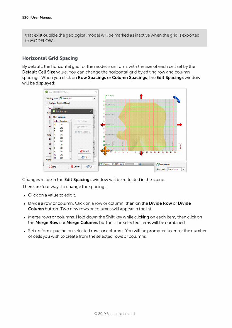
520 | User Manual
that exist outside the geological model will bemarked as inactive when the grid is exportedtoMODFLOW .
Horizontal Grid Spacing
By default, the horizontal grid for themodel is uniform, with the size of each cell set by theDefault Cell Size value. You can change the horizontal grid by editing row and columnspacings. When you click on Row Spacings orColumn Spacings, the Edit Spacings windowwill be displayed:
Changesmade in the Edit Spacings windowwill be reflected in the scene.
There are four ways to change the spacings:
l Click on a value to edit it.
l Divide a row or column. Click on a row or column, then on theDivide Row orDivideColumn button. Two new rowsor columnswill appear in the list.
l Merge rowsor columns. Hold down the Shift keywhile clicking on each item, then click ontheMerge Rows orMerge Columns button. The selected itemswill be combined.
l Set uniform spacing on selected rowsor columns. You will be prompted to enter the numberof cells you wish to create from the selected rowsor columns.
© 2019 Seequent Limited
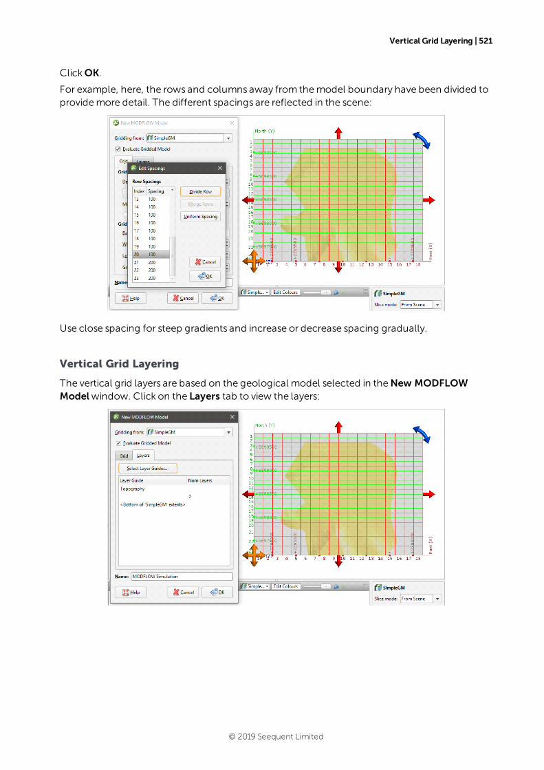
Vertical Grid Layering | 521
ClickOK.
For example, here, the rows and columns away from themodel boundary have been divided toprovidemore detail. The different spacings are reflected in the scene:
Use close spacing for steep gradients and increase or decrease spacing gradually.
Vertical Grid Layering
The vertical grid layers are based on the geological model selected in theNew MODFLOWModelwindow. Click on the Layers tab to view the layers:
© 2019 Seequent Limited
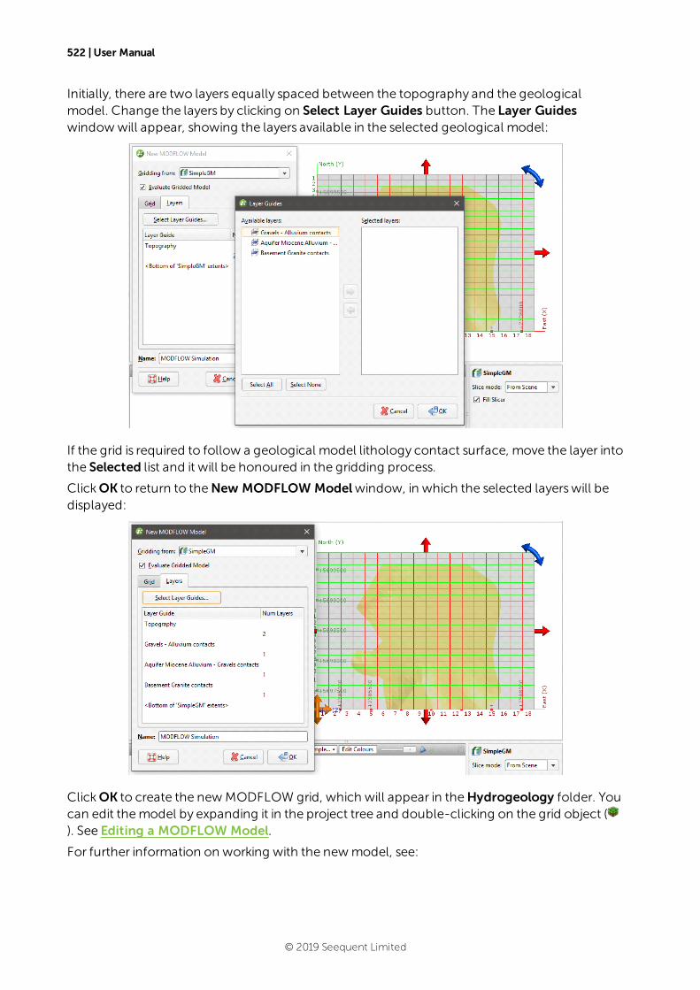
522 | User Manual
Initially, there are two layers equally spaced between the topography and the geologicalmodel. Change the layers by clicking on Select Layer Guides button. The Layer Guideswindowwill appear, showing the layers available in the selected geological model:
If the grid is required to follow a geological model lithology contact surface, move the layer intothe Selected list and it will be honoured in the gridding process.
ClickOK to return to theNew MODFLOW Modelwindow, in which the selected layerswill bedisplayed:
ClickOK to create the newMODFLOW grid, which will appear in theHydrogeology folder. Youcan edit themodel by expanding it in the project tree and double-clicking on the grid object (). See Editing a MODFLOW Model.
For further information on working with the newmodel, see:
© 2019 Seequent Limited
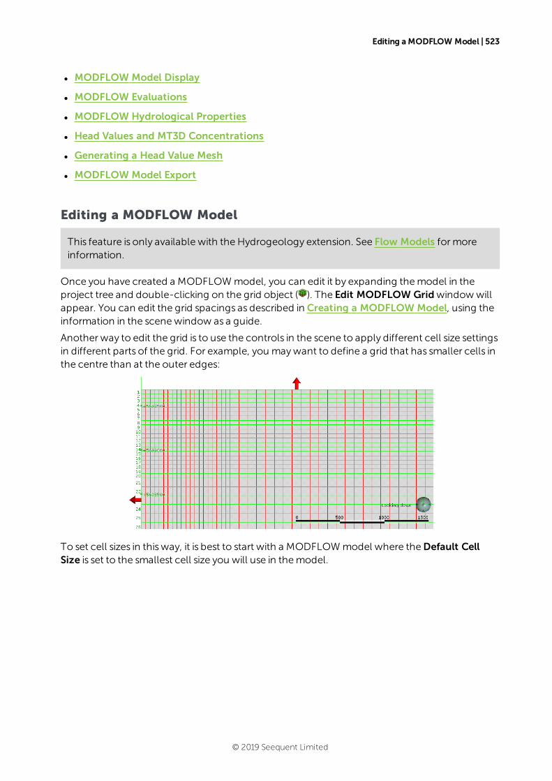
Editing a MODFLOW Model | 523
l MODFLOW Model Display
l MODFLOW Evaluations
l MODFLOW Hydrological Properties
l Head Values and MT3D Concentrations
l Generating a Head Value Mesh
l MODFLOW Model Export
Editing a MODFLOW Model
This feature is only available with the Hydrogeology extension. See Flow Models formoreinformation.
Once you have created a MODFLOWmodel, you can edit it by expanding themodel in theproject tree and double-clicking on the grid object ( ). The Edit MODFLOW Gridwindowwillappear. You can edit the grid spacings as described in Creating a MODFLOW Model, using theinformation in the scenewindow as a guide.
Another way to edit the grid is to use the controls in the scene to apply different cell size settingsin different parts of the grid. For example, you maywant to define a grid that has smaller cells inthe centre than at the outer edges:
To set cell sizes in thisway, it is best to start with a MODFLOWmodel where theDefault CellSize is set to the smallest cell size you will use in themodel.
© 2019 Seequent Limited
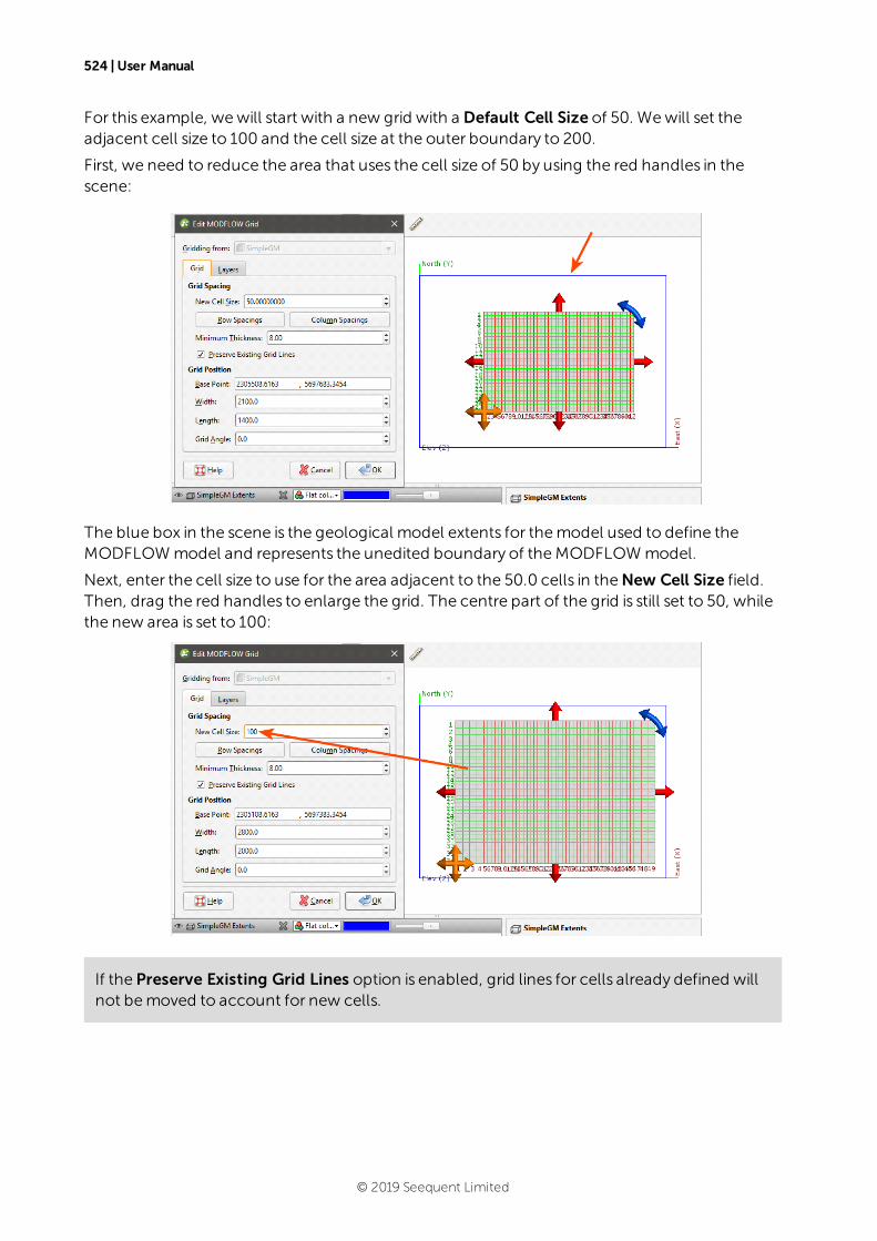
524 | User Manual
For this example, wewill start with a new grid with a Default Cell Size of 50. Wewill set theadjacent cell size to 100 and the cell size at the outer boundary to 200.
First, we need to reduce the area that uses the cell size of 50 by using the red handles in thescene:
The blue box in the scene is the geological model extents for themodel used to define theMODFLOWmodel and represents the unedited boundary of theMODFLOWmodel.
Next, enter the cell size to use for the area adjacent to the 50.0 cells in theNew Cell Size field.Then, drag the red handles to enlarge the grid. The centre part of the grid is still set to 50, whilethe new area is set to 100:
If the Preserve Existing Grid Lines option is enabled, grid lines for cells already defined willnot bemoved to account for new cells.
© 2019 Seequent Limited
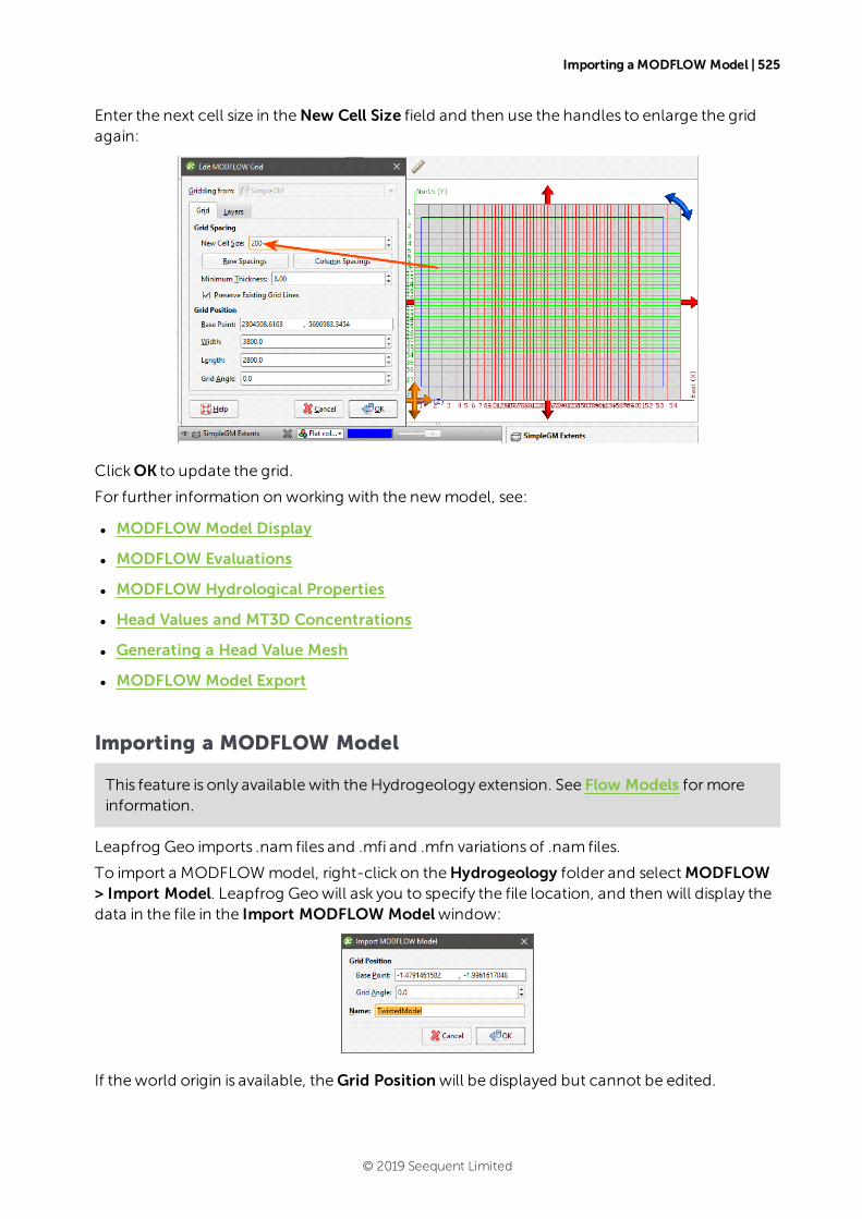
Importing a MODFLOW Model | 525
Enter the next cell size in theNew Cell Size field and then use the handles to enlarge the gridagain:
ClickOK to update the grid.
For further information on working with the newmodel, see:
l MODFLOW Model Display
l MODFLOW Evaluations
l MODFLOW Hydrological Properties
l Head Values and MT3D Concentrations
l Generating a Head Value Mesh
l MODFLOW Model Export
Importing a MODFLOW Model
This feature is only available with the Hydrogeology extension. See Flow Models formoreinformation.
Leapfrog Geo imports .nam files and .mfi and .mfn variations of .nam files.
To import a MODFLOWmodel, right-click on theHydrogeology folder and selectMODFLOW> Import Model. Leapfrog Geowill ask you to specify the file location, and then will display thedata in the file in the Import MODFLOW Modelwindow:
If theworld origin is available, theGrid Positionwill be displayed but cannot be edited.
© 2019 Seequent Limited
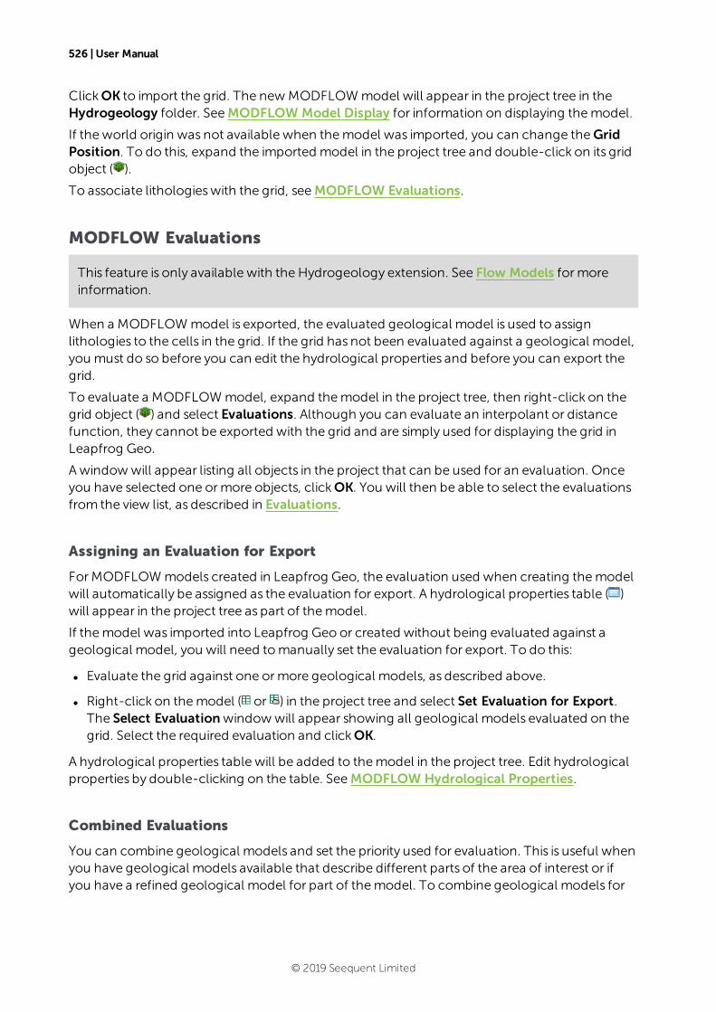
526 | User Manual
ClickOK to import the grid. The newMODFLOWmodel will appear in the project tree in theHydrogeology folder. SeeMODFLOW Model Display for information on displaying themodel.
If the world origin was not available when themodel was imported, you can change theGridPosition. To do this, expand the imported model in the project tree and double-click on its gridobject ( ).
To associate lithologieswith the grid, seeMODFLOW Evaluations.
MODFLOW Evaluations
This feature is only available with the Hydrogeology extension. See Flow Models formoreinformation.
When a MODFLOWmodel is exported, the evaluated geological model is used to assignlithologies to the cells in the grid. If the grid has not been evaluated against a geological model,you must do so before you can edit the hydrological properties and before you can export thegrid.
To evaluate a MODFLOWmodel, expand themodel in the project tree, then right-click on thegrid object ( ) and select Evaluations. Although you can evaluate an interpolant or distancefunction, they cannot be exported with the grid and are simply used for displaying the grid inLeapfrog Geo.
A windowwill appear listing all objects in the project that can be used for an evaluation. Onceyou have selected one ormore objects, clickOK. You will then be able to select the evaluationsfrom the view list, as described in Evaluations.
Assigning an Evaluation for Export
ForMODFLOWmodels created in Leapfrog Geo, the evaluation used when creating themodelwill automatically be assigned as the evaluation for export. A hydrological properties table ( )will appear in the project tree as part of themodel.
If themodel was imported into Leapfrog Geo or created without being evaluated against ageological model, you will need tomanually set the evaluation for export. To do this:
l Evaluate the grid against one ormore geological models, as described above.
l Right-click on themodel ( or ) in the project tree and select Set Evaluation for Export.The Select Evaluationwindowwill appear showing all geological models evaluated on thegrid. Select the required evaluation and clickOK.
A hydrological properties table will be added to themodel in the project tree. Edit hydrologicalproperties by double-clicking on the table. SeeMODFLOW Hydrological Properties.
Combined Evaluations
You can combine geological models and set the priority used for evaluation. This is useful whenyou have geological models available that describe different parts of the area of interest or ifyou have a refined geological model for part of themodel. To combine geological models for
© 2019 Seequent Limited

MODFLOW Hydrological Properties | 527
evaluation, select the required models in the Select Models To Evaluatewindow, then click ontheCombined Evaluation button.
In this example, there are three geological models selected:
The GM and GM fromcontactsmodels describe similar areas, but GM hasmore detail. The GMlargermodel describes a larger area but with less detail. Tick themodels to combine themandset their priority. ClickOK to create the combined evaluation, then clickOK in the Select ModelsTo Evaluatewindow. The combined evaluation will be available from the view list and can beselected as the evaluation for export.
To delete a combined evaluation, click on theDelete Combined button in the Select ModelsTo Evaluatewindow.
MODFLOW Hydrological Properties
This feature is only available with the Hydrogeology extension. See Flow Models formoreinformation.
When a MODFLOWmodel is evaluated against a geological model, a hydrological propertiestable ( ) is added to themodel in the project tree. You can edit hydrological properties bydouble-clicking on the table. You can also open the table by right-clicking on themodel in theproject tree and selecting Edit Hydrological Properties.
If themodel has been imported into Leapfrog Geo and has not yet been evaluated against ageological model, you will be prompted to do so. Expand themodel in the project tree, right-click on the grid object and select Evaluations. SeeMODFLOW Evaluations formoreinformation.
Hydrological properties are assigned tomodel blocks based on the position of the block’scentroid relative to the geological model used to evaluate the grid. The position of the centroidis calculated and Leapfrog Geo then determineswhich lithology the centroid falls inside. The Kvalues for the assigned lithology are assigned to the entire block; there is no averaging.
© 2019 Seequent Limited
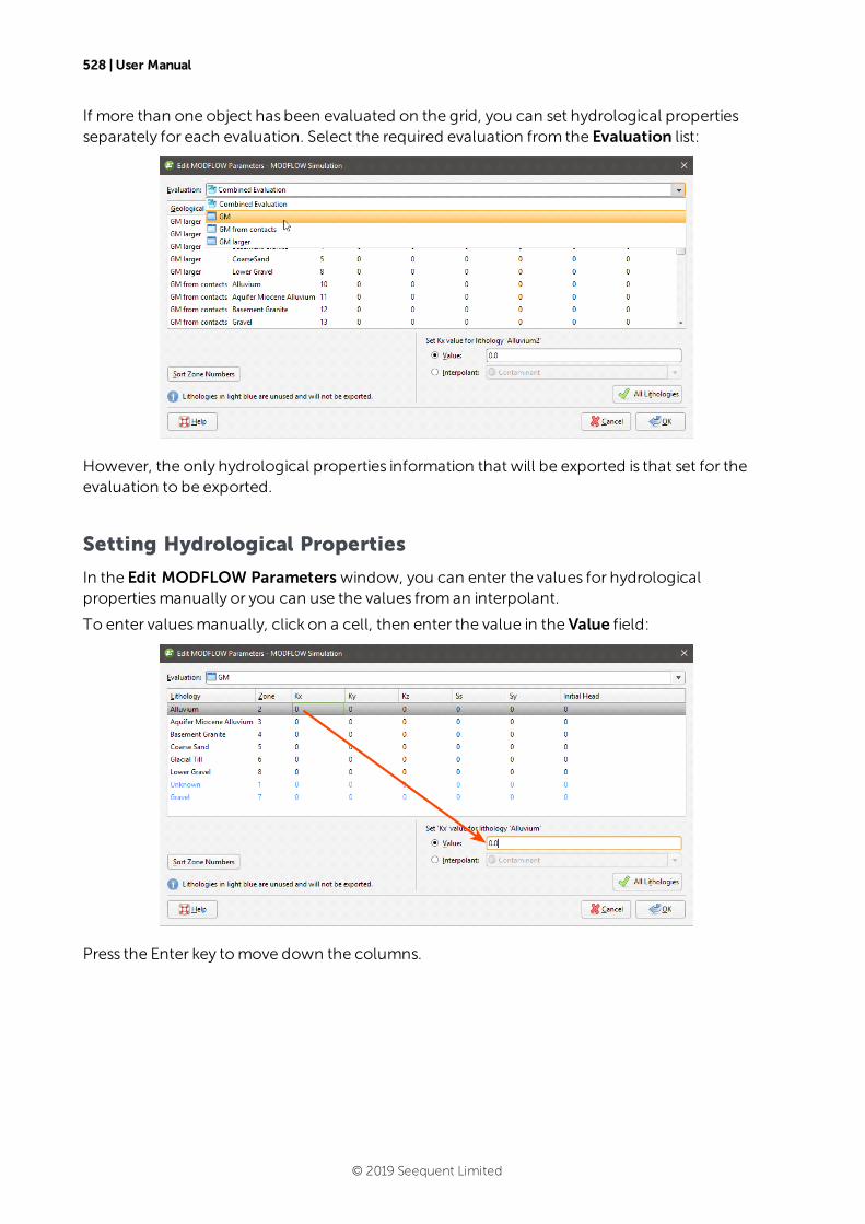
528 | User Manual
If more than one object has been evaluated on the grid, you can set hydrological propertiesseparately for each evaluation. Select the required evaluation from the Evaluation list:
However, the only hydrological properties information that will be exported is that set for theevaluation to be exported.
Setting Hydrological Properties
In the Edit MODFLOW Parameters window, you can enter the values for hydrologicalpropertiesmanually or you can use the values froman interpolant.
To enter valuesmanually, click on a cell, then enter the value in the Value field:
Press the Enter key tomove down the columns.
© 2019 Seequent Limited
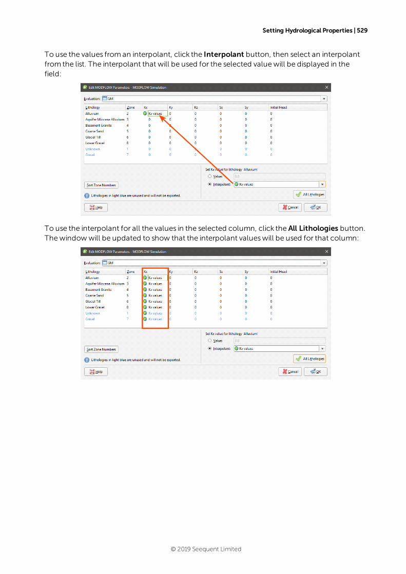
Setting Hydrological Properties | 529
To use the values froman interpolant, click the Interpolant button, then select an interpolantfrom the list. The interpolant that will be used for the selected valuewill be displayed in thefield:
To use the interpolant for all the values in the selected column, click the All Lithologies button.Thewindowwill be updated to show that the interpolant valueswill be used for that column:
© 2019 Seequent Limited
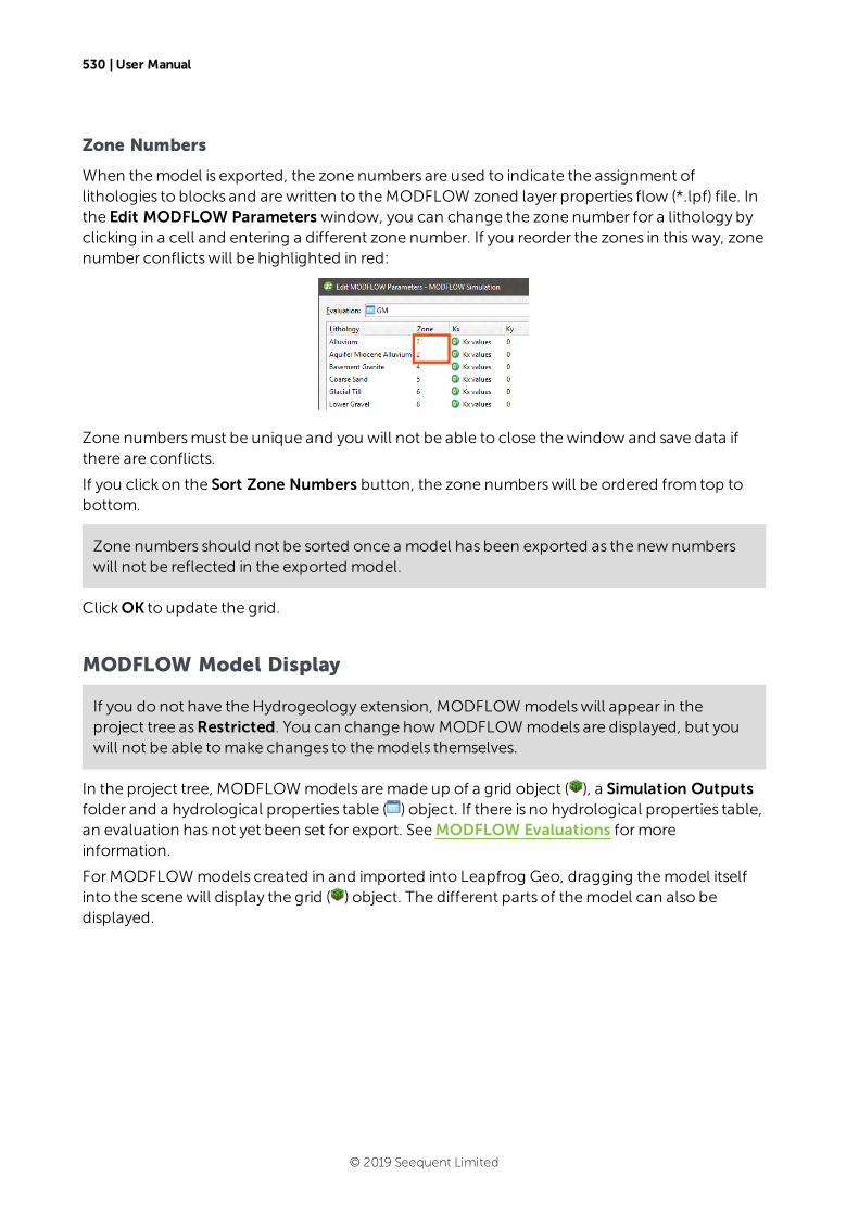
530 | User Manual
Zone Numbers
When themodel is exported, the zone numbers are used to indicate the assignment oflithologies to blocks and are written to theMODFLOW zoned layer properties flow (*.lpf) file. Inthe Edit MODFLOW Parameters window, you can change the zone number for a lithology byclicking in a cell and entering a different zone number. If you reorder the zones in thisway, zonenumber conflictswill be highlighted in red:
Zone numbersmust be unique and you will not be able to close thewindow and save data ifthere are conflicts.
If you click on the Sort Zone Numbers button, the zone numberswill be ordered from top tobottom.
Zone numbers should not be sorted once a model has been exported as the new numberswill not be reflected in the exported model.
ClickOK to update the grid.
MODFLOW Model Display
If you do not have the Hydrogeology extension, MODFLOWmodelswill appear in theproject tree asRestricted. You can change howMODFLOWmodels are displayed, but youwill not be able tomake changes to themodels themselves.
In the project tree, MODFLOWmodels aremade up of a grid object ( ), a Simulation Outputsfolder and a hydrological properties table ( ) object. If there is no hydrological properties table,an evaluation has not yet been set for export. SeeMODFLOW Evaluations formoreinformation.
ForMODFLOWmodels created in and imported into Leapfrog Geo, dragging themodel itselfinto the scenewill display the grid ( ) object. The different parts of themodel can also bedisplayed.
© 2019 Seequent Limited
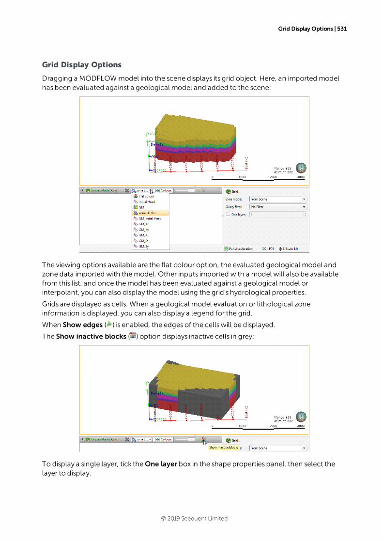
Grid Display Options | 531
Grid Display Options
Dragging a MODFLOWmodel into the scene displays its grid object. Here, an imported modelhas been evaluated against a geological model and added to the scene:
The viewing options available are the flat colour option, the evaluated geological model andzone data imported with themodel. Other inputs imported with a model will also be availablefrom this list, and once themodel has been evaluated against a geological model orinterpolant, you can also display themodel using the grid’s hydrological properties.
Grids are displayed as cells. When a geological model evaluation or lithological zoneinformation is displayed, you can also display a legend for the grid.
When Show edges ( ) is enabled, the edges of the cellswill be displayed.
The Show inactive blocks ( ) option displays inactive cells in grey:
To display a single layer, tick theOne layer box in the shape properties panel, then select thelayer to display.
© 2019 Seequent Limited
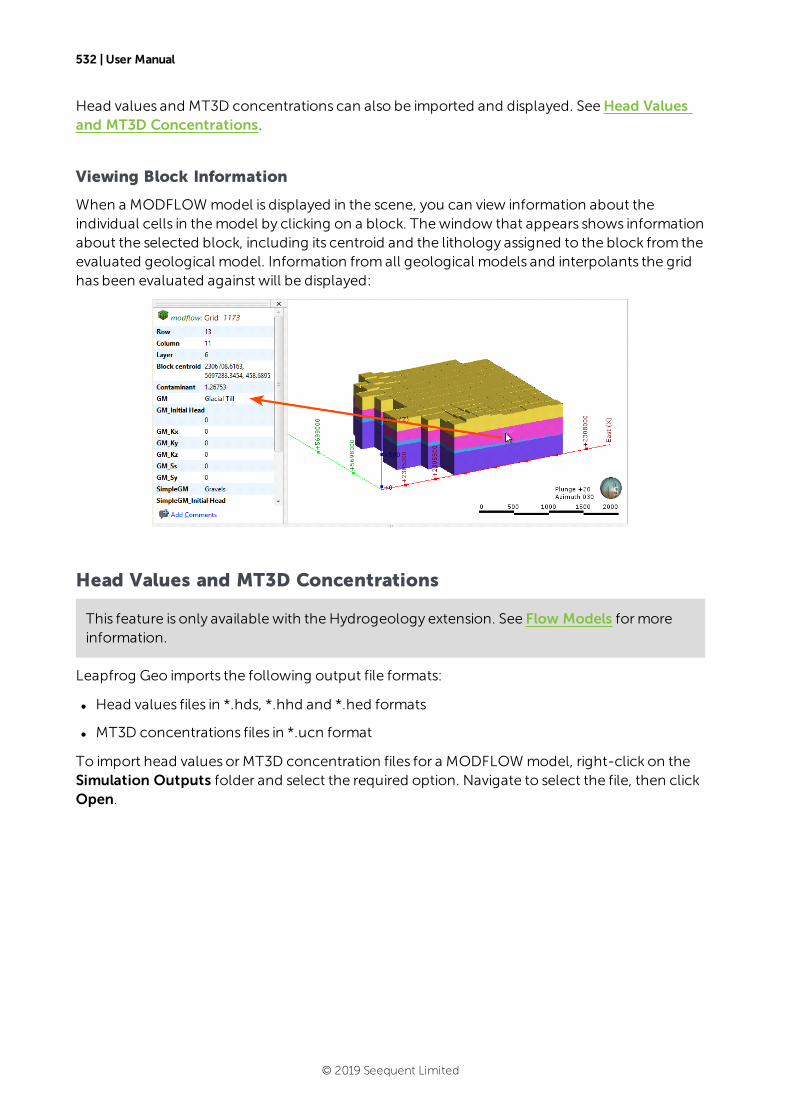
532 | User Manual
Head values and MT3D concentrations can also be imported and displayed. SeeHead Valuesand MT3D Concentrations.
Viewing Block Information
When a MODFLOWmodel is displayed in the scene, you can view information about theindividual cells in themodel by clicking on a block. Thewindow that appears shows informationabout the selected block, including its centroid and the lithology assigned to the block from theevaluated geological model. Information fromall geological models and interpolants the gridhas been evaluated against will be displayed:
Head Values and MT3D Concentrations
This feature is only available with the Hydrogeology extension. See Flow Models formoreinformation.
Leapfrog Geo imports the following output file formats:
l Head values files in *.hds, *.hhd and *.hed formats
l MT3D concentrations files in *.ucn format
To import head values orMT3D concentration files for a MODFLOWmodel, right-click on theSimulation Outputs folder and select the required option. Navigate to select the file, then clickOpen.
© 2019 Seequent Limited

Generating a Head Value Mesh | 533
The information will be added to theMODFLOW grid, and you can then select the head valuesand MT3D concentrations in the shape list when you display the grid in the scene. If the outputis time-dependent, a timestep slider will be available from the shape properties panel. Click anddrag the slider or click along the timeline to view the different timesteps available:
Imported head values and MT3D concentrations are stored in the project tree in the SimulationOutputs folder:
To delete head values orMT3D concentrations, right-click on the object in the project tree andselectDelete.
Once head values have been imported, you can generate a head valuemesh. SeeGenerating aHead Value Mesh.
Generating a Head Value Mesh
This feature is only available with the Hydrogeology extension. See Flow Models formoreinformation.
Once head values have been imported for a MODFLOWmodel, you can generate a head valuemesh. To do this, expand the Simulation Outputs folder. Right-click on the head values objectand selectGenerate Head Value Mesh. TheGenerate Head Value Meshwindowwill appear,showing the layers in themodel and the timesteps available. Select the layer of themodel youwish to generate a head valuemesh for, then choose the heads. ClickOK to create themesh,which will be saved to theMeshes folder.
MODFLOW Model Export
This feature is only available with the Hydrogeology extension. See Flow Models formoreinformation.
Leapfrog Geo has three options for exporting MODFLOW grids:
l Export the grid as a MODFLOW file.
l Export for Groundwater Vistas. Use this option the first time you export a grid for use inGroundwater Vistas.
© 2019 Seequent Limited
534 | User Manual
l Export a Groundwater Vistas update. Use this option to generate a set of files that can beimported into Groundwater Vistas as an update.
The Groundwater Vistas options include a zoned layer properties flow (*.lpf) file that includesinformation about the zones in the grid.
As a MODFLOW File
To export a grid as a MODFLOW file for use in a package other than Groundwater Vistas, right-click on the grid in the project tree and select Export to MODFLOW . You will be prompted tochoose a File name and location. Select the options required, then click Save.
For Groundwater Vistas
To export a grid for use in Groundwater Vistas for the first time, right-click on the grid in theproject tree and select Export to MODFLOW for GWV. You will be prompted to choose a Filename and location. Select the options required, then click Save.
If you have previously exported the grid to Groundwater Vistas and havemade changes to thegrid, use the Export to GWV Updates option.
As a Groundwater Vistas Update
If you have exported a grid to Groundwater Vistas but then make changes to the Leapfrog Geomodel, you can export the changes to themodel. The set of files containing the changes canthen be imported to Groundwater Vistas.
To export a Groundwater Vistas update, right-click on the grid in the project tree and selectExport GWV Updates. TheUpdate Groundwater Vistas windowwill appear listing the filesthat will be exported. Enter a Base file name to differentiate the original files from the updates.Click Export. The fileswill be saved in the specified directory.
FEFLOW Models
These features are only available as part of the Hydrogeology extension. See Flow Modelsformore information.
In Leapfrog Geo, creating a 3D FEFLOWmodel requires:
l A geological model that will be used to assign lithologies to the FEFLOWmodel’s blocks.
l A 2D grid that defines the block size, boundaries and surface features.
Steps for creating a 3D FEFLOWmodel that can be exported and run outside Leapfrog Geo are:
1. Create a geological model.
2. Create and refine a 2Dmodel in Leapfrog Geo or import a FEFLOWmodel.
3. Create the 3Dmodel from the 2Dmodel or another 3Dmodel in the project.
4. Evaluate the new 3Dmodel against a geological model.
© 2019 Seequent Limited
FEFLOW Model Display | 535
5. Edit thematerial types.
6. Export the 3D FEFLOWmodel.
Once themodel has been processed outside of Leapfrog Geo, a results file can be saved thatcan be imported into Leapfrog Geo and visualised in the scene.
A 2D grid can be created in or imported into Leapfrog Geo. A 3D grid can also be used, in whichcase the layer information is not used in creating the 3D grid. Creating the 2D grid in LeapfrogGeo provides themost flexibility, as the block sizes can easily be changed, the boundariesmodified and features added to provide finer resolution where there ismore data available.
For information about creating 2D and 3D grids, seeCreating a 2D FEFLOW Model andCreating a 3D FEFLOW Model.
You can also import FEFLOW problem files and result files, visualise them in Leapfrog Geo anduse themas the basis for newmodels. See Importing a FEFLOW Grid.
See FEFLOW Model Display for information on options for displaying FEFLOWmodels in thescene.
3D grids created in Leapfrog Geo can be evaluated against a geological model when they arecreated. Grids imported into Leapfrog Geo or that were not evaluated when theywere createdcan be evaluated as described in FEFLOW Evaluations.
Once a model has been defined and evaluated against a geological model, material types canbe assigned and the grid can be exported. See FEFLOW Material Types and FEFLOW ModelExport.
FEFLOW Model Display
If you do not have the Hydrogeology extension, FEFLOWmodelswill appear in the projecttree asRestricted. You can change how FEFLOWmodels are displayed, but you will not beable tomake changes to themodels themselves.
In the project tree, 3D FEFLOWmodels aremade up of a grid object representing the finiteelements, a nodes object and a material types table ( ) object. If there is nomaterial types table,an evaluation has not yet been set for export. See FEFLOW Evaluations formore information.
A 2D FEFLOW grid ismade up of a grid object and a nodes object. Here, three types of FEFLOWmodels are shown expanded in the project tree:
l Feflow 3D Simulation is a 3Dmodel created in Leapfrog Geo.
l Feflow 2D Simulation is a 2Dmodel created in Leapfrog Geo.
l Feflow Results is an imported 3Dmodel (DAC file).
© 2019 Seequent Limited
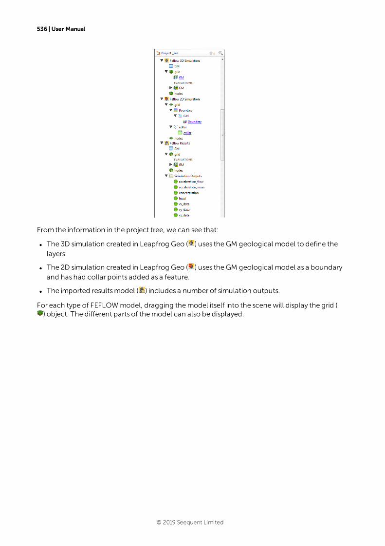
536 | User Manual
From the information in the project tree, we can see that:
l The 3D simulation created in Leapfrog Geo ( ) uses the GM geological model to define thelayers.
l The 2D simulation created in Leapfrog Geo ( ) uses the GM geological model as a boundaryand has had collar points added as a feature.
l The imported resultsmodel ( ) includes a number of simulation outputs.
For each type of FEFLOWmodel, dragging themodel itself into the scenewill display the grid () object. The different parts of themodel can also be displayed.
© 2019 Seequent Limited
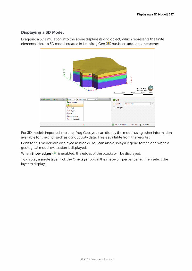
Displaying a 3D Model | 537
Displaying a 3D Model
Dragging a 3D simulation into the scene displays its grid object, which represents the finiteelements. Here, a 3Dmodel created in Leapfrog Geo ( ) has been added to the scene:
For 3Dmodels imported into Leapfrog Geo, you can display themodel using other informationavailable for the grid, such as conductivity data. This is available from the view list.
Grids for 3Dmodels are displayed as blocks. You can also display a legend for the grid when ageological model evaluation is displayed.
When Show edges ( ) is enabled, the edges of the blockswill be displayed.
To display a single layer, tick theOne layer box in the shape properties panel, then select thelayer to display.
© 2019 Seequent Limited
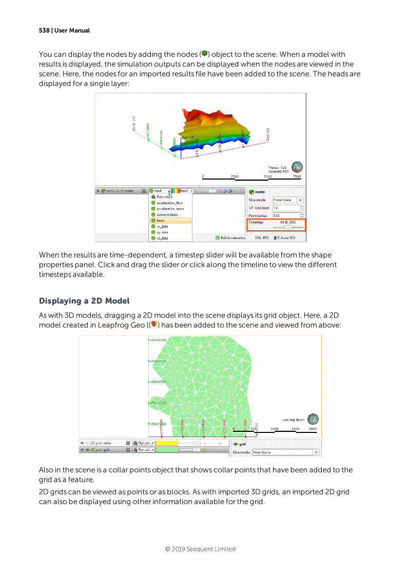
538 | User Manual
You can display the nodes by adding the nodes ( ) object to the scene. When a model withresults is displayed, the simulation outputs can be displayed when the nodes are viewed in thescene. Here, the nodes for an imported results file have been added to the scene. The heads aredisplayed for a single layer:
When the results are time-dependent, a timestep slider will be available from the shapeproperties panel. Click and drag the slider or click along the timeline to view the differenttimesteps available.
Displaying a 2D Model
Aswith 3Dmodels, dragging a 2Dmodel into the scene displays its grid object. Here, a 2Dmodel created in Leapfrog Geo (( ) has been added to the scene and viewed fromabove:
Also in the scene is a collar points object that shows collar points that have been added to thegrid as a feature.
2D grids can be viewed as points or as blocks. Aswith imported 3D grids, an imported 2D gridcan also be displayed using other information available for the grid.
© 2019 Seequent Limited
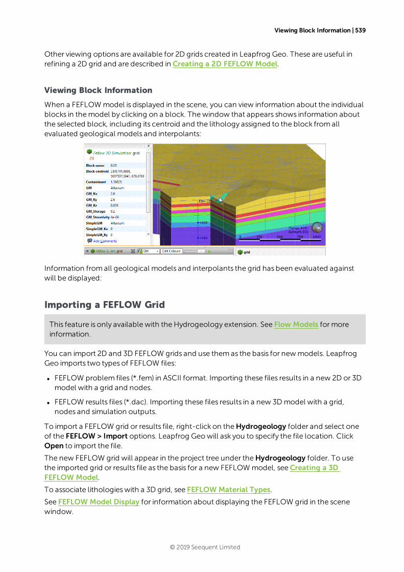
Viewing Block Information | 539
Other viewing options are available for 2D grids created in Leapfrog Geo. These are useful inrefining a 2D grid and are described in Creating a 2D FEFLOW Model.
Viewing Block Information
When a FEFLOWmodel is displayed in the scene, you can view information about the individualblocks in themodel by clicking on a block. Thewindow that appears shows information aboutthe selected block, including its centroid and the lithology assigned to the block fromallevaluated geological models and interpolants:
Information fromall geological models and interpolants the grid has been evaluated againstwill be displayed:
Importing a FEFLOW Grid
This feature is only available with the Hydrogeology extension. See Flow Models formoreinformation.
You can import 2D and 3D FEFLOW grids and use themas the basis for newmodels. LeapfrogGeo imports two types of FEFLOW files:
l FEFLOW problem files (*.fem) in ASCII format. Importing these files results in a new 2D or 3Dmodel with a grid and nodes.
l FEFLOW results files (*.dac). Importing these files results in a new 3Dmodel with a grid,nodes and simulation outputs.
To import a FEFLOW grid or results file, right-click on theHydrogeology folder and select oneof the FEFLOW > Import options. Leapfrog Geowill ask you to specify the file location. ClickOpen to import the file.
The new FEFLOW grid will appear in the project tree under theHydrogeology folder. To usethe imported grid or results file as the basis for a new FEFLOWmodel, seeCreating a 3DFEFLOW Model.
To associate lithologieswith a 3D grid, see FEFLOW Material Types.
See FEFLOW Model Display for information about displaying the FEFLOW grid in the scenewindow.
© 2019 Seequent Limited
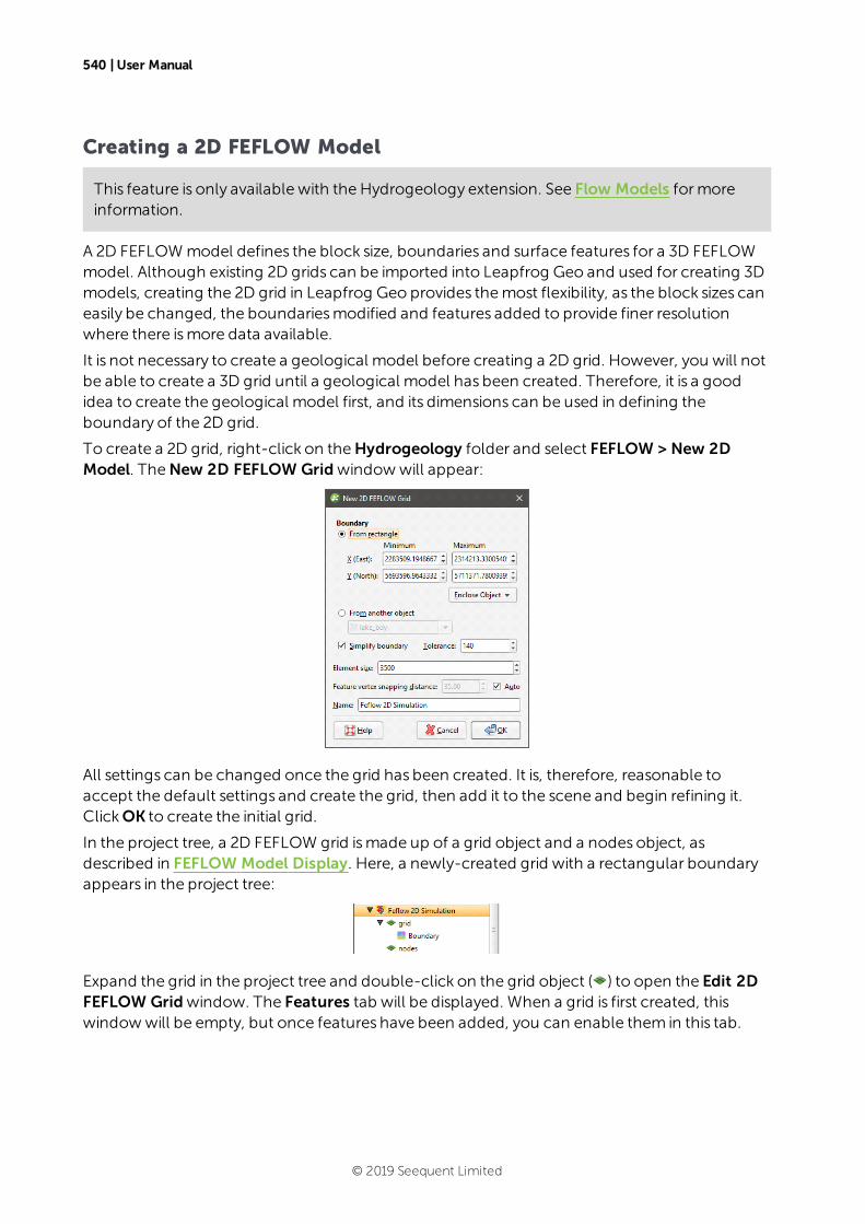
540 | User Manual
Creating a 2D FEFLOW Model
This feature is only available with the Hydrogeology extension. See Flow Models formoreinformation.
A 2D FEFLOWmodel defines the block size, boundaries and surface features for a 3D FEFLOWmodel. Although existing 2D grids can be imported into Leapfrog Geo and used for creating 3Dmodels, creating the 2D grid in Leapfrog Geo provides themost flexibility, as the block sizes caneasily be changed, the boundariesmodified and features added to provide finer resolutionwhere there ismore data available.
It is not necessary to create a geological model before creating a 2D grid. However, you will notbe able to create a 3D grid until a geological model has been created. Therefore, it is a goodidea to create the geological model first, and its dimensions can be used in defining theboundary of the 2D grid.
To create a 2D grid, right-click on theHydrogeology folder and select FEFLOW > New 2DModel. TheNew 2D FEFLOW Gridwindowwill appear:
All settings can be changed once the grid has been created. It is, therefore, reasonable toaccept the default settings and create the grid, then add it to the scene and begin refining it.ClickOK to create the initial grid.
In the project tree, a 2D FEFLOW grid ismade up of a grid object and a nodes object, asdescribed in FEFLOW Model Display. Here, a newly-created grid with a rectangular boundaryappears in the project tree:
Expand the grid in the project tree and double-click on the grid object ( ) to open the Edit 2DFEFLOW Gridwindow. The Features tab will be displayed. When a grid is first created, thiswindowwill be empty, but once features have been added, you can enable them in this tab.
© 2019 Seequent Limited
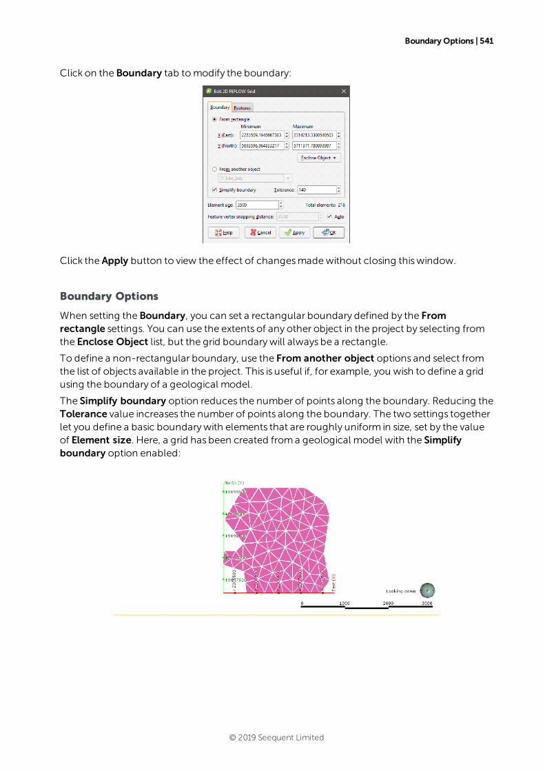
Boundary Options | 541
Click on the Boundary tab tomodify the boundary:
Click the Apply button to view the effect of changesmadewithout closing thiswindow.
Boundary Options
When setting the Boundary, you can set a rectangular boundary defined by the Fromrectangle settings. You can use the extents of any other object in the project by selecting fromthe Enclose Object list, but the grid boundarywill always be a rectangle.
To define a non-rectangular boundary, use the From another object options and select fromthe list of objects available in the project. This is useful if, for example, you wish to define a gridusing the boundary of a geological model.
The Simplify boundary option reduces the number of points along the boundary. Reducing theTolerance value increases the number of points along the boundary. The two settings togetherlet you define a basic boundarywith elements that are roughly uniform in size, set by the valueof Element size. Here, a grid has been created froma geological model with the Simplifyboundary option enabled:
© 2019 Seequent Limited
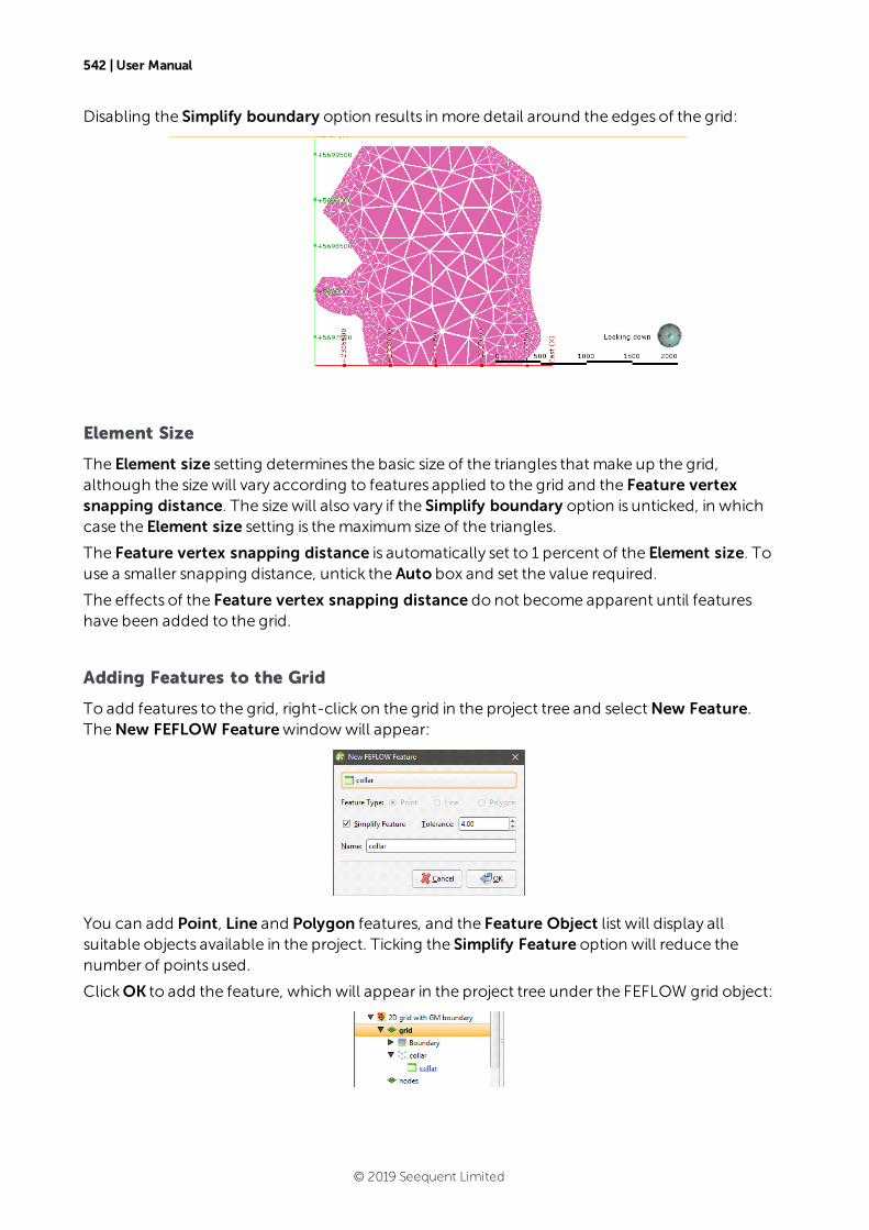
542 | User Manual
Disabling the Simplify boundary option results in more detail around the edges of the grid:
Element Size
The Element size setting determines the basic size of the triangles that make up the grid,although the size will vary according to features applied to the grid and the Feature vertexsnapping distance. The size will also vary if the Simplify boundary option is unticked, in whichcase the Element size setting is themaximumsize of the triangles.
The Feature vertex snapping distance is automatically set to 1 percent of the Element size. Touse a smaller snapping distance, untick the Auto box and set the value required.
The effects of the Feature vertex snapping distance do not become apparent until featureshave been added to the grid.
Adding Features to the Grid
To add features to the grid, right-click on the grid in the project tree and selectNew Feature.TheNew FEFLOW Featurewindowwill appear:
You can add Point, Line and Polygon features, and the Feature Object list will display allsuitable objects available in the project. Ticking the Simplify Feature option will reduce thenumber of points used.
ClickOK to add the feature, which will appear in the project tree under the FEFLOW grid object:
© 2019 Seequent Limited

Adding Features to the Grid | 543
You can edit the feature by double-clicking on it or by right-clicking and selecting Open.However, the feature has not yet been applied to the grid. To enable the feature, double-clickon the grid to open the Edit 2D FEFLOW Gridwindow. Tick the box to enable the feature, thenadjust the number of Refinement Steps:
MoreRefinement Steps will producemore detail near the feature.
ClickApply orOK to view the effect the feature and its settings have on the grid.
If you want tomodify a feature without having to reprocess the grid, untick it in the Featurestab. If you want to delete a feature, right-click on it in the project tree and selectDelete.
The images below show a grid displayed with collar points (in red) to demonstrate the effects ofno features and collars applied with different refinement steps:
No features Collars with 2 refinement steps Collars with 10 refinement steps
© 2019 Seequent Limited

544 | User Manual
To view all features added to a grid, right-click on the grid and select View Snapped Features. ASnapped Features object will appear in the shape list that represents all objects used to addfeatures to the grid:
Here, four snapped objects appear in the scene: the three features listed in the Features tab andthe grid’s boundary.
SeeCreating a 3D FEFLOW Model for information on using the 2D grid as the basis for a 3Dmodel.
Creating a 3D FEFLOW Model
This feature is only available with the Hydrogeology extension. See Flow Models formoreinformation.
To create a new 3D FEFLOWmodel, you must first create or import a 2D FEFLOW grid asdescribed in Creating a 2D FEFLOW Model and Importing a FEFLOW Grid.
Once you have created or imported a 2D FEFLOW grid, right-click on theHydrogeology folderand select FEFLOW > New 3D Model. The Extrude 3D FEFLOW Gridwindowwill appear:
© 2019 Seequent Limited
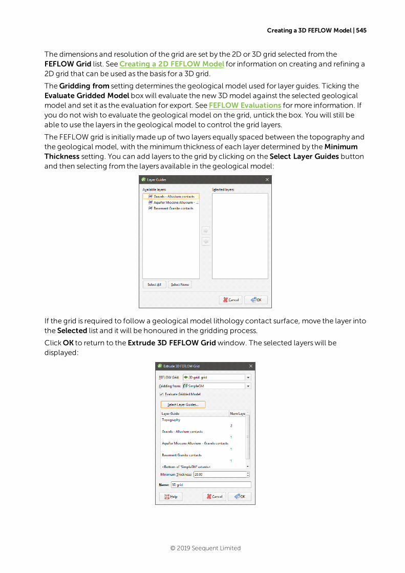
Creating a 3D FEFLOW Model | 545
The dimensions and resolution of the grid are set by the 2D or 3D grid selected from theFEFLOW Grid list. SeeCreating a 2D FEFLOW Model for information on creating and refining a2D grid that can be used as the basis for a 3D grid.
TheGridding from setting determines the geological model used for layer guides. Ticking theEvaluate Gridded Model boxwill evaluate the new 3Dmodel against the selected geologicalmodel and set it as the evaluation for export. See FEFLOW Evaluations formore information. Ifyou do not wish to evaluate the geological model on the grid, untick the box. You will still beable to use the layers in the geological model to control the grid layers.
The FEFLOW grid is initiallymade up of two layers equally spaced between the topography andthe geological model, with theminimum thickness of each layer determined by theMinimumThickness setting. You can add layers to the grid by clicking on the Select Layer Guides buttonand then selecting from the layers available in the geological model:
If the grid is required to follow a geological model lithology contact surface, move the layer intothe Selected list and it will be honoured in the gridding process.
ClickOK to return to the Extrude 3D FEFLOW Gridwindow. The selected layerswill bedisplayed:
© 2019 Seequent Limited
546 | User Manual
ClickOK to generate the new FEFLOW grid, which will appear in the project tree under theHydrogeology folder.
Once themodel has been created, you can edit it by expanding themodel in the project treeand double-clicking on its grid object. The layer guides selected, the number defined and theMinimum Thickness can bemodified, but the FEFLOW grid on which themodel is based andthe geological model used for gridding cannot be changed.
The boundaries of the selected geological model must be larger than the FEFLOW grid usedas the basis for the newmodel. If this is not the case, you can change the geological model’sextents so that they enclose the FEFLOW grid.
For further information on working with the new grid, see:
l FEFLOW Model Display
l FEFLOW Evaluations
l FEFLOW Material Types
l FEFLOW Model Export
FEFLOW Evaluations
This feature is only available with the Hydrogeology extension. See Flow Models formoreinformation.
When a 3D FEFLOWmodel is exported, the evaluated geological model is used to assignlithologies to the blocks in the grid. If the grid has not been evaluated against a geologicalmodel, you must do so before you can edit thematerial types and before you can export thegrid.
To evaluate a FEFLOW grid, expand themodel in the project tree. Right-click on the grid object () and select Evaluations. Although you can evaluate an interpolant or distance function, they
cannot be exported with the grid and are simply used for displaying the grid in Leapfrog Geo.
A windowwill appear listing all objects in the project that can be used for an evaluation. Onceyou have selected one ormore objects, clickOK. You will then be able to select the evaluationsfrom the view list, as described in Evaluations.
Assigning an Evaluation for Export
For 3D grids created in Leapfrog Geo, the evaluation used when creating the grid willautomatically be assigned as the evaluation for export. Amaterial types table ( ) will appear inthe project tree as part of the 3D grid.
If the grid was imported into Leapfrog Geo or created without being evaluated against ageological model, you will need tomanually set the evaluation for export. To do this:
l Evaluate the grid against one ormore geological models, as described above.
© 2019 Seequent Limited
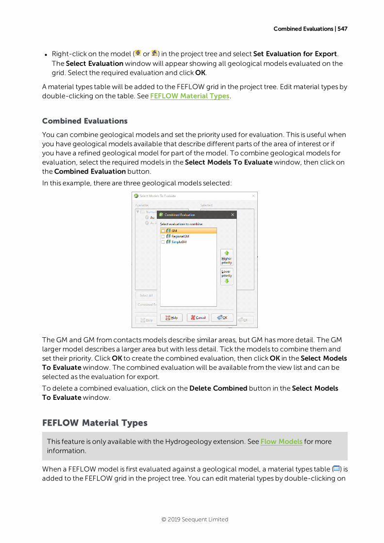
Combined Evaluations | 547
l Right-click on themodel ( or ) in the project tree and select Set Evaluation for Export.The Select Evaluationwindowwill appear showing all geological models evaluated on thegrid. Select the required evaluation and clickOK.
Amaterial types table will be added to the FEFLOW grid in the project tree. Edit material types bydouble-clicking on the table. See FEFLOW Material Types.
Combined Evaluations
You can combine geological models and set the priority used for evaluation. This is useful whenyou have geological models available that describe different parts of the area of interest or ifyou have a refined geological model for part of themodel. To combine geological models forevaluation, select the required models in the Select Models To Evaluatewindow, then click ontheCombined Evaluation button.
In this example, there are three geological models selected:
The GM and GM fromcontactsmodels describe similar areas, but GM hasmore detail. The GMlargermodel describes a larger area but with less detail. Tick themodels to combine themandset their priority. ClickOK to create the combined evaluation, then clickOK in the Select ModelsTo Evaluatewindow. The combined evaluation will be available from the view list and can beselected as the evaluation for export.
To delete a combined evaluation, click on theDelete Combined button in the Select ModelsTo Evaluatewindow.
FEFLOW Material Types
This feature is only available with the Hydrogeology extension. See Flow Models formoreinformation.
When a FEFLOWmodel is first evaluated against a geological model, a material types table ( ) isadded to the FEFLOW grid in the project tree. You can edit material types by double-clicking on
© 2019 Seequent Limited
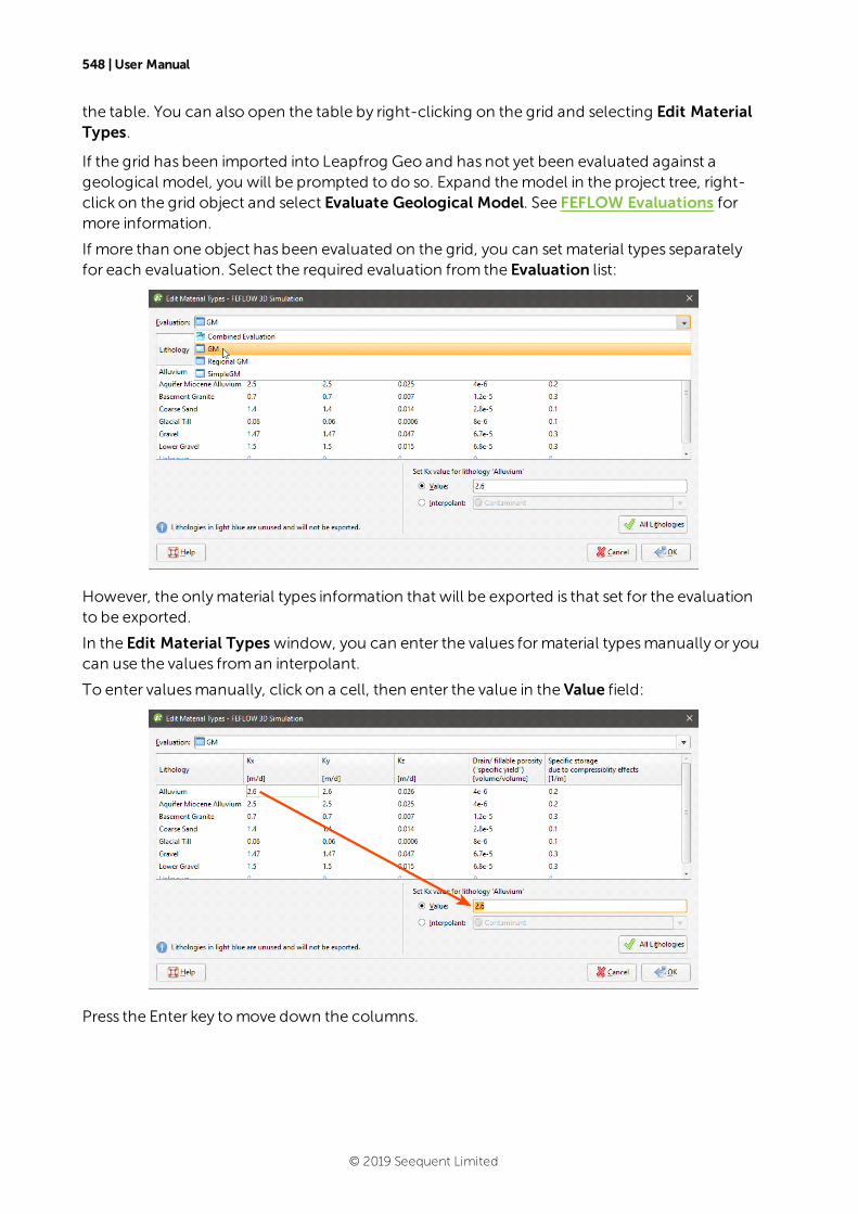
548 | User Manual
the table. You can also open the table by right-clicking on the grid and selecting Edit MaterialTypes.
If the grid has been imported into Leapfrog Geo and has not yet been evaluated against ageological model, you will be prompted to do so. Expand themodel in the project tree, right-click on the grid object and select Evaluate Geological Model. See FEFLOW Evaluations formore information.
If more than one object has been evaluated on the grid, you can set material types separatelyfor each evaluation. Select the required evaluation from the Evaluation list:
However, the onlymaterial types information that will be exported is that set for the evaluationto be exported.
In the Edit Material Types window, you can enter the values formaterial typesmanually or youcan use the values froman interpolant.
To enter valuesmanually, click on a cell, then enter the value in the Value field:
Press the Enter key tomove down the columns.
© 2019 Seequent Limited
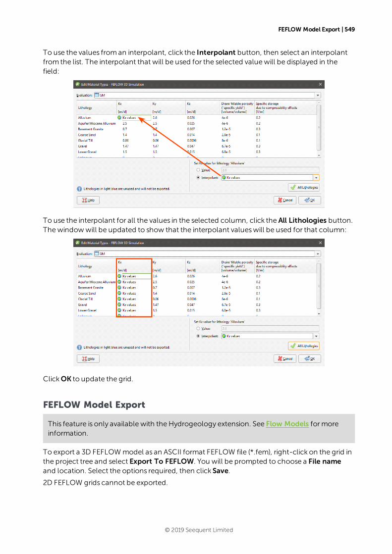
FEFLOW Model Export | 549
To use the values froman interpolant, click the Interpolant button, then select an interpolantfrom the list. The interpolant that will be used for the selected valuewill be displayed in thefield:
To use the interpolant for all the values in the selected column, click the All Lithologies button.Thewindowwill be updated to show that the interpolant valueswill be used for that column:
ClickOK to update the grid.
FEFLOW Model Export
This feature is only available with the Hydrogeology extension. See Flow Models formoreinformation.
To export a 3D FEFLOWmodel as an ASCII format FEFLOW file (*.fem), right-click on the grid inthe project tree and select Export To FEFLOW. You will be prompted to choose a File nameand location. Select the options required, then click Save.
2D FEFLOW grids cannot be exported.
© 2019 Seequent Limited
Block ModelsThe Block Models folder can be used to import and create blockmodels. Model types that canbe imported are:
l Isatis files
l CSV files
You can also create blockmodels and sub-blocked models, which can then be exported for usein other applications. Creating blockmodelswithin Leapfrog Geo has the advantage that theresolution can easily be changed.
Blockmodels can be evaluated against geological models and interpolants as described inEvaluations. If you have the Leapfrog Edge extension, blockmodels can also be evaluatedagainst estimators.
The rest of this topic describes importing blockmodels in Isatis and CSV formats, creating blockmodels in Leapfrog Geo, viewing blockmodel statistics and exporting blockmodels. It is dividedinto:
l Importing a Block Model
l Creating a Block Model
l Displaying a Block Model
l Viewing Block Model Statistics
l Exporting Block Models
Importing a Block Model
Leapfrog Geo imports blockmodels in the following formats:
l CSV + Text Header (*.csv, *.csv.txt)
l CSVwith Embedded Header (*.csv)
l Isatis BlockModel Files (*.asc)
Note that neither CSV format requires a header; once you start the import process, LeapfrogGeowill use the data in the file to locate theminimumand maximumcentroids. You can viewthis information and change how the data ismapped before the file is saved into the project.
Importing an Isatis Block Model
To import an Isatis format blockmodel, right-click on the Block Models folder and selectImport Block Model. Select the file you wish to import and clickOpen. Themodel will beimported and added to the Block Models folder.
© 2019 Seequent Limited
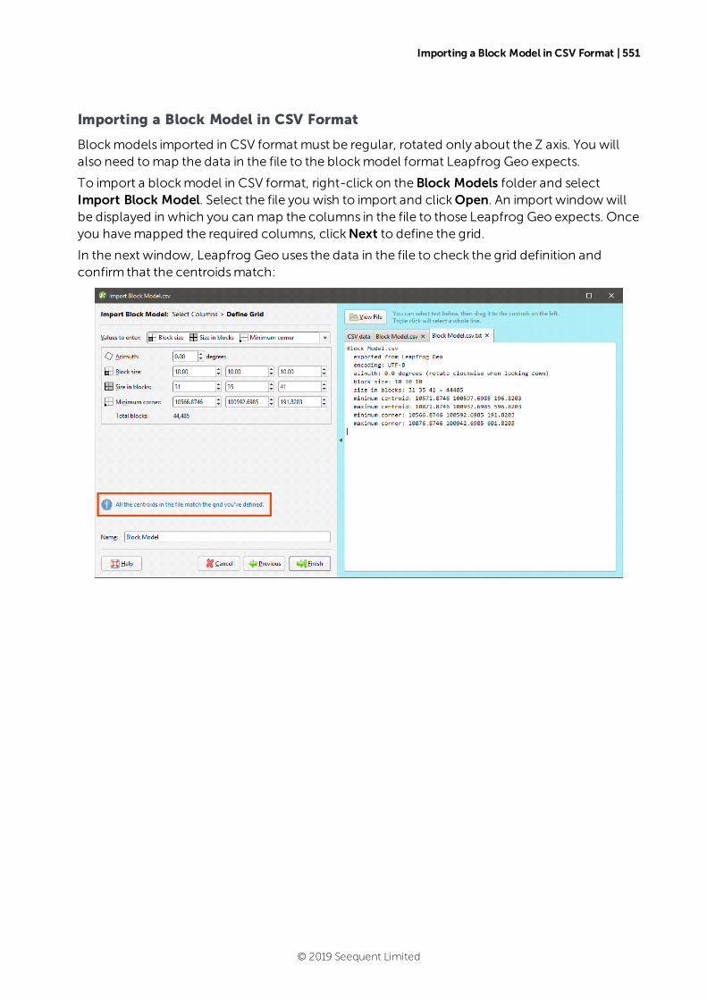
Importing a Block Model in CSV Format | 551
Importing a Block Model in CSV Format
Blockmodels imported in CSV format must be regular, rotated only about the Z axis. You willalso need tomap the data in the file to the blockmodel format Leapfrog Geo expects.
To import a blockmodel in CSV format, right-click on the Block Models folder and selectImport Block Model. Select the file you wish to import and clickOpen. An import windowwillbe displayed in which you can map the columns in the file to those Leapfrog Geo expects. Onceyou havemapped the required columns, clickNext to define the grid.
In the next window, Leapfrog Geo uses the data in the file to check the grid definition andconfirm that the centroidsmatch:
© 2019 Seequent Limited
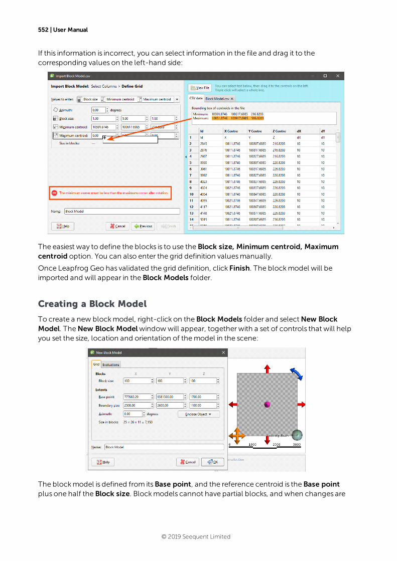
552 | User Manual
If this information is incorrect, you can select information in the file and drag it to thecorresponding values on the left-hand side:
The easiest way to define the blocks is to use the Block size, Minimum centroid, Maximumcentroid option. You can also enter the grid definition valuesmanually.
Once Leapfrog Geo has validated the grid definition, click Finish. The blockmodel will beimported and will appear in the Block Models folder.
Creating a Block Model
To create a new blockmodel, right-click on the Block Models folder and selectNew BlockModel. TheNew Block Modelwindowwill appear, together with a set of controls that will helpyou set the size, location and orientation of themodel in the scene:
The blockmodel is defined from itsBase point, and the reference centroid is the Base pointplus one half the Block size. Blockmodels cannot have partial blocks, and when changes are
© 2019 Seequent Limited
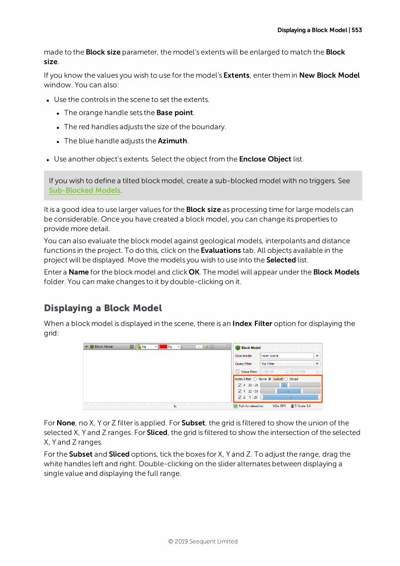
Displaying a Block Model | 553
made to the Block size parameter, themodel’s extentswill be enlarged tomatch the Blocksize.
If you know the values you wish to use for themodel’sExtents, enter them in New Block Modelwindow. You can also:
l Use the controls in the scene to set the extents.
l The orange handle sets the Base point.
l The red handles adjusts the size of the boundary.
l The blue handle adjusts the Azimuth.
l Use another object’s extents. Select the object from the Enclose Object list.
If you wish to define a tilted blockmodel, create a sub-blocked model with no triggers. SeeSub-Blocked Models.
It is a good idea to use larger values for the Block size as processing time for largemodels canbe considerable. Once you have created a blockmodel, you can change its properties toprovidemore detail.
You can also evaluate the blockmodel against geological models, interpolants and distancefunctions in the project. To do this, click on the Evaluations tab. All objects available in theproject will be displayed. Move themodels you wish to use into the Selected list.
Enter a Name for the blockmodel and clickOK. Themodel will appear under the Block Modelsfolder. You can make changes to it by double-clicking on it.
Displaying a Block Model
When a blockmodel is displayed in the scene, there is an Index Filter option for displaying thegrid:
ForNone, no X, Y or Z filter is applied. For Subset, the grid is filtered to show the union of theselected X, Y and Z ranges. For Sliced, the grid is filtered to show the intersection of the selectedX, Y and Z ranges.
For the Subset and Sliced options, tick the boxes for X, Y and Z. To adjust the range, drag thewhite handles left and right. Double-clicking on the slider alternates between displaying asingle value and displaying the full range.
© 2019 Seequent Limited
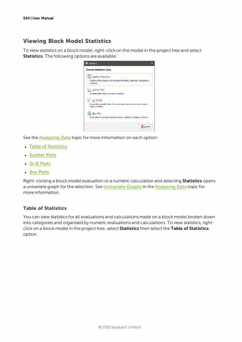
554 | User Manual
Viewing Block Model Statistics
To view statistics on a blockmodel, right-click on themodel in the project tree and selectStatistics. The following options are available:
See the Analysing Data topic formore information on each option:
l Table of Statistics
l Scatter Plots
l Q-Q Plots
l Box Plots
Right-clicking a blockmodel evaluation or a numeric calculation and selecting Statistics opensa univariate graph for the selection. SeeUnivariate Graphs in the Analysing Data topic formore information.
Table of Statistics
You can view statistics for all evaluations and calculationsmade on a blockmodel broken downinto categories and organised by numeric evaluations and calculations. To view statistics, right-click on a blockmodel in the project tree, select Statistics then select the Table of Statisticsoption.
© 2019 Seequent Limited
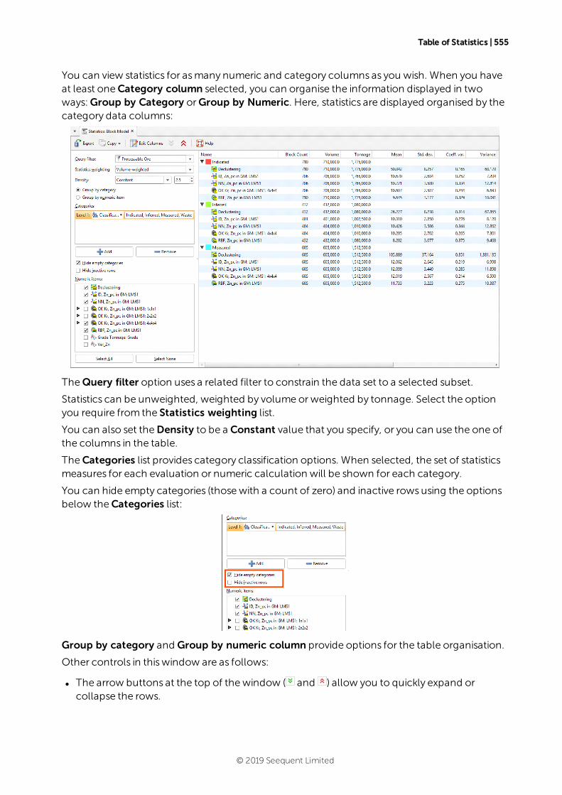
Table of Statistics | 555
You can view statistics for asmany numeric and category columns as you wish. When you haveat least oneCategory column selected, you can organise the information displayed in twoways:Group by Category orGroup by Numeric. Here, statistics are displayed organised by thecategory data columns:
TheQuery filter option uses a related filter to constrain the data set to a selected subset.
Statistics can be unweighted, weighted by volume orweighted by tonnage. Select the optionyou require from the Statistics weighting list.
You can also set theDensity to be a Constant value that you specify, or you can use the one ofthe columns in the table.
TheCategories list provides category classification options. When selected, the set of statisticsmeasures for each evaluation or numeric calculation will be shown for each category.
You can hide empty categories (thosewith a count of zero) and inactive rowsusing the optionsbelow theCategories list:
Group by category and Group by numeric column provide options for the table organisation.
Other controls in thiswindow are as follows:
l The arrow buttons at the top of thewindow ( and ) allow you to quickly expand orcollapse the rows.
© 2019 Seequent Limited
556 | User Manual
l Click rows to select them.
l Select multiple rowsby holding down the Shift or Ctrl keywhile clicking rows.
l TheCopy button ( ) copies the selected rows to the clipboard so you can paste them intoanother application.
Exporting Block Models
Blockmodels created in Leapfrog Geo can be exported in the following formats:
l CSV + Text Header (*.csv, *.csv.txt)
l CSVwith Embedded Header (*.csv)
l CSV as points (*.csv)
l Isatis BlockModel Files (*.asc)
l Surpac BlockModel Files (*.mdl)
l Datamine BlockModel Files (*.dm)
To export a blockmodel, right-click on the blockmodel in the project tree and select Export.You will be prompted to select the file format.
If you wish to export themodel in one of the CSV formats, selectCSV Block Model Files(*.csv) in the Export Block Modelwindow. You will be able to choose between the threeCSV formats in the next step.
Enter a name and location for the file and click Save. Next, you will be able to choose customsettings for the selected format.
The rest of this topic providesmore information about exporting blockmodels in CSV, Isatis,Datamine and Surpac formats.
l Exporting Block Models in CSV Format
l Exporting Block Models in Isatis Format
l Exporting Block Models in Datamine Format
l Exporting Block Models in Surpac Format
Exporting Block Models in CSV Format
The selections you makewhen you export a blockmodel will be saved. This streamlines theprocess of subsequent exports of themodel.
When you choose to export a blockmodel in CSV format, you must first choose the type of CSVexport. Options are:
l With an embedded header file. The blockmodel definition is included at the top of the CSVfile.
© 2019 Seequent Limited
Selecting From Evaluated Items | 557
l With a separate text header. The blockmodel definition iswritten as a separate text file.
l As points. The CSV file does not include the block sizes and model description.
ClickNext. The steps that follow are:
l Selecting From Evaluated Items
l Setting Row Filtering Options
l Setting Numeric Precision
l Setting Status Code Text Sequences
l Selecting the Character Set
Selecting From Evaluated Items
Choosewhich objectswill be included in the exported file. The Available items list includes allevaluationsmade onto themodel. If you have the Leapfrog Edge extension, you can alsoinclude calculations and filters, which will be exported as separate columns. The order ofcolumns in the exported file will match the order shown in the project tree.
ClickNext.
Setting Row Filtering Options
If you have the Leapfrog Edge extension, you can use a Query filter to filter rowsout of the dataexported.
This is different fromexporting filters as columns, as selected in the previous step.
The second option in thiswindow is useful when all block results are consistently the same non-Normal status. Select from Error, Without grade, Blank orOutside; all rows that consistentlyshow the selected statuseswill not be included in the exported file.
ClickNext.
Setting Numeric Precision
There are three encoding options forNumeric Precision:
l TheDouble, floating point option provides precision of 15 to 17 significant decimal places.
l The Single, floating point option provides precision of 6 to 9 significant decimal places.
l TheCustomoption lets you set a specific number of decimal places.
To change either theCentroid and size precision and Column data precision options, untickthe box forUse default precision and select the required option.
ClickNext.
Setting Status Code Text Sequences
When a blockmodel is exported, non-Normal status codes can be represented in the exportedfile using custom text sequences.
© 2019 Seequent Limited
558 | User Manual
The Status Code sequences are used for category status codes and filter status codes exportedas columns. For filter status codes, Boolean value resultswill show FALSE and TRUE for Normalvalues or the defined Status Codes for non-Normal values.
Boolean values on blockmodels are only available if you have the Leapfrog Edge extension.
Numeric Status Codes can be represented using custom text sequences. This is optional; if noseparate codes are defined for numeric items, the defined Status Codes will be used.
ClickNext.
Selecting the Character Set
The selection you makewill depend on the target for your exported file. You can choose acharacter set and seewhat changeswill bemade.
ClickNext to view a summary of the selected options, then click Export to save the file.
Exporting Block Models in Isatis Format
The selections you makewhen you export a blockmodel will be saved. This streamlines theprocess of subsequent exports of themodel.
When exporting a blockmodel in Isatis format, the steps to follow are:
l Selecting From Evaluated Items
l Setting Status Code Text Sequences
l Selecting the Character Set
Selecting From Evaluated Items
Choosewhich objectswill be included in the exported file. The Available items list includes allevaluationsmade onto themodel. If you have the Leapfrog Edge extension, you can alsoinclude calculations and filters, which will be exported as separate columns. The order ofcolumns in the exported file will match the order shown in the project tree.
ClickNext.
Setting Status Code Text Sequences
When a blockmodel is exported, non-Normal status codes can be represented in the exportedfile using custom text sequences.
When exporting blockmodels in Isatis format, both category and numeric status codes can useindependent custom text sequences. For filter status codes, Boolean values are exported using0 for false and 1 for true; non-Normal valueswill be left blank and status codes cannot bedistinguished.
Boolean Status Codes on blockmodels are only available if you have the Leapfrog Edgeextension.
ClickNext.
© 2019 Seequent Limited
Selecting the Character Set | 559
Selecting the Character Set
The selection you makewill depend on the target for your exported file. You can choose acharacter set and seewhat changeswill bemade.
ClickNext to view a summary of the selected options, then click Export to save the file.
Exporting Block Models in Datamine Format
The selections you makewhen you export a blockmodel will be saved. This streamlines theprocess of subsequent exports of themodel.
When exporting a blockmodel in Datamine format, the steps to follow are:
l Selecting From Evaluated Items
l Setting Row Filtering Options
l Setting Status Code Text Sequences
l Selecting the Character Set
l Renaming Items
Selecting From Evaluated Items
Choosewhich objectswill be included in the exported file. The Available items list includes allevaluationsmade onto themodel. If you have the Leapfrog Edge extension, you can alsoinclude calculations and filters, which will be exported as separate columns. The order ofcolumns in the exported file will match the order shown in the project tree.
ClickNext.
Setting Row Filtering Options
If you have the Leapfrog Edge extension, you can use a Query filter to filter rowsout of the dataexported.
This is different fromexporting filters as columns, as selected in the previous step.
The second option in thiswindow is useful when all block results are consistently the same non-Normal status. Select from Error, Without grade, Blank orOutside; all rows that consistentlyshow the selected statuseswill not be included in the exported file.
ClickNext.
Setting Status Code Text Sequences
When a blockmodel is exported, non-Normal status codes can be represented in the exportedfile using custom text sequences.
When exporting blockmodels in Datamine format, both category and numeric status codes canuse independent custom text sequences. Boolean values are exported using values 0 for falseand 1 for true; specify if non-Normal values should be represented by 0 or by the numeric statuscodes.
© 2019 Seequent Limited
560 | User Manual
Boolean Status Codes on blockmodels are only available if you have the Leapfrog Edgeextension.
ClickNext.
Selecting the Character Set
The selection you makewill depend on the target for your exported file. You can choose acharacter set and seewhat changeswill bemade.
ClickNext.
Renaming Items
When exporting a blockmodel in Datamine format, column names for the evaluated objectshave a maximum length of 8 characters. Leapfrog Geowill recommend truncated columnnames, but if you wish to use different abbreviations, click on the item’sNew Name to edit it.
ClickNext to view a summary of the selected options, then click Export to save the file.
Exporting Block Models in Surpac Format
The selections you makewhen you export a blockmodel will be saved. This streamlines theprocess of subsequent exports of themodel.
When you choose to export a blockmodel in Surpac format, you must first choosewhether toexport themodel in Surpac version 3.2 or Surpac version 5.0. Considerations are as follows:
l Blockmodels exported in Surpac version 5.0 cannot be imported into versions of Surpacbefore 5.0.
l Blockmodelswith more than 512 blocks per side can only be exported in Surpac version 5.0format.
Choosewhich format you wish to use.
ClickNext. The steps that follow are:
l Selecting From Evaluated Items
l Setting Row Filtering Options
l Setting Numeric Precision
l Setting Status Code Text Sequences
l Selecting the Character Set
Selecting From Evaluated Items
Choosewhich objectswill be included in the exported file. The Available items list includes allevaluationsmade onto themodel. If you have the Leapfrog Edge extension, you can alsoinclude calculations and filters, which will be exported as separate columns. The order ofcolumns in the exported file will match the order shown in the project tree.
ClickNext.
© 2019 Seequent Limited
Setting Row Filtering Options | 561
Setting Row Filtering Options
If you have the Leapfrog Edge extension, you can use a Query filter to filter rowsout of the dataexported.
This is different fromexporting filters as columns, as selected in the previous step.
The second option in thiswindow is useful when all block results are consistently the same non-Normal status. Select from Error, Without grade, Blank orOutside; all rows that consistentlyshow the selected statuseswill not be included in the exported file.
ClickNext.
Setting Numeric Precision
There are two encoding options forNumeric Precision:
l TheDouble, floating point option provides precision of 15 to 17 significant decimal places.
l The Single, floating point option provides precision of 6 to 9 significant decimal places.
To use one of these options, untick the box forUse default precision and select the requiredoption.
If you are exporting themodel in Surpac version 5.0, you can change theDisplay precisionused for theDouble, floating point and Single, floating point options.
ClickNext.
Setting Status Code Text Sequences
When exporting blockmodels in Surpac format, non-Normal category and numeric statuscodes can be represented in the exported file using custom text sequences. Status codescannot be used for Boolean values; non-Normal values are set to false.
ClickNext.
Selecting the Character Set
The selection you makewill depend on the target for your exported file. You can choose acharacter set and seewhat changeswill bemade.
ClickNext to view a summary of the selected options, then click Export to save the file.
© 2019 Seequent Limited
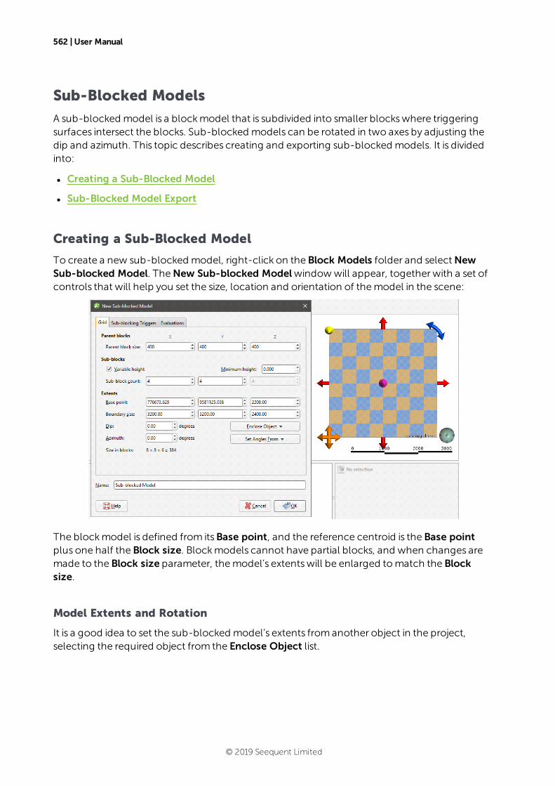
562 | User Manual
Sub-Blocked Models
A sub-blocked model is a blockmodel that is subdivided into smaller blockswhere triggeringsurfaces intersect the blocks. Sub-blocked models can be rotated in two axes by adjusting thedip and azimuth. This topic describes creating and exporting sub-blocked models. It is dividedinto:
l Creating a Sub-Blocked Model
l Sub-Blocked Model Export
Creating a Sub-Blocked Model
To create a new sub-blocked model, right-click on the Block Models folder and selectNewSub-blocked Model. TheNew Sub-blocked Modelwindowwill appear, together with a set ofcontrols that will help you set the size, location and orientation of themodel in the scene:
The blockmodel is defined from itsBase point, and the reference centroid is the Base pointplus one half the Block size. Blockmodels cannot have partial blocks, and when changes aremade to the Block size parameter, themodel’s extentswill be enlarged tomatch the Blocksize.
Model Extents and Rotation
It is a good idea to set the sub-blocked model’s extents fromanother object in the project,selecting the required object from the Enclose Object list.
© 2019 Seequent Limited
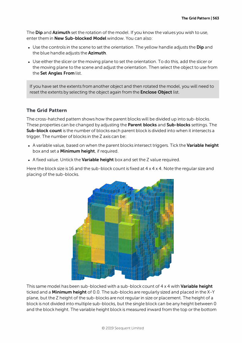
The Grid Pattern | 563
TheDip and Azimuth set the rotation of themodel. If you know the values you wish to use,enter them in New Sub-blocked Modelwindow. You can also:
l Use the controls in the scene to set the orientation. The yellow handle adjusts theDip andthe blue handle adjusts the Azimuth.
l Use either the slicer or themoving plane to set the orientation. To do this, add the slicer orthemoving plane to the scene and adjust the orientation. Then select the object to use fromthe Set Angles From list.
If you have set the extents fromanother object and then rotated themodel, you will need toreset the extents by selecting the object again from the Enclose Object list.
The Grid Pattern
The cross-hatched pattern showshow the parent blockswill be divided up into sub-blocks.These properties can be changed by adjusting the Parent blocks and Sub-blocks settings. TheSub-block count is the number of blocks each parent block is divided intowhen it intersects atrigger. The number of blocks in the Z axis can be:
l A variable value, based on when the parent blocks intersect triggers. Tick the Variable heightbox and set a Minimum height, if required.
l A fixed value. Untick the Variable height box and set the Z value required.
Here the block size is 16 and the sub-block count is fixed at 4 x 4 x 4. Note the regular size andplacing of the sub-blocks.
This samemodel has been sub-blocked with a sub-block count of 4 x 4 with Variable heightticked and a Minimum height of 0.0. The sub-blocks are regularly sized and placed in the X-Yplane, but the Z height of the sub-blocks are not regular in size or placement. The height of ablock is not divided intomultiple sub-blocks, but the single block can be any height between 0and the block height. The variable height block ismeasured inward from the top or the bottom
© 2019 Seequent Limited
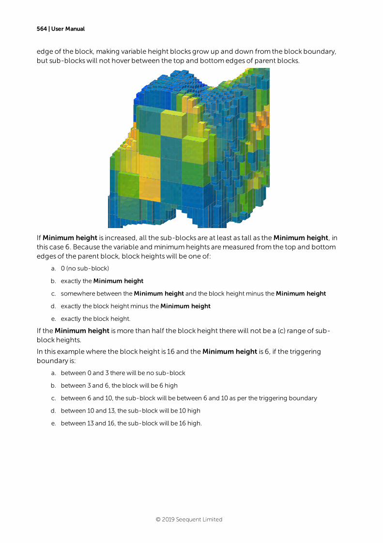
564 | User Manual
edge of the block, making variable height blocks grow up and down from the block boundary,but sub-blockswill not hover between the top and bottomedges of parent blocks.
If Minimum height is increased, all the sub-blocks are at least as tall as theMinimum height, inthis case 6. Because the variable and minimumheights aremeasured from the top and bottomedges of the parent block, block heightswill be one of:
a. 0 (no sub-block)
b. exactly theMinimum height
c. somewhere between theMinimum height and the block heightminus theMinimum height
d. exactly the block heightminus theMinimum height
e. exactly the block height.
If theMinimum height ismore than half the block height there will not be a (c) range of sub-block heights.
In this example where the block height is 16 and theMinimum height is 6, if the triggeringboundary is:
a. between 0 and 3 there will be no sub-block
b. between 3 and 6, the block will be 6 high
c. between 6 and 10, the sub-block will be between 6 and 10 as per the triggering boundary
d. between 10 and 13, the sub-block will be 10 high
e. between 13 and 16, the sub-block will be 16 high.
© 2019 Seequent Limited

Triggers and Evaluations | 565
Triggers and Evaluations
Click on the Sub-blocking Triggers tab to select triggers from the volumes available in theproject. Triggers can be:
l Geological model volumes
l Interpolant volumes
l Openmeshes
All suitable objects in the project will be displayed in the Available triggers list.
Sub-blocked models can be evaluated against geological models, interpolants and distancefunctions in the project. To do this, click on the Evaluations tab. All objects available in theproject will be displayed. Move themodels you wish to use into the Selected list, then select theEvaluation Type, which can be on the sub-block centroids or on the parent block centroids.
Enter a Name for the sub-blocked model and clickOK. Themodel will appear under the BlockModels folder. You can make changes to it by double-clicking on it.
Sub-Blocked Model Statistics
You can view statistics for all evaluations and calculationsmade on a sub-blocked modelbroken down into categories and organised by numeric evaluations and calculations. To viewsummary statistics, right-click on a sub-blocked model in the project tree and select Statistics.
See Viewing Block Model Statistics in the Block Models topic formore information.
© 2019 Seequent Limited

566 | User Manual
Sub-Blocked Model Export
Sub-blocked models created in Leapfrog Geo can be exported in the following formats:
l CSV + Text header (*.csv, *.csv.txt)
l CSVwith embedded header (*.csv)
l CSV as points (*.csv)
l Datamine BlockModel (*.dm)
To export a sub-blocked model, right-click on themodel in the project tree and select Export.You will be prompted to select the file format.
If you wish to export themodel in one of the CSV formats, selectCSV Block Model Files(*.csv) in the Export Block Modelwindow. You will be able to choose between the threeCSV formats in the next step.
Enter a name and location for the file and click Save. Next, you will be able to choose customsettings for each formats.
The Export as Points menu option available in previous versions of Leapfrog Geo has beenremoved. This functionality has been integrated into the Export menu option.
The rest of this topic providesmore information about exporting sub-blocked models in CSVand Datamine formats.
l Exporting Sub-Blocked Models in CSV Format
l Exporting Sub-Blocked Models in Datamine Format
Exporting Sub-Blocked Models in CSV Format
The selections you makewhen you export a blockmodel will be saved. This streamlines theprocess of subsequent exports of themodel.
When you choose to export a sub-blocked model in CSV format, you must first choose the typeof CSV export. Options are:
l With an embedded header file. The sub-blocked model definition is included at the top ofthe CSV file.
l With a separate text header. The sub-blocked model definition iswritten as a separate textfile.
l As points. The CSV file does not include the block sizes and the sub-blocked modeldescription.
© 2019 Seequent Limited
Selecting From Evaluated Items | 567
ClickNext. The steps that follow are:
l Selecting From Evaluated Items
l Setting Row Filtering Options
l Setting Numeric Precision
l Setting Status Code Text Sequences
l Selecting the Character Set
Selecting From Evaluated Items
Choosewhich objectswill be included in the exported file. The Available items list includes allevaluationsmade onto themodel. If you have the Leapfrog Edge extension, you can alsoinclude calculations and filters, which will be exported as separate columns. The order ofcolumns in the exported file will match the order shown in the project tree.
ClickNext.
Setting Row Filtering Options
If you have the Leapfrog Edge extension, you can use a Query filter to filter rowsout of the dataexported.
This is different fromexporting filters as columns, as selected in the previous step.
The second option in thiswindow is useful when all block results are consistently the same non-Normal status. Select from Error, Without grade, Blank orOutside; all rows that consistentlyshow the selected statuseswill not be included in the exported file.
ClickNext.
Setting Numeric Precision
There are three encoding options forNumeric Precision:
l TheDouble, floating point option provides precision of 15 to 17 significant decimal places.
l The Single, floating point option provides precision of 6 to 9 significant decimal places.
l TheCustomoption lets you set a specific number of decimal places.
To change either theCentroid and size precision and Column data precision options, untickthe box forUse default precision and select the required option.
ClickNext.
Setting Status Code Text Sequences
When a blockmodel is exported, non-Normal status codes can be represented in the exportedfile using custom text sequences.
The Status Code sequences are used for category status codes and filter status codes exportedas columns. For filter status codes, Boolean value resultswill show FALSE and TRUE for Normalvalues or the defined Status Codes for non-Normal values.
© 2019 Seequent Limited
568 | User Manual
Boolean values on blockmodels are only available if you have the Leapfrog Edge extension.
Numeric Status Codes can be represented using custom text sequences. This is optional; if noseparate codes are defined for numeric items, the defined Status Codes will be used.
ClickNext.
Selecting the Character Set
The selection you makewill depend on the target for your exported file. You can choose acharacter set and seewhat changeswill bemade.
ClickNext to view a summary of the selected options, then click Export to save the file.
Exporting Sub-Blocked Models in Datamine Format
The selections you makewhen you export a sub-blocked model will be saved. Thisstreamlines the process of subsequent exports of themodel.
When exporting a sub-blocked model in Datamine format, the steps to follow are:
l Selecting From Evaluated Items
l Setting Row Filtering Options
l Setting Status Code Text Sequences
l Selecting the Character Set
l Renaming Items
Selecting From Evaluated Items
Choosewhich objectswill be included in the exported file. The Available items list includes allevaluationsmade onto themodel. If you have the Leapfrog Edge extension, you can alsoinclude calculations and filters, which will be exported as separate columns. The order ofcolumns in the exported file will match the order shown in the project tree.
ClickNext.
Setting Row Filtering Options
If you have the Leapfrog Edge extension, you can use a Query filter to filter rowsout of the dataexported.
This is different fromexporting filters as columns, as selected in the previous step.
The second option in thiswindow is useful when all block results are consistently the same non-Normal status. Select from Error, Without grade, Blank orOutside; all rows that consistentlyshow the selected statuseswill not be included in the exported file.
ClickNext.
© 2019 Seequent Limited

Setting Status Code Text Sequences | 569
Setting Status Code Text Sequences
When a sub-blocked model is exported, non-Normal status codes can be represented in theexported file using custom text sequences.
When exporting sub-blocked models in Datamine format, both category and numeric statuscodes can use independent custom text sequences. Boolean values are exported using values 0for false and 1 for true; specify if non-Normal values should be represented by 0 or by thenumeric status codes.
Boolean Status Codes on sub-blocked models are only available if you have the LeapfrogEdge extension
ClickNext.
Selecting the Character Set
The selection you makewill depend on the target for your exported file. You can choose acharacter set and seewhat changeswill bemade.
ClickNext.
Renaming Items
When exporting a sub-blocked model in Datamine format, column names for the evaluatedobjects have a maximum length of 8 characters. Leapfrog Geowill recommend truncatedcolumn names, but if you wish to use different abbreviations, click on the item’sNew Name toedit it.
ClickNext to view a summary of the selected options, then click Export to save the file.
© 2019 Seequent Limited
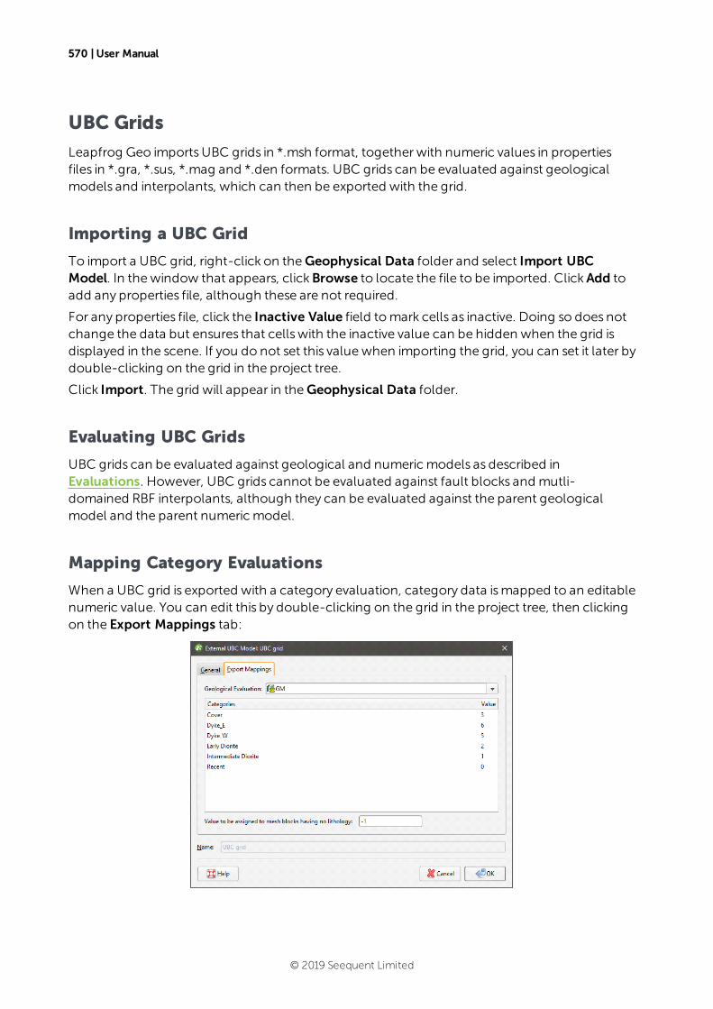
570 | User Manual
UBC Grids
Leapfrog Geo importsUBC grids in *.msh format, together with numeric values in propertiesfiles in *.gra, *.sus, *.mag and *.den formats. UBC grids can be evaluated against geologicalmodels and interpolants, which can then be exported with the grid.
Importing a UBC Grid
To import a UBC grid, right-click on theGeophysical Data folder and select Import UBCModel. In thewindow that appears, clickBrowse to locate the file to be imported. ClickAdd toadd any properties file, although these are not required.
For any properties file, click the Inactive Value field tomark cells as inactive. Doing so does notchange the data but ensures that cellswith the inactive value can be hidden when the grid isdisplayed in the scene. If you do not set this valuewhen importing the grid, you can set it later bydouble-clicking on the grid in the project tree.
Click Import. The grid will appear in theGeophysical Data folder.
Evaluating UBC Grids
UBC grids can be evaluated against geological and numericmodels as described inEvaluations. However, UBC grids cannot be evaluated against fault blocks and mutli-domained RBF interpolants, although they can be evaluated against the parent geologicalmodel and the parent numericmodel.
Mapping Category Evaluations
When a UBC grid is exported with a category evaluation, category data ismapped to an editablenumeric value. You can edit this by double-clicking on the grid in the project tree, then clickingon the Export Mappings tab:
© 2019 Seequent Limited

Exporting a UBC Grid | 571
Change the numeric value assigned to each lithology, if required. You can also change thevalue assigned to blocks that have no lithology.
The Export Mappings tab does not appear for UBC grids that have no geological modelevaluations.
Exporting a UBC Grid
To export a UBC grid, right-click on it in the project tree and select Export. Select theevaluations to export with the grid, then select a folder. ClickOK to export the grid.
A UBC grid can also be exported as points to a CSV file. To do this, right-click on the grid andselect Export as Points. You will then be prompted to select a file name and location. Once youhave clicked Save, select the CSV export options for null values and numeric precision, thenclickOK.
The CSV file will contain:
l X, Y and Z columns, which represent the centre of each grid block
l I, J and K columns, which is the grid block index. I is in the range 1 to NI, J is in the range 1 toNJ and K is in the range 1 to NK, where NI, NJ and NK are the grid dimensions.
l One ormore data columns
© 2019 Seequent Limited

572 | User Manual
Leapfrog Edge
Leapfrog Edge features are only available if you have the Leapfrog Edge extension.
Carry out robust resource estimates in an intuitive and highly visual environment. Leapfrog Edgehas the industry-standard tools you need most, arranged into a streamlined but not prescriptiveworkflow.
l Fully integrate your resource estimation workflow with your geological model. Refine or adddata at any stage and changes flow downstream fromyour geological model to theresourcemodel and everywhere in between.
l Intuitive, flexible workflows and refined, uncluttered workspaces accelerate the learningcurve, improve productivity and reduce training time and frustration.
l Visualise and interact with your data throughout the resource estimation process. Iterate andsee the results in 3D to gain new insights.
Best Practices
Expertise is a Prerequisite
Geological expertise and understanding are essential in estimation, and Leapfrog Geo does notdispensewith this crucial element. An unskilled user can produce a model that faithfullyadheres to unprocessed data but is geologically unreasonable and invalid. In the hands of aninformed expert, on the other hand, Leapfrog Geo estimation toolswill expedite the process ofestimation and enhance themodels used by the organisation.
The Geology is Fundamental
Geological modelling is the building block of an estimate, and themodel needs to begeologically reasonable. A poor-quality geological model and a poor understanding of themineralisation controlswill prevent the development of a valid estimate using any process.
Analyse the Data First
Data will have errors in it that require correction. The quality of the data needs to be assessedand understood; it is important to understand how the data was collected and samplesanalysed. This data quality control work is essential.
Estimation specific data analysis is also required. It is important to understand the spatialrelationships between the sample locations and samples and the area being studied. Tools toassist in this are described in Data Analysis.
© 2019 Seequent Limited

Domaining | 573
Domaining
Domains are defined for stationarity, enclosing a volumewhere the resource can be assumed tohave an expected mean value anywherewithin the boundary. The domain will typically be acollection of logical unitswith similarmineralisation characteristics. It is important to spend timeup front building geologically reasonable wireframes and mineralisation envelopes to conditionthe domain shapes for reasonable estimates. Defining domains to demonstrate goodstationarity is important to producing good resource estimates. Domains that mix populations ofmineralisation will likely result in over- or under-estimates of themetal that can be obtainedfrom the ore.
Choose the domain to be estimated and the samples to use for estimation. Any volume in theproject can be used when defining the domain, as can boundary objects and closed meshes.
The domain boundary can be defined as a hard boundary, excluding values frombeyond theboundary fromconsideration during estimation. Or the boundary can be soft, including valuesup to a specified range beyond the boundarywhen processing the data. The selection shouldbemade on the basis of the nature of the data, and this boundary analysis ismade easier withthe boundary plot that provides a visualisation of the data at and around the boundarythreshold.
Variogram Hypothesis and Experimentation, Analysis
In the estimation workflow, the geologist makes a scientific hypothesis and assesses thathypothesis against the experimental data. In Leapfrog Geo, geologistsmake interpolants usingthe existing Leapfrog Geo approach, then check their estimated interpolant with traditionalexperimental variograms. Based on these experimental results, geologists can makeadjustments to the range, nugget and other settings tomake themodel consistent with theexperimental results, adjusting the hypothesis.
Variography tools are described in Experimental Variography and Variogram Models.
Estimation Functions
Use traditional estimation methods: Nearest Neighbour, Inverse Distance, and Kriging.Additionally, use the RBF estimation method, and compare and contrast the results producedby the different methods.
The estimation functions available in Leapfrog Geo are described in Standard Estimators.
Block Modelling
Estimators can be visualised by evaluating themon blockmodels, which is described inVisualising Sample Geometries and Estimators. Calculations and filters further enhance thevisualisation options, adding computational analysis and processing of data capabilities tocreate new types of data to visualise. Use calculations and filters to derive a new column of datafromother data, including estimator function results, or define a filter to select particularinformation out of the data. SeeCalculations and Filters on Block Models.
© 2019 Seequent Limited

574 | User Manual
Data AnalysisThe first step in the process of resource estimation is gaining a thorough understanding of yourdata. Leapfrog Geo has general tools that help you understand your data, which are describedin Analysing Data. These tools help you become familiar with your data, identify possible errorsand identify or confirmdifferent mineralisation populations.
Make sure that the data is clean, with special and invalid values in the assay data properlyhandled. SeeHandling Special Values formore details.
© 2019 Seequent Limited
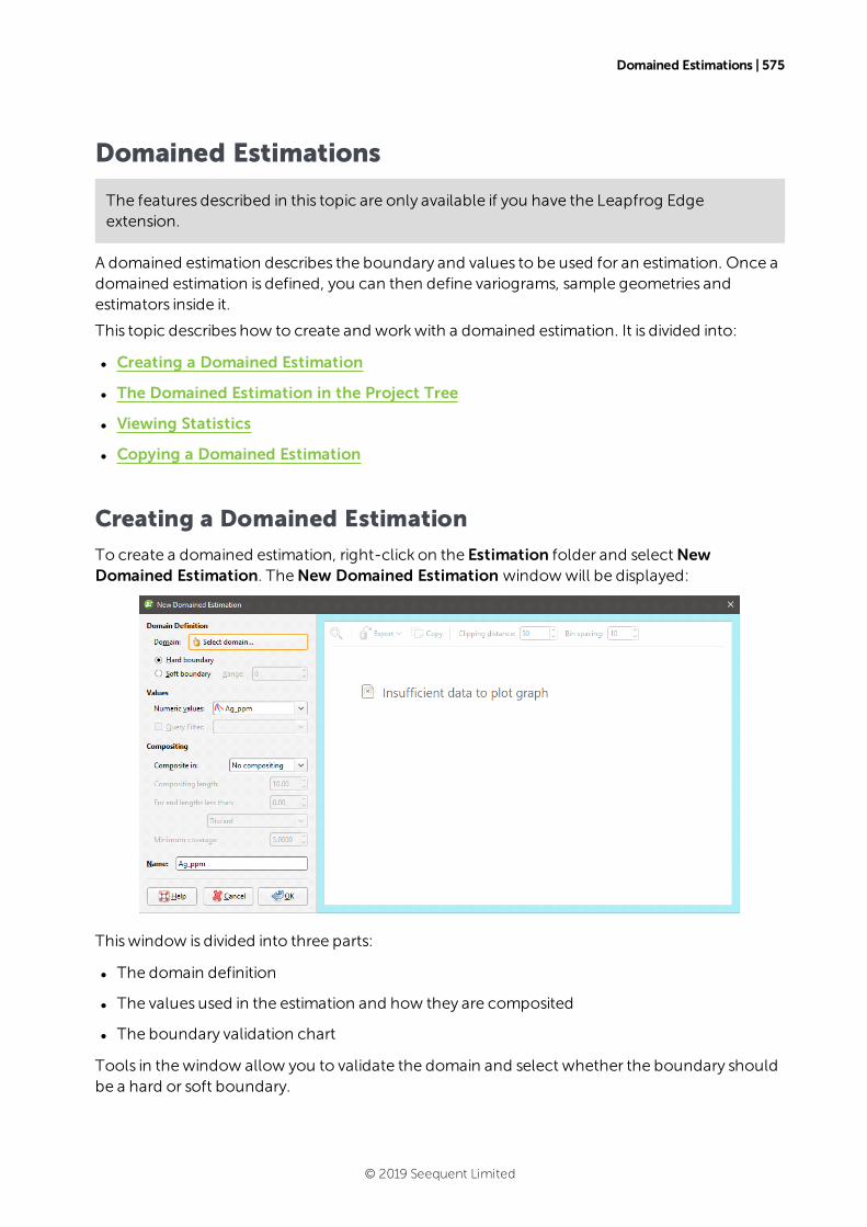
Domained Estimations | 575
Domained Estimations
The features described in this topic are only available if you have the Leapfrog Edgeextension.
A domained estimation describes the boundary and values to be used for an estimation. Once adomained estimation is defined, you can then define variograms, sample geometries andestimators inside it.
This topic describes how to create and workwith a domained estimation. It is divided into:
l Creating a Domained Estimation
l The Domained Estimation in the Project Tree
l Viewing Statistics
l Copying a Domained Estimation
Creating a Domained Estimation
To create a domained estimation, right-click on the Estimation folder and selectNewDomained Estimation. TheNew Domained Estimation windowwill be displayed:
Thiswindow is divided into three parts:
l The domain definition
l The values used in the estimation and how they are composited
l The boundary validation chart
Tools in thewindow allow you to validate the domain and select whether the boundary shouldbe a hard or soft boundary.
© 2019 Seequent Limited
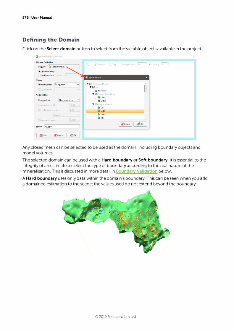
576 | User Manual
Defining the Domain
Click on the Select domain button to select from the suitable objects available in the project:
Any closed mesh can be selected to be used as the domain, including boundary objects andmodel volumes.
The selected domain can be used with a Hard boundary or Soft boundary. It is essential to theintegrity of an estimate to select the type of boundary according to the real nature of themineralisation. This is discussed in more detail in Boundary Validation below.
AHard boundary uses only data within the domain’s boundary. This can be seen when you adda domained estimation to the scene; the values used do not extend beyond the boundary:
© 2019 Seequent Limited
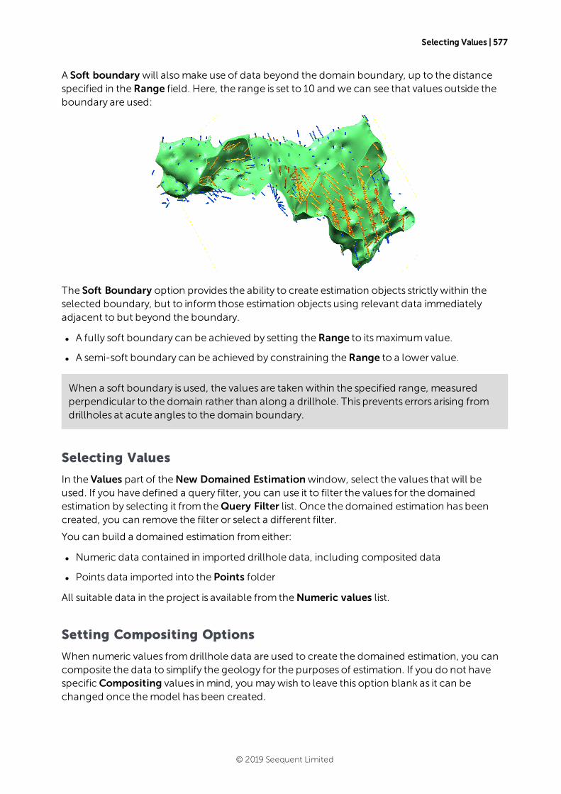
Selecting Values | 577
A Soft boundary will alsomake use of data beyond the domain boundary, up to the distancespecified in theRange field. Here, the range is set to 10 and we can see that values outside theboundary are used:
The Soft Boundary option provides the ability to create estimation objects strictly within theselected boundary, but to inform those estimation objects using relevant data immediatelyadjacent to but beyond the boundary.
l A fully soft boundary can be achieved by setting theRange to itsmaximumvalue.
l A semi-soft boundary can be achieved by constraining theRange to a lower value.
When a soft boundary is used, the values are taken within the specified range, measuredperpendicular to the domain rather than along a drillhole. This prevents errors arising fromdrillholes at acute angles to the domain boundary.
Selecting Values
In the Values part of theNew Domained Estimationwindow, select the values that will beused. If you have defined a query filter, you can use it to filter the values for the domainedestimation by selecting it from theQuery Filter list. Once the domained estimation has beencreated, you can remove the filter or select a different filter.
You can build a domained estimation fromeither:
l Numeric data contained in imported drillhole data, including composited data
l Points data imported into the Points folder
All suitable data in the project is available from theNumeric values list.
Setting Compositing Options
When numeric values fromdrillhole data are used to create the domained estimation, you cancomposite the data to simplify the geology for the purposes of estimation. If you do not havespecificCompositing values in mind, you maywish to leave this option blank as it can bechanged once themodel has been created.
© 2019 Seequent Limited

578 | User Manual
If the numeric values selected have already been composited, theCompositing settingswillnot be available in theNew Domained Estimationwindow. Drillhole data can becomposited directly by right-clicking on theComposites folder (under theDrillholes object)and selecting New Numeric Composite. SeeNumeric Composites.
There are three compositing options:
l No compositing
l Entire drillhole
l Within boundary
The compositing settings available depend on whether the boundary type is a hard or softboundary. For soft boundaries, compositing is limited to the Entire drillhole option, whereas forhard boundaries, compositing can also be limited to the data within the domained estimation’sboundary.
SeeNumeric Composites formore information on the effects of theCompositing length, Forend lengths less than and Minimum coverage settings.
When selecting compositing options, you may see a message:Warning: missing numericdata. This is not an error, but alerts you that some intervals aremissing data.
Boundary Validation
Once you have selected the domain and the values you wish to use and set compositingoptions, the boundary analysis tools in theNew Domained Estimationwindow help you todetermine the best type of boundary to use:
If compositing is enabled for the domained estimation, the boundary validation informationdisplayed is that for the uncomposited data.
© 2019 Seequent Limited
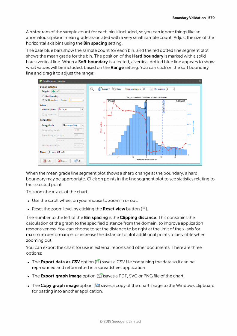
Boundary Validation | 579
A histogramof the sample count for each bin is included, so you can ignore things like ananomalous spike in mean grade associated with a very small sample count. Adjust the size of thehorizontal axis bins using the Bin spacing setting.
The pale blue bars show the sample count for each bin, and the red dotted line segment plotshows themean grade for the bin. The position of theHard boundary ismarked with a solidblack vertical line. When a Soft boundary is selected, a vertical dotted blue line appears to showwhat valueswill be included, based on theRange setting. You can click on the soft boundaryline and drag it to adjust the range:
When themean grade line segment plot shows a sharp change at the boundary, a hardboundarymay be appropriate. Click on points in the line segment plot to see statistics relating tothe selected point.
To zoom the x-axis of the chart:
l Use the scroll wheel on yourmouse to zoom in or out.
l Reset the zoom level by clicking theReset view button ( ).
The number to the left of the Bin spacing is theClipping distance. This constrains thecalculation of the graph to the specified distance from the domain, to improve applicationresponsiveness. You can choose to set the distance to be right at the limit of the x-axis formaximumperformance, or increase the distance to plot additional points to be visible whenzooming out.
You can export the chart for use in external reports and other documents. There are threeoptions:
l The Export data as CSVoption ( ) saves a CSV file containing the data so it can bereproduced and reformatted in a spreadsheet application.
l The Export graph image option ( )saves a PDF, SVG or PNG file of the chart.
l TheCopy graph image option ( ) saves a copy of the chart image to theWindows clipboardfor pasting into another application.
© 2019 Seequent Limited

580 | User Manual
Note that when the Export data as CSVoption is used, it is the last three columns (Startingbin edge, Mean grade and Sample count) that are required to reproduce the chart. The firsttwo columns, Signed distance to boundary and Numeric value, contain all the data pointsrequired to create a new chart with different bin spacing:
Filtering During Boundary Analysis
In this dataset, themain gold-rich zone is in green, while the hangingwall is shown in blue andthe footwall in magenta. Two query filters have been created, onewith the assays coded withthemain zone and including the hangingwall zone, and another filter with the assays codedwith themain zone and including the footwall zone.
© 2019 Seequent Limited
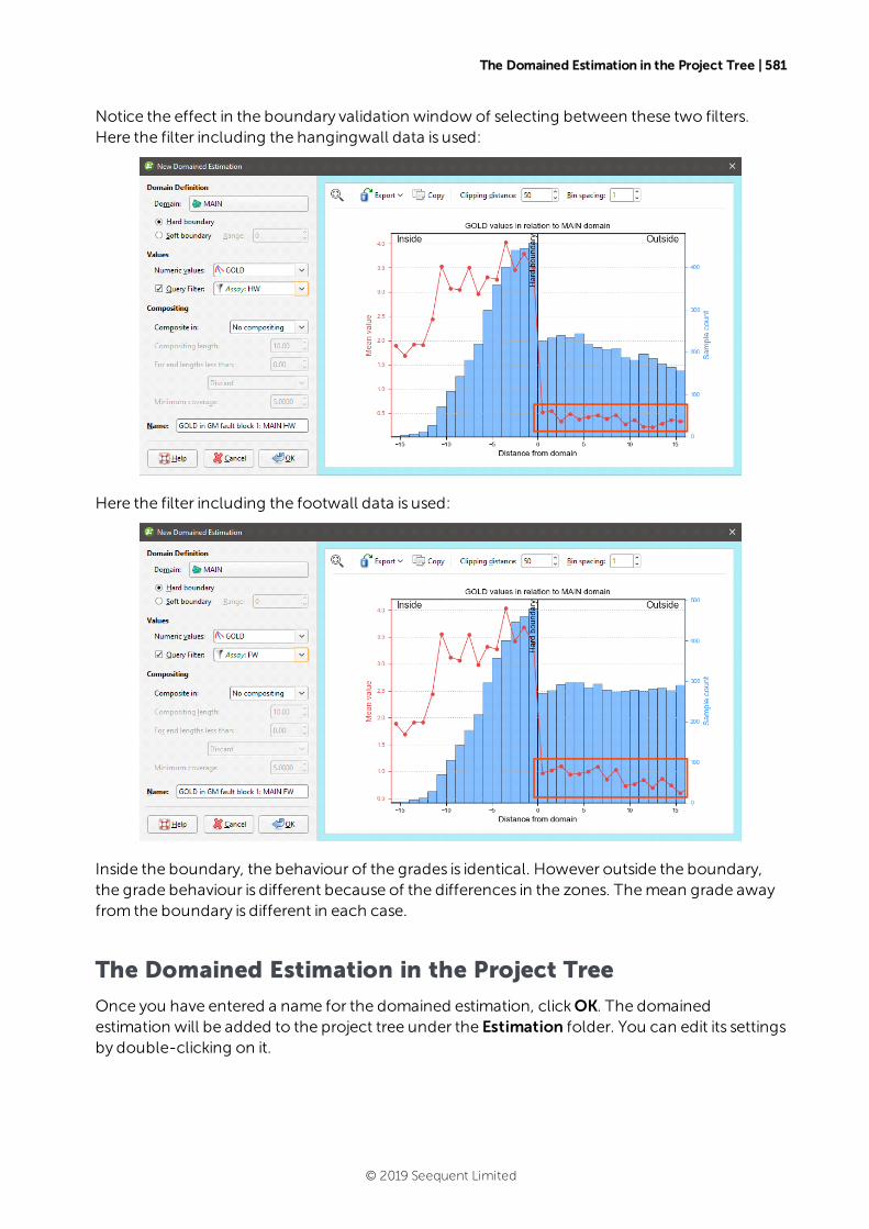
The Domained Estimation in the Project Tree | 581
Notice the effect in the boundary validation window of selecting between these two filters.Here the filter including the hangingwall data is used:
Here the filter including the footwall data is used:
Inside the boundary, the behaviour of the grades is identical. However outside the boundary,the grade behaviour is different because of the differences in the zones. Themean grade awayfrom the boundary is different in each case.
The Domained Estimation in the Project Tree
Once you have entered a name for the domained estimation, clickOK. The domainedestimation will be added to the project tree under the Estimation folder. You can edit its settingsby double-clicking on it.
© 2019 Seequent Limited
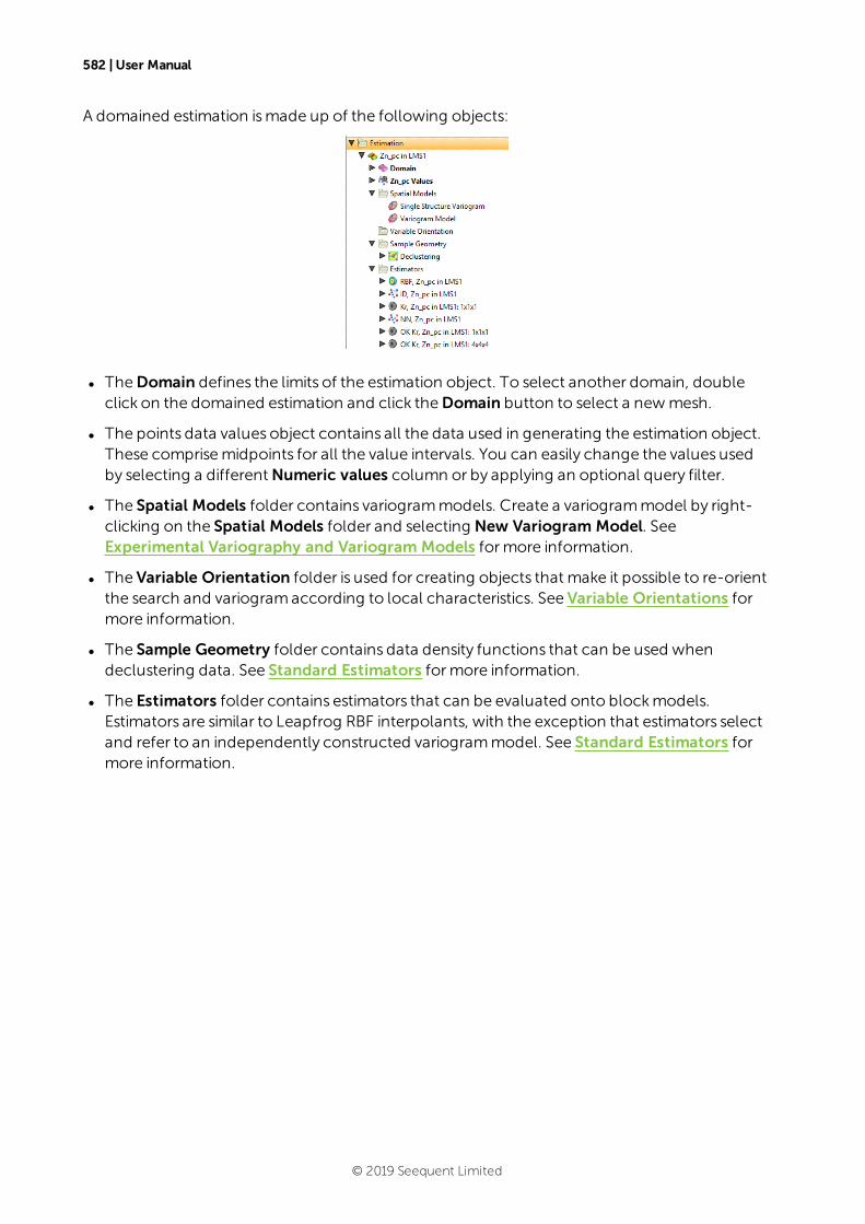
582 | User Manual
A domained estimation ismade up of the following objects:
l TheDomain defines the limits of the estimation object. To select another domain, doubleclick on the domained estimation and click theDomain button to select a newmesh.
l The points data values object contains all the data used in generating the estimation object.These comprisemidpoints for all the value intervals. You can easily change the values usedby selecting a differentNumeric values column or by applying an optional query filter.
l The Spatial Models folder contains variogrammodels. Create a variogrammodel by right-clicking on the Spatial Models folder and selecting New Variogram Model. SeeExperimental Variography and Variogram Models formore information.
l The Variable Orientation folder is used for creating objects that make it possible to re-orientthe search and variogramaccording to local characteristics. See Variable Orientations formore information.
l The Sample Geometry folder contains data density functions that can be used whendeclustering data. See Standard Estimators formore information.
l The Estimators folder contains estimators that can be evaluated onto blockmodels.Estimators are similar to Leapfrog RBF interpolants, with the exception that estimators selectand refer to an independently constructed variogrammodel. See Standard Estimators formore information.
© 2019 Seequent Limited
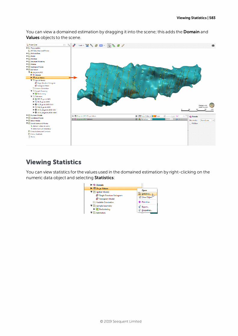
Viewing Statistics | 583
You can view a domained estimation by dragging it into the scene; this adds theDomain andValues objects to the scene.
Viewing Statistics
You can view statistics for the values used in the domained estimation by right-clicking on thenumeric data object and selecting Statistics:
© 2019 Seequent Limited
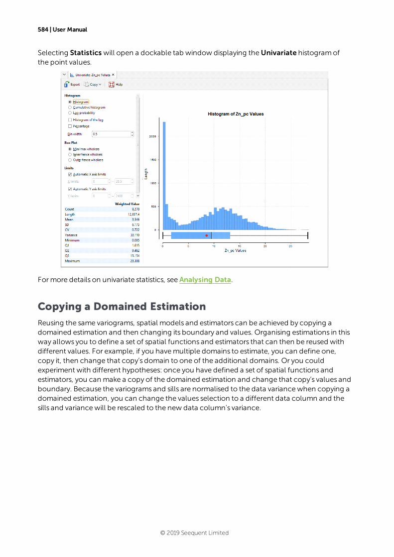
584 | User Manual
Selecting Statistics will open a dockable tab window displaying theUnivariate histogramofthe point values.
Formore details on univariate statistics, see Analysing Data.
Copying a Domained Estimation
Reusing the same variograms, spatial models and estimators can be achieved by copying adomained estimation and then changing its boundary and values. Organising estimations in thisway allows you to define a set of spatial functions and estimators that can then be reused withdifferent values. For example, if you havemultiple domains to estimate, you can define one,copy it, then change that copy’s domain to one of the additional domains. Or you couldexperiment with different hypotheses: once you have defined a set of spatial functions andestimators, you can make a copy of the domained estimation and change that copy’s values andboundary. Because the variograms and sills are normalised to the data variancewhen copying adomained estimation, you can change the values selection to a different data column and thesills and variancewill be rescaled to the new data column's variance.
© 2019 Seequent Limited
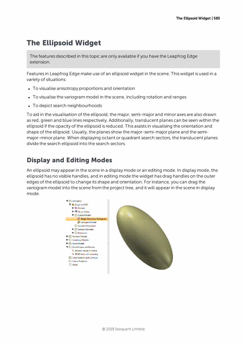
The Ellipsoid Widget | 585
The Ellipsoid Widget
The features described in this topic are only available if you have the Leapfrog Edgeextension.
Features in Leapfrog Edgemake use of an ellipsoid widget in the scene. Thiswidget is used in avariety of situations:
l To visualise anisotropy proportions and orientation
l To visualise the variogrammodel in the scene, including rotation and ranges
l To depict search neighbourhoods
To aid in the visualisation of the ellipsoid, themajor, semi-major and minor axes are also drawnas red, green and blue lines respectively. Additionally, translucent planes can be seen within theellipsoid if the opacity of the ellipsoid is reduced. This assists in visualising the orientation andshape of the ellipsoid. Usually, the planes show themajor-semi-major plane and the semi-major-minor plane. When displaying octant or quadrant search sectors, the translucent planesdivide the search ellipsoid into the search sectors.
Display and Editing Modes
An ellipsoid may appear in the scene in a displaymode or an editing mode. In displaymode, theellipsoid has no visible handles, and in editing mode thewidget has drag handles on the outeredges of the ellipsoid to change its shape and orientation. For instance, you can drag thevariogrammodel into the scene from the project tree, and it will appear in the scene in displaymode.
© 2019 Seequent Limited
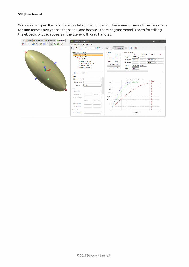
586 | User Manual
You can also open the variogrammodel and switch back to the scene or undock the variogramtab and move it away to see the scene, and because the variogrammodel is open for editing,the ellipsoid widget appears in the scenewith drag handles.
© 2019 Seequent Limited

Change Movement Handles | 587
Change Movement Handles
Ellipsoid widgets can be repositioned, perhaps so the ellipsoid is not obstructing the view of partof themodel. To reposition thewidget, select thewidget in the shape list then click thewidgetin the scene. If the ellipsoid does not have arrows in the centre, click the ellipsoid and themovement arrowswill appear. You can click the ellipsoid again to turn themoff.
In the properties panel for the selected widget, settings control theCentre Point of theellipsoid. The X, Y and Z position can be specified directly.
There are twomodes for thewidget movement handles. In the properties panel for the selectedwidget, Align movement handles to has the optionsAxes and Camera.
If the option is set to Align movement handles to Axes the drag handles in the centre of thewidget will be red, green and blue and point along the directions of the project axis lines.
© 2019 Seequent Limited
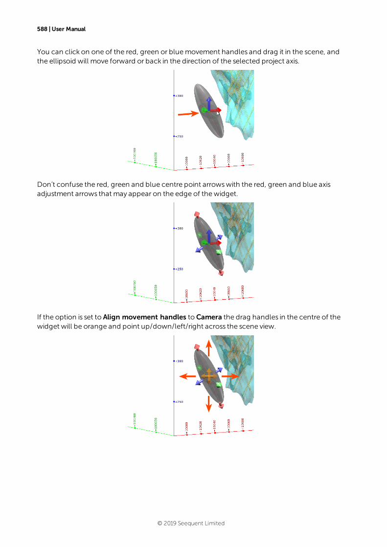
588 | User Manual
You can click on one of the red, green or bluemovement handles and drag it in the scene, andthe ellipsoid will move forward or back in the direction of the selected project axis.
Don’t confuse the red, green and blue centre point arrowswith the red, green and blue axisadjustment arrows that may appear on the edge of thewidget.
If the option is set to Align movement handles toCamera the drag handles in the centre of thewidget will be orange and point up/down/left/right across the scene view.
© 2019 Seequent Limited
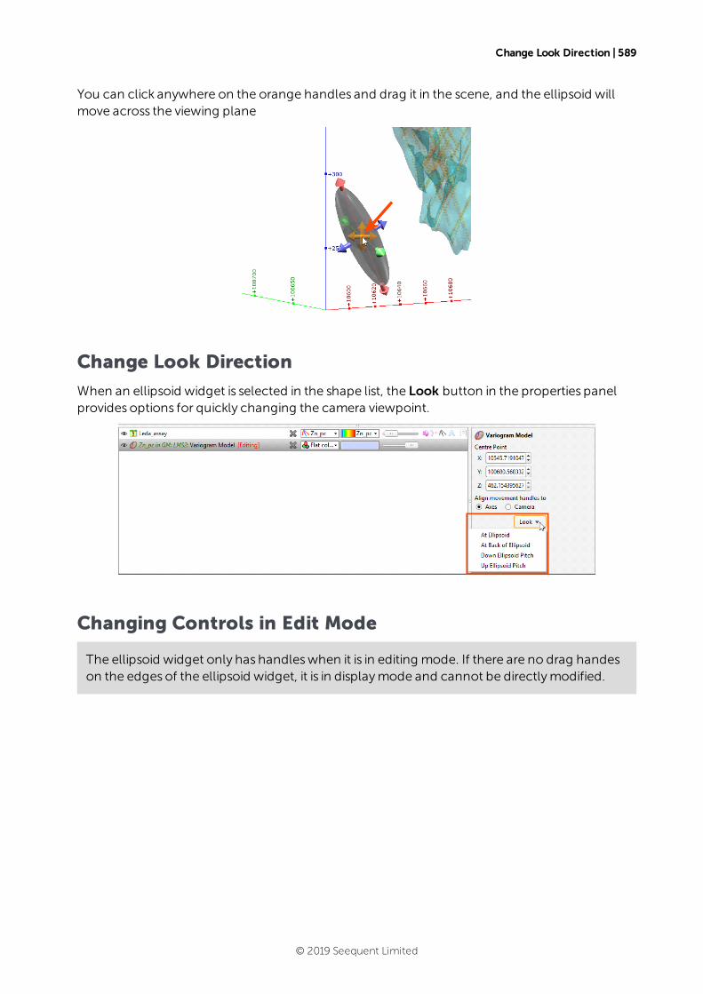
Change Look Direction | 589
You can click anywhere on the orange handles and drag it in the scene, and the ellipsoid willmove across the viewing plane
Change Look Direction
When an ellipsoid widget is selected in the shape list, the Look button in the properties panelprovides options for quickly changing the camera viewpoint.
Changing Controls in Edit Mode
The ellipsoid widget only has handleswhen it is in editing mode. If there are no drag handeson the edges of the ellipsoid widget, it is in displaymode and cannot be directlymodified.
© 2019 Seequent Limited

590 | User Manual
If your ellipsoid widget is in edit mode, you will see drag handles on the edges of thewidget.There are twomodes for these controls. Click on thewidget to toggle between control modes.Each mode offers different handles for directlymanipulating the ellipsoid widget. When thearrowson the edge of thewidget are yellow, blue and red, the handles adjust the ellipsoidtrend.
Drag a yellow arrow handle to adjust theDip, blue to adjust theDip Azimuth and red to adjustthe Pitch.
When the arrowson the edge of thewidget are red, green and blue, the handles adjust theellipsoid ranges.
Drag a red arrow handle to adjust theMaximum axis range, green to adjust the Semi-majorrange and blue to adjust theMinimum range.
If you click on thewidget and the outer arrowsdo not change, you probably have avariogrammodel with a second structure defined. Once the second structure is defined, thestructure that is controlled by the arrowswould be ambiguous, which iswhy the rangearrows are disabled formultiple structure variograms.
As you modify the ellipsoid bymanipulating the drag handles, the respective settings values areupdated.
© 2019 Seequent Limited
Variography and Estimators | 591
Variography and EstimatorsAfter data analysis and domaining comes the key part of the resource estimation workflow:variography. A theoretical variogrammodel is proposed and tested using experimentalvariography. Kriging, nearest neighbour, inverse distanceweighting or RBF estimators aredefined and potentially combined.
See:
l Experimental Variography and Variogram Models
l Transform Variography
l Standard Estimators
l Variable Orientations
Experimental Variography and Variogram Models
The features described in this topic are only available if you have the Leapfrog Edgeextension.
Variography is the analysis of spatial variability of gradewithin a region. Some deposit types, e.g.gold, have high spatial variability between samples, whereas others, e.g. iron, have relatively lowspatial variability between samples. Understanding how sample grades relate to each other inspace is a vital step in informing grades in a blockmodel. A variogram is used to quantify thisspatial variability between samples.
In estimation, the variogram is used for:
l Selecting appropriate sample weighting in Kriging and RBF estimators to produce the bestpossible estimate at a given location
l Calculating the estimators’ associated quality and diagnostic statistics
In Leapfrog Geo domained estimations, variograms are created and modified using the SpatialModels folder. To create a new variogrammodel, right-click on the Spatial Models folder andselectNew Variogram Model.
A new variogrammodel is not auto-fitted and should not be assumed to be the initialhypothesis for theworkflow. While some reasonable defaults have been selected for thevariogrammodel, the geologist’s personal hypothesis should be the starting point for theestimation workflow.
© 2019 Seequent Limited
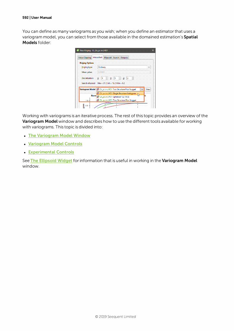
592 | User Manual
You can define asmany variograms as you wish; when you define an estimator that uses avariogrammodel, you can select from those available in the domained estimation’s SpatialModels folder:
Working with variograms is an iterative process. The rest of this topic provides an overview of theVariogram Modelwindow and describes how to use the different tools available for workingwith variograms. This topic is divided into:
l The Variogram Model Window
l Variogram Model Controls
l Experimental Controls
See The Ellipsoid Widget for information that is useful in working in the Variogram Modelwindow.
© 2019 Seequent Limited
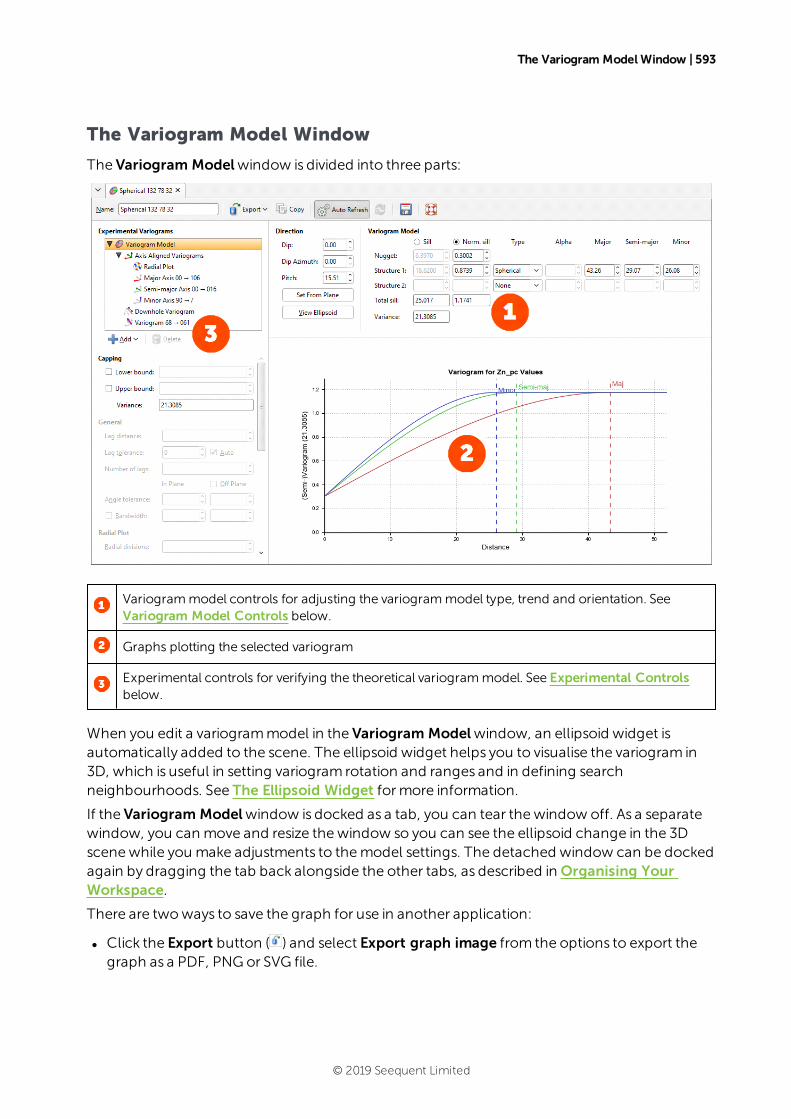
The Variogram Model Window | 593
The Variogram Model Window
The Variogram Modelwindow is divided into three parts:
Variogrammodel controls for adjusting the variogrammodel type, trend and orientation. SeeVariogram Model Controls below.
Graphs plotting the selected variogram
Experimental controls for verifying the theoretical variogrammodel. See Experimental Controlsbelow.
When you edit a variogrammodel in the Variogram Modelwindow, an ellipsoid widget isautomatically added to the scene. The ellipsoid widget helps you to visualise the variogram in3D, which is useful in setting variogram rotation and ranges and in defining searchneighbourhoods. See The Ellipsoid Widget formore information.
If the Variogram Modelwindow is docked as a tab, you can tear thewindow off. As a separatewindow, you can move and resize thewindow so you can see the ellipsoid change in the 3Dscenewhile you make adjustments to themodel settings. The detached window can be dockedagain by dragging the tab back alongside the other tabs, as described in Organising YourWorkspace.
There are twoways to save the graph for use in another application:
l Click the Export button ( ) and select Export graph image from the options to export thegraph as a PDF, PNGor SVG file.
© 2019 Seequent Limited

594 | User Manual
l Click theCopy graph button ( ) to copy the graph to the clipboard. You can then paste itinto another application.
Additionally, you can save variogramparameter data by clicking the Export button ( ) andselecting Export data from the options.
There are two buttons for refreshing the graphswhen changes aremade:
l When Auto Refresh is enabled, recalculationswill be carried out each time you change avariogramvalue. This can produce a brief lag.
l When auto refresh is disabled, you can click theRefresh button ( ) whenever you want thegraphs to be updated. This is the best option to usewhen working with a large dataset.
© 2019 Seequent Limited
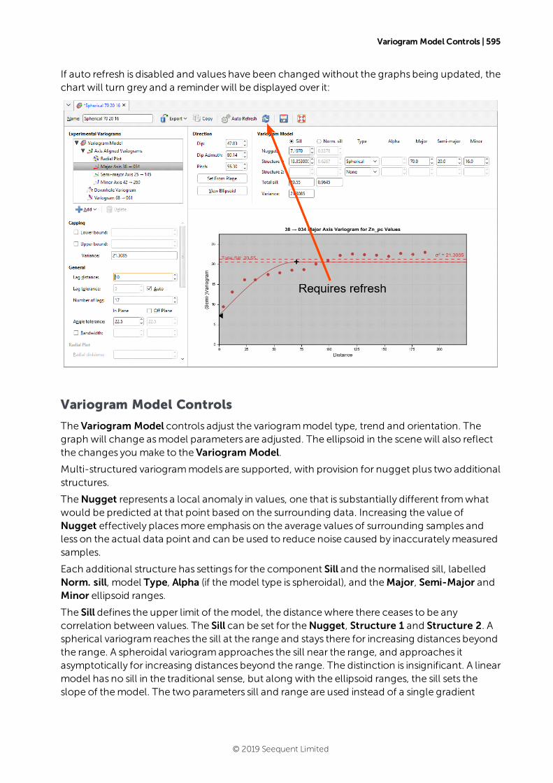
Variogram Model Controls | 595
If auto refresh is disabled and values have been changed without the graphs being updated, thechart will turn grey and a reminderwill be displayed over it:
Variogram Model Controls
The Variogram Model controls adjust the variogrammodel type, trend and orientation. Thegraph will change asmodel parameters are adjusted. The ellipsoid in the scenewill also reflectthe changes you make to the Variogram Model.
Multi-structured variogrammodels are supported, with provision for nugget plus two additionalstructures.
TheNugget represents a local anomaly in values, one that is substantially different fromwhatwould be predicted at that point based on the surrounding data. Increasing the value ofNugget effectively placesmore emphasis on the average values of surrounding samples andless on the actual data point and can be used to reduce noise caused by inaccuratelymeasuredsamples.
Each additional structure has settings for the component Sill and the normalised sill, labelledNorm. sill, model Type, Alpha (if themodel type is spheroidal), and theMajor, Semi-Major andMinor ellipsoid ranges.
The Sill defines the upper limit of themodel, the distancewhere there ceases to be anycorrelation between values. The Sill can be set for theNugget, Structure 1 and Structure 2. Aspherical variogram reaches the sill at the range and stays there for increasing distances beyondthe range. A spheroidal variogramapproaches the sill near the range, and approaches itasymptotically for increasing distances beyond the range. The distinction is insignificant. A linearmodel has no sill in the traditional sense, but along with the ellipsoid ranges, the sill sets theslope of themodel. The two parameters sill and range are used instead of a single gradient
© 2019 Seequent Limited
596 | User Manual
parameter to permit switching between linear, spherical and spheroidal interpolant functionswithout alsomanipulating these settings.
TheNorm. sill represents the same information as the Sill, but proportionally scaled to a rangebetween 0 and 1, where 1 represents the data Variance. As you select the radio buttons for Silland Norm. sill, the Y-axis scale on the displayed chart will change to correspond to yourselection.
The Total sill is the sumof the component sills for both the data sills and the normalised sills.
The Variance is calculated automatically from the data and shows themagnitude of thevariance for the dataset.
Linear, Spherical and Spheroidal Model Options
Themodel Type provides three options: Linear, Spherical and Spheroidal.
Linear is a general-purposemulti-scale option suited to sparsely and/or irregularly sampleddata. Spherical and Spheroidal are suitable formodelling most metallic ores, where there is afinite range beyond which the influence of the data should fall to zero. A Sphericalmodel has arange beyond which the value is the constant sill. A Spheroidalmodel flattens out when thedistance from the sample data point is greater than the range. At the range, the function value is96% of the sill with no nugget, and beyond the range the function asymptotically approachesthe sill. Each axis of the variogramellipsoid has its own range, adjusted using Major, Semi-Majorand Minor. The ranges are colour-coded in the variogrammodel plot.
The spherical model is not available for standard Leapfrog RBF interpolants created in theNumeric Models folder.
Alpha is only available when themodel Type is Spheroidal. The Alpha constant determines howsteeply the interpolant rises towards the Sill. A low Alpha valuewill produce a variogram thatrisesmore steeply than a high Alpha value. A high Alpha value gives points at intermediatedistancesmoreweighting, compared to lowerAlpha values. An Alpha of 9 provides the curvethat is closest in shape to a spherical variogram. In ideal situations, it would probably be the firstchoice; however, high Alpha values requiremore computation and processing time, asmorecomplex approximation calculations are required. A smaller value forAlphawill result in shortertimes to evaluate the variogram.
RBF estimatorswill onlyworkwhen the Structure 2 model Type is set toNone.
When Structure 2 is defined, themodel ranges cannot be adjusted bymanipulation of draghandles on the ellipsoid. Because it would not be clear which structure was beingmanipulated, the drag handles to change the range settings do not appear.
Normalised Y Axis
A key use of copying a variogram is to apply it to another geologically correlated mineralresource. Thiswould typically be accomplished, having determined the appropriate variogramusing the values for onemineral, by copying the domained estimation and changing theNumeric values field to a different mineral. However, the absolute values for the nugget and
© 2019 Seequent Limited
Direction | 597
sills for each structure would be completely inappropriate for the newmineral; while we desirethe shape to be the same, the values for different mineralisationswill inevitably be different. Tomake thiswork correctly, the variogram is normalised or standardised, rescaling the range of Y-axis values to between 0 and 1, where 1 is equivalent to the data Variance. Thismakes thevariogram information portable between domained estimations. This is performedautomatically, requiring no intervention on your part.
You can freely switch between the Sill and Norm. sill options. The selection only changes theY-axis scale on the displayed chart.
You do not need to select theNormalised option before copying the domained estimationand using it as the basis for a different mineral resource. The normalised scale will always beused when applying the variogrammodel to the new data set.
As you adjust theNugget or the Structure 1 or Structure 2 sill values, the Total sillwill changeboth for the absolute Sill values and theNorm. sill values. TheNorm. sill total may end upbeing something other than 1.0. This is expected, as the value reference for the normalisedscale uses the data Variance for 1.0, not the total sill.
Note that the data Variance is recorded in the Y axis label so the chart scale is alwaysmeaningful, including when the chart is exported.
Direction
The trend Direction fields set the orientation of the variogramellipsoid. Adjust the ellipsoid axesorientation using theDip, Dip Azimuth and Pitch fields.
The Set From Plane button sets the trend orientation of themodel ellipsoid based upon thecurrent settings of themoving plane.
The View Ellipsoid button adds a 3D ellipsoid widget visualisation to the scene, in case it hasbeen deleted from the scene since the variogrammodel windowwasopened for editing.
Experimental Controls
A variogrammodel can be verified through the use of the experimental variography tools thatuse data acquired in the drilling process. Use these to find the directions of maximum,intermediate and minimumcontinuity.
The variogramdisplayed in the chart is selected from the variograms listed in the panel in thetop left corner of thewindow.
© 2019 Seequent Limited
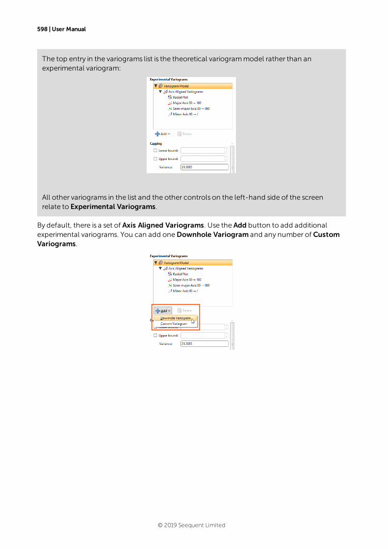
598 | User Manual
The top entry in the variograms list is the theoretical variogrammodel rather than anexperimental variogram:
All other variograms in the list and the other controls on the left-hand side of the screenrelate to Experimental Variograms.
By default, there is a set of Axis Aligned Variograms. Use the Add button to add additionalexperimental variograms. You can add oneDownhole Variogram and any number of CustomVariograms.
© 2019 Seequent Limited
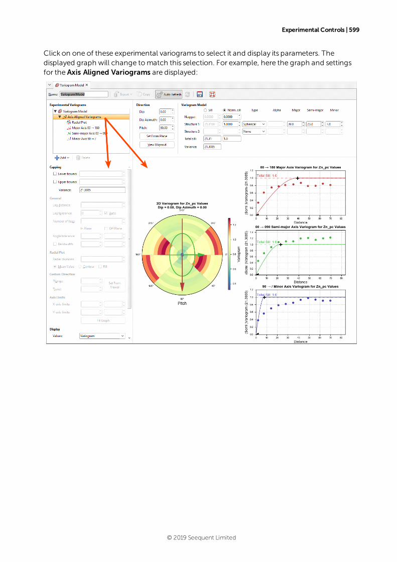
Experimental Controls | 599
Click on one of these experimental variograms to select it and display its parameters. Thedisplayed graph will change tomatch this selection. For example, here the graph and settingsfor the Axis Aligned Variograms are displayed:
© 2019 Seequent Limited
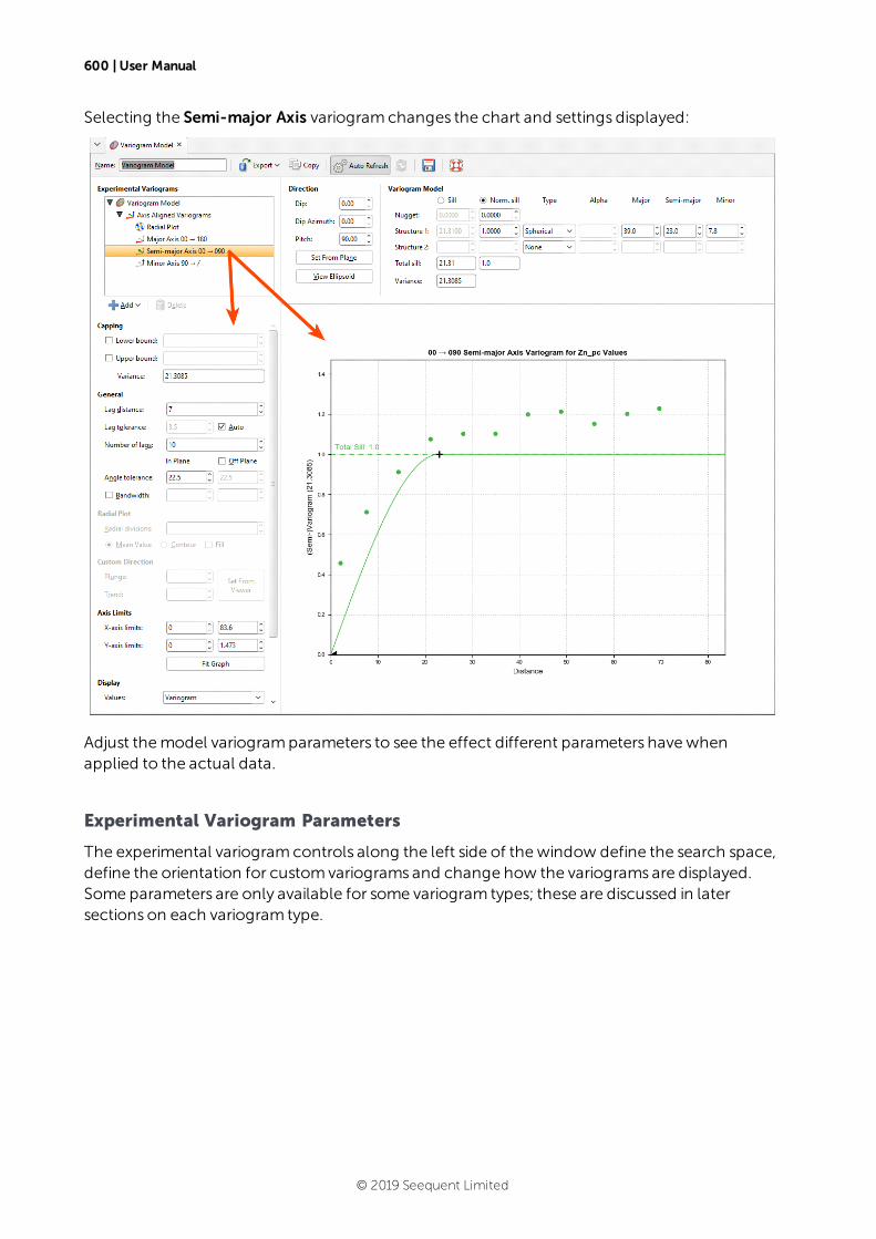
600 | User Manual
Selecting the Semi-major Axis variogramchanges the chart and settings displayed:
Adjust themodel variogramparameters to see the effect different parameters havewhenapplied to the actual data.
Experimental Variogram Parameters
The experimental variogramcontrols along the left side of thewindow define the search space,define the orientation for customvariograms and change how the variograms are displayed.Some parameters are only available for some variogram types; these are discussed in latersections on each variogram type.
© 2019 Seequent Limited
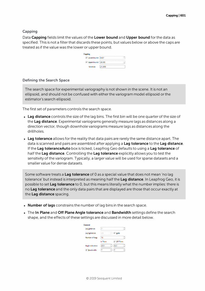
Capping | 601
Capping
Data Capping fields limit the values of the Lower bound and Upper bound for the data asspecified. This is not a filter that discards these points, but values below or above the caps aretreated as if the valuewas the lower or upper bound.
Defining the Search Space
The search space for experimental variography is not shown in the scene. It is not anellipsoid, and should not be confused with either the variogrammodel ellipsoid or theestimator's search ellipsoid.
The first set of parameters controls the search space.
l Lag distance controls the size of the lag bins. The first bin will be one quarter of the size ofthe Lag distance. Experimental variogramsgenerallymeasure lags as distances along adirection vector, though downhole variogramsmeasure lags as distances along thedrillholes.
l Lag tolerance allows for the reality that data pairs are rarely the same distance apart. Thedata is scanned and pairs are assembled after applying a Lag tolerance to the Lag distance.If the Lag toleranceAuto box is ticked, Leapfrog Geo defaults to using a Lag tolerance ofhalf the Lag distance. Controlling the Lag tolerance explicitly allows you to test thesensitivity of the variogram. Typically, a larger valuewill be used for sparse datasets and asmaller value for dense datasets.
Some software treats a Lag tolerance of 0 as a special value that does not mean ‘no lagtolerance’ but instead is interpreted asmeaning half the Lag distance. In Leapfrog Geo, it ispossible to set Lag tolerance to 0, but thismeans literally what the number implies: there isno Lag tolerance and the only data pairs that are displayed are those that occur exactly atthe Lag distance spacing.
l Number of lags constrains the number of lag bins in the search space.
l The In Plane and Off Plane Angle tolerance and Bandwidth settings define the searchshape, and the effects of these settings are discussed in more detail below.
© 2019 Seequent Limited
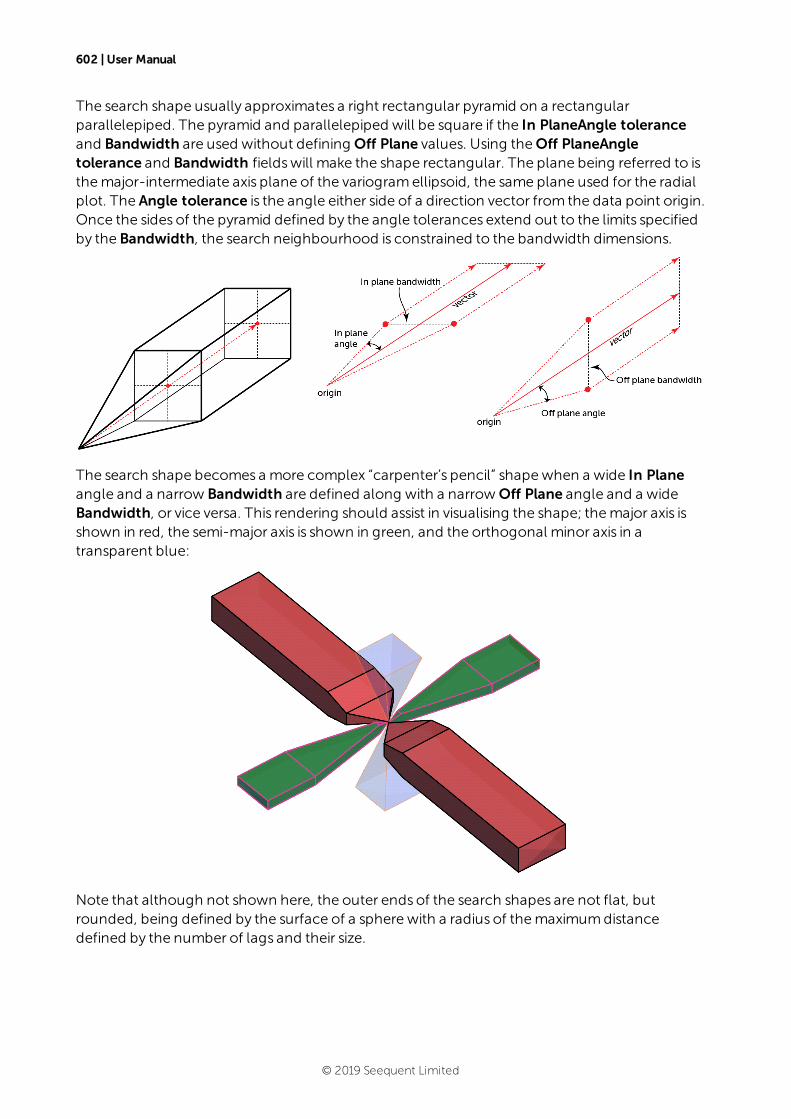
602 | User Manual
The search shape usually approximates a right rectangular pyramid on a rectangularparallelepiped. The pyramid and parallelepiped will be square if the In PlaneAngle toleranceand Bandwidth are used without defining Off Plane values. Using theOff PlaneAngletolerance and Bandwidth fieldswill make the shape rectangular. The plane being referred to isthemajor-intermediate axis plane of the variogramellipsoid, the same plane used for the radialplot. The Angle tolerance is the angle either side of a direction vector from the data point origin.Once the sides of the pyramid defined by the angle tolerances extend out to the limits specifiedby the Bandwidth, the search neighbourhood is constrained to the bandwidth dimensions.
The search shape becomes a more complex “carpenter’s pencil” shapewhen a wide In Planeangle and a narrow Bandwidth are defined along with a narrow Off Plane angle and a wideBandwidth, or vice versa. This rendering should assist in visualising the shape; themajor axis isshown in red, the semi-major axis is shown in green, and the orthogonal minor axis in atransparent blue:
Note that although not shown here, the outer ends of the search shapes are not flat, butrounded, being defined by the surface of a sphere with a radius of themaximumdistancedefined by the number of lags and their size.
© 2019 Seequent Limited
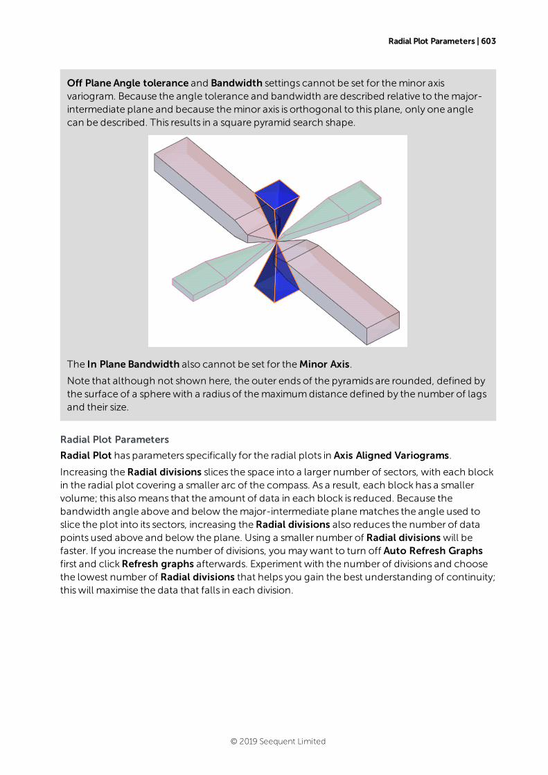
Radial Plot Parameters | 603
Off Plane Angle tolerance and Bandwidth settings cannot be set for theminor axisvariogram. Because the angle tolerance and bandwidth are described relative to themajor-intermediate plane and because theminor axis is orthogonal to this plane, only one anglecan be described. This results in a square pyramid search shape.
The In Plane Bandwidth also cannot be set for theMinor Axis.
Note that although not shown here, the outer ends of the pyramids are rounded, defined bythe surface of a sphere with a radius of themaximumdistance defined by the number of lagsand their size.
Radial Plot Parameters
Radial Plot has parameters specifically for the radial plots in Axis Aligned Variograms.
Increasing theRadial divisions slices the space into a larger number of sectors, with each blockin the radial plot covering a smaller arc of the compass. As a result, each block has a smallervolume; this alsomeans that the amount of data in each block is reduced. Because thebandwidth angle above and below themajor-intermediate planematches the angle used toslice the plot into its sectors, increasing theRadial divisions also reduces the number of datapoints used above and below the plane. Using a smaller number of Radial divisions will befaster. If you increase the number of divisions, you maywant to turn off Auto Refresh Graphsfirst and clickRefresh graphs afterwards. Experiment with the number of divisions and choosethe lowest number of Radial divisions that helps you gain the best understanding of continuity;thiswill maximise the data that falls in each division.
© 2019 Seequent Limited
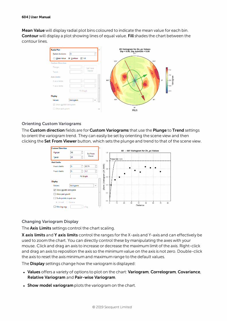
604 | User Manual
Mean Valuewill display radial plot bins coloured to indicate themean value for each bin.Contour will display a plot showing lines of equal value. Fill shades the chart between thecontour lines.
Orienting Custom Variograms
TheCustom direction fields are forCustom Variograms that use the Plunge to Trend settingsto orient the variogram trend. They can easily be set by orienting the scene view and thenclicking the Set From Viewer button, which sets the plunge and trend to that of the scene view.
Changing Variogram Display
The Axis Limits settings control the chart scaling.
X axis limits and Y axis limits control the ranges for the X-axis and Y-axis and can effectively beused to zoom the chart. You can directly control these bymanipulating the axeswith yourmouse. Click and drag an axis to increase or decrease themaximum limit of the axis. Right-clickand drag an axis to reposition the axis so theminimumvalue on the axis is not zero. Double-clickthe axis to reset the axisminimumand maximum range to the default values.
TheDisplay settings change how the variogram is displayed:
l Values offers a variety of options to plot on the chart:Variogram, Correlogram, Covariance,Relative Variogram and Pair-wise Variogram.
l Show model variogram plots the variogramon the chart.
© 2019 Seequent Limited
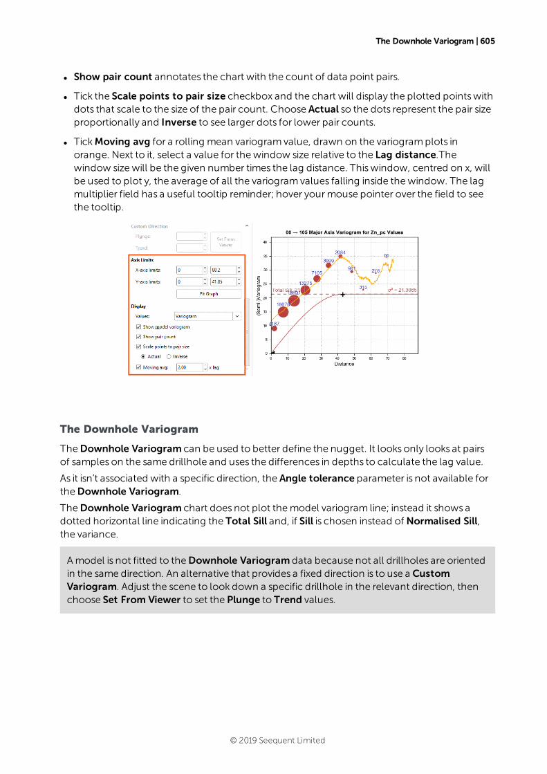
The Downhole Variogram | 605
l Show pair count annotates the chart with the count of data point pairs.
l Tick the Scale points to pair size checkbox and the chart will display the plotted pointswithdots that scale to the size of the pair count. Choose Actual so the dots represent the pair sizeproportionally and Inverse to see larger dots for lower pair counts.
l TickMoving avg for a rolling mean variogramvalue, drawn on the variogramplots inorange. Next to it, select a value for thewindow size relative to the Lag distance.Thewindow size will be the given number times the lag distance. Thiswindow, centred on x, willbe used to plot y, the average of all the variogramvalues falling inside thewindow. The lagmultiplier field has a useful tooltip reminder; hover yourmouse pointer over the field to seethe tooltip.
The Downhole Variogram
TheDownhole Variogram can be used to better define the nugget. It looks only looks at pairsof samples on the same drillhole and uses the differences in depths to calculate the lag value.
As it isn’t associated with a specific direction, the Angle tolerance parameter is not available fortheDownhole Variogram.
TheDownhole Variogram chart does not plot themodel variogram line; instead it shows adotted horizontal line indicating the Total Sill and, if Sill is chosen instead of Normalised Sill,the variance.
Amodel is not fitted to theDownhole Variogram data because not all drillholes are orientedin the same direction. An alternative that provides a fixed direction is to use a CustomVariogram. Adjust the scene to look down a specific drillhole in the relevant direction, thenchoose Set From Viewer to set the Plunge to Trend values.
© 2019 Seequent Limited
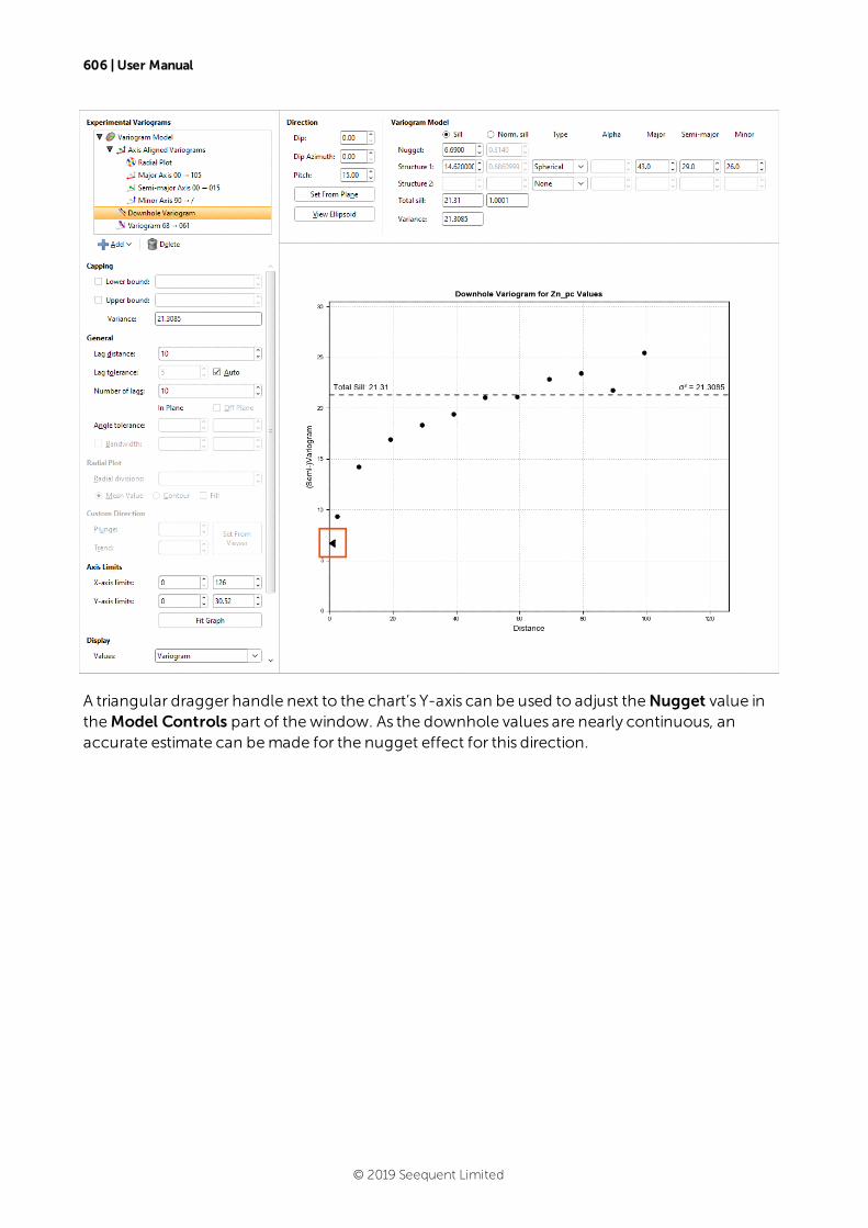
606 | User Manual
A triangular dragger handle next to the chart’s Y-axis can be used to adjust theNugget value intheModel Controls part of thewindow. As the downhole values are nearly continuous, anaccurate estimate can bemade for the nugget effect for this direction.
© 2019 Seequent Limited

Axis Aligned Variograms | 607
Axis Aligned Variograms
The Axis Aligned Variograms are useful for determining the direction of maximum,intermediate and minimumcontinuity. When you select the Axis Aligned Variograms option, allfour variograms are displayed in the chart:
© 2019 Seequent Limited
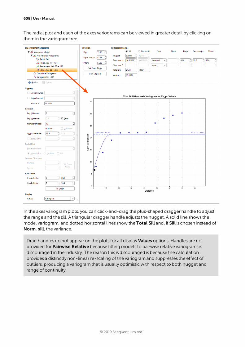
608 | User Manual
The radial plot and each of the axes variograms can be viewed in greater detail by clicking onthem in the variogram tree:
In the axes variogramplots, you can click-and-drag the plus-shaped dragger handle to adjustthe range and the sill. A triangular dragger handle adjusts the nugget. A solid line shows themodel variogram, and dotted horizontal lines show the Total Sill and, if Sill is chosen instead ofNorm. sill, the variance.
Drag handles do not appear on the plots for all displayValues options. Handles are notprovided for Pairwise Relative because fitting models to pairwise relative variograms isdiscouraged in the industry. The reason this is discouraged is because the calculationprovides a distinctly non-linear re-scaling of the variogramand suppresses the effect ofoutliers, producing a variogram that is usually optimistic with respect to both nugget andrange of continuity.
© 2019 Seequent Limited
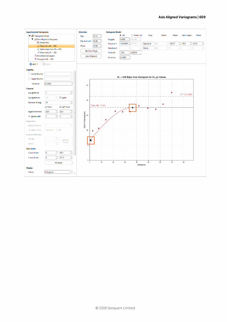
Axis Aligned Variograms | 609
© 2019 Seequent Limited
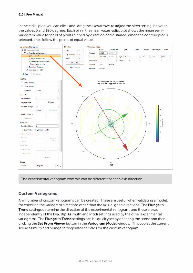
610 | User Manual
In the radial plot, you can click-and-drag the axes arrows to adjust the pitch setting, betweenthe values 0 and 180 degrees. Each bin in themean value radial plot shows themean semi-variogramvalue for pairs of points binned by direction and distance. When the contour plot isselected, lines follow the points of equal value.
The experimental variogramcontrols can be different for each axis direction.
Custom Variograms
Any number of customvariograms can be created. These are useful when validating a model,for checking the variogramdirections other than the axis-aligned directions. The Plunge toTrend settings determine the direction of the experimental variogram, and these are setindependently of theDip, Dip Azimuth and Pitch settings used by the other experimentalvariograms. The Plunge to Trend settings can be quickly set by orienting the scene and thenclicking the Set From Viewer button in the Variogram Modelwindow. This copies the currentscene azimuth and plunge settings into the fields for the customvariogram.
© 2019 Seequent Limited

Transform Variography | 611
When selected, the customvariogram shows a semi-variogramplot, with themodel variogramplotted:
There are no handles on this chart. Dotted horizontal lines indicate the Total Sill and, if Sill ischosen instead of Norm. sill, the variance.
Transform Variography
The features described in this topic are only available if you have the Leapfrog Edgeextension.
When data sets have highly skewed distributions, experimental variograms can be poorlystructured and fitting a model can be difficult. Capping or discarding high values can help incertain situations but a better approach is to transform the data values into a more tractabledistribution prior to calculating variograms. Transformvariography offers a more generalmethod that does not involve discarding or redefining data, reducing the effect that extremevalues have on variogramcalculationswhile retaining the ordering relationships between datavalues. Variogrammodels can bemore easily defined and fitted in this transformed data space.
© 2019 Seequent Limited
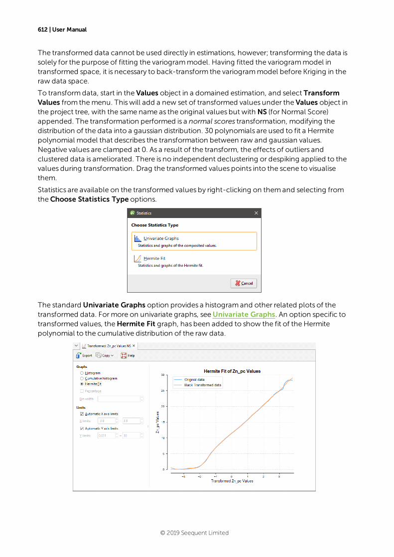
612 | User Manual
The transformed data cannot be used directly in estimations, however; transforming the data issolely for the purpose of fitting the variogrammodel. Having fitted the variogrammodel intransformed space, it is necessary to back-transform the variogrammodel before Kriging in theraw data space.
To transformdata, start in the Values object in a domained estimation, and select TransformValues from themenu. Thiswill add a new set of transformed values under the Values object inthe project tree, with the same name as the original values but with NS (for Normal Score)appended. The transformation performed is a normal scores transformation, modifying thedistribution of the data into a gaussian distribution. 30 polynomials are used to fit a Hermitepolynomial model that describes the transformation between raw and gaussian values.Negative values are clamped at 0. As a result of the transform, the effects of outliers andclustered data is ameliorated. There is no independent declustering or despiking applied to thevalues during transformation. Drag the transformed values points into the scene to visualisethem.
Statistics are available on the transformed values by right-clicking on themand selecting fromtheChoose Statistics Type options.
The standard Univariate Graphs option provides a histogramand other related plots of thetransformed data. Formore on univariate graphs, seeUnivariate Graphs. An option specific totransformed values, theHermite Fit graph, has been added to show the fit of the Hermitepolynomial to the cumulative distribution of the raw data.
© 2019 Seequent Limited
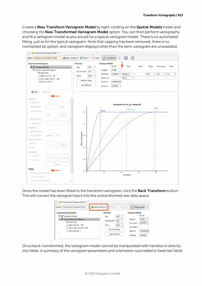
Transform Variography | 613
Create a New Transform Variogram Model by right-clicking on the Spatial Models folder andchoosing theNew Transformed Variogram Model option. You can then perform variographyand fit a variogrammodel as you would for a typical variogrammodel. There is no automatedfitting, just as for the typical variogram. Note that capping has been removed, there is nonormalised sill option, and variogramdisplays other than the semi-variogramare unavailable.
Once themodel has been fitted to the transformvariogram, click the Back Transform button.Thiswill convert the variogramback into the untransformed raw data space.
Once back-transformed, the variogrammodel cannot bemanipulated with handles or directlyinto fields. A summary of the variogramparameters and orientation is provided in fixed text fields
© 2019 Seequent Limited
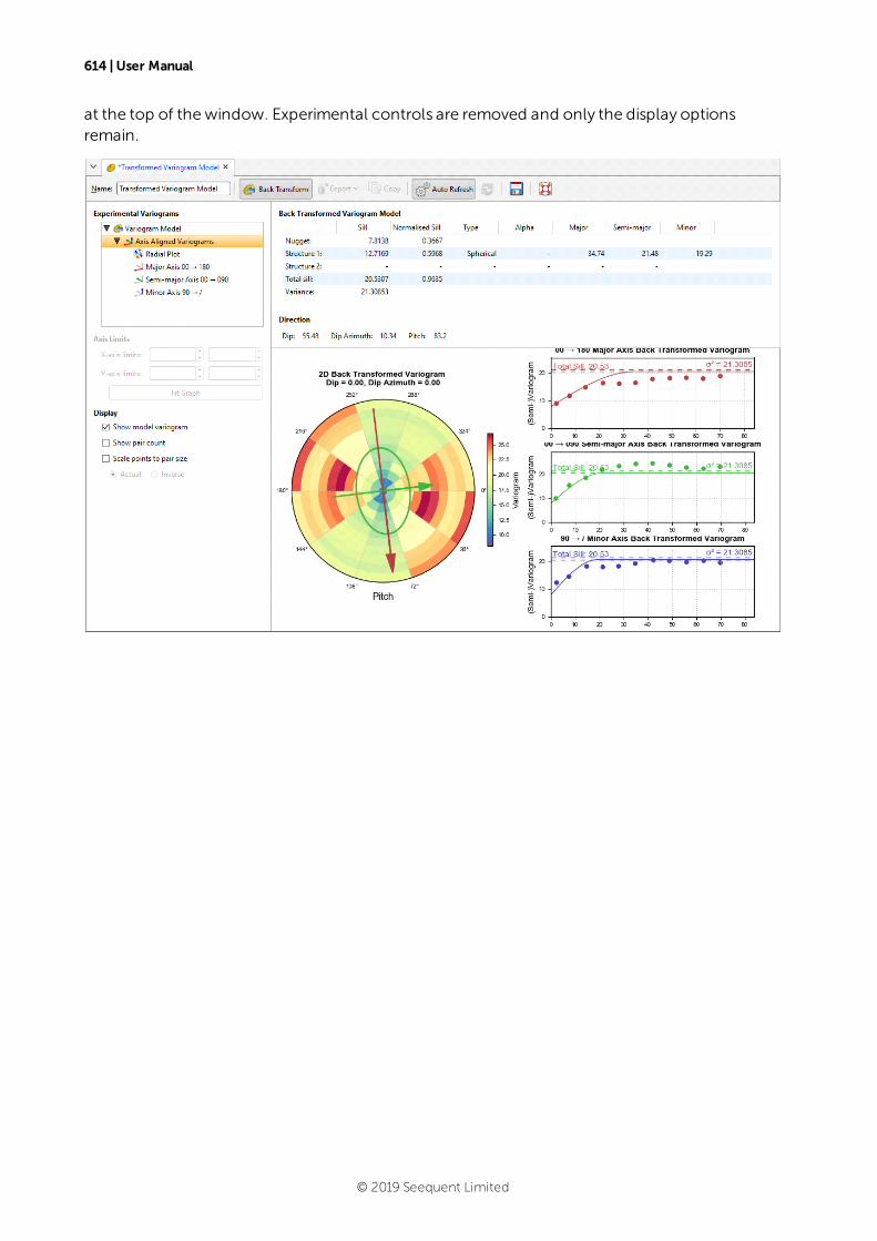
614 | User Manual
at the top of thewindow. Experimental controls are removed and only the display optionsremain.
© 2019 Seequent Limited
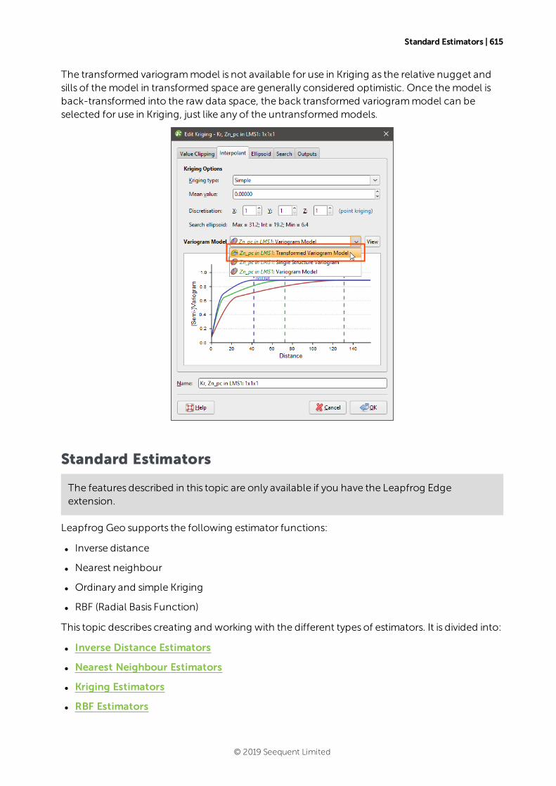
Standard Estimators | 615
The transformed variogrammodel is not available for use in Kriging as the relative nugget andsills of themodel in transformed space are generally considered optimistic. Once themodel isback-transformed into the raw data space, the back transformed variogrammodel can beselected for use in Kriging, just like any of the untransformedmodels.
Standard Estimators
The features described in this topic are only available if you have the Leapfrog Edgeextension.
Leapfrog Geo supports the following estimator functions:
l Inverse distance
l Nearest neighbour
l Ordinary and simple Kriging
l RBF (Radial Basis Function)
This topic describes creating and working with the different types of estimators. It is divided into:
l Inverse Distance Estimators
l Nearest Neighbour Estimators
l Kriging Estimators
l RBF Estimators
© 2019 Seequent Limited
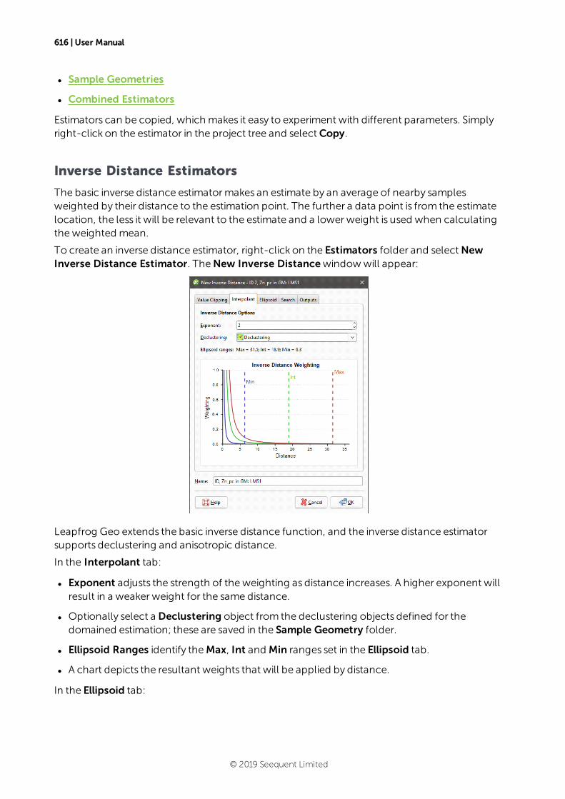
616 | User Manual
l Sample Geometries
l Combined Estimators
Estimators can be copied, which makes it easy to experiment with different parameters. Simplyright-click on the estimator in the project tree and selectCopy.
Inverse Distance Estimators
The basic inverse distance estimatormakes an estimate by an average of nearby samplesweighted by their distance to the estimation point. The further a data point is from the estimatelocation, the less it will be relevant to the estimate and a lowerweight is used when calculatingtheweighted mean.
To create an inverse distance estimator, right-click on the Estimators folder and selectNewInverse Distance Estimator. TheNew Inverse Distancewindowwill appear:
Leapfrog Geo extends the basic inverse distance function, and the inverse distance estimatorsupports declustering and anisotropic distance.
In the Interpolant tab:
l Exponent adjusts the strength of theweighting as distance increases. A higher exponent willresult in a weaker weight for the same distance.
l Optionally select a Declustering object from the declustering objects defined for thedomained estimation; these are saved in the Sample Geometry folder.
l Ellipsoid Ranges identify theMax, Int and Min ranges set in the Ellipsoid tab.
l A chart depicts the resultant weights that will be applied by distance.
In the Ellipsoid tab:
© 2019 Seequent Limited
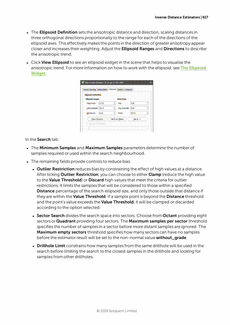
Inverse Distance Estimators | 617
l The Ellipsoid Definition sets the anisotropic distance and direction, scaling distances inthree orthogonal directions proportionally to the range for each of the directions of theellipsoid axes. This effectivelymakes the points in the direction of greater anisotropy appearcloser and increases their weighting. Adjust the Ellipsoid Ranges and Directions to describethe anisotropic trend.
l ClickView Ellipsoid to see an ellipsoid widget in the scene that helps to visualise theanisotropic trend. Formore information on how toworkwith the ellipsoid, see The EllipsoidWidget.
In the Search tab:
l TheMinimum Samples and Maximum Samples parameters determine the number ofsamples required or used within the search neighbourhood.
l The remaining fields provide controls to reduce bias.
l Outlier Restriction reduces bias by constraining the effect of high values at a distance.After ticking Outlier Restriction, you can choose to eitherClamp (reduce the high valueto the Value Threshold) orDiscard high values that meet the criteria for outlierrestrictions. It limits the samples that will be considered to thosewithin a specifiedDistance percentage of the search ellipsoid size, and only those outside that distance ifthey are within the Value Threshold. If a sample point is beyond theDistance thresholdand the point's value exceeds the Value Threshold, it will be clamped or discardedaccording to the option selected.
l Sector Search divides the search space into sectors. Choose fromOctant providing eightsectors orQuadrant providing four sectors. TheMaximum samples per sector thresholdspecifies the number of samples in a sector beforemore distant samples are ignored. TheMaximum empty sectors threshold specifies howmany sectors can have no samplesbefore the estimator result will be set to the non-normal valuewithout_grade.
l Drillhole Limit constrains howmany samples from the same drillhole will be used in thesearch before limiting the search to the closest samples in the drillhole and looking forsamples fromother drillholes.
© 2019 Seequent Limited
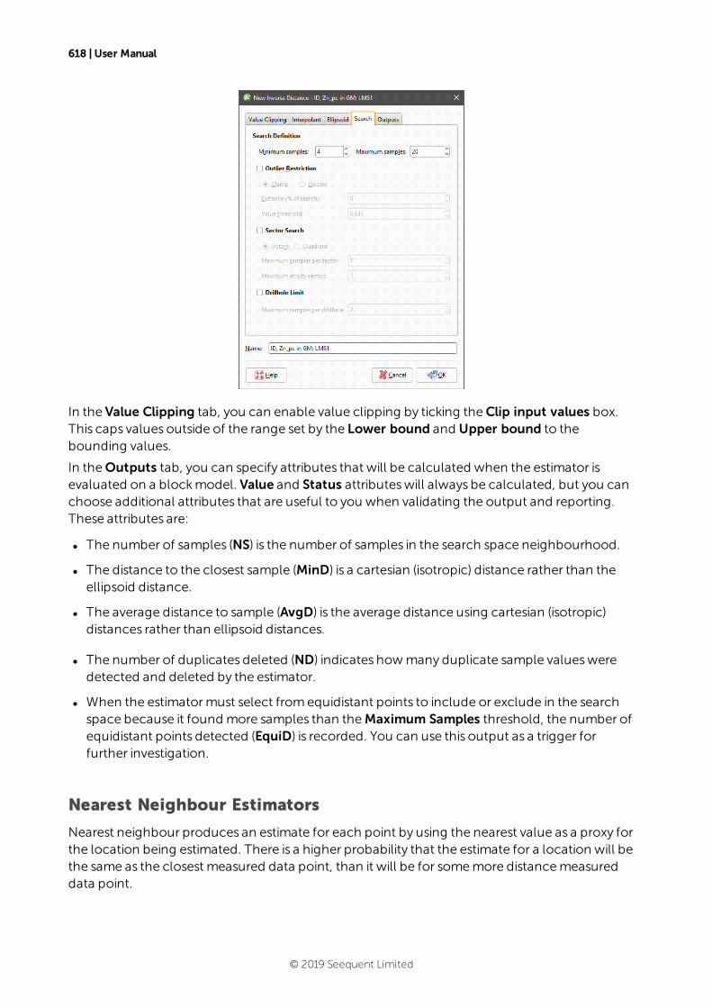
618 | User Manual
In the Value Clipping tab, you can enable value clipping by ticking theClip input values box.This caps values outside of the range set by the Lower bound and Upper bound to thebounding values.
In theOutputs tab, you can specify attributes that will be calculated when the estimator isevaluated on a blockmodel. Value and Status attributeswill always be calculated, but you canchoose additional attributes that are useful to you when validating the output and reporting.These attributes are:
l The number of samples (NS) is the number of samples in the search space neighbourhood.
l The distance to the closest sample (MinD) is a cartesian (isotropic) distance rather than theellipsoid distance.
l The average distance to sample (AvgD) is the average distance using cartesian (isotropic)distances rather than ellipsoid distances.
l The number of duplicates deleted (ND) indicates howmany duplicate sample valuesweredetected and deleted by the estimator.
l When the estimatormust select fromequidistant points to include or exclude in the searchspace because it found more samples than theMaximum Samples threshold, the number ofequidistant points detected (EquiD) is recorded. You can use this output as a trigger forfurther investigation.
Nearest Neighbour Estimators
Nearest neighbour produces an estimate for each point by using the nearest value as a proxy forthe location being estimated. There is a higher probability that the estimate for a location will bethe same as the closest measured data point, than it will be for somemore distancemeasureddata point.
© 2019 Seequent Limited
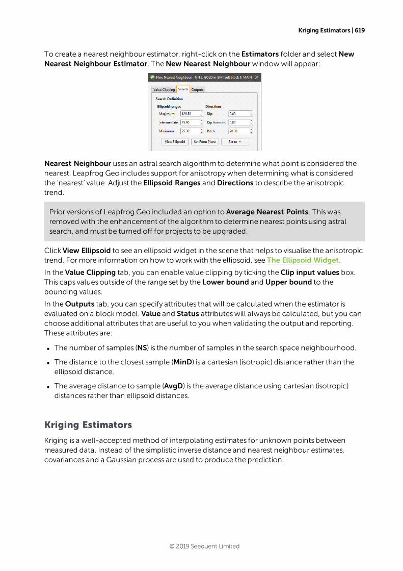
Kriging Estimators | 619
To create a nearest neighbour estimator, right-click on the Estimators folder and selectNewNearest Neighbour Estimator. TheNew Nearest Neighbour windowwill appear:
Nearest Neighbour uses an astral search algorithm to determinewhat point is considered thenearest. Leapfrog Geo includes support for anisotropywhen determining what is consideredthe ‘nearest’ value. Adjust the Ellipsoid Ranges and Directions to describe the anisotropictrend.
Prior versions of Leapfrog Geo included an option to Average Nearest Points. Thiswasremoved with the enhancement of the algorithm to determine nearest points using astralsearch, and must be turned off for projects to be upgraded.
ClickView Ellipsoid to see an ellipsoid widget in the scene that helps to visualise the anisotropictrend. Formore information on how toworkwith the ellipsoid, see The Ellipsoid Widget.
In the Value Clipping tab, you can enable value clipping by ticking theClip input values box.This caps values outside of the range set by the Lower bound and Upper bound to thebounding values.
In theOutputs tab, you can specify attributes that will be calculated when the estimator isevaluated on a blockmodel. Value and Status attributeswill always be calculated, but you canchoose additional attributes that are useful to you when validating the output and reporting.These attributes are:
l The number of samples (NS) is the number of samples in the search space neighbourhood.
l The distance to the closest sample (MinD) is a cartesian (isotropic) distance rather than theellipsoid distance.
l The average distance to sample (AvgD) is the average distance using cartesian (isotropic)distances rather than ellipsoid distances.
Kriging Estimators
Kriging is a well-accepted method of interpolating estimates for unknown points betweenmeasured data. Instead of the simplistic inverse distance and nearest neighbour estimates,covariances and a Gaussian process are used to produce the prediction.
© 2019 Seequent Limited
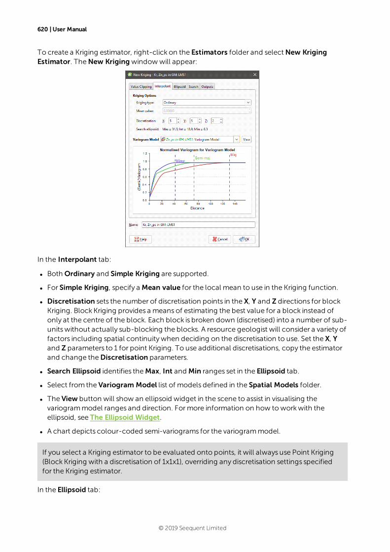
620 | User Manual
To create a Kriging estimator, right-click on the Estimators folder and selectNew KrigingEstimator. TheNew Krigingwindowwill appear:
In the Interpolant tab:
l Both Ordinary and Simple Kriging are supported.
l For Simple Kriging, specify a Mean value for the local mean to use in the Kriging function.
l Discretisation sets the number of discretisation points in the X, Y and Z directions for blockKriging. Block Kriging provides a meansof estimating the best value for a block instead ofonly at the centre of the block. Each block is broken down (discretised) into a number of sub-unitswithout actually sub-blocking the blocks. A resource geologist will consider a variety offactors including spatial continuitywhen deciding on the discretisation to use. Set the X, Yand Z parameters to 1 for point Kriging. To use additional discretisations, copy the estimatorand change theDiscretisation parameters.
l Search Ellipsoid identifies theMax, Int and Min ranges set in the Ellipsoid tab.
l Select from the Variogram Model list of models defined in the Spatial Models folder.
l The View button will show an ellipsoid widget in the scene to assist in visualising thevariogrammodel ranges and direction. Formore information on how toworkwith theellipsoid, see The Ellipsoid Widget.
l A chart depicts colour-coded semi-variograms for the variogrammodel.
If you select a Kriging estimator to be evaluated onto points, it will always use Point Kriging(Block Kriging with a discretisation of 1x1x1), overriding any discretisation settings specifiedfor the Kriging estimator.
In the Ellipsoid tab:
© 2019 Seequent Limited
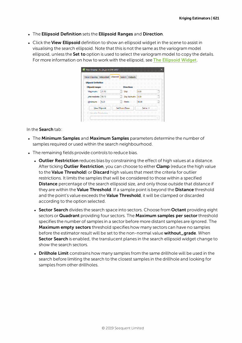
Kriging Estimators | 621
l The Ellipsoid Definition sets the Ellipsoid Ranges and Direction.
l Click the View Ellipsoid definition to show an ellipsoid widget in the scene to assist invisualising the search ellipsoid. Note that this is not the same as the variogrammodelellipsoid, unless the Set to option is used to select the variogrammodel to copy the details.Formore information on how toworkwith the ellipsoid, see The Ellipsoid Widget.
In the Search tab:
l TheMinimum Samples and Maximum Samples parameters determine the number ofsamples required or used within the search neighbourhood.
l The remaining fields provide controls to reduce bias.
l Outlier Restriction reduces bias by constraining the effect of high values at a distance.After ticking Outlier Restriction, you can choose to eitherClamp (reduce the high valueto the Value Threshold) orDiscard high values that meet the criteria for outlierrestrictions. It limits the samples that will be considered to thosewithin a specifiedDistance percentage of the search ellipsoid size, and only those outside that distance ifthey are within the Value Threshold. If a sample point is beyond theDistance thresholdand the point's value exceeds the Value Threshold, it will be clamped or discardedaccording to the option selected.
l Sector Search divides the search space into sectors. Choose fromOctant providing eightsectors orQuadrant providing four sectors. TheMaximum samples per sector thresholdspecifies the number of samples in a sector beforemore distant samples are ignored. TheMaximum empty sectors threshold specifies howmany sectors can have no samplesbefore the estimator result will be set to the non-normal valuewithout_grade. WhenSector Search is enabled, the translucent planes in the search ellipsoid widget change toshow the search sectors.
l Drillhole Limit constrains howmany samples from the same drillhole will be used in thesearch before limiting the search to the closest samples in the drillhole and looking forsamples fromother drillholes.
© 2019 Seequent Limited

622 | User Manual
In the Value Clipping tab, you can enable value clipping by ticking theClip input values box.This caps values outside of the range set by the Lower bound and Upper bound to thebounding values.
Kriging Attributes
In theOutputs tab, you can specify attributes that will be calculated when the estimator isevaluated on a blockmodel. Value and Status attributeswill always be calculated, but you canchoose additional attributes that are useful to you when validating the output and reporting.These attributes are organised into two categories, Sample properties and Estimation results.
Sample properties are output attributes that relate to data sample statistics:
l The number of samples (NS) is the number of samples in the search space neighbourhood.
l The distance to the closest sample (MinD) is a cartesian (isotropic) distance rather than theellipsoid distance.
l The average distance to sample (AvgD) is the average distance using cartesian (isotropic)distances rather than ellipsoid distances.
l The number of duplicates deleted (ND) indicates howmany duplicate sample valuesweredetected and deleted by the estimator.
Estimation results are additional information produced by the estimation:
l Valuewill always be included as it is the actual estimate result.
l Status will always be included as it classifies the estimation result as a Normal result, or non-normal Blank, Without-grade, Outside or Error result.
l The Kriging mean (KM) is the local mean used for the estimate based around the selectedsample data. For simple Kriging, this is the specified global mean. For ordinary Kriging, it is the
© 2019 Seequent Limited
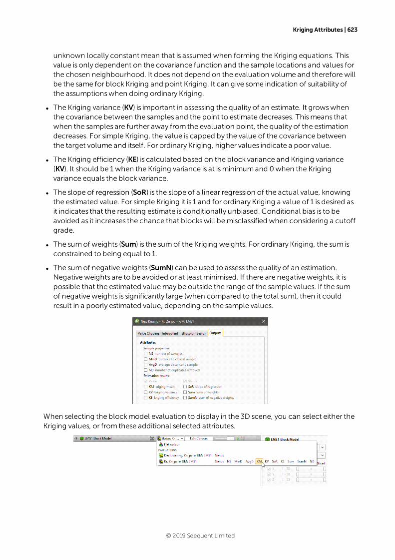
Kriging Attributes | 623
unknown locally constant mean that is assumed when forming the Kriging equations. Thisvalue is only dependent on the covariance function and the sample locations and values forthe chosen neighbourhood. It does not depend on the evaluation volume and therefore willbe the same for block Kriging and point Kriging. It can give some indication of suitability ofthe assumptionswhen doing ordinary Kriging.
l The Kriging variance (KV) is important in assessing the quality of an estimate. It growswhenthe covariance between the samples and the point to estimate decreases. Thismeans thatwhen the samples are further away from the evaluation point, the quality of the estimationdecreases. For simple Kriging, the value is capped by the value of the covariance betweenthe target volume and itself. For ordinary Kriging, higher values indicate a poor value.
l The Kriging efficiency (KE) is calculated based on the block variance and Kriging variance(KV). It should be 1 when the Kriging variance is at isminimumand 0when the Krigingvariance equals the block variance.
l The slope of regression (SoR) is the slope of a linear regression of the actual value, knowingthe estimated value. For simple Kriging it is 1 and for ordinary Kriging a value of 1 is desired asit indicates that the resulting estimate is conditionally unbiased. Conditional bias is to beavoided as it increases the chance that blockswill bemisclassified when considering a cutoffgrade.
l The sumof weights (Sum) is the sumof the Kriging weights. For ordinary Kriging, the sum isconstrained to being equal to 1.
l The sumof negative weights (SumN) can be used to assess the quality of an estimation.Negative weights are to be avoided or at least minimised. If there are negative weights, it ispossible that the estimated valuemay be outside the range of the sample values. If the sumof negative weights is significantly large (when compared to the total sum), then it couldresult in a poorly estimated value, depending on the sample values.
When selecting the blockmodel evaluation to display in the 3D scene, you can select either theKriging values, or from these additional selected attributes.
© 2019 Seequent Limited
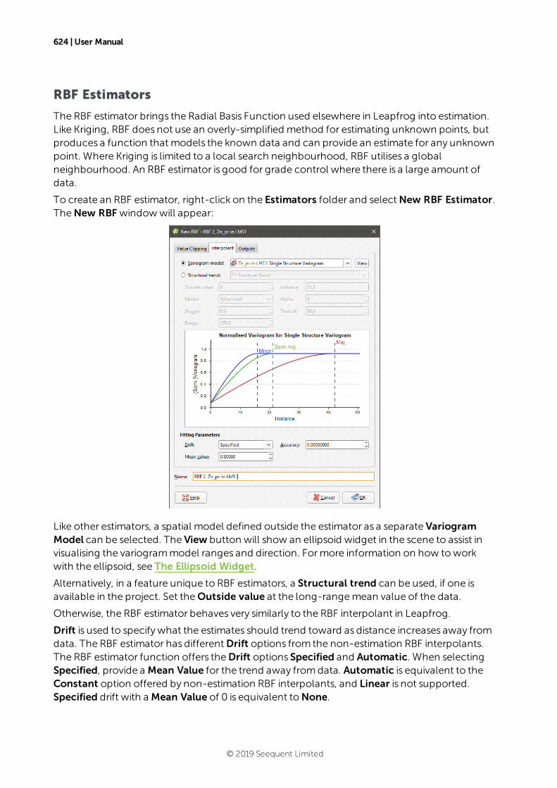
624 | User Manual
RBF Estimators
The RBF estimator brings the Radial Basis Function used elsewhere in Leapfrog into estimation.Like Kriging, RBF does not use an overly-simplified method for estimating unknown points, butproduces a function that models the known data and can provide an estimate for any unknownpoint. Where Kriging is limited to a local search neighbourhood, RBF utilises a globalneighbourhood. An RBF estimator is good for grade control where there is a large amount ofdata.
To create an RBF estimator, right-click on the Estimators folder and selectNew RBF Estimator.TheNew RBF windowwill appear:
Like other estimators, a spatial model defined outside the estimator as a separate VariogramModel can be selected. The View button will show an ellipsoid widget in the scene to assist invisualising the variogrammodel ranges and direction. Formore information on how toworkwith the ellipsoid, see The Ellipsoid Widget.
Alternatively, in a feature unique to RBF estimators, a Structural trend can be used, if one isavailable in the project. Set theOutside value at the long-rangemean value of the data.
Otherwise, the RBF estimator behaves very similarly to the RBF interpolant in Leapfrog.
Drift is used to specifywhat the estimates should trend toward as distance increases away fromdata. The RBF estimator has differentDrift options from the non-estimation RBF interpolants.The RBF estimator function offers theDrift options Specified and Automatic. When selectingSpecified, provide a Mean Value for the trend away fromdata. Automatic is equivalent to theConstant option offered by non-estimation RBF interpolants, and Linear is not supported.Specified drift with a Mean Value of 0 is equivalent toNone.
© 2019 Seequent Limited
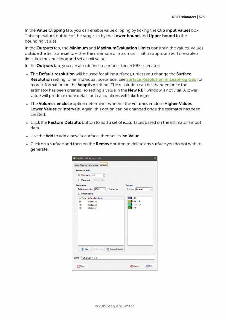
RBF Estimators | 625
In the Value Clipping tab, you can enable value clipping by ticking theClip input values box.This caps values outside of the range set by the Lower bound and Upper bound to thebounding values.
In theOutputs tab, theMinimum and MaximumEvaluation Limits constrain the values. Valuesoutside the limits are set to either theminimumormaximum limit, as appropriate. To enable alimit, tick the checkbox and set a limit value.
In theOutputs tab, you can also define isosurfaces for an RBF estimator:
l TheDefault resolutionwill be used for all isosurfaces, unless you change the SurfaceResolution setting for an individual isosurface. See Surface Resolution in Leapfrog Geo formore information on the Adaptive setting. The resolution can be changed once theestimator has been created, so setting a value in theNew RBF window is not vital. A lowervaluewill producemore detail, but calculationswill take longer.
l The Volumes enclose option determineswhether the volumes encloseHigher Values,Lower Values or Intervals. Again, this option can be changed once the estimator has beencreated.
l Click theRestore Defaults button to add a set of isosurfaces based on the estimator’s inputdata.
l Use the Add to add a new isosurface, then set its Iso Value.
l Click on a surface and then on theRemove button to delete any surface you do not wish togenerate.
© 2019 Seequent Limited
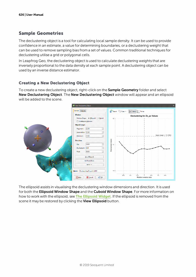
626 | User Manual
Sample Geometries
The declustering object is a tool for calculating local sample density. It can be used to provideconfidence in an estimate, a value for determining boundaries, or a declustering weight thatcan be used to remove sampling bias froma set of values. Common traditional techniques fordeclustering utilise a grid or polygonal cells.
In Leapfrog Geo, the declustering object is used to calculate declustering weights that areinversely proportional to the data density at each sample point. A declustering object can beused by an inverse distance estimator.
Creating a New Declustering Object
To create a new declustering object, right-click on the Sample Geometry folder and selectNew Declustering Object. TheNew Declustering Object windowwill appear and an ellipsoidwill be added to the scene.
The ellipsoid assists in visualising the declustering window dimensions and direction. It is usedfor both the Ellipsoid Window Shape and theCuboid Window Shape. Formore information onhow toworkwith the ellipsoid, see The Ellipsoid Widget. If the ellipsoid is removed from thescene it may be restored by clicking the View Ellipsoid button.
© 2019 Seequent Limited

Creating a New Declustering Object | 627
On the right side of theNew Declustering Object window is a declustering chart. This is used toguide the selection of settings for the declustering object, particularly the ranges for the searchellipsoid. There are two chart views. The default view, Ratio, shows a chart of the declusteredmean against relative window size:
Range shows three declustering charts, one for each axis of the search ellipsoid:
All charts indicate the naïvemean using a dotted horizontal line.
You can interact with the charts by dragging the dotted vertical line to the left or right. In theRatio view, this changes the current ellipsoid range settings by a proportional ratio, as indicated
© 2019 Seequent Limited
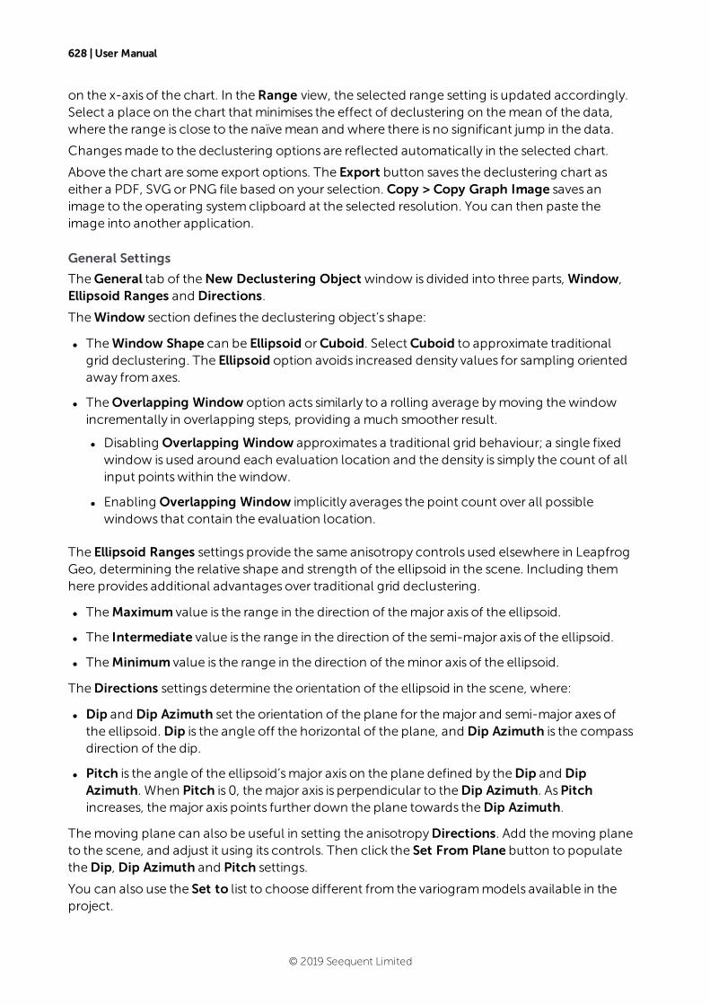
628 | User Manual
on the x-axis of the chart. In theRange view, the selected range setting is updated accordingly.Select a place on the chart that minimises the effect of declustering on themean of the data,where the range is close to the naïvemean and where there is no significant jump in the data.
Changesmade to the declustering options are reflected automatically in the selected chart.
Above the chart are some export options. The Export button saves the declustering chart aseither a PDF, SVG or PNG file based on your selection. Copy > Copy Graph Image saves animage to the operating systemclipboard at the selected resolution. You can then paste theimage into another application.
General Settings
TheGeneral tab of theNew Declustering Object window is divided into three parts, Window,Ellipsoid Ranges and Directions.
TheWindow section defines the declustering object’s shape:
l TheWindow Shape can be Ellipsoid orCuboid. SelectCuboid to approximate traditionalgrid declustering. The Ellipsoid option avoids increased density values for sampling orientedaway fromaxes.
l TheOverlapping Window option acts similarly to a rolling average bymoving thewindowincrementally in overlapping steps, providing a much smoother result.
l Disabling Overlapping Window approximates a traditional grid behaviour; a single fixedwindow is used around each evaluation location and the density is simply the count of allinput pointswithin thewindow.
l Enabling Overlapping Window implicitly averages the point count over all possiblewindows that contain the evaluation location.
The Ellipsoid Ranges settings provide the same anisotropy controls used elsewhere in LeapfrogGeo, determining the relative shape and strength of the ellipsoid in the scene. Including themhere provides additional advantages over traditional grid declustering.
l TheMaximum value is the range in the direction of themajor axis of the ellipsoid.
l The Intermediate value is the range in the direction of the semi-major axis of the ellipsoid.
l TheMinimum value is the range in the direction of theminor axis of the ellipsoid.
TheDirections settings determine the orientation of the ellipsoid in the scene, where:
l Dip and Dip Azimuth set the orientation of the plane for themajor and semi-major axes ofthe ellipsoid. Dip is the angle off the horizontal of the plane, and Dip Azimuth is the compassdirection of the dip.
l Pitch is the angle of the ellipsoid’smajor axis on the plane defined by theDip and DipAzimuth. When Pitch is 0, themajor axis is perpendicular to theDip Azimuth. AsPitchincreases, themajor axis points further down the plane towards theDip Azimuth.
Themoving plane can also be useful in setting the anisotropyDirections. Add themoving planeto the scene, and adjust it using its controls. Then click the Set From Plane button to populatetheDip, Dip Azimuth and Pitch settings.
You can also use the Set to list to choose different from the variogrammodels available in theproject.
© 2019 Seequent Limited
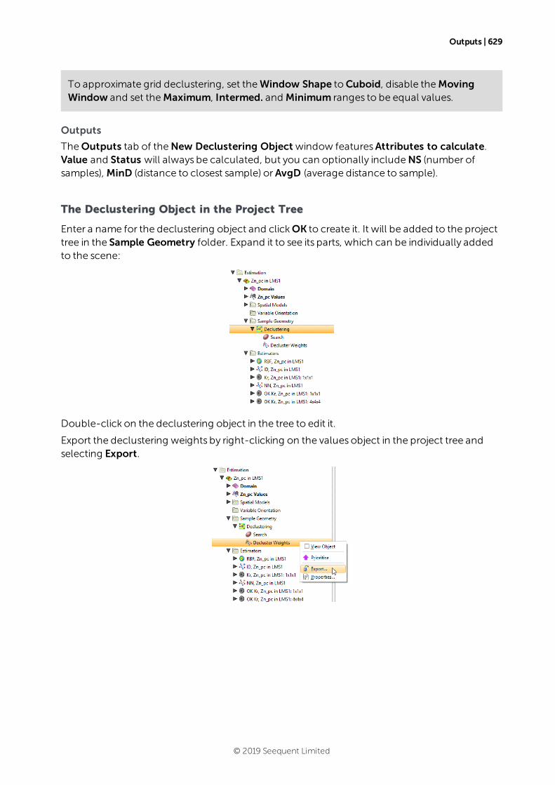
Outputs | 629
To approximate grid declustering, set theWindow Shape toCuboid, disable theMovingWindow and set theMaximum, Intermed. and Minimum ranges to be equal values.
Outputs
TheOutputs tab of theNew Declustering Object window featuresAttributes to calculate.Value and Status will always be calculated, but you can optionally includeNS (number ofsamples), MinD (distance to closest sample) orAvgD (average distance to sample).
The Declustering Object in the Project Tree
Enter a name for the declustering object and clickOK to create it. It will be added to the projecttree in the Sample Geometry folder. Expand it to see its parts, which can be individually addedto the scene:
Double-click on the declustering object in the tree to edit it.
Export the declustering weights by right-clicking on the values object in the project tree andselecting Export.
© 2019 Seequent Limited
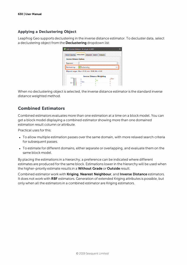
630 | User Manual
Applying a Declustering Object
Leapfrog Geo supports declustering in the inverse distance estimator. To decluster data, selecta declustering object from theDeclustering dropdown list:
When no declustering object is selected, the inverse distance estimator is the standard inversedistanceweighted method.
Combined Estimators
Combined estimators evaluatesmore than one estimation at a time on a blockmodel. You canget a blockmodel displaying a combined estimator showing more than one domainedestimation result column or attribute.
Practical uses for this:
l To allowmultiple estimation passes over the same domain, with more relaxed search criteriafor subsequent passes.
l To estimate for different domains, either separate or overlapping, and evaluate themon thesame blockmodel.
By placing the estimations in a hierarchy, a preference can be indicated where differentestimates are produced for the same block. Estimations lower in the hierarchywill be used whenthe higher-priority estimate results in a Without Grade orOutside result.
Combined estimator workwith Kriging, Nearest Neighbour, and Inverse Distance estimators.It does not workwith RBF estimators. Generation of extended Kriging attributes is possible, butonlywhen all the estimators in a combined estimator are Kriging estimators.
© 2019 Seequent Limited
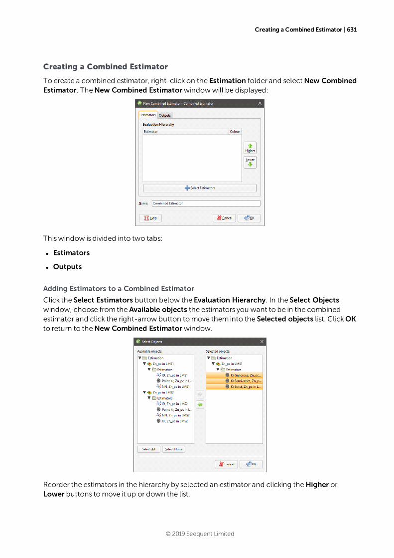
Creating a Combined Estimator | 631
Creating a Combined Estimator
To create a combined estimator, right-click on the Estimation folder and selectNew CombinedEstimator. TheNew Combined Estimator windowwill be displayed:
Thiswindow is divided into two tabs:
l Estimators
l Outputs
Adding Estimators to a Combined Estimator
Click the Select Estimators button below the Evaluation Hierarchy. In the Select Objectswindow, choose from the Available objects the estimators you want to be in the combinedestimator and click the right-arrow button tomove them into the Selected objects list. ClickOKto return to theNew Combined Estimator window.
Reorder the estimators in the hierarchy by selected an estimator and clicking theHigher orLower buttons tomove it up or down the list.
© 2019 Seequent Limited

632 | User Manual
Give the combined estimator a recognisable identifying label by changing theName.
In theOutputs tab, select attributes you wish to be generated along with the estimate.
Value and Statuswill always be generated. Other attributesmay be selected if all the estimatorsare Kriging estimators. If one ormore estimators is a nearest neighbour or inverse distanceestimator, many of the attributeswill not be available.
Most of the attributes are identical to those described for the Kriging estimator. See KrigingAttributes formore information.
Two attributes specific to combined estimators are new category/lithology columns:
l Dom (domain), which domain from the domained estimations the evaluation came from.
l Est (estimator), which estimator was used to estimate the block.
When you clickOK a new combined estimator will appear in the Estimation folder. Below it willbe links to the estimators that are being combined.
© 2019 Seequent Limited
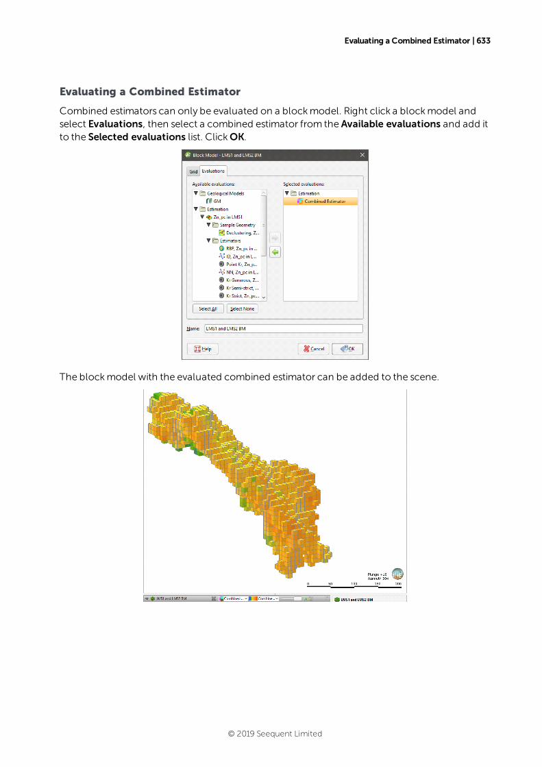
Evaluating a Combined Estimator | 633
Evaluating a Combined Estimator
Combined estimators can only be evaluated on a blockmodel. Right click a blockmodel andselect Evaluations, then select a combined estimator from the Available evaluations and add itto the Selected evaluations list. ClickOK.
The blockmodel with the evaluated combined estimator can be added to the scene.
© 2019 Seequent Limited
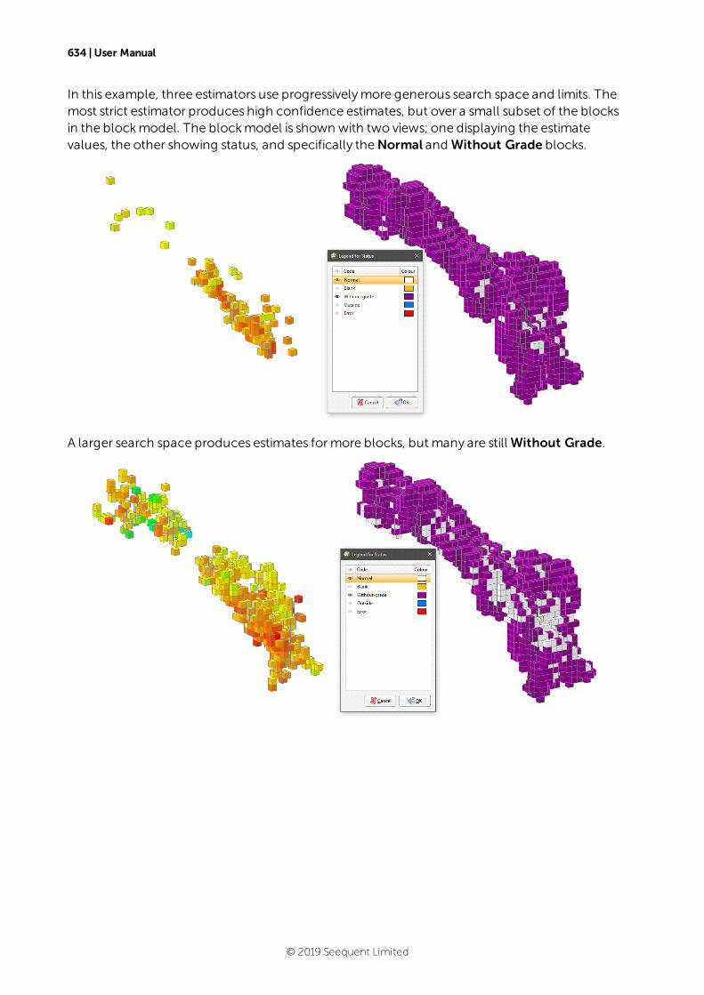
634 | User Manual
In this example, three estimators use progressivelymore generous search space and limits. Themost strict estimator produces high confidence estimates, but over a small subset of the blocksin the blockmodel. The blockmodel is shown with two views; one displaying the estimatevalues, the other showing status, and specifically theNormal and Without Grade blocks.
A larger search space produces estimates formore blocks, but many are still Without Grade.
© 2019 Seequent Limited
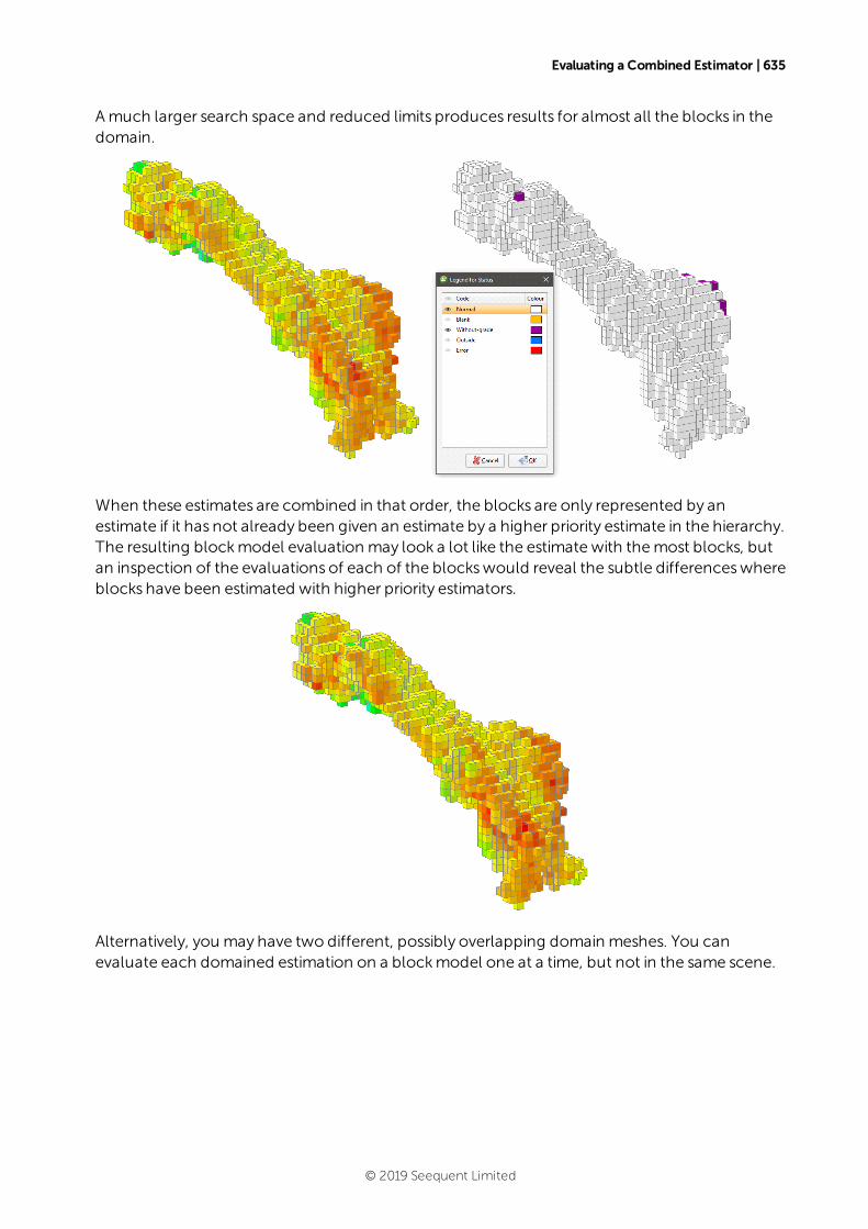
Evaluating a Combined Estimator | 635
Amuch larger search space and reduced limits produces results for almost all the blocks in thedomain.
When these estimates are combined in that order, the blocks are only represented by anestimate if it has not already been given an estimate by a higher priority estimate in the hierarchy.The resulting blockmodel evaluation may look a lot like the estimate with themost blocks, butan inspection of the evaluations of each of the blockswould reveal the subtle differenceswhereblocks have been estimated with higher priority estimators.
Alternatively, you may have two different, possibly overlapping domain meshes. You canevaluate each domained estimation on a blockmodel one at a time, but not in the same scene.
© 2019 Seequent Limited
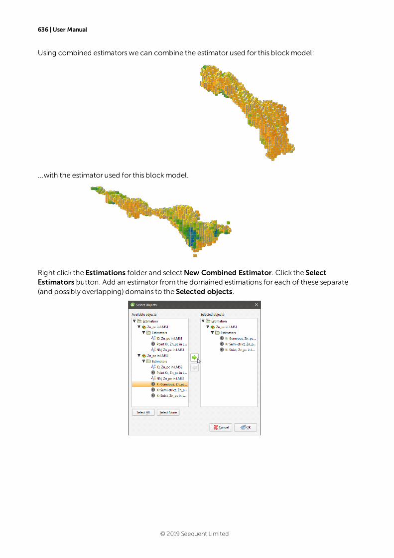
636 | User Manual
Using combined estimatorswe can combine the estimator used for this blockmodel:
...with the estimator used for this blockmodel.
Right click the Estimations folder and selectNew Combined Estimator. Click the SelectEstimators button. Add an estimator from the domained estimations for each of these separate(and possibly overlapping) domains to the Selected objects.
© 2019 Seequent Limited
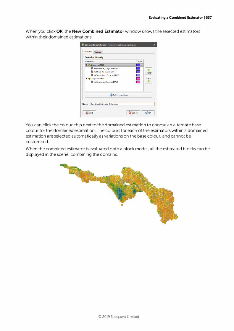
Evaluating a Combined Estimator | 637
When you clickOK, theNew Combined Estimator window shows the selected estimatorswithin their domained estimations.
You can click the colour chip next to the domained estimation to choose an alternate basecolour for the domained estimation. The colours for each of the estimatorswithin a domainedestimation are selected automatically as variations on the base colour, and cannot becustomised.
When the combined estimator is evaluated onto a blockmodel, all the estimated blocks can bedisplayed in the scene, combining the domains.
© 2019 Seequent Limited
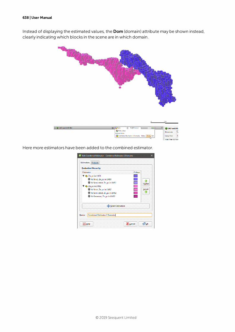
638 | User Manual
Instead of displaying the estimated values, theDom (domain) attributemay be shown instead,clearly indicating which blocks in the scene are in which domain.
Heremore estimators have been added to the combined estimator.
© 2019 Seequent Limited
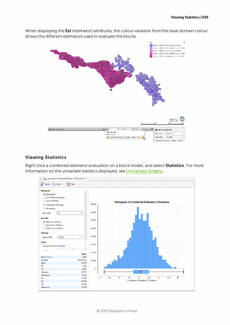
Viewing Statistics | 639
When displaying the Est (estimator) attributes, the colour variation from the base domain colourshows the different estimators used to evaluate the blocks.
Viewing Statistics
Right click a combined estimator evaluation on a blockmodel, and select Statistics. Formoreinformation on the univariate statistics displayed, seeUnivariate Graphs.
© 2019 Seequent Limited
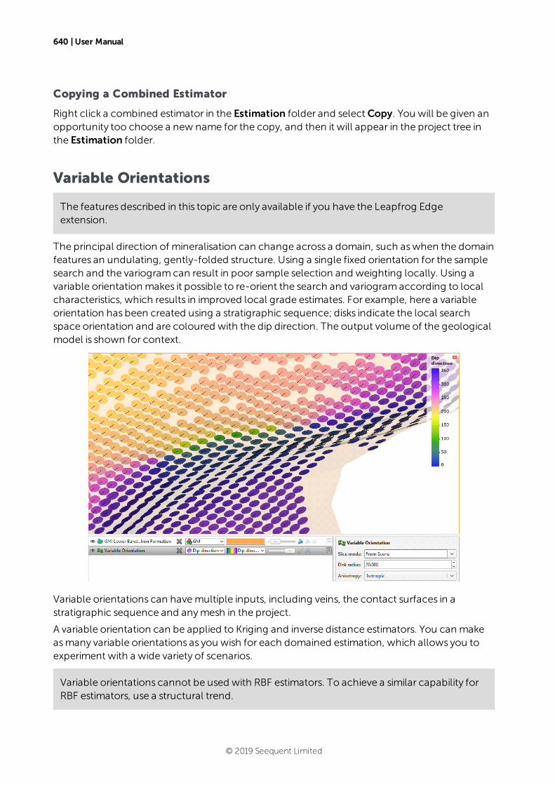
640 | User Manual
Copying a Combined Estimator
Right click a combined estimator in the Estimation folder and selectCopy. You will be given anopportunity too choose a new name for the copy, and then it will appear in the project tree inthe Estimation folder.
Variable Orientations
The features described in this topic are only available if you have the Leapfrog Edgeextension.
The principal direction of mineralisation can change across a domain, such aswhen the domainfeatures an undulating, gently-folded structure. Using a single fixed orientation for the samplesearch and the variogramcan result in poor sample selection and weighting locally. Using avariable orientation makes it possible to re-orient the search and variogramaccording to localcharacteristics, which results in improved local grade estimates. For example, here a variableorientation has been created using a stratigraphic sequence; disks indicate the local searchspace orientation and are coloured with the dip direction. The output volume of the geologicalmodel is shown for context.
Variable orientations can havemultiple inputs, including veins, the contact surfaces in astratigraphic sequence and anymesh in the project.
A variable orientation can be applied to Kriging and inverse distance estimators. You can makeasmany variable orientations as you wish for each domained estimation, which allows you toexperiment with a wide variety of scenarios.
Variable orientations cannot be used with RBF estimators. To achieve a similar capability forRBF estimators, use a structural trend.
© 2019 Seequent Limited
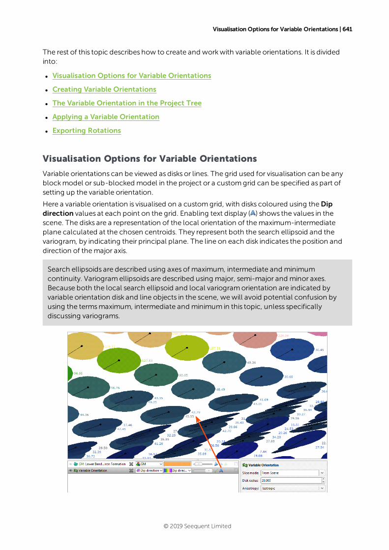
Visualisation Options for Variable Orientations | 641
The rest of this topic describes how to create and workwith variable orientations. It is dividedinto:
l Visualisation Options for Variable Orientations
l Creating Variable Orientations
l The Variable Orientation in the Project Tree
l Applying a Variable Orientation
l Exporting Rotations
Visualisation Options for Variable Orientations
Variable orientations can be viewed as disks or lines. The grid used for visualisation can be anyblockmodel or sub-blocked model in the project or a customgrid can be specified as part ofsetting up the variable orientation.
Here a variable orientation is visualised on a customgrid, with disks coloured using theDipdirection values at each point on the grid. Enabling text display ( ) shows the values in thescene. The disks are a representation of the local orientation of themaximum-intermediateplane calculated at the chosen centroids. They represent both the search ellipsoid and thevariogram, by indicating their principal plane. The line on each disk indicates the position anddirection of themajor axis.
Search ellipsoids are described using axes of maximum, intermediate and minimumcontinuity. Variogramellipsoids are described using major, semi-major and minor axes.Because both the local search ellipsoid and local variogramorientation are indicated byvariable orientation disk and line objects in the scene, wewill avoid potential confusion byusing the termsmaximum, intermediate and minimum in this topic, unless specificallydiscussing variograms.
© 2019 Seequent Limited

642 | User Manual
Click on a disk to view further information about it.
There is also the Show as lines option ( ), which hides the disks to reduce visual clutter whilestill showing the fundamental orientation information in the formof themaximumaxis directionfor each search space local to each centroid:
You can also change the Anisotropy used to display the variable orientation. Options areIsotropic and any variogrammodels and search spaces defined in the domained estimation:
When anisotropy is displayed, the ratio of themaximum-intermediate axis of the chosen objectis indicated as a ratio. The actual range is not shown.
Creating Variable Orientations
Variable orientations are created on a per-domained estimation basis. You can copy variableorientations and make adjustments to them, but you cannot copy them to another domainedestimation.
© 2019 Seequent Limited
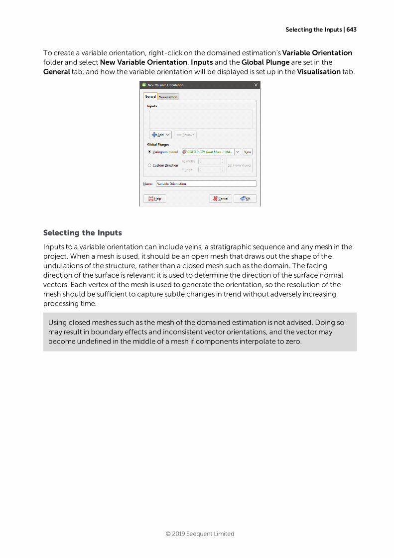
Selecting the Inputs | 643
To create a variable orientation, right-click on the domained estimation’sVariable Orientationfolder and selectNew Variable Orientation. Inputs and theGlobal Plunge are set in theGeneral tab, and how the variable orientation will be displayed is set up in the Visualisation tab.
Selecting the Inputs
Inputs to a variable orientation can include veins, a stratigraphic sequence and anymesh in theproject. When a mesh is used, it should be an openmesh that drawsout the shape of theundulations of the structure, rather than a closed mesh such as the domain. The facingdirection of the surface is relevant; it is used to determine the direction of the surface normalvectors. Each vertex of themesh is used to generate the orientation, so the resolution of themesh should be sufficient to capture subtle changes in trend without adversely increasingprocessing time.
Using closed meshes such as themesh of the domained estimation is not advised. Doing somay result in boundary effects and inconsistent vector orientations, and the vectormaybecome undefined in themiddle of a mesh if components interpolate to zero.
© 2019 Seequent Limited
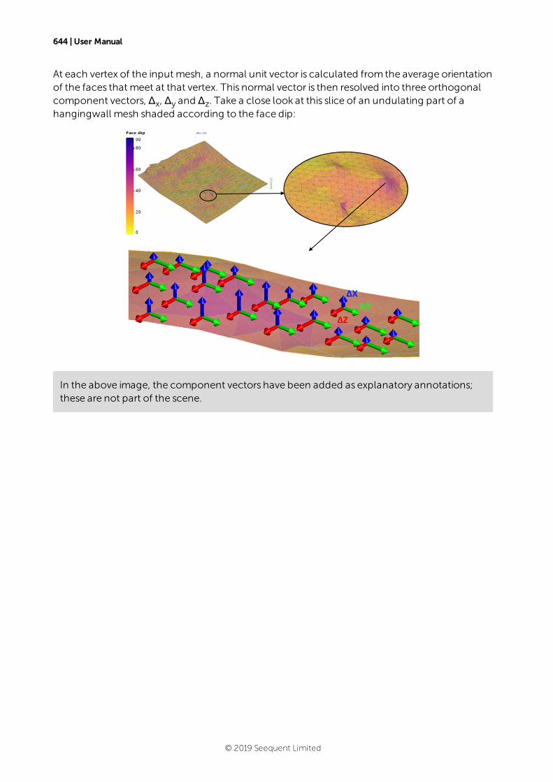
644 | User Manual
At each vertex of the input mesh, a normal unit vector is calculated from the average orientationof the faces that meet at that vertex. This normal vector is then resolved into three orthogonalcomponent vectors, Δx, Δy and Δz. Take a close look at this slice of an undulating part of ahangingwall mesh shaded according to the face dip:
In the above image, the component vectors have been added as explanatory annotations;these are not part of the scene.
© 2019 Seequent Limited
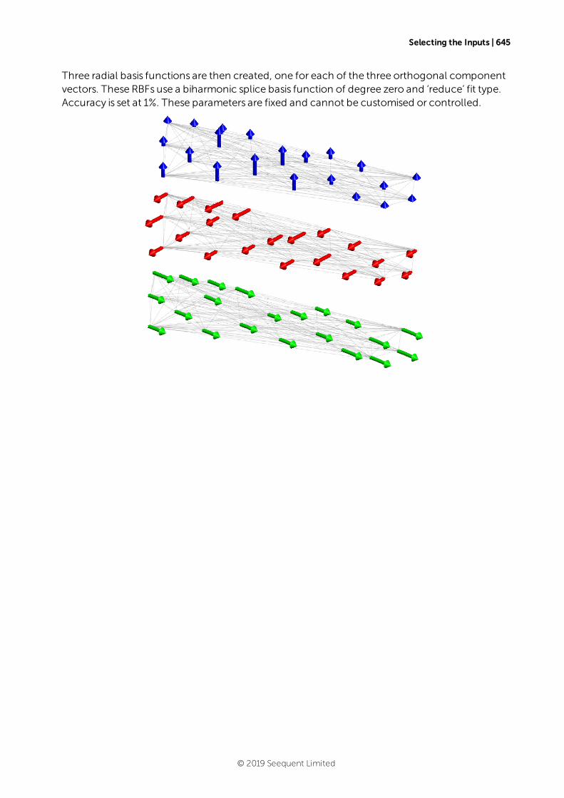
Selecting the Inputs | 645
Three radial basis functions are then created, one for each of the three orthogonal componentvectors. These RBFs use a biharmonic splice basis function of degree zero and ‘reduce’ fit type.Accuracy is set at 1%. These parameters are fixed and cannot be customised or controlled.
© 2019 Seequent Limited
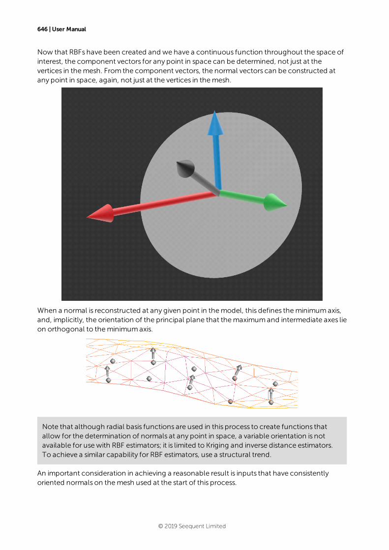
646 | User Manual
Now that RBFs have been created and we have a continuous function throughout the space ofinterest, the component vectors for any point in space can be determined, not just at thevertices in themesh. From the component vectors, the normal vectors can be constructed atany point in space, again, not just at the vertices in themesh.
When a normal is reconstructed at any given point in themodel, this defines theminimumaxis,and, implicitly, the orientation of the principal plane that themaximumand intermediate axes lieon orthogonal to theminimumaxis.
Note that although radial basis functions are used in this process to create functions thatallow for the determination of normals at any point in space, a variable orientation is notavailable for usewith RBF estimators; it is limited to Kriging and inverse distance estimators.To achieve a similar capability for RBF estimators, use a structural trend.
An important consideration in achieving a reasonable result is inputs that have consistentlyoriented normals on themesh used at the start of this process.
© 2019 Seequent Limited

Setting the Global Plunge | 647
l Whenmultiplemeshes are used, you need to ensure that themeshes are consistentlyoriented.
l Veins and stratigraphic sequences aremade up of multiple surfaces, and the normals forthese surfaces are combined into a single cloud of normal vectors.
l When a vein is used as an input, the hangingwall and footwall surfaces are used. Tomakenormal directions consistent, the hangingwall normals are flipped to point in the samedirection as the footwall normals. Common vertices in the footwall and hangingwall,where the vein pinches out, produce duplicate locationswith slightly different normals.The two normals at these locations are averaged to give a single normal vector for thatlocation.
l When a stratigraphic sequence is used, each point of each contact surface produces anormal vector.
Closed surfaces have a consistent inside and outside direction. Normals on a closed surfacewill therefore point either inwards or outwards, resulting in the normals on the opposite sideof themesh pointing in the opposing direction. Interpolating these conflicting normalswilllead to sudden unpredictable changes in orientation.
Setting the Global Plunge
Next, theGlobal Plunge is used to determine the direction of the principal axis on the principalplane. TheGlobal Plunge is a vector defined by either themajor axis of the global variogramorglobally defined search, or it is set from the view. This vector is used to determinewhere thedirection of the principal axis should lie within the direction of the locally re-oriented principalplane. This is achieved by finding the direction on the local plane that is closest in orientation tothe global vector. In practise this amounts to projecting the shadow of the global plungevector, in the direction of the local normal vector, onto the re-oriented local plane.
You have two choices for theGlobal Plunge:
l Use one of the variogrammodels defined for the domained estimation. Select one from thedropdown list.
l Set a Custom Direction. Click and drag in the scene to align the view, then click Set FromViewer.
© 2019 Seequent Limited

648 | User Manual
TheGlobal Plunge is projected onto the principal plane to define the direction of the principalaxis. Imagine a flashlight shining down the normal vector towards the principal plane andshining through a variogrammodel ellipsoid. The shadow cast by themajor axis defines theprincipal direction.
The intermediate axiswill lie on the principal plane at 90° to the principal direction axis.Together the normal vector, the principal direction and the intermediate axis orthogonal tothemdefine the orientation for theminimum, maximumand intermediate axes for use at eachpoint required for estimation, reorienting the search and variogram for that specific location inspace. These directions are determined for each required location.
© 2019 Seequent Limited
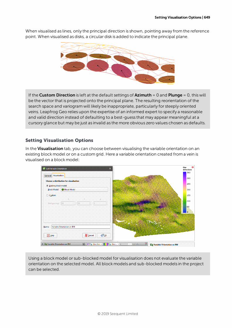
Setting Visualisation Options | 649
When visualised as lines, only the principal direction is shown, pointing away from the referencepoint. When visualised as disks, a circular disk is added to indicate the principal plane.
If theCustom Direction is left at the default settings of Azimuth= 0 and Plunge= 0, thiswillbe the vector that is projected onto the principal plane. The resulting reorientation of thesearch space and variogramwill likely be inappropriate, particularly for steeply orientedveins. Leapfrog Geo relies upon the expertise of an informed expert to specify a reasonableand valid direction instead of defaulting to a best-guess that may appearmeaningful at acursory glance but may be just as invalid as themore obvious zero values chosen as defaults.
Setting Visualisation Options
In the Visualisation tab, you can choose between visualising the variable orientation on anexisting blockmodel or on a customgrid. Here a variable orientation created froma vein isvisualised on a blockmodel:
Using a blockmodel or sub-blocked model for visualisation does not evaluate the variableorientation on the selected model. All blockmodels and sub-blocked models in the projectcan be selected.
© 2019 Seequent Limited
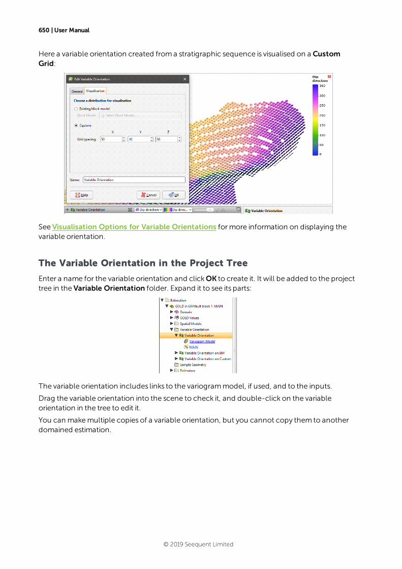
650 | User Manual
Here a variable orientation created froma stratigraphic sequence is visualised on a CustomGrid:
See Visualisation Options for Variable Orientations formore information on displaying thevariable orientation.
The Variable Orientation in the Project Tree
Enter a name for the variable orientation and clickOK to create it. It will be added to the projecttree in the Variable Orientation folder. Expand it to see its parts:
The variable orientation includes links to the variogrammodel, if used, and to the inputs.
Drag the variable orientation into the scene to check it, and double-click on the variableorientation in the tree to edit it.
You can makemultiple copies of a variable orientation, but you cannot copy them to anotherdomained estimation.
© 2019 Seequent Limited
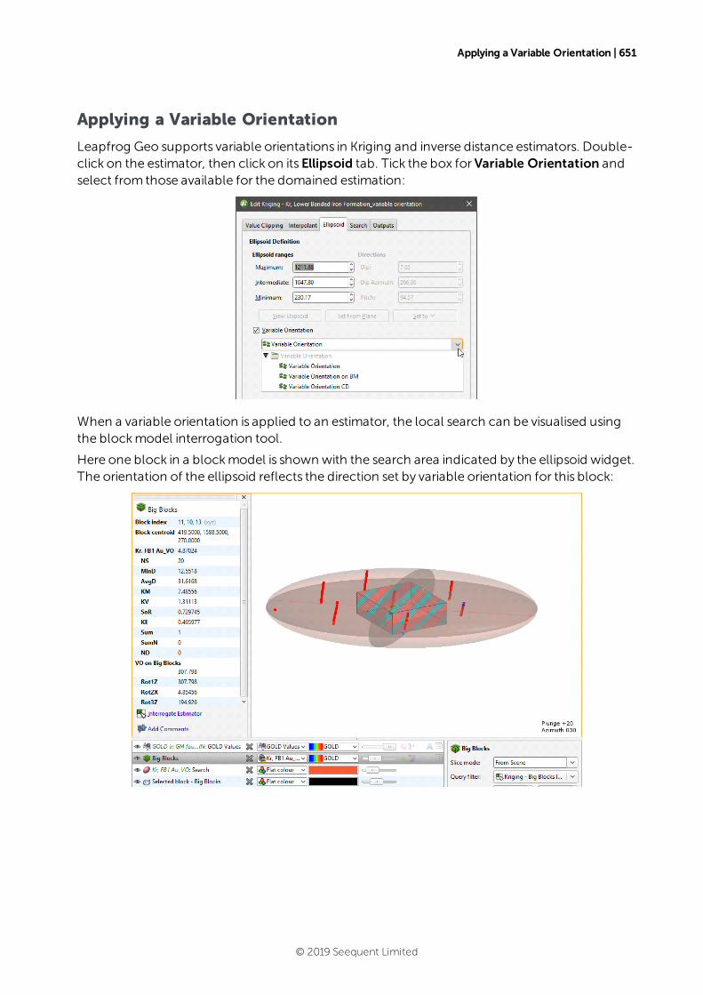
Applying a Variable Orientation | 651
Applying a Variable Orientation
Leapfrog Geo supports variable orientations in Kriging and inverse distance estimators. Double-click on the estimator, then click on itsEllipsoid tab. Tick the box forVariable Orientation andselect from those available for the domained estimation:
When a variable orientation is applied to an estimator, the local search can be visualised usingthe blockmodel interrogation tool.
Here one block in a blockmodel is shown with the search area indicated by the ellipsoid widget.The orientation of the ellipsoid reflects the direction set by variable orientation for this block:
© 2019 Seequent Limited
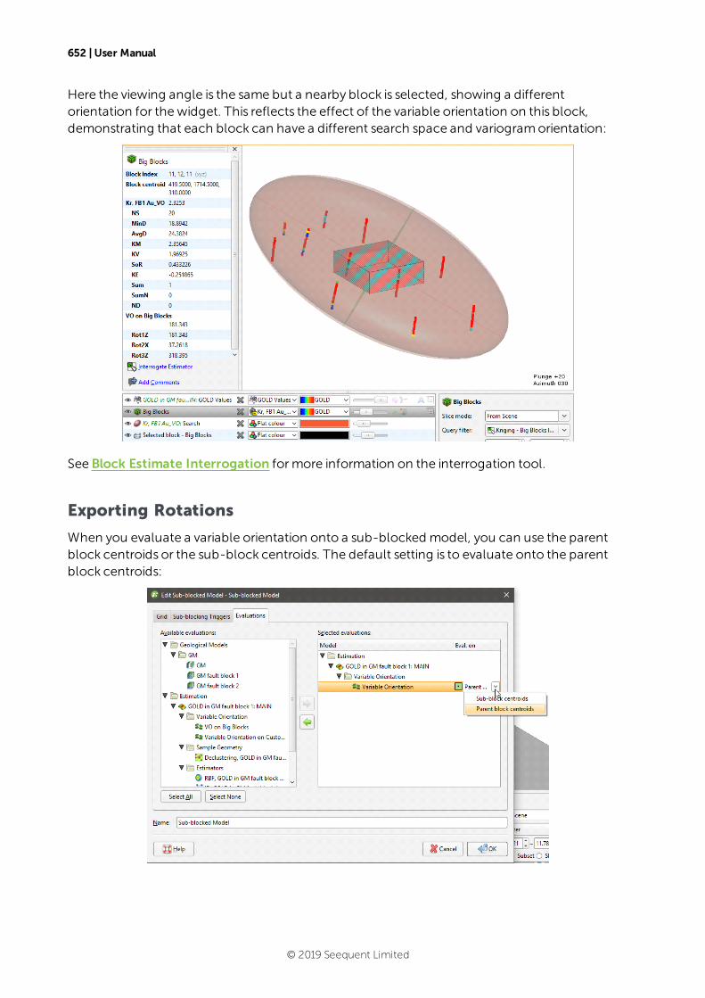
652 | User Manual
Here the viewing angle is the same but a nearby block is selected, showing a differentorientation for thewidget. This reflects the effect of the variable orientation on this block,demonstrating that each block can have a different search space and variogramorientation:
See Block Estimate Interrogation formore information on the interrogation tool.
Exporting Rotations
When you evaluate a variable orientation onto a sub-blocked model, you can use the parentblock centroids or the sub-block centroids. The default setting is to evaluate onto the parentblock centroids:
© 2019 Seequent Limited
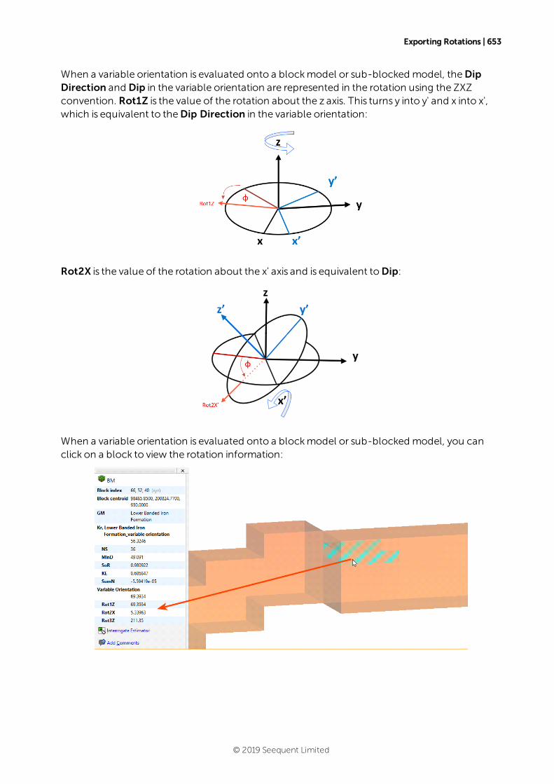
Exporting Rotations | 653
When a variable orientation is evaluated onto a blockmodel or sub-blocked model, theDipDirection and Dip in the variable orientation are represented in the rotation using the ZXZconvention. Rot1Z is the value of the rotation about the z axis. This turns y into y' and x into x',which is equivalent to theDip Direction in the variable orientation:
Rot2X is the value of the rotation about the x' axis and is equivalent toDip:
When a variable orientation is evaluated onto a blockmodel or sub-blocked model, you canclick on a block to view the rotation information:
© 2019 Seequent Limited
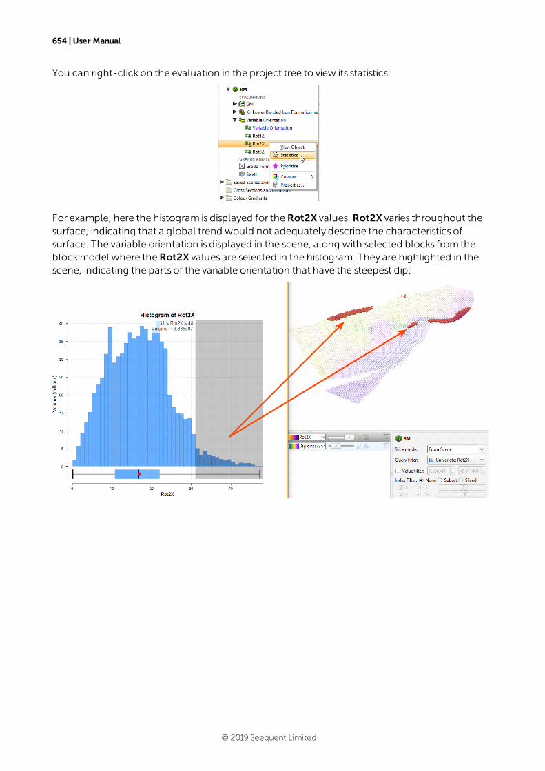
654 | User Manual
You can right-click on the evaluation in the project tree to view its statistics:
For example, here the histogram is displayed for theRot2X values. Rot2X varies throughout thesurface, indicating that a global trend would not adequately describe the characteristics ofsurface. The variable orientation is displayed in the scene, along with selected blocks from theblockmodel where theRot2X values are selected in the histogram. They are highlighted in thescene, indicating the parts of the variable orientation that have the steepest dip:
© 2019 Seequent Limited

Exporting Rotations | 655
If required, you can export the rotations for use in other packages. When exporting the blockmodel, be sure to select the variable orientation evaluation:
© 2019 Seequent Limited

656 | User Manual
Block Model EvaluationsThe product of variography and the definition of estimators now need to be visualised on blockmodels. See:
l Visualising Sample Geometries and Estimators
l Calculations and Filters on Block Models
l Catalogue of Metadata, Syntax and Functions
Visualising Sample Geometries and Estimators
The features described in this topic are only available if you have the Leapfrog Edgeextension.
Sample geometries and estimators can be visualised by evaluating themon blockmodels. Toevaluate an estimator on a blockmodel, right-click on the blockmodel in the project tree andselect Evaluations. See Block Models on how toworkwith the different types of blockmodelsavailable in Leapfrog Geo.
Calculations and filters further enhance the visualisation options, adding computationalanalysis and processing of data capabilities to create new types of data to visualise. To createcalculations and filters, right-click on a blockmodel in the project tree and selectCalculationsand Filters. SeeCalculations and Filters on Block Models for information on creating filtersand building calculations.
When you select Evaluations, the blockmodel’smain windowwill be opened with theEvaluations tab displayed:
You can add all of, for example, a domained estimations sample geometries and estimators tothe Selected evaluations list by double-clicking on the domained estimation itself.
© 2019 Seequent Limited

Visualising Sample Geometries and Estimators | 657
ClickOK to process the evaluations, which will be added to the blockmodel in the project tree:
When selecting evaluations on a sub-blocked model, you can evaluate onto the parent blockcentroids or the sub-block centroids:
When discretisation is used to estimate onto sub-blocks, the relative discretisation point spacingfor the parent block is used, recentred on the sub-block centroid. The block discretisation is notscaled down to the sub-block size, and some of the discretisation points used to compute thesub-block estimatemay lie outside the sub-block.
Display an evaluation by dragging it into the scene or by right-clicking on it in the project treeand selecting View Object.
Each evaluation will appear in the list of blockmodel evaluations:
AnyAttributes generated along with the estimator can also be displayed evaluated on theblocks:
© 2019 Seequent Limited
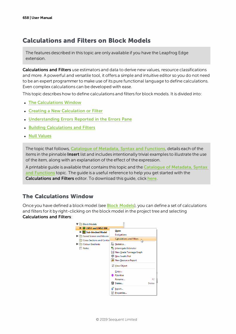
658 | User Manual
Calculations and Filters on Block Models
The features described in this topic are only available if you have the Leapfrog Edgeextension.
Calculations and Filters use estimators and data to derive new values, resource classificationsand more. A powerful and versatile tool, it offers a simple and intuitive editor so you do not needto be an expert programmer tomake use of its pure functional language to define calculations.Even complex calculations can be developed with ease.
This topic describes how to define calculations and filters for blockmodels. It is divided into:
l The Calculations Window
l Creating a New Calculation or Filter
l Understanding Errors Reported in the Errors Pane
l Building Calculations and Filters
l Null Values
The topic that follows, Catalogue of Metadata, Syntax and Functions, details each of theitems in the pinnable Insert list and includes intentionally trivial examples to illustrate the useof the item, along with an explanation of the effect of the expression.
A printable guide is available that contains this topic and theCatalogue of Metadata, Syntaxand Functions topic. The guide is a useful reference to help you get started with theCalculations and Filters editor. To download this guide, clickhere.
The Calculations Window
Once you have defined a blockmodel (see Block Models), you can define a set of calculationsand filters for it by right-clicking on the blockmodel in the project tree and selectingCalculations and Filters:
© 2019 Seequent Limited

The Calculations Window | 659
When theCalculations window is first opened, the Insert list is pinned to the right-hand side.You can untick the Pin Window box to get more screen space:
You can then select itemsby clicking on the Insert menu:
Items in this list are divided into Existing items and Syntax and functions. Existing itemsinclude handymetadata items you can use immediately, e.g. block size and volumemeasurements. It also includes evaluations that can be selected, such as estimators. Syntax and
© 2019 Seequent Limited
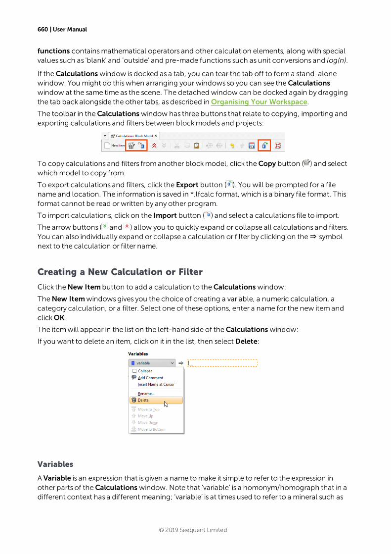
660 | User Manual
functions containsmathematical operators and other calculation elements, along with specialvalues such as 'blank' and 'outside' and pre-made functions such as unit conversions and log(n).
If theCalculations window is docked as a tab, you can tear the tab off to forma stand-alonewindow. You might do thiswhen arranging yourwindows so you can see theCalculationswindow at the same time as the scene. The detached window can be docked again by draggingthe tab back alongside the other tabs, as described in Organising Your Workspace.
The toolbar in theCalculations window has three buttons that relate to copying, importing andexporting calculations and filters between blockmodels and projects:
To copy calculations and filters fromanother blockmodel, click theCopy button ( ) and selectwhich model to copy from.
To export calculations and filters, click the Export button ( ). You will be prompted for a filename and location. The information is saved in *.lfcalc format, which is a binary file format. Thisformat cannot be read orwritten by any other program.
To import calculations, click on the Import button ( ) and select a calculations file to import.
The arrow buttons ( and ) allow you to quickly expand or collapse all calculations and filters.You can also individually expand or collapse a calculation or filter by clicking on the⇒ symbolnext to the calculation or filter name.
Creating a New Calculation or Filter
Click theNew Item button to add a calculation to theCalculations window:
TheNew Itemwindowsgives you the choice of creating a variable, a numeric calculation, acategory calculation, or a filter. Select one of these options, enter a name for the new itemandclickOK.
The itemwill appear in the list on the left-hand side of theCalculations window:
If you want to delete an item, click on it in the list, then selectDelete:
Variables
A Variable is an expression that is given a name tomake it simple to refer to the expression inother parts of theCalculations window. Note that ‘variable’ is a homonym/homograph that in adifferent context has a different meaning; ‘variable’ is at times used to refer to a mineral such as
© 2019 Seequent Limited
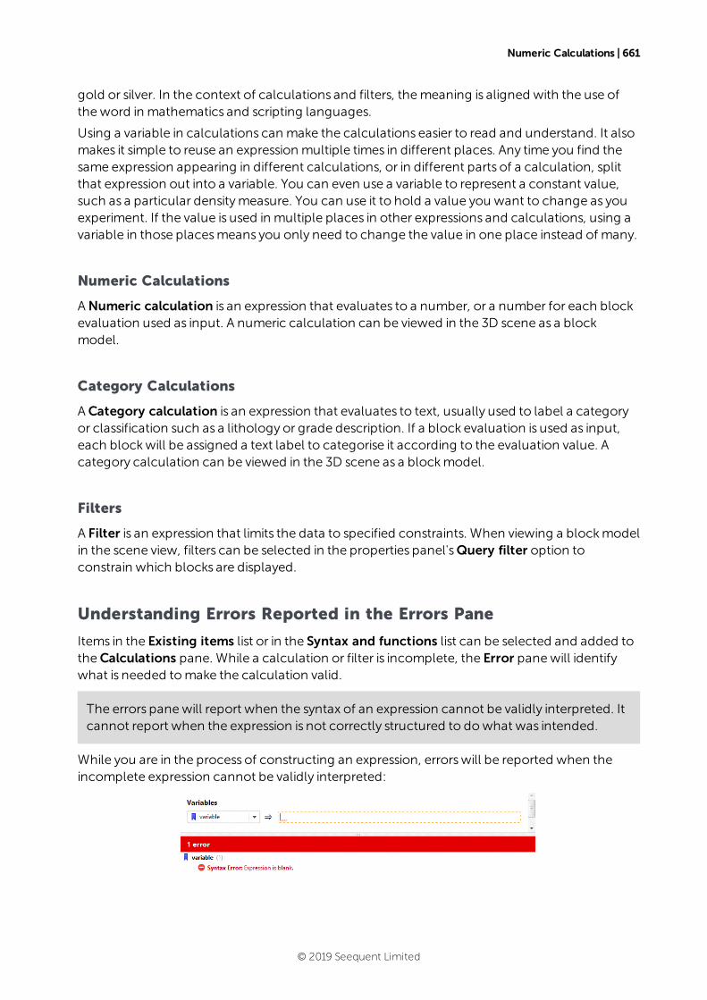
Numeric Calculations | 661
gold or silver. In the context of calculations and filters, themeaning is aligned with the use oftheword in mathematics and scripting languages.
Using a variable in calculations can make the calculations easier to read and understand. It alsomakes it simple to reuse an expression multiple times in different places. Any time you find thesame expression appearing in different calculations, or in different parts of a calculation, splitthat expression out into a variable. You can even use a variable to represent a constant value,such as a particular densitymeasure. You can use it to hold a value you want to change as youexperiment. If the value is used in multiple places in other expressions and calculations, using avariable in those placesmeans you only need to change the value in one place instead of many.
Numeric Calculations
ANumeric calculation is an expression that evaluates to a number, or a number for each blockevaluation used as input. A numeric calculation can be viewed in the 3D scene as a blockmodel.
Category Calculations
ACategory calculation is an expression that evaluates to text, usually used to label a categoryor classification such as a lithology or grade description. If a block evaluation is used as input,each blockwill be assigned a text label to categorise it according to the evaluation value. Acategory calculation can be viewed in the 3D scene as a blockmodel.
Filters
A Filter is an expression that limits the data to specified constraints. When viewing a blockmodelin the scene view, filters can be selected in the properties panel'sQuery filter option toconstrain which blocks are displayed.
Understanding Errors Reported in the Errors Pane
Items in the Existing items list or in the Syntax and functions list can be selected and added totheCalculations pane. While a calculation or filter is incomplete, the Error panewill identifywhat is needed tomake the calculation valid.
The errors panewill report when the syntax of an expression cannot be validly interpreted. Itcannot report when the expression is not correctly structured to dowhat was intended.
While you are in the process of constructing an expression, errorswill be reported when theincomplete expression cannot be validly interpreted:
© 2019 Seequent Limited
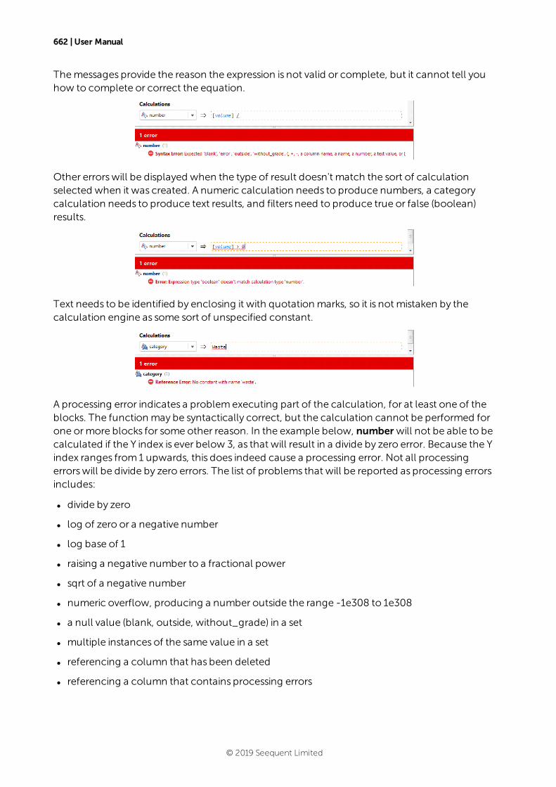
662 | User Manual
Themessages provide the reason the expression is not valid or complete, but it cannot tell youhow to complete or correct the equation.
Other errorswill be displayed when the type of result doesn't match the sort of calculationselected when it was created. A numeric calculation needs to produce numbers, a categorycalculation needs to produce text results, and filters need to produce true or false (boolean)results.
Text needs to be identified by enclosing it with quotation marks, so it is not mistaken by thecalculation engine as some sort of unspecified constant.
A processing error indicates a problemexecuting part of the calculation, for at least one of theblocks. The function may be syntactically correct, but the calculation cannot be performed forone ormore blocks for some other reason. In the example below, number will not be able to becalculated if the Y index is ever below 3, as that will result in a divide by zero error. Because the Yindex ranges from1 upwards, this does indeed cause a processing error. Not all processingerrorswill be divide by zero errors. The list of problems that will be reported as processing errorsincludes:
l divide by zero
l log of zero or a negative number
l log base of 1
l raising a negative number to a fractional power
l sqrt of a negative number
l numeric overflow, producing a number outside the range -1e308 to 1e308
l a null value (blank, outside, without_grade) in a set
l multiple instances of the same value in a set
l referencing a column that has been deleted
l referencing a column that contains processing errors
© 2019 Seequent Limited
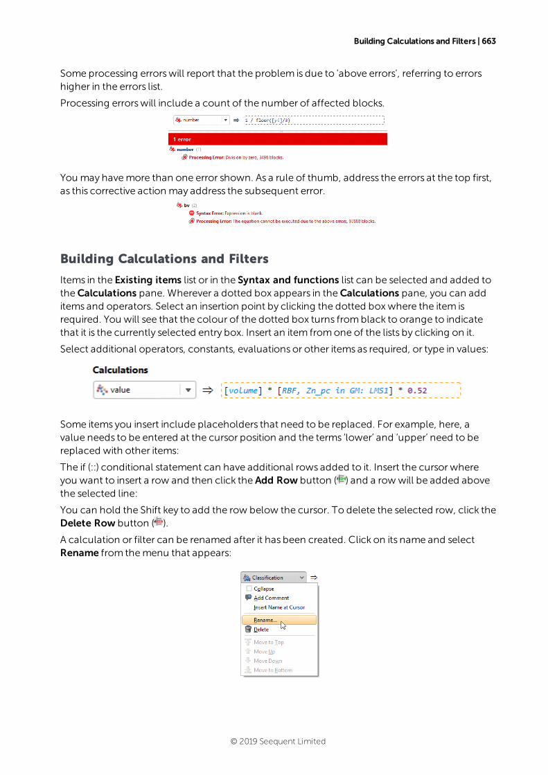
Building Calculations and Filters | 663
Some processing errorswill report that the problem is due to 'above errors', referring to errorshigher in the errors list.
Processing errorswill include a count of the number of affected blocks.
You may havemore than one error shown. As a rule of thumb, address the errors at the top first,as this corrective action may address the subsequent error.
Building Calculations and Filters
Items in the Existing items list or in the Syntax and functions list can be selected and added totheCalculations pane. Wherever a dotted box appears in theCalculations pane, you can additems and operators. Select an insertion point by clicking the dotted boxwhere the item isrequired. You will see that the colour of the dotted box turns fromblack to orange to indicatethat it is the currently selected entry box. Insert an item fromone of the lists by clicking on it.
Select additional operators, constants, evaluations or other items as required, or type in values:
Some items you insert include placeholders that need to be replaced. For example, here, avalue needs to be entered at the cursor position and the terms ‘lower’ and ‘upper’ need to bereplaced with other items:
The if (::) conditional statement can have additional rows added to it. Insert the cursor whereyou want to insert a row and then click the Add Row button ( ) and a row will be added abovethe selected line:
You can hold the Shift key to add the row below the cursor. To delete the selected row, click theDelete Row button ( ).
A calculation or filter can be renamed after it has been created. Click on its name and selectRename from themenu that appears:
© 2019 Seequent Limited
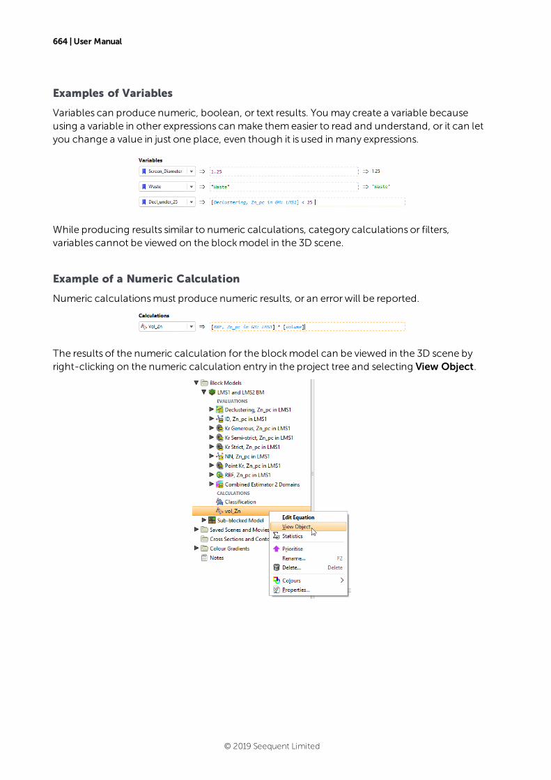
664 | User Manual
Examples of Variables
Variables can produce numeric, boolean, or text results. You may create a variable becauseusing a variable in other expressions can make themeasier to read and understand, or it can letyou change a value in just one place, even though it is used in many expressions.
While producing results similar to numeric calculations, category calculations or filters,variables cannot be viewed on the blockmodel in the 3D scene.
Example of a Numeric Calculation
Numeric calculationsmust produce numeric results, or an error will be reported.
The results of the numeric calculation for the blockmodel can be viewed in the 3D scene byright-clicking on the numeric calculation entry in the project tree and selecting View Object.
© 2019 Seequent Limited
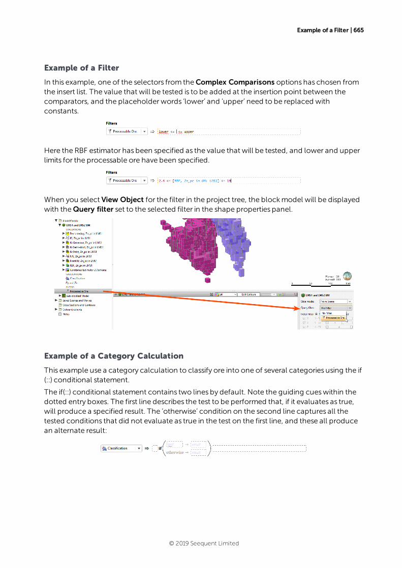
Example of a Filter | 665
Example of a Filter
In this example, one of the selectors from theComplex Comparisons options has chosen fromthe insert list. The value that will be tested is to be added at the insertion point between thecomparators, and the placeholder words ‘lower’ and ‘upper’ need to be replaced withconstants.
Here the RBF estimator has been specified as the value that will be tested, and lower and upperlimits for the processable ore have been specified.
When you select View Object for the filter in the project tree, the blockmodel will be displayedwith theQuery filter set to the selected filter in the shape properties panel.
Example of a Category Calculation
This example use a category calculation to classify ore into one of several categories using the if(::) conditional statement.
The if(::) conditional statement contains two lines by default. Note the guiding cueswithin thedotted entry boxes. The first line describes the test to be performed that, if it evaluates as true,will produce a specified result. The ‘otherwise’ condition on the second line captures all thetested conditions that did not evaluate as true in the test on the first line, and these all producean alternate result:
© 2019 Seequent Limited
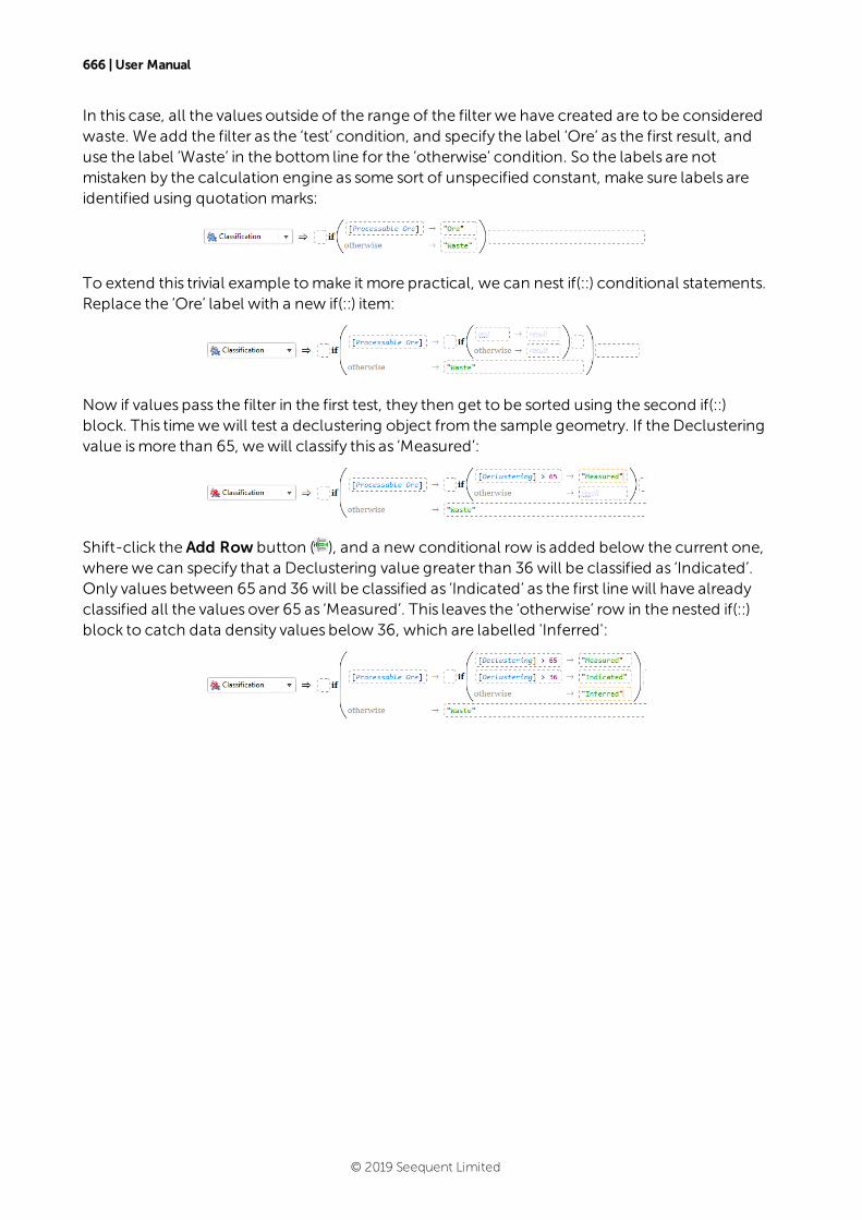
666 | User Manual
In this case, all the values outside of the range of the filter we have created are to be consideredwaste. We add the filter as the ‘test’ condition, and specify the label ‘Ore’ as the first result, anduse the label ‘Waste’ in the bottom line for the ‘otherwise’ condition. So the labels are notmistaken by the calculation engine as some sort of unspecified constant, make sure labels areidentified using quotation marks:
To extend this trivial example tomake it more practical, we can nest if(::) conditional statements.Replace the ‘Ore’ label with a new if(::) item:
Now if values pass the filter in the first test, they then get to be sorted using the second if(::)block. This timewewill test a declustering object from the sample geometry. If the Declusteringvalue ismore than 65, wewill classify this as ‘Measured’:
Shift-click the Add Row button ( ), and a new conditional row is added below the current one,wherewe can specify that a Declustering value greater than 36 will be classified as ‘Indicated’.Only values between 65 and 36 will be classified as ‘Indicated’ as the first line will have alreadyclassified all the values over 65 as ‘Measured’. This leaves the ‘otherwise’ row in the nested if(::)block to catch data density values below 36, which are labelled 'Inferred':
© 2019 Seequent Limited
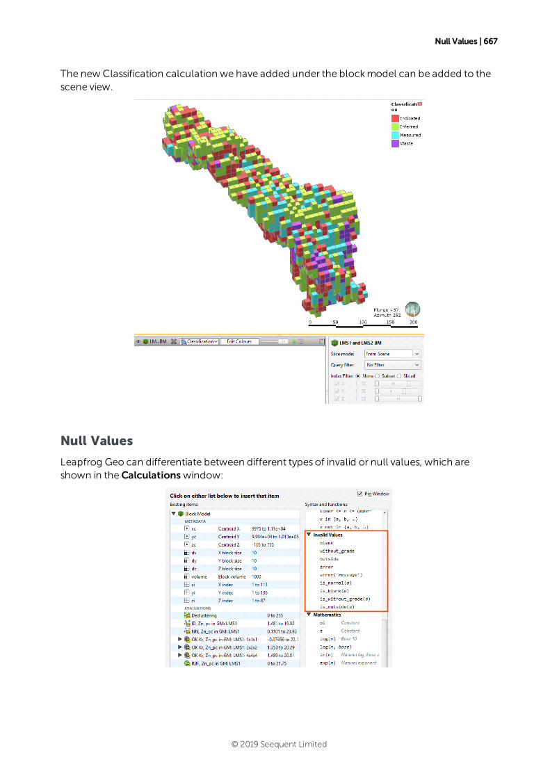
Null Values | 667
The new Classification calculation we have added under the blockmodel can be added to thescene view.
Null Values
Leapfrog Geo can differentiate between different types of invalid or null values, which areshown in theCalculations window:
© 2019 Seequent Limited
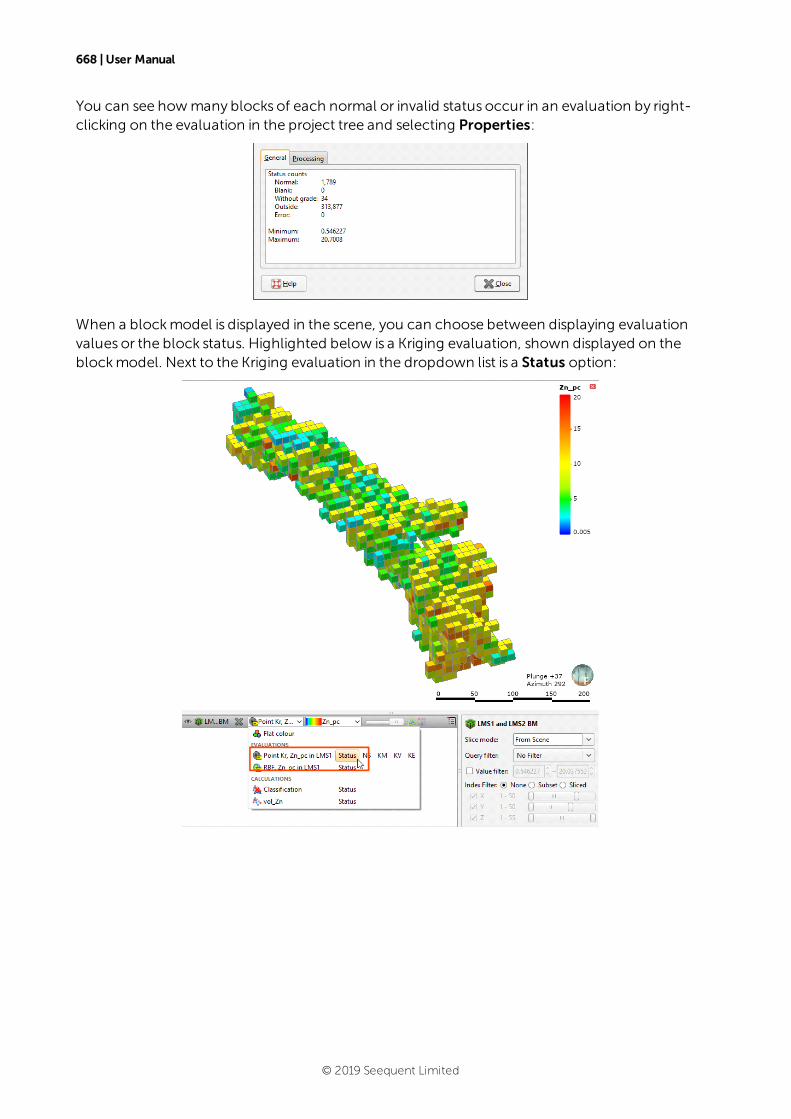
668 | User Manual
You can see howmany blocks of each normal or invalid status occur in an evaluation by right-clicking on the evaluation in the project tree and selecting Properties:
When a blockmodel is displayed in the scene, you can choose between displaying evaluationvalues or the block status. Highlighted below is a Kriging evaluation, shown displayed on theblockmodel. Next to the Kriging evaluation in the dropdown list is a Status option:
© 2019 Seequent Limited
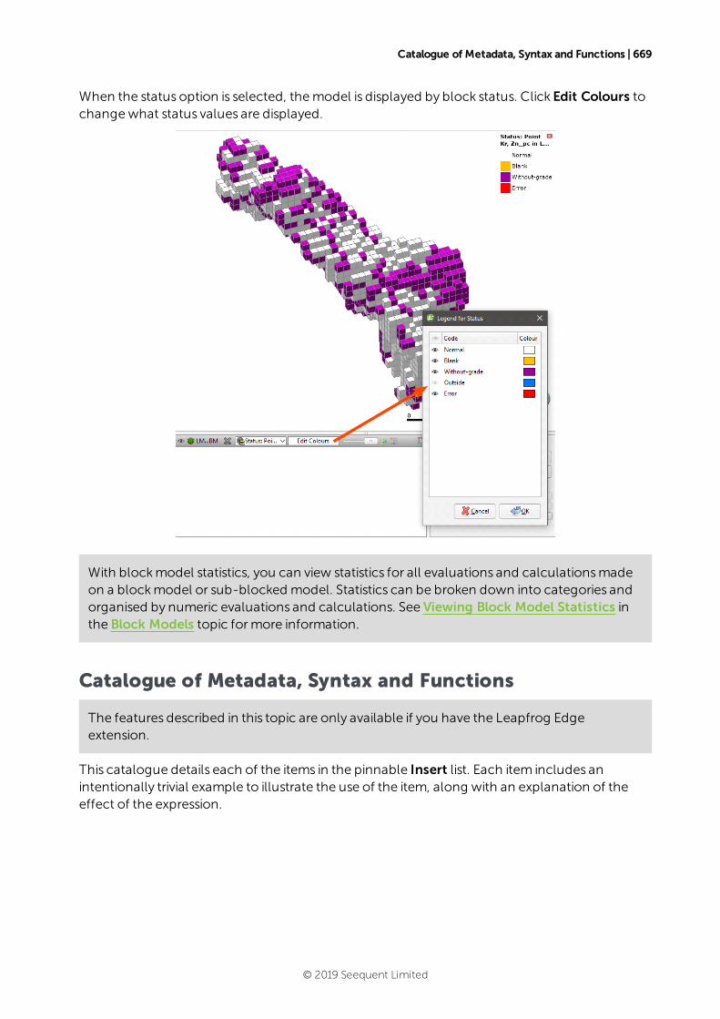
Catalogue of Metadata, Syntax and Functions | 669
When the status option is selected, themodel is displayed by block status. Click Edit Colours tochangewhat status values are displayed.
With blockmodel statistics, you can view statistics for all evaluations and calculationsmadeon a blockmodel or sub-blocked model. Statistics can be broken down into categories andorganised by numeric evaluations and calculations. See Viewing Block Model Statistics inthe Block Models topic formore information.
Catalogue of Metadata, Syntax and Functions
The features described in this topic are only available if you have the Leapfrog Edgeextension.
This catalogue details each of the items in the pinnable Insert list. Each item includes anintentionally trivial example to illustrate the use of the item, along with an explanation of theeffect of the expression.
© 2019 Seequent Limited
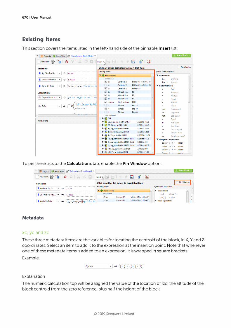
670 | User Manual
Existing Items
This section covers the items listed in the left-hand side of the pinnable Insert list:
To pin these lists to theCalculations tab, enable the Pin Window option:
Metadata
xc, yc and zc
These threemetadata items are the variables for locating the centroid of the block, in X, Y and Zcoordinates. Select an item to add it to the expression at the insertion point. Note that wheneverone of thesemetadata items is added to an expression, it iswrapped in square brackets.
Example
Explanation
The numeric calculation top will be assigned the value of the location of [zc] the altitude of theblock centroid from the zero reference, plus half the height of the block.
© 2019 Seequent Limited
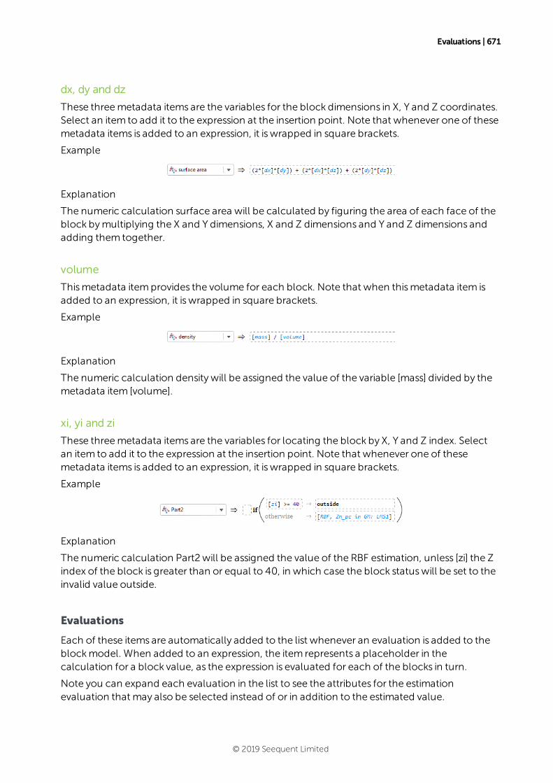
Evaluations | 671
dx, dy and dz
These threemetadata items are the variables for the block dimensions in X, Y and Z coordinates.Select an item to add it to the expression at the insertion point. Note that whenever one of thesemetadata items is added to an expression, it iswrapped in square brackets.
Example
Explanation
The numeric calculation surface area will be calculated by figuring the area of each face of theblock bymultiplying the X and Y dimensions, X and Z dimensions and Y and Z dimensions andadding them together.
volume
Thismetadata itemprovides the volume for each block. Note that when thismetadata item isadded to an expression, it iswrapped in square brackets.
Example
Explanation
The numeric calculation densitywill be assigned the value of the variable [mass] divided by themetadata item [volume].
xi, yi and zi
These threemetadata items are the variables for locating the block by X, Y and Z index. Selectan item to add it to the expression at the insertion point. Note that whenever one of thesemetadata items is added to an expression, it iswrapped in square brackets.
Example
Explanation
The numeric calculation Part2will be assigned the value of the RBF estimation, unless [zi] the Zindex of the block is greater than or equal to 40, in which case the block statuswill be set to theinvalid value outside.
Evaluations
Each of these items are automatically added to the list whenever an evaluation is added to theblockmodel. When added to an expression, the item represents a placeholder in thecalculation for a block value, as the expression is evaluated for each of the blocks in turn.
Note you can expand each evaluation in the list to see the attributes for the estimationevaluation that may also be selected instead of or in addition to the estimated value.
© 2019 Seequent Limited
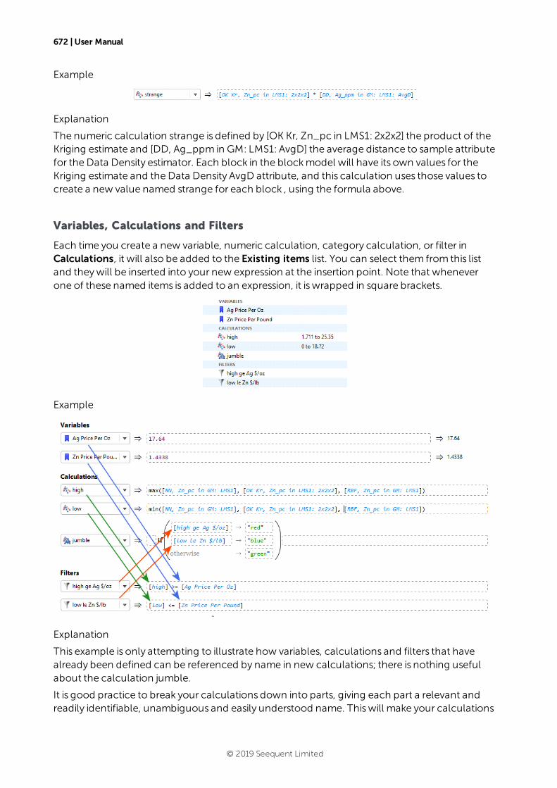
672 | User Manual
Example
Explanation
The numeric calculation strange is defined by [OK Kr, Zn_pc in LMS1: 2x2x2] the product of theKriging estimate and [DD, Ag_ppm in GM: LMS1: AvgD] the average distance to sample attributefor the Data Density estimator. Each block in the blockmodel will have its own values for theKriging estimate and the Data Density AvgD attribute, and this calculation uses those values tocreate a new value named strange for each block , using the formula above.
Variables, Calculations and Filters
Each time you create a new variable, numeric calculation, category calculation, or filter inCalculations, it will also be added to the Existing items list. You can select them from this listand theywill be inserted into your new expression at the insertion point. Note that wheneverone of these named items is added to an expression, it iswrapped in square brackets.
Example
Explanation
This example is only attempting to illustrate how variables, calculations and filters that havealready been defined can be referenced by name in new calculations; there is nothing usefulabout the calculation jumble.
It is good practice to break your calculations down into parts, giving each part a relevant andreadily identifiable, unambiguous and easily understood name. Thiswill make your calculations
© 2019 Seequent Limited
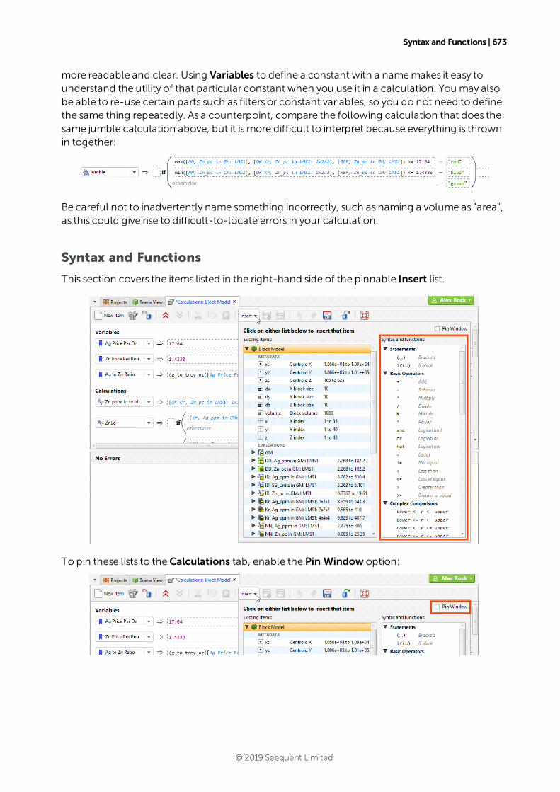
Syntax and Functions | 673
more readable and clear. Using Variables to define a constant with a namemakes it easy tounderstand the utility of that particular constant when you use it in a calculation. You may alsobe able to re-use certain parts such as filters or constant variables, so you do not need to definethe same thing repeatedly. As a counterpoint, compare the following calculation that does thesame jumble calculation above, but it ismore difficult to interpret because everything is thrownin together:
Be careful not to inadvertently name something incorrectly, such as naming a volume as "area",as this could give rise to difficult-to-locate errors in your calculation.
Syntax and Functions
This section covers the items listed in the right-hand side of the pinnable Insert list.
To pin these lists to theCalculations tab, enable the Pin Window option:
© 2019 Seequent Limited
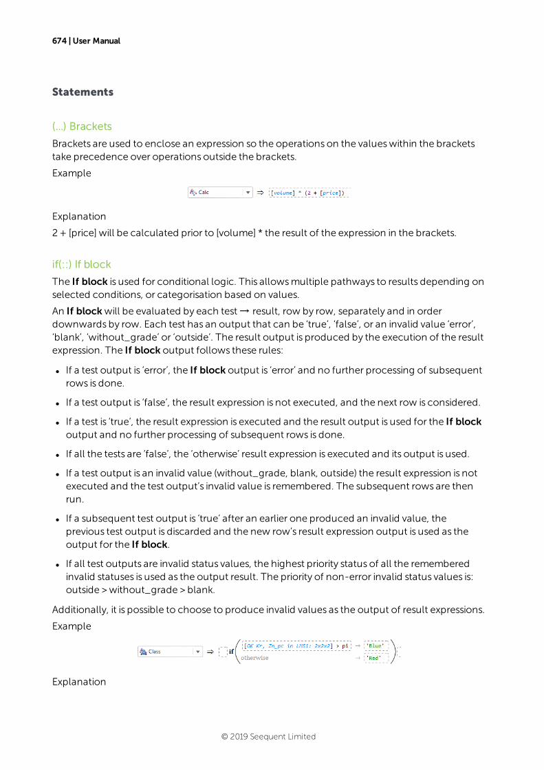
674 | User Manual
Statements
(…) Brackets
Brackets are used to enclose an expression so the operations on the valueswithin the bracketstake precedence over operations outside the brackets.
Example
Explanation
2+ [price] will be calculated prior to [volume] * the result of the expression in the brackets.
if(::) If block
The If block is used for conditional logic. This allowsmultiple pathways to results depending onselected conditions, or categorisation based on values.
An If blockwill be evaluated by each test→ result, row by row, separately and in orderdownwards by row. Each test has an output that can be ‘true’, ‘false’, or an invalid value ‘error’,‘blank’, ‘without_grade’ or ‘outside’. The result output is produced by the execution of the resultexpression. The If block output follows these rules:
l If a test output is ‘error’, the If block output is ‘error’ and no further processing of subsequentrows is done.
l If a test output is ‘false’, the result expression is not executed, and the next row is considered.
l If a test is ‘true’, the result expression is executed and the result output is used for the If blockoutput and no further processing of subsequent rows is done.
l If all the tests are ‘false’, the ‘otherwise’ result expression is executed and its output is used.
l If a test output is an invalid value (without_grade, blank, outside) the result expression is notexecuted and the test output’s invalid value is remembered. The subsequent rows are thenrun.
l If a subsequent test output is ‘true’ after an earlier one produced an invalid value, theprevious test output is discarded and the new row’s result expression output is used as theoutput for the If block.
l If all test outputs are invalid status values, the highest priority status of all the rememberedinvalid statuses is used as the output result. The priority of non-error invalid status values is:outside >without_grade > blank.
Additionally, it is possible to choose to produce invalid values as the output of result expressions.
Example
Explanation
© 2019 Seequent Limited
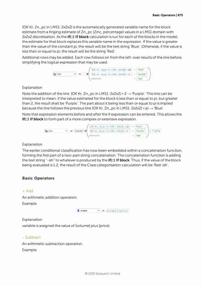
Basic Operators | 675
[OK Kr, Zn_pc in LMS1: 2x2x2] is the automatically generated variable name for the blockestimate froma Kriging estimate of Zn_pc (Zinc, percentage) values in a LMS1 domain with2x2x2 discretisation. As the if(::) If block calculation is run for each of the blocks in themodel,the estimate for that block replaces this variable name in the expression. If the value is greaterthan the value of the constant pi, the result will be the text string ‘Blue’. Otherwise, if the value isless than or equal to pi, the result will be the string ‘Red’.
Additional rowsmay be added. Each row followson from the left-over results of the line before,simplifying the logical expression that may be used.
Explanation
Note the addition of the line [OK Kr, Zn_pc in LMS1: 2x2x2] > 2→ ‘Purple’. This line can beinterpreted tomean: if the value estimated for the block is less than or equal to pi, but greaterthan 2, the result shall be ‘Purple’. The part about it being less than or equal to pi is impliedbecause the line follows the previous line [OK Kr, Zn_pc in LMS1: 2x2x2] > pi→ ‘Blue’.
Note that expression elements before and after the if expression can be entered. This allows theif(::) If block to formpart of a more complex or extensive expression.
Explanation
The earlier conditional classification has now been embedded within a concatenation function,forming the first part of a two-part string concatenation. The concatenation function is addingthe text string “-ish” to whatever is produced by the if(::) If block. Thus, if the value of the blockbeing evaluated is 1.2, the result of the Class categorisation calculation will be ‘Red-ish’.
Basic Operators
+ Add
An arithmetic addition operation.
Example
Explanation
variable is assigned the value of [volume] plus [price].
- Subtract
An arithmetic subtraction operation.
Example
© 2019 Seequent Limited

676 | User Manual
Explanation
variable is assigned the value of [volume]minus [price].
* Multiply
An arithmeticmultiplication operation.
Example
Explanation
block_vol is assigned the value of [dx] times [dy] times [dz]. Note: you do not need to calculatethe block volume like this, as the volumemetadata itemalready exists under Existing items.
/ Divide
An arithmetic division operation.
Example
Explanation
variable is assigned the value of [volume] divided by [price].
% Modulo
An arithmeticmodulo operation. This is an integer division operation that returns the remainderinstead of the integer quotient.
Example
Explanation
variable is assigned the value of [volume]modulo [price], or in other words, [volume] is dividedby [price] to produce an integer quotient , the number of times [price] goes into [volume], andthe remainder, which is the number returned by thismodulo function.
^ Power
Amathematical exponentiation operation where a base is raised to the power of the exponent.
Example
Explanation
variable is assigned the value of pi * [radius]2 (because ^2 is interpreted as ‘exponent 2’ or'squared'). Because [radius] happened to be defined as equalling 1, the result of pi * 12 equals pi,as can be seen from the result at the end of the expression⇒ 3.141592653589…
© 2019 Seequent Limited
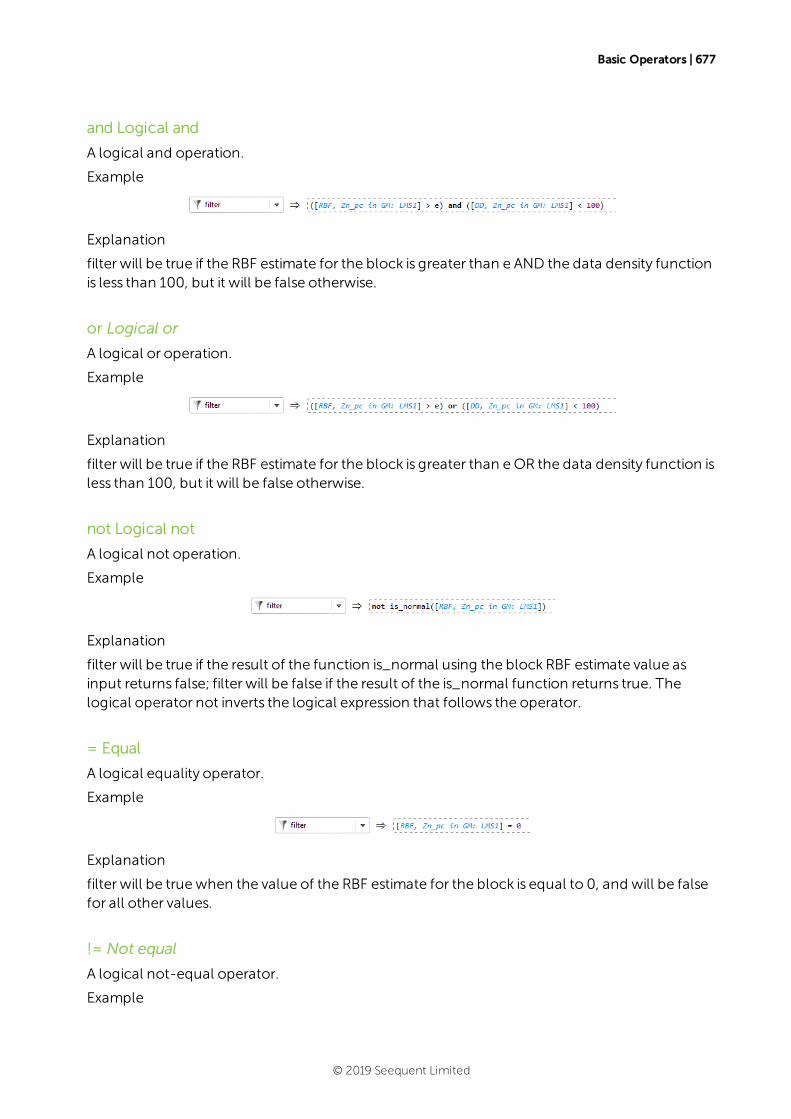
Basic Operators | 677
and Logical and
A logical and operation.
Example
Explanation
filter will be true if the RBF estimate for the block is greater than e AND the data density functionis less than 100, but it will be false otherwise.
or Logical or
A logical or operation.
Example
Explanation
filter will be true if the RBF estimate for the block is greater than eOR the data density function isless than 100, but it will be false otherwise.
not Logical not
A logical not operation.
Example
Explanation
filter will be true if the result of the function is_normal using the block RBF estimate value asinput returns false; filter will be false if the result of the is_normal function returns true. Thelogical operator not inverts the logical expression that follows the operator.
= Equal
A logical equality operator.
Example
Explanation
filter will be truewhen the value of the RBF estimate for the block is equal to 0, and will be falsefor all other values.
!= Not equal
A logical not-equal operator.
Example
© 2019 Seequent Limited
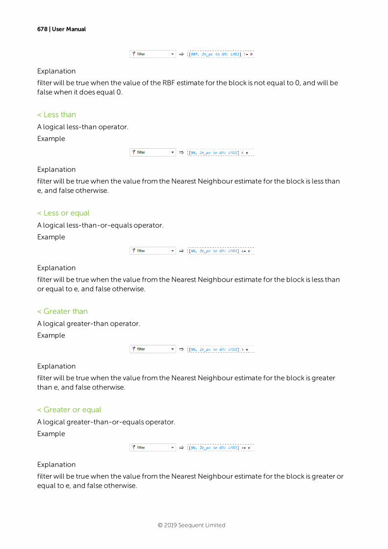
678 | User Manual
Explanation
filter will be truewhen the value of the RBF estimate for the block is not equal to 0, and will befalse when it does equal 0.
< Less than
A logical less-than operator.
Example
Explanation
filter will be truewhen the value from the Nearest Neighbour estimate for the block is less thane, and false otherwise.
< Less or equal
A logical less-than-or-equals operator.
Example
Explanation
filter will be truewhen the value from the Nearest Neighbour estimate for the block is less thanor equal to e, and false otherwise.
< Greater than
A logical greater-than operator.
Example
Explanation
filter will be truewhen the value from the Nearest Neighbour estimate for the block is greaterthan e, and false otherwise.
< Greater or equal
A logical greater-than-or-equals operator.
Example
Explanation
filter will be truewhen the value from the Nearest Neighbour estimate for the block is greater orequal to e, and false otherwise.
© 2019 Seequent Limited
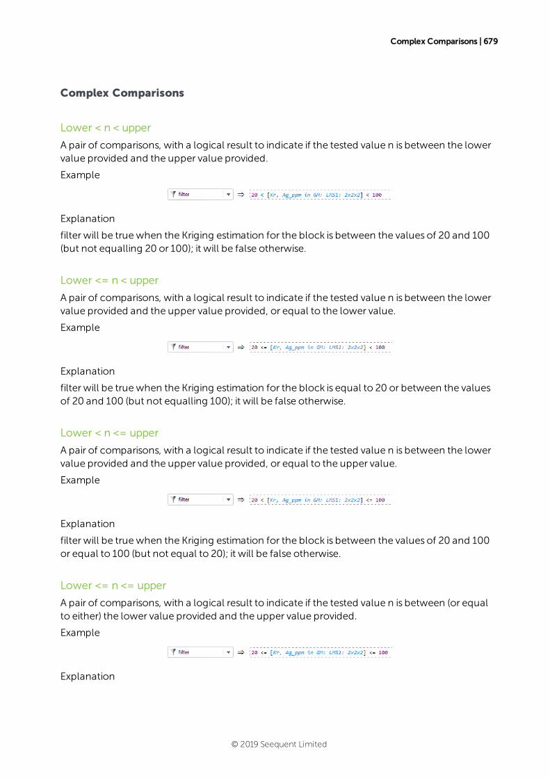
Complex Comparisons | 679
Complex Comparisons
Lower < n < upper
A pair of comparisons, with a logical result to indicate if the tested value n is between the lowervalue provided and the upper value provided.
Example
Explanation
filter will be truewhen the Kriging estimation for the block is between the values of 20 and 100(but not equalling 20 or 100); it will be false otherwise.
Lower <= n < upper
A pair of comparisons, with a logical result to indicate if the tested value n is between the lowervalue provided and the upper value provided, or equal to the lower value.
Example
Explanation
filter will be truewhen the Kriging estimation for the block is equal to 20 or between the valuesof 20 and 100 (but not equalling 100); it will be false otherwise.
Lower < n <= upper
A pair of comparisons, with a logical result to indicate if the tested value n is between the lowervalue provided and the upper value provided, or equal to the upper value.
Example
Explanation
filter will be truewhen the Kriging estimation for the block is between the values of 20 and 100or equal to 100 (but not equal to 20); it will be false otherwise.
Lower <= n <= upper
A pair of comparisons, with a logical result to indicate if the tested value n is between (or equalto either) the lower value provided and the upper value provided.
Example
Explanation
© 2019 Seequent Limited
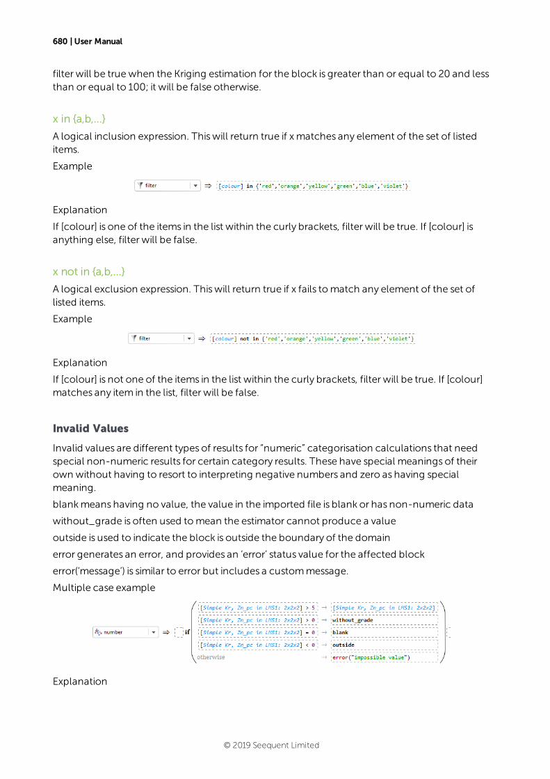
680 | User Manual
filter will be truewhen the Kriging estimation for the block is greater than or equal to 20 and lessthan or equal to 100; it will be false otherwise.
x in {a,b,...}
A logical inclusion expression. Thiswill return true if xmatches any element of the set of listeditems.
Example
Explanation
If [colour] is one of the items in the list within the curly brackets, filter will be true. If [colour] isanything else, filter will be false.
x not in {a,b,...}
A logical exclusion expression. Thiswill return true if x fails tomatch any element of the set oflisted items.
Example
Explanation
If [colour] is not one of the items in the list within the curly brackets, filter will be true. If [colour]matches any item in the list, filter will be false.
Invalid Values
Invalid values are different types of results for “numeric” categorisation calculations that needspecial non-numeric results for certain category results. These have special meanings of theirown without having to resort to interpreting negative numbers and zero as having specialmeaning.
blankmeans having no value, the value in the imported file is blank or has non-numeric data
without_grade is often used tomean the estimator cannot produce a value
outside is used to indicate the block is outside the boundary of the domain
error generates an error, and provides an ‘error’ status value for the affected block
error(‘message’) is similar to error but includes a custommessage.
Multiple case example
Explanation
© 2019 Seequent Limited
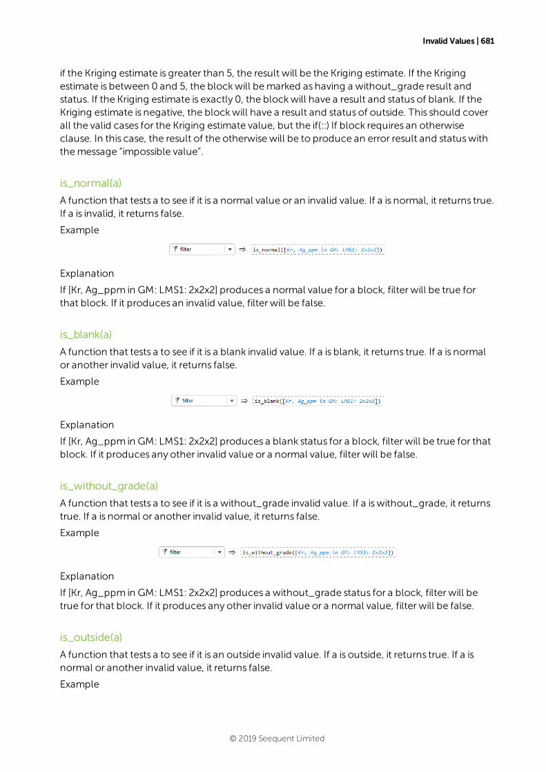
Invalid Values | 681
if the Kriging estimate is greater than 5, the result will be the Kriging estimate. If the Krigingestimate is between 0 and 5, the blockwill bemarked as having a without_grade result andstatus. If the Kriging estimate is exactly 0, the blockwill have a result and status of blank. If theKriging estimate is negative, the blockwill have a result and status of outside. This should coverall the valid cases for the Kriging estimate value, but the if(::) If block requires an otherwiseclause. In this case, the result of the otherwise will be to produce an error result and statuswiththemessage “impossible value”.
is_normal(a)
A function that tests a to see if it is a normal value or an invalid value. If a is normal, it returns true.If a is invalid, it returns false.
Example
Explanation
If [Kr, Ag_ppm in GM: LMS1: 2x2x2] produces a normal value for a block, filter will be true forthat block. If it produces an invalid value, filter will be false.
is_blank(a)
A function that tests a to see if it is a blank invalid value. If a is blank, it returns true. If a is normalor another invalid value, it returns false.
Example
Explanation
If [Kr, Ag_ppm in GM: LMS1: 2x2x2] produces a blank status for a block, filter will be true for thatblock. If it produces any other invalid value or a normal value, filter will be false.
is_without_grade(a)
A function that tests a to see if it is a without_grade invalid value. If a iswithout_grade, it returnstrue. If a is normal or another invalid value, it returns false.
Example
Explanation
If [Kr, Ag_ppm in GM: LMS1: 2x2x2] produces a without_grade status for a block, filter will betrue for that block. If it produces any other invalid value or a normal value, filter will be false.
is_outside(a)
A function that tests a to see if it is an outside invalid value. If a is outside, it returns true. If a isnormal or another invalid value, it returns false.
Example
© 2019 Seequent Limited
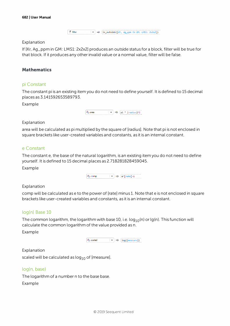
682 | User Manual
Explanation
If [Kr, Ag_ppm in GM: LMS1: 2x2x2] produces an outside status for a block, filter will be true forthat block. If it produces any other invalid value or a normal value, filter will be false.
Mathematics
pi Constant
The constant pi is an existing itemyou do not need to define yourself. It is defined to 15 decimalplaces as 3.141592653589793.
Example
Explanation
area will be calculated as pimultiplied by the square of [radius]. Note that pi is not enclosed insquare brackets like user-created variables and constants, as it is an internal constant.
e Constant
The constant e, the base of the natural logarithm, is an existing itemyou do not need to defineyourself. It is defined to 15 decimal places as 2.718281828459045.
Example
Explanation
comp will be calculated as e to the power of [rate] minus 1. Note that e is not enclosed in squarebrackets like user-created variables and constants, as it is an internal constant.
log(n) Base 10
The common logarithm, the logarithmwith base 10, i.e. log10(n) or lg(n). This function willcalculate the common logarithmof the value provided as n.
Example
Explanation
scaled will be calculated as log10 of [measure].
log(n, base)
The logarithmof a number n to the base base.
Example
© 2019 Seequent Limited
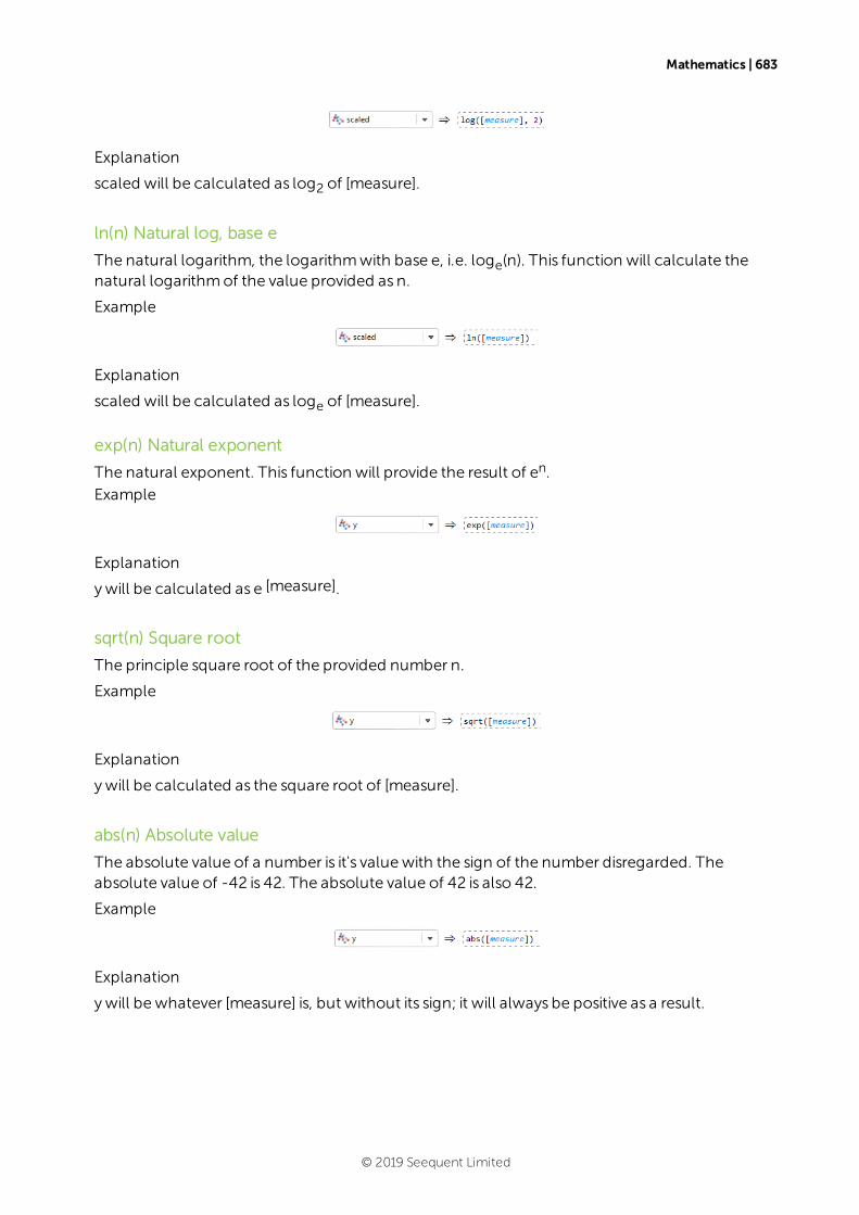
Mathematics | 683
Explanation
scaled will be calculated as log2 of [measure].
ln(n) Natural log, base e
The natural logarithm, the logarithmwith base e, i.e. loge(n). This function will calculate thenatural logarithmof the value provided as n.
Example
Explanation
scaled will be calculated as loge of [measure].
exp(n) Natural exponent
The natural exponent. This function will provide the result of en.
Example
Explanation
ywill be calculated as e [measure].
sqrt(n) Square root
The principle square root of the provided number n.
Example
Explanation
ywill be calculated as the square root of [measure].
abs(n) Absolute value
The absolute value of a number is it's valuewith the sign of the number disregarded. Theabsolute value of -42 is 42. The absolute value of 42 is also 42.
Example
Explanation
ywill be whatever [measure] is, but without its sign; it will always be positive as a result.
© 2019 Seequent Limited
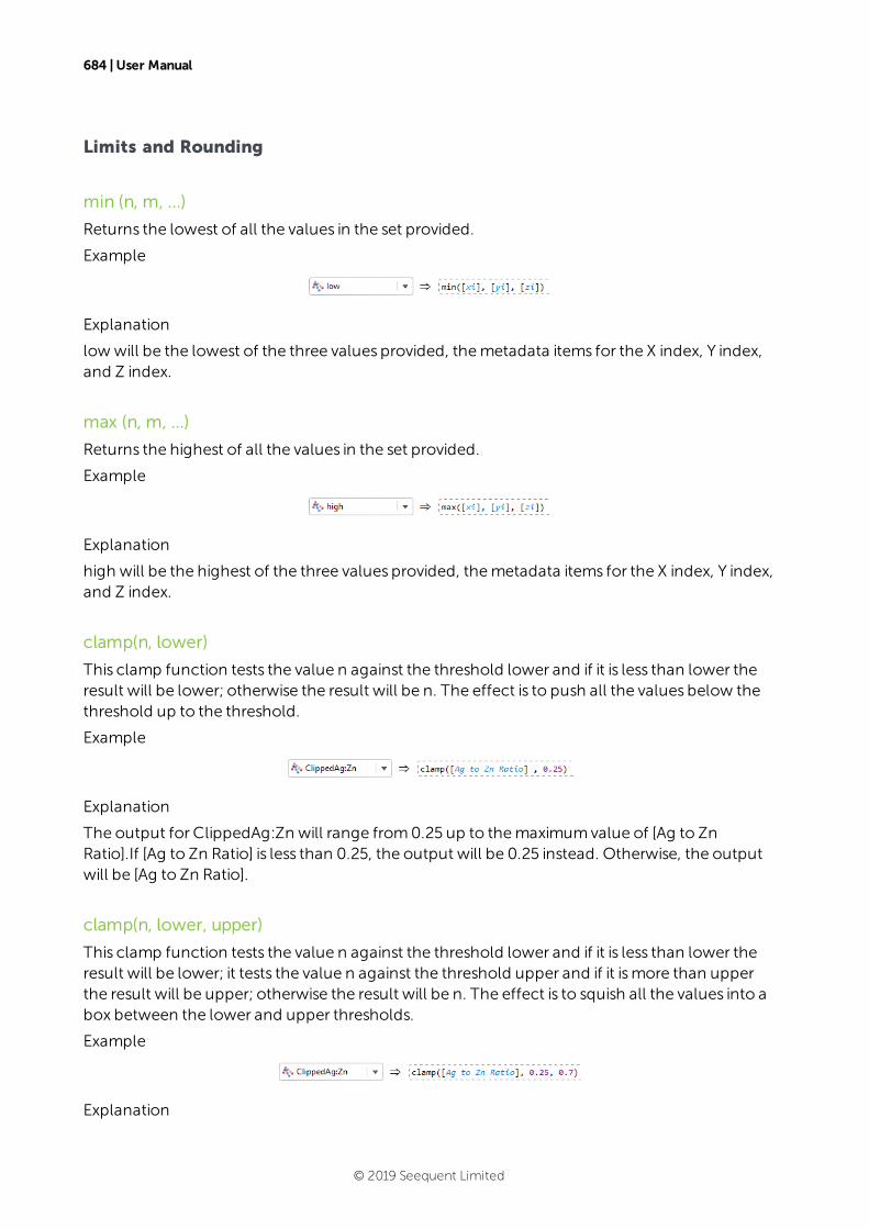
684 | User Manual
Limits and Rounding
min (n, m, ...)
Returns the lowest of all the values in the set provided.
Example
Explanation
low will be the lowest of the three values provided, themetadata items for the X index, Y index,and Z index.
max (n, m, ...)
Returns the highest of all the values in the set provided.
Example
Explanation
high will be the highest of the three values provided, themetadata items for the X index, Y index,and Z index.
clamp(n, lower)
This clamp function tests the value n against the threshold lower and if it is less than lower theresult will be lower; otherwise the result will be n. The effect is to push all the values below thethreshold up to the threshold.
Example
Explanation
The output for ClippedAg:Zn will range from0.25 up to themaximumvalue of [Ag to ZnRatio].If [Ag to Zn Ratio] is less than 0.25, the output will be 0.25 instead. Otherwise, the outputwill be [Ag to Zn Ratio].
clamp(n, lower, upper)
This clamp function tests the value n against the threshold lower and if it is less than lower theresult will be lower; it tests the value n against the threshold upper and if it ismore than upperthe result will be upper; otherwise the result will be n. The effect is to squish all the values into abox between the lower and upper thresholds.
Example
Explanation
© 2019 Seequent Limited
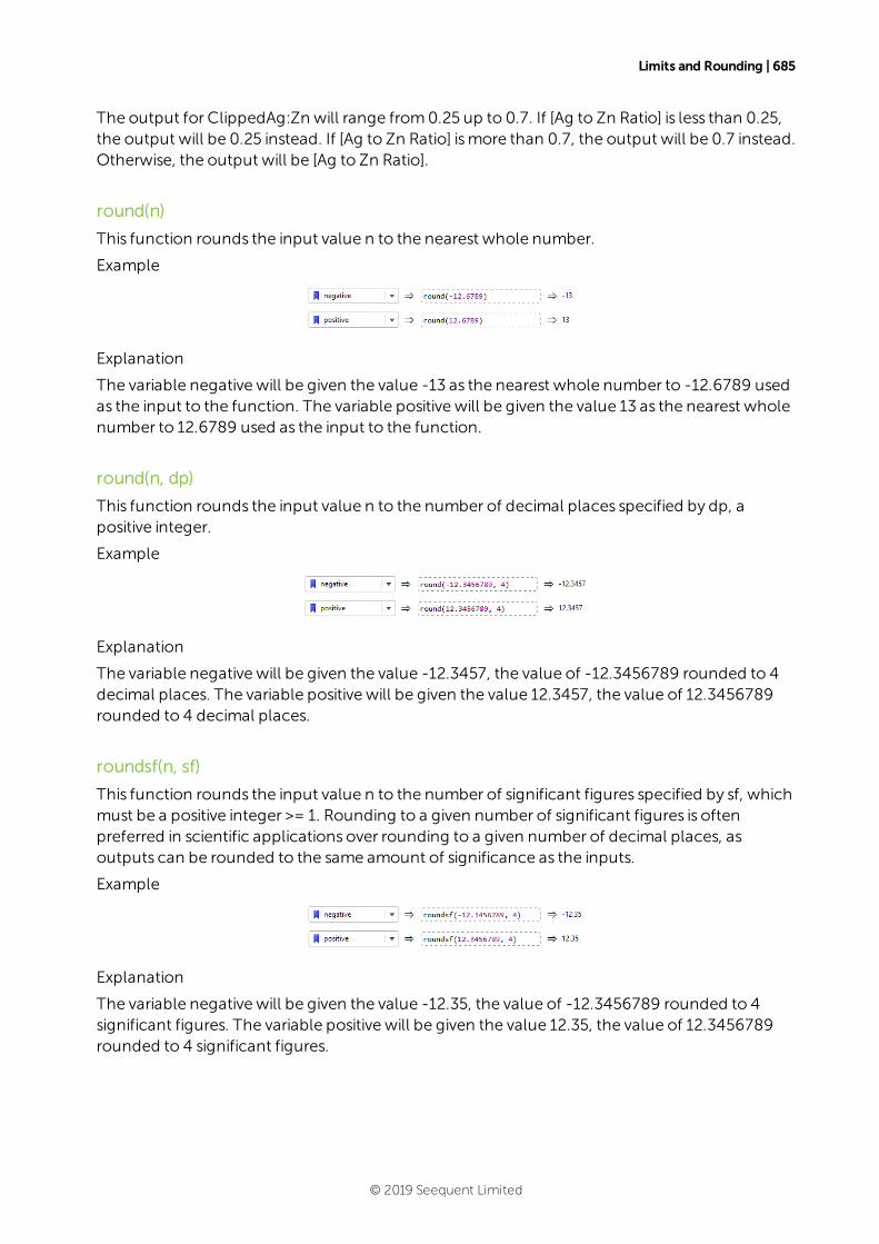
Limits and Rounding | 685
The output for ClippedAg:Zn will range from0.25 up to 0.7. If [Ag to Zn Ratio] is less than 0.25,the output will be 0.25 instead. If [Ag to Zn Ratio] ismore than 0.7, the output will be 0.7 instead.Otherwise, the output will be [Ag to Zn Ratio].
round(n)
This function rounds the input value n to the nearest whole number.
Example
Explanation
The variable negative will be given the value -13 as the nearest whole number to -12.6789 usedas the input to the function. The variable positive will be given the value 13 as the nearest wholenumber to 12.6789 used as the input to the function.
round(n, dp)
This function rounds the input value n to the number of decimal places specified by dp, apositive integer.
Example
Explanation
The variable negative will be given the value -12.3457, the value of -12.3456789 rounded to 4decimal places. The variable positive will be given the value 12.3457, the value of 12.3456789rounded to 4 decimal places.
roundsf(n, sf)
This function rounds the input value n to the number of significant figures specified by sf, whichmust be a positive integer >= 1. Rounding to a given number of significant figures is oftenpreferred in scientific applications over rounding to a given number of decimal places, asoutputs can be rounded to the same amount of significance as the inputs.
Example
Explanation
The variable negative will be given the value -12.35, the value of -12.3456789 rounded to 4significant figures. The variable positive will be given the value 12.35, the value of 12.3456789rounded to 4 significant figures.
© 2019 Seequent Limited
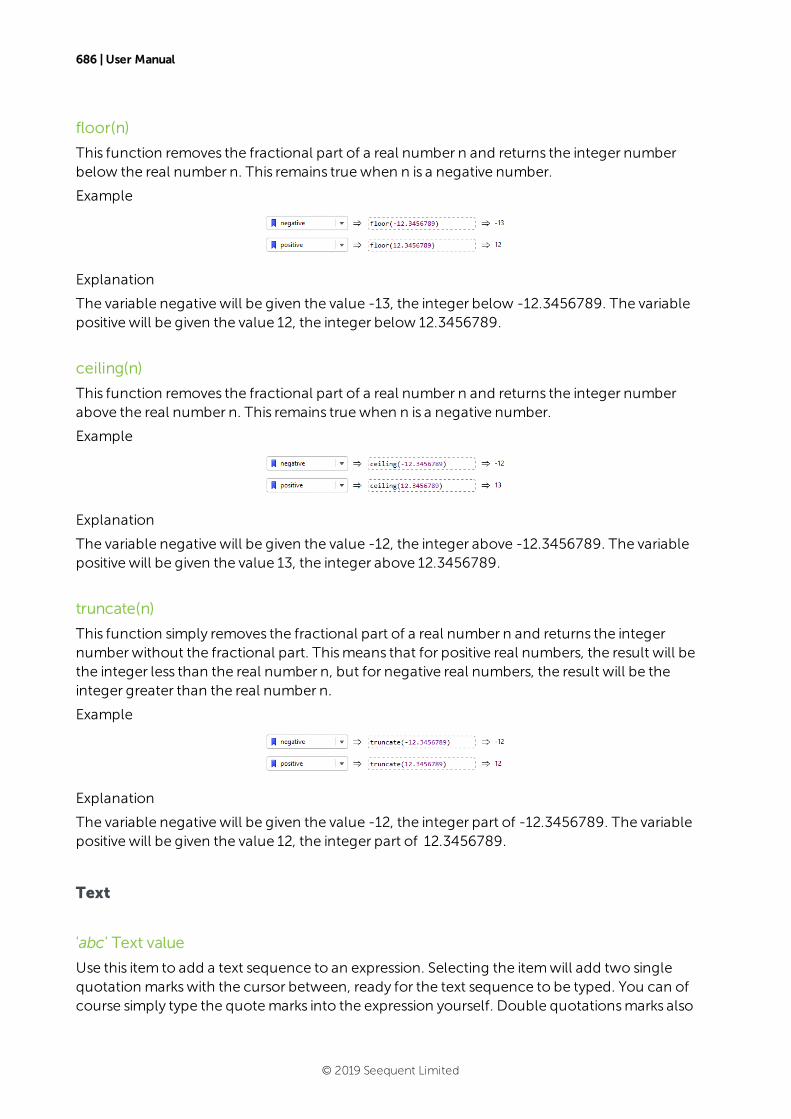
686 | User Manual
floor(n)
This function removes the fractional part of a real number n and returns the integer numberbelow the real number n. This remains truewhen n is a negative number.
Example
Explanation
The variable negative will be given the value -13, the integer below -12.3456789. The variablepositive will be given the value 12, the integer below 12.3456789.
ceiling(n)
This function removes the fractional part of a real number n and returns the integer numberabove the real number n. This remains truewhen n is a negative number.
Example
Explanation
The variable negative will be given the value -12, the integer above -12.3456789. The variablepositive will be given the value 13, the integer above 12.3456789.
truncate(n)
This function simply removes the fractional part of a real number n and returns the integernumberwithout the fractional part. Thismeans that for positive real numbers, the result will bethe integer less than the real number n, but for negative real numbers, the result will be theinteger greater than the real number n.
Example
Explanation
The variable negative will be given the value -12, the integer part of -12.3456789. The variablepositive will be given the value 12, the integer part of 12.3456789.
Text
'abc' Text value
Use this item to add a text sequence to an expression. Selecting the itemwill add two singlequotation markswith the cursor between, ready for the text sequence to be typed. You can ofcourse simply type the quotemarks into the expression yourself. Double quotationsmarks also
© 2019 Seequent Limited
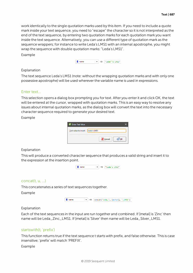
Text | 687
work identically to the single quotation marks used by this item. If you need to include a quotemark inside your text sequence, you need to "escape" the character so it is not interpreted as theend of the text sequence, by entering two quotation marks for each quotation mark you wantinside the text sequence. Alternatively, you can use a different type of quotation mark as thesequencewrappers; for instance towrite Leda's LMS1 with an internal apostrophe, you mightwrap the sequencewith double quotation marks: "Leda's LMS1".
Example
Explanation
The text sequence Leda's LMS1 (note: without thewrapping quotation marks and with only onepossessive apostrophe) will be used wherever the variable name is used in expressions.
Enter text...
This selection opens a dialog box prompting you for text. After you enter it and clickOK, the textwill be entered at the cursor, wrapped with quotation marks. This is an easyway to resolve anyissues about internal quotation marks, as the dialog boxwill convert the text into the necessarycharacter sequence required to generate your desired text.
Example
Explanation
Thiswill produce a converted character sequence that produces a valid string and insert it tothe expression at the insertion point.
concat(t, u, ...)
This concatenates a series of text sequences together.
Example
Explanation
Each of the text sequences in the input are run together and combined. If [metal] is 'Zinc' thennamewill be Leda_Zinc_LMS1. If [metal] is 'Silver' then namewill be Leda_Silver_LMS1.
startswith(t, 'prefix')
This function returns true if the text sequence t startswith prefix, and false otherwise. This is caseinsensitive; 'prefix' will match 'PREFIX'.
Example
© 2019 Seequent Limited
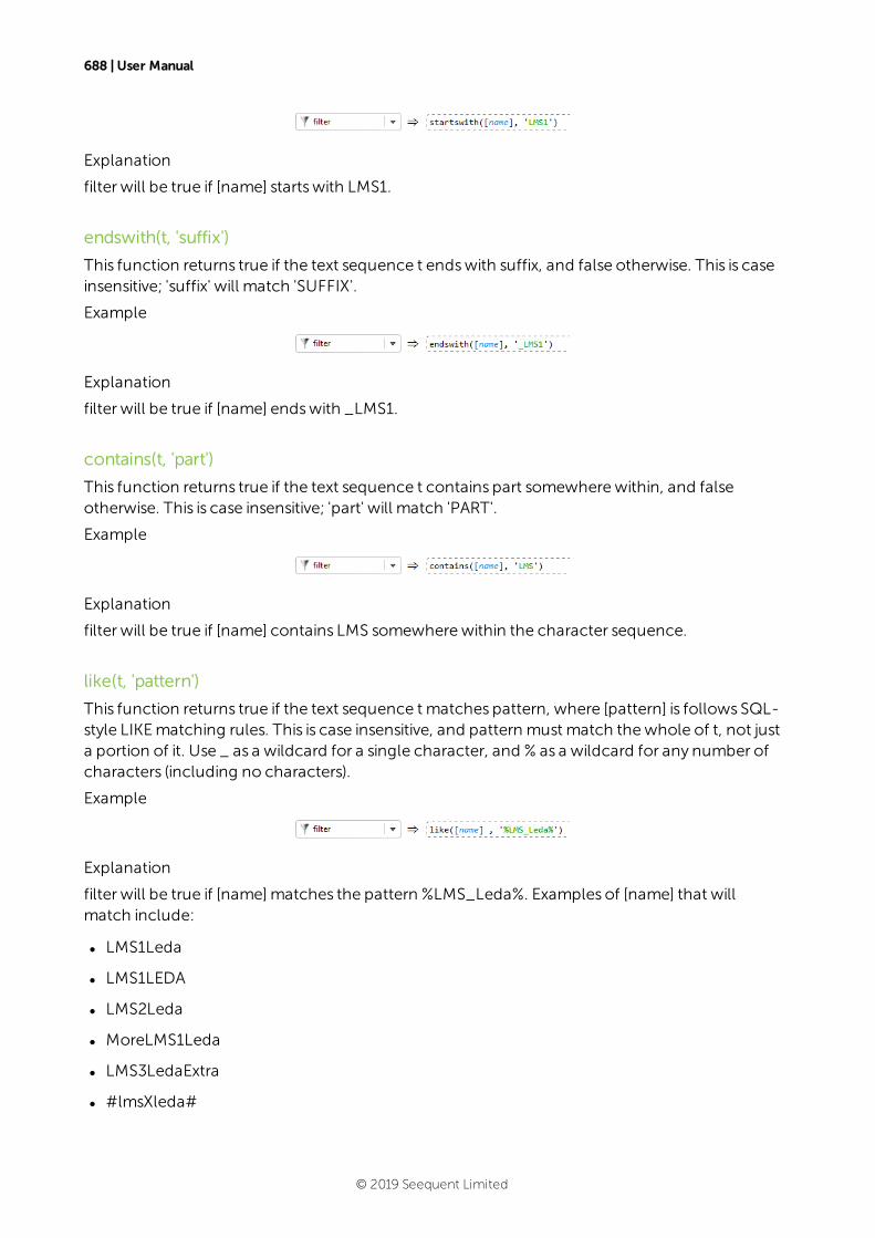
688 | User Manual
Explanation
filter will be true if [name] startswith LMS1.
endswith(t, 'suffix')
This function returns true if the text sequence t endswith suffix, and false otherwise. This is caseinsensitive; 'suffix' will match 'SUFFIX'.
Example
Explanation
filter will be true if [name] endswith _LMS1.
contains(t, 'part')
This function returns true if the text sequence t contains part somewherewithin, and falseotherwise. This is case insensitive; 'part' will match 'PART'.
Example
Explanation
filter will be true if [name] contains LMS somewherewithin the character sequence.
like(t, 'pattern')
This function returns true if the text sequence t matches pattern, where [pattern] is follows SQL-style LIKEmatching rules. This is case insensitive, and pattern must match thewhole of t, not justa portion of it. Use _ as a wildcard for a single character, and % as a wildcard for any number ofcharacters (including no characters).
Example
Explanation
filter will be true if [name]matches the pattern %LMS_Leda%. Examples of [name] that willmatch include:
l LMS1Leda
l LMS1LEDA
l LMS2Leda
l MoreLMS1Leda
l LMS3LedaExtra
l #lmsXleda#
© 2019 Seequent Limited
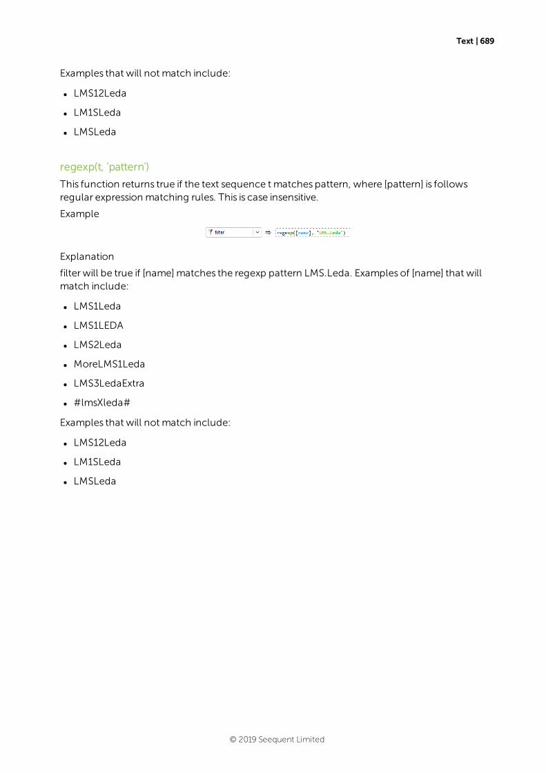
Text | 689
Examples that will not match include:
l LMS12Leda
l LM1SLeda
l LMSLeda
regexp(t, 'pattern')
This function returns true if the text sequence t matches pattern, where [pattern] is followsregular expression matching rules. This is case insensitive.
Example
Explanation
filter will be true if [name]matches the regexp pattern LMS.Leda. Examples of [name] that willmatch include:
l LMS1Leda
l LMS1LEDA
l LMS2Leda
l MoreLMS1Leda
l LMS3LedaExtra
l #lmsXleda#
Examples that will not match include:
l LMS12Leda
l LM1SLeda
l LMSLeda
© 2019 Seequent Limited
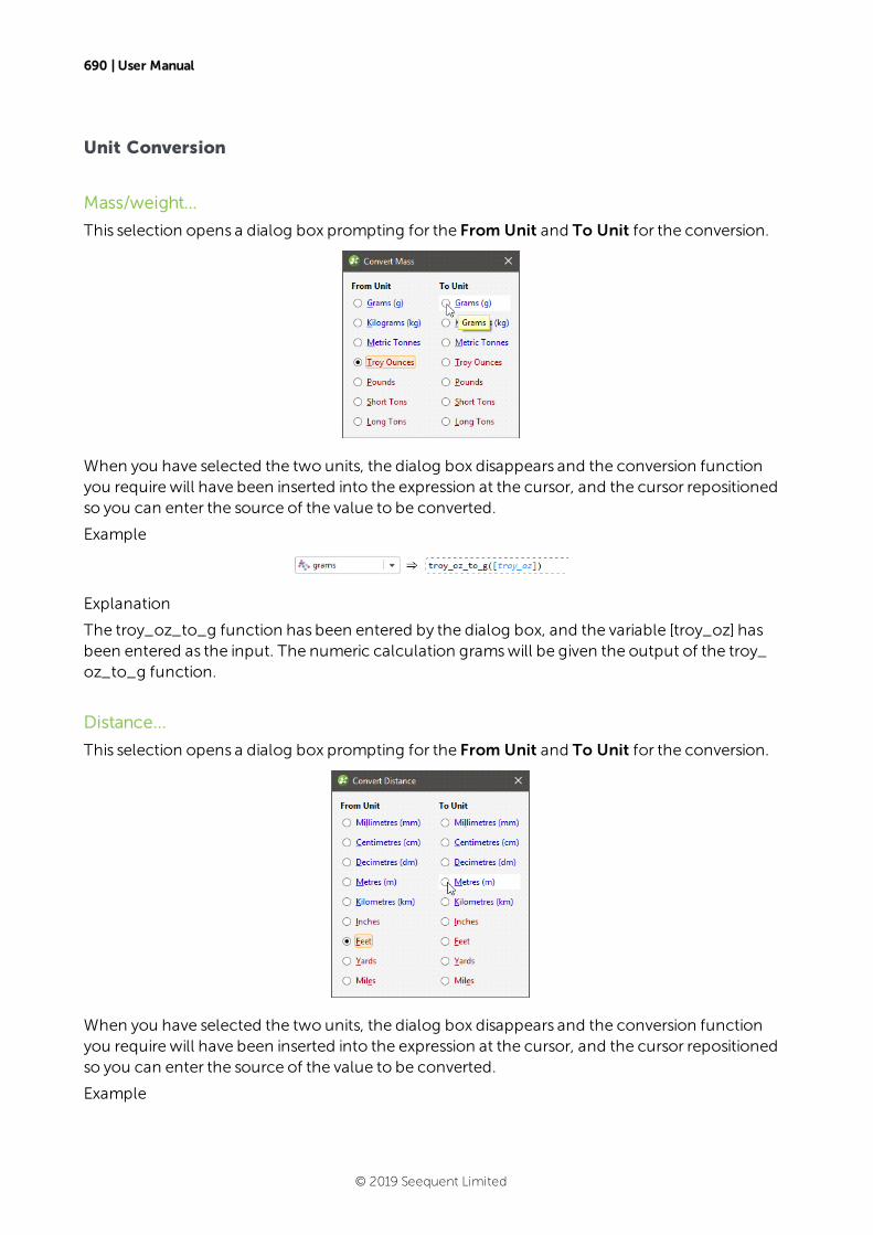
690 | User Manual
Unit Conversion
Mass/weight...
This selection opens a dialog box prompting for the From Unit and To Unit for the conversion.
When you have selected the two units, the dialog box disappears and the conversion functionyou require will have been inserted into the expression at the cursor, and the cursor repositionedso you can enter the source of the value to be converted.
Example
Explanation
The troy_oz_to_g function has been entered by the dialog box, and the variable [troy_oz] hasbeen entered as the input. The numeric calculation gramswill be given the output of the troy_oz_to_g function.
Distance...
This selection opens a dialog box prompting for the From Unit and To Unit for the conversion.
When you have selected the two units, the dialog box disappears and the conversion functionyou require will have been inserted into the expression at the cursor, and the cursor repositionedso you can enter the source of the value to be converted.
Example
© 2019 Seequent Limited
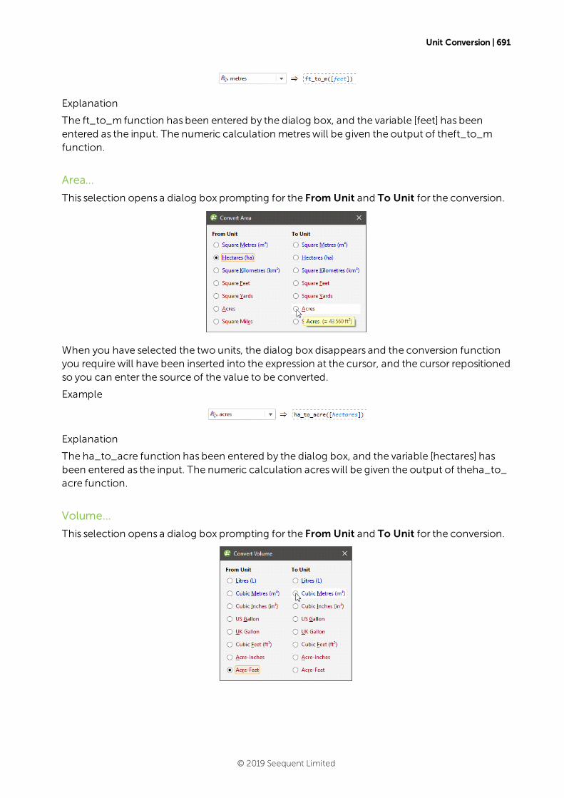
Unit Conversion | 691
Explanation
The ft_to_m function has been entered by the dialog box, and the variable [feet] has beenentered as the input. The numeric calculation metreswill be given the output of theft_to_mfunction.
Area...
This selection opens a dialog box prompting for the From Unit and To Unit for the conversion.
When you have selected the two units, the dialog box disappears and the conversion functionyou require will have been inserted into the expression at the cursor, and the cursor repositionedso you can enter the source of the value to be converted.
Example
Explanation
The ha_to_acre function has been entered by the dialog box, and the variable [hectares] hasbeen entered as the input. The numeric calculation acreswill be given the output of theha_to_acre function.
Volume...
This selection opens a dialog box prompting for the From Unit and To Unit for the conversion.
© 2019 Seequent Limited
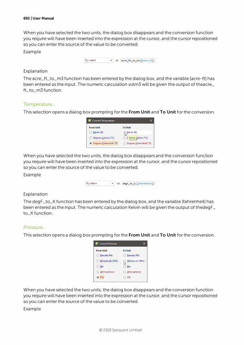
692 | User Manual
When you have selected the two units, the dialog box disappears and the conversion functionyou require will have been inserted into the expression at the cursor, and the cursor repositionedso you can enter the source of the value to be converted.
Example
Explanation
The acre_ft_to_m3 function has been entered by the dialog box, and the variable [acre-ft] hasbeen entered as the input. The numeric calculation volm3will be given the output of theacre_ft_to_m3 function.
Temperature...
This selection opens a dialog box prompting for the From Unit and To Unit for the conversion.
When you have selected the two units, the dialog box disappears and the conversion functionyou require will have been inserted into the expression at the cursor, and the cursor repositionedso you can enter the source of the value to be converted.
Example
Explanation
The degF_to_K function has been entered by the dialog box, and the variable [fahrenheit] hasbeen entered as the input. The numeric calculation Kelvin will be given the output of thedegF_to_K function.
Pressure...
This selection opens a dialog box prompting for the From Unit and To Unit for the conversion.
When you have selected the two units, the dialog box disappears and the conversion functionyou require will have been inserted into the expression at the cursor, and the cursor repositionedso you can enter the source of the value to be converted.
Example
© 2019 Seequent Limited
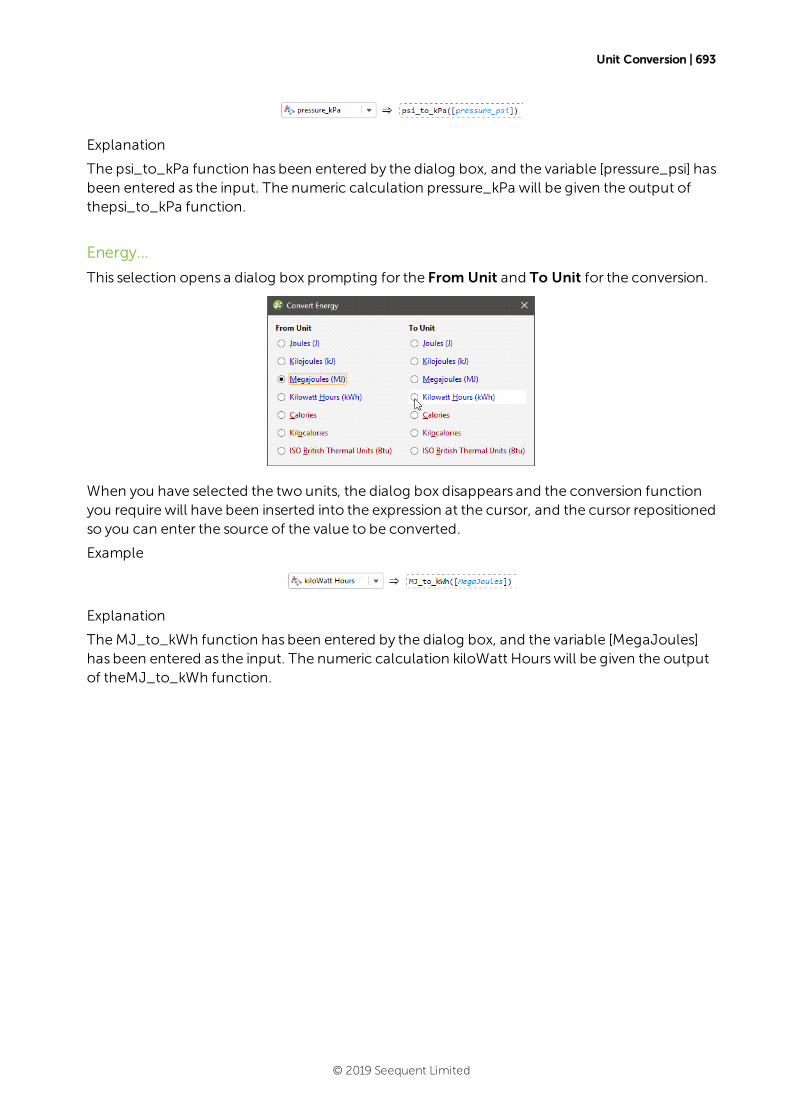
Unit Conversion | 693
Explanation
The psi_to_kPa function has been entered by the dialog box, and the variable [pressure_psi] hasbeen entered as the input. The numeric calculation pressure_kPa will be given the output ofthepsi_to_kPa function.
Energy...
This selection opens a dialog box prompting for the From Unit and To Unit for the conversion.
When you have selected the two units, the dialog box disappears and the conversion functionyou require will have been inserted into the expression at the cursor, and the cursor repositionedso you can enter the source of the value to be converted.
Example
Explanation
TheMJ_to_kWh function has been entered by the dialog box, and the variable [MegaJoules]has been entered as the input. The numeric calculation kiloWatt Hourswill be given the outputof theMJ_to_kWh function.
© 2019 Seequent Limited
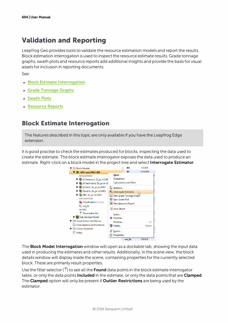
694 | User Manual
Validation and ReportingLeapfrog Geo provides tools to validate the resource estimation models and report the results.Block estimation interrogation is used to inspect the resource estimate results. Grade tonnagegraphs, swath plots and resource reports add additional insights and provide the basis for visualassets for inclusion in reporting documents.
See:
l Block Estimate Interrogation
l Grade Tonnage Graphs
l Swath Plots
l Resource Reports
Block Estimate Interrogation
The features described in this topic are only available if you have the Leapfrog Edgeextension.
It is good practise to check the estimates produced for blocks, inspecting the data used tocreate the estimate. The block estimate interrogator exposes the data used to produce anestimate. Right-click on a blockmodel in the project tree and select Interrogate Estimator.
The Block Model Interrogationwindowwill open as a dockable tab, showing the input dataused in producing the estimates and other results. Additionally, in the scene view, the blockdetailswindowwill display inside the scene, containing properties for the currently selectedblock. These are primarily result properties.
Use the filter selector ( ) to see all the Found data points in the block estimate interrogatortable, or only the data points Included in the estimate, or only the data points that areClamped.TheClamped option will only be present if Outlier Restrictions are being used by theestimator.
© 2019 Seequent Limited
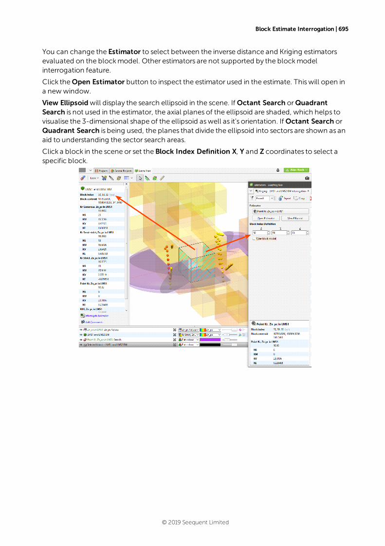
Block Estimate Interrogation | 695
You can change the Estimator to select between the inverse distance and Kriging estimatorsevaluated on the blockmodel. Other estimators are not supported by the blockmodelinterrogation feature.
Click theOpen Estimator button to inspect the estimator used in the estimate. Thiswill open ina newwindow.
View Ellipsoidwill display the search ellipsoid in the scene. If Octant Search orQuadrantSearch is not used in the estimator, the axial planes of the ellipsoid are shaded, which helps tovisualise the 3-dimensional shape of the ellipsoid aswell as it’s orientation. If Octant Search orQuadrant Search is being used, the planes that divide the ellipsoid into sectors are shown as anaid to understanding the sector search areas.
Click a block in the scene or set the Block Index Definition X, Y and Z coordinates to select aspecific block.
© 2019 Seequent Limited
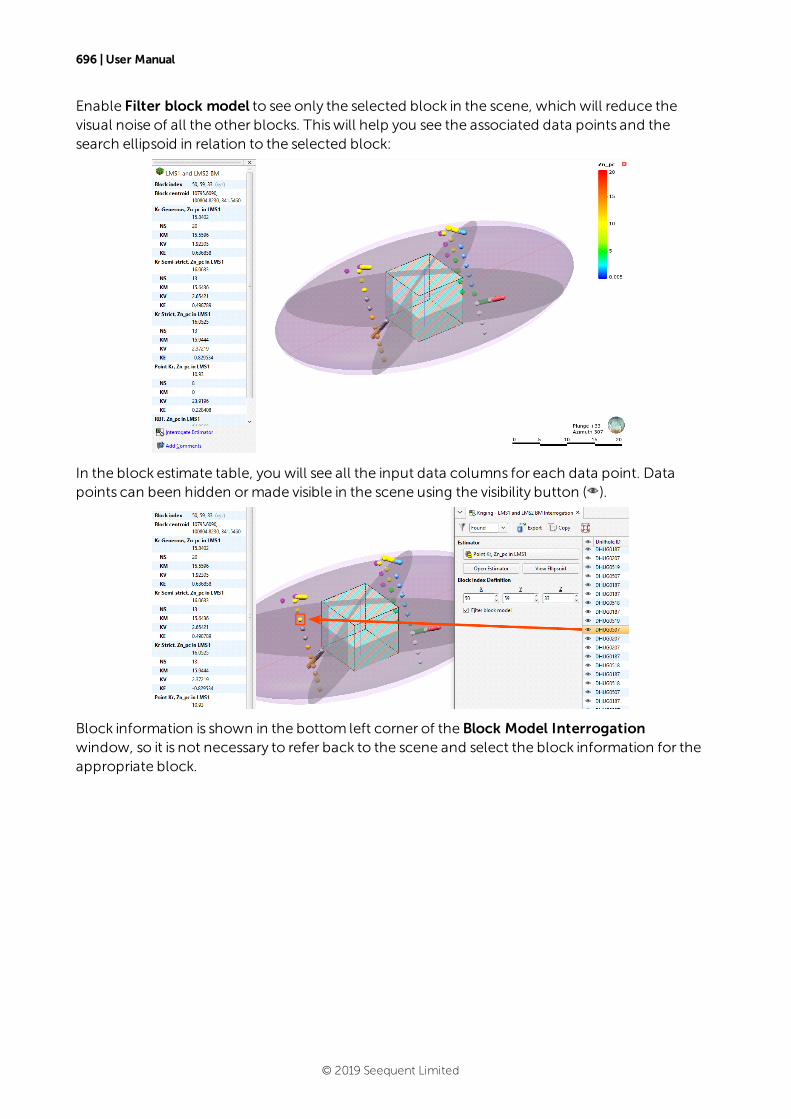
696 | User Manual
Enable Filter block model to see only the selected block in the scene, which will reduce thevisual noise of all the other blocks. Thiswill help you see the associated data points and thesearch ellipsoid in relation to the selected block:
In the block estimate table, you will see all the input data columns for each data point. Datapoints can been hidden ormade visible in the scene using the visibility button ( ).
Block information is shown in the bottom left corner of the Block Model Interrogationwindow, so it is not necessary to refer back to the scene and select the block information for theappropriate block.
© 2019 Seequent Limited
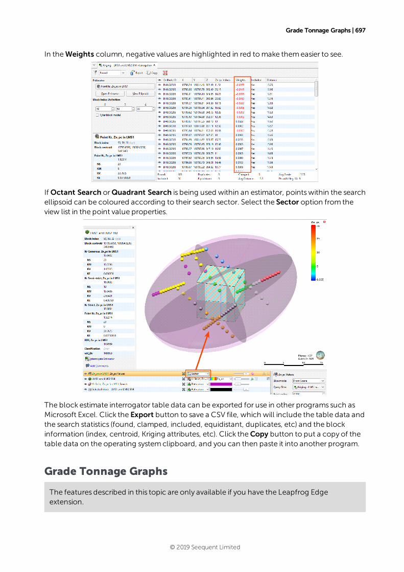
Grade Tonnage Graphs | 697
In theWeights column, negative values are highlighted in red tomake themeasier to see.
If Octant Search orQuadrant Search is being used within an estimator, pointswithin the searchellipsoid can be coloured according to their search sector. Select the Sector option from theview list in the point value properties.
The block estimate interrogator table data can be exported for use in other programs such asMicrosoft Excel. Click the Export button to save a CSV file, which will include the table data andthe search statistics (found, clamped, included, equidistant, duplicates, etc) and the blockinformation (index, centroid, Kriging attributes, etc). Click theCopy button to put a copy of thetable data on the operating systemclipboard, and you can then paste it into another program.
Grade Tonnage Graphs
The features described in this topic are only available if you have the Leapfrog Edgeextension.
© 2019 Seequent Limited
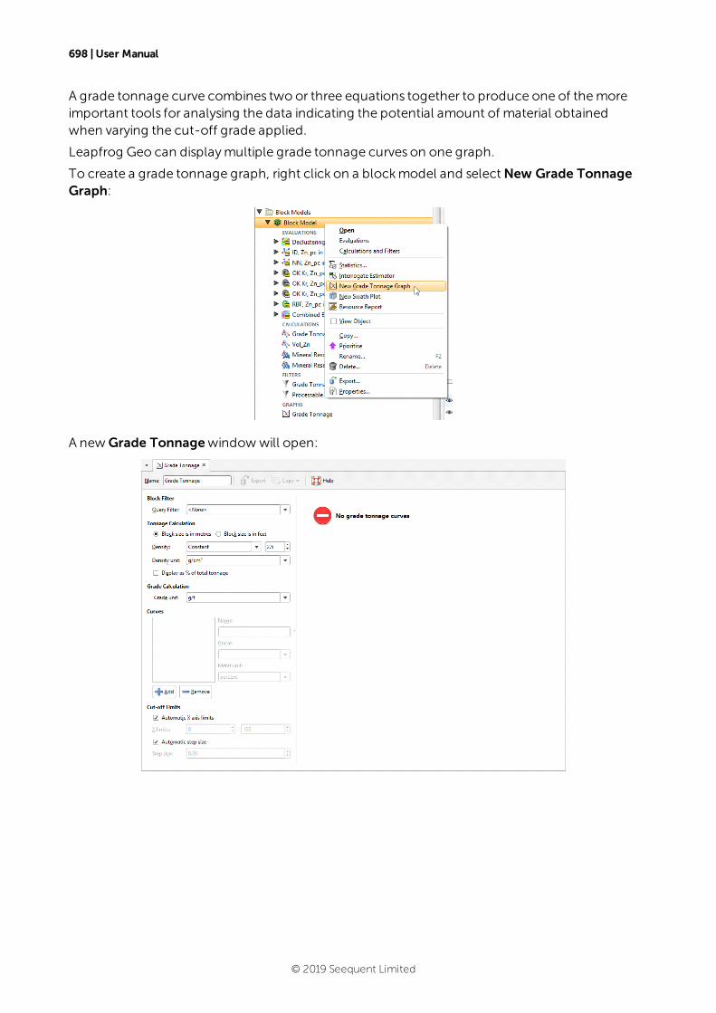
698 | User Manual
A grade tonnage curve combines two or three equations together to produce one of themoreimportant tools for analysing the data indicating the potential amount of material obtainedwhen varying the cut-off grade applied.
Leapfrog Geo can displaymultiple grade tonnage curves on one graph.
To create a grade tonnage graph, right click on a blockmodel and selectNew Grade TonnageGraph:
A new Grade Tonnagewindowwill open:
© 2019 Seequent Limited
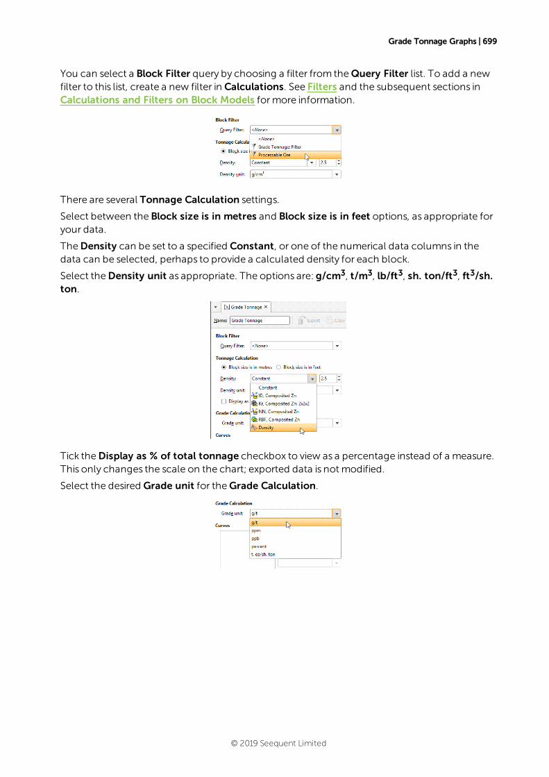
Grade Tonnage Graphs | 699
You can select a Block Filter query by choosing a filter from theQuery Filter list. To add a newfilter to this list, create a new filter in Calculations. See Filters and the subsequent sections inCalculations and Filters on Block Models formore information.
There are several Tonnage Calculation settings.
Select between the Block size is in metres and Block size is in feet options, as appropriate foryour data.
TheDensity can be set to a specified Constant, or one of the numerical data columns in thedata can be selected, perhaps to provide a calculated density for each block.
Select theDensity unit as appropriate. The options are: g/cm3, t/m3, lb/ft3, sh. ton/ft3, ft3/sh.ton.
Tick theDisplay as % of total tonnage checkbox to view as a percentage instead of a measure.This only changes the scale on the chart; exported data is not modified.
Select the desired Grade unit for theGrade Calculation.
© 2019 Seequent Limited
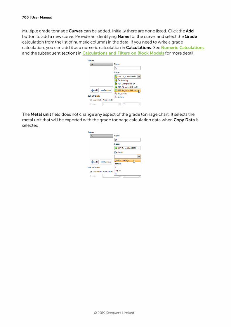
700 | User Manual
Multiple grade tonnageCurves can be added. Initially there are none listed. Click the Addbutton to add a new curve. Provide an identifying Name for the curve, and select theGradecalculation from the list of numeric columns in the data. If you need towrite a gradecalculation, you can add it as a numeric calculation in Calculations. SeeNumeric Calculationsand the subsequent sections in Calculations and Filters on Block Models formore detail.
TheMetal unit field does not change any aspect of the grade tonnage chart. It selects themetal unit that will be exported with the grade tonnage calculation data when Copy Data isselected.
© 2019 Seequent Limited
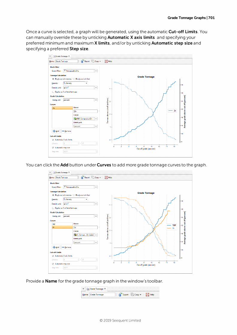
Grade Tonnage Graphs | 701
Once a curve is selected, a graph will be generated, using the automaticCut-off Limits. Youcan manually override these by unticking Automatic X axis limits and specifying yourpreferred minimumand maximumX limits, and/or by unticking Automatic step size andspecifying a preferred Step size.
You can click the Add button underCurves to add more grade tonnage curves to the graph.
Provide a Name for the grade tonnage graph in thewindow’s toolbar.
© 2019 Seequent Limited
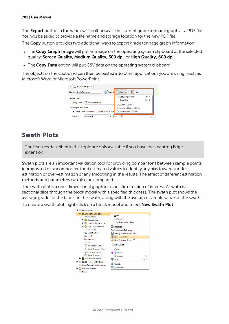
702 | User Manual
The Export button in thewindow’s toolbar saves the current grade tonnage graph as a PDF file.You will be asked to provide a file name and storage location for the new PDF file.
TheCopy button provides two additional ways to export grade tonnage graph information:
l TheCopy Graph Imagewill put an image on the operating systemclipboard at the selectedquality: Screen Quality, Medium Quality, 300 dpi, orHigh Quality, 600 dpi.
l TheCopy Data option will put CSV data on the operating systemclipboard.
The objects on the clipboard can then be pasted into other applications you are using, such asMicrosoft Word orMicrosoft PowerPoint.
Swath Plots
The features described in this topic are only available if you have the Leapfrog Edgeextension.
Swath plots are an important validation tool for providing comparisons between sample points(composited or uncomposited) and estimated values to identify any bias towards under-estimation or over-estimation or any smoothing in the results. The effect of different estimationmethods and parameters can also be compared.
The swath plot is a one-dimensional graph in a specific direction of interest. A swath is asectional slice through the blockmodel with a specified thickness. The swath plot shows theaverage grade for the blocks in the swath, along with the averaged sample values in the swath.
To create a swath plot, right-click on a blockmodel and selectNew Swath Plot:
© 2019 Seequent Limited
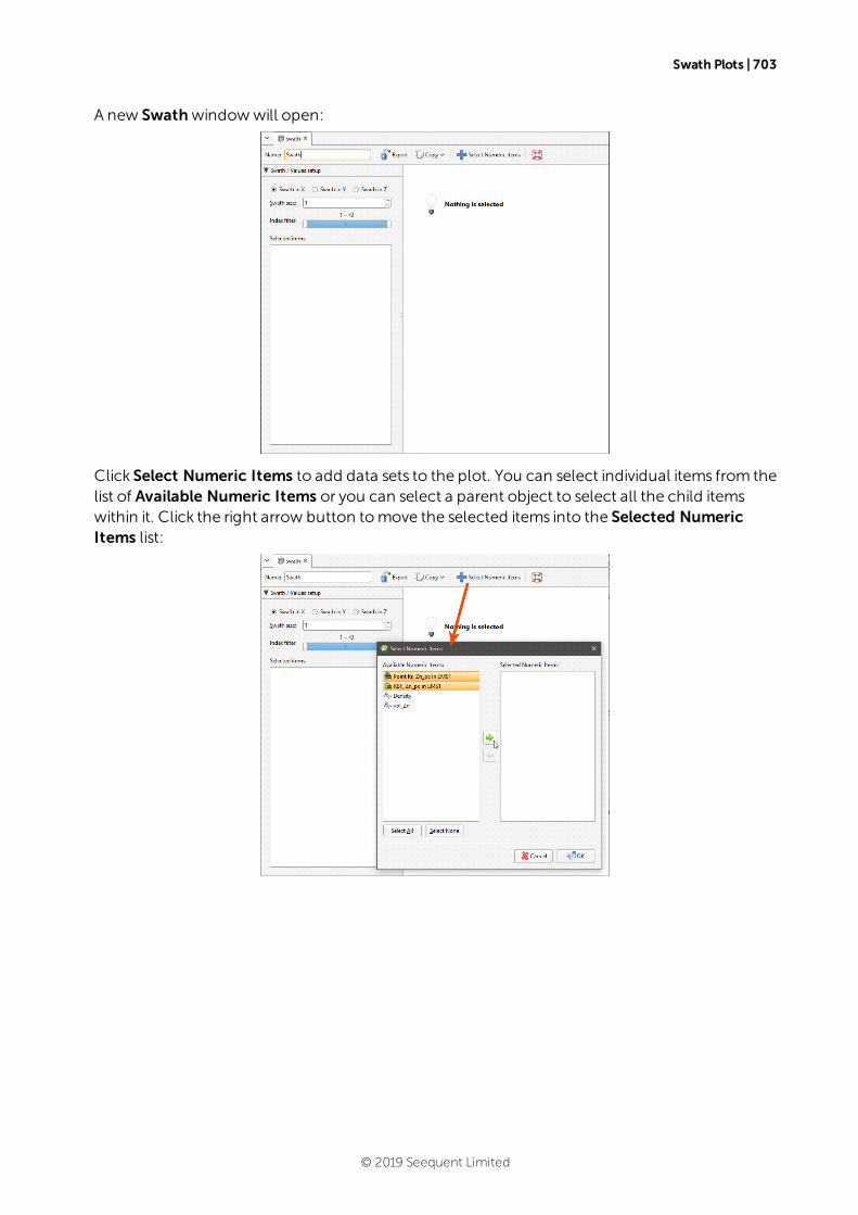
Swath Plots | 703
A new Swathwindowwill open:
Click Select Numeric Items to add data sets to the plot. You can select individual items from thelist of Available Numeric Items or you can select a parent object to select all the child itemswithin it. Click the right arrow button tomove the selected items into the Selected NumericItems list:
© 2019 Seequent Limited
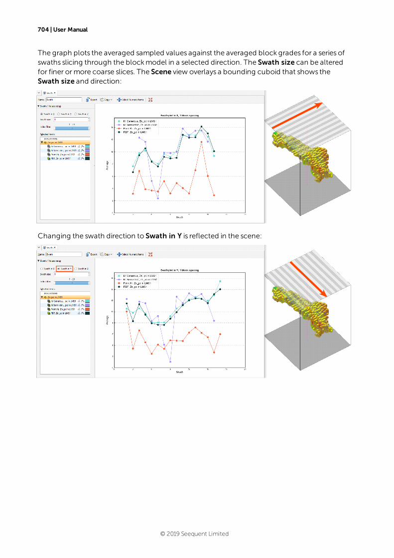
704 | User Manual
The graph plots the averaged sampled values against the averaged block grades for a series ofswaths slicing through the blockmodel in a selected direction. The Swath size can be alteredfor finer ormore coarse slices. The Scene view overlays a bounding cuboid that shows theSwath size and direction:
Changing the swath direction to Swath in Y is reflected in the scene:
© 2019 Seequent Limited
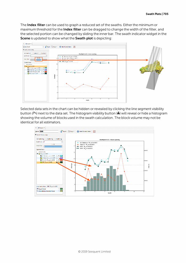
Swath Plots | 705
The Index filter can be used to graph a reduced set of the swaths. Either theminimumormaximum threshold for the Index filter can be dragged to change thewidth of the filter, andthe selected portion can be changed by sliding the inner bar. The swath indicator widget in theScene is updated to showwhat the Swath plot is depicting:
Selected data sets in the chart can be hidden or revealed by clicking the line segment visibilitybutton ( ) next to the data set. The histogramvisibility button ( ) will reveal or hide a histogramshowing the volume of blocks used in the swath calculation. The block volumemay not beidentical for all estimators.
© 2019 Seequent Limited
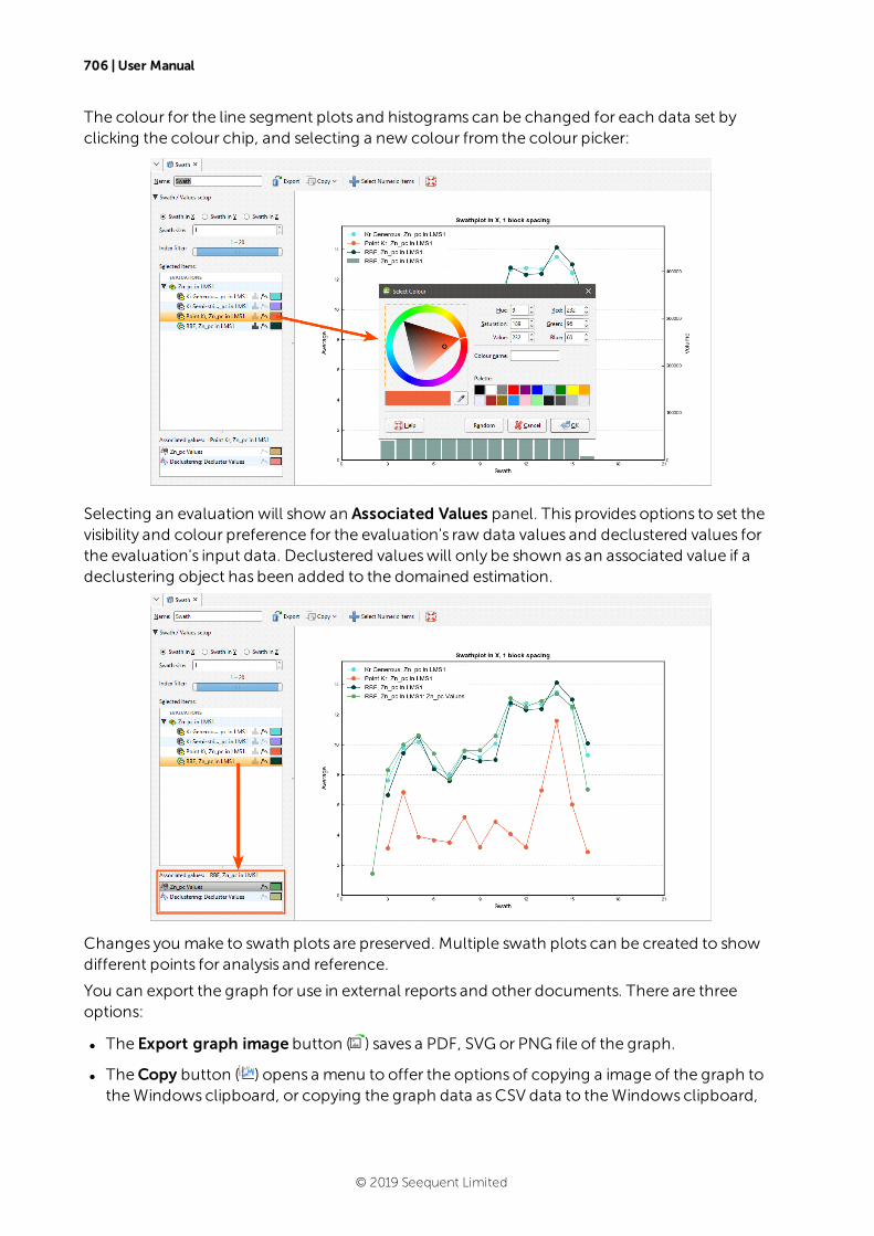
706 | User Manual
The colour for the line segment plots and histograms can be changed for each data set byclicking the colour chip, and selecting a new colour from the colour picker:
Selecting an evaluation will show an Associated Values panel. This provides options to set thevisibility and colour preference for the evaluation's raw data values and declustered values forthe evaluation's input data. Declustered valueswill only be shown as an associated value if adeclustering object has been added to the domained estimation.
Changes you make to swath plots are preserved. Multiple swath plots can be created to showdifferent points for analysis and reference.
You can export the graph for use in external reports and other documents. There are threeoptions:
l The Export graph image button ( ) saves a PDF, SVG or PNG file of the graph.
l TheCopy button ( ) opens a menu to offer the options of copying a image of the graph totheWindows clipboard, or copying the graph data asCSV data to theWindows clipboard,
© 2019 Seequent Limited
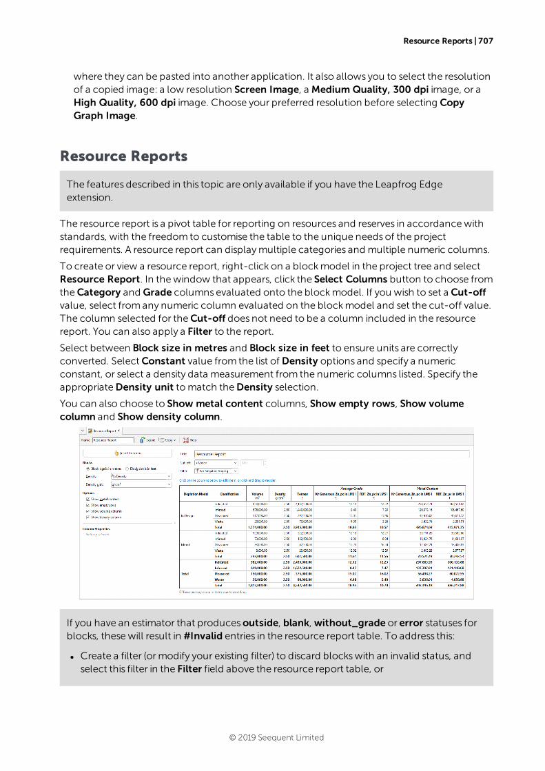
Resource Reports | 707
where they can be pasted into another application. It also allows you to select the resolutionof a copied image: a low resolution Screen Image, a Medium Quality, 300 dpi image, or aHigh Quality, 600 dpi image. Choose your preferred resolution before selecting CopyGraph Image.
Resource Reports
The features described in this topic are only available if you have the Leapfrog Edgeextension.
The resource report is a pivot table for reporting on resources and reserves in accordancewithstandards, with the freedom to customise the table to the unique needs of the projectrequirements. A resource report can displaymultiple categories and multiple numeric columns.
To create or view a resource report, right-click on a blockmodel in the project tree and selectResource Report. In thewindow that appears, click the Select Columns button to choose fromtheCategory and Grade columns evaluated onto the blockmodel. If you wish to set a Cut-offvalue, select fromany numeric column evaluated on the blockmodel and set the cut-off value.The column selected for theCut-off does not need to be a column included in the resourcereport. You can also apply a Filter to the report.
Select between Block size in metres and Block size in feet to ensure units are correctlyconverted. SelectConstant value from the list of Density options and specify a numericconstant, or select a density data measurement from the numeric columns listed. Specify theappropriateDensity unit tomatch theDensity selection.
You can also choose to Show metal content columns, Show empty rows, Show volumecolumn and Show density column.
If you have an estimator that producesoutside, blank, without_grade or error statuses forblocks, thesewill result in #Invalid entries in the resource report table. To address this:
l Create a filter (ormodify your existing filter) to discard blockswith an invalid status, andselect this filter in the Filter field above the resource report table, or
© 2019 Seequent Limited
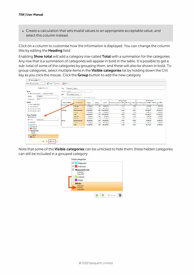
708 | User Manual
l Create a calculation that sets invalid values to an appropriate acceptable value, andselect this column instead.
Click on a column to customise how the information is displayed. You can change the columntitle by editing theHeading field.
Enabling Show totalwill add a category row called Totalwith a summation for the categories.Any row that is a summation of categorieswill appear in bold in the table. It is possible to get asub-total of some of the categories by grouping them, and thesewill also be shown in bold. Togroup categories, select multiple items in the Visible categories list by holding down the Ctrlkey as you click themouse. Click theGroup button to add the new category.
Note that some of the Visible categories can be unticked to hide them; these hidden categoriescan still be included in a grouped category:
© 2019 Seequent Limited
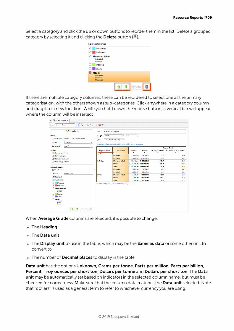
Resource Reports | 709
Select a category and click the up or down buttons to reorder them in the list. Delete a groupedcategory by selecting it and clicking theDelete button ( ).
If there aremultiple category columns, these can be reordered to select one as the primarycategorisation, with the others shown as sub-categories. Click anywhere in a category columnand drag it to a new location. While you hold down themouse button, a vertical bar will appearwhere the column will be inserted:
When Average Grade columns are selected, it is possible to change:
l TheHeading
l TheData unit
l TheDisplay unit to use in the table, which may be the Same as data or some other unit toconvert to
l The number of Decimal places to display in the table
Data unit has the optionsUnknown, Grams per tonne, Parts per million, Parts per billion,Percent, Troy ounces per short ton, Dollars per tonne and Dollars per short ton. TheDataunit may be automatically set based on indicators in the selected column name, but must bechecked for correctness. Make sure that the column data matches theData unit selected. Notethat "dollars" is used as a general term to refer to whichever currency you are using.
© 2019 Seequent Limited
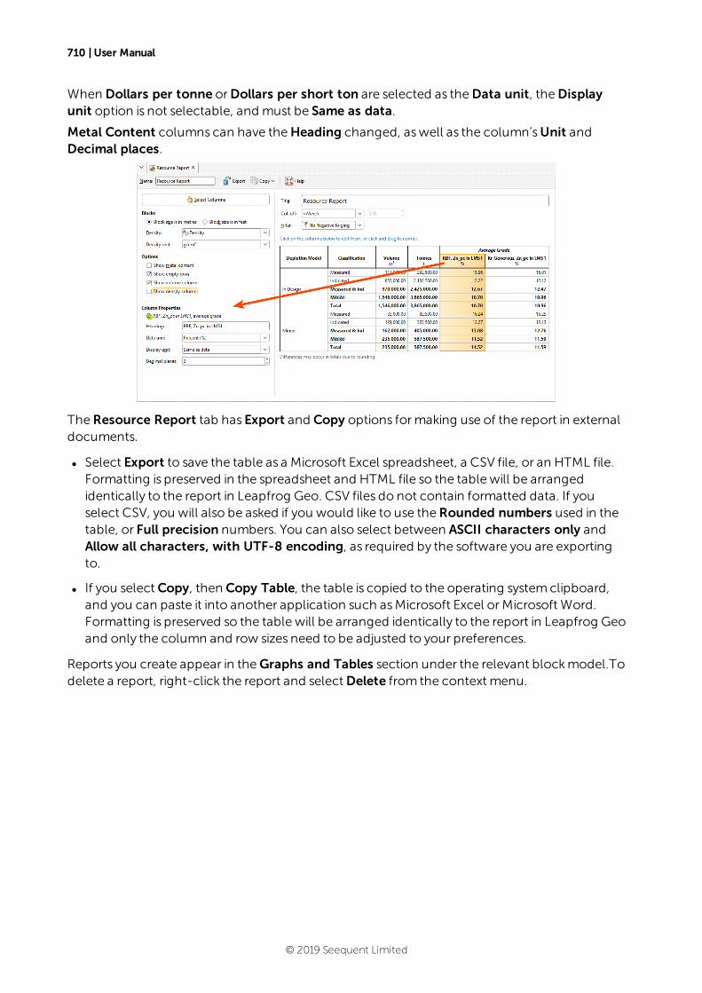
710 | User Manual
When Dollars per tonne orDollars per short ton are selected as theData unit, theDisplayunit option is not selectable, and must be Same as data.
Metal Content columns can have theHeading changed, aswell as the column’sUnit andDecimal places.
TheResource Report tab hasExport and Copy options formaking use of the report in externaldocuments.
l Select Export to save the table as a Microsoft Excel spreadsheet, a CSV file, or an HTML file.Formatting is preserved in the spreadsheet and HTML file so the table will be arrangedidentically to the report in Leapfrog Geo. CSV files do not contain formatted data. If youselect CSV, you will also be asked if you would like to use theRounded numbers used in thetable, or Full precision numbers. You can also select between ASCII characters only andAllow all characters, with UTF-8 encoding, as required by the software you are exportingto.
l If you selectCopy, then Copy Table, the table is copied to the operating systemclipboard,and you can paste it into another application such asMicrosoft Excel orMicrosoft Word.Formatting is preserved so the table will be arranged identically to the report in Leapfrog Geoand only the column and row sizes need to be adjusted to your preferences.
Reports you create appear in theGraphs and Tables section under the relevant blockmodel.Todelete a report, right-click the report and selectDelete from the context menu.
© 2019 Seequent Limited
Presentation
Leapfrog Geo has a number of tools for displaying and presenting data for use in reports andpresentations.
l Sharemodels and data to View, a web-based model sharing platform that allows you tovisualise 3Dmodels and share themwith collaborators. SeeUploading to View.
l Create and export cross sections, fence sections and serial sections. See Sections.
l Create and export contours. SeeContour Lines.
l Render and save images for use outside of Leapfrog Geo. SeeRendered Images.
l Save scenes that demonstrate different aspects of themodel and themodel-buildingprocess. These scenes can then be saved as a movie or as a scene file that can be opened inLeapfrog Viewer. See Saved Scenes.
See Visualising Data for information about the tools available in Leapfrog Geo for changinghow data is displayed.
Uploading to ViewView is a web-based model sharing platform. You can upload Leapfrog Geo data to View,visualise the data and organise it into slides. You can also share viewswith collaborators, all inyourweb browser, with data saved securely to the cloud. All your collaborators need is a MySeequent ID; a Leapfrog Geo entitlement is not required.
There are twoworkflows for uploading data fromLeapfrog Geo to View, uploading the datacurrently displayed in the 3D scene and uploading saved scenes. Both techniques are describedbelow, but first it is important to understand how View handles data objects uploaded fromLeapfrog Geo.
© 2019 Seequent Limited
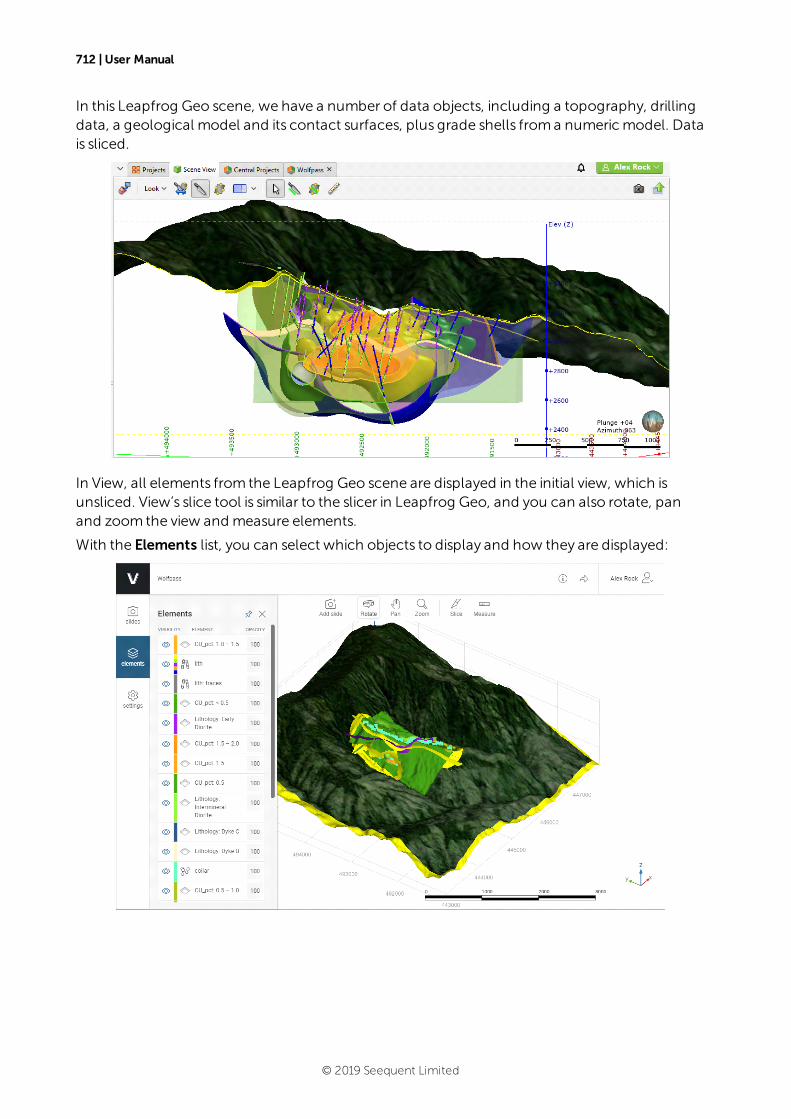
712 | User Manual
In this Leapfrog Geo scene, we have a number of data objects, including a topography, drillingdata, a geological model and its contact surfaces, plus grade shells froma numericmodel. Datais sliced.
In View, all elements from the Leapfrog Geo scene are displayed in the initial view, which isunsliced. View’s slice tool is similar to the slicer in Leapfrog Geo, and you can also rotate, panand zoom the view and measure elements.
With the Elements list, you can select which objects to display and how they are displayed:
© 2019 Seequent Limited
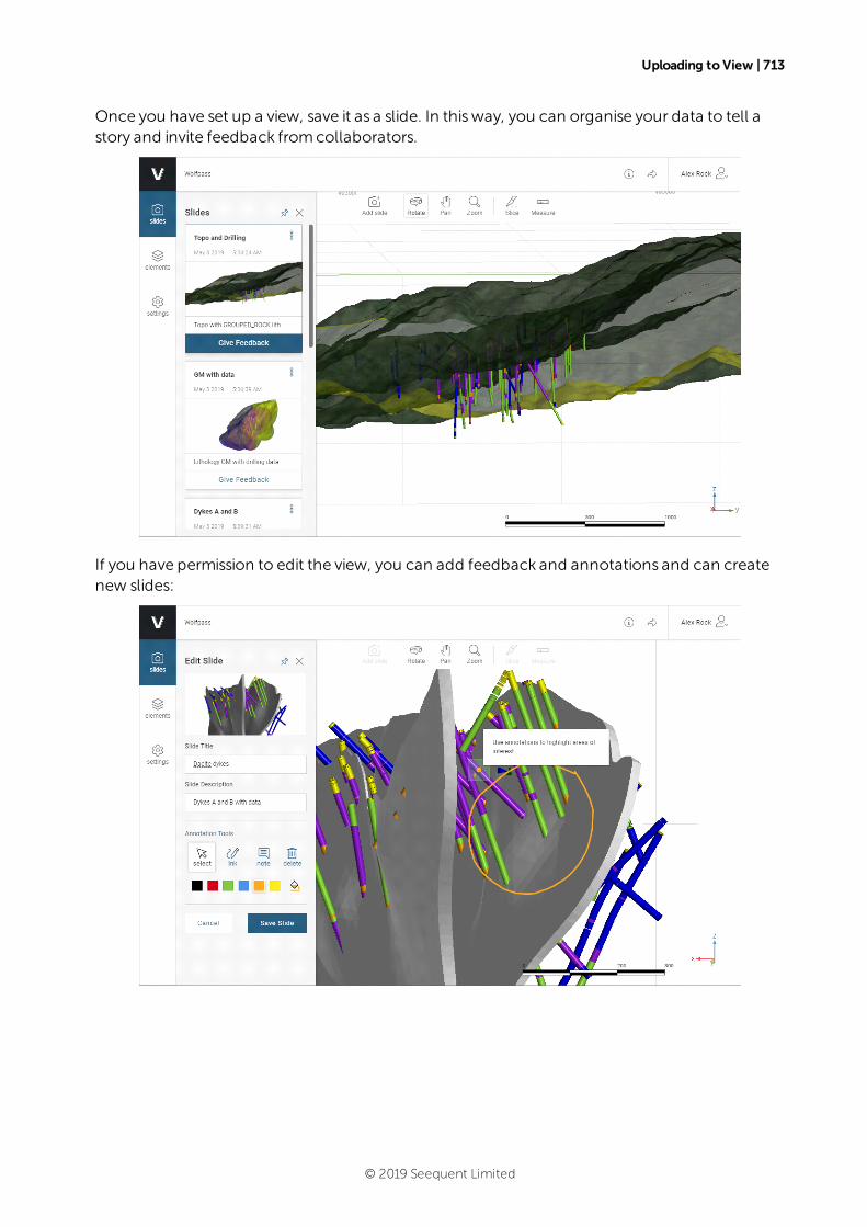
Uploading to View | 713
Once you have set up a view, save it as a slide. In thisway, you can organise your data to tell astory and invite feedback fromcollaborators.
If you have permission to edit the view, you can add feedback and annotations and can createnew slides:
© 2019 Seequent Limited
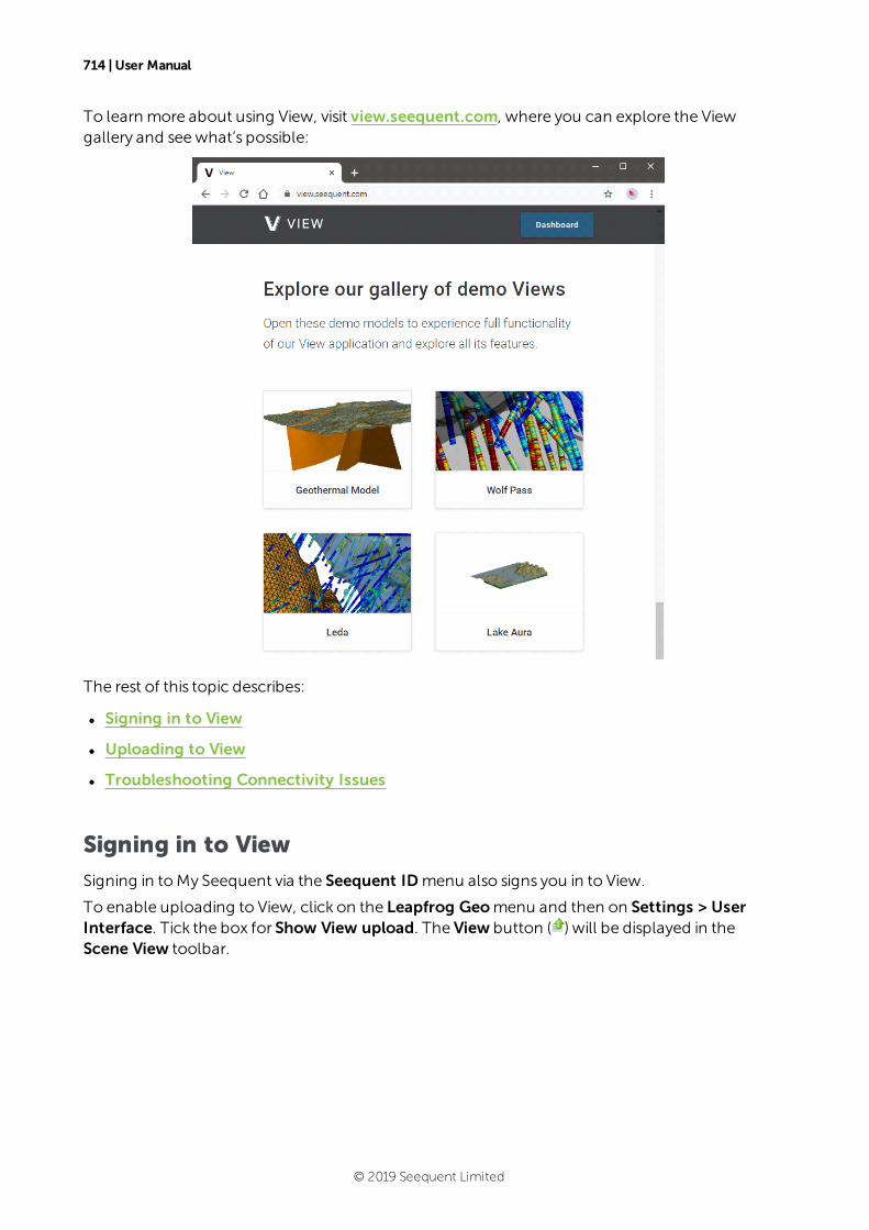
714 | User Manual
To learn more about using View, visit view.seequent.com, where you can explore the Viewgallery and seewhat’s possible:
The rest of this topic describes:
l Signing in to View
l Uploading to View
l Troubleshooting Connectivity Issues
Signing in to View
Signing in toMy Seequent via the Seequent IDmenu also signs you in to View.
To enable uploading to View, click on the Leapfrog Geomenu and then on Settings > UserInterface. Tick the box for Show View upload. The View button ( ) will be displayed in theScene View toolbar.
© 2019 Seequent Limited
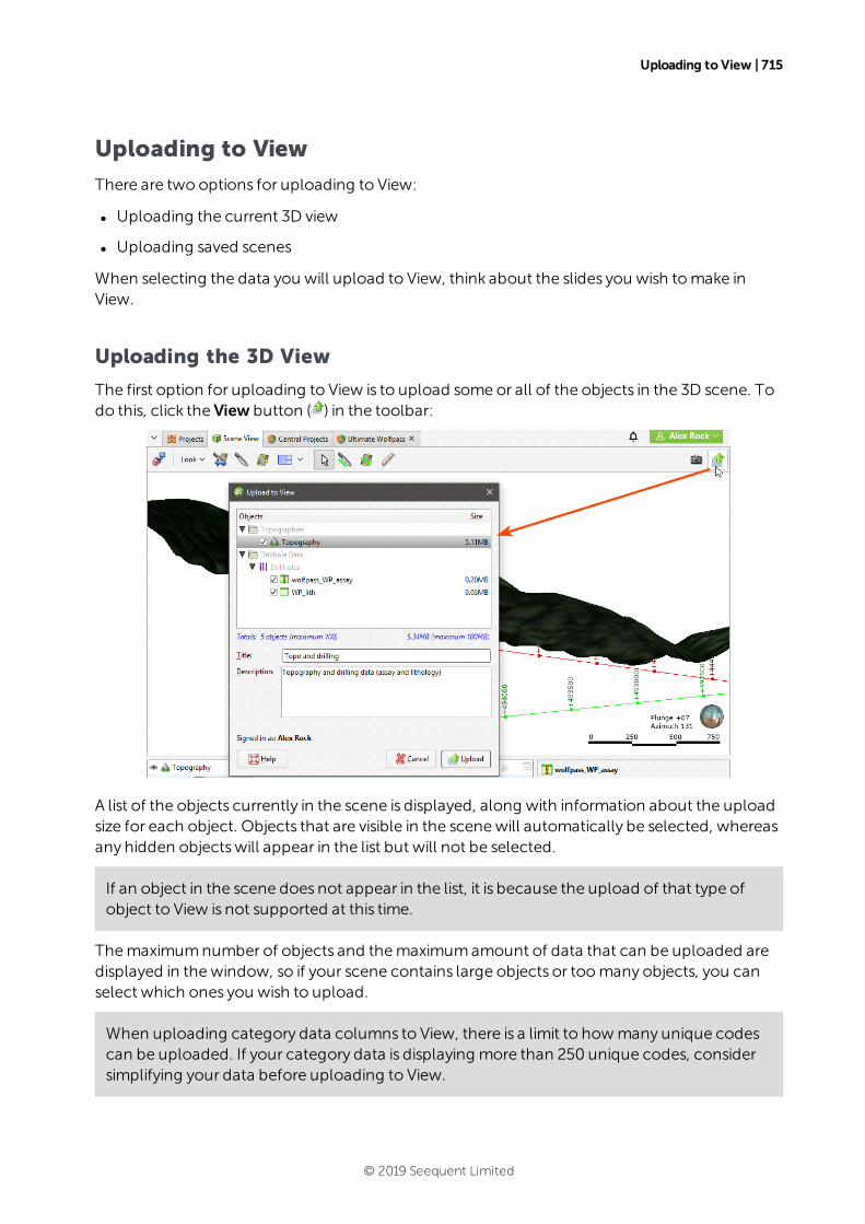
Uploading to View | 715
Uploading to View
There are two options for uploading to View:
l Uploading the current 3D view
l Uploading saved scenes
When selecting the data you will upload to View, think about the slides you wish tomake inView.
Uploading the 3D View
The first option for uploading to View is to upload some or all of the objects in the 3D scene. Todo this, click the View button ( ) in the toolbar:
A list of the objects currently in the scene is displayed, along with information about the uploadsize for each object. Objects that are visible in the scenewill automatically be selected, whereasany hidden objectswill appear in the list but will not be selected.
If an object in the scene does not appear in the list, it is because the upload of that type ofobject to View is not supported at this time.
Themaximumnumber of objects and themaximumamount of data that can be uploaded aredisplayed in thewindow, so if your scene contains large objects or toomany objects, you canselect which ones you wish to upload.
When uploading category data columns to View, there is a limit to howmany unique codescan be uploaded. If your category data is displaying more than 250 unique codes, considersimplifying your data before uploading to View.
© 2019 Seequent Limited
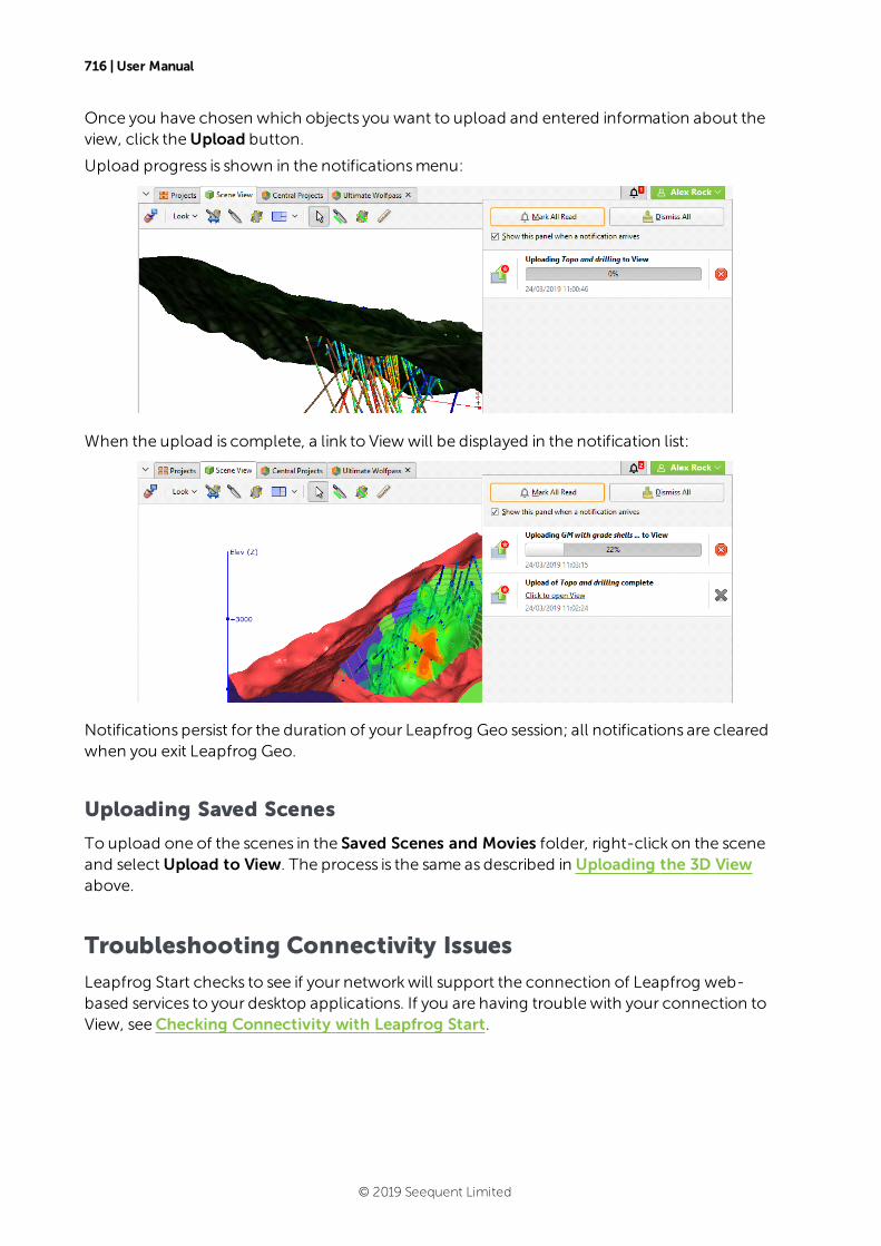
716 | User Manual
Once you have chosen which objects you want to upload and entered information about theview, click theUpload button.
Upload progress is shown in the notificationsmenu:
When the upload is complete, a link to View will be displayed in the notification list:
Notifications persist for the duration of your Leapfrog Geo session; all notifications are clearedwhen you exit Leapfrog Geo.
Uploading Saved Scenes
To upload one of the scenes in the Saved Scenes and Movies folder, right-click on the sceneand selectUpload to View. The process is the same as described in Uploading the 3D Viewabove.
Troubleshooting Connectivity Issues
Leapfrog Start checks to see if your networkwill support the connection of Leapfrog web-based services to your desktop applications. If you are having trouble with your connection toView, seeChecking Connectivity with Leapfrog Start.
© 2019 Seequent Limited
Sections | 717
SectionsThere are three types of sections in Leapfrog Geo:
l A typical cross section is a vertical planewith an image or geologic cross section applied to it.In Leapfrog Geo, this type of cross section can be created directly in the scene, from theslicer or froman imported image.
l A fence section deviates. In Leapfrog Geo, a fence section can be created froma polylinedrawn in the scene or fromany line object in the project.
l A serial section is a series of typical cross sections taken at an offset froma single base section.
Evaluating on Sections
Different objects in the project can be evaluated on sections, as described in Evaluations. Suchobjects include:
l Geological models
l Numericmodels
l Distance functions
l Surfaces
l GIS lines
l Polylines
l Combined models
When evaluating objects on sections, you can limit the evaluation to the section extents. To dothis, enable theClip evaluations to section extents option when selecting what objects youare evaluating.
Blockmodels can be evaluated on cross sections but not on serial sections and fence sections.
Objects evaluated on sections can be included when the section is exported.
Exporting Sections
Sections can be exported in the following formats:
l DXF Files (11/12 [AC1009]) (*.dxf)
l Drawing Files (2013/LT2013) (*.dwg)
l BentleyDrawing Files (v8) (*.dgn)
Exporting a section as a DXF file (*.dxf) exports a series of DXF lines created from the intersectionof the evaluation volumes and the section plane. The lines generated fromeach volume aresaved as separate layers in the file.
© 2019 Seequent Limited
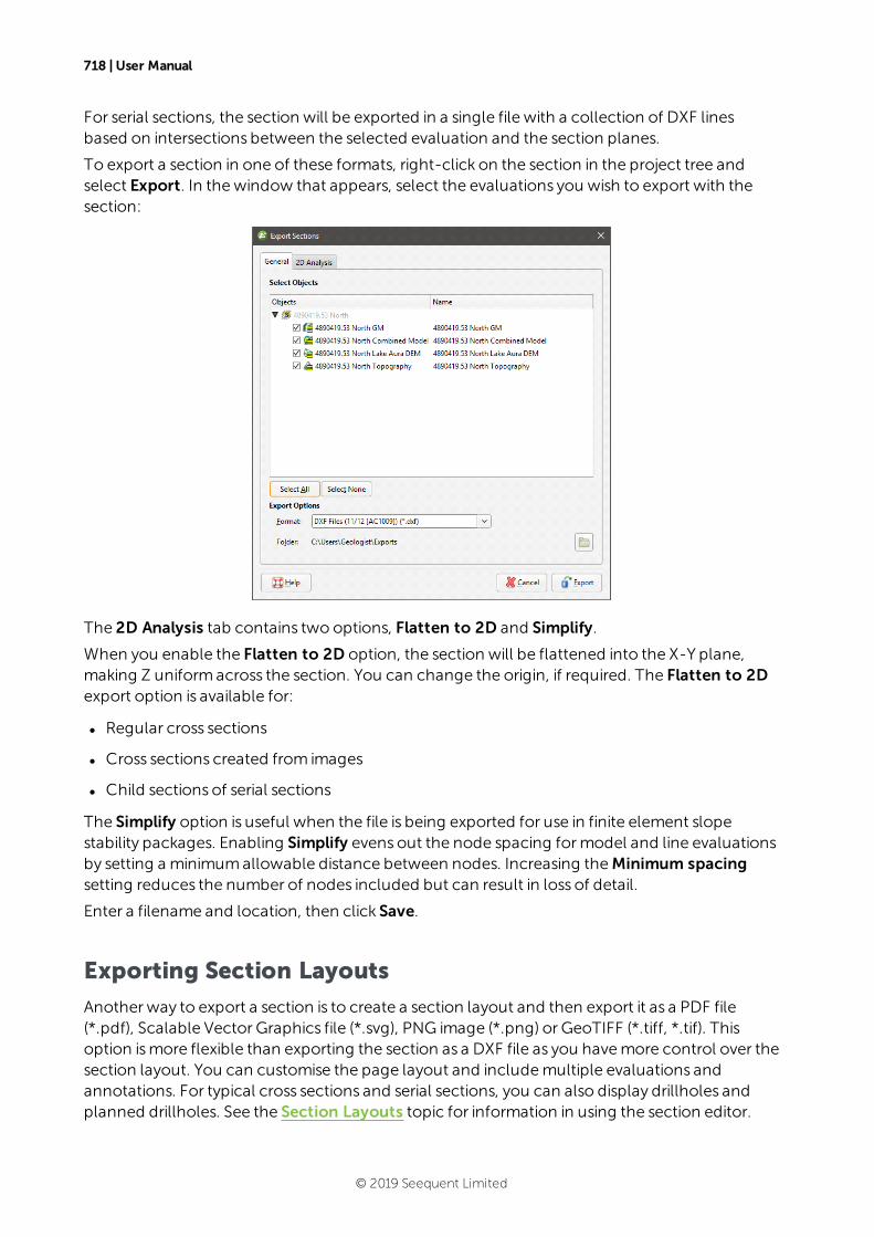
718 | User Manual
For serial sections, the section will be exported in a single file with a collection of DXF linesbased on intersections between the selected evaluation and the section planes.
To export a section in one of these formats, right-click on the section in the project tree andselect Export. In thewindow that appears, select the evaluations you wish to export with thesection:
The 2D Analysis tab contains two options, Flatten to 2D and Simplify.
When you enable the Flatten to 2D option, the section will be flattened into the X-Y plane,making Z uniformacross the section. You can change the origin, if required. The Flatten to 2Dexport option is available for:
l Regular cross sections
l Cross sections created from images
l Child sections of serial sections
The Simplify option is useful when the file is being exported for use in finite element slopestability packages. Enabling Simplify evens out the node spacing formodel and line evaluationsby setting a minimumallowable distance between nodes. Increasing theMinimum spacingsetting reduces the number of nodes included but can result in loss of detail.
Enter a filename and location, then click Save.
Exporting Section Layouts
Another way to export a section is to create a section layout and then export it as a PDF file(*.pdf), Scalable Vector Graphics file (*.svg), PNG image (*.png) or GeoTIFF (*.tiff, *.tif). Thisoption ismore flexible than exporting the section as a DXF file as you havemore control over thesection layout. You can customise the page layout and includemultiple evaluations andannotations. For typical cross sections and serial sections, you can also display drillholes andplanned drillholes. See the Section Layouts topic for information in using the section editor.
© 2019 Seequent Limited

Creating Cross Sections | 719
Once you have finished adjusting the section layout, you can export it in one of the followingformats:
l PDF Files (*.pdf)
l Scalable Vector Graphics Files (*.svg)
l PNG Image Files (*.png)
l GeoTIFF Files (*.tiff, *.tif)
Click the Save and Export button ( ) at the top of thewindow. You will be prompted for afilename and location.
For serial sections, you can batch export multiple section layouts.All selected sections can beexported as a single PDF or individually in PDF file (*.pdf), Scalable Vector Graphics file (*.svg),PNG image (*.png) or GeoTIFF (*.tiff, *.tif) formats. When section layouts are exportedindividually, all outputs can be combined into a zip archive. To do this, right-click on theCrossSections and Contours folder and select Batch Export Layouts.
In thewindow that appears, selection the layouts you wish to export, then select a format. If youselect a format other than Single PDF, you can combine all outputs into a zip archive. Selectwhere you wish to save the outputs, then click Export. Progresswill be displayed at the top ofthe Batch Export Section Layouts window:
Creating Cross Sections
To create a cross section in the scene, add a model to the scene. Next, right-click on theCrossSections and Contours folder and selectNew Cross Section. TheNew Cross Sectionwindowwill appear, together with a section plane and controls in the scene that let you adjust theposition of the section plane:
If the slicer is already in the scenewhen you selectNew Cross Section, the position of theslicer will be used to define the initial orientation of the section. This is an effective way of
© 2019 Seequent Limited

720 | User Manual
creating a section from the slicer: add themodel to the scene, draw a slice and then create across section.
The front (F) and back (B) of the section plane is indicated in the scene. To swap the front andback, click the Swap Front button ( ).
Use the handles in the scene to position the section plane. The handleswork in the samemanner as themoving plane controls, as described in The Moving Plane.
Two buttons in theNew Cross Sectionwindow let you create a cross section that is alignednorth-to-south ( ) or east-to-west ( ):
The other two buttons are active when the slicer is in the scene. Clicking the Set section toslicer button ( ) creates a cross section from the position of the slicer in the scene. When theLock section to slicer button ( ) is enabled, moving the position of the slicer will update theposition of the cross section in theNew Cross Sectionwindow.
Once the section plane is positioned as required, clickOK to create the new cross section, whichwill appear in theCross Sections and Contours folder. Display it by clearing the scene, thenadding the cross section to the scene.
Many objects in a project can be evaluated on cross sections, as described in Evaluations. Suchobjects include:
l Geological models
l Interpolants
l Distance functions
l Surfaces
l GIS lines
l Polylines
Objects evaluated on a cross section or fence section can be included when the section isexported.
© 2019 Seequent Limited
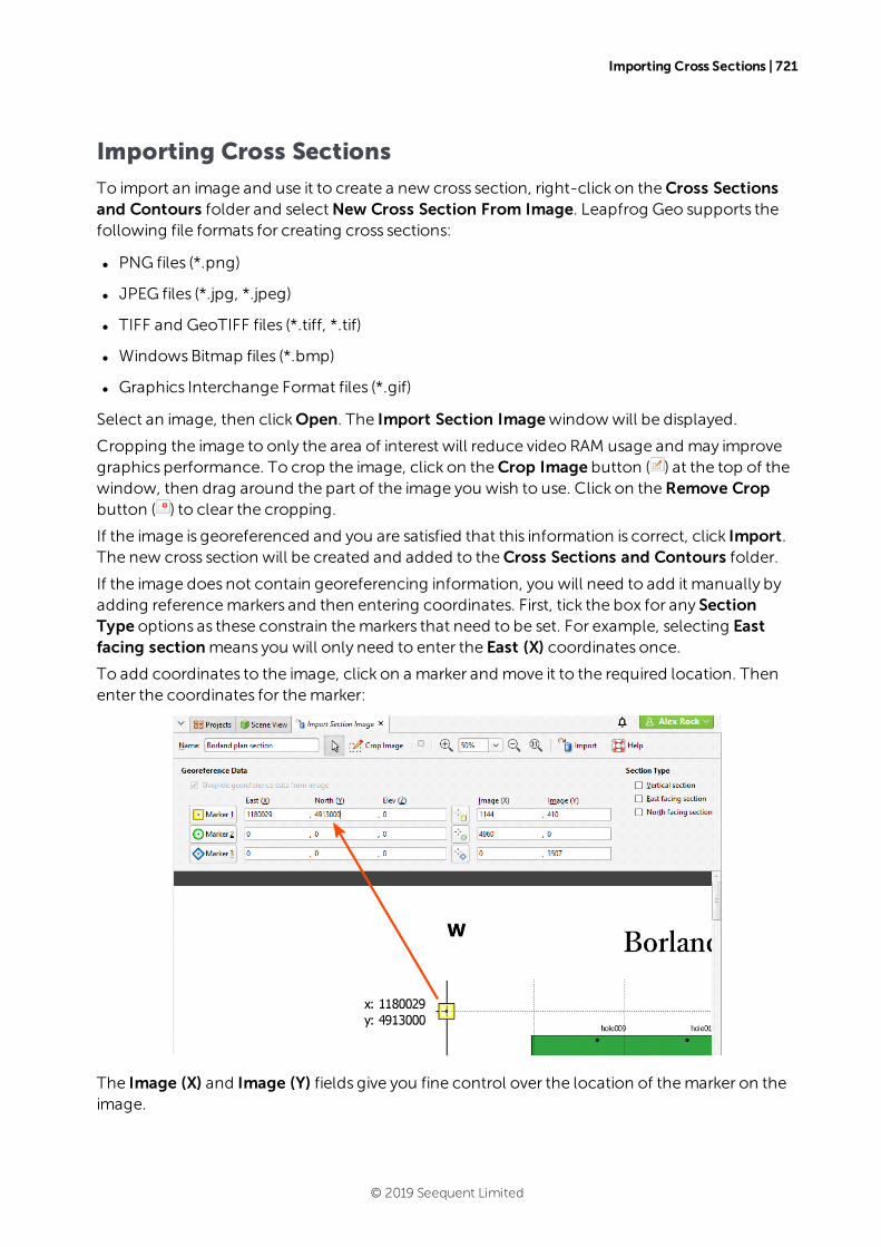
Importing Cross Sections | 721
Importing Cross Sections
To import an image and use it to create a new cross section, right-click on theCross Sectionsand Contours folder and selectNew Cross Section From Image. Leapfrog Geo supports thefollowing file formats for creating cross sections:
l PNG files (*.png)
l JPEG files (*.jpg, *.jpeg)
l TIFF and GeoTIFF files (*.tiff, *.tif)
l WindowsBitmap files (*.bmp)
l Graphics Interchange Format files (*.gif)
Select an image, then clickOpen. The Import Section Imagewindowwill be displayed.
Cropping the image to only the area of interest will reduce video RAM usage and may improvegraphics performance. To crop the image, click on theCrop Image button ( ) at the top of thewindow, then drag around the part of the image you wish to use. Click on theRemove Cropbutton ( ) to clear the cropping.
If the image is georeferenced and you are satisfied that this information is correct, click Import.The new cross section will be created and added to theCross Sections and Contours folder.
If the image does not contain georeferencing information, you will need to add it manually byadding referencemarkers and then entering coordinates. First, tick the box for any SectionType options as these constrain themarkers that need to be set. For example, selecting Eastfacing sectionmeans you will only need to enter the East (X) coordinates once.
To add coordinates to the image, click on a marker and move it to the required location. Thenenter the coordinates for themarker:
The Image (X) and Image (Y) fields give you fine control over the location of themarker on theimage.
© 2019 Seequent Limited
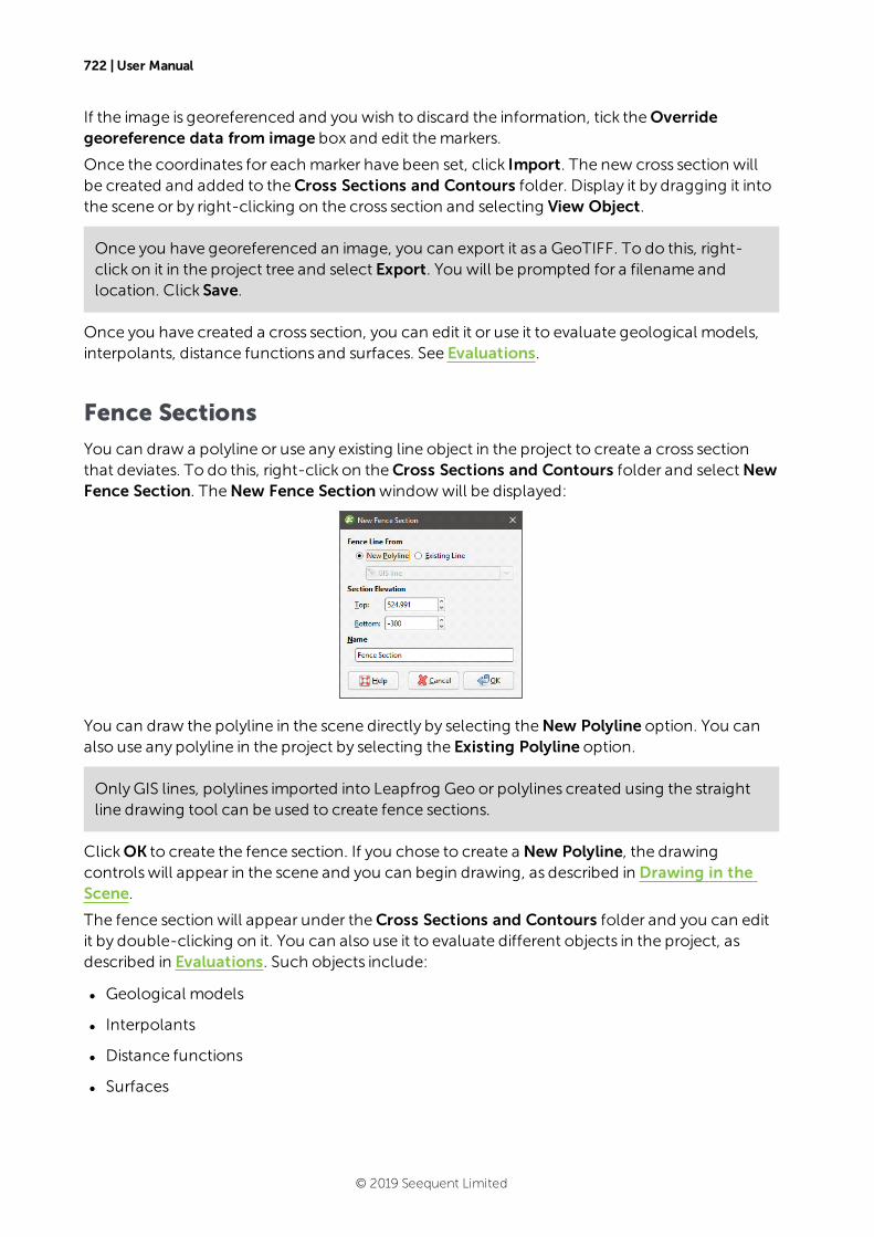
722 | User Manual
If the image is georeferenced and you wish to discard the information, tick theOverridegeoreference data from image box and edit themarkers.
Once the coordinates for each marker have been set, click Import. The new cross section willbe created and added to theCross Sections and Contours folder. Display it by dragging it intothe scene or by right-clicking on the cross section and selecting View Object.
Once you have georeferenced an image, you can export it as a GeoTIFF. To do this, right-click on it in the project tree and select Export. You will be prompted for a filename andlocation. Click Save.
Once you have created a cross section, you can edit it or use it to evaluate geological models,interpolants, distance functions and surfaces. See Evaluations.
Fence Sections
You can draw a polyline or use any existing line object in the project to create a cross sectionthat deviates. To do this, right-click on theCross Sections and Contours folder and selectNewFence Section. TheNew Fence Sectionwindowwill be displayed:
You can draw the polyline in the scene directly by selecting theNew Polyline option. You canalso use any polyline in the project by selecting the Existing Polyline option.
OnlyGIS lines, polylines imported into Leapfrog Geo or polylines created using the straightline drawing tool can be used to create fence sections.
ClickOK to create the fence section. If you chose to create a New Polyline, the drawingcontrolswill appear in the scene and you can begin drawing, as described in Drawing in theScene.
The fence section will appear under theCross Sections and Contours folder and you can editit by double-clicking on it. You can also use it to evaluate different objects in the project, asdescribed in Evaluations. Such objects include:
l Geological models
l Interpolants
l Distance functions
l Surfaces
© 2019 Seequent Limited

Serial Sections | 723
l GIS lines
l Polylines
If you create a section layout for a fence section, you can includemultiple evaluations andannotations on the section layout. See Section Layouts.
Serial Sections
This topic describes the process of creating a serial section, which is a series of cross sectionstaken at an offset froma single base section. The topic is divided into:
l Setting the Base Section
l Setting the Offset Sections
l The Serial Section in the Project Tree
l Displaying a Serial Section
l Exporting a Serial Section
To create a serial section, add a model to the scene. Next, right-click on theCross Sections andContours folder and selectNew Serial Section. TheNew Serial Sectionwindowwill appearand planes representing the base section and the offset sectionswill be added to the scene:
If the slicer is already in the scenewhen you selectNew Serial Section, the position of theslicer will be used to define the initial orientation of the base section.
Setting the Base Section
The handles in the scene control the position of the base section and work in the samemanneras themoving plane controls (see The Moving Plane).
© 2019 Seequent Limited

724 | User Manual
The front (F) and back (B) of the base section plane are indicated in the scene. To swap the frontand back, click the Swap Front button ( ).
Two buttons in theNew Serial Sectionwindow let you create a base section that is alignednorth-to-south ( ) or east-to-west ( ). The other two buttons are active when the slicer is inthe scene. Clicking the Set section to slicer button ( ) creates a cross section from the positionof the slicer in the scene. When the Lock section to slicer button ( ) is enabled, moving theposition of the slicer will update the position of the cross section in theNew Serial Sectionwindow.
Setting the Offset Sections
The number of offset sections is determined by the value of the Spacing setting and the Frontand Back Extents:
You can change the number of offset sections by:
l Changing the Spacing setting. The number of offset sectionswill be recalculated andupdated in the scene.
l Changing the Front orBack settings. For example, increasing the Front setting adds anoffset section on the front of the base section, increasing the extents by the value of Spacing.
l Changing the object used to define the extents. Select an object from the Enclose Objectlist. The base section will bemoved to the centre of the selected object.
© 2019 Seequent Limited
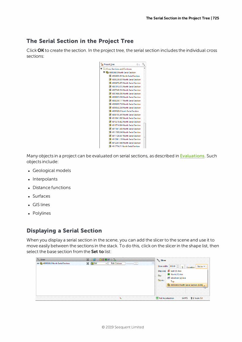
The Serial Section in the Project Tree | 725
The Serial Section in the Project Tree
ClickOK to create the section. In the project tree, the serial section includes the individual crosssections:
Many objects in a project can be evaluated on serial sections, as described in Evaluations. Suchobjects include:
l Geological models
l Interpolants
l Distance functions
l Surfaces
l GIS lines
l Polylines
Displaying a Serial Section
When you display a serial section in the scene, you can add the slicer to the scene and use it tomove easily between the sections in the stack. To do this, click on the slicer in the shape list, thenselect the base section from the Set to list:
© 2019 Seequent Limited

726 | User Manual
Next, set the Step size to the Spacing setting used to create the section. You can then use the <and > keys to view each individual cross section.
Exporting a Serial Section
The options for exporting serial sections differ for the section itself and the offset sections:
l A serial section cannot be used to create a section layout. When exported as a DXF file, theserial section will be exported in a single file with a collection of DXF lines based onintersections between the selected evaluation and the section planes.
l The offset sections that make up a serial section can be exported in DXF format or as asection layout. See Exporting Sections and Section Layouts formore information.
© 2019 Seequent Limited
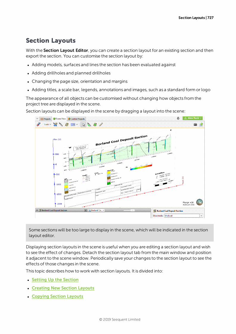
Section Layouts | 727
Section Layouts
With the Section Layout Editor, you can create a section layout for an existing section and thenexport the section. You can customise the section layout by:
l Adding models, surfaces and lines the section has been evaluated against
l Adding drillholes and planned drillholes
l Changing the page size, orientation and margins
l Adding titles, a scale bar, legends, annotations and images, such as a standard formor logo
The appearance of all objects can be customised without changing how objects from theproject tree are displayed in the scene.
Section layouts can be displayed in the scene by dragging a layout into the scene:
Some sectionswill be too large to display in the scene, which will be indicated in the sectionlayout editor.
Displaying section layouts in the scene is useful when you are editing a section layout and wishto see the effect of changes. Detach the section layout tab from themain window and positionit adjacent to the scenewindow. Periodically save your changes to the section layout to see theeffects of those changes in the scene.
This topic describes how toworkwith section layouts. It is divided into:
l Setting Up the Section
l Creating New Section Layouts
l Copying Section Layouts
© 2019 Seequent Limited
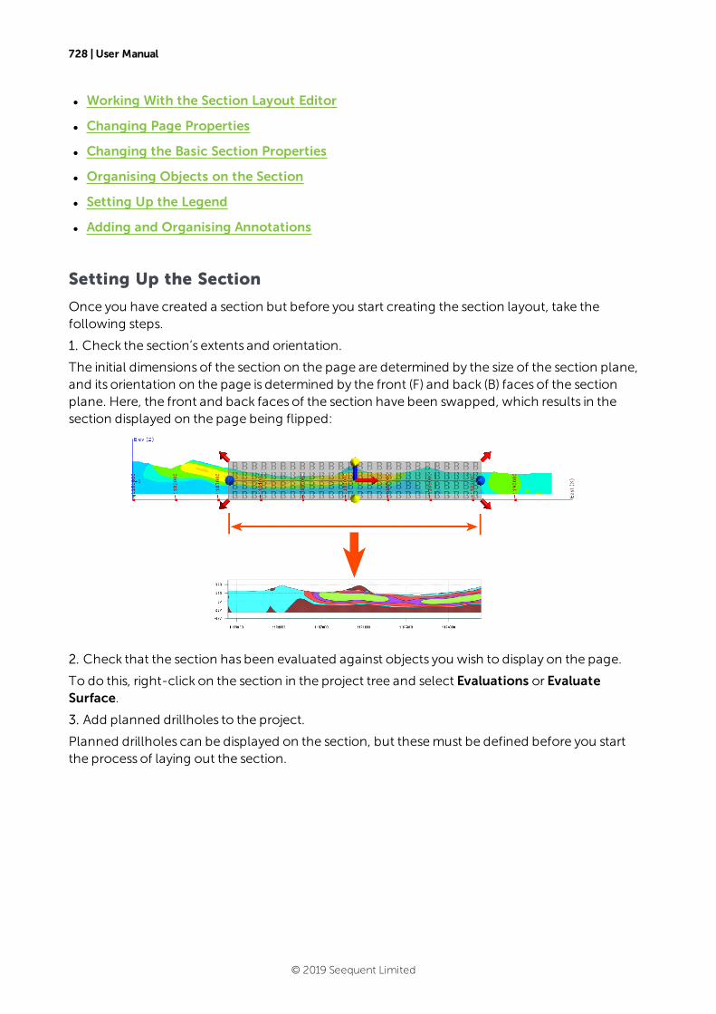
728 | User Manual
l Working With the Section Layout Editor
l Changing Page Properties
l Changing the Basic Section Properties
l Organising Objects on the Section
l Setting Up the Legend
l Adding and Organising Annotations
Setting Up the Section
Once you have created a section but before you start creating the section layout, take thefollowing steps.
1. Check the section’s extents and orientation.
The initial dimensions of the section on the page are determined by the size of the section plane,and its orientation on the page is determined by the front (F) and back (B) faces of the sectionplane. Here, the front and back faces of the section have been swapped, which results in thesection displayed on the page being flipped:
2. Check that the section has been evaluated against objects you wish to display on the page.
To do this, right-click on the section in the project tree and select Evaluations or EvaluateSurface.
3. Add planned drillholes to the project.
Planned drillholes can be displayed on the section, but thesemust be defined before you startthe process of laying out the section.
© 2019 Seequent Limited
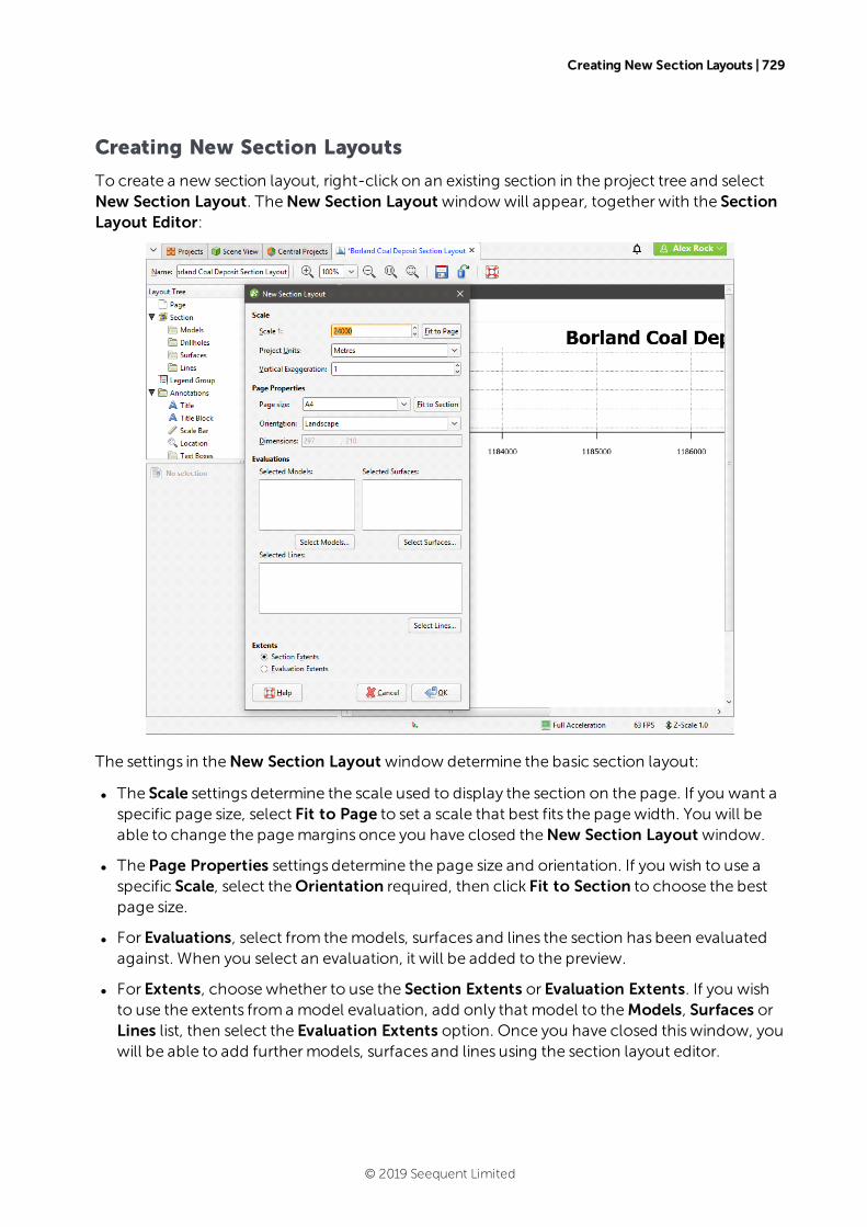
Creating New Section Layouts | 729
Creating New Section Layouts
To create a new section layout, right-click on an existing section in the project tree and selectNew Section Layout. TheNew Section Layout windowwill appear, together with the SectionLayout Editor:
The settings in theNew Section Layout window determine the basic section layout:
l The Scale settings determine the scale used to display the section on the page. If you want aspecific page size, select Fit to Page to set a scale that best fits the pagewidth. You will beable to change the pagemargins once you have closed theNew Section Layout window.
l The Page Properties settings determine the page size and orientation. If you wish to use aspecific Scale, select theOrientation required, then click Fit to Section to choose the bestpage size.
l For Evaluations, select from themodels, surfaces and lines the section has been evaluatedagainst. When you select an evaluation, it will be added to the preview.
l For Extents, choosewhether to use the Section Extents or Evaluation Extents. If you wishto use the extents froma model evaluation, add only that model to theModels, Surfaces orLines list, then select the Evaluation Extents option. Once you have closed thiswindow, youwill be able to add furthermodels, surfaces and lines using the section layout editor.
© 2019 Seequent Limited
730 | User Manual
As you change settings and add objects to the section, the preview in the Section Layout Editorwindowwill be updated. All settings in theNew Section Layout window can be changed oncethe layout has been created.
ClickOK to close theNew Section Layout window. You can then make further changes to thepage layout in the Section Layout Editor. SeeWorking With the Section Layout Editor.
Copying Section Layouts
If you have already created a section layout and wish to reuse it, you can copy it to othersections.
Copying a section layout copies the evaluations used in the original section layout, togetherwith the page size and orientation and the position of the Layout Tree objects on the page.Howmodels, surfaces and drillholes are copied dependson the section towhich the layout isbeing copied:
l All models and surfaces that can be displayed on the section will be copied.
l The drillholes copied to the layout will depend on the type of section the layout is beingcopied fromand whether or not a filter is set for the layout:
o If no distance filter was set for the original layout, all drillholes selected for the originallayout will be copied.
o If a distance filter was applied to the original section, the filter will be applied anddrillholes selected that are within that distance of the section towhich the layout is beingcopied.
o When the original layout is froma fence section, drillhole evaluationswill not be copiedwith the section layout.
To copy a layout, right-click on the layout you wish to copy and selectCopy Layout To. In thewindow that appears, a summary of the information that will be copied is displayed so you canseewhat information will be copied to the selected sections. Move the sections you wish tocopy the layout to into the Selected Sections list, then clickOK. A copy of the layout will appearin the project tree under each section you selected. The layout copies are not linked to theoriginal layout and sowill not be updated when the original is updated.
Copying section layouts tomultiple sections can result in numerous section layouts in aproject, which can be difficult to workwith. The recommended workflow for creating asection layout that you intend tomakemultiple copies of is to first get the layout right on onesection before copying it to other sections.
© 2019 Seequent Limited
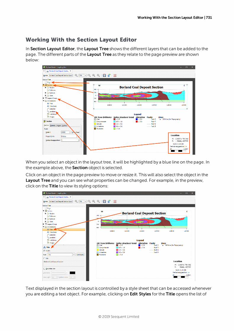
Working With the Section Layout Editor | 731
Working With the Section Layout Editor
In Section Layout Editor, the Layout Tree shows the different layers that can be added to thepage. The different parts of the Layout Tree as they relate to the page preview are shownbelow:
When you select an object in the layout tree, it will be highlighted by a blue line on the page. Inthe example above, the Section object is selected.
Click on an object in the page preview tomove or resize it. Thiswill also select the object in theLayout Tree and you can seewhat properties can be changed. For example, in the preview,click on the Title to view its styling options:
Text displayed in the section layout is controlled by a style sheet that can be accessed wheneveryou are editing a text object. For example, clicking on Edit Styles for the Title opens the list of
© 2019 Seequent Limited

732 | User Manual
Text Styles with the Title selected, but also allows you to change the appearance of styles usedfor other text objects visible in the preview:
Changing Page Properties
In the Layout Tree, click on Page to change the Page Size, Orientation and Margins:
If you wish to use a specific Scale, select theOrientation required, then click Fit to Section tochoose the best page size.
© 2019 Seequent Limited

Changing the Basic Section Properties | 733
Changing the Basic Section Properties
To change the section layout’s basic properties, click on the Section object in the Layout Tree.In the Section tab, you can change the scale and units used in the layout and the amount ofVertical Exaggeration:
For the Scale, you can enter a specific value to use in displaying the section on the page, or, ifyou want a specific page size, select Fit to Page to set a scale that best fits the pagewidth.
If you want to change the page size and themargins used, click on the Page object.
To change the size of the section contents (models, drillholes, surfaces and lines) on the page,click on the Extents tab:
For Extents, choosewhether to use the Section Extents or Evaluation Extents.
© 2019 Seequent Limited
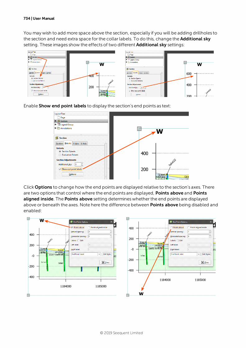
734 | User Manual
You maywish to add more space above the section, especially if you will be adding drillholes tothe section and need extra space for the collar labels. To do this, change the Additional skysetting. These images show the effects of two different Additional sky settings:
Enable Show end point labels to display the section’s end points as text:
ClickOptions to change how the end points are displayed relative to the section’s axes. Thereare two options that control where the end points are displayed, Points above and Pointsaligned inside. The Points above setting determineswhether the end points are displayedabove or beneath the axes. Note here the difference between Points above being disabled andenabled:
© 2019 Seequent Limited
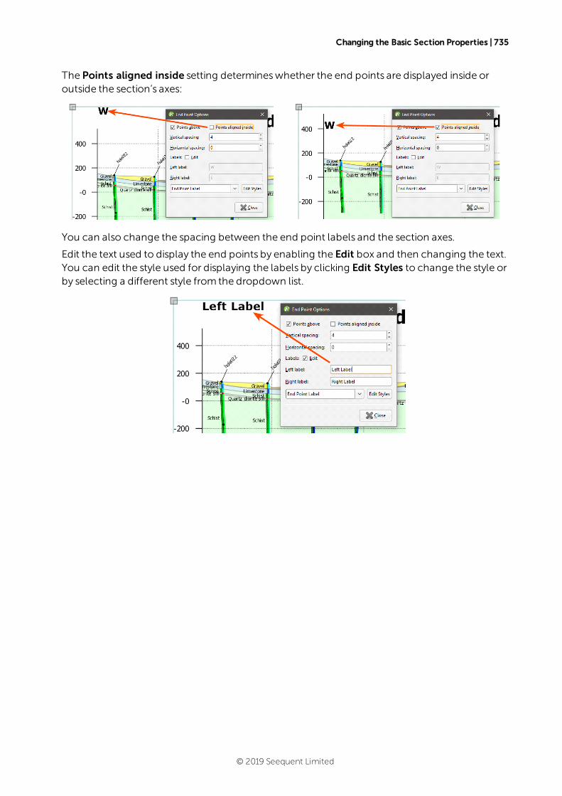
Changing the Basic Section Properties | 735
The Points aligned inside setting determineswhether the end points are displayed inside oroutside the section’s axes:
You can also change the spacing between the end point labels and the section axes.
Edit the text used to display the end points by enabling the Edit box and then changing the text.You can edit the style used for displaying the labels by clicking Edit Styles to change the style orby selecting a different style from the dropdown list.
© 2019 Seequent Limited
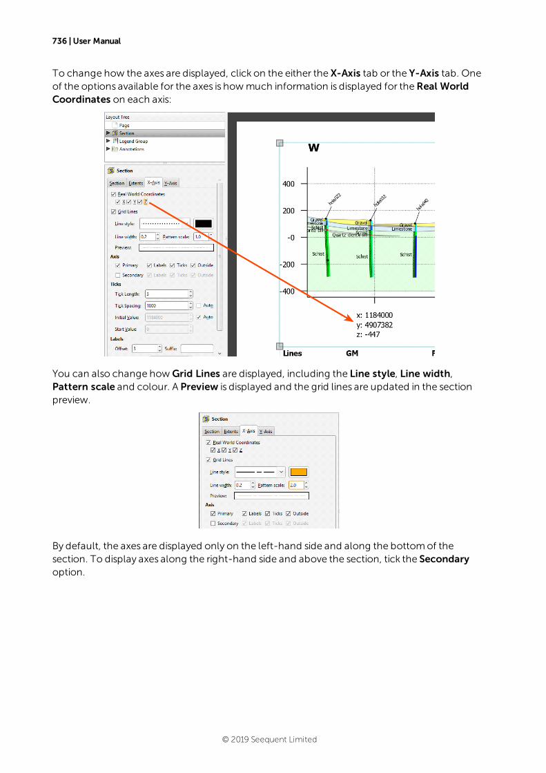
736 | User Manual
To change how the axes are displayed, click on the either the X-Axis tab or the Y-Axis tab. Oneof the options available for the axes is howmuch information is displayed for theReal WorldCoordinates on each axis:
You can also change how Grid Lines are displayed, including the Line style, Line width,Pattern scale and colour. A Preview is displayed and the grid lines are updated in the sectionpreview.
By default, the axes are displayed only on the left-hand side and along the bottomof thesection. To display axes along the right-hand side and above the section, tick the Secondaryoption.
© 2019 Seequent Limited
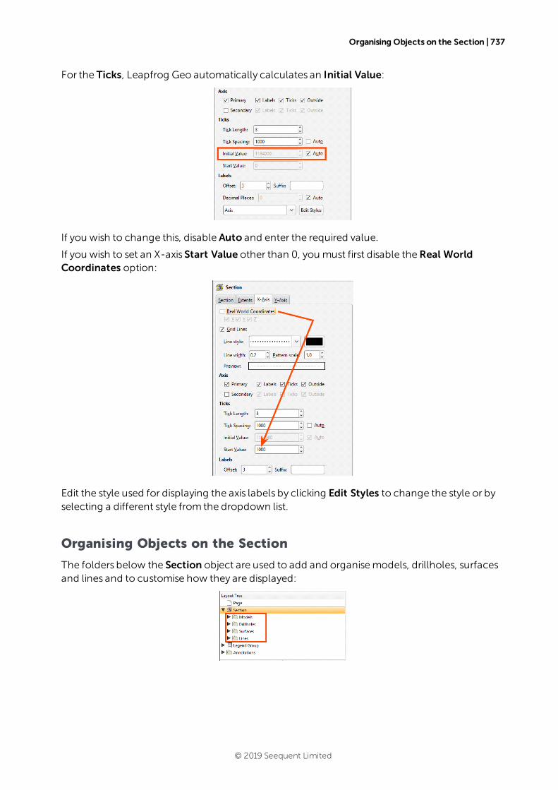
Organising Objects on the Section | 737
For the Ticks, Leapfrog Geo automatically calculates an Initial Value:
If you wish to change this, disable Auto and enter the required value.
If you wish to set an X-axis Start Value other than 0, you must first disable theReal WorldCoordinates option:
Edit the style used for displaying the axis labels by clicking Edit Styles to change the style or byselecting a different style from the dropdown list.
Organising Objects on the Section
The folders below the Section object are used to add and organisemodels, drillholes, surfacesand lines and to customise how they are displayed:
© 2019 Seequent Limited
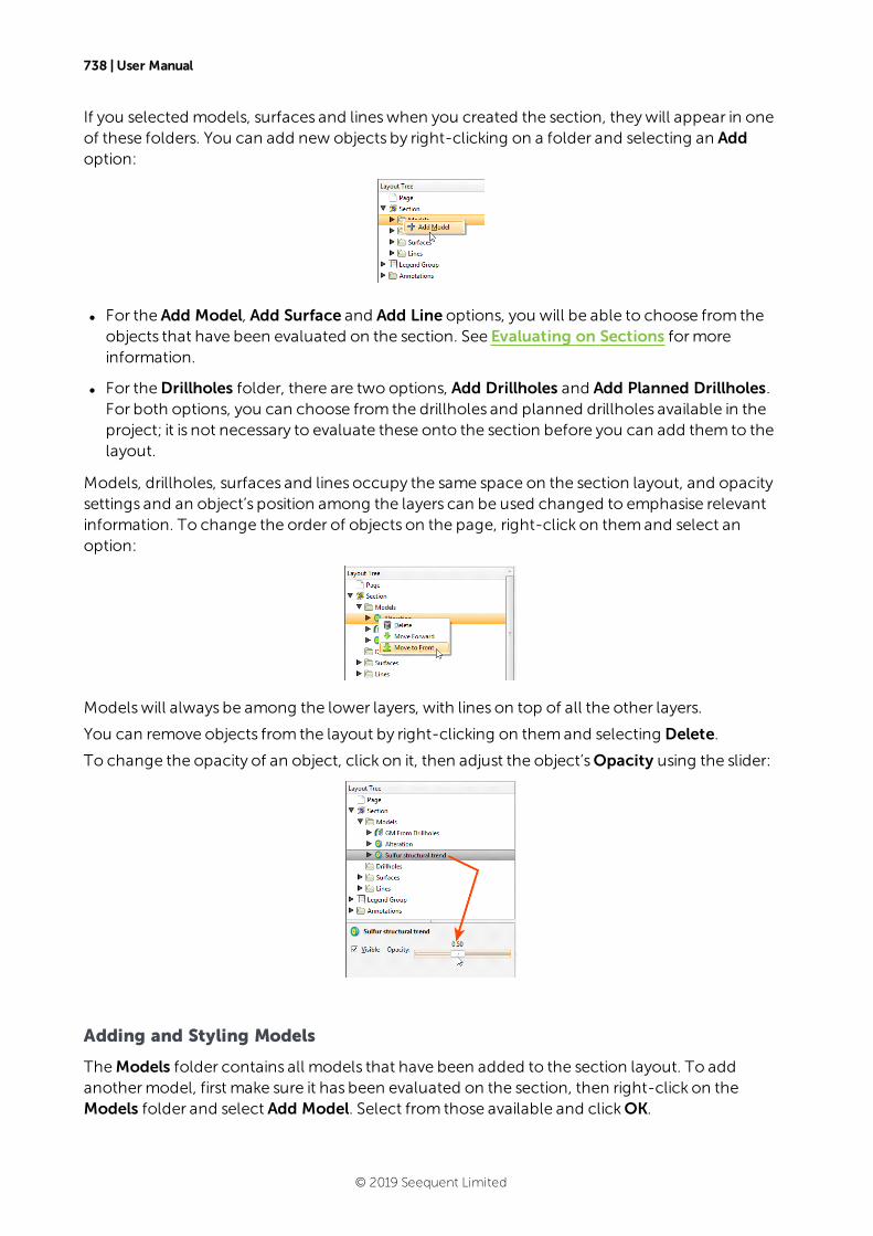
738 | User Manual
If you selected models, surfaces and lineswhen you created the section, theywill appear in oneof these folders. You can add new objects by right-clicking on a folder and selecting an Addoption:
l For the Add Model, Add Surface and Add Line options, you will be able to choose from theobjects that have been evaluated on the section. See Evaluating on Sections formoreinformation.
l For theDrillholes folder, there are two options, Add Drillholes and Add Planned Drillholes.For both options, you can choose from the drillholes and planned drillholes available in theproject; it is not necessary to evaluate these onto the section before you can add them to thelayout.
Models, drillholes, surfaces and lines occupy the same space on the section layout, and opacitysettings and an object’s position among the layers can be used changed to emphasise relevantinformation. To change the order of objects on the page, right-click on themand select anoption:
Modelswill always be among the lower layers, with lines on top of all the other layers.
You can remove objects from the layout by right-clicking on themand selecting Delete.
To change the opacity of an object, click on it, then adjust the object’sOpacity using the slider:
Adding and Styling Models
TheModels folder contains all models that have been added to the section layout. To addanothermodel, first make sure it has been evaluated on the section, then right-click on theModels folder and select Add Model. Select from those available and clickOK.
© 2019 Seequent Limited
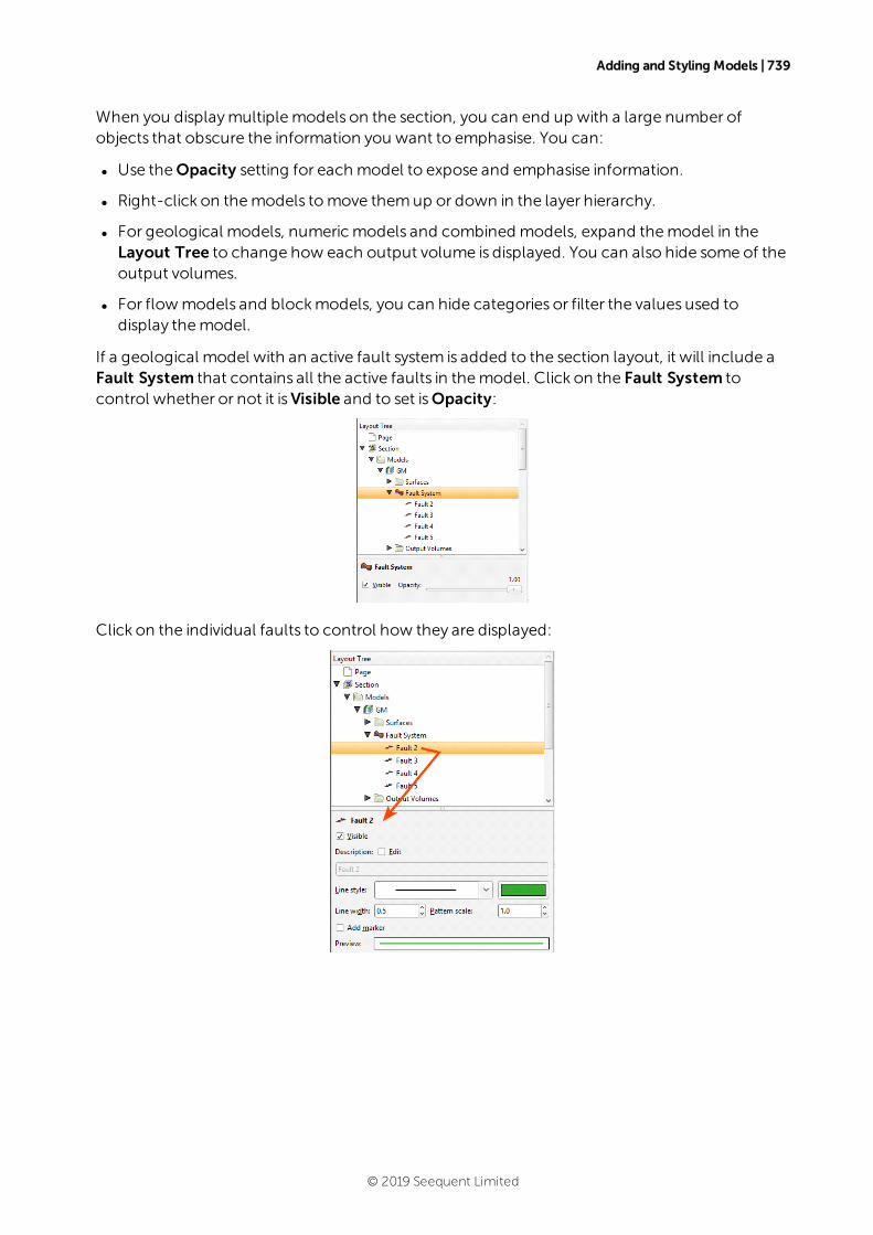
Adding and Styling Models | 739
When you displaymultiplemodels on the section, you can end up with a large number ofobjects that obscure the information you want to emphasise. You can:
l Use theOpacity setting for each model to expose and emphasise information.
l Right-click on themodels tomove themup or down in the layer hierarchy.
l For geological models, numericmodels and combined models, expand themodel in theLayout Tree to change how each output volume is displayed. You can also hide some of theoutput volumes.
l For flowmodels and blockmodels, you can hide categories or filter the values used todisplay themodel.
If a geological model with an active fault system is added to the section layout, it will include aFault System that contains all the active faults in themodel. Click on the Fault System tocontrol whether or not it isVisible and to set isOpacity:
Click on the individual faults to control how they are displayed:
© 2019 Seequent Limited
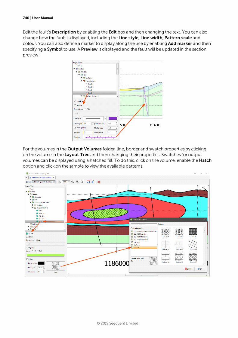
740 | User Manual
Edit the fault’sDescription by enabling the Edit box and then changing the text. You can alsochange how the fault is displayed, including the Line style, Line width, Pattern scale andcolour. You can also define a marker to display along the line by enabling Add marker and thenspecifying a Symbol to use. A Preview is displayed and the fault will be updated in the sectionpreview:
For the volumes in theOutput Volumes folder, line, border and swatch properties by clickingon the volume in the Layout Tree and then changing their properties. Swatches for outputvolumes can be displayed using a hatched fill. To do this, click on the volume, enable theHatchoption and click on the sample to view the available patterns:
© 2019 Seequent Limited
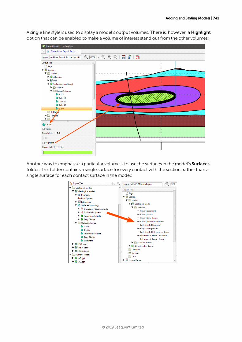
Adding and Styling Models | 741
A single line style is used to display a model’s output volumes. There is, however, a Highlightoption that can be enabled tomake a volume of interest stand out from the other volumes:
Another way to emphasise a particular volume is to use the surfaces in themodel’s Surfacesfolder. This folder contains a single surface for every contact with the section, rather than asingle surface for each contact surface in themodel:
© 2019 Seequent Limited
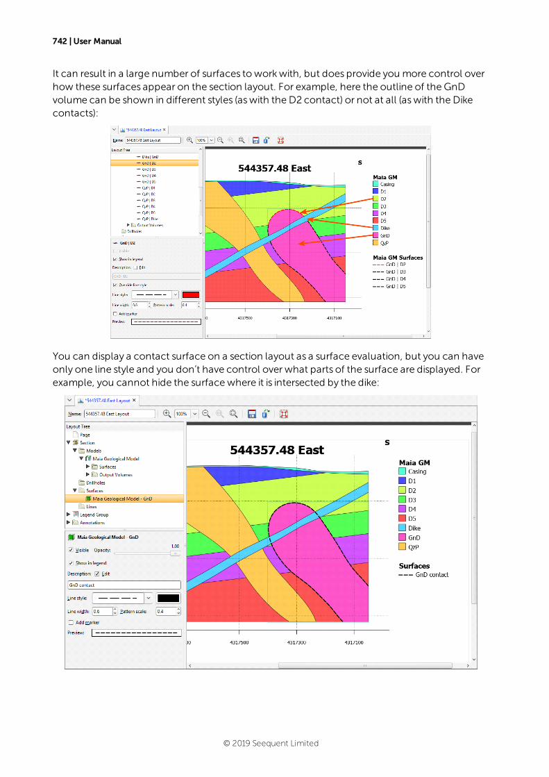
742 | User Manual
It can result in a large number of surfaces toworkwith, but does provide you more control overhow these surfaces appear on the section layout. For example, here the outline of the GnDvolume can be shown in different styles (aswith the D2 contact) or not at all (aswith the Dikecontacts):
You can display a contact surface on a section layout as a surface evaluation, but you can haveonly one line style and you don’t have control over what parts of the surface are displayed. Forexample, you cannot hide the surfacewhere it is intersected by the dike:
© 2019 Seequent Limited
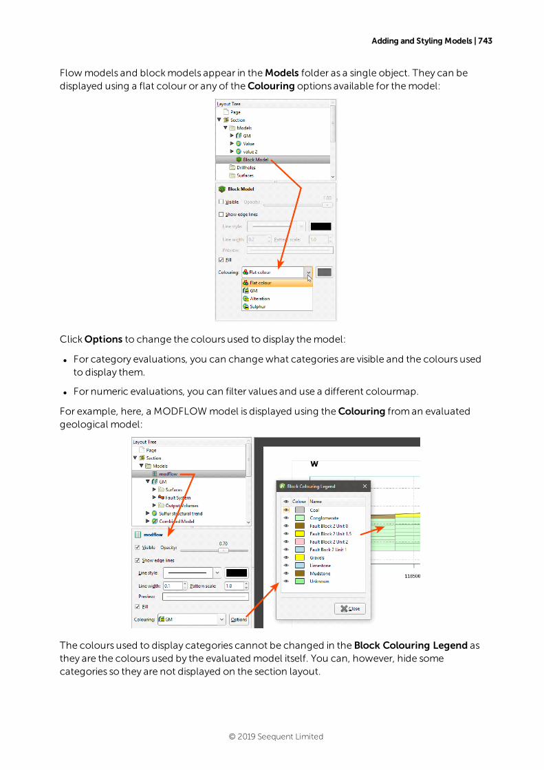
Adding and Styling Models | 743
Flowmodels and blockmodels appear in theModels folder as a single object. They can bedisplayed using a flat colour or any of theColouring options available for themodel:
ClickOptions to change the colours used to display themodel:
l For category evaluations, you can changewhat categories are visible and the colours usedto display them.
l For numeric evaluations, you can filter values and use a different colourmap.
For example, here, a MODFLOW model is displayed using theColouring froman evaluatedgeological model:
The colours used to display categories cannot be changed in the Block Colouring Legend asthey are the colours used by the evaluated model itself. You can, however, hide somecategories so they are not displayed on the section layout.
© 2019 Seequent Limited
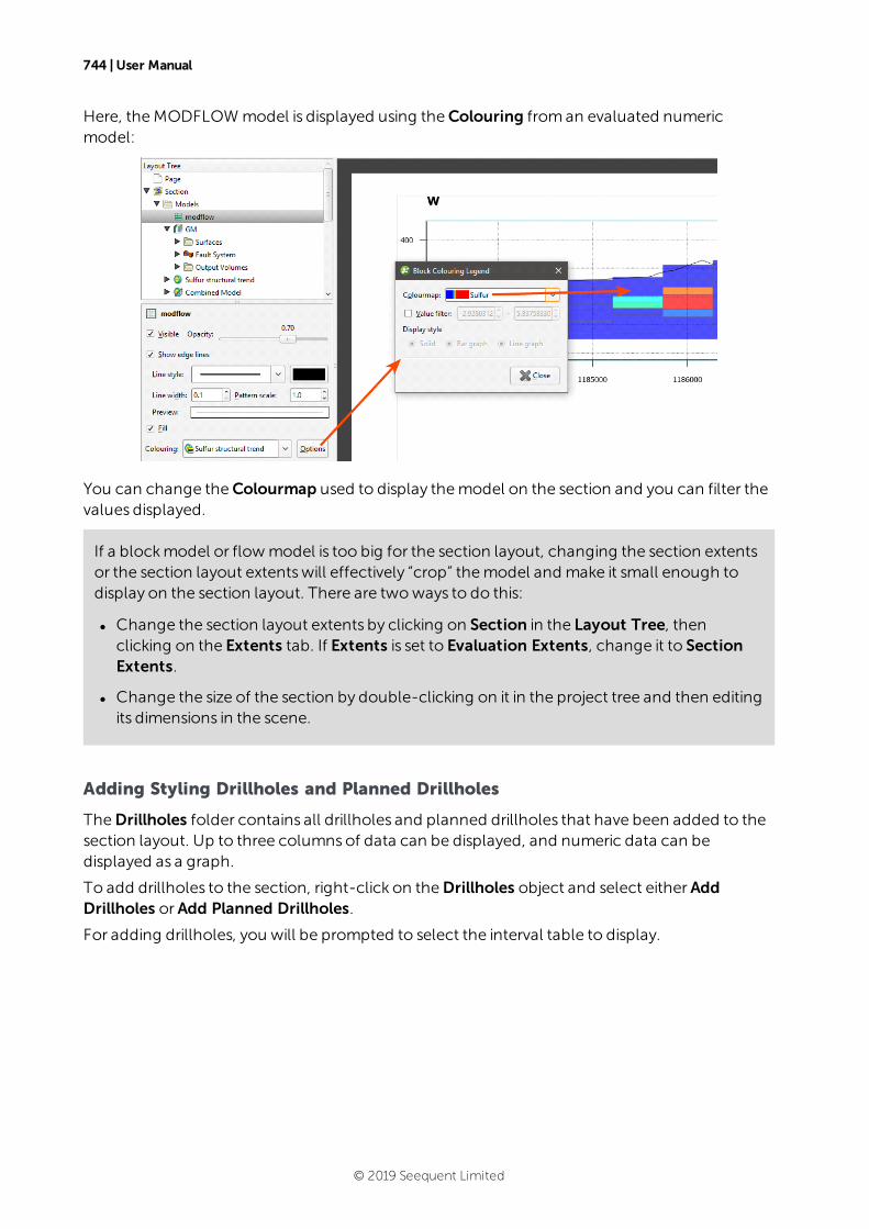
744 | User Manual
Here, theMODFLOW model is displayed using theColouring froman evaluated numericmodel:
You can change theColourmap used to display themodel on the section and you can filter thevalues displayed.
If a blockmodel or flowmodel is too big for the section layout, changing the section extentsor the section layout extentswill effectively “crop” themodel and make it small enough todisplay on the section layout. There are twoways to do this:
l Change the section layout extents by clicking on Section in the Layout Tree, thenclicking on the Extents tab. If Extents is set to Evaluation Extents, change it to SectionExtents.
l Change the size of the section by double-clicking on it in the project tree and then editingits dimensions in the scene.
Adding Styling Drillholes and Planned Drillholes
TheDrillholes folder contains all drillholes and planned drillholes that have been added to thesection layout. Up to three columnsof data can be displayed, and numeric data can bedisplayed as a graph.
To add drillholes to the section, right-click on theDrillholes object and select eitherAddDrillholes orAdd Planned Drillholes.
For adding drillholes, you will be prompted to select the interval table to display.
© 2019 Seequent Limited
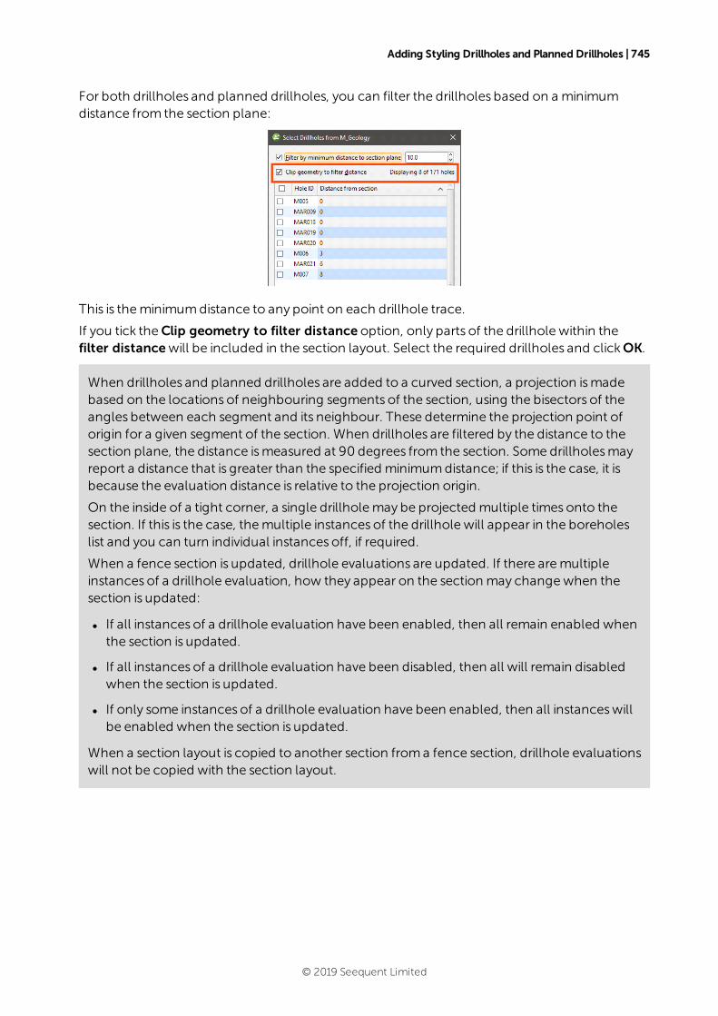
Adding Styling Drillholes and Planned Drillholes | 745
For both drillholes and planned drillholes, you can filter the drillholes based on a minimumdistance from the section plane:
This is theminimumdistance to any point on each drillhole trace.
If you tick theClip geometry to filter distance option, only parts of the drillhole within thefilter distancewill be included in the section layout. Select the required drillholes and clickOK.
When drillholes and planned drillholes are added to a curved section, a projection ismadebased on the locations of neighbouring segments of the section, using the bisectors of theangles between each segment and its neighbour. These determine the projection point oforigin for a given segment of the section. When drillholes are filtered by the distance to thesection plane, the distance ismeasured at 90 degrees from the section. Some drillholesmayreport a distance that is greater than the specified minimumdistance; if this is the case, it isbecause the evaluation distance is relative to the projection origin.
On the inside of a tight corner, a single drillholemay be projected multiple timesonto thesection. If this is the case, themultiple instances of the drillhole will appear in the boreholeslist and you can turn individual instances off, if required.
When a fence section is updated, drillhole evaluations are updated. If there aremultipleinstances of a drillhole evaluation, how they appear on the section may changewhen thesection is updated:
l If all instances of a drillhole evaluation have been enabled, then all remain enabled whenthe section is updated.
l If all instances of a drillhole evaluation have been disabled, then all will remain disabledwhen the section is updated.
l If only some instances of a drillhole evaluation have been enabled, then all instanceswillbe enabled when the section is updated.
When a section layout is copied to another section froma fence section, drillhole evaluationswill not be copied with the section layout.
© 2019 Seequent Limited
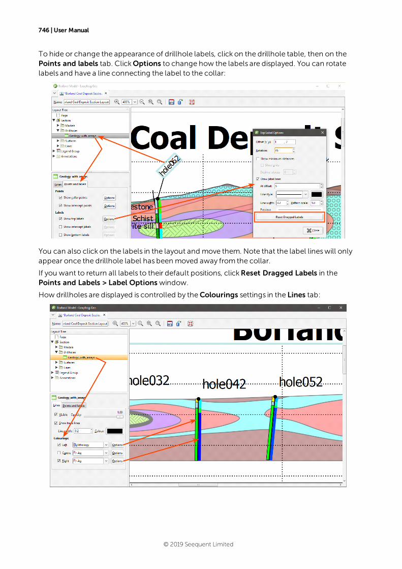
746 | User Manual
To hide or change the appearance of drillhole labels, click on the drillhole table, then on thePoints and labels tab. ClickOptions to change how the labels are displayed. You can rotatelabels and have a line connecting the label to the collar:
You can also click on the labels in the layout and move them. Note that the label lineswill onlyappear once the drillhole label has been moved away from the collar.
If you want to return all labels to their default positions, clickReset Dragged Labels in thePoints and Labels > Label Options window.
How drillholes are displayed is controlled by theColourings settings in the Lines tab:
© 2019 Seequent Limited

Adding Styling Drillholes and Planned Drillholes | 747
Click theOptions button to display data (category data) or filter values (numeric data) on thedrillholes:
Drillholes can be displayed using hatching patterns. In theDisplay style tab, tick theHatchedoption, then select from the patterns available:
© 2019 Seequent Limited
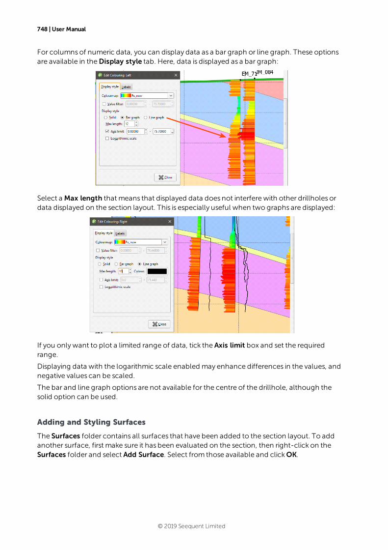
748 | User Manual
For columnsof numeric data, you can display data as a bar graph or line graph. These optionsare available in theDisplay style tab. Here, data is displayed as a bar graph:
Select a Max length that means that displayed data does not interfere with other drillholes ordata displayed on the section layout. This is especially useful when two graphs are displayed:
If you onlywant to plot a limited range of data, tick the Axis limit box and set the requiredrange.
Displaying data with the logarithmic scale enabled may enhance differences in the values, andnegative values can be scaled.
The bar and line graph options are not available for the centre of the drillhole, although thesolid option can be used.
Adding and Styling Surfaces
The Surfaces folder contains all surfaces that have been added to the section layout. To addanother surface, first make sure it has been evaluated on the section, then right-click on theSurfaces folder and select Add Surface. Select from those available and clickOK.
© 2019 Seequent Limited
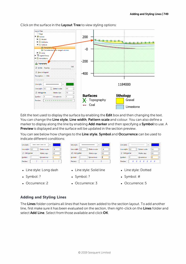
Adding and Styling Lines | 749
Click on the surface in the Layout Tree to view styling options:
Edit the text used to display the surface by enabling the Edit box and then changing the text.You can change the Line style, Line width, Pattern scale and colour. You can also define amarker to display along the line by enabling Add marker and then specifying a Symbol to use. APreview is displayed and the surfacewill be updated in the section preview.
You can see below how changes to the Line style, Symbol and Occurrence can be used toindicate different conditions:
l Line style: Long dash
l Symbol: ?
l Occurrence: 2
l Line style: Solid line
l Symbol: ?
l Occurrence: 3
l Line style: Dotted
l Symbol: #
l Occurrence: 5
Adding and Styling Lines
The Lines folder contains all lines that have been added to the section layout. To add anotherline, first make sure it has been evaluated on the section, then right-click on the Lines folder andselect Add Line. Select from those available and clickOK.
© 2019 Seequent Limited
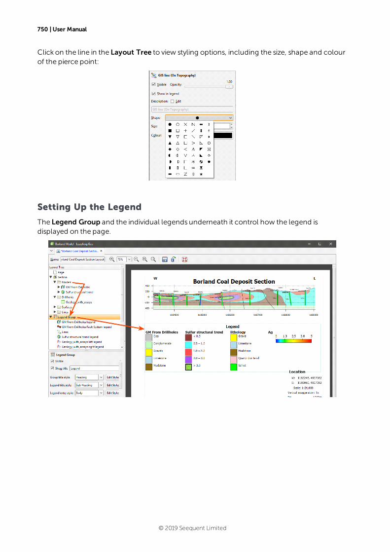
750 | User Manual
Click on the line in the Layout Tree to view styling options, including the size, shape and colourof the pierce point:
Setting Up the Legend
The Legend Group and the individual legends underneath it control how the legend isdisplayed on the page.
© 2019 Seequent Limited
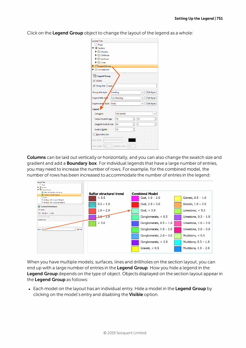
Setting Up the Legend | 751
Click on the Legend Group object to change the layout of the legend as a whole:
Columns can be laid out vertically or horizontally, and you can also change the swatch size andgradient and add a Boundary box. For individual legends that have a large number of entries,you may need to increase the number of rows. For example, for the combined model, thenumber of rowshas been increased to accommodate the number of entries in the legend:
When you havemultiplemodels, surfaces, lines and drillholes on the section layout, you canend up with a large number of entries in the Legend Group. How you hide a legend in theLegend Group dependson the type of object. Objects displayed on the section layout appear inthe Legend Group as follows:
l Each model on the layout has an individual entry. Hide a model in the Legend Group byclicking on themodel’s entry and disabling the Visible option.
© 2019 Seequent Limited
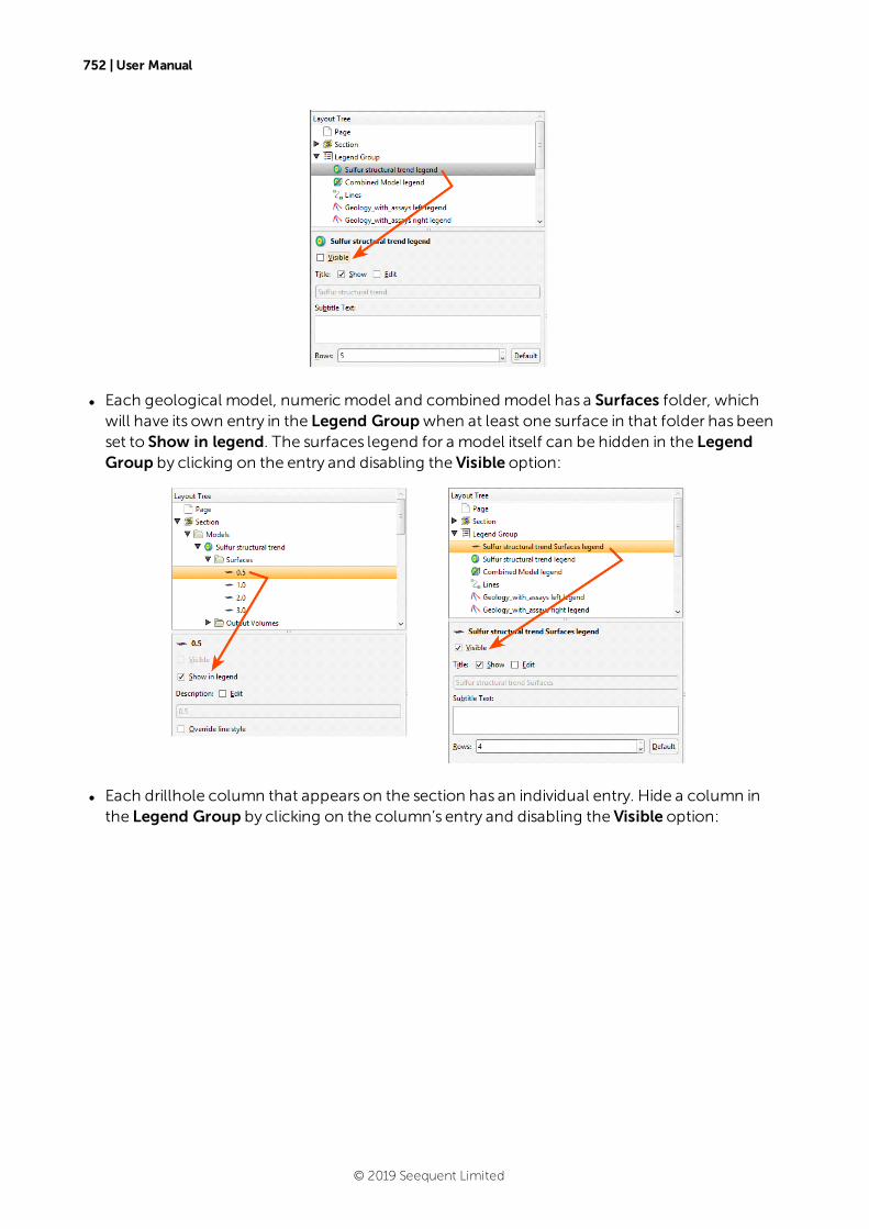
752 | User Manual
l Each geological model, numericmodel and combined model has a Surfaces folder, whichwill have its own entry in the Legend Groupwhen at least one surface in that folder has beenset to Show in legend. The surfaces legend for a model itself can be hidden in the LegendGroup by clicking on the entry and disabling the Visible option:
l Each drillhole column that appears on the section has an individual entry. Hide a column inthe Legend Group by clicking on the column’s entry and disabling the Visible option:
© 2019 Seequent Limited
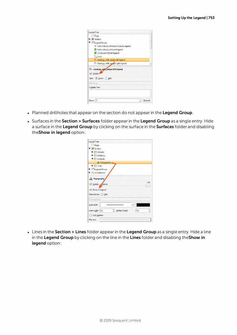
Setting Up the Legend | 753
l Planned drillholes that appear on the section do not appear in the Legend Group.
l Surfaces in the Section > Surfaces folder appear in the Legend Group as a single entry. Hidea surface in the Legend Group by clicking on the surface in the Surfaces folder and disablingtheShow in legend option:
l Lines in the Section > Lines folder appear in the Legend Group as a single entry. Hide a linein the Legend Group by clicking on the line in the Lines folder and disabling theShow inlegend option:
© 2019 Seequent Limited
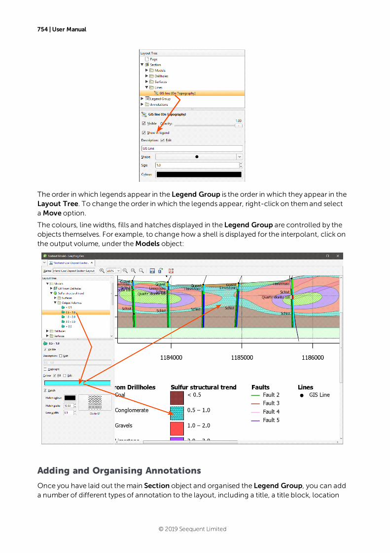
754 | User Manual
The order in which legends appear in the Legend Group is the order in which they appear in theLayout Tree. To change the order in which the legends appear, right-click on themand selecta Move option.
The colours, line widths, fills and hatches displayed in the Legend Group are controlled by theobjects themselves. For example, to change how a shell is displayed for the interpolant, click onthe output volume, under theModels object:
Adding and Organising Annotations
Once you have laid out themain Section object and organised the Legend Group, you can adda number of different types of annotation to the layout, including a title, a title block, location
© 2019 Seequent Limited
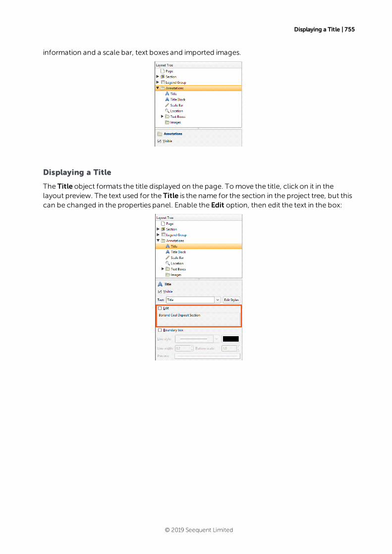
Displaying a Title | 755
information and a scale bar, text boxes and imported images.
Displaying a Title
The Title object formats the title displayed on the page. Tomove the title, click on it in thelayout preview. The text used for the Title is the name for the section in the project tree, but thiscan be changed in the properties panel. Enable the Edit option, then edit the text in the box:
© 2019 Seequent Limited
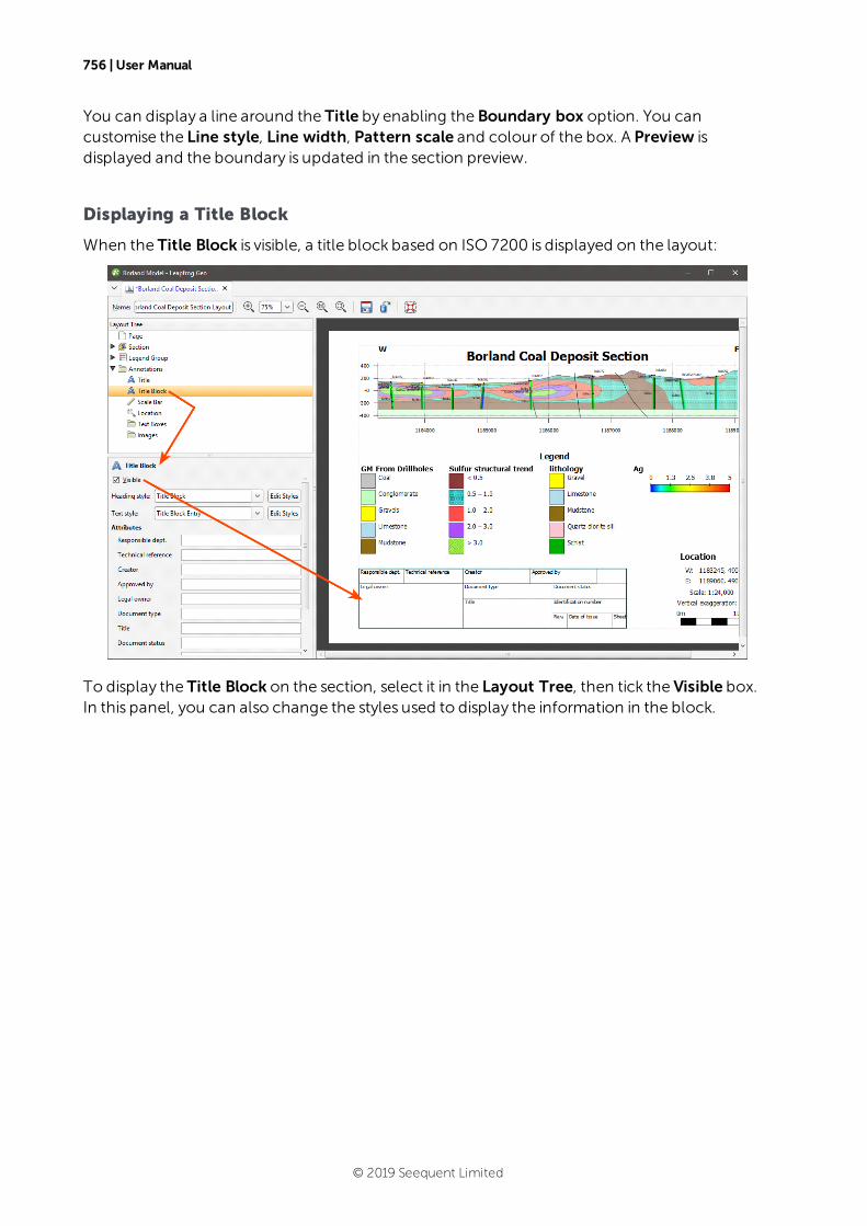
756 | User Manual
You can display a line around the Title by enabling the Boundary box option. You cancustomise the Line style, Line width, Pattern scale and colour of the box. A Preview isdisplayed and the boundary is updated in the section preview.
Displaying a Title Block
When the Title Block is visible, a title block based on ISO 7200 is displayed on the layout:
To display the Title Block on the section, select it in the Layout Tree, then tick the Visible box.In this panel, you can also change the styles used to display the information in the block.
© 2019 Seequent Limited
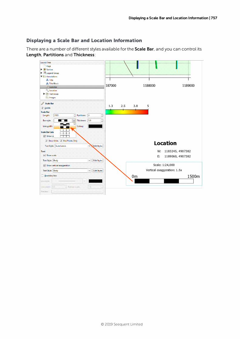
Displaying a Scale Bar and Location Information | 757
Displaying a Scale Bar and Location Information
There are a number of different styles available for the Scale Bar, and you can control itsLength, Partitions and Thickness:
© 2019 Seequent Limited
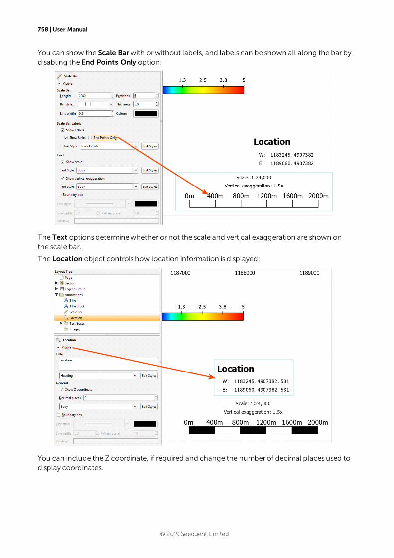
758 | User Manual
You can show the Scale Bar with orwithout labels, and labels can be shown all along the bar bydisabling the End Points Only option:
The Text options determinewhether or not the scale and vertical exaggeration are shown onthe scale bar.
The Location object controls how location information is displayed:
You can include the Z coordinate, if required and change the number of decimal places used todisplay coordinates.
© 2019 Seequent Limited
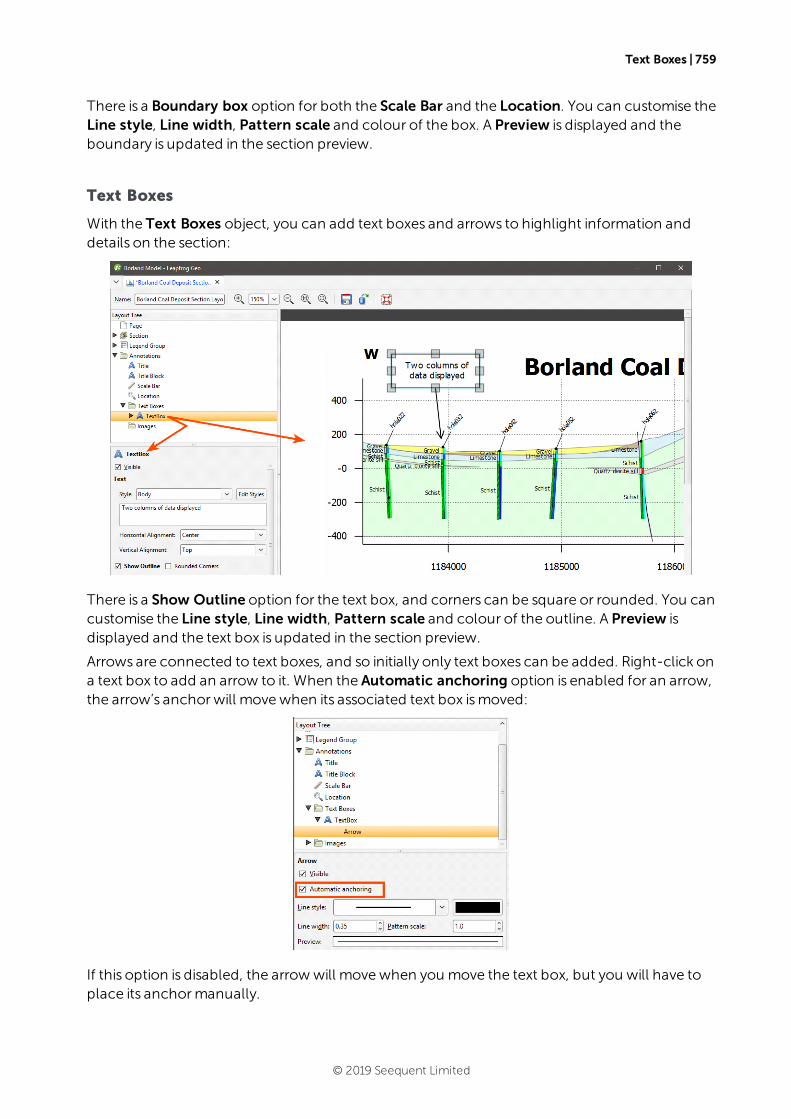
Text Boxes | 759
There is a Boundary box option for both the Scale Bar and the Location. You can customise theLine style, Line width, Pattern scale and colour of the box. A Preview is displayed and theboundary is updated in the section preview.
Text Boxes
With the Text Boxes object, you can add text boxes and arrows to highlight information anddetails on the section:
There is a Show Outline option for the text box, and corners can be square or rounded. You cancustomise the Line style, Line width, Pattern scale and colour of the outline. A Preview isdisplayed and the text box is updated in the section preview.
Arrows are connected to text boxes, and so initially only text boxes can be added. Right-click ona text box to add an arrow to it. When the Automatic anchoring option is enabled for an arrow,the arrow’s anchorwill movewhen its associated text box ismoved:
If this option is disabled, the arrow will movewhen you move the text box, but you will have toplace its anchormanually.
© 2019 Seequent Limited
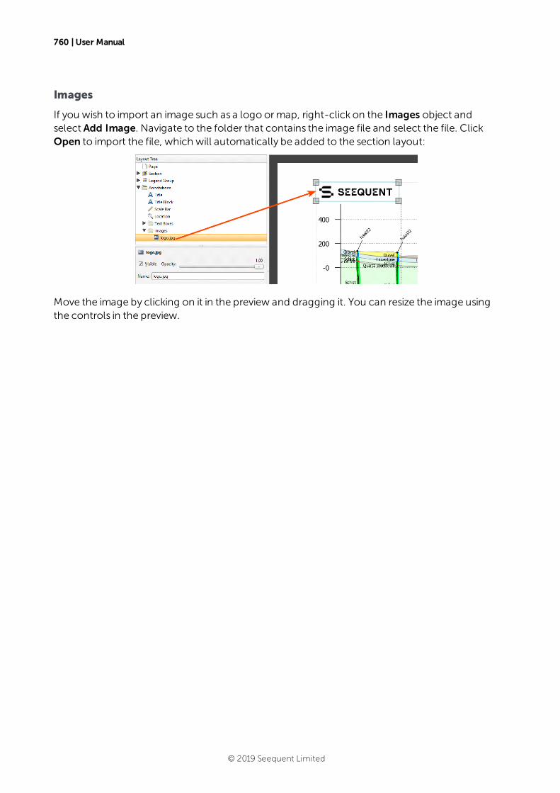
760 | User Manual
Images
If you wish to import an image such as a logo ormap, right-click on the Images object andselect Add Image. Navigate to the folder that contains the image file and select the file. ClickOpen to import the file, which will automatically be added to the section layout:
Move the image by clicking on it in the preview and dragging it. You can resize the image usingthe controls in the preview.
© 2019 Seequent Limited
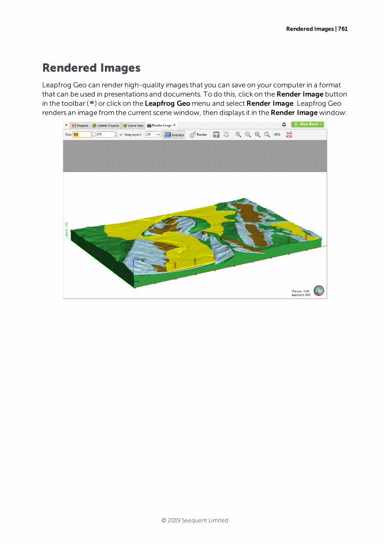
Rendered Images | 761
Rendered ImagesLeapfrog Geo can render high-quality images that you can save on your computer in a formatthat can be used in presentations and documents. To do this, click on theRender Image buttonin the toolbar ( ) or click on the Leapfrog Geomenu and select Render Image. Leapfrog Georenders an image from the current scenewindow, then displays it in theRender Imagewindow:
© 2019 Seequent Limited
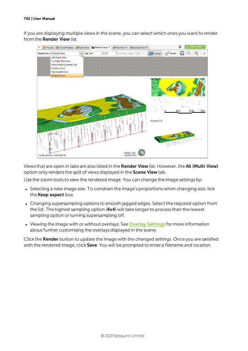
762 | User Manual
If you are displaying multiple views in the scene, you can select which ones you want to renderfrom theRender View list:
Views that are open in tabs are also listed in theRender View list. However, the All (Multi View)option only renders the split of views displayed in the Scene View tab.
Use the zoom tools to view the rendered image. You can change the image settings by:
l Selecting a new image size. To constrain the image’s proportionswhen changing size, tickthe Keep aspect box.
l Changing supersampling options to smooth jagged edges. Select the required option fromthe list. The highest sampling option (4x4) will take longer to process than the lowestsampling option or turning supersampling off.
l Viewing the imagewith or without overlays. SeeOverlay Settings formore informationabout further customising the overlays displayed in the scene.
Click theRender button to update the imagewith the changed settings. Once you are satisfiedwith the rendered image, click Save. You will be prompted to enter a filename and location.
© 2019 Seequent Limited
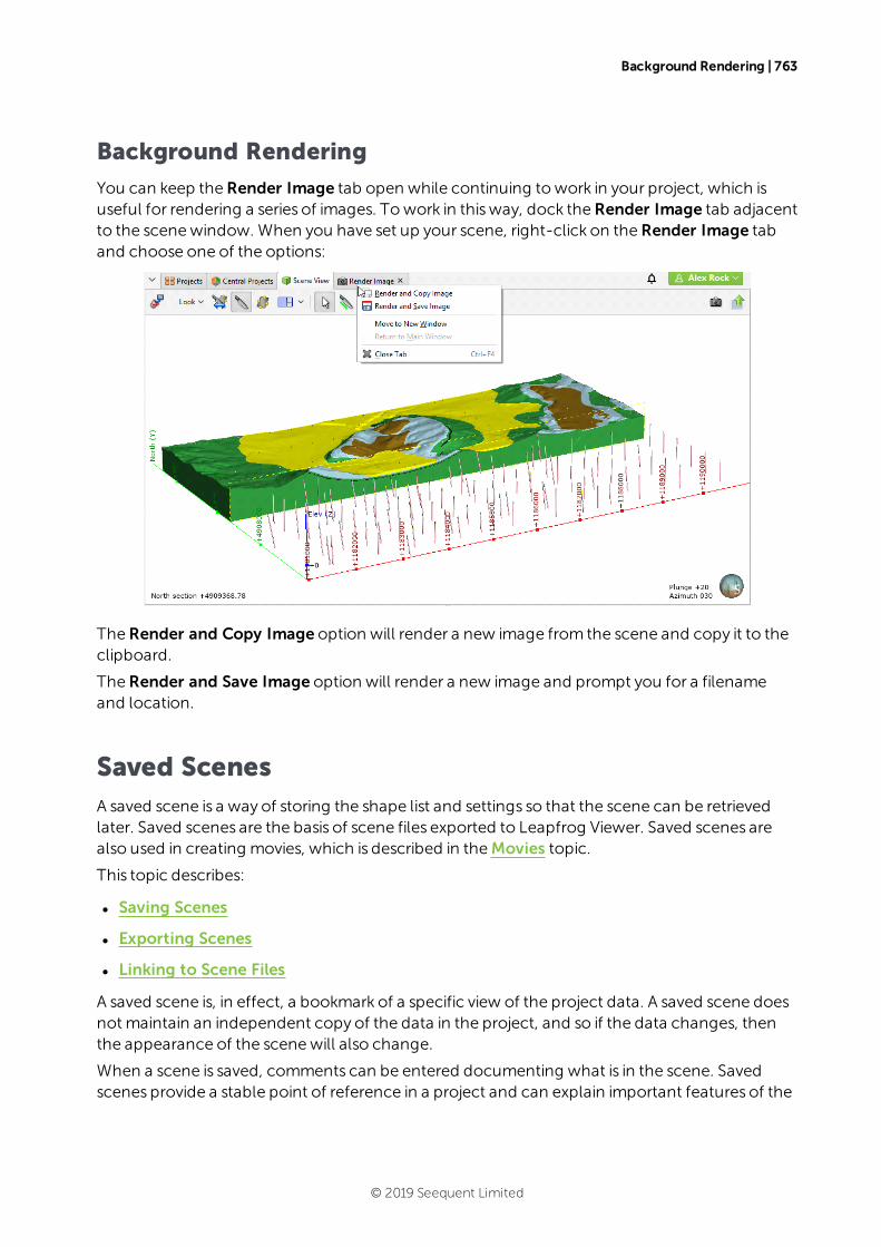
Background Rendering | 763
Background Rendering
You can keep theRender Image tab open while continuing towork in your project, which isuseful for rendering a series of images. Towork in thisway, dock theRender Image tab adjacentto the scenewindow. When you have set up your scene, right-click on theRender Image taband choose one of the options:
TheRender and Copy Image option will render a new image from the scene and copy it to theclipboard.
TheRender and Save Image option will render a new image and prompt you for a filenameand location.
Saved ScenesA saved scene is a way of storing the shape list and settings so that the scene can be retrievedlater. Saved scenes are the basis of scene files exported to Leapfrog Viewer. Saved scenes arealso used in creating movies, which is described in theMovies topic.
This topic describes:
l Saving Scenes
l Exporting Scenes
l Linking to Scene Files
A saved scene is, in effect, a bookmark of a specific view of the project data. A saved scene doesnot maintain an independent copy of the data in the project, and so if the data changes, thenthe appearance of the scenewill also change.
When a scene is saved, comments can be entered documenting what is in the scene. Savedscenes provide a stable point of reference in a project and can explain important features of the
© 2019 Seequent Limited
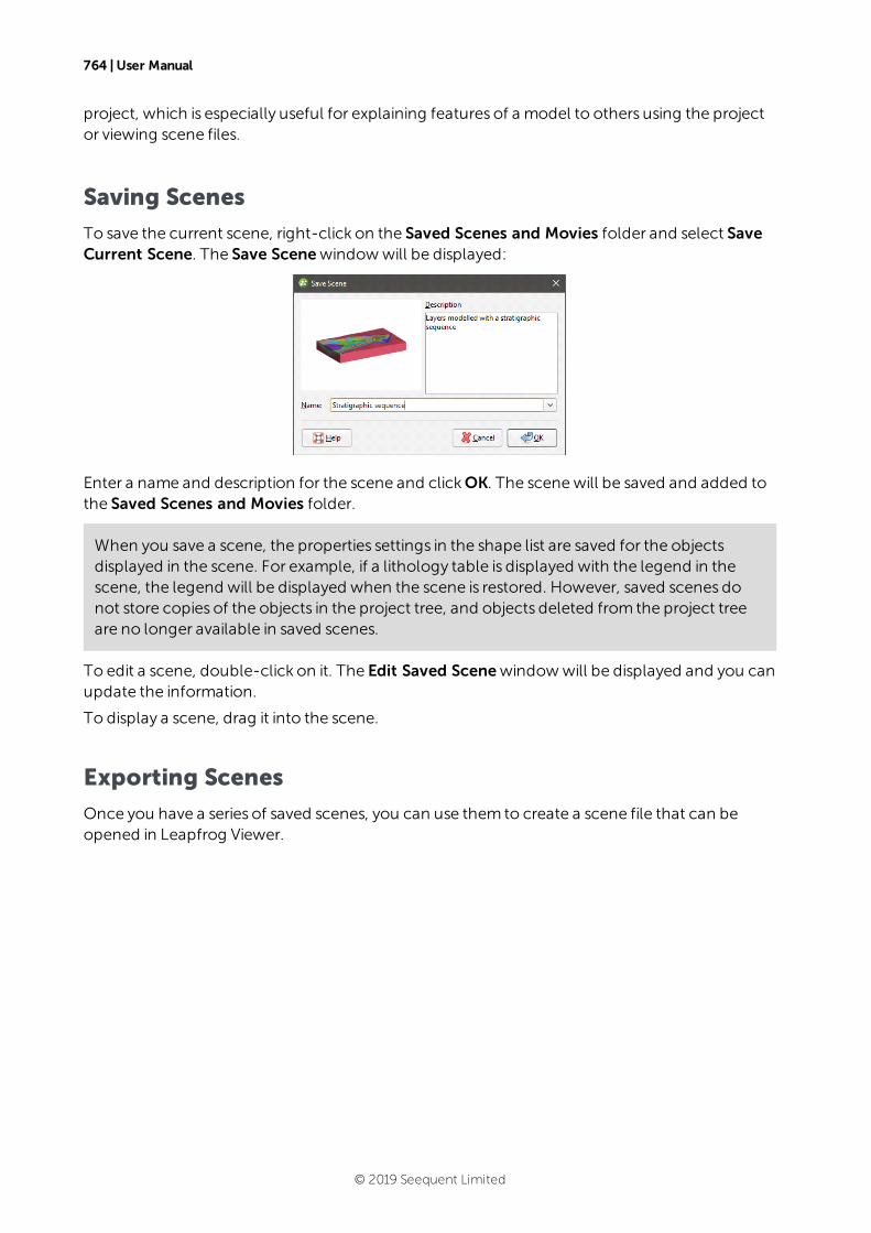
764 | User Manual
project, which is especially useful for explaining features of a model to others using the projector viewing scene files.
Saving Scenes
To save the current scene, right-click on the Saved Scenes and Movies folder and select SaveCurrent Scene. The Save Scenewindowwill be displayed:
Enter a name and description for the scene and clickOK. The scenewill be saved and added tothe Saved Scenes and Movies folder.
When you save a scene, the properties settings in the shape list are saved for the objectsdisplayed in the scene. For example, if a lithology table is displayed with the legend in thescene, the legend will be displayed when the scene is restored. However, saved scenes donot store copies of the objects in the project tree, and objects deleted from the project treeare no longer available in saved scenes.
To edit a scene, double-click on it. The Edit Saved Scenewindowwill be displayed and you canupdate the information.
To display a scene, drag it into the scene.
Exporting Scenes
Once you have a series of saved scenes, you can use them to create a scene file that can beopened in Leapfrog Viewer.
© 2019 Seequent Limited
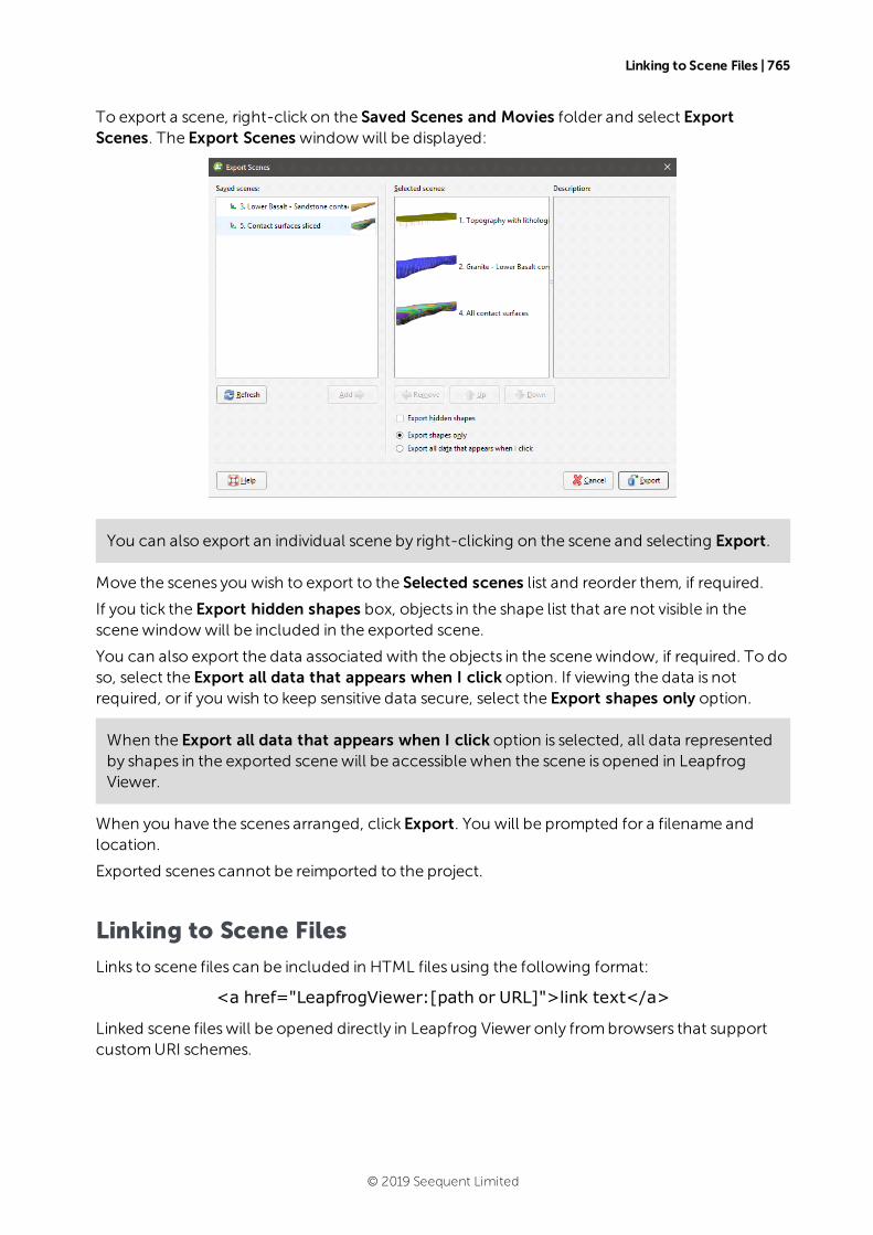
Linking to Scene Files | 765
To export a scene, right-click on the Saved Scenes and Movies folder and select ExportScenes. The Export Scenes windowwill be displayed:
You can also export an individual scene by right-clicking on the scene and selecting Export.
Move the scenes you wish to export to the Selected scenes list and reorder them, if required.
If you tick the Export hidden shapes box, objects in the shape list that are not visible in thescenewindowwill be included in the exported scene.
You can also export the data associated with the objects in the scenewindow, if required. To doso, select the Export all data that appears when I click option. If viewing the data is notrequired, or if you wish to keep sensitive data secure, select the Export shapes only option.
When the Export all data that appears when I click option is selected, all data representedby shapes in the exported scenewill be accessible when the scene is opened in LeapfrogViewer.
When you have the scenes arranged, click Export. You will be prompted for a filename andlocation.
Exported scenes cannot be reimported to the project.
Linking to Scene Files
Links to scene files can be included in HTML files using the following format:
<a href="LeapfrogViewer:[path or URL]">link text</a>
Linked scene fileswill be opened directly in Leapfrog Viewer only frombrowsers that supportcustomURI schemes.
© 2019 Seequent Limited
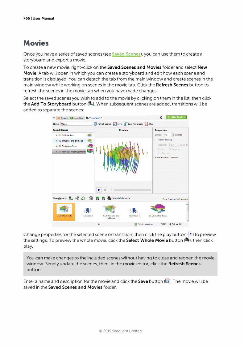
766 | User Manual
MoviesOnce you have a series of saved scenes (see Saved Scenes), you can use them to create astoryboard and export a movie.
To create a newmovie, right-click on the Saved Scenes and Movies folder and selectNewMovie. A tab will open in which you can create a storyboard and edit how each scene andtransition is displayed. You can detach the tab from themain window and create scenes in themain windowwhile working on scenes in themovie tab. Click theRefresh Scenes button torefresh the scenes in themovie tab when you havemade changes.
Select the saved scenes you wish to add to themovie by clicking on them in the list, then clickthe Add To Storyboard button ( ). When subsequent scenes are added, transitionswill beadded to separate the scenes:
Change properties for the selected scene or transition, then click the play button ( ) to previewthe settings. To preview thewholemovie, click the Select Whole Movie button ( ), then clickplay.
You can make changes to the included sceneswithout having to close and reopen themoviewindow. Simply update the scenes, then, in themovie editor, click theRefresh Scenesbutton.
Enter a name and description for themovie and click the Save button ( ). Themovie will besaved in the Saved Scenes and Movies folder.
© 2019 Seequent Limited
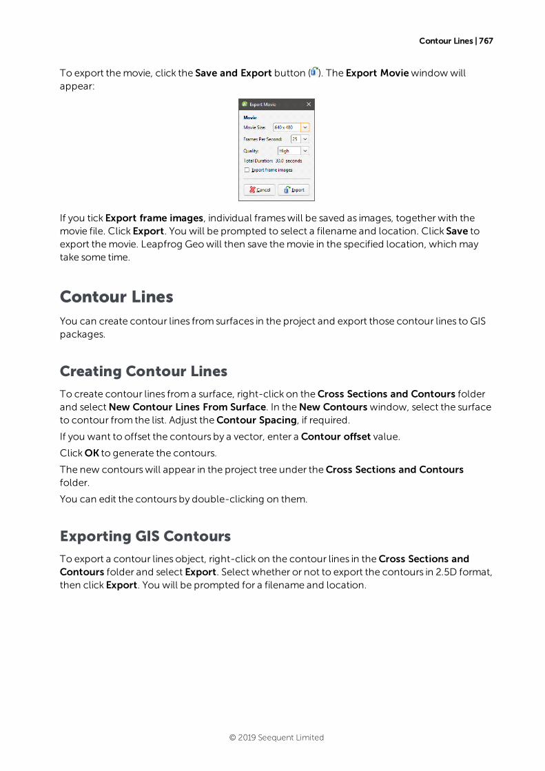
Contour Lines | 767
To export themovie, click the Save and Export button ( ). The Export Moviewindowwillappear:
If you tick Export frame images, individual frameswill be saved as images, together with themovie file. Click Export. You will be prompted to select a filename and location. Click Save toexport themovie. Leapfrog Geowill then save themovie in the specified location, which maytake some time.
Contour LinesYou can create contour lines from surfaces in the project and export those contour lines to GISpackages.
Creating Contour Lines
To create contour lines froma surface, right-click on theCross Sections and Contours folderand selectNew Contour Lines From Surface. In theNew Contours window, select the surfaceto contour from the list. Adjust theContour Spacing, if required.
If you want to offset the contours by a vector, enter a Contour offset value.
ClickOK to generate the contours.
The new contourswill appear in the project tree under theCross Sections and Contoursfolder.
You can edit the contours by double-clicking on them.
Exporting GIS Contours
To export a contour lines object, right-click on the contour lines in theCross Sections andContours folder and select Export. Select whether or not to export the contours in 2.5D format,then click Export. You will be prompted for a filename and location.
© 2019 Seequent Limited