Astrophys. Space Sci. Trans., 7, 425–434, 2011www.astrophys-space-sci-trans.net/7/425/2011/doi:10.5194/astra-7-425-2011© Author(s) 2011. CC Attribution 3.0 License. Astrophysics andSpace Sciences

Tr ansactions

Latitudinal and radial gradients of galactic cosmic ray protons inthe inner heliosphere – PAMELA and Ulysses observations

N. De Simone1, V. Di Felice1, J. Gieseler3, M. Boezio2, M. Casolino1, P. Picozza1, PAMELA Collaboration † , andB. Heber3

1INFN, Structure of Rome “Tor Vergata” and Physics Department of University of Rome “Tor Vergata”, Via della RicercaScientifica 1, I-00133 Rome, Italy2INFN, Structure of Trieste and Physics Department of University of Trieste, I-34147 Trieste, Italy3Inst. fur Experimentelle und Angewandte Physik, Christian-Albrechts-Universitat Kiel, Leibnizstr. 11, 24118 Kiel, Germany

Received: 15 November 2010 – Revised: 7 March 2011 – Accepted: 13 April 2011 – Published: 22 September 2011

Abstract. Ulysses, launched on 6 October 1990, was placedin an elliptical, high inclined (80.2◦) orbit around the Sun,and was switched off in June 2009. It has been the onlyspacecraft exploring high-latitude regions of the inner helio-sphere. The Kiel Electron Telescope (KET) aboard Ulyssesmeasures electrons from 3 MeV to a few GeV and protonsand helium in the energy range from 6 MeV/nucleon to above2 GeV/nucleon. The PAMELA (Payload for Antimatter Mat-ter Exploration and Light-nuclei Astrophysics) space borneexperiment was launched on 15 June 2006 and is contin-uously collecting data since then. The apparatus measureselectrons, positrons, protons, anti-protons and heavier nucleifrom about 100 MeV to several hundreds of GeV. Thus thecombination of Ulysses and PAMELA measurements is ide-ally suited to determine the spatial gradients during the ex-tended minimum of solar cycle 23. For protons in the rigidityinterval 1.6−1.8 GV we find a radial gradient of 2.7%/AUand a latitudinal gradient of−0.024%/degree. Although thelatitudinal gradient is as expected negative, its value is muchsmaller than predicted by current particle propagation mod-els. This result is of relevance for the study of propagationparameters in the inner heliosphere.

1 Introduction

Energetic charged particles propagating in the heliosphereare scattered by irregularities in the heliospheric magneticfield, undergo gradient and curvature drifts, convection and

Correspondence to:N. De Simone(desimone@roma2.infn.it)

adiabatic deceleration in the expanding solar wind. Aspointed out byJokipii et al.(1977) these drift effects shouldalso be an important element of cosmic ray modulation.Models taking these effects into account (Potgieter et al.,2001) predict the latitudinal distribution of galactic cosmicray (GCR) protons and electrons. In the 1980s and in the2000s, during anA < 0-solar magnetic epoch, a negative lat-itudinal gradient for positively charged cosmic rays is pre-dicted. Such gradients were found by the cosmic ray instru-ments aboard the two Voyagers (Cummings et al., 1987; Mc-Donald et al., 1997a). In the 1970s and 1990s, during anA < 0-solar magnetic epoch, Pioneer and Ulysses measure-ments in 1974 to 1977 and 1994 to 1995 confirmed the ex-pectation of positive latitudinal gradients (McKibben, 1989;Heber et al., 1996a). In particular, Ulysses measurementsduring the previous solar minimum have been reported byHeber et al.(1996b) andHeber et al.(1999) using the mea-surements of the IMP 8 spacecraft as a baseline close toEarth.

In this work the data comparison with PAMELA has beencarried out in the period of overlap of the two missions, be-tween July 2006 and July 2009. Because the solar activitychanges the GCR intensity in a rigidity dependent way, itis important to compare data samples at the same rigidity.Therefore, after a brief description of the two instruments inSect.2, we will use two different methods in Sect.3 to definethe most suitable rigidity range for comparison and we willthen calculate the corresponding gradients.

2 Instrumentation

The observations presented here were made with the Cos-mic and Solar Particle Investigation (COSPIN) Kiel Electron

Published by Copernicus Publications on behalf of the Arbeitsgemeinschaft Extraterrestrische Forschung e.V.

426 N. De Simone et al.: Spatial gradients

0

10

20

30

Su

nsp

ot

nu

mb

er

0

10

20

30

0

20

40

Tilt

an

gle

[d

eg]

0

2

4

6

Jan2006

Jul2006

Jan2007

Jul2007

Jan2008

Jul2008

Jan2009

Jul2009

Jan2010

-50

0

50

r [A

U]

Lat

itu

de

[deg

]

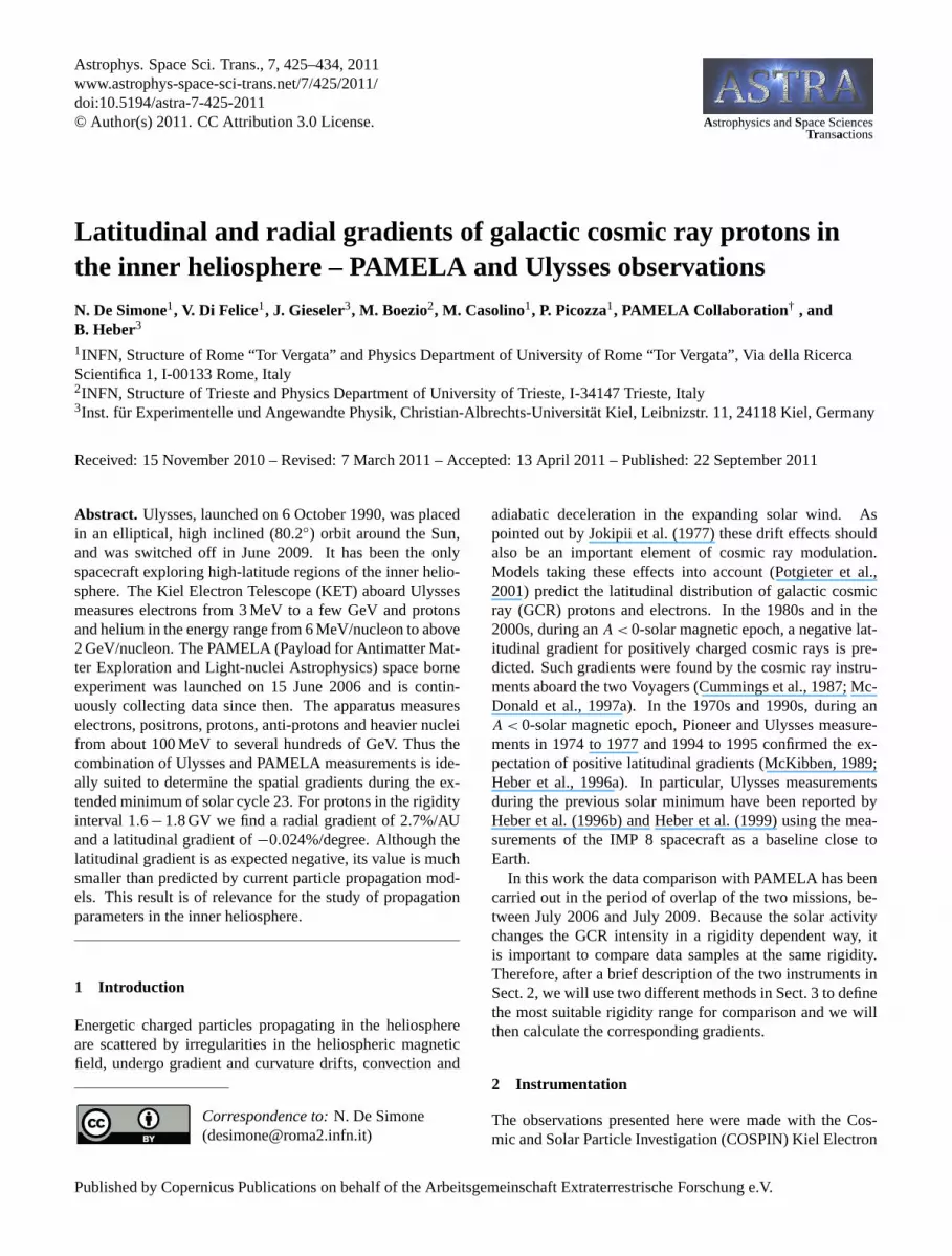
Fig. 1: As a function of time: tilt angle and sunspot number(upper panel), KET heliocentric latitude and radial distance(lower panel). Marked by shading are the comparison inter-vals used to investigate the temporal variation (see Sect.3.1).

Telescope (KET) aboard Ulysses (Simpson et al., 1992) be-tween 1.4 and 5 AU and PAMELA apparatus (Picozza et al.,2007) in low Earth orbit.

2.1 The out-of-ecliptic Ulysses mission

The main scientific goal of the joint ESA-NASA Ulyssesdeep-space mission was to make the first-ever measurementsof the unexplored region of space above the solar poles. TheGCR intensity measured along the Ulysses orbit results froma combination of temporal and spatial variations. Ulysseswas launched first towards Jupiter. Following the fly-by ofJupiter in February 1992, the spacecraft has been traveling inan elliptical, Sun-focused orbit inclined at 80.2 degrees to thesolar equator. The characteristics of the Ulysses trajectoryafter January 2006, during the declining phase of solar cy-cle 23, are displayed in the lower panel of Fig.1. The upperpanel of that figure shows the sunspot number (black curve)and tilt angle (red curve), respectively, indicating a period ofseveral years of very low solar activity. Marked by shadingare two periods after the launch of the PAMELA spacecraftin October 2006 and July 2008 when Ulysses was at about3.5 AU and 50◦. The polar passes are defined to be thoseperiods during which the spacecraft is above 70 degrees he-liographic latitude in either hemisphere. Beginning of 2007,the spacecraft reached a maximum southern latitude of 80◦ata distance of 2.3 AU. The spacecraft then performed a wholelatitude scan of 160◦within 11 months. On 30 June 2009, atthe minimum of the solar cycle, Ulysses was switched off onits way returning towards the heliographic equator at a radialdistance of 5.3 AU.

2.2 Ulysses Kiel electron telescope

The KET measures protons andα-particles in the energyrange from 6 MeV/n to above 2 GeV/n, and electrons in the

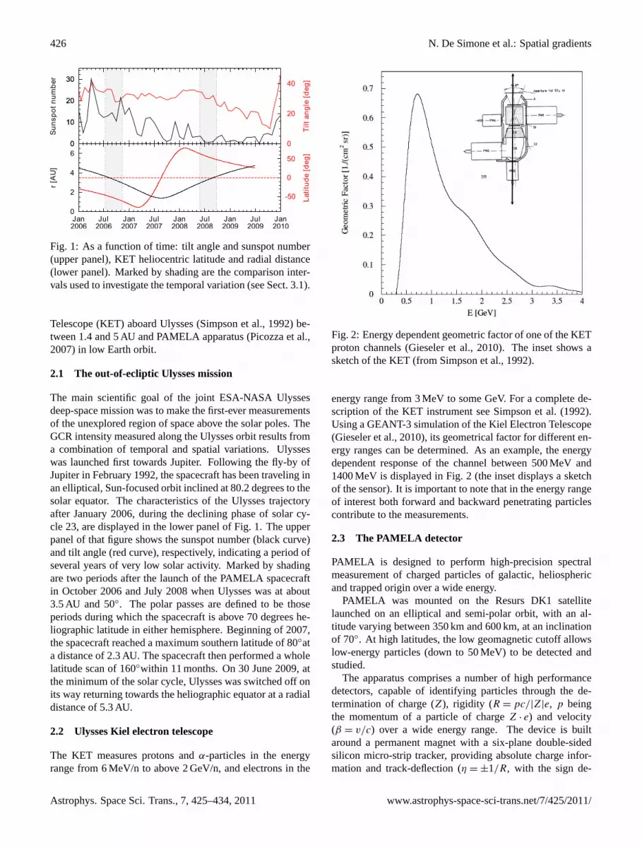
Fig. 2: Energy dependent geometric factor of one of the KETproton channels (Gieseler et al., 2010). The inset shows asketch of the KET (fromSimpson et al., 1992).

energy range from 3 MeV to some GeV. For a complete de-scription of the KET instrument seeSimpson et al.(1992).Using a GEANT-3 simulation of the Kiel Electron Telescope(Gieseler et al., 2010), its geometrical factor for different en-ergy ranges can be determined. As an example, the energydependent response of the channel between 500 MeV and1400 MeV is displayed in Fig.2 (the inset displays a sketchof the sensor). It is important to note that in the energy rangeof interest both forward and backward penetrating particlescontribute to the measurements.

2.3 The PAMELA detector

PAMELA is designed to perform high-precision spectralmeasurement of charged particles of galactic, heliosphericand trapped origin over a wide energy.

PAMELA was mounted on the Resurs DK1 satellitelaunched on an elliptical and semi-polar orbit, with an al-titude varying between 350 km and 600 km, at an inclinationof 70◦. At high latitudes, the low geomagnetic cutoff allowslow-energy particles (down to 50 MeV) to be detected andstudied.

The apparatus comprises a number of high performancedetectors, capable of identifying particles through the de-termination of charge (Z), rigidity (R = pc/|Z|e, p beingthe momentum of a particle of chargeZ · e) and velocity(β = v/c) over a wide energy range. The device is builtaround a permanent magnet with a six-plane double-sidedsilicon micro-strip tracker, providing absolute charge infor-mation and track-deflection (η = ±1/R, with the sign de-

Astrophys. Space Sci. Trans., 7, 425–434, 2011 www.astrophys-space-sci-trans.net/7/425/2011/

N. De Simone et al.: Spatial gradients 427

pending on the sign of the charge derived from the curva-ture direction) information. A scintillator system, composedof three double layers of scintillators (S1, S2, S3), providesthe trigger, a time-of-flight measurement and an additionalestimation of absolute charge. A silicon-tungsten imagingcalorimeter, a bottom scintillator (S4) and a neutron detectorare used to perform lepton-hadron discrimination. An anti-coincidence system is used off-line to reject spurious eventsgenerated by particles interacting in the apparatus. A moredetailed description of PAMELA and the analysis methodol-ogy can be found inCasolino et al.(2008).

3 Data analysis

For our analysis we assume that in the inner solar systemthe variation of the cosmic ray flux is separable in timeand space (McDonald et al., 1997b). Let JU (R,t, r,θ) andJE(R,t, rE,θE) be the flux intensities at rigidityR andtime t averaged over one solar rotation and measured byUlysses KET along its orbit and PAMELA at Earth, respec-tively. Then:

JU (R,t,r,θ)= JE(R,t,rE,θE) ·f (R,1r,1θ) (1)

wheref (R,1r,1θ) is a function of the rigidityR and ofthe heliospheric radial (1r) and latitudinal (1θ ) distancesbetween the two spacecraft. The radial distance1r is deter-mined by:

1r = rU −rE . (2)

Although Heber et al.(1996b) andSimpson et al.(1996)found a small asymmetry of the GCR flux with respect tothe heliographic equator, we assume that the proton inten-sity is symmetric. Thus, the latitudinal distance1θ is deter-mined by:

1θ = |θU |−|θE |. (3)

In both formulasU andE indicate the spatial positions ofUlysses and Earth, respectively.

Assuming that latitudinal and radial variations are separa-ble and that the variation inr (see Eq. (2)) andθ (see Eq. (3))can be approximated by an exponential law, Eq. (1) can berewritten as:

JU (R,t,r,θ)= JE(R,t, rE,θE) exp(Gr ·1r) exp(Gθ ·1θ) (4)

where,Gr and Gθ are the rigidity dependent (Cummingset al., 1987; Fujii and McDonald, 1999; Heber et al., 1996a;McDonald et al., 1997a; McKibben, 1989) radial and latitu-dinal gradients, respectively.

3.1 Determination of the mean rigidity throughtemporal variation

In order to use Eq. (4) to estimate the gradients, we need todefine the rigiditiesR for the comparison, taking into accountthe rigidity dependent geometric factor of the KET channel.

Rigidity (GV)0.8 1 1.2 1.4 1.6 1.8 2 2.2 2.40.65

0.7

0.75

0.8

0.85

0.9

0.95

1 PAMELA

KET subchan

Proton flux 2006 / Proton flux 2008

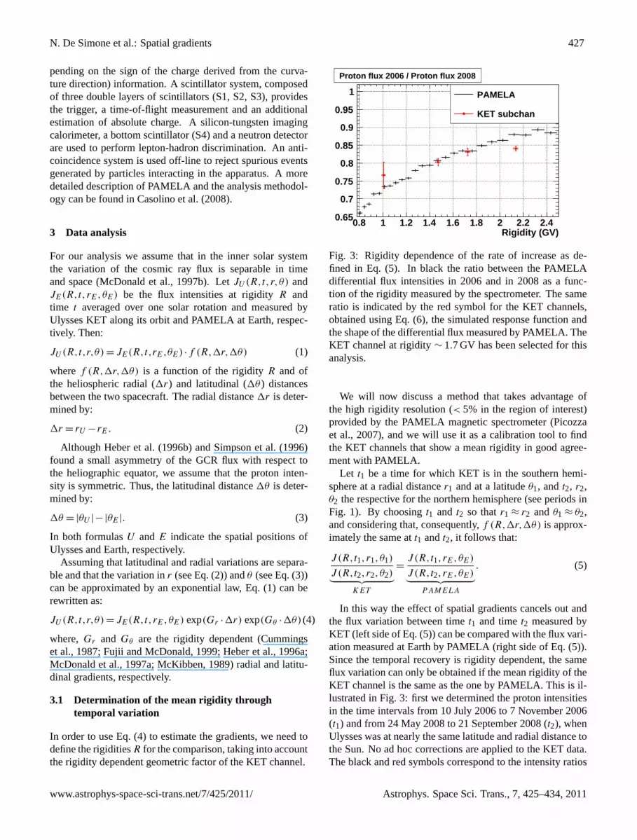
Fig. 3: Rigidity dependence of the rate of increase as de-fined in Eq. (5). In black the ratio between the PAMELAdifferential flux intensities in 2006 and in 2008 as a func-tion of the rigidity measured by the spectrometer. The sameratio is indicated by the red symbol for the KET channels,obtained using Eq. (6), the simulated response function andthe shape of the differential flux measured by PAMELA. TheKET channel at rigidity∼ 1.7 GV has been selected for thisanalysis.

We will now discuss a method that takes advantage ofthe high rigidity resolution (< 5% in the region of interest)provided by the PAMELA magnetic spectrometer (Picozzaet al., 2007), and we will use it as a calibration tool to findthe KET channels that show a mean rigidity in good agree-ment with PAMELA.

Let t1 be a time for which KET is in the southern hemi-sphere at a radial distancer1 and at a latitudeθ1, andt2, r2,θ2 the respective for the northern hemisphere (see periods inFig. 1). By choosingt1 and t2 so thatr1 ≈ r2 andθ1 ≈ θ2,and considering that, consequently,f (R,1r,1θ) is approx-imately the same att1 andt2, it follows that:

J (R,t1, r1,θ1)

J (R,t2, r2,θ2)︸ ︷︷ ︸KET

=J (R,t1, rE,θE)

J (R,t2, rE,θE)︸ ︷︷ ︸PAMELA

. (5)

In this way the effect of spatial gradients cancels out andthe flux variation between timet1 and timet2 measured byKET (left side of Eq. (5)) can be compared with the flux vari-ation measured at Earth by PAMELA (right side of Eq. (5)).Since the temporal recovery is rigidity dependent, the sameflux variation can only be obtained if the mean rigidity of theKET channel is the same as the one by PAMELA. This is il-lustrated in Fig.3: first we determined the proton intensitiesin the time intervals from 10 July 2006 to 7 November 2006(t1) and from 24 May 2008 to 21 September 2008 (t2), whenUlysses was at nearly the same latitude and radial distance tothe Sun. No ad hoc corrections are applied to the KET data.The black and red symbols correspond to the intensity ratios

www.astrophys-space-sci-trans.net/7/425/2011/ Astrophys. Space Sci. Trans., 7, 425–434, 2011

428 N. De Simone et al.: Spatial gradients

Heliocentric distance (AU)0 0.5 1 1.5 2 2.5 3 3.5 4

Hel

iog

rap

hic

lati

tud

e (d

eg)

-80

-60

-40

-20

0

20

40

60

80

Earth

Ulysses orbit

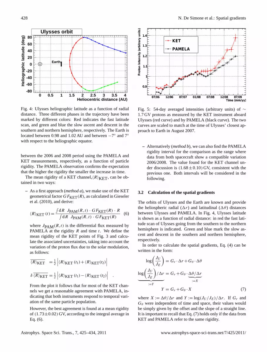
Fig. 4: Ulysses heliographic latitude as a function of radialdistance. Three different phases in the trajectory have beenmarked by different colors: Red indicates the fast latitudescan, and green and blue the slow ascent and descent in thesouthern and northern hemisphere, respectively. The Earth islocated between 0.98 and 1.02 AU and between−7◦ and 7◦

with respect to the heliographic equator.

between the 2006 and 2008 period using the PAMELA andKET measurements, respectively, as a function of particlerigidity. The PAMELA observation confirms the expectationthat the higher the rigidity the smaller the increase in time.

The mean rigidity of a KET channel,〈R〉KET, can be ob-tained in two ways:

– As a first approach (method a), we make use of the KETgeometrical factorGFKET(R), as calculated inGieseleret al.(2010), and derive:

〈R〉KET (t) =

∫dR JPAM(R, t) · GFKET(R) · R∫

dR JPAM(R, t) · GFKET(R)(6)

whereJPAM(R,t) is the differential flux measured byPAMELA at the rigidity R and timet . We define themean rigidity of the KET points of Fig.3 and calcu-late the associated uncertainties, taking into account thevariation of the proton flux due to the solar modulation,as follows:

〈R〉KET =12

∣∣∣〈R〉KET (t1)+〈R〉KET(t2)

∣∣∣δ 〈R〉KET =

12

∣∣∣〈R〉KET (t1)−〈R〉KET (t2)

∣∣∣ .

From the plot it follows that for most of the KET chan-nels we get a reasonable agreement with PAMELA, in-dicating that both instruments respond to temporal vari-ation of the same particle population.

However, the best agreement is found at a mean rigidityof (1.73±0.02) GV, according to the integral average inEq. (6).

Fig. 5: 54-day averaged intensities (arbitrary units) of∼

1.7 GV protons as measured by the KET instrument aboardUlysses (red curve) and by PAMELA (black curve). The twocurves are scaled to match at the time of Ulysses’ closest ap-proach to Earth in August 2007.

– Alternatively (method b), we can also find the PAMELArigidity interval for the comparison as the range wheredata from both spacecraft show a compatible variation2006/2008. The value found for the KET channel un-der discussion is(1.68±0.10) GV, consistent with theprevious one. Both intervals will be considered in thefollowing.

3.2 Calculation of the spatial gradients

The orbits of Ulysses and the Earth are known and providethe heliospheric radial (1r) and latitudinal (1θ ) distancesbetween Ulysses and PAMELA. In Fig.4, Ulysses latitudeis shown as a function of radial distance: in red the fast lati-tude scan of Ulysses going from the southern to the northernhemisphere is indicated. Green and blue mark the slow as-cent and descent in the southern and northern hemisphere,respectively.

In order to calculate the spatial gradients, Eq. (4) can bewritten in the form:

log

(JU

JE

)= Gr ·1r +Gθ ·1θ

log

(JU

JE

)/1r︸ ︷︷ ︸

:=Y

= Gr +Gθ ·1θ/1r︸ ︷︷ ︸:=X

Y = Gr +Gθ ·X (7)

whereX := 1θ/1r andY := log(JU/JE)/1r. If Gr andGθ were independent of time and space, their values wouldbe simply given by the offset and the slope of a straight line.It is important to recall that Eq. (7) holds only if the data fromKET and PAMELA refer to the same rigidity.

Astrophys. Space Sci. Trans., 7, 425–434, 2011 www.astrophys-space-sci-trans.net/7/425/2011/

N. De Simone et al.: Spatial gradients 429

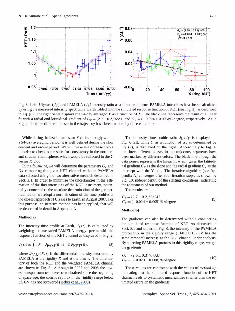
Fig. 6: Left: Ulysses (JU ) and PAMELA (JE) intensity ratio as a function of time. PAMELA intensities have been calculatedby using the measured intensity spectrum at Earth folded with the simulated response function of KET (see Fig.2), as describedin Eq. (8). The right panel displays the 54-day averagedY as a function ofX. The black line represents the result of a linearfit with a radial and latitudinal gradient ofGr = (2.7±0.2)%/AU andGθ = (−0.024±0.005)%/degree, respectively. As inFig. 4, the three different phases in the trajectory have been marked by different colors.

While during the fast latitude scanX varies strongly withina 54-day averaging period, it is well defined during the slowdescent and ascent period. We will make use of these colorsin order to check our results for consistency in the northernand southern hemisphere, which would be reflected in theY

versusX plot.In the following we will determine the parametersGr and

Gθ comparing the given KET channel with the PAMELAdata selected using the two alternative methods described inSect.3.1. In order to minimize the uncertainties in the esti-mation of the flux intensities of the KET instrument, poten-tially connected to the absolute determination of the geomet-rical factor, we adopt a normalization of the time profiles atthe closest approach of Ulysses to Earth, in August 2007. Forthis purpose, an iterative method has been applied, that willbe described in detail in AppendixA.

Method a)

The intensity time profile at Earth,JE(t), is calculated byweighting the measured PAMELA energy spectra with theresponse function of the KET channel as displayed in Fig.2:

JE(t) ∝

∫dR JPAM(R, t) · GFKET(R), (8)

whereJPAM(R, t) is the differential intensity measured byPAMELA at the rigidityR and at the timet . The time his-tory of both the KET and the weighted PAMELA channelare shown in Fig.5. Although in 2007 and 2008 the low-est sunspot numbers have been obtained since the beginningof space age, the cosmic ray flux in the rigidity range below2.5 GV has not recovered (Heber et al., 2009).

The intensity time profile ratioJU/JE is displayed inFig. 6 left, while Y as a function ofX, as determined byEq. (7), is displayed on the right. Accordingly to Fig.4,the three different phases in the trajectory segments havebeen marked by different colors. The black line through thedata points represents the linear fit which gives the latitudi-nal gradientGθ as the slope and the radial gradientGr as theintercept with the Y-axis. The iterative algorithm (see Ap-pendixA) converges after four iteration steps, as shown byFig. 10, independently of the starting conditions, indicatingthe robustness of our method.

The results are:

Gr = (2.7± 0.2) %/AUGθ = (−0.024± 0.005) %/degree .

(9)

Method b)

The gradients can also be determined without consideringthe simulated response function of KET. As discussed inSect.3.1 and shown in Fig.3, the intensity of the PAMELAproton flux in the rigidity range(1.68± 0.10) GV has thesame temporal increase as the KET channel under analysis.By selecting PAMELA protons in this rigidity range, we getthe gradients:

Gr = (2.6± 0.3) %/AUGθ = (−0.023± 0.008) %/degree .

(10)

These values are consistent with the values ofmethod a),indicating that the simulated response function of the KETchannel leads to systematic uncertainties smaller than the es-timated errors on the gradients.

www.astrophys-space-sci-trans.net/7/425/2011/ Astrophys. Space Sci. Trans., 7, 425–434, 2011

430 N. De Simone et al.: Spatial gradients

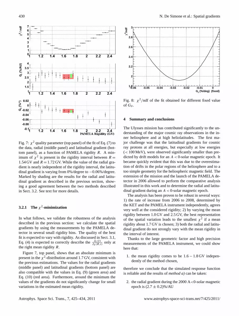
Fig. 7:χ2 quality parameter (top panel) of the fit of Eq. (7) tothe data, radial (middle panel) and latitudinal gradient (bot-tom panel), as a function of PAMELA rigidityR. A min-imum of χ2 is present in the rigidity interval betweenR =

1.54 GV andR = 1.72 GV. While the value of the radial gra-dient is nearly independent of the rigidity interval, the latitu-dinal gradient is varying from 0%/degree to−0.06%/degree.Marked by shading are the results for the radial and latitu-dinal gradient as described in the previous section, show-ing a good agreement between the two methods describedin Sect.3.2. See text for more details.

3.2.1 Theχ2-minimization

In what follows, we validate the robustness of the analysisdescribed in the previous section: we calculate the spatialgradients by using the measurements by the PAMELA de-tector in several small rigidity bins. The quality of the bestfit is expected to vary with rigidity. As discussed in Sect.3.1,Eq. (4) is expected to correctly describe theJU (t)

JE(R,t)only at

the right mean rigidityR.

Figure 7, top panel, shows that an absolute minimum ispresent in theχ2-distribution around 1.7 GV, consistent withthe previous estimations. The values for the radial gradients(middle panel) and latitudinal gradients (bottom panel) arealso compatible with the values in Eq. (9) (green area) andEq. (10) (red area). Furthermore, around the minimum thevalues of the gradients do not significantly change for smallvariations in the estimated mean rigidity.

(%/deg) (fixed)θG-0.06 -0.05 -0.04 -0.03 -0.02 -0.01 0

/nd

f2 χ

1.8

2

2.2

2.4

2.6

2.8

3

Fig. 8: χ2/ndf of the fit obtained for different fixed valueof Gθ .

4 Summary and conclusions

The Ulysses mission has contributed significantly to the un-derstanding of the major cosmic ray observations in the in-ner heliosphere and at high heliolatitudes. The first ma-jor challenge was that the latitudinal gradients for cosmicray protons at all energies, but especially at low energies(< 100 MeV), were observed significantly smaller than pre-dicted by drift models for anA < 0-solar magnetic epoch. Itbecame quickly evident that this was due to the overestima-tion of drifts in the polar regions of the heliosphere and to atoo simple geometry for the heliospheric magnetic field. Theextension of the mission and the launch of the PAMELA de-tector in 2006 allowed to perform the comparative analysisillustrated in this work and to determine the radial and latitu-dinal gradient during anA < 0-solar magnetic epoch.

The analysis has been proven to be robust in several ways:1) the rate of increase from 2006 to 2008, determined bythe KET and the PAMELA instrument independently, agreesvery well at the considered rigidity; 2) by varying the meanrigidity between 1.0 GV and 2.5 GV, the best representationof the spatial variation leads to the smallestχ2 if a meanrigidity about 1.7 GV is chosen; 3) both the radial and latitu-dinal gradient do not strongly vary with the mean rigidity inthe interval of interest.

Thanks to the large geometric factor and high precisionmeasurements of the PAMELA instrument, we could showhere that:

1. the mean rigidity comes to be 1.6− 1.8 GV indepen-dently of the method chosen,

therefore we conclude that the simulated response functionis reliable and the results ofmethod a)can be taken:

2. the radial gradient during the 2000 A<0-solar magneticepoch is (2.7± 0.2)%/AU

Astrophys. Space Sci. Trans., 7, 425–434, 2011 www.astrophys-space-sci-trans.net/7/425/2011/

N. De Simone et al.: Spatial gradients 431

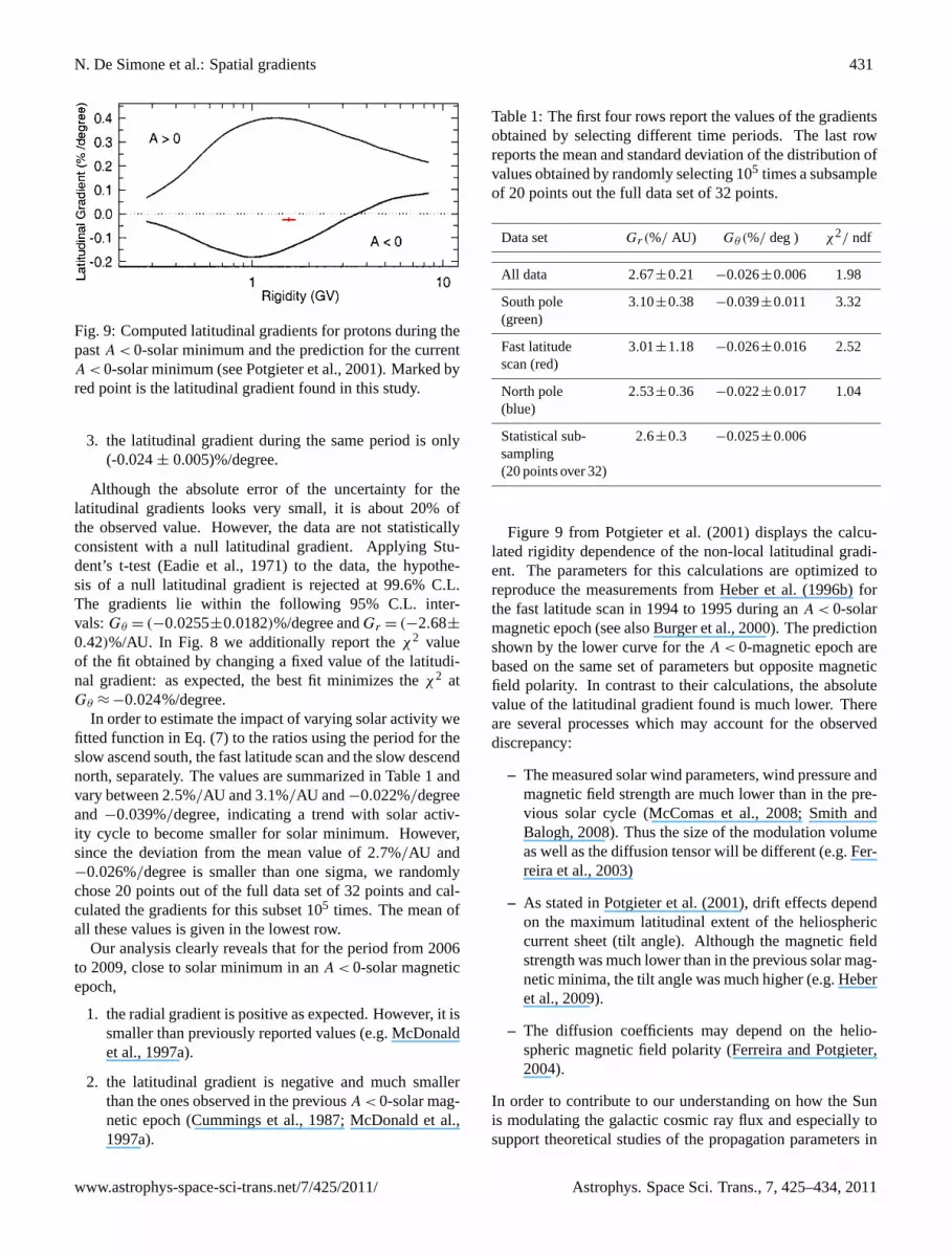
Fig. 9: Computed latitudinal gradients for protons during thepastA < 0-solar minimum and the prediction for the currentA < 0-solar minimum (seePotgieter et al., 2001). Marked byred point is the latitudinal gradient found in this study.

3. the latitudinal gradient during the same period is only(-0.024± 0.005)%/degree.

Although the absolute error of the uncertainty for thelatitudinal gradients looks very small, it is about 20% ofthe observed value. However, the data are not statisticallyconsistent with a null latitudinal gradient. Applying Stu-dent’s t-test (Eadie et al., 1971) to the data, the hypothe-sis of a null latitudinal gradient is rejected at 99.6% C.L.The gradients lie within the following 95% C.L. inter-vals:Gθ = (−0.0255±0.0182)%/degree andGr = (−2.68±

0.42)%/AU. In Fig. 8 we additionally report theχ2 valueof the fit obtained by changing a fixed value of the latitudi-nal gradient: as expected, the best fit minimizes theχ2 atGθ ≈ −0.024%/degree.

In order to estimate the impact of varying solar activity wefitted function in Eq. (7) to the ratios using the period for theslow ascend south, the fast latitude scan and the slow descendnorth, separately. The values are summarized in Table1 andvary between 2.5%/AU and 3.1%/AU and−0.022%/degreeand −0.039%/degree, indicating a trend with solar activ-ity cycle to become smaller for solar minimum. However,since the deviation from the mean value of 2.7%/AU and−0.026%/degree is smaller than one sigma, we randomlychose 20 points out of the full data set of 32 points and cal-culated the gradients for this subset 105 times. The mean ofall these values is given in the lowest row.

Our analysis clearly reveals that for the period from 2006to 2009, close to solar minimum in anA < 0-solar magneticepoch,

1. the radial gradient is positive as expected. However, it issmaller than previously reported values (e.g.McDonaldet al., 1997a).

2. the latitudinal gradient is negative and much smallerthan the ones observed in the previousA < 0-solar mag-netic epoch (Cummings et al., 1987; McDonald et al.,1997a).

Table 1: The first four rows report the values of the gradientsobtained by selecting different time periods. The last rowreports the mean and standard deviation of the distribution ofvalues obtained by randomly selecting 105 times a subsampleof 20 points out the full data set of 32 points.

Data set Gr (%/ AU) Gθ (%/ deg ) χ2/ ndf

All data 2.67±0.21 −0.026±0.006 1.98

South pole 3.10±0.38 −0.039±0.011 3.32(green)

Fast latitude 3.01±1.18 −0.026±0.016 2.52scan (red)

North pole 2.53±0.36 −0.022±0.017 1.04(blue)

Statistical sub- 2.6±0.3 −0.025±0.006sampling(20 points over 32)

Figure9 from Potgieter et al.(2001) displays the calcu-lated rigidity dependence of the non-local latitudinal gradi-ent. The parameters for this calculations are optimized toreproduce the measurements fromHeber et al.(1996b) forthe fast latitude scan in 1994 to 1995 during anA < 0-solarmagnetic epoch (see alsoBurger et al., 2000). The predictionshown by the lower curve for theA < 0-magnetic epoch arebased on the same set of parameters but opposite magneticfield polarity. In contrast to their calculations, the absolutevalue of the latitudinal gradient found is much lower. Thereare several processes which may account for the observeddiscrepancy:

– The measured solar wind parameters, wind pressure andmagnetic field strength are much lower than in the pre-vious solar cycle (McComas et al., 2008; Smith andBalogh, 2008). Thus the size of the modulation volumeas well as the diffusion tensor will be different (e.g.Fer-reira et al., 2003)

– As stated inPotgieter et al.(2001), drift effects dependon the maximum latitudinal extent of the heliosphericcurrent sheet (tilt angle). Although the magnetic fieldstrength was much lower than in the previous solar mag-netic minima, the tilt angle was much higher (e.g.Heberet al., 2009).

– The diffusion coefficients may depend on the helio-spheric magnetic field polarity (Ferreira and Potgieter,2004).

In order to contribute to our understanding on how the Sunis modulating the galactic cosmic ray flux and especially tosupport theoretical studies of the propagation parameters in

www.astrophys-space-sci-trans.net/7/425/2011/ Astrophys. Space Sci. Trans., 7, 425–434, 2011

432 N. De Simone et al.: Spatial gradients

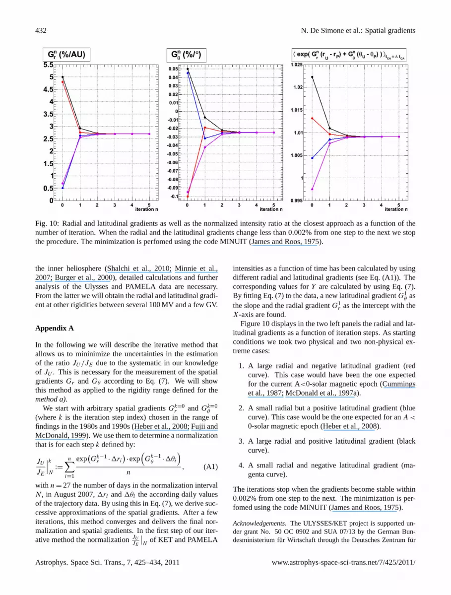
Fig. 10: Radial and latitudinal gradients as well as the normalized intensity ratio at the closest approach as a function of thenumber of iteration. When the radial and the latitudinal gradients change less than 0.002% from one step to the next we stopthe procedure. The minimization is perfomed using the code MINUIT (James and Roos, 1975).

the inner heliosphere (Shalchi et al., 2010; Minnie et al.,2007; Burger et al., 2000), detailed calculations and furtheranalysis of the Ulysses and PAMELA data are necessary.From the latter we will obtain the radial and latitudinal gradi-ent at other rigidities between several 100 MV and a few GV.

Appendix A

In the following we will describe the iterative method thatallows us to mininimize the uncertainties in the estimationof the ratioJU/JE due to the systematic in our knowledgeof JU . This is necessary for the measurement of the spatialgradientsGr and Gθ according to Eq. (7). We will showthis method as applied to the rigidity range defined for themethod a).

We start with arbitrary spatial gradientsGk=0r andGk=0

θ

(wherek is the iteration step index) chosen in the range offindings in the 1980s and 1990s (Heber et al., 2008; Fujii andMcDonald, 1999). We use them to determine a normalizationthat is for each stepk defined by:

JU

JE

∣∣∣kN

:=

n∑i=1

exp(Gk−1

r ·1ri)·exp

(Gk−1

θ ·1θi

)n

, (A1)

with n = 27 the number of days in the normalization intervalN , in August 2007,1ri and1θi the according daily valuesof the trajectory data. By using this in Eq. (7), we derive suc-cessive approximations of the spatial gradients. After a fewiterations, this method converges and delivers the final nor-malization and spatial gradients. In the first step of our iter-ative method the normalizationJU

JE

∣∣N

of KET and PAMELA

intensities as a function of time has been calculated by usingdifferent radial and latitudinal gradients (see Eq. (A1)). Thecorresponding values forY are calculated by using Eq. (7).By fitting Eq. (7) to the data, a new latitudinal gradientG1

θ asthe slope and the radial gradientG1

r as the intercept with theX-axis are found.

Figure10displays in the two left panels the radial and lat-itudinal gradients as a function of iteration steps. As startingconditions we took two physical and two non-physical ex-treme cases:

1. A large radial and negative latitudinal gradient (redcurve). This case would have been the one expectedfor the current A<0-solar magnetic epoch (Cummingset al., 1987; McDonald et al., 1997a).

2. A small radial but a positive latitudinal gradient (bluecurve). This case would be the one expected for anA <

0-solar magnetic epoch (Heber et al., 2008).

3. A large radial and positive latitudinal gradient (blackcurve).

4. A small radial and negative latitudinal gradient (ma-genta curve).

The iterations stop when the gradients become stable within0.002% from one step to the next. The minimization is per-fomed using the code MINUIT (James and Roos, 1975).

Acknowledgements.The ULYSSES/KET project is supported un-der grant No. 50 OC 0902 and SUA 07/13 by the German Bun-desministerium fur Wirtschaft through the Deutsches Zentrum fur

Astrophys. Space Sci. Trans., 7, 425–434, 2011 www.astrophys-space-sci-trans.net/7/425/2011/

N. De Simone et al.: Spatial gradients 433

Luft- und Raumfahrt (DLR). The PAMELA mission is sponsored bythe Italian National Institute of Nuclear Physics (INFN), the ItalianSpace Agency (ASI), the Russian Space Agency (Roskosmos), theRussian Academy of Science, the Deutsches Zentrum fur Luft- undRaumfahrt (DLR), the Swedish National Space Board (SNSB) andthe Swedish Research Council (VR). The German - Italian collabo-ration has been supported by the Deutsche Forschungsgemeinschaftunder grant HE3279/11-1. This work profited from the discussionswith the participants of the ISSI workshop “Cosmic Rays in the He-liosphere II”.

†PAMELA CollaborationO. Adriani1,2, G. C. Barbarino3,4, G. A. Bazilevskaya5,R. Bellotti6,7, M. Boezio8, E. A. Bogomolov9, L. Bonechi1,2,M. Bongi2, V. Bonvicini8, S. Borisov10,11,12, S. Bottai2,A. Bruno6,7, F. Cafagna7, D. Campana4, R. Carbone4,11,P. Carlson13, M. Casolino10, G. Castellini14, L. Consiglio4,M. P. De Pascale10,11, C. De Santis10,11, N. De Simone10,11,V. Di Felice10,11, A. M. Galper12, W. Gillard13, L. Grishantseva12,P. Hofverberg13, G. Jerse8,15, A. V. Karelin12, S. V. Koldashov12,S. Y. Krutkov9, A. N. Kvashnin5, A. Leonov12, V. Malvezzi10,L. Marcelli10, M. Martucci10,11 A. G. Mayorov12, W. Menn16,V. V. Mikhailov12, E. Mocchiutti8, A. Monaco6,7, N. Mori2,N. Nikonov9,10,11, G. Osteria4, F. Palma10,11, P. Papini2,M. Pearce13, P. Picozza10,11, C. Pizzolotto8, M. Ricci17,S. B. Ricciarini2, L. Rossetto13, M. Simon16, R. Sparvoli10,11,P. Spillantini1,2, Y. I. Stozhkov5, A. Vacchi8, E. Vannuccini2,G. Vasilyev9, S. A. Voronov12, J. Wu13,∗, Y. T. Yurkin12,G. Zampa8, N. Zampa8, V. G. Zverev12

1University of Florence, Department of Physics, I-50019Sesto Fiorentino, Florence, Italy2INFN, Sezione di Florence, I-50019 Sesto Fiorentino,Florence, Italy3University of Naples “Federico II”, Department of Physics,I-80126 Naples, Italy4INFN, Sezione di Naples, I-80126 Naples, Italy5Lebedev Physical Institute, RU-119991, Moscow, Russia6University of Bari, Department of Physics, I-70126 Bari,Italy7INFN, Sezione di Bari, I-70126 Bari, Italy8INFN, Sezione di Trieste, I-34149 Trieste, Italy9Ioffe Physical Technical Institute, RU-194021 St. Peters-burg, Russia10INFN, Sezione di Rome “Tor Vergata”, I-00133 Rome,Italy11University of Rome “Tor Vergata”, Department of Physics,I-00133 Rome, Italy12Moscow Engineering and Physics Institute, RU-11540Moscow, Russia13KTH, Department of Physics, and the Oskar Klein Centrefor Cosmoparticle PhysicsAlbaNova University Centre, SE-10691 Stockholm, Sweden14IFAC, I-50019 Sesto Fiorentino, Florence, Italy15University of Trieste, Department of Physics, I-34147Trieste, Italy

16Universitat Siegen, Department of Physics, D-57068Siegen, Germany17INFN, Laboratori Nazionali di Frascati, Via Enrico Fermi40, I-00044 Frascati, Italy∗On leave from School of Mathematics and Physics, ChinaUniversity of Geosciences, CN-430074 Wuhan, China

Edited by: R. VainioReviewed by: two anonymous referees

References

Burger, R. A., Potgieter, M. S., and Heber, B.: Rigidity depen-dence of cosmic ray proton latitudinal gradients measured by theUlysses spacecraft: Implications for the diffusion tensor, J. Geo-phys. Res., 105, 27 447–27 456,doi:10.1029/2000JA000153,2000.

Casolino, M., Picozza, P., Altamura, F., Basili, A., De Si-mone, N., Di Felice, V., Pascale, M. D., Marcelli, L., Mi-nori, M., Nagni, M., Sparvoli, R., Galper, A., Mikhailov, V.,Runtso, M., Voronov, S., Yurkin, Y., Zverev, V., Castellini, G.,Adriani, O., Bonechi, L., Bongi, M., Taddei, E., Vannuc-cini, E., Fedele, D., Papini, P., Ricciarini, S., Spillantini, P.,Ambriola, M., Cafagna, F., Marzo, C. D., Barbarino, G., Cam-pana, D., Rosa, G. D., Osteria, G., Russo, S., Bazilevskaja, G.,Kvashnin, A., Maksumov, O., Misin, S., Stozhkov, Y., Bogo-molov, E., Krutkov, S., Nikonov, N., Bonvicini, V., Boezio, M.,Lundquist, J., Mocchiutti, E., Vacchi, A., Zampa, G.,Zampa, N., Bongiorno, L., Ricci, M., Carlson, P., Hofver-berg, P., Lund, J., Orsi, S., Pearce, M., Menn, W., andSimon, M.: Launch of the space experiment PAMELA, Adv.Space Res., 42, 455–466,doi:10.1016/j.asr.2007.07.023, http://www.sciencedirect.com/science/article/B6V3S-4P9625D-1/2/7b49861564f9fa0f239fb6523df2f03a, 2008.

Cummings, A. C., Stone, E. C., and Webber, W. R.: Latitudinaland radial gradients of anomalous and galactic cosmic rays inthe outer heliosphere, Geophys. Res. Lett., 14, 174–177, 1987.

Eadie, W. T., Drijard, D., James, F. E., Roos, M., and Sadoulet, B.:Statistical methods in experimental physics, North-Holland, Am-sterdam, 1971.

Ferreira, S. E. S. and Potgieter, M. S.: Long-Term Cosmic-RayModulation in the Heliosphere, Astrophys. J., 603, 744–752,doi:10.1086/381649, 2004.

Ferreira, S. E. S., Potgieter, M. S., Heber, B., and Fichtner, H.:Charge-sign dependent modulation in the heliosphere over a 22-year cycle, Ann. Geophys., 21, 1359–1366, 2003.

Fujii, Z. and McDonald, F. B.: The radial intensity gradients ofgalactic and anomalous cosmic rays, Adv. Space Res., 23, 437–441,doi:10.1016/S0273-1177(99)00101-5, 1999.

Gieseler, J., De Simone, N., Heber, B., and Di Felice, V.: The re-sponse function of the Kiel Electron Telescope, re-investigated ,Adv. Space Res., p. in preparation, 2010.

Heber, B., Droge, W., Ferrando, P., Haasbroek, L., Kunow, H.,Muller-Mellin, R., Paizis, C., Potgieter, M., Raviart, A., and Wib-berenz, G.: Spatial variation of> 40 MeV/n nuclei fluxes ob-served during Ulysses rapid latitude scan, Astron. Astrophys.,316, 538–546, 1996a.

www.astrophys-space-sci-trans.net/7/425/2011/ Astrophys. Space Sci. Trans., 7, 425–434, 2011

434 N. De Simone et al.: Spatial gradients

Heber, B., Droge, W., Kunow, H., Muller-Mellin, R., Wib-berenz, G., Ferrando, P., Raviart, A., and Paizis, C.: Spatial vari-ation of > 106 MeV proton fluxes observed during the Ulyssesrapid latitude scan: Ulysses COSPIN/KET results, Geophys.Res. Lett., 23, 1513–1516, 1996b.

Heber, B., Ferrando, P., Raviart, A., Wibberenz, G., Muller-Mellin, R., Kunow, H., Sierks, H., Bothmer, V., Posner, A.,Paizis, C., and Potgieter, M. S.: Differences in the temporal vari-ation of galactic cosmic ray electrons and protons: Implicationsfrom Ulysses at solar minimum, Geophys. Res. Lett., 26, 2133–2136, 1999.

Heber, B., Gieseler, J., Dunzlaff, P., Gomez-Herrero, R., Muller-Mellin, R., Mewaldt, R., Potgieter, M. S., and Ferreira, S.: Lat-itudinal gradients of galactic cosmic rays during the 2007 solarminimum, Astrophys. J., 1,doi:10.1086/592596, 2008.

Heber, B., Kopp, A., Gieseler, J., Muller-Mellin, R., Fichtner, H.,Scherer, K., Potgieter, M. S., and Ferreira, S. E. S.: Modu-lation of Galactic Cosmic Ray Protons and Electrons Duringan Unusual Solar Minimum, Astrophys. J., 699, 1956–1963,doi:10.1088/0004-637X/699/2/1956, 2009.

James, F. and Roos, M.: Minuit - a system for function minimiza-tion and analysis of the parameter errors and correlations, Com-puter Physics Communications, 10, 343–367,doi:10.1016/0010-4655(75)90039-9http://www.sciencedirect.com/science/article/B6TJ5-46FPXJ7-2C/2/58a665cfee07e122711a859fef69c955,1975.

Jokipii, J. R., Levy, E. H., and Hubbard, W. B.: Effects of particledrift on cosmic ray transport, I. General properties, applicationto solar modulation , Astrophys. J., 213, 861–868, 1977.

McComas, D. J., Ebert, R. W., Elliott, H. A., Goldstein, B. E.,Gosling, J. T., Schwadron, N. A., and Skoug, R. M.: Weakersolar wind from the polar coronal holes and the whole Sun, Geo-phys. Res. Lett., 35, 18103,doi:10.1029/2008GL034896, 2008.

McDonald, F. B., Ferrando, P., Heber, B., Kunow, H., McGuire, R.,Muller-Mellin, R., Paizis, C., Raviart, A., and Wibberenz, G.: Acomparative study of cosmic ray radial and latitudinal gradientsin the inner and outer heliosphere, J. Geophys. Res., 102, 4643–4652,doi:10.1029/96JA03673, 1997a.

McDonald, F. B., Ferrando, P., Heber, B., Kunow, H., McGuire, R.,Mller-Mellin, R., Paizis, C., Raviart, A., and Wibberenz, G.: Acomparative study of cosmic ray radial and latitudinal gradientsin the inner and outer heliosphere, J. Geophys. Res., 102, 4643–4652,doi:10.1029/96JA03673, 1997b.

McKibben, R. B.: Reanalysis and confirmation of positive latitudegradients for anomalous helium and Galactic cosmic rays mea-sured in 1975-1976 with Pioneer II, J. Geophys. Res., 94, 17021–17033, 1989.

Minnie, J., Bieber, J. W., Matthaeus, W. H., and Burger, R. A.:On the Ability of Different Diffusion Theories to Account forDirectly Simulated Diffusion Coefficients, Astrophys. J., 663,1049–1054,doi:10.1086/518765, 2007.

Picozza, P., Galper, A. M., Castellini, G., Adriani, O., Altamura, F.,Ambriola, M., Barbarino, G. C., Basili, A., Bazilevskaja, G. A.,Bencardino, R., et al.: PAMELA-A payload for antimatter matterexploration and light-nuclei astrophysics, Astroparticle Physics,27, 296315, 2007.

Potgieter, M. S., Ferreira, S. E. S., and Burger, R.: Modulation ofcosmic rays in the heliosphere over 11 and 22 year cycles: amodelling perspective, Adv. Space Res., 27, 481–492, 2001.

Shalchi, A., Li, G., and Zank, G. P.: Analytic forms of the perpen-dicular cosmic ray diffusion coefficient for an arbitrary turbu-lence spectrum and applications on transport of Galactic protonsand acceleration at interplanetary shocks, Astrophys. Space Sci.,325, 99–111,doi:10.1007/s10509-009-0168-6, 2010.

Simpson, J., Anglin, J., Barlogh, A., Bercovitch, M., Bouman, J.,Budzinski, E., Burrows, J., Carvell, R., Connell, J., Ducros, R.,Ferrando, P., Firth, J., Garcia-Munoz, M., Henrion, J., Hynds, R.,Iwers, B., Jacquet, R., Kunow, H., Lentz, G., Marsden, R., McK-ibben, R., Muller-Mellin, R., Page, D., Perkins, M., Raviart, A.,Sanderson, T., Sierks, H., Treguer, L., Tuzzolino, A., Wenzel, K.-P., and Wibberenz, G.: The Ulysses Cosmic-Ray and Solar Parti-cle Investigation, Astron. Astrophys. Suppl., 92, 365–399, 1992.

Simpson, J. A., Zhang, M., and Bame, S.: A Solar Polar North-South Asymmetry for Cosmic-Ray Propagation in the Helio-sphere: The ULYSSES Pole-to-Pole Rapid Transit, Astrophys.J. Lett., 465, L69, 1996.

Smith, E. J. and Balogh, A.: Decrease in heliospheric mag-netic flux in this solar minimum: Recent Ulysses mag-netic field observations, Geophys. Res. Lett., 35, 22 103,doi:10.1029/2008GL035345, 2008.

Astrophys. Space Sci. Trans., 7, 425–434, 2011 www.astrophys-space-sci-trans.net/7/425/2011/