The Cryosphere, 6, 273–286, 2012www.the-cryosphere.net/6/273/2012/doi:10.5194/tc-6-273-2012© Author(s) 2012. CC Attribution 3.0 License.

The Cryosphere

Kinematic first-order calving law implies potential forabrupt ice-shelf retreat

A. Levermann1,2, T. Albrecht1,2, R. Winkelmann1,2, M. A. Martin 1,2, M. Haseloff1,3, and I. Joughin4

1Earth System Analysis, Potsdam Institute for Climate Impact Research, Potsdam, Germany2Institute of Physics, Potsdam University, Potsdam, Germany3University of British Columbia, Vancouver, Canada4Polar Science Center, APL, University of Washington, Seattle, Washington, USA

Correspondence to:A. Levermann (anders.levermann@pik-potsdam.de)

Received: 28 September 2011 – Published in The Cryosphere Discuss.: 12 October 2011Revised: 30 January 2012 – Accepted: 21 February 2012 – Published: 13 March 2012

Abstract. Recently observed large-scale disintegration ofAntarctic ice shelves has moved their fronts closer towardsgrounded ice. In response, ice-sheet discharge into the oceanhas accelerated, contributing to global sea-level rise and em-phasizing the importance of calving-front dynamics. Theposition of the ice front strongly influences the stress fieldwithin the entire sheet-shelf-system and thereby the massflow across the grounding line. While theories for an ad-vance of the ice-front are readily available, no general ruleexists for its retreat, making it difficult to incorporate the re-treat in predictive models. Here we extract the first-orderlarge-scale kinematic contribution to calving which is con-sistent with large-scale observation. We emphasize that theproposed equation does not constitute a comprehensive calv-ing law but represents the first-order kinematic contributionwhich can and should be complemented by higher order con-tributions as well as the influence of potentially heteroge-neous material properties of the ice. When applied as a calv-ing law, the equation naturally incorporates the stabilizingeffect of pinning points and inhibits ice shelf growth out-side of embayments. It depends only on local ice propertieswhich are, however, determined by the full topography of theice shelf. In numerical simulations the parameterization re-produces multiple stable fronts as observed for the Larsen Aand B Ice Shelves including abrupt transitions between themwhich may be caused by localized ice weaknesses. We alsofind multiple stable states of the Ross Ice Shelf at the gatewayof the West Antarctic Ice Sheet with back stresses onto thesheet reduced by up to 90 % compared to the present state.

1 Introduction

Recent observations have shown rapid acceleration of lo-cal ice streams after the collapse of ice shelves fringing theAntarctic Peninsula, such as Larsen A and B (De Angelisand Skvarca, 2003; Scambos et al., 2004; Rignot et al., 2004;Rott et al., 2007; Pritchard and Vaughan, 2007). Lateral dragexerted by an ice-shelf’s embayment on the flow yields backstresses that restrain grounded ice as long as the ice shelf isintact (Dupont and Alley, 2005, 2006). Ice-shelf disintegra-tion eliminates this buttressing effect and may even lead toabrupt retreat of the grounding line that separates groundedice sheet from floating ice shelf (Weertman, 1974; Schoof,2007; Pollard and Deconto, 2009). The dynamics at the calv-ing front of an ice shelf is thus of major importance for thestability of the Antarctic Ice Sheet and thereby global sealevel (Cazenave et al., 2009; Thomas et al., 2004; Bamberet al., 2009; Winkelmann et al., 2012). Small-scale physicsof calving events is complicated and a number of differentapproaches to derive rates of large- and small-scale calv-ing events have been proposed (Bassis, 2011; Amundson andTruffer, 2010; Grosfeld and Sandhager, 2004; Kenneally andHughes, 2002; Pelto and Warren, 1991; Reeh, 1968). Dif-ferent modes of calving will depend to a different extent onmaterial properties of the ice and on the local flow field. Asan example, considerable effort has been made to incorpo-rate fracture dynamics into diagnostic ice shelf models (Ristet al., 1999; Jansen et al., 2010; Hulbe et al., 2010; Hum-bert et al., 2009; Saheicha et al., 2006; Luckman et al., 2011;Albrecht and Levermann, 2012). Furthermore ice fractureswill alter the stress field and thereby also influence the flow

Published by Copernicus Publications on behalf of the European Geosciences Union.

274 A. Levermann et al.: First-order calving law

field and calving indirectly (Larour et al., 2004; Vieli et al.,2006, 2007; Khazendar et al., 2009; Humbert and Steinhage,2011).

Here we take a simplifying approach and seek the first-order kinematic contribution to iceberg calving ignoringhigher order effects as well as potential interactions of ma-terial properties with the kinematic field. We thus do notseek to understand the initiation, propagation and alterationof material defects of the ice such as crevasses or other frac-tures. While such properties are important for calving theywill be comprised here in a proportionality factor which weseek to determine elsewhere, for example, by use of a frac-ture field as recently introduced (Albrecht and Levermann,2012). These material properties and their alterations withthe flow field are beyond the focus of this study. Insteadwe seek to describe the effect that the large-scale ice flowwill have on the calving of an ice shelf with homogeneousmaterial properties represented by this proportionality fac-tor which is taken to be constant in this study. We furtherdo not seek a comprehensive kinematic calving law whichwill most likely be of complicated nature; instead we deter-mine the first-order contribution that is consistent with uni-versal characteristics found in any ice shelf. Herein we fol-low a procedure commonly applied in theoretical elementaryparticle physics using an expansion of the unknown compre-hensive calving law with respect to the eigenvalues of thelarge-scale spreading rate tensor (e.g.Peskin and Schroeder,1995). General arguments often referred to as symmetry con-siderations then lead to the proposed parameterisation. Webuild on observations which found that the integrated large-scale calving rate shows a dependence on the local ice-flowspreading rate (Alley et al., 2008) and that ice fronts tend tofollow lines of zero across-flow spreading rates (Doake et al.,1998; Doake, 2001). Taking a macroscopic viewpoint, wepropose a simple kinematic calving law applicable to three-dimensional ice shelves, which is consistent with these ob-servations (Figs.1, 3 and4) and unifies previous approachesin the sense that it extracts the first order-dependence on thespreading rate tensor.

2 First-order kinematic contribution to calving

Direct observations in Antarctica show that local calvingrates increase with along-flow ice-shelf spreading-rates,ε‖,i.e. the local spatial derivative of the horizontal velocity fieldalong the ice-flow direction. Across different ice shelves thecalving rate is proportional to the product of this along-flowspreading-rate and the width of the shelf’s embayment (Alleyet al., 2008). Dynamically this width strongly influences thespreading rate perpendicular to the calving frontε⊥ (Fig. 2).Observations furthermore suggest that spreading perpendic-ular to the main flow controls formation and propagation ofintersecting crevasses in the ice and thereby determines po-tential calving locations and influences calving rates (Ken-

0 2 4 6 85

6

7

8

9

10

11

12

13

ε+. ε− [10−6 a−2]

Cal

ving

rate

[100

m/a

]

Filchner Ice ShelfK±

2 = 47 . 106 m a

Larsen C Ice ShelfK±

2 = 110 . 106 m a

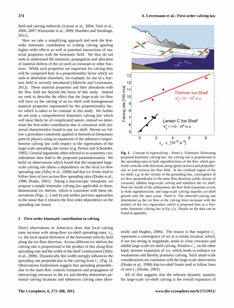
Fig. 1. Concept ofeigencalving– Panel a: Schematic illustratingproposed kinematic calving law: the calving rate is proportional tothe spreading rates in both eigendirections of the flow which gen-erally coincide with directions along (green arrows) and perpendic-ular to (red arrows) the flow field. In the confined region of theice shelf, e.g. in the vicinity of the grounding line, convergence ofice flow perpendicular to the main flow direction yields closure ofcrevasses, inhibits large-scale calving and stabilizes the ice shelf.Near the mouth of the embayment, the flow field expansion occursin both eigendirections and large-scale calving impedes ice-shelfgrowth onto the open ocean. Panel b: The observed calving ratedetermined as the ice flow at the calving front increases with theproduct of the two eigenvalues which is proposed here as a first-order kinematic calving law in Eq. (1). Details on the data can befound in appendix.

neally and Hughes, 2006). The reason is that negativeε⊥

represents a convergence of ice at a certain location, which,if not too strong in magnitude, tends to close crevasses andinhibit large-scale ice-shelf calving. Positiveε⊥, on the otherhand, denotes expansion of ice, which tends to enhance iceweaknesses and thereby promotes calving. Such small-scaleconsiderations are consistent with the large-scale observation(Doake et al., 1998) that ice-shelf fronts tend to follow linesof zeroε⊥(Doake, 2001).

All of this suggests that the relevant dynamic quantityfor large-scale ice-shelf calving is the overall expansion of

The Cryosphere, 6, 273–286, 2012 www.the-cryosphere.net/6/273/2012/

A. Levermann et al.: First-order calving law 275

(a)

300km600km900km

200 400 600 800 10000

1

2

3

4

5x 10

−4

width of embayment in km

e- in 1/a.

(b)

Fig. 2. Simplified set-up to investigate width dependence of sec-ond spreading-rate eigenvalueε−. Panel a: Geometry of basin andresulting calving front for different width of the rectangular embay-ment. Panel b: Quasi-linear relation between minor spreading rateeigenvalueε− in the center of the shelf at the calving front and thewidth of the embayment.

ice flow as represented by the determinant of the horizon-tal spreading-rate matrix. Mathematically the determinant isone of two rotationally-invariant characteristics of the hori-zontal spreading-rate matrix and thus particularly represen-tative of isotropic effects in ice dynamics. The determinantis computed as the product of the spreading rates in the twoprincipal directions of horizontal flow on ice shelves,ε+ · ε−.In most areas along the calving front, these so-called eigendi-rections will coincide with directions along and transversal tothe flow, i.e.ε+ ≈ ε‖ andε− ≈ ε⊥. We thus propose that in re-gions of divergent flow, whereε± > 0, the rate of large-scalecalving,C, is

C = K±

2 · ε+ · ε− for ε± > 0. (1)

HereK±

2 is a proportionality constant that captures the ma-terial properties relevant for calving. The macroscopic view-point of Eq. (1) comprises a number of small-scale physicalprocesses of different calving mechanisms as well as inter-mittent occurrences of tabular iceberg release averaged overa sufficient period of time (see reference (Benn et al., 2007)for a detailed discussion).

Consistent with Eq. (1), we find that the productε+ · ε− asderived from satellite observations (Joughin, 2002; Joughinand Padman, 2003) of the ice flow field of the ice shelvesLarsen C and Filchner is indeed proportional to the calv-ing rate estimated by the terminal velocity at the ice front(Fig.1and appendix for details on the data). Similar relationsare found in the more recent surface-velocity field (Rignotet al., 2011) for the Larsen C-, Ronne- and Ross-ice shelves(Fig. 3) and the Amery- and Filchner-ice shelves (Fig.4).Please note that spatially heterogeneous material propertiesare comprised in the proportionality constantK±

2 . It is thusneither to be expected that the relations shown in Figs.1–4are linear nor that the slopes provided as regression lines areequal. In fact the slopes for the relatively narrow ice shelvesAmery and Filchner are considerably smaller than those forthe other comparably broader shelves. (Note that in using theterminal velocity as an indicator for calving rate, we assumethat changes in ice velocity and glacier length are small inrelation to the calving rate and the changes in the ice-frontposition.)

Equation (1) can be considered the first-order kine-matic contribution to calving under three basic assumptions:(a) stable calving fronts exist, (b)material properties of icenear the calving front can be assumed to be isotropic to lead-ing order and (c) of all availablekinematicproperties it is thevertically averaged spreading rate tensor on which calvingdepends to leading order. In other words, if a calving law issought that assumes isotropic material properties of the iceand one asks for the dependence of this law on the horizon-tal spreading rate field, then such a law can be expanded interms of the the eigenvalues of the spreading rate tensor asfollows:

C = K+

1 · ε+ +K−

1 · ε− +K+

2 · ε2+ +K−

2 · ε2− +K±

2 · ε+ · ε− + ... (2)

with parametersK±

i which may depend on the material prop-erties of the ice. In this formal expansion a number of termsneed to be dismissed on the ground of large-scale physi-cal reasoning. Since the largest eigenvalueε+ generally in-creases within the ice shelf when approaching the groundingline upstream (compare for example Fig.5c),K+

1 has to van-ish or otherwise ice shelves would generally not be stableat all. On the other hand, a non-vanishingK−

1 would meanthat calving is determined mainly by ice divergence acrossthe main flow direction. While we argue that this is indeeda relevant quantity, observations (Fig.1 and reference (Al-ley et al., 2008)) suggest that there has to be a leading role ofε+. The same arguments make it necessary that bothK+

2 andK−

2 vanish. Thus the first-order term of such a law has to bethe one associated withK±

2 as we propose in Eq. (1). Pleasenote that Eq. (1) is not in contradiction with the relation de-rived from Amundson and Truffer(2010). They computedthe steady-state calving rate that is required to balance theice-front advance as governed by the Shallow Shelf Approx-imation, i.e. within the framework of continuum mechanics.

www.the-cryosphere.net/6/273/2012/ The Cryosphere, 6, 273–286, 2012

276 A. Levermann et al.: First-order calving law

+-2

+-2

+-2 10.

10.

10.

a b

c d

e f

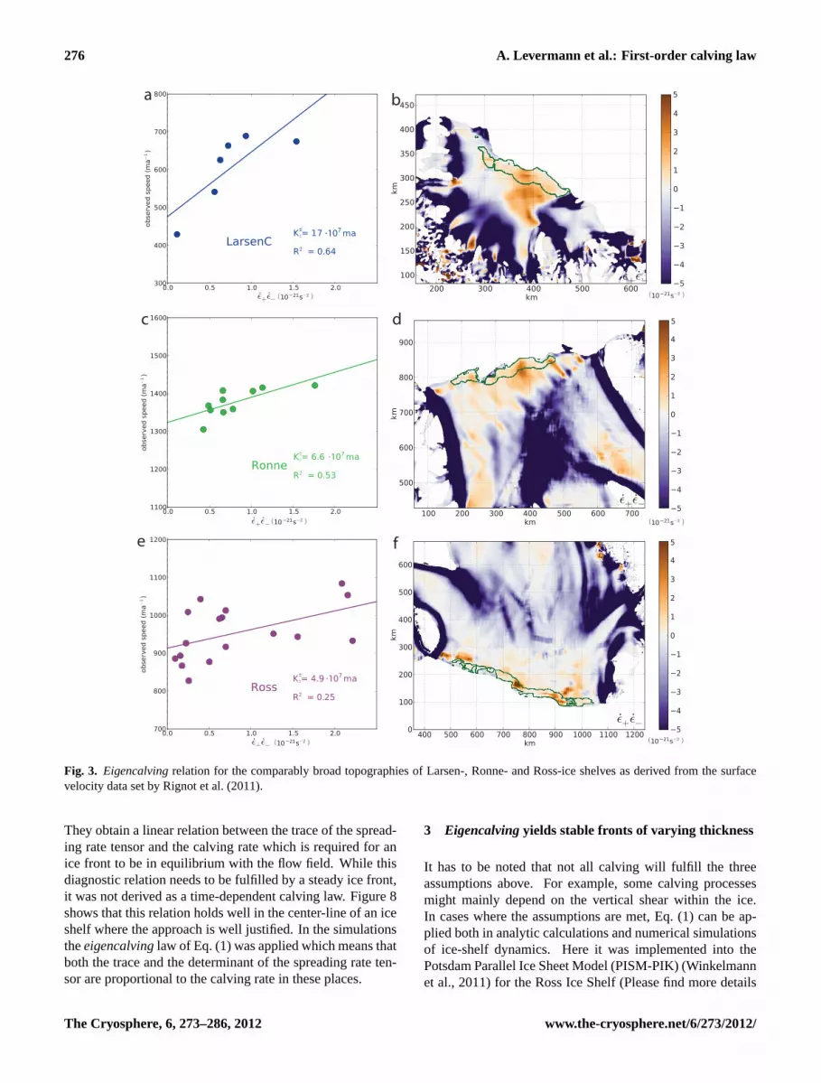
Fig. 3. Eigencalvingrelation for the comparably broad topographies of Larsen-, Ronne- and Ross-ice shelves as derived from the surfacevelocity data set byRignot et al.(2011).

They obtain a linear relation between the trace of the spread-ing rate tensor and the calving rate which is required for anice front to be in equilibrium with the flow field. While thisdiagnostic relation needs to be fulfilled by a steady ice front,it was not derived as a time-dependent calving law. Figure8shows that this relation holds well in the center-line of an iceshelf where the approach is well justified. In the simulationstheeigencalvinglaw of Eq. (1) was applied which means thatboth the trace and the determinant of the spreading rate ten-sor are proportional to the calving rate in these places.

3 Eigencalvingyields stable fronts of varying thickness

It has to be noted that not all calving will fulfill the threeassumptions above. For example, some calving processesmight mainly depend on the vertical shear within the ice.In cases where the assumptions are met, Eq. (1) can be ap-plied both in analytic calculations and numerical simulationsof ice-shelf dynamics. Here it was implemented into thePotsdam Parallel Ice Sheet Model (PISM-PIK) (Winkelmannet al., 2011) for the Ross Ice Shelf (Please find more details

The Cryosphere, 6, 273–286, 2012 www.the-cryosphere.net/6/273/2012/

A. Levermann et al.: First-order calving law 277

a b

c d

10.

10.

0

0

Fig. 4. Eigencalvingrelation for the comparably narrow topographies of Amery- and Filchner-ice shelves as derived from the surface velocitydata set byRignot et al.(2011).

on the experimental set-up in the appendix.) For low valuesof the proportionality constant,K±

2 , calving is not sufficientto ensure a stable calving front (Fig.5a, b). Above a cer-tain threshold,K∗

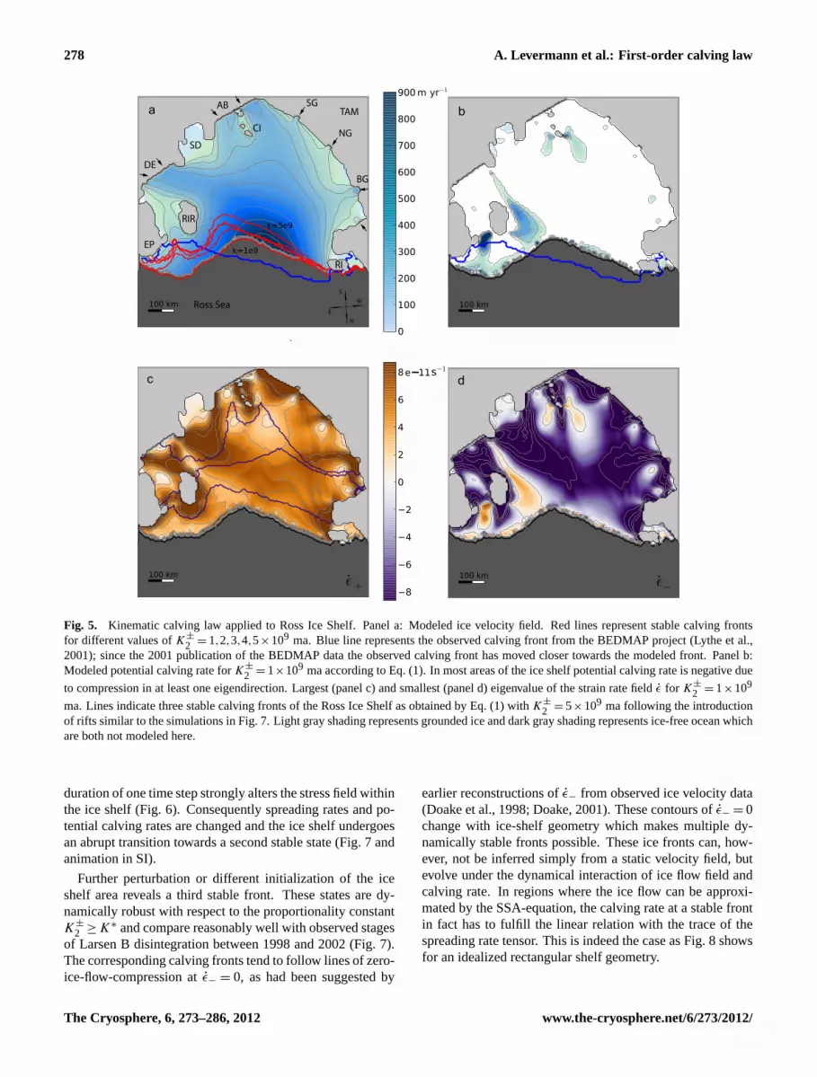
≈ 1×109 ma, the calving front is dynami-cally stable, i.e. the variability of the ice front becomes small(compare gray lines adjacent to the calving front in Figs.6–9). The lack of bottom drag induces a maximum spreadingrate along the ice-flow direction downstream of, but close to,the grounding line (Fig.5c). Thus, as argued above, a calv-ing rate which depends only onε+ would generally increasetowards the grounding line so that no stable ice-shelf frontwould develop. Stability arises through the dependence onthe overall expansion of the velocity field, which is nega-tive for most of the shelf area (Fig.5d) and prohibits calvingthere. Spreading rate fields and thereby areas of potentialcalving according to Eq. (1) are strongly influenced by thegeometry of the shelf ice. The proposed kinematic calvinglaw thereby incorporates the effect of pinning points, such asRoosevelt Ice Rise (RIS) amidst the Ross Ice Shelf. Thesepinning points produce convergence of ice flow and therebystabilize the calving front. In contrast to these regions of con-vergence, ice flow strongly expands towards the mouth of the

shelf’s embayment. Here, calving rates strongly increase andhinder ice-shelf growth outside the bay.

For the Larsen A and B Ice Shelves, application of Eq. (1)in numerical simulations with PISM-PIK yields a stable calv-ing front that compares well with the observed state before1999 (Fig.6a). These fronts are obtained with the same pro-portionality factorK±

2 = 5×109 ma as used for the Ross IceShelf. Eigencalvingthus allows to reproduce calving frontswith varying ice thickness as also found in simulations of thewhole Antarctic Ice Sheet (Martin et al., 2011).

4 Multiple stable fronts and abrupt transitions betweenthem

Inverse computation of ice softness prior to the major dis-integration of Larsen B Ice Shelf in 2002 suggested regionsof strongly weakened ice rheology along the fringing pin-ning points of Robertson Island (RI), Seal Nunataks Islands(SN) in the North East and Jason Peninsula (JP) and CapeDisappointment (CD) in the South West (Khazendar et al.,2007; Vieli et al., 2006). Instantaneous introduction of ice-free rifts in the vicinity of these locations for the minimal

www.the-cryosphere.net/6/273/2012/ The Cryosphere, 6, 273–286, 2012

278 A. Levermann et al.: First-order calving law

NE

S

WRoss Sea

TAM

RIR

CI

EP

BG

RI

NG

SGAB

DE

SD

a b

c d

Fig. 5. Kinematic calving law applied to Ross Ice Shelf. Panel a: Modeled ice velocity field. Red lines represent stable calving frontsfor different values ofK±

2 = 1,2,3,4,5×109 ma. Blue line represents the observed calving front from the BEDMAP project (Lythe et al.,2001); since the 2001 publication of the BEDMAP data the observed calving front has moved closer towards the modeled front. Panel b:Modeled potential calving rate forK±

2 = 1×109 ma according to Eq. (1). In most areas of the ice shelf potential calving rate is negative due

to compression in at least one eigendirection. Largest (panel c) and smallest (panel d) eigenvalue of the strain rate fieldε for K±

2 = 1×109

ma. Lines indicate three stable calving fronts of the Ross Ice Shelf as obtained by Eq. (1) with K±

2 = 5×109 ma following the introductionof rifts similar to the simulations in Fig.7. Light gray shading represents grounded ice and dark gray shading represents ice-free ocean whichare both not modeled here.

duration of one time step strongly alters the stress field withinthe ice shelf (Fig.6). Consequently spreading rates and po-tential calving rates are changed and the ice shelf undergoesan abrupt transition towards a second stable state (Fig.7 andanimation in SI).

Further perturbation or different initialization of the iceshelf area reveals a third stable front. These states are dy-namically robust with respect to the proportionality constantK±

2 ≥ K∗ and compare reasonably well with observed stagesof Larsen B disintegration between 1998 and 2002 (Fig.7).The corresponding calving fronts tend to follow lines of zero-ice-flow-compression atε− = 0, as had been suggested by

earlier reconstructions ofε− from observed ice velocity data(Doake et al., 1998; Doake, 2001). These contours ofε− = 0change with ice-shelf geometry which makes multiple dy-namically stable fronts possible. These ice fronts can, how-ever, not be inferred simply from a static velocity field, butevolve under the dynamical interaction of ice flow field andcalving rate. In regions where the ice flow can be approxi-mated by the SSA-equation, the calving rate at a stable frontin fact has to fulfill the linear relation with the trace of thespreading rate tensor. This is indeed the case as Fig.8 showsfor an idealized rectangular shelf geometry.

The Cryosphere, 6, 273–286, 2012 www.the-cryosphere.net/6/273/2012/

A. Levermann et al.: First-order calving law 279

N E

S

LG

FGCG

DG

HG

EG

RI

SNI

CD

CF

JP

A

B

W

Weddel Sea

Grahamland

GG

EBD

JG

a b

c d

Fig. 6. Kinematic calving law applied to Larsen A and B Ice Shelves withK±

2 = 1×109 ma. Change in spreading-rate components ineigendirections due to instantaneous introduction of ice rift of 2000 m width, which separates ice flow from its pinning points. While thespreading rate in the direction of maximum ice flowε+ ≈ ε‖ does not change significantly (panel a→ b). Spreading rateε− ≈ ε⊥ changessign near the rift (panel c→ d) and thereby initiates an abrupt transition towards a second stable state as shown in Fig.7c. Light gray shadingrepresents grounded ice and dark gray shading represents ice-free ocean which are both not modeled here. Gray lines adjacent to the calvingfront represents the variability of the front in the equilibrium simulation. Time step for plotted front-front positions is two years.

Rapid retreat as governed by Eq. (1) occurs within sev-eral months after the perturbation depending on the value ofK±

2 (compare animation in SI). The analysis of satellite datashow that the 2002-Larsen-B disintegration was not causedby localized calving near the ice front but by emergence ofsurface ponds which weakened the ice shelf and caused asudden collapse (MacAyeal et al., 2003; Glasser and Scam-bos, 2008). Our simulations thus do not provide an explana-tion of this event but show that the emerging stable calving

fronts are consistent with the calving, which is governed bythe first-order kinematic law (Eq.1) and may explain tempo-ral stability of these fronts.

Simulations of the Ross Ice Shelf reproduce the presentlyobserved calving front and suggests two additional stablefront position (Fig.5c). These are associated with reduc-tions in ice-shelf areas by 37 % and 60 %. Back stress ontothe West Antarctic Ice Sheet in these states is reduced by upto 90 % (Fig.9).

www.the-cryosphere.net/6/273/2012/ The Cryosphere, 6, 273–286, 2012

280 A. Levermann et al.: First-order calving law

a b

c d

Fig. 7. Simulation of multiple stable calving front position of ice shelves Larsen A and B. Abrupt transitions between the states can betriggered by instantaneous introduction of ice rifts of 2000 m width (two grid cells) for one time step along the purple lines (compare alsoanimation in SI). Shading represents strongest spreading rateε+ ≈ ε‖. Gray lines adjacent to the calving front represents the variability ofthe front in the equilibrium simulation. Time step for plotted front-front positions is two years. Panel a: Calving front after 100 years offree propagation (purple line) is stabilized by calving rate according to Eq. (1) near the observed 1998 extension (compare Fig.2). Panel b:Initialization of ice front at the year 1998 positions (purple line) plus rifts in the southern parts of Larsen A, induces a collapse of Larsen AIce Shelf and a retreat of the Larsen B front to the 1999 position. Panel c: Rift applied along northern margin of Larsen B yields a secondstable state of the Larsen B ice front similar to the observed 2002 position. Panel d: Rift applied along southern margins of Larsen B yieldsthird stable state with strongly reduced ice-shelf area.

5 Discussions and conclusions

Reliable projection of the evolution of the Antarctic Ice Sheetunder future climate change need to take calving-front dy-namics into account. We present a calving law that re-produces presently observed ice fronts of ice shelves withstrongly varying ice thickness, e.g. the Larsen Ice Shelf and

the Ross Ice Shelf. The calving law has been applied insimulations of the entire Antarctic Ice Sheet (Martin et al.,2011) where it produces a realistic ice front for all major iceshelves. The calving law of Eq. (1) represents the first-orderkinematic contribution of calving under the assumption thatcalving depends kinematically to first-order on the horizon-tal strain rate field and that ice properties are to first-order

The Cryosphere, 6, 273–286, 2012 www.the-cryosphere.net/6/273/2012/

A. Levermann et al.: First-order calving law 281

+ +

- -

Fig. 8. Comparison with relation derived for steady-state calving rate from the SSA-equation (Amundson and Truffer, 2010). Propertiesfor an ice shelf confined in a rectangular narrow basin of 150×103 m width and 250×103 m length with time-dependent calving accordingto Eq. (1). Left column: properties for the center-line along the main flow direction. Right column: properties for a cross-section at themouth of the embayment. Shown are ice thickness and speed (H andv, top) along with the spreading rate components (middle). Analyticsolutions for an unconfined ice shelf are provided as dashed curves. The lower panels compare the steady-state estimate of the calving rateas computed fromAmundson and Truffer(2010) with the ice speed. While the two compare very well along the center-line, the estimatedeviates slightly near the margin where buttressing becomes important and the assumption that the ice velocity has the same direction asthe gradient of H becomes slightly less accurate. The good agreement shows that at the calving front at which theAmundson and Truffer(2010)-assumptions hold, the calving rate has to be proportional to the trace as well as to the determinant of the spreading rate tensor.

isotropic. Not all calving has to fulfill these assumptions.While isotropic material properties can be captured in theproportionality constantK±

2 , ice can be anisotropic near theice front. Furthermore, some calving processes might mainlydepend on the vertical shear within the ice as opposed to thehorizontal strain rate field. The reasoning and conditions un-der which Eq. (1) can be considered a calving law are dis-cussed in detail in the introduction and Sect.2. Under these

conditions, we proposeeigencalvingas a first-order law forlarge-scale calving comprising a number of small-scale pro-cesses. For a comprehensive description of calving front dy-namics our approach may be complemented by additionalprocesses that are not captured by Eq. (1).

www.the-cryosphere.net/6/273/2012/ The Cryosphere, 6, 273–286, 2012

282 A. Levermann et al.: First-order calving law

a b

Fig. 9. Additional stable calving front of the Ross Ice Shelf undereigencalving. Colors represent relative change in longitudinal stressbetween the modeled presently observed extent of the ice shelf (thick blue line) and the second and third stable states of the ice shelf. Graylines adjacent to the calving front represents the variability of the front in the equilibrium simulation. Panel a: State with 37 % reducedice shelf area. Panel b: State with 60 % reduced ice shelf area compared to the modeled present-day situation. Back stress onto the WestAntarctic Ice Sheet in these states is reduced by up to 90 %.

Appendix A

Radar data

Ice-velocity fields for the computation of the spreading rateswere derived from radar satellite data. In the case of Fig.1SAR speckle tracking algorithms were used and provided ona regular grid of grid length 1 km in Polar Stereographic pro-jection with 71◦S as the latitude of true scale (Joughin, 2002).Data are based on observations of the years 2006–2008 forLarsen C (JAXA ALOS L-band SAR) and 1997–2000 forFilchner-Ronne (Joughin and Padman, 2003) (RADARSATAntarctic Mapping Mission). In the case of Figs.3 and 4they were assembled from multiple satellite interferomet-ric synthetic-aperture radar data acquired during the Interna-tional Polar Year 2007 to 2009 (Rignot et al., 2011). Strainrates were computed as the spatial derivative of the velocityfield (neglecting projection errors) with a centered scheme(along the boundaries inward). In order to reduce the ef-fect of undulations of length scale 5–8 km that are due to themeasuring and processing technique, we long-pass filteredthe velocity field with a two-dimensional sliding window of21 × 21 km size. In order to avoid data from groundedice only data points with a velocity magnitude larger thana threshold of 10 m yr−1 within this window were taken intoaccount. Independent data points were computed in 30 kmsections (15 km for the more narrow ice shelves Amery andFilchner) along the ice shelf front in which average velocitiesand horizontal spreading rate eigenvalues were computed.Figures1, 3 and4 show the relation between ice velocity at

the ice front (assumed to be a measure for the calving rate fora steady calving front) and the product of the spreading rateeigenvalues, i.e. the determinant of the spreading rate matrixfor the respective ice shelves.

Appendix B

Brief model description of PISM-PIK

In this study, we apply a derived version of the open-source Parallel Ice Sheet Model version stable 0.2 (PISM,see user’s manual (PISM-authors, 2012) and model descrip-tion paper (Bueler and Brown, 2009)). Starting from PISMstable 0.4 most features of the Potsdam Parallel Ice SheetModel (PISM-PIK,Winkelmann et al.(2011)) have been in-tegrated in the openly available PISM code. It is a thermo-mechanically coupled model developed at the University ofAlaska, Fairbanks, USA. The thickness, temperature, veloc-ity and age of the ice can be simulated, as well as the defor-mation of Earth underneath the ice sheets. Verification of thecode with exact analytical solutions were used to test its nu-merical accuracy (Bueler et al., 2007). Ice softness,A(T ∗),is determined followingPaterson and Budd(1982). PISMgenerally applies a combination of the Shallow Ice Approx-imation (SIA) and the Shallow Shelf Approximation (SSA)(Morland, 1987; Weis et al., 1999) to simulate grounded ice.In all simulations presented here ice is floating and thus thevelocity field is computed by application of SSA only. Nu-merical solutions of the SSA-matrix inversion were obtained

The Cryosphere, 6, 273–286, 2012 www.the-cryosphere.net/6/273/2012/

A. Levermann et al.: First-order calving law 283

using the Portable Extensible Toolkit for Scientific computa-tion (PETSc) library (Balay et al., 2008).

Compared to PISM (version stable 0.2), the Potsdam Par-allel Ice Sheet Model (PISM-PIK) as used here, applies twomajor modifications to the original version of PISM. First, asubgrid scale representation of the calving front was imple-mented in order to be able to apply a continuous calving rate(compare ref. (Albrecht et al., 2011) for a detailed descrip-tion). Secondly, we introduced physical boundary conditionsat the calving front to ensure that the non-local velocity cal-culation yields a reasonable and physically based distributionof the velocity throughout the ice shelf which is crucial forthis study. For a full description of PISM-PIK please conferref. (Winkelmann et al., 2011). The models performance un-der present day boundary conditions is provided in ref. (Mar-tin et al., 2011).

Appendix C

Experimental setup of ice-shelf simulations

In the experimental setups used in this study an ice flow froma region of grounded ice is prescribed by Dirichlet boundaryconditions (fixed ice thickness and velocity) and the dynami-cally evolving ice-shelf is computed according to SSA. Sim-ulations have all been integrated into equilibrium for severalthousand of years. Grounded ice was not taken into account(margins fixed) and in order to ensure that no grounding oc-curs during the simulation the bathymetry within the confin-ing bay is set to 2000 m.

C1 Ross Ice Shelf (RIS)

The Ross Ice Shelf setup has been derived from data usedfor the ice-shelf model-intercomparison, EISMINT II - Ross(MacAyeal et al., 1996). Ice thickness, surface temperatureand accumulation rate of the main part of the Ross ice shelfwere applied on a 6.82 km resolution grid (Fig.5). The com-putational domain in total measures 1000× 1000 km2, ap-proximately between 150◦ W and 160◦ E, as well as between75◦ S and 85◦ S. Inflow velocities at the grounding line havebeen prescribed from RIGGS data (Ross Ice shelf Geophys-ical and Glaciological Survey (Thomas et al., 1984; Bentley,1984)). Broad ice streams drain into the shelf over the SipleCoast (SC) in the south-east draining the West Antarctic IceSheet (WAIS), smaller ones urge through the TransantarcticMountains (TAM) in the west, e.g. the Byrd Glacier (BG),feeding the Ross Ice Shelf with ice from East Antarctica.Properties in the grounded part are held constant during thesimulation and friction is prescribed at the margin. The Roo-sevelt (RIR) and Crary Ice Rises (CIR) are prescribed as el-evations of the bedrock. RIGGS velocity data, acquired at afew hundred locations in the years 1973–1978, has been usedto validate the SSA-velocity calculations of the model. Com-

pared to the original data the setup has been slightly modi-fied in the vicinity of the outer pinning points according toBEDMAP (Lythe et al., 2001) data, such as Ross Island (RI)in the west, where the 3894 m high volcano Mount Erebuscan be found, and the Edward-VII-Peninsula (EP) with CapeColbeck (CC) in the east. These areas had been roughly ex-trapolated in the original model intercomparison, but they arecrucial in our studies in finding a more realistic steady stateof the calving front position and are thus more realisticallyrepresented in our simulations.

C2 Larsen Ice Shelves A and B

Our computational setup incorporates part A and B of theLarsen Ice Shelf which has undergone some dramatical re-treats in the last two decades (Fig.7). These compara-bly small ice shelves are fringing the Antarctic Peninsulabetween 64.5◦S-66◦S and 63◦W-59◦W. Surface elevationand velocity data have been raised in the Modified Antarc-tic Mapping Mission (MAMM), by the Byrd Center group(Liu et al., 1999; Jezek et al., 2003). We apply them on a2 km grid as provided by Dave Covey from the Universityof Alaska, Fairbanks (UAF). The computational domain is200×170 km2 and has been re-gridded to 1 km resolution.Gaps in the data were filled as average over existing neigh-boring values up to the ice front in the year 1999 for Larsen B(Ice front of Larsen A at position of about beginning 1995).The surface temperature (Comiso, 2000) and accumulationdata (Van de Berg et al., 2006) has been taken from present-day Antarctica SeaRISE Data Set on a 5km grid (Le Brocqet al., 2010), regridded to 1 km resolution. Ice shelf thicknessis calculated from surface elevation, assuming hydrostaticequilibrium. The grounding line was expected to be locatedwhere the surface gradient exceeds a critical value (also forice rises). Observed velocities and calculated ice thicknesseswere set as a Dirichlet condition on the supposed groundingline in inlet regions simulating the ice stream inflow throughthe mountains. Six important tributaries can be located alongthe western grounding line, from south to north: LeppardGlacier (LG), Flask Glacier (FG), Crane Glacier (CG), EvansGlacier (EG) and Hektoria Glacier (HG). Drygalsky Glacier(DG) is feeding Larsen A north of the Seal Nunataks Islands(SNI) with the prominent Robertson Island (RI) that separateLarsen A and B Ice Shelves; Larsen B and C are physicallydivided by Jason Peninsula (JP). Larsen C is much larger andnot taken into account in these studies. There, ice is cut offat the coastline south of Cape Framnes (CF).

www.the-cryosphere.net/6/273/2012/ The Cryosphere, 6, 273–286, 2012

284 A. Levermann et al.: First-order calving law

Appendix D

Animation of simulation of Larsen A andB Ice Shelves

The animation in this SI shows the smaller eigenvalue ofthe spreading rate matrixε− for the Larsen A and B IceShelves. Time is plotted as a running number in years of in-tegration. The animation begins without any calving startingfrom a steady state with front position comparable to the ob-served situation of the year 1997. Consequently, the shelvesgrow out of the embayment where it builds up a region withstrongly positiveε−. After 100 yearseigencalving(follow-ing Eq. (1) with K±

2 = 1×109 ma is introduced which stabi-lizes the calving front at the position of 1997. After another100 years an ice rift along the margins of Larsen A of 2-grid-box-width is introduced by removing ice there for one timestep. As a consequence the calving front of Larsen A sponta-neously retreats to a new remanent position. This affects thecalving front of Larsen B which stabilizes near the observedposition of the year 1999. Further rifts are introduced alongthe north-east shear margin of Larsen B Ice Shelf and thesouth-west margin of the Larsen B Ice Shelf successively.The resulting remanent steady state calving front positionsare similar to the observed ones after March 2002.

Supplementary material related to thisarticle is available online at:http://www.the-cryosphere.net/6/273/2012/tc-6-273-2012-supplement.zip.

Acknowledgements.We would like to thank Ed Bueler andConstantine Khroulev for invaluable help with the PISM model andDavid M. Holland for useful comments on the work. The study wasfunded by the German National Academic Foundation, the GermanLeibniz association and a doctoral fellowship of the University ofBritish Columbia.

Edited by: I. M. Howat

References

Albrecht, T. and Levermann, A.: Fracture field for large-scale ice dynamics, Journal of Glaciology, 58, 165–176,doi:10.3189/2012JoG11J191, 2012.

Albrecht, T., Martin, M., Haseloff, M., Winkelmann, R., and Lever-mann, A.: Parameterization for subgrid-scale motion of ice-shelfcalving fronts, The Cryosphere, 5, 35–44,doi:10.5194/tc-5-35-2011, 2011.

Alley, R. B., Horgan, H. J., Joughin, I., Cuffey, K. M., Dupont,T. K., Parizek, B. R., Anandakrishnan, S., and Bassis, J.: A Sim-ple Law for Ice-Shelf Calving, Science, 322, 1344, 2008.

Amundson, J. M. and Truffer, M.: A unifying framework foriceberg-calving models, J. Glaciol., 56, 822–830, 2010.

Balay, S., Buschelman, K., Eijkhout, V., Gropp, W., Kaushik, D.,Knepley, M., McInnes, L. C., Smith, B., and Zhang, H.: PETScUsers Manual, Argonne National Laboratory,http://www.mcs.anl.gov/petsc/, 2008.

Bamber, J. L., Riva, R. E. M., Vermeersen, B. L. A., and LeBrocq,A. M.: Reassessment of the Potential Sea-Level Rise from a Col-lapse of the West Antarctic Ice Sheet, Science, 324, 901–903,doi:10.1126/science.1169335, 2009.

Bassis, J. N.: The statistical physics of iceberg calving and theemergence of universal calving laws, J. Geolog., 57, 3–16, 2011.

Benn, D. I., Hulton, N. R. J., and Mottram, R. H.: “Calvinglaws”, ’sliding laws’ and the stability of tidewater glaciers, Ann.Glaciol., 46, 123–130, 2007.

Bentley, C. R.: The Ross Ice shelf Geophysical and Glaciologi-cal Survey (RIGGS): Introduction and summary of measurmentsperformed; Glaciological studies on the Ross Ice Shelf, Antarc-tica, 1973–1978, Antarc. Res. Ser., 42, 1–53, 1984.

Bueler, E. and Brown, J.: The shallow shelf approximation as asliding law in a thermomechanically coupled ice sheet model, J.Geophys. Res., 114, F03008, 2009.

Bueler, E., Brown, J., and Lingle, C.: Exact solutions to the thermo-mechanically coupled shallow-ice approximation: effective toolsfor verification, J. Glaciol., 53, 499–516, 2007.

Cazenave, A., Dominh, K., Guinehut, S., Berthier, E., Llovel, W.,Ramillien, G., Ablain, M., and Larnicol, G.: Sea Level Budgetover 2003-2008: a reevaluation from GRACE space gravimetry,satellite altimetry and Argo, GPC, 56, 83–88, 2009.

Comiso, J. C.: Variability and Trends in Antarctic Surface Tem-peratures from In Situ and Satellite Infrared Measurements., J.Climate, 13, 1674–1696, 2000.

De Angelis, H. and Skvarca, P.: Glacier Surge After Ice Shelf Col-lapse, Science, 299, 1560–1563, 2003.

Doake, C. S. M.: Ice Shelf Stability, British Antarctic Survey, 1282–1290, 2001.

Doake, C. S. M., Corr, H. F. J., Skvarca, P., and Young, N. W.:Breakup and conditions for stability of the northern Larsen IceShelf, Antarctica, Nature, 391, 778–780, 1998.

Dupont, T. K. and Alley, R. B.: Assessment of the importance ofice-shelf buttressing to ice-sheet flow, Geophys. Res. Lett., 32,4503, 2005.

Dupont, T. K. and Alley, R. B.: Role of small ice shelves in sea-level rise, Geophys. Res. Lett., 33, 9503, 2006.

Glasser, N. F. and Scambos, T. A.: A structural glaciological analy-sis of the 2002 Larsen B Ice Shelf collapse, J. Glaciol., 54, 3–16,2008.

Grosfeld, K. and Sandhager, H.: The evolution of a coupled iceshelf-ocean system under different climate states, Glob. Planet.Change, 42, 107–132, 2004.

Hulbe, C. L., LeDoux, C., and Cruikshank, K.: Propagation of longfractures in the Ronne Ice Shelf, Antarctica, investigated usinga numerical model of fracture propagation, J. Glaciol., 56, 459–472, 2010.

Humbert, A. and Steinhage, D.: The evolution of the western riftarea of the Fimbul Ice Shelf, Antarctica, The Cryosphere, 5, 931–944, doi:10.5194/tc-5-931-2011, 2011.

Humbert, A., Kleiner, T., Mohrholz, C. O., Oelke, C., Greve, R.,and Lange, M. A.: A comparative modeling study of the BruntIce Shelf/Stancomb-Wills Ice Tongue system, East Antarctica, J.Glaciol., 55, 53–65, 2009.

The Cryosphere, 6, 273–286, 2012 www.the-cryosphere.net/6/273/2012/

A. Levermann et al.: First-order calving law 285

Jansen, D., Kulessa, B., Sammonds, P. R., Luckman, A., King,E., and Glasser, N.: Present stability of the Larsen C ice shelf,Antarctic Peninsula, J. Geolog., 56, 593–600, 2010.

Jezek, K. C., Farness, K., Carande, R., Wu, X., and Labelle-Hamer, N.: RADARSAT 1 synthetic aperture radar observationsof Antarctica: Modified Antarctic Mapping Mission, 2000, Ra-dio Science, 38, 32–1, 2003.

Joughin, I.: Ice-sheet velocity mapping: a combined interferomet-ric and speckle-tracking approach, Ann. Glaciol., 34, 195–201,2002.

Joughin, I. and Padman, L.: Melting and freezing beneath Filchner-Ronne Ice Shelf, Antarctica, Geophys. Res. Lett., 30, 1477,doi:10.1029/2003GL016941, 2003.

Kenneally, J. P. and Hughes, T. J.: The calving constraints on incep-tion Quternary ice sheets, Quat. Internat., 95–96, 43–53, 2002.

Kenneally, J. P. and Hughes, T. J.: Calving giant icebergs: old prin-ciples, new applications, Antarctic Sci., 18, 409–419, 2006.

Khazendar, A., Rignot, E., and Larour, E.: Larsen B Ice Shelf rhe-ology preceding its disintegration inferred by a control method,Geophys. Res. Lett., 34, L19503, 2007.

Khazendar, A., Rignot, E., and Larour, E.: Roles of marineice, rheology, and fracture in the flow and stability of theBrunt/Stancomb-Wills Ice Shelf, J. Geophys. Res., 114, F04007,2009.

Larour, E., Rignot, E., and Aubry, D.: Modelling of rift propagationon Ronne Ice Shelf, Antarctica, and sensitivity to climate change,Geophys. Res. Lett., 31, L16404, 2004.

Larour, E., Rignot, E., and Aubry, D.: Processes involved in thepropagation of rifts near Hemmen Ice Rise, Ronne Ice Shelf,Antarctica, J. Glaciol., 50, 329–341, 2004.

Le Brocq, A. M., Payne, A. J., and Vieli, A.: An improvedAntarctic dataset for high resolution numerical ice sheet models(ALBMAP v1), Earth System Science Data, 2, 247–260, 2010.

Liu, H., Jezek, K. C., and Li, B.: Development of an Antarcticdigital elevation model by integrating cartographic and remotelysensed data: A geographic information system based approach,J. Geophys. Res., 104, 23199–23214, 1999.

Luckman, A., Jansen, D., Kulessa, B., King, E. C., Sammonds, P.,and Benn, D. I.: Basal crevasses in Larsen C Ice Shelf and impli-cations for their global abundance, The Cryosphere, 6, 113–123,doi:10.5194/tc-6-113-2012, 2012.

Lythe, M. B., Vaughan, D. G., and BEDMAP Consortium: A newice thickness and subglacial topographic model of Antarctica, J.Geophys. Res., 106, 11335–11351,http://www.nerc-bas.ac.uk/public/aedc/bedmap/bedmap.html, 2001.

Lythe, M. B., Vaughan, D. G., and BEDMAP Consortium:BEDMAP: A new ice thickness and subglacial topographicmodel of Antarctica, J. Geophys. Res., 106, 11335–11351, 2001.

MacAyeal, D. R., Rommelaere, V., Huybrechts, P., Hulbe, C. L.,Determann, J., and Ritz, C.: An ice-shelf model test based on theRoss Ice Shelf, Ann. Glaciol., 23, 46–51, 1996.

MacAyeal, D. R., Scambos, T. A., Hulbe, C. L., and Fahnestock,M. A.: Catastrophic ice-shelf break-up by an ice-shelf-fragment-capsize mechanism, J. Glaciol., 49, 22–36, 2003.

Martin, M. A., Winkelmann, R., Haseloff, M., Albrecht, T., Bueler,E., Khroulev, C., and Levermann, A.: The Potsdam Parallel IceSheet Model (PISM-PIK) - Part 2: Dynamic equilibrium simu-lation of the Antarctic ice sheet, The Cryosphere, 5, 727–740,doi:10.5194/tc-5-727-2011, 2011.

Morland, L. W.: Unconfined Ice-Shelf flow, in: Dynamics of theWest Antarctic Ice Sheet, edited by: Van der Veen, C. J., andOerlemans, J., 117–140, Cambridge University Press, 1987.

Paterson, W. S. B. and Budd, W. F.: Flow parameters for ice sheetmodelling, Cold. Reg. Sci. Technol., 6, 175–177, 1982.

Pelto, M. S. and Warren, C. R.: Relationship between tidewaterglacier calving velocity and water depth at the calving front, Ann.Glaciol., 15, 115–118, 1991.

Peskin, M. and Schroeder, D.: An Introduction to Quantum FieldTheory, Addison-Wesley Publishing Company, 1995.

PISM-authors: PISM, a Parallel Ice Sheet Model: User’s man-ual, http://www.pism-docs.org/wiki/lib/exe/fetch.php?media=manual.pdf, 2012.

Pollard, D. and Deconto, R. M.: Modelling West Antarctic ice sheetgrowth and collapse through the past five million years, Nature,458, 329–332, 2009.

Pritchard, H. D. and Vaughan, D. G.: Widespread acceleration oftidewater glaciers on the Antarctic Peninsula, J. Geophys. Res.,112, F03S29, 2007.

Reeh, N.: On the calving of ice from floating glaciers and iceshelves, J. Glaciol., 7, 215–232, 1968.

Rignot, E., Casassa, G., Gogieneni, P., Rivera, A., and Thomas, R.:Accelerated ice discharge from the Antarctic Penninsular follow-ing the collapse of Larsen B Ice Shelf, Geophys. Res. Lett., 31,L18401, 2004.

Rignot, E., Mouginot, J., and Scheuchl, B.: Ice Flowof the Antarctic Ice Sheet, Science, 333, 1427–1430,doi:10.1126/science.1208336, http://www.sciencemag.org/content/333/6048/1427.abstract, 2011.

Rist, M. A., Sammonds, P. R., Murrell, S. A. F., Meredith, P. G.,Doake, C. S. M., Oerter, H., and Matsuki, K.: Experimental andtheoretical fracture mechanics applied to Antarctic ice fractureand surface crevassing, J. Geophys. Res., 104, 2973–2988, 1999.

Rott, H., Rack, W., and Nagler, T.: Increased export of grounded iceafter the collapse of northern Larsen ice shelf, Antarctic Penin-sula, observed by Envisat ASAR, Geoscience and Remote Sens-ing Symposium, IEEE International, 1174–1176, 2007.

Saheicha, K., Sandhager, H., and Lange, M. A.: Modelling the flowregime of Filchner-Shelfeis, FRISP Report No. 14, 58–62, 2006.

Scambos, T., Bohlander, J., Shuman, J. A., and Skvarca, P.: Glacieracceleration and thinning after ice shelf collapse in the Larsen Bembayment, Antarctica, Geophys. Res. Lett., 31, L18402, 2004.

Schoof, C.: Ice sheet grounding line dynamics: Steady states, sta-bility, and hysteresis, J. Geophys. Res., 112, F03S28, 2007.

Thomas, R., MacAyeal, D., Eilers, D., and Gaylord, D.: Glacio-logical Studies on the Ross Ice Shelf, Antarctica, 1972-1978,Glaciol. Geophys. Antarc. Res.-Ser., 42, 21–53, 1984.

Thomas, R., Rignot, E., Casassa, G., Kanagaratnam, P., Acuna, C.,Akins, T., Brecher, H., Frederick, E., Gogineni, P., Krabill, W.,Manizade, S., Ramamoorthy, H., Rivera, A., Russell, R., Son-ntag, J., Swift, R., Yungel, J., and Zwally, J.: Accelerated Sea-Level Rise from West Antarctica, Science, 306, 255–258, 2004.

Van de Berg, W. J., Van den Broeke, M. R., Reijmer, C. H.,and Van Meijgaard, E.: Reassessment of the Antarctic sur-face mass balance using calibrated output of a regional atmo-spheric climate model, J. Geophys. Res.-Atmos., 111, 11104,doi:10.1029/2005JD006495, 2006.

Vieli, A., Payne, A. J., Du, Z., and et al.: Numerical modelling anddata assimilation of the Larsen B ice shelf, Antarctic Peninsula,

www.the-cryosphere.net/6/273/2012/ The Cryosphere, 6, 273–286, 2012

286 A. Levermann et al.: First-order calving law

R. Soc. Lond. Philos. Trans. A, 364, 1815–1839, 2006.Vieli, A., Payne, A. J., Shepherd, A., and Du, Z.: Causes of pre-

collapse changes of the Larsen B ice shelf: Numerical modellingand assimilation of satellite observations, Earth Planet. Sci. Lett.,259, 297–306, 2007.

Weertman, J.: Stability of the junction of an ice sheet and an iceshelf, J. Glaciol., 13, 3–11, 1974.

Weis, M., Greve, R., and Hutter, K.: Theory of shallow ice shelves,Continuum Mech. Thermodyn., 11, 15–50, 1999.

Winkelmann, R., Martin, M. A., Haseloff, M., Albrecht, T., Bueler,E., Khroulev, C., and Levermann, A.: The Potsdam ParallelIce Sheet Model (PISM-PIK) - Part 1: Model description, TheCryosphere, 5, 715–726,doi:10.5194/tc-5-715-2011, 2011.

Winkelmann, R., Levermann, A., Frieler, K., and Martin, M. A.:Uncertainty in future solid ice discharge from Antarctica, TheCryosphere Discuss., 6, 673–714,doi:10.5194/tcd-6-673-2012,2012.

The Cryosphere, 6, 273–286, 2012 www.the-cryosphere.net/6/273/2012/