introduction - su lms
TRANSCRIPT

Introduction
CHAPTER ONE
21 Information about Warren Buffett's investment philosophy and Berkshire Hathaway, Inc.,
can be found on the Internet (http://www.berkshirehathaway.com).
Warren E. Buffett, the celebrated chairman and chief executive officerof Omaha, Nebraska–based Berkshire Hathaway, Inc., started an
investment partnership with $100 in 1956 and has gone on to accumulate apersonal net worth in excess of $30 billion. As both a manager and an investor,Buffett is renowned for focusing on the economics of businesses.
Berkshire’s collection of operating businesses, including the GEICOInsurance Company, International Dairy Queen, Inc., the Nebraska FurnitureMart, and See’s Candies, commonly earn 30 percent to 50 percent per year oninvested capital. This is astonishingly good performance in light of the 10percent to 12 percent return typical of industry in general. A second andequally important contributor to Berkshire’s outstanding performance is ahandful of substantial holdings in publicly traded common stocks, such asThe American Express Company, The Coca-Cola Company, and TheWashington Post Company, among others. As both manager and investor,Buffett looks for “wonderful businesses” with outstanding economic charac-teristics: high rates of return on invested capital, substantial profit margins onsales, and consistent earnings growth. Complicated businesses that facefierce competition or require large capital investment are shunned.1
Buffett’s success is powerful testimony to the practical usefulness of man-agerial economics. Managerial economics answers fundamental questions.When is the market for a product so attractive that entry or expansionbecomes appealing? When is exit preferable to continued operation? Why dosome professions pay well, while others offer only meager pay? Successfulmanagers make good decisions, and one of their most useful tools is themethodology of managerial economics.
1
1

HOW IS MANAGERIAL ECONOMICS USEFUL?
Managerial economics applies economic theory and methods to business and administrativedecision making. Managerial economics prescribes rules for improving managerial decisions.Managerial economics also helps managers recognize how economic forces affect organiza-tions and describes the economic consequences of managerial behavior. It links economicconcepts with quantitative methods to develop vital tools for managerial decision making.This process is illustrated in Figure 1.1.
Evaluating Choice AlternativesManagerial economics identifies ways to efficiently achieve goals. For example, suppose asmall business seeks rapid growth to reach a size that permits efficient use of national mediaadvertising. Managerial economics can be used to identify pricing and production strategiesto help meet this short-run objective quickly and effectively. Similarly, managerial economicsprovides production and marketing rules that permit the company to maximize net profitsonce it has achieved growth or market share objectives.
managerial economicsApplies economic toolsand techniques to business and adminis-trative decision making
Chapter One Introduction 3
FIGURE 1.1Managerial Economics Is a Tool for Improving Management Decision MakingManagerial economics uses economic concepts and quantitative methods to solve managerial problems.
¥ Product Selection, Output, and Pricing¥ Internet Strategy¥ Organization Design¥ Product Development and Promotion �Strategy
¥ Worker Hiring and Training¥ Investment and Financing
¥ Marginal Analysis¥ Theory of Consumer Demand¥ Theory of the Firm¥ Industrial Organization and Firm �Behavior
¥ Public Choice Theory
¥ Numerical Analysis¥ Statistical Estimation¥ Forecasting Procedures¥ Game Theory Concepts¥ Optimization Techniques¥ Information Systems
Economic Concepts Quantitative Methods
Optimal Solutions to ManagementDecision Problems
Managerial Economics
Management Decision Problems
Use of Economic Concepts andQuantitative Methods to Solve �Management Decision Problems
Managerial Economics
2 Introduction

Managerial economics has applications in both profit and not-for-profit sectors. Forexample, an administrator of a nonprofit hospital strives to provide the best medical carepossible given limited medical staff, equipment, and related resources. Using the tools andconcepts of managerial economics, the administrator can determine the optimal allocationof these limited resources. In short, managerial economics helps managers arrive at a set ofoperating rules that aid in the efficient use of scarce human and capital resources. By fol-lowing these rules, businesses, nonprofit organizations, and government agencies are ableto meet objectives efficiently.
Making the Best DecisionTo establish appropriate decision rules, managers must understand the economic environ-ment in which they operate. For example, a grocery retailer may offer consumers a highlyprice-sensitive product, such as milk, at an extremely low markup over cost—say, 1 percentto 2 percent—while offering less price-sensitive products, such as nonprescription drugs, atmarkups of as high as 40 percent over cost. Managerial economics describes the logic of thispricing practice with respect to the goal of profit maximization. Similarly, managerial eco-nomics reveals that auto import quotas reduce the availability of substitutes for domesticallyproduced cars, raise auto prices, and create the possibility of monopoly profits for domesticmanufacturers. It does not explain whether imposing quotas is good public policy; that is adecision involving broader political considerations. Managerial economics only describes thepredictable economic consequences of such actions.
Managerial economics offers a comprehensive application of economic theory and method-ology to management decision making. It is as relevant to the management of governmentagencies, cooperatives, schools, hospitals, museums, and similar not-for-profit institutions as it
4 Part One Overview of Managerial Economics
Managerial Ethics
In The Wall Street Journal, it is not hard to find evidenceof unscrupulous business behavior. However, unethicalconduct is neither consistent with value maximizationnor with the enlightened self-interest of managementand other employees. If honesty did not pervade corpo-rate America, the ability to conduct business would col-lapse. Eventually, the truth always comes out, and whenit does the unscrupulous lose out. For better or worse,we are known by the standards we adopt.
To become successful in business, everyone mustadopt a set of principles. Ethical rules to keep in mindwhen conducting business include the following:
• Above all else, keep your word. Say what you mean,and mean what you say.
• Do the right thing. A handshake with an honorableperson is worth more than a ton of legal documentsfrom a corrupt individual.
• Accept responsibility for your mistakes, and fixthem. Be quick to share credit for success.
• Leave something on the table. Profit with your cus-tomer, not off your customer.
• Stick by your principles. Principles are not for sale atany price.
Does the “high road” lead to corporate success? Considerthe experience of one of America’s most famous winners—Omaha billionaire Warren E. Buffett, chairman ofBerkshire Hathaway, Inc. Buffett and Charlie Munger, thenumber-two man at Berkshire, are famous for doing multimillion-dollar deals on the basis of a simple hand-shake. At Berkshire, management relies upon the charac-ter of the people that they are dealing with rather thanexpensive accounting audits, detailed legal opinions, orliability insurance coverage. Buffett says that after someearly mistakes, he learned to go into business only withpeople whom he likes, trusts, and admires. Although acompany will not necessarily prosper because its man-agers display admirable qualities, Buffett says he hasnever made a good deal with a bad person.
Doing the right thing not only makes sense from anethical perspective, but it makes business $ense, too!
See: Emelie Rutherford, “Lawmakers Involved with Enron Probe HadPersonal Stake in the Company,” The Wall Street Journal Online, March 4,2002 (http://online.wsj.com).
M A N A G E R I A L A P P L I C AT I O N 1 . 1
Introduction 3
is to the management of profit-oriented businesses. Although this text focuses primarily onbusiness applications, it also includes examples and problems from the government and non-profit sectors to illustrate the broad relevance of managerial economics.
THEORY OF THE FIRM
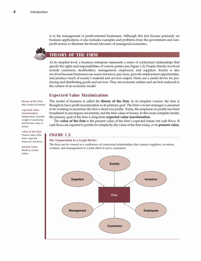
At its simplest level, a business enterprise represents a series of contractual relationships thatspecify the rights and responsibilities of various parties (see Figure 1.2). People directly involvedinclude customers, stockholders, management, employees, and suppliers. Society is alsoinvolved because businesses use scarce resources, pay taxes, provide employment opportunities,and produce much of society’s material and services output. Firms are a useful device for pro-ducing and distributing goods and services. They are economic entities and are best analyzed inthe context of an economic model.
Expected Value MaximizationThe model of business is called the theory of the firm. In its simplest version, the firm isthought to have profit maximization as its primary goal. The firm’s owner-manager is assumedto be working to maximize the firm’s short-run profits. Today, the emphasis on profits has beenbroadened to encompass uncertainty and the time value of money. In this more complete model,the primary goal of the firm is long-term expected value maximization.
The value of the firm is the present value of the firm’s expected future net cash flows. Ifcash flows are equated to profits for simplicity, the value of the firm today, or its present value,
theory of the firm Basic model of business
expected valuemaximization Optimization of profitsin light of uncertaintyand the time value ofmoney
value of the firm Present value of thefirm’s expected future net cash flows
present value Worth in current dollars
Chapter One Introduction 5
FIGURE 1.2The Corporation Is a Legal DeviceThe firm can be viewed as a confluence of contractual relationships that connect suppliers, investors,workers, and management in a joint effort to serve customers.
Management Employees
Customers
Suppliers Investors
Society
Firm
4 Introduction
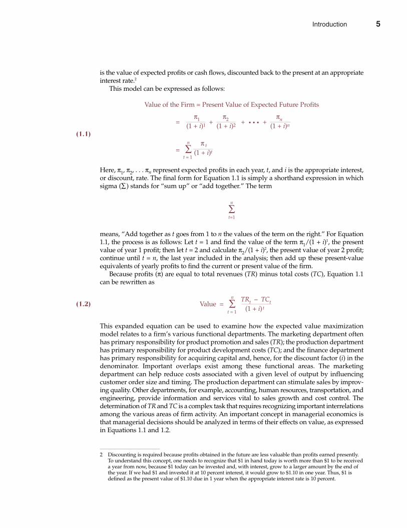
is the value of expected profits or cash flows, discounted back to the present at an appropriateinterest rate.2
This model can be expressed as follows:
Value of the Firm = Present Value of Expected Future Profits
=π1 π2 πn
(1 + i)1 + (1 + i)2 + • • • + (1 + i)n
(1.1)n π t
= ∑ (1 + i)tt = 1
Here, π1, π2, . . . πn represent expected profits in each year, t, and i is the appropriate interest,or discount, rate. The final form for Equation 1.1 is simply a shorthand expression in whichsigma (∑) stands for “sum up” or “add together.” The term
n
∑t=1
means, “Add together as t goes from 1 to n the values of the term on the right.” For Equation1.1, the process is as follows: Let t = 1 and find the value of the term π1/(1 + i)1, the presentvalue of year 1 profit; then let t = 2 and calculate π2/(1 + i)2, the present value of year 2 profit;continue until t = n, the last year included in the analysis; then add up these present-valueequivalents of yearly profits to find the current or present value of the firm.
Because profits (π) are equal to total revenues (TR) minus total costs (TC), Equation 1.1can be rewritten as
n TRt – TCt(1.2) Value = ∑ (1 + i) tt = 1
This expanded equation can be used to examine how the expected value maximizationmodel relates to a firm’s various functional departments. The marketing department oftenhas primary responsibility for product promotion and sales (TR); the production departmenthas primary responsibility for product development costs (TC); and the finance departmenthas primary responsibility for acquiring capital and, hence, for the discount factor (i) in thedenominator. Important overlaps exist among these functional areas. The marketingdepartment can help reduce costs associated with a given level of output by influencingcustomer order size and timing. The production department can stimulate sales by improv-ing quality. Other departments, for example, accounting, human resources, transportation, andengineering, provide information and services vital to sales growth and cost control. Thedetermination of TR and TC is a complex task that requires recognizing important interrelationsamong the various areas of firm activity. An important concept in managerial economics isthat managerial decisions should be analyzed in terms of their effects on value, as expressedin Equations 1.1 and 1.2.
6 Part One Overview of Managerial Economics
2 Discounting is required because profits obtained in the future are less valuable than profits earned presently.To understand this concept, one needs to recognize that $1 in hand today is worth more than $1 to be receiveda year from now, because $1 today can be invested and, with interest, grow to a larger amount by the end ofthe year. If we had $1 and invested it at 10 percent interest, it would grow to $1.10 in one year. Thus, $1 isdefined as the present value of $1.10 due in 1 year when the appropriate interest rate is 10 percent.
Introduction 5
Constraints and the Theory of the FirmManagerial decisions are often made in light of constraints imposed by technology, resourcescarcity, contractual obligations, laws, and regulations. To make decisions that maximizevalue, managers must consider how external constraints affect their ability to achieve organ-ization objectives.
Organizations frequently face limited availability of essential inputs, such as skilled labor,raw materials, energy, specialized machinery, and warehouse space. Managers often face lim-itations on the amount of investment funds available for a particular project or activity.Decisions can also be constrained by contractual requirements. For example, labor contractslimit flexibility in worker scheduling and job assignments. Contracts sometimes require thata minimum level of output be produced to meet delivery requirements. In most instances,output must also meet quality requirements. Some common examples of output quality con-straints are nutritional requirements for feed mixtures, audience exposure requirements formarketing promotions, reliability requirements for electronic products, and customer servicerequirements for minimum satisfaction levels.
Legal restrictions, which affect both production and marketing activities, can also play animportant role in managerial decisions. Laws that define minimum wages, health and safetystandards, pollution emission standards, fuel efficiency requirements, and fair pricing andmarketing practices all limit managerial flexibility.
The role that constraints play in managerial decisions makes the topic of constrained opti-mization a basic element of managerial economics. Later chapters consider important eco-nomic implications of self-imposed and social constraints. This analysis is important becausevalue maximization and allocative efficiency in society depend on the efficient use of scarceeconomic resources.
Limitations of the Theory of the FirmSome critics question why the value maximization criterion is used as a foundation for study-ing firm behavior. Do managers try to optimize (seek the best result) or merely satisfice(seek satisfactory rather than optimal results)? Do managers seek the sharpest needle in ahaystack (optimize), or do they stop after finding one sharp enough for sewing (satisfice)?How can one tell whether company support of the United Way, for example, leads to long-runvalue maximization? Are generous salaries and stock options necessary to attract and retainmanagers who can keep the firm ahead of the competition? When a risky venture is turneddown, is this inefficient risk avoidance? Or does it reflect an appropriate decision from thestandpoint of value maximization?
It is impossible to give definitive answers to questions like these, and this dilemma has led tothe development of alternative theories of firm behavior. Some of the more prominent alterna-tives are models in which size or growth maximization is the assumed primary objective of man-agement, models that argue that managers are most concerned with their own personal utilityor welfare maximization, and models that treat the firm as a collection of individuals with wide-ly divergent goals rather than as a single, identifiable unit. These alternative theories, or models,of managerial behavior have added to our understanding of the firm. Still, none can supplant thebasic value maximization model as a foundation for analyzing managerial decisions. Examiningwhy provides additional insight into the value of studying managerial economics.
Research shows that vigorous competition in markets for most goods and services typical-ly forces managers to seek value maximization in their operating decisions. Competition in thecapital markets forces managers to seek value maximization in their financing decisions aswell. Stockholders are, of course, interested in value maximization because it affects their ratesof return on common stock investments. Managers who pursue their own interests instead ofstockholders’ interests run the risk of losing their job. Buyout pressure from unfriendly firms
optimize Seek the best solution
satisfice Seek satisfactory ratherthan optimal results
Chapter One Introduction 7
6 Introduction

(“raiders”) has been considerable during recent years. Unfriendly takeovers are especially hos-tile to inefficient management that is replaced. Further, because recent studies show a strongcorrelation between firm profits and managerial compensation, managers have strong eco-nomic incentives to pursue value maximization through their decisions.
It is also sometimes overlooked that managers must fully consider costs and benefits beforethey can make reasoned decisions. Would it be wise to seek the best technical solution to aproblem if the costs of finding this solution greatly exceed resulting benefits? Of course not.What often appears to be satisficing on the part of management can be interpreted as value-maximizing behavior once the costs of information gathering and analysis are considered.Similarly, short-run growth maximization strategies are often consistent with long-run valuemaximization when the production, distribution, or promotional advantages of large firmsize are better understood.
Finally, the value maximization model also offers insight into a firm’s voluntary “sociallyresponsible” behavior. The criticism that the traditional theory of the firm emphasizes profitsand value maximization while ignoring the issue of social responsibility is important and willbe discussed later in the chapter. For now, it will prove useful to examine the concept of prof-its, which is central to the theory of the firm.
PROFIT MEASUREMENT
The free enterprise system would fail without profits and the profit motive. Even in plannedeconomies, where state ownership rather than private enterprise is typical, the profit motiveis increasingly used to spur efficient resource use. In the former Eastern Bloc countries, the
8 Part One Overview of Managerial Economics
The World Is Turning to Capitalism and Democracy
Capitalism and democracy are mutually reinforcing.Some philosophers have gone so far as to say that capi-talism and democracy are intertwined. Without capital-ism, democracy may be impossible. Without democracy,capitalism may fail. At a minimum, freely competitivemarkets give consumers broad choices and reinforce theindividual freedoms protected in a democratic society.In democracy, government does not grant individualfreedom. Instead, the political power of governmentemanates from the people. Similarly, the flow of eco-nomic resources originates with the individual cus-tomer in a capitalistic system. It is not centrally directedby government.
Capitalism is socially desirable because of its decen-tralized and customer-oriented nature. The menu ofproducts to be produced is derived from market priceand output signals originating in competitive markets,not from the output schedules of a centralized planningagency. Resources and products are also allocated throughmarket forces. They are not earmarked on the basis offavoritism or social status. Through their purchase deci-sions, customers dictate the quantity and quality ofproducts brought to market.
Competition is a fundamentally attractive feature ofthe capitalistic system because it keeps costs and pricesas low as possible. By operating efficiently, firms are ableto produce the maximum quantity and quality of goodsand services possible. Mass production is, by definition,production for the masses. Competition also limits con-centration of economic and political power. Similarly,the democratic form of government is inconsistent withconsolidated economic influence and decision making.
Totalitarian forms of government are in retreat. Chinahas experienced violent upheaval as the country embarkson much-needed economic and political reforms. In theformer Soviet Union, Eastern Europe, India, and LatinAmerica, years of economic failure forced governments todismantle entrenched bureaucracy and install economicincentives. Rising living standards and political freedomhave made life in the West the envy of the world.Against this backdrop, the future is bright for capitalismand democracy!
See: Karen Richardson, “China and India Could Lead Asia inTechnology Spending,” The Wall Street Journal Online, March 4, 2002(http://online.wsj.com).
M A N A G E R I A L A P P L I C AT I O N 1 . 2
Introduction 7
former Soviet Union, China, and other nations, new profit incentives for managers and employ-ees have led to higher product quality and cost efficiency. Thus, profits and the profit motiveplay a growing role in the efficient allocation of economic resources worldwide.
Business Versus Economic ProfitThe general public and the business community typically define profit as the residual of salesrevenue minus the explicit costs of doing business. It is the amount available to fund equitycapital after payment for all other resources used by the firm. This definition of profit isaccounting profit, or business profit.
The economist also defines profit as the excess of revenues over costs. However, inputsprovided by owners, including entrepreneurial effort and capital, are resources that must becompensated. The economist includes a normal rate of return on equity capital plus an oppor-tunity cost for the effort of the owner-entrepreneur as costs of doing business, just as theinterest paid on debt and the wages are costs in calculating business profit. The risk-adjustednormal rate of return on capital is the minimum return necessary to attract and retaininvestment. Similarly, the opportunity cost of owner effort is determined by the value thatcould be received in alternative employment. In economic terms, profit is business profitminus the implicit (noncash) costs of capital and other owner-provided inputs used by thefirm. This profit concept is frequently referred to as economic profit.
The concepts of business profit and economic profit can be used to explain the role ofprofits in a free enterprise economy. A normal rate of return, or profit, is necessary to induceindividuals to invest funds rather than spend them for current consumption. Normal profitis simply a cost for capital; it is no different from the cost of other resources, such as labor,materials, and energy. A similar price exists for the entrepreneurial effort of a firm’s owner-manager and for other resources that owners bring to the firm. These opportunity costs forowner-provided inputs offer a primary explanation for the existence of business profits, espe-cially among small businesses.
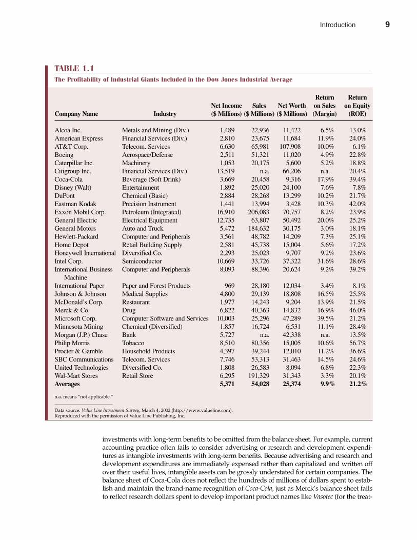
Variability of Business ProfitsIn practice, reported profits fluctuate widely. Table 1.1 shows business profits for a well-knownsample of 30 industrial giants: those companies that comprise the Dow Jones IndustrialAverage. Business profit is often measured in dollar terms or as a percentage of sales revenue,called profit margin, as in Table 1.1. The economist’s concept of a normal rate of profit is typ-ically assessed in terms of the realized rate of return on stockholders’ equity (ROE). Returnon stockholders’ equity is defined as accounting net income divided by the book value of thefirm. As seen in Table 1.1, the average ROE for industrial giants found in the Dow JonesIndustrial Average falls in a broad range of around 15 percent to 25 percent per year. Althoughan average annual ROE of roughly 10 percent can be regarded as a typical or normal rate ofreturn in the United States and Canada, this standard is routinely exceeded by companies suchas Coca-Cola, which has consistently earned a ROE in excess of 35 percent per year. It is a stan-dard seldom met by International Paper, a company that has suffered massive losses in anattempt to cut costs and increase product quality in the face of tough environmental regulationsand foreign competition.
Some of the variation in ROE depicted in Table 1.1 represents the influence of differentialrisk premiums. In the pharmaceuticals industry, for example, hoped-for discoveries of effec-tive therapies for important diseases are often a long shot at best. Thus, profit rates reportedby Merck and other leading pharmaceutical companies overstate the relative profitability ofthe drug industry; it could be cut by one-half with proper risk adjustment. Similarly, reportedprofit rates can overstate differences in economic profits if accounting error or bias causes
business profit Residual of sales rev-enue minus the explicitaccounting costs ofdoing business
normal rate ofreturn Average profit necessaryto attract and retaininvestment
economic profit Business profit minusthe implicit costs ofcapital and any otherowner-provided inputs
profit margin Accounting net incomedivided by sales
return on stock-holders’ equity Accounting net incomedivided by the bookvalue of total assetsminus total liabilities
Chapter One Introduction 9
8 Introduction
investments with long-term benefits to be omitted from the balance sheet. For example, currentaccounting practice often fails to consider advertising or research and development expendi-tures as intangible investments with long-term benefits. Because advertising and research anddevelopment expenditures are immediately expensed rather than capitalized and written offover their useful lives, intangible assets can be grossly understated for certain companies. Thebalance sheet of Coca-Cola does not reflect the hundreds of millions of dollars spent to estab-lish and maintain the brand-name recognition of Coca-Cola, just as Merck’s balance sheet failsto reflect research dollars spent to develop important product names like Vasotec (for the treat-
10 Part One Overview of Managerial Economics
TABLE 1.1The Profitability of Industrial Giants Included in the Dow Jones Industrial Average
Return ReturnNet Income Sales Net Worth on Sales on Equity
Company Name Industry ($ Millions) ($ Millions) ($ Millions) (Margin) (ROE)
Alcoa Inc. Metals and Mining (Div.) 1,489 22,936 11,422 6.5% 13.0%American Express Financial Services (Div.) 2,810 23,675 11,684 11.9% 24.0%AT&T Corp. Telecom. Services 6,630 65,981 107,908 10.0% 6.1%Boeing Aerospace/Defense 2,511 51,321 11,020 4.9% 22.8%Caterpillar Inc. Machinery 1,053 20,175 5,600 5.2% 18.8%Citigroup Inc. Financial Services (Div.) 13,519 n.a. 66,206 n.a. 20.4%Coca-Cola Beverage (Soft Drink) 3,669 20,458 9,316 17.9% 39.4%Disney (Walt) Entertainment 1,892 25,020 24,100 7.6% 7.8%DuPont Chemical (Basic) 2,884 28,268 13,299 10.2% 21.7%Eastman Kodak Precision Instrument 1,441 13,994 3,428 10.3% 42.0%Exxon Mobil Corp. Petroleum (Integrated) 16,910 206,083 70,757 8.2% 23.9%General Electric Electrical Equipment 12,735 63,807 50,492 20.0% 25.2%General Motors Auto and Truck 5,472 184,632 30,175 3.0% 18.1%Hewlett-Packard Computer and Peripherals 3,561 48,782 14,209 7.3% 25.1%Home Depot Retail Building Supply 2,581 45,738 15,004 5.6% 17.2%Honeywell International Diversified Co. 2,293 25,023 9,707 9.2% 23.6%Intel Corp. Semiconductor 10,669 33,726 37,322 31.6% 28.6%International Business Computer and Peripherals 8,093 88,396 20,624 9.2% 39.2%
MachineInternational Paper Paper and Forest Products 969 28,180 12,034 3.4% 8.1%Johnson & Johnson Medical Supplies 4,800 29,139 18,808 16.5% 25.5%McDonald’s Corp. Restaurant 1,977 14,243 9,204 13.9% 21.5%Merck & Co. Drug 6,822 40,363 14,832 16.9% 46.0%Microsoft Corp. Computer Software and Services 10,003 25,296 47,289 39.5% 21.2%Minnesota Mining Chemical (Diversified) 1,857 16,724 6,531 11.1% 28.4%Morgan (J.P.) Chase Bank 5,727 n.a. 42,338 n.a. 13.5%Philip Morris Tobacco 8,510 80,356 15,005 10.6% 56.7%Procter & Gamble Household Products 4,397 39,244 12,010 11.2% 36.6%SBC Communications Telecom. Services 7,746 53,313 31,463 14.5% 24.6%United Technologies Diversified Co. 1,808 26,583 8,094 6.8% 22.3%Wal-Mart Stores Retail Store 6,295 191,329 31,343 3.3% 20.1%Averages 5,371 54,028 25,374 9.9% 21.2%
n.a. means “not applicable.”
Data source: Value Line Investment Survey, March 4, 2002 (http://www.valueline.com).Reproduced with the permission of Value Line Publishing, Inc.
Introduction 9
ment of high blood pressure), Zocor (an antiarthritic drug), and Singulair (asthma medication).As a result, business profit rates for both Coca-Cola and Merck overstate each company’s trueeconomic performance.
WHY DO PROFITS VARY AMONG FIRMS?Even after risk adjustment and modification to account for the effects of accounting error andbias, ROE numbers reflect significant variation in economic profits. Many firms earn significanteconomic profits or experience meaningful economic losses at any given point. To better under-stand real-world differences in profit rates, it is necessary to examine theories used to explainprofit variations.
Frictional Theory of Economic ProfitsOne explanation of economic profits or losses is frictional profit theory. It states that marketsare sometimes in disequilibrium because of unanticipated changes in demand or cost condi-tions. Unanticipated shocks produce positive or negative economic profits for some firms.
For example, automated teller machines (ATMs) make it possible for customers of financialinstitutions to easily obtain cash, enter deposits, and make loan payments. ATMs render obsoletemany of the functions that used to be carried out at branch offices and foster ongoing consoli-dation in the industry. Similarly, new user-friendly software increases demand for high-poweredpersonal computers (PCs) and boosts returns for efficient PC manufacturers. Alternatively, a risein the use of plastics and aluminum in automobiles drives down the profits of steel manufactur-ers. Over time, barring impassable barriers to entry and exit, resources flow into or out of finan-cial institutions, computer manufacturers, and steel manufacturers, thus driving rates of returnback to normal levels. During interim periods, profits might be above or below normal becauseof frictional factors that prevent instantaneous adjustment to new market conditions.
Monopoly Theory of Economic ProfitsA further explanation of above-normal profits, monopoly profit theory, is an extension of fric-tional profit theory. This theory asserts that some firms are sheltered from competition by highbarriers to entry. Economies of scale, high capital requirements, patents, or import protectionenable some firms to build monopoly positions that allow above-normal profits for extendedperiods. Monopoly profits can even arise because of luck or happenstance (being in the rightindustry at the right time) or from anticompetitive behavior. Unlike other potential sources ofabove-normal profits, monopoly profits are often seen as unwarranted. Thus, monopoly profitsare usually taxed or otherwise regulated. Chapters 10, 11, and 13 consider the causes and con-sequences of monopoly and how society attempts to mitigate its potential costs.
Innovation Theory of Economic ProfitsAn additional theory of economic profits, innovation profit theory, describes the above-normalprofits that arise following successful invention or modernization. For example, innovationprofit theory suggests that Microsoft Corporation has earned superior rates of return because itsuccessfully developed, introduced, and marketed the Graphical User Interface, a superior image-based rather than command-based approach to computer software instructions. Microsoft hascontinued to earn above-normal returns as other firms scramble to offer a wide variety of “userfriendly” software for personal and business applications. Only after competitors have intro-duced and successfully saturated the market for user-friendly software will Microsoft profitsbe driven down to normal levels. Similarly, McDonald’s Corporation earned above-normalrates of return as an early innovator in the fast-food business. With increased competition fromBurger King, Wendy’s, and a host of national and regional competitors, McDonald’s, like
frictional profit theory Abnormal profitsobserved followingunanticipated changesin demand or cost conditions
monopoly profittheoryAbove-normal profitscaused by barriers toentry that limit competition
innovation profittheory Above-normal profitsthat follow successfulinvention or modern-ization
Chapter One Introduction 11
10 Introduction
Apple, IBM, Xerox, and other early innovators, has seen its above-normal returns decline. As inthe case of frictional or disequilibrium profits, profits that are due to innovation are susceptibleto the onslaught of competition from new and established competitors.
Compensatory Theory of Economic ProfitsCompensatory profit theory describes above-normal rates of return that reward firms forextraordinary success in meeting customer needs, maintaining efficient operations, and soforth. If firms that operate at the industry’s average level of efficiency receive normal rates ofreturn, it is reasonable to expect firms operating at above-average levels of efficiency to earnabove-normal rates of return. Inefficient firms can be expected to earn unsatisfactory, below-normal rates of return.
Compensatory profit theory also recognizes economic profit as an important reward tothe entrepreneurial function of owners and managers. Every firm and product starts as anidea for better serving some established or perceived need of existing or potential customers.This need remains unmet until an individual takes the initiative to design, plan, and imple-ment a solution. The opportunity for economic profits is an important motivation for suchentrepreneurial activity.
Role of Profits in the EconomyEach of the preceding theories describes economic profits obtained for different reasons. In somecases, several reasons might apply. For example, an efficient manufacturer may earn an above-normal rate of return in accordance with compensatory theory, but, during a strike by a com-petitor’s employees, these above-average profits may be augmented by frictional profits.Similarly, Microsoft’s profit position might be partly explained by all four theories: The companyhas earned high frictional profits while Adobe Systems, Computer Associates, Oracle, Veritas,and a host of other software companies tool up in response to the rapid growth in demand foruser-friendly software; it has earned monopoly profits because it has some patent protection; ithas certainly benefited from successful innovation; and it is well managed and thus has earnedcompensatory profits.
Economic profits play an important role in a market-based economy. Above-normal profitsserve as a valuable signal that firm or industry output should be increased. Expansion by estab-lished firms or entry by new competitors often occurs quickly during high profit periods. Justas above-normal profits provide a signal for expansion and entry, below-normal profits providea signal for contraction and exit. Economic profits are one of the most important factors affectingthe allocation of scarce economic resources. Above-normal profits can also constitute an impor-tant reward for innovation and efficiency, just as below-normal profits can serve as a penalty forstagnation and inefficiency. Profits play a vital role in providing incentives for innovation andproductive efficiency and in allocating scarce resources.
ROLE OF BUSINESS IN SOCIETY
Business contributes significantly to social welfare. The economy in the United States andseveral other countries has sustained notable growth over many decades. Benefits of thatgrowth have also been widely distributed. Suppliers of capital, labor, and other resources allreceive substantial returns for their contributions. Consumers benefit from an increasingquantity and quality of goods and services available for consumption. Taxes on the businessprofits of firms, as well as on the payments made to suppliers of labor, materials, capital, andother inputs, provide revenues needed to increase government services. All of these contri-butions to social welfare stem from the efficiency of business in serving economic needs.
12 Part One Overview of Managerial Economics
compensatory profittheory Above-normal rates of return that rewardefficiency
Introduction 11
Why Firms ExistFirms exist by public consent to serve social needs. If social welfare could be measured, businessfirms might be expected to operate in a manner that would maximize some index of social well-being. Maximization of social welfare requires answering the following important questions:What combination of goods and services (including negative by-products, such as pollution)should be produced? How should goods and services be provided? How should goods and serv-ices be distributed? These are the most vital questions faced in a free enterprise system, and theyare key issues in managerial economics.
In a free market economy, the economic system produces and allocates goods and servicesaccording to the forces of demand and supply. Firms must determine what products cus-tomers want, bid for necessary resources, and then offer products for sale. In this process, eachfirm actively competes for a share of the customer’s dollar. Suppliers of capital, labor, and rawmaterials must then be compensated out of sales proceeds. The share of revenues paid to eachsupplier depends on relative productivity, resource scarcity, and the degree of competition ineach input market.
Role of Social ConstraintsAlthough the process of market-determined production and allocation of goods and services ishighly efficient, there are potential difficulties in an unconstrained market economy. Society hasdeveloped a variety of methods for alleviating these problems through the political system. Onepossible difficulty with an unconstrained market economy is that certain groups could gainexcessive economic power. To illustrate, the economics of producing and distributing electricpower are such that only one firm can efficiently serve a given community. Furthermore, there
Chapter One Introduction 13
The “Tobacco” Issue
The “tobacco” issue is charged with emotion. From thestandpoint of a business manager or individual investor,there is the economic question of whether or not it is possibleto earn above-normal returns by investing in a productknown for killing its customers. From a philosophicalstandpoint, there is also the ethical question of whetheror not it is desirable to earn such returns, if available.
Among the well-known gloomy particulars are
• Medical studies suggest that breaking the tobaccohabit may be as difficult as curing heroin addiction.This fuels the fire of those who seek to restrict smokingopportunities among children and “addicted” consumers.
• With the declining popularity of smoking, there arefewer smokers among potential jurors. This mayincrease the potential for adverse jury decisions incivil litigation against the tobacco industry.
• Prospects for additional “sin” and “health care”taxes on smoking appear high.
Some underappreciated positive counterpoints to con-sider are
• Although smoking is most common in the mostprice-sensitive sector of our society, profit marginsremain sky high.
• Tax revenues from smokers give the government anincentive to keep smoking legal.
• High excise taxes kill price competition in the tobaccoindustry. Huge changes in manufacturer prices barelybudge retail prices.
Although many suggest that above-average returnscan be derived from investing in the tobacco business,a “greater fool” theory may be at work here. Tobaccocompanies and their investors only profit by finding“greater fools” to pay high prices for products thatmany would not buy for themselves. This is riskybusiness, and a business plan that seldom works outin the long run.
See: Ann Zimmerman, “Wal-Mart Rejects Shareholder Call to ExplainPolicies on Tobacco Ads,” The Wall Street Journal Online, March 1, 2002(http://online.wsj.com).
M A N A G E R I A L A P P L I C AT I O N 1 . 3
12 Introduction
are no good substitutes for electric lighting. As a result, electric companies are in a position toexploit consumers; they could charge high prices and earn excessive profits. Society’s solutionto this potential exploitation is regulation. Prices charged by electric companies and other utili-ties are held to a level that is thought to be just sufficient to provide a fair rate of return on invest-ment. In theory, the regulatory process is simple; in practice, it is costly, difficult to implement,and in many ways arbitrary. It is a poor, but sometimes necessary, substitute for competition.
An additional problem can occur when, because of economies of scale or other barriersto entry, a limited number of firms serve a given market. If firms compete fairly with eachother, no difficulty arises. However, if they conspire with one another in setting prices, theymay be able to restrict output, obtain excessive profits, and reduce social welfare. Antitrustlaws are designed to prevent such collusion. Like direct regulation, antitrust laws containarbitrary elements and are costly to administer, but they too are necessary if economic jus-tice, as defined by society, is to be served.
To avoid the potential for worker exploitation, laws have been developed to equalize bar-gaining power of employers and employees. These labor laws require firms to allow collectivebargaining and to refrain from unfair practices. The question of whether labor’s bargainingposition is too strong in some instances also has been raised. For example, can powerful nation-al unions such as the Teamsters use the threat of a strike to obtain excessive increases in wages?Those who believe this to be the case have suggested that the antitrust laws should be appliedto labor unions, especially those that bargain with numerous small employers.
Amarket economy also faces difficulty when firms impose costs on others by dumping wastesinto the air or water. If a factory pollutes the air, causing nearby residents to suffer lung ailments,a meaningful cost is imposed on these people and society in general. Failure to shift these costsback onto the firm and, ultimately, to the consumers of its products means that the firm and itscustomers benefit unfairly by not having to pay the full costs of production. Pollution and otherexternalities may result in an inefficient and inequitable allocation of resources. In both govern-
14 Part One Overview of Managerial Economics
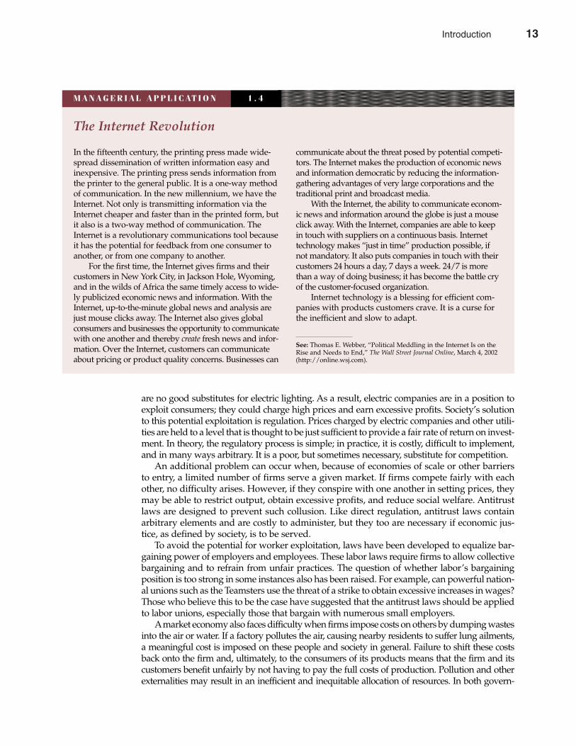
The Internet Revolution
In the fifteenth century, the printing press made wide-spread dissemination of written information easy andinexpensive. The printing press sends information fromthe printer to the general public. It is a one-way methodof communication. In the new millennium, we have theInternet. Not only is transmitting information via theInternet cheaper and faster than in the printed form, butit also is a two-way method of communication. TheInternet is a revolutionary communications tool becauseit has the potential for feedback from one consumer toanother, or from one company to another.
For the first time, the Internet gives firms and theircustomers in New York City, in Jackson Hole, Wyoming,and in the wilds of Africa the same timely access to wide-ly publicized economic news and information. With theInternet, up-to-the-minute global news and analysis arejust mouse clicks away. The Internet also gives global consumers and businesses the opportunity to communicatewith one another and thereby create fresh news and infor-mation. Over the Internet, customers can communicateabout pricing or product quality concerns. Businesses can
communicate about the threat posed by potential competi-tors. The Internet makes the production of economic newsand information democratic by reducing the information-gathering advantages of very large corporations and thetraditional print and broadcast media.
With the Internet, the ability to communicate econom-ic news and information around the globe is just a mouseclick away. With the Internet, companies are able to keepin touch with suppliers on a continuous basis. Internettechnology makes “just in time” production possible, ifnot mandatory. It also puts companies in touch with theircustomers 24 hours a day, 7 days a week. 24/7 is morethan a way of doing business; it has become the battle cryof the customer-focused organization.
Internet technology is a blessing for efficient com-panies with products customers crave. It is a curse forthe inefficient and slow to adapt.
See: Thomas E. Webber, “Political Meddling in the Internet Is on theRise and Needs to End,” The Wall Street Journal Online, March 4, 2002(http://online.wsj.com).
M A N A G E R I A L A P P L I C AT I O N 1 . 4
Introduction 13
ment and business, considerable attention is being directed to the problem of internalizing thesecosts. Some of the practices used to internalize social costs include setting health and safetystandards for products and work conditions, establishing emissions limits on manufacturingprocesses and products, and imposing fines or closing firms that do not meet established standards.
Social Responsibility of BusinessWhat does all this mean with respect to the value maximization theory of the firm? Is the modeladequate for examining issues of social responsibility and for developing rules that reflect therole of business in society?
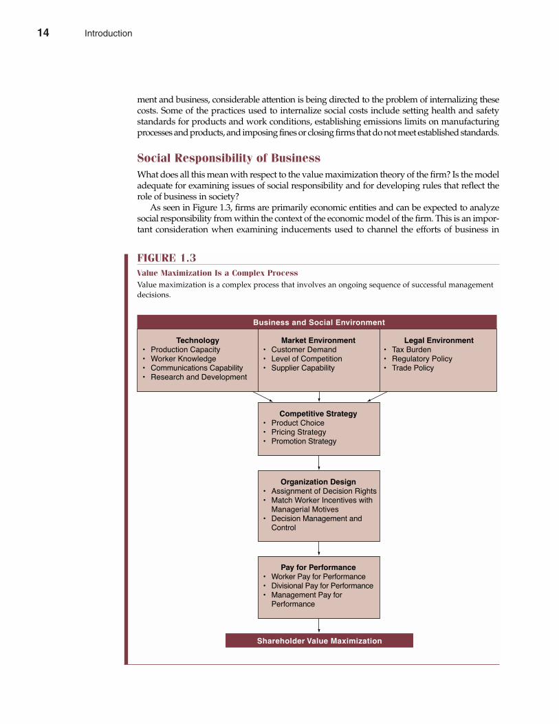
As seen in Figure 1.3, firms are primarily economic entities and can be expected to analyzesocial responsibility from within the context of the economic model of the firm. This is an impor-tant consideration when examining inducements used to channel the efforts of business in
Chapter One Introduction 15
FIGURE 1.3Value Maximization Is a Complex ProcessValue maximization is a complex process that involves an ongoing sequence of successful managementdecisions.
¥ Production Capacity¥ Worker Knowledge¥ Communications Capability¥ Research and Development
Technology¥ Tax Burden¥ Regulatory Policy¥ Trade Policy
Legal Environment¥ Customer Demand¥ Level of Competition¥ Supplier Capability
Market Environment
Business and Social Environment
¥ Product Choice¥ Pricing Strategy¥ Promotion Strategy
Competitive Strategy
¥ Assignment of Decision Rights¥ Match Worker Incentives with �Managerial Motives
¥ Decision Management and �Control
Organization Design
¥ Worker Pay for Performance¥ Divisional Pay for Performance¥ Management Pay for �Performance
Pay for Performance
Shareholder Value Maximization
14 Introduction
directions that society desires. Similar considerations should also be taken into account beforeapplying political pressure or regulations to constrain firm operations. For example, from theconsumer’s standpoint it is desirable to pay low rates for gas, electricity, and telecom services.If public pressures drive rates down too low, however, utility profits could fall below the levelnecessary to provide an adequate return to investors. In that event, capital would flow out ofregulated industries, innovation would cease, and service would deteriorate. When suchissues are considered, the economic model of the firm provides useful insight. This modelemphasizes the close relation between the firm and society, and indicates the importance ofbusiness participation in the development and achievement of social objectives.
STRUCTURE OF THIS TEXT
ObjectivesThis text should help you accomplish the following objectives:
• Develop a clear understanding of the economic method in managerial decision making;• Acquire a framework for understanding the nature of the firm as an integrated whole as
opposed to a loosely connected set of functional departments; and• Recognize the relation between the firm and society and the role of business as a tool for
social betterment.
Throughout the text, the emphasis is on the practical application of economic analysis tomanagerial decision problems.
Development of TopicsThe value maximization framework is useful for characterizing actual managerial decisionsand for developing rules that can be used to improve those decisions. The basic test of thevalue maximization model, or any model, is its ability to explain real-world behavior. Thistext highlights the complementary relation between theory and practice. Theory is used toimprove managerial decision making, and practical experience leads to the development ofbetter theory.
Chapter 2, “Basic Economic Relations,” begins by examining the important role that marginalanalysis plays in the optimization process. The balancing of marginal revenues and marginalcosts to determine the profit-maximizing output level is explored, as are other fundamentaleconomic relations that help organizations efficiently employ scarce resources. All of theseeconomic relations are considered based on the simplifying assumption that cost and revenuerelations are known with certainty. Later in the book, this assumption is relaxed, and the morerealistic circumstance of decision making under conditions of uncertainty is examined. Thismaterial shows how optimization concepts can be effectively employed in situations whenmanagers have extensive information about the chance or probability of certain outcomes, butthe end result of managerial decisions cannot be forecast precisely. Given the challenges posedby a rapidly changing global environment, a careful statistical analysis of economic relations isoften conducted to provide the information necessary for effective decision making. Tools usedby managers in the statistical analysis of economic relations are the subject of Chapter 3,“Statistical Analysis of Economic Relations.”
The concepts of demand and supply are basic to understanding the effective use of econom-ic resources. The general overview of demand and supply in Chapter 4 provides a frameworkfor the more detailed inquiry that follows. In Chapter 5, “Demand Analysis and Estimation,”attention is turned to the study and calculation of demand relations. The successful management
16 Part One Overview of Managerial Economics
Introduction 15
of any organization requires understanding the demand for its products. The demand functionrelates the sales of a product to such important factors as the price of the product itself, prices ofother goods, income, advertising, and even weather. The role of demand elasticities, which meas-ure the strength of the relations expressed in the demand function, is also emphasized. Issuesaddressed in the prediction of demand and cost conditions are explored more fully in Chapter 6,“Forecasting.” Material in this chapter provides a useful framework for the estimation ofdemand and cost relations.
Chapters 7, 8, and 9 examine production and cost concepts. The economics of resourceemployment in the manufacture and distribution of goods and services is the focus of thismaterial. These chapters present economic analysis as a context for understanding the logicof managerial decisions and as a means for developing improved practices. Chapter 7,“Production Analysis and Compensation Policy,” develops rules for optimal employment anddemonstrates how labor and other resources can be used in a profit-maximizing manner.Chapter 8, “Cost Analysis and Estimation,” focuses on the identification of cost-output relationsso that appropriate decisions regarding product pricing, plant size and location, and so on canbe made. Chapter 9, “Linear Programming,” introduces a tool from the decision sciences thatcan be used to solve a variety of optimization problems. This technique offers managers inputfor short-run operating decisions and information helpful in the long-run planning process.
The remainder of the book builds on the foundation provided in Chapters 1 through 9 toexamine a variety of topics in the theory and practice of managerial economics. Chapters 10and 11 explore market structures and their implications for the development and implemen-tation of effective competitive strategy. Demand and supply relations are integrated to examinethe dynamics of economic markets. Chapter 10, “Perfect Competition and Monopoly,” offersperspective on how product differentiation, barriers to entry, and the availability of informa-tion interact to determine the vigor of competition. Chapter 11, “Monopolistic Competitionand Oligopoly,” considers “competition among the few” for industries in which interactionsamong competitors are normal. Chapter 12, “Pricing Practices,” shows how the forces of supplyand demand interact under a variety of market settings to signal appropriate pricing policies.Importantly, this chapter analyzes pricing practices commonly observed in business andshows how they reflect the predictions of economic theory.
Chapter 13, “Regulation of the Market Economy,” focuses on the role of government byconsidering how the external economic environment affects the managerial decision-makingprocess. This chapter investigates how interactions among business, government, and thepublic result in antitrust and regulatory policies with direct implications for the efficiency andfairness of the economic system. Chapter 14, “Risk Analysis,” illustrates how the predictionsof economic theory can be applied in the real-world setting of uncertainty. Chapter 15, “CapitalBudgeting,” examines the key elements necessary for an effective planning framework formanagerial decision making. It investigates the capital budgeting process and how firmscombine demand, production, cost, and risk analyses to effectively make strategic long-runinvestment decisions. Finally, Chapter 16, “Public Management,” studies how the tools andtechniques of managerial economics can be used to analyze decisions in the public and not-for-profit sectors and how that decision-making process can be improved.
SUMMARY
Managerial economics links economics and the decision sciences to develop tools for mana-gerial decision making. This approach is successful because it focuses on the application ofeconomic analysis to practical business problem solving.
• Managerial economics applies economic theory and methods to business and adminis-trative decision making.
Chapter One Introduction 17
16 Introduction
• The basic model of the business enterprise is called the theory of the firm. The primary goalis seen as long-term expected value maximization. The value of the firm is the presentvalue of the firm’s expected future net cash flows, whereas present value is the value ofexpected cash flows discounted back to the present at an appropriate interest rate.
• Valid questions are sometimes raised about whether managers really optimize (seek thebest solution) or merely satisfice (seek satisfactory rather than optimal results). Most often,especially when information costs are considered, managers can be seen as optimizing.
• Business profit, or accounting profit, is the residual of sales revenue minus the explicitaccounting costs of doing business. Business profit often incorporates a normal rate of returnon capital, or the minimum return necessary to attract and retain investment for a particularuse. Economic profit is business profit minus the implicit costs of equity and other owner-provided inputs used by the firm. Profit margin, or net income divided by sales, and thereturn on stockholders’ equity, or accounting net income divided by the book value of totalassets minus total liabilities, are practical indicators of firm performance.
• Frictional profit theory describes abnormal profits observed following unanticipatedchanges in product demand or cost conditions. Monopoly profit theory asserts that above-normal profits are sometimes caused by barriers to entry that limit competition. Innovationprofit theory describes above-normal profits that arise as a result of successful invention ormodernization. Compensatory profit theory holds that above-normal rates of return cansometimes be seen as a reward to firms that are extraordinarily successful in meeting cus-tomer needs, maintaining efficient operations, and so forth.
The use of economic methodology to analyze and improve the managerial decision-makingprocess combines the study of theory and practice. Although the logic of managerial econom-ics is intuitively appealing, the primary virtue of managerial economics lies in its usefulness.It works!
QUESTIONS
Q1.1 Why is it appropriate to view firms primarily as economic entities?Q1.2 Explain how the valuation model given in Equation 1.2 could be used to describe the inte-
grated nature of managerial decision making across the functional areas of business.Q1.3 Describe the effects of each of the following managerial decisions or economic influences on
the value of the firm:A. The firm is required to install new equipment to reduce air pollution.B. Through heavy expenditures on advertising, the firm’s marketing department increases
sales substantially.C. The production department purchases new equipment that lowers manufacturing costs.D. The firm raises prices. Quantity demanded in the short run is unaffected, but in the longer
run, unit sales are expected to decline.E. The Federal Reserve System takes actions that lower interest rates dramatically.F. An expected increase in inflation causes generally higher interest rates, and, hence, the
discount rate increases.Q1.4 It is sometimes argued that managers of large, publicly owned firms make decisions to maximize
their own welfare as opposed to that of stockholders. Would such behavior create problems inusing value maximization as a basis for examining managerial decision making?
Q1.5 How is the popular notion of business profit different from the economic profit conceptdescribed in the chapter? What role does the idea of normal profits play in this difference?
18 Part One Overview of Managerial Economics
Introduction 17
Q1.6 Which concept—the business profit concept or the economic profit concept—provides themore appropriate basis for evaluating business operations? Why?
Q1.7 What factors should be considered in examining the adequacy of profits for a firm or indus-try?
Q1.8 Why is the concept of self-interest important in economics?Q1.9 “In the long run, a profit-maximizing firm would never knowingly market unsafe products.
However, in the short run, unsafe products can do a lot of damage.” Discuss this statement.Q1.10 Is it reasonable to expect firms to take actions that are in the public interest but are detri-
mental to stockholders? Is regulation always necessary and appropriate to induce firms toact in the public interest?
Chapter One Introduction 19
CASE STUDY
Is Coca-Cola the “Perfect” Business?3
What does a perfect business look like? For Warren Buffett and his partner Charlie Munger,vice-chairman of Berkshire Hathaway, Inc., it looks a lot like Coca-Cola. To see why, imaginegoing back in time to 1885, to Atlanta, Georgia, and trying to invent from scratch a nonalcoholicbeverage that would make you, your family, and all of your friends rich.
Your beverage would be nonalcoholic to ensure widespread appeal among both young andold alike. It would be cold rather than hot so as to provide relief from climatic effects. It mustbe ordered by name—a trademarked name. Nobody gets rich selling easy-to-imitate genericproducts. It must generate a lot of repeat business through what psychologists call conditionedreflexes. To get the desired positive conditioned reflex, you will want to make it sweet, ratherthan bitter, with no after-taste. Without any after-taste, consumers will be able to drink as muchof your product as they like. By adding sugar to make your beverage sweet, it gains food valuein addition to a positive stimulant. To get extra-powerful combinatorial effects, you maywant to add caffeine as an additional stimulant. Both sugar and caffeine work; by combiningthem, you get more than a double effect—you get what Munger calls a “lollapalooza” effect.Additional combinatorial effects could be realized if you design the product to appear exotic.Coffee is another popular product, so making your beverage dark in color seems like a safe bet.By adding carbonation, a little fizz can be added to your beverage’s appearance and its appeal.
To keep the lollapalooza effects coming, you will want to advertise. If people associate yourbeverage with happy times, they will tend to reach for it whenever they are happy, or want tobe happy. (Isn’t that always, as in “Always Coca-Cola”?) Make it available at sporting events,concerts, the beach, and at theme parks—wherever and whenever people have fun. Encloseyour product in bright, upbeat colors that customers tend to associate with festive occasions(another combinatorial effect). Red and white packaging would be a good choice. Also makesure that customers associate your beverage with festive occasions. Well-timed advertisingand price promotions can help in this regard—annual price promotions tied to the Fourth ofJuly holiday, for example, would be a good idea.
To ensure enormous profits, profit margins and the rate of return on invested capital mustboth be high. To ensure a high rate of return on sales, the price charged must be substantiallyabove unit costs. Because consumers tend to be least price sensitive for moderately priceditems, you would like to have a modest “price point,” say roughly $1–$2 per serving. This is abig problem for most beverages because water is a key ingredient, and water is very expen-sive to ship long distances. To get around this cost-of-delivery difficulty, you will not want to
3 See Charles T. Munger, “How Do You Get Worldly Wisdom?” Outstanding Investor Digest, December 29, 1997, 24–31.
18 Introduction
20 Part One Overview of Managerial Economics
sell the beverage itself, but a key ingredient, like syrup, to local bottlers. By selling syrup toindependent bottlers, your company can also better safeguard its “secret ingredients.” Thisalso avoids the problem of having to invest a substantial amount in bottling plants, machinery,delivery trucks, and so on. This minimizes capital requirements and boosts the rate of returnon invested capital. Moreover, if you correctly price the key syrup ingredient, you can ensurethat the enormous profits generated by carefully developed lollapalooza effects accrue to yourcompany, and not to the bottlers. Of course, you want to offer independent bottlers the poten-tial for highly satisfactory profits in order to provide the necessary incentive for them to push
CASE STUDY (continued)
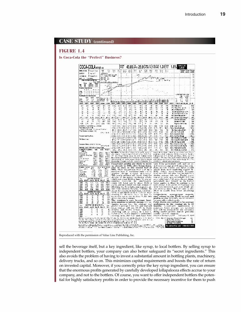
FIGURE 1.4Is Coca-Cola the “Perfect” Business?
Reproduced with the permission of Value Line Publishing, Inc.
Introduction 19
SELECTED REFERENCESAddleson, Mark. “Stories About Firms: Boundaries, Structures, Strategies, and Processes.” Managerial
& Decision Economics 22 (June/August 2001): 169–182.Austen-Smith, David. “Charity and the Bequest Motive: Evidence from Seventeenth-Century Wills.”
Journal of Political Economy 108 (December 2000): 1270–1291. Baltagi, Badi H., and James M. Griffin. “The Econometrics of Rational Addiction: The Case of Cigarettes.”
Journal of Business & Economic Statistics 19 (October 2001): 449–454.Block, Walter. “Cyberslacking, Business Ethics and Managerial Economics.” Journal of Business Ethics
33 (October 2001): 225–231.Demsetz, Harold, and Belén Villalonga. “Ownership Structure and Corporate Performance.” Journal of
Corporate Finance 7 (September 2001): 209–233.Fourer, Robert, and Jean-Pierre Goux. “Optimization as an Internet Resource.” Interfaces 31 (March
2001): 130–150.Furubotn, Eirik G. “The New Institutional Economics and the Theory of the Firm.” Journal of Economic
Behavior & Organization 45 (June 2001): 133–153.
Chapter One Introduction 21
CASE STUDY (continued)
your product. You not only want to “leave something on the table” for the bottlers in terms ofthe bottlers’ profit potential, but they in turn must also be encouraged to “leave something onthe table” for restaurant and other customers. This means that you must demand that bottlersdeliver a consistently high-quality product at carefully specified prices if they are to maintaintheir valuable franchise to sell your beverage in the local area.
If you had indeed gone back to 1885, to Atlanta, Georgia, and followed all of these sug-gestions, you would have created what you and I know as The Coca-Cola Company. To besure, there would have been surprises along the way. Take widespread refrigeration, forexample. Early on, Coca-Cola management saw the fountain business as the primary driverin cold carbonated beverage sales. They did not foretell that widespread refrigeration wouldmake grocery store sales and in-home consumption popular. Still, much of Coca-Cola’s successhas been achieved because its management had, and still has, a good grasp of both the eco-nomics and the psychology of the beverage business. By getting into rapidly growing foreignmarkets with a winning formula, they hope to create local brand-name recognition, scaleeconomies in distribution, and achieve other “first mover” advantages like the ones they havenurtured in the United States for more than 100 years.
As shown in Figure 1.4, in a world where the typical company earns 10 percent rates ofreturn on invested capital, Coca-Cola earns three and four times as much. Typical profitrates, let alone operating losses, are unheard of at Coca-Cola. It enjoys large and growingprofits, and requires practically no tangible capital investment. Almost its entire value isderived from brand equity derived from generations of advertising and carefully nurturedpositive lollapalooza effects. On an overall basis, it is easy to see why Buffett and Mungerregard Coca-Cola as a “perfect” business.A. One of the most important skills to learn in managerial economics is the ability to identify
a good business. Discuss at least four characteristics of a good business.B. Identify and talk about at least four companies that you regard as having the characteristics
listed here.C. Suppose you bought common stock in each of the four companies identified here. Three
years from now, how would you know if your analysis was correct? What would convinceyou that your analysis was wrong?
20 Introduction
Grinols, Earl L., and David B. Mustard. “Business Profitability Versus Social Profitability: EvaluatingIndustries with Externalities—The Case of Casinos.” Managerial & Decision Economics 22 (January–May2001): 143–162.
Gruber, Jonathan, and Botond Köszegi. “Is Addiction ‘Rational’? Theory and Evidence.” QuarterlyJournal of Economics 116 (November 2001): 1261–1303.
Harbaugh, William T., Kate Krause, and Timothy R. Berry. “Garp for Kids: On the Development ofRational Choice Behavior.” American Economic Review 91 (December 2001): 1539–1545.
Karahan, R. Sitki. “Towards an Eclectic Theory of Firm Globalization.” International Journal of Management18 (December 2001): 523–532.
McWilliams, Abagail, and Donald Siegel. “Corporate Social Responsibility: A Theory of the FirmPerspective.” Academy of Management Review 26 (January 2001): 117–127.
Muller, Holger M., and Karl Warneryd. “Inside Versus Outside Ownership: A Political Theory of theFirm.” Rand Journal of Economics 32 (Autumn 2001): 527–541.
Subrahmanyam, Avanidhar, and Sheridan Titman. “Feedback from Stock Prices to Cash Flows.”Journal of Finance 56 (December 2001): 2389–2414.
Woidtke, Tracie. “Agents Watching Agents? Evidence from Pension Fund Ownership and Firm Value.”Journal of Financial Economics 63 (January 2002): 99–131.
22 Part One Overview of Managerial Economics
Introduction 21


Basic EconomicRelations
CHAPTER TWO
231 See Kevin Voigt and William Fraser, “Are You a Bad Boss?” The Wall Street Journal Online,
March 15, 2002 (http://www.online.wsj.com).
Managers have to make tough choices that involve benefits and costs.Until recently, however, it was simply impractical to compare the rel-
ative pluses and minuses of a large number of managerial decisions under awide variety of operating conditions. For many large and small organizations,economic optimization remained an elusive goal. It is easy to understand whyearly users of personal computers were delighted when they learned howeasy it was to enter and manipulate operating information within spread-sheets. Spreadsheets were a pivotal innovation because they put the tools forinsightful demand, cost, and profit analysis at the fingertips of managers andother decision makers. Today’s low-cost but powerful PCs and user-friendlysoftware make it possible to efficiently analyze company-specific data andbroader industry and macroeconomic information from the Internet. It hasnever been easier nor more vital for managers to consider the implications ofvarious managerial decisions under an assortment of operating scenarios.
Effective managers in the twenty-first century must be able to collect,organize, and process a vast assortment of relevant operating information.However, efficient information processing requires more than electronic com-puting capability; it requires a fundamental understanding of basic economicrelations. Within such a framework, powerful PCs and a wealth of operatingand market information become an awesome aid to effective managerialdecision making.1
This chapter introduces a number of fundamental principles of economicanalysis. These ideas form the basis for describing all demand, cost, and profitrelations. Once the basics of economic relations are understood, the tools andtechniques of optimization can be applied to find the best course of action.
23
2
ECONOMIC OPTIMIZATION PROCESS
Effective managerial decision making is the process of arriving at the best solution to a prob-lem. If only one solution is possible, then no decision problem exists. When alternative coursesof action are available, the best decision is the one that produces a result most consistent withmanagerial objectives. The process of arriving at the best managerial decision is the goal of eco-nomic optimization and the focus of managerial economics.
Optimal DecisionsShould the quality of inputs be enhanced to better meet low-cost import competition? Is anecessary reduction in labor costs efficiently achieved through an across-the-board decreasein staffing, or is it better to make targeted cutbacks? Following an increase in product demand,is it preferable to increase managerial staff, line personnel, or both? These are the types ofquestions facing managers on a regular basis that require a careful consideration of basic eco-nomic relations. Answers to these questions depend on the objectives and preferences of man-agement. Just as there is no single “best” purchase decision for all customers at all times, thereis no single “best” investment decision for all managers at all times. When alternative coursesof action are available, the decision that produces a result most consistent with managerialobjectives is the optimal decision.
A challenge that must be met in the decision-making process is characterizing the desirabil-ity of decision alternatives in terms of the objectives of the organization. Decision makers mustrecognize all available choices and portray them in terms of appropriate costs and benefits. Thedescription of decision alternatives is greatly enhanced through application of the principles ofmanagerial economics. Managerial economics also provides tools for analyzing and evaluatingdecision alternatives. Economic concepts and methodology are used to select the optimal courseof action in light of available options and objectives.
Principles of economic analysis form the basis for describing demand, cost, and profit rela-tions. Once basic economic relations are understood, the tools and techniques of optimizationcan be applied to find the best course of action. Most important, the theory and process ofoptimization gives practical insight concerning the value maximization theory of the firm.Optimization techniques are helpful because they offer a realistic means for dealing with thecomplexities of goal-oriented managerial activities.
Maximizing the Value of the FirmIn managerial economics, the primary objective of management is assumed to be maximiza-tion of the value of the firm. This value maximization objective was introduced in Chapter 1and is again expressed in Equation 2.1:
n Profittn Total Revenuet – Total Costt(2.1) Value = ∑
(1 + i)t= ∑
(1 + i)tt = 1 t = 1
Maximizing Equation 2.1 is a complex task that involves consideration of future revenues,costs, and discount rates. Total revenues are directly determined by the quantity sold andthe prices received. Factors that affect prices and the quantity sold include the choice ofproducts made available for sale, marketing strategies, pricing and distribution policies,competition, and the general state of the economy. Cost analysis includes a detailed exami-nation of the prices and availability of various input factors, alternative production sched-ules, production methods, and so on. Finally, the relation between an appropriate discountrate and the company’s mix of products and both operating and financial leverage must bedetermined. All these factors affect the value of the firm as described in Equation 2.1.
24 Part One Overview of Managerial Economics
optimal decision Choice alternative thatproduces a result mostconsistent with manage-rial objectives
24 Basic Economic Relations
To determine the optimal course of action, marketing, production, and financial decisionsmust be integrated within a decision analysis framework. Similarly, decisions related to per-sonnel retention and development, organization structure, and long-term business strategymust be combined into a single integrated system that shows how managerial initiatives affectall parts of the firm. The value maximization model provides an attractive basis for such an inte-gration. Using the principles of economic analysis, it is also possible to analyze and compare thehigher costs or lower benefits of alternative, suboptimal courses of action.
The complexity of completely integrated decision analysis—or global optimization—confines its use to major planning decisions. For many day-to-day operating decisions, man-agers typically use less complicated, partial optimization techniques. For example, the market-ing department is usually required to determine the price and advertising strategy that achievessome sales goal given the firm’s current product line and marketing budget. Alternatively, aproduction department might minimize the cost of output at a stated quality level.
The decision process, whether it is applied to fully integrated or partial optimization problems,involves two steps. First, important economic relations must be expressed in analytical terms.Second, various optimization techniques must be applied to determine the best, or optimal,solution in the light of managerial objectives. The following material introduces a number ofconcepts that are useful for expressing decision problems in an economic framework.
BASIC ECONOMIC RELATIONS
Tables are the simplest and most direct form for presenting economic data. When these dataare displayed electronically in the format of an accounting income statement or balance sheet,the tables are referred to as spreadsheets. When the underlying relation between economicdata is simple, tables and spreadsheets may be sufficient for analytical purposes. In such
table List of economic data
spreadsheet Table of electronicallystored data
Chapter Two Basic Economic Relations 25
Greed Versus Self-Interest
Capitalism is based on voluntary exchange between self-interested parties. Given that the exchange is voluntary,both parties must perceive benefits, or profit, for markettransactions to take place. If only one party were to bene-fit from a given transaction, there would be no incentivefor the other party to cooperate, and no voluntaryexchange would take place. A self-interested capitalistmust also have in mind the interest of others. In contrast,a truly selfish individual is only concerned with himselfor herself, without regard for the well-being of others.Self-interested behavior leads to profits and successunder capitalism; selfish behavior does not.
Management guru Peter Drucker has written that thepurpose of business is to create a customer—someone thatwill want to do business with you and your company on aregular basis. In a business deal, both parties must benefit.If not, there will be no ongoing business relationship.
The only way this can be done is to make sure thatyou continually take the customer’s perspective. Howcan customer needs be met better, cheaper, or faster?
Don’t wait for customers to complain or seek alternatesuppliers: Seek out ways of helping before they becomeobvious. When customers benefit, so do you and yourcompany. Take the customer’s perspective, always.Similarly, it is best to see every business transaction fromthe standpoint of the person on the other side of the table.
In dealing with employees, it is best to be honest andforthright. If you make a mistake, admit it and go on.When management accepts responsibility for its failures,they gain the trust of employees and their help in findingsolutions for the inevitable problems that always arise. Ina job interview, for example, strive to see how you cancreate value for a potential employer. It is natural to seethings from one’s own viewpoint; it is typically muchmore beneficial to see things from the perspective of theperson sitting on the other side of the table.
See: Ianthe Jeanne Dugan, “Before Enron, Greed Helped Sink theRespectability of Accounting,” The Wall Street Journal Online, March 14,2002 (http://online.wsj.com).
M A N A G E R I A L A P P L I C AT I O N 2 . 1
Basic Economic Relations 25
26 Part One Overview of Managerial Economics
graph Visual representationof data
equation Analytical expression offunctional relationships
dependent variable Y variable determinedby X values
independent variable X variable determinedseparately from the Y variable
instances, a simple graph or visual representation of the data can provide valuable insight.Complex economic relations require more sophisticated methods of expression. An equationis an expression of the functional relationship or connection among economic variables. Whenthe underlying relation among economic variables is uncomplicated, equations offer a com-pact means for data description; when underlying relations are complex, equations are help-ful because they permit the powerful tools of mathematical and statistical analysis to be used.
Functional Relations: EquationsThe easiest way to examine basic economic concepts is to consider the functional relationsincorporated in the basic valuation model. Consider the relation between output, Q, andtotal revenue, TR. Using functional notation, total revenue is
(2.2) TR = f(Q)
Equation 2.2 is read, “Total revenue is a function of output.” The value of the dependentvariable (total revenue) is determined by the independent variable (output). The variable tothe left of the equal sign is called the dependent variable. Its value depends on the size ofthe variable or variables to the right of the equal sign. Variables on the right-hand side of theequal sign are called independent variables. Their values are determined independentlyof the functional relation expressed by the equation.
Equation 2.2 does not indicate the specific relation between output and total revenue; itmerely states that some relation exists. Equation 2.3 provides a more precise expression ofthis functional relation:
(2.3) TR = P � Q
where P represents the price at which each unit of Q is sold. Total revenue is equal to pricetimes the quantity sold. If price is constant at $1.50 regardless of the quantity sold, the relationbetween quantity sold and total revenue is
(2.4) TR = $1.50 � Q
Data in Table 2.1 are specified by Equation 2.4 and graphically illustrated in Figure 2.1.
Total, Average, and Marginal RelationsTotal, average, and marginal relations are very useful in optimization analysis. Whereas thedefinitions of totals and averages are well known, the meaning of marginals needs further
TABLE 2.1Relation Between Total Revenue and Output; Total Revenue = $1.50 � Output
Total Revenue Output
$1.50 13.00 24.50 36.00 47.50 59.00 6
26 Basic Economic Relations
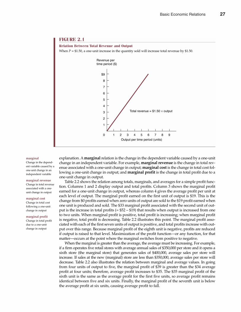
explanation. A marginal relation is the change in the dependent variable caused by a one-unitchange in an independent variable. For example, marginal revenue is the change in total rev-enue associated with a one-unit change in output; marginal cost is the change in total cost fol-lowing a one-unit change in output; and marginal profit is the change in total profit due to aone-unit change in output.
Table 2.2 shows the relation among totals, marginals, and averages for a simple profit func-tion. Columns 1 and 2 display output and total profits. Column 3 shows the marginal profitearned for a one-unit change in output, whereas column 4 gives the average profit per unit ateach level of output. The marginal profit earned on the first unit of output is $19. This is thechange from $0 profits earned when zero units of output are sold to the $19 profit earned whenone unit is produced and sold. The $33 marginal profit associated with the second unit of out-put is the increase in total profits (= $52 – $19) that results when output is increased from oneto two units. When marginal profit is positive, total profit is increasing; when marginal profitis negative, total profit is decreasing. Table 2.2 illustrates this point. The marginal profit asso-ciated with each of the first seven units of output is positive, and total profits increase with out-put over this range. Because marginal profit of the eighth unit is negative, profits are reducedif output is raised to that level. Maximization of the profit function—or any function, for thatmatter—occurs at the point where the marginal switches from positive to negative.
When the marginal is greater than the average, the average must be increasing. For example,if a firm operates five retail stores with average annual sales of $350,000 per store and it opens asixth store (the marginal store) that generates sales of $400,000, average sales per store willincrease. If sales at the new (marginal) store are less than $350,000, average sales per store willdecrease. Table 2.2 also illustrates the relation between marginal and average values. In goingfrom four units of output to five, the marginal profit of $39 is greater than the $34 averageprofit at four units; therefore, average profit increases to $35. The $35 marginal profit of thesixth unit is the same as the average profit for the first five units, so average profit remainsidentical between five and six units. Finally, the marginal profit of the seventh unit is belowthe average profit at six units, causing average profit to fall.
marginal Change in the depend-ent variable caused by aone-unit change in anindependent variable
marginal revenue Change in total revenueassociated with a one-unit change in output
marginal cost Change in total costfollowing a one-unitchange in output
marginal profit Change in total profitdue to a one-unitchange in output
Chapter Two Basic Economic Relations 27
FIGURE 2.1Relation Between Total Revenue and OutputWhen P = $1.50, a one-unit increase in the quantity sold will increase total revenue by $1.50.
Revenue pertime period ($)
Total revenue = $1.50 × output
$9
8
7
6
5
4
3
2
1
0 4 91 5
Output per time period (units)
82 6 73
Basic Economic Relations 27
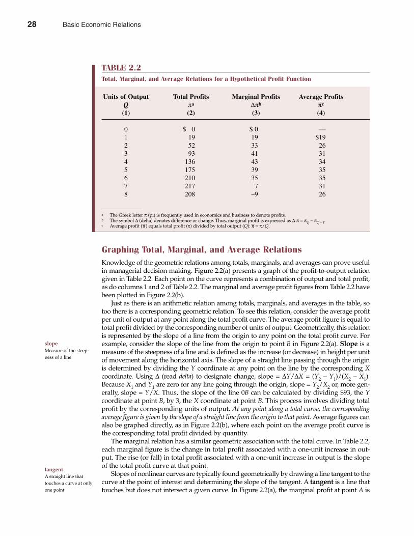
Graphing Total, Marginal, and Average RelationsKnowledge of the geometric relations among totals, marginals, and averages can prove usefulin managerial decision making. Figure 2.2(a) presents a graph of the profit-to-output relationgiven in Table 2.2. Each point on the curve represents a combination of output and total profit,as do columns 1 and 2 of Table 2.2. The marginal and average profit figures from Table 2.2 havebeen plotted in Figure 2.2(b).
Just as there is an arithmetic relation among totals, marginals, and averages in the table, sotoo there is a corresponding geometric relation. To see this relation, consider the average profitper unit of output at any point along the total profit curve. The average profit figure is equal tototal profit divided by the corresponding number of units of output. Geometrically, this relationis represented by the slope of a line from the origin to any point on the total profit curve. Forexample, consider the slope of the line from the origin to point B in Figure 2.2(a). Slope is ameasure of the steepness of a line and is defined as the increase (or decrease) in height per unitof movement along the horizontal axis. The slope of a straight line passing through the originis determined by dividing the Y coordinate at any point on the line by the corresponding Xcoordinate. Using ∆ (read delta) to designate change, slope = ∆Y/∆X = (Y2 – Y1)/(X2 – X1).Because X1 and Y1 are zero for any line going through the origin, slope = Y2/X2 or, more gen-erally, slope = Y/X. Thus, the slope of the line 0B can be calculated by dividing $93, the Ycoordinate at point B, by 3, the X coordinate at point B. This process involves dividing totalprofit by the corresponding units of output. At any point along a total curve, the correspondingaverage figure is given by the slope of a straight line from the origin to that point. Average figures canalso be graphed directly, as in Figure 2.2(b), where each point on the average profit curve isthe corresponding total profit divided by quantity.
The marginal relation has a similar geometric association with the total curve. In Table 2.2,each marginal figure is the change in total profit associated with a one-unit increase in out-put. The rise (or fall) in total profit associated with a one-unit increase in output is the slopeof the total profit curve at that point.
Slopes of nonlinear curves are typically found geometrically by drawing a line tangent to thecurve at the point of interest and determining the slope of the tangent. A tangent is a line thattouches but does not intersect a given curve. In Figure 2.2(a), the marginal profit at point A is
28 Part One Overview of Managerial Economics
slope Measure of the steep-ness of a line
tangent A straight line thattouches a curve at onlyone point
TABLE 2.2Total, Marginal, and Average Relations for a Hypothetical Profit Function
Units of Output Total Profits Marginal Profits Average Profits Q πa ∆πb πc
(1) (2) (3) (4)
0 $ 0 $ 0 —1 19 19 $192 52 33 263 93 41 314 136 43 345 175 39 356 210 35 357 217 7 318 208 –9 26
a The Greek letter π (pi) is frequently used in economics and business to denote profits.b The symbol ∆ (delta) denotes difference or change. Thus, marginal profit is expressed as ∆ π = πQ – πQ – 1.c Average profit (π) equals total profit (π) divided by total output (Q): π = π/Q.
28 Basic Economic Relations
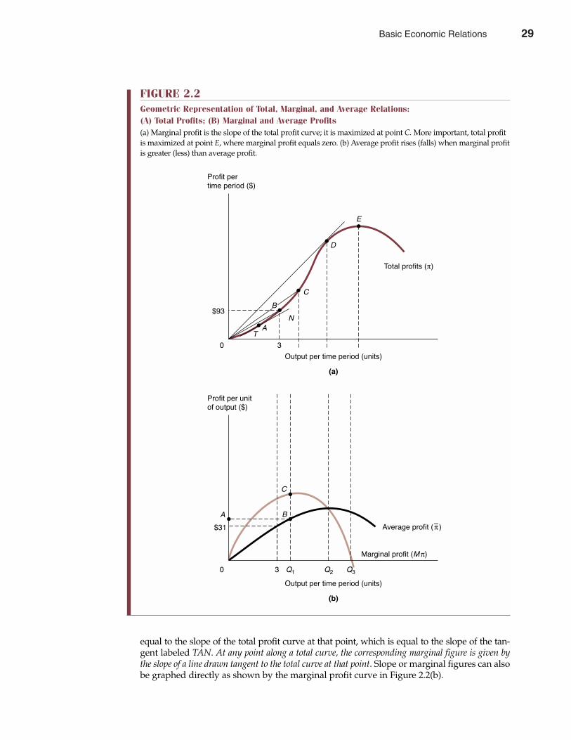
equal to the slope of the total profit curve at that point, which is equal to the slope of the tan-gent labeled TAN. At any point along a total curve, the corresponding marginal figure is given bythe slope of a line drawn tangent to the total curve at that point. Slope or marginal figures can alsobe graphed directly as shown by the marginal profit curve in Figure 2.2(b).
Chapter Two Basic Economic Relations 29
FIGURE 2.2Geometric Representation of Total, Marginal, and Average Relations: (A) Total Profits; (B) Marginal and Average Profits(a) Marginal profit is the slope of the total profit curve; it is maximized at point C. More important, total profitis maximized at point E, where marginal profit equals zero. (b) Average profit rises (falls) when marginal profitis greater (less) than average profit.
Profit pertime period ($)
Total profits (π)
E
D
C
NA
T
Output per time period (units)
(a)
3
$93B
Profit per unitof output ($)
Average profit (πÐ)
Marginal profit (M π)
C
Output per time period (units)
(b)
Q3Q130
0
Q2
$31
A B
Basic Economic Relations 29

Several important relations among totals, marginals, and averages become apparent whenconsidering Figure 2.2(a). First, note that the slope of the total profit curve is increasing from theorigin to point C. Lines drawn tangent to the total profit curve become steeper as the point oftangency approaches point C, so marginal profit is increasing up to this point. This is also illus-trated in Figure 2.2(b), where the marginal profit curve increases up to output Q1, correspon-ding to point C on the total profit curve. At point C, called an inflection point, the slope of thetotal profit curve is maximized; marginal, but not average or total, profits are maximized at thatoutput. Between points C and E, total profit continues to increase because marginal profit is stillpositive even though it is declining. At point E, the total profit curve has a slope of zero and thusis neither rising nor falling. Marginal profit at this point is zero, and total profit is maximized.Beyond E [output Q3 in Figure 2.2(b)], the total profit curve has a negative slope and marginalprofit is negative.
Figure 2.2(b) also shows the relation between marginals and averages. At low output levels,where the marginal profit curve lies above the average, the average is rising. Although marginalprofit reaches a maximum at output Q1 and declines thereafter, the average curve continues torise so long as the marginal lies above it. At output Q2, marginal and average profits are equal,and the average profit curve reaches its maximum value. Beyond Q2, the marginal curve liesbelow the average, which is falling.
MARGINAL ANALYSIS IN DECISION MAKING
Marginal analysis gives clear rules to follow for optimal resource allocation. As a result, geo-metric relations between totals and marginals offer a fruitful basis for examining the role ofmarginal analysis in managerial decision making.
30 Part One Overview of Managerial Economics
inflection point Point of maximum orminimum slope
Does Good Theory Always Work in Practice?
Have you ever been at a sporting event when a particularathlete’s play became the center of attention and wondered“Where did that woman study physics?” or “Wow, whotaught that guy physiology?” No, of course not. Instead,the discussion probably centered on the player’s skill,finesse, or tenacity. Natural talent developed throughlong hours of dedicated training and intense competitionare chief prerequisites for becoming an accomplishedamateur or professional athlete. But if you think about it,successful athletes must also know a great deal aboutangles, speed, and acceleration.
Although success in sports requires that one under-stands the basic principles of physics and physiology, mostathletes develop their “feel” for their sports on the tenniscourt, golf course, baseball diamond, or gridiron. Similarly,some very successful businesses are run by people withlittle or no formal training in accounting, finance, man-agement, or marketing. These executives’ successes testifyto their ability to develop a feel for business in much thesame way that the successful athlete develops a feel forhis or her sport. Although the term optimization may beforeign to such individuals, the methodology of opti-
mization is familiar to each of them in terms of theireveryday business practice. Adjusting prices to avoidstockout situations, increasing product quality to “meetthe competition,” and raising salaries to retain valuedemployees all involve a basic, practical understanding ofoptimization concepts.
The behavior of both the successful athlete and thesuccessful executive can be described, or modeled, asconsistent with a process of optimization. The fact thatsome practitioners learn their “lessons” through hands-on experience rather than in the classroom does notdiminish the value of the formal educational experience.Useful theory describes and predicts actual businessdecisions. The old saw “That may be okay in theory, butit doesn’t work in practice” is plainly incorrect. Economictheory is useful for studying managerial decision makingfor one simple reason—it works.
See: Peter Wonacott, “Searching for Profits, Finding Trouble,” The WallStreet Journal Online, March 19, 2002 (http://online.wsj.com).
M A N A G E R I A L A P P L I C AT I O N 2 . 2
30 Basic Economic Relations
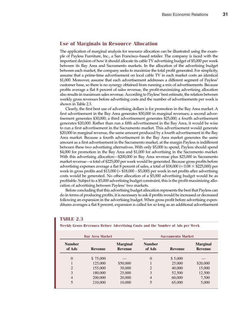
Use of Marginals in Resource AllocationThe application of marginal analysis for resource allocation can be illustrated using the exam-ple of Payless Furniture, Inc., a San Francisco–based retailer. The company is faced with theimportant decision of how it should allocate its cable TV advertising budget of $5,000 per weekbetween its Bay Area and Sacramento markets. In the allocation of the advertising budgetbetween each market, the company seeks to maximize the total profit generated. For simplicity,assume that a prime-time advertisement on local cable TV in each market costs an identical$1,000. Moreover, assume that each advertisement addresses a different segment of Payless’customer base, so there is no synergy obtained from running a mix of advertisements. Becauseprofits average a flat 8 percent of sales revenue, the profit-maximizing advertising allocationalso results in maximum sales revenue. According to Payless’ best estimate, the relation betweenweekly gross revenues before advertising costs and the number of advertisements per week isshown in Table 2.3.
Clearly, the first best use of advertising dollars is for promotion in the Bay Area market. Afirst advertisement in the Bay Area generates $50,000 in marginal revenues; a second adver-tisement generates $30,000; a third advertisement generates $25,000; a fourth advertisementgenerates $20,000. Rather than run a fifth advertisement in the Bay Area, it would be wiseto run a first advertisement in the Sacramento market. This advertisement would generate$20,000 in marginal revenue, the same amount produced by a fourth advertisement in the BayArea market. Because a fourth advertisement in the Bay Area market generates the sameamount as a first advertisement in the Sacramento market, at the margin Payless is indifferentbetween these two advertising alternatives. With only $5,000 to spend, Payless should spend$4,000 for promotion in the Bay Area and $1,000 for advertising in the Sacramento market.With this advertising allocation—$200,000 in Bay Area revenue plus $25,000 in Sacramentomarket revenue—a total of $225,000 per week would be generated. Because gross profits beforeadvertising expenses average a flat 8 percent of sales, a total of $18,000 (= 0.08 � $225,000) perweek in gross profits and $13,000 (= $18,000 – $5,000) per week in net profits after advertisingcosts would be generated. No other allocation of a $5,000 advertising budget would be asprofitable. Subject to a $5,000 advertising budget constraint, this is the profit-maximizing allo-cation of advertising between Payless’ two markets.
Before concluding that this advertising budget allocation represents the best that Payless cando in terms of producing profits, it is necessary to ask if profits would be increased or decreasedfollowing an expansion in the advertising budget. When gross profit before advertising expen-ditures averages a flat 8 percent, expansion is called for so long as an additional advertisement
Chapter Two Basic Economic Relations 31
TABLE 2.3Weekly Gross Revenues Before Advertising Costs and the Number of Ads per Week
Bay Area Market Sacramento Market
Number Marginal Number Marginalof Ads Revenue Revenue of Ads Revenue Revenue
0 $ 75,000 — 0 $ 5,000 —1 125,000 $50,000 1 25,000 $20,0002 155,000 30,000 2 40,000 15,0003 180,000 25,000 3 52,500 12,5004 200,000 20,000 4 60,000 7,5005 210,000 10,000 5 65,000 5,000
Basic Economic Relations 31
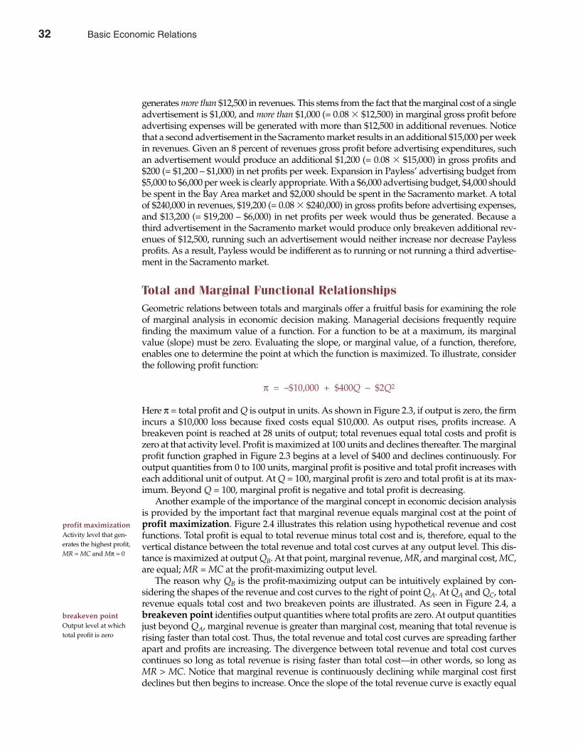
generates more than $12,500 in revenues. This stems from the fact that the marginal cost of a singleadvertisement is $1,000, and more than $1,000 (= 0.08 � $12,500) in marginal gross profit beforeadvertising expenses will be generated with more than $12,500 in additional revenues. Noticethat a second advertisement in the Sacramento market results in an additional $15,000 per weekin revenues. Given an 8 percent of revenues gross profit before advertising expenditures, suchan advertisement would produce an additional $1,200 (= 0.08 � $15,000) in gross profits and$200 (= $1,200 – $1,000) in net profits per week. Expansion in Payless’ advertising budget from$5,000 to $6,000 per week is clearly appropriate. With a $6,000 advertising budget, $4,000 shouldbe spent in the Bay Area market and $2,000 should be spent in the Sacramento market. A totalof $240,000 in revenues, $19,200 (= 0.08 � $240,000) in gross profits before advertising expenses,and $13,200 (= $19,200 – $6,000) in net profits per week would thus be generated. Because athird advertisement in the Sacramento market would produce only breakeven additional rev-enues of $12,500, running such an advertisement would neither increase nor decrease Paylessprofits. As a result, Payless would be indifferent as to running or not running a third advertise-ment in the Sacramento market.
Total and Marginal Functional RelationshipsGeometric relations between totals and marginals offer a fruitful basis for examining the roleof marginal analysis in economic decision making. Managerial decisions frequently requirefinding the maximum value of a function. For a function to be at a maximum, its marginalvalue (slope) must be zero. Evaluating the slope, or marginal value, of a function, therefore,enables one to determine the point at which the function is maximized. To illustrate, considerthe following profit function:
π = –$10,000 + $400Q – $2Q2
Here π = total profit and Q is output in units. As shown in Figure 2.3, if output is zero, the firmincurs a $10,000 loss because fixed costs equal $10,000. As output rises, profits increase. Abreakeven point is reached at 28 units of output; total revenues equal total costs and profit iszero at that activity level. Profit is maximized at 100 units and declines thereafter. The marginalprofit function graphed in Figure 2.3 begins at a level of $400 and declines continuously. Foroutput quantities from 0 to 100 units, marginal profit is positive and total profit increases witheach additional unit of output. At Q = 100, marginal profit is zero and total profit is at its max-imum. Beyond Q = 100, marginal profit is negative and total profit is decreasing.
Another example of the importance of the marginal concept in economic decision analysisis provided by the important fact that marginal revenue equals marginal cost at the point ofprofit maximization. Figure 2.4 illustrates this relation using hypothetical revenue and costfunctions. Total profit is equal to total revenue minus total cost and is, therefore, equal to thevertical distance between the total revenue and total cost curves at any output level. This dis-tance is maximized at output QB. At that point, marginal revenue, MR, and marginal cost, MC,are equal; MR = MC at the profit-maximizing output level.
The reason why QB is the profit-maximizing output can be intuitively explained by con-sidering the shapes of the revenue and cost curves to the right of point QA. At QA and QC, totalrevenue equals total cost and two breakeven points are illustrated. As seen in Figure 2.4, abreakeven point identifies output quantities where total profits are zero. At output quantitiesjust beyond QA, marginal revenue is greater than marginal cost, meaning that total revenue isrising faster than total cost. Thus, the total revenue and total cost curves are spreading fartherapart and profits are increasing. The divergence between total revenue and total cost curvescontinues so long as total revenue is rising faster than total cost—in other words, so long asMR > MC. Notice that marginal revenue is continuously declining while marginal cost firstdeclines but then begins to increase. Once the slope of the total revenue curve is exactly equal
32 Part One Overview of Managerial Economics
profit maximization Activity level that gen-erates the highest profit,MR = MC and Mπ = 0
breakeven point Output level at whichtotal profit is zero
32 Basic Economic Relations
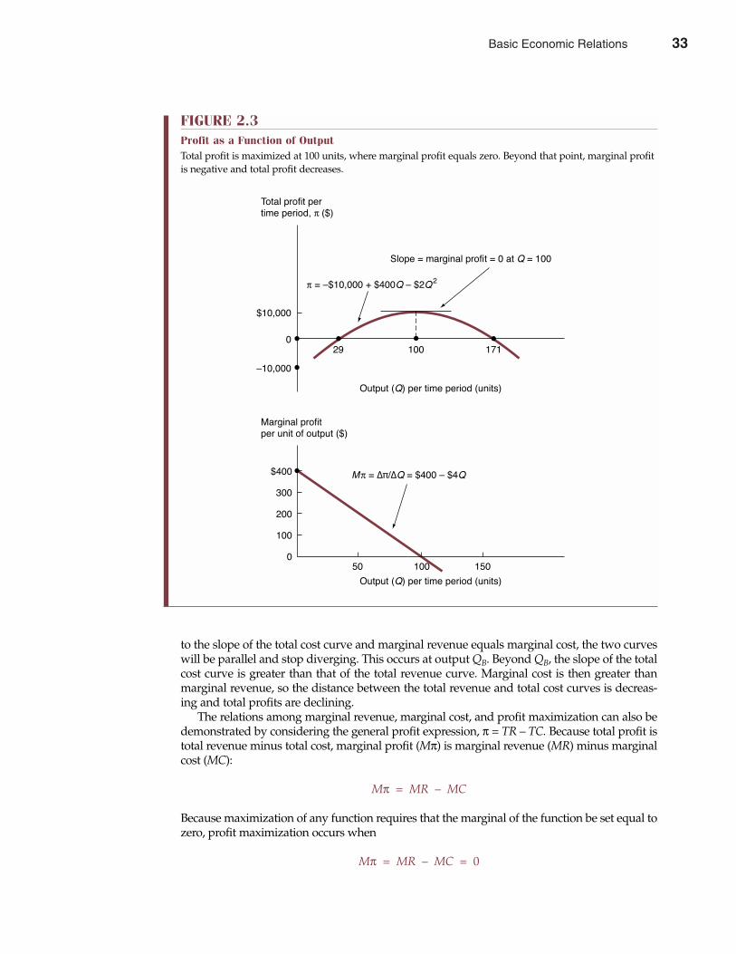
to the slope of the total cost curve and marginal revenue equals marginal cost, the two curveswill be parallel and stop diverging. This occurs at output QB. Beyond QB, the slope of the totalcost curve is greater than that of the total revenue curve. Marginal cost is then greater thanmarginal revenue, so the distance between the total revenue and total cost curves is decreas-ing and total profits are declining.
The relations among marginal revenue, marginal cost, and profit maximization can also bedemonstrated by considering the general profit expression, π = TR – TC. Because total profit istotal revenue minus total cost, marginal profit (Mπ) is marginal revenue (MR) minus marginalcost (MC):
Mπ = MR – MC
Because maximization of any function requires that the marginal of the function be set equal tozero, profit maximization occurs when
Mπ = MR – MC = 0
Chapter Two Basic Economic Relations 33
FIGURE 2.3Profit as a Function of OutputTotal profit is maximized at 100 units, where marginal profit equals zero. Beyond that point, marginal profitis negative and total profit decreases.
Total profit pertime period, π ($)
π = Ð$10,000 + $400Q Ð $2Q2
Slope = marginal profit = 0 at Q = 100
Output (Q) per time period (units)
Ð10,000
100 171290
$10,000
Marginal profitper unit of output ($)
Output (Q) per time period (units)
$400
300
200
100
0100 15050
Mπ = ƹ/ÆQ = $400 Ð $4Q
Basic Economic Relations 33
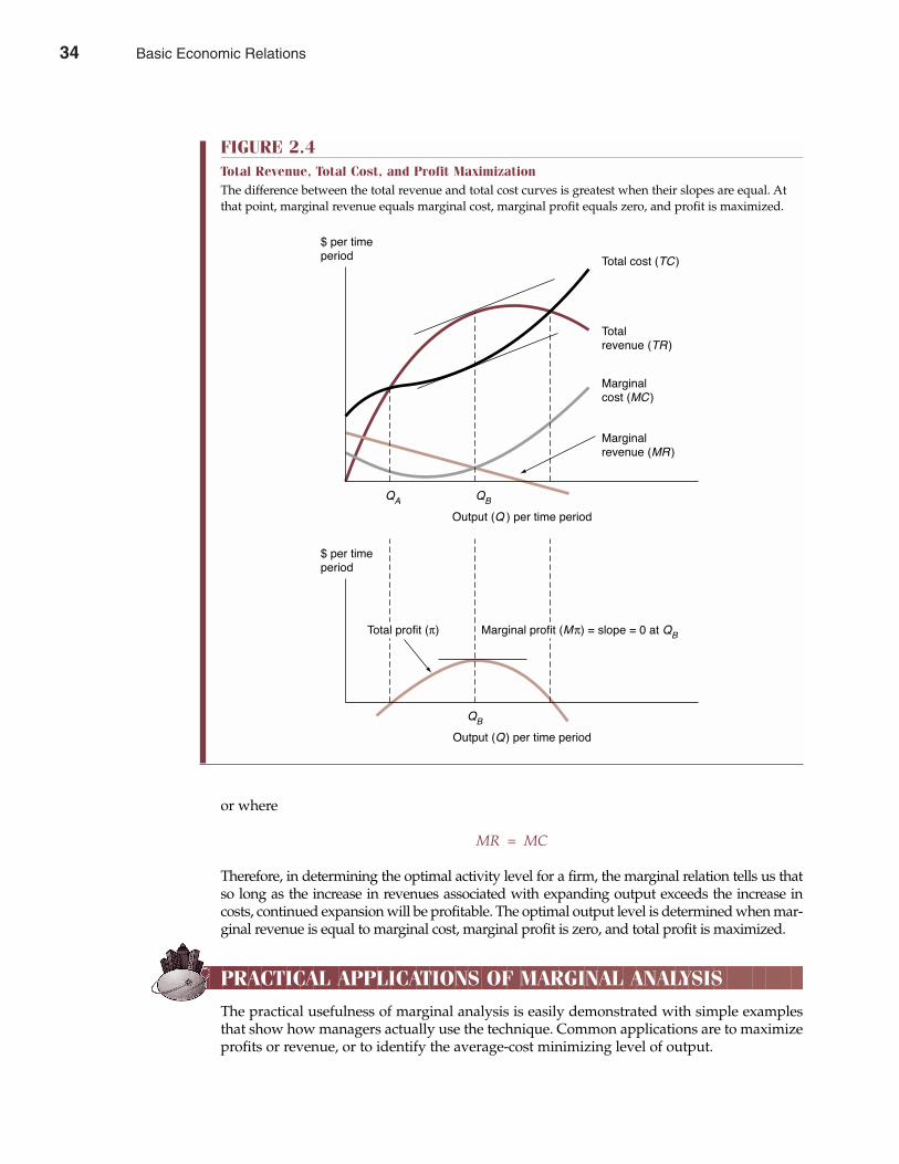
or where
MR = MC
Therefore, in determining the optimal activity level for a firm, the marginal relation tells us thatso long as the increase in revenues associated with expanding output exceeds the increase incosts, continued expansion will be profitable. The optimal output level is determined when mar-ginal revenue is equal to marginal cost, marginal profit is zero, and total profit is maximized.
PRACTICAL APPLICATIONS OF MARGINAL ANALYSIS
The practical usefulness of marginal analysis is easily demonstrated with simple examplesthat show how managers actually use the technique. Common applications are to maximizeprofits or revenue, or to identify the average-cost minimizing level of output.
34 Part One Overview of Managerial Economics
FIGURE 2.4Total Revenue, Total Cost, and Profit MaximizationThe difference between the total revenue and total cost curves is greatest when their slopes are equal. Atthat point, marginal revenue equals marginal cost, marginal profit equals zero, and profit is maximized.
$ per timeperiod Total cost (TC )
Totalrevenue (TR )
Marginalcost (MC )
Marginalrevenue (MR )
QA QB
Output (Q ) per time period
$ per timeperiod
QB
Output (Q ) per time period
Total profit (π) Marginal profit (Mπ) = slope = 0 at QB
34 Basic Economic Relations
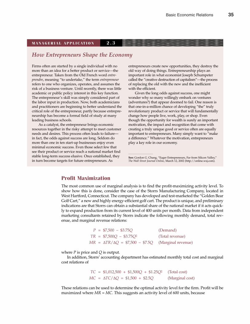
Profit MaximizationThe most common use of marginal analysis is to find the profit-maximizing activity level. Toshow how this is done, consider the case of the Storrs Manufacturing Company, located inWest Hartford, Connecticut. The company has developed and test-marketed the “Golden BearGolf Cart,” a new and highly energy-efficient golf cart. The product is unique, and preliminaryindications are that Storrs can obtain a substantial share of the national market if it acts quick-ly to expand production from its current level of 400 units per month. Data from independentmarketing consultants retained by Storrs indicate the following monthly demand, total rev-enue, and marginal revenue relations:
P = $7,500 – $3.75Q (Demand)TR = $7,500Q – $3.75Q2 (Total revenue)
MR = ∆TR/∆Q = $7,500 – $7.5Q (Marginal revenue)
where P is price and Q is output.In addition, Storrs’ accounting department has estimated monthly total cost and marginal
cost relations of
TC = $1,012,500 + $1,500Q + $1.25Q2 (Total cost)MC = ∆TC/∆Q = $1,500 + $2.5Q (Marginal cost)
These relations can be used to determine the optimal activity level for the firm. Profit will bemaximized where MR = MC. This suggests an activity level of 600 units, because
Chapter Two Basic Economic Relations 35
How Entrepreneurs Shape the Economy
Firms often are started by a single individual with nomore than an idea for a better product or service—theentrepreneur. Taken from the Old French word entre-prendre, meaning “to undertake,” the term entrepreneurrefers to one who organizes, operates, and assumes therisk of a business venture. Until recently, there was littleacademic or public policy interest in this key function.The entrepreneur’s skill was simply considered part ofthe labor input in production. Now, both academiciansand practitioners are beginning to better understand thecritical role of the entrepreneur, partly because entrepre-neurship has become a formal field of study at manyleading business schools.
As a catalyst, the entrepreneur brings economicresources together in the risky attempt to meet customerneeds and desires. This process often leads to failure—in fact, the odds against success are long. Seldom domore than one in ten start-up businesses enjoy evenminimal economic success. Even those select few thatsee their product or service reach a national market findstable long-term success elusive. Once established, theyin turn become targets for future entrepreneurs. As
entrepreneurs create new opportunities, they destroy theold way of doing things. Entrepreneurship plays animportant role in what economist Joseph Schumpetercalled the “creative destruction of capitalism”—the processof replacing the old with the new and the inefficientwith the efficient.
Given the long odds against success, one mightwonder why so many willingly embark on ventures(adventures?) that appear doomed to fail. One reason isthat one-in-a-million chance of developing “the” trulyrevolutionary product or service that will fundamentallychange how people live, work, play, or shop. Eventhough the opportunity for wealth is surely an importantmotivation, the impact and recognition that come withcreating a truly unique good or service often are equallyimportant to entrepreneurs. Many simply want to “makea difference.” Whatever the motivation, entrepreneursplay a key role in our economy.
See: Gordon G. Chang, “Eager Entrepreneurs, Far from Silicon Valley,”The Wall Street Journal Online, March 12, 2002 (http://online.wsj.com).
M A N A G E R I A L A P P L I C AT I O N 2 . 3
Basic Economic Relations 35
MR = MC
$7,500 – $7.5Q = $1,500 + $2.5Q
$10Q = $6,000Q = 600 units
At this optimal activity level, price, total revenue, and the maximum total profit can be calcu-lated as
P = $7,500 – $3.75Q
= $7,500 – $3.75(600)= $5,250 per unit
TR = $7,500Q – $3.75Q2
= $7,500(600) – $3.75(6002)= $3,150,000
π = TR – TC
= $7,500Q – $3.75Q2 – $1,012,500 – $1,500Q – $1.25Q2
= –$5Q2 + $6,000Q – $1,012,500= –$5(6002) + $6,000(600) – $1,012,500= $787,500
To maximize short-run profits, Storrs should expand from its current level of 400 units to 600units per month. Any deviation from an output of 600 units and price of $5,250 per unitwould lower Storrs’ short-run profits.
Revenue MaximizationAlthough marginal analysis is commonly employed to find the profit-maximizing activitylevel, managers can use the technique to achieve a variety of operating objectives. For exam-ple, consider the possibility that a company such as Storrs might wish to deviate from theshort-run profit-maximizing activity level in order to achieve certain long-run objectives.Suppose Storrs fears that short-run profits as high as $787,500 per month (or 25 percent ofsales) would provide a powerful enticement for new competitors.
To limit an increase in current and future competition, Storrs may decide to lower prices torapidly penetrate the market and preclude entry by new rivals. For example, Storrs might wishto adopt a short-run operating philosophy of revenue maximization as part of a long-runvalue maximization strategy. In this instance, Storrs’ short-run operating philosophy would beto set MR = 0, which would result in the following activity level:
MR = 0$7,500 – $7.5Q = 0
$7.5Q = $7,500Q = 1,000 unitsP = $7,500 – $3.75(1,000)
= $3,750TR = $7,500(1,000) – $3.75(1,0002)
= $3,750,000π = –$5(1,0002) + $6,000(1,000) – $1,012,500
= –$12,500 (A loss)
36 Part One Overview of Managerial Economics
revenue maximization Activity level that generates the highestrevenue, MR = 0
36 Basic Economic Relations
Notice that revenue maximization involves a consideration of revenue or “demand-side”influences only. In this instance, the revenue-maximizing activity occurs when a loss of $12,500per month is incurred. In other instances, profits may be high or low at the point of revenuemaximization. Unlike profit maximization, cost relations are not considered at all. Relative toprofit maximization, revenue maximization increases both unit sales and total revenue butsubstantially decreases short-run profitability. These effects are typical and a direct result of thelower prices that accompany a revenue maximization strategy. Because revenue maximizationinvolves setting MR = 0, whereas profit maximization involves setting MR = MC, the twostrategies will only lead to identical activity levels in the unlikely event that MC = 0. Althoughmarginal cost sometimes equals zero when services are provided, such as allowing a few morefans to watch a scarcely attended baseball game, such instances are rare. Most goods and serv-ices involve at least some variable production and distribution costs, and hence marginal coststypically will be positive. Thus, revenue maximization typically involves moving down alongthe demand and marginal revenue curves to lower prices and greater unit sales levels thanwould be indicated for profit maximization. Of course, for this strategy to be optimal, the long-run benefits derived from greater market penetration and scale advantages must be sufficientto overcome the short-run disadvantage of lost profits.
Average Cost MinimizationProfit and revenue maximization may be the most common uses of marginal analysis, but otheruseful applications are also prevalent. Consider the implications of still another possible short-run strategy for Storrs. Suppose that instead of short-run profit or revenue maximization, thecompany decides on an intermediate strategy of expanding sales beyond the short-run profit-maximizing activity level but to a lesser extent than that suggested by revenue maximization.This might be appropriate if, for example, Storrs is unable to finance the very high rate of growthnecessary for short-run revenue maximization. Given the specific nature of Storrs’ total cost andprofit relations, the company might decide on a short-run operating strategy of average costminimization. To find this activity level, remember that average cost is falling when MC < AC,rising when MC > AC, and at a minimum when MC = AC. Therefore, the average cost minimiz-ing activity level for Storrs is
MC = AC = TCQ
$1,500 + $2.5Q =$1,012,500 + $1,500Q + $1.25Q2
Q
$1,500 + $2.5Q = $1,012,500 + $1,500 + $1.25QQ
$1.25Q = $1,012,500Q
(2.2) Q2 = 810,000Q = 900 unitsP = $7,500 – $3.75(900)
= $4,125TR = $7,500(900) – $3.75(9002)
= $3,712,500π = –$5(9002) + $6,000(900) – $1,012,500
= $337,500
For Storrs, average cost minimization involves operation at an activity level that lies betweenthose indicated by profit maximization and revenue maximization strategies. Because average
average cost minimization Activity level that generates the lowestaverage cost, MC = AC
Chapter Two Basic Economic Relations 37
Basic Economic Relations 37

cost minimization reflects a consideration of cost relations or “supply-side” influences only,however, either greater or lesser activity levels than those indicated by profit maximizationand revenue maximization strategies might result. In Storrs’ case, average cost minimizationleads to some of the market penetration advantages of revenue maximization but achievessome of the greater profits associated with lower activity levels. As such, it might be an attrac-tive short-run strategy for the company.
In general, revenue and cost relations as well as entry conditions must be considered beforesettling on an appropriate short-run operating strategy. Once such a strategy is identified, astudy of the specific revenue and cost relations and other influences facing the firm will suggestan appropriate activity level.
INCREMENTAL CONCEPT IN ECONOMIC ANALYSISThe marginal concept is a key component of the economic decision-making process. It isimportant to recognize, however, that marginal relations measure only the effect associatedwith unitary changes in output or some other important decision variable. Many managerialdecisions involve a consideration of changes that are broader in scope. For example, a manag-er might be interested in analyzing the potential effects on revenues, costs, and profits of a 25percent increase in the firm’s production level. Alternatively, a manager might want to analyzethe profit impact of introducing an entirely new product line or assess the cost impact of chang-ing the entire production system. In all managerial decisions, the study of differences or changesis the key element in the selection of an optimal course of action. The marginal concept,although correct for analyzing unitary changes, is too narrow to provide a general methodologyfor evaluating alternative courses of action.
The incremental concept is the economist’s generalization of the marginal concept.Incremental analysis involves examining the impact of alternative managerial decisions or
38 Part One Overview of Managerial Economics
Information Brought Down the Berlin Wall
The most important ingredient for a well-functioningcompany, and a free market economy, is information thatis accurate, timely, and inexpensive. In November 1989,the world got a renewed sense of how powerful economicinformation can be when the Berlin Wall, which kept EastBerliners captive and barred them from the West, cametumbling down.
Obviously, the communist system was flawed as aneconomic and political model. It placed an extraordinaryburden on the citizens of the former Soviet Union andEastern Bloc countries. The economic inefficiency ofcommunism resulted in an extremely low standard ofliving for millions of hardworking and talented people.However, economic inefficiency does not explain whythe downfall of communism, punctuated by the fall ofthe Berlin Wall in November 1989, took place at a specif-ic point in history. Why didn’t the Berlin Wall comedown during 1961 and the Berlin Blockade, or in the1950s when Hungary and Yugoslavia were in ferment?
During 1990, while in Berlin, I heard a startlinganswer to a simple, but important, question: “Why did
the Berlin Wall come down in November 1989?” “It’sCNN,” was the common refrain. “CNN?” I asked. “Youmean the news on CNN couldn’t be kept from the peopleanymore?” “Oh no, it wasn’t the news on CNN. It was thecommercials.” I was dumbfounded. “The commercials onCNN brought down the Berlin Wall?” I asked. For manyBerliners, that is indeed the case.
Before CNN became widely popular around theglobe, millions of people under communist rule had noidea of the quality of life enjoyed by people in the West.Once CNN broadcast advertisements showing the won-derful variety of consumer goods and services availablein the West, the secret was out and communism wasdoomed. Of course, the prominent role played by politi-cal and religious leaders in the fall of communismshould not be minimized. Still, it is worth noting theimportant role played by communications technology.
See: David Bank, “Soros Insists Government Funding Must RaisePhilanthropy for Gains,” The Wall Street Journal Online, March 14, 2002(http://online.wsj.com).
M A N A G E R I A L A P P L I C AT I O N 2 . 4
38 Basic Economic Relations
courses of action on revenues, costs, and profit. It focuses on changes or differences between theavailable alternatives. The incremental change is the change resulting from a given manage-rial decision. For example, the incremental revenue of a new item in a firm’s product line ismeasured as the difference between the firm’s total revenue before and after the new productis introduced.
Incremental ProfitsFundamental relations of incremental analysis are essentially the same as those of marginal analy-sis. Incremental profit is the profit gain or loss associated with a given managerial decision. Totalprofit increases so long as incremental profit is positive. When incremental profit is negative, totalprofit declines. Similarly, incremental profit is positive (and total profit increases) if the incremen-tal revenue associated with a decision exceeds the incremental cost. The incremental concept is sointuitively obvious that it is easy to overlook both its significance in managerial decision makingand the potential for difficulty in correctly applying it.
For this reason, the incremental concept is often violated in practice. For example, a firmmay refuse to sublet excess warehouse space for $5,000 per month because it figures its cost as$7,500 per month—a price paid for a long-term lease on the facility. However, if the warehousespace represents excess capacity with no current value to the company, its historical cost of$7,500 per month is irrelevant and should be disregarded. The firm would forego $5,000 inprofits by turning down the offer to sublet the excess warehouse space. Similarly, any firm thatadds a standard allocated charge for fixed costs and overhead to the true incremental cost ofproduction runs the risk of turning down profitable sales.
Care must also be exercised to ensure against incorrectly assigning overly low incrementalcosts to a decision. Incremental decisions involve a time dimension that simply cannot beignored. Not only must all current revenues and costs associated with a given decision be con-sidered, but any likely future revenues and costs must also be incorporated in the analysis. Forexample, assume that the excess warehouse space described earlier came about following adownturn in the overall economy. Also, assume that the excess warehouse space was subletfor 1 year at a price of $5,000 per month, or a total of $60,000. An incremental loss might beexperienced if the firm later had to lease additional, more costly space to accommodate anunexpected increase in production. If $75,000 had to be spent to replace the sublet warehousefacility, the decision to sublet would involve an incremental loss of $15,000. To be sure, makingaccurate projections concerning the future pattern of revenues and costs is risky and subject toerror. Nevertheless, they cannot be ignored in incremental analysis.
Another example of the incremental concept involves measurement of the incremental rev-enue resulting from a new product line. Incremental revenue in this case includes not only therevenue received from sale of the new product but also any change in the revenues generatedby the remainder of the firm’s product line. Incremental revenues include any revenue resultingfrom increased sales of another product, where that increase was the result of adding the newproduct to the firm’s line. Similarly, if the new item took sales away from another of the firm’sproducts, this loss in revenue would be accounted for in measuring the incremental revenueof the new product.
Incremental Concept ExampleTo further illustrate the incremental concept, consider the financing decision typically associ-ated with business plant and equipment financing. Consider a business whose $100,000 pur-chase offer was accepted by the seller of a small retail facility. The firm must obtain financingto complete the transaction. The best rates it has found are at a local financial institution thatoffers a renewable 5-year mortgage at 9 percent interest with a down payment of 20 percent,or 9.5 percent interest on a loan with only 10 percent down. In the first case, the borrower is
incremental change Total difference resultingfrom a decision
incremental profit Gain or loss associatedwith a given managerialdecision
Chapter Two Basic Economic Relations 39
Basic Economic Relations 39
able to finance 80 percent of the purchase price; in the second case, the borrower is able tofinance 90 percent. For simplicity, assume that both loans require interest payments only duringthe first 5 years. After 5 years, either note would be renewable at then-current interest rates andwould be restructured with monthly payments designed to amortize the loan over 20 years.An important question facing the firm is: What is the incremental cost of additional fundsborrowed when 90 percent versus 80 percent of the purchase price is financed?
Because no principal payments are required, the annual financing cost under each loan alter-native can be calculated easily. For the 80 percent loan, the annual financing cost in dollar terms is
Financing Cost = Interest Rate � Loan Percentage � Purchase Price(2.3) = (0.09)(0.8)($100,000)
= $7,200
For a 90 percent loan, the corresponding annual financing cost is
Financing Cost = (0.095)(0.9)($100,000)= $8,550
To calculate the incremental cost of added funds borrowed under the 90 percent financingalternative, the firm must compare the additional financing costs incurred with the additionalfunds borrowed. In dollar terms, the incremental annual financing cost is
Incremental Cost = 90% Loan Financing Cost – 80% Loan Financing Cost(2.4) = $8,550 – $7,200
= $1,350
In percentage terms, the incremental cost of the additional funds borrowed under the 90 percentfinancing alternative is
Incremental Cost = Incremental Financing Costsin Percentage Terms Incremental Funds Borrowed
= $8,550 – $7,200$90,000 – $80,000
= $1,350$10,000
= 0.135, or 13.5%
The true incremental cost of funds for the last $10,000 borrowed under the 90 percent financingalternative is 13.5 percent, not the 9.5 percent interest rate quoted for the loan. Although thishigh incremental cost of funds is perhaps surprising, it is not unusual. It results because with a90 percent loan the higher 9.5 percent interest rate is charged on the entire balance of the loan,not just on the incremental $10,000 in borrowed funds.
The incremental concept is important for managerial decision making because it focusesattention on changes or differences between available alternatives. Revenues and costs unaf-fected by the decision are irrelevant and should be ignored in the analysis.
SUMMARY
Effective managerial decision making is the process of finding the best solution to a givenproblem. Both the methodology and tools of managerial economics play an important role inthis process.
40 Part One Overview of Managerial Economics
40 Basic Economic Relations
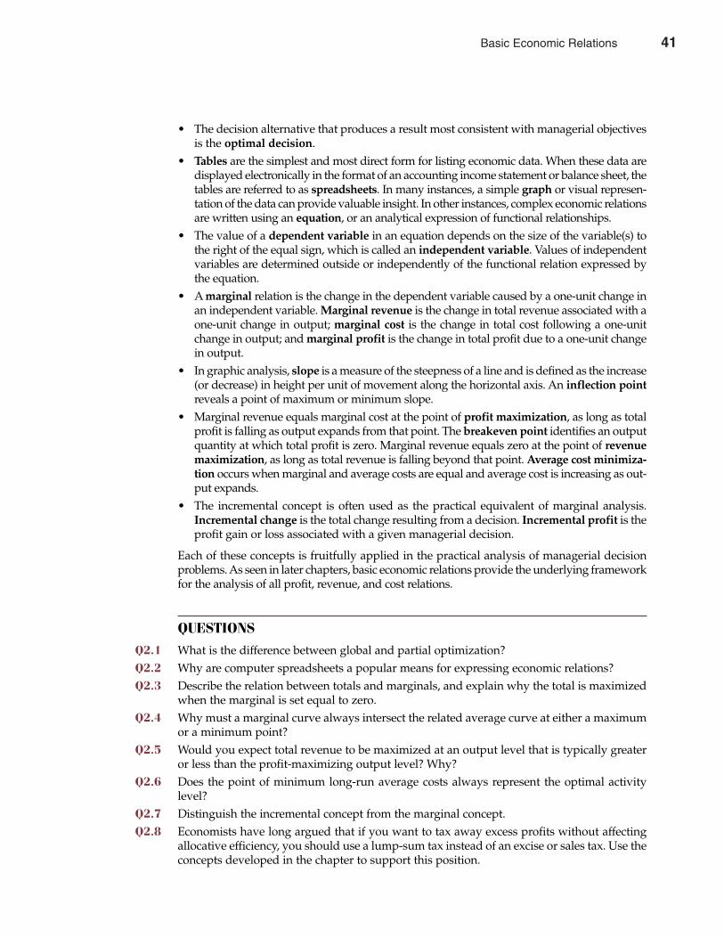
• The decision alternative that produces a result most consistent with managerial objectivesis the optimal decision.
• Tables are the simplest and most direct form for listing economic data. When these data aredisplayed electronically in the format of an accounting income statement or balance sheet, thetables are referred to as spreadsheets. In many instances, a simple graph or visual represen-tation of the data can provide valuable insight. In other instances, complex economic relationsare written using an equation, or an analytical expression of functional relationships.
• The value of a dependent variable in an equation depends on the size of the variable(s) tothe right of the equal sign, which is called an independent variable. Values of independentvariables are determined outside or independently of the functional relation expressed bythe equation.
• A marginal relation is the change in the dependent variable caused by a one-unit change inan independent variable. Marginal revenue is the change in total revenue associated with aone-unit change in output; marginal cost is the change in total cost following a one-unitchange in output; and marginal profit is the change in total profit due to a one-unit changein output.
• In graphic analysis, slope is a measure of the steepness of a line and is defined as the increase(or decrease) in height per unit of movement along the horizontal axis. An inflection pointreveals a point of maximum or minimum slope.
• Marginal revenue equals marginal cost at the point of profit maximization, as long as totalprofit is falling as output expands from that point. The breakeven point identifies an outputquantity at which total profit is zero. Marginal revenue equals zero at the point of revenuemaximization, as long as total revenue is falling beyond that point. Average cost minimiza-tion occurs when marginal and average costs are equal and average cost is increasing as out-put expands.
• The incremental concept is often used as the practical equivalent of marginal analysis.Incremental change is the total change resulting from a decision. Incremental profit is theprofit gain or loss associated with a given managerial decision.
Each of these concepts is fruitfully applied in the practical analysis of managerial decisionproblems. As seen in later chapters, basic economic relations provide the underlying frameworkfor the analysis of all profit, revenue, and cost relations.
QUESTIONS
Q2.1 What is the difference between global and partial optimization?Q2.2 Why are computer spreadsheets a popular means for expressing economic relations?Q2.3 Describe the relation between totals and marginals, and explain why the total is maximized
when the marginal is set equal to zero.Q2.4 Why must a marginal curve always intersect the related average curve at either a maximum
or a minimum point?Q2.5 Would you expect total revenue to be maximized at an output level that is typically greater
or less than the profit-maximizing output level? Why?Q2.6 Does the point of minimum long-run average costs always represent the optimal activity
level?Q2.7 Distinguish the incremental concept from the marginal concept.Q2.8 Economists have long argued that if you want to tax away excess profits without affecting
allocative efficiency, you should use a lump-sum tax instead of an excise or sales tax. Use theconcepts developed in the chapter to support this position.
Chapter Two Basic Economic Relations 41
Basic Economic Relations 41
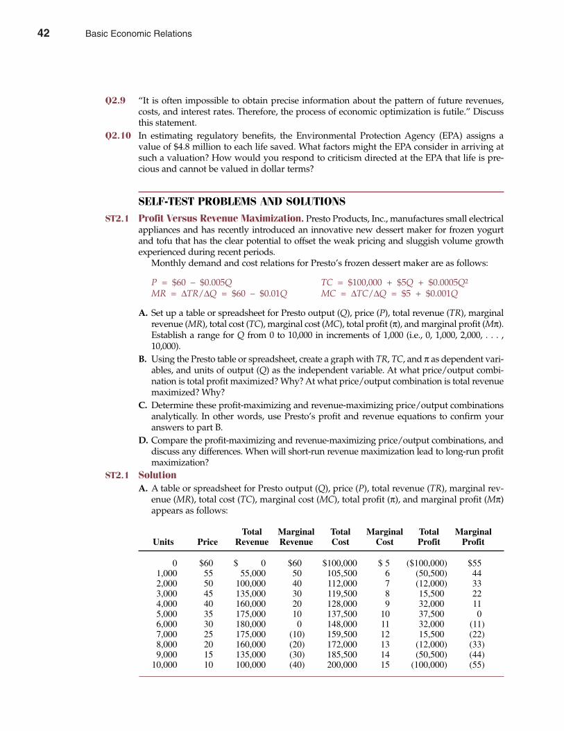
Q2.9 “It is often impossible to obtain precise information about the pattern of future revenues,costs, and interest rates. Therefore, the process of economic optimization is futile.” Discussthis statement.
Q2.10 In estimating regulatory benefits, the Environmental Protection Agency (EPA) assigns avalue of $4.8 million to each life saved. What factors might the EPA consider in arriving atsuch a valuation? How would you respond to criticism directed at the EPA that life is pre-cious and cannot be valued in dollar terms?
SELF-TEST PROBLEMS AND SOLUTIONS
ST2.1 Profit Versus Revenue Maximization. Presto Products, Inc., manufactures small electricalappliances and has recently introduced an innovative new dessert maker for frozen yogurtand tofu that has the clear potential to offset the weak pricing and sluggish volume growthexperienced during recent periods.
Monthly demand and cost relations for Presto’s frozen dessert maker are as follows:
P = $60 – $0.005Q TC = $100,000 + $5Q + $0.0005Q2
MR = ∆TR/∆Q = $60 – $0.01Q MC = ∆TC/∆Q = $5 + $0.001Q
A. Set up a table or spreadsheet for Presto output (Q), price (P), total revenue (TR), marginalrevenue (MR), total cost (TC), marginal cost (MC), total profit (π), and marginal profit (Mπ).Establish a range for Q from 0 to 10,000 in increments of 1,000 (i.e., 0, 1,000, 2,000, . . . ,10,000).
B. Using the Presto table or spreadsheet, create a graph with TR, TC, and π as dependent vari-ables, and units of output (Q) as the independent variable. At what price/output combi-nation is total profit maximized? Why? At what price/output combination is total revenuemaximized? Why?
C. Determine these profit-maximizing and revenue-maximizing price/output combinationsanalytically. In other words, use Presto’s profit and revenue equations to confirm youranswers to part B.
D. Compare the profit-maximizing and revenue-maximizing price/output combinations, anddiscuss any differences. When will short-run revenue maximization lead to long-run profitmaximization?
ST2.1 SolutionA. A table or spreadsheet for Presto output (Q), price (P), total revenue (TR), marginal rev-
enue (MR), total cost (TC), marginal cost (MC), total profit (π), and marginal profit (Mπ)appears as follows:
42 Part One Overview of Managerial Economics
Total Marginal Total Marginal Total MarginalUnits Price Revenue Revenue Cost Cost Profit Profit
0 $60 $ 0 $60 $100,000 $ 5 ($100,000) $551,000 55 55,000 50 105,500 6 (50,500) 442,000 50 100,000 40 112,000 7 (12,000) 333,000 45 135,000 30 119,500 8 15,500 224,000 40 160,000 20 128,000 9 32,000 115,000 35 175,000 10 137,500 10 37,500 0 6,000 30 180,000 0 148,000 11 32,000 (11)7,000 25 175,000 (10) 159,500 12 15,500 (22)8,000 20 160,000 (20) 172,000 13 (12,000) (33)9,000 15 135,000 (30) 185,500 14 (50,500) (44)
10,000 10 100,000 (40) 200,000 15 (100,000) (55)
42 Basic Economic Relations
B. Using the Presto table or spreadsheet, a graph with TR, TC, and π as dependent variablesand units of output (Q) as the independent variable appears as follows:
The price/output combination at which total profit is maximized is P = $35 and Q =5,000 units. At that point, MR = MC and total profit is maximized at $37,500.
The price/output combination at which total revenue is maximized is P = $30 and Q= 6,000 units. At that point, MR = 0 and total revenue is maximized at $180,000.
C. To find the profit-maximizing output level analytically, set MR = MC, or set Mπ = 0, andsolve for Q. Because
MR = MC$60 – $0.01Q = $5 + $0.001Q
0.011Q = 55Q = 5,000
At Q = 5,000,
P = $60 – $0.005(5,000)= $35
π = –$100,000 + $55(5,000) – $0.0055(5,0002)= $37,500
(Note: This is a maximum because total profit is falling for Q > 5,000.)To find the revenue-maximizing output level, set MR = 0, and solve for Q. Thus,
MR = $60 – $0.01Q = 00.01Q = 60
Q = 6,000
At Q = 6,000,
Chapter Two Basic Economic Relations 43
$250,000
200,000
150,000
100,000
50,000
0
Ð50,000
Ð100,000
Ð150,0001,000 10,0007,0004,000 6,0003,000 8,0002,000 5,000 9,000
Total cost
Total profit
Total revenue
Maximum revenue
Maximum profit
Dollars
Units of output (Q )
Presto Products, Inc.Profit Vs. Revenue Maximization
0
Basic Economic Relations 43
P = $60 – $0.005(6,000)= $30
π = TR – TC= ($60 – $0.005Q)Q – $100,000 – $5Q – $0.0005Q2
= –$100,000 + $55Q – $0.0055Q2
= –$100,000 + $55(6,000) – $0.0055(6,0002)= $32,000
(Note: This is a revenue maximum because total revenue is decreasing for output beyondQ > 6,000.)
D. Given downward-sloping demand and marginal revenue curves, and positive marginalcosts, the profit-maximizing price/output combination is always at a higher price andlower production level than the revenue-maximizing price/output combination. Thisstems from the fact that profit is maximized when MR = MC, whereas revenue is maxi-mized when MR = 0. It follows that profits and revenue are only maximized at the sameprice/output combination in the unlikely event that MC = 0.
In pursuing a short-run revenue rather than profit-maximizing strategy, Presto can expectto gain a number of important advantages, including enhanced product awareness amongconsumers, increased customer loyalty, potential economies of scale in marketing and pro-motion, and possible limitations in competitor entry and growth. To be consistent with long-run profit maximization, these advantages of short-run revenue maximization must be atleast worth Presto’s short-run sacrifice of $5,500 (= $37,500 – $32,000) in monthly profits.
ST2.2 Average Cost Minimization. Pharmed Caplets, Inc., is an international manufacturer of bulkantibiotics for the animal feed market. Dr. Indiana Jones, head of marketing and research, seeksyour advice on an appropriate pricing strategy for Pharmed Caplets, an antibiotic for sale tothe veterinarian and feedlot-operator market. This product has been successfully launchedduring the past few months in a number of test markets, and reliable data are now availablefor the first time.
The marketing and accounting departments have provided you with the following monthlytotal revenue and total cost information:
TR = $900Q – $0.1Q2 TC = $36,000 + $200Q + $0.4Q2
MR = ∆TR/∆Q = $900 – $0.2Q MC = ∆TC/∆Q = $200 + $0.8Q
A. Set up a table or spreadsheet for Pharmed Caplets output (Q), price (P), total revenue (TR),marginal revenue (MR), total cost (TC), marginal cost (MC), average cost (AC), total profit(π), and marginal profit (Mπ). Establish a range for Q from 0 to 1,000 in increments of 100(i.e., 0, 100, 200, . . . , 1,000).
B. Using the Pharmed Caplets table or spreadsheet, create a graph with AC and MC as depend-ent variables and units of output (Q) as the independent variable. At what price/outputcombination is total profit maximized? Why? At what price/output combination is averagecost minimized? Why?
C. Determine these profit-maximizing and average-cost minimizing price/output combinationsanalytically. In other words, use Pharmed Caplets’ revenue and cost equations to confirmyour answers to part B.
D. Compare the profit-maximizing and average-cost minimizing price/output combinations,and discuss any differences. When will average-cost minimization lead to long-run profitmaximization?
ST2.2 SolutionA. A table or spreadsheet for Pharmed Caplets output (Q), price (P), total revenue (TR), mar-
ginal revenue (MR), total cost (TC), marginal cost (MC), average cost (AC), total profit (π),and marginal profit (Mπ) appears as follows:
44 Part One Overview of Managerial Economics
44 Basic Economic Relations
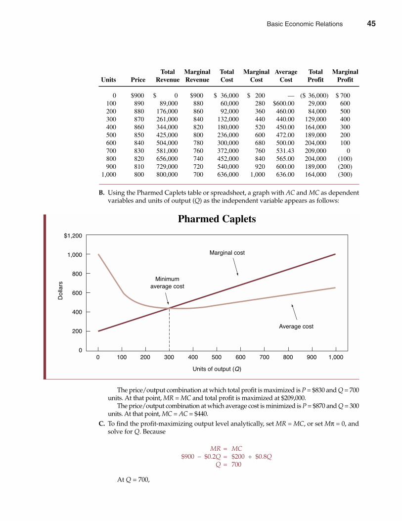
B. Using the Pharmed Caplets table or spreadsheet, a graph with AC and MC as dependentvariables and units of output (Q) as the independent variable appears as follows:
The price/output combination at which total profit is maximized is P = $830 and Q = 700units. At that point, MR = MC and total profit is maximized at $209,000.
The price/output combination at which average cost is minimized is P = $870 and Q = 300units. At that point, MC = AC = $440.
C. To find the profit-maximizing output level analytically, set MR = MC, or set Mπ = 0, andsolve for Q. Because
MR = MC$900 – $0.2Q = $200 + $0.8Q
Q = 700
At Q = 700,
Chapter Two Basic Economic Relations 45
Total Marginal Total Marginal Average Total MarginalUnits Price Revenue Revenue Cost Cost Cost Profit Profit
0 $900 $ 0 $900 $ 36,000 $ 200 — ($ 36,000) $ 700 100 890 89,000 880 60,000 280 $600.00 29,000 600 200 880 176,000 860 92,000 360 460.00 84,000 500 300 870 261,000 840 132,000 440 440.00 129,000 400 400 860 344,000 820 180,000 520 450.00 164,000 300 500 850 425,000 800 236,000 600 472.00 189,000 200 600 840 504,000 780 300,000 680 500.00 204,000 100 700 830 581,000 760 372,000 760 531.43 209,000 0 800 820 656,000 740 452,000 840 565.00 204,000 (100)900 810 729,000 720 540,000 920 600.00 189,000 (200)
1,000 800 800,000 700 636,000 1,000 636.00 164,000 (300)
$1,200
1,000
800
600
400
200
0100 1,000700400 600300 800200 500 900
Dollars
Units of output (Q)
Pharmed Caplets
Minimumaverage cost
Average cost
Marginal cost
0
Basic Economic Relations 45
P = TR/Q= ($900Q – $0.1Q2)/Q= $900 – $0.1(700)= $830
π = TR – TC= $900Q – $0.1Q2 – $36,000 – $200Q – $0.4Q2
= –$36,000 + $700(700) – $0.5(7002)= $209,000
(Note: This is a profit maximum because profits are falling for Q > 700.)To find the average-cost minimizing output level, set MC = AC, and solve for Q. Because
AC = TC/Q= ($36,000 + $200Q + $0.4Q2)/Q= $36,000Q-1 + $200 + $0.4Q
it follows that
MC = AC$200 + $0.8Q = $36,000Q-1 + $200 + $0.4Q
0.4Q = 36,000Q-1
0.4Q2 = 36,000Q2 = 36,000/0.4Q2 = 90,000Q = 300
At Q = 300,
P = $900 – $0.1(300)= $870
π = –$36,000 + $700(300) – $0.5(3002)= $129,000
(Note: This is an average-cost minimum because average cost is rising for Q > 300.)D. Given downward-sloping demand and marginal revenue curves, and a U-shaped or
quadratic AC function, the profit-maximizing price/output combination will often be ata different price and production level than the average-cost minimizing price/outputcombination. This stems from the fact that profit is maximized when MR = MC, whereasaverage cost is minimized when MC = AC. Profits are maximized at the same price/out-put combination as where average costs are minimized in the unlikely event that MR =MC and MC = AC and, therefore, MR = MC = AC.
It is often true that the profit-maximizing output level differs from the average-cost mini-mizing activity level. In this instance, expansion beyond Q = 300, the average-cost minimiz-ing activity level, can be justified because the added gain in revenue more than compensatesfor the added costs. Note that total costs rise by $240,000, from $132,000 to $372,000 as outputexpands from Q = 300 to Q = 700, as average cost rises from $440 to $531.43. Nevertheless,profits rise by $80,000, from $129,000 to $209,000, because total revenue rises by $320,000,from $261,000 to $581,000. The profit-maximizing activity level can be less than, greater than,or equal to the average-cost minimizing activity level depending on the shape of relevantdemand and cost relations.
46 Part One Overview of Managerial Economics
46 Basic Economic Relations
PROBLEMS
P2.1 Graph AnalysisA. Given the output (Q) and price (P) data in the following table, calculate the related total
revenue (TR), marginal revenue (MR), and average revenue (AR) figures:
B. Graph these data using “dollars” on the vertical axis and “quantity” on the horizontal axis.At what output level is revenue maximized?
C. Why is marginal revenue less than average revenue at each price level?P2.2 A. Fill in the missing data for price (P), total revenue (TR), marginal revenue (MR), total cost
(TC), marginal cost (MC), profit (π), and marginal profit (Mπ) in the following table:
B. At what output level is profit maximized?C. At what output level is revenue maximized?D. Discuss any differences in your answers to parts B and C.
P2.3 Marginal Analysis. Characterize each of the following statements as true or false, andexplain your answer.A. If marginal revenue is less than average revenue, the demand curve will be downward
sloping.B. Profits will be maximized when total revenue equals total cost.
Chapter Two Basic Economic Relations 47
Q P TR MR AR
0 $101 92 83 74 65 56 47 38 29 1
10 0
Q P TR MR TC MC π Mπ
0 $160 $ 0 $ — $ 0 $ — $ 0 $ —1 150 150 150 25 25 125 1252 140 55 30 1003 390 35 300 754 90 130 3505 110 550 1756 600 50 55 3707 630 290 60 –308 80 640 355 2859 75 –85
10 600 525
Basic Economic Relations 47
C. Given a downward-sloping demand curve and positive marginal costs, profit-maximizingfirms will always sell less output at higher prices than will revenue-maximizing firms.
D. Marginal cost must be falling for average cost to decline as output expands.E. Marginal profit is the difference between marginal revenue and marginal cost and will
always equal zero at the profit-maximizing activity level.P2.4 Marginal Analysis: Tables. Sarah Berra is a regional sales representative for Dental Labor-
atories, Inc. Berra sells alloy products created from gold, silver, platinum, and other precious metalsto several dental laboratories in Maine, New Hampshire, and Vermont. Berra’s goal is to maxi-mize her total monthly commission income, which is figured at 10% of gross sales. In reviewingher monthly experience over the past year, Berra found the following relations between daysspent in each state and monthly sales generated:
A. Construct a table showing Berra’s marginal sales per day in each state.B. If administrative duties limit Berra to only 10 selling days per month, how should she spend
them?C. Calculate Berra’s maximum monthly commission income.
P2.5 Marginal Analysis: Tables. Climate Control Devices, Inc., estimates that sales of defectivethermostats cost the firm an average of $25 each for replacement or repair. An independentengineering consultant has recommended hiring quality control inspectors so that defectivethermostats can be identified and corrected before shipping. The following schedule shows theexpected relation between the number of quality control inspectors and the thermostat failurerate, defined in terms of the percentage of total shipments that prove to be defective.
The firm expects to ship 250,000 thermostats during the coming year, and quality controlinspectors each command a salary of $30,000 per year.A. Construct a table showing the marginal failure reduction (in units) and the dollar value
of these reductions for each inspector hired.B. How many inspectors should the firm hire?
48 Part One Overview of Managerial Economics
Maine New Hampshire Vermont
Days Gross Sales Days Gross Sales Days Gross Sales
0 $ 4,000 0 $ 0 0 $ 2,500 1 10,000 1 3,500 1 5,000 2 15,000 2 6,500 2 7,000 3 19,000 3 9,000 3 8,500 4 22,000 4 10,500 4 9,500 5 24,000 5 11,500 5 10,000 6 25,000 6 12,000 6 10,000 7 25,000 7 12,500 7 10,000
Number of Quality Control Inspectors Thermostat Failure Rate (percent)
0 5.01 4.02 3.23 2.64 2.25 2.0
48 Basic Economic Relations
C. How many inspectors would be hired if additional indirect costs (lost customer goodwilland so on) were to average 30% of direct replacement or repair costs?
P2.6 Profit Maximization: Equations. Rochester Instruments, Inc., operates in the highly com-petitive electronics industry. Prices for its RII-X control switches are stable at $50 each. Thismeans that P = MR = $50 in this market. Engineering estimates indicate that relevant total andmarginal cost relations for the RII-X model are
TC = $78,000 + $18Q + $0.002Q2
MC = ∆TC/∆Q = $18 + $0.004Q
A. Calculate the output level that will maximize RII-X profit.B. Calculate this maximum profit.
P2.7 Profit Maximization: Equations. 21st Century Insurance offers mail-order automobile insur-ance to preferred-risk drivers in the Los Angeles area. The company is the low-cost provider ofinsurance in this market but does not believe its $750 annual premium can be raised for com-petitive reasons. Its rates are expected to remain stable during coming periods; hence, P = MR =$750. Total and marginal cost relations for the company are as follows:
TC = $2,500,000 + $500Q + $0.005Q2
MC = ∆TC/∆Q = $500 + $0.01Q
A. Calculate the profit-maximizing activity level.B. Calculate the company’s optimal profit and return-on-sales levels.
P2.8 Not-for-Profit Analysis. The Denver Athlete’s Club (DAC) is a private, not-for-profit athleticclub located in Denver, Colorado. DAC currently has 3,500 members but is planning on a mem-bership drive to increase this number significantly. An important issue facing Jessica Nicholson,DAC’s administrative director, is the determination of an appropriate membership level. Toefficiently use scarce DAC resources, the board of directors has instructed Nicholson to maxi-mize DAC’s operating surplus, defined as revenues minus operating costs. They have alsoasked Nicholson to determine the effects of a proposed agreement between DAC and a neigh-boring club with outdoor recreation and swimming pool facilities. Plan A involves paying theneighboring club $100 per DAC member. Plan B involves payment of a fixed fee of $400,000per year. Finally, the board has determined that the membership fee for the coming year willremain constant at $2,500 per member irrespective of the number of new members added andwhether Plan A or Plan B is adopted.
In the calculations for determining an optimal membership level, Nicholson regards priceas fixed; therefore, P = MR = $2,500. Before considering the effects of any agreement with theneighboring club, Nicholson projects total and marginal cost relations during the coming yearto be as follows:
TC = $3,500,000 + $500Q + $0.25Q2
MC = ∆TC/∆Q = $500 + $0.5Q
where Q is the number of DAC members.A. Before considering the effects of the proposed agreement with the neighboring club, cal-
culate DAC’s optimal membership and operating surplus levels.B. Calculate these levels under Plan A.C. Calculate these levels under Plan B.
Chapter Two Basic Economic Relations 49
Basic Economic Relations 49
P2.9 Revenue Maximization. Desktop Publishing Software, Inc., develops and markets softwarepackages for business computers. Although sales have grown rapidly during recent years, thecompany’s management fears that a recent onslaught of new competitors may severely retardfuture growth opportunities. Therefore, it believes that the time has come to “get big or get out.”
The marketing and accounting departments have provided management with the follow-ing monthly demand and cost information:
P = $1,000 – $1Q TC = $50,000 + $100QMR = ∆TR/∆Q = $1,000 – $2Q MC = ∆TC/∆Q = $100
A. Calculate monthly quantity, price, and profit at the short-run revenue-maximizing outputlevel.
B. Calculate these same values for the short-run profit-maximizing level of output.C. When would short-run revenue maximization lead to long-run profit maximization?
P2.10 Average Cost Minimization. Giant Screen TV, Inc., is a San Diego–based importer and dis-tributor of 60-inch screen, high-resolution televisions for individual and commercial customers.Revenue and cost relations are as follows:
TR = $1,800Q – $0.006Q2
MR = ∆TR/∆Q = $1,800 – $0.012QTC = $12,100,000 + $800Q + $0.004Q2
MC = ∆TC/∆Q = $800 + $0.008Q
A. Calculate output, marginal cost, average cost, price, and profit at the average-cost mini-mizing activity level.
B. Calculate these values at the profit-maximizing activity level.C. Compare and discuss your answers to parts A and B.
50 Part One Overview of Managerial Economics
CASE STUDY
A Spreadsheet Approach to Finding the Economic Order QuantityA spreadsheet is a table of data that is organized in a logical framework similar to an account-ing income statement or balance sheet. At first, this marriage of computers and accountinginformation might seem like a minor innovation. However, it is not. For example, with com-puterized spreadsheets it becomes possible to easily reflect the effects on revenue, cost, andprofit of a slight change in demand conditions. Similarly, the effects on the profit-maximizingor breakeven activity levels can be easily determined. Various “what if?” scenarios can alsobe tested to determine the optimal or profit-maximizing activity level under a wide variety ofoperating conditions. Thus, it becomes easy to quantify in dollar terms the pluses and minus-es (revenues and costs) of alternate decisions. Each operating and planning decision can beeasily evaluated in light of available alternatives. Through the use of spreadsheet formulasand so-called “macros,” managers are able to locate maximum or minimum values for anyobjective function based on the relevant marginal relations. Therefore, spreadsheets are a veryuseful tool that can be used to analyze a variety of typical optimization problems.
To illustrate the use of spreadsheets in economic analysis, consider the case of The Neighbor-hood Pharmacy, Inc. (NPI), a small but rapidly growing operator of a number of large-scalediscount pharmacies in the greater Boston, Massachusetts, metropolitan area. A key contributorto the overall success of the company is a system of tight controls over inventory acquisition
50 Basic Economic Relations
SELECTED REFERENCESBascha, Andreas, and Uwe Walz. “Convertible Securities and Optimal Exit Decisions in Venture Capital
Finance.” Journal of Corporate Finance 7 (September 2001): 285–306.Epstein, Larry G. “Sharing Ambiguity.” American Economic Review 91 (May 2001): 45–50.French, Nick. “Decision Theory and Real Estate Investment: An Analysis of the Decision-Making Processes
of Real Estate Investment Fund Managers.” Managerial & Decision Economics 22 (October/November2001): 399–410.
Genesove, David, and Christopher Mayer. “Loss Aversion and Seller Behavior: Evidence from theHousing Market.” Quarterly Journal of Economics 116 (November 2001): 1233–1260.
Chapter Two Basic Economic Relations 51
and carrying costs. The company’s total annual costs for acquisition and inventory of phar-maceutical items are composed of the purchase cost of individual products supplied by whole-salers (purchase costs); the clerical, transportation, and other costs associated with placing eachindividual order (order costs); and the interest, insurance, and other expenses involved withcarrying inventory (carrying costs). The company’s total inventory-related costs are given bythe expression
TC = P � X + � � X/Q + C � Q/2
where TC is inventory-related total costs during the planning period, P is the purchase price of theinventory item, X is the total quantity of the inventory item that is to be ordered (used) during theplanning period (use requirement), � is the cost of placing an individual order for the inventoryitem (order cost), C is inventory carrying costs expressed on a per unit of inventory basis (carry-ing cost), and Q is the quantity of inventory ordered at any one point in time (order quantity). HereQ is NPI’s decision variable, whereas each other variable contained in the total cost function isbeyond control of the firm (exogenous). In analyzing this total cost relation, NPI is concerned withpicking the order quantity that will minimize total inventory-related costs. The optimal or total-cost minimizing order quantity is typically referred to as the “economic order quantity.”
During the relevant planning period, the per unit purchase cost for an important prescribed(ethical) drug is P = $4, the total estimated use for the planning period is X = 5,000, the cost ofplacing an order is � = $50; and the per unit carrying cost is C = $0.50, calculated as the currentinterest rate of 12.5% multiplied by the per unit purchase cost of the item.A. Set up a table or spreadsheet for NPI’s order quantity (Q), inventory-related total cost (TC),
purchase price (P), use requirement (X), order cost (�), and carrying cost (C). Establish arange for Q from 0 to 2,000 in increments of 100 (i.e., 0, 100, 200, . . . , 2,000).
B. Based on the NPI table or spreadsheet, determine the order quantity that will minimizethe company’s inventory-related total costs during the planning period.
C. Placing inventory-related total costs, TC, on the vertical or Y-axis and the order quantity,Q, on the horizontal or X-axis, plot the relation between inventory-related total costs andthe order quantity.
D. Based on the same data as previously, set up a table or spreadsheet for NPI’s orderquantity (Q), inventory-related total cost (TC), and each component part of total costs,including inventory purchase (acquisition) costs, P � X; total order costs, � � X/Q;and total carrying costs, C � Q/2. Placing inventory-related total costs, TC, and eachcomponent cost category as dependent variables on the vertical or Y-axis and the orderquantity, Q, as the independent variable on the horizontal or X-axis, plot the relationbetween inventory-related cost categories and the order quantity.
CASE STUDY (continued)
Basic Economic Relations 51

Hansen, Lars Peter, and Thomas J. Sargent. “Robust Control and Model Uncertainty.” American EconomicReview 91 (May 2001): 60–66.
Hobijn, Bart, and Boyan Jovanovic. “The Information-Technology Revolution and the Stock Market:Evidence.” American Economic Review 91 (December 2001): 1203–1220.
Lamont, Owen A., and Christopher Polk. “Does Diversification Destroy Value? Evidence from theIndustry Shocks.” Journal of Financial Economics 63 (January 2002): 51–77.
Loasby, Brian L. “An Entrepreneurial Theory of the Firm: Foreword by Israel M. Kirzner.” EconomicJournal 111 (June 2001): F537–F538.
Madrian, Brigitte C., and Dennis F. Shea. “The Power of Suggestion: Inertia in 401(K) Participation andSavings Behavior.” Quarterly Journal of Economics 116 (November 2001): 1149–1187.
Nissim, Doron, and Amir Ziv. “Dividend Changes and Future Profitability.” Journal of Finance 56(December 2001): 2211–2134.
Persson, Torsten, Géérard Roland, and Guido Tabellini. “Disability Insurance Benefits and Labor Supply.”Journal of Political Economy 108 (December 2000): 1162–1184.
Rajan, Raghuram G., and Luigi Zingales. “The Firm as a Dedicated Hierarchy: A Theory of the Originsand Growth of Firms.” Quarterly Journal of Economics 116 (August 2001): 805–851.
Roberts, Peter W. “Innovation and Firm-Level Persistent Profitability: A Schumpeterian Framework.”Managerial & Decision Economics 22 (June/August 2001): 239–250.
Rogers, Edward W. “A Theoretical Look at Firm Performance in High-Tech Organizations: What DoesExisting Theory Tell Us?” Journal of High Technology Management Research 12 (Spring 2001): 39–61.
Wakely, Tim. “Economic Organization and Economic Knowledge, and Contingency, Complexity andthe Theory of the Firm: Essays in Honour of Brian J. Loasby, Vols. I and II.” Information Economics &Policy 13 (March 2001): 117–125.
52 Part One Overview of Managerial Economics
52 Basic Economic Relations
Statistical Analysis ofEconomic Relations
CHAPTER THREE
531 See Robert O’Brien, “Economic Data, Bargain Hunting Offset Fears About Accounting,”
The Wall Street Journal Online, February 20, 2002 (http://online.wsj.com).
It is common knowledge that average scores achieved by U.S. students onthe Scholastic Aptitude Test (SAT) have been declining for years. It is less
known that average SAT test scores among whites and blacks, Asians,Mexicans, and Puerto Ricans have generally risen over the past two decades.Average test scores have been declining while the “average” student is doingbetter. How can the overall average go down if subaverages for all of theconstituent subgroups are going up? What has changed is not student per-formance, but demographics. Minority students, whose scores are rising thefastest, but from a lower base, are a rapidly growing part of the test pool. Byfocusing on the overall average rather than the averages of constituent sub-groups, a picture of declining performance has been painted when perform-ance has instead been improving. In business, the client of a major auditingfirm encountered a similar problem. The company feared a loss in marketshare, as it noted a disturbing erosion in overall profit margins. Upon closerexamination, the auditing firm found that profit margins were holdingsteady or rising in each product line, but that the product mix was changingin favor of lower margin products. As in the case of declining SAT scores, the“lie of averages” had emerged. Statistics such as overall averages do not lie,but they can be easily manipulated.1
Effective managers are adept at information processing made difficult by anenvironment that is complex and constantly changing. In this chapter, methodsfor characterizing the central tendency and dispersion of economic data arepresented. This provides the background necessary for a more detailed exam-ination of the statistical analysis of economic relations.
53
3
DATA SUMMARY AND DESCRIPTION
Information analysis and management is perhaps the key function of management. Workingwith the best information available, managers must be able to condense and characterizeimportant economic information so that the best operating and planning decisions can be made.
Population ParametersThe population of potential buyers includes those persons who may be favorably disposed topurchase a given product. Just as a complete census of city, county, and state residents is a time-consuming and expensive means for determining characteristics of the local population, acomplete census of potential buyers is a costly means for determining the likely customerresponse to a change in product design, quality, or price. Rather than conduct a cursory analy-sis of each and every potential buyer, it is often desirable to conduct a detailed analysis of asample or subset of buyers. Similarly, it is often too expensive or otherwise impractical to testthe reliability or cost of each and every unit produced, so the reliability or cost of a sample ofproducts is analyzed instead.
In the absence of a complete and detailed census of the entire population, summary anddescriptive measures of the overall population, called population parameters, are not knownand must be estimated.
Sample StatisticsThe most effective means for doing so is to rely on sample statistics, or summary and descrip-tive measures that describe a representative subset of the overall population.
A complete and detailed study of all those factors and individuals that influence the firm’seconomic environment is seldom practical or even possible. Therefore, the statistical analysisof economic relations usually focuses on the estimation and interpretation of sample statisticsrather than population parameters. In the design and application of statistical methods,managers wish to draw important inferences about overall population parameters based ona detailed analysis of sample statistics. The first important class of sample summary anddescriptive statistics that managers must consider involves measures of central tendency.
MEASURES OF CENTRAL TENDENCY
A number that tells the “typical” value of sales, costs, profits, or any amount is called a measureof central tendency. Measures of central tendency present important features of the data in a con-cise fashion that offers managers a reasonable basis for operating and planning decisions.Although statisticians have constructed several useful measures of central tendency, managersoften focus on the mean, median, and mode. Which among these is most appropriate for a giventask depends on the nature of the underlying data and the need being addressed by the manager.
MeanThe arithmetic mean or average is the sum of numbers included in a given sample divided bythe number of observations. If n is the number of sample observations, X1 is the first observa-tion, X2 is the second observation, X3 is the third observation, and so on, then the sample meanis calculated as
(3.1)X = X1 + X2 + X3 + • • • + Xn
n
54 Part One Overview of Managerial Economics
population parametersSummary and descrip-tive measures for thepopulation
sample statisticsSummary and descrip-tive measures for asample
mean Average
54 Statistical Analysis of Economic Relations
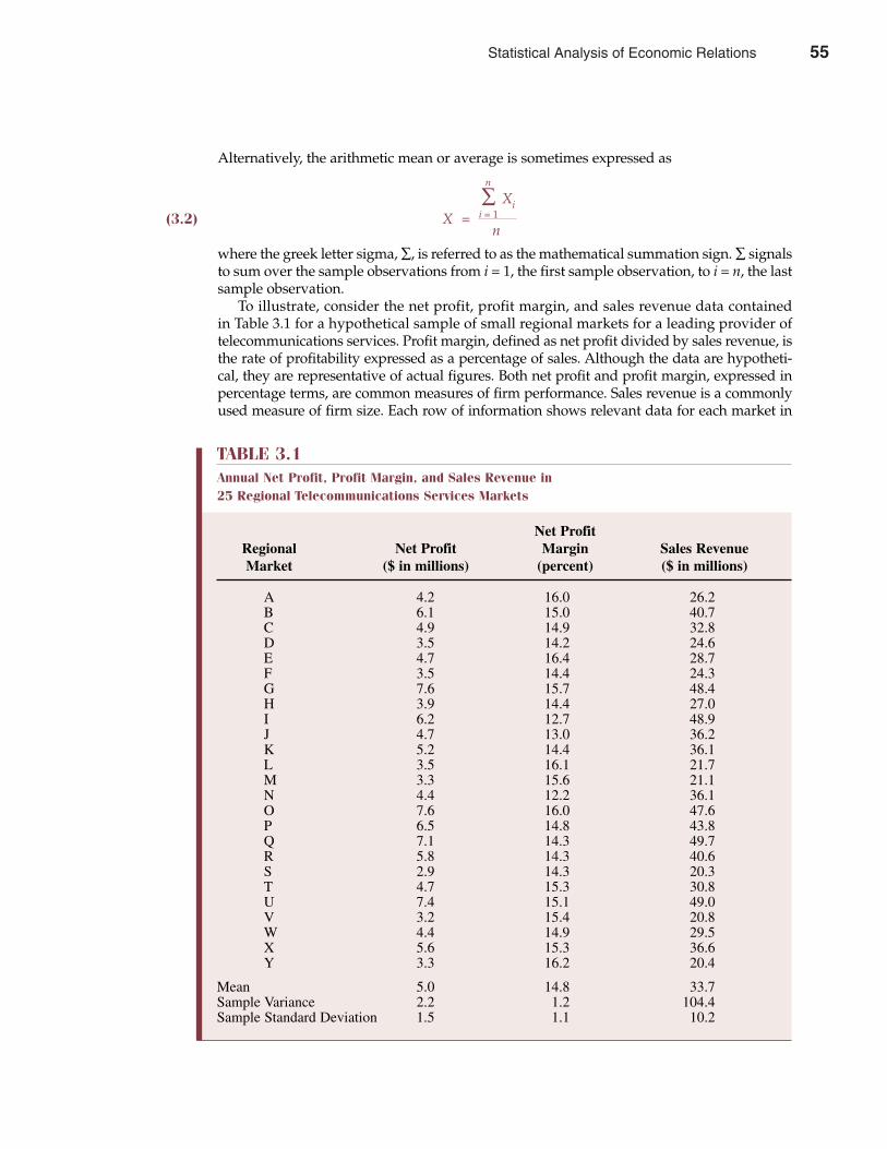
Alternatively, the arithmetic mean or average is sometimes expressed as
n
(3.2) X =∑ Xii = 1
n
where the greek letter sigma, ∑, is referred to as the mathematical summation sign. ∑ signalsto sum over the sample observations from i = 1, the first sample observation, to i = n, the lastsample observation.
To illustrate, consider the net profit, profit margin, and sales revenue data containedin Table 3.1 for a hypothetical sample of small regional markets for a leading provider oftelecommunications services. Profit margin, defined as net profit divided by sales revenue, isthe rate of profitability expressed as a percentage of sales. Although the data are hypotheti-cal, they are representative of actual figures. Both net profit and profit margin, expressed inpercentage terms, are common measures of firm performance. Sales revenue is a commonlyused measure of firm size. Each row of information shows relevant data for each market in
Chapter Three Statistical Analysis of Economic Relations 55
TABLE 3.1Annual Net Profit, Profit Margin, and Sales Revenue in 25 Regional Telecommunications Services Markets
Net ProfitRegional Net Profit Margin Sales RevenueMarket ($ in millions) (percent) ($ in millions)
A 4.2 16.0 26.2B 6.1 15.0 40.7C 4.9 14.9 32.8D 3.5 14.2 24.6E 4.7 16.4 28.7F 3.5 14.4 24.3G 7.6 15.7 48.4H 3.9 14.4 27.0I 6.2 12.7 48.9J 4.7 13.0 36.2K 5.2 14.4 36.1L 3.5 16.1 21.7M 3.3 15.6 21.1N 4.4 12.2 36.1O 7.6 16.0 47.6P 6.5 14.8 43.8Q 7.1 14.3 49.7R 5.8 14.3 40.6S 2.9 14.3 20.3T 4.7 15.3 30.8U 7.4 15.1 49.0V 3.2 15.4 20.8W 4.4 14.9 29.5X 5.6 15.3 36.6Y 3.3 16.2 20.4
Mean 5.0 14.8 33.7Sample Variance 2.2 1.2 104.4Sample Standard Deviation 1.5 1.1 10.2
Statistical Analysis of Economic Relations 55
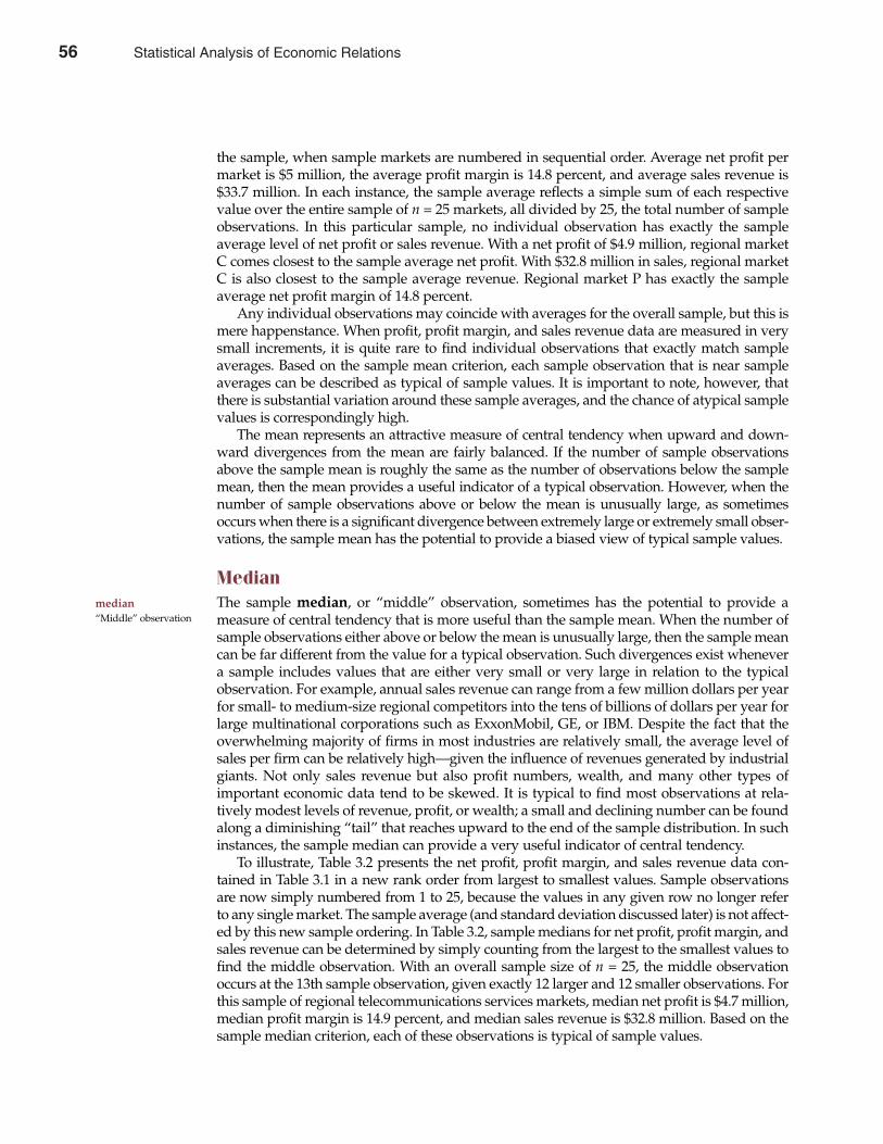
the sample, when sample markets are numbered in sequential order. Average net profit permarket is $5 million, the average profit margin is 14.8 percent, and average sales revenue is$33.7 million. In each instance, the sample average reflects a simple sum of each respectivevalue over the entire sample of n = 25 markets, all divided by 25, the total number of sampleobservations. In this particular sample, no individual observation has exactly the sampleaverage level of net profit or sales revenue. With a net profit of $4.9 million, regional marketC comes closest to the sample average net profit. With $32.8 million in sales, regional marketC is also closest to the sample average revenue. Regional market P has exactly the sampleaverage net profit margin of 14.8 percent.
Any individual observations may coincide with averages for the overall sample, but this ismere happenstance. When profit, profit margin, and sales revenue data are measured in verysmall increments, it is quite rare to find individual observations that exactly match sampleaverages. Based on the sample mean criterion, each sample observation that is near sampleaverages can be described as typical of sample values. It is important to note, however, thatthere is substantial variation around these sample averages, and the chance of atypical samplevalues is correspondingly high.
The mean represents an attractive measure of central tendency when upward and down-ward divergences from the mean are fairly balanced. If the number of sample observationsabove the sample mean is roughly the same as the number of observations below the samplemean, then the mean provides a useful indicator of a typical observation. However, when thenumber of sample observations above or below the mean is unusually large, as sometimesoccurs when there is a significant divergence between extremely large or extremely small obser-vations, the sample mean has the potential to provide a biased view of typical sample values.
MedianThe sample median, or “middle” observation, sometimes has the potential to provide ameasure of central tendency that is more useful than the sample mean. When the number ofsample observations either above or below the mean is unusually large, then the sample meancan be far different from the value for a typical observation. Such divergences exist whenevera sample includes values that are either very small or very large in relation to the typicalobservation. For example, annual sales revenue can range from a few million dollars per yearfor small- to medium-size regional competitors into the tens of billions of dollars per year forlarge multinational corporations such as ExxonMobil, GE, or IBM. Despite the fact that theoverwhelming majority of firms in most industries are relatively small, the average level ofsales per firm can be relatively high—given the influence of revenues generated by industrialgiants. Not only sales revenue but also profit numbers, wealth, and many other types ofimportant economic data tend to be skewed. It is typical to find most observations at rela-tively modest levels of revenue, profit, or wealth; a small and declining number can be foundalong a diminishing “tail” that reaches upward to the end of the sample distribution. In suchinstances, the sample median can provide a very useful indicator of central tendency.
To illustrate, Table 3.2 presents the net profit, profit margin, and sales revenue data con-tained in Table 3.1 in a new rank order from largest to smallest values. Sample observationsare now simply numbered from 1 to 25, because the values in any given row no longer referto any single market. The sample average (and standard deviation discussed later) is not affect-ed by this new sample ordering. In Table 3.2, sample medians for net profit, profit margin, andsales revenue can be determined by simply counting from the largest to the smallest values tofind the middle observation. With an overall sample size of n = 25, the middle observationoccurs at the 13th sample observation, given exactly 12 larger and 12 smaller observations. Forthis sample of regional telecommunications services markets, median net profit is $4.7 million,median profit margin is 14.9 percent, and median sales revenue is $32.8 million. Based on thesample median criterion, each of these observations is typical of sample values.
56 Part One Overview of Managerial Economics
median“Middle” observation
56 Statistical Analysis of Economic Relations
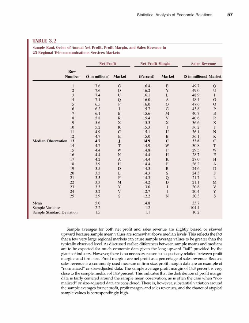
Sample averages for both net profit and sales revenue are slightly biased or skewedupward because sample mean values are somewhat above median levels. This reflects the factthat a few very large regional markets can cause sample average values to be greater than thetypically observed level. As discussed earlier, differences between sample means and mediansare to be expected for much economic data given the long upward “tail” provided by thegiants of industry. However, there is no necessary reason to suspect any relation between profitmargins and firm size. Profit margins are net profit as a percentage of sales revenue. Becausesales revenue is a commonly used measure of firm size, profit margin data are an example of“normalized” or size-adjusted data. The sample average profit margin of 14.8 percent is veryclose to the sample median of 14.9 percent. This indicates that the distribution of profit margindata is fairly centered around the sample mean observation, as is often the case when “nor-malized” or size-adjusted data are considered. There is, however, substantial variation aroundthe sample averages for net profit, profit margin, and sales revenues, and the chance of atypicalsample values is correspondingly high.
Chapter Three Statistical Analysis of Economic Relations 57
TABLE 3.2Sample Rank Order of Annual Net Profit, Profit Margin, and Sales Revenue in 25 Regional Telecommunications Services Markets
Net Profit Net Profit Margin Sales Revenue
RowNumber ($ in millions) Market (Percent) Market ($ in millions) Market
1 7.6 G 16.4 E 49.7 Q2 7.6 O 16.2 Y 49.0 U3 7.4 U 16.1 L 48.9 I4 7.1 Q 16.0 A 48.4 G5 6.5 P 16.0 O 47.6 O6 6.2 I 15.7 G 43.8 P7 6.1 B 15.6 M 40.7 B8 5.8 R 15.4 V 40.6 R9 5.6 X 15.3 X 36.6 X
10 5.2 K 15.3 T 36.2 J11 4.9 C 15.1 U 36.1 N12 4.7 E 15.0 B 36.1 K
Median Observation 13 4.7 J 14.9 C 32.8 C14 4.7 T 14.9 W 30.8 T15 4.4 W 14.8 P 29.5 W16 4.4 N 14.4 H 28.7 E17 4.2 A 14.4 K 27.0 H18 3.9 H 14.4 F 26.2 A19 3.5 D 14.3 R 24.6 D20 3.5 L 14.3 S 24.3 F21 3.5 F 14.3 Q 21.7 L22 3.3 M 14.2 D 21.1 M23 3.3 Y 13.0 J 20.8 V24 3.2 V 12.7 I 20.4 Y25 2.9 S 12.2 N 20.3 S
Mean 5.0 14.8 33.7Sample Variance 2.2 1.2 104.4Sample Standard Deviation 1.5 1.1 10.2
Statistical Analysis of Economic Relations 57
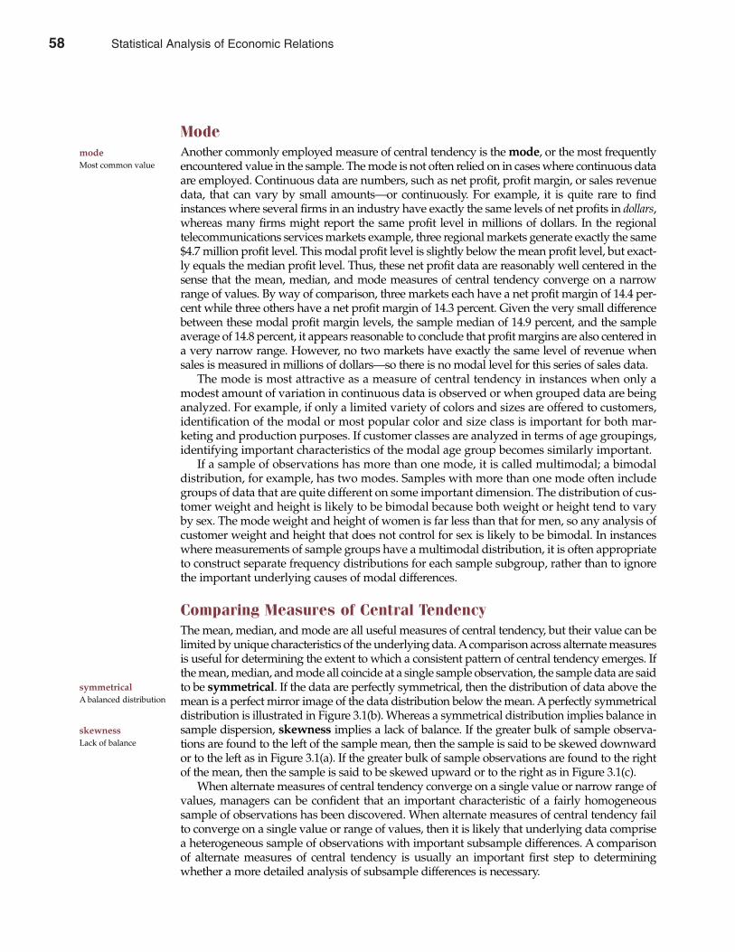
ModeAnother commonly employed measure of central tendency is the mode, or the most frequentlyencountered value in the sample. The mode is not often relied on in cases where continuous dataare employed. Continuous data are numbers, such as net profit, profit margin, or sales revenuedata, that can vary by small amounts—or continuously. For example, it is quite rare to findinstances where several firms in an industry have exactly the same levels of net profits in dollars,whereas many firms might report the same profit level in millions of dollars. In the regionaltelecommunications services markets example, three regional markets generate exactly the same$4.7 million profit level. This modal profit level is slightly below the mean profit level, but exact-ly equals the median profit level. Thus, these net profit data are reasonably well centered in thesense that the mean, median, and mode measures of central tendency converge on a narrowrange of values. By way of comparison, three markets each have a net profit margin of 14.4 per-cent while three others have a net profit margin of 14.3 percent. Given the very small differencebetween these modal profit margin levels, the sample median of 14.9 percent, and the sampleaverage of 14.8 percent, it appears reasonable to conclude that profit margins are also centered ina very narrow range. However, no two markets have exactly the same level of revenue whensales is measured in millions of dollars—so there is no modal level for this series of sales data.
The mode is most attractive as a measure of central tendency in instances when only amodest amount of variation in continuous data is observed or when grouped data are beinganalyzed. For example, if only a limited variety of colors and sizes are offered to customers,identification of the modal or most popular color and size class is important for both mar-keting and production purposes. If customer classes are analyzed in terms of age groupings,identifying important characteristics of the modal age group becomes similarly important.
If a sample of observations has more than one mode, it is called multimodal; a bimodaldistribution, for example, has two modes. Samples with more than one mode often includegroups of data that are quite different on some important dimension. The distribution of cus-tomer weight and height is likely to be bimodal because both weight or height tend to varyby sex. The mode weight and height of women is far less than that for men, so any analysis ofcustomer weight and height that does not control for sex is likely to be bimodal. In instanceswhere measurements of sample groups have a multimodal distribution, it is often appropriateto construct separate frequency distributions for each sample subgroup, rather than to ignorethe important underlying causes of modal differences.
Comparing Measures of Central TendencyThe mean, median, and mode are all useful measures of central tendency, but their value can belimited by unique characteristics of the underlying data. Acomparison across alternate measuresis useful for determining the extent to which a consistent pattern of central tendency emerges. Ifthe mean, median, and mode all coincide at a single sample observation, the sample data are saidto be symmetrical. If the data are perfectly symmetrical, then the distribution of data above themean is a perfect mirror image of the data distribution below the mean. A perfectly symmetricaldistribution is illustrated in Figure 3.1(b). Whereas a symmetrical distribution implies balance insample dispersion, skewness implies a lack of balance. If the greater bulk of sample observa-tions are found to the left of the sample mean, then the sample is said to be skewed downwardor to the left as in Figure 3.1(a). If the greater bulk of sample observations are found to the rightof the mean, then the sample is said to be skewed upward or to the right as in Figure 3.1(c).
When alternate measures of central tendency converge on a single value or narrow range ofvalues, managers can be confident that an important characteristic of a fairly homogeneoussample of observations has been discovered. When alternate measures of central tendency failto converge on a single value or range of values, then it is likely that underlying data comprisea heterogeneous sample of observations with important subsample differences. A comparisonof alternate measures of central tendency is usually an important first step to determiningwhether a more detailed analysis of subsample differences is necessary.
58 Part One Overview of Managerial Economics
modeMost common value
symmetrical A balanced distribution
skewnessLack of balance
58 Statistical Analysis of Economic Relations
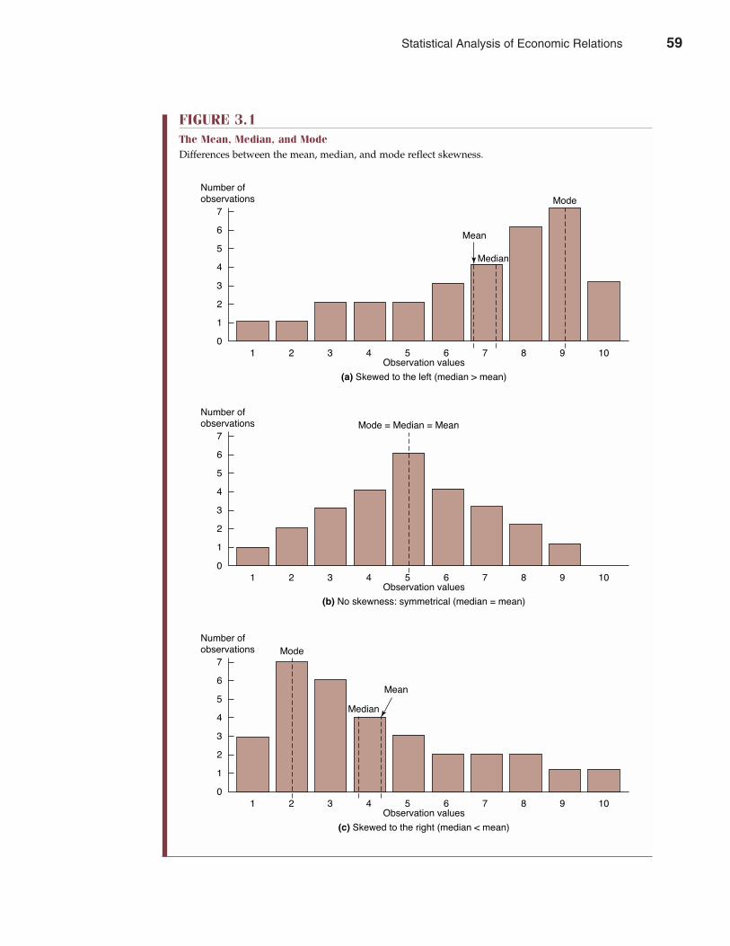
Chapter Three Statistical Analysis of Economic Relations 59
FIGURE 3.1The Mean, Median, and ModeDifferences between the mean, median, and mode reflect skewness.
Number of�observations
7
6
5
4
3
2
1
0
4 91 5Observation values
(a) Skewed to the left (median > mean)
82 6 73 10
Mean
Mode
Median
Number of�observations
7
6
5
4
3
2
1
0
4 91 5Observation values
(b) No skewness: symmetrical (median = mean)
82 6 73 10
Mode = Median = Mean
Number of�observations
7
6
5
4
3
2
1
0
4 91 5Observation values
(c) Skewed to the right (median < mean)
82 6 73 10
Mean
Mode
Median
Statistical Analysis of Economic Relations 59
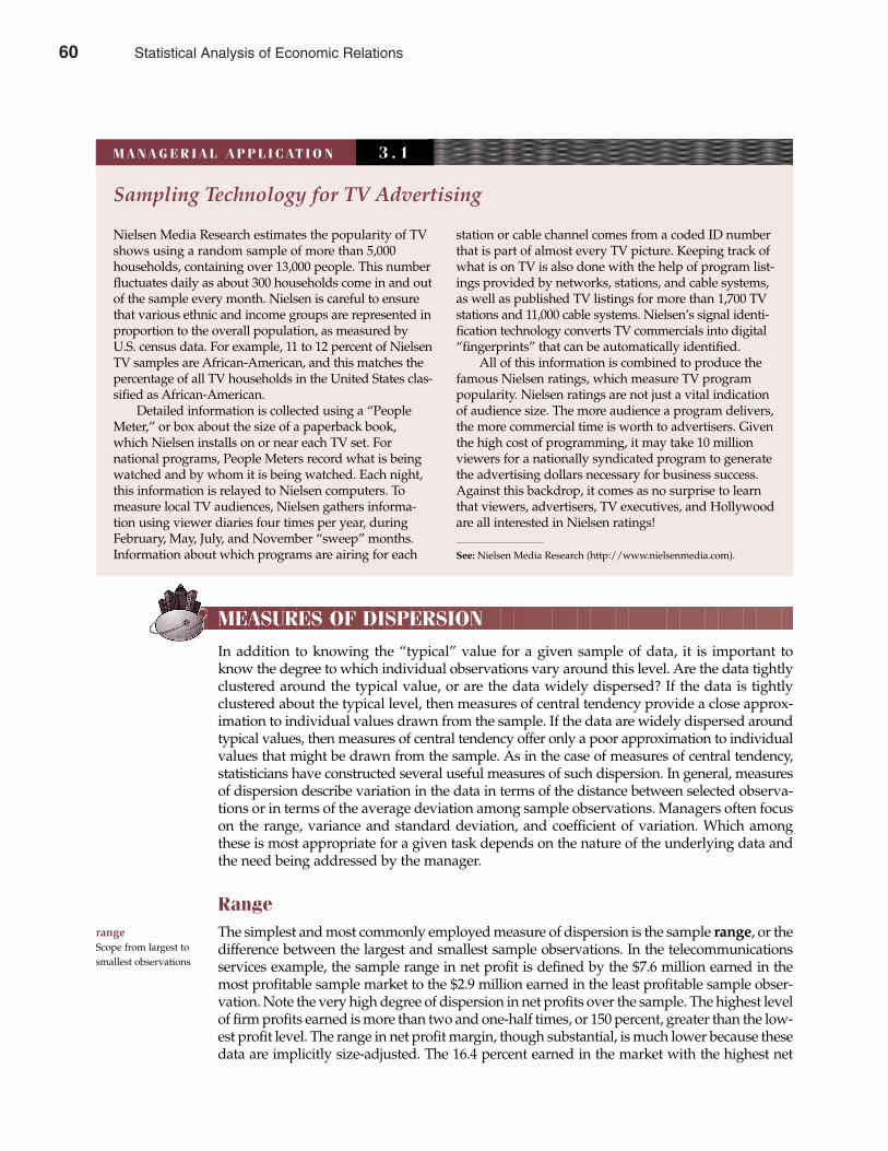
MEASURES OF DISPERSION
In addition to knowing the “typical” value for a given sample of data, it is important toknow the degree to which individual observations vary around this level. Are the data tightlyclustered around the typical value, or are the data widely dispersed? If the data is tightlyclustered about the typical level, then measures of central tendency provide a close approx-imation to individual values drawn from the sample. If the data are widely dispersed aroundtypical values, then measures of central tendency offer only a poor approximation to individualvalues that might be drawn from the sample. As in the case of measures of central tendency,statisticians have constructed several useful measures of such dispersion. In general, measuresof dispersion describe variation in the data in terms of the distance between selected observa-tions or in terms of the average deviation among sample observations. Managers often focuson the range, variance and standard deviation, and coefficient of variation. Which amongthese is most appropriate for a given task depends on the nature of the underlying data andthe need being addressed by the manager.
RangeThe simplest and most commonly employed measure of dispersion is the sample range, or thedifference between the largest and smallest sample observations. In the telecommunicationsservices example, the sample range in net profit is defined by the $7.6 million earned in themost profitable sample market to the $2.9 million earned in the least profitable sample obser-vation. Note the very high degree of dispersion in net profits over the sample. The highest levelof firm profits earned is more than two and one-half times, or 150 percent, greater than the low-est profit level. The range in net profit margin, though substantial, is much lower because thesedata are implicitly size-adjusted. The 16.4 percent earned in the market with the highest net
60 Part One Overview of Managerial Economics
range Scope from largest tosmallest observations
Sampling Technology for TV Advertising
Nielsen Media Research estimates the popularity of TVshows using a random sample of more than 5,000households, containing over 13,000 people. This numberfluctuates daily as about 300 households come in and outof the sample every month. Nielsen is careful to ensurethat various ethnic and income groups are represented inproportion to the overall population, as measured byU.S. census data. For example, 11 to 12 percent of NielsenTV samples are African-American, and this matches thepercentage of all TV households in the United States clas-sified as African-American.
Detailed information is collected using a “PeopleMeter,” or box about the size of a paperback book,which Nielsen installs on or near each TV set. Fornational programs, People Meters record what is beingwatched and by whom it is being watched. Each night,this information is relayed to Nielsen computers. Tomeasure local TV audiences, Nielsen gathers informa-tion using viewer diaries four times per year, duringFebruary, May, July, and November “sweep” months.Information about which programs are airing for each
station or cable channel comes from a coded ID numberthat is part of almost every TV picture. Keeping track ofwhat is on TV is also done with the help of program list-ings provided by networks, stations, and cable systems,as well as published TV listings for more than 1,700 TVstations and 11,000 cable systems. Nielsen’s signal identi-fication technology converts TV commercials into digital“fingerprints” that can be automatically identified.
All of this information is combined to produce thefamous Nielsen ratings, which measure TV programpopularity. Nielsen ratings are not just a vital indicationof audience size. The more audience a program delivers,the more commercial time is worth to advertisers. Giventhe high cost of programming, it may take 10 millionviewers for a nationally syndicated program to generatethe advertising dollars necessary for business success.Against this backdrop, it comes as no surprise to learnthat viewers, advertisers, TV executives, and Hollywoodare all interested in Nielsen ratings!
See: Nielsen Media Research (http://www.nielsenmedia.com).
M A N A G E R I A L A P P L I C AT I O N 3 . 1
60 Statistical Analysis of Economic Relations
profit margin is only 34 percent greater than the 12.2 percent margin earned in the market withthe lowest profit margin. Profit variation is much less when one explicitly controls for firm sizedifferences. As might be expected, the range in market size as measured by sales revenue is sub-stantial. The $49.7 million in sales revenue earned in the largest market is roughly 150 percentgreater than the $20.3 million size of the smallest market in the sample.
Range has intuitive appeal as a measure of dispersion because it identifies the distancebetween the largest and smallest sample observations. Range can be used to identify likely val-ues that might be associated with “best case” and “worst case” scenarios. Although range is apopular measure of variability that is easy to compute, it has the unfortunate characteristic ofignoring all but the two most extreme observations. As such, the range measure of dispersioncan be unduly influenced by highly unusual outlying observations. The effects of outlyers aresometimes minimized by relying on interquartile or percentile range measures. For example,the interquartile range identifies the spread that bounds the middle 50th percent of sampleobservations by measuring the distance between the first and third quartiles. Similarly, bymeasuring the distance between the 90th and 10th percentile of sample observations, thebounds on the middle 80 percent of sample observations can be determined. Both interquartileand percentile range measures are attractive because they retain the ease of calculation andintuitive appeal of the range measure of dispersion. However, like any range measure, they donot provide detailed information on the degree of variation among all sample observations. Forthis reason, range measures are often considered in conjunction with measures of dispersionthat reflect the average deviation among all sample observations.
Variance and Standard DeviationDespite their ease of calculation and intuitive interpretation, the usefulness of range measuresof dispersion is limited by the fact that only two data points, the high and low observations,are reflected. For this reason, range measures of dispersion are often supplemented by meas-ures that reflect dispersion through the sample or entire population. A measure of dispersionthroughout the population is given by the population variance, or the arithmetic mean ofthe squared deviation of each observation from the overall mean. The squared deviation ofeach observation from the overall mean is considered in order to give equal weight to upsideas well as downside variation within the population. Without this squaring process, positiveand negative deviations would tend to cancel and result in an understatement of the degreeof overall variability. Population variance is calculated using the following expression:
�2 =(X1 – µ)2 + (X2 – µ)2 + · · · + (XN – µ)2
N
N(3.3)
=∑ (Xi – µ)2
i = 1
N
where the greek letter mu, µ, is used to represent the mean of the population, and N is thenumber of observations in the overall population. The population variance is expressed inunits of squared deviations, or squared values of individual observations, rather than in thesame units as the individual observations. In the case of net profit and sales revenue, varianceis expressed in terms of dollars squared. In the case of net profit margin, variance is expressedin terms of squared percentages. The population standard deviation, or square root of thepopulation variance, is a measure that describes dispersion throughout the entire populationin the same units as is characteristic of the underlying data (e.g., dollars or percentages). Thestandard deviation for a measure that describes the overall population is given by
population varianceAverage squared devi-ation from the overallmean
population standarddeviationSquare root of the population variance
Chapter Three Statistical Analysis of Economic Relations 61
Statistical Analysis of Economic Relations 61
62 Part One Overview of Managerial Economics
sample varianceAverage squared devi-ation from the samplemean
sample standarddeviationSquare root of the pop-ulation variance
N
(3.4)� = �� (Xi – µ)2
i=1
N
Like the population variance, the population standard deviation reflects both upside and down-side variation throughout the entire population. Because the population standard deviation isexpressed in the same units as individual observations, it is also a measure of dispersion that hasa very simple and intuitive interpretation. For both reasons, it is possibly the most commonlyemployed measure of dispersion that managers rely on.
Of course, it is often too expensive and impractical to measure the variance or standard devi-ation of the entire population. When a subset or sample of the overall population is analyzed, aslightly different formula must be employed to properly calculate variance and standard devia-tion. The sample variance is given by the expression
s2 =(X1 – –X)2 + (X2 – –X)2 + · · · + (Xn – –X)2
n – 1n(3.5)
=∑ (Xi – –X)2
i = 1
n – 1
where –X denotes mean for a sample of n observations. The sample standard deviation isgiven by the expression
n
(3.6)s = �� (Xi – –
X)2
i=1
n – 1
Three differences between these formulas and those for the population variance and stan-dard deviation are obvious: The sample mean X is substituted for the population mean µ,squared deviations are measured over the sample observations rather than over the entirepopulation, and the denominator is n–1 rather than n. The answer as to why n–1 is usedrather than n is quite complex, but reflects the fact that dispersion in the overall populationwould be underestimated if n were used in the denominator of the sample variance andstandard deviation calculations. It is therefore necessary to rely on the population varianceand standard deviation formulas when calculating measures of dispersion for an entirepopulation. If the list of markets in the telecommunications services example comprises acomplete list of the markets served by a given firm, then it would be appropriate to calcu-late the dispersion in net profits, profit margins, and sales revenue using formulas for thepopulation variance and standard deviation. If this list comprised only a sample or subsetof all markets served by the firm, then it would be appropriate to calculate the dispersionin net profits, profit margins, and sales revenue using formulas for the sample variance andstandard deviation.
From a practical standpoint, when a relatively large number of sample observations isinvolved, only a modest difference results from using n–1 versus n in the calculation of varianceand standard deviation. Table 3.1 shows variance and standard deviation calculations based onthe assumptions that the list of telecommunications services markets comprises only a subsetor sample of relevant markets versus the overall population. When as few as 25 observationsare considered, only modest differences would be noted between the population parameter cal-culations for variance and standard deviation and the relevant sample statistics.
62 Statistical Analysis of Economic Relations
Coefficient of VariationThe variance and standard deviation are absolute measures of dispersion that are directlyinfluenced by size and the unit of measurement. The variance and standard deviation forsales revenue will almost always exceed those for net profit because net profit (defined asrevenue minus cost) is almost always less than total revenues. In a true economic sense,however, profits tend to be more unpredictable than sales revenue because profit variationreflects the underlying variability in both sales (demand) and cost (supply) conditions. As aresult, managers often rely on a measure of dispersion that does not depend on size or theunit of measurement. The coefficient of variation compares the standard deviation to themean in an attractive relative measure of dispersion within a population or sample. For apopulation, the coefficient of variation equals
(3.7) V = �µ
For a sample, the coefficient of variation equals
(3.8) V = s–X
Because it is unaffected by size or the unit of measure, the coefficient of variation can be usedto compare relative dispersion across a wide variety of data. In capital budgeting, for example,managers use the coefficient of variation to compare “risk/reward” ratios for projects of widelydifferent investment requirements or profitability. Because managers are sometimes only ableto withstand a fixed dollar amount of loss or foregone profit, the coefficient of variation is oftenused in conjunction with absolute risk measures such as the variance and standard deviation.Taken together, absolute and relative measures give managers an especially useful means forassessing the magnitude of dispersion within a population or sample of data.
HYPOTHESIS TESTING
Experiments involving measures of central tendency and measures of dispersion are often usedto provide the information necessary for informed managerial decisions. A hypothesis test isa statistical experiment used to measure the reasonableness of a given theory or premise. Inhypothesis testing, two different types of experimental error are encountered. Type I error isthe incorrect rejection of a true hypothesis; Type II error is the failure to reject a false hypothesis.Because both can lead to bad managerial decisions, the probability of both types of error mustbe quantified and entered into the decision analysis. Although a wide variety of differenthypothesis tests are often employed by managers, the basics of the technique can be illustratedusing a simple means test example.
Means Tests for Large SamplesThe first step in hypothesis testing is to formally state the basic premise or null hypothesis,along with the converse premise or alternative hypothesis. The significance level of the test andthe test statistic must then be determined, and the decision rule must be stated. Finally, datamust be collected and the test must be performed so that an informed managerial decision canbe made.
The sample mean can be compared to the population mean to learn if any given sample is typ-ical or atypical of the population. A typical sample has a mean that is “close” to the population
coefficient of variationStandard deviationdivided by the mean
hypothesis testStatistical experiment
Type I errorIncorrect rejection of atrue hypothesis
Type II errorFailure to reject a falsehypothesis
Chapter Three Statistical Analysis of Economic Relations 63
Statistical Analysis of Economic Relations 63
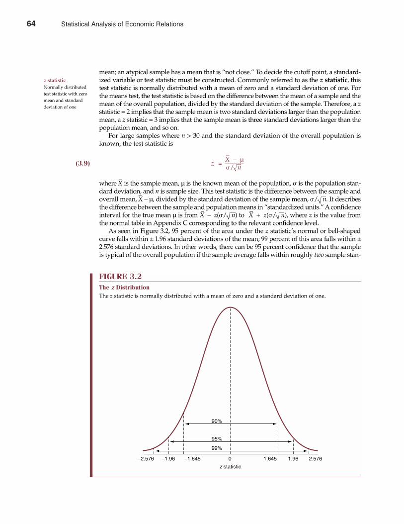
mean; an atypical sample has a mean that is “not close.” To decide the cutoff point, a standard-ized variable or test statistic must be constructed. Commonly referred to as the z statistic, thistest statistic is normally distributed with a mean of zero and a standard deviation of one. Forthe means test, the test statistic is based on the difference between the mean of a sample and themean of the overall population, divided by the standard deviation of the sample. Therefore, a zstatistic = 2 implies that the sample mean is two standard deviations larger than the populationmean, a z statistic = 3 implies that the sample mean is three standard deviations larger than thepopulation mean, and so on.
For large samples where n > 30 and the standard deviation of the overall population isknown, the test statistic is
(3.9) z =–X – µ�/√n
where –X is the sample mean, µ is the known mean of the population, � is the population stan-
dard deviation, and n is sample size. This test statistic is the difference between the sample andoverall mean, –X – µ, divided by the standard deviation of the sample mean, �/√n. It describesthe difference between the sample and population means in “standardized units.” Aconfidenceinterval for the true mean µ is from –
X – z(�/√n) to –X + z(�/√n), where z is the value fromthe normal table in Appendix C corresponding to the relevant confidence level.
As seen in Figure 3.2, 95 percent of the area under the z statistic’s normal or bell-shapedcurve falls within ± 1.96 standard deviations of the mean; 99 percent of this area falls within ±2.576 standard deviations. In other words, there can be 95 percent confidence that the sampleis typical of the overall population if the sample average falls within roughly two sample stan-
64 Part One Overview of Managerial Economics
z statisticNormally distributedtest statistic with zeromean and standarddeviation of one
FIGURE 3.2The z DistributionThe z statistic is normally distributed with a mean of zero and a standard deviation of one.
99%
95%
90%
Ð2.576 2.576Ð1.96 1.961.645Ð1.645 0
z statistic
64 Statistical Analysis of Economic Relations
dard deviations of the average for the overall population. There can be 99 percent confidencethat the sample is typical of the overall population if the sample average falls within roughlythree sample standard deviations of the population average.
To illustrate, consider the case of a retailer that receives a large shipment of lightbulbs froma new supplier and wishes to learn if these new bulbs are of standard quality. Lightbulbsreceived from the retailer’s current supplier have an average life of 2,000 hours, with a standarddeviation of 200 hours. The retailer’s null hypothesis is that the new bulbs are of equal quality,or H0: µ = 2,000 hours. The alternate hypothesis is that the new bulbs are not of equal quality, orHa: µ ± 2,000. Obviously, all new bulbs cannot be tested. To test the null hypothesis, the retailermight decide to test the life of a random sample of 100 bulbs. The retailer would be inclined toreject the new bulbs if this sample had a dramatically shorter mean life than bulbs from its cur-rent supplier. To minimize the Type I error of incorrectly deciding to reject new bulbs of equalquality, the significance level of the hypothesis test might be set at � = 0.05 or � = 0.01. The retail-er will purchase the new bulbs provided the chance of incorrectly rejecting equal quality bulbsis only 5 percent or 1 percent, respectively.
In the lightbulb example, the relevant test statistic z = (X – 2,000) � 20; because µ = 2,000hours, � = 200 hours, and n = 100 sample observations. So long as the computed value for thistest statistic is within roughly ± 2, the retailer could safely infer with 95 percent confidencethat the new bulbs are of the same quality as those obtained from current suppliers. Thechance of incorrectly rejecting equal quality bulbs is 5 percent when the test statistic falls inthe range between ± 2. Such a value for the test statistic requires a sample average bulb lifewithin the range from 1,960 hours to 2,040. The 99 percent confidence interval requires thetest statistic to fall within the range ± 3, and a sample average bulb life of 1,940 hours to 2,060hours. By accepting bulbs with a sample average life that falls within this broader range, thechance of wrongly rejecting equal quality bulbs (Type I error) can be cut to 1 percent.
If the population standard deviation � is unknown and the sample size is large, n > 30,the sample standard deviation s can be substituted for � in the test statistic calculation:
(3.10) z =–X – µs/√n
where –X is the sample mean, µ is the known mean of the population, s is the sample standard devi-
ation, and n is sample size. Again, a confidence interval for the true mean µ is from –X – z(s/√n)to –
X + z(s/√n), where z is from the normal table in Appendix C for the relevant confidencelevel. This test statistic formula, like that given in Equation 3.9, is based on the assumption thatthe sample is “small” relative to the size of the overall population. If sample size exceeds 5 per-cent of the overall population, then the denominator of each equation must be multiplied bywhat is known as the finite population correction factor, or √–(N – n)/(N – 1) where N is thesize of the overall population and n is sample size.
Means Tests for Small SamplesFor meaningful statistical analysis, sample size must be sufficiently large to accurately reflectimportant characteristics of the overall population. Although it is typically desirable to have30 or more sample observations, this is not always possible. Sometimes, managers must relyon very small samples of data, say n < 30. In such instances, the test statistic formula mustbe altered slightly.
If the population is normally distributed, the distribution around the small sample meanwill be approximately normal. In this situation, the test statistic formula is written
(3.11) t =–X – µs/√n
Chapter Three Statistical Analysis of Economic Relations 65
Statistical Analysis of Economic Relations 65
where –X is the sample mean, µ is the known mean of the population, s is the sample stan-
dard deviation, and n is sample size. A confidence interval for the true mean µ can be cal-culated as –
X – t(s/√n) to –X + t(s/√n) where t is from the t table in Appendix C for (n–1)
degrees of freedom and the relevant confidence level.This so-called t statistic is a test statistic that has an approximately normal distribution
with a mean of zero and a standard deviation of one. The t statistic (or t value) is normallydistributed for large samples, but is less so in the case of small samples. Like the z statistic, itdescribes the difference between the sample and population means in “standardized units,” orby the number of sample standard deviations. Because the t statistic is only approximately nor-mal, the rules of thumb of two standard deviations for the 95 percent confidence interval andthree standard deviations for the 99 percent confidence interval hold only for large sampleswhere n > 30. The “hurdle” or critical t value is adjusted upward when sample size is reduced.The amount of upward adjustment depends on the test statistic’s degrees of freedom, or thenumber of observations beyond the absolute minimum required to calculate the statistic.Because at least two observations are necessary before a mean can be calculated, degrees offreedom for a means test are calculated as df = n – 1. The precise critical t value to use in ameans test for very small sample sizes is obtained from a t table, such as that found inAppendix C. For example, when sample size is n = 10 observations, the critical t value for ameans test with df = 10 – 1 = 9 is 2.262 at the � = 0.05 significance level, and 3.25 at the � = 0.01significance level. The population mean is expected to be found within ± 2.262 standard devi-ations of the sample mean with 95 percent confidence, and within ± 3.25 standard deviationsof the sample mean with 99 percent confidence.
To this point, measures of central tendency and measures of dispersion have been consid-ered useful for describing populations and samples of data. These measures are very useful tomanagers who seek a detailed statistical profile of customer characteristics, cost experience,industry profits, and a host of other important economic variables. However, managers are
66 Part One Overview of Managerial Economics
Market Experiments on the Web
In pre-Internet days, companies spent huge amounts oftime and money simply trying to measure perceptionsabout how well customer needs have been met by thefirm’s products. Now, companies can instantaneouslyreview customer orders and see how well the company isactually satisfying customer needs. Early adopters ofInternet-based customer delivery systems have learned (orrelearned) a number of fundamental marketing concepts:
• Successful companies define value in terms ofproduct attributes desired by the customer. In old-fashioned terminology, customers are always right.
• Customer value depends upon both physical and sit-uational characteristics of products. What, how, andwhen are often equally important to the customer.
• Customer value perceptions are dynamic and canchange rapidly over time.
The Internet is spawning a revolution in the way thingsare made and services are delivered. Companies asdiverse as BMW, Dell Computer, Levi Strauss, Mattel,McGraw-Hill, and Wells Fargo are all embracing Internettechnology as a means for learning and delivering pre-
cisely what consumers want. In fact, these and a growinglist of companies are building customized productsdesigned by millions of customers. Dell led the way byallowing customers to order computers assembled toexact specifications. Now, manufacturers are allowingcustomers to order computer-fitted apparel, like Levi’s cutto fit your body. Men can stop worrying about why 37”pant waist sizes aren’t offered; women can stop trying tofigure out what the size “petite large” means. Just use theInternet to tell Eddie Bauer, Lands’ End, or Levi’s how tocut your own perfect fit. Using Internet technology, cus-tomers can also buy customized blends of vitamins,music compilations on CDs, and mortgage paymentterms. Professors can also assign “textbooks” whosechapters are compiled from diverse material written by avariety of authors. This Internet-spawned revolution isjust another step along the path of serving customerneeds quicker, better, and cheaper.
See: Martha Francois, “We Need an Education Experiment,” The WallStreet Journal Online, March 6, 2002 (http://online.wsj.com).
M A N A G E R I A L A P P L I C AT I O N 3 . 2
t statisticApproximately normaltest statistic
degrees of freedomNumber of observationsbeyond the minimumrequired to calculate astatistic
66 Statistical Analysis of Economic Relations
often interested in the central tendency and dispersion of these data and in the extent to whichthese patterns can be described. For this reason, successful real-world managers devote sig-nificant effort to describing the causes and consequences of important economic relations.
REGRESSION ANALYSIS
The most compelling challenge faced by management is the accurate estimation of demand,cost, and profit relations. Not only must the range of important factors that affect demand, costs,and profits be determined, but the relative magnitude of each influence must also be assessed.Regression analysis is a powerful and extremely useful statistical technique that describes theway in which one important economic variable is related to one or more other economic vari-ables. Although there are clear limitations to the technique, regression analysis is often used toprovide successful managers with valuable insight concerning a variety of significant economicrelations. Given the widespread success of regression analysis in real-world applications, it iswell worth gaining a careful understanding of the technique.
What Is a Statistical Relation?To understand when the use of regression analysis is appropriate, one must appreciate a basicdifference between two broad classes of economic relations.
A deterministic relation is one that is known with certainty. For example, total profitequals total revenue minus total cost, or π = TR – TC. Once the levels of total revenue and totalcost are known with certainty, total profits can be exactly determined. The profit relation is anexample of a deterministic relation. If total cost = $5 � quantity, then total cost can be exactlydetermined once the level of quantity is known, just as quantity can be determined once thetotal cost level is known. If all economic relations were deterministic, then managers wouldnever be surprised by higher or lower than expected profits; total revenues and total costscould be exactly determined at the start of every planning period. As it turns out, few eco-nomic relations are deterministic in nature. It is far more common that economic variables arerelated to each other in ways that cannot be predicted with absolute accuracy. Almost all eco-nomic relations must be estimated.
A statistical relation exists between two economic variables if the average of one is relatedto another, but it is impossible to predict with certainty the value of one based on the value ofanother. In the earlier example, if TC = $5Q on average, then a one-unit increase in quantitywould tend to result in an average $5 increase in total cost. Sometimes the actual increase in totalcost would be more than $5; sometimes it would be less. In such circumstances, a statistical rela-tion exists between total costs and output.
When a statistical relation exists, the exact or “true” relation between two economic vari-ables is not known with certainty and must be estimated. Perhaps the most common meansfor doing so is to gather and analyze historical data on the economic variables of interest. Atime series of data is a daily, weekly, monthly, or annual sequence of data on an economicvariable such as price, income, cost, or revenue. To judge the trend in profitability over time, afirm would analyze the time series of profit numbers. A cross section of data is a group ofobservations on an important economic variable at any point in time. If a firm were interest-ed in learning the relative importance of market share versus advertising as determinants ofprofitability, it might analyze a cross section of profit, advertising, and market share data fora variety of regional or local markets. To assess the effectiveness of a quality managementprogram, the firm might consider both time-series and cross-section data.
The simplest and most common means for analyzing a sample of historical data is to plotand visually study the data. A scatter diagram is a plot of data where the dependent variableis plotted on the vertical or Y-axis, and the independent variable is plotted on the horizontal orX-axis. Figure 3.3 shows scatter diagrams that plot the relation between four different unit cost
regression analysisStatistical method fordescribing XY relations
deterministic relationRelation known withcertainty
statistical relationInexact relation
time seriesDaily, weekly, monthlyor annual sequence ofdata
cross sectionData from a commonpoint in time
scatter diagramPlot of XY data
Chapter Three Statistical Analysis of Economic Relations 67
Statistical Analysis of Economic Relations 67
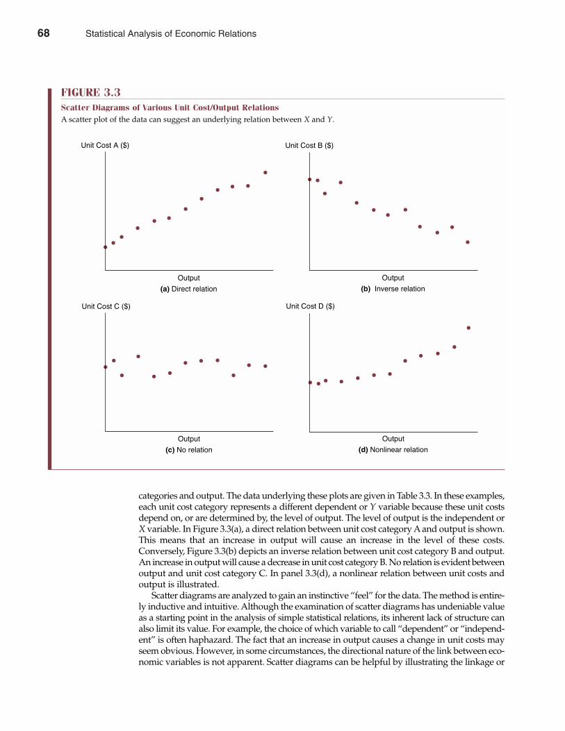
categories and output. The data underlying these plots are given in Table 3.3. In these examples,each unit cost category represents a different dependent or Y variable because these unit costsdepend on, or are determined by, the level of output. The level of output is the independent orX variable. In Figure 3.3(a), a direct relation between unit cost category A and output is shown.This means that an increase in output will cause an increase in the level of these costs.Conversely, Figure 3.3(b) depicts an inverse relation between unit cost category B and output.An increase in output will cause a decrease in unit cost category B. No relation is evident betweenoutput and unit cost category C. In panel 3.3(d), a nonlinear relation between unit costs andoutput is illustrated.
Scatter diagrams are analyzed to gain an instinctive “feel” for the data. The method is entire-ly inductive and intuitive. Although the examination of scatter diagrams has undeniable valueas a starting point in the analysis of simple statistical relations, its inherent lack of structure canalso limit its value. For example, the choice of which variable to call “dependent” or “independ-ent” is often haphazard. The fact that an increase in output causes a change in unit costs mayseem obvious. However, in some circumstances, the directional nature of the link between eco-nomic variables is not apparent. Scatter diagrams can be helpful by illustrating the linkage or
68 Part One Overview of Managerial Economics
FIGURE 3.3Scatter Diagrams of Various Unit Cost/Output RelationsA scatter plot of the data can suggest an underlying relation between X and Y.
Output
(a) Direct relation
Unit Cost A ($)
Output
(b) Inverse relation
Unit Cost C ($)
Output
(c) No relation
Unit Cost D ($)
Output
(d) Nonlinear relation
Unit Cost B ($)
68 Statistical Analysis of Economic Relations
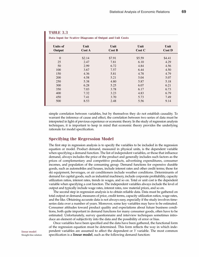
simple correlation between variables, but by themselves they do not establish causality. Towarrant the inference of cause and effect, the correlation between two series of data must beinterpreted in light of previous experience or economic theory. In the study of regression analysistechniques, it is important to keep in mind that economic theory provides the underlyingrationale for model specification.
Specifying the Regression ModelThe first step in regression analysis is to specify the variables to be included in the regressionequation or model. Product demand, measured in physical units, is the dependent variablewhen specifying a demand function. The list of independent variables, or those that influencedemand, always includes the price of the product and generally includes such factors as theprices of complementary and competitive products, advertising expenditures, consumerincomes, and population of the consuming group. Demand functions for expensive durablegoods, such as automobiles and houses, include interest rates and other credit terms; those forski equipment, beverages, or air conditioners include weather conditions. Determinants ofdemand for capital goods, such as industrial machinery, include corporate profitability, capacityutilization ratios, interest rates, trends in wages, and so on. Total or unit cost is the dependentvariable when specifying a cost function. The independent variables always include the level ofoutput and typically include wage rates, interest rates, raw material prices, and so on.
The second step in regression analysis is to obtain reliable data. Data must be gathered ontotal output or demand, measures of price, credit terms, capacity utilization ratios, wage rates,and the like. Obtaining accurate data is not always easy, especially if the study involves time-series data over a number of years. Moreover, some key variables may have to be estimated.Consumer attitudes toward product quality and expectations about future business condi-tions, both quite important in demand functions for many consumer goods, often have to beestimated. Unfortunately, survey questionnaire and interview techniques sometimes intro-duce an element of subjectivity into the data and the possibility of error or bias.
Once variables have been specified and the data have been gathered, the functional formof the regression equation must be determined. This form reflects the way in which inde-pendent variables are assumed to affect the dependent or Y variable. The most commonspecification is a linear model, such as the following demand function:
linear modelStraight-line relation
Chapter Three Statistical Analysis of Economic Relations 69
TABLE 3.3Data Input for Scatter Diagrams of Output and Unit Costs
Units of Unit Unit Unit UnitOutput Cost A Cost B Cost C Cost D
0 $2.14 $7.91 $5.59 $4.4125 2.47 7.81 6.10 4.2950 2.99 6.72 4.84 4.56
100 3.67 7.57 6.44 4.50150 4.36 5.81 4.78 4.79200 4.58 5.21 5.04 5.07250 5.38 4.80 5.87 5.18300 6.28 5.25 6.07 6.21350 7.03 3.78 6.17 6.73400 7.32 3.23 4.83 6.79450 7.41 3.70 5.73 7.49500 8.53 2.48 5.56 9.14
Statistical Analysis of Economic Relations 69
(3.12) Q = a + bP + cA + dI
Here Q represents the unit demand for a particular product, P is the price charged, A representsadvertising expenditures, and I is per capita disposable income. Unit demand is assumed tochange in a linear fashion with changes in each independent variable. For example, if b = –1.5,the quantity demanded will decline by one and one-half units with each one-unit increase inprice. This implies a linear, or straight line, demand curve. Each coefficient measures the changein Y following a one-unit change in each respective X variable. Note that the size of this influ-ence does not depend on the size of the X variable. In a linear regression model, the marginaleffect of each X variable on Y is constant. The broad appeal of linear functions stems from thefact that many demand and cost relations are in fact approximately linear. Furthermore, themost popular regression technique, the method of least squares, can be used to estimate thecoefficients a, b, c, and d for linear equations.
Another common regression model form is the multiplicative model:
(3.13) Q = aPbAcId
Amultiplicative model is used when the marginal effect of each independent variable is thoughtto depend on the value of all independent variables in the regression equation. For example, theeffect on quantity demanded of a price increase often depends not just on the price level, butalso on the amount of advertising, competitor prices and advertising, and so on. Similarly, theeffect on costs of a wage hike can depend on the output level, raw material prices, R&D expendi-tures, and so on. Allowing for such changes in the marginal relation is sometimes more realisticthan the implicit assumption of a constant marginal, as in the linear model.
Happily, the benefits of added realism for the multiplicative model have no offsetting costsin terms of added complexity or difficulty in estimation. Equation 3.13 can be transformed intoa linear relation using logarithms and then estimated by the least squares technique. Thus,Equation 3.13 is equivalent to
(3.14) logQ = loga + b � logP + c � logA + d � logI
When written in the form of Equation 3.12, the coefficients of Equation 3.14 (log a, b, c, and d)can be easily estimated. Given the multiplicative or log-linear form of the regression model,these coefficient estimates can also be interpreted as estimates of the constant elasticity of Ywith respect to X, or the percentage change in Y due to a one percent change in X. Much morewill be said about elasticity later in the book, but for now it is worth noting that multiplicativeor log-linear models imply constant elasticity.
To summarize, multiplicative models imply a changing absolute effect on the Y variable dueto changes in the various independent variables. This is sometimes attractive in demand analy-sis because the marginal effect of a dollar spent on advertising, for example, can vary accordingto overall levels of advertising, prices, income, and so on. Similarly, this is sometimes appealingin cost analysis because the effect on costs of a one-unit change in output can depend on thelevel of output, wages, raw material prices, and so on. The changing marginal effect implicit inthe multiplicative or log-linear model contrasts with the constant marginal effect of independ-ent variables in linear models. Multiplicative demand and cost functions are also based on theassumption of constant elasticities, whereas elasticity varies along linear demand functions. Ofcourse, the specific form of any regression model—linear, multiplicative, or otherwise—shouldalways be chosen to reflect the true relation among the economic variables being studied. Caremust be taken to ensure that the model chosen is consistent with underlying economic theory.
70 Part One Overview of Managerial Economics
multiplicative modelLog-linear relation
70 Statistical Analysis of Economic Relations
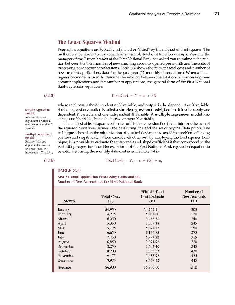
The Least Squares MethodRegression equations are typically estimated or “fitted” by the method of least squares. Themethod can be illustrated by considering a simple total cost function example. Assume themanager of the Tucson branch of the First National Bank has asked you to estimate the rela-tion between the total number of new checking accounts opened per month and the costs ofprocessing new account applications. Table 3.4 shows the relevant total cost and number ofnew account applications data for the past year (12 monthly observations). When a linearregression model is used to describe the relation between the total cost of processing newaccount applications and the number of applications, the general form of the First NationalBank regression equation is
(3.15) Total Cost = Y = a + bX
where total cost is the dependent or Y variable, and output is the dependent or X variable.Such a regression equation is called a simple regression model, because it involves only onedependent Y variable and one independent X variable. A multiple regression model alsoentails one Y variable, but includes two or more X variables.
The method of least squares estimates or fits the regression line that minimizes the sum ofthe squared deviations between the best fitting line and the set of original data points. Thetechnique is based on the minimization of squared deviations to avoid the problem of havingpositive and negative deviations cancel each other out. By employing the least squares tech-nique, it is possible to estimate the intercept a and slope coefficient b that correspond to thebest fitting regression line. The exact form of the First National Bank regression equation tobe estimated using the monthly data contained in Table 3.4 is
(3.16) Total Costt = Yt = a + bXt + ut
simple regressionmodelRelation with onedependent Y variableand one independent Xvariable
multiple regressionmodelRelation with onedependent Y variableand more than oneindependent X variable
Chapter Three Statistical Analysis of Economic Relations 71
TABLE 3.4New Account Application Processing Costs and the Number of New Accounts at the First National Bank
“Fitted” Total Number ofTotal Costs Cost Estimate New Accounts
Month (Yt) (Yt) (Xt)
January $4,950 $4,755.91 205February 4,275 5,061.00 220March 6,050 5,467.78 240April 5,350 5,569.48 245May 5,125 5,671.17 250June 6,650 6,179.65 275July 7,450 6,993.22 315August 6,850 7,094.92 320September 8,250 7,603.40 345October 8,700 9,332.23 430November 9,175 9,433.92 435December 9,975 9,637.32 445
Average $6,900 $6,900.00 310
Statistical Analysis of Economic Relations 71
where total cost in month t is the dependent or Y variable, and the number of new account appli-cations in month t is the independent output or X variable. ut is a residual or disturbance termthat reflects the influences of stochastic or random elements and of any other determinants oftotal costs that have been omitted from the regression equation. When time-series data are being
72 Part One Overview of Managerial Economics
FIGURE 3.4Regression Relation Between New Account Application Costs and the Number of New Accounts at the First National BankThe regression line minimizes the sum of squared deviations.
400350300
Number of new account applications
250200150
X
$10,000
9,000
8,000
7,000
6,000
5,000
4,000
Total cost
uDec.
XJuly
Sept.
XDec.
XOct.
450
Model: Y = $586.4 + $20.339X
Predictor
Constant�Number of�Applications
Coefficient t ratio
0.99�
10.99
StandardDeviation
594.5
�1.850
p0.347�0.000
586.4�
20.339
SEE = $531.9
R 2 = 92.4%
R 2 = 91.6%
F = 120.86
XJune
XMar.
XNov.
XAug.
uSept.
uMar.
XJan. X
May
XApr.
XFeb.
uFeb.
Mean sales = Ŷ
72 Statistical Analysis of Economic Relations

examined, as they are in this example, the term t is used to signify subscript. If cross-section datawere being examined—for example, processing costs at a number of branch offices during anygiven month—the various branch offices would be designated using the subscript i.
The a intercept marks the intersection of the regression line with the sales axis. The b slopecoefficient is the slope of the regression line, and the ut error term measures the vertical devia-tion of each tth data point from the fitted regression line. The least squares technique minimizesthe total sum of squared ut values by the choice of the a and b coefficients. When the a and bcoefficients are combined with actual data on the independent X variable (the number of appli-cations) as shown in Equation 3.15, the estimated or fitted total cost values shown in Table 3.4can be calculated. These fitted values are connected by the fitted regression line drawn in Figure3.4. Fitted values for the dependent Y variable, called Ŷ or “Y hat,” are extremely valuablebecause they indicate the expected total cost level associated with a given number of newaccount applications, or X variable. However, regression analysis also provides managementwith a number of additional insights concerning the total cost/output relation. In the next sec-tion, important insights offered by commonly reported regression statistics are investigated.
REGRESSION STATISTICS
Just a few years ago, the process of estimating economic relations was painstaking and costly.Only the largest and most advanced organizations could afford the necessary investment insophisticated computers and highly trained staff. Today, powerful desktop personal comput-ers (PCs) with sophisticated but user-friendly statistical software make the estimation of evencomplex economic relations both quick and easy. As a result, the accurate estimation of statis-tical relations has become a standard tool of the successful manager in organizations of allsizes. The two leading software programs used for this purpose are MINITAB statistical software,
Chapter Three Statistical Analysis of Economic Relations 73
Lies, Damn Lies, and Government Statistics
Once a reliable source of timely and accurate statisticson the U.S. economy, the federal government’s systemfor gathering and interpreting economic data has fallenon hard times. To illustrate, consider the tough question:How much have prices risen or fallen lately?
Think about how much more you are paying formonthly long-distance telephone service and you’ll seewhat economists mean when they complain aboutadjusting for quality improvements. Chances are thatyour monthly long-distance bill is higher today than itwas 5 years ago, but your higher bill is accounted forby more frequent and/or longer phone conversations,Internet service, and so on. The cost per minute forlong-distance phone service has fallen precipitously fordecades. How about the cost for a personal computer?Although the price of a PC has fallen from roughly$3,000 to less than $1,000 during the last decade, desk-top computers are more powerful and easier to usethan a room full of computers in the 1970s. Even whenproducts change little, consumers adapt buying habitsto moderate the effects of price increases. How do you
account for the fact that shoppers shift to apples whenoranges jump from 79¢ to 89¢ per pound?
The problem is that admittedly imperfect govern-ment statistics involve errors and bias. Governmentstatisticians are slow to recognize the effects of newtechnology and better products. The producer price index,which contains thousands of values for products suchas bolts and valves, still has no accurate measure forsemiconductors or for communications equipment,arguably the biggest category of producer durables.
What should be done? To better measure consumerprices, electronic scanning data must be utilized. Price andproduction indexes must also reflect quality adjustmentsfor new products and technologies, and surveys of changesin employment must be refined. In some instances, govern-ment spending on data gathering and analysis needs to beincreased. Americans and their government simply need toknow what’s really happening in the economy.
See: Gene Epstein, “Blame the Median When Inflation Resurges,” TheWall Street Journal Online, February 25, 2002 (http://online.wsj.com).
M A N A G E R I A L A P P L I C AT I O N 3 . 3
Statistical Analysis of Economic Relations 73
published by MINITAB, Inc., and SPSS Advanced Statistics, published by SPSS, Inc. Both are inex-pensive, easy to learn, and offer a wealth of powerful techniques for data analysis and regres-sion model estimation. Less comprehensive statistical software that run along with MicrosoftExcel and other spreadsheet programs can also be useful, especially when detailed statisticalanalysis is unnecessary. This section focuses on the interpretation of regression output.
Standard Error of the EstimateA useful measure for examining the accuracy of any regression model is the standard error ofthe estimate, SEE, or the standard deviation of the dependent Y variable after controlling forthe influence of all X variables. The standard error of the estimate increases with the amountof scatter about the sample regression line. If each data point were to lie exactly on the regres-sion line, then the standard error of the estimate would equal zero since each Ŷt would exactlyequal Yt . No scatter about the regression line exists when the standard error of the estimateequals zero. If there is a great deal of scatter about the regression line, then Ŷt often differs greatlyfrom each Yt, and the standard error of the estimate will be large.
The standard error of the estimate provides a very useful means for estimating confidenceintervals around any particular Ŷt estimate, given values for the independent X variables. Inother words, the standard error of the estimate can be used to determine a range within whichthe dependent Y variable can be predicted with varying degrees of statistical confidence basedon the regression coefficients and values for the X variables. Because the best estimate of thetth value for the dependent variable is Ŷt, as predicted by the regression equation, the stan-dard error of the estimate can be used to determine just how accurate a predictionŶt is likelyto be. If the ut error terms are normally distributed about the regression equation, as would betrue when large samples of more than 30 or so observations are analyzed, there is a 95 percentprobability that observations of the dependent variable will lie within the range Ŷt ± (1.96 �SEE), or within roughly two standard errors of the estimate. The probability is 99 percent thatany given Ŷt will lie within the range Ŷt ± (2.576 � SEE), or within roughly three standarderrors of its predicted value. When very small samples of data are analyzed, “critical” valuesslightly larger than two or three are multiplied by the SEE to obtain the 95 percent and 99 per-cent confidence intervals. Precise values can be obtained from a t table such as that found inAppendix C, as described in the following discussion of t statistics. For both small and largesamples of data, greater predictive accuracy for the regression model is obviously associatedwith smaller standard errors of the estimate.
The standard error of the estimate concept is portrayed graphically in Figure 3.5. The leastsquares regression line is illustrated as a bold straight line; the upper and lower 95 percent con-fidence interval limits are shown as broken curved lines. On average, 95 percent of all actualdata observations will lie within roughly two standard errors of the estimate. Given a value Xt,the interval between the upper and lower confidence bounds can be used to predict the corre-sponding Yt value with a 95 percent probability that the actual outcome will lie within thatconfidence interval. Notice that this confidence interval widens for sample observations thatare much higher or much lower than the sample mean. This is because the standard error of theestimate calculation is based on observations drawn from the sample rather than the overallpopulation and provides only an approximation to the true distribution of errors. Confidencebounds are closest to the regression line in the vicinity of mean values for Xt and Yt, or at thecenter of the scatter diagram. Confidence bounds diverge from the regression line toward theextreme values of the sample observations. An obvious implication worth remembering is thatrelatively little confidence can be placed in the predictive value of a regression equation extended beyondthe range of sample observations.
In the First National Bank cost estimation example, the standard error of the estimate is531.9. This means that the standard deviation of actual Yt values about the regression line is
74 Part One Overview of Managerial Economics
standard error ofthe estimateStandard deviation ofthe dependent Yvariable after control-ling for all X variables
74 Statistical Analysis of Economic Relations
$531.90, because the standard error of the estimate is always in the same units as the depend-ent Y variable. There is a 95 percent probability that any given observation Yt will lie with-in roughly two standard errors of the relevant Ŷt estimate.2 For example, the number of newaccount applications during the month of July is 315 per month, and the expected or fittedtotal cost level is $6,993.19 (= $586.4 + $20.339(315)). The corresponding confidence boundsfor the 95 percent confidence interval are $6,993.19 ± (2 � $531.9). This means that there isroughly a 95 percent chance that actual total costs per month for the 315 unit activity levelwill fall in a range from $5,929.39 to $8,056.99. Similarly, there is a 99 percent probability thatactual total costs will fall within roughly three standard errors of the predicted value, or inthe range from $5,397.49 to $8,588.89. The wider the confidence interval, the higher is theconfidence level that actual values will be found within the predicted range. Greater pre-dictive accuracy is obviously also associated with smaller standard errors of the estimate.
Chapter Three Statistical Analysis of Economic Relations 75
FIGURE 3.5Illustration of the Use of the Standard Error of the Estimate to Define Confidence IntervalsThe standard error of the estimate (SEE) is used to construct a confidence interval.
Y
a
Y
^X
Upper 95% confidence bound:+1.96 standard errors of the estimate
Lower 95% confidence bound:+1.96 standard errors of the estimate
Y = a + bX
b = Slope of curve
^
X
2 The precise “critical” number used in the multiplication of SEE is found in a t table such as that in Appendix C.This value is adjusted downward when sample size n is small relative to the number of coefficients k estimatedin the regression model. To find the precise critical value, calculate the number of degrees of freedom, defined asdf = n – k, and read the appropriate t value from the table. In this example, df = n – k = 12 – 2 = 10 and there is a95 percent probability that any given observation Yt will lie within precisely 2.228 standard errors of the relevantŶt estimate. There is a 99 percent probability that actual total costs will fall within precisely 3.169 standard errorsof the predicted value. Therefore, even for the very small sample size analyzed in this example, the rough rulesof thumb of two standard deviations for the 95 percent confidence bounds and three standard deviations for the99 percent confidence bounds work quite well.
Statistical Analysis of Economic Relations 75
Goodness of Fit, r and R2
In a simple regression model with only one independent variable the correlation coefficient, r,measures goodness of fit. The correlation coefficient falls in the range between 1 and –1. If r = 1,there is a perfect direct linear relation between the dependent Y variable and the independent Xvariable. If r = –1, there is a perfect inverse linear relation between Y and X. In both instances,actual values for Yt all fall exactly on the regression line. The regression equation explains all ofthe underlying variation in the dependent Y variable in terms of variation in the independentX variable. If r = 0, zero correlation exists between the dependent and independent variables;they are autonomous. When r = 0, there is no relation at all between actual Yt observations andfitted Ŷt values.
In multiple regression models where more than one independent X variable is considered,the squared value of the coefficient of multiple correlation is used in a similar manner. Thesquare of the coefficient of multiple correlation, called the coefficient of determination orR2, shows how well a multiple regression model explains changes in the value of the depend-ent Y variable. R2 is defined as the proportion of the total variation in the dependent variablethat is explained by the full set of independent variables. In equation form, R2 is written
(3.17) R2 = Variation Explained by RegressionTotal Variation of Y
Accordingly, R2 can take on values ranging from 0, indicating that the model provides no expla-nation of the variation in the dependent variable, to 1.0, indicating that all the variation has beenexplained by the independent variables. The coefficient of determination for the regressionmodel illustrated in Figure 3.4 is 92.4, indicating that 92.4 percent of the total variation in FirstNational Bank new account application costs can be explained by the underlying variation inthe number of new account applications. If R2 is relatively high, deviations about the regressionline will be relatively small, as shown in Figure 3.6. In such instances, actual Yt values will beclose to the regression line, and values for ut will be small. As the size of the deviations aboutthe regression line increases, the coefficient of determination falls. At the extreme, the sum ofthe squared error terms equals the total variation in the dependent variable, and R2 = 0. In thiscase, the regression model is unable to explain any variation in the dependent Y variable.
A relatively low value for R2 indicates that a given model is inadequate in terms of its over-all explanatory power. The most general cause for this problem is the omission of importantexplanatory variables. In practice, the coefficient of determination will seldom equal either 0 or100 percent. In the First National Bank example, R2 = 92.4 percent, and a relatively high level ofexplanatory power is realized by the regression model. Fully 92.4 percent of cost variation isexplained by the variation in new account applications—a level of explanation that is often veryuseful for planning purposes. In empirical demand estimation, values for R2 of 80 percent, indi-cating that 80 percent of demand variation has been explained, are often quite acceptable. Forgoods with highly stable and predictable demand patterns, demand function R2s as high as 90percent to 95 percent are sometimes achieved. Very high levels of R2 can also be attained in costfunction analysis of output produced under controlled conditions. Generally speaking, demandand cost analysis for a given firm or industry over time (time-series analysis) will lead to higherlevels for R2 than would a similar analysis across firms or industries at a given point in time(cross-sectional analysis). This is because most economic phenomena are closely related to theoverall pace of economic activity and thus have an important time or trend element. Suchexogenous forces are held constant in cross-section analyses and cannot contribute to the overallexplanatory power of the regression model. In judging whether or not a given R2 is sufficientlyhigh to be satisfactory, the type of analysis conducted and the anticipated use of statistical resultsmust be considered.
76 Part One Overview of Managerial Economics
correlation coefficientGoodness of fit measurefor a simple regressionmodel
coefficient of determinationGoodness of fit measurefor a multiple regressionmodel
76 Statistical Analysis of Economic Relations
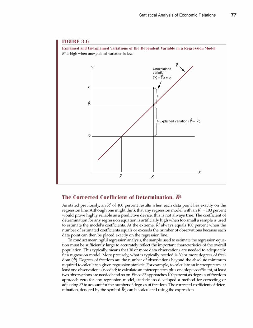
The Corrected Coefficient of Determination, R2
As stated previously, an R2 of 100 percent results when each data point lies exactly on theregression line. Although one might think that any regression model with an R2 = 100 percentwould prove highly reliable as a predictive device, this is not always true. The coefficient ofdetermination for any regression equation is artificially high when too small a sample is usedto estimate the model’s coefficients. At the extreme, R2 always equals 100 percent when thenumber of estimated coefficients equals or exceeds the number of observations because eachdata point can then be placed exactly on the regression line.
To conduct meaningful regression analysis, the sample used to estimate the regression equa-tion must be sufficiently large to accurately reflect the important characteristics of the overallpopulation. This typically means that 30 or more data observations are needed to adequatelyfit a regression model. More precisely, what is typically needed is 30 or more degrees of free-dom (df). Degrees of freedom are the number of observations beyond the absolute minimumrequired to calculate a given regression statistic. For example, to calculate an intercept term, atleast one observation is needed; to calculate an intercept term plus one slope coefficient, at leasttwo observations are needed; and so on. Since R2 approaches 100 percent as degrees of freedomapproach zero for any regression model, statisticians developed a method for correcting oradjusting R2 to account for the number of degrees of freedom. The corrected coefficient of deter-mination, denoted by the symbol –R2, can be calculated using the expression
Chapter Three Statistical Analysis of Economic Relations 77
FIGURE 3.6Explained and Unexplained Variations of the Dependent Variable in a Regression ModelR2 is high when unexplained variation is low.
Y
Yt
Yt
Y
X Xt
X
^
Yt^
Unexplainedvariation
(Yt Ð Yt) = ut^
Explained variation (Yt Ð Y )^ Ð
Ð
Ð
Statistical Analysis of Economic Relations 77
(3.18)–R2 = R2 – �k – 1 (1 – R2)
n – k
where n is the number of sample observations (data points) and k is the number of estimatedcoefficients (intercept plus the number of slope coefficients). Note that the –
R2 calculation alwaysinvolves a downward adjustment to R2. The downward adjustment to R2 is large when n, thesample size, is small relative to k, the number of coefficients being estimated. This downwardadjustment to R2 is small when n is large relative to k. In the First National Bank example, –
R2 =91.6 percent—a relatively modest downward adjustment to the R2 = 92.4 percent—and suggeststhat the high level of explanatory power achieved by the regression model cannot be attributedto an overly small sample size.
Like R2, statistical software programs typically perform the –R2 adjustment, so there is often
no need to actually make such calculations in practice. Still, knowing what is involved makesthe reasons for the practice obvious. Clearly, confidence in the reliability of a given regressionmodel will be higher when both R2 and the number of degrees of freedom are substantial.
The F StatisticBoth the coefficient of determination, R2, and corrected coefficient of determination, –
R2, provideevidence on whether or not the proportion of explained variation is relatively “high” or “low.”However, neither tells if the independent variables as a group explain a statistically significantshare of variation in the dependent Y variable. The F statistic provides evidence on whether ornot a statistically significant proportion of total variation in the dependent variable has beenexplained. Like –
R2 , the F statistic is adjusted for degrees of freedom and is defined as
(3.19) Fk–1,n–k = Explained Variation/(k – 1)Unexplained Variation/(n – k)
Once again, n is the number of observations (data points) and k is the number of estimatedcoefficients (intercept plus the number of slope coefficients). Also like –
R2, the F statistic can becalculated in terms of the coefficient of determination, where
(3.20) Fk–1,n–k = R2/(k – 1)(1 – R2)/(n – k)
The F statistic is used to indicate whether or not a significant share of the variation in the depend-ent variable is explained by the regression model. The hypothesis actually tested is that thedependent Y variable is unrelated to all of the independent X variables included in the model. Ifthis hypothesis cannot be rejected, the total explained variation in the regression will be quitesmall. At the extreme, if R2 = 0, then F = 0, and the regression equation provides absolutely noexplanation of the variation in the dependent Y variable. As the F statistic increases from zero,the hypothesis that the dependent Y variable is not statistically related to one or more of theregression’s independent X variables becomes easier to reject. At some point, the F statisticbecomes sufficiently large to reject the independence hypothesis and warrants the conclusionthat at least some of the model’s X variables are significant factors in explaining variation in thedependent Y variable.
The F test is used to determine whether a given F statistic is statistically significant.Performing F tests involves comparing F statistics with critical values from a table of the F dis-tribution. If a given F statistic exceeds the critical value from the F distribution table, the hypoth-esis of no relation between the dependent Y variable and the set of independent X variables canbe rejected. Taken as a whole, the regression equation can then be seen as explaining significantvariation in the dependent Y variable. Critical values for the F distribution are provided at the10 percent, 5 percent, and 1 percent significance levels in Appendix C. If the F statistic for a given
78 Part One Overview of Managerial Economics
F statisticOffers evidence ifexplained variation inY is significant
78 Statistical Analysis of Economic Relations
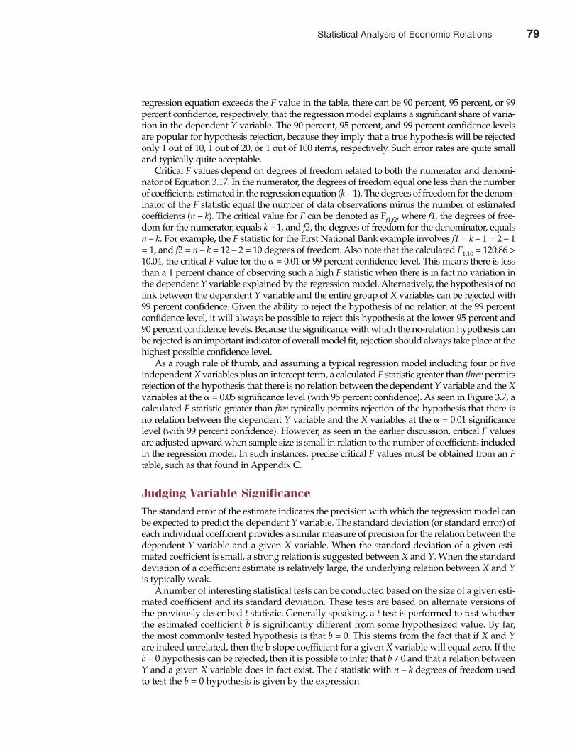
regression equation exceeds the F value in the table, there can be 90 percent, 95 percent, or 99percent confidence, respectively, that the regression model explains a significant share of varia-tion in the dependent Y variable. The 90 percent, 95 percent, and 99 percent confidence levelsare popular for hypothesis rejection, because they imply that a true hypothesis will be rejectedonly 1 out of 10, 1 out of 20, or 1 out of 100 items, respectively. Such error rates are quite smalland typically quite acceptable.
Critical F values depend on degrees of freedom related to both the numerator and denomi-nator of Equation 3.17. In the numerator, the degrees of freedom equal one less than the numberof coefficients estimated in the regression equation (k – 1). The degrees of freedom for the denom-inator of the F statistic equal the number of data observations minus the number of estimatedcoefficients (n – k). The critical value for F can be denoted as Ff1,f2, where f1, the degrees of free-dom for the numerator, equals k – 1, and f2, the degrees of freedom for the denominator, equalsn – k. For example, the F statistic for the First National Bank example involves f1 = k – 1 = 2 – 1= 1, and f2 = n – k = 12 – 2 = 10 degrees of freedom. Also note that the calculated F1,10 = 120.86 >10.04, the critical F value for the � = 0.01 or 99 percent confidence level. This means there is lessthan a 1 percent chance of observing such a high F statistic when there is in fact no variation inthe dependent Y variable explained by the regression model. Alternatively, the hypothesis of nolink between the dependent Y variable and the entire group of X variables can be rejected with99 percent confidence. Given the ability to reject the hypothesis of no relation at the 99 percentconfidence level, it will always be possible to reject this hypothesis at the lower 95 percent and90 percent confidence levels. Because the significance with which the no-relation hypothesis canbe rejected is an important indicator of overall model fit, rejection should always take place at thehighest possible confidence level.
As a rough rule of thumb, and assuming a typical regression model including four or fiveindependent X variables plus an intercept term, a calculated F statistic greater than three permitsrejection of the hypothesis that there is no relation between the dependent Y variable and the Xvariables at the � = 0.05 significance level (with 95 percent confidence). As seen in Figure 3.7, acalculated F statistic greater than five typically permits rejection of the hypothesis that there isno relation between the dependent Y variable and the X variables at the � = 0.01 significancelevel (with 99 percent confidence). However, as seen in the earlier discussion, critical F valuesare adjusted upward when sample size is small in relation to the number of coefficients includedin the regression model. In such instances, precise critical F values must be obtained from an Ftable, such as that found in Appendix C.
Judging Variable SignificanceThe standard error of the estimate indicates the precision with which the regression model canbe expected to predict the dependent Y variable. The standard deviation (or standard error) ofeach individual coefficient provides a similar measure of precision for the relation between thedependent Y variable and a given X variable. When the standard deviation of a given esti-mated coefficient is small, a strong relation is suggested between X and Y. When the standarddeviation of a coefficient estimate is relatively large, the underlying relation between X and Yis typically weak.
A number of interesting statistical tests can be conducted based on the size of a given esti-mated coefficient and its standard deviation. These tests are based on alternate versions ofthe previously described t statistic. Generally speaking, a t test is performed to test whetherthe estimated coefficient b̂ is significantly different from some hypothesized value. By far,the most commonly tested hypothesis is that b = 0. This stems from the fact that if X and Yare indeed unrelated, then the b slope coefficient for a given X variable will equal zero. If theb = 0 hypothesis can be rejected, then it is possible to infer that b ≠ 0 and that a relation betweenY and a given X variable does in fact exist. The t statistic with n – k degrees of freedom usedto test the b = 0 hypothesis is given by the expression
Chapter Three Statistical Analysis of Economic Relations 79
Statistical Analysis of Economic Relations 79
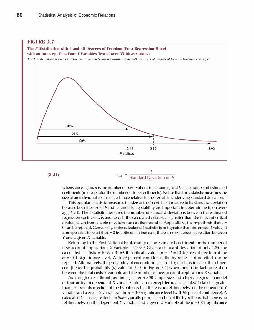
(3.21) tn–k = b̂Standard Deviation of b̂
where, once again, n is the number of observations (data points) and k is the number of estimatedcoefficients (intercept plus the number of slope coefficients). Notice that this t statistic measures thesize of an individual coefficient estimate relative to the size of its underlying standard deviation.
This popular t statistic measures the size of the b coefficient relative to its standard deviationbecause both the size of b and its underlying stability are important in determining if, on aver-age, b ≠ 0. The t statistic measures the number of standard deviations between the estimatedregression coefficient, b̂, and zero. If the calculated t statistic is greater than the relevant criticalt value, taken from a table of values such as that found in Appendix C, the hypothesis that b =0 can be rejected. Conversely, if the calculated t statistic is not greater than the critical t value, itis not possible to reject the b = 0 hypothesis. In that case, there is no evidence of a relation betweenY and a given X variable.
Returning to the First National Bank example, the estimated coefficient for the number ofnew account applications X variable is 20.339. Given a standard deviation of only 1.85, thecalculated t statistic = 10.99 > 3.169, the critical t value for n – k = 10 degrees of freedom at the� = 0.01 significance level. With 99 percent confidence, the hypothesis of no effect can berejected. Alternatively, the probability of encountering such a large t statistic is less than 1 per-cent [hence the probability (p) value of 0.000 in Figure 3.4] when there is in fact no relationbetween the total costs Y variable and the number of new account applications X variable.
As a rough rule of thumb, assuming a large n > 30 sample size and a typical regression modelof four or five independent X variables plus an intercept term, a calculated t statistic greaterthan two permits rejection of the hypothesis that there is no relation between the dependent Yvariable and a given X variable at the � = 0.05 significance level (with 95 percent confidence). Acalculated t statistic greater than three typically permits rejection of the hypothesis that there is norelation between the dependent Y variable and a given X variable at the � = 0.01 significance
80 Part One Overview of Managerial Economics
FIGURE 3.7The F Distribution with 4 and 30 Degrees of Freedom (for a Regression Model with an Intercept Plus Four X Variables Tested over 35 Observations)The F distribution is skewed to the right but tends toward normality as both numbers of degrees of freedom become very large.
F statistic
90%
95%
99%
2.14 2.69 4.02
80 Statistical Analysis of Economic Relations

level (with 99 percent confidence). However, as described earlier, critical t values are adjustedupward when sample size is small in relation to the number of coefficients included in the regres-sion model. In such instances, precise critical t values can be obtained from a t table, such as thatfound in Appendix C.
DEMAND ESTIMATION EXAMPLE
An example of demand estimation can be used to illustrate how regression models areestimated—or fitted—by the method of least squares. Assume that monthly data have beenassembled by Electronic Data Processing (EDP), Inc., a small but rapidly growing firm thatprovides electronic data processing services to companies, hospitals, and other organiza-tions. EDP’s main business is to maintain and monitor payroll records on a contractual basisand issue payroll checks, W-2 forms, and so on, to the employees of client customers. The com-pany has aggressively expanded its personal selling efforts and experienced a rapid expansionin annual revenues during the past year. In a tough economic environment, year-end salesrevenue grew to an annual rate of $79.2 million per year. Table 3.5 shows EDP data on contractsales (Q), personal selling expenses (PSE), advertising expenditures (AD), and average con-tract price (P) over the past year (12 observations). Because of a stagnant national economy,industry-wide growth was halted during the year, and the usually positive effect of incomegrowth on demand was missing. Thus, the trend in national income was not relevant duringthis period. For simplicity, assume that the data contained in Table 3.5 include all relevantfactors influencing EDP’s monthly sales.
If a linear relation between unit sales, contract price, personal selling expenditures, andadvertising is hypothesized, the EDP regression equation takes the following form:
Chapter Three Statistical Analysis of Economic Relations 81
Spreadsheet and Statistical Software for the PC
The personal computer revolution in business really gotunderway in the 1980s following the publication ofpowerful and easy-to-use spreadsheet software.Microsoft’s Excel has blown away the original standard,Lotus 1-2-3, to make income statement and balance sheetanalysis quick and easy. Recent versions incorporate abroad range of tools for analysis, including net presentvalue, internal rate of return, linear programming, andregression. Such software also allows managers to ana-lyze and display operating data using a wide variety ofcharting and graphing techniques. For basic statisticalanalysis, Excel features easy-to-use statistical capabilitieslike regression and correlation analysis.
For more detailed analysis, thousands of successfulcompanies worldwide, including GE, 3M, and FordMotor Company, use MINITAB statistical software. Thelatest version, MINITAB Release 13, is a complete statpackage that makes statistical analysis easy and fast. Forexample, the Stat Guide is extremely helpful for interpret-ing statistical graphs and analyses. MINITAB Studentsoftware is a streamlined and economical version ofProfessional MINITAB, designed specially for introductory
general and business statistics courses. The latest releaseof MINITAB Student features an intuitive and easy-to-useinterface, clear manuals, and online help. MINITAB is apowerful programming language with sufficient docu-mentation to help even novice users analyze data andinterpret results.
For advanced statistical processing software, SPSS®
11.0 for Windows® embodies powerful statistical tools forin-depth analysis and modeling of business and economicdata. SPSS® 11.0 for Windows® helps managers access dataeasily, quickly prepare data for analysis, analyze datathoroughly, and present results clearly. SPSS® 11.0 forWindows®is packed with online tutorials and plenty ofexamples to guide users, while interactive charts and tableshelp users understand and present their results effectively.
More than simply changing historical methods ofdata manipulation and analysis, this user-friendly soft-ware for the PC is fundamentally changing the waymanagers visualize and run their businesses.
See: For MINITAB software, see http://www.minitab.com; for SPSSproducts, see http://www.spss.com.
M A N A G E R I A L A P P L I C AT I O N 3 . 4
Statistical Analysis of Economic Relations 81
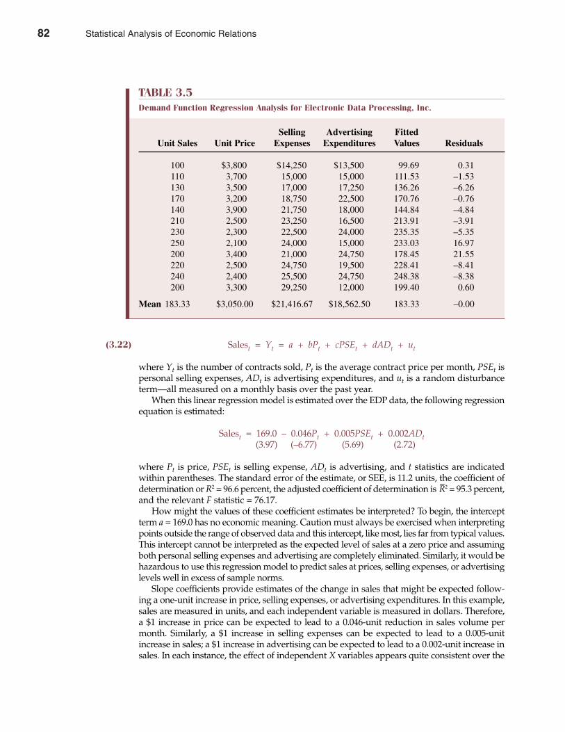
(3.22) Salest = Yt = a + bPt + cPSEt + dADt + ut
where Yt is the number of contracts sold, Pt is the average contract price per month, PSEt ispersonal selling expenses, ADt is advertising expenditures, and ut is a random disturbanceterm—all measured on a monthly basis over the past year.
When this linear regression model is estimated over the EDP data, the following regressionequation is estimated:
Salest = 169.0 – 0.046Pt + 0.005PSEt + 0.002ADt(3.97) (–6.77) (5.69) (2.72)
where Pt is price, PSEt is selling expense, ADt is advertising, and t statistics are indicatedwithin parentheses. The standard error of the estimate, or SEE, is 11.2 units, the coefficient ofdetermination or R2 = 96.6 percent, the adjusted coefficient of determination is –
R2 = 95.3 percent,and the relevant F statistic = 76.17.
How might the values of these coefficient estimates be interpreted? To begin, the interceptterm a = 169.0 has no economic meaning. Caution must always be exercised when interpretingpoints outside the range of observed data and this intercept, like most, lies far from typical values.This intercept cannot be interpreted as the expected level of sales at a zero price and assumingboth personal selling expenses and advertising are completely eliminated. Similarly, it would behazardous to use this regression model to predict sales at prices, selling expenses, or advertisinglevels well in excess of sample norms.
Slope coefficients provide estimates of the change in sales that might be expected follow-ing a one-unit increase in price, selling expenses, or advertising expenditures. In this example,sales are measured in units, and each independent variable is measured in dollars. Therefore,a $1 increase in price can be expected to lead to a 0.046-unit reduction in sales volume permonth. Similarly, a $1 increase in selling expenses can be expected to lead to a 0.005-unitincrease in sales; a $1 increase in advertising can be expected to lead to a 0.002-unit increase insales. In each instance, the effect of independent X variables appears quite consistent over the
82 Part One Overview of Managerial Economics
TABLE 3.5Demand Function Regression Analysis for Electronic Data Processing, Inc.
Selling Advertising FittedUnit Sales Unit Price Expenses Expenditures Values Residuals
100 $3,800 $14,250 $13,500 99.69 0.31110 3,700 15,000 15,000 111.53 –1.53130 3,500 17,000 17,250 136.26 –6.26170 3,200 18,750 22,500 170.76 –0.76140 3,900 21,750 18,000 144.84 –4.84210 2,500 23,250 16,500 213.91 –3.91230 2,300 22,500 24,000 235.35 –5.35250 2,100 24,000 15,000 233.03 16.97200 3,400 21,000 24,750 178.45 21.55220 2,500 24,750 19,500 228.41 –8.41240 2,400 25,500 24,750 248.38 –8.38200 3,300 29,250 12,000 199.40 0.60
Mean 183.33 $3,050.00 $21,416.67 $18,562.50 183.33 –0.00
82 Statistical Analysis of Economic Relations
entire sample. The t statistics for both price and selling expenses exceed a value of three.3 Thechance of observing such high t statistics when in fact no relation exists between sales andthese X variables is less than 1 percent. Though less strong, the link between sales and adver-tising expenditures is also noteworthy. The t statistic for advertising exceeds the value of two,meaning that there can be 95 percent confidence that advertising has an effect on sales. Thechance of observing such a high t statistic for advertising expenditures when in fact advertisinghas no effect on sales is less than 5 percent. Again, caution must be used when interpreting theseindividual regression coefficients. It is important not to extend the analysis beyond the range ofdata used to estimate the regression coefficients.
The standard error of the estimate or SEE of 11.2 units can be used to construct a confidenceinterval within which actual values are likely to be found based on the size of individual regres-sion coefficients and various values for the X variables. For example, given this regression modeland values of Pt = $3,200, PSEt = $18,750, and ADt = $22,500 for the independent X variables, thefitted value Ŷt = 170.76 can be calculated (see Table 3.5). Given these values for the independentX variables, 95 percent of the time actual observations will lie within roughly two standard errorsof the estimate; 99 percent of the time actual observations will lie within roughly three standarderrors of the estimate. Thus, the bounds for the 95 percent confidence interval are given by theexpression 170.76 ± (2 � 11.2), or from 148.36 to 193.16 units. Bounds for the 99 percent confi-dence interval are given by the expression 170.76 ± (3 � 11.2), or from 137.16 to 204.36. units.
Finally, the coefficient of determination R2 = 96.6 percent and indicates the share of variationin EDP demand explained by the regression model. Only 3.4 percent is left unexplained.Moreover, the adjusted coefficient of determination is –
R2 = 95.3% percent and reflects only amodest downward adjustment to R2 based on the size of the sample analyzed relative to thenumber of estimated coefficients. This suggests that the regression model explains a significantshare of demand variation—a suggestion that is supported by the F statistic. F3,8 = 76.17 and isfar greater than five, meaning that the hypothesis of no relation between sales and this groupof independent X variables can be rejected with 99 percent confidence. There is less than a 1 per-cent chance of encountering such a large F statistic when in fact there is no relation betweensales and these X variables as a group.
SUMMARY
This chapter introduces various methods for characterizing central tendency and dispersionthroughout samples and populations of data. An understanding of these statistics is a nec-essary prelude to the detailed examination of the highly useful regression analysis techniquefor the study of statistical relations.
• Summary and descriptive measures of the overall population, called population parameters,are seldom known and must typically be estimated. The most effective means for doing so isto rely on sample statistics, or summary and descriptive measures that describe a represen-tative sample.
• Useful measures of central tendency include the arithmetic mean or average, median or“middle” observation, and mode or most frequently encountered value in the sample. Ifthe data are perfectly balanced or symmetrical, then measures of central tendency willconverge on a single typical value. Otherwise, skewness and a lack of symmetry in sam-ple dispersion is implied.
Chapter Three Statistical Analysis of Economic Relations 83
3 The t statistics for both price and selling expenses exceed 3.355, the precise critical t value for the � = 0.01 leveland n – k = 12 – 4 = 8 degrees of freedom. The t statistic for advertising exceeds 2.306, the critical t value for the� = 0.05 level and 8 degrees of freedom, meaning that there can be 95 percent confidence that advertising hasan effect on sales. Note also that F3,8 = 76.17 > 7.58, the precise critical F value for the � = 0.01 significance level.
Statistical Analysis of Economic Relations 83
• Commonly employed measures of dispersion include the range, or the difference betweenthe largest and smallest sample observations; variance, or average squared deviation fromthe mean; and standard deviation, or square root of the variance. The standard deviationmeasures dispersion in the same units as the underlying data. The coefficient of variationcompares the standard deviation to the mean in an attractive relative measure of dispersion.The coefficient of determination shows the share of variation in Y that is explained by theregression model.
• A hypothesis test is a statistical experiment used to measure the reasonableness of a giventheory or premise. Type I error is the incorrect rejection of a true hypothesis; Type II erroris the failure to reject a false hypothesis. The z statistic is a test statistic that is normallydistributed with a mean of zero and a standard deviation of one. A t statistic has the same dis-tribution for large samples, but is approximately normal over small samples. Critical t valuesare adjusted upward as sample size is reduced, depending on degrees of freedom, or thenumber of observations beyond the absolute minimum required to calculate the statistic.
• A deterministic relation is one that is known with certainty. A statistical relation exists ifthe average of one variable is related to another, but it is impossible to predict with certaintythe value of one based on the value of another.
• A time series of data is a daily, weekly, monthly, or annual sequence of economic data. Across section of data is a group of observations on an important economic variable at anygiven point in time.
• A scatter diagram is a plot of data where the dependent variable is plotted on the vertical orY-axis, and the independent variable is plotted on the horizontal or X-axis.
• The most common specification for economic relations is a linear model, or straight-linerelation, where the marginal effect of each X variable on Y is constant. Another commonregression model form is the multiplicative model, or log-liner relation, used when themarginal effect of each independent variable is thought to depend on the value of allindependent variables in the regression equation.
• A simple regression model involves only one dependent Y variable and one independentX variable. Amultiple regression model also entails one Y variable, but includes two or moreX variables.
• The standard error of the estimate, or SEE, measures the standard deviation of the depend-ent Y variable after controlling for the influence of all X variables.
• In a simple regression model with only one independent variable, the correlation coefficient,r, measures goodness of fit. The coefficient of determination, or R2, shows how well a mul-tiple regression model explains changes in the value of the dependent Y variable.
• The F statistic provides evidence on whether or not a statistically significant share of vari-ation in the dependent Y variable has been explained by all the X variables. T statistics areused to measure the significance of the relation between a dependent Y variable and agiven X variable.
Methods examined in this chapter are commonly employed by both large and small corpo-rations and other organizations in their ongoing statistical analysis of economic relations.Given the continuing rise in both the diversity and complexity of the economic environment,the use of such tools is certain to grow in the years ahead.
QUESTIONS
Q3.1 Is the mean or the median more likely to provide a better measure of the typical profit level forcorporations?
Q3.2 What important advantage do the variance and standard deviation have over the range meas-ure of dispersion?
84 Part One Overview of Managerial Economics
84 Statistical Analysis of Economic Relations
Q3.3 When dispersion in dollars of total cost is being analyzed, in what units are the variance andstandard deviation measured?
Q3.4 If a regression model estimate of total monthly profits is $50,000 with a standard error of theestimate of $25,000, what is the chance of an actual loss?
Q3.5 A simple regression TC = a + bQ is unable to explain 19% of the variation in total costs. Whatis the coefficient of correlation between TC and Q?
Q3.6 In a regression-based estimate of a demand function, the b coefficient for advertising equals3.75 with a standard deviation of 1.25 units. What is the range within which there can be 99%confidence that the actual parameter for advertising can be found?
Q3.7 Describe the benefits and risks entailed with an experimental approach to regression analysis.Q3.8 Describe a circumstance in which a situation of very high correlation between two independ-
ent variables, called multicollinearity, is likely to be a problem, and discuss a possible remedy.Q3.9 When residual or error terms are related over time, serial correlation is said to exist. Is serial
correlation apt to be a problem in a time-series analysis of quarterly sales data over a 10-yearperiod? Identify a possible remedy, if necessary.
Q3.10 Managers often study the profit margin-sales relation over the life cycle of individual products,rather than the more direct profit-sales relation. In addition to the economic reasons for doingso, are there statistical advantages as well? (Note: Profit margin equals profit divided by sales.)
SELF-TEST PROBLEMS AND SOLUTIONS
ST3.1 Data Description and Analysis. Doug Ross, a staff research assistant with Market ResearchAssociates, Ltd., has conducted a survey of households in the affluent Denver suburb ofGenesee, Colorado. The focus of Ross’s survey is to gain information on the buying habits ofpotential customers for a local new car dealership. Among the data collected by Ross is the fol-lowing information on number of cars per household and household disposable income for asample of n = 15 households:
A. Calculate the mean, median, and mode measures of central tendency for the number of carsper household and household disposable income. Which measure does the best job ofdescribing central tendency for each variable?
B. Based on this n = 15 sample, calculate the range, variance, and standard deviation for eachdata series and the 95% confidence interval within which you would expect to find eachvariable’s true population mean.
Chapter Three Statistical Analysis of Economic Relations 85
Number of Cars Household Income (in $000)
1 100 3 100 0 302 500 302 302 100 0 30 2 100 2 50 3 100 2 50 1 50 1 30 2 50
Statistical Analysis of Economic Relations 85
C. Consulting a broader study, Ross found a $60,000 mean level of disposable income per house-hold for a larger sample of n = 196 Genesee households. Assume Ross knows that disposableincome per household in the Denver area has a population mean of $42,500 and � = $3,000.At the 95% confidence level, can you reject the hypothesis that the Genesee area has a typicalaverage income?
ST3.1 SolutionA. The mean, or average number of 1.533 cars per household, and mean household dispos-
able income of $60,000 are calculated as follows:
CARS: –X = (1+3+0+2+0+2+2+0+2+2+3+2+1+1+2)/15 = 23/15= 1.533
INCOME: –X = (100+100+30+50+30+30+100+30+100+50+100+50+50+30+50)/15= $60,000
By inspection of a rank-order from highest to lowest values, the “middle” or median valuesare two cars per household and $50,000 in disposable income per household. The mode forthe number of cars per household is two cars, owned by seven households. The distributionof disposable income per household is trimodal with five households each having income of$30,000, $50,000, and $100,000.
In this instance, the median appears to provide the best measure of central tendency.B. The range is from zero to three cars per household, and from $30,000 to $100,000 in dis-
posable income. For the number of cars per household, the sample variance is 0.98 (carssquared), and the sample standard deviation is 0.9809 cars. For disposable income perhousehold, the sample variance is 928.42 (dollars squared), and the standard deviation is$30.47. These values are calculated as follows:
Cars: s2 = [(1–1.533)2 + (3–1.533)2 + (0–1.533)2 + (2–1.533)2 + (0–1.533)2
+ (2–1.533)2 + (2–1.533)2 + (0–1.533)2 + (2–1.533)2 + (2–1.533)2
+ (3–1.533)2 + (2–1.533)2 + (1–1.533)2 + (1–1.533)2
+ (2–1.533)2]/14= 13.733/14= 0.9809
s = √s2 = 0.990
Income: s2 = [(100–60)2 + (100–60)2 + (30–60)2 + (50–60)2 + (30–60)2
+ (30–60)2 + (100–60)2 + (30–60)2 + (100–60)2 + (50–60)2
+ (100–60)2 + (50–60)2 + (50–60)2 + (30–60)2 + (50–60)2]/14= 13,000/14= 928.42
s = √s2 = $30.470(000)
Given the very small sample size involved, the t test with df = n – 1 = 15 - 1 = 14 is usedto determine the 95% confidence intervals within which you would expect to find eachvariable’s true population mean. The exact confidence intervals are from 0.985 cars to2.082 cars per household, and from $43,120 to $76,880 in disposable income per household,calculated as follows:
Cars: –X – t(s/√n) = 1.533 – 2.145(0.99/3.873) = 0.985 (lower bound)–X + t(s/√n) = 1.533 + 2.145(0.99/3.873) = 2.082 (upper bound)
Income: –X – t(s/√n) = 60 – 2.145(30.47/3.873) = 43.12 (lower bound)–X + t(s/√n) = 60 + 2.145(30.47/3.873) = 76.88 (upper bound)
Of course, if the rule of thumb of t = 2 were used rather than the exact critical value of t =2.145 (df = 14), then a somewhat narrower confidence interval would be calculated.
86 Part One Overview of Managerial Economics
86 Statistical Analysis of Economic Relations
C. Yes. The z statistic can be used to test the hypothesis that the mean level of income in Geneseeis the same as that for the Denver area given this larger sample size because disposableincome per household has a known population mean and standard deviation. Given thissample size of n = 196, the 95% confidence interval for the mean level of income in Geneseeis from $58,480 to $61,520—both well above the population mean of $42,500:
–X – z(�/√n) = $60,000 – 1.96($3,000/√196) = $59,580 (lower bound)–X + z(�/√n) = $60,000 + 1.96($3,000/√196) = $60,420 (upper bound)
Had the rule of thumb z = 2 been used rather than the exact z = 1.96, a somewhat widerconfidence interval would have been calculated.
The hypothesis to be tested is that the mean income for the Genesee area equals that forthe overall population, H0: µ = $42,500, when � = $3,000. The test statistic for this hypothesisis z = 81.67, meaning that the null hypothesis can be rejected:
z =–x – µ = $60,000 – $42,500 = 81.67�/√N $30,000/√196
The probability of finding such a high sample average income when Genesee is in facttypical of the overall population average income of $42,500 is less than 5%. Genesee areaincome appears to be higher than that for the Denver area in general.
ST3.2 Simple Regression. The global computer software industry is dominated by Microsoft Corp.and a handful of large competitors from the United States. During the early 2000s, fallout fromthe government’s antitrust case against Microsoft and changes tied to the Internet have causedcompany and industry analysts to question the profitability and long-run advantages of theindustry’s massive long-term investments in research and development (R&D).
The following table shows sales revenue, profit, and R&D data for a n = 15 sample of large firmstaken from the U.S. computer software industry. Data are for the most recent fiscal year availableon the academic-use version of Compustat PC+ as of September 2001. Net sales revenue, net incomebefore extraordinary items, and research and development (R&D) expenditures are shown. R&Dis the dollar amount of company-sponsored expenditures during the most recent fiscal year, asreported to the Securities and Exchange Commission on Form 10-K. Excluded from such numbersis R&D under contract to others, such as U.S. government agencies. All figures are in $ millions.
Chapter Three Statistical Analysis of Economic Relations 87
Company Name Sales Net Income R&D
Microsoft Corp. $22,956.0 $9,421.0 $3,775.0Electronic Arts, Inc. 1,420.0 116.8 267.3Adobe Systems, Inc. 1,266.4 287.8 240.7Novell, Inc. 1,161.7 49.5 234.6Intuit, Inc. 1,093.8 305.7 170.4Siebel Systems, Inc. 790.9 122.1 72.9Symantec Corp. 745.7 170.1 112.7Networks Associates, Inc. 683.7 –159.9 148.2Activision, Inc. 583.9 –34.1 26.3Rational Software Corp. 572.2 85.3 106.4National Instruments Corp. 410.1 55.2 56.0Citrix Systems, Inc. 403.3 116.9 39.7Take-Two Interactive Software 387.0 25.0 5.7Midway Games, Inc. 341.0 –12.0 83.8Eidos Plc. 311.1 40.2 75.3
Averages $ 2,208.5 $ 706.0 $ 361.0
Data source: Compustat PC+, September 2001.
Statistical Analysis of Economic Relations 87
A. A simple regression model with sales revenue as the dependent Y variable and R&D expen-ditures as the independent X variable yields the following results (t statistics in parentheses):
Salesi = $20.065 + $6.062 R&Di , –R2 = 99.8%, SEE = 233.75, F = 8460.40
(0.31) (91.98)
How would you interpret these findings?B. A simple regression model with net income (profits) as the dependent Y variable and
R&D expenditures as the independent X variable yields the following results (t statisticsin parentheses):
Profitsi = –$210.31 + $2.538 R&Di ,–R2 = 99.3%, SEE = 201.30, F = 1999.90
(0.75) (7.03)
How would you interpret these findings?C. Discuss any differences between your answers to parts A and B.
ST3.2 SolutionA. First of all, the constant in such a regression typically has no meaning. Clearly, the intercept
should not be used to suggest the value of sales revenue that might occur for a firm that hadzero R&D expenditures. As discussed in the problem, this sample of firms is restricted to largecompanies with significant R&D spending. The R&D coefficient is statistically significant atthe � = 0.01 level with a calculated t statistic value of 91.98, meaning that it is possible to bemore than 99% confident that R&D expenditures affect firm sales. The probability of observ-ing such a large t statistic when there is in fact no relation between sales revenue and R&Dexpenditures is less than 1%. The R&D coefficient estimate of $6.062 implies that a $1 rise inR&D expenditures leads to an average $6.062 increase in sales revenue.
The –R2 = 99.8% indicates the share of sales variation that can be explained by the varia-
tion in R&D expenditures. Note that F = 8460.40 > F*1,13, �=0.01 = 9.07, implying that variationin R&D spending explains a significant share of the total variation in firm sales. This suggeststhat R&D expenditures are a key determinant of sales in the computer software industry, asone might expect.
The standard error of the Y estimate, or SEE = $233.75 (million), is the average amountof error encountered in estimating the level of sales for any given level of R&D spending. Ifthe ui error terms are normally distributed about the regression equation, as would be truewhen large samples of more than 30 or so observations are analyzed, there is a 95% proba-bility that observations of the dependent variable will lie within the range Ŷi ± (1.96 � SEE),or within roughly two standard errors of the estimate. The probability is 99% that any givenŶi will lie within the range Ŷi ± (2.576 � SEE), or within roughly three standard errors of itspredicted value. When very small samples of data are analyzed, as is the case here, “critical”values slightly larger than two or three are multiplied by the SEE to obtain the 95% and 99%confidence intervals.
Precise critical t values obtained from a t table, such as that found in Appendix C, aret*13, �=0.05 = 2.160 (at the 95% confidence level) and t*13, �=0.01 = 3.012 (at the 99% confidencelevel) for df = 15 – 2 = 13. This means that actual sales revenue Yi can be expected to fall inthe range Ŷi ± (2.160 � $233.75), or Ŷi ± $504.90, with 95% confidence; and within the rangeŶi ± (3.012 � $233.75), or Ŷi ± $704.055, with 99% confidence.
B. As in part A, the constant in such a regression typically has no meaning. Clearly, the interceptshould not be used to suggest the level of profits that might occur for a firm that had zeroR&D expenditures. Again, the R&D coefficient is statistically significant at the � = 0.01 levelwith a calculated t statistic value of 44.72, meaning that it is possible to be more than 99% con-fident that R&D expenditures affect firm profits. The probability of observing such a large tstatistic when there is in fact no relation between profits and R&D expenditures is less than
88 Part One Overview of Managerial Economics
88 Statistical Analysis of Economic Relations
1%. The R&D coefficient estimate of $2.538 suggests that a $1 rise in R&D expenditures leadsto an average $2.538 increase in current-year profits.
The –R2 = 99.3% indicates the share of profit variation that can be explained by the varia-
tion in R&D expenditures. This suggests that R&D expenditures are a key determinant ofprofits in the aerospace industry. Again, notice that F = 1999.90 > F*1,13, �=0.01 = 9.07, meaningthat variation in R&D spending can explain a significant share of profit variation.
The standard error of the Y estimate of SEE = $201.30 (million) is the average amount oferror encountered in estimating the level of profit for any given level of R&D spending.Actual profits Yi can be expected to fall in the range Ŷi ± (2.160 � $201.30), or Ŷi ± $434.808,with 95% confidence; and within the range Ŷi ± (3.012 � $201.30), or Ŷi ± $606.3156, with99% confidence.
C. Clearly, a strong link between both sales revenue and profits and R&D expenditures issuggested by a regression analysis of the computer software industry. There appears to beslightly less variation in the sales-R&D relation than in the profits-R&D relation. As indi-cated by –
R2 the linkage between sales and R&D is a bit stronger than the relation betweenprofits and R&D. At least in part, this may stem from the fact that the sample was limitedto large R&D intensive firms, whereas no such screen for profitability was included.
PROBLEMS
P3.1 Regression Analysis. Identify each of the following statements as true or false andexplain why:A. A parameter is a population characteristic that is estimated by a coefficient derived from
a sample of data.B. A one-tail t test is used to indicate whether the independent variables as a group explain
a significant share of demand variation.C. Given values for independent variables, the estimated demand relation can be used to
derive a predicted value for demand.D. A two-tail t test is an appropriate means for testing direction (positive or negative) of the
influences of independent variables.E. The coefficient of determination shows the share of total variation in demand that cannot
be explained by the regression model.P3.2 Data Description. Universal Package Service, Ltd., delivers small parcels to business address-
es in the Greater Boston area. To learn more about the demand for its service, UPS has collectedthe following data on the number of deliveries per week for a sample of ten customers:
3 3 4 2 4 2 3 3 23 3A. Calculate the mean, median, and mode measures of central tendency for the number of
deliveries per week. Which measure does the best job of describing central tendency forthis variable?
B. Calculate the range, variance, and standard deviation for this data series. Which measuredoes the best job of describing the dispersion in this variable?
P3.3 Data Description. Scanning America, Inc., is a small but rapidly growing firm in the digitizeddocument translation business. The company reads architectural and engineering drawingsinto a scanning device that translates graphic information into a digitalized format that can bemanipulated on a personal computer or workstation. During recent weeks, the company hasadded a total of 10 new clerical and secretarial personnel to help answer customer questionsand process orders. Data on the number of years of work experience for these ten new workersare as follows:
Chapter Three Statistical Analysis of Economic Relations 89
Statistical Analysis of Economic Relations 89

5 3 3 5 4 5 4 3 4 3A. Calculate the mean, median, and mode measures of central tendency for the number of
years of work experience. Which measure does the best job of describing central tenden-cy for this variable?
B. Calculate the range, variance, and standard deviation for this data series, and the 95%confidence interval within which you would expect to find the population’s true mean.
P3.4 Hypothesis Testing: z Tests. Olae Oil Beauty Lotion is a skin moisturizing product that con-tains rich oils, blended especially for overly dry or neglected skin. The product is sold in 5-ouncebottles by a wide range of retail outlets. In an ongoing review of product quality and consis-tency, the manufacturer of Olae Oil Beauty Lotion found a sample average product volume of5.2 ounces per unit with a sample standard deviation of 0.12 ounces, when a sample of n = 144observations was studied.A. Calculate the range within which the population average volume can be found with 99%
confidence.B. Assuming that s = 0.12 cannot be reduced, and a sample size of n = 144, what is the minimum
range within which the sample average volume must be found to justify with 99% confidencethe advertised volume of 5 ounces?
P3.5 Hypothesis Testing: t Tests. Syndicated Publications, Inc., publishes a number of spe-cialty magazines directed at dairy producers located throughout the midwest. As part of theits sales trainee program, the company closely monitors the performance of new advertisingspace sales personnel. During a recent 2-week period, the number of customer contacts weremonitored and recorded for two new sales representatives:
A. Calculate the 95% confidence interval for the population mean number of customer contactsfor each sales representative.
B. At this confidence level, is it possible to reject the hypothesis that these two representativescall on an equal number of potential clients?
P3.6 Hypothesis Testing: t Tests. Onyx Corporation designs and manufactures a broad range offluid handling and industrial products. Although fluid handling products have been a rapidlygrowing market for Onyx during recent years, operating margins dipped recently as customershave complained about lower reliability for one of the company’s principal products. Indeed,one of its leading customers provided Onyx with 2 years of data on the customer’s downtimeexperience:
90 Part One Overview of Managerial Economics
Service Calls per Day
Staff Member A Staff Member B
8 6 7 6 5 5 5 6 6 7 6 6 4 6 7 6 5 6 7 6
90 Statistical Analysis of Economic Relations
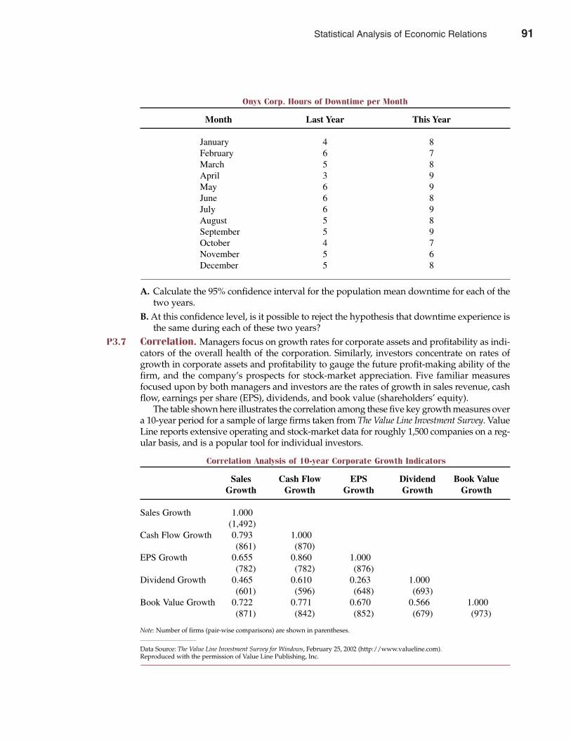
A. Calculate the 95% confidence interval for the population mean downtime for each of thetwo years.
B. At this confidence level, is it possible to reject the hypothesis that downtime experience isthe same during each of these two years?
P3.7 Correlation. Managers focus on growth rates for corporate assets and profitability as indi-cators of the overall health of the corporation. Similarly, investors concentrate on rates ofgrowth in corporate assets and profitability to gauge the future profit-making ability of thefirm, and the company’s prospects for stock-market appreciation. Five familiar measuresfocused upon by both managers and investors are the rates of growth in sales revenue, cashflow, earnings per share (EPS), dividends, and book value (shareholders’ equity).
The table shown here illustrates the correlation among these five key growth measures overa 10-year period for a sample of large firms taken from The Value Line Investment Survey. ValueLine reports extensive operating and stock-market data for roughly 1,500 companies on a reg-ular basis, and is a popular tool for individual investors.
Chapter Three Statistical Analysis of Economic Relations 91
Onyx Corp. Hours of Downtime per Month
Month Last Year This Year
January 4 8 February 6 7 March 5 8 April 3 9 May 6 9 June 6 8 July 6 9 August 5 8 September 5 9 October 4 7 November 5 6 December 5 8
Correlation Analysis of 10-year Corporate Growth Indicators
Sales Cash Flow EPS Dividend Book ValueGrowth Growth Growth Growth Growth
Sales Growth 1.000 (1,492)
Cash Flow Growth 0.793 1.000 (861) (870)
EPS Growth 0.655 0.860 1.000 (782) (782) (876)
Dividend Growth 0.465 0.610 0.263 1.000 (601) (596) (648) (693)
Book Value Growth 0.722 0.771 0.670 0.566 1.000 (871) (842) (852) (679) (973)
Note: Number of firms (pair-wise comparisons) are shown in parentheses.
Data Source: The Value Line Investment Survey for Windows, February 25, 2002 (http://www.valueline.com).Reproduced with the permission of Value Line Publishing, Inc.
Statistical Analysis of Economic Relations 91
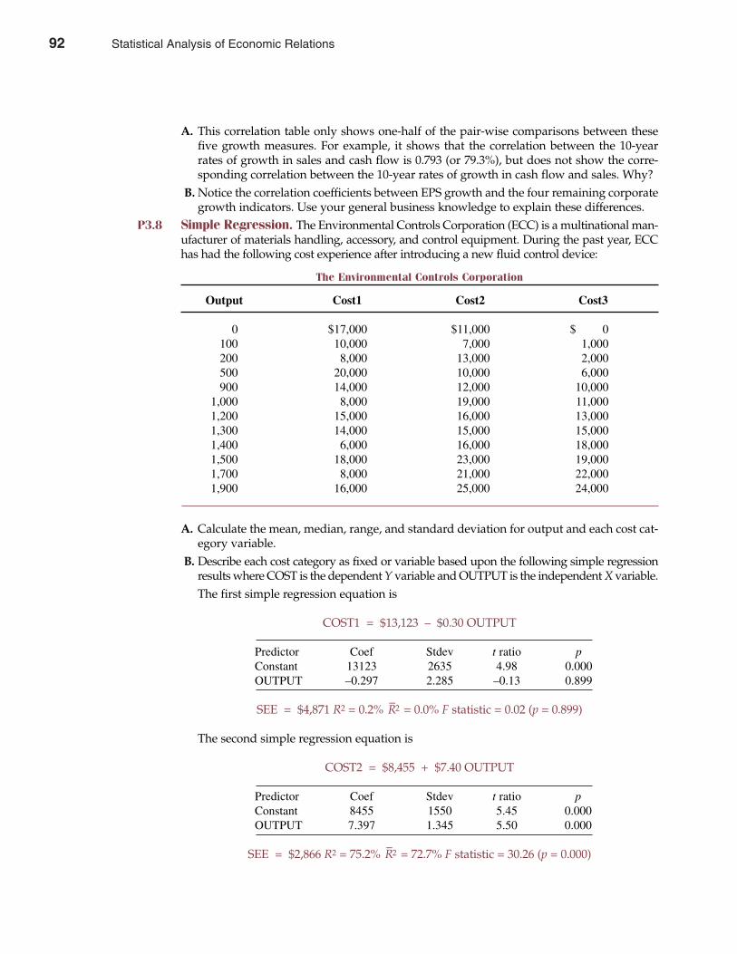
A. This correlation table only shows one-half of the pair-wise comparisons between thesefive growth measures. For example, it shows that the correlation between the 10-yearrates of growth in sales and cash flow is 0.793 (or 79.3%), but does not show the corre-sponding correlation between the 10-year rates of growth in cash flow and sales. Why?
B. Notice the correlation coefficients between EPS growth and the four remaining corporategrowth indicators. Use your general business knowledge to explain these differences.
P3.8 Simple Regression. The Environmental Controls Corporation (ECC) is a multinational man-ufacturer of materials handling, accessory, and control equipment. During the past year, ECChas had the following cost experience after introducing a new fluid control device:
A. Calculate the mean, median, range, and standard deviation for output and each cost cat-egory variable.
B. Describe each cost category as fixed or variable based upon the following simple regressionresults where COST is the dependent Y variable and OUTPUT is the independent X variable.The first simple regression equation is
COST1 = $13,123 – $0.30 OUTPUT
Predictor Coef Stdev t ratio pConstant 13123 2635 4.98 0.000OUTPUT –0.297 2.285 –0.13 0.899
SEE = $4,871 R2 = 0.2% –R2 = 0.0% F statistic = 0.02 (p = 0.899)
The second simple regression equation is
COST2 = $8,455 + $7.40 OUTPUT
Predictor Coef Stdev t ratio pConstant 8455 1550 5.45 0.000OUTPUT 7.397 1.345 5.50 0.000
SEE = $2,866 R2 = 75.2% –R2 = 72.7% F statistic = 30.26 (p = 0.000)
92 Part One Overview of Managerial Economics
The Environmental Controls Corporation
Output Cost1 Cost2 Cost3
0 $17,000 $11,000 $ 0 100 10,000 7,000 1,000 200 8,000 13,000 2,000 500 20,000 10,000 6,000 900 14,000 12,000 10,000
1,000 8,000 19,000 11,000 1,200 15,000 16,000 13,000 1,300 14,000 15,000 15,000 1,400 6,000 16,000 18,000 1,500 18,000 23,000 19,000 1,700 8,000 21,000 22,000 1,900 16,000 25,000 24,000
92 Statistical Analysis of Economic Relations
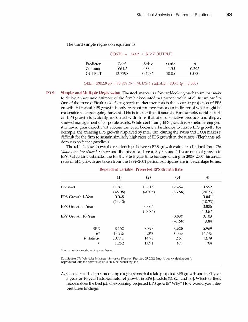
The third simple regression equation is
COST3 = –$662 + $12.7 OUTPUT
Predictor Coef Stdev t ratio pConstant –661.5 488.4 –1.35 0.205OUTPUT 12.7298 0.4236 30.05 0.000
SEE = $902.8 R2 = 98.9% –R2 = 98.8% F statistic = 903.1 (p = 0.000)
P3.9 Simple and Multiple Regression. The stock market is a forward-looking mechanism that seeksto derive an accurate estimate of the firm’s discounted net present value of all future profits.One of the most difficult tasks facing stock-market investors is the accurate projection of EPSgrowth. Historical EPS growth is only relevant for investors as an indicator of what might bereasonable to expect going forward. This is trickier than it sounds. For example, rapid histori-cal EPS growth is typically associated with firms that offer distinctive products and displayshrewd management of corporate assets. While continuing EPS growth is sometimes enjoyed,it is never guaranteed. Past success can even become a hindrance to future EPS growth. Forexample, the amazing EPS growth displayed by Intel, Inc., during the 1980s and 1990s makes itdifficult for the firm to sustain similarly high rates of EPS growth in the future. (Elephants sel-dom run as fast as gazelles.)
The table below shows the relationships between EPS growth estimates obtained from TheValue Line Investment Survey and the historical 1-year, 5-year, and 10-year rates of growth inEPS. Value Line estimates are for the 3 to 5 year time horizon ending in 2005–2007; historicalrates of EPS growth are taken from the 1992–2001 period. All figures are in percentage terms.
A. Consider each of the three simple regressions that relate projected EPS growth and the 1-year,5-year, or 10-year historical rates of growth in EPS [models (1), (2), and (3)]. Which of thesemodels does the best job of explaining projected EPS growth? Why? How would you inter-pret these findings?
Chapter Three Statistical Analysis of Economic Relations 93
Dependent Variable: Projected EPS Growth Rate
(1) (2) (3) (4)
Constant 11.871 13.615 12.464 10.552(48.08) (40.06) (33.86) (28.73)
EPS Growth 1-Year 0.048 0.041(14.40) (10.73)
EPS Growth 5-Year –0.064 –0.086(–3.84) (–3.67)
EPS Growth 10-Year –0.038 0.103(–1.58) (3.84)
SEE 8.162 8.898 8.620 6.969 R2 13.9% 1.3% 0.3% 14.4%
F statistic 207.41 14.73 2.51 42.79n 1,282 1,091 871 764
Note: t statistics are shown in parentheses.
Data Source: The Value Line Investment Survey for Windows, February 25, 2002 (http://www.valueline.com).Reproduced with the permission of Value Line Publishing, Inc.
Statistical Analysis of Economic Relations 93
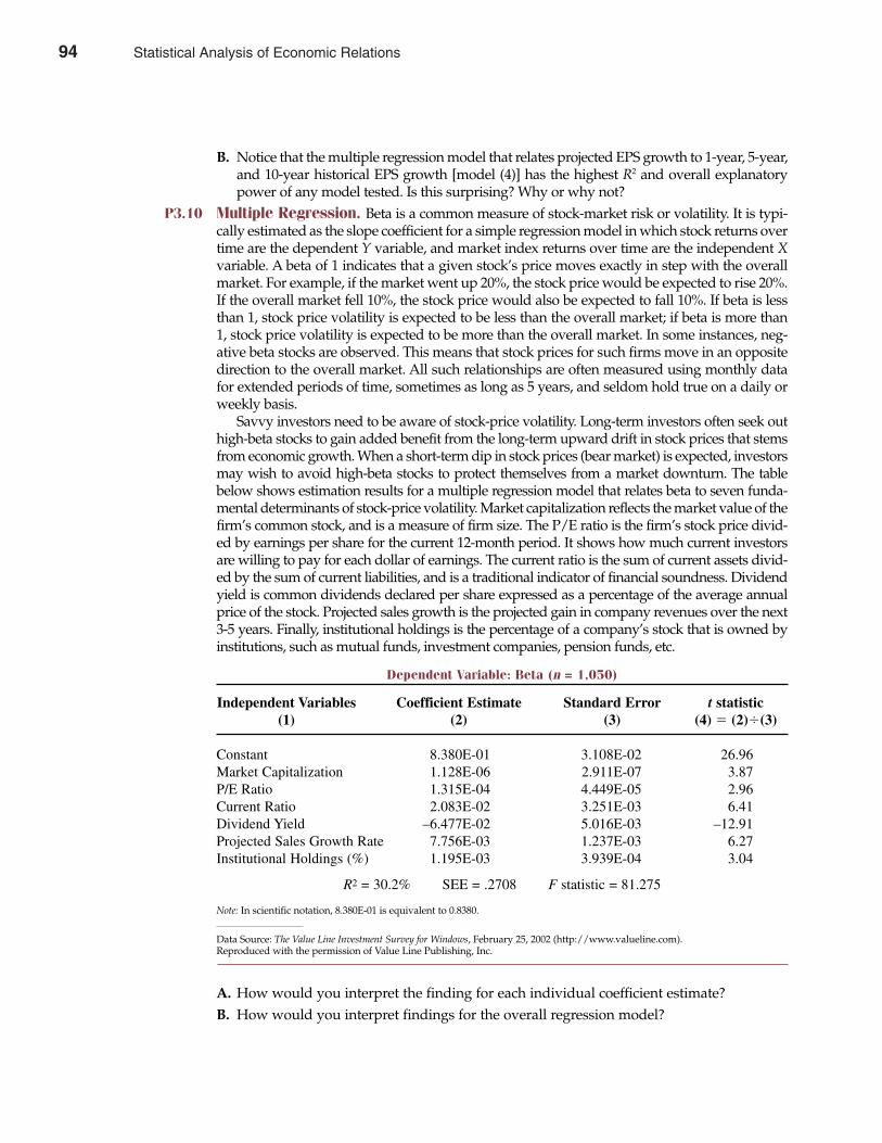
B. Notice that the multiple regression model that relates projected EPS growth to 1-year, 5-year,and 10-year historical EPS growth [model (4)] has the highest R2 and overall explanatorypower of any model tested. Is this surprising? Why or why not?
P3.10 Multiple Regression. Beta is a common measure of stock-market risk or volatility. It is typi-cally estimated as the slope coefficient for a simple regression model in which stock returns overtime are the dependent Y variable, and market index returns over time are the independent Xvariable. A beta of 1 indicates that a given stock’s price moves exactly in step with the overallmarket. For example, if the market went up 20%, the stock price would be expected to rise 20%.If the overall market fell 10%, the stock price would also be expected to fall 10%. If beta is lessthan 1, stock price volatility is expected to be less than the overall market; if beta is more than1, stock price volatility is expected to be more than the overall market. In some instances, neg-ative beta stocks are observed. This means that stock prices for such firms move in an oppositedirection to the overall market. All such relationships are often measured using monthly datafor extended periods of time, sometimes as long as 5 years, and seldom hold true on a daily orweekly basis.
Savvy investors need to be aware of stock-price volatility. Long-term investors often seek outhigh-beta stocks to gain added benefit from the long-term upward drift in stock prices that stemsfrom economic growth. When a short-term dip in stock prices (bear market) is expected, investorsmay wish to avoid high-beta stocks to protect themselves from a market downturn. The tablebelow shows estimation results for a multiple regression model that relates beta to seven funda-mental determinants of stock-price volatility. Market capitalization reflects the market value of thefirm’s common stock, and is a measure of firm size. The P/E ratio is the firm’s stock price divid-ed by earnings per share for the current 12-month period. It shows how much current investorsare willing to pay for each dollar of earnings. The current ratio is the sum of current assets divid-ed by the sum of current liabilities, and is a traditional indicator of financial soundness. Dividendyield is common dividends declared per share expressed as a percentage of the average annualprice of the stock. Projected sales growth is the projected gain in company revenues over the next3-5 years. Finally, institutional holdings is the percentage of a company’s stock that is owned byinstitutions, such as mutual funds, investment companies, pension funds, etc.
A. How would you interpret the finding for each individual coefficient estimate?B. How would you interpret findings for the overall regression model?
94 Part One Overview of Managerial Economics
Dependent Variable: Beta (n = 1,050)
Independent Variables Coefficient Estimate Standard Error t statistic(1) (2) (3) (4) (2)�(3)
Constant 8.380E-01 3.108E-02 26.96Market Capitalization 1.128E-06 2.911E-07 3.87P/E Ratio 1.315E-04 4.449E-05 2.96Current Ratio 2.083E-02 3.251E-03 6.41Dividend Yield –6.477E-02 5.016E-03 –12.91Projected Sales Growth Rate 7.756E-03 1.237E-03 6.27Institutional Holdings (%) 1.195E-03 3.939E-04 3.04
R2 = 30.2% SEE = .2708 F statistic = 81.275
Note: In scientific notation, 8.380E-01 is equivalent to 0.8380.
Data Source: The Value Line Investment Survey for Windows, February 25, 2002 (http://www.valueline.com).Reproduced with the permission of Value Line Publishing, Inc.
94 Statistical Analysis of Economic Relations
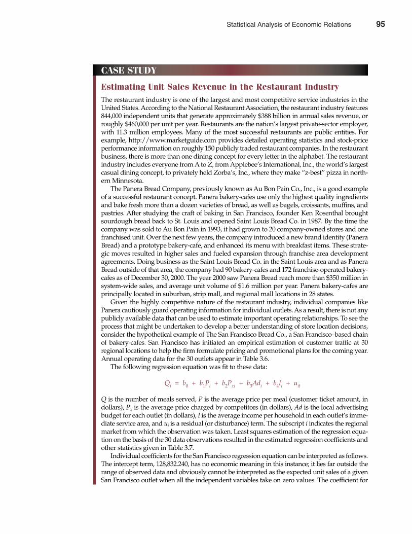
Chapter Three Statistical Analysis of Economic Relations 95
CASE STUDY
Estimating Unit Sales Revenue in the Restaurant IndustryThe restaurant industry is one of the largest and most competitive service industries in theUnited States. According to the National Restaurant Association, the restaurant industry features844,000 independent units that generate approximately $388 billion in annual sales revenue, orroughly $460,000 per unit per year. Restaurants are the nation’s largest private-sector employer,with 11.3 million employees. Many of the most successful restaurants are public entities. Forexample, http://www.marketguide.com provides detailed operating statistics and stock-priceperformance information on roughly 150 publicly traded restaurant companies. In the restaurantbusiness, there is more than one dining concept for every letter in the alphabet. The restaurantindustry includes everyone from A to Z, from Applebee’s International, Inc., the world’s largestcasual dining concept, to privately held Zorba’s, Inc., where they make “z-best” pizza in north-ern Minnesota.
The Panera Bread Company, previously known as Au Bon Pain Co., Inc., is a good exampleof a successful restaurant concept. Panera bakery-cafes use only the highest quality ingredientsand bake fresh more than a dozen varieties of bread, as well as bagels, croissants, muffins, andpastries. After studying the craft of baking in San Francisco, founder Ken Rosenthal broughtsourdough bread back to St. Louis and opened Saint Louis Bread Co. in 1987. By the time thecompany was sold to Au Bon Pain in 1993, it had grown to 20 company-owned stores and onefranchised unit. Over the next few years, the company introduced a new brand identity (PaneraBread) and a prototype bakery-cafe, and enhanced its menu with breakfast items. These strate-gic moves resulted in higher sales and fueled expansion through franchise area developmentagreements. Doing business as the Saint Louis Bread Co. in the Saint Louis area and as PaneraBread outside of that area, the company had 90 bakery-cafes and 172 franchise-operated bakery-cafes as of December 30, 2000. The year 2000 saw Panera Bread reach more than $350 million insystem-wide sales, and average unit volume of $1.6 million per year. Panera bakery-cafes areprincipally located in suburban, strip mall, and regional mall locations in 28 states.
Given the highly competitive nature of the restaurant industry, individual companies likePanera cautiously guard operating information for individual outlets. As a result, there is not anypublicly available data that can be used to estimate important operating relationships. To see theprocess that might be undertaken to develop a better understanding of store location decisions,consider the hypothetical example of The San Francisco Bread Co., a San Francisco–based chainof bakery-cafes. San Francisco has initiated an empirical estimation of customer traffic at 30regional locations to help the firm formulate pricing and promotional plans for the coming year.Annual operating data for the 30 outlets appear in Table 3.6.
The following regression equation was fit to these data:
Qi = b0 + b1Pi + b2Pxi + b3Adi + b4Ii + uit
Q is the number of meals served, P is the average price per meal (customer ticket amount, indollars), Px is the average price charged by competitors (in dollars), Ad is the local advertisingbudget for each outlet (in dollars), I is the average income per household in each outlet’s imme-diate service area, and ui is a residual (or disturbance) term. The subscript i indicates the regionalmarket from which the observation was taken. Least squares estimation of the regression equa-tion on the basis of the 30 data observations resulted in the estimated regression coefficients andother statistics given in Table 3.7.
Individual coefficients for the San Francisco regression equation can be interpreted as follows.The intercept term, 128,832.240, has no economic meaning in this instance; it lies far outside therange of observed data and obviously cannot be interpreted as the expected unit sales of a givenSan Francisco outlet when all the independent variables take on zero values. The coefficient for
Statistical Analysis of Economic Relations 95
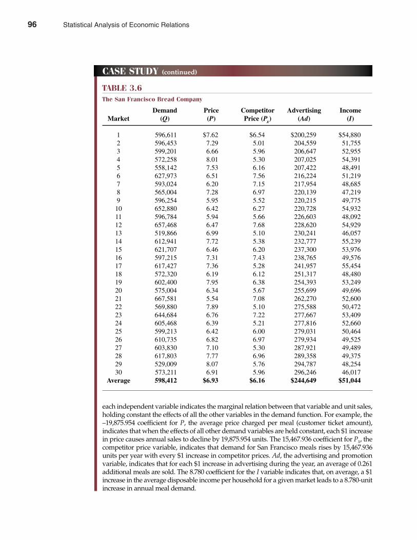
96 Part One Overview of Managerial Economics
each independent variable indicates the marginal relation between that variable and unit sales,holding constant the effects of all the other variables in the demand function. For example, the–19,875.954 coefficient for P, the average price charged per meal (customer ticket amount),indicates that when the effects of all other demand variables are held constant, each $1 increasein price causes annual sales to decline by 19,875.954 units. The 15,467.936 coefficient for Px, thecompetitor price variable, indicates that demand for San Francisco meals rises by 15,467.936units per year with every $1 increase in competitor prices. Ad, the advertising and promotionvariable, indicates that for each $1 increase in advertising during the year, an average of 0.261additional meals are sold. The 8.780 coefficient for the I variable indicates that, on average, a $1increase in the average disposable income per household for a given market leads to a 8.780-unitincrease in annual meal demand.
CASE STUDY (continued)
TABLE 3.6The San Francisco Bread Company
Demand Price Competitor Advertising Income Market (Q) (P) Price (Px) (Ad) (I)
1 596,611 $7.62 $6.54 $200,259 $54,880 2 596,453 7.29 5.01 204,559 51,755 3 599,201 6.66 5.96 206,647 52,955 4 572,258 8.01 5.30 207,025 54,391 5 558,142 7.53 6.16 207,422 48,491 6 627,973 6.51 7.56 216,224 51,219 7 593,024 6.20 7.15 217,954 48,685 8 565,004 7.28 6.97 220,139 47,219 9 596,254 5.95 5.52 220,215 49,775 10 652,880 6.42 6.27 220,728 54,932 11 596,784 5.94 5.66 226,603 48,092 12 657,468 6.47 7.68 228,620 54,929 13 519,866 6.99 5.10 230,241 46,057 14 612,941 7.72 5.38 232,777 55,239 15 621,707 6.46 6.20 237,300 53,976 16 597,215 7.31 7.43 238,765 49,576 17 617,427 7.36 5.28 241,957 55,454 18 572,320 6.19 6.12 251,317 48,480 19 602,400 7.95 6.38 254,393 53,249 20 575,004 6.34 5.67 255,699 49,696 21 667,581 5.54 7.08 262,270 52,600 22 569,880 7.89 5.10 275,588 50,472 23 644,684 6.76 7.22 277,667 53,409 24 605,468 6.39 5.21 277,816 52,660 25 599,213 6.42 6.00 279,031 50,464 26 610,735 6.82 6.97 279,934 49,525 27 603,830 7.10 5.30 287,921 49,489 28 617,803 7.77 6.96 289,358 49,375 29 529,009 8.07 5.76 294,787 48,254 30 573,211 6.91 5.96 296,246 46,017
Average 598,412 $6.93 $6.16 $244,649 $51,044
96 Statistical Analysis of Economic Relations
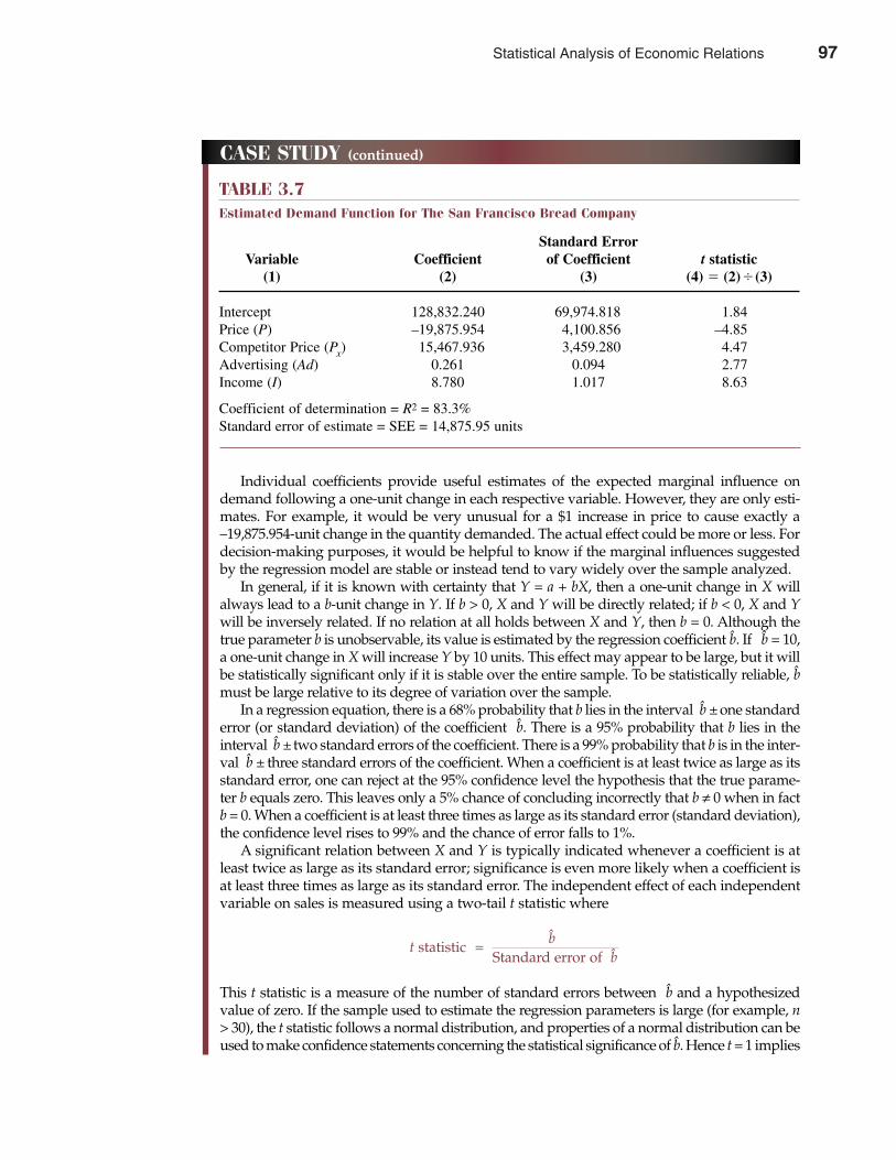
Chapter Three Statistical Analysis of Economic Relations 97
CASE STUDY (continued)
Individual coefficients provide useful estimates of the expected marginal influence ondemand following a one-unit change in each respective variable. However, they are only esti-mates. For example, it would be very unusual for a $1 increase in price to cause exactly a–19,875.954-unit change in the quantity demanded. The actual effect could be more or less. Fordecision-making purposes, it would be helpful to know if the marginal influences suggestedby the regression model are stable or instead tend to vary widely over the sample analyzed.
In general, if it is known with certainty that Y = a + bX, then a one-unit change in X willalways lead to a b-unit change in Y. If b > 0, X and Y will be directly related; if b < 0, X and Ywill be inversely related. If no relation at all holds between X and Y, then b = 0. Although thetrue parameter b is unobservable, its value is estimated by the regression coefficient b̂. If b̂ = 10,a one-unit change in X will increase Y by 10 units. This effect may appear to be large, but it willbe statistically significant only if it is stable over the entire sample. To be statistically reliable, b̂must be large relative to its degree of variation over the sample.
In a regression equation, there is a 68% probability that b lies in the interval b̂ ±one standarderror (or standard deviation) of the coefficient b̂. There is a 95% probability that b lies in theinterval b̂ ±two standard errors of the coefficient. There is a 99% probability that b is in the inter-val b̂ ± three standard errors of the coefficient. When a coefficient is at least twice as large as itsstandard error, one can reject at the 95% confidence level the hypothesis that the true parame-ter b equals zero. This leaves only a 5% chance of concluding incorrectly that b ≠ 0 when in factb = 0. When a coefficient is at least three times as large as its standard error (standard deviation),the confidence level rises to 99% and the chance of error falls to 1%.
A significant relation between X and Y is typically indicated whenever a coefficient is atleast twice as large as its standard error; significance is even more likely when a coefficient isat least three times as large as its standard error. The independent effect of each independentvariable on sales is measured using a two-tail t statistic where
t statistic = b̂Standard error of b̂
This t statistic is a measure of the number of standard errors between b̂ and a hypothesizedvalue of zero. If the sample used to estimate the regression parameters is large (for example, n> 30), the t statistic follows a normal distribution, and properties of a normal distribution can beused to make confidence statements concerning the statistical significance of b̂. Hence t = 1 implies
TABLE 3.7Estimated Demand Function for The San Francisco Bread Company
Standard ErrorVariable Coefficient of Coefficient t statistic
(1) (2) (3) (4) (2)�(3)
Intercept 128,832.240 69,974.818 1.84Price (P) –19,875.954 4,100.856 –4.85Competitor Price (Px) 15,467.936 3,459.280 4.47Advertising (Ad) 0.261 0.094 2.77Income (I) 8.780 1.017 8.63
Coefficient of determination = R2 = 83.3%Standard error of estimate = SEE = 14,875.95 units
Statistical Analysis of Economic Relations 97
SELECTED REFERENCESCalfee, John, Clifford Winston, and Randolph Stempski. “Econometric Issues in Estimating Consumer
Preferences from Stated Preference Data: A Case Study of the Value of Automobile Travel Time.”Review of Economics and Statistics 83 (November 2001): 699–707.
Chay, Kenneth Y., and James L. Powell. “Semiparametric Censored Regression Models.” Journal ofEconomic Perspectives 15 (Fall 2001): 29–42.
Emery, Gary W. “Cyclical Demand and the Choice of Debt Maturity.” Journal of Business 74 (October 2001):557–590.
Fiess, Norbert, and Ronald Macdonald. “The Instability of the Money Demand Function: An I(2) Interpre-tation.” Oxford Bulletin of Economics & Statistics 63 (September 2001): 475–495.
Fraumeni, Barbara M. “E-Commerce: Measurement and Measurement Issues.” American Economic Review91 (May 2001): 318–322.
Funke, Michael. “Money Demand in Euroland.” Journal of International Money & Finance 20 (October 2001):701–713.
Grytten, Jostein, Fredrik Carlsen, and Irene Skau. “The Income Effect and Supplier Induced Demand:Evidence from Primary Physician Services in Norway.” Applied Economics 33 (September 2001):1455–1467.
98 Part One Overview of Managerial Economics
CASE STUDY (continued)
68% confidence, t = 2 implies 95% confidence, t = 3 implies 99% confidence, and so on. Forsmall sample sizes (for example, df = n – k < 30), the t distribution deviates from a normal dis-tribution, and a t table should be used for testing the significance of estimated regressionparameters.
Another regression statistic, the standard error of the estimate (SEE), is used to predict val-ues for the dependent variable given values for the various independent variables. Thus, it ishelpful in determining a range within which one can predict values for the dependent variablewith varying degrees of statistical confidence. Although the best estimate of the value for thedependent variable isŶ, the value predicted by the regression equation, the standard error of theestimate can be used to determine just how accurate this prediction Ŷ is likely to be. Assumingthat the standard errors are normally distributed about the regression equation, there is a 68%probability that actual observations of the dependent variable Y will lie within the range Ŷ ±one standard error of the estimate. The probability that an actual observation of Y will lie with-in two standard errors of its predicted value increases to 95%. There is a 99% chance that anactual observed value for Y will lie in the range Ŷ ± three standard errors. Obviously, greaterpredictive accuracy is associated with smaller standard errors of the estimate.
San Francisco could forecast total unit demand, forecasting sales in each of the 30 marketareas and then summing these area forecasts to obtain an estimate of total demand. Using theresults from the demand estimation model and data from each individual market, it wouldalso be possible to construct a confidence interval for total demand based on the standarderror of the estimate.A. Describe the statistical significance of each individual independent variable included in the
San Francisco demand equation.B. Interpret the coefficient of determination (R2) for the San Francisco demand equation.C. What are expected unit sales and sales revenue in a typical market?D. To illustrate use of the standard error of the estimate statistic, derive the 95% confidence
interval for expected unit sales and total sales revenue in a typical market.
98 Statistical Analysis of Economic Relations
Heiman, Amir, David R. Just, Bruce McWilliams, et al. “Incorporating Family Interactions and Socio-economic Variables Into Family Production Functions: The Case of Demand for Meats.” Agribusiness17 (Autumn 2001): 455–468.
Henrich, Joseph, Robert Boyd, Samuel Bowles, Colin Camerer, Ernst Fehr, Herbert Gintis, and RichardMcElreath. “In Search of Homo Economicus: Behavioral Experiments in 15 Small-Scale Societies.”American Economic Review 91 (May 2001): 73–78.
Horowitz, Joel L., and N. E. Savin. “Binary Response Models: Logits, Probits and Semiparametrics.”Journal of Economic Perspectives 15 (Fall 2001): 43–56.
Krueger, Alan B. “Symposium on Econometric Tools.” Journal of Economic Perspectives 15 (Fall 2001): 3–10. Lim, Christine, and Michael McAleer. “Cointegration Analysis of Quarterly Tourism Demand by Hong
Kong and Singapore for Australia.” Applied Economics 33 (October 2001): 1599–1619.Manmohan S. Sodhi. “Applications and Opportunities for Operations Research in Internet-Enabled
Supply Chains and Electronic Marketplaces.” Interfaces 31 (March 2001): 56–69.Newey, Whitney K. “Flexible Simulated Moment Estimation of Nonlinear Errors-in-Variables Models.”
Review of Economics and Statistics 83 (November 2001): 616–627.Smith, V. Kerry, Donald H. Taylor, Jr., Frank A. Sloan, F. Reed Johnson, and William H. Desvousges. “Do
Smokers Respond to Health Shocks?” Review of Economics and Statistics 83 (November 2001): 675–687.
Chapter Three Statistical Analysis of Economic Relations 99
Statistical Analysis of Economic Relations 99

100 Part One Overview of Managerial Economics

Demand and Supply
CHAPTER FOUR
102
Around the globe, 24 hours per day, impossible-to-regulate currencymarkets set prices for the U.S. dollar, Japanese yen, and the European
Economic and Monetary Union’s euro. Much to the chagrin of sovereigngovernments and their official representatives, minute-by-minute variationsin currency prices are wholly determined by the converging forces of supplyand demand.
For example, U.S. stock markets plunged an unprecedented 684.81 pointson Monday, September 17, 2001, following the resumption of trading afterterrorist attacks in New York City and Washington, DC. Those attacks leftthousands dead and millions of investors understandably nervous about theeconomy and a potential meltdown in investor confidence. Securities mar-kets fell sharply as investors worried that the attacks could chill consumersentiment and throw the world economy into recession. In the currency mar-ket, the dollar plunged more than three yen, from roughly 120 yen per dollarto 117 yen per dollar, to its lowest level in nearly seven months.
When the number of yen that can be bought for a dollar falls, the dollarprice of Japanese–made goods rises in the United States. This hurts both U.S.consumers and Japanese exporters. To stem the slide in the dollar, Japanesemonetary authorities intervened in the currency market to buy dollars andsell yen. This had the temporary effect of increasing the supply of yen relativeto dollars, and the dollar quickly jumped from just below 117 yen to nearly118.50 yen. However, both currencies quickly slipped back to preinterventionlevels when it became clear that it was the Japanese central bank, and not mar-ket forces, that had caused the dollar to rise and the yen to fall. The upshot issimple: The laws of demand and supply are so powerful that they dictate thevalue of money itself!1
1 See Dow Jones Newswires, “Dollar Steadies vs. Euro, Yen As Bank of Japan Intervenes,”The Wall Street Journal Online, September 17, 2001 (http://online.wsj.com).
101
4
Chapter Four Demand and Supply 103
BASIS FOR DEMAND
Demand is the quantity of a good or service that customers are willing and able to purchaseduring a specified period under a given set of economic conditions. The time frame might bean hour, a day, a month, or a year. Conditions to be considered include the price of the good inquestion, prices and availability of related goods, expectations of price changes, consumerincomes, consumer tastes and preferences, advertising expenditures, and so on. The amount ofthe product that consumers are prepared to purchase, its demand, depends on all these factors.
For managerial decision making, a prime focus is on market demand. Market demand is theaggregate of individual, or personal, demand. Insight into market demand relations requires anunderstanding of the nature of individual demand. Individual demand is determined by thevalue associated with acquiring and using any good or service and the ability to acquire it. Bothare necessary for effective individual demand. Desire without purchasing power may lead towant, but not to demand.
Direct DemandThere are two basic models of individual demand. One, known as the theory of consumerbehavior, relates to the direct demand for personal consumption products. This model isappropriate for analyzing individual demand for goods and services that directly satisfyconsumer desires. The value or worth of a good or service, its utility, is the prime determi-nant of direct demand. Individuals are viewed as attempting to maximize the total utility orsatisfaction provided by the goods and services they acquire and consume. This optimiza-tion process requires that consumers focus on the marginal utility (gain in satisfaction) ofacquiring additional units of a given product. Product characteristics, individual preferences(tastes), and the ability to pay are all important determinants of direct demand.
Derived DemandGoods and services are sometimes acquired because they are important inputs in the man-ufacture and distribution of other products. The outputs of engineers, production workers,sales staff, managers, lawyers, consultants, office business machines, production facilitiesand equipment, natural resources, and commercial airplanes are all examples of goods andservices demanded not for direct consumption but rather for their use in providing othergoods and services. Their demand is derived from the demand for the products they areused to provide. Input demand is called derived demand.
The demand for mortgage money is an example. The quantity of mortgage credit demand-ed is not determined directly; it is derived from the more fundamental demand for housing. Thedemand for air transportation to resort areas is not a direct demand but is derived from thedemand for recreation. Similarly, the demand for producers’ goods and services used to man-ufacture products for final consumption is derived. Aggregate demand for consumption goodsand services determines demand for the capital equipment, materials, labor, and energy usedto manufacture them. For example, the demands for steel, aluminum, and plastics are allderived demands, as are the demands for machine tools and labor. None of these producers’goods are demanded because of their direct value to consumers but because of the role theyplay in production.
Demand for producers’ goods and services is closely related to final products demand. Anexamination of final product demand is an important part of demand analysis for intermediate,or producers,’ goods. For products whose demand is derived rather than direct, demand stemsfrom their value in the manufacture and sale of other products. They have value because their
demand Total quantity customersare willing and able topurchase
direct demand Demand for consump-tion products
utility Value
derived demand Demand for inputsused in production
102 Demand and Supply
employment has the potential to generate profits. Key components in the determination ofderived demand are the marginal benefits and marginal costs associated with using a giveninput or factor of production. The amount of any good or service used rises when its marginalbenefit, measured in terms of the value of resulting output, is greater than the marginal costs ofusing the input, measured in terms of wages, interest, raw material costs, or related expenses.Conversely, the amount of any input used in production falls when resulting marginal benefitsare less than the marginal cost of employment. In short, derived demand is related to the prof-itability of using a good or service.
Regardless of whether a good or service is demanded by individuals for final consumption(direct demand) or as an input used in providing other goods and services (derived demand),the fundamentals of economic analysis offer a basis for investigating demand characteristics.For final consumption products, utility maximization as described by the theory of consumerbehavior explains the basis for direct demand. For inputs used in the production of other prod-ucts, profit maximization provides the underlying rationale for derived demand. Because bothdemand models are based on the optimization concept, fundamental direct and derived demandrelations are essentially the same.
MARKET DEMAND FUNCTION
The market demand function for a product is a statement of the relation between the aggregatequantity demanded and all factors that affect this quantity. In functional form, a demandfunction may be expressed as
104 Part Two Demand Analysis
demand function Relation betweendemand and factorsinfluencing its level
How the Internet Affects Demand and Supply
From an economic perspective, the Internet is the enemyof high prices and high profit margins. By greatlyexpanding the scope of the market, the Internet effective-ly eliminates geographic boundaries, especially for easilytransported goods and services. This greatly increases theelasticity of demand and supply.
For example, in the pre-Internet era, anyone lookingfor a good deal on a high-quality vacuum cleaner mighthave gone to the local Wal-Mart, Target, or a specialtyshop to look for the best bargain available. With theInternet, consumers can log onto Google.com, or yourfavorite Internet search engine; do a search on vacuumcleaners; and get data on hundreds of high-qualityvacuums at extremely attractive prices. For example,with $15 to $20 for shipping via Federal Express orUPS, it is possible to have vacuums delivered inLawrence, Kansas, from http://www.vacdepot.com/in Houston, Texas, at prices far below those offered bythe local vacuum cleaner shop.
Successful Internet retailers offer bargain prices, abroad assortment of attractive products, and speedydelivery. They also effectively handle returns and basic
customer service. Of course, traditional retailers cannotstand idly by as Internet-based retailers drive them outof business. They must fight back with competitiveprices, high-quality products, and an enticing in-storeshopping experience. Borders is a good example of abookseller that has effectively distinguished itself fromAmazon.com and other Internet retailers by offering anappealing in-store shopping experience.
When considering the economic potential ofInternet-based commerce, it is important to keep in mindthat successful firms use Internet technology to maintainsignificant competitive advantages. The Internet, byitself, seldom confers long-lasting competitive advantages.The Internet is a marvelous communications device thatgreatly improves access to information about productquality, prices, and performance. The Internet broadensthe market, and makes demand and supply much moresensitive to changing economic conditions.
See: Kristi Essick, “Young Guns Get Creative in Life After Venture Capital,”The Wall Street Journal Online, December 7, 2001 (http://online.wsj.com).
M A N A G E R I A L A P P L I C AT I O N 4 . 1
Demand and Supply 103

Chapter Four Demand and Supply 105
f (Price of X, Prices of Related Quantity of Goods, Expectations of Price
(4.1) Product X = Qx = Changes, Consumer Incomes, Demanded Tastes and Preferences, Advertising
Expenditures, and so on)
The generalized demand function expressed in Equation 4.1 lists variables that commonlyinfluence demand. For use in managerial decision making, the relation between quantity andeach demand-determining variable must be specified. To illustrate what is involved, assumethat the demand function for the automobile industry is
(4.2) Q = a1P + a2PI + a3 I + a4Pop + a5i + a6A
This equation states that the number of new domestic automobiles demanded during a givenyear (in millions), Q, is a linear function of the average price of new domestic cars (in $), P; theaverage price for new import cars (in $), PI; disposable income per household (in $), I; popula-tion (in millions), Pop; average interest rate on car loans (in percent), i; and industry advertisingexpenditures (in $ millions), A. The terms a1, a2, . . ., a6 are called the parameters of the demandfunction. Assume that the parameters of this demand function are known with certainty, asshown in the following equation:
(4.3) Q = –500P + 210PX + 200I + 20,000Pop – 1,000,000i + 600A
Equation 4.3 states that automobile demand falls by 500 for each $1 increase in the averageprice charged by domestic manufacturers; it rises by 210 with every $1 increase in the averageprice of new luxury cars (PX), a prime substitute; it increases by 200 for each $1 increase in dis-posable income per household (I); it increases by 20,000 with each additional million personsin the population (Pop); it decreases by 1 million for every 1 percent rise in interest rates (i); andit increases by 600 with each unit ($1 million) spent on advertising (A).
To derive an estimate of industry demand in any given year, each parameter in Equation4.3 is multiplied by the value of the related variable and then summed. Table 4.1 illustratesthis process, showing that the estimated annual demand for new domestic automobiles is 8million cars, assuming the stated values of each independent variable.
Industry Demand Versus Firm DemandMarket demand functions can be specified for an entire industry or for an individual firm,though somewhat different variables would typically be used in each case. Variables repre-senting competitors’ actions would be stressed in firm demand functions. For example, a firm’sdemand function would typically include competitors’ prices and advertising expenditures.Demand for the firm’s product line is negatively related to its own prices but positively relatedto the prices charged by competing firms. Demand for the firm’s products would typicallyincrease with its own advertising expenditures, but it could increase or decrease with addition-al advertising by other firms.
The parameters for specific variables ordinarily differ in industry versus firm demandfunctions. Consider the positive influence of population on the demand for Ford automobilesas opposed to automobiles in general. Although the effect is positive in each instance, theparameter value in the Ford demand function would be much smaller than that in the industrydemand function. Only if Ford had 100 percent of the market—that is, if Ford were the industry—would the parameters for firm and industry demand be identical.
Because firm and industry demand functions differ, different models or equations mustbe estimated for analyzing these two levels of demand. However, demand concepts devel-oped in this chapter apply to both firm and industry demand functions.
104 Demand and Supply
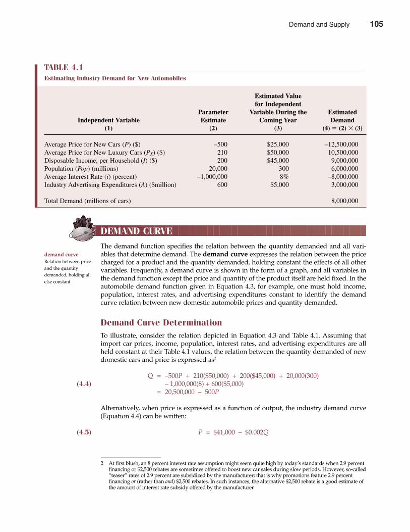
DEMAND CURVE
The demand function specifies the relation between the quantity demanded and all vari-ables that determine demand. The demand curve expresses the relation between the pricecharged for a product and the quantity demanded, holding constant the effects of all othervariables. Frequently, a demand curve is shown in the form of a graph, and all variables inthe demand function except the price and quantity of the product itself are held fixed. In theautomobile demand function given in Equation 4.3, for example, one must hold income,population, interest rates, and advertising expenditures constant to identify the demandcurve relation between new domestic automobile prices and quantity demanded.
Demand Curve DeterminationTo illustrate, consider the relation depicted in Equation 4.3 and Table 4.1. Assuming thatimport car prices, income, population, interest rates, and advertising expenditures are allheld constant at their Table 4.1 values, the relation between the quantity demanded of newdomestic cars and price is expressed as2
Q = –500P + 210($50,000) + 200($45,000) + 20,000(300)(4.4) – 1,000,000(8) + 600($5,000)
= 20,500,000 – 500P
Alternatively, when price is expressed as a function of output, the industry demand curve(Equation 4.4) can be written:
(4.5) P = $41,000 – $0.002Q
106 Part Two Demand Analysis
demand curve Relation between priceand the quantitydemanded, holding allelse constant
TABLE 4.1Estimating Industry Demand for New Automobiles
Estimated Valuefor Independent
Parameter Variable During the EstimatedIndependent Variable Estimate Coming Year Demand
(1) (2) (3) (4) � (2) � (3)
Average Price for New Cars (P) ($) –500 $25,000 –12,500,000Average Price for New Luxury Cars (PX) ($) 210 $50,000 10,500,000Disposable Income, per Household (I) ($) 200 $45,000 9,000,000Population (Pop) (millions) 20,000 300 6,000,000Average Interest Rate (i) (percent) –1,000,000 8% –8,000,000Industry Advertising Expenditures (A) ($million) 600 $5,000 3,000,000
Total Demand (millions of cars) 8,000,000
2 At first blush, an 8 percent interest rate assumption might seem quite high by today’s standards when 2.9 percentfinancing or $2,500 rebates are sometimes offered to boost new car sales during slow periods. However, so-called“teaser” rates of 2.9 percent are subsidized by the manufacturer; that is why promotions feature 2.9 percentfinancing or (rather than and) $2,500 rebates. In such instances, the alternative $2,500 rebate is a good estimate ofthe amount of interest rate subsidy offered by the manufacturer.
Demand and Supply 105
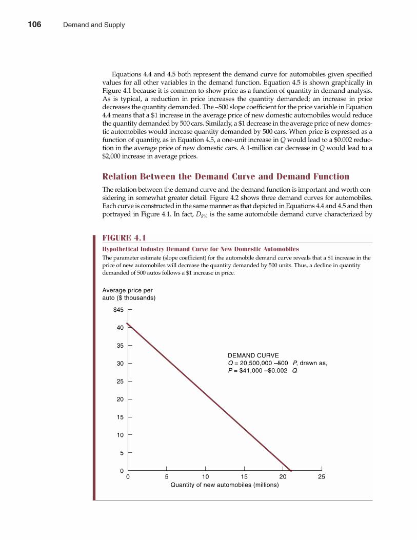
Equations 4.4 and 4.5 both represent the demand curve for automobiles given specifiedvalues for all other variables in the demand function. Equation 4.5 is shown graphically inFigure 4.1 because it is common to show price as a function of quantity in demand analysis.As is typical, a reduction in price increases the quantity demanded; an increase in pricedecreases the quantity demanded. The –500 slope coefficient for the price variable in Equation4.4 means that a $1 increase in the average price of new domestic automobiles would reducethe quantity demanded by 500 cars. Similarly, a $1 decrease in the average price of new domes-tic automobiles would increase quantity demanded by 500 cars. When price is expressed as afunction of quantity, as in Equation 4.5, a one-unit increase in Q would lead to a $0.002 reduc-tion in the average price of new domestic cars. A 1-million car decrease in Q would lead to a$2,000 increase in average prices.
Relation Between the Demand Curve and Demand FunctionThe relation between the demand curve and the demand function is important and worth con-sidering in somewhat greater detail. Figure 4.2 shows three demand curves for automobiles.Each curve is constructed in the same manner as that depicted in Equations 4.4 and 4.5 and thenportrayed in Figure 4.1. In fact, D8% is the same automobile demand curve characterized by
Chapter Four Demand and Supply 107
FIGURE 4.1Hypothetical Industry Demand Curve for New Domestic AutomobilesThe parameter estimate (slope coefficient) for the automobile demand curve reveals that a $1 increase in theprice of new automobiles will decrease the quantity demanded by 500 units. Thus, a decline in quantitydemanded of 500 autos follows a $1 increase in price.
$45
40
35
30
25
20
15
10
5
0
DEMAND CURVEQ = 20,500,000 — 500 P, drawn as,P = $41,000 — $0.002 Q
0 5 10Quantity of new automobiles (millions)
Average price perauto ($ thousands)
15 20 25
106 Demand and Supply
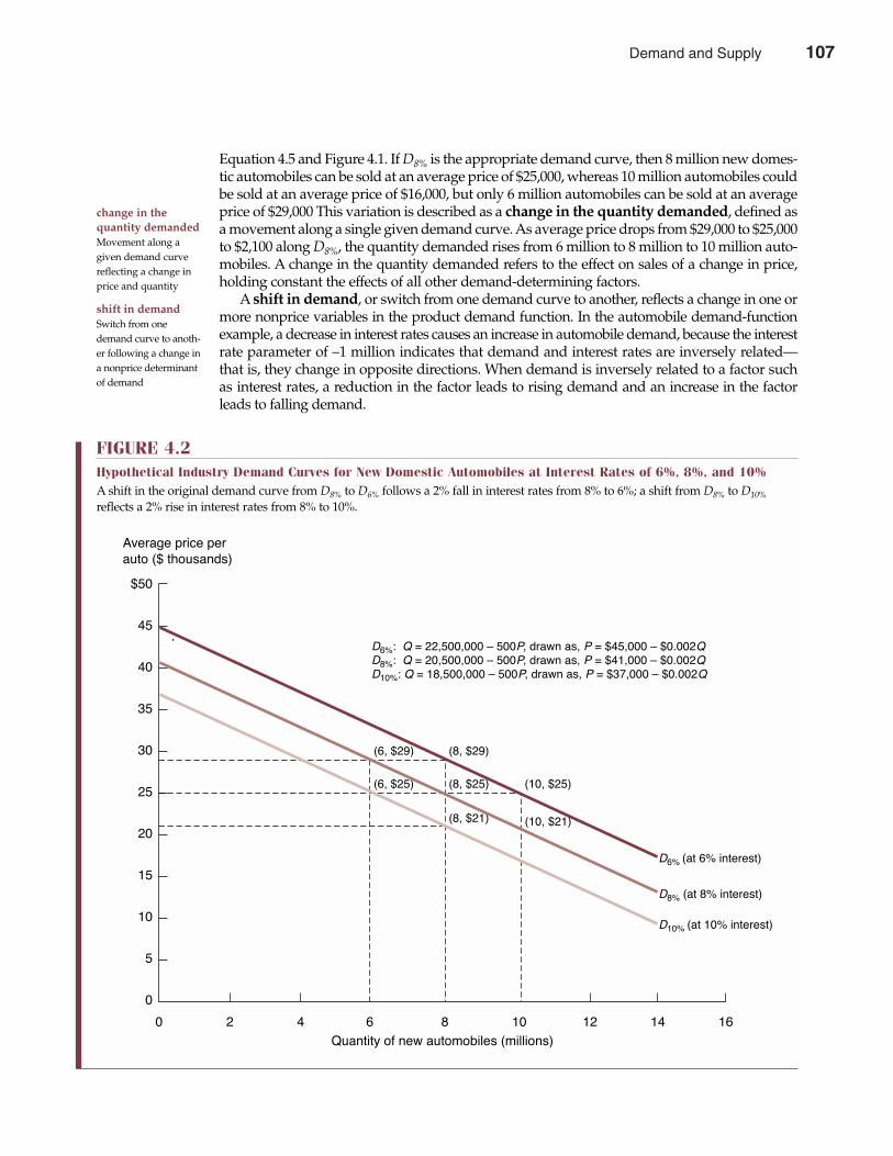
Equation 4.5 and Figure 4.1. If D8% is the appropriate demand curve, then 8 million new domes-tic automobiles can be sold at an average price of $25,000, whereas 10 million automobiles couldbe sold at an average price of $16,000, but only 6 million automobiles can be sold at an averageprice of $29,000 This variation is described as a change in the quantity demanded, defined asa movement along a single given demand curve. As average price drops from $29,000 to $25,000to $2,100 along D8%, the quantity demanded rises from 6 million to 8 million to 10 million auto-mobiles. A change in the quantity demanded refers to the effect on sales of a change in price,holding constant the effects of all other demand-determining factors.
A shift in demand, or switch from one demand curve to another, reflects a change in one ormore nonprice variables in the product demand function. In the automobile demand-functionexample, a decrease in interest rates causes an increase in automobile demand, because the interestrate parameter of –1 million indicates that demand and interest rates are inversely related—that is, they change in opposite directions. When demand is inversely related to a factor suchas interest rates, a reduction in the factor leads to rising demand and an increase in the factorleads to falling demand.
108 Part Two Demand Analysis
change in the quantity demanded Movement along agiven demand curvereflecting a change inprice and quantity
shift in demand Switch from onedemand curve to anoth-er following a change ina nonprice determinantof demand
FIGURE 4.2Hypothetical Industry Demand Curves for New Domestic Automobiles at Interest Rates of 6%, 8%, and 10%A shift in the original demand curve from D8% to D6% follows a 2% fall in interest rates from 8% to 6%; a shift from D8% to D10%
reflects a 2% rise in interest rates from 8% to 10%.
Average price perauto ($ thousands)
$50
45
40
35
30
25
20
15
10
5
0
0 2 4 6 8
Quantity of new automobiles (millions)
10 12 14 16
(8, $21) (10, $21)
(8, $25) (10, $25)(6, $25)
(8, $29)(6, $29)
D6% (at 6% interest)
D8% (at 8% interest)
D10% (at 10% interest)
D6%: Q = 22,500,000 Ð 500P, drawn as, P = $45,000 Ð $0.002QD8%: Q = 20,500,000 Ð 500P, drawn as, P = $41,000 Ð $0.002QD10%: Q = 18,500,000 Ð 500P, drawn as, P = $37,000 Ð $0.002Q
Demand and Supply 107
Chapter Four Demand and Supply 109
D6% is another automobile demand curve. The sole difference between D8% and D6% is thatD8% assumes an interest rate of 8 percent rather than the 6 percent interest rate used to constructD6%. Because the interest rate parameter is negative, a decrease in interest rates causes an increasein automobile demand. Holding all else equal, a 2 percent reduction in interest rates leads to a 2-million-unit [= –1 million � (–2)] increase in automobile demand. A 2 percent decrease in aver-age interest rates leads to an upward or rightward shift in the original demand curve D8% to thenew demand curve D6%. This also means that a 2 percent interest rate reduction will increaseautomobile demand by 2 million units at each price level. At an average price of $25,000, forexample, a 2 percent reduction in interest rates increases automobile demand from 8 million to10 million units per year, as shown on D6%. Also as shown on D6%, after a 2 percent decrease ininterest rates, the original quantity of 8 million automobiles could be sold at a higher averageprice of $29,000. Notice that demand curve D8% indicates that only 8 million units could be soldat an average industry price of $25,000, when interest rates average 8 percent per year.
However, a 2 percent increase in interest rates, from 8 percent to 10 percent, causes aninward or leftward shift in the original demand curve D8% to the new demand curve D10%. A2 percent increase in interest rates reduces automobile demand by 2 million cars at each pricelevel. At a price of $25,000, a 2 percent increase in interest rates reduces demand for newdomestic cars from 8 million cars, the D8% level, to only 6 million units, the D6% level. Withinterest rates at 10 percent, demand for 8 million cars would only arise at the lower averageprice of $21,000, the D10% level, again holding all other demand-determining factors constant.
From the advertising parameter of 600, it is possible to infer that demand and advertisingare positively related. Rising demand follows increases in advertising, and falling demandfollows reductions in advertising. The shift from D8% to D6% in Figure 4.2, for example, couldalso have resulted from a $2.5 billion increase in industry advertising rather than a 2 percent
ISP Customers Learn About Demand and Supply
In 1996, America Online, Inc. (AOL), the leader in theburgeoning Internet service provider (ISP) industry, suc-cumbed to pressure from competitors and cut its price forunlimited access to the Internet to $19.95 per month.Usage skyrocketed. Because flat-rate pricing does notpenalize unlimited usage, many subscribers simplydecided to leave their connection running all day andnight. Because of surging popularity among novice users,long-time subscribers found themselves locked out of theAOL system. Dedicated users became especially iratewhen AOL kept running TV commercials and offeringpromotional rates to new subscribers when it was clearlyunable to handle the traffic such promotions generated.Subscriber frustration turned to litigation, and AOL washit with lawsuits charging the company with negligenceand consumer fraud.
Overloaded, facing lawsuits and the potential ofmassive defections from dissatisfied customers, AOLmade a radical decision. AOL slashed marketing effortsaimed at recruiting new subscribers and stepped upinvestment in network capacity. By 1998, continuinggrowth in the popularity of the Internet allowed AOL to
boost spending on infrastructure and even raise its fixed-rate monthly charge for unlimited access to $21.95 permonth. Still, AOL suffers from having to employ a fixed-rate pricing structure that is incapable of balancingdemand and supply. Like all ISPs, AOL suffers from abusiness plan featuring fixed-rate pricing that encouragesunlimited demand and time-dependent supply costs thatare variable with usage. Unlike local phone service, wherefixed costs predominate and marginal usage costs arenear zero, ISPs closely resemble long-distance telephoneservice providers. ISP costs are closely tied to time ofusage, and efficient pricing must be on a per unit basis.
With time-based pricing, ISP demand will be cur-tailed during peak hours, and the practice of noviceusers logging on for days at a time will end. In themeantime, frustrated ISP customers will suffer fromdemand/supply imbalances created by the industry’sfixed-rate pricing model.
See: Julia Angwin, Martin Peers, and Matthew Rose, “Parsons’s AscendanceSends AOL a Message from Time Warner: We’re in Charge Here,” The WallStreet Journal Online, December 6, 2001 (http://online.wsj.com).
M A N A G E R I A L A P P L I C AT I O N 4 . 2
108 Demand and Supply
110 Part Two Demand Analysis
reduction in interest rates, or it could be the result of a $1.25 billion increase in industry adver-tising coupled with a 1 percent reduction in interest rates. In each case, the resulting demandcurve is given by the equation Q = 20,000,000 – 500P, or P = $40,000 – $0.002Q. However, thedownward shift from D8% to D10% in Figure 4.2 could have resulted from a $3.3 billiondecrease in industry advertising rather than a 2 percent increase in interest rates, or it couldbe the result of a $1.67 billion decrease in industry advertising coupled with a 1 percentincrease in interest rates. In each case, the resulting demand curve is given by the equationQ = 22,500,000 – 500P, or P = $45,000 – $0.002Q.
The distinction between changes in the quantity demanded, which reflect movements along agiven demand curve, and changes in demand, which reflect shifts from one demand curve toanother, is extremely important. Failure to understand the causes of changes in demand for a com-pany’s products can lead to costly, even disastrous, mistakes in managerial decision making. Thetask of demand analysis is made especially difficult by the fact that under normal circumstances,not only prices but also prices of other goods, income, population, interest rates, advertising, andmost other demand-related factors vary from period to period. Sorting out the impact of each fac-tor makes demand analysis one of the most challenging aspects of managerial economics.
BASIS FOR SUPPLY
The term supply refers to the quantity of a good or service that producers are willing and ableto sell during a certain period under a given set of conditions. Factors that must be specifiedinclude the price of the good in question, prices of related goods, the current state of technology,levels of input prices, weather, and so on. The amount of product that producers bring to themarket—the supply of the product—depends on all these influences.
Factors That Influence SupplyThe supply of a product in the market is the aggregate amount supplied by individual firms. Thesupply of products arises from their ability to enhance the firm’s value-maximization objective.The amount of any good or service supplied will rise when the marginal benefit to producers,measured in terms of the value of output, is greater than the marginal cost of production. Theamount of any good or service supplied will fall when the marginal benefit to producers is lessthan the marginal costs of production. Thus, individual firms will expand or reduce supplybased on the expected impact on profits.
Among the factors influencing the supply of a product, the price of the product itself isoften the most important. Higher prices increase the quantity of output producers want tobring to market. When marginal revenue exceeds marginal cost, firms increase supply to earnthe greater profits associated with expanded output. Higher prices allow firms to pay thehigher production costs that are sometimes associated with expansions in output. Conversely,lower prices typically cause producers to supply a lower quantity of output. At the margin,lower prices can have the effect of making previous levels of production unprofitable.
The prices of related goods and services can also play an important role in determining sup-ply of a product. If a firm uses resources that can be used to produce several different products,it may switch production from one product to another depending on market conditions. Forexample, the supply of gasoline typically declines in autumn when the price of heating oil rises.Gasoline supply typically increases during the spring and summer months with the seasonaldecline in heating oil prices. Whereas the substitution of one output for another can cause aninverse relation between the supply of one product and the price of a second, complementaryproduction relationships result in a positive relation between supply and the price of a relatedproduct. For example, ore deposits containing lead often also contain silver. An increase in theprice of lead can therefore lead to an expansion in both lead and silver production.
supply Total quantity offeredfor sale
Demand and Supply 109
Chapter Four Demand and Supply 111
Technology is a key determinant of product supply. The current state of technology refersto the manner in which inputs are transformed into output. An improvement in the state oftechnology, including any product invention or process innovation that reduces productioncosts, increases the quantity and/or quality of products offered for sale at a given price.
Changes in input prices also affect supply in that an increase in input prices will raise costsand reduce the quantity that can be supplied profitably at a given market price. Alternatively,a decrease in input prices increases profitability and the quantity supplied at a given price.
For some products, especially agricultural products, weather can play an important role indetermining supply. Temperature, rainfall, and wind all influence the quantity that can be sup-plied. Heavy rainfall in early spring, for example, can delay or prevent the planting of crops,significantly limiting supply. Abundant rain during the growing season can greatly increase theavailable supply at harvest time. An early freeze that prevents full maturation or heavy snowthat limits harvesting activity both reduce the supply of agricultural products.
Managerial decision making requires understanding both individual firm supply andmarket supply conditions. Market supply is the aggregate of individual firm supply, so it isultimately determined by factors affecting firm supply. Firm supply is examined in greaterdetail in Chapters 7 and 8. For now, meaningful insight can be gained by understanding thenature of market supply.
MARKET SUPPLY FUNCTION
The market supply function for a product is a statement of the relation between the quantitysupplied and all factors affecting that quantity. In functional form, a supply function can beexpressed as
Quantity of f(Price of X, Prices of Related Goods,(4.6) Product X = Q = Current State of Technology, Input
Supplied Prices, Weather, and so on)
The generalized supply function expressed in Equation 4.6 lists variables that influence supply.As is true with the demand function, the supply function must be made explicit to be useful formanagerial decision making.
Determinants of SupplyTo illustrate, consider the automobile industry example discussed previously and assumethat the supply function has been specified as follows:
(4.7) Q = b1P + b2PSUV + b3W + b4S + b5E + b6i
This equation states that the number of new domestic automobiles supplied during a givenperiod (in millions), Q, is a linear function of the average price of new domestic cars (in $), P;average price of new sport utility vehicles (SUVs) (in $), PSUV; average hourly price of labor(wages in $ per hour), W; average cost of steel ($ per ton), S; average cost of energy ($ per mcfnatural gas), E; and average interest rate (cost of capital in percent), i. The terms b1, b2, . . . , b6 arethe parameters of the supply function. Note that no explicit term describes technology, or themethod by which inputs are combined to produce output. The current state of technology is anunderlying or implicit factor in the industry supply function.
Substituting a set of assumed parameter values into Equation 4.7 gives the following supplyfunction for the automobile industry:
supply function Relation between sup-ply and all factorsinfluencing its level
110 Demand and Supply
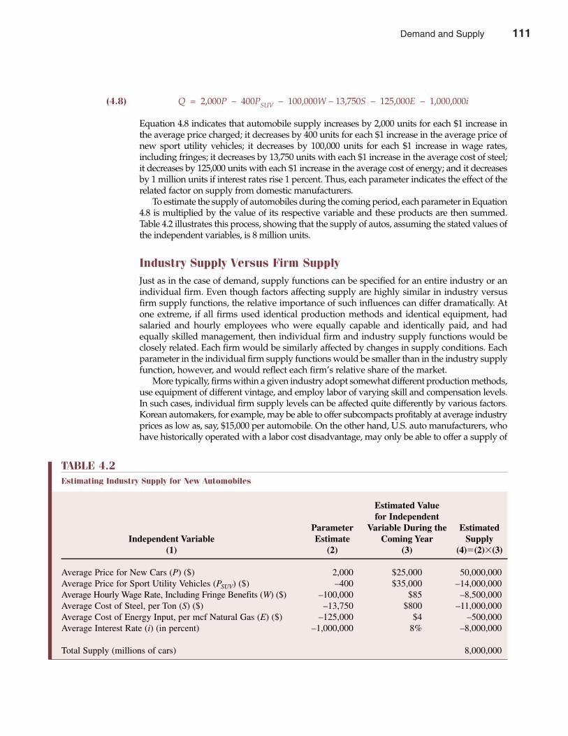
112 Part Two Demand Analysis
(4.8) Q = 2,000P – 400PSUV – 100,000W – 13,750S – 125,000E – 1,000,000i
Equation 4.8 indicates that automobile supply increases by 2,000 units for each $1 increase inthe average price charged; it decreases by 400 units for each $1 increase in the average price ofnew sport utility vehicles; it decreases by 100,000 units for each $1 increase in wage rates,including fringes; it decreases by 13,750 units with each $1 increase in the average cost of steel;it decreases by 125,000 units with each $1 increase in the average cost of energy; and it decreasesby 1 million units if interest rates rise 1 percent. Thus, each parameter indicates the effect of therelated factor on supply from domestic manufacturers.
To estimate the supply of automobiles during the coming period, each parameter in Equation4.8 is multiplied by the value of its respective variable and these products are then summed.Table 4.2 illustrates this process, showing that the supply of autos, assuming the stated values ofthe independent variables, is 8 million units.
Industry Supply Versus Firm SupplyJust as in the case of demand, supply functions can be specified for an entire industry or anindividual firm. Even though factors affecting supply are highly similar in industry versusfirm supply functions, the relative importance of such influences can differ dramatically. Atone extreme, if all firms used identical production methods and identical equipment, hadsalaried and hourly employees who were equally capable and identically paid, and hadequally skilled management, then individual firm and industry supply functions would beclosely related. Each firm would be similarly affected by changes in supply conditions. Eachparameter in the individual firm supply functions would be smaller than in the industry supplyfunction, however, and would reflect each firm’s relative share of the market.
More typically, firms within a given industry adopt somewhat different production methods,use equipment of different vintage, and employ labor of varying skill and compensation levels.In such cases, individual firm supply levels can be affected quite differently by various factors.Korean automakers, for example, may be able to offer subcompacts profitably at average industryprices as low as, say, $15,000 per automobile. On the other hand, U.S. auto manufacturers, whohave historically operated with a labor cost disadvantage, may only be able to offer a supply of
TABLE 4.2Estimating Industry Supply for New Automobiles
Estimated Valuefor Independent
Parameter Variable During the EstimatedIndependent Variable Estimate Coming Year Supply
(1) (2) (3) (4)�(2)�(3)
Average Price for New Cars (P) ($) 2,000 $25,000 50,000,000 Average Price for Sport Utility Vehicles (PSUV) ($) –400 $35,000 –14,000,000Average Hourly Wage Rate, Including Fringe Benefits (W) ($) –100,000 $85 –8,500,000Average Cost of Steel, per Ton (S) ($) –13,750 $800 –11,000,000Average Cost of Energy Input, per mcf Natural Gas (E) ($) –125,000 $4 –500,000Average Interest Rate (i) (in percent) –1,000,000 8% –8,000,000
Total Supply (millions of cars) 8,000,000
Demand and Supply 111
Chapter Four Demand and Supply 113
subcompacts at average industry prices in excess of, say, $21,000. This means that at relativelyhigh average prices for the industry above $21,000 per unit, both foreign and domestic automanufacturers would be actively engaged in car production. At relatively low average pricesbelow $21,000, only foreign producers would offer cars. This would be reflected by differentparameters describing the relation between price and quantity supplied in the individual firmsupply functions for Korean and U.S. automobile manufacturers.
Individual firms supply output only when doing so is profitable. When industry prices arehigh enough to cover the marginal costs of increased production, individual firms expand out-put, thereby increasing total profits and the value of the firm. To the extent that the economiccapabilities of industry participants vary, so too does the scale of output supplied by individualfirms at various prices.
Similarly, supply is affected by production technology. Firms operating with highly auto-mated facilities incur large fixed costs and relatively small variable costs. The supply of productfrom such firms is likely to be relatively insensitive to price changes when compared to lessautomated firms, for which variable production costs are higher and thus more closely affectedby production levels. Relatively low-cost producers can and do supply output at relatively lowmarket prices. Of course, both relatively low-cost and high-cost producers are able to supplyoutput profitably when market prices are high.
SUPPLY CURVE
The supply function specifies the relation between the quantity supplied and all variablesthat determine supply. The supply curve expresses the relation between the price chargedand the quantity supplied, holding constant the effects of all other variables. As is true withdemand curves, supply curves are often shown graphically, and all independent variablesin the supply function except the price of the product itself are fixed at specified levels. In
supply curve Relation between priceand the quantity sup-plied, holding all elseconstant
The Import Supply Battle in the U.S. Auto Industry
The “Big Three” U.S. manufacturers typically account for60 percent to 65 percent of the U.S. market. Japanese nameplates account for roughly 25 percent; European makes areresponsible for the remainder. Despite a continuing ero-sion in market share during the 1980s and 1990s, GeneralMotors (GM) remains by far the largest company in theU.S. auto market. GM’s current market share is in the 30percent to 35 percent range, followed by the Ford MotorCompany with roughly 25 percent; DaimlerChrysler andToyota with 10 percent to 15 percent each; Honda, roughly6 percent; and Nissan, roughly 4 percent. Other compa-nies, like Hyundai (Kia), Mazda, Mitsubishi, Subaru, andVolkswagen, account for the rest.
As companies fight for market share, many newproducts are aimed at market niches. Chrysler, for exam-ple, returned from the brink of bankruptcy in the 1980s torecord profits in the 1990s on the basis of its astonishingsuccess with minivans. At the same time, Ford took aimat Chrysler’s lucrative Jeep franchise with the FordExplorer and outran both Jeep and Chevrolet to take firstplace in the sport-utility vehicle (SUV) segment.
Meanwhile, Mercedes has made significant inroads inthe luxury segment of the SUV market; Honda has suc-cessfully launched “economy” SUVs.
To gain entry into important market niches, everyoneseems to be merging or working together. During recentyears, GM bought Saab; Ford bought Jaguar, Land Rover,and Volvo; and Chrysler hooked up with Mercedes. Thethree largest U.S. manufacturers all enjoy important linkswith foreign producers, thus blurring the distinctionbetween foreign and domestic vehicles. From a consumer’sstandpoint, import competition has been a beneficial spurto innovation and quality improvement, as it keeps the lidon auto industry prices and profits. The active interplay ofdemand and supply through stiff global competitionseems to be the industry’s—and the consumer’s—best betfor an efficiently functioning auto market.
See: Sholnn Freeman, “GM, Ford Report Higher U.S. Sales, But DemandIs Beginning to Slow,” The Wall Street Journal Online, December 4, 2001(http://online.wsj.com).
M A N A G E R I A L A P P L I C AT I O N 4 . 3
112 Demand and Supply
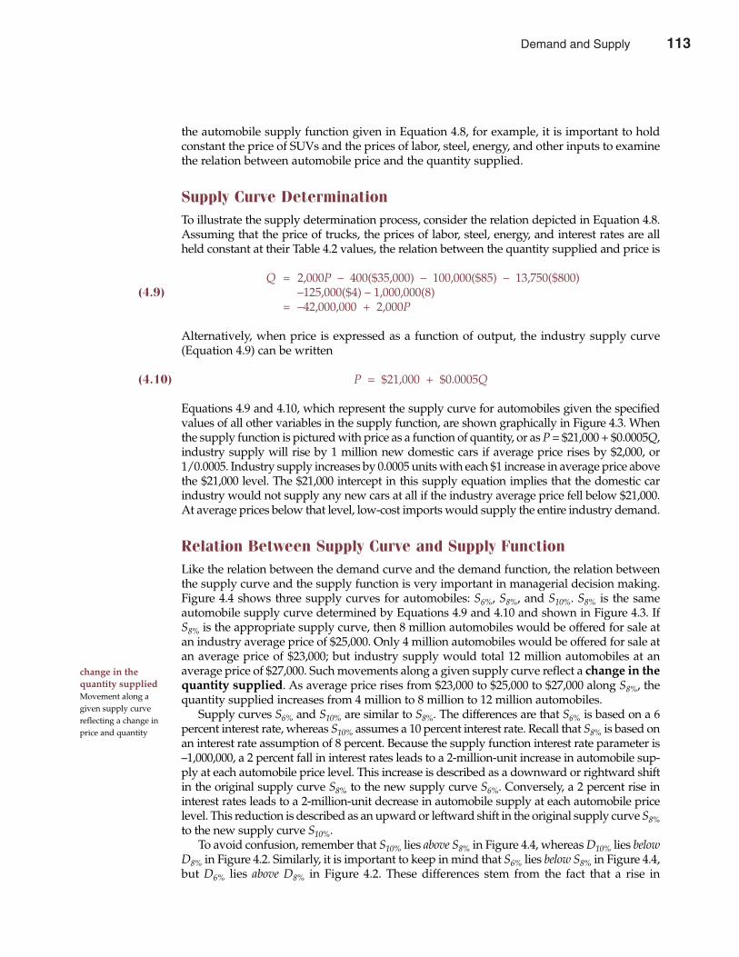
114 Part Two Demand Analysis
the automobile supply function given in Equation 4.8, for example, it is important to holdconstant the price of SUVs and the prices of labor, steel, energy, and other inputs to examinethe relation between automobile price and the quantity supplied.
Supply Curve DeterminationTo illustrate the supply determination process, consider the relation depicted in Equation 4.8.Assuming that the price of trucks, the prices of labor, steel, energy, and interest rates are allheld constant at their Table 4.2 values, the relation between the quantity supplied and price is
Q = 2,000P – 400($35,000) – 100,000($85) – 13,750($800)(4.9) –125,000($4) – 1,000,000(8)
= –42,000,000 + 2,000P
Alternatively, when price is expressed as a function of output, the industry supply curve(Equation 4.9) can be written
(4.10) P = $21,000 + $0.0005Q
Equations 4.9 and 4.10, which represent the supply curve for automobiles given the specifiedvalues of all other variables in the supply function, are shown graphically in Figure 4.3. Whenthe supply function is pictured with price as a function of quantity, or as P = $21,000 + $0.0005Q,industry supply will rise by 1 million new domestic cars if average price rises by $2,000, or1/0.0005. Industry supply increases by 0.0005 units with each $1 increase in average price abovethe $21,000 level. The $21,000 intercept in this supply equation implies that the domestic carindustry would not supply any new cars at all if the industry average price fell below $21,000.At average prices below that level, low-cost imports would supply the entire industry demand.
Relation Between Supply Curve and Supply FunctionLike the relation between the demand curve and the demand function, the relation betweenthe supply curve and the supply function is very important in managerial decision making.Figure 4.4 shows three supply curves for automobiles: S6%, S8%, and S10%. S8% is the sameautomobile supply curve determined by Equations 4.9 and 4.10 and shown in Figure 4.3. IfS8% is the appropriate supply curve, then 8 million automobiles would be offered for sale atan industry average price of $25,000. Only 4 million automobiles would be offered for sale atan average price of $23,000; but industry supply would total 12 million automobiles at anaverage price of $27,000. Such movements along a given supply curve reflect a change in thequantity supplied. As average price rises from $23,000 to $25,000 to $27,000 along S8%, thequantity supplied increases from 4 million to 8 million to 12 million automobiles.
Supply curves S6% and S10% are similar to S8%. The differences are that S6% is based on a 6percent interest rate, whereas S10% assumes a 10 percent interest rate. Recall that S8% is based onan interest rate assumption of 8 percent. Because the supply function interest rate parameter is–1,000,000, a 2 percent fall in interest rates leads to a 2-million-unit increase in automobile sup-ply at each automobile price level. This increase is described as a downward or rightward shiftin the original supply curve S8% to the new supply curve S6%. Conversely, a 2 percent rise ininterest rates leads to a 2-million-unit decrease in automobile supply at each automobile pricelevel. This reduction is described as an upward or leftward shift in the original supply curve S8%to the new supply curve S10%.
To avoid confusion, remember that S10% lies above S8% in Figure 4.4, whereas D10% lies belowD8% in Figure 4.2. Similarly, it is important to keep in mind that S6% lies below S8% in Figure 4.4,but D6% lies above D8% in Figure 4.2. These differences stem from the fact that a rise in
change in the quantity supplied Movement along agiven supply curvereflecting a change inprice and quantity
Demand and Supply 113
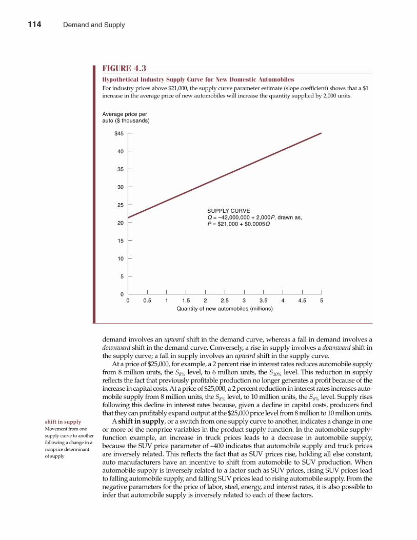
Chapter Four Demand and Supply 115
demand involves an upward shift in the demand curve, whereas a fall in demand involves adownward shift in the demand curve. Conversely, a rise in supply involves a downward shift inthe supply curve; a fall in supply involves an upward shift in the supply curve.
At a price of $25,000, for example, a 2 percent rise in interest rates reduces automobile supplyfrom 8 million units, the S8% level, to 6 million units, the S10% level. This reduction in supplyreflects the fact that previously profitable production no longer generates a profit because of theincrease in capital costs. At a price of $25,000, a 2 percent reduction in interest rates increases auto-mobile supply from 8 million units, the S8% level, to 10 million units, the S6% level. Supply risesfollowing this decline in interest rates because, given a decline in capital costs, producers findthat they can profitably expand output at the $25,000 price level from 8 million to 10 million units.
A shift in supply, or a switch from one supply curve to another, indicates a change in oneor more of the nonprice variables in the product supply function. In the automobile supply-function example, an increase in truck prices leads to a decrease in automobile supply,because the SUV price parameter of –400 indicates that automobile supply and truck pricesare inversely related. This reflects the fact that as SUV prices rise, holding all else constant,auto manufacturers have an incentive to shift from automobile to SUV production. Whenautomobile supply is inversely related to a factor such as SUV prices, rising SUV prices leadto falling automobile supply, and falling SUV prices lead to rising automobile supply. From thenegative parameters for the price of labor, steel, energy, and interest rates, it is also possible toinfer that automobile supply is inversely related to each of these factors.
shift in supply Movement from onesupply curve to anotherfollowing a change in anonprice determinantof supply
FIGURE 4.3Hypothetical Industry Supply Curve for New Domestic AutomobilesFor industry prices above $21,000, the supply curve parameter estimate (slope coefficient) shows that a $1increase in the average price of new automobiles will increase the quantity supplied by 2,000 units.
$45
40
35
30
25
20
15
10
5
0
SUPPLY CURVEQ = Ð42,000,000 + 2,000P, drawn as,P = $21,000 + $0.0005Q
0 0.5 1 1.5 2 2.5
Quantity of new automobiles (millions)
Average price perauto ($ thousands)
3 3.5 4 4.5 5
114 Demand and Supply
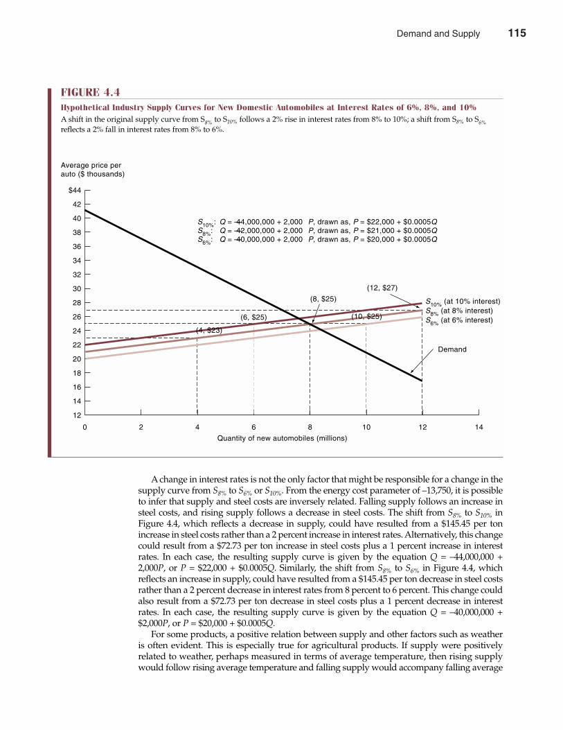
116 Part Two Demand Analysis
A change in interest rates is not the only factor that might be responsible for a change in thesupply curve from S8% to S6% or S10%. From the energy cost parameter of –13,750, it is possibleto infer that supply and steel costs are inversely related. Falling supply follows an increase insteel costs, and rising supply follows a decrease in steel costs. The shift from S8% to S10% inFigure 4.4, which reflects a decrease in supply, could have resulted from a $145.45 per tonincrease in steel costs rather than a 2 percent increase in interest rates. Alternatively, this changecould result from a $72.73 per ton increase in steel costs plus a 1 percent increase in interestrates. In each case, the resulting supply curve is given by the equation Q = –44,000,000 +2,000P, or P = $22,000 + $0.0005Q. Similarly, the shift from S8% to S6% in Figure 4.4, whichreflects an increase in supply, could have resulted from a $145.45 per ton decrease in steel costsrather than a 2 percent decrease in interest rates from 8 percent to 6 percent. This change couldalso result from a $72.73 per ton decrease in steel costs plus a 1 percent decrease in interestrates. In each case, the resulting supply curve is given by the equation Q = –40,000,000 +$2,000P, or P = $20,000 + $0.0005Q.
For some products, a positive relation between supply and other factors such as weatheris often evident. This is especially true for agricultural products. If supply were positivelyrelated to weather, perhaps measured in terms of average temperature, then rising supplywould follow rising average temperature and falling supply would accompany falling average
FIGURE 4.4Hypothetical Industry Supply Curves for New Domestic Automobiles at Interest Rates of 6%, 8%, and 10%A shift in the original supply curve from S8% to S10% follows a 2% rise in interest rates from 8% to 10%; a shift from S8% to S6%reflects a 2% fall in interest rates from 8% to 6%.
$44
42
40
38
36
34
32
30
28
26
24
22
20
18
16
14
12
0 2 4
(6, $25)
(8, $25)
(12, $27)
6
Quantity of new automobiles (millions)
8 10 12 14
Demand
S10% (at 10% interest)S8% (at 8% interest)S6% (at 6% interest)
S10%: Q = —44,000,000 + 2,000 P, drawn as, P = $22,000 + $0.0005QS8%: Q = —42,000,000 + 2,000 P, drawn as, P = $21,000 + $0.0005QS6%: Q = —40,000,000 + 2,000 P, drawn as, P = $20,000 + $0.0005Q
Average price perauto ($ thousands)
(10, $25)
(4, $23)
Demand and Supply 115
Chapter Four Demand and Supply 117
temperature. Weather is not included in the automobile supply function because there is noclose relation between automobile supply and weather.
The distinction between changes in the quantity supplied, which reflect movementsalong a given supply curve, and a shift in supply, which reflects movement from one supplycurve to another, is important, as was the distinction between changes in the quantitydemanded and a shift in demand. Because the prices of related products, input prices, taxes,weather, and other factors affecting supply can be expected to vary from one period to thenext, assessing the individual importance of each factor becomes a challenging aspect ofmanagerial economics.
MARKET EQUILIBRIUM
Integrating the concepts of demand and supply establishes a framework for understandinghow they interact to determine market prices and quantities for all goods and services.When quantity demanded and quantity supplied are in perfect balance at a given price, theproduct market is said to be in equilibrium. An equilibrium is stable when underlyingdemand and supply conditions are expected to remain stationary in the foreseeable future.When underlying demand and supply are dynamic rather than constant, a change in cur-rent market prices and quantities is likely. A temporary market equilibrium of this type isoften referred to as an unstable equilibrium. To understand the forces that drive marketprices and quantities either up or down to achieve equilibrium, the concepts of surplus andshortage must be introduced.
equilibriumPerfect balance indemand and supply
Demand and Supply Conditions for Economists
The forces of demand and supply exert a powerfulinfluence on the market for goods and services, and forlabor and other inputs. An interesting case in point is theeconomics industry itself. The demand for economistsoriginates in the private sector, where they areemployed in business—usually in staff rather than linepositions—as consultants and commentators; in gov-ernment, where economic analysis often guides publicpolicy; and in academia, where economists are employedin teaching capacities, primarily at the college and uni-versity levels.
Financial economists on Wall Street help price andmarket complex financial instruments. Although no morethan 500 to 1,000 financial economists are employed inthis capacity, lucrative bonus-based compensation plansmake them highly visible. The National Association ofBusiness Economists counts roughly 3,000 members.However, the employment of business economists iscyclical. During recessions, brokerages, banks, and otherfinancial institutions trim their economics staff consider-ably. Consulting and speech making is the glamour endof the business. Stars can earn hundreds of thousands of
dollars per year, but the supply of such “superstars” isseverely limited.
An overwhelming majority of the 20,000 members ofthe American Economic Association (AEA) hold academicjobs. According to Job Openings for Economists, an AEApublication, 80 percent to 90 percent of all job opportunitiesfor Ph.D. economists are in four-year colleges and univer-sities. Since the mid-1970s, the number of new Ph.D.s ineconomics has held steady at 750 to 800 per year, orroughly equivalent to the number of Ph.D.s granted in allareas of business administration combined. With relativelyscarce supply, new Ph.D.s in accounting and finance enjoymuch higher starting salaries than new Ph.D.s in econom-ics. Good business opportunities explain the lack of Ph.D.candidates from undergraduate programs in accountingand finance, but why don’t economics Ph.D. studentsswitch to accounting or finance?
See: Dow Jones Newswires, “Economists See Short, Mild Recession,Subject to Terrorism,” The Wall Street Journal Online, December 3, 2001(http://online.wsj.com).
M A N A G E R I A L A P P L I C AT I O N 4 . 4
116 Demand and Supply
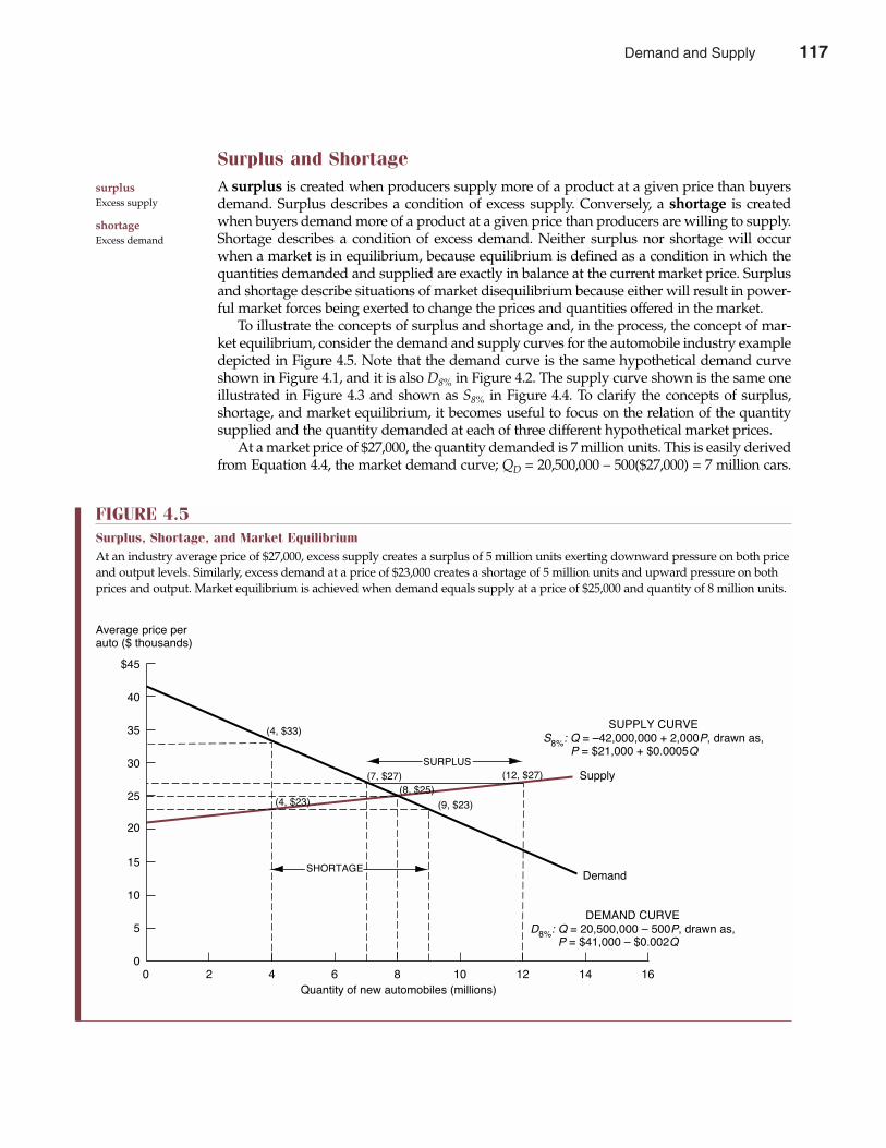
Surplus and ShortageA surplus is created when producers supply more of a product at a given price than buyersdemand. Surplus describes a condition of excess supply. Conversely, a shortage is createdwhen buyers demand more of a product at a given price than producers are willing to supply.Shortage describes a condition of excess demand. Neither surplus nor shortage will occurwhen a market is in equilibrium, because equilibrium is defined as a condition in which thequantities demanded and supplied are exactly in balance at the current market price. Surplusand shortage describe situations of market disequilibrium because either will result in power-ful market forces being exerted to change the prices and quantities offered in the market.
To illustrate the concepts of surplus and shortage and, in the process, the concept of mar-ket equilibrium, consider the demand and supply curves for the automobile industry exampledepicted in Figure 4.5. Note that the demand curve is the same hypothetical demand curveshown in Figure 4.1, and it is also D8% in Figure 4.2. The supply curve shown is the same oneillustrated in Figure 4.3 and shown as S8% in Figure 4.4. To clarify the concepts of surplus,shortage, and market equilibrium, it becomes useful to focus on the relation of the quantitysupplied and the quantity demanded at each of three different hypothetical market prices.
At a market price of $27,000, the quantity demanded is 7 million units. This is easily derivedfrom Equation 4.4, the market demand curve; QD = 20,500,000 – 500($27,000) = 7 million cars.
118 Part Two Demand Analysis
surplusExcess supply
shortageExcess demand
FIGURE 4.5Surplus, Shortage, and Market EquilibriumAt an industry average price of $27,000, excess supply creates a surplus of 5 million units exerting downward pressure on both priceand output levels. Similarly, excess demand at a price of $23,000 creates a shortage of 5 million units and upward pressure on bothprices and output. Market equilibrium is achieved when demand equals supply at a price of $25,000 and quantity of 8 million units.
$45
40
35
30
25
20
15
10
5
00 168 10 122 4 6 14
Quantity of new automobiles (millions)
Average price perauto ($ thousands)
Supply
Demand
(7, $27) (12, $27)
SUPPLY CURVES8%
: Q = Ð42,000,000 + 2,000P, drawn as, P = $21,000 + $0.0005Q
DEMAND CURVED8%
: Q = 20,500,000 Ð 500P, drawn as, P = $41,000 Ð $0.002Q
(4, $33)
(4, $23) (9, $23)
SHORTAGE
SURPLUS
(8, $25)
Demand and Supply 117
Chapter Four Demand and Supply 119
The quantity supplied at an industry average price of $27,000 is derived from the market supplycurve, Equation 4.9, which indicates that QS = –42,000,000 + 2,000($27,000) = 12 million cars. Atan average automobile price of $27,000, the quantity supplied greatly exceeds the quantitydemanded. This difference of 5 million cars per year (= 12 – 7) constitutes a surplus.
An automobile surplus results in a near-term buildup in inventories and downward pressureon market prices and production. This is typical for a market with a surplus of product. Pricestend to decline as firms recognize that consumers are unwilling to purchase the quantity of prod-uct available at prevailing prices. Similarly, producers cut back on production as inventoriesbuild up and prices soften, reducing the quantity of product supplied in future periods. Theautomobile industry uses rebate programs and dealer-subsidized low-interest-rate financing onnew cars to effectively combat the problem of periodic surplus automobile production.
A different type of market imbalance is also illustrated in Figure 4.5. At an average pricefor new domestic cars of $23,000, the quantity demanded rises to 9 million cars, QD =20,500,000 – 500($23,000) = 9 million. At the same time, the quantity supplied falls to 4 mil-lion units, QS = –42,000,000 + 2,000($23,000) = 4 million. This difference of 5 million cars peryear (= 9 – 4) constitutes a shortage. Shortage, or excess demand, reflects the fact that, giventhe current productive capability of the industry (including technology, input prices, and soon), producers cannot profitably supply more than 4 million units of output per year at anaverage price of $23,000, despite buyer demand for more output.
Shortages exert a powerful upward force on both market prices and output levels. In thisexample, the demand curve indicates that with only 4 million automobiles supplied, buyers wouldbe willing to pay an industry average price of $33,000 [= $41,000 – $0.002(4,000,000)]. Consumerswould bid against one another for the limited supply of automobiles and cause prices to rise. Theresulting increase in price would motivate manufacturers to increase production while reducingthe number of buyers willing and able to purchase cars. The resulting increase in the quantitysupplied and reduction in quantity demanded work together to eventually eliminate the shortage.
The market situation at a price of $25,000 and a quantity of 8 million automobiles per yearis displayed graphically as a balance between the quantity demanded and the quantity sup-plied. This is a condition of market equilibrium. There is no tendency for change in either priceor quantity at a price of $25,000 and a quantity of 8 million units. The graph shows that any priceabove $25,000 results in surplus production. Prices in this range create excess supply, a buildupin inventories, and pressure for an eventual decline in prices to the $25,000 equilibrium level. Atprices below $25,000, shortage occurs, which creates pressure for price increases. With pricesmoving up, producers are willing to supply more product and the quantity demanded declines,thus reducing the shortage.
Only a market price of $25,000 brings the quantity demanded and the quantity suppliedinto perfect balance. This price is referred to as the market equilibrium price, or the marketclearing price, because it just clears the market of all supplied product. Table 4.3 shows thesurplus of quantity supplied at prices above the market equilibrium price and the shortagethat results at prices below the market equilibrium price.
In short, surplus describes an excess in the quantity supplied over the quantity demandedat a given market price. A surplus results in downward pressure on both market prices andindustry output. Shortage describes an excess in the quantity demanded over the quantitysupplied at a given market price. A shortage results in upward pressure on both market pricesand industry output. Market equilibrium describes a condition of perfect balance in the quanti-ty demanded and the quantity supplied at a given price. In equilibrium, there is no tendency forchange in either price or quantity.
Comparative Statics: Changing DemandManagers typically control a number of the factors that affect product demand or supply. Tomake appropriate decisions concerning those variables, it is often useful to know how altering
market equilibriumpriceMarket clearing price
118 Demand and Supply
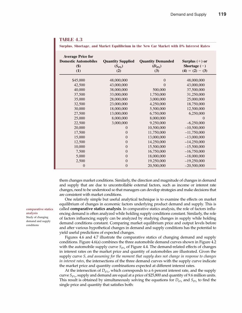
120 Part Two Demand Analysis
them changes market conditions. Similarly, the direction and magnitude of changes in demandand supply that are due to uncontrollable external factors, such as income or interest ratechanges, need to be understood so that managers can develop strategies and make decisions thatare consistent with market conditions.
One relatively simple but useful analytical technique is to examine the effects on marketequilibrium of changes in economic factors underlying product demand and supply. This iscalled comparative statics analysis. In comparative statics analysis, the role of factors influ-encing demand is often analyzed while holding supply conditions constant. Similarly, the roleof factors influencing supply can be analyzed by studying changes in supply while holdingdemand conditions constant. Comparing market equilibrium price and output levels beforeand after various hypothetical changes in demand and supply conditions has the potential toyield useful predictions of expected changes.
Figures 4.6 and 4.7 illustrate the comparative statics of changing demand and supplyconditions. Figure 4.6(a) combines the three automobile demand curves shown in Figure 4.2with the automobile supply curve S8% of Figure 4.4. The demand-related effects of changesin interest rates on the market price and quantity of automobiles are illustrated. Given thesupply curve S, and assuming for the moment that supply does not change in response to changesin interest rates, the intersections of the three demand curves with the supply curve indicatethe market price and quantity combinations expected at different interest rates.
At the intersection of D6%, which corresponds to a 6 percent interest rate, and the supplycurve S8%, supply and demand are equal at a price of $25,800 and quantity of 9.6 million units.This result is obtained by simultaneously solving the equations for D6% and S8% to find thesingle price and quantity that satisfies both:
comparative staticsanalysis Study of changingdemand and supplyconditions
TABLE 4.3Surplus, Shortage, and Market Equilibrium in the New Car Market with 8% Interest Rates
Average Price forDomestic Automobiles Quantity Supplied Quantity Demanded Surplus (�) or
($) (S8%) (D8%) Shortage (�)(1) (2) (3) (4) � (2) � (3)
$45,000 48,000,000 0 48,000,00042,500 43,000,000 0 43,000,00040,000 38,000,000 500,000 37,500,00037,500 33,000,000 1,750,000 31,250,00035,000 28,000,000 3,000,000 25,000,00032,500 23,000,000 4,250,000 18,750,00030,000 18,000,000 5,500,000 12,500,00027,500 13,000,000 6,750,000 6,250,00025,000 8,000,000 8,000,000 022,500 3,000,000 9,250,000 –6,250,00020,000 0 10,500,000 –10,500,00017,500 0 11,750,000 –11,750,00015,000 0 13,000,000 –13,000,00012,500 0 14,250,000 –14,250,00010,000 0 15,500,000 –15,500,0007,500 0 16,750,000 –16,750,0005,000 0 18,000,000 –18,000,0002,500 0 19,250,000 –19,250,000
0 0 20,500,000 –20,500,000
Demand and Supply 119
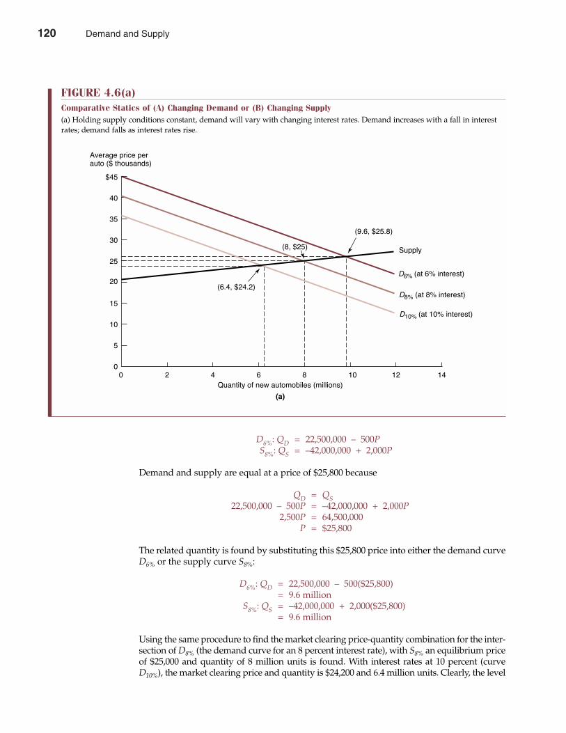
Chapter Four Demand and Supply 121
D6%: QD = 22,500,000 – 500PS8%: QS = –42,000,000 + 2,000P
Demand and supply are equal at a price of $25,800 because
QD = QS22,500,000 – 500P = –42,000,000 + 2,000P
2,500P = 64,500,000P = $25,800
The related quantity is found by substituting this $25,800 price into either the demand curveD6% or the supply curve S8%:
D6%: QD = 22,500,000 – 500($25,800)= 9.6 million
S8%: QS = –42,000,000 + 2,000($25,800)= 9.6 million
Using the same procedure to find the market clearing price-quantity combination for the inter-section of D8% (the demand curve for an 8 percent interest rate), with S8% an equilibrium priceof $25,000 and quantity of 8 million units is found. With interest rates at 10 percent (curveD10%), the market clearing price and quantity is $24,200 and 6.4 million units. Clearly, the level
FIGURE 4.6(a)Comparative Statics of (A) Changing Demand or (B) Changing Supply(a) Holding supply conditions constant, demand will vary with changing interest rates. Demand increases with a fall in interestrates; demand falls as interest rates rise.
Quantity of new automobiles (millions)
(a)
(9.6, $25.8)
D10% (at 10% interest)
D8% (at 8% interest)
D6% (at 6% interest)
Supply
(6.4, $24.2)
(8, $25)
$45
40
35
30
25
20
15
10
5
00 8 10 122 4 6 14
Average price perauto ($ thousands)
120 Demand and Supply
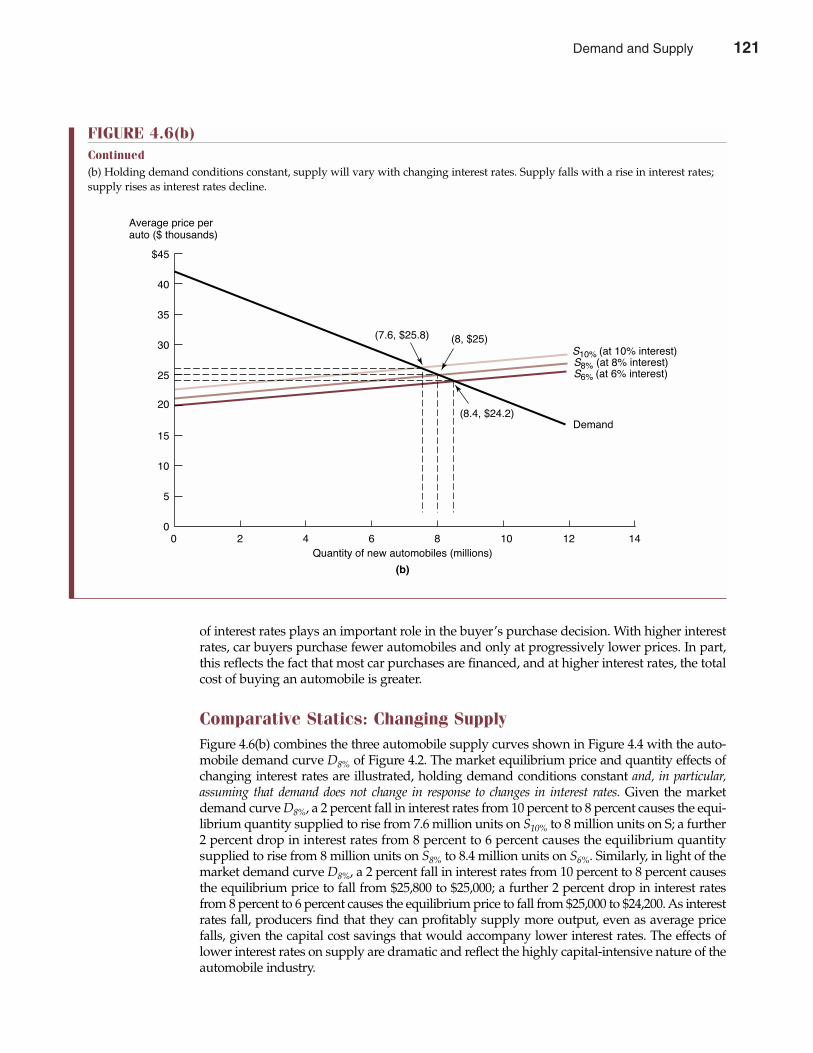
122 Part Two Demand Analysis
of interest rates plays an important role in the buyer’s purchase decision. With higher interestrates, car buyers purchase fewer automobiles and only at progressively lower prices. In part,this reflects the fact that most car purchases are financed, and at higher interest rates, the totalcost of buying an automobile is greater.
Comparative Statics: Changing SupplyFigure 4.6(b) combines the three automobile supply curves shown in Figure 4.4 with the auto-mobile demand curve D8% of Figure 4.2. The market equilibrium price and quantity effects ofchanging interest rates are illustrated, holding demand conditions constant and, in particular,assuming that demand does not change in response to changes in interest rates. Given the marketdemand curve D8%, a 2 percent fall in interest rates from 10 percent to 8 percent causes the equi-librium quantity supplied to rise from 7.6 million units on S10% to 8 million units on S; a further2 percent drop in interest rates from 8 percent to 6 percent causes the equilibrium quantitysupplied to rise from 8 million units on S8% to 8.4 million units on S6%. Similarly, in light of themarket demand curve D8%, a 2 percent fall in interest rates from 10 percent to 8 percent causesthe equilibrium price to fall from $25,800 to $25,000; a further 2 percent drop in interest ratesfrom 8 percent to 6 percent causes the equilibrium price to fall from $25,000 to $24,200. As interestrates fall, producers find that they can profitably supply more output, even as average pricefalls, given the capital cost savings that would accompany lower interest rates. The effects oflower interest rates on supply are dramatic and reflect the highly capital-intensive nature of theautomobile industry.
FIGURE 4.6(b)Continued(b) Holding demand conditions constant, supply will vary with changing interest rates. Supply falls with a rise in interest rates;supply rises as interest rates decline.
Quantity of new automobiles (millions)
(b)
(8, $25)
S6% (at 6% interest)S8% (at 8% interest)S10% (at 10% interest)
Demand
(7.6, $25.8)
(8.4, $24.2)
0 8 10 122 4 6 14
Average price perauto ($ thousands)
$45
40
35
30
25
20
15
10
5
0
Demand and Supply 121
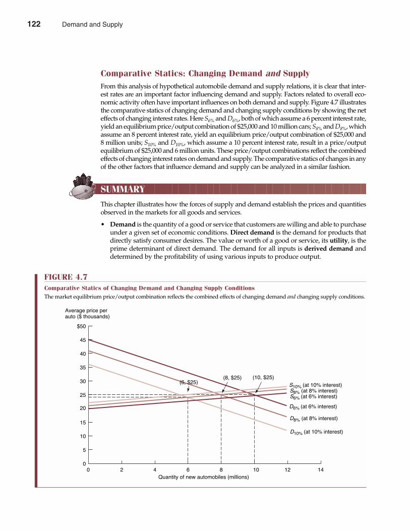
Comparative Statics: Changing Demand and SupplyFrom this analysis of hypothetical automobile demand and supply relations, it is clear that inter-est rates are an important factor influencing demand and supply. Factors related to overall eco-nomic activity often have important influences on both demand and supply. Figure 4.7 illustratesthe comparative statics of changing demand and changing supply conditions by showing the neteffects of changing interest rates. Here S6% and D6%, both of which assume a 6 percent interest rate,yield an equilibrium price/output combination of $25,000 and 10 million cars; S8% and D8%, whichassume an 8 percent interest rate, yield an equilibrium price/output combination of $25,000 and8 million units; S10% and D10%, which assume a 10 percent interest rate, result in a price/outputequilibrium of $25,000 and 6 million units. These price/output combinations reflect the combinedeffects of changing interest rates on demand and supply. The comparative statics of changes in anyof the other factors that influence demand and supply can be analyzed in a similar fashion.
SUMMARY
This chapter illustrates how the forces of supply and demand establish the prices and quantitiesobserved in the markets for all goods and services.
• Demand is the quantity of a good or service that customers are willing and able to purchaseunder a given set of economic conditions. Direct demand is the demand for products thatdirectly satisfy consumer desires. The value or worth of a good or service, its utility, is theprime determinant of direct demand. The demand for all inputs is derived demand anddetermined by the profitability of using various inputs to produce output.
Chapter Four Demand and Supply 123
FIGURE 4.7Comparative Statics of Changing Demand and Changing Supply ConditionsThe market equilibrium price/output combination reflects the combined effects of changing demand and changing supply conditions.
S6% (at 6% interest)S8% (at 8% interest)S10% (at 10% interest)
Quantity of new automobiles (millions)
D10% (at 10% interest)
D8% (at 8% interest)
D6% (at 6% interest)
$50
45
40
35
30
25
20
15
10
5
00 8 10 122 4 6 14
Average price perauto ($ thousands)
(10, $25)(8, $25)(6, $25)
122 Demand and Supply
124 Part Two Demand Analysis
• The market demand function for a product is a statement of the relation between theaggregate quantity demanded and all factors that affect this quantity. The demand curveexpresses the relation between the price charged for a product and the quantity demanded,holding constant the effects of all other variables.
• A change in the quantity demanded is a movement along a single demand curve. A shiftin demand, or shift from one demand curve to another, reflects a change in one or more ofthe nonprice variables in the product demand function.
• The term supply refers to the quantity of a good or service that producers are willing andable to sell under a given set of conditions. The market supply function for a product is astatement of the relation between the quantity supplied and all factors affecting that quantity.A supply curve expresses the relation between the price charged and the quantity supplied,holding constant the effects of all other variables.
• Movements along a supply curve reflect change in the quantity supplied. A shift in supply,or a switch from one supply curve to another, indicates a change in one or more of the non-price variables in the product supply function.
• A market is in equilibrium when the quantity demanded and the quantity supplied are inperfect balance at a given price. Surplus describes a condition of excess supply. Shortage iscreated when buyers demand more of a product at a given price than producers are willingto supply. The market equilibrium price just clears the market of all supplied product.
• In comparative statics analysis, the role of factors influencing demand or supply is analyzedwhile holding all else equal.
A fundamental understanding of demand and supply concepts is essential to the successfuloperation of any economic organization. The concepts introduced in this chapter provide thestructure for the more detailed analysis of demand and supply in subsequent chapters.
QUESTIONS
Q4.1 What key ingredients are necessary for the creation of economic demand?Q4.2 Describe the difference between direct demand and derived demand.Q4.3 Explain the rationale for each of the demand variables in Equation 4.1.Q4.4 Distinguish between a demand function and a demand curve. What is the difference between
a change in the quantity demanded and a shift in the demand curve?Q4.5 What key ingredients are necessary for the creation of economic supply?Q4.6 Explain the rationale for each of the supply variables in Equation 4.5.Q4.7 Distinguish between a supply function and a supply curve. What is the difference between a
change in the quantity supplied and a shift in the supply curve?Q4.8 “Dynamic rather than static demand and supply conditions are typically observed in real-world
markets. Therefore, comparative statics analysis has only limited value.” Discuss this statement.Q4.9 Contrast the supply and demand conditions for new Ph.D.s in economics and accounting.
Why do such large differences in starting salaries seem to persist over time?Q4.10 Suppose the personal income tax was replaced with a national sales tax. How would this
affect aggregate supply, aggregate demand, and interest rates?
SELF-TEST PROBLEMS AND SOLUTIONS
ST4.1 Demand and Supply Curves. The following relations describe demand and supply conditionsin the lumber/forest products industry:
Demand and Supply 123
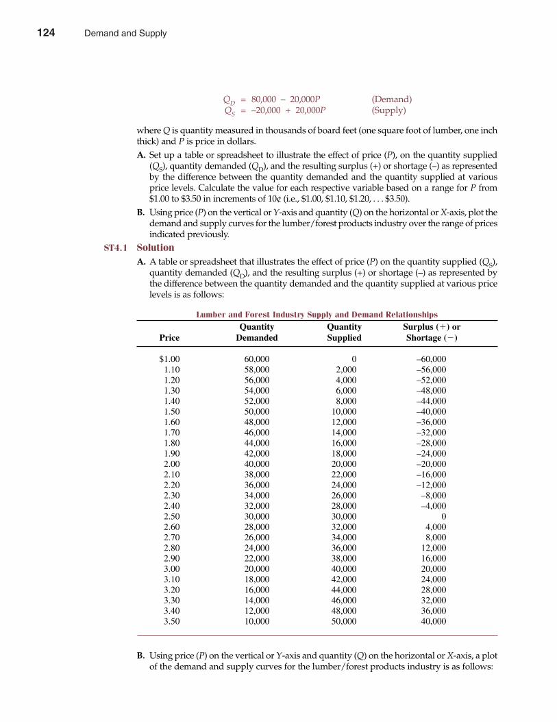
Chapter Four Demand and Supply 125
QD = 80,000 – 20,000P (Demand)QS = –20,000 + 20,000P (Supply)
where Q is quantity measured in thousands of board feet (one square foot of lumber, one inchthick) and P is price in dollars.A. Set up a table or spreadsheet to illustrate the effect of price (P), on the quantity supplied
(QS), quantity demanded (QD), and the resulting surplus (+) or shortage (–) as representedby the difference between the quantity demanded and the quantity supplied at variousprice levels. Calculate the value for each respective variable based on a range for P from$1.00 to $3.50 in increments of 10¢ (i.e., $1.00, $1.10, $1.20, . . . $3.50).
B. Using price (P) on the vertical or Y-axis and quantity (Q) on the horizontal or X-axis, plot thedemand and supply curves for the lumber/forest products industry over the range of pricesindicated previously.
ST4.1 SolutionA. A table or spreadsheet that illustrates the effect of price (P) on the quantity supplied (QS),
quantity demanded (QD), and the resulting surplus (+) or shortage (–) as represented bythe difference between the quantity demanded and the quantity supplied at various pricelevels is as follows:
B. Using price (P) on the vertical or Y-axis and quantity (Q) on the horizontal or X-axis, a plotof the demand and supply curves for the lumber/forest products industry is as follows:
Lumber and Forest Industry Supply and Demand Relationships
Quantity Quantity Surplus (�) orPrice Demanded Supplied Shortage (�)
$1.00 60,000 0 –60,0001.10 58,000 2,000 –56,0001.20 56,000 4,000 –52,0001.30 54,000 6,000 –48,0001.40 52,000 8,000 –44,0001.50 50,000 10,000 –40,0001.60 48,000 12,000 –36,0001.70 46,000 14,000 –32,0001.80 44,000 16,000 –28,0001.90 42,000 18,000 –24,0002.00 40,000 20,000 –20,0002.10 38,000 22,000 –16,0002.20 36,000 24,000 –12,0002.30 34,000 26,000 –8,0002.40 32,000 28,000 –4,0002.50 30,000 30,000 02.60 28,000 32,000 4,0002.70 26,000 34,000 8,0002.80 24,000 36,000 12,0002.90 22,000 38,000 16,0003.00 20,000 40,000 20,0003.10 18,000 42,000 24,0003.20 16,000 44,000 28,0003.30 14,000 46,000 32,0003.40 12,000 48,000 36,0003.50 10,000 50,000 40,000
124 Demand and Supply
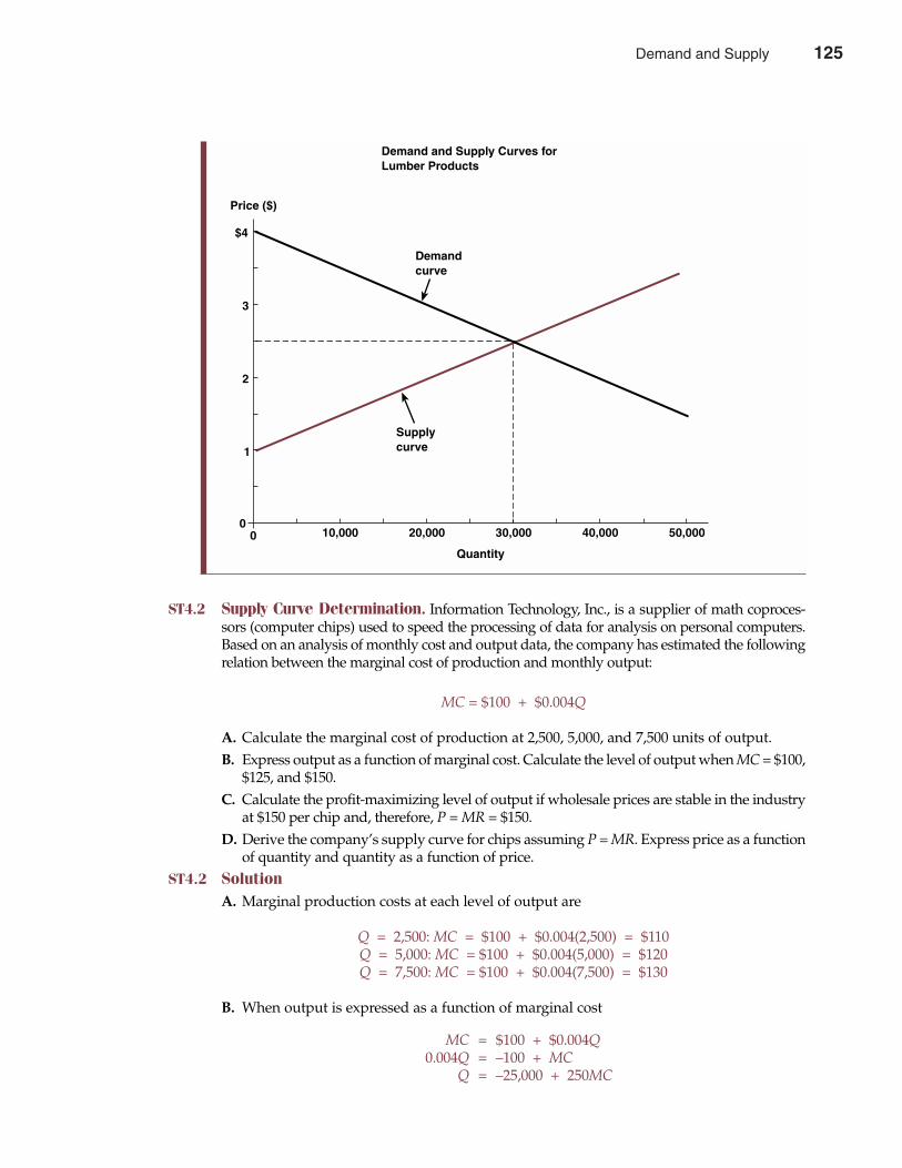
126 Part Two Demand Analysis
ST4.2 Supply Curve Determination. Information Technology, Inc., is a supplier of math coproces-sors (computer chips) used to speed the processing of data for analysis on personal computers.Based on an analysis of monthly cost and output data, the company has estimated the followingrelation between the marginal cost of production and monthly output:
MC = $100 + $0.004Q
A. Calculate the marginal cost of production at 2,500, 5,000, and 7,500 units of output.B. Express output as a function of marginal cost. Calculate the level of output when MC = $100,
$125, and $150.C. Calculate the profit-maximizing level of output if wholesale prices are stable in the industry
at $150 per chip and, therefore, P = MR = $150.D. Derive the company’s supply curve for chips assuming P = MR. Express price as a function
of quantity and quantity as a function of price.ST4.2 Solution
A. Marginal production costs at each level of output are
Q = 2,500: MC = $100 + $0.004(2,500) = $110Q = 5,000: MC = $100 + $0.004(5,000) = $120Q = 7,500: MC = $100 + $0.004(7,500) = $130
B. When output is expressed as a function of marginal cost
MC = $100 + $0.004Q0.004Q = –100 + MC
Q = –25,000 + 250MC
Demand and Supply Curves forLumber Products
Price ($)
Demandcurve
Supplycurve
Quantity
1
2
3
$4
00 10,000 20,000 30,000 40,000 50,000
Demand and Supply 125
The level of output at each respective level of marginal cost is
MC = $100: Q = –25,000 + 250($100) = 0MC = $125: Q = –25,000 + 250($125) = 6,250MC = $150: Q = –25,000 + 250($150) = 12,500
C. Note from part B that MC = $150 when Q = 12,500. Therefore, when MR = $150, Q = 12,500will be the profit-maximizing level of output. More formally,
MR = MC$150 = $100 + $0.004Q
0.004Q = 50Q = 12,500
D. Because prices are stable in the industry, P = MR, this means that the company will supplychips at the level of output where
MR = MC
and, therefore, that
P = $100 + $0.004Q
This is the supply curve for math chips, where price is expressed as a function of quantity.When quantity is expressed as a function of price
P = $100 + $0.004Q0.004Q = –100 + P
Q = –25,000 + 250P
PROBLEMS
P4.1 Demand and Supply Curves. The following relations describe monthly demand and supplyconditions in the metropolitan area for recyclable aluminum:
QD = 317,500 – 10,000P (Demand)QS = 2,500 + 7,500P (Supply)
where Q is quantity measured in pounds of scrap aluminum and P is price in cents.Complete the following table:
Chapter Four Demand and Supply 127
Quantity Quantity Surplus (�) orPrice Supplied Demanded Shortage (�)
(1) (2) (3) (4) � (2) � (3)
15¢1617181920
126 Demand and Supply
P4.2 Demand and Supply Curves. The following relations describe monthly demand and supplyrelations for dry cleaning services in the metropolitan area:
QD = 500,000 – 50,000P (Demand)QS = –100,000 + 100,000P (Supply)
where Q is quantity measured by the number of items dry cleaned per month and P is averageprice in dollars.A. At what average price level would demand equal zero?B. At what average price level would supply equal zero?C. Calculate the equilibrium price/output combination.
P4.3 Demand Analysis. The demand for housing is often described as being highly cyclical andvery sensitive to housing prices and interest rates. Given these characteristics, describe theeffect of each of the following in terms of whether it would increase or decrease the quantitydemanded or the demand for housing. Moreover, when price is expressed as a function ofquantity, indicate whether the effect of each of the following is an upward or downward move-ment along a given demand curve or involves an outward or inward shift in the relevantdemand curve for housing. Explain your answers.A. An increase in housing pricesB. A fall in interest ratesC. A rise in interest ratesD. A severe economic recessionE. A robust economic expansion
P4.4 Demand and Supply Curves. Demand and supply conditions in the market for unskilledlabor are important concerns to business and government decision makers. Consider the caseof a federally mandated minimum wage set above the equilibrium, or market clearing, wagelevel. Some of the following factors have the potential to influence the demand or quantitydemanded of unskilled labor. Influences on the supply or quantity supplied may also result.Holding all else equal, describe these influences as increasing or decreasing, and indicate thedirection of the resulting movement along or shift in the relevant curve(s).A. An increase in the quality of secondary educationB. A rise in welfare benefitsC. An increase in the popularity of self-service gas stations, car washes, and so onD. A fall in interest ratesE. An increase in the minimum wage
P4.5 Demand Function. The Creative Publishing Company (CPC) is a coupon book publisherwith markets in several southeastern states. CPC coupon books are either sold directly to thepublic, sold through religious and other charitable organizations, or given away as promo-tional items. Operating experience during the past year suggests the following demandfunction for CPC’s coupon books:
Q = 5,000 – 4,000P + 0.02Pop + 0.5I + 1.5A
where Q is quantity, P is price ($), Pop is population, I is disposable income per household ($),and A is advertising expenditures ($).A. Determine the demand faced by CPC in a typical market in which P = $10, Pop = 1,000,000
persons, I = $30,000, and A = $10,000.
128 Part Two Demand Analysis
Demand and Supply 127
Chapter Four Demand and Supply 129
B. Calculate the level of demand if CPC increases annual advertising expenditures from$10,000 to $15,000.
C. Calculate the demand curves faced by CPC in parts A and B.P4.6 Demand Curves. The Eastern Shuttle, Inc., is a regional airline providing shuttle service
between New York and Washington, DC. An analysis of the monthly demand for service hasrevealed the following demand relation:
Q = 26,000 – 500P – 250POG + 200IB – 5,000S
where Q is quantity measured by the number of passengers per month, P is price ($), POG is aregional price index for other consumer goods (1967 = 1.00), IB is an index of business activity,and S, a binary or dummy variable, equals 1 in summer months and 0 otherwise.A. Determine the demand curve facing the airline during the winter month of January if POG =
4 and IB = 250.B. Determine the demand curve facing the airline, quantity demanded, and total revenues
during the summer month of July if P = $100 and all other price-related and businessactivity variables are as specified previously.
P4.7 Supply Function. A review of industrywide data for the jelly and jam manufacturingindustry suggests the following industry supply function:
Q = –59,000,000 + 500,000P – 125,000PL– 500,000PK + 2,000,000W
where Q is cases supplied per year, P is the wholesale price per case ($), PL is the average pricepaid for unskilled labor ($), PK is the average price of capital (in percent), and W is weathermeasured by the average seasonal rainfall in growing areas (in inches).A. Determine the industry supply curve for a recent year when PL = $8, PK = 10 percent, and
W = 20 inches of rainfall. Show the industry supply curve with quantity expressed as afunction of price and price expressed as a function of quantity.
B. Calculate the quantity supplied by the industry at prices of $50, $60, and $70 per case.C. Calculate the prices necessary to generate a supply of 4 million, 6 million, and 8 million cases.
P4.8 Supply Curve Determination. Olympia Natural Resources, Inc., and Yakima Lumber, Ltd.,supply cut logs (raw lumber) to lumber and paper mills located in the Cascade Mountainregion in the state of Washington. Each company has a different marginal cost of productiondepending on its own cost of landowner access, labor and other cutting costs, the distance cutlogs must be shipped, and so on. The marginal cost of producing one unit of output, measuredas 1,000 board feet of lumber (where 1 board foot is 1 square foot of lumber, 1-inch thick), is
MCO = $350 + $0.00005QO (Olympia)MCY = $150 + $0.0002QY (Yakima)
The wholesale market for cut logs is vigorously price competitive, and neither firm is able tocharge a premium for its products. Thus, P = MR in this market.A. Determine the supply curve for each firm. Express price as a function of quantity and
quantity as a function of price. (Hint: Set P = MR = MC to find each firm’s supply curve.)B. Calculate the quantity supplied by each firm at prices of $325, $350, and $375. What is the
minimum price necessary for each individual firm to supply output?
128 Demand and Supply
C. Assuming these two firms make up the entire industry in the local area, determine theindustry supply curve when P < $350.
D. Determine the industry supply curve when P > $350. To check your answer, calculatequantity at an industry price of $375 and compare your result with part B.
P4.9 Supply Curve Determination. Cornell Pharmaceutical, Inc., and Penn Medical, Ltd.,supply generic drugs to treat a variety of illnesses. A major product for each company is ageneric equivalent of an antibiotic used to treat postoperative infections. Proprietary costand output information for each company reveal the following relations between marginalcost and output:
MCC = $10 + $0.004QC (Cornell)MCP = $8 + $0.008QP (Penn)
The wholesale market for generic drugs is vigorously price competitive, and neither firm is ableto charge a premium for its products. Thus, P = MR in this market.A. Determine the supply curve for each firm. Express price as a function of quantity and
quantity as a function of price. (Hint: Set P = MR = MC to find each firm’s supply curve.)B. Calculate the quantity supplied by each firm at prices of $8, $10, and $12. What is the
minimum price necessary for each individual firm to supply output?C. Assuming these two firms make up the entire industry, determine the industry supply curve
when P < $10.D. Determine the industry supply curve when P > $10. To check your answer, calculate
quantity at an industry price of $12 and compare your answer with part B.P4.10 Market Equilibrium. Eye-de-ho Potatoes is a product of the Coeur d’Alene Growers’
Association. Producers in the area are able to switch back and forth between potato andwheat production depending on market conditions. Similarly, consumers tend to regardpotatoes and wheat (bread and bakery products) as substitutes. As a result, the demandand supply of Eye-de-ho Potatoes are highly sensitive to changes in both potato and wheatprices.
Demand and supply functions for Eye-de-ho Potatoes are as follows:
QD = –1,450 – 25P + 12.5PW + 0.2Y (Demand)QS = –100 + 75P – 25PW – 12.5PL + 10R (Supply)
where P is the average wholesale price of Eye-de-ho Potatoes ($ per bushel), PW is the averagewholesale price of wheat ($ per bushel), Y is income (GNP in $ billions), PL is the average priceof unskilled labor ($ per hour), and R is the average annual rainfall (in inches). Both QD andQS are in millions of bushels of potatoes.A. When quantity is expressed as a function of price, what are the Eye-de-ho Potatoes demand
and supply curves if P = $2, PW = $4, Y = $7,500 billion, PL = $8, and R = 20 inches?B. Calculate the surplus or shortage of Eye-de-ho Potatoes when P = $1.50, $2, and $2.50.C. Calculate the market equilibrium price/output combination.
130 Part Two Demand Analysis
Demand and Supply 129
Chapter Four Demand and Supply 131
CASE STUDY
A Spreadsheet Analysis of Product Demand and Supply ConditionsSpreadsheet analysis is an appropriate means for studying the demand and supply effects ofpossible changes in various exogenous and endogenous variables. Endogenous variablesinclude all important demand- and supply-related factors that are within the control of thefirm. Examples include product pricing, advertising, product design, and so on. Exogenousvariables consist of all significant demand- and supply-related influences that are beyond thecontrol of the firm. Examples include competitor pricing, competitor advertising, weather,general economic conditions, and related factors.
In comparative statics analysis, the marginal influence on demand and supply of a changein any one factor can be isolated and studied in depth. The advantage of this approach is thatcausal relationships can be identified and responded to, if appropriate. The disadvantage ofthis marginal approach is that it becomes rather tedious to investigate the marginal effects ofa wide range of demand and supply influences. It is here that spreadsheet analysis of demandand supply conditions becomes useful. Using spreadsheet analysis, it is possible to learn thedemand and supply implications of an almost limitless range of operating scenarios. Ratherthan calculating the effects of only a few possibilities, it is feasible to consider even ratherunlikely outcomes. A complete picture can be drawn of the firm’s operating environment, andstrategies for responding to a host of operating conditions can be drawn up.
To illustrate this process, consider the case of Sunbest Orange Juice, a product of California’sOrange County Growers’ Association. Both demand and supply of the product are highlysensitive to changes in the weather. During hot summer months, demand for Sunbest and otherbeverages grows rapidly. However, hot, dry weather has an adverse effect on supply by reducingthe size of the orange crop.
Demand and supply functions for Sunbest are as follows:
QD = 12,275,000 – 2,500,000P + 200,000PS + 75Y + 5,000T (Demand)QS = –27,450 + 6,000,000P – 240,000PL – 220,000PK – 200,000T (Supply)
where P is the average wholesale price of Sunbest ($ per case), PS is the average wholesale priceof canned soda ($ per case), Y is disposable income per household ($), T is the average dailyhigh temperature (degrees), PL is the average price of unskilled labor ($ per hour), and PK isthe risk-adjusted cost of capital (in percent).
During the coming planning period, a wide variety of operating conditions are possible.To gauge the sensitivity of demand and supply to changes in these operating conditions, anumber of scenarios that employ a range from optimistic to relatively pessimistic assump-tions have been drawn up:
Operating Environment Price of Sunbest Price of Soda Disposable Income Temperaturefor Demand (P) (PS) (I) (T)
Optimistic Scenario 1 $5.00 $4.00 $39,500 78.75 2 4.80 4.10 39,400 79.00 3 4.60 4.20 39,300 79.25 4 4.40 4.30 39,200 79.50 5 4.20 4.40 39,100 79.75 6 4.00 4.50 39,000 80.00 7 3.80 4.60 38,900 80.25 8 3.60 4.70 38,800 80.50 9 3.40 4.80 38,700 80.75
Pessimistic Scenario 10 3.20 4.90 38,600 81.00
130 Demand and Supply
132 Part Two Demand Analysis
SELECTED REFERENCESArgon, Nilay Tanik, Refik Gullu, and Nesim Erkip. “Analysis of an Inventory System Under Backorder
Correlated Deterministic Demand and Geometric Supply Process.” International Journal ofProduction Economics 71 (May 2001): 247–254.
Bianchi, Marco, Bjöörn R. Gudmundsson, and Gylfi Zoega. “Iceland’s Natural Experiment in Supply-Side Economics.” American Economic Review 91 (December 2001): 1564–1579.
Bolle, Friedel. “Competition with Supply and Demand Functions.” Energy Economics 23 (May 2001):253–277.
CASE STUDY (continued)
Demand and supply functions for Sunbest orange juice can be combined with data on theoperating environment to construct estimates of demand, supply, and the amount of surplusor shortage under each operating scenario.A. Set up a table or spreadsheet to illustrate the effects of changing economic assumptions
on the demand for Sunbest orange juice. Use the demand function to calculate demandbased on three different underlying assumptions concerning changes in the operatingenvironment. First, assume that all demand factors change in unison from levels indicatedin the Optimistic Scenario #1 to the levels indicated in Pessimistic Scenario #10. Second,fix all demand factors except the price of Sunbest at Scenario #6 levels, and then calculatethe quantity demanded at each scenario price level. Finally, fix all demand factorsexcept temperature at Scenario #6 levels, and then calculate demand at each scenariotemperature level.
B. Set up a table or spreadsheet to illustrate the effects of changing economic assumptions onthe supply of Sunbest orange juice. Use the supply function to calculate supply based onthree different underlying assumptions concerning changes in the operating environment.First, assume that all supply factors change in unison from levels indicated in theOptimistic Scenario #1 to the levels indicated in Pessimistic Scenario #10. Second, fix allsupply factors except the price of Sunbest at Scenario #6 levels, and then calculate thequantity supplied at each scenario price level. Finally, fix all supply factors except temper-ature at Scenario #6 levels, and then calculate supply at each scenario temperature level.
C. Set up a table or spreadsheet to illustrate the effect of changing economic assumptions onthe surplus or shortage of Sunbest orange juice that results from each scenario detailed inpart A and part B. Which operating scenario results in market equilibrium?
D. Are demand and supply more sensitive to changes in the price of Sunbest or to changesin temperature?
Operating Environment Price of Sunbest Price of Labor Cost of Capital Temperaturefor Supply (P) (PL) (PK) (T)
Optimistic Scenario 1 $5.00 $8.00 9.00% 78.00 2 4.80 8.15 9.25% 77.75 3 4.60 8.30 9.50% 77.50 4 4.40 8.45 9.75% 77.25 5 4.20 8.60 10.00% 77.00 6 4.00 8.75 10.25% 76.75 7 3.80 8.90 10.50% 76.50 8 3.60 9.05 10.75% 76.25 9 3.40 9.20 11.00% 76.00
Pessimistic Scenario 10 3.20 9.35 11.25% 75.75
Demand and Supply 131

Cachon, Gerard P., and Martin A. Lariviere. “Contracting to Assure Supply: How to Share DemandForecasts in a Supply Chain.” Management Science 47 (May 2001): 629–646.
Canzoneri, Matthew B., Robert E. Cumby, and Behzad T. Diba. “Is the Price Level Determined by theNeeds of Fiscal Solvency?” American Economic Review 91 (December 2001): 1221–1238.
Colander, David. “Effective Supply and Effective Demand.” Journal of Post Keynesian Economics 23 (Spring2001): 375–381.
Corbett, Charles J., and Uday S. Karmarkar. “Competition and Structure in Serial Supply Chains withDeterministic Demand.” Management Science 47 (July 2001): 966–978.
Friedberg, Rachel M. “The Impact of Mass Migration on the Israeli Labor Market.” Quarterly Journal ofEconomics 116 (November 2001): 1373–1408.
Grahovac, Jovan, and Amiya Chakravarty. “Sharing and Lateral Transshipment of Inventory in a SupplyChain with Expensive Low-Demand Items.” Management Science 47 (April 2001): 579–594.
Kemp, Alexander G., and Linda Stephen. “Prospects for Gas Supply and Demand and TheirImplications with Special Reference to the U.K.” Oxford Review of Economic Policy 17 (Autumn 2001):346–364.
Keskinocak, Pinar, and Sridhar Tayur. “Quantitative Analysis for Internet-Enabled Supply Chains.”Interfaces 31 (March 2001): 70–109.
Milner, Josheph M., and Edieal J. Pinker. “Contingent Labor Contracting Under Demand and SupplyUncertainty.” Management Science 47 (August 2001): 1046–1062.
Prencipe, Loretta W. “Relief Is Here: Demand For IT Talent Remains High, But Supply Is GreatlyImproved.” Infoworld 23 (April 2001): 49.
Reeder, George, and Tim Rowell. “Integration of Supply Chain with Demand Planning—Tropicana’sJourney.” Journal of Business Forecasting Methods & Systems 20 (Fall 2001): 3–8.
Van Donselaar, Karel, Kopczak, Laura Rock, and Marc Wouters. “The Use of Advance DemandInformation in a Project-Based Supply Chain.” European Journal of Operational Research 130 (May2001): 519–538.
Chapter Four Demand and Supply 133
132 Demand and Supply
Demand Analysis and Estimation
CHAPTER FIVE
1341 See Emily Nelson, “Procter & Gamble’s Net Increases 8.8% on Cost-Cutting, Sales of
Pricier Items,” The Wall Street Journal Online, February 5, 2002 (http://online.wsj.com).
Procter & Gamble Co. (P&G) helps consumers clean up. Householdsaround the world rely on “new and improved” Tide to clean their clothes,
Ivory and Ariel detergents to wash dishes, and Pantene Pro-V to shampoo andcondition hair. Other P&G products dominate a wide range of lucrative, butslow-growing, product lines, including disposable diapers (Pampers), femininehygiene (Always), and facial moisturizers (Oil of Olay). P&G’s ongoing chal-lenge is to figure out ways of continuing to grow aggressively outside the UnitedStates while it cultivates the profitability of dominant consumer franchises hereat home. P&G’s challenge is made difficult by the fact that the company alreadyenjoys a dominant market position in many of its slow-growing domestic mar-kets. Worse yet, most of its brand names are aging, albeit gracefully. Tide, forexample, has been “new and improved” almost continuously over its 70-yearhistory. Ivory virtually introduced the concept of bar soap nearly 100 years ago;Jif peanut butter and Pampers disposable diapers are more than 40 years old.
How does P&G succeed in businesses where others routinely fail? Quitesimply, P&G is a marketing juggernaut. Although P&G’s vigilant cost-cutting islegendary, its marketing expertise is without peer. Nobody does a better job atfinding out what consumers want. At P&G, demand estimation is the lynchpinof its “getting close to the customer” operating philosophy.1
Nothing is more important in business than the need to identify and effec-tively meet customer demand. This chapter examines the elasticity concept as auseful means for measuring the sensitivity of demand to changes in underlyingconditions.
133
5

elasticityPercentage change in a dependent variableresulting from a 1 percent change in anindependent variable
endogenous variablesFactors controlled bythe firm
exogenous variablesFactors outside thecontrol of the firm
point elasticityElasticity at a givenpoint on a function
arc elasticityAverage elasticity overa given range of afunction
Chapter Five Demand Analysis and Estimation 135
DEMAND SENSITIVITY ANALYSIS: ELASTICITY
For constructive managerial decision making, the firm must know the sensitivity or responsive-ness of demand to changes in factors that make up the underlying demand function.
The Elasticity ConceptOne measure of responsiveness employed not only in demand analysis but throughout mana-gerial decision making is elasticity, defined as the percentage change in a dependent variable,Y, resulting from a 1 percent change in the value of an independent variable, X. The equationfor calculating elasticity is
(5.1) Elasticity = Percentage Change in YPercentage Change in X
The concept of elasticity simply involves the percentage change in one variable associated witha given percentage change in another variable. In addition to being used in demand analysis, theconcept is used in finance, where the impact of changes in sales on earnings under different pro-duction levels (operating leverage) and different financial structures (financial leverage) aremeasured by an elasticity factor. Elasticities are also used in production and cost analysis to eval-uate the effects of changes in input on output as well as the effects of output changes on costs.
Factors such as price and advertising that are within the control of the firm are calledendogenous variables. It is important that management know the effects of altering thesevariables when making decisions. Other important factors outside the control of the firm, suchas consumer incomes, competitor prices, and the weather, are called exogenous variables.The effects of changes in both types of influences must be understood if the firm is to respondeffectively to changes in the economic environment. For example, a firm must understand theeffects on demand of changes in both prices and consumer incomes to determine the price cutnecessary to offset a decline in sales caused by a business recession (fall in income). Similarly,the sensitivity of demand to changes in advertising must be quantified if the firm is torespond appropriately with price or advertising changes to an increase in competitor adver-tising. Determining the effects of changes in both controllable and uncontrollable influenceson demand is the focus of demand analysis.
Point Elasticity and Arc ElasticityElasticity can be measured in two different ways, point elasticity and arc elasticity. Point elasticitymeasures elasticity at a given point on a function. The point elasticity concept is used to measure theeffect on a dependent variable Y of a very small or marginal change in an independent variable X.Although the point elasticity concept can often give accurate estimates of the effect on Y of very small(less than 5 percent) changes in X, it is not used to measure the effect on Y of large-scale changes,because elasticity typically varies at different points along a function. To assess the effects of large-scalechanges in X, the arc elasticity concept is employed. Arc elasticity measures the average elasticityover a given range of a function.
Using the lowercase epsilon as the symbol for point elasticity, the point elasticity formula iswritten
Point Elasticity = �X = Percentage Change in YPercentage Change in X
(5.2) = ∆Y/Y∆X/X
= ∆Y � X∆X Y
134 Demand Analysis and Estimation
The ∆Y/∆X term in the point elasticity formula is the marginal relation between Y and X, andit shows the effect on Y of a one-unit change in X. Point elasticity is determined by multiplyingthis marginal relation by the relative size of X to Y, or the X/Y ratio at the point being analyzed.
Point elasticity measures the percentage effect on Y of a percentage change in X at a givenpoint on a function. If �X = 5, a 1 percent increase in X will lead to a 5 percent increase in Y, anda 1 percent decrease in X will lead to a 5 percent decrease in Y. Thus, when �X > 0, Y changesin the same positive or negative direction as X. Conversely, when �X < 0, Y changes in theopposite direction of changes in X. For example, if �X = –3, a 1 percent increase in X will leadto a 3 percent decrease in Y, and a 1 percent decrease in X will lead to a 3 percent increase in Y.
Advertising Elasticity ExampleAn example can be used to illustrate the calculation and use of a point elasticity estimate.Assume that management is interested in analyzing the responsiveness of movie ticket demandto changes in advertising for the Empire State Cinema, a regional chain of movie theaters. Alsoassume that analysis of monthly data for six outlets covering the past year suggests the fol-lowing demand function:
(5.3) Q = 8,500 – 5,000P + 3,500PV + 150I + 1,000A
where Q is the quantity of movie tickets, P is average ticket price (in dollars), PV is the 3-daymovie rental price at video outlets in the area (in dollars), I is average disposable income perhousehold (in thousands of dollars), and A is monthly advertising expenditures (in thousandsof dollars). (Note that I and A are expressed in thousands of dollars in this demand function.)For a typical theater, P = $7, PV = $3, and income and advertising are $40,000 and $20,000,respectively. The demand for movie tickets at a typical theater can be estimated as
Q = 8,500 – 5,000(7) + 3,500(3) + 150(40) + 1,000(20)= 10,000
The numbers that appear before each variable in Equation 5.3 are called coefficients or parameterestimates. They indicate the expected change in movie ticket sales associated with a one-unitchange in each relevant variable. For example, the number 5,000 indicates that the quantity ofmovie tickets demanded falls by 5,000 units with every $1 increase in the price of movie tickets,or ∆Q/∆P = –5,000. Similarly, a $1 increase in the price of videocassette rentals causes a 3,500-unitincrease in movie ticket demand, or ∆Q/∆PV = 3,500; a $1,000 (one-unit) increase in disposableincome per household leads to a 150-unit increase in demand. In terms of advertising, theexpected change in demand following a one-unit ($1,000) change in advertising, or ∆Q/∆A, is1,000. With advertising expenditures of $20,000, the point advertising elasticity at the 10,000-unitdemand level is
�A = Point Advertising Elasticity
= Percentage Change in Quantity (Q)Percentage Change in Advertising (A)
= ∆Q/Q(5.4) ∆A/A
= ∆Q � A∆A Q
= 1,000 � $2010,000
= 2
Thus, a 1 percent change in advertising expenditures results in a 2 percent change in movie tick-et demand. This elasticity is positive, indicating a direct relation between advertising outlays
136 Part Two Demand Analysis
Demand Analysis and Estimation 135
and movie ticket demand. An increase in advertising expenditures leads to higher demand; adecrease in advertising leads to lower demand.
For many business decisions, managers are concerned with the impact of substantialchanges in a demand-determining factor, such as advertising, rather than with the impact ofvery small (marginal) changes. In these instances, the point elasticity concept suffers a con-ceptual shortcoming.
To see the nature of the problem, consider the calculation of the advertising elasticity ofdemand for movie tickets as advertising increases from $20,000 to $50,000. Assume that all otherdemand-influencing variables retain their previous values. With advertising at $20,000, demandis 10,000 units. Changing advertising to $50,000 (∆A = 30) results in a 30,000-unit increase in movieticket demand, so total demand at that level is 40,000 tickets. Using Equation 5.2 to calculate theadvertising point elasticity for the change in advertising from $20,000 to $50,000 indicates that
Advertising Elasticity = ∆Q � A = 30,000 � $20 = 2∆A Q $30 10,000
The advertising point elasticity is �A = 2, just as that found previously. Consider, however, theindicated elasticity if one moves in the opposite direction—that is, if advertising is decreasedfrom $50,000 to $20,000. The indicated elasticity point is
Advertising Elasticity = ∆Q � A = –30,000 � $50 = 1.25∆A Q –$30 40,000
The indicated elasticity �A = 1.25 is now quite different. This problem occurs because elastic-ities are not typically constant but vary at different points along a given demand function. Theadvertising elasticity of 1.25 is the advertising point elasticity when advertising expendituresare $50,000 and the quantity demanded is 40,000 tickets.
To overcome the problem of changing elasticities along a demand function, the arc elasticityformula was developed to calculate an average elasticity for incremental as opposed to marginalchanges. The arc elasticity formula is
Change in Q Q2 – Q1
E = Arc Elasticity = Average Q = (Q2 + Q1)/2Change in X X2 – X1Average X (X2 + X1)/2
(5.5)∆Q
= (Q2 + Q1) = ∆Q � X2 + X1∆X ∆X Q2 +Q1
(X2 + X1)
The percentage change in quantity demanded is divided by the percentage change in ademand-determining variable, but the bases used to calculate percentage changes are averagesof the two data endpoints rather than the initially observed value. The arc elasticity equationeliminates the problem of the elasticity measure depending on which end of the range isviewed as the initial point. This yields a more accurate measure of the relative relation betweenthe two variables over the range indicated by the data. The advertising arc elasticity over the$20,000–$50,000 range of advertising expenditures can be calculated as
Advertising Arc Elasticity = Percentage Change in Quantity (Q)Percentage Change in Advertising (A)
= (Q2 – Q1)/(Q2 + Q1)(A2 – A1)/(A2 + A1)
= ∆Q � A2 + A1∆A Q2 + Q1
Chapter Five Demand Analysis and Estimation 137
136 Demand Analysis and Estimation
= 30,000 � $50 + $20$30 40,000 + 10,000
= 1.4
Thus, a 1 percent change in the level of advertising expenditures in the range of $20,000 to$50,000 results, on average, in a 1.4 percent change in movie ticket demand.
To summarize, it is important to remember that point elasticity is a marginal concept. It meas-ures the elasticity at a specific point on a function. Proper use of point elasticity is limited toanalysis of very small changes, say 0 percent to 5 percent, in the relevant independent variable.Arc elasticity is a better concept for measuring the average elasticity over an extended rangewhen the change in a relevant independent variable is 5 percent or more. It is the appropriatetool for incremental analysis.
PRICE ELASTICITY OF DEMAND
The most widely used elasticity measure is the price elasticity of demand, which measuresthe responsiveness of the quantity demanded to changes in the price of the product, holdingconstant the values of all other variables in the demand function.
Price Elasticity FormulaUsing the formula for point elasticity, price elasticity of demand is found as
�P = Point Price Elasticity = Percentage Change in Quantity (Q)Percentage Change in Price (P)
138 Part Two Demand Analysis
price elasticity of demandResponsiveness of thequantity demanded tochanges in the price ofthe product, holdingconstant the values ofall other variables inthe demand function
Dell’s Price War with Itself
Dell Computer Corp. is fighting a price war with itself. Onany given business day, the company may offer differentprices for the same personal computer (PC) sold to smallbusinesses, large companies, or state and local govern-ments. These price differences are no mistake. In theviciously price-competitive PC industry, the companymust respond flexibly to the purchase plans of variouscustomer groups. The company’s salespeople constantlyquiz customers on purchase plans, and on deals with Dellrivals. In a sense, Dell negotiates with its customers muchlike an auto dealer negotiates with car buyers to get theright price and financing package to close the deal.
To maintain profit margins, Dell demands flexiblepricing in its contracts with suppliers. In fact, manysuppliers continually update Dell on their own costs.This lets Dell adjust prices and incentives immediatelyin response to changes in its own costs. Dell’s dynamicpricing policy lets prices adjust almost continuously. Attimes, Dell’s PC price quote over the phone or on thecompany Web page can be up to $50 less than the pricetouted in print advertisements on the very same day!
Dell’s “price war” strategy is aimed at aggressivelycollapsing profit margins throughout the PC market. Withthe lowest costs in the industry, constantly falling pricesand razor-thin profit margins work to Dell’s advantage.Rising sales volumes and increasing market share com-pensate for thinner margins and allow Dell to rapidlygrow profits. Dell’s “price war” policy is squarely aimedat forcing slower-moving and less efficient rivals toretrench or exit the business.
Dell’s price war strategy is clearly paying off. Dell’sshipments continue to grow much faster than the PCindustry. In the United States, Dell accounts for morethan a quarter of PC sales, compared with 6.8 percent in1996. As rivals cut back and retrench, Dell continues topower ahead in hand-to-hand combat with its toughestcompetitor—itself.
See: Gary McWilliams, “Dell Will Move Its Senior Executives FromAustin to Suburban Campus,” The Wall Street Journal Online, March 11,2002 (http://online.wsj.com).
M A N A G E R I A L A P P L I C AT I O N 5 . 1
Demand Analysis and Estimation 137
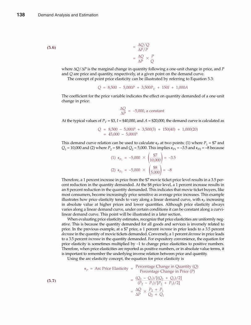
= ∆Q/Q(5.6) ∆P/P
= ∆Q � P∆P Q
where ∆Q/∆P is the marginal change in quantity following a one-unit change in price, and Pand Q are price and quantity, respectively, at a given point on the demand curve.
The concept of point price elasticity can be illustrated by referring to Equation 5.3:
Q = 8,500 – 5,000P + 3,500PV + 150I + 1,000A
The coefficient for the price variable indicates the effect on quantity demanded of a one-unitchange in price:
∆Q = –5,000, a constant∆P
At the typical values of PV = $3, I = $40,000, and A = $20,000, the demand curve is calculated as
Q = 8,500 – 5,000P + 3,500(3) + 150(40) + 1,000(20)= 45,000 – 5,000P
This demand curve relation can be used to calculate �P at two points: (1) where P1 = $7 andQ1 = 10,000 and (2) where P2 = $8 and Q2 = 5,000. This implies �P1 = –3.5 and �P2 = –8 because
(1) �P1= –5,000 � $7 = –3.5�10,000�
(2) �P2= –5,000 � $8 = –8�5,000�
Therefore, a 1 percent increase in price from the $7 movie ticket price level results in a 3.5 per-cent reduction in the quantity demanded. At the $8 price level, a 1 percent increase results inan 8 percent reduction in the quantity demanded. This indicates that movie ticket buyers, likemost consumers, become increasingly price sensitive as average price increases. This exampleillustrates how price elasticity tends to vary along a linear demand curve, with �P increasingin absolute value at higher prices and lower quantities. Although price elasticity alwaysvaries along a linear demand curve, under certain conditions it can be constant along a curvi-linear demand curve. This point will be illustrated in a later section.
When evaluating price elasticity estimates, recognize that price elasticities are uniformly neg-ative. This is because the quantity demanded for all goods and services is inversely related toprice. In the previous example, at a $7 price, a 1 percent increase in price leads to a 3.5 percentdecrease in the quantity of movie tickets demanded. Conversely, a 1 percent decrease in price leadsto a 3.5 percent increase in the quantity demanded. For expository convenience, the equation forprice elasticity is sometimes multiplied by –1 to change price elasticities to positive numbers.Therefore, when price elasticities are reported as positive numbers, or in absolute value terms, itis important to remember the underlying inverse relation between price and quantity.
Using the arc elasticity concept, the equation for price elasticity is
�P = Arc Price Elasticity = Percentage Change in Quantity (Q)Percentage Change in Price (P)
= (Q2 – Q1)/[(Q2 + Q1)/2](5.7) (P2 – P1)/[P2 + P1)/2]
= ∆Q � P2 + P1∆P Q2 + Q1
Chapter Five Demand Analysis and Estimation 139
138 Demand Analysis and Estimation
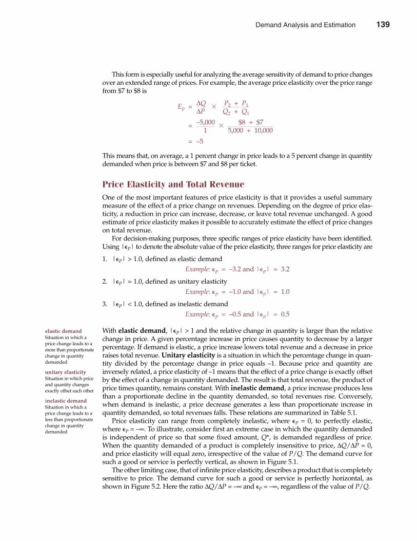
This form is especially useful for analyzing the average sensitivity of demand to price changesover an extended range of prices. For example, the average price elasticity over the price rangefrom $7 to $8 is
EP = ∆Q � P2 + P1∆P Q2 + Q1
= –5,000 � $8 + $71 5,000 + 10,000
= –5
This means that, on average, a 1 percent change in price leads to a 5 percent change in quantitydemanded when price is between $7 and $8 per ticket.
Price Elasticity and Total RevenueOne of the most important features of price elasticity is that it provides a useful summarymeasure of the effect of a price change on revenues. Depending on the degree of price elas-ticity, a reduction in price can increase, decrease, or leave total revenue unchanged. A goodestimate of price elasticity makes it possible to accurately estimate the effect of price changeson total revenue.
For decision-making purposes, three specific ranges of price elasticity have been identified.Using |�P| to denote the absolute value of the price elasticity, three ranges for price elasticity are
1. |�P| > 1.0, defined as elastic demandExample: �P = –3.2 and |�P| = 3.2
2. |�P| = 1.0, defined as unitary elasticityExample: �P = –1.0 and |�P| = 1.0
3. |�P| < 1.0, defined as inelastic demandExample: �P = –0.5 and |�P| = 0.5
With elastic demand, |�P| > 1 and the relative change in quantity is larger than the relativechange in price. A given percentage increase in price causes quantity to decrease by a largerpercentage. If demand is elastic, a price increase lowers total revenue and a decrease in priceraises total revenue. Unitary elasticity is a situation in which the percentage change in quan-tity divided by the percentage change in price equals –1. Because price and quantity areinversely related, a price elasticity of –1 means that the effect of a price change is exactly offsetby the effect of a change in quantity demanded. The result is that total revenue, the product ofprice times quantity, remains constant. With inelastic demand, a price increase produces lessthan a proportionate decline in the quantity demanded, so total revenues rise. Conversely,when demand is inelastic, a price decrease generates a less than proportionate increase inquantity demanded, so total revenues falls. These relations are summarized in Table 5.1.
Price elasticity can range from completely inelastic, where �P = 0, to perfectly elastic,where �P = –∞. To illustrate, consider first an extreme case in which the quantity demandedis independent of price so that some fixed amount, Q*, is demanded regardless of price.When the quantity demanded of a product is completely insensitive to price, ∆Q/∆P = 0,and price elasticity will equal zero, irrespective of the value of P/Q. The demand curve forsuch a good or service is perfectly vertical, as shown in Figure 5.1.
The other limiting case, that of infinite price elasticity, describes a product that is completelysensitive to price. The demand curve for such a good or service is perfectly horizontal, asshown in Figure 5.2. Here the ratio ∆Q/∆P = –∞ and �P = –∞, regardless of the value of P/Q.
140 Part Two Demand Analysis
elastic demandSituation in which aprice change leads to amore than proportionatechange in quantitydemanded
unitary elasticitySituation in which priceand quantity changesexactly offset each other
inelastic demandSituation in which aprice change leads to aless than proportionatechange in quantitydemanded
Demand Analysis and Estimation 139
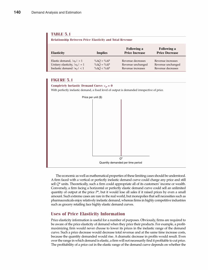
The economic as well as mathematical properties of these limiting cases should be understood.A firm faced with a vertical or perfectly inelastic demand curve could charge any price and stillsell Q* units. Theoretically, such a firm could appropriate all of its customers’ income or wealth.Conversely, a firm facing a horizontal or perfectly elastic demand curve could sell an unlimitedquantity of output at the price P*, but it would lose all sales if it raised prices by even a smallamount. Such extreme cases are rare in the real world, but monopolies that sell necessities such aspharmaceuticals enjoy relatively inelastic demand, whereas firms in highly competitive industriessuch as grocery retailing face highly elastic demand curves.
Uses of Price Elasticity InformationPrice elasticity information is useful for a number of purposes. Obviously, firms are required tobe aware of the price elasticity of demand when they price their products. For example, a profit-maximizing firm would never choose to lower its prices in the inelastic range of the demandcurve. Such a price decrease would decrease total revenue and at the same time increase costs,because the quantity demanded would rise. A dramatic decrease in profits would result. Evenover the range in which demand is elastic, a firm will not necessarily find it profitable to cut price.The profitability of a price cut in the elastic range of the demand curve depends on whether the
Chapter Five Demand Analysis and Estimation 141
TABLE 5.1Relationship Between Price Elasticity and Total Revenue
Following a Following aElasticity Implies Price Increase Price Decrease
Elastic demand, |�P| > 1 %∆Q > %∆P Revenue decreases Revenue increasesUnitary elasticity, |�P| = 1 %∆Q = %∆P Revenue unchanged Revenue unchangedInelastic demand |�P| < 1 %∆Q < %∆P Revenue increases Revenue decreases
FIGURE 5.1Completely Inelastic Demand Curve: �P = 0With perfectly inelastic demand, a fixed level of output is demanded irrespective of price.
Q*
Quantity demanded per time period
Price per unit ($)
140 Demand Analysis and Estimation
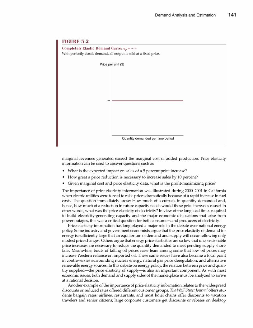
marginal revenues generated exceed the marginal cost of added production. Price elasticityinformation can be used to answer questions such as
• What is the expected impact on sales of a 5 percent price increase?• How great a price reduction is necessary to increase sales by 10 percent?• Given marginal cost and price elasticity data, what is the profit-maximizing price?
The importance of price elasticity information was illustrated during 2000–2001 in Californiawhen electric utilities were forced to raise prices dramatically because of a rapid increase in fuelcosts. The question immediately arose: How much of a cutback in quantity demanded and,hence, how much of a reduction in future capacity needs would these price increases cause? Inother words, what was the price elasticity of electricity? In view of the long lead times requiredto build electricity-generating capacity and the major economic dislocations that arise frompower outages, this was a critical question for both consumers and producers of electricity.
Price elasticity information has long played a major role in the debate over national energypolicy. Some industry and government economists argue that the price elasticity of demand forenergy is sufficiently large that an equilibrium of demand and supply will occur following onlymodest price changes. Others argue that energy price elasticities are so low that unconscionableprice increases are necessary to reduce the quantity demanded to meet pending supply short-falls. Meanwhile, bouts of falling oil prices raise fears among some that low oil prices mayincrease Western reliance on imported oil. These same issues have also become a focal pointin controversies surrounding nuclear energy, natural gas price deregulation, and alternativerenewable energy sources. In this debate on energy policy, the relation between price and quan-tity supplied—the price elasticity of supply—is also an important component. As with mosteconomic issues, both demand and supply sides of the marketplace must be analyzed to arriveat a rational decision.
Another example of the importance of price elasticity information relates to the widespreaddiscounts or reduced rates offered different customer groups. The Wall Street Journal offers stu-dents bargain rates; airlines, restaurants, and most hotel chains offer discounts to vacationtravelers and senior citizens; large corporate customers get discounts or rebates on desktop
142 Part Two Demand Analysis
FIGURE 5.2Completely Elastic Demand Curve: �P = –∞With perfectly elastic demand, all output is sold at a fixed price.
Price per unit ($)
P*
Quantity demanded per time period
Demand Analysis and Estimation 141

computers, auto leases, and many other items. Many such discounts are substantial, some-times in the range of 30 percent to 40 percent off standard list prices. The question of whetherreduced prices attract sufficient additional customers to offset lower revenues per unit isdirectly related to the price elasticity of demand.
Additional uses of price elasticity information are examined in later chapters. At this point,it becomes useful to consider some other important demand elasticities.
PRICE ELASTICITY AND MARGINAL REVENUE
There are simple, direct relations between price elasticity, marginal revenue, and total revenue.It is worth examining such relations in detail, given their importance for pricing policy.
Varying Elasticity at Different Points on a Demand CurveAll linear demand curves, except perfectly elastic or perfectly inelastic ones, are subject tovarying elasticities at different points on the curve. In other words, any linear demand curveis price elastic at some output levels but inelastic at others. To see this, recall the definitionof point price elasticity expressed in Equation 5.6:
�P = ∆Q � P∆P Q
The slope of a linear demand curve, ∆P/∆Q, is constant; thus, its reciprocal, 1/(∆P/∆Q) =∆Q/∆P, is also constant. However, the ratio P/Q varies from 0 at the point where the demandcurve intersects the horizontal axis and price = 0, to +∞ at the vertical price axis intercept where
Chapter Five Demand Analysis and Estimation 143
Due Diligence in E-Commerce
In the Internet environment, the authenticity of peopleand products being represented are often called intoquestion. To successfully match qualified buyers and sell-ers, and to complete e-commerce transactions, companiesneed information about trading partners in a trusted,secure environment. This is especially true in business-to-business transactions where the stakes are high, andmisjudgments can impact the public reputation of abrand. From a financial management standpoint, elec-tronic transactions with unknown parties can haveimportant implications for the efficient operation of acompany’s purchasing and receivables functions.
As electronic networks rush to bring millions ofpotential buyers and sellers together, sellers must answera host of important questions: Is the buyer who it claimsto be? Does the buyer have authority to transact for thestated business entity? Is the buyer eligible for specialpromotional offers? Should goods get shipped? From thebuyer’s perspective, similar questions must getanswered: Is the seller in fact who it claims to be? Is theseller authorized to sell/service the goods being repre-sented? Is the seller likely to be in business long enough
to honor any service agreements? How well does theseller rate in terms of on-time delivery, product satisfac-tion, or customer service?
Although businesses have been answering suchquestions for centuries, the anonymous Internet envi-ronment affords little time for face-to-face interaction ortrust building. As a result, e-commerce opens the doorto new customers, global reach, and exponential growth,but it also increases business risk. Effective e-commercecompanies now rely upon “smart transactions” monitoredby Dun & Bradstreet and other third-party guarantors that“know” automatically when to approve, deny, or seek fur-ther review of a transaction. Electronic “client certificates”ensure authenticity, confidentiality, integrity, and nonre-pudiation. Using such innovations, Dun & Bradstreet,among others, is working to bring safety and confidenceto e-commerce.
See: Julia Angwin, “Barry Diller Bets Big: Seeks $9 Billion in Acquisitionsof E-Commerce Firms,” The Wall Street Journal Online, March 1, 2002(http://online.wsj.com).
M A N A G E R I A L A P P L I C AT I O N 5 . 2
142 Demand Analysis and Estimation
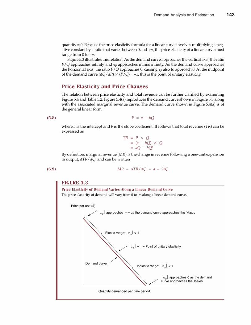
quantity = 0. Because the price elasticity formula for a linear curve involves multiplying a neg-ative constant by a ratio that varies between 0 and +∞, the price elasticity of a linear curve mustrange from 0 to –∞.
Figure 5.3 illustrates this relation. As the demand curve approaches the vertical axis, the ratioP/Q approaches infinity and �P approaches minus infinity. As the demand curve approachesthe horizontal axis, the ratio P/Q approaches 0, causing �P also to approach 0. At the midpointof the demand curve (∆Q/∆P) � (P/Q) = –1; this is the point of unitary elasticity.
Price Elasticity and Price ChangesThe relation between price elasticity and total revenue can be further clarified by examiningFigure 5.4 and Table 5.2. Figure 5.4(a) reproduces the demand curve shown in Figure 5.3 alongwith the associated marginal revenue curve. The demand curve shown in Figure 5.4(a) is ofthe general linear form
(5.8) P = a – bQ
where a is the intercept and b is the slope coefficient. It follows that total revenue (TR) can beexpressed as
TR = P � Q= (a – bQ) � Q= aQ – bQ2
By definition, marginal revenue (MR) is the change in revenue following a one-unit expansionin output, ∆TR/∆Q, and can be written
(5.9) MR = ∆TR/∆Q = a – 2bQ
144 Part Two Demand Analysis
FIGURE 5.3Price Elasticity of Demand Varies Along a Linear Demand CurveThe price elasticity of demand will vary from 0 to -∞ along a linear demand curve.
Price per unit ($)
Elastic range: ∈p > 1
∈p = 1 = Point of unitary elasticity
Inelastic range: ∈p < 1
Quantity demanded per time period
Demand curve
∈p approaches �∞ as the demand curve approaches the Y-axis
∈p approaches 0 as the demandcurve approaches the X-axis
Demand Analysis and Estimation 143
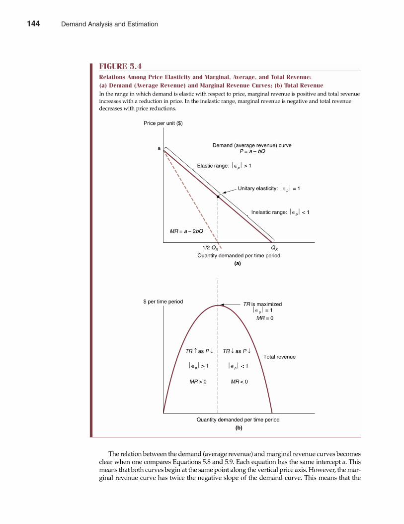
The relation between the demand (average revenue) and marginal revenue curves becomesclear when one compares Equations 5.8 and 5.9. Each equation has the same intercept a. Thismeans that both curves begin at the same point along the vertical price axis. However, the mar-ginal revenue curve has twice the negative slope of the demand curve. This means that the
Chapter Five Demand Analysis and Estimation 145
FIGURE 5.4Relations Among Price Elasticity and Marginal, Average, and Total Revenue: (a) Demand (Average Revenue) and Marginal Revenue Curves; (b) Total RevenueIn the range in which demand is elastic with respect to price, marginal revenue is positive and total revenueincreases with a reduction in price. In the inelastic range, marginal revenue is negative and total revenuedecreases with price reductions.
Price per unit ($)
a
1/2 QX QX
MR = a Ð 2bQ
Elastic range: ∈p > 1
Unitary elasticity: ∈p = 1
Inelastic range: ∈p < 1
∈p < 1∈p > 1
(a)
Demand (average revenue) curveP = a Ð bQ
Quantity demanded per time period
(b)
Quantity demanded per time period
$ per time period TR is maximized∈p = 1
MR = 0
TR ↑ as P ↓ TR ↓ as P ↓
MR > 0 MR < 0
Total revenue
144 Demand Analysis and Estimation
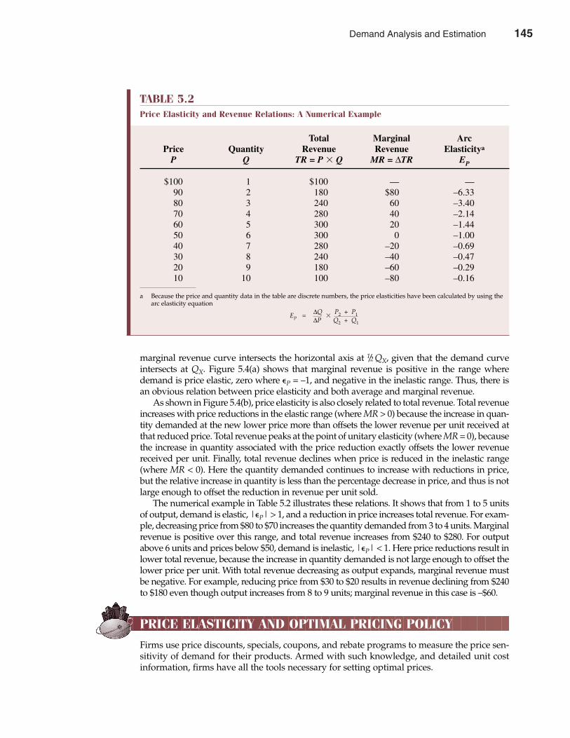
marginal revenue curve intersects the horizontal axis at 1/2 QX, given that the demand curveintersects at QX. Figure 5.4(a) shows that marginal revenue is positive in the range wheredemand is price elastic, zero where �P = –1, and negative in the inelastic range. Thus, there isan obvious relation between price elasticity and both average and marginal revenue.
As shown in Figure 5.4(b), price elasticity is also closely related to total revenue. Total revenueincreases with price reductions in the elastic range (where MR > 0) because the increase in quan-tity demanded at the new lower price more than offsets the lower revenue per unit received atthat reduced price. Total revenue peaks at the point of unitary elasticity (where MR = 0), becausethe increase in quantity associated with the price reduction exactly offsets the lower revenuereceived per unit. Finally, total revenue declines when price is reduced in the inelastic range(where MR < 0). Here the quantity demanded continues to increase with reductions in price,but the relative increase in quantity is less than the percentage decrease in price, and thus is notlarge enough to offset the reduction in revenue per unit sold.
The numerical example in Table 5.2 illustrates these relations. It shows that from 1 to 5 unitsof output, demand is elastic, |�P| > 1, and a reduction in price increases total revenue. For exam-ple, decreasing price from $80 to $70 increases the quantity demanded from 3 to 4 units. Marginalrevenue is positive over this range, and total revenue increases from $240 to $280. For outputabove 6 units and prices below $50, demand is inelastic, |�P| < 1. Here price reductions result inlower total revenue, because the increase in quantity demanded is not large enough to offset thelower price per unit. With total revenue decreasing as output expands, marginal revenue mustbe negative. For example, reducing price from $30 to $20 results in revenue declining from $240to $180 even though output increases from 8 to 9 units; marginal revenue in this case is –$60.
PRICE ELASTICITY AND OPTIMAL PRICING POLICY
Firms use price discounts, specials, coupons, and rebate programs to measure the price sen-sitivity of demand for their products. Armed with such knowledge, and detailed unit costinformation, firms have all the tools necessary for setting optimal prices.
146 Part Two Demand Analysis
TABLE 5.2Price Elasticity and Revenue Relations: A Numerical Example
Total Marginal ArcPrice Quantity Revenue Revenue Elasticitya
P Q TR = P � Q MR = ∆TR EP
$100 1 $100 — —90 2 180 $80 –6.3380 3 240 60 –3.4070 4 280 40 –2.1460 5 300 20 –1.4450 6 300 0 –1.0040 7 280 –20 –0.6930 8 240 –40 –0.4720 9 180 –60 –0.2910 10 100 –80 –0.16
a Because the price and quantity data in the table are discrete numbers, the price elasticities have been calculated by using thearc elasticity equation
EP = ∆Q�
P2 + P1∆P Q2 + Q1
Demand Analysis and Estimation 145
Optimal Price FormulaAs a practical matter, firms devote enormous resources to obtain current and detailed infor-mation concerning the price elasticity of demand for their products. Price elasticity estimatesrepresent vital information because these data, along with relevant unit cost information, areessential inputs for setting a pricing policy that is consistent with value maximization. Thisstems from the fact that there is a relatively simple mathematical relation between marginalrevenue, price, and the point price elasticity of demand.
Given any point price elasticity estimate, relevant marginal revenues can be determinedeasily. When this marginal revenue information is combined with pertinent marginal cost data,the basis for an optimal pricing policy is created.
The relation between marginal revenue, price, and the point price elasticity of demand fol-lows directly from the mathematical definition of a marginal relation.2 In equation form, the linkbetween marginal revenue, price, and the point price elasticity of demand is
(5.10) MR = P � 1 + 1 ��P
Because �P < 0, the number contained within brackets in Equation 5.10 is always less than one.This means that MR < P, and the gap between MR and P will fall as the price elasticity of demandincreases (in absolute value terms). For example, when P = $8 and �P = –1.5, MR = $2.67. Thus,when price elasticity is relatively low, the optimal price is much greater than marginal revenue.Conversely, when P = $8 and �P = –10, MR = $7.20. When the quantity demanded is highly elas-tic with respect to price, the optimal price is close to marginal revenue.
Optimal Pricing Policy ExampleThe simple relation between marginal revenue, price, and the point price elasticity is very use-ful in the setting of pricing policy. To see the usefulness of Equation 5.10 in practical pricing
Chapter Five Demand Analysis and Estimation 147
2 In calculus notation, marginal revenue is the derivative of the total revenue function. That is, MR = dTR/dQ.Because total revenue equals price times quantity (TR = P � Q), marginal revenue is found by taking thederivative of the function P � Q with respect to Q:
MR =d(P � Q)
dQBecause price and quantity are interdependent in the typical demand situation, the rule for differentiating aproduct must be employed in taking the preceding derivative:
MR = dTR
=d(P � Q)
= P �dQ
+ Q �dP
dQ dQ dQ dQ
= P � 1 + Q �dPdQ
= P � Q �dPdQ
This relation is a completely general specification of marginal revenue, which, if P is factored out from theright-hand side, can be rewritten as
MR = P �1 +Q
�dP �P dQ
Note that the term Q/P � dP/dQ in the preceding expression is the reciprocal of the definition for point priceelasticity, �P = dQ/dP � (P/Q):
Q�
dP=
1=
1P dQ dQ
�P �P
dP QThus, marginal revenue can be rewritten as
MR = P �1 +1 ��P
146 Demand Analysis and Estimation
policy, consider the pricing problem faced by a profit-maximizing firm. Recall that profit max-imization requires operating at the activity level where marginal cost equals marginal rev-enue. Most firms have extensive cost information and can estimate marginal cost reasonablywell. By equating marginal costs with marginal revenue as identified by Equation 5.10, theprofit-maximizing price level can be easily determined. Using Equation 5.10, set marginalcost equal to marginal revenue, where
MC = MR
and, therefore,
MC = P � 1 + 1 ��P
which implies that the optimal or profit-maximizing price, P*, equals
(5.11)P* = MC
�1 + 1 ��P
This simple relation between price, marginal cost, and the point price elasticity of demand isthe most useful pricing tool offered by managerial economics.
To illustrate the usefulness of Equation 5.11, suppose that manager George Stevens notes a2 percent increase in weekly sales following a 1 percent price discount on The Kingfish fishingreels. The point price elasticity of demand for The Kingfish fishing reels is
�P = Percentage Change in QPercentage Change in P
= 2%–1%
= –2
What is the optimal retail price for The Kingfish fishing reels if the company’s wholesale costper reel plus display and marketing expenses—or relevant marginal costs—total $25 per unit?With marginal costs of $25 and �P = –2, the profit-maximizing price is
P = $25
�1 + 1 �–2
= $50
Therefore, the profit-maximizing price on The Kingfish fishing reels is $50.To see how Equation 5.11 can be used for planning purposes, suppose Stevens can order
reels through a different distributor at a wholesale price that reduces marginal costs by $1 to $24per unit. Under these circumstances, the new optimal retail price is
P = $24
�1 + 1 �–2
= $48
Thus, the optimal retail price would fall by $2 following a $1 reduction in The Kingfish’s relevantmarginal costs.
148 Part Two Demand Analysis
Demand Analysis and Estimation 147
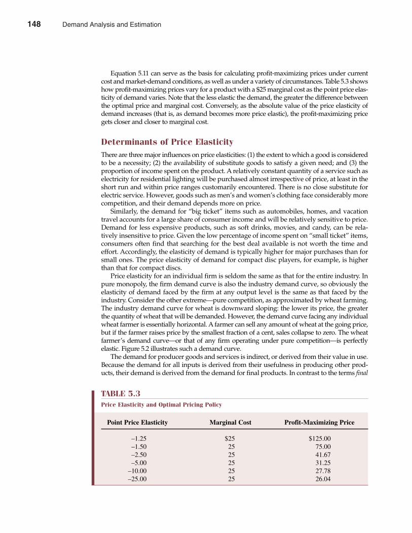
Equation 5.11 can serve as the basis for calculating profit-maximizing prices under currentcost and market-demand conditions, as well as under a variety of circumstances. Table 5.3 showshow profit-maximizing prices vary for a product with a $25 marginal cost as the point price elas-ticity of demand varies. Note that the less elastic the demand, the greater the difference betweenthe optimal price and marginal cost. Conversely, as the absolute value of the price elasticity ofdemand increases (that is, as demand becomes more price elastic), the profit-maximizing pricegets closer and closer to marginal cost.
Determinants of Price ElasticityThere are three major influences on price elasticities: (1) the extent to which a good is consideredto be a necessity; (2) the availability of substitute goods to satisfy a given need; and (3) theproportion of income spent on the product. A relatively constant quantity of a service such aselectricity for residential lighting will be purchased almost irrespective of price, at least in theshort run and within price ranges customarily encountered. There is no close substitute forelectric service. However, goods such as men’s and women’s clothing face considerably morecompetition, and their demand depends more on price.
Similarly, the demand for “big ticket” items such as automobiles, homes, and vacationtravel accounts for a large share of consumer income and will be relatively sensitive to price.Demand for less expensive products, such as soft drinks, movies, and candy, can be rela-tively insensitive to price. Given the low percentage of income spent on “small ticket” items,consumers often find that searching for the best deal available is not worth the time andeffort. Accordingly, the elasticity of demand is typically higher for major purchases than forsmall ones. The price elasticity of demand for compact disc players, for example, is higherthan that for compact discs.
Price elasticity for an individual firm is seldom the same as that for the entire industry. Inpure monopoly, the firm demand curve is also the industry demand curve, so obviously theelasticity of demand faced by the firm at any output level is the same as that faced by theindustry. Consider the other extreme—pure competition, as approximated by wheat farming.The industry demand curve for wheat is downward sloping: the lower its price, the greaterthe quantity of wheat that will be demanded. However, the demand curve facing any individualwheat farmer is essentially horizontal. A farmer can sell any amount of wheat at the going price,but if the farmer raises price by the smallest fraction of a cent, sales collapse to zero. The wheatfarmer’s demand curve—or that of any firm operating under pure competition—is perfectlyelastic. Figure 5.2 illustrates such a demand curve.
The demand for producer goods and services is indirect, or derived from their value in use.Because the demand for all inputs is derived from their usefulness in producing other prod-ucts, their demand is derived from the demand for final products. In contrast to the terms final
Chapter Five Demand Analysis and Estimation 149
TABLE 5.3Price Elasticity and Optimal Pricing Policy
Point Price Elasticity Marginal Cost Profit-Maximizing Price
–1.25 $25 $125.00–1.50 25 75.00–2.50 25 41.67–5.00 25 31.25
–10.00 25 27.78–25.00 25 26.04
148 Demand Analysis and Estimation
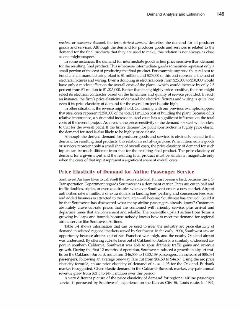
product or consumer demand, the term derived demand describes the demand for all producergoods and services. Although the demand for producer goods and services is related to thedemand for the final products that they are used to make, this relation is not always as closeas one might suspect.
In some instances, the demand for intermediate goods is less price sensitive than demandfor the resulting final product. This is because intermediate goods sometimes represent only asmall portion of the cost of producing the final product. For example, suppose the total cost tobuild a small manufacturing plant is $1 million, and $25,000 of this cost represents the cost ofelectrical fixtures and wiring. Even a doubling in electrical costs from $25,000 to $50,000 wouldhave only a modest effect on the overall costs of the plant—which would increase by only 2.5percent from $1 million to $1,025,000. Rather than being highly price sensitive, the firm mightselect its electrical contractor based on the timeliness and quality of service provided. In suchan instance, the firm’s price elasticity of demand for electrical fixtures and wiring is quite low,even if its price elasticity of demand for the overall project is quite high.
In other situations, the reverse might hold. Continuing with our previous example, supposethat steel costs represent $250,000 of the total $1 million cost of building the plant. Because of itsrelative importance, a substantial increase in steel costs has a significant influence on the totalcosts of the overall project. As a result, the price sensitivity of the demand for steel will be closeto that for the overall plant. If the firm’s demand for plant construction is highly price elastic,the demand for steel is also likely to be highly price elastic.
Although the derived demand for producer goods and services is obviously related to thedemand for resulting final products, this relation is not always close. When intermediate goodsor services represent only a small share of overall costs, the price elasticity of demand for suchinputs can be much different from that for the resulting final product. The price elasticity ofdemand for a given input and the resulting final product must be similar in magnitude onlywhen the costs of that input represent a significant share of overall costs.
Price Elasticity of Demand for Airline Passenger ServiceSouthwest Airlines likes to call itself the Texas state bird. It must be some bird, because the U.S.Transportation Department regards Southwest as a dominant carrier. Fares are cut in half andtraffic doubles, triples, or even quadruples whenever Southwest enters a new market. Airportauthorities rake in millions of extra dollars in landing fees, parking and concession fees soar,and added business is attracted to the local area—all because Southwest has arrived! Could itbe that Southwest has discovered what many airline passengers already know? Customersabsolutely crave cut-rate prices that are combined with friendly service, plus arrival anddeparture times that are convenient and reliable. The once-little upstart airline from Texas isgrowing by leaps and bounds because nobody knows how to meet the demand for regionalairline service like Southwest Airlines.
Table 5.4 shows information that can be used to infer the industry arc price elasticity ofdemand in selected regional markets served by Southwest. In the early 1990s, Southwest saw anopportunity because airfares out of San Francisco were high, and the nearby Oakland airportwas underused. By offering cut-rate fares out of Oakland to Burbank, a similarly underused air-port in southern California, Southwest was able to spur dramatic traffic gains and revenuegrowth. During the first 12 months of operation, Southwest induced a growth in airport traf-fic on the Oakland–Burbank route from 246,555 to 1,053,139 passengers, an increase of 806,584passengers, following an average one-way fare cut from $86.50 to $44.69. Using the arc priceelasticity formula, an arc price elasticity of demand of �P = –1.95 for the Oakland–Burbankmarket is suggested. Given elastic demand in the Oakland–Burbank market, city-pair annualrevenue grew from $21.3 to $47.1 million over this period.
A very different picture of the price elasticity of demand for regional airline passengerservice is portrayed by Southwest’s experience on the Kansas City–St. Louis route. In 1992,
150 Part Two Demand Analysis
Demand Analysis and Estimation 149
Southwest began offering cut-rate fares between Kansas City and St. Louis and was, once again,able to spur dramatic traffic growth. However, in the Kansas City–St. Louis market, trafficgrowth was not sufficient to generate added revenue. During the first 12 months of Southwest’soperation in this market, traffic growth in the Kansas City–St. Louis route was from 428,711 to722,425 passengers, an increase of 293,714 passengers, following an average one-way fare cutfrom $154.42 to $45.82. Again using the arc price elasticity formula, a market arc price elasticityof demand of only �P = –0.47 is suggested. With inelastic demand, Kansas City–St. Louis marketrevenue fell from $66.2 to $33.1 million over this period.
In considering these arc price elasticity estimates, remember that they correspond to eachmarket rather than to Southwest Airlines itself. If Southwest were the single carrier or monop-olist in the Kansas City–St. Louis market, it could gain revenues and cut variable costs by rais-ing fares and reducing the number of daily departures. As a monopolist, such a fare increasewould lead to higher revenues and profits. However, given the fact that other airlines operatein each market, Southwest’s own demand is likely to be much more price elastic than themarket demand elasticity estimates shown in Table 5.4. To judge the profitability of any fare,it is necessary to consider Southwest’s revenue and cost structure in each market. For example,service in the Kansas City–St. Louis market might allow Southwest to more efficiently use air-craft and personnel used to serve the Dallas–Chicago market and thus be highly profitableeven when bargain-basement fares are charged.
The importance of price elasticity information is examined further in later chapters. At thispoint, it becomes useful to consider other important demand elasticities.
Chapter Five Demand Analysis and Estimation 151
TABLE 5.4How Prices Plunge and Traffic Soars When Southwest Airlines Enters a Market
Burbank–Oakland
Passengers in 12 months before Southwest 246,555Passengers in 12 months after Southwest 1,053,139Increase in passengers 806,584Average one-way fare before Southwest $86.50Average one-way fare after Southwest $44.69Decrease in one-way fares –$41.81Market revenue in 12 months before Southwest $21,327,008Market revenue in 12 months after Southwest $47,064,782Increase in market revenue $25,737,774Implied arc price elasticity of demand (EP) –1.95
Kansas City–St. Louis
Passengers in 12 months before Southwest 428,711Passengers in 12 months after Southwest 722,425Increase in passengers 293,714Average one-way fare before Southwest $154.42Average one-way fare after Southwest $45.82Decrease in one-way fares –$108.60Market revenue in 12 months before Southwest $66,201,553Market revenue in 12 months after Southwest $33,101,514Decrease in market revenue –$33,100,039Implied arc price elasticity of demand (EP) –0.47
Data source: Del Jones, “Business Soars Where Airline Flies,” USA Today, 9/17/93, 1B–2B.
150 Demand Analysis and Estimation

CROSS-PRICE ELASTICITY OF DEMAND
Demand for most products is influenced by prices for other products. Such demand interrela-tionships are an important consideration in demand analysis and estimation.
Substitutes and ComplementsThe demand for beef is related to the price of chicken. As the price of chicken increases, sodoes the demand for beef; consumers substitute beef for the now relatively more expensivechicken. On the other hand, a price decrease for chicken leads to a decrease in the demand forbeef as consumers substitute chicken for the now relatively more expensive beef. In general,a direct relation between the price of one product and the demand for a second product holdsfor all substitutes. A price increase for a given product will increase demand for substitutes;a price decrease for a given product will decrease demand for substitutes.
Some goods and services—for example, cameras and film—exhibit a completely differentrelation. Here price increases in one product typically lead to a reduction in demand for theother. Goods that are inversely related in this manner are known as complements; they areused together rather than in place of each other.
The concept of cross-price elasticity is used to examine the responsiveness of demandfor one product to changes in the price of another. Point cross-price elasticity is given by thefollowing equation:
�PX = Percentage Change in Quantity of YPercentage Change in Price of X
152 Part Two Demand Analysis
substitutesRelated products forwhich a price increasefor one leads to anincrease in demand forthe other
complementsRelated products forwhich a price increasefor one leads to areduction in demandfor the other
cross-price elasticityResponsiveness ofdemand for one productto changes in the priceof another
Relationship Marketing
Saturn prides itself on the notion that it manufactures asuperior automotive product and provides superior serv-ice. Part of this superior service involves better listeningto its customers and responding to their suggestions.During early summer, for example, thousands of Saturnowners typically respond to the company’s invitation toattend a 3-day picnic at company headquarters in SpringHill, Tennessee. Not only is it a way to thank owners fortheir business, but it also is a proven means of buildingcustomer loyalty. Mail-order merchants Cabela’s, L.L.Bean, and Lands’ End, among others, deploy impressivecomputer capabilities to better track and anticipate cus-tomer needs. At Cabela’s, for example, customers thatorder camping equipment and hiking boots are good candidates for the company’s camping and outdoor gearcatalog. Lands’ End customers who order chinos andother casual attire also receive specialized catalogs. AtL.L. Bean, the company’s unconditional 100 percent satis-faction guarantee keeps valued customers coming back.At FedEx, highly profitable customers get special attention.
Car companies, mail-order merchants, airlines (withfrequent flyer programs), and hotels with repeat business
customers are obvious candidates for effective relationshipmarketing. The untapped potential for relationship mar-keting lies in new and innovative applications. For example,if a company wants to sell detergent, it might obtain adatabase of large families and offer them a bargain price.While a typical product promotion effort would stopthere, relationship marketing goes further. Relationshipmarketing would suggest that the firm offer such familiesa free washer or dryer if they remained a loyal customerfor, say, 5 years. Because the markup on detergent is substantial, such a long-term promotion could be highlybeneficial for both the customer and the company.
The logic behind relationship marketing is simple. Itcosts much more to get a new customer than it does tokeep a current one, so the retention of valued customersis key to long-term success.
See: Dow Jones Newswires, “Expedia, Delta Set Marketing Deal,” TheWall Street Journal Online, March 20, 2002 (http://online.wsj.com).
M A N A G E R I A L A P P L I C AT I O N 5 . 3
Demand Analysis and Estimation 151
= ∆QY/QY(5.12) ∆PX/PX
= ∆QY � PX∆PX QY
where Y and X are two different products. The arc cross-price elasticity relationship is construct-ed in the same manner as was previously described for price elasticity:
EPX = Percentage Change in Quantity of YPercentage Change in Price of X
= (QY2 – QY1)/[(QY2 + QY1)/2](5.13) (PX2 – PX1)/[(PX2 + PX1)/2]
= ∆QY � PX2 + PX1∆PX QY2 + QY1
The cross-price elasticity for substitutes is always positive; the price of one good and thedemand for the other always move in the same direction. Cross-price elasticity is negativefor complements; price and quantity move in opposite directions for complementary goodsand services. Finally, cross-price elasticity is zero, or nearly zero, for unrelated goods inwhich variations in the price of one good have no effect on demand for the second.
Cross-Price Elasticity ExampleThe cross-price elasticity concept can be illustrated by considering the demand function formonitored in-home health-care services provided by Home Medical Support (HMS), Inc.
QY = f(PY,PD,PH, PT,i,I)
Here, QY is the number of patient days of service per year; PY is the average price of HMSservice; PD is an industry price index for prescription drugs; PH is an index of the averageprice of hospital service, a primary competitor; PT is a price index for the travel industry; i isthe interest rate; and I is disposable income per capita. Assume that the parameters of theHMS demand function have been estimated as follows:
QY = 25,000 – 5PY – 3PD + 10PH + 0.0001PT – 0.02i + 2.5I
The effects on QY caused by a one-unit change in the prices of other goods are
∆QY = –3∆PD
∆QY = +10∆PH
∆QY = 0.0001 ≈ 0∆PT
Because both prices and quantities are always positive, the ratios PD/QY, PH/QY, and PT/QYare also positive. Therefore, the signs of the three cross-price elasticities in this example aredetermined by the sign of each relevant parameter estimate in the HMS demand function:
�PD = (–3)(PD/QY) < 0
HMS service and prescription drugs are complements.
Chapter Five Demand Analysis and Estimation 153
152 Demand Analysis and Estimation
�PH = (+10)(PH/QY) > 0
HMS service and hospital service are substitutes.
�PT = (+0.0001)(PT/QY) ≈ 0, so long as the ratio PT/QY is not extremely large
Demand for travel and HMS service are independent.The concept of cross-price elasticity serves two main purposes. First, it is important for the
firm to be aware of how demand for its products is likely to respond to changes in the prices ofother goods. Such information is necessary for formulating the firm’s own pricing strategy andfor analyzing the risks associated with various products. This is particularly important for firmswith a wide variety of products, where meaningful substitute or complementary relations existwithin the firm’s own product line. Second, cross-price elasticity information allows managersto measure the degree of competition in the marketplace. For example, a firm might appear todominate a particular market or market segment, especially if it is the only supplier of a par-ticular product. However, if the cross-price elasticity between a firm’s output and productsproduced in related industries is large and positive, the firm is not a monopolist in the truesense and is not immune to the threat of competitor encroachment. In the banking industry,for example, individual banks clearly compete with money market mutual funds, savings andloan associations, credit unions, and commercial finance companies. The extent of competitioncan be measured only in terms of the cross-price elasticities of demand.
INCOME ELASTICITY OF DEMAND
For many goods, income is another important determinant of demand. Income is frequentlyas important as price, advertising expenditures, credit terms, or any other variable in thedemand function. This is particularly true of luxury items such as big screen televisions,country club memberships, elegant homes, and so on. In contrast, the demand for such basiccommodities as salt, bread, and milk is not very responsive to income changes. These goodsare bought in fairly constant amounts regardless of changes in income. Of course, income canbe measured in many ways—for example, on a per capita, per household, or aggregate basis.Gross national product, national income, personal income, and disposable personal incomehave all served as income measures in demand studies.
Normal Versus Inferior GoodsThe income elasticity of demand measures the responsiveness of demand to changes inincome, holding constant the effect of all other variables that influence demand. Letting Irepresent income, income point elasticity is defined as
�I = Percentage Change in Quantity (Q)Percentage Change in Income (I)
= ∆Q/Q(5.14) ∆I/I
= ∆Q � I∆I Q
Income and the quantity purchased typically move in the same direction; that is, income andsales are directly rather than inversely related. Therefore, ∆Q/∆I and hence �I are positive. Thisdoes not hold for a limited number of products termed inferior goods. Individual consumerdemand for such products as beans and potatoes, for example, is sometimes thought to declineas income increases, because consumers replace them with more desirable alternatives. More
154 Part Two Demand Analysis
income elasticityResponsiveness ofdemand to changes inincome, holding con-stant the effect of allother variables
inferior goodsProducts for which con-sumer demand declinesas income rises
Demand Analysis and Estimation 153
typical products, whose individual and aggregate demand is positively related to income, aredefined as normal goods.
To examine income elasticity over a range of incomes rather than at a single level, the arcelasticity relation is employed:
EI = Percentage Change in Quantity (Q)Percentage Change in Income (I)
= (Q2 – Q1)/[(Q2 + Q1)/2](5.15) (I2 – I1)/[(I2 + I1)/2]
= ∆Q � I2 + I1∆I Q2 + Q1
Arc income elasticity provides a measure of the average responsiveness of demand for a givenproduct to a relative change in income over the range from I1 to I2.
In the case of inferior goods, individual demand actually rises during an economic downturn.As workers get laid off from their jobs, for example, they might tend to substitute potatoes formeat, hamburgers for steak, bus rides for automobile trips, and so on. As a result, demand forpotatoes, hamburgers, bus rides, and other inferior goods can actually rise during recessions.Their demand is countercyclical.
Types of Normal GoodsFor most products, income elasticity is positive, indicating that demand rises as the economyexpands and national income increases. The actual size of the income elasticity coefficient isvery important. Suppose, for example, that �I = 0.3. This means that a 1 percent increase inincome causes demand for the product to increase by only .3 percent. Given growing nationalincome over time, such a product would not maintain its relative importance in the economy.Another product might have �I = 2.5; its demand increases 2.5 times as fast as income. If, �I < 1.0for a particular product, its producers will not share proportionately in increases in nationalincome. However, if �I > 1.0, the industry will gain more than a proportionate share of increasesin income.
Goods for which 0 < �I < 1 are referred to as noncyclical normal goods, because demandis relatively unaffected by changing income. Sales of most convenience goods, such as tooth-paste, candy, soda, and movie tickets, account for only a small share of the consumer’s overallbudget, and spending on such items tends to be relatively unaffected by changing economicconditions. For goods having �I > 1, referred to as cyclical normal goods, demand is stronglyaffected by changing economic conditions. Purchase of “big ticket” items such as homes, auto-mobiles, boats, and recreational vehicles can be postponed and tend to be put off by consumersduring economic downturns. Housing demand, for example, can collapse during recessionsand skyrocket during economic expansions. These relations between income and productdemand are summarized in Table 5.5.
normal goodsProducts for whichdemand is positivelyrelated to income
countercyclicalInferior goods whosedemand falls with risingincome, and rises withfalling income
noncyclical normalgoodsProducts for whichdemand is relativelyunaffected by changingincome
cyclical normalgoodsProducts for whichdemand is stronglyaffected by changingincome
Chapter Five Demand Analysis and Estimation 155
TABLE 5.5Relationship Between Income and Product Demand
Inferior goods (countercyclical) �I < 0 Basic foodstuffs, generic products, bus ridesNoncyclical normal goods 0 < �I < 1 Toiletries, movies, liquor, cigarettesCyclical normal goods �I > 1 Automobiles, housing, vacation travel, capital
equipment
154 Demand Analysis and Estimation

Firms whose demand functions indicate high income elasticities enjoy good growth oppor-tunities in expanding economies. Forecasts of aggregate economic activity figure importantlyin their plans. Companies faced with low income elasticities are relatively unaffected by thelevel of overall business activity. This is desirable from the standpoint that such a business isharmed relatively little by economic downturns. Nevertheless, such a company cannot expectto share fully in a growing economy and might seek to enter industries that provide bettergrowth opportunities.
Income elasticity figures importantly in several key national debates. Agriculture is oftendepressed because of the low income elasticity for most food products. This has made it difficultfor farmers’ incomes to keep up with those of urban workers. A somewhat similar problem aris-es in housing. Improving the housing stock is a primary national goal. If the income elasticity forhousing is high and �I > 1, an improvement in the housing stock will be a natural by-product ofa prosperous economy. However, if the housing income elasticity �I < 1, a relatively small per-centage of additional income will be spent on houses. As a result, housing stock would notimprove much over time despite a growing economy and increasing incomes. In the event that�I < 1, direct government investment in public housing or rent and interest subsidies might benecessary to bring about a dramatic increase in the housing stock over time.
ADDITIONAL DEMAND ELASTICITY CONCEPTS
The most common demand elasticities—price elasticity, cross-price elasticity, and incomeelasticity—are emphasized in this chapter. Examples of other demand elasticities can be usedto reinforce the generality of the concept.
156 Part Two Demand Analysis
What’s in a Name?
When it comes to financial information, privately-heldMars Incorporated, in MacLean, Virginia, is secretive.With annual sales of $15 billion in pet foods, candies, andother food products, the company is also immensely prof-itable. According to Forbes’ annual survey, Forrest EdwardMars, Sr., Edward Mars, Jr., Jacqueline Mars Vogel, JohnMars, and the rest of the clan are worth more than $16 billion—one of the richest families in the world. How doesMars do it? That’s simple: brand-name advertising.
Like top rivals Hershey’s, Nestle, and RalstonPurina, Mars advertises like mad to create durable brandnames. Since 1954, M&M’s Peanut and M&M’s ChocolateCandies have been known by the slogan “Melts in yourmouth—not in your hand.” With constant reminders, themessage has not been lost on consumers who also flockto other Mars candies like Royals Mint Chocolate, KudosGranola Bars, Skittles Fruit Chews, Snickers Candy & IceCream Bars, and Starburst Fruit Chews. Brand-nameadvertising is also a cornerstone of Mars’ marketing ofKal-Kan petfoods; Expert, a superpremium dog and catfood line; and Sheba and Whiskas cat foods.
Mars is like many top-tier consumer products com-panies; their good name is their most valuable asset. Forexample, although Coca-Cola enjoys undeniableeconomies of scale in distribution, nothing is more valuablethan its telltale moniker in white on red background. ForPhilip Morris, the Marlboro brand is the source of a largeand growing river of cash flow. In the United States, morethan one-half of all cigarettes are sold on the basis of a redand white box and the rugged image of a weather-beatenand sun-dried cowboy. Owners of trademarks such asAstroturf, Coke, Frisbee, Kleenex, Kitty Litter, Styrofoam,Walkman, and Xerox employ a veritable army of lawyersin an endless struggle against “generic” treatment. Theyknow that well-established brand-name products enjoyenormous profits.
See: Suzanne Vranica, “American Express Launches Ads to BoostBrand Hurt by Travel,” The Wall Street Journal Online, March 15, 2002(http://online.wsj.com).
M A N A G E R I A L A P P L I C AT I O N 5 . 4
Demand Analysis and Estimation 155
Other Demand ElasticitiesAdvertising elasticity plays an important role in marketing activities for a broad range ofgoods and services. A low advertising elasticity means that a firm must spend substantialsums to shift demand for its products through media-based promotion. In such cases,alternative marketing approaches—such as personal selling or direct marketing—areoften more productive.
In the housing market, mortgage interest rates are an important determinant of demand.Accordingly, interest rate elasticities have been used to analyze and forecast the demand forhousing construction. To be sure, this elasticity coefficient varies over time as other conditionsin the economy change. Other things are held constant when measuring elasticity, but in thebusiness world other things do not typically remain constant. Studies indicate that the interestrate elasticity of residential housing demand averages about –0.15. This means that a 10 percentrise in interest rates decreases the demand for housing by 1.5 percent, provided that all othervariables remain unchanged. If Federal Reserve policy is expected to cause mortgage interestrates to rise from 6 percent to 8 percent (a 33 percent increase), a 4.95 percent decrease (= –0.15� 33) in housing demand can be projected, on average.
Not surprisingly, public utilities calculate the weather elasticity of demand for their serv-ices. They measure weather using degree days as an indicator of average temperatures. Thiselasticity factor is used, in conjunction with weather forecasts, to anticipate service demandand peak-load conditions.
Time Factor in Elasticity AnalysisTime itself is also an important factor in demand elasticity analysis, especially when transactionscosts or imperfect information limit the potential for instantaneous responses by consumersand producers. Consumers sometimes react slowly to changes in prices and other demandconditions. To illustrate this delayed or lagged effect, consider the demand for electric power.Suppose that an electric utility raises rates by 30 percent. How will this affect the quantity ofelectric power demanded? In the very short run, any effects will be slight. Customers may bemore careful to turn off unneeded lights, but total demand, which is highly dependent on thetypes of appliances owned by residential customers and the equipment operated by indus-trial and commercial customers, will probably not be greatly affected. Prices will go up andthe quantity of electricity service demanded will not fall much, so the utility’s total revenuewill increase substantially. In other words, the short-run demand for electric power is rela-tively inelastic.
In the long run, however, an increase in power rates can have a substantial effect on elec-tricity demand. Residential users will buy new and more energy-efficient air conditioners,furnaces, dishwashers, and other appliances. As electricity rates rise, many consumers alsoadd insulation or temperature-control devices that limit energy use. All such actions reducethe consumer’s long-run demand for power. When energy costs rise, industrial users oftenswitch to natural gas or other energy sources, employ less energy-intensive productionmethods, or relocate to areas where electric costs are lower. The ultimate effect of a priceincrease on electricity demand may be substantial, but it might take years before its fullimpact is felt.
In general, opportunities to respond to price changes tend to increase with the passage oftime as customers obtain more and better information. There is a similar phenomenon withrespect to income changes. It takes time for consumers’ purchasing habits to respond tochanged income levels. For these reasons, long-run elasticities tend to be greater than short-runelasticities for most demand variables.
Chapter Five Demand Analysis and Estimation 157
156 Demand Analysis and Estimation
SUMMARY
Product demand is a critical determinant of profitability, and demand estimates are key consid-erations in virtually all managerial decisions. This chapter considers methods for quantifyingand interpreting demand relations.
• Elasticity is the percentage change in a dependent variable, Y, resulting from a 1 percentchange in the value of an independent variable, X. Point elasticity measures elasticity ata point on a function. Arc elasticity measures the average elasticity over a given range ofa function.
• Factors such as price and advertising that are within the control of the firm are calledendogenous variables; factors outside the control of the firm such as consumer incomes,competitor prices, and the weather are called exogenous variables.
• The price elasticity of demand measures the responsiveness of the quantity demanded tochanges in the price of the product, holding constant the values of all other variables in thedemand function. With elastic demand, a price increase will lower total revenue and adecrease in price will raise total revenue. Unitary elasticity describes a situation in whichthe effect of a price change is exactly offset by the effect of a change in quantity demanded.Total revenue, the product of price times quantity, remains constant. With inelastic demand,a price increase produces a less than proportionate decline in quantity demanded, so totalrevenue rises. Conversely, a price decrease produces less than a proportionate increase inquantity demanded, so total revenue falls.
• A direct relation between the price of one product and the demand for another holds for allsubstitutes. A price increase for a given product will increase demand for substitutes; aprice decrease for a given product will decrease demand for substitutes. Goods that areinversely related in terms of price and quantity are known as complements; they are usedtogether rather than in place of each other. The concept of cross-price elasticity is used toexamine the responsiveness of demand for one product to changes in the price of another.
• The income elasticity of demand measures the responsiveness of demand to changes inincome, holding constant the effect of all other variables that influence demand. For a lim-ited number of inferior goods, individual consumer demand is thought to decline as incomeincreases because consumers replace them with more desirable alternatives. Demand forsuch products is countercyclical, actually rising during recessions and falling during eco-nomic booms. More typical products, whose individual and aggregate demand is positivelyrelated to income, are defined as normal goods. Goods for which 0 < �I < 1 are often referredto as noncyclical normal goods, because demand is relatively unaffected by changingincome. For goods having �I > 1, referred to as cyclical normal goods, demand is stronglyaffected by changing economic conditions.
Demand analysis and estimation is one of the most interesting and challenging topics in man-agerial economics. This chapter provides a valuable, albeit brief, introduction to several keyconcepts that are useful in the practical analysis and estimation of demand functions. As such,this material offers constructive input that is useful for understanding the underlying eco-nomic causes of demand.
QUESTIONS
Q5.1 Is the economic demand for a product determined solely by its usefulness?Q5.2 Assume that the price of Coca-Cola in soda machines is increased from 75¢ to $1.50 per can, while
the price of Pepsi and all other soft drinks remains the same. Is it likely to discover a negative valuefor the price elasticity of demand for Coca-Cola following such a price increase? Is it possible tofind a positive value?
158 Part Two Demand Analysis
Demand Analysis and Estimation 157
Q5.3 Name products for which you believe the price elasticity of demand might in fact be positive.What errors in demand analysis and estimation might lead to the erroneous conclusion thatthe price elasticity of demand is positive when in fact it is negative?
Q5.4 Describe how cents-off coupons can be used as an effective device for estimating the price elas-ticity of demand for grocery items. Why do retailers and manufacturers offer such coupons inlieu of across-the-board price cuts?
Q5.5 Describe the income, substitution, and total effects on consumption following a price increase.Q5.6 Define each of the following terms, giving each a verbal explanation and an equation:
A. Point elasticityB. Arc elasticityC. Price elasticityD. Cross-price elasticityE. Income elasticity
Q5.7 When is use of the arc elasticity concept valid as compared with the use of the point elasticityconcept?
Q5.8 Why is the price elasticity of demand typically greater for an industry than for a single firm inthe industry?
Q5.9 Is the cross-price elasticity concept useful for identifying the boundaries of an industry or market?Q5.10 Individual consumer demand declines for inferior goods as personal income increases because
consumers replace them with more desirable alternatives. Is an inverse relation between demandand national income likely for such products?
SELF-TEST PROBLEMS AND SOLUTIONS
ST5.1 Elasticity Estimation. Distinctive Designs, Inc., imports and distributes dress and sportswatches. At the end of the company’s fiscal year, brand manager J. Peterman has asked youto evaluate sales of the sports watch line using the following data:
In particular, Peterman has asked you to estimate relevant demand elasticities. Rememberthat to estimate the required elasticities, you should consider months only when the otherimportant factors considered in the preceding table have not changed. Also note that byrestricting your analysis to consecutive months, changes in any additional factors not explicitly
Chapter Five Demand Analysis and Estimation 159
Number of Sports WatchSports Watches Advertising Sports Watch Dress Watch
Month Sold Expenditures Price, P Price, PD
July 4,500 $10,000 $26 $50 August 5,500 10,000 24 50 September 4,500 9,200 24 50 October 3,500 9,200 24 46 November 5,000 9,750 25 50 December 15,000 9,750 20 50 January 5,000 8,350 25 50 February 4,000 7,850 25 50 March 5,500 9,500 25 55 April 6,000 8,500 24 51 May 4,000 8,500 26 51 June 5,000 8,500 26 57
158 Demand Analysis and Estimation

included in the analysis are less likely to affect estimated elasticities. Finally, the average arcelasticity of demand for each factor is simply the average of monthly elasticities calculatedduring the past year.A. Indicate whether there was or was not a change in each respective independent variable for
each month pair during the past year.
B. Calculate and interpret the average advertising arc elasticity of demand for sportswatches.
C. Calculate and interpret the average arc price elasticity of demand for sports watches.D. Calculate and interpret the average arc cross-price elasticity of demand between sports
and dress watches.ST5.1 Solution
A.
B. In calculating the arc advertising elasticity of demand, only consider consecutive monthswhen there was a change in advertising but no change in the prices of sports and dresswatches:
160 Part Two Demand Analysis
Sports WatchAdvertising Sports Watch Dress Watch
Month–Pair Expenditures, A Price, P Price, PD
July–August ____________ ____________ ____________August–September ____________ ____________ ____________September–October ____________ ____________ ____________October–November ____________ ____________ ____________November–December ____________ ____________ ____________December–January ____________ ____________ ____________January–February ____________ ____________ ____________February–March ____________ ____________ ____________March–April ____________ ____________ ____________April–May ____________ ____________ ____________May–June ____________ ____________ ____________
Sports WatchAdvertising Sports Watch Dress Watch
Month–Pair Expenditures, A Price, P Price, PD
July–August No change Change No changeAugust–September Change No change No changeSeptember–October No change No change ChangeOctober–November Change Change ChangeNovember–December No change Change No changeDecember–January Change Change No changeJanuary–February Change No change No changeFebruary–March Change No change ChangeMarch–April Change Change ChangeApril–May No change Change No changeMay–June No change No change Change
Demand Analysis and Estimation 159
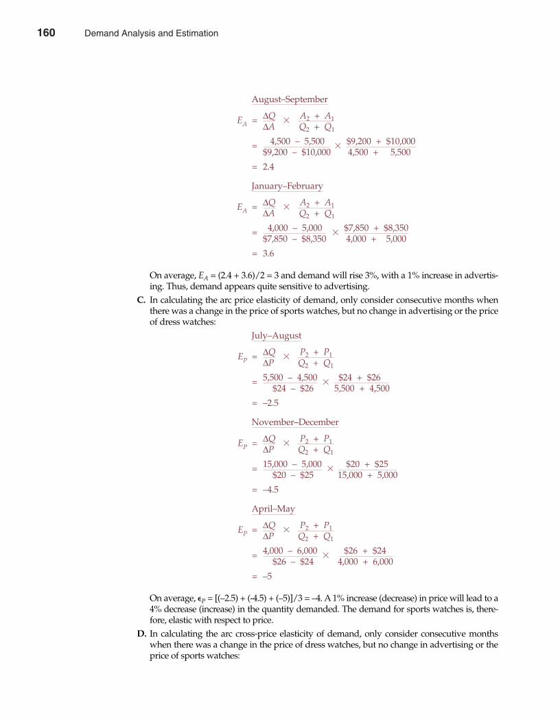
August–September
EA = ∆Q � A2 + A1∆A Q2 + Q1
= 4,500 – 5,500 � $9,200 + $10,000$9,200 – $10,000 4,500 + 5,500
= 2.4
January–February
EA = ∆Q � A2 + A1∆A Q2 + Q1
= 4,000 – 5,000 � $7,850 + $8,350$7,850 – $8,350 4,000 + 5,000
= 3.6
On average, EA = (2.4 + 3.6)/2 = 3 and demand will rise 3%, with a 1% increase in advertis-ing. Thus, demand appears quite sensitive to advertising.
C. In calculating the arc price elasticity of demand, only consider consecutive months whenthere was a change in the price of sports watches, but no change in advertising or the priceof dress watches:
July–August
EP = ∆Q � P2 + P1∆P Q2 + Q1
= 5,500 – 4,500 � $24 + $26$24 – $26 5,500 + 4,500
= –2.5
November–December
EP = ∆Q � P2 + P1∆P Q2 + Q1
= 15,000 – 5,000 � $20 + $25$20 – $25 15,000 + 5,000
= –4.5
April–May
EP = ∆Q � P2 + P1∆P Q2 + Q1
= 4,000 – 6,000 � $26 + $24$26 – $24 4,000 + 6,000
= –5
On average, �P = [(–2.5) + (-4.5) + (–5)]/3 = –4. A 1% increase (decrease) in price will lead to a4% decrease (increase) in the quantity demanded. The demand for sports watches is, there-fore, elastic with respect to price.
D. In calculating the arc cross-price elasticity of demand, only consider consecutive monthswhen there was a change in the price of dress watches, but no change in advertising or theprice of sports watches:
Chapter Five Demand Analysis and Estimation 161
160 Demand Analysis and Estimation
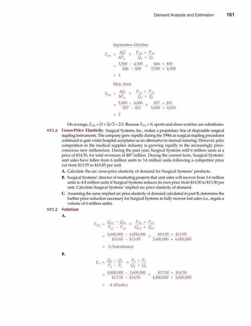
September–October
EPX = ∆Q � PX2 + PX1∆PX Q2 + Q1
= 3,500 – 4,500 � $46 + $50$46 – $50 3,500 + 4,500
= 3
May–June
EPX = ∆Q � PX2 + PX1∆PX Q2 + Q1
= 5,000 – 4,000 � $57 + $51$57 – $51 5,000 + 4,000
= 2
On average, EPX = (3 + 2)/2 = 2.5. Because EPX > 0, sports and dress watches are substitutes.ST5.2 Cross-Price Elasticity. Surgical Systems, Inc., makes a proprietary line of disposable surgical
stapling instruments. The company grew rapidly during the 1990s as surgical stapling procedurescontinued to gain wider hospital acceptance as an alternative to manual suturing. However, pricecompetition in the medical supplies industry is growing rapidly in the increasingly price-conscious new millennium. During the past year, Surgical Systems sold 6 million units at aprice of $14.50, for total revenues of $87 million. During the current term, Surgical Systems’unit sales have fallen from 6 million units to 3.6 million units following a competitor pricecut from $13.95 to $10.85 per unit.A. Calculate the arc cross-price elasticity of demand for Surgical Systems’ products.B. Surgical Systems’ director of marketing projects that unit sales will recover from 3.6 million
units to 4.8 million units if Surgical Systems reduces its own price from $14.50 to $13.50 perunit. Calculate Surgical Systems’ implied arc price elasticity of demand.
C. Assuming the same implied arc price elasticity of demand calculated in part B, determine thefurther price reduction necessary for Surgical Systems to fully recover lost sales (i.e., regain avolume of 6 million units).
ST5.2 SolutionA.
EPX = QY2 – QY1 � PX2 + PX1PX2 – PX1 QY2 + QY1
= 3,600,000 – 6,000,000 � $10.85 + $13.95$10.85 – $13.95 3,600,000 + 6,000,000
= 2 (Substitutes)
B.
EP = Q2 – Q1 � P2 + P1P2 – P1 Q2 + Q1
= 4,800,000 – 3,600,000 � $13.50 + $14.50$13.50 – $14.50 4,800,000 + 3,600,000
= –4 (Elastic)
162 Part Two Demand Analysis
Demand Analysis and Estimation 161
C.
EP = Q2 – Q1 � P2 + P1P2 – P1 Q2 + Q1
–4 = 6,000,000 – 4,800,000 � P2 + $13.50P2 – $13.50 6,000,000 + 4,800,000
–4 = P2 + $13.509(P2 – $13.50)
–36P2 + $486 = P2 + $13.50
37P2 = $472.50
P2 = $12.77
This implies a further price reduction of 73¢:
∆P = $12.77 – $13.50 = –$0.73
PROBLEMS
P5.1 Price Elasticity. Characterize each of the following goods and services in terms of their priceelasticity of demand. In so doing, indicate whether a steeply sloped (vertical) and relativelyinelastic demand curve, or a flat (horizontal) and relatively elastic demand curve, is typicalunder normal market conditions. Why?A. Unleaded gasolineB. WheatC. Individual income tax preparation servicesD. A cure for AIDSE. Lottery tickets
P5.2 Cross-Price Elasticity. Characterize each of the following pairs of goods and/or services interms of their cross-price elasticity of demand. In so doing, indicate whether the cross-priceelasticity of demand is apt to be positive, negative, or zero. Similarly, describe each of thesepairs of products as substitutes, complements, or independent goods. Why?A. Computer memory chips and user-friendly softwareB. Self-service and unskilled laborC. Video games and “surfing the Web”D. Movies and popcornE. Spreadsheet software and bookkeeper labor
P5.3 Income Elasticity. During recent years, the president and Congress have complained aboutskyrocketing public and private expenditures for Medicare and Medicaid services. At the sametime, the demand for privately financed medical care has also increased significantly.A. Use the concept of the income elasticity of demand to explain why the demand for medical
services has grown over time.B. Is it surprising that the share of national income devoted to medical services in the United
States is greater than the share of national income devoted to medical care in less prosperouscountries around the world?
Chapter Five Demand Analysis and Estimation 163
162 Demand Analysis and Estimation
P5.4 Elasticity. The demand for personal computers can be characterized by the following pointelasticities: price elasticity = –5, cross-price elasticity with software = –4, and income elasticity =2.5. Indicate whether each of the following statements is true or false, and explain your answer.A. A price reduction for personal computers will increase both the number of units demanded
and the total revenue of sellers.B. The cross-price elasticity indicates that a 5% reduction in the price of personal computers
will cause a 20% increase in software demand.C. Demand for personal computers is price elastic and computers are cyclical normal goods.D. Falling software prices will increase revenues received by sellers of both computers and
software.E. A 2% price reduction would be necessary to overcome the effects of a 1% decline in income.
P5.5 Demand Curves. KRMY-TV is contemplating a T-shirt advertising promotion. Monthly salesdata from T-shirt shops marketing the “Eye Watch KRMY-TV” design indicate that
Q = 1,500 – 200P
where Q is T-shirt sales and P is price.A. How many T-shirts could KRMY-TV sell at $4.50 each?B. What price would KRMY-TV have to charge to sell 900 T-shirts?C. At what price would T-shirt sales equal zero?D. How many T-shirts could be given away?E. Calculate the point price elasticity of demand at a price of $5.
P5.6 Optimal Pricing. In an effort to reduce excess end-of-the-model-year inventory, HarrisonFord offered a 2.5% discount off the average list price of Focus SE sedans sold during the monthof August. Customer response was enthusiastic, with unit sales rising by 10% over the previousmonth’s level.A. Calculate the point price elasticity of demand for Harrison Ford Focus SE sedans.B. Calculate the profit-maximizing price per unit if Harrison Ford has an average wholesale
cost of $10,000 and incurs marginal selling costs of $875 per unit.P5.7 Cross-Price Elasticity. Kitty Russell’s Longbranch Cafe in Sausalito recently reduced Nachos
Supreme appetizer prices from $5 to $3 for afternoon “early bird” customers and enjoyed aresulting increase in sales from 60 to 180 orders per day. Beverage sales also increased from 30 to150 units per day.A. Calculate the arc price elasticity of demand for Nachos Supreme appetizers.B. Calculate the arc cross-price elasticity of demand between beverage sales and appetizer prices.C. Holding all else equal, would you expect an additional appetizer price decrease to $2.50 to
cause both appetizer and beverage revenues to rise? Explain.P5.8 Income Elasticity. Ironside Industries, Inc., is a leading manufacturer of tufted carpeting under
the Ironside brand. Demand for Ironside’s products is closely tied to the overall pace of buildingand remodeling activity and, therefore, is highly sensitive to changes in national income. The car-pet manufacturing industry is highly competitive, so Ironside’s demand is also very price sensitive.
During the past year, Ironside sold 15 million square yards (units) of carpeting at an averagewholesale price of $7.75 per unit. This year, income per capita is expected to surge from $17,250to $18,750 as the nation recovers from a steep recession. Without any price change, Ironside’smarketing director expects current-year sales to rise to 25 million units.A. Calculate the implied income arc elasticity of demand.B. Given the projected rise in income, the marketing director believes that the current volume
of 15 million units could be maintained despite an increase in price of 50¢ per unit. On thisbasis, calculate the implied arc price elasticity of demand.
164 Part Two Demand Analysis
Demand Analysis and Estimation 163
C. Holding all else equal, would a further increase in price result in higher or lower totalrevenue?
P5.9 Cross-Price Elasticity. B. B. Lean is a catalog retailer of a wide variety of sporting goodsand recreational products. Although the market response to the company’s spring catalog wasgenerally good, sales of B. B. Lean’s $140 deluxe garment bag declined from 10,000 to 4,800units. During this period, a competitor offered a whopping $52 off their regular $137 price ondeluxe garment bags.A. Calculate the arc cross-price elasticity of demand for B. B. Lean’s deluxe garment bag.B. B. B. Lean’s deluxe garment bag sales recovered from 4,800 units to 6,000 units following
a price reduction to $130 per unit. Calculate B. B. Lean’s arc price elasticity of demand forthis product.
C. Assuming the same arc price elasticity of demand calculated in part B, determine the furtherprice reduction necessary for B. B. Lean to fully recover lost sales (i.e., regain a volume of10,000 units).
P5.10 Advertising Elasticity. Enchantment Cosmetics, Inc., offers a line of cosmetic and perfumeproducts marketed through leading department stores. Product manager Erica Kane recentlyraised the suggested retail price on a popular line of mascara products from $9 to $12 followingincreases in the costs of labor and materials. Unfortunately, sales dropped sharply from 16,200to 9,000 units per month. In an effort to regain lost sales, Enchantment ran a coupon promotionfeaturing $5 off the new regular price. Coupon printing and distribution costs totaled $500 permonth and represented a substantial increase over the typical advertising budget of $3,250 permonth. Despite these added costs, the promotion was judged to be a success, as it proved to behighly popular with consumers. In the period prior to expiration, coupons were used on 40%of all purchases and monthly sales rose to 15,000 units.A. Calculate the arc price elasticity implied by the initial response to the Enchantment price
increase.B. Calculate the effective price reduction resulting from the coupon promotion.C. In light of the price reduction associated with the coupon promotion and assuming no
change in the price elasticity of demand, calculate Enchantment’s arc advertising elastic-ity.
D. Why might the true arc advertising elasticity differ from that calculated in part C?
Chapter Five Demand Analysis and Estimation 165
CASE STUDY
Demand Estimation for Branded Consumer ProductsDemand estimation for brand-name consumer products is made difficult by the fact that man-agers must rely on proprietary data. There simply is not any publicly available data that can beused to estimate demand elasticities for brand-name orange juice, frozen entrès, pies, and thelike—and with good reason. Competitors would be delighted to know profit margins across abroad array of competing products so that advertising, pricing policy, and product developmentstrategy could all be targeted for maximum benefit. Product demand information is valuable,and jealously guarded.
To see the process that might be undertaken to develop a better understanding of productdemand conditions, consider the hypothetical example of Mrs. Smyth’s Inc., a Chicago–basedfood company. In early 2002, Mrs. Smyth’s initiated an empirical estimation of demand for itsgourmet frozen fruit pies. The firm is formulating pricing and promotional plans for the com-ing year, and management is interested in learning how pricing and promotional decisionsmight affect sales. Mrs. Smyth’s has been marketing frozen fruit pies for several years, and its
164 Demand Analysis and Estimation
166 Part Two Demand Analysis
market research department has collected quarterly data over two years for six important mar-keting areas, including sales quantity, the retail price charged for the pies, local advertising andpromotional expenditures, and the price charged by a major competing brand of frozen pies.Statistical data published by the U.S. Census Bureau (http://www.census.gov) on populationand disposable income in each of the six market areas were also available for analysis. It wastherefore possible to include a wide range of hypothesized demand determinants in an empir-ical estimation of fruit pie demand. These data appear in Table 5.6.
The following regression equation was fit to these data:
Qit = b0 + b1Pit + b2Ait + b3PXit + b4Yit + b5Popit + b6Tit + uit
Q is the quantity of pies sold during the tth quarter; P is the retail price in dollars of Mrs. Smyth’sfrozen pies; A represents the dollars spent for advertising; PX is the price, measured in dollars,charged for competing premium-quality frozen fuit pies; Y is dollars of disposable income per capi-ta; Pop is the population of the market area; T is the trend factor (2000–1 = 1, . . . , 2001–4 = 8); anduit is a residual (or disturbance) term. The subscript i indicates the regional market from whichthe observation was taken, whereas the subscript t represents the quarter during which theobservation occurred. Least squares estimation of the regression equation on the basis of the 48data observations (eight quarters of data for each of six areas) resulted in the estimated regres-sion coefficients and other statistics given in Table 5.7.
The individual coefficients for the Mrs. Smyth’s pie demand regression equation can beinterpreted as follows. The intercept term, 646,958, has no economic meaning in this instance; itlies far outside the range of observed data and obviously cannot be interpreted as the demandfor Mrs. Smyth’s frozen fruit pies when all the independent variables take on zero values. Thecoefficient for each independent variable indicates the marginal relation between that variableand sales of pies, holding constant the effect of all the other variables in the demand function.For example, the –127,443 coefficient for P, the price charged for Mrs. Smyth’s pies, indicatesthat when the effects of all other demand variables are held constant, each $1 increase in pricecauses quarterly sales to decline by roughly 127,443 pies. Similarly, the 5.353 coefficient for A,the advertising variable, indicates that for each $1 increase in advertising during the quarter,roughly 5.353 additional pies are sold. The 29,337 coefficient for the competitor-price variableindicates that demand for Mrs. Smyth’s pies rises by roughly 29,337 pies with every $1 increasein competitor prices. The 0.344 coefficient for the Y variable indicates that, on average, a $1increase in the average disposable income per capita for a given market leads to roughly a 0.344-unit increase in quarterly pie demand. Similarly, a one person increase in the population of agiven market area leads to a small 0.024-unit increase in quarterly pie demand. Finally, the–4,406 coefficient for the trend variable indicates that pie demand is falling in a typical marketby roughly 4,406 units per quarter. This means that Mrs. Smyth’s is enjoying secular growth inpie demand, perhaps as a result of the growing popularity of Mrs. Smyth’s products or of frozenfoods in general.
Individual coefficients provide useful estimates of the expected marginal influence ondemand following a one-unit change in each respective variable. However, they are onlyestimates. For example, it would be very unusual for a 1¢ increase in price to cause exactly a–127,443-unit change in the quantity demanded. The actual effect could be more or less. Fordecision-making purposes, it would be helpful to know if the marginal influences suggestedby the regression model are stable or instead tend to vary widely over the sample analyzed.
In general, if it is known with certainty that Y = a + bX, then a one-unit change in X willalways lead to a b-unit change in Y. If b > 0, X and Y will be directly related; if b < 0, X andY will be inversely related. If no relation at all holds between X and Y, then b = 0. Althoughthe true parameter b is unobservable, its value is estimated by the regression coefficient b̂.If b̂ = 10, a one-unit change in X will increase Y by 10 units. This effect may appear to be
CASE STUDY (continued)
Demand Analysis and Estimation 165
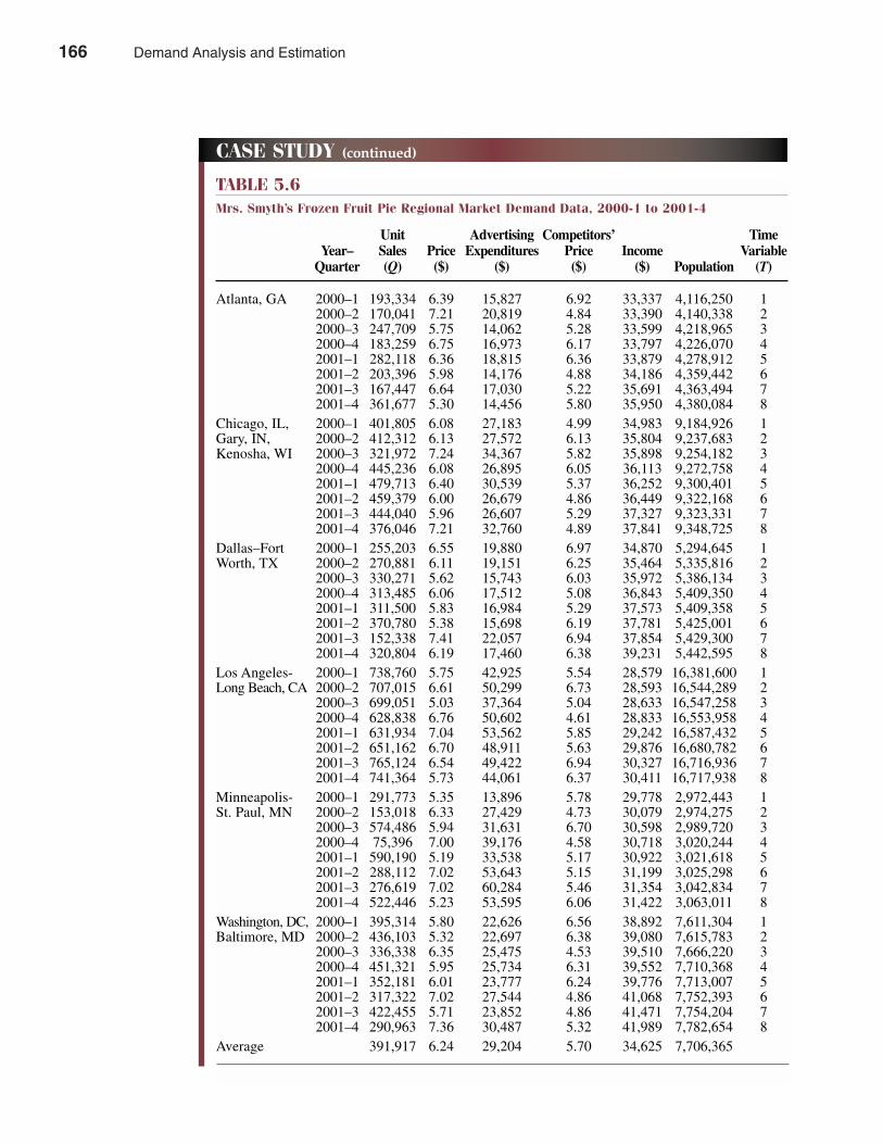
Chapter Five Demand Analysis and Estimation 167
TABLE 5.6Mrs. Smyth’s Frozen Fruit Pie Regional Market Demand Data, 2000-1 to 2001-4
Unit Advertising Competitors’ TimeYear– Sales Price Expenditures Price Income Variable
Quarter (Q) ($) ($) ($) ($) Population (T)
Atlanta, GA 2000–1 193,334 6.39 15,827 6.92 33,337 4,116,250 12000–2 170,041 7.21 20,819 4.84 33,390 4,140,338 22000–3 247,709 5.75 14,062 5.28 33,599 4,218,965 32000–4 183,259 6.75 16,973 6.17 33,797 4,226,070 42001–1 282,118 6.36 18,815 6.36 33,879 4,278,912 52001–2 203,396 5.98 14,176 4.88 34,186 4,359,442 62001–3 167,447 6.64 17,030 5.22 35,691 4,363,494 72001–4 361,677 5.30 14,456 5.80 35,950 4,380,084 8
Chicago, IL, 2000–1 401,805 6.08 27,183 4.99 34,983 9,184,926 1Gary, IN, 2000–2 412,312 6.13 27,572 6.13 35,804 9,237,683 2Kenosha, WI 2000–3 321,972 7.24 34,367 5.82 35,898 9,254,182 3
2000–4 445,236 6.08 26,895 6.05 36,113 9,272,758 42001–1 479,713 6.40 30,539 5.37 36,252 9,300,401 52001–2 459,379 6.00 26,679 4.86 36,449 9,322,168 62001–3 444,040 5.96 26,607 5.29 37,327 9,323,331 72001–4 376,046 7.21 32,760 4.89 37,841 9,348,725 8
Dallas–Fort 2000–1 255,203 6.55 19,880 6.97 34,870 5,294,645 1Worth, TX 2000–2 270,881 6.11 19,151 6.25 35,464 5,335,816 2
2000–3 330,271 5.62 15,743 6.03 35,972 5,386,134 32000–4 313,485 6.06 17,512 5.08 36,843 5,409,350 42001–1 311,500 5.83 16,984 5.29 37,573 5,409,358 52001–2 370,780 5.38 15,698 6.19 37,781 5,425,001 62001–3 152,338 7.41 22,057 6.94 37,854 5,429,300 72001–4 320,804 6.19 17,460 6.38 39,231 5,442,595 8
Los Angeles- 2000–1 738,760 5.75 42,925 5.54 28,579 16,381,600 1Long Beach, CA 2000–2 707,015 6.61 50,299 6.73 28,593 16,544,289 2
2000–3 699,051 5.03 37,364 5.04 28,633 16,547,258 32000–4 628,838 6.76 50,602 4.61 28,833 16,553,958 42001–1 631,934 7.04 53,562 5.85 29,242 16,587,432 52001–2 651,162 6.70 48,911 5.63 29,876 16,680,782 62001–3 765,124 6.54 49,422 6.94 30,327 16,716,936 72001–4 741,364 5.73 44,061 6.37 30,411 16,717,938 8
Minneapolis- 2000–1 291,773 5.35 13,896 5.78 29,778 2,972,443 1St. Paul, MN 2000–2 153,018 6.33 27,429 4.73 30,079 2,974,275 2
2000–3 574,486 5.94 31,631 6.70 30,598 2,989,720 32000–4 75,396 7.00 39,176 4.58 30,718 3,020,244 42001–1 590,190 5.19 33,538 5.17 30,922 3,021,618 52001–2 288,112 7.02 53,643 5.15 31,199 3,025,298 62001–3 276,619 7.02 60,284 5.46 31,354 3,042,834 72001–4 522,446 5.23 53,595 6.06 31,422 3,063,011 8
Washington, DC, 2000–1 395,314 5.80 22,626 6.56 38,892 7,611,304 1Baltimore, MD 2000–2 436,103 5.32 22,697 6.38 39,080 7,615,783 2
2000–3 336,338 6.35 25,475 4.53 39,510 7,666,220 32000–4 451,321 5.95 25,734 6.31 39,552 7,710,368 42001–1 352,181 6.01 23,777 6.24 39,776 7,713,007 52001–2 317,322 7.02 27,544 4.86 41,068 7,752,393 62001–3 422,455 5.71 23,852 4.86 41,471 7,754,204 72001–4 290,963 7.36 30,487 5.32 41,989 7,782,654 8
Average 391,917 6.24 29,204 5.70 34,625 7,706,365
CASE STUDY (continued)
166 Demand Analysis and Estimation
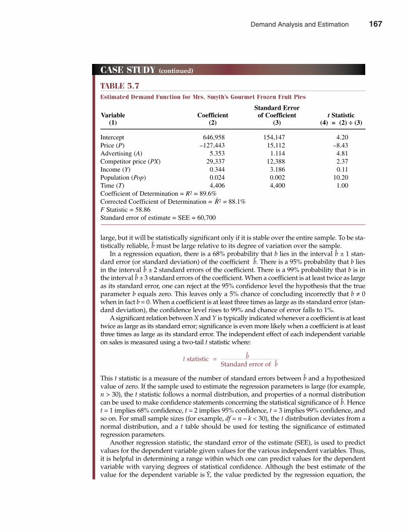
168 Part Two Demand Analysis
CASE STUDY (continued)
large, but it will be statistically significant only if it is stable over the entire sample. To be sta-tistically reliable, b̂ must be large relative to its degree of variation over the sample.
In a regression equation, there is a 68% probability that b lies in the interval b̂ ± 1 stan-dard error (or standard deviation) of the coefficient b̂. There is a 95% probability that b liesin the interval b̂ ± 2 standard errors of the coefficient. There is a 99% probability that b is inthe interval b̂ ± 3 standard errors of the coefficient. When a coefficient is at least twice as largeas its standard error, one can reject at the 95% confidence level the hypothesis that the trueparameter b equals zero. This leaves only a 5% chance of concluding incorrectly that b ≠ 0when in fact b = 0. When a coefficient is at least three times as large as its standard error (stan-dard deviation), the confidence level rises to 99% and chance of error falls to 1%.
Asignificant relation between X and Y is typically indicated whenever a coefficient is at leasttwice as large as its standard error; significance is even more likely when a coefficient is at leastthree times as large as its standard error. The independent effect of each independent variableon sales is measured using a two-tail t statistic where:
t statistic = b̂Standard error of b̂
This t statistic is a measure of the number of standard errors between b̂ and a hypothesizedvalue of zero. If the sample used to estimate the regression parameters is large (for example,n > 30), the t statistic follows a normal distribution, and properties of a normal distributioncan be used to make confidence statements concerning the statistical significance of b̂. Hencet = 1 implies 68% confidence, t = 2 implies 95% confidence, t = 3 implies 99% confidence, andso on. For small sample sizes (for example, df = n – k < 30), the t distribution deviates from anormal distribution, and a t table should be used for testing the significance of estimatedregression parameters.
Another regression statistic, the standard error of the estimate (SEE), is used to predictvalues for the dependent variable given values for the various independent variables. Thus,it is helpful in determining a range within which one can predict values for the dependentvariable with varying degrees of statistical confidence. Although the best estimate of thevalue for the dependent variable is Ŷ, the value predicted by the regression equation, the
TABLE 5.7Estimated Demand Function for Mrs. Smyth’s Gourmet Frozen Fruit Pies
Standard ErrorVariable Coefficient of Coefficient t Statistic
(1) (2) (3) (4) = (2) ÷ (3)
Intercept 646,958 154,147 4.20Price (P) –127,443 15,112 –8.43Advertising (A) 5.353 1.114 4.81Competitor price (PX) 29,337 12,388 2.37Income (Y) 0.344 3.186 0.11Population (Pop) 0.024 0.002 10.20Time (T) 4,406 4,400 1.00Coefficient of Determination = R2 = 89.6%Corrected Coefficient of Determination =
-R2 = 88.1%
F Statistic = 58.86Standard error of estimate = SEE = 60,700
Demand Analysis and Estimation 167
SELECTED REFERENCES Berndt, Ernst R., and Neal J. Rappaport. “Price and Quality of Desktop and Mobile Personal Computers:
A Quarter-Century Historical Overview.” American Economic Review 91 (May 2001): 268–273.Bils, Mark, and Peter J. Klenow. “The Acceleration in Variety Growth.” American Economic Review 91 (May
2001): 274–280.Dur, Robert A. J. “Wage-Setting Institutions, Unemployment, and Voters’ Demand for Redistribution
Policy.” Scottish Journal of Political Economy 48 (November 2001): 517–531.Fehr, Ernst, and Jean-Robert Tyran. “Does Money Illusion Matter?” American Economic Review 91
(December 2001): 1239–1262.Goodman, Jack. “The Latest on Demand for In-Town Real Estate.” Real Estate Finance 17 (Winter 2001): 41–48.Hausman, Jerry A., J. Gregory Sidak, and Hal J. Singer. “Residential Demand for Broadband Telecom-
munications and Consumer Access to Unaffiliated Internet Content Providers.” Yale Journal onRegulation 18 (Winter 2001): 129–173.
Jesswein, Wayne, Kjell Knudsen, Richard Lichty, et al. “Regional Competitiveness: Determining Demandfor Skilled Workers in Northeast Minnesota.” Economic Development Review 17 (Winter 2001): 70–75.
Krishna, Pravin, Devashish Mitra, and Sajjid Chinoy. “Trade Liberalization and Labor DemandElasticities: Evidence from Turkey.” Journal of International Economics 55 (December 2001): 391–409.
Montgomery, Alan L. “Applying Quantitative Marketing Techniques to the Internet.” Interfaces 31(March 2001): 90–108.
Nijs, Vincent R., Marnik G. Dekimpe, Jan-Benedict E. M. Steenkamp, et al. “The Category-Demand Effectsof Price Promotions.” Marketing Science 20 (Winter 2001): 1–22.
Pedroni, Peter. “Purchasing Power Parity Tests in Cointegrated Panels.” Review of Economics and Statistics83 (November 2001): 727–731.
Staunton, Robert H., John D. Kueck, Brendan J. Kirby, et al. “Demand Response: An Overview ofEnabling Technologies.” Public Utilities Fortnightly 139 (Nov 2001): 32–39.
Chapter Five Demand Analysis and Estimation 169
CASE STUDY (continued)
standard error of the estimate can be used to determine just how accurate this prediction Ŷis likely to be. Assuming that the standard errors are normally distributed about the regres-sion equation, there is a 68% probability that actual observations of the dependent variableY will lie within the rangeŶ ± 1 standard error of the estimate. The probability that an actualobservation of Y will lie within two standard errors of its predicted value increases to 95%.There is a 99% chance that an actual observed value for Y will lie in the rangeŶ ± 3 standarderrors. Obviously, greater predictive accuracy is associated with smaller standard errors ofthe estimate.
Mrs. Smyth’s could forecast the total demand for its pies by forecasting sales in each of thesix market areas, then summing these area forecasts to obtain an estimate of total pie demand.Using the results from the demand estimation model and data from each individual market,it would also be possible to construct a confidence interval for total pie demand based on thestandard error of the estimate.A. Describe the statistical significance of each individual independent variable included in
the Mrs. Smyth’s frozen fruit pie demand equation.B. Interpret the coefficient of determination (R2) for the Mrs. Smyth’s frozen fruit pie
demand equation.C. Use the regression model and 2001–4 data to estimate 2002–1 unit sales in the Washington,
DC–Baltimore, MD, market.D. To illustrate use of the standard error of the estimate statistic, derive the 95% confidence
interval for 2002–1 actual unit sales in the Washington, DC–Baltimore, MD, market.
168 Demand Analysis and Estimation

Wagner, Todd H., Teh-Wei Hu, and Judith H. Hibbard. “The Demand for Consumer Health Information.”Journal of Health Economics 20 (November 2001): 1059–1075.
Wiser, Ryan H., Meredith Fowlie, and Edward A. Holt. “Public Goods and Private Interests:Understanding Non-Residential Demand for Green Power.” Energy Policy 29 (November 2001):1085–1097.
Yatchew, Adonis, and Joungyeo Angela No. “Household Gasoline Demand in Canada.” Econometrica 69(November 2001): 1697–1709.
170 Part Two Demand Analysis
Demand Analysis and Estimation 169


Forecasting
CHAPTER SIX
171
Afamous economist once remarked, “We have two classes of forecasters:Those who don’t know—and those who don’t know that they don’t
know.” There is more than a bit of truth to this witticism.Experienced economists know that economic forecasting is fraught with
uncertainty. To see why, consider the interrelated nature of economic forecasts.One might ask an economist, will the pace of real economic growth in theUnited States average an anemic 2 percent, a healthy 3 percent, or a robust 3.5percent? What will be the rate of inflation? How will investors respond to aproposed change in the tax law, if and when such a change is passed by bothHouses of Congress and signed into law by the president? Most important,how is the rate of growth in the overall economy related to inflation, and howare both apt to be affected by an important change in tax law that, at this point,is only at the proposal stage?
When chemists and physicists run experiments, they have carefully con-trolled laboratory environments. Economists enjoy no such luxury; they mustmake assumptions based on volatile economic and political conditions subjectto random and violent shocks. No wonder that economic forecasters lamentthe difficulty of making accurate economic projections.1
Predicting trends in the overall economy and its impact on the cost ordemand for company goods and services is one of the most difficult responsi-bilities facing management. However, it is a necessary task because, for better orworse, all decisions are made on the basis of future expectations. This chapterillustrates a number of forecasting techniques that have proven successful informing accurate expectations in a wide variety of real-world applications.
1 See Erin Schulte, “Economists Say Fed Moves May Still Be Months Away,” The Wall StreetJournal Online, March 23, 2002 (http://online.wsj.com).
171
6
WHAT IS ECONOMIC FORECASTING?
When companies hire new workers, they must predict the relative productivity of a wide vari-ety of individuals with diverse skills, work histories, and personalities. How much inventoryshould be carried? What price should be charged during the coming holiday season? Whichmarket is the most natural path for expansion? These and a host of everyday business deci-sions require that managers make informed forecasts of future economic events.
Why Is Forecasting Useful?Managers sometimes must integrate quantitative and nonquantitative information in a way noteasily modeled or characterized by numbers. In such instances, there is no substitute for theextraordinary pattern recognition capabilities of the human mind. Experienced managerssometimes “know” the correct level of inventory, or right price, despite their inability to easilyexplain all the factors that weigh in their decisions. Although there is no good substitute forthe careful intuition of an experienced manager, some firms err in their over reliance onjudgmental forecasts. In some cases, the concept of forecasting is confused with goal setting.If a company asks its staff to forecast sales for the mid-Atlantic region, for example, these“forecasts” are sometimes used as yardsticks to judge sales performance. If forecast sales areexceeded, sales performance is “good”; if forecast sales are not achieved, sales performanceis “poor.” This sometimes leads sales staffs to underestimate future sales in a effort to boostperceived performance. Just as a successful college football coach predicts a tough year toenhance the popular perception of a winning record, sales personnel have incentives to beoverly conservative in their sales projections for new or improved products. Coaches of footballteams with 8-3 records sometimes lose their jobs if fans had expected a perfect 11-0 season;brand managers of even highly successful new product introductions sometimes get fired ifrosy predictions are not met.
A big advantage of the wide variety of statistical techniques commonly used in economicforecasting is that they separate the process of forecasting from the firm’s goal-setting activity.When sales are forecast in an objective, systematic, and unbiased manner, the potential for accu-rate forecasts increases, as does the capacity for appropriate operating and planning decisions.When these forecasts involve outcomes and precipitating factors that can be quantified, it alsobecomes possible to access the direct ramifications of changes in controllable and uncontrollableconditions. Optimistic through pessimistic scenarios can be tested and analyzed for their per-formance implications and for their significance in terms of the decision-making process.Forecasting that is objective and quantitative has the potential to help almost any business;accurate business forecasting is a value-added undertaking.
COMMON TYPES OF FORECASTING PROBLEMS
Macroeconomic Forecast ProblemsMacroeconomic forecasting involves predicting aggregate measures of economic activity atthe international, national, regional, or state level. Predictions of gross domestic product (GDP),unemployment, and interest rates by “blue chip” business economists capture the attention ofnational media, business, government, and the general public on a daily basis.2 Other macro-economic forecasts commonly reported in the press include predictions of consumer spending,
172 Part Two Demand Analysis
macroeconomicforecastingPrediction of aggregateeconomic activity
2 GDP measures aggregate business activity as described by the value at final point of sale of all goods and servicesproduced in the domestic economy during a given period by both domestic and foreign-owned enterprises. Grossnational product (GNP) is the value at final point of sale of all goods and services produced by domestic firms. Assuch, GNP does not reflect domestic production by foreign-owned firms (e.g., Toyota Camrys produced in Kentucky).
172 Forecasting
business investment, homebuilding, exports, imports, federal purchases, state and local gov-ernment spending, and so on. Macroeconomic predictions are important because they are usedby businesses and individuals to make day-to-day operating decisions and long-term planningdecisions. If interest rates are projected to rise, homeowners may rush to refinance fixed-ratemortgages, while businesses float new bond and stock offerings to refinance existing debt ortake advantage of investment opportunities. When such predictions are accurate, significantcost savings or revenue gains become possible. When such predictions are inaccurate, highercosts and lost marketing opportunities occur.
The accuracy of any forecast is subject to the influence of controllable and uncontrollablefactors. In the case of macroeconomic forecasting, uncontrollable factors loom large. Takeinterest rate forecasting, for example. The demand for credit and short-term interest ratesrises if businesses seek to build inventories or expand plant and equipment, or if consumerswish to increase installment credit. The supply of credit rises and short-term interest ratesfall if the Federal Reserve System acts to increase the money supply, or if consumers cut backon spending to increase savings. Interest rate forecasting is made difficult by the fact thatbusiness decisions to build inventories, for example, are largely based on the expected paceof overall economic activity—which itself depends on interest-rate expectations. The macro-economic environment is interrelated in ways that are unstable and cannot be easily predict-ed. Even policy decisions are hard to predict. For example, Federal Reserve System policymeeting minutes are confidential until months after the fact. Is it any wonder that “Fedwatching” is a favorite pastime of business economists?
Microeconomic Forecast ProblemsIn contrast with macroeconomic forecasting, microeconomic forecasting involves the pre-diction of disaggregate economic data at the industry, firm, plant, or product level. Unlikepredictions of GDP growth, which are widely followed in the press, the general public oftenignores microeconomic forecasts of scrap prices for aluminum, the demand for new cars, orproduction costs for Crest toothpaste. It is unlikely that the CBS Evening News will ever beinterrupted to discuss an upward trend in used car prices, even though these data are an excel-lent predictor of new car demand. When used car prices surge, new car demand often growsrapidly; when used car prices sag, new car demand typically drops. The fact that used carprices and new car demand are closely related is not surprising given the strong substitute-good relation that exists between used cars and new cars.
Trained and experienced analysts often find it easier to accurately forecast microeconomictrends, such as the demand for new cars, than macroeconomic trends, such as GDP growth.This is because microeconomic forecasts abstract from the multitude of interrelationships thattogether determine the macroeconomy. With specialized knowledge about changes in new carprices, car import tariffs, car loan rates, and used cars prices, among other factors, it is possi-ble to focus on the fairly narrow range of important factors that influence new car demand. Incontrast, a similarly precise model of aggregate demand in the macroeconomy might involvethousands of economic variables and hundreds of functional relationships.
This is not to say that precise microeconomic forecasting is easy. For example, in August1999, Standard and Poor’s DRI forecast new car and light truck sales of 15.7 million units forthe 2000 model year. This was a reasonable number, and within the 15.3–16.0 million unitrange of forecasts provided by the University of Michigan, Blue Chip Economic Forecasters,and others. Unfortunately, in September 2000, all such forecasts proved too conservative inlight of the 17.2 million units actually sold in a robust economic environment. Undaunted,forecasters expected unit sales of 16.1 million in 2001 and 16.8 million in 2002. Those numberslooked good, until terrorist attacks in New York City and Washington, DC, on September 11,2001, sent new car and light truck sales into a tailspin as consumer confidence plummeted.At that point, it became anybody’s guess as to how long it would take for consumer confi-
microeconomicforecastingPrediction of partialeconomic data
Chapter Six Forecasting 173
Forecasting 173
dence and new car and light truck sales to recover. Obviously, accurate auto and light truckdemand forecasting is tough even for industry experts.
Problem of Changing ExpectationsThe subtle problem of changing expectations bedevils both macroeconomic and microeco-nomic forecasting. If business purchasing agents are optimistic about future trends in theeconomy and boost inventories in anticipation of surging customer demand, the resultinginventory buildup can itself contribute to economic growth. Conversely, if purchasing agentsfear an economic downturn and cut back on orders and inventory growth, they themselves canbe a main contributor to any resulting economic downturn. The expectations of purchasingagents and other managers can become a self-fulfilling prophecy because the macroeconomicenvironment represents the sum of the investment and spending decisions of business, govern-ment, and the public. In fact, the link between expectations and realizations has the potential tocreate an optimistic bias in government-reported statistics.
Government economists are sometimes criticized for being overly optimistic about therate of growth in the overall economy, the future path of interest rates, or the magnitude ofthe federal deficit. As consumers of economic statistics, managers must realize that it can payfor government or politically motivated economists to be optimistic. If business leaders canbe led to make appropriate decisions for a growing economy, their decisions can in fact help leadto a growing economy. Unlike many business economists from the private sector, government-employed and/or politically motivated economists often actively seek to manage the economicexpectations of business leaders and the general public.
It is vital for managers to appreciate the link between economic expectations and realizations,and to be wary of the potential for forecast bias.
Data Quality ProblemsAccurate forecasts require pertinent data that are current, complete, and free from error.Almost everyone has heard the familiar warning about the relation between data quality andforecast accuracy: “garbage in, garbage out.” However, this statement is true in ways that arenot immediately obvious. For example, if a manager wants to forecast demand for consumeror producer goods, it is often better to input incoming orders rather than shipments becauseshipments are sometimes subject to production delays. Similarly, the timing of order fulfill-ment is sometimes subject to delays in transit that are beyond the control of the shipping firm.
In addition to carefully considering the quality of data used to generate forecasts, the quan-tity of available data is also important. A general rule is: The more data that can be subject toanalysis, the better. Some advanced forecasting software that works on desktop personal com-puters can function with as few as five data points. However, forecasts that result from suchpaltry bodies of data are often simplistic, if not trivial. Although the collection of large samplesof data on market transactions can be expensive and tedious, the payoff in forecast accuracycan justify the effort.
If monthly data are seasonal in nature, it is important to have an extended time series tofacilitate forecast accuracy. Most forecasting software programs used to monitor monthlyactivity require a minimum of 2 years of data (24 observations) to build a seasonally adjustedforecast model. Practically speaking, 2 years of monthly data are often not enough; 5 years ofmonthly data (60 observations) are typically necessary before a high level of monthly forecastaccuracy can be achieved. Of course, most forecast software works with data of any periodic-ity, be it hourly, daily, weekly, monthly, or annual in nature. The ultimate consideration thatmust be addressed is whether the quantity and quality of data analyzed are sufficient to shedmeaningful light on the forecast problem being addressed. The acid test is: Can useful forecastsbe generated?
174 Part Two Demand Analysis
174 Forecasting
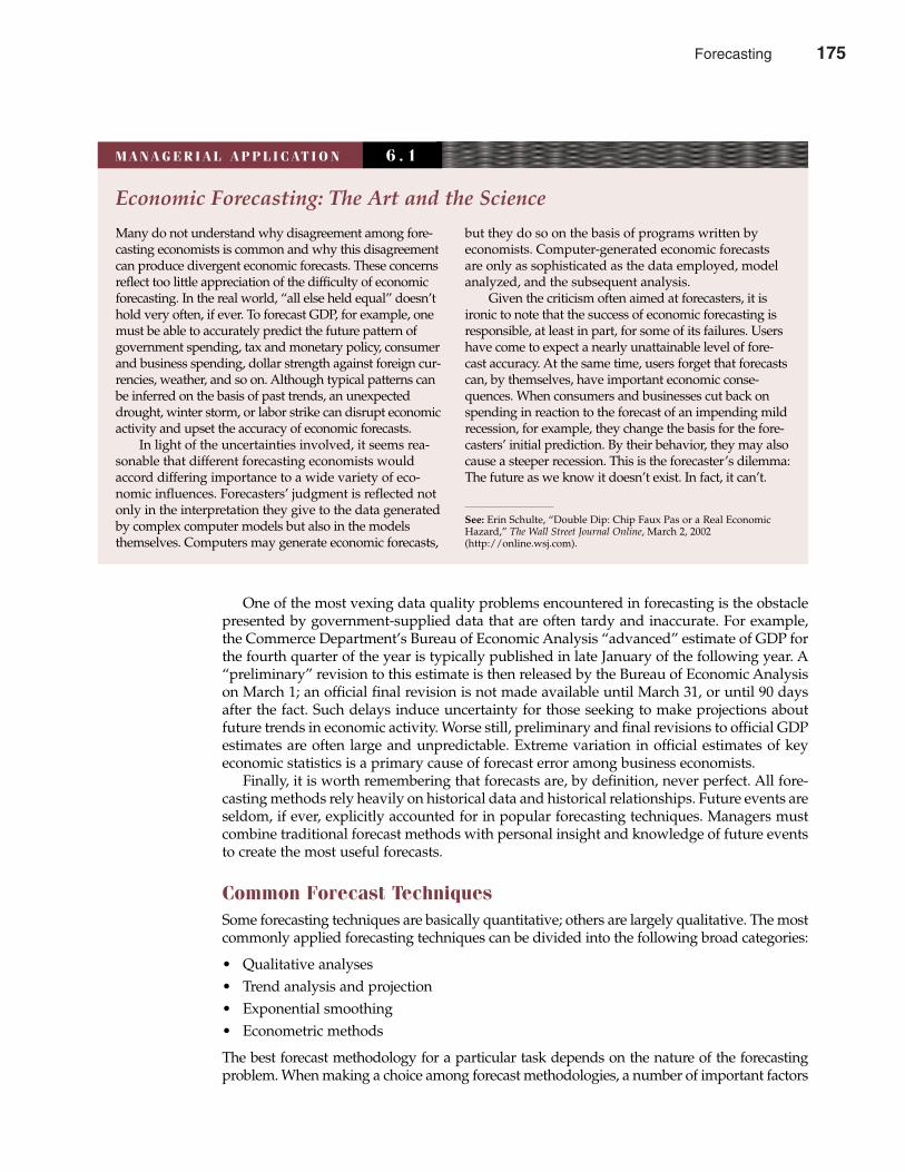
One of the most vexing data quality problems encountered in forecasting is the obstaclepresented by government-supplied data that are often tardy and inaccurate. For example,the Commerce Department’s Bureau of Economic Analysis “advanced” estimate of GDP forthe fourth quarter of the year is typically published in late January of the following year. A“preliminary” revision to this estimate is then released by the Bureau of Economic Analysison March 1; an official final revision is not made available until March 31, or until 90 daysafter the fact. Such delays induce uncertainty for those seeking to make projections aboutfuture trends in economic activity. Worse still, preliminary and final revisions to official GDPestimates are often large and unpredictable. Extreme variation in official estimates of keyeconomic statistics is a primary cause of forecast error among business economists.
Finally, it is worth remembering that forecasts are, by definition, never perfect. All fore-casting methods rely heavily on historical data and historical relationships. Future events areseldom, if ever, explicitly accounted for in popular forecasting techniques. Managers mustcombine traditional forecast methods with personal insight and knowledge of future eventsto create the most useful forecasts.
Common Forecast TechniquesSome forecasting techniques are basically quantitative; others are largely qualitative. The mostcommonly applied forecasting techniques can be divided into the following broad categories:
• Qualitative analyses• Trend analysis and projection• Exponential smoothing• Econometric methods
The best forecast methodology for a particular task depends on the nature of the forecastingproblem. When making a choice among forecast methodologies, a number of important factors
Chapter Six Forecasting 175
Economic Forecasting: The Art and the Science
Many do not understand why disagreement among fore-casting economists is common and why this disagreementcan produce divergent economic forecasts. These concernsreflect too little appreciation of the difficulty of economicforecasting. In the real world, “all else held equal” doesn’thold very often, if ever. To forecast GDP, for example, onemust be able to accurately predict the future pattern ofgovernment spending, tax and monetary policy, consumerand business spending, dollar strength against foreign cur-rencies, weather, and so on. Although typical patterns canbe inferred on the basis of past trends, an unexpecteddrought, winter storm, or labor strike can disrupt economicactivity and upset the accuracy of economic forecasts.
In light of the uncertainties involved, it seems rea-sonable that different forecasting economists wouldaccord differing importance to a wide variety of eco-nomic influences. Forecasters’ judgment is reflected notonly in the interpretation they give to the data generatedby complex computer models but also in the modelsthemselves. Computers may generate economic forecasts,
but they do so on the basis of programs written byeconomists. Computer-generated economic forecastsare only as sophisticated as the data employed, modelanalyzed, and the subsequent analysis.
Given the criticism often aimed at forecasters, it isironic to note that the success of economic forecasting isresponsible, at least in part, for some of its failures. Usershave come to expect a nearly unattainable level of fore-cast accuracy. At the same time, users forget that forecastscan, by themselves, have important economic conse-quences. When consumers and businesses cut back onspending in reaction to the forecast of an impending mildrecession, for example, they change the basis for the fore-casters’ initial prediction. By their behavior, they may alsocause a steeper recession. This is the forecaster’s dilemma:The future as we know it doesn’t exist. In fact, it can’t.
See: Erin Schulte, “Double Dip: Chip Faux Pas or a Real EconomicHazard,” The Wall Street Journal Online, March 2, 2002(http://online.wsj.com).
M A N A G E R I A L A P P L I C AT I O N 6 . 1
Forecasting 175
must be considered. It is always worth considering the distance into the future that one mustforecast, the lead time available for making decisions, the level of accuracy required, the qualityof data available for analysis, the stochastic or deterministic nature of forecast relations, and thecost and benefits associated with the forecasting problem.
Trend analysis, market experiments, consumer surveys, and the leading indicator approachto forecasting are well suited for short-term projections. Forecasting with complex econometricmodels and systems of simultaneous equations have proven somewhat more useful for long-run forecasting. Typically, the greater the level of sophistication, the higher the cost. If therequired level of accuracy is low, less sophisticated methods can provide adequate results atminimal cost.
QUALITATIVE ANALYSIS
Qualitative analysis, an intuitive judgmental approach to forecasting, can be useful if itallows for the systematic collection and organization of data derived from unbiased, informedopinion. However, qualitative methods can produce biased results when specific individualsdominate the forecasting process through reputation, force of personality, or strategic positionwithin the organization.
Expert OpinionThe most basic form of qualitative analysis forecasting is personal insight, in which an informedindividual uses personal or company experience as a basis for developing future expectations.Although this approach is subjective, the reasoned judgment of informed individuals often pro-vides valuable insight. When the informed opinion of several individuals is relied on, theapproach is called forecasting through panel consensus. The panel consensus method assumesthat several experts can arrive at forecasts that are superior to those that individuals generate.Direct interaction among experts can help ensure that resulting forecasts embody all availableobjective and subjective information.
Although the panel consensus method often results in forecasts that embody the collectivewisdom of consulted experts, it can be unfavorably affected by the forceful personality of one ora few key individuals. A related approach, the delphi method, has been developed to counterthis disadvantage. In the delphi method, members of a panel of experts individually receive aseries of questions relating to the underlying forecasting problem. Responses are analyzed by anindependent party, who then tries to elicit a consensus opinion by providing feedback to panelmembers in a manner that prevents direct identification of individual positions. This methodhelps limit the steamroller or bandwagon problems of the basic panel consensus approach.
Survey TechniquesSurvey techniques that skillfully use interviews or mailed questionnaires are an important fore-casting tool, especially for short-term projection. Designing surveys that provide unbiased andreliable information is a challenging task. When properly carried out, however, survey researchcan provide managers with valuable information that would otherwise be unobtainable.
Surveys generally use interviews or mailed questionnaires that ask firms, governmentagencies, and individuals about their future plans. Businesses plan and budget virtually alltheir expenditures in advance of actual purchase or production decisions. Surveys askingabout capital budgets, sales budgets, and operating budgets can thus provide useful forecastinformation. Government departments that prepare formal budgets also provide a wealth ofinformation to the forecaster. Finally, because individual consumers routinely plan expendi-tures for such major items as automobiles, furniture, housing, vacations, and education, sur-veys of consumer intentions often accurately predict future spending on consumer goods.
176 Part Two Demand Analysis
qualitative analysisAn intuitive judgmentalapproach to forecastingbased on opinion
personal insightForecast method basedon personal or organi-zational experience
panel consensusForecast method basedon the informed opinionof several individuals
delphi methodMethod that uses fore-casts derived from anindependent analysisof expert opinion
survey techniquesInterview or mailedquestionnaire approachto forecasting
176 Forecasting
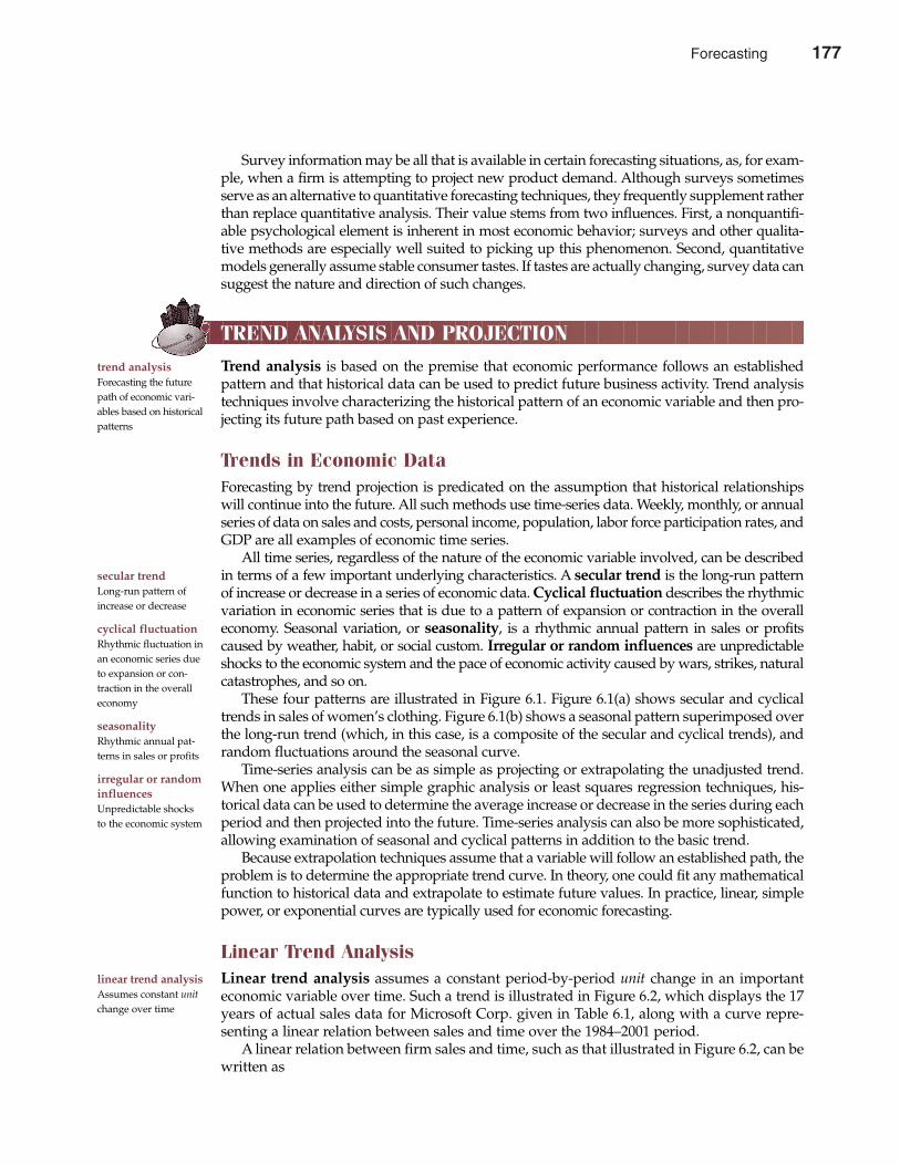
Survey information may be all that is available in certain forecasting situations, as, for exam-ple, when a firm is attempting to project new product demand. Although surveys sometimesserve as an alternative to quantitative forecasting techniques, they frequently supplement ratherthan replace quantitative analysis. Their value stems from two influences. First, a nonquantifi-able psychological element is inherent in most economic behavior; surveys and other qualita-tive methods are especially well suited to picking up this phenomenon. Second, quantitativemodels generally assume stable consumer tastes. If tastes are actually changing, survey data cansuggest the nature and direction of such changes.
TREND ANALYSIS AND PROJECTION
Trend analysis is based on the premise that economic performance follows an establishedpattern and that historical data can be used to predict future business activity. Trend analysistechniques involve characterizing the historical pattern of an economic variable and then pro-jecting its future path based on past experience.
Trends in Economic DataForecasting by trend projection is predicated on the assumption that historical relationshipswill continue into the future. All such methods use time-series data. Weekly, monthly, or annualseries of data on sales and costs, personal income, population, labor force participation rates, andGDP are all examples of economic time series.
All time series, regardless of the nature of the economic variable involved, can be describedin terms of a few important underlying characteristics. A secular trend is the long-run patternof increase or decrease in a series of economic data. Cyclical fluctuation describes the rhythmicvariation in economic series that is due to a pattern of expansion or contraction in the overalleconomy. Seasonal variation, or seasonality, is a rhythmic annual pattern in sales or profitscaused by weather, habit, or social custom. Irregular or random influences are unpredictableshocks to the economic system and the pace of economic activity caused by wars, strikes, naturalcatastrophes, and so on.
These four patterns are illustrated in Figure 6.1. Figure 6.1(a) shows secular and cyclicaltrends in sales of women’s clothing. Figure 6.1(b) shows a seasonal pattern superimposed overthe long-run trend (which, in this case, is a composite of the secular and cyclical trends), andrandom fluctuations around the seasonal curve.
Time-series analysis can be as simple as projecting or extrapolating the unadjusted trend.When one applies either simple graphic analysis or least squares regression techniques, his-torical data can be used to determine the average increase or decrease in the series during eachperiod and then projected into the future. Time-series analysis can also be more sophisticated,allowing examination of seasonal and cyclical patterns in addition to the basic trend.
Because extrapolation techniques assume that a variable will follow an established path, theproblem is to determine the appropriate trend curve. In theory, one could fit any mathematicalfunction to historical data and extrapolate to estimate future values. In practice, linear, simplepower, or exponential curves are typically used for economic forecasting.
Linear Trend AnalysisLinear trend analysis assumes a constant period-by-period unit change in an importanteconomic variable over time. Such a trend is illustrated in Figure 6.2, which displays the 17years of actual sales data for Microsoft Corp. given in Table 6.1, along with a curve repre-senting a linear relation between sales and time over the 1984–2001 period.
A linear relation between firm sales and time, such as that illustrated in Figure 6.2, can bewritten as
trend analysisForecasting the futurepath of economic vari-ables based on historicalpatterns
secular trendLong-run pattern ofincrease or decrease
cyclical fluctuationRhythmic fluctuation inan economic series dueto expansion or con-traction in the overalleconomy
seasonality Rhythmic annual pat-terns in sales or profits
irregular or randominfluencesUnpredictable shocksto the economic system
linear trend analysisAssumes constant unitchange over time
Chapter Six Forecasting 177
Forecasting 177
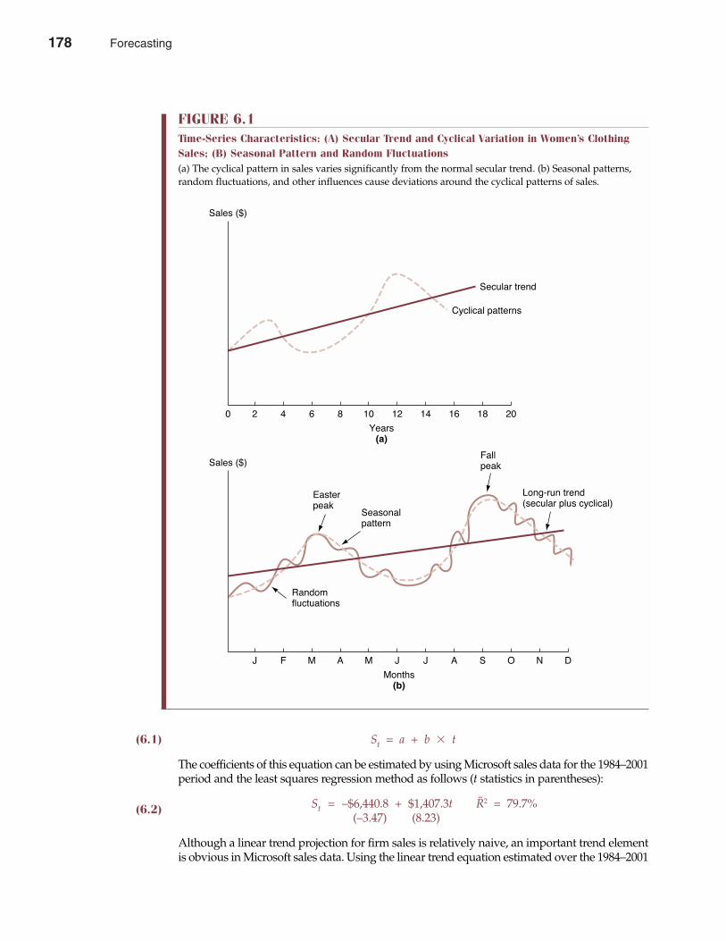
(6.1) St = a + b � t
The coefficients of this equation can be estimated by using Microsoft sales data for the 1984–2001period and the least squares regression method as follows (t statistics in parentheses):
(6.2) St = –$6,440.8 + $1,407.3t-R2 = 79.7%
(–3.47) (8.23)
Although a linear trend projection for firm sales is relatively naive, an important trend elementis obvious in Microsoft sales data. Using the linear trend equation estimated over the 1984–2001
178 Part Two Demand Analysis
FIGURE 6.1Time-Series Characteristics: (A) Secular Trend and Cyclical Variation in Women’s ClothingSales; (B) Seasonal Pattern and Random Fluctuations(a) The cyclical pattern in sales varies significantly from the normal secular trend. (b) Seasonal patterns,random fluctuations, and other influences cause deviations around the cyclical patterns of sales.
Long-run trend(secular plus cyclical)
Fallpeak
Easterpeak
Seasonalpattern
Randomfluctuations
J F M A M J J A S O N D
Months(b)
0 2 4 6 8 10 12 14 16 18 20
Years(a)
Sales ($)
Sales ($)
Secular trend
Cyclical patterns
178 Forecasting
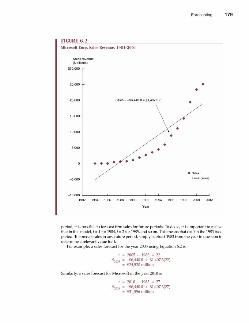
period, it is possible to forecast firm sales for future periods. To do so, it is important to realizethat in this model, t = 1 for 1984, t = 2 for 1985, and so on. This means that t = 0 in the 1983 baseperiod. To forecast sales in any future period, simply subtract 1983 from the year in question todetermine a relevant value for t.
For example, a sales forecast for the year 2005 using Equation 6.2 is
t = 2005 – 1983 = 22S2005 = –$6,440.8 + $1,407.3(22)
= $24,520 million
Similarly, a sales forecast for Microsoft in the year 2010 is
t = 2010 – 1983 = 27S2008 = –$6,440.8 + $1,407.3(27)
= $31,556 million
Chapter Six Forecasting 179
FIGURE 6.2Microsoft Corp. Sales Revenue, 1984–2001
$30,000
25,000
20,000
15,000
10,000
5,000
0
Ð5,000
Ð10,000
Year
Sales revenue($ billions)
Sales = Ð$6,440.8 + $1,407.3 t
1982 1984 1986 1988 1990 1992 1994 1996 1998 2000 2002
Linear (sales)
Sales
Forecasting 179
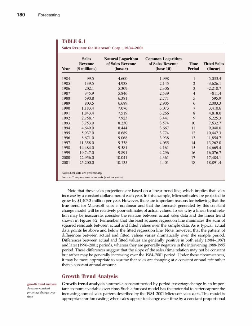
Note that these sales projections are based on a linear trend line, which implies that salesincrease by a constant dollar amount each year. In this example, Microsoft sales are projected togrow by $1,407.3 million per year. However, there are important reasons for believing that thetrue trend for Microsoft sales is nonlinear and that the forecasts generated by this constantchange model will be relatively poor estimates of actual values. To see why a linear trend rela-tion may be inaccurate, consider the relation between actual sales data and the linear trendshown in Figure 6.2. Remember that the least squares regression line minimizes the sum ofsquared residuals between actual and fitted values over the sample data. As is typical, actualdata points lie above and below the fitted regression line. Note, however, that the pattern ofdifferences between actual and fitted values varies dramatically over the sample period.Differences between actual and fitted values are generally positive in both early (1984–1987)and later (1996–2001) periods, whereas they are generally negative in the intervening 1988-1995period. These differences suggest that the slope of the sales/time relation may not be constantbut rather may be generally increasing over the 1984–2001 period. Under these circumstances,it may be more appropriate to assume that sales are changing at a constant annual rate ratherthan a constant annual amount.
Growth Trend AnalysisGrowth trend analysis assumes a constant period-by-period percentage change in an impor-tant economic variable over time. Such a forecast model has the potential to better capture theincreasing annual sales pattern described by the 1984–2001 Microsoft sales data. This model isappropriate for forecasting when sales appear to change over time by a constant proportional
180 Part Two Demand Analysis
growth trend analysisAssumes constant percentage change overtime
TABLE 6.1Sales Revenue for Microsoft Corp., 1984–2001
Sales Natural Logarithm Common Logarithm Revenue of Sales Revenue of Sales Revenue Time Fitted Sales
Year ($ millions) (base e) (base 10) Period (linear)
1984 99.5 4.600 1.998 1 –5,033.41985 139.5 4.938 2.145 2 –3,626.11986 202.1 5.309 2.306 3 –2,218.71987 345.9 5.846 2.539 4 –811.41988 590.8 6.381 2.771 5 595.91989 803.5 6.689 2.905 6 2,003.31990 1,183.4 7.076 3.073 7 3,410.61991 1,843.4 7.519 3.266 8 4,818.01992 2,758.7 7.923 3.441 9 6,225.31993 3,753.0 8.230 3.574 10 7,632.71994 4,649.0 8.444 3.667 11 9,040.01995 5,937.0 8.689 3.774 12 10,447.31996 8,671.0 9.068 3.938 13 11,854.71997 11,358.0 9.338 4.055 14 13,262.01998 14,484.0 9.581 4.161 15 14,669.41999 19,747.0 9.891 4.296 16 16,076.72000 22,956.0 10.041 4.361 17 17,484.12001 25,200.0 10.135 4.401 18 18,891.4
Note: 2001 data are preliminary.
Source: Company annual reports (various years).
180 Forecasting
amount rather than by the constant absolute amount assumption implicit in a simple linearmodel. The constant annual rate of growth model, assuming annual compounding, is describedas follows:
(6.3) Sales in t Years = Current Sales � (1 + Growth Rate)t
St = S0(1 + g)t
In words, Equation 6.3 means that sales in t years in the future are equal to current-periodsales, S0, compounded at a constant annual growth rate, g, for a period of t years. Use of theconstant annual rate of growth model involves determining the average historical rate ofgrowth in a variable such as sales and then using that rate of growth in a forecast equation suchas Equation 6.3 to project future values. This approach is identical to the compounding valuemodel used in finance.
Just as it is possible to estimate the constant rate of unit change in an economic time seriesby fitting historical data to a linear regression model of the form Y = a + bt, a constant annualrate of growth can be estimated using that same technique. In this case, the relevant growthrate is estimated using a linear regression model that is fit to a logarithmic transformation ofthe historical data. Taking common logarithms (to the base 10) of both sides of Equation 6.3results in the expression
(6.4) log St = log S0 + log (1 + g) � t
Notice that Equation 6.4 is an expression of the form
Yt = a + bt
where Yt = log St, a = log S0, b = log (1 + g), and t is an independent, or X variable. The coefficientslog S0 and log (1 + g) can be estimated using the least squares regression technique.
Applying this technique to the Microsoft sales data for the 1984–2001 period results in thelinear constant annual rate of growth regression model (t statistics in parentheses):
(6.5) log St = 1.984 + 0.146t-R2 = 98.2%
(38.39) (30.57)
Sales revenue forecasts (in millions of dollars) can be determined by transforming this estimatedequation back to its original form:
(6.6) St = (Antilog 1.984) � (Antilog 0.146)t
or
St = $96.38(1.400)t
In this model, $96.38 million is the adjusted level of sales for t = 0, or 1983, because the firstyear of data used in the regression estimation, t = 1, was 1984. The number 1.400 equals 1 plusthe average rate of growth using annual compounding, meaning that Microsoft sales increasedat a 40.0 percent annual rate from 1984–2001.
To forecast sales in any future year by using this model, subtract 1983 from the year beingforecast to determine t. Thus, a constant annual rate of growth model forecast for sales in2005 is
t = 2005 – 1983 = 22S2003 = $96.38(1.40022)
= $158,053 million
Chapter Six Forecasting 181
Forecasting 181
Similarly, a constant growth model forecast of Microsoft sales in the year 2010 is
t = 2010 – 1983 = 27S2008 = $96.38(1.40027)
= $850,049 million
Another frequently used form of the constant growth model is based on an underlyingassumption of continuous, as opposed to annual, compounding. The continuous growthmodel is expressed by the exponential equation:
(6.7) Yt = Y0egt
Taking the natural logarithm (to the base e) of Equation 6.7 gives:
ln Yt = ln Y0 + gt
Under an exponential rate of growth assumption, the regression model estimate of the slopecoefficient, g, is a direct estimate of the continuous rate of growth. For example, a continuousgrowth model estimate for Microsoft sales is (t statistics in parentheses):
ln St = 4.568 + 0.336t -R2 = 98.2%
(6.8) (38.39) (30.57)
In this equation, the coefficient 0.336 (= 33.6 percent) is a direct estimate of the continuous com-pounding growth rate for Microsoft sales. Notice that t statistics for the intercept and slopecoefficients are identical to those derived for the constant annual rate of growth regressionmodel (Equation 6.5).
Again, sales revenue forecasts (in millions of dollars) can be derived by transforming thisestimated equation back to its original form:
(6.9) St = (Exponentiate 4.568) � (Exponentiate 0.336)t
or
St = $96.38(1.400)t
Notice that Equations 6.6 and 6.9 are identical. Subject to rounding error, identical 2005 and2010 sales forecasts result by using either the constant annual rate of growth or the continuouscompounding assumption. Either method can be relied on with an equal degree of confidenceas a useful basis for a constant growth model approach to forecasting.
Linear and Growth Trend ComparisonThe importance of selecting the correct structural form for a trending model can be demon-strated by comparing the sales projections that result from the two basic approaches that havebeen considered. Recall that with the constant change model, sales were projected to be $24.5billion in 2005 and $31.6 billion in 2010. Compare these sales forecasts with projections of$158.1 billion in 2005 and $850.0 billion in 2010 for the constant growth rate model. Notice thatthe difference in the near-term forecasts (2005) is smaller than the difference between longer-term (2010) projections. This shows that if an economic time series is growing at a constant raterather than increasing by a constant dollar amount, forecasts based on a linear trend modelwill tend to be less accurate the further one forecasts into the future.
The pattern of future sales for any company, and therefore the reasonableness of a lineartrend projection using either a constant change model or a constant growth model, depends
182 Part Two Demand Analysis
182 Forecasting
upon firm and industry-specific considerations. Whether a firm is able to maintain a rapid paceof growth depends on a host of factors both within and beyond its own control. Successfullymanaging rapid growth over extended periods is extraordinarily difficult and is rarelyobserved in practice. To this point, Microsoft has defied conventional wisdom by maintainingrapid growth for almost 20 years. At some point, however, its massive size will limit futuregrowth opportunities, and Microsoft’s rate of growth will slow down dramatically. Whenapplying trend projection methods, it is important to establish the degree of similarity ingrowth opportunities between the historical and forecast periods. Prudence also suggests thatthe forecast horizon be limited to a relatively short time frame (5 or 10 years, maximum).
Although trend projections provide useful results for some forecasting purposes, short-comings can limit their usefulness. An obvious problem is that the accuracy of trend projec-tions depends upon a continuation of historical patterns for sales, costs, and profits. Seriousforecasting errors resulted when this technique was employed in the periods just prior tounanticipated economic downturns in 1982, 1991 and 2000. Trend projections cannot predictcyclical turning points and offer no help in describing why a particular series moves as it does.More sophisticated time-series forecasting methods, such as the Box-Jenkins technique, pro-vide the means for analyzing trend, seasonal, cyclical, and random influences that often shapeeconomic time series in complex business environments. For many forecasting applications,they offer a big improvement over simple extrapolation procedures.
BUSINESS CYCLE
Many important economic time series are regularly influenced by cyclical and seasonal vari-ations. It is worth considering these influences further, because the treatment of cyclical andseasonal variations plays an important role in economic forecasting.
Chapter Six Forecasting 183
The Dire Prediction Business
From time to time, the business and popular press arefilled with dire predictions of pending economic doom orpolitical collapse. The reason is quite simple: Dire predic-tions sell newspapers and magazines, and fill conferencehalls or cruise ships with seminar participants.
Economists know that most people are risk averse.People tend to worry more about the potential loss of afixed sum, say $100,000, than they would celebrate a simi-lar gain. This is especially true of successful retirees, whowant to keep the wealth they have accumulated ratherthan risk an irretrievable loss. In an economic environmentwith rapid technical advance, well-to-do elderly becomeeasy marks for doomsayers with dire predictions. This isdespite the fact that predictions of economic collapse orpolitical disintegration seldom prove accurate.
For example, on August 13, 1979, the Dow JonesIndustrial Average (DJIA) stood at 875.30, and BusinessWeek magazine ran a haunting cover story titled “TheDeath of Equities.” To drive home the risk of imminentstock market collapse, the cover illustrated crashed paperairplanes fashioned from stock certificates. Who could
doubt its logic? During 1979, the DJIA languishedbetween 800 and 900, levels first reached more than adecade earlier. Rising inflation, high interest rates, and astagnant economy had taken its toll. Why not extrapolatethat sorry trend and suggest that stocks would continueto fare poorly?
The answer is simple. In 1979, after more than adecade of stagnant stock prices in the face of rising busi-ness revenues and growing profits, stocks were poised fora sharp rebound, and they did. If investors had listenedto the doomsayers, they would have missed the biggestbull market in history.
The U.S. economy and stock market have displayedenormous strength and resilience for more than 100 years.Before buying into a “doom and gloom” scenario, checkthe record.
See: Joel Baglole, “Canada’s GDP Tops Forecasts As Country Dodges a Recession,” The Wall Street Journal Online, March 1, 2002(http://online.wsj.com).
M A N A G E R I A L A P P L I C AT I O N 6 . 2
Forecasting 183
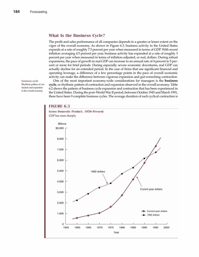
What Is the Business Cycle?The profit and sales performance of all companies depends to a greater or lesser extent on thevigor of the overall economy. As shown in Figure 6.3, business activity in the United Statesexpands at a rate of roughly 7.5 percent per year when measured in terms of GDP. With recentinflation averaging 4.5 percent per year, business activity has expanded at a rate of roughly 3percent per year when measured in terms of inflation-adjusted, or real, dollars. During robustexpansions, the pace of growth in real GDP can increase to an annual rate of 4 percent to 5 per-cent or more for brief periods. During especially severe economic downturns, real GDP canactually decline for an extended period. In the case of firms that use significant financial andoperating leverage, a difference of a few percentage points in the pace of overall economicactivity can make the difference between vigorous expansion and gut-wrenching contraction.
One of the most important economy-wide considerations for managers is the businesscycle, or rhythmic pattern of contraction and expansion observed in the overall economy. Table6.2 shows the pattern of business cycle expansion and contraction that has been experienced inthe United States. During the post–World War II period, between October 1945 and March 1991,there have been 9 complete business cycles. The average duration of each cyclical contraction is
184 Part Two Demand Analysis
business cycleRhythmic pattern of con-traction and expansionin the overall economy
FIGURE 6.3Gross Domestic Product, 1959–PresentGDP has risen sharply.
$9,000
8,000
7,000
6,000
5,000
4,000
3,000
2,000
1,000
0
Year
Billions
1992 dollars
1955 1960 1965 1970 1975 1980 1985 1990 1995 2000
Curent-year dollars
1992 dollars
Current-year dollars
184 Forecasting
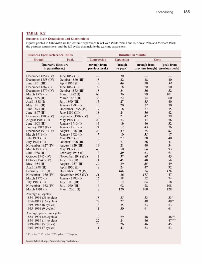
Chapter Six Forecasting 185
TABLE 6.2Business Cycle Expansions and ContractionsFigures printed in bold italic are the wartime expansions (Civil War, World Wars I and II, Korean War, and Vietnam War); the postwar contractions; and the full cycles that include the wartime expansions.
Business Cycle Reference Dates Duration in Months
Trough Peak Contraction Expansion Cycle
(Quarterly dates are (trough from (trough (trough from (peak from in parentheses.) previous peak) to peak) previous trough) previous peak)
December 1854 (IV) June 1857 (II) — 30 — —December 1858 (IV) October 1860 (III) 18 22 48 40June 1861 (III) April 1865 (I) 8 46 30 54December 1867 (I) June 1869 (II) 32 18 78 50December 1870 (IV) October 1873 (III) 18 34 36 52March 1879 (I) March 1882 (I) 65 36 99 101May 1885 (II) March 1887 (II) 38 22 74 60April 1888 (I) July 1890 (III) 13 27 35 40May 1891 (II) January 1893 (I) 10 20 37 30June 1894 (II) December 1895 (IV) 17 18 37 35June 1897 (II) June 1899 (III) 18 24 36 42December 1900 (IV) September 1902 (IV) 18 21 42 39August 1904 (III) May 1907 (II) 23 33 44 56June 1908 (II) January 1910 (I) 13 19 46 32January 1912 (IV) January 1913 (I) 24 12 43 36December 1914 (IV) August 1918 (III) 23 44 35 67March 1919 (I) January 1920 (I) 7 10 51 17July 1921 (III) May 1923 (II) 18 22 28 40July 1924 (III) October 1926 (III) 14 27 36 41November 1927 (IV) August 1929 (III) 13 21 40 34March 1933 (I) May 1937 (II) 43 50 64 93June 1938 (II) February 1945 (I) 13 80 63 93October 1945 (IV) November 1948 (IV) 8 37 88 45October 1949 (IV) July 1953 (II) 11 45 48 56May 1954 (II) August 1957 (III) 10 39 55 49April 1958 (II) April 1960 (II) 8 24 47 32February 1961 (I) December 1969 (IV) 10 106 34 116November 1970 (IV) November 1973 (IV) 11 36 117 47March 1975 (I) January 1980 (I) 16 58 52 74July 1980 (III) July 1981 (III) 6 12 64 18November 1982 (IV) July 1990 (III) 16 92 28 108March 1991 (I) March 2001 (I) 8 120 100 128
Average all cycles:1854–1991 (31 cycles) 18 35 53 53*
1854–1919 (16 cycles) 22 27 48 49**
1919–1945 (6 cycles) 18 35 53 531945–1991 (9 cycles) 11 50 61 61
Average, peacetime cycles:1854–1991 (26 cycles) 19 29 48 48***
1854–1919 (14 cycles) 22 24 46 47****
1919–1945 (5 cycles) 20 26 46 451945–1991 (7 cycles) 11 43 53 53
Source: NBER at http://www.nber.org/cycles.html.
* 30 cycles; ** 15 cycles; ***25 cycles; ****13 cycles.
Forecasting 185
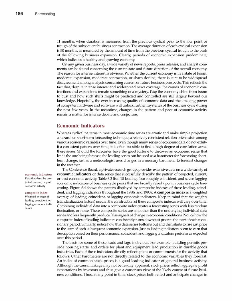
11 months, when duration is measured from the previous cyclical peak to the low point ortrough of the subsequent business contraction. The average duration of each cyclical expansionis 50 months, as measured by the amount of time from the previous cyclical trough to the peakof the following business expansion. Clearly, periods of economic expansion predominate,which indicates a healthy and growing economy.
On any given business day, a wide variety of news reports, press releases, and analyst com-ments can be found concerning the current state and future direction of the overall economy.The reason for intense interest is obvious. Whether the current economy is in a state of boom,moderate expansion, moderate contraction, or sharp decline, there is sure to be widespreaddisagreement among analysts concerning current or future business prospects. This reflects thefact that, despite intense interest and widespread news coverage, the causes of economic con-tractions and expansions remain something of a mystery. Why the economy shifts from boomto bust and how such shifts might be predicted and controlled are still largely beyond ourknowledge. Hopefully, the ever-increasing quality of economic data and the amazing powerof computer hardware and software will unlock further mysteries of the business cycle duringthe next few years. In the meantime, changes in the pattern and pace of economic activityremain a matter for intense debate and conjecture.
Economic IndicatorsWhereas cyclical patterns in most economic time series are erratic and make simple projectiona hazardous short-term forecasting technique, a relatively consistent relation often exists amongvarious economic variables over time. Even though many series of economic data do not exhib-it a consistent pattern over time, it is often possible to find a high degree of correlation acrossthese series. Should the forecaster have the good fortune to discover an economic series thatleads the one being forecast, the leading series can be used as a barometer for forecasting short-term change, just as a meteorologist uses changes in a mercury barometer to forecast changesin the weather.
The Conference Board, a private research group, provides extensive data on a wide variety ofeconomic indicators or data series that successfully describe the pattern of projected, current,or past economic activity. Table 6.3 lists 10 leading, four roughly coincident, and seven laggingeconomic indicators of business cycle peaks that are broadly relied upon in business cycle fore-casting. Figure 6.4 shows the pattern displayed by composite indexes of these leading, coinci-dent, and lagging indicators throughout the 1980s and 1990s. A composite index is a weightedaverage of leading, coincident, or lagging economic indicators. Keep in mind that the weights(standardization factors) used in the construction of these composite indexes will vary over time.Combining individual data into a composite index creates a forecasting series with less randomfluctuation, or noise. These composite series are smoother than the underlying individual dataseries and less frequently produce false signals of change in economic conditions. Notice how thecomposite index of leading indicators consistently turns down just prior to the start of each reces-sionary period. Similarly, notice how this data series bottoms out and then starts to rise just priorto the start of each subsequent economic expansion. Just as leading indicators seem to earn thatdescription based on their performance, coincident and lagging indicators perform as expectedover this period.
The basis for some of these leads and lags is obvious. For example, building permits pre-cede housing starts, and orders for plant and equipment lead production in durable goodsindustries. Each of these indicators directly reflects plans or commitments for the activity thatfollows. Other barometers are not directly related to the economic variables they forecast.An index of common stock prices is a good leading indicator of general business activity.Although the causal linkage may not be readily apparent, stock prices reflect aggregate profitexpectations by investors and thus give a consensus view of the likely course of future busi-ness conditions. Thus, at any point in time, stock prices both reflect and anticipate changes in
186 Part Two Demand Analysis
economic indicatorsData that describe pro-jected, current, or pasteconomic activity
composite indexWeighted average ofleading, coincident, orlagging economic indi-cators
186 Forecasting

aggregate economic conditions. All of this makes macroeconomic forecasting particularly net-tlesome for investors.
Economic RecessionsAn economic recession is defined by the National Bureau of Economic Research (NBER), aprivate nonprofit research organization, as a significant decline in activity spread across theeconomy that lasts more than a few months. Recessions are visible in terms of falling industrialproduction, declining real income, and shrinking wholesale-retail trade. Recessions are alsomarked by rising unemployment. Although many economic recessions consist of two or morequarters of declining real GDP, it is most accurate to describe recession as a period of diminish-ing economic activity rather than a period of diminished economic activity. A recession beginsjust after the economy reaches a peak of output and employment and ends as the economyreaches its trough. The period between a month of peak economic activity and the subsequenteconomic low point defines the length of a recession. During recessions, economic growth isfalling or the economy is actually contracting. As shown in Figure 6.4, recessions in the UnitedStates are rare and tend to be brief.
The period following recession is called economic expansion. In many cases, economicactivity is below normal during both recessions and through the early part of the subsequent
economic recessionA decline in economicactivity that lasts morethan a few months
economic expansionA period of rising economic activity
Chapter Six Forecasting 187
TABLE 6.3Leading, Coincident, and Lagging Economic Indicators
The Conference Board’s Index of Leading Economic Indicators (LEI) is designed to signal peaks and troughs in the businesscycle. The LEI is derived from 10 leading indicators, four coincident indicators, and seven lagging indicators. The LEI is a usefulbarometer of economic activity over 3 to 6 months.
Ten Leading Indicators Average workweek of production workers in manufacturingAverage initial weekly claims for state unemployment insuranceNew orders for consumer goods and materials, adjusted for inflationVendor performance (companies receiving slower deliveries from suppliers)New orders for nonmilitary capital goods, adjusted for inflation New building permits issuedIndex of stock pricesMoney supply: M2 adjusted for inflationSpread between rates on 10-year Treasury bonds and federal fundsIndex of consumer expectations
Four Coincident Indicators Manufacturing and trade salesEmployees on nonagricultural payrollsIndustrial productionPersonal income minus transfer payments
Seven Lagging Indicators Average duration of unemploymentInventories to sales ratio, manufacturing, and trade Change in labor cost per unit of output, manufacturing Average prime rateCommercial and industrial loansConsumer installment credit to personal income ratioChange in consumer price index for services
Source: The Conference Board Web site at http://www.conference-board.org/economics/indicators/leading.htm.
Forecasting 187
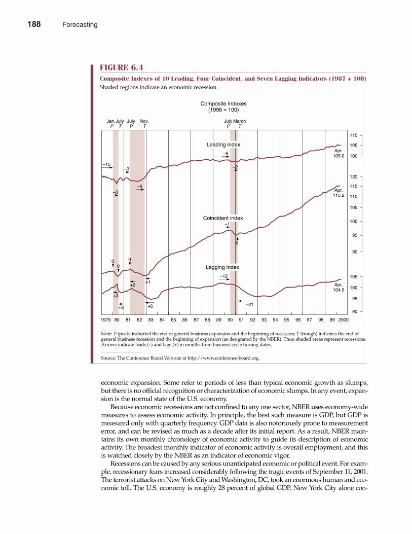
economic expansion. Some refer to periods of less than typical economic growth as slumps,but there is no official recognition or characterization of economic slumps. In any event, expan-sion is the normal state of the U.S. economy.
Because economic recessions are not confined to any one sector, NBER uses economy-widemeasures to assess economic activity. In principle, the best such measure is GDP, but GDP ismeasured only with quarterly frequency. GDP data is also notoriously prone to measurementerror, and can be revised as much as a decade after its initial report. As a result, NBER main-tains its own monthly chronology of economic activity to guide its description of economicactivity. The broadest monthly indicator of economic activity is overall employment, and thisis watched closely by the NBER as an indicator of economic vigor.
Recessions can be caused by any serious unanticipated economic or political event. For exam-ple, recessionary fears increased considerably following the tragic events of September 11, 2001.The terrorist attacks on New York City and Washington, DC, took an enormous human and eco-nomic toll. The U.S. economy is roughly 28 percent of global GDP. New York City alone con-
188 Part Two Demand Analysis
FIGURE 6.4Composite Indexes of 10 Leading, Four Coincident, and Seven Lagging Indicators (1987 + 100)Shaded regions indicate an economic recession.
Ð3
0
+2
Ð21
110
105
100
120
115
110
105
100
95
90
105
100
95
90
Jan. P
July�T
Ð15
1979 80 81 82 83 84 85 86 87 88 89 90 91 92 93 94 95 96 97 98 99 2000
July�P
Nov.�T
July�P
March�T
Leading index
Coincident index
Lagging index
Apr.�105.0
Apr.�115.2
Apr.�104.5
Ð6
Ð3
Ð2
Ð6
Ð1
Ð12
+1
+6
+3
+3
00
0
Composite Indexes�(1996 = 100)
Note: P (peak) indicated the end of general business expansion and the beginning of recession; T (trough) indicates the end ofgeneral business recession and the beginning of expansion (as designated by the NBER). Thus, shaded areas represent recessions.Arrows indicate leads (–) and lage (+) in months from business cycle turning dates.
Source: The Conference Board Web site at http://www.conference-board.org.
188 Forecasting
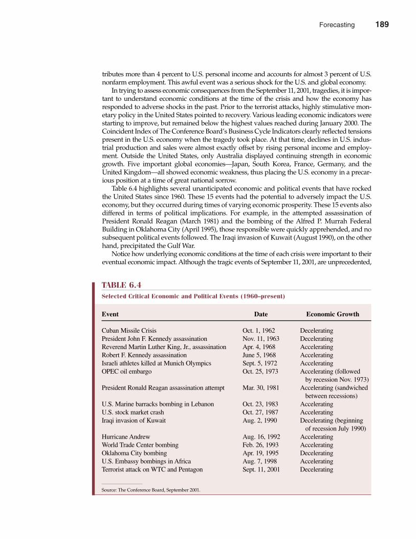
tributes more than 4 percent to U.S. personal income and accounts for almost 3 percent of U.S.nonfarm employment. This awful event was a serious shock for the U.S. and global economy.
In trying to assess economic consequences from the September 11, 2001, tragedies, it is impor-tant to understand economic conditions at the time of the crisis and how the economy hasresponded to adverse shocks in the past. Prior to the terrorist attacks, highly stimulative mon-etary policy in the United States pointed to recovery. Various leading economic indicators werestarting to improve, but remained below the highest values reached during January 2000. TheCoincident Index of The Conference Board’s Business Cycle Indicators clearly reflected tensionspresent in the U.S. economy when the tragedy took place. At that time, declines in U.S. indus-trial production and sales were almost exactly offset by rising personal income and employ-ment. Outside the United States, only Australia displayed continuing strength in economicgrowth. Five important global economies—Japan, South Korea, France, Germany, and theUnited Kingdom—all showed economic weakness, thus placing the U.S. economy in a precar-ious position at a time of great national sorrow.
Table 6.4 highlights several unanticipated economic and political events that have rockedthe United States since 1960. These 15 events had the potential to adversely impact the U.S.economy, but they occurred during times of varying economic prosperity. These 15 events alsodiffered in terms of political implications. For example, in the attempted assassination ofPresident Ronald Reagan (March 1981) and the bombing of the Alfred P. Murrah FederalBuilding in Oklahoma City (April 1995), those responsible were quickly apprehended, and nosubsequent political events followed. The Iraqi invasion of Kuwait (August 1990), on the otherhand, precipitated the Gulf War.
Notice how underlying economic conditions at the time of each crisis were important to theireventual economic impact. Although the tragic events of September 11, 2001, are unprecedented,
Chapter Six Forecasting 189
TABLE 6.4Selected Critical Economic and Political Events (1960–present)
Event Date Economic Growth
Cuban Missile Crisis Oct. 1, 1962 DeceleratingPresident John F. Kennedy assassination Nov. 11, 1963 DeceleratingReverend Martin Luther King, Jr., assassination Apr. 4, 1968 AcceleratingRobert F. Kennedy assassination June 5, 1968 AcceleratingIsraeli athletes killed at Munich Olympics Sept. 5, 1972 AcceleratingOPEC oil embargo Oct. 25, 1973 Accelerating (followed
by recession Nov. 1973)President Ronald Reagan assassination attempt Mar. 30, 1981 Accelerating (sandwiched
between recessions)U.S. Marine barracks bombing in Lebanon Oct. 23, 1983 AcceleratingU.S. stock market crash Oct. 27, 1987 AcceleratingIraqi invasion of Kuwait Aug. 2, 1990 Decelerating (beginning
of recession July 1990)Hurricane Andrew Aug. 16, 1992 AcceleratingWorld Trade Center bombing Feb. 26, 1993 AcceleratingOklahoma City bombing Apr. 19, 1995 DeceleratingU.S. Embassy bombings in Africa Aug. 7, 1998 AcceleratingTerrorist attack on WTC and Pentagon Sept. 11, 2001 Decelerating
Source: The Conference Board, September 2001.
Forecasting 189
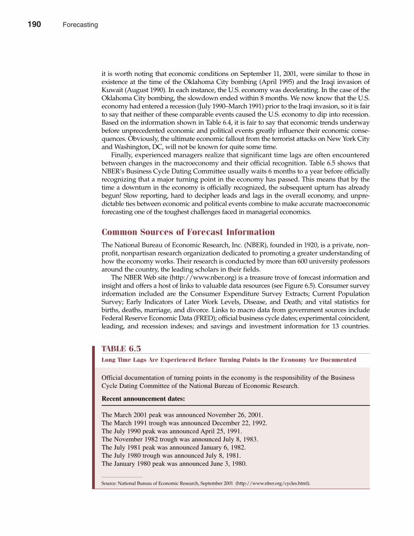
it is worth noting that economic conditions on September 11, 2001, were similar to those inexistence at the time of the Oklahoma City bombing (April 1995) and the Iraqi invasion ofKuwait (August 1990). In each instance, the U.S. economy was decelerating. In the case of theOklahoma City bombing, the slowdown ended within 8 months. We now know that the U.S.economy had entered a recession (July 1990–March 1991) prior to the Iraqi invasion, so it is fairto say that neither of these comparable events caused the U.S. economy to dip into recession.Based on the information shown in Table 6.4, it is fair to say that economic trends underwaybefore unprecedented economic and political events greatly influence their economic conse-quences. Obviously, the ultimate economic fallout from the terrorist attacks on New York Cityand Washington, DC, will not be known for quite some time.
Finally, experienced managers realize that significant time lags are often encounteredbetween changes in the macroeconomy and their official recognition. Table 6.5 shows thatNBER’s Business Cycle Dating Committee usually waits 6 months to a year before officiallyrecognizing that a major turning point in the economy has passed. This means that by thetime a downturn in the economy is officially recognized, the subsequent upturn has alreadybegun! Slow reporting, hard to decipher leads and lags in the overall economy, and unpre-dictable ties between economic and political events combine to make accurate macroeconomicforecasting one of the toughest challenges faced in managerial economics.
Common Sources of Forecast InformationThe National Bureau of Economic Research, Inc. (NBER), founded in 1920, is a private, non-profit, nonpartisan research organization dedicated to promoting a greater understanding ofhow the economy works. Their research is conducted by more than 600 university professorsaround the country, the leading scholars in their fields.
The NBER Web site (http://www.nber.org) is a treasure trove of forecast information andinsight and offers a host of links to valuable data resources (see Figure 6.5). Consumer surveyinformation included are the Consumer Expenditure Survey Extracts; Current PopulationSurvey; Early Indicators of Later Work Levels, Disease, and Death; and vital statistics forbirths, deaths, marriage, and divorce. Links to macro data from government sources includeFederal Reserve Economic Data (FRED); official business cycle dates; experimental coincident,leading, and recession indexes; and savings and investment information for 13 countries.
190 Part Two Demand Analysis
TABLE 6.5Long Time Lags Are Experienced Before Turning Points in the Economy Are Documented
Official documentation of turning points in the economy is the responsibility of the BusinessCycle Dating Committee of the National Bureau of Economic Research.
Recent announcement dates:
The March 2001 peak was announced November 26, 2001.The March 1991 trough was announced December 22, 1992.The July 1990 peak was announced April 25, 1991.The November 1982 trough was announced July 8, 1983.The July 1981 peak was announced January 6, 1982.The July 1980 trough was announced July 8, 1981.The January 1980 peak was announced June 3, 1980.
Source: National Bureau of Economic Research, September 2001 (http://www.nber.org/cycles.html).
190 Forecasting
Industry data include the Manufacturing Industry Productivity Database, patent data, importsand exports by Standard Industrial Classification (SIC) category, and various IRS information.
Resources for Economists on the Internet (RFE) is another extremely valuable Web sitemaintained by the American Economic Association and professor Bill Goffe of the Departmentof Economics at the State University of New York (SUNY), Oswego campus (see Figure 6.6).The table of contents for RFE lists 1,265 resources in 74 sections and subsections of interest toacademic and practicing economists, and those interested in economics. Almost all resourcesare also described in simple-to-understand language. RFE is a particularly good place to lookfor a broad array of business and economic forecasting resources on the Web. For example,under economic forecasting and consulting resources the reader will find the ConferenceBoard’s Leading Economic Indicators and various other nongovernmental data; economiccommentary from Bank of America Economics and Financial Reports; macro, regional, andelectrical forecasts from Foster Associates; microeconomic analysis from Glassman-OliverEconomic Consultants, Inc.; global financial market and foreign exchange analysis from WellsFargo Economic Reports; and so on.
Information about economic trends is also found in leading business publications, like TheWall Street Journal and Barron’s. As shown in Figure 6.7, Barron’s survey of economic indicators
Chapter Six Forecasting 191
FIGURE 6.5The National Bureau of Economic Research Web Site Is a Treasure Trove of Forecast Information
Forecasting 191
depicts the rate of change in the overall level of economic activity as indicated by GDP,durable and nondurable manufacturing, factory utilization, and other statistics. Alsoprovided are specific data on the level of production in a wide range of basic industriessuch as autos, electric power, paper, petroleum, and steel. Data published weekly inBarron’s include not only the level of production (what is made), but also distribution(what is sold), inventories (what is on hand), new orders received, unfilled orders, pur-chasing power, employment, and construction activity. Forbes magazine publishes its ownbiweekly index of economic activity using government data on consumer prices, manufac-turer’s new orders and inventories, industrial production, new housing starts, personalincome, new unemployment claims, retail sales, and consumer installment credit. To measurethese eight elements of the Forbes Index, 10 series of U.S. government data are monitoredover a 14-month period.
Fortune and Business Week magazines also offer regular coverage of data on current andprojected levels of economic activity. The quarterly Fortune Forecast of economic activity isbased on a proprietary econometric model developed by the company’s own staff econo-mists. The forecast data and analysis published in these leading business periodicals providemanagers with a useful starting point in the development of their own expectations.
192 Part Two Demand Analysis
FIGURE 6.6Resources for Economists on the Internet Is a Valuable Forecasting Resource
192 Forecasting
EXPONENTIAL SMOOTHING TECHNIQUES
A wide variety of statistical forecasting techniques can be used to predict unit sales growth,revenue, costs, and profit performance. These techniques range from quite simple to verysophisticated.
Exponential Smoothing ConceptExponential smoothing is a method for forecasting trends in unit sales, unit costs, wageexpenses, and so on. The technique identifies historical patterns of trend or seasonality in thedata and then extrapolates these patterns forward into the forecast period. Its accuracydepends on the degree to which established patterns of change are apparent and constantover time. The more regular the pattern of change in any given data series, the easier it is toforecast. Exponential smoothing (or “averaging”) techniques are among the most widelyused forecasting methods in business.
All leading methods of exponential smoothing involve the same essential process of dataaveraging. The data series to be forecast is assumed to be modeled by one, two, or three
exponentialsmoothingAveraging method forforecasting time seriesof data
Chapter Six Forecasting 193
FIGURE 6.7Barron’s Publishes Timely Information on Economic Indicators
Forecasting 193
essential components. Key components represent the level, trend, or seasonality of the databeing forecast. The level of the time series to be forecast is the average about which it fluctuates.This level may be constant or slowly changing. Trend is any systematic change in the level ofthe time series of data. If a given forecast model includes a trend, then that trend is either pro-jected as a straight line into the future or as a gradually diminishing amount that eventually diesout. The seasonality of a time series is a pattern of change tied to weather, custom, or tradition.Retail sales typically exhibit a strong seasonal trend over the course of the year. Many storesbook 30 percent or more of annual sales during the busy Christmas selling season. Seasonalcomponents can be additive, meaning that seasonal patterns remain constant over time, or mul-tiplicative, meaning that seasonal patterns grow with the average level of the series.
Figure 6.8 shows nine common profiles of data that can be forecast by using popular expo-nential smoothing techniques. They range in complexity from the constant level of data shownin Figure 6.8(a) to the more complex dampened trend with a multiplicative seasonal influenceshown in Figure 6.8(i). To ensure that the correct exponential smoothing technique is chosen,a method with sufficient flexibility to conform to the underlying data must be used. A goodfirst step in the exponential smoothing process is to graph the data series to be forecast andthen choose the exponential smoothing method that best resembles the data.
One-Parameter (Simple) Exponential SmoothingIn one-parameter (simple) exponential smoothing, the sole regular component is the levelof the forecast data series. It is implicitly assumed that the data consist of irregular fluctuationsaround a constant or very slowly changing level. Simple exponential smoothing is appropriatefor forecasting sales in mature markets with stable activity; it is inappropriate for forecasting inmarkets that are growing rapidly or are seasonal.
194 Part Two Demand Analysis
one-parameter (simple) exponentialsmoothingMethod for forecastingslowly changing levels
The Stock Market and the Business Cycle
Many stock market prognosticators advise long-terminvestors to lighten up in advance of deteriorating economic conditions. Why buy and hold when the eco-nomic environment is worsening? Shouldn’t smartinvestors hold cash until the economic experts knowthat recovery has begun? Then, business news reporterscan issue the “all clear” sign, and savvy investors canreestablish long-term positions. If only life were thatsimple. Unfortunately, it’s not.
Economic recessions are notoriously hard to identi-fy. Typically, the National Bureau of Economic Research(NBER) is able to identify the start of an economicrecession only months after the recession has begun. By the time economic recessions are identified, theeconomy is often already well on its way to recovery. In addition, the stock market usually starts to sag wellin advance of economic downturns and rally inadvance of economic recoveries. Near-term fluctuationsin the stock market also give many false signals con-cerning economic conditions. As a famous economistonce remarked, “The stock market has correctly forecast10 of the last 6 recessions.”
Look at how stock market prices change betweenimportant economic turning points and when suchturns in the economy are officially recognized:
• The March 2001 peak (S&P 500 = 1160.33)announced November 26, 2001 (S&P 500 = 1157.42).
• The March 1991 trough (S&P 500 = 375.22)announced December 22, 1992 (S&P 500 = 440.31).
• The July 1990 peak (S&P 500 = 356.15) announced April 25, 1991 (S&P 500 = 379.25).
• The November 1982 trough (S&P 500 = 138.93)announced July 8, 1983 (S&P 500 = 167.08).
• The July 1981 peak (S&P 500 = 130.92) announced January 6, 1982 (S&P 500 = 119.18).
• The July 1980 trough (S&P 500 = 121.67) announced July 8, 1981 (S&P 500 = 132.24).
• The January 1980 peak (S&P 500 = 114.16)announced June 3, 1980 (S&P 500 = 110.51).
Upshot: Trading stocks based upon NBER announce-ments sure isn’t a sophisticated way of market timing.
See: Michael Santoli, “Building a Better Bull,” Barron’s Online, April 8,2002 (http://online.wsj.com).
M A N A G E R I A L A P P L I C AT I O N 6 . 3
194 Forecasting
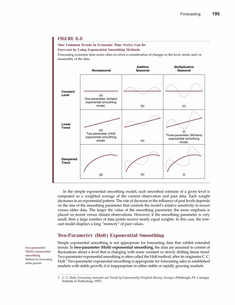
In the simple exponential smoothing model, each smoothed estimate of a given level iscomputed as a weighted average of the current observation and past data. Each weightdecreases in an exponential pattern. The rate of decrease in the influence of past levels dependson the size of the smoothing parameter that controls the model’s relative sensitivity to newerversus older data. The larger the value of the smoothing parameter, the more emphasis isplaced on recent versus distant observations. However, if the smoothing parameter is verysmall, then a large number of data points receive nearly equal weights. In this case, the fore-cast model displays a long “memory” of past values.
Two-Parameter (Holt) Exponential SmoothingSimple exponential smoothing is not appropriate for forecasting data that exhibit extendedtrends. In two-parameter (Holt) exponential smoothing, the data are assumed to consist offluctuations about a level that is changing with some constant or slowly drifting linear trend.Two-parameter exponential smoothing is often called the Holt method, after its originator C. C.Holt.3 Two-parameter exponential smoothing is appropriate for forecasting sales in establishedmarkets with stable growth; it is inappropriate in either stable or rapidly growing markets.
two-parameter(Holt) exponentialsmoothingMethod for forecastingstable growth
Chapter Six Forecasting 195
FIGURE 6.8Nine Common Trends in Economic Time Series Can Be Forecast by Using Exponential Smoothing MethodsForecasting economic time series often involves a consideration of changes in the level, trend, and/or seasonality of the data.
(c)
MultiplicativeSeasonal
AdditiveSeasonalNonseasonal
(i)
(b)
(e)
(h)
(a)One-parameter (simple)exponential smoothing
model.
(d)Two-parameter (Holt)exponential smoothing
model.
(f)Three-parameter (Winters)exponential smoothing
model.
(g)
ConstantLevel
LinearTrend
DampenedTrend
3 C. C. Holt, Forecasting Seasonals and Trends by Exponentially Weighted Moving Averages (Pittsburgh, PA: CarnegieInstitute of Technology, 1957).
Forecasting 195
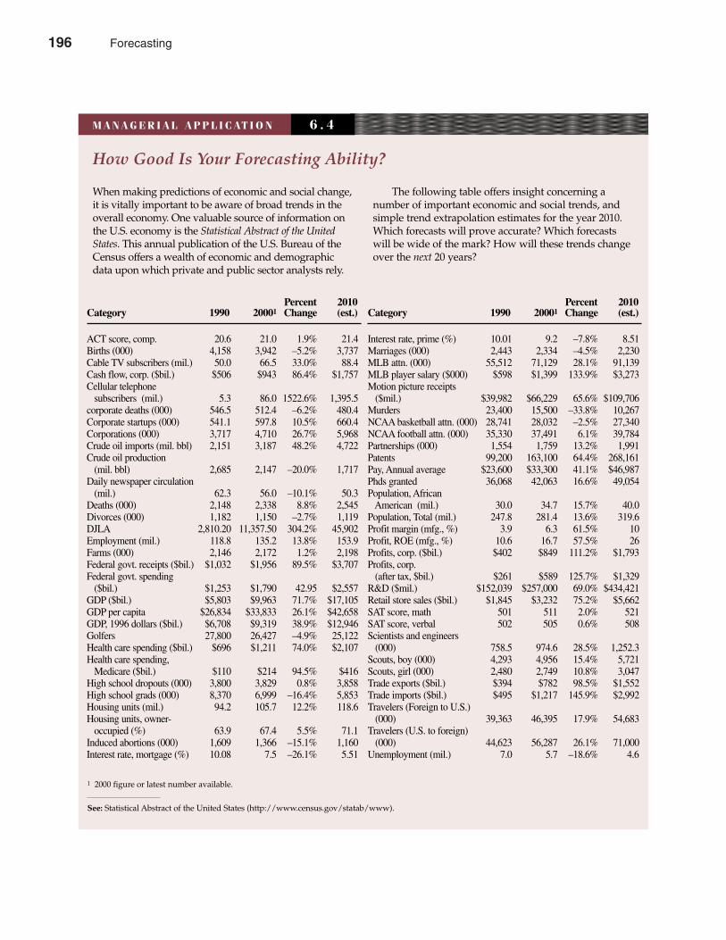
196 Part Two Demand Analysis
How Good Is Your Forecasting Ability?
When making predictions of economic and social change,it is vitally important to be aware of broad trends in theoverall economy. One valuable source of information onthe U.S. economy is the Statistical Abstract of the UnitedStates. This annual publication of the U.S. Bureau of theCensus offers a wealth of economic and demographicdata upon which private and public sector analysts rely.
The following table offers insight concerning a number of important economic and social trends, andsimple trend extrapolation estimates for the year 2010.Which forecasts will prove accurate? Which forecastswill be wide of the mark? How will these trends changeover the next 20 years?
M A N A G E R I A L A P P L I C AT I O N 6 . 4
Percent 2010Category 1990 20001 Change (est.)
ACT score, comp. 20.6 21.0 1.9% 21.4Births (000) 4,158 3,942 –5.2% 3,737Cable TV subscribers (mil.) 50.0 66.5 33.0% 88.4Cash flow, corp. ($bil.) $506 $943 86.4% $1,757Cellular telephone
subscribers (mil.) 5.3 86.0 1522.6% 1,395.5corporate deaths (000) 546.5 512.4 –6.2% 480.4Corporate startups (000) 541.1 597.8 10.5% 660.4Corporations (000) 3,717 4,710 26.7% 5,968Crude oil imports (mil. bbl) 2,151 3,187 48.2% 4,722Crude oil production
(mil. bbl) 2,685 2,147 –20.0% 1,717Daily newspaper circulation
(mil.) 62.3 56.0 –10.1% 50.3Deaths (000) 2,148 2,338 8.8% 2,545Divorces (000) 1,182 1,150 –2.7% 1,119DJLA 2,810.20 11,357.50 304.2% 45,902Employment (mil.) 118.8 135.2 13.8% 153.9Farms (000) 2,146 2,172 1.2% 2,198Federal govt. receipts ($bil.) $1,032 $1,956 89.5% $3,707Federal govt. spending
($bil.) $1,253 $1,790 42.95 $2,557GDP ($bil.) $5,803 $9,963 71.7% $17,105GDP per capita $26,834 $33,833 26.1% $42,658GDP, 1996 dollars ($bil.) $6,708 $9,319 38.9% $12,946Golfers 27,800 26,427 –4.9% 25,122Health care spending ($bil.) $696 $1,211 74.0% $2,107Health care spending,
Medicare ($bil.) $110 $214 94.5% $416High school dropouts (000) 3,800 3,829 0.8% 3,858High school grads (000) 8,370 6,999 –16.4% 5,853Housing units (mil.) 94.2 105.7 12.2% 118.6Housing units, owner-
occupied (%) 63.9 67.4 5.5% 71.1Induced abortions (000) 1,609 1,366 –15.1% 1,160Interest rate, mortgage (%) 10.08 7.5 –26.1% 5.51
Percent 2010Category 1990 20001 Change (est.)
Interest rate, prime (%) 10.01 9.2 –7.8% 8.51Marriages (000) 2,443 2,334 –4.5% 2,230MLB attn. (000) 55,512 71,129 28.1% 91,139MLB player salary ($000) $598 $1,399 133.9% $3,273Motion picture receipts
($mil.) $39,982 $66,229 65.6% $109,706Murders 23,400 15,500 –33.8% 10,267NCAA basketball attn. (000) 28,741 28,032 –2.5% 27,340NCAA football attn. (000) 35,330 37,491 6.1% 39,784Partnerships (000) 1,554 1,759 13.2% 1,991Patents 99,200 163,100 64.4% 268,161Pay, Annual average $23,600 $33,300 41.1% $46,987Phds granted 36,068 42,063 16.6% 49,054Population, African
American (mil.) 30.0 34.7 15.7% 40.0Population, Total (mil.) 247.8 281.4 13.6% 319.6Profit margin (mfg., %) 3.9 6.3 61.5% 10Profit, ROE (mfg., %) 10.6 16.7 57.5% 26Profits, corp. ($bil.) $402 $849 111.2% $1,793Profits, corp.
(after tax, $bil.) $261 $589 125.7% $1,329R&D ($mil.) $152,039 $257,000 69.0% $434,421Retail store sales ($bil.) $1,845 $3,232 75.2% $5,662SAT score, math 501 511 2.0% 521SAT score, verbal 502 505 0.6% 508Scientists and engineers
(000) 758.5 974.6 28.5% 1,252.3Scouts, boy (000) 4,293 4,956 15.4% 5,721Scouts, girl (000) 2,480 2,749 10.8% 3,047Trade exports ($bil.) $394 $782 98.5% $1,552Trade imports ($bil.) $495 $1,217 145.9% $2,992Travelers (Foreign to U.S.)
(000) 39,363 46,395 17.9% 54,683Travelers (U.S. to foreign)
(000) 44,623 56,287 26.1% 71,000Unemployment (mil.) 7.0 5.7 –18.6% 4.6
1 2000 figure or latest number available.
See: Statistical Abstract of the United States (http://www.census.gov/statab/www).
196 Forecasting
Holt’s exponential smoothing model uses a smoothed estimate of the trend component aswell as the level component to produce forecasts. In the two-parameter exponential smoothingforecast equation, the current smoothed level is added to a linear trend to forecast future values.The updated value of the smoothed level is computed as the weighted average of new data andthe best estimate of the new level based on old data. The Holt method combines old and newestimates of the one-period change of the smoothed level, thus defining the current linear orlocal trend.
Three-Parameter (Winters) Exponential SmoothingThe three-parameter (Winters) exponential smoothing method extends the two-parametertechnique by including a smoothed multiplicative index to account for the seasonal behaviorof the forecast series. The three-parameter exponential smoothing technique is often called theWinters method, after its originator P. R. Winters.4 Because much economic data involve bothgrowth trend and seasonal considerations, three-parameter exponential smoothing is one ofthe most commonly used forecasting methods. It is best suited for forecasting problems thatinvolve rapid and/or changing rates of growth combined with seasonal influences. Three-parameter exponential smoothing is suitable for forecasting sales in both rapidly growing mar-kets and in rapidly decaying markets with seasonal influences.
Winters’ three-parameter exponential smoothing model assumes that each observation isthe product of a deseasonalized value and a seasonal index for that particular month or quar-ter. The deseasonalized values are assumed to be described by the Holt model. The Wintersmodel involves three smoothing parameters to be used in level, trend, and seasonal indexsmoothing equations. The Winters model forecast is computed similarly to the Holt model fore-cast and then multiplied by the seasonal index for the current period. Smoothing in the Wintersmodel is similar to the Holt model, except that in the Winters model the measurement of levelis deseasonalized through dividing by the seasonal index calculated one year before. The trendsmoothing equations of the two models are identical. The seasonal index is estimated as theratio of the current observation to the current smoothed level, averaged with the previous valuefor that particular period.
Practical Use of Exponential SmoothingThe important point to remember about exponential smoothing, or any forecast method, isthat the choice of an appropriate forecasting technique depends on the pattern data that isto be forecast.
As a case in point, Figure 6.9 shows a typical pattern of sales for the life cycle of a prod-uct. Product life cycles often progress from the introduction point, to rapid growth andmarket penetration, to a mature phase of sales stability, to periods of declining marketshare and abandonment. Over this life cycle, different methods of sales forecasting may beappropriate.
In the initial phase, and before the generation of significant market data, qualitative analysesand market experiments are highly appropriate. Once the product has been launched and israpidly gaining market acceptance, in phase II, three-parameter exponential smoothing methodsthat involve level, trend, and seasonal components become relevant. In the mature phase ofsales stability, phase III, two-parameter exponential smoothing models (or econometric models)
three-parameter(Winters) exponen-tial smoothingMethod for forecastingseasonally adjustedgrowth
Chapter Six Forecasting 197
4 P. R. Winters, “Forecasting Sales by Exponentially Weighted Moving Averages,” Management Science 6 (April1960), 324–342.
Forecasting 197
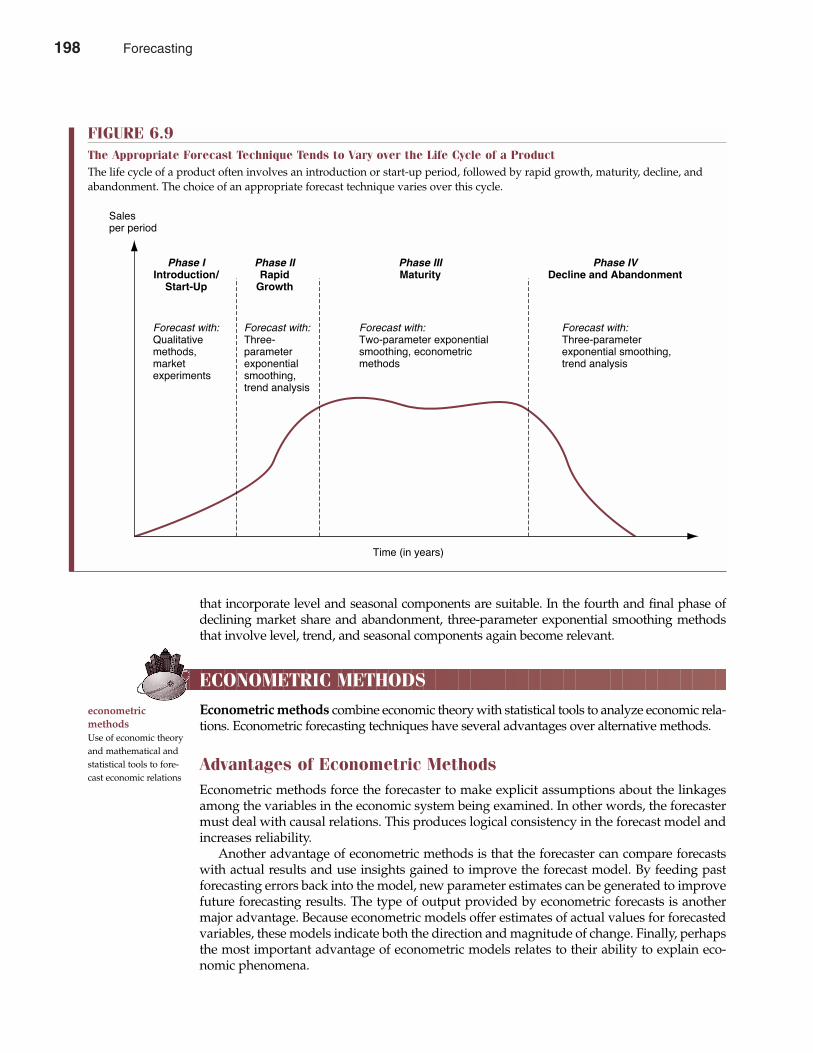
that incorporate level and seasonal components are suitable. In the fourth and final phase ofdeclining market share and abandonment, three-parameter exponential smoothing methodsthat involve level, trend, and seasonal components again become relevant.
ECONOMETRIC METHODS
Econometric methods combine economic theory with statistical tools to analyze economic rela-tions. Econometric forecasting techniques have several advantages over alternative methods.
Advantages of Econometric MethodsEconometric methods force the forecaster to make explicit assumptions about the linkagesamong the variables in the economic system being examined. In other words, the forecastermust deal with causal relations. This produces logical consistency in the forecast model andincreases reliability.
Another advantage of econometric methods is that the forecaster can compare forecastswith actual results and use insights gained to improve the forecast model. By feeding pastforecasting errors back into the model, new parameter estimates can be generated to improvefuture forecasting results. The type of output provided by econometric forecasts is anothermajor advantage. Because econometric models offer estimates of actual values for forecastedvariables, these models indicate both the direction and magnitude of change. Finally, perhapsthe most important advantage of econometric models relates to their ability to explain eco-nomic phenomena.
198 Part Two Demand Analysis
econometric methodsUse of economic theoryand mathematical andstatistical tools to fore-cast economic relations
FIGURE 6.9The Appropriate Forecast Technique Tends to Vary over the Life Cycle of a ProductThe life cycle of a product often involves an introduction or start-up period, followed by rapid growth, maturity, decline, andabandonment. The choice of an appropriate forecast technique varies over this cycle.
Time (in years)
Salesper period
Phase IIntroduction/
Start-Up
Forecast with:Qualitativemethods,marketexperiments
Phase IIRapid
Growth
Forecast with:Three-parameterexponentialsmoothing,trend analysis
Phase IIIMaturity
Forecast with:Two-parameter exponentialsmoothing, econometricmethods
Phase IVDecline and Abandonment
Forecast with:Three-parameterexponential smoothing,trend analysis
198 Forecasting
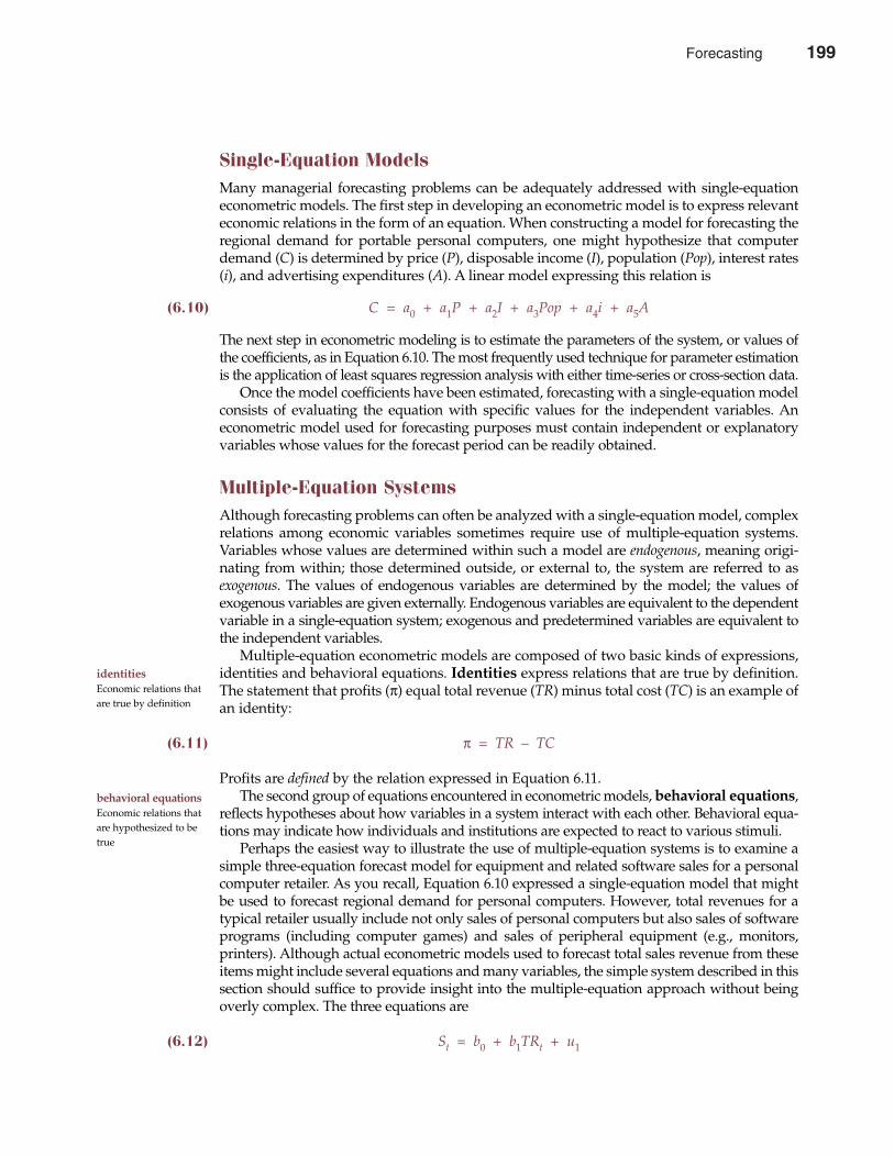
Single-Equation ModelsMany managerial forecasting problems can be adequately addressed with single-equationeconometric models. The first step in developing an econometric model is to express relevanteconomic relations in the form of an equation. When constructing a model for forecasting theregional demand for portable personal computers, one might hypothesize that computerdemand (C) is determined by price (P), disposable income (I), population (Pop), interest rates(i), and advertising expenditures (A). A linear model expressing this relation is
(6.10) C = a0 + a1P + a2I + a3Pop + a4i + a5A
The next step in econometric modeling is to estimate the parameters of the system, or values ofthe coefficients, as in Equation 6.10. The most frequently used technique for parameter estimationis the application of least squares regression analysis with either time-series or cross-section data.
Once the model coefficients have been estimated, forecasting with a single-equation modelconsists of evaluating the equation with specific values for the independent variables. Aneconometric model used for forecasting purposes must contain independent or explanatoryvariables whose values for the forecast period can be readily obtained.
Multiple-Equation SystemsAlthough forecasting problems can often be analyzed with a single-equation model, complexrelations among economic variables sometimes require use of multiple-equation systems.Variables whose values are determined within such a model are endogenous, meaning origi-nating from within; those determined outside, or external to, the system are referred to asexogenous. The values of endogenous variables are determined by the model; the values ofexogenous variables are given externally. Endogenous variables are equivalent to the dependentvariable in a single-equation system; exogenous and predetermined variables are equivalent tothe independent variables.
Multiple-equation econometric models are composed of two basic kinds of expressions,identities and behavioral equations. Identities express relations that are true by definition.The statement that profits (π) equal total revenue (TR) minus total cost (TC) is an example ofan identity:
(6.11) π = TR – TC
Profits are defined by the relation expressed in Equation 6.11.The second group of equations encountered in econometric models, behavioral equations,
reflects hypotheses about how variables in a system interact with each other. Behavioral equa-tions may indicate how individuals and institutions are expected to react to various stimuli.
Perhaps the easiest way to illustrate the use of multiple-equation systems is to examine asimple three-equation forecast model for equipment and related software sales for a personalcomputer retailer. As you recall, Equation 6.10 expressed a single-equation model that mightbe used to forecast regional demand for personal computers. However, total revenues for atypical retailer usually include not only sales of personal computers but also sales of softwareprograms (including computer games) and sales of peripheral equipment (e.g., monitors,printers). Although actual econometric models used to forecast total sales revenue from theseitems might include several equations and many variables, the simple system described in thissection should suffice to provide insight into the multiple-equation approach without beingoverly complex. The three equations are
(6.12) St = b0 + b1TRt + u1
identitiesEconomic relations thatare true by definition
behavioral equationsEconomic relations thatare hypothesized to betrue
Chapter Six Forecasting 199
Forecasting 199
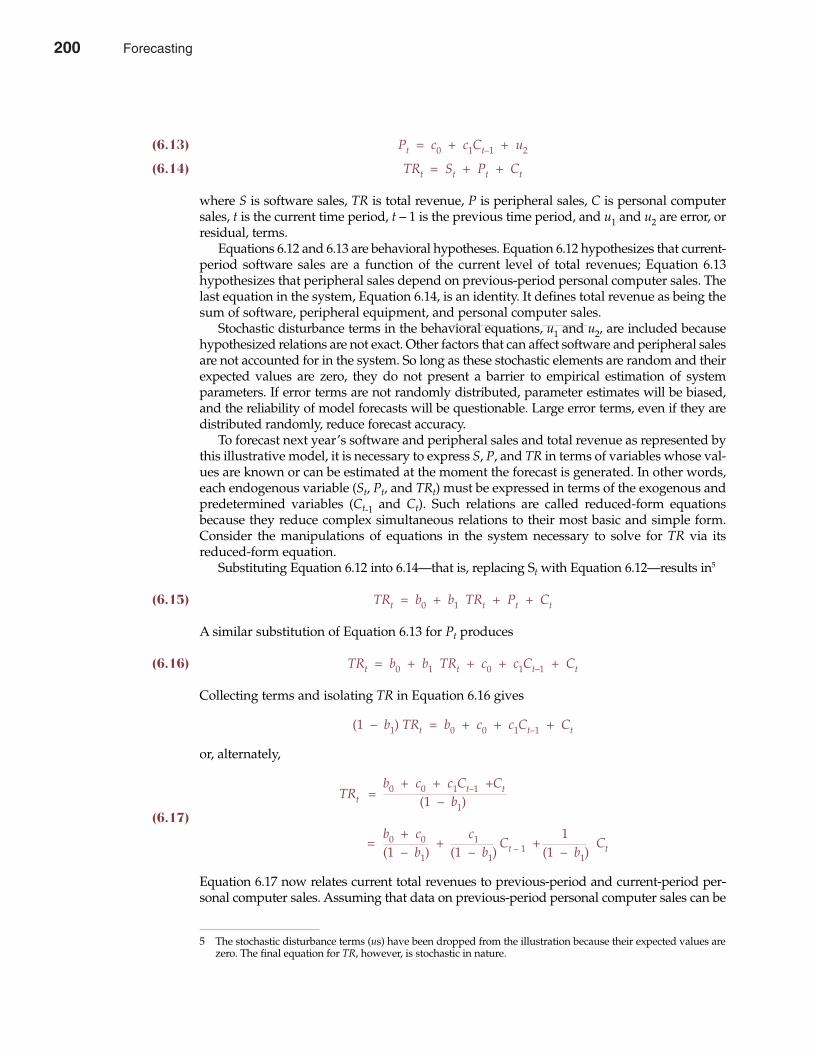
(6.13) Pt = c0 + c1Ct–1 + u2
(6.14) TRt = St + Pt + Ct
where S is software sales, TR is total revenue, P is peripheral sales, C is personal computersales, t is the current time period, t – 1 is the previous time period, and u1 and u2 are error, orresidual, terms.
Equations 6.12 and 6.13 are behavioral hypotheses. Equation 6.12 hypothesizes that current-period software sales are a function of the current level of total revenues; Equation 6.13hypothesizes that peripheral sales depend on previous-period personal computer sales. Thelast equation in the system, Equation 6.14, is an identity. It defines total revenue as being thesum of software, peripheral equipment, and personal computer sales.
Stochastic disturbance terms in the behavioral equations, u1 and u2, are included becausehypothesized relations are not exact. Other factors that can affect software and peripheral salesare not accounted for in the system. So long as these stochastic elements are random and theirexpected values are zero, they do not present a barrier to empirical estimation of systemparameters. If error terms are not randomly distributed, parameter estimates will be biased,and the reliability of model forecasts will be questionable. Large error terms, even if they aredistributed randomly, reduce forecast accuracy.
To forecast next year’s software and peripheral sales and total revenue as represented bythis illustrative model, it is necessary to express S, P, and TR in terms of variables whose val-ues are known or can be estimated at the moment the forecast is generated. In other words,each endogenous variable (St, Pt, and TRt) must be expressed in terms of the exogenous andpredetermined variables (Ct-1 and Ct). Such relations are called reduced-form equationsbecause they reduce complex simultaneous relations to their most basic and simple form.Consider the manipulations of equations in the system necessary to solve for TR via itsreduced-form equation.
Substituting Equation 6.12 into 6.14—that is, replacing St with Equation 6.12—results in5
(6.15) TRt = b0 + b1 TRt + Pt + Ct
A similar substitution of Equation 6.13 for Pt produces
(6.16) TRt = b0 + b1 TRt + c0 + c1Ct–1 + Ct
Collecting terms and isolating TR in Equation 6.16 gives
(1 – b1) TRt = b0 + c0 + c1Ct–1 + Ct
or, alternately,
TRt =b0 + c0 + c1Ct–1 +Ct
(6.17)(1 – b1)
=b0 + c0 +
c1 Ct – 1 +1
Ct(1 – b1) (1 – b1) (1 – b1)
Equation 6.17 now relates current total revenues to previous-period and current-period per-sonal computer sales. Assuming that data on previous-period personal computer sales can be
200 Part Two Demand Analysis
5 The stochastic disturbance terms (us) have been dropped from the illustration because their expected values arezero. The final equation for TR, however, is stochastic in nature.
200 Forecasting
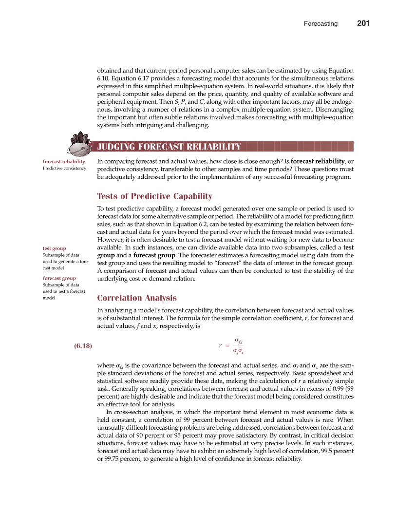
obtained and that current-period personal computer sales can be estimated by using Equation6.10, Equation 6.17 provides a forecasting model that accounts for the simultaneous relationsexpressed in this simplified multiple-equation system. In real-world situations, it is likely thatpersonal computer sales depend on the price, quantity, and quality of available software andperipheral equipment. Then S, P, and C, along with other important factors, may all be endoge-nous, involving a number of relations in a complex multiple-equation system. Disentanglingthe important but often subtle relations involved makes forecasting with multiple-equationsystems both intriguing and challenging.
JUDGING FORECAST RELIABILITY
In comparing forecast and actual values, how close is close enough? Is forecast reliability, orpredictive consistency, transferable to other samples and time periods? These questions mustbe adequately addressed prior to the implementation of any successful forecasting program.
Tests of Predictive CapabilityTo test predictive capability, a forecast model generated over one sample or period is used toforecast data for some alternative sample or period. The reliability of a model for predicting firmsales, such as that shown in Equation 6.2, can be tested by examining the relation between fore-cast and actual data for years beyond the period over which the forecast model was estimated.However, it is often desirable to test a forecast model without waiting for new data to becomeavailable. In such instances, one can divide available data into two subsamples, called a testgroup and a forecast group. The forecaster estimates a forecasting model using data from thetest group and uses the resulting model to “forecast” the data of interest in the forecast group.A comparison of forecast and actual values can then be conducted to test the stability of theunderlying cost or demand relation.
Correlation AnalysisIn analyzing a model’s forecast capability, the correlation between forecast and actual valuesis of substantial interest. The formula for the simple correlation coefficient, r, for forecast andactual values, f and x, respectively, is
(6.18) r =�fx
�f�x
where �fx is the covariance between the forecast and actual series, and �f and �x are the sam-ple standard deviations of the forecast and actual series, respectively. Basic spreadsheet andstatistical software readily provide these data, making the calculation of r a relatively simpletask. Generally speaking, correlations between forecast and actual values in excess of 0.99 (99percent) are highly desirable and indicate that the forecast model being considered constitutesan effective tool for analysis.
In cross-section analysis, in which the important trend element in most economic data isheld constant, a correlation of 99 percent between forecast and actual values is rare. Whenunusually difficult forecasting problems are being addressed, correlations between forecast andactual data of 90 percent or 95 percent may prove satisfactory. By contrast, in critical decisionsituations, forecast values may have to be estimated at very precise levels. In such instances,forecast and actual data may have to exhibit an extremely high level of correlation, 99.5 percentor 99.75 percent, to generate a high level of confidence in forecast reliability.
forecast reliabilityPredictive consistency
test groupSubsample of dataused to generate a fore-cast model
forecast groupSubsample of dataused to test a forecastmodel
Chapter Six Forecasting 201
Forecasting 201
Sample Mean Forecast Error AnalysisFurther evaluation of a model’s predictive capability can be made through consideration of ameasure called the sample mean forecast error, which provides a useful estimate of the aver-age forecast error of the model. It is sometimes called the root mean squared forecast error andis denoted by the symbol U. The sample mean forecast error is calculated as
n(6.19) U = � 1
� (fi – xi)2n
i=1
where n is the number of sample observations, fi is a forecast value, and xi is the correspon-ding actual value. Deviations between forecast and actual values are squared in the calcula-tion of the mean forecast error to prevent positive and negative deviations from cancelingeach other out. The smaller the sample mean forecast error, the greater the accuracy associ-ated with the forecasting model.
CHOOSING THE BEST FORECAST TECHNIQUE
To select the best technique, managers must be knowledgeable about the strengths and weak-nesses of various forecast methods, the amount and quality of available data, and the humanand other costs associated with generating reliable forecasts.
Data RequirementsThe choice of an appropriate forecast technique often hinges on the amount of relevant histor-ical data that is readily available and any obvious patterns in that data. For many importantforecast problems, 10 years of monthly data (120 observations) are available and appropriatefor forecasting future activity. In such cases, the full range of advanced forecast techniques canbe considered. If only more restricted samples of data are available for analysis, then simplerforecast methods must be used.
If trend, cyclical, seasonal, or irregular patterns can be recognized, then forecast techniquesthat are capable of handling those patterns can be readily selected. For example, if the data arerelatively stable, a simple exponential smoothing approach may be adequate. Other exponentialsmoothing models are appropriate for trending and seasonal data; the same model will not beapplicable in all cases.
As the forecast horizon increases, the cyclical pattern of economic data may also becomesignificant. In these cases, the need to relate the forecast variable to economic, market, andcompetitive factors increases, because simple trend projections may no longer be appropriate.
Time Horizon ConsiderationsExperience shows that sophisticated time-series models can provide accurate short-term forecasts.In the short term, the momentum of existing consumer behavior often resists dramatic change.Over a 5-year period, however, customers can find new suppliers, and needs may change. Forlong-range forecasts, econometric models are often appropriate. In the long term, it is essential torelate the item being forecast to its “drivers,” as explanatory factors are sometimes called.
The accuracy of econometric models depends on the precision with which explanatory fac-tors can be predicted. Although these models can also be used in the short term, they are costlierand more complex than simple exponential smoothing methods. When economic conditions arestable, econometric models are seldom more accurate than more simple trend projections andexponential smoothing methods.
202 Part Two Demand Analysis
sample mean forecast errorEstimate of averageforecast error
202 Forecasting
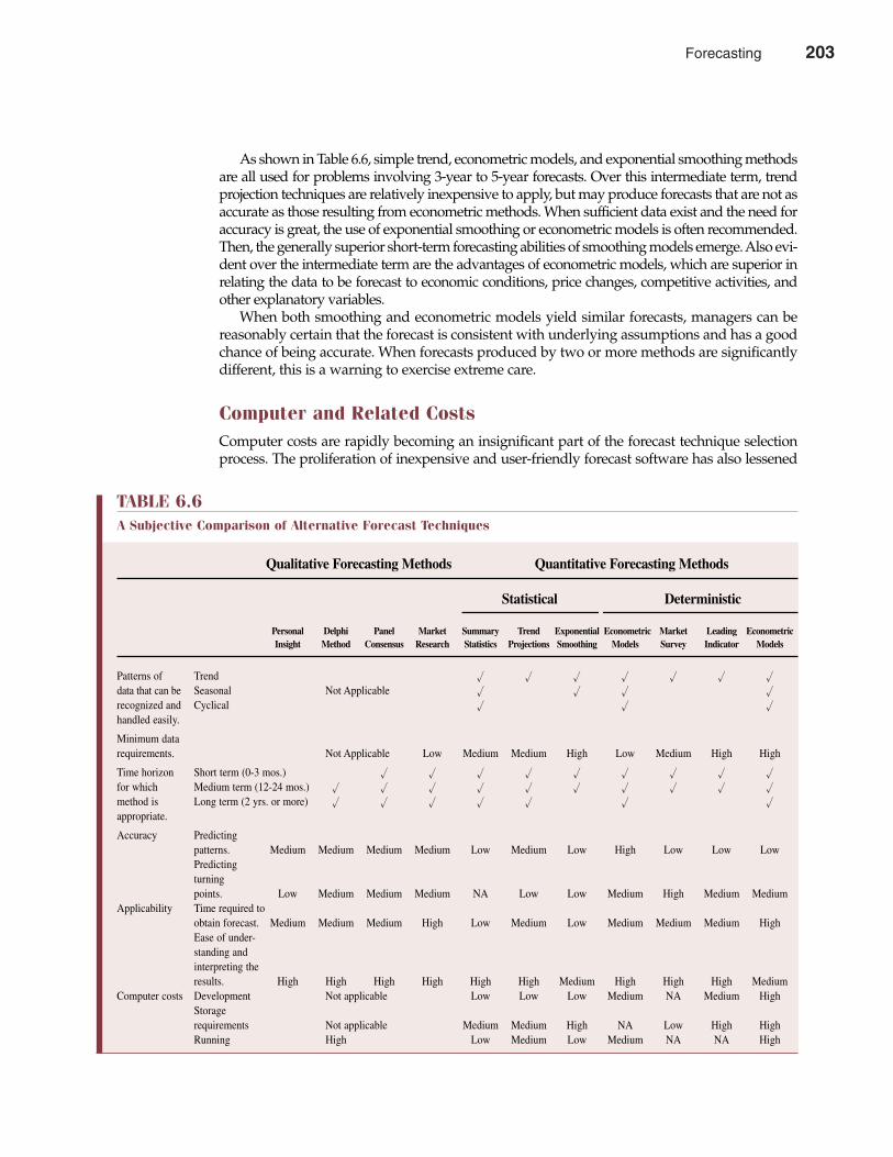
As shown in Table 6.6, simple trend, econometric models, and exponential smoothing methodsare all used for problems involving 3-year to 5-year forecasts. Over this intermediate term, trendprojection techniques are relatively inexpensive to apply, but may produce forecasts that are not asaccurate as those resulting from econometric methods. When sufficient data exist and the need foraccuracy is great, the use of exponential smoothing or econometric models is often recommended.Then, the generally superior short-term forecasting abilities of smoothing models emerge. Also evi-dent over the intermediate term are the advantages of econometric models, which are superior inrelating the data to be forecast to economic conditions, price changes, competitive activities, andother explanatory variables.
When both smoothing and econometric models yield similar forecasts, managers can bereasonably certain that the forecast is consistent with underlying assumptions and has a goodchance of being accurate. When forecasts produced by two or more methods are significantlydifferent, this is a warning to exercise extreme care.
Computer and Related CostsComputer costs are rapidly becoming an insignificant part of the forecast technique selectionprocess. The proliferation of inexpensive and user-friendly forecast software has also lessened
Chapter Six Forecasting 203
TABLE 6.6A Subjective Comparison of Alternative Forecast Techniques
Qualitative Forecasting Methods Quantitative Forecasting Methods
Statistical Deterministic
Personal Delphi Panel Market Summary Trend Exponential Econometric Market Leading Econometric Insight Method Consensus Research Statistics Projections Smoothing Models Survey Indicator Models
Patterns of Trend � � � � � � �
data that can be Seasonal Not Applicable � � � �
recognized and Cyclical � � �
handled easily.
Minimum data requirements. Not Applicable Low Medium Medium High Low Medium High High
Time horizon Short term (0-3 mos.) � � � � � � � � �
for which Medium term (12-24 mos.) � � � � � � � � � �
method is Long term (2 yrs. or more) � � � � � � �
appropriate.
Accuracy Predictingpatterns. Medium Medium Medium Medium Low Medium Low High Low Low LowPredictingturningpoints. Low Medium Medium Medium NA Low Low Medium High Medium Medium
Applicability Time required to obtain forecast. Medium Medium Medium High Low Medium Low Medium Medium Medium HighEase of under-standing and interpreting the results. High High High High High High Medium High High High Medium
Computer costs Development Not applicable Low Low Low Medium NA Medium HighStoragerequirements Not applicable Medium Medium High NA Low High HighRunning High Low Medium Low Medium NA NA High
Forecasting 203
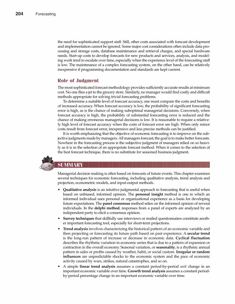
the need for sophisticated support staff. Still, other costs associated with forecast developmentand implementation cannot be ignored. Some major cost considerations often include data pro-cessing and storage costs, database maintenance and retrieval charges, and special hardwareneeds. Start-up costs to develop forecasts for new products and services, analysis, and model-ing work tend to escalate over time, especially when the experience level of the forecasting staffis low. The maintenance of a complex forecasting system, on the other hand, can be relativelyinexpensive if programming documentation and standards are kept current.
Role of JudgmentThe most sophisticated forecast methodology provides sufficiently accurate results at minimumcost. No one flies a jet to the grocery store. Similarly, no manager would find costly and difficultmethods appropriate for solving trivial forecasting problems.
To determine a suitable level of forecast accuracy, one must compare the costs and benefitsof increased accuracy. When forecast accuracy is low, the probability of significant forecastingerror is high, as is the chance of making suboptimal managerial decisions. Conversely, whenforecast accuracy is high, the probability of substantial forecasting error is reduced and thechance of making erroneous managerial decisions is low. It is reasonable to require a relative-ly high level of forecast accuracy when the costs of forecast error are high. When only minorcosts result from forecast error, inexpensive and less precise methods can be justified.
It is worth emphasizing that the objective of economic forecasting is to improve on the sub-jective judgments made by managers. All managers forecast; the goal is to make better forecasts.Nowhere in the forecasting process is the subjective judgment of managers relied on so heavi-ly as it is in the selection of an appropriate forecast method. When it comes to the selection ofthe best forecast technique, there is no substitute for seasoned business judgment.
SUMMARY
Managerial decision making is often based on forecasts of future events. This chapter examinesseveral techniques for economic forecasting, including qualitative analysis, trend analysis andprojection, econometric models, and input-output methods.
• Qualitative analysis is an intuitive judgmental approach to forecasting that is useful whenbased on unbiased, informed opinion. The personal insight method is one in which aninformed individual uses personal or organizational experience as a basis for developingfuture expectations. The panel consensus method relies on the informed opinion of severalindividuals. In the delphi method, responses from a panel of experts are analyzed by anindependent party to elicit a consensus opinion.
• Survey techniques that skillfully use interviews or mailed questionnaires constitute anoth-er important forecasting tool, especially for short-term projections.
• Trend analysis involves characterizing the historical pattern of an economic variable andthen projecting or forecasting its future path based on past experience. A secular trendis the long-run pattern of increase or decrease in economic data. Cyclical fluctuationdescribes the rhythmic variation in economic series that is due to a pattern of expansion orcontraction in the overall economy. Seasonal variation, or seasonality, is a rhythmic annualpattern in sales or profits caused by weather, habit, or social custom. Irregular or randominfluences are unpredictable shocks to the economic system and the pace of economicactivity caused by wars, strikes, natural catastrophes, and so on.
• A simple linear trend analysis assumes a constant period-by-period unit change in animportant economic variable over time. Growth trend analysis assumes a constant period-by-period percentage change in an important economic variable over time.
204 Part Two Demand Analysis
204 Forecasting
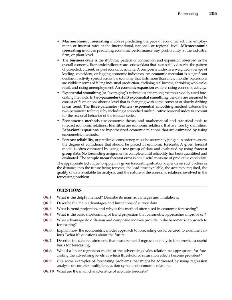
• Macroeconomic forecasting involves predicting the pace of economic activity, employ-ment, or interest rates at the international, national, or regional level. Microeconomicforecasting involves predicting economic performance, say, profitability, at the industry,firm, or plant level.
• The business cycle is the rhythmic pattern of contraction and expansion observed in theoverall economy. Economic indicators are series of data that successfully describe the patternof projected, current, or past economic activity. A composite index is a weighted average ofleading, coincident, or lagging economic indicators. An economic recession is a significantdecline in activity spread across the economy that lasts more than a few months. Recessionsare visible in terms of falling industrial production, declining real income, shrinking wholesale-retail, and rising unemployment. An economic expansion exhibits rising economic activity.
• Exponential smoothing (or “averaging”) techniques are among the most widely used fore-casting methods. In two-parameter (Holt) exponential smoothing, the data are assumed toconsist of fluctuations about a level that is changing with some constant or slowly driftinglinear trend. The three-parameter (Winters) exponential smoothing method extends thetwo-parameter technique by including a smoothed multiplicative seasonal index to accountfor the seasonal behavior of the forecast series.
• Econometric methods use economic theory and mathematical and statistical tools toforecast economic relations. Identities are economic relations that are true by definition.Behavioral equations are hypothesized economic relations that are estimated by usingeconometric methods.
• Forecast reliability, or predictive consistency, must be accurately judged in order to assessthe degree of confidence that should be placed in economic forecasts. A given forecastmodel is often estimated by using a test group of data and evaluated by using forecastgroup data. No forecasting assignment is complete until reliability has been quantified andevaluated. The sample mean forecast error is one useful measure of predictive capability.
The appropriate technique to apply in a given forecasting situation depends on such factors asthe distance into the future being forecast, the lead time available, the accuracy required, thequality of data available for analysis, and the nature of the economic relations involved in theforecasting problem.
QUESTIONS
Q6.1 What is the delphi method? Describe its main advantages and limitations.Q6.2 Describe the main advantages and limitations of survey data.Q6.3 What is trend projection, and why is this method often used in economic forecasting?Q6.4 What is the basic shortcoming of trend projection that barometric approaches improve on?Q6.5 What advantage do diffusion and composite indexes provide in the barometric approach to
forecasting?Q6.6 Explain how the econometric model approach to forecasting could be used to examine var-
ious “what if” questions about the future.Q6.7 Describe the data requirements that must be met if regression analysis is to provide a useful
basis for forecasting.Q6.8 Would a linear regression model of the advertising/sales relation be appropriate for fore-
casting the advertising levels at which threshold or saturation effects become prevalent?Q6.9 Cite some examples of forecasting problems that might be addressed by using regression
analysis of complex multiple-equation systems of economic relations.Q6.10 What are the main characteristics of accurate forecasts?
Chapter Six Forecasting 205
Forecasting 205
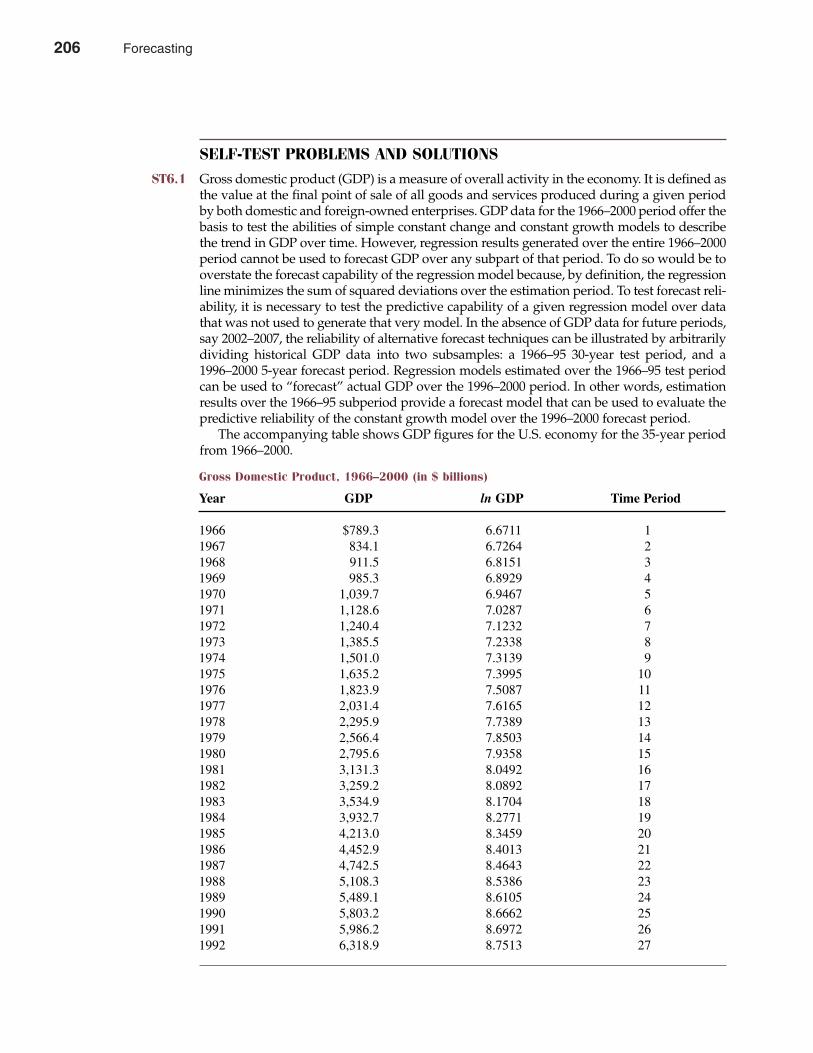
SELF-TEST PROBLEMS AND SOLUTIONS
ST6.1 Gross domestic product (GDP) is a measure of overall activity in the economy. It is defined asthe value at the final point of sale of all goods and services produced during a given periodby both domestic and foreign-owned enterprises. GDP data for the 1966–2000 period offer thebasis to test the abilities of simple constant change and constant growth models to describethe trend in GDP over time. However, regression results generated over the entire 1966–2000period cannot be used to forecast GDP over any subpart of that period. To do so would be tooverstate the forecast capability of the regression model because, by definition, the regressionline minimizes the sum of squared deviations over the estimation period. To test forecast reli-ability, it is necessary to test the predictive capability of a given regression model over datathat was not used to generate that very model. In the absence of GDP data for future periods,say 2002–2007, the reliability of alternative forecast techniques can be illustrated by arbitrarilydividing historical GDP data into two subsamples: a 1966–95 30-year test period, and a1996–2000 5-year forecast period. Regression models estimated over the 1966–95 test periodcan be used to “forecast” actual GDP over the 1996–2000 period. In other words, estimationresults over the 1966–95 subperiod provide a forecast model that can be used to evaluate thepredictive reliability of the constant growth model over the 1996–2000 forecast period.
The accompanying table shows GDP figures for the U.S. economy for the 35-year periodfrom 1966–2000.
206 Part Two Demand Analysis
Gross Domestic Product, 1966–2000 (in $ billions)
Year GDP ln GDP Time Period
1966 $789.3 6.6711 11967 834.1 6.7264 21968 911.5 6.8151 31969 985.3 6.8929 41970 1,039.7 6.9467 51971 1,128.6 7.0287 61972 1,240.4 7.1232 71973 1,385.5 7.2338 81974 1,501.0 7.3139 91975 1,635.2 7.3995 101976 1,823.9 7.5087 111977 2,031.4 7.6165 121978 2,295.9 7.7389 131979 2,566.4 7.8503 141980 2,795.6 7.9358 151981 3,131.3 8.0492 161982 3,259.2 8.0892 171983 3,534.9 8.1704 181984 3,932.7 8.2771 191985 4,213.0 8.3459 201986 4,452.9 8.4013 211987 4,742.5 8.4643 221988 5,108.3 8.5386 231989 5,489.1 8.6105 241990 5,803.2 8.6662 251991 5,986.2 8.6972 261992 6,318.9 8.7513 27
206 Forecasting
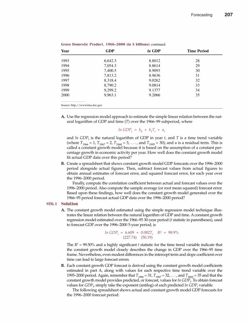
A. Use the regression model approach to estimate the simple linear relation between the nat-ural logarithm of GDP and time (T) over the 1966–99 subperiod, where
ln GDPt = b0 + b1Tt + ut
and ln GDPt is the natural logarithm of GDP in year t, and T is a time trend variable(where T1966 = 1, T1967 = 2, T1968 = 3, . . . , and T1995 = 30); and u is a residual term. This iscalled a constant growth model because it is based on the assumption of a constant per-centage growth in economic activity per year. How well does the constant growth modelfit actual GDP data over this period?
B. Create a spreadsheet that shows constant growth model GDP forecasts over the 1996–2000period alongside actual figures. Then, subtract forecast values from actual figures toobtain annual estimates of forecast error, and squared forecast error, for each year overthe 1996–2000 period.
Finally, compute the correlation coefficient between actual and forecast values over the1996–2000 period. Also compute the sample average (or root mean squared) forecast error.Based upon these findings, how well does the constant growth model generated over the1966–95 period forecast actual GDP data over the 1996–2000 period?
ST6.1 SolutionA. The constant growth model estimated using the simple regression model technique illus-
trates the linear relation between the natural logarithm of GDP and time. A constant growthregression model estimated over the 1966–95 30-year period (t statistic in parentheses), usedto forecast GDP over the 1996–2000 5-year period, is
ln GDPt = 6.609 + 0.082Tt R2 = 98.9%(227.74) (50.19)
The R2 = 99.50% and a highly significant t statistic for the time trend variable indicate thatthe constant growth model closely describes the change in GDP over the 1966–95 timeframe. Nevertheless, even modest differences in the intercept term and slope coefficient overtime can lead to large forecast errors.
B. Each constant growth GDP forecast is derived using the constant growth model coefficientsestimated in part A, along with values for each respective time trend variable over the1995–2000 period. Again, remember that T1996 = 31, T1997 = 32, . . . , and T2000 = 35 and that theconstant growth model provides predicted, or forecast, values for ln GDPt. To obtain forecastvalues for GDPt, simply take the exponent (antilog) of each predicted ln GDPt variable.
The following spreadsheet shows actual and constant growth model GDP forecasts forthe 1996–2000 forecast period:
Chapter Six Forecasting 207
Gross Domestic Product, 1966–2000 (in $ billions) continued
Year GDP ln GDP Time Period
1993 6,642.3 8.8012 281994 7,054.3 8.8614 291995 7,400.5 8.9093 301996 7,813.2 8.9636 311997 8,318.4 9.0262 321998 8,790.2 9.0814 331999 9,299.2 9.1377 342000 9,963.1 9.2066 35
Source: http://www.bea.doc.gov.
Forecasting 207
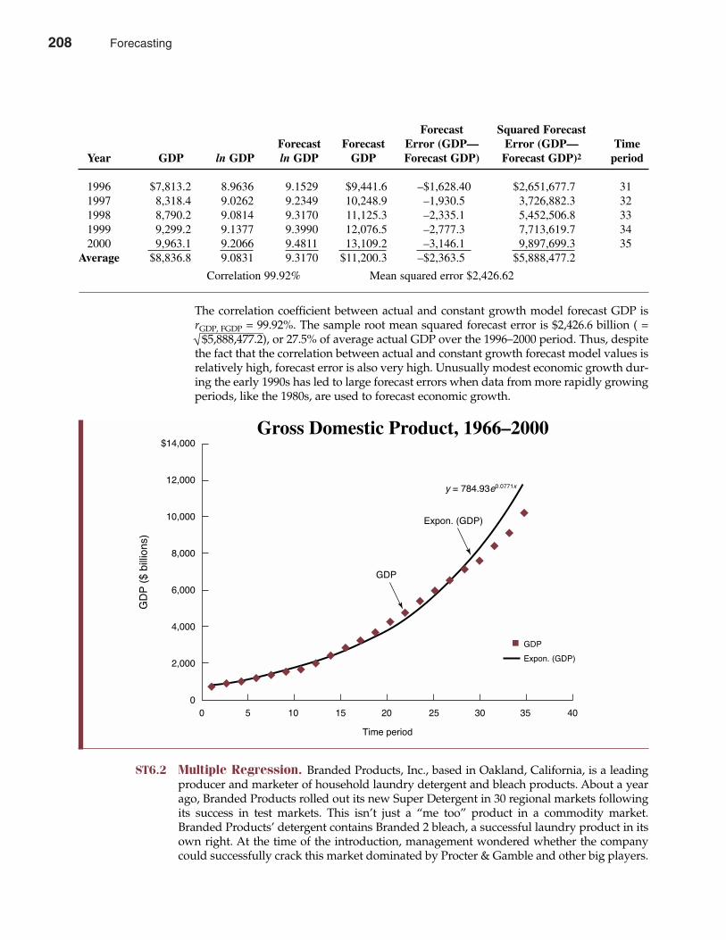
The correlation coefficient between actual and constant growth model forecast GDP isrGDP, FGDP = 99.92%. The sample root mean squared forecast error is $2,426.6 billion ( =√$5,888,477.2), or 27.5% of average actual GDP over the 1996–2000 period. Thus, despitethe fact that the correlation between actual and constant growth forecast model values isrelatively high, forecast error is also very high. Unusually modest economic growth dur-ing the early 1990s has led to large forecast errors when data from more rapidly growingperiods, like the 1980s, are used to forecast economic growth.
ST6.2 Multiple Regression. Branded Products, Inc., based in Oakland, California, is a leadingproducer and marketer of household laundry detergent and bleach products. About a yearago, Branded Products rolled out its new Super Detergent in 30 regional markets followingits success in test markets. This isn’t just a “me too” product in a commodity market.Branded Products’ detergent contains Branded 2 bleach, a successful laundry product in itsown right. At the time of the introduction, management wondered whether the companycould successfully crack this market dominated by Procter & Gamble and other big players.
208 Part Two Demand Analysis
Forecast Squared ForecastForecast Forecast Error (GDP— Error (GDP— Time
Year GDP ln GDP ln GDP GDP Forecast GDP) Forecast GDP)2 period
1996 $7,813.2 8.9636 9.1529 $9,441.6 –$1,628.40 $2,651,677.7 311997 8,318.4 9.0262 9.2349 10,248.9 –1,930.5 3,726,882.3 321998 8,790.2 9.0814 9.3170 11,125.3 –2,335.1 5,452,506.8 331999 9,299.2 9.1377 9.3990 12,076.5 –2,777.3 7,713,619.7 342000 9,963.1 9.2066 9.4811 13,109.2 –3,146.1 9,897,699.3 35
Average $8,836.8 9.0831 9.3170 $11,200.3 –$2,363.5 $5,888,477.2
Correlation 99.92% Mean squared error $2,426.62
$14,000
12,000
10,000
8,000
6,000
4,000
2,000
0
Time period
GDP
0 5 10 15 20 25 30 35 40
Gross Domestic Product, 1966–2000
GDP($
billions)
Expon. (GDP)
y = 784.93e0.0771x
Expon. (GDP)
GDP
208 Forecasting
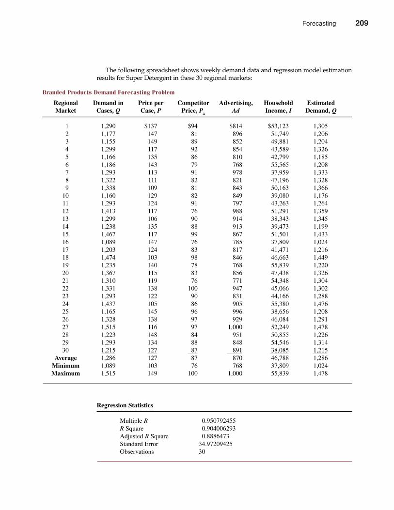
The following spreadsheet shows weekly demand data and regression model estimationresults for Super Detergent in these 30 regional markets:
Chapter Six Forecasting 209
Branded Products Demand Forecasting Problem
Regional Demand in Price per Competitor Advertising, Household Estimated Market Cases, Q Case, P Price, Px Ad Income, I Demand, Q
1 1,290 $137 $94 $814 $53,123 1,3052 1,177 147 81 896 51,749 1,2063 1,155 149 89 852 49,881 1,2044 1,299 117 92 854 43,589 1,3265 1,166 135 86 810 42,799 1,1856 1,186 143 79 768 55,565 1,2087 1,293 113 91 978 37,959 1,3338 1,322 111 82 821 47,196 1,3289 1,338 109 81 843 50,163 1,366
10 1,160 129 82 849 39,080 1,17611 1,293 124 91 797 43,263 1,26412 1,413 117 76 988 51,291 1,35913 1,299 106 90 914 38,343 1,34514 1,238 135 88 913 39,473 1,19915 1,467 117 99 867 51,501 1,43316 1,089 147 76 785 37,809 1,02417 1,203 124 83 817 41,471 1,21618 1,474 103 98 846 46,663 1,44919 1,235 140 78 768 55,839 1,22020 1,367 115 83 856 47,438 1,32621 1,310 119 76 771 54,348 1,30422 1,331 138 100 947 45,066 1,30223 1,293 122 90 831 44,166 1,28824 1,437 105 86 905 55,380 1,47625 1,165 145 96 996 38,656 1,20826 1,328 138 97 929 46,084 1,29127 1,515 116 97 1,000 52,249 1,47828 1,223 148 84 951 50,855 1,22629 1,293 134 88 848 54,546 1,31430 1,215 127 87 891 38,085 1,215
Average 1,286 127 87 870 46,788 1,286Minimum 1,089 103 76 768 37,809 1,024Maximum 1,515 149 100 1,000 55,839 1,478
Regression Statistics
Multiple R 0.950792455R Square 0.904006293Adjusted R Square 0.8886473Standard Error 34.97209425Observations 30
Forecasting 209
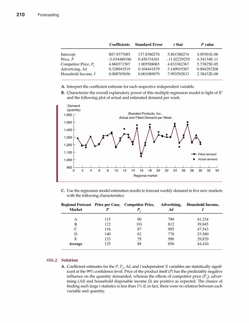
A. Interpret the coefficient estimate for each respective independent variable.B. Characterize the overall explanatory power of this multiple regression model in light of R2
and the following plot of actual and estimated demand per week.
C. Use the regression model estimation results to forecast weekly demand in five new marketswith the following characteristics:
ST6.2 SolutionA. Coefficient estimates for the P, Px, Ad, and I independent X variables are statistically signif-
icant at the 99% confidence level. Price of the product itself (P) has the predictably negativeinfluence on the quantity demanded, whereas the effects of competitor price (Px), adver-tising (Ad) and household disposable income (I) are positive as expected. The chance offinding such large t statistics is less than 1% if, in fact, there were no relation between eachvariable and quantity.
210 Part Two Demand Analysis
Coefficients Standard Error t Stat P value
Intercept 807.9377685 137.8360278 5.861586274 4.09301E-06Price, P –5.034480186 0.456754361 –11.02229255 4.34134E-11Competitor Price, Px 4.860371507 1.005588065 4.833362367 5.73825E-05Advertising, Ad 0.328043519 0.104441879 3.140919367 0.004293208Household Income, I 0.008705656 0.001089079 7.993592833 2.38432E-08
Regional Forecast Price per Case, Competitor Price, Advertising, Household Income,Market P Px Ad I
A 115 90 790 41,234B 122 101 812 39,845C 116 87 905 47,543D 140 82 778 53,560E 133 79 996 39,870
Average 125 88 856 44,410
0 2 4 6 8 10
Regional market
Demand
(quantity)
12 14 16 18 20 22 24 26 28 30 32 34
1,600
1,500
1,400
1,300
1,200
1,100
1,000
900
Branded Products, Inc.,
Actual and Fitted Demand per Week
Actual demand
Fitted demand
210 Forecasting
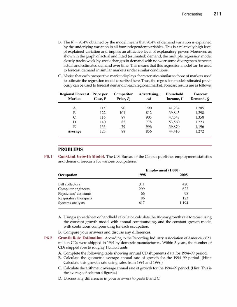
B. The R2 = 90.4% obtained by the model means that 90.4% of demand variation is explainedby the underlying variation in all four independent variables. This is a relatively high levelof explained variation and implies an attractive level of explanatory power. Moreover, asshown in the graph of actual and fitted (estimated) demand, the multiple regression modelclosely tracks week-by-week changes in demand with no worrisome divergences betweenactual and estimated demand over time. This means that this regression model can be usedto forecast demand in similar markets under similar conditions.
C. Notice that each prospective market displays characteristics similar to those of markets usedto estimate the regression model described here. Thus, the regression model estimated previ-ously can be used to forecast demand in each regional market. Forecast results are as follows:
PROBLEMS
P6.1 Constant Growth Model. The U.S. Bureau of the Census publishes employment statisticsand demand forecasts for various occupations.
A. Using a spreadsheet or handheld calculator, calculate the 10-year growth rate forecast usingthe constant growth model with annual compounding, and the constant growth modelwith continuous compounding for each occupation.
B. Compare your answers and discuss any differences.P6.2 Growth Rate Estimation. According to the Recording Industry Association of America, 662.1
million CDs were shipped in 1994 by domestic manufacturers. Within 5 years, the number ofCDs shipped rose to roughly 1 billion units.A. Complete the following table showing annual CD shipments data for 1994–99 period.B. Calculate the geometric average annual rate of growth for the 1994–99 period. (Hint:
Calculate this growth rate using sales from 1994 and 1999.)C. Calculate the arithmetic average annual rate of growth for the 1994–99 period. (Hint: This is
the average of column 4 figures.)D. Discuss any differences in your answers to parts B and C.
Chapter Six Forecasting 211
Employment (1,000)Occupation 1998 2008
Bill collectors 311 420Computer engineers 299 622Physicians’ assistants 66 98Respiratory therapists 86 123Systems analysts 617 1,194
Regional Forecast Price per Competitor Advertising, Household Forecast Market Case, P Price, Px Ad Income, I Demand, Q
A 115 90 790 41,234 1,285B 122 101 812 39,845 1,298C 116 87 905 47,543 1,358D 140 82 778 53,560 1,223E 133 79 996 39,870 1,196
Average 125 88 856 44,410 1,272
Forecasting 211
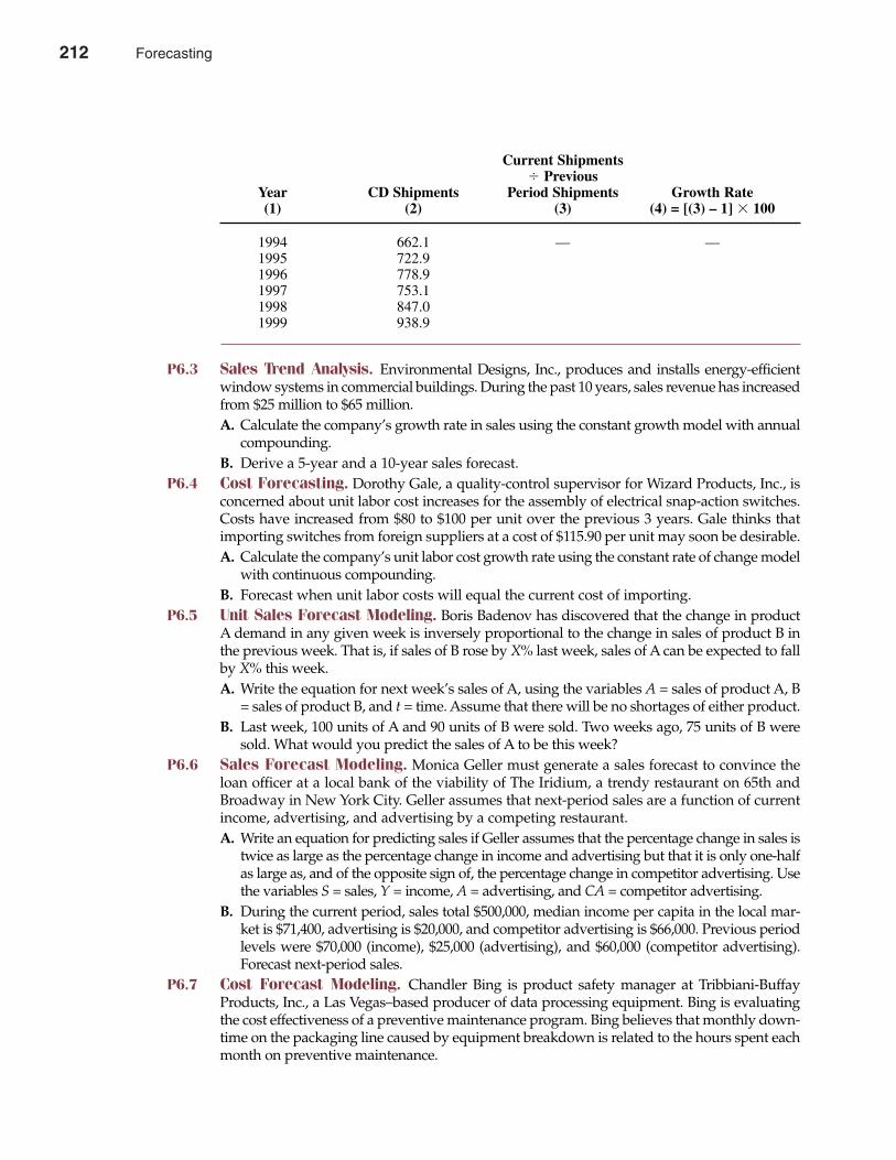
P6.3 Sales Trend Analysis. Environmental Designs, Inc., produces and installs energy-efficientwindow systems in commercial buildings. During the past 10 years, sales revenue has increasedfrom $25 million to $65 million.A. Calculate the company’s growth rate in sales using the constant growth model with annual
compounding.B. Derive a 5-year and a 10-year sales forecast.
P6.4 Cost Forecasting. Dorothy Gale, a quality-control supervisor for Wizard Products, Inc., isconcerned about unit labor cost increases for the assembly of electrical snap-action switches.Costs have increased from $80 to $100 per unit over the previous 3 years. Gale thinks thatimporting switches from foreign suppliers at a cost of $115.90 per unit may soon be desirable.A. Calculate the company’s unit labor cost growth rate using the constant rate of change model
with continuous compounding.B. Forecast when unit labor costs will equal the current cost of importing.
P6.5 Unit Sales Forecast Modeling. Boris Badenov has discovered that the change in productA demand in any given week is inversely proportional to the change in sales of product B inthe previous week. That is, if sales of B rose by X% last week, sales of A can be expected to fallby X% this week.A. Write the equation for next week’s sales of A, using the variables A = sales of product A, B
= sales of product B, and t = time. Assume that there will be no shortages of either product.B. Last week, 100 units of A and 90 units of B were sold. Two weeks ago, 75 units of B were
sold. What would you predict the sales of A to be this week?P6.6 Sales Forecast Modeling. Monica Geller must generate a sales forecast to convince the
loan officer at a local bank of the viability of The Iridium, a trendy restaurant on 65th andBroadway in New York City. Geller assumes that next-period sales are a function of currentincome, advertising, and advertising by a competing restaurant.A. Write an equation for predicting sales if Geller assumes that the percentage change in sales is
twice as large as the percentage change in income and advertising but that it is only one-halfas large as, and of the opposite sign of, the percentage change in competitor advertising. Usethe variables S = sales, Y = income, A = advertising, and CA = competitor advertising.
B. During the current period, sales total $500,000, median income per capita in the local mar-ket is $71,400, advertising is $20,000, and competitor advertising is $66,000. Previous periodlevels were $70,000 (income), $25,000 (advertising), and $60,000 (competitor advertising).Forecast next-period sales.
P6.7 Cost Forecast Modeling. Chandler Bing is product safety manager at Tribbiani-BuffayProducts, Inc., a Las Vegas–based producer of data processing equipment. Bing is evaluatingthe cost effectiveness of a preventive maintenance program. Bing believes that monthly down-time on the packaging line caused by equipment breakdown is related to the hours spent eachmonth on preventive maintenance.
212 Part Two Demand Analysis
Current Shipments� Previous
Year CD Shipments Period Shipments Growth Rate(1) (2) (3) (4) = [(3) – 1] � 100
1994 662.1 — —1995 722.91996 778.91997 753.11998 847.01999 938.9
212 Forecasting
A. Write an equation to predict next month’s downtime using the variables D = downtime, M =preventive maintenance, t = time, a0 = constant term, a1 = regression slope coefficient, and u =random disturbance. Assume that downtime in the forecast (next) month decreases by the samepercentage as preventive maintenance increased during the month preceding the current one.
B. If 40 hours were spent last month on preventive maintenance and this month’s downtimewas 500 hours, what should downtime be next month if preventive maintenance this monthis 50 hours? Use the equation developed in part A.
P6.8 Sales Forecast Modeling. Toys Unlimited, Ltd., must forecast sales for a popular adult com-puter game to avoid stockouts or excessive inventory charges during the upcoming Christmasseason. In percentage terms, the company estimates that game sales fall at double the rate ofprice increases and that they grow at triple the rate of customer traffic increases. Furthermore,these effects seem to be independent.A. Write an equation for estimating the Christmas season sales, using the variables S = sales,
P = price, T = traffic, and t = time.B. Forecast this season’s sales if Toys Unlimited sold 10,000 games last season at $15 each, this
season’s price is anticipated to be $16.50, and customer traffic is expected to rise by 15% overprevious levels.
P6.9 Simultaneous Equations. Mid-Atlantic Cinema, Inc., runs a chain of movie theaters in theeast-central states and has enjoyed great success with a Tuesday Night at the Movies promo-tion. By offering half off its regular $9 admission price, average nightly attendance has risenfrom 500 to 1,500 persons. Popcorn and other concession revenues tied to attendance have alsorisen dramatically. Historically, Mid-Atlantic has found that 50% of all moviegoers buy a $4 cupof buttered popcorn. Eighty percent of these popcorn buyers, plus 40% of the moviegoers thatdo not buy popcorn, each spend an average of $3 on soda and other concessions.A. Write an expression describing total revenue from tickets plus popcorn plus other con-
cessions.B. Forecast total revenues for both regular and special Tuesday night pricing.C. Forecast the total profit contribution earned for the regular and special Tuesday night
pricing strategies if the profit contribution is 25% on movie ticket revenues and 80% onpopcorn and other concession revenues.
P6.10 Simultaneous Equations. Supersonic Industries, based in Seattle, Washington, manufac-tures a wide range of parts for aircraft manufacturers. The company is currently evaluatingthe merits of building a new plant to fulfill a new contract with the federal government. Thealternatives to expansion are to use additional overtime, to reduce other production, or both.The company will add new capacity only if the economy appears to be expanding. Therefore,forecasting the general pace of economic activity for the United States is an important inputto the decision-making process. The firm has collected data and estimated the following rela-tions for the U.S. economy:
Forecast each of the preceding variables through the simultaneous relations expressed in themultiple equation system. Assume that all random disturbances average out to zero.
Chapter Six Forecasting 213
Last year’s total profits (all corporations) Pt–1 = $800 billionThis year’s government expenditures G = $2,000 billion
Annual consumption expenditures C = $600 billion + 0.75Y + uAnnual investment expenditures I = $1,080 billion + 0.9Pt–1 + u
Annual tax receipts T = 0.16GDPNet exports X = 0.03GDP
National income Y = GDP – TGross domestic product (GDP) = C + I + G – X
Forecasting 213
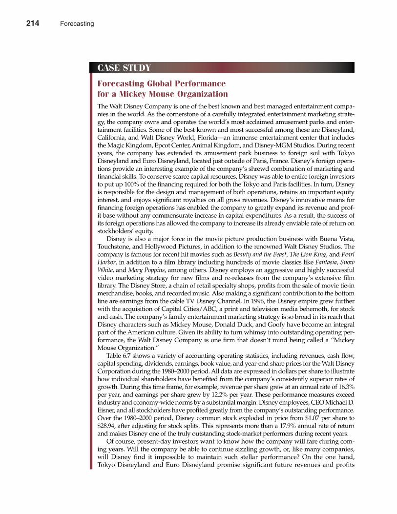
214 Part Two Demand Analysis
CASE STUDY
Forecasting Global Performance for a Mickey Mouse OrganizationThe Walt Disney Company is one of the best known and best managed entertainment compa-nies in the world. As the cornerstone of a carefully integrated entertainment marketing strate-gy, the company owns and operates the world’s most acclaimed amusement parks and enter-tainment facilities. Some of the best known and most successful among these are Disneyland,California, and Walt Disney World, Florida—an immense entertainment center that includesthe Magic Kingdom, Epcot Center, Animal Kingdom, and Disney-MGM Studios. During recentyears, the company has extended its amusement park business to foreign soil with TokyoDisneyland and Euro Disneyland, located just outside of Paris, France. Disney’s foreign opera-tions provide an interesting example of the company’s shrewd combination of marketing andfinancial skills. To conserve scarce capital resources, Disney was able to entice foreign investorsto put up 100% of the financing required for both the Tokyo and Paris facilities. In turn, Disneyis responsible for the design and management of both operations, retains an important equityinterest, and enjoys significant royalties on all gross revenues. Disney’s innovative means forfinancing foreign operations has enabled the company to greatly expand its revenue and prof-it base without any commensurate increase in capital expenditures. As a result, the success ofits foreign operations has allowed the company to increase its already enviable rate of return onstockholders’ equity.
Disney is also a major force in the movie picture production business with Buena Vista,Touchstone, and Hollywood Pictures, in addition to the renowned Walt Disney Studios. Thecompany is famous for recent hit movies such as Beauty and the Beast, The Lion King, and PearlHarbor, in addition to a film library including hundreds of movie classics like Fantasia, SnowWhite, and Mary Poppins, among others. Disney employs an aggressive and highly successfulvideo marketing strategy for new films and re-releases from the company’s extensive filmlibrary. The Disney Store, a chain of retail specialty shops, profits from the sale of movie tie-inmerchandise, books, and recorded music. Also making a significant contribution to the bottomline are earnings from the cable TV Disney Channel. In 1996, the Disney empire grew furtherwith the acquisition of Capital Cities/ABC, a print and television media behemoth, for stockand cash. The company’s family entertainment marketing strategy is so broad in its reach thatDisney characters such as Mickey Mouse, Donald Duck, and Goofy have become an integralpart of the American culture. Given its ability to turn whimsy into outstanding operating per-formance, the Walt Disney Company is one firm that doesn’t mind being called a “MickeyMouse Organization.”
Table 6.7 shows a variety of accounting operating statistics, including revenues, cash flow,capital spending, dividends, earnings, book value, and year-end share prices for the Walt DisneyCorporation during the 1980–2000 period. All data are expressed in dollars per share to illustratehow individual shareholders have benefited from the company’s consistently superior rates ofgrowth. During this time frame, for example, revenue per share grew at an annual rate of 16.3%per year, and earnings per share grew by 12.2% per year. These performance measures exceedindustry and economy-wide norms by a substantial margin. Disney employees, CEO Michael D.Eisner, and all stockholders have profited greatly from the company’s outstanding performance.Over the 1980–2000 period, Disney common stock exploded in price from $1.07 per share to$28.94, after adjusting for stock splits. This represents more than a 17.9% annual rate of returnand makes Disney one of the truly outstanding stock-market performers during recent years.
Of course, present-day investors want to know how the company will fare during com-ing years. Will the company be able to continue sizzling growth, or, like many companies,will Disney find it impossible to maintain such stellar performance? On the one hand,Tokyo Disneyland and Euro Disneyland promise significant future revenues and profits
214 Forecasting
Chapter Six Forecasting 215
from previously untapped global markets. Anyone with young children who has visitedDisneyland or Disney World has seen their delight and fascination with Disney characters.It is also impossible not to notice how much foreign travelers to the United States seem toenjoy the Disney experience. Donald Duck and Mickey Mouse will do a lot of businessabroad. Future expansion possibilities in Malaysia, China, or the former Soviet Union alsohold the potential for rapid growth into the next century. On the other hand, growth of 20%per year is exceedingly hard to maintain for any length of time. At that pace, the 120,000workers employed by Disney in 2001 would grow to over 288,000 by the year 2005, and toroughly 619,000 by the year 2010. Maintaining control with such a rapidly growing workforcewould be challenging, to say the least; maintaining Disney’s high level of creative energymight not be possible.
Given the many uncertainties faced by Disney and most major corporations, long-termforecasts of operating performance by industry analysts are usually restricted to a fairly shorttime perspective. The Value Line Investment Survey, one of the most widely respected forecastservices, focuses on a 3- to 5-year time horizon. To forecast performance for any individualcompany, Value Line starts with an underlying forecast of the economic environment 3 to 5
TABLE 6.7Operating Statistics for the Walt Disney Company (all data in dollars per share)
Cash Capital Book Year-EndYear Revenues Flow Spending Dividends Earnings Value Stock Price1
1980 $0.59 $0.11 $0.10 $0.02 $0.09 $0.69 $1.07 1981 0.65 0.10 0.21 0.02 0.08 0.75 1.09 1982 0.64 0.09 0.38 0.03 0.06 0.80 1.32 1983 0.79 0.11 0.20 0.03 0.06 0.85 1.10 1984 1.02 0.13 0.12 0.03 0.06 0.71 1.25 1985 1.30 0.18 0.12 0.03 0.11 0.76 2.35 1986 1.58 0.24 0.11 0.03 0.15 0.90 3.59 1987 1.82 0.34 0.18 0.03 0.24 1.17 4.94 1988 2.15 0.42 0.37 0.03 0.32 1.48 5.48 1989 2.83 0.55 0.46 0.04 0.43 1.87 9.33 1990 3.70 0.65 0.45 0.05 0.50 2.21 8.46 1991 3.96 0.58 0.59 0.06 0.40 2.48 9.54 1992 4.77 0.72 0.35 0.07 0.51 2.99 14.33 1993 5.31 0.78 0.49 0.08 0.54 3.13 14.21 1994 6.40 0.97 0.65 0.10 0.68 3.50 15.33 1995 7.70 1.15 0.57 0.12 0.84 4.23 19.63 1996 10.50 1.32 0.86 0.14 0.74 7.96 23.25 1997 11.10 1.51 0.95 0.17 0.92 8.54 33.00 1998 11.21 1.52 1.13 0.20 0.90 9.46 30.00 1999 11.34 1.30 1.03 0.00 0.66 10.16 29.25 2000 12.09 1.58 1.02 0.21 0.90 11.65 28.94
2004-20062 15.15 2.20 1.05 0.31 1.35 14.75
CASE STUDY (continued)
1 Split-adjusted share prices.2 Value Line estimates.
Sources: Company annual reports (various years); http://www.valueline.com.
Forecasting 215
216 Part Two Demand Analysis
CASE STUDY (continued)
years hence. During mid-2001 for example, Value Line forecast a 2004–06 economic environ-ment in which unemployment will average 4.4% of the workforce, compared to 4.0% in 2001.Industrial production will be expanding about 3.5% per year; inflation measured by theConsumer Price Index will continue at a modest 2.5% per year. Long-term interest rates areprojected to be about 6.6%, and gross domestic product will average over $11 trillion in theyears 2004 through 2006, or about 15% above the 2001 total of $9.7 trillion. As Value Line states,things may turn out differently, but these plausible assumptions offer a fruitful basis for meas-uring the relative growth potential of various firms like Disney.6
The most interesting economic statistic for Disney stockholders is, of course, its stockprice during some future period, say 2004–06. In economic terms, stock prices represent thenet present value of future cash flows, discounted at an appropriate risk-adjusted rate ofreturn. To forecast Disney’s stock price during the 2004–06 period, one might use any or allof the data in Table 6.7. Historical numbers for a recent period, like 1980–2000, often representa useful context for projecting future stock prices. For example, Fidelity’s legendary mutualfund investor Peter Lynch argues that stock prices are largely determined by the future pat-tern of earnings per share. Stock prices typically rise following an increase in earnings pershare and plunge when earnings per share plummet. Another renown investor, Sir JohnTempleton, the father of global stock market investing, focuses on book value per share.Templeton contends that future earnings are closely related to the book value of the firm, oraccounting net worth. According to Templeton, “bargains” can be found when stock can bepurchased in companies that sell in the marketplace at a significant discount to book value,or when book value per share is expected to rise dramatically. Both Lynch and Templetonhave built a large following among investors who have profited mightily using their stock-market selection techniques.
As an experiment, it will prove interesting to employ the data provided in Table 6.7 to esti-mate regression models that can be used to forecast the average common stock price for TheWalt Disney Company over the 2004–06 period.A. A simple regression model over the 1980–2000 period where the Y variable is the
Disney year-end stock price and the X variable is Disney’s earnings per share reads asfollows (t statistics in parentheses):
Pt = –$2.311 + $33.296EPSt-R2 = 89.2%
(–1.68) (12.92)
Use this model to forecast Disney’s average stock price for the 2004–06 period using theValue Line estimate of Disney’s average earnings per share for 2004–06. Discuss this share-price forecast.
B. A simple regression model over the 1980–2000 period where the Y variable is theDisney year-end stock price and the X variable is Disney’s book value per share readsas follows (t statistics in parentheses):
Pt = $1.638 + $2.924BVt-R2 = 90.9%
(1.57) (14.15)
Use this model to forecast Disney’s average stock price for the 2004–06 period using theValue Line estimate of Disney’s average book value per share for 2004–06. Discuss thisshare-price forecast.
6 See “Economic Series,” The Value Line Investment Survey (http://www.valueline.com).
216 Forecasting
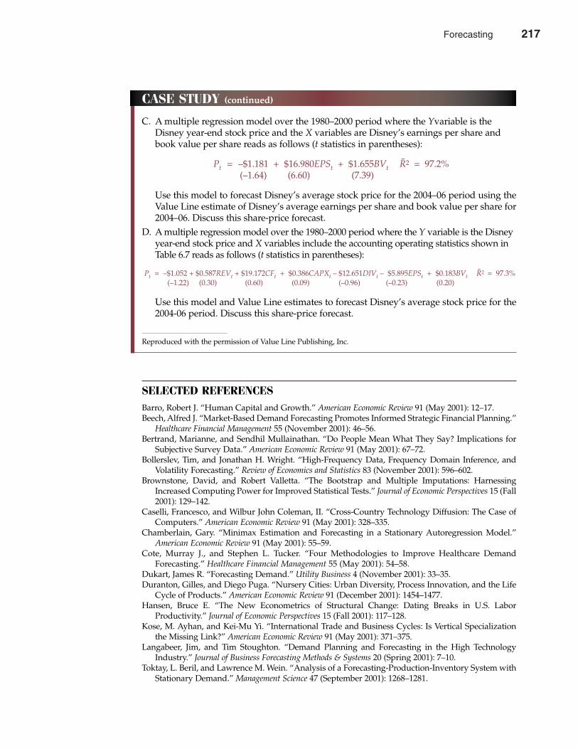
SELECTED REFERENCESBarro, Robert J. “Human Capital and Growth.” American Economic Review 91 (May 2001): 12–17.Beech, Alfred J. “Market-Based Demand Forecasting Promotes Informed Strategic Financial Planning.”
Healthcare Financial Management 55 (November 2001): 46–56.Bertrand, Marianne, and Sendhil Mullainathan. “Do People Mean What They Say? Implications for
Subjective Survey Data.” American Economic Review 91 (May 2001): 67–72.Bollerslev, Tim, and Jonathan H. Wright. “High-Frequency Data, Frequency Domain Inference, and
Volatility Forecasting.” Review of Economics and Statistics 83 (November 2001): 596–602.Brownstone, David, and Robert Valletta. “The Bootstrap and Multiple Imputations: Harnessing
Increased Computing Power for Improved Statistical Tests.” Journal of Economic Perspectives 15 (Fall2001): 129–142.
Caselli, Francesco, and Wilbur John Coleman, II. “Cross-Country Technology Diffusion: The Case ofComputers.” American Economic Review 91 (May 2001): 328–335.
Chamberlain, Gary. “Minimax Estimation and Forecasting in a Stationary Autoregression Model.”American Economic Review 91 (May 2001): 55–59.
Cote, Murray J., and Stephen L. Tucker. “Four Methodologies to Improve Healthcare DemandForecasting.” Healthcare Financial Management 55 (May 2001): 54–58.
Dukart, James R. “Forecasting Demand.” Utility Business 4 (November 2001): 33–35.Duranton, Gilles, and Diego Puga. “Nursery Cities: Urban Diversity, Process Innovation, and the Life
Cycle of Products.” American Economic Review 91 (December 2001): 1454–1477.Hansen, Bruce E. “The New Econometrics of Structural Change: Dating Breaks in U.S. Labor
Productivity.” Journal of Economic Perspectives 15 (Fall 2001): 117–128.Kose, M. Ayhan, and Kei-Mu Yi. “International Trade and Business Cycles: Is Vertical Specialization
the Missing Link?” American Economic Review 91 (May 2001): 371–375. Langabeer, Jim, and Tim Stoughton. “Demand Planning and Forecasting in the High Technology
Industry.” Journal of Business Forecasting Methods & Systems 20 (Spring 2001): 7–10.Toktay, L. Beril, and Lawrence M. Wein. “Analysis of a Forecasting-Production-Inventory System with
Stationary Demand.” Management Science 47 (September 2001): 1268–1281.
Chapter Six Forecasting 217
CASE STUDY (continued)
C. A multiple regression model over the 1980–2000 period where the Yvariable is theDisney year-end stock price and the X variables are Disney’s earnings per share andbook value per share reads as follows (t statistics in parentheses):
Pt = –$1.181 + $16.980EPSt + $1.655BVt-R2 = 97.2%
(–1.64) (6.60) (7.39)
Use this model to forecast Disney’s average stock price for the 2004–06 period using theValue Line estimate of Disney’s average earnings per share and book value per share for2004–06. Discuss this share-price forecast.
D. A multiple regression model over the 1980–2000 period where the Y variable is the Disneyyear-end stock price and X variables include the accounting operating statistics shown inTable 6.7 reads as follows (t statistics in parentheses):
Pt = –$1.052 + $0.587REVt + $19.172CFt + $0.386CAPXt – $12.651DIVt – $5.895EPSt + $0.183BVt-R2 = 97.3%
(–1.22) (0.30) (0.60) (0.09) (–0.96) (–0.23) (0.20)
Use this model and Value Line estimates to forecast Disney’s average stock price for the2004-06 period. Discuss this share-price forecast.
Reproduced with the permission of Value Line Publishing, Inc.
Forecasting 217

218 Part Two Demand Analysis
Production Analysis andCompensation Policy
CHAPTER SEVEN
220 1 T. J. Rodgers, “Options Aren’t Optional in Silicon Valley,” The Wall Street Journal Online,March 4, 2002 (http://online.wsj.com).
Hiring the right workers, providing proper training, and offering theman effective incentive compensation package is tough because the
ongoing relationship between employers and their employees is differentfrom any other business affiliation. If a company buys a piece of land, forexample, the terms of trade can be clearly set in advance. In the case of realestate, a mutually acceptable price is determined, a deed is delivered, andthe transaction is completed. However, what works for real estate transac-tions is far from sufficient for setting a compensation policy. “One shot”deals are fundamentally different from the typical employment relationship.
The employment relationship is never fully completed because effort iscontinuously renegotiable. If employees feel slighted or underpaid, theyalways have the option of reducing effort to the point where the resultingrate per hour or month gives an acceptable return for the amount of effortexpended. However, what passes for equity in the eyes of workers createsfundamental problems for managers concerned with the health of the over-all organization. As a result, managers face the continuing need to designmutually attractive compensation packages that align worker incentives andperformance with organizational objectives.
Like the economic concepts to measure worker productivity, managersrely upon managerial economics to help them assess the productivity of allinput factors. This makes production analysis and compensation policy oneof the most interesting and fundamental challenges facing management.Production analysis is concerned with more than low-cost defect preven-tion. It is about producing exciting products that customers want at pricesthat beat the competition.1
219
7
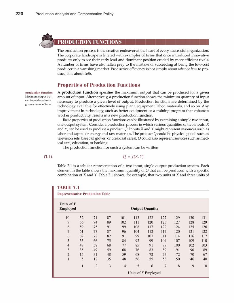
PRODUCTION FUNCTIONS
The production process is the creative endeavor at the heart of every successful organization.The corporate landscape is littered with examples of firms that once introduced innovativeproducts only to see their early lead and dominant position eroded by more efficient rivals.A number of firms have also fallen prey to the mistake of succeeding at being the low-costproducer in a vanishing market. Productive efficiency is not simply about what or how to pro-duce; it is about both.
Properties of Production FunctionsA production function specifies the maximum output that can be produced for a givenamount of input. Alternatively, a production function shows the minimum quantity of inputnecessary to produce a given level of output. Production functions are determined by thetechnology available for effectively using plant, equipment, labor, materials, and so on. Anyimprovement in technology, such as better equipment or a training program that enhancesworker productivity, results in a new production function.
Basic properties of production functions can be illustrated by examining a simple two-input,one-output system. Consider a production process in which various quantities of two inputs, Xand Y, can be used to produce a product, Q. Inputs X and Y might represent resources such aslabor and capital or energy and raw materials. The product Q could be physical goods such astelevision sets, baseball gloves, or breakfast cereal; Q could also represent services such as med-ical care, education, or banking.
The production function for such a system can be written
(7.1) Q = f (X, Y)
Table 7.1 is a tabular representation of a two-input, single-output production system. Eachelement in the table shows the maximum quantity of Q that can be produced with a specificcombination of X and Y. Table 7.1 shows, for example, that two units of X and three units of
production function Maximum output thatcan be produced for agiven amount of input
Chapter Seven Production Analysis and Compensation Policy 221
TABLE 7.1Representative Production Table
Units of YEmployed Output Quantity
10 52 71 87 101 113 122 127 129 130 1319 56 74 89 102 111 120 125 127 128 1298 59 75 91 99 108 117 122 124 125 1267 61 77 87 96 104 112 117 120 121 1226 62 72 82 91 99 107 111 114 116 1175 55 66 75 84 92 99 104 107 109 1104 47 58 68 77 85 91 97 100 102 1033 35 49 59 68 76 83 89 91 90 892 15 31 48 59 68 72 73 72 70 671 5 12 35 48 56 55 53 50 46 40
1 2 3 4 5 6 7 8 9 10
Units of X Employed
220 Production Analysis and Compensation Policy
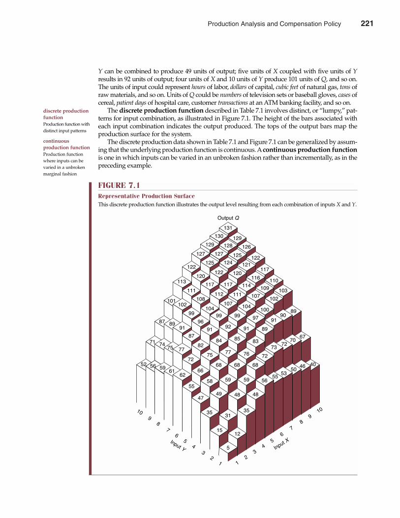
Y can be combined to produce 49 units of output; five units of X coupled with five units of Yresults in 92 units of output; four units of X and 10 units of Y produce 101 units of Q, and so on.The units of input could represent hours of labor, dollars of capital, cubic feet of natural gas, tons ofraw materials, and so on. Units of Q could be numbers of television sets or baseball gloves, cases ofcereal, patient days of hospital care, customer transactions at an ATM banking facility, and so on.
The discrete production function described in Table 7.1 involves distinct, or “lumpy,” pat-terns for input combination, as illustrated in Figure 7.1. The height of the bars associated witheach input combination indicates the output produced. The tops of the output bars map theproduction surface for the system.
The discrete production data shown in Table 7.1 and Figure 7.1 can be generalized by assum-ing that the underlying production function is continuous. Acontinuous production functionis one in which inputs can be varied in an unbroken fashion rather than incrementally, as in thepreceding example.
222 Part Three Production and Cost Analysis
FIGURE 7.1Representative Production SurfaceThis discrete production function illustrates the output level resulting from each combination of inputs X and Y.
Input Y
109
8
76
54
32
1
131
130 129
126128129
127 127 125
124122
117121
120122
125122
120
117 117
116
114
111
107
112
110
109
107
10489
102
100
103
9091
89
97
6770
7273
72
83
9999
919291
96
99
102101
113
111
108
104
84 85
767775
82
87
918987
71 7475 77
72
6668 68 68
5655
5350
46 40
59595855
4749 48 48
12
3135
15
5
6261
565259
35
Input
X
12
34
5
6
7
89
10
Output Q
discrete productionfunction Production function withdistinct input patterns
continuous production function Production functionwhere inputs can bevaried in a unbrokenmarginal fashion
Production Analysis and Compensation Policy 221
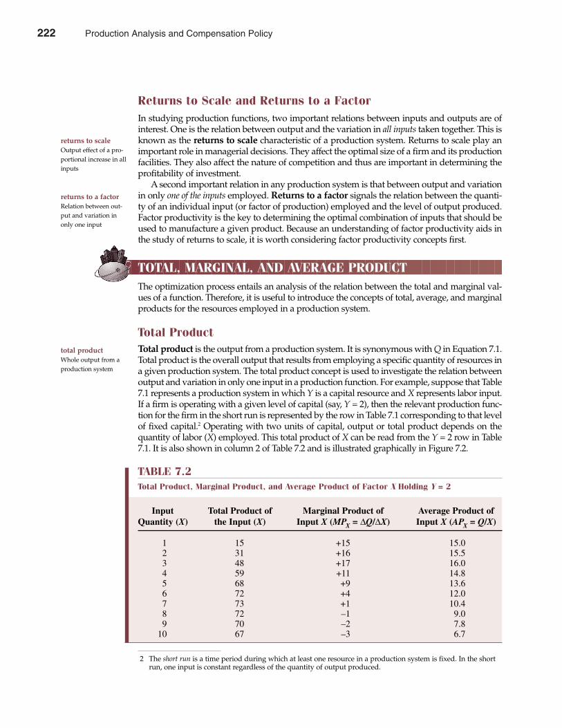
Returns to Scale and Returns to a FactorIn studying production functions, two important relations between inputs and outputs are ofinterest. One is the relation between output and the variation in all inputs taken together. This isknown as the returns to scale characteristic of a production system. Returns to scale play animportant role in managerial decisions. They affect the optimal size of a firm and its productionfacilities. They also affect the nature of competition and thus are important in determining theprofitability of investment.
A second important relation in any production system is that between output and variationin only one of the inputs employed. Returns to a factor signals the relation between the quanti-ty of an individual input (or factor of production) employed and the level of output produced.Factor productivity is the key to determining the optimal combination of inputs that should beused to manufacture a given product. Because an understanding of factor productivity aids inthe study of returns to scale, it is worth considering factor productivity concepts first.
TOTAL, MARGINAL, AND AVERAGE PRODUCTThe optimization process entails an analysis of the relation between the total and marginal val-ues of a function. Therefore, it is useful to introduce the concepts of total, average, and marginalproducts for the resources employed in a production system.
Total ProductTotal product is the output from a production system. It is synonymous with Q in Equation 7.1.Total product is the overall output that results from employing a specific quantity of resources ina given production system. The total product concept is used to investigate the relation betweenoutput and variation in only one input in a production function. For example, suppose that Table7.1 represents a production system in which Y is a capital resource and X represents labor input.If a firm is operating with a given level of capital (say, Y = 2), then the relevant production func-tion for the firm in the short run is represented by the row in Table 7.1 corresponding to that levelof fixed capital.2 Operating with two units of capital, output or total product depends on thequantity of labor (X) employed. This total product of X can be read from the Y = 2 row in Table7.1. It is also shown in column 2 of Table 7.2 and is illustrated graphically in Figure 7.2.
returns to scale Output effect of a pro-portional increase in allinputs
returns to a factorRelation between out-put and variation inonly one input
total product Whole output from aproduction system
Chapter Seven Production Analysis and Compensation Policy 223
TABLE 7.2Total Product, Marginal Product, and Average Product of Factor X Holding Y = 2
Input Total Product of Marginal Product of Average Product of Quantity (X) the Input (X) Input X (MPX = ∆Q/∆X) Input X (APX = Q/X)
1 15 +15 15.02 31 +16 15.53 48 +17 16.04 59 +11 14.85 68 +9 13.66 72 +4 12.07 73 +1 10.48 72 –1 9.09 70 –2 7.8
10 67 –3 6.7
2 The short run is a time period during which at least one resource in a production system is fixed. In the shortrun, one input is constant regardless of the quantity of output produced.
222 Production Analysis and Compensation Policy
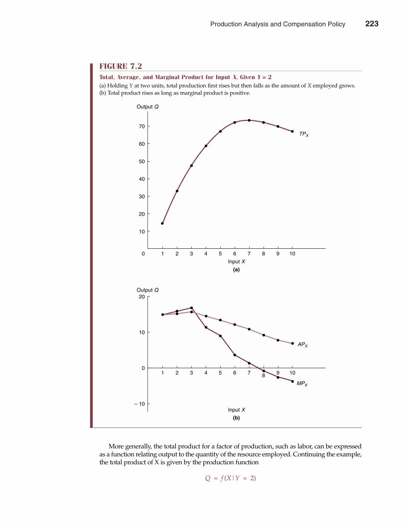
More generally, the total product for a factor of production, such as labor, can be expressedas a function relating output to the quantity of the resource employed. Continuing the example,the total product of X is given by the production function
Q = f (X|Y = 2)
224 Part Three Production and Cost Analysis
FIGURE 7.2Total, Average, and Marginal Product for Input X, Given Y = 2(a) Holding Y at two units, total production first rises but then falls as the amount of X employed grows.(b) Total product rises as long as marginal product is positive.
1 2 3 4 5 6 78
9 10
1 2 3 4 5 6 7 8 9 10
Input X
(a)
Input X
(b)
20
10
0
Ð 10
Output Q
Output Q
70
60
50
40
30
20
10
0
TPX
APX
MPX
Production Analysis and Compensation Policy 223
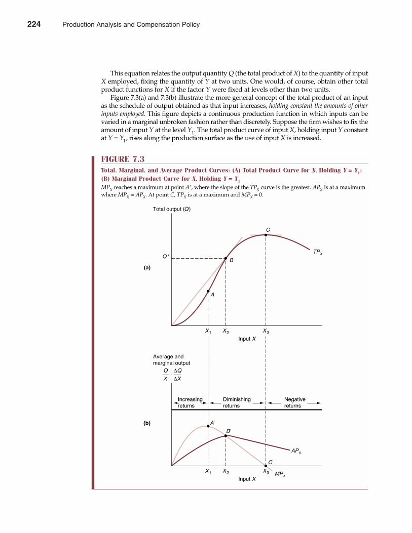
This equation relates the output quantity Q (the total product of X) to the quantity of inputX employed, fixing the quantity of Y at two units. One would, of course, obtain other totalproduct functions for X if the factor Y were fixed at levels other than two units.
Figure 7.3(a) and 7.3(b) illustrate the more general concept of the total product of an inputas the schedule of output obtained as that input increases, holding constant the amounts of otherinputs employed. This figure depicts a continuous production function in which inputs can bevaried in a marginal unbroken fashion rather than discretely. Suppose the firm wishes to fix theamount of input Y at the level Y1. The total product curve of input X, holding input Y constantat Y = Y1, rises along the production surface as the use of input X is increased.
Chapter Seven Production Analysis and Compensation Policy 225
FIGURE 7.3Total, Marginal, and Average Product Curves: (A) Total Product Curve for X, Holding Y = Y1;(B) Marginal Product Curve for X, Holding Y = Y1
MPX reaches a maximum at point A�, where the slope of the TPX curve is the greatest. APX is at a maximumwhere MPX = APX. At point C, TPX is at a maximum and MPX = 0.
X3X2X1
X3X2X1
A'
B '
C '
MPx
APx
Input X
Average and
marginal output
Q
X
∆Q
∆X,
(b)
(a)
Total output (Q )
Q*
A
B
C
TPx
Increasing
returns
Diminishing
returns
Negative
returns
Input X
224 Production Analysis and Compensation Policy

Marginal ProductGiven the total product function for an input, both marginal and average products can be easilyderived. The marginal product of a factor, MPX, is the change in output associated with a one-unit change in the factor input, holding all other inputs constant. For a total product functionsuch as that shown in Table 7.2 and Figure 7.2(a), the marginal product is expressed as
MPX = ∆Q∆X
where ∆Q is the change in output resulting from a one-unit change, ∆X, in the variable factor.This expression assumes that the quantity of the other input, Y, remains unchanged. Marginalproduct is shown in column 3 of Table 7.2 and in Figure 7.2(b).
Average ProductAverage product is total product divided by the number of units of input employed:
(7.2) APX = QX
The average product for X given Y = 2 units is shown in column 4 of Table 7.2 and in Figure 7.2(b).For a continuous total product function, as illustrated in Figure 7.3(a), marginal product
equals the slope of the total product curve, whereas average product equals the slope of a linedrawn from the origin to a point on the total product curve. The average and marginal productsfor input X can be determined in this manner, and these points are plotted to form the averageand marginal product curves shown in Figure 7.3(b).
226 Part Three Production and Cost Analysis
marginal product Change in output asso-ciated with a one-unitchange in a singleinput
average productTotal product divided byunits of input employed
Total Quality Management
One of the hottest management concepts in recentyears—the total quality management, or TQMapproach—has failed to deliver promised results inmany companies. However, once implementation prob-lems are overcome, the method becomes a cornerstone ofenlightened management strategy. In today’s global economic environment, both large and small companieshave come to recognize that improved quality is anessential ingredient for success. Still, quality manage-ment programs are not painless.
TQM requires a major commitment. In simplestterms, TQM involves a keen attention to the productionprocess, a high level of commitment to the customer, andthe involvement of employees in identifying and contin-uously improving upon the best production practices.TQM is not a quick fix; TQM sometimes requires basicreengineering of the firm’s entire operation. TQM startswith a fundamental question—Should we be doing thisat all? If affirmative, TQM then asks, “How can we dothis cheaper, faster, or better?”
Analysts agree that adherence to basic conceptsdetermines the success of any TQM effort. Among thosefactors thought to be most important are the following:
• The CEO must be actively and visibly behind it.• Tunnel vision must be avoided. Ask what change
does for the customer.• Limit yourself to a few critical goals.• Link change to a clear financial payback.• Customize the TQM concept to meet the specific
needs of customers.
Like any sound theory, these principles represent morethan simply an enlightened operating philosophy; theywork well in practice, too. TQM helps boost productquality, customer satisfaction, and profits. Experienceshows that continuous monitoring is required to ensurethat the TQM process retains an effective customer focus.TQM must be outward rather than inward looking.
See: Walter S. Mossberg, “Cheaper Office Suite Challenges Mircrosoft,But Trails on Quality,” The Wall Street Journal Online, January 10, 2002(http://online.wsj.com).
M A N A G E R I A L A P P L I C AT I O N 7 . 1
Production Analysis and Compensation Policy 225
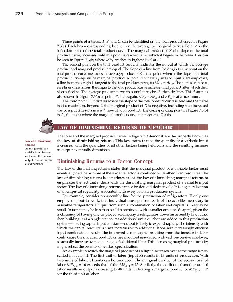
Three points of interest, A, B, and C, can be identified on the total product curve in Figure7.3(a). Each has a corresponding location on the average or marginal curves. Point A is theinflection point of the total product curve. The marginal product of X (the slope of the totalproduct curve) increases until this point is reached, after which it begins to decrease. This canbe seen in Figure 7.3(b) where MPX reaches its highest level at A�.
The second point on the total product curve, B, indicates the output at which the averageproduct and marginal product are equal. The slope of a line from the origin to any point on thetotal product curve measures the average product of X at that point, whereas the slope of the totalproduct curve equals the marginal product. At point B, where X2 units of input X are employed,a line from the origin is tangent to the total product curve, so MPX = APX. The slopes of succes-sive lines drawn from the origin to the total product curve increase until point B, after which theirslopes decline. The average product curve rises until it reaches B, then declines. This feature isalso shown in Figure 7.3(b) as point B�. Here again, MPX = APX and APX is at a maximum.
The third point, C, indicates where the slope of the total product curve is zero and the curveis at a maximum. Beyond C the marginal product of X is negative, indicating that increaseduse of input X results in a reduction of total product. The corresponding point in Figure 7.3(b)is C�, the point where the marginal product curve intersects the X-axis.
LAW OF DIMINISHING RETURNS TO A FACTOR
The total and the marginal product curves in Figure 7.3 demonstrate the property known asthe law of diminishing returns. This law states that as the quantity of a variable inputincreases, with the quantities of all other factors being held constant, the resulting increasein output eventually diminishes.
Diminishing Returns to a Factor ConceptThe law of diminishing returns states that the marginal product of a variable factor musteventually decline as more of the variable factor is combined with other fixed resources. Thelaw of diminishing returns is sometimes called the law of diminishing marginal returns toemphasize the fact that it deals with the diminishing marginal product of a variable inputfactor. The law of diminishing returns cannot be derived deductively. It is a generalizationof an empirical regularity associated with every known production system.
For example, consider an assembly line for the production of refrigerators. If only oneemployee is put to work, that individual must perform each of the activities necessary toassemble refrigerators. Output from such a combination of labor and capital is likely to besmall. In fact, it may be less than could be achieved with a smaller amount of capital, given theinefficiency of having one employee accompany a refrigerator down an assembly line ratherthan building it at a single station. As additional units of labor are added to this productionsystem—holding capital input constant—output is likely to expand rapidly. The intensity withwhich the capital resource is used increases with additional labor, and increasingly efficientinput combinations result. The improved use of capital resulting from the increase in laborcould cause the marginal product, or rise in output associated with each successive employee,to actually increase over some range of additional labor. This increasing marginal productivitymight reflect the benefits of worker specialization.
An example in which the marginal product of an input increases over some range is pre-sented in Table 7.2. The first unit of labor (input X) results in 15 units of production. Withtwo units of labor, 31 units can be produced. The marginal product of the second unit oflabor MPX=2 = 16 exceeds that of the MPX=1 = 15. Similarly, the addition of another unit oflabor results in output increasing to 48 units, indicating a marginal product of MPX=3 = 17for the third unit of labor.
law of diminishingreturnsAs the quantity of avariable input increas-es, the resulting rate ofoutput increase eventu-ally diminishes
Chapter Seven Production Analysis and Compensation Policy 227
226 Production Analysis and Compensation Policy
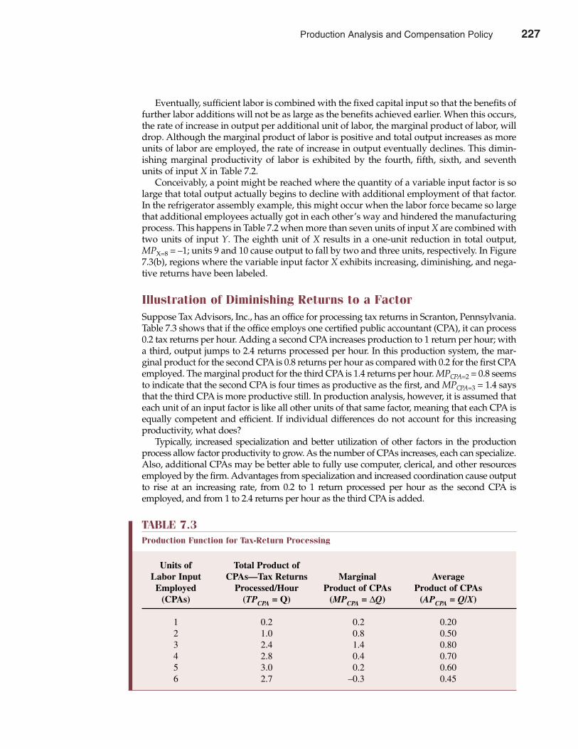
Eventually, sufficient labor is combined with the fixed capital input so that the benefits offurther labor additions will not be as large as the benefits achieved earlier. When this occurs,the rate of increase in output per additional unit of labor, the marginal product of labor, willdrop. Although the marginal product of labor is positive and total output increases as moreunits of labor are employed, the rate of increase in output eventually declines. This dimin-ishing marginal productivity of labor is exhibited by the fourth, fifth, sixth, and seventhunits of input X in Table 7.2.
Conceivably, a point might be reached where the quantity of a variable input factor is solarge that total output actually begins to decline with additional employment of that factor.In the refrigerator assembly example, this might occur when the labor force became so largethat additional employees actually got in each other’s way and hindered the manufacturingprocess. This happens in Table 7.2 when more than seven units of input X are combined withtwo units of input Y. The eighth unit of X results in a one-unit reduction in total output,MPX=8 = –1; units 9 and 10 cause output to fall by two and three units, respectively. In Figure7.3(b), regions where the variable input factor X exhibits increasing, diminishing, and nega-tive returns have been labeled.
Illustration of Diminishing Returns to a FactorSuppose Tax Advisors, Inc., has an office for processing tax returns in Scranton, Pennsylvania.Table 7.3 shows that if the office employs one certified public accountant (CPA), it can process0.2 tax returns per hour. Adding a second CPA increases production to 1 return per hour; witha third, output jumps to 2.4 returns processed per hour. In this production system, the mar-ginal product for the second CPA is 0.8 returns per hour as compared with 0.2 for the first CPAemployed. The marginal product for the third CPA is 1.4 returns per hour. MPCPA=2 = 0.8 seemsto indicate that the second CPA is four times as productive as the first, and MPCPA=3 = 1.4 saysthat the third CPA is more productive still. In production analysis, however, it is assumed thateach unit of an input factor is like all other units of that same factor, meaning that each CPA isequally competent and efficient. If individual differences do not account for this increasingproductivity, what does?
Typically, increased specialization and better utilization of other factors in the productionprocess allow factor productivity to grow. As the number of CPAs increases, each can specialize.Also, additional CPAs may be better able to fully use computer, clerical, and other resourcesemployed by the firm. Advantages from specialization and increased coordination cause outputto rise at an increasing rate, from 0.2 to 1 return processed per hour as the second CPA isemployed, and from 1 to 2.4 returns per hour as the third CPA is added.
228 Part Three Production and Cost Analysis
TABLE 7.3Production Function for Tax-Return Processing
Units of Total Product ofLabor Input CPAs—Tax Returns Marginal Average
Employed Processed/Hour Product of CPAs Product of CPAs(CPAs) (TPCPA = Q) (MPCPA = ∆Q) (APCPA = Q/X)
1 0.2 0.2 0.202 1.0 0.8 0.503 2.4 1.4 0.804 2.8 0.4 0.705 3.0 0.2 0.606 2.7 –0.3 0.45
Production Analysis and Compensation Policy 227
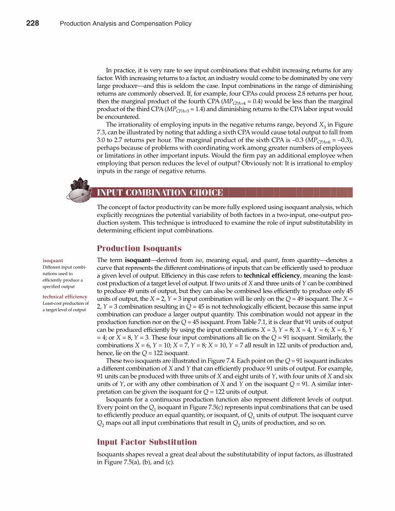
In practice, it is very rare to see input combinations that exhibit increasing returns for anyfactor. With increasing returns to a factor, an industry would come to be dominated by one verylarge producer—and this is seldom the case. Input combinations in the range of diminishingreturns are commonly observed. If, for example, four CPAs could process 2.8 returns per hour,then the marginal product of the fourth CPA (MPCPA=4 = 0.4) would be less than the marginalproduct of the third CPA (MPCPA=3 = 1.4) and diminishing returns to the CPA labor input wouldbe encountered.
The irrationality of employing inputs in the negative returns range, beyond X3 in Figure7.3, can be illustrated by noting that adding a sixth CPA would cause total output to fall from3.0 to 2.7 returns per hour. The marginal product of the sixth CPA is –0.3 (MPCPA=6 = –0.3),perhaps because of problems with coordinating work among greater numbers of employeesor limitations in other important inputs. Would the firm pay an additional employee whenemploying that person reduces the level of output? Obviously not: It is irrational to employinputs in the range of negative returns.
INPUT COMBINATION CHOICE
The concept of factor productivity can be more fully explored using isoquant analysis, whichexplicitly recognizes the potential variability of both factors in a two-input, one-output pro-duction system. This technique is introduced to examine the role of input substitutability indetermining efficient input combinations.
Production IsoquantsThe term isoquant—derived from iso, meaning equal, and quant, from quantity—denotes acurve that represents the different combinations of inputs that can be efficiently used to producea given level of output. Efficiency in this case refers to technical efficiency, meaning the least-cost production of a target level of output. If two units of X and three units of Y can be combinedto produce 49 units of output, but they can also be combined less efficiently to produce only 45units of output, the X = 2, Y = 3 input combination will lie only on the Q = 49 isoquant. The X =2, Y = 3 combination resulting in Q = 45 is not technologically efficient, because this same inputcombination can produce a larger output quantity. This combination would not appear in theproduction function nor on the Q = 45 isoquant. From Table 7.1, it is clear that 91 units of outputcan be produced efficiently by using the input combinations X = 3, Y = 8; X = 4, Y = 6; X = 6, Y= 4; or X = 8, Y = 3. These four input combinations all lie on the Q = 91 isoquant. Similarly, thecombinations X = 6, Y = 10; X = 7, Y = 8; X = 10, Y = 7 all result in 122 units of production and,hence, lie on the Q = 122 isoquant.
These two isoquants are illustrated in Figure 7.4. Each point on the Q = 91 isoquant indicatesa different combination of X and Y that can efficiently produce 91 units of output. For example,91 units can be produced with three units of X and eight units of Y, with four units of X and sixunits of Y, or with any other combination of X and Y on the isoquant Q = 91. A similar inter-pretation can be given the isoquant for Q = 122 units of output.
Isoquants for a continuous production function also represent different levels of output.Every point on the Q1 isoquant in Figure 7.5(c) represents input combinations that can be usedto efficiently produce an equal quantity, or isoquant, of Q1 units of output. The isoquant curveQ2 maps out all input combinations that result in Q2 units of production, and so on.
Input Factor SubstitutionIsoquants shapes reveal a great deal about the substitutability of input factors, as illustratedin Figure 7.5(a), (b), and (c).
isoquant Different input combi-nations used to efficiently produce aspecified output
technical efficiencyLeast-cost production ofa target level of output
Chapter Seven Production Analysis and Compensation Policy 229
228 Production Analysis and Compensation Policy
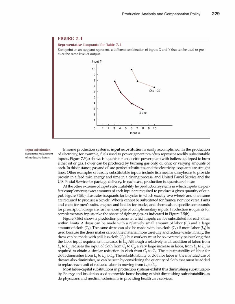
In some production systems, input substitution is easily accomplished. In the productionof electricity, for example, fuels used to power generators often represent readily substitutableinputs. Figure 7.5(a) shows isoquants for an electric power plant with boilers equipped to burneither oil or gas. Power can be produced by burning gas only, oil only, or varying amounts ofeach. In this instance, gas and oil are perfect substitutes, and the electricity isoquants are straightlines. Other examples of readily substitutable inputs include fish meal and soybeans to provideprotein in a feed mix, energy and time in a drying process, and United Parcel Service and theU.S. Postal Service for package delivery. In each case, production isoquants are linear.
At the other extreme of input substitutability lie production systems in which inputs are per-fect complements; exact amounts of each input are required to produce a given quantity of out-put. Figure 7.5(b) illustrates isoquants for bicycles in which exactly two wheels and one frameare required to produce a bicycle. Wheels cannot be substituted for frames, nor vice versa. Pantsand coats for men’s suits, engines and bodies for trucks, and chemicals in specific compoundsfor prescription drugs are further examples of complementary inputs. Production isoquants forcomplementary inputs take the shape of right angles, as indicated in Figure 7.5(b).
Figure 7.5(c) shows a production process in which inputs can be substituted for each otherwithin limits. A dress can be made with a relatively small amount of labor (L1) and a largeamount of cloth (C1). The same dress can also be made with less cloth (C2) if more labor (L2) isused because the dress maker can cut the material more carefully and reduce waste. Finally, thedress can be made with still less cloth (C3), but workers must be so extremely painstaking thatthe labor input requirement increases to L3. Although a relatively small addition of labor, fromL1 to L2, reduces the input of cloth from C1 to C2, a very large increase in labor, from L2 to L3, isrequired to obtain a similar reduction in cloth from C2 to C3. The substitutability of labor forcloth diminishes from L1 to L2 to L3. The substitutability of cloth for labor in the manufacture ofdresses also diminishes, as can be seen by considering the quantity of cloth that must be addedto replace each unit of reduced labor in moving from L3 to L1.
Most labor-capital substitutions in production systems exhibit this diminishing substitutabil-ity. Energy and insulation used to provide home heating exhibit diminishing substitutability, asdo physicians and medical technicians in providing health care services.
230 Part Three Production and Cost Analysis
input substitutionSystematic replacementof productive factors
FIGURE 7.4Representative Isoquants for Table 7.1Each point on an isoquant represents a different combination of inputs X and Y that can be used to pro-duce the same level of output.
10
9
8
7
6
5
4
3
2
1
1 2 3 4 5 6 7 8 9 10
Input X
Input Y
Q = 122
Q = 91
0
Production Analysis and Compensation Policy 229
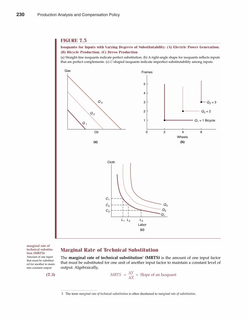
Marginal Rate of Technical SubstitutionThe marginal rate of technical substitution3 (MRTS) is the amount of one input factorthat must be substituted for one unit of another input factor to maintain a constant level ofoutput. Algebraically,
(7.3) MRTS = ∆Y = Slope of an Isoquant∆X
Chapter Seven Production Analysis and Compensation Policy 231
FIGURE 7.5Isoquants for Inputs with Varying Degrees of Substitutability: (A) Electric Power Generation;(B) Bicycle Production; (C) Dress Production(a) Straight-line isoquants indicate perfect substitution. (b) A right-angle shape for isoquants reflects inputsthat are perfect complements. (c) C-shaped isoquants indicate imperfect substitutability among inputs.
Gas
Q 3
Q 2
Q 1
Oil 2 4 6
Wheels
1
2
3
4
5
Frames
Q1 = 1 Bicycle
Q2 = 2
Q3 = 3
Cloth
Labor
L1 L2 L3
C3
C2
C1
Q1
Q2
Q3
(a) (b)
(c)
0
marginal rate oftechnical substitu-tion (MRTS)Amount of one inputthat must be substitut-ed for another to main-tain constant output
3 The term marginal rate of technical substitution is often shortened to marginal rate of substitution.
230 Production Analysis and Compensation Policy
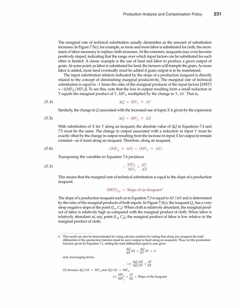
The marginal rate of technical substitution usually diminishes as the amount of substitutionincreases. In Figure 7.5(c), for example, as more and more labor is substituted for cloth, the incre-ment of labor necessary to replace cloth increases. At the extremes, isoquants may even becomepositively sloped, indicating that the range over which input factors can be substituted for eachother is limited. A classic example is the use of land and labor to produce a given output ofgrain. At some point, as labor is substituted for land, the farmers will trample the grain. As morelabor is added, more land eventually must be added if grain output is to be maintained.
The input substitution relation indicated by the slope of a production isoquant is directlyrelated to the concept of diminishing marginal productivity. The marginal rate of technicalsubstitution is equal to –1 times the ratio of the marginal products of the input factors [MRTS= –1(MPX/MPY)]. To see this, note that the loss in output resulting from a small reduction inY equals the marginal product of Y, MPY, multiplied by the change in Y, ∆Y. That is,
(7.4) ∆Q = MPY � ∆Y
Similarly, the change in Q associated with the increased use of input X is given by the expression
(7.5) ∆Q = MPX � ∆X
With substitution of X for Y along an isoquant, the absolute value of ∆Q in Equations 7.4 and7.5 must be the same. The change in output associated with a reduction in input Y must beexactly offset by the change in output resulting from the increase in input X for output to remainconstant—as it must along an isoquant. Therefore, along an isoquant,
(7.6) –(MPX � ∆X) = (MPY � ∆Y)
Transposing the variables in Equation 7.6 produces
(7.7) – MPX = ∆YMPY ∆X
This means that the marginal rate of technical substitution is equal to the slope of a productionisoquant:
MRTSXY = Slope of an Isoquant4
The slope of a production isoquant such as in Equation 7.3 is equal to ∆Y/∆X and is determinedby the ratio of the marginal products of both inputs. In Figure 7.5(c), the isoquant Q1 has a verysteep negative slope at the point (L1, C1). When cloth is relatively abundant, the marginal prod-uct of labor is relatively high as compared with the marginal product of cloth. When labor isrelatively abundant at, say, point (L3, C3), the marginal product of labor is low relative to themarginal product of cloth.
232 Part Three Production and Cost Analysis
4 This result can also be demonstrated by using calculus notation by noting that along any isoquant the total differential of the production function must be zero (output is fixed along an isoquant). Thus, for the productionfunction given by Equation 7.1, setting the total differential equal to zero gives
∆Q dX +
∆Q dY = 0∆X ∆Y
and, rearranging terms,
(–)∆Q/∆X
=dY
∆Q/∆Y dX
Or, because ∆Q/∆X = MPX and ∆Q/∆Y = MPY,
(–)MPX =
dY= Slope of the Isoquant
MPY dX
Production Analysis and Compensation Policy 231
Rational Limits of Input SubstitutionIt is irrational for a firm to combine resources in such a way that the marginal product of anyinput is negative, because this implies that output could be increased by using less of thatresource.5 Note from Equation 7.6 that if the inputs X and Y are combined in proportionssuch that the marginal product of either factor is negative, then the slope of the productionisoquant will be positive. For a production isoquant to be positively sloped, one of the inputfactors must have a negative marginal product. Input combinations lying along a positivelysloped portion of a production isoquant are irrational and would be avoided by the firm.
In Figure 7.6, the rational limits of input substitution are where the isoquants become posi-tively sloped. Limits to the range of substitutability of X for Y are indicated by the points oftangency between the isoquants and a set of lines drawn perpendicular to the Y-axis. Limits ofeconomic substitutability of Y for X are shown by the tangents of lines perpendicular to the X-axis.Maximum and minimum proportions of Y and X that would be combined to produce each levelof output are determined by points of tangency between these lines and the production isoquants.
It is irrational to use any input combination outside these tangents, or ridge lines, as they arecalled. Such combinations are irrational because the marginal product of the relatively moreabundant input is negative outside the ridge lines. The addition of the last unit of the excessiveinput factor actually reduces output. Obviously, it would be irrational for a firm to buy andemploy additional units that cause production to decrease. To illustrate, suppose a firm is cur-rently operating with a fixed quantity of input Y equal to Y1 units, as shown in Figure 7.6. In sucha situation, the firm would never employ more than X3 units of input X, because employment of
ridge lines Graphic bounds forpositive marginalproducts
Chapter Seven Production Analysis and Compensation Policy 233
Are CEOs Overpaid?
Citigroup, Inc., CEO Sanford “Sandy” Weill is a favoritetarget of those who believe CEOs are overpaid. Citigroup,with 2000 revenue of $64.9 billion, is the largest and mostprofitable financial services company in the world. It’s acomplex company with a wide variety of holdings. Overthe 1995–2000 period, Citigroup had a 5-year growth rateof 21.3 percent, or somewhat better than average forfinancial service companies. Critics contend thatCitigroup has done well during Weill’s tenure, but notnearly so well as its CEO. Between 1995 and 2000, Weillpulled in an astonishing $785 million in total compensa-tion. In 2000 alone, Weill cashed in stock options worth$196.2 million on top of a bonus of $18.4 million. Weill’spay is unusual, but CEOs of large U.S. corporations rou-tinely take home total compensation that runs in excess of$5 million per year. For top CEOs with over 5 years at thehelm, pay averages more than $7.5 million per year.
Proponents of modern CEO pay plans contend thatcompanies like Citigroup have been revitalized whenmanagement focuses on bottom-line performance.Opponents argue that such plans allow CEOs to take
unfair advantage of their positions. They cite examplesof millions of dollars in compensation being paid to topexecutives in the auto, steel, and other industries follow-ing wage cuts for blue-collar workers, mass layoffs, andplant closures. Although proponents admit the need forclose public scrutiny, they argue that corporate restruc-turing is an important requirement of a vital economyand a key task facing top executives. Proponents also notethat running a large modern corporation is an exceed-ingly complex task and requires an individual with raremanagement skill.
CEOs of major U.S. corporations command billionsof dollars in shareholder resources. Good decisions canmean billions of dollars in shareholder benefits; baddecisions can cost billions. In a global marketplace, it’s asimple fact that good management is worth a lot.
See: Paul Beckett, “Citigroup Posts Stong Earnings Growth DespiteArgentina Crisis, Enron Collapse,” The Wall Street Journal Online, January18, 2002 (http://online.wsj.com).
M A N A G E R I A L A P P L I C AT I O N 7 . 2
5 This is technically correct only if the resource has a positive cost. Thus, for example, a firm might employadditional workers even though the marginal product of labor was negative if it received a government sub-sidy for that employment that more than offset the cost of the output reduction.
232 Production Analysis and Compensation Policy
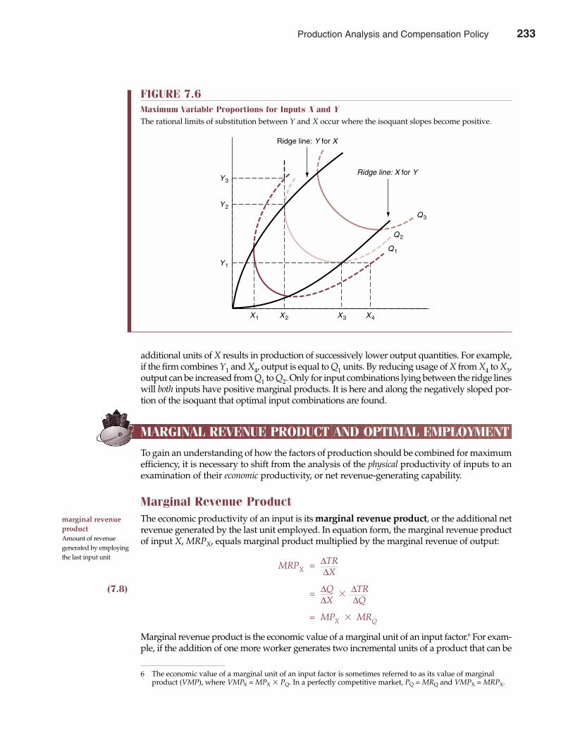
additional units of X results in production of successively lower output quantities. For example,if the firm combines Y1 and X4, output is equal to Q1 units. By reducing usage of X from X4 to X3,output can be increased from Q1 to Q2. Only for input combinations lying between the ridge lineswill both inputs have positive marginal products. It is here and along the negatively sloped por-tion of the isoquant that optimal input combinations are found.
MARGINAL REVENUE PRODUCT AND OPTIMAL EMPLOYMENT
To gain an understanding of how the factors of production should be combined for maximumefficiency, it is necessary to shift from the analysis of the physical productivity of inputs to anexamination of their economic productivity, or net revenue-generating capability.
Marginal Revenue ProductThe economic productivity of an input is its marginal revenue product, or the additional netrevenue generated by the last unit employed. In equation form, the marginal revenue productof input X, MRPX, equals marginal product multiplied by the marginal revenue of output:
MRPX = ∆TR∆X
(7.8) = ∆Q � ∆TR∆X ∆Q
= MPX � MRQ
Marginal revenue product is the economic value of a marginal unit of an input factor.6 For exam-ple, if the addition of one more worker generates two incremental units of a product that can be
234 Part Three Production and Cost Analysis
marginal revenueproduct Amount of revenuegenerated by employingthe last input unit
FIGURE 7.6Maximum Variable Proportions for Inputs X and YThe rational limits of substitution between Y and X occur where the isoquant slopes become positive.
Ridge line: Y for X
Ridge line: X for Y Y3
Y2
Y1
X1 X2 X3 X4
Q1
Q2
Q3
6 The economic value of a marginal unit of an input factor is sometimes referred to as its value of marginalproduct (VMP), where VMPX = MPX � PQ. In a perfectly competitive market, PQ = MRQ and VMPX = MRPX.
Production Analysis and Compensation Policy 233
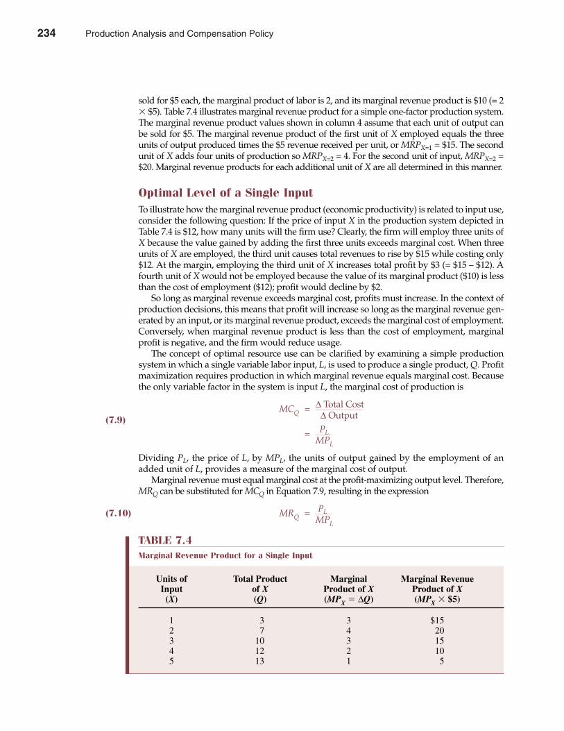
sold for $5 each, the marginal product of labor is 2, and its marginal revenue product is $10 (= 2� $5). Table 7.4 illustrates marginal revenue product for a simple one-factor production system.The marginal revenue product values shown in column 4 assume that each unit of output canbe sold for $5. The marginal revenue product of the first unit of X employed equals the threeunits of output produced times the $5 revenue received per unit, or MRPX=1 = $15. The secondunit of X adds four units of production so MRPX=2 = 4. For the second unit of input, MRPX=2 =$20. Marginal revenue products for each additional unit of X are all determined in this manner.
Optimal Level of a Single InputTo illustrate how the marginal revenue product (economic productivity) is related to input use,consider the following question: If the price of input X in the production system depicted inTable 7.4 is $12, how many units will the firm use? Clearly, the firm will employ three units ofX because the value gained by adding the first three units exceeds marginal cost. When threeunits of X are employed, the third unit causes total revenues to rise by $15 while costing only$12. At the margin, employing the third unit of X increases total profit by $3 (= $15 – $12). Afourth unit of X would not be employed because the value of its marginal product ($10) is lessthan the cost of employment ($12); profit would decline by $2.
So long as marginal revenue exceeds marginal cost, profits must increase. In the context ofproduction decisions, this means that profit will increase so long as the marginal revenue gen-erated by an input, or its marginal revenue product, exceeds the marginal cost of employment.Conversely, when marginal revenue product is less than the cost of employment, marginalprofit is negative, and the firm would reduce usage.
The concept of optimal resource use can be clarified by examining a simple productionsystem in which a single variable labor input, L, is used to produce a single product, Q. Profitmaximization requires production in which marginal revenue equals marginal cost. Becausethe only variable factor in the system is input L, the marginal cost of production is
MCQ = ∆ Total Cost∆ Output(7.9)
= PLMPL
Dividing PL, the price of L, by MPL, the units of output gained by the employment of anadded unit of L, provides a measure of the marginal cost of output.
Marginal revenue must equal marginal cost at the profit-maximizing output level. Therefore,MRQ can be substituted for MCQ in Equation 7.9, resulting in the expression
(7.10) MRQ = PLMPL
Chapter Seven Production Analysis and Compensation Policy 235
TABLE 7.4Marginal Revenue Product for a Single Input
Units of Total Product Marginal Marginal RevenueInput of X Product of X Product of X
(X) (Q) (MPX � ∆Q) (MPX � $5)
1 3 3 $152 7 4 203 10 3 154 12 2 105 13 1 5
234 Production Analysis and Compensation Policy
Equation 7.10 must hold for profit maximization because its right-hand side is just anoth-er expression for marginal cost. Solving Equation 7.10 for PL results in
PL = MRQ � MPL
or, because MRQ � MPL is defined as the marginal revenue product of L,
(7.11) PL = MRPL
A profit-maximizing firm will always set marginal revenue product equal to price (marginal cost) forevery input. If marginal revenue product exceeds the cost of an input, profits could be increasedby employing additional units. When the marginal cost of an input factor is greater than its mar-ginal revenue product, profit would increase by reducing employment. Only when MRP = P isprofit maximized. Optimal employment and economic efficiency is achieved in the overalleconomy when all firms employ resources so as to equate each input’s marginal revenueproduct and marginal cost.
An Illustration of Optimal EmploymentDetermination of the optimal input level can be clarified by reconsidering the Tax Advisors,Inc., example, illustrated in Table 7.3. If three CPAs can process 2.4 returns per hour andemploying a fourth CPA increases total output per hour to 2.8, then employing a fourth CPAreduces marginal product from MPCPA=3 = 1.4 to MPCPA=4 = 0.4. Employment is in a range ofdiminishing returns. Nevertheless, a fourth CPA should be hired if expanding employmentwill increase profits.
For simplicity, assume that CPA time is the only input required to process additional taxreturns and that CPAs earn $35 per hour, or roughly $70,000 per year including fringe benefits.If Tax Advisors, Inc., receives $100 in revenue for each tax return prepared by the fourth CPA,a comparison of the price of labor and marginal revenue product for the fourth CPA reveals
PCPA < MRPCPA=4 = MRQ � MPCPA=4
because
$35 < $40 = $100 � 0.4
If a fourth CPA is hired, total profits will rise by $5 per hour (= $40 – $35). The additional CPAshould be employed.
Because the marginal product for the fifth CPA equals 0.2, MPCPA=5 = 0.2, the marginalrevenue product falls to only $20 per hour, or less than the $35-per-hour cost of hiring thatperson. The firm would incur a $15-per-hour loss by expanding hiring to that level andwould, therefore, stop with employment of four CPAs.
This example assumes that CPA time is the only variable input involved in tax-returnpreparation. In reality, other inputs are apt to be necessary. Additional computer time, officesupplies, and clerical support may also be required to increase output. If such were the case,determining the independent contribution or value of CPA input would be more complex. Ifvariable overhead for CPA support staff and supplies equals 50 percent of sales revenue, thenthe net marginal revenue, or marginal revenue after all variable costs, for CPA time wouldbe only $50 per unit (= 0.5 � MRQ). In this instance, Tax Advisors, Inc., would find that the $20(= 0.4 � (0.5)($100)) net marginal revenue product generated by the fourth CPA would not off-set the necessary $35 per hour cost (wage rate). It would, therefore, employ no more than threeCPAs, a level at which MRP = 1.4 � (0.5)($100) = $70 > $35 = PCPA. The firm will employ addi-tional CPAs only so long as their net marginal revenue product equals or exceeds their mar-ginal cost (price of labor).
236 Part Three Production and Cost Analysis
economic efficiencyAchieved when all firmsequate input marginalrevenue product andmarginal cost (maximizeprofits)
net marginal revenue Marginal revenue afterall variable costs
Production Analysis and Compensation Policy 235
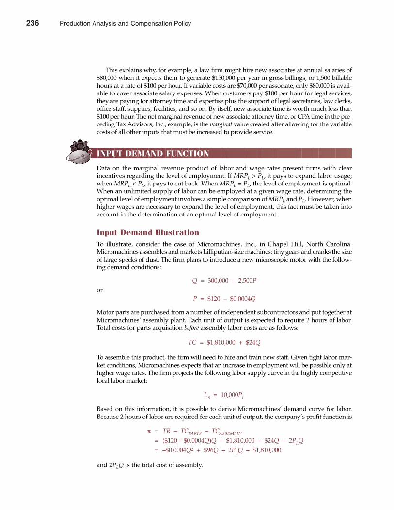
This explains why, for example, a law firm might hire new associates at annual salaries of$80,000 when it expects them to generate $150,000 per year in gross billings, or 1,500 billablehours at a rate of $100 per hour. If variable costs are $70,000 per associate, only $80,000 is avail-able to cover associate salary expenses. When customers pay $100 per hour for legal services,they are paying for attorney time and expertise plus the support of legal secretaries, law clerks,office staff, supplies, facilities, and so on. By itself, new associate time is worth much less than$100 per hour. The net marginal revenue of new associate attorney time, or CPA time in the pre-ceding Tax Advisors, Inc., example, is the marginal value created after allowing for the variablecosts of all other inputs that must be increased to provide service.
INPUT DEMAND FUNCTION
Data on the marginal revenue product of labor and wage rates present firms with clearincentives regarding the level of employment. If MRPL > PL, it pays to expand labor usage;when MRPL < PL, it pays to cut back. When MRPL = PL, the level of employment is optimal.When an unlimited supply of labor can be employed at a given wage rate, determining theoptimal level of employment involves a simple comparison of MRPL and PL. However, whenhigher wages are necessary to expand the level of employment, this fact must be taken intoaccount in the determination of an optimal level of employment.
Input Demand IllustrationTo illustrate, consider the case of Micromachines, Inc., in Chapel Hill, North Carolina.Micromachines assembles and markets Lilliputian-size machines: tiny gears and cranks the sizeof large specks of dust. The firm plans to introduce a new microscopic motor with the follow-ing demand conditions:
Q = 300,000 – 2,500Por
P = $120 – $0.0004Q
Motor parts are purchased from a number of independent subcontractors and put together atMicromachines’ assembly plant. Each unit of output is expected to require 2 hours of labor.Total costs for parts acquisition before assembly labor costs are as follows:
TC = $1,810,000 + $24Q
To assemble this product, the firm will need to hire and train new staff. Given tight labor mar-ket conditions, Micromachines expects that an increase in employment will be possible only athigher wage rates. The firm projects the following labor supply curve in the highly competitivelocal labor market:
LS = 10,000PL
Based on this information, it is possible to derive Micromachines’ demand curve for labor.Because 2 hours of labor are required for each unit of output, the company’s profit function is
π = TR – TCPARTS – TCASSEMBLY
= ($120 – $0.0004Q)Q – $1,810,000 – $24Q – 2PLQ
= –$0.0004Q2 + $96Q – 2PLQ – $1,810,000
and 2PLQ is the total cost of assembly.
Chapter Seven Production Analysis and Compensation Policy 237
236 Production Analysis and Compensation Policy
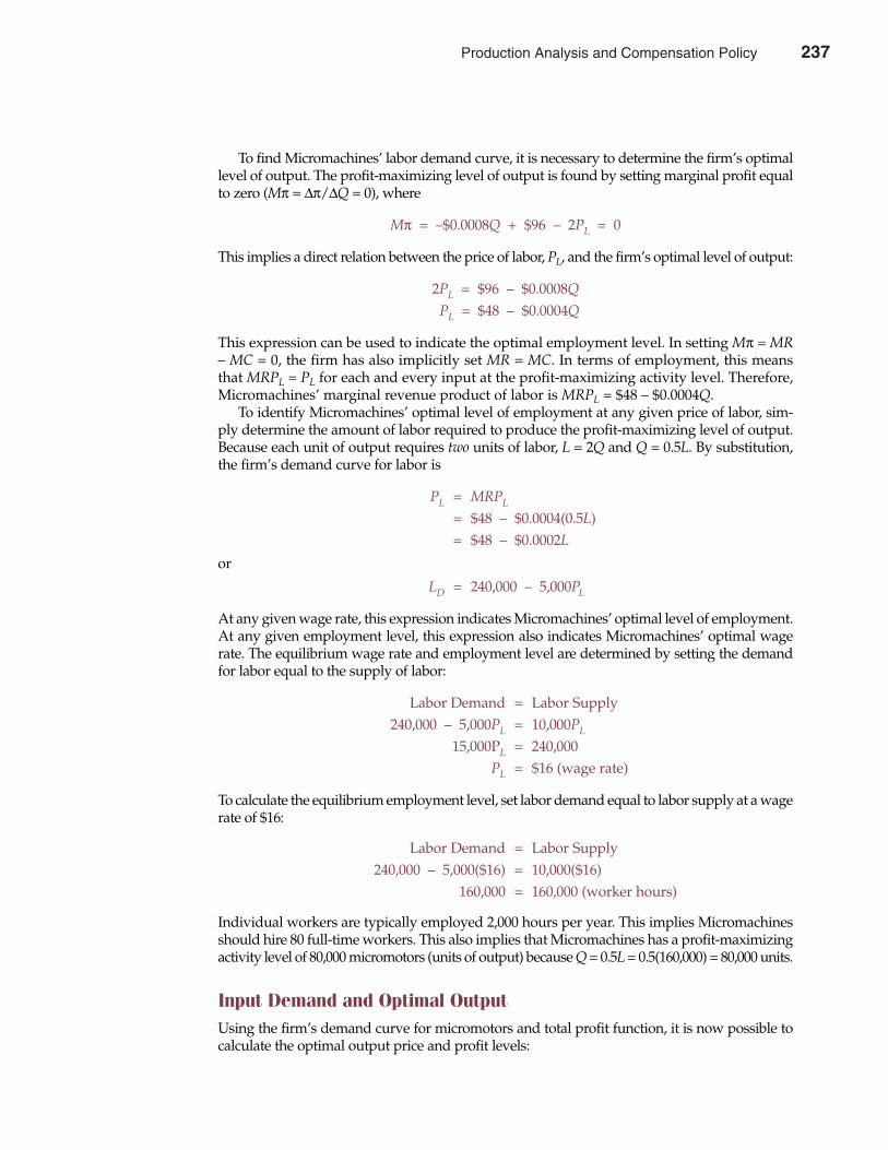
To find Micromachines’ labor demand curve, it is necessary to determine the firm’s optimallevel of output. The profit-maximizing level of output is found by setting marginal profit equalto zero (Mπ = ∆π/∆Q = 0), where
Mπ = –$0.0008Q + $96 – 2PL = 0
This implies a direct relation between the price of labor, PL, and the firm’s optimal level of output:
2PL = $96 – $0.0008Q
PL = $48 – $0.0004Q
This expression can be used to indicate the optimal employment level. In setting Mπ = MR– MC = 0, the firm has also implicitly set MR = MC. In terms of employment, this meansthat MRPL = PL for each and every input at the profit-maximizing activity level. Therefore,Micromachines’ marginal revenue product of labor is MRPL = $48 – $0.0004Q.
To identify Micromachines’ optimal level of employment at any given price of labor, sim-ply determine the amount of labor required to produce the profit-maximizing level of output.Because each unit of output requires two units of labor, L = 2Q and Q = 0.5L. By substitution,the firm’s demand curve for labor is
PL = MRPL
= $48 – $0.0004(0.5L)= $48 – $0.0002L
or
LD = 240,000 – 5,000PL
At any given wage rate, this expression indicates Micromachines’ optimal level of employment.At any given employment level, this expression also indicates Micromachines’ optimal wagerate. The equilibrium wage rate and employment level are determined by setting the demandfor labor equal to the supply of labor:
Labor Demand = Labor Supply240,000 – 5,000PL = 10,000PL
15,000PL = 240,000PL = $16 (wage rate)
To calculate the equilibrium employment level, set labor demand equal to labor supply at a wagerate of $16:
Labor Demand = Labor Supply240,000 – 5,000($16) = 10,000($16)
160,000 = 160,000 (worker hours)
Individual workers are typically employed 2,000 hours per year. This implies Micromachinesshould hire 80 full-time workers. This also implies that Micromachines has a profit-maximizingactivity level of 80,000 micromotors (units of output) because Q = 0.5L = 0.5(160,000) = 80,000 units.
Input Demand and Optimal OutputUsing the firm’s demand curve for micromotors and total profit function, it is now possible tocalculate the optimal output price and profit levels:
238 Part Three Production and Cost Analysis
Production Analysis and Compensation Policy 237
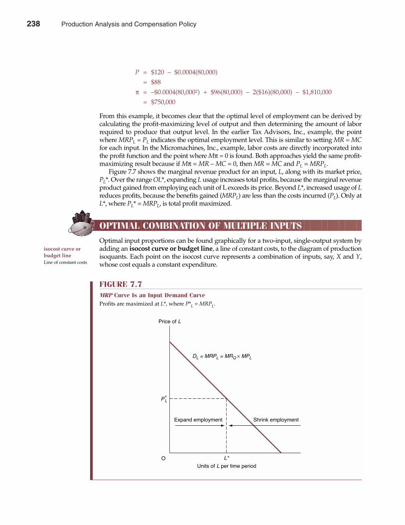
P = $120 – $0.0004(80,000)= $88
π = –$0.0004(80,0002) + $96(80,000) – 2($16)(80,000) – $1,810,000= $750,000
From this example, it becomes clear that the optimal level of employment can be derived bycalculating the profit-maximizing level of output and then determining the amount of laborrequired to produce that output level. In the earlier Tax Advisors, Inc., example, the pointwhere MRPL = PL indicates the optimal employment level. This is similar to setting MR = MCfor each input. In the Micromachines, Inc., example, labor costs are directly incorporated intothe profit function and the point where Mπ = 0 is found. Both approaches yield the same profit-maximizing result because if Mπ = MR – MC = 0, then MR = MC and PL = MRPL.
Figure 7.7 shows the marginal revenue product for an input, L, along with its market price,PL*. Over the range OL*, expanding L usage increases total profits, because the marginal revenueproduct gained from employing each unit of L exceeds its price. Beyond L*, increased usage of Lreduces profits, because the benefits gained (MRPL) are less than the costs incurred (PL). Only atL*, where PL* = MRPL, is total profit maximized.
OPTIMAL COMBINATION OF MULTIPLE INPUTS
Optimal input proportions can be found graphically for a two-input, single-output system byadding an isocost curve or budget line, a line of constant costs, to the diagram of productionisoquants. Each point on the isocost curve represents a combination of inputs, say, X and Y,whose cost equals a constant expenditure.
isocost curve orbudget lineLine of constant costs
Chapter Seven Production Analysis and Compensation Policy 239
FIGURE 7.7MRP Curve Is an Input Demand CurveProfits are maximized at L*, where P*L = MRPL.
P*L
Expand employment Shrink employment
Units of L per time period
L*
Price of L
DL = MRPL = MRQ × MPL
O
238 Production Analysis and Compensation Policy
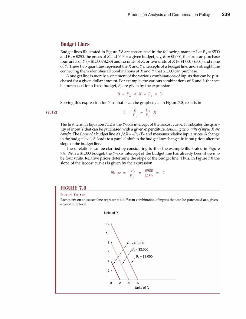
Budget LinesBudget lines illustrated in Figure 7.8 are constructed in the following manner: Let PX = $500and PY = $250, the prices of X and Y. For a given budget, say, B1 = $1,000, the firm can purchasefour units of Y (= $1,000/$250) and no units of X, or two units of X (= $1,000/$500) and noneof Y. These two quantities represent the X and Y intercepts of a budget line, and a straight lineconnecting them identifies all combinations of X and Y that $1,000 can purchase.
A budget line is merely a statement of the various combinations of inputs that can be pur-chased for a given dollar amount. For example, the various combinations of X and Y that canbe purchased for a fixed budget, B, are given by the expression
B = PX � X + PY � Y
Solving this expression for Y so that it can be graphed, as in Figure 7.8, results in
(7.12) Y = B – PX XPY PY
The first term in Equation 7.12 is the Y-axis intercept of the isocost curve. It indicates the quan-tity of input Y that can be purchased with a given expenditure, assuming zero units of input X arebought. The slope of a budget line ∆Y/∆X = –PX/PY and measures relative input prices. Achangein the budget level, B, leads to a parallel shift in the budget line; changes in input prices alter theslope of the budget line.
These relations can be clarified by considering further the example illustrated in Figure7.8. With a $1,000 budget, the Y-axis intercept of the budget line has already been shown tobe four units. Relative prices determine the slope of the budget line. Thus, in Figure 7.8 theslope of the isocost curves is given by the expression
Slope = –PX = –$500 = –2PY $250
240 Part Three Production and Cost Analysis
FIGURE 7.8Isocost CurvesEach point on an isocost line represents a different combination of inputs that can be purchased at a givenexpenditure level.
Units of X
0 2 4 6
2
4
6
8
10
12
Units of Y
B1 = $1,000
B2 = $2,000
B3 = $3,000
Production Analysis and Compensation Policy 239
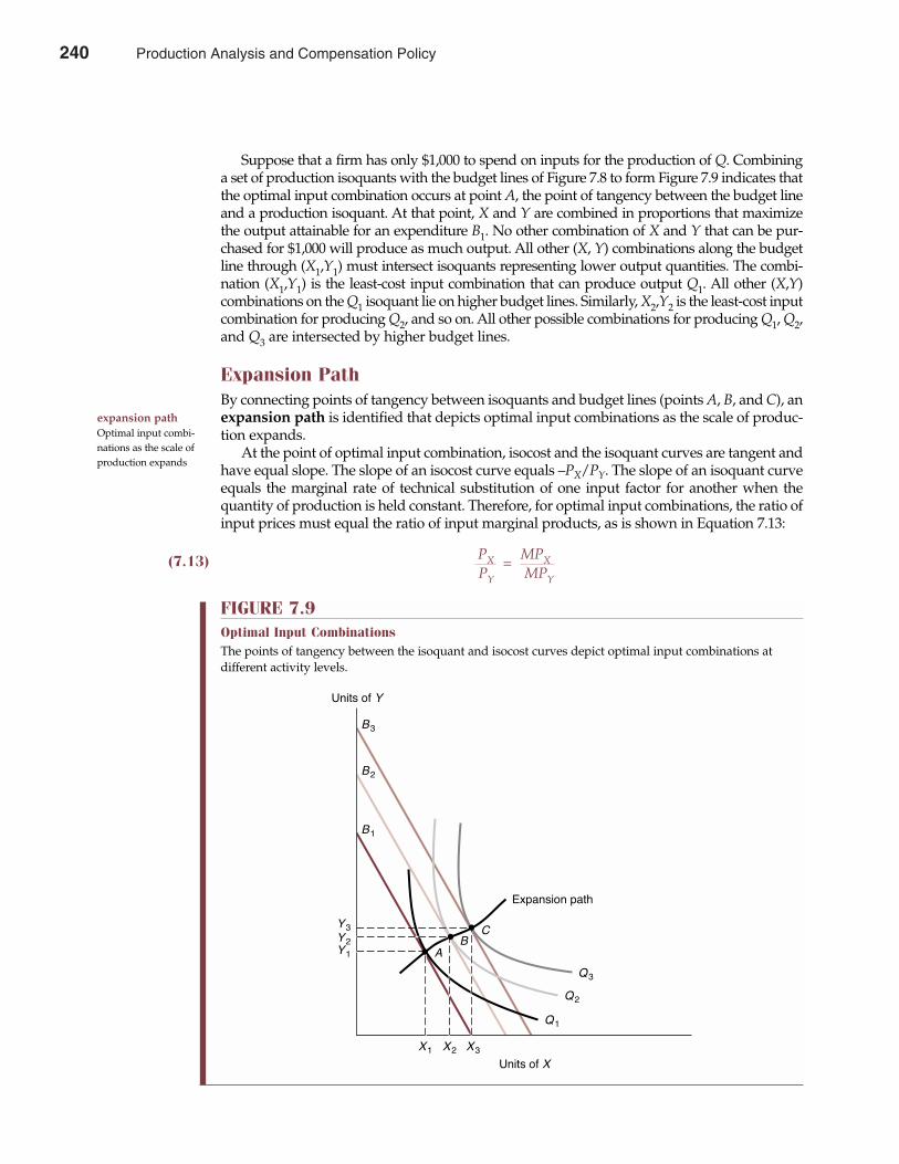
Suppose that a firm has only $1,000 to spend on inputs for the production of Q. Combininga set of production isoquants with the budget lines of Figure 7.8 to form Figure 7.9 indicates thatthe optimal input combination occurs at point A, the point of tangency between the budget lineand a production isoquant. At that point, X and Y are combined in proportions that maximizethe output attainable for an expenditure B1. No other combination of X and Y that can be pur-chased for $1,000 will produce as much output. All other (X, Y) combinations along the budgetline through (X1,Y1) must intersect isoquants representing lower output quantities. The combi-nation (X1,Y1) is the least-cost input combination that can produce output Q1. All other (X,Y)combinations on the Q1 isoquant lie on higher budget lines. Similarly, X2,Y2 is the least-cost inputcombination for producing Q2, and so on. All other possible combinations for producing Q1, Q2,and Q3 are intersected by higher budget lines.
Expansion PathBy connecting points of tangency between isoquants and budget lines (points A, B, and C), anexpansion path is identified that depicts optimal input combinations as the scale of produc-tion expands.
At the point of optimal input combination, isocost and the isoquant curves are tangent andhave equal slope. The slope of an isocost curve equals –PX/PY. The slope of an isoquant curveequals the marginal rate of technical substitution of one input factor for another when thequantity of production is held constant. Therefore, for optimal input combinations, the ratio ofinput prices must equal the ratio of input marginal products, as is shown in Equation 7.13:
(7.13) PX = MPXPY MPY
expansion path Optimal input combi-nations as the scale ofproduction expands
Chapter Seven Production Analysis and Compensation Policy 241
FIGURE 7.9Optimal Input CombinationsThe points of tangency between the isoquant and isocost curves depict optimal input combinations at different activity levels.
B1
X2
Q3
Y2
Y3
B2
B3
X1
Units of Y
Units of X
Expansion path
AB
C
Q2
Q1
Y1
X3
240 Production Analysis and Compensation Policy
Alternatively, marginal product-to-price ratio must be equal for each input:
(7.14) MPX = MPYPX PY
Optimal input proportions are employed when an additional dollar spent on any input yields the sameincrease in output. Any input combination violating this rule is suboptimal because a changein input proportions could result in the same quantity of output at lower cost.
Illustration of Optimal Input ProportionsThe Tax Advisors, Inc., example can further illustrate these relations. Assume that in additionto three CPAs, four bookkeepers are employed at a wage (including fringes) of $15 per hourand that MPB=4 = 0.3. This compares with a CPA wage of $35 per hour and MPCPA=3 = 1.4.Based on these assumptions, the marginal product per dollar spent on each input is
MPB=4 =0.3
= 0.02 Units per Dollar (for bookkeepers)PB $15
and
MPCPA=3 =1.4
= 0.04 Units per Dollar (for CPAs)PCPA $35
Such an input combination violates the optimal proportions rule because the ratios of marginalproducts to input prices are not equal. The last dollar spent on bookkeeper labor input produces(“buys”) 0.02 units of output (tax-return preparations), whereas the last dollar spent on CPAtimeproduces twice as much, 0.04 units. By transferring $1 of cost from bookkeeper time to CPAtime,the firm could increase total output by 0.02 tax-return preparations per hour without increasingtotal cost. Expenditures on the CPA input represent a better use of firm resources, and thecompany should reallocate resources to employ relatively more CPAs and relatively fewerbookkeepers.
In Equation 7.9, it was shown that the marginal product-to-price ratio indicates the margin-al cost of output from a marginal unit of input X or Y. In terms of this example, this implies that
MCQ =PB =
$15 = $50 per Unit (using bookkeepers)
MPB=4 0.3
and
MCQ =PCPA =
$35 = $25 per Unit (using CPAs)
MPCPA=3 1.4
Again, the superior economic productivity of CPAs is indicated; they are able to produce outputat one-half the marginal cost of output produced by bookkeepers.
It is important to recognize that the preceding analysis for determining optimal proportionsof multiple inputs considers input price and input marginal product (productivity) relationsonly. Because the economic value of output is not considered, these data are insufficient to allowcalculation of optimal employment levels. Notice in the Tax Advisors, Inc., example that themarginal cost of output using either input is much less than the $100 marginal revenue per taxreturn. It is quite possible that more CPAs and more bookkeepers should be hired. The next sec-tion introduces output value to determine the optimal level of resource employment.
242 Part Three Production and Cost Analysis
Production Analysis and Compensation Policy 241
OPTIMAL LEVELS OF MULTIPLE INPUTS
Cost minimization requires only that the ratios of marginal product to price be equal for allinputs. Alternatively, cost minimization dictates that inputs be combined in optimal propor-tions for a given or target level of output.
Optimal Employment and Profit MaximizationProfit maximization requires that a firm employ optimal input proportions and produce anoptimal quantity of output. Cost minimization and optimal input proportions are necessary but notsufficient conditions for profit maximization.
Profit maximization dictates that the firm employ all inputs up to the point where MCQ =MRQ. Profit maximization requires for each and every input that
(7.15) PX = MRQMPX
and
(7.16) PY = MRQMPY
Rearranging produces
(7.17) PX = MPX � MRQ = MRPX
and
(7.18) PY = MPY � MRQ = MRPY
Chapter Seven Production Analysis and Compensation Policy 243
Should We Raise the Minimum Wage?
Congress raised the minimum wage to $4.75 per hour onOctober 1, 1996, and to $5.15 per hour on September 1,1997. At that time, a youth subminimum wage of $4.25per hour was also established for newly-hired employeesunder the age of 20 during their first 90 consecutive calen-dar days of employment. President Clinton argued that aboost, offered as a well-deserved raise for hardworkingAmericans, was the right thing to do because the mini-mum wage had been relatively stagnant during recentyears. Indeed, after adjusting for inflation, the minimumwage has fallen sharply. In 1960, when the minimumwage was $1.60 per hour, it was equivalent to $7.92 perhour in current, or 2000, dollars.
When workers retain their jobs after the minimumwage has been boosted, it’s mainly teenagers in part-timeservice occupations, like fast-food restaurants, who bene-fit. The potential benefits of an increase in the minimumwage, namely higher incomes for teenagers and the work-ing poor, are obvious. What is less obvious is the cost in
terms of lost employment opportunities. Whenever thedecision to add or subtract workers is faced, an employercompares the marginal revenue product of the last workerhired to the marginal cost of employment. At the margin,each worker’s job must be justified by bringing to theemployer at least as much in added revenue as is neces-sary to pay the marginal cost of employment. When theminimum wage is increased from $5.15 to $6.50 or higher,low-skill workers unable to produce more than $5.15 perhour in employer benefits get laid off.
The bottom line is simple: Worker productivity mustbe enhanced if you want to increase incomes among theworking poor. Raising the minimum wage while holdingjob skills constant will reduce not enhance income oppor-tunities for minimum-wage workers.
See: A Wall Street Journal News Roundup, “Brazil Raises MinimumWage 11.1%, Posts Trade Surplus of $594 Million,” The Wall StreetJournal Online, April 2, 2002 (http://online.wsj.com).
M A N A G E R I A L A P P L I C AT I O N 7 . 3
242 Production Analysis and Compensation Policy
Profits are maximized when inputs are employed so that price equals marginal revenue product foreach input.
The difference between cost minimization and profit maximization is simple. Cost minimiza-tion requires efficient resource use, as reflected by optimal input proportions. Profit maximizationrequires efficient resource use and production of an optimal level of output, as made possible bythe optimal employment of all inputs.
Illustration of Optimal Levels of Multiple InputsA final look at the Tax Advisors, Inc., example illustrates these relations. Recall that withthree CPAs and four bookkeepers, the ratio of marginal products to price for each inputindicates a need to employ more CPAs relative to the number of bookkeepers. Assume thathiring one more bookkeeper leaves unchanged their marginal product of 0.3 tax returnsprocessed per hour (MPB=5 = 0.3). In addition, assume that with this increased employmentof bookkeepers the marginal product of the fourth CPA increases from 0.4 to 0.7 tax returnsprocessed per hour. This assumption reflects the fact that the marginal productivity of aninput factor (CPAs) is typically enhanced when used in conjunction with more of a com-plementary input, bookkeepers in this case. Now MPB=5 = 0.3 and MPCPA=4 = 0.7. With thecosts of each input remaining constant at PB = $15 and PCPA = $35, the marginal product-to-price ratios are now equal:
MPB=5 =0.3
= 0.02 Units per Dollar (for bookkeepers)PB $15
and
MPCPA=4 =0.7
= 0.02 Units per Dollar (for CPAs)PCPA $35
The combination of four CPAs and five bookkeepers is now optimal from a cost-minimizingstandpoint, and input proportions are optimal. However, it is unclear whether an optimal levelof input has been employed. Does the resulting output level maximize profit? To answer thisquestion, it becomes necessary to determine if marginal revenue product equals the mar-ginal cost of each input. If net marginal revenue (NMR) per return remains at $50 = ($100 �0.5), then
MRPB = MPB � NMRQ
= 0.3 � $50 = $15MRPB = $15 = PB
and
MRPCPA = MPCPA � NMRQ
= 0.7 � $50 = $35MRPCPA = $35 = PCPA
Marginal revenue product equals marginal cost for each input. The combination of four CPAsand five bookkeepers is an optimal level of employment because the resulting output quantitymaximizes profit.
244 Part Three Production and Cost Analysis
Production Analysis and Compensation Policy 243
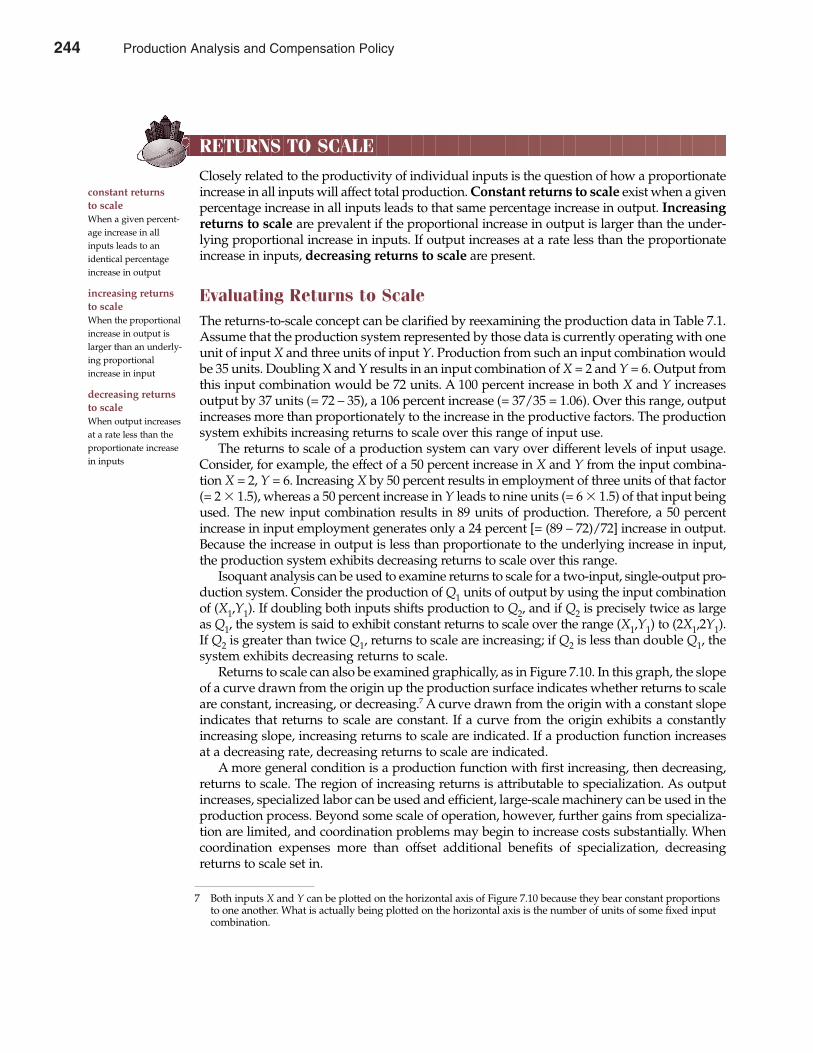
RETURNS TO SCALE
Closely related to the productivity of individual inputs is the question of how a proportionateincrease in all inputs will affect total production. Constant returns to scale exist when a givenpercentage increase in all inputs leads to that same percentage increase in output. Increasingreturns to scale are prevalent if the proportional increase in output is larger than the under-lying proportional increase in inputs. If output increases at a rate less than the proportionateincrease in inputs, decreasing returns to scale are present.
Evaluating Returns to ScaleThe returns-to-scale concept can be clarified by reexamining the production data in Table 7.1.Assume that the production system represented by those data is currently operating with oneunit of input X and three units of input Y. Production from such an input combination wouldbe 35 units. Doubling X and Y results in an input combination of X = 2 and Y = 6. Output fromthis input combination would be 72 units. A 100 percent increase in both X and Y increasesoutput by 37 units (= 72 – 35), a 106 percent increase (= 37/35 = 1.06). Over this range, outputincreases more than proportionately to the increase in the productive factors. The productionsystem exhibits increasing returns to scale over this range of input use.
The returns to scale of a production system can vary over different levels of input usage.Consider, for example, the effect of a 50 percent increase in X and Y from the input combina-tion X = 2, Y = 6. Increasing X by 50 percent results in employment of three units of that factor(= 2 � 1.5), whereas a 50 percent increase in Y leads to nine units (= 6 � 1.5) of that input beingused. The new input combination results in 89 units of production. Therefore, a 50 percentincrease in input employment generates only a 24 percent [= (89 – 72)/72] increase in output.Because the increase in output is less than proportionate to the underlying increase in input,the production system exhibits decreasing returns to scale over this range.
Isoquant analysis can be used to examine returns to scale for a two-input, single-output pro-duction system. Consider the production of Q1 units of output by using the input combinationof (X1,Y1). If doubling both inputs shifts production to Q2, and if Q2 is precisely twice as largeas Q1, the system is said to exhibit constant returns to scale over the range (X1,Y1) to (2X1,2Y1).If Q2 is greater than twice Q1, returns to scale are increasing; if Q2 is less than double Q1, thesystem exhibits decreasing returns to scale.
Returns to scale can also be examined graphically, as in Figure 7.10. In this graph, the slopeof a curve drawn from the origin up the production surface indicates whether returns to scaleare constant, increasing, or decreasing.7 A curve drawn from the origin with a constant slopeindicates that returns to scale are constant. If a curve from the origin exhibits a constantlyincreasing slope, increasing returns to scale are indicated. If a production function increasesat a decreasing rate, decreasing returns to scale are indicated.
A more general condition is a production function with first increasing, then decreasing,returns to scale. The region of increasing returns is attributable to specialization. As outputincreases, specialized labor can be used and efficient, large-scale machinery can be used in theproduction process. Beyond some scale of operation, however, further gains from specializa-tion are limited, and coordination problems may begin to increase costs substantially. Whencoordination expenses more than offset additional benefits of specialization, decreasingreturns to scale set in.
constant returns to scaleWhen a given percent-age increase in allinputs leads to an identical percentageincrease in output
increasing returnsto scale When the proportionalincrease in output islarger than an underly-ing proportionalincrease in input
decreasing returnsto scale When output increasesat a rate less than theproportionate increasein inputs
Chapter Seven Production Analysis and Compensation Policy 245
7 Both inputs X and Y can be plotted on the horizontal axis of Figure 7.10 because they bear constant proportionsto one another. What is actually being plotted on the horizontal axis is the number of units of some fixed inputcombination.
244 Production Analysis and Compensation Policy
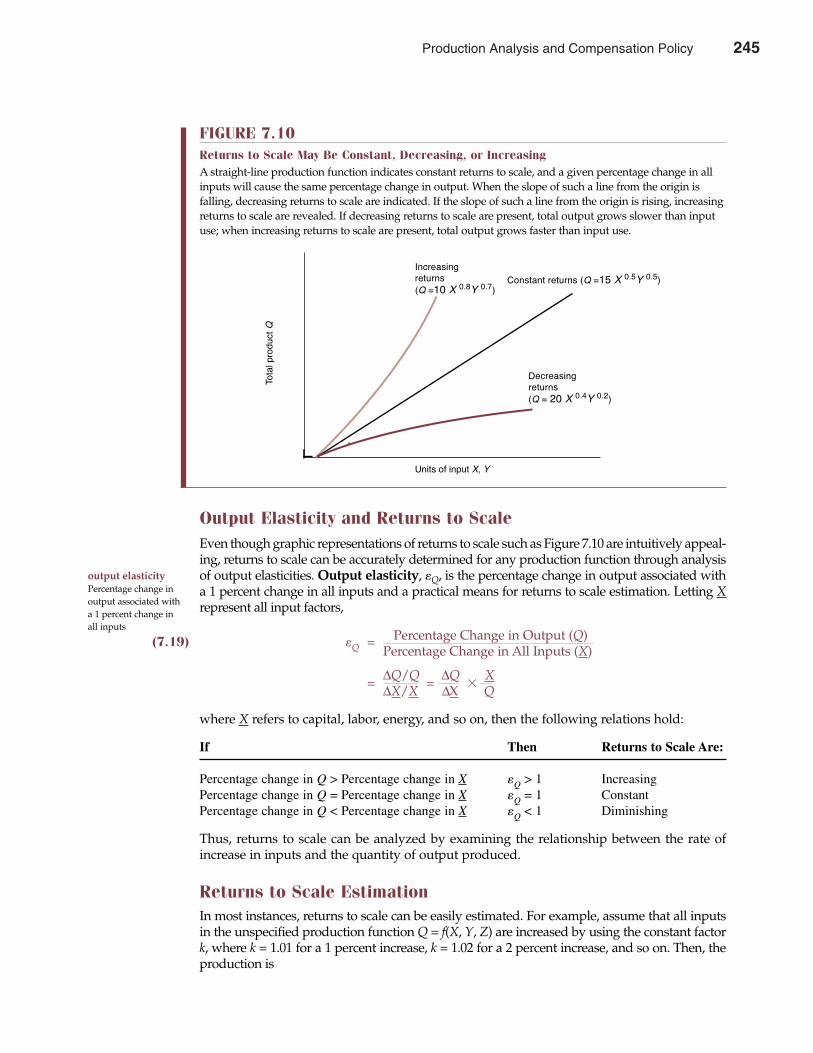
Output Elasticity and Returns to ScaleEven though graphic representations of returns to scale such as Figure 7.10 are intuitively appeal-ing, returns to scale can be accurately determined for any production function through analysisof output elasticities. Output elasticity, �Q, is the percentage change in output associated witha 1 percent change in all inputs and a practical means for returns to scale estimation. Letting Xrepresent all input factors,
(7.19) �Q = Percentage Change in Output (Q)Percentage Change in All Inputs (X)
= ∆Q/Q = ∆Q�
X∆X/X ∆X Q
where X refers to capital, labor, energy, and so on, then the following relations hold:
If Then Returns to Scale Are:
Percentage change in Q > Percentage change in X �Q > 1 IncreasingPercentage change in Q = Percentage change in X �Q = 1 ConstantPercentage change in Q < Percentage change in X �Q < 1 Diminishing
Thus, returns to scale can be analyzed by examining the relationship between the rate ofincrease in inputs and the quantity of output produced.
Returns to Scale EstimationIn most instances, returns to scale can be easily estimated. For example, assume that all inputsin the unspecified production function Q = f(X, Y, Z) are increased by using the constant factork, where k = 1.01 for a 1 percent increase, k = 1.02 for a 2 percent increase, and so on. Then, theproduction is
246 Part Three Production and Cost Analysis
output elasticityPercentage change inoutput associated witha 1 percent change inall inputs
FIGURE 7.10Returns to Scale May Be Constant, Decreasing, or IncreasingA straight-line production function indicates constant returns to scale, and a given percentage change in allinputs will cause the same percentage change in output. When the slope of such a line from the origin isfalling, decreasing returns to scale are indicated. If the slope of such a line from the origin is rising, increasingreturns to scale are revealed. If decreasing returns to scale are present, total output grows slower than inputuse; when increasing returns to scale are present, total output grows faster than input use.
Totalproduct
QIncreasing
returns
(Q =10 X 0.8Y 0.7)Constant returns (Q =15 X 0.5Y 0.5)
Decreasing
returns
(Q = 20 X 0.4Y 0.2)
Units of input X, Y
Production Analysis and Compensation Policy 245
(7.20) hQ = f(kX, kY, kZ)
where h is the proportional increase in Q resulting from a k-fold increase in each input factor.From Equation 7.20, it is evident that the following relationships hold:
• If h > k, then the percentage change in Q is greater than the percentage change in the inputs,�Q > 1, and the production function exhibits increasing returns to scale.
• If h = k, then the percentage change in Q equals the percentage change in the inputs, �Q = 1,and the production function exhibits constant returns to scale.
• If h < k, then the percentage change in Q is less than the percentage change in the inputs,�Q < 1, and the production function exhibits decreasing returns to scale.
For certain production functions, called homogeneous production functions, when each inputfactor is multiplied by a constant k, the constant can be completely factored out of the produc-tion function expression. Following a k-fold increase in all inputs, the production functiontakes the form hQ = knf(X,Y,Z). The exponent n provides the key to returns-to-scale estimation.If n = 1, then h = k and the function exhibits constant returns to scale. If n > 1, then h > k, indicat-ing increasing returns to scale, whereas n < 1 indicates h < k and decreasing returns to scale. Inall other instances, the easiest means for determining the nature of returns to scale is throughnumerical example.
To illustrate, consider the production function Q = 2X + 3Y + 1.5Z. Returns to scale canbe determined by learning how an arbitrary, say 2 percent, increase in all inputs affects out-put. If, initially, X = 100, Y = 200, and Z = 200, output is found to be
Q1 = 2(100) + 3(200) + 1.5(200)= 200 + 600 + 300 = 1,100 units
Increasing all inputs by 2 percent (letting k = 1.02) leads to the input quantities X = 102, Y = 204,and Z = 204, and
Q2 = 2(102) + 3(204) + 1.5(204)= 204 + 612 + 306 = 1,122 units
Because a 2 percent increase in all inputs has led to a 2 percent increase in output (1.02 =1,122/1,100), this production system exhibits constant returns to scale.
PRODUCTION FUNCTION ESTIMATION
Given enough input/output observations, either over time for a single firm or at a singlepoint in time for a number of firms in an industry, regression techniques can be used to esti-mate the parameters of production functions.
Cubic Production FunctionsFrom a theoretical standpoint, the most appealing functional form for production functionestimation might be cubic, such as the equation
(7.21) Q = a + bXY + cX2Y + dXY2 – eX3Y – fXY3
This form is general in that it exhibits stages of first increasing and then decreasing returns toscale. The marginal products of the input factors exhibit a pattern of first increasing and thendecreasing returns, as was illustrated in Figure 7.3.
Chapter Seven Production Analysis and Compensation Policy 247
246 Production Analysis and Compensation Policy
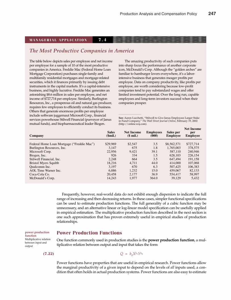
Frequently, however, real-world data do not exhibit enough dispersion to indicate the fullrange of increasing and then decreasing returns. In these cases, simpler functional specificationscan be used to estimate production functions. The full generality of a cubic function may beunnecessary, and an alternative linear or log-linear model specification can be usefully appliedin empirical estimation. The multiplicative production function described in the next section isone such approximation that has proven extremely useful in empirical studies of productionrelationships.
Power Production FunctionsOne function commonly used in production studies is the power production function, a mul-tiplicative relation between output and input that takes the form
(7.22) Q = b0Xb1Yb2
Power functions have properties that are useful in empirical research. Power functions allowthe marginal productivity of a given input to depend on the levels of all inputs used, a con-dition that often holds in actual production systems. Power functions are also easy to estimate
248 Part Three Production and Cost Analysis
power productionfunctionMultiplicative relationbetween input and output
The Most Productive Companies in America
The table below depicts sales per employee and net incomeper employee for a sample of 10 of the most productivecompanies in America. Freddie Mac (Federal Home LoanMortgage Corporation) purchases single-family and multifamily residential mortgages and mortgage-relatedsecurities, which it finances primarily by issuing debtinstruments in the capital markets. It’s a capital-intensivebusiness, and highly lucrative. Freddie Mac generates anastonishing $8.6 million in sales per employee, and netincome of $727,714 per employee. Similarly, BurlingtonResources, Inc., a prosperous oil and natural gas producer,requires few employees to efficiently conduct its business.Others that generate enormous profits per employeeinclude software juggernaut Microsoft Corp., financialservices powerhouse Stilwell Financial (purveyor of Janusmutual funds), and biopharmaceutical leader Biogen.
The amazing productivity of such companies putsinto sharp focus the performance of another corporateicon, McDonald’s Corp. Although the “golden arches” arefamiliar to hamburger lovers everywhere, it’s a labor-intensive business that generates meager profits peremployee. Data on company productivity, like profits peremployee, are worth considering because low-profit companies tend to pay substandard wages and offer limited investment potential. Over the long run, capableemployees and long-term investors succeed when theircompanies prosper.
See: Aaron Lucchetti, “Stilwell to Give Janus Employees Larger Stakein Fund Company,” The Wall Street Journal Online, February 19, 2002(http://online.wsj.com).
M A N A G E R I A L A P P L I C AT I O N 7 . 4
Net IncomeSales Net Income Employees Sales per per
Company ($mil.) ($ mil.) (000) Employee Employee
Federal Home Loan Mortgage (“Freddie Mac”) $29,969 $2,547 3.5 $8,562,571 $727,714Burlington Resources, Inc. 3,147 675 1.8 1,765,003 378,575Microsoft Corp. 22,956 9,421 39.1 587,110 240,946Biogen, Inc. 926 334 1.5 628,103 226,154Stilwell Financial, Inc. 2,248 664 3.5 647,494 191,158Bristol Myers Squibb 18,216 4,711 44.0 414,000 107,068Qualcomm Inc. 3,197 670 6.3 507,425 106,383AOL Time Warner Inc. 6,886 1,232 15.0 459,067 82,133Coca-Cola Co. 20,458 2,177 36.9 554,417 58,997McDonald’s Corp. 14,243 1,977 364.0 39,129 5,432
Production Analysis and Compensation Policy 247
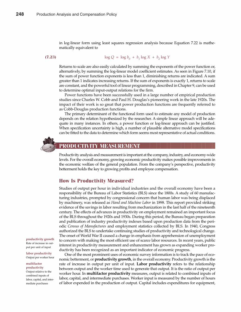
in log-linear form using least squares regression analysis because Equation 7.22 is mathe-matically equivalent to
(7.23) log Q = log b0 + b1 log X + b2 log Y
Returns to scale are also easily calculated by summing the exponents of the power function or,alternatively, by summing the log-linear model coefficient estimates. As seen in Figure 7.10, ifthe sum of power function exponents is less than 1, diminishing returns are indicated. A sumgreater than 1 indicates increasing returns. If the sum of exponents is exactly 1, returns to scaleare constant, and the powerful tool of linear programming, described in Chapter 9, can be usedto determine optimal input-output relations for the firm.
Power functions have been successfully used in a large number of empirical productionstudies since Charles W. Cobb and Paul H. Douglas’s pioneering work in the late 1920s. Theimpact of their work is so great that power production functions are frequently referred toas Cobb-Douglas production functions.
The primary determinant of the functional form used to estimate any model of productiondepends on the relation hypothesized by the researcher. A simple linear approach will be ade-quate in many instances. In others, a power function or log-linear approach can be justified.When specification uncertainty is high, a number of plausible alternative model specificationscan be fitted to the data to determine which form seems most representative of actual conditions.
PRODUCTIVITY MEASUREMENT
Productivity analysis and measurement is important at the company, industry, and economy-widelevels. For the overall economy, growing economic productivity makes possible improvements inthe economic welfare of the general population. From the company’s perspective, productivitybetterment holds the key to growing profits and employee compensation.
How Is Productivity Measured?Studies of output per hour in individual industries and the overall economy have been aresponsibility of the Bureau of Labor Statistics (BLS) since the 1800s. A study of 60 manufac-turing industries, prompted by congressional concern that human labor was being displacedby machinery, was released as Hand and Machine Labor in 1898. This report provided strikingevidence of the savings in labor resulting from mechanization in the last half of the nineteenthcentury. The effects of advances in productivity on employment remained an important focusof the BLS throughout the 1920s and 1930s. During this period, the Bureau began preparationand publication of industry productivity indexes based upon production data from the peri-odic Census of Manufactures and employment statistics collected by BLS. In 1940, Congressauthorized the BLS to undertake continuing studies of productivity and technological change.The onset of World War II caused a change in emphasis from apprehension of unemploymentto concern with making the most efficient use of scarce labor resources. In recent years, publicinterest in productivity measurement and enhancement has grown as expanding worker pro-ductivity has been recognized as an important indicator of economic progress.
One of the most prominent uses of economic survey information is to track the pace of eco-nomic betterment, or productivity growth, in the overall economy. Productivity growth is therate of increase in output per unit of input. Labor productivity refers to the relationshipbetween output and the worker time used to generate that output. It is the ratio of output perworker hour. In multifactor productivity measures, output is related to combined inputs oflabor, capital, and intermediate purchases. Worker input is measured by the number of hoursof labor expended in the production of output. Capital includes expenditures for equipment,
productivity growthRate of increase in out-put per unit of input
labor productivityOutput per worker hour
multifactor productivityOutput relative to thecombined inputs oflabor, capital, and inter-mediate purchases
Chapter Seven Production Analysis and Compensation Policy 249
248 Production Analysis and Compensation Policy
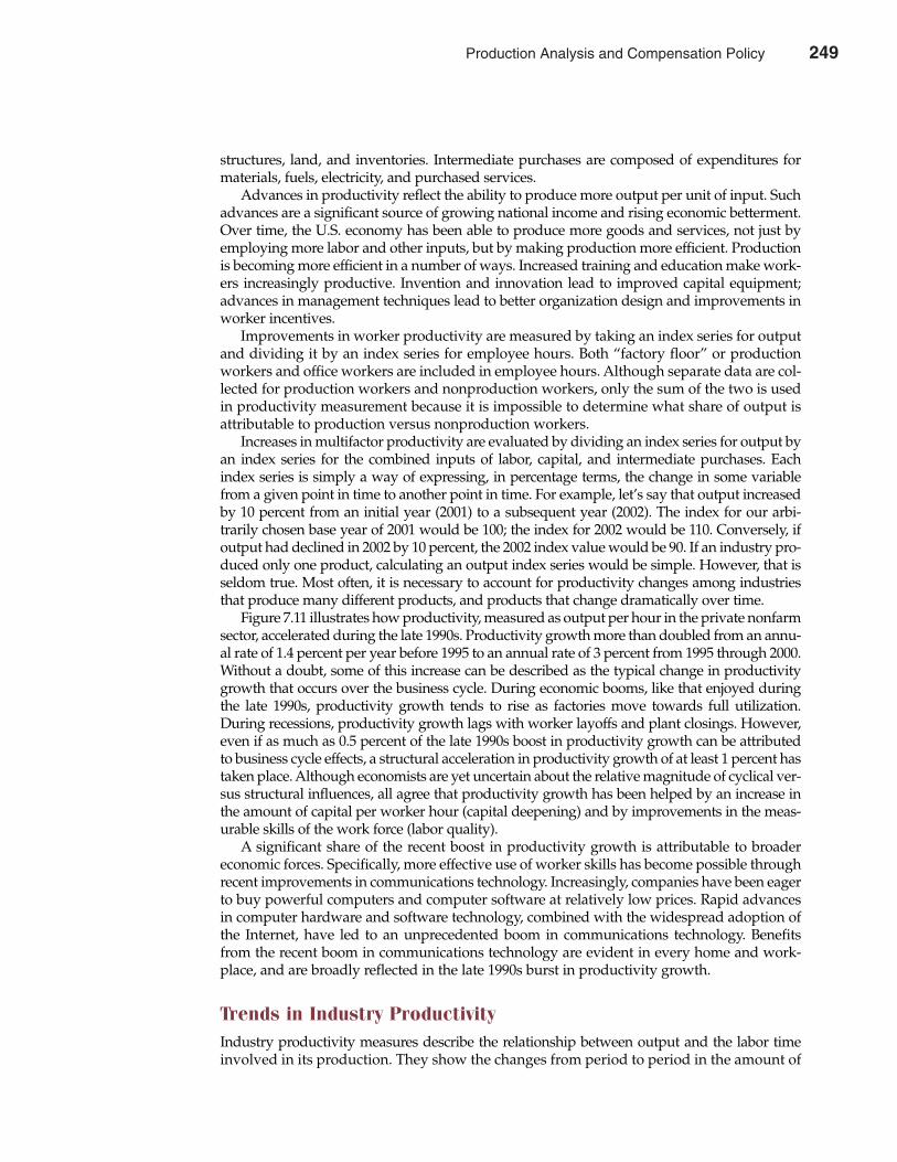
structures, land, and inventories. Intermediate purchases are composed of expenditures formaterials, fuels, electricity, and purchased services.
Advances in productivity reflect the ability to produce more output per unit of input. Suchadvances are a significant source of growing national income and rising economic betterment.Over time, the U.S. economy has been able to produce more goods and services, not just byemploying more labor and other inputs, but by making production more efficient. Productionis becoming more efficient in a number of ways. Increased training and education make work-ers increasingly productive. Invention and innovation lead to improved capital equipment;advances in management techniques lead to better organization design and improvements inworker incentives.
Improvements in worker productivity are measured by taking an index series for outputand dividing it by an index series for employee hours. Both “factory floor” or productionworkers and office workers are included in employee hours. Although separate data are col-lected for production workers and nonproduction workers, only the sum of the two is usedin productivity measurement because it is impossible to determine what share of output isattributable to production versus nonproduction workers.
Increases in multifactor productivity are evaluated by dividing an index series for output byan index series for the combined inputs of labor, capital, and intermediate purchases. Eachindex series is simply a way of expressing, in percentage terms, the change in some variablefrom a given point in time to another point in time. For example, let’s say that output increasedby 10 percent from an initial year (2001) to a subsequent year (2002). The index for our arbi-trarily chosen base year of 2001 would be 100; the index for 2002 would be 110. Conversely, ifoutput had declined in 2002 by 10 percent, the 2002 index value would be 90. If an industry pro-duced only one product, calculating an output index series would be simple. However, that isseldom true. Most often, it is necessary to account for productivity changes among industriesthat produce many different products, and products that change dramatically over time.
Figure 7.11 illustrates how productivity, measured as output per hour in the private nonfarmsector, accelerated during the late 1990s. Productivity growth more than doubled from an annu-al rate of 1.4 percent per year before 1995 to an annual rate of 3 percent from 1995 through 2000.Without a doubt, some of this increase can be described as the typical change in productivitygrowth that occurs over the business cycle. During economic booms, like that enjoyed duringthe late 1990s, productivity growth tends to rise as factories move towards full utilization.During recessions, productivity growth lags with worker layoffs and plant closings. However,even if as much as 0.5 percent of the late 1990s boost in productivity growth can be attributedto business cycle effects, a structural acceleration in productivity growth of at least 1 percent hastaken place. Although economists are yet uncertain about the relative magnitude of cyclical ver-sus structural influences, all agree that productivity growth has been helped by an increase inthe amount of capital per worker hour (capital deepening) and by improvements in the meas-urable skills of the work force (labor quality).
A significant share of the recent boost in productivity growth is attributable to broadereconomic forces. Specifically, more effective use of worker skills has become possible throughrecent improvements in communications technology. Increasingly, companies have been eagerto buy powerful computers and computer software at relatively low prices. Rapid advancesin computer hardware and software technology, combined with the widespread adoption ofthe Internet, have led to an unprecedented boom in communications technology. Benefitsfrom the recent boom in communications technology are evident in every home and work-place, and are broadly reflected in the late 1990s burst in productivity growth.
Trends in Industry ProductivityIndustry productivity measures describe the relationship between output and the labor timeinvolved in its production. They show the changes from period to period in the amount of
250 Part Three Production and Cost Analysis
Production Analysis and Compensation Policy 249
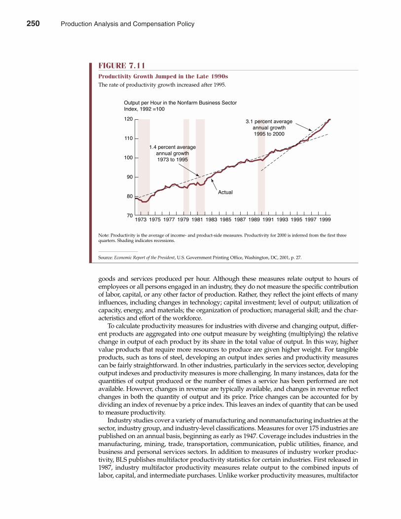
goods and services produced per hour. Although these measures relate output to hours ofemployees or all persons engaged in an industry, they do not measure the specific contributionof labor, capital, or any other factor of production. Rather, they reflect the joint effects of manyinfluences, including changes in technology; capital investment; level of output; utilization ofcapacity, energy, and materials; the organization of production; managerial skill; and the char-acteristics and effort of the workforce.
To calculate productivity measures for industries with diverse and changing output, differ-ent products are aggregated into one output measure by weighting (multiplying) the relativechange in output of each product by its share in the total value of output. In this way, highervalue products that require more resources to produce are given higher weight. For tangibleproducts, such as tons of steel, developing an output index series and productivity measurescan be fairly straightforward. In other industries, particularly in the services sector, developingoutput indexes and productivity measures is more challenging. In many instances, data for thequantities of output produced or the number of times a service has been performed are notavailable. However, changes in revenue are typically available, and changes in revenue reflectchanges in both the quantity of output and its price. Price changes can be accounted for bydividing an index of revenue by a price index. This leaves an index of quantity that can be usedto measure productivity.
Industry studies cover a variety of manufacturing and nonmanufacturing industries at thesector, industry group, and industry-level classifications. Measures for over 175 industries arepublished on an annual basis, beginning as early as 1947. Coverage includes industries in themanufacturing, mining, trade, transportation, communication, public utilities, finance, andbusiness and personal services sectors. In addition to measures of industry worker produc-tivity, BLS publishes multifactor productivity statistics for certain industries. First released in1987, industry multifactor productivity measures relate output to the combined inputs oflabor, capital, and intermediate purchases. Unlike worker productivity measures, multifactor
Chapter Seven Production Analysis and Compensation Policy 251
FIGURE 7.11Productivity Growth Jumped in the Late 1990sThe rate of productivity growth increased after 1995.
120
110
100
90
80
70
Output per Hour in the Nonfarm Business Sector�Index, 1992 =100
Actual
1.4 percent average�annual growth�1973 to 1995
3.1 percent average�annual growth�1995 to 2000
1973 1975 1977 1979 1981 1983 1985 1987 1989 1991 1993 1995 1997 1999
Note: Productivity is the average of income- and product-side measures. Productivity for 2000 is inferred from the first threequarters. Shading indicates recessions.
Source: Economic Report of the President, U.S. Government Printing Office, Washington, DC, 2001, p. 27.
250 Production Analysis and Compensation Policy
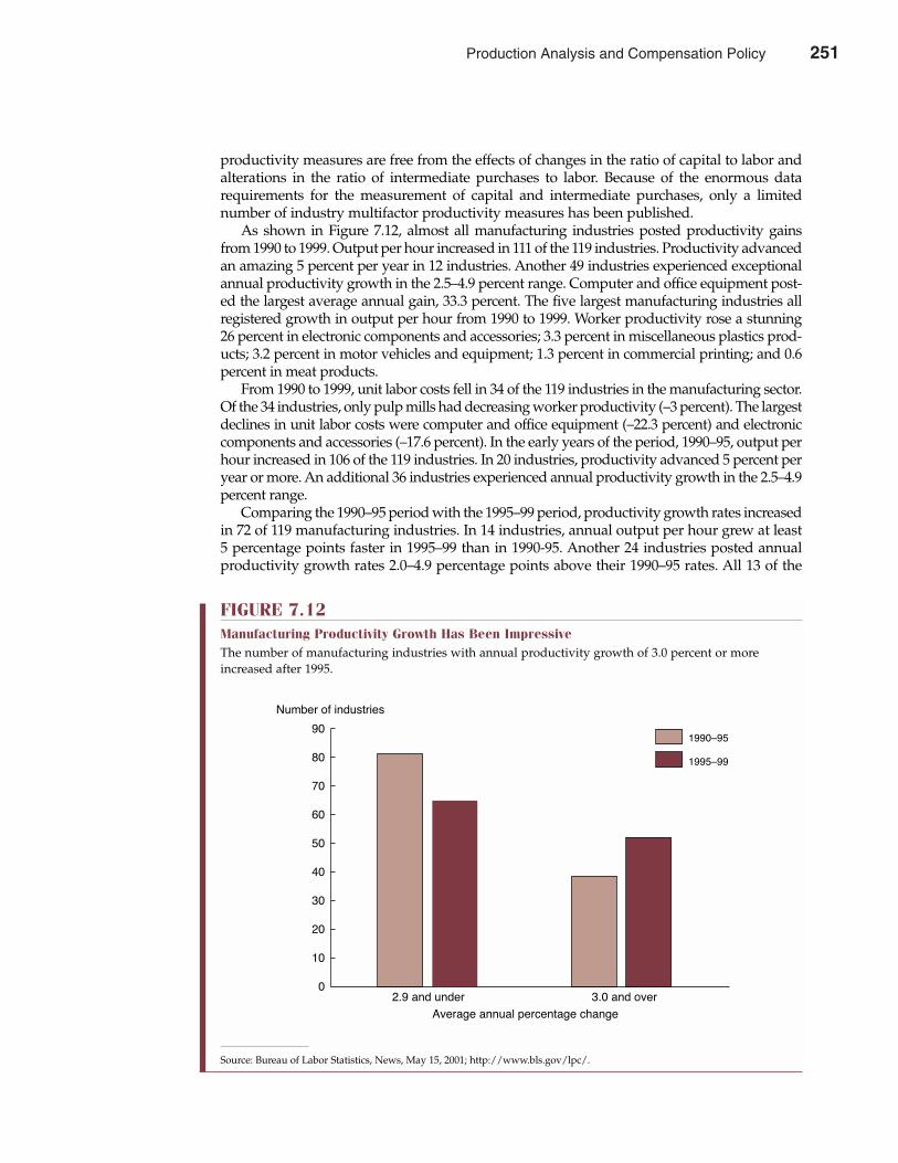
productivity measures are free from the effects of changes in the ratio of capital to labor andalterations in the ratio of intermediate purchases to labor. Because of the enormous datarequirements for the measurement of capital and intermediate purchases, only a limitednumber of industry multifactor productivity measures has been published.
As shown in Figure 7.12, almost all manufacturing industries posted productivity gainsfrom 1990 to 1999. Output per hour increased in 111 of the 119 industries. Productivity advancedan amazing 5 percent per year in 12 industries. Another 49 industries experienced exceptionalannual productivity growth in the 2.5–4.9 percent range. Computer and office equipment post-ed the largest average annual gain, 33.3 percent. The five largest manufacturing industries allregistered growth in output per hour from 1990 to 1999. Worker productivity rose a stunning26 percent in electronic components and accessories; 3.3 percent in miscellaneous plastics prod-ucts; 3.2 percent in motor vehicles and equipment; 1.3 percent in commercial printing; and 0.6percent in meat products.
From 1990 to 1999, unit labor costs fell in 34 of the 119 industries in the manufacturing sector.Of the 34 industries, only pulp mills had decreasing worker productivity (–3 percent). The largestdeclines in unit labor costs were computer and office equipment (–22.3 percent) and electroniccomponents and accessories (–17.6 percent). In the early years of the period, 1990–95, output perhour increased in 106 of the 119 industries. In 20 industries, productivity advanced 5 percent peryear or more. An additional 36 industries experienced annual productivity growth in the 2.5–4.9percent range.
Comparing the 1990–95 period with the 1995–99 period, productivity growth rates increasedin 72 of 119 manufacturing industries. In 14 industries, annual output per hour grew at least5 percentage points faster in 1995–99 than in 1990-95. Another 24 industries posted annualproductivity growth rates 2.0–4.9 percentage points above their 1990–95 rates. All 13 of the
252 Part Three Production and Cost Analysis
FIGURE 7.12Manufacturing Productivity Growth Has Been ImpressiveThe number of manufacturing industries with annual productivity growth of 3.0 percent or moreincreased after 1995.
90
80
70
60
50
40
30
20
10
0
Number of industries
2.9 and under 3.0 and over
Average annual percentage change
1995Ð99
1990Ð95
Source: Bureau of Labor Statistics, News, May 15, 2001; http://www.bls.gov/lpc/.
Production Analysis and Compensation Policy 251
industries that experienced productivity declines in the earlier period registered productivityimprovements in the later period. Seven of these 13 industries experienced positive produc-tivity growth in the 1995–99 period.
Uses and Limitations of Productivity DataMeasures of output per hour are useful for analyzing trends in labor costs across industries,comparing productivity progress among countries, examining the effects of technologicalimprovements, and analyzing related economic and industrial activities. Such analyses usuallyrequire that indexes of output per hour be used in conjunction with other data. Related data onproduction and employment are useful in studying technological effects. To study trends inlabor costs, data on earnings and other labor expenditures must be compiled.
It is important to recognize that productivity measures of output per hour are subject tocertain qualifications. Among these is the fact that existing techniques may not fully take intoaccount changes in the quality of goods and services produced. Although efforts have beenmade to maintain consistency of coverage between the output and labor input estimates,some statistical differences remain that can confound intertemporal comparisons. Estimatesof influences tied to nonproduction worker hours, unpaid family workers, the self-employed,and paid managers are also subject to a wide margin of error. Finally, year-to-year changes inoutput per hour are sometimes irregular and, therefore, are not necessarily indicative of basicchanges in long-term trends. Because of these statistical limitations, productivity measurescannot be considered precise. Instead, they should be interpreted as useful indicators subjectto measurement error.
Unfortunately, industry productivity measures are not available at the county, state, orregional level. They are nationwide averages that can sometimes vary from one locale to anoth-er. BLS worker productivity and multifactor productivity indexes are published annually in thebulletin, Productivity Measures for Selected Industries. Indexes of output per hour also are pub-lished in the Statistical Abstract of the United States and are available in the Bureau’s LABSTATdatabase, on BLS data diskettes, or on the Internet at the BLS Web site (http://stats.bls.gov). Alimited amount of the most current data is provided in annual news releases. Technical notesdescribing the methodology used to develop the indexes are available on request.
SUMMARY
This chapter introduces and analyzes the creative process of production. Several importantproperties of production systems are examined.
• A production function specifies the maximum output that can be produced for a givenamount of inputs. A discrete production function involves distinct, or “lumpy,” patternsfor input combinations. In a continuous production function, inputs can be varied in aunbroken marginal fashion.
• The returns to scale characteristic of a production system describes the output effect of aproportional increase in all inputs. The relation between output and variation in only oneof the inputs used is described as the returns to a factor.
• The total product indicates the total output from a production system. The marginalproduct of a factor, MPX, is the change in output associated with a one-unit change in thefactor input, holding all other inputs constant. A factor’s average product is the totalproduct divided by the number of units of that input employed.
• The law of diminishing returns states that as the quantity of a variable input increases,with the quantities of all other factors being held constant, and the resulting rate of increasein output eventually diminishes.
Chapter Seven Production Analysis and Compensation Policy 253
252 Production Analysis and Compensation Policy
• An isoquant represents the different combinations of inputs that can be used efficiently toproduce a specified quantity of output. Efficiency in this case refers to technical efficiency,meaning the least-cost production of a target level of output.
• Input substitution, or the systematic replacement of productive factors, is an importantconsideration when judging the efficiency of any production system. The marginal rate oftechnical substitution measures the amount of one input that must be substituted foranother to maintain a constant level of output. It is irrational for a firm to use any inputcombination outside the ridge lines that indicate the bounds of positive marginal products.
• The marginal revenue product is the amount of revenue generated by employing the lastinput unit. Profit maximization requires that marginal revenue product and marginal costbe set equal for each input. Economic efficiency is achieved in the overall economy whenall firms employ resources to equate each input’s marginal revenue product and marginalcost. In all instances, it is important to consider the net marginal revenue of each input, ormarginal revenue after all variable costs. Similarly important is the firm’s isocost curve (orbudget line), or line of constant costs. An expansion path depicts optimal input combina-tions as the scale of production expands.
• Constant returns to scale exist when a given percentage increase in all inputs leads to thatsame percentage increase in output. Increasing returns to scale are prevalent if the pro-portional increase in output is larger than the underlying proportional increase in inputs.If output increases at a rate less than the proportionate increase in inputs, decreasingreturns to scale are present.
• Output elasticity, �Q, is the percentage change in output associated with a 1 percent changein all inputs, and it is a practical means for returns-to-scale estimation. Power productionfunctions indicate a multiplicative relation between input and output and are often usedin production function estimation.
• One of the most prominent uses of economic survey information is to track the pace of eco-nomic betterment, or productivity growth, in the overall economy. Productivity growth isthe rate of increase in output per unit of input. Labor productivity refers to the relationshipbetween output and the worker time used to generate that output. It is the ratio of outputper worker hour. In multifactor productivity measures, output is related to combined inputsof labor, capital, and intermediate purchases.
The successful analysis and estimation of production relations is fundamental to the ongo-ing success of any organization. Concepts developed in this chapter can be used to under-stand, refine, and improve the policies of successful companies.
QUESTIONS
Q7.1 Is use of the least-cost input combinations a necessary condition for profit maximization? Is ita sufficient condition? Explain.
Q7.2 “Output per worker is expected to increase by 10% during the next year. Therefore, wages canalso increase by 10% with no harmful effects on employment, output prices, or employerprofits.” Discuss this statement.
Q7.3 Commission-based and piece-rate–based compensation plans are commonly employed bybusinesses. Use the concepts developed in the chapter to explain these phenomena.
Q7.4 “Hourly wage rates are an anachronism. Efficiency requires incentive-based pay tied to per-formance.” Discuss this statement.
Q7.5 Explain why the MP/P relation is deficient as the sole mechanism for determining the optimallevel of resource employment.
254 Part Three Production and Cost Analysis
Production Analysis and Compensation Policy 253
Chapter Seven Production Analysis and Compensation Policy 255
Q7.6 Develop the appropriate relations for determining the optimal quantities of all inputs to employin a production system, and explain the underlying rationale.
Q7.7 Suppose that labor, capital, and energy inputs must be combined in fixed proportions. Does thismean that returns to scale will be constant?
Q7.8 What is meant by the ”pace” of economic productivity growth, and why is it important to eco-nomic welfare?
Q7.9 Cite some potential causes and possible cures for increasing productivity growth in the UnitedStates.
Q7.10 Explain why company productivity is important to managers, employees, and investors. Is supe-rior worker productivity a necessary and sufficient condition for above-average compensation?
SELF-TEST PROBLEMS AND SOLUTIONS
ST7.1 Optimal Input Usage. Medical Testing Labs, Inc., provides routine testing services for bloodbanks in the Los Angeles area. Tests are supervised by skilled technicians using equipment pro-duced by two leading competitors in the medical equipment industry. Records for the currentyear show an average of 27 tests per hour being performed on the Testlogic-1 and 48 tests perhour on a new machine, the Accutest-3. The Testlogic-1 is leased for $18,000 per month, and theAccutest-3 is leased at $32,000 per month. On average, each machine is operated 25 8-hour daysper month.A. Describe the logic of the rule used to determine an optimal mix of input usage.B. Does Medical Testing Lab usage reflect an optimal mix of testing equipment?C. Describe the logic of the rule used to determine an optimal level of input usage.D. If tests are conducted at a price of $6 each while labor and all other costs are fixed, should
the company lease more machines?ST7.1 Solution
A. The rule for an optimal combination of Testlogic-1 (T) and Accutest-3 (A) equipment is
MPT = MPA
PT PA
This rule means that an identical amount of additional output would be produced withan additional dollar expenditure on each input. Alternatively, an equal marginal cost ofoutput is incurred irrespective of which input is used to expand output. Of course, mar-ginal products and equipment prices must both reflect the same relevant time frame,either hours or months.
B. On a per-hour basis, the relevant question is
27 ? 48$18,000/(25 � 8) = $32,000/(25 � 8)
�0.3 = 0.3
On a per-month basis, the relevant question is
27 � (25 � 8) ? 48 � (25 � 8)$18,000 = $32,000
�0.3 = 0.3
254 Production Analysis and Compensation Policy
In both instances, the last dollar spent on each machine increased output by the same 0.3units, indicating an optimal mix of testing machines.
C. The rule for optimal input employment is
MRP = MP � MRQ = Input Price
This means that the level of input employment is optimal when the marginal sales rev-enue derived from added input usage is just equal to input price, or the marginal cost ofemployment.
D. For each machine hour, the relevant question is
Testlogic-1?MRPT = MPT � MRQ = PT
?27 � $6 = $18,000/(25 � 8)$162 > $90
Accutest-3?MRPA = MPA � MRQ = PA
?48 � $6 = $32,000/(25 � 8)$288 > $160
Or, in per-month terms (assuming 25 8-hour workdays per month):
Testlogic-1?MRPT = MPT � MRQ = PT
?27 � (25 � 8) � $6 = $18,000$32,400 > $18,000
Accutest-3?MRPA = MPA � MRQ = PA
?48 � (25 � 8) � $6 = $32,000$57,600 > $32,000
In both cases, each machine returns more than its marginal cost (price) of employment,and expansion would be profitable.
ST7.2 Production Function Estimation. Washington-Pacific, Inc., manufactures and sells lumber,plywood, veneer, particle board, medium-density fiberboard, and laminated beams. The com-pany has estimated the following multiplicative production function for basic lumber productsin the Pacific Northwest market using monthly production data over the past 21/2 years (30observations):
Q = b0Lb1Kb2Eb3
where
256 Part Three Production and Cost Analysis
Production Analysis and Compensation Policy 255
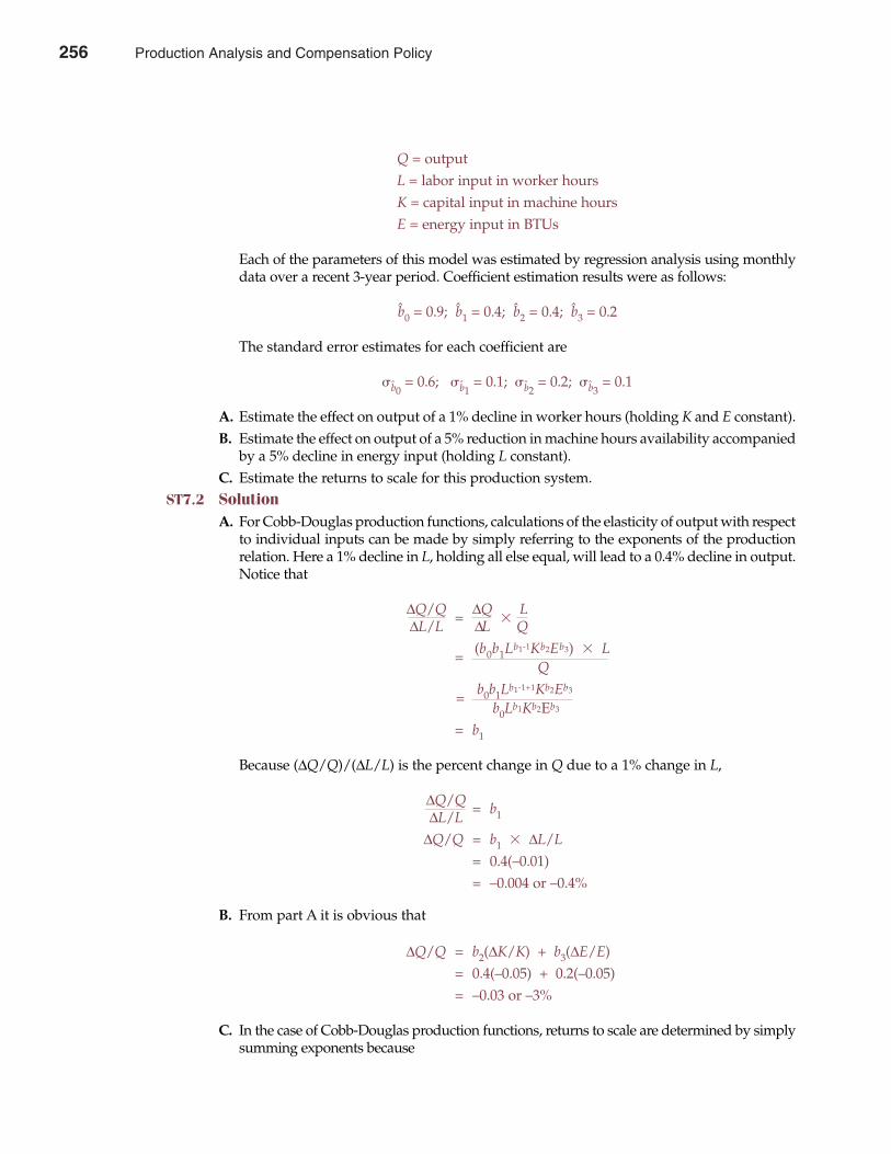
Q = outputL = labor input in worker hoursK = capital input in machine hoursE = energy input in BTUs
Each of the parameters of this model was estimated by regression analysis using monthlydata over a recent 3-year period. Coefficient estimation results were as follows:
b̂0 = 0.9; b̂1 = 0.4; b̂2 = 0.4; b̂3 = 0.2
The standard error estimates for each coefficient are
�b̂0= 0.6; �b̂1
= 0.1; �b̂2= 0.2; �b̂3
= 0.1
A. Estimate the effect on output of a 1% decline in worker hours (holding K and E constant).B. Estimate the effect on output of a 5% reduction in machine hours availability accompanied
by a 5% decline in energy input (holding L constant).C. Estimate the returns to scale for this production system.
ST7.2 SolutionA. For Cobb-Douglas production functions, calculations of the elasticity of output with respect
to individual inputs can be made by simply referring to the exponents of the productionrelation. Here a 1% decline in L, holding all else equal, will lead to a 0.4% decline in output.Notice that
∆Q/Q = ∆Q �
L∆L/L ∆L Q
= (b0b1Lb1-1Kb2Eb3) � LQ
= b0b1Lb1-1+1Kb2Eb3
b0Lb1Kb2Eb3
= b1
Because (∆Q/Q)/(∆L/L) is the percent change in Q due to a 1% change in L,
∆Q/Q = b1∆L/L
∆Q/Q = b1 � ∆L/L
= 0.4(–0.01)= –0.004 or –0.4%
B. From part A it is obvious that
∆Q/Q = b2(∆K/K) + b3(∆E/E)= 0.4(–0.05) + 0.2(–0.05)= –0.03 or –3%
C. In the case of Cobb-Douglas production functions, returns to scale are determined by simplysumming exponents because
Chapter Seven Production Analysis and Compensation Policy 257
256 Production Analysis and Compensation Policy
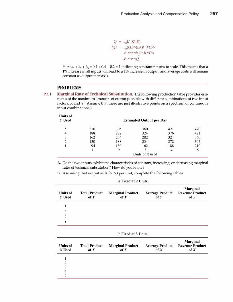
Q = b0Lb1Kb2Eb3
hQ = b0(kL)b1(kK)b2(kE)b3
kb1+b2+b3b0Lb1Kb2Eb3
kb1+b2+b3Q
Here b1 + b2 + b3 = 0.4 + 0.4 + 0.2 = 1 indicating constant returns to scale. This means that a1% increase in all inputs will lead to a 1% increase in output, and average costs will remainconstant as output increases.
PROBLEMS P7.1 Marginal Rate of Technical Substitution. The following production table provides esti-
mates of the maximum amounts of output possible with different combinations of two inputfactors, X and Y. (Assume that these are just illustrative points on a spectrum of continuousinput combinations.)
A. Do the two inputs exhibit the characteristics of constant, increasing, or decreasing marginalrates of technical substitution? How do you know?
B. Assuming that output sells for $3 per unit, complete the following tables:
258 Part Three Production and Cost Analysis
Units ofY Used Estimated Output per Day
5 210 305 360 421 4704 188 272 324 376 4213 162 234 282 324 3602 130 188 234 272 3051 94 130 162 188 210
1 2 3 4 5Units of X used
X Fixed at 2 Units
MarginalUnits of Total Product Marginal Product Average Product Revenue ProductY Used of Y of Y of Y of Y
12345
Y Fixed at 3 Units
MarginalUnits of Total Product Marginal Product Average Product Revenue ProductX Used of X of X of X of X
12345
Production Analysis and Compensation Policy 257
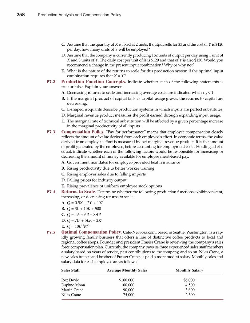
C. Assume that the quantity of X is fixed at 2 units. If output sells for $3 and the cost of Y is $120per day, how many units of Y will be employed?
D. Assume that the company is currently producing 162 units of output per day using 1 unit ofX and 3 units of Y. The daily cost per unit of X is $120 and that of Y is also $120. Would yourecommend a change in the present input combination? Why or why not?
E. What is the nature of the returns to scale for this production system if the optimal inputcombination requires that X = Y?
P7.2 Production Function Concepts. Indicate whether each of the following statements istrue or false. Explain your answers.A. Decreasing returns to scale and increasing average costs are indicated when �Q < 1.B. If the marginal product of capital falls as capital usage grows, the returns to capital are
decreasing.C. L-shaped isoquants describe production systems in which inputs are perfect substitutes.D. Marginal revenue product measures the profit earned through expanding input usage.E. The marginal rate of technical substitution will be affected by a given percentage increase
in the marginal productivity of all inputs.P7.3 Compensation Policy. “Pay for performance” means that employee compensation closely
reflects the amount of value derived from each employee’s effort. In economic terms, the valuederived from employee effort is measured by net marginal revenue product. It is the amountof profit generated by the employee, before accounting for employment costs. Holding all elseequal, indicate whether each of the following factors would be responsible for increasing ordecreasing the amount of money available for employee merit-based pay.A. Government mandates for employer-provided health insuranceB. Rising productivity due to better worker trainingC. Rising employer sales due to falling importsD. Falling prices for industry outputE. Rising prevalence of uniform employee stock options
P7.4 Returns to Scale. Determine whether the following production functions exhibit constant,increasing, or decreasing returns to scale.A. Q = 0.5X + 2Y + 40ZB. Q = 3L + 10K + 500C. Q = 4A + 6B + 8ABD. Q = 7L2 + 5LK + 2K2
E. Q = 10L0.5K0.3
P7.5 Optimal Compensation Policy. Café-Nervosa.com, based in Seattle, Washington, is a rap-idly growing family business that offers a line of distinctive coffee products to local andregional coffee shops. Founder and president Frasier Crane is reviewing the company’s salesforce compensation plan. Currently, the company pays its three experienced sales staff membersa salary based on years of service, past contributions to the company, and so on. Niles Crane, anew sales trainee and brother of Fraiser Crane, is paid a more modest salary. Monthly sales andsalary data for each employee are as follows:
Chapter Seven Production Analysis and Compensation Policy 259
Sales Staff Average Monthly Sales Monthly Salary
Roz Doyle $160,000 $6,000Daphne Moon 100,000 4,500Martin Crane 90,000 3,600Niles Crane 75,000 2,500
258 Production Analysis and Compensation Policy
Niles Crane has shown great promise during the past year, and Fraiser Crane believes that asubstantial raise is clearly justified. At the same time, some adjustment to the compensationpaid to other sales personnel also seems appropriate. Fraiser Crane is considering changingfrom the current compensation plan to one based on a 5% commission. He sees such a planas being more fair to the parties involved and believes it would also provide strong incentivesfor needed market expansion.
A. Calculate Café-Nervosa.com’s salary expense for each employee expressed as a percentageof the monthly sales generated by that individual.
B. Calculate monthly income for each employee under a 5% of monthly sales commission-based system.
C. Will a commission-based plan result in efficient relative salaries, efficient salary levels, orboth?
P7.6 Optimal Input Mix. The First National Bank received 3,000 inquiries following the latestadvertisement describing its 30-month IRAaccounts in the Boston World, a local newspaper. Themost recent ad in a similar advertising campaign in Massachusetts Business, a regional businessmagazine, generated 1,000 inquiries. Each newspaper ad costs $500, whereas each magazine adcosts $125.A. Assuming that additional ads would generate similar response rates, is the bank running an
optimal mix of newspaper and magazine ads? Why or why not?B. Holding all else equal, how many inquiries must a newspaper ad attract for the current
advertising mix to be optimal?P7.7 Optimal Input Level. The Route 66 Truck Stop, Inc., sells gasoline to both self-service and
full-service customers. Those who pump their own gas benefit from the lower self-serviceprice of $1.50 per gallon. Full-service customers enjoy the service of an attendant, but they paya higher price of $1.60 per gallon. The company has observed the following relation betweenthe number of attendants employed per day and full-service output:
A. Construct a table showing the net marginal revenue product derived from attendantemployment.
B. How many attendants would Route 66 employ at a daily wage rate of $160 (including wagesand benefits)?
C. What is the highest daily wage rate Route 66 would pay to hire four attendants per day?P7.8 Optimal Input Level. Ticket Services, Inc., offers ticket promotion and handling services for
concerts and sporting events. The Sherman Oaks, California, branch office makes heavy use ofspot radio advertising on WHAM-AM, with each 30-second ad costing $100. During the pastyear, the following relation between advertising and ticket sales per event has been observed:
Sales (units) = 5,000 + 100A – 0.5A2
∆Sales (units)/∆Advertising = 100 – A
260 Part Three Production and Cost Analysis
Route 66 Truck Stop, Inc.
Number of Attendants per Day Full-Service Output (gallons)
0 01 2,0002 3,8003 5,4004 6,8005 8,000
Production Analysis and Compensation Policy 259
Here, A represents a 30-second radio spot ad, and sales are measured in numbers of tickets.Rachel Green, manager for the Sherman Oaks office, has been asked to recommend an
appropriate level of advertising. In thinking about this problem, Green noted its resem-blance to the optimal resource employment problem she had studied in a managerial eco-nomics course that was part of her M.B.A. program. The advertising/sales relation could bethought of as a production function, with advertising as an input and sales as the output.The problem is to determine the profit-maximizing level of employment for the input,advertising, in this “production” system. Green recognized that to solve the problem, sheneeded a measure of output value. After reflection, she determined that the value of outputis $2 per ticket, the net marginal revenue earned by Ticket Services (price minus all marginalcosts except advertising).
A. Continuing with Green’s production analogy, what is the marginal product of advertising?B. What is the rule for determining the optimal amount of a resource to employ in a production
system? Explain the logic underlying this rule.C. Using the rule for optimal resource employment, determine the profit-maximizing number
of radio ads.P7.9 Net Marginal Revenue. Will Truman & Associates, LLC, is a successful Manhattan–based
law firm. Worker productivity at the firm is measured in billable hours, which vary betweenpartners and associates.
Partner time is billed to clients at a rate of $250 per hour, whereas associate time is billed ata rate of $125 per hour. On average, each partner generates 25 billable hours per 40-hour workweek, with 15 hours spent on promotion, administrative, and supervisory responsibilities.Associates generate an average of 35 billable hours per 40-hour work week and spend 5 hoursper week in administrative and training meetings. Variable overhead costs average 50% of rev-enues generated by partners and, given supervisory requirements, 60% of revenues generatedby associates.A. Calculate the annual (50 work weeks) net marginal revenue product of partners and
associates.B. If partners earn $175,000 and associates earn $70,000 per year, does the company have an
optimal combination of partners and associates? If not, why not? Make your answerexplicit and support any recommendations for change.
P7.10 Production Function Estimation. Consider the following Cobb-Douglas production func-tion for bus service in a typical metropolitan area:
Q = b0Lb1Kb2Fb3
where
Q = output in millions of passenger milesL = labor input in worker hoursK = capital input in bus transit hoursF = fuel input in gallons
Each of the parameters of this model was estimated by regression analysis using monthlydata over a recent 3-year period. Results obtained were as follows (standard errors in paren-theses):
b̂0 = 1.2; b̂1 = 0.28; b̂2 = 0.63; b̂3 = 0.12
The standard error estimates for each coefficient are
�b̂0= 0.4; �b̂1
= 0.15; �b̂2= 0.12; �b̂3
= 0.07
Chapter Seven Production Analysis and Compensation Policy 261
260 Production Analysis and Compensation Policy

A. Estimate the effect on output of a 4% decline in worker hours (holding K and F constant).B. Estimate the effect on output of a 3% reduction in fuel availability accompanied by a 4%
decline in bus transit hours (holding L constant).C. Estimate the returns to scale for this production system.
262 Part Three Production and Cost Analysis
CASE STUDY
Productivity Measurement and Enhancement in the Services SectorThe measurement and enhancement of worker productivity is an important challenge facingall managers. Productivity enhancement is vital given the role of labor as a key input in theproduction of goods and services and in light of the generally increasing vigor of domestic andimport competition. Of course, before incentives to enhance worker productivity can be intro-duced, the multiple dimensions of worker productivity must be made explicit and accuratelymeasured. Management must be able to clearly articulate the many important dimensions ofworker output and communicate this information effectively to workers.
The business and popular press is replete with examples of firms and industries that havefoundered because of problems tied to the inaccurate measurement of “blue-collar” worker pro-ductivity. When worker incentives are carelessly tied to piece-rate production, mass quantitiesof low-quality output sometimes result. Similarly, worker incentive pay plans that emphasizehigh-quality output can fail to provide necessary incentives for timely delivery. What is oftenoverlooked in the discussion of workers’ efficiency and labor productivity is that the definitionand measurement of productivity is perhaps even more difficult in the case of managers andother “white-collar” workers. Problems encountered in the definition and measurement ofwhite-collar worker productivity can be illustrated by considering the productivity of collegeand university professors.
For most 2-year and 4-year college and university professors, teaching is a primary com-ponent of their work assignment. Faculty members have a standard teaching load, defined bythe number of class hours per term, number of students taught, or a multiple of the two, called“student contact hours.” However, not all student contact hours are alike. For example, it ispossible to generate large numbers of student contact hours per faculty member simply byoffering courses in a mass lecture setting with hundreds of students per class. In other cases, afaculty member might work with a very small number of students in an advanced seminar orlaboratory course, generating relatively few student credit hours. The teaching “product” ineach of these course settings is fundamentally similar, and few would argue that the numberof students taught is an irrelevant basis for comparing the productivity of professors teachingthese different types of classes.
On the other hand, few would suggest defining teaching productivity solely in terms of thesheer quantity of students taught. Student course evaluations are typically required to provideevidence from student “customers” concerning the quality of instruction. Many schools rely onsuch data as an exclusive measure of teaching quality. At other schools, student course-evaluationdata are supplemented by peer review of teaching methods and materials, interviews of formerstudents, and so on. Measures of both the quantity and quality of instruction must be employedin the measurement of teaching productivity.
In addition to their important teaching role, faculty members are expected to play anactive role in the ongoing administration of their academic institution. At a minimum, theyparticipate in the peer review of faculty, in student and faculty recruiting, and in curriculumand program development. Faculty often play an active role on committees that conduct the
Production Analysis and Compensation Policy 261
Chapter Seven Production Analysis and Compensation Policy 263
everyday management of the institution. This faculty governance system is an important orga-nizational difference between most academic and nonacademic institutions. Faculty membersare both workers and management. Measuring “output” as related to these activities, andhence productivity, is very difficult.
At many schools, faculty members also play an important liaison role with external con-stituents. Alumni provide important financial resources to colleges and universities andappreciate programs designed for their benefit. Nondegree “short courses” are often offeredon topical subjects at nominal charge for the benefit of alumni and the community at large.Similarly, faculty are asked to give lectures to local groups, interviews for local media, and infor-mal consulting services to local firms and organizations. Often these services are provided for freeor at nominal charge as part of the faculty member’s “service” function. Similarly, faculty aresometimes called on to provide service to external academic and professional organizations.Participation at national and regional academic conventions, editing academic journals, and help-ing design and write professional exams are typical examples of expected but unpaid services.
The preceding duties are supplemented by faculty research requirements at most 4-yearcolleges and universities and at all graduate institutions. This requirement is fundamental tothe growth and development of colleges and universities but is often misunderstood by thoseoutside of academia. To be granted the doctoral degree, doctoral candidates must complete arigorous series of courses and exams and meet a dissertation requirement. A doctoral disser-tation is a book-length independent study that makes an important contribution to knowledgein a scholarly discipline. In fulfilling this requirement, doctoral students demonstrate theircapacity to participate in the discovery of new knowledge. A key difference between therole of university professors and that of other teachers is that professors must be intimatelyinvolved with the creation and dissemination of new knowledge. Thus, the research com-ponent is a key ingredient of professorial output.
Research output is extremely varied. In the physical sciences, new compounds or otherphysical products may result. Similarly, such research may lead to new process techniques. Inmost academic fields, the primary research product is new knowledge communicated in theform of research reports or other scholarly publications. As with teaching, measuring thequantity and quality of research output proves to be most challenging. Judging the value of aresearch product is often quite subjective, and its worth may not be recognized for years.
Given the difficulties involved with evaluating highly specialized and detailed research,many institutions consider the dollar amount of research funds awarded to an individual tobe a useful indicator of the quantity and quality of research output. It is anomalous that aschool’s best researchers and highest-paid faculty members may be the least expensive interms of their net costs to the institution. When established researchers are able to consistent-ly obtain external funding in excess of incremental costs, their net employment costs can be nil.In such instances, the disadvantages to an institution of losing a star researcher are obvious.
Of course, just as in the case of measuring teaching quality, difficulties are encountered inmeasuring the quality of published research output. In most instances, the quality of publishedarticles and books is judged in terms of the reputation of the publisher or editor, the level ofreadership enjoyed, and so on. Over time, the number of new research outlets has grown tokeep pace with the growing level of specialization in the various disciplines. In economics, forexample, there are as many as 200 possible research outlets. However, only a relative handfulare widely read in any given subdiscipline. Competition for scarce journal space in such outletsis fierce. Acceptance rates at leading journals often average no more than 5% to 10% of thosearticles submitted. When one considers that a productive scholar is typically able to completeno more than one or two substantial research projects per year, the odds are very much againstachieving publication of one or two first-rate journal articles per year. Thus, research produc-tivity is usually measured in terms of both the quantity and quality of published research.
CASE STUDY (continued)
262 Production Analysis and Compensation Policy
SELECTED REFERENCES Autor, David H. “Why Do Temporary Help Firms Provide Free General Skills Training?” Quarterly
Journal of Economics 116 (November 2001): 1409–1448.Bowles, Samuel, Herbert Gintis, and Melissa Osborne. “Incentive-Enhancing Preferences: Personality,
Behavior, and Earnings.” American Economic Review 91 (May 2001): 155–158.Brickley, James A., and Jerold L. Zimmerman. “Changing Incentives in a Multitask Environment:
Evidence from a Top-Tier Business School.” Journal of Corporate Finance 7 (December 2001): 367–396. Cutler, David M., and Mark Mcclellan. “Productivity Change in Health Care.” American Economic Review
91 (May 2001): 281–286.Datta, Sudip, Mai Iskandar-Datta, and Kartik Raman. “Executive Compensations and Corporate
Acquisition Decisions.” Journal of Finance 56 (December 2001): 2299–2336.Deli, Daniel N., and Raj Varma. “Contracting in the Investment Management Industry.” Journal of Financial
Economics 63 (January 2002): 79–98.Dhawan, Rajeev. “Firm Size and Productivity Differential: Theory and Evidence from a Panel of U.S.
Firms.” Journal of Economic Behavior & Organization 44 (March 2001): 269–293.Findlay, Ronald, and Ronald W. Jones. “Input Trade and the Location of Production.” American Economic
Review 91 (May 2001): 29–33.Geoffrion, Arthur M., and Ramayya Krishnan. “Prospects for Operations Research in the E-Business
Era.” Interfaces 31 (March 2001): 6–36.Hermalin, Benjamin, and Nancy Wallace. “Firm Performance and Executive Compensation in the Savings
and Loan Industry.” Journal of Financial Economics 61 (July 2001): 139–170.Matolcsy, Zoltan P. “Executive Cash Compensation and Corporate Performance During Different
Economic Cycles.” Contemporary Accounting Research 17 (Winter 2000): 671–692.Meulbroek, Lisa K. “The Efficiency of Equity-Linked Compensation: Understanding the Full Cost of
Awarding Executive Stock Options.” Financial Management 30 (Summer 2001): 5–44.Morgan, Angela G., and Annette B. Poulsen. “Linking Pay to Performance—Compensation Proposals in
the S&P 500.” Journal of Business 62 (December 2001): 489–523.Ohanian, Lee E. “Why Did Productivity Fall So Much During the Great Depression?” American Economic
Review 91 (May 2001): 34–38.Perry, Tod, and Marc Zenner. “Pay for Performance? Government Regulation and the Structure of
Compensation Contracts.” Journal of Business 62 (December 2001): 453–488.
264 Part Three Production and Cost Analysis
CASE STUDY (continued)
In sum, defining the role of professors at colleges and universities provides an interestingexample of the difficulties involved in measuring worker productivity. Each individual academ-ic institution must define on an ongoing basis the relative importance of the teaching, research,and service components of faculty output. Once this has been determined, the difficult task ofdefining and measuring faculty-member productivity on each dimension must begin.
Based on the preceding information and in light of the focus of your academic institution,answer the following questions:A. How would you define faculty-member productivity?B. Do you agree with the view that many elements of professorial output do not easily lend
themselves to quantitative evaluation? How might you measure such productivity?C. Would productivity clauses for professors’ contracts make sense economically? What
problems do you see in implementing such clauses in actual practice?D. Reconsider your answers to parts A through C for other service-industry occupations (for
example, doctors, lawyers, and legislators). Are the issues discussed unique to academia?
Production Analysis and Compensation Policy 263

Cost Analysis and Estimation
CHAPTER EIGHT
265
Fans of the Chevrolet Camaro and Pontiac Firebird mourned when GeneralMotors (GM) announced that these classic muscle cars were headed for
that big parking lot in the sky at the end of the 2001 model year. GM man-agement said the Camaro and Firebird had become victims of America’sobsession with sport utility vehicles and light trucks. Management wouldhave us believe that the kids who used to crave inexpensive but fun-to-drivemuscle cars were now driving $35,000 Ford Explorers.
The truth is that poor product quality, outdated design, lackluster market-ing, and tough competition from foreign rivals killed the Camaro and Firebird.It’s simply not true that young people, and the young at heart, no longerwant cars that are fast, loud, and cheap. To convince yourself of this, simplygo downtown in almost any city or suburb in America on Friday or Saturdaynight. It won’t be long before you get nearly blown off the sidewalk by somekid slouched behind the wheel of a “low-rider” with windows vibrating to thethump of ultra-amplified bass. In the 1970s or 1980s, that kid was in a Camaroor Firebird. Today, they probably drive a Honda Civic or Acura Integra. Bothare relatively cheap, stylish, and easy to customize. If you’re not into cus-tomizing, try a Toyota Celica GT-S 2133 Liftback 2D (6-Spd.). It’s more than astylish, dependable bargain priced at about $23,000. It’s fun to drive. A high-quality car is more than neat looking and dependable; it’s a blast to get behindthe wheel of a high-quality car.
Cost estimation and control is part of the continual process of makingproducts that exceed customer expectations. Quick fixes don’t work. Thischapter shows how making things faster, cheaper, and better requires a fun-damental appreciation of cost concepts.1
1 Karen Lundegaard, “Big Three Trail Their Rivals in Consumer Reports Survey,” The WallStreet Journal Online, March 13, 2002 (http://online.wsj.com).
265
8
WHAT MAKES COST ANALYSIS DIFFICULT?
Cost analysis is made difficult by the effects of unforeseen inflation, unpredictable changes intechnology, and the dynamic nature of input and output markets. Wide divergences betweeneconomic costs and accounting valuations are common. This makes it extremely important toadjust accounting data to create an appropriate basis for managerial decisions.
The Link Between Accounting and Economic Valuations Accurate cost analysis involves careful consideration of relevant decision alternatives. In manyinstances, the total costs of making a given decision are clear only when viewed in light of whatis done and what is not done. Careful decision analysis includes comparing the relative costsand benefits of each decision alternative. No option can be viewed in isolation; each choice playsan important role in shaping the relevant costs and benefits of all decision alternatives.
Evaluation of a proposal to expand output requires that revenues gained from added salesbe compared with the higher production costs incurred. In weighing a recommendation toexpand, managers must compare the revenues derived from investment and the cost of need-ed funds. Expected benefits from an advertising promotion must be measured in relation tothe costs of personal selling, media promotion, and direct marketing. Even a decision to pavethe employees’ parking lot or to refurbish the company lunchroom involves a comparisonbetween projected costs and the expected benefits derived from improved morale and workerproductivity. In every case, the decision-making process involves a comparison between thecosts and the benefits resulting from various decision alternatives.
Corporate restructuring often involves eliminating nonstrategic operations to redeploy assetsand strengthen core lines of business. When nonessential assets are disposed of in a depressedmarket, there is typically no relation between low “fire sale” proceeds and book value, historicalcost, or replacement cost. Conversely, when assets are sold to others who can more effectivelyuse such resources, sale proceeds can approximate replacement value and greatly exceed histor-ical costs and book values. Even under normal circumstances, the link between economic andaccounting values can be tenuous. Economic worth as determined by profit-generating capability,rather than accounting value, is always the most vital consideration when determining the costand use of specific assets.
Historical Versus Current Costs The term cost can be defined in a number of ways. The correct definition varies from situationto situation. In popular terminology, cost generally refers to the price that must be paid for anitem. If a firm buys an input for cash and uses it immediately, few problems arise in definingand measuring its cost. However, if an input is purchased, stored for a time, and then used,complications can arise. The problem can be acute if the item is a long-lived asset like a build-ing that will be used at varying rates for an indeterminate period.
When costs are calculated for a firm’s income tax returns, the law requires use of the actualdollar amount spent to purchase the labor, raw materials, and capital equipment used in pro-duction. For tax purposes, historical cost, or actual cash outlay, is the relevant cost. This is alsogenerally true for annual 10-K reports to the Securities and Exchange Commission and forreports to stockholders.
Despite their usefulness, historical costs are not appropriate as a sole basis for many mana-gerial decisions. Current costs are typically much more relevant. Current cost is the amount thatmust be paid under prevailing market conditions. Current cost is influenced by market condi-tions measured by the number of buyers and sellers, the present state of technology, inflation,and so on. For assets purchased recently, historical cost and current cost are typically the same.
266 Part Three Production and Cost Analysis
historical cost Actual cash outlay
current cost Amount paid underprevailing market conditions
266 Cost Analysis and Estimation
For assets purchased several years ago, historical cost and current cost are often quite different.Since World War II, inflation has been an obvious source of large differences between current andhistorical costs throughout most of the world. With an inflation rate of roughly 5 percent per year,prices double in less than 15 years and triple in roughly 22 years. Land purchased for $50,000 in1970 often has a current cost in excess of $200,000. In California, Florida, Texas, and other rapid-ly growing areas, current costs run much higher. Just as no homeowner would sell his or herhome for a lower price based on lower historical costs, no manager can afford to sell assets orproducts for less than current costs.
A firm also cannot assume that the accounting historical cost is the same as the relevanteconomic cost of using a given piece of equipment. For example, it is not always appropriateto assume that use costs equal zero just because a machine has been fully depreciated usingappropriate accounting methods. If a machine could be sold for $10,000 now, but its marketvalue is expected to be only $2,000 1 year from now, the relevant cost of using the machinefor one additional year is $8,000.2 Again, there is little relation between the $8,000 relevant costof using the machine and the zero cost reported on the firm’s income statement.
Historical costs provide a measure of the market value of an asset at the time of purchase.Current costs are a measure of the market value of an asset at the present time. Traditionalaccounting methods and the IRS rely heavily on the historical cost concept because it can beapplied consistently across firms and is easily verifiable. However, when historical and currentcosts differ markedly, reliance on historical costs sometimes leads to operating decisions withdisastrous consequences. The savings and loan (S&L) industry debacle in the United Statesduring the late 1980s is a clear case in point. On a historical cost basis, almost all thrifts appearedto have solid assets to back up liabilities. On a current cost basis, however, many S&Ls provedinsolvent because assets had a current market value below the current market value of liabilities.The move by federal and state bank regulators toward market-value-based accounting methodsis motivated by a desire to avoid S&L-type disasters in the future.
Replacement Cost Although it is typical for current costs to exceed historical costs, this is not always the case.Computers and many types of electronic equipment cost much less today than they did justa few years ago. In many high-tech industries, the rapid advance of technology has overcomethe general rate of inflation. As a result, current costs are falling. Current costs for computersand electronic equipment are determined by what is referred to as replacement cost, or thecost of duplicating productive capability using current technology. For example, the value ofused personal computers tends to fall by 30 to 40 percent per year. In valuing such assets, theappropriate measure is the much lower replacement cost—not the historical cost. Similarly, ifa company holds electronic components in inventory, the relevant cost for pricing purposesis replacement costs.
In a more typical example, consider a construction company that has an inventory of1,000,000 board feet of lumber, purchased at a historical cost of $200,000, or $200 per 1,000 boardfeet (a board foot of lumber is 1 square foot of lumber, 1 inch thick). Assume that lumber pricesrise by 50 percent, and the company is asked to bid on a construction project that would requirelumber. What cost should the construction company assign to the lumber—the $200,000 histor-ical cost or the $300,000 replacement cost? The answer is the replacement cost of $300,000. Thecompany will have to pay $300,000 to replace the lumber it uses on the new construction proj-ect. In fact, the construction company could sell its current inventory of lumber to others for the
replacement cost The cost of duplicatingproductive capabilityusing current technology
Chapter Eight Cost Analysis and Estimation 267
2 This statement involves a slight oversimplification. The economic cost of using a machine for 1 year is its currentmarket value minus the discounted present value of its worth 1 year from now. This adjustment is necessary toaccount for the fact that future dollars have a lower present value than dollars received today.
Cost Analysis and Estimation 267
prevailing market price of $300,000. Under current market conditions, the lumber has a worthof $300,000. The amount of $300,000 is the relevant economic cost for purposes of bidding onthe new construction project. For income tax purposes, however, the appropriate cost basis forthe lumber inventory is still the $200,000 historical cost.
OPPORTUNITY COSTS
When a firm uses resources, it bids against alternative users. To be efficient, a resource’s valuein use must be at least as much as its value in alternative opportunities. The role played bychoice alternatives in cost analysis is formalized by the opportunity cost concept.
Opportunity Cost Concept Opportunity cost is the foregone value associated with the current rather than next-best useof an asset. In other words, cost is determined by the highest-valued opportunity that mustbe foregone to allow current use. The cost of aluminum used in the manufacture of soft drinkcontainers, for example, is determined by its value in alternative uses. Soft drink bottlersmust pay an aluminum price equal to this value, or the aluminum will be used in the pro-duction of alternative goods, such as airplanes, building materials, cookware, and so on.Similarly, if a firm owns capital equipment that can be used to produce either product A orproduct B, the relevant cost of product A includes the profit of the alternative product B thatcannot be produced because the equipment is tied up in manufacturing product A.
The opportunity cost concept explains asset use in a wide variety of circumstances. Gold andsilver are pliable yet strong precious metals. As such, they make excellent material for dentalfillings. However, when speculation drove precious metals prices skyrocketing during the1970s, plastic and ceramic materials became a common substitute for dental gold and silver.More recently, lower market prices have again allowed widespread dental use of both metals.Still, dental customers must be willing to pay a price for dental gold and silver that is competi-tive with the price paid by jewelry customers and industrial users.
Explicit and Implicit Costs Typically, the costs of using resources in production involve both out-of-pocket costs, orexplicit costs, and other noncash costs, called implicit costs. Wages, utility expenses, pay-ment for raw materials, interest paid to the holders of the firm’s bonds, and rent on a buildingare all examples of explicit expenses. The implicit costs associated with any decision are muchmore difficult to compute. These costs do not involve cash expenditures and are therefore oftenoverlooked in decision analysis. Because cash payments are not made for implicit costs, theopportunity cost concept must be used to measure them. The rent that a shop owner couldreceive on buildings and equipment if they were not used in the business is an implicit cost ofthe owner’s own retailing activity, as is the salary that an individual could receive by workingfor someone else instead of operating his or her own establishment.
An example should clarify these cost distinctions. Consider the costs associated with thepurchase and operation of a law practice. Assume that the minority partners in an establishedpractice, Donnell, Young, Doyle & Frutt, can be bought for $225,000, with an additional $25,000needed for initial working capital. Lindsay Doyle has personal savings of $250,000 to invest insuch an enterprise; Bobby Donnell, another possible buyer, must borrow the entire $250,000 ata cost of 15 percent, or $37,500 per year. Assume that operating costs are the same no matterwho owns the practice and that Doyle and Donnell are equally capable of completing the pur-chase. Does the $37,500 in annual interest expenses make Donnell’s potential operating cost
268 Part Three Production and Cost Analysis
opportunity cost Foregone value associ-ated with currentrather than next-bestuse of an asset
explicit cost Out-of-pocket expendi-tures
implicit cost Noncash costs
268 Cost Analysis and Estimation
greater than that of Doyle? For managerial decision purposes, the answer is no. Even thoughDonnell has higher explicit interest costs, true financing costs may well be the same for bothindividuals. Doyle has an implicit interest cost equal to the amount that could be earned on analternative $250,000 investment. If a 15 percent return can be earned by investing in otherassets of equal risk, then Doyle’s implicit investment opportunity cost is also $37,500 per year.In this case, Doyle and Donnell each have a financing cost of $37,500 per year. Doyle’s cost isimplicit and Donnell’s is explicit.
Will total operating costs be identical for both individuals? Not necessarily. Just as theimplicit cost of Doyle’s capital must be included in the analysis, so too must implicit laborcosts be included for each individual. If Doyle is a senior partner earning $250,000 a year andDonnell is a junior partner earning $150,000 annually, implicit labor costs will be different.When both individuals have ready employment alternatives, the implicit labor expense foreach potential buyer is the amount of income forfeited by foregoing such alternative employ-ment. Thus, implicit labor costs are $250,000 for Doyle and $150,000 for Donnell. On anannual basis, Doyle’s total capital plus labor costs are $287,500, all of which are implicit.Donnell’s total annual costs are $187,500, including explicit capital costs of $37,500 plusimplicit labor costs of $150,000.
INCREMENTAL AND SUNK COSTS IN DECISION ANALYSIS
Relevant costs and benefits for any decision are limited to those that are affected by it. Tolimit the confounding influence of irrelevant cost information, it is helpful to focus on thecausal relation between costs and a given managerial decision, as well as on the reversibleor nonreversible nature of some cost categories.
Chapter Eight Cost Analysis and Estimation 269
GE’s “20-70-10” Plan
The General Electric Co. (GE) routinely identifies thetop 20 percent, the middle 70 percent, and the bottom10 percent of its 100,000 managerial and professionalemployees. According to Jack Welch, legendary formerchairman of GE, the top 20 percent and middle 70 per-cent often trade places, but the bottom 10 percent tendto remain there. At GE, those employees found in thebottom 10 percent are given a chance to improve.However, if performance doesn’t improve quickly, theyhad better find another job.
Among its managers and professionals, GE losesabout 8,000 per year through turnover and attrition. Ofthose, about 60 percent, or 4,800, are forced out—both ingood times and bad. Even among the highest-ranking600 GE executives, about 60 leave each year. Fewer than20 are due to retirement or opportunities elsewhere.There just isn’t much empathy for underperformance atGE. Welch was famous for arguing that underperform-ing managers and professionals will eventually be firedanyway, and delaying the inevitable is a form of “corporate cruelty.”
Welch retired at the end of 2001, but GE has no plansto retire its 20-70-10 plan. Not only is the plan embracedby new CEO Jeffrey Immelt, but other top corporationsare also seeking to emulate GE’s success. Althoughemployee performance reviews have long been an impor-tant part of effective management, it’s new for bosses torank every employee in each department. Newer still isthe practice of asking those at the bottom to leave. Therationale for tough performance reviews is that compa-nies want to make way for promising new hires.Similarly, if downsizing becomes necessary, is it fair tothrow out solid performers and keep weaker employees?
To be sure, GE’s tough 20-70-10 plan has its detrac-tors. Critics argue that top-to-bottom rankings aresometimes arbitrary. In some instances, dischargedworkers have filed lawsuits charging discrimination.Unfazed, GE and its imitators are going forward withtheir top-to-bottom rankings.
See: Dow Jones Newswires,” GE’s Immelt: Willing to Cooperate withUS’s EPA on Hudson,” The Wall Street Journal Online, January 18, 2002(http://online.wsj.com).
M A N A G E R I A L A P P L I C AT I O N 8 . 1
Cost Analysis and Estimation 269
Incremental Cost Incremental cost is the change in cost caused by a given managerial decision. Whereas marginalcost is the change in cost following a one-unit change in output, incremental costs typicallyinvolve multiple units of output. For example, incremental costs are the relevant considerationwhen an air carrier considers the cost of adding an additional departure from New York’s LaGuardia Airport to upstate New York. When all current departures are full, it is impractical toconsider adding a single passenger-mile unit of output. Similarly, the incremental cost conceptcomes into play when judging the costs of adding a new product line, advertising campaign, pro-duction shift, or organization structure.
Inappropriate managerial decisions can result when the incremental concept is ignored orapplied incorrectly. Consider, for example, a commercial real estate firm that refuses to rentexcess office space for $750 per month because it figures cost as $1,000 per month—or incre-mental operating costs of $150 plus interest and overhead charges of $850. If the relevantincremental cost is indeed only $150 per month, turning away the prospective renter causesa $600 (= $750 – $150) per month loss in profit contribution, or profit before fixed charges.Interest and overhead charges will be incurred irrespective of whether the excess space isrented. By adding the prospective renter, the landlord has the same interest and overheadexpenses as before, plus $600 in added revenues after incremental operating expenses. The neteffect of rejecting such a renter would be to reduce profit contribution and net profits by $600.
Care must be exercised to ensure against incorrectly assigning a lower than appropriateincremental cost. If excess capacity results from a temporary reduction in demand, this must betaken into account. Accepting the $750 per month renter in the previous example is a mistake ifdoing so causes more profitable renters to be turned away. When excess capacity is caused bya temporary drop in demand, only short-term or month-to-month leases should be offered atthe bargain price of $750 per month. In this way, pricing flexibility can be maintained while thenet cost of temporary excess capacity is minimized. In any event, all incremental costs, includingthose that might be incurred in the future, must be considered.
Sunk Costs Inherent in the incremental cost concept is the principle that any cost not affected by a decisionis irrelevant to that decision. A cost that does not vary across decision alternatives is called asunk cost; such costs do not play a role in determining the optimal course of action.
For example, suppose a firm has spent $5,000 on an option to purchase land for a newfactory at a price of $100,000. Also assume that it is later offered an equally attractive site for$90,000. What should the firm do? The first thing to recognize is that the $5,000 spent on thepurchase option is a sunk cost that must be ignored. If the firm purchases the first property,it must pay a price of $100,000. The newly offered property requires an expenditure of only$90,000 and results in a $10,000 savings. In retrospect, purchase of the $5,000 option was amistake. It would be a compounding of this initial error to follow through with the purchaseof the first property and lose an additional $10,000.
In managerial decision making, care must be taken to ensure that only those costs actuallyaffected by a decision are considered. These incremental costs can include both implicit andexplicit costs. If long-term commitments are involved, both current and future incrementalcosts must also be accounted for. Any costs not affected by available decision alternatives aresunk and irrelevant.
SHORT-RUN AND LONG-RUN COSTS Proper use of relevant cost concepts requires an understanding of the relation between costand output, or the cost function. Two basic cost functions are used in managerial decision
270 Part Three Production and Cost Analysis
incremental cost Change in cost causedby a given managerialdecision
profit contribution Profit before fixedcharges
sunk cost Cost that does not vary across decisionalternatives
cost function The cost-output relation
270 Cost Analysis and Estimation
making: short-run cost functions, used for day-to-day operating decisions, and long-runcost functions, used for long-range planning.
How Is the Operating Period Defined? The short run is the operating period during which the availability of at least one input isfixed. In the long run, the firm has complete flexibility with respect to input use. In theshort run, operating decisions are typically constrained by prior capital expenditures. In thelong run, no such restrictions exist. For example, a management consulting firm operatingout of rented office space might have a short-run period as brief as several weeks, the timeremaining on the office lease. A firm in the hazardous waste disposal business with 25- to 30-year leases on disposal sights has significant long-lived assets and faces a lengthy period ofoperating constraints.
The economic life of an asset and the degree of specialization affect the time length of oper-ating period constraints. Consider, for example, a health maintenance organization’s (HMO)automobile purchase for delivering home-based health care. If the car is a standard model with-out modification, it represents an unspecialized input factor with a resale value based on theused car market in general. However, if the car has been modified by adding refrigerationequipment for transporting perishable medicines, it becomes a more specialized input with fullvalue only for those who need a vehicle with refrigeration equipment. In this case, the marketprice of the car might not equal its value in use to the HMO. To the extent that specialized inputfactors are employed, the short run is lengthened. When only unspecialized factors are used,the short run is condensed.
The amount of time required to order, receive, and install new assets also influences theduration of the short run. Many manufacturers face delays of several months when orderingnew plant and equipment. Air carriers must place their equipment orders 5 or more years inadvance of delivery. Electric utilities frequently require 8 or more years to bring new generatingplants on line. For all such firms, the short-run operating period is an extended period of time.
Long-run cost curves are called planning curves; short-run cost curves are called operatingcurves. In the long run, plant and equipment are variable, so management can plan the most effi-cient physical plant, given an estimate of the firm’s demand function. Once the optimal planthas been determined and the resulting investment in equipment has been made, short-runoperating decisions are constrained by these prior decisions.
Fixed and Variable Costs Fixed costs do not vary with output. These costs include interest expenses, rent on leasedplant and equipment, depreciation charges associated with the passage of time, property taxes,and salaries for employees not laid off during periods of reduced activity. Because all costs arevariable in the long run, long-run fixed costs always equal zero. Variable costs fluctuate withoutput. Expenses for raw materials, depreciation associated with the use of equipment, thevariable portion of utility charges, some labor costs, and sales commissions are all examples ofvariable expenses. In the short run, both variable and fixed costs are often incurred. In the longrun, all costs are variable.
A sharp distinction between fixed and variable costs is not always possible nor realistic. Forexample, CEO and staff salaries may be largely fixed, but during severe business downturns,even CEOs take a pay cut. Similarly, salaries for line managers and supervisors are fixed onlywithin certain output ranges. Below a lower limit, supervisors and managers get laid off.Above an upper limit, additional supervisors and managers get hired. The longer the durationof abnormal demand, the greater the likelihood that some fixed costs will actually vary. Inrecognition of this, such costs are sometimes referred to as semivariable.
short-run cost functions Basis for day-to-dayoperating decisions
long-run cost functions Basis for long-rangeplanning
short run Operating period dur-ing which at least oneinput is fixed
long run Planning period withcomplete input flexibility
fixed cost Expense that does notvary with output
variable cost Expense that fluctuateswith output
Chapter Eight Cost Analysis and Estimation 271
Cost Analysis and Estimation 271
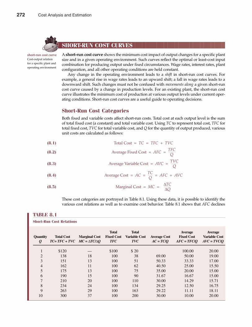
SHORT-RUN COST CURVES
A short-run cost curve shows the minimum cost impact of output changes for a specific plantsize and in a given operating environment. Such curves reflect the optimal or least-cost inputcombination for producing output under fixed circumstances. Wage rates, interest rates, plantconfiguration, and all other operating conditions are held constant.
Any change in the operating environment leads to a shift in short-run cost curves. Forexample, a general rise in wage rates leads to an upward shift; a fall in wage rates leads to adownward shift. Such changes must not be confused with movements along a given short-runcost curve caused by a change in production levels. For an existing plant, the short-run costcurve illustrates the minimum cost of production at various output levels under current oper-ating conditions. Short-run cost curves are a useful guide to operating decisions.
Short-Run Cost Categories Both fixed and variable costs affect short-run costs. Total cost at each output level is the sumof total fixed cost (a constant) and total variable cost. Using TC to represent total cost, TFC fortotal fixed cost, TVC for total variable cost, and Q for the quantity of output produced, variousunit costs are calculated as follows:
(8.1) Total Cost = TC = TFC + TVC
(8.2) Average Fixed Cost = AFC = TFCQ
(8.3) Average Variable Cost = AVC = TVCQ
(8.4) Average Cost = AC = TC = AFC + AVCQ
(8.5) Marginal Cost = MC =∆TC∆Q
These cost categories are portrayed in Table 8.1. Using these data, it is possible to identify thevarious cost relations as well as to examine cost behavior. Table 8.1 shows that AFC declines
272 Part Three Production and Cost Analysis
short-run cost curve Cost-output relationfor a specific plant andoperating environment
TABLE 8.1Short-Run Cost Relations
Total Total Average Average Quantity Total Cost Marginal Cost Fixed Cost Variable Cost Average Cost Fixed Cost Variable Cost
Q TC= TFC + TVC MC = ∆TC/∆Q TFC TVC AC = TC/Q AFC = TFC/Q AVC = TVC/Q
1 $120 — $100 $ 20 100.00 20.002 138 18 100 38 69.00 50.00 19.003 151 13 100 51 50.33 33.33 17.004 162 11 100 62 40.50 25.00 15.505 175 13 100 75 35.00 20.00 15.006 190 15 100 90 31.67 16.67 15.007 210 20 100 110 30.00 14.29 15.718 234 24 100 134 29.25 12.50 16.759 263 29 100 163 29.22 11.11 18.11
10 300 37 100 200 30.00 10.00 20.00
272 Cost Analysis and Estimation
continuously with increases in output. AC and AVC also decline as long as they exceed MC, butincrease when they are less than MC. Alternatively, so long as MC is less than AC and AVC, bothaverage cost categories will decline. When MC is greater than AC and AVC, both average costcategories will rise. Also note that TFC is invariant with increases in output and that TVC at eachlevel of output equals the sum of MC up to that output.
Marginal cost is the change in cost associated with a one-unit change in output. Becausefixed costs do not vary with output, fixed costs do not affect marginal costs. Only variable costsaffect marginal costs. Therefore, marginal costs equal the change in total costs or the change intotal variable costs following a one-unit change in output:
MC = ∆TC = ∆TVC∆Q ∆Q
Short-Run Cost Relations Relations among short-run cost categories are shown in Figure 8.1. Figure 8.1(a) illustratestotal cost and total variable cost curves. The shape of the total cost curve is determinedentirely by the total variable cost curve. The slope of the total cost curve at each output levelis identical to the slope of the total variable cost curve. Fixed costs merely shift the total costcurve to a higher level. This means that marginal costs are independent of fixed cost.
The shape of the total variable cost curve, and hence the shape of the total cost curve, isdetermined by the productivity of variable input factors employed. The variable cost curvein Figure 8.1 increases at a decreasing rate up to output level Q1, then at an increasing rate.Assuming constant input prices, this implies that the marginal productivity of variable inputsfirst increases, then decreases. Variable input factors exhibit increasing returns in the rangefrom 0 to Q1 units and show diminishing returns thereafter. This is a typical finding. Fixed
Chapter Eight Cost Analysis and Estimation 273
Gaps in GAAP?
Generally accepted accounting principles (GAAP) offercompanies and their auditors a consistent set of rules tofollow in their reporting of company income statementand balance sheet information. GAAP also offers ameasure of “quality control” that assures investors thatreported numbers have been consistently derived from aset of uniform principles applied to all companies. Thismakes it possible for investors to compare reportedresults over time and across firms and industries. Atleast, this is how GAAP works in theory. Sometimes,accounting practice falls far short of the ideal. In someinstances, it seems as if companies and their auditorscome up with the numbers the companies want, irre-spective of actual economic performance.
Common accounting tricks that managers andinvestors must be on the lookout for include• Misleading focus on pro-forma results. Some firms seek
to minimize poor operating performance by encourag-ing investors to overlook standard accounting charges.
• Excessive one-time R&D charges. These one-timecharges are taken at the time of an acquisition to cover
expenses for research and development that is ‘’inprocess’’ but not yet commercially viable. By separat-ing these expenses from revenues that might be gainedin the future, future earnings can be overstated.
• Extravagant one-time “restructuring reserves.” Whennormal expenses are written off ahead of time, futureearnings are overstated.
• Aggressive revenue recognition. When service con-tracts stretch out for years, booking revenue tooearly inflates sales and earnings.
The Securities and Exchange Commission (SEC) hasbecome concerned that the quality of financial reportingis eroding. It should be. If basic accounting practices everlose credibility with investors and the general public,financial markets and economic performance would suf-fer greatly.
See: Alen Mattich, “Accountants Under the Microscope Post Enron,”The Wall Street Journal Online, January 18, 2002 (http://online.wsj.com).
M A N A G E R I A L A P P L I C AT I O N 8 . 2
Cost Analysis and Estimation 273
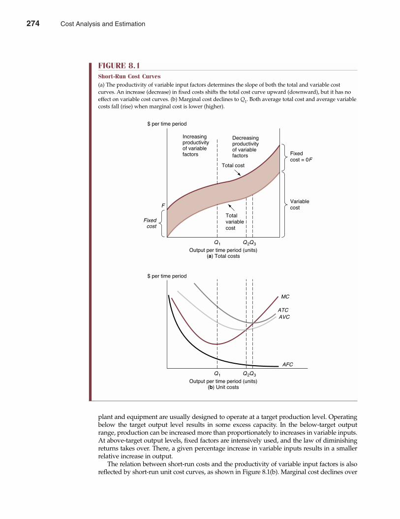
plant and equipment are usually designed to operate at a target production level. Operatingbelow the target output level results in some excess capacity. In the below-target outputrange, production can be increased more than proportionately to increases in variable inputs.At above-target output levels, fixed factors are intensively used, and the law of diminishingreturns takes over. There, a given percentage increase in variable inputs results in a smallerrelative increase in output.
The relation between short-run costs and the productivity of variable input factors is alsoreflected by short-run unit cost curves, as shown in Figure 8.1(b). Marginal cost declines over
274 Part Three Production and Cost Analysis
FIGURE 8.1Short-Run Cost Curves(a) The productivity of variable input factors determines the slope of both the total and variable costcurves. An increase (decrease) in fixed costs shifts the total cost curve upward (downward), but it has noeffect on variable cost curves. (b) Marginal cost declines to Q1. Both average total cost and average variablecosts fall (rise) when marginal cost is lower (higher).
Decreasingproductivityof variablefactors
Increasingproductivityof variablefactors
$ per time period
Total cost
Totalvariablecost
Fixedcost = 0F
Variablecost
Q3Q2Q1
F
Fixedcost
$ per time period
Output per time period (units)(a) Total costs
Q3Q2Q1
Output per time period (units)(b) Unit costs
MC
ATCAVC
AFC
274 Cost Analysis and Estimation
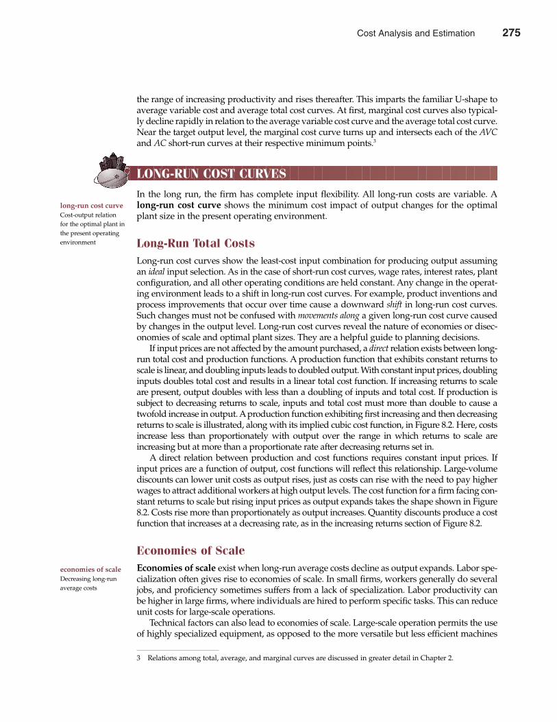
the range of increasing productivity and rises thereafter. This imparts the familiar U-shape toaverage variable cost and average total cost curves. At first, marginal cost curves also typical-ly decline rapidly in relation to the average variable cost curve and the average total cost curve.Near the target output level, the marginal cost curve turns up and intersects each of the AVCand AC short-run curves at their respective minimum points.3
LONG-RUN COST CURVES
In the long run, the firm has complete input flexibility. All long-run costs are variable. Along-run cost curve shows the minimum cost impact of output changes for the optimalplant size in the present operating environment.
Long-Run Total Costs Long-run cost curves show the least-cost input combination for producing output assumingan ideal input selection. As in the case of short-run cost curves, wage rates, interest rates, plantconfiguration, and all other operating conditions are held constant. Any change in the operat-ing environment leads to a shift in long-run cost curves. For example, product inventions andprocess improvements that occur over time cause a downward shift in long-run cost curves.Such changes must not be confused with movements along a given long-run cost curve causedby changes in the output level. Long-run cost curves reveal the nature of economies or disec-onomies of scale and optimal plant sizes. They are a helpful guide to planning decisions.
If input prices are not affected by the amount purchased, a direct relation exists between long-run total cost and production functions. A production function that exhibits constant returns toscale is linear, and doubling inputs leads to doubled output. With constant input prices, doublinginputs doubles total cost and results in a linear total cost function. If increasing returns to scaleare present, output doubles with less than a doubling of inputs and total cost. If production issubject to decreasing returns to scale, inputs and total cost must more than double to cause atwofold increase in output. Aproduction function exhibiting first increasing and then decreasingreturns to scale is illustrated, along with its implied cubic cost function, in Figure 8.2. Here, costsincrease less than proportionately with output over the range in which returns to scale areincreasing but at more than a proportionate rate after decreasing returns set in.
A direct relation between production and cost functions requires constant input prices. Ifinput prices are a function of output, cost functions will reflect this relationship. Large-volumediscounts can lower unit costs as output rises, just as costs can rise with the need to pay higherwages to attract additional workers at high output levels. The cost function for a firm facing con-stant returns to scale but rising input prices as output expands takes the shape shown in Figure8.2. Costs rise more than proportionately as output increases. Quantity discounts produce a costfunction that increases at a decreasing rate, as in the increasing returns section of Figure 8.2.
Economies of Scale Economies of scale exist when long-run average costs decline as output expands. Labor spe-cialization often gives rise to economies of scale. In small firms, workers generally do severaljobs, and proficiency sometimes suffers from a lack of specialization. Labor productivity canbe higher in large firms, where individuals are hired to perform specific tasks. This can reduceunit costs for large-scale operations.
Technical factors can also lead to economies of scale. Large-scale operation permits the useof highly specialized equipment, as opposed to the more versatile but less efficient machines
long-run cost curve Cost-output relationfor the optimal plant inthe present operatingenvironment
economies of scale Decreasing long-runaverage costs
Chapter Eight Cost Analysis and Estimation 275
3 Relations among total, average, and marginal curves are discussed in greater detail in Chapter 2.
Cost Analysis and Estimation 275
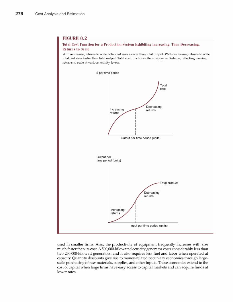
used in smaller firms. Also, the productivity of equipment frequently increases with sizemuch faster than its cost. A 500,000-kilowatt electricity generator costs considerably less thantwo 250,000-kilowatt generators, and it also requires less fuel and labor when operated atcapacity. Quantity discounts give rise to money-related pecuniary economies through large-scale purchasing of raw materials, supplies, and other inputs. These economies extend to thecost of capital when large firms have easy access to capital markets and can acquire funds atlower rates.
276 Part Three Production and Cost Analysis
FIGURE 8.2Total Cost Function for a Production System Exhibiting Increasing, Then Decreasing,Returns to ScaleWith increasing returns to scale, total cost rises slower than total output. With decreasing returns to scale,total cost rises faster than total output. Total cost functions often display an S-shape, reflecting varyingreturns to scale at various activity levels.
Output per time period (units)
$ per time period
Totalcost
DecreasingreturnsIncreasing
returns
Input per time period (units)
Output pertime period (units)
Total product
Decreasingreturns
Increasingreturns
276 Cost Analysis and Estimation
At some output level, economies of scale are typically exhausted, and average costs levelout and begin to rise. Increasing average costs at high output levels are often attributed tolimitations in the ability of management to coordinate large-scale organizations. Staff over-head also tends to grow more than proportionately with output, again raising unit costs. Thecurrent trend toward small to medium-sized businesses indicates that diseconomies limitfirm sizes in many industries.
Cost Elasticities and Economies of Scale It is often easy to calculate scale economies by considering cost elasticities. Cost elasticity, �C,measures the percentage change in total cost associated with a 1 percent change in output.
Algebraically, the elasticity of cost with respect to output is
�C = Percentage Change in Total Cost (TC)Percentage Change in Output (Q)
= ∆TC/TC∆Q/Q
= ∆TC�
Q∆Q TC
Cost elasticity is related to economies of scale as follows:
If Then Which Implies
Percentage change in TC < Percentage change in Q �C < 1 Economies of scale (decreasing AC)Percentage change in TC = Percentage change in Q �C = 1 No economies of scale (constant AC)Percentage change in TC > Percentage change in Q �C > 1 Diseconomies of scale (increasing AC)
With a cost elasticity of less than one (�C < 1), costs increase at a slower rate than output.Given constant input prices, this implies higher output-to-input ratios and economies ofscale. If �C = 1, output and costs increase proportionately, implying no economies of scale.Finally, if �C > 1, for any increase in output, costs increase by a greater relative amount,implying decreasing returns to scale. To prevent confusion concerning cost elasticity andreturns to scale, remember that an inverse relation holds between average costs and scaleeconomies but that a direct relation holds between resource usage and returns to scale. Thus,although �C < 1 implies falling AC and economies of scale, because costs are increasing moreslowly than output, recall from Chapter 7 that an output elasticity greater than 1 (�Q > 1)implies increasing returns to scale, because output is increasing faster than input usage.Similarly, diseconomies of scale are implied by �C > 1, diminishing returns are indicatedwhen �Q < 1.
Long-Run Average Costs Short-run cost curves relate costs and output for a specific scale of plant. Long-run costcurves identify the optimal scale of plant for each production level. Long-run average cost(LRAC) curves can be thought of as an envelope of short-run average cost (SRAC) curves.
This concept is illustrated in Figure 8.3, which shows four short-run average cost curvesrepresenting four different scales of plant. Each of the four plants has a range of output overwhich it is most efficient. Plant A, for example, provides the least-cost production system foroutput in the range 0 to Q1 units; plant B provides the least-cost system for output in the range
cost elasticity Percentage change intotal cost associatedwith a 1 percentchange in output
Chapter Eight Cost Analysis and Estimation 277
Cost Analysis and Estimation 277
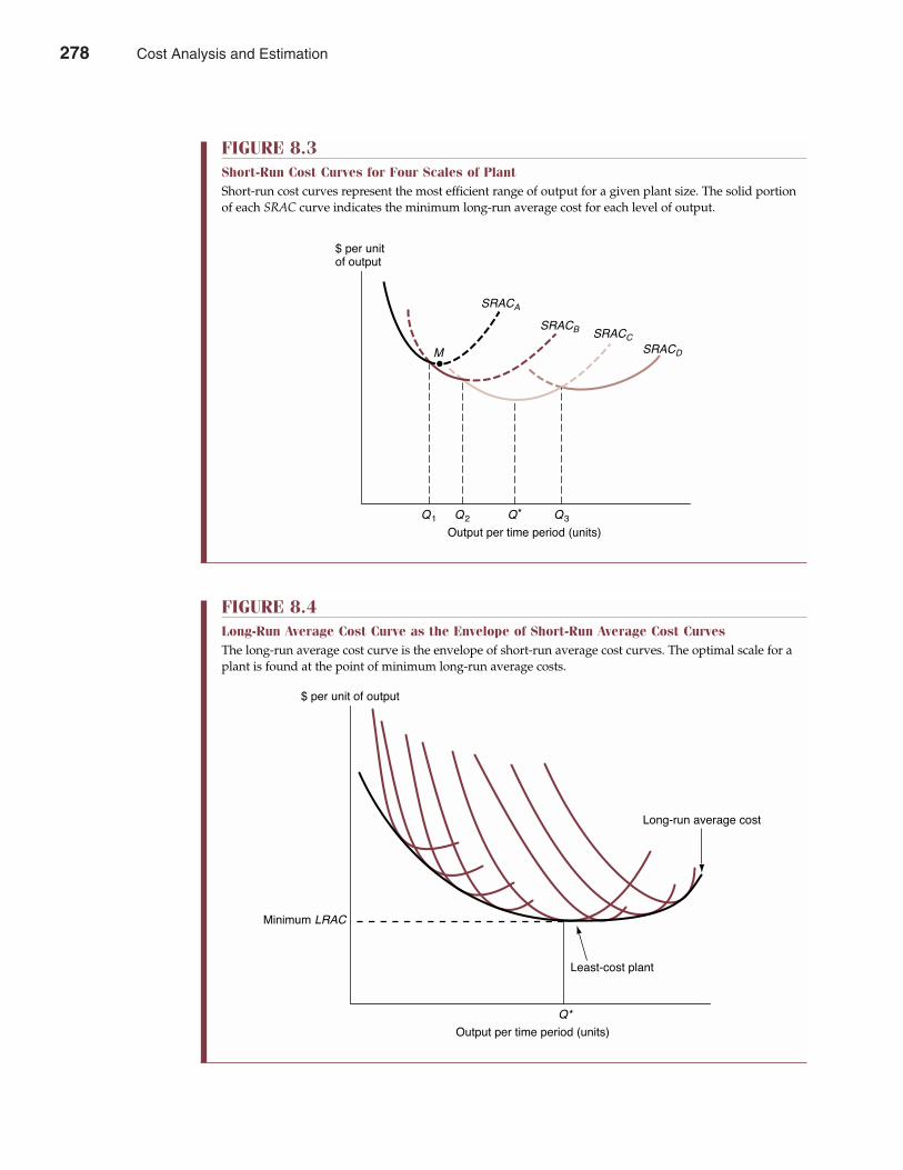
278 Part Three Production and Cost Analysis
FIGURE 8.3Short-Run Cost Curves for Four Scales of PlantShort-run cost curves represent the most efficient range of output for a given plant size. The solid portionof each SRAC curve indicates the minimum long-run average cost for each level of output.
Output per time period (units)
$ per unitof output
Q1 Q2 Q* Q3
M
SRACA
SRACB SRACCSRACD
FIGURE 8.4Long-Run Average Cost Curve as the Envelope of Short-Run Average Cost CurvesThe long-run average cost curve is the envelope of short-run average cost curves. The optimal scale for aplant is found at the point of minimum long-run average costs.
$ per unit of output
Least-cost plant
Long-run average cost
Output per time period (units)
Q*
Minimum LRAC
278 Cost Analysis and Estimation
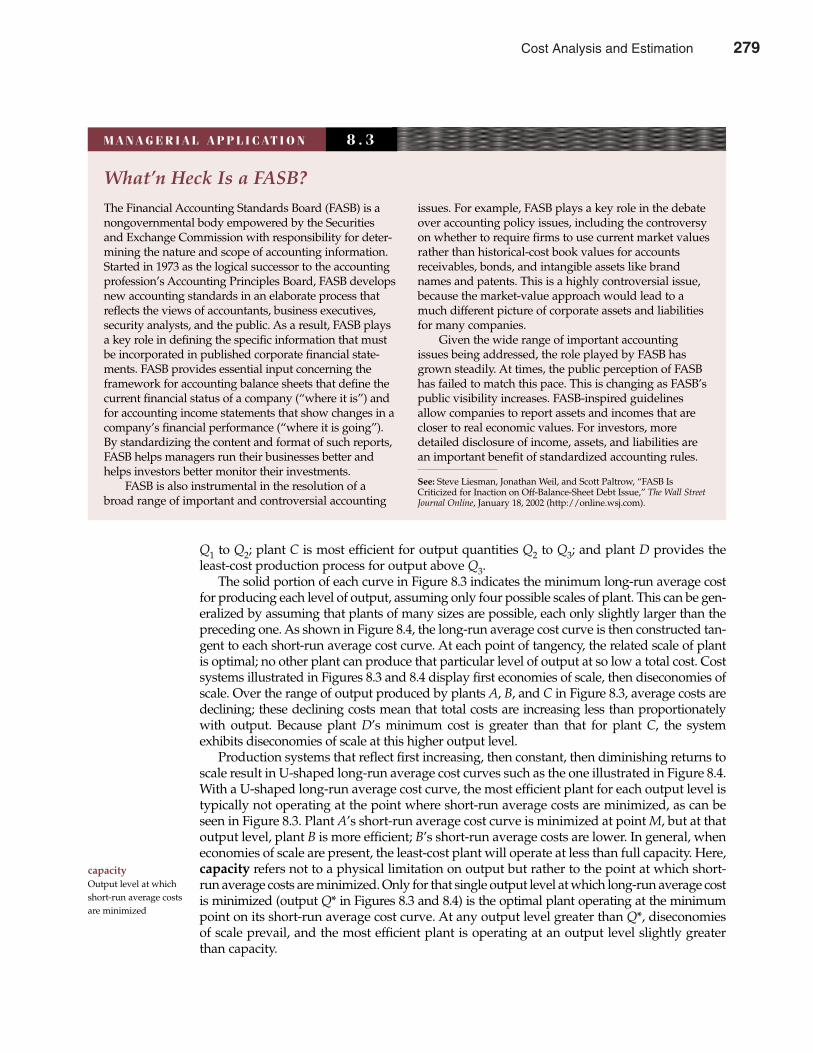
Q1 to Q2; plant C is most efficient for output quantities Q2 to Q3; and plant D provides theleast-cost production process for output above Q3.
The solid portion of each curve in Figure 8.3 indicates the minimum long-run average costfor producing each level of output, assuming only four possible scales of plant. This can be gen-eralized by assuming that plants of many sizes are possible, each only slightly larger than thepreceding one. As shown in Figure 8.4, the long-run average cost curve is then constructed tan-gent to each short-run average cost curve. At each point of tangency, the related scale of plantis optimal; no other plant can produce that particular level of output at so low a total cost. Costsystems illustrated in Figures 8.3 and 8.4 display first economies of scale, then diseconomies ofscale. Over the range of output produced by plants A, B, and C in Figure 8.3, average costs aredeclining; these declining costs mean that total costs are increasing less than proportionatelywith output. Because plant D’s minimum cost is greater than that for plant C, the systemexhibits diseconomies of scale at this higher output level.
Production systems that reflect first increasing, then constant, then diminishing returns toscale result in U-shaped long-run average cost curves such as the one illustrated in Figure 8.4.With a U-shaped long-run average cost curve, the most efficient plant for each output level istypically not operating at the point where short-run average costs are minimized, as can beseen in Figure 8.3. Plant A’s short-run average cost curve is minimized at point M, but at thatoutput level, plant B is more efficient; B’s short-run average costs are lower. In general, wheneconomies of scale are present, the least-cost plant will operate at less than full capacity. Here,capacity refers not to a physical limitation on output but rather to the point at which short-run average costs are minimized. Only for that single output level at which long-run average costis minimized (output Q* in Figures 8.3 and 8.4) is the optimal plant operating at the minimumpoint on its short-run average cost curve. At any output level greater than Q*, diseconomiesof scale prevail, and the most efficient plant is operating at an output level slightly greaterthan capacity.
capacity Output level at whichshort-run average costsare minimized
Chapter Eight Cost Analysis and Estimation 279
What’n Heck Is a FASB?
The Financial Accounting Standards Board (FASB) is anongovernmental body empowered by the Securitiesand Exchange Commission with responsibility for deter-mining the nature and scope of accounting information.Started in 1973 as the logical successor to the accountingprofession’s Accounting Principles Board, FASB developsnew accounting standards in an elaborate process thatreflects the views of accountants, business executives,security analysts, and the public. As a result, FASB playsa key role in defining the specific information that mustbe incorporated in published corporate financial state-ments. FASB provides essential input concerning theframework for accounting balance sheets that define thecurrent financial status of a company (“where it is”) andfor accounting income statements that show changes in acompany’s financial performance (“where it is going”).By standardizing the content and format of such reports,FASB helps managers run their businesses better andhelps investors better monitor their investments.
FASB is also instrumental in the resolution of abroad range of important and controversial accounting
issues. For example, FASB plays a key role in the debateover accounting policy issues, including the controversyon whether to require firms to use current market valuesrather than historical-cost book values for accountsreceivables, bonds, and intangible assets like brandnames and patents. This is a highly controversial issue,because the market-value approach would lead to amuch different picture of corporate assets and liabilitiesfor many companies.
Given the wide range of important accountingissues being addressed, the role played by FASB hasgrown steadily. At times, the public perception of FASBhas failed to match this pace. This is changing as FASB’spublic visibility increases. FASB-inspired guidelinesallow companies to report assets and incomes that arecloser to real economic values. For investors, moredetailed disclosure of income, assets, and liabilities arean important benefit of standardized accounting rules.
See: Steve Liesman, Jonathan Weil, and Scott Paltrow, “FASB IsCriticized for Inaction on Off-Balance-Sheet Debt Issue,” The Wall StreetJournal Online, January 18, 2002 (http://online.wsj.com).
M A N A G E R I A L A P P L I C AT I O N 8 . 3
Cost Analysis and Estimation 279

MINIMUM EFFICIENT SCALE
The number of competitors and ease of entry is typically greater in industries with U-shapedlong-run average cost curves than in those with L-shaped or downward-sloping long-runaverage cost curves. Insight on the competitive implications of cost/output relations can begained by considering the minimum efficient scale concept.
Competitive Implications of Minimum Efficient Scale Minimum efficient scale (MES) is the output level at which long-run average costs are min-imized. MES is at the minimum point on a U-shaped long-run average cost curve (output Q*in Figures 8.3 and 8.4) and at the corner of an L-shaped long-run average cost curve.
Generally speaking, competition is vigorous when MES is low relative to total industrydemand. This fact follows from the correspondingly low barriers to entry from capital invest-ment and skilled labor requirements. Competition can be less vigorous when MES is largerelative to total industry output because barriers to entry tend to be correspondingly highand can limit the number of potential competitors. When considering the competitiveimpact of MES, industry size must always be considered. Some industries are large enoughto accommodate many effective competitors. In such instances, even though MES is large inan absolute sense, it can be relatively small and allow vigorous competition.
When the cost disadvantage of operating plants that are of less than MES size is modest,there will seldom be serious anticompetitive consequences. The somewhat higher productioncosts of small producers can be overcome by superior customer service and regional locationto cut transport costs and delivery lags. In such instances, significant advantages to large-scaleoperation have little economic impact. Therefore, the barrier-to-entry effects of MES dependon the size of MES relative to industry demand and the slope of the long-run average cost curveat points of less-than-MES-size operations. Both must be considered.
Transportation Costs and MES Transportation costs include terminal, line-haul, and inventory charges associated with movingoutput from production facilities to customers. Terminal charges consist of handling expensesnecessary for loading and unloading shipped materials. Because terminal charges do not varywith the distance of shipment, they are as high for short hauls as for long hauls.
Line-haul expenses include equipment, labor, and fuel costs associated with moving prod-ucts a specified distance. They vary directly with the distance shipped. Although line-haulexpenses are relatively constant on a per-mile basis, they vary widely from one commodityto another. It costs more to ship a ton of fresh fruit 500 miles than to ship a ton of coal a similardistance. Fresh fruit comes in odd shapes and sizes and requires more container space perpound than a product like coal. Any product that is perishable, fragile, or particularly sus-ceptible to theft (e.g., consumer electronics, cigarettes, liquor) has high line-haul expensesbecause of greater equipment, insurance, and handling costs.
Finally, there is an inventory cost component to transportation costs related to the time ele-ment involved in shipping goods. The time required in transit is extremely important becauseslower modes such as railroads and barges delay the receipt of sale proceeds from customers.Even though out-of-pocket expenses are greater, air cargo or motor carrier shipments speeddelivery and can reduce the total economic costs of transporting goods to market.
As more output is produced at a given plant, it becomes necessary to reach out to more dis-tant customers. This can lead to increased transportation costs per unit sold. Figure 8.5 illustratesan L-shaped long-run average cost curve reflecting average production costs that first declineand then become nearly constant. Assuming relatively modest terminal and inventory costs,greater line-haul expenses cause transportation costs per unit to increase at a relatively constant
280 Part Three Production and Cost Analysis
minimum efficientscale Output level at whichlong-run average costsare minimized
280 Cost Analysis and Estimation
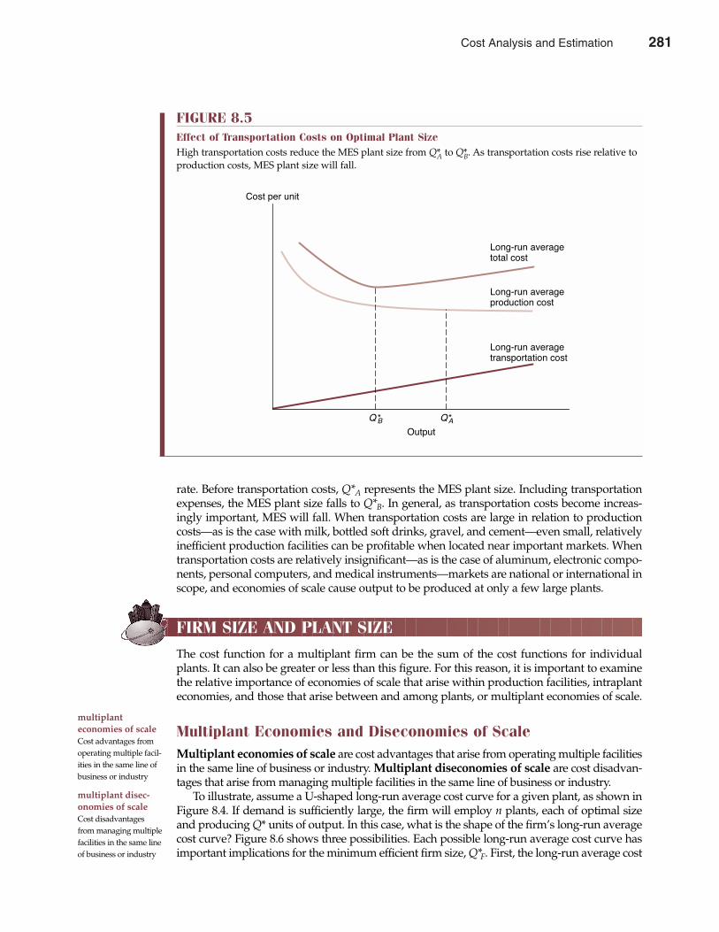
rate. Before transportation costs, Q*A represents the MES plant size. Including transportationexpenses, the MES plant size falls to Q*B. In general, as transportation costs become increas-ingly important, MES will fall. When transportation costs are large in relation to productioncosts—as is the case with milk, bottled soft drinks, gravel, and cement—even small, relativelyinefficient production facilities can be profitable when located near important markets. Whentransportation costs are relatively insignificant—as is the case of aluminum, electronic compo-nents, personal computers, and medical instruments—markets are national or international inscope, and economies of scale cause output to be produced at only a few large plants.
FIRM SIZE AND PLANT SIZE
The cost function for a multiplant firm can be the sum of the cost functions for individualplants. It can also be greater or less than this figure. For this reason, it is important to examinethe relative importance of economies of scale that arise within production facilities, intraplanteconomies, and those that arise between and among plants, or multiplant economies of scale.
Multiplant Economies and Diseconomies of Scale Multiplant economies of scale are cost advantages that arise from operating multiple facilitiesin the same line of business or industry. Multiplant diseconomies of scale are cost disadvan-tages that arise from managing multiple facilities in the same line of business or industry.
To illustrate, assume a U-shaped long-run average cost curve for a given plant, as shown inFigure 8.4. If demand is sufficiently large, the firm will employ n plants, each of optimal sizeand producing Q* units of output. In this case, what is the shape of the firm’s long-run averagecost curve? Figure 8.6 shows three possibilities. Each possible long-run average cost curve hasimportant implications for the minimum efficient firm size, Q*F. First, the long-run average cost
multiplanteconomies of scale Cost advantages fromoperating multiple facil-ities in the same line ofbusiness or industry
multiplant disec-onomies of scale Cost disadvantagesfrom managing multiplefacilities in the same lineof business or industry
Chapter Eight Cost Analysis and Estimation 281
FIGURE 8.5Effect of Transportation Costs on Optimal Plant SizeHigh transportation costs reduce the MES plant size from Q*A to Q*B. As transportation costs rise relative toproduction costs, MES plant size will fall.
Output
Q*AQ *B
Long-run averagetransportation cost
Long-run averageproduction cost
Long-run averagetotal cost
Cost per unit
Cost Analysis and Estimation 281
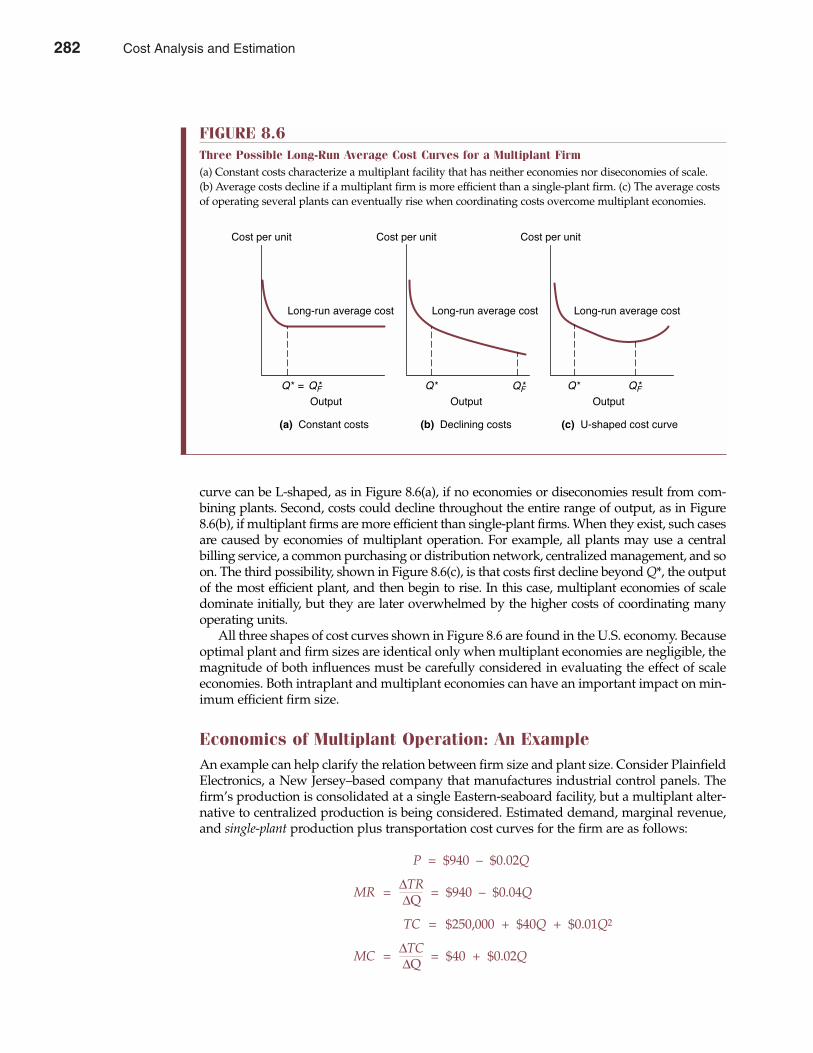
curve can be L-shaped, as in Figure 8.6(a), if no economies or diseconomies result from com-bining plants. Second, costs could decline throughout the entire range of output, as in Figure8.6(b), if multiplant firms are more efficient than single-plant firms. When they exist, such casesare caused by economies of multiplant operation. For example, all plants may use a centralbilling service, a common purchasing or distribution network, centralized management, and soon. The third possibility, shown in Figure 8.6(c), is that costs first decline beyond Q*, the outputof the most efficient plant, and then begin to rise. In this case, multiplant economies of scaledominate initially, but they are later overwhelmed by the higher costs of coordinating manyoperating units.
All three shapes of cost curves shown in Figure 8.6 are found in the U.S. economy. Becauseoptimal plant and firm sizes are identical only when multiplant economies are negligible, themagnitude of both influences must be carefully considered in evaluating the effect of scaleeconomies. Both intraplant and multiplant economies can have an important impact on min-imum efficient firm size.
Economics of Multiplant Operation: An Example An example can help clarify the relation between firm size and plant size. Consider PlainfieldElectronics, a New Jersey–based company that manufactures industrial control panels. Thefirm’s production is consolidated at a single Eastern-seaboard facility, but a multiplant alter-native to centralized production is being considered. Estimated demand, marginal revenue,and single-plant production plus transportation cost curves for the firm are as follows:
P = $940 – $0.02Q
MR = ∆TR = $940 – $0.04Q∆Q
TC = $250,000 + $40Q + $0.01Q2
MC = ∆TC = $40 + $0.02Q∆Q
282 Part Three Production and Cost Analysis
FIGURE 8.6Three Possible Long-Run Average Cost Curves for a Multiplant Firm(a) Constant costs characterize a multiplant facility that has neither economies nor diseconomies of scale. (b) Average costs decline if a multiplant firm is more efficient than a single-plant firm. (c) The average costsof operating several plants can eventually rise when coordinating costs overcome multiplant economies.
(a) Constant costs
Long-run average cost Long-run average cost
Cost per unit Cost per unit Cost per unit
(b) Declining costs (c) U-shaped cost curve
Long-run average cost
Output Output Output
QF* Q*Q*Q* = QF* QF*
282 Cost Analysis and Estimation

Plainfield’s total profit function is
π = TR – TC
= P � Q – TC
= ($940 – $0.02Q)Q – $250,000 – $40Q – $0.01Q2
= –$0.03Q2 + $900Q – $250,000
The profit-maximizing activity level with centralized production is the output level at whichMπ = MR – MC = 0 and, therefore, MR = MC.
Setting marginal revenue equal to marginal cost and solving for the related output quan-tity gives
MR = MC
$940 – $0.04Q = $40Q + $0.02Q
$0.06Q = $900 Q = 15,000
At Q = 15,000,
P = $940 - $0.02Q
= $940 – $0.02(15,000) = $640
and
π = –$0.03(15,000)2 + $900(15,000) – $250,000 = $6,500,000
Therefore, profits are maximized at the Q = 15,000 output level under the assumption of cen-tralized production. At that activity level, MC = MR = $640, and Mπ = 0.
To gain insight regarding the possible advantages of operating multiple smaller plants, theaverage cost function for a single plant must be examined. To simplify matters, assume thatmultiplant production is possible under the same cost conditions described previously. Alsoassume that there are no other multiplant economies or diseconomies of scale.
The activity level at which average cost is minimized is found by setting marginal cost equalto average cost and solving for Q:
AC = TC/Q
= ($250,000 + $40Q + $0.01Q2)/Q
= $250,000Q–1 + $40 + $0.01Q
and
MC = AC
$40 + $0.02Q = $250,000Q–1 + $40 + $0.01Q
250,000Q–1 = 0.01Q
Q2 = 250,0000.01
Q = √25,000,000= 5,000
Chapter Eight Cost Analysis and Estimation 283
Cost Analysis and Estimation 283
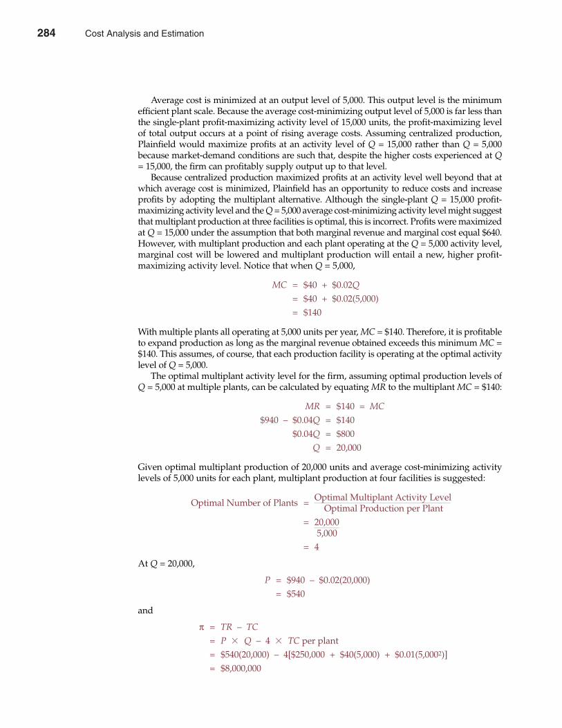
Average cost is minimized at an output level of 5,000. This output level is the minimumefficient plant scale. Because the average cost-minimizing output level of 5,000 is far less thanthe single-plant profit-maximizing activity level of 15,000 units, the profit-maximizing levelof total output occurs at a point of rising average costs. Assuming centralized production,Plainfield would maximize profits at an activity level of Q = 15,000 rather than Q = 5,000because market-demand conditions are such that, despite the higher costs experienced at Q= 15,000, the firm can profitably supply output up to that level.
Because centralized production maximized profits at an activity level well beyond that atwhich average cost is minimized, Plainfield has an opportunity to reduce costs and increaseprofits by adopting the multiplant alternative. Although the single-plant Q = 15,000 profit-maximizing activity level and the Q = 5,000 average cost-minimizing activity level might suggestthat multiplant production at three facilities is optimal, this is incorrect. Profits were maximizedat Q = 15,000 under the assumption that both marginal revenue and marginal cost equal $640.However, with multiplant production and each plant operating at the Q = 5,000 activity level,marginal cost will be lowered and multiplant production will entail a new, higher profit-maximizing activity level. Notice that when Q = 5,000,
MC = $40 + $0.02Q
= $40 + $0.02(5,000) = $140
With multiple plants all operating at 5,000 units per year, MC = $140. Therefore, it is profitableto expand production as long as the marginal revenue obtained exceeds this minimum MC =$140. This assumes, of course, that each production facility is operating at the optimal activitylevel of Q = 5,000.
The optimal multiplant activity level for the firm, assuming optimal production levels ofQ = 5,000 at multiple plants, can be calculated by equating MR to the multiplant MC = $140:
MR = $140 = MC
$940 – $0.04Q = $140 $0.04Q = $800
Q = 20,000
Given optimal multiplant production of 20,000 units and average cost-minimizing activitylevels of 5,000 units for each plant, multiplant production at four facilities is suggested:
Optimal Number of Plants = Optimal Multiplant Activity LevelOptimal Production per Plant
= 20,0005,000
= 4
At Q = 20,000,
P = $940 – $0.02(20,000) = $540
and
π = TR – TC
= P � Q – 4 � TC per plant = $540(20,000) – 4[$250,000 + $40(5,000) + $0.01(5,0002)] = $8,000,000
284 Part Three Production and Cost Analysis
284 Cost Analysis and Estimation
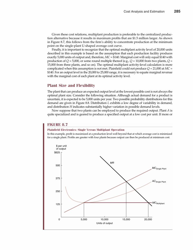
Given these cost relations, multiplant production is preferable to the centralized produc-tion alternative because it results in maximum profits that are $1.5 million larger. As shownin Figure 8.7, this follows from the firm’s ability to concentrate production at the minimumpoint on the single-plant U-shaped average cost curve.
Finally, it is important to recognize that the optimal multiplant activity level of 20,000 unitsdescribed in this example is based on the assumption that each production facility producesexactly 5,000 units of output and, therefore, MC = $140. Marginal cost will only equal $140 withproduction of Q = 5,000, or some round multiple thereof (e.g., Q = 10,000 from two plants, Q =15,000 from three plants, and so on). The optimal multiplant activity-level calculation is morecomplicated when this assumption is not met. Plainfield could not produce Q = 21,000 at MC =$140. For an output level in the 20,000 to 25,000 range, it is necessary to equate marginal revenuewith the marginal cost of each plant at its optimal activity level.
Plant Size and Flexibility The plant that can produce an expected output level at the lowest possible cost is not always theoptimal plant size. Consider the following situation. Although actual demand for a product isuncertain, it is expected to be 5,000 units per year. Two possible probability distributions for thisdemand are given in Figure 8.8. Distribution L exhibits a low degree of variability in demand,and distribution H indicates substantially higher variation in possible demand levels.
Now suppose that two plants can be employed to produce the required output. Plant A isquite specialized and is geared to produce a specified output at a low cost per unit. If more or
Chapter Eight Cost Analysis and Estimation 285
FIGURE 8.7Plainfield Electronics: Single Versus Multiplant OperationIn this example, profit is maximized at a production level well beyond that at which average cost is minimizedfor a single plant. Profits are greater with four plants because output can then be produced at minimum cost.
0
125
250
375
500
$625
5,000 10,000 15,000 20,000
Units of output
MCMultiplant
ACSingle Plant
MCSingle Plant
MR
$ per unitof output
Cost Analysis and Estimation 285
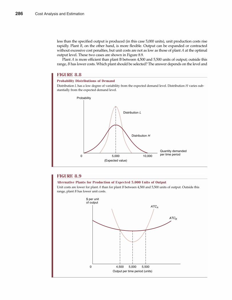
less than the specified output is produced (in this case 5,000 units), unit production costs riserapidly. Plant B, on the other hand, is more flexible. Output can be expanded or contractedwithout excessive cost penalties, but unit costs are not as low as those of plant A at the optimaloutput level. These two cases are shown in Figure 8.9.
Plant A is more efficient than plant B between 4,500 and 5,500 units of output; outside thisrange, B has lower costs. Which plant should be selected? The answer depends on the level and
286 Part Three Production and Cost Analysis
FIGURE 8.8Probability Distributions of DemandDistribution L has a low degree of variability from the expected demand level. Distribution H varies sub-stantially from the expected demand level.
Distribution L
Distribution H
Quantity demandedper time period
(Expected value)
5,000 10,0000
Probability
FIGURE 8.9Alternative Plants for Production of Expected 5,000 Units of OutputUnit costs are lower for plant A than for plant B between 4,500 and 5,500 units of output. Outside thisrange, plant B has lower unit costs.
4,500 5,000 5,500
Output per time period (units)
ATCB
ATCA
$ per unitof output
0
286 Cost Analysis and Estimation
variability of expected average total costs. If the demand probability distribution with lowvariation, distribution L, is correct, the more specialized facility is optimal. If probability dis-tribution H more correctly describes the demand situation, the lower minimum cost of morespecialized facilities is more than offset by the possibility of very high costs of producing outsidethe 4,500- to 5,500-unit range. Plant B could then have lower expected costs or a more attractivecombination of expected costs and potential variation.
LEARNING CURVES
For many manufacturing processes, average costs decline substantially as cumulative total out-put increases. Improvements in the use of production equipment and procedures are importantin this process, as are reduced waste from defects and decreased labor requirements as workersbecome more proficient in their jobs.
Learning Curve Concept When knowledge gained from manufacturing experience is used to improve production meth-ods, the resulting decline in average costs is said to reflect the effects of the firm’s learning curve.The learning curve or experience curve phenomenon affects average costs in a way similar to thatfor any technical advance that improves productive efficiency. Both involve a downward shift inthe long-run average cost curve at all levels of output. Learning through production experiencepermits the firm to produce output more efficiently at each and every output level.
To illustrate, consider Figure 8.10, which shows hypothetical long-run average cost curvesfor periods t and t + 1. With increased knowledge about production methods gained throughthe experience of producing Qt units in period t, long-run average costs have declined for
learning curve Average cost reductionover time due to pro-duction experience
Chapter Eight Cost Analysis and Estimation 287
Bigger Isn’t Always Better
When economies of scale are substantial, larger firms areable to achieve lower costs of production or distributionthan their smaller rivals. These cost advantages translateinto higher and more stable profits and a permanent com-petitive advantage for larger firms in some industries.When diseconomies of scale are operative, larger firmssuffer a cost disadvantage when compared to their smallerrivals. Smaller firms are then able to translate the benefitsof small size into a distinct competitive advantage.
In general, industries dominated by large firms tendto be those in which there are significant economies ofscale, important advantages to vertical integration, and aprevalence of mass marketing. As a result, large organiza-tions with sprawling plants emphasize large quantities ofoutput at low production costs. Use of national media,especially TV advertising, is common. In contrast, indus-tries in which “small is beautiful” tend to be those charac-terized by diseconomies of scale, considerable advantagesto subcontracting for “just in time” assembly and manu-facturing, and niche marketing that emphasizes the use ofhighly skilled individuals adept at personal selling. Smallfactories with flexible production schedules are common.
Rather than mass quantity, many smaller companiesemphasize quality. Instead of the sometimes slow-to-respond hierarchical organizations of large companies,smaller companies feature “flat” organizations withdecentralized decision making and authority.
Even though the concept of diseconomies of largesize is well known, it is sometimes not appreciated howcommon the phenomenon is in actual practice. Manysectors of industrial manufacturing have found that thehighly flexible and customer-sensitive nature of smallercompanies can lead to distinct competitive advantages.The villain sometimes encountered by large-scale firms isnot any diseconomy of scale in the production processitself, but rather the burden that size places on effectivemanagement. Big often means complex, and complexityresults in inefficiencies and bureaucratic snarls that canstrangle effective communication.
See: Dow Jones Newswires, “Arbitrage Spreads on Pending Mergersand Acquisitions,” The Wall Street Journal Online, January 18, 2002(http://online.wsj.com).
M A N A G E R I A L A P P L I C AT I O N 8 . 4
Cost Analysis and Estimation 287
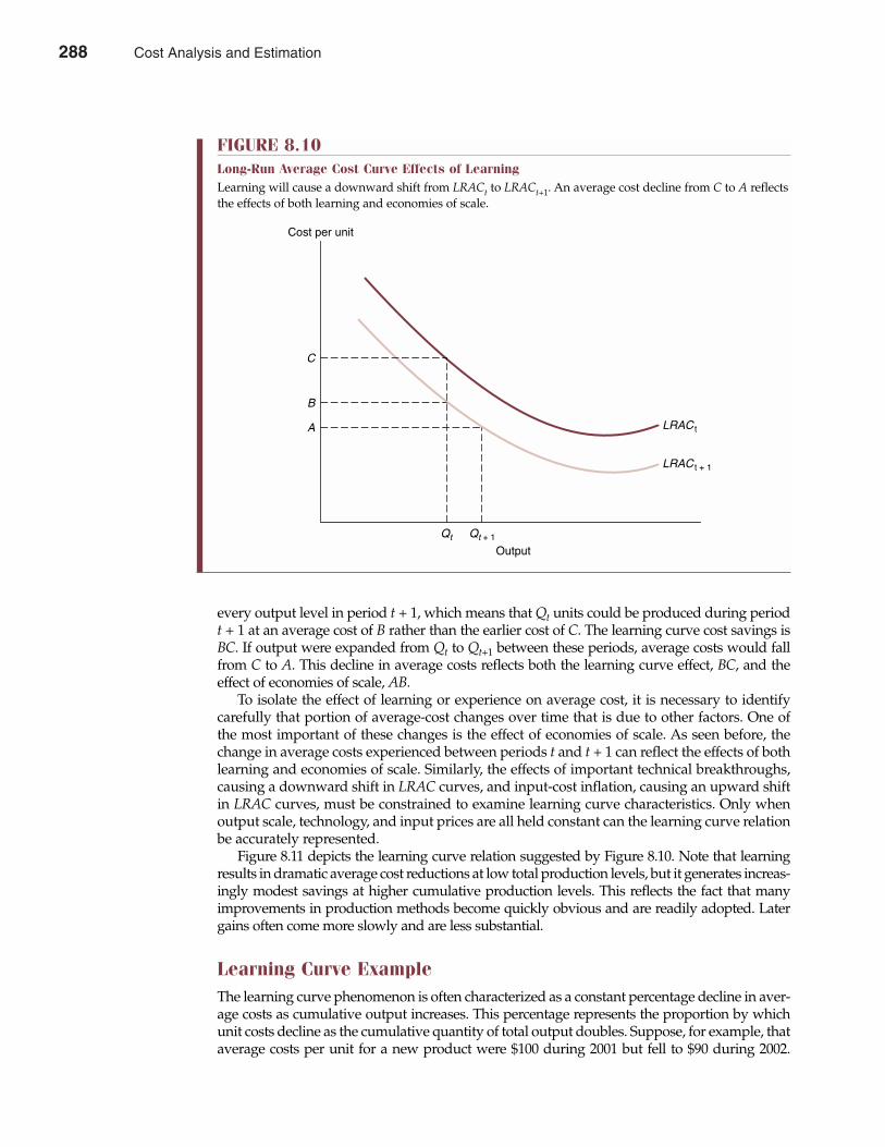
every output level in period t + 1, which means that Qt units could be produced during periodt + 1 at an average cost of B rather than the earlier cost of C. The learning curve cost savings isBC. If output were expanded from Qt to Qt+1 between these periods, average costs would fallfrom C to A. This decline in average costs reflects both the learning curve effect, BC, and theeffect of economies of scale, AB.
To isolate the effect of learning or experience on average cost, it is necessary to identifycarefully that portion of average-cost changes over time that is due to other factors. One ofthe most important of these changes is the effect of economies of scale. As seen before, thechange in average costs experienced between periods t and t + 1 can reflect the effects of bothlearning and economies of scale. Similarly, the effects of important technical breakthroughs,causing a downward shift in LRAC curves, and input-cost inflation, causing an upward shiftin LRAC curves, must be constrained to examine learning curve characteristics. Only whenoutput scale, technology, and input prices are all held constant can the learning curve relationbe accurately represented.
Figure 8.11 depicts the learning curve relation suggested by Figure 8.10. Note that learningresults in dramatic average cost reductions at low total production levels, but it generates increas-ingly modest savings at higher cumulative production levels. This reflects the fact that manyimprovements in production methods become quickly obvious and are readily adopted. Latergains often come more slowly and are less substantial.
Learning Curve Example The learning curve phenomenon is often characterized as a constant percentage decline in aver-age costs as cumulative output increases. This percentage represents the proportion by whichunit costs decline as the cumulative quantity of total output doubles. Suppose, for example, thataverage costs per unit for a new product were $100 during 2001 but fell to $90 during 2002.
288 Part Three Production and Cost Analysis
FIGURE 8.10Long-Run Average Cost Curve Effects of LearningLearning will cause a downward shift from LRACt to LRACt+1. An average cost decline from C to A reflectsthe effects of both learning and economies of scale.
Cost per unit
C
B
A
Qt Qt + 1
Output
LRAC t + 1
LRAC t
288 Cost Analysis and Estimation
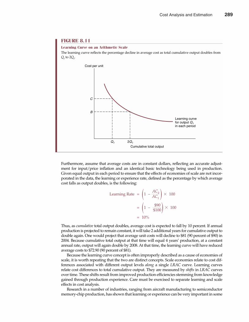
Furthermore, assume that average costs are in constant dollars, reflecting an accurate adjust-ment for input/price inflation and an identical basic technology being used in production.Given equal output in each period to ensure that the effects of economies of scale are not incor-porated in the data, the learning or experience rate, defined as the percentage by which averagecost falls as output doubles, is the following:
Learning Rate = 1 –AC2 � 100� AC1 �
= 1 – $90 � 100� $100�
= 10%
Thus, as cumulative total output doubles, average cost is expected to fall by 10 percent. If annualproduction is projected to remain constant, it will take 2 additional years for cumulative output todouble again. One would project that average unit costs will decline to $81 (90 percent of $90) in2004. Because cumulative total output at that time will equal 4 years’ production, at a constantannual rate, output will again double by 2008. At that time, the learning curve will have reducedaverage costs to $72.90 (90 percent of $81).
Because the learning curve concept is often improperly described as a cause of economies ofscale, it is worth repeating that the two are distinct concepts. Scale economies relate to cost dif-ferences associated with different output levels along a single LRAC curve. Learning curvesrelate cost differences to total cumulative output. They are measured by shifts in LRAC curvesover time. These shifts result from improved production efficiencies stemming from knowledgegained through production experience. Care must be exercised to separate learning and scaleeffects in cost analysis.
Research in a number of industries, ranging from aircraft manufacturing to semiconductormemory-chip production, has shown that learning or experience can be very important in some
Chapter Eight Cost Analysis and Estimation 289
FIGURE 8.11Learning Curve on an Arithmetic ScaleThe learning curve reflects the percentage decline in average cost as total cumulative output doubles fromQt to 2Qt.
Cumulative total output
Learning curvefor output Qtin each period
Qt 2Qt
C
Cost per unit
B
Cost Analysis and Estimation 289

production systems. Learning or experience rates of 20 percent to 30 percent are sometimesreported. These high learning rates imply rapidly declining manufacturing costs as cumulativetotal output increases. It should be noted, however, that many learning curve studies fail toaccount adequately for the expansion of production. Therefore, reported learning or experiencerates sometimes include the effects of both learning and economies of scale. Nevertheless, man-agers in a wide variety of industries have found that the learning curve concept has considerablestrategic implications.
Strategic Implications of the Learning Curve Concept What makes the learning curve phenomenon important for competitive strategy is its possiblecontribution to achieving and maintaining a dominant position in a given market. By virtue oftheir large relative volume, dominant firms have greater opportunity for learning than dosmaller, nonleading firms. In some instances, the market share leader is able to drive down itsaverage cost curve faster than its competitors, underprice them, and permanently maintain aleadership position. Nonleading firms face an important and perhaps insurmountable barrierto relative improvement in performance. Where the learning curve advantages of leadingfirms are important, it may be prudent to relinquish nonleading positions and redeploy assetsto markets in which a dominant position can be achieved or maintained.
A classic example illustrating the successful use of the learning curve concept is Dallas–based Texas Instruments (TI). TI’s main business is producing semiconductor chips, which arekey components used to store information in computers and a wide array of electronic products.With growing applications for computers and “intelligent” electronics, the demand for semicon-ductors is expanding rapidly. Some years ago, TI was one of a number of leading semiconductormanufacturers. At this early stage in the development of the industry, TI made the decision toprice its semiconductors well below then-current production costs, given expected learning curveadvantages in the 20 percent range. TI’s learning curve strategy proved spectacularly successful.With low prices, volume increased dramatically. Because TI was making so many chips, averagecosts were even lower than anticipated; it could price below the competition; and dozens ofcompetitors were knocked out of the world market. Given a relative cost advantage and strictquality controls, TI rapidly achieved a position of dominant leadership in a market that becamea source of large and rapidly growing profits.
To play an important role in competitive strategy, learning must be significant. Cost savingsof 20 percent to 30 percent as cumulative output doubles must be possible. If only modest effectsof learning are present, product quality or customer service often plays a greater role in deter-mining firm success. Learning is also apt to be more important in industries with an abundanceof new products or new production techniques rather than in mature industries with well-known production methods. Similarly, learning tends to be important in industries with stan-dardized products and competition based on price rather than product variety or service.Finally, the beneficial effects of learning are realized only when management systems tightlycontrol costs and monitor potential sources of increased efficiency. Continuous feedback ofinformation between production and management personnel is essential.
ECONOMIES OF SCOPE Cost analysis focuses not just on how much to produce but also on what combination ofproducts to offer. By virtue of their efficiency in the production of a given product, firmsoften enjoy cost advantages in the production of related products.
Economies of Scope Concept Economies of scope exist when the cost of joint production is less than the cost of produc-ing multiple outputs separately. A firm will produce products that are complementary in the
290 Part Three Production and Cost Analysis
economies of scope Cost reduction fromproducing complemen-tary products
290 Cost Analysis and Estimation
sense that producing them together costs less than producing them individually. Supposethat a regional airline offers regularly scheduled passenger service between midsize citypairs and that it expects some excess capacity. Also assume that there is a modest localdemand for air parcel and small-package delivery service. Given current airplane sizes andconfigurations, it is often less costly for a single carrier to provide both passenger and cargoservices in small regional markets than to specialize in one or the other. Regional air carriersoften provide both services. This is an example of economies of scope. Other examples ofscope economies abound in the provision of both goods and services. In fact, the economiesof scope concept explains why firms typically produce multiple products.
Studying economies of scope forces management to consider both direct and indirectbenefits associated with individual lines of business. For example, some financial servicesfirms regard checking accounts and money market mutual funds as “loss leaders.” Whenone considers just the revenues and costs associated with marketing and offering checkingservices or running a money market mutual fund, they may just break even or yield only amarginal profit. However, successful firms like Dreyfus, Fidelity, and Merrill Lynch correctlyevaluate the profitability of their money market mutual funds within the context of overalloperations. These funds are a valuable delivery vehicle for a vast array of financial prod-ucts and services. By offering money market funds on an attractive basis, financial servicescompanies establish a working relation with an ideal group of prospective customers forstocks, bonds, and other investments. When viewed as a delivery vehicle or marketingdevice, money market mutual funds may be one of the industry’s most profitable financialproduct lines.
Exploiting Scope Economies Economies of scope are important because they permit a firm to translate superior skill in agiven product line into unique advantages in the production of complementary products.Effective competitive strategy often emphasizes the development or extension of product linesrelated to a firm’s current stars, or areas of recognized strength.
For example, PepsiCo, Inc., has long been a leader in the soft drink market. Over time, thecompany has gradually broadened its product line to include various brands of regular anddiet soft drinks, Gatorade, Tropicana, Fritos and Doritos chips, Grandma’s Cookies, and othersnack foods. PepsiCo can no longer be considered just a soft drink manufacturer. It is a widelydiversified beverages and snack foods company for whom well over one-half of total currentprofits come from non–soft drink lines. PepsiCo’s snack foods and sport drink product lineextension strategy was effective because it capitalized on the distribution network and mar-keting expertise developed in the firm’s soft drink business. In the case of PepsiCo, soft drinks,snack foods and sports beverages are a natural fit and a good example of how a firm has beenable to take the skills gained in developing one star (soft drinks) and use them to develop others(snack foods, sport drinks).
The economies of scope concept offers a useful means for evaluating the potential of currentand prospective lines of business. It naturally leads to definition of those areas in which the firmhas a comparative advantage and its greatest profit potential.
COST-VOLUME-PROFIT ANALYSIS
Cost-volume-profit analysis, sometimes called breakeven analysis, is an important ana-lytical technique used to study relations among costs, revenues, and profits. Both graphicand algebraic methods are employed. For simple problems, simple graphic methods workbest. In more complex situations, analytic methods, possibly involving spreadsheet softwareprograms, are preferable.
cost-volume-profitanalysis Analytical techniqueused to study relationsamong costs, revenues,and profits
Chapter Eight Cost Analysis and Estimation 291
Cost Analysis and Estimation 291
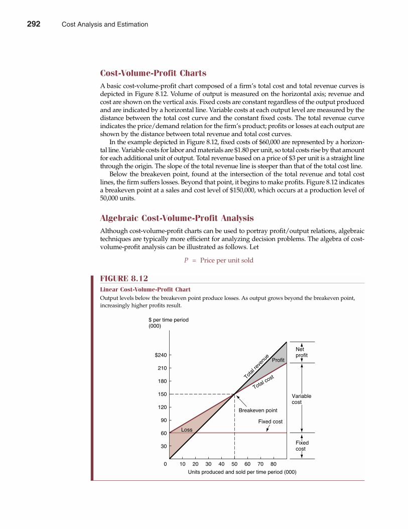
Cost-Volume-Profit Charts A basic cost-volume-profit chart composed of a firm’s total cost and total revenue curves isdepicted in Figure 8.12. Volume of output is measured on the horizontal axis; revenue andcost are shown on the vertical axis. Fixed costs are constant regardless of the output producedand are indicated by a horizontal line. Variable costs at each output level are measured by thedistance between the total cost curve and the constant fixed costs. The total revenue curveindicates the price/demand relation for the firm’s product; profits or losses at each output areshown by the distance between total revenue and total cost curves.
In the example depicted in Figure 8.12, fixed costs of $60,000 are represented by a horizon-tal line. Variable costs for labor and materials are $1.80 per unit, so total costs rise by that amountfor each additional unit of output. Total revenue based on a price of $3 per unit is a straight linethrough the origin. The slope of the total revenue line is steeper than that of the total cost line.
Below the breakeven point, found at the intersection of the total revenue and total costlines, the firm suffers losses. Beyond that point, it begins to make profits. Figure 8.12 indicatesa breakeven point at a sales and cost level of $150,000, which occurs at a production level of50,000 units.
Algebraic Cost-Volume-Profit Analysis Although cost-volume-profit charts can be used to portray profit/output relations, algebraictechniques are typically more efficient for analyzing decision problems. The algebra of cost-volume-profit analysis can be illustrated as follows. Let
P = Price per unit sold
292 Part Three Production and Cost Analysis
FIGURE 8.12Linear Cost-Volume-Profit ChartOutput levels below the breakeven point produce losses. As output grows beyond the breakeven point,increasingly higher profits result.
$240
210
180
150
120
90
60
30
0 10 20 30 40 50 60 70 80
$ per time period(000)
Netprofit
Variablecost
Fixedcost
Fixed cost
Breakeven point
Total revenue
Total
cost
Profit
Loss
Units produced and sold per time period (000)
292 Cost Analysis and Estimation
Q = Quantity produced and sold TFC = Total fixed costs AVC = Average variable cost
πC = Profit contribution
On a per-unit basis, profit contribution equals price minus average variable cost (πC = P – AVC).Profit contribution can be applied to cover fixed costs and then to provide profits. It is the foun-dation of cost-volume-profit analysis.
One useful application of cost-volume-profit analysis lies in the determination of breakevenactivity levels. A breakeven quantity is a zero profit activity level. At breakeven quantity levels,total revenue (P � Q) exactly equals total costs (TFC + AVC � Q):
Total Revenue = Total Cost P � Q = TFC + AVC � Q
(P – AVC)Q = TFC
It follows that breakeven quantity levels occur where
QBE = TFC
(8.6)P – AVC
= TFCπC
Thus, breakeven quantity levels are found by dividing the per-unit profit contribution into totalfixed costs. In the example illustrated in Figure 8.12, P = $3, AVC = $1.80, and TFC = $60,000.Profit contribution is $1.20 (= $3.00 – $1.80), and the breakeven quantity is
Q = $60,000$1.20
= 50,000 units
Textbook Publishing: A Cost-Volume-Profit Example The textbook publishing business provides a good illustration of the effective use of cost-volume-profit analysis for new product decisions. Consider the hypothetical cost-volume-profitanalysis data shown in Table 8.2. Fixed costs of $100,000 can be estimated quite accurately.Variable costs are linear and set by contract. List prices are variable, but competition keepsprices within a sufficiently narrow range to make a linear total revenue curve reasonable.Variable costs for the proposed book are $92 a copy, and the price is $100. This means thateach copy sold provides $8 in profit contribution. Applying the breakeven formula fromEquation 8.6, the breakeven sales volume is 12,500 units, calculated as
Q = $100,000$8
= 12,500 units
Publishers evaluate the size of the total market for a given book, competition, and other fac-tors. With these data in mind, they estimate the probability that a given book will reach orexceed the breakeven point. If the publisher estimates that the book will neither meet norexceed the breakeven point, they may consider cutting production costs by reducing the
breakeven quantity A zero profit activitylevel
Chapter Eight Cost Analysis and Estimation 293
Cost Analysis and Estimation 293
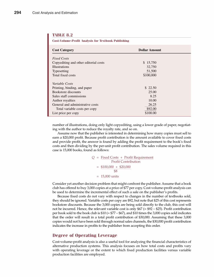
number of illustrations, doing only light copyediting, using a lower grade of paper, negotiat-ing with the author to reduce the royalty rate, and so on.
Assume now that the publisher is interested in determining how many copies must sell toearn a $20,000 profit. Because profit contribution is the amount available to cover fixed costsand provide profit, the answer is found by adding the profit requirement to the book’s fixedcosts and then dividing by the per-unit profit contribution. The sales volume required in thiscase is 15,000 books, found as follows:
Q = Fixed Costs + Profit RequirementProfit Contribution
= $100,000 + $20,000$8
= 15,000 units
Consider yet another decision problem that might confront the publisher. Assume that a bookclub has offered to buy 3,000 copies at a price of $77 per copy. Cost-volume-profit analysis canbe used to determine the incremental effect of such a sale on the publisher’s profits.
Because fixed costs do not vary with respect to changes in the number of textbooks sold,they should be ignored. Variable costs per copy are $92, but note that $25 of this cost representsbookstore discounts. Because the 3,000 copies are being sold directly to the club, this cost willnot be incurred. Hence, the relevant variable cost is only $67 (= $92 – $25). Profit contributionper book sold to the book club is $10 (= $77 – $67), and $10 times the 3,000 copies sold indicatesthat the order will result in a total profit contribution of $30,000. Assuming that these 3,000copies would not have been sold through normal sales channels, the $30,000 profit contributionindicates the increase in profits to the publisher from accepting this order.
Degree of Operating Leverage Cost-volume-profit analysis is also a useful tool for analyzing the financial characteristics ofalternative production systems. This analysis focuses on how total costs and profits varywith operating leverage or the extent to which fixed production facilities versus variableproduction facilities are employed.
294 Part Three Production and Cost Analysis
TABLE 8.2Cost-Volume-Profit Analysis for Textbook Publishing
Cost Category Dollar Amount
Fixed CostsCopyediting and other editorial costs $ 15,750Illustrations 32,750Typesetting 51,500Total fixed costs $100,000
Variable CostsPrinting, binding, and paper $ 22.50Bookstore discounts 25.00Sales staff commissions 8.25Author royalties 10.00General and administrative costs 26.25
Total variable costs per copy $92.00List price per copy $100.00
294 Cost Analysis and Estimation
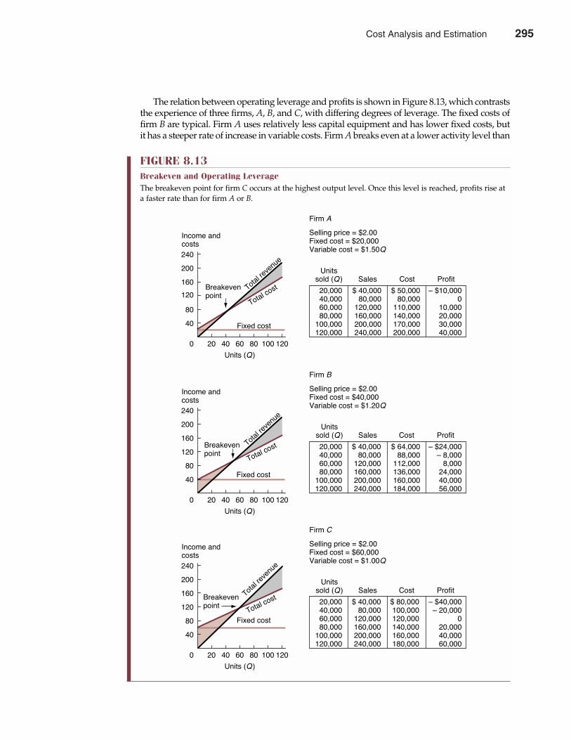
The relation between operating leverage and profits is shown in Figure 8.13, which contraststhe experience of three firms, A, B, and C, with differing degrees of leverage. The fixed costs offirm B are typical. Firm A uses relatively less capital equipment and has lower fixed costs, butit has a steeper rate of increase in variable costs. Firm A breaks even at a lower activity level than
Chapter Eight Cost Analysis and Estimation 295
FIGURE 8.13Breakeven and Operating LeverageThe breakeven point for firm C occurs at the highest output level. Once this level is reached, profits rise ata faster rate than for firm A or B.
Selling price = $2.00Fixed cost = $20,000Variable cost = $1.50Q
Sales Cost ProfitUnits
sold (Q )
20,00040,00060,00080,000
100,000120,000
$ 40,00080,000
120,000160,000200,000240,000
$ 50,00080,000
110,000140,000170,000200,000
Ð $10,0000
10,00020,00030,00040,000
Firm A
Income andcosts
240
200
160
120
80
40
0 20 40 60 80 100 120
Units (Q )
Fixed cost
Total
costTo
tal revenue
Breakevenpoint
Selling price = $2.00Fixed cost = $40,000Variable cost = $1.20Q
20,00040,00060,00080,000
100,000120,000
$ 40,00080,000
120,000160,000200,000240,000
$ 64,00088,000
112,000136,000160,000184,000
Ð $24,000Ð 8,0008,000
24,00040,00056,000
Firm B
Income andcosts
240
200
160
120
80
40
0 20 40 60 80 100 120
Units (Q )
Fixed cost
Total
costTo
tal revenue
Breakevenpoint
Selling price = $2.00Fixed cost = $60,000Variable cost = $1.00Q
20,00040,00060,00080,000
100,000120,000
$ 40,00080,000
120,000160,000200,000240,000
$ 80,000100,000120,000140,000160,000180,000
Ð $40,000Ð 20,000
020,00040,00060,000
Firm C
Income andcosts
240
200
160
120
80
40
0 20 40 60 80 100 120
Units (Q )
Fixed cost
Total
costTo
tal revenue
Breakevenpoint
Sales Cost ProfitUnits
sold (Q )
Sales Cost ProfitUnits
sold (Q )
Cost Analysis and Estimation 295
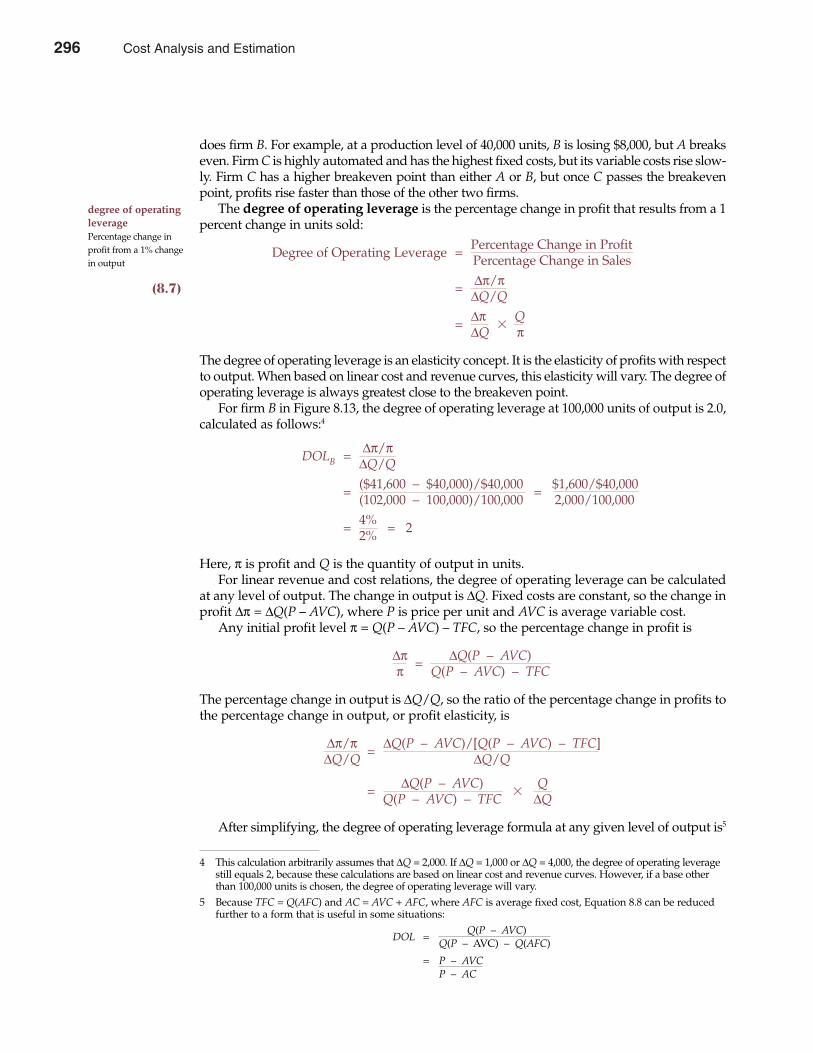
does firm B. For example, at a production level of 40,000 units, B is losing $8,000, but A breakseven. Firm C is highly automated and has the highest fixed costs, but its variable costs rise slow-ly. Firm C has a higher breakeven point than either A or B, but once C passes the breakevenpoint, profits rise faster than those of the other two firms.
The degree of operating leverage is the percentage change in profit that results from a 1percent change in units sold:
Degree of Operating Leverage = Percentage Change in ProfitPercentage Change in Sales
(8.7) = ∆π/π∆Q/Q
= ∆π�
Q∆Q π
The degree of operating leverage is an elasticity concept. It is the elasticity of profits with respectto output. When based on linear cost and revenue curves, this elasticity will vary. The degree ofoperating leverage is always greatest close to the breakeven point.
For firm B in Figure 8.13, the degree of operating leverage at 100,000 units of output is 2.0,calculated as follows:4
DOLB = ∆π/π∆Q/Q
= ($41,600 – $40,000)/$40,000 = $1,600/$40,000(102,000 – 100,000)/100,000 2,000/100,000
= 4% = 22%
Here, π is profit and Q is the quantity of output in units. For linear revenue and cost relations, the degree of operating leverage can be calculated
at any level of output. The change in output is ∆Q. Fixed costs are constant, so the change inprofit ∆π = ∆Q(P – AVC), where P is price per unit and AVC is average variable cost.
Any initial profit level π = Q(P – AVC) – TFC, so the percentage change in profit is
∆π = ∆Q(P – AVC)π Q(P – AVC) – TFC
The percentage change in output is ∆Q/Q, so the ratio of the percentage change in profits tothe percentage change in output, or profit elasticity, is
∆π/π = ∆Q(P – AVC)/[Q(P – AVC) – TFC]∆Q/Q ∆Q/Q
= ∆Q(P – AVC)�
QQ(P – AVC) – TFC ∆Q
After simplifying, the degree of operating leverage formula at any given level of output is5
296 Part Three Production and Cost Analysis
degree of operatingleverage Percentage change inprofit from a 1% changein output
4 This calculation arbitrarily assumes that ∆Q = 2,000. If ∆Q = 1,000 or ∆Q = 4,000, the degree of operating leveragestill equals 2, because these calculations are based on linear cost and revenue curves. However, if a base otherthan 100,000 units is chosen, the degree of operating leverage will vary.
5 Because TFC = Q(AFC) and AC = AVC + AFC, where AFC is average fixed cost, Equation 8.8 can be reducedfurther to a form that is useful in some situations:
DOL =Q(P – AVC)
Q(P – AVC) – Q(AFC)
= P – AVCP – AC
296 Cost Analysis and Estimation
(8.8) Degree of Operating Leverage at Point Q = Q(P – AVC)Q(P – AVC) – TFC
Using Equation 8.8, firm B’s degree of operating leverage at 100,000 units of output is cal-culated as
DOLB at 100,000 units = 100,000($2.00 – $1.20)100,000($2.00 – $1.20) – $40,000
= $80,000 = 2$40,000
Equation 8.8 can also be applied to firms A and C. When this is done, firm A’s degree of oper-ating leverage at 100,000 units equals 1.67 and firm C’s equals 2.5. With a 2 percent increase involume, firm C, the firm with the most operating leverage, will experience a profit increase of5 percent. For the same 2 percent gain in volume, the firm with the least leverage, firm A, willhave only a 3.3 percent profit gain. As seen in Figure 8.13, the profits of firm C are most sensi-tive to changes in sales volume, whereas firm A’s profits are relatively insensitive to volumechanges. Firm B, with an intermediate degree of leverage, lies between these two extremes.
Limitations of Linear Cost-Volume-Profit Analysis Cost-volume-profit analysis helps explain relations among volume, prices, and costs. It is alsouseful for pricing, cost control, and other financial decisions. However, linear cost-volume-profit analysis has its limitations.
Linear cost-volume-profit analysis has a weakness in what it implies about sales possi-bilities for the firm. Linear cost-volume-profit charts are based on constant selling prices. Tostudy profit possibilities with different prices, a whole series of charts is necessary, with onechart for each price. With sophisticated spreadsheet software, the creation of a wide varietyof cost-volume-profit charts is relatively easy. Using such software, profit possibilities fordifferent pricing strategies can be quickly determined. Alternatively, nonlinear cost-volume-profit analysis can be used to show the effects of changing prices.
Linear cost-volume-profit analysis can be hampered by the underlying assumption ofconstant average costs. As unit sales increase, existing plant and equipment can be workedbeyond capacity, thus reducing efficiency. The need for additional workers, longer workperiods, and overtime wages can also cause variable costs to rise sharply. If additional plantand equipment is required, fixed costs will also rise. Such changes influence both the leveland the slope of cost functions.
Although linear cost-volume-profit analysis has proven useful for managerial decisionmaking, care must be taken to ensure that it is not applied when underlying assumptions areviolated. Like any decision tool, cost-volume-profit analysis must be used with discretion.
SUMMARY
Cost analysis plays a key role in most managerial decisions. This chapter introduces a num-ber of cost concepts, shows the relation between cost functions and production functions,and examines several cost analysis issues.
• For tax purposes, historical cost, or historical cash outlay, is the relevant cost. This is alsogenerally true for annual 10-K reports to the Securities and Exchange Commission andfor reports to stockholders. Current cost, the amount that must be paid under prevailingmarket conditions, is typically more relevant for decision-making purposes.
Chapter Eight Cost Analysis and Estimation 297
Cost Analysis and Estimation 297
• Current costs are often determined by replacement costs, or the cost of duplicating pro-ductive capability using present technology. Another prime determinant of current cost isopportunity cost, or the foregone value associated with the current rather than the next-best use of a given asset. Both of these cost categories typically involve out-of-pocket costs,or explicit costs, and noncash costs, called implicit costs.
• Incremental cost is the change in cost caused by a given managerial decision and ofteninvolves multiple units of output. Incremental costs are a prime determinant of profitcontribution, or profit before fixed charges. Neither are affected by sunk costs, which donot vary across decision alternatives.
• Proper use of relevant cost concepts requires an understanding of the cost/output relation,or cost function. Short-run cost functions are used for day-to-day operating decisions;long-run cost functions are employed in the long-range planning process. The short run isthe operating period during which the availability of at least one input is fixed. In the longrun, the firm has complete flexibility. Fixed costs do not vary with output and are incurredonly in the short run. Variable costs fluctuate with output in both the short and the long run.
• A short-run cost curve shows the minimum cost impact of output changes for a specificplant size and in a given operating environment. A long-run cost curve shows the minimumcost impact of output changes for the optimal plant size using current technology in thepresent operating environment.
• Economies of scale originate from production and market-related sources and cause long-run average costs to decline. Cost elasticity, �C, measures the percentage change in totalcost associated with a 1 percent change in output.
• Capacity refers to the output level at which short-run average costs are minimized.Minimum efficient scale (MES) is the output level at which long-run average costs areminimized.
• Multiplant economies of scale are cost advantages that arise from operating multiplefacilities in the same line of business or industry. Conversely, multiplant diseconomiesof scale are cost disadvantages that arise from managing multiple facilities in the sameline of business or industry.
• When knowledge gained from manufacturing experience is used to improve productionmethods, the resulting decline in average cost reflects the effects of the firm’s learningcurve. Economies of scope exist when the cost of joint production is less than the cost ofproducing multiple outputs separately.
• Cost-volume-profit analysis, sometimes called breakeven analysis, is used to study relationsamong costs, revenues, and profits. A breakeven quantity is a zero profit activity level. Thedegree of operating leverage is the percentage change in profit that results from a 1 percentchange in units sold; it can be understood as the elasticity of profits with respect to output.
Cost analysis poses a continuing challenge to management in all types of organizations. Usingthe concepts and tools discussed in this chapter, successful managers are able to manage costseffectively.
QUESTIONS
Q8.1 The relevant cost for most managerial decisions is the current cost of an input. The relevant costfor computing income for taxes and stockholder reporting is the historical cost. What advantagesor disadvantages do you see in using current costs for tax and stockholder reporting purposes?
Q8.2 What are the relations among historical costs, current costs, and opportunity costs?
298 Part Three Production and Cost Analysis
298 Cost Analysis and Estimation
Q8.3 What is the difference between marginal and incremental cost? Q8.4 What is a sunk cost, and how is it related to a decision problem? Q8.5 What is the relation between production functions and cost functions? Be sure to include in
your discussion the effect of conditions in input factor markets. Q8.6 Explain why �Q > 1 indicates increasing returns to scale, where �C < 1 indicates economies of
scale. (See Chapter 7 for the definition of output elasticity.) Q8.7 The president of a small firm has been complaining to his controller about rising labor and
material costs. However, the controller notes that average costs have not increased duringthe past year. Is this possible?
Q8.8 Given the short-run total cost curve in Figure 8.1(b), explain why (a) Q1 is the minimum of theMC curve, (b) Q2 is the minimum of the AVC curve, (c) Q3 is the minimum of the ATC curve,and (d) the MC curve cuts the AVC and ATC curves at their minimum points.
Q8.9 Will firms in industries in which high levels of output are necessary for minimum efficient scaletend to have substantial degrees of operating leverage?
Q8.10 Do operating strategies of average cost minimization and profit maximization always lead toidentical levels of output?
SELF-TEST PROBLEMS AND SOLUTIONS
ST8.1 Learning Curves. Modern Merchandise, Inc., makes and markets do-it-yourself hardware,housewares, and industrial products. The company’s new Aperture Miniblind is winning cus-tomers by virtue of its high quality and quick order turnaround time. The product also benefitsbecause its price point bridges the gap between ready-made vinyl blinds and their high-pricedcustom counterpart. In addition, the company’s expanding product line is sure to benefit fromcross-selling across different lines. Given the success of the Aperture Miniblind product, ModernMerchandise plans to open a new production facility near Beaufort, South Carolina. Based oninformation provided by its chief financial officer, the company estimates fixed costs for thisproduct of $50,000 per year and average variable costs of
AVC = $0.5 + $0.0025Q
where AVC is average variable cost (in dollars) and Q is output. A. Estimate total cost and average total cost for the projected first-year volume of 20,000
units. B. An increase in worker productivity because of greater experience or learning during the
course of the year resulted in a substantial cost saving for the company. Estimate theeffect of learning on average total cost if actual second-year total cost was $848,000 at anactual volume of 20,000 units.
ST8.1 SolutionA. The total variable cost function for the first year is
TVC = AVC � Q
= ($0.5 + $0.0025Q)Q= $0.5Q + $0.0025Q2
At a volume of 20,000 units, estimated total cost is
Chapter Eight Cost Analysis and Estimation 299
Cost Analysis and Estimation 299

TC = TFC + TVC
= $50,000 + $0.5Q + $0.0025Q2
= $50,000 + $0.5(20,000) + $0.0025(20,0002) = $1,060,000
Estimated average cost is
AC = TC/Q
= $1,060,000/20,000 = $53 per case
B. If actual total costs were $848,000 at a volume of 20,000 units, actual average total costs were
AC = TC/Q
= $848,000/20,000 = $42.40 per case
Therefore, greater experience or learning has resulted in an average cost saving of $10.60 percase because
Learning Effect = Actual AC — Estimated AC
= $42.40 – $53 = –$10.60 per case
Alternatively,
Learning Rate = 1 –AC2 � 100� AC1 �
= 1 – $42.40 � 100� $53 �
= 20%
ST8.2 Minimum Efficient Scale Estimation. Kanata Corporation is a leading manufacturer oftelecommunications equipment based in Ontario, Canada. Its main product is microprocessor-controlled telephone switching equipment, called automatic private branch exchanges (PABXs),capable of handling 8 to 3,000 telephone extensions. Severe price cutting throughout the PABXindustry continues to put pressure on sales and margins. To better compete against increasinglyaggressive rivals, the company is contemplating the construction of a new production facilitycapable of producing 1.5 million units per year. Kanata’s in-house engineering estimate of thetotal cost function for the new facility is
TC = $3,000 + $1,000Q + $0.003Q2
MC = $1,000 + $0.006Q
where TC = total costs in thousands of dollars, Q = output in thousands of units, and MC =marginal costs in thousands of dollars.
A. Estimate minimum efficient scale in this industry. B. In light of current PABX demand of 30 million units per year, how would you evaluate
the future potential for competition in the industry?
300 Part Three Production and Cost Analysis
300 Cost Analysis and Estimation
ST8.2 Solution A. Minimum efficient scale is reached when average costs are first minimized. This occurs at
the point where MC = AC.
Average Costs = AC = TC/Q
= ($3,000 + $1,000Q + $0.003Q2)/Q
= $3,000 + $1,000 + $0.003QQ
Therefore,
MC = AC
$1,000 + $0.006Q = $3,000 + $1,000 + $0.003QQ
0.003Q = 3,000Q
3,000 = 0.003Q2
Q2 = 1,000,000 Q = 1,000(000) or 1 million
(Note: AC is rising for Q > 1,000(000).) Alternatively, MES can be calculated using the point cost elasticity formula, because MESis reached when �C = 1.
�C = ∆TC�
Q∆Q TC
($1,000 + $0.006Q)Q = 1($3,000 + $1,000Q + $0.003Q2) 1,000Q + 0.006Q2 = 3,000 + 1,000Q + 0.003Q2
0.003Q2 = 3,000 Q2 = 1,000,000
QMES = 1,000(000) or 1 million
B. With a minimum efficient scale of 1 million units and total industry sales of 30 million units,up to 30 efficiently sized competitors are possible in Kanata’s market.
Potential Number of Efficient Competitors = Market SizeMES Size
= 30,000,0001,000,000
= 30
Thus, there is the potential for n = 30 efficiently sized competitors and, therefore, vigorouscompetition in Kanata’s industry.
Chapter Eight Cost Analysis and Estimation 301
Cost Analysis and Estimation 301
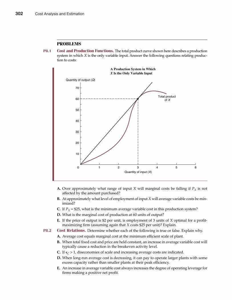
PROBLEMS
P8.1 Cost and Production Functions. The total product curve shown here describes a productionsystem in which X is the only variable input. Answer the following questions relating produc-tion to costs:
A. Over approximately what range of input X will marginal costs be falling if PX is notaffected by the amount purchased?
B. At approximately what level of employment of input X will average variable costs be min-imized?
C. If PX = $25, what is the minimum average variable cost in this production system? D. What is the marginal cost of production at 60 units of output? E. If the price of output is $2 per unit, is employment of 3 units of X optimal for a profit-
maximizing firm (assuming again that X costs $25 per unit)? Explain. P8.2 Cost Relations. Determine whether each of the following is true or false. Explain why.
A. Average cost equals marginal cost at the minimum efficient scale of plant. B. When total fixed cost and price are held constant, an increase in average variable cost will
typically cause a reduction in the breakeven activity level. C. If �C > 1, diseconomies of scale and increasing average costs are indicated. D. When long-run average cost is decreasing, it can pay to operate larger plants with some
excess capacity rather than smaller plants at their peak efficiency. E. An increase in average variable cost always increases the degree of operating leverage for
firms making a positive net profit.
302 Part Three Production and Cost Analysis
70
60
50
40
30
20
10
0 1 2 3 4 5 6
Quantity of input (X)
Quantity of output (Q)
Total productof X
302 Cost Analysis and Estimation
P8.3 Cost Curves. Indicate whether each of the following involves an upward or downward shift inthe long-run average cost curve or, instead, involves a leftward or rightward movement along agiven curve. Also indicate whether each will have an increasing, decreasing, or uncertain effecton the level of average cost. A. A rise in wage rates B. A decline in output C. An energy-saving technical change D. A fall in interest rates E. An increase in learning or experience
P8.4 Incremental Cost. McFarland-Adler, Inc., produces innovative interior decorating softwarethat it sells to design studios, home furnishing stores, and so on. The yearly volume of outputis 15,000 units. Selling price and costs per unit are as follows:
Management is evaluating the possibility of using the Internet to sell its software directly toconsumers at a price of $300 per unit. Although no added capital investment is required,additional shipping and handling costs are estimated as follows:
A. Calculate the incremental profit that McFarland-Adler would earn by customizing itsinstruments and marketing them directly to end users.
P8.5 Accounting and Economic Costs. Three graduate business students are considering oper-ating a fruit smoothie stand in the Harbor Springs, Michigan, resort area during their summerbreak. This is an alternative to summer employment with a local firm, where they would eachearn $6,000 over the 3-month summer period. A fully equipped facility can be leased at a costof $8,000 for the summer. Additional projected costs are $1,000 for insurance and $1.20 per unitfor materials and supplies. Their fruit smoothies would be priced at $3 per unit. A. What is the accounting cost function for this business? B. What is the economic cost function for this business? C. What is the economic breakeven number of units for this operation? (Assume a $1 price and
ignore interest costs associated with the timing of lease payments.) P8.6 Profit Contribution. Angelica Pickles is manager of a Quick Copy franchise in White Plains,
New York. Pickles projects that by reducing copy charges from 5¢ to 4¢ each, Quick Copy’s$600-per-week profit contribution will increase by one-third. A. If average variable costs are 2¢ per copy, calculate Quick Copy’s projected increase in volume. B. What is Pickles’ estimate of the arc price elasticity of demand for copies?
Chapter Eight Cost Analysis and Estimation 303
Selling Price $250 Costs:
Direct material $40 Direct labor 60 Variable overhead 30 Variable selling expenses 25 Fixed selling expenses 20 – $175
Unit profit before tax $ 75
Direct labor $30 per unit Variable overhead $5 per unit Variable selling expenses $2 per unit Fixed selling expenses $20,000 per year
Cost Analysis and Estimation 303
P8.7 Cost Elasticity. Power Brokers, Inc. (PBI), a discount brokerage firm, is contemplating open-ing a new regional office in Providence, Rhode Island. An accounting cost analysis of monthlyoperating costs at a dozen of its regional outlets reveals average fixed costs of $4,500 per monthand average variable costs of
AVC = $59 – $0.006Q
where AVC is average variable costs (in dollars) and Q is output measured by number of stockand bond trades.
A typical stock or bond trade results in $100 gross commission income, with PBI paying35% of this amount to its sales representatives. A. Estimate the trade volume necessary for PBI to reach a target return of $7,500 per month
for a typical office. B. Estimate and interpret the elasticity of cost with respect to output at the trade volume
found in part A. P8.8 Multiplant Operation. Appalachia Beverage Company, Inc., is considering alternative pro-
posals for expansion into the Midwest. Alternative 1: Construct a single plant in Indianapolis,Indiana, with a monthly production capacity of 300,000 cases, a monthly fixed cost of$262,500, and a variable cost of $3.25 per case. Alternative 2: Construct three plants, one eachin Muncie, Indiana; Normal, Illinois; and Dayton, Ohio, with capacities of 120,000, 100,000,and 80,000, respectively, and monthly fixed costs of $120,000, $110,000, and $95,000 each.Variable costs would be only $3 per case because of lower distribution costs. To achieve thesecost savings, sales from each smaller plant would be limited to demand within its homestate. The total estimated monthly sales volume of 200,000 cases in these three Midwesternstates is distributed as follows: 80,000 cases in Indiana, 70,000 cases in Illinois, and 50,000cases in Ohio. A. Assuming a wholesale price of $5 per case, calculate the breakeven output quantities for
each alternative. B. At a wholesale price of $5 per case in all states, and assuming sales at the projected levels,
which alternative expansion scheme provides Appalachia with the highest profit per month? C. If sales increase to production capacities, which alternative would prove to be more prof-
itable? P8.9 Learning Curves. The St. Thomas Winery plans to open a new production facility in the
Napa Valley of California. Based on information provided by the accounting department,the company estimates fixed costs of $250,000 per year and average variable costs of
AVC = $10 + $0.01Q
where AVC is average variable cost (in dollars) and Q is output measured in cases of outputper year. A. Estimate total cost and average total cost for the coming year at a projected volume of
4,000 cases. B. An increase in worker productivity because of greater experience or learning during the
course of the year resulted in a substantial cost saving for the company. Estimate the effectof learning on average total cost if actual total cost was $522,500 at an actual volume of5,000 cases.
P8.10 Cost-Volume-Profit Analysis. Untouchable Package Service (UPS) offers overnight pack-age delivery to Canadian business customers. UPS has recently decided to expand its facilitiesto better satisfy current and projected demand. Current volume totals 2 million packages perweek at a price of $12 each, and average variable costs are constant at all output levels. Fixed
304 Part Three Production and Cost Analysis
304 Cost Analysis and Estimation

costs are $3 million per week, and profit contribution averages one-third of revenues on eachdelivery. After completion of the expansion project, fixed costs will double, but variable costswill decline by 25%. A. Calculate the change in UPS’s weekly breakeven output level that is due to expansion. B. Assuming that volume remains at 2 million packages per week, calculate the change in
the degree of operating leverage that is due to expansion. C. Again assuming that volume remains at 2 million packages per week, what is the effect
of expansion on weekly profit?
Chapter Eight Cost Analysis and Estimation 305
CASE STUDY
Estimating the Costs of Nursing Care Cost estimation and cost containment are an important concern for a wide range of for-profit andnot-for-profit organizations offering health care services. For such organizations, the accuratemeasurement of nursing costs per patient day (a measure of output) is necessary for effectivemanagement. Similarly, such cost estimates are of significant interest to public officials at the fed-eral, state, and local government levels. For example, many state Medicaid reimbursement pro-grams base their payment rates on historical accounting measures of average costs per unit ofservice. However, these historical average costs may or may not be relevant for hospital man-agement decisions. During periods of substantial excess capacity, the overhead component ofaverage costs may become irrelevant. When the facilities of providers are fully used and facilityexpansion becomes necessary to increase services, then all costs, including overhead, are rele-vant. As a result, historical average costs provide a useful basis for planning purposes only ifappropriate assumptions can be made about the relative length of periods of peak versus off-peak facility usage. From a public-policy perspective, a further potential problem arises whenhospital expense reimbursement programs are based on historical average costs per day, becausethe care needs and nursing costs of various patient groups can vary widely. For example, if thecare received by the average publicly supported Medicaid patient actually costs more than thatreceived by non-Medicaid patients, Medicaid reimbursement based on average costs for theentire facility would be inequitable to providers and could create access barriers for someMedicaid patients.
As an alternative to traditional cost estimation methods, one might consider using the engi-neering technique to estimate nursing costs. For example, the labor cost of each type of servicecould be estimated as the product of an estimate of the time required to perform each service timesthe estimated wage rate per unit of time. Multiplying this figure by an estimate of the frequencyof service provides an estimate of the aggregate cost of the service. A possible limitation to theaccuracy of this engineering cost-estimation method is that treatment of a variety of illnesses oftenrequires a combination of nursing services. To the extent that multiple services can be providedsimultaneously, the engineering technique will tend to overstate actual costs unless the effect oncosts of service “packaging” is allowed for.
Nursing cost estimation is also possible by means of a carefully designed regression-basedapproach using variable cost and service data collected at the ward, unit, or facility level. Weeklylabor costs for registered nurses (RNs), licensed practical nurses (LPNs), and nursing aides mightbe related to a variety of patient services performed during a given measurement period. With suf-ficient variability in cost and service levels over time, useful estimates of variable labor costs becomepossible for each type of service and for each patient category (e.g., Medicaid, non-Medicaid). Animportant advantage of a regression-based approach is that it explicitly allows for the effect of serv-ice packaging on variable costs. For example, if shots and wound-dressing services are typicallyprovided together, this will be reflected in the regression-based estimates of variable costs per unit.
Cost Analysis and Estimation 305
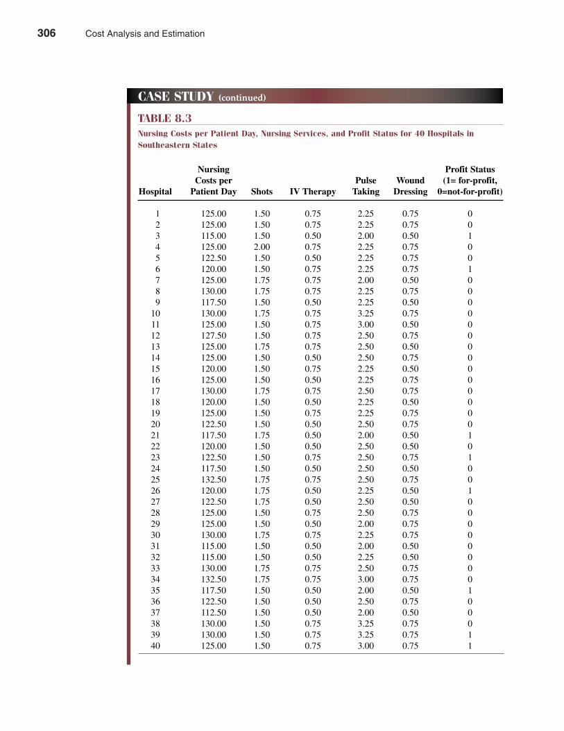
306 Part Three Production and Cost Analysis
TABLE 8.3Nursing Costs per Patient Day, Nursing Services, and Profit Status for 40 Hospitals inSoutheastern States
Nursing Profit StatusCosts per Pulse Wound (1= for-profit,
Hospital Patient Day Shots IV Therapy Taking Dressing 0=not-for-profit)
1 125.00 1.50 0.75 2.25 0.75 0 2 125.00 1.50 0.75 2.25 0.75 0 3 115.00 1.50 0.50 2.00 0.50 1 4 125.00 2.00 0.75 2.25 0.75 0 5 122.50 1.50 0.50 2.25 0.75 0 6 120.00 1.50 0.75 2.25 0.75 1 7 125.00 1.75 0.75 2.00 0.50 0 8 130.00 1.75 0.75 2.25 0.75 0 9 117.50 1.50 0.50 2.25 0.50 0
10 130.00 1.75 0.75 3.25 0.75 0 11 125.00 1.50 0.75 3.00 0.50 0 12 127.50 1.50 0.75 2.50 0.75 0 13 125.00 1.75 0.75 2.50 0.50 0 14 125.00 1.50 0.50 2.50 0.75 0 15 120.00 1.50 0.75 2.25 0.50 0 16 125.00 1.50 0.50 2.25 0.75 0 17 130.00 1.75 0.75 2.50 0.75 0 18 120.00 1.50 0.50 2.25 0.50 0 19 125.00 1.50 0.75 2.25 0.75 0 20 122.50 1.50 0.50 2.50 0.75 0 21 117.50 1.75 0.50 2.00 0.50 1 22 120.00 1.50 0.50 2.50 0.50 0 23 122.50 1.50 0.75 2.50 0.75 1 24 117.50 1.50 0.50 2.50 0.50 0 25 132.50 1.75 0.75 2.50 0.75 0 26 120.00 1.75 0.50 2.25 0.50 1 27 122.50 1.75 0.50 2.50 0.50 0 28 125.00 1.50 0.75 2.50 0.75 0 29 125.00 1.50 0.50 2.00 0.75 0 30 130.00 1.75 0.75 2.25 0.75 0 31 115.00 1.50 0.50 2.00 0.50 0 32 115.00 1.50 0.50 2.25 0.50 0 33 130.00 1.75 0.75 2.50 0.75 0 34 132.50 1.75 0.75 3.00 0.75 0 35 117.50 1.50 0.50 2.00 0.50 1 36 122.50 1.50 0.50 2.50 0.75 0 37 112.50 1.50 0.50 2.00 0.50 0 38 130.00 1.50 0.75 3.25 0.75 0 39 130.00 1.50 0.75 3.25 0.75 1 40 125.00 1.50 0.75 3.00 0.75 1
CASE STUDY (continued)
306 Cost Analysis and Estimation
Chapter Eight Cost Analysis and Estimation 307
CASE STUDY (continued)
Long-run costs per nursing facility can be estimated using either cross-section or time-seriesmethods. By relating total facility costs to the service levels provided by a number of hospitals,nursing homes, or out-patient care facilities during a specific period, useful cross-section esti-mates of total service costs are possible. If case mixes were to vary dramatically according totype of facility, then the type of facility would have to be explicitly accounted for in the regres-sion model analyzed. Similarly, if patient mix or service-provider efficiency is expected todepend, at least in part, on the for-profit or not-for-profit organization status of the care facility,the regression model must also recognize this factor. These factors plus price-level adjustmentsfor inflation would be accounted for in a time-series approach to nursing cost estimation.
To illustrate a regression-based approach to nursing cost estimation, consider the follow-ing cross-section analysis of variable nursing costs conducted by the Southeast Association ofHospital Administrators (SAHA). Using confidential data provided by 40 regional hospitals,SAHA studied the relation between nursing costs per patient day and four typical categories ofnursing services. These annual data appear in Table 8.3 The four categories of nursing servicesstudied include shots, intravenous (IV) therapy, pulse taking and monitoring, and wounddressing. Each service is measured in terms of frequency per patient day. An output of 1.50 inthe shots service category means that, on average, patients received one and one-half shots perday. Similarly, an output of 0.75 in the IV service category means that IV services were provideddaily to 75% of a given hospital’s patients, and so on. In addition to four categories of nursingservices, the not-for-profit or for-profit status of each hospital is also indicated. Using a “dummy”(or binary) variable approach, the profit status variable equals 1 for the eight for-profit hospitalsincluded in the study and zero for the remaining 32 not-for-profit hospitals.
Cost estimation results for nursing costs per patient day derived using a regression-basedapproach are shown in Table 8.4. A. Interpret the coefficient of determination (R2) estimated for the nursing cost function. B. Describe the economic and statistical significance of each estimated coefficient in the
nursing cost function. C. Average nursing costs for the eight for-profit hospitals in the sample are only $120.94
per patient day, or $3.28 per patient day less than the $124.22 average cost experiencedby the 32 not-for-profit hospitals. How can this fact be reconciled with the estimatedcoefficient of –2.105 for the for-profit status variable?
D. Would such an approach for nursing cost estimation have practical relevance for pub-licly funded nursing cost reimbursement systems?
TABLE 8.4Nursing Costs per Patient Day: Cost Estimation Results
Standard Error t StatisticVariable Name Coefficient (1) of Coefficient (2) (1)�(2)�(3)
Intercept 76.182 5.086 14.98 Shots 11.418 2.851 4.00 IV 10.052 3.646 2.76 Pulse 4.532 1.153 3.93 Wound dressing 18.932 3.370 5.62 For-profit status –2.105 0.883 –2.38
Coefficient of determination = R2 = 84.1% Standard error of estimate = SEE = $2.21
Cost Analysis and Estimation 307

SELECTED REFERENCES Achee, Rebecca, Thornton and Peter Thompson. “Learning from Experience and Learning from Others:
An Exploration of Learning and Spillovers in Wartime Shipbuilding.” American Economic Review 91(December 2001): 1350–1368.
Angrist, Joshua D., and Alan B. Krueger. “Instrumental Variables and the Search for Identification: FromSupply and Demand to Natural Experiments.” Journal of Economic Perspectives 15 (Fall 2001): 69–87.
Baily, Martin Neal, and Robert Z. Lawrence. “Do We Have a New E-Conomy?” American Economic Review91 (May 2001): 308–312.
Chan, Louis K. C., Josef Lakonishok, and Theodore Sougiannis. “The Stock Market Valuation of Researchand Development Expenditures.” Journal of Finance 56 (December 2001): 2431–2456.
Gul, Ferdinand A. “Free Cash Flow, Debt-Monitoring and Managers’ Lifo/Fifo Policy Choice.” Journal ofCorporate Finance 7 (December 2001): 475–492.
Hausman, Jerry. “Mismeasured Variables in Econometric Analysis: Problems from the Right and Problemsfrom the Left.” Journal of Economic Perspectives 15 (Fall 2001): 57–68.
Ittner, Christopher D., and David F. Larcker. “Assessing Empirical Research in Managerial Accounting:A Value-Based Management Perspective.” Journal of Accounting and Economics 32 (December 2001):349–410.
Lambert, Richard A. “Contracting Theory and Accounting.” Journal of Accounting and Economics 32(December 2001): 3–87.
Levitt, Steven D., and Jack Porter. “Sample Selection in the Estimation of Air Bag and Seat BeltEffectiveness.” Review of Economics and Statistics 83 (November 2001): 603–615.
Litan, Robert E., and Alice M. Rivlin. “Projecting the Economic Impact of the Internet.” American EconomicReview 91 (May 2001): 313–317.
Morgenstern, Richard D., William A. Pizer, and Jhih-Shyang Shih. “The Cost of EnvironmentalProtection.” Review of Economics and Statistics 83 (November 2001): 732–738.
Verrecchia, Robert E. “Essays on Disclosure.” Journal of Accounting and Economics 32 (December 2001):97–180.
Wooldridge, Jeffrey M. “Applications of Generalized Method of Moments Estimation.” Journal of EconomicPerspectives 15 (Fall 2001): 87–100.
Worthington, Andres C. “Efficiency in Pre-Merger and Post-Merger Non-Bank Financial Institutions.”Managerial & Decision Economics 22 (December 2001): 439–452.
Zimmerman, Jerold L. “Conjectures Regarding Empirical Managerial Accounting Research.” Journal ofAccounting and Economics 32 (December 2001): 411–427.
308 Part Three Production and Cost Analysis
308 Cost Analysis and Estimation
Linear Programming
CHAPTER NINE
3091 Kornelia Heusener and Gesa Von Wichert, “Profit Pressure in the Cargo Industry,”
The Wall Street Journal Online, March 18, 2002 (http://online.wsj.com).
L inear programming, or so-called “solver” PC software, can be used to fig-ure out the best answer to an assortment of questions expressed in terms
of functional relationships. In a fundamental sense, linear programming is astraightforward development from the more basic “what if” approach to prob-lem solving. In a traditional “what-if” approach, one simply enters data or achange in input values in a computer spreadsheet and uses spreadsheet for-mulas and macros to calculate resulting output values. A prime advantage ofthe “what if” approach is that it allows managers to consider the cost, revenue,and profit implications of changes in a wide variety of operating conditions.An important limitation of the “what if” method is that it can become a tediousmeans of searching for the best answer to planning and operating decisions.
Linear programming can be thought of as performing “what-if in reverse.”All you do is specify appropriate objectives and a series of constraint conditions,and the software will determine the appropriate input values. When productiongoals are specified in light of operating constraints, linear programming can beused to identify the cost-minimizing operating plan. Alternatively, using linearprogramming techniques, a manager might find the profit-maximizing activitylevel by specifying production relationships and the amount of availableresources.
Linear programming has proven to be an adept tool for solving problemsencountered in a number of business, engineering, financial, and scientificapplications. In a practical sense, typically encountered constrained opti-mization problems seldom have a simple rule-of-thumb solution. This chapterillustrates how linear programming can be used to quickly and easily solvereal-world decision problems.1
309
9
BASIC ASSUMPTIONS
Linear programming is a useful method for analyzing and solving certain types of manage-ment decision problems. To know when linear programming techniques can be applied, it isnecessary to understand basic underlying assumptions.
Inequality ConstraintsMany production or resource constraints faced by managers are inequalities. Constraintsoften limit the resource employed to less than or equal to (≤) some fixed amount available. Inother instances, constraints specify that the quantity or quality of output must be greater thanor equal to (≥) some minimum requirement. Linear programming handles such constraintinequalities easily, making it a useful technique for finding the optimal solution to manymanagement decision problems.
Atypical linear programming problem might be to maximize output subject to the constraintthat no more than 40 hours of skilled labor per week be used. This labor constraint is expressedas an inequality where skilled labor ≤ 40 hours per week. Such an operating constraint meansthat no more than 40 hours of skilled labor can be used, but some excess capacity is permissible,at least in the short run. If 36 hours of skilled labor were fruitfully employed during a given week,the 4 hours per week of unused labor is called excess capacity.
Linearity AssumptionAs its name implies, linear programming can be applied only in situations in which the relevantobjective function and constraint conditions are linear. Typical managerial decision problemsthat can be solved using the linear programming method involve revenue and cost functionsand their composite, the profit function. Each must be linear; as output increases, revenues,costs, and profits must increase in a linear fashion. For revenues to be a linear function of out-put, product prices must be constant. For costs to be a linear function of output, both returns toscale and input prices must be constant. Constant input prices, when combined with constantreturns to scale, result in a linear total cost function. If both output prices and unit costs are con-stant, then profit contribution and profits also rise in a linear fashion with output.
Product and input prices are relatively constant when a typical firm can buy unlimitedquantities of input and sell an unlimited amount of output without changing prices. This occursunder conditions of pure competition. Therefore, linear programming methods are clearly appli-cable for firms in perfectly competitive industries with constant returns to scale. However, lin-ear programming is also applicable in many other instances. Because linear programming isused for marginal analysis, it focuses on the effects of fairly modest output, price, and inputchanges. For moderate changes in current operating conditions, a constant-returns-to-scaleassumption is often valid. Similarly, input and output prices are typically unaffected by modestchanges from current levels. As a result, sales revenue, cost, and profit functions are often linearwhen only moderate changes in operations are contemplated and use of linear programmingmethods is valid.
To illustrate, suppose that an oil company must choose the optimal output mix for a refin-ery with a capacity of 150,000 barrels of oil per day. The oil company is justified in basing itsanalysis on the $25-per-barrel prevailing market price for crude oil, regardless of how muchis purchased or sold. This assumption might not be valid if the company were to quicklyexpand refinery output by a factor of 10, but within the 150,000 barrels per day range of fea-sible output, prices will be approximately constant. Up to capacity limits, it is also reasonableto expect that a doubling of crude oil input would lead to a doubling of refined output, andthat returns to scale are constant.
310 Part Three Production and Cost Analysis
linear programmingA solution method formaximization or mini-mization decisionproblems subject tounderlying constraints
optimal solutionBest answer
310 Linear Programming
In many instances, the underlying assumption of linearity is entirely valid. In otherinstances in which the objective function and constraint conditions can be usefully approxi-mated by linear relations, the linear programming technique can also be fruitfully applied.Only when objective functions and constraint conditions are inherently nonlinear must morecomplicated mathematical programming techniques be applied. In most managerial applications,even when the assumption of linearity does not hold precisely, linear approximations seldomdistort the analysis.
PRODUCTION PLANNING FOR A SINGLE PRODUCT
Although linear programming has been widely applied in managerial decision making, it hasbeen used most frequently in production decisions. To illustrate the method, a simple two-input/one-output problem is examined. Later sections consider more realistic and complexproblems.
Production ProcessesAssume that a firm produces a single product, Q, using two inputs, L and K, which mightrepresent labor and capital. Instead of assuming continuous substitution between L and K,as in Chapter 7, assume that Q can be produced using only four input combinations. In otherwords, four different production processes are available for making Q, each of which uses adifferent fixed combination of inputs L and K. The production processes might representfour different plants, each with its own fixed asset configuration and labor requirements.Alternatively, they could be four different assembly lines, each using a different combinationof capital equipment and labor.
Chapter Nine Linear Programming 311
LP: More Than a Visual Approach
LP is often portrayed as a visual means of characterizingmanagement problems. It is—at least when a limitednumber of products or product dimensions are beinganalyzed. When the optimal level of production for twoproducts is sought, for example, a simple graph of theappropriate LP problem gives managers a useful intu-itive basis for considering the best means of meeting avariety of production criteria. When a multitude of prod-ucts are offered, or when a large number of productioncharacteristics must be considered, the typical LP problembecomes too complex to be visualized graphically. Insuch instances, computer-based solutions using spread-sheets offer a tractable alternative for analyzing and solv-ing LP problems.
LP techniques are commonly used to solve prob-lems in transportation routing, staff scheduling, andfinancial planning. Whenever a company needs to movea quantity of goods from and to multiple locations, suchas plants, regional warehouses, or retail stores, it faces apractical LP problem. By minimizing route mileage,operating costs can also be minimized, and outlays for
capital investment can be kept at a minimum. Manycompanies routinely save thousands of dollars per yearon shipping costs by solving LP problems of this type.Businesses and government agencies use LP methods tosolve the problem of scheduling employees’ workinghours to meet customer service demands, which mightvary by the hour or the day, in light of employee avail-ability and preferences. Other examples of practicalapplications include models to help investors decide onthe optimal allocation of a stock and bond portfolio.
Detailed user tips on successful LP applications, oftenwith free follow-up from the author, can be found in analmost limitless number on the Internet. One of the bestsites for getting started is sponsored by Lindo Systems,Inc. There you can find LP case studies for telecommuni-cations network design, supply chain management, andso on. These examples provide the best reason to becomefamiliar with the technique. LP works!
See: Lindo Systems, Inc. (http://www.lindo.com).
M A N A G E R I A L A P P L I C AT I O N 9 . 1
Linear Programming 311
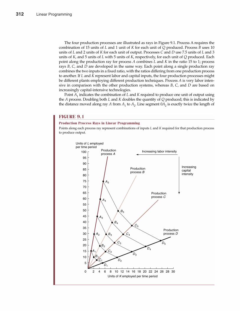
The four production processes are illustrated as rays in Figure 9.1. Process A requires thecombination of 15 units of L and 1 unit of K for each unit of Q produced. Process B uses 10units of L and 2 units of K for each unit of output. Processes C and D use 7.5 units of L and 3units of K, and 5 units of L with 5 units of K, respectively, for each unit of Q produced. Eachpoint along the production ray for process A combines L and K in the ratio 15 to 1; processrays B, C, and D are developed in the same way. Each point along a single production raycombines the two inputs in a fixed ratio, with the ratios differing from one production processto another. If L and K represent labor and capital inputs, the four production processes mightbe different plants employing different production techniques. Process A is very labor inten-sive in comparison with the other production systems, whereas B, C, and D are based onincreasingly capital-intensive technologies.
Point A1 indicates the combination of L and K required to produce one unit of output usingthe A process. Doubling both L and K doubles the quantity of Q produced; this is indicated bythe distance moved along ray A from A1 to A2. Line segment 0A2 is exactly twice the length of
312 Part Three Production and Cost Analysis
FIGURE 9.1Production Process Rays in Linear ProgrammingPoints along each process ray represent combinations of inputs L and K required for that production processto produce output.
0
5
10
15
20
25
30
35
40
45
50
55
60
65
70
75
80
85
90
95
100
Units of K employed per time period
Units of L employedper time period
Productionprocess A
Productionprocess B
Productionprocess C
Productionprocess DA2
B2
C2
D2
A1
B1C1
D1
D3
D4
D5C3
C4
C5
B3
B4
B5
A3
A4
A5
Increasingcapitalintensity
Increasing labor intensity
2 4 6 8 10 12 14 16 18 20 22 24 26 28 30
312 Linear Programming
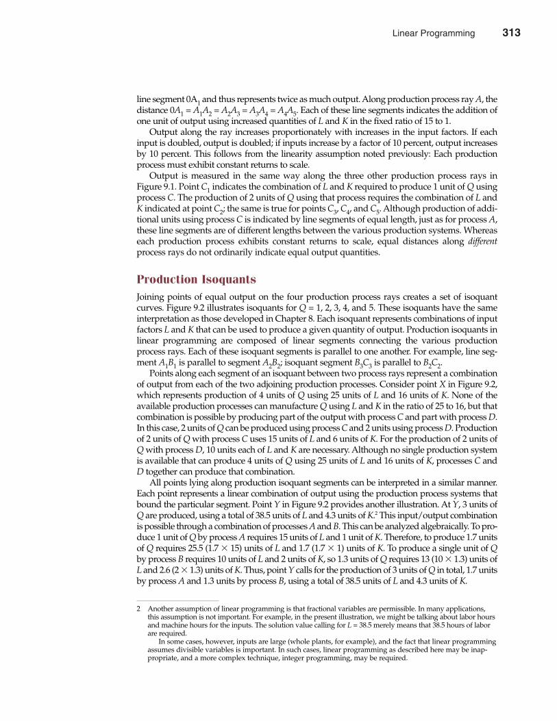
line segment 0A1 and thus represents twice as much output. Along production process ray A, thedistance 0A1 = A1A2 = A2A3 = A3A4 = A4A5. Each of these line segments indicates the addition ofone unit of output using increased quantities of L and K in the fixed ratio of 15 to 1.
Output along the ray increases proportionately with increases in the input factors. If eachinput is doubled, output is doubled; if inputs increase by a factor of 10 percent, output increasesby 10 percent. This follows from the linearity assumption noted previously: Each productionprocess must exhibit constant returns to scale.
Output is measured in the same way along the three other production process rays inFigure 9.1. Point C1 indicates the combination of L and K required to produce 1 unit of Q usingprocess C. The production of 2 units of Q using that process requires the combination of L andK indicated at point C2; the same is true for points C3, C4, and C5. Although production of addi-tional units using process C is indicated by line segments of equal length, just as for process A,these line segments are of different lengths between the various production systems. Whereaseach production process exhibits constant returns to scale, equal distances along differentprocess rays do not ordinarily indicate equal output quantities.
Production IsoquantsJoining points of equal output on the four production process rays creates a set of isoquantcurves. Figure 9.2 illustrates isoquants for Q = 1, 2, 3, 4, and 5. These isoquants have the sameinterpretation as those developed in Chapter 8. Each isoquant represents combinations of inputfactors L and K that can be used to produce a given quantity of output. Production isoquants inlinear programming are composed of linear segments connecting the various productionprocess rays. Each of these isoquant segments is parallel to one another. For example, line seg-ment A1B1 is parallel to segment A2B2; isoquant segment B3C3 is parallel to B2C2.
Points along each segment of an isoquant between two process rays represent a combinationof output from each of the two adjoining production processes. Consider point X in Figure 9.2,which represents production of 4 units of Q using 25 units of L and 16 units of K. None of theavailable production processes can manufacture Q using L and K in the ratio of 25 to 16, but thatcombination is possible by producing part of the output with process C and part with process D.In this case, 2 units of Q can be produced using process C and 2 units using process D. Productionof 2 units of Q with process C uses 15 units of L and 6 units of K. For the production of 2 units ofQ with process D, 10 units each of L and K are necessary. Although no single production systemis available that can produce 4 units of Q using 25 units of L and 16 units of K, processes C andD together can produce that combination.
All points lying along production isoquant segments can be interpreted in a similar manner.Each point represents a linear combination of output using the production process systems thatbound the particular segment. Point Y in Figure 9.2 provides another illustration. At Y, 3 units ofQ are produced, using a total of 38.5 units of L and 4.3 units of K.2 This input/output combinationis possible through a combination of processes A and B. This can be analyzed algebraically. To pro-duce 1 unit of Q by process A requires 15 units of L and 1 unit of K. Therefore, to produce 1.7 unitsof Q requires 25.5 (1.7 � 15) units of L and 1.7 (1.7 � 1) units of K. To produce a single unit of Qby process B requires 10 units of L and 2 units of K, so 1.3 units of Q requires 13 (10 � 1.3) units ofL and 2.6 (2 � 1.3) units of K. Thus, point Y calls for the production of 3 units of Q in total, 1.7 unitsby process A and 1.3 units by process B, using a total of 38.5 units of L and 4.3 units of K.
Chapter Nine Linear Programming 313
2 Another assumption of linear programming is that fractional variables are permissible. In many applications,this assumption is not important. For example, in the present illustration, we might be talking about labor hoursand machine hours for the inputs. The solution value calling for L = 38.5 merely means that 38.5 hours of laborare required.
In some cases, however, inputs are large (whole plants, for example), and the fact that linear programmingassumes divisible variables is important. In such cases, linear programming as described here may be inap-propriate, and a more complex technique, integer programming, may be required.
Linear Programming 313
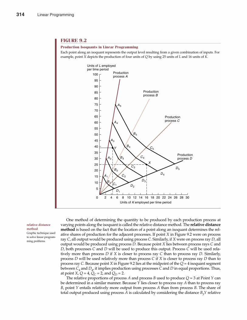
One method of determining the quantity to be produced by each production process atvarying points along the isoquant is called the relative distance method. The relative distancemethod is based on the fact that the location of a point along an isoquant determines the rel-ative shares of production for the adjacent processes. If point X in Figure 9.2 were on processray C, all output would be produced using process C. Similarly, if X were on process ray D, alloutput would be produced using process D. Because point X lies between process rays C andD, both processes C and D will be used to produce this output. Process C will be used rela-tively more than process D if X is closer to process ray C than to process ray D. Similarly,process D will be used relatively more than process C if X is closer to process ray D than toprocess ray C. Because point X in Figure 9.2 lies at the midpoint of the Q = 4 isoquant segmentbetween C4 and D4, it implies production using processes C and D in equal proportions. Thus,at point X, Q = 4, QC = 2, and QD = 2.
The relative proportions of process A and process B used to produce Q = 3 at Point Y canbe determined in a similar manner. Because Y lies closer to process ray A than to process rayB, point Y entails relatively more output from process A than from process B. The share oftotal output produced using process A is calculated by considering the distance B3Y relative
314 Part Three Production and Cost Analysis
relative distancemethodGraphic technique usedto solve linear program-ming problems
FIGURE 9.2Production Isoquants in Linear ProgrammingEach point along an isoquant represents the output level resulting from a given combination of inputs. Forexample, point X depicts the production of four units of Q by using 25 units of L and 16 units of K.
0
5
10
15
20
25
30
35
40
45
50
55
60
65
70
75
80
85
90
95
100
Units of K employed per time period
Units of L employedper time period
Productionprocess A
Productionprocess B
Productionprocess C
Productionprocess DA2
B2
C2
D2
A1
B1 C1
D1
D3
D4
D5C3
C4
C5
B3
B4
B5
A3
A4
A5
2 4 6 8 10 12 14 16 18 20 22 24 26 28 30
Y
X
314 Linear Programming
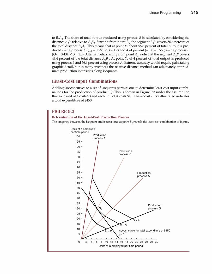
to B3A3. The share of total output produced using process B is calculated by considering thedistance A3Y relative to A3B3. Starting from point B3, the segment B3Y covers 56.6 percent ofthe total distance B3A3. This means that at point Y, about 56.6 percent of total output is pro-duced using process A (QA = 0.566 � 3 = 1.7) and 43.4 percent (= 1.0 – 0.566) using process B(QB = 0.434 � 3 = 1.3). Alternatively, starting from point A3, note that the segment A3Y covers43.4 percent of the total distance A3B3. At point Y, 43.4 percent of total output is producedusing process B and 56.6 percent using process A. Extreme accuracy would require painstakinggraphic detail, but in many instances the relative distance method can adequately approxi-mate production intensities along isoquants.
Least-Cost Input CombinationsAdding isocost curves to a set of isoquants permits one to determine least-cost input combi-nations for the production of product Q. This is shown in Figure 9.3 under the assumptionthat each unit of L costs $3 and each unit of K costs $10. The isocost curve illustrated indicatesa total expenditure of $150.
Chapter Nine Linear Programming 315
FIGURE 9.3Determination of the Least-Cost Production ProcessThe tangency between the isoquant and isocost lines at point B3 reveals the least-cost combination of inputs.
0
5
10
15
20
25
30
35
40
45
50
55
60
65
70
75
80
85
90
95
100
Units of K employed per time period
Units of L employedper time period
Productionprocess A
Productionprocess B
Productionprocess C
Productionprocess D
Q = 2
B3
2 4 6 8 10 12 14 16 18 20 22 24 26 28 30
Q = 3
Q = 4
Isocost curve for total expenditure of $150
Linear Programming 315
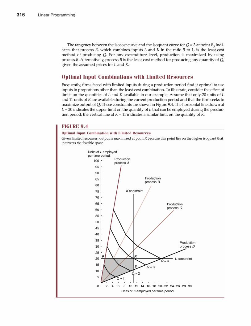
The tangency between the isocost curve and the isoquant curve for Q = 3 at point B3 indi-cates that process B, which combines inputs L and K in the ratio 5 to 1, is the least-costmethod of producing Q. For any expenditure level, production is maximized by usingprocess B. Alternatively, process B is the least-cost method for producing any quantity of Q,given the assumed prices for L and K.
Optimal Input Combinations with Limited ResourcesFrequently, firms faced with limited inputs during a production period find it optimal to useinputs in proportions other than the least-cost combination. To illustrate, consider the effect oflimits on the quantities of L and K available in our example. Assume that only 20 units of Land 11 units of K are available during the current production period and that the firm seeks tomaximize output of Q. These constraints are shown in Figure 9.4. The horizontal line drawn atL = 20 indicates the upper limit on the quantity of L that can be employed during the produc-tion period; the vertical line at K = 11 indicates a similar limit on the quantity of K.
316 Part Three Production and Cost Analysis
FIGURE 9.4Optimal Input Combination with Limited ResourcesGiven limited resources, output is maximized at point R because this point lies on the higher isoquant thatintersects the feasible space.
0
5
10
15
20
25
30
35
40
45
50
55
60
65
70
75
80
85
90
95
100
Units of K employed per time period
Units of L employedper time period
Productionprocess A
Productionprocess B
Productionprocess C
Productionprocess D
2 4 6 8 10 12 14 16 18 20 22 24 26 28 30
Q = 3
Q = 4
Q = 1
S
RL constraint
P
K constraint
Q = 2
316 Linear Programming
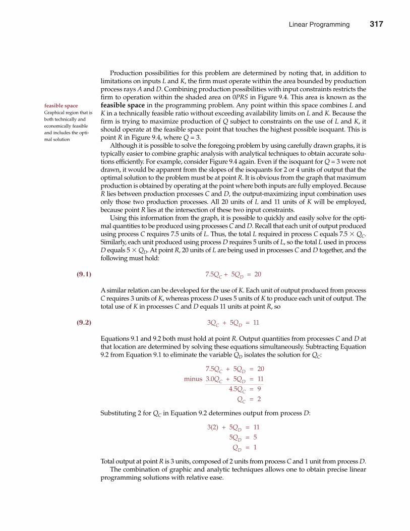
Production possibilities for this problem are determined by noting that, in addition tolimitations on inputs L and K, the firm must operate within the area bounded by productionprocess rays A and D. Combining production possibilities with input constraints restricts thefirm to operation within the shaded area on 0PRS in Figure 9.4. This area is known as thefeasible space in the programming problem. Any point within this space combines L andK in a technically feasible ratio without exceeding availability limits on L and K. Because thefirm is trying to maximize production of Q subject to constraints on the use of L and K, itshould operate at the feasible space point that touches the highest possible isoquant. This ispoint R in Figure 9.4, where Q = 3.
Although it is possible to solve the foregoing problem by using carefully drawn graphs, it istypically easier to combine graphic analysis with analytical techniques to obtain accurate solu-tions efficiently. For example, consider Figure 9.4 again. Even if the isoquant for Q = 3 were notdrawn, it would be apparent from the slopes of the isoquants for 2 or 4 units of output that theoptimal solution to the problem must be at point R. It is obvious from the graph that maximumproduction is obtained by operating at the point where both inputs are fully employed. BecauseR lies between production processes C and D, the output-maximizing input combination usesonly those two production processes. All 20 units of L and 11 units of K will be employed,because point R lies at the intersection of these two input constraints.
Using this information from the graph, it is possible to quickly and easily solve for the opti-mal quantities to be produced using processes C and D. Recall that each unit of output producedusing process C requires 7.5 units of L. Thus, the total L required in process C equals 7.5 � QC.Similarly, each unit produced using process D requires 5 units of L, so the total L used in processD equals 5 � QD. At point R, 20 units of L are being used in processes C and D together, and thefollowing must hold:
(9.1) 7.5QC + 5QD = 20
A similar relation can be developed for the use of K. Each unit of output produced from processC requires 3 units of K, whereas process D uses 5 units of K to produce each unit of output. Thetotal use of K in processes C and D equals 11 units at point R, so
(9.2) 3QC + 5QD = 11
Equations 9.1 and 9.2 both must hold at point R. Output quantities from processes C and D atthat location are determined by solving these equations simultaneously. Subtracting Equation9.2 from Equation 9.1 to eliminate the variable QD isolates the solution for QC:
7.5QC + 5QD = 20minus 3.0QC + 5QD = 11
4.5QC = 9QC = 2
Substituting 2 for QC in Equation 9.2 determines output from process D:
3(2) + 5QD = 115QD = 5QD = 1
Total output at point R is 3 units, composed of 2 units from process C and 1 unit from process D.The combination of graphic and analytic techniques allows one to obtain precise linear
programming solutions with relative ease.
feasible spaceGraphical region that isboth technically andeconomically feasibleand includes the opti-mal solution
Chapter Nine Linear Programming 317
Linear Programming 317
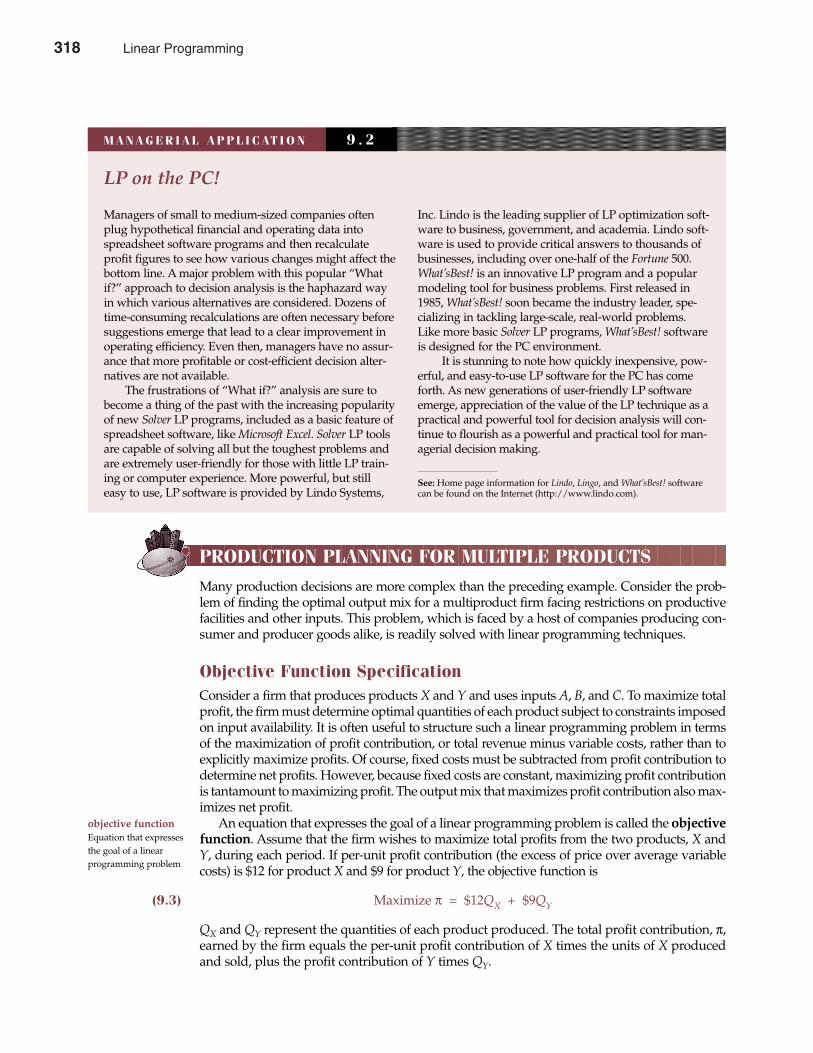
PRODUCTION PLANNING FOR MULTIPLE PRODUCTS
Many production decisions are more complex than the preceding example. Consider the prob-lem of finding the optimal output mix for a multiproduct firm facing restrictions on productivefacilities and other inputs. This problem, which is faced by a host of companies producing con-sumer and producer goods alike, is readily solved with linear programming techniques.
Objective Function SpecificationConsider a firm that produces products X and Y and uses inputs A, B, and C. To maximize totalprofit, the firm must determine optimal quantities of each product subject to constraints imposedon input availability. It is often useful to structure such a linear programming problem in termsof the maximization of profit contribution, or total revenue minus variable costs, rather than toexplicitly maximize profits. Of course, fixed costs must be subtracted from profit contribution todetermine net profits. However, because fixed costs are constant, maximizing profit contributionis tantamount to maximizing profit. The output mix that maximizes profit contribution also max-imizes net profit.
An equation that expresses the goal of a linear programming problem is called the objectivefunction. Assume that the firm wishes to maximize total profits from the two products, X andY, during each period. If per-unit profit contribution (the excess of price over average variablecosts) is $12 for product X and $9 for product Y, the objective function is
(9.3) Maximize π = $12QX + $9QY
QX and QY represent the quantities of each product produced. The total profit contribution, π,earned by the firm equals the per-unit profit contribution of X times the units of X producedand sold, plus the profit contribution of Y times QY.
318 Part Three Production and Cost Analysis
objective functionEquation that expressesthe goal of a linear programming problem
LP on the PC!
Managers of small to medium-sized companies oftenplug hypothetical financial and operating data intospreadsheet software programs and then recalculateprofit figures to see how various changes might affect thebottom line. A major problem with this popular “Whatif?” approach to decision analysis is the haphazard wayin which various alternatives are considered. Dozens oftime-consuming recalculations are often necessary beforesuggestions emerge that lead to a clear improvement inoperating efficiency. Even then, managers have no assur-ance that more profitable or cost-efficient decision alter-natives are not available.
The frustrations of “What if?” analysis are sure tobecome a thing of the past with the increasing popularityof new Solver LP programs, included as a basic feature ofspreadsheet software, like Microsoft Excel. Solver LP toolsare capable of solving all but the toughest problems andare extremely user-friendly for those with little LP train-ing or computer experience. More powerful, but stilleasy to use, LP software is provided by Lindo Systems,
Inc. Lindo is the leading supplier of LP optimization soft-ware to business, government, and academia. Lindo soft-ware is used to provide critical answers to thousands ofbusinesses, including over one-half of the Fortune 500.What’sBest! is an innovative LP program and a popularmodeling tool for business problems. First released in1985, What’sBest! soon became the industry leader, spe-cializing in tackling large-scale, real-world problems.Like more basic Solver LP programs, What’sBest! softwareis designed for the PC environment.
It is stunning to note how quickly inexpensive, pow-erful, and easy-to-use LP software for the PC has comeforth. As new generations of user-friendly LP softwareemerge, appreciation of the value of the LP technique as apractical and powerful tool for decision analysis will con-tinue to flourish as a powerful and practical tool for man-agerial decision making.
See: Home page information for Lindo, Lingo, and What’sBest! softwarecan be found on the Internet (http://www.lindo.com).
M A N A G E R I A L A P P L I C AT I O N 9 . 2
318 Linear Programming
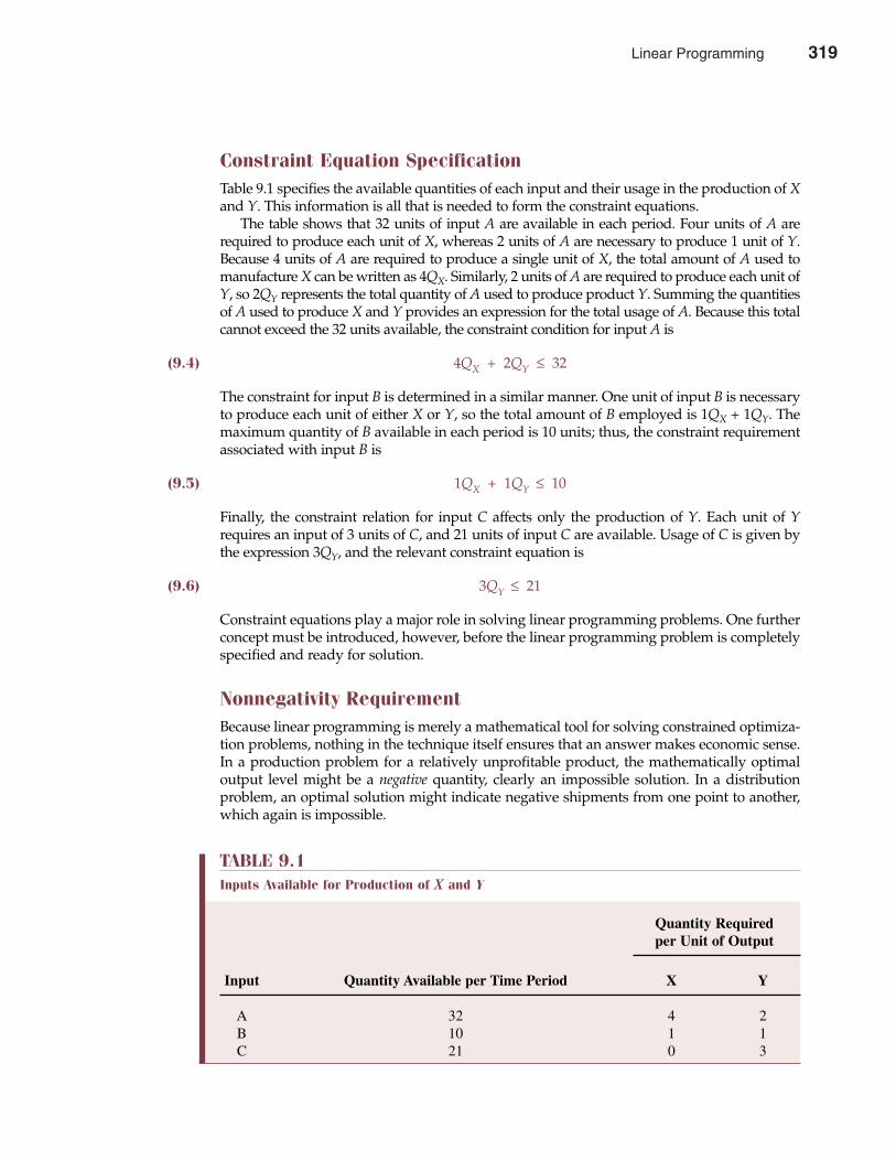
Constraint Equation SpecificationTable 9.1 specifies the available quantities of each input and their usage in the production of Xand Y. This information is all that is needed to form the constraint equations.
The table shows that 32 units of input A are available in each period. Four units of A arerequired to produce each unit of X, whereas 2 units of A are necessary to produce 1 unit of Y.Because 4 units of A are required to produce a single unit of X, the total amount of A used tomanufacture X can be written as 4QX. Similarly, 2 units of A are required to produce each unit ofY, so 2QY represents the total quantity of A used to produce product Y. Summing the quantitiesof A used to produce X and Y provides an expression for the total usage of A. Because this totalcannot exceed the 32 units available, the constraint condition for input A is
(9.4) 4QX + 2QY ≤ 32
The constraint for input B is determined in a similar manner. One unit of input B is necessaryto produce each unit of either X or Y, so the total amount of B employed is 1QX + 1QY. Themaximum quantity of B available in each period is 10 units; thus, the constraint requirementassociated with input B is
(9.5) 1QX + 1QY ≤ 10
Finally, the constraint relation for input C affects only the production of Y. Each unit of Yrequires an input of 3 units of C, and 21 units of input C are available. Usage of C is given bythe expression 3QY, and the relevant constraint equation is
(9.6) 3QY ≤ 21
Constraint equations play a major role in solving linear programming problems. One furtherconcept must be introduced, however, before the linear programming problem is completelyspecified and ready for solution.
Nonnegativity RequirementBecause linear programming is merely a mathematical tool for solving constrained optimiza-tion problems, nothing in the technique itself ensures that an answer makes economic sense.In a production problem for a relatively unprofitable product, the mathematically optimaloutput level might be a negative quantity, clearly an impossible solution. In a distributionproblem, an optimal solution might indicate negative shipments from one point to another,which again is impossible.
Chapter Nine Linear Programming 319
TABLE 9.1Inputs Available for Production of X and Y
Quantity Requiredper Unit of Output
Input Quantity Available per Time Period X Y
A 32 4 2B 10 1 1C 21 0 3
Linear Programming 319
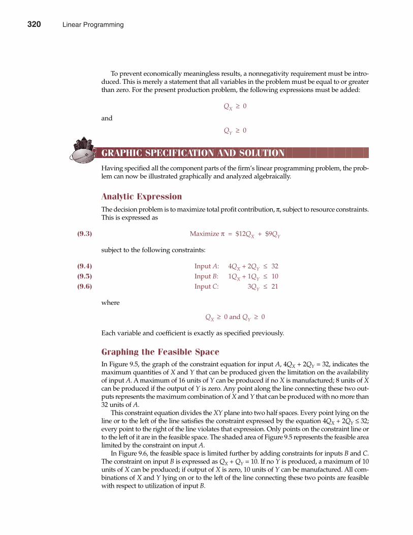
To prevent economically meaningless results, a nonnegativity requirement must be intro-duced. This is merely a statement that all variables in the problem must be equal to or greaterthan zero. For the present production problem, the following expressions must be added:
QX ≥ 0
and
QY ≥ 0
GRAPHIC SPECIFICATION AND SOLUTION
Having specified all the component parts of the firm’s linear programming problem, the prob-lem can now be illustrated graphically and analyzed algebraically.
Analytic ExpressionThe decision problem is to maximize total profit contribution, π, subject to resource constraints.This is expressed as
(9.3) Maximize π = $12QX + $9QY
subject to the following constraints:
(9.4) Input A: 4QX + 2QY ≤ 32(9.5) Input B: 1QX + 1QY ≤ 10(9.6) Input C: 3QY ≤ 21
where
QX ≥ 0 and QY ≥ 0
Each variable and coefficient is exactly as specified previously.
Graphing the Feasible SpaceIn Figure 9.5, the graph of the constraint equation for input A, 4QX + 2QY = 32, indicates themaximum quantities of X and Y that can be produced given the limitation on the availabilityof input A. A maximum of 16 units of Y can be produced if no X is manufactured; 8 units of Xcan be produced if the output of Y is zero. Any point along the line connecting these two out-puts represents the maximum combination of X and Y that can be produced with no more than32 units of A.
This constraint equation divides the XY plane into two half spaces. Every point lying on theline or to the left of the line satisfies the constraint expressed by the equation 4QX + 2QY ≤ 32;every point to the right of the line violates that expression. Only points on the constraint line orto the left of it are in the feasible space. The shaded area of Figure 9.5 represents the feasible arealimited by the constraint on input A.
In Figure 9.6, the feasible space is limited further by adding constraints for inputs B and C.The constraint on input B is expressed as QX + QY = 10. If no Y is produced, a maximum of 10units of X can be produced; if output of X is zero, 10 units of Y can be manufactured. All com-binations of X and Y lying on or to the left of the line connecting these two points are feasiblewith respect to utilization of input B.
320 Part Three Production and Cost Analysis
320 Linear Programming
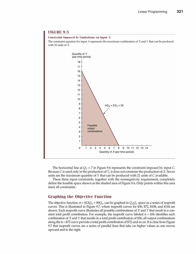
The horizontal line at QY = 7 in Figure 9.6 represents the constraint imposed by input C.Because C is used only in the production of Y, it does not constrain the production of X. Sevenunits are the maximum quantity of Y that can be produced with 21 units of C available.
These three input constraints, together with the nonnegativity requirement, completelydefine the feasible space shown as the shaded area of Figure 9.6. Only points within this areameet all constraints.
Graphing the Objective FunctionThe objective function, π = $12QX + $9QY, can be graphed in QXQY space as a series of isoprofitcurves. This is illustrated in Figure 9.7, where isoprofit curves for $36, $72, $108, and $144 areshown. Each isoprofit curve illustrates all possible combinations of X and Y that result in a con-stant total profit contribution. For example, the isoprofit curve labeled π = $36 identifies eachcombination of X and Y that results in a total profit contribution of $36; all output combinationsalong the π = $72 curve provide a total profit contribution of $72; and so on. It is clear from Figure9.7 that isoprofit curves are a series of parallel lines that take on higher values as one movesupward and to the right.
Chapter Nine Linear Programming 321
FIGURE 9.5Constraint Imposed by Limitations on Input AThe constraint equation for input A represents the maximum combination of X and Y that can be producedwith 32 units of A.
0 1 2 3 4 5 6 7 8 9 10 11 12 13 14
1
2
3
4
5
6
7
8
9
10
11
12
13
14
15
16
17
18
Quantity of X (per time period)
Quantity of Y(per time period)
Feasibleoutputcombinations
4QX + 2QY = 32
Linear Programming 321
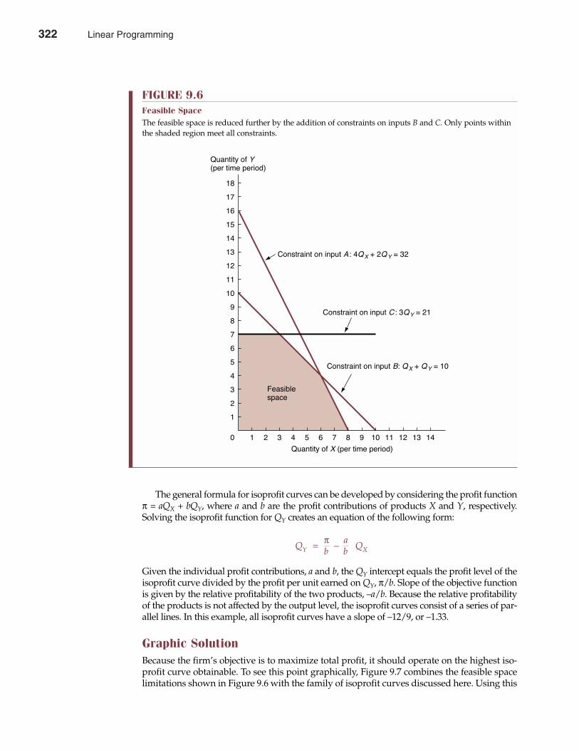
The general formula for isoprofit curves can be developed by considering the profit functionπ = aQX + bQY, where a and b are the profit contributions of products X and Y, respectively.Solving the isoprofit function for QY creates an equation of the following form:
QY = π – aQXb b
Given the individual profit contributions, a and b, the QY intercept equals the profit level of theisoprofit curve divided by the profit per unit earned on QY, π/b. Slope of the objective functionis given by the relative profitability of the two products, –a/b. Because the relative profitabilityof the products is not affected by the output level, the isoprofit curves consist of a series of par-allel lines. In this example, all isoprofit curves have a slope of –12/9, or –1.33.
Graphic SolutionBecause the firm’s objective is to maximize total profit, it should operate on the highest iso-profit curve obtainable. To see this point graphically, Figure 9.7 combines the feasible spacelimitations shown in Figure 9.6 with the family of isoprofit curves discussed here. Using this
322 Part Three Production and Cost Analysis
FIGURE 9.6Feasible SpaceThe feasible space is reduced further by the addition of constraints on inputs B and C. Only points withinthe shaded region meet all constraints.
Constraint on input A : 4QX + 2QY = 32
Constraint on input C : 3QY = 21
Constraint on input B: QX + QY = 10
Feasiblespace
0 1 2 3 4 5 6 7 8 9 10 11 12 13 14
1
2
3
4
5
6
7
8
9
10
11
12
13
14
15
16
17
18
Quantity of X (per time period)
Quantity of Y(per time period)
322 Linear Programming
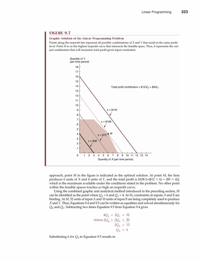
approach, point M in the figure is indicated as the optimal solution. At point M, the firmproduces 6 units of X and 4 units of Y, and the total profit is $108 [=($12 � 6) + ($9 � 4)],which is the maximum available under the conditions stated in the problem. No other pointwithin the feasible spaces touches so high an isoprofit curve.
Using the combined graphic and analytical method introduced in the preceding section, Mcan be identified as the point where QX = 6 and QY = 4. At M, constraints on inputs A and B arebinding. At M, 32 units of input A and 10 units of input B are being completely used to produceX and Y. Thus, Equations 9.4 and 9.5 can be written as equalities and solved simultaneously forQX and QY. Subtracting two times Equation 9.5 from Equation 9.4 gives
4QX + 2QY = 32minus 2QX + 2QY = 20
2QX = 12QX = 6
Substituting 6 for QX in Equation 9.5 results in
Chapter Nine Linear Programming 323
FIGURE 9.7Graphic Solution of the Linear Programming ProblemPoints along the isoprofit line represent all possible combinations of X and Y that result in the same profitlevel. Point M is on the highest isoprofit curve that intersects the feasible space. Thus, it represents the out-put combination that will maximize total profit given input constraints.
0 1 2 3 4 5 6 7 8 9 10 11 12 13 14
1
2
3
4
5
6
7
8
9
10
11
12
13
14
15
16
17
18
Quantity of X (per time period)
Quantity of Y(per time period)
π = $144
π = $108
Mπ = $72
π = $36
Total profit contribution = $12QX + $9QY
Linear Programming 323
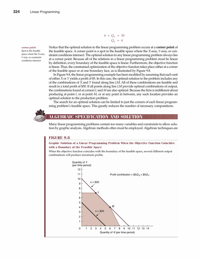
6 + QY = 10QY = 4
Notice that the optimal solution to the linear programming problem occurs at a corner point ofthe feasible space. A corner point is a spot in the feasible space where the X-axis, Y-axis, or con-straint conditions intersect. The optimal solution to any linear programming problem always liesat a corner point. Because all of the relations in a linear programming problem must be linearby definition, every boundary of the feasible space is linear. Furthermore, the objective functionis linear. Thus, the constrained optimization of the objective function takes place either at a cornerof the feasible space or at one boundary face, as is illustrated by Figure 9.8.
In Figure 9.8, the linear programming example has been modified by assuming that each unitof either X or Y yields a profit of $5. In this case, the optimal solution to the problem includes anyof the combinations of X and Y found along line LM. All of these combinations are feasible andresult in a total profit of $50. If all points along line LM provide optimal combinations of output,the combinations found at corners L and M are also optimal. Because the firm is indifferent aboutproducing at point L or at point M, or at any point in between, any such location provides anoptimal solution to the production problem.
The search for an optimal solution can be limited to just the corners of each linear program-ming problem’s feasible space. This greatly reduces the number of necessary computations.
ALGEBRAIC SPECIFICATION AND SOLUTION
Many linear programming problems contain too many variables and constraints to allow solu-tion by graphic analysis. Algebraic methods often must be employed. Algebraic techniques are
324 Part Three Production and Cost Analysis
corner point Spot in the feasiblespace where the X-axis,Y-axis, or constraintconditions intersect
FIGURE 9.8Graphic Solution of a Linear Programming Problem When the Objective Function Coincideswith a Boundary of the Feasible SpaceWhen the objective function coincides with the boundary of the feasible space, several different outputcombinations will produce maximum profits.
0 1 2 3 4 5 6 7 8 9 10 11 12 13 14
1
2
3
4
5
6
7
8
9
10
11
12
Quantity of X (per time period)
Quantity of Y(per time period)
π = $50
π = $25
M
L
Profit contribution = $5QX + $5QY
324 Linear Programming
slack variables Factors that indicatethe amount by whichconstraint conditionsare exceeded
Chapter Nine Linear Programming 325
of great practical relevance because they can be used to solve complex linear programmingproblems with user-friendly computer software.
Slack VariablesThe concept of slack variables must be introduced to solve linear programming problemsalgebraically. In the case of less-than-or-equal-to constraints, slack variables are used to increasethe left side to equal the right side limits of the constraint conditions. In the illustrative problem,one slack variable is added to each constraint to account for excess capacity. The firm is facedwith capacity constraints on input factors A, B, and C, so the algebraic specification of the prob-lem contains three slack variables: SA, indicating the units of A that are not used in any givensolution; SB, representing unused units of B; and SC, which measures the unused units of C.
With slack variables, each constraint equation becomes an equality rather than an inequality.After adding the relevant slack variable, the constraint on input A, 4QX + 2QY ≤ 32, is
(9.7) 4QX + 2QY + SA = 32
SA = 32 – 4QX – 2QY is the amount of input A not used to produce X or Y. Similar equality con-straints can be specified for inputs B and C. The equality form of the constraint on input B is
(9.8) 1QX + 1QY + SB = 10
The constraint equation for input C is
(9.9) 3QY + SC = 21
The introduction of slack variables not only simplifies algebraic analysis, but slack variables’solution values also provide useful information. In a production problem, for example, slackvariables with zero values at the optimal solution indicate inputs that are limiting factors andcause bottlenecks. Slack variables with positive values at the optimal solution indicate excesscapacity in the related input factor. Slack variables cannot take on negative values, becausethis would imply that the amount of resource use exceeds available supply. The informationprovided by slack variable solution values is important in long-range planning and is a keybenefit derived from algebraic solution methods.
Algebraic SolutionThe complete specification of the illustrative programming problem is as follows:
(9.3) Maximize π = $12QX + $9QY
subject to these constraints:
(9.7) 4QX + 2QY + SA = 32(9.8) 1QX + 1QY + SB = 10(9.9) 3QY + SC = 21
where
QX ≥ 0, QY ≥ 0, SA ≥ 0, SB ≥ 0, SC ≥ 0
The problem is to find the set of values for variables QX, QY, SA, SB, and SC that maximizesEquation 9.3 and at the same time satisfies the constraints imposed by Equations 9.7, 9.8, and 9.9.
Linear Programming 325
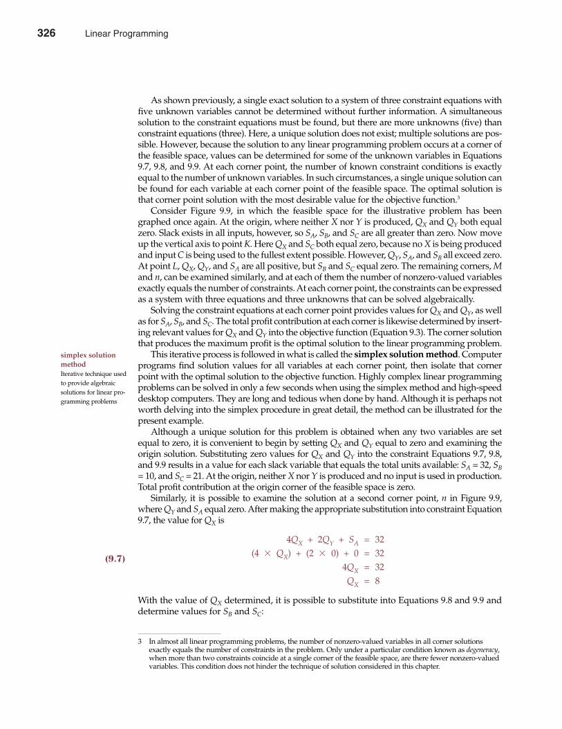
As shown previously, a single exact solution to a system of three constraint equations withfive unknown variables cannot be determined without further information. A simultaneoussolution to the constraint equations must be found, but there are more unknowns (five) thanconstraint equations (three). Here, a unique solution does not exist; multiple solutions are pos-sible. However, because the solution to any linear programming problem occurs at a corner ofthe feasible space, values can be determined for some of the unknown variables in Equations9.7, 9.8, and 9.9. At each corner point, the number of known constraint conditions is exactlyequal to the number of unknown variables. In such circumstances, a single unique solution canbe found for each variable at each corner point of the feasible space. The optimal solution isthat corner point solution with the most desirable value for the objective function.3
Consider Figure 9.9, in which the feasible space for the illustrative problem has beengraphed once again. At the origin, where neither X nor Y is produced, QX and QY both equalzero. Slack exists in all inputs, however, so SA, SB, and SC are all greater than zero. Now moveup the vertical axis to point K. Here QX and SC both equal zero, because no X is being producedand input C is being used to the fullest extent possible. However, QY, SA, and SB all exceed zero.At point L, QX, QY, and SA are all positive, but SB and SC equal zero. The remaining corners, Mand n, can be examined similarly, and at each of them the number of nonzero-valued variablesexactly equals the number of constraints. At each corner point, the constraints can be expressedas a system with three equations and three unknowns that can be solved algebraically.
Solving the constraint equations at each corner point provides values for QX and QY, as wellas for SA, SB, and SC. The total profit contribution at each corner is likewise determined by insert-ing relevant values for QX and QY into the objective function (Equation 9.3). The corner solutionthat produces the maximum profit is the optimal solution to the linear programming problem.
This iterative process is followed in what is called the simplex solution method. Computerprograms find solution values for all variables at each corner point, then isolate that cornerpoint with the optimal solution to the objective function. Highly complex linear programmingproblems can be solved in only a few seconds when using the simplex method and high-speeddesktop computers. They are long and tedious when done by hand. Although it is perhaps notworth delving into the simplex procedure in great detail, the method can be illustrated for thepresent example.
Although a unique solution for this problem is obtained when any two variables are setequal to zero, it is convenient to begin by setting QX and QY equal to zero and examining theorigin solution. Substituting zero values for QX and QY into the constraint Equations 9.7, 9.8,and 9.9 results in a value for each slack variable that equals the total units available: SA = 32, SB= 10, and SC = 21. At the origin, neither X nor Y is produced and no input is used in production.Total profit contribution at the origin corner of the feasible space is zero.
Similarly, it is possible to examine the solution at a second corner point, n in Figure 9.9,where QY and SA equal zero. After making the appropriate substitution into constraint Equation9.7, the value for QX is
4QX + 2QY + SA = 32
(9.7)(4 � QX) + (2 � 0) + 0 = 32
4QX = 32QX = 8
With the value of QX determined, it is possible to substitute into Equations 9.8 and 9.9 anddetermine values for SB and SC:
326 Part Three Production and Cost Analysis
simplex solutionmethodIterative technique usedto provide algebraicsolutions for linear pro-gramming problems
3 In almost all linear programming problems, the number of nonzero-valued variables in all corner solutionsexactly equals the number of constraints in the problem. Only under a particular condition known as degeneracy,when more than two constraints coincide at a single corner of the feasible space, are there fewer nonzero-valuedvariables. This condition does not hinder the technique of solution considered in this chapter.
326 Linear Programming
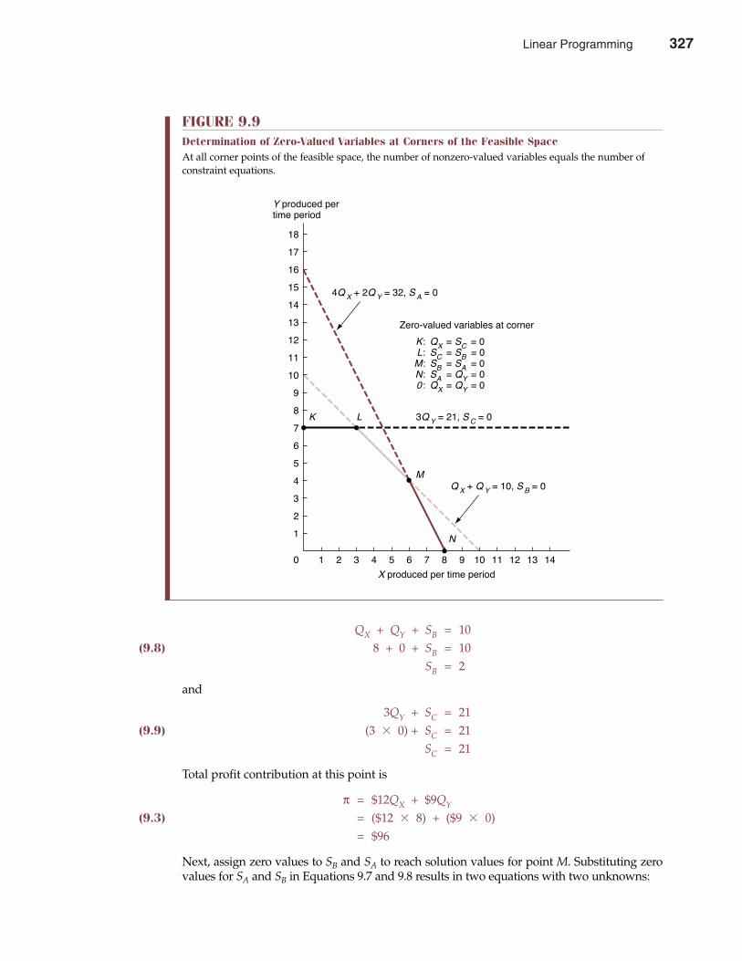
QX + QY + SB = 10(9.8) 8 + 0 + SB = 10
SB = 2
and
3QY + SC = 21(9.9) (3 � 0) + SC = 21
SC = 21
Total profit contribution at this point is
π = $12QX + $9QY
(9.3) = ($12 � 8) + ($9 � 0)= $96
Next, assign zero values to SB and SA to reach solution values for point M. Substituting zerovalues for SA and SB in Equations 9.7 and 9.8 results in two equations with two unknowns:
Chapter Nine Linear Programming 327
FIGURE 9.9Determination of Zero-Valued Variables at Corners of the Feasible SpaceAt all corner points of the feasible space, the number of nonzero-valued variables equals the number ofconstraint equations.
0 1 2 3 4 5 6 7 8 9 10 11 12 13 14
1
2
3
4
5
6
7
8
9
10
11
12
13
14
15
16
17
18
X produced per time period
Y produced pertime period
4Q X + 2Q Y = 32, S A = 0
Q X + Q Y = 10, S B = 0
N
M
LK 3Q Y = 21, S C = 0
QX = SC = 0SC = SB = 0SB = SA = 0SA = QY = 0QX = QY = 0
Zero-valued variables at corner
K:L:M:N:0 :
Linear Programming 327
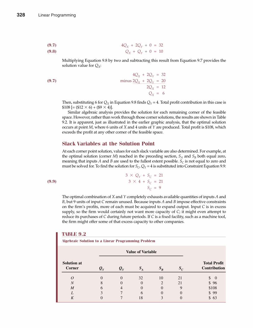
(9.7) 4QX + 2QY + 0 = 32(9.8) QX + QY + 0 = 10
Multiplying Equation 9.8 by two and subtracting this result from Equation 9.7 provides thesolution value for QX:
4QX + 2QY = 32(9.7) minus 2QX + 2QY = 20
2QX = 12QX = 6
Then, substituting 6 for QX in Equation 9.8 finds QY = 4. Total profit contribution in this case is$108 [= ($12 � 6) + ($9 � 4)].
Similar algebraic analysis provides the solution for each remaining corner of the feasiblespace. However, rather than work through those corner solutions, the results are shown in Table9.2. It is apparent, just as illustrated in the earlier graphic analysis, that the optimal solutionoccurs at point M, where 6 units of X and 4 units of Y are produced. Total profit is $108, whichexceeds the profit at any other corner of the feasible space.
Slack Variables at the Solution PointAt each corner point solution, values for each slack variable are also determined. For example, atthe optimal solution (corner M) reached in the preceding section, SA and SB both equal zero,meaning that inputs A and B are used to the fullest extent possible. SC is not equal to zero andmust be solved for. To find the solution for SC, QY = 4 is substituted into Constraint Equation 9.9:
3 � QY + SC = 21(9.9) 3 � 4 + SC = 21
SC = 9
The optimal combination of X and Y completely exhausts available quantities of inputs A andB, but 9 units of input C remain unused. Because inputs A and B impose effective constraintson the firm’s profits, more of each must be acquired to expand output. Input C is in excesssupply, so the firm would certainly not want more capacity of C; it might even attempt toreduce its purchases of C during future periods. If C is a fixed facility, such as a machine tool,the firm might offer some of that excess capacity to other companies.
328 Part Three Production and Cost Analysis
TABLE 9.2Algebraic Solution to a Linear Programming Problem
Value of Variable
Solution at Total ProfitCorner QY QY SA SB SC Contribution
O 0 0 32 10 21 $ 0N 8 0 0 2 21 $ 96M 6 4 0 0 9 $108L 3 7 6 0 0 $ 99K 0 7 18 3 0 $ 63
328 Linear Programming
Computer-Based Solution MethodsThe linear programming problem illustrated thus far is simple by design. It can be solved graph-ically and algebraically to illustrate the linear programming technique using both methods.However, linear programming problems encountered in the real world are often quite complexand frequently involve a large number of constraints and output variables. Such problems aretoo complicated to solve graphically. The geometry is messy for three outputs and impossible forfour or more. In real-world applications, computer software programs use algebraic techniquesto handle large numbers of variables and constraints.
THE DUAL IN LINEAR PROGRAMMING
For every maximization problem in linear programming, there exists a symmetrical minimizationproblem; for every minimization problem, there exists a symmetrical maximization problem.
The Duality ConceptPairs of related maximization and minimization problems are known as primal and duallinear programming problems. The concept of duality demonstrates the symmetry betweenthe value of a firm’s products and the value of resources used in production. With the dual-ity concept, it is possible to show that value maximization can be attained by focusing oneither resource requirements and the revenue-generating capability of a firm’s products oron the cost of resources and their productivity.
In addition to providing valuable insight into the economics of optimal resource employ-ment, duality provides the key to solving difficult constrained optimization problems. Because
primalOriginal problem statement (symmetricalto dual)
dualSecondary problemstatement (symmetricalto primal)
Chapter Nine Linear Programming 329
Internet Message Boards
Message boards are online “communities” that allowpeople to communicate about common interests on theInternet. Common interests might include business topics,like linear programming and long-term investing, ornonbusiness interests, like gardening. On messageboards, the communication is ongoing and broad-based.Hundreds of individuals may contribute to an especiallyactive message board during the course of a few days.This is different from online “chat,” where conversationsare brief and visible only to a small handful of currentparticipants. Although chat dialogue disappears afteronly a few moments, message board posts are longerand remain visible for extended periods. Message boarddialogue is typically linked, so that interested parties cango back and forth about a given topic. Message boarddialogue is also searchable, thus allowing for detailedexchanges to take place. Lively message board communi-ties can be a productive and entertaining way of gather-ing useful business and economic information.
Message board categories contain different boardswith a common theme. For example, there are 16 cate-gories or broad grouping of interests listed on the Yahoo!Message Boards. The “Business & Finance” category, for
example, has individual boards for discussing“Investments,” “Services,” “Communications Services,”and Level 3 Communications, along with several hundredother individual companies in this field.
When using message boards, it’s important toremember to• Be careful what you believe. Message board infor-
mation is no substitute for independent research.Don’t rely on it for business or investment decisions.
• Be skeptical of other posters. Never assume peopleare who they say they are, know what they say theyknow, or are affiliated with whom they say they areaffiliated.
• Be careful what you post. Never assume that youare anonymous and cannot be identified by yourmessages.
With these caveats in mind, by all means log on andcheck it out. You’ll be amazed at what people are talk-ing about on the Internet!
See: Nicholas Kulish, “SBC Official Says Microsoft’s Power Could LimitNew Messaging Service,” The Wall Street Journal Online, April 9, 2002(http://online.wsj.com).
M A N A G E R I A L A P P L I C AT I O N 9 . 3
Linear Programming 329
of the symmetry between primal and dual problem specifications, either one can be construct-ed from the other and the solution to either problem can be used to solve both. This is helpfulbecause it is sometimes easier to obtain the solution to the dual problem than to the original orprimal problem.
Finally, the duality concept also allows one to evaluate the solution to a constrained decisionproblem in terms of the activity required for optimization and in terms of the economic impactof constraint conditions. Analysis of the constraint conditions and slack variable solutions fre-quently provides important information for long-range planning. In fact, the primal solutionis often described as a tool for short-run operating decisions, whereas the dual solution is oftenseen as a tool for long-range planning. The duality concept shows how operating decisions andlong-range planning are related.
Shadow PricesTo examine the duality concept, the idea of implicit values or shadow prices must be intro-duced. In the primal linear programming problem discussed previously, the values QX and QYmaximize the firm’s profit subject to constraints imposed by limitations of input factors A, B,and C. Duality theory indicates that an identical operating decision would result if one hadinstead chosen to minimize the costs of resources employed in producing QX and QY, subjectto an output constraint.
The key to this duality is that relevant costs are not the acquisition costs of inputs but,rather, the economic costs of using them. For a resource that is available in a fixed amount,this cost is not acquisition cost but opportunity cost. Consider, for example, a skilled labor forceemployed by a firm. If workers are fully utilized producing valuable products, a reduction inskilled labor will reduce valuable output, and an increase in skilled labor will increase theproduction of valuable output. If some labor is shifted from the production of one productto another, the cost of using skilled labor in this new activity is the value of the originalproduct that can no longer be produced. The marginal cost of a constrained resource that isfully utilized is its opportunity cost as measured by the value of foregone production. If alimited resource such as skilled labor is not fully utilized, then at least the last unit of thatresource is not productive and its marginal value is zero. Acquiring additional excess resourcesdoes not increase valuable output. The firm would incur a zero opportunity cost if it appliedcurrently unused resources in some different activity.
The economic value, or opportunity cost, of a constrained resource depends on the extent towhich it is utilized. When a limited resource is fully utilized, its marginal value in use is positive.When a constrained resource is not fully utilized, its marginal value in use is zero. Minimizingthe value of limited resources used to produce valuable output is nothing more than minimiz-ing the opportunity cost of employing those resources. Minimization of opportunity costs isequivalent to maximizing the value of output produced with those resources.
Because the economic value of constrained resources is determined by their value in userather than by historical acquisition costs, such amounts are called implicit values or shadowprices. The term shadow price is used because it represents the price that a manager would bewilling to pay for additional units of a constrained resource. Comparing the shadow price ofa resource with its acquisition price indicates whether the firm has an incentive to increase ordecrease the amount acquired during future production periods. If shadow prices exceedacquisition prices, the resource’s marginal value exceeds marginal cost and the firm has anincentive to expand employment. If acquisition cost exceeds the shadow price, there is anincentive to reduce employment. These relations and the importance of duality can be clari-fied by relating the dual to the linear programming problem discussed previously.
330 Part Three Production and Cost Analysis
primal solution Input for short-runoperating decisions
dual solution Input for long-rangeplanning
shadow pricesImplicit values associ-ated with linear-programming-problemdecision variables
330 Linear Programming
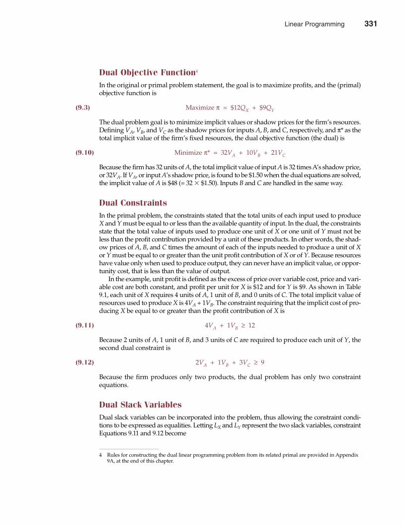
Dual Objective Function4
In the original or primal problem statement, the goal is to maximize profits, and the (primal)objective function is
(9.3) Maximize π = $12QX + $9QY
The dual problem goal is to minimize implicit values or shadow prices for the firm’s resources.Defining VA, VB, and VC as the shadow prices for inputs A, B, and C, respectively, and π* as thetotal implicit value of the firm’s fixed resources, the dual objective function (the dual) is
(9.10) Minimize π* = 32VA + 10VB + 21VC
Because the firm has 32 units of A, the total implicit value of input A is 32 times A’s shadow price,or 32VA. If VA, or input A’s shadow price, is found to be $1.50 when the dual equations are solved,the implicit value of A is $48 (= 32 � $1.50). Inputs B and C are handled in the same way.
Dual ConstraintsIn the primal problem, the constraints stated that the total units of each input used to produceX and Y must be equal to or less than the available quantity of input. In the dual, the constraintsstate that the total value of inputs used to produce one unit of X or one unit of Y must not beless than the profit contribution provided by a unit of these products. In other words, the shad-ow prices of A, B, and C times the amount of each of the inputs needed to produce a unit of Xor Y must be equal to or greater than the unit profit contribution of X or of Y. Because resourceshave value only when used to produce output, they can never have an implicit value, or oppor-tunity cost, that is less than the value of output.
In the example, unit profit is defined as the excess of price over variable cost, price and vari-able cost are both constant, and profit per unit for X is $12 and for Y is $9. As shown in Table9.1, each unit of X requires 4 units of A, 1 unit of B, and 0 units of C. The total implicit value ofresources used to produce X is 4VA + 1VB. The constraint requiring that the implicit cost of pro-ducing X be equal to or greater than the profit contribution of X is
(9.11) 4VA + 1VB ≥ 12
Because 2 units of A, 1 unit of B, and 3 units of C are required to produce each unit of Y, thesecond dual constraint is
(9.12) 2VA + 1VB + 3VC ≥ 9
Because the firm produces only two products, the dual problem has only two constraintequations.
Dual Slack VariablesDual slack variables can be incorporated into the problem, thus allowing the constraint condi-tions to be expressed as equalities. Letting LX and LY represent the two slack variables, constraintEquations 9.11 and 9.12 become
Chapter Nine Linear Programming 331
4 Rules for constructing the dual linear programming problem from its related primal are provided in Appendix9A, at the end of this chapter.
Linear Programming 331
(9.13) 4VA + 1VB – LX = 12
and
(9.14) 2VA + 1VB + 3VC – LY = 9
These slack variables are subtracted from the constraint equations, because greater-than-or-equal-to inequalities are involved. Using slack variables, the left-hand sides of the constraint conditionsare thus decreased to equal the right-hand sides’ profit contributions. Dual slack variables measurethe excess of input value over output value for each product. Alternatively, dual slack variablesmeasure the opportunity cost associated with producing X and Y. This can be seen by examiningthe two constraint equations. Solving constraint Equation 9.13 for LX, for example, provides
LX = 4VA + 1VB – 12
This expression states that LX is equal to the implicit cost of producing 1 unit of X minus theprofit contribution provided by that product. The dual slack variable LX is a measure of theopportunity cost of producing product X. It compares the profit contribution of product X, $12,with the value to the firm of the resources necessary to produce it.
A zero value for LX indicates that the marginal value of resources required to produce 1 unitof X is exactly equal to the profit contribution received. This is similar to marginal cost beingequal to marginal revenue at the profit-maximizing output level. Apositive value for LX indicatesthat the resources used to produce X are more valuable, in terms of the profit contribution theycan generate, when used to produce the other product Y. A positive value for LX measures thefirm’s opportunity cost (profit loss) associated with production of product X. The slack variableLY is the opportunity cost of producing product Y. It will have a value of zero if the implicit valueof resources used to produce 1 unit of Y exactly equals the $9 profit contribution provided by thatproduct. A positive value for LY measures the opportunity loss in terms of the foregone profitcontribution associated with product Y.
A firm would not choose to produce if the value of resources required were greater than thevalue of resulting output. It follows that a product with a positive slack variable (opportunitycost) is not included in the optimal production combination.
Solving the Dual ProblemThe dual programming problem can be solved with the same algebraic technique that wasemployed to obtain the primal solution. In this case, the dual problem is
(9.10) Minimize π* = 34VA + 10VB + 21VC
subject to
(9.13) 4VA + 1VB – LX = 12
and
(9.14) 2VA + 1VB + 3VC – LY = 9
where
VA, VB, VC, LX, and LY all ≥ 0
Because there are only two constraints in this programming problem, the maximum number ofnonzero-valued variables at any corner solution is two. One can proceed with the solution by
332 Part Three Production and Cost Analysis
332 Linear Programming
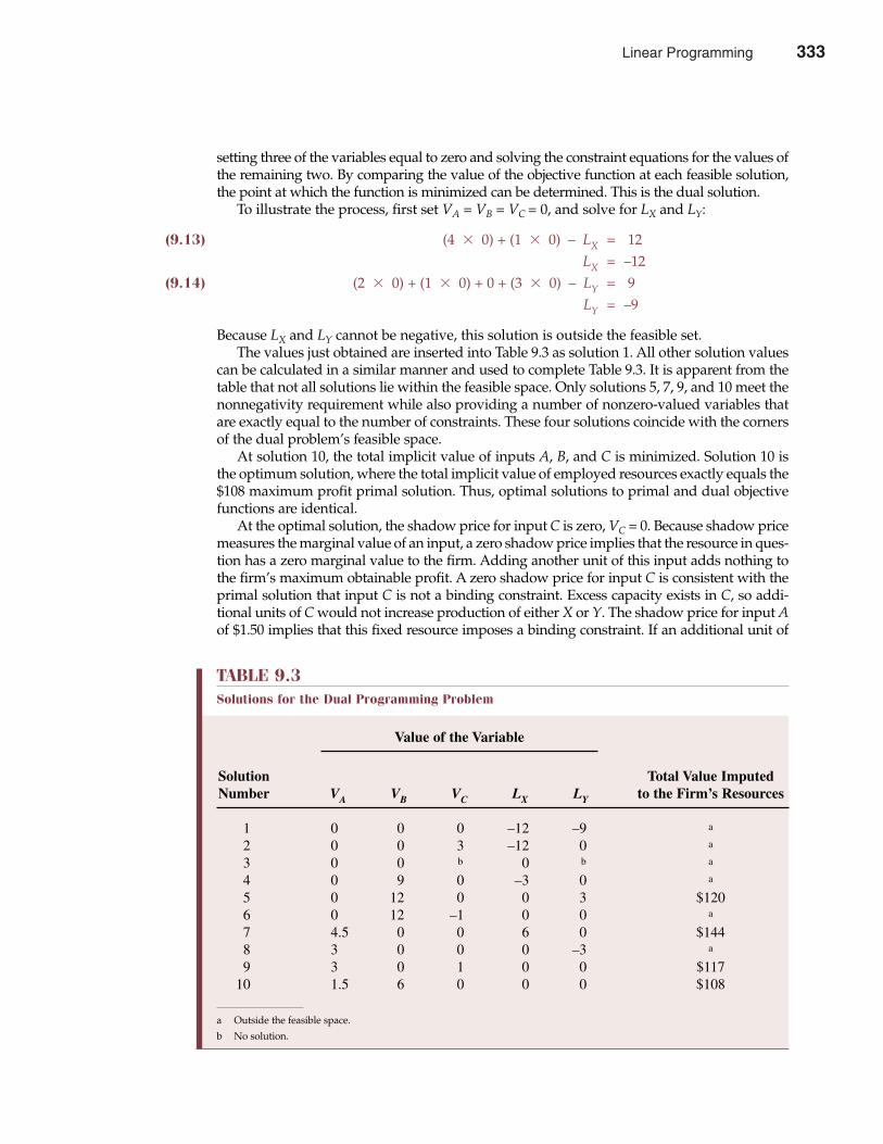
setting three of the variables equal to zero and solving the constraint equations for the values ofthe remaining two. By comparing the value of the objective function at each feasible solution,the point at which the function is minimized can be determined. This is the dual solution.
To illustrate the process, first set VA = VB = VC = 0, and solve for LX and LY:
(9.13) (4 � 0) + (1 � 0) – LX = 12LX = –12
(9.14) (2 � 0) + (1 � 0) + 0 + (3 � 0) – LY = 9LY = –9
Because LX and LY cannot be negative, this solution is outside the feasible set.The values just obtained are inserted into Table 9.3 as solution 1. All other solution values
can be calculated in a similar manner and used to complete Table 9.3. It is apparent from thetable that not all solutions lie within the feasible space. Only solutions 5, 7, 9, and 10 meet thenonnegativity requirement while also providing a number of nonzero-valued variables thatare exactly equal to the number of constraints. These four solutions coincide with the cornersof the dual problem’s feasible space.
At solution 10, the total implicit value of inputs A, B, and C is minimized. Solution 10 isthe optimum solution, where the total implicit value of employed resources exactly equals the$108 maximum profit primal solution. Thus, optimal solutions to primal and dual objectivefunctions are identical.
At the optimal solution, the shadow price for input C is zero, VC = 0. Because shadow pricemeasures the marginal value of an input, a zero shadow price implies that the resource in ques-tion has a zero marginal value to the firm. Adding another unit of this input adds nothing tothe firm’s maximum obtainable profit. A zero shadow price for input C is consistent with theprimal solution that input C is not a binding constraint. Excess capacity exists in C, so addi-tional units of C would not increase production of either X or Y. The shadow price for input Aof $1.50 implies that this fixed resource imposes a binding constraint. If an additional unit of
Chapter Nine Linear Programming 333
TABLE 9.3Solutions for the Dual Programming Problem
Value of the Variable
Solution Total Value ImputedNumber VA VB VC LX LY to the Firm’s Resources
1 0 0 0 –12 –9 a
2 0 0 3 –12 0 a
3 0 0 b 0 b a
4 0 9 0 –3 0 a
5 0 12 0 0 3 $1206 0 12 –1 0 0 a
7 4.5 0 0 6 0 $1448 3 0 0 0 –3 a
9 3 0 1 0 0 $11710 1.5 6 0 0 0 $108
a Outside the feasible space.
b No solution.
Linear Programming 333
334 Part Three Production and Cost Analysis
A is added, the firm can increase total profit by $1.50. It would increase profits to buy addi-tional units of input A at any price less than $1.50 per unit, at least up until the point at whichA is no longer a binding constraint. This assumes that the cost of input A is currently fixed. Ifthose costs are variable, the firm would be willing to pay $1.50 above the current price of inputA to eliminate this constraint. Because availability of B also imposes an effective constraint, thefirm can also afford to pay up to $6 for a marginal unit of B.
Finally, both dual slack variables equal zero at the optimal solution. This means that theimplicit value of resources required to produce a single unit of X or Y is exactly equal to theprofit contribution provided. The opportunity cost of producing X and Y is zero, meaning thatthe resources required for their production are not more valuable in some alternative use. Thisis consistent with the primal solution, because both X and Y are produced at the optimal solu-tion. Any product with a positive opportunity cost is suboptimal and would not be produced.
Using the Dual Solution to Solve the PrimalThe dual solution does not indicate optimal amounts of X and Y. It does, however, provide all theinformation necessary to determine the optimum output mix. The dual solution shows that inputC does not impose a binding constraint on output of X and Y. Further, it demonstrates that π = π*= $108 at the optimum output of X and Y. The dual solution also offers evidence on the value ofprimal constraint slack variables. To see this, recall the three constraints in the primal problem:
Constraint on A: 4QX + 2QY + SA = 32Constraint on B: 1QX + 1QY + SB = 10Constraint on C: 3QY + SC = 21
The dual solution indicates that the constraints on A and B are binding, because both inputs havepositive shadow prices, and only resources that are fully utilized have a nonzero marginal value.Accordingly, the slack variables SA and SB equal zero, and the binding primal constraints can berewritten as
4QX + 2QY = 32
and
1QX + 1QY = 10
With two equations and only two unknowns, this system can be solved for QX and QY.Multiplying the second constraint by two and subtracting from the first provides
4QX + 2QY = 32minus 2QX + 2QY = 20
2QX = 12QX = 6
and
6 + QY = 10QY = 4
These values of QX and QY, found after learning from the dual which constraints were binding,are identical to the values found by solving the primal problem directly. Having obtained thevalue for QY, it is possible to substitute value for QY in constraint C and solve for the amount ofslack in that resource:
334 Linear Programming
3QY + SC = 21SC = 21 – 3 � 4 = 9
These relations, which allow one to solve either the primal or the dual specification of a linearprogramming problem and then quickly obtain the solution to the other, can be generalized bythe two following expressions:
(9.15) Primal Objective Variablei � Dual Slack Variablei � 0(9.16) Primal Slack Variablej � Dual Objective Variablej � 0
Equation 9.15 states that if an ordinary variable in the primal problem takes on a nonzero valuein the optimal solution to that problem, its related dual slack variable must be zero. Only if a par-ticular Qi is zero valued in the solution to the primal can its related dual slack variable, Li, takeon a nonzero value. A similar relation exists between the slack variables in the primal problemand their related ordinary variables in the dual, as indicated by Equation 9.16. If the primal slackvariable is nonzero valued, then the related dual variable will be zero valued, and vice versa.
CONSTRAINED COST MINIMIZATION: ANOTHER LP EXAMPLE
Constrained cost-minimization problems are frequently encountered in managerial decisionmaking. One such example is the problem of minimizing advertising expenditures subject tocertain audience exposure requirements.
Chapter Nine Linear Programming 335
It’s a RIOT on the Internet!
Here’s an idea for you. How would you like access to aRemote Interactive Optimization Testbed (RIOT) on theInternet? It’s a simple concept, as in simply amazing.
RIOT creates an interface between the Web and linearprogramming solver programs that allows anyone withaccess to the Web to submit a linear program and have itsolved. There has been a proliferation of linear program-ming solver software since 1980, like Cplex, Lingo, Minos,and so on. However, each of these solver programs imple-ments different algorithms, like the simplex method, andoffers different solution options, like sensitivity analysis.Depending on the problem to be solved, some solvers canbe more or less efficient than others in terms of speed,accuracy, number of iterations, and available options.
LP applications on RIOT range from the serious, likea planar robot simulator with obstacle avoidance andopen-pit mining problems, to the whimsical, like majorleague baseball and basketball elimination problems.Over time, continuing improvements promise users theopportunity to find the optimal value (maximum orminimum) for any linear function of a certain number ofvariables given a set of m linear constraints on thesevariables (equalities or inequalities).
Like everything on the Web, RIOT is still relativelynew and bound to evolve rapidly over time. At thispoint, it is a free offering designed to achieve four mainobjectives:.
• Educational. RIOT provides educational informationvia HTML and interactive problems presentedthrough an easy-to-use interface.
• Research. RIOT showcases state-of-the-art algorithmsdeveloped locally by UC Berkeley engineering facultyand others.
• Comparative research. RIOT provides efficiencyinformation for different algorithms that solve similarproblems.
• Showcase applications. RIOT provides a forum toshowcase new and innovative applications of linearprogramming techniques.
RIOT is an enormously practical tool. It’s on the Internet.It’s free. What a RIOT!
See: Home page for RIOT can be found on the Internet(http://riot.ieor.berkeley.edu/riot/index.html).
M A N A G E R I A L A P P L I C AT I O N 9 . 4
Linear Programming 335
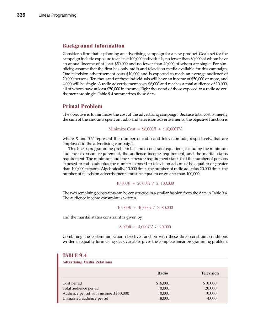
Background InformationConsider a firm that is planning an advertising campaign for a new product. Goals set for thecampaign include exposure to at least 100,000 individuals, no fewer than 80,000 of whom havean annual income of at least $50,000 and no fewer than 40,000 of whom are single. For sim-plicity, assume that the firm has only radio and television media available for this campaign.One television advertisement costs $10,000 and is expected to reach an average audience of20,000 persons. Ten thousand of these individuals will have an income of $50,000 or more, and4,000 will be single. A radio advertisement costs $6,000 and reaches a total audience of 10,000,all of whom have at least $50,000 in income. Eight thousand of those exposed to a radio adver-tisement are single. Table 9.4 summarizes these data.
Primal ProblemThe objective is to minimize the cost of the advertising campaign. Because total cost is merelythe sum of the amounts spent on radio and television advertisements, the objective function is
Minimize Cost = $6,000R + $10,000TV
where R and TV represent the number of radio and television ads, respectively, that areemployed in the advertising campaign.
This linear programming problem has three constraint equations, including the minimumaudience exposure requirement, the audience income requirement, and the marital statusrequirement. The minimum audience exposure requirement states that the number of personsexposed to radio ads plus the number exposed to television ads must be equal to or greaterthan 100,000 persons. Algebraically, 10,000 times the number of radio ads plus 20,000 times thenumber of television advertisements must be equal to or greater than 100,000:
10,000R + 20,000TV ≥ 100,000
The two remaining constraints can be constructed in a similar fashion from the data in Table 9.4.The audience income constraint is written
10,000R + 10,000TV ≥ 80,000
and the marital status constraint is given by
8,000R + 4,000TV ≥ 40,000
Combining the cost-minimization objective function with these three constraint conditionswritten in equality form using slack variables gives the complete linear programming problem:
336 Part Three Production and Cost Analysis
TABLE 9.4Advertising Media Relations
Radio Television
Cost per ad $ 6,000 $10,000Total audience per ad 10,000 20,000Audience per ad with income ≥$50,000 10,000 10,000Unmarried audience per ad 8,000 4,000
336 Linear Programming
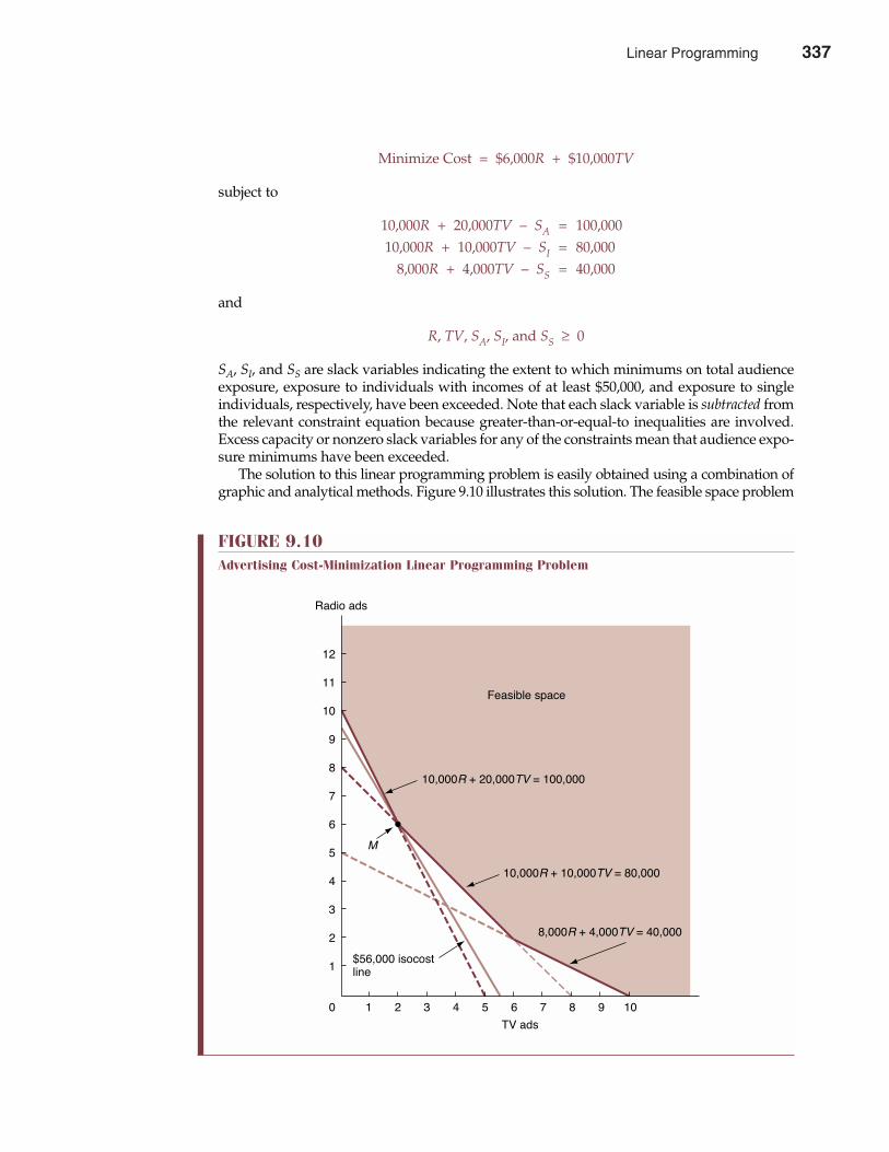
Minimize Cost = $6,000R + $10,000TV
subject to
10,000R + 20,000TV – SA = 100,00010,000R + 10,000TV – SI = 80,000
8,000R + 4,000TV – SS = 40,000
and
R, TV, SA, SI, and SS ≥ 0
SA, SI, and SS are slack variables indicating the extent to which minimums on total audienceexposure, exposure to individuals with incomes of at least $50,000, and exposure to singleindividuals, respectively, have been exceeded. Note that each slack variable is subtracted fromthe relevant constraint equation because greater-than-or-equal-to inequalities are involved.Excess capacity or nonzero slack variables for any of the constraints mean that audience expo-sure minimums have been exceeded.
The solution to this linear programming problem is easily obtained using a combination ofgraphic and analytical methods. Figure 9.10 illustrates this solution. The feasible space problem
Chapter Nine Linear Programming 337
FIGURE 9.10Advertising Cost-Minimization Linear Programming Problem
12
11
10
9
8
7
6
5
4
3
2
1
0 1 2 3 4 5 6 7 8 9 10
TV ads
Radio ads
M
$56,000 isocostline
8,000R + 4,000TV = 40,000
10,000R + 10,000TV = 80,000
10,000R + 20,000TV = 100,000
Feasible space
Linear Programming 337
is bordered by the three constraint equations and the nonnegativity requirements. An isocostcurve shows that costs are minimized at point M, where the total audience exposure and incomeconstraints are binding. With these constraints binding, slack variables SA = SI = 0. Thus,
10,000R + 20,000TV = 100,000minus 10,000R + 10,000TV = 80,000
10,000TV = 20,000TV = 2
and
10,000R + 20,000(2) = 100,00010,000R = 60,000
R = 6
The firm should employ six radio advertisements and two television advertisements to mini-mize costs while still meeting audience exposure requirements. Total cost for such a campaignis $56,000.
Dual ProblemThe dual to the advertising-mix problem is a constrained-maximization problem, because theprimal is a minimization problem. The objective function of the dual is expressed in terms ofshadow prices or implicit values for the primal constraint conditions. The dual objective func-tion includes an implicit value, or shadow price, for the minimum audience exposure require-ment, the audience income requirement, and the marital status requirement. Because constraintlimits in the primal problem become the dual objective function coefficients, the dual objectivefunction is
Maximize C* = 100,000VA + 80,000VI + 40,000VS
where VA, VI, and VS are shadow prices for the minimum audience exposure, audience income,and marital status requirements.
Dual constraints are based on the two variables from the primal objective function. Thus,there are two constraint conditions in the dual, the first associated with radio advertisementsand the second with television advertisements. Both constraints are of the less-than-or-equal-totype, because primal constraints are of the greater-than-or-equal-to type.
The radio advertising constraint limit is the $6,000 radio advertisements coefficient from theprimal objective function. Coefficients for each shadow price in this constraint equation aregiven by the advertising effectiveness measures for a single radio advertisement. The coefficientfor the audience exposure shadow price, VA, is 10,000, the number of individuals reached by asingle radio advertisement. Similarly, the coefficient for VI is 10,000 and that for VS is 8,000.Thus, the dual radio advertisements constraint is
10,000VA + 10,000VI + 8,000VS ≤ $6,000
The dual television advertising constraint is developed in the same fashion. Because each TVadvertisement reaches a total audience of 20,000, this is the coefficient for the VA variable in thesecond dual constraint equation. Coefficients for VI and VS are 10,000 and 4,000, respectively,because these are the numbers of high-income and single persons reached by one TV adver-tisement. The $10,000 cost of a television advertisement is the limit to the second dual constraint,which can be written
338 Part Three Production and Cost Analysis
338 Linear Programming
20,000VA + 10,000VI + 4,000VS ≤ $10,000
Following the introduction of constraint slack variables, the dual programming problem is
Maximize C* = 100,000VA + 80,000VI + 40,000VS
subject to
10,000VA + 10,000VI + 8,000VS + LR = $ 6,00020,000VA + 10,000VI + 4,000VS + LTV = $10,000
and
VA, VI, VS, LR, and LTV ≥ 0
Solving the DualIt is possible but difficult to solve this dual problem using a three-dimensional graph or the sim-plex method. However, because the primal problem has been solved already, information fromthis solution can be used to easily solve the dual. Remember that the solutions to the primal anddual of a single linear programming problem are complementary, and the following must hold:
Primal Objective Variablei � Dual Slack Variablei = 0Primal Slack Variablej � Dual Objective Variablej = 0
In this linear programming problem,
R � LR = 0 and TV � LTV = 0
and
SA � VA = 0, SI � VI = 0, and SS � VS = 0
Because both R and TV have nonzero solutions in the primal, the dual slack variables LR and LTVmust equal zero at the optimal solution. Furthermore, because there is excess audience exposureto the single marital status category in the primal solution, SS ≠ 0, the related dual shadow pricevariable VS must also equal zero in the optimal solution. This leaves only VA and VI as twounknowns in the two-equation system of dual constraints:
10,000VA + 10,000VI = $ 6,00020,000VA + 10,000VI = $10,000
Subtracting the second constraint equation from the first gives
–10,000VA = –$4,000VA = $0.40
Substituting the value $0.40 for VA in either constraint equation produces a value of $0.20 for VI.Finally, substituting the appropriate values for VA, VI, and VS into the dual objective functiongives a value of C* = $56,000 [= ($0.40 � 100,000) + ($0.20 � 80,000) + ($0 � 40,000)]. This is thesame figure as the $56,000 minimum cost solution to the primal.
Chapter Nine Linear Programming 339
Linear Programming 339
Interpreting the Dual SolutionThe primal solution tells management the minimum-cost advertising mix. The dual problemresults are equally valuable. Each dual shadow price indicates the change in cost that wouldaccompany a one-unit change in the various audience exposure requirements. These pricesshow the marginal costs of increasing each audience exposure requirement by one unit. Forexample, VA is the marginal cost of reaching the last individual in the overall audience. Ifthere were a one-person reduction in the total audience exposure requirement, a cost savingof VA = $0.40 would be realized. The marginal cost of increasing total audience exposurefrom 100,000 to 100,001 individuals would also be 40¢.
Shadow prices for the remaining constraint conditions are interpreted in a similar manner.The shadow price for reaching individuals with incomes of at least $50,000 is VI = $0.20, or 20¢.It would cost an extra 20¢ per person to reach more high-income individuals. A zero value forVS, the marital status shadow price, means that the proposed advertising campaign alreadyreaches more than the 40,000 minimum required number of single persons. Thus, a smallchange in the marital status constraint has no effect on total costs.
By comparing these marginal costs with the benefits derived from additional exposure,management is able to judge the effectiveness of its media advertising campaign. If the expect-ed profit per exposure exceeds 40¢, it would prove profitable to design an advertising campaignfor a larger audience. Likewise, if the expected return per exposure to high-income individualsis greater than 20¢, promotion to this category of potential customers should be increased.Conversely, if marginal profitability is less than marginal cost, audience size and/or incomerequirements should be reduced.
Dual slack variables also have an interesting interpretation. They represent opportunity costsof using each advertising medium. LR measures the excess of cost over benefit associated withusing radio, whereas LTV indicates the excess of cost over benefit for television. Since LR = LTV =0, the marginal benefit derived just equals the marginal cost incurred for both media. Both radioand TV are included in the optimal media mix, as was indicated in the primal solution.
This example again demonstrates the symmetry of the primal and dual specifications oflinear programming problems. Either specification can be used to describe and solve thesame basic problem. Both primal and dual problem statements and solutions offer valuableinsight for decision making.
SUMMARY
Linear programming is a valuable technique for solving maximization or minimizationproblems in which inequality constraints are imposed on the decision maker. This chapterintroduces graphic and analytic approaches for setting up, solving, and interpreting thesolutions to such problems.
• Linear programming is a proven tool used to isolate the best solution, or optimal solution,to decision problems. The technique is ideally suited to solving decision problems thatinvolve an objective function to be maximized or minimized, where the relevant objectivefunction is subject to inequality constraints.
• Simple linear programming problems can be solved graphically using the relative dis-tance method. The feasible space is the graphical region showing the linear programmingproblem solution space that is both technically and economically feasible.
• An equation that expresses the goal of a linear programming problem is called the objectivefunction.
• The optimal solution to a linear programming problem occurs at the intersection of theobjective function and a corner point of the feasible space. A corner point is a spot in thefeasible space where the X-axis, Y-axis, or constraint conditions intersect.
340 Part Three Production and Cost Analysis
340 Linear Programming
• Slack variables indicate the amount by which constraint conditions are exceeded. In thecase of less-than-or-equal-to constraints, slack variables are used to increase the left side toequal the right side limits of the constraint conditions. In the case of greater-than-or-equal-to constraints, slack variables are used to decrease the left side to equal the right side limitsof the constraint conditions.
• The simplex solution method is an iterative method used to solve linear programmingproblems. In this procedure, computer programs find solution values for all variables ateach corner point, then isolate that corner point with the optimal solution to the objectivefunction.
• For every maximization problem in linear programming, there exists a symmetrical min-imization problem; for every minimization problem, there exists a symmetrical maxi-mization problem. These pairs of related maximization and minimization problems areknown as the primal and dual linear programming problems.
• The primal solution is often described as a tool for short-run operating decisions, whereasthe dual solution is often seen as a tool for long-range planning. Both provide managementwith valuable insight for the decision-making process.
• Shadow prices are implicit values or opportunity costs associated with linear programmingproblem decision variables. In the case of output, shadow prices indicate the marginal costof a one-unit increase in output. In the case of the constraints, shadow prices indicate themarginal cost of a one-unit relaxation in the constraint condition.
During recent years, rapid advances in user-friendly computer software have allowed thewidespread application of linear programming techniques to a broad range of complexmanagerial decision problems. With the background provided in this chapter, it is possibleto apply this powerful technique to a wide array of problems in business, government, andthe not-for-profit sector.
QUESTIONS
Q9.1 Give some illustrations of managerial decision situations in which you think the linear pro-gramming technique would be useful.
Q9.2 Why can’t linear programming be used in each of the following circumstancesA. Strong economies of scale exist.B. As the firm expands output, the prices of variable factors of production increase.C. As output increases, product prices decline.
Q9.3 Do equal distances along a given production process ray in a linear programming problemalways represent an identical level of output?
Q9.4 Assume that output can be produced only using processes A and B. Process A requiresinputs L and K to be combined in the fixed ratio 2L:4K, and process B requires 4L:2K. Is itpossible to produce output efficiently using 3L and 3K? Why or why not?
Q9.5 Describe the relative distance method used in graphic linear programming analysis.Q9.6 Is the number of isocost, isorevenue, or isoprofit lines in a typical two-input bounded feasible
space limited?Q9.7 In linear programming, why is it so critical that the number of nonzero-valued variables
exactly equals the number of constraints at corners of the feasible space?Q9.8 Will maximizing a profit contribution objective function always result in also maximizing
total net profits?Q9.9 The primal problem calls for determining the set of outputs that will maximize profit, subject
to input constraints.
Chapter Nine Linear Programming 341
Linear Programming 341
A. What is the dual objective function?B. What interpretation can be given to the dual variables called the shadow prices or implicit
values?C. What does it mean if a dual variable or shadow price equals zero?
Q9.10 How are the solution values for primal and dual linear programming problems actuallyemployed in practice?
SELF-TEST PROBLEMS AND SOLUTIONS
ST9.1 Cost Minimization. Idaho Natural Resources (INR) has two mines with different productioncapabilities for producing the same type of ore. After mining and crushing, the ore is gradedinto three classes: high, medium, and low. The company has contracted to provide localsmelters with 24 tons of high-grade ore, 16 tons of medium-grade ore, and 48 tons of low-gradeore each week. It costs INR $10,000 per day to operate mine A and $5,000 per day to run mineB. In a day’s time, mine A produces 6 tons of high-grade ore, 2 tons of medium-grade ore, and4 tons of low-grade ore. Mine B produces 2, 2, and 12 tons per day of each grade, respectively.Management’s short-run problem is to determine how many days per week to operate eachmine under current conditions. In the long run, management wishes to know how sensitivethese decisions will be to changing economic conditions.
A report prepared for the company by an independent management consultant addressedthe company’s short-run operating concerns. The consultant claimed that the operating problemcould be solved using linear programming techniques by which the firm would seek to mini-mize the total cost of meeting contractual requirements. Specifically, the consultant recommendedthat INR do the following:
Minimize Total Cost = $10,000A + $5,000B
subject to
6A + 2B ≥ 24 (high-grade ore constraint)2A + 2B ≥ 16 (medium-grade ore constraint)4A + 12B ≥ 48 (low-grade ore constraint)
A ≤ 7 (mine A operating days in a week constraint)B ≤ 7 (mine B operating days in a week constraint)
or, in their equality form,
6A + 2B – SH = 242A + 2B – SM = 164A + 12B – SL = 48
A + SA = 7B + SB = 7
where
A, B, SH, SM, SL, SA, and SB ≥ 0
Here, A and B represent the days of operation per week for each mine; SH, SM, and SL representexcess production of high-, medium-, and low-grade ore, respectively; and SA and SB are daysper week that each mine is not operated.
342 Part Three Production and Cost Analysis
342 Linear Programming
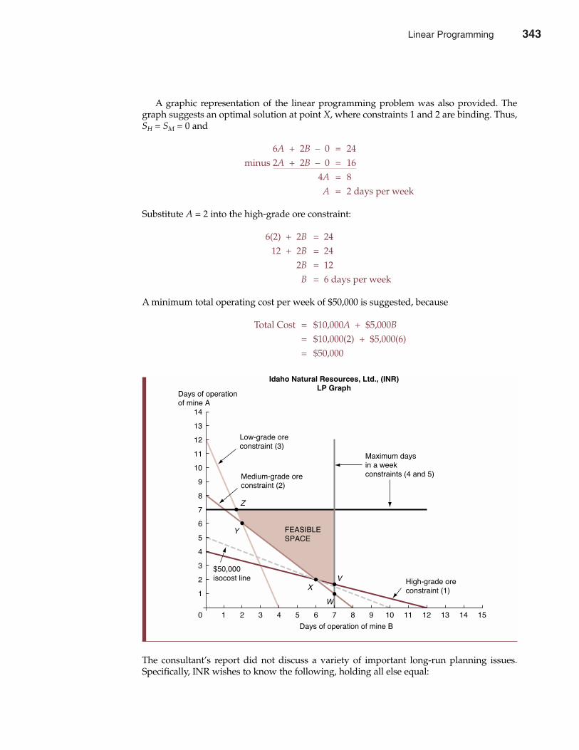
A graphic representation of the linear programming problem was also provided. Thegraph suggests an optimal solution at point X, where constraints 1 and 2 are binding. Thus,SH = SM = 0 and
6A + 2B – 0 = 24minus 2A + 2B – 0 = 16
4A = 8A = 2 days per week
Substitute A = 2 into the high-grade ore constraint:
6(2) + 2B = 2412 + 2B = 24
2B = 12B = 6 days per week
A minimum total operating cost per week of $50,000 is suggested, because
Total Cost = $10,000A + $5,000B
= $10,000(2) + $5,000(6)= $50,000
The consultant’s report did not discuss a variety of important long-run planning issues.Specifically, INR wishes to know the following, holding all else equal:
Chapter Nine Linear Programming 343
14
13
12
11
10
9
8
7
6
5
4
3
2
1
0 1 2 3 4 5 6 7 8 9 10 11 12 13 14 15
Days of operation of mine B
Days of operationof mine A
Maximum daysin a weekconstraints (4 and 5)
High-grade oreconstraint (1)
$50,000isocost line
Medium-grade oreconstraint (2)
Low-grade oreconstraint (3)
Z
Y
X
W
V
FEASIBLESPACE
Idaho Natural Resources, Ltd., (INR)LP Graph
Linear Programming 343
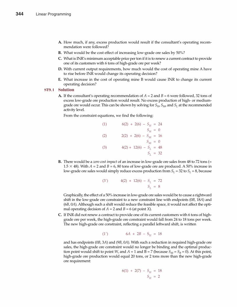
A. How much, if any, excess production would result if the consultant’s operating recom-mendation were followed?
B. What would be the cost effect of increasing low-grade ore sales by 50%?C. What is INR’s minimum acceptable price per ton if it is to renew a current contract to provide
one of its customers with 6 tons of high-grade ore per week?D. With current output requirements, how much would the cost of operating mine A have
to rise before INR would change its operating decision?E. What increase in the cost of operating mine B would cause INR to change its current
operating decision?ST9.1 Solution
A. If the consultant’s operating recommendation of A = 2 and B = 6 were followed, 32 tons ofexcess low-grade ore production would result. No excess production of high- or medium-grade ore would occur. This can be shown by solving for SH, SM, and SL at the recommendedactivity level.From the constraint equations, we find the following:
(1) 6(2) + 2(6) – SH = 24SH = 0
(2) 2(2) + 2(6) – SM = 16SM = 0
(3) 4(2) + 12(6) – SL = 48SL = 32
B. There would be a zero cost impact of an increase in low-grade ore sales from 48 to 72 tons (=1.5 � 48). With A = 2 and B = 6, 80 tons of low-grade ore are produced. A 50% increase inlow-grade ore sales would simply reduce excess production from SL = 32 to SL = 8, because
(3�) 4(2) + 12(6) – SL = 72SL = 8
Graphically, the effect of a 50% increase in low-grade ore sales would be to cause a rightwardshift in the low-grade ore constraint to a new constraint line with endpoints (0B, 18A) and(6B, 0A). Although such a shift would reduce the feasible space, it would not affect the opti-mal operating decision of A = 2 and B = 6 (at point X).
C. If INR did not renew a contract to provide one of its current customers with 6 tons of high-grade ore per week, the high-grade ore constraint would fall from 24 to 18 tons per week.The new high-grade ore constraint, reflecting a parallel leftward shift, is written
(1�) 6A + 2B – SH = 18
and has endpoints (0B, 3A) and (9B, 0A). With such a reduction in required high-grade oresales, the high-grade ore constraint would no longer be binding and the optimal produc-tion point would shift to point W, and A = 1 and B = 7 (because SM = SB = 0). At this point,high-grade ore production would equal 20 tons, or 2 tons more than the new high-gradeore requirement:
6(1) + 2(7) – SH = 18SH = 2
344 Part Three Production and Cost Analysis
344 Linear Programming
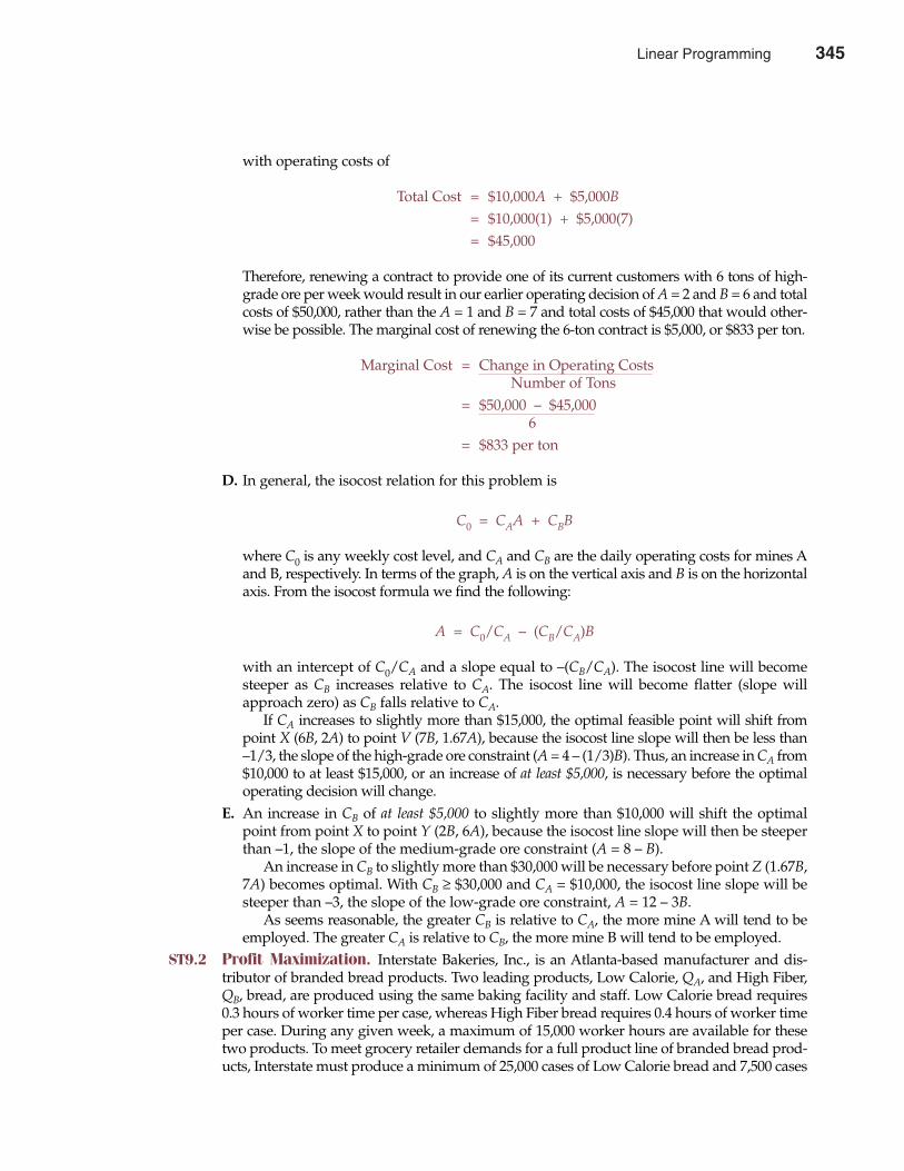
with operating costs of
Total Cost = $10,000A + $5,000B
= $10,000(1) + $5,000(7)= $45,000
Therefore, renewing a contract to provide one of its current customers with 6 tons of high-grade ore per week would result in our earlier operating decision of A = 2 and B = 6 and totalcosts of $50,000, rather than the A = 1 and B = 7 and total costs of $45,000 that would other-wise be possible. The marginal cost of renewing the 6-ton contract is $5,000, or $833 per ton.
Marginal Cost = Change in Operating CostsNumber of Tons
= $50,000 – $45,0006
= $833 per ton
D. In general, the isocost relation for this problem is
C0 = CAA + CBB
where C0 is any weekly cost level, and CA and CB are the daily operating costs for mines Aand B, respectively. In terms of the graph, A is on the vertical axis and B is on the horizontalaxis. From the isocost formula we find the following:
A = C0/CA – (CB/CA)B
with an intercept of C0/CA and a slope equal to –(CB/CA). The isocost line will becomesteeper as CB increases relative to CA. The isocost line will become flatter (slope willapproach zero) as CB falls relative to CA.
If CA increases to slightly more than $15,000, the optimal feasible point will shift frompoint X (6B, 2A) to point V (7B, 1.67A), because the isocost line slope will then be less than–1/3, the slope of the high-grade ore constraint (A = 4 – (1/3)B). Thus, an increase in CA from$10,000 to at least $15,000, or an increase of at least $5,000, is necessary before the optimaloperating decision will change.
E. An increase in CB of at least $5,000 to slightly more than $10,000 will shift the optimalpoint from point X to point Y (2B, 6A), because the isocost line slope will then be steeperthan –1, the slope of the medium-grade ore constraint (A = 8 – B).
An increase in CB to slightly more than $30,000 will be necessary before point Z (1.67B,7A) becomes optimal. With CB ≥ $30,000 and CA = $10,000, the isocost line slope will besteeper than –3, the slope of the low-grade ore constraint, A = 12 – 3B.
As seems reasonable, the greater CB is relative to CA, the more mine A will tend to beemployed. The greater CA is relative to CB, the more mine B will tend to be employed.
ST9.2 Profit Maximization. Interstate Bakeries, Inc., is an Atlanta-based manufacturer and dis-tributor of branded bread products. Two leading products, Low Calorie, QA, and High Fiber,QB, bread, are produced using the same baking facility and staff. Low Calorie bread requires0.3 hours of worker time per case, whereas High Fiber bread requires 0.4 hours of worker timeper case. During any given week, a maximum of 15,000 worker hours are available for thesetwo products. To meet grocery retailer demands for a full product line of branded bread prod-ucts, Interstate must produce a minimum of 25,000 cases of Low Calorie bread and 7,500 cases
Chapter Nine Linear Programming 345
Linear Programming 345
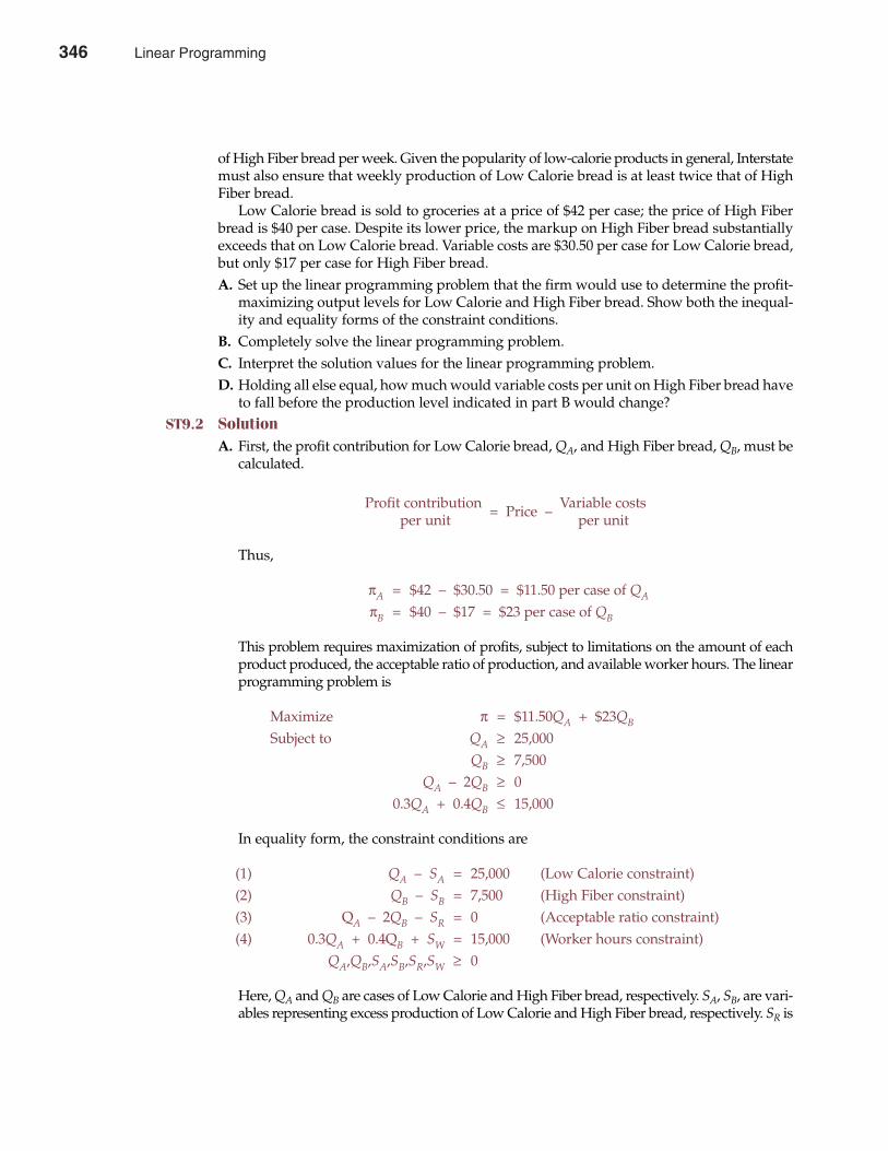
of High Fiber bread per week. Given the popularity of low-calorie products in general, Interstatemust also ensure that weekly production of Low Calorie bread is at least twice that of HighFiber bread.
Low Calorie bread is sold to groceries at a price of $42 per case; the price of High Fiberbread is $40 per case. Despite its lower price, the markup on High Fiber bread substantiallyexceeds that on Low Calorie bread. Variable costs are $30.50 per case for Low Calorie bread,but only $17 per case for High Fiber bread.A. Set up the linear programming problem that the firm would use to determine the profit-
maximizing output levels for Low Calorie and High Fiber bread. Show both the inequal-ity and equality forms of the constraint conditions.
B. Completely solve the linear programming problem.C. Interpret the solution values for the linear programming problem.D. Holding all else equal, how much would variable costs per unit on High Fiber bread have
to fall before the production level indicated in part B would change?ST9.2 Solution
A. First, the profit contribution for Low Calorie bread, QA, and High Fiber bread, QB, must becalculated.
Profit contribution = Price – Variable costsper unit per unit
Thus,
πA = $42 – $30.50 = $11.50 per case of QA
πB = $40 – $17 = $23 per case of QB
This problem requires maximization of profits, subject to limitations on the amount of eachproduct produced, the acceptable ratio of production, and available worker hours. The linearprogramming problem is
Maximize π = $11.50QA + $23QB
Subject to QA ≥ 25,000QB ≥ 7,500
QA – 2QB ≥ 00.3QA + 0.4QB ≤ 15,000
In equality form, the constraint conditions are
(1) QA – SA = 25,000 (Low Calorie constraint)(2) QB – SB = 7,500 (High Fiber constraint)(3) QA – 2QB – SR = 0 (Acceptable ratio constraint)(4) 0.3QA + 0.4QB + SW = 15,000 (Worker hours constraint)
QA,QB,SA,SB,SR,SW ≥ 0
Here, QA and QB are cases of Low Calorie and High Fiber bread, respectively. SA, SB, are vari-ables representing excess production of Low Calorie and High Fiber bread, respectively. SR is
346 Part Three Production and Cost Analysis
346 Linear Programming

the amount by which the production of Low Calorie bread exceeds the minimally acceptableamount, given High Fiber production. SW is excess worker capacity.
B. By graphing the constraints and the highest possible isoprofit line, the optimal point Xoccurs where SR = SW = 0.Thus,
(1) QA – SA = 25,000(2) QB – SB = 0(3) QA – 2QB – 0 = 0(4) 0.3QA + 0.4QB + 0 = 15,000
From (3), QA = 2QB. Substituting this value into (4) yields
0.3(2QB) + 0.4QB = 15,000QB = 15,000
From (3),
QA – 2(15,000) = 0QA = 30,000
From (1),
30,000 – SA = 25,000SA = 5,000
From (2),
15,000 – SB = 7,500SB = 7,500
And the total profit contribution per week is
π = $11.50(30,000) + $23(15,000)= $690,000
C. Solution values can be interpreted as follows:
QA = 30,000 Optimal production of Low Calorie bread is 30,000 cases per week.QB = 15,000 Optimal production of High Fiber bread is 15,000 cases per week.SA = 5,000 The production of Low Calorie bread exceeds the 25,000 case minimum
by 5,000 units.SB = 7,500 The production of High Fiber bread exceeds the 7,500 case minimum
by 7,500 units.SR = 0 The minimally acceptable 2:1 ratio of Low Calorie:High Fiber bread is
produced.SW = 0 All worker hours are utilized; no excess worker capacity exists.
π = $690,000 Maximum weekly profit contribution given constraints
Chapter Nine Linear Programming 347
Linear Programming 347
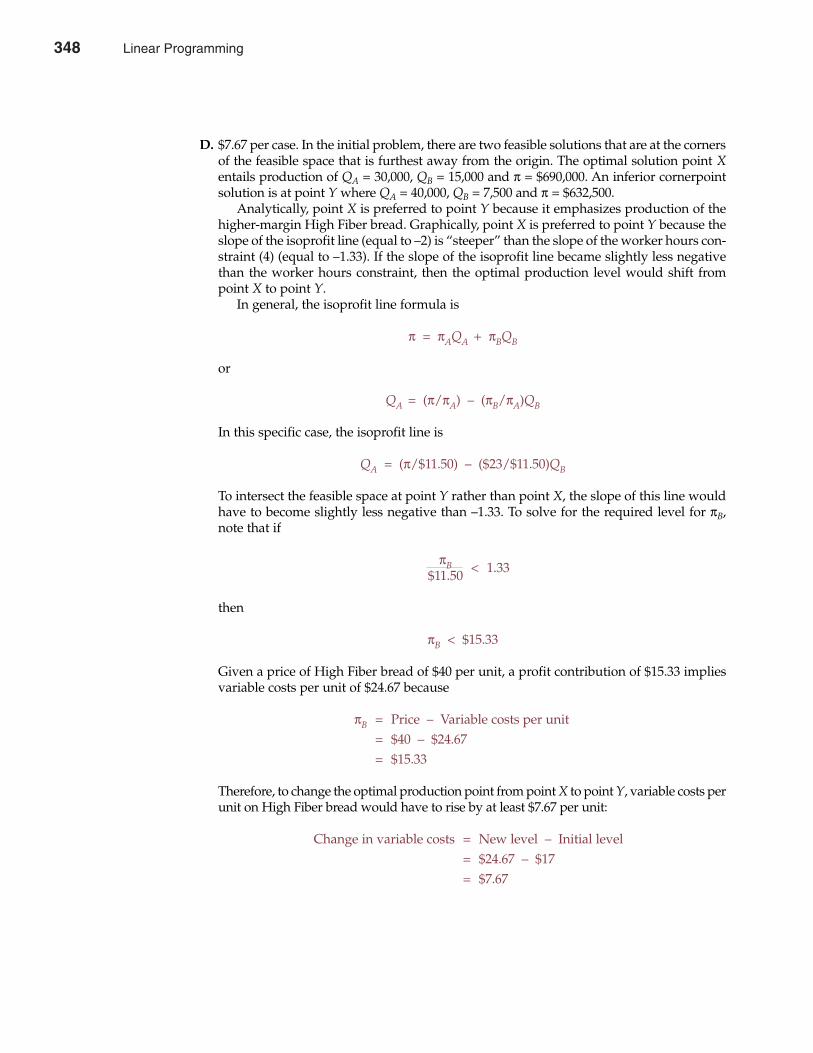
D. $7.67 per case. In the initial problem, there are two feasible solutions that are at the cornersof the feasible space that is furthest away from the origin. The optimal solution point Xentails production of QA = 30,000, QB = 15,000 and π = $690,000. An inferior cornerpointsolution is at point Y where QA = 40,000, QB = 7,500 and π = $632,500.
Analytically, point X is preferred to point Y because it emphasizes production of thehigher-margin High Fiber bread. Graphically, point X is preferred to point Y because theslope of the isoprofit line (equal to –2) is “steeper” than the slope of the worker hours con-straint (4) (equal to –1.33). If the slope of the isoprofit line became slightly less negativethan the worker hours constraint, then the optimal production level would shift frompoint X to point Y.
In general, the isoprofit line formula is
π = πAQA + πBQB
or
QA = (π/πA) – (πB/πA)QB
In this specific case, the isoprofit line is
QA = (π/$11.50) – ($23/$11.50)QB
To intersect the feasible space at point Y rather than point X, the slope of this line wouldhave to become slightly less negative than –1.33. To solve for the required level for πB,note that if
πB < 1.33$11.50
then
πB < $15.33
Given a price of High Fiber bread of $40 per unit, a profit contribution of $15.33 impliesvariable costs per unit of $24.67 because
πB = Price – Variable costs per unit= $40 – $24.67= $15.33
Therefore, to change the optimal production point from point X to point Y, variable costs perunit on High Fiber bread would have to rise by at least $7.67 per unit:
Change in variable costs = New level – Initial level= $24.67 – $17= $7.67
348 Part Three Production and Cost Analysis
348 Linear Programming
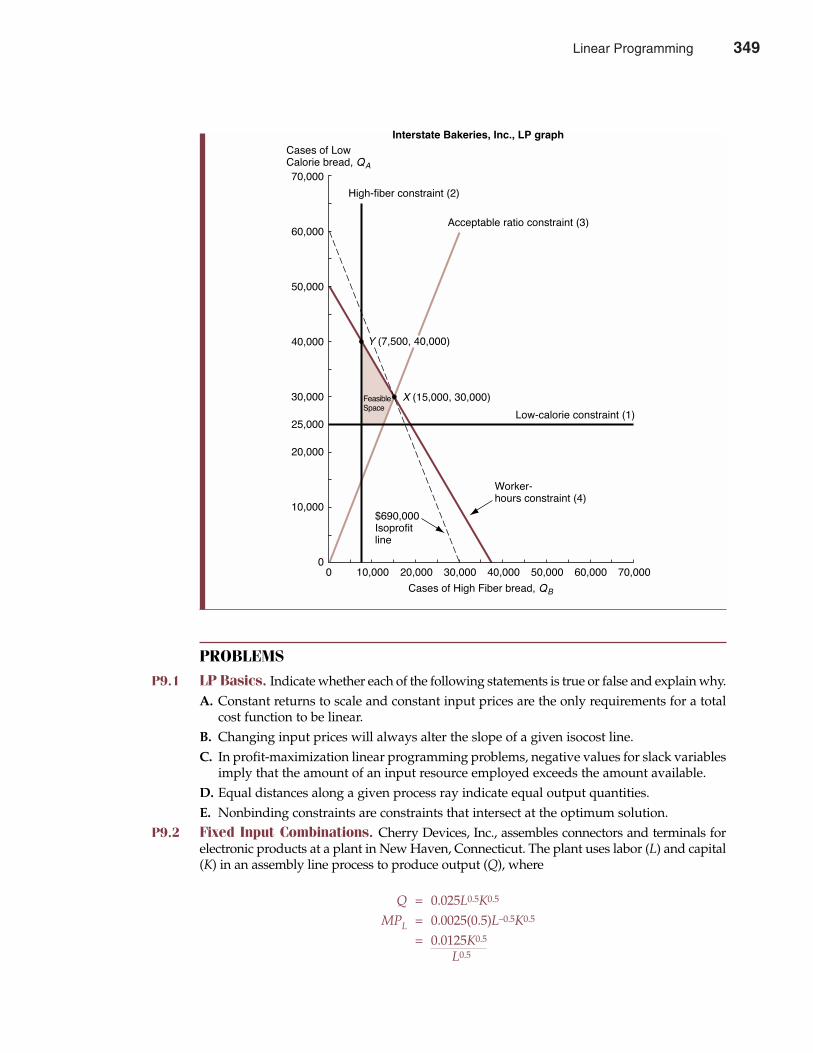
PROBLEMS
P9.1 LP Basics. Indicate whether each of the following statements is true or false and explain why.A. Constant returns to scale and constant input prices are the only requirements for a total
cost function to be linear.B. Changing input prices will always alter the slope of a given isocost line.C. In profit-maximization linear programming problems, negative values for slack variables
imply that the amount of an input resource employed exceeds the amount available.D. Equal distances along a given process ray indicate equal output quantities.E. Nonbinding constraints are constraints that intersect at the optimum solution.
P9.2 Fixed Input Combinations. Cherry Devices, Inc., assembles connectors and terminals forelectronic products at a plant in New Haven, Connecticut. The plant uses labor (L) and capital(K) in an assembly line process to produce output (Q), where
Q = 0.025L0.5K0.5
MPL = 0.0025(0.5)L–0.5K0.5
= 0.0125K0.5
L0.5
Chapter Nine Linear Programming 349
Y (7,500, 40,000)
0 10,000 20,000 30,000 40,000 50,000 60,000 70,000
70,000
60,000
50,000
40,000
30,000
25,000
20,000
10,000
0
High-fiber constraint (2)
Acceptable ratio constraint (3)
X (15,000, 30,000)
Low-calorie constraint (1)
Worker-hours constraint (4)
$690,000Isoprofitline
FeasibleSpace
Cases of High Fiber bread, QB
Cases of LowCalorie bread, QA
Interstate Bakeries, Inc., LP graph
Linear Programming 349
MPK = 0.025(0.5)L0.5K–0.5
= 0.0125L0.5
K0.5
A. Calculate how many units of output can be produced with 4 units of labor and 400 units ofcapital and with 16 units of labor and 1,600 units of capital. Are returns to scale increasing,constant, or diminishing?
B. Calculate the change in the marginal product of labor as labor grows from 4 to 16 units, hold-ing capital constant at 400 units. Similarly, calculate the change in the marginal product ofcapital as capital grows from 400 to 1,600 units, holding labor constant at 4 units. Are returnsto each factor increasing, constant, or diminishing?
C. Assume now and throughout the remainder of the problem that labor and capital mustbe combined in the ratio 4L:400K. How much output could be produced if Cherry has aconstraint of L = 4,000 and K = 480,000 during the coming production period?
D. What are the marginal products of each factor under the conditions described in part C?P9.3 LP Setup and Interpretation. The Syflansyd Nut Company has enjoyed booming sales
following the success of its “Sometimes You Feel Like a Nut, Sometimes You Don’t” adver-tising campaign. Syflansyd packages and sells four types of nuts in four different types ofmixed-nut packages. These products include bulk (B), economy (E), fancy (F), and regular (R)mixed-nut packages. Each of these packages contains a different mixture of almonds (A),cashews (C), filberts (F), and peanuts (P). Based on its contracts with current suppliers, thecompany has the following daily inventory of each of the following nuts: almonds, 8,000ounces; cashews, 7,000 ounces; filberts, 7,500 ounces; and peanuts, 10,000 ounces.
Given available inventory, it is management’s goal to maximize profits by offering theoptimum mix of the four package types. Profit earned per package type is as follows:
Bulk $0.50Economy $0.25Fancy $1.25Regular $0.75
The composition of each of the four package types can be summarized as follows:
Solution values for the optimal number of packages to produce (decision variables) and excesscapacity (slack variables) are the following:
B = 0 E = 0F = 1,100R = 1,300
SA = 2,100
350 Part Three Production and Cost Analysis
Ounces per Package
Bulk Economy Fancy Regular
Almonds 35 2 3 2Cashews 35 1 4 2Filberts 35 1 3 2Peanuts 35 8 2 6Total 140 12 12 12
350 Linear Programming
SC = 0SF = 1,600SP = 0
A. Identify and interpret the appropriate Syflansyd objective function.B. Using both inequality and equality forms, set up and interpret the resource constraints
facing the Syflansyd Company.C. Calculate optimal daily profit, and provide a complete interpretation of the full solution
to this linear programming problem.P9.4 Cost Minimization. Ray Barone is sole proprietor of Delmar Custom Homes (DCH), a family-
run construction company. The company uses two types of crews on its Long Island, New York,home construction projects. Type A crews consist of master carpenters and skilled carpenters,whereas B crews include skilled carpenters and unskilled labor. Each home involves framing(F), roofing (R), and finish carpentry (FC). During recent months, A crews have demonstrated acapability of framing one home, roofing two, and doing finish carpentry for no more than fourhomes per month. Capabilities for B crews are framing three homes, roofing two, and complet-ing finish carpentry for one during a month. DCH has agreed to build 10 homes during themonth of July but has subcontracted 10% of framing and 20% of finish carpentry requirements.Labor costs are $60,000 per month for A crews and $45,000 per month for B crews.A. Formulate the linear programming problem that DCH would use to minimize its total labor
costs per month, showing both the inequality and equality forms of the constraint conditions.B. Solve the linear programming problem and interpret your solution values.C. Assuming that DCH can both buy and sell subcontracting services at prevailing prices of
$8,000 per unit for framing and $14,000 per unit for finish carpentry, would you recommendthat the company alter its subcontracting policy? If so, how much could the company savethrough such a change?
D. Calculate the minimum increase in A-crew costs necessary to cause DCH to change itsoptimal employment combination for July.
P9.5 Optimal Credit Policy. Mimi Bobeck is a senior loan officer with Citybank in Cleveland, Ohio.Bobeck has both corporate and personal lending customers. On average, the profit contributionmargin or interest rate spread is 1.5% on corporate loans and 2% on personal loans. This returndifference reflects the fact that personal loans tend to be riskier than corporate loans. Bobeckseeks to maximize the total dollar profit contribution earned, subject to a variety of restrictions onher lending practices. To limit default risk, Bobeck must restrict personal loans to no more than50% of the total loans outstanding. Similarly, to ensure adequate diversification against business-cycle risk, corporate lending cannot exceed 75% of loaned funds. To maintain good customerrelations by serving the basic needs of the local business community, Bobeck has decided toextend at least 25% of her total credit authorization to corporate customers on an ongoing basis.Finally, Bobeck cannot exceed her current total credit authorization of $100 million.A. Using the inequality form of the constraint conditions, set up and interpret the linear pro-
gramming problem that Bobeck would use to determine the optimal dollar amount ofcredit to extend to corporate (C) and personal (P) lending customers. Also formulate theLP problem using the equality form of the constraint conditions.
B. Use a graph to determine the optimal solution, and check your solution algebraically.Fully interpret solution values.
P9.6 Optimal Portfolio Decisions. The James Bond Fund is a mutual fund (open-end investmentcompany) with an objective of maximizing income from a widely diversified corporate bondportfolio. The fund has a policy of remaining invested largely in a diversified portfolio ofinvestment-grade bonds. Investment-grade bonds have high investment quality and receive a
Chapter Nine Linear Programming 351
Linear Programming 351
rating of Baa or better by Moody’s, a bond-rating service. The fund’s investment policy statesthat investment-grade bonds are to be emphasized, representing at least three times theamount of junk bond holdings. Junk bonds pay high nominal returns but have low investmentquality, and they receive a rating of less than Baa from Moody’s. To maintain the potential forhigh investor income, at least 20% of the fund’s total portfolio must be invested in junk bonds.Like many funds, the James Bond Fund cannot use leverage (or borrowing) to enhanceinvestor returns. As a result, total bond investments cannot total more than 100% of the port-folio. Finally, the current expected return for investment-grade (I) bonds is 9%, and it is 12%for junk (J) bonds.A. Using the inequality form of the constraint conditions, set up and interpret the linear pro-
gramming problem that the James Bond Fund would use to determine the optimal port-folio percentage holdings of investment-grade (I) and junk (J) bonds. Also formulate theproblem using the equality form of the constraint conditions. (Assume that the fundmanagers have decided to remain fully invested and therefore hold no cash at this time.)
B. Use a graph to determine the optimal solution, and check your solution algebraically.Fully interpret solution values.
C. Holding all else equal, how much would the expected return on junk bonds have to fallto alter the optimal investment policy determined in part B? Alternatively, how muchwould the return on investment-grade bonds have to rise before a change in investmentpolicy would be warranted?
D. In anticipation of a rapid increase in interest rates and a subsequent economic downturn,the investment committee has decided to minimize the fund’s exposure to bond price fluc-tuations. In adopting a defensive position, what is the maximum share of the portfolio thatcan be held in cash given the investment policies stated in the problem?
P9.7 Cost Minimization. Carolina Power and Light (CP&L) is a small electric utility located in theSoutheast. CP&L currently uses coal-fired capacity to satisfy its base load electricity demand,which is the minimum level of electricity demanded 24 hours per day, 365 days per year.
CP&L currently burns both high-sulfur eastern coal and low-sulfur western coal. Each typeof coal has its advantages. Eastern coal is more expensive ($50 per ton) but has higher heat-generating capabilities. Although western coal does not generate as much heat as eastern coal,western coal is less expensive ($25 per ton) and does not cause as much sulfur dioxide pollution.CP&L’s base load requirements are such that at least 2,400 million BTUs must be generated perhour. Each ton of eastern coal burned generates 40 million BTUs, and each ton of western coalburned generates 30 million BTUs. To limit sulfur dioxide emissions, the state’s EnvironmentalProtection Agency (EPA) requires CP&L to limit its total burning of sulfur to no more than 1.5tons per hour. This affects CP&L’s coal usage, because eastern coal contains 2.5% sulfur and west-ern coal contains 1.5% sulfur. The EPA also limits CP&L particulate emissions to no more than900 pounds per hour. CP&L emits 10 pounds of particulates per ton of eastern coal burned and15 pounds of particulates per ton of western coal burned.A. Set up and interpret the linear program that CP&L would use to minimize hourly coal
usage costs in light of its constraints.B. Calculate and interpret all relevant solution values.C. Holding all else equal, how much would the price of western coal have to rise before only
eastern coal would be used? Explain.P9.8 Profit Maximization. Creative Accountants, Ltd., is a small San Francisco–based accounting
partnership specializing in the preparation of individual (I) and corporate (C) income taxreturns. Prevailing prices in the local market are $125 for individual tax return preparation and$250 for corporate tax return preparation.
Five accountants run the firm and are assisted by four bookkeepers and four secretaries,all of whom work a typical 40-hour workweek. The firm must decide how to target its pro-
352 Part Three Production and Cost Analysis
352 Linear Programming
motional efforts to best use its resources during the coming tax preparation season. Based onprevious experience, the firm expects that an average of 1 hour of accountant time will berequired for each individual return prepared. Corporate return preparation will require anaverage of 2 accountant-hours and 2 bookkeeper-hours. One hour of secretarial time will alsobe required for typing each individual or corporate return. In addition, variable computerand other processing costs are expected to average $25 per individual return and $100 per cor-porate return.A. Set up the linear programming problem that the firm would use to determine the profit-
maximizing output levels for preparing individual and corporate returns. Show both theinequality and equality forms of the constraint conditions.
B. Completely solve and interpret the solution values for the linear programming problem.C. Calculate maximum possible net profits per week for the firm, assuming that the account-
ants earn $1,500 per week, bookkeepers earn $500 per week, secretaries earn $10 per hour,and fixed overhead (including promotion and other expenses) averages $5,000 per week.
D. After considering the preceding data, one senior accountant recommended letting twobookkeepers go while retaining the rest of the current staff. Another accountant suggestedthat if any bookkeepers were let go, an increase in secretarial staff would be warranted.Which is the more profitable suggestion? Why?
E. Using the equality form of the constraint conditions, set up, solve, and interpret solutionvalues for the dual linear programming problem.
F. Does the dual solution provide information useful for planning purposes? Explain.P9.9 Revenue Maximization. Architect Elaine Benes is managing director of Designed for Sales
(DFS), Inc., an Evanston, Illinois–based designer of single-family and multifamily housingunits for real estate developers, building contractors, and so on. Benes’ challenge is to deter-mine an optimal mix of output during the current planning period. DFS offers customdesigns for single-family units, Q1, for $3,000 and custom designs for multifamily units (e.g.,duplexes, fourplexes), Q2, for $2,000 each. Both types of output make use of scarce drafting,artwork, and architectural resources. Each custom design for single-family units requires 12hours of drafting, 2 hours of artwork, and 6 hours of architectural input. Each custom designfor multifamily units requires 4 hours of drafting, 5 hours of artwork, and 6 hours of archi-tectural input. Currently, DFS has 72 hours of drafting, 30 hours of artwork, and 48 hours ofarchitectural services available on a weekly basis.A. Using the equality form of the constraint conditions, set up the primal linear program
that Benes would use to determine the sales revenue-maximizing product mix. Also setup the dual.
B. Solve for and interpret all solution values.C. Would DFS’s optimal product mix be different with a profit-maximization goal rather
than a sales revenue-maximization goal? Why or why not?P9.10 Optimal Output. Omaha Meat Products (OMP) produces and markets Cornhusker
Plumpers, an extra-large frankfurter product being introduced on a test market basis into theSt. Louis, Missouri, area. This product is similar to several others offered by OMP, and it canbe produced with currently available equipment and personnel using any of three alterna-tive production methods. Method A requires 1 hour of labor and 4 processing-facility hoursto produce 100 packages of plumpers, one unit of QA. Method B requires 2 labor hours and2 processing-facility hours for each unit of QB, and method C requires 5 labor hours and 1processing-facility hour for each unit of QC. Because of slack demand for other products,OMP currently has 14 labor hours and 6 processing-facility hours available per week for pro-ducing Cornhusker Plumpers. Cornhusker Plumpers are currently being marketed to gro-cery retailers at a wholesale price of $1.50 per package, and demand exceeds current supply.
Chapter Nine Linear Programming 353
Linear Programming 353
A. Using the equality form of the constraint conditions, set up the primal and dual linearprograms that OMP would use to maximize production of Cornhusker Plumpers givencurrently available resources.
B. Calculate and interpret all solution values.C. Should OMP expand its processing-facility capacity if it can do so at a cost of $40 per hour?D. Discuss the implications of a new union scale calling for a wage rate of $20 per hour.
354 Part Three Production and Cost Analysis
CASE STUDY
LP Pension Funding ModelSeveral companies have learned that a well-funded and comprehensive employee benefitspackage constitutes an important part of the compensation plan needed to attract and retain keypersonnel. An employee stock ownership plan, profit-sharing arrangements, and deferred com-pensation to fund employee retirement are all used to allow productive employees to share inthe firm’s growth and development. Among the fringe benefits offered under the cafeteria-stylebenefits plans is comprehensive medical and dental care furnished through local health main-tenance organizations, on-site daycare centers for employee children, and “eldercare” supportfor the aging parents and other dependents of workers.
Many companies also provide their employees with so-called “defined benefit” pensionplans. Under defined benefit plans, employers usually offer workers a fixed percentage of theirfinal salary as a retirement annuity. In a typical arrangement, a company might offer employ-ees a retirement annuity of 1.5% of their final salary for each year employed. A 10-year veteranwould earn a retirement annuity of 15% of final salary, a 20-year veteran would earn a retire-ment annuity of 30% of final salary, and so on. Because each employee’s retirement benefits aredefined by the company, the company itself is obligated to pay for promised benefits.
Over time, numerous firms have found it increasingly difficult to forecast the future rateof return on invested assets, the future rate of inflation, and the morbidity (death rate) ofyoung, healthy, active retirees. As a result, several organizations have discontinued tradition-al defined benefit pension plans and instead have begun to offer new “defined contribution”plans. A defined contribution plan features a matching of company plus employee retirementcontributions, with no prescribed set of retirement income benefits defined beforehand. Eachemployee is typically eligible to contribute up to 10% of their pre-tax income into the plan,with the company matching the first 5% or so of such contributions. Both company andemployee contributions compound on a tax-deferred basis until the point of retirement. Atthat time, employees can use their pension funds to purchase an annuity, or draw a pensionincome from earned interest, plus dividends and capital gains.
Defined contribution plans have some obvious advantages over traditional defined bene-fit pension plans. From the company’s perspective, defined benefit pension plans becamemuch less attractive when accounting rule changes during the late 1980s required them torecord as a liability any earned but not funded pension obligations. Unfunded pension lia-bilities caused gigantic one-time charges against operating income during the early 1990s forAT&T, General Motors, IBM, and a host of other large corporations. Faced with enormousone-time charges during an initial catch-up phase, plus the prospect of massive and rapidlygrowing retirement expenses over time, many large and small firms have simply elected todiscontinue their defined contribution plan altogether. From the employee’s perspective,defined contribution plans are attractive because they are portable from one employer toanother. Rather than face the prospect of losing pension benefits after changing from oneemployer to another, employees appreciate the advantage of being able to take their pensionplans with them as they switch jobs. Defined contribution plans are also attractive because
354 Linear Programming
Chapter Nine Linear Programming 355
they allow employees to tailor retirement funding contributions to fit individual needs.Younger employees faced with the necessity of buying a home or paying for children’s edu-cational expenses can limit pension contributions to minimal levels; older workers withgreater discretionary income and a more imminent retirement can provide the maximumpension contribution allowed by law. An added benefit of defined contribution compensationplans is that individual workers can allocate pension investments according to individual riskpreferences. Older workers who are extremely risk averse can focus their investments onshort-term government securities; younger and more venturesome employees can devote alarger share of their retirement investment portfolio to common stocks.
Workers appreciate companies that offer flexible defined contribution pension plans andclosely related profit-sharing and deferred compensation arrangements. To maximize planbenefits, firms must make modest efforts to educate and inform employees about retirementincome needs and objectives. Until recently, compensation consultants suggested that employ-ees could retire comfortably on a retirement income that totaled 80% of their final salary.However, concerns about the underfunding of federal Social Security and Medicaid pro-grams and apprehension about the rapid escalation of medical care costs make retirementwith sufficient assets to fund a pension income equal to 100% of final salary a worthy goal.To fund such a nest egg requires substantial regular savings and an impressive rate of returnon pension plan assets. Workers who save 10% of income for an extended period, say, 30years, have historically been able to fund a retirement income equal to 100% of final salary.This assumes, of course, that the pension plan portfolio is able to earn significant returns overtime. Investing in a broadly diversified portfolio of common stocks has historically providedthe best returns. Since 1926, the real (after-inflation) rate of return on NYSE stocks is 6.4% peryear; the real return on bonds is only 0.5% per year. Indeed, over every 30-year investmenthorizon during that time interval, stocks have beat short-term bonds (money market instru-ments) and long-term bonds. The added return from common stocks is the predictablereward for assuming the greater risks of stock-market investing. However, to be sure of earn-ing the market risk premium on stocks, one must invest in several different companies (atleast 30) for several years (at least 30). For most pension plans, investments in no-load low-expense common stock index funds work best in the long run. However, bond market fundshave a place in some pension portfolios, especially for those at or near the retirement age.
To illustrate the type of retirement income funding model that a company might makeavailable to employees, consider the following scenario. Suppose that an individual employeehas accumulated a pension portfolio worth $250,000 and hopes to receive initial post-retirementincome of $500 per month, or $6,000 per year. To provide a total return from current income(yield) plus growth (capital gains) of at least 7%, a minimum of 25% of the portfolio should beinvested in common stocks. To limit risk, stocks should total no more than 50% of the overallportfolio, and a minimum of 5% should be invested in long-term taxable bonds, 5% in medium-term tax-exempt bonds, and 5% in a short-term money-market mutual fund. Moreover, notmore than 75% of the overall portfolio should be invested in stocks plus long-term taxablebonds, and at least $30,000 should be available in money markets plus medium-term tax-exempt bonds to provide sufficient liquidity to fund emergencies. Assume that common stockshave a before-tax dividend yield of 3.5%, with expected growth from capital appreciation of6.5% per year. Similar figures for long-term taxable bonds are 6% plus 1.5%, 4% plus 1% formedium-term tax-exempt bonds, and 4.5% plus 0% for money market instruments. Alsoassume that the effective marginal tax rate is 30%.A. Set up the linear programming problem that a benefits officer might use to determine the
total-return maximizing allocation of the employee’s pension portfolio. Use the inequalityforms of the constraint conditions.
CASE STUDY (continued)
Linear Programming 355

356 Part Three Production and Cost Analysis
CASE STUDY (continued)
B. Solve this linear programming problem and interpret all solution values. Also determinethe employee’s expected before-tax and after-tax income levels.
C. Calculate the amount of unrealized capital gain earned per year on this investmentportfolio.
D. What is the total return opportunity cost of the $6,000 after-tax income constraint?
356 Linear Programming
A P P E N D I X 9 A
Rules for Forming the Dual LinearProgramming Problem
357
Given the importance of duality, a list of simple rules that can be used to form the dualprogram to any given primal program would be useful. Four such rules exist. They are
as follows:
1. Change a maximize objective to minimize, and vice versa.2. Reverse primal constraint inequality signs in dual constraints (i.e., change ≥ to ≤, and ≤ to ≥).3. Transpose primal constraint coefficients to get dual constraint coefficients.4. Transpose objective function coefficients to get limits in dual constraints, and vice versa.
(The word transpose is a matrix algebra term that simply means that each row of coefficients isrearranged into columns so that row 1 becomes column 1, row 2 becomes column 2, and so on.)
To illustrate the rules for transformation from primal and dual, consider the followingsimple example.
Primal ProblemMaximize π = π1Q1 + π2Q2 + π3Q3
subject to a11Q1 + a12Q2 + a13Q3 ≤ r1
a21Q1 + a22Q2 + a23Q3 ≤ r2
Q1, Q2, Q3 ≥ 0
where π is profits and Q is output. Thus, π1, π2 and π3 are unit profits for Q1, Q2 and Q3, respec-tively. The resource constraints are given by r1 and r2. The constants in the primal constraintsreflect the input requirements for each type of output. For example, a11 is the amount ofresource r1 in one unit of output Q1. Similarly, a12 is the amount of resource r1 in one unit ofoutput Q2, and a13 is the amount of resource r1 in one unit of output Q3. Thus, a11Q1 + a12Q2 +a13Q3 is the total amount of resource r1 used in production. The remaining input require-ments, a21, a22 and a23, have a similar interpretation. For convenience, this primal problemstatement can be rewritten in matrix notation as follows:
357
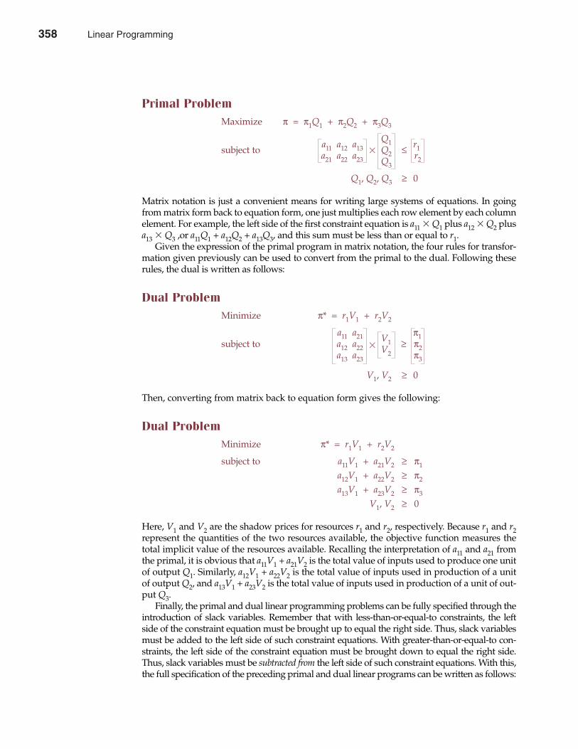
Primal ProblemMaximize π = π1Q1 + π2Q2 + π3Q3
a11 a12 a13Q1 r1subject to
a21 a22 a23Q2 ≤
r2Q3
Q1, Q2, Q3 ≥ 0
Matrix notation is just a convenient means for writing large systems of equations. In goingfrom matrix form back to equation form, one just multiplies each row element by each columnelement. For example, the left side of the first constraint equation is a11 � Q1 plus a12 � Q2 plusa13 � Q3 ,or a11Q1 + a12Q2 + a13Q3, and this sum must be less than or equal to r1.
Given the expression of the primal program in matrix notation, the four rules for transfor-mation given previously can be used to convert from the primal to the dual. Following theserules, the dual is written as follows:
Dual ProblemMinimize π* = r1V1 + r2V2
a11 a21 π1subject to a12 a22
V1 ≥ π2a13 a23
V2 π3
V1, V2 ≥ 0
Then, converting from matrix back to equation form gives the following:
Dual ProblemMinimize π* = r1V1 + r2V2
subject to a11V1 + a21V2 ≥ π1
a12V1 + a22V2 ≥ π2
a13V1 + a23V2 ≥ π3
V1, V2 ≥ 0
Here, V1 and V2 are the shadow prices for resources r1 and r2, respectively. Because r1 and r2represent the quantities of the two resources available, the objective function measures thetotal implicit value of the resources available. Recalling the interpretation of a11 and a21 fromthe primal, it is obvious that a11V1 + a21V2 is the total value of inputs used to produce one unitof output Q1. Similarly, a12V1 + a22V2 is the total value of inputs used in production of a unitof output Q2, and a13V1 + a23V2 is the total value of inputs used in production of a unit of out-put Q3.
Finally, the primal and dual linear programming problems can be fully specified through theintroduction of slack variables. Remember that with less-than-or-equal-to constraints, the leftside of the constraint equation must be brought up to equal the right side. Thus, slack variablesmust be added to the left side of such constraint equations. With greater-than-or-equal-to con-straints, the left side of the constraint equation must be brought down to equal the right side.Thus, slack variables must be subtracted from the left side of such constraint equations. With this,the full specification of the preceding primal and dual linear programs can be written as follows:
358 Part Three Production and Cost Analysis
�
�
358 Linear Programming
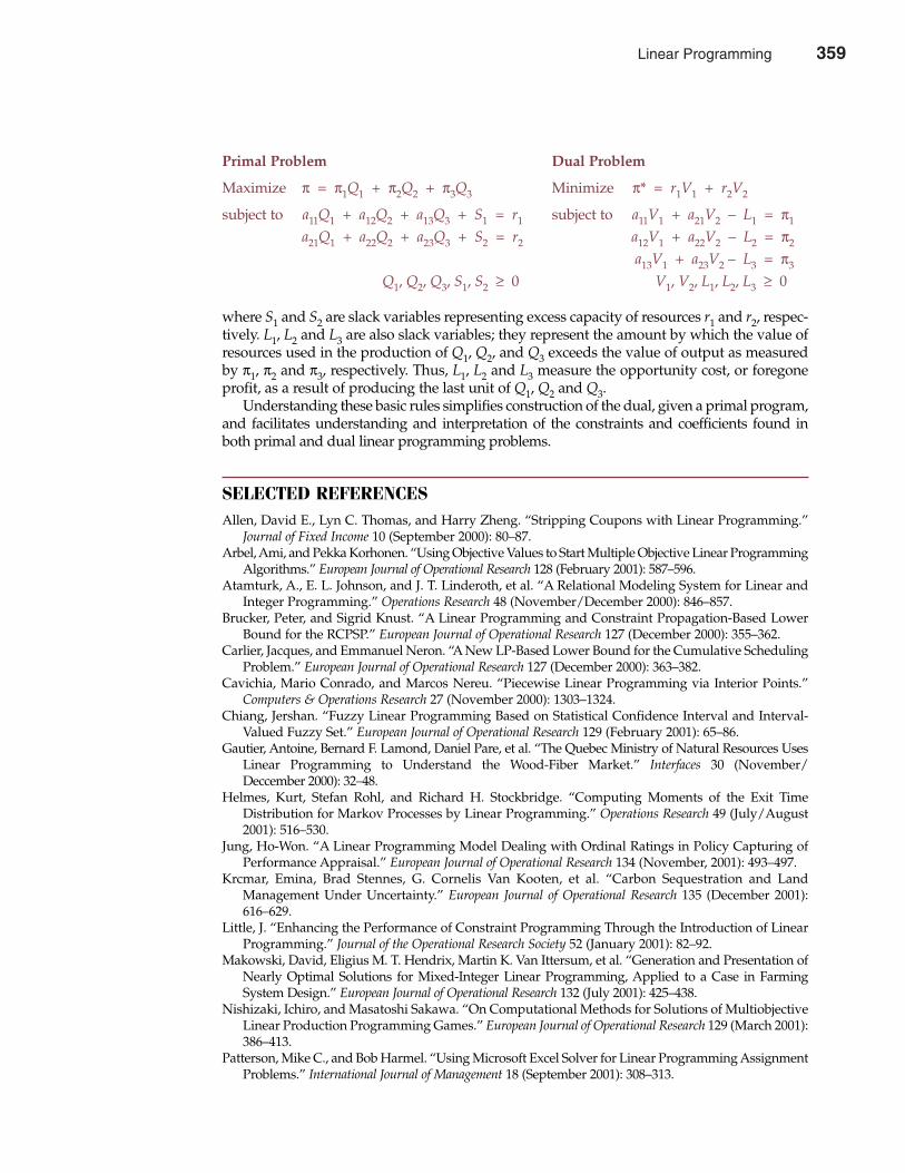
Primal Problem Dual Problem
Maximize π = π1Q1 + π2Q2 + π3Q3 Minimize π* = r1V1 + r2V2
subject to a11Q1 + a12Q2 + a13Q3 + S1 = r1 subject to a11V1 + a21V2 – L1 = π1
a21Q1 + a22Q2 + a23Q3 + S2 = r2 a12V1 + a22V2 – L2 = π2
a13V1 + a23V2 – L3 = π3
Q1, Q2, Q3, S1, S2 ≥ 0 V1, V2, L1, L2, L3 ≥ 0
where S1 and S2 are slack variables representing excess capacity of resources r1 and r2, respec-tively. L1, L2 and L3 are also slack variables; they represent the amount by which the value ofresources used in the production of Q1, Q2, and Q3 exceeds the value of output as measuredby π1, π2 and π3, respectively. Thus, L1, L2 and L3 measure the opportunity cost, or foregoneprofit, as a result of producing the last unit of Q1, Q2 and Q3.
Understanding these basic rules simplifies construction of the dual, given a primal program,and facilitates understanding and interpretation of the constraints and coefficients found inboth primal and dual linear programming problems.
SELECTED REFERENCES Allen, David E., Lyn C. Thomas, and Harry Zheng. “Stripping Coupons with Linear Programming.”
Journal of Fixed Income 10 (September 2000): 80–87.Arbel, Ami, and Pekka Korhonen. “Using Objective Values to Start Multiple Objective Linear Programming
Algorithms.” European Journal of Operational Research 128 (February 2001): 587–596. Atamturk, A., E. L. Johnson, and J. T. Linderoth, et al. “A Relational Modeling System for Linear and
Integer Programming.” Operations Research 48 (November/December 2000): 846–857. Brucker, Peter, and Sigrid Knust. “A Linear Programming and Constraint Propagation-Based Lower
Bound for the RCPSP.” European Journal of Operational Research 127 (December 2000): 355–362. Carlier, Jacques, and Emmanuel Neron. “A New LP-Based Lower Bound for the Cumulative Scheduling
Problem.” European Journal of Operational Research 127 (December 2000): 363–382. Cavichia, Mario Conrado, and Marcos Nereu. “Piecewise Linear Programming via Interior Points.”
Computers & Operations Research 27 (November 2000): 1303–1324. Chiang, Jershan. “Fuzzy Linear Programming Based on Statistical Confidence Interval and Interval-
Valued Fuzzy Set.” European Journal of Operational Research 129 (February 2001): 65–86. Gautier, Antoine, Bernard F. Lamond, Daniel Pare, et al. “The Quebec Ministry of Natural Resources Uses
Linear Programming to Understand the Wood-Fiber Market.” Interfaces 30 (November/Deccember 2000): 32–48.
Helmes, Kurt, Stefan Rohl, and Richard H. Stockbridge. “Computing Moments of the Exit TimeDistribution for Markov Processes by Linear Programming.” Operations Research 49 (July/August2001): 516–530.
Jung, Ho-Won. “A Linear Programming Model Dealing with Ordinal Ratings in Policy Capturing ofPerformance Appraisal.” European Journal of Operational Research 134 (November, 2001): 493–497.
Krcmar, Emina, Brad Stennes, G. Cornelis Van Kooten, et al. “Carbon Sequestration and LandManagement Under Uncertainty.” European Journal of Operational Research 135 (December 2001):616–629.
Little, J. “Enhancing the Performance of Constraint Programming Through the Introduction of LinearProgramming.” Journal of the Operational Research Society 52 (January 2001): 82–92.
Makowski, David, Eligius M. T. Hendrix, Martin K. Van Ittersum, et al. “Generation and Presentation ofNearly Optimal Solutions for Mixed-Integer Linear Programming, Applied to a Case in FarmingSystem Design.” European Journal of Operational Research 132 (July 2001): 425–438.
Nishizaki, Ichiro, and Masatoshi Sakawa. “On Computational Methods for Solutions of MultiobjectiveLinear Production Programming Games.” European Journal of Operational Research 129 (March 2001):386–413.
Patterson, Mike C., and Bob Harmel. “Using Microsoft Excel Solver for Linear Programming AssignmentProblems.” International Journal of Management 18 (September 2001): 308–313.
Chapter Nine Linear Programming 359
Linear Programming 359

360 Part Three Production and Cost Analysis

Perfect Competition and Monopoly
CHAPTER TEN
362 1 David Dakshaw, “The Competition Prevention Center,” The Wall Street Journal Online,January 29, 2002 (http://online.wsj.com).
Firms operating in perfectly competitive industries find it very difficult tosustain attractive rates of return on investment. Take newsprint produc-
tion, for example. When the economy is booming, newspapers are able toattract lots of advertisers and the demand for newsprint soars. During reces-sions, advertising falls as does the demand for newsprint. As the demand fornewsprint rises and falls with trends in the overall economy, newsprint pricesoscillate wildly. Because newsprint is a commodity-like product, Abitibi Con-solidated, the leading newsprint manufacturer in North America, andBowater, Inc., the second-largest newsprint manufacturer, struggle to earnnominal rates of return of 8 percent on stockholders’ equity. Much higherprofit rates are earned by their customers, newspaper companies like DowJones & Co., publisher of The Wall Street Journal and Barron’s, and Gannett Co.,publisher of USA Today and a host of local papers. Local newspapers in one-newspaper towns have a limited monopoly on the provision of want-adadvertising, regional news, and sports reporting. Monopoly power allows dis-tinctive newspapers to consistently earn 15 percent to 20 percent and more onstockholders’ equity.1
This chapter shows why producers of commodity-like products earn onlymeager rates of return, while monopoly producers of distinctive goods andservices have the potential for significant above-normal profits. Taken together,these market structures can be viewed as the endpoints along a continuumof decreasing competition, moving from perfect competition to monopolisticcompetition to oligopoly to monopoly. Monopolistic competition and oligopolyare the subjects of Chapter 11.
361
10
CONTRAST BETWEEN PERFECT COMPETITION AND MONOPOLY
Stark differences between buyer and seller behavior in perfectly competitive and monopolymarkets are evident. These dissimilarities are characterized briefly in this section and thendiscussed more fully in the rest of the chapter.
What Is Market Structure?A market consists of all firms and individuals willing and able to buy or sell a particular prod-uct. This includes firms and individuals currently engaged in buying and selling a particularproduct, as well as potential entrants. Market structure describes the competitive environ-ment in the market for any good or service. Market structure is typically characterized on thebasis of four important industry characteristics: the number and size distribution of activebuyers and sellers and potential entrants, the degree of product differentiation, the amountand cost of information about product price and quality, and conditions of entry and exit.
Effects of market structure are measured in terms of the prices paid by consumers, availabili-ty and quality of output, employment and career advancement opportunities, and the pace ofproduct innovation, among other factors. Generally speaking, the greater the number of marketparticipants, the more vigorous is price and product quality competition. The more even the bal-ance of power between sellers and buyers, the more likely it is that the competitive process willyield maximum benefits. However, a close link between the numbers of market participants andthe vigor of price competition does not always hold true. For example, there are literally thou-sands of producers in most major milk markets. Price competition is nonexistent, however, givenan industry cartel that is sustained by a federal program of milk price supports. Nevertheless,there are few barriers to entry, and individual milk producers struggle to earn a normal return. Incontrast, price competition can be spirited in aircraft manufacturing, newspaper, cable television,long-distance telephone service, and other markets with as few as two competitors. This is par-ticularly true when market participants are constrained by the viable threat of potential entrants.
A potential entrant is an individual or firm posing a sufficiently credible threat of marketentry to affect the price/output decisions of incumbent firms. Potential entrants play extreme-ly important roles in many industries. Some industries with only a few active participantsmight at first appear to hold the potential for substantial economic profits. However, a numberof potential entrants can have a substantial effect on the price/output decisions of incumbentfirms. For example, Dell, Gateway, Hewlett-Packard, IBM, and other leading computer manu-facturers are viable potential entrants into the computer component manufacturing industry.These companies use their threat of potential entry to obtain favorable prices from suppliers ofmicroprocessors, monitors, and peripheral equipment. Despite having only a relative handfulof active foreign and domestic participants, computer components manufacturing is both highlyinnovative and vigorously price competitive. The mere threat of entry by potential entrants issometimes enough to keep industry prices and profits in check and to maintain a high level ofproductive efficiency.
Perfect CompetitionPerfect competition is a market structure characterized by a large number of buyers and sell-ers of essentially the same product. Each market participant is too small to influence marketprices. Individual buyers and sellers are price takers. Firms take market prices as given anddevise their production strategies accordingly. Free and complete demand and supply infor-mation is available in a perfectly competitive market, and there are no meaningful barriers toentry and exit. As a result, vigorous price competition prevails. Only a normal rate of returnon investment is possible in the long run. Economic profits are possible only during periods ofshort-run disequilibrium before rivals mount an effective competitive response.
marketFirms and individualswilling and able to buyor sell a given product
market structureThe competitive envi-ronment
potential entrantsFirms and individualswith the economicresources to enter aparticular market,given sufficient eco-nomic incentives
perfect competitionA market structure char-acterized by a large num-ber of buyers and sellersof an identical product
price takersBuyers and sellers whoseindividual transactionsare so small that they donot affect market prices
Chapter Ten Perfect Competition and Monopoly 363
362 Perfect Competition and Monopoly
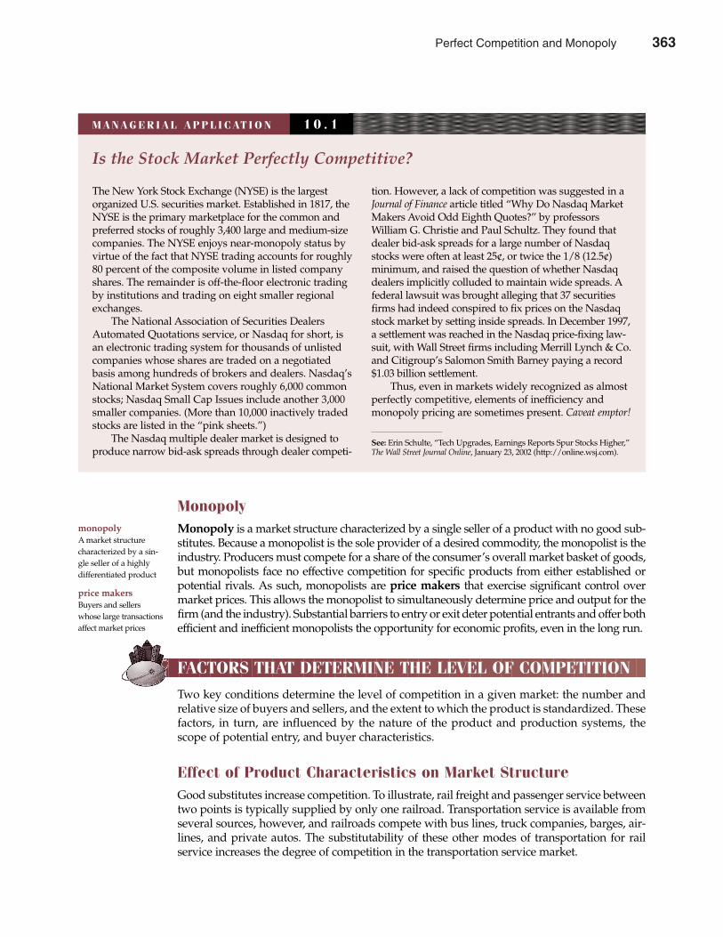
MonopolyMonopoly is a market structure characterized by a single seller of a product with no good sub-stitutes. Because a monopolist is the sole provider of a desired commodity, the monopolist is theindustry. Producers must compete for a share of the consumer’s overall market basket of goods,but monopolists face no effective competition for specific products from either established orpotential rivals. As such, monopolists are price makers that exercise significant control overmarket prices. This allows the monopolist to simultaneously determine price and output for thefirm (and the industry). Substantial barriers to entry or exit deter potential entrants and offer bothefficient and inefficient monopolists the opportunity for economic profits, even in the long run.
FACTORS THAT DETERMINE THE LEVEL OF COMPETITION
Two key conditions determine the level of competition in a given market: the number andrelative size of buyers and sellers, and the extent to which the product is standardized. Thesefactors, in turn, are influenced by the nature of the product and production systems, thescope of potential entry, and buyer characteristics.
Effect of Product Characteristics on Market StructureGood substitutes increase competition. To illustrate, rail freight and passenger service betweentwo points is typically supplied by only one railroad. Transportation service is available fromseveral sources, however, and railroads compete with bus lines, truck companies, barges, air-lines, and private autos. The substitutability of these other modes of transportation for railservice increases the degree of competition in the transportation service market.
364 Part Four Market Structure Analysis and Estimation
monopolyA market structurecharacterized by a sin-gle seller of a highlydifferentiated product
price makersBuyers and sellerswhose large transactionsaffect market prices
Is the Stock Market Perfectly Competitive?
The New York Stock Exchange (NYSE) is the largestorganized U.S. securities market. Established in 1817, theNYSE is the primary marketplace for the common andpreferred stocks of roughly 3,400 large and medium-sizecompanies. The NYSE enjoys near-monopoly status byvirtue of the fact that NYSE trading accounts for roughly80 percent of the composite volume in listed companyshares. The remainder is off-the-floor electronic tradingby institutions and trading on eight smaller regionalexchanges.
The National Association of Securities DealersAutomated Quotations service, or Nasdaq for short, isan electronic trading system for thousands of unlistedcompanies whose shares are traded on a negotiatedbasis among hundreds of brokers and dealers. Nasdaq’sNational Market System covers roughly 6,000 commonstocks; Nasdaq Small Cap Issues include another 3,000smaller companies. (More than 10,000 inactively tradedstocks are listed in the “pink sheets.”)
The Nasdaq multiple dealer market is designed toproduce narrow bid-ask spreads through dealer competi-
tion. However, a lack of competition was suggested in aJournal of Finance article titled “Why Do Nasdaq MarketMakers Avoid Odd Eighth Quotes?” by professorsWilliam G. Christie and Paul Schultz. They found thatdealer bid-ask spreads for a large number of Nasdaqstocks were often at least 25¢, or twice the 1/8 (12.5¢)minimum, and raised the question of whether Nasdaqdealers implicitly colluded to maintain wide spreads. Afederal lawsuit was brought alleging that 37 securitiesfirms had indeed conspired to fix prices on the Nasdaqstock market by setting inside spreads. In December 1997,a settlement was reached in the Nasdaq price-fixing law-suit, with Wall Street firms including Merrill Lynch & Co.and Citigroup’s Salomon Smith Barney paying a record$1.03 billion settlement.
Thus, even in markets widely recognized as almostperfectly competitive, elements of inefficiency andmonopoly pricing are sometimes present. Caveat emptor!
See: Erin Schulte, “Tech Upgrades, Earnings Reports Spur Stocks Higher,”The Wall Street Journal Online, January 23, 2002 (http://online.wsj.com).
M A N A G E R I A L A P P L I C AT I O N 1 0 . 1
Perfect Competition and Monopoly 363
It is important to realize that market structures are not static. In the 1800s and early 1900s—before the introduction of trucks, buses, automobiles, and airplanes—railroads faced very littlecompetition. Railroads could charge excessive prices and earn monopoly profits. Because ofthis exploitation, laws were passed giving public authorities permission to regulate railroadprices. Over the years, such regulation became superfluous given intermodal competition.Other firms were enticed by railroad profits to develop competing transportation service sys-tems, which ultimately led to a much more competitive market structure. Today, few wouldargue that railroads retain significant monopoly power, and public regulation of the railroadshas been greatly reduced in recognition of this fact.
Physical characteristics of a product can also influence the degree of competition. A lowratio of distribution cost to total cost, for example, tends to increase competition by wideningthe geographic area over which any particular producer can compete. Rapid perishability of aproduct yields the opposite effect. In considering the level of competition for a product, thenational, regional, or local nature of the market must be considered.
Effect of Production Characteristics on CompetitionWhen minimum efficient scale is large in relation to overall industry output, only a few firmsare able to attain the output size necessary for productive efficiency. In such instances, com-petitive pressures may allow only a few firms to survive. On the other hand, when minimumefficient scale is small in relation to overall industry output, many firms are able to attain thesize necessary for efficient operation. Holding all else equal, competition tends to be most vig-orous when many efficient competitors are present in the market. This is especially true whenfirms of smaller-than-minimum-efficient scale face considerably higher production costs, andwhen the construction of minimum-efficient–scale plants involves the commitment of substan-tial capital, skilled labor, and material resources. When construction of minimum-efficient–scaleplants requires the commitment of only modest resources or when smaller firms face noimportant production cost disadvantages, economies of scale have little or no effect on thecompetitive potential of new or entrant firms.
Effect of Entry and Exit Conditions on CompetitionMaintaining above-normal profits or inefficient operations over the long run requires sub-stantial barriers to entry, mobility, or exit. A barrier to entry is any factor or industry charac-teristic that creates an advantage for incumbents over new arrivals. Legal rights such aspatents and local, state, or federal licenses can present formidable barriers to entry in pharma-ceuticals, cable television, television and radio broadcasting, and other industries. A barrier tomobility is any factor or industry characteristic that creates an advantage for large leadingfirms over smaller nonleading rivals. Factors that sometimes create barriers to entry and/ormobility include substantial economies of scale, scope economies, large capital or skilled-laborrequirements, and ties of customer loyalty created through advertising and other means.
It is worth keeping in mind that barriers to entry and mobility can sometimes result in com-pensating advantages for consumers. Even though patents can lead to monopoly profits forinventing firms, they also spur valuable new product and process development. Althoughefficient and innovative leading firms make life difficult for smaller rivals, they can have thefavorable effect of lowering prices and increasing product quality. Therefore, a completeevaluation of the economic effects of entry barriers involves a consideration of both costsand benefits realized by suppliers and customers.
Whereas barriers to entry can impede competition by making entry or nonleading firmgrowth difficult, competitive forces can also be diminished through barriers to exit. A barrier toexit is any restriction on the ability of incumbents to redeploy assets from one industry or line ofbusiness to another. During the late 1980s, for example, several state governments initiated legal
barrier to entryAny advantage forindustry incumbentsover new arrivals
barrier to mobilityAny advantage forlarge leading firms oversmall nonleading rivals
barrier to exitAny limit on assetredeployment fromone line of business orindustry to another
Chapter Ten Perfect Competition and Monopoly 365
364 Perfect Competition and Monopoly
proceedings to impede plant closures by large employers in the steel, glass, automobile, andother industries. By imposing large fines or severance taxes or requiring substantial expendituresfor worker retraining, they created significant barriers to exit.
By impeding the asset redeployment that is typical of any vigorous competitive environ-ment, barriers to exit can dramatically increase both the costs and risks of doing business. Eventhough one can certainly sympathize with the difficult adjustments faced by both individualsand firms affected by plant closures, government actions that create barriers to exit can have theunintended effect of retarding industrial development and market competition.
Effect of Buyers on CompetitionGenerally speaking, if there are only a few buyers in a given market, there will be less compe-tition than if there are many buyers. Monopsony exists when a single firm is the sole buyer ofa desired product or input. Monopsony characterizes local labor markets with a single majoremployer, as well as many local agricultural markets with a single feed mill or livestock buyer.Similarly, the federal government is a monopsony buyer of military weapons and equipment.Major retailers such as Wal-Mart, Target, and Sears all enjoy monopsony power in the purchaseof apparel, appliances, auto parts, and other consumer products. Such buyer power is especial-ly strong in the purchase of “house brand” goods, where suppliers sell much if not all of theirproduction to a single retailer. Monopsony is more common in factor input markets than inmarkets for final demand.
In terms of economic efficiency, monopsony is least harmful, and can sometimes even bebeneficial, in those markets in which a monopsony buyer faces a monopoly seller. For example,consider the case of the town in which one mill is the sole employer of unskilled labor. The millis a monopsony because it is a single buyer of labor, and it may be able to use its power to reducewage rates below competitive levels. If workers organize a union to bargain collectively withtheir employer, a single monopoly seller of labor is created that could offset the employer’smonopsony power and increase wages toward competitive market norms. Not only is monop-sony accepted in such situations, but it is sometimes encouraged by public policy.
Effect of Product Differentiation on CompetitionIn addition to the number and size distribution of actual and potential competitors, market struc-ture is also described by the degree of product differentiation. Product differentiation includesany real or perceived differences in the quality of goods and services offered to consumers.Sources of product differentiation include all of the various forms of advertising promotion, plusnew products and processes made possible by effective programs of research and development.
The availability and cost of information about prices and output quality is a similarlyimportant determinant of market structure. Competition is always most vigorous whenbuyers and sellers have ready access to detailed price/performance information.
Finally, market structure is broadly determined by entry and exit conditions. Low regulato-ry barriers, modest capital requirements, and nominal standards for skilled labor and otherinputs all increase the likelihood that competition will be vigorous. Because all of these elementsof market structure have important consequences for the price/output decisions made by firms,the study of market structure is an important ingredient of managerial economics
PERFECT COMPETITION
Market characteristics described in the preceding section determine the level of competition inthe market for any good or service. This section focuses on the special features of perfectly com-petitive markets and illustrates why perfect competition is desirable from a social perspective.
366 Part Four Market Structure Analysis and Estimation
monopsonyA market with onebuyer
Perfect Competition and Monopoly 365
Characteristics of Perfectly Competitive MarketsPerfect competition exists when individual producers have no influence on market prices; theyare price takers as opposed to price makers. This lack of influence on price typically requires
• Large numbers of buyers and sellers. Each firm produces a small portion of industry output,and each customer buys only a small part of the total.
• Product homogeneity. The output of each firm is essentially the same as the output of anyother firm in the industry.
• Free entry and exit. Firms are not restricted from entering or leaving the industry.• Perfect dissemination of information. Cost, price, and product quality information is known by
all buyers and all sellers.
These basic conditions are too restrictive for perfect competition to be commonplace. Althoughthe stock market approaches the perfectly competitive ideal, imperfections occur even there.For example, the acquisition or sale of large blocks of securities by institutional investors clear-ly affects prices, at least in the short run. Nevertheless, because up to 1,000 shares of any stockcan be bought or sold at the current market price, the stock market approaches the ideal of aperfectly competitive market. Similarly, many industrial firms must make output decisionswithout any control over price, and examination of a perfectly competitive market structureprovides insights into these operating decisions. A clear understanding of perfect competitionalso provides a reference point from which to analyze monopolistic competition and oligop-oly, as described in Chapter 11.
Market Price DeterminationMarket prices in competitive industries are determined by aggregate supply and demand; indi-vidual firms have no control over price. Total industry demand reflects an aggregation of thequantities that individual firms will buy at each price. Industry supply reflects a summation ofthe quantities that individual firms are willing to supply at different prices. The intersection ofindustry demand and supply curves determines market price.
Data in Table 10.1 illustrate the process by which an industry supply curve is constructed.First, suppose that each of five firms in an industry is willing to supply varying quantities atdifferent prices. Summing the individual supply quantities of these five firms at each pricedetermines their combined supply schedule, shown in the Partial Market Supply column. Forexample, at a price of $2, the output supplied by the five firms are 15, 0, 5, 25, and 45 (thou-sand) units, respectively, resulting in a combined supply of 90 (000) units at that price. With aproduct price of $8, supply quantities become 45, 115, 40, 55, and 75, for a total supply by thefive firms of 330 (000) units.
Now assume that there are actually 5,000 firms in the industry, each with an individualsupply schedule identical to one of the five firms illustrated in the table. There are 1,000 firmsjust like each one illustrated in Table 10.1; the total quantity supplied at each price is 1,000 timesthat shown under the Partial Market Supply schedule. This supply schedule is illustrated inFigure 10.1. Adding the market demand curve to the industry supply curve, as in Figure 10.2,allows one to determine the equilibrium market price.
Market price is found by equating market supply and market demand to find the equi-librium price/output level. Using the curves illustrated in Figure 10.2, we have
Demand = Supply$40 – $0.0001Q = –$0.254 + $0.000025Q
$0.000125Q = $40.254Q = 322,032
Chapter Ten Perfect Competition and Monopoly 367
366 Perfect Competition and Monopoly
P = $40 – $0.0001(322,032)= $40 – $32.20= $7.80
Although both the quantity demanded and supplied depend on price, a simple exampledemonstrates the inability of individual firms to affect price. The total demand function inFigure 10.2 is described by the equation
(10.1) Quantity Demanded = Q = 400,000 – 10,000P
or, solving for price,
(10.1a)$10,000P = $400,000 – Q
P = $40 – $0.0001Q
According to Equation 10.1a, a 100-unit change in Q would cause only a $0.01 change inprice. A $0.0001 price increase would lead to a one-unit decrease in total market demand; a$0.0001 price reduction would lead to a one-unit increase in total market demand.
The demand curve shown in Figure 10.2 is redrawn for an individual firm in Figure 10.3. Theslope of the curve is –0.0001, the same as in Figure 10.2; only the scales have been changed. The$7.80 intercept is the going market price as determined by the intersection of the market supplyand demand curves in Figure 10.2.
At the scale shown in Figure 10.3, the firm’s demand curve is seen to be, for all practicalpurposes, a horizontal line. Thus, it is clear that under perfect competition, the individualfirm’s output decisions do not affect price in any meaningful way. Price can be assumed con-stant irrespective of the output level at which the firm chooses to operate.
Firm Price/Output DecisionProfit maximization requires that a firm operate at the output level at which marginal revenueand marginal cost are equal. With price constant, average revenue equals marginal revenue.Therefore, maximum profits result when market price is set equal to marginal cost for firms in aperfectly competitive industry. In the example shown in Figure 10.4, the firm chooses to operate
368 Part Four Market Structure Analysis and Estimation
TABLE 10.1Market Supply Schedule Determination
Quantity Supplied by Firm (000)
Partial TotalPrice Market Market
($) 1 � 2 � 3 � 4 � 5 � Supply �1,000�Supply
1 5 0 5 10 30 50 50,0002 15 0 5 25 45 90 90,0003 20 20 10 30 50 130 130,0004 25 35 20 35 55 170 170,0005 30 55 25 40 60 210 210,0006 35 75 30 45 65 250 250,0007 40 95 35 50 70 290 290,0008 45 115 40 55 75 330 330,0009 50 130 45 65 80 370 370,000
10 55 145 50 75 85 410 410,000
Perfect Competition and Monopoly 367
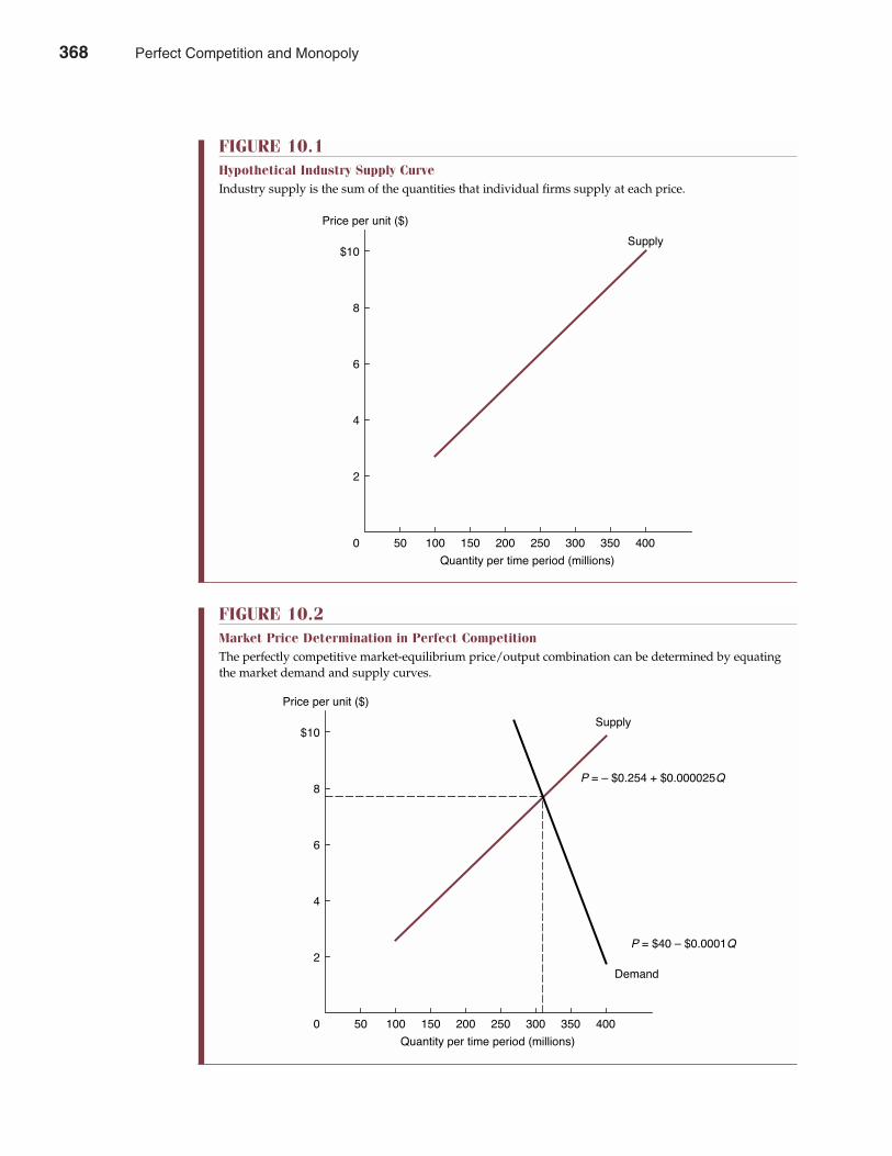
Chapter Ten Perfect Competition and Monopoly 369
FIGURE 10.1Hypothetical Industry Supply CurveIndustry supply is the sum of the quantities that individual firms supply at each price.
$10
8
6
4
2
0
Supply
50 100 150 200 250 300 350 400
Quantity per time period (millions)
Price per unit ($)
FIGURE 10.2Market Price Determination in Perfect CompetitionThe perfectly competitive market-equilibrium price/output combination can be determined by equatingthe market demand and supply curves.
$10
8
6
4
2
0
Supply
50 100 150 200 250 300 350 400
Quantity per time period (millions)
Price per unit ($)
P = Ð $0.254 + $0.000025Q
P = $40 Ð $0.0001Q
Demand
368 Perfect Competition and Monopoly
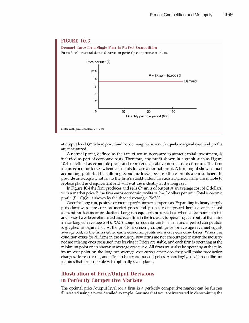
at output level Q*, where price (and hence marginal revenue) equals marginal cost, and profitsare maximized.
A normal profit, defined as the rate of return necessary to attract capital investment, isincluded as part of economic costs. Therefore, any profit shown in a graph such as Figure10.4 is defined as economic profit and represents an above-normal rate of return. The firmincurs economic losses whenever it fails to earn a normal profit. A firm might show a smallaccounting profit but be suffering economic losses because these profits are insufficient toprovide an adequate return to the firm’s stockholders. In such instances, firms are unable toreplace plant and equipment and will exit the industry in the long run.
In Figure 10.4 the firm produces and sells Q* units of output at an average cost of C dollars;with a market price P, the firm earns economic profits of P – C dollars per unit. Total economicprofit, (P – C)Q*, is shown by the shaded rectangle PMNC.
Over the long run, positive economic profits attract competitors. Expanding industry supplyputs downward pressure on market prices and pushes cost upward because of increaseddemand for factors of production. Long-run equilibrium is reached when all economic profitsand losses have been eliminated and each firm in the industry is operating at an output that min-imizes long-run average cost (LRAC). Long-run equilibrium for a firm under perfect competitionis graphed in Figure 10.5. At the profit-maximizing output, price (or average revenue) equalsaverage cost, so the firm neither earns economic profits nor incurs economic losses. When thiscondition exists for all firms in the industry, new firms are not encouraged to enter the industrynor are existing ones pressured into leaving it. Prices are stable, and each firm is operating at theminimum point on its short-run average cost curve. All firms must also be operating at the min-imum cost point on the long-run average cost curve; otherwise, they will make productionchanges, decrease costs, and affect industry output and prices. Accordingly, a stable equilibriumrequires that firms operate with optimally sized plants.
Illustration of Price/Output Decisions in Perfectly Competitive MarketsThe optimal price/output level for a firm in a perfectly competitive market can be furtherillustrated using a more detailed example. Assume that you are interested in determining the
370 Part Four Market Structure Analysis and Estimation
FIGURE 10.3Demand Curve for a Single Firm in Perfect CompetitionFirms face horizontal demand curves in perfectly competitive markets.
$10
8
6
4
2
0
Price per unit ($)
50 100 150
Demand
P = $7.80 Ð $0.0001Q
Quantity per time period (000)
Note: With price constant, P = MR.
Perfect Competition and Monopoly 369
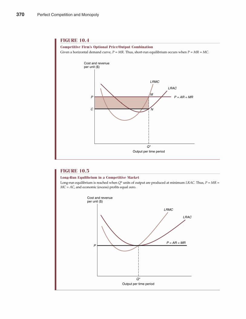
Chapter Ten Perfect Competition and Monopoly 371
FIGURE 10.4Competitive Firm’s Optional Price/Output CombinationGiven a horizontal demand curve, P = MR. Thus, short-run equilibrium occurs when P = MR = MC.
LRAC
Cost and revenueper unit ($)
Output per time period
Q*
N
M
LRMC
P = AR = MRP
C
FIGURE 10.5Long-Run Equilibrium in a Competitive MarketLong-run equilibrium is reached when Q* units of output are produced at minimum LRAC. Thus, P = MR =MC = AC, and economic (excess) profits equal zero.
LRAC
Cost and revenueper unit ($)
Output per time period
Q*
LRMC
P = AR = MRP
370 Perfect Competition and Monopoly

372 Part Four Market Structure Analysis and Estimation
Is Ticketmaster a Monopoly?
In the 1980s, a small upstart named Ticketmaster decid-ed to pay arenas millions of dollars for the right to selltheir tickets and helped them develop effective market-ing tactics. With Ticketmaster’s help, selling ticketswent from being a costly headache to a care-free andrevenue-maximizing endeavor. As part of the bargain,Ticketmaster gained exclusive marketing rights for ini-tial ticket sales. Because on-site box offices open later,and only when tickets are left over, Ticketmaster oftenaccounts for 85 to 90 percent of sales for hundreds ofon-site facilities.
Most people concede that Ticketmaster providesvaluable services for venue operators and their cus-tomers. However, few would describe Ticketmaster serv-ice charges as modest. Long ago, Ticketmaster recog-nized that customers would pay a lot for ticket-buyingservices. Ticketmaster levels convenience fees, buildingfacility charges, and order handling charges. For exam-ple, on April 14, 2002, Crosby, Stills, Nash & Young gave
a concert at the Ice Palace Arena in Tampa, Florida. Afirst-level seat cost $125. The Ticketmaster conveniencecharge was $11.75, the building facility charge was $2.75,and the order handling charge was $3.30 (see table below).That’s $167.80 for a single ticket, provided standard maildelivery was okay; UPS delivery cost more. That’s aprice that might bring tears to Suite Judy Blue Eyes.
In defense of such high fees, Ticketmaster arguesthat venue promotion services do not come cheap. As thesole ticket vendor, Ticketmaster can also assure venueoperators that tickets will be priced properly in light ofbooking alternatives. However, it is Ticketmaster’s mar-keting savvy and choke-hold on information concerningthe ticket-buying habits of the general public that hastrustbusters worried about monopoly power in the com-puterized ticketing services industry.
At what point is it reasonable for society to limit thesuccess of dominant, innovative companies like Ticket-master? Are such limits ever reasonable?
M A N A G E R I A L A P P L I C AT I O N 1 0 . 2
The Cost of Being a Fan: Selected Prices for Tickets Sold Through TicketmasterConvenience
Ticket Charge + Building HandlingVenue Primary Act Location Price Facility Charge1 Fee2
Philips Arena Creed Atlanta, GA $40.50 $6.00 $1.65Pantages Theatre Walt Disney’s Los Angeles, CA 15.00–125.00 7.50 + 2.00 3.05
The Lion KingFleet Center Elton John & Billy Joel Boston, MA 45.00–175.00 9.00 3.00D.A.R. Constitution Hall Alicia Keys Washington, DC 40.00 7.70 + 0.50 3.50Nassau Coliseum Janet Jackson Uniondale, NY 32.50–92.50 7.90 + 2.50 3.00Pebble Beach Golf Links AT&T Pebble Beach Monterey, CA 40.00 4.50 2.00
National Pro-AmIce Palace Arena Crosby, Stills, Nash & Tampa, FL 39.50–150.00 11.75+2.75 3.30
YoungFreeman Coliseum San Antonio Stock Show San Antonio, TX 12.00–22.00 3.75 + 1.50 3.10Sovereign Bank Arena World Wrestling Trenton, NJ 18.00–40.00 6.20 + 0.50 2.50
FederationNationwide Arena Ringling Bros. and Columbus, OH 10.00–35.00 3.50 + 1.00 2.00
Barnum & Bailey Circus
1 Each ticket purchased through ticket centers, over the telephone, or on Ticketmaster Online is subject to a per ticket convenience charge.Telephone and online orders require use of a major credit card.
2 Orders processed over the telephone or on Ticketmaster Online are also subject to a per order handling charge. With standard mail delivery, ticketswill be received at least 48 hours prior to the event (no additional charge). UPS delivery by 5:00 P.M. in 2 business days ($19.50), or by noon on Sat.,if order placed by Wed. prior ($25.00).
Source: Web survey by the author, December 14, 2001 (http://www.ticketmaster.com).
See: Julia Angwin, “Ticketmaster’s Online Resell System to Compete with Scalpers and eBay,” The Wall Street Journal Online, April 5, 2002(http://online.wsj.com).
Perfect Competition and Monopoly 371
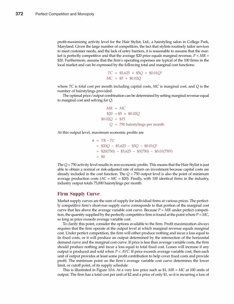
profit-maximizing activity level for the Hair Stylist, Ltd., a hairstyling salon in College Park,Maryland. Given the large number of competitors, the fact that stylists routinely tailor servicesto meet customer needs, and the lack of entry barriers, it is reasonable to assume that the mar-ket is perfectly competitive and that the average $20 price equals marginal revenue, P = MR =$20. Furthermore, assume that the firm’s operating expenses are typical of the 100 firms in thelocal market and can be expressed by the following total and marginal cost functions:
TC = $5,625 + $5Q + $0.01Q2
MC = $5 + $0.02Q
where TC is total cost per month including capital costs, MC is marginal cost, and Q is thenumber of hairstylings provided.
The optimal price/output combination can be determined by setting marginal revenue equalto marginal cost and solving for Q:
MR = MC$20 = $5 + $0.02Q
$0.02Q = $15Q = 750 hairstylings per month
At this output level, maximum economic profits are
π = TR – TC= $20Q – $5,625 – $5Q – $0.01Q2
= $20(750) – $5,625 – $5(750) – $0.01(7502)= $0
The Q = 750 activity level results in zero economic profits. This means that the Hair Stylist is justable to obtain a normal or risk-adjusted rate of return on investment because capital costs arealready included in the cost function. The Q = 750 output level is also the point of minimumaverage production costs (AC = MC = $20). Finally, with 100 identical firms in the industry,industry output totals 75,000 hairstylings per month.
Firm Supply CurveMarket supply curves are the sum of supply for individual firms at various prices. The perfect-ly competitive firm’s short-run supply curve corresponds to that portion of the marginal costcurve that lies above the average variable cost curve. Because P = MR under perfect competi-tion, the quantity supplied by the perfectly competitive firm is found at the point where P = MC,so long as price exceeds average variable cost.
To clarify this point, consider the options available to the firm. Profit maximization alwaysrequires that the firm operate at the output level at which marginal revenue equals marginalcost. Under perfect competition, the firm will either produce nothing and incur a loss equal toits fixed costs, or it will produce an output determined by the intersection of the horizontaldemand curve and the marginal cost curve. If price is less than average variable costs, the firmshould produce nothing and incur a loss equal to total fixed cost. Losses will increase if anyoutput is produced and sold when P < AVC. If price exceeds average variable cost, then eachunit of output provides at least some profit contribution to help cover fixed costs and provideprofit. The minimum point on the firm’s average variable cost curve determines the lowerlimit, or cutoff point, of its supply schedule.
This is illustrated in Figure 10.6. At a very low price such as $1, MR = MC at 100 units ofoutput. The firm has a total cost per unit of $2 and a price of only $1, so it is incurring a loss of
Chapter Ten Perfect Competition and Monopoly 373
372 Perfect Competition and Monopoly
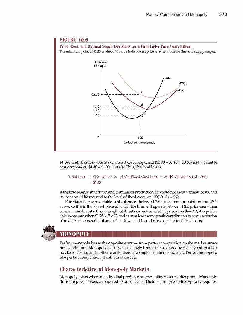
$1 per unit. This loss consists of a fixed cost component ($2.00 – $1.40 = $0.60) and a variablecost component ($1.40 – $1.00 = $0.40). Thus, the total loss is
Total Loss = (100 Units) � ($0.60 Fixed Cost Loss + $0.40 Variable Cost Loss)= $100
If the firm simply shut down and terminated production, it would not incur variable costs, andits loss would be reduced to the level of fixed costs, or 100($0.60) = $60.
Price fails to cover variable costs at prices below $1.25, the minimum point on the AVCcurve, so this is the lowest price at which the firm will operate. Above $1.25, price more thancovers variable costs. Even though total costs are not covered at prices less than $2, it is prefer-able to operate when $1.25 < P < $2 and earn at least some profit contribution to cover a portionof total fixed costs rather than to shut down and incur losses equal to total fixed costs.
MONOPOLY
Perfect monopoly lies at the opposite extreme from perfect competition on the market struc-ture continuum. Monopoly exists when a single firm is the sole producer of a good that hasno close substitutes; in other words, there is a single firm in the industry. Perfect monopoly,like perfect competition, is seldom observed.
Characteristics of Monopoly MarketsMonopoly exists when an individual producer has the ability to set market prices. Monopolyfirms are price makers as opposed to price takers. Their control over price typically requires
374 Part Four Market Structure Analysis and Estimation
FIGURE 10.6Price, Cost, and Optimal Supply Decisions for a Firm Under Pure CompetitionThe minimum point of $1.25 on the AVC curve is the lowest price level at which the firm will supply output.
$ per unitof output
Output per time period
MC
ATC
AVC
1000
1.00
1.251.40
$2.00D
B
A
Perfect Competition and Monopoly 373
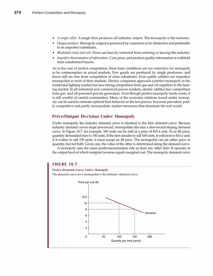
• A single seller. A single firm produces all industry output. The monopoly is the industry.• Unique product. Monopoly output is perceived by customers to be distinctive and preferable
to its imperfect substitutes.• Blockaded entry and exit. Firms are heavily restricted from entering or leaving the industry.• Imperfect dissemination of information. Cost, price, and product quality information is withheld
from uninformed buyers.
As in the case of perfect competition, these basic conditions are too restrictive for monopolyto be commonplace in actual markets. Few goods are produced by single producers, andfewer still are free from competition of close substitutes. Even public utilities are imperfectmonopolies in most of their markets. Electric companies approach a perfect monopoly in theresidential lighting market but face strong competition from gas and oil suppliers in the heat-ing market. In all industrial and commercial power markets, electric utilities face competitionfrom gas- and oil-powered private generators. Even though perfect monopoly rarely exists, itis still worthy of careful examination. Many of the economic relations found under monop-oly can be used to estimate optimal firm behavior in the less precise, but more prevalent, part-ly competitive and partly monopolistic market structures that dominate the real world.
Price/Output Decision Under MonopolyUnder monopoly, the industry demand curve is identical to the firm demand curve. Becauseindustry demand curves slope downward, monopolists also face a downward-sloping demandcurve. In Figure 10.7, for example, 100 units can be sold at a price of $10 a unit. At an $8 price,quantity demanded rises to 150 units. If the firm decides to sell 100 units, it will receive $10 a unit;if it wishes to sell 150 units, it must accept an $8 price. The monopolist can set either price orquantity, but not both. Given one, the value of the other is determined along the demand curve.
A monopoly uses the same profit-maximization rule as does any other firm: It operates atthe output level at which marginal revenue equals marginal cost. The monopoly demand curve
Chapter Ten Perfect Competition and Monopoly 375
FIGURE 10.7Firm’s Demand Curve Under MonopolyThe demand curve for a monopolist is the industry demand curve.
Demand
Quantity per time period
200150100500
2
4
8
10
$12
Price per unit ($)
6
374 Perfect Competition and Monopoly
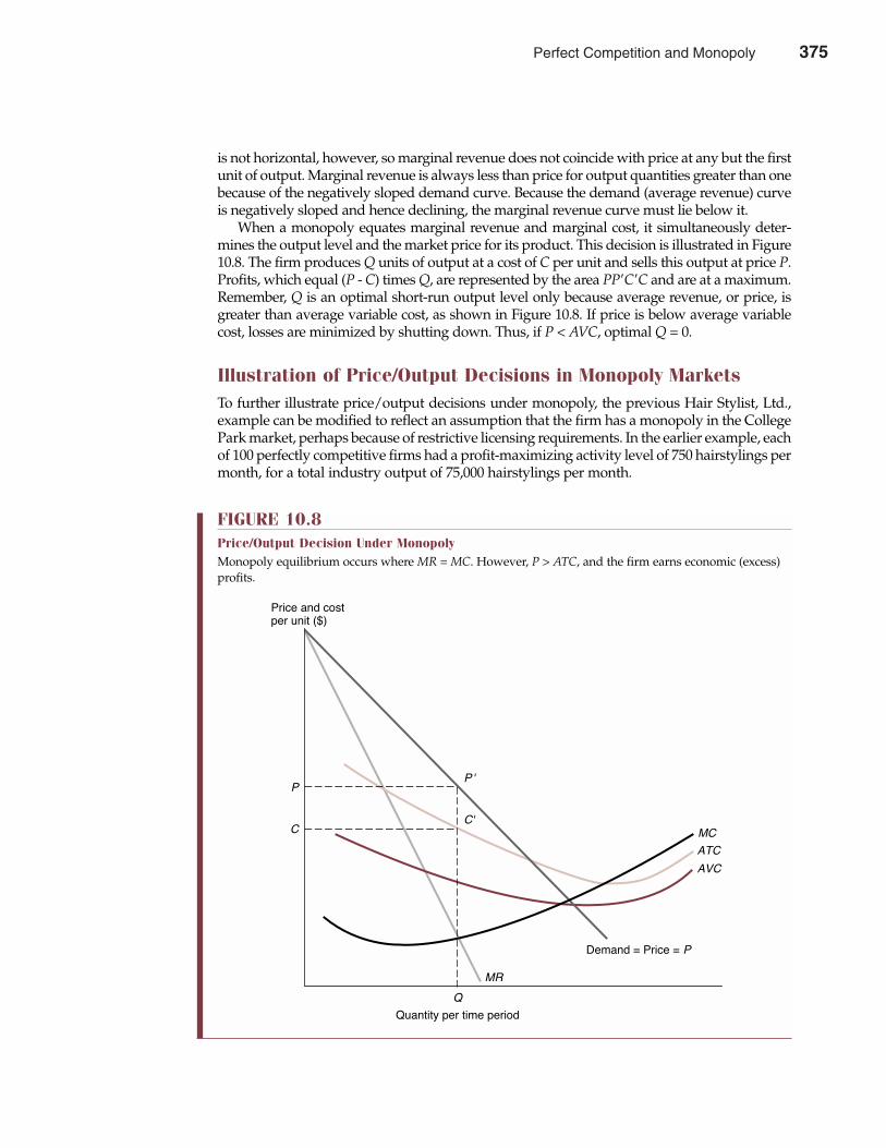
is not horizontal, however, so marginal revenue does not coincide with price at any but the firstunit of output. Marginal revenue is always less than price for output quantities greater than onebecause of the negatively sloped demand curve. Because the demand (average revenue) curveis negatively sloped and hence declining, the marginal revenue curve must lie below it.
When a monopoly equates marginal revenue and marginal cost, it simultaneously deter-mines the output level and the market price for its product. This decision is illustrated in Figure10.8. The firm produces Q units of output at a cost of C per unit and sells this output at price P.Profits, which equal (P - C) times Q, are represented by the area PP�C�C and are at a maximum.Remember, Q is an optimal short-run output level only because average revenue, or price, isgreater than average variable cost, as shown in Figure 10.8. If price is below average variablecost, losses are minimized by shutting down. Thus, if P < AVC, optimal Q = 0.
Illustration of Price/Output Decisions in Monopoly MarketsTo further illustrate price/output decisions under monopoly, the previous Hair Stylist, Ltd.,example can be modified to reflect an assumption that the firm has a monopoly in the CollegePark market, perhaps because of restrictive licensing requirements. In the earlier example, eachof 100 perfectly competitive firms had a profit-maximizing activity level of 750 hairstylings permonth, for a total industry output of 75,000 hairstylings per month.
376 Part Four Market Structure Analysis and Estimation
FIGURE 10.8Price/Output Decision Under MonopolyMonopoly equilibrium occurs where MR = MC. However, P > ATC, and the firm earns economic (excess)profits.
C'
Price and costper unit ($)
P'P
C
MR
Demand = Price = P
MC
ATC
AVC
Quantity per time period
Q
Perfect Competition and Monopoly 375
As a monopoly, the Hair Stylist provides all industry output. For simplicity, assume that theHair Stylist operates a chain of salons and that the cost function for each shop is the same as inthe previous example. By operating each shop at its average cost-minimizing activity level of 750hairstylings per month, the Hair Stylist can operate with Marginal Cost = Average Cost = $20.
Assume that industry demand and marginal revenue curves for hair stylings in the CollegePark market are
P = $80 – $0.0008Q
MR = $80 – $0.0016Q
The monopoly profit-maximizing activity level is obtained by setting marginal revenue equalto marginal cost, or marginal profit equal to zero (Mπ = 0), and solving for Q:
MR = MC
$80 – $0.0016Q = $20$0.0016Q = $60
Q = 37,500 hairstylings per month
The optimal market price is
P = $80 – $0.0008(37,500)= $50
At the Q = 37,500 activity level, the Hair Stylist will operate a chain of 50 salons (= 37,500/750).Although each outlet produces Q = 750 hairstylings per month, a point of optimum efficiency,the benefits of this efficiency accrue to the company in the form of economic profits rather thanto consumers in the form of lower prices. Economic profits from each shop are
π = TR – TC
= P � Q – AC � Q
= $50(750) - $20(750)= $22,500 per month
With 50 shops, the Hair Stylist earns total economic profits of $1,125,000 per month. As amonopoly, the industry provides only 37,500 units of output, down from the 75,000 units pro-vided in the case of a perfectly competitive industry. The new price of $50 per hairstyling is upsubstantially from the perfectly competitive price of $20. The effects of monopoly power arereflected in terms of higher consumer prices, reduced levels of output, and substantial economicprofits for the Hair Stylist, Inc.
Long-Run Equilibrium Under MonopolyIn general, any industry characterized by monopoly sells less output at higher prices thanwould the same industry if it were perfectly competitive. From the perspective of the firmand its stockholders, the benefits of monopoly are measured in terms of the economicprofits that are possible when competition is reduced or eliminated. From a broader socialperspective, these private benefits must be weighed against the costs borne by consumersin the forms of higher prices and reduced availability of desired products. Employees andsuppliers also suffer from the reduced employment opportunities associated with lowerproduction in monopoly markets.
Chapter Ten Perfect Competition and Monopoly 377
376 Perfect Competition and Monopoly

Monopolies have an incentive to underproduce and earn economic profits. Underproductionresults when a monopoly curtails output to a level at which the value of resources employed, asmeasured by the marginal cost of production, is less than the social benefit derived, where socialbenefit is measured by the price that customers are willing to pay for additional output. Undermonopoly, marginal cost is less than price at the profit-maximizing output level. Although result-ing economic profits serve the useful functions of providing incentives and helping allocateresources, it is difficult to justify above-normal profits that result from market power rather thanfrom exceptional performance.
As shown earlier, in equilibrium, perfectly competitive firms must operate at the minimumpoint on the LRAC curve. This requirement does not hold under monopoly. For example, againconsider Figure 10.8 and assume that the ATC curve represents the long-run average cost curvefor the firm. The monopolist will produce Q units of output at an average cost of C per unit,somewhat above the minimum point on the ATC curve.
In this case, the firm is called a natural monopoly, because the market-clearing price, whereP = MC, occurs at a point at which long-run average costs are still declining. In other words,market demand is insufficient to justify full utilization of even one minimum efficient–scaleplant. A single monopolist can produce the total market supply at a lower total cost than couldany number of smaller firms, and competition naturally reduces the number of competitorsuntil only a single monopoly supplier remains. Electric and local telephone utilities are classicexamples of natural monopoly, because any duplication in production and distribution facili-ties would increase consumer costs.
Is Monopoly Always Bad?Natural monopoly presents something of a dilemma. On the one hand, economic efficiency couldbe enhanced by restricting the number of producers to a single firm. On the other hand, monop-olies have an incentive to underproduce and can generate unwarranted economic profits.
378 Part Four Market Structure Analysis and Estimation
underproductionA situation that occurswhen a monopolistcurtails production to alevel at which marginalcost is less than price
natural monopolyAn industry in whichthe market-clearingprice occurs at a point atwhich the monopolist’slong-run average costsare still declining
Is This Why They Call It “Hardball”?
In late 2001, commissioner Bud Selig broke open thebooks to show that major league baseball (MLB) had lost$1.4 billion during the previous 5 years. Worse yet, oper-ating losses of more than $500 million per year on stag-nant revenues of $3.5 billion are threatening to kill thegame, according to Selig. Obviously, Congress and theplayers’ union need to rally around Selig’s plan to reduceplayer salaries and allow him to get rid of the MontrealExpos and the Minnesota Twins. Local governments alsoneed to pony up for new and more elaborate stadiums.
Selig’s ploy may be nothing more than public pos-turing ahead of what promises to be tough labor negoti-ations. MLB operates much like a corporation with 30different regional offices (local franchises). Althoughindividual clubs compete on the playing field, theyaren’t economic competitors. In a competitive market,one competitor’s gain comes at the expense of others. Inbaseball, the success of one franchise brings increasedprosperity for all. Through revenue sharing, all clubsprospered when Barry Bonds broke Mark McGwire’s
home run record. When the Giants or the Yankees cometo town, home team ticket sales soar. Ineptitude at onefranchise weakens the profit picture for everyone.
MLB is clearly concerned about its poisoned collec-tive bargaining environment. On the other side of thetable is the Major League Players’ Association. The play-ers’ association is a monopoly seller of baseball playertalent, and the owners are a monopsony employer. Thelabor-market standoff in major league baseball is a classicconfrontation between a powerful monopsony employer(the owners) and a powerful monopoly employee group(the players’ association). It will indeed be interesting tosee if Selig and the player’s association are successful ingetting the general public to pay part of the tab for esca-lating player salaries and ever more elaborate stadiums.
See: Dow Jones Newswires, “Minnesota Court Upholds InjunctionForcing Twins to Play in ‘02,” The Wall Street Journal Online, January 22,2002 (http://online.wsj.com).
M A N A G E R I A L A P P L I C AT I O N 1 0 . 3
Perfect Competition and Monopoly 377
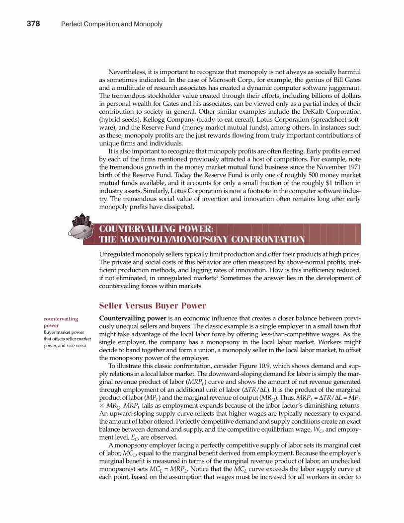
Nevertheless, it is important to recognize that monopoly is not always as socially harmfulas sometimes indicated. In the case of Microsoft Corp., for example, the genius of Bill Gatesand a multitude of research associates has created a dynamic computer software juggernaut.The tremendous stockholder value created through their efforts, including billions of dollarsin personal wealth for Gates and his associates, can be viewed only as a partial index of theircontribution to society in general. Other similar examples include the DeKalb Corporation(hybrid seeds), Kellogg Company (ready-to-eat cereal), Lotus Corporation (spreadsheet soft-ware), and the Reserve Fund (money market mutual funds), among others. In instances suchas these, monopoly profits are the just rewards flowing from truly important contributions ofunique firms and individuals.
It is also important to recognize that monopoly profits are often fleeting. Early profits earnedby each of the firms mentioned previously attracted a host of competitors. For example, notethe tremendous growth in the money market mutual fund business since the November 1971birth of the Reserve Fund. Today the Reserve Fund is only one of roughly 500 money marketmutual funds available, and it accounts for only a small fraction of the roughly $1 trillion inindustry assets. Similarly, Lotus Corporation is now a footnote in the computer software indus-try. The tremendous social value of invention and innovation often remains long after earlymonopoly profits have dissipated.
COUNTERVAILING POWER: THE MONOPOLY/MONOPSONY CONFRONTATION
Unregulated monopoly sellers typically limit production and offer their products at high prices.The private and social costs of this behavior are often measured by above-normal profits, inef-ficient production methods, and lagging rates of innovation. How is this inefficiency reduced,if not eliminated, in unregulated markets? Sometimes the answer lies in the development ofcountervailing forces within markets.
Seller Versus Buyer PowerCountervailing power is an economic influence that creates a closer balance between previ-ously unequal sellers and buyers. The classic example is a single employer in a small town thatmight take advantage of the local labor force by offering less-than-competitive wages. As thesingle employer, the company has a monopsony in the local labor market. Workers mightdecide to band together and form a union, a monopoly seller in the local labor market, to offsetthe monopsony power of the employer.
To illustrate this classic confrontation, consider Figure 10.9, which shows demand and sup-ply relations in a local labor market. The downward-sloping demand for labor is simply the mar-ginal revenue product of labor (MRPL) curve and shows the amount of net revenue generatedthrough employment of an additional unit of labor (∆TR/∆L). It is the product of the marginalproduct of labor (MPL) and the marginal revenue of output (MRQ). Thus, MRPL = ∆TR/∆L = MPL� MRQ. MRPL falls as employment expands because of the labor factor’s diminishing returns.An upward-sloping supply curve reflects that higher wages are typically necessary to expandthe amount of labor offered. Perfectly competitive demand and supply conditions create an exactbalance between demand and supply, and the competitive equilibrium wage, WC, and employ-ment level, EC, are observed.
A monopsony employer facing a perfectly competitive supply of labor sets its marginal costof labor, MCL, equal to the marginal benefit derived from employment. Because the employer’smarginal benefit is measured in terms of the marginal revenue product of labor, an uncheckedmonopsonist sets MCL = MRPL. Notice that the MCL curve exceeds the labor supply curve ateach point, based on the assumption that wages must be increased for all workers in order to
countervailingpowerBuyer market powerthat offsets seller marketpower, and vice versa
Chapter Ten Perfect Competition and Monopoly 379
378 Perfect Competition and Monopoly
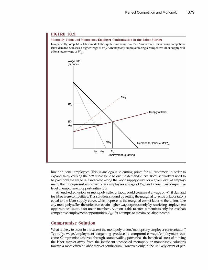
hire additional employees. This is analogous to cutting prices for all customers in order toexpand sales, causing the MR curve to lie below the demand curve. Because workers need tobe paid only the wage rate indicated along the labor supply curve for a given level of employ-ment, the monopsonist employer offers employees a wage of WM and a less than competitivelevel of employment opportunities, EM.
An unchecked union, or monopoly seller of labor, could command a wage of WU if demandfor labor were competitive. This solution is found by setting the marginal revenue of labor (MRL)equal to the labor supply curve, which represents the marginal cost of labor to the union. Likeany monopoly seller, the union can obtain higher wages (prices) only by restricting employmentopportunities (output) for union members. Aunion is able to offer its members only the less thancompetitive employment opportunities, EU, if it attempts to maximize labor income.
Compromise SolutionWhat is likely to occur in the case of the monopoly union/monopsony employer confrontation?Typically, wage/employment bargaining produces a compromise wage/employment out-come. Compromise achieved through countervailing power has the beneficial effect of movingthe labor market away from the inefficient unchecked monopoly or monopsony solutionstoward a more efficient labor market equilibrium. However, only in the unlikely event of per-
380 Part Four Market Structure Analysis and Estimation
FIGURE 10.9Monopoly Union and Monopsony Employer Confrontation in the Labor MarketIn a perfectly competitive labor market, the equilibrium wage is at WC. A monopoly union facing competitivelabor demand will seek a higher wage of WU. A monopsony employer facing a competitive labor supply willoffer a lower wage of WM.
Employment (quantity)
Demand for labor = MRPL
ECEMEU
MRL
MCL
WU
WCWM
Wage rate(or price)
Supply of labor
Perfect Competition and Monopoly 379
fectly matched monopoly/monopsony protagonists will the perfectly competitive outcomeoccur. Depending on the relative power of the union and the employer, either an above-marketor a below-market wage outcome typically results, and employment opportunities are oftenbelow competitive employment levels. Nevertheless, monopoly/monopsony confrontationscan have the beneficial effect of improving economic efficiency from that experienced undereither unchecked monopoly or monopsony.
MEASUREMENT OF BUSINESS PROFIT RATES
In long-run equilibrium, profits in perfectly competitive industries are usually just sufficient toprovide a normal risk-adjusted rate of return. In monopoly markets, barriers to entry or exitcan allow above-normal profits, even over the long run. Nevertheless, high profits are some-times observed in vigorously competitive markets, while some monopolies stumble from oneyear to the next without realizing superior rates of return. To appreciate the sources of profitdifferences, it is first necessary to understand conventional measures of business profits.
Rate of Return on Stockholders’ EquityBusiness profit rates are best evaluated using the accounting rate of return on stockholders’equity (ROE). ROE is net income divided by the book value of stockholders’ equity, wherestockholders’ equity is total assets minus total liabilities. As seen in Table 10.2, ROE can alsobe described as the product of three common accounting ratios. ROE equals the firm’s profitmargin multiplied by the total asset turnover ratio, all times the firm’s leverage ratio:
ROE = Net IncomeEquity
= Net Income�
Sales�
Total Assets(10.2) Sales Total Assets Equity
= Profit Margin �Total Asset
� LeverageTurnover
Profit margin is accounting net income expressed as a percentage of sales revenue and shows theamount of profit earned per dollar of sales. When profit margins are high, robust demand or strin-gent cost controls, or both, allow the firm to earn a significant profit contribution. Holding capitalrequirements constant, profit margin is a useful indicator of managerial efficiency in respondingto rapidly growing demand and/or effective measures of cost containment. Table 10.2 shows theoutstanding profit margins reported by smokeless tobacco producer UST, Inc.; diversified financialservices provider Stilwell Financial, Inc., growth stock manager of the Janus Group of mutualfunds; and Internet portal Yahoo! However, rich profit margins do not necessarily guarantee ahigh rate of return on stockholders’ equity. Despite high profit margins, firms in mining, con-struction, heavy equipment manufacturing, cable TV, and motion picture production often earnonly modest rates of return because significant capital expenditures are required before mean-ingful sales revenues can be generated. Thus, it is vitally important to consider the magnitude ofcapital requirements when interpreting the size of profit margins for a firm or an industry.
Total asset turnover is sales revenue divided by the book value of total assets. When totalasset turnover is high, the firm makes its investments work hard in the sense of generating alarge amount of sales volume. A broad range of business and consumer service businessenjoys high rates of total asset turnover that allow efficient firms to earn attractive rates ofreturn on stockholders’ equity despite modest profit margins. For example, consider envi-ronmental services juggernaut Waste Management, Inc. Despite modest profit margins and aconservative financial structure, Waste Management reports a sterling ROE by virtue of the
return on stockhold-ers’ equity (ROE)Business profits express-ed as a percentage ofowner-supplied capital
profit marginNet income expressedas a percentage of salesrevenue
total asset turnoverSales revenue dividedby the book value oftotal assets
Chapter Ten Perfect Competition and Monopoly 381
380 Perfect Competition and Monopoly

382 Part Four Market Structure Analysis and Estimation
TABLE 10.2Operating Statistics for a Sample of 50 Large Firms Taken from the Standard & Poor’s 500
Return on Stockholders’ Total AssetEquity (ROE) Profit Turnover Leverage
Company Name Industry Name (%) Margin (%) Ratio Ratio
Alberto Culver ‘B’ Toiletries/cosmetics 15.3% 4.3% 0.62 2.18 Albertson’s, Inc. Grocery 16.7% 2.5% 0.42 2.75 Anheuser-Busch Beverage (alcoholic) 35.8% 12.0% 1.08 3.22 AOL-Time Warner Entertainment 5.6% 2.0% 1.87 5.28 Apple Computer Computer and peripherals 14.9% 7.7% 0.85 1.66 Bank of America Bank 18.5% n.a. n.a. 14.24 Bed Bath & Beyond Retail (special lines) 23.5% 7.0% 0.46 1.55 Bristol-Myers Squibb Drug 48.2% 20.6% 0.85 1.98 Deere & Co. Machinery 5.8% 2.5% 1.06 2.51 Dell Computer Computer and peripherals 35.0% 7.4% 0.45 2.16 Delta Air Lines Air transport 20.0% 6.4% 1.29 4.04 Dillard’s, Inc. Retail store 7.7% 2.5% 0.91 2.80 Dow Jones & Co. Newspaper 40.2% 11.1% 0.76 2.77 EMC Corp. Computer and peripherals 23.5% 17.4% 1.07 1.45 Fannie Mae Financial svcs. (div.) 22.2% n.a. n.a. 32.63 Ford Motor Auto and truck 26.3% 4.5% 1.70 10.03 Freddie Mac Financial svcs. (div.) 19.0% n.a. n.a. 33.18 Gannett Co. Newspaper 19.9% 17.5% 1.71 1.95 Gateway Inc. Computer and peripherals 22.0% 5.1% 0.46 1.96 Harley-Davidson Recreation 23.0% 10.9% 0.86 1.82 Hershey Foods Food processing 26.9% 7.4% 0.84 3.05 Hilton Hotels Hotel/gaming 12.4% 8.2% 4.30 6.54 Home Depot Retail building supply 18.8% 6.0% 0.44 1.38 Limited Inc. Retail (special lines) 20.4% 4.5% 0.42 1.90 Mattel, Inc. Recreation 9.3% 3.3% 0.93 2.61 Merck & Co. Drug 44.5% 18.0% 1.09 2.69 Merrill Lynch & Co. Securities brokerage 20.4% 7.5% 9.41 25.63 N.Y. Times Newspaper 21.4% 9.9% 1.12 2.41 NIKE, Inc. ‘B’ Shoe 18.5% 6.4% 0.65 1.87 Nordstrom, Inc. Retail store 17.1% 4.0% 0.60 2.58 Nortel Networks Foreign telecom. 10.5% 6.7% 1.13 1.75 Palm, Inc. Wireless networking 5.6% 5.4% 1.21 1.25 Quaker Oats Food processing 180.6% 8.4% 0.51 10.90 Schwab (Charles) Securities brokerage 25.9% 12.5% 6.22 12.88Southwest Airlines Air transport 16.7% 10.0% 1.19 1.99 Sprint Corp. Telecom. services 16.5% 10.2% 1.28 2.07 St. Jude Medical Medical supplies 18.1% 12.9% 1.39 1.96 Starbucks Corp. Restaurant 10.6% 6.1% 0.75 1.30 Stilwell Fin’l Financial svcs. (div.) 38.4% 25.8% 1.02 1.51 SunTrust Banks Bank 14.7% n.a. n.a. 12.51 Target Corp. Retail store 20.2% 3.5% 0.51 2.92 Texas Instruments Semiconductor 16.6% 16.2% 1.59 1.62 UST, Inc. Tobacco 233.7% 31.0% 0.67 5.06 Wal-Mart Stores Retail store 22.1% 3.5% 0.43 2.72 Waste Management Environmental 25.2% 8.5% 1.73 5.15 Wells Fargo Bank 16.9% n.a. n.a. 9.86 Wendy’s Int’l Restaurant 15.6% 8.0% 0.91 1.77 WorldCom Inc. Telecom. Services 7.7% 10.8% 2.45 1.75 Wrigley (Wm.) Jr. Food processing 27.1% 14.9% 0.75 1.36 Yahoo! Inc. Internet 10.7% 22.9% 2.50 1.17 Averages 27.7% 9.6% 1.39 5.25
Source: Value Line Investment Survey for Windows, July 1, 2001.Reproduced with permission of Value Line Publishing, Inc.
Perfect Competition and Monopoly 381
fact that it reports a total asset turnover rate that is well in excess of industry and corporatenorms. Waste Management has learned that the wise use of assets is a key ingredient of successin the often cutthroat environmental services business.
Leverage is often defined as the ratio of total assets divided by stockholders’ equity. It reflectsthe extent to which debt and preferred stock are used in addition to common stock financing.Leverage is used to amplify firm profit rates over the business cycle. During economic booms,leverage can dramatically increase the firm’s profit rate; during recessions and other economiccontractions, leverage can just as dramatically decrease realized rates of return, if not lead to loss-es. Despite ordinary profit margins and modest rates total asset turnover, ROE in the securitiesbrokerage, hotel, and gaming industries can sometimes benefit through use of a risky financialstrategy that employs significant leverage. However, it is worth remembering that a risky finan-cial structure can lead to awe-inspiring profit rates during economic expansions, such as thatexperienced during the late 1990s; it can also lead to huge losses during economic downturns,such as that in 2001.
Typical Business Profit RatesFor successful large and small firms in the United States and Canada, ROE averages rough-ly 12 percent during a typical year. This average ROE is comprised of a typical profit mar-gin on sales revenue of roughly 4 percent, a standard total asset turnover ratio of 1.0 times,and a common leverage ratio of roughly 3:1:
Typical = Profit Margin � Total Asset� LeverageROE Turnover
(10.2a) = 4% � 1.0 � 3= 12%
ROE is an attractive measure of firm performance because it shows the rate of profit earned onfunds committed to the enterprise by its owners, the stockholders. When ROE is at or above 12percent per year, the rate of profit is generally sufficient to compensate investors for the riskinvolved with a typical business enterprise. When ROE consistently falls far below 12 percentper year, profit rates are generally insufficient to compensate investors for the risks undertaken.Of course, when business risk is substantially higher than average, a commensurately higherrate of return is required. When business risk is somewhat lower than average, a somewhatlower than average profit rate is adequate.
This naturally suggests an important question: How is it possible to know if business profitrates in any given circumstance are sufficient to compensate investors for the risks undertaken?The answer to this difficult question turns out to be rather simple: just ask current and potentialshareholders and bondholders. Shareholders and bondholders implicitly inform management oftheir risk/return assessment of the firm’s performance on a daily basis. If performance is abovethe minimum required, the firm’s bond and stock prices rise; if performance is below the mini-mum required, bond and stock prices fall. For privately held companies, the market’s risk/returnassessment comes at less frequent intervals, such as when new bank financing is required. If per-formance is above the minimum required, bank financing is easy to obtain; if performance isbelow the minimum required, bank financing is difficult or impossible to procure. As a practicalmatter, firms must consistently earn a business profit rate or ROE of at least 12 percent per year inorder to grow and prosper. If ROE consistently falls below this level, sources of financing tend todry up and the firm withers and dies. If ROE consistently exceeds this level, new debt and equi-ty financing are easy to obtain, and growth by new and established competitors is rapid.
Although ROE is perhaps the most useful available indicator of business profits, otheraccounting measures can also be used to compare profit rates across different lines of business.
leverageThe ratio of the bookvalue of assets dividedby stockholders’ equity
Chapter Ten Perfect Competition and Monopoly 383
382 Perfect Competition and Monopoly

The accounting return on assets (ROA), defined as net income divided by total assets, is alsoa useful indicator of the business profit rate. Like ROE, ROA captures the effects of manageri-al operating decisions; unlike ROE, ROA is unaffected by the amount of leverage. Therefore,although ROA is a useful alternative indicator of the basic profitability of a business, it fails toaccount for the effects of financial leverage decisions on firm performance. As such, ROE hassome advantages over ROA as a fundamental measure of business profits. Irrespective ofwhether ROE, ROA, or some other measure of business profits is employed, consistencyrequires that comparisons be made using a common basis.
LINK BETWEEN MARKET STRUCTURE AND BUSINESS PROFIT RATES
High business profit rates are derived from some combination of high profit margins, quicktotal asset turnover, and a high rate of total assets to stockholders’ equity. High businessprofits generally indicate superior efficiency, modest competition, a wise use of assets,and/or use of a risky financial structure.
Business Profit Rates by Industry GroupIn a perfectly competitive market, profit margins are low. This stems from the fact that in aperfectly competitive market, theory suggests that P = MC and MC = AC. As a result, whenaverage cost includes a risk-adjusted normal rate of return on investment, P = AC. This meansthat when profit margin is measured as (P – AC)/P, profit margins will tend to be low andreflect only a normal rate of return in perfectly competitive markets. On the other hand, the-
384 Part Four Market Structure Analysis and Estimation
return on assets(ROA)Net income divided bythe book value of totalassets
Wrigley’s Success Formula
People have enjoyed chewing gum–like substances for along time. From the Native Americans of New England,the early colonists learned to chew the gum-like resin thatformed on spruce trees when the bark was cut. Lumps ofspruce gum were sold in the eastern United States duringthe early 1800s, making it the first commercial chewinggum in the United States. Modern chewing gum began inthe late 1860s when chicle was brought to this countryand tried as a chewing gum ingredient. Chicle comesfrom the latex of the sapodilla tree, which grows in thetropical rain forests of Central America. It made possible asmooth, springy, satisfying chew and holds flavors longerand better. By the start of the twentieth century, modernchewing gum was well on its way to popularity.
This is when William Wrigley, Jr., came to Chicagofrom Philadelphia. His father sold Wrigley’s ScouringSoap. As an extra incentive to merchants, Wrigley offeredpremiums. One of these premiums was baking powder.When baking powder proved to be more popular thansoap, Wrigley switched to the baking powder business.In 1892, Wrigley got the idea of offering two packages of
chewing gum with each can of baking powder. Onceagain the premium—chewing gum—seemed morepromising than the product it was supposed to promote.Wrigley began marketing that chewing gum under hisown name. His first two brands were Lotta and Vassar.Juicy Fruit and Spearmint came in 1893
Getting a foothold in the chewing gum businesswas not easy. Wrigley built a loyal following as he stuckto a basic principle: “Even in a little thing like a stick ofgum, quality is important.” Wrigley was also a pioneerin the use of advertising to promote the sale of brandedmerchandise. He saw that consumer acceptance ofWrigley’s gum could be built faster by telling peopleabout the product through newspaper and magazineads, outdoor posters, and other forms of advertising.
For more than 100 years, quality products andrelentless brand-name advertising has been Wrigley’ssuccess formula. It’s a formula that works.
See: Home page information for Wrigley’s can be found on the Internet(http://www.wrigley.com).
M A N A G E R I A L A P P L I C AT I O N 1 0 . 4
Perfect Competition and Monopoly 383
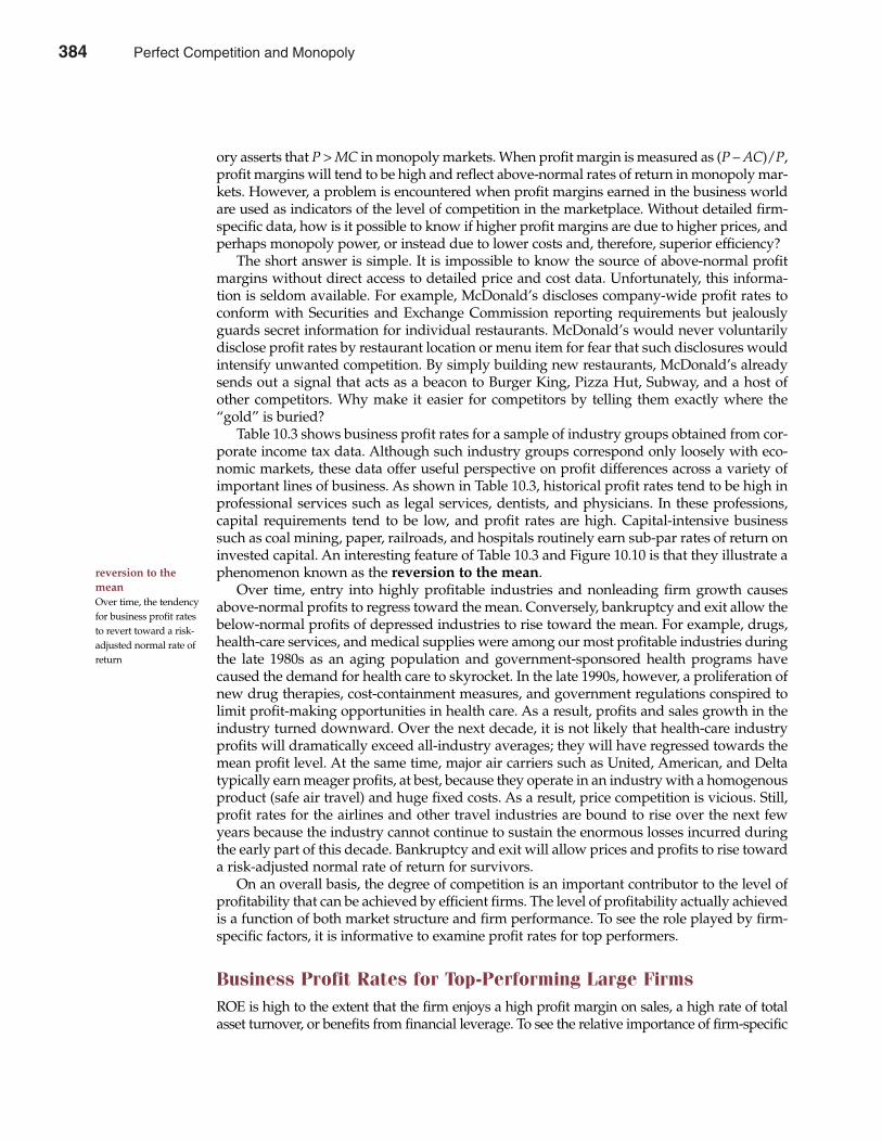
ory asserts that P > MC in monopoly markets. When profit margin is measured as (P – AC)/P,profit margins will tend to be high and reflect above-normal rates of return in monopoly mar-kets. However, a problem is encountered when profit margins earned in the business worldare used as indicators of the level of competition in the marketplace. Without detailed firm-specific data, how is it possible to know if higher profit margins are due to higher prices, andperhaps monopoly power, or instead due to lower costs and, therefore, superior efficiency?
The short answer is simple. It is impossible to know the source of above-normal profitmargins without direct access to detailed price and cost data. Unfortunately, this informa-tion is seldom available. For example, McDonald’s discloses company-wide profit rates toconform with Securities and Exchange Commission reporting requirements but jealouslyguards secret information for individual restaurants. McDonald’s would never voluntarilydisclose profit rates by restaurant location or menu item for fear that such disclosures wouldintensify unwanted competition. By simply building new restaurants, McDonald’s alreadysends out a signal that acts as a beacon to Burger King, Pizza Hut, Subway, and a host ofother competitors. Why make it easier for competitors by telling them exactly where the“gold” is buried?
Table 10.3 shows business profit rates for a sample of industry groups obtained from cor-porate income tax data. Although such industry groups correspond only loosely with eco-nomic markets, these data offer useful perspective on profit differences across a variety ofimportant lines of business. As shown in Table 10.3, historical profit rates tend to be high inprofessional services such as legal services, dentists, and physicians. In these professions,capital requirements tend to be low, and profit rates are high. Capital-intensive businesssuch as coal mining, paper, railroads, and hospitals routinely earn sub-par rates of return oninvested capital. An interesting feature of Table 10.3 and Figure 10.10 is that they illustrate aphenomenon known as the reversion to the mean.
Over time, entry into highly profitable industries and nonleading firm growth causesabove-normal profits to regress toward the mean. Conversely, bankruptcy and exit allow thebelow-normal profits of depressed industries to rise toward the mean. For example, drugs,health-care services, and medical supplies were among our most profitable industries duringthe late 1980s as an aging population and government-sponsored health programs havecaused the demand for health care to skyrocket. In the late 1990s, however, a proliferation ofnew drug therapies, cost-containment measures, and government regulations conspired tolimit profit-making opportunities in health care. As a result, profits and sales growth in theindustry turned downward. Over the next decade, it is not likely that health-care industryprofits will dramatically exceed all-industry averages; they will have regressed towards themean profit level. At the same time, major air carriers such as United, American, and Deltatypically earn meager profits, at best, because they operate in an industry with a homogenousproduct (safe air travel) and huge fixed costs. As a result, price competition is vicious. Still,profit rates for the airlines and other travel industries are bound to rise over the next fewyears because the industry cannot continue to sustain the enormous losses incurred duringthe early part of this decade. Bankruptcy and exit will allow prices and profits to rise towarda risk-adjusted normal rate of return for survivors.
On an overall basis, the degree of competition is an important contributor to the level ofprofitability that can be achieved by efficient firms. The level of profitability actually achievedis a function of both market structure and firm performance. To see the role played by firm-specific factors, it is informative to examine profit rates for top performers.
Business Profit Rates for Top-Performing Large FirmsROE is high to the extent that the firm enjoys a high profit margin on sales, a high rate of totalasset turnover, or benefits from financial leverage. To see the relative importance of firm-specific
reversion to themeanOver time, the tendencyfor business profit ratesto revert toward a risk-adjusted normal rate ofreturn
Chapter Ten Perfect Competition and Monopoly 385
384 Perfect Competition and Monopoly

386 Part Four Market Structure Analysis and Estimation
TABLE 10.3Corporate Profitability in 50 Large Industry Groups
Total Active Gross Profit Net Profit Margin Return onIndustry Group Corporations (% of sales) (% of sales) Equity (ROE)
Agricultural production 91,164 47.20% 2.50% 6.50%Alcoholic beverages 4,615 25.30% 3.10% 22.30%Auto repair and services 98,333 55.70% 1.30% 9.40%Banks 3,820 99.60% 21.90% 11.20%Bottled soft drinks and flavorings 653 47.50% 9.80% 21.20%Chemicals and allied products 9,079 22.30% 1.90% 11.90%Coal mining 1,521 31.10% 3.90% 3.80%Computers and office machines 3,782 37.80% 8.20% 26.40%Crude petroleum and natural gas 13,772 41.70% 6.30% 4.10%Drugs 2,536 56.80% 15.40% 22.80%Eating and drinking places 215,393 56.70% 2.50% 15.00%Electrical goods 30,004 18.90% 1.00% 8.20%Farm machinery 1,984 37.10% 8.80% 27.70%Footwear, except rubber 191 36.00% 4.00% 14.20%Furniture and home furnishings stores 48,678 35.30% 1.60% 9.50%Gasoline service stations 31,376 15.50% 0.70% 11.70%Grocery stores 45,534 24.40% 1.40% 18.40%Hardware stores 10,677 32.60% 0.60% 4.10%Heavy construction contractors 23,071 22.20% 3.20% 11.10%Hospitals 1,493 90.10% 1.50% 1.40%Hotels and other lodging places 30,636 58.70% 4.40% 9.80%Industrial chemicals, plastics, and synthetics 4,219 32.20% 7.40% 12.50%Knitting mills 552 25.70% 3.00% 11.00%Legal services 72,848 98.40% 4.80% 101.50%Life insurance companies 1,685 25.90% 7.00% 8.50%Liquor stores 14,407 20.00% 1.00% 11.50%Local and interurban passenger transit 18,155 80.40% 2.00% 10.80%Logging, sawmills, and planing mills 11,694 22.60% 1.10% 2.90%Metals and minerals 6,377 10.50% 1.60% 9.00%Motion picture production and distribution 20,925 53.50% 2.70% 2.60%Motion picture theaters 1,711 71.20% 2.50% 5.70%Motor vehicle dealers 42,289 11.70% 0.80% 17.50%Motor vehicles and automotive equipment 27,667 22.20% 1.30% 9.50%Newspapers 5,936 68.30% 14.90% 25.20%Nursing and personal care facilities 15,303 88.00% 1.10% 5.10%Offices of dentists 47,344 96.40% 3.60% 77.10%Offices of physicians 127,872 95.50% 1.20% 38.70%Paper and paper products 11,362 24.00% 1.40% 5.50%Petroleum and petroleum products 13,828 11.10% 1.10% 7.80%Petroleum refining 224 21.20% 6.60% 10.70%Plumbing and heating, except electric 995 34.90% 7.50% 15.40%Pulp, paper, and board mills 293 28.40% 1.90% 3.20%Radio, TV, and communication equipment 3,182 36.70% 4.60% 14.90%Railroad transportation 780 71.90% 3.10% 2.10%Security brokers and services 10,468 97.80% 21.80% 17.80%Soaps, cleaners, and toilet goods 3,056 38.10% 11.50% 33.70%Telephone and other communication services 17,302 73.50% 7.30% 9.20%Toys, sporting, and photographic goods 12,537 28.00% 2.60% 26.80%Trucking and warehousing 82,313 70.60% 2.60% 14.40%Water supply and other sanitary services 13,661 72.20% 5.60% 9.90%Averages 25,146 46.47% 4.75% 15.82%
Source: U.S. corporate federal income tax data, 2001 (http://www.bizstats.com).
Perfect Competition and Monopoly 385
factors as contributors to high rates of business profits, it is interesting to analyze the compo-nents of ROE for top-performing large firms shown in Table 10.2. Many such companies earn aROE of 20 to 35 percent per year on a regular basis. Drug companies such as Bristol-MyersSquibb and Merck display the lofty profit margins associated with the marketing of innovativepatent-protected pharmaceuticals. Other firms with special characteristics are also foundamong high-profit margin firms. For example, the William Wrigley Jr. Co. and Hershey FoodsCorp. enjoy dominant market positions in the chewing gum and candy industries, respectively.Dow Jones & Co., publishers of The Wall Street Journal and Barron’s financial weekly, producesinformation that is a must read for Wall Street professionals and thereby enjoys enviable brand-name recognition in the financial news and reporting business.
It is interesting to note that the top-performing firms displayed in Table 10.2 exemplify widevariety in terms of industry and in terms of the relative importance of profit margins, total assetturnover, and leverage as contributors to ROE. This diversity suggests that firm-specific factors,such as superior efficiency, and industry-related factors, such as market power, both contributeto the realization of above-normal rates of return.
COMPETITIVE STRATEGY IN PERFECTLY COMPETITIVE ANDMONOPOLY MARKETS
In perfectly competitive markets, the ready imitation of rivals makes ongoing success a constantstruggle. In monopoly markets, entry and growth by nonleading firms often eat away at pro-prietary advantages. In both instances, development of an effective competitive strategy is vitalto long-run success.
Chapter Ten Perfect Competition and Monopoly 387
FIGURE 10.10Profit Rates Display Mean Reversion over TimeEntry into high-profit industries drives down both prices and profits. Over time, entry causes above-normal profits to regresstoward normal profit rate, whereas exit allows the below-normal profits of depressed industries to rise toward the mean.
(%)
0
Above-normalprofits (+)
Below-normalprofits (Ð)
Profit rateover time
Bankruptcy orExit
Entry or nonleadingfirm growth
Above-normal profits range
Below-normal profits range
386 Perfect Competition and Monopoly
Competitive Strategy in Perfectly Competitive MarketsCompetitive strategy is the search for a favorable competitive position and durable above-normal profits in an industry or line of business.
In perfectly competitive industries, above-normal returns sometimes reflect economic luck,or temporary good fortune due to unexpected changes in industry demand or cost conditions.For example, during 2001 many small to mid-size oil refineries and gasoline retailers benefitedgreatly when oil prices unexpectedly shot up following temporary oil shortages. At the sametime, many other firms experienced economic losses following the unanticipated rise in energycosts. Both sets of companies experienced a reversal of fortune when energy prices plummeted.Grain farmers also benefit mightily when export demand for agricultural products skyrocketsand suffer when export demand withers.
In other instances, above-normal returns in perfectly competitive industries reflect what isknown as economic rents, or profits due to uniquely productive inputs. An exceptionally well-trained workforce, talented management, or superior land and raw materials can all lead toabove-normal profits. In parts of the country where school systems provide outstanding primaryand secondary education, firms are able to hire a basic workforce with a high rate of literacy andstrong basic skills. Businesses that are able to employ such workers at a typical wage are able toearn superior profits when compared with the average rate of return for all competitors in theUnited States and Canada. Local tax subsidies designed to attract investment and job opportu-nities can also lower the cost of capital and create economic rents for affected firms. In many partsof the country, government initiatives often lead to economic rents for affected firms. On theother hand, if local taxes or government regulations prove to be especially onerous, economiclosses can result for affected companies.
Another important source of above-normal profits in perfectly competitive industries isdisequilibrium profits. Disequilibrium profits are above-normal returns that can be earnedin the time interval that often exists between when a favorable influence on industrydemand or cost conditions first transpires and the time when competitor entry or growthfinally develops.
Disequilibrium losses are below-normal returns suffered in the time interval that can arisebetween when an unfavorable influence on industry demand or cost conditions first transpiresand the time when exit or downsizing finally occurs. When barriers to entry and exit are mini-mal, competitor reactions tend to be quick and disequilibrium profits are fleeting. When barriersto entry and exit are significant, competitor reactions tend to be slow and disequilibrium profitscan persist for extended periods. In the quintessential perfectly competitive industry, disequilib-rium profits are quickly dissipated. In real-world markets, disequilibrium profits can persist overan entire business cycle even in the most competitive industries. In retailing, for example, laborand inventory costs have been cut dramatically following the introduction of computerized pricescanners. Despite the vigorously price-competitive nature of the retailing business, early inno-vators who first adopted the bar code technology have been able to earn above-normal profitsfor a number of years. Innovative grocery retailers have enjoyed dramatically lower costs andprofit margins on sales of 2 percent to 3.5 percent, versus a more typical 1 percent, over a decadeand more.
In equilibrium, perfectly competitive markets only offer the potential for a normal rate ofreturn on investment. If many capable competitors offer identical products, vigorous pricecompetition tends to eliminate disequilibrium profits. The only exception to this rule is thatsuperior efficiency can sometimes lead to superior profits, even in perfectly competitivemarkets. Above-normal profits in perfectly competitive industries are usually transitory andreflect the influences of economic rents, luck, or disequilibrium conditions. If above-normalreturns persist for extended periods in a given industry or line of business, then elements ofuniqueness are probably at work.
388 Part Four Market Structure Analysis and Estimation
competitive strategyThe search for a favor-able competitive posi-tion in an industry orline of business
economic luckTemporary good fortune due to unex-pected changes inindustry demand orcost conditions
economic rentsProfits due to uniquelyproductive inputs
disequilibriumprofitsAbove-normal returnsthat can be earned inthe time intervalbetween when a favorable influence onindustry demand orcost conditions firsttranspires and the timewhen competitor entryor growth finallydevelops
disequilibriumlossesBelow-normal returnsthat can be suffered inthe time interval thatoften exists betweenwhen an unfavorableinfluence on industrydemand or cost condi-tions first transpiresand the time when exitor downsizing finallyoccurs
Perfect Competition and Monopoly 387

Competitive Strategy in Monopoly MarketsAbove-normal returns tend to be fleeting in perfectly competitive industries but can bedurable for efficient firms that benefit from meaningful monopoly advantages. As in anyperfectly competitive industry, above-normal profit rates can be observed if monopoly firmstemporarily benefit from some unanticipated increase in demand or decrease in costs. Similarly,monopolists can benefit from temporary affluence due to unexpected changes in industrydemand or cost conditions or uniquely productive inputs. What is unique about monopoly isthe potential for long-lasting above-normal rates of return.
In this age of instant global communication and rapid technical advance, no monopoly ispermanently secure from the threat of current or potential competitors. Product characteristics,the local or regional limits of the market, the time necessary for reactions by established or newcompetitors, the pace of innovation, unanticipated changes in government regulation and taxpolicy, and a host of additional considerations all play an important role in defining the scopeand durability of monopoly power. When attempting to describe monopoly advantages, it isalways helpful to consider the number and size of potential competitors, degree of product dif-ferentiation, level of information available in the marketplace, and conditions of entry.
Table 10.4 summarizes major characteristics typical of perfectly competitive and monopo-listic markets. To develop an effective competitive strategy, it is necessary to assess the degreeto which the characteristics of an individual market embody elements of each. Although theprobability of successful entry is greater in perfectly competitive markets, monopoly marketslure new and established competitors with the promise of long-lasting, above-normal returns.Because the decision to enter any new market or line of business involves a careful balancing
Chapter Ten Perfect Competition and Monopoly 389
TABLE 10.4Summary of Perfect Competition and Monopoly (Monopsony) Market-Structure Characteristics
Perfect Competition Monopoly (Monopsony)
Number of actual or Many small buyers and sellers A single seller (buyer) of a potential competitors valued product
Product differentiation None—each buyer and seller Very high—no close substitutes deals in an identical product available
Information Complete and free information Highly restricted access to priceon price and product quality and product-quality information
Conditions of entry Complete freedom of entry Very high barriers caused by and exit and exit economies of scale (natural
monopoly), patents, copyrights, government franchises, or other factors
Profit potential Normal profit in long run; Potential for economic profits economic profits (losses) in in both short and long runshort run only
Examples Some agricultural markets Monopoly (sellers): Local telephone (grain); commodity, stock, and service (basic hook-up); municipal bond markets; some bus companies; gas, water, and nonspecialized input markets electric utilities. Monopsony (buyers): (unskilled labor) state and local governments (roads):
U.S. government (defense electronics)
388 Perfect Competition and Monopoly

of expected costs and expected benefits, the monopoly advantages can act as a powerful induce-ment to competitors. Preservation of monopoly advantages is only likely when firms maintainthe distinctive and valuable characteristics sought by customers. Similarly, the search for above-normal profits is only likely to be successful when firms create products that are faster, cheaper,or better than those offered by rivals.
Why Market Niches Are AttractiveEntry into a perfectly competitive industry is not apt to result in long-lasting, above-normalrates of return under even the best of circumstances. For example, a grain producer locatedalong a river or on exceptionally fertile soil would enjoy lower-than-average irrigation costsand fertilizer expenses, and higher profits could result. However, potential buyers would haveto pay a price premium for such productive land, and subsequent investors would earn onlya normal rate of return on their investment. No landowner is going to sell highly productiveor well-situated land at a bargain-basement price. Similarly, purchase of a business that enjoysrecognized monopoly power seldom leads to economic profits because anticipated abnormalreturns on plant and equipment are reflected in purchase prices. Much like fertile land bringsa price premium in the real estate market, monopoly franchises bring a premium price in thestock market. As a result, the purchase of a recognized monopoly leads to only a risk-adjustednormal rate of return for subsequent investors. Monopolists make money; investors in fullyappreciated monopoly do not.
Only new and unique products or services have the potential to create monopoly profits.Imitation of such products may be protected by patents, copyrights, or other means. In manyinstances, these above-normal profits reflect the successful exploitation of a market niche. Amarket niche is a segment of a market that can be successfully exploited through the specialcapabilities of a given firm or individual. To be durable, above-normal profits derived from amarket niche must not be vulnerable to imitation by competitors.
For example, Avon Products, Inc., is rightly famous for its entrepreneurial army of inde-pendent sales representatives. “Avon Calling!” is a greeting that has long generated huge cashreturns for the company in the United States and abroad. In Japan, for example, Avon’s profitrate and popularity is even greater than that enjoyed in the United States. Avon has succeededwhere others have failed because it has developed and nurtured the direct selling market forcosmetics. Better than anyone else, Avon knows cosmetics, toiletries, costume jewelry, and otherproducts that many women want and knows how much they are willing to pay for them. Avonkeeps on growing despite numerous assaults from would-be competitors and regular predic-tions that its primary market is a sure-fire casualty of dual-income households. Indeed, itsdomestic and foreign business is so profitable that Avon has been the subject of repeatedtakeover speculation. To thwart such advances, the company has initiated a dramatic programto streamline operations in an effort to enhance already high profits. In the meantime, Avonkeeps on dominating its market niche.
Another interesting example of a firm that successfully exploits a profitable market nicheis provided by Stilwell Financial, Inc., a diversified financial services firm best known for itsJanus Group of mutual funds. Janus has a dominant and extraordinarily profitable marketniche in the worldwide mutual fund business. Founder Tom Bailey was an early advocate ofgrowth stock investing in the technology sector. Not only has the idea proved popular to U.S.investors, but Japanese and European investors have jumped on the Janus bandwagon as well.As a result, Stilwell enjoys double-digit growth, net profit margins that average in excess of 25percent of sales, and a rate of return on assets of roughly 40 percent per year.
Avon Products and Stilwell Financial are only two examples of the many firms that enjoytremendous success through market niche dominance. To attain similar success, a firm mustfirst recognize the attractiveness of the market niche and then successfully apply the conceptto its own business. Few firms achieve any great measure of success in trying to be all things
390 Part Four Market Structure Analysis and Estimation
market nicheA segment of a marketthat can be successfullyexploited through thespecial capabilities of agiven firm or individual
Perfect Competition and Monopoly 389
to all customers. Lasting success requires exploitation of those segments of the market thatcan be best served using the special capabilities of a given firm or individual.
Information Barriers to Competitive StrategyAny use of market structure information as a guide to competitive strategy must address thechallenge posed by measurement problems encountered in defining the magnitude and rootcause of above-normal rates of return. To be sure, accounting profit data derived from a his-torical perspective give much useful information for operating decisions and tax purposes.However, these data sometimes measure economic profits only imperfectly. For example,advertising and research and development (R&D) expenditures are expensed for both report-ing and tax purposes, even though each can give rise to long-term economic benefits. Anexpense-as-incurred treatment of advertising and R&D expenditures can lead to errors inprofit measurement. Although current net income is depressed when advertising and R&Dare written off before the end of their useful lives, intangible assets can be understated whenthey fail to reflect the value of brand names and other innovative products. Depending onthe true rate of economic amortization for advertising and R&D and the rate of growth inexpenditures for each, business profit rates can be either understated or overstated. In eitherevent, reported business profit rates, such as ROE, can substantially misstate economic profits.At the same time, other imperfections in accrual accounting methods lead to imperfectlymatched revenues and costs and, therefore, to some misstatement of economic profitsover time.
Beyond these and other obvious limitations of accounting data, business practices are oftenexpressly intended to limit the loss of valuable trade secret information. Why would anyone givecompetitors any more than the bare minimum of information? It is well-known, for example,that firms patent only what they cannot otherwise keep secret. Combined with the limitations ofpublicly available data on profitability, business practices create an information barrier that hidesthe true details about economic profit rates. At the same time, such obfuscation makes definingthe scope of monopoly power difficult, as it hides the costs and benefits of entry into monopolymarkets from both private and public decision makers.
SUMMARY
Market structure analysis begins with the study of perfect competition and monopoly.Competition is said to be perfect when producers offer what buyers want at prices just sufficientto cover the marginal cost of output. Monopoly is socially less desirable given its tendency forunderproduction, high prices, and excess profits.
• Market structure describes the competitive environment in the market for any good or serv-ice. A market consists of all firms and individuals willing and able to buy or sell a particu-lar product. This includes firms and individuals currently engaged in buying and selling aparticular product, as well as potential entrants. A potential entrant is an individual or firmposing a sufficiently credible threat of market entry to affect the price/output decisions ofincumbent firms.
• Perfect competition is a market structure characterized by a large number of buyers andsellers of essentially the same product, where each market participant’s transactions are sosmall that they have no influence on the market price of the product. Individual buyers andsellers are price takers. Such firms take market prices as given and devise their productionstrategies accordingly.
• Monopoly is a market structure characterized by a single seller of a highly differentiated prod-uct. Monopoly firms are price makers that exercise significant control over market prices.
Chapter Ten Perfect Competition and Monopoly 391
390 Perfect Competition and Monopoly
• A barrier to entry is any factor or industry characteristic that creates an advantage forincumbents over new arrivals. A barrier to mobility is any factor or industry characteristicthat creates an advantage for large leading firms over smaller nonleading rivals. A barrierto exit is any restriction on the ability of incumbents to redeploy assets from one industryor line of business to another.
• Monopsony exists when a single firm is the sole buyer of a desired product or input.• A natural monopoly occurs when the market-clearing price, where P = MC, occurs at a
point at which long-run average costs are still declining.• Underproduction results when a monopoly curtails output to a level at which the value
of resources employed, as measured by the marginal cost of production, is less than thesocial benefit derived, where social benefit is measured by the price customers are willingto pay for additional output.
• Countervailing power is an economic influence that creates a closer balance betweenpreviously unequal sellers and buyers.
• Business profit rates are best measured by the accounting rate of return on stockholders’equity measure. ROE is defined as net income divided by the book value of stockholders’equity, where stockholders’ equity is the book value of total assets minus total liabilities.High ROE is derived from some combination of high profit margins, quick total assetturnover, and high leverage or a high rate of total assets to stockholders’ equity. Businessprofits are also sometimes measured by the return on assets, defined as net income dividedby the book value of total assets. Although ROA is a useful alternative indicator of the basicprofitability of a business, it fails to account for the effects of financial leverage decisions onfirm performance.
• Business profit rates often display a phenomenon known as reversion to the mean. Overtime, entry into highly profitable industries tends to cause above-normal profits to regresstoward the mean, just as bankruptcy and exit allow the below-normal profits of depressedindustries to rise toward the mean.
• The nature of competition determines the suitability of managerial decisions and the speedwith which they must be made. Survival of the fittest translates into success for the mostable, and extinction of the least capable. Competitive strategy is the search for a favorablecompetitive position in an industry or line of business.
• In perfectly competitive industries, above-normal returns sometimes reflect economicluck, or temporary good fortune due to unexpected changes in industry demand or costconditions. In other instances, above-normal returns in perfectly competitive industriesreflect economic rents, or profits due to uniquely productive inputs. Another importantsource of above-normal profits in perfectly competitive industries is disequilibriumprofits. Disequilibrium profits are above-normal returns that can be earned in the timeinterval between when a favorable influence on industry demand or cost conditions firsttranspires and the time when competitor reactions finally develop. Disequilibrium lossesare below-normal returns that can be suffered in the time interval that often exists betweenwhen an unfavorable influence on industry demand or cost conditions first transpires andthe time when exit or downsizing finally occurs.
• Only new and unique products or services have the potential to create monopoly profits. Inmany instances, these above-normal profits reflect the successful exploitation of a marketniche. A market niche is a segment of a market that can be successfully exploited throughthe special capabilities of a given firm or individual.
Many real-world markets do in fact closely approximate the perfectly competitive ideal, butelements of monopoly are often encountered. As a result, these market structure conceptsoften provide a valuable guide to managerial decision making.
392 Part Four Market Structure Analysis and Estimation
Perfect Competition and Monopoly 391
QUESTIONS
Q10.1 What are the primary elements of market structure?Q10.2 Describe the perfectly competitive market structure and provide some examples.Q10.3 Describe the monopoly market structure and provide some examples.Q10.4 How are barriers to entry and exit similar? How are they different?Q10.5 Why is the firm demand curve horizontal in perfectly competitive markets? Does this mean
that the perfectly competitive industry demand curve is also horizontal?Q10.6 Why are the perfectly competitive firm and the perfectly competitive industry supply curves
upward sloping?Q10.7 From a social standpoint, what is the problem with monopoly?Q10.8 Why are both industry and firm demand curves downward sloping in monopoly market
structure?Q10.9 Give an example of monopoly in the labor market. Discuss such a monopoly’s effect on wage
rates and on inflation.Q10.10 Describe the economic effects of countervailing power, and cite examples of markets in
which countervailing power is observed.
SELF-TEST PROBLEMS AND SOLUTIONS
ST10.1 Market Value and Profitability. The paper and forest products industry is dominated bylarge integrated manufacturers. According to data from the Census of Manufacturers,roughly 50% of industry output comes from giant plants with more than 500 employees.This is despite the fact that specialized minimills with as few as 20 to 49 employees haverecently emerged in the industry to take advantage of market niches. On an overall basis,this major industry group is one of the largest and most important in our economy in termsof sales, profits, and employment. Low prices combined with innovative new products, suchas recycled newspaper products, have swept the industry and given innovative competitorsthe means to earn above-average rates of return. In this highly competitive environment, theway to survive and prosper is to reduce operating expenses, increase product quality, andimprove customer service. As much as any other single industry, paper and forest productscompanies have taken advantage of advances in computer-based methods of data collectionand analysis to improve their relation with suppliers, keep inventories lean, and boost salesby better serving customer demands.
To assess the effect of firm size on the business success of these companies, the tableshows the rate of return on stockholders’ equity (%), firm size as measured by the bookvalue of stockholders’ equity (in $ millions), rate of growth in book value (%), and leverageas captured by the ratio of long-term debt to total capital (%) for an n = 17 sample of paperand forest product companies. The profitability effects of firm size indicate how economiesof scale translate into higher profits, or how diseconomies of large-scale production trans-late into lower profits. Growth can have positive effects on profit rates because rapid growthtypically reflects companies with attractive product lines and/or cost-efficient operations.Finally, leverage has the potential to contribute to higher profits during periods of robusteconomic conditions, but can penalize profit rates during recessions or periods of tepiddemand.
Chapter Ten Perfect Competition and Monopoly 393
392 Perfect Competition and Monopoly
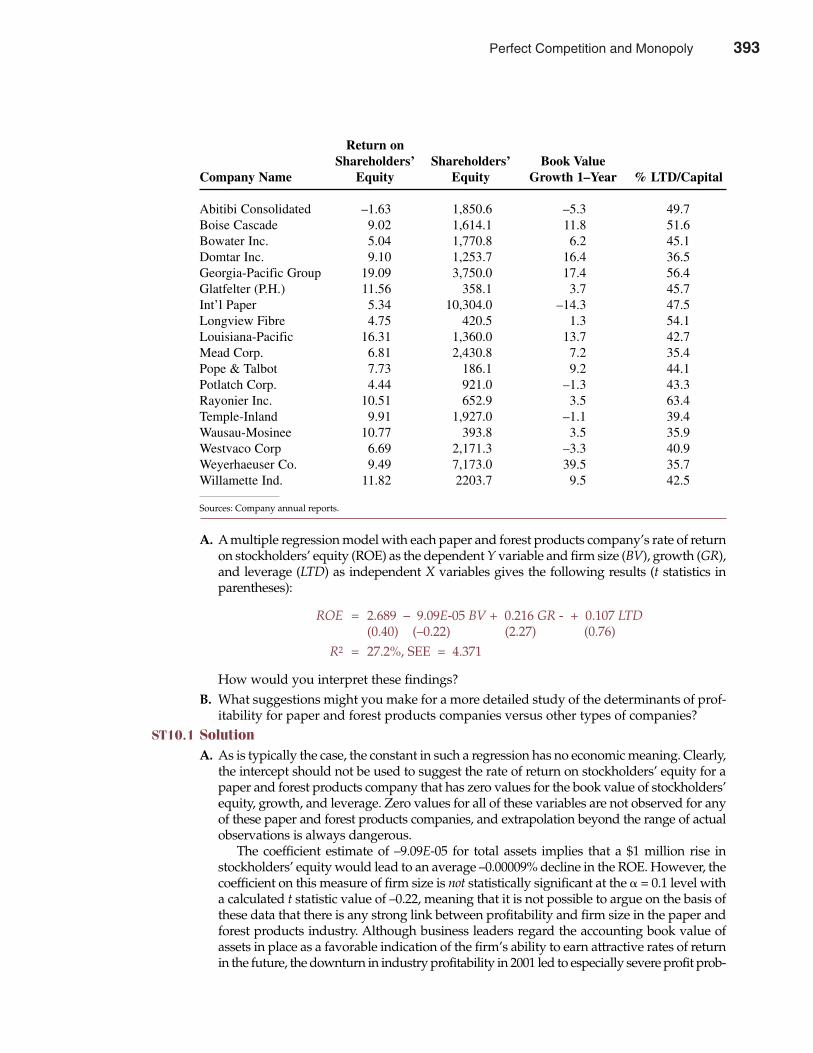
A. A multiple regression model with each paper and forest products company’s rate of returnon stockholders’ equity (ROE) as the dependent Y variable and firm size (BV), growth (GR),and leverage (LTD) as independent X variables gives the following results (t statistics inparentheses):
ROE = 2.689 – 9.09E-05 BV + 0.216 GR - + 0.107 LTD(0.40) (–0.22) (2.27) (0.76)
R2 = 27.2%, SEE = 4.371
How would you interpret these findings?B. What suggestions might you make for a more detailed study of the determinants of prof-
itability for paper and forest products companies versus other types of companies?ST10.1 Solution
A. As is typically the case, the constant in such a regression has no economic meaning. Clearly,the intercept should not be used to suggest the rate of return on stockholders’ equity for apaper and forest products company that has zero values for the book value of stockholders’equity, growth, and leverage. Zero values for all of these variables are not observed for anyof these paper and forest products companies, and extrapolation beyond the range of actualobservations is always dangerous.
The coefficient estimate of –9.09E-05 for total assets implies that a $1 million rise instockholders’ equity would lead to an average –0.00009% decline in the ROE. However, thecoefficient on this measure of firm size is not statistically significant at the � = 0.1 level witha calculated t statistic value of –0.22, meaning that it is not possible to argue on the basis ofthese data that there is any strong link between profitability and firm size in the paper andforest products industry. Although business leaders regard the accounting book value ofassets in place as a favorable indication of the firm’s ability to earn attractive rates of returnin the future, the downturn in industry profitability in 2001 led to especially severe profit prob-
394 Part Four Market Structure Analysis and Estimation
Return onShareholders’ Shareholders’ Book Value
Company Name Equity Equity Growth 1–Year % LTD/Capital
Abitibi Consolidated –1.63 1,850.6 –5.3 49.7Boise Cascade 9.02 1,614.1 11.8 51.6Bowater Inc. 5.04 1,770.8 6.2 45.1Domtar Inc. 9.10 1,253.7 16.4 36.5Georgia-Pacific Group 19.09 3,750.0 17.4 56.4Glatfelter (P.H.) 11.56 358.1 3.7 45.7Int’l Paper 5.34 10,304.0 –14.3 47.5Longview Fibre 4.75 420.5 1.3 54.1Louisiana-Pacific 16.31 1,360.0 13.7 42.7Mead Corp. 6.81 2,430.8 7.2 35.4Pope & Talbot 7.73 186.1 9.2 44.1Potlatch Corp. 4.44 921.0 –1.3 43.3Rayonier Inc. 10.51 652.9 3.5 63.4Temple-Inland 9.91 1,927.0 –1.1 39.4Wausau-Mosinee 10.77 393.8 3.5 35.9Westvaco Corp 6.69 2,171.3 –3.3 40.9Weyerhaeuser Co. 9.49 7,173.0 39.5 35.7Willamette Ind. 11.82 2203.7 9.5 42.5
Sources: Company annual reports.
Perfect Competition and Monopoly 393
lems for industry leaders. Controversies tied to environmental concerns, like the spotted-owlcrisis, make matters even worse for large companies that are convenient targets of consumeractivists and regulators.
The coefficient estimate of 0.216 for growth implies that a 1% rise in growth leads to anaverage 0.216% increase in ROE. The growth coefficient is statistically significant at the � =0.05 level with a calculated t statistic value of 2.27, meaning that it is possible to be more than95% confident that growth has a statistically significant affect on ROE. The probability ofobserving such a large t statistic when there is in fact no relation between ROE and growthis less than 5%.
The coefficient estimate of 0.107 for LTD implies that a 1% rise in leverage leads to anaverage 0.107% increase in ROE. However, this effect is not significant at even the � = 0.1level, meaning theat there is no strong link between ROE and leverage in the sample ana-lyzed. Given rather tepid economic growth, high financial leverage had no beneficialeffect of boosting profitability during the 2001 sample period.
The R2 = 27.2% is quite modest and indicates the share of variation in ROE that can beexplained by the model as a whole. This relatively low level of explained variation must beinterpreted in light of the very small sample size involved. The standard error of the Yestimate of SEE = 4.371% is the average amount of error encountered in estimating ROEusing this multiple regression model. If the ui error terms are normally distributed aboutthe regression equation, as would be true when large samples of more than 30 or so obser-vations are analyzed, there is a 95% probability that observations of the dependent variablewill lie within the rangeŶi ± (1.96 � SEE), or within roughly two standard errors of the esti-mate. The probability is 99% that any givenŶi will lie within the rangeŶi ± (2.576 � SEE), orwithin roughly three standard errors of its predicted value. When very small samples ofdata are analyzed, as is the case here, “critical” t values slightly larger than two or three aremultiplied by the SEE to obtain the 95% and 99% confidence intervals.
Precise critical t values obtained from a t table, such as that found in Appendix C, aret*14,�=0.05 = 2.145 (at the 95% confidence level) and t*14,�=0.01 = 2.977 (at the 99% confidencelevel) for df = 18 – 4 = 14. This means that actual ROE can be expected to fall in the rangeŶi ± (2.145 � 4.371), or Ŷi ± 9.376, with 95% confidence; and within the range Ŷi ± (2.977�4.371), or Ŷi ± 13.012, with 99% confidence.
B. Collection of a broader and more descriptive sample of data is a necessary first step in a moredetailed study of the determinants of the return on stockholders’ equity for paper and forestproducts companies. With only 18 observations of annual data, the regression technique isclearly handicapped in this application. Perhaps a pooled cross-section sample of annual dataover the past 5 years, or n = 90 (= 18 � 5) observations, would provide a sufficiently broadsample of data to offer a meaningful perspective on the determinants of profitability for for-est and paper products companies. In addition, a larger sample of data would make it possibleto investigate the potential role of additional independent variables, such as the level ofadvertising spending, the role of regional economic growth, and so on.
ST10.2 Perfect Competition and Monopoly. The City of Columbus, Ohio, is considering two pro-posals to privatize municipal garbage collection. First, a leading waste disposal firm has offeredto purchase the city’s plant and equipment at an attractive price in return for an exclusive fran-chise on residential service. Asecond proposal would allow several individual workers and smallcompanies to enter the business without any exclusive franchise agreement or competitiverestrictions. Under this plan, individual companies would bid for the right to provide service ina given residential area. The city would then allocate business to the lowest bidder.
The city has conducted a survey of Columbus residents to estimate the amount that theywould be willing to pay for various frequencies of service. The city has also estimated the totalcost of service per resident. Service costs are expected to be the same whether or not an exclusivefranchise is granted.
Chapter Ten Perfect Competition and Monopoly 395
394 Perfect Competition and Monopoly
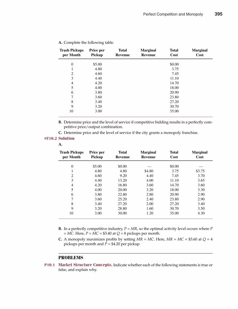
A. Complete the following table.
B. Determine price and the level of service if competitive bidding results in a perfectly com-petitive price/output combination.
C. Determine price and the level of service if the city grants a monopoly franchise.ST10.2 Solution
A.
B. In a perfectly competitive industry, P = MR, so the optimal activity level occurs where P= MC. Here, P = MC = $3.40 at Q = 8 pickups per month.
C. A monopoly maximizes profits by setting MR = MC. Here, MR = MC = $3.60 at Q = 4pickups per month and P = $4.20 per pickup.
PROBLEMS
P10.1 Market Structure Concepts. Indicate whether each of the following statements is true orfalse, and explain why.
396 Part Four Market Structure Analysis and Estimation
Trash Pickups Price per Total Marginal Total Marginalper Month Pickup Revenue Revenue Cost Cost
0 $5.00 $0.001 4.80 3.752 4.60 7.453 4.40 11.104 4.20 14.705 4.00 18.006 3.80 20.907 3.60 23.808 3.40 27.209 3.20 30.70
10 3.00 35.00
Trash Pickups Price per Total Marginal Total Marginalper Month Pickup Revenue Revenue Cost Cost
0 $5.00 $0.00 — $0.00 —1 4.80 4.80 $4.80 3.75 $3.752 4.60 9.20 4.40 7.45 3.703 4.40 13.20 4.00 11.10 3.654 4.20 16.80 3.60 14.70 3.605 4.00 20.00 3.20 18.00 3.306 3.80 22.80 2.80 20.90 2.907 3.60 25.20 2.40 23.80 2.908 3.40 27.20 2.00 27.20 3.409 3.20 28.80 1.60 30.70 3.50
10 3.00 30.00 1.20 35.00 4.30
Perfect Competition and Monopoly 395
A. In long-run equilibrium, every firm in a perfectly competitive industry earns zero profit.Thus, if price falls, none of these firms will be able to survive.
B. Perfect competition exists in a market when all firms are price takers as opposed to pricemakers.
C. A natural monopoly results when the profit-maximizing output level occurs at a point wherelong-run average costs are declining.
D. Downward-sloping industry demand curves characterize both perfectly competitive andmonopoly markets.
E. A decrease in the price elasticity of demand would follow an increase in monopoly power.P10.2 Perfectly Competitive Firm Supply. Mankato Paper, Inc., produces uncoated paper used
in a wide variety of industrial applications. Newsprint, a major product, is sold in a perfectlycompetitive market. The following relation exists between the firm’s newsprint output andtotal production costs:
A. Construct a table showing Mankato’s marginal cost of newsprint production.B. What is the minimum price necessary for Mankato to supply one ton of newsprint?C. How much newsprint would Mankato supply at industry prices of $75 and $100 per ton?
P10.3 Perfectly Competitive Equilibrium. Demand and supply conditions in the perfectly com-petitive market for unskilled labor are as follows:
QD = 150 – 16P (Demand)QS = 8P (Supply)
where Q is millions of hours of unskilled labor and P is the wage rate per hour.A. Graph the industry demand and supply curves.B. Determine the industry equilibrium price/output combination both graphically and alge-
braically.C. Calculate the level of excess supply (unemployment) if the minimum wage is set at $7
per hour.P10.4 Perfectly Competitive Industry Supply. Farm Fresh, Inc., supplies sweet peas to canners
located throughout the Mississippi River Valley. Like some grain and commodity markets, themarket for sweet peas is perfectly competitive. The company’s total and marginal costs per tonare given by the following relations:
Chapter Ten Perfect Competition and Monopoly 397
Total Output (tons) Total Cost (per ton)
0 $251 752 1353 2054 2855 3756 4757 600
396 Perfect Competition and Monopoly
TC = $250,000 + $200Q + $0.02Q2
MC = ∆TC/∆Q = $200 + $0.04Q
A. Calculate the industry price necessary for the firm to supply 5,000, 10,000, and 15,000 tonsof sweet peas.
B. Calculate the quantity supplied by Farm Fresh at industry prices of $200, $500, and $1,000per ton.
P10.5 Perfectly Competitive Firm and Industry Supply. New England Textiles, Inc., is a medium-sized manufacturer of blue denim that sells in a market for which it is perfectly competitive. Thetotal cost function for this product is described by the following relation:
TC = $25,000 + $1Q + $0.000008Q2
MC = ∆TC/∆Q = $1 + $0.000016Q
where Q is square yards of blue denim produced per month.A. Derive the firm’s supply curve, expressing quantity as a function of price.B. Derive the industry’s supply curve if New England Textiles is one of 500 competitors.C. Calculate industry supply per month at a market price of $2 per square yard.
P10.6 Perfectly Competitive Equilibrium. Bada Bing, Ltd., supplies standard 128 MB-RAMchips to the U.S. computer and electronics industry. Like the output of its competitors, BadaBing’s chips must meet strict size, shape, and speed specifications. As a result, the chip-supplyindustry can be regarded as perfectly competitive. The total cost and marginal cost functionsfor Bada Bing are
TC = $1,000,000 + $20Q + $0.0001Q2
MC = ∆TC/∆Q = $20 + $0.0002Q
where Q is the number of chips produced.A. Calculate Bada Bing’s optimal output and profits if chip prices are stable at $60 each.B. Calculate Bada Bing’s optimal output and profits if chip prices fall to $30 each.C. If Bada Bing is typical of firms in the industry, calculate the firm’s equilibrium output,
price, and profit levels.P10.7 Monopoly Equilibrium. Parvati Fluid Controls, Inc., (PFC) is a major supplier of reverse
osmosis and ultrafiltration equipment, which helps industrial and commercial customersachieve improved production processes and a cleaner work environment. The company hasrecently introduced a new line of ceramic filters that enjoy patent protection. Relevant costand revenue relations for this product are as follows:
TR = $300Q – $0.001Q2
MR = ∆TR/∆Q = $300 – $0.002Q
TC = $9,000,000 + $20Q + $0.0004Q2
MC = ∆TC/∆Q = $20 + $0.0008Q
where TR is total revenue, Q is output, MR is marginal revenue, TC is total cost, including a risk-adjusted normal rate of return on investment, and MC is marginal cost.A. As a monopoly, calculate PFC’s optimal price/output combination.
398 Part Four Market Structure Analysis and Estimation
Perfect Competition and Monopoly 397
B. Calculate monopoly profits and the optimal profit margin at this profit-maximizingactivity level.
P10.8 Monopoly Versus Perfectly Competitive Equilibrium. Big Apple Music, Inc., enjoys anexclusive copyright on music written and produced by the Fab Four, a legendary British rockgroup. Total and marginal revenues for the group’s CDs are given by the following relations:
TR = $15Q – $0.000005Q2
MR = ∆TR/∆Q = $15 – $0.00001Q
Marginal costs for production and distribution are stable at $5 per unit. All other costs havebeen fully amortized.A. Calculate Big Apple’s output, price, and profits at the profit-maximizing activity level.B. What record price and profit levels would prevail following expiration of copyright pro-
tection based on the assumption that perfectly competitive pricing would result?P10.9 Monopoly Versus Perfectly Competitive Equilibrium. During recent years, Moon Macro
Systems, Inc., has enjoyed substantial economic profits derived from patents covering a widerange of inventions and innovations for high-performance workstations used in a variety ofscientific applications. A recent introduction, the Ultra80, has proved especially profitable.Market demand and marginal revenue relations for the Ultra80 are as follows:
P = $5,500 – $0.005Q
MR = ∆TR/∆Q = $5,500 – $0.01Q
Fixed costs are nil because research and development expenses have been fully amortizedduring previous periods. Average variable costs are constant at $4,500 per unit.A. Calculate the profit-maximizing price/output combination and economic profits if Moon
enjoys an effective monopoly on the Ultra80 because of its patent protection.B. Calculate the price/output combination and total economic profits that would result if com-
petitors offer clones that make the Ultra80 market perfectly competitive.P10.10 Monopoly/Monopsony Confrontation. Safecard Corporation offers a unique service. The
company notifies credit card issuers after being informed that a subscriber’s credit card hasbeen lost or stolen. The Safecard service is sold to card issuers on a 1-year subscription basis.Relevant revenue and cost relations for the service are as follows:
TR = $5Q – $0.00001Q2
MR = ∆TR/∆Q = $5 – $0.00002Q
TC = $50,000 + $0.5Q + $0.000005Q2
MC = ∆TC/∆Q = $0.5 + $0.00001Q
where TR is total revenue, Q is output measured in terms of the number of subscriptions inforce, MR is marginal revenue, TC is total cost, including a risk-adjusted normal rate of returnon investment, and MC is marginal cost.A. If Safecard has a monopoly in this market, calculate the profit-maximizing price/output
combination and optimal total profit.B. Calculate Safecard’s optimal price, output, and profits if credit card issuers effectively exert
monopsony power and force a perfectly competitive equilibrium in this market.
Chapter Ten Perfect Competition and Monopoly 399
398 Perfect Competition and Monopoly
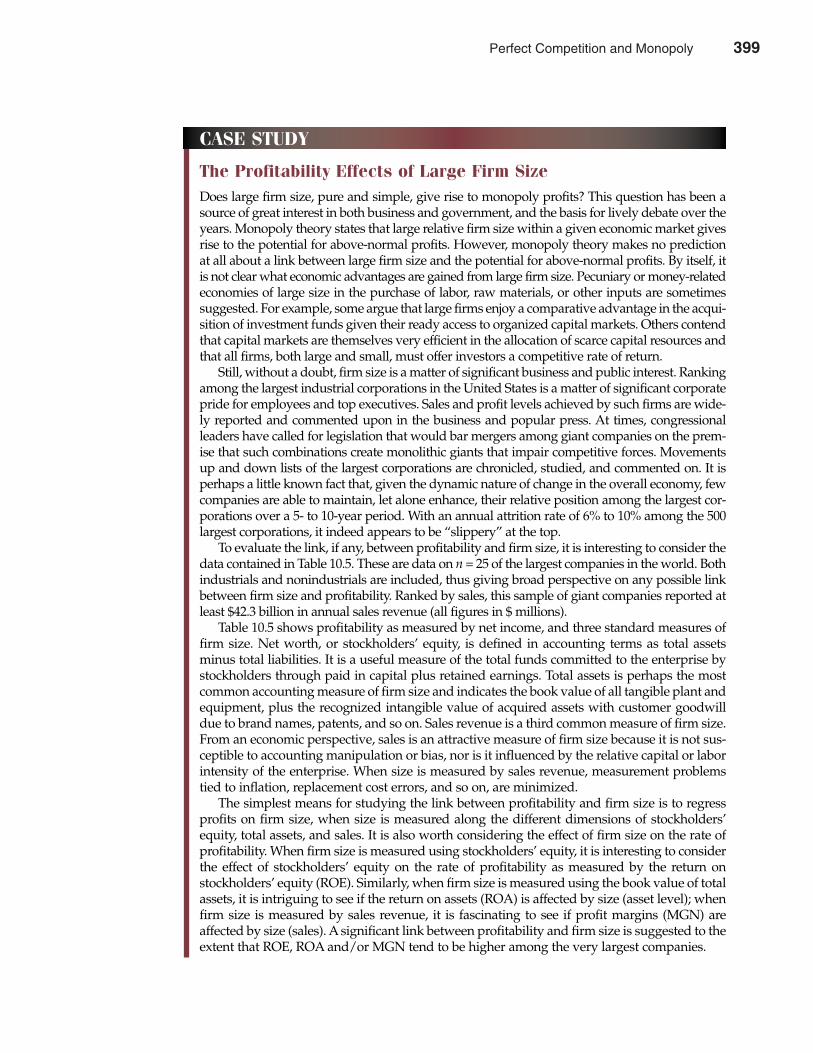
400 Part Four Market Structure Analysis and Estimation
CASE STUDY
The Profitability Effects of Large Firm SizeDoes large firm size, pure and simple, give rise to monopoly profits? This question has been asource of great interest in both business and government, and the basis for lively debate over theyears. Monopoly theory states that large relative firm size within a given economic market givesrise to the potential for above-normal profits. However, monopoly theory makes no predictionat all about a link between large firm size and the potential for above-normal profits. By itself, itis not clear what economic advantages are gained from large firm size. Pecuniary or money-relatedeconomies of large size in the purchase of labor, raw materials, or other inputs are sometimessuggested. For example, some argue that large firms enjoy a comparative advantage in the acqui-sition of investment funds given their ready access to organized capital markets. Others contendthat capital markets are themselves very efficient in the allocation of scarce capital resources andthat all firms, both large and small, must offer investors a competitive rate of return.
Still, without a doubt, firm size is a matter of significant business and public interest. Rankingamong the largest industrial corporations in the United States is a matter of significant corporatepride for employees and top executives. Sales and profit levels achieved by such firms are wide-ly reported and commented upon in the business and popular press. At times, congressionalleaders have called for legislation that would bar mergers among giant companies on the prem-ise that such combinations create monolithic giants that impair competitive forces. Movementsup and down lists of the largest corporations are chronicled, studied, and commented on. It isperhaps a little known fact that, given the dynamic nature of change in the overall economy, fewcompanies are able to maintain, let alone enhance, their relative position among the largest cor-porations over a 5- to 10-year period. With an annual attrition rate of 6% to 10% among the 500largest corporations, it indeed appears to be “slippery” at the top.
To evaluate the link, if any, between profitability and firm size, it is interesting to consider thedata contained in Table 10.5. These are data on n = 25 of the largest companies in the world. Bothindustrials and nonindustrials are included, thus giving broad perspective on any possible linkbetween firm size and profitability. Ranked by sales, this sample of giant companies reported atleast $42.3 billion in annual sales revenue (all figures in $ millions).
Table 10.5 shows profitability as measured by net income, and three standard measures offirm size. Net worth, or stockholders’ equity, is defined in accounting terms as total assetsminus total liabilities. It is a useful measure of the total funds committed to the enterprise bystockholders through paid in capital plus retained earnings. Total assets is perhaps the mostcommon accounting measure of firm size and indicates the book value of all tangible plant andequipment, plus the recognized intangible value of acquired assets with customer goodwilldue to brand names, patents, and so on. Sales revenue is a third common measure of firm size.From an economic perspective, sales is an attractive measure of firm size because it is not sus-ceptible to accounting manipulation or bias, nor is it influenced by the relative capital or laborintensity of the enterprise. When size is measured by sales revenue, measurement problemstied to inflation, replacement cost errors, and so on, are minimized.
The simplest means for studying the link between profitability and firm size is to regressprofits on firm size, when size is measured along the different dimensions of stockholders’equity, total assets, and sales. It is also worth considering the effect of firm size on the rate ofprofitability. When firm size is measured using stockholders’ equity, it is interesting to considerthe effect of stockholders’ equity on the rate of profitability as measured by the return onstockholders’ equity (ROE). Similarly, when firm size is measured using the book value of totalassets, it is intriguing to see if the return on assets (ROA) is affected by size (asset level); whenfirm size is measured by sales revenue, it is fascinating to see if profit margins (MGN) areaffected by size (sales). A significant link between profitability and firm size is suggested to theextent that ROE, ROA and/or MGN tend to be higher among the very largest companies.
Perfect Competition and Monopoly 399
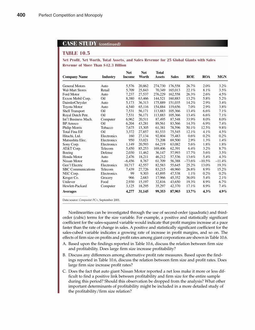
Chapter Ten Perfect Competition and Monopoly 401
Nonlinearities can be investigated through the use of second-order (quadratic) and third-order (cubic) terms for the size variable. For example, a positive and statistically significantcoefficient for the sales-squared variable would indicate that profit margins increase at a pacefaster than the rate of change in sales. A positive and statistically significant coefficient for thesales-cubed variable indicates a growing rate of increase in profit margins, and so on. Theeffects of firm size on profits and profit rates among giant corporations are shown in Table 10.6.A. Based upon the findings reported in Table 10.6, discuss the relation between firm size
and profitability. Does large firm size increase profitability?B. Discuss any differences among alternative profit rate measures. Based upon the find-
ings reported in Table 10.6, discuss the relation between firm size and profit rates. Doeslarge firm size increase profit rates?
C. Does the fact that auto giant Nissan Motor reported a net loss make it more or less dif-ficult to find a positive link between profitability and firm size for the entire sampleduring this period? Should this observation be dropped from the analysis? What otherimportant determinants of profitability might be included in a more detailed study ofthe profitability/firm size relation?
CASE STUDY (continued)
TABLE 10.5Net Profit, Net Worth, Total Assets, and Sales Revenue for 25 Global Giants with SalesRevenue of More Than $42.3 Billion
Net Net Total Company Name Industry Income Worth Assets Sales ROE ROA MGN
General Motors Auto 5,576 20,862 274,730 176,558 26.7% 2.0% 3.2%Wal-Mart Stores Retail 5,709 25,843 70,349 165,013 22.1% 8.1% 3.5%Ford Motor Auto 7,237 27,537 276,229 162,558 26.3% 2.6% 4.5%Exxon Mobil Corp. Oil 8,380 63,466 144,521 160,883 13.2% 5.8% 5.2%DaimlerChrysler Auto 5,173 36,313 175,889 151,035 14.2% 2.9% 3.4%Toyota Motor Auto 4,540 65,116 154,884 119,656 7.0% 2.9% 3.8%Shell Transport Oil 7,531 56,171 113,883 105,366 13.4% 6.6% 7.1%Royal Dutch Petr. Oil 7,531 56,171 113,883 105,366 13.4% 6.6% 7.1%Int’l Business Mach. Computer 6,962 20,511 87,495 87,548 33.9% 8.0% 8.0%BP Amoco Oil 6,204 43,281 89,561 83,566 14.3% 6.9% 7.4%Philip Morris Tobacco 7,675 15,305 61,381 78,596 50.1% 12.5% 9.8%Total Fina Elf Oil 3,372 27,857 81,533 75,545 12.1% 4.1% 4.5%Hitachi, Ltd. Electronics 160 27,134 92,804 75,483 0.6% 0.2% 0.2%Matsushita Elec. Electronics 950 33,021 73,208 69,500 2.9% 1.3% 1.4%Sony Corp. Electronics 1,149 20,593 64,219 63,082 5.6% 1.8% 1.8%AT&T Corp. Telecom 5,450 85,253 169,406 62,391 6.4% 3.2% 8.7%Boeing Defense 2,030 11,462 36,147 57,993 17.7% 5.6% 3.5%Honda Motor Auto 2,476 18,211 46,212 57,536 13.6% 5.4% 4.3%Nissan Motor Auto –6,456 8,767 61,709 56,388 –73.6% –10.5% –11.4%Gen’l Electric Electronics 10,717 42,557 82,583 55,645 25.2% 13.0% 19.3%SBC Communications Telecom 7,439 27,726 83,215 48,960 26.8% 8.9% 15.2%NEC Corp. Electronics 99 9,303 43,895 47,538 1.1% 0.2% 0.2%Kroger Co. Grocery 966 2,683 17,966 45,352 36.0% 5.4% 2.1%Unilever Food 2,930 15,197 32,816 43,650 19.3% 8.9% 6.7%Hewlett-Packard Computer 3,125 18,295 35,297 42,370 17.1% 8.9% 7.4%
Averages 4,277 31,145 99,353 87,903 13.7% 4.3% 4.9%
Data source: Compustat PC+, September 2001.
400 Perfect Competition and Monopoly
SELECTED REFERENCESArmstrong, Mark. “Access Pricing, Bypass, and Universal Service.” American Economic Review 91 (May
2001): 297–301.Bacidore, Jeffrey M., and George Sofianos. “Liquidity Provision and Specialist Trading in NYSE-Listed
Non-U.S. Stocks.” Journal of Financial Economics 63 (January 2002): 133–158.Biehl, Andrew R. “Durable-Goods Monopoly with Stochastic Values.” Rand Journal of Economics 32
(Autumn 2001): 565–577.Cope, Robert F., III, David E. Dismukes, and Rachelle F. Cope. “Modeling Regional Electric Power Markets
and Market Power.” Managerial & Decision Economics 22 (December 2001): 411–429.Feinberg, Yossi, and Morton I. Kamien. “Highway Robbery: Complementary Monopoly and the Hold-Up
Problem.” International Journal of Industrial Organization 19 (December 2001): 1603–1621.Fernandez, Raquel, and Richard Rogerson. “Sorting and Long-Run Inequality.” Quarterly Journal of
Economics 116 (November 2001): 1305–1341.Garza-Gomez, Xavier. “The Information Content of the Book-to-Market Ratio.” Financial Analysts Journal
57 (November/December 2001): 78–95.Hausman, Jerry A., J. Gregory Sidak, and Hal J. Singer. “Cable Modems and DSL: Broadband Internet
Access for Residential Customers.” American Economic Review 91 (May 2001): 302–307.Huang, S., Y. Yang, and K. Anderson. “A Theory of Finitely Durable Goods Monopoly with Used-Goods
Market and Transaction Costs.” Management Science 47 (November 2001): 1515–1532.Jacobson, Robert, and Gary Hansen. “Modeling in the Competitive Process.” Managerial & Decision
Economics 22 (June/August 2001): 251–263.Lamoreaux, Naomi R., and Kenneth L. Sokoloff. “Market Trade in Patents and the Rise of a Class of
Specialized Inventors in the 19th Century United States.” American Economic Review 91 (May 2001):39–44.
Mini, Federico. “The Role of Incentives for Opening Monopoly Markets: Comparing GTE and BOCCooperation with Local Entrants.” Journal of Industrial Economics 49 (September 2001): 379–414.
Ottaviani, Marco, and Andrea Prat. “The Value of Public Information in Monopoly.” Econometrica 69(November 2001): 1673–1683.
Uri, Noel D. “Monopoly Power and the Problem of CLEC Access Charges.” Telecommunications Policy 25(September/October 2001): 611–623.
Weaver, Samuel C. “Measuring Economic Value Added: A Survey of the Practices of EVA Proponents.”Journal of Applied Finance 11 (2001): 50–60.
402 Part Four Market Structure Analysis and Estimation
CASE STUDY (continued)
TABLE 10.6Profitability Effects of Firm Size (t statistics in parentheses)
Dependent Variable Size Measure Intercept Size Size2 Size3 R2 F stat.
Profits Net worth –2372.400 3.76E-02 –4.30E-06 1.08E-11 40.3% 4.72(–0.87) (1.47) (–0.63) (0.21)
Profits Total assets –2016.240 1.24E-02 –6.00E-07 9.27E-13 24.5% 2.27(–0.52) (1.07) (–0.63) (0.43)
Profits Sales 3392.820 –9.63E-02 1.97E-06 –7.70E-12 21.7% 1.94(0.25) (–0.21) (0.41) (–0.50)
ROE Net worth –0.0191 1.40E-05 –2.90E-10 1.63E-15 4.1% 0.30(–0.09) (0.72) (–0.57) (0.42)
ROA Total assets 0.050 1.36E-07 –1.50E-12 2.24E-18 3.6% 0.26(0.89) (0.08) (–0.11) (0.07)
MGN Sales 0.116 –2.40E-06 2.79E-11 –9.70E-17 1.6% 0.12(0.51) (–0.31) (0.34) (–0.37)
Perfect Competition and Monopoly 401

MonopolisticCompetition andOligopoly
CHAPTER ELEVEN
403
Once the seventh-highest market capitalization company in America,Houston’s energy giant Enron Corp. stumbled from a stock-market
valuation of $62 billion in January 2001 to penny stock status and Chapter11 bankruptcy protection in less than a year. A similar fate befell Troy,Michigan–based discount retailer Kmart Corp., which on January 22, 2002,became the largest retailer to ever seek bankruptcy protection. With 275,000employees and more than 2,100 stores, Kmart is trying to restructure andavoid becoming road kill for retail juggernaut Wal-Mart Stores, Inc.
The demise of corporate titans did not begin with Enron and end withKmart. The creative destruction of capitalism is ongoing and unforgiving. From1928–1996, Bethlehem Steel Corp. was a fixture in the Dow Jones IndustrialAverage. In 1972, imaging company Polaroid Corp. was the most revered mem-ber of the Nifty 50, a group of stock-market favorites. Both filed for federalbankruptcy protection in 2001. Xerox Corp., another Nifty 50 favorite, was onceso dominant in the copy business that it became a verb, as in “Xerox this.” Xeroxhangs on, but business has dwindled in the face of growing competition fromelectronic media.
Despite massive financial resources and compelling brand names, corpo-rate behemoths often stumble. Large size can breed deadly complacency. Tosurvive and prosper in the new millennium, many large-scale organizationshave cut back and refocused in order to become smaller, more nimble organ-izations.1 This chapter offers perspective on how the nature of competition isaffected by the number and size distribution of buyers and sellers; it examinescompetition in the partly competitive, partly monopolistic world of monopo-listic competition and oligopoly.
1 See Amy Merrick, “Kmart Lays Out Plans to Trim Its Size, Boost Efficiency, in BankruptcyFiling,” The Wall Street Journal Online, January 22, 2002 (http://online.wsj.com).
403
11

CONTRAST BETWEEN MONOPOLISTIC COMPETITION AND OLIGOPOLY
Monopolistic competition and oligopoly provide differing perspectives on the nature ofcompetition in imperfectly competitive markets. Attributes of the monopolistic competitionand oligopoly market models are outlined in this section and then elaborated on in the restof the chapter.
Monopolistic CompetitionThe economic environment faced by many firms cannot be described as perfectly competitive.Likewise, few firms enjoy clear monopoly. Real-world markets commonly embody elementsof both perfect competition and monopoly. Firms often introduce valuable new products orprocess innovations that give rise to above-normal rates of return in the short run. In the longrun, however, entry and imitation by new rivals erode the dominant market share enjoyed byearly innovators, and profits eventually return to normal. Still, in sharp contrast to perfectlycompetitive markets, the unique product characteristics of individual firms often remain val-ued by consumers. Consumers often continue to prefer Campbell’s Soup, Dockers, Oil of Olay,Rubbermaid, Tide, and other favorite brands long after comparable products have been intro-duced by rivals. The partly competitive, partly monopolistic market structure encountered byfirms in the apparel, food, hotel, retailing, and consumer products industries is called monop-olistic competition. Given the lack of perfect substitutes, monopolistically competitive firmsexercise some discretion in setting prices—they are not price takers. However, given vigorouscompetition from imitators offering close but not identical substitutes, such firms enjoy only anormal risk-adjusted rate of return on investment in long-run equilibrium.
Monopolistic competition is similar to perfect competition in that it entails vigorous pricecompetition among a large number of firms. The major difference between these two marketstructure models is that consumers perceive important differences among the products offeredby monopolistically competitive firms, whereas the output of perfectly competitive firms ishomogeneous. This gives monopolistically competitive firms at least some discretion in settingprices. However, the availability of many close substitutes limits this price-setting ability anddrives profits down to a normal risk-adjusted rate of return in the long run. As in the case ofperfect competition, above-normal profits are possible only in the short run, before the monop-olistically competitive firm’s rivals can take effective countermeasures.
OligopolyOligopoly is the market structure model that describes competition among a handful of com-petitors sheltered by significant barriers to entry. Oligopolists might produce a homogeneousproduct, such as aluminum, steel, or semiconductors; or differentiated products such as Cheerios,Coca-Cola, Marlboro, MTV, and Nintendo. Innovative leading firms in the ready-to-eat cereal,beverage, cigarette, entertainment, and computer software industries, among others, have thepotential for economic profits even in the long run. With few competitors, economic incentivesalso exist for such firms to devise illegal agreements to limit competition, fix prices, or otherwisedivide markets. The history of antitrust enforcement in the United States provides numerousexamples of “competitors” who illegally entered into such agreements. Yet there are also exam-ples of markets in which vigorous competition among a small number of firms generates obviouslong-term benefits for consumers. It is therefore erroneous to draw a simple link between thenumber of competitors and the vigor of competition.
In an industry characterized by oligopoly, only a few large rivals are responsible for the bulkof industry output. As in the case of monopoly, high to very high barriers to entry are typical.
404 Part Four Market Structure Analysis and Estimation
monopolistic com-petitionA market structurecharacterized by a largenumber of sellers ofdifferentiated products
oligopolyA market structurecharacterized by fewsellers and interde-pendent price/outputdecisions
404 Monopolistic Competition and Oligopoly

Under oligopoly, the price/output decisions of firms are interrelated in the sense that directreactions among rivals can be expected. As a result, decisions of individual firms anticipate thelikely response of competitors. This competition among the few involves a wide variety of priceand nonprice methods of rivalry, as determined by the institutional characteristics of each par-ticular market. Even though limited numbers of competitors give rise to a potential for eco-nomic profits, above-normal rates of return are far from guaranteed. Competition among thefew can be vigorous.
Dynamic Nature of CompetitionIn characterizing the descriptive relevance of the monopolistic competition and oligopoly modelsof seller behavior, it is important to recognize the dynamic nature of real-world markets. Forexample, as late as the mid 1980s it seemed appropriate to regard the automobile and personalcomputer manufacturing markets as oligopolistic in nature. Today, it seems fairer to regard eachindustry as monopolistically competitive. In the automobile industry, GM, Ford, and DaimlerChrysler have found Toyota, Honda, Nissan, and a host of specialized competitors to be formi-dable foes. Aggressive competitors like Dell, Compaq, Hewlett-Packard, and Gateway firstweakened, and then obliterated, IBM’s early lead in the PC business. Prices and profit marginsfor PCs continue to fall as improving technology continues to enhance product quality.
In many formerly oligopolistic markets, the market discipline provided by a competitivefringe of smaller domestic and foreign rivals is sufficient to limit the potential abuse of a fewlarge competitors. In the long-distance telephone service market, for example, AT&T, MCIWorldCom, and Sprint have long dominated the industry. However, emerging competitionfrom the so-called regional Bell operating companies (REBOCs), along with a host of smallerspecialized providers, cause long-distance phone service price and service quality competitionto be spirited. Similarly, the competitive fringe in wireless communications and cable TVpromises to force dramatic change during the years ahead.
It is unfortunate, but public perceptions and government regulatory policy sometimes lagbehind economic reality. It is essential that timely and accurate market structure information beavailable to form the basis for managerial investment decisions that relate to entry or exit fromspecific lines of business. Similarly, enlightened public policy requires timely information.
MONOPOLISTIC COMPETITION
Most firms are subject to rivalry, though perhaps not as vigorous as would exist under perfectcompetition. Even though most firms face a large number of competitors with similar prod-ucts, many still have some control over the price of their product. They cannot sell all that theywant at a fixed price, nor would they lose all sales if they raised prices slightly. Most firms facedownward-sloping demand curves, signifying less-than-perfect competition.
Characteristics of Monopolistically Competitive MarketsMonopolistic competition exists when individual producers have moderate influence over prod-uct prices, where each product enjoys a degree of uniqueness in the perception of customers. Thismarket structure has some important similarities and dissimilarities with perfectly competitivemarkets. Monopolistic competition is characterized by
• Large numbers of buyers and sellers. Each firm produces a small portion of industry output,and each customer buys only a small part of the total.
• Product heterogeneity. The output of each firm is perceived to be essentially different from,though comparable with, the output of other firms in the industry.
Chapter Eleven Monopolistic Competition and Oligopoly 405
Monopolistic Competition and Oligopoly 405
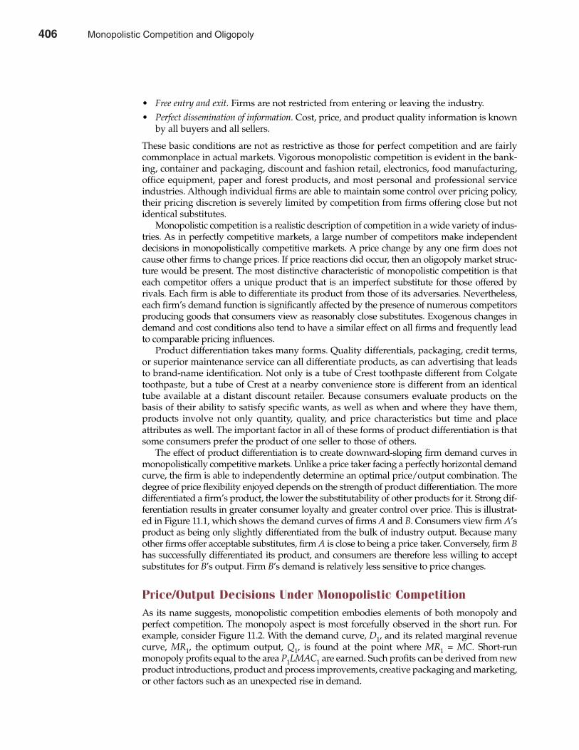
• Free entry and exit. Firms are not restricted from entering or leaving the industry.• Perfect dissemination of information. Cost, price, and product quality information is known
by all buyers and all sellers.
These basic conditions are not as restrictive as those for perfect competition and are fairlycommonplace in actual markets. Vigorous monopolistic competition is evident in the bank-ing, container and packaging, discount and fashion retail, electronics, food manufacturing,office equipment, paper and forest products, and most personal and professional serviceindustries. Although individual firms are able to maintain some control over pricing policy,their pricing discretion is severely limited by competition from firms offering close but notidentical substitutes.
Monopolistic competition is a realistic description of competition in a wide variety of indus-tries. As in perfectly competitive markets, a large number of competitors make independentdecisions in monopolistically competitive markets. A price change by any one firm does notcause other firms to change prices. If price reactions did occur, then an oligopoly market struc-ture would be present. The most distinctive characteristic of monopolistic competition is thateach competitor offers a unique product that is an imperfect substitute for those offered byrivals. Each firm is able to differentiate its product from those of its adversaries. Nevertheless,each firm’s demand function is significantly affected by the presence of numerous competitorsproducing goods that consumers view as reasonably close substitutes. Exogenous changes indemand and cost conditions also tend to have a similar effect on all firms and frequently leadto comparable pricing influences.
Product differentiation takes many forms. Quality differentials, packaging, credit terms,or superior maintenance service can all differentiate products, as can advertising that leadsto brand-name identification. Not only is a tube of Crest toothpaste different from Colgatetoothpaste, but a tube of Crest at a nearby convenience store is different from an identicaltube available at a distant discount retailer. Because consumers evaluate products on thebasis of their ability to satisfy specific wants, as well as when and where they have them,products involve not only quantity, quality, and price characteristics but time and placeattributes as well. The important factor in all of these forms of product differentiation is thatsome consumers prefer the product of one seller to those of others.
The effect of product differentiation is to create downward-sloping firm demand curves inmonopolistically competitive markets. Unlike a price taker facing a perfectly horizontal demandcurve, the firm is able to independently determine an optimal price/output combination. Thedegree of price flexibility enjoyed depends on the strength of product differentiation. The moredifferentiated a firm’s product, the lower the substitutability of other products for it. Strong dif-ferentiation results in greater consumer loyalty and greater control over price. This is illustrat-ed in Figure 11.1, which shows the demand curves of firms A and B. Consumers view firm A’sproduct as being only slightly differentiated from the bulk of industry output. Because manyother firms offer acceptable substitutes, firm A is close to being a price taker. Conversely, firm Bhas successfully differentiated its product, and consumers are therefore less willing to acceptsubstitutes for B’s output. Firm B’s demand is relatively less sensitive to price changes.
Price/Output Decisions Under Monopolistic CompetitionAs its name suggests, monopolistic competition embodies elements of both monopoly andperfect competition. The monopoly aspect is most forcefully observed in the short run. Forexample, consider Figure 11.2. With the demand curve, D1, and its related marginal revenuecurve, MR1, the optimum output, Q1, is found at the point where MR1 = MC. Short-runmonopoly profits equal to the area P1LMAC1 are earned. Such profits can be derived from newproduct introductions, product and process improvements, creative packaging and marketing,or other factors such as an unexpected rise in demand.
406 Part Four Market Structure Analysis and Estimation
406 Monopolistic Competition and Oligopoly
Over time, short-run monopoly profits attract competition, and other firms enter the indus-try. This competitive aspect of monopolistic competition is seen most forcefully in the long run.As competitors emerge to offer close but imperfect substitutes, the market share and profits ofthe initial innovating firm diminish. Firm demand and marginal revenue curves shift to the leftas, for example, from D1 to D2 and from MR1 to MR2 in Figure 11.2. Optimal long-run outputoccurs at Q2, the point where MR2 = MC. Because the optimal price P2 equals ATC2, where costincludes a normal profit just sufficient to maintain capital investment, economic profits are zero.
The price/output combination (P2Q2) describes a monopolistically competitive marketequilibrium characterized by a high degree of product differentiation. If new entrants offeredperfect rather than close substitutes, each firm’s long-run demand curve would become morenearly horizontal, and the perfectly competitive equilibrium, D3 with P3 and Q3, would beapproached. Like the (P2Q2) high-differentiation equilibrium, the (P3Q3) no-differentiationequilibrium is something of an extreme case. In most instances, competitor entry reduces butdoes not eliminate product differentiation. An intermediate price/output solution, one between(P2Q2) and (P3Q3), is often achieved in long-run equilibrium. Indeed, it is the retention of at leastsome degree of product differentiation that distinguishes the monopolistically competitiveequilibrium from that achieved in perfectly competitive markets.
A firm will never operate at the minimum point on its average cost curve in monopolisti-cally competitive equilibrium. Each firm’s demand curve is downward sloping and is tangentto the ATC curve at some point above minimum ATC. However, this does not mean that amonopolistically competitive industry is inefficient. The very existence of a downward-slopingdemand curve implies that consumers value an individual firm’s products more highly than theydo products of other producers. The higher prices and costs of monopolistically competitiveindustries, as opposed to perfectly competitive industries, reflect the economic cost of productvariety. If consumers are willing to bear such costs, then such costs must not be excessive. The suc-cess of branded products in the face of generic competition, for example, is powerful evidence ofconsumer preferences for product variety.
Chapter Eleven Monopolistic Competition and Oligopoly 407
FIGURE 11.1Relation Between Product Differentiation and Elasticity of DemandFirm B’s steeper demand curve relative to firm A’s reflects stronger product differentiation and hence lesssensitivity to price changes.
DA
DB
Price per unit ($)
Quantity per time period
Monopolistic Competition and Oligopoly 407
Although perfect competition and monopoly are somewhat rare in real-world markets,monopolistic competition is frequently observed. For example, in 1960 a small ($37 million insales) office-machine company, Haloid Xerox, Inc., revolutionized the copy industry with theintroduction of the Xerox 914 copier. Xerography was a tremendous improvement over electro-fax and other coated-paper copiers. It permitted the use of untreated paper, which producedclearer and less expensive copies. Invention of the dry copier established what is now XeroxCorporation at the forefront of a rapidly growing office-copier industry and propelled the firmto a position of virtual monopoly by 1970. Between 1970 and 1980, the industry’s market structurechanged dramatically because of an influx of competition as many of Xerox’s original patentsexpired. IBM entered the copier market in April 1970 with its Copier I model and expanded itsparticipation in November 1972 with Copier II. Eastman Kodak made its entry into the marketin 1975 with its Ektaprint model. Of course, Minnesota Mining and Manufacturing (3M) hadlong been a factor in the electrofax copier segment of the market. A more complete list of Xerox’srecent domestic and international competitors would include at least 30 firms. The effect of thisentry on Xerox’s market share and profitability was dramatic. Between 1970 and 1978, for exam-ple, Xerox’s share of the domestic copier market fell from 98 percent to 56 percent, and its returnon stockholders’ equity fell from 23.6 percent to 18.2 percent.
More recently, Xerox’s leadership position has been squandered and its profitability has col-lapsed in the face of vicious price and product quality competition. Because Canon, Kodak, 3M,Panasonic, Ricoh, Savin, and Sharp copiers are only close rather than perfect substitutes for Xeroxmachines, the industry is commonly described as monopolistically competitive. Effective (butimperfect) competition for paper copies also comes from low-cost printers tied to PCs and fromelectronic communications, which obviate the need for paper copies. Make no mistake about it,monopolistic competition can be tough on industry leaders that fail to keep up—just ask Xerox.
408 Part Four Market Structure Analysis and Estimation
FIGURE 11.2Price/Output Combinations Under Monopolistic CompetitionLong-run equilibrium under monopolistic competition occurs when MR = MC and P = AC. This typicallyoccurs between (P2, Q2) (the high-price/low-output equilibrium) and (P3, Q3) (the low-price/high-outputequilibrium).
D2
$ per unitof output
Q2
Quantity per time period
D1
D3
MR2MR1
Q1 Q3
P3
ATC1
P2 = ATC2
P1 L
M
MCAC
O
408 Monopolistic Competition and Oligopoly
ILLUSTRATION OF MONOPOLISTICALLY COMPETITIVE EQUILIBRIUM
The process of price/output adjustment and the concept of equilibrium in monopolisticallycompetitive markets can be further illustrated by the following example. Assume that theSkyhawk Trailer Company, located in Toronto, Ontario, owns patents covering importantdesign features of its Tomahawk II, an ultralight camping trailer that can safely be towed byhigh-mileage subcompact cars. Skyhawk’s patent protection has made it very difficult for com-petitors to offer similar ultralight trailers. The Tomahawk II is highly successful, and a flood ofsimilar products can be expected within 5 years as Skyhawk’s patent protection expires.
Skyhawk has asked its financial planning committee to identify short- and long-run pricingand production strategies for the Tomahawk II. To facilitate the decision-making process, thecommittee has received the following revenue and cost data from Skyhawk’s marketing andproduction departments:
TR = $20,000Q – $15.6Q2
MR = ∆TR/∆Q = $20,000 – $31.2Q
TC = $400,000 + $4,640Q + $10Q2
MC = ∆TC/∆Q = $4,640 + $20Q
where TR is revenue (in dollars), Q is quantity (in units), MR is marginal revenue (in dollars),TC is total cost per month, including a risk-adjusted normal rate of return on investment (indollars), and MC is marginal cost (in dollars).
As a first step in the analysis, one might determine the optimal price/output combination ifthe committee were to decide that Skyhawk should take full advantage of its current monopoly
Chapter Eleven Monopolistic Competition and Oligopoly 409
Intel: Running Fast to Stay in Place
Intel is the dominant and most profitable maker of inte-grated circuits, the microscopic pieces of silicon chips usedto power electronic computers, calculators, video games,and a burgeoning array of other products. intel inside™ is atrademark that identifies products produced by a compa-ny whose microprocessors are the brains of more than fivetimes as many personal computers as its nearest rival. Socomplete has been Intel’s grip on the PC market that salesare expected to explode from $33.7 billion in 2000 toroughly $53.5 billion in 2005, while profits surge from$10.7 billion to roughly $14.5 billion.
Despite its enviable record of success, and despiteobvious strengths, Intel’s core business is facing itsbiggest challenge in a decade. Led by Advanced MicroDevices, Inc., Cyrix, Inc., International Business Machines,Inc., Texas Instruments, Inc., and a handful of foreignfirms, competitors are rushing to produce alternatives toIntel chips. Imitators can quickly erode the profits of earlyinnovators like Intel, a company that has come to counton giant-sized operating margins of over 40 percent.During recent years, investors and market analysts have
both posed an important question: Is Intel’s dominance ofthe integrated circuits market coming to an end?
Not without a fight, it won’t. Intel is led by visionarychairman Andrew S. Grove, author of the best-sellerOnly the Paranoid Survive, and his hand-picked successorCEO Craig R. Barrett. Driven by paranoia, Intel is drag-ging competitors into court for patent infringement,slashing prices, and boldly promoting its products. Thecompany is strengthening its close working relationshipwith manufacturers of end-user products to ensure com-patibility and maximize the benefits of new microproces-sor innovations. Most important, Intel has launched acampaign to speed product development and expand itspotential market.
Intel’s speedup of microprocessor technology willaffect everyone who uses electronic products. Not theleast of those affected will be Intel’s competitors.
See: Terho Vimonen, “Intel Clears $100 Million to Upgrade Its PhilippineChip-Making Facilities,” The Wall Street Journal Online, January 23, 2002(http://online.wsj.com).
M A N A G E R I A L A P P L I C AT I O N 1 1 . 1
Monopolistic Competition and Oligopoly 409
position and maximize short-run profits. To find the short-run profit-maximizing price/outputcombination, set Skyhawk’s marginal revenue equal to marginal cost and solve for Q:
MR = MC
$20,000 – $31.2Q = $4,640 + $20Q
$51.2Q = $15,360Q = 300 units
and
P = $20,000 – $15.6(300)= $15,320
π = TR – TC
= –$25.6(3002) + $15,360(300) – $400,000= $1,904,000
Therefore, the financial planning committee should recommend a $15,320 price and 300-unitoutput level to Skyhawk management if the firm’s objective is to maximize short-run profit.Such a planning decision results in roughly $1.9 million in profit during those months whenSkyhawk’s patent protection effectively deters competitors.
Now assume that Skyhawk can maintain a high level of brand loyalty and product differen-tiation in the long run, despite competitor offerings of similar trailers, but that such competitioneliminates any potential for economic profits. This is consistent with a market in monopolisticallycompetitive equilibrium, where P = AC at a point above minimum long-run average costs.Skyhawk’s declining market share is reflected by a leftward shift in its demand curve to a pointof tangency with its average cost curve. Although precise identification of the long-runprice/output combination is very difficult, the planning committee can identify the boundswithin which this price/output combination can be expected to occur.
The high-price/low-output combination is identified by the point of tangency between thefirm’s average cost curve and a new demand curve reflecting a parallel leftward shift in demand(D2 in Figure 11.2). This parallel leftward shift assumes that the firm can maintain a high degreeof product differentiation in the long run. The low-price/high-output equilibrium combinationassumes no residual product differentiation in the long run and it is identified by the point of tan-gency between the average cost curve and a new horizontal firm demand curve (D3 in Figure11.2). This is, of course, also the perfectly competitive equilibrium price/output combination.
The equilibrium high-price/low-output combination that follows a parallel leftward shiftin Skyhawk’s demand curve can be determined by equating the slopes of the firm’s originaldemand curve and its long-run average cost curve. Because a parallel leftward shift in firmdemand results in a new demand curve with an identical slope, equating the slopes of thefirm’s initial demand and average cost curves identifies the monopolistically competitivehigh-price/low-output equilibrium.
For simplicity, assume that the previous total cost curve for Skyhawk also holds in the longrun. To determine the slope of this average cost curve, one must find out how average costsvary with respect to output.
AC = TC/Q = ($400,000 + $4,640Q + $10Q2)/Q
= $400,000 + $4,640 + $10QQ
= $400,000Q-1 + $4,640 + $10Q
The slope of this average cost curve is given by the expression
410 Part Four Market Structure Analysis and Estimation
410 Monopolistic Competition and Oligopoly
∆AC/∆Q = –400,000Q-2 + 10
The slope of the new demand curve is given by
∆P/∆Q = –15.6 (same as the original demand curve)
In equilibrium,
Slope of AC Curve = Slope of Demand Curve–400,000Q–2 + 10 = –15.6
Q-2 = 25.6/400,000Q2 = 400,000/25.6Q = 125 UnitsP = AC
= $400,000 + $4,640 + $10(125)125= $9,090
and
π = P � Q – TC
= $9,090(125) – $400,000 – $4,640(125) – $10(1252)= $0
This high-price/low-output monopolistically competitive equilibrium results in a decrease inprice from $15,320 to $9,090 and a fall in output from 300 to 125 units per year. Only a risk-adjusted normal rate of return will be earned, eliminating Skyhawk’s economic profits. Thislong-run equilibrium assumes that Skyhawk would enjoy the same low price elasticity ofdemand that it experienced as a monopolist. This assumption may or may not be appropriate.New entrants often have the effect of both cutting a monopolist’s market share and increasingthe price elasticity of demand. It is often reasonable to expect entry to cause both a leftward shiftof and some flattening in Skyhawk’s demand curve. To see the extreme limit of the demandcurve–flattening process, the case of a perfectly horizontal demand curve can be considered.
The low-price/high-output (perfectly competitive) equilibrium combination occurs at thepoint where P = MR = MC = AC. This reflects that the firm’s demand curve is perfectly hori-zontal, and average costs are minimized. To find the output level of minimum average costs,set MC = AC and solve for Q:
$4,640 + $20Q = $400,000Q-1 + $4,640 + $10Q
$10Q = $400,000Q-1
Q2 = 40,000Q2 = √40,000
= 200 unitsP = AC
= $400,000 + $4,640 + $10(200)200= $8,640
Chapter Eleven Monopolistic Competition and Oligopoly 411
Monopolistic Competition and Oligopoly 411
and
π = P � Q – TC
= $8,640(200) – $400,000 – $4,640(200) – $10(2002)= $0
Under this low-price equilibrium scenario, Skyhawk’s monopoly price falls in the long runfrom an original $15,320 to $8,640, and output falls from the monopoly level of 300 units to thecompetitive equilibrium level of 200 units per month. The company would earn only a risk-adjusted normal rate of return, and economic profits would equal zero.
Following expiration of its patent protection, management can expect that competitorentry will reduce Skyhawk’s volume from 300 units per month to a level between Q = 125and Q = 200 units per month. The short-run profit-maximizing price of $15,320 will fall to amonopolistically competitive equilibrium price between P = $9,090, the high-price/low-outputequilibrium, and P = $8,640, the low-price/high-output equilibrium. In deciding on an optimalshort-run price/output strategy, Skyhawk must weigh the benefits of high near-term prof-itability against the long-run cost of lost market share resulting from competitor entry. Such adecision involves consideration of current interest rates, the speed of competitor imitation, andthe future pace of innovation in the industry, among other factors.
OLIGOPOLY
The theory of monopolistic competition recognizes that firms often have some control overprice but that their price flexibility is limited by a large number of close substitutes. This theoryassumes that in making decisions firms do not consider competitor reactions. Such a behavioralassumption is appropriate for some industries but not others. When individual firm actionscause competitors to react, oligopoly exists.
Characteristics of Oligopoly MarketsOligopoly is present when a handful of competitors dominate the market for a good or serviceand each firm makes pricing and marketing decisions in light of the expected response byrivals. Individual firms have the ability to set pricing and production strategy, and they enjoythe potential for economic profits in both the short run and the long run. Oligopoly describesmarkets that can be characterized as follows:
• Few sellers. A handful of firms produces the bulk of industry output.• Homogeneous or unique product. Oligopoly output can be homogeneous (e.g., aluminum) or
distinctive (e.g., ready-to-eat cereal). • Blockaded entry and exit. Firms are heavily restricted from entering or leaving the industry.• Imperfect dissemination of information. Cost, price, and product quality information is withheld
from uninformed buyers.
In the United States, aluminum, cigarettes, electrical equipment, filmed entertainment pro-duction and distribution, glass, long-distance telecommunications, and ready-to-eat cerealsare all produced and sold under conditions of oligopoly. In each of these industries, a smallnumber of firms produces a dominant percentage of all industry output. In the ready-to-eatbreakfast cereal industry, for example, Kellogg, Kraft (Post cereals), General Mills, Nabisco,and Quaker Oats are responsible for almost all domestic production in the United States.Durable customer loyalty gives rise to fat profit margins and rates of return on assets that aretwo to three times food industry norms. Corn Flakes, Sugar Frosted Flakes, Cheerios, Raisin
412 Part Four Market Structure Analysis and Estimation
412 Monopolistic Competition and Oligopoly
Bran, Wheaties, and a handful of other brands continue to dominate the industry year afteryear and make successful entry extremely difficult. Even multinational food giant Nestlésought and obtained a joint venture agreement with General Mills rather than enter thepotentially lucrative European breakfast cereal market by itself. Long-distance telephone serviceis also highly concentrated, with AT&T, Sprint, and WorldCom providing almost all domesticwire-line service to residential customers.
Oligopoly also is present in a number of local markets. In many retail markets for gasolineand food, for example, only a few service stations and grocery stores compete within a smallgeographic area. Drycleaning services are also sometimes provided by a relative handful offirms in small to medium-size cities and towns.
Price/Output Decisions Under OligopolyDemand curves relate quantity demanded to price, holding constant the effect of all other vari-ables. One variable that is typically assumed to remain fixed is the price charged by competingfirms. In oligopoly, however, if one firm changes its price, other firms react by changing theirprices. The demand curve for the initial firm shifts position so that instead of moving along asingle demand curve as it changes price, the firm moves to an entirely new demand curve.
The phenomenon of shifting demand curves is illustrated in Figure 11.3(a). Firm A is ini-tially producing Q1 units of output and selling them at a price of P1. Demand curve D1 applieshere, assuming that prices charged by other firms remain fixed. Under this assumption, a pricecut from P1 to P2 would increase demand to Q2. Assume, however, that only a few firms operatein the market and that each has a fairly large share of total sales. If one firm cuts its price andobtains a substantial increase in volume, other firms lose a large part of their business.Furthermore, they know exactly why their sales have fallen and react by cutting their ownprices. This action shifts firm A down to the second demand curve, D2, reducing its demandat P2 from Q2 to Q3 units. The new curve is just as unstable as the old one, so knowledge of itsshape is useless to firm A; if it tries to move along D2, competitors will react, forcing the com-pany to yet another demand curve.
Shifting demand curves presents no real difficulty in making price/output decisions if eachfirm knows how rivals will react to price changes. The reactions would just be built into theprice/demand relation, and a new demand curve could be constructed to include interactionsamong firms. Curve D3 in Figure 11.3(b) represents such a reaction-based demand curve; itshows how price reductions affect quantity demanded after competitive reactions have beentaken into account. The problem with this approach is that different interfirm behavior leadsto different pricing decision rules.
Cartel ArrangementsAll firms in an oligopoly market benefit if they get together and set prices to maximize industryprofits. A group of competitors operating under such a formal overt agreement is called a cartel.If an informal covert agreement is reached, the firms are said to be operating in collusion. Bothpractices are illegal in the United States. However, cartels are legal in some parts of the world,and U.S. multinational corporations sometimes become involved with them in foreign markets.Several important domestic markets are also dominated by producer associations that operatelike cartels and appear to flourish without interference from the government. Agricultural com-modities such as milk are prime examples of products marketed under cartel-like arrangements.
A cartel that has absolute control over all firms in an industry can operate as a monopoly. Toillustrate, consider the situation shown in Figure 11.4. The marginal cost curves of each firm aresummed horizontally to arrive at an industry marginal cost curve. Equating the cartel’s totalmarginal cost with the industry marginal revenue curve determines the profit-maximizing out-put and the price, P*, to be charged. Once this profit-maximizing price/output level has been
cartelFirms operating with aformal agreement to fixprices and output
collusionA covert, informalagreement amongfirms in an industry tofix prices and outputlevels
Chapter Eleven Monopolistic Competition and Oligopoly 413
Monopolistic Competition and Oligopoly 413
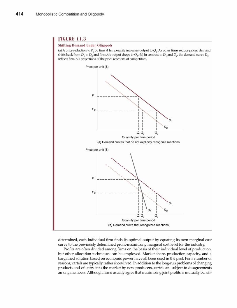
determined, each individual firm finds its optimal output by equating its own marginal costcurve to the previously determined profit-maximizing marginal cost level for the industry.
Profits are often divided among firms on the basis of their individual level of production,but other allocation techniques can be employed. Market share, production capacity, and abargained solution based on economic power have all been used in the past. For a number ofreasons, cartels are typically rather short-lived. In addition to the long-run problems of changingproducts and of entry into the market by new producers, cartels are subject to disagreementsamong members. Although firms usually agree that maximizing joint profits is mutually benefi-
414 Part Four Market Structure Analysis and Estimation
FIGURE 11.3Shifting Demand Under Oligopoly(a) A price reduction to P2 by firm A temporarily increases output to Q2. As other firms reduce prices, demandshifts back from D1 to D2 and firm A’s output drops to Q3. (b) In contrast to D1 and D2, the demand curve D3reflects firm A’s projections of the price reactions of competitors.
D2
D1
Q2Q3
Quantity per time period
P2
P1
(a) Demand curves that do not explicitly recognize reactions
Price per unit ($)
D2
D1
Q2Q3
Quantity per time period
P2
P1
(b) Demand curve that recognizes reactions
Price per unit ($)
Q1
Q1
D3
414 Monopolistic Competition and Oligopoly
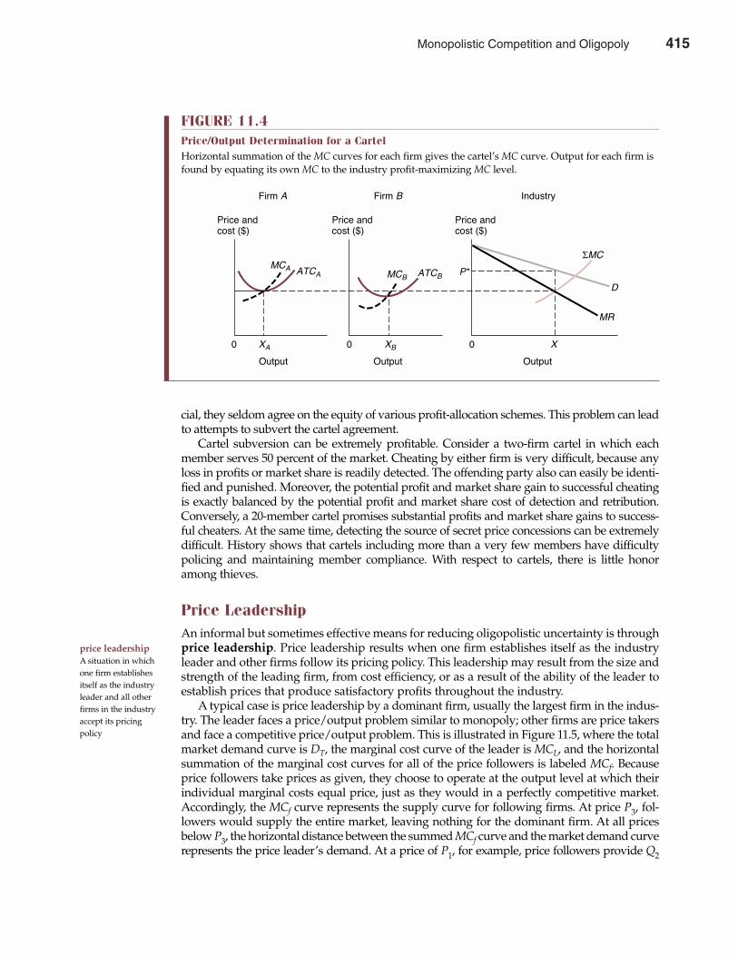
cial, they seldom agree on the equity of various profit-allocation schemes. This problem can leadto attempts to subvert the cartel agreement.
Cartel subversion can be extremely profitable. Consider a two-firm cartel in which eachmember serves 50 percent of the market. Cheating by either firm is very difficult, because anyloss in profits or market share is readily detected. The offending party also can easily be identi-fied and punished. Moreover, the potential profit and market share gain to successful cheatingis exactly balanced by the potential profit and market share cost of detection and retribution.Conversely, a 20-member cartel promises substantial profits and market share gains to success-ful cheaters. At the same time, detecting the source of secret price concessions can be extremelydifficult. History shows that cartels including more than a very few members have difficultypolicing and maintaining member compliance. With respect to cartels, there is little honoramong thieves.
Price LeadershipAn informal but sometimes effective means for reducing oligopolistic uncertainty is throughprice leadership. Price leadership results when one firm establishes itself as the industryleader and other firms follow its pricing policy. This leadership may result from the size andstrength of the leading firm, from cost efficiency, or as a result of the ability of the leader toestablish prices that produce satisfactory profits throughout the industry.
A typical case is price leadership by a dominant firm, usually the largest firm in the indus-try. The leader faces a price/output problem similar to monopoly; other firms are price takersand face a competitive price/output problem. This is illustrated in Figure 11.5, where the totalmarket demand curve is DT, the marginal cost curve of the leader is MCL, and the horizontalsummation of the marginal cost curves for all of the price followers is labeled MCf. Becauseprice followers take prices as given, they choose to operate at the output level at which theirindividual marginal costs equal price, just as they would in a perfectly competitive market.Accordingly, the MCf curve represents the supply curve for following firms. At price P3, fol-lowers would supply the entire market, leaving nothing for the dominant firm. At all pricesbelow P3, the horizontal distance between the summed MCf curve and the market demand curverepresents the price leader’s demand. At a price of P1, for example, price followers provide Q2
price leadershipA situation in whichone firm establishesitself as the industryleader and all otherfirms in the industryaccept its pricing policy
Chapter Eleven Monopolistic Competition and Oligopoly 415
FIGURE 11.4Price/Output Determination for a CartelHorizontal summation of the MC curves for each firm gives the cartel’s MC curve. Output for each firm isfound by equating its own MC to the industry profit-maximizing MC level.
Firm A Firm B Industry
Price andcost ($)
Price andcost ($)
Price andcost ($)
MCAMCB
ATCA ATCB
0 0 0
P*
ΣMC
D
MR
XA XB X
Output Output Output
Monopolistic Competition and Oligopoly 415
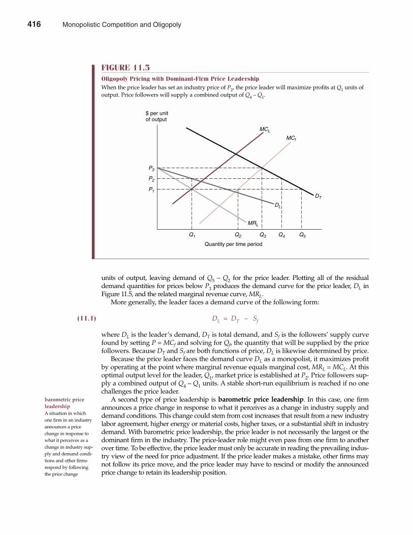
units of output, leaving demand of Q5 – Q2 for the price leader. Plotting all of the residualdemand quantities for prices below P3 produces the demand curve for the price leader, DL inFigure 11.5, and the related marginal revenue curve, MRL.
More generally, the leader faces a demand curve of the following form:
(11.1) DL = DT – Sf
where DL is the leader’s demand, DT is total demand, and Sf is the followers’ supply curvefound by setting P = MCf and solving for Qf, the quantity that will be supplied by the pricefollowers. Because DT and Sf are both functions of price, DL is likewise determined by price.
Because the price leader faces the demand curve DL as a monopolist, it maximizes profitby operating at the point where marginal revenue equals marginal cost, MRL = MCL. At thisoptimal output level for the leader, Q1, market price is established at P2. Price followers sup-ply a combined output of Q4 – Q1 units. A stable short-run equilibrium is reached if no onechallenges the price leader.
A second type of price leadership is barometric price leadership. In this case, one firmannounces a price change in response to what it perceives as a change in industry supply anddemand conditions. This change could stem from cost increases that result from a new industrylabor agreement, higher energy or material costs, higher taxes, or a substantial shift in industrydemand. With barometric price leadership, the price leader is not necessarily the largest or thedominant firm in the industry. The price-leader role might even pass from one firm to anotherover time. To be effective, the price leader must only be accurate in reading the prevailing indus-try view of the need for price adjustment. If the price leader makes a mistake, other firms maynot follow its price move, and the price leader may have to rescind or modify the announcedprice change to retain its leadership position.
416 Part Four Market Structure Analysis and Estimation
barometric priceleadershipA situation in whichone firm in an industryannounces a pricechange in response towhat it perceives as achange in industry sup-ply and demand condi-tions and other firmsrespond by followingthe price change
FIGURE 11.5Oligopoly Pricing with Dominant-Firm Price LeadershipWhen the price leader has set an industry price of P2, the price leader will maximize profits at Q1 units ofoutput. Price followers will supply a combined output of Q4 – Q1.
$ per unitof output
MCL
P3
Quantity per time period
MCf
DT
DL
MRL
P2
P1
Q1 Q2 Q3 Q4 Q5
416 Monopolistic Competition and Oligopoly
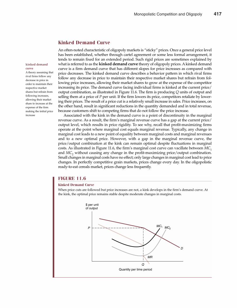
Kinked Demand CurveAn often-noted characteristic of oligopoly markets is “sticky” prices. Once a general price levelhas been established, whether through cartel agreement or some less formal arrangement, ittends to remain fixed for an extended period. Such rigid prices are sometimes explained bywhat is referred to as the kinked demand curve theory of oligopoly prices. A kinked demandcurve is a firm demand curve that has different slopes for price increases as compared withprice decreases. The kinked demand curve describes a behavior pattern in which rival firmsfollow any decrease in price to maintain their respective market shares but refrain from fol-lowing price increases, allowing their market shares to grow at the expense of the competitorincreasing its price. The demand curve facing individual firms is kinked at the current price/output combination, as illustrated in Figure 11.6. The firm is producing Q units of output andselling them at a price of P per unit. If the firm lowers its price, competitors retaliate by lower-ing their prices. The result of a price cut is a relatively small increase in sales. Price increases, onthe other hand, result in significant reductions in the quantity demanded and in total revenue,because customers shift to competing firms that do not follow the price increase.
Associated with the kink in the demand curve is a point of discontinuity in the marginalrevenue curve. As a result, the firm’s marginal revenue curve has a gap at the current price/output level, which results in price rigidity. To see why, recall that profit-maximizing firmsoperate at the point where marginal cost equals marginal revenue. Typically, any change inmarginal cost leads to a new point of equality between marginal costs and marginal revenuesand to a new optimal price. However, with a gap in the marginal revenue curve, theprice/output combination at the kink can remain optimal despite fluctuations in marginalcosts. As illustrated in Figure 11.6, the firm’s marginal cost curve can vacillate between MC1and MC2 without causing any change in the profit-maximizing price/output combination.Small changes in marginal costs have no effect; only large changes in marginal cost lead to pricechanges. In perfectly competitive grain markets, prices change every day. In the oligopolisticready-to-eat cereals market, prices change less frequently.
kinked demandcurveA theory assuming thatrival firms follow anydecrease in price inorder to maintain theirrespective marketshares but refrain fromfollowing increases,allowing their marketshare to increase at theexpense of the firmmaking the initial priceincrease
Chapter Eleven Monopolistic Competition and Oligopoly 417
FIGURE 11.6Kinked Demand CurveWhen price cuts are followed but price increases are not, a kink develops in the firm’s demand curve. Atthe kink, the optimal price remains stable despite moderate changes in marginal costs.
$ per unitof output
MC1
Quantity per time period
Q
MC2
D
MR
P
Monopolistic Competition and Oligopoly 417
NONPRICE COMPETITION
“Meet it or beat it” is a pricing challenge that often results in quick competitor price reductions,and price wars always favor the deep pockets of established incumbents. As a result, manysuccessful entrants find nonprice methods of competition an effective means for growing mar-ket share and profitability in the face of entrenched rivals.
Advantages of Nonprice CompetitionBecause rival firms are likely to retaliate against price cuts, oligopolists often emphasize nonpricecompetition to boost demand. To illustrate, assume that a firm demand function is given byEquation 11.2:
QA = f(PA, PX, AdA, AdX, SQA, SQX, I, Pop, . . .)(11.2) = a – bPA + cPX + dAdA – eAdX + fSQA
– gSQX + hI + iPop + . . .
where QA is the quantity of output demanded from firm A, PA is A’s price, PX is the averageprice charged by other firms in the industry, Ad is advertising expenditures, SQ denotes anindex of styling and quality, I represents income, and Pop is population. The firm can controlthree variables in Equation 11.2: PA, AdA, and SQA. If it reduces PA in an effort to stimulatedemand, it will probably cause a reduction in PX, offsetting the hoped-for effects of the initialprice cut. Rather than boosting sales, firm A may have simply started a price war.
Now consider the effects of changing AdA and SQA. Effective advertising shifts the firm’sdemand curve to the right, thus enabling the firm to increase sales at a given price or to sell the
418 Part Four Market Structure Analysis and Estimation
Government-Guaranteed Oligopoly
The Federal National Mortgage Association and theFederal Home Loan Mortgage Corp., or Fannie Maeand Freddie Mac, enjoy immense benefits from being government-sponsored entities that are also for-profit,publicly traded stockholder-owned corporations. Bothare huge and highly profitable, despite the fact that theyoperate in a relatively simple and low-risk business.Fannie and Freddie purchase billions in home mortgagesfrom thrifts and other financial institutions every year.Most of these loans are packaged and resold to investorsas mortgage-backed securities, thus enabling home buyersto tap pension funds and other institutional money.
Both have implied U.S. government guarantees oftheir liabilities. This earns them the highest possiblecredit ratings on their debt securities and allows them toattract institutional investors at the lowest possible inter-est rate. Although the U.S. government charges nothingfor its implied credit guarantee, Fannie and Freddietogether reap billions of dollars per year in profits. In nosmall part, the amazingly good profit performance ofFannie and Freddie comes from the fact that they enjoy
much lower interest costs on borrowed funds than theamount paid by their purely private-sector competitors.
Both Fannie and Freddie make a profit by sellingpackages of home loans to investors at an interest rate thatis roughly 1 percent per year lower than that on theunderlying pool of mortgages. In so doing, they earn anannual rate of return on stockholders’ equity in excess of25 percent per year, or nearly double the profit rate earnedby the average financial institution. These extraordinaryprofit rates are also remarkably stable. As a result, theirstock-price performance has been sensational. Long-terminvestors saw their initial investments in Fannie andFreddie multiply more than ten-fold over the past decadeand look forward to continued gains of 12 percent to 15percent per year.
Obviously, there are tangible rewards to government-guaranteed oligopoly!
See: Janet Morrissey, “Wachovia, Fannie Mae Offer Home Loans forNation’s Finest,” The Wall Street Journal Online, January 8, 2002(http://online.wsj.com).
M A N A G E R I A L A P P L I C AT I O N 1 1 . 2
418 Monopolistic Competition and Oligopoly
Chapter Eleven Monopolistic Competition and Oligopoly 419
same quantity at a higher price. Any improvement in styling or quality would have a compara-ble effect, as would easier credit terms, better service, and more convenient retail locations.Although competitors react to nonprice competition, their reaction is often slower and less directthan that for price changes. Nonprice changes are generally less obvious to rivals, and the designof an effective response is often time-consuming and difficult. Advertising campaigns have to bedesigned; media time and space must be purchased. Styling and quality changes frequentlyrequire long lead times, as do fundamental improvements in customer service. Furthermore,nonprice competition can alter customer buying habits, and regaining lost customers can prove tobe difficult. Although it may take longer to establish a reputation through nonprice competition,its advantageous effects are likely to be more persistent than the fleeting benefits of a price cut.
The optimal level of nonprice competition is defined by resulting marginal benefits andmarginal costs. Any form of nonprice competition should be pursued as long as marginalbenefits exceed marginal costs. For example, suppose that a product has a market price of $10per unit and a variable cost per unit of $8. If sales can be increased at an additional cost of lessthan $2 per unit, these additional expenditures will increase profits and should be made.
Optimal Level of AdvertisingAdvertising is one of the most common methods of nonprice competition. Others include per-sonal selling, improvements in product quality, expansions in customer service, research anddevelopment, and so on. The profit-maximizing amount of nonprice competition is found bysetting the marginal cost of the activity involved equal to the marginal revenue or marginalbenefit derived from it. For example, the optimal level of advertising occurs at that point wherethe marginal revenues derived from advertising just offset the marginal cost of advertising.
The marginal revenue derived from advertising is measured by the marginal profit contri-bution generated. This is the difference between marginal revenue, MR, and the marginal costof production and distribution, MCQ, before advertising costs:
Marginal Revenue = Marginal – Marginal Cost(11.3) Derived from Advertising Revenue of Output
MRA = MR – MCQ
The marginal cost of advertising, again expressed in terms of the marginal cost of selling oneadditional unit of output, can be written:
Marginal Cost = Change in Advertising Expenditures
(11.4)of Advertising One-Unit Change in Demand
MCA = ∆Advertising Expenditures = ∆Ad∆Demand ∆Q
The optimal level of advertising is found where
Marginal Revenue = Marginal Cost of AdvertisingDerived from Advertising
MR – MCQ = ∆Advertising Expenditures∆Demand
MRA = MCA
In general, it will pay to expand advertising expenditures so long as MRA > MCA. Because themarginal profit derived from advertising is
Monopolistic Competition and Oligopoly 419
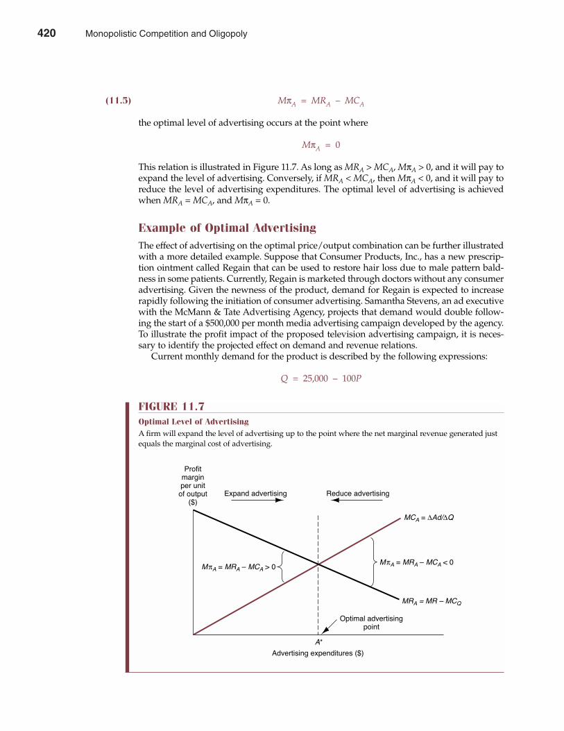
(11.5) MπA = MRA – MCA
the optimal level of advertising occurs at the point where
MπA = 0
This relation is illustrated in Figure 11.7. As long as MRA > MCA, MπA > 0, and it will pay toexpand the level of advertising. Conversely, if MRA < MCA, then MπA < 0, and it will pay toreduce the level of advertising expenditures. The optimal level of advertising is achievedwhen MRA = MCA, and MπA = 0.
Example of Optimal AdvertisingThe effect of advertising on the optimal price/output combination can be further illustratedwith a more detailed example. Suppose that Consumer Products, Inc., has a new prescrip-tion ointment called Regain that can be used to restore hair loss due to male pattern bald-ness in some patients. Currently, Regain is marketed through doctors without any consumeradvertising. Given the newness of the product, demand for Regain is expected to increaserapidly following the initiation of consumer advertising. Samantha Stevens, an ad executivewith the McMann & Tate Advertising Agency, projects that demand would double follow-ing the start of a $500,000 per month media advertising campaign developed by the agency.To illustrate the profit impact of the proposed television advertising campaign, it is neces-sary to identify the projected effect on demand and revenue relations.
Current monthly demand for the product is described by the following expressions:
Q = 25,000 – 100P
420 Part Four Market Structure Analysis and Estimation
FIGURE 11.7Optimal Level of AdvertisingA firm will expand the level of advertising up to the point where the net marginal revenue generated justequals the marginal cost of advertising.
Profitmarginper unitof output
($)Expand advertising Reduce advertising
MπA = MRA – MCA > 0
MCA = ∆Ad/∆Q
MRA = MR – MCQ
MπA = MRA – MCA < 0
Optimal advertisingpoint
A*
Advertising expenditures ($)
420 Monopolistic Competition and Oligopoly
or
P = $250 – $0.01Q
This market demand implies total and marginal revenue functions of
TR = P � Q = $250Q – $0.01Q2
MR = ∆TR/∆Q = $250 – $0.02Q
Assume total and marginal costs before advertising expenses are given by the expressions
TC = $250,000 + $50Q
MC = ∆TC/∆Q = $50
The optimal price/output combination is found by setting MR = MC and solving for Q.Because marginal costs are constant at $50 per unit, the pre-advertising optimal activity levelfor Regain is
MR = MC
$250 – $0.02Q = $500.02Q = 200
Q = 10,000
and
P = $250 – $0.01Q
= $250 – $0.01(10,000)= $150
π = TR – TC
= $250(10,000) – $0.01(10,0002) – $250,000 – $50(10,000)= $750,000 per month
Following a 100 percent advertising-inspired increase in demand, the new monthly demandrelations for Regain are
Q = 2(25,000 – 100P)= 50,000 – 200P
or
P = $250 – $0.005Q
This new advertising-induced market demand implies new total and marginal revenue func-tions of
TR = $250Q – $0.005Q2
MR = $250 – $0.01Q
The new optimal price/output combination is found by setting the new MR = MC and solvingfor Q. Because marginal costs remain constant at $50 per unit, the new optimal activity level forRegain is
Chapter Eleven Monopolistic Competition and Oligopoly 421
Monopolistic Competition and Oligopoly 421
MR = MC
$250 – $0.01Q = $500.01Q = 200
Q = 20,000
and
P = $250 – $0.005Q
= $250 – $0.005(20,000)= $150
π = TR – TC
= $250(20,000) – $0.005(20,0002) – $250,000– $50(20,000) – $500,000
= $1,250,000 per month
Notice that sales have doubled from 10,000 to 20,000 at the $150 price. The effect on profits isdramatic, rising from $750,000 to $1.25 million, even after accounting for the additional $500,000in media expenditures. Therefore, the new advertising campaign appears fully warranted. Infact, given the $1.25 million in profits that are generated by a doubling in unit sales at a price of$150, Consumer Products would be willing to pay up to that full amount to double sales. Fromthis perspective, the $500,000 price charge for the advertising campaign represents a relativebargain. The profit implications of other forms of advertising, or other types of nonprice com-petition, can be measured in a similar fashion.
GAME THEORY
Game theory concepts are used to develop effective competitive strategies for setting prices,the level of product quality, research and development, advertising, and other forms of non-price competition in oligopoly markets. Game theory concepts have also been used to setpublic policy for currency market intervention in emerging markets and auction strategies forbroadcast spectrum in the telecommunications industry. This brief introduction shows howmanagers can use a simple understanding of game theory concepts to make better manage-rial decisions.
Prisoner’s Dilemma Game theory is a general framework to help decision making when firm payoffs depend onactions taken by other firms. Because decision interdependence is a prime characteristic ofoligopoly markets, game theory concepts have a wide variety of applications in the study ofoligopoly. In a simultaneous-move game, each decision maker makes choices without spe-cific knowledge of competitor counter moves. In a sequential-move game, decision makersmake their move after observing competitor moves. If two firms set prices without knowledgeof each other’s decisions, it is a simultaneous-move game. If one firm sets its price only afterobserving its rival’s price, the firm is said to be involved in a sequential-move game. In a one-shot game, the underlying interaction between competitors occurs only once; in a repeatgame, there is an ongoing interaction between competitors.
A game theory strategy is a decision rule that describes the action taken by a decision makerat any point in time. A simple introduction to game theory strategy is provided by perhaps the
422 Part Four Market Structure Analysis and Estimation
game theoryGeneral framework tohelp decision makingwhen firm payoffsdepend on actionstaken by other firms
simultaneous-movegameChoices are made with-out specific knowledgeof competitor countermoves
sequential-movegameChoices are made afterobserving competitormoves
one-shot gameA one-time interaction
repeat gameOngoing interaction
422 Monopolistic Competition and Oligopoly
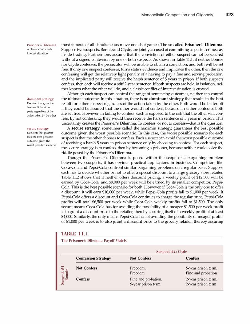
most famous of all simultaneous-move one-shot games: The so-called Prisoner’s Dilemma.Suppose two suspects, Bonnie and Clyde, are jointly accused of committing a specific crime, sayinside trading. Furthermore, assume that the conviction of either suspect cannot be securedwithout a signed confession by one or both suspects. As shown in Table 11.1, if neither Bonnienor Clyde confesses, the prosecutor will be unable to obtain a conviction, and both will be setfree. If only one suspect confesses, turns state’s evidence and implicates the other, then the oneconfessing will get the relatively light penalty of a having to pay a fine and serving probation,and the implicated party will receive the harsh sentence of 5 years in prison. If both suspectsconfess, then each will receive a stiff 2-year sentence. If both suspects are held in isolation, nei-ther knows what the other will do, and a classic conflict-of-interest situation is created.
Although each suspect can control the range of sentencing outcomes, neither can controlthe ultimate outcome. In this situation, there is no dominant strategy that results in the bestresult for either suspect regardless of the action taken by the other. Both would be better offif they could be assured that the other would not confess, because if neither confesses bothare set free. However, in failing to confess, each is exposed to the risk that the other will con-fess. By not confessing, they would then receive the harsh sentence of 5 years in prison. Thisuncertainty creates the Prisoner’s Dilemma. To confess, or not to confess—that is the question.
A secure strategy, sometimes called the maximin strategy, guarantees the best possibleoutcome given the worst possible scenario. In this case, the worst possible scenario for eachsuspect is that the other chooses to confess. Each suspect can avoid the worst possible outcomeof receiving a harsh 5 years in prison sentence only by choosing to confess. For each suspect,the secure strategy is to confess, thereby becoming a prisoner, because neither could solve theriddle posed by the Prisoner’s Dilemma.
Though the Prisoner’s Dilemma is posed within the scope of a bargaining problembetween two suspects, it has obvious practical applications in business. Competitors likeCoca-Cola and Pepsi-Cola confront similar bargaining problems on a regular basis. Supposeeach has to decide whether or not to offer a special discount to a large grocery store retailer.Table 11.2 shows that if neither offers discount pricing, a weekly profit of $12,500 will beearned by Coca-Cola, and $9,000 per week will be earned by its smaller competitor, Pepsi-Cola. This is the best possible scenario for both. However, if Coca-Cola is the only one to offera discount, it will earn $10,000 per week, while Pepsi-Cola profits fall to $1,000 per week. IfPepsi-Cola offers a discount and Coca-Cola continues to charge the regular price, Pepsi-Colaprofits will total $6,500 per week while Coca-Cola weekly profits fall to $1,500. The onlysecure means Coca-Cola has for avoiding the possibility of a meager $1,500 per week profitis to grant a discount price to the retailer, thereby assuring itself of a weekly profit of at least$4,000. Similarly, the only means Pepsi-Cola has of avoiding the possibility of meager profitsof $1,000 per week is to also grant a discount price to the grocery retailer, thereby assuring
Prisoner’s DilemmaA classic conflict-of-interest situation
dominant strategyDecision that gives thebest result for eitherparty regardless of theaction taken by the other
secure strategyDecision that guaran-tees the best possibleoutcome given theworst possible scenario
Chapter Eleven Monopolistic Competition and Oligopoly 423
TABLE 11.1The Prisoner’s Dilemma Payoff Matrix
Suspect #2: Clyde
Confession Strategy Not Confess Confess
Not Confess Freedom, 5-year prison term,Freedom Fine and probation
Confess Fine and probation, 2-year prison term,5-year prison term 2-year prison termSu
spec
t #
1:
Bon
nie
Monopolistic Competition and Oligopoly 423
itself of at least $2,000 in weekly profits. For both Coca-Cola and Pepsi-Cola, the only securestrategy is to offer discount prices, thereby assuring consumers of bargain prices and them-selves of modest profits of $4,000 and $2,000 per week, respectively.
Nash EquilibriumIn Table 11.2, each firm’s secure strategy is to offer a discount price regardless of the otherfirm’s actions. The outcome is that both firms offer discount prices and earn relatively modestprofits. This outcome is also called a Nash equilibrium because, given the strategy of its com-petitor, neither firm can improve its own payoff by unilaterally changing its own strategy. Inthe case of Coca-Cola, given that Pepsi-Cola has chosen a discount pricing strategy, it toowould decide to offer discount prices. When Pepsi-Cola offers discount prices, Coca-Cola canearn profits of $4,000 rather than $1,500 per week by also offering a discount. Similarly, whenCoca-Cola offers discount prices, Pepsi-Cola can earn maximum profits of $2,000 per week,versus $1,000 per week, by also offering a discount.
Clearly, profits are less than if they colluded and both charged regular prices. As seen inTable 11.2, Coca-Cola would earn $12,500 per week and Pepsi-Cola would earn $9,000 per weekif both charged regular prices. This is a business manifestation of the Prisoner’s Dilemmabecause the dual discount pricing Nash equilibrium is inferior from the firms’ viewpoint to acollusive outcome where both competitors agree to charge regular prices.
Of course, if firms collude and agree to charge high prices, consumers are made worse off.This is why price collusion among competitors is illegal in the United States, as discussed inChapter 13.
Nash BargainingA Nash bargaining game is another application of the simultaneous-move, one-shot game.In Nash bargaining, two competitors or players “bargain” over some item of value. In asimultaneous-move, one-shot game, the players have only one chance to reach an agreement.
For example, suppose the board of directors specifies a $1 million profit-sharing pool pro-vided that both management and workers can come to agreement concerning how such profitsare to be distributed. For simplicity, assume that this pool can only be distributed in amounts of$0, $500,000, and $1 million. If the sum of the amounts requested by each party totals more than$1 million, neither party receives anything. If the sum of the amounts requested by each partytotals no more than $1 million, each party receives the amount requested.
Table 11.3 shows the nine possible outcomes from such a profit-sharing bargaining game. Ifthe workers request $1 million, the only way that they would get any money at all is if man-agement requests nothing. Similarly, if management requests $1 million, the only way they getmoney is if workers request nothing. If either party requests nothing, Nash equilibrium solu-tions are achieved when the other party requests the full $1 million. Thus, the ($1 million, $0)and ($0, $1 million) solutions are both Nash equilibriums. However, suppose the workers
424 Part Four Market Structure Analysis and Estimation
Nash equilibriumSet of decision strate-gies where no playercan improve through aunilateral change instrategy
Nash bargainingWhere two competitorshaggle over some itemof value
TABLE 11.2A Hypothetical Prisoner’s Dilemma Faced by Coca-Cola and Pepsi-Cola
Pepsi-Cola
Discount Price Regular Price
Discount Price $4,000, $2,000 $10,000, $1,000Regular Price $1,500, $6,500 $12,500, $9,000C
oca-
Col
a
424 Monopolistic Competition and Oligopoly
request $500,000; then the Nash equilibrium response from management would be to alsorequest $500,000. If management requests $500,000, then the Nash equilibrium response fromworkers would be to also request $500,000. Thus, the ($500,000, $500,000) payoff is also a Nashequilibrium. This game involves three Nash equilibriums out of nine possible solutions. In eachNash equilibrium, the entire profit-sharing pool is paid out. In the six remaining outcomes, someof the profit-sharing pool would not be distributed. Such suboptimal outcomes can and do occurin real-life situations.
However, in contemplating the bargaining process, workers are apt to note that a request for$0 is dominated by asking for either $500,000 or $1 million. If you do not ask for anything, youare sure of getting nothing. Similarly, management will never do worse, and may do better, if itasks for something. As a result, the $0 request strategy is dominated for both parties and willtend not to be followed. In addition, a request for the entire $1 million by either party will notbe successful unless the other party requests nothing. Because a $0 request by either party is notlikely, neither party is likely to request the full $1 million. In this case, the logical and rationalrequest from each party is $500,000, or an equal 50/50 sharing of the profit pool.
Repeat GamesThe study of one-shot pricing and product quality games might lead one to conclude that eventacit collusion is impossible. This is not true because competitors often interact on a continuousbasis. In such circumstances, firms are said to be involved in repeat games.
When a competitive game is repeated over and over, firms receive sequential payoffs thatshape current and future strategies. For example, in Table 11.2, both Coca-Cola and Pepsi-Colamight tacitly or secretly agree to charge regular prices so long as the other party continues todo so. If neither firm cheats on such a collusive agreement, discounts will never be offered, andmaximum profits will be earned. Although there is an obvious risk involved with chargingregular prices, there is also an obvious cost if either or both firms offer discount pricing. If eachfirm is convinced that the other will maintain regular prices, both will enjoy high profits. Thisresolve is increased if each firm is convinced that the other will quickly match any discountpricing strategy. In fact, it is rational for colluding firms to quickly and severely punish col-luding competitors who “cheat” by lowering prices.
However, although it is important to recognize that the repeat nature of competitor interac-tions can sometimes harm consumers, it is equally important to recognize that repetitive inter-actions in the marketplace provide necessary incentives for firms to produce high-qualitygoods. In any one-shot game, it would pay firms with high-quality reputations to producelow-cost or shoddy goods. In the real world, the ongoing interaction between firms and theircustomers provides incentives for firms to maintain product consistency. For example, both
repeat gamesA comprehensive statis-tical profile of the econ-omy, from the national,to the state, to the locallevel
Chapter Eleven Monopolistic Competition and Oligopoly 425
TABLE 11.3Nash Bargaining Game over Profit-Pool Sharing
Management
Request Strategy $0 $500,000 $1,000,000
$0 $0 $0, $0,$0 $500,000 $1,000,000
$500,000 $500,000, $500,000, $0,$0 $500,000 $0
$1,000,000 $1,000,000, $0, $0,$0 $0 $0
Wor
kers
Monopolistic Competition and Oligopoly 425
Coca-Cola and Pepsi-Cola have well-deserved reputations for providing uniformly high-quality soft drinks. They have both invested millions of dollars in product development andquality control to ensure that consumers can depend upon the taste, smell, and feel of Coca-Cola and Pepsi-Cola products. Moreover, because the value of millions of dollars spent onbrand-name advertising would be lost if product quality were to deteriorate, that brand-name advertising is itself a type of quality assurance provided to customers of Coca-Cola andPepsi-Cola. At Wal-Mart, Satisfaction Guaranteed, or your money back, is more than just a slogan.It is their business; it is what separates Wal-Mart from fly-by-night operators or low-qualitydiscount stores. Similarly, customers of DaimlerChrysler depend upon that company’s well-deserved reputation for producing high-quality cars, trucks, and minivans. Like any writtenguarantee or insurance policy, repeat transactions in the marketplace give consumers confi-dence that they will get what they pay for.
MARKET STRUCTURE MEASUREMENT
To formulate an effective competitive strategy, managers must accurately assess the currentcompetitive environment for actual and potential products. Data gathered by the federalgovernment, private market research firms, and trade associations are often useful for thispurpose. This section shows the types of market structure data available from public sourcesand explains why they are important for decision-making purposes.
How Are Economic Markets Measured?An economic market consists of all individuals and firms willing and able to buy or sell com-peting products during a given period. The key criterion in identifying competing products is
426 Part Four Market Structure Analysis and Estimation
Dot.com
With all the hoopla, it is tough to sort out what’s realand what’s Internet hype. For companies, building apublishing-only Web site is the first step to becoming ane-business. Most businesses have already done this.That’s fine as far as it goes; it’s an extremely cost-efficientway to distribute basic information. However, the payofffor business starts with “self-service” Web sites wherecustomers can do things like check the status of anaccount or trace a package online (like at FedEX). Thereal payoff begins with transaction-based Web sites thatgo beyond just buying and selling to create a dynamicand interactive flow of information.
An e-business is created when companies put theircore processes online to improve service, cut costs, orboost revenue. For example, IBM helped Charles SchwabWeb-enable their brokerage systems for online tradingand customer service. Since opening, Schwab’s Web service has generated over 1 million online accountstotaling over $50 billion in assets. E-business economicsare compelling. According to management consultants,traditional bank transactions cost more than a dollar; thesame transaction over the Web costs about 1¢. Issuing a
paper airline ticket costs about $8; an e-ticket costs just$1. Customers love the convenience; management lovesthe lower costs.
Although a number of companies use the Web tofurther exploit long-standing competitive advantages, itis not clear that companies can use the Web to createdurable competitive advantages. Hoping to stand outfrom the crowd, some Internet merchants devote asmuch as 70 percent of total revenues to advertising. “Getahead and stay ahead” is the mantra at Amazon.com, acompany trying to create a durable online marketingpresence in books, electronics, computers, toys andgames, health and beauty aids, DVDs, and much more.To date, Amazon.com has proven adept at quickly grow-ing online revenues. It’s a widely recognized onlineleader. However, even for Amazon.com, building onlineprofits has proven elusive.
See: Nick Wingfield, “Amazon Posts Surprise Profit; Sales Rose 15% in4th Quarter,” The Wall Street Journal Online, January 23, 2002(http://online.wsj.com).
M A N A G E R I A L A P P L I C AT I O N 1 1 . 3
426 Monopolistic Competition and Oligopoly
similarity in use. Precise determination of whether a specific good is a distinct economic prod-uct involves an evaluation of cross-price elasticities for broad classes of goods. When cross-priceelasticities are large and positive, goods are substitutes for each other and can be thought of ascompeting products in a single market. Conversely, large negative cross-price elasticities indi-cate complementary products. Complementary products produced by a single firm must beevaluated as a single product line serving the same market. If complementary products are pro-duced by other companies, evaluating the potential of a given product line involves incorpo-rating exogenous influences beyond the firm’s control. When cross-price elasticities are nearzero, goods are in separate economic markets and can be separately analyzed as serving distinctconsumer needs. Therefore, using cross-price elasticity criteria to desegregate the firm’s overallproduct line into its distinct economic markets is an important task confronting managers.
To identify relevant economic markets and define their characteristics, firms in the UnitedStates make extensive use of economic data collected by the Bureau of the Census of the U.S.Department of Commerce. Because these data provide valuable information on economicactivity across the broad spectrum of U.S. industry, it is worthwhile to briefly consider themethod and scope of the economic censuses.
Economic CensusOnce every 5 years, the economic census provides a comprehensive statistical profile of theeconomy, from the national, to the state, to the local level. Censuses are taken at 5-year intervalsduring years ending with the digits 2 and 7—for example, 1992, 1997, 2002, 2007, and so on. Asshown in Figure 11.8, the economic census covers economic activity in important sectors suchas manufacturing, retail and wholesale trade, services, minerals, and construction. Sectorscovered account for roughly three-quarters of total economic activity originating in the pri-vate sector. Principal industry groups with incomplete coverage are agriculture, education,financial services, forestry, professional services, and transportation.
The economic census is the primary source of detailed public facts about the nation’s econ-omy. As such, census data are essential inputs for decisions made by managers in government,business, and the not-for-profit sector. Economic census data allows businesses to comparecompany sales to census totals for specific industries or areas, calculate market share, evaluateperformance, and make plans for expansion or asset redeployment. Companies can use censusdata to lay out territories, allocate advertising, and locate new stores or offices. Firms supplyinggoods and services to other businesses also use census data to target industries for business-to-business marketing. Manufacturers look at statistics on materials consumed to learn more aboutindustries that use their products and to gain insight concerning industry growth potential. Allfirms compare operating ratios to census averages to see how they stack up against competitivenorms. Consultants, government researchers, and job seekers use census data to analyze changesin industrial structure, location, and the pace of growth in job opportunities. Both state and fed-eral regulators use census data to monitor business activity as captured by fluctuations inmonthly retail sales, gross domestic product (GDP), and other such measures. Industry tradeassociations and news media study census data to learn key business facts and to project trends.Legislators use census data in the preparation and evaluation of new legislation designed tospur economic development. State and local government agencies monitor census informationto better understand their regional economic base and to help them better focus efforts to attractnew businesses and/or retain existing firms.
The economic census covers nearly all of the U.S. economy in its establishment statistics.There also are several related programs, including the collection and publication of statistics onminority- and women-owned businesses. Separate censuses of agriculture and government arealso conducted at the same time as the economic census. Results from this most recent economiccensus were issued on CD-ROM and on the Internet in a series of continuing reports over a peri-od of more than 2 years, starting in early 1999. Only summary reports are issued in print.
economic censusA comprehensive statistical profile of theeconomy, from thenational, to the state, tothe local level
Chapter Eleven Monopolistic Competition and Oligopoly 427
Monopolistic Competition and Oligopoly 427
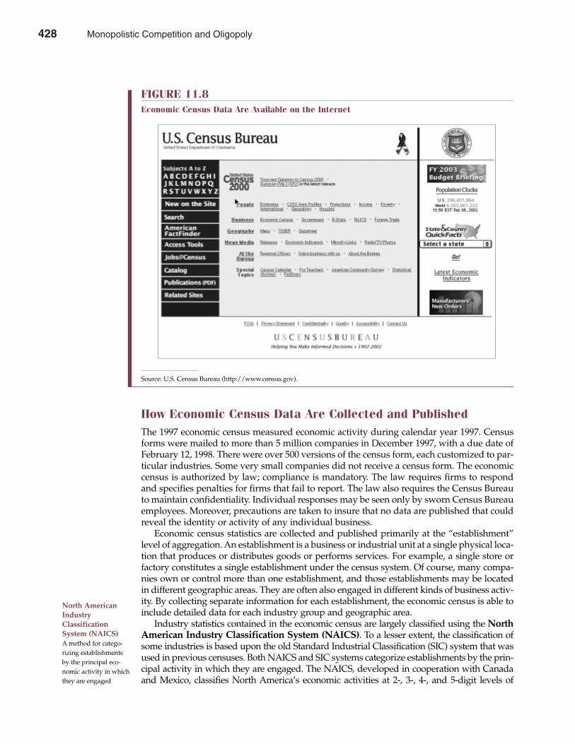
How Economic Census Data Are Collected and PublishedThe 1997 economic census measured economic activity during calendar year 1997. Censusforms were mailed to more than 5 million companies in December 1997, with a due date ofFebruary 12, 1998. There were over 500 versions of the census form, each customized to par-ticular industries. Some very small companies did not receive a census form. The economiccensus is authorized by law; compliance is mandatory. The law requires firms to respondand specifies penalties for firms that fail to report. The law also requires the Census Bureauto maintain confidentiality. Individual responses may be seen only by sworn Census Bureauemployees. Moreover, precautions are taken to insure that no data are published that couldreveal the identity or activity of any individual business.
Economic census statistics are collected and published primarily at the “establishment”level of aggregation. An establishment is a business or industrial unit at a single physical loca-tion that produces or distributes goods or performs services. For example, a single store orfactory constitutes a single establishment under the census system. Of course, many compa-nies own or control more than one establishment, and those establishments may be locatedin different geographic areas. They are often also engaged in different kinds of business activ-ity. By collecting separate information for each establishment, the economic census is able toinclude detailed data for each industry group and geographic area.
Industry statistics contained in the economic census are largely classified using the NorthAmerican Industry Classification System (NAICS). To a lesser extent, the classification ofsome industries is based upon the old Standard Industrial Classification (SIC) system that wasused in previous censuses. Both NAICS and SIC systems categorize establishments by the prin-cipal activity in which they are engaged. The NAICS, developed in cooperation with Canadaand Mexico, classifies North America’s economic activities at 2-, 3-, 4-, and 5-digit levels of
428 Part Four Market Structure Analysis and Estimation
North AmericanIndustryClassificationSystem (NAICS)A method for catego-rizing establishmentsby the principal eco-nomic activity in whichthey are engaged
FIGURE 11.8Economic Census Data Are Available on the Internet
Source: U.S. Census Bureau (http://www.census.gov).
428 Monopolistic Competition and Oligopoly
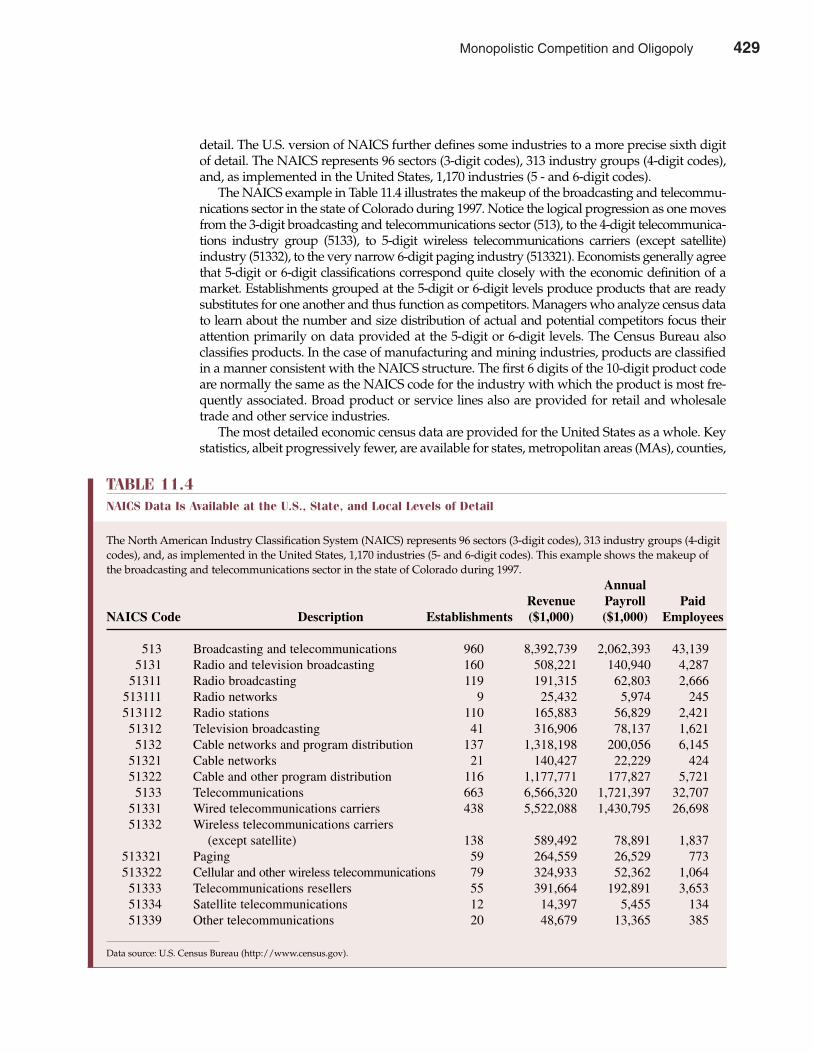
detail. The U.S. version of NAICS further defines some industries to a more precise sixth digitof detail. The NAICS represents 96 sectors (3-digit codes), 313 industry groups (4-digit codes),and, as implemented in the United States, 1,170 industries (5 - and 6-digit codes).
The NAICS example in Table 11.4 illustrates the makeup of the broadcasting and telecommu-nications sector in the state of Colorado during 1997. Notice the logical progression as one movesfrom the 3-digit broadcasting and telecommunications sector (513), to the 4-digit telecommunica-tions industry group (5133), to 5-digit wireless telecommunications carriers (except satellite)industry (51332), to the very narrow 6-digit paging industry (513321). Economists generally agreethat 5-digit or 6-digit classifications correspond quite closely with the economic definition of amarket. Establishments grouped at the 5-digit or 6-digit levels produce products that are readysubstitutes for one another and thus function as competitors. Managers who analyze census datato learn about the number and size distribution of actual and potential competitors focus theirattention primarily on data provided at the 5-digit or 6-digit levels. The Census Bureau alsoclassifies products. In the case of manufacturing and mining industries, products are classifiedin a manner consistent with the NAICS structure. The first 6 digits of the 10-digit product codeare normally the same as the NAICS code for the industry with which the product is most fre-quently associated. Broad product or service lines also are provided for retail and wholesaletrade and other service industries.
The most detailed economic census data are provided for the United States as a whole. Keystatistics, albeit progressively fewer, are available for states, metropolitan areas (MAs), counties,
Chapter Eleven Monopolistic Competition and Oligopoly 429
TABLE 11.4NAICS Data Is Available at the U.S., State, and Local Levels of Detail
The North American Industry Classification System (NAICS) represents 96 sectors (3-digit codes), 313 industry groups (4-digitcodes), and, as implemented in the United States, 1,170 industries (5- and 6-digit codes). This example shows the makeup ofthe broadcasting and telecommunications sector in the state of Colorado during 1997.
Annual Revenue Payroll Paid
NAICS Code Description Establishments ($1,000) ($1,000) Employees
513 Broadcasting and telecommunications 960 8,392,739 2,062,393 43,1395131 Radio and television broadcasting 160 508,221 140,940 4,287
51311 Radio broadcasting 119 191,315 62,803 2,666513111 Radio networks 9 25,432 5,974 245513112 Radio stations 110 165,883 56,829 2,42151312 Television broadcasting 41 316,906 78,137 1,6215132 Cable networks and program distribution 137 1,318,198 200,056 6,145
51321 Cable networks 21 140,427 22,229 42451322 Cable and other program distribution 116 1,177,771 177,827 5,7215133 Telecommunications 663 6,566,320 1,721,397 32,707
51331 Wired telecommunications carriers 438 5,522,088 1,430,795 26,69851332 Wireless telecommunications carriers
(except satellite) 138 589,492 78,891 1,837513321 Paging 59 264,559 26,529 773513322 Cellular and other wireless telecommunications 79 324,933 52,362 1,06451333 Telecommunications resellers 55 391,664 192,891 3,65351334 Satellite telecommunications 12 14,397 5,455 13451339 Other telecommunications 20 48,679 13,365 385
Data source: U.S. Census Bureau (http://www.census.gov).
Monopolistic Competition and Oligopoly 429
and other places with 2,500 or more inhabitants. Only limited data are provided for ZIP codes.Statistics for smaller areas are typically withheld to avoid disclosing information about individ-ual firms. The level of geographic detail varies widely for major data items. Basic census contentincludes several key statistics such as the number of establishments (or companies), number ofemployees, payroll, and measures of output like sales revenue, which the economic census refersto as the value of shipments.
Because the economic census is now based on the NAICS, only limited information is pub-lished according to the old SIC system. However, a detailed “bridge table” showing the rela-tionships between NAICS and SIC categories makes for an easier comparison between currentand previous statistics. Although still very slow by private-sector standards, 2002 economiccensus results will become available on the Internet much faster than the results from priorcensuses, which were largely distributed in printed form. Although only highlights of recenteconomic censuses are available in printed form, software on both CD-ROM and the Internetallows companies to print detailed data. Given a faster publication cycle, industry reports formanufacturing, mining, and construction, previously issued in both preliminary and finalform, are now issued only once. In another recent change, all reports are now titled simply aseconomic census reports. They are no longer treated as if each sector had a separate census,e.g., the census of manufacturers.
Detailed data are issued, sector by sector, on CD-ROM and on the Internet. Geographicarea series (published for all sectors) provide detail for establishments with employees, forthe nation, states, and substate areas. ZIP code statistics are also published for most sectors.Industry series reports for manufacturing, mining, and construction provide national totalson groups of related industries and their products. Limited data are available for individualstates. Subject series (all sectors) provide national and limited local data on special topicsincluding merchandise line sales, concentration ratios, and both establishment and firm sizes.Summary reports by sector provide highlights of the data in print. They feature primarilynational data and general statistics by state, and include illustrations of some of the moredetailed data available in electronic media. Table 11.4 shows a typical example of the level ofdetail available in the geographic area series. This example shows the makeup of the broad-casting and telecommunications sector in the state of Colorado during 1997.
CENSUS MEASURES OF MARKET CONCENTRATION
Pricing strategies and profit rates tend to be heavily influenced by the vigor of competition.As a result, information from the economic census on the number and size distribution ofcompetitors is a vital input into the managerial decision-making process.
Concentration RatiosIn addition to those directly engaged in business, both government and the public share aninterest in the number and size distribution of competitors. A small number of competitors cansometimes have direct implications for regulation and antitrust policy. Thus, considerablepublic resources are devoted to monitoring both the size distribution and economic perform-ance of firms in several important sectors of the economy. Among those sectors covered by theeconomic census, manufacturing is clearly the largest, accounting for approximately 20 per-cent of aggregate economic activity in the United States. Firm sizes in manufacturing are alsomuch larger than in other major sectors such as retail and wholesale trade, construction, legaland medical services, and so on. Among the more than 16 million business enterprises in theUnited States, manufacturing is the domain of the large corporation. Thus, the manufacturingsector provides an interesting basis for considering data that are available on the size distribu-tion of firms.
430 Part Four Market Structure Analysis and Estimation
430 Monopolistic Competition and Oligopoly
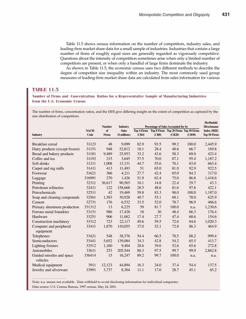
Table 11.5 shows census information on the number of competitors, industry sales, andleading-firm market share data for a small sample of industries. Industries that contain a largenumber of firms of roughly equal sizes are generally regarded as vigorously competitive.Questions about the intensity of competition sometimes arise when only a limited number ofcompetitors are present, or when only a handful of large firms dominate the industry.
As shown in Table 11.5, the economic census uses two different methods to describe thedegree of competitor size inequality within an industry. The most commonly used groupmeasures of leading-firm market share data are calculated from sales information for various
Chapter Eleven Monopolistic Competition and Oligopoly 431
TABLE 11.5Number of Firms and Concentration Ratios for a Representative Sample of Manufacturing Industries from the U.S. Economic Census
The number of firms, concentration ratios, and the HHI give differing insight on the extent of competition as captured by thesize distribution of competitors.
Herfindahl Number Industry Percentage of Sales Accounted for by Hirschmann
NACIS of Sales Top 4 Firms Top 8 Firms Top 20 Firms Top 50 Firms Index (HHI)Industry Code Firms ($ millions) (CR4) (CR8) (CR20) (CR50) Top 50 Firms
Breakfast cereal 31123 48 9,099 82.9 93.5 99.2 100.0 2,445.9 Dairy products (except frozen) 31151 948 52,812 18.1 28.4 48.6 66.7 169.8 Bread and bakery products 31181 9,489 25,953 33.2 43.6 58.3 69.0 423.4 Coffee and tea 31192 215 3,645 57.5 70.0 87.1 95.4 1,187.2 Soft drinks 31211 1,008 13,131 44.7 55.6 70.1 83.0 663.4 Carpet and rug mills 31411 413 11,493 51 65.0 81.0 92.9 922.5 Footwear 31621 366 4,211 27.7 42.4 65.0 84.3 317.0 Luggage 316991 270 1,426 51.9 62.4 75.0 86.8 1,418.6 Printing 32311 36,617 90,565 10.1 14.8 22.4 29.7 43.3 Petroleum refineries 32411 122 158,668 28.5 48.6 81.6 97.6 422.1 Petrochemicals 32511 42 19,469 59.8 83.3 98.0 100.0 1,187.0 Soap and cleaning compounds 32561 1,583 30,928 40.7 55.1 68.1 78.0 625.9 Cement 32731 176 6,532 33.5 52.0 78.7 96.9 466.6 Primary aluminum production 331312 13 6,225 59 81.7 100.0 n.a. 1,230.6 Ferrous metal foundries 33151 986 17,428 18 30 48.4 66.3 176.4 Hardware 33251 906 11,062 17.4 27.7 47.4 68.6 154.6 Construction machinery 33312 723 22,117 49.6 59.5 72.6 84.6 1,020.3 Computer and peripheral 33411 1,870 110,055 37.0 52.1 72.8 86.3 464.9
equipmentTelephones 33421 548 38,376 54.4 66.5 78.5 88.2 999.4 Semiconductors 33441 5,652 139,084 34.3 42.8 54.2 65.5 413.7 Lighting fixtures 33512 1,160 9,404 28.6 39.6 52.6 65.6 272.8 Automobiles 33611 253 205,544 88.3 97.5 99.7 99.9 2,862.8 Guided missiles and space 336414 15 16,247 89.2 99.7 100.0 n.a. n.a.
vehiclesMedical equipment 3911 12,123 44,894 16.3 24.0 37.4 54.4 137.5 Jewelry and silverware 33991 3,737 8,304 11.1 17.0 28.7 45.1 65.2
Note: n.a. means not available. Data withheld to avoid disclosing information for individual companies.Data source: U.S. Census Bureau, 1997 census, May 24, 2001.
Monopolistic Competition and Oligopoly 431
clusters of top firms. These group market share data are called concentration ratios becausethey measure the percentage market share concentrated in (or held by) an industry’s top four(CR4), eight (CR8), 20 (CR20), or 50 (CR50) firms. Thus, the concentration ratio for a group of nleading firms is defined in percentage terms as:
n
(11.6) CRn =∑ Firm Salesii = 1
Industry Sales � 100
where i refers to an individual firm.Theoretically, concentration ratios can range between CRn = 0 for an industry with a massive
number of small competitors, to CRn = 100 for an industry represented by a single monopolist.In the manufacturing sector where concentration tends to be highest, four-firm concentrationratios tend to fall in a broad range between CR4 = 20 and CR4 = 60; eight-firm concentrationratios often lie in a range between CR8 = 30 and CR8 = 70. When concentration ratios are low,industries tend to include many firms, and competition tends to be vigorous. Industries inwhich the four leading firms are responsible for less than 20 percent of total industry sales (i.e.,CR4 < 20) are highly competitive and approximate the perfect competition model. On the otherhand, when concentration ratios are high, leading firms dominate following firms in terms ofsize, and leading firms may have more potential for pricing flexibility and economic profits.Industries in which the four leading firms control more than 80 percent of total industry sales(i.e., CR4 > 80) are often described as highly concentrated. Industries with a CR4 < 20 or CR4 > 80,however, are quite rare. Three-quarters of all manufacturing activity takes place in industrieswith concentration ratios falling in the range 20 ≤ CR4 ≤ 80. In terms of relative importance, mar-ket structures that can be described as monopolistically competitive are much more commonthan perfect competition or monopoly.
Herfindahl Hirschmann IndexBy definition, concentration ratios rise with greater competitor size inequality within a givenindustry. Concentration ratios, however, are unaffected by the degree of size inequality withineach respective group of leading firms. This can create problems because competition withinindustries featuring a handful of large competitors can be much more vigorous than in thosewhere a single dominant firm faces no large adversaries. For example, although CR4 = 100would signal monopoly in the case of a single dominant firm, it might describe a vigorouslycompetitive industry if each of the leading four firms enjoy roughly equal market shares of 25percent. The Herfindahl Hirschmann Index (HHI), named after the economists who invent-ed it, is a popular measure of competitor size inequality that reflects size differences among largeand small firms. Calculated in percentage terms, the HHI is the sum of the squared market sharesfor all n industry competitors:
n
(11.7)HHI = ∑ � Firm Salesi �
2
i = 1 Industry Sales � 100
For example, a monopoly industry with a single dominant firm is described by a CR4 = 100 andan HHI = 1002 = 10,000. A vigorously competitive industry where each of the leading four firmsenjoys market shares of 25 percent is also described by a CR4 = 100, but features an HHI = 252
+252 +252 +252 = 2,500. Like concentration ratios, the HHI approaches zero for industries char-acterized by a large number of very small competitors.
432 Part Four Market Structure Analysis and Estimation
concentration ratiosData that show thepercentage marketshare held by a groupof leading firms
HerfindahlHirschmann Index(HHI)The sum of squaredmarket shares for all nindustry competitors
432 Monopolistic Competition and Oligopoly
Limitations of Concentration Ratios and HHI InformationDespite the obvious attraction of census concentration ratios and HHI data as useful infor-mation on the number and size distribution of current competitors, it is prudent to remaincautious in their use and interpretation. Important limitations must be recognized. By notappreciating these limitations, one might make fundamental errors in judging the vigor ofcompetition within industries.
A major drawback of concentration ratio and HHI information is that they take a longtime to collect and publish. Data for 1997 were not generally available on the Internet until2000 and 2001; data for 2002 will be collected in 2003 and published in 2004 and 2005. Inmany fast-moving markets, these data are obsolete before they are published. Even in lessdynamic markets, they provide only an imperfect guide to managerial decision making. Asa result, many managers supplement census information with current data available on theInternet from market research firms.
Afurther important weakness of census concentration ratio and HHI information is that theyignore domestic sales by foreign competitors (imports) as well as exports by domestic firms.Only data on domestic sales from domestic production, not total domestic sales, are reported. Thismeans, for example, that if foreign imports have a market share of 25 percent, the four leadingdomestic automobile manufacturers account for 66.2 percent (= 88.3 percent of 75 percent) oftotal U.S. foreign plus domestic car sales (NAICS 33611), rather than the 88.3 percent, as Table11.5 suggests. For industries with significant import competition, concentration ratios and HHIdata significantly overstate the relative importance of leading domestic firms. Concentrationratios and HHI information also overstate market power for several industries in which increas-ing foreign competition has been responsible for the liquidation or merger of many smallerdomestic firms with older, less efficient production facilities. Despite reduced numbers of domes-tic firms and the consequent rise in concentration, an increase in foreign competition often makesaffected industries more efficient and more competitive rather than less so. The impact of foreigncompetition is important in many industries, but it is particularly so in manufacturing industriessuch as apparel, steel, automobiles, cameras, copiers, motorcycles, and television sets.
Another limitation of concentration ratio data is that they are national totals, whereas a rel-evant economic market may be national, regional, or local in scope. If high transportation costsor other product characteristics keep markets regional or local rather than national in scope,concentration ratios can significantly understate the relative importance of leading firms. Forexample, the leading firm in many metropolitan newspaper markets often approaches 100 per-cent of classified advertising and subscription revenues. Thus, a national CR4 for newspaperswould significantly understate local market power. Although national four-firm concentrationratios of less than 25 percent usually suggest a highly competitive market, the local or regionalcharacter of some markets can make national concentration figures meaningless. Examples ofother products with local or regional rather than national markets include milk, bread andbakery products, commercial printing, and ready-mix concrete.
Additional problems occur because concentration ratios and HHI information providean imperfect view of market structure by including only firms that are currently active in aparticular industry. Recall that an economic market includes all firms willing and able to sellan identifiable product. Besides firms currently active in an industry, this includes those thatcan be regarded as likely potential entrants. Often the mere presence of one or more poten-tial entrants constitutes a sufficient threat to force competitive market behavior in industrieswith only a handful of established competitors. Major retailers such as Wal-Mart, Target, andSears, for example, use their positions as potential entrants into manufacturing to obtainattractive prices on a wide range of private-label merchandise such as clothing, lawn mow-ers, washing machines, and so on.
Chapter Eleven Monopolistic Competition and Oligopoly 433
Monopolistic Competition and Oligopoly 433
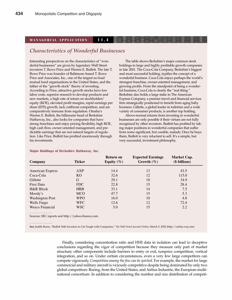
Finally, considering concentration ratio and HHI data in isolation can lead to deceptiveconclusions regarding the vigor of competition because they measure only part of marketstructure; other components include barriers to entry or exit, nonprice competition, verticalintegration, and so on. Under certain circumstances, even a very few large competitors cancompete vigorously. Competition among the few can be spirited. For example, the market for largecommercial and military aircraft is viciously competitive despite being dominated by only twoglobal competitors: Boeing, from the United States, and Airbus Industrie, the European multi-national consortium. In addition to considering the number and size distribution of competi-
434 Part Four Market Structure Analysis and Estimation
Characteristics of Wonderful Businesses
Interesting perspectives on the characteristics of “won-derful businesses” are given by legendary Wall Streetinvestors T. Rowe Price and Warren E. Buffett. The late T.Rowe Price was founder of Baltimore–based T. RowePrice and Associates, Inc., one of the largest no-loadmutual fund organizations in the United States, and thefather of the “growth stock” theory of investing.According to Price, attractive growth stocks have lowlabor costs, superior research to develop products andnew markets, a high rate of return on stockholders’ equity (ROE), elevated profit margins, rapid earnings pershare (EPS) growth, lack cutthroat competition, and arecomparatively immune from regulation. Omaha’sWarren E. Buffett, the billionaire head of BerkshireHathaway, Inc., also looks for companies that havestrong franchises and enjoy pricing flexibility, high ROE,high cash flow, owner-oriented management, and pre-dictable earnings that are not natural targets of regula-tion. Like Price, Buffett has profited enormously throughhis investments.
The table shows Berkshire’s major common stockholdings in large and highly profitable growth companiesin late 2001. The Coca-Cola Company, Berkshire’s biggestand most successful holding, typifies the concept of awonderful business. Coca-Cola enjoys perhaps the world’sstrongest franchise, owner-oriented management, andgrowing profits. From the standpoint of being a wonder-ful business, Coca-Cola is clearly the “real thing.”Berkshire also holds a large stake in The AmericanExpress Company, a premier travel and financial servicesfirm strategically positioned to benefit from aging babyboomers. Gillette, a global leader in toiletries and a widevariety of consumer products, is another top holding.
Above-normal returns from investing in wonderfulbusinesses are only possible if their virtues are not fullyrecognized by other investors. Buffett has profited by tak-ing major positions in wonderful companies that sufferfrom some significant, but curable, malady. Once he buysthem, Buffett is very reluctant to sell. It’s a simple, butvery successful, investment philosophy.
M A N A G E R I A L A P P L I C AT I O N 1 1 . 4
Major Holdings of Berkshire Hathaway, Inc.
Return on Expected Earnings Market Cap.Company Ticker Equity (%) Growth (%) ($ billions)
American Express AXP 14.4 13 43.5Coca-Cola KO 32.6 12 115.0 Gillette G 29.1 10 34.9First Data FDC 22.8 15 28.4H&R Block HRB 33.1 14 7.5Moody’s MCO 47.7 15 5.3Washington Post WPO 16.0 10 4.8Wells Fargo WFC 12.6 12 72.4Wesco Financial WSC 5.0 15 2.2
Sources: SEC reports and http://yahoo.finance.com.
See: Judith Burns, “Buffett Tells Investors to Get Tough with Companies,” The Wall Street Journal Online, March 5, 2002 (http://online.wsj.com).
434 Monopolistic Competition and Oligopoly

tors, firms must judge the competitive environment in light of foreign competition, transporta-tion costs, regional product differences, likely potential entrants, advertising, customer loyalty,research and development, demand growth, and economies of scale in production, among otherfactors, to make accurate pricing and output decisions. All of these features constitute importantelements of market structure.
COMPETITIVE STRATEGY IN MONOPOLISTIC COMPETITIONAND OLIGOPOLY MARKETS
Developing and implementing an effective competitive strategy in imperfectly competitivemarkets involves a never-ending search for uniquely attractive products. Not all industries offerthe same potential for sustained profitability; not all firms are equally capable of exploiting theprofit potential that is available.
Competitive Strategy in Imperfectly Competitive MarketsIt is always helpful to consider the number and size distribution of competitors, degree ofproduct differentiation, level of information available in the marketplace, and conditions ofentry when attempting to define market structure. Unfortunately, these and other readilyobtained data are seldom definitive. Conditions of entry and exit are subtle and dynamic, asis the role of unseen potential entrants. All of this contributes to the difficulty of correctlyassessing the profit potential of current products or prospective lines of business.
Rather than consider simply what is, effective managers must contemplate what mightbe. This is especially true when seeking to develop an effective competitive strategy. Aneffective competitive strategy in imperfectly competitive markets must be founded on thefirm’s competitive advantage. A competitive advantage is a unique or rare ability to create,distribute, or service products valued by customers. It is the business-world analog to whateconomists call comparative advantage, or when one nation or region of the country is bettersuited to the production of one product than to the production of some other product. Forexample, when compared with the United States and Canada, Mexico enjoys a relativeabundance of raw materials and cheap labor. As such, Mexico is in a relatively good positionto export agricultural products, oil, and finished goods that require unskilled labor to the U.S.and Canadian market. At the same time, the United States and Canada enjoy a relative abun-dance of highly educated people, capital goods, and investment resources. Therefore, the UnitedStates and Canada are in a relatively good position to export machine tools, computer equip-ment, education, and professional services to Mexico.
An effective competitive strategy in imperfectly competitive markets grows out of a sophis-ticated understanding of the rules of competition in a given line of business or industry. The ulti-mate aim of this strategy is to cope with or, better still, change those rules in the company’s favor.To do so, managers must understand and contend with the rivalry among existing competitors,entry of new rivals, threat of substitutes, bargaining power of suppliers, and the bargainingpower of buyers. Just as all industries are not alike in terms of their inherent profit potential, allfirms are not alike in terms of their capacity to exploit available opportunities. In the businessworld, long-lasting above-normal rates of return require a sustainable competitive advantagethat, by definition, cannot be easily duplicated.
Nike’s use of basketball superstar Michael Jordan as the focal point of its extensive mediaadvertising and product development campaign is an interesting case in point. Like otherhighly successful and innovative advertising campaigns, the Nike promotion captured theimagination of consumers and put competitors like Reebok at a distinct disadvantage. Afterall, there is only one Michael Jordan. Nike sales surged as consumers got caught up in theenthusiasm of Jordan’s amazing basketball prowess and the excitement generated as the
competitive advantageA unique or rare abilityto create, distribute, orservice products valuedby customers
comparative advantageWhen one nation orregion of the country isbetter suited to the pro-duction of one productthan to the productionof some other product
Chapter Eleven Monopolistic Competition and Oligopoly 435
Monopolistic Competition and Oligopoly 435
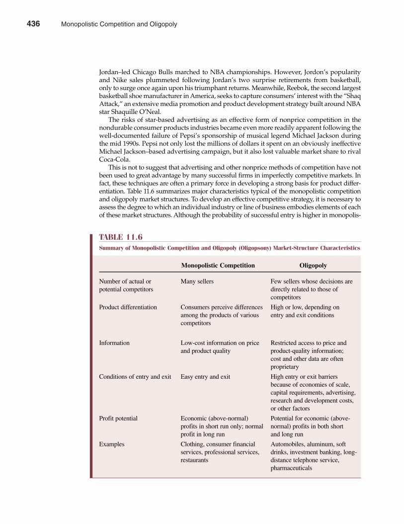
Jordan–led Chicago Bulls marched to NBA championships. However, Jordon’s popularityand Nike sales plummeted following Jordan’s two surprise retirements from basketball,only to surge once again upon his triumphant returns. Meanwhile, Reebok, the second largestbasketball shoe manufacturer in America, seeks to capture consumers’ interest with the “ShaqAttack,” an extensive media promotion and product development strategy built around NBAstar Shaquille O’Neal.
The risks of star-based advertising as an effective form of nonprice competition in thenondurable consumer products industries became even more readily apparent following thewell-documented failure of Pepsi’s sponsorship of musical legend Michael Jackson duringthe mid 1990s. Pepsi not only lost the millions of dollars it spent on an obviously ineffectiveMichael Jackson–based advertising campaign, but it also lost valuable market share to rivalCoca-Cola.
This is not to suggest that advertising and other nonprice methods of competition have notbeen used to great advantage by many successful firms in imperfectly competitive markets. Infact, these techniques are often a primary force in developing a strong basis for product differ-entiation. Table 11.6 summarizes major characteristics typical of the monopolistic competitionand oligopoly market structures. To develop an effective competitive strategy, it is necessary toassess the degree to which an individual industry or line of business embodies elements of eachof these market structures. Although the probability of successful entry is higher in monopolis-
436 Part Four Market Structure Analysis and Estimation
TABLE 11.6Summary of Monopolistic Competition and Oligopoly (Oligopsony) Market-Structure Characteristics
Monopolistic Competition Oligopoly
Number of actual or Many sellers Few sellers whose decisions are potential competitors directly related to those of
competitors
Product differentiation Consumers perceive differences High or low, depending on among the products of various entry and exit conditionscompetitors
Information Low-cost information on price Restricted access to price and and product quality product-quality information;
cost and other data are often proprietary
Conditions of entry and exit Easy entry and exit High entry or exit barriers because of economies of scale, capital requirements, advertising, research and development costs, or other factors
Profit potential Economic (above-normal) Potential for economic (above-profits in short run only; normal normal) profits in both short profit in long run and long run
Examples Clothing, consumer financial Automobiles, aluminum, soft services, professional services, drinks, investment banking, long-restaurants distance telephone service,
pharmaceuticals
436 Monopolistic Competition and Oligopoly

tically competitive markets, only difficult-to-enter oligopoly markets hold the potential forlong-lasting above-normal returns.
In sum, firms in imperfectly competitive markets have the potential to earn economicprofits in the long run only to the extent that they impart a valuable degree of uniqueness tothe goods or services provided. Success, measured in terms of above-normal rates of return,requires a comparative advantage in production, distribution, or marketing that cannot eas-ily be copied. That such success is difficult to achieve and is often rather fleeting is obviouswhen one considers the most profitable companies in America.
The Most Profitable Companies in AmericaTable 11.7 shows business profit rates for a sample of top-performing large firms from theUnited States. Profitability is measured by the rate of return on equity, thereby including theeffects of both operating and financing decisions. These data demonstrate that market leadersearn truly extraordinary profits. In industries that produce distinctive goods and services, andin others that offer fairly mundane products, the most profitable firms in America earn an aver-age rate of return on equity (ROE) that is a whopping 310.4 percent of all-industry norms. Thismeans that the most profitable firm in a typical industry earns roughly 42.09 percent on capital,or far in excess of the average return on capital of 14.12 percent per year for large and highlysuccessful U.S. companies. Notice that this average profit rate is only slightly above the 12 per-cent long-term average ROE typical for all companies.
It is obvious that the most profitable companies in America are able to outpace industrynorms by a significant margin. Some of this variation in business profits represents the influenceof risk premiums necessary to compensate investors if one business is inherently riskier thananother. In the prescription pharmaceuticals industry, for example, hoped-for discoveries ofeffective therapies for important diseases are often a long-shot at best. However, apart from suchrisks, the observed intraindustry variation in profitability makes it clear that many firms earn sig-nificant economic profits or experience meaningful economic losses at any given point in time.Some above-normal returns in monopolistically competitive and oligopoly markets also reflecttemporary good fortune due to unexpected changes in industry demand or cost conditionsand/or profits due to uniquely productive inputs. However, most superior performers clearlyare doing something faster, better, or cheaper than the competition.
When Large Size Is a DisadvantageIf economies of scale are substantial, larger firms are able to achieve lower costs of productionor distribution than their smaller rivals. These cost advantages can translate into higher andmore stable profits, and a significant competitive advantage for larger firms. Diseconomies oflarge-scale organizations work in the opposite direction. When diseconomies of scale are oper-ative, larger firms suffer a cost disadvantage when compared to smaller rivals. Smaller firmsare then able to translate the benefits of small size into a distinct competitive advantage. Ratherthan losing profits and sales opportunities to larger rivals, smaller firms can enjoy higher profitrates and gain market share over time.
Industries dominated by large firms tend to be those in which there are significant economiesof scale, important advantages to vertical integration, and a prevalence of mass marketing. Asa result, large organizations with sprawling plants emphasize large quantities of output at lowproduction costs. Use of national media, especially TV advertising, is common. Industries inwhich “small is beautiful” tend to be characterized by diseconomies of scale, “just in time”assembly and manufacturing, and niche marketing that emphasizes the use of highly skilledindividuals adept at personal selling. Small factories with flexible production schedules arecommon. Rather than emphasize long production runs, many smaller companies focus onproduct quality. Instead of the sometimes slow-to-respond hierarchical organizations of large
Chapter Eleven Monopolistic Competition and Oligopoly 437
Monopolistic Competition and Oligopoly 437
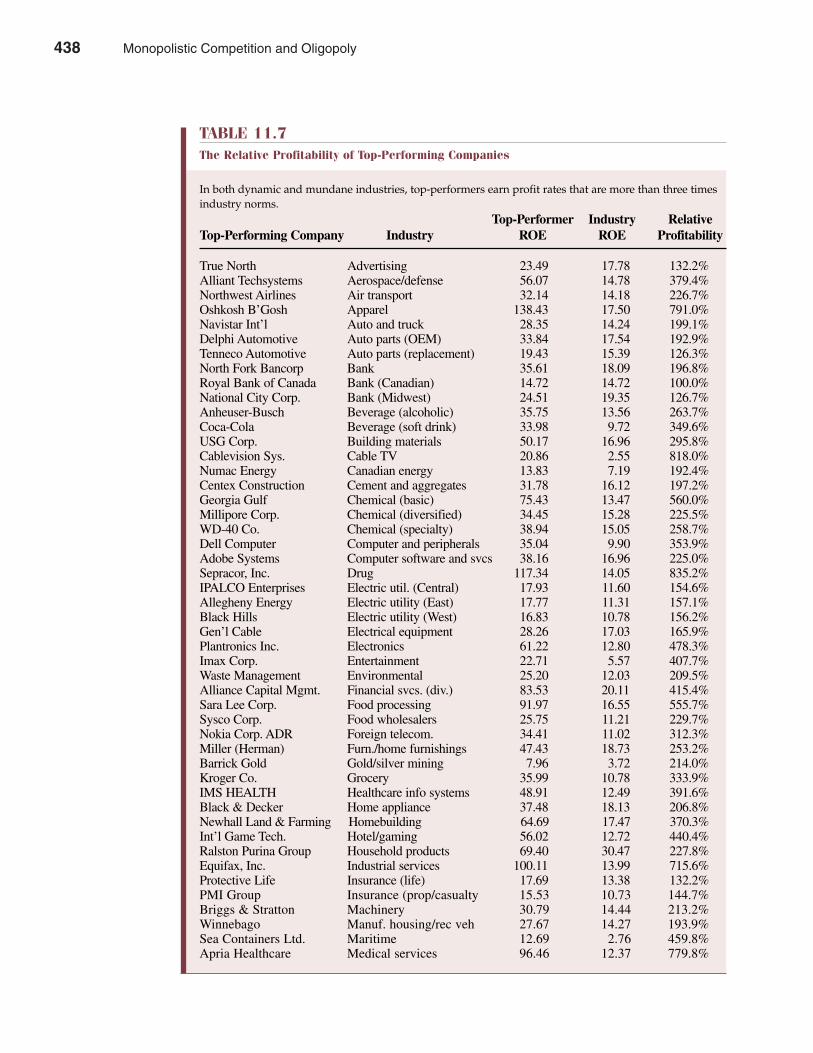
438 Part Four Market Structure Analysis and Estimation
TABLE 11.7The Relative Profitability of Top-Performing Companies
In both dynamic and mundane industries, top-performers earn profit rates that are more than three timesindustry norms.
Top-Performer Industry Relative Top-Performing Company Industry ROE ROE Profitability
True North Advertising 23.49 17.78 132.2%Alliant Techsystems Aerospace/defense 56.07 14.78 379.4%Northwest Airlines Air transport 32.14 14.18 226.7%Oshkosh B’Gosh Apparel 138.43 17.50 791.0%Navistar Int’l Auto and truck 28.35 14.24 199.1%Delphi Automotive Auto parts (OEM) 33.84 17.54 192.9%Tenneco Automotive Auto parts (replacement) 19.43 15.39 126.3%North Fork Bancorp Bank 35.61 18.09 196.8%Royal Bank of Canada Bank (Canadian) 14.72 14.72 100.0%National City Corp. Bank (Midwest) 24.51 19.35 126.7%Anheuser-Busch Beverage (alcoholic) 35.75 13.56 263.7%Coca-Cola Beverage (soft drink) 33.98 9.72 349.6%USG Corp. Building materials 50.17 16.96 295.8%Cablevision Sys. Cable TV 20.86 2.55 818.0%Numac Energy Canadian energy 13.83 7.19 192.4% Centex Construction Cement and aggregates 31.78 16.12 197.2%Georgia Gulf Chemical (basic) 75.43 13.47 560.0%Millipore Corp. Chemical (diversified) 34.45 15.28 225.5%WD-40 Co. Chemical (specialty) 38.94 15.05 258.7%Dell Computer Computer and peripherals 35.04 9.90 353.9%Adobe Systems Computer software and svcs 38.16 16.96 225.0%Sepracor, Inc. Drug 117.34 14.05 835.2%IPALCO Enterprises Electric util. (Central) 17.93 11.60 154.6%Allegheny Energy Electric utility (East) 17.77 11.31 157.1%Black Hills Electric utility (West) 16.83 10.78 156.2%Gen’l Cable Electrical equipment 28.26 17.03 165.9%Plantronics Inc. Electronics 61.22 12.80 478.3%Imax Corp. Entertainment 22.71 5.57 407.7%Waste Management Environmental 25.20 12.03 209.5%Alliance Capital Mgmt. Financial svcs. (div.) 83.53 20.11 415.4%Sara Lee Corp. Food processing 91.97 16.55 555.7%Sysco Corp. Food wholesalers 25.75 11.21 229.7%Nokia Corp. ADR Foreign telecom. 34.41 11.02 312.3%Miller (Herman) Furn./home furnishings 47.43 18.73 253.2%Barrick Gold Gold/silver mining 7.96 3.72 214.0%Kroger Co. Grocery 35.99 10.78 333.9%IMS HEALTH Healthcare info systems 48.91 12.49 391.6%Black & Decker Home appliance 37.48 18.13 206.8%Newhall Land & Farming Homebuilding 64.69 17.47 370.3%Int’l Game Tech. Hotel/gaming 56.02 12.72 440.4%Ralston Purina Group Household products 69.40 30.47 227.8%Equifax, Inc. Industrial services 100.11 13.99 715.6%Protective Life Insurance (life) 17.69 13.38 132.2%PMI Group Insurance (prop/casualty 15.53 10.73 144.7%Briggs & Stratton Machinery 30.79 14.44 213.2%Winnebago Manuf. housing/rec veh 27.67 14.27 193.9%Sea Containers Ltd. Maritime 12.69 2.76 459.8%Apria Healthcare Medical services 96.46 12.37 779.8%
438 Monopolistic Competition and Oligopoly

companies, smaller companies feature “flat” organizations with quick, decentralized decisionmaking and authority.
The villain sometimes encountered by large-scale firms is not any diseconomy of scale inthe production process itself, but rather the burden that size places on effective management.Big often means complex, and complexity results in inefficiencies and bureaucratic snarls thatcan strangle effective communication. In the former Soviet Union, a huge, highly centralized,run-from-the-top system came crashing down as a result of its own gigantic weight. Hopingto avoid a similar fate, many large organizations are now splitting assets into smaller inde-pendent operating units that can react quickly to customer needs without the typically longdelays of large organizations. IBM, for example, has split into independent operating units
Chapter Eleven Monopolistic Competition and Oligopoly 439
TABLE 11.7 (continued)
The Relative Profitability of Top-Performing Companies
Top-Performer Industry Relative Top-Performing Company Industry ROE ROE Profitability
AmeriSource Health Medical supplies 49.96 15.01 332.8%Illinois Tool Works Metal fabricating 18.93 13.95 135.7%Freep’t-McMoRan C&G Metals and mining (div.) 19.94 6.50 307.0%UGI Corp. Natural gas (distrib.) 16.84 10.05 167.6%Mitchell Energy Natural gas (diversified 20.21 9.87 204.8%Dow Jones & Co. Newspaper 40.16 12.29 326.8%Lexmark Int’l `A’ Office equip and supplies 48.32 17.13 282.1%Diamond Offshore Oilfield services/equip. 8.84 2.37 373.0%Sealed Air Packaging and container 9.15 21.30 43.0%Georgia-Pacific Group Paper and forest products 19.09 9.30 205.4%Conoco Inc. Petroleum (integrated) 17.16 9.81 174.9%Berry Petroleum Petroleum (producing) 15.49 5.42 286.1%Mettler-Toledo Int’l Precision instrument 51.71 13.13 394.0%Deluxe Corp. Publishing 48.65 21.30 228.4%Burlington Northern Railroad 13.86 9.54 145.4%Topps Co. Recreation 45.84 14.23 322.2%Jack in the Box Restaurant 35.09 14.68 239.0%Intimate Brands Retail (special lines) 84.24 15.44 545.6%Fastenal Co. Retail building supply 23.21 14.69 158.0%Dollar General Corp. Retail store 23.69 15.31 154.7%Morgan S. Dean Witter Securities brokerage 28.15 18.95 148.5%PMC-Sierra Semiconductor 31.04 13.66 227.2%Lam Research Semiconductor cap equip 27.35 17.07 160.2%Timberland Co. Shoe 27.62 14.06 196.4%Worthington Inds. Steel (general) 14.77 10.81 136.6%Pohang Iron ADR Steel (integrated) 15.96 12.99 122.9%Tellabs, Inc. Telecom. equipment 26.29 2.32 1133.2%Polymer Group Textile 13.80 6.05 228.1%N.Y. Community Bancorp Thrift 21.99 15.97 137.7%Carlisle Cos. Tire and rubber 19.94 13.21 150.9%Philip Morris Tobacco 50.14 17.62 284.6%Chattem Inc. Toiletries/cosmetics 46.28 18.76 246.7%Forward Air Trucking/transp. leasing 29.19 15.65 186.6%Sawtek Inc. Wireless networking 23.08 2.35 982.1%
Averages 42.09 14.12 310.4%
Data source: The Value Line Investment Survey for Windows, September, 2001.Reproduced with the permission of Value Line Publishing, Inc.
Monopolistic Competition and Oligopoly 439
that compete directly with each other to provide customers with the latest in computer equip-ment and software. GM, seeking to become more lean and agile like Japanese competitors,established Saturn as an independent operating unit. Exxon is selling domestic explorationand production operations to smaller independents that chop overhead and earn significantprofits despite low volume and depressed oil prices. These examples suggest that many largecorporations are going through a metamorphosis that will favor organizations that are espe-cially adept at reallocating capital among nimble, entrepreneurial operating units.
In the past, when foreign visitors wanted to experience firsthand the latest innovations inU.S. business and administrative practice, they found it mandatory to visit major corporationsin Chicago, Detroit, New York, and Pittsburgh. Today, it is more likely that they would makestops at Boston’s Route 128, California’s Silicon Valley, or North Carolina’s Research Triangle.From electronics instrumentation to specialized steel, smaller companies have replaced largercompanies in positions of industry leadership. The trend towards a higher level of efficiencyfor smaller companies has become so widespread that larger companies are now finding thatmeeting the needs of the customer sometimes requires a dramatic downsizing of the large-scale organization.
Threat of Potential CompetitionThe potential for above-normal rates of return is a powerful inducement to the entry of newcompetitors and to the rapid growth of nonleading firms. Imitation may be the sincerest formof flattery, but it is also the most effective enemy of above-normal rates of return. Regression tothe mean is the rule rather than the exception for above-normal corporate profit rates over time.During recent years, after-tax rates of return on stockholders’ equity have usually been in therange of 9 percent to 10 percent per year. Just as in the stock market where investors rarely earnexcess returns, individual companies rarely earn in excess of 15 percent to 20 percent for morethan a decade. A consistent ROE ≥ 20 percent is simply unheard of for an entire industry withseveral competitors over a sustained period. Therefore, it seems reasonable to conclude thatprice and nonprice methods of competition are often vigorous, even in imperfectly competitiveindustries with few active or potential competitors.
SUMMARYThis chapter extends the study of market structure to monopolistic competition and oligopoly.These models describe the behavior of competitors in imperfectly competitive markets acrossa broad spectrum of our economy in which both price competition and a wide variety ofmethods of nonprice competition are observed.
• Monopolistic competition is similar to perfect competition in that it entails vigorous pricecompetition among a large number of firms and individuals. The major difference is thatconsumers perceive important differences among the products offered by monopolisticallycompetitive firms, whereas the output of perfectly competitive firms is homogeneous.
• In an industry characterized by oligopoly, only a few large rivals are responsible for the bulkof industry output. High to very high barriers to entry are typical, and the price/outputdecisions of firms are interrelated in the sense that direct reactions from rivals can beexpected. This “competition among the few” involves a wide variety of price and nonpricemethods of rivalry.
• A group of competitors operating under a formal overt agreement is called a cartel. If aninformal covert agreement is reached, the firms are said to be operating in collusion.Both practices are generally illegal in the United States. However, cartels are legal inmany parts of the world, and multinational corporations often become involved withthem in foreign markets.
440 Part Four Market Structure Analysis and Estimation
440 Monopolistic Competition and Oligopoly
• Price leadership results when one firm establishes itself as the industry leader and allother firms accept its pricing policy. This leadership may result from the size and strengthof the leading firm, from cost efficiency, or as a result of the recognized ability of the leaderto forecast market conditions accurately and to establish prices that produce satisfactoryprofits for all firms in the industry. Under a second type of price leadership, barometricprice leadership, the price leader is not necessarily the largest or dominant firm in theindustry. The price leader must only be accurate in reading the prevailing industry viewof the need for price adjustment.
• An often-noted characteristic of oligopoly markets is “sticky” prices. Once a general pricelevel has been established, whether through cartel agreement or some less formal arrange-ment, it tends to remain fixed for an extended period. Such rigid prices are often explainedby what is referred to as the kinked demand curve theory of oligopoly prices. A kinkeddemand curve is a firm demand curve that has different slopes for price increases versusprice decreases.
• Game theory is a general framework to help decision making when firm payoffs dependon actions taken by other firms. In a simultaneous-move game, each decision maker makeschoices without specific knowledge of competitor counter moves. In a sequential-movegame, decision makers make their move after observing competitor moves. In a one-shotgame, the underlying interaction between competitors occurs only once; in a repeat game,there is an ongoing interaction between competitors.
• The so-called Prisoner’s Dilemma is a classic conflict-of-interest situation. A dominantstrategy gives the best result for either party regardless of the action taken by the other. Asecure strategy guarantees the best possible outcome given the worst possible scenario. In aNash equilibrium, neither player can improve its own payoff by unilaterally changing itsown strategy. In a Nash bargaining game, two competitors or players “bargain” over someitem of value. When competitors interact on a continuous basis, they are said to be involvedin repeat games. Like any written guarantee or insurance policy, repeat transactions in themarketplace give consumers confidence that they’ll get what they pay for.
• The economic census provides a comprehensive statistical profile of the national economy.They are taken at 5-year intervals during years ending with the digits 2 and 7—for example,1992,1997, 2002, and so on. The North American Industry Classification System (NAICS)categorizes establishments by the principal economic activity in which they are engaged.Below the 2-digit major group or sector level, the NAICS system proceeds to desegregatedlevels of increasingly narrowly defined activity.
• Concentration ratios measure the percentage market share held by (concentrated in) agroup of top firms. When concentration ratios are low, industries tend to be made up ofmany firms, and competition tends to be vigorous. When concentration ratios are high, lead-ing firms dominate and sometimes have the potential for pricing flexibility and economicprofits. The Herfindahl Hirschmann Index (HHI) is a measure of competitor size inequal-ity that reflects size differences among both large and small firms. Calculated in percentageterms, the HHI is the sum of the squared market shares for all n industry competitors:
• An effective competitive strategy in imperfectly competitive markets must be founded onthe firm’s competitive advantage. A competitive advantage is a unique or rare ability tocreate, distribute, or service products valued by customers. It is the business-world ana-log to what economists call comparative advantage, or when one nation or region of thecountry is better suited to the production of one product than to the production of someother product.
Public and private sources offer valuable service through their regular collection and publica-tion of market structure data on the number and size distribution of competitors, market size,growth, capital intensity, investment, and so on. All of this information is useful to the process
Chapter Eleven Monopolistic Competition and Oligopoly 441
Monopolistic Competition and Oligopoly 441
of managerial decision making and provides a useful starting point for the development ofsuccessful competitive strategy.
QUESTIONS
Q11.1 Describe the monopolistically competitive market structure and provide some examples.Q11.2 Describe the oligopolistic market structure and provide some examples.Q11.3 Explain the process by which economic profits are eliminated in a monopolistically competitive
industry as compared to a perfectly competitive industry.Q11.4 Would you expect the demand curve for a firm in a monopolistically competitive industry
to be more or less elastic after economic profits have been eliminated?Q11.5 “One might expect firms in a monopolistically competitive industry to experience greater
swings in the price of their products over the business cycle than those in an oligopolisticindustry. However, fluctuations in profits do not necessarily follow the same pattern.” Discussthis statement.
Q11.6 Will revenue-maximizing firms have short-run profits as large as or larger than profit-maximizingfirms? If so, when? If not, why not?
Q11.7 Is short-run revenue maximization necessarily inconsistent with the more traditional long-runprofit-maximizing model of firm behavior? Why or why not?
Q11.8 Why is the four-firm concentration ratio only an imperfect measure of market power?Q11.9 The statement “You get what you pay for” reflects the common perception that high prices indi-
cate high product quality and low prices indicate low quality. Irrespective of market structureconsiderations, is this statement always correct?
Q11.10 “Economic profits result whenever only a few large competitors are active in a given market.”Discuss this statement.
SELF-TEST PROBLEMS AND SOLUTIONS
ST11.1 Game Theory. One of the most dynamic changes taking place in our economy is the evolutionof the personal computer from a document preparation and computing device to a communi-cating device. What we used to view as stand-alone personal computers, televisions, VCRs, tele-phones, fax and copy machines are all converging toward nimble communications devices withthe ability to fulfill a number of tasks simultaneously. Nowhere is the influence of this trendmore obvious than in the communications equipment industries. This is the sector withinwhich manufacturers produce household audio and video equipment, prerecorded records andtapes, telephone and telegraph apparatus, and radio and television communications equip-ment. Because many commercial users have unique needs, equipment suppliers sometimeshave significant ability to influence the price charged for what is often a bundle of specializedgoods and services. As a result, game theory concepts prove useful to both buyers and sellersof communications devices.
To illustrate, suppose two local suppliers are seeking to win the right to upgrade the com-munications capability of the internal “intranets” that link a number of customers with theirsuppliers. The system quality decision facing each competitor, and potential profit payoffs, areillustrated in the table. The first number listed in each cell is the profit earned by U.S. EquipmentSupply; the second number indicates the profit earned by Business Systems, Inc. For example,if both competitors, U.S. Equipment Supply and Business Systems, Inc., pursue a high-qualitystrategy, U.S. Equipment Supply will earn $25,000 and Business Systems, Inc., will earn $50,000.If U.S. Equipment Supply pursues a high-quality strategy while Business Systems, Inc., offers
442 Part Four Market Structure Analysis and Estimation
442 Monopolistic Competition and Oligopoly
low-quality goods and services, U.S. Equipment Supply will earn $40,000; Business Systems, Inc.,earns $22,000. If U.S. Equipment Supply offers low-quality goods while Business Systems, Inc.,offers high-quality goods, U.S. Equipment Supply will suffer a net loss of $25,000, and BusinessSystems, Inc., will earn $20,000. Finally, if U.S. Equipment Supply offers low-quality goods whileBusiness Systems, Inc., offers low-quality goods, both U.S. Equipment Supply and BusinessSystems, Inc., will earn $25,000.
A. Does U.S. Equipment Supply and/or Business Systems, Inc., have a dominant strategy?If so, what is it?
B. Does U.S. Equipment Supply and/or Business Systems, Inc., have a secure strategy? Ifso, what is it?
C. What is the Nash equilibrium concept, and why is it useful? What is the Nash equilibri-um for this problem?
ST11.1 SolutionA. The dominant strategy for U.S. Equipment Supply is to provide high-quality goods.
Irrespective of the quality strategy chosen by Business Systems, Inc., U.S. Equipment Supplycan do no better than to choose a high-quality strategy. To see this, note that if BusinessSystems, Inc., chooses to produce high-quality goods, the best choice for U.S. EquipmentSupply is to also provide high-quality goods because the $25,000 profit then earned is betterthan the $25,000 loss that would be incurred if U.S. Equipment Supply chose a low-qualitystrategy. If Business Systems, Inc., chose a low-quality strategy, the best choice by U.S.Equipment Supply would again be to produce high-quality goods. U.S. Equipment Supply’shigh-quality strategy profit of $40,000 dominates the low-quality payoff for U.S. EquipmentSupply of $25,000.
Business Systems, Inc., does not have a dominant strategy. To see this, note that if U.S.Equipment Supply chooses to produce high-quality goods, the best choice for BusinessSystems, Inc., is to also provide high-quality goods because the $50,000 profit then earned isbetter than the $22,000 profit if Business Systems, Inc., chose a low-quality strategy. If U.S.Equipment Supply chose a low-quality strategy, the best choice by Business Systems, Inc.,would be to produce low-quality goods and earn $25,000 versus $20,000.
B. The secure strategy for U.S. Equipment Supply is to provide high-quality goods. By choosingto provide high-quality goods, U.S. Equipment Supply can be guaranteed a profit payoff ofat least $25,000. By pursuing a high-quality strategy, U.S. Equipment Supply can eliminate thechance of losing $25,000, as would happen if U.S. Equipment Supply chose a low-qualitystrategy while Business Systems, Inc., chose to produce high-quality goods.
The secure strategy for Business Systems, Inc., is to provide low-quality goods. By choos-ing to provide high-quality goods, Business Systems, Inc., can guarantee a profit payoffof only $20,000. Business Systems, Inc., can be assured of earning at least $22,000 with alow-quality strategy. Thus, the secure strategy for Business Systems, Inc., is to providelow-quality goods.
C. A set of strategies constitutes a Nash equilibrium if, given the strategies of other players, noplayer can improve its payoff through a unilateral change in strategy. The concept of Nash
Chapter Eleven Monopolistic Competition and Oligopoly 443
Business Systems, Inc.
Quality Strategy High Quality Low Quality
High Quality $25,000, $50,000 $40,000, $22,000
Low Quality –$25,000, $20,000 $25,000, $25,000
U.S
.E
quip
men
tSu
pply
Monopolistic Competition and Oligopoly 443
equilibrium is very important because it represents a situation where every player is doingthe best possible in light of what other players are doing.
Although useful, the notion of a secure strategy suffers from a serious shortcoming. Inthe present example, suppose Business Systems, Inc., reasoned as follows: “U.S. EquipmentSupply will surely choose its high-quality dominant strategy. Therefore, I should not choosemy secure low-quality strategy and earn $22,000. I should instead choose a high-qualitystrategy and earn $50,000.” A natural way of formalizing the “end result” of such a thoughtprocess is captured in the definition of Nash equilibrium.
In the present example, if U.S. Equipment Supply chooses a high-quality strategy, theNash equilibrium strategy is for Business Systems, Inc., to also choose a high-qualitystrategy. Similarly, if Business Systems, Inc., chooses a high-quality strategy, the Nashequilibrium strategy is for U.S. Equipment Supply to also choose a high-quality strategy.Thus, a Nash equilibrium is reached when both firms adopt high-quality strategies.
Although some problems have multiple Nash equilibriums, that is not true in this case.A combination of high-quality strategies for both firms is the only set of strategies whereno player can improve its payoff through a unilateral change in strategy.
ST11.2 Columbia Drugstores, Inc., based in Seattle, Washington, operates a chain of 30 drugstoresin the Pacific Northwest. During recent years, the company has become increasingly con-cerned with the long-run implications of competition from a new type of competitor, the so-called superstore.
To measure the effects of superstore competition on current profitability, Columbia askedmanagement consultant Mindy McConnell to conduct a statistical analysis of the company’sprofitability in its various markets. To net out size-related influences, profitability was measuredby Columbia’s gross profit margin, or earnings before interest and taxes divided by sales.Columbia provided proprietary company profit, advertising, and sales data covering the lastyear for all 30 outlets, along with public trade association and Census Bureau data concerningthe number and relative size distribution of competitors in each market, among other marketcharacteristics.
As a first step in the study, McConnell decided to conduct a regression-based analysis ofthe various factors thought to affect Columbia’s profitability. The first is the relative size ofleading competitors in the relevant market, measured at the Standard Metropolitan StatisticalArea (SMSA) level. Columbia’s market share, MS, in each market area is expected to have apositive effect on profitability given the pricing, marketing, and average-cost advantages thataccompany large relative size. The market concentration ratio, CR, measured as the combinedmarket share of the four largest competitors in any given market, is expected to have a nega-tive effect on Columbia’s profitability given the stiff competition from large, well-financedrivals. Of course, the expected negative effect of high concentration on Columbia profitabilitycontrasts with the positive influence of high concentration on industry profits that is some-times observed.
Both capital intensity, K/S, measured by the ratio of the book value of assets to sales, andadvertising intensity, A/S, measured by the advertising-to-sales ratio, are expected to exertpositive influences on profitability. Given that profitability is measured by Columbia’s grossprofit margin, the coefficient on capital intensity measured Columbia’s return on tangibleinvestment. Similarly, the coefficient on the advertising variable measures the profit effects ofadvertising. Growth, GR, measured by the geometric mean rate of change in total disposableincome in each market, is expected to have a positive influence on Columbia’s profitability,because some disequilibrium in industry demand and supply conditions is often observed inrapidly growing areas.
444 Part Four Market Structure Analysis and Estimation
444 Monopolistic Competition and Oligopoly
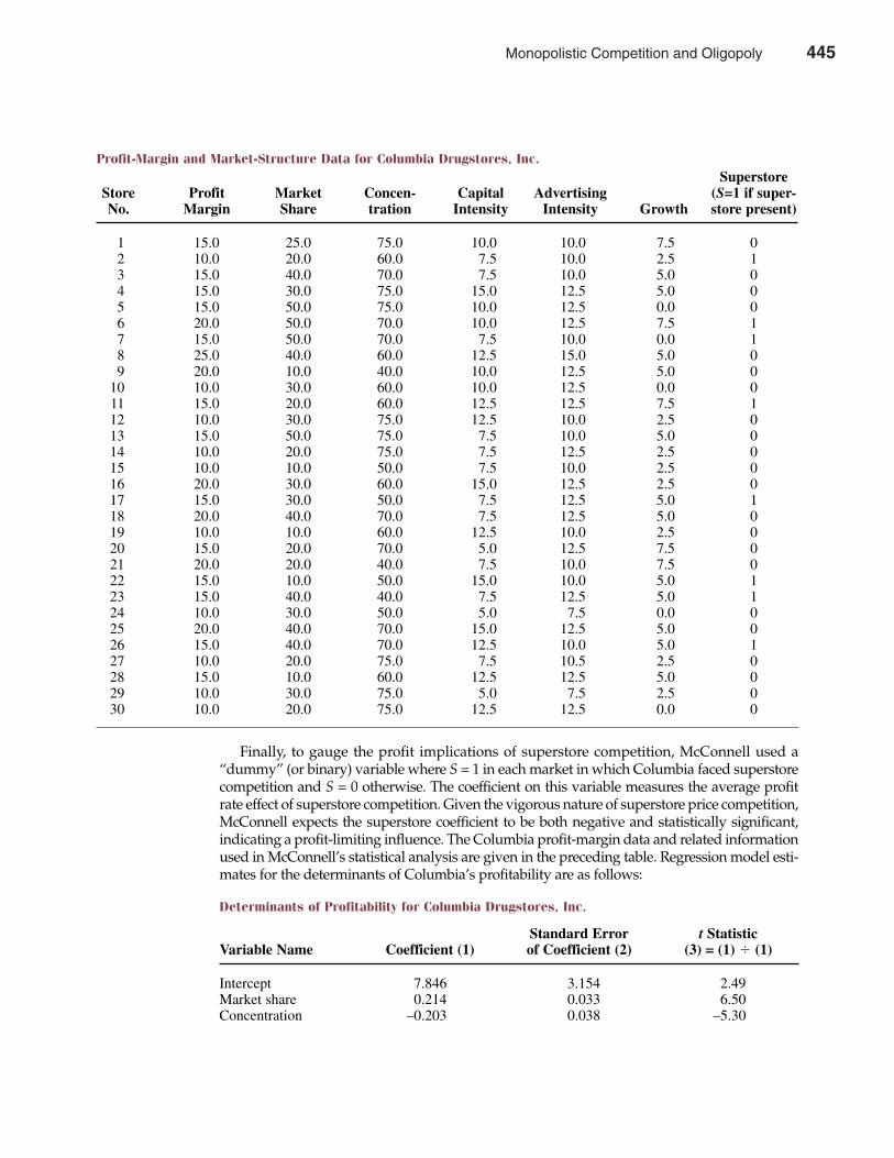
Finally, to gauge the profit implications of superstore competition, McConnell used a“dummy” (or binary) variable where S = 1 in each market in which Columbia faced superstorecompetition and S = 0 otherwise. The coefficient on this variable measures the average profitrate effect of superstore competition. Given the vigorous nature of superstore price competition,McConnell expects the superstore coefficient to be both negative and statistically significant,indicating a profit-limiting influence. The Columbia profit-margin data and related informationused in McConnell’s statistical analysis are given in the preceding table. Regression model esti-mates for the determinants of Columbia’s profitability are as follows:
Chapter Eleven Monopolistic Competition and Oligopoly 445
Profit-Margin and Market-Structure Data for Columbia Drugstores, Inc.Superstore
Store Profit Market Concen- Capital Advertising (S=1 if super-No. Margin Share tration Intensity Intensity Growth store present)
1 15.0 25.0 75.0 10.0 10.0 7.5 02 10.0 20.0 60.0 7.5 10.0 2.5 13 15.0 40.0 70.0 7.5 10.0 5.0 04 15.0 30.0 75.0 15.0 12.5 5.0 05 15.0 50.0 75.0 10.0 12.5 0.0 06 20.0 50.0 70.0 10.0 12.5 7.5 17 15.0 50.0 70.0 7.5 10.0 0.0 18 25.0 40.0 60.0 12.5 15.0 5.0 09 20.0 10.0 40.0 10.0 12.5 5.0 0
10 10.0 30.0 60.0 10.0 12.5 0.0 011 15.0 20.0 60.0 12.5 12.5 7.5 112 10.0 30.0 75.0 12.5 10.0 2.5 013 15.0 50.0 75.0 7.5 10.0 5.0 014 10.0 20.0 75.0 7.5 12.5 2.5 015 10.0 10.0 50.0 7.5 10.0 2.5 016 20.0 30.0 60.0 15.0 12.5 2.5 017 15.0 30.0 50.0 7.5 12.5 5.0 118 20.0 40.0 70.0 7.5 12.5 5.0 019 10.0 10.0 60.0 12.5 10.0 2.5 020 15.0 20.0 70.0 5.0 12.5 7.5 021 20.0 20.0 40.0 7.5 10.0 7.5 022 15.0 10.0 50.0 15.0 10.0 5.0 123 15.0 40.0 40.0 7.5 12.5 5.0 124 10.0 30.0 50.0 5.0 7.5 0.0 025 20.0 40.0 70.0 15.0 12.5 5.0 026 15.0 40.0 70.0 12.5 10.0 5.0 127 10.0 20.0 75.0 7.5 10.5 2.5 028 15.0 10.0 60.0 12.5 12.5 5.0 029 10.0 30.0 75.0 5.0 7.5 2.5 030 10.0 20.0 75.0 12.5 12.5 0.0 0
Determinants of Profitability for Columbia Drugstores, Inc.
Standard Error t StatisticVariable Name Coefficient (1) of Coefficient (2) (3) = (1) � (1)
Intercept 7.846 3.154 2.49 Market share 0.214 0.033 6.50 Concentration –0.203 0.038 –5.30
Monopolistic Competition and Oligopoly 445
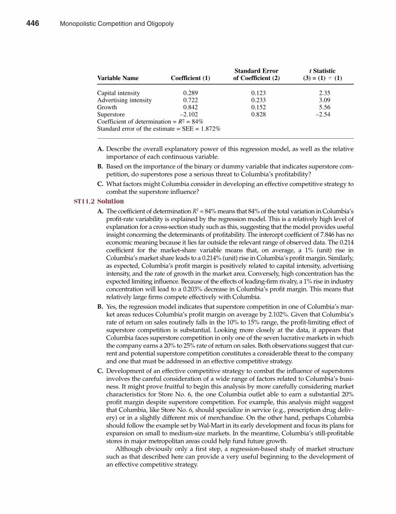
A. Describe the overall explanatory power of this regression model, as well as the relativeimportance of each continuous variable.
B. Based on the importance of the binary or dummy variable that indicates superstore com-petition, do superstores pose a serious threat to Columbia’s profitability?
C. What factors might Columbia consider in developing an effective competitive strategy tocombat the superstore influence?
ST11.2 SolutionA. The coefficient of determination R2 = 84% means that 84% of the total variation in Columbia’s
profit-rate variability is explained by the regression model. This is a relatively high level ofexplanation for a cross-section study such as this, suggesting that the model provides usefulinsight concerning the determinants of profitability. The intercept coefficient of 7.846 has noeconomic meaning because it lies far outside the relevant range of observed data. The 0.214coefficient for the market-share variable means that, on average, a 1% (unit) rise inColumbia’s market share leads to a 0.214% (unit) rise in Columbia’s profit margin. Similarly,as expected, Columbia’s profit margin is positively related to capital intensity, advertisingintensity, and the rate of growth in the market area. Conversely, high concentration has theexpected limiting influence. Because of the effects of leading-firm rivalry, a 1% rise in industryconcentration will lead to a 0.203% decrease in Columbia’s profit margin. This means thatrelatively large firms compete effectively with Columbia.
B. Yes, the regression model indicates that superstore competition in one of Columbia’s mar-ket areas reduces Columbia’s profit margin on average by 2.102%. Given that Columbia’srate of return on sales routinely falls in the 10% to 15% range, the profit-limiting effect ofsuperstore competition is substantial. Looking more closely at the data, it appears thatColumbia faces superstore competition in only one of the seven lucrative markets in whichthe company earns a 20% to 25% rate of return on sales. Both observations suggest that cur-rent and potential superstore competition constitutes a considerable threat to the companyand one that must be addressed in an effective competitive strategy.
C. Development of an effective competitive strategy to combat the influence of superstoresinvolves the careful consideration of a wide range of factors related to Columbia’s busi-ness. It might prove fruitful to begin this analysis by more carefully considering marketcharacteristics for Store No. 6, the one Columbia outlet able to earn a substantial 20%profit margin despite superstore competition. For example, this analysis might suggestthat Columbia, like Store No. 6, should specialize in service (e.g., prescription drug deliv-ery) or in a slightly different mix of merchandise. On the other hand, perhaps Columbiashould follow the example set by Wal-Mart in its early development and focus its plans forexpansion on small to medium-size markets. In the meantime, Columbia’s still-profitablestores in major metropolitan areas could help fund future growth.
Although obviously only a first step, a regression-based study of market structuresuch as that described here can provide a very useful beginning to the development ofan effective competitive strategy.
446 Part Four Market Structure Analysis and Estimation
Standard Error t StatisticVariable Name Coefficient (1) of Coefficient (2) (3) = (1) � (1)
Capital intensity 0.289 0.123 2.35 Advertising intensity 0.722 0.233 3.09 Growth 0.842 0.152 5.56 Superstore –2.102 0.828 –2.54 Coefficient of determination = R2 = 84%Standard error of the estimate = SEE = 1.872%
446 Monopolistic Competition and Oligopoly
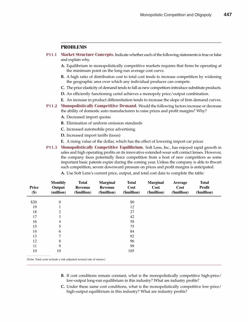
PROBLEMS
P11.1 Market Structure Concepts. Indicate whether each of the following statements is true or falseand explain why.A. Equilibrium in monopolistically competitive markets requires that firms be operating at
the minimum point on the long-run average cost curve.B. A high ratio of distribution cost to total cost tends to increase competition by widening
the geographic area over which any individual producer can compete.C. The price elasticity of demand tends to fall as new competitors introduce substitute products.D. An efficiently functioning cartel achieves a monopoly price/output combination.E. An increase in product differentiation tends to increase the slope of firm demand curves.
P11.2 Monopolistically Competitive Demand. Would the following factors increase or decreasethe ability of domestic auto manufacturers to raise prices and profit margins? Why?A. Decreased import quotasB. Elimination of uniform emission standardsC. Increased automobile price advertisingD. Increased import tariffs (taxes)E. A rising value of the dollar, which has the effect of lowering import car prices
P11.3 Monopolistically Competitive Equilibrium. Soft Lens, Inc., has enjoyed rapid growth insales and high operating profits on its innovative extended-wear soft contact lenses. However,the company faces potentially fierce competition from a host of new competitors as someimportant basic patents expire during the coming year. Unless the company is able to thwartsuch competition, severe downward pressure on prices and profit margins is anticipated.A. Use Soft Lens’s current price, output, and total cost data to complete the table:
B. If cost conditions remain constant, what is the monopolistically competitive high-price/low-output long-run equilibrium in this industry? What are industry profits?
C. Under these same cost conditions, what is the monopolistically competitive low-price/high-output equilibrium in this industry? What are industry profits?
Chapter Eleven Monopolistic Competition and Oligopoly 447
Monthly Total Marginal Total Marginal Average TotalPrice Output Revenue Revenue Cost Cost Cost Profit
($) (million) ($million) ($million) ($million) ($million) ($million) ($million)
$20 0 $0 19 1 12 18 2 27 17 3 42 16 4 58 15 5 75 14 6 84 13 7 92 12 8 96 11 9 99 10 10 105
(Note: Total costs include a risk-adjusted normal rate of return.)
Monopolistic Competition and Oligopoly 447
D. Now assume that Soft Lens is able to enter into restrictive licensing agreements withpotential competitors and create an effective cartel in the industry. If demand and costconditions remain constant, what is the cartel price/output and profit equilibrium?
P11.4 Competitive Strategy. Gray Computer, Inc., located in Colorado Springs, Colorado, is aprivately held producer of high-speed electronic computers with immense storage capacityand computing capability. Although Gray’s market is restricted to industrial users and a fewlarge government agencies (e.g., Department of Health, NASA, National Weather Service),the company has profitably exploited its market niche.
Glen Gray, founder and research director, has recently announced his retirement, the timingof which will unfortunately coincide with the expiration of several patents covering key aspectsof the Gray computer. Your company, a potential entrant into the market for supercomputers,has asked you to evaluate the short- and long-run potential of this market. Based on data gath-ered from your company’s engineering department, user surveys, trade associations, and othersources, the following market demand and cost information has been developed:
P = $54 – $1.5Q
MR = ∆TR/∆Q = $54 – $3Q
TC = $200 + $6Q + $0.5Q2
MC = ∆TC/∆Q = $6 + $1Q
where P is price, Q is units measured by the number of supercomputers, MR is marginalrevenue, TC is total costs including a normal rate of return, MC is marginal cost, and all fig-ures are in millions of dollars.A. Assume that these demand and cost data are descriptive of Gray’s historical experience.
Calculate output, price, and economic profits earned by the Gray company as a monopolist.What is the point price elasticity of demand at this output level?
B. Calculate the range within which a long-run equilibrium price/output combination wouldbe found for individual firms if entry eliminated Gray’s economic profits. (Note: Assumethat the cost function is unchanged and that the high-price/low-output solution resultsfrom a parallel shift in the demand curve while the low-price/high-output solution resultsfrom a competitive equilibrium.)
C. Assume that the point price elasticity of demand calculated in part Ais a good estimate of therelevant arc price elasticity. What is the potential overall market size for supercomputers?
D. If no other near-term entrants are anticipated, should your company enter the market forsupercomputers? Why or why not?
P11.5 Game Theory. Assume that IBM and Dell Computer have an inventory of personal computersthat they would like to sell before a new generation of faster, cheaper machines is introduced.The question facing each competitor is whether or not they should widely advertise a “close out”sale on these discontinued items or instead let excess inventory work itself off over the next fewmonths. If both aggressively promote their products with a nationwide advertising campaign,each will earn profits of $5 million. If one advertises while the other does not, the firm that adver-tises will earn $20 million, while the one that does not advertise will earn $2 million. If neitheradvertises, both will earn $10 million. Assume this is a one-shot game and both firms seek tomaximize profits.
448 Part Four Market Structure Analysis and Estimation
Dell Computer
Promotion Strategy Advertise Do Not Advertise
Advertise $5, $5 $20, $2
Do Not Advertise $2, $20 $10, $10
IBM
448 Monopolistic Competition and Oligopoly
A. What is the dominant strategy for each firm? Are these also secure strategies?B. What is the Nash equilibrium?C. Would collusion work in this case?
P11.6 Cartel Equilibrium. The Hand Tool Manufacturing Industry Trade Association recentlypublished the following estimates of demand and supply relations for hammers:
QD = 60,000 – 10,000P (Demand)QS = 20,000P (Supply)
A. Calculate the perfectly competitive industry equilibrium price/output combination.B. Now assume that the industry output is organized into a cartel. Calculate the industry
price/output combination that will maximize profits for cartel members. (Hint: As a cartel,industry MR = $6 – $0.0002Q.)
C. Compare your answers to parts A and B. Calculate the price/output effects of the cartel.P11.7 Kinked Demand Curves. Safety Service Products (SSP) faces the following segmented
demand and marginal revenue curves for its new infant safety seat:1. Over the range from 0 to 10,000 units of output,
P1 = $60 – QMR1 = ∆TR1/∆Q = $60 – $2Q
2. When output exceeds 10,000 units,
P2 = $80 – $3Q
MR2 = ∆TR2/∆Q = $80 – $6Q
The company’s total and marginal cost functions are as follows:
TC = $100 + $20Q + $0.5Q2
MC = ∆TC/∆Q = $20 + $1Q
where P is price (in dollars), Q is output (in thousands), MR is marginal revenue, TC is totalcost, and MC is marginal cost, all in thousands of dollars.A. Graph the demand, marginal revenue, and marginal cost curves.B. How would you describe the market structure of the industry in which SSP operates?
Explain why the demand curve takes the shape indicated previously.C. Calculate price, output, and profits at the profit-maximizing activity level.D. How much could marginal costs rise before the optimal price would increase? How much
could they fall before the optimal price would decrease?P11.8 Supply Reactions. Anaheim Industries, Inc., and Binghampton Electronics, Ltd., are the only
suppliers to the National Weather Service of an important electronic instrument. The WeatherService has established a fixed-price procurement policy, however, so P = MR in this market.Total and marginal cost relations for each firm are as follows:
TCA = $7,000 + $250QA + $0.5QA2 (Anaheim)
MCA = ∆TCA/∆QA = $250 + $1QA
TCB = $8,000 + $200QB + $1QB2 (Binghampton)
MCB = ∆TCB/∆QB = $200 + $2QB
Chapter Eleven Monopolistic Competition and Oligopoly 449
Monopolistic Competition and Oligopoly 449
where Q is output in units, and MC > AVC for each firm.A. What is the minimum price necessary for each firm to supply output?B. Determine the supply curve for each firm.C. Based on the assumption that P = PA = PB, determine industry supply curves when P < $200,
$200 < P < $250, and P > $250.P11.9 Nonprice Competition. General Cereals, Inc. (GCI), produces and markets Sweeties!, a
popular ready-to-eat breakfast cereal. In an effort to expand sales in the Secaucus, New Jersey,market, the company is considering a 1-month promotion whereby GCI would distribute acoupon for a free daily pass to a local amusement park in exchange for three box tops, as sentin by retail customers. A 25% boost in demand is anticipated, even though only 15% of all eli-gible customers are expected to redeem their coupons. Each redeemed coupon costs GCI $6,so the expected cost of this promotion is 30¢ (= 0.15 � $6 � 3) per unit sold. Other marginalcosts for cereal production and distribution are constant at $1 per unit.
Current demand and marginal revenue relations for Sweeties! are
Q = 16,000 – 2,000P
MR = ∆TR/∆Q = $8 – $0.001Q
Demand and marginal revenue relations that reflect the expected 25% boost in demand forSweeties! are the following:
Q = 20,000 – 2,500P
MR = ∆TR/∆Q = $8 – $0.0008Q
A. Calculate the profit-maximizing price/output and profit levels for Sweeties! prior to thecoupon promotion.
B. Calculate these same values subsequent to the Sweeties! coupon promotion and followingthe expected 25% boost in demand.
P11.10 Price Leadership. Louisville Communications, Inc., offers 24-hour telephone answeringservice for individuals and small businesses in southeastern states. Louisville is a dominant,price-leading firm in many of its markets. Recently, Memphis Answering Service, Inc., andNashville Recording, Ltd., have begun to offer services with the same essential characteris-tics as Louisville’s service. Total and marginal cost functions for Memphis (M) and Nashville(N) services are as follows:
TCM = $75,000 – $7QM + $0.0025Q2M
MCM = ∆TCM/∆QM = –$7 + $0.005QM
TCN = $50,000 + $3QN + $0.0025Q2N
MCN = ∆TCN/∆QN = $3 + $0.005QN
Louisville’s total and marginal cost relations are as follows:
TCL = $300,000 + $5QL + $0.0002Q2L
MCL = ∆TCL/∆QL = $5 + $0.0004QL
The industry demand curve for telephone answering service is
Q = 500,800 – 19,600P
Assume throughout this problem that the Memphis and Nashville services are perfect sub-stitutes for Louisville’s service.
450 Part Four Market Structure Analysis and Estimation
450 Monopolistic Competition and Oligopoly
A. Determine the supply curves for the Memphis and Nashville services, assuming that thefirms operate as price takers.
B. What is the demand curve faced by Louisville?C. Calculate Louisville’s profit-maximizing price and output levels. (Hint: Louisville’s total
and marginal revenue relations are TRL = $25QL – $0.00005Q2L, and MRL = $25 – $0.0001QL.)
D. Calculate profit-maximizing output levels for the Memphis and Nashville services.E. Is the market for service from these three firms in short-run equilibrium?
Chapter Eleven Monopolistic Competition and Oligopoly 451
CASE STUDY
The Profitability of Multinational OperationsLike market power in domestic markets, market power in foreign markets will have positiveeffects on the market value of the firm when it is an important determinant of future above-normal returns. In fact, greater valuation effects may be associated with market power in foreignas opposed to domestic operations. Although substantial numbers of efficiently sized competi-tors are available in an overwhelming share of U.S. markets, generally smaller foreign marketstend to be dominated by few large competitors. Entry barriers due to economies of scale tend tobe more onerous, and the advantages to established leading firms greater, in foreign as opposedto U.S. markets. Antitrust and other policies limiting monopoly power also tend to be morevigorously pursued in the United States than in many foreign countries. In fact, some foreigngovernments encourage monopoly to gain a comparative advantages in foreign trade. Thus, thevaluation effects of market power in foreign operations can be interesting in isolation, as well asin contrast with perhaps smaller effects due to market power in domestic operations.
Although the effects of market power are often indirectly measured using concentrationratios in studies conducted at the industry level of aggregation, studies using firm-level dataoften consider profit rate data directly. Generally speaking, concentration ratios for a firm’sprimary product industry are only a poor measure of market power for widely diversifiedfirms. Even weighted average concentration ratios reflecting firm involvement in a numberof industries can fail to capture market power influences because the possibility of a criticalconcentration ratio is neglected. Both reasons help explain why concentration ratios seldomhave any discernible influence on the market value of the firm.
High profit rates can show the influences of relatively higher prices, lower costs, or both. Bythemselves, it is impossible to determine if high profit rates reflect the exercise of market poweror superior efficiency. As such, profit rate data are an imperfect proxy for market power. Theyremain, however, a useful index of the relative attractiveness of one line of business or industry.If profit rates for foreign operations consistently exceed profit rates for U.S. operations, onemight conclude that foreign markets are generally more attractive because they entail relativelyless product market competition than U.S. markets. If profit rates for foreign operations havemarket value effects that invariably exceed the valuation effects of profit rates for U.S. opera-tions, one might conclude that profit rates from foreign markets tend to be both higher andmore long-lasting than profit rates earned in U.S. markets.
To estimate the effects of profit rates on the market value of the firm, it is necessary to builda simple economic model. To illustrate, consider the simple accounting identity that total assetsequal the value of stockholders’ equity plus total liabilities:
(11.8) Total Assets = Stockholders’ Equity + Total Liabilities
This means that the total assets of any corporation are financed either through the sale ofcommon stock and retained earnings or through debt financing. When the market value of
Monopolistic Competition and Oligopoly 451

452 Part Four Market Structure Analysis and Estimation
common stock is used as an economic measure of the value of stockholder equity, then Equation11.6 implies:
(11.9)Market Value of = Total – Total + �Common Stock Assets Liabilities
The error term � (epsilon) allows for the fact that the market value of common stock seldomexactly equals the difference between assets and liabilities, which is defined as the book valueof stockholders’ equity. As such, � reflects the combined influence of accounting errors andbias. For example, because the accounting profession does not typically assign a value tointangible assets like advertising and R&D, the market price of common stock is often muchgreater than the accountant’s book value of stockholders’ equity.
The effects of profit rates on the market value of the firm can be estimated by expandingthe number of independent X variables in Equation 11.9 to include profit rates on domesticand foreign operations. If current profit rates are a useful indicator of the multinational firm’sfuture profit-making potential, an impact on the current market value of the firm can be antic-ipated. If profit rates on foreign operations are higher and/or more stable than profit rates ondomestic operations, a somewhat greater influence of foreign profit rates on the market valueof the firm can also be anticipated.
To properly isolate the market value effects of profit rates in both foreign and domestic mar-kets, it is important to control for the risk implications of multinational involvement. In manyinstances, multinational involvement not only allows firms to expand product markets, but alsoprovides a “portfolio” of regulatory environments, economic conditions, and trade currencies.Although exchange risk can be limited at minimal cost through participation in highly devel-oped currency markets, limiting risks associated with political intervention (increased taxation,expropriation) and localized economic fluctuations can be costly. Thus, a firm’s degree of“multinationalism” may have important implications for its overall risk level. To the extent thatconventional measures fail to reflect the greater risks associated with multinational activity, thedegree of multinational involvement can convey additional risk information. If multinationalsface greater than typical levels of risk, or involve substantial hedging expenses, a firm’s degreeof multinational involvement can have negative valuation effects. In addition, one might expectpositive valuation effects to accompany high expected growth because a firm’s options for futureinvestment are largely determined by expected growth in demand.
Based on these considerations, a regression model that can be used to learn the relativemarket-value impacts of domestic versus foreign profit rates can be written
(11.10)Market Value/Assets = b0 + b1 1/Assets + b2 Debt/Assets
+ b3 ROAi + b4 Growth + b5 Foreign/Domestic + u
In this equation, notice that each size-related variable has been deflated, or normalized, by thebook value of total assets. Without deflation of size-related variables, the link between marketvalue and profits could be dominated by size effects: By definition, large firms have high marketvalues and profits. The deflation of all size-related variables makes it possible to focus on the val-uation effects of profit rate differences between foreign and domestic operations. In this model,the profit rate of interest is called the return on total assets, or ROA, and defined as net income(profits) divided by the book value of total assets. Like ROE, ROAis a basic measure of the firm’srate of return on investment; unlike ROE, the ROA measure does not directly reflect the firm’suse of financial leverage.
For exploratory purposes, the simple economic model described in Equation 11.10 is esti-mated over an n = 25 sample of the largest U.S. multinationals. In an annual survey, Forbesshows foreign sales, foreign profits, and foreign assets for top U.S. multinationals. To estimate
CASE STUDY (continued)
452 Monopolistic Competition and Oligopoly
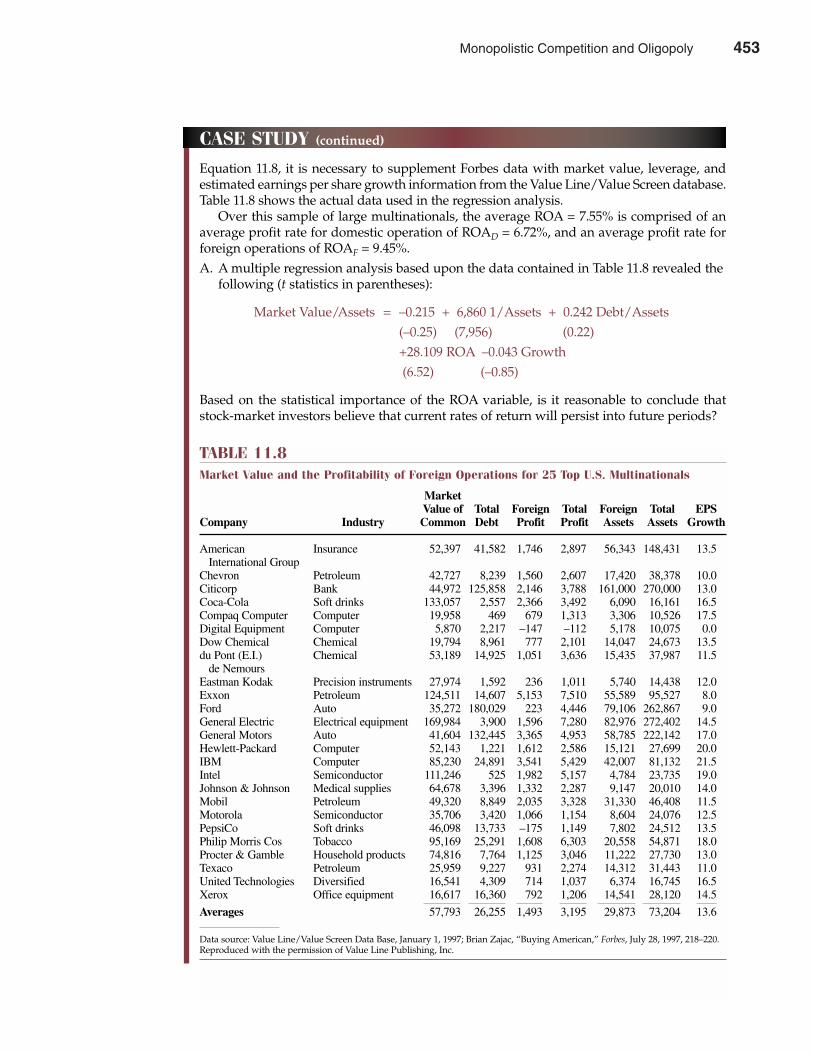
Chapter Eleven Monopolistic Competition and Oligopoly 453
CASE STUDY (continued)
Equation 11.8, it is necessary to supplement Forbes data with market value, leverage, andestimated earnings per share growth information from the Value Line/Value Screen database.Table 11.8 shows the actual data used in the regression analysis.
Over this sample of large multinationals, the average ROA = 7.55% is comprised of anaverage profit rate for domestic operation of ROAD = 6.72%, and an average profit rate forforeign operations of ROAF = 9.45%.A. A multiple regression analysis based upon the data contained in Table 11.8 revealed the
following (t statistics in parentheses):
Market Value/Assets = –0.215 + 6,860 1/Assets + 0.242 Debt/Assets(–0.25) (7,956) (0.22)+28.109 ROA –0.043 Growth(6.52) (–0.85)
Based on the statistical importance of the ROA variable, is it reasonable to conclude thatstock-market investors believe that current rates of return will persist into future periods?
TABLE 11.8Market Value and the Profitability of Foreign Operations for 25 Top U.S. Multinationals
Market Value of Total Foreign Total Foreign Total EPS
Company Industry Common Debt Profit Profit Assets Assets Growth
American Insurance 52,397 41,582 1,746 2,897 56,343 148,431 13.5International Group
Chevron Petroleum 42,727 8,239 1,560 2,607 17,420 38,378 10.0Citicorp Bank 44,972 125,858 2,146 3,788 161,000 270,000 13.0Coca-Cola Soft drinks 133,057 2,557 2,366 3,492 6,090 16,161 16.5Compaq Computer Computer 19,958 469 679 1,313 3,306 10,526 17.5Digital Equipment Computer 5,870 2,217 –147 –112 5,178 10,075 0.0Dow Chemical Chemical 19,794 8,961 777 2,101 14,047 24,673 13.5du Pont (E.I.) Chemical 53,189 14,925 1,051 3,636 15,435 37,987 11.5
de NemoursEastman Kodak Precision instruments 27,974 1,592 236 1,011 5,740 14,438 12.0Exxon Petroleum 124,511 14,607 5,153 7,510 55,589 95,527 8.0Ford Auto 35,272 180,029 223 4,446 79,106 262,867 9.0General Electric Electrical equipment 169,984 3,900 1,596 7,280 82,976 272,402 14.5General Motors Auto 41,604 132,445 3,365 4,953 58,785 222,142 17.0Hewlett-Packard Computer 52,143 1,221 1,612 2,586 15,121 27,699 20.0IBM Computer 85,230 24,891 3,541 5,429 42,007 81,132 21.5Intel Semiconductor 111,246 525 1,982 5,157 4,784 23,735 19.0Johnson & Johnson Medical supplies 64,678 3,396 1,332 2,287 9,147 20,010 14.0Mobil Petroleum 49,320 8,849 2,035 3,328 31,330 46,408 11.5Motorola Semiconductor 35,706 3,420 1,066 1,154 8,604 24,076 12.5PepsiCo Soft drinks 46,098 13,733 –175 1,149 7,802 24,512 13.5Philip Morris Cos Tobacco 95,169 25,291 1,608 6,303 20,558 54,871 18.0Procter & Gamble Household products 74,816 7,764 1,125 3,046 11,222 27,730 13.0Texaco Petroleum 25,959 9,227 931 2,274 14,312 31,443 11.0United Technologies Diversified 16,541 4,309 714 1,037 6,374 16,745 16.5Xerox Office equipment 16,617 16,360 792 1,206 14,541 28,120 14.5
Averages 57,793 26,255 1,493 3,195 29,873 73,204 13.6
Data source: Value Line/Value Screen Data Base, January 1, 1997; Brian Zajac, “Buying American,” Forbes, July 28, 1997, 218–220.Reproduced with the permission of Value Line Publishing, Inc.
Monopolistic Competition and Oligopoly 453

SELECTED REFERENCESAnderson, Simon P., and Andre De Palma. “Product Diversity in Asymmetric Oligopoly: Is the Quality
of Consumer Goods Too Low.” Journal of Industrial Economics 49 (June 2001): 113–135.Arthur, N. “Board Composition as the Outcome of an Internal Bargaining Process: Empirical Evidence.”
Journal of Corporate Finance 7 (September 2001): 307–340.Bennett, James A., and Richard W. Sias. “Can Money Flows Predict Stock Returns?” Financial Analysts
Journal 57 (November/December 2001): 64–77.Coate, Malcolm B. “Market Structure and Competition Policy: Game-Theoretic Approaches.”
Managerial & Decision Economics 22 (December 2001): 465–466.Fiegenbaum, Avi, Howard Thomas, and Ming-Je Tang. “Linking Hypercompetition and Strategic Group
Theories: Strategic Maneuvering in the US Insurance Industry.” Managerial & Decision Economics 22(June/August 2001): 265–279.
Friedman, James. “Oligopoly Pricing: Old Ideas and New Tools.” Journal of Economic Literature 39 (June2001): 573–575.
Hirschey, Mark. “Cisco and the Kids.” Financial Analysts Journal 57 (July/August 2001): 48–59.Jacobs, Michael S. “Second Order Oligopoly Problems with International Dimensions: Sequential Mergers,
Maverick Firms and Buyer Power.” Antitrust Bulletin 46 (Fall 2001): 537–568.Jin, Jim Y. “Monopolistic Competition and Bounded Rationality.” Journal of Economic Behavior &
Organization 45 (June 2001): 175–184.Kramer, Jonathan K., and Jonathan R. Peters. “An Interindustry Analysis of Economic Value Added as a
Proxy for Market Value Added.” Journal of Applied Finance 11 (2001): 41–49.Linnemann, Ludger. “The Price Index Effect, Entry, and Endogenous Markups in a Macroeconomic
Model of Monopolistic Competition.” Journal of Macroeconomics 23 (Summer 2001): 441–458.Merlone, Ugo. “Cartelizing Effects of Horizontal Shareholding Interlocks.” Managerial & Decision
Economics 22 (September 2001): 333–337.Pichler, Pegaret, and William Wilhelm. “A Theory of The Syndicate: Form Follows Function.” Journal
of Finance 56 (December 2001): 2237–2264. Sims, Christopher A. “Pitfalls of a Minimax Approach to Model Uncertainty.” American Economic Review
91 (May 2001): 51–54.Walker, Mark, and John Wooders. “Minimax Play at Wimbledon.” American Economic Review 91
(December 2001): 1521–1538.
454 Part Four Market Structure Analysis and Estimation
CASE STUDY (continued)
B. A second multiple regression analysis based upon the data contained in Table 11.8revealed the following (t statistics in parentheses):
Market Value/Assets = –0.016 + 7,145 1/Assets + 0.660 Debt/Assets(–0.01) (0.82) (0.52)+13.018 ROAF + 6.885 ROAD – 0.040 Growth + 0.150 Foreign/Domestic
(4.52) (1.30) (–0.72) (0.94)
Based on the importance of the ROA variables for foreign versus domestic operations, is it rea-sonable to conclude that foreign markets may be more or less competitive than the U.S. market?
454 Monopolistic Competition and Oligopoly

Pricing Practices
CHAPTER TWELVE
455
Pricing practices sometimes seem peculiar. When first-class hotel roomsin London, Tokyo, or Paris go for $300 to $500 per night, Holiday Inns
offers Weekend WebSaversSM rates at Chicago’s O’Hare International Airportfrom as low as $62.48 per night—more than 50 percent off regular prices. Notto be outdone, Howard Johnson’s says vacations are more fun with familypackage rates up to 70 percent off regular prices. Meanwhile, Marriott offersadvance purchase rates on the Internet for as low as $59 per night at theCourtyard Marriott Village at Lake Buena Vista, Florida. At the Hilton Durham,in North Carolina, weekday rates are $109.95 and $89.95 on the weekend. Whatis going on here?
Rather than a mad scramble to build market share at any cost, hotel-chain rates represent a shrewd use of information technology. Any night thathotel rooms stand empty represents lost revenue, and because hotel costsare largely fixed, revenue losses translate directly into lost profits. A roomrate of $59 per night does not begin to cover fixed construction, mainte-nance, and interest costs, but it makes a nice profit contribution when thealternative is weekend vacancy. By segmenting their markets, hotels are ableto charge the maximum amount the market will bear on weekdays and onweekends. Similarly, hotel marketing gets fierce for convention business,especially when conventions meet at traditionally slack periods. Is it any won-der that the American Economic Association holds annual meetings aroundNew Year’s Day in cold-weather cities?1
This chapter examines common pricing practices and illustrates theirvalue as a practical means for achieving profit-maximizing prices under awide variety of demand and cost conditions.
1 See Motoko Rich, “Holiday Inn Owner Will Build Hotels Even as Industry Slows,” The WallStreet Journal Online, January 16, 2002 (http://online.wsj.com).
455
12
MARKUP PRICING
Markup pricing is the most commonly employed pricing method. Given the popularity of thetechnique, it behooves managers to fully understand the rationale for markup pricing. Whenthis rationale is understood, markup pricing methods can be seen as the practical means forachieving optimal prices under a wide variety of demand and cost conditions.
Markup Pricing TechnologyThe development of pricing practices to profitably segment markets has reached a fine art withthe Internet and use of high-speed computer technology. Why do Business Week, Forbes, Fortune,and The Wall Street Journal offer bargain rates to students but not to business executives? It issurely not because it costs less to deliver the Journal to students, and it is not out of benevolence;it is because students are not willing or able to pay the standard rate. Even at 50 percent off reg-ular prices, student bargain rates more than cover marginal costs and make a significant profitcontribution. Similarly, senior citizens who eat at Holiday Inns enjoy a 10 to 15 percent discountand make a meaningful contribution to profits. Conversely, relatively high prices for popcornat movie theaters, peanuts at the ball park, and clothing at the height of the season reflect thefact that customers can be insensitive to price changes at different places and at different timesof the year. Regular prices, discounts, rebates, and coupon promotions are all pricing mecha-nisms used to probe the breadth and depth of customer demand and to maximize profitability.
Although profit maximization requires that prices be set so that marginal revenues equalmarginal cost, it is not necessary to calculate both to set optimal prices. Just using informationon marginal costs and the point price elasticity of demand, the calculation of profit-maximizingprices is quick and easy. Many firms derive an optimal pricing policy using prices set to coverdirect costs plus a percentage markup for profit contribution. Flexible markup pricing practicesthat reflect differences in marginal costs and demand elasticities constitute an efficient methodfor ensuring that MR = MC for each line of products sold. Similarly, peak and off-peak pricing,price discrimination, and joint product pricing practices are efficient means for operating so thatMR = MC for each customer or customer group and product class.
Markup on CostIn a conventional approach, firms estimate the average variable costs of producing and mar-keting a given product, add a charge for variable overhead, and then add a percentage markup,or profit margin. Variable overhead costs are usually allocated among all products according toaverage variable costs. For example, if total variable overhead costs are projected at $1.3 millionper year and variable costs for planned production total $1 million, then variable overhead isallocated to individual products at the rate of 130 percent of variable cost. If the average vari-able cost of a product is estimated to be $1, the firm adds a charge of 130 percent of variablecosts, or $1.30, for variable overhead, obtaining a fully allocated cost of $2.30. To this figure thefirm might add a 30 percent markup for profits, or 69¢, to obtain a price of $2.99 per unit.
Markup on cost is the profit margin for an individual product or product line expressed asa percentage of unit cost. The markup-on-cost, or cost-plus, formula is given by the expression:
(12.1) Markup on Cost = Price – CostCost
The numerator of this expression, called the profit margin, is measured by the differencebetween price and cost. In the example cited previously, the 30 percent markup on cost iscalculated as
456 Part Four Market Structure Analysis and Estimation
markup pricingSetting prices to coverdirect costs plus a percentage profit contribution
markup on costThe difference betweenprice and cost, measured relative tocost, expressed as apercentage
profit marginThe difference betweenthe price and cost of aproduct
456 Pricing Practices
Markup on Cost = Price – CostCost
= $2.99 – $2.30$2.30
= 0.30, or 30%
Solving Equation 12.1 for price provides the expression that determines price in a cost-pluspricing system:
(12.2) Price = Cost (1 + Markup on Cost)
Continuing with the previous example, the product selling price is found as
Price = Cost (1 + Markup on Cost)= $2.30(1.30)= $2.99
Markup on PriceProfit margins, or markups, are sometimes calculated as a percentage of price instead of cost.Markup on price is the profit margin for an individual product or product line expressed asa percentage of price, rather than unit cost as in the markup-on-cost formula. This alternativemeans of expressing profit margins can be illustrated by the markup-on-price formula:
(12.3) Markup on Price = Price – CostPrice
Profit margin is the numerator of the markup-on-price formula, as in the markup-on-costformula. However, unit cost has been replaced by price in the denominator.
The markup-on-cost and markup-on-price formulas are simply alternative means forexpressing the relative size of profit margins. To convert from one markup formula to the other,just use the following expressions:
(12.4) Markup on Cost = Markup on Price1 – Markup on Price
(12.5) Markup on Price = Markup on Cost1 + Markup on Cost
Therefore, the 30 percent markup on cost described in the previous example is equivalent to a23 percent markup on price:
Markup on Price = 0.3 = 0.23 or 23%1 + 0.3
An item with a cost of $2.30, a 69¢ markup, and a price of $2.99 has a 30 percent markup oncost and a 23 percent markup on price. This illustrates the importance of being consistent inthe choice of a cost or price basis when comparing markups among products or sellers.
Markup pricing is sometimes criticized as a naive pricing method based solely on cost con-siderations—and the wrong costs at that. Some who employ the technique may ignore demandconditions, emphasize fully allocated accounting costs rather than marginal costs, and arrive at
markup on priceThe difference betweenprice and cost, meas-ured relative to price,expressed as a percent-age
Chapter Twelve Pricing Practices 457
Pricing Practices 457
suboptimal price decisions. However, a categorical rejection of such a popular and successfulpricing practice is clearly wrong. Although inappropriate use of markup pricing formulas willlead to suboptimal managerial decisions, successful firms typically employ the method in a waythat is consistent with profit maximization. Markup pricing can be viewed as an efficient rule-of-thumb approach to setting optimal prices.
Role of Cost in Markup PricingAlthough a variety of cost concepts are employed in markup pricing, most firms use a standard,or fully allocated, cost concept. Fully allocated costs are determined by first estimating directcosts per unit, then allocating the firm’s expected indirect expenses, or overhead, assuming astandard or normal output level. Price is then based on standard costs per unit, irrespective ofshort-term variations in actual unit costs.
Unfortunately, use of the standard cost concept can create several problems. Sometimes,firms fail to adjust historical costs to reflect recent or expected price changes. Also, accountingcosts may not reflect true economic costs. For example, fully allocated costs can be appropriatewhen a firm is operating at full capacity. During peak periods, when facilities are fully utilized,expansion is required to increase production. Under such conditions, an increase in productionrequires an increase in all plant, equipment, labor, materials, and other expenditures. However,if a firm has excess capacity, as during off-peak periods, only those costs that actually rise withproduction—the incremental costs per unit—should form a basis for setting prices.
Successful firms that employ markup pricing use fully allocated costs under normal con-ditions but offer price discounts or accept lower margins during off-peak periods when excesscapacity is available. In some instances, output produced during off-peak periods is much cheap-er than output produced during peak periods. When fixed costs represent a substantial share oftotal production costs, discounts of 30 percent to 50 percent for output produced during off-peakperiods can often be justified on the basis of lower costs.
“Early bird” or afternoon matinee discounts at movie theaters provide an interesting exam-ple. Except for cleaning expenses, which vary according to the number of customers, mostmovie theater expenses are fixed. As a result, the revenue generated by adding customers dur-ing off-peak periods can significantly increase the theater’s profit contribution. When off-peakcustomers buy regularly priced candy, popcorn, and soda, even lower afternoon ticket pricescan be justified. Conversely, on Friday and Saturday nights when movie theaters operate atpeak capacity, a small increase in the number of customers would require a costly expansionof facilities. Ticket prices during these peak periods reflect fully allocated costs. Similarly,McDonald’s, Burger King, Arby’s, and other fast-food outlets have increased their profitabil-ity substantially by introducing breakfast menus. If fixed restaurant expenses are covered bylunch and dinner business, even promotionally priced breakfast items can make a notablecontribution to profits.
Role of Demand in Markup PricingSuccessful companies differentiate markups according to variations in product demand elastic-ities. Foreign and domestic automobile companies regularly offer rebates or special equipmentpackages for slow-selling models. Similarly, airlines promote different pricing schedules forbusiness and vacation travelers. The airline and automobile industries are only two examplesof sectors in which vigorous competition requires a careful reflection of demand and supply factorsin pricing practice. In the production and distribution of many goods and services, successful firmsquickly adjust prices to different market conditions.
Examining the margins set by a successful regional grocery store chain provides interest-ing evidence that demand conditions play an important role in cost-plus pricing. Table 12.1shows the firm’s typical markup on cost and markup on price for a variety of products. A field
458 Part Four Market Structure Analysis and Estimation
peakPeriod of full capacityusage
off-peakPeriod of excess capacity
458 Pricing Practices
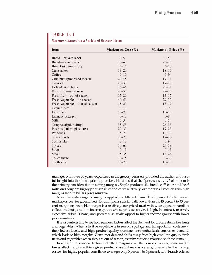
manager with over 20 years’ experience in the grocery business provided the author with use-ful insight into the firm’s pricing practices. He stated that the “price sensitivity” of an item isthe primary consideration in setting margins. Staple products like bread, coffee, ground beef,milk, and soup are highly price sensitive and carry relatively low margins. Products with highmargins tend to be less price sensitive.
Note the wide range of margins applied to different items. The 0 percent to 10 percentmarkup on cost for ground beef, for example, is substantially lower than the 15 percent to 35 per-cent margin on steak. Hamburger is a relatively low-priced meat with wide appeal to families,college students, and low-income groups whose price sensitivity is high. In contrast, relativelyexpensive sirloin, T-bone, and porterhouse steaks appeal to higher-income groups with lowerprice sensitivity.
It is also interesting to see how seasonal factors affect the demand for grocery items like fruitsand vegetables. When a fruit or vegetable is in season, spoilage and transportation costs are attheir lowest levels, and high product quality translates into enthusiastic consumer demand,which leads to high margins. Consumer demand shifts away from high-cost/low-quality freshfruits and vegetables when they are out of season, thereby reducing margins on these items.
In addition to seasonal factors that affect margins over the course of a year, some marketforces affect margins within a given product class. In breakfast cereals, for example, the markupon cost for highly popular corn flakes averages only 5 percent to 6 percent, with brands offered
Chapter Twelve Pricing Practices 459
TABLE 12.1Markups Charged on a Variety of Grocery Items
Item Markup on Cost (%) Markup on Price (%)
Bread—private label 0–5 0–5Bread—brand name 30–40 23–29Breakfast cereals (dry) 5–15 5–13Cake mixes 15–20 13–17Coffee 0–10 0–9Cold cuts (processed meats) 20–45 17–31Cookies 20–30 17–23Delicatessen items 35–45 26–31Fresh fruit—in season 40–50 29–33Fresh fruit—out of season 15–20 13–17Fresh vegetables—in season 40–50 29–33Fresh vegetables—out of season 15–20 13–17Ground beef 0–10 0–9Ice cream 15–20 13–17Laundry detergent 5–10 5–9Milk 0–5 0–5Nonprescription drugs 33–55 26–35Pastries (cakes, pies, etc.) 20–30 17–23Pet foods 15–20 13–17Snack foods 20–25 17–20Soft drinks 0–10 0–9Spices 30–60 23–38Soup 0–15 0–13Steak 15–35 13–26Toilet tissue 10–15 9–13Toothpaste 15–20 13–17
Pricing Practices 459
by Post and Kellogg’s competing with a variety of local store brands. Cheerios and Wheaties,both offered only by General Mills, Inc., enjoy a markup on cost of 15 percent to 20 percent. Thus,availability of substitutes directly affects the markups on various cereals. It is interesting to notethat among the wide variety of items sold in a typical grocery store, the highest margins arecharged on spices. Apparently, consumer demand for nutmeg, cloves, thyme, bay leaves, andother spices is quite insensitive to price. The manager interviewed said that in more than 20 yearsin the grocery business, he could not recall a single store coupon or special offered on spices.
This retail grocery store pricing example provides valuable insight into how markup pricingrules can be used in setting an efficient pricing policy. It is clear that the price elasticity conceptplays a key role in the firm’s pricing decisions. To examine those decisions further, it is necessaryto develop a method for determining optimal markups in practical pricing policy.
MARKUP PRICING AND PROFIT MAXIMIZATION
There is a simple inverse relation between the optimal markup and the price sensitivity ofdemand. The optimal markup is large when the underlying price elasticity of demand islow; the optimal markup is small when the underlying price elasticity of demand is high.
Optimal Markup on CostRecall from Chapter 4 that there is a direct relation among marginal revenue, price elasticityof demand, and the profit-maximizing price for a product. This relation was expressed as
(12.6) MR = P 1 + 1� �P �
460 Part Four Market Structure Analysis and Estimation
10¢ for a Gallon of Gas in Dayton, Ohio
In every state, retail gasoline prices must be clearly visibleto passing motorists. At the same time, octane content isregulated so that the gas available for sale meets mini-mum standards as a clean-burning fuel. With prominentlydisplayed prices, and consistently high gas quality, thegroundwork is in place for vicious price competition.
Price-conscious drivers commonly bypass high-pricestations in the effort to save as little as 2¢ or 3¢ per gallon.As a result, profit margins on gasoline are notoriouslylow. Margins are typically so low that convenience storessee gasoline as a “loss leader” for other high-marginproducts. Although the typical driver will go out of theway to save no more than 50¢ on a tank of gas, that samedriver will see nothing wrong with going inside the con-venience store and paying $1.29 for a large cup of soda,89¢ for a candy bar, or $3.49 for a pack of cigarettes. In nosmall way, convenience stores offer gasoline as a means ofgenerating traffic for soda, candy, and cigarettes.
For example, in November 2001, Cincinnati–basedKroger Co., which has about 180 grocery stores with
gas stations, opened a new store and gas station inDayton, Ohio. During a 3-day grand opening period,Kroger decided to price its gasoline 10¢ per gallonbelow local market norms as a means for generatingfavorable customer interest and publicity. Competitorstook notice, too. Just down the street, the Meijer super-store/gas station, owned by closely held Meijer Inc. ofGrand Rapids, Michigan, decided to cut its price. Anall-out price war developed. Within hours, gasolineprices in Dayton fell from $1.08 (the Midwest marketaverage) to 50¢ per gallon, and briefly all the way downto 10¢ per gallon! In commenting on the situation,Kroger officials said that such prices were not part ofthe company’s “everyday price strategy,” but “weintend to be competitive.”
See: Maxwell Murphy, “Kroger Versus Meijer: Gasoline Price WarRages in Dayton,”The Wall Street Journal Online, November 30, 2001(http://online.wsj.com).
M A N A G E R I A L A P P L I C AT I O N 1 2 . 1
460 Pricing Practices
To maximize profit, a firm must operate at the activity level at which marginal revenue equalsmarginal cost. Because marginal revenue always equals the right side of Equation 12.6, at theprofit-maximizing output level, it follows that MR = MC and
(12.7) P 1 + 1 = MC� �P �or
(12.8) P = MC1� 1 + 1 �
�P
Equation 12.8 provides a formula for the profit-maximizing price for any product in terms ofits price elasticity of demand. The equation states that the profit-maximizing price is foundby multiplying marginal cost by the term
1� 1 + 1 ��P
To derive the optimal markup-on-cost formula, recall from Equation 12.2 that the price establishedby a cost-plus method equals cost multiplied by the expression (1 + Markup on Cost). Equation12.7 implies that marginal cost is the appropriate cost basis for cost-plus pricing and that
MC(1 + Markup on Cost) = MC1� 1 + 1 �
�P
By dividing each side of this expression by MC and subtracting 1 yields the expression
Markup on Cost =1 – 1� 1 + 1 �
�P
After simplifying, the optimal markup on cost, or profit-maximizing markup-on-cost, formulacan be written
(12.9)Optimal Markup = OMC* = –1
on Cost �P + 1
The optimal markup-on-cost formula can be illustrated through use of a simple example.Consider the case of a leading catalog retailer of casual clothing and sporting equipment thatwishes to offer a basic two-strap design of Birkenstock leather sandals for easy on-and-offcasual wear. Assume the catalog retailer pays a wholesale price of $25 per pair for Birkenstocksandals and markets them at a regular catalog price of $75 per pair. This typical $50 profit mar-gin implies a standard markup on cost of 200 percent because
Markup on Cost = Price – CostCost
= $75 – $25$25
= 2, or 200%
optimal markup oncostThe profit-maximizingcost markup, equal to–1 divided by the quan-tity 1 plus the priceelasticity of demand
Chapter Twelve Pricing Practices 461
Pricing Practices 461
In a preseason sale, the catalog retailer offered a discounted “early bird” price of $70 onBirkenstock sandals and noted a moderate increase in weekly sales from 275 to 305 pairs perweek. This $5 discount from the regular price of $75 represents a modest 6.7 percent mark-down. Using the arc price elasticity formula, the implied arc price elasticity of demand onBirkenstock sandals is
EP = Q2 – Q1 �P2 + P1
P2 – P1 Q2 + Q1
= 305 – 275 �
$70 + $75$70 – $75 305 + 275
= –1.5
In the absence of additional evidence, this arc price elasticity of demand EP = –1.5 is the bestavailable estimate of the current point price elasticity of demand. Using Equation 12.9, the $75regular catalog price reflects an optimal markup on cost of 200 percent because
Optimal Markup = –1on Cost �P + 1
= –1–1.5 + 1
= 2.0 or 200%
Optimal Markup on PriceJust as there is a simple inverse relation between a product’s price sensitivity and the opti-mal markup on cost, so too is there a simple inverse relation between price sensitivity andthe optimal markup on price. The profit-maximizing markup on price is easily deter-mined using relations derived previously. Dividing each side of Equation 12.7 by P yieldsthe expression
MC = 1 + 1P �P
Subtracting 1 from each side of this equation and simplifying gives
MC – P = 1P �P
Then, multiplying each side of this expression by –1 yields
(12.10)P – MC = –1
P �P
Notice that the left side of Equation 12.9 is an expression for markup on price. Thus, the optimalmarkup-on-price formula is
(12.11)Optimal Markup = OMP* = –1
on Price �P
The optimal markup-on-price formula can be illustrated by continuing with the previousexample of a catalog retailer and its optimal pricing policy for Birkenstock leather sandals. As
462 Part Four Market Structure Analysis and Estimation
optimal markup onpriceThe profit-maximizingprice markup, equal to–1 times the inverse ofthe price elasticity ofdemand
462 Pricing Practices
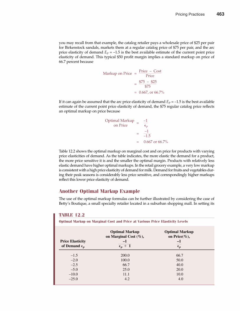
you may recall from that example, the catalog retailer pays a wholesale price of $25 per pairfor Birkenstock sandals, markets them at a regular catalog price of $75 per pair, and the arcprice elasticity of demand EP = –1.5 is the best available estimate of the current point priceelasticity of demand. This typical $50 profit margin implies a standard markup on price of66.7 percent because
Markup on Price = Price – CostPrice
= $75 – $25$75
= 0.667, or 66.7%
If it can again be assumed that the arc price elasticity of demand EP = –1.5 is the best availableestimate of the current point price elasticity of demand, the $75 regular catalog price reflectsan optimal markup on price because
Optimal Markup = –1on Price �P
= –1–1.5
= 0.667 or 66.7%
Table 12.2 shows the optimal markup on marginal cost and on price for products with varyingprice elasticities of demand. As the table indicates, the more elastic the demand for a product,the more price sensitive it is and the smaller the optimal margin. Products with relatively lesselastic demand have higher optimal markups. In the retail grocery example, a very low markupis consistent with a high price elasticity of demand for milk. Demand for fruits and vegetables dur-ing their peak seasons is considerably less price sensitive, and correspondingly higher markupsreflect this lower price elasticity of demand.
Another Optimal Markup ExampleThe use of the optimal markup formulas can be further illustrated by considering the case ofBetty’s Boutique, a small specialty retailer located in a suburban shopping mall. In setting its
Chapter Twelve Pricing Practices 463
TABLE 12.2Optimal Markup on Marginal Cost and Price at Various Price Elasticity Levels
Optimal Markup Optimal Markup on Marginal Cost (%), on Price(%),
Price Elasticity –1 –1of Demand �P �P � 1 �P
–1.5 200.0 66.7–2.0 100.0 50.0–2.5 66.7 40.0–5.0 25.0 20.0
–10.0 11.1 10.0–25.0 4.2 4.0
Pricing Practices 463
initial $36 price for a new spring line of blouses, Betty’s added a 50 percent markup on cost.Costs were estimated at $24 each: the $12 purchase price of each blouse, plus $6 in allocatedvariable overhead costs, plus an allocated fixed overhead charge of $6. Customer response wasso strong that when Betty’s raised prices from $36 to $39 per blouse, sales fell only from 54 to46 blouses per week. Was Betty’s initial $36 price optimal? Is the new $39 price suboptimal? Ifso, what is the optimal price?
At first blush, Betty’s pricing policy seems clearly inappropriate. It is always improper toconsider allocated fixed costs in setting prices for any good or service; only marginal or incre-mental costs should be included. However, by adjusting the amount of markup on cost ormarkup on price employed, Betty’s can implicitly compensate for the inappropriate use of fullyallocated costs. It is necessary to carefully analyze both the cost categories included and themarkup percentages chosen before judging a given pricing practice.
To determine Betty’s optimal markup, it is necessary to calculate an estimate of the pointprice elasticity of demand and relevant marginal cost, and then apply the optimal markup for-mula. Betty’s standard cost per blouse includes the $12 purchase cost, plus $6 allocated variablecosts, plus $6 fixed overhead charges. However, for pricing purposes, only the $12 purchase costplus the allocated variable overhead charge of $6 are relevant. Thus, the relevant marginal costfor pricing purposes is $18 per blouse. The allocated fixed overhead charge of $6 is irrelevantfor pricing purposes because fixed overhead costs are unaffected by blouse sales.
The $3 price increase to $39 represents a moderate 7.7 percent rise in price. Using the arcprice elasticity formula, the implied arc price elasticity of demand for Betty’s blouses is
EP = Q2 – Q1 �P2 + P1
P2 – P1 Q2 + Q1
= 46 – 54 �
$39 + $36$39 – $36 46 + 54
= –2
If it can be assumed that this arc price elasticity of demand �P = –2 is the best available estimateof the current point price elasticity of demand, the $36 price reflects an optimal markup of 100percent on relevant marginal costs of $18 because
Optimal Markup = –1on Cost �P + 1
= –1–2 + 1
= 1 or 100%
Similarly, the $36 price reflects an optimal markup on price because
Optimal Markup = –1on Price �P
= –1–2
= 0.5 or 50%
Betty’s actual markup on relevant marginal costs per blouse is an optimal 100 percent,because
Markup on Cost = $36 – $18$18
= 1 (or 100%)
464 Part Four Market Structure Analysis and Estimation
464 Pricing Practices
Similarly, Betty’s markup on price is an optimal 50 percent, because
Markup on Price = $36 – $18$36
= 0.5 (or 50%)
Therefore, Betty’s initial $36 price on blouses is optimal, and the subsequent $3 price increaseshould be rescinded.
This simple example teaches an important lesson. Despite the improper consideration offixed overhead costs and a markup that might at first appear unsuitable, Betty’s pricing poli-cy is entirely consistent with profit-maximizing behavior because the end result is an efficientpricing policy. Given the prevalence of markup pricing in everyday business practice, it isimportant that these pricing practices be carefully analyzed before they are judged suboptimal.The widespread use of markup pricing methods among highly successful firms suggests thatthe method is typically employed in ways that are consistent with profit maximization. Farfrom being a naive rule of thumb, markup pricing practices allow firms to arrive at optimalprices in an efficient manner.
PRICE DISCRIMINATION
With multiple markets or customer groups, the potential exists to enhance profits by chargingdifferent prices and markups to each relevant market segment. Market segmentation is animportant fact of life for firms in the airline, entertainment, hotel, medical, legal, and profes-sional services industries. Firms that offer goods also often segment their market betweenwholesale and retail buyers and between business, educational, not-for-profit, and govern-ment customers.
Chapter Twelve Pricing Practices 465
Why Do Some Price Wars Never Seem to End?
In supermarkets, permanent price wars rage for itemssuch as coffee, cola, pet foods, paper products, andfrozen foods. Top-of-the-line frozen food entré pricescontinue to drop as H.J. Heinz, Nestlé, ConAgra,Campbell’s Soup, and Kraft battle for overcrowdedfreezer space. In the salty snacks business, PepsiCo andBorden continue years of price warfare that has crum-bled the margins of a once highly profitable business. Inconsumer electronics, computer manufacturers havehad to contend with a marketplace that sees decliningprices on a monthly, weekly, or even daily basis.
Price wars, once a tool of limited strategic value inmature businesses, are becoming a disheartening fact oflife in industries ranging from autos to credit cards tosteel to computers. A growing number of companiestrapped into protecting investments that are too big towrite off are forced to pursue market share at all costs.Worse yet, using price wars to bump off competitors ismuch more difficult these days because weak competi-tors are often acquired by firms with deep pockets, orcan file for bankruptcy protection from creditors and
keep operating. The only clear winners in this ongoingprocess of constant price warfare are consumers, whohave come to enjoy and expect ever lower prices.
Businesses with high fixed costs are likely to displaysavage price competition. With commodity-like products,widely available price and product-quality information,and/or high fixed costs, competition to fill excesscapacity can be fierce. Nowhere are the effects of savageprice-cutting more evident than on the Internet, wheremarginal costs are often near zero. With negligible costsfor downloading to new customers, free software,sometimes called “freeware, “ is standard. Similarly,when distant suppliers are no more than a mouse clickaway, local and regional suppliers face unrelentingprice competition. This is all bad news for companies,and good news for the consumer. More than ever, thecustomer is king!
See: Sholnn Freeman and Joseph B. White, “Auto Price War Persistswith GM Expected to Introduce $2002 Cash-Rebate,” The Wall StreetJournal Online, January 3, 2002 (http://online.wsj.com).
M A N A G E R I A L A P P L I C AT I O N 1 2 . 2
Pricing Practices 465
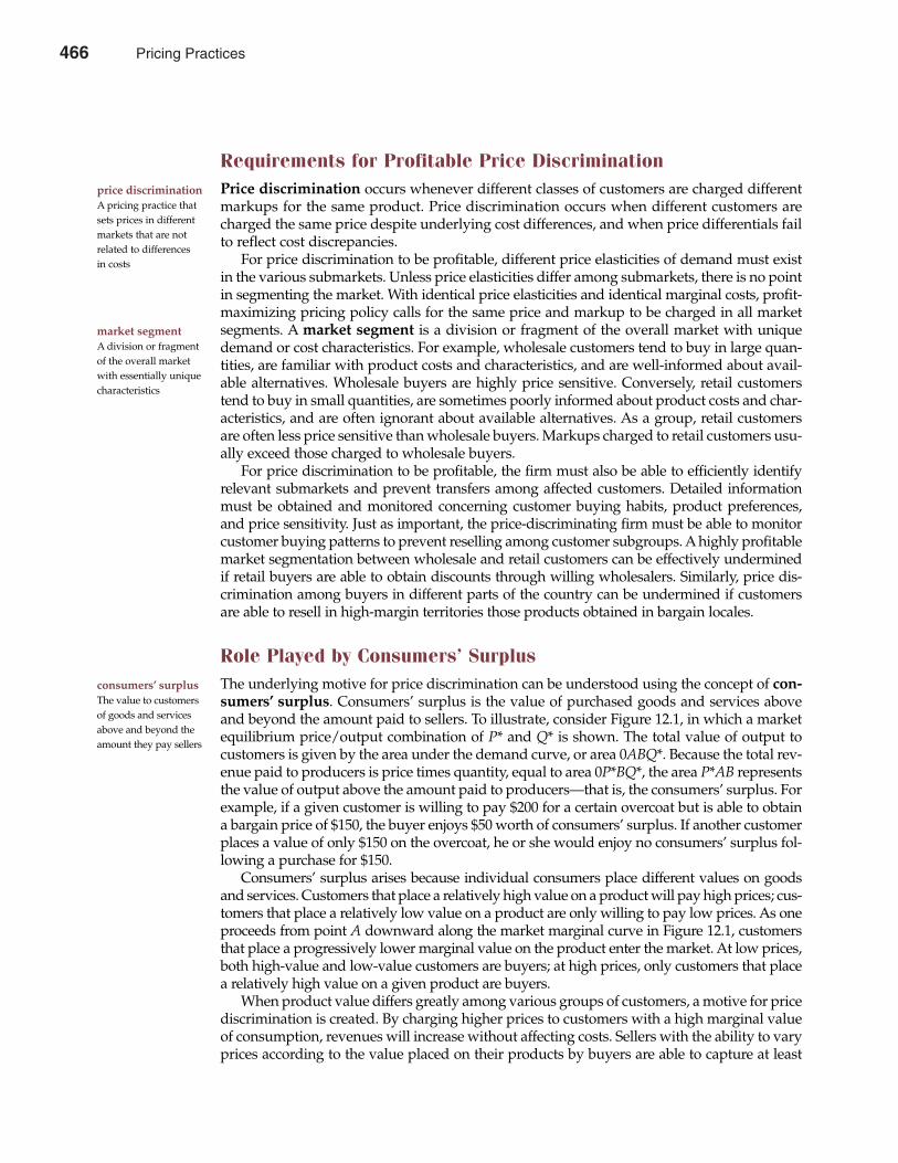
Requirements for Profitable Price DiscriminationPrice discrimination occurs whenever different classes of customers are charged differentmarkups for the same product. Price discrimination occurs when different customers arecharged the same price despite underlying cost differences, and when price differentials failto reflect cost discrepancies.
For price discrimination to be profitable, different price elasticities of demand must existin the various submarkets. Unless price elasticities differ among submarkets, there is no pointin segmenting the market. With identical price elasticities and identical marginal costs, profit-maximizing pricing policy calls for the same price and markup to be charged in all marketsegments. A market segment is a division or fragment of the overall market with uniquedemand or cost characteristics. For example, wholesale customers tend to buy in large quan-tities, are familiar with product costs and characteristics, and are well-informed about avail-able alternatives. Wholesale buyers are highly price sensitive. Conversely, retail customerstend to buy in small quantities, are sometimes poorly informed about product costs and char-acteristics, and are often ignorant about available alternatives. As a group, retail customersare often less price sensitive than wholesale buyers. Markups charged to retail customers usu-ally exceed those charged to wholesale buyers.
For price discrimination to be profitable, the firm must also be able to efficiently identifyrelevant submarkets and prevent transfers among affected customers. Detailed informationmust be obtained and monitored concerning customer buying habits, product preferences,and price sensitivity. Just as important, the price-discriminating firm must be able to monitorcustomer buying patterns to prevent reselling among customer subgroups. A highly profitablemarket segmentation between wholesale and retail customers can be effectively underminedif retail buyers are able to obtain discounts through willing wholesalers. Similarly, price dis-crimination among buyers in different parts of the country can be undermined if customersare able to resell in high-margin territories those products obtained in bargain locales.
Role Played by Consumers’ SurplusThe underlying motive for price discrimination can be understood using the concept of con-sumers’ surplus. Consumers’ surplus is the value of purchased goods and services aboveand beyond the amount paid to sellers. To illustrate, consider Figure 12.1, in which a marketequilibrium price/output combination of P* and Q* is shown. The total value of output tocustomers is given by the area under the demand curve, or area 0ABQ*. Because the total rev-enue paid to producers is price times quantity, equal to area 0P*BQ*, the area P*AB representsthe value of output above the amount paid to producers—that is, the consumers’ surplus. Forexample, if a given customer is willing to pay $200 for a certain overcoat but is able to obtaina bargain price of $150, the buyer enjoys $50 worth of consumers’ surplus. If another customerplaces a value of only $150 on the overcoat, he or she would enjoy no consumers’ surplus fol-lowing a purchase for $150.
Consumers’ surplus arises because individual consumers place different values on goodsand services. Customers that place a relatively high value on a product will pay high prices; cus-tomers that place a relatively low value on a product are only willing to pay low prices. As oneproceeds from point A downward along the market marginal curve in Figure 12.1, customersthat place a progressively lower marginal value on the product enter the market. At low prices,both high-value and low-value customers are buyers; at high prices, only customers that placea relatively high value on a given product are buyers.
When product value differs greatly among various groups of customers, a motive for pricediscrimination is created. By charging higher prices to customers with a high marginal valueof consumption, revenues will increase without affecting costs. Sellers with the ability to varyprices according to the value placed on their products by buyers are able to capture at least
466 Part Four Market Structure Analysis and Estimation
price discriminationA pricing practice thatsets prices in differentmarkets that are notrelated to differences in costs
market segmentA division or fragmentof the overall marketwith essentially uniquecharacteristics
consumers’ surplusThe value to customersof goods and servicesabove and beyond theamount they pay sellers
466 Pricing Practices
some of the value represented by consumers’ surplus. Such price discrimination will alwaysincrease profits because it allows the firm to increase total revenue without affecting costs. Afirm that is precise in its price discrimination always charges the maximum each market seg-ment is willing to pay. Price discrimination is charging what the market will bear.
Finally, it is important to recognize that price discrimination does not carry any evil connota-tion in a moral sense. In some circumstances, price discrimination leads to lower prices for somecustomer groups and to a wider availability of goods and services. For example, a municipal buscompany might charge lower prices for the elderly and the handicapped. In such circumstances,the bus company is price discriminating in favor of elderly and handicapped riders and againstother customers. This type of price discrimination provides elderly and handicapped customersa greater opportunity to ride the bus. Because of incremental revenues provided by elderlyand handicapped riders, the bus company may also be able to offer routes that could not besupported by revenues from full-fare customers alone, or it may be able to operate with alower taxpayer subsidy.
Degrees of Price DiscriminationThe extent to which a firm can engage in price discrimination is classified into three majorcategories. Under first-degree price discrimination, the firm extracts the maximum amounteach customer is willing to pay for its products. Each unit is priced separately at the priceindicated along each product demand curve. Such pricing precision is rare because itrequires that sellers know the maximum price each buyer is willing to pay for each unit ofoutput. Purchase decisions must also be monitored closely to prevent reselling amongcustomers. Although first-degree price discrimination is uncommon, it has the potential toemerge in any market where discounts from posted prices are standard and effective pricesare individually negotiated between buyers and sellers. When sellers possess a significantamount of market power, consumer purchases of big-ticket items such as appliances, auto-mobiles, homes, and professional services all have the potential to involve first-degree pricediscrimination.
Second-degree price discrimination, a more frequently employed type of price discrim-ination, involves setting prices on the basis of the quantity purchased. Bulk rates are typicallyset with high prices and markups charged for the first unit or block of units purchased, but
first-degree pricediscriminationCharging differentprices to each customer
second-degree pricediscriminationCharging differentprices based on userates or quantities pur-chased
Chapter Twelve Pricing Practices 467
FIGURE 12.1Consumers’ SurplusConsumers’ surplus is shown by the area P*AB and represents the value of output to consumers above andbeyond the amount they pay to producers.
ConsumersÕ surplus Supply
Demand
Price perunit ($)
B
A
P*
Q*0
Quantity
Pricing Practices 467
progressively greater discounts are offered for greater quantities. Quantity discounts that leadto lower markups for large versus small customers are a common means of discriminating inprice between retail and wholesale customers. Book publishers often charge full price for smallpurchases but offer 40 percent to 50 percent off list prices when 20 or more units are purchased.Public utilities, such as electric companies, gas companies, and water companies, also frequentlycharge block rates that are discriminatory. Consumers pay a relatively high markup for residen-tial service, whereas commercial and industrial customers pay relatively low markups. Officeequipment such as copy machines and servers (mainframe computers) are other examples ofproducts for which second-degree price discrimination is practiced, especially when time shar-ing among customers is involved.
The most commonly observed form of price discrimination, third-degree price discrim-ination, results when a firm separates its customers into several classes and sets a differentprice for each customer class. Customer classifications can be based on for-profit or not-for-profit status, regional location, or customer age. Barron’s, Forbes, The Wall Street Journal, andother publishers routinely offer educational discounts that can be in excess of 30 percent to 40percent off list prices. These publishers are eager to penetrate the classroom on the assumptionthat student users will become loyal future customers. Auto companies, personal computermanufacturers, and others also prominently feature educational discounts as part of their mar-keting strategy. Many hospitals also offer price discounts to various patient groups. If unem-ployed and uninsured patients are routinely charged only what they can easily afford to payfor medical service, whereas employed and insured medical patients are charged maximumallowable rates, the hospital is price discriminating in favor of the unemployed and against theemployed. Widespread price discounts for senior citizens represent a form of price discrimi-nation in favor of older customers but against younger customers.
PRICE DISCRIMINATION EXAMPLE
Price discrimination is profitable because it allows the firm to enhance revenues without increas-ing costs. It is an effective means for increasing profits because it allows the firm to more closelymatch marginal revenues and marginal costs. A firm that can segment its market maximizesprofits by operating at the point where marginal revenue equals marginal cost in each marketsegment. A detailed example is a helpful means for illustrating this process.
Price/Output DeterminationSuppose that Midwest State University (MSU) wants to reduce the athletic department’s
operating deficit and increase student attendance at home football games. To achieve theseobjectives, a new two-tier pricing structure for season football tickets is being considered.
A market survey conducted by the school suggests the following market demand andmarginal revenue relations:
Public Demand Student Demand
PP = $225 – $0.005QP PS = $125 – $0.00125QSMRP = ∆TRP/∆QP = $225 – $0.01QP MRS = ∆TRS/∆QS = $125 – $0.0025QS
From these market demand and marginal revenue curves, it is obvious that the general public iswilling to pay higher prices than are students. The general public is willing to purchase ticketsup to a market price of $225, above which point market demand equals zero. Students are will-ing to enter the market only at ticket prices below $125.
468 Part Four Market Structure Analysis and Estimation
third-degree pricediscriminationCharging differentprices to each customerclass
468 Pricing Practices
During recent years, the football program has run on an operating budget of $1.5 million peryear. This budget covers fixed salary, recruiting, insurance, and facility-maintenance expenses. Inaddition to these fixed expenses, the university incurs variable ticket-handling, facility-cleaning,insurance, and security costs of $25 per season ticketholder. The resulting total cost and marginalcost functions are
TC = $1,500,000 + $25QMC = ∆TC/∆Q = $25
What are the optimal football ticket prices and quantities for each market, assuming thatMSU adopts a new season ticket pricing policy featuring student discounts? To answer thisquestion, one must realize that because MC = $25, the athletic department’s operating deficitis minimized by setting MR = MC = $25 in each market segment and solving for Q. This isalso the profit-maximizing strategy for the football program. Therefore
Public Demand
MRP = MC
$225 – $0.01QP = $25$0.01QP = $200
QP = 20,000
and
PP = $225 – $0.005(20,000)= $125
Student Demand
MRS = MC
$125 – $0.0025QS = $25$0.0025QS = $100
QS = 40,000
and
PS = $125 – $0.00125(40,000)= $75
The football program’s resulting total operating surplus (profit) is
Operating Surplus (Profit) = TRP + TRS – TC
= $125(20,000) + $75(40,000)– $1,500,000 – $25(60,000)
= $2.5 million
To summarize, the optimal price/output combination with price discrimination is 20,000 in unitsales to the general public at a price of $125 and 40,000 in unit sales to students at a price of $75.This two-tier pricing practice results in an optimal operating surplus (profit) of $2.5 million.
Chapter Twelve Pricing Practices 469
Pricing Practices 469
Comparison with the One-Price AlternativeTo gauge the implications of this new two-tier ticket pricing practice, it is interesting to contrastthe resulting price/output and surplus levels with those that would result if MSU maintainedits current one-price ticket policy.
If tickets are offered to students and the general public at the same price, the total amountof ticket demand equals the sum of student plus general public demand. The student andgeneral public market demand curves are
QP = 45,000 – 200PP and QS = 100,000 – 800PS
Under the assumption PP = PS, total demand (QT) equals
QT = QP + QS
= 145,000 – 1,000P
and
P = $145 – $0.001Q
which implies that
MR = ∆TR/∆Q = $145 – $0.002Q
These aggregate student-plus-general-public market demand and marginal revenue curveshold only for prices below $125, a level at which both the general public and students purchasetickets. For prices above $125, only nonstudent purchasers buy tickets, and the public demandcurve PP = $225 – $0.005QP represents total market demand as well. This causes the actual totaldemand curve to be kinked at a price of $125, as shown in Figure 12.2.
The uniform season ticket price that maximizes operating surplus (or profits) is found bysetting MR = MC for the total market and solving for Q:
MR = MC
$145 – $0.002Q = $25$0.002Q = $120
Q = 60,000P = $145 – $0.001(60,000)
= $85
and
QP = 45,000 – 200($85) QS = 100,000 – 800($85)= 28,000 = 32,000
Operating surplus (profit) = TR – TC
= $85(60,000) – $1,500,000– $25(60,000)
= $2.1 million
Observe that the total number of tickets sold equals 60,000 under both the two-tier and thesingle-price policies. This results because the marginal cost of a ticket is the same under eachscenario. Ticket-pricing policies featuring student discounts increase student attendance from
470 Part Four Market Structure Analysis and Estimation
470 Pricing Practices
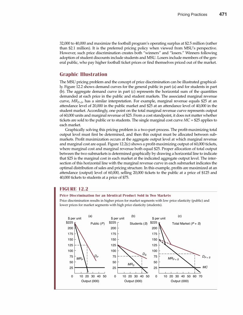
32,000 to 40,000 and maximize the football program’s operating surplus at $2.5 million (ratherthan $2.1 million). It is the preferred pricing policy when viewed from MSU’s perspective.However, such price discrimination creates both “winners” and “losers.” Winners followingadoption of student discounts include students and MSU. Losers include members of the gen-eral public, who pay higher football ticket prices or find themselves priced out of the market.
Graphic IllustrationThe MSU pricing problem and the concept of price discrimination can be illustrated graphical-ly. Figure 12.2 shows demand curves for the general public in part (a) and for students in part(b). The aggregate demand curve in part (c) represents the horizontal sum of the quantitiesdemanded at each price in the public and student markets. The associated marginal revenuecurve, MRP+S, has a similar interpretation. For example, marginal revenue equals $25 at anattendance level of 20,000 in the public market and $25 at an attendance level of 40,000 in thestudent market. Accordingly, one point on the total marginal revenue curve represents outputof 60,000 units and marginal revenue of $25. From a cost standpoint, it does not matter whethertickets are sold to the public or to students. The single marginal cost curve MC = $25 applies toeach market.
Graphically solving this pricing problem is a two-part process. The profit-maximizing totaloutput level must first be determined, and then this output must be allocated between sub-markets. Profit maximization occurs at the aggregate output level at which marginal revenueand marginal cost are equal. Figure 12.2(c) shows a profit-maximizing output of 60,000 tickets,where marginal cost and marginal revenue both equal $25. Proper allocation of total outputbetween the two submarkets is determined graphically by drawing a horizontal line to indicatethat $25 is the marginal cost in each market at the indicated aggregate output level. The inter-section of this horizontal line with the marginal revenue curve in each submarket indicates theoptimal distribution of sales and pricing structure. In this example, profits are maximized at anattendance (output) level of 60,000, selling 20,000 tickets to the public at a price of $125 and40,000 tickets to students at a price of $75.
Chapter Twelve Pricing Practices 471
FIGURE 12.2Price Discrimination for an Identical Product Sold in Two MarketsPrice discrimination results in higher prices for market segments with low price elasticity (public) andlower prices for market segments with high price elasticity (students).
10 20 30 40 500
25
50
75
100
125
150
175
200
$225
$ per unit
Public (P )
Output (000)
MRPDP
10 20 30 40 500
25
50
75
100
125
150
175
200
$225
$ per unit
Students (S)
Output (000)
MRS
DS
10 20 30 40 500
25
50
75
100
125
150
175
200
$225
$ per unit
Total Market (P + S)
Output (000)
(a) (b) (c)
MRP + SDP + S
MC
60 70
Pricing Practices 471
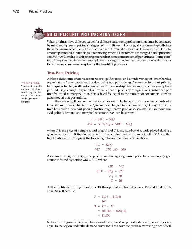
MULTIPLE-UNIT PRICING STRATEGIES
When products have different values for different customers, profits can sometimes be enhancedby using multiple-unit pricing strategies. With multiple-unit pricing, all customers typically facethe same pricing schedule, but the price paid is determined by the value to consumers of the totalamount purchased. Unlike single-unit pricing, where all customers are charged a unit price thatsets MR = MC, multiple-unit pricing can result in some combination of per-unit and “lump sum”fees. Like price discrimination, multiple-unit pricing strategies have proven an effective meansfor extracting consumers’ surplus for the benefit of producers.
Two-Part PricingAthletic clubs, time-share vacation resorts, golf courses, and a wide variety of “membershiporganizations” offer goods and services using two-part pricing. A common two-part pricingtechnique is to charge all customers a fixed “membership” fee per month or per year, plus aper-unit usage charge. In general, a firm can enhance profits by charging each customer a per-unit fee equal to marginal cost, plus a fixed fee equal to the amount of consumers’ surplusgenerated at that per-unit fee.
In the case of golf course memberships, for example, two-part pricing often consists of alarge lifetime membership fee plus “greens fees” charged for each round of golf played. To illus-trate how such a two-part pricing practice might prove profitable, assume that an individualavid golfer’s demand and marginal revenue curves can be written
P = $100 – $1Q
MR = ∆TR/∆Q = $100 – $2Q
where P is the price of a single round of golf, and Q is the number of rounds played during agiven year. For simplicity, also assume that the marginal cost of a round of golf is $20, and thatfixed costs are nil. This gives the following total and marginal cost relations:
TC = $20Q
MC = ∆TC/∆Q = $20
As shown in Figure 12.3(a), the profit-maximizing single-unit price for a monopoly golfcourse is found by setting MR = MC, where
MR = MC
$100 – $2Q = $202Q = 80Q = 40
At the profit-maximizing quantity of 40, the optimal single-unit price is $60 and total profitsequal $1,600 because
P = $100 – $1(40)= $60
π = TR – TC
= $60(40) – $20(40)= $1,600
Notice from Figure 12.3 (a) that the value of consumers’ surplus at a standard per-unit price isequal to the region under the demand curve that lies above the profit-maximizing price of $60.
472 Part Four Market Structure Analysis and Estimation
two-part pricingA per-unit fee equal tomarginal cost, plus afixed fee equal to theamount of consumers’surplus generated atthat price
472 Pricing Practices
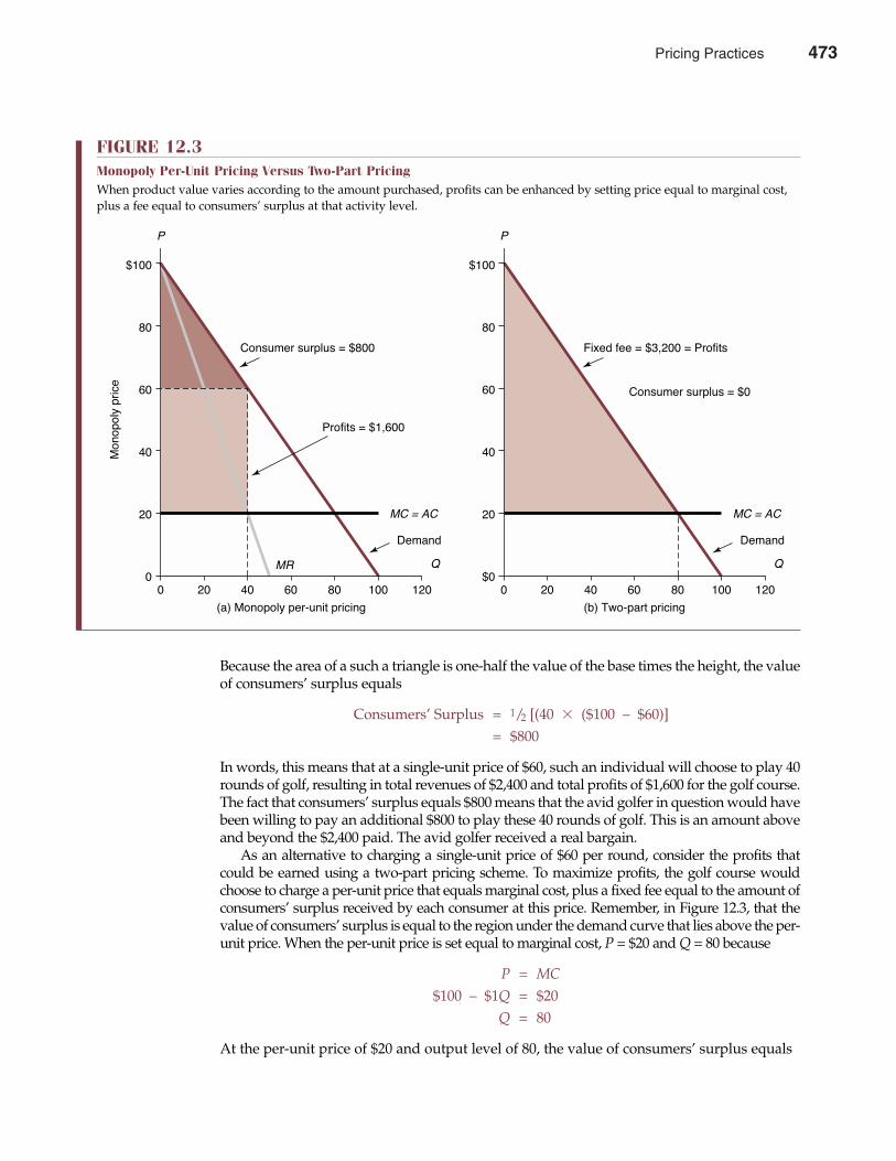
Because the area of a such a triangle is one-half the value of the base times the height, the valueof consumers’ surplus equals
Consumers’ Surplus = 1/2 [(40 � ($100 – $60)]= $800
In words, this means that at a single-unit price of $60, such an individual will choose to play 40rounds of golf, resulting in total revenues of $2,400 and total profits of $1,600 for the golf course.The fact that consumers’ surplus equals $800 means that the avid golfer in question would havebeen willing to pay an additional $800 to play these 40 rounds of golf. This is an amount aboveand beyond the $2,400 paid. The avid golfer received a real bargain.
As an alternative to charging a single-unit price of $60 per round, consider the profits thatcould be earned using a two-part pricing scheme. To maximize profits, the golf course wouldchoose to charge a per-unit price that equals marginal cost, plus a fixed fee equal to the amount ofconsumers’ surplus received by each consumer at this price. Remember, in Figure 12.3, that thevalue of consumers’ surplus is equal to the region under the demand curve that lies above the per-unit price. When the per-unit price is set equal to marginal cost, P = $20 and Q = 80 because
P = MC
$100 – $1Q = $20Q = 80
At the per-unit price of $20 and output level of 80, the value of consumers’ surplus equals
Chapter Twelve Pricing Practices 473
FIGURE 12.3Monopoly Per-Unit Pricing Versus Two-Part PricingWhen product value varies according to the amount purchased, profits can be enhanced by setting price equal to marginal cost,plus a fee equal to consumers’ surplus at that activity level.
P
Q
MC = AC
Demand
$100
80
60
40
20
$00 12020 10040 8060
(b) Two-part pricing
Fixed fee = $3,200 = Profits
Consumer surplus = $0
P
Q
MC = AC
MR
Demand
$100
80
60
40
20
00 12020 10040 8060
(a) Monopoly per-unit pricing
Monopolyprice
Profits = $1,600
Consumer surplus = $800
Pricing Practices 473
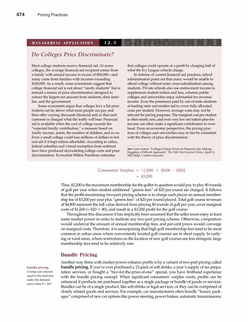
Consumers’ Surplus = 1/2 [(80 � ($100 – $20)]= $3,200
Thus, $3,200 is the maximum membership fee the golfer in question would pay to play 80 roundsof golf per year when modest additional “greens fees” of $20 per round are charged. It followsthat the profit-maximizing two-part pricing scheme is to charge each player an annual member-ship fee of $3,200 per year plus “greens fees” of $20 per round played. Total golf course revenuesof $4,800 represent the full value derived from playing 80 rounds of golf per year, cover marginalcosts of $1,600 (= $20 � 80), and result in a $3,200 profit for the golf course.
Throughout this discussion it has implicitly been assumed that the seller must enjoy at leastsome market power in order to institute any two-part pricing scheme. Otherwise, competitorswould undercut the amount of annual membership fees, and per-unit prices would convergeon marginal costs. Therefore, it is unsurprising that high golf membership fees tend to be mostcommon in urban areas where conveniently located golf courses are in short supply. In outly-ing or rural areas, where restrictions on the location of new golf courses are less stringent, largemembership fees tend to be relatively rare.
Bundle PricingAnother way firms with market power enhance profits is by a variant of two-part pricing calledbundle pricing. If you’ve ever purchased a 12-pack of soft drinks, a year’s supply of tax prepa-ration services, or bought a “two-for-the-price-of-one” special, you have firsthand experiencewith the bundle pricing concept. When significant consumers’ surplus exists, profits can beenhanced if products are purchased together as a single package or bundle of goods or services.Bundles can be of a single product, like soft drinks or legal services, or they can be comprised ofclosely related goods and services. For example, car manufacturers often bundle “luxury pack-ages” comprised of new car options like power steering, power brakes, automatic transmissions,
474 Part Four Market Structure Analysis and Estimation
bundle pricing A lump sum amountequal to the total areaunder the demandcurve when P = MC
Do Colleges Price Discriminate?
Most college students receive financial aid. At many colleges, the average financial aid recipient comes froma family with annual income in excess of $50,000—andmany came from families with incomes exceeding$100,000. As a result, some economists suggest that college financial aid is not about “needy students” but isinstead a means of price discrimination designed toextract the largest net amount from students, their fami-lies, and the government.
Some economists argue that colleges levy a list price(tuition) set far above what most people can pay andthen offer varying discounts (financial aid) so that eachcustomer is charged what the traffic will bear. Financialaid is available when the cost of college exceeds the“expected family contribution,” a measure based on family income, assets, the number of children, and so on.Even a small college could lose millions of dollars in fed-eral aid if it kept tuition affordable. According to critics,federal subsidies and virtual exemption from antitrustlaws have produced skyrocketing college costs and pricediscrimination. Economist Milton Friedman estimates
that colleges could operate at a profit by charging half ofwhat the Ivy League schools charge.
In defense of current financial aid practices, schooladministrators point out that many would be unable toafford college without some cross-subsidization amongstudents. Private schools also use endowment income tosupplement student tuition and fees, whereas public colleges and universities enjoy substantial tax-revenueincome. Even the premiums paid by out-of-state studentsat leading state universities fail to cover fully allocatedcosts per student. However, average costs may not be relevant for pricing purposes. The marginal cost per studentis often nearly zero, and even very low net tuition-plus-feeincome can often make a significant contribution to over-head. From an economic perspective, the pricing prac-tices of colleges and universities may in fact be consistentwith the theory of price discrimination.
See: Lynn Asinof, “Colleges Clamp Down on Financial Aid, MakingHaggling a Difficult Approach,” The Wall Street Journal Online, April 11,2002 (http://online.wsj.com).
M A N A G E R I A L A P P L I C AT I O N 1 2 . 3
474 Pricing Practices
tinted glass, and so on. Similarly, car dealers often bundle services, like oil changes, transmissionfluid changes, radiator flushes, and tune-ups at a “special package price.”
In the case of a single product sold in multiple-unit bundles, the optimal bundle price isderived in a manner similar to the optimal two-part price calculation described in Figure 12.3.As in the case of two-part pricing, the optimal level of output is determined by setting priceequal to marginal cost and solving for quantity. Then, the optimal bundle price is a single lumpsum amount equal to the total area under the demand curve at that point. In Figure 12.3(b), forexample, the optimal bundle price of $4,800 would include the total value of consumers’ sur-plus generated with a single per-unit price (or $3,200), plus total cost (or $1,600).
Optimal pricing for bundles of related but not identical products is figured in an analogousmanner. Again, the total amount charged equals the value of the total area under the demandcurve at the optimal output level, where output is defined as a bundle of related goods or serv-ices. As in the case of two-part pricing, the optimal level of output is determined by setting priceequal to marginal cost and solving for quantity. Then, the optimal bundle price is simply a lumpsum amount equal to the total area under the demand curve at that activity level. In the case ofrelated but not identical products, bundle pricing is sometimes used because firms are not ableto precisely determine the amounts different consumers are willing to pay for different products.If managers had precise information about the value of each individual product for each indi-vidual consumer, the firm could earn even higher profits by precisely tying the price charged tothe value derived by each customer.
MULTIPLE-PRODUCT PRICING
It is difficult to think of a firm that does not produce a variety of products. Almost all companiesproduce multiple models, styles, or sizes of output, and each of these variations can represent aseparate product for pricing purposes. Although multiple-product pricing requires the samebasic analysis as for a single product, the analysis is complicated by demand and productioninterrelations.
Demand InterrelationsDemand interrelations arise because of competition or complementarity among various prod-ucts or product lines. If products are interrelated, either as substitutes or complements, a changein the price of one affects demand for the other. Multiple-product pricing decisions must reflectsuch influences. In the case of a two-product firm, the marginal revenue functions for each prod-uct can be written as
(12.12) MRA = ∆TR=
∆TRA +∆TRB
∆QA ∆QA ∆QA
(12.13) MRB = ∆TR=
∆TRB +∆TRA
∆QB ∆QB ∆QB
The first term on the right side of each equation represents the marginal revenue directly associ-ated with each product. The second term depicts the indirect marginal revenue associatedwith each product and indicates the change in revenues due to a change in sales of the alternativeproduct. For example, ∆TRB/∆QA in Equation 12.12 shows the effect on product B revenues of anadditional unit sold of product A. Likewise, ∆TRA/∆QB in Equation 12.13 represents the changein revenues received from product A when an additional unit of product B is sold.
Cross-marginal revenue terms that reflect demand interrelations can be positive or negative.For complementary products, the net effect is positive because increased sales of one productlead to increased revenues from another. For substitute products, increased sales of one prod-uct reduce demand for another, and the cross-marginal revenue term is negative. Accurate price
Chapter Twelve Pricing Practices 475
Pricing Practices 475
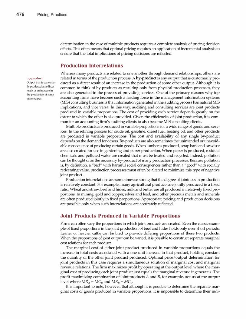
determination in the case of multiple products requires a complete analysis of pricing decisioneffects. This often means that optimal pricing requires an application of incremental analysis toensure that the total implications of pricing decisions are reflected.
Production InterrelationsWhereas many products are related to one another through demand relationships, others arerelated in terms of the production process. A by-product is any output that is customarily pro-duced as a direct result of an increase in the production of some other output. Although it iscommon to think of by-products as resulting only from physical production processes, theyare also generated in the process of providing services. One of the primary reasons why topaccounting firms have become such a leading force in the management information systems(MIS) consulting business is that information generated in the auditing process has natural MISimplications, and vice versa. In this way, auditing and consulting services are joint productsproduced in variable proportions. The cost of providing each service depends greatly on theextent to which the other is also provided. Given the efficiencies of joint production, it is com-mon for an accounting firm’s auditing clients to also become MIS consulting clients.
Multiple products are produced in variable proportions for a wide range of goods and serv-ices. In the refining process for crude oil, gasoline, diesel fuel, heating oil, and other productsare produced in variable proportions. The cost and availability of any single by-productdepends on the demand for others. By-products are also sometimes the unintended or unavoid-able consequence of producing certain goods. When lumber is produced, scrap bark and sawdustare also created for use in gardening and paper production. When paper is produced, residualchemicals and polluted water are created that must be treated and recycled. Indeed, pollutioncan be thought of as the necessary by-product of many production processes. Because pollutionis, by definition, a “bad” with harmful social consequences rather than a “good” with sociallyredeeming value, production processes must often be altered to minimize this type of negativejoint product.
Production interrelations are sometimes so strong that the degree of jointness in productionis relatively constant. For example, many agricultural products are jointly produced in a fixedratio. Wheat and straw, beef and hides, milk and butter are all produced in relatively fixed pro-portions. In mining, gold and copper, silver and lead, and other precious metals and mineralsare often produced jointly in fixed proportions. Appropriate pricing and production decisionsare possible only when such interrelations are accurately reflected.
Joint Products Produced in Variable ProportionsFirms can often vary the proportions in which joint products are created. Even the classic exam-ple of fixed proportions in the joint production of beef and hides holds only over short periods:Leaner or heavier cattle can be bred to provide differing proportions of these two products.When the proportions of joint output can be varied, it is possible to construct separate marginalcost relations for each product.
The marginal cost of either joint product produced in variable proportions equals theincrease in total costs associated with a one-unit increase in that product, holding constantthe quantity of the other joint product produced. Optimal price/output determination forjoint products in this case requires a simultaneous solution of marginal cost and marginalrevenue relations. The firm maximizes profit by operating at the output level where the mar-ginal cost of producing each joint product just equals the marginal revenue it generates. Theprofit-maximizing combination of joint products A and B, for example, occurs at the outputlevel where MRA = MCB and MRB = MCB.
It is important to note, however, that although it is possible to determine the separate mar-ginal costs of goods produced in variable proportions, it is impossible to determine their indi-
476 Part Four Market Structure Analysis and Estimation
by-productOutput that is customar-ily produced as a directresult of an increase inthe production of someother output
476 Pricing Practices
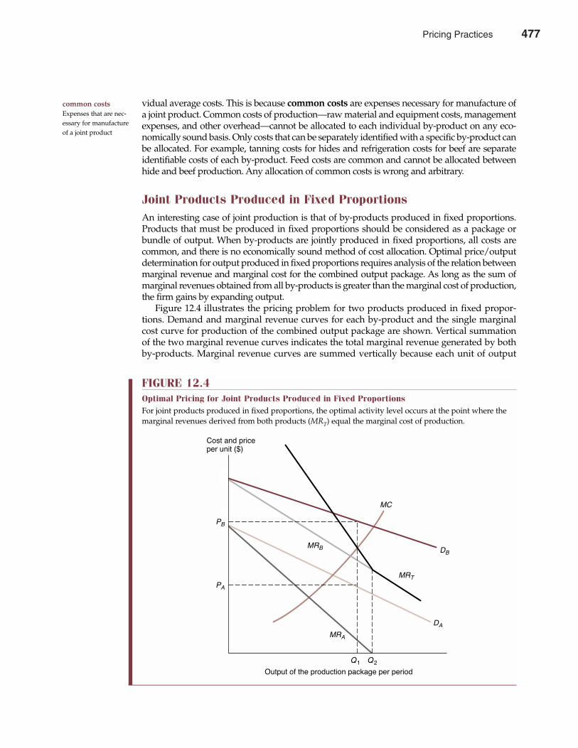
vidual average costs. This is because common costs are expenses necessary for manufacture ofa joint product. Common costs of production—raw material and equipment costs, managementexpenses, and other overhead—cannot be allocated to each individual by-product on any eco-nomically sound basis. Only costs that can be separately identified with a specific by-product canbe allocated. For example, tanning costs for hides and refrigeration costs for beef are separateidentifiable costs of each by-product. Feed costs are common and cannot be allocated betweenhide and beef production. Any allocation of common costs is wrong and arbitrary.
Joint Products Produced in Fixed ProportionsAn interesting case of joint production is that of by-products produced in fixed proportions.Products that must be produced in fixed proportions should be considered as a package orbundle of output. When by-products are jointly produced in fixed proportions, all costs arecommon, and there is no economically sound method of cost allocation. Optimal price/outputdetermination for output produced in fixed proportions requires analysis of the relation betweenmarginal revenue and marginal cost for the combined output package. As long as the sum ofmarginal revenues obtained from all by-products is greater than the marginal cost of production,the firm gains by expanding output.
Figure 12.4 illustrates the pricing problem for two products produced in fixed propor-tions. Demand and marginal revenue curves for each by-product and the single marginalcost curve for production of the combined output package are shown. Vertical summationof the two marginal revenue curves indicates the total marginal revenue generated by bothby-products. Marginal revenue curves are summed vertically because each unit of output
common costsExpenses that are nec-essary for manufactureof a joint product
Chapter Twelve Pricing Practices 477
FIGURE 12.4Optimal Pricing for Joint Products Produced in Fixed ProportionsFor joint products produced in fixed proportions, the optimal activity level occurs at the point where themarginal revenues derived from both products (MRT) equal the marginal cost of production.
MC
DB
MRT
DA
MRB
MRA
Q1 Q2
PA
PB
Output of the production package per period
Cost and priceper unit ($)
Pricing Practices 477
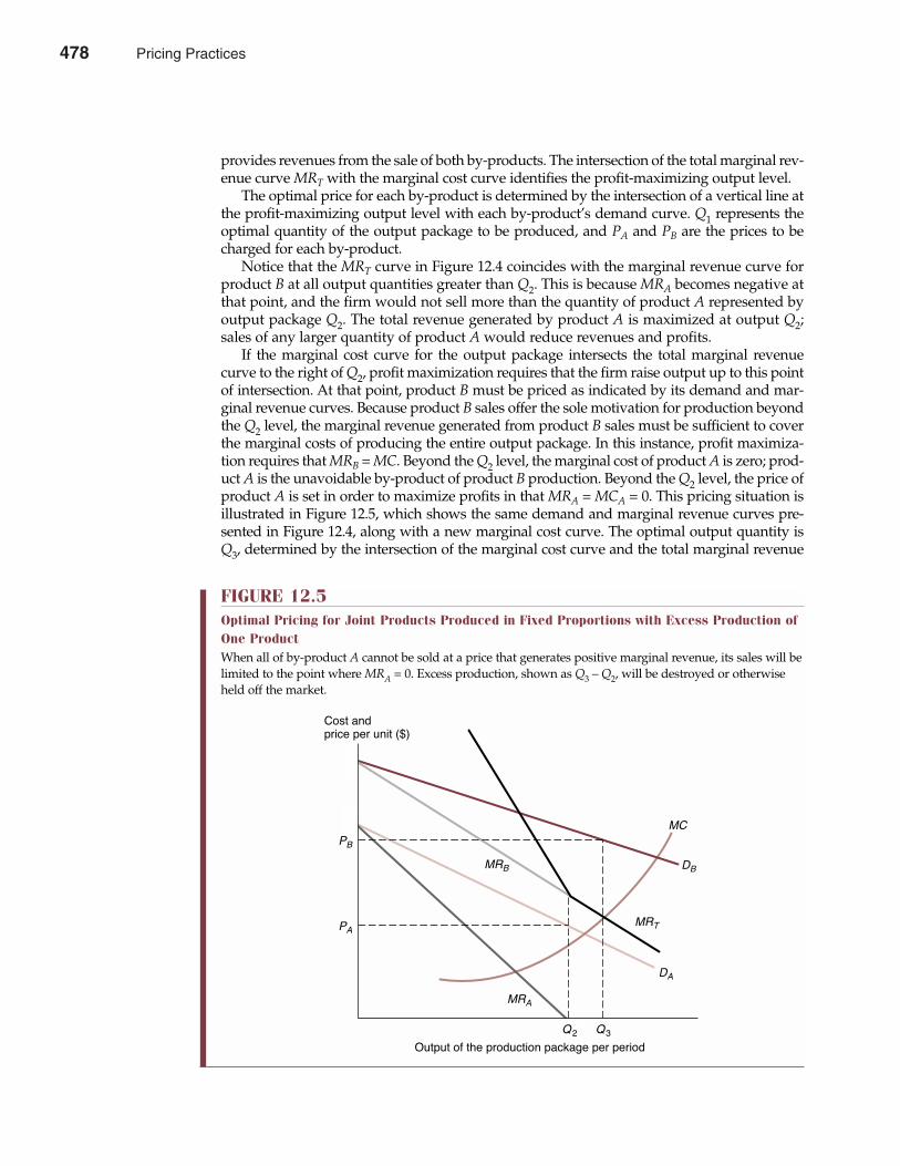
provides revenues from the sale of both by-products. The intersection of the total marginal rev-enue curve MRT with the marginal cost curve identifies the profit-maximizing output level.
The optimal price for each by-product is determined by the intersection of a vertical line atthe profit-maximizing output level with each by-product’s demand curve. Q1 represents theoptimal quantity of the output package to be produced, and PA and PB are the prices to becharged for each by-product.
Notice that the MRT curve in Figure 12.4 coincides with the marginal revenue curve forproduct B at all output quantities greater than Q2. This is because MRA becomes negative atthat point, and the firm would not sell more than the quantity of product A represented byoutput package Q2. The total revenue generated by product A is maximized at output Q2;sales of any larger quantity of product A would reduce revenues and profits.
If the marginal cost curve for the output package intersects the total marginal revenuecurve to the right of Q2, profit maximization requires that the firm raise output up to this pointof intersection. At that point, product B must be priced as indicated by its demand and mar-ginal revenue curves. Because product B sales offer the sole motivation for production beyondthe Q2 level, the marginal revenue generated from product B sales must be sufficient to coverthe marginal costs of producing the entire output package. In this instance, profit maximiza-tion requires that MRB = MC. Beyond the Q2 level, the marginal cost of product A is zero; prod-uct A is the unavoidable by-product of product B production. Beyond the Q2 level, the price ofproduct A is set in order to maximize profits in that MRA = MCA = 0. This pricing situation isillustrated in Figure 12.5, which shows the same demand and marginal revenue curves pre-sented in Figure 12.4, along with a new marginal cost curve. The optimal output quantity isQ3, determined by the intersection of the marginal cost curve and the total marginal revenue
478 Part Four Market Structure Analysis and Estimation
FIGURE 12.5Optimal Pricing for Joint Products Produced in Fixed Proportions with Excess Production ofOne ProductWhen all of by-product A cannot be sold at a price that generates positive marginal revenue, its sales will belimited to the point where MRA = 0. Excess production, shown as Q3 – Q2, will be destroyed or otherwiseheld off the market.
MC
DB
MRT
DA
MRB
MRA
Q2 Q3
PA
PB
Output of the production package per period
Cost andprice per unit ($)
478 Pricing Practices
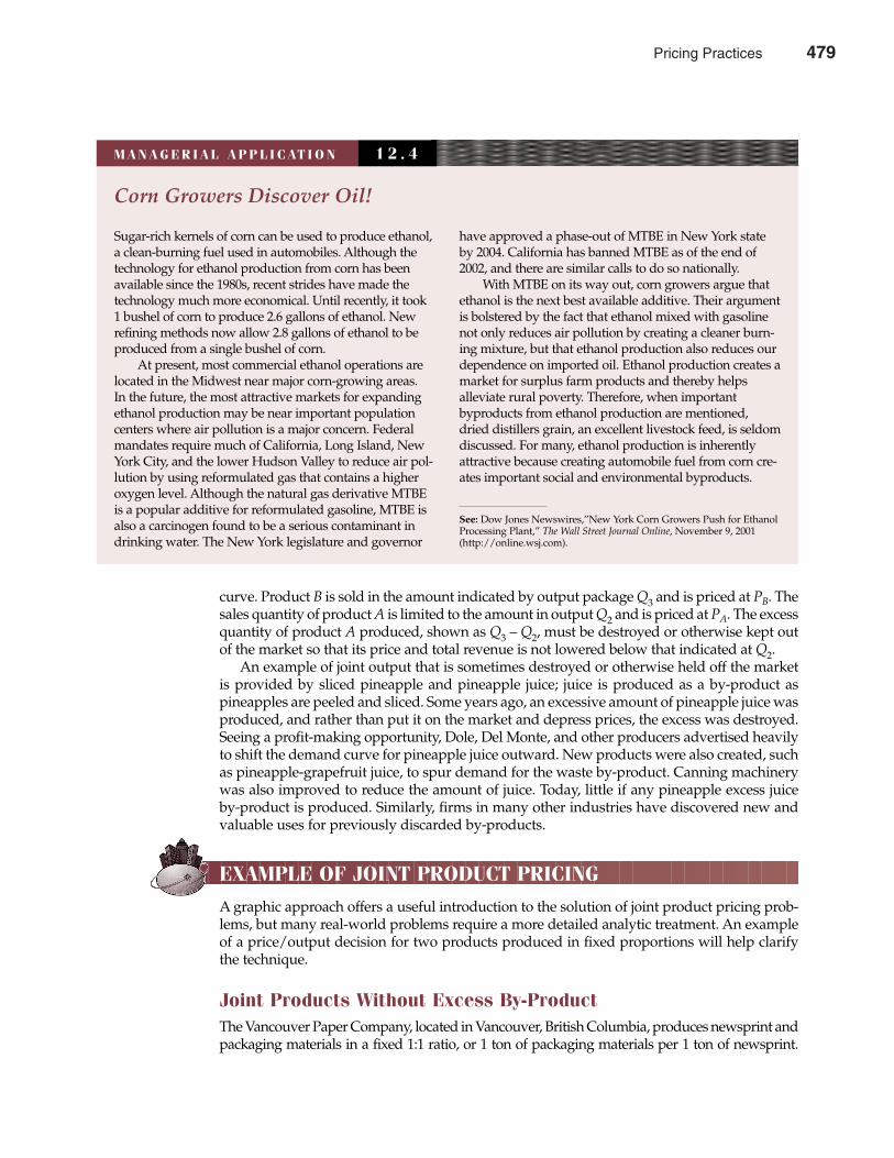
curve. Product B is sold in the amount indicated by output package Q3 and is priced at PB. Thesales quantity of product A is limited to the amount in output Q2 and is priced at PA. The excessquantity of product A produced, shown as Q3 – Q2, must be destroyed or otherwise kept outof the market so that its price and total revenue is not lowered below that indicated at Q2.
An example of joint output that is sometimes destroyed or otherwise held off the marketis provided by sliced pineapple and pineapple juice; juice is produced as a by-product aspineapples are peeled and sliced. Some years ago, an excessive amount of pineapple juice wasproduced, and rather than put it on the market and depress prices, the excess was destroyed.Seeing a profit-making opportunity, Dole, Del Monte, and other producers advertised heavilyto shift the demand curve for pineapple juice outward. New products were also created, suchas pineapple-grapefruit juice, to spur demand for the waste by-product. Canning machinerywas also improved to reduce the amount of juice. Today, little if any pineapple excess juiceby-product is produced. Similarly, firms in many other industries have discovered new andvaluable uses for previously discarded by-products.
EXAMPLE OF JOINT PRODUCT PRICING
A graphic approach offers a useful introduction to the solution of joint product pricing prob-lems, but many real-world problems require a more detailed analytic treatment. An exampleof a price/output decision for two products produced in fixed proportions will help clarifythe technique.
Joint Products Without Excess By-ProductThe Vancouver Paper Company, located in Vancouver, British Columbia, produces newsprint andpackaging materials in a fixed 1:1 ratio, or 1 ton of packaging materials per 1 ton of newsprint.
Chapter Twelve Pricing Practices 479
Corn Growers Discover Oil!
Sugar-rich kernels of corn can be used to produce ethanol,a clean-burning fuel used in automobiles. Although thetechnology for ethanol production from corn has beenavailable since the 1980s, recent strides have made thetechnology much more economical. Until recently, it took1 bushel of corn to produce 2.6 gallons of ethanol. Newrefining methods now allow 2.8 gallons of ethanol to beproduced from a single bushel of corn.
At present, most commercial ethanol operations arelocated in the Midwest near major corn-growing areas. In the future, the most attractive markets for expandingethanol production may be near important populationcenters where air pollution is a major concern. Federalmandates require much of California, Long Island, NewYork City, and the lower Hudson Valley to reduce air pol-lution by using reformulated gas that contains a higheroxygen level. Although the natural gas derivative MTBEis a popular additive for reformulated gasoline, MTBE isalso a carcinogen found to be a serious contaminant indrinking water. The New York legislature and governor
have approved a phase-out of MTBE in New York stateby 2004. California has banned MTBE as of the end of2002, and there are similar calls to do so nationally.
With MTBE on its way out, corn growers argue thatethanol is the next best available additive. Their argumentis bolstered by the fact that ethanol mixed with gasolinenot only reduces air pollution by creating a cleaner burn-ing mixture, but that ethanol production also reduces ourdependence on imported oil. Ethanol production creates amarket for surplus farm products and thereby helps alleviate rural poverty. Therefore, when importantbyproducts from ethanol production are mentioned,dried distillers grain, an excellent livestock feed, is seldomdiscussed. For many, ethanol production is inherentlyattractive because creating automobile fuel from corn cre-ates important social and environmental byproducts.
See: Dow Jones Newswires,”New York Corn Growers Push for EthanolProcessing Plant,” The Wall Street Journal Online, November 9, 2001(http://online.wsj.com).
M A N A G E R I A L A P P L I C AT I O N 1 2 . 4
Pricing Practices 479
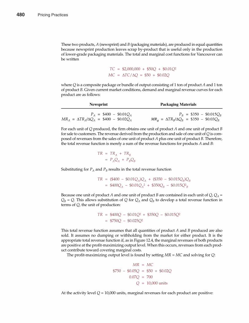
480 Part Four Market Structure Analysis and Estimation
These two products, A (newsprint) and B (packaging materials), are produced in equal quantitiesbecause newsprint production leaves scrap by-product that is useful only in the productionof lower-grade packaging materials. The total and marginal cost functions for Vancouver canbe written
TC = $2,000,000 + $50Q + $0.01Q2
MC = ∆TC/∆Q = $50 + $0.02Q
where Q is a composite package or bundle of output consisting of 1 ton of product A and 1 tonof product B. Given current market conditions, demand and marginal revenue curves for eachproduct are as follows:
Newsprint Packaging Materials
PA = $400 – $0.01QA PB = $350 – $0.015QBMRA = ∆TRA/∆QA = $400 – $0.02QA MRB = ∆TRB/∆QB = $350 – $0.03QB
For each unit of Q produced, the firm obtains one unit of product A and one unit of product Bfor sale to customers. The revenue derived from the production and sale of one unit of Q is com-posed of revenues from the sales of one unit of product A plus one unit of product B. Therefore,the total revenue function is merely a sum of the revenue functions for products A and B:
TR = TRA + TRB
= PAQA + PBQB
Substituting for PA and PB results in the total revenue function
TR = ($400 – $0.01QA)QA + ($350 – $0.015QB)QB
= $400QA – $0.01QA2 + $350QB – $0.015Q2
B
Because one unit of product A and one unit of product B are contained in each unit of Q, QA =QB = Q. This allows substitution of Q for QA and QB to develop a total revenue function interms of Q, the unit of production:
TR = $400Q – $0.01Q2 + $350Q – $0.015Q2
= $750Q – $0.025Q2
This total revenue function assumes that all quantities of product A and B produced are alsosold. It assumes no dumping or withholding from the market for either product. It is theappropriate total revenue function if, as in Figure 12.4, the marginal revenues of both productsare positive at the profit-maximizing output level. When this occurs, revenues from each prod-uct contribute toward covering marginal costs.
The profit-maximizing output level is found by setting MR = MC and solving for Q:
MR = MC
$750 – $0.05Q = $50 + $0.02Q
0.07Q = 700Q = 10,000 units
At the activity level Q = 10,000 units, marginal revenues for each product are positive:
480 Pricing Practices
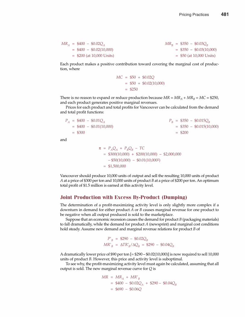
MRA = $400 – $0.02QA MRB = $350 – $0.03QB
= $400 – $0.02(10,000) = $350 – $0.03(10,000)= $200 (at 10,000 Units) = $50 (at 10,000 Units)
Each product makes a positive contribution toward covering the marginal cost of produc-tion, where
MC = $50 + $0.02Q
= $50 + $0.02(10,000)= $250
There is no reason to expand or reduce production because MR = MRA + MRB = MC = $250,and each product generates positive marginal revenues.
Prices for each product and total profits for Vancouver can be calculated from the demandand total profit functions:
PA = $400 – $0.01QA PB = $350 – $0.015QB
= $400 – $0.01(10,000) = $350 – $0.015(10,000)= $300 = $200
and
π = PAQA + PBQB – TC
= $300(10,000) + $200(10,000) – $2,000,000– $50(10,000) – $0.01(10,0002)
= $1,500,000
Vancouver should produce 10,000 units of output and sell the resulting 10,000 units of productA at a price of $300 per ton and 10,000 units of product B at a price of $200 per ton. An optimumtotal profit of $1.5 million is earned at this activity level.
Joint Production with Excess By-Product (Dumping)The determination of a profit-maximizing activity level is only slightly more complex if adownturn in demand for either product A or B causes marginal revenue for one product tobe negative when all output produced is sold to the marketplace.
Suppose that an economic recession causes the demand for product B (packaging materials)to fall dramatically, while the demand for product A (newsprint) and marginal cost conditionshold steady. Assume new demand and marginal revenue relations for product B of
P�B = $290 – $0.02QB
MR�B = ∆TR�B/∆QB = $290 – $0.04QB
A dramatically lower price of $90 per ton [= $290 – $0.02(10,000)] is now required to sell 10,000units of product B. However, this price and activity level is suboptimal.
To see why, the profit-maximizing activity level must again be calculated, assuming that alloutput is sold. The new marginal revenue curve for Q is
MR = MRA + MR�B
= $400 – $0.02QA + $290 – $0.04QB
= $690 – $0.06Q
Chapter Twelve Pricing Practices 481
Pricing Practices 481
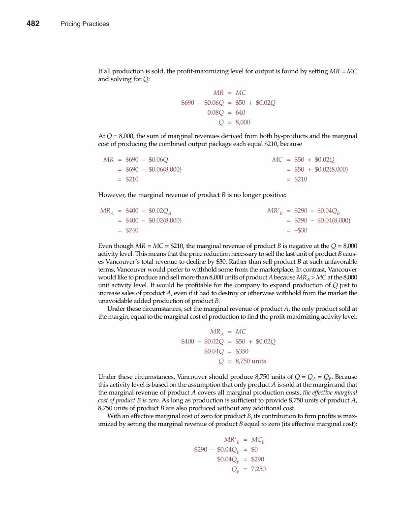
If all production is sold, the profit-maximizing level for output is found by setting MR = MCand solving for Q:
MR = MC
$690 – $0.06Q = $50 + $0.02Q
0.08Q = 640Q = 8,000
At Q = 8,000, the sum of marginal revenues derived from both by-products and the marginalcost of producing the combined output package each equal $210, because
MR = $690 – $0.06Q MC = $50 + $0.02Q
= $690 – $0.06(8,000) = $50 + $0.02(8,000)= $210 = $210
However, the marginal revenue of product B is no longer positive:
MRA = $400 – $0.02QA MR�B = $290 – $0.04QB
= $400 – $0.02(8,000) = $290 – $0.04(8,000)= $240 = –$30
Even though MR = MC = $210, the marginal revenue of product B is negative at the Q = 8,000activity level. This means that the price reduction necessary to sell the last unit of product B caus-es Vancouver’s total revenue to decline by $30. Rather than sell product B at such unfavorableterms, Vancouver would prefer to withhold some from the marketplace. In contrast, Vancouverwould like to produce and sell more than 8,000 units of product Abecause MRA > MC at the 8,000unit activity level. It would be profitable for the company to expand production of Q just toincrease sales of product A, even if it had to destroy or otherwise withhold from the market theunavoidable added production of product B.
Under these circumstances, set the marginal revenue of product A, the only product sold atthe margin, equal to the marginal cost of production to find the profit-maximizing activity level:
MRA = MC
$400 – $0.02Q = $50 + $0.02Q
$0.04Q = $350Q = 8,750 units
Under these circumstances, Vancouver should produce 8,750 units of Q = QA = QB. Becausethis activity level is based on the assumption that only product A is sold at the margin and thatthe marginal revenue of product A covers all marginal production costs, the effective marginalcost of product B is zero. As long as production is sufficient to provide 8,750 units of product A,8,750 units of product B are also produced without any additional cost.
With an effective marginal cost of zero for product B, its contribution to firm profits is max-imized by setting the marginal revenue of product B equal to zero (its effective marginal cost):
MR�B = MCB
$290 – $0.04QB = $0$0.04QB = $290
QB = 7,250
482 Part Four Market Structure Analysis and Estimation
482 Pricing Practices
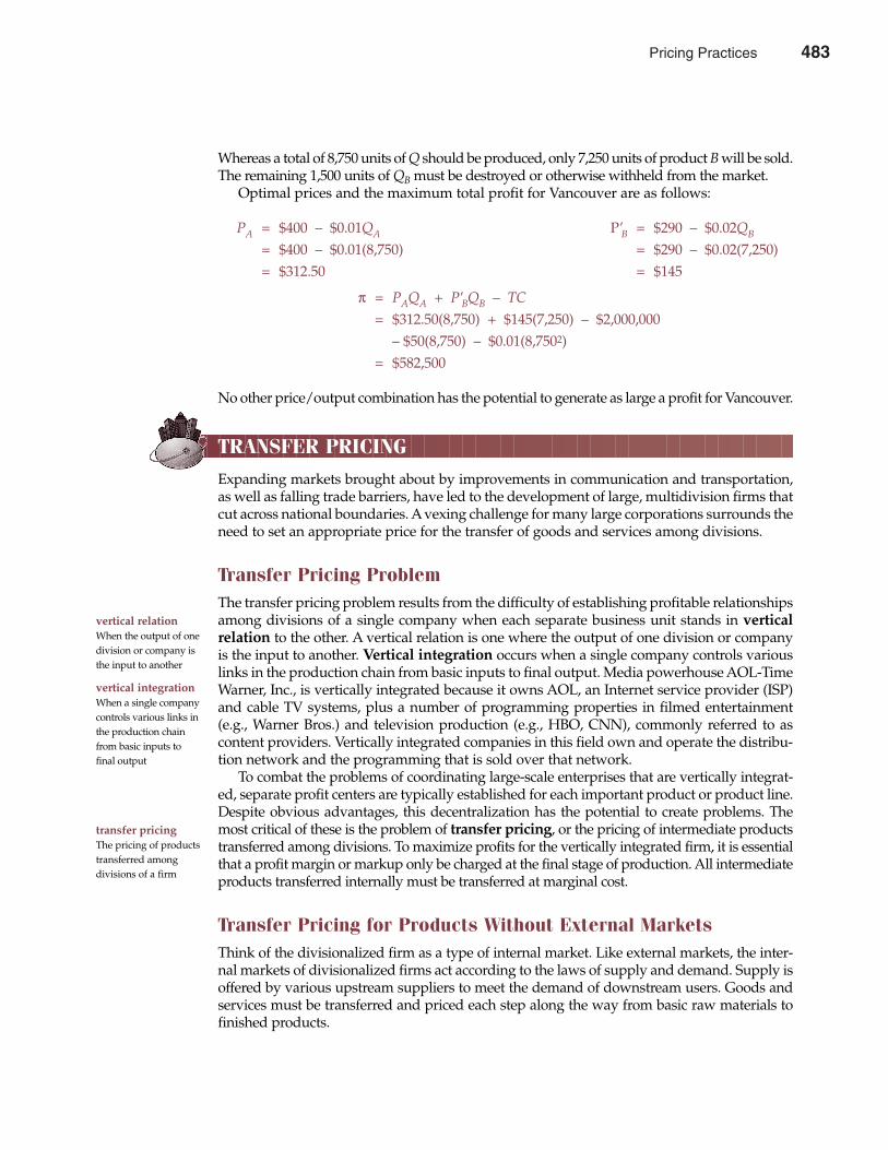
Whereas a total of 8,750 units of Q should be produced, only 7,250 units of product B will be sold.The remaining 1,500 units of QB must be destroyed or otherwise withheld from the market.
Optimal prices and the maximum total profit for Vancouver are as follows:
PA = $400 – $0.01QA P�B = $290 – $0.02QB
= $400 – $0.01(8,750) = $290 – $0.02(7,250)= $312.50 = $145
π = PAQA + P�BQB – TC
= $312.50(8,750) + $145(7,250) – $2,000,000– $50(8,750) – $0.01(8,7502)
= $582,500
No other price/output combination has the potential to generate as large a profit for Vancouver.
TRANSFER PRICING
Expanding markets brought about by improvements in communication and transportation,as well as falling trade barriers, have led to the development of large, multidivision firms thatcut across national boundaries. A vexing challenge for many large corporations surrounds theneed to set an appropriate price for the transfer of goods and services among divisions.
Transfer Pricing ProblemThe transfer pricing problem results from the difficulty of establishing profitable relationshipsamong divisions of a single company when each separate business unit stands in verticalrelation to the other. A vertical relation is one where the output of one division or companyis the input to another. Vertical integration occurs when a single company controls variouslinks in the production chain from basic inputs to final output. Media powerhouse AOL-TimeWarner, Inc., is vertically integrated because it owns AOL, an Internet service provider (ISP)and cable TV systems, plus a number of programming properties in filmed entertainment(e.g., Warner Bros.) and television production (e.g., HBO, CNN), commonly referred to ascontent providers. Vertically integrated companies in this field own and operate the distribu-tion network and the programming that is sold over that network.
To combat the problems of coordinating large-scale enterprises that are vertically integrat-ed, separate profit centers are typically established for each important product or product line.Despite obvious advantages, this decentralization has the potential to create problems. Themost critical of these is the problem of transfer pricing, or the pricing of intermediate productstransferred among divisions. To maximize profits for the vertically integrated firm, it is essentialthat a profit margin or markup only be charged at the final stage of production. All intermediateproducts transferred internally must be transferred at marginal cost.
Transfer Pricing for Products Without External MarketsThink of the divisionalized firm as a type of internal market. Like external markets, the inter-nal markets of divisionalized firms act according to the laws of supply and demand. Supply isoffered by various upstream suppliers to meet the demand of downstream users. Goods andservices must be transferred and priced each step along the way from basic raw materials tofinished products.
vertical relationWhen the output of onedivision or company isthe input to another
vertical integrationWhen a single companycontrols various links inthe production chainfrom basic inputs tofinal output
transfer pricingThe pricing of productstransferred amongdivisions of a firm
Chapter Twelve Pricing Practices 483
Pricing Practices 483
For simplicity, consider the problem faced by a vertically integrated firm that has differentdivisions at distinct points along the various steps of the production process, and assume for themoment that no external market exists for transferred inputs. If each separate division is estab-lished as a profit center to provide employees with an efficiency incentive, a transfer pricingproblem can occur. Suppose each selling division adds a markup over its marginal cost for inputssold to other divisions. Each buying division would then set its marginal revenue from outputequal to the division’s marginal cost of input. This process would culminate in a marginal costto the ultimate upstream user that exceeds the sum total of marginal costs for each transferringdivision. All of the markups charged by each transferring division drive a wedge between thefirm’s true marginal cost of production and the marginal cost to the last or ultimate upstreamuser. As a result, the ultimate upstream user buys less than the optimal amount of input and pro-duces less than the profit-maximizing level of output.
For example, it would be inefficient if AOL, a major ISP, paid more than the marginal costof programming produced by its own subsidiaries. If each subsidiary added a markup to themarginal cost of programming sold to the parent company, AOL would buy less than a profit-maximizing amount of its own programming. In fact, AOL would have an incentive to seekprogramming from other purveyors so long as the external market price was less than theinternal transfer price. Such an incentive could create extreme inefficiencies, especially whenthe external market price is less than the transfer price but greater than the marginal cost ofprogramming produced by AOL’s own subsidiaries.
An effective transfer pricing system leads to activity levels in each division that are consis-tent with profit maximization for the overall enterprise. This observation leads to the mostbasic rule for optimal transfer pricing: When transferred products cannot be sold in external mar-kets, the marginal cost of the transferring division is the optimal transfer price. One practical meansfor insuring that an optimal amount of input is transferred at an optimal transfer price is toinform buying divisions that the marginal cost curve of supplying divisions is to be treated likea supply schedule. Alternatively, supplying divisions could be informed about the buyingdivision’s marginal revenue or demand curve and told to use this information in determiningthe quantity supplied. In either case, each division would voluntarily choose to transfer anoptimal amount of input at the optimal transfer price.
Transfer Pricing with Perfectly Competitive External MarketsThe transfer pricing problem is only sightly more complicated when transferred inputs can besold in external markets. When transferred inputs can be sold in a perfectly competitive externalmarket, the external market price represents the firm’s opportunity cost of employing suchinputs internally. As such, it would never pay to use inputs internally unless their value to thefirm is at least as great as their value to others in the external market. This observation leads to asecond key rule for optimal transfer pricing: When transferred products can be sold in perfectly com-petitive external markets, the external market price is the optimal transfer price. If upstream supplierswish to supply more than downstream users desire to employ at a perfectly competitive price,excess input can be sold in the external market. If downstream users wish to employ more thanupstream suppliers seek to furnish at a perfectly competitive price, excess input demand can bemet through purchases in the external market. In either event, an optimal amount of input istransferred internally.
Of course, it is hard to imagine why a firm would be vertically integrated in the first placeif all inputs could be purchased in perfectly competitive markets. Neither Kellogg’s norMcDonald’s, for example, have extensive agricultural operations to ensure a steady supply offoodstuffs. Grains for cereal and beef for hamburgers can both be purchased at prices thatclosely approximate marginal cost in perfectly competitive input markets. On the other hand,if an input market is typically competitive but punctuated by periods of scarcity and shortage,it can pay to maintain some input producing capability. For example, ExxonMobil Corp. has
484 Part Four Market Structure Analysis and Estimation
484 Pricing Practices

considerable production facilities that supply its extensive distribution network with gasoline,oil, and petroleum products. These production facilities offer ExxonMobil some protectionagainst the threat of supply stoppages. Similarly, Coca-Cola has long-term supply contractswith orange growers to ensure a steady supply of product for its Minute Maid juice operation.Both ExxonMobil and Coca-Cola are examples of vertically integrated firms with inputsoffered in markets that are usually, but not always, perfectly competitive.
Transfer Pricing with Imperfectly Competitive External MarketsThe typical case of vertical integration involves firms with inputs that can be transferred inter-nally or sold in external markets that are not perfectly competitive. Again, it never pays to useinputs internally unless their value to the firm is at least as great as their value to others in theexternal market. This observation leads to a third and final fundamental rule for optimal trans-fer pricing: When transferred products can be sold in imperfectly competitive external markets, the opti-mal transfer price equates the marginal cost of the transferring division to the marginal revenuederived from the combined internal and external markets. In other words, when inputs can be sold inimperfectly competitive external markets, internal input demand must reflect the opportunityto supply input to the external market at a price in excess of marginal cost. If upstream sup-pliers wish to offer more input than downstream users desire to employ when input MC = MRfrom the combined market, excess supply can be sold in the external market. If downstreamusers want to employ more than upstream suppliers seek to furnish when MC = MR, excessinternal demand can be met through added purchases in the external market. In both cases, anoptimal amount of input is transferred internally.
GLOBAL TRANSFER PRICING EXAMPLE
Although the transfer pricing concept can be introduced conceptually through the use of graph-ic analysis, most real-world applications are complex and must be solved algebraically. For thisreason, examination of a detailed numerical example can be fruitful.
Profit Maximization for an Integrated FirmJosiah Bartlet & Sons, Inc., is a small integrated domestic manufacturer of material handlingequipment. Demand and marginal revenue curves for the firm are
P = $100 – $0.001Q
MR = ∆TR/∆Q = $100 – $0.002Q
Relevant total cost, marginal cost, and profit functions are
TC = $312,500 + $25Q + $0.0015Q2
MC = ∆TC/∆Q = $25 + $0.003Q
π = TR – TC
= $100Q – $0.001Q2 – $312,500 – $25Q – $0.0015Q2
= –$0.0025Q2 + $75Q – $312,500
Profit maximization occurs at the point where MR = MC, so the optimal output level is
MR = MC
$100 – $0.002Q = $25 + $0.003Q
Chapter Twelve Pricing Practices 485
Pricing Practices 485
75 = 0.005Q
Q = 15,000
This implies that
P = $100 – $0.001(15,000)= $85
π = TR – TC
= –$0.0025(15,0002) + $75(15,000) – $312,500= $250,000
Therefore, the optimal price/output combination is $85 and 15,000 units for this integrated firm,and profits total $250,000. To be optimal, transfer prices must ensure operation at these levels.
Transfer Pricing with No External MarketConsider how the situation changes if the firm is reorganized into separate manufacturing anddistribution division profit centers, and no external market exists for the transferred product.The demand curve facing the distribution division is precisely the same as the firm’s outputdemand curve. Although the total cost function of the firm is unchanged, it can be brokendown into the costs of manufacturing and distribution.
Assume that such a breakdown results in the following divisional cost functions:
TCMfg = $250,000 + $20Q + $0.001Q2
MCMfg = ∆TCMfg/∆Q = $20 + $0.002Q
and
TCDistr = $62,500 + $5Q + $0.0005Q2
MCDistr = ∆TCDistr/∆Q = $5 + $0.001Q
With divisional operation, the total and marginal cost functions for the firm are
TC = TCMfg + TCDistr
MC = MCMfg + MCDistr
and precisely the same as before.To demonstrate the derivation of an appropriate activity level, the net marginal revenue for
the distribution division is set equal to the marginal cost of the manufacturing division:
MR – MCDistr = MCMfg
$100 – $0.002Q – $5 – $0.001Q = $20 + $0.002Q
75 = 0.005Q
Q = 15,000
The 15,000-unit output level remains optimal for profit maximization. If the distribution divisiondetermines the quantity it will purchase by movement along its marginal revenue curve, and themanufacturing division supplies output along its marginal cost curve, then the market-clearingtransfer price is the price that results when MR – MCDistr = MCMfg. At 15,000 units of output, theoptimal transfer price is
486 Part Four Market Structure Analysis and Estimation
486 Pricing Practices
PT = MCMfg
= $20 + $0.002(15,000)= $50
At a transfer price of PT = $50, the quantity supplied by the manufacturing division equals15,000. This is the same quantity demanded by the distribution division at a PT = $50, because
MR – MCDistr = PT
$100 – $0.002Q – $5 – $0.001Q = $5045 = 0.003Q
Q = 15,000
At a transfer price of PT > $50, the distribution division will accept fewer units of output thanthe manufacturing division wants to supply. If PT < $50, the distribution division will seek topurchase more units than the manufacturing division desires to produce. Only at a $50 transferprice are supply and demand in balance in the firm’s internal market.
Competitive External Market with Excess Internal DemandTo consider the effects of an external market for the transferred product, assume that the com-pany is able to buy an unlimited quantity of a comparable product from a foreign supplier ata price of $35. The product supplied by the foreign manufacturer meets the exact same speci-fications as that produced by Josiah Bartlet & Sons. Because an unlimited quantity can be pur-chased for $35, a perfectly competitive external market exists for the transferred product, andthe optimal transfer price equals the external market price. For PT = $35, the quantitydemanded by the distribution division is
MR – MCDistr = PT
$100 – $0.002Q – $5 – $0.001Q = $3560 = 0.003Q
Q = 20,000
whereas the quantity supplied by the manufacturing division is
PT = MCMfg
$35 = $20 + $0.002Q
15 = 0.002Q
Q = 7,500
In this case of excess internal demand, the distribution division will purchase all 7,500 unitsproduced internally plus an additional 12,500 units from the foreign supplier. The price impactfor customers and the profit impact for Josiah Bartlet & Sons are dramatic. Domestic customerprices and total profits are now calculated as
P = $100 – $0.001(20,000)= $80
and
Chapter Twelve Pricing Practices 487
Pricing Practices 487
π = TR – TCMfg – TCFor – TCDistr
= $100(20,000) – $0.001(20,0002) – $250,000 – $20(7,500)– $0.001(7,5002) – $35(12,500) – $62,500 – $5(20,000)– $0.0005(20,0002)
= $343,750
Josiah Bartlet & Sons’ domestic customers benefit from the increased availability of goods,20,000 versus 15,000 units, and lower prices, $80 versus $85 per unit. The opportunity to pur-chase goods at a price of $35 from a foreign supplier benefits the company because profits growfrom $250,000 to $343,750. The firm now manufactures only 7,500 of the units sold to customersand has become much more of a distributor than an integrated manufacturer and distributor.Josiah Bartlet & Sons has been able to make its business and profits grow by focusing efforts ondistribution, where it enjoys a comparative advantage.
Competitive External Market with Excess Internal SupplyIt is interesting to contrast these results with those achieved under somewhat different circum-stances. For example, assume that Josiah Bartlet & Sons is able to sell an unlimited quantity ofits goods to a foreign distributor at a price of $80. For simplicity, also assume that sales to thisnew market have no impact on the firm’s ability to sell to current domestic customers and thatthis market can be supplied under the same cost conditions as previously. If PT = $80, the quan-tity demanded by the distribution division is
MR – MCDist. = PT
$100 – $0.002Q – $5 – $0.001Q = $8015 = 0.003Q
Q = 5,000
whereas the quantity supplied by the manufacturing division is
PT = MCMfg
$80 = $20 + $0.002Q
60 = 0.002Q
Q = 30,000
In this instance of excess internal supply, the distribution division will purchase all 5,000 unitsdesired internally, while the manufacturing division will offer an additional 25,000 units to thenew foreign distributor. Again, the price impact for customers and the profit impact for JosiahBartlet & Sons are dramatic. Domestic customer prices and total profits are now as follows:
P = $100 – $0.001(5,000)= $95
and
π = TRDom + TRFor – TCMfg – TCDistr
= $100(5,000) – $0.001(5,0002) + $80(25,000) – $250,000– $20(30,000) – $0.001(30,0002) – $62,500 – $5(5,000)– $0.0005(5,0002)
= $625,000
488 Part Four Market Structure Analysis and Estimation
488 Pricing Practices
Under this scenario, Josiah Bartlet & Sons’ domestic market shrinks from an initial 15,000to 5,000 units, and prices rise somewhat from $85 to $95 per unit. At the same time, foreign cus-tomers benefit from the increased availability of goods, 25,000 versus none previously, and theattractive purchase price of $80 per unit. The opportunity to sell at a price of $80 to a foreigndistributor has also benefited the company, because profits grew from $250,000 to $625,000.The company now distributes only 5,000 of 30,000 units sold to customers and has becomemuch more of a manufacturer than a distributor. By emphasizing manufacturing, JosiahBartlet & Sons makes its business and profits grow by focusing efforts on what it does best.
RIDDLES IN PRICING PRACTICEAs this chapter illustrates, economic reasoning is a powerful tool that can be used to understandand improve pricing practices. For example, popular markup pricing methods can be inter-preted as an efficient rule-of-thumb approach toward setting profit-maximizing prices.Similarly, multiple-unit pricing methods, like two-part pricing and bundle pricing, are efficientmeans for capturing additional profits when the value of goods and services varies from oneconsumer to another.
Still, it would be misleading to infer that there are no important remaining mysteries in pric-ing practice. In fact, significant riddles remain. For example, no doubt you have noticed thepopularity of what is sometimes called “odd-number pricing.” Prices like $6.99 are much morecommon than $7; 99¢ is much more commonly employed than $1. You and I both know that99¢ is much more commonly employed than $1 because buyers feel they are getting a “bargain”for 99¢. A $1 price seems “significantly” more expensive. For buyers, 99¢ often “feels” morethan 1¢ cheaper than $1. This we all know. What economists and marketing scholars don’tknow is why buyers can be lured by a 99¢ price, and be turned off by a $1 price. Is there somefailure in the computational ability of buyers? Does it have something to do with the way thebrain processes information? To this point, there is no conclusive answer.
One innovative explanation for the popularity of odd-number pricing is that readers ofLatin-based languages like English process written material from left to right. For example, asyou read this page, you are processing information from left to right. As a result, the first digitprocessed when a consumer notes a price of $6.99 is the number six, not the higher numberseven, as would be the case with a price of $7. Thus, in the English-speaking world, a price of$6.99 often seems “significantly” less than $7.
This interpretation gains favor when one considers the fact that the popularity of odd-numbered pricing is greatest in the case of goods and services offered in vigorously price compet-itive environments. For example, most states have regulations governing both the octane content,or quality, of motor car gasoline and the advertising of pump prices. It is a typical requirement thatgasoline prices must be prominently displayed so that drivers can easily evaluate prices from curb-side as they drive down the street. This makes the retail gasoline market one of the most viciouslyprice competitive of all consumer markets. Just think of the times you have gone out of your wayto save 2¢ or 3¢ per gallon, or a total of only 30¢ or 40¢ on a tank of gas. Gasoline customers arenotoriously price sensitive, and gasoline retailers know this. Perhaps that is why gasoline retailersuse odd-numbered pricing to such an extreme that gas prices are typically expressed in terms of9/10 of a cent! Can you think of another product you buy regularly where the price charged isexpressed in terms of 9/10 of a cent? I can’t. Of course, it is difficult to explain why such price-sensitive gasoline customers will feverishly search for the very best bargain on gasoline and thenturn around and spend 99¢ at that same gasoline station on a large ice-filled cup of Coca-Cola!
In short, economic reasoning has long proved an effective means for understanding pric-ing practices and for designing improvements in the pricing practices of individual firms. Atthe same time, the relevance of input from psychology and other social and physical sciencesshould not be minimized. The ongoing design of effective pricing practices benefits fromknowledge gained in a wide variety of areas.
Chapter Twelve Pricing Practices 489
Pricing Practices 489
SUMMARY
This chapter examines a number of popular pricing practices. It becomes apparent that, whenstudied in detail, the methods commonly employed by successful firms reflect a carefulappreciation of the use of marginal analysis to derive profit-maximizing prices.
• Many firms derive an optimal pricing policy using a technique called markup pricing,whereby prices are set to cover all direct costs plus a percentage markup for profit con-tribution. Flexible markup pricing practices that reflect differences in marginal costs anddemand elasticities constitute an efficient method for ensuring that MR = MC.
• Markup on cost is the profit margin for an individual product or product line expressed asa percentage of unit cost. The numerator of this expression, called the profit margin, is thedifference between price and cost. Markup on price is the profit margin for an individualproduct or product line expressed as a percentage of price, rather than unit cost.
• During peak periods, facilities are fully utilized. A firm has excess capacity during off-peakperiods. Successful firms that employ markup pricing typically base prices on fully allocatedcosts under normal conditions but offer price discounts or accept lower margins duringoff-peak periods when substantial excess capacity is available.
• The optimal markup-on-cost formula is OMC* = –1/(�P + 1). The optimal markup-on-priceformula is OMP* = –1/�P. Either formula can be used to derive profit-maximizing pricessolely on the basis of marginal cost and price elasticity of demand information.
• Price discrimination occurs whenever different market segments are charged different pricemarkups for the same product. A market segment is a division or fragment of the overallmarket with essentially different or unique demand or cost characteristics. Price discrimina-tion is evident whenever identical customers are charged different prices, or when pricedifferences are not proportional to cost differences. Through price discrimination, sellersare able to increase profits by appropriating the consumers’ surplus. Consumers’ surplus(or customers’ surplus) is the value of purchased goods and services above and beyond theamount paid to sellers.
• The extent to which a firm can engage in price discrimination is classified into three majorcategories. Under first-degree price discrimination, the firm extracts the maximumamount each customer is willing to pay for its products. Each unit is priced separately atthe price indicated along each product demand curve. Second-degree price discrimina-tion involves setting prices on the basis of the quantity purchased. Quantity discounts thatlead to lower markups for large versus small customers are a common means for second-degree price discrimination. The most commonly observed form of price discrimination,third-degree price discrimination, results when a firm separates its customers into severalclasses and sets a different price for each customer class.
• Multiple-unit pricing strategies have also proved an effective means for extracting con-sumers’ surplus for the benefit of producers. In general, a firm can enhance profits by usingtwo-part pricing comprised of a per-unit fee equal to marginal cost, plus a fixed fee equalto the amount of consumers’ surplus generated at that per-unit fee. If you have ever pur-chased a 12-pack of soft drinks, a year’s supply of tax preparation services, or bought a“two-for-the-price-of-one” special, you have firsthand experience with the bundle pricingconcept. As in the case of two-part pricing, the optimal level of output is determined by set-ting price equal to marginal cost and solving for quantity. Then, the optimal bundle priceis a single lump sum amount equal to the total area under the demand curve at that point.
• A by-product is any output that is customarily produced as a direct result of an increase inthe production of some other output. Profit maximization requires that marginal revenue beset equal to marginal cost for each by-product. Although the marginal costs of by-productsproduced in variable proportions can be determined, it is impossible to do so for by-products
490 Part Four Market Structure Analysis and Estimation
490 Pricing Practices
produced in fixed proportions. Common costs, or expenses that are necessary for manu-facture of a joint product, cannot be allocated on any economically sound basis.
• A vertical relation is one where the output of one division or company is the input toanother. Vertical integration occurs when a single company controls various links in theproduction chain from basic inputs to final output. Transfer pricing deals with the prob-lem of pricing intermediate products transferred among divisions of vertically integratedfirms. When transferred products cannot be sold in competitive external markets, the mar-ginal cost of the transferring division is the optimal transfer price. When transferred productscan be sold in perfectly competitive external markets, the external market price is the optimaltransfer price. When transferred products can be sold in imperfectly competitive externalmarkets, the optimal transfer price equates the marginal cost of the transferring division tothe marginal revenue derived from the combined internal and external markets.
Throughout the chapter, it has been shown that efficient pricing practices require a carefulanalysis of marginal revenues and marginal costs for each relevant product or product line.Rule-of-thumb pricing practices employed by successful firms can be reconciled with profit-maximizing behavior when the costs and benefits of pricing information are properly under-stood. These practices add tremendous value to the managerial decision-making process.
QUESTIONS
Q12.1 What is markup pricing?Q12.2 Develop and explain the relation between the markup-on-cost and the markup-on-price
formulas.Q12.3 Identify and interpret the relation between the optimal markup on cost and the point price
elasticity of demand.Q12.4 Illustrate the relation between the optimal markup on price and the point price elasticity of
demand.Q12.5 “One of the least practical suggestions that economists have offered to managers is that they
set marginal revenues equal to marginal costs.” Discuss this statement.Q12.6 “Marginal cost pricing, as well as the use of incremental analysis, is looked upon with favor
by economists, especially those on the staffs of regulatory agencies. With this encouragement,regulated industries do indeed employ these rational techniques quite frequently. Unregulatedfirms, on the other hand, use marginal or incremental cost pricing much less frequently, stick-ing to cost-plus, or full-cost, pricing except under unusual circumstances. In my opinion, thisgoes a long way toward explaining the problems of the regulated firms vis-à-vis unregulatedindustry.” Discuss this statement.
Q12.7 What is price discrimination?Q12.8 What conditions are necessary before price discrimination is both possible and profitable?
Why does price discrimination result in higher profits?Q12.9 Discuss the role of common costs in pricing practice.Q12.10 Why is it possible to determine the marginal costs of joint products produced in variable
proportions but not those of joint products produced in fixed proportions?
SELF-TEST PROBLEMS AND SOLUTIONS
ST12.1 George Constanza is a project coordinator at Kramer-Seinfeld & Associates, Ltd., a largeBrooklyn-based painting contractor. Constanza has asked you to complete an analysis ofprofit margins earned on a number of recent projects. Unfortunately, your predecessor on
Chapter Twelve Pricing Practices 491
Pricing Practices 491
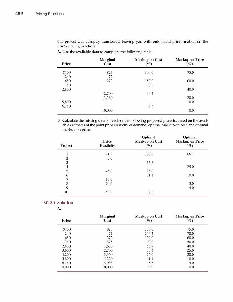
this project was abruptly transferred, leaving you with only sketchy information on thefirm’s pricing practices.A. Use the available data to complete the following table:
B. Calculate the missing data for each of the following proposed projects, based on the avail-able estimates of the point price elasticity of demand, optimal markup on cost, and optimalmarkup on price:
ST12.1 SolutionA.
492 Part Four Market Structure Analysis and Estimation
Marginal Markup on Cost Markup on PricePrice Cost (%) (%)
$100 $25 300.0 75.0240 72 680 272 150.0 60.0750 100.0
2,800 40.02,700 33.33,360 20.0
5,800 10.06,250 5.3
10,000 0.0
Marginal Markup on Cost Markup on PricePrice Cost (%) (%)
$100 $25 300.0 75.0240 72 233.3 70.0680 272 150.0 60.0750 375 100.0 50.0
2,800 1,680 66.7 40.03,600 2,700 33.3 25.04,200 3,360 25.0 20.05,800 5,220 11.1 10.06,250 5,938 5.3 5.0
10,000 10,000 0.0 0.0
Optimal OptimalPrice Markup on Cost Markup on Price
Project Elasticity (%) (%)
1 –1.5 200.0 66.72 –2.0 3 66.74 25.05 –5.0 25.06 11.1 10.07 –15.0 8 –20.0 5.09 4.0
10 –50.0 2.0
492 Pricing Practices
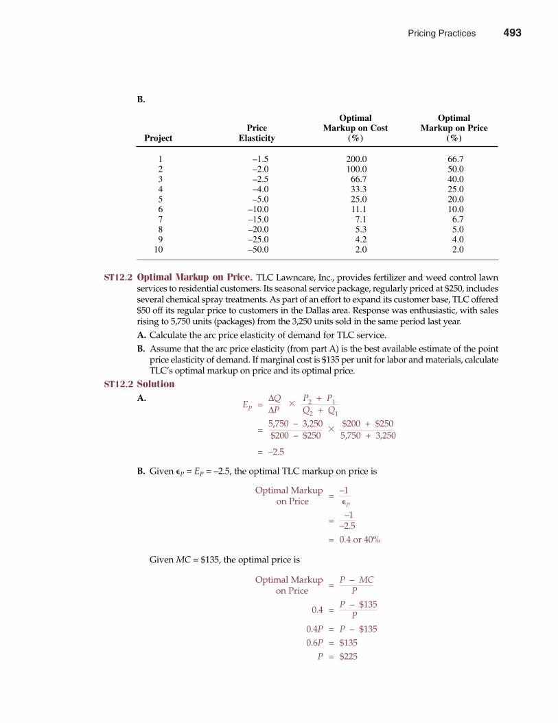
B.
ST12.2 Optimal Markup on Price. TLC Lawncare, Inc., provides fertilizer and weed control lawnservices to residential customers. Its seasonal service package, regularly priced at $250, includesseveral chemical spray treatments. As part of an effort to expand its customer base, TLC offered$50 off its regular price to customers in the Dallas area. Response was enthusiastic, with salesrising to 5,750 units (packages) from the 3,250 units sold in the same period last year.A. Calculate the arc price elasticity of demand for TLC service.B. Assume that the arc price elasticity (from part A) is the best available estimate of the point
price elasticity of demand. If marginal cost is $135 per unit for labor and materials, calculateTLC’s optimal markup on price and its optimal price.
ST12.2 Solution A.
EP =∆Q
�P2 + P1
∆P Q2 + Q1
=5,750 – 3,250
�$200 + $250
$200 – $250 5,750 + 3,250
= –2.5
B. Given �P = EP = –2.5, the optimal TLC markup on price is
Optimal Markup = –1on Price �P
= –1–2.5
= 0.4 or 40%
Given MC = $135, the optimal price is
Optimal Markup = P – MCon Price P
0.4 = P – $135P
0.4P = P – $1350.6P = $135
P = $225
Chapter Twelve Pricing Practices 493
Optimal OptimalPrice Markup on Cost Markup on Price
Project Elasticity (%) (%)
1 –1.5 200.0 66.72 –2.0 100.0 50.03 –2.5 66.7 40.04 –4.0 33.3 25.05 –5.0 25.0 20.06 –10.0 11.1 10.07 –15.0 7.1 6.78 –20.0 5.3 5.09 –25.0 4.2 4.0
10 –50.0 2.0 2.0
Pricing Practices 493
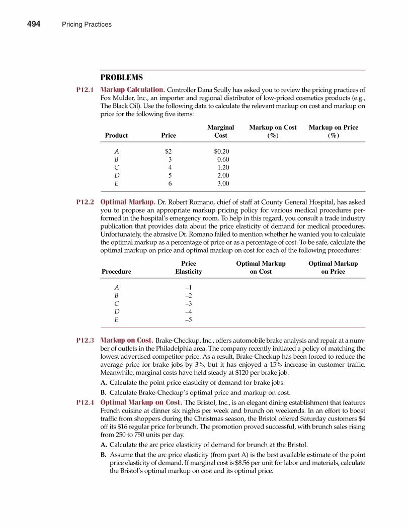
PROBLEMS
P12.1 Markup Calculation. Controller Dana Scully has asked you to review the pricing practices ofFox Mulder, Inc., an importer and regional distributor of low-priced cosmetics products (e.g.,The Black Oil). Use the following data to calculate the relevant markup on cost and markup onprice for the following five items:
P12.2 Optimal Markup. Dr. Robert Romano, chief of staff at County General Hospital, has askedyou to propose an appropriate markup pricing policy for various medical procedures per-formed in the hospital’s emergency room. To help in this regard, you consult a trade industrypublication that provides data about the price elasticity of demand for medical procedures.Unfortunately, the abrasive Dr. Romano failed to mention whether he wanted you to calculatethe optimal markup as a percentage of price or as a percentage of cost. To be safe, calculate theoptimal markup on price and optimal markup on cost for each of the following procedures:
P12.3 Markup on Cost. Brake-Checkup, Inc., offers automobile brake analysis and repair at a num-ber of outlets in the Philadelphia area. The company recently initiated a policy of matching thelowest advertised competitor price. As a result, Brake-Checkup has been forced to reduce theaverage price for brake jobs by 3%, but it has enjoyed a 15% increase in customer traffic.Meanwhile, marginal costs have held steady at $120 per brake job.A. Calculate the point price elasticity of demand for brake jobs.B. Calculate Brake-Checkup’s optimal price and markup on cost.
P12.4 Optimal Markup on Cost. The Bristol, Inc., is an elegant dining establishment that featuresFrench cuisine at dinner six nights per week and brunch on weekends. In an effort to boosttraffic from shoppers during the Christmas season, the Bristol offered Saturday customers $4off its $16 regular price for brunch. The promotion proved successful, with brunch sales risingfrom 250 to 750 units per day.A. Calculate the arc price elasticity of demand for brunch at the Bristol.B. Assume that the arc price elasticity (from part A) is the best available estimate of the point
price elasticity of demand. If marginal cost is $8.56 per unit for labor and materials, calculatethe Bristol’s optimal markup on cost and its optimal price.
494 Part Four Market Structure Analysis and Estimation
Marginal Markup on Cost Markup on PriceProduct Price Cost (%) (%)
A $2 $0.20B 3 0.60C 4 1.20D 5 2.00E 6 3.00
Price Optimal Markup Optimal MarkupProcedure Elasticity on Cost on Price
A –1B –2C –3D –4E –5
494 Pricing Practices
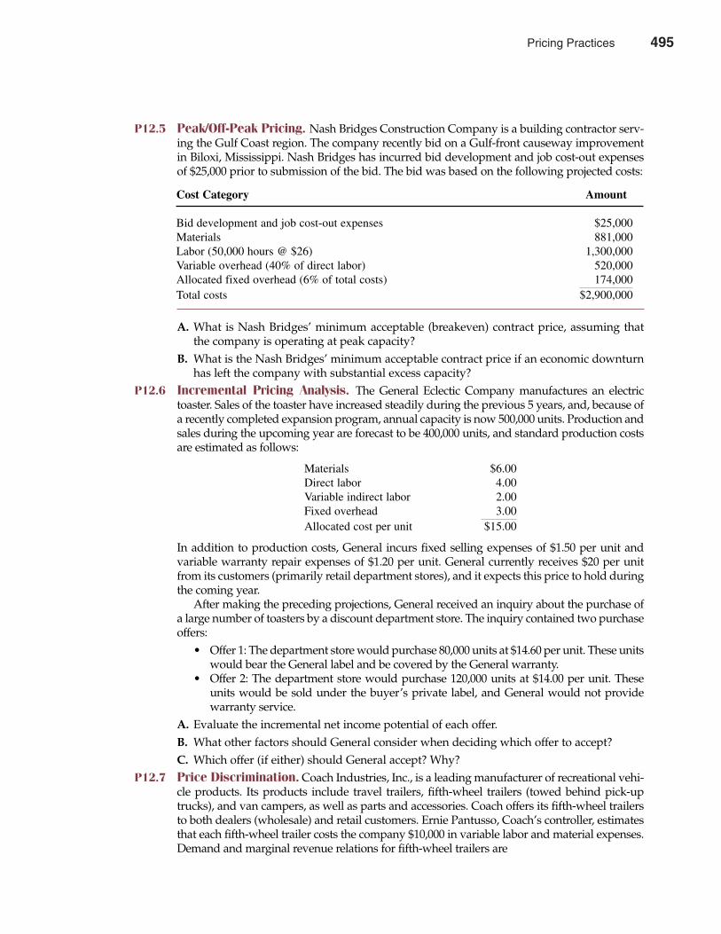
P12.5 Peak/Off-Peak Pricing. Nash Bridges Construction Company is a building contractor serv-ing the Gulf Coast region. The company recently bid on a Gulf-front causeway improvementin Biloxi, Mississippi. Nash Bridges has incurred bid development and job cost-out expensesof $25,000 prior to submission of the bid. The bid was based on the following projected costs:
A. What is Nash Bridges’ minimum acceptable (breakeven) contract price, assuming thatthe company is operating at peak capacity?
B. What is the Nash Bridges’ minimum acceptable contract price if an economic downturnhas left the company with substantial excess capacity?
P12.6 Incremental Pricing Analysis. The General Eclectic Company manufactures an electrictoaster. Sales of the toaster have increased steadily during the previous 5 years, and, because ofa recently completed expansion program, annual capacity is now 500,000 units. Production andsales during the upcoming year are forecast to be 400,000 units, and standard production costsare estimated as follows:
Materials $6.00Direct labor 4.00Variable indirect labor 2.00Fixed overhead 3.00Allocated cost per unit $15.00
In addition to production costs, General incurs fixed selling expenses of $1.50 per unit andvariable warranty repair expenses of $1.20 per unit. General currently receives $20 per unitfrom its customers (primarily retail department stores), and it expects this price to hold duringthe coming year.
After making the preceding projections, General received an inquiry about the purchase ofa large number of toasters by a discount department store. The inquiry contained two purchaseoffers:
• Offer 1: The department store would purchase 80,000 units at $14.60 per unit. These unitswould bear the General label and be covered by the General warranty.
• Offer 2: The department store would purchase 120,000 units at $14.00 per unit. Theseunits would be sold under the buyer’s private label, and General would not providewarranty service.
A. Evaluate the incremental net income potential of each offer.B. What other factors should General consider when deciding which offer to accept?C. Which offer (if either) should General accept? Why?
P12.7 Price Discrimination. Coach Industries, Inc., is a leading manufacturer of recreational vehi-cle products. Its products include travel trailers, fifth-wheel trailers (towed behind pick-uptrucks), and van campers, as well as parts and accessories. Coach offers its fifth-wheel trailersto both dealers (wholesale) and retail customers. Ernie Pantusso, Coach’s controller, estimatesthat each fifth-wheel trailer costs the company $10,000 in variable labor and material expenses.Demand and marginal revenue relations for fifth-wheel trailers are
Chapter Twelve Pricing Practices 495
Cost Category Amount
Bid development and job cost-out expenses $25,000Materials 881,000Labor (50,000 hours @ $26) 1,300,000Variable overhead (40% of direct labor) 520,000Allocated fixed overhead (6% of total costs) 174,000Total costs $2,900,000
Pricing Practices 495
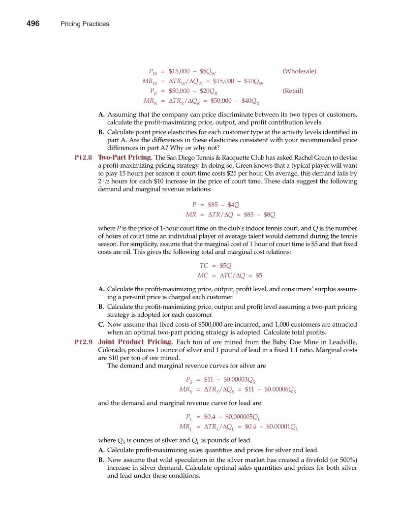
PW = $15,000 – $5QW (Wholesale)MRW = ∆TRW/∆QW = $15,000 – $10QW
PR = $50,000 – $20QR (Retail)MRR = ∆TRR/∆QR = $50,000 – $40QR
A. Assuming that the company can price discriminate between its two types of customers,calculate the profit-maximizing price, output, and profit contribution levels.
B. Calculate point price elasticities for each customer type at the activity levels identified inpart A. Are the differences in these elasticities consistent with your recommended pricedifferences in part A? Why or why not?
P12.8 Two-Part Pricing. The San Diego Tennis & Racquette Club has asked Rachel Green to devisea profit-maximizing pricing strategy. In doing so, Green knows that a typical player will wantto play 15 hours per season if court time costs $25 per hour. On average, this demand falls by21/2 hours for each $10 increase in the price of court time. These data suggest the followingdemand and marginal revenue relations:
P = $85 – $4Q
MR = ∆TR/∆Q = $85 – $8Q
where P is the price of 1-hour court time on the club’s indoor tennis court, and Q is the numberof hours of court time an individual player of average talent would demand during the tennisseason. For simplicity, assume that the marginal cost of 1 hour of court time is $5 and that fixedcosts are nil. This gives the following total and marginal cost relations:
TC = $5Q
MC = ∆TC/∆Q = $5
A. Calculate the profit-maximizing price, output, profit level, and consumers’ surplus assum-ing a per-unit price is charged each customer.
B. Calculate the profit-maximizing price, output and profit level assuming a two-part pricingstrategy is adopted for each customer.
C. Now assume that fixed costs of $500,000 are incurred, and 1,000 customers are attractedwhen an optimal two-part pricing strategy is adopted. Calculate total profits.
P12.9 Joint Product Pricing. Each ton of ore mined from the Baby Doe Mine in Leadville,Colorado, produces 1 ounce of silver and 1 pound of lead in a fixed 1:1 ratio. Marginal costsare $10 per ton of ore mined.
The demand and marginal revenue curves for silver are
PS = $11 – $0.00003QS
MRS = ∆TRS/∆QS = $11 – $0.00006QS
and the demand and marginal revenue curve for lead are
PL = $0.4 – $0.000005QL
MRL = ∆TRL/∆QL = $0.4 – $0.00001QL
where QS is ounces of silver and QL is pounds of lead.A. Calculate profit-maximizing sales quantities and prices for silver and lead.B. Now assume that wild speculation in the silver market has created a fivefold (or 500%)
increase in silver demand. Calculate optimal sales quantities and prices for both silverand lead under these conditions.
496 Part Four Market Structure Analysis and Estimation
496 Pricing Practices
P12.10 Transfer Pricing. Simpson Flanders, Inc., is a Motor City–based manufacturer and distrib-utor of valves used in nuclear power plants. Currently, all output is sold to North Americancustomers. Demand and marginal revenue curves for the firm are as follows:
P = $1,000 – $0.015Q
MR = ∆TR/∆Q = $1,000 – $0.03Q
Relevant total cost, marginal cost, and profit functions are
TC = $1,500,000 + $600Q + $0.005Q2
MC = ∆TC/∆Q = $600 + $0.01Q
π = TR – TC
= –$0.02Q2 + $400Q – $1,500,000
A. Calculate the profit-maximizing activity level for Simpson Flanders when the firm is oper-ated as an integrated unit.
B. Assume that the company is reorganized into two independent profit centers with thefollowing cost conditions:
TCMfg = $1,250,000 + $500Q + $0.005Q2
MCMfg = $500 + $0.01Q
and,TCDistr = $250,000 + $100Q
MCDistr = $100
Calculate the transfer price that ensures a profit-maximizing level of profit for the firm,with divisional operation based on the assumption that all output produced is to be trans-ferred internally.
C. Now assume that a major distributor in the European market offers to buy as many valves asSimpson Flanders wishes to offer at a price of $645. No impact on demand from the compa-ny’s North American customers is expected, and current facilities can be used to supply bothmarkets. Calculate the company’s optimal price(s), output(s), and profits in this situation.
Chapter Twelve Pricing Practices 497
CASE STUDY
Pricing Practices in the Denver, Colorado, Newspaper MarketOn May 12, 2000, the two daily newspapers in Denver, Colorado, filed an application with theU.S. Department of Justice for approval of a joint operating arrangement. The application wasfiled by The E.W. Scripps Company, whose subsidiary, the Denver Publishing Company, pub-lished the Rocky Mountain News, and the MediaNews Group, Inc., whose subsidiary, the DenverPost Corporation, published the Denver Post. Under the proposed joint operating agreement,printing and commercial operations of both newspapers were to be handled by a new entity, the“Denver Newspaper Agency,” owned by the parties in equal shares. This type of joint operatingagreement provides for the complete independence of the news and editorial departments of thetwo newspapers. The rationale for such an arrangement, as provided for under the NewspaperPreservation Act, is to preserve multiple independent editorial voices in towns and cities toosmall to support two or more newspapers. The act requires joint operating arrangements, suchas that proposed by the Denver newspapers, to obtain the prior written consent of the attorneygeneral of the United States in order to qualify for the antitrust exemption provided by the act.
Pricing Practices 497
498 Part Four Market Structure Analysis and Estimation
Scripps initiated discussions for a joint operating agreement after determining that the Newswould probably fail without such an arrangement. In their petition to the Justice Department,the newspapers argued that the News had sustained $123 million in net operating losses whilethe financially stronger Post had reaped $200 million in profits during the 1990s. This was a cru-cial point in favor of the joint operating agreement application because the attorney generalmust find that one of the publications is a failing newspaper and that approval of the arrange-ment is necessary to maintain the independent editorial content of both newspapers. Like anybusiness, newspapers cannot survive without a respectable bottom line. In commenting on thejoint operating agreement application, Attorney General Janet Reno noted that Denver was oneof only five major American cities still served by competing daily newspapers. The other fourare Boston, Chicago, New York, and Washington, DC. Of course, these other four cities are notcomparable in size to Denver; they are much bigger. None of those four cities can lay claim totwo newspapers that are more or less equally matched and strive for the same audience. In fact,that there is not a single city in the United States that still supports two independently ownedand evenly matched, high-quality newspapers that vie for the same broad base of readership.
Economies of scale in production explain why few cities can support more than one localnewspaper. Almost all local newspaper production and distribution costs are fixed. Marginalproduction and distribution costs are almost nil. After the local news stories and local advertis-ing copy are written, there is practically no additional cost involved with expanding productionfrom, say, 200,000 to 300,000 newspapers per day. Once a daily edition is produced, marginalcosts may be as little as 5¢ per newspaper. When marginal production costs are minimal, pricecompetition turns vicious. Whichever competitor is out in front in terms of total circulation sim-ply keeps prices down until the competition goes out of business or is forced into accepting ajoint operating agreement. This is exactly what happened in Denver. Until recently, the cost ofa daily newspaper in Denver was only 25¢ each weekday and 50¢ on Sunday at the newsstand,and even less when purchased on an annual subscription basis. The smaller News had muchhigher unit costs and simply could not afford to compete with the Post at such ruinously lowprices. This is why the production of local newspapers is often described as a classic exampleof natural monopoly.
On Friday, January 5, 2001, Attorney General Reno gave the green light to a 50-year joint oper-ating agreement between the News and its longtime rival, the Post. Starting January 22, 2001, thepublishing operations of the News and the Post were consolidated. The Denver NewspaperAgency, owned 50/50 by the owners of the News and Post, is now responsible for the advertis-ing, circulation, production, and other business departments of the newspapers. Newsroomsand editorial functions remain independent. Therefore, the owners of the News and Post are nowworking together to achieve financial success, but the newsroom operations remain competitors.Under terms of the agreement, E.W. Scripps Company, parent of the struggling News, agreed topay owners of the Post $60 million. Both newspapers publish separately Monday through Friday.The News publishes the only Saturday paper and the Post the only Sunday paper.A. Use your knowledge of monopoly pricing practices to explain why advertising rates and
newspaper circulation prices were likely to increase, and jobs were likely to be lost, follow-ing adoption of this joint operating agreement. Use company information to support yourargument (see http://www.denverpost.com and http://www.rockymountainnews.com).
B. In many cases, classified ads to sell real estate in a local newspaper can cost five to ten timesas much as a similar ad used to announce a garage sale. Use your knowledge of price dis-crimination to explain how local newspaper monopolies generate enormous profits fromselling classified advertising that varies in price according to the value of the item advertised.
C. Widely differing fares for business and vacation travelers on the same flight have led someto accuse the airlines of price discrimination. Do airline fare differences or local newspaperclassified-ad rate differences provide stronger evidence of price discrimination?
CASE STUDY (continued)
498 Pricing Practices
SELECTED REFERENCESAllen, Ralph C., and Jack H. Stone. “Rent Extraction, Principal-Agent Relationships, and Pricing Strategies:
Vendor Licensing During the 1996 Olympic Games in Atlanta.” Managerial & Decision Economics 22(December 2001): 431–438.
Baker, George, Robert Gibbons, and Kevin J. Murphy. “Bringing the Market Inside the Firm?” AmericanEconomic Review 91 (May 2001): 212–218.
Bernstein, Jerry, and David Macias. “Engineering New-Product Success: The New-Product PricingProcess at Emerson.” Industrial Marketing Management 31 (January 2002): 51–64.
Brown, Ken, Anthony Damiano, Brian Jenkins, et al. “Congestion Pricing: New Risks for Lenders.”Journal of Project Finance 6 (Winter 2001): 21–29.
Considine, Timothy J. “Markup Pricing in Petroleum Refining: A Multiproduct Framework.” InternationalJournal of Industrial Organization 19 (December 2001): 1499–1526.
Cornell, Bradford, and Qaio Liu. “The Parent Company Puzzle: When Is the Whole Worth Less ThanOne of the Parts?” Journal of Corporate Finance 7 (December 2001): 341–366.
Ellig, Jerry. “Internal Markets and the Theory of the Firm.” Managerial & Decision Economics 22 (June/August 2001): 227–237.
Malkiel, Burton G., and Aleksander Radisich. “The Growth of Index Funds and the Pricing of EquitySecurities.” Journal of Portfolio Management 27 (Winter 2001): 9–21.
O’Connell, Paul G. J., and Shang-Jin Wei. “The Bigger They Are, the Harder They Fall: Retail PriceDifferences Across U.S. Cities.” Journal of International Economics 56 (January 2002): 21–53.
Partington, Graham, and Max Stevenson. “The Probability and Timing of Price Reversals in the PropertyMarket.” Managerial & Decision Economics 22 (October/November 2001): 389–398.
Rogoff, Kenneth. “Why Not a Global Currency?” American Economic Review 91 (May 2001): 243–247.Schill, Michael J., and Chunsheng Zhou. “Pricing and Emerging Industry: Evidence from Internet
Subsidiary Carve-Outs.” Financial Management 30 (Autumn 2001): 5–33.Smith, Barry C., Dirk P. Gunther, B. Venkateshwara Rao, and Richard M. Ratliff. “E-Commerce and
Operations Research in Airline Planning, Marketing, and Distribution.” Interfaces 31 (March 2001):37–55.
Sudhir, K. “Competitive Pricing Behavior in the Auto Market: A Structural Analysis.” Marketing Science 20(Winter 2001): 42–60.
Yamawaki, Hideki. “Price Reactions to New Competition: A Study of U.S. Luxury Car Market,1986–1997.” International Journal of Industrial Organization 20, (January 2002): 19–39.
Chapter Twelve Pricing Practices 499
Pricing Practices 499

500 Part Four Market Structure Analysis and Estimation
Regulation of the Market Economy
CHAPTER THIRTEEN
502 1 See Andy Pasztor and JoAnne Lublin, “Skeptics Wonder if Honeywell CEO Will Revive,Expand Firm’s Business,” The Wall Street Journal Online, February 21, 2002(http://online.wsj.com).
In the new millennium, managers must be sensitive to regulatory policiesboth at home and abroad. If there was ever any doubt about the far-reaching
importance of foreign regulatory bodies, that doubt was eliminated on July 3,2001, when the European Commission turned thumbs down on the proposedacquisition of Honeywell, Inc., by General Electric Co (GE).
According to the commission, GE’s dominant position in the markets for jetengines, combined with its financial strength and vertical integration into air-craft leasing, gave GE significant market power. At the same time, Honeywellis a leading supplier of avionics products and jet engines for corporate aircraft.The commission found that a merged entity would be able to leverage therespective market power of each company. Market dominance would havebeen created or strengthened as a result of horizontal overlaps in some marketsas well as through the extension of GE’s financial power and vertical integra-tion to Honeywell activities. According to the commission, a merger betweenGE and Honeywell would foreclose competition and adversely affect productquality, service, and consumers’ prices.1
What is captivating about this case is that the European Commission andthe U.S. Department of Justice worked together during the investigation butreached different conclusions. Ironically, the Justice Department voted to allowthe GE–Honeywell merger. This chapter considers the economic and socialrationale for regulation, and explains the reasons behind conflicting opinions ongovernment regulation in the market economy. Regulators must balance effi-ciency and equity considerations. This is a fascinating and controversial process.
501
13
COMPETITION AND THE ROLE OF GOVERNMENT
When considering the role of government in the market economy, it has been traditional tofocus on how government influences economic activity through tax policies, law enforcement,and infrastructure investments in highways, water treatment facilities, and the like. Morerecently, interest has shifted to how and why the government regulates private market activity.
How Government Influences BusinessGovernment affects what and how firms produce, influences conditions of entry and exit,dictates marketing practices, prescribes hiring and personnel policies, and imposes a host ofother requirements on private enterprise. Government regulation of the market economy isa controversial topic because the power to tax or compel has direct economic consequences.
For example, local telephone service monopolies are protected by a web of local and feder-al regulation that gives rise to above-normal rates of return while providing access to below-market financing. Franchises that confer the right to offer cellular telephone service in a majormetropolitan area are literally worth millions of dollars and can be awarded in the United Statesonly by the Federal Communications Commission (FCC). The federal government also spendshundreds of millions of dollars per year to maintain artificially high price supports for selectedagricultural products such as milk and grain, but not chicken and pork. Careful study of themotivation and methods of such regulation is essential to the study of managerial economicsbecause of regulation’s key role in shaping the managerial decision-making process.
The pervasive and expanding influence of government in the market economy can beillustrated by considering the growing role played by the FCC, a once obscure agency knownonly for regulation of the broadcast industry and AT&T. The FCC currently holds the keys tosuccess for a number of emerging communications technologies. The FCC determines the fateof digital audio broadcasting, which does away with static on car radio channels; personalcommunication networks that make users reachable anywhere with a pocket phone; andinteractive television, which lets customers order goods and communicate with othersthrough a television set. The FCC has also taken on the daunting and controversial task ofrestricting indecent and obscene material broadcast over the Internet. As such, the FCC is thefocus of debates over free speech and the government’s role in shaping rapid advances incommunications technology.
Although all sectors of the U.S. economy are regulated to some degree, the method andscope of regulation vary widely. Most companies escape price and profit restraint, except dur-ing periods of general wage-price control, but they are subject to operating regulations gov-erning pollution emissions, product packaging and labeling, worker safety and health, and soon. Other firms, particularly in the financial and the public utility sectors, must comply withfinancial regulation in addition to such operating controls. Banks and savings and loan insti-tutions, for example, are subject to state and federal regulation of interest rates, fees, lendingpolicies, and capital requirements. Unlike firms in the electric power and telecommunicationsindustries, banks and savings and loans face no explicit limit on profitability.
Economic and social considerations enter into decisions of what and how to regulate.Economic considerations relate to the cost and efficiency implications of regulatory methods.From an economic efficiency standpoint, a given mode of regulation or government controlis desirable to the extent that benefits exceed costs. In terms of efficiency, the question iswhether market competition by itself is sufficient, or if it needs to be supplemented with gov-ernment regulation. Equity, or fairness, criteria must also be carefully weighed when socialconsiderations bear on the regulatory decision-making process. Therefore, the incidence, orplacement, of costs and benefits of regulatory decisions is important. If a given change in reg-ulatory policy provides significant benefits to the poor, society may willingly bear substantialcosts in terms of lost efficiency.
efficiencyProduction of whatconsumers demand ina least-cost fashion
regulationGovernment orderhaving the force of law
equityConcern for a just distribution of wealth
Chapter Thirteen Regulation of the Market Economy 503
502 Regulation of the Market Economy
Economic ConsiderationsEconomic regulation began and continues in part because of the public’s perception of marketimperfections. It is sometimes believed that unregulated market activity can lead to inefficiencyand waste or to market failure. Market failure is the inability of a system of market institutionsto sustain socially desirable activities or to eliminate undesirable ones.
Afirst cause of market failure is failure by market structure. For a market to realize the ben-eficial effects of competition, it must have many producers (sellers) and consumers (buyers), orat least the ready potential for many to enter. Some markets do not meet this condition. Consider,for example, water, power, and some telecommunications markets. If customer service in a givenmarket area can be most efficiently provided by a single firm (a natural monopoly situation),such providers would enjoy market power and could earn economic profits by limiting outputand charging high prices. As a result, utility prices and profits were placed under regulatory con-trol, which has continued with the goal of preserving the efficiency of large-scale productionwhile preventing the higher prices and economic profits of monopoly. When the efficiencyadvantages of large size are not thought to be compelling, antitrust policy limits the marketpower of large firms.
A second kind of market failure is failure by incentive. In the production and consump-tion of goods and services, social values and costs often differ from the private costs and valuesof producers and consumers. Differences between private and social costs or benefits are calledexternalities. A negative externality is a cost of producing, marketing, or consuming a productthat is not borne by the product’s producers or consumers. A positive externality is a benefit ofproduction, marketing, or consumption that is not reflected in the product pricing structureand, hence, does not accrue to the product’s producers or consumers.
Environmental pollution is one well-known negative externality. Negative externalitiesalso arise when employees are exposed to hazardous working conditions for which they arenot fully compensated. Similarly, a firm that dams a river to produce energy and therebylimits the access of others to hydropower creates a negative externality. Positive externalitiescan result if an increase in a firm’s activity reduces costs for its suppliers, who pass these costsavings on to their other customers. For example, economies of scale in semiconductor pro-duction made possible by increased computer demand have lowered input costs for all usersof semiconductors. As a result, prices have fallen for computers and a wide variety of “intel-ligent” electronic appliances, calculators, toys, and so on. Positive externalities in productioncan result when a firm trains employees who later apply their knowledge in work for otherfirms. Positive externalities also arise when an improvement in production methods is trans-ferred from one firm to another without compensation. The dam cited previously for itspotential negative externalities might also provide positive externalities by offering floodcontrol or recreational benefits.
In short, externalities lead to a difference between private and social costs and benefits.Firms that provide substantial positive externalities without compensation are unlikely to pro-duce at the socially optimal level. Consumption activities that confer positive externalities maynot reach the socially optimal level. In contrast, negative externalities can channel too manyresources to a particular activity. Producers or consumers that generate negative externalitiesdo not pay the full costs of production or consumption and tend to overutilize social resources.
Social ConsiderationsCompetition promotes efficiency by giving firms incentives to produce the types and quanti-ties of products that consumers want. Competitive pressures force each firm to use resourceswisely to earn at least a normal profit. The market-based resource allocation system is efficientwhen it responds quickly and accurately to consumer preferences. Not only are these features
504 Part Five Long-Term Investment Decisions
market failureThe inability of marketinstitutions to sustaindesirable activity oreliminate undesirableactivity
failure by marketstructureInsufficient marketparticipants for activecompetition
failure by incentiveBreakdown of the pricing mechanism as areflection of all costsand benefits of produc-tion and consumption
externalitiesDifferences betweenprivate and social costsor benefits
Regulation of the Market Economy 503
of competitive markets attractive on an economic basis, but they are also consistent with basicdemocratic principles. Preservation of consumer choice or consumer sovereignty is an impor-tant feature of competitive markets. By encouraging and rewarding individual initiative, com-petition greatly enhances personal freedom. For this reason, less vigorous competitive pressureindicates diminishing buyer supremacy in the marketplace. Firms with market power canlimit output and raise prices to earn economic profits, whereas firms in competitive marketsrefer to market prices to determine optimal output quantities. Regulatory policy can be a valu-able tool with which to control monopolies, restoring control over price and quantity decisionsto the public.
A second social purpose of regulatory intervention is to limit concentration of economicand political power. It has long been recognized that economic and social relations becomeintertwined and that concentrated economic power is generally inconsistent with the demo-cratic process. The laws of incorporation, first passed during the 1850s, play an important rolein the U.S. economic system. These laws have allowed owners of capital (stockholders) to pooleconomic resources without also pooling political resources, thereby allowing big businessand democracy to coexist. Of course, the large scale of modern corporations has sometimesdiminished the controlling influence of individual stockholders. In these instances, regulatoryand antitrust policy have limited the growth of large firms to avoid undue concentration ofpolitical power.
Important social considerations often constitute compelling justification for governmentintervention in the marketplace. Deciding whether a particular regulatory reform is warrantedis complicated because social considerations can run counter to efficiency considerations.
consumer sovereigntyBuyer supremacy inthe marketplace
limit concentrationSocial goal of regulationis to restrict undueinfluence
Chapter Thirteen Regulation of the Market Economy 505
How Do You Regulate a Global Economy?
Pressed by the emergence of regional trading blocs inNorth America, Europe, and East Asia, global corpora-tions are developing chameleon-like abilities to changequickly to fit a rapidly evolving global economic envi-ronment. Government intervention in world currency,bond, and stock markets—sometimes used to stemshort-term capital flows—can have the unintendedeffect of choking off long-term investment and economicgrowth. At the same time, global manufacturers movefactories and labs around the world without reference tonational boundaries.
The global focus of modern corporations represents astriking evolution from the U.S. multinational alternatelyfeared and courted by developing countries around theglobe since the 1960s. These giants treated foreign opera-tions as subsidiaries for producing products designed andengineered back home. The chain of command andnationality of the company were clear. This is not the casetoday. With the United States no longer dominating theworld economy, new technologies, capital, and talentsflow in multiple directions. The most sophisticated manu-facturing companies often make breakthroughs in foreignlabs, place shares with foreign investors, and put foreigners
on the fast track to the top. The recent wave of mergers,acquisitions, and strategic alliances has further cloudedtraditional corporate/national relations. Internationalcompetitors seeking cost efficiencies and product-qualityimprovements now often find themselves working togeth-er to efficiently penetrate new and emerging markets. Atthe same time, the pro-capitalism revolution of the pastdecade has resulted in market-driven policies that makesocial, political, and cultural differences among companiesless significant.
Nagging questions remain. Does corporate nation-ality matter? What nation, if any, controls the technologydeveloped by global companies? What obligation doglobal corporations have to follow rules imposed byWashington, Ottawa, Paris, or Tokyo on their foreignoperations?
Global companies clearly raise important questionsfor government regulations and policies designed toretain control over national identities.
See: Shirley Leving, “McDonald’s Profits Sink 40%, Weakened byGlobal Slump,” The Wall Street Journal Online, January 28, 2002(http://online.wsj.com).
M A N A G E R I A L A P P L I C AT I O N 1 3 . 1
504 Regulation of the Market Economy
REGULATORY RESPONSE TO INCENTIVE FAILURES
To help preserve the competitive environment, government regulation addresses problemscreated by positive and negative externalities in production, marketing, and consumption. Ingranting patents and operating subsidies, government provides compensation to rewardactivity that provides positive externalities. Local, state, and federal governments levy taxes tolimit negative externalities. Property rights, grants, taxes, and operating controls are commonfocal points of government/business interaction.
Property Rights RegulationProperty rights give the power to limit use by others of specific land, plant and equipment, andother assets. The deed to a piece of land, for example, explicitly defines a property right. Theestablishment and maintenance of private property rights is essential to the workings of a com-petitive market. Property rights are so fundamental to the free market economy and democraticform of government that they are protected in the United States by the Fifth Amendment to theConstitution. Although local zoning laws limit property rights by restricting the types of build-ings allowed in a particular neighborhood, these laws cannot be so burdensome as to depriveowners from the rightful use of their property. Although the public interest might be served byregulations designed to preserve wetlands or endangered species, owners are entitled to com-pensation for any loss they might suffer as a result.
Regulation of property rights is a common, though seldom discussed, method of givingincentives to promote service in the public interest. Common examples are FCC control of localtelevision and radio broadcasting rights; federal and state regulatory bodies that govern nation-al or state chartering of banks and savings and loan institutions; and insurance commissionsthat oversee insurance company licensing at the state level. In each of these instances, firmsmust be able to demonstrate fiscal responsibility and evidence that they are meeting customerneeds. Should firms fail to meet established criteria, public franchises can be withdrawn, or newfranchises can be offered to potential competitors.
Property rights regulation can be effective, but can be frustrated by imprecise operatingcriteria. For example, how much poorly rated local programming should any given televisionstation be required to produce? How progressive a stance should local banks take towardelectronic funds transfer services? Without clear, consistent, and workable standards of per-formance, operating grant regulation is hampered by inefficiency and waste.
Patents and the Tort SystemPatents grant an exclusive right to produce, use, or sell an invention or innovation for a limitedperiod of time. For U.S. patent applications filed on or after June 8, 1995, utility and plant patentscan be granted for a term that begins with the date of the grant and usually ends 20 years fromthe date of the patent application. Utility patents may be granted to anyone who invents or dis-covers any new or improved process, machine, manufactured product, or composition of matter.Plant patents may be granted to anyone who invents or discovers and asexually reproduces anydistinct and new variety of plant. Maintenance fees totaling a few thousand dollars must be paidover the life of such patents. Design patents may be granted to anyone who invents a new, orig-inal, and ornamental design for a manufactured product, and last 14 years from the grant date.Design patents do not involve maintenance fees.
Without patents, competitors could quickly develop identical substitutes for new products orprocesses, and inventing firms would fail to reap the full benefit of their technological break-throughs. In granting patents, the public confers a limited opportunity for monopoly profits tostimulate research activity and economic growth. By limiting the patent monopoly, competitionis encouraged to extend and develop the common body of knowledge. The patent monopoly issubject to other restrictions besides the time limit. Firms cannot use patents to unfairly monopo-
506 Part Five Long-Term Investment Decisions
property rightsThe license to limit useby others
patentsExclusive propertyrights to produce, use,or sell an invention orinnovation for a limitedperiod
Regulation of the Market Economy 505
lize or otherwise limit competition, as the Federal Trade Commission (FTC) claimed in a 1995action against Dell Computer Corp.
At that time, Dell was a member of the Video Electronics Standards Association (VESA), astandards-setting body for the computer industry. In 1992, VESA set a new standard for thedesign of computer bus hardware, or the equipment that transmits information from one com-puter component to another. According to the FTC, before the new standard was approved,Dell certified that it did not violate any of its intellectual property rights. However, after the newVESA standard was implemented, Dell changed its mind and announced that the standard didin fact violate one of its patents. By then, over a million computers using the new VESA stan-dard had already been sold, and other computer manufacturers could not switch to an alternatedesign without creating a vexing compatibility problem. This would have put Dell in a positionto collect substantial royalty payments were it not for a settlement with the FTC in which Dellagreed not to enforce its patent rights against computer manufacturers using the standard.
The rules of contract law provide for the enforcement of patents and other legal agreementsamong firms. Because it is impossible to specify all possible outcomes in writing a legal con-tract, the court system provides an open forum for dispute resolution. Even if all possible out-comes could be specified beforehand, legal enforcement would still be necessary to ensure thatall parties honor their agreements. If a manufacturer fails to deliver goods to a wholesaler aspromised, the wholesaler can go to the courts to enforce its agreement with the manufacturer.Without such enforcement, firms would have no recourse but to depend exclusively on thegoodwill of others. The legal system also includes a body of law designed to provide a mech-anism for victims of accidents and injury to receive just compensation for their loss. Called thetort system, these laws create an incentive for firms and other parties to act responsibly incommerce. Because of the threat of being sued for their transgressions, firms are encouragedto prevent accidents and resulting economic damages.
Like patents that are difficult and costly to enforce in the courts, the tort system can itselfresult in significant costs. For example, both sides to a legal dispute have almost unlimited abil-ity to take sworn depositions from witnesses and seek documents in the pretrial “discovery”process. Because discovery must be provided without payment from the requesting party, thereis no incentive to limit the size of any request. Requesting parties can and have used the dis-covery process to impose significant litigation costs on the other side, even in lawsuits thatlater prove frivolous. As a result, proposals have been made to place limits on the amount offree discovery that can be requested, set caps on the amount of punitive damages, foster prop-er use of expert testimony, and encourage other means of dispute resolution.
Subsidy PolicyGovernment sometimes responds to positive externalities by providing subsidies. Subsidypolicy can be indirect, like government construction and highway maintenance grants thatbenefit the trucking industry. They can be direct payments, such as agricultural payment-in-kind (PIK) programs, special tax treatments, and government-provided low-cost financing.
Tax credits on business investment and depletion allowances on natural resource extractionare examples of tax subsidies given in recognition of social benefits such as job creation andenergy independence. Positive externalities associated with industrial parks induce govern-ment to provide local tax incremental financing or industrial revenue bond financing for suchfacilities. This low-cost financing is thought to provide compensation for the external benefitsof economic development.
Tradable emissions permits are pollution licenses granted by the government to firms andindividuals. Rather than spend millions of dollars on new equipment, raw materials, or pro-duction methods to meet pollution abatement regulations, firms sometimes purchase tradableemissions permits from other companies. These tradable emmissions permits are a valuablecommodity that can be worth millions of dollars. Opponents of this system argue that theyinfringe on the public’s right to a clean and safe environment. Proponents contend that the
tort systemA body of law that provides a means forvictims of accidentsand injury to receivejust compensation fortheir loss
subsidy policyGovernment grantsthat benefit firms andindividuals
tradable emissionspermitsPermits that give firmsthe property right topollute and then sellthat right to others
Chapter Thirteen Regulation of the Market Economy 507
506 Regulation of the Market Economy
costs of pollution abatement make trade-offs inevitable. Moreover, they argue that the tradableemissions permits do not confer new licenses to pollute; they merely transfer licenses from onepolluter to another. Nevertheless, by awarding tradable emissions permits worth millions ofdollars to the worst offenders of a clean environment, environmentally sensitive firms andconsumers have been hurt, at least on a relative basis.
Tax PolicyWhereas subsidy policy gives firms positive incentives for desirable performance, tax policyconfers penalties designed to limit undesirable performance. Tax policy includes both regulartax payments and fines or penalties that may be assessed intermittently.
Local, state, or federal fines for exceeding specified weight limits on trucks, pollution taxes,and effluent charges are common examples of tax policies intended to limit negative externali-ties. The appropriate tax level is extremely difficult to determine because of problems associatedwith estimating the magnitude of negative externalities. For example, calculating some of thesocial costs of air pollution, such as more frequent house painting, is relatively straightforward.Calculating the costs of increased discomfort—even death—for emphysema patients is moredifficult. Nevertheless, regulators must consider the full range of consequences of negativeexternalities to create appropriate and effective incentives for pollution control.
Although tax policy complements subsidy and property rights grant policies, an impor-tant distinction should not be overlooked. If society wants to limit the harmful consequencesof air pollution, either subsidies for pollution reduction or taxes on pollution can provideeffective incentives. Subsidies imply that firms have a right to pollute because society pays toreduce pollution. In contrast, a system of pollution tax penalties asserts society’s right to aclean environment. Firms must reimburse society for the damage caused by their pollution.Many prefer tax policy as a method for pollution reduction on the grounds that it explicitlyrecognizes the public’s right to a clean and safe environment.
508 Part Five Long-Term Investment Decisions
tax policyFines and penaltiesthat limit undesirableperformance
The Sotheby’s Price-Fixing Scandal
The art world and social elite of New York were shockedin December 2001 when jurors found that A. AlfredTaubman, former chairman of venerable Sotheby’sHoldings, Inc., had conspired with Sir Anthony Tennant,the former chairman of rival Christie’s International PLC,to fix the commission rates charged its wealthy artclients. Sotheby’s, like Christie’s, is an auctioneer of finearts, antiques, and collectibles. Property in a variety ofcollecting categories are featured, including paintings,jewelry, decorative arts, and books. The company’s auctionbusiness is comprised of a number of related activities,including on-site and Internet auctions, the purchase andresale of art and other collectibles, and the brokering of artand collectibles through negotiated sales. The companyalso markets and brokers luxury residential real estate,conducts art-related financing activities, and providesinsurance brokerage services.
A chronology of at least a dozen meetings betweenTaubman and Tennant convinced jurors that the two hadmet to set identical rates for art-selling clients. Tennantwas also indicted on price-fixing charges but refused to
leave Britain to stand trial; the United States cannotextradite him under British law. The government’s keywitness in the case was Sotheby’s former chief executive,Diana D. Brooks, who testified that Taubman instructedher to strike an agreement on commission rates with hercounterpart at Christie’s.
This conviction represents a spectacular downfallfor Taubman, who made a fortune developing shoppingmalls and rose to social prominence by buying a control-ling stake in Sotheby’s. At the time of his price-fixingconviction, Taubman had already agreed to pay $186million toward the settlement of civil charges stemmingfrom the case. His holdings, including stakes in TaubmanCenters Inc., are valued at $700 million to $1 billion. The76-year-old Taubman faces a maximum of 3 years inprison and a $350,000 fine.
See: Kathryn Kranhold, “Former Sotheby’s Chairman Is Found Guiltyof Conspiring to Fix Client Fees,” The Wall Street Journal Online,December 6, 2001 (http://online.wsj.com).
M A N A G E R I A L A P P L I C AT I O N 1 3 . 2
Regulation of the Market Economy 507
Operating ControlsOperating controls prohibit certain actions while compelling others. Operating controls thatachieve 100 percent compliance create a situation similar to that reached under a prohibitivetax policy. In each instance, undesirable activity is completely eliminated, and no tax revenuesare collected. When operating controls result in less than full compliance, operating controlregulation becomes like tax policy because fines and levies increase the costs to violators.
The effectiveness of operating control regulation can be limited by vague or imprecise statu-tory standards. If sanctions against violators are poorly defined or lenient, incentives for compli-ance can be weak. Beyond the difficulties created by poorly defined regulations and sanctions,problems can arise when conflicting operating controls are imposed. For example, mandatorysafety standards and pollution controls have increased automobile costs by several hundreddollars per unit. Other indirect costs are also incurred. Auto safety and pollution standardshave the effect of reducing fuel efficiency and thus reduce U.S. energy independence.
The clearest difference between operating control regulation and regulation via tax or sub-sidy policies is the reliance on nonmonetary incentives for compliance. There are no easyalternatives to operating control regulation when social costs are prohibitive (e.g., nucleardisaster, groundwater contamination, and so on). Unfortunately, many firms direct theirefforts toward being exempted from operating controls rather than toward reducing the neg-ative externalities of concern to society.
WHO PAYS THE COSTS OF REGULATION?Regulation is expensive. The regulatory system can increase consumer prices and cut profitswhen dispute resolution is slow, litigation costs are high, and the outcomes of legal proceedingsare risky. Socially beneficial regulatory reform involves setting rules that provide fair and effi-cient dispute resolution.
Demand and Supply EffectsThe question of who pays for regulation can seldom be determined merely by identifyingthe fined, taxed, or otherwise regulated party. Although the point of tax collection, or the taxincidence, of pollution charges may be a given corporation, this tax burden may be passedon to customers or suppliers.
In general, who pays for operating control regulation depends on the elasticity of demand forthe final products of affected firms. Figure 13.1 illustrates this issue by considering the theoreti-cally polar extremes of perfectly elastic demand for final products, [Fig. 13.1(a)], and perfectlyinelastic demand for final products, [Fig. 13.1(b)]. Identically upward-sloping MC curves areassumed in each instance. Here, as is often the case, regulation is assumed to increase marginalcosts by a fixed amount per unit. This amount, t, can reflect pollution taxes per unit of output orregulation-induced cost increases.
Figure 13.1(a) shows that good substitutes for a firm’s product and highly elastic demandprevent producers from passing taxes or regulation-induced cost increases on to customers. Inthis case, producers—including investors, employees, and suppliers—are forced to bear theburden of regulation. Falling rates of return on invested capital and high unemployment aresymptomatic of such influences.
Figure 13.1(b) shows the effect of regulation-induced cost or tax increases in the case of per-fectly inelastic final-product demand. Without substitute products, producers can pass the burdenof regulation on to customers and encounter relatively few disadvantages because of regulation-induced cost increases. When demand is inelastic, the consumer pays for regulation.
Although the preceding analysis is greatly simplified, it shows that taxes or regulation-induced cost increases have differing effects when demand relationships vary. Similarly, theeffect of regulation on industries with similar product-demand elasticities varies to the extentthat supply characteristics differ.
operating controlsRegulation by govern-ment directive
tax incidencePoint of tax collection
tax burdenEconomic cost of tax
Chapter Thirteen Regulation of the Market Economy 509
508 Regulation of the Market Economy
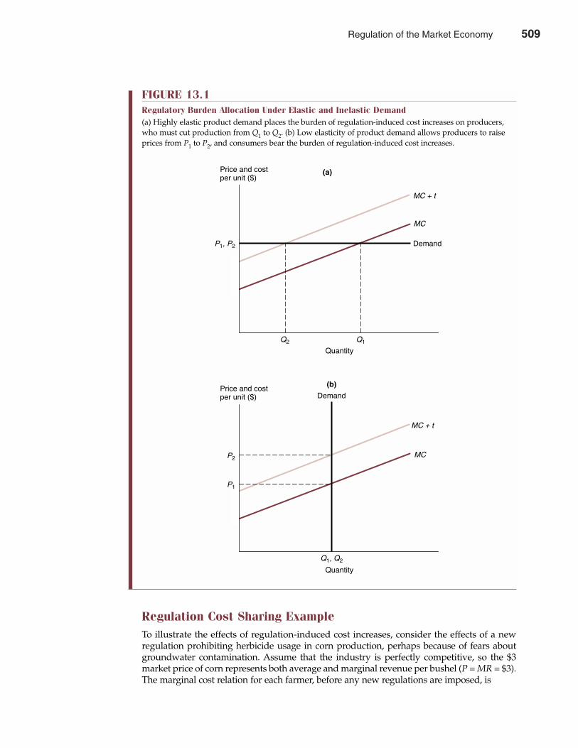
Regulation Cost Sharing ExampleTo illustrate the effects of regulation-induced cost increases, consider the effects of a newregulation prohibiting herbicide usage in corn production, perhaps because of fears aboutgroundwater contamination. Assume that the industry is perfectly competitive, so the $3market price of corn represents both average and marginal revenue per bushel (P = MR = $3).The marginal cost relation for each farmer, before any new regulations are imposed, is
510 Part Five Long-Term Investment Decisions
FIGURE 13.1Regulatory Burden Allocation Under Elastic and Inelastic Demand(a) Highly elastic product demand places the burden of regulation-induced cost increases on producers,who must cut production from Q1 to Q2. (b) Low elasticity of product demand allows producers to raiseprices from P1 to P2, and consumers bear the burden of regulation-induced cost increases.
Quantity
Price and costper unit ($)
(a)
P1, P2
Q2 Q1
MC
MC + t
Demand
Quantity
Price and costper unit ($)
(b)
Q1, Q2
P2
P1
MC
MC + t
Demand
Regulation of the Market Economy 509
MC = ∆TC/∆Q = $0.6 + $0.04Q
where Q is bushels of corn (in thousands). The optimal level of corn production per farm iscalculated by setting MR = MC and solving for Q:
MR = MC
$3 = $0.6 + $0.04Q
$0.04Q = $2.4Q = 60(000) or 60,000 bushels
Given a perfectly competitive market, the supply curve for each producer is given by the mar-ginal cost curve. From the marginal cost relation, the quantity of corn supplied by each farmer is
Supply Price = Marginal CostP = $0.6 + $0.04Q
or
Q = –15 + 25P
If the corn industry consists of 200,000 farmers with farms of equal size, total industry supply is
QS = 200,000(–15 + 25P)= –3,000,000 + 5,000,000P (Supply)
To complete the industry profile prior to the new regulation on herbicides, assume that industrydemand is given by the relation
QD = 15,000,000 – 1,000,000P (Demand)
In equilibrium,
QS = QD
–3,000,000 + 5,000,000P = 15,000,000 – 1,000,000P
6,000,000P = 18,000,000P = $3 per bushel
and
QS = –3,000,000 + 5,000,000(3)= 12,000,000(000), or 12 billion bushels
QD = 15,000,000 – 1,000,000(3)= 12,000,000(000), or 12 billion bushels
Now assume that reducing herbicide usage increases the amount of tillage needed to keepweed growth controlled and causes the yield per acre to drop, resulting in a 25 percent increasein the marginal costs of corn production. For individual farmers, the effect on marginal costsis reflected as
MC� = 1.25($0.6 + $0.04Q)= $0.75 + $0.05Q
Chapter Thirteen Regulation of the Market Economy 511
510 Regulation of the Market Economy
If only a few farmers in a narrow region of the country are subject to the new regulation, aswould be true in the case of state or local pollution regulations, then market prices wouldremain stable at $3, and affected farmers would curtail production dramatically to 45,000bushels each, because
MR = MC�
$3 = $0.75 + $0.05Q
$0.05Q = $2.25Q = 45(000), or 45,000 bushels
Given a perfectly competitive industry and, therefore, a perfectly elastic demand for corn, localpollution regulations will force producers to bear the entire burden of regulation-induced costincreases.
A different situation arises when all producers are subject to the new herbicide regulation.In this instance, the revised individual-firm supply curve is
Supply Price = Marginal CostP = $0.75 + $0.05Q
or
Q = –15 + 20P
Total industry supply, assuming that all 200,000 farmers remain in business (something that maynot happen if the resulting changes in profit levels are substantial), equals
Q�S = 200,000(–15 + 20P)= –3,000,000 + 4,000,000P (New Supply)
The equilibrium industry price/output combination is found where
Q�S = QD
–3,000,000 + 4,000,000P = 15,000,000 – 1,000,000P
5,000,000P = 18,000,000P = $3.60 per bushel
and
Q�S = –3,000,000 + 4,000,000(3.60)= 11,400,000(000), or 11.4 billion bushels
QD = 15,000,000 – 1,000,000(3.60)= 11,400,000(000), or 11.4 billion bushels
At the new market price, each individual farm produces 57,000 bushels of corn:
Q = –15 + 20(3.60)= 57(000), or 57,000 bushels
Thus, industry-wide regulation of herbicides has a relatively smaller impact on producersbecause the effects of regulation are partially borne by consumers through the price increase from
512 Part Five Long-Term Investment Decisions
Regulation of the Market Economy 511
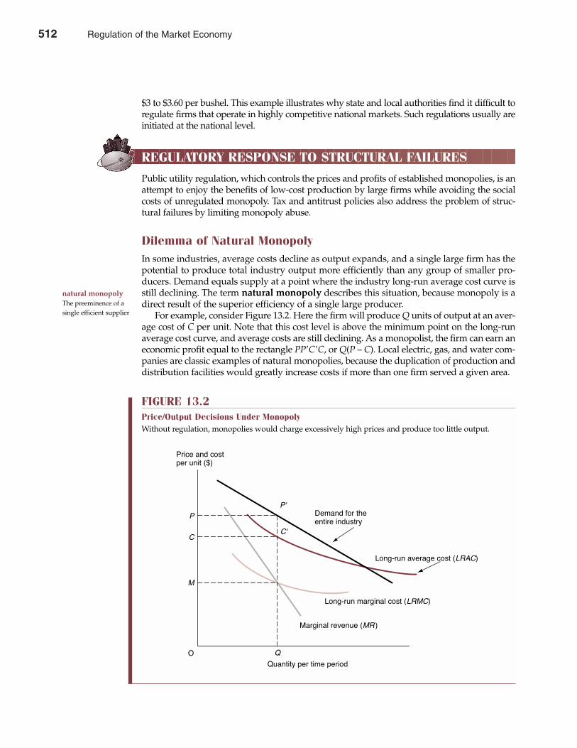
$3 to $3.60 per bushel. This example illustrates why state and local authorities find it difficult toregulate firms that operate in highly competitive national markets. Such regulations usually areinitiated at the national level.
REGULATORY RESPONSE TO STRUCTURAL FAILURES
Public utility regulation, which controls the prices and profits of established monopolies, is anattempt to enjoy the benefits of low-cost production by large firms while avoiding the socialcosts of unregulated monopoly. Tax and antitrust policies also address the problem of struc-tural failures by limiting monopoly abuse.
Dilemma of Natural MonopolyIn some industries, average costs decline as output expands, and a single large firm has thepotential to produce total industry output more efficiently than any group of smaller pro-ducers. Demand equals supply at a point where the industry long-run average cost curve isstill declining. The term natural monopoly describes this situation, because monopoly is adirect result of the superior efficiency of a single large producer.
For example, consider Figure 13.2. Here the firm will produce Q units of output at an aver-age cost of C per unit. Note that this cost level is above the minimum point on the long-runaverage cost curve, and average costs are still declining. As a monopolist, the firm can earn aneconomic profit equal to the rectangle PP�C�C, or Q(P – C). Local electric, gas, and water com-panies are classic examples of natural monopolies, because the duplication of production anddistribution facilities would greatly increase costs if more than one firm served a given area.
natural monopolyThe preeminence of asingle efficient supplier
Chapter Thirteen Regulation of the Market Economy 513
FIGURE 13.2Price/Output Decisions Under MonopolyWithout regulation, monopolies would charge excessively high prices and produce too little output.
Quantity per time period
Price and costper unit ($)
Marginal revenue (MR )
Long-run marginal cost (LRMC)
Long-run average cost (LRAC)
Demand for theentire industry
P'
C'C
P
M
QO
512 Regulation of the Market Economy
This situation presents a dilemma. Economic efficiency could be enhanced by restricting thenumber of producers to a single firm. However, this entails risk because monopolists tend tounderproduce and earn economic profits. Although such profits give powerful incentives forefficiency, they are difficult to justify when they result from market power rather than fromexceptional performance.
Underproduction occurs when the firm curtails production to a level at which the marginalvalue of resources needed to produce an additional unit of output (marginal cost) is less thanthe benefit derived from the additional unit. For example, at output levels just greater than Q inFigure 13.2, consumers are willing to pay approximately P dollars per unit, so the value of addi-tional units is P. However, the marginal cost of producing an additional unit is slightly less thanM dollars and well below P, so marginal cost does not equal marginal value. Society would findan expansion of output desirable.
Natural monopoly poses a dilemma because monopoly has the potential for greatest effi-ciency, but unregulated monopoly can lead to economic profits and underproduction. One pos-sible solution is to allow natural monopoly to persist but to impose price and profit regulations.
Utility Price and Profit RegulationsThe most common method of monopoly regulation is price and profit control. Such regulationsresult in larger output quantities and lower profits than would be the case with unrestrictedmonopoly. This situation is illustrated in Figure 13.3. A monopolist operating without regula-tion would produce Q1 units of output and charge a price of P1. If regulators set a ceiling onprices at P2, the firm’s effective demand curve becomes the kinked curve P2AD. Because priceis a constant from 0 to Q2 units of output, marginal revenue equals price in this range; that is,P2A is the marginal revenue curve over the output range 0Q2. For output beyond Q2, marginalrevenue is given by the original marginal revenue function. The marginal revenue curve is nowdiscontinuous at Q2, with a gap between points A and L. This regulated firm maximizes profitsby operating at Q2 and charging the ceiling price, P2. Marginal revenue is greater than marginalcost up to that output but is less than marginal cost beyond it.
Profits are also reduced by this regulatory action. Without price regulation, price P1 ischarged, a cost of C1 per unit is incurred, and Q1 is produced. Profit is (P1 – C1) � (Q1), whichequals the area P1BFC1. With price regulation, the price is P2, the cost is C2, Q2 units are sold, andprofits are represented by the smaller area P2AEC2.
To determine a fair price, a regulatory commission must estimate a fair or normal rate ofreturn, given the risk inherent in the enterprise. The commission then approves prices that pro-duce the target rate of return on the required level of investment. In the case illustrated by Figure13.3, if the profit at price P2, when divided by the investment required to produce Q2, were toproduce more than the target rate of return, price would be reduced until actual and target ratesof return became equal. This assumes, of course, that cost curves in Figure 13.3 do not includeequity capital costs. The profit that the regulator allows is business profit, not economic profit.
Utility Price and Profit Regulation ExampleTo further illustrate the concept of public utility regulation, consider the case of the MalibuBeach Telephone Company, a small telephone utility serving urban customers in southernCalifornia. At issue is the monthly rate for local telephone service. The monthly demand forservice is given by the relation
P = $22.50 – $0.00004Q
where P is service price in dollars and Q is the number of customers served. Annual total cost andmarginal cost curves, excluding a normal rate of return, are given by the following expressions:
514 Part Five Long-Term Investment Decisions
Regulation of the Market Economy 513
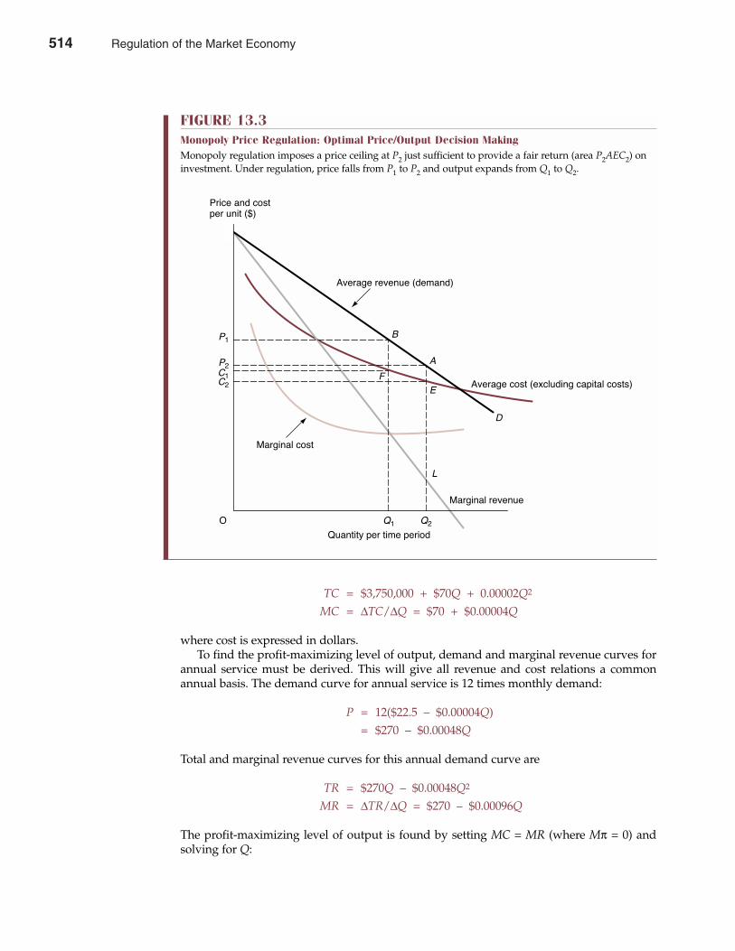
TC = $3,750,000 + $70Q + 0.00002Q2
MC = ∆TC/∆Q = $70 + $0.00004Q
where cost is expressed in dollars.To find the profit-maximizing level of output, demand and marginal revenue curves for
annual service must be derived. This will give all revenue and cost relations a commonannual basis. The demand curve for annual service is 12 times monthly demand:
P = 12($22.5 – $0.00004Q)= $270 – $0.00048Q
Total and marginal revenue curves for this annual demand curve are
TR = $270Q – $0.00048Q2
MR = ∆TR/∆Q = $270 – $0.00096Q
The profit-maximizing level of output is found by setting MC = MR (where Mπ = 0) andsolving for Q:
Chapter Thirteen Regulation of the Market Economy 515
FIGURE 13.3Monopoly Price Regulation: Optimal Price/Output Decision MakingMonopoly regulation imposes a price ceiling at P2 just sufficient to provide a fair return (area P2AEC2) oninvestment. Under regulation, price falls from P1 to P2 and output expands from Q1 to Q2.
Marginal cost
Marginal revenue
Average cost (excluding capital costs)
P1
Price and costper unit ($)
P2
C2
C1
Q2Q1
Quantity per time period
L
EF
B
A
D
Average revenue (demand)
O
514 Regulation of the Market Economy
MC = MR
$70 + $0.00004Q = $270 – $0.00096Q
$0.001Q = $200Q = 200,000
The monthly service price is
P = $22.50 – $0.00004(200,000)= $14.50 per month (or $174 per year)
This price/output combination generates annual total profits of
π = $270Q – $0.00048Q2 – $3,750,000 – $70Q – $0.00002Q2
= –$0.0005Q2 + $200Q – $3,750,000= –$0.0005(200,0002) + $200(200,000) - $3,750,000= $16,250,000
If the company has $125 million invested in plant and equipment, the annual rate of return oninvestment is
Return on Investment = $16,250,000 = 0.13, or 13%$125,000,000
Now assume that the State Public Utility Commission decides that a 12 percent rate of returnis fair given the level of risk taken and conditions in the financial markets. With a 12 percentrate of return on total assets, Malibu Beach would earn business profits of
π = Allowed Return � Total Assets= 0.12 � $125,000,000= $15,000,000
To determine the level of output that would generate this level of total profits, total profitmust be set equal to $15 million:
π = TR – TC
$15,000,000 = –$0.0005Q2 + $200Q – $3,750,000
This implies that
–$0.0005Q2 + $200Q – $18,750,000 = 0
which is a function of the form aQ2 + bQ – c = 0. Solving for the roots of this equation providesthe target output level. We use the quadratic equation as follows:
Q = –b ± √b2 – 4ac2a
= –200 ± √2002 – 4(–0.0005)(18,750,000)2(–0.0005)
= –200 ± √2,500–0.001
= 150,000 or 250,000
516 Part Five Long-Term Investment Decisions
Regulation of the Market Economy 515

Because public utility commissions generally want utilities to provide service to the greatestpossible number of customers at the lowest possible price, the upper figure Q = 250,000 is theappropriate output level. To induce Malibu Beach Telephone to operate at this output level,regulatory authorities would determine the maximum allowable price for monthly service as
P = $22.50 – $0.00004(250,000)= $12.50
This $12.50-per-month price provides service to the broadest customer base possible, giventhe need to provide Malibu Beach with the opportunity to earn a 12 percent rate of returnon investment.
Problems with Utility Price and Profit RegulationAlthough the concept of utility price and profit regulation is simple, several practical problemsarise in public utility regulation. In practice, it is impossible to exactly determine cost anddemand schedules, or the minimum investment required to support a given level of output.Moreover, because utilities serve several classes of customers, many different rate schedulescould produce the desired profit level. If profits for the local electric power company are toolow, should rates be raised for summer (peak) or for winter (off-peak) users? Should industrial,commercial, or residential customers bear the burden of higher rates?
Regulators also make mistakes with regard to the optimal level and growth of service. Forexample, if a local telephone utility is permitted to charge excessive rates, the system will growat a faster-than-optimal rate. Similarly, when the allowed rate of return exceeds the cost of cap-ital, electric, gas, and water utilities have an incentive to overexpand fixed assets and shift to
Chapter Thirteen Regulation of the Market Economy 517
Microsoft’s Antitrust Woes
On November 2, 2001, Microsoft Corp. announced thatit had reached a settlement with the U. S. government inits 3-year antitrust case. The settlement pact imposesrestrictions for a 5-year period on how the companydevelops and licenses software, works with independentsoftware vendors, and communicates about the innerworkings of its software with partners and competitors.Microsoft’s compliance with the agreement will be veri-fied by an independent, on-site, three-member panel ofcomputer experts.
Under the terms of the accord, Microsoft may notenter into licensing agreements with PC manufacturersthat restrict such manufacturers from working with othersoftware developers, a practice referred to as “exclusivedealing.” It also requires Microsoft to provide other software makers with access to elements of its Windowssource code, called “application programming interfaces,”which are necessary for them to make independentapplications work under the Windows operating system.
In an important win for Microsoft, the JusticeDepartment settlement does not impose any restrictionson features Microsoft is allowed to incorporate in newer
versions of its Windows operating system. Microsoft willbe able to continue to innovate and combine newInternet browser software with its basic operating system.This is important because the personal computer hasbeen transformed from a computing device, where desk-top applications like Microsoft Word are important, to anInternet communications device, where efficient informa-tion search and communication are key.
What remains to be seen is if Microsoft can recapturesome of the excitement that made it a stock-market dar-ling during the 1990s when investors saw the value ofMicrosoft stock multiply more than 100:1. Microsoft firstwent public in 1986, when it generated $197.5 million inrevenues and $39.3 million in net income. By 2005,Microsoft revenues are expected to surge to $45 billion,while profits swell to $16.7 billion. Hitting these revenueand profit targets will be tough in an increasingly com-petitive market environment.
See: Mark Wigfield, “Federal Judge Says No New Hearings Are Neededto Weigh Microsoft Pact,” The Wall Street Journal Online, March 6, 2002(http://online.wsj.com).
M A N A G E R I A L A P P L I C AT I O N 1 3 . 3
516 Regulation of the Market Economy
overly capital-intensive methods of production. In contrast, if prices allowed to natural gas pro-ducers are too low, consumers will be encouraged to deplete scarce gas supplies, producers willlimit exploration and development, and gas shortages can occur. If gas prices are too low andoffer only a below-market rate of return on capital, necessary expansion will be thwarted.
A related problem is that of regulatory lag, or the delay between when a change in regu-lation is appropriate and the date it becomes effective. During the 1970s and 1980s, inflationexerted constant upward pressure on costs. At the same time, consumers and voters were ableto reduce, delay, or deny reasonable rate increases. This caused severe financial hardship for anumber of utilities and their stockholders. More recently, rapid changes in technology andcompetitive conditions have rendered obsolete many traditional forms of regulation in theelectricity and telecommunications industries. When regulators are slow to react to suchchanges, both consumers and the industry suffer.
Traditional forms of regulation can also lead to inefficiency. If a utility is guaranteed a mini-mum return on investment, operating inefficiencies can be offset by higher prices. The process ofutility regulation itself is also costly. Detailed demand and cost analyses are necessary to providea reasonable basis for rate decisions. It is expensive to pay regulatory officials, full-time utilitycommission staffs, record-keeping costs, and the expense of processing rate cases. All of theseexpenses are ultimately borne by consumers. Although many economists can see no reasonablealternative to utility regulation for electric, gas, local telephone, and private water companies, thecosts and inefficiency of such regulation are troubling.
ANTITRUST POLICY
Antitrust policy in the United States is designed to protect competition. If competitive forcesare vibrant, consumer prices are and unwarranted economic profits are low. Product quality,innovation, and economic growth also tend to be high. In a vigorously competitive economicenvironment, there will be corporate winners and losers. This is fine so long as the game isplayed fairly. When unfair methods of competition emerge, antitrust policy is brought to bear.
Overview of Antitrust LawAntitrust laws are designed to promote competition and prevent unwarranted monopoly. Byitself, large firm size or market dominance is no offense; it is any unfairly gained competitiveadvantage that is against the law. The primary objection to monopolies, cartels, and otherrestraints of trade is that they injure consumers by increasing prices. High monopoly pricesalso curtail consumption and thereby reduce consumer welfare. A further objection to monop-oly is that unchecked economic power stiffles innovation and often fails to provide necessaryincentives for operating efficiency. As British economist John Hicks once wrote, “The best of allmonopoly profits is a quiet life.” Thus, complacency on the part of monopolists can impedeeconomic progress.
The choice between pure competition and monopoly is easy. Unfortunately, that is seldomthe decision facing those charged with antitrust enforcement. Antitrust concerns tend to arise inindustries where firms have some market power, but also face competition. In such instances,mergers and restrictive practices that may create or enhance market power may also promoteefficiency and benefit consumers. Antitrust enforcement is made difficult by the need to identi-fy corporate conduct whose primary effect is to lessen competition and harm consumers.
There is no single antitrust statute in the United States. Federal antitrust law is based ontwo important statutes—the Sherman Act and the Clayton Act—and their amendments. Animportant characteristic of these laws is that they broadly ban, but never define, “restraints oftrade,” “monopolization,” “unfair competition,” and so on. By never precisely defining suchkey terms, the statutes left the courts to decide the specific legality or illegality of various busi-
518 Part Five Long-Term Investment Decisions
regulatory lagThe delay betweenwhen a change in regulation is appropri-ate and the date itbecomes effective
antitrust lawsLaws that promotecompetition and prevent monopoly
Regulation of the Market Economy 517
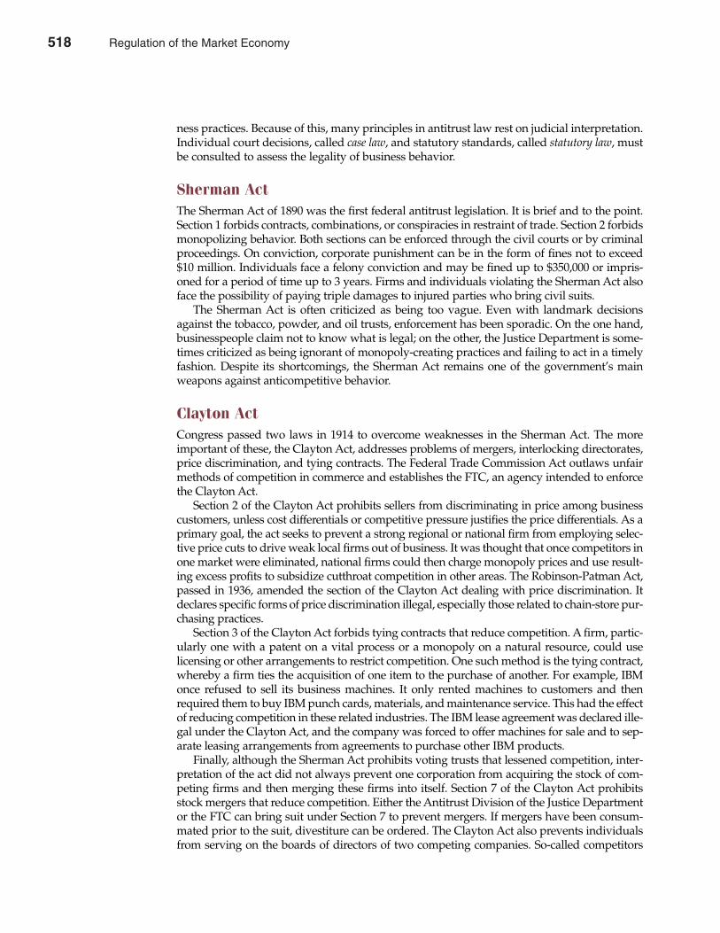
ness practices. Because of this, many principles in antitrust law rest on judicial interpretation.Individual court decisions, called case law, and statutory standards, called statutory law, mustbe consulted to assess the legality of business behavior.
Sherman ActThe Sherman Act of 1890 was the first federal antitrust legislation. It is brief and to the point.Section 1 forbids contracts, combinations, or conspiracies in restraint of trade. Section 2 forbidsmonopolizing behavior. Both sections can be enforced through the civil courts or by criminalproceedings. On conviction, corporate punishment can be in the form of fines not to exceed$10 million. Individuals face a felony conviction and may be fined up to $350,000 or impris-oned for a period of time up to 3 years. Firms and individuals violating the Sherman Act alsoface the possibility of paying triple damages to injured parties who bring civil suits.
The Sherman Act is often criticized as being too vague. Even with landmark decisionsagainst the tobacco, powder, and oil trusts, enforcement has been sporadic. On the one hand,businesspeople claim not to know what is legal; on the other, the Justice Department is some-times criticized as being ignorant of monopoly-creating practices and failing to act in a timelyfashion. Despite its shortcomings, the Sherman Act remains one of the government’s mainweapons against anticompetitive behavior.
Clayton ActCongress passed two laws in 1914 to overcome weaknesses in the Sherman Act. The moreimportant of these, the Clayton Act, addresses problems of mergers, interlocking directorates,price discrimination, and tying contracts. The Federal Trade Commission Act outlaws unfairmethods of competition in commerce and establishes the FTC, an agency intended to enforcethe Clayton Act.
Section 2 of the Clayton Act prohibits sellers from discriminating in price among businesscustomers, unless cost differentials or competitive pressure justifies the price differentials. As aprimary goal, the act seeks to prevent a strong regional or national firm from employing selec-tive price cuts to drive weak local firms out of business. It was thought that once competitors inone market were eliminated, national firms could then charge monopoly prices and use result-ing excess profits to subsidize cutthroat competition in other areas. The Robinson-Patman Act,passed in 1936, amended the section of the Clayton Act dealing with price discrimination. Itdeclares specific forms of price discrimination illegal, especially those related to chain-store pur-chasing practices.
Section 3 of the Clayton Act forbids tying contracts that reduce competition. A firm, partic-ularly one with a patent on a vital process or a monopoly on a natural resource, could uselicensing or other arrangements to restrict competition. One such method is the tying contract,whereby a firm ties the acquisition of one item to the purchase of another. For example, IBMonce refused to sell its business machines. It only rented machines to customers and thenrequired them to buy IBM punch cards, materials, and maintenance service. This had the effectof reducing competition in these related industries. The IBM lease agreement was declared ille-gal under the Clayton Act, and the company was forced to offer machines for sale and to sep-arate leasing arrangements from agreements to purchase other IBM products.
Finally, although the Sherman Act prohibits voting trusts that lessened competition, inter-pretation of the act did not always prevent one corporation from acquiring the stock of com-peting firms and then merging these firms into itself. Section 7 of the Clayton Act prohibitsstock mergers that reduce competition. Either the Antitrust Division of the Justice Departmentor the FTC can bring suit under Section 7 to prevent mergers. If mergers have been consum-mated prior to the suit, divestiture can be ordered. The Clayton Act also prevents individualsfrom serving on the boards of directors of two competing companies. So-called competitors
Chapter Thirteen Regulation of the Market Economy 519
518 Regulation of the Market Economy
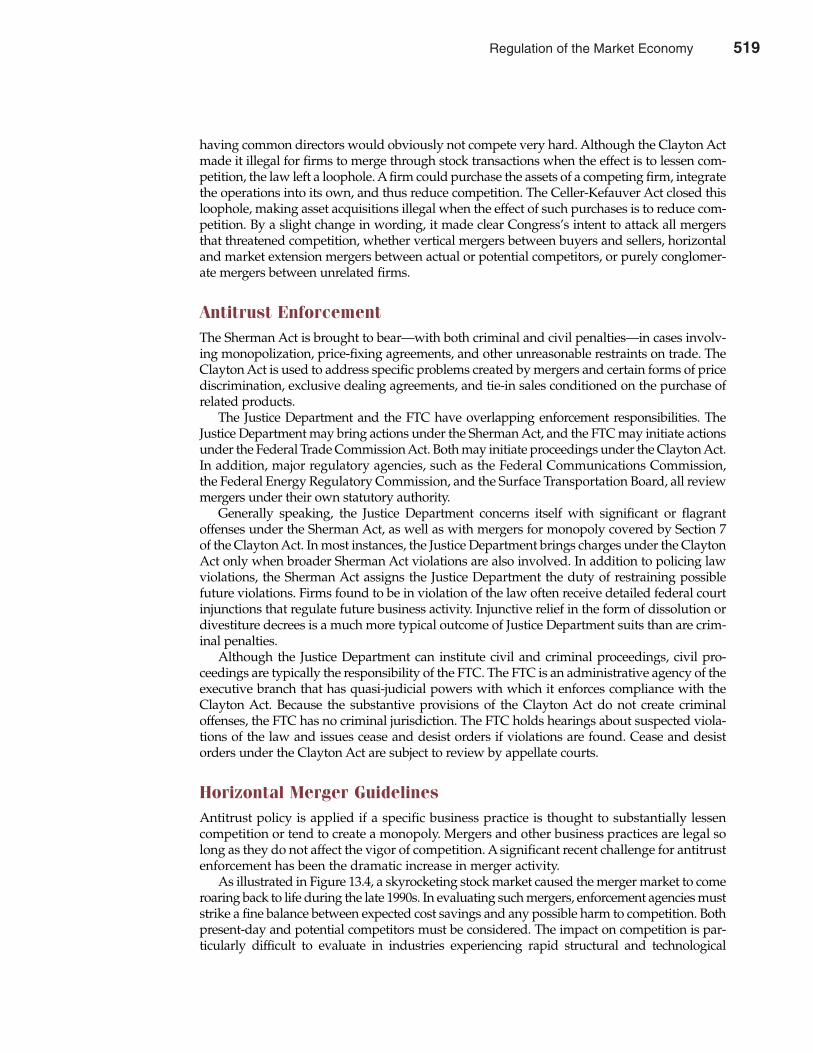
having common directors would obviously not compete very hard. Although the Clayton Actmade it illegal for firms to merge through stock transactions when the effect is to lessen com-petition, the law left a loophole. A firm could purchase the assets of a competing firm, integratethe operations into its own, and thus reduce competition. The Celler-Kefauver Act closed thisloophole, making asset acquisitions illegal when the effect of such purchases is to reduce com-petition. By a slight change in wording, it made clear Congress’s intent to attack all mergersthat threatened competition, whether vertical mergers between buyers and sellers, horizontaland market extension mergers between actual or potential competitors, or purely conglomer-ate mergers between unrelated firms.
Antitrust EnforcementThe Sherman Act is brought to bear—with both criminal and civil penalties—in cases involv-ing monopolization, price-fixing agreements, and other unreasonable restraints on trade. TheClayton Act is used to address specific problems created by mergers and certain forms of pricediscrimination, exclusive dealing agreements, and tie-in sales conditioned on the purchase ofrelated products.
The Justice Department and the FTC have overlapping enforcement responsibilities. TheJustice Department may bring actions under the Sherman Act, and the FTC may initiate actionsunder the Federal Trade Commission Act. Both may initiate proceedings under the Clayton Act.In addition, major regulatory agencies, such as the Federal Communications Commission,the Federal Energy Regulatory Commission, and the Surface Transportation Board, all reviewmergers under their own statutory authority.
Generally speaking, the Justice Department concerns itself with significant or flagrantoffenses under the Sherman Act, as well as with mergers for monopoly covered by Section 7of the Clayton Act. In most instances, the Justice Department brings charges under the ClaytonAct only when broader Sherman Act violations are also involved. In addition to policing lawviolations, the Sherman Act assigns the Justice Department the duty of restraining possiblefuture violations. Firms found to be in violation of the law often receive detailed federal courtinjunctions that regulate future business activity. Injunctive relief in the form of dissolution ordivestiture decrees is a much more typical outcome of Justice Department suits than are crim-inal penalties.
Although the Justice Department can institute civil and criminal proceedings, civil pro-ceedings are typically the responsibility of the FTC. The FTC is an administrative agency of theexecutive branch that has quasi-judicial powers with which it enforces compliance with theClayton Act. Because the substantive provisions of the Clayton Act do not create criminaloffenses, the FTC has no criminal jurisdiction. The FTC holds hearings about suspected viola-tions of the law and issues cease and desist orders if violations are found. Cease and desistorders under the Clayton Act are subject to review by appellate courts.
Horizontal Merger GuidelinesAntitrust policy is applied if a specific business practice is thought to substantially lessencompetition or tend to create a monopoly. Mergers and other business practices are legal solong as they do not affect the vigor of competition. A significant recent challenge for antitrustenforcement has been the dramatic increase in merger activity.
As illustrated in Figure 13.4, a skyrocketing stock market caused the merger market to comeroaring back to life during the late 1990s. In evaluating such mergers, enforcement agencies muststrike a fine balance between expected cost savings and any possible harm to competition. Bothpresent-day and potential competitors must be considered. The impact on competition is par-ticularly difficult to evaluate in industries experiencing rapid structural and technological
520 Part Five Long-Term Investment Decisions
Regulation of the Market Economy 519
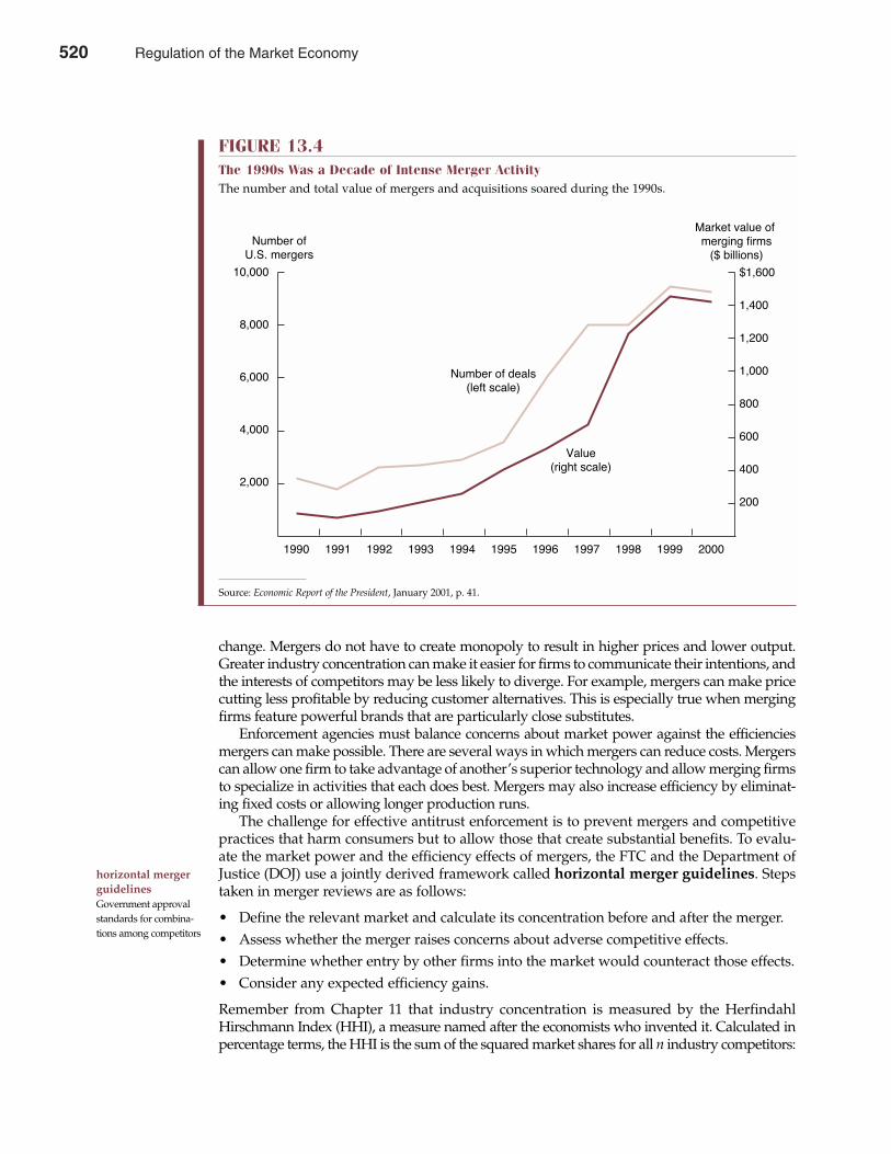
change. Mergers do not have to create monopoly to result in higher prices and lower output.Greater industry concentration can make it easier for firms to communicate their intentions, andthe interests of competitors may be less likely to diverge. For example, mergers can make pricecutting less profitable by reducing customer alternatives. This is especially true when mergingfirms feature powerful brands that are particularly close substitutes.
Enforcement agencies must balance concerns about market power against the efficienciesmergers can make possible. There are several ways in which mergers can reduce costs. Mergerscan allow one firm to take advantage of another’s superior technology and allow merging firmsto specialize in activities that each does best. Mergers may also increase efficiency by eliminat-ing fixed costs or allowing longer production runs.
The challenge for effective antitrust enforcement is to prevent mergers and competitivepractices that harm consumers but to allow those that create substantial benefits. To evalu-ate the market power and the efficiency effects of mergers, the FTC and the Department ofJustice (DOJ) use a jointly derived framework called horizontal merger guidelines. Stepstaken in merger reviews are as follows:
• Define the relevant market and calculate its concentration before and after the merger.• Assess whether the merger raises concerns about adverse competitive effects.• Determine whether entry by other firms into the market would counteract those effects.• Consider any expected efficiency gains.
Remember from Chapter 11 that industry concentration is measured by the HerfindahlHirschmann Index (HHI), a measure named after the economists who invented it. Calculated inpercentage terms, the HHI is the sum of the squared market shares for all n industry competitors:
horizontal mergerguidelinesGovernment approvalstandards for combina-tions among competitors
Chapter Thirteen Regulation of the Market Economy 521
FIGURE 13.4The 1990s Was a Decade of Intense Merger ActivityThe number and total value of mergers and acquisitions soared during the 1990s.
10,000
8,000
6,000
4,000
2,000
Number of�U.S. mergers
Number of deals�(left scale)
1990 1991 1992 1993 1994 1995 1996 1997 1998 1999 2000
$1,600
1,400
1,200
1,000
800
600
400
200�
Market value of �merging firms�($ billions)
Value�(right scale)
Source: Economic Report of the President, January 2001, p. 41.
520 Regulation of the Market Economy
n
(13.1)HHI = ∑ � Firm Salesi �
2
i = 1 Industry Sales � 100
For example, a market consisting of four firms with market shares of 30 percent, 30 percent, 20percent, and 20 percent has an HHI of 2,600 (= 302 + 302 + 202 + 202). Although it is desirable toinclude all firms in the calculation, lack of information about small firms is not critical becausesuch firms do not affect the HHI significantly. A monopoly industry with a single dominantfirm is described by a four-firm concentration ratio of 100 percent, or CR4 = 100, and a HHI = 1002
= 10,000. A vigorously competitive industry where each of the leading four firms enjoys marketshares of 25 percent is also described by a CR4 = 100, but features a HHI = 252 +252 +252 +252 =2,500. Like the four-firm concentration ratio, the HHI approaches zero for industries character-ized by a large number of very small competitors.
When a merger occurs, or a pending merger is proposed, the increase in concentration asmeasured by the HHI can be calculated by doubling the product of the market shares of themerging firms. For example, the merger of firms with 5 percent and 10 percent shares of themarket would increase the HHI by l00 (= 2 � 5 � 10). To see this is the case, simply recallthat in calculating the HHI before the merger, the market shares of merging firms aresquared individually, or a2 + b2. After the merger, the sum of those individual firm marketshares would be squared, or (a + b)2, which equals a2 + 2ab + b2. The merger-induced increasein the HHI, therefore, is represented by 2ab, which is the product of two times the marketshares of the merging firms.
In evaluating horizontal mergers, the FTC and DOJ consider both the post-merger marketconcentration and the increase in concentration resulting from the merger as potentially usefulindicators of competitive implications. According to horizontal merger guidelines, the generalstandards for horizontal mergers are as follows:
1. Unconcentrated Markets with Post-Merger HHI Below 1,000. Mergers resulting in relativelyunconcentrated markets are not likely to have adverse competitive effects and ordinarilywill be approved.
2. Moderately Concentrated Markets with Post-Merger HHI Between 1,000 and 1,800. Mergersproducing an increase in the HHI of less than 100 points in moderately concentratedmarkets are unlikely to have adverse competitive consequences and ordinarily will beapproved. Mergers producing an increase in the HHI of more than 100 points in mod-erately concentrated markets have the potential to raise significant competitive concernsand would be scrutinized.
3. Highly Concentrated Markets with Post-Merger HHI Above 1,800. Mergers producing anincrease in the HHI of less than 50 points, even in highly concentrated markets, are unlike-ly to have adverse competitive consequences and ordinarily will be approved. Mergersproducing an increase in the HHI of more than 50 points in highly concentrated marketshave the potential to raise significant competitive concerns and would be scrutinized.Where the post-merger HHI exceeds 1,800, it will be presumed that mergers producing anincrease in the HHI of more than 100 points are likely to create or enhance market powerand would ordinarily not be approved.
Although the FTC and DOJ realize that the post-merger level of market concentration and thechange in concentration resulting from a merger affect the degree to which a merger raisescompetitive concerns, both recognize that market concentration data sometimes misstate thecompetitive significance of a given merger. For example, changes in technology can makelong-entrenched rivals susceptible to innovative products produced by new foreign ordomestic competitors. Changes in technology also have the potential to reshape the demandfor substitutes outside historically relevant markets. Recent advances in the satellite trans-mission of voice and data communication have clearly reduced the market power of local
522 Part Five Long-Term Investment Decisions
Regulation of the Market Economy 521
telecommunications and cable television companies. Similarly, the exploding use of theInternet allows customers to compare the price and performance of goods and servicesoffered by both local and distant providers.
It is from within this framework that recent antitrust policy initiatives can be evaluated.
Recent Antitrust Policy InitiativesThe development and adoption of new technology is essential to economic growth overtime. To the extent that recent antitrust policy initiatives hinder or otherwise interfere withinvention and innovation, such initiatives come at a significant social cost, irrespective of anycompensating virtues. During recent years, some of the most important and controversialantitrust initiatives have come in increasingly important network industries.
Americans are intimately familiar with networks such as credit card networks, telephonenetworks, and computer networks. The distinguishing feature of all such networks is thattheir value grows as customer use becomes more widespread. New telephone subscribersincrease the potential number of people that one can call; expanding use of the Internetincreases the amount of information on the Web. Similarly, when more retail outlets, depart-ment stores, and restaurants adopt a given credit card, the value of that credit card grows forall its holders. The added value that new users add to network goods and services is called anetwork externality. Networks became a recent concern in antitrust policy because the ClintonJustice Department feared that if inferior networks got a decisive lead in “installed base”among consumers, switching costs might be sufficient to keep customers from switching to asuperior standard. Switching costs might also constitute a barrier to entry in the industry andenable network monopolists to tie or bundle a second product in such a way as to foreclosecompetition in that secondary market.
Concern over competition and innovation among general-purpose credit cards recent-ly prompted the Justice department to file suit against the two largest networks, Visa andMasterCard. Although Visa and MasterCard began as separate and competing networksowned and governed by their card-issuing members, substantial overlap now exists given thewillingness of each network to accept new members. The Justice Department case focuses onthe potential innovation-reducing effects of this overlapping ownership and governancearrangement. In particular, the Justice Department alleges that Visa and MasterCard haveunnecessarily delayed implementation of “smart card” technology that has the potential tobetter monitor fraud and credit risk. Although the outcome of this case remains in doubt, itremains as an example of aggressive antitrust policy in this area.
Preserving competition in telecommunications networks has also been a high priority inantitrust policy. As you know, a computer network is nothing more than a means for linkingcomputers and peripheral equipment (e.g., printers) so that they can communicate with oneanother. The Internet is simply a seamless connection that allows information to freely travelfrom one computer network to another. An Internet backbone is a powerful, high-message-capacity system that links regional or metropolitan networks to the Internet. For example,when customers use AOL as their Internet service provider (ISP), they often use a telephonemodem to connect to AOL’s network [sometimes called a local area network (LAN)]. In turn,AOL’s network is connected to the Internet via several Internet backbones. To provide readycustomer service, AOL and other ISPs must lease capacity on the Internet backbone facilitiesprovided by major telecommunications providers. In 1998, fearing an anticompetitive increasein concentration in this “network of networks,” the Justice Department required MCI Communi-cations Corp. to divest its Internet backbone business as a precondition to its approval of MCI’smerger with WorldCom, Inc. Two years later, in 2000, the proposed merger of MCI-WorldCom,Inc., and Sprint Corp., the nation’s No. 2 and No. 3 long-distance companies and the top twoInternet backbone providers, proved too much for antitrust authorities, who turned thumbsdown on the deal.
network externalityAdded value that newusers add to networkgoods and services
Chapter Thirteen Regulation of the Market Economy 523
522 Regulation of the Market Economy
Clearly the biggest and most controversial antitrust initiative undertaken in the networkingarea is the Justice Department’s case against Microsoft Corp. The Justice Department claims thatMicrosoft has misused its dominance of the market for personal computer operating systems tomaintain dominance of that market and to extend dominance to related markets, primarily themarket for browser software. A browser is computer software that allows users to access andnavigate the Internet. The Justice Department claims that Microsoft has unfairly required com-puter manufacturers to install the Microsoft browser as a precondition of their receiving licensesto install Windows (its dominant personal computer operating system) and that Microsoft hasrequired computer manufacturers to display ISP icons on the main “pop-up screen” only whensuch ISPs agree to employ the Microsoft browser. For its part, Microsoft contends that integrat-ing its browser with the Windows operating system enhances the functionality of both and thatits contractual arrangements with computer manufacturers and ISPs are nothing more thanstandard cross-promotional arrangements.
The case against Microsoft, like actions against Visa and MasterCard and telecom mergers,represents historic initiatives designed to maintain vigorous competition in markets dominat-ed by network externalities. The challenge for antitrust policy makers is to preserve competitiveopportunities without punishing successful competitors. Striking the right balance betweenregulation and market pressure is essential for promoting innovation and protecting consumerwelfare in fast-moving high-tech markets.
PROBLEMS WITH REGULATION
The need for regulation stems from economic and social factors that stimulate market failuresdue to incentive or structural problems. However, despite obvious benefits, there are costs to
524 Part Five Long-Term Investment Decisions
The Enron Debacle
In November 2001, Enron Corp. filed the largest volun-tary Chapter 11 bankruptcy petition in U.S. history—a stunning collapse for a company worth more than $60billion less than a year earlier. Historically, Enron’s prin-cipal business was the transportation and marketing ofnatural gas and electricity to markets throughout theUnited States. More recently, the company built a largecommodities trading, risk management, and financialservices business that led to its eventual downfall.
Enron ran into trouble trading energy futures con-tracts. A futures contract is a binding legal documentthat commits the buyer to take delivery, and the sellerto make delivery, of an underlying asset in a specifiedquantity and quality at a specific delivery time andplace. Because futures contracts involve obligations tobuy and sell a specific commodity for a preset price,both buyers and sellers of futures contracts are exposedto the potential for unlimited losses in the event ofadverse market conditions. Like stock options andstock index options, futures contracts on commoditieslike natural gas are called “financial derivatives”because their economic value is derived from changes
in the price of natural gas or some other underlyingcommodity.
To control risk and lend stability to futures markets,Congress enacted the Commodity Exchange Act in 1974and established the Commodity Futures TradingCommission (CFTC), an independent federal regulatoryagency with jurisdiction over futures trading. The CFTCstrives to protect market participants against manipula-tion, abusive trade practices, and fraud. Critics contendthat the Enron bankruptcy could have been averted hadthe company not won various regulatory exemptions inthe Commodity Futures Modernization Act of 2000, alaw that drastically reduced the power of governmentregulatory agencies overseeing futures markets. Withoutsuch exemptions, the CFTC might have regulatedEnronOnline as an “organized exchange” and put controlsin place to avoid financial disaster for Enron employees,investors, and trading partners.
See: Michael Schroeder and Cassell Bryan-Low, “After Enron, CongressBacks Off from Deregulation, Calls for Controls,” The Wall Street JournalOnline, January 29, 2002 (http://online.wsj.com).
M A N A G E R I A L A P P L I C AT I O N 1 3 . 4
Regulation of the Market Economy 523
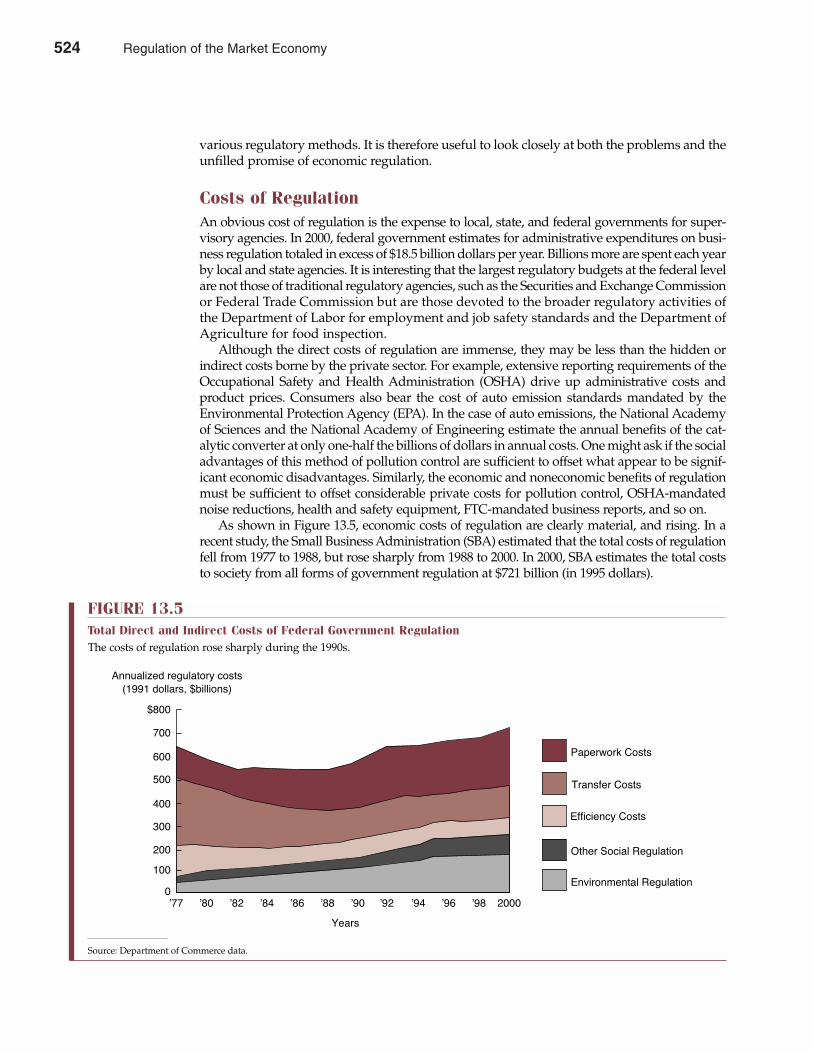
various regulatory methods. It is therefore useful to look closely at both the problems and theunfilled promise of economic regulation.
Costs of RegulationAn obvious cost of regulation is the expense to local, state, and federal governments for super-visory agencies. In 2000, federal government estimates for administrative expenditures on busi-ness regulation totaled in excess of $18.5 billion dollars per year. Billions more are spent each yearby local and state agencies. It is interesting that the largest regulatory budgets at the federal levelare not those of traditional regulatory agencies, such as the Securities and Exchange Commissionor Federal Trade Commission but are those devoted to the broader regulatory activities ofthe Department of Labor for employment and job safety standards and the Department ofAgriculture for food inspection.
Although the direct costs of regulation are immense, they may be less than the hidden orindirect costs borne by the private sector. For example, extensive reporting requirements of theOccupational Safety and Health Administration (OSHA) drive up administrative costs andproduct prices. Consumers also bear the cost of auto emission standards mandated by theEnvironmental Protection Agency (EPA). In the case of auto emissions, the National Academyof Sciences and the National Academy of Engineering estimate the annual benefits of the cat-alytic converter at only one-half the billions of dollars in annual costs. One might ask if the socialadvantages of this method of pollution control are sufficient to offset what appear to be signif-icant economic disadvantages. Similarly, the economic and noneconomic benefits of regulationmust be sufficient to offset considerable private costs for pollution control, OSHA-mandatednoise reductions, health and safety equipment, FTC-mandated business reports, and so on.
As shown in Figure 13.5, economic costs of regulation are clearly material, and rising. In arecent study, the Small Business Administration (SBA) estimated that the total costs of regulationfell from 1977 to 1988, but rose sharply from 1988 to 2000. In 2000, SBA estimates the total coststo society from all forms of government regulation at $721 billion (in 1995 dollars).
Chapter Thirteen Regulation of the Market Economy 525
FIGURE 13.5Total Direct and Indirect Costs of Federal Government RegulationThe costs of regulation rose sharply during the 1990s.
100
600
700
$800
0
200
300
400
500
Paperwork Costs
Transfer Costs
Efficiency Costs
Other Social Regulation
Environmental Regulation
2000Õ98Õ96Õ94Õ92Õ90Õ88Õ86Õ84Õ82Õ80Õ77
Annualized regulatory costs
(1991 dollars, $billions)
Years
Source: Department of Commerce data.
524 Regulation of the Market Economy
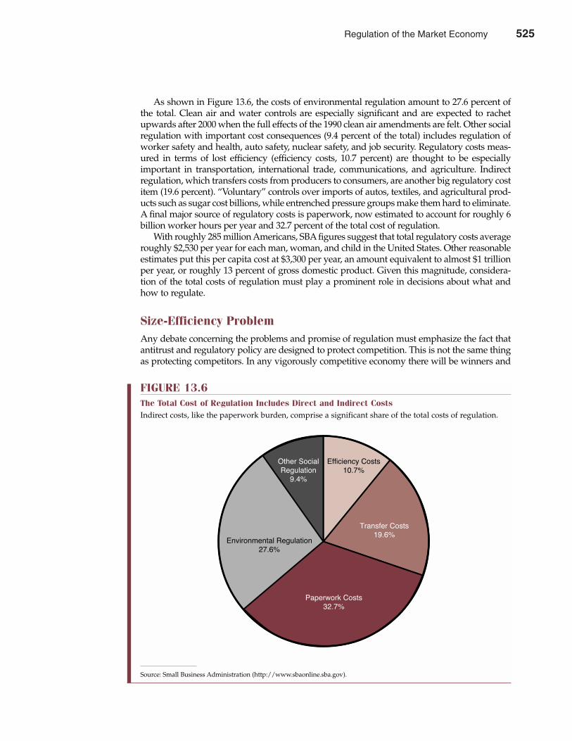
As shown in Figure 13.6, the costs of environmental regulation amount to 27.6 percent ofthe total. Clean air and water controls are especially significant and are expected to rachetupwards after 2000 when the full effects of the 1990 clean air amendments are felt. Other socialregulation with important cost consequences (9.4 percent of the total) includes regulation ofworker safety and health, auto safety, nuclear safety, and job security. Regulatory costs meas-ured in terms of lost efficiency (efficiency costs, 10.7 percent) are thought to be especiallyimportant in transportation, international trade, communications, and agriculture. Indirectregulation, which transfers costs from producers to consumers, are another big regulatory costitem (19.6 percent). “Voluntary” controls over imports of autos, textiles, and agricultural prod-ucts such as sugar cost billions, while entrenched pressure groups make them hard to eliminate.A final major source of regulatory costs is paperwork, now estimated to account for roughly 6billion worker hours per year and 32.7 percent of the total cost of regulation.
With roughly 285 million Americans, SBA figures suggest that total regulatory costs averageroughly $2,530 per year for each man, woman, and child in the United States. Other reasonableestimates put this per capita cost at $3,300 per year, an amount equivalent to almost $1 trillionper year, or roughly 13 percent of gross domestic product. Given this magnitude, considera-tion of the total costs of regulation must play a prominent role in decisions about what andhow to regulate.
Size-Efficiency ProblemAny debate concerning the problems and promise of regulation must emphasize the fact thatantitrust and regulatory policy are designed to protect competition. This is not the same thingas protecting competitors. In any vigorously competitive economy there will be winners and
526 Part Five Long-Term Investment Decisions
FIGURE 13.6The Total Cost of Regulation Includes Direct and Indirect CostsIndirect costs, like the paperwork burden, comprise a significant share of the total costs of regulation.
Efficiency Costs�10.7%
Paperwork Costs�32.7%
Transfer Costs�19.6%
Other Social�Regulation�
9.4%
Environmental Regulation�27.6%
Source: Small Business Administration (http://www.sbaonline.sba.gov).
Regulation of the Market Economy 525
losers. In a competitive market as large as the United States, winners tend to be enormouslysuccessful; losers quickly fade or go out of business altogether. Is Microsoft Corp. enormouslyprofitable and successful simply because it offers new and innovative products, or is it able tooffer new and innovative products simply because it is large and enormously profitable?Obviously, Microsoft’s ongoing battles with regulatory authorities continue because of differingviews concerning the origin of the company’s size-efficiency linkage. Company officials main-tain that Microsoft’s growth and profitability are a direct result of its ability to offer innovativecomputer software. Meanwhile, government regulators contend that the company has used itsdominance of the marketplace to unfairly eclipse software rivals.
The size-efficiency debate between Microsoft and the federal government is the type of“chicken or the egg” argument common to high-technology industries. Mergers that seeminnocuous today may eliminate future competition; others that increase concentration todaypose no significant anticompetitive problem. For example, the 1997 merger between BoeingCo. and McDonnell Douglas Corp. reduced the number of sellers of large commercial aircraftworldwide from only three to two, the other being Airbus Industrie, the European multina-tional consortium. Nevertheless, the FTC decided that McDonnell Douglas’s 5 percent marketshare overstated that company’s future competitive significance because it only reflected thefilling of old orders. Advances in aviation design had left McDonnell Douglas behind, and thevast majority of airlines no longer considered purchasing its aircraft. As a result, the Boeing-McDonnell Douglas merger did not eliminate viable future competition in the commercial air-craft market. Moreover, after consulting with the Department of Defense, the FTC concludedthat there were no prospects for Boeing and McDonnell Douglas to bid on the same defenseprojects. Having concluded that the merger raised antitrust concerns in neither commercialnor defense markets, the FTC did not challenge the merger agreement.
Apart from such a case-by-case review, critics point to a general perception of rising monop-oly profits as evidence of overly lenient antitrust policy during recent years. For example, Figure13.7 shows the dramatic increase in Tobin’s q ratio, defined as the ratio of market value relativeto the replacement cost of tangible assets that occurred for nonfinancial firms during the 1990s.In the early 1980s, Nobel laureate James Tobin conceived of this measure as an indicator of pend-ing capital investment. According to Tobin, when high profits cause market values to greatlyexceed replacement costs, firms have powerful incentives to expand, and capital investmentshould boom. Conversely, when low profits cause market values to fall below replacement costs,firms will shrink, and capital investment can be expected to wither.
More recently, economists have used Tobin’s q ratio as an indicator of above-normal ormonopoly profits. As seen in Figure 13.7, Tobin’s q ratio surged from below 100 percent in 1990to above 200 percent by the end of the decade. However, it is difficult to make the simple con-clusion that monopoly profits soared during this period. In the early 1990s, the overall economysuffered a sharp recession that dramatically reduced corporate profits and stock prices. By theend of the 1990s, the economy had logged the longest peacetime expansion in history, and bothcorporate profits and stock prices surged to record levels. Much of the trend in Tobin’s q depict-ed in Figure 13.7 can be explained by the business cycle. More fundamental changes were alsoat work. Leading firms today are characterized by growing reliance on what economists refer toas intangible assets, like advertising capital, brand names, customer goodwill, patents, and so on.For leading firms like Coca-Cola, Intel, and Microsoft, tangible assets play a relatively small rolein company valuation. Given the growing importance of intangible capital in our economy, itbecomes misleading to infer a simple increase in monopoly profits following an increase inTobin’s q over time.
Capture ProblemIt is a widely held belief that regulation is in the public interest and influences firm behaviortoward socially desirable ends. However, in the early 1970s, Nobel laureate George Stigler
Tobin’s q ratioA ratio calculated asthe market value of thefirm divided by thereplacement cost oftangible assets
Chapter Thirteen Regulation of the Market Economy 527
526 Regulation of the Market Economy
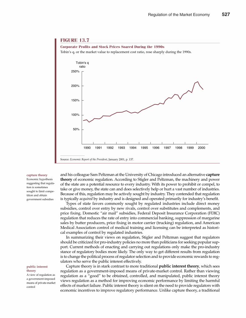
and his colleague Sam Peltzman at the University of Chicago introduced an alternative capturetheory of economic regulation. According to Stigler and Peltzman, the machinery and powerof the state are a potential resource to every industry. With its power to prohibit or compel, totake or give money, the state can and does selectively help or hurt a vast number of industries.Because of this, regulation may be actively sought by industry. They contended that regulationis typically acquired by industry and is designed and operated primarily for industry’s benefit.
Types of state favors commonly sought by regulated industries include direct moneysubsidies, control over entry by new rivals, control over substitutes and complements, andprice fixing. Domestic “air mail” subsidies, Federal Deposit Insurance Corporation (FDIC)regulation that reduces the rate of entry into commercial banking, suppression of margarinesales by butter producers, price fixing in motor carrier (trucking) regulation, and AmericanMedical Association control of medical training and licensing can be interpreted as histori-cal examples of control by regulated industries.
In summarizing their views on regulation, Stigler and Peltzman suggest that regulatorsshould be criticized for pro-industry policies no more than politicians for seeking popular sup-port. Current methods of enacting and carrying out regulations only make the pro-industrystance of regulatory bodies more likely. The only way to get different results from regulationis to change the political process of regulator selection and to provide economic rewards to reg-ulators who serve the public interest effectively.
Capture theory is in stark contrast to more traditional public interest theory, which seesregulation as a government-imposed means of private-market control. Rather than viewingregulation as a “good” to be obtained, controlled, and manipulated, public interest theoryviews regulation as a method for improving economic performance by limiting the harmfuleffects of market failure. Public interest theory is silent on the need to provide regulators witheconomic incentives to improve regulatory performance. Unlike capture theory, a traditional
528 Part Five Long-Term Investment Decisions
capture theoryEconomic hypothesissuggesting that regula-tion is sometimessought to limit compe-tition and obtain government subsidies
public interest theoryA view of regulation asa government-imposedmeans of private-marketcontrol
FIGURE 13.7Corporate Profits and Stock Prices Soared During the 1990sTobin’s q, or the market value to replacement cost ratio, rose sharply during the 1990s.
250%
200%
150%
100%
50%
Tobin's q�
ratio
1990 1991 1992 1993 1994 1995 1996 1997 1998 1999 2000
Source: Economic Report of the President, January 2001, p. 137.
Regulation of the Market Economy 527
view has been that the public can trust regulators to make a good-faith effort to establish reg-ulatory policy in the public interest.
To be sure, suggestions of a capture problem are debatable. The need to provide regulatorswith positive economic incentives to ensure regulation in the public interest is also highly con-troversial. Nevertheless, growing dissatisfaction with traditional approaches to governmentregulation has led to a deregulation movement that continues today.
DEREGULATION MOVEMENT
Growing concern with the costs and problems of government regulation gave birth to aderegulation movement that has grown to impressive dimensions. Although it is difficult topinpoint a single catalyst for the movement, it is hard to overlook the role played by Stigler,Peltzman, and other economists (notably, Alfred E. Kahn) who illustrated that the regulatoryprocess can sometimes harm consumer interests.
Major Steps Toward DeregulationA recent study by the Brookings Institution documented important benefits of deregulation. Infive major industries—natural gas, telecommunications, airlines, trucking, and railroads—thatwere deregulated, it was found that regulatory reform generated highly beneficial results.2 Pricesfell 4 percent to 15 percent within the first 2 years after deregulation. Within 10 years, prices were25 percent to 50 percent lower. Deregulation also leads to service quality improvements. Crucialsocial goals like airline safety, reliability of gas service, and reliability of the telecommunicationsnetwork were maintained or improved by deregulation. Regulatory reform also tends to conferbenefits on most consumers. Although it is possible to find narrowly defined groups of customersin special circumstances who paid somewhat higher prices after deregulation, the gains to thevast majority of consumers far outweighed negative effects on small groups. Finally, deregulationoffers benefits in the sense of permitting greater customer choice.
Table 13.1 highlights some of the major steps taken toward deregulation in the United Statessince 1970. Although many industries have felt the effects of changing state and local regulation,changing federal regulation has been most pronounced in the financial, telecommunications,and transportation sectors. Since 1975, for example, it has been illegal for securities dealers to fixcommission rates. This broke a 182-year tradition under which the New York Stock Exchange(NYSE) set minimum rates for each 100-share (“round lot”) purchase. Until 1975, everyonecharged the minimum rate approved by the NYSE. Purchase of 1,000 shares cost a commissionof 10 times the minimum, even though the overhead and work involved are roughly the samefor small and large stock transactions. Following deregulation, commission rates tumbled, and,predictably, some of the least efficient brokerage firms merged or otherwise went out of business.Today, commission rates have fallen 70 percent to 90 percent or more, and the industry is note-worthy for increasing productivity and the variety of new product introductions. It is also worthmentioning that since brokerage rates were deregulated, the number of sales offices in theindustry, trading volume, employment, and profits have skyrocketed. All of this may lead manyobservers to conclude that deregulation can benefit consumers without causing any lastingdamage to industry. In fact, a leaner, more efficient industry may be one of the greatest benefitsof deregulation.
In Canada, the deregulation movement led to privatization of government-owned AirCanada. Trucking, historically a regulated industry, also was deregulated. Specialized telecom-munications services industries were deregulated and thrown open to competition. In other
deregulationThe reduction of government control ofthe free market
Chapter Thirteen Regulation of the Market Economy 529
2 See Robert Crandall and Jerry Ellig, Economic Deregulation and Customer Choice: Lessons for the Electric Industry,Center for Market Processes, Fairfax, VA, 1997.
528 Regulation of the Market Economy
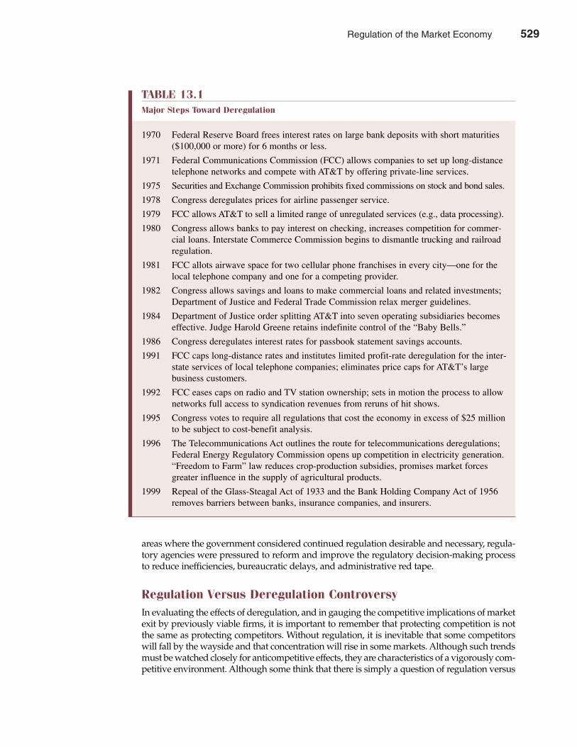
areas where the government considered continued regulation desirable and necessary, regula-tory agencies were pressured to reform and improve the regulatory decision-making processto reduce inefficiencies, bureaucratic delays, and administrative red tape.
Regulation Versus Deregulation ControversyIn evaluating the effects of deregulation, and in gauging the competitive implications of marketexit by previously viable firms, it is important to remember that protecting competition is notthe same as protecting competitors. Without regulation, it is inevitable that some competitorswill fall by the wayside and that concentration will rise in some markets. Although such trendsmust be watched closely for anticompetitive effects, they are characteristics of a vigorously com-petitive environment. Although some think that there is simply a question of regulation versus
530 Part Five Long-Term Investment Decisions
TABLE 13.1Major Steps Toward Deregulation
1970 Federal Reserve Board frees interest rates on large bank deposits with short maturities($100,000 or more) for 6 months or less.
1971 Federal Communications Commission (FCC) allows companies to set up long-distancetelephone networks and compete with AT&T by offering private-line services.
1975 Securities and Exchange Commission prohibits fixed commissions on stock and bond sales.
1978 Congress deregulates prices for airline passenger service.
1979 FCC allows AT&T to sell a limited range of unregulated services (e.g., data processing).
1980 Congress allows banks to pay interest on checking, increases competition for commer-cial loans. Interstate Commerce Commission begins to dismantle trucking and railroadregulation.
1981 FCC allots airwave space for two cellular phone franchises in every city—one for thelocal telephone company and one for a competing provider.
1982 Congress allows savings and loans to make commercial loans and related investments;Department of Justice and Federal Trade Commission relax merger guidelines.
1984 Department of Justice order splitting AT&T into seven operating subsidiaries becomeseffective. Judge Harold Greene retains indefinite control of the “Baby Bells.”
1986 Congress deregulates interest rates for passbook statement savings accounts.
1991 FCC caps long-distance rates and institutes limited profit-rate deregulation for the inter-state services of local telephone companies; eliminates price caps for AT&T’s largebusiness customers.
1992 FCC eases caps on radio and TV station ownership; sets in motion the process to allownetworks full access to syndication revenues from reruns of hit shows.
1995 Congress votes to require all regulations that cost the economy in excess of $25 millionto be subject to cost-benefit analysis.
1996 The Telecommunications Act outlines the route for telecommunications deregulations;Federal Energy Regulatory Commission opens up competition in electricity generation.“Freedom to Farm” law reduces crop-production subsidies, promises market forcesgreater influence in the supply of agricultural products.
1999 Repeal of the Glass-Steagal Act of 1933 and the Bank Holding Company Act of 1956removes barriers between banks, insurance companies, and insurers.
Regulation of the Market Economy 529
deregulation, this is seldom the case. On grounds of economic and political feasibility, it is oftenmost fruitful to consider approaches to improving existing methods of regulation.
An important problem with regulation is that regulators seldom have the information orexpertise to specify, for example, the correct level of utility investment, minimum transporta-tion costs, or the optimum method of pollution control. Because technology changes rapidly inmost regulated industries, only industry personnel working at the frontier of current technolo-gy have such specialized knowledge. One method for dealing with this technical expertiseproblem is to have regulators focus on the preferred outcomes of regulatory processes, ratherthan on the technical means that industry adopts to achieve those ends. The FCC’s decision toadopt downward-adjusting price caps for long-distance telephone service is an example of thisdeveloping trend toward incentive-based regulation. If providers of long-distance telephoneservice are able to reduce costs faster than the FCC-mandated decline in prices, they will enjoyan increase in profitability. By setting price caps that fall over time, the FCC ensures that con-sumers share in expected cost savings while companies enjoy a positive incentive to innovate.This approach to regulation focuses on the objectives of regulation while allowing industry tomeet those goals in new and unique ways. Tying regulator rewards and regulated industryprofits to objective, output-oriented performance criteria has the potential to create a desirablewin/win situation for regulators, utilities, and the general public. For example, the public hasa real interest in safe, reliable, and low-cost electric power. State and federal regulators whooversee the operations of utilities could develop objective standards for measuring utility safe-ty, reliability, and cost efficiency. Tying firm profit rates to such performance-oriented criteriacould stimulate real improvements in utility and regulator performance.
REGULATORY REFORM FOR THE NEW MILLENNIUM
Competitive forces provide a persistent and socially desirable constraining influence on firmbehavior. When vigorous competition is absent, government regulation can be justified throughboth efficiency and equity criteria. When regulation is warranted, business, government, andthe public must work together to ensure that regulatory processes represent the public interest.The unnecessary costs of antiquated regulations dictate that regulatory reform is likely to remaina significant social concern.
Promoting Competition in Electric Power GenerationThe electric power industry comprises three different components: the generation of electricpower, the transmission of electric power from generators to local utilities, and the distributionof electricity by local utilities to commercial and residential customers. All three segments ofthe industry are currently subject to some state and federal regulation. Competition has gen-erally been regarded as unlikely in the transmission and local distribution of electricity, giventheir natural monopoly characteristics. However, competition has emerged in the wholesalegeneration of electric power, and regulators now face the question of how to foster and encour-age such competition.
The ability to buy and sell electric power permits utilities to efficiently employ existingcapacity. By buying power from unregulated sources, utilities can meet peak-load demands onhot days or during winter storms and avoid the need to invest in additional production facil-ities. When utilities purchase power from others, the Federal Power Act of 1935 requires theFederal Energy Regulatory Commission (FERC) to ensure that prices charged on interstatesales are “just and reasonable” in light of necessary costs. With the emergence of competitionin the electric power generation market, however, the need for FERC regulation of all interstatesales on a cost-of-service basis has diminished.
incentive-basedregulationRules that benefit consumers throughenhanced efficiency
regulatory reformImprovement in gov-ernment control toenhance efficiency andfairness
Chapter Thirteen Regulation of the Market Economy 531
530 Regulation of the Market Economy
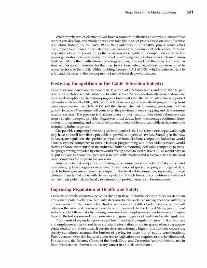
When purchasers of electric power have a number of alternative sources, a competitivemarket can develop, and market prices can take the place of prices based on cost-of-serviceregulation. Indeed, by the early 1990s, the availability of alternative power sources hadencouraged more than a dozen states to use competitive procurement policies for intrastateacquisition of electric power, rather than cost-of-service regulation. Competition in the electricpower generation industry can be promoted by allowing local utilities access to transmissionfacilities that link them with alternative energy sources, provided that the owners of transmis-sion facilities are compensated for their use. In addition, federal legislation may be required torepeal sections of the Public Utility Holding Company Act of 1935, which creates barriers toentry and obstacles to the development of new wholesale power sources.
Fostering Competition in the Cable Television IndustryCable television is available to more than 90 percent of U.S. households, and more than 60 per-cent of all such households subscribe to cable service. Services historically provided includeimproved reception for television programs broadcast over the air on advertiser-supportednetworks such as CBS, NBC, ABC, and the FOX network, and specialized programming fromcable networks such as CNN, MTV, and the Disney Channel. In coming years, much of thegrowth in cable TV revenues will come from the provision of new shopping and data commu-nication services. The problem is that consumers in most communities receive these servicesfrom a single monopoly provider. Regulators must decide how to encourage continued inno-vation in programming and in the development of new cable services, while at the same timerestraining industry prices.
One possible competitor for existing cable companies is the local telephone company, althoughthey have to install new fiber-optic cable to provide competitive services. Standing in the way,however, are regulations that prohibit competition from telephone companies. Rules that wouldallow telephone companies to carry television programming and other video services wouldclearly enhance competition in the industry. Similarly, requiring local cable companies to trans-mit programming provided by others would free up access to local markets. Rules would have tobe put in place to guarantee open access to local cable markets and reasonable fees to the localcable companies for program transmission.
Another potential competitor for existing cable companies is provided by “sky cable” andnew emerging technologies for over-the-air transmission of specialized programming and data.Such technologies are an effective competitor for local cable companies, especially in largecities and residential areas with dense population. If such forms of competition are allowedto meet their potential, the local cable monopoly problem may soon become moot.
Improving Regulation of Health and SafetyDecisions to smoke cigarettes, go scuba diving in Baja, California, or ride a roller coaster at anamusement park involve risk. Similarly, decisions to take a job as a management consultant, asan ironworker in the construction trades, or as a commodities broker involve a trade-offbetween the risks and perceived benefits of employment. In the United States, governmentseeks to control these risks by offering consumers and employees redress for wrongful injurythrough the tort system and by an extensive and growing policy of health and safety regulation.
Proponents of expanded government health and safety regulation assert that consumersand employees either do not have sufficient information or are incapable of making appro-priate decisions in these areas. If certain risks are extremely high or prohibitively expensive,society sometimes assumes the burden of paying for them out of equity considerations.Public concern over risk has also given rise to legislation that requires risk to be eliminated.For example, the Delaney Clause of the Food, Drug, and Cosmetics Act prohibits the use infood of substances shown to cause any cancer in animals or humans.
532 Part Five Long-Term Investment Decisions
Regulation of the Market Economy 531
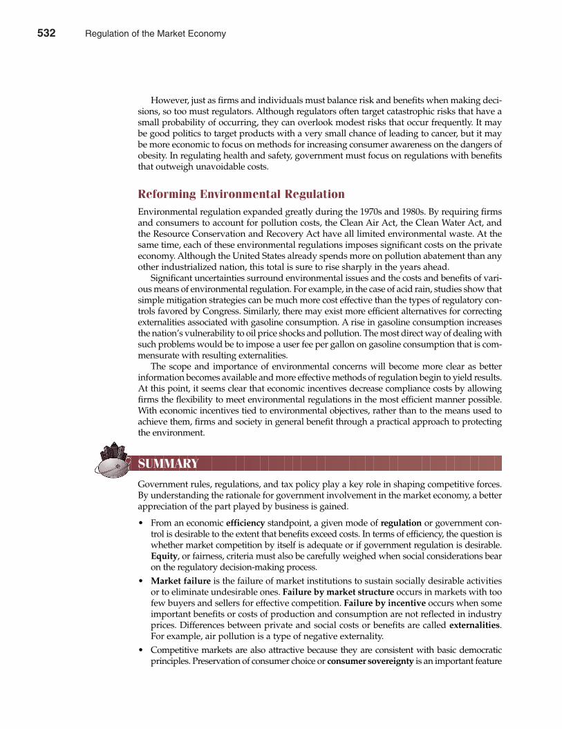
However, just as firms and individuals must balance risk and benefits when making deci-sions, so too must regulators. Although regulators often target catastrophic risks that have asmall probability of occurring, they can overlook modest risks that occur frequently. It maybe good politics to target products with a very small chance of leading to cancer, but it maybe more economic to focus on methods for increasing consumer awareness on the dangers ofobesity. In regulating health and safety, government must focus on regulations with benefitsthat outweigh unavoidable costs.
Reforming Environmental RegulationEnvironmental regulation expanded greatly during the 1970s and 1980s. By requiring firmsand consumers to account for pollution costs, the Clean Air Act, the Clean Water Act, andthe Resource Conservation and Recovery Act have all limited environmental waste. At thesame time, each of these environmental regulations imposes significant costs on the privateeconomy. Although the United States already spends more on pollution abatement than anyother industrialized nation, this total is sure to rise sharply in the years ahead.
Significant uncertainties surround environmental issues and the costs and benefits of vari-ous means of environmental regulation. For example, in the case of acid rain, studies show thatsimple mitigation strategies can be much more cost effective than the types of regulatory con-trols favored by Congress. Similarly, there may exist more efficient alternatives for correctingexternalities associated with gasoline consumption. A rise in gasoline consumption increasesthe nation’s vulnerability to oil price shocks and pollution. The most direct way of dealing withsuch problems would be to impose a user fee per gallon on gasoline consumption that is com-mensurate with resulting externalities.
The scope and importance of environmental concerns will become more clear as betterinformation becomes available and more effective methods of regulation begin to yield results.At this point, it seems clear that economic incentives decrease compliance costs by allowingfirms the flexibility to meet environmental regulations in the most efficient manner possible.With economic incentives tied to environmental objectives, rather than to the means used toachieve them, firms and society in general benefit through a practical approach to protectingthe environment.
SUMMARY
Government rules, regulations, and tax policy play a key role in shaping competitive forces.By understanding the rationale for government involvement in the market economy, a betterappreciation of the part played by business is gained.
• From an economic efficiency standpoint, a given mode of regulation or government con-trol is desirable to the extent that benefits exceed costs. In terms of efficiency, the question iswhether market competition by itself is adequate or if government regulation is desirable.Equity, or fairness, criteria must also be carefully weighed when social considerations bearon the regulatory decision-making process.
• Market failure is the failure of market institutions to sustain socially desirable activitiesor to eliminate undesirable ones. Failure by market structure occurs in markets with toofew buyers and sellers for effective competition. Failure by incentive occurs when someimportant benefits or costs of production and consumption are not reflected in industryprices. Differences between private and social costs or benefits are called externalities.For example, air pollution is a type of negative externality.
• Competitive markets are also attractive because they are consistent with basic democraticprinciples. Preservation of consumer choice or consumer sovereignty is an important feature
Chapter Thirteen Regulation of the Market Economy 533
532 Regulation of the Market Economy
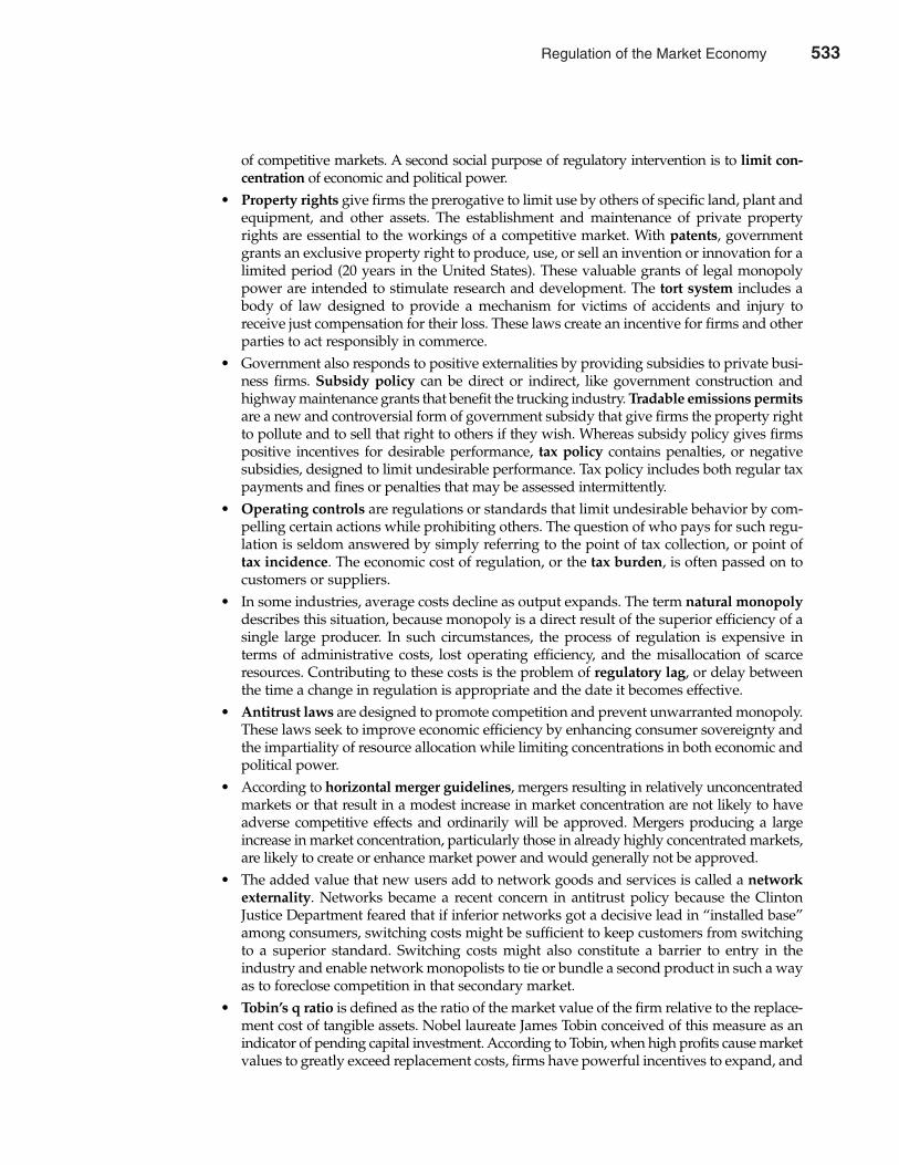
of competitive markets. A second social purpose of regulatory intervention is to limit con-centration of economic and political power.
• Property rights give firms the prerogative to limit use by others of specific land, plant andequipment, and other assets. The establishment and maintenance of private propertyrights are essential to the workings of a competitive market. With patents, governmentgrants an exclusive property right to produce, use, or sell an invention or innovation for alimited period (20 years in the United States). These valuable grants of legal monopolypower are intended to stimulate research and development. The tort system includes abody of law designed to provide a mechanism for victims of accidents and injury toreceive just compensation for their loss. These laws create an incentive for firms and otherparties to act responsibly in commerce.
• Government also responds to positive externalities by providing subsidies to private busi-ness firms. Subsidy policy can be direct or indirect, like government construction andhighway maintenance grants that benefit the trucking industry. Tradable emissions permitsare a new and controversial form of government subsidy that give firms the property rightto pollute and to sell that right to others if they wish. Whereas subsidy policy gives firmspositive incentives for desirable performance, tax policy contains penalties, or negativesubsidies, designed to limit undesirable performance. Tax policy includes both regular taxpayments and fines or penalties that may be assessed intermittently.
• Operating controls are regulations or standards that limit undesirable behavior by com-pelling certain actions while prohibiting others. The question of who pays for such regu-lation is seldom answered by simply referring to the point of tax collection, or point oftax incidence. The economic cost of regulation, or the tax burden, is often passed on tocustomers or suppliers.
• In some industries, average costs decline as output expands. The term natural monopolydescribes this situation, because monopoly is a direct result of the superior efficiency of asingle large producer. In such circumstances, the process of regulation is expensive interms of administrative costs, lost operating efficiency, and the misallocation of scarceresources. Contributing to these costs is the problem of regulatory lag, or delay betweenthe time a change in regulation is appropriate and the date it becomes effective.
• Antitrust laws are designed to promote competition and prevent unwarranted monopoly.These laws seek to improve economic efficiency by enhancing consumer sovereignty andthe impartiality of resource allocation while limiting concentrations in both economic andpolitical power.
• According to horizontal merger guidelines, mergers resulting in relatively unconcentratedmarkets or that result in a modest increase in market concentration are not likely to haveadverse competitive effects and ordinarily will be approved. Mergers producing a largeincrease in market concentration, particularly those in already highly concentrated markets,are likely to create or enhance market power and would generally not be approved.
• The added value that new users add to network goods and services is called a networkexternality. Networks became a recent concern in antitrust policy because the ClintonJustice Department feared that if inferior networks got a decisive lead in “installed base”among consumers, switching costs might be sufficient to keep customers from switchingto a superior standard. Switching costs might also constitute a barrier to entry in theindustry and enable network monopolists to tie or bundle a second product in such a wayas to foreclose competition in that secondary market.
• Tobin’s q ratio is defined as the ratio of the market value of the firm relative to the replace-ment cost of tangible assets. Nobel laureate James Tobin conceived of this measure as anindicator of pending capital investment. According to Tobin, when high profits cause marketvalues to greatly exceed replacement costs, firms have powerful incentives to expand, and
534 Part Five Long-Term Investment Decisions
Regulation of the Market Economy 533
capital investment should boom. Conversely, when low profits cause market values to fallbelow replacement costs, firms will shrink, and capital investment can be expected to wither.More recently, economists have used Tobin’s q ratio as an indicator of above-normal ormonopoly profits. However, given the growing importance of intangible capital in our econ-omy, it becomes misleading to infer a simple increase in monopoly profits following anincrease in Tobin’s q over time.
• The capture theory of economic regulation says that the power of the state to prohibit orcompel and to take or give money is often manipulated to selectively help or hurt a vastnumber of industries. Because of this, regulation may be actively sought by an industry.Capture theory contrasts sharply with the more traditional public interest theory viewof regulation as a government-imposed means of private-market control.
• State and federal regulators have begun to address the high costs of regulation throughnew methods of incentive-based regulation, whereby both companies and their customersbenefit through enhanced efficiency.
• In recognition that the regulatory process can sometimes harm rather than help consumerinterests, a deregulation movement has sprung up and has grown to impressive dimen-sions. Similarly, the unnecessary costs of other forms of regulation dictate that regulatoryreform is likely to remain a significant social concern.
Government regulation of the market economy is a natural by-product of public concern thatunrestricted market competition has the potential to harm economic performance. As thebenefits and costs of government/business interaction become better understood, the poten-tial grows for a more constructive approach to government regulation.
QUESTIONS
Q13.1 Define the term market failure and cite some causes. Also, cite some examples of market failure.Q13.2 What role does the price elasticity of demand play in determining the short-run effects of
regulations that increase fixed costs? What if they lead to increased variable costs?Q13.3 Given the difficulties encountered with utility regulation, it has been suggested that nation-
alization might lead to a more socially optimal allocation of resources. Do you agree? Whyor why not?
Q13.4 Antitrust statutes in the United States have been used to attack monopolization by big busi-ness. Does labor monopolization by giant unions have the same potential for the misallocationof economic resources?
Q13.5 When will an increase in the minimum wage increase employment income for unskilledlaborers? When will it cause this income to fall? Based on your experience, which is morelikely?
Q13.6 Explain why state tax rates on personal income vary more on a state-by-state basis than docorresponding tax rates on corporate income.
Q13.7 Do the U.S. antitrust statutes protect competition or competitors? What is the difference?Q13.8 Define price discrimination. When is it legal? When is it illegal? Cite some common examples
of price discrimination.Q13.9 Is the deregulation movement consistent or inconsistent with the capture theory of economic
regulation?Q13.10 “Regulation is often proposed on the basis of equity considerations and opposed on the basis
of efficiency considerations. As a result, the regulation versus deregulation controversy is noteasily resolved.” Discuss this statement.
Chapter Thirteen Regulation of the Market Economy 535
534 Regulation of the Market Economy
SELF-TEST PROBLEMS AND SOLUTIONS
ST13.1 During each 24-hour period, coal-fired electricity-generating plants emit substantial amountsof sulfur dioxide and particulate pollution into the atmosphere. Concerned citizens are appalledat the aesthetic and environmental implications of such pollution, as well as the potential healthhazard to the local population.
In analyzing remedies to the current situation, three general methods used to control pol-lution are generally considered:
• Regulations—licenses, permits, compulsory standards, and so on.• Payments—various types of government aid to help companies install pollution-control
equipment. Aid can take the form of forgiven local property taxes, income tax credits, specialaccelerated depreciation allowances for pollution-control equipment, low-cost governmentloans, and so on.
• Charges—excise taxes on polluting fuels (e.g., coal or oil), pollution discharge taxes, andother taxes.
Answer the following questions in light of these alternative methods of pollution control.A. Pollution is a negative production externality and an example of market failure. Why do
markets fail?B. What is the incentive provided to polluters under each method of pollution control?C. Who pays for a clean environment under each form of control?D. On the basis of both efficiency and equity considerations, which form of pollution control
is most attractive?ST13.1 Solution
A. Market failure sometimes occurs because the number of buyers and sellers is too small toensure vigorous competition. Small numbers of sellers are sometimes caused by economiesof scale in production, distribution, or marketing; barriers to entry caused by high capital,skilled labor, or other input requirement; or government-imposed barriers due to franchisegrants, rules, or regulations.
Market failure can also occur if some of the costs or benefits of production or consump-tion are not reflected in market prices. Air, water, and noise pollution that emits from anindustrial facility represent a cost of production that is imposed on society in general.Without appropriate charges for such pollution, producers, suppliers, and customers receivean implicit subsidy from the public at large. By failing to pay such environmental costs, theyavoid paying the full cost of production and consumption. In general, if some product ben-efit (cost) is not reflected in firm revenues (costs), then suboptimal production quantities andoutput prices will result and provide both firms and their customers improper economicincentives.
B. Each alternative method of pollution control provides producers with a different set ofincentives. With rules and regulations, producers often have an incentive to litigate or oth-erwise petition to be made a “special case” and thereby avoid regulatory costs. Rules andregulations are also sometimes difficult to monitor and enforce given the problems ofdetermining legislative intent and regulated firm compliance. With a scheme of paymentsto reduce the flow of pollution, polluters have positive incentives to reduce emissions andimprove economic performance. A benefit of this approach is that firms often respond bet-ter to the “carrot” of promised rewards than to the “stick” of threatened penalties. Undera pollution control method of fines or dollar penalties for noncompliance, firms have aneconomic incentive to reduce pollution in order to avoid charges. However, this methodof forcing compliance is sometimes regarded as coercive and met with resistance.
536 Part Five Long-Term Investment Decisions
Regulation of the Market Economy 535
C. When polluters are forced to respond to rules and regulations, the company, customers,employees, and stockholders are all faced with the prospect of paying the costs of pollu-tion reduction. The incidence of pollution cleanup costs depends on the elasticity ofdemand for the firm’s products and on the elasticity of supply. When product demand ishighly inelastic, customers have no good substitutes for the products of the pollutingfirm and therefore must ultimately pay the costs of cleanup. When product demand ishighly elastic, customers are able to avoid the costs of pollution reduction by transferringtheir business to other providers who need not charge for such expenses. In such cir-cumstances, the firm, suppliers, employees, and stockholders bear the costs of pollutionreduction. This situation is very similar to that faced by firms subject to pollution charges.In both instances, society’s right to a clean environment is implied.
A system of payments to encourage pollution reduction contrasts in fundamental wayswith rules and regulations and pollution charges and taxes. This method of pollution reduc-tion is obviously attractive to polluters in that it is free and voluntary, rather than compul-sory. It even provides a profit-making opportunity in pollution reduction that increasesaccording to the scope of pollution. Moreover, when society pays a firm to reduce the levelof its own pollution, the company’s right to pollute is implicitly recognized.
D. Efficiency considerations typically favor payments and charges over rules and regulationsas the more efficient methods of pollution control. From an efficiency standpoint, pollutioncharges are especially attractive in that they recognize pollution as a sometimes necessarycost of doing business, and they force cleanup costs to be borne by those who benefit mostdirectly.
However, equity considerations make the choice among pollution control methods lesscertain. The regulatory process is attractive from an equity standpoint in that it ensures dueprocess (a day in court) for the polluter. All parties are also treated equitably in the sense thatall polluters are equal before the law. Payments for pollution reduction are sometimes favoredon an equity basis in that it avoids penalizing polluters with “sunk” investment costs andemployees that work in older production facilities that face new domestic and foreign com-petitors. Pollution charges are often favored on an equity basis in that it forces a close linkbetween prices and full economic costs. Pollution charges, like payments for pollution reduc-tion, are sometimes criticized as favoring large companies versus their smaller competitors.
Therefore, there is no single “best” method of pollution regulation. All are employedbecause each has the ability to meet efficiency and equity criteria in specific circumstances.
ST13.2 Pollution Control Costs. Anthony Soprano is head of Satriale Pork Producers, Inc., afamily-run pork producer with a hog-processing facility in Musconetcong, New Jersey. Eachhog processed yields both pork and a render by-product in a fixed 1:1 ratio. Although theby-product is unfit for human consumption, some can be sold to a local pet food companyfor further processing. Relevant annual demand and cost relations are as follows:
PP = $110 – $0.00005QP(Demand for pork)
MRP = ∆TRP/∆QP = $110 – $0.0001QP(Marginal revenue from pork)
PB = $10 – $0.0001QB(Demand for render by-product)
MRB = ∆TRB/∆QB = $10 – $0.0002QB(Marginal revenue from render by-product)
TC = $10,000,000 + $60Q(Total cost)
MC = ∆TC/∆Q = $60(Marginal cost)
Chapter Thirteen Regulation of the Market Economy 537
536 Regulation of the Market Economy
Here, P is price in dollars, Q is the number of hogs processed (with an average weight of 100pounds), and QP and QB are pork and render by-product per hog, respectively; both totaland marginal costs are in dollars. Total costs include a risk-adjusted normal return of 15% ona $50 million investment in plant and equipment.
Currently, the city allows the company to dump excess by-product into its sewage treatmentfacility at no charge, viewing the service as an attractive means of keeping a valued employerin the area. However, the sewage treatment facility is quickly approaching peak capacity andmust be expanded at an expected operating cost of $3 million per year. This is an impossibleburden on an already strained city budget.A. Calculate the profit-maximizing price/output combination and optimal total profit level for
Satriale.B. How much by-product will the company dump into the Musconetcong sewage treatment
facility at the profit-maximizing activity level?C. Calculate output and total profits if the city imposes a $35 per unit charge on the amount of
by-product Satriale dumps.D. Calculate output and total profits if the city imposes a fixed $3-million-per-year tax on Satriale
to pay for the sewage treatment facility expansion.E. Will either tax alternative permit Satriale to survive in the long run? In your opinion,
what should the city of Musconetcong do about its sewage treatment problem?ST13.2 Solution
A. Solution to this problem requires that one look at several production and sales optionsavailable to the firm. One option is to produce and sell equal quantities of pork (P) and by-product (B). In this case, the firm sets relevant MC = MR.
MC = MRP + MRB = MR
$60 = $110 – $0.0001Q + $10 – $0.0002Q
0.0003Q = 60Q = 200,000 hogs
Thus, the profit-maximizing output level for production and sale of equal quantities of Pand B would be 200,000 hogs. However, the marginal revenues of both products must bepositive at this sales level for this to be an optimal activity level.
Evaluated at 200,000 hogs:
MRP = $110 – $0.0001(200,000)= $90
MRB = $10 – $0.0002(200,000)= –$30
Because the marginal revenue for B is negative, and Satriale can costlessly dump excessproduction, the sale of 200,000 units of B is suboptimal. This invalidates the entire solutiondeveloped previously because output of P is being held down by the negative marginalrevenue associated with B. The problem must be set up to recognize that Satriale will stopselling B at the point where its marginal revenue becomes zero because, given productionfor P, the marginal cost of B is zero.
Set:
MRB = MCB
$10 – $0.0002QB = $0
538 Part Five Long-Term Investment Decisions
Regulation of the Market Economy 537
0.0002QB = 10QB = 50,000 units
Thus, 50,000 units of B are the maximum that would be sold. Any excess units will bedumped into the city’s sewage treatment facility. The price for B at 50,000 units is
PB = $10 – $0.0001QB
= 10 – 0.0001(50,000)= $5
To determine the optimal production of P (pork), set the marginal revenue of P equal to themarginal cost of hog processing because pork production is the only motive for processingmore than 50,000 units:
MRP = MCP = MCQ
$110 – $0.0001QP = $600.0001QP = 50
QP = 500,000 units(Remember (QP = Q)
and
PP = $110 – $0.00005QP
= 110 – 0.00005(500,000)= $85
Excess profits at the optimal activity level for Satriale are
Excess profits = π = TRP + TRB – TC
= PP � QP + PB � QB – TCQ
= $85(500,000) + $5(50,000) – $10,000,000 – $60(500,000)= $2,750,000
Because total costs include a normal return of 15% on $50 million in investment,
Total profits = Required return + Excess profits= 0.15($50,000,000) + $2,750,000= $10,250,000
B. With 500,000 hogs being processed, but only 50,000 units of B sold, dumping of B is
Units B dumped = Units produced – Units sold= 500,000 – 50,000= 450,000 units
C. In part A, it is shown that if all P and B produced is sold, an activity level of Q = 200,000results in MRB = –$30. A dumping charge of $35 per unit of B will cause Satriale to preferto sell the last unit of B produced (and lose $30) rather than pay a $35 fine. Therefore, this
Chapter Thirteen Regulation of the Market Economy 539
538 Regulation of the Market Economy
fine, as does any fine greater than $30, will eliminate dumping and cause Satriale to reduceprocessing to 200,000 hogs per year. This fine structure would undoubtedly reduce oreliminate the need for a new sewage treatment facility.
Although eliminating dumping is obviously attractive in the sense of reducing sewagetreatment costs, the $35 fine has the unfortunate consequence of cutting output substan-tially. Pork prices rise to PP = $110 – $0.00005(200,000) = $100, and by-product prices fall toPB = $10 – $0.0001(200,000) = –$10. This means Satriale will pay the pet food company $10per unit to accept all of its by-product sludge. Employment will undoubtedly fall as well.In addition to these obvious short-run effects, long-run implications may be especiallyserious. At Q = 200,000, Satriale’s excess profits are
Excess profits = TRP + TRB – TC
= $110Q – $0.00005Q2 + $10Q – $0.0001Q2 – $10,000,000 – $60Q
= $110(200,000) – $0.00005(200,0002) + $10(200,000)– $0.0001(200,0002) – $10,000,000 – $60(200,000)
= –$4,000,000 (a loss)
This means that total profits are
Total profits = Required return + Excess profits= 0.15($50,000,000) + (–$4,000,000)= $3,500,000
This level of profit is insufficient to maintain investment. Although a $35 dumping chargewill eliminate dumping, it is likely to cause the firm to close down or move to some otherlocation. The effect on employment in Musconetcong could be disastrous.
D. In the short run, a $3 million tax on Satriale has no effect on dumping, output, or employ-ment. At the Q = 500,000 activity level, a $3 million tax would reduce Satriale’s total profitsto $7,250,000, or $250,000 below the required return on investment. However, followingimposition of a $3 million tax, the firm’s survival and total employment would be imperiledin the long run.
E. No. Satriale is not able to bear the burden of either tax alternative. Obviously, there is nosingle best alternative here. The highest fixed tax the company can bear in the long run is$2.75 million, the full amount of excess profits. If the city places an extremely high priorityon maintaining employment, perhaps a $2.75 million tax on Satriale plus $250,000 in gen-eral city tax revenues could be used to pay for the new sewage system treatment facility.
PROBLEMS
P13.1 Costs of Regulation. People of many different age groups and circumstances take advantageof part-time employment opportunities provided by the fast-food industry. Given the widevariety of different fast-food vendors, the industry is fiercely competitive, as is the so-calledunskilled labor market. In each of the following circumstances, indicate whether the proposedchanges in government policy are likely to have an increasing, a decreasing, or an uncertaineffect on employment opportunities in this industry.A. Elimination of minimum wage law coverage for those working less than 20 hours per weekB. An increase in spending for education that raises basic worker skillsC. An increase in the employer portion of federally mandated FICA insurance costsD. A requirement that employers install expensive new worker-safety equipment
540 Part Five Long-Term Investment Decisions
Regulation of the Market Economy 539
E. A state requirement that employers pay 8% of wages to fund a new national health-careprogram
P13.2 Natural Monopoly. On May 12, 2000, the two daily newspapers in Denver, Colorado, filedan application with the U.S. Department of Justice for approval of a joint operating agree-ment. The application was filed by The E.W. Scripps Company, whose subsidiary, the DenverPublishing Company, published the Rocky Mountain News, and the MediaNews Group, Inc.,whose subsidiary, the Denver Post Corporation, published the Denver Post. Under the pro-posed arrangement, printing and commercial operations of both newspapers were to be han-dled by a new entity, the “Denver Newspaper Agency,” owned by the parties in equal shares.This type of joint operating agreement provides for the complete independence of the newsand editorial departments of the two newspapers. The rationale for such an arrangement, asprovided for under the Newspaper Preservation Act, is to preserve multiple independent edi-torial voices in towns and cities too small to support two or more newspapers. The act requiresjoint operating arrangements, such as that proposed by the Denver newspapers, obtain theprior written consent of the Attorney General of the United States in order to qualify for theantitrust exemption provided by the act.
Scripps initiated discussions for a joint operating agreement after determining that the Newswould probably fail without such an arrangement. In their petition to the Justice Department,the newspapers argued that the News had sustained $123 million in net operating losses whilethe financially stronger Post had reaped $200 million in profits during the 1990s. This was acrucial point in favor of the joint operating agreement application because the attorney generalmust find that one of the publications is a failing newspaper and that approval of thearrangement is necessary to maintain the independent editorial content of both newspapers.Like any business, newspapers cannot survive without a respectable bottom line. In com-menting on the joint operating agreement application, Attorney General Janet Reno notedthat Denver was one of only five major American cities still served by competing daily news-papers. The other four are Boston, Chicago, New York, and Washington, DC. Of course theseother four cities are not comparable in size to Denver; they are much bigger. None of thosefour cities can lay claim to two newspapers that are more or less equally matched and striveafter the same audience.A. Use the natural monopoly concept to explain why there is not a single city in the United
States that still supports two independently owned and evenly matched, high-qualitynewspapers that vie for the same broad base of readership.
B. On Friday January 5, 2001, Attorney General Reno gave the green light to a 50-year jointoperating agreement between News and its longtime rival, the Post. Starting January 22,2001, the publishing operations of the News and the Post were consolidated. At the timethe joint operating agreement was formed, neither news organization would speculateon job losses or advertising and circulation rate increases from the deal. Based upon yourknowledge of natural monopoly, would you predict an increase or decrease in prices fol-lowing establishment of the joint operating agreement? Would you expect newspaperproduction (and employment) to rise or fall? Why?
P13.3 Price Fixing. An antitrust case launched more than a decade ago sent tremors throughout theacademic community. Over the 1989–1991 period, the Department of Justice (DOJ) investigateda number of highly selective private colleges for price fixing. The investigation focused on“overlap group” meetings comprised of about half of the most selective private colleges anduniversities in the United States. The group included 23 colleges, from small liberal arts schoolslike Colby, Vassar, and Middlebury to larger research universities like Princeton and MIT. DOJfound that when students applied to more than one of the 23 institutions, school officials met tocoordinate the exact calculation of such students’ financial need.
Although all of the overlap colleges attempted to use the same need formula, difficult-to-interpret information from students and parents introduced some variation into their actualneed calculations. DOJ alleged that the meetings enabled the colleges to collude on higher
Chapter Thirteen Regulation of the Market Economy 541
540 Regulation of the Market Economy
tuition and to increase their tuition revenue. The colleges defended their meetings, saying thatthey needed coordination to fully cover the needs of students from low-income families.Although colleges want able, needy students to add diversity to their student body, no collegecan afford a disproportionate share of needy students simply because it makes relatively gen-erous need calculations.
Although the colleges denied DOJ’s price-fixing allegation, they discontinued their annualmeetings in 1991.A. How would you determine if the overlap college meetings resulted in price fixing?B. If price fixing did indeed occur at these meetings, which laws might be violated?
P13.4 Tying Contracts. In a celebrated 4-year antitrust case, the Department of Justice chargedMicrosoft Corporation with a wide range of anticompetitive behavior. Among the chargesleveled by the DOJ was the allegation that Microsoft illegally “bundled” the sale of itsMicrosoft Explorer Internet browser software with its basic Windows operating system. DOJalleged that by offering a free browser program, Microsoft was able to extend its operatingsystem monopoly and “substantially lessen competition and tend to create a monopoly” inthe browser market by undercutting rival Netscape Communications, Inc. Microsoft retortedthat it had the right to innovate and broaden the capability of its operating system software overtime. Moreover, Microsoft noted that Netscape distributed its rival Internet browser softwareNetscape Navigator free to customers, and that it was merely meeting the competition byoffering its own free browser program.A. Explain how Microsoft’s bundling of free Internet browser software with its Windows
operating system could violate U.S. antitrust laws, and be sure to mention which laws inparticular might be violated.
B. Who was right in this case? In other words, did Microsoft’s bundling of Microsoft Explorerwith Windows extend its operating system monopoly and “substantially lessen competi-tion and tend to create a monopoly” in the browser market?
P13.5 Horizontal Merger Guidelines. The following table shows premerger market share datafor four hypothetical markets. Assume that the Department of Justice has received a mergerproposal from the third-largest and the fifth-largest competitors in each market. Attorneysfor each firm have petitioned the government for advice as to whether or not their mergerproposal would or would not be acceptable under the horizontal merger guidelines prom-ulgated by the FTC and DOJ.
542 Part Five Long-Term Investment Decisions
Premerger Firm Market Share Data
Competitor Market Market Market MarketRank A B C D
1 40% 25% 10% 50%2 30% 25% 10% 25%3 15% 10% 8% 10%4 10% 10% 8% 10%5 5% 6% 8% 2%6 5% 8% 2%7 5% 8% 1%8 5% 8%9 5% 8%
10 4% 8%11 8%12 8%
Totals 100% 100% 100% 100%
Regulation of the Market Economy 541
A. Calculate the premerger HHI measures for each market and the change in the HHI assum-ing each proposed merger were approved.
B. In each market, indicate whether or not the proposed merger is apt to be approved accord-ing to the horizontal merger guidelines. Why or why not?
P13.6 Costs of Regulation. Hathaway-Ross Instruments, Inc., manufactures an innovative piece ofdiagnostic equipment used in medical laboratories and hospitals. OSHA has determined thatadditional safety precautions are necessary to bring radioactive leakage occurring during use ofthis equipment down to ascceptable levels. Total and marginal production costs, including a nor-mal rate of return on investment but before additional safeguards are installed, are as follows:
TC = $5,000,000 + $5,000Q
MC = ∆TC/∆Q = $5,000
Market demand and marginal revenue relations are the following:
PL = $15,000 – $12.5QL (Medical Laboratory Demand)MRL = ∆TR/∆QL = $15,000 – $25QL
PH = $10,000 – $1QH (Hospital Demand)MRH = ∆TR/∆QH = $10,000 – $2QH
A. Assuming that the company faces two distinct markets, calculate the profit-maximizingprice/output combination in each market and economic profits.
B. Describe the short- and long-run implications of meeting OSHA standards if doing soraises marginal cost by $1,000 per machine.
C. Calculate the point price elasticity at the initial (part A) profit-maximizing activity level ineach market. Are the differential effects on sales in each market that were seen in part Btypical or atypical?
P13.7 Incidence of Regulation Costs. The Smokey Mountain Coal Company sells coal to electricutilities in the southeast. Unfortunately, Smokey’s coal has a high particulate content, and,therefore, the company is adversely affected by state and local regulations governing smokeand dust emissions at its customers’ electricity-generating plants. Smokey’s total and marginalcost relations are
TC = $1,000,000 + $5Q + $0.0001Q2
MC = ∆TC/∆Q = $5 + $0.0002Q
where Q is tons of coal produced per month and TC includes a risk-adjusted normal rate ofreturn on investment.A. Calculate Smokey’s profit at the profit-maximizing activity level if prices in the industry
are stable at $25 per ton and therefore P = MR = $25.B. Calculate Smokey’s optimal price, output, and profit levels if a new state regulation
results in a $5-per-ton cost increase that can be fully passed on to customers.C. Determine the effect on output and profit if Smokey must fully absorb the $5-per-ton cost
increase.P13.8 Cost of Import Tariffs. Topo Gigo Imports, Ltd., located in San Francisco, California, is an
importer and distributor of a leading Japanese–made desktop dry copier. The U.S. CommerceDepartment recently told the company that it will be subject to a new 5.75% tariff on theimport cost of copiers. Topo Gigo is concerned that the tariff will slow its sales, given the high-ly competitive nature of the copier market. Relevant market demand and marginal revenuerelations are as follows:
Chapter Thirteen Regulation of the Market Economy 543
542 Regulation of the Market Economy
P = $13,800 – $0.23Q
MR = ∆TR/∆Q = $13,800 – $0.46Q
Topo Gigo’s marginal cost per copier equals the import cost of $8,000 per unit, plus 15% tocover transportation, insurance, and related selling expenses. In addition to these costs, TopoGigo’s fixed costs, including a normal rate of return, come to $15 million per year.A. Calculate Topo Gigo’s optimal price/output combination and economic profits before
imposition of the tariff.B. Calculate Topo Gigo’s optimal price/output combination and economic profits after
imposition of the tariff.C. Compare your answers to parts A and B. Who pays the economic burden of the import
tariff?P13.9 Utility Regulation. The Woebegone Water Company, a small water utility serving rural cus-
tomers in Minnesota, is currently engaged in a rate case with the regulatory commissionunder whose jurisdiction it operates. At issue is the monthly rate that the company willcharge for unmetered sewer and water service. The demand curve for monthly service is P =$40 – $0.01Q. This implies annual demand and marginal revenue curves of
P = $480 – $0.12Q
MR = ∆TR/∆Q = $480 – $0.24Q
where P is service price in dollars and Q is the number of customers served. Total and mar-ginal costs per year (before investment return) are described by the following function:
TC = $70,000 + $80Q + $0.005Q2
MC = ∆TC/∆Q = $80 + $0.01Q
The company has assets of $2 million and the utility commission has authorized an 11.5%return on investment.A. Calculate Woebegone’s profit-maximizing price (monthly and annually), output, and rate-
of-return levels.B. Woebegone has requested a monthly price of $22. Calculate Woebegone’s output and total
return on investment if the request were to be granted. Why are these values different fromthose calculated in part A?
C. What monthly price should the commission grant to limit Woebegone to an 11.5% rate ofreturn?
P13.10 Costs of Regulation. The Klamath Paper Company produces corrugated boxes for industrialpackaging at a plant located in Klamath Falls, Oregon. For each ton of packaging materialsproduced, 100 gallons of waste-water pollutant is dumped into the Klamath River. Klamath’srevenue and manufacturing cost relations for corrugated boxes are
TR = $6,000Q – $0.15Q2
MR = ∆TR/∆Q = $6,000 – $0.3Q
TC = $18,000,000 + $2,000Q + $0.05Q2
MC = ∆TC/∆Q = $2,000 + $0.1Q
Both price and total manufacturing cost (which includes capital costs) are in dollars, and Q is intons of output. The Oregon Department of Natural Resources (DNR) is considering various pol-
544 Part Five Long-Term Investment Decisions
Regulation of the Market Economy 543
lution tax schemes designed to provide funding for clean-up operations as well as reduceKlamath’s waste-water pollution. The DNR has determined that discharges into the river mustbe cut to meet new federal water-quality guidelines. Alternatively, the Klamath Water Districtwater-treatment facility could be expanded to deal with water-treatment needs at a public costof $2.5 million per year—costs that must be met through pollution charges, other taxes, or both.A. Calculate Klamath’s optimal output, price, discharge, and profit levels based on the assump-
tion of no pollution taxes nor disposal costs.B. Calculate these same levels if a $2-per-gallon waste-water disposal charge is imposed on
the company.C. If Klamath is required to recycle all waste water, Klamath calculates total recycling costs
(in dollars) as
TCR = $2W + $0.000005W2
= $2(100Q) – $0.000005(100Q)2
= $200Q + $0.05Q2
where W is gallons of recycled waste water. This implies a marginal recycling cost per tonof production of
MCR = ∆TCR/∆Q = $200 + $0.1Q
Calculate optimal output, price, discharge, and profit levels in this situation.D. Describe the advantages and disadvantages of the disposal charge and recycling alternatives.
Chapter Thirteen Regulation of the Market Economy 545
CASE STUDY
The Network Television Fin-Syn Regulation ControversyWhen viewers think of FCC regulation of network television, they often think of censorshipor of the FCC controlling the renewal of local broadcast licenses. Although TV censors are thebutt of frequent jokes by David Letterman on CBS’s “Late Show” and Jay Leno on NBC’s“The Tonight Show,” TV censorship in the United States is very mild when compared to thatin many foreign countries, and it has little economic or political impact. Although moreimportant, FCC control over the renewal of local broadcast licenses also has little direct effecton the network broadcasting business.
It might come as a big surprise to many viewers that network television was historicallysubject to heavy economic regulation in terms of what are referred to as financial interest andnetwork syndication rules. These so-called fin-syn rules were adopted in the early 1970s to pre-vent ABC, CBS, and NBC from collectively dominating the broadcast industry. The financialinterest rule long prohibited networks from having an ownership interest in shows producedfor them by others. The network syndication rule barred networks from selling internally pro-duced programs into the domestic syndication or rerun market. Limits on network access tothe rerun market were an important disincentive to network production of new televisionshows. Asingle half-hour episode of prime-time programming can cost several million dollars.Given tremendous costs, few television programs, even popular hit shows like “Seinfeld,”“Drew Carey,” and “The Simpsons,” make money on their initial runs. The big profits comefrom subsequent syndication sales of reruns to network affiliates or independent stations inthe late afternoon or early evening hours.
544 Regulation of the Market Economy
546 Part Five Long-Term Investment Decisions
Fin-syn rules effectively brought about a separation between the production of televisionentertainment programming and broadcasting. With the exception of prime-time sports andnews coverage, which they offered without restriction, the networks used to serve primarilyas distributors of entertainment programs produced by independent Hollywood producers.The networks paid fees for the rights to distribute specific shows. They hoped to make enoughmoney from selling advertising time on their initial run to more than offset fees and earn aprofit. Fin-syn rules were introduced because the FCC was concerned that vertical integration(control of production, distribution, and exhibition) unfairly enhanced the power of the net-works. By taking away long-term rights to programs created by the networks, and severelyrestricting their participation in syndication, the FCC effectively eliminated incentives for thenetworks to produce programs. This effectively separated production from distribution. Thosein favor of fin-syn regulation hoped that the rules would benefit independent television pro-ducers by giving them more autonomy from the networks and allow the producers to benefitfrom the lucrative syndication market. Proponents believed the rules would cultivate morediverse and innovative television content. Another potential advantage was that independenttelevision stations stand to benefit when networks are barred from syndication. If the networksowned the syndication rights to off-network programs, they might “warehouse” their bestprograms, or steer popular reruns to network owned and operated stations.
From the beginning, fin-syn regulation was controversial. Networks felt that fin-syn reg-ulation was unfair and did not solve perceived problems. Some argued that fin-syn rulesundermined the role of independent producers. Small independent producers, for example,often cannot afford to fund expensive new series that often lose money during their initialnetwork run. Hence, fin-syn rules tend to favor large production companies tied to majormovie studios, like Hollywood–based Time-Warner Television. In 1983, swayed by anti-fin-syn arguments and a political climate favoring deregulation, the FCC proposed eliminatingmost of the rules. At that time, a massive lobbying effort by Hollywood production compa-nies defeated the deregulation efforts and kept the rules in place. It was only in the early1990s, and after the combined television audience controlled by the three major networks(ABC, CBS, and NBC) had fallen from 90% to 65%, that change became imminent. An intenselobbying effort pitted major television producers (for fin-syn) against the networks (againstfin-syn). In 1991, the FCC relaxed fin-syn regulation. A federal appeals court relaxed the ruleseven further and effectively eliminated fin-syn regulation altogether by November 1995.
The elimination of fin-syn rules has increased in-house production by the big three networks.By 1992, for example, NBC was the single largest supplier of its own prime-time programming.Production companies have also gotten more involved with distribution. Fox Broadcasting, sup-ported by its direct relationship with a major Hollywood studio, was an early innovator inexpanding from production into the distribution of television programming. Once the rulesagainst combining production with distribution were eliminated, it also became possible for WaltDisney, a major Hollywood studio, to purchase Cap Cities/ABC, one of the three major net-works. Despite obvious benefits, some worries still remain. Independent producers worry thatnetworks will no longer require their services, or show favoritism toward in-house productions.
Briefly explain the following:A. The causes and consequences of regulation according to the public interest theory of reg-
ulationB. The causes and consequences of regulation according to the capture theory of regulationC. How the network television fin-syn deregulation controversy supports or contradicts
each theory
CASE STUDY (continued)
Regulation of the Market Economy 545

SELECTED REFERENCES Arocena, Pablo, and Catherine Waddams Price. “Generating Efficiency: Economic and Environmental
Regulation of Public and Private Electricity Generators in Spain.” International Journal of IndustrialOrganization 20 (January 2002): 41–69.
Banerjee, Ajeyo, and E. Woodrow Eckard. “Why Regulate Insider Trading? Evidence from the FirstGreat Merger Wave (1897–1903).” American Economic Review 91 (December 2001): 1329–1349.
Besley, Timothy, and Maitreesh Ghatak. “Government Versus Private Ownership of Public Goods.”Quarterly Journal of Economics 116 (November 2001): 1343–1372.
Bittlingmayer, George. “Regulatory Uncertainty and Investment: Evidence from Antitrust Enforcement.”Cato Journal 20 (Winter 2001): 295–325.
Coates, Dennis. “The Microeconomics of Market Failures.” Managerial & Decision Economics 22 (September2001): 339–340.
Daines, Robert. “Does Delaware Law Improve Firm Value?” Journal of Financial Economics 62 (December2001): 525–558.
Evenett, Simon. “The Antitrust of Nations.” Harvard International Review 23 (Fall 2001): 76–77.Glaeser, Edward L., and Andrei Shleifer. “A Reason for Quantity Regulation.” American Economic Review
91 (May 2001): 431–435.Hirschey, Mark, Vernon J. Richardson, and Susan Scholz. “Value Relevance of Nonfinancial Information:
The Case of Patent Data.” Review of Quantitative Finance & Accounting 17 (November 2001): 223–235.Minda, Gary. “Antitrust Regulability and the New Digital Economy: A Proposal for Integrating ‘Hard’
and ‘Soft’ Regulation.” Antitrust Bulletin 46 (Fall 2001): 439–511.Nakamura, Masao, Takuya Takahashi, and Ilan Vertinsky. “Why Japanese Firms Choose to Certify: A
Study of Managerial Responses to Environmental Issues.” Journal of Environmental Economics &Management 42 (July 2001): 23–52.
Peoples, Jr., James, and Wayne K. Talley. “Black–White Earnings Differentials: Privatization VersusDeregulation.” American Economic Review 91 (May 2001): 164–168.
Sauer, Raymond D. “The Political Economy of Gambling Regulation.” Managerial & Decision Economics22 (January-May 2001): 5–15.
Sidak, J Gregory. “An Antitrust Rule for Software Integration.” Yale Journal on Regulation 18 (Winter2001): 1.
Weller, Charles D. “Can Japan Compete? Empirical Findings Just in Time for International AntitrustPolicy.” Antitrust Bulletin 46 (Fall 2001): 569–590.
Chapter Thirteen Regulation of the Market Economy 547
546 Regulation of the Market Economy

Risk Analysis
CHAPTER FOURTEEN
548 1 See Daniel A. Greenbaum, “401(k)s Shift Risk to Workers,” The Wall Street Journal Online, March 6, 2002(http://online.wsj.com).
At the dawn of the new millennium, stock-market speculators scrambledto bet their hard-earned money on Amazon.com, Cisco Systems, Yahoo!,
and others poised to take advantage of the Internet. Speculators piled into ahandful of stock-market favorites at unheard of valuations, only to see a sig-nificant chunk of their portfolios vanish as the Internet bubble burst. Within 18months, the S&P 500 crumbled by more than 30 percent and Nasdaq crashedby more than 70 percent. Many dot.com investors lost everything as The WallStreet Journal mused about “the madness of crowds.”
Then, to make a bad situation worse, the terrorist attacks of September 11,2001, on New York City and Washington, DC, sent a shiver through globalfinancial markets that caused a plunge in both consumer confidence and retailsales. Add in a currency crisis emanating from Argentina and other emergingmarkets, and the essential elements fell into place for a sharp economic down-turn in the United States, Europe, and Asia. Against this background, managersfaced a host of vital decisions necessary for shrewd risk management. Will savvyrisk management by public officials and business leaders bring a quick returnto prosperity, or will decision makers stumble and see economic recessionspread around the globe? Time will tell, but stock-market investors were clearlyhedging their bets during early 2002.1
This chapter introduces certainty equivalents, risk-adjusted discount rates,decision trees, simulation, and game theory techniques as practical means fordealing with such questions. They are effective tools for decision making underconditions of risk and uncertainty.
547
14
CONCEPTS OF RISK AND UNCERTAINTY
Let’s face it, risk is a four-letter word. When it comes to investing, managers and other investorsoften prefer not to hear much about the chance of loss. That is why billions of dollars sit in low-yielding certificates of deposit or Treasury securities “backed by the full faith and credit of theU.S. government.” However, although the local bank can guarantee savers that their funds willbe returned intact, it does nothing to protect them from the risk that inflation will reduce thereal value of their assets. To make effective investment decisions, managers must understandthe many faces of risk.
Economic Risk and UncertaintyManagers sometimes know with certainty the outcomes that each possible course of actionwill produce. A firm with $100,000 in cash that can be invested in a 30-day Treasury bill yield-ing 6 percent ($493 interest income for 30 days) or used to prepay a 10 percent bank loan ($822interest expense for 30 days) can determine with certainty that prepayment of the bank loanprovides a $329 higher 1-month return. A retailer can just as easily predict the cost savingsearned by placing a given order directly with the manufacturer versus through an independ-ent wholesaler; manufacturers can often forecast the precise cost effect of meeting a rush orderwhen overtime wages rather than standard labor rates are required. Order backlogs give awide variety of consumer and producer goods manufacturers a clear indication of productdemand conditions. Similarly, book, magazine, and trade journal publishers accurately judgeproduct demand conditions on the basis of subscription revenues. Resort hotels can often fore-tell with a high degree of accuracy the amount of food, beverages, and linen service requiredto meet the daily needs of a 1,500-person convention, especially when such conventions arebooked on a regular basis. Even when events cannot be predicted exactly, only a modest levelof decision uncertainty is present in such situations.
Many other important managerial decisions are made under conditions of risk or uncer-tainty. Economic risk is the chance of loss because all possible outcomes and their probabilityof happening are unknown. Actions taken in such a decision environment are purely specula-tive, such as the buy and sell decisions made by traders and other speculators in commodity,futures, and options markets. All decision makers are equally likely to profit as well as to lose;luck is the sole determinant of success or failure. Uncertainty exists when the outcomes ofmanagerial decisions cannot be predicted with absolute accuracy but all possibilities and theirassociated probabilities are known. Under conditions of uncertainty, informed managerialdecisions are possible. Experience, insight, and prudence allow managers to devise strategiesfor minimizing the chance of failing to meet business objectives. Although luck still plays a rolein determining ultimate success, managers can deal effectively with an uncertain decisionenvironment by limiting the scope of individual projects and developing contingency plans fordealing with failure.
When the level of risk and the attitudes toward risk taking are known, the effects of uncer-tainty can be directly reflected in the basic valuation model of the firm. The certainty equivalentmethod converts expected risky profit streams to their certain sum equivalents to eliminatevalue differences that result from different risk levels. For risk-averse decision makers, thevalue of a risky stream of payments is less than the value of a certain stream, and the appli-cation of certainty equivalent adjustment factors results in a downward adjustment in thevalue of expected returns. For risk-seeking decision makers, the value of a risky stream ofpayments is greater than that of a certain stream, and application of certainty equivalentadjustment factors results in an upward adjustment in the value of expected returns. In bothcases, risky dollars are converted into certain-sum equivalents. Another method used to reflectuncertainty in the basic valuation model is the risk-adjusted discount rate approach. In this tech-nique, the interest rate used in the denominator of the basic valuation model depends on the
economic riskChance of loss due tothe fact that all possibleoutcomes and theirprobability of occur-rence are unknown
uncertaintyWhen the outcomes ofmanagerial decisionscannot be predictedwith absolute accuracybut all possibilities andtheir associated proba-bilities of occurrenceare known
Chapter Fourteen Risk Analysis 549
548 Risk Analysis
level of risk. For highly risk-averse decision makers, higher discount rates are implemented; forless risk-averse decision makers, lower discount rates are employed. Using this technique, dis-counted expected profit streams reflect risk differences and become directly comparable.
General Risk CategoriesBusiness risk is the chance of loss associated with a given managerial decision. Such losses area normal by-product of the unpredictable variation in product demand and cost conditions.Business risk must be dealt with effectively; it seldom can be eliminated.
In a globally competitive environment with instant communication, managers face a widevariety of risks. For managers, a main worry is something called market risk, or the chancethat a portfolio of investments can lose money because of overall swings in the financialmarkets. Managers must be concerned about market risk because it influences the cost andtiming of selling new debt and equity securities to investors. When a bear market ensues,investors are not the only ones to lose. Companies unable to raise funds for new plant andequipment must forego profitable investment opportunities when the cost of financing esca-lates. Inflation risk is the danger that a general increase in the price level will underminethe real economic value of corporate agreements that involve a fixed promise to pay a spec-ified amount over an extended period. Leases, rental agreements, and corporate bonds areall examples of business contracts that can be susceptible to inflation risk. Interest-rate riskis another type of market risk that can severely affect the value of corporate investments andobligations. This stems from the fact that a fall in interest rates will increase the value of anycontract that involves a fixed promise to pay over an extended time frame. Conversely, a risein interest rates will decrease the value of any agreement that involves fixed interest andprincipal payments.
Credit risk is the chance that another party will fail to abide by its contractual obligations.A number of companies have lost substantial sums because other parties were either unableor unwilling to provide raw commodities, rental space, or financing at agreed-upon prices.Like other investors, corporations must also consider the problem of liquidity risk, or thedifficulty of selling corporate assets or investments that are not easily transferable at favor-able prices under typical market conditions. Another type of risk is related to the rapidlyexpanding financial derivatives market. A financial derivative is a security that derives valuefrom price movements in some other security. Derivative risk is the chance that volatilefinancial derivatives such as commodities futures and index options could create losses inunderlying investments by increasing price volatility.
Special Risks of Global OperationsCultural risk is borne by companies that pursue a global investment strategy. Product marketdifferences due to distinctive social customs make it difficult to predict which products mightdo well in foreign markets. For example, breakfast cereal is extremely popular and one of themost profitable industries in the United States, Canada, and the United Kingdom. However, inFrance, Germany, Italy, and many other foreign countries, breakfast cereal is less popular andless profitable. In business terms, breakfast cereal doesn’t “travel” as well as U.S.–made enter-tainment like movies and television programming.
Currency risk is another important danger facing global businesses because most compa-nies wish to eventually repatriate foreign earnings back to the domestic parent. When the U.S.dollar rises in value against foreign currencies such as the Canadian dollar, foreign profitstranslate into fewer U.S. dollars. Conversely, when the U.S. dollar falls in value against theCanadian dollar, profits earned in Canada translate into more U.S. dollars. Because priceswings in the relative value of currencies are unpredictable and can be significant, many multi-
550 Part Five Long-Term Investment Decisions
business riskChance of loss associat-ed with a given mana-gerial decision
market riskChance that a portfolioof investments can losemoney because ofswings in the financialmarkets as a whole
inflation riskDanger that a generalincrease in the pricelevel will underminethe real economic valueof any legal agreementthat involves a fixedpromise to pay over anextended period
interest-rate riskMarket risk that stemsfrom the fact thatchanging interest ratesaffect the value of anyagreement that involvesa fixed promise to payover a specified period
credit riskChance that anotherparty will fail to abide byits contractual obligations
liquidity riskDifficulty of selling cor-porate assets or invest-ments that have only afew willing buyers orare otherwise not easilytransferable at favorableprices under typicalmarket conditions
derivative riskChance that volatilefinancial derivativessuch as commoditiesfutures and indexoptions could createlosses in underlyinginvestments by increas-ing rather than decreas-ing price volatility
cultural riskChance of loss becauseof product market dif-ferences due to distinc-tive social customs
currency riskLoss due to changes inthe domestic-currencyvalue of foreign profits
Risk Analysis 549
national firms hedge against currency price swings using financial derivatives in the foreigncurrency market. This hedging is not only expensive but can be risky during volatile markets.
Global investors also experience government policy risk because foreign governmentgrants of monopoly franchises, tax abatements, and favored trade status can be tenuous. In the“global friendly” 1990s, many corporate investors seem to have forgotten the widespread con-fiscations of private property owned by U.S. corporations in Mexico, Cuba, Libya, the formerSoviet Union, and in a host of other countries. Expropriation risk, or the risk that businessproperty located abroad might be seized by host governments, is a risk that global investorsmust not forget. During every decade of the twentieth century, U.S. and other multinationalcorporations have suffered from expropriation and probably will in the years ahead.
PROBABILITY CONCEPTS
A clear understanding of probability concepts provides a background for discussing variousmethods of effective risk analysis. Marketing directors cannot accurately assess the potentialof new products or pricing strategies without data. Managers cannot make insightful invest-ment decisions without reliable information about risk.
Probability DistributionThe probability of an event is the chance, or odds, that the incident will occur. If all possibleevents or outcomes are listed, and if a probability is assigned to each event, the listing is called aprobability distribution. For example, suppose a sales manager observes that there is a 70 per-cent chance that a given customer will place a specific order versus a 30 percent chance that thecustomer will not. This situation is described by the probability distribution shown in Table 14.1.
government policyriskChance of loss becauseforeign governmentgrants of monopoly fran-chises, tax abatements,and favored trade statuscan be tenuous
expropriation riskDanger that businessproperty located abroadmight be seized by hostgovernments
probabilityChance of occurrence
probability distributionList of possible eventsand probabilities
Chapter Fourteen Risk Analysis 551
Internet Fraud
The Internet allows individuals or companies to com-municate with a large audience without spending a lotof time, effort, or money. Anyone can reach tens ofthousands of people by building an Internet Web site,posting a message on an online bulletin board, enteringa discussion in a live “chat” room, or sending mass e-mails. It is easy for fraud perpetrators to make theirmessages look credible; it is nearly impossible forinvestors to tell the difference between fact and fiction.
Investment frauds seen online mirror frauds perpe-trated over the phone or by mail:
• The “pump and dump” scam. Paid promoters some-times accumulate stock and then leak imaginaryfavorable information to pump up the stock price.After the stock price has risen, fraudulent promotersdump their shares on an unsuspecting public.
• The pyramid. Many Internet frauds are merely elec-tronic versions of the classic “pyramid” scheme inwhich participants attempt to make money solely byrecruiting new participants.
• The “risk-free” fraud. Be wary of opportunitiesthat promise spectacular profits or “guaranteed”returns. If the deal sounds too good to be true, thenit probably is.
• Off-shore frauds. Watch out for off-shore scams andinvestment “opportunities” in other countries. Whenyou send your money abroad and something goeswrong, it is more difficult to find out what happenedand to locate your money.
The Securities and Exchange Commission (SEC) iseffectively tracking Internet investment fraud and hastaken quick action to stop scams. With the cooperationof federal and state criminal authorities, the SEC hasalso helped put Internet fraudsters in jail. If you believeany person or entity may have violated the federalsecurities laws, submit a complaint athttp://www.sec.gov.
See: John Hart and Michael Rothberg, “Anonymous Internet PostingPits Free Speech Against Accountability,” The Wall Street Journal Online,March 6, 2002 (http://online.wsj.com).
M A N A G E R I A L A P P L I C AT I O N 1 4 . 1
550 Risk Analysis
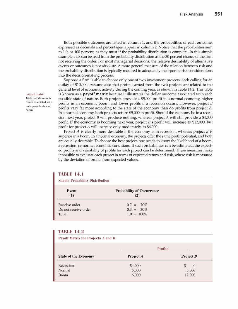
Both possible outcomes are listed in column 1, and the probabilities of each outcome,expressed as decimals and percentages, appear in column 2. Notice that the probabilities sumto 1.0, or 100 percent, as they must if the probability distribution is complete. In this simpleexample, risk can be read from the probability distribution as the 30 percent chance of the firmnot receiving the order. For most managerial decisions, the relative desirability of alternativeevents or outcomes is not absolute. A more general measure of the relation between risk andthe probability distribution is typically required to adequately incorporate risk considerationsinto the decision-making process.
Suppose a firm is able to choose only one of two investment projects, each calling for anoutlay of $10,000. Assume also that profits earned from the two projects are related to thegeneral level of economic activity during the coming year, as shown in Table 14.2. This tableis known as a payoff matrix because it illustrates the dollar outcome associated with eachpossible state of nature. Both projects provide a $5,000 profit in a normal economy, higherprofits in an economic boom, and lower profits if a recession occurs. However, project Bprofits vary far more according to the state of the economy than do profits from project A.In a normal economy, both projects return $5,000 in profit. Should the economy be in a reces-sion next year, project B will produce nothing, whereas project A will still provide a $4,000profit. If the economy is booming next year, project B’s profit will increase to $12,000, butprofit for project A will increase only moderately, to $6,000.
Project A is clearly more desirable if the economy is in recession, whereas project B issuperior in a boom. In a normal economy, the projects offer the same profit potential, and bothare equally desirable. To choose the best project, one needs to know the likelihood of a boom,a recession, or normal economic conditions. If such probabilities can be estimated, the expect-ed profits and variability of profits for each project can be determined. These measures makeit possible to evaluate each project in terms of expected return and risk, where risk is measuredby the deviation of profits from expected values.
552 Part Five Long-Term Investment Decisions
payoff matrixTable that shows out-comes associated witheach possible state ofnature
TABLE 14.1Simple Probability Distribution
Event Probability of Occurrence(1) (2)
Receive order 0.7 = 70%Do not receive order 0.3 = 30%Total 1.0 = 100%
TABLE 14.2Payoff Matrix for Projects A and B
Profits
State of the Economy Project A Project B
Recession $4,000 $ 0Normal 5,000 5,000Boom 6,000 12,000
Risk Analysis 551
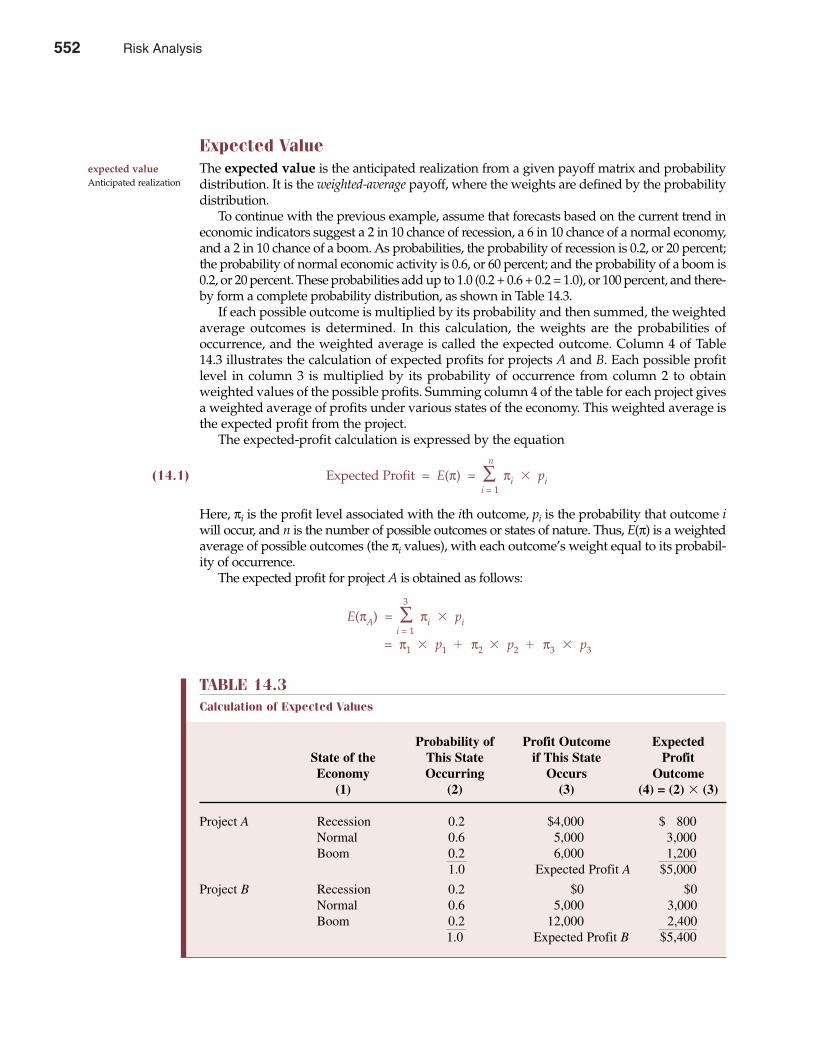
Expected ValueThe expected value is the anticipated realization from a given payoff matrix and probabilitydistribution. It is the weighted-average payoff, where the weights are defined by the probabilitydistribution.
To continue with the previous example, assume that forecasts based on the current trend ineconomic indicators suggest a 2 in 10 chance of recession, a 6 in 10 chance of a normal economy,and a 2 in 10 chance of a boom. As probabilities, the probability of recession is 0.2, or 20 percent;the probability of normal economic activity is 0.6, or 60 percent; and the probability of a boom is0.2, or 20 percent. These probabilities add up to 1.0 (0.2 + 0.6 + 0.2 = 1.0), or 100 percent, and there-by form a complete probability distribution, as shown in Table 14.3.
If each possible outcome is multiplied by its probability and then summed, the weightedaverage outcomes is determined. In this calculation, the weights are the probabilities ofoccurrence, and the weighted average is called the expected outcome. Column 4 of Table14.3 illustrates the calculation of expected profits for projects A and B. Each possible profitlevel in column 3 is multiplied by its probability of occurrence from column 2 to obtainweighted values of the possible profits. Summing column 4 of the table for each project givesa weighted average of profits under various states of the economy. This weighted average isthe expected profit from the project.
The expected-profit calculation is expressed by the equationn
(14.1) Expected Profit = E(π) = ∑ πi � pii = 1
Here, πi is the profit level associated with the ith outcome, pi is the probability that outcome iwill occur, and n is the number of possible outcomes or states of nature. Thus, E(π) is a weightedaverage of possible outcomes (the πi values), with each outcome’s weight equal to its probabil-ity of occurrence.
The expected profit for project A is obtained as follows:
3
E(πA) = ∑ πi � pii = 1
= π1 � p1 � π2 � p2 � π3 � p3
expected valueAnticipated realization
Chapter Fourteen Risk Analysis 553
TABLE 14.3Calculation of Expected Values
Probability of Profit Outcome ExpectedState of the This State if This State ProfitEconomy Occurring Occurs Outcome
(1) (2) (3) (4) = (2) � (3)
Project A Recession 0.2 $4,000 $ 800Normal 0.6 5,000 3,000Boom 0.2 6,000 1,200
1.0 Expected Profit A $5,000
Project B Recession 0.2 $0 $0Normal 0.6 5,000 3,000Boom 0.2 12,000 2,400
1.0 Expected Profit B $5,400
552 Risk Analysis
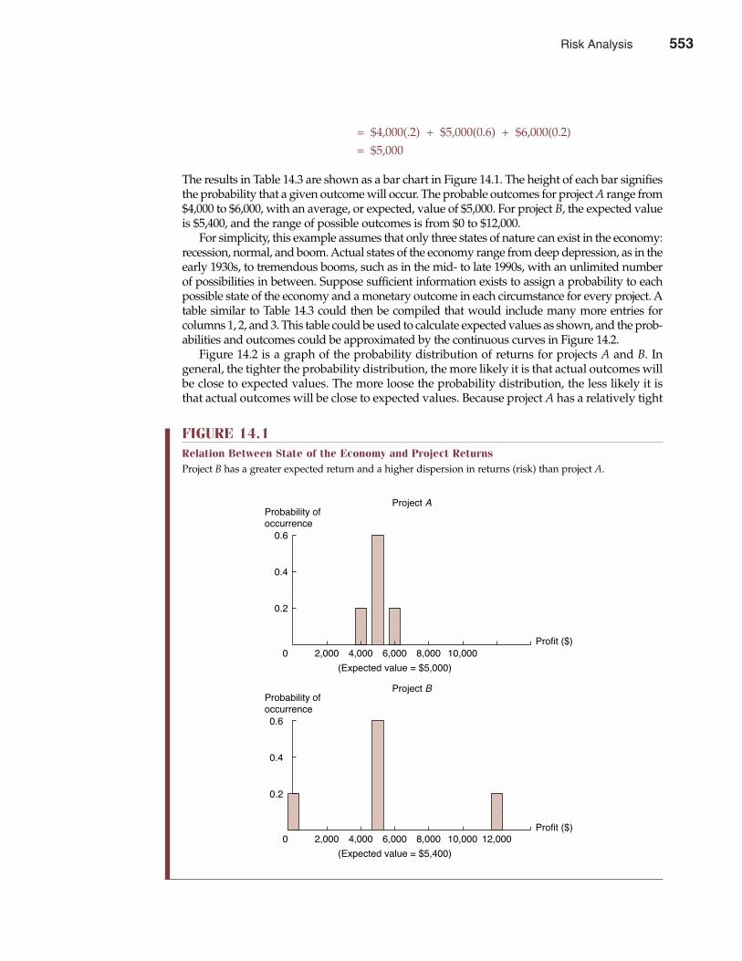
= $4,000(.2) + $5,000(0.6) + $6,000(0.2)= $5,000
The results in Table 14.3 are shown as a bar chart in Figure 14.1. The height of each bar signifiesthe probability that a given outcome will occur. The probable outcomes for project A range from$4,000 to $6,000, with an average, or expected, value of $5,000. For project B, the expected valueis $5,400, and the range of possible outcomes is from $0 to $12,000.
For simplicity, this example assumes that only three states of nature can exist in the economy:recession, normal, and boom. Actual states of the economy range from deep depression, as in theearly 1930s, to tremendous booms, such as in the mid- to late 1990s, with an unlimited numberof possibilities in between. Suppose sufficient information exists to assign a probability to eachpossible state of the economy and a monetary outcome in each circumstance for every project. Atable similar to Table 14.3 could then be compiled that would include many more entries forcolumns 1, 2, and 3. This table could be used to calculate expected values as shown, and the prob-abilities and outcomes could be approximated by the continuous curves in Figure 14.2.
Figure 14.2 is a graph of the probability distribution of returns for projects A and B. Ingeneral, the tighter the probability distribution, the more likely it is that actual outcomes willbe close to expected values. The more loose the probability distribution, the less likely it isthat actual outcomes will be close to expected values. Because project A has a relatively tight
554 Part Five Long-Term Investment Decisions
FIGURE 14.1Relation Between State of the Economy and Project ReturnsProject B has a greater expected return and a higher dispersion in returns (risk) than project A.
Probability ofoccurrence
0.6
0.4
0.2
Project A
0 2,000 4,000 6,000 8,000 10,000
(Expected value = $5,000)
Probability ofoccurrence
0.6
0.4
0.2
Project B
0 2,000 4,000 6,000 8,000 10,000
(Expected value = $5,400)
12,000Profit ($)
Profit ($)
Risk Analysis 553
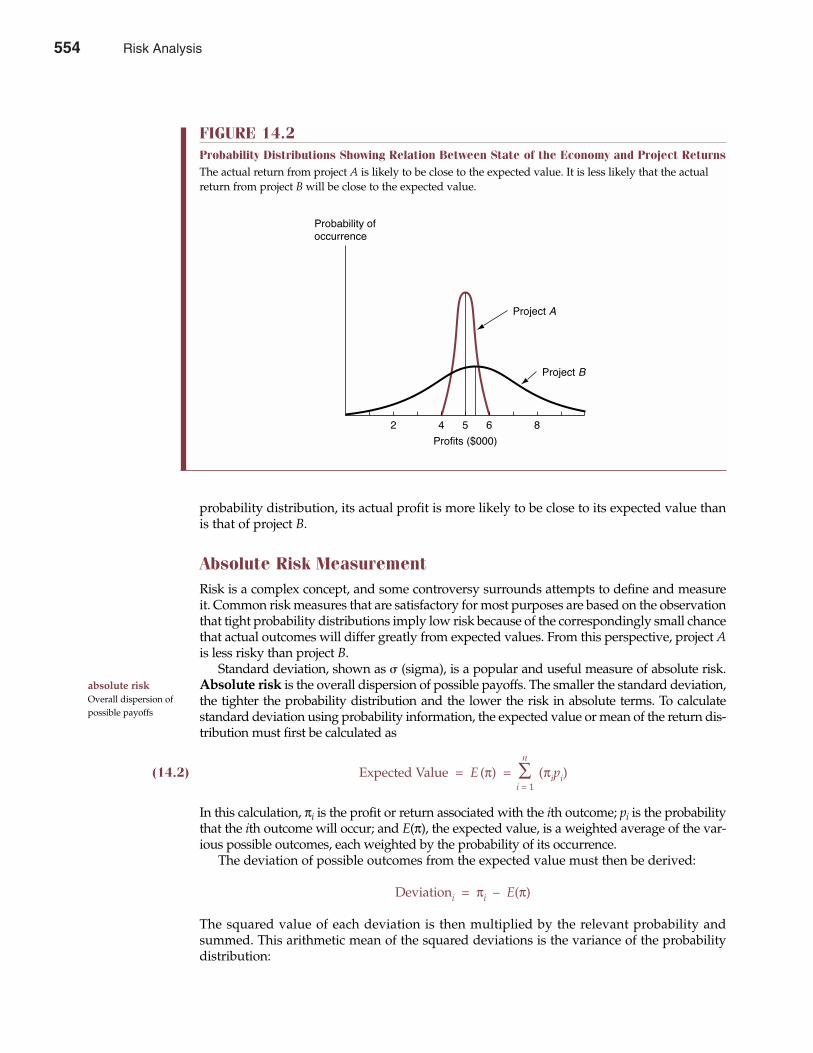
probability distribution, its actual profit is more likely to be close to its expected value thanis that of project B.
Absolute Risk MeasurementRisk is a complex concept, and some controversy surrounds attempts to define and measureit. Common risk measures that are satisfactory for most purposes are based on the observationthat tight probability distributions imply low risk because of the correspondingly small chancethat actual outcomes will differ greatly from expected values. From this perspective, project Ais less risky than project B.
Standard deviation, shown as � (sigma), is a popular and useful measure of absolute risk.Absolute risk is the overall dispersion of possible payoffs. The smaller the standard deviation,the tighter the probability distribution and the lower the risk in absolute terms. To calculatestandard deviation using probability information, the expected value or mean of the return dis-tribution must first be calculated as
n
(14.2) Expected Value = E (π) = ∑ (πipi)i = 1
In this calculation, πi is the profit or return associated with the ith outcome; pi is the probabilitythat the ith outcome will occur; and E(π), the expected value, is a weighted average of the var-ious possible outcomes, each weighted by the probability of its occurrence.
The deviation of possible outcomes from the expected value must then be derived:
Deviationi = πi – E(π)
The squared value of each deviation is then multiplied by the relevant probability andsummed. This arithmetic mean of the squared deviations is the variance of the probabilitydistribution:
absolute riskOverall dispersion ofpossible payoffs
Chapter Fourteen Risk Analysis 555
FIGURE 14.2Probability Distributions Showing Relation Between State of the Economy and Project ReturnsThe actual return from project A is likely to be close to the expected value. It is less likely that the actualreturn from project B will be close to the expected value.
2 4 5 6 8
Project A
Project B
Probability ofoccurrence
Profits ($000)
554 Risk Analysis
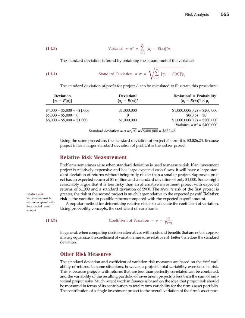
n
(14.3) Variance = �2 = ∑ [πi – E(π)]2pii = 1
The standard deviation is found by obtaining the square root of the variance:
n
(14.4) Standard Deviation = � = �∑ [πi – E(π)]2pii = 1
The standard deviation of profit for project A can be calculated to illustrate this procedure:
Deviation Deviation2 Deviation2 � Probability[πi � E(π)] [πi � E(π)]2 [πi � E(π)]2 � pi
$4,000 – $5,000 = –$1,000 $1,000,000 $1,000,000(0.2) = $200,000$5,000 – $5,000 = 0 0 $0(0.6) = $0$6,000 – $5,000 = $1,000 $1,000,000 $1,000,000(0.2) = $200,000
Variance = �2 = $400,000
Standard deviation = � = √�2 = √$400,000 = $632.46
Using the same procedure, the standard deviation of project B’s profit is $3,826.23. Becauseproject B has a larger standard deviation of profit, it is the riskier project.
Relative Risk MeasurementProblems sometimes arise when standard deviation is used to measure risk. If an investmentproject is relatively expensive and has large expected cash flows, it will have a large stan-dard deviation of returns without being truly riskier than a smaller project. Suppose a proj-ect has an expected return of $1 million and a standard deviation of only $1,000. Some mightreasonably argue that it is less risky than an alternative investment project with expectedreturns of $1,000 and a standard deviation of $900. The absolute risk of the first project isgreater; the risk of the second project is much larger relative to the expected payoff. Relativerisk is the variation in possible returns compared with the expected payoff amount.
A popular method for determining relative risk is to calculate the coefficient of variation.Using probability concepts, the coefficient of variation is
(14.5) Coefficient of Variation = v = �E(π)
In general, when comparing decision alternatives with costs and benefits that are not of approx-imately equal size, the coefficient of variation measures relative risk better than does the standarddeviation.
Other Risk MeasuresThe standard deviation and coefficient of variation risk measures are based on the total vari-ability of returns. In some situations, however, a project’s total variability overstates its risk.This is because projects with returns that are less than perfectly correlated can be combined,and the variability of the resulting portfolio of investment projects is less than the sum of indi-vidual project risks. Much recent work in finance is based on the idea that project risk shouldbe measured in terms of its contribution to total return variability for the firm’s asset portfolio.The contribution of a single investment project to the overall variation of the firm’s asset port-
556 Part Five Long-Term Investment Decisions
relative riskVariation in possiblereturns compared withthe expected payoffamount
Risk Analysis 555
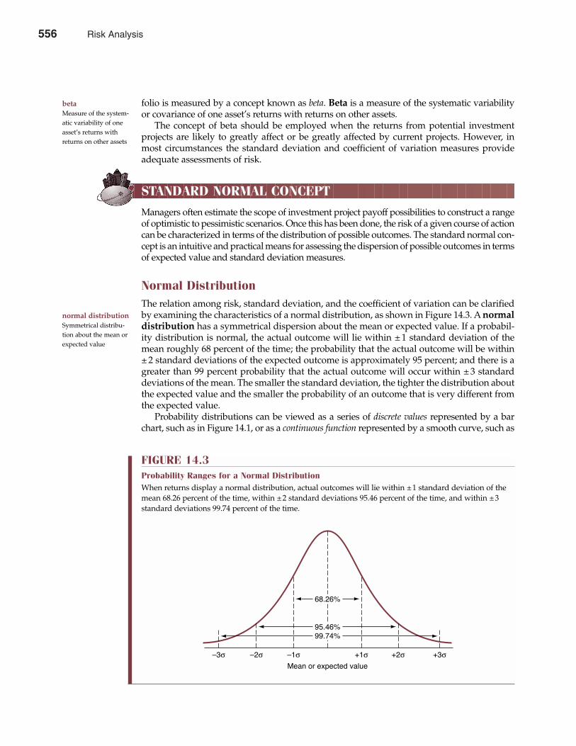
folio is measured by a concept known as beta. Beta is a measure of the systematic variabilityor covariance of one asset’s returns with returns on other assets.
The concept of beta should be employed when the returns from potential investmentprojects are likely to greatly affect or be greatly affected by current projects. However, inmost circumstances the standard deviation and coefficient of variation measures provideadequate assessments of risk.
STANDARD NORMAL CONCEPT
Managers often estimate the scope of investment project payoff possibilities to construct a rangeof optimistic to pessimistic scenarios. Once this has been done, the risk of a given course of actioncan be characterized in terms of the distribution of possible outcomes. The standard normal con-cept is an intuitive and practical means for assessing the dispersion of possible outcomes in termsof expected value and standard deviation measures.
Normal DistributionThe relation among risk, standard deviation, and the coefficient of variation can be clarifiedby examining the characteristics of a normal distribution, as shown in Figure 14.3. A normaldistribution has a symmetrical dispersion about the mean or expected value. If a probabil-ity distribution is normal, the actual outcome will lie within ± 1 standard deviation of themean roughly 68 percent of the time; the probability that the actual outcome will be within± 2 standard deviations of the expected outcome is approximately 95 percent; and there is agreater than 99 percent probability that the actual outcome will occur within ± 3 standarddeviations of the mean. The smaller the standard deviation, the tighter the distribution aboutthe expected value and the smaller the probability of an outcome that is very different fromthe expected value.
Probability distributions can be viewed as a series of discrete values represented by a barchart, such as in Figure 14.1, or as a continuous function represented by a smooth curve, such as
betaMeasure of the system-atic variability of oneasset’s returns withreturns on other assets
normal distributionSymmetrical distribu-tion about the mean orexpected value
Chapter Fourteen Risk Analysis 557
FIGURE 14.3Probability Ranges for a Normal DistributionWhen returns display a normal distribution, actual outcomes will lie within ±1 standard deviation of themean 68.26 percent of the time, within ±2 standard deviations 95.46 percent of the time, and within ±3standard deviations 99.74 percent of the time.
68.26%
95.46%
99.74%
Ð3σ Ð2σ Ð1σ +1σ +2σ +3σMean or expected value
556 Risk Analysis
that in Figure 14.2. Probabilities associated with the outcomes in Figure 14.1 are given by theheights of the bars, whereas in Figure 14.2, the probabilities must be found by calculating thearea under the curve between points of interest.
Standardized VariablesDistribution of costs or revenues can be transformed or standardized. A standardized vari-able has a mean of 0 and a standard deviation equal to 1. Any distribution of revenue, cost,or profit data can be standardized with the following formula:
(14.6) z = x – µ�
where z is the standardized variable, x is the outcome of interest, and µ and � are the meanand standard deviation of the distribution, respectively. If the point of interest is 1� away fromthe mean, then x – µ = �, so z = �/� = 1.0. When z = 1.0, the point of interest is 1� away fromthe mean; when z = 2, the value is 2� away from the mean; and so on. Although the standardnormal distribution theoretically runs from minus infinity to plus infinity, the probability ofoccurrences beyond 3 standard deviations is very near zero.
Use of the Standard Normal Concept: An ExampleSuppose that the Martha Stewart Realty is considering a boost in advertising to reduce a largeinventory of unsold homes. Management plans to make its media decision using the datashown in Table 14.4 on the expected success of television versus newspaper promotions. Forsimplicity, assume that the returns from each promotion are normally distributed. If the televi-sion promotion costs $2,295 and the newspaper promotion costs $4,013, what is the probabilitythat each will generate a profit?
To calculate the probability that each promotion will generate a profit, it is necessary tocalculate the portion of the total area under the normal curve that is to the right of (greaterthan) each breakeven point (see Figure 14.3). Here, the breakeven point is where the profitcontribution before advertising costs just equals the required advertising expenditure. Usingmethods described earlier, relevant expected values and standard deviations are E(RTV) =$2,500, �TV = $250, E(RN) = $5,000, and �N = $600. For the television promotion, the breakeven
558 Part Five Long-Term Investment Decisions
standardized variableVariable with a meanof 0 and a standarddeviation equal to 1
TABLE 14.4Return Distributions for Television and Newspaper Promotions
Return (Ri)Market Probability of (profit contribution
Response Occurring (Pi) before ad costs)
Television Poor 0.125 $2,000Good 0.750 2,500Very Good 0.125 3,000
Newspaper Poor 0.125 3,800Good 0.750 5,000Very Good 0.125 6,200
Risk Analysis 557
revenue level of $2,295 is 0.82 standard deviations less than (to the left of) the expected returnlevel of $2,500 because
z = xTV – E(RTV)�TV
= $2,295 – $2,500$250
= –0.82
Table B1 in Appendix B at the back of the book shows that the standard normal distributionfunction value for z = –0.82 is 0.2939. This means that 29.39 percent of the region under thenormal curve lies between $2,295 (z = –0.82) and the expected revenue level of $2,500. Because29.39 percent of the total area under the normal curve lies between xTV and E(RTV), the profitprobability for the television promotion is 0.2939 + 0.5 = 0.7939 or 79.39 percent.
For the newspaper promotion, z is calculated as
z = xN – E(RN)�N
= $4,013 – $5,000$600
= –1.645
After interpolating, the probability value for z = –1.645 is 0.45. This means that 0.45, or 45 per-cent, of the total area under the normal curve lies between xN and E(RN), and it implies a profitprobability for the newspaper promotion of 0.45 + 0.5 = 0.95, or 95 percent. In terms of profitprobability, the newspaper advertisement is the less risky alternative.
Chapter Fourteen Risk Analysis 559
Why Lotteries Are Popular
The success of state-run lotteries is convincing evidencethat many in our society display risk-seeking behavior,especially when small sums of money are involved. Thepopularity of lotteries stems from the fact that ticket buy-ers appear eager to pay $1 for a bet that has an expectedreturn of less than $1. When only 50 percent of lottery-ticket revenues are paid out in the form of prizes, each $1ticket has an expected return of only 50¢. In such circum-stances, the “price” of $1 in expected return is $2 in cer-tain dollars. The willingness to pay such a premium forthe unlikely chance at a lottery payoff that might reachinto the millions of dollars stems from the fact that suchopportunities are rare and lottery-ticket buyers valuethem highly. Many of the poor, uneducated, or elderlyhave no opportunity for hitting the jackpot in theircareers. The lottery is their only chance, however remote,at a substantial sum of money. It should therefore comeas no surprise that lottery-ticket buyers tend to be poor,uneducated, and elderly.
The success of state-run lotteries is noteworthybecause it reflects risk attitudes that are fairly unusual.
Typically, consumers and investors display risk-aversebehavior, especially when substantial sums of money areinvolved. Still, the eagerness of consumers to take onenormous risks when small sums of money are involvedhas made gambling one of America’s great growthindustries.
If legislative agendas are any indication, Americanscan expect to see even more riverboat gambling, cardclubs, off-track betting parlors, and casinos in their ownbackyards. Indian-run casinos are also becoming increas-ingly popular. Americans are so eager to gamble thatthey are shifting long-established leisure-time expendi-tures. Today, U.S. consumers spend more on legal gamesof chance than on movie theaters, books, amusementattractions, and recorded music combined!
Pouring quarters into a slot machine is easy andapparently appealing to a growing number of Americans.
See: Dow Jones Newswires, “Gtech, Kentucky Lottery Get Deal,” TheWall Street Journal Online, January 29, 2002 (http://online.wsj.com).
M A N A G E R I A L A P P L I C AT I O N 1 4 . 2
558 Risk Analysis
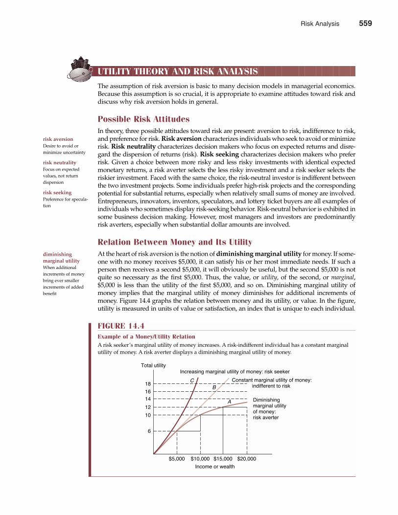
UTILITY THEORY AND RISK ANALYSIS
The assumption of risk aversion is basic to many decision models in managerial economics.Because this assumption is so crucial, it is appropriate to examine attitudes toward risk anddiscuss why risk aversion holds in general.
Possible Risk AttitudesIn theory, three possible attitudes toward risk are present: aversion to risk, indifference to risk,and preference for risk. Risk aversion characterizes individuals who seek to avoid or minimizerisk. Risk neutrality characterizes decision makers who focus on expected returns and disre-gard the dispersion of returns (risk). Risk seeking characterizes decision makers who preferrisk. Given a choice between more risky and less risky investments with identical expectedmonetary returns, a risk averter selects the less risky investment and a risk seeker selects theriskier investment. Faced with the same choice, the risk-neutral investor is indifferent betweenthe two investment projects. Some individuals prefer high-risk projects and the correspondingpotential for substantial returns, especially when relatively small sums of money are involved.Entrepreneurs, innovators, inventors, speculators, and lottery ticket buyers are all examples ofindividuals who sometimes display risk-seeking behavior. Risk-neutral behavior is exhibited insome business decision making. However, most managers and investors are predominantlyrisk averters, especially when substantial dollar amounts are involved.
Relation Between Money and Its UtilityAt the heart of risk aversion is the notion of diminishing marginal utility for money. If some-one with no money receives $5,000, it can satisfy his or her most immediate needs. If such aperson then receives a second $5,000, it will obviously be useful, but the second $5,000 is notquite so necessary as the first $5,000. Thus, the value, or utility, of the second, or marginal,$5,000 is less than the utility of the first $5,000, and so on. Diminishing marginal utility ofmoney implies that the marginal utility of money diminishes for additional increments ofmoney. Figure 14.4 graphs the relation between money and its utility, or value. In the figure,utility is measured in units of value or satisfaction, an index that is unique to each individual.
560 Part Five Long-Term Investment Decisions
risk aversionDesire to avoid or minimize uncertainty
risk neutralityFocus on expected values, not return dispersion
risk seekingPreference for specula-tion
diminishing marginal utilityWhen additional increments of moneybring ever smallerincrements of addedbenefit
FIGURE 14.4Example of a Money/Utility RelationA risk seeker’s marginal utility of money increases. A risk-indifferent individual has a constant marginalutility of money. A risk averter displays a diminishing marginal utility of money.
Constant marginal utility of money:indifferent to risk
Diminishingmarginal utilityof money:risk averter
Increasing marginal utility of money: risk seekerTotal utility
18
16
14
12
10
6
$5,000 $10,000 $15,000 $20,000
Income or wealth
C
A
B
Risk Analysis 559

For risk averters, money has diminishing marginal utility. If such an individual’s wealthwere to double suddenly, he or she would experience an increase in happiness or satisfaction,but the new level of well-being would not be twice the previous level. In cases of diminish-ing marginal utility, a less than proportional relation holds between total utility and money.Accordingly, the utility of a doubled quantity of money is less than twice the utility of theoriginal level. In contrast, those who are indifferent to risk perceive a strictly proportionalrelationship between total utility and money. Such a relation implies a constant marginal util-ity of money, and the utility of a doubled quantity of money is exactly twice the utility of theoriginal level. Risk seekers perceive a more than proportional relation between total utilityand money. In this case, the marginal utility of money increases. With increasing marginalutility of money, the utility of doubled wealth is more than twice the utility of the originalamount. These relations are illustrated in Figure 14.4.
Even though total utility increases with increased money for risk averters, risk seekers, andthose who are indifferent to risk, the relation between total utility and money is quite differentfor each group. These differences lead to dissimilar risk attitudes. Because individuals with adiminishing marginal utility for money suffer more pain from a dollar lost than the pleasurederived from a dollar gained, they seek to avoid risk. Risk averters require a very high returnon any investment that is subject to much risk.
In Figure 14.4, for example, a gain of $5,000 from a base of $10,000 brings 2 units of addi-tional satisfaction, but a $5,000 loss causes a 4-unit loss in satisfaction. A person with thisutility function and $10,000 would be unwilling to make an investment with a 50/50 chanceof winning or losing $5,000. The 9-unit expected utility of such a gamble [E(u) = 0.5 times theutility of $5,000 + 0.5 times the utility of $15,000 = 0.5 � 6 + 0.5 � 12 = 9] is less than the 10units of utility obtained by forgoing the gamble and keeping $10,000 in certain wealth.
Because an individual with a constant marginal utility for money values a dollar gainedjust as highly as a dollar lost, the expected utility from a fair gamble always exactly equalsthe utility of the expected outcome. An individual indifferent to risk makes decisions on the
Chapter Fourteen Risk Analysis 561
Employee Stock Options
In a conventional employee stock option plan, keyemployees are granted the right to buy a fixed number ofshares for a predetermined period. The number of sharesgranted depends on the employee’s level of responsibility.Usually, the number of shares granted under an employeestock option plan is commensurate with total compensa-tion. According to current tax law, the exercise period foremployee stock options cannot exceed 10 years, but maybe less. Because stock prices usually rise from 12 percentto 14 percent per year, on average, from the employee’sperspective, the longer the exercise period, the better.
An employee can exercise the right to buy stock cov-ered by a stock option plan once the vesting period hasbeen completed. The vesting period is an employment timeframe after which granted options can be exercised. Thelength of the vesting period is designed by the employer tokeep valued employees motivated. It is also designed tokeep employees from bolting to the competition. Structuredproperly, an employee stock option plan with appropriatevesting requirements can create “golden handcuffs” thatbenefit both valued employees and their employers.
Once exercised, employee stock options create a tax-able event for the employee. The difference between thecurrent market price and the original exercise price, multi-plied by the number of shares covered, is used to calculatethe amount of employee compensation derived from theoption exercise. By granting employee stock options,employers replace cash compensation that reduces operat-ing income with contingent-based pay that never appearson the income statement. Income statements issued bycompanies with extensive stock option plans can dramati-cally understate the total amount of employee compensa-tion. This can result in earnings statements that present toorosy a picture of corporate performance. Such problemsbecome evident when the company’s stock price falters,and employees clamor for more cash compensation.
In the long run, investors lose out unless they con-sider the economic cost of employee stock options.
See: T. J. Rogers, “Options Aren’t Optional in Silicon Valley,” The WallStreet Journal Online, March 4, 2002 (http://online.wsj.com).
M A N A G E R I A L A P P L I C AT I O N 1 4 . 3
560 Risk Analysis
basis of expected monetary outcomes and is not concerned with possible variation in the dis-tribution of outcomes.
ADJUSTING THE VALUATION MODEL FOR RISK
Diminishing marginal utility leads directly to risk aversion, and risk aversion is reflected in thebasic valuation model used to determine the worth of a firm. If a managerial decision affectsthe firm’s risk level, the value of the firm is impacted. Two primary methods are used to adjustthe basic valuation model to account for decision making under conditions of uncertainty.
Basic Valuation ModelThe basic valuation model developed in Chapter 1 is
n
(14.7) V = ∑ πi
t = 1 (1 + i)t
This model states that the value of the firm is equal to the discounted present worth of futureprofits. Under conditions of certainty, the numerator is profit, and the denominator is a time-value adjustment using the risk-free rate of return i. After time-value adjustment, the profitsto be earned from various projects are strictly and completely comparable.
Under conditions of uncertainty, the profits shown in the numerator of the valuation modelas π equal the expected value of profits during each future period. This expected value is thebest available estimate of the amount to be earned during any given period. However, becauseprofits cannot be predicted with absolute precision, some variability is to be anticipated. If thefirm must choose between two alternative methods of operation, one with high expected prof-its and high risk and another with smaller expected profits and lower risks, some techniquemust be available for making the alternative investments comparable. An appropriate rankingand selection of projects is possible only if each respective investment project can be adjustedfor considerations of both time value of money and risk. At least two popular methods areemployed to make such adjustments. In the first, expected profits are adjusted to account forrisk. In the second, the interest rate used in the denominator of the valuation model is increasedto reflect risk considerations. Either method can be used to ensure that value-maximizing deci-sions are made.
Certainty Equivalent AdjustmentsThe certainty equivalent method is an adjustment to the numerator of the basic valuationmodel to account for risk. Under the certainty equivalent approach, decision makers speci-fy the certain sum that they regard comparable to the expected value of a risky investmentalternative. The certainty equivalent of an expected risk amount typically differs in dollarterms but not in terms of the amount of utility provided. To illustrate, suppose that you facethe following choices:
• Invest $100,000. From a successful project, you receive $1,000,000; if it fails, you receivenothing. If the probability of success is 0.5, or 50 percent, the investment’s expected payoffis $500,000 (= 0.5 � $1,000,000 + 0.5 � $0).
• You do not make the investment; you keep the $100,000.
If you find yourself indifferent between the two alternatives, $100,000 is your certainty equiv-alent for the risky expected return of $500,000. In other words, a certain or riskless amount of$100,000 provides exactly the same utility as the 50/50 chance to earn $1,000,000 or $0. Youare indifferent between these two alternatives.
562 Part Five Long-Term Investment Decisions
certainty equivalentAssured sum thatequals an expectedrisky amount in utilityterms
Risk Analysis 561
In this example, any certainty equivalent of less than $500,000 indicates risk aversion. If themaximum amount that you are willing to invest in the project is only $100,000, you are exhibit-ing very risk-averse behavior. Each certain dollar is “worth” five times as much as each riskydollar of expected return. Alternatively, each risky dollar of expected return is worth only 20¢in terms of certain dollars. In general, any risky investment with a certainty equivalent lessthan the expected dollar value indicates risk aversion. A certainty equivalent greater than theexpected value of a risky investment indicates risk preference.
Any expected risky amount can be converted to an equivalent certain sum using the cer-tainty equivalent adjustment factor, �, calculated as the ratio of a certain sum divided byan expected risky amount, where both dollar values provide the same level of utility:
Certainty Equivalent = � = Equivalent Certain Sum(14.8) Adjustment Factor Expected Risky Sum
The certain sum numerator and expected return denominator may vary in dollar terms, butthey provide the exact same reward in terms of utility. In the previous investment problem,in which a certain sum of $100,000 provides the same utility as an expected risky return of$500,000, the certainty equivalent adjustment factor � = 0.2 = $100,000/$500,000. This meansthat the “price” of one dollar in risky expected return is 20¢ in certain dollar terms.
The following general relations enable managers to use the certainty equivalent adjustmentfactor to analyze risk attitudes:
If Then Implies
Equivalent certain sum < Expected risky sum � < 1 Risk aversionEquivalent certain sum = Expected risky sum � = 1 Risk indifferenceEquivalent certain sum > Expected risky sum � > 1 Risk preference
The appropriate � value for a given managerial decision varies according to the level of riskand degree of the decision maker’s risk aversion.
The basic valuation model (Equation 14.7) can be converted into a risk-adjusted valuationmodel, one that explicitly accounts for risk:
n
(14.9) V = ∑ �E(πi)
t = 1 (1 + i)t
In this risk-adjusted valuation model, expected future profits, E(πt), are converted to theircertainty equivalents, �E(πt), and are discounted at a risk-free rate, i, to obtain the risk-adjusted present value of a firm or project. With the valuation model in this form, one canappraise the effects of different courses of action with different risks and expected returns.
To use Equation 14.9 for real-world decision making, managers must estimate appropriate�s for various investment opportunities. Deriving such estimates can prove difficult, because� varies according to the size and riskiness of investment projects as well as according to the riskattitudes of managers and investors. In many instances, however, the record of past investmentdecisions offers a guide that can be used to determine appropriate certainty equivalent adjustmentfactors. The following example illustrates how managers use certainty equivalent adjustment fac-tors in practical decision making.
Certainty Equivalent Adjustment ExampleAssume that operations at Burns & Allen Industries have been seriously disrupted by problemswith a faulty boiler at its main fabrication facility. In fact, state fire marshals shut the facility
certainty equivalentadjustment factor, �Ratio of a certain sumdivided by an expectedrisky amount, whereboth dollar values pro-vide the same level ofutility
risk-adjusted valuation modelValuation model thatreflects time-value andrisk considerations
Chapter Fourteen Risk Analysis 563
562 Risk Analysis
down for an extended period recently following repeated overheating and minor explosions.The boiler problem was solved when it was discovered that a design flaw had made the pilotlight safety switch inoperable.
Burns & Allen retained the Denver law firm of Dewey, Cheetum & Howe to recover eco-nomic damages from the boiler manufacturer. The company has filed suit in state court for$250,000 in damages. Prior to filing suit, the attorney estimated legal, expert witness, and otherlitigation costs to be $10,000 for a fully litigated case, for which Burns & Allen had a 10 percentchance of receiving a favorable judgment. For simplicity, assume that a favorable judgmentwill award Burns & Allen 100 percent of the damages sought, whereas an unfavorable judg-ment will result in the firm receiving zero damages. Also assume that $10,000 is the most Burns& Allen would be willing to pay to sue the boiler manufacturer.
In filing suit against the boiler manufacturer, Burns & Allen has made a risky investmentdecision. By its willingness to bear litigation costs of $10,000, the company has implicitly stat-ed that it regards these out-of-pocket costs to be at least equivalent to the value of the riskyexpectation of receiving a favorable judgment against the boiler manufacturer. In other words,Burns & Allen is willing to exchange $10,000 in certain litigation costs for the possibility ofreceiving a $250,000 judgment against the boiler manufacturer.
Burns & Allen’s investment decision can be characterized using the certainty equivalentadjustment method. To do this, it is important to realize that the $10,000 in litigation costs isincurred irrespective of the outcome of a fully litigated case. This $10,000 represents a certainsum that the company must value as highly as the expected risky outcome to be willing to filesuit. The expected risky outcome, or expected return from filing suit, is
Expected Return = Favorable Judgment Payoff � Probability+ Unfavorable Judgment Payoff � Probability
= $250,000(0.1) + $0(0.9)= $25,000
To justify filing suit, Burns & Allen’s certainty equivalent adjustment factor for investment proj-ects of this risk class must be
� = Certain SumExpected Risky Sum
= Litigation CostsExpected Return
= $10,000$25,000
= 0.4
Therefore, each risky dollar of expected return from the litigation effort is worth, in terms ofutility, at least 40¢ in certain dollars. Alternatively, $10,000 is the certain sum equivalent of therisky expected return of $25,000.
Now assume that after Burns & Allen goes to court, incurring $5,000 in litigation costs,especially damaging testimony by an expert witness dramatically changes the outlook of thecase in Burns & Allen’s favor. In response, the boiler manufacturer’s attorney offers an out-of-court settlement in the amount of $30,000. However, Burns & Allen’s attorney recommendsthat the company reject this offer, estimating that it now has a 50/50 chance of obtaining afavorable judgment in the case. Should Burns & Allen follow the attorney’s advice and rejectthe settlement offer?
564 Part Five Long-Term Investment Decisions
Risk Analysis 563
In answering this question, one must keep in mind that having already spent (“sunk”)$5,000 in litigation costs, Burns & Allen must consider as relevant litigation costs only the addi-tional $5,000 necessary to complete litigation. These $5,000 litigation costs, plus the $30,000out-of-court settlement offer, represent the relevant certain sum, because proceeding with thesuit will require an “investment” of these additional litigation plus opportunity costs. Giventhe revised outlook for a favorable judgment, the expected return to full litigation is
Expected Return = ($250,000)(0.5) + ($0)(0.5)= $125,000
In light of Burns & Allen’s earlier decision to file suit on the basis that each dollar of expectedrisky return was “worth” 40¢ in certain dollars, this expected return would have a $50,000(=$125,000 � 0.4) certainty equivalent value. Because this amount exceeds the settlement offerplus remaining litigation costs, the settlement offer seems deficient and should be rejected. Onthe basis of Burns & Allen’s revealed risk attitude, an out-of-court settlement offer has to be atleast $45,000 to receive favorable consideration. At that point, the settlement plus saved litiga-tion costs of $5,000 would equal the certainty equivalent value of the expected return from con-tinuing litigation.
This simple example illustrates that historical investment decisions offer a useful guide tocurrent decisions. If a potential project’s required investment and risk levels are known, the �implied by a decision to accept the investment project can be calculated. This project-specific� can then be compared with �s for prior projects with similar risks. Risk-averse individualsshould invest in projects if calculated �s are less than or equal to those for accepted historicalprojects in the same risk class. Furthermore, given an estimate of expected return and risk, themaximum amount that the firm should be willing to invest in a given project can also be deter-mined from the certainty equivalent adjustment factor. Risk-averse management will acceptnew projects if the level of required investment per dollar of expected return is less than orequal to that for historical projects of similar risk.
Risk-Adjusted Discount RatesAnother way to incorporate risk in managerial decision making is to adjust the discount rate ordenominator of the basic valuation model (Equation 14.7). Like certainty equivalent factors, risk-adjusted discount rates are based on the trade-off between risk and return for individualinvestors. Suppose an investor is indifferent to a riskless asset with a sure 5 percent rate of return,a moderately risky asset with a 10 percent expected return, and a very risky asset with a 15 per-cent expected return. As risk increases, higher expected returns on investment are required tocompensate for additional risk. Observe also that the required risk premium is directly relatedto the level of risk associated with a particular investment. This is a common situation.
The basic valuation model shown in Equation 14.7 can be adapted to account for risk throughadjustment of the discount rate, i, where
n
(14.10) V = ∑ E(πi)
t = 1 (1 + k)t
The risk-adjusted discount rate k is the sum of the risk-free rate of return, RF, plus the requiredrisk premium, Rp:
k = RF + Rp
In Equation 14.10, value is measured by the present worth of expected future income or profits,E(πt), discounted at a risk-adjusted rate.
risk-adjusted discount rateRisk-free rate of returnplus the required riskpremium
risk premiumAdded expected returnfor a risky asset overthat of a riskless asset
Chapter Fourteen Risk Analysis 565
564 Risk Analysis
Risk-Adjusted Discount Rate ExampleSuppose the Property & Casualty Insurance Company (P&C) is contemplating the purchase ofone of the two database and file management software systems offered by Rockford Files, Inc.System A is specifically designed for P&C’s current computer software system and cannot beused with those of other providers; system B is compatible with a broad variety of computersoftware systems, including P&C’s and those of other software providers. The expected invest-ment outlay is $500,000 for each alternative. Expected annual cost savings (cash inflows) over5 years are $175,000 per year for system A and $185,000 per year for system B. The standarddeviation of expected annual returns from system A is $10,000, whereas that of system B is$15,000. In view of this risk differential, P&C management has decided to evaluate system Awith a 10 percent cost of capital and system B with a 15 percent cost of capital.
The risk-adjusted value for each system is as follows:2
5
ValueA = ∑ $175,000 – $500,000t = 1 (1.10)t
5
= $175,000 � �∑ 1 – $500,000t = 1 (1.10)t
= $175,000 � 3.7908 – $500,000
= $163,390
5
ValueB = ∑ $185,000 – $500,000t = 1 (1.15)t
5
= $185,000 � �∑ 1 – $500,000t = 1 (1.15)t
= $185,000 � 3.3522 – $500,000
= $120,157
Because the risk-adjusted value of system A is larger than that for system B, P&C shouldchoose system A. This choice maximizes the value of the firm.
DECISION TREES AND COMPUTER SIMULATION
Decision trees that follow the sequential nature of the decision-making process provide alogical framework for decision analysis under conditions of uncertainty. When a high degreeof uncertainty exists and data are not readily available, computer simulation often provides
566 Part Five Long-Term Investment Decisions
2 The terms5
∑ 1 = 3.7908t = 1 (1.10)t
and5
∑ 1 = 3.3522t = 1 (1.15)t
are present-value-of-an-annuity interest factors. Tables of interest factors for various interest rates and years(t values) appear in Appendix B.4.
Risk Analysis 565
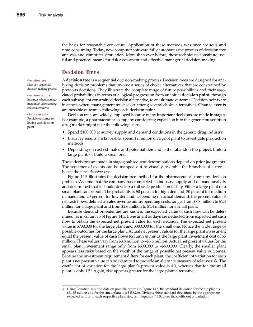
the basis for reasonable conjecture. Application of these methods was once arduous andtime-consuming. Today, new computer software fully automates the process of decision treeanalysis and computer simulation. More than ever before, these techniques constitute use-ful and practical means for risk assessment and effective managerial decision making.
Decision TreesA decision tree is a sequential decision-making process. Decision trees are designed for ana-lyzing decision problems that involve a series of choice alternatives that are constrained byprevious decisions. They illustrate the complete range of future possibilities and their asso-ciated probabilities in terms of a logical progression from an initial decision point, througheach subsequent constrained decision alternative, to an ultimate outcome. Decision points areinstances where management must select among several choice alternatives. Chance eventsare possible outcomes following each decision point.
Decision trees are widely employed because many important decisions are made in stages.For example, a pharmaceutical company considering expansion into the generic prescriptiondrug market might take the following steps:
• Spend $100,000 to survey supply and demand conditions in the generic drug industry.• If survey results are favorable, spend $2 million on a pilot plant to investigate production
methods.• Depending on cost estimates and potential demand, either abandon the project, build a
large plant, or build a small one.
These decisions are made in stages; subsequent determinations depend on prior judgments.The sequence of events can be mapped out to visually resemble the branches of a tree—hence the term decision tree.
Figure 14.5 illustrates the decision-tree method for the pharmaceutical company decisionproblem. Assume that the company has completed its industry supply and demand analysisand determined that it should develop a full-scale production facility. Either a large plant or asmall plant can be built. The probability is 50 percent for high demand, 30 percent for mediumdemand, and 20 percent for low demand. Depending on actual demand, the present value ofnet cash flows, defined as sales revenue minus operating costs, ranges from $8.8 million to $1.4million for a large plant and from $2.6 million to $1.4 million for a small plant.
Because demand probabilities are known, the expected value of cash flow can be deter-mined, as in column 5 of Figure 14.5. Investment outlays are deducted from expected net cashflow to obtain the expected net present value for each decision. The expected net presentvalue is $730,000 for the large plant and $300,000 for the small one. Notice the wide range ofpossible outcomes for the large plant. Actual net present values for the large plant investmentequal the present value of cash flows (column 4) minus the large plant investment cost of $5million. These values vary from $3.8 million to –$3.6 million. Actual net present values for thesmall plant investment range only from $600,000 to –$600,000. Clearly, the smaller plantappears less risky based on the width of the range of possible net present value outcomes.Because the investment requirement differs for each plant, the coefficient of variation for eachplant’s net present value can be examined to provide an alternate measure of relative risk. Thecoefficient of variation for the large plant’s present value is 4.3, whereas that for the smallplant is only 1.5.3 Again, risk appears greater for the large plant alternative.
decision treeMap of a sequentialdecision-making process
decision pointsInstances when manage-ment must select amongchoice alternatives
chance eventsPossible outcomes fol-lowing each decisionpoint
Chapter Fourteen Risk Analysis 567
3 Using Equation 14.6 and data on possible returns in Figure 14.5, the standard deviation for the big plant is$3.155 million and for the small plant it is $458,260. Dividing these standard deviations by the appropriateexpected return for each respective plant size, as in Equation 14.5, gives the coefficient of variation.
566 Risk Analysis
These risk and expected return differentials can be incorporated into the decision-makingprocess in a variety of ways. Assigning utility values to the cash flows given in column 4 ofFigure 14.5 would state column 5 in terms of expected utility. The company could then choosethe plant size that provided the greatest expected utility. Alternatively, present values givenin column 4 could be adjusted using the certainty equivalent or risk-adjusted discount ratemethod. The plant that offers the largest risk-adjusted net present value is the optimal choice.
Computer SimulationAnother technique designed to assist managers in making decisions under uncertainty iscomputer simulation. Computer simulation involves the use of computer software andsophisticated desktop computers to create a wide variety of decision outcome scenarios.These simulations illustrate a broad range of possible outcomes to help managers assess thepossible and probable consequences of decision alternatives. Using the computer simulationtechnique, a variety of hypothetical “What if?” questions can be asked and answered on thebasis of measurable differences in underlying assumptions. More than just informed conjecture,computer simulation allows managers to make precise judgments concerning the desirabilityof various choices on the basis of highly detailed probability information.
Computer simulations require probability distribution estimates for a number of variables,such as investment outlays, unit sales, product prices, input prices, and asset lives. In someinstances, full-scale simulations are expensive and time-consuming and therefore restricted toprojects such as major plant expansions or new-product decisions. When a firm is decidingwhether to accept a major undertaking involving an outlay of millions of dollars, full-scalecomputer simulations provide valuable insights that are well worth their cost. Somewhat lessexpensive, limited-scale simulations are used to project outcomes for projects or strategies.
568 Part Five Long-Term Investment Decisions
computer simulationUse of computer soft-ware and workstationsor sophisticated desk-top computers to createoutcome scenarios
FIGURE 14.5Illustrative Decision TreeThe expected net present value of each investment alternative (column 5) is determined by linking possibleoutcomes (column 2), probabilities (column 3), and monetary values (column 4).
Decisionpoint
Build big plant:invest $5 million
Build small plant:invest $2 million
Action(1)
Demandconditions (2)
High
Medium
Low
High
Medium
Low
Probability (3)
Present valueof cash flows (4)
(5) = (3) × (4)
0.5
0.3
0.2
0.5
0.3
0.2
$2,600,000
$2,400,000
$1,400,000
$8,800,000
$3,500,000
$1,400,000
$4,400,000
1,050,000
280,000
$1,300,000
720,000
280,000
$2,300,0002,000,000
$ 300,000
$5,730,0005,000,000
$ 730,000
Expected value of cash flowsCost
Expected net present value
Expected value of cash flowsCost
Expected net present value
Risk Analysis 567
Instead of using complete probability distributions for each variable included in the problem,results are simulated based on best-guess estimates for each variable. Changes in the valuesof each variable are then considered to see the effects of such changes on project returns.Typically, returns are highly sensitive to some variables, less so to others. Attention is thenfocused on the variables to which profitability is most sensitive. This technique, known assensitivity analysis, is less expensive and less time-consuming than full-scale computer sim-ulation, but it still provides valuable insight for decision-making purposes.
Computer Simulation ExampleTo illustrate the computer simulation technique, consider the evaluation of a new minimillinvestment project by Remington Steel, Inc. The exact cost of the plant is not known, but it isexpected to be about $150 million. If no difficulties arise in construction, this cost can be aslow as $125 million. An unfortunate series of events such as strikes, greater than projectedincreases in material costs, and/or technical problems could drive the required investmentoutlay as high as $225 million. Revenues from the new facility depend on the growth ofregional income and construction, competition, developments in the field of metallurgy, steelimport quotas and tariffs, and so on. Operating costs depend on production efficiency, thecost of raw materials, and the trend in wage rates. Because sales revenues and operating costsare uncertain, annual profits are unpredictable.
Assuming that probability distributions can be developed for each major cost and revenuecategory, a computer program can be constructed to simulate the pattern of future events.Computer simulation randomly selects revenue and cost levels from each relevant distributionand uses this information to estimate future profits, net present values, or the rate of return oninvestment. This process is repeated a large number of times to identify the central tendencyof projected returns and their expected values. When the computer simulation is completed,the frequency pattern and range of future returns can be plotted and analyzed. Although the
sensitivity analysisLimited form of com-puter simulation thatfocuses on importantdecision variables
Chapter Fourteen Risk Analysis 569
Game Theory at the FCC
One of the most successful game theory applications hasbeen in the design of FCC auctions used to allocate elec-tromagnetic spectrum, a highly valuable and finite publicresource. In the design of the auction process, the FCChas relied on advice from top game theorists at Stanford,Yale, and other leading universities. The agency has gen-erally adopted a standard English auction in which thewinner pays what it bids, and everyone can see all bidsas they are made. Game theory research shows that openauctions stimulate bidding, whereas sealed auctions fos-ter restraint for fear of needlessly paying too much.
Although the FCC initially favored auctioning offvital spectrum licenses all at once to make it easier forbidders to assemble efficient blocs of adjoining areas, thisapproach entails a nightmare of complexity. Complicatingthe problem is the fact that bidders must be allowed someflexibility to withdraw bids when adjoining areas are soldto others. If all offers could be withdrawn easily, however,the integrity of the process would suffer. A sequentialauction, where areas are put up for bid one at a time, also
involves problems because it denies participants theopportunity to bid more for economically efficient blocksof service areas. Winning bidders in a sequential auctionhave the potential for a snowballing effect where one suc-cess leads to another, and another, and another. After con-sidering a wide variety of options, the FCC adopted amodified sequential bidding approach.
How does it work? Consider the PCS spectrum auc-tion, which began on December 12, 2000, and ended onJanuary 26, 2001. After 101 rounds of bidding, 422 licensescovering 195 markets, including New York, Los Angeles,Chicago, Boston and Washington, DC, were allocated.The FCC’s competitive bidding process allowed for rapiddeployment and ensured that spectrum went to the high-est value use. The American taxpayer also benefitedwhen the PCS auction raised $16,857,046,150!
See: Jacquie Jordan, “Triton PCS to Acquire Excess PCS Spectrum fromNtelos,” The Wall Street Journal Online, December 12, 2001(http://online.wsj.com).
M A N A G E R I A L A P P L I C AT I O N 1 4 . 4
568 Risk Analysis
expected value of future profits is of obvious interest, the range of possible outcomes is simi-larly important as a useful indicator of risk.
The computer simulation technique is illustrated in Figures 14.6 and 14.7. Figure 14.6 is aflow chart that shows the information flow pattern for the simulation procedure just described.Figure 14.7 illustrates the frequency distribution of rates of return generated by such a simu-
570 Part Five Long-Term Investment Decisions
FIGURE 14.6Simulation for Investment PlanningComputer simulation allows detailed analysis of managerial problems involving complex cost and revenue relations.
Size of market
Market growth rate
Required investment
Operating expenses
Useful life of facilities
Selling price
Market share
Residual or scrapvalue of investment
Fixed costs
Chances that outcomewill be achieved
Investment analyst identifiesprobability values for significantfactors
Using computer simulationsoftware, analyst randomlyselects sets of investmentcharacteristics based on theirchances of turning up inthe future
Return on investment (ROI) isestimated for specified scenario
ROI is reestimated hundreds,or thousands, of times underalternative scenarios to giveclear picture of returndistribution (investment risk)
ChancesthatROI
willbeachieved
Range of outcomes
Rate of returnon investment (ROI)
E.V.
Risk Analysis 569
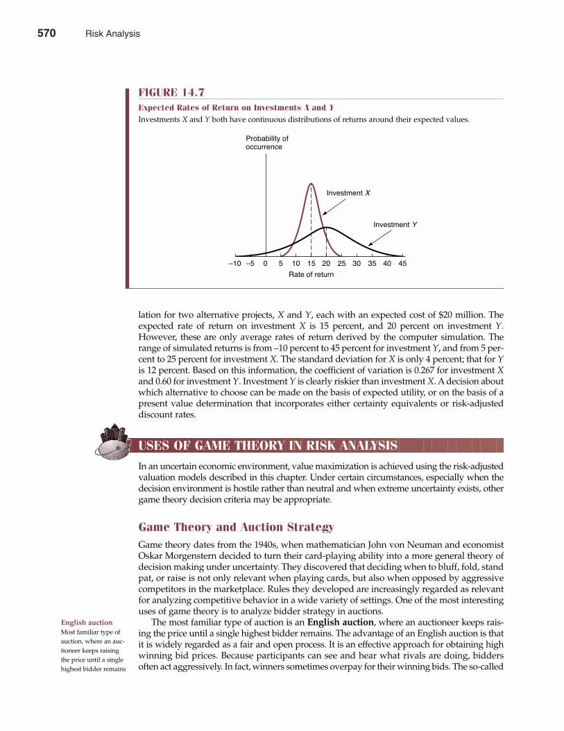
lation for two alternative projects, X and Y, each with an expected cost of $20 million. Theexpected rate of return on investment X is 15 percent, and 20 percent on investment Y.However, these are only average rates of return derived by the computer simulation. Therange of simulated returns is from –10 percent to 45 percent for investment Y, and from 5 per-cent to 25 percent for investment X. The standard deviation for X is only 4 percent; that for Yis 12 percent. Based on this information, the coefficient of variation is 0.267 for investment Xand 0.60 for investment Y. Investment Y is clearly riskier than investment X. A decision aboutwhich alternative to choose can be made on the basis of expected utility, or on the basis of apresent value determination that incorporates either certainty equivalents or risk-adjusteddiscount rates.
USES OF GAME THEORY IN RISK ANALYSIS
In an uncertain economic environment, value maximization is achieved using the risk-adjustedvaluation models described in this chapter. Under certain circumstances, especially when thedecision environment is hostile rather than neutral and when extreme uncertainty exists, othergame theory decision criteria may be appropriate.
Game Theory and Auction StrategyGame theory dates from the 1940s, when mathematician John von Neuman and economistOskar Morgenstern decided to turn their card-playing ability into a more general theory ofdecision making under uncertainty. They discovered that deciding when to bluff, fold, standpat, or raise is not only relevant when playing cards, but also when opposed by aggressivecompetitors in the marketplace. Rules they developed are increasingly regarded as relevantfor analyzing competitive behavior in a wide variety of settings. One of the most interestinguses of game theory is to analyze bidder strategy in auctions.
The most familiar type of auction is an English auction, where an auctioneer keeps rais-ing the price until a single highest bidder remains. The advantage of an English auction is thatit is widely regarded as a fair and open process. It is an effective approach for obtaining highwinning bid prices. Because participants can see and hear what rivals are doing, biddersoften act aggressively. In fact, winners sometimes overpay for their winning bids. The so-called
English auctionMost familiar type ofauction, where an auc-tioneer keeps raisingthe price until a singlehighest bidder remains
Chapter Fourteen Risk Analysis 571
FIGURE 14.7Expected Rates of Return on Investments X and YInvestments X and Y both have continuous distributions of returns around their expected values.
15 25 35 455Ð5 100Ð10 20 30 40
Probability ofoccurrence
Investment X
Investment Y
Rate of return
570 Risk Analysis
winner’s curse results when overly aggressive bidders pay more than the economic value ofauctioned-off items. For example, participants in the bidding process for off-shore oil proper-ties in the Gulf of Mexico routinely seemed to overestimate the amount of oil to be found.
Another commonly employed auction method is a sealed-bid auction, where all bidsare secret and the highest bid wins. Local and state governments, for example, employ thesealed-bid approach to build roads, buy fuel for schools and government offices, and to pro-cure equipment and general supplies. A compelling advantage of the sealed-bid approach isthat it is relatively free from the threat of collusion because, at least ostensibly, no one knowswhat anyone else is doing. The downside to the approach is that it could yield less to thegovernment when airwave space is auctioned off because the approach often encouragesbidders to act cautiously.
A relatively rare sealed-bid auction method is a Vickrey auction, where the highestsealed bid wins, but the winner pays the price of the second-highest bid. The reason for thisdesign is that the technique tends to produce high bids because participants know before-hand that they will not be forced to pay the full amount of their winning bid. A disadvan-tage of the technique is that it creates the perception that the buyer is taking advantage ofthe seller by paying only the second highest price.
Another uncommon auctioning method is the so-called reverse or Dutch auction. In aDutch auction, the auctioneer keeps lowering a very high price until a winning bidder emerges.The winning bidder is the first participant willing to pay the auctioneer’s price. A disadvantageof this approach is that bidders tend to act cautiously out of fear of overpaying for auctioneditems. In terms of the FCC’s sale of airwave space, a Dutch auction might yield less to the gov-ernment than an English auction. Offsetting this disadvantage is the fact that winning bidderswould then be left with greater resources to quickly build a viable service network.
In auctions of airwave space for new communications services, the FCC uses a number ofauction strategies to achieve a variety of sometimes conflicting goals. To raise the most moneywhile creating efficient service areas and encouraging competitive bidding, the FCC uses allfour basic auction strategies. To better understand the motives behind these auction strate-gies, it is necessary to examine game theory rules for decision making under uncertainty.
Maximin Decision RuleOne decision standard that is sometimes applicable for decision making under uncertainty isthe maximin criterion.4 This criterion states that the decision maker should select the alter-native that provides the best of the worst possible outcomes. This is done by finding the worstpossible (minimum) outcome for each decision alternative and then choosing the optionwhose worst outcome provides the highest (maximum) payoff. This criterion instructs one tomaximize the minimum possible outcome.
To illustrate, consider Table 14.5, which shows the weekly profit contribution payoffs fromalternative gasoline-pricing strategies by the self-service U-Pump gas station in Jackson,Wyoming. Assume that U-Pump has just been notified of a 3¢ reduction in the wholesale priceof gas. If U-Pump reduces its current self-service price by 3¢ per gallon, its weekly profit con-tribution will depend on the reaction, if any, of its nearest competitor. If U-Pump’s competitormatches the price reduction, a $2,500 profit contribution will result. Without any competitorreaction, U-Pump would earn $3,000. If U-Pump and its competitor both maintain currentprices, U-Pump will earn $5,000, whereas if U-Pump did not match the competitor’s price cut,U-Pump would earn only $1,000. The worst possible outcome following a price reduction byU-Pump is $2,500, but a $1,000 outcome is possible if U-Pump maintains its current price. Themaximin criterion requires U-Pump to reduce its price, because the minimum possible out-
572 Part Five Long-Term Investment Decisions
winner’s curseWhere overly aggres-sive bidders pay morethan the economic valueof auctioned-off items
sealed-bid auctionAuction where all bidsare secret and the high-est bid wins
Vickrey auctionWhere the highestsealed bid wins, but thewinner pays the price ofthe second-highest bid
Dutch auctionWinning bidder is thefirst participant willingto pay the auctioneer’sprice
maximin criterionDecision choicemethod that providesthe best of the worstpossible outcomes
4 As seen in Chapter 11, this is equivalent to a secure strategy.
Risk Analysis 571
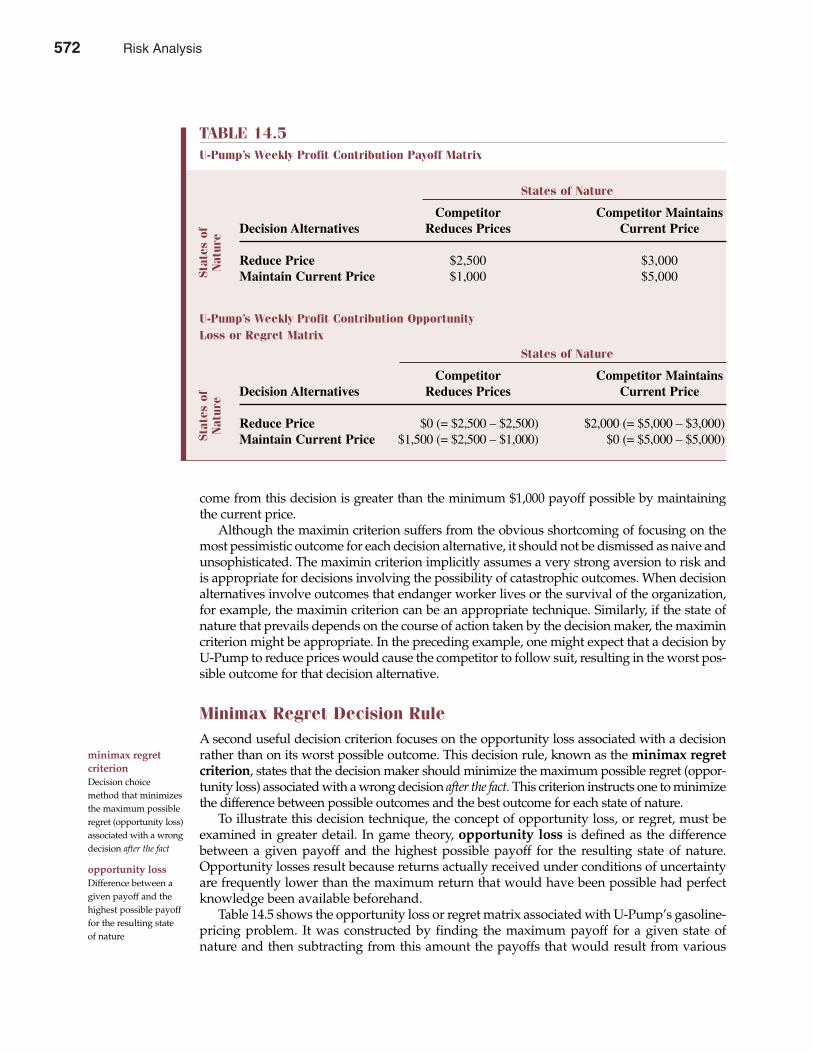
come from this decision is greater than the minimum $1,000 payoff possible by maintainingthe current price.
Although the maximin criterion suffers from the obvious shortcoming of focusing on themost pessimistic outcome for each decision alternative, it should not be dismissed as naive andunsophisticated. The maximin criterion implicitly assumes a very strong aversion to risk andis appropriate for decisions involving the possibility of catastrophic outcomes. When decisionalternatives involve outcomes that endanger worker lives or the survival of the organization,for example, the maximin criterion can be an appropriate technique. Similarly, if the state ofnature that prevails depends on the course of action taken by the decision maker, the maximincriterion might be appropriate. In the preceding example, one might expect that a decision byU-Pump to reduce prices would cause the competitor to follow suit, resulting in the worst pos-sible outcome for that decision alternative.
Minimax Regret Decision RuleA second useful decision criterion focuses on the opportunity loss associated with a decisionrather than on its worst possible outcome. This decision rule, known as the minimax regretcriterion, states that the decision maker should minimize the maximum possible regret (oppor-tunity loss) associated with a wrong decision after the fact. This criterion instructs one to minimizethe difference between possible outcomes and the best outcome for each state of nature.
To illustrate this decision technique, the concept of opportunity loss, or regret, must beexamined in greater detail. In game theory, opportunity loss is defined as the differencebetween a given payoff and the highest possible payoff for the resulting state of nature.Opportunity losses result because returns actually received under conditions of uncertaintyare frequently lower than the maximum return that would have been possible had perfectknowledge been available beforehand.
Table 14.5 shows the opportunity loss or regret matrix associated with U-Pump’s gasoline-pricing problem. It was constructed by finding the maximum payoff for a given state ofnature and then subtracting from this amount the payoffs that would result from various
minimax regret criterionDecision choicemethod that minimizesthe maximum possibleregret (opportunity loss)associated with a wrongdecision after the fact
opportunity lossDifference between agiven payoff and thehighest possible payofffor the resulting stateof nature
Chapter Fourteen Risk Analysis 573
Stat
es o
fN
atur
e
TABLE 14.5U-Pump’s Weekly Profit Contribution Payoff Matrix
States of Nature
Competitor Competitor MaintainsDecision Alternatives Reduces Prices Current Price
Reduce Price $2,500 $3,000Maintain Current Price $1,000 $5,000
U-Pump’s Weekly Profit Contribution OpportunityLoss or Regret Matrix
States of Nature
Competitor Competitor MaintainsDecision Alternatives Reduces Prices Current Price
Reduce Price $0 (= $2,500 – $2,500) $2,000 (= $5,000 – $3,000)Maintain Current Price $1,500 (= $2,500 – $1,000) $0 (= $5,000 – $5,000)St
ates
of
Nat
ure
572 Risk Analysis
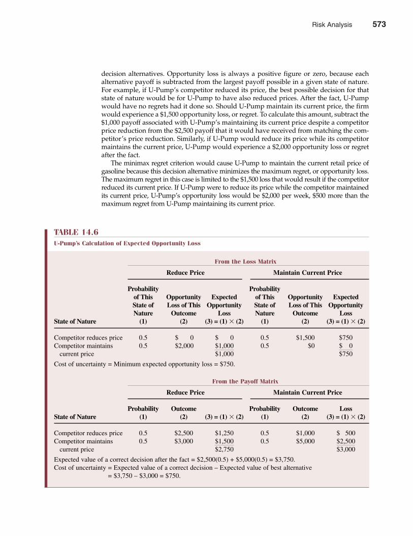
decision alternatives. Opportunity loss is always a positive figure or zero, because eachalternative payoff is subtracted from the largest payoff possible in a given state of nature.For example, if U-Pump’s competitor reduced its price, the best possible decision for thatstate of nature would be for U-Pump to have also reduced prices. After the fact, U-Pumpwould have no regrets had it done so. Should U-Pump maintain its current price, the firmwould experience a $1,500 opportunity loss, or regret. To calculate this amount, subtract the$1,000 payoff associated with U-Pump’s maintaining its current price despite a competitorprice reduction from the $2,500 payoff that it would have received from matching the com-petitor’s price reduction. Similarly, if U-Pump would reduce its price while its competitormaintains the current price, U-Pump would experience a $2,000 opportunity loss or regretafter the fact.
The minimax regret criterion would cause U-Pump to maintain the current retail price ofgasoline because this decision alternative minimizes the maximum regret, or opportunity loss.The maximum regret in this case is limited to the $1,500 loss that would result if the competitorreduced its current price. If U-Pump were to reduce its price while the competitor maintainedits current price, U-Pump’s opportunity loss would be $2,000 per week, $500 more than themaximum regret from U-Pump maintaining its current price.
574 Part Five Long-Term Investment Decisions
TABLE 14.6U-Pump’s Calculation of Expected Opportunity Loss
From the Loss Matrix
Reduce Price Maintain Current Price
Probability Probabilityof This Opportunity Expected of This Opportunity ExpectedState of Loss of This Opportunity State of Loss of This OpportunityNature Outcome Loss Nature Outcome Loss
State of Nature (1) (2) (3) = (1) � (2) (1) (2) (3) = (1) � (2)
Competitor reduces price 0.5 $ 0 $ 0 0.5 $1,500 $750Competitor maintains 0.5 $2,000 $1,000 0.5 $0 $ 0
current price $1,000 $750
Cost of uncertainty = Minimum expected opportunity loss = $750.
From the Payoff Matrix
Reduce Price Maintain Current Price
Probability Outcome Probability Outcome LossState of Nature (1) (2) (3) = (1) � (2) (1) (2) (3) = (1) � (2)
Competitor reduces price 0.5 $2,500 $1,250 0.5 $1,000 $ 500Competitor maintains 0.5 $3,000 $1,500 0.5 $5,000 $2,500
current price $2,750 $3,000
Expected value of a correct decision after the fact = $2,500(0.5) + $5,000(0.5) = $3,750.Cost of uncertainty = Expected value of a correct decision – Expected value of best alternative
= $3,750 – $3,000 = $750.
Risk Analysis 573
Cost of UncertaintyAn unavoidable opportunity loss is the cost associated with uncertainty. Therefore, the expect-ed opportunity loss associated with a decision provides a measure of the expected monetarygain from the removal of all uncertainty about future events. From the opportunity loss orregret matrix, the cost of uncertainty is measured by the minimum expected opportunityloss. From the payoff matrix, the cost of uncertainty is measured by the difference between theexpected payoff associated with choosing the correct alternative under each state of nature(which will be known only after the fact) and the highest expected payoff available fromamong the decision alternatives. The cost of uncertainty is the unavoidable economic loss thatis due to chance. Using this concept, it becomes possible to judge the value of gaining addi-tional information before choosing among decision alternatives.
The previous gasoline-pricing problem can illustrate this use of opportunity loss. On thebasis of the data in Table 14.5, the expected opportunity loss of each decision alternative can becalculated as shown in Table 14.6. Here it is assumed that U-Pump projects a 50/50, or 50 per-cent, chance of a competitor price reduction. The minimum expected opportunity cost in thiscase is $750 and represents U-Pump’s loss from not knowing its competitor’s pricing reactionwith certainty. This cost of uncertainty represents the $750 value to U-Pump of resolving doubtabout its competitor’s pricing policy. U-Pump would be better off if it could eliminate thisuncertainty by making an expenditure of less than $750 on information gathering.
Firms often engage in activities aimed at reducing the uncertainty of various alternativesbefore making an irrevocable decision. For example, a food-manufacturing company willemploy extensive marketing tests in selected areas to gain better estimates of sales potentialbefore going ahead with the large-scale introduction of a new product. Manufacturers ofconsumer goods frequently install new equipment in a limited number of models to judgereliability and customer reaction before including the equipment in all models. Similarly,competitors often announce price changes well in advance of their effective date to elicit thereaction of rivals.
SUMMARY
Risk analysis plays an integral role in the decision process for most business problems. Thischapter defines the concept of economic risk and illustrates how the concept can be dealtwith in the managerial decision-making process.
• Economic risk is the chance of loss due to the fact that all possible outcomes and theirprobability of occurrence are unknown. Uncertainty exists when the outcomes of mana-gerial decisions cannot be predicted with absolute accuracy but all possibilities and theirassociated probabilities of occurrence are known.
• Business risk is the chance of loss associated with a given managerial decision. Many differ-ent types of business risk are apparent in the globally competitive 1990s. Market risk is thechance that a portfolio of investments can lose money because of swings in the stock marketas a whole. Inflation risk is the danger that a general increase in the price level will under-mine real economic values. Interest-rate risk stems from the fact that a fall in interest rateswill increase the value of any agreement that involves a fixed promise to pay interest andprincipal over a specified period. Credit risk is the chance that another party will fail to abideby its contractual obligations. Corporations must also consider the problem of liquidity risk,or the difficulty of selling corporate assets or investments that have only a few willing buy-ers or that are otherwise not easily transferable at favorable prices under typical market con-ditions. Derivative risk is the chance that volatile financial derivatives could create losses inunderlying investments by increasing rather than decreasing price volatility.
cost of uncertaintyMinimum expectedopportunity loss
Chapter Fourteen Risk Analysis 575
574 Risk Analysis
• Cultural risk is borne by companies that pursue a global rather than a solely domesticinvestment strategy. Product market differences due to distinctive social customs make itdifficult to predict which products might do well in foreign markets. Currency risk is anoth-er important danger facing global businesses because most companies wish to eventuallyrepatriate foreign earnings back to the domestic parent. Finally, global investors also experi-ence government policy risk because foreign government grants of monopoly franchises,tax abatements, and favored trade status can be tenuous. Expropriation risk, or the risk thatbusiness property located abroad might be seized by host governments, is another type ofrisk that global investors must not forget.
• The probability of an event is the chance, or odds, that the incident will occur. If all possibleevents or outcomes are listed, and if a probability of occurrence is assigned to each event, thelisting is called a probability distribution. A payoff matrix illustrates the outcome associat-ed with each possible state of nature. The expected value is the anticipated realization froma given payoff matrix.
• Absolute risk is the overall dispersion of possible payoffs. The smaller the standard devi-ation, the tighter the probability distribution and the lower the risk in absolute terms.Relative risk is the variation in possible returns compared with the expected payoffamount. Beta is a measure of the systematic variability or covariance of one asset’s returnswith returns on other assets.
• A normal distribution has a symmetrical distribution about the mean or expected value. Ifa probability distribution is normal, the actual outcome will lie within ±1 standard deviationof the mean roughly 68 percent of the time. The probability that the actual outcome will bewithin ±2 standard deviations of the expected outcome is approximately 95 percent; andthere is a greater than 99 percent probability that the actual outcome will occur within ±3standard deviations of the mean. A standardized variable has a mean of 0 and a standarddeviation equal to 1.
• Risk aversion characterizes individuals who seek to avoid or minimize risk. Risk neutralitycharacterizes decision makers who focus on expected returns and disregard the dispersion ofreturns (risk). Risk seeking characterizes decision makers who prefer risk. At the heart of riskaversion is the notion of diminishing marginal utility, where additional increments of moneybring ever smaller increments of marginal utility.
• Under the certainty equivalent approach, decision makers specify the certain sum thatthey regard comparable to the expected value of a risky investment alternative. Anyexpected risky amount can be converted to an equivalent certain sum using the certaintyequivalent adjustment factor, �, calculated as the ratio of a certain sum divided by anexpected risky amount, where both dollar values provide the same level of utility. Therisk-adjusted valuation model reflects both time value and risk considerations.
• The risk-adjusted discount rate k is the sum of the risk-free rate of return, RF, plus therequired risk premium, Rp. The difference between the expected rate of return on a riskyasset and the rate of return on a riskless asset is the risk premium on the risky asset.
• A decision tree is a map of a sequential decision-making process. Decision trees aredesigned for analyzing decision problems that involve a series of choice alternatives thatare constrained by previous decisions. Decision points represent instances when manage-ment must select among several choice alternatives. Chance events are possible outcomesfollowing each decision point.
• Computer simulation involves the use of computer software and workstations or sophisti-cated desktop computers to create a wide variety of decision outcome scenarios. Sensitivityanalysis focuses on those variables that most directly affect decision outcomes, and it is lessexpensive and less time-consuming than full-scale computer simulation.
576 Part Five Long-Term Investment Decisions
Risk Analysis 575
• Game theory is a useful decision framework employed to make choices in hostile envi-ronments and under extreme uncertainty. A variety of auction strategies are based on gametheory principles.
• The most familiar type of auction is an English auction, where an auctioneer keeps rais-ing the price until a single highest bidder remains. A winner’s curse results when overlyaggressive bidders pay more than the economic value of auctioned items. In a sealed-bidauction, all bids are secret and the highest bid wins. A relatively rare sealed-bid auctionmethod is a Vickrey auction, where the highest sealed bid wins, but the winner pays theprice of the second-highest bid. Another auctioning method is the so-called reverse orDutch auction. In a Dutch auction, the auctioneer keeps lowering a very high price untila winning bidder emerges. The winning bidder is the first participant willing to pay theauctioneer’s price.
• A game-theory decision standard that is sometimes applicable for decision making underuncertainty is the maximin criterion, which states that the decision maker should select thealternative that provides the best of the worst possible outcomes. The minimax regret crite-rion states that the decision maker should minimize the maximum possible regret (oppor-tunity loss) associated with a wrong decision after the fact. In game theory, opportunity lossis defined as the difference between a given payoff and the highest possible payoff for theresulting state of nature. From the opportunity loss or regret matrix, the cost of uncertaintyis measured by the minimum expected opportunity loss.
Decision making under conditions of uncertainty is greatly facilitated by use of the tools andtechniques discussed in this chapter. Although uncertainty can never be eliminated, it can beassessed and dealt with to minimize its harmful consequences.
QUESTIONS
Q14.1 Define the following terms:A. Probability distributionB. Expected valueC. Standard deviationD. Coefficient of variationE. RiskF. Diminishing marginal utility of moneyG. Certainty equivalentH. Risk-adjusted discount rateI. Decision treeJ. Simulation
Q14.2 What is the main difficulty associated with making decisions solely on the basis of comparisonsof expected returns?
Q14.3 The standard deviation measure of risk implicitly gives equal weight to variations on bothsides of the expected value. Can you see any potential limitations of this treatment?
Q14.4 “Utility is a theoretical concept that cannot be observed or measured in the real world. Hence,it has no practical value in decision analysis.” Discuss this statement.
Q14.5 Graph the relation between money and its utility for an individual who buys both householdfire insurance and state lottery tickets.
Q14.6 When the basic valuation model is adjusted using the risk-free rate, i, what economic factoris being explicitly accounted for?
Chapter Fourteen Risk Analysis 577
576 Risk Analysis
Q14.7 If the expected net present value of returns from an investment project is $50,000, what is themaximum price that a risk-neutral investor would pay for it? Explain.
Q14.8 “Market estimates of investors’ reactions to risk cannot be measured precisely, so it is impos-sible to set risk-adjusted discount rates for various classes of investment with a high degreeof precision.” Discuss this statement.
Q14.9 What is the value of decision trees in managerial decision making?Q14.10 When is it most useful to use game theory in decision analysis?
SELF-TEST PROBLEMS AND SOLUTIONS
ST14.1 Certainty Equivalent Method. MacKenzie-Rabb, Inc., is a Texas–based manufacturer anddistributor of components and replacement parts for the auto, machinery, farm, and construc-tion equipment industries. The company is currently funding a program of capital investmentthat is necessary to reduce production costs and thereby meet an onslaught of competition fromlow-cost suppliers located in Mexico and throughout Latin America. MacKenzie-Rabb has alimited amount of capital available and must carefully weigh both the risks and potentialrewards associated with alternative investments. In particular, the company seeks to weigh theadvantages and disadvantages of a new investment project, project X, in light of two otherrecently adopted investment projects, project Y and project Z:
A. Using a 5% risk-free rate, calculate the present value of expected cash flows after tax (CFAT)for the 10-year life of project X.
B. Calculate the minimum certainty equivalent adjustment factor for each project’s CFAT thatwould justify investment in each project.
C. Assume that the management of MacKenzie-Rabb is risk averse and uses the certaintyequivalent method in decision making. Is project X as attractive or more attractive thanprojects Y and Z?
D. If the company would not have been willing to invest more than $60,000 in project Y normore than $50,000 in project Z, should project X be undertaken?
ST14.1 SolutionA. Using a 5% risk-free rate, the present value of expected cash flows after tax (CFAT) for the
10-year life of project X is $77,217, calculated as follows:
578 Part Five Long-Term Investment Decisions
Expected Cash Flows After Tax (CFAT) per Year
Year Project X Project Y Project Z
2001 $10,000 $20,000 $02002 10,000 18,000 2,5002003 10,000 16,000 5,0002004 10,000 14,000 7,5002005 10,000 12,000 10,0002006 10,000 10,000 12,5002007 10,000 8,000 15,0002008 10,000 6,000 17,5002009 10,000 4,000 20,0002010 10,000 2,000 22,500
PV of Cash Flow @ 5% $91,131 $79,130Investment Outlay in 2000: $60,000 $60,000 $50,000
Risk Analysis 577
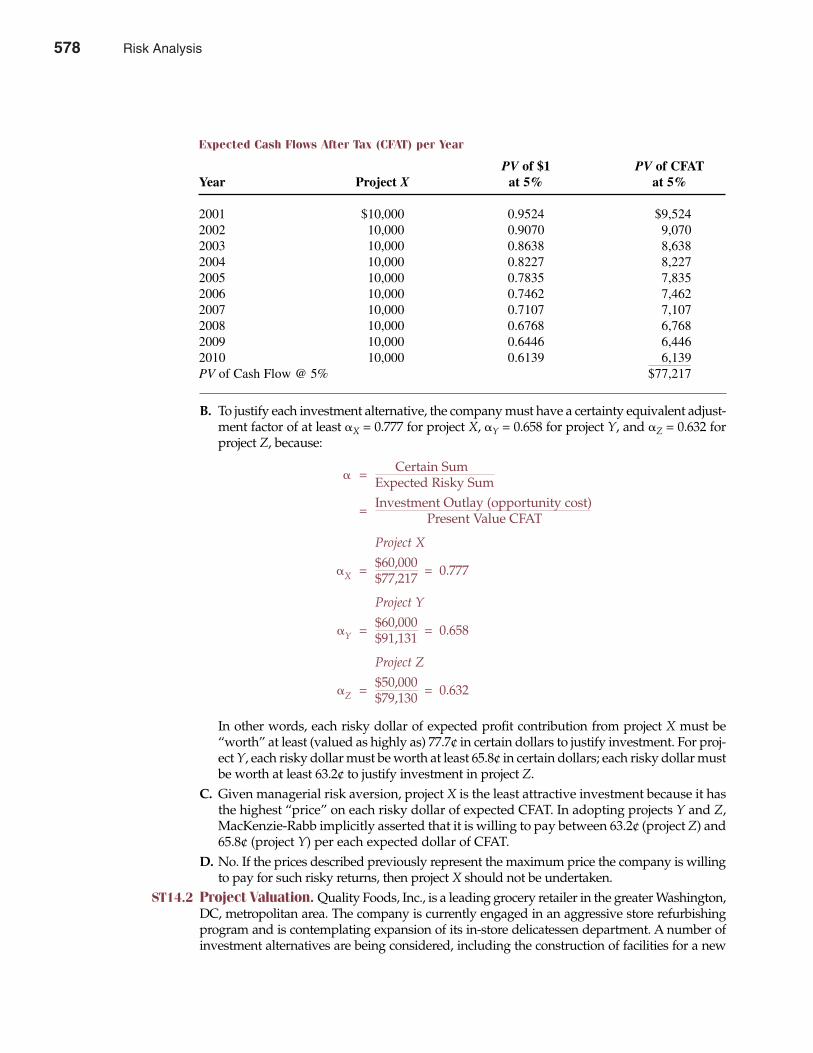
Chapter Fourteen Risk Analysis 579
B. To justify each investment alternative, the company must have a certainty equivalent adjust-ment factor of at least �X = 0.777 for project X, �Y = 0.658 for project Y, and �Z = 0.632 forproject Z, because:
� = Certain SumExpected Risky Sum
= Investment Outlay (opportunity cost)Present Value CFAT
Project X
�X = $60,000 = 0.777$77,217
Project Y
�Y = $60,000 = 0.658$91,131
Project Z
�Z = $50,000 = 0.632$79,130
In other words, each risky dollar of expected profit contribution from project X must be“worth” at least (valued as highly as) 77.7¢ in certain dollars to justify investment. For proj-ect Y, each risky dollar must be worth at least 65.8¢ in certain dollars; each risky dollar mustbe worth at least 63.2¢ to justify investment in project Z.
C. Given managerial risk aversion, project X is the least attractive investment because it hasthe highest “price” on each risky dollar of expected CFAT. In adopting projects Y and Z,MacKenzie-Rabb implicitly asserted that it is willing to pay between 63.2¢ (project Z) and65.8¢ (project Y) per each expected dollar of CFAT.
D. No. If the prices described previously represent the maximum price the company is willingto pay for such risky returns, then project X should not be undertaken.
ST14.2 Project Valuation. Quality Foods, Inc., is a leading grocery retailer in the greater Washington,DC, metropolitan area. The company is currently engaged in an aggressive store refurbishingprogram and is contemplating expansion of its in-store delicatessen department. A number ofinvestment alternatives are being considered, including the construction of facilities for a new
Expected Cash Flows After Tax (CFAT) per Year
PV of $1 PV of CFATYear Project X at 5% at 5%
2001 $10,000 0.9524 $9,5242002 10,000 0.9070 9,0702003 10,000 0.8638 8,6382004 10,000 0.8227 8,2272005 10,000 0.7835 7,8352006 10,000 0.7462 7,4622007 10,000 0.7107 7,1072008 10,000 0.6768 6,7682009 10,000 0.6446 6,4462010 10,000 0.6139 6,139 PV of Cash Flow @ 5% $77,217
578 Risk Analysis
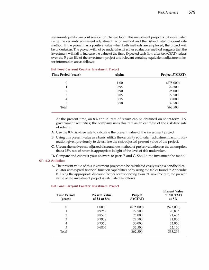
restaurant-quality carryout service for Chinese food. This investment project is to be evaluatedusing the certainty equivalent adjustment factor method and the risk-adjusted discount ratemethod. If the project has a positive value when both methods are employed, the project willbe undertaken. The project will not be undertaken if either evaluation method suggests that theinvestment will fail to increase the value of the firm. Expected cash flow after tax (CFAT) valuesover the 5-year life of the investment project and relevant certainty equivalent adjustment fac-tor information are as follows:
At the present time, an 8% annual rate of return can be obtained on short-term U.S.government securities; the company uses this rate as an estimate of the risk-free rateof return.
A. Use the 8% risk-free rate to calculate the present value of the investment project.B. Using this present value as a basis, utilize the certainty equivalent adjustment factor infor-
mation given previously to determine the risk-adjusted present value of the project.C. Use an alternative risk-adjusted discount rate method of project valuation on the assumption
that a 15% rate of return is appropriate in light of the level of risk undertaken.D. Compare and contrast your answers to parts B and C. Should the investment be made?
ST14.2 SolutionA. The present value of this investment project can be calculated easily using a handheld cal-
culator with typical financial function capabilities or by using the tables found in AppendixB. Using the appropriate discount factors corresponding to an 8% risk-free rate, the presentvalue of the investment project is calculated as follows:
580 Part Five Long-Term Investment Decisions
Hot Food Carryout Counter Investment Project
Time Period (years) Alpha Project E(CFAT)
0 1.00 ($75,000)1 0.95 22,5002 0.90 25,0003 0.85 27,5004 0.75 30,0005 0.70 32,500
Total $62,500
Hot Food Carryout Counter Investment Project
Present ValueTime Period Present Value Project of E(CFAT)
(years) of $1 at 8% E (CFAT) at 8%
0 1.0000 ($75,000) ($75,000)1 0.9259 22,500 20,8332 0.8573 25,000 21,4333 0.7938 27,500 21,8304 0.7350 30,000 22,0505 0.6806 32,500 22,120
Total $62,500 $33,266
Risk Analysis 579
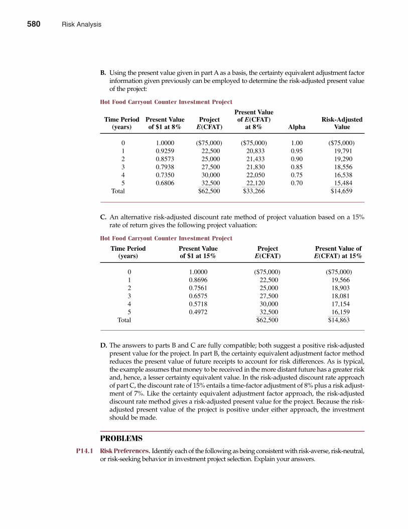
B. Using the present value given in part A as a basis, the certainty equivalent adjustment factorinformation given previously can be employed to determine the risk-adjusted present valueof the project:
C. An alternative risk-adjusted discount rate method of project valuation based on a 15%rate of return gives the following project valuation:
D. The answers to parts B and C are fully compatible; both suggest a positive risk-adjustedpresent value for the project. In part B, the certainty equivalent adjustment factor methodreduces the present value of future receipts to account for risk differences. As is typical,the example assumes that money to be received in the more distant future has a greater riskand, hence, a lesser certainty equivalent value. In the risk-adjusted discount rate approachof part C, the discount rate of 15% entails a time-factor adjustment of 8% plus a risk adjust-ment of 7%. Like the certainty equivalent adjustment factor approach, the risk-adjusteddiscount rate method gives a risk-adjusted present value for the project. Because the risk-adjusted present value of the project is positive under either approach, the investmentshould be made.
PROBLEMS
P14.1 Risk Preferences. Identify each of the following as being consistent with risk-averse, risk-neutral,or risk-seeking behavior in investment project selection. Explain your answers.
Chapter Fourteen Risk Analysis 581
Hot Food Carryout Counter Investment Project
Present ValueTime Period Present Value Project of E(CFAT) Risk-Adjusted
(years) of $1 at 8% E(CFAT) at 8% Alpha Value
0 1.0000 ($75,000) ($75,000) 1.00 ($75,000)1 0.9259 22,500 20,833 0.95 19,7912 0.8573 25,000 21,433 0.90 19,2903 0.7938 27,500 21,830 0.85 18,5564 0.7350 30,000 22,050 0.75 16,5385 0.6806 32,500 22,120 0.70 15,484
Total $62,500 $33,266 $14,659
Hot Food Carryout Counter Investment Project
Time Period Present Value Project Present Value of(years) of $1 at 15% E(CFAT) E(CFAT) at 15%
0 1.0000 ($75,000) ($75,000)1 0.8696 22,500 19,5662 0.7561 25,000 18,9033 0.6575 27,500 18,0814 0.5718 30,000 17,1545 0.4972 32,500 16,159
Total $62,500 $14,863
580 Risk Analysis
A. Larger risk premiums for riskier projectsB. Preference for smaller, as opposed to larger, coefficients of variationC. Valuing certain sums and expected risky sums of equal dollar amounts equallyD. Having an increasing marginal utility of moneyE. Ignoring the risk levels of investment alternatives
P14.2 Certainty Equivalents. The certainty equivalent concept can be widely employed in theanalysis of personal and business decision making. Indicate whether each of the followingstatements is true or false and explain why:A. The appropriate certainty equivalent adjustment factor, �, indicates the minimum price in
certain dollars that an individual should be willing to pay per risky dollar of expected return.B. An � ≠ 1 implies that a certain sum and a risky expected return of different dollar amounts
provide equivalent utility to a given decision maker.C. If previously accepted projects with similar risk have �s in a range from � = 0.4 to � = 0.5,
an investment with an expected return of $150,000 is acceptable at a cost of $50,000.D. A project for which NPV > 0 using an appropriate risk-adjusted discount rate has an
implied � factor that is too large to allow project acceptance.E. State lotteries that pay out 50% of the revenues that they generate require players who
place at least a certain $2 value on each $1 of expected risky return.P14.3 Expected Value. Duddy Kravitz, a broker with Caveat Emptor, Ltd., offers free investment
seminars to local PTA groups. On average, Kravitz expects 1% of seminar participants topurchase $25,000 in tax-sheltered investments and 5% to purchase $5,000 in stocks andbonds. Kravitz earns a 4% net commission on tax shelters and a 1% commission on stocksand bonds. Calculate Kravitz’s expected net commissions per seminar if attendance aver-ages 10 persons.
P14.4 Probability Concepts. Aquarius Products, Inc., has just completed development of anew line of skin-care products. Preliminary market research indicates two feasible market-ing strategies: (1) creating general consumer acceptance through media advertising or (2)creating distributor acceptance through intensive personal selling by company representa-tives. The marketing manager has developed the following estimates for sales under eachalternative:
A. Assume that the company has a 50% profit margin on sales (that is, profits equal one-halfof sales revenue). Calculate expected profits for each plan.
B. Construct a simple bar graph of the possible profit outcomes for each plan. Which planappears to be riskier?
C. Assume that management’s utility function resembles the one illustrated in the follow-ing figure. Which strategy should the marketing manager recommend?
582 Part Five Long-Term Investment Decisions
Media Advertising Strategy Personal Selling Strategy
Probability Sales Probability Sales
0.1 $ 500,000 0.3 $1,000,0000.4 1,500,000 0.4 1,500,0000.4 2,500,000 0.3 2,000,0000.1 3,500,000
Risk Analysis 581
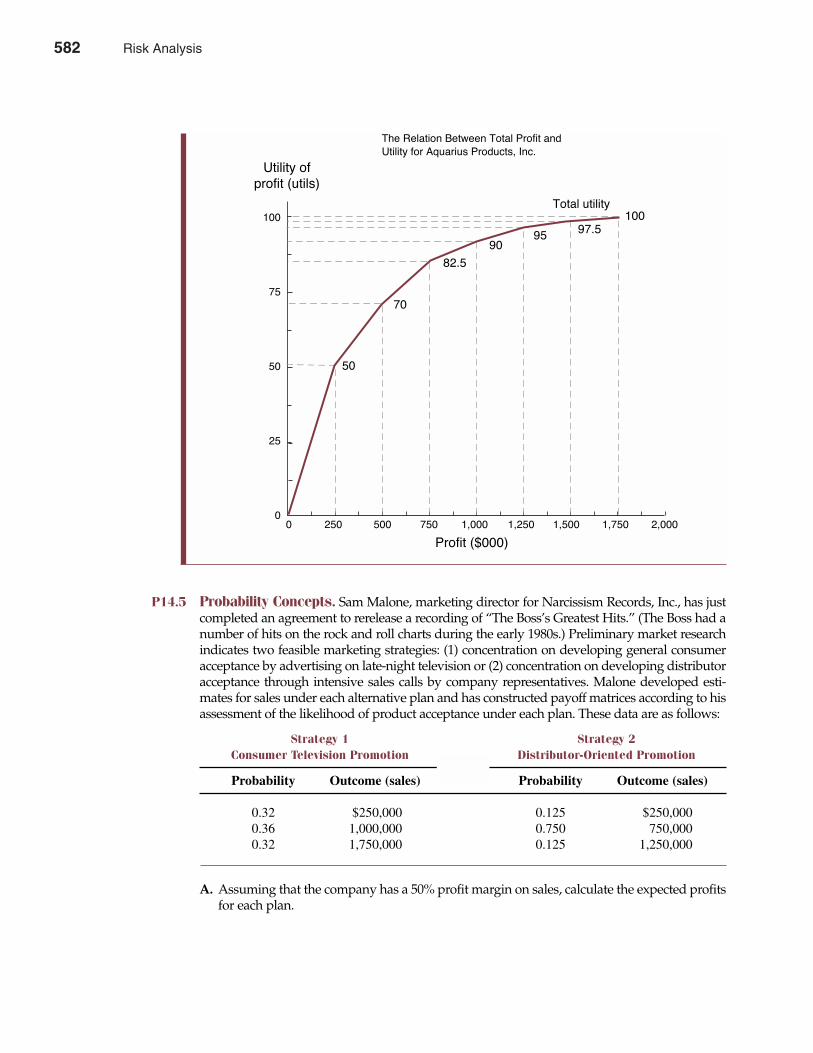
P14.5 Probability Concepts. Sam Malone, marketing director for Narcissism Records, Inc., has justcompleted an agreement to rerelease a recording of “The Boss’s Greatest Hits.” (The Boss had anumber of hits on the rock and roll charts during the early 1980s.) Preliminary market researchindicates two feasible marketing strategies: (1) concentration on developing general consumeracceptance by advertising on late-night television or (2) concentration on developing distributoracceptance through intensive sales calls by company representatives. Malone developed esti-mates for sales under each alternative plan and has constructed payoff matrices according to hisassessment of the likelihood of product acceptance under each plan. These data are as follows:
A. Assuming that the company has a 50% profit margin on sales, calculate the expected profitsfor each plan.
Chapter Fourteen Risk Analysis 583
Strategy 1 Strategy 2Consumer Television Promotion Distributor-Oriented Promotion
Probability Outcome (sales) Probability Outcome (sales)
0.32 $250,000 0.125 $250,0000.36 1,000,000 0.750 750,0000.32 1,750,000 0.125 1,250,000
The Relation Between Total Profit and
Utility for Aquarius Products, Inc.
100
75
50
25
00 250 500 750 1,000 1,250 1,500 1,750 2,000
Profit ($000)
Utility ofprofit (utils)
Total utility100
97.595
90
82.5
70
50
582 Risk Analysis
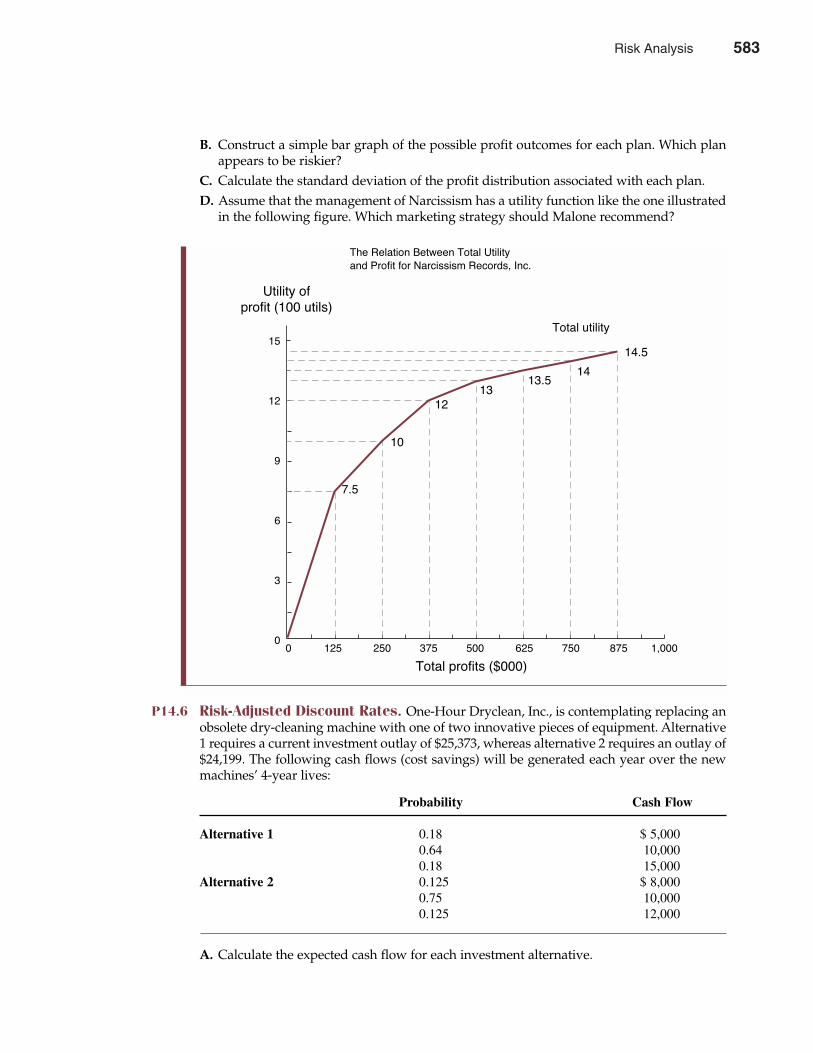
B. Construct a simple bar graph of the possible profit outcomes for each plan. Which planappears to be riskier?
C. Calculate the standard deviation of the profit distribution associated with each plan.D. Assume that the management of Narcissism has a utility function like the one illustrated
in the following figure. Which marketing strategy should Malone recommend?
P14.6 Risk-Adjusted Discount Rates. One-Hour Dryclean, Inc., is contemplating replacing anobsolete dry-cleaning machine with one of two innovative pieces of equipment. Alternative1 requires a current investment outlay of $25,373, whereas alternative 2 requires an outlay of$24,199. The following cash flows (cost savings) will be generated each year over the newmachines’ 4-year lives:
A. Calculate the expected cash flow for each investment alternative.
584 Part Five Long-Term Investment Decisions
The Relation Between Total Utility
and Profit for Narcissism Records, Inc.
15
12
9
6
3
00 125 250 375 500 625 750 875 1,000
Total profits ($000)
Utility ofprofit (100 utils)
Total utility
14.5
1413.5
1312�
10
7.5�
Probability Cash Flow
Alternative 1 0.18 $ 5,0000.64 10,0000.18 15,000
Alternative 2 0.125 $ 8,0000.75 10,0000.125 12,000
Risk Analysis 583
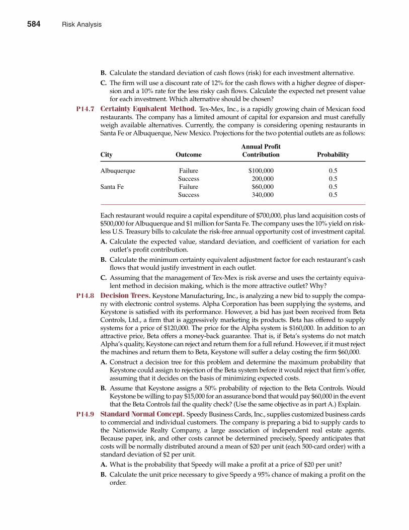
B. Calculate the standard deviation of cash flows (risk) for each investment alternative.C. The firm will use a discount rate of 12% for the cash flows with a higher degree of disper-
sion and a 10% rate for the less risky cash flows. Calculate the expected net present valuefor each investment. Which alternative should be chosen?
P14.7 Certainty Equivalent Method. Tex-Mex, Inc., is a rapidly growing chain of Mexican foodrestaurants. The company has a limited amount of capital for expansion and must carefullyweigh available alternatives. Currently, the company is considering opening restaurants inSanta Fe or Albuquerque, New Mexico. Projections for the two potential outlets are as follows:
Each restaurant would require a capital expenditure of $700,000, plus land acquisition costs of$500,000 for Albuquerque and $1 million for Santa Fe. The company uses the 10% yield on risk-less U.S. Treasury bills to calculate the risk-free annual opportunity cost of investment capital.A. Calculate the expected value, standard deviation, and coefficient of variation for each
outlet’s profit contribution.B. Calculate the minimum certainty equivalent adjustment factor for each restaurant’s cash
flows that would justify investment in each outlet.C. Assuming that the management of Tex-Mex is risk averse and uses the certainty equiva-
lent method in decision making, which is the more attractive outlet? Why?P14.8 Decision Trees. Keystone Manufacturing, Inc., is analyzing a new bid to supply the compa-
ny with electronic control systems. Alpha Corporation has been supplying the systems, andKeystone is satisfied with its performance. However, a bid has just been received from BetaControls, Ltd., a firm that is aggressively marketing its products. Beta has offered to supplysystems for a price of $120,000. The price for the Alpha system is $160,000. In addition to anattractive price, Beta offers a money-back guarantee. That is, if Beta’s systems do not matchAlpha’s quality, Keystone can reject and return them for a full refund. However, if it must rejectthe machines and return them to Beta, Keystone will suffer a delay costing the firm $60,000.A. Construct a decision tree for this problem and determine the maximum probability that
Keystone could assign to rejection of the Beta system before it would reject that firm’s offer,assuming that it decides on the basis of minimizing expected costs.
B. Assume that Keystone assigns a 50% probability of rejection to the Beta Controls. WouldKeystone be willing to pay $15,000 for an assurance bond that would pay $60,000 in the eventthat the Beta Controls fail the quality check? (Use the same objective as in part A.) Explain.
P14.9 Standard Normal Concept. Speedy Business Cards, Inc., supplies customized business cardsto commercial and individual customers. The company is preparing a bid to supply cards tothe Nationwide Realty Company, a large association of independent real estate agents.Because paper, ink, and other costs cannot be determined precisely, Speedy anticipates thatcosts will be normally distributed around a mean of $20 per unit (each 500-card order) with astandard deviation of $2 per unit.A. What is the probability that Speedy will make a profit at a price of $20 per unit?B. Calculate the unit price necessary to give Speedy a 95% chance of making a profit on the
order.
Chapter Fourteen Risk Analysis 585
Annual ProfitCity Outcome Contribution Probability
Albuquerque Failure $100,000 0.5Success 200,000 0.5
Santa Fe Failure $60,000 0.5Success 340,000 0.5
584 Risk Analysis
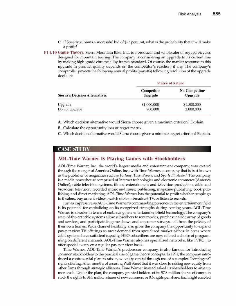
C. If Speedy submits a successful bid of $23 per unit, what is the probability that it will makea profit?
P14.10 Game Theory. Sierra Mountain Bike, Inc., is a producer and wholesaler of rugged bicyclesdesigned for mountain touring. The company is considering an upgrade to its current lineby making high-grade chrome alloy frames standard. Of course, the market response to thisupgrade in product quality depends on the competitor’s reaction, if any. The company’scomptroller projects the following annual profits (payoffs) following resolution of the upgradedecision:
A. Which decision alternative would Sierra choose given a maximin criterion? Explain.B. Calculate the opportunity loss or regret matrix.C. Which decision alternative would Sierra choose given a minimax regret criterion? Explain.
586 Part Five Long-Term Investment Decisions
States of Nature
Competitor No Competitor Sierra’s Decision Alternatives Upgrade Upgrade
Upgrade $1,000,000 $1,500,000Do not upgrade 800,000 2,000,000
CASE STUDY
AOL-Time Warner Is Playing Games with StockholdersAOL-Time Warner, Inc., the world’s largest media and entertainment company, was createdthrough the merger of America Online, Inc., with Time Warner, a company that is best knownas the publisher of magazines such as Fortune, Time, People, and Sports Illustrated. The companyis a media powerhouse comprised of Internet technologies and electronic commerce (AmericaOnline), cable television systems, filmed entertainment and television production, cable andbroadcast television, recorded music and music publishing, magazine publishing, book pub-lishing, and direct marketing. AOL-Time Warner has the potential to profit whether people goto theaters, buy or rent videos, watch cable or broadcast TV, or listen to records.
Just as impressive as AOL-Time Warner’s commanding presence in the entertainment fieldis its potential for capitalizing on its recognized strengths during coming years. AOL-TimeWarner is a leader in terms of embracing new entertainment-field technology. The company’sstate-of-the-art cable systems allow subscribers to rent movies, purchase a wide array of goodsand services, and participate in game shows and consumer surveys—all from the privacy oftheir own homes. Wide channel flexibility also gives the company the opportunity to expandpay-per-view TV offerings to meet demand from specialized market niches. In areas wherecable systems have sufficient capacity, HBO subscribers are now offered a choice of program-ming on different channels. AOL-Time Warner also has specialized networks, like TVKO , tooffer special events on a regular pay-per-view basis.
Time Warner, AOL-Time Warner’s predecessor company, is also famous for introducingcommon stockholders to the practical use of game theory concepts. In 1991, the company intro-duced a controversial plan to raise new equity capital through use of a complex “contingent”rights offering. After months of assuring Wall Street that it was close to raising new equity fromother firms through strategic alliances, Time Warner instead asked its shareholders to ante upmore cash. Under the plan, the company granted holders of its 57.8 million shares of commonstock the rights to 34.5 million shares of new common, or 0.6 rights per share. Each right enabled
Risk Analysis 585
Chapter Fourteen Risk Analysis 587
a shareholder to pay Time Warner $105 for an unspecified number of new common shares.Because the number of new shares that might be purchased for $105 was unspecified, so toowas the price per share. Time Warner’s Wall Street advisers structured the offer so that the newstock would be offered at cheaper prices if fewer shareholders chose to exercise their rights.
In an unusual arrangement, the rights from all participating shareholders were to beplaced in a pool to determine their pro rata share of the 34.45 million shares to be distributed.If 100% of Time Warner shareholders chose to exercise their rights, the price per share wouldbe $105; the number of shares owned by each shareholder would increase by 60%; and eachshareholder would retain his or her same proportionate ownership in the company. In theevent that less than 100% of the shareholders chose to participate, participating shareholderswould receive a discount price and increase their proportionate interest in the company. Ifonly 80% of Time Warner shareholders chose to exercise their rights, the price per sharewould be $84; if 60% chose to exercise their rights, the price per share would be $63. Theselower prices reflect the fact that if only 80% of Time Warner shareholders chose to exercisetheir rights, each $105 right would purchase 1.25 shares; if 60% chose to exercise their rights,each $105 right would purchase roughly 1.667 shares. Finally, to avoid the possibility of issu-ing equity at fire-sale prices, Time Warner reserved the privilege to cancel the equity offeringentirely if fewer than 60% of holders chose to exercise their rights.
The terms of the offer were designed to make Time Warner shareholders feel compelled toexercise their rights in hopes of getting cheap stock and avoiding seeing their holdings dilut-ed. Although such contingent rights offerings are a common capital-raising technique inBritain, prior to the Time Warner offering they had never been proposed on such a large scalein the United States. Wall Street traders and investment bankers lauded the Time Warner offeras a brilliant coercive device—a view that might have been colored by the huge fees they stoodto make on the offering. Advisory fees for Merrill Lynch and Time Warner’s seven other keyadvisers were projected at $41.5 million to $145 million, depending on the number of partici-pating shareholders. An additional $20.7 million to $34.5 million was set aside to pay otherinvestment bankers for soliciting shareholders to exercise their rights. Time Warner’s advisersargued that their huge fees totaling 5.22% of the proceeds to the company were justifiedbecause the offering entered uncharted ground in terms of Wall Street experience. Disgruntledshareholders noted that a similar contingent rights offering by Bass PLC of Britain involved afee of only 2.125% of the proceeds to the company, despite the fact that the lead underwriter,Schroders PLC, agreed to buy and resell any new stock that was not claimed by rights hold-ers. This led to charges that Time Warner’s advisers were charging underwriters’ fees withoutrisking any of their own capital.
Proceeds from the offering were earmarked to help pay down the $11.3 billion debt Time Inc.took on to buy Warner Communications Inc. 2 years previously, when Time Warner was formed.Time Warner maintained that it was in intensive talks with potential strategic partners and thatthe rights offering would strengthen its hand in those negotiations by improving the company’sbalance sheet. Time Warner said that the rights offering would enhance its ability to enter intostrategic alliances or joint ventures with partners overseas. Such alliances would help the com-pany penetrate markets in Japan, Europe, and elsewhere. Critics of the plan argued that thebenefits from strategic alliances come in small increments and that Time Warner had failed tostrike any such deals previously because it wants both management control and a premiumprice from potential partners. These critics also maintained that meaningful revenue from anysuch projects is probably years away.
Stockholder reaction to the Time Warner offering was immediate and overwhelminglynegative. On the day the offering was announced, Time Warner shares closed at $99.50, down$11.25, in New York Stock Exchange composite trading. This was in addition to a decline of$6 suffered the previous day on the basis of a report in The Wall Street Journal that some form
CASE STUDY (continued)
586 Risk Analysis

SELECTED REFERENCESAbel, Andrew B. “Will Bequests Attenuate the Predicted Meltdown in Stock Prices When Baby
Boomers Retire?” Review of Economics and Statistics 83 (November 2001): 589–595.Bell, Timothy B., Wayne R. Landsman, and Douglas A. Shackelford. “Auditors’ Perceived Business
Risk and Audit Fees: Analysis and Evidence.” Journal of Accounting Research 39 (June 2001): 35–43.Byrne, Peter J, and Stephen Lee. “Risk Reduction and Real Estate Portfolio Size.” Managerial & Decision
Economics 22 (October/November 2001): 369–379.Cooley, Thomas F., and Vincenzo Quadrini. “Financial Markets and Firm Dynamics.” American Economic
Review 91 (December 2001): 1286–1310.Deck, Cary A. “A Test of Game-Theoretic and Behavioral Models of Play in Exchange and Insurance
Environments.” American Economic Review 91 (December 2001): 1546–1555.Dee, Thomas S., and William N. Evans. “Behavioral Policies and Teen Traffic Safety.” American Economic
Review 91 (May 2001): 91–96.Docking, Dianne Scott, Mark Hirschey, and Elaine Jones. “Reaction of Bank Stock Prices to Loan-Loss
Reserve Announcements.” Review of Quantitative Finance & Accounting 15 (November 2000): 277–297.Goeree, Jacob K., and Charles A. Holt. “Ten Little Treasures of Game Theory and Ten Intuitive Contra-
dictions.” American Economic Review 91 (December 2001): 1402–1422.Hirschey, Mark, Vernon J. Richardson, and Susan Scholz. “How ‘Foolish’ Are Internet Investors?” Financial
Analysts Journal 56 (January/February 2000): 62–69.Kroszner, Randall S., and Philip E. Strahan. “Bankers on Boards: Monitoring, Conflicts of Interest, and
Lender Liability.” Journal of Business 62 (December 2001): 415–452. Lewis, Craig M., Richard J. Rogalski, and James K. Seward. “The Long-Run Performance of Firms That
Issue Convertible Debt: An Empirical Analysis of Operating Characteristics and Analyst Forecasts.”Journal of Corporate Finance 7 (December 2001): 447–474.
588 Part Five Long-Term Investment Decisions
CASE STUDY (continued)
of equity offering was being considered. After trading above $120 per share in the days priorto the first reports of a pending offer, Time Warner shares plummeted by more than 25% to$88 per share within a matter of days. This is yet one more disappointment for the company’slong-suffering common stockholders. During the summer of 1989, Time cited a wide range ofsynergistic benefits to be gained from a merger with Warner Communications and spurneda $200 per share buyout offer from Paramount Communications, Inc. This is despite the factthat the Paramount offer represented a fat 60% premium to the then prevailing market priceof $125 for Time stock. During the succeeding 2-year period, Time Warner stock failed to riseabove this $125 level and traded as low as $66 per share during the fall of 1990. Meanwhile,the hoped-for Time Warner synergy has yet to emerge.A. Was Paramount’s above-market offer for Time, Inc., consistent with the notion that the
prevailing market price for common stock is an accurate reflection of the discounted netpresent value of future cash flows? Was management’s rejection of Paramount’s above-market offer for Time, Inc., consistent with the value-maximization concept?
B. Assume that a Time Warner shareholder could buy additional shares at a market price of$90 or participate in the company’s rights offering. Construct the payoff and regret matri-ces per share that correspond to a $90 per share purchase decision versus a decision toparticipate in the rights offering with subsequent 100%, 80%, and 60% participation by allTime Warner shareholders.
C. Describe the relevant maximin and minimax shareholder strategies.D. Explain why the price of Time Warner common stock fell following the announcement
of the company’s controversial rights offering. Is such an offering in the best interests ofcurrent shareholders?
Risk Analysis 587

Lo, Andrew W. “Risk Management for Hedge Funds: Introduction and Overview.” Financial AnalystsJournal 57 (November/December 2001): 16–33.
Mitchell, Mark, and Todd Pulvino. “Characteristics of Risk and Return in Risk Arbitrage.” Journal ofFinance 56 (December 2001): 2135–2176.
Pan, Jun. “The Jump-Risk Premia Implicit in Options: Evidence from an Integrated Time-Series Study.”Journal of Financial Economics 63 (January 2002): 3–50.
Syau, Yu-Ru, and Hai-Teh Hsieh. “Fuzzy Numbers in the Credit Rating of Enterprise Financial Condition.”Review of Quantitative Finance and Accounting 17 (December 2001): 351–360.
Chapter Fourteen Risk Analysis 589
588 Risk Analysis

Capital Budgeting
CHAPTER FIFTEEN
590 1 Ben Siegel, “Filing Shows Berkshire Hathaway Paid $223.4 Million for Albecca,” The WallStreet Journal Online, February 22, 2002 (http://online.wsj.com).
B erkshire Hathaway, General Electric, and Johnson & Johnson are stand-out performers in terms of the amount of wealth created for sharehold-
ers. What these diverse companies share is a common devotion to the capitalbudgeting process. They manage capital resources using two simple concepts:(1) Funds employed in the business have a cost that must be paid, and (2) fundsshould be allocated where they generate the largest profit.
For example, careful asset redeployment within the General Electric empireallows GE to maintain rapid growth and an enviable rate of return on investedcapital. At the cornerstone of GE’s capital budgeting process is a “value added”concept that measures wealth created, or lost, for GE shareholders. To deter-mine the value added from a given line of business or investment project, GEdeducts the explicit or implicit cost of capital employed from the after-tax prof-it earned on operations. What’s left over is the amount of value added forshareholders. GE then simply allocates its capital among those investment ideasthat generate the most value added. If attractive investment opportunities areabundant, GE seeks additional debt or equity financing. If too few compellinginvestment projects are available, GE uses excess capital to buy back its stock orpay down debt. This simple philosophy has propelled GE, and companies likeit, to stunning success.1
This chapter describes the mechanics of capital budgeting as an applica-tion of marginal analysis. In capital budgeting, marginal revenue is measuredby the incremental cash flows derived from investment projects; marginalcost is the added expense of new investment capital. The value of the firm ismaximized when these marginal revenues and marginal costs are equal.
589
15
CAPITAL BUDGETING PROCESS
Management invests hundreds of billions of dollars per year in fixed assets. By their verynature, these investment decisions have the potential to affect a firm’s fortunes over severalyears. A good decision can boost earnings sharply and dramatically increase the value of thefirm. A bad decision can lead to bankruptcy. Effective planning and control is essential if thehealth and long-run viability of the firm is to be assured.
What Is Capital Budgeting?The term capital refers to the funds employed to finance fixed assets used in production; a budg-et is a detailed plan of projected inflows and outflows over future periods. Capital budgetingis the process of planning expenditures that generate cash flows expected to extend beyond 1year. The choice of 1 year is arbitrary, of course, but it is a convenient cutoff for distinguishingbetween classes of expenditures. Examples of capital outlays are expenditures for land, buildingsand equipment, and for additions to working capital (e.g., inventories and receivables) madenecessary by expansion. New advertising campaigns or research and development programsare also likely to have impacts beyond 1 year and come within the classification of capitalbudgeting expenditures.
Capital budgeting integrates the various elements of the firm. Although the financial man-ager generally has administrative control of the capital budgeting process, the effectiveness ofa firm’s capital investments depends on input from all major departments. The marketingdepartment makes a key contribution by providing sales forecasts. Because operating costsmust be estimated, the accounting, production, engineering, and purchasing departments arealso involved. The initial outlay, or investment cost, must be estimated; again, engineering andpurchasing typically provide input. Obtaining funds and estimating their cost are major tasksof the financial manager. Finally, these various estimates must be drawn together in the formof a project evaluation. Although the finance department generally writes up the evaluationreport, top management ultimately sets standards of acceptability.
Project Selection ProcessA firm’s growth and development, even its ability to remain competitive and to survive,depend on a constant flow of ideas for new products and ways to make existing products bet-ter and at lower cost. A well-managed firm goes to great lengths to develop good capital budg-eting proposals. For example, a sales representative may report that customers are asking fora particular product that the company does not now produce. The sales manager then will dis-cuss the idea with the marketing research group to determine the size of the market for theproposed product. If it appears likely that a substantial market does exist, cost accountants andengineers will be asked to estimate production costs. If it appears that the product can be pro-duced and sold to yield a sufficient profit, the project will be undertaken.
If a firm has capable and imaginative managers and other employees, and if its incentivesystem is working properly, several ideas for capital investment will be advanced. Some ideaswill be both practical and profitable, whereas others will not. As a result, procedures must beestablished for screening project alternatives.
Project Classification TypesAnalyzing capital expenditure proposals is not a costless operation; benefits can be gainedfrom careful analysis, but such investigations are costly. For certain types of projects, a rela-tively detailed analysis may be warranted; for others, cost/benefit studies suggest that simpler
capital budgetingLong-term investmentplanning process
Chapter Fifteen Capital Budgeting 591
590 Capital Budgeting
procedures should be used. Firms generally classify projects into a number of categories andanalyze those projects in each category somewhat differently.
Replacement projects are expenditures necessary to replace worn-out or damaged equip-ment. These projects are necessary if the firm is to continue in its current businesses. The relevantissues are (a) Should the company continue to offer current products and services? and (b) Shouldexisting plant and equipment be employed for this purpose? Usually, the answers to both ques-tions are yes, so maintenance decisions are typically routine and made without going through anelaborate decision process.
Cost reduction projects include expenditures to replace serviceable but obsolete plant andequipment. The purpose of these investment projects is to lower production costs by loweringexpenses for labor, raw materials, heat, or electricity. These decisions are often discretionary, soa more detailed analysis is generally required to support the expenditure. Decision-makingauthority usually rests at the manager or higher level in the organization.
Capital expenditures made necessary by government regulation, collective bargainingagreements, or insurance policy requirements fall into a further safety and environmentalprojects category. Such capital expenditures are sometimes called “mandatory” investmentsbecause they often are nonrevenue-producing in nature. How they are handled depends ontheir size and complexity; most often they are quite routine, and treatment is similar to replace-ment and cost reduction projects.
Expansion projects involve expenditures to increase the availability of existing productsand services. For example, investment projects to expand the number of service outlets ordistribution facilities are included in this category. These investment decisions are relativelycomplex because they require an explicit forecast of the firm’s future supply and demandconditions. Detailed analysis is required, and the final decision is made at a high level withinthe firm, perhaps at the level of the controller or chief financial officer.
Expansion into new products or markets requires expenditures necessary to produce newproducts and services or to expand into new geographic areas. Strategic decisions that couldchange the fundamental nature of the firm’s business are involved. Expenditures of large sumsover extended investment horizons are often necessary. Final decisions are often made by thechief executive officer or board of directors.
STEPS IN CAPITAL BUDGETING
If an individual investor identifies and invests in a stock or bond whose expected return isgreater than the cost of funds, the investor’s portfolio will increase in value. Similarly, if a firmidentifies or creates an investment opportunity with a present value greater than its cost, thevalue of the firm will increase. The more effective the firm’s capital budgeting process, thehigher its growth rate and the greater its future value. In theory, the capital budgeting processinvolves six logical steps.
Sequence of Project ValuationFirst, the cost of the project must be determined. This is similar to finding the price that must bepaid for a stock or bond. Next, management must estimate the expected cash flows from theproject, including the value of the asset at a specified terminal date. This is similar to estimatingthe future dividend or interest payment stream on a stock or bond. Third, the riskiness of pro-jected cash flows must be estimated. To do this, management needs information about theprobability distributions of future cash flows. Fourth, given the riskiness of projected cashflows and the cost of funds under prevailing economic conditions as reflected by the risklessrate, the firm must determine the appropriate discount rate, or cost of capital, at which the pro-ject’s cash flows are to be discounted. This is equivalent to finding the required rate of return
592 Part Five Long-Term Investment Decisions
replacement projectsMaintenance of busi-ness investments
cost reduction projectsExpenditures to replaceobsolete plant andequipment
safety and environ-mental projectsMandatory nonrevenue-producing investments
expansion projectsExpenditures toincrease availability ofexisting products
Capital Budgeting 591
on a stock or bond investment. Fifth, expected cash flows are converted to a present value toobtain a clear estimate of the investment project’s value to the firm. This is equivalent to find-ing the present value of expected future dividends or interest plus principal payments. Finally,the present value of expected cash inflows is compared with the required outlay, or cost, of theproject. If the present value of cash flows derived from a project exceeds the cost of the invest-ment, the project should be accepted. Otherwise, the project should be rejected.
Cash Flow EstimationThe most important and difficult step in the analysis of a capital budgeting project is estimatingits cash flows—the investment outlays and the annual net cash inflows after the project goesinto operation. Many variables are involved in cash flow forecasting, and several individualsand departments participate in the process. For example, forecasts of unit sales and sales pricesare normally made by the marketing department, based on its knowledge of price elasticity,advertising effects, the state of the economy, competitors’ reactions, and trends in consumers’tastes. The size of necessary capital outlays associated with a new product are generally obtainedfrom the engineering and product development staffs; operating costs are estimated by costaccountants, production experts, personnel specialists, purchasing agents, and so forth.
It is difficult to make accurate forecasts of the costs and revenues associated with a large,complex project, so forecast errors can be large. For example, when several major oil companiesdecided to build the Alaska pipeline, the original cost forecasts were in the neighborhood of$700 million, but the final cost was closer to $7 billion. Similar miscalculations are common inforecasts of new product design costs. As difficult as plant and equipment costs are to estimate,sales revenues and operating costs over the life of the project are generally even more uncertain.
In October 2001, for example, a slowing economy and sluggish customer acceptance finallyspelled the end to one of the most expensive Internet access projects in the nation. After 31/2
years and $5 billion in expenses, Sprint FON Group (Sprint), a subsidiary of Sprint Corporation,pulled the plug on a project affectionately known as its integrated on-demand network, orION. After attracting only 4,000 customers, ION proved to be an extravagant money pit. Sprintspent roughly $1.25 million per ION customer and staked ambitious growth plans on theprospect of marrying voice and data services. However, a sharp downturn in the telecom sectorraised the risk of ION and other speculative spending projects aimed at connecting local tele-com customers to high-speed broadband communications networks. In a company pressrelease, Sprint CEO William T. Esrey killed the massive project with the terse comment: “Weare taking significant steps to reduce our cost structure and sharpen our focus on the productsand services that hold the best potential for growth and return on investment.”
Unfortunately, although the Sprint ION fiasco represents a spectacular flop in corporatecapital budgeting, it is not a unique example. In 1999, and only 6 months after launching theworld’s first global satellite phone network, Iridium LLC fell deep into the red as it failed tocome close to meeting sales targets. At that time, Iridium reported a quarterly loss of $505 mil-lion on revenues of only $1.45 million. Bankruptcy followed when the company failed to finda market niche for its mobile phone handsets serviced by an expensive network of satellites.In the aftermath, investors and creditors sued Motorola, Inc., contending that Motorola hadkept control of Iridium, a former subsidiary, after it went public in 1997. Creditors of Iridiumcontended in court filings that money lent to Iridium was actually funneled to Motorola andshould be returned. At the time, creditors and investors sought more than $2 billion in dam-ages from Motorola and another $3.5 billion for damages from Iridium. This litigation came ata bad time for Motorola, which announced its first quarterly loss in 15 years, plant closings,and worker layoffs.
Given enormous financial strength, Sprint has been able to absorb losses on the ION project,and Motorola has recovered from the Iridium debacle. Such miscues would have forced weakerfirms into bankruptcy. Still, the enormous burden imposed on shareholders and creditors by
Chapter Fifteen Capital Budgeting 593
592 Capital Budgeting
such capital budgeting mistakes makes clear the importance of sound forecasting in the capitalbudgeting process.
The financial staff’s role in the forecasting process involves coordinating the efforts of theother departments, such as engineering and marketing; ensuring that everyone involved withthe forecast uses a consistent set of economic assumptions; and making sure that no biases areinherent in the forecasts. This last point is extremely important, because division managersoften become emotionally involved with pet projects or develop empire-building complexes,leading to cash flow forecasting biases that make bad projects look good—on paper. For thecapital budgeting process to be successful, the pattern of expected cash inflows and outflowsmust be established within a consistent and unbiased framework.
Incremental Cash Flow Evaluation Accounting income statements reflect a mix of cash and noncash expenses and revenues.Accountants deduct labor costs, which are cash outflows, from revenues, which may or may notbe entirely in cash because sales are often made on credit. At the same time, accountants do notdeduct capital outlays, which are cash outflows, but do deduct depreciation expenses, which arenot cash outflows. In capital budgeting, it is critical that decisions are based strictly on cash flows,the actual dollars that flow into and out of the company during each time period.
The relevant cash flows for capital budgeting purposes are the incremental cash flows attrib-utable to a project. Incremental cash flows are the period-by-period changes in net cash flowsthat are due to an investment project:
(15.1) Project CFt = CFt for Corporation – CFt for Corporationwith Project Without Project
It is possible to construct a firm’s pro forma cash flow statements with and without a projectfor each year of the project’s life and then measure annual project cash flows as the differencesin cash flows between the two sets of statements. In practice, a number of problems must beaddressed successfully if the incremental cash flows from a given investment project are to beestimated successfully.
As described in Chapter 8, a sunk cost is any expenditure outlay that has already occurredor has been agreed to on a contractual basis. Sunk costs are not incremental costs, they are notrelevant to subsequent investment decisions, and they should not be included in the analysis ofsuch decisions. Suppose, for example, that Gourmet Foods, Ltd., is evaluating the possibility ofopening a retail store in a newly developed section of Albuquerque. Ayear ago, Gourmet Foodshired a consulting firm to perform an on-site analysis at a cost of $100,000, and this $100,000 hasalready been paid and expensed for tax purposes. Is this expenditure a relevant cost with respectto Gourmet’s still-pending capital budgeting decision? The answer is no. The $100,000 repre-sents a sunk cost. Gourmet Foods cannot recover this amount regardless of whether the newfacility is opened. This money is gone. Whether the pending investment project should beaccepted or rejected depends on the incremental costs and revenues associated with the projectfrom this point forward. Whether the earlier commitment of $100,000 looks good or bad in hind-sight is irrelevant. It is essential that irrelevant sunk costs not confound investment decisions.
It sometimes turns out that a project looks unprofitable when all costs, including sunk costs,are considered. On an incremental basis, however, many of these same projects have the poten-tial to generate a significant profit contribution when only incremental cash flows are included.An investment project should be undertaken only when incremental cash flows exceed the costof investment on a present-value basis. It is essential that irrelevant sunk costs be deleted fromthe analysis so that correct forward-looking investment decisions can be made.
A second possible problem relates to the improper treatment of opportunity costs. All rele-vant opportunity costs must be included in the capital budgeting process. For example, suppose
594 Part Five Long-Term Investment Decisions
incremental cashflowsChange in net cashflows due to an invest-ment project
Capital Budgeting 593
Gourmet Foods already owns a piece of land that is suitable for the new store. When evaluat-ing the new retail facility, should the cost of the land be disregarded because no additional cashoutlay would be required? Certainly not, because there is an opportunity cost inherent in theuse of the property. Suppose that the land could be sold to net $150,000 after commissions andtaxes. Use of the site for the new store would require foregoing this inflow, so the $150,000must be charged as an opportunity cost against the project. The proper land cost is the $150,000market-determined value, irrespective of historical acquisition costs.
A further potential problem involves the effects of the project on other parts of the firm. Forexample, suppose that some of the new outlet’s customers are already customers at GourmetFoods’ downtown store. Revenues and profits generated by these customers would not benew to the firm but would represent transfers from one outlet to another. Cash flows producedby such customers should not be treated as incremental in the capital budgeting analysis. Onthe other hand, having a new suburban store might actually increase customer awareness inthe local market and thereby attract additional customers to the downtown outlet. In this case,additional revenues projected to flow to the downtown store should be attributed to the newsuburban facility. Although they are often difficult to identify and quantify, externalities suchas these are important and must be considered.
A fourth problem can relate to the timing of cash flows. Year-end accounting incomestatements seldom reflect exactly when revenues or expenses occur. Because of the time valueof money, capital budgeting cash flows should be analyzed according to when they occur. Atime line of daily cash flows would in theory be most accurate, but it is sometimes costly toconstruct and unwieldy to use. In the case of Gourmet Foods, it may be appropriate to meas-ure incremental cash flows on a quarterly or monthly basis using an electronic spreadsheet.In other cases, it may be appropriate simply to assume that all cash flows occur at the end ormidpoint of every year.
Finally, tax considerations are often important because they can have a major impact oncash flows. In some cases, tax effects can make or break a project. It is critical that taxes be
Chapter Fifteen Capital Budgeting 595
Market-Based Capital Budgeting
The real key to creating corporate wealth is to apply amarket-based approach to capital budgeting. The powerof the market-based capital budgeting concept stems fromthe fact that managers cannot know if an operation is real-ly creating value for the corporation until they calculateand apply the true cost of capital to all assets employed.To grow the company in a value-maximizing manner, thefirm must weigh the answers to two important questions.
Question No. 1: What is the true cost of capital? Thecost of borrowed capital is easy to estimate. It is the inter-est paid, adjusted to reflect the tax deductibility of interestpayments. The cost of equity capital is more difficult toestimate. It is the return shareholders could get if theyinvested in a portfolio of companies about as risky as thecompany itself. From this perspective, the relevant cost ofcapital is its opportunity cost.
Question No. 2: How much capital is tied up in theoperation? Capital traditionally consists of the currentvalue of real estate, machines, vehicles, and the like, plusworking capital. Proponents of market-based capital
budgeting say there is more. What about the money spenton R&D and on employee training? For decision-makingpurposes the return on all investments must be calculatedover a reasonable life, say 3 to 5 years.
When both questions are answered, multiply theamount of capital from Question No. 2 by the rate ofreturn from Question No. 1 to get the dollar cost of capital.The market value added by the capital budgeting processis operating earnings minus these capital costs, all on anafter-tax basis. If the amount of market value added ispositive, the operation is creating wealth. If market valueadded is negative, the operation is destroying capital.
The key is to ensure that the firm’s investments gen-erate a profit above and beyond the explicit and implicitcost of capital.
See: Dow Jones Newswires, “Kerr-McGee Announces 2002 CapitalBudget,” The Wall Street Journal Online, January 8, 2002(http://online.wsj.com).
M A N A G E R I A L A P P L I C AT I O N 1 5 . 1
594 Capital Budgeting
dealt with correctly in capital budgeting decisions. This is difficult because the tax laws areextremely complex and are subject to interpretation and change. For example, salvage valuehas no effect on the depreciable basis and hence on the annual depreciation expense that canbe taken. Still, when performing a cash flow analysis, the market value of an asset at the endof the project represents a relevant expected cash inflow. Any difference between salvagevalue and depreciated book value at the end of a project is currently treated as ordinaryincome and is taxed at the firm’s marginal tax rate. The staff in charge of evaluating capitalinvestment projects must rely heavily on the firm’s accountants and tax lawyers and alsomust develop a working knowledge of current tax law.
Accounting income statements provide a crucial basis for estimating the relevant cash flowsfrom investment projects. This information must be adjusted, however, to carefully reflect theeconomic pattern of inflows and outflows so that value-maximizing investment decisions canbe made. Though a formidable task, firms can and do overcome problems posed by sunk costs,opportunity costs, spillovers, and tax considerations. To illustrate, the following section offersa simplified example of cash flow estimation.
CASH FLOW ESTIMATION EXAMPLE
To illustrate several important aspects of cash flow analysis and see how they relate to one anoth-er, consider a capital budgeting decision that faces Silicon Valley Controls Corp. (SVCC), aCalifornia–based high-tech firm. SVCC’s research and development department has beenapplying its expertise in microprocessor technology to develop a small computer specificallydesigned to control home appliances. Once programmed, the computer system automaticallycontrols the heating and air-conditioning systems, security system, hot water heater, and evensmall appliances such as a coffee maker. By increasing the energy efficiency of a home, the appli-ance control computer can save on energy costs and hence pay for itself. The project evaluationeffort has reached the stage at which a decision about whether to go forward with productionmust be made.
SVCC’s marketing department plans to target sales of the appliance control computer to theowners of larger homes; the computer is cost-effective only for homes with 2,000 or more squarefeet of heated and air-conditioned space. The marketing vice president believes that annual saleswould be 25,000 units if the appliance control computers were priced at $2,200 each. The engi-neering department has estimated that the firm would need a new manufacturing facility. Sucha plant could be built and made ready for production in 2 years, once the “go ahead” decision ismade. The plant would require a 25-acre site, and SVCC currently has an option to purchase asuitable tract of land for $1.2 million. If the decision is made to go ahead with the project, build-ing construction could begin immediately and would continue for 2 years. Because the projecthas an estimated economic life of 6 years, the overall planning period is 8 years: 2 years for plantconstruction (years 1 and 2) plus 6 years for operation (years 3 through 8). The building wouldcost $8 million and have a 31.5-year life for tax purposes. A $4 million payment would be duethe building contractor at the end of each year of construction. Manufacturing equipment, witha cost of $10 million and a 7-year life for tax purposes, is to be installed and paid for at the endof the second year of construction, just prior to the beginning of operations.
The project also requires a working capital investment equal to 12 percent of estimated salesduring the coming year. The initial working capital investment is to be made at the end of year2 and is increased at the end of each subsequent period by 12 percent of the expected increasein the following year’s sales. After completion of the project’s 6-year operating period, the landis expected to have a market value of $1.7 million; the building, a value of $1 million; and theequipment, a value of $2 million. The production department has estimated that variable man-ufacturing costs would total 65 percent of dollar sales and that fixed overhead costs, excludingdepreciation, would be $8 million for the first year of operations. Sales prices and fixed over-
596 Part Five Long-Term Investment Decisions
Capital Budgeting 595
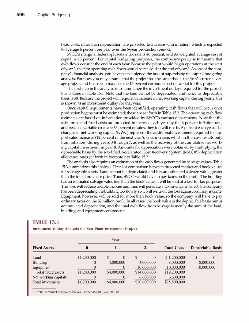
head costs, other than depreciation, are projected to increase with inflation, which is expectedto average 6 percent per year over the 6-year production period.
SVCC’s marginal federal-plus-state tax rate is 40 percent, and its weighted average cost ofcapital is 15 percent. For capital budgeting purposes, the company’s policy is to assume thatcash flows occur at the end of each year. Because the plant would begin operations at the startof year 3, the first operating cash flows would be realized at the end of year 3. As one of the com-pany’s financial analysts, you have been assigned the task of supervising the capital budgetinganalysis. For now, you may assume that the project has the same risk as the firm’s current aver-age project, and hence you may use the 15 percent corporate cost of capital for this project.
The first step in the analysis is to summarize the investment outlays required for the project;this is done in Table 15.1. Note that the land cannot be depreciated, and hence its depreciablebasis is $0. Because the project will require an increase in net working capital during year 2, thisis shown as an investment outlay for that year.
Once capital requirements have been identified, operating cash flows that will occur onceproduction begins must be estimated; these are set forth in Table 15.2. The operating cash flowestimates are based on information provided by SVCC’s various departments. Note that thesales price and fixed costs are projected to increase each year by the 6 percent inflation rate,and because variable costs are 65 percent of sales, they too will rise by 6 percent each year. Thechanges in net working capital (NWC) represent the additional investments required to sup-port sales increases (12 percent of the next year’s sales increase, which in this case results onlyfrom inflation) during years 3 through 7, as well as the recovery of the cumulative net work-ing capital investment in year 8. Amounts for depreciation were obtained by multiplying thedepreciable basis by the Modified Accelerated Cost Recovery System (MACRS) depreciationallowance rates set forth in footnote c to Table 15.2.
The analysis also requires an estimation of the cash flows generated by salvage values. Table15.3 summarizes this analysis. First is a comparison between projected market and book valuesfor salvageable assets. Land cannot be depreciated and has an estimated salvage value greaterthan the initial purchase price. Thus, SVCC would have to pay taxes on the profit. The buildinghas an estimated salvage value less than the book value; it will be sold at a loss for tax purposes.This loss will reduce taxable income and thus will generate a tax savings; in effect, the companyhas been depreciating the building too slowly, so it will write off the loss against ordinary income.Equipment, however, will be sold for more than book value, so the company will have to payordinary taxes on the $2 million profit. In all cases, the book value is the depreciable basis minusaccumulated depreciation, and the total cash flow from salvage is merely the sum of the land,building, and equipment components.
Chapter Fifteen Capital Budgeting 597
TABLE 15.1Investment Outlay Analysis for New Plant Investment Project
Year
Fixed Assets 0 1 2 Total Costs Depreciable Basis
Land $1,200,000 $ 0 $ 0 $ 1,200,000 $ 0 Building 0 4,000,000 4,000,000 8,000,000 8,000,000Equipment 0 0 10,000,000 10,000,000 10,000,000
Total fixed assets $1,200,000 $4,000,000 $14,000,000 $19,200,000 Net working capitala 0 0 6,600,000 6,600,000Total investment $1,200,000 $4,000,000 $20,600,000 $25,800,000
a Twelve percent of first year’s sales or 0.12 ($55,000,000) = $6,600,000.
596 Capital Budgeting
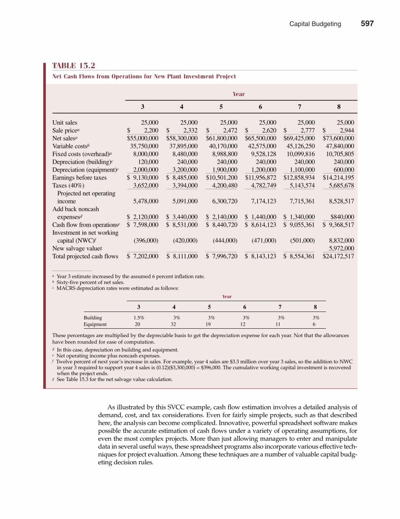
As illustrated by this SVCC example, cash flow estimation involves a detailed analysis ofdemand, cost, and tax considerations. Even for fairly simple projects, such as that describedhere, the analysis can become complicated. Innovative, powerful spreadsheet software makespossible the accurate estimation of cash flows under a variety of operating assumptions, foreven the most complex projects. More than just allowing managers to enter and manipulatedata in several useful ways, these spreadsheet programs also incorporate various effective tech-niques for project evaluation. Among these techniques are a number of valuable capital budg-eting decision rules.
598 Part Five Long-Term Investment Decisions
TABLE 15.2Net Cash Flows from Operations for New Plant Investment Project
Year
3 4 5 6 7 8
Unit sales 25,000 25,000 25,000 25,000 25,000 25,000 Sale pricea $ 2,200 $ 2,332 $ 2,472 $ 2,620 $ 2,777 $ 2,944Net salesa $55,000,000 $58,300,000 $61,800,000 $65,500,000 $69,425,000 $73,600,000Variable costsb 35,750,000 37,895,000 40,170,000 42,575,000 45,126,250 47,840,000Fixed costs (overhead)a 8,000,000 8,480,000 8,988,800 9,528,128 10,099,816 10,705,805Depreciation (building)c 120,000 240,000 240,000 240,000 240,000 240,000Depreciation (equipment)c 2,000,000 3,200,000 1,900,000 1,200,000 1,100,000 600,000Earnings before taxes $ 9,130,000 $ 8,485,000 $10,501,200 $11,956,872 $12,858,934 $14,214,195Taxes (40%) 3,652,000 3,394,000 4,200,480 4,782,749 5,143,574 5,685,678
Projected net operating income 5,478,000 5,091,000 6,300,720 7,174,123 7,715,361 8,528,517
Add back noncash expensesd $ 2,120,000 $ 3,440,000 $ 2,140,000 $ 1,440,000 $ 1,340,000 $840,000
Cash flow from operationse $ 7,598,000 $ 8,531,000 $ 8,440,720 $ 8,614,123 $ 9,055,361 $ 9,368,517Investment in net working
capital (NWC)f (396,000) (420,000) (444,000) (471,000) (501,000) 8,832,000 New salvage valueg 5,972,000 Total projected cash flows $ 7,202,000 $ 8,111,000 $ 7,996,720 $ 8,143,123 $ 8,554,361 $24,172,517
a Year 3 estimate increased by the assumed 6 percent inflation rate.b Sixty-five percent of net sales.c MACRS depreciation rates were estimated as follows:
Year
3 4 5 6 7 8
Building 1.5% 3% 3% 3% 3% 3% Equipment 20 32 19 12 11 6
These percentages are multiplied by the depreciable basis to get the depreciation expense for each year. Not that the allowanceshave been rounded for ease of computation.d In this case, depreciation on building and equipment.e Net operating income plus noncash expenses.f Twelve percent of next year’s increase in sales. For example, year 4 sales are $3.3 million over year 3 sales, so the addition to NWC
in year 3 required to support year 4 sales is (0.12)($3,300,000) = $396,000. The cumulative working capital investment is recoveredwhen the project ends.
g See Table 15.3 for the net salvage value calculation.
Capital Budgeting 597
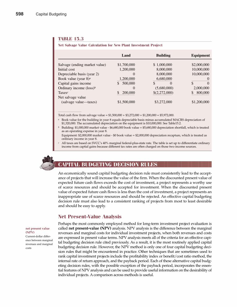
CAPITAL BUDGETING DECISION RULES
An economically sound capital budgeting decision rule must consistently lead to the accept-ance of projects that will increase the value of the firm. When the discounted present value ofexpected future cash flows exceeds the cost of investment, a project represents a worthy useof scarce resources and should be accepted for investment. When the discounted presentvalue of expected future cash flows is less than the cost of investment, a project represents aninappropriate use of scarce resources and should be rejected. An effective capital budgetingdecision rule must also lead to a consistent ranking of projects from most to least desirableand should be easy to apply.
Net Present-Value AnalysisPerhaps the most commonly employed method for long-term investment project evaluation iscalled net present-value (NPV) analysis. NPV analysis is the difference between the marginalrevenues and marginal costs for individual investment projects, when both revenues and costsare expressed in present value terms. NPV analysis meets all of the criteria for an effective capi-tal budgeting decision rule cited previously. As a result, it is the most routinely applied capitalbudgeting decision rule. However, the NPV method is only one of four capital budgeting deci-sion rules that might be encountered in practice. Other techniques that are sometimes used torank capital investment projects include the profitability index or benefit/cost ratio method, theinternal rate of return approach, and the payback period. Each of these alternative capital budg-eting decision rules, with the possible exception of the payback period, incorporates the essen-tial features of NPV analysis and can be used to provide useful information on the desirability ofindividual projects. A comparison across methods is useful.
net present value(NPV)Current-dollar differ-ence between marginalrevenues and marginalcosts
Chapter Fifteen Capital Budgeting 599
TABLE 15.3Net Salvage Value Calculation for New Plant Investment Project
Land Building Equipment
Salvage (ending market value) $1,700,000 $ 1,000,000 $2,000,000 Initial cost 1,200,000 8,000,000 10,000,000Depreciable basis (year 2) 0 8,000,000 10,000,000Book value (year 8)a 1,200,000 6,680,000 0Capital gains income $ 500,000 $ 0 $ 0 Ordinary income (loss)b 0 (5,680,000) 2,000,000Taxesc $ 200,000 $(2,272,000) $ 800,000 Net salvage value
(salvage value—taxes) $1,500,000 $3,272,000 $1,200,000
Total cash flow from salvage value = $1,500,000 + $3,272,000 + $1,200,000 = $5,972,000.a Book value for the building in year 8 equals depreciable basis minus accumulated MACRS depreciation of
$1,320,000. The accumulated depreciation on the equipment is $10,000,000. See Table15.2.b Building: $1,000,000 market value - $6,680,000 book value = $5,680,000 depreciation shortfall, which is treated
as an operating expense in year 8.Equipment: $2,000,000 market value - $0 book value = $2,000,000 depreciation recapture, which is treated asordinary income in year 8.
c All taxes are based on SVCC’s 40% marginal federal-plus-state rate. The table is set up to differentiate ordinaryincome from captial gains because different tax rates are often charged on those two income sources.
598 Capital Budgeting
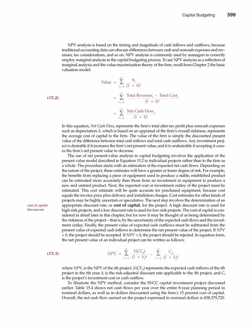
600 Part Five Long-Term Investment Decisions
cost of capitalDiscount rate
NPV analysis is based on the timing and magnitude of cash inflows and outflows, becausetraditional accounting data can obscure differences between cash and noncash expenses and rev-enues, tax considerations, and so on. NPV analysis is commonly used by managers to correctlyemploy marginal analysis in the capital budgeting process. To see NPV analysis as a reflection ofmarginal analysis and the value-maximization theory of the firm, recall from Chapter 2 the basicvaluation model:
n
Value = ∑ πt
t = 1 (1 + k)t
n
(15.2) = ∑ Total Revenuet – Total Costt
t = 1 (1 + k)t
n
= ∑ Net Cash Flowt
t = 1 (1 + k)t
In this equation, Net Cash Flowt represents the firm’s total after-tax profit plus noncash expensessuch as depreciation; k, which is based on an appraisal of the firm’s overall riskiness, representsthe average cost of capital to the firm. The value of the firm is simply the discounted presentvalue of the difference between total cash inflows and total cash outflows. Any investment proj-ect is desirable if it increases the firm’s net present value, and it is undesirable if accepting it caus-es the firm’s net present value to decrease.
The use of net present-value analysis in capital budgeting involves the application of thepresent value model described in Equation 15.2 to individual projects rather than to the firm asa whole. The procedure starts with an estimation of the expected net cash flows. Depending onthe nature of the project, these estimates will have a greater or lesser degree of risk. For example,the benefits from replacing a piece of equipment used to produce a stable, established productcan be estimated more accurately than those from an investment in equipment to produce anew and untried product. Next, the expected cost or investment outlay of the project must beestimated. This cost estimate will be quite accurate for purchased equipment, because costequals the invoice price plus delivery and installation charges. Cost estimates for other kinds ofprojects may be highly uncertain or speculative. The next step involves the determination of anappropriate discount rate, or cost of capital, for the project. A high discount rate is used forhigh-risk projects, and a low discount rate is used for low-risk projects. The cost of capital is con-sidered in detail later in this chapter, but for now it may be thought of as being determined bythe riskiness of the project—that is, by the uncertainty of the expected cash flows and the invest-ment outlay. Finally, the present value of expected cash outflows must be subtracted from thepresent value of expected cash inflows to determine the net present value of the project. If NPV> 0, the project should be accepted. If NPV < 0, the project should be rejected. In equation form,the net present value of an individual project can be written as follows:
n n
(15.3) NPVi = ∑ E(CFit) – ∑ Cit
t = 1 (1 + ki)t t = 1 (1 + ki)t
where NPVi is the NPV of the ith project, E(CFit) represents the expected cash inflows of the ithproject in the tth year, ki is the risk-adjusted discount rate applicable to the ith project, and Ciis the project’s investment cost or cash outflow.
To illustrate the NPV method, consider the SVCC capital investment project discussedearlier. Table 15.4 shows net cash flows per year over the entire 8-year planning period innominal dollars, as well as in dollars discounted using the firm’s 15 percent cost of capital.Overall, the net cash flow earned on the project expressed in nominal dollars is $38,379,720.
Capital Budgeting 599
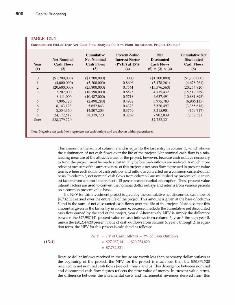
This amount is the sum of column 2 and is equal to the last entry in column 3, which showsthe culmination of net cash flows over the life of the project. Net nominal cash flow is a mis-leading measure of the attractiveness of the project, however, because cash outlays necessaryto fund the project must be made substantially before cash inflows are realized. A much morerelevant measure of the attractiveness of this project is net cash flow expressed in present-valueterms, where each dollar of cash outflow and inflow is converted on a common current-dollarbasis. In column 5, net nominal cash flows from column 2 are multiplied by present-value inter-est factors from column 4 that reflect a 15 percent cost of capital assumption. These present-valueinterest factors are used to convert the nominal dollar outlays and returns from various periodson a common present-value basis.
The NPV for this investment project is given by the cumulative net discounted cash flow of$7,732,321 earned over the entire life of the project. This amount is given at the base of column5 and is the sum of net discounted cash flows over the life of the project. Note also that thisamount is given as the last entry in column 6, because it reflects the cumulative net discountedcash flow earned by the end of the project, year 8. Alternatively, NPV is simply the differencebetween the $27,987,141 present value of cash inflows from column 5, year 3 through year 8,minus the $20,254,820 present value of cash outflows from column 5, year 0 through 2. In equa-tion form, the NPV for this project is calculated as follows:
NPV = PV of Cash Inflows – PV of Cash Outflows(15.4) = $27,987,141 – $20,254,820
= $7,732,321
Because dollar inflows received in the future are worth less than necessary dollar outlays atthe beginning of the project, the NPV for the project is much less than the $38,379,720received in net nominal cash flows (see columns 2 and 3). This divergence between nominaland discounted cash flow figures reflects the time value of money. In present-value terms,the difference between the incremental costs and incremental revenues derived from this
Chapter Fifteen Capital Budgeting 601
TABLE 15.4Consolidated End-of-Year Net Cash Flow Analysis for New Plant Investment Project Example
Cumulative Present-Value Net Cumulative Net Net Nominal Net Nominal Interest Factor Discounted Discounted
Year Cash Flows Cash Flows (PVIF) at 15% Cash Flows Cash Flows(1) (2) (3) (4) (5) � (2) � (4) (6)
0 ($1,200,000) ($1,200,000) 1.0000 ($1,200,000) ($1,200,000)1 (4,000,000) (5,200,000) 0.8696 (3,478,261) (4,678,261)2 (20,600,000) (25,800,000) 0.7561 (15,576,560) (20,254,820)3 7,202,000 (18,598,000) 0.6575 4,735,432 (15,519,389)4 8,111,000 (10,487,000) 0.5718 4,637,491 (10,881,898)5 7,996,720 (2,490,280) 0.4972 3,975,783 (6,906,115)6 8,143,123 5,652,843 0.4323 3,520,497 (3,385,618)7 8,554,360 14,207,203 0.3759 3,215,901 (169,717)8 24,172,517 38,379,720 0.3269 7,902,039 7,732,321
Sum $38,379,720 $7,732,321
Note: Negative net cash flows represent net cash outlays and are shown within parentheses.
600 Capital Budgeting
project is $7,732,321. This is a desirable project that if undertaken would increase the valueof the firm by this amount.
Firms typically make investments in projects showing positive net present values, reject thosewith negative net present values, and choose between mutually exclusive investments on thebasis of higher net present values. For many capital budgeting problems, the use of the NPVmethod is far more complex than the preceding description suggests. The capital budgetingproblem may require analysis of mutually exclusive projects with different expected lives orwith substantially different initial costs. A complication also arises when the size of the firm’scapital budget is limited. Under these conditions, a variant of the simple NPV is used to selectprojects that maximize the value of the firm.
Profitability Index or Benefit/Cost Ratio AnalysisAlthough individual projects might promise relatively attractive yields, combining them can cre-ate unforeseen difficulties. Undertaking a large number of projects simultaneously can require avery fast rate of expansion. Additional personnel requirements and organizational problemscan arise that diminish overall rates of return. At some point in the capital budgeting process,management must decide what total volume of favorable projects the firm can successfullyundertake without significantly reducing projected returns. Another reason for limiting the cap-ital budget at some firms is the reluctance or inability to obtain external financing by issuingdebt or selling stock. For example, considering the plight of firms with substantial amounts ofdebt during economic recession, management may simply refuse to use high levels of debtfinancing. Such capital rationing complicates the capital budgeting process and requires morecomplex tools of analysis.
A variant of NPV analysis that is often used in complex capital budgeting situations iscalled the profitability index (PI), or the benefit/cost ratio method. The profitability index iscalculated as follows:
n
(15.5)PI =
PV of Cash Inflows=
∑ [E(CFit)/(1 + ki)t]
PV of Cash Outflowst = 1
n
∑ [Cit/(1 + ki)t]t = 1
The PI shows the relative profitability of any project, or the present value of benefits per dollarof cost.
In the SVCC example described in Table 15.4, NPV > 0 implies a desirable investmentproject and PI > 1. To see that this is indeed the case, we can use the profitability index for-mula, given in Equation 15.5, and the present value of cash inflows and outflows from theproject, given in Equation 15.4. The profitability index for the SVCC project is
PI = PV of Cash InflowsPV of Outflows
= $27,987,141$20,254,820
= 1.38
This means that the SVCC capital investment project returns $1.38 in cash inflows for eachdollar of cash outflow, when both figures are expressed in present-value terms.
In PI analysis, a project with PI > 1 should be accepted and a project with PI < 1 should berejected. Projects will be accepted provided that they return more than a dollar of discounted
602 Part Five Long-Term Investment Decisions
profitability index(PI)Benefit/cost ratio
Capital Budgeting 601
benefits for each dollar of cost. Thus, the PI and NPV methods always indicate the same accept/reject decisions for independent projects, because PI > 1 implies NPV > 0 and PI < 1 impliesNPV < 0. However, for alternative projects of unequal size, PI and NPV criteria can give dif-ferent project rankings. This can sometimes cause problems when mutually exclusive projectsare being evaluated. Before investigating the source of such conflicts, however, it is worth-while to introduce two additional capital budgeting decision rules.
Internal Rate of Return AnalysisThe internal rate of return (IRR) is the interest or discount rate that equates the present valueof the future receipts of a project to the initial cost or outlay. The equation for calculating theinternal rate of return is simply the NPV formula set equal to zero:
n n
(15.6) NPVi = 0 = ∑ E(CFit) – ∑ Cit
t = 1 (1 + k*i )t t = 1 (1 + k*i )t
Here the equation is solved for the discount rate, ki*, which produces a zero net present valueor causes the sum of the discounted future receipts to equal the initial cost. That discount rateis the internal rate of return earned by the project.
Because the net present-value equation is complex, it is difficult to solve for the actual inter-nal rate of return on an investment without a computer or sophisticated calculator. For this rea-son, trial and error is sometimes employed. One begins by arbitrarily selecting a discount rate.If it yields a positive NPV, the internal rate of return must be greater than the discount rate used,and another higher rate is tried. If the chosen rate yields a negative NPV, the internal rate ofreturn on the project is lower than the discount rate, and the NPV calculation must be repeatedusing a lower discount rate. This process of changing the discount rate and recalculating the netpresent value continues until the discounted present value of the future cash flows equals theinitial cost. The interest rate that brings about this equality is the yield, or internal rate of returnon the project.
Using trial and error, an electronic financial calculator, or a spreadsheet software programsuch as Microsoft Excel, the internal rate of return for the SVCC investment project is IRR = 25.1percent. Because this IRR exceeds the 15 percent cost of capital, the project is attractive andshould be undertaken. In general, internal rate of return analysis suggests that projects shouldbe accepted when the IRR > k and rejected when the IRR < k. When the IRR > k, the marginalrate of return earned on the project exceeds the marginal cost of capital. As in the case of proj-ects with an NPV > 0 and PI > 1, the acceptance of all investment projects with IRR > k willlead management to maximize the value of the firm. In instances in which capital is scarce andonly a limited number of desirable projects can be undertaken at one point in time, the IRR canbe used to derive a rank ordering of projects from most desirable to least desirable. Like a rankordering of all NPV > 0 projects from highest to lowest PIs, a rank ordering of potential invest-ment projects from highest to lowest IRRs allows managers to effectively employ scarce funds.
Payback Period AnalysisThe payback period is the expected number of years of operation required to recover an initialinvestment. When project cash flows are discounted using an appropriate cost of capital, the dis-counted payback period is the expected number of years required to recover the initial invest-ment from discounted net cash flows. Payback period calculation is quick and easy using actualor discounted net cash flows. In equation form, the payback period is
(15.7) Payback Period = Number of Years to Recover Investment
internal rate ofreturn (IRR)Discount rate thatequates present valueof cash inflows andoutflows
payback periodNumber of yearsrequired to recover initial investment
Chapter Fifteen Capital Budgeting 603
602 Capital Budgeting
The payback period can be thought of as a breakeven time period. The shorter the paybackperiod, the more desirable the investment project. The longer the payback period, the less desir-able the investment project.
To illustrate, consider the SVCC capital investment project discussed earlier. Table 15.4 showsnet cash flows per year over the entire 8-year planning period in nominal dollars, as well as indollars discounted using the firm’s 15 percent cost of capital. In nominal dollars, the totalamount of investment is $25.8 million, which is the sum of the dollar outlays given in the firstthree rows of column 2. As shown in the third row of column 3, a negative $25.8 million is alsothe cumulative value of the nominal net cash flow as of the end of year 2, just prior to thebeginning of plant operations. When the nominal cash outlay of $25.8 million is discountedusing the firm’s 15 percent cost of capital, the present value of the investment cash outlay is$20,254,820, the sum of discounted cash outlays given in the first three rows of column 5. Asshown in the third row of column 6, a negative $20,254,820 is also the cumulative value of netdiscounted cash flow as of the end of year 2, just prior to the beginning of plant operations.
Based on nominal dollar cash outflows and inflows, the payback period is completed betweenthe end of year 5, when the cumulative net nominal cash flow is a negative $2,490,280, and the endof year 6, when the cumulative net nominal cash flow is a positive $5,652,843. Using nominal dol-lars, the payback period in years is calculated as
Nominal Payback Period = 5.00 + $2,490,280/$8,143,123= 5.30 years
Based on cash outflows and inflows discounted using the firm’s 15 percent cost of capital, thepayback period is completed between the end of year 7, when the cumulative net discountedcash flow is a negative $169,717, and the end of year 8, when the cumulative net discountedcash flow is a positive $7,732,321. Using discounted net cash flows, the payback period in yearsis calculated as
Discounted Payback Period = 7.00 + $169,717/$7,902,039= 7.02 years
Of course, these payback period calculations are based on the typical assumption that cashinflows are received continuously throughout the operating period. If cash inflows arereceived only at the end of the operating period, then the nominal payback period in thisexample would be 6 years and the discounted payback period would be 8 years. The exactlength of the payback period depends on underlying assumptions concerning the patternof cash inflows.
Note that the payback period is a breakeven calculation in that if cash flows come in atthe expected rate until the payback year, the project will break even in an accounting sense.However, the nominal payback period does not take into account the cost of capital; thecost of the debt and equity used to undertake the project is not reflected in the cash flowcalculation. The discounted payback period does take account of capital costs—it shows thebreakeven year after covering debt and equity costs. Both payback methods have the seri-ous deficiency of not taking into account any cash flows beyond the payback year. Othercapital budgeting decision rules are more likely to lead to better project rankings and selec-tions. The discounted payback period, however, does provide useful information about howlong funds will be tied up in a project. The shorter the discounted payback period, the greaterthe project’s liquidity. Also, cash flows expected in the distant future are generally regardedas riskier than near-term cash flows. Therefore, the discounted payback period is a usefulbut rough measure of liquidity and project risk.
604 Part Five Long-Term Investment Decisions
Capital Budgeting 603

CHOOSING AMONG ALTERNATIVE PROJECTS
The preceding section shows how application of the net present-value method in the capitalbudgeting process permits a rank ordering of investment projects from most attractive to leastattractive. An investment project is attractive and should be pursued as long as the discountednet present value of cash inflows is greater than the discounted net present value of the invest-ment requirement, or net cash outlay.
Decision Rule Conflict ProblemThe attractiveness of investment projects increases with the size of NPV. High NPV projectsare inherently more appealing and are preferred to low NPV projects. Any investment projectthat is incapable of generating sufficient cash inflows to cover necessary cash outlays, whenboth are expressed on a present-value basis, should not be undertaken. In the case of a projectwith NPV = 0, project acceptance would neither increase nor decrease the value of the firm.Management would be indifferent to pursuing such a project. NPV analysis represents a prac-tical application of the marginal concept, in which the marginal revenues and marginal costsof investment projects are considered on a present-value basis. Use of the NPV technique inthe evaluation of alternative investment projects allows managers to apply the principles ofmarginal analysis in a simple and clear manner. The widespread practical use of the NPV tech-nique lends support to the view that value maximization is the prime objective pursued bymanagers in the capital budgeting process.
Just as acceptance of NPV > 0 projects will enhance the value of the firm, so too will accept-ance of projects for which the PI > 1 and the IRR > k. Acceptance of projects for which NPV <0, PI < 1, or IRR < k would be unwise and would reduce the value of the firm. Because each of
Chapter Fifteen Capital Budgeting 605
Is the Sun Setting on Japan’s Vaunted MOF?
Long the power center of Japanese government, Japan’sMinistry of Finance (MOF) is under attack for bunglingeconomic policy and manipulating the Japanese stockmarket and real estate values. At risk is its bureaucraticauthority and the whole concept of the managed Japaneseeconomy. MOF officials argue that relinquishing controlover the economy would imperil full employment andcause a stock-market crash in Japan. However, continuedtrade surpluses with Canada, the United States, and othertrade partners have caused trade friction and stifled globaleconomic growth.
The aura of infallibility that the MOF cultivatedduring Japan’s postwar “economic miracle” has all butdisappeared in the gloom of Japan’s deepening eco-nomic malaise. No longer can supporters point to acontinuing series of economic triumphs. Instead, theMOF has made a number of foolish public errors byfailing to deal effectively with stock manipulation scan-dals and by botching privatization plans for governmentmonopolies. It also alienated Japan’s biggest banks and
brokerages throughout a series of embarrassing scandals.Politicians whom the MOF used to dominate now open-ly challenge the ministry’s role in Japanese government.
It may be several years before fundamental economicreforms take hold in Japan. Many Japanese politiciansand business leaders remain fervent nationalists whobelieve that Japan continues to work superbly as a society.It is a common view that the extent to which the countrybecomes less Japanese, or more integrated globally, it canno longer be Japan. In a real sense, the MOF sees itself asthe guardian of Japan’s conservative heritage. Thus,although there is a clear move underway in Japan tomake the MOF more accountable, any severe undermin-ing of its authority seems years away, at best. AlthoughJapanese bureaucracy, elected officials, and industry arestrongly motivated to change, they remain even moretightly bound to Japanese tradition and culture.
See: Nathan K. Lewis, “Japan Needs a Reagan Revolution,” The WallStreet Journal Online, April 1, 2002 (http://online.wsj.com).
M A N A G E R I A L A P P L I C AT I O N 1 5 . 2
604 Capital Budgeting
these project evaluation techniques shares a common focus on the present value of net cashinflows and outflows, these techniques display a high degree of consistency in terms of theproject accept/reject decision. This high degree of consistency might even lead one to questionthe usefulness of having these alternative ways of project evaluation when only one, the NPVmethod, seems sufficient for decision-making purposes.
However, even though alternative capital budgeting decision rules consistently lead to thesame project accept/reject decision, they involve important differences in terms of project rank-ing. Projects ranked most favorably using the NPV method may appear less so when analyzedusing the PI or IRR methods. Projects ranked most favorably using the PI or IRR methods mayappear less so when analyzed using the NPV technique.
If the application of any capital budgeting decision rule is to consistently lead to correctinvestment decisions, it must consider the time value of money in the evaluation of all cashflows and must rank projects according to their ultimate impact on the value of the firm. NPV,PI, and IRR methods satisfy both criteria, and each can be used to value and rank capital budg-eting projects. The payback method does not meet both of the preceding criteria and shouldbe used only as a complement to the other techniques. However, each of the NPV, PI, and IRRmethods incorporates certain assumptions that can and do affect project rankings. Understandingthe sources of these differences and learning how to deal with them is an important part of know-ing how to correctly evaluate alternative investment projects.
Reasons for Decision Rule ConflictAs discussed earlier, NPV is the difference between the marginal revenues and marginal costsof an individual investment project, when both revenues and costs are expressed in present-value terms. NPV measures the relative attractiveness of alternative investment projects by thediscounted dollar difference between revenues and costs. NPV is an absolute measure of theattractiveness of a given investment project. Conversely, the PI reflects the difference betweenthe marginal revenues and marginal costs of an individual project in ratio form. The PI is theratio of the discounted present value of cash inflows divided by the discounted present valueof cash outflows. PI is a relative measure of project attractiveness. It follows that application ofthe NPV method leads to the highest ranking for large profitable projects. Use of the PI methodleads to the highest ranking for projects that return the greatest amount of cash inflow per dol-lar of outflow, regardless of project size. At times, application of the NPV method can create abias for larger as opposed to smaller projects—a problem when all favorable NPV > 0 projectscannot be pursued. When capital is scarce, application of the PI method has the potential tocreate a better project mix for the firm’s overall investment portfolio.
Both NPV and PI methods differ from the IRR technique in terms of their underlyingassumptions regarding the reinvestment of cash flows during the life of the project. In theNPV and PI methods, excess cash flows generated over the life of the project are “reinvested”at the firm’s cost of capital. In the IRR method, excess cash flows are reinvested at the IRR.For especially attractive investment projects that generate an exceptionally high rate of return,the IRR can actually overstate project attractiveness because reinvestment of excess cash flowsat a similarly high IRR is not possible. When reinvestment at the project-specific IRR is notpossible, the IRR method must be adapted to take into account the lower rate of return thatcan actually be earned on excess cash flows generated over the life of individual projects.Otherwise, use of the NPV or PI methods is preferable.
Ranking Reversal ProblemA further and more serious conflict can arise between NPV and IRR methods when projects dif-fer significantly in terms of the magnitude and timing of cash flows. When the size or pattern ofalternative project cash flows differ greatly, each project’s NPV can react quite differently to
606 Part Five Long-Term Investment Decisions
Capital Budgeting 605
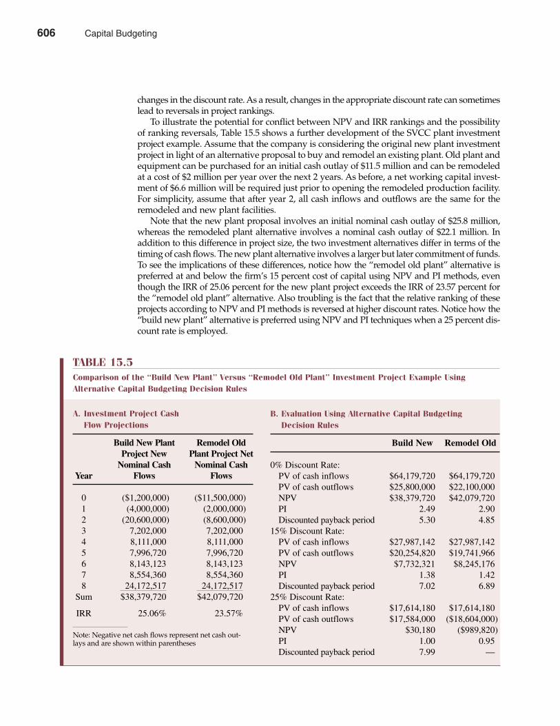
changes in the discount rate. As a result, changes in the appropriate discount rate can sometimeslead to reversals in project rankings.
To illustrate the potential for conflict between NPV and IRR rankings and the possibilityof ranking reversals, Table 15.5 shows a further development of the SVCC plant investmentproject example. Assume that the company is considering the original new plant investmentproject in light of an alternative proposal to buy and remodel an existing plant. Old plant andequipment can be purchased for an initial cash outlay of $11.5 million and can be remodeledat a cost of $2 million per year over the next 2 years. As before, a net working capital invest-ment of $6.6 million will be required just prior to opening the remodeled production facility.For simplicity, assume that after year 2, all cash inflows and outflows are the same for theremodeled and new plant facilities.
Note that the new plant proposal involves an initial nominal cash outlay of $25.8 million,whereas the remodeled plant alternative involves a nominal cash outlay of $22.1 million. Inaddition to this difference in project size, the two investment alternatives differ in terms of thetiming of cash flows. The new plant alternative involves a larger but later commitment of funds.To see the implications of these differences, notice how the “remodel old plant” alternative ispreferred at and below the firm’s 15 percent cost of capital using NPV and PI methods, eventhough the IRR of 25.06 percent for the new plant project exceeds the IRR of 23.57 percent forthe “remodel old plant” alternative. Also troubling is the fact that the relative ranking of theseprojects according to NPV and PI methods is reversed at higher discount rates. Notice how the“build new plant” alternative is preferred using NPV and PI techniques when a 25 percent dis-count rate is employed.
Chapter Fifteen Capital Budgeting 607
TABLE 15.5Comparison of the “Build New Plant” Versus “Remodel Old Plant” Investment Project Example UsingAlternative Capital Budgeting Decision Rules
A. Investment Project Cash Flow Projections
Build New Plant Remodel Old Project New Plant Project Net
Nominal Cash Nominal CashYear Flows Flows
0 ($1,200,000) ($11,500,000)1 (4,000,000) (2,000,000)2 (20,600,000) (8,600,000)3 7,202,000 7,202,0004 8,111,000 8,111,0005 7,996,720 7,996,7206 8,143,123 8,143,1237 8,554,360 8,554,3608 24,172,517 24,172,517
Sum $38,379,720 $42,079,720
IRR 25.06% 23.57%
Note: Negative net cash flows represent net cash out-lays and are shown within parentheses
B. Evaluation Using Alternative Capital Budgeting Decision Rules
Build New Remodel Old
0% Discount Rate:PV of cash inflows $64,179,720 $64,179,720 PV of cash outflows $25,800,000 $22,100,000 NPV $38,379,720 $42,079,720 PI 2.49 2.90 Discounted payback period 5.30 4.85
15% Discount Rate:PV of cash inflows $27,987,142 $27,987,142 PV of cash outflows $20,254,820 $19,741,966 NPV $7,732,321 $8,245,176 PI 1.38 1.42 Discounted payback period 7.02 6.89
25% Discount Rate:PV of cash inflows $17,614,180 $17,614,180 PV of cash outflows $17,584,000 ($18,604,000)NPV $30,180 ($989,820)PI 1.00 0.95 Discounted payback period 7.99 —
606 Capital Budgeting
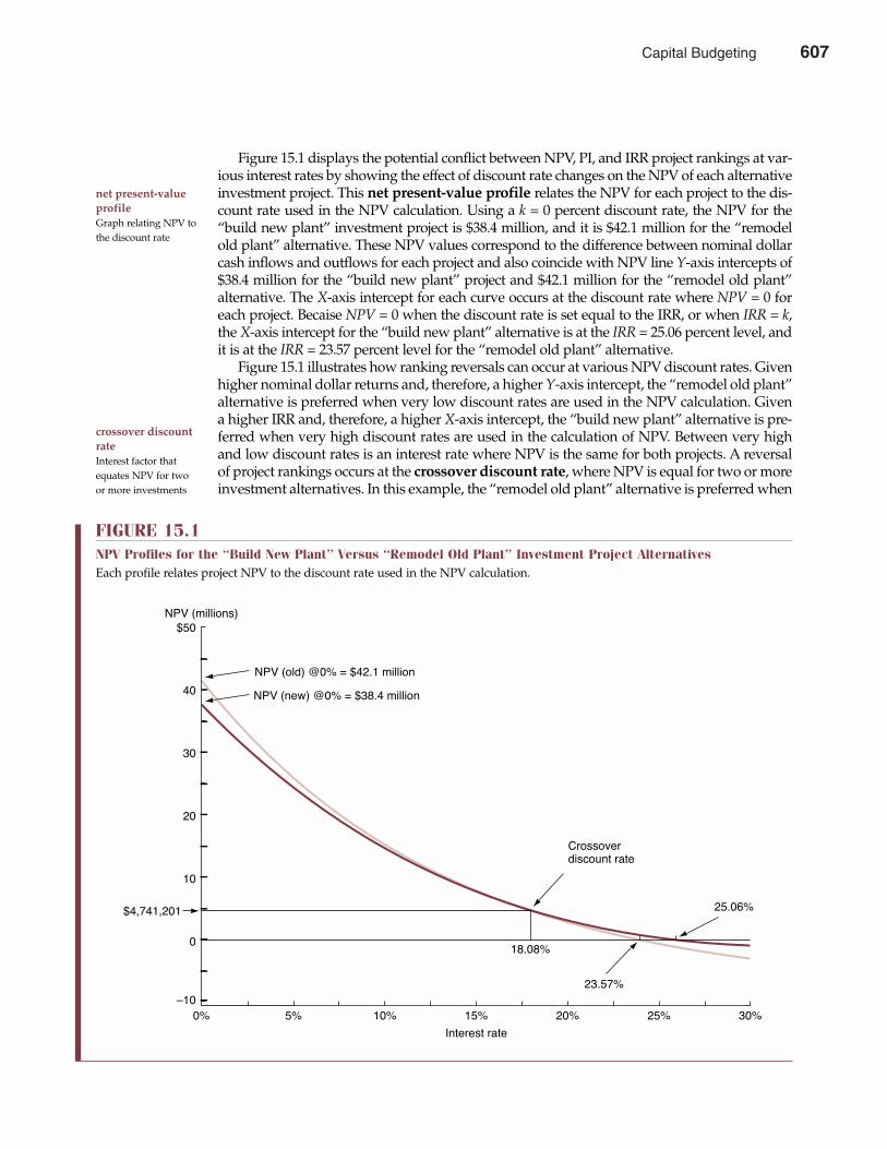
Figure 15.1 displays the potential conflict between NPV, PI, and IRR project rankings at var-ious interest rates by showing the effect of discount rate changes on the NPV of each alternativeinvestment project. This net present-value profile relates the NPV for each project to the dis-count rate used in the NPV calculation. Using a k = 0 percent discount rate, the NPV for the“build new plant” investment project is $38.4 million, and it is $42.1 million for the “remodelold plant” alternative. These NPV values correspond to the difference between nominal dollarcash inflows and outflows for each project and also coincide with NPV line Y-axis intercepts of$38.4 million for the “build new plant” project and $42.1 million for the “remodel old plant”alternative. The X-axis intercept for each curve occurs at the discount rate where NPV = 0 foreach project. Becaise NPV = 0 when the discount rate is set equal to the IRR, or when IRR = k,the X-axis intercept for the “build new plant” alternative is at the IRR = 25.06 percent level, andit is at the IRR = 23.57 percent level for the “remodel old plant” alternative.
Figure 15.1 illustrates how ranking reversals can occur at various NPV discount rates. Givenhigher nominal dollar returns and, therefore, a higher Y-axis intercept, the “remodel old plant”alternative is preferred when very low discount rates are used in the NPV calculation. Givena higher IRR and, therefore, a higher X-axis intercept, the “build new plant” alternative is pre-ferred when very high discount rates are used in the calculation of NPV. Between very highand low discount rates is an interest rate where NPV is the same for both projects. A reversalof project rankings occurs at the crossover discount rate, where NPV is equal for two or moreinvestment alternatives. In this example, the “remodel old plant” alternative is preferred when
608 Part Five Long-Term Investment Decisions
FIGURE 15.1NPV Profiles for the “Build New Plant” Versus “Remodel Old Plant” Investment Project AlternativesEach profile relates project NPV to the discount rate used in the NPV calculation.
5% 10% 15% 20% 25% 30%0%
$50
40
30
20
10
0
Ð10
Interest rate
NPV (millions)
NPV (old) @0% = $42.1 million
NPV (new) @0% = $38.4 million
Crossoverdiscount rate
25.06%$4,741,201
23.57%
18.08%
net present-valueprofileGraph relating NPV tothe discount rate
crossover discountrateInterest factor thatequates NPV for twoor more investments
Capital Budgeting 607
using the NPV criterion and a discount rate k that is less than the crossover discount rate. The“build new plant” alternative is preferred when using the NPV criterion and a discount rate kthat is greater than the crossover discount rate. This ranking reversal problem is typical of situ-ations in which investment projects differ greatly in terms of their underlying NPV profiles.Hence, a potentially troubling conflict exists between NPV, PI, and IRR methods.
Making the Correct Investment DecisionThe ranking reversal problem and suggested conflict between NPV, PI, and IRR methods isactually much less serious than one might imagine. Many comparisons between alternativeinvestment projects involve neither crossing NPV profiles nor crossover discount rates as shownin Figure 15.1. Some other project comparisons involve crossover discount rates that are eithertoo low or too high to affect project rankings at the current cost of capital. As a result, there isoften no meaningful conflict between NPV and IRR project rankings.
When crossover discount rates are relevant, they can be easily calculated as the IRR of thecash flow difference between two investment alternatives. To see that this is indeed the case,consider how cash flows differ between each of the two plant investment alternatives con-sidered previously. The “build new plant” alternative involves a smaller initial cash outflowof $1.2 million versus $11.5 million, a $10.3 million saving, but it requires additional outlaysof $2 million at the end of year 1 plus an additional $12 million at the end of year 2. Exceptfor these differences, the timing and magnitude of cash inflows and outflows from the twoprojects are identical. The IRR for the cash flow difference between two investment alterna-tives exactly balances the present-value cost of higher cash outflows with the present-valuebenefit of higher cash inflows. At this IRR, the cash flow difference between the two invest-ment alternatives has an NPV equal to zero. When k is less than this crossover IRR, theinvestment project with the greater nominal dollar return will have a larger NPV and willtend to be favored. In the current example, this is the “remodel old plant” alternative. Whenk is greater than the crossover IRR, the project with an earlier cash flow pattern will have thelarger NPV and be favored. In the current example, this is the “build new plant” alternative.When k equals the crossover IRR, the cash flow difference between projects has an NPV = 0,and each project has exactly the same NPV.
Once an economically relevant crossover discount rate has been determined, managementmust decide whether to rely on NPV or IRR decision rules in the resolution of the rankingreversal problem. Logic suggests that the NPV ranking should dominate because that methodwill result in a value-maximizing selection of projects. In most situations, it is also more real-istic to assume reinvestment of excess cash flows during the life of a project at the current costof capital k. This again favors NPV over IRR rankings. As a result, conflicts between NPV andIRR project rankings are usually resolved in favor of the NPV rank order.
Given the size-based conflict between the NPV and PI methods, which one should be reliedon in the ranking of potential investment projects? The answer depends upon the amount ofavailable resources. For a firm with substantial investment resources and a goal of maximizingshareholder wealth, the NPV method is better. For a firm with limited resources, the PI approachallocates scarce resources to the projects with the greatest relative effect on value. Using the PImethod, projects are evaluated on the basis of their NPV per dollar of investment, avoiding apossible bias toward larger projects. In some cases, this leads to a better combination of investmentprojects and higher firm value. The PI, or benefit/cost ratio, approach has also proved to be auseful tool in public-sector decision making, where allocating scarce public resources amongcompeting projects is a typical problem.
As seen in the evaluation of alternative capital budgeting decision rules, the attractivenessof investment projects varies significantly depending on the interest rate used to discountfuture cash flows. Determination of the correct discount rate is a vitally important aspect of thecapital budgeting process. This important issue is the subject of the next section.
Chapter Fifteen Capital Budgeting 609
608 Capital Budgeting
COST OF CAPITAL
If firms typically considered projects one by one and raised investment funds for each proj-ect separately, calculation of a suitable discount rate would be easy. The correct discount rateto employ for each investment project would simply be the marginal cost of capital for thatproject. However, determination of the correct discount rate for individual projects is seldomthat straightforward.
Component Cost of Debt FinancingFirms rarely consider individual projects in isolation but instead tend to evaluate portfoliosof potential investment projects to be funded from an ongoing stream of new capital fundsgenerated by retained earnings and new capital-raising efforts. New projects are funded bya mix of debt and equity financing, and each debt and equity component of new capital canbe expected to have different costs. Calculation of the correct discount rate for any givenpotential investment project typically involves weighing the relative importance of eachcomponent cost of new financing.
The component cost of debt is the interest rate that investors require on debt, adjusted fortaxes. If a firm borrows $100,000 for 1 year at 10 percent interest, the before-tax cost is $10,000and the before-tax interest rate is 10 percent. However, interest payments on debt are deductiblefor income tax purposes. It is necessary to account for this tax deductibility by adjusting thecost of debt to an after-tax basis. The deductibility of interest payments means, in effect, that
610 Part Five Long-Term Investment Decisions
component cost ofdebtInterest rate investorsrequire on debt, adjust-ed for taxes
Federal Government Support for R&D
The National Science Foundation (NSF) is an independentU.S. government agency responsible for promoting sci-ence and engineering in the United States. NSF programsinvest over $3.3 billion per year in almost 20,000 researchand education projects in science and engineering. NSF isalso responsible for keeping track of research and develop-ment (R&D) spending and productivity in governmentagencies, firms, universities and colleges, or other non-profit institutions.
At present, more than $250 billion per year is spentin the United States on R&D. Roughly 15 percent to 20percent of this amount is spent on basic research thatadvances scientific knowledge but has no immediatecommercial objective. Another 20 percent to 25 percentis spent on applied research that brings scientificknowledge closer to specific commercial application.The results of basic and applied research in science andengineering are ordinarily published and shared broadlywithin the scientific community. Such efforts can be distinguished from proprietary research and industrialdevelopment, the results of which are kept confidentialfor commercial reasons or for national security. MostR&D spending, roughly 60 percent to 65 percent, isdevoted to industrial development.
Federal government agencies provide about 30 per-cent percent of all R&D funding, but as much as 60 per-cent of basic research funding. The National Institutes ofHealth (NIH), for example, are a principal source offunding for biomedical research. NIH programs providefunds for such projects as AIDS/HIV treatment, cancerresearch, and the Human Genome Project. The govern-ment has also taken a direct role in scientific educationthrough the NSF and other agencies such as theDepartment of Energy. Federally funded research hasbeen directly responsible for major developments inspace technology, defense systems, energy, medicine, andagriculture. Federal tax incentives also encourage inno-vation in the private sector. Through grants, subsidies,and tax incentives, the federal government has support-ed basic research that underlies important appliedadvances in private industry. Partnerships with institu-tions such as universities have also proven to be an effec-tive risk-sharing mechanism for R&D efforts that havethe potential to create widespread social benefits.
This is a private-public partnership that works!
See: Home page information for the National Science Foundation can befound on the Internet (http://www.nsf.gov/start.htm).
M A N A G E R I A L A P P L I C AT I O N 1 5 . 3
Capital Budgeting 609
the government pays part of a firm’s interest charges. This reduces the firm’s cost of debtfinancing. The after-tax component cost of debt is given by the following expression:
(15.8) kd = (Interest Rate) � (1.0 – Tax Rate)
Assuming that the firm’s marginal federal-plus-state tax rate is 40 percent, the after-tax cost ofdebt will be 60 percent (= 1.0 – 0.4) of the nominal interest rate.
The relevant component cost of debt applies only to new debt, not to the interest on old orpreviously outstanding debt. In other words, the cost of new debt financing is what is relevantin terms of the marginal cost of debt. It is irrelevant that the firm borrowed at higher or lowerrates in the past.
Component Cost of Equity FinancingThe component cost of equity is the rate of return stockholders require on common stock.This return includes a compensation to investors for postponing their consumption, plus areturn to compensate for risk taking. Therefore, the component cost of equity consists of arisk-free rate of return, RF, plus a risk premium, RP:
(15.9) ke = RF + RP
The risk-free return is typically estimated by the interest rate on short-term U.S. governmentsecurities. On a daily basis, these rates of return can be obtained from The Wall Street Journaland other sources. Various methods can be used to estimate RP for different securities. Becausedividends paid to stockholders are not deductible for income tax purposes, dividend pay-ments must be made with after-tax dollars. There is no tax adjustment for the component costof equity capital.
Afirst method for estimating ke and RP is based on the capital asset pricing model, or CAPM.This method assumes that the risk of a stock depends on the sensitivity of its return tochanges in the return on all securities. A stock that is twice as risky as the overall marketwould entail twice the market risk premium; a security that is one-half as risky as the overallmarket would earn one-half the market risk premium, and so on. In the CAPM approach, theriskiness of a given stock is measured in terms of the variability of its return relative to thevariability of returns on all stocks, perhaps as represented by the volatility in the Standard andPoor’s 500 Index. A firm’s beta coefficient, �, is a measure of this variability. In a simpleregression model, the beta coefficient for an individual firm, �i , is estimated as
(15.10) Ri = �i + �i RM + e
where Ri is the weekly or monthly return on a given stock and RM is a similar return on themarket as a whole (e.g., the Standard and Poor’s 500 Index). A stock with average risk has a betaof 1.0. Low-risk stocks have betas less than 1.0; high-risk stocks have betas greater than 1.0.Although beta estimation is a relatively simple task, managers seldom need to actually runsuch regressions. Analysts at Merrill Lynch and other leading brokerage houses, as well asinvestment advisory services such as The Value Line Investment Survey, provide beta estimatesthat can be used for equity capital cost estimation for individual companies and/or operat-ing divisions.
In addition to data on the RF rate and �i for a given company, the CAPM approach requiresan estimate of the expected rate of return on the market as a whole. This return, kM, is a relativebenchmark for measuring the risk premium on the market. With these three inputs, RF, �i,and kM, the CAPM estimate of the required rate of return on any given stock is
component cost ofequityRate of return stock-holders require oncommon stock
risk-free rate ofreturn (RF)Investor reward forpostponing consump-tion
risk premium (RP)Investor reward forrisk taking
beta coefficientMeasure of relativestock-price variability
Chapter Fifteen Capital Budgeting 611
610 Capital Budgeting
(15.11) ke = RF + �i(kM – RF)
where the value (kM – RF) is the market risk premium, or risk premium on an average stock.Multiplying this market risk premium by the index of risk for a particular stock, or �i, givesthe risk premium for that stock.
To illustrate, assume that RF = 8 percent, kM = 14 percent, and �i = 0.5 for a given stock.Remember, �i = 0.5 means that a given stock is only one-half as risky as the overall market.Under such circumstances, the stock’s required return is
ke = 8 + 0.5(14 – 8) = 8 + 3 = 11%
If �i = 1.5, indicating that a stock is 50% riskier than the average security, then ke is
ke = 8 + 1.5(14 – 8) = 8 + 9 = 17%
A second common technique adds a premium of 4 percent or 5 percent onto the risk premiumpaid on a firm’s long-term bonds. Using this approach, the total risk premium on equity equalsthe difference between the yield on the firm’s debt and that on risk-free government bonds,plus 4 percent to 5 percent. For example, if risk-free government bonds yield 8 percent, and afirm’s bonds are priced to yield 10 percent, the cost of equity, ke, is
ke = Firm Bond Rate + 4% to 5% Risk Premium= 10% + (4% to 5%) = 14% to 15%
Given an 8 percent return on risk-free government bonds, this implies a total risk premium forequity of 6 percent to 7 percent, because
14% to 15% = 8% + Rp
Rp = 6% to 7%
Managers who rely on this method often cite historical studies suggesting that the long-termannual risk premium on investments in common stocks is generally 6 percent to 7 percent overthat earned on government bonds. The primary difficulty with estimating risk premiums fromhistorical returns is that historical returns differ depending on the beginning and ending datesof the estimation period, and past differences in stock and bond returns may not preciselyindicate future required risk premiums.
Yet another method for determining the cost of equity is to use a constant growth model. Ifearnings, dividends, and the stock price all grow at the same rate, then
Required Return = Dividend Yield + Capital Gainson Equity
= Expected Dividend + Expected(15.12) Current Stock Price Growth Rate
= Dividend + ExpectedPrice Rate Growth
ke = D1 + gP0
The rationale for this equation is that stockholder returns are derived from dividends andcapital gains. If past growth rates in earnings and dividends have been relatively stable, andif investors expect a continuation of past trends, then g may be based on the firm’s historicgrowth rate. However, if the company’s growth has been abnormally high or low, either
612 Part Five Long-Term Investment Decisions
Capital Budgeting 611
because of its own unique situation or because of general economic conditions, investors can-not project historical growth rate into the future. Security analyst estimates of g must then berelied on. These earnings forecasts are regularly found in Barron’s, The Value Line InvestmentSurvey, and other sources and offer a useful proxy for the growth expectations of investors ingeneral. When security analyst growth projections are combined with the dividend yieldexpected during the coming period, ke can be estimated as
(15.13) ke = D1 +Growth Rate Projected
P0 by Security Analysts
In practice, it is often best to use all of these methods and try to arrive at a consensus estimateof the component cost of equity financing.
Weighted Average Cost of CapitalSuppose that the interest rate on new debt is 7.5 percent and the firm’s marginal federal-plus-state income tax rate is 40 percent. This implies a 4.5 percent after-tax component cost of debt.Also assume that the firm has decided to finance next year’s projects by selling debt. Does thismean that next year’s investment projects have a 4.5 percent cost of capital? The answer is no,at least not usually. In financing a particular set of projects with debt, the firm typically usessome of its potential for obtaining further low-cost debt financing. As expansion takes place,the firm typically finds it necessary to raise additional high-cost equity to avoid unacceptablyhigh leverage. As a result, the current component cost of debt seldom measures the true long-term opportunity cost of debt financing. To illustrate, suppose that the firm has a current 4.5percent cost of debt and a 10 percent cost of equity. In the first year it borrows heavily, usingits debt capacity in the process, to finance projects yielding 6 percent. In the second year, it hasprojects available that yield 9 percent, or substantially above the return on first-year projects,but it cannot accept them because they would have to be financed with 10 percent equity. Toavoid this problem, the firm should be viewed as an ongoing concern, and the cost of capitalshould be calculated as a weighted average of the various types of funds it uses.
The weighted-average cost of capital is the interest rate necessary to attract additionalfunds for new capital investment projects. It is the marginal cost of a composite dollar ofdebt and equity financing. The proper set of weights to employ in computing the weighted-average cost of capital is determined by the firm’s optimal capital structure. The optimalcapital structure is the combination of debt and equity financing that minimizes the firm’soverall weighted-average cost of capital.
In general, the risk to investors is lower on debt and higher on common stock. Risk aver-sion among investors makes debt the lowest component-cost source of funds and equity thehighest component-cost source. However, the firm’s risk increases as debt financing grows,because the higher the debt level, the greater the probability that under adverse conditions thefirm will not make interest and principal payments. Because interest rates on debt are lowerthan the expected rate of return (dividends plus capital gains) on common stock, this can causethe weighted-average cost of capital to decline with modest amounts of debt financing. More debtmeans higher financial risk, which offsets this effect to some extent. As a result, the weighted-average cost of capital first declines as a firm moves from zero debt to some positive amountof debt, hits a minimum (perhaps over a range rather than at some specific amount of debt),and then rises as an increasing level of debt drives the firm’s risk position beyond acceptablelevels. Thus, each firm has an optimal amount of debt that minimizes its cost of capital andmaximizes its value.
Figure 15.2 shows how the cost of capital changes as the debt ratio increases for a hypo-thetical industry with about average risk. The average cost of capital figures in the graph arecalculated in Table 15.6. In the figure, each dot represents one of the firms in the industry.
weighted-averagecost of capitalMarginal cost of a com-posite dollar of debtand equity financing
optimal capitalstructureCombination of debtand equity that mini-mizes the firm’sweighted-average costof capital
Chapter Fifteen Capital Budgeting 613
612 Capital Budgeting
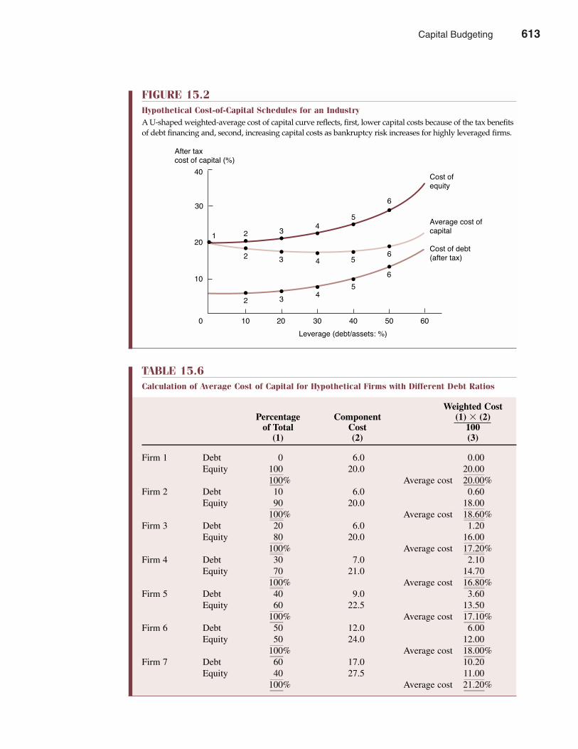
614 Part Five Long-Term Investment Decisions
FIGURE 15.2Hypothetical Cost-of-Capital Schedules for an IndustryA U-shaped weighted-average cost of capital curve reflects, first, lower capital costs because of the tax benefitsof debt financing and, second, increasing capital costs as bankruptcy risk increases for highly leveraged firms.
40
30
20
10
0 10 20 30 40 50 60
Leverage (debt/assets: %)
After taxcost of capital (%)
Cost ofequity
Average cost ofcapital
Cost of debt(after tax)
6
54
3
3
21
2
2 3
4
4
5
5
6
6
TABLE 15.6Calculation of Average Cost of Capital for Hypothetical Firms with Different Debt Ratios
Weighted CostPercentage Component (1) � (2)
of Total Cost 100(1) (2) (3)
Firm 1 Debt 0 6.0 0.00Equity 100 20.0 20.00
100% Average cost 20.00%Firm 2 Debt 10 6.0 0.60
Equity 90 20.0 18.00100% Average cost 18.60%
Firm 3 Debt 20 6.0 1.20Equity 80 20.0 16.00
100% Average cost 17.20%Firm 4 Debt 30 7.0 2.10
Equity 70 21.0 14.70100% Average cost 16.80%
Firm 5 Debt 40 9.0 3.60Equity 60 22.5 13.50
100% Average cost 17.10%Firm 6 Debt 50 12.0 6.00
Equity 50 24.0 12.00100% Average cost 18.00%
Firm 7 Debt 60 17.0 10.20Equity 40 27.5 11.00
100% Average cost 21.20%
Capital Budgeting 613
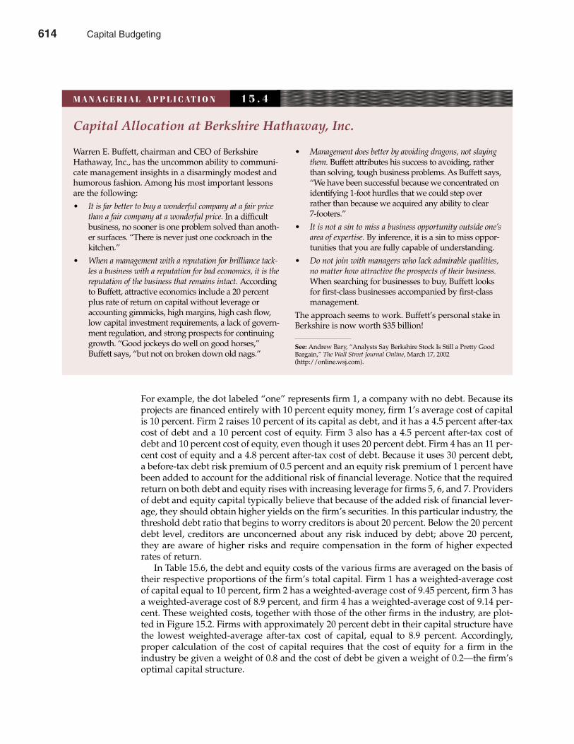
For example, the dot labeled “one” represents firm 1, a company with no debt. Because itsprojects are financed entirely with 10 percent equity money, firm 1’s average cost of capitalis 10 percent. Firm 2 raises 10 percent of its capital as debt, and it has a 4.5 percent after-taxcost of debt and a 10 percent cost of equity. Firm 3 also has a 4.5 percent after-tax cost ofdebt and 10 percent cost of equity, even though it uses 20 percent debt. Firm 4 has an 11 per-cent cost of equity and a 4.8 percent after-tax cost of debt. Because it uses 30 percent debt,a before-tax debt risk premium of 0.5 percent and an equity risk premium of 1 percent havebeen added to account for the additional risk of financial leverage. Notice that the requiredreturn on both debt and equity rises with increasing leverage for firms 5, 6, and 7. Providersof debt and equity capital typically believe that because of the added risk of financial lever-age, they should obtain higher yields on the firm’s securities. In this particular industry, thethreshold debt ratio that begins to worry creditors is about 20 percent. Below the 20 percentdebt level, creditors are unconcerned about any risk induced by debt; above 20 percent,they are aware of higher risks and require compensation in the form of higher expectedrates of return.
In Table 15.6, the debt and equity costs of the various firms are averaged on the basis oftheir respective proportions of the firm’s total capital. Firm 1 has a weighted-average costof capital equal to 10 percent, firm 2 has a weighted-average cost of 9.45 percent, firm 3 hasa weighted-average cost of 8.9 percent, and firm 4 has a weighted-average cost of 9.14 per-cent. These weighted costs, together with those of the other firms in the industry, are plot-ted in Figure 15.2. Firms with approximately 20 percent debt in their capital structure havethe lowest weighted-average after-tax cost of capital, equal to 8.9 percent. Accordingly,proper calculation of the cost of capital requires that the cost of equity for a firm in theindustry be given a weight of 0.8 and the cost of debt be given a weight of 0.2—the firm’soptimal capital structure.
Chapter Fifteen Capital Budgeting 615
Capital Allocation at Berkshire Hathaway, Inc.
Warren E. Buffett, chairman and CEO of BerkshireHathaway, Inc., has the uncommon ability to communi-cate management insights in a disarmingly modest andhumorous fashion. Among his most important lessonsare the following:
• It is far better to buy a wonderful company at a fair pricethan a fair company at a wonderful price. In a difficultbusiness, no sooner is one problem solved than anoth-er surfaces. “There is never just one cockroach in thekitchen.”
• When a management with a reputation for brilliance tack-les a business with a reputation for bad economics, it is thereputation of the business that remains intact. Accordingto Buffett, attractive economics include a 20 percentplus rate of return on capital without leverage oraccounting gimmicks, high margins, high cash flow,low capital investment requirements, a lack of govern-ment regulation, and strong prospects for continuinggrowth. “Good jockeys do well on good horses,”Buffett says, “but not on broken down old nags.”
• Management does better by avoiding dragons, not slayingthem. Buffett attributes his success to avoiding, ratherthan solving, tough business problems. As Buffett says,“We have been successful because we concentrated onidentifying 1-foot hurdles that we could step overrather than because we acquired any ability to clear 7-footers.”
• It is not a sin to miss a business opportunity outside one’sarea of expertise. By inference, it is a sin to miss oppor-tunities that you are fully capable of understanding.
• Do not join with managers who lack admirable qualities,no matter how attractive the prospects of their business.When searching for businesses to buy, Buffett looksfor first-class businesses accompanied by first-classmanagement.
The approach seems to work. Buffett’s personal stake inBerkshire is now worth $35 billion!
See: Andrew Bary, “Analysts Say Berkshire Stock Is Still a Pretty GoodBargain,” The Wall Street Journal Online, March 17, 2002(http://online.wsj.com).
M A N A G E R I A L A P P L I C AT I O N 1 5 . 4
614 Capital Budgeting
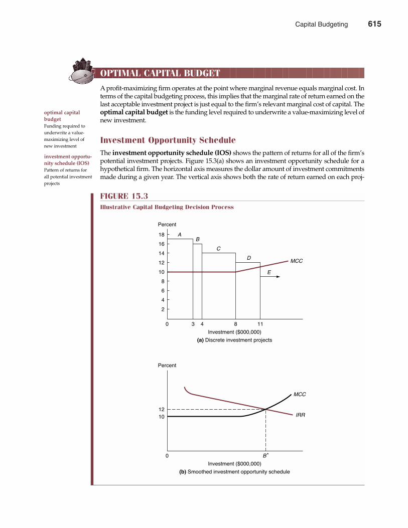
OPTIMAL CAPITAL BUDGET
A profit-maximizing firm operates at the point where marginal revenue equals marginal cost. Interms of the capital budgeting process, this implies that the marginal rate of return earned on thelast acceptable investment project is just equal to the firm’s relevant marginal cost of capital. Theoptimal capital budget is the funding level required to underwrite a value-maximizing level ofnew investment.
Investment Opportunity ScheduleThe investment opportunity schedule (IOS) shows the pattern of returns for all of the firm’spotential investment projects. Figure 15.3(a) shows an investment opportunity schedule for ahypothetical firm. The horizontal axis measures the dollar amount of investment commitmentsmade during a given year. The vertical axis shows both the rate of return earned on each proj-
616 Part Five Long-Term Investment Decisions
FIGURE 15.3Illustrative Capital Budgeting Decision Process
18
16
14
12
10
8
6
4
2
MCCD
E
C
BA
Percent
0 3 4 8 11
Investment ($000,000)
(a) Discrete investment projects
Percent
Investment ($000,000)
12
10
0 B*
(b) Smoothed investment opportunity schedule
IRR
MCC
optimal capitalbudgetFunding required tounderwrite a value-maximizing level ofnew investment
investment opportu-nity schedule (IOS)Pattern of returns forall potential investmentprojects
Capital Budgeting 615
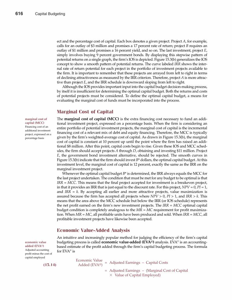
ect and the percentage cost of capital. Each box denotes a given project. Project A, for example,calls for an outlay of $3 million and promises a 17 percent rate of return; project B requires anoutlay of $1 million and promises a 16 percent yield, and so on. The last investment, project E,simply involves buying 9 percent government bonds. By displaying this stepwise pattern ofpotential returns on a single graph, the firm’s IOS is depicted. Figure 15.3(b) generalizes the IOSconcept to show a smooth pattern of potential returns. The curve labeled IRR shows the inter-nal rate of return potential for each project in the portfolio of investment projects available tothe firm. It is important to remember that these projects are arrayed from left to right in termsof declining attractiveness as measured by the IRR criterion. Therefore, project A is more attrac-tive than project E, and the IRR schedule is downward sloping from left to right.
Although the IOS provides important input into the capital budget decision-making process,by itself it is insufficient for determining the optimal capital budget. Both the returns and costsof potential projects must be considered. To define the optimal capital budget, a means forevaluating the marginal cost of funds must be incorporated into the process.
Marginal Cost of CapitalThe marginal cost of capital (MCC) is the extra financing cost necessary to fund an addi-tional investment project, expressed on a percentage basis. When the firm is considering anentire portfolio of potential investment projects, the marginal cost of capital is the incrementalfinancing cost of a relevant mix of debt and equity financing. Therefore, the MCC is typicallygiven by the firm’s weighted-average cost of capital. As drawn in Figure 15.3(b), the marginalcost of capital is constant at 10 percent up until the point where the firm has raised an addi-tional $8 million. After this point, capital costs begin to rise. Given these IOS and MCC sched-ules, the firm should accept projects A through D, obtaining and investing $11 million. ProjectE, the government bond investment alternative, should be rejected. The smooth curves inFigure 15.3(b) indicate that the firm should invest B* dollars, the optimal capital budget. At thisinvestment level, the marginal cost of capital is 12 percent, exactly the same as the IRR on themarginal investment project.
Whenever the optimal capital budget B* is determined, the IRR always equals the MCC forthe last project undertaken. The condition that must be met for any budget to be optimal is thatIRR = MCC. This means that the final project accepted for investment is a breakeven project,in that it provides an IRR that is just equal to the discount rate. For this project, NPV = 0, PI = 1,and IRR = k. By accepting all earlier and more attractive projects, value maximization isassured because the firm has accepted all projects where NPV > 0, PI > 1, and IRR > k. Thismeans that the area above the MCC schedule but below the IRR (or IOS schedule) representsthe net profit earned on the firm’s new investment projects. The IRR = MCC optimal capitalbudget condition is completely analogous to the MR = MC requirement for profit maximiza-tion. When MR = MC, all profitable units have been produced and sold. When IRR = MCC, allprofitable investment projects have likewise been accepted.
Economic Value-Added AnalysisAn intuitive and increasingly popular method for judging the efficiency of the firm’s capitalbudgeting process is called economic value-added (EVA©) analysis. EVA© is an accounting-based estimate of the profit added through the firm’s capital budgeting process. The formulafor EVA© is
Economic Value = Adjusted Earnings – Capital Costs(15.14) Added (EVA®)
= Adjusted Earnings – (Marginal Cost of Capital � Value of Capital Employed)
marginal cost ofcapital (MCC)Financing cost of anadditional investmentproject, expressed on apercentage basis
economic valueadded (EVA©)Adjusted accountingprofit minus the cost ofcapital employed
Chapter Fifteen Capital Budgeting 617
616 Capital Budgeting
As shown in Equation 15.14, EVA© is an accounting-based measure of the net profit contri-bution earned after adjusting accounting earnings for noncash expenses and the cost of capitalemployed by the firm or division. Like NPV analysis, firm or divisional activity adds valuewhen EVA© > 0; firm or divisional activity destroys value when EVA© < 0. Value maximizationrequires that the firm undertake all investment projects that feature positive EVA©; projects fea-turing negative EVA© should be rejected. For positive EVA© investment projects, the greater theEVA©, the more desirable the investment project.
When EVA© is calculated, accounting net income provides a useful starting point for analy-sis. However, if net income is negatively affected by the amortization of goodwill, or the failureto capitalize and amortize investments in intangible assets like research and development andbrand-name advertising, net income can fail to provide an accurate indication of economic per-formance. In such instances, cash flow numbers may provide better insight regarding firm ordivisional performance. Earnings before interest, taxes, depreciation, and amortization(EBITDA) is one such cash flow measure that is commonly employed. EBITDA is simply rev-enue minus all expenses, except interest charges, income taxes, depreciation, and amortizationcharges. EBITDA shows the gross amount of cash flow that the company is bringing in, andreflects the cash flow available to finance corporate acquisitions. The advantage of focusing onEBITDA rather than net income numbers is that EBITDA avoids any errors in the application ofaccounting accrual methodology. A disadvantage of focusing on EBITDA is that managers cansometimes overlook the need to make necessary investments in plant and equipment. To ensurethat funds for necessary capital expenditures will be available, prudent managers often focuson free cash flow, or EBITDA minus the cost of essential new plant and equipment. Althoughsuch cash flow adjustments to accounting net income numbers can be controversial, they aresometimes necessary if the firm’s capital budgeting process is to reflect economic reality.
Of course, in actual practice the estimation of an appropriate marginal cost of capital canitself be controversial. When EVA© analysis is being conducted, it is essential that managersremember that an appropriate marginal cost of capital reflects the opportunity cost of employedfunds. If free cash flow derived from operations is to be retained in the organization, it must pro-duce a return that is at least commensurate with that available on similar investment projectsinside and outside the firm. As a result, a practical and typical hurdle rate is the firm’s expect-ed marginal rate of return on investment. For example, if the corporation as a whole earns anaverage return of 12 percent on invested capital, it is rare that investment projects promising lessthan that amount will be approved. Instead of adopting marginal investment projects thatpromise below-average returns, top management will typically use free cash flow to buy backstock or repay borrowed funds. Of course, if special financing is obtained to fund division activ-ity, and particularly if division assets are used to secure such financing, then division-specificcost of funds can be readily calculated. Otherwise, the divisional cost of financing must be esti-mated based upon the firm’s overall marginal cost of capital.
EVA© methodology is helpful because it forces managers at all levels in the corporation toexplicitly consider the cost of capital in their planning and operating decisions. As such, it hasbecome a vital tool in the ongoing success of such standout performers as the Coca-ColaCompany, General Electric Company, Gillette Co., and Procter & Gamble Co., among others.
PostauditTo assure that an optimal capital budget has indeed been determined, the methods and dataemployed must often be carefully reexamined at the end of the capital budgeting process. Thepostaudit is a careful examination of actual and predicted results, coupled with a detailedreconciliation of any differences.
One of the most important advantages of the postaudit is that managerial forecasts of rev-enues and costs tend to improve when decision makers systematically compare projections toactual outcomes. Conscious or subconscious biases can be observed and eliminated, and new
618 Part Five Long-Term Investment Decisions
EBITDAEarnings before inter-est, taxes, depreciation,and amortization
free cash flowEBITDA minus the costof essential new plantand equipment
postauditCareful reconciliationof actual and predictedresults
Capital Budgeting 617
forecasting methods can be sought as their need becomes apparent. People simply tend towork better if they know that their actions are being monitored. It is important to rememberthat businesses are run by people, and people can perform at higher or lower levels of efficien-cy. When a divisional team has made a forecast in a capital budgeting proposal, it is putting itsreputation on the line. Because of the postaudit, these managers have every incentive to makegood on their projections. If costs rise above predicted levels or sales fall below expectations,managers in production, sales, and related areas have incentives to strive to bring results into linewith earlier forecasts.
Of course, it must be recognized that each element of the cash flow forecast is subject touncertainty, so a percentage of all projects undertaken by a reasonably aggressive firm willprove to be unsuccessful. This must be considered when appraising the performances ofmanagers who submit capital expenditure requests. Projects also sometimes fail to meetexpectations for reasons that no one could realistically have anticipated. For example, wildfluctuations in both oil prices and interest rates during recent years have made long-termforecasts of any sort very difficult. It is also sometimes hard to separate the operating resultsof one investment from those of contemporaneous projects. If the postaudit process is notused carefully, managers may be reluctant to suggest potentially profitable but risky projects.Because of these difficulties, some firms tend to play down the importance of the postaudit.However, the best-run and most successful organizations in business and government arethose that put the greatest emphasis on postaudits. Accordingly, the postaudit process is oneof the most important elements in an effective capital budgeting system.
SUMMARY
Long-term investment decisions are important because substantial amounts of funds areoften committed for extended periods. They are difficult because they entail forecasts ofuncertain future events that must be relied on heavily.
• Capital budgeting is the process of planning expenditures that generate cash flows expect-ed to extend beyond 1 year. Several different types of investment projects may be involved,including replacement projects, or maintenance of business projects; cost reduction proj-ects to replace obsolete plant and equipment; mandatory nonrevenue-producing safetyand environmental projects; and expansion projects to increase the availability of existingproducts and services.
• In all cases, the focus is on incremental cash flows, or the period-by-period changes in netcash flows that are due to the investment project. The most common tool for project valu-ation is net present-value (NPV) analysis, where NPV is the difference between projectmarginal revenues and marginal costs, when both are expressed in present-value terms.The conversion to present-value terms involves use of an appropriate discount rate, orcost of capital.
• Alternative decision rules include the profitability index (PI), or benefit/cost ratio; internalrate of return (IRR), or discount rate that equates the present value of receipts and outlays;and the payback period, or number of years required to recover the initial investment.
• Managers must be aware of the net present-value profile for individual projects, a graphthat relates the NPV for each project to the discount rate used in the NPV calculation. Areversal of project rankings occurs at the crossover discount rate, where NPV is equal fortwo or more investment alternatives.
• To properly value cash flows over the life of a project, the cost of capital funds must bedetermined. The component cost of debt is the interest rate that investors require on debt,adjusted for taxes. The component cost of equity is the rate of return stockholders requireon common stock. This includes a risk-free rate of return to compensate investors for
Chapter Fifteen Capital Budgeting 619
618 Capital Budgeting
postponing their consumption, plus a risk premium to compensate them for risk taking.The riskiness of a given stock is measured in terms of the firm’s beta coefficient, a measureof return variability.
• The weighted-average cost of capital is the marginal cost of a composite dollar of debt andequity financing. The proper set of weights to employ in computing the weighted-averagecost of capital is determined by the firm’s optimal capital structure, or combination of debtand equity financing that minimizes the firm’s overall weighted-average cost of capital.
• The optimal capital budget is the funding level required to underwrite a value-maximizinglevel of new investment. Graphically, the optimal capital budget is determined by theintersection of the investment opportunity schedule (IOS), or pattern of returns for all ofthe firm’s potential investment projects, and the marginal cost of capital (MCC), or IRRschedule.
• An intuitive and increasingly popular method for judging the efficiency of the firm’s capitalbudgeting process is called economic value-added (EVA©) analysis. EVA© is an accounting-based estimate of the profit added through the firm’s capital budgeting process. If netincome fails to provide an accurate indication of economic performance, cash flow numbersmay offer better insight regarding firm or divisional performance. Earnings before interest,taxes, depreciation, and amortization (EBITDA) is one such cash flow measure that is com-monly employed. To ensure that funds for necessary capital expenditures will be available,prudent managers often focus on free cash flow, or EBITDA minus the cost of essential plantand equipment.
• The postaudit is the final step in the capital budgeting process and consists of a carefulexamination of actual and predicted results, coupled with a detailed reconciliation of anydifferences.
Taken as a whole, the capital budgeting process is one in which the principles of marginalanalysis are applied in a systematic way to long-term investment decision making. As such,the process provides further evidence of managers actually going through the process of valuemaximization.
QUESTIONS
Q15.1 What is capital budgeting?Q15.2 What major steps are involved in the capital budgeting process?Q15.3 Why do accounting income statements provide only an imperfect basis for investment decisions,
and what steps must be taken to adjust these data?Q15.4 Explain the underlying rationale for using the NPV approach to investment project selection.Q15.5 Why do the NPV, PI, and IRR capital budgeting decision rules sometimes provide conflict-
ing rank orderings of investment project alternatives?Q15.6 How is a crossover discount rate calculated, and how does it affect capital budgeting decisions?Q15.7 In an earlier chapter, it was argued that factors should be used in such proportions that the mar-
ginal product/price ratios for all inputs are equal. In terms of capital budgeting, this impliesthat the marginal net cost of debt should equal the marginal net cost of equity in the optimalcapital structure. Yet firms often issue debt at interest rates substantially below the yield thatinvestors require on the firm’s equity shares. Does this mean that such firms are not operatingwith optimal capital structures? Explain.
Q15.8 Explain why the intersection of the IOS and MCC curves defines an economically optimalcapital budget.
620 Part Five Long-Term Investment Decisions
Capital Budgeting 619
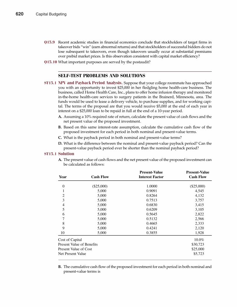
Q15.9 Recent academic studies in financial economics conclude that stockholders of target firms intakeover bids “win” (earn abnormal returns) and that stockholders of successful bidders do notlose subsequent to takeovers, even though takeovers usually occur at substantial premiumsover prebid market prices. Is this observation consistent with capital market efficiency?
Q15.10 What important purposes are served by the postaudit?
SELF-TEST PROBLEMS AND SOLUTIONS
ST15.1 NPV and Payback Period Analysis. Suppose that your college roommate has approachedyou with an opportunity to invest $25,000 in her fledgling home health-care business. Thebusiness, called Home Health Care, Inc., plans to offer home infusion therapy and monitoredin-the-home health-care services to surgery patients in the Brainerd, Minnesota, area. Thefunds would be used to lease a delivery vehicle, to purchase supplies, and for working capi-tal. The terms of the proposal are that you would receive $5,000 at the end of each year ininterest on a $25,000 loan to be repaid in full at the end of a 10-year period.A. Assuming a 10% required rate of return, calculate the present value of cash flows and the
net present value of the proposed investment.B. Based on this same interest-rate assumption, calculate the cumulative cash flow of the
proposed investment for each period in both nominal and present-value terms.C. What is the payback period in both nominal and present-value terms?D. What is the difference between the nominal and present-value payback period? Can the
present-value payback period ever be shorter than the nominal payback period? ST15.1 Solution
A. The present value of cash flows and the net present value of the proposed investment canbe calculated as follows:
B. The cumulative cash flow of the proposed investment for each period in both nominal andpresent-value terms is
Chapter Fifteen Capital Budgeting 621
Present-Value Present-ValueYear Cash Flow Interest Factor Cash Flow
0 ($25,000) 1.0000 ($25,000) 1 5,000 0.9091 4,545 2 5,000 0.8264 4,132 3 5,000 0.7513 3,757 4 5,000 0.6830 3,415 5 5,000 0.6209 3,105 6 5,000 0.5645 2,822 7 5,000 0.5132 2,566 8 5,000 0.4665 2,333 9 5,000 0.4241 2,120
10 5,000 0.3855 1,928
Cost of Capital 10.0% Present Value of Benefits $30,723 Present Value of Cost $25,000 Net Present Value $5,723
620 Capital Budgeting
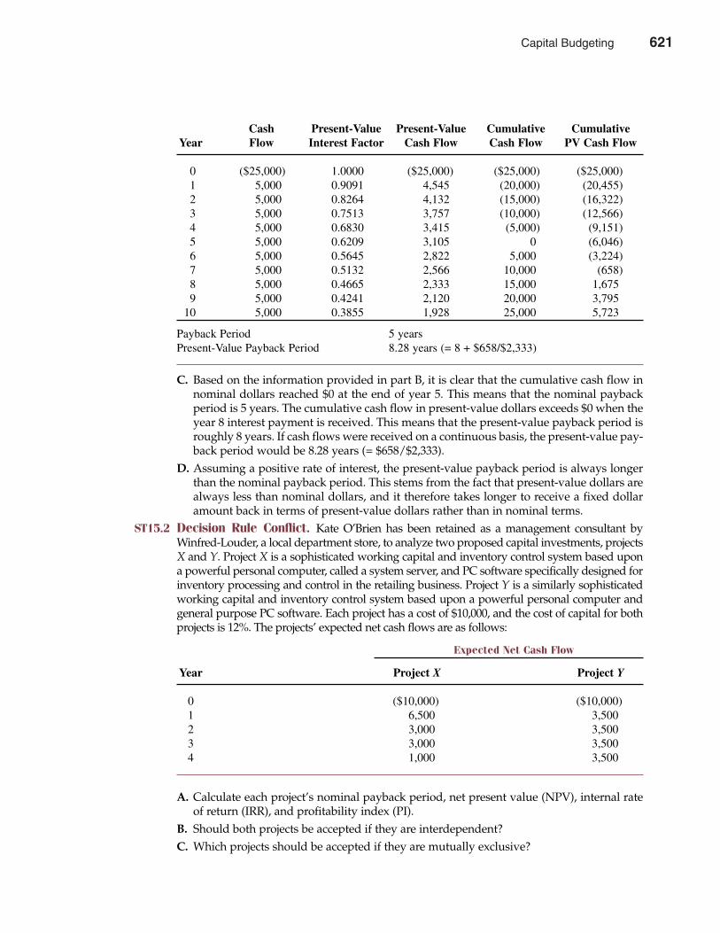
C. Based on the information provided in part B, it is clear that the cumulative cash flow innominal dollars reached $0 at the end of year 5. This means that the nominal paybackperiod is 5 years. The cumulative cash flow in present-value dollars exceeds $0 when theyear 8 interest payment is received. This means that the present-value payback period isroughly 8 years. If cash flows were received on a continuous basis, the present-value pay-back period would be 8.28 years (= $658/$2,333).
D. Assuming a positive rate of interest, the present-value payback period is always longerthan the nominal payback period. This stems from the fact that present-value dollars arealways less than nominal dollars, and it therefore takes longer to receive a fixed dollaramount back in terms of present-value dollars rather than in nominal terms.
ST15.2 Decision Rule Conflict. Kate O’Brien has been retained as a management consultant byWinfred-Louder, a local department store, to analyze two proposed capital investments, projectsX and Y. Project X is a sophisticated working capital and inventory control system based upona powerful personal computer, called a system server, and PC software specifically designed forinventory processing and control in the retailing business. Project Y is a similarly sophisticatedworking capital and inventory control system based upon a powerful personal computer andgeneral purpose PC software. Each project has a cost of $10,000, and the cost of capital for bothprojects is 12%. The projects’ expected net cash flows are as follows:
A. Calculate each project’s nominal payback period, net present value (NPV), internal rateof return (IRR), and profitability index (PI).
B. Should both projects be accepted if they are interdependent?C. Which projects should be accepted if they are mutually exclusive?
622 Part Five Long-Term Investment Decisions
Cash Present-Value Present-Value Cumulative CumulativeYear Flow Interest Factor Cash Flow Cash Flow PV Cash Flow
0 ($25,000) 1.0000 ($25,000) ($25,000) ($25,000) 1 5,000 0.9091 4,545 (20,000) (20,455) 2 5,000 0.8264 4,132 (15,000) (16,322) 3 5,000 0.7513 3,757 (10,000) (12,566) 4 5,000 0.6830 3,415 (5,000) (9,151) 5 5,000 0.6209 3,105 0 (6,046) 6 5,000 0.5645 2,822 5,000 (3,224) 7 5,000 0.5132 2,566 10,000 (658) 8 5,000 0.4665 2,333 15,000 1,675 9 5,000 0.4241 2,120 20,000 3,795
10 5,000 0.3855 1,928 25,000 5,723
Payback Period 5 yearsPresent-Value Payback Period 8.28 years (= 8 + $658/$2,333)
Expected Net Cash Flow
Year Project X Project Y
0 ($10,000) ($10,000)1 6,500 3,5002 3,000 3,5003 3,000 3,5004 1,000 3,500
Capital Budgeting 621
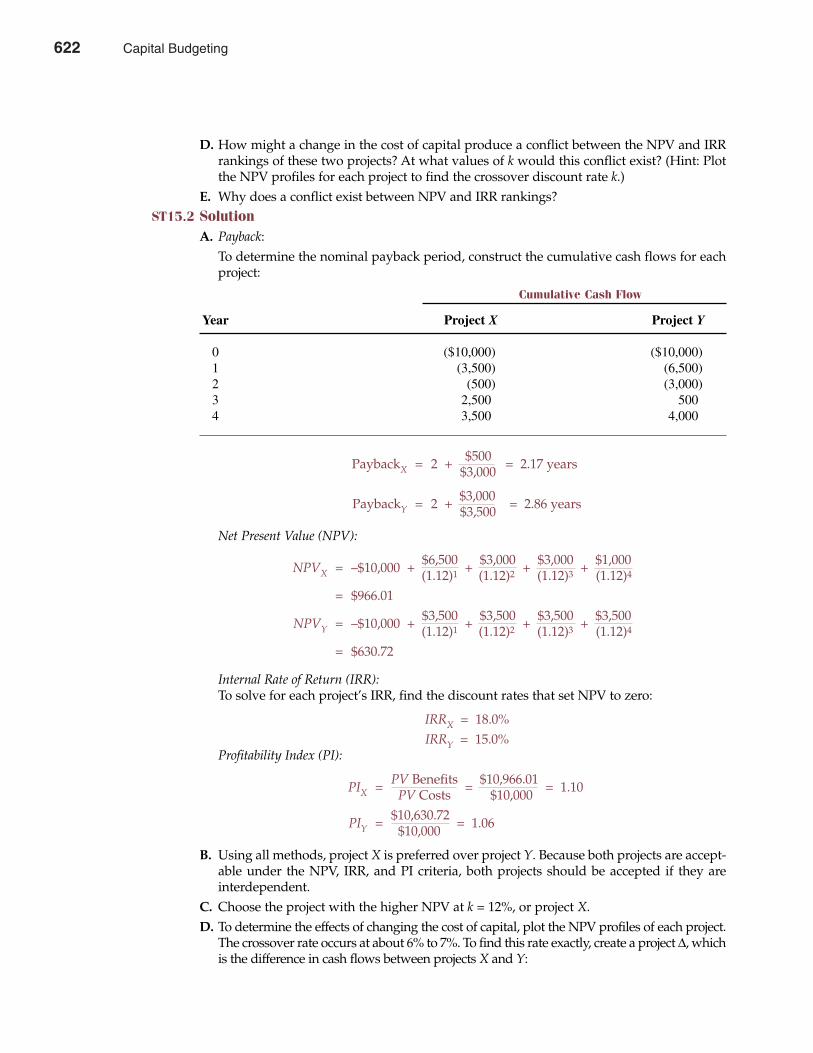
Chapter Fifteen Capital Budgeting 623
D. How might a change in the cost of capital produce a conflict between the NPV and IRRrankings of these two projects? At what values of k would this conflict exist? (Hint: Plotthe NPV profiles for each project to find the crossover discount rate k.)
E. Why does a conflict exist between NPV and IRR rankings?ST15.2 Solution
A. Payback:To determine the nominal payback period, construct the cumulative cash flows for eachproject:
PaybackX = 2 + $500 = 2.17 years$3,000
PaybackY = 2 + $3,000 = 2.86 years$3,500
Net Present Value (NPV):
NPVX = –$10,000 + $6,500 + $3,000 + $3,000 + $1,000(1.12)1 (1.12)2 (1.12)3 (1.12)4
= $966.01
NPVY = –$10,000 + $3,500 + $3,500 + $3,500 + $3,500(1.12)1 (1.12)2 (1.12)3 (1.12)4
= $630.72
Internal Rate of Return (IRR):To solve for each project’s IRR, find the discount rates that set NPV to zero:
IRRX = 18.0% IRRY = 15.0%
Profitability Index (PI):
PIX = PV Benefits = $10,966.01 = 1.10PV Costs $10,000
PIY = $10,630.72 = 1.06$10,000
B. Using all methods, project X is preferred over project Y. Because both projects are accept-able under the NPV, IRR, and PI criteria, both projects should be accepted if they areinterdependent.
C. Choose the project with the higher NPV at k = 12%, or project X.D. To determine the effects of changing the cost of capital, plot the NPV profiles of each project.
The crossover rate occurs at about 6% to 7%. To find this rate exactly, create a project ∆, whichis the difference in cash flows between projects X and Y:
Cumulative Cash Flow
Year Project X Project Y
0 ($10,000) ($10,000)1 (3,500) (6,500)2 (500) (3,000)3 2,500 5004 3,500 4,000
622 Capital Budgeting
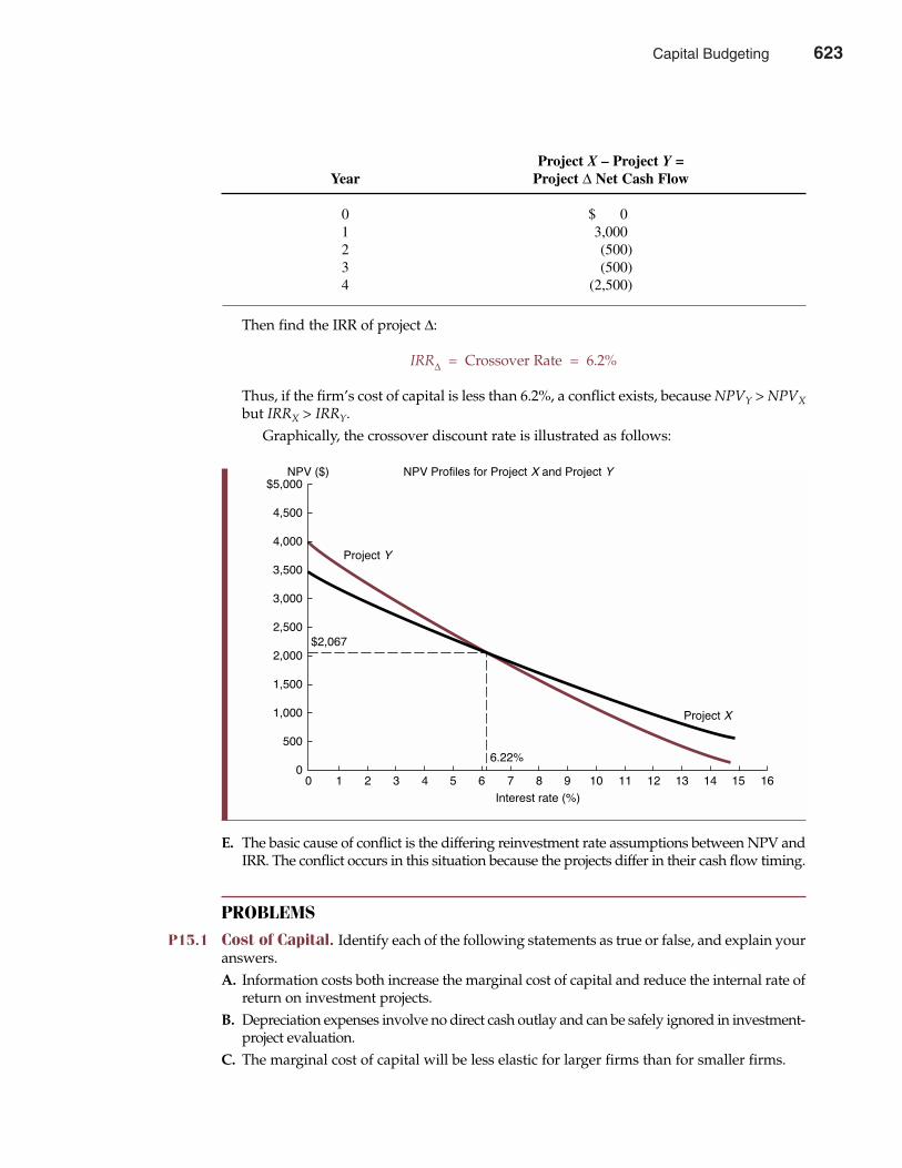
Then find the IRR of project ∆:
IRR∆ = Crossover Rate = 6.2%
Thus, if the firm’s cost of capital is less than 6.2%, a conflict exists, because NPVY > NPVXbut IRRX > IRRY.
Graphically, the crossover discount rate is illustrated as follows:
E. The basic cause of conflict is the differing reinvestment rate assumptions between NPV andIRR. The conflict occurs in this situation because the projects differ in their cash flow timing.
PROBLEMS
P15.1 Cost of Capital. Identify each of the following statements as true or false, and explain youranswers.A. Information costs both increase the marginal cost of capital and reduce the internal rate of
return on investment projects.B. Depreciation expenses involve no direct cash outlay and can be safely ignored in investment-
project evaluation.C. The marginal cost of capital will be less elastic for larger firms than for smaller firms.
624 Part Five Long-Term Investment Decisions
Project X – Project Y =Year Project ∆ Net Cash Flow
0 $ 01 3,0002 (500)3 (500)4 (2,500)
$5,000
4,500
4,000
3,500
3,000
2,500
2,000
1,500
1,000
500
0
NPV ($) NPV Profiles for Project X and Project Y
0 1 2 3 4 5 6 7 8 9 10 11 12 13 14 15 16
Interest rate (%)
Project Y
Project X
6.22%
$2,067
Capital Budgeting 623
D. In practice, the component costs of debt and equity are jointly rather than independentlydetermined.
E. Investments necessary to replace worn-out or damaged equipment tend to have low levelsof risk.
P15.2 Decision Rule Criteria. The net present value (NPV), profitability index (PI), and internal rateof return (IRR) methods are often employed in project valuation. Identify each of the followingstatements as true or false, and explain your answers.A. The IRR method can tend to understate the relative attractiveness of superior investment
projects when the opportunity cost of cash flows is below the IRR.B. A PI = 1 describes a project with an NPV = 0.C. Selection solely according to the NPV criterion will tend to favor larger rather than smaller
investment projects.D. When NPV = 0, the IRR exceeds the cost of capital.E. Use of the PI criterion is especially appropriate for larger firms with easy access to capi-
tal markets.P15.3 Cost of Capital. Indicate whether each of the following would increase or decrease the cost
of capital that should be used by the firm in investment project evaluation. Explain.A. Interest rates rise because the Federal Reserve System tightens the money supply.B. The stock market suffers a sharp decline, as does the company’s stock price, without (in
management’s opinion) any decline in the company’s earnings potential.C. The company’s home state eliminates the corporate income tax in an effort to keep or attract
valued employers.D. In an effort to reduce the federal deficit, Congress raises corporate income tax rates.E. A merger with a leading competitor increases the company’s stock price substantially.
P15.4 Present Value. New York City licenses taxicabs in two classes: (1) for operation by companieswith fleets and (2) for operation by independent driver-owners having only one cab. Strict lim-its are imposed on the number of taxicabs by restricting the number of licenses, or medallions,that are issued to provide service on the streets of New York City. This medallion system datesfrom a Depression-era city law designed to address an overabundance of taxis that depresseddriver earnings and congested city streets. In 1937, the city slapped a moratorium on the issuanceof new taxicab licenses. The number of cabs, which peaked at 21,000 in 1931, fell from 13,500 in1937 to 11,787 in May 1996 when the city broke a 59-year cap and issued an additional 400 licens-es. However, because the city has failed to allow sufficient expansion, taxicab medallions havedeveloped a trading value in the open market. After decades of often-explosive medallion priceincreases, individually-owned licenses now trade for more than $200,000 each, and fleet licensesfetch more than $250,000 each. A. Discuss the factors determining the value of a license. To make your answer concrete,
estimate numerical values for the various components that together can be summarizedin a medallion price of $200,000.
B. What factors would determine whether a change in the fare fixed by the city would raise orlower the value of a medallion?
C. Cab drivers, whether hired by companies or as owners of their own cabs, seem unani-mous in opposing any increase in the number of cabs licensed. They argue that an increasein the number of cabs would increase competition for customers and drive down whatthey regard as an already unduly low return to drivers. Is their economic analysis correct?Who would gain and who would lose from an expansion in the number of licenses issuedat a nominal fee?
Chapter Fifteen Capital Budgeting 625
624 Capital Budgeting
P15.5 NPV and PI. The Pacific Princess luxury cruise line is contemplating leasing an additionalcruise ship to expand service from the Hawaiian Islands to Long Beach or San Diego. Afinancial analysis by staff personnel resulted in the following projections for a 5-year plan-ning horizon:
A. Calculate the net present value for each service. Which is more desirable according to theNPV criterion?
B. Calculate the profitability index for each service. Which is more desirable according tothe PI criterion?
C. Under what conditions would either or both of the services be undertaken?P15.6 NPV and PI. Louisiana Drilling and Exploration, Inc. (LD&E), has the funds necessary to
complete one of two risky oil and gas drilling projects. The first, Permian Basin 1, involvesthe recovery of a well that was plugged and abandoned 5 years ago but that may now beprofitable, given improved recovery techniques. The second, Permian Basin 2, is a newonshore exploratory well that appears to be especially promising. Based on a detailed analy-sis by its technical staff, LD&E projects a 10-year life for each well with annual net cash flowsas follows:
In the recovery-project valuation, LD&E uses an 8% riskless rate and a standard 12% risk pre-mium. For exploratory drilling projects, the company uses larger risk premiums proportionateto project risks as measured by the project coefficient of variation. For example, an exploratoryproject with a coefficient of variation one and one-half times that for recovery projects wouldrequire a risk premium of 18% (= 1.5 � 12%). Both projects involve land acquisition, as well assurface preparation and subsurface drilling costs of $3 million each.A. Calculate the expected value, standard deviation, and coefficient of variation for annual net
operating revenues from each well.B. Calculate and evaluate the NPV for each project using the risk-adjusted discount rate
method.C. Calculate and evaluate the PI for each project.
P15.7 Investment Project Choice. Monk’s Coffee Shop is considering investment in two alter-native capital budgeting projects. Project A is an investment of $75,000 to replace working butobsolete refrigeration equipment. Project B is an investment of $150,000 to expand diningroom facilities. Relevant cash flow data for the two projects over their expected 2-year livesare as follows:
626 Part Five Long-Term Investment Decisions
Long Beach San Diego
Cost $2,000,000 $3,000,000PV of expected cash flow @ k = 15% 2,500,000 3,600,000
Project Probability Annual Cash Flow
Permian Basin 1 0.08 $ 500,0000.84 1,000,0000.08 1,500,000
Permian Basin 2 0.18 300,0000.64 900,0000.18 1,500,000
Capital Budgeting 625
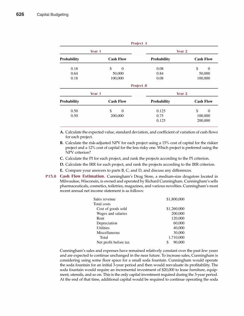
A. Calculate the expected value, standard deviation, and coefficient of variation of cash flowsfor each project.
B. Calculate the risk-adjusted NPV for each project using a 15% cost of capital for the riskierproject and a 12% cost of capital for the less risky one. Which project is preferred using theNPV criterion?
C. Calculate the PI for each project, and rank the projects according to the PI criterion.D. Calculate the IRR for each project, and rank the projects according to the IRR criterion.E. Compare your answers to parts B, C, and D, and discuss any differences.
P15.8 Cash Flow Estimation. Cunningham’s Drug Store, a medium-size drugstore located inMilwaukee, Wisconsin, is owned and operated by Richard Cunningham. Cunningham’s sellspharmaceuticals, cosmetics, toiletries, magazines, and various novelties. Cunningham’s mostrecent annual net income statement is as follows:
Sales revenue $1,800,000Total costs
Cost of goods sold $1,260,000Wages and salaries 200,000Rent 120,000Depreciation 60,000Utilities 40,000Miscellaneous 30,000
Total 1,710,000Net profit before tax $ 90,000
Cunningham’s sales and expenses have remained relatively constant over the past few yearsand are expected to continue unchanged in the near future. To increase sales, Cunningham isconsidering using some floor space for a small soda fountain. Cunningham would operatethe soda fountain for an initial 3-year period and then would reevaluate its profitability. Thesoda fountain would require an incremental investment of $20,000 to lease furniture, equip-ment, utensils, and so on. This is the only capital investment required during the 3-year period.At the end of that time, additional capital would be required to continue operating the soda
Chapter Fifteen Capital Budgeting 627
Project A
Year 1 Year 2
Probability Cash Flow Probability Cash Flow
0.18 $ 0 0.08 $ 00.64 50,000 0.84 50,0000.18 100,000 0.08 100,000
Project B
Year 1 Year 2
Probability Cash Flow Probability Cash Flow
0.50 $ 0 0.125 $ 00.50 200,000 0.75 100,000
0.125 200,000
626 Capital Budgeting
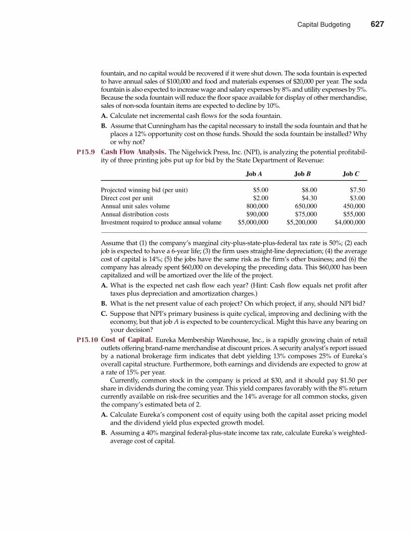
fountain, and no capital would be recovered if it were shut down. The soda fountain is expectedto have annual sales of $100,000 and food and materials expenses of $20,000 per year. The sodafountain is also expected to increase wage and salary expenses by 8% and utility expenses by 5%.Because the soda fountain will reduce the floor space available for display of other merchandise,sales of non-soda fountain items are expected to decline by 10%.A. Calculate net incremental cash flows for the soda fountain.B. Assume that Cunningham has the capital necessary to install the soda fountain and that he
places a 12% opportunity cost on those funds. Should the soda fountain be installed? Whyor why not?
P15.9 Cash Flow Analysis. The Nigelwick Press, Inc. (NPI), is analyzing the potential profitabil-ity of three printing jobs put up for bid by the State Department of Revenue:
Assume that (1) the company’s marginal city-plus-state-plus-federal tax rate is 50%; (2) eachjob is expected to have a 6-year life; (3) the firm uses straight-line depreciation; (4) the averagecost of capital is 14%; (5) the jobs have the same risk as the firm’s other business; and (6) thecompany has already spent $60,000 on developing the preceding data. This $60,000 has beencapitalized and will be amortized over the life of the project.A. What is the expected net cash flow each year? (Hint: Cash flow equals net profit after
taxes plus depreciation and amortization charges.)B. What is the net present value of each project? On which project, if any, should NPI bid?C. Suppose that NPI’s primary business is quite cyclical, improving and declining with the
economy, but that job A is expected to be countercyclical. Might this have any bearing onyour decision?
P15.10 Cost of Capital. Eureka Membership Warehouse, Inc., is a rapidly growing chain of retailoutlets offering brand-name merchandise at discount prices. A security analyst’s report issuedby a national brokerage firm indicates that debt yielding 13% composes 25% of Eureka’soverall capital structure. Furthermore, both earnings and dividends are expected to grow ata rate of 15% per year.
Currently, common stock in the company is priced at $30, and it should pay $1.50 pershare in dividends during the coming year. This yield compares favorably with the 8% returncurrently available on risk-free securities and the 14% average for all common stocks, giventhe company’s estimated beta of 2.A. Calculate Eureka’s component cost of equity using both the capital asset pricing model
and the dividend yield plus expected growth model.B. Assuming a 40% marginal federal-plus-state income tax rate, calculate Eureka’s weighted-
average cost of capital.
628 Part Five Long-Term Investment Decisions
Job A Job B Job C
Projected winning bid (per unit) $5.00 $8.00 $7.50Direct cost per unit $2.00 $4.30 $3.00Annual unit sales volume 800,000 650,000 450,000Annual distribution costs $90,000 $75,000 $55,000Investment required to produce annual volume $5,000,000 $5,200,000 $4,000,000
Capital Budgeting 627
Chapter Fifteen Capital Budgeting 629
CASE STUDY
Investment Project Analysis at FlightSafety International, Inc.FlightSafety International, Inc., trains more than 30,000 corporate, commercial, and militarypilots per year and has found its niche business to be enormously profitable. Net profit marginshave averaged roughly 30% of sales during the 1980s and mid-1990s. It is the only company tohave earned a spot on Forbes’ annual list of the best up-and-comers in every year during this peri-od. Over this period, FlightSafety’s profits rose more than fivefold, and the company racked upan average rate of return on common equity of 18% to 20% per year. Its stock was up from $7 ashare (split-adjusted) in 1982 to more than $50 in 1996, at which point FlightSafety was purchasedby Berkshire Hathaway, Inc., in a cash and stock transaction worth $1.5 billion. Among the 9,500stockholders that benefited from the company’s amazing success is company founder, chairman,and president Albert Ueltschi and his family, who owned roughly one-third of FlightSafety com-mon stock prior to the Berkshire buyout.
What separates FlightSafety from other small companies that look good for a couple ofyears and then crash and burn is the quality of top management. Ueltschi is widely regardedas dedicated, highly intelligent, and honest. He started FlightSafety in 1951, while working asa pilot for Pan American Airways. Since 1946 he had served as the personal pilot to Pan Am’scolorful founder, Juan Trippe, flying Trippe around in a converted B-23 military transport.During the early years of this association, Ueltschi noticed that other corporate CEOs werebuying surplus military planes and converting them into corporate aircraft. He also noticedthat many of the former military pilots who were signing on as corporate pilots had little or notraining on the specific planes they were being hired to fly. Ueltschi reasoned that corporationswould pay to rectify this dangerous situation.
Ueltschi opened an office next to Pan Am’s LaGuardia terminal and began hiring moon-lighting pilots from Pan Am and United to train corporate pilots. Actual flight instruction wasdone in the clients’ aircraft. Additional instrument training was done on instrument trainers,rented by the hour from United Airlines. Early clients included Kodak, Burlington Industries,and National Distillers. Ueltschi poured all the profits back into the business, a practice he stillabides by. During the past decade, the company has spent ever-increasing amounts on newplant and equipment; current capital expenditures total roughly $100 million per year.
Today FlightSafety is the largest independent flight trainer in the United States. So completeis its grip on the market that 20 aircraft manufacturers, among them Gulfstream, Cessna, andLearjet, include its training with the price of a new plane. The company trains pilots on sophis-ticated flight simulators at training centers located adjacent to manufacturers’ plants, militarybases, and commercial airports. Flight simulators not only recreate the look, feel, and sound offlying specific planes but also simulate emergency flight conditions—such as wind shear or theloss of a hydraulic system—that one does not want to attempt with an actual plane. Training ona simulator is also significantly cheaper than training in an actual plane. FlightSafety’s simulatortime for a Boeing 737, for example, costs about $550 an hour. Operating costs for an actual 737are about $3,000 an hour. The company, which now builds most of its own simulators at a costof $8 million to $12 million each, is putting new ones into service at a rate of three per quarter.
To illustrate the company’s capital budgeting process, assume that FlightSafety had built agiven simulator for $8 million 2 years ago. The company uses straight-line depreciation overthe simulator’s projected 12-year life. Therefore, the used flight simulator has a present depre-ciated book value of $6.5 million; it has a current market value of $7.5 million (before taxes). Ifkept, the used simulator will last 10 more years and produce an expected net cash flow beforetax (CFBT) of $2.5 million per year. A new flight simulator costs $12 million to build but hasgreater capabilities and is expected to generate CFBT of $4 million per year over a useful lifeof 15 years. Assume that neither the new nor the used flight simulator has any salvage value
628 Capital Budgeting

SELECTED REFERENCESAllen, Jeffrey W. “Private Information and Spin-Off Performance.” Journal of Business 74 (April 2001):
281–306. Arnold, Glen C., and Panos D. Hatzopoulos. “The Theory-Practice Gap in Capital Budgeting: Evidence
from the United Kingdom.” Journal of Business Finance & Accounting 27 (June/July 2000): 603–626. Bernardo, Antonio, Hongbin Cai, and Jiang Luo. “Capital Budgeting and Compensation with Asymmetric
Information and Moral Hazard.” Journal of Financial Economics 61 (September 2001): 311–344.Bhattacharya, Utpal, and B. Ravikumar. “Capital Markets and the Evolution of Family Businesses.”
Journal of Business 74 (April 2001): 187–220.Brockman, Paul, and Dennis Chung. “Managerial Timing and Corporate Liquidity: Evidence from
Actual Share Repurchases.” Journal of Financial Economics 61 (September 2001): 417–448.Doyle, Joanne M., and Toni M. Whited. “Fixed Costs of Adjustment, Coordination, and Industry
Investment.” Review of Economics and Statistics 83 (November 2001): 628–638.Gelos, R. Gaston, and Alberto Isgut. “Fixed Capital Adjustment: Is Latin America Different?” Review of
Economics and Statistics 83 (November 2001): 717–726.Goergen, Marc, and Luc Renneboog. “Investment Policy, Internal Financing and Ownership Concentration
in the U.K.” Journal of Corporate Finance 7 (September 2001): 257–284.Gomes, Joao F. “Financing Investment.” American Economic Review 91 (December 2001): 1263–1285.Hall, Robert E. “Struggling to Understand the Stock Market.” American Economic Review 91 (May 2001):
1–11.Hall, Robert E. “The Stock Market and Capital Accumulation.” American Economic Review 91 (December
2001): 1185–1202.Hirschey, Mark, and Vernon J. Richardson. “Valuation Effects of Patent Quality: A Comparison for
Japanese and U.S. Firms.” Pacific Basin Finance Journal 9 (January 2001): 65–72.Kogan, Leonid. “An Equilibrium Model of Irreversible Investment.” Journal of Financial Economics 62
(November 2001): 201–245McConnell, John J., Mehmet Ozbilgin, and Sunil Wahal. “Spin-offs, Ex Ante.” Journal of Business 74 (April
2001): 245–280.Poterba, James M. “Demographic Structure and Asset Returns.” Review of Economics and Statistics 83
(November 2001): 565–584.
630 Part Five Long-Term Investment Decisions
at the end of its projected useful life, a marginal state-plus-federal tax rate of 40%, a currentafter-tax discount rate of 20%, and straight-line depreciation.A. Calculate the expected NPV for retention of the used flight simulator equipment.B. Calculate the expected NPV for construction of the new flight simulator equipment.C. Based on the NPV criterion, should FlightSafety retain the used flight simulator equip-
ment, build new equipment, or both? Why?
CASE STUDY (continued)
Capital Budgeting 629


PublicManagement
CHAPTER SIXTEEN
6311 See Mary Anastasia O’Grady, “Should U.S. Taxpayers Subsidize More Bad Government inArgentina?” The Wall Street Journal Online, February 1, 2002 (http://online.wsj.com).
The information age has revolutionized the competitive environment andled to gut-wrenching corporate change. Instant awareness and account-
ability now demand the same level of dramatic, structural change in govern-ment. Rising demands for a balanced federal budget mark a fundamentalshift in taxpayer attitudes toward the public management of economicresources. No longer is government seen as the clear and easy solution to alleconomic and social problems. Instead, it is sometimes viewed as an unneces-sary impediment to lower taxes, lower interest rates, and more growth in afreer and more vibrant economy.1 Like corporate executives who must justifyinvestment decisions to increasingly wary stockholders, public-sector man-agers often find themselves before restive taxpayers defending basic dutiesand responsibilities that had long been taken for granted.
This chapter focuses on how national, state, and local governments can pur-sue wise public policies that have the potential to improve economic perform-ance. Such policies have the capacity to lay a better foundation for economicgrowth, a healthy environment, and the necessary balance between the privateand public sectors. A balanced view is presented that recognizes limitations ofpublic policy without precluding the possibility that well-articulated policy canbe immensely helpful. From this perspective, the methodology of managerialeconomics provides a practical framework for effectively comparing the relativecosts and benefits of social programs and public-sector investment decisions. Assuch, managerial economics can help improve both the efficiency and equity ofthe public-sector decision-making process.
631
16

632 Part Five Long-Term Investment Decisions
RATIONALE FOR PUBLIC MANAGEMENT
Managers in the public and not-for-profit sectors must optimize resource use under a variety ofoperating constraints. When issues of economic efficiency are encountered, the decision toolsand criteria discussed throughout managerial economics can be applied across the entire spec-trum of the economy. As issues of economic equity or fairness are addressed, economic theoryand methodology can be used to understand and improve the public decision-making process.
Public Versus Private GoodsGovernment regulation and antitrust policy are often used to protect consumers, workers, andthe environment; to discourage and regulate monopoly; and to overcome problems posed byexternalities such as pollution. Another important function of government is to provide goodsand services that cannot be provided and allocated in optimal quantities by the private sector.
If the consumption of a product by one individual does not reduce the amount available forothers, the product is a public good. Once public goods are provided for a single consumer, theybecome available to all consumers at no additional marginal cost. Classic examples of publicgoods include national defense and police and fire protection. Over-the-air radio and TV broad-casts are typical examples of public goods provided by the private sector in the United States,even though radio and TV programming is provided by the public sector in many foreign coun-tries. By way of contrast, a private good is one where consumption by one individual precludesor limits consumption by others. Food, clothing, and shelter are all private goods because thenumber of potential consumers of a fixed amount is strictly limited. The distinguishing charac-teristic of public goods is that they share the attribute of nonrival consumption. In the case ofpublic goods, use by certain individuals does not reduce availability for others. For example,when an individual watches a network broadcast of a popular TV program such as The Simpsons,this does not interfere with the enjoyment of that same TV program by others. In contrast, if anindividual consumes a 12-ounce can of Diet Coke, this same can of soda is not available for oth-ers to consume.
The concept of nonrival consumption must be distinguished from the nonexclusion con-cept. A good or service is characterized as nonexclusionary if it is impossible or prohibitive-ly expensive to confine the benefits of consumption to paying customers. Although nonrivalconsumption and nonexclusion often go hand-in-hand, theory defines public goods only interms of the nonrival consumption concept. Because national defense and network TV broad-casts can be enjoyed equally by more than one consumer at the same point in time, they areboth public goods. National defense also exhibits the characteristic of nonexclusion becausewhen it is provided for by taxpayers, nontax-paying citizens cannot be excluded from alsoenjoying the benefits of a strong national defense. On the other hand, the enjoyment of TVbroadcasts can be made exclusive by restricting viewership, as is true with cable TV cus-tomers. Public goods that are nonrival in consumption would not be provided in the optimalamount by the private sector.
Because public goods can be enjoyed by more than one consumer at the same point in time,the aggregate or total demand for a public good is determined through the vertical summationof the demand curves of all consuming individuals. As shown in Figure 16.1, DA is the demandcurve of consumer A, and DB is the demand curve of consumer B for public good Y. If con-sumers A and B are the only two individuals in the market, the aggregate demand curve forpublic good Y, DT is obtained by the vertical summation of DA and DB. This contrasts with themarket demand curve for any private good, which is determined by the horizontal summationof individual demand curves. Given market supply curve SY for public good Y in Figure 16.1,the optimal amount of Y is QY units per time period given by the intersection of DT and SY atpoint T. At point T, the sum of marginal benefits enjoyed by both consumers equals the mar-ginal social cost of producing QY units of the public good. That is, PT = PA + PB = MCY.
public goodProducts or services inwhich consumption byone individual doesnot reduce the amountavailable for others
private goodProducts or services inwhich consumption byone individual pre-cludes or limits con-sumption by others
nonrival consumptionWhen use by certainindividuals does notreduce availability forothers
nonexclusion conceptWhen it is impossible orprohibitively expensiveto confine the benefitsof consumption to pay-ing customers
632 Public Management
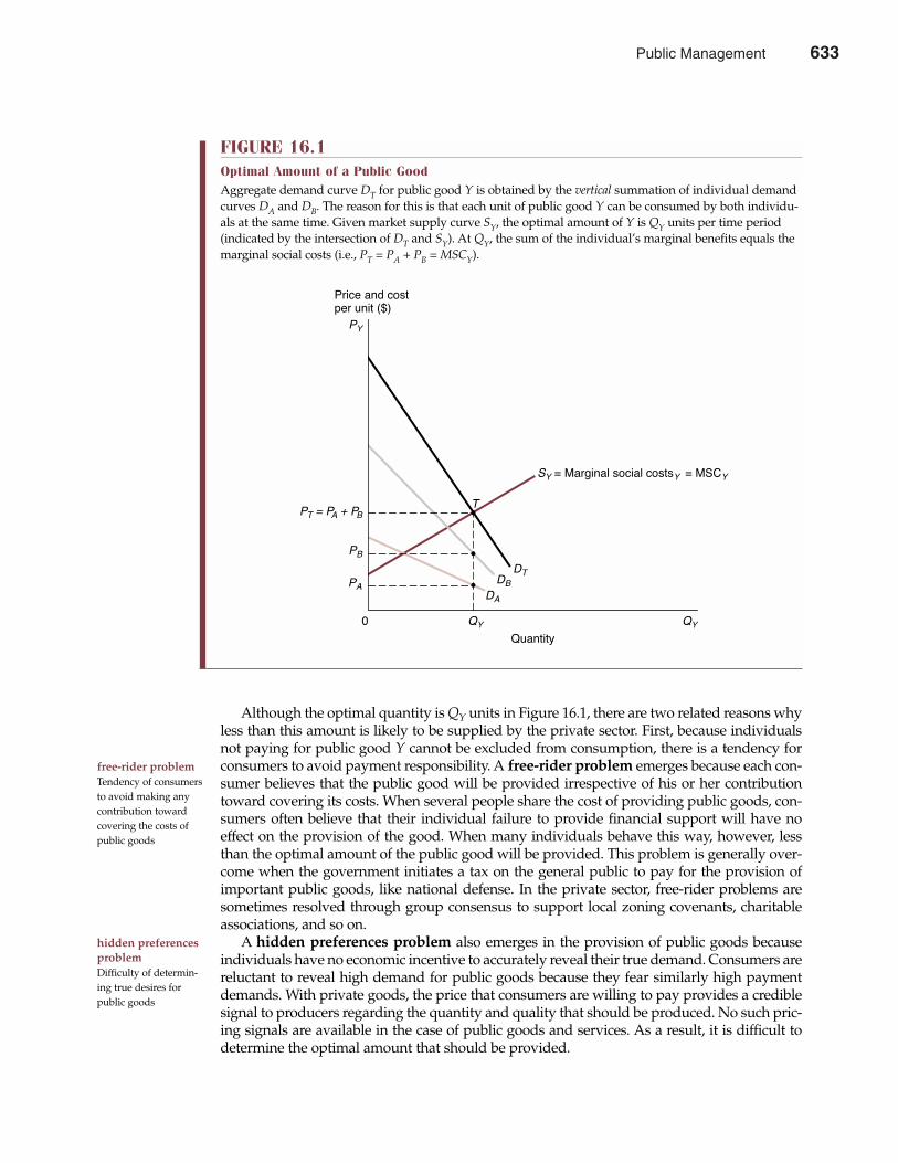
Although the optimal quantity is QY units in Figure 16.1, there are two related reasons whyless than this amount is likely to be supplied by the private sector. First, because individualsnot paying for public good Y cannot be excluded from consumption, there is a tendency forconsumers to avoid payment responsibility. A free-rider problem emerges because each con-sumer believes that the public good will be provided irrespective of his or her contributiontoward covering its costs. When several people share the cost of providing public goods, con-sumers often believe that their individual failure to provide financial support will have noeffect on the provision of the good. When many individuals behave this way, however, lessthan the optimal amount of the public good will be provided. This problem is generally over-come when the government initiates a tax on the general public to pay for the provision ofimportant public goods, like national defense. In the private sector, free-rider problems aresometimes resolved through group consensus to support local zoning covenants, charitableassociations, and so on.
A hidden preferences problem also emerges in the provision of public goods becauseindividuals have no economic incentive to accurately reveal their true demand. Consumers arereluctant to reveal high demand for public goods because they fear similarly high paymentdemands. With private goods, the price that consumers are willing to pay provides a crediblesignal to producers regarding the quantity and quality that should be produced. No such pric-ing signals are available in the case of public goods and services. As a result, it is difficult todetermine the optimal amount that should be provided.
Chapter Sixteen Public Management 633
free-rider problemTendency of consumersto avoid making anycontribution towardcovering the costs ofpublic goods
hidden preferencesproblemDifficulty of determin-ing true desires forpublic goods
FIGURE 16.1Optimal Amount of a Public GoodAggregate demand curve DT for public good Y is obtained by the vertical summation of individual demandcurves DA and DB. The reason for this is that each unit of public good Y can be consumed by both individu-als at the same time. Given market supply curve SY, the optimal amount of Y is QY units per time period(indicated by the intersection of DT and SY). At QY, the sum of the individual’s marginal benefits equals themarginal social costs (i.e., PT = PA + PB = MSCY).
Quantity
Price and costper unit ($)
PT = PA + PB
PY
DBDA
DT
SY = Marginal social costsY = MSCY
QY QY0
PB
PA
T
Public Management 633
Of course, many goods and services do not fit neatly within the categories of pure privategoods and pure public goods. Examples of goods and services with some but not all of thecharacteristics of public goods include airports, basic research programs, day-care centers,highways, hospital facilities, immunization programs, the judicial system, parks, primaryand secondary education, and trash collection. Given the many difficulties involved withaccurately determining the demand for these and other quasi-public goods, it is necessary tobe cautious when using the power of government to tax or otherwise compel popular support.Public policy must focus narrowly on the source of any perceived private-market imperfec-tions and address these impediments directly.
For example, trash collection involves elements of a public good because the timely removalof trash and other debris limits the propagation of insects and rodents and, therefore, the spreadof infectious diseases. Moreover, there are immense economies of density in trash collection. Itis far more efficient for a monopoly trash hauler to service an entire neighborhood on a weeklybasis than it is to have multiple competitors serve a single area. In recognition of the potentialfor problems with unregulated private-market trash collection, some local governments regu-late private suppliers while others pay for this service out of general tax revenues. In theory,either approach has the potential to result in better trash collection services. In practice, regula-tion is seldom perfect, and local governments often find it difficult to maintain a high level ofefficiency in the public provision of trash collection services.
Finally, it must be recognized that some goods and services provided by the public and not-for-profit sectors are designed to meet social goals of equity or fairness, rather than efficiency-oriented objectives. These purposes include redistributing income by giving assistance to thepoor, sick, and uneducated; stabilizing economic growth; and providing for the nationaldefense. However, efficiency considerations remain important even when these alternativeobjectives are important concerns of a government-sponsored or regulated program. Governmenthas an obligation to use public funds wisely.
Public Choice TheoryPublic choice theory is a philosophy of how government decisions are made and imple-mented. Public choice theory considers how government and the political process actuallywork, rather than how they should work. It explicitly recognizes the possibility of govern-ment failure, or circumstances where public policies reflect narrow private interests, ratherthan the public interest. Just because unregulated market activity does not always work per-fectly does not mean that government policies will improve the situation. It is possible thatgovernment intervention will make a bad situation worse. Similarly, the fact that governmentpolicies are inefficient does not necessarily mean that private markets can do better. For exam-ple, substantial waste in government defense expenditures does not necessarily mean that theprovision of national defense should be left to private interests.
Like the capture theory of regulation discussed in Chapter 13, the theory of public choiceis based on the premise that individuals attempt to further personal interests in the politicalarena just as they seek to further private economic interests in the marketplace. Economistshave long recognized that when an individual pursues private economic interests in the mar-ketplace, that person is moved by an “invisible hand” to also promote the welfare of societyas whole. The study of public choice theory seeks to learn whether such an invisible handmechanism is also at work in the political system. In other words, when individuals attemptto further personal interests through political activity, is the welfare of society also promoted?
Public choice theory examines how government decisions are made and implemented byanalyzing the behavior of four broad groups of participants in the political system. Voters inthe political process are the counterpart of consumers in the marketplace. Instead of purchasinggoods and services in the marketplace, voters elect government representatives who make and
634 Part Five Long-Term Investment Decisions
public choice theoryPhilosophy of how gov-ernment decisions aremade and implemented
government failureCircumstances in whichpublic policies reflectnarrow private interests,rather than the generalpublic interest
votersPersons who electpublic officials
634 Public Management
enforce government policies. Other things being equal, voters support candidates who favorpolicies that further their personal economic interests. According to public choice theory, how-ever, voters are less informed about political decisions than about market decisions due to theirrational ignorance. Because elected officials act for the community as a whole, there is less ofa need for individual voters to be fully informed about public choices. It is also generally moreexpensive for individuals to gather information about public choices than about market choic-es. Moreover, as a voter, each individual has relatively little ability to directly influence publicchoices. For all of these reasons, voters find it sensible to remain relatively uninformed aboutpublic policy decisions.
Politicians are the political-system counterpart of entrepreneurs and managers in the pri-vate market system. Although the entrepreneur or manager of a private firm seeks to maximizethe value of the firm, politicians seek to maximize chances for reelection. In doing so, politiciansmust respond to the desires of well-organized, well-informed, and well-funded special-interestgroups. Examples of such interest groups in the United States include associations of primaryand secondary school teachers, farmers, medical doctors, and many others. Faced with therational ignorance of the majority of voters, politicians often support policies that greatly bene-fit special-interest groups who contribute heavily to reelection campaigns at the expense of themostly silent and uninformed majority.
Perhaps the most maligned and misunderstood groups participating in the political processare special-interest groups. Organized lobbyists actively support the passage of laws andregulations that further narrow economic interests. For example, the National EducationAssociation has successfully blocked the advance of innovative voucher systems of publicschool financing and maintained a public school monopoly on public financing of primaryand secondary education. The American Medical Association has succeeded in limitingadmissions to medical schools, thereby reducing the supply of medical doctors and increas-ing doctors’ incomes. Grain and dairy farmers have successfully lobbied the government toprovide billions of dollars in subsidies each year, while poultry and pork producers fail toshare in such benefits. Restrictions on auto and truck imports from Japan and other countriesbenefit General Motors and Ford, while consumers pay higher than necessary prices. The suc-cess of special-interest groups is explained by the fact that such bodies provide millions of dol-lars in financial support to politicians who advocate their cause. Although special-interestgroups play a valuable role in the democratic process, problems are often obvious.Unfortunately, when large economic benefits for special interests are weighed against indi-vidually small but collectively huge social costs, it is the economic interest of special-interestgroups that often prevails.
Bureaus are government agencies that carry out policies enacted by Congress and other leg-islative bodies. According to public choice theory, public employees, or bureaucrats, are notpassive executors of adopted policies; they actively seek to influence policies to further person-al interests. They do so by seeking to increase the magnitude and scope of bureau activity andfunding. This stems from the fact that the income, power, and prestige of top bureaucrats aredirectly related to the employment size and growth of the bureau. Bureaucrats can become aseparate special-interest group within government.
Policy Implications of Public Choice TheoryThe characterization of the political process by public choice theorists is sometimes viewed ascynical. Many voters are well informed and unselfish in their political beliefs. Politicians alsosometimes refuse to compromise basic principles simply to maximize chances for reelection.Collectively important public interests prevail more often than one might expect; powerfulspecial-interest groups are sometimes defeated. Government bureaucracies are often staffed bywell-intentioned and committed public servants. For example, a majority of high-income voters
Chapter Sixteen Public Management 635
rational ignoranceTendency to remainrelatively uninformedabout public policydecisions
politiciansElected representativesor leaders
special-interestgroupsOrganized lobbyiststhat actively supportthe passage of laws andregulations that furthertheir own narrow eco-nomic interests
bureaucratsAppointed govern-ment employees andcivil servants
Public Management 635

consistently support social welfare programs that involve a redistribution of income to poorpeople. During the 1990s, large cuts in defense spending occurred despite the best efforts ofthe military-industrial complex; the tobacco lobby has suffered one defeat after another. TheAmerican Medical Association is no longer able to restrict admissions to medical schools; milkand grain price supports are under attack. Even the Civil Aeronautics Board, a large and influ-ential agency of the federal government, proposed its own elimination following airlinederegulation and was abolished.
Nevertheless, these contradictions do not invalidate the theory of public choice. Althoughpublic policy can improve the economic system in the presence of market failures, the publicpolicy process itself is subject to systematic influences that can lead to government failure. Thetheory of public choice can be used to suggest institutional changes that can lead to improve-ments in public-sector performance.
One method that public choice theory suggests for improving public-sector performance isto subject government bureaus and agencies to private-market competition whenever possi-ble. For example, families could be provided with vouchers to finance primary and secondaryeducation at public or private institutions. This would stimulate competition among privateand public schools, just like student-specific federal support for higher education stimulatescompetition among private and public colleges and universities. Still another means for increas-ing government efficiency is to encourage interagency competition. Although streamlininggovernment eliminates some duplication and waste, it also eliminates competition and incen-tives for efficient operation. For example, the cost effectiveness of the Department of Defensemight actually have declined following the consolidation of the three branches of the armedforces to a single department.
636 Part Five Long-Term Investment Decisions
Global Political Corruption
Nobel Laureate Gary S. Becker, who teaches at theUniversity of Chicago, believes that the best way toreduce undesirable business influence over the politicalprocess is to discard regulations that serve as tollgatesfor graft. In support of this argument, Becker citesmajor scandals that involve corruption by prominentpoliticians and businessmen. Despite fundamental differences in political and business systems around theglobe, Becker argues that corruption is a commondenominator whenever big government infiltrates allfacets of economic life.
Bribery and illegal favor-seeking do considerabledamage. They always divert resources away from theproduction of useful goods and services. Such activitiesalso promote policies that distort economic efficiency.Criminals are sometimes able to wrest monopoly pricesthrough bribes and intimidation. Roads are sometimesbadly built or diverted to less useful routes to rewardbuilders and landowners with undue influence. Loansfrom government banks and agencies sometimes go tocompanies with political clout rather than where they canbe invested most fruitfully.
In several countries, politicians caught with theirhands in the till have been ousted. Evidence of politicalcorruption has been highlighted by scandals in theClinton Administration, as well as in several Spanish-speaking and African countries. Public corruption isoften seen as rampant in Cameroon, Paraguay, Honduras,Nigeria, and Tanzania. In these and other emerging mar-kets, political corruption is a significant drag on economicgrowth. By contrast, Denmark, Finland, Sweden, NewZealand, and Canada benefit from having what are wide-ly regarded as the cleanest political systems.
One way to discourage corruption is to vote outcrooked politicians and punish people in business whoillegally influence the political process. Becker arguesthat the only way to permanently reduce undesirablebusiness influence over the political process is to simplifyand standardize needed regulations. The temptation tobribe public officials is weakened considerably when theylack the power to “bend” the rules.
See: Timothy Mapes and Tom Wright, “Foreign Investors in IndonesiaBattle Lawsuits and Corruption,” The Wall Street Journal Online, April 9,2002 (http://online.wsj.com).
M A N A G E R I A L A P P L I C AT I O N 1 6 . 1
636 Public Management
Chapter Sixteen Public Management 637
Public choice theory also proposes at least two ways for reducing the leverage of special-interest groups. One is to rely more on referenda to decide important political issues. Whenimportant decisions are subject to popular referendum, special-interest groups must focustheir energy on influencing the general public rather than on currying favor with importantpoliticians. Another method for reducing the influence of special-interest groups is to specifythe total amount of public funds budgeted for the year and encourage different groups tocompete for government funding and support. When the total amount of public expendituresis fixed, one group can gain only at the expense of others. Each group is then likely to pres-ent its best case for funding while exposing the weakness in competitor funding requests.
BENEFIT-COST ANALYSIS
As the trustees of valuable public resources, public-sector managers must administer economicresources in a responsible manner. This task is made difficult by problems involved with assess-ing the true level of public demand for government-provided or government-administeredgoods and services. A variety of nonmarket-based mechanisms have evolved that can be usedto effectively administer government programs and investment expenditures. The mostprevalent of these methods compares relative costs and benefits.
Benefit-Cost Analysis TheoryMany public programs are promoted on the premise that all citizens will benefit. If investmentin a public project makes at least one individual better off and no one worse off, then the proj-ect is described as Pareto satisfactory, after the noted Italian economist Vilfredo Pareto. Whenall such projects have been undertaken, the situation is deemed Pareto optimal. In practice,most public expenditures increase the welfare of some individuals while reducing the welfareof others. As a result, it is often regarded as too stringent to require that all public works fit thePareto satisfactory criterion. Instead, it is often required that they meet the criteria of a potentialPareto improvement, where there are positive net benefits. In other words, a governmentprogram or project is deemed attractive under the potential Pareto improvement criterionwhen beneficiaries could fully compensate losers and still receive positive net benefit.
The potential Pareto improvement criterion provides the rationale for benefit-costanalysis: Public programs and projects are desirable from a social standpoint so long asbenefits exceed costs. Whether beneficiaries actually compensate losers is immaterial. Theallocation of benefits and costs among various individuals is a separate equity issue. Muchlike the distribution of tax burdens, the allocation of costs and benefits from public pro-grams and projects is thought to depend upon popular notions of fairness, rather than uponefficiency considerations.
In theory, any public good or service should be supplied up to the amount that equates mar-ginal social costs and marginal social benefits. This principle is similar to the profit-maximizingstandard that output should increase to the point where marginal revenue equals marginal cost.For purposes of public-sector analysis, social benefits play the role of revenue and social costsplay the role of production expenditures. As in the process of profit maximization, benefit-costanalysis presumes that all relevant pluses and minuses associated with public programs andprojects can be measured in present-day dollar terms.
The marginal social costs of any good or service equal the marginal cost of productionplus any marginal external costs, such as pollution (discussed in Chapter 13), that are notdirectly borne by producers or their customers. Production costs borne by producers andtheir customers represent private economic costs; external costs include the value of foregone
Pareto satisfactoryIf investment in a publicproject makes at leastone individual better offand no one worse off
Pareto optimalWhen all Pareto satis-factory programs andinvestment projectshave been undertaken
potential ParetoimprovementWhen an anticipatedprogram or projectinvolves positive netbenefits
marginal social costsAdded private andpublic expenses
marginal externalcostsExpenses that are notdirectly borne by producers or their customers
Public Management 637
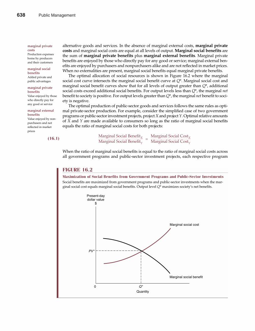
alternative goods and services. In the absence of marginal external costs, marginal privatecosts and marginal social costs are equal at all levels of output. Marginal social benefits arethe sum of marginal private benefits plus marginal external benefits. Marginal privatebenefits are enjoyed by those who directly pay for any good or service; marginal external ben-efits are enjoyed by purchasers and nonpurchasers alike and are not reflected in market prices.When no externalities are present, marginal social benefits equal marginal private benefits.
The optimal allocation of social resources is shown in Figure 16.2 where the marginalsocial cost curve intersects the marginal social benefit curve at Q*. Marginal social cost andmarginal social benefit curves show that for all levels of output greater than Q*, additionalsocial costs exceed additional social benefits. For output levels less than Q*, the marginal netbenefit to society is positive. For output levels greater than Q*, the marginal net benefit to soci-ety is negative.
The optimal production of public-sector goods and services follows the same rules as opti-mal private-sector production. For example, consider the simplified case of two governmentprograms or public-sector investment projects, project X and project Y. Optimal relative amountsof X and Y are made available to consumers so long as the ratio of marginal social benefitsequals the ratio of marginal social costs for both projects:
(16.1)Marginal Social BenefitX =
Marginal Social CostXMarginal Social BenefitY Marginal Social CostY
When the ratio of marginal social benefits is equal to the ratio of marginal social costs acrossall government programs and public-sector investment projects, each respective program
638 Part Five Long-Term Investment Decisions
marginal privatecostsProduction expensesborne by producersand their customers
marginal socialbenefitsAdded private andpublic advantages
marginal privatebenefitsValue enjoyed by thosewho directly pay forany good or service
marginal externalbenefitsValue enjoyed by non-purchasers and notreflected in marketprices
FIGURE 16.2Maximization of Social Benefits from Government Programs and Public-Sector InvestmentsSocial benefits are maximized from government programs and public-sector investments when the mar-ginal social cost equals marginal social benefits. Output level Q* maximizes society’s net benefits.
Quantity
Present-daydollar value
$
PV*
Marginal social benefit
Marginal social cost
Q*0
638 Public Management
Chapter Sixteen Public Management 639
and/or project represents an equally effective use of taxpayer funds in that it results in anidentical payoff per dollar of marginal social cost.
Alternatively, optimal relative amounts of X and Y are made available to consumers so longas the marginal social benefit to marginal social cost ratio is equal for each respective programor public-sector investment project:
(16.2)Marginal Social BenefitX =
Marginal Social BenefitYMarginal Social CostX Marginal Social CostY
Notice that each side of Equation 16.2 shows the dollar amount of marginal social benefit rel-ative to the dollar amount of marginal social cost for each project. When the MSB/MSC ratio isequal across all government programs and public-sector investment projects, each respectiveprogram and/or project represents an equally effective use of taxpayer funds and results in anidentical payoff per dollar of marginal social cost. When the ratio MSB/MSC > 1, the value ofmarginal social benefits exceeds the value of marginal social costs. When the ratio MSB/MSC< 1, then the value of marginal social benefits is less than the value of marginal social costs. Ifthe ratio MSB/MSC = 1, the value of marginal social benefits exactly equals the value of mar-ginal social costs.
When MSB/MSC = 1, a dollar’s worth of social benefit is received for each additional dollarspent on government programs and public-investment projects. This relationship implies animportant decision rule, assuming that marginal social benefits fall and marginal social costsrise with an increase in the number of government programs and public-sector investment proj-ects. If resources are fully employed throughout the economy, society’s net benefit will be max-imized when MSB/MSC = 1 for the last or marginal government program or public-sectorinvestment project. Further net marginal benefits to society are possible through an expansionin the public sector when MSB/MSC > 1 for the marginal public-sector project; resources arebeing squandered in the public sector when MSB/MSC < 1 for the marginal public-sector proj-ect. Only when MSB/MSC = 1 for the marginal public-sector project and private-sector projectare resources effectively allocated between the public and private sectors.
Benefit-Cost Analysis MethodologyBenefit-cost analysis is often used when the economic consequences of a project or a policychange are apt to extend beyond 1 year. When compared to the capital budgeting processemployed by a private firm, benefit-cost analysis is more complex because it seeks to measureboth direct and indirect effects of government programs and public-sector investment projects.Although the activities of both private firms and public agencies produce externalities, privatefirms do not typically consider external effects because they are not able to charge for them.Because public agencies seek to maximize social benefits, they must measure both direct andindirect benefits and costs.
The guiding principle of benefit-cost analysis is economic efficiency in a global sense.Resources are allocated efficiently when they lead to the maximization of total social benefits.The purpose of benefit-cost analysis is to determine if a given public expenditure would pro-duce greater benefits than if such funds were invested in an alternative public program, or ifthey were instead left in the private sector. The method has been used to determine whether apublic-sector program should be undertaken or expanded and the funding level at which suchprograms should be supported. Although benefit-cost analysis was first applied in France in the1840s, it was not until the early part of the twentieth century that it was used extensively in theUnited States to evaluate river and harbor projects. It has also been applied to projects involv-ing defense, hydroelectric power, water supply availability, recreational facilities, transportationsystems, urban renewal projects, educational systems, health, and job creation programs.
Public Management 639
640 Part Five Long-Term Investment Decisions
All benefit-cost analyses consist of five major elements: (1) statement of objectives, (2) dis-cussion of alternatives, (3) quantification of related costs and benefits, (4) selection of a criteri-on for acceptable project determination, and (5) specification of an appropriate social discountrate. Benefit-cost analysis objectives must be stated clearly. Objectives should specify a targetgroup, problem, or condition and the nature of the change expected as a result of implement-ing the program. For example, reducing the nighttime crime rate is not a clear enough objectivefor effective police department management. A clear objective would be to reduce burglariesby 20 percent and car thefts by 10 percent, following an increase in nighttime patrol hours by50 percent. The discussion of project alternatives may consist of a choice between one projectand no project, or among several public projects differing in purpose, scope, location, and size.If no public project is chosen, the implicit decision is to leave resources in the private sector. Acommon criticism of benefit-cost analysis is that sophisticated models are applied to poorly cho-sen alternatives. Because the goal of benefit-cost analysis is the efficient use of social resources, itis necessary to include all realistic alternatives.
Social Rate of DiscountBecause the benefits and costs of most government programs and public-sector investmentprojects extend beyond 1 year, it is necessary to convert these benefits and costs into present-day dollars to accurately compare decision alternatives. Determining the appropriate socialrate of discount, or interest-rate cost of public funds, is critical to the selection of appropriatealternatives. A low rate favors long-term investments with substantial future benefits; a higherrate favors short-term projects with benefits that accrue soon after the initial investment.
A common approach is to discount the benefits and costs associated with public projectsbased on the government’s cost of borrowed funds. Because government loans are consideredrisk-free, the government’s cost of borrowing is much lower than the private cost of borrowing.An important disadvantage of these low public-sector rates is that they fail to recognize theopportunity cost of funds transferred from the private sector to the public sector. Competitionbetween public-sector and private-sector projects for resources is essential to the efficient alloca-tion of investment capital. Most economists argue that because private-sector resources are usedto fund public-sector projects, the marginal private-sector opportunity cost of funds of roughly10 percent is the appropriate social rate of discount. The opportunity cost of funds transferredfrom private investment to the public sector is computed from the average pretax rate of returnon private corporate investments. This rate includes a risk premium for the uncertainty about thereturns accruing as a result of allocating funds for a given venture. The pretax rate of return forprivate investments must be used because returns from public-sector projects are not taxed.
The average pretax rate of return on government securities is a very conservative estimateof the opportunity cost of private-sector consumption that is diverted to public use. This is aconservative basis because the interest rate on government securities does not embody anydefault risk premium, as would be true of long-term corporate bonds. The average pretax rateof return on private-sector investment is a similarly useful estimate of the opportunity cost offunds diverted from private investment. In both cases, the pretax rate of return is usedbecause personal and corporate income taxes simply represent a redistribution of incomefrom the private to the public sector. Because funds for public investments are likely to comefrom both private consumption and private investments, the weighted average of the oppor-tunity cost of funds coming from these two components of the private sector should be usedto compute the social rate of discount.
During recent years, a typical pretax rate of return on long-term government bonds is 7.5percent, a standard after-tax return on investment in the private sector is 10 percent, the mar-ginal corporate and individual tax rate is roughly 40 percent, and consumption averages 94percent of total income. Using the assumptions provided, an appropriate average social rateof discount of 8 percent is calculated as follows:
social rate of discountThe interest-rate cost ofpublic funds
640 Public Management
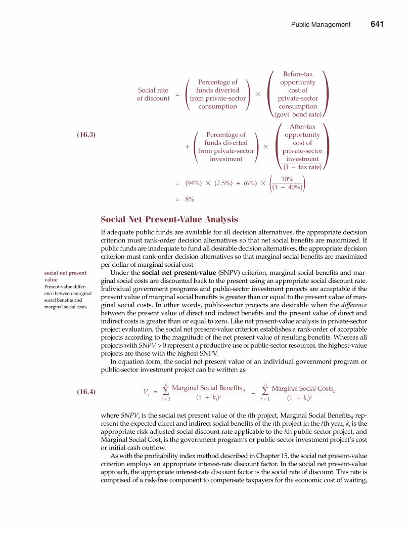
Chapter Sixteen Public Management 641
Before-taxPercentage of opportunity
Social rate funds diverted cost ofof discount = �from private-sector� � � private-sector �consumption consumption
(govt. bond rate)
After-tax(16.3) Percentage of opportunity
funds diverted cost of� �from private-sector� � �private-sector�investment investment
(1 – tax rate)
= (94%) � (7.5%) + (6%) � 10%�(1 – 40%)�= 8%
Social Net Present-Value AnalysisIf adequate public funds are available for all decision alternatives, the appropriate decisioncriterion must rank-order decision alternatives so that net social benefits are maximized. Ifpublic funds are inadequate to fund all desirable decision alternatives, the appropriate decisioncriterion must rank-order decision alternatives so that marginal social benefits are maximizedper dollar of marginal social cost.
Under the social net present-value (SNPV) criterion, marginal social benefits and mar-ginal social costs are discounted back to the present using an appropriate social discount rate.Individual government programs and public-sector investment projects are acceptable if thepresent value of marginal social benefits is greater than or equal to the present value of mar-ginal social costs. In other words, public-sector projects are desirable when the differencebetween the present value of direct and indirect benefits and the present value of direct andindirect costs is greater than or equal to zero. Like net present-value analysis in private-sectorproject evaluation, the social net present-value criterion establishes a rank-order of acceptableprojects according to the magnitude of the net present value of resulting benefits. Whereas allprojects with SNPV > 0 represent a productive use of public-sector resources, the highest-valueprojects are those with the highest SNPV.
In equation form, the social net present value of an individual government program orpublic-sector investment project can be written as
n n
(16.4) Vi = ∑ Marginal Social Benefitsit – ∑ Marginal Social Costsit
t = 1 (1 + ki)t t = 1 (1 + ki)t
where SNPVi is the social net present value of the ith project, Marginal Social Benefitsit rep-resent the expected direct and indirect social benefits of the ith project in the tth year, ki is theappropriate risk-adjusted social discount rate applicable to the ith public-sector project, andMarginal Social Costi is the government program’s or public-sector investment project’s costor initial cash outflow.
As with the profitability index method described in Chapter 15, the social net present-valuecriterion employs an appropriate interest-rate discount factor. In the social net present-valueapproach, the appropriate interest-rate discount factor is the social rate of discount. This rate iscomprised of a risk-free component to compensate taxpayers for the economic cost of waiting,
social net presentvaluePresent-value differ-ence between marginalsocial benefits andmarginal social costs
Public Management 641
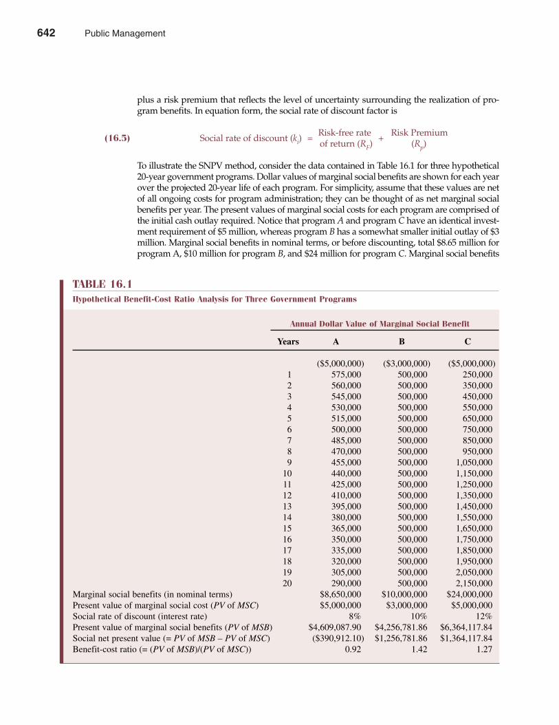
plus a risk premium that reflects the level of uncertainty surrounding the realization of pro-gram benefits. In equation form, the social rate of discount factor is
(16.5) Social rate of discount (ki) = Risk-free rate + Risk Premiumof return (RF) (Rp)
To illustrate the SNPV method, consider the data contained in Table 16.1 for three hypothetical20-year government programs. Dollar values of marginal social benefits are shown for each yearover the projected 20-year life of each program. For simplicity, assume that these values are netof all ongoing costs for program administration; they can be thought of as net marginal socialbenefits per year. The present values of marginal social costs for each program are comprised ofthe initial cash outlay required. Notice that program A and program C have an identical invest-ment requirement of $5 million, whereas program B has a somewhat smaller initial outlay of $3million. Marginal social benefits in nominal terms, or before discounting, total $8.65 million forprogram A, $10 million for program B, and $24 million for program C. Marginal social benefits
642 Part Five Long-Term Investment Decisions
TABLE 16.1Hypothetical Benefit-Cost Ratio Analysis for Three Government Programs
Annual Dollar Value of Marginal Social Benefit
Years A B C
($5,000,000) ($3,000,000) ($5,000,000)1 575,000 500,000 250,000 2 560,000 500,000 350,0003 545,000 500,000 450,0004 530,000 500,000 550,0005 515,000 500,000 650,0006 500,000 500,000 750,0007 485,000 500,000 850,0008 470,000 500,000 950,0009 455,000 500,000 1,050,000
10 440,000 500,000 1,150,00011 425,000 500,000 1,250,00012 410,000 500,000 1,350,00013 395,000 500,000 1,450,00014 380,000 500,000 1,550,00015 365,000 500,000 1,650,00016 350,000 500,000 1,750,00017 335,000 500,000 1,850,00018 320,000 500,000 1,950,00019 305,000 500,000 2,050,00020 290,000 500,000 2,150,000
Marginal social benefits (in nominal terms) $8,650,000 $10,000,000 $24,000,000 Present value of marginal social cost (PV of MSC) $5,000,000 $3,000,000 $5,000,000Social rate of discount (interest rate) 8% 10% 12%Present value of marginal social benefits (PV of MSB) $4,609,087.90 $4,256,781.86 $6,364,117.84Social net present value (= PV of MSB – PV of MSC) ($390,912.10) $1,256,781.86 $1,364,117.84Benefit-cost ratio (= (PV of MSB)/(PV of MSC)) 0.92 1.42 1.27
642 Public Management
Chapter Sixteen Public Management 643
before discounting are a misleading measure of the attractiveness of each project because they donot reflect differences in the time frame over which program benefits and costs are generated.
A relevant measure of the attractiveness of each respective program is the social net presentvalue of each program, where each dollar of marginal social benefits and marginal social costsis converted into a common current-dollar basis. The social rate of discount used to convertnominal dollar values into present-value terms is 8 percent for program A, 10 percent for pro-gram B, and 12 percent for program C. Each respective social discount rate plays the role of apresent-value interest factor that can be used to convert nominal dollar costs and benefits to acommon present-value basis. If a 5 percent yield to maturity on short-term Treasury bills istaken as a proxy for the risk-free rate, program A involves a 3 percent risk premium, programB entails a 5 percent risk premium, and program C employs a 7 percent risk premium.
Because social benefits received in the future are worth less than social costs incurred at thebeginning of the program, the SNPV for any public program tends to be much less than thenominal dollar amount of social benefits. Using a program-specific social rate of discount, thepresent value of marginal social benefits is $4,609,087.90 for program A, $4,256,781.86 for pro-gram B, and $6,364,117.84 for program C. After considering the present value of marginal socialcost for each program, the SNPV for program A is SNPVA = –$390,912.10, calculated as follows:
SNPVA = PV of MSB – PV of MSC
(16.6) = $4,609,087.90 – $5,000,000= –$390,912.10
The SNPVA = –$390,912.10 means that the present value of marginal social costs for this programexceeds the present value of marginal social benefits. Funding program A would represent anunwise use of public resources. Whenever SNPV < 0, program funding is unwise on an eco-nomic basis. A judicious use of social resources requires that SNPV > 0 for every public programor public investment project.
Again using an appropriate program-specific social rate of discount, the present value ofmarginal social benefits is $4,256,781.86 for program B and $6,364,117.84 for program C. Afterconsidering the present value of marginal social cost for each program, the SNPV for programB is $1,256,781.86 and for program C is $1,364,117.84. Both programs B and C represent a wiseuse of public resources because SNPVB > 0 and SNPVC > 0. If public funding is sufficient to fundboth projects at the same time, both should be underwritten. If public funding is scarce and bothprograms cannot be funded, program C is preferred to program B since SNPVC > SNPVB.
As discussed in Chapter 15, large projects tend to be favored through the use of net present-value criterion because large net present values usually require the commitment of significantcapital resources. In a similar fashion, the SNPV can result in a bias toward larger projectsbecause a large social net present value typically requires the commitment of significant mar-ginal social costs. This has the potential to result in a bias toward larger as opposed to smallersocial programs and public-sector investment projects when the SNPV criterion is employed.To avoid such a bias, it becomes necessary to introduce two additional public-sector capitalbudgeting decision rules.
Benefit-Cost Ratio AnalysisA variant of SNPV analysis that is often used in complex capital budgeting situations iscalled benefit-cost (B/C) ratio analysis. The benefit-cost ratio is calculated as follows:
n
(16.7)B/C ratioi =
PV of MSBi =∑ [MSBit/(1 + ki)t]
PV of MSCi
t = 1n
∑ [MSCit/(1 + ki)t]t = 1
benefit-cost (B/C)ratio analysisPresent value of mar-ginal social benefits perdollar of marginalsocial cost
Public Management 643
644 Part Five Long-Term Investment Decisions
The B/C ratio shows the relative attractiveness of any social program or public-sector invest-ment project, or the present value of marginal social benefits per dollar of marginal social cost.
In Table 16.1, SNPV > 0 implies a desirable investment program and B/C ratio > 1. Forexample, the benefit-cost ratio for program B is
B/C ratio = PV of MSBPV of MSC
= $4,256,781.86$3,000,000
= 1.42
This means that program B returns $1.42 in marginal social benefits for each dollar of marginalsocial costs, when both figures are expressed in present-value terms. On the other hand, programA returns only 92¢ in marginal social benefits for each dollar of marginal social costs, whereasprogram C returns $1.27 in marginal social benefits for each dollar of marginal social cost.
In B/C ratio analysis, any social program with B/C ratio > 1 should be accepted; any pro-gram with B/C ratio < 1 should be rejected. Programs will be accepted provided that theyreturn more than a dollar of discounted benefits for each dollar of cost. The B/C ratio and SNPVmethods always indicate the same accept/reject decisions for independent programs, becauseB/C ratio > 1 implies SNPV > 0 and B/C ratio < 1 implies SNPV < 0. However, for alternativeprograms of unequal size, B/C ratio and SNPV criteria can give different program rankings.
Internal Rate of Return AnalysisThe social internal rate of return (SIRR) is the interest or discount rate that equates thepresent value of future receipts to the initial cost or outlay. The equation for calculating thesocial internal rate of return is simply the SNPV formula set equal to zero:
n n
(16.8) SNPVi = 0 = ∑ MSBit – ∑ MSCit
t = 1 (1 + ki*)t t = 1 (1 + ki*)t
This equation is solved for the discount rate, ki*, that produces a zero net present value by set-ting discounted future marginal social benefits equal to marginal social costs. That discountrate is the social internal rate of return earned by the program, that is, SIRRi = ki*.
Because the social net present-value equation is complex, it is difficult to solve for the actu-al social internal rate of return on an investment without a computer spreadsheet. For this rea-son, trial and error is sometimes employed. One begins by arbitrarily selecting a social discountrate, such as 10 percent. If it yields a positive SNPV, the social internal rate of return must begreater than the 10 percent interest or discount rate used, and another higher rate is tried. If thechosen rate yields a negative SNPV, the internal rate of return on the program is lower than the10 percent social discount rate, and the SNPV calculation must be repeated using a lower socialdiscount rate. This process of changing the social discount rate and recalculating the net pres-ent value continues until the discounted present value of future marginal social benefits equalsthe present value of marginal social costs. The interest rate that brings about this equality is theyield, or social internal rate of return on the program.
Using trial and error, an electronic financial calculator, or a spreadsheet software program,the internal rate of return for program A is SIRRA = 6.79%. Similarly, SIRRB = 15.78% and SIRRC= 14.81%. Because SIRRB and SIRRC exceed the cost of capital, program B and program C areattractive and should be undertaken. Because SIRRA is less than the cost of capital, program Ais unattractive and should not be undertaken. In general, social internal rate of return analysissuggests that programs should be accepted when the SIRR > k and rejected when the SIRR < k.
social internal rateof returnInterest or discountrate that equates thepresent value of thefuture benefits to theinitial cost or outlay
644 Public Management
Chapter Sixteen Public Management 645
When the SIRR > k, the marginal rate of return exceeds the marginal cost of capital. As in thecase of programs with an SNPV > 0 and B/C ratio > 1, the acceptance of all investment programswith SIRR > k will lead public-sector managers to maximize net social benefits. In instances inwhich capital is scarce and only a limited number of desirable programs can be undertaken atone point in time, the SIRR can be used to derive a rank-ordering of programs from most desir-able to least desirable. Like a rank-ordering of all SNPV > 0 programs from highest to lowestB/C ratios, a rank-ordering of potential investment programs from highest to lowest SIRRsallows public-sector managers to effectively employ scarce public funds.
Limitations of Benefit-Cost AnalysisAlthough the benefit-cost analysis is conceptually appealing, it has several limitations thatmust be considered. Primary among these is the fact that existing measurement techniques aresometimes inadequate for comparing diverse public programs. Without competitive marketsfor public goods and services, it is difficult to ascertain the social value placed on public pro-grams. How much is it worth to society to provide food stamps and other financial support topoor parents and their children? Is this value reduced when the poor refuse minimum-wageemployment opportunities or when government funds are used for unintended purposes(e.g., to buy alcohol, cigarettes, or illegal drugs)? How do you measure the social value ofsophisticated new defense weapons, and how do you compare this value to the value of socialprograms? What is the social value of the agricultural milk-price support program?
Benefit-cost analysis requires public-sector managers to quantify all relevant factors in dol-lar terms. Where dollar-value estimation is not possible, qualitative factors must still be con-sidered to prevent the omission of important indirect and intangible impacts. However, theinclusion of qualitative factors makes benefit-cost analysis more complex and its conclusions
Global Competition Policy
One of the most striking economic differences betweenthe United States and Canada and the rest of the worldis the extreme lack of competition in many local markets.U.S. and Canadian consumers have a plethora of depart-ment stores, specialty outlets, and discount retailers tochoose among, while Asian consumers, for example,typically face severely limited shopping alternatives.Whereas U.S. and Canadian shoppers have access to awide variety of domestic and imported goods and serv-ices, Asian consumers typically have only Asian–madeproducts at their disposal. In fact, the typical Asian consumer is completely unaware of how the lack ofcompetition in Asian retail trade restricts purchaseoptions and raises prices. As a result, Asian consumershave never lobbied government trade officials forgreater retail competition and for access to large retailstores that offer bargain prices.
Thanks to relentless pressure by foreign trade repre-sentatives, government officials in Japan and other coun-tries have moved to free up anticompetitive trade laws.Before recent changes, mom-and-pop retail stores in Japanwere able to delay the opening of any large chain or retailstore for as long as 10 years. Since trade reforms instituted
in the early 1990s, stores like U.S. retail giant Toys “R” Usare opening at a quicker pace.
Well-designed public policies have the effect ofreducing barriers to competition and facilitating economicgrowth. Among the most important lessons learned dur-ing recent years are
• Stable money policies promote low inflation andmodest interest rates.
• Low tax rates provide positive incentives for savings,investment, and economic growth.
• Open markets facilitate trade and the growth of bothforeign and domestic markets.
Poorly designed policies stifle competition and delay eco-nomic betterment. The increasingly competitive globaleconomy has already conferred significant benefits onconsumers, but policy initiatives must be designed tomaintain that momentum. Competitive markets workbest when public policy creates an environment thatallows efficient firms to win and lets inefficient firms lose.
See: Michael Williams, “Japan Will Muddle Through...Again,” The WallStreet Journal Online, January 29, 2002 (http://online.wsj.com).
M A N A G E R I A L A P P L I C AT I O N 1 6 . 2
Public Management 645

646 Part Five Long-Term Investment Decisions
more ambiguous. At times, analytical results cannot be summarized in a single comparableratio. Evaluation problems also occur when a nonefficiency objective, such as reducing thelevel of highway noise pollution around a schoolyard, must be considered alongside an effi-ciency objective, such as increasing business activity along a new highway corridor.
Despite these and other obvious problems, benefit-cost analysis enjoys well-documentedsuccess as a vital tool for public-sector decision making. At a minimum, benefit-cost analy-sis forces the itemization and computation of costs and benefits in a manner that is far moreprecise and useful than many other methods of public-sector decision making. As a result,benefit-cost analysis allows for a more thorough analysis of public policy alternatives thanother more limited techniques.
ADDITIONAL METHODS FOR IMPROVING PUBLIC MANAGEMENT
Whereas benefit-cost studies attempt to measure all relevant factors in dollar terms, measure-ment problems sometimes preclude this possibility. In such situations, alternative means forassessing the effectiveness of decision alternatives must be explored. The most popular of suchmethods allow public-sector managers to focus attention on narrowly monitoring the resultsof existing programs.
Cost-Effectiveness AnalysisAnother technique commonly used to improve public-sector performance is cost-effectivenessanalysis. The purpose of cost-effectiveness analysis is to determine how to best employ resourcesin a given social program or public-sector investment project. One common approach is to holdoutput or service levels constant and then evaluate cost differences resulting from alternativeprogram strategies. For example, a local school board might be interested in evaluating alter-native special education programs and their respective costs. The cost-effectiveness analysisapproach might compare mainstreaming, separate classrooms, or itinerant teaching in termsof their effectiveness in meeting important special education goals. The most cost-effectivemethod is the decision alternative that meets specific educational goals at minimum cost.
Cost-effectiveness analysis is useful for evaluating the effectiveness of social programsand public-sector investment projects where output can be identified and measured in qual-itative terms but is difficult to express in monetary terms. For example, cost-effectivenessanalysis can be used to evaluate the success of alternative transportation programs such astaxis or social service vehicles for the handicapped but cannot be used to determine if pro-viding transportation for the handicapped is worthwhile from a resource allocation stand-point. Cost-effectiveness studies are also useful in situations where significant externalitiesor other intangibles exist that cannot be easily measured in dollar terms. In such cases, neg-ative impacts of social programs can be dealt with by excluding from consideration all deci-sion alternatives that generate negative impacts beyond a certain level. The selection of apreferred alternative is made on the basis of differences in tangible performance measures.
PrivatizationDuring the 1980s, a privatization movement began and accelerated in Europe, the formerSoviet Union, and former Eastern Bloc countries. With privatization, public-sector resourcesare transferred to the private sector in the hope that the profit motive might spur higherproduct quality, better customer service, and lower costs. The privatization movementgained momentum during the 1990s in response to growing dissatisfaction with the lowquality of many government services and increasing dissatisfaction with cost overruns at thefederal, state, and local levels of government.
cost-effectivenessanalysisMethod used to deter-mine how to bestemploy resources in agiven social programor public-sector invest-ment project
privatizationTransfer of public-sector resources to theprivate sector
646 Public Management
In the United States, the privatization movement has thus far failed to generate the typeof enthusiasm seen in many foreign countries. Nevertheless, local municipalities across theUnited States are increasing the amount of private-sector contracting for snow removal,garbage collection, and transit services. Since the late 1980s, a majority of state and localgovernments have greatly increased the amount of public goods and services contractedout to private providers. At the federal level, the U.S. Postal Service, now a quasi-privatemonopoly, has long used private carriers for rural deliveries. Similarly, the Department ofHealth and Human Services uses private contractors to process Medicare claims. The pri-vatization movement has clearly made dramatic inroads in countries throughout Europe andLatin America, where government control over the economy has traditionally been compre-hensive. During the 1990s, European and Latin American governments greatly increased thepace at which previously nationalized companies have been returned to the private sector.Prominent examples include electrical utilities, railroads, telecommunications businesses,and steel companies.
The economic justification for privatization is that cheaper and better goods and servicesresult as the profit motive entices firms to improve quality and cut costs. Public agencies andgovernment employees that face competition from the private sector also display an encour-aging tendency to improve performance and operating efficiency. In Chicago, for example,competitive bidding between private contractors and city cleanup and repair crews createsincentives for public employees and public managers to become more effective. In a similar sit-uation, the city of Phoenix Public Works Department won back a number of garbage collectiondistricts previously lost to private bidders after instituting innovations that lowered operatingcosts below that of private competitors. Several city and county administrators have reportedsimilar cost savings as a result of privatizing public services. In Milwaukee, school vouchersare given to low-income children to select the private school of their choice. Although parentalsatisfaction with Milwaukee’s school voucher program is high, it is too early to tell whethereducational quality has risen for both private and public schoolchildren.
Opponents of privatization argue that the transfer of government programs to the privatesector does not necessarily lead to smaller government and fewer budget deficits. Profit-seekingfirms who become dependent on public financing lobby for an expansion of public-sectorspending with as much vigor as public-sector employees. Evaluating the success of privatefirms in providing public goods is also made difficult by inadequate performance measuresand lax performance monitoring. For example, after the federal government relinquisheddirect control for job training, under the Job Training Partnership Act, measures used to eval-uate program quality appeared to show the program was a success. Fully two-thirds of adulttrainees found jobs. These performance measures were biased, however, because training con-tractors boosted their measured performance by only selecting the most promising job appli-cants. Similarly, in 1963, the federal government gave millions of dollars to private firms tobuild and staff mental health centers without developing a process to track results. By the1980s, many of these centers were converted to for-profit status and served only those able topay, leaving the poor and indigent without adequate mental healthcare.
A final argument against privatization is that the goal of public services is not just toachieve a high level of efficiency but to provide benefits that private markets cannot or do notprovide. A private firm may, for example, find it unprofitable to educate unruly children fromsingle-parent homes with little commitment to education. For-profit hospitals may find it pro-hibitively expensive to offer emergency room care to violent teens from inner-city neighbor-hoods. As a result, questions of what and how much to privatize must focus on those instanceswhere privatization can work best. Successful privatization also requires specific goals andmeasurement criteria that clearly define the public interest. Finally, successful privatizationefforts depend upon a direct link between the achievement of recognized goals and the com-pensation of public-sector and private-sector managers.
Chapter Sixteen Public Management 647
Public Management 647
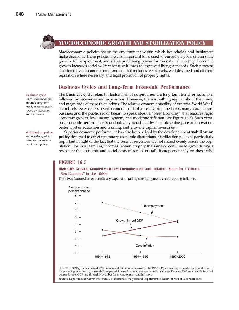
MACROECONOMIC GROWTH AND STABILIZATION POLICY
Macroeconomic policies shape the environment within which households and businessesmake decisions. These policies are also important tools used to pursue the goals of economicgrowth, full employment, and stable purchasing power for the national currency. Economicgrowth increases social welfare because it leads to improved living standards. Such progressis fostered by an economic environment that includes fee markets, well-designed and efficientregulation where necessary, and legal protection of property rights.
Business Cycles and Long-Term Economic PerformanceThe business cycle refers to fluctuations of output around a long-term trend, or recessionsfollowed by recoveries and expansions. However, there is nothing regular about the timingand magnitude of these fluctuations. The relative economic stability of the post–World War IIera reflects fewer or less severe economic disturbances. During the 1990s, many leaders frombusiness and the public sector began to speak about a “New Economy” that features rapideconomic growth, low unemployment, and moderate inflation (see Figure 16.3). Such virtu-ous economic performance is undoubtably nourished by the quickening pace of innovation,better worker education and training, and growing capital investment.
Superior economic performance has also been helped by the development of stabilizationpolicy designed to offset temporary economic disruptions. Stabilization policy is particularlyimportant in light of the fact that the costs of recessions are not shared evenly across the pop-ulation. For most families, incomes remain roughly the same or continue to grow during arecession; the economic and social costs of recessions fall disproportionately on those who
648 Part Five Long-Term Investment Decisions
business cycleFluctuations of outputaround a long-termtrend, or recessions fol-lowed by recoveriesand expansions
stabilization policyStrategy designed tooffset temporary eco-nomic disruptions
FIGURE 16.3High GDP Growth, Coupled with Low Unemployment and Inflation, Made for a Vibrant “New Economy” in the 1990sThe 1990s featured an extraordinary expansion, falling unemployment, and dropping inflation.
8
7
6
5
4
3
2
1
0
Average annual�percent change
1991Ð1993 1994Ð1996 1997Ð2000
Unemployment
Growth in real GDP
Core inflation
Note: Real GDP growth (chained 1996 dollars) and inflation (measured by the CPI-U-RS) are average annual rates from the end ofthe preceding year through the end of the period. Unemployment rates are monthly averages. Data for 2000 are through the thirdquarter for real GDP and through November for unemployment and inflation.
Sources: Department of Commerce (Bureau of Economic Analysis) and Department of Labor (Bureau of Labor Statistics).
648 Public Management
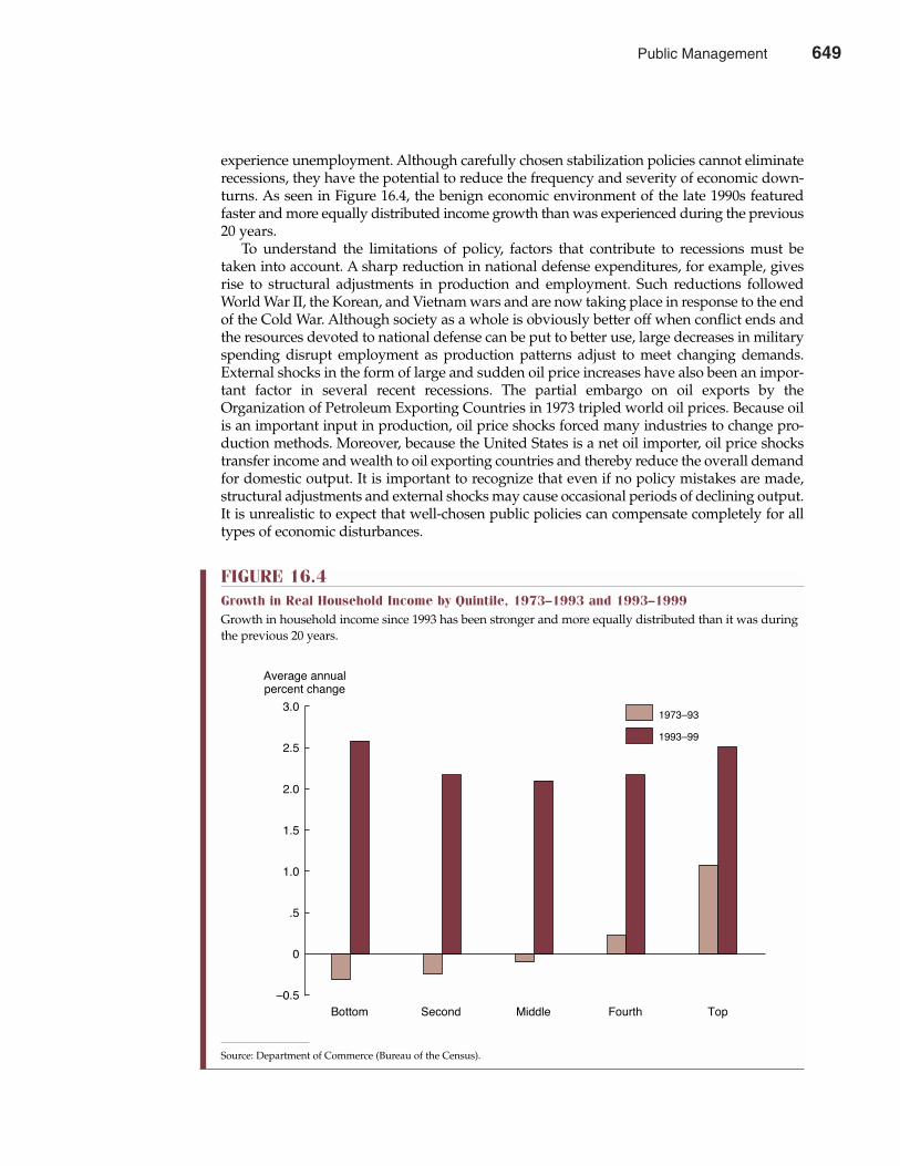
experience unemployment. Although carefully chosen stabilization policies cannot eliminaterecessions, they have the potential to reduce the frequency and severity of economic down-turns. As seen in Figure 16.4, the benign economic environment of the late 1990s featuredfaster and more equally distributed income growth than was experienced during the previous20 years.
To understand the limitations of policy, factors that contribute to recessions must betaken into account. A sharp reduction in national defense expenditures, for example, givesrise to structural adjustments in production and employment. Such reductions followedWorld War II, the Korean, and Vietnam wars and are now taking place in response to the endof the Cold War. Although society as a whole is obviously better off when conflict ends andthe resources devoted to national defense can be put to better use, large decreases in militaryspending disrupt employment as production patterns adjust to meet changing demands.External shocks in the form of large and sudden oil price increases have also been an impor-tant factor in several recent recessions. The partial embargo on oil exports by theOrganization of Petroleum Exporting Countries in 1973 tripled world oil prices. Because oilis an important input in production, oil price shocks forced many industries to change pro-duction methods. Moreover, because the United States is a net oil importer, oil price shockstransfer income and wealth to oil exporting countries and thereby reduce the overall demandfor domestic output. It is important to recognize that even if no policy mistakes are made,structural adjustments and external shocks may cause occasional periods of declining output.It is unrealistic to expect that well-chosen public policies can compensate completely for alltypes of economic disturbances.
Chapter Sixteen Public Management 649
FIGURE 16.4Growth in Real Household Income by Quintile, 1973–1993 and 1993–1999Growth in household income since 1993 has been stronger and more equally distributed than it was duringthe previous 20 years.
3.0
2.5
2.0
1.5
1.0
.5
0
Ð0.5
Average annual�percent change
Bottom Second Middle Fourth Top
1973Ð93
1993Ð99
Source: Department of Commerce (Bureau of the Census).
Public Management 649
650 Part Five Long-Term Investment Decisions
Monetary PolicyMonetary policy refers to actions taken by the Federal Reserve (the Fed) that influence bankreserves, the money stock, and interest rates. An expansionary monetary policy lowers short-term interest rates by increasing the availability of money and credit. Lower interest ratesencourage spending, particularly on investment projects. If the economy is operating wellbelow capacity, increased spending is likely to lead to increased output. Once the economy isat or near capacity, however, rapid monetary expansion leads to inflation (a sustained increasein prices) rather than output growth. Conversely, tight monetary policy reduces the growthrate of the money stock, increases short-term interest rates, and eventually lowers inflation. Inthe short run, the Fed can use monetary policy to increase the availability of credit and to lowerinterest rates. In the long run, an excessively expansionary monetary policy leads to inflationand higher nominal interest rates. Although interest rates, monetary aggregates, and otherindicators help the Fed assess the effects of its actions, no set of indicators provides a reliableforecast of the future consequences of current monetary policy choices.
The goal of using monetary policy to increase output without increasing inflation is inher-ently difficult to achieve. When the Fed increases or decreases bank reserves, the path fromreserve changes to interest rates to output and prices is often unpredictable. In recent years, anumber of factors have further complicated the task of setting monetary policy. The weaken-ing in the relation among the money supply, interest rates, and nominal GDP has decreasedthe reliability of monetary aggregates as indicators of policy. Transitory problems in financialmarkets and structural changes in the global economy have also altered the response of theU.S. economy to Fed policy. As such, the use of monetary policy to fine-tune the U.S. economyhas become increasingly problematic.
Fiscal PolicyFiscal policy refers to the spending and taxing policies of the federal government. Fiscal policycan influence total demand in the economy by changing taxes and government spending.Expansionary fiscal policy, for example, implements tax cuts, increases government spending, orboth, to increase economic activity during business downturns. Fiscal policy can also affectincentives to work, save, invest, and innovate. Changes in taxes on capital, for example, affect theafter-tax return on investment in physical assets and thus the incentive for capital accumulation.
Automatic stabilizers act as buffers when the economy weakens by automatically reduc-ing taxes and increasing government spending. Mandatory spending for programs such asunemployment insurance, food stamps, welfare programs, and Medicaid increases when theeconomy slows down because benefit criteria depend upon income or employment status.These transfer payments help consumers maintain spending. The tax system as a whole alsoacts as an automatic stabilizer. In an economic slump, personal income and corporate profitsare lower, so tax payments fall, thus helping to reduce the decline in after-tax incomes thatmight otherwise occur. Government revenues from excise and other sales-based taxes also fallwhen purchases decline. In fact, taxes typically change by a larger proportion than GDP, pri-marily because average income tax rates fall with income levels. This feature of the tax systemmakes after-tax income more stable than pretax income, which helps insulate consumptionspending from changes in income.
Discretionary policy refers to new changes in spending and taxes. Classic examples ofdiscretionary fiscal policy include the 2001 tax cut intended to stimulate spending and eco-nomic expansion, and the income tax surcharge of 1968 designed to curb rising inflation.Because the change in total expenditures determines whether policy has been expansionary orcontractionary, it is difficult to attribute expansionary fiscal policy to specific acts of spending.For example, increased highway spending is expansionary only if it is not offset by a declinein some other appropriation. Nevertheless, net changes in discretionary spending by federal,state, and local governments can have significant effects on the overall economy.
monetary policyActions taken by theFederal Reserve thatinfluence bank reserves,the money stock, andinterest rates
fiscal policySpending and taxingpolicies of the govern-ment
automatic stabilizersBuffers designed tosmooth the pace of eco-nomic activity
discretionary policyUnrestricted changes inspending and taxes
650 Public Management
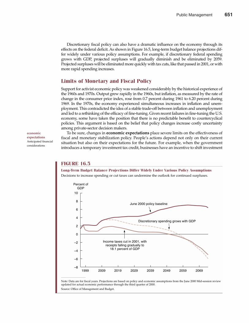
Discretionary fiscal policy can also have a dramatic influence on the economy through itseffects on the federal deficit. As shown in Figure 16.5, long-term budget balance projections dif-fer widely under various policy assumptions. For example, if discretionary federal spendinggrows with GDP, projected surpluses will gradually diminish and be eliminated by 2059.Projected surpluses will be eliminated more quickly with tax cuts, like that passed in 2001, or withmore rapid spending increases.
Limits of Monetary and Fiscal PolicySupport for activist economic policy was weakened considerably by the historical experience ofthe 1960s and 1970s. Output grew rapidly in the 1960s, but inflation, as measured by the rate ofchange in the consumer price index, rose from 0.7 percent during 1961 to 6.20 percent during1969. In the 1970s, the economy experienced simultaneous increases in inflation and unem-ployment. This contradicted the idea of a stable trade-off between inflation and unemploymentand led to a rethinking of the efficacy of fine-tuning. Given recent failures in fine-tuning the U.S.economy, some have taken the position that there is no predictable benefit to countercyclicalpolicies. This argument is based on the belief that policy changes increase costly uncertaintyamong private-sector decision makers.
To be sure, changes in economic expectations place severe limits on the effectiveness offiscal and monetary stabilization policy. People’s actions depend not only on their currentsituation but also on their expectations for the future. For example, when the governmentintroduces a temporary investment tax credit, businesses have an incentive to shift investment
Chapter Sixteen Public Management 651
economic expectationsAnticipated financialconsiderations
FIGURE 16.5Long-Term Budget Balance Projections Differ Widely Under Various Policy AssumptionsDecisions to increase spending or cut taxes can undermine the outlook for continued surpluses.
10
8
6
4
2
0
Ð2
Ð4
Ð6
Ð8
Percent of�GDP
1999 2009 2019 2029 2039 2049 2059 2069
June 2000 policy baseline
Discretionary spending grows with GDP
Income taxes cut in 2001, with�receipts falling gradually to�
18.1 percent of GDP
Note: Data are for fiscal years. Projections are based on policy and economic assumptions from the June 2000 Mid-session reviewupdated for actual economic performance through the third quarter of 2000.
Source: Office of Management and Budget.
Public Management 651
expenditures to the period in which the credit applies. However, if they merely shift capitalspending from one period to another rather than increase the overall amount of investment,the positive effect on economic growth will be limited.
Changes in government purchases may also have limited effects on total spending. Forexample, if an appropriation for the construction of a new highway system is not accompaniedby a corresponding increase in tax revenues, the budget deficit and government borrowingwill increase. Such an increase in government borrowing can put upward pressure on interestrates and discourage investment spending, thus offsetting at least part of the increase in totaldemand resulting from the construction project. The reduction in private and consumptioninvestment associated with an increase in government spending is known as the crowdingout phenomenon. Given the already enormous public-sector budgets of the 1990s, furtherincreases in government spending can create tighter conditions in credit markets and exacerbatethe crowding out problem.
ECONOMIC GROWTH POLICY
Americans enjoy a remarkably high average standard of living. Retirees today enjoy roughlythree times the level of real personal consumption expenditures typical when they were born.At this same rate of growth, our current standard of living will rise by 50 percent in less than25 years and double in roughly 40 years. Such is the power of economic growth.
652 Part Five Long-Term Investment Decisions
crowding outReduction in privateinvestment associatedwith an increase ingovernment spending
Free Trade Helps Everyone
In the early 1990s, backers of the North American FreeTrade Agreement (NAFTA) argued that free trade wouldopen Mexico’s economy, causing a surge in exports fromthe United States and Canada. It was also argued thatNAFTA would reduce illegal immigration by raising thestandard of living for Mexican workers. The case againstNAFTA was most forcefully carried by the former headof Electronic Data Systems, ex-presidential candidateRoss Perot. It was Perot’s suggestion of “a giant suckingsound” that fueled the debate. That’s the sound onewould supposedly hear as, in one great whoosh, theUnited States lost millions of jobs to low-wage Mexicans.Happily, the economic facts are more positive than thepolitical rhetoric.
When NAFTA went into effect on January 1, 1994,the United States and Canada already had a free tradeagreement. NAFTA merely extended that agreement toinclude Mexico and permit duty-free and quota-freemovement of goods across all of North America.Perhaps the most glaring irony of the NAFTA debate isthat much of the job opportunity loss feared by Perot andother critics failed to materialize. When productivity differences are considered, Mexican labor is no cheaperthan higher-priced but more efficient labor from theUnited States and Canada.
The economic facts are obvious. Free trade is enor-mously beneficial to all Americans, whether they be fromCanada, Mexico, or the United States. Before NAFTA,the tariff imposed by the United States on Mexicangoods averaged about 4 percent, while the tariff imposedby Mexico on U.S. goods averaged about 11 percent.With NAFTA, Mexican, U.S., and Canadian exportindustries and their workers benefit enormously fromthe increased access across national boundaries that follows from the abolition of all such tariffs. To extendthe many benefits of free and open trade, Congress isnow considering bills that would extend NAFTA privi-leges to Caribbean nations. Such a pact would makeway for broad trade agreements that might encompassthe southern hemisphere and eventually our Europeanand Asian trade partners as well.
With free trade, economic activity flows to wherebusiness is most efficient in producing the high-qualitygoods and services that customers demand. It is a factthat every business day, talented and well-educated U.S.workers compete effectively with low-wage competitors.
See: Damian Milverton, “U.S. Says NAFTA Partners Agree to AccelerateTariff Cuts,” The Wall Street Journal Online, January 9, 2002(http://online.wsj.com).
M A N A G E R I A L A P P L I C AT I O N 1 6 . 3
652 Public Management
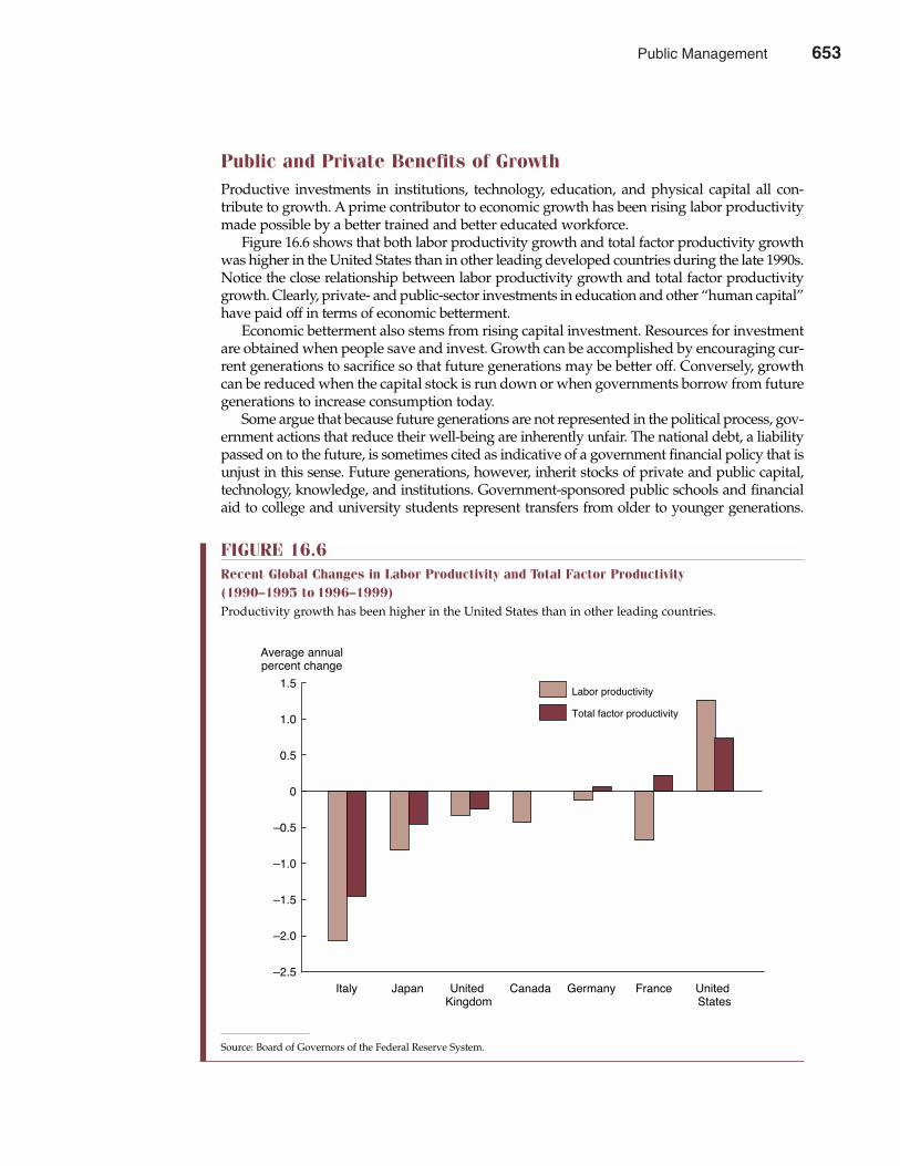
Public and Private Benefits of GrowthProductive investments in institutions, technology, education, and physical capital all con-tribute to growth. A prime contributor to economic growth has been rising labor productivitymade possible by a better trained and better educated workforce.
Figure 16.6 shows that both labor productivity growth and total factor productivity growthwas higher in the United States than in other leading developed countries during the late 1990s.Notice the close relationship between labor productivity growth and total factor productivitygrowth. Clearly, private- and public-sector investments in education and other “human capital”have paid off in terms of economic betterment.
Economic betterment also stems from rising capital investment. Resources for investmentare obtained when people save and invest. Growth can be accomplished by encouraging cur-rent generations to sacrifice so that future generations may be better off. Conversely, growthcan be reduced when the capital stock is run down or when governments borrow from futuregenerations to increase consumption today.
Some argue that because future generations are not represented in the political process, gov-ernment actions that reduce their well-being are inherently unfair. The national debt, a liabilitypassed on to the future, is sometimes cited as indicative of a government financial policy that isunjust in this sense. Future generations, however, inherit stocks of private and public capital,technology, knowledge, and institutions. Government-sponsored public schools and financialaid to college and university students represent transfers from older to younger generations.
Chapter Sixteen Public Management 653
FIGURE 16.6Recent Global Changes in Labor Productivity and Total Factor Productivity (1990–1995 to 1996–1999)Productivity growth has been higher in the United States than in other leading countries.
1.5
1.0
0.5
0
Ð0.5
Ð1.0
Ð1.5
Ð2.0
Ð2.5
Average annual�percent change
Italy Japan United Canada Germany France United �Kingdom States
Labor productivity
Total factor productivity
Source: Board of Governors of the Federal Reserve System.
Public Management 653
654 Part Five Long-Term Investment Decisions
Government-sponsored scientific research also provides benefits to both current and futuregenerations. With a constantly growing stock of productive assets, consumers on average arelikely to be better off in the future than they are today. Some argue that given rising income, itis proper for the government to redistribute income from future generations to the current gen-eration, much like any income redistribution from the rich to the poor. Others seek to increasethe ability of future generations to raise living standards, as have past generations.
Few people, however, would argue that ever-higher economic growth rates are worthwhileregardless of cost. Even if such increases were desirable, current sacrifice alone does not ensurerapid growth. For example, the former Soviet Union directed massive amounts of resourcesaway from consumption and into investment, but such investments were so poorly managedthat this sacrifice went largely unrewarded. The collapse of communism in Eastern Europeand the former Soviet Union is in large part the result of the failure of that economic system toraise living standards.
Economic Growth and the EnvironmentProperly understood, economic growth means not just “more” but “better.” Living standardsrise not just because people consume more goods and services, but because the quality ofthose goods and services improves. This includes the services of a sound environment. As theUnited States has grown economically, it has also devoted an increasing share of nationalincome to environmental protection.
To ensure economic progress consistent with environmental concerns, some have advocatedthe concept of “sustainable development.” To some, sustainable development means that eachgeneration should pass on to future generations an undiminished stock of natural resources.However, such a definition fails to take into account the fact that a reduction in the stock of oneresource can be worthwhile for present and future generations if it generates more valuableincreases in another resource. For example, future generations could benefit if part of a forestis harvested to build a school, yet they might be harmed if the school were built with the lastremaining ancient forest. A better definition of sustainable development is growth in whichevery generation passes on a stock of “net resources” no lower in per-capita value than thestock it received. Net resources include natural and environmental resources as well as knowl-edge, technology, and physical capital.
Limits to Growth?Some believe that economic growth is severely constrained by finite natural resources. This viewtraces its roots at least as far back as Thomas Malthus, who wrote in the eighteenth century thatthe population has a natural tendency to grow faster than food production and hence is con-strained by starvation, pestilence, and war. The “limits-to-growth” view, however, neglects thefact that competitive markets adjust to scarcity. When goods, services, or raw materials becomescarce, prices rise, and both consumers and producers are motivated to find more efficient waysof obtaining and using them. Rising energy prices encourage conservation; rising land pricesencourage improvements in agricultural techniques that increase food output. Contrary to theMalthusian view, world cereal production has actually grown faster than global population fornearly 200 years.
Nevertheless, when markets do not operate well, valuable resources can be consumed toorapidly or be exhausted. Inadequate property rights in water or forest resources, for example,can result in their future value being neglected. In such cases, establishing reliable propertyrights or, where markets are seriously deficient, establishing appropriate fees or regulationsconstitute the economically sensible approach.
Public policies designed to enhance the skills and productivity of the labor force are critical toensuring that the rising living standards made possible by economic growth are spread through-
654 Public Management
Chapter Sixteen Public Management 655
out the economy. Increased funding for Head Start, a program aimed at developing learningskills at an early age; promoting school choice for elementary and secondary education; betteraccess to higher education; and improved job training all have the potential to spur eco-nomic growth. Sound policies to protect the environment and manage natural resources canalso strengthen the framework for growth. The current income tax system can also bereformed to eliminate aspects that inhibit growth. Among these modifications are cutting thetax rate on savings and entrepreneurship, depreciation reform, and eliminating the doubletaxation of corporate dividends.
TRADE POLICY
International trade, or the voluntary exchange of goods and services across national bound-aries, increases the well-being of all participants by promoting economic efficiency in a variety ofways. International trade allows each country to concentrate on its most productive activities.Trade also gives firms access to the large international market, allowing them to increase outputand lower average costs by taking advantage of scale economies. Access to world markets forraw materials, capital goods, and technology also improves productivity. Foreign competitionforces domestic monopolies or oligopolies to lower prices, and imported goods provide con-sumers with greater choice. Finally, a liberal trade environment can provide a better climate forinvestment and innovation, thus raising the rate of economic growth.
Public Benefits of Free TradeInternational trade has grown much faster than world production during recent years. The rapidrecent increase in world trade is, in part, the result of the General Agreement on Tariffs andTrade (GATT), which was created after World War II to reduce tariffs and remove other non-tariff barriers to international trade. Expanding opportunities for international trade haveeffects similar to those of technological improvements: For the same amount of input, moreoutput will be produced.
In the United States, expanding world trade has created new employment opportunitiesin high-wage industries. As shown in Figure 16.7, trade in capital goods industries grewespecially fast during the late 1990s. Open trade is also beneficial to developing economiesthat have less competitive markets and need modern capital goods. By creating new competi-tion, providing domestic producers with access to large international markets, and improvingthe environment for investment, international trade can make a vital contribution to globaleconomic development.
An important counterpart to an integrated global trade system is a well-functioning inter-national financial system. The international financial system serves several important func-tions. It provides traders with access to foreign exchange and credit, thereby expanding thescope for commercial transactions. It also allows nations to finance trade imbalances throughprivate capital flows, government borrowing and lending, or changes in reserves. The inter-national financial system also encourages capital to move to countries where it is more pro-ductive. Capital inflows can finance domestic investment and thereby enable a country toinvest more than it saves. Finally, international finance allows investors to diversify investmentportfolios and reduce the risk of loss due to poor economic performance or political upheavalin any single country.
The growth in international finance is the result not only of the increase in international tradebut also of improvements in technology, financial innovations, and changes in regulation. As animportant example, the removal of external capital restrictions in Europe contributed to the cre-ation in the 1950s and 1960s of Eurodollar markets, in which banks outside the United Statesaccept deposits and make loans denominated in dollars. More recently, Eurodollar markets have
international tradeVoluntary exchange ofgoods and servicesacross national bound-aries
Eurodollar marketMarket in which banksoutside the UnitedStates accept depositsand make loansdenominated in dollars
Public Management 655
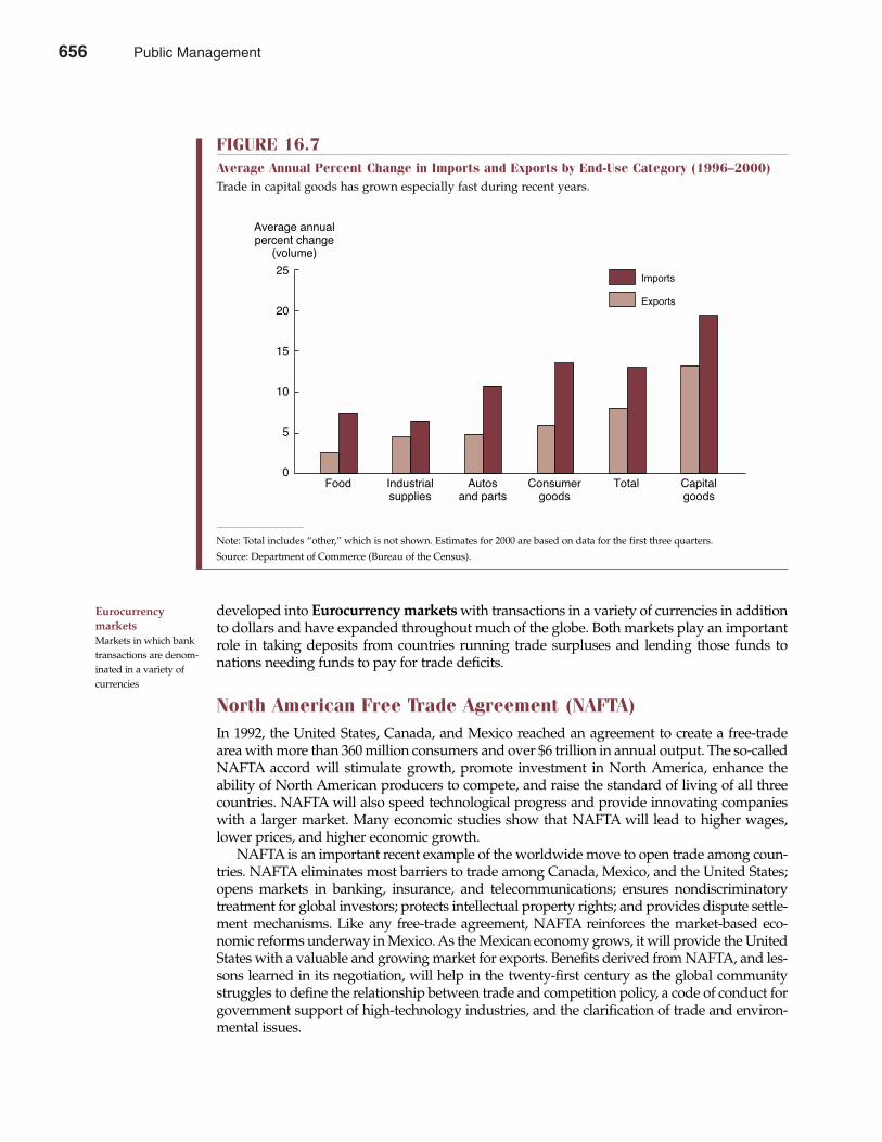
developed into Eurocurrency markets with transactions in a variety of currencies in additionto dollars and have expanded throughout much of the globe. Both markets play an importantrole in taking deposits from countries running trade surpluses and lending those funds tonations needing funds to pay for trade deficits.
North American Free Trade Agreement (NAFTA)In 1992, the United States, Canada, and Mexico reached an agreement to create a free-tradearea with more than 360 million consumers and over $6 trillion in annual output. The so-calledNAFTA accord will stimulate growth, promote investment in North America, enhance theability of North American producers to compete, and raise the standard of living of all threecountries. NAFTA will also speed technological progress and provide innovating companieswith a larger market. Many economic studies show that NAFTA will lead to higher wages,lower prices, and higher economic growth.
NAFTA is an important recent example of the worldwide move to open trade among coun-tries. NAFTA eliminates most barriers to trade among Canada, Mexico, and the United States;opens markets in banking, insurance, and telecommunications; ensures nondiscriminatorytreatment for global investors; protects intellectual property rights; and provides dispute settle-ment mechanisms. Like any free-trade agreement, NAFTA reinforces the market-based eco-nomic reforms underway in Mexico. As the Mexican economy grows, it will provide the UnitedStates with a valuable and growing market for exports. Benefits derived from NAFTA, and les-sons learned in its negotiation, will help in the twenty-first century as the global communitystruggles to define the relationship between trade and competition policy, a code of conduct forgovernment support of high-technology industries, and the clarification of trade and environ-mental issues.
656 Part Five Long-Term Investment Decisions
Eurocurrency marketsMarkets in which banktransactions are denom-inated in a variety ofcurrencies
FIGURE 16.7Average Annual Percent Change in Imports and Exports by End-Use Category (1996–2000)Trade in capital goods has grown especially fast during recent years.
25
20
15
10
5
0
Average annual�percent change�
(volume)
Food Industrial Autos Consumer Total Capital�supplies and parts goods goods
Exports
Imports
Note: Total includes “other,” which is not shown. Estimates for 2000 are based on data for the first three quarters.
Source: Department of Commerce (Bureau of the Census).
656 Public Management

Chapter Sixteen Public Management 657
PUBLIC MANAGEMENT OF HEALTH CARE
Americans are living longer, healthier lives. Since 1960, average life expectancy has increased bymore than 5 years. American physicians have access to the best technology in the world, andmore than one-half of the world’s medical research is funded by private and public sources inthe United States. At the same time, the share of national income devoted to health care has beengrowing rapidly. Concern about rising expenditures and reduced access to insurance has led tothe development of a variety of proposals for health-care reform, from market-based managedcare to calls for a government-run national health insurance program. Economic analysis is veryhelpful in understanding the potential of these alternative approaches.
Economics of Health CareTwo features of health-care services have significant economic implications. First, it is diffi-cult for consumers to independently evaluate the quality of health-care services. Consumerstypically rely on the advice of service providers in deciding what to buy. Although the lackof independent information is not unique to the health-care market (car owners often rely onmechanics), it can lead to the purchase of poor quality, unnecessary, or high-cost services.Second, to protect consumers from unscrupulous or incompetent providers, licensing boardsin every state regulate those who work in the health-care field. Such licensing procedures canincrease the cost of health-care services by limiting price and product quality competition.
Physicians have much more information about treating particular illnesses than do patients.Patients often find it difficult to evaluate the efficacy of their treatment. Even if they get better,they may not be able to tell whether they have enjoyed a natural recovery or have benefitedfrom especially effective treatment. Lack of service quality information also makes it difficult for
Global Price Controls for Pharmaceutical Drugs
In the United States, Medicare, Medicaid, and state-runhealth-care cost reimbursement plans funnel federal andstate dollars to help share the burden of exploding health-care costs. What is not generally understood is that suchprograms in the United States and abroad can contributeto higher health-care prices.
Consider the market for pharmaceuticals. If the market for prescription drugs was a typical free market,demand would be limited by the extent to which con-sumers are willing to pay for innovative therapies.However, if each dollar of consumer demand is matchedby federal or state funds, the demand for prescriptiondrugs skyrockets. Suppose a given prescription costs $15,but that 80 percent of this cost is borne by the government.Most consumers focus on the $3 cost that they must pay,rather than the overall cost of $15. As governmenthealth-care benefits rise, it is the matching share paid byconsumers that constrains industry demand. Rather thancut the cost to consumers of high-priced drugs, govern-ment matching schemes allow drug companies and otherhealth-care providers to raise prices. In the United States,
the eruption in prescription drug prices and other health-care costs coincides with the growth of government-sponsored cost-sharing plans. It is perhaps ironic thatgovernment-sponsored plans designed to help con-sumers with sky-high drug prices actually contribute tohigher drug prices.
Now, global governments are getting tight-fisted. In the United States, cost containment measures are sureto pinch profit margins for prescription drugs. Europeangovernments go one step further and demand stiff dis-counts from drug prices prevalent in the United States.For example, French price controls set prices at only 42percent of the U.S. average for prescription drugs. InJapan, allowed prices are based upon a weighted averageof prices in other markets. Clearly, global governmentsare using their buying power to reduce the industry’spricing flexibility. Stay tuned. It looks like price controlsmight give the industry a headache.
See: Stephen Pollard, “Big Pharmaceuticals Take the Gloves Off,” TheWall Street Journal Online, December 17, 2001 (http://online.wsj.com).
M A N A G E R I A L A P P L I C AT I O N 1 6 . 4
Public Management 657
658 Part Five Long-Term Investment Decisions
people to make rational decisions about purchasing health-care services. Without an accurateway to measure quality, health-care plans, hospitals, and providers have a difficult time com-peting on the basis of the price of services they offer. To address this problem, insurers andemployers have recently been working together to develop systems for measuring the qualityof health-care provided.
In some instances, health-care costs have risen because of restrictive government regula-tions. Industry costs typically rise when skilled personnel and materials are in short supply.In most cases, short-term shortages cause wages to rise, attracting new supplies of skilledworkers. As a result, extreme personnel shortages and the high wages that they produce arenot likely to persist. Historically, high physician incomes did not lead to an increased supplyof doctors because the medical profession limited the number of new physicians receivinglicenses. For many years, professional associations also controlled advertising and the typesof fee arrangements that doctors could accept. These problems are less serious today. Withnew and more enlightened government regulation, the number of practicing doctors andprice competition have increased greatly.
A further problem stems from the fact that all medical insurance, whether privately or pub-licly provided, affects the incentives of the insured. Because they are protected against the fullcost of a serious illness or injury, insureds have less incentive to take steps to limit the lossesassociated with such events. The change in incentives that results from the purchase of insur-ance is known as the moral hazard problem, or the difficulty encountered when the full costsof economic activity are not directly borne by the consumer. This term carries no connotationof dishonesty; it simply refers to the typical reduction in the economic incentive to avoid unde-sirable events. For example, people insured against car theft may leave their doors unlocked,increasing the chance that their cars may be stolen. Although people with health insurancemay be careful about avoiding health risks, they are prone to go to the doctor often and choosecomplex medical procedures. Among health economists, the term moral hazard has come toexplain why insurance provides incentives for the overconsumption of health-care services.
Market-Based Health-Care ReformUncontrolled increases in health-care expenditures and a growing number of uninsured, espe-cially among the poor (see Figure 16.8), have led to a proliferation of proposals for U.S. health-care reform. Although most of these plans seek to alleviate the symptoms of trouble in thehealth-care market, relatively few address underlying causes of health-care cost increases andgaps in insurance coverage. Because the health-care sector is flexible and responsive, healthreforms that address underlying economic problems and provide sound incentives can beeffective. Reforms that ignore the economics of health care are likely to lead to unexpected andundesirable results. Table 16.2 summarizes general features of four well-known proposals forhealth-care reform.
Among the most promising health-care reform proposals is a market-based reform plandesigned to expand access to health insurance and to improve the private markets for health-care services. The market-based plan would provide low-income Americans with a transferabletax credit for purchasing health insurance. Those who do not file tax returns would receive thecredit in the form of a transferable health insurance certificate. Because low-income Americanswould be able to purchase basic health insurance using tax credits, they would no longer haveto rely on the public hospital safety net. At the same time, the fixed-dollar nature of the creditor deduction would discourage overconsumption of health insurance.
The market-based plan would expand health insurance coverage by promoting the useof health insurance networks to act as group purchasing agents for smaller employers, thusobtaining more favorable premiums and reducing administrative costs. The plan wouldincorporate health risk pools that spread the cost of serious health problems among all those
moral hazard problemChanges in incentivesthat results from thepurchase of insurance
658 Public Management

Chapter Sixteen Public Management 659
purchasing health insurance. Low- and middle-income people with chronic health problemswould have greatly improved access to health care through this combination of tax creditsand health risk pools. Under the market-based plan, everyone would not be required to pur-chase health insurance. Those eligible for only a partial credit or deduction could decide notto purchase health insurance and continue to pay their own expenses or rely on the existinghealth-care safety net.
In any such market-based system, the role played by health maintenance organizations(HMOs) would continue to grow. During the 1990s, HMOs became a vital part of our health-care system by helping stem the rate of cost inflation. As shown in Figure 16.9, growth inhealth-care expenditures tends to slow with rising HMO enrollments.
Public Management of Health-Care ReformIn an evolving plan for comprehensive health-care reform, the Clinton Administration pro-posed an alternative “managed competition” approach. Although managed competition hassome market-oriented features, it would greatly increase the role of government in the health-care system and limit the range of health insurance options available. The concept of managedcompetition is built around the “accountable health partnership,” an organization similar to anHMO that would provide both health benefits and consumer information. Each accountablehealth partnership would be registered with a national health board that would define “uni-form effective health benefits” that each partnership would be required to provide. All insurers,both private and public, would be required to offer the same basic benefit plan.
FIGURE 16.8Health Insurance Coverage of Those Under Age 65, by Insurance Type and Income, 1999Higher income people generally receive health insurance through employers. Lower income people tendto receive it through government programs, or not at all.
100
90
80
70
60
50
40
30
20
10
0
Percent
Total Below 100 300 or more100Ð199 200Ð299
Household income as percent of poverty threshold
No health�insurance
Other Medicaid Employer
Source: Department of Commerce (Bureau of the Census).
Public Management 659

The mechanism for cost containment under this plan is competition among accountablehealth partnerships over the price of a minimum benefit package. Although taxpayers couldchoose any minimum benefits insurance package offered by any participating accountablehealth partnership, they would not be able to deduct from taxable income more than the costof the minimum benefit package offered by the cheapest accountable health partnership.Theoretically, this tax subsidy limit would encourage taxpayers to choose less comprehensivehealth insurance and efficiently run insurance plans. With managed competition, the gov-ernment would take an active role in selecting the basic benefit package and in defining thetype of insurance that most people would be able to purchase.
Outlook for Health-Care ReformIt is speculative to project that the U.S. health-care system will evolve along the lines of market-based proposals, managed competition plans, or by more traditional “play-or-pay” or nationalhealth insurance proposals. Pay-or-play plans require firms to provide basic health insurance toemployees and their dependents (“play”) or pay a payroll tax to cover enrollment in a publichealth-care plan (“pay”). Proposals for national health insurance envision replacing the pri-vate health insurance market with a single national health insurer. National health insurancewould be funded through taxes and care would be free (as in Canada) or provided at a lowcost-sharing level.
660 Part Five Long-Term Investment Decisions
TABLE 16.2Side-by-Side Comparison of Health-Care Reform Proposals
Managed NationalCompetition Health
Issue Market-Based Proposal Proposal Pay-or-Play Insurance
Moral hazard Encourages managed care for public Promotes use of basic — —programs benefit package
Cost containment Increases competition in small Increases competition Provider and Global budgetsgroup market and public programs in small group markets hospital fee Physician and Improves availability of health-care schedule hospital fee quality information scheduleSimplifies recordkeeping and billingReduces malpractice litigation costs
Access to poor Provides low- and middle-income Mandates coverage Requires Universal people with insurance certificate/ through employers employers to coveragededuction Provides subsidies to offer insurance
low-income people who or pay into are not employed and public planto part-time workers
Access for those Implements health risk adjusters for Provides age-adjusted Covers Universalin ill health high-risk people in individual and community-rated employed coverage
small group health insurance markets coverage in individual persons in ill and small group health healthinsurance markets
Source: Economic Report of the President, 1993, p. 155.
660 Public Management
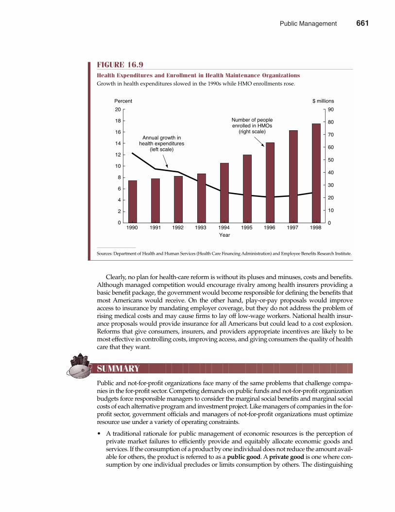
Chapter Sixteen Public Management 661
Clearly, no plan for health-care reform is without its pluses and minuses, costs and benefits.Although managed competition would encourage rivalry among health insurers providing abasic benefit package, the government would become responsible for defining the benefits thatmost Americans would receive. On the other hand, play-or-pay proposals would improveaccess to insurance by mandating employer coverage, but they do not address the problem ofrising medical costs and may cause firms to lay off low-wage workers. National health insur-ance proposals would provide insurance for all Americans but could lead to a cost explosion.Reforms that give consumers, insurers, and providers appropriate incentives are likely to bemost effective in controlling costs, improving access, and giving consumers the quality of healthcare that they want.
SUMMARY
Public and not-for-profit organizations face many of the same problems that challenge compa-nies in the for-profit sector. Competing demands on public funds and not-for-profit organizationbudgets force responsible managers to consider the marginal social benefits and marginal socialcosts of each alternative program and investment project. Like managers of companies in the for-profit sector, government officials and managers of not-for-profit organizations must optimizeresource use under a variety of operating constraints.
• A traditional rationale for public management of economic resources is the perception ofprivate market failures to efficiently provide and equitably allocate economic goods andservices. If the consumption of a product by one individual does not reduce the amount avail-able for others, the product is referred to as a public good. A private good is one where con-sumption by one individual precludes or limits consumption by others. The distinguishing
FIGURE 16.9Health Expenditures and Enrollment in Health Maintenance OrganizationsGrowth in health expenditures slowed in the 1990s while HMO enrollments rose.
20
18
16
14
12
10
8
6
4
2
0
Percent
1990 1991 1992 1993 1994 1995 1996 1997 1998
Year
90
80
70
60
50
40
30
20
10
0
$ millions
Number of people�enrolled in HMOs�
(right scale)Annual growth in�
health expenditures�(left scale)
Sources: Department of Health and Human Services (Health Care Financing Administration) and Employee Benefits Research Institute.
Public Management 661
662 Part Five Long-Term Investment Decisions
characteristic of public goods is the concept of nonrival consumption. In the case of publicgoods, use by certain individuals does not reduce availability for others. A good or serviceis characterized by the nonexclusion concept if it is impossible or prohibitively expensive toconfine the benefits of consumption to paying customers.
• A free-rider problem often materializes in the case of public goods because each consumerbelieves that the public good will be provided irrespective of his or her contribution towardcovering its costs. A hidden preferences problem also emerges in the provision of publicgoods because individuals have no economic incentive to accurately reveal their truedemand for public goods.
• Public choice theory is the philosophy of how government decisions are made andimplemented. The study of public choice theory considers how government and thepolitical process actually work, rather than how they should work. It explicitly recog-nizes the possibility of government failure, or circumstances where public policies reflectnarrow private interests, rather than the general public interest.
• Voters in the political process are the counterpart of consumers in the marketplace.According to public choice theory, voters are less informed about political decisions thanabout market decisions due to their rational ignorance. Because elected officials act for thecommunity as a whole, high information costs and each individual’s low ability to directlyinfluence public choices, voters often find it sensible to remain relatively uninformed aboutpublic policy decisions. Politicians are the political system counterpart of entrepreneurs andmanagers in the private market system. Special-interest groups are organized lobbyists thatactively support the passage of laws and regulations that further their own narrow eco-nomic interests. According to public choice theory, public employees, or bureaucrats, are notpassive executors of adopted policies; they actively seek to influence these policies to furtherpersonal interests.
• If investment in a public project makes at least one individual better off and no one worseoff, then the project is described as Pareto satisfactory. When all such government pro-grams and investment projects have been undertaken, the situation is deemed to be Paretooptimal. In practice, it is often deemed adequate when public programs and projects meetthe criteria of a potential Pareto improvement, in which there are positive net benefits.
• The marginal social costs of any good or service equal the marginal cost of production plusany marginal external costs that are not directly borne by producers or their customers.Production costs that are borne by producers and their customers represent private eco-nomic costs; external costs include the value of foregone alternative goods and services. Inthe absence of marginal external costs, marginal private costs and marginal social costs areequal at all levels of output. Marginal social benefits are the sum of marginal private ben-efits plus marginal external benefits. Marginal private benefits are enjoyed by those whodirectly pay for any good or service; marginal external benefits are enjoyed by purchasersand nonpurchasers alike and are not reflected in market prices. When no externalities arepresent, marginal social benefits equal marginal private benefits.
• The social rate of discount is the interest-rate cost of public funds. According to the socialnet present-value (SNPV) criterion, social programs and public-sector investment projectsare acceptable if the present value of marginal social benefits is greater than or equal to thepresent value of marginal social costs. Benefit-cost (B-C) ratio analysis shows the relativeattractiveness of any social program or public-sector investment project, or the presentvalue of marginal social benefits per dollar of marginal social cost. The social internal rateof return (SIRR) is the interest or discount rate that equates the present value of the futurereceipts of a program to the initial cost or outlay.
• Once the resource allocation decision has been made, the purpose of cost-effectivenessanalysis is to determine how to best employ resources in a given social program or public-
662 Public Management
sector investment project. With privatization, public-sector resources are sold or otherwisetransferred to the private sector in the hope that the profit motive might spur higher prod-uct quality, better customer service, and lower costs for production and distribution.
• Monetary policy refers to actions taken by the Federal Reserve (the Fed) that influencebank reserves, the money stock, and interest rates. Fiscal policy refers to the spending andtaxing policies of the federal government. The business cycle refers to fluctuations of out-put around a long-term trend, or recessions followed by recoveries and expansions. Recentreductions in the volatility of economic activity may be due to the development of stabi-lization policy designed to offset temporary economic disruptions. Automatic stabilizersact as buffers when the economy weakens by automatically reducing taxes and increasinggovernment spending. Discretionary policy refers to new changes in spending and taxes.
• International trade, or the voluntary exchange of goods and services across national bound-aries, increases the well-being of all participants by promoting economic efficiency in avariety of ways. The Eurodollar market is a market in which banks outside the UnitedStates accept deposits and make loans denominated in dollars. Eurodollar markets havedeveloped into Eurocurrency markets with transactions in a variety of currencies in addi-tion to dollars.
• Although sometimes effective, changes in economic expectations and certain indirecteffects of government actions place severe limits on the effectiveness of fiscal and mone-tary stabilization policy. The reduction in private investment associated with an increasein government spending is known as the crowding out phenomenon. Change in incen-tives that results from the purchase of insurance is known as the moral hazard problem,or the difficulty encountered when the full costs of economic activity are not directly borneby the consumer.
During the 1990s, microeconomic and macroeconomic policies were employed by all levels ofgovernment as a means for improving upon private-sector price and output decisions. At thesame time, government agencies and not-for-profit organizations found themselves besiegedby competing demands for scarce goods and services. This chapter illustrates how the toolsand techniques of managerial economics can be employed to improve decision making in thenot-for-profit sector and refine the management of scarce public resources.
QUESTIONS
Q16.1 Describe the traditional rationale for public management of economic resources. Is this ration-ale viable when government deficit spending is substantial?
Q16.2 What is the essential difference between public and private goods? Give some examples of eachand some examples of goods and services that involve elements of both.
Q16.3 Does the fact that public decisions are sometimes made by self-interested politicians and bureau-crats undermine the basic premise of public choice theory?
Q16.4 List some potential causes of the Great Depression and the range of factors that influence thetiming and magnitude of economic fluctuations in general.
Q16.5 One of the most vexing issues to complicate the health-care debate is the problem that there isno simple link between general health and well-being and the amount spent on health care.Briefly describe why the connection between health care and health is not a simple one. Doesthe weakness of the link between health and health care have any implications for mandatoryuniversal coverage proposals?
Q16.6 What features of the health-care services market can lead to the purchase of poor quality,unnecessary, or high-cost services?
Chapter Sixteen Public Management 663
Public Management 663
664 Part Five Long-Term Investment Decisions
Q16.7 Among health economists, the term moral hazard has come to explain why insurance providesincentives for the overconsumption of health-care services. Describe this idea and its economicimplications.
Q16.8 Is government policy that increases the well-being of one generation at the expense of anotherjust in the ethical sense?
Q16.9 “Economic growth is ultimately constrained by finite natural resources. In a capitalist system,the population has a natural tendency to grow faster than food production and hence is onlyconstrained by starvation, pestilence, and war. It is the proper role of government to own andmanage natural resources so that the limits to growth are managed in a humane manner.”Discuss this statement.
Q16.10 Describe some of the social benefits of international trade.
SELF-TEST PROBLEMS AND SOLUTIONS
ST16.1 Benefit-Cost Analysis Methodology. The benefit-cost approach is not new: The concept firstsurfaced in France in 1844. In this century, benefit-cost analysis has been widely used in theevaluation of river and harbor projects since as early as 1902. In the United States, the 1936 FloodControl Act authorized federal assistance in developing flood-control programs “if the benefitsto whomsoever they may accrue are in excess of the estimated costs.” By 1950, federal agencypractice required the consideration of both direct and indirect benefits and costs and that unmea-sured intangible influences be listed. Despite this long history of widespread use, it has only beensince 1970 that public-sector managers have sought to broadly apply the principles of benefit-cost analysis to the evaluation of agricultural programs, rapid transit projects, highway con-struction, urban renewal projects, recreation facility construction, job training programs,health-care reform, education, research and development projects, and defense policies.A. Briefly describe major similarities and differences between public-sector benefit-cost analy-
sis and the private-sector capital budgeting process.B. What major questions must be answered before meaningful benefit-cost analysis is possible?C. Although the maximization of society’s wealth is the primary objective of benefit-cost
analysis, it is important to recognize that constraints often limit government’s ability toachieve certain objectives. Enumerate some of the common economic, political, and socialconstraints faced in public-sector benefit-cost analysis.
D. In light of these constraints, discuss some of the pluses and minuses associated with theuse of benefit-cost analysis as the foundation for a general approach to the allocation ofgovernment-entrusted resources.
ST16.1 SolutionA. Benefit-cost analysis is a method for assessing the desirability of social programs and public-
sector investment projects when it is necessary to take a long view of the public and privaterepercussions of such expenditures. As in the case of private-sector capital budgeting, benefit-cost analysis is frequently used in cases where the economic consequences of a program orproject are likely to extend beyond 1 year in time. Unlike capital budgeting, however, benefit-cost analysis seeks to measure both direct private effects and indirect social implications ofpublic-sector investment decisions and policy changes.
B. Before meaningful benefit-cost analysis is possible, a number of important policy questionsmust be answered. Among these policy questions are• What is the social objective function that is to be maximized?• What constraints are placed on the decision-making process?
664 Public Management
Chapter Sixteen Public Management 665
• What marginal social benefits and marginal social costs are to be included, and howare they to be measured?
• What social investment criterion should be used?• What is the appropriate social rate of discount?
C. A number of constraints impinge upon society’s ability to maximize the social benefitsderived from public expenditures. Among these constraints are• Physical constraints. Program alternatives are limited by the available state of technology
and by current production possibilities. For example, it is not yet possible to cure AIDS.Therefore, major emphasis for public policy in this area must be directed toward pre-vention, early detection and treatment, and research.
• Legal constraints. Domestic laws and international agreements place limits on proper-ty rights, the right of eminent domain, due process, constitutional limits on a particu-lar agency’s activities, and so on. These legal constraints often play an important rolein shaping the realm of public policy.
• Administrative constraints. Effective programs require competent management andexecution. Qualified individuals must be available to carry out social objectives. Eventhe best-conceived program is doomed to failure unless managers and workers withthe proper mix of technical and administrative skill are available.
• Distributional constraints. Social programs and public-sector investment projects affect dif-ferent groups in different ways. The “gainers” are seldom the same as “losers.” When dis-tributional impacts of public policy are of paramount concern, the objective of benefit-costanalysis might maximize subject to the constraint that equity considerations be met.
• Political constraints. That which is optimal may not be feasible because of slowness andinefficiency in the political process. Often what is best is tempered by what is possi-ble, given the existence of strong competing special-interest groups.
• Budget constraints. Public agencies often work within the bounds of a predeterminedbudget. As a result, virtually all social programs and public-sector investment projectshave some absolute financial ceiling above which the program cannot be expanded,irrespective of social benefits.
• Social or religious constraints. Social or religious constraints may limit the range of feasi-ble program alternatives. It is futile to attempt to combat teen pregnancy with publicsupport for family planning if religious constraints prohibit the use of modern birthcontrol methods.
D. An important potential use of benefit-cost analysis is as the structure for a general phi-losophy of government resource allocation. As such, the results of benefit-cost studieshave the potential to serve as a guide for resource-allocation decisions within and amonggovernment programs and investment projects in agriculture, defense, education, healthcare, welfare, and other areas. The objective of such a comprehensive benefit-cost approachto government would be to maximize the net present value of the difference between themarginal social benefits and the marginal social costs derived from all social programsand public-sector investment projects.
Although a benefit-cost approach to evaluating all levels and forms of government isconceptually appealing on an efficiency basis, it suffers from a number of serious practi-cal limitations. Perhaps most importantly, the measurement of marginal social benefitsand marginal social costs for goods and services that are not or cannot be provided by theprivate sector is often primitive, at best. Measurement systems have not been sufficientlyrefined or standardized to permit meaningful comparisons among the social net presentvalue of “Star Wars” defense systems, the guaranteed student loan program for collegestudents, funding for AIDS research, Medicare, and Medicaid. A further problem arisesbecause benefit-cost analysis is largely restricted to a consideration of the efficiency objective;
Public Management 665
666 Part Five Long-Term Investment Decisions
equity-related considerations are seldom accorded full treatment in benefit-cost analysis. Inaddition, as discussed previously, a number of important economic, political, and social con-straints limit the effectiveness of benefit-cost analysis. As a result, significant problems arisewhen a given social program or public-sector investment project is designed to meet effi-ciency and equity-related objectives.
For these reasons, benefit-cost analysis is traditionally viewed within the narrow contextof a decision technique that is helpful in focusing interest on the economic consequences ofproposed social programs and public-sector investment projects. Its greatest use is in com-paring programs and projects that are designed to achieve the same or similar objectives andas a tool for focusing resources on the best use of resources intended to meet a given socialobjective.
ST16.2 Trade Policy. In 1992, the United States, Canada, and Mexico reached an agreement to createa free-trade area with more than 360 million consumers and over $6 trillion in annual output.This so-called North American Free Trade Agreement (NAFTA) accord links the United Stateswith its first- and third-largest trading partners.A. Summarize the main economic features of NAFTA.B. In the years prior to NAFTA, Mexico had opened its markets and implemented sweeping
economic reforms. Briefly describe some of the economic and political benefits derivedfrom these reforms.
C. In light of this experience, what economic and political benefits do you project as a resultof NAFTA?
ST16.2 SolutionA. According to NAFTA, existing duties on most goods and services will be either eliminated
or phased out. NAFTA will also eliminate quotas along with import licenses unless they areessential for such purposes as protecting human health. In addition to dismantling tradebarriers in industrial goods, NAFTA includes agreements in services, investment, intellec-tual property rights, agriculture, and the strengthening of trade rules. There are also sideagreements on labor provisions and protection of the environment.
Under NAFTA, the three countries extend most-favored-nation treatment in services toeach other. Each NAFTA country must treat service providers from other NAFTA countriesno less favorably than it treats its own service providers and no less favorably than it treatsservice providers from non-NAFTAcountries. In addition, a NAFTAcountry may not requirethat a service provider of another NAFTA country establish or maintain a residence as a con-dition for providing the service.
B. In recent years, Mexico has opened its markets and implemented sweeping economicreforms. In 1986, Mexico joined the General Agreement on Tariffs and Trade (GATT) andbegan to unilaterally lower its tariffs and other trade barriers. Mexico’s reforms have raisedits economic growth rate and helped make it an important export market for the UnitedStates. As an added economic benefit, as economic opportunities in Mexico improve, Mexicanworkers will have fewer incentives to migrate to the United States. Thus, a stable and pros-perous Mexico is important from both an economic and a political standpoint.
C. NAFTA will stimulate growth, promote investment in North America, enhance the ability ofNorth American producers to compete, and raise the standard of living of all three countries.NAFTA will also speed technological progress and provide innovating companies with alarger market. Many economic studies show that NAFTA will lead to higher wages, lowerprices, and higher economic growth rates. NAFTA will also reinforce market reforms alreadyunderway in Mexico.
Perhaps most importantly, passage of NAFTA strengthens peaceful ties among theUnited States, Canada, and Mexico. As important partners in mutually beneficial trade,these three countries have a common interest in maintaining a strong peaceful coexistence.
666 Public Management
Chapter Sixteen Public Management 667
PROBLEMS
P16.1 Public Versus Private Goods. Publicly funded lighthouses provide a valuable service alongcoastal waterways and in the Great Lakes Region. Through visual light-beam signals, light-houses mark the route of safe passage for cargo ships and pleasure craft 24 hours per day, 365days per year. The service provided by such lighthouses is an often-cited classic example of apublic good. Once a lighthouse is built, it can send signals to additional cargo ships and pleas-ure craft at practically zero marginal cost. Thus, lighthouse signals are said to be an excellentexample of a government-provided service that is nonrival in consumption. As such, propo-nents of government funding for lighthouses argue that such services would not be providedby the private sector.A. Briefly describe and contrast the nonrival consumption and nonexclusion concepts.B. Do lighthouse services display both nonrival consumption and nonexclusion characteristics?C. Explain how private-sector providers of public goods can operate profitably when such
goods and services do not embody the nonexclusion concept.P16.2 Goal Setting in Public Management. The objectives of social programs are set by the public
through their support for various political representatives. In the election process, policy alter-natives are enumerated, explored, and revised in light of popular preferences and operative con-straints. These alternatives are then evaluated by comparing the present-value size of marginalsocial benefits and marginal social costs. According to the social net present-value criterion, anysocial program or public-sector investment project is desirable so long as the present value ofmarginal social benefits exceeds the present value of marginal social costs.A. Explain how the social net present-value criterion is related to the Pareto satisfactory concept.B. Do you see any problems with the adoption of the Pareto satisfactory criterion?C. Is there any straightforward method for overcoming the limitations of the Pareto satis-
factory criterion?P16.3 Social Rate of Discount. Because resources for social programs and public-sector invest-
ment projects come from private-sector consumption and/or investment, economists typicallyadvocate the use of a social rate of discount that reflects this private-sector opportunity cost. Agood estimate of the opportunity cost of funds diverted from private consumption is the rateof return on government securities that is available to individual investors. Similarly, the averagerate of return on private investments can be taken as the opportunity cost of private-sectorinvestment funds.A. Should pretax or after-tax rates of return be used to estimate the opportunity cost of
resources diverted from the private sector to fund social programs or public-sector invest-ment projects? Why?
B. Assume that the rate of return on long-term government bonds is 8%, a typical after-taxreturn on investment in the private sector is 10%, the marginal corporate and individualtax rate is 30%, and consumption averages 95% of total income. Based on the informationprovided, calculate an economically appropriate social rate of discount.
P16.4 Equity and Efficiency in Benefit-Cost Analysis. In benefit-cost analysis, public-sector man-agers seek to learn if society as a whole will be better off by the adoption of a specific socialprogram or public-sector investment project. Rather than seeking to maximize profits or thevalue of the firm, public-sector managers use benefit-cost analysis to maximize, or at leastmove toward a maximization of, the excess of marginal social benefits over marginal socialcosts. With this goal in mind, from an efficiency perspective, the distribution of any social netpresent value is of no importance. For example, when the city of Denver sponsors a newDenver International Airport at an initial cost of $3.5 billion, it makes no difference whether thecity pays the entire cost or whether the city, the state of Colorado, and the federal government
Public Management 667
668 Part Five Long-Term Investment Decisions
split these costs. Similarly, if the city of Denver is motivated by the desire to lure business andtourist traffic from Chicago or Los Angeles, the benefits of increased economic activity inDenver that has merely shifted from other transportation centers should not be counted. Inboth instances, the proper concern is the increase in aggregate social wealth, not aggregatelocal wealth.A. Assume that the city of Denver and local airline customers must pay only 10% of the
costs of Denver International Airport, with the federal government picking up the other90% of the tab. Describe how a local benefit-cost analysis of the airport project might bedistorted by this cost-sharing arrangement.
B. Under the federal revenue sharing program, the federal government collects tax revenuesthat are then returned to states and other local units of government to support a widevariety of social programs. Can you see any problems for an efficient allocation of publicexpenditures when the spending and taxing authority of government is divided in thismanner?
C. As a practical matter, can the equity and efficiency implications of social programs andpublic-sector investment projects be completely separated?
P16.5 Benefit-Cost Analysis. According to the National Highway Traffic Safety Administration(NHTSA), 41,800 people were killed in highway crashes in 2000, up from 41,611 in 1999, a0.5% increase. The fatality rate per 100 million vehicle miles was 1.6, which means that 1.6people were killed for every 100 million miles traveled. This figure is up from a record lowfatality rate of 1.5 in 1999. “These statistics underscore the challenges facing this country inhighway safety,” said U.S. Transportation Secretary Norman Mineta. “Safety is an individualas well as government responsibility, and we must work together to improve it.”
As a practical matter, it is important to recognize that almost all of the tens of thousands ofhighway fatalities per year are preventable. Using current technology, highway fatalities couldbe substantially reduced or eliminated by draconian public policy measures such as a strictlyenforced nationwide 20 mph speed limit. Needless to say, popular opposition would beintense for any such proposal. Speed limits as high as 75 mph on major highways are widelypopular because consumers derive significant economic and social benefits from speedy auto-mobile transportation. However, by failing to sharply reduce or eliminate highway fatalities,speed limit policy places a finite and measurable value on human life.A. From an economic standpoint, explain how practical public policy sets a dollar value on
human life. Is it efficient to do so?B. Are there equity considerations one must weigh in judging the fairness of dollar estimates
of the value of human life?P16.6 Privatization. In Massachusetts, a state education law authorized the establishment of up
to 25 so-called charter schools. Charter schools are public schools that receive state fundingas well as some measure of autonomy from local school boards and the rules that governconventional schools. As a result, students and educators in Boston face the ready prospectof classrooms with politicians as lecturers, academic instruction aided by yoga, school doorsopen from dawn to dusk, and public schools run on a for-profit basis.
Charter schools already are operating in Minnesota and California, and five other statespromise to join the trend with recently enacted charter-school legislation. Advocates of suchschools argue that they provide badly needed competition for existing public schools. Underthe charter-school concept, anyone with a good education idea gets access to governmentfunding, so long as they can attract and effectively train students.A. Explain how breaking the public-school monopoly on access to public funding could help
improve the quality of public- and private-school primary education.B. Explain why primary-school privatization might not create such benefits.
668 Public Management

Chapter Sixteen Public Management 669
P16.7 Growth Implications of the Federal Deficit. The amount of federal debt held by the pub-lic is the sum total of all previous deficits minus any surpluses. Federal debt held by the publicequals the value of outstanding Treasury bills, notes, bonds, U.S. savings bonds, and otherfinancial obligations of the federal government that the Treasury sells to the public. Debt heldby the public does not include debt held in government trust funds. This debt is owed by thegovernment to itself, so economists generally use the debt held by the public as the economi-cally meaningful measure of the national debt. In 2001, government debt held by the public wasroughly $5.8 trillion, or roughly $20,606 for every man, woman, and child in the United States.
Of the many government activities that may affect future living standards, considerableattention has focused on the federal debt and the large and persistent federal budget deficits.A. Explain how government debt and deficits can affect intergenerational equity and, under
certain conditions, adversely affect the economy’s productive capacity.B. Explain why government debt and deficits may not affect intergenerational equity and
adversely affect the economy’s productive capacity.C. Illustrate how balancing the budget might actually harm the economy, and why zero deficits
are not a prerequisite to reducing the debt-to-GDP ratio.P16.8 Trade Policy. The past half-century has been marked by a number of experiments with dif-
ferent international exchange-rate arrangements. Under the Bretton Woods system, designedat the end of World War II, currencies of participating nations were pegged to the dollar andonly occasionally adjusted. Since that system was abandoned in the early 1970s, exchangerates of major industrialized countries have generally “floated” against each other in responseto market forces. However, a number of European countries revived the pegged exchange-ratesystem when they created the European Monetary System (EMS) in 1979.
In the Maastricht Treaty of 1991, members of the European Community agreed to replacetheir national currencies with a single currency by the year 2000, thereby superseding the cur-rent system of pegged exchange rates under the EMS and permanently ruling out exchange-rate changes. Ironically, events in 1992, including the temporary withdrawal of a number ofcountries from the EMS exchange-rate mechanism, underscored the shortcomings of a peggedexchange-rate system in the face of economic disturbances.A. Explain why progress toward a single European currency might be viewed as comple-
mentary to the increasing integration of the European market for goods and services.B. Contrast the economic benefits of a single European currency with the economic benefits
of an elimination of European trade barriers. Is a single European currency necessary for acomplete integration of the European market?
P16.9 The Economics of Health Care. The United States spends more per person on health carethan any other country in the world. Still, recent studies show that the United States ranks rela-tively low in the overall quality of health care provided. France is often described as providingits citizens with the globe’s best health care. Japan wins the distinction as having the world’shealthiest people. Although good at expensive care, like open-heart surgery, the U.S. health-care delivery system is often described as poor for low-cost preventive care. Measuring howlong people live in good health, and not just how long they live, the Japanese beat Americans by4.5 years. Yet it is surprising that Japan spends just $1,750 per person on health care, and Francespends $2,100. Both figures are far below the standard set in the United States, where health-carespending was a whopping $3,724 per person in 2001.A. Why is health-care demand different from the demand for many other services?B. Consumers buy health care to improve their health and well-being, but research suggests
only a weak connection between health-care spending and health. Explain why theremight be only a weak link between health-care expenditures and health.
C. Why is health-care spending rising rapidly on a worldwide basis? Is robust growth inhealth-care spending likely to continue?
Public Management 669
P16.10 Health-Care Reform. Representative Tom Allen (D-ME) introduced the Prescription DrugFairness for Seniors Act (H.R. 664) on February 10, 1999, and quickly amassed over 100 sponsors.If made law, the bill would force prescription drug manufacturers to sell their products to retailpharmacies at the lowest price paid by any agency or department of the U.S. government, or themanufacturer’s best price for outpatient drugs, whichever is lower. Critics contend that such pre-scription drug price regulation would not lower patient costs but instead result in higher pricesand reduced availability of new prescription drugs.A. With respect to the demand for prescription drugs, explain how price controls might have
the unintended effect of actually increasing prices.B. Explain how price controls might affect the supply of new and innovative drugs.
670 Part Five Long-Term Investment Decisions
CASE STUDY
Oh, Lord, Won’t You Buy Me a Mercedes-Benz (Factory)?2
On October 1, 1993, Alabama emerged victorious as the site of Mercedes-Benz AG’s first U.S.car plant. States like Alabama are vying more desperately than ever to lure new industrial jobsand hold on to those they have. To start with, they give away millions of dollars in free land.After that come fat checks for site clearance, training, even employee salaries. Both foreign anddomestic companies are finding ingenious ways to cash in.
Mercedes initially had so little interest in Alabama that Andreas Renschler, who headedMercedes’s site-selection team and is expected to run the new factory, says he did not evenplan to visit. Of more than 20 states that Mercedes looked at seriously, it initially leaned towardNorth Carolina, where Mercedes’s parent, Daimler-Benz AG, already builds Freightliner trucks.North Carolina officials say Governor Jim Hunt pursued Mercedes harder than he ever hadpursued a potential investor. Mercedes officials were reportedly surprised at the various states’ardor, but they quickly cashed in on it. Mercedes would get offers for certain things from cer-tain states, put it on their ideal contract proposal, and then come back to the other states andask if they would be willing to do the same. For example, Mercedes persuaded all the maincompetitors to offer $5 million for a welcome center next to the factory, where customers couldpick up cars, have them serviced, and visit an auto museum. It got commitments for free 18-month employee-training programs. It also got state governments and utilities to promise tobuy large quantities of the four-wheel-drive recreational vehicles that the new factory will pro-duce. Perhaps the biggest bombshell, Mercedes officials even asked the states to pick up thesalaries of its 1,500 workers for their first year or so on the job, at a cost of $45 million. Theworkers would be in a training program and would not be producing anything, Mercedesexplained. Although North Carolina and other state officials said no, Alabama said yes, evento the salary request. “The Mercedes project simply was worth more to us than it was to anyother state,” says Billy Joe Camp, Alabama’s economic development director.
When Mercedes found North Carolina proposing to build a $35 million training center atthe company’s plant, the German automaker enticed Alabama to more than match the NorthCarolina offer. To outbid the competition, the Alabama governor hurriedly won legislativeapproval for special, lavish tax concessions—dubbed Alabama’s Mercedes Law—and offeredto spend tens of millions of dollars buying more than 2,500 Mercedes vehicles for state use.In the bargain, Mercedes says it agreed to limit itself to using just $42.6 million per year inincome and payroll tax credits; Alabama officials say that was all Mercedes expected to be
2 Rick Brooks, “How Big Incentives Won Alabama a Piece of the Auto Industry,” The Wall Street Journal, April 3,2002, A1, A24.
670 Public Management

SELECTED REFERENCESAthanasoulis, Stefano G., and Eric Van Wincoop. “Risk Sharing Within the United States: What Do Financial
Markets and Fiscal Federalism Accomplish?” Review of Economics and Statistics 83 (November 2001):688–698.
Davis, Donald R., and David E. Weinstein. “An Account of Global Factor Trade.” American EconomicReview 91 (December 2001): 1423–1453.
Chapter Sixteen Public Management 671
able to use, based on profit projections. It also will be allowed, however, to escape more than $9million a year in property taxes and other fees, as permitted under existing law. Although SouthCarolina offered $80 million in tax credits over a period of 20 years, Alabama granted Mercedesa more attractive tax credit, available in advance in the form of an interest-free loan. Mercedesofficials also say Alabama’s promised education spending was double any other state’s promise.Alabama officials even agreed to place Mercedes’s distinctive emblem atop a local scoreboard intime for the big, televised Alabama-Tennessee football game. The price? Why, free, of course.
In all, Alabama wound up promising Mercedes over $300 million in incentives, which eco-nomic development experts call a record package for a foreign company. How has it workedout in the long run? Very well, say supporters of the Alabama program. On August 30, 2000,DaimlerChrysler announced it will invest another $1 billion in a major expansion at itsTuscaloosa, Alabama, site to double production for the next generation Mercedes-Benz M-classsport utility vehicle. The expansion is expected to double production capacity from 80,000 unitsto roughly 160,000 units at the Tuscaloosa facility and generate up to 2,000 new jobs. Inannouncing the expansion, company officials stressed that their success would not have beenpossible without the great partnership they had formed with the state of Alabama and thestrong workforce that they found there. With the new expansion, DaimlerChrysler couldbecome the fifth largest employer in Alabama, with more than 7,000 employees between itsChrysler electronics plant in Huntsville, Alabama, and the Tuscaloosa Mercedes-Benz factory.The total capital investment made by DaimlerChrysler since 1994 in Alabama is expect to riseto more than $2.5 billion, once the expansion is completeA. With $300 million in state aid to attract 1,500 new jobs, the initial marginal social cost to
Alabama taxpayers of attracting the Mercedes plant was $200,000 per job. Estimate theminimum marginal social benefit required to make this a reasonable expenditure from theperspective of Alabama taxpayers. Do the facts of this case lead you to believe that it ismore likely that Alabama underbid or overbid for this project? Explain.
B. Does the fact that the bidding process for the Mercedes plant took place at the state andlocal level of government have any implications for the amount of inducements offered?Would these numbers change dramatically if only the federal government could offer taxbreaks for industrial development? Explain.
C. In 1993, Ypsilanti, Michigan, lost a court battle to reverse General Motors Corp.’s 1991decision to close a plant. Local authorities had just given it a $13 million tax credit in avain attempt to keep the plant open. In its ruling, the Michigan Court of Appeals said, “Ithas never been held that . . . an abatement carries a promise of continued employment.”Explain how such risks could be accounted for in a benefit-cost analysis of the AlabamaMercedes project.
D. Explain how a benefit-cost analysis of the Alabama Mercedes project could account forany potential erosion of the local tax base at the state and local level.
CASE STUDY (continued)
Public Management 671

Dornisch, David. “Competitive Dynamics in Polish Telecommunications, 1990–2000: Growth, Regulation,and Privatization of an Infrastructural Multinetwork.” Telecommunications Policy 25 (July 2001):381–407.
Ederington, Josh. “International Coordination of Trade and Domestic Policies.” American Economic Review91 (December 2001): 1580–1593.
Ellingsen, Tore, and Ulf Sööderströöm. “Monetary Policy and Market Interest Rates.” American EconomicReview 91 (December 2001): 1594–1607.
Hanushek, Eric A. “Black-White Achievement Differences and Governmental Interventions.” AmericanEconomic Review 91 (May 2001): 24–28.
Henriksson, Lennart E. “Gambling in Canada: Some Insights for Cost-Benefit Analysis.” Managerial &Decision Economics 22 (January–May 2001): 113–123.
Hoxby, Caroline M. “All School Finance Equalizations Are Not Created Equal.” Quarterly Journal ofEconomics 116 (November 2001): 1189–1231.
Jaksch, John, Mark Weimar, Joan Young, et al. “Privatization: The Use of Risk, Economic, and FinanceModels to Ensure Its Success.” Journal of Project Finance 6 (Winter 2001): 37–48.
Littlechild, Stephen. “Privatization, Restructuring, and Regulation of Network Utilities: The Walras-ParetoLectures.” Economic Journal 111 (November 2001): F753–F755.
Matsuyama, Kiminori. “Comparative Politics and Public Finance.” Journal of Political Economy 108(December 2000): 1121–1161.
Persky, Joseph. “Retrospectives: Cost-Benefit Analysis and the Classical Creed.” Journal of EconomicPerspectives 15 (Fall 2001): 199–208.
Sappington, David E. M. “You Don’t Always Get What You Pay For: The Economics of Privatization.”Journal of Economic Literature 39 (June 2001): 601–603.
Uddin, Shahzad, and Trevor A. Hopper. “Bangladesh Soap Opera: Privatization, Accounting, and Regimesof Control in a Less Developed Country.” Accounting, Organizations & Society 26 (October/November2001): 643–672.
Wolfson, Adam. “The Costs and Benefits of Cost-Benefit Analysis.” Public Interest 145 (Fall 2001): 93–99.
672 Part Five Long-Term Investment Decisions
672 Public Management
The concepts of compound growth and the time value of money are widely used in allaspects of business and economics. Compounding is the principle that underlies growth,
whether it is growth in value, growth in sales, or growth in assets. The time value of money—the fact that a dollar received in the future is worth less than a dollar in hand today—also playsan important role in managerial economics. Cash flows occurring in different periods must beadjusted to their value at a common point in time to be analyzed and compared. Because ofthe importance of these concepts in economic analysis, thorough understanding of the mate-rial on future (compound) and present values in the appendix is important for the study ofmanagerial economics.
FUTURE VALUE (OR COMPOUND VALUE)
Suppose that you deposit $100 in a bank savings account that pays 5% interest compoundedannually. How much will you have at the end of one year? Let us define terms as follows:
PV = Present value of your account, or the beginning amount, $100i = Interest rate the bank pays you = 5% per year, or, expressed in decimal terms,
0.05I = Dollars of interest earned during the year
FVn = Future value, or ending amount, of your account at the end of n years. WhereasPV is the value now, at the present time, FVn is the value n years into the future,after compound interest has been earned. Note also that FV0 is the future valuezero years into the future, which is the present, so FV0 = PV.
In our example, n = 1, so FVn = FV1, and it is calculated as follows:
FV1 = PV + I(A.1) = PV + PV � i
= PV(1 + i)
A P P E N D I X A
Compounding and the Time Value of Money
675
673
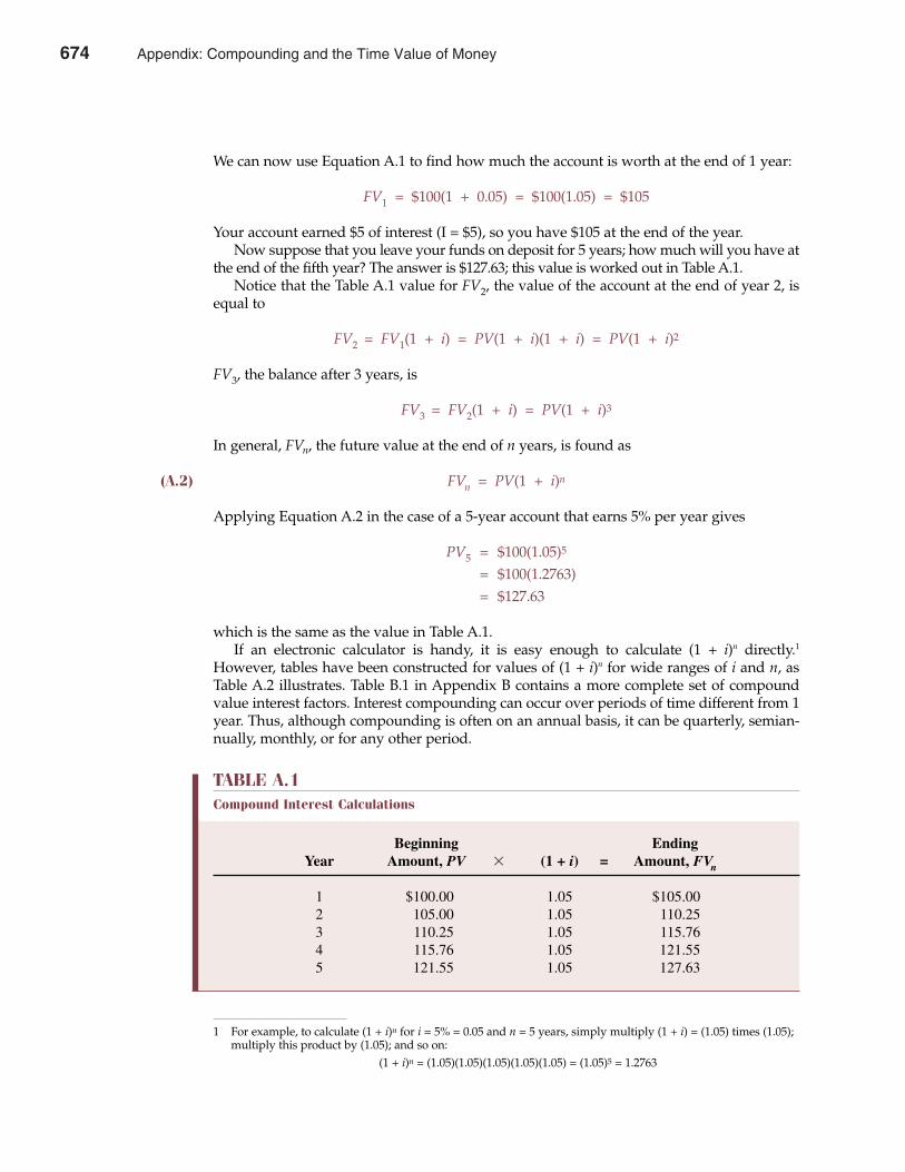
We can now use Equation A.1 to find how much the account is worth at the end of 1 year:
FV1 = $100(1 + 0.05) = $100(1.05) = $105
Your account earned $5 of interest (I = $5), so you have $105 at the end of the year.Now suppose that you leave your funds on deposit for 5 years; how much will you have at
the end of the fifth year? The answer is $127.63; this value is worked out in Table A.1.Notice that the Table A.1 value for FV2, the value of the account at the end of year 2, is
equal to
FV2 = FV1(1 + i) = PV(1 + i)(1 + i) = PV(1 + i)2
FV3, the balance after 3 years, is
FV3 = FV2(1 + i) = PV(1 + i)3
In general, FVn, the future value at the end of n years, is found as
(A.2) FVn = PV(1 + i)n
Applying Equation A.2 in the case of a 5-year account that earns 5% per year gives
PV5 = $100(1.05)5
= $100(1.2763)= $127.63
which is the same as the value in Table A.1.If an electronic calculator is handy, it is easy enough to calculate (1 + i)n directly.1
However, tables have been constructed for values of (1 + i)n for wide ranges of i and n, asTable A.2 illustrates. Table B.1 in Appendix B contains a more complete set of compoundvalue interest factors. Interest compounding can occur over periods of time different from 1year. Thus, although compounding is often on an annual basis, it can be quarterly, semian-nually, monthly, or for any other period.
676 Appendix A Compounding and the Time Value of Money
TABLE A.1Compound Interest Calculations
Beginning Ending Year Amount, PV � (1 + i) = Amount, FVn
1 $100.00 1.05 $105.002 105.00 1.05 110.253 110.25 1.05 115.764 115.76 1.05 121.555 121.55 1.05 127.63
1 For example, to calculate (1 + i)n for i = 5% = 0.05 and n = 5 years, simply multiply (1 + i) = (1.05) times (1.05);multiply this product by (1.05); and so on:
(1 + i)n = (1.05)(1.05)(1.05)(1.05)(1.05) = (1.05)5 = 1.2763
674 Appendix: Compounding and the Time Value of Money
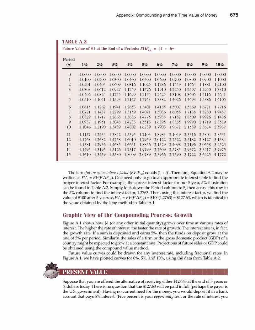
The term future value interest factor (FVIFi,n) equals (1 + i)n. Therefore, Equation A.2 may bewritten as FVn = PV(FVIFi,n). One need only to go to an appropriate interest table to find theproper interest factor. For example, the correct interest factor for our 5-year, 5% illustrationcan be found in Table A.2. Simply look down the Period column to 5, then across this row tothe 5% column to find the interest factor, 1.2763. Then, using this interest factor, we find thevalue of $100 after 5 years as FVn = PV(FVIFi,n) = $100(1.2763) = $127.63, which is identical tothe value obtained by the long method in Table A.1.
Graphic View of the Compounding Process: GrowthFigure A.1 shows how $1 (or any other initial quantity) grows over time at various rates ofinterest. The higher the rate of interest, the faster the rate of growth. The interest rate is, in fact,the growth rate: If a sum is deposited and earns 5%, then the funds on deposit grow at therate of 5% per period. Similarly, the sales of a firm or the gross domestic product (GDP) of acountry might be expected to grow at a constant rate. Projections of future sales or GDP couldbe obtained using the compound value method.
Future value curves could be drawn for any interest rate, including fractional rates. InFigure A.1, we have plotted curves for 0%, 5%, and 10%, using the data from Table A.2.
PRESENT VALUE
Suppose that you are offered the alternative of receiving either $127.63 at the end of 5 years orX dollars today. There is no question that the $127.63 will be paid in full (perhaps the payer isthe U.S. government). Having no current need for the money, you would deposit it in a bankaccount that pays 5% interest. (Five percent is your opportunity cost, or the rate of interest you
Appendix A Compounding and the Time Value of Money 677
TABLE A.2Future Value of $1 at the End of n Periods: FVIFi,n = (1 + i)n
Period(n) 1% 2% 3% 4% 5% 6% 7% 8% 9% 10%
0 1.0000 1.0000 1.0000 1.0000 1.0000 1.0000 1.0000 1.0000 1.0000 1.00001 1.0100 1.0200 1.0300 1.0400 1.0500 1.0600 1.0700 1.0800 1.0900 1.10002 1.0201 1.0404 1.0609 1.0816 1.1025 1.1236 1.1449 1.1664 1.1881 1.21003 1.0303 1.0612 1.0927 1.1249 1.1576 1.1910 1.2250 1.2597 1.2950 1.33104 1.0406 1.0824 1.1255 1.1699 1.2155 1.2625 1.3108 1.3605 1.4116 1.46415 1.0510 1.1041 1.1593 1.2167 1.2763 1.3382 1.4026 1.4693 1.5386 1.6105
6 1.0615 1.1262 1.1941 1.2653 1.3401 1.4185 1.5007 1.5869 1.6771 1.77167 1.0721 1.1487 1.2299 1.3159 1.4071 1.5036 1.6058 1.7138 1.8280 1.94878 1.0829 1.1717 1.2668 1.3686 1.4775 1.5938 1.7182 1.8509 1.9926 2.14369 1.0937 1.1951 1.3048 1.4233 1.5513 1.6895 1.8385 1.9990 2.1719 2.3579
10 1.1046 1.2190 1.3439 1.4802 1.6289 1.7908 1.9672 2.1589 2.3674 2.5937
11 1.1157 1.2434 1.3842 1.5395 1.7103 1.8983 2.1049 2.3316 2.5804 2.853112 1.1268 1.2682 1.4258 1.6010 1.7959 2.0122 2.2522 2.5182 2.8127 3.138413 1.1381 1.2936 1.4685 1.6651 1.8856 2.1329 2.4098 2.7196 3.0658 3.452314 1.1495 1.3195 1.5126 1.7317 1.9799 2.2609 2.5785 2.9372 3.3417 3.797515 1.1610 1.3459 1.5580 1.8009 2.0789 2.3966 2.7590 3.1722 3.6425 4.1772
Appendix: Compounding and the Time Value of Money 675
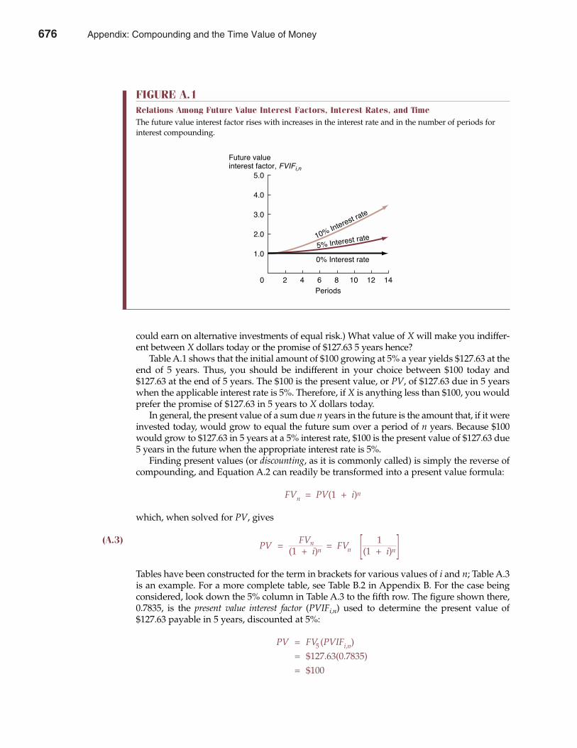
could earn on alternative investments of equal risk.) What value of X will make you indiffer-ent between X dollars today or the promise of $127.63 5 years hence?
Table A.1 shows that the initial amount of $100 growing at 5% a year yields $127.63 at theend of 5 years. Thus, you should be indifferent in your choice between $100 today and$127.63 at the end of 5 years. The $100 is the present value, or PV, of $127.63 due in 5 yearswhen the applicable interest rate is 5%. Therefore, if X is anything less than $100, you wouldprefer the promise of $127.63 in 5 years to X dollars today.
In general, the present value of a sum due n years in the future is the amount that, if it wereinvested today, would grow to equal the future sum over a period of n years. Because $100would grow to $127.63 in 5 years at a 5% interest rate, $100 is the present value of $127.63 due5 years in the future when the appropriate interest rate is 5%.
Finding present values (or discounting, as it is commonly called) is simply the reverse ofcompounding, and Equation A.2 can readily be transformed into a present value formula:
FVn = PV(1 + i)n
which, when solved for PV, gives
(A.3)PV = FVn = FVn
1(1 + i)n [(1 + i)n]
Tables have been constructed for the term in brackets for various values of i and n; Table A.3is an example. For a more complete table, see Table B.2 in Appendix B. For the case beingconsidered, look down the 5% column in Table A.3 to the fifth row. The figure shown there,0.7835, is the present value interest factor (PVIFi,n) used to determine the present value of$127.63 payable in 5 years, discounted at 5%:
PV = FV5 (PVIFi,n)= $127.63(0.7835)= $100
678 Appendix A Compounding and the Time Value of Money
FIGURE A.1Relations Among Future Value Interest Factors, Interest Rates, and TimeThe future value interest factor rises with increases in the interest rate and in the number of periods forinterest compounding.
Future value
interest factor, FVIFi,n5.0
4.0
3.0
2.0
1.0
0 2 4 6 8 10 12 14
Periods
0% Interest rate
5% Interest rate
10%
Intere
strat
e
676 Appendix: Compounding and the Time Value of Money
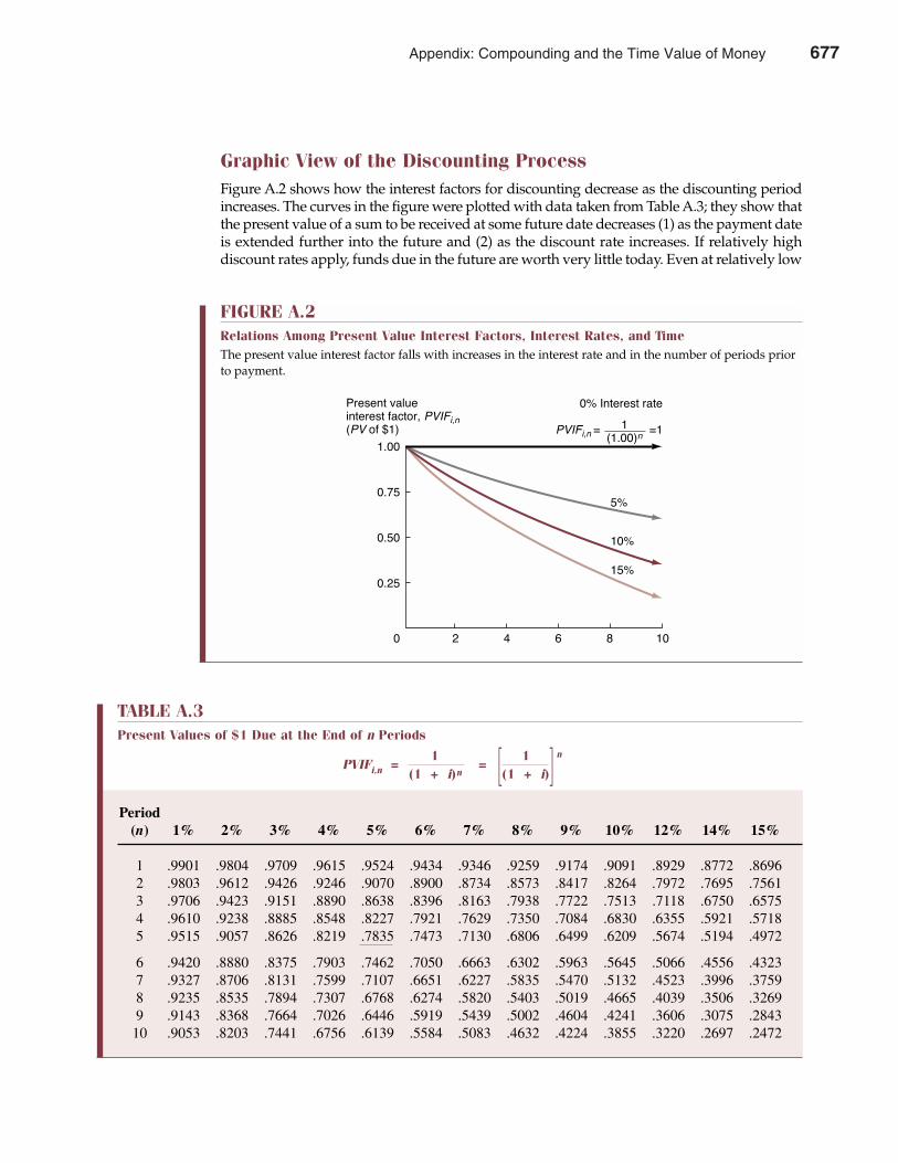
Graphic View of the Discounting ProcessFigure A.2 shows how the interest factors for discounting decrease as the discounting periodincreases. The curves in the figure were plotted with data taken from Table A.3; they show thatthe present value of a sum to be received at some future date decreases (1) as the payment dateis extended further into the future and (2) as the discount rate increases. If relatively highdiscount rates apply, funds due in the future are worth very little today. Even at relatively low
Appendix A Compounding and the Time Value of Money 679
TABLE A.3Present Values of $1 Due at the End of n Periods
PVIFi,n =1
=1 n
(1 + i)n [(1 + i)]Period
(n) 1% 2% 3% 4% 5% 6% 7% 8% 9% 10% 12% 14% 15%
1 .9901 .9804 .9709 .9615 .9524 .9434 .9346 .9259 .9174 .9091 .8929 .8772 .86962 .9803 .9612 .9426 .9246 .9070 .8900 .8734 .8573 .8417 .8264 .7972 .7695 .75613 .9706 .9423 .9151 .8890 .8638 .8396 .8163 .7938 .7722 .7513 .7118 .6750 .65754 .9610 .9238 .8885 .8548 .8227 .7921 .7629 .7350 .7084 .6830 .6355 .5921 .57185 .9515 .9057 .8626 .8219 .7835 .7473 .7130 .6806 .6499 .6209 .5674 .5194 .4972
6 .9420 .8880 .8375 .7903 .7462 .7050 .6663 .6302 .5963 .5645 .5066 .4556 .43237 .9327 .8706 .8131 .7599 .7107 .6651 .6227 .5835 .5470 .5132 .4523 .3996 .37598 .9235 .8535 .7894 .7307 .6768 .6274 .5820 .5403 .5019 .4665 .4039 .3506 .32699 .9143 .8368 .7664 .7026 .6446 .5919 .5439 .5002 .4604 .4241 .3606 .3075 .284310 .9053 .8203 .7441 .6756 .6139 .5584 .5083 .4632 .4224 .3855 .3220 .2697 .2472
FIGURE A.2Relations Among Present Value Interest Factors, Interest Rates, and TimeThe present value interest factor falls with increases in the interest rate and in the number of periods priorto payment.
Present valueinterest factor, PVIFi,n(PV of $1)
1.00
0.75
0.50
0.25
0 2 4 6 8 10
15%
10%
5%
0% Interest rate
PVIFi,n = =11(1.00)n
Appendix: Compounding and the Time Value of Money 677
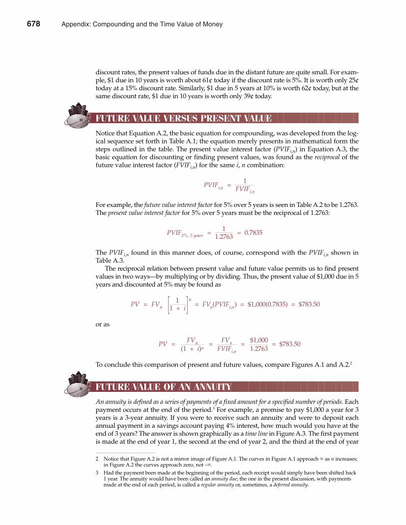
discount rates, the present values of funds due in the distant future are quite small. For exam-ple, $1 due in 10 years is worth about 61¢ today if the discount rate is 5%. It is worth only 25¢today at a 15% discount rate. Similarly, $1 due in 5 years at 10% is worth 62¢ today, but at thesame discount rate, $1 due in 10 years is worth only 39¢ today.
FUTURE VALUE VERSUS PRESENT VALUE
Notice that Equation A.2, the basic equation for compounding, was developed from the log-ical sequence set forth in Table A.1; the equation merely presents in mathematical form thesteps outlined in the table. The present value interest factor (PVIFi,n) in Equation A.3, thebasic equation for discounting or finding present values, was found as the reciprocal of thefuture value interest factor (FVIFi,n) for the same i, n combination:
PVIFi,n = 1FVIFi,n
For example, the future value interest factor for 5% over 5 years is seen in Table A.2 to be 1.2763.The present value interest factor for 5% over 5 years must be the reciprocal of 1.2763:
PVIF5%, 5 years = 1 = 0.78351.2763
The PVIFi,n found in this manner does, of course, correspond with the PVIFi,n shown inTable A.3.
The reciprocal relation between present value and future value permits us to find presentvalues in two ways—by multiplying or by dividing. Thus, the present value of $1,000 due in 5years and discounted at 5% may be found as
PV = FVn1 n
= FVn(PVIFi,n) = $1,000(0.7835) = $783.50[1 + i]or as
PV = FVn = FVn = $1,000 = $783.50(1 + i)n FVIFi,n 1.2763
To conclude this comparison of present and future values, compare Figures A.1 and A.2.2
FUTURE VALUE OF AN ANNUITY
An annuity is defined as a series of payments of a fixed amount for a specified number of periods. Eachpayment occurs at the end of the period.3 For example, a promise to pay $1,000 a year for 3years is a 3-year annuity. If you were to receive such an annuity and were to deposit eachannual payment in a savings account paying 4% interest, how much would you have at theend of 3 years? The answer is shown graphically as a time line in Figure A.3. The first paymentis made at the end of year 1, the second at the end of year 2, and the third at the end of year
680 Appendix A Compounding and the Time Value of Money
2 Notice that Figure A.2 is not a mirror image of Figure A.1. The curves in Figure A.1 approach � as n increases;in Figure A.2 the curves approach zero, not –�.
3 Had the payment been made at the beginning of the period, each receipt would simply have been shifted back1 year. The annuity would have been called an annuity due; the one in the present discussion, with paymentsmade at the end of each period, is called a regular annuity or, sometimes, a deferred annuity.
678 Appendix: Compounding and the Time Value of Money
3. The last payment is not compounded at all, the second payment is compounded for 1 year,and the first is compounded for 2 years. When the future values of each of the payments areadded, their total is the sum of the annuity. In the example, this total is $3,121.60.
Expressed algebraically, with SN defined as the future value, R as the periodic receipt, nas the length of the annuity, and FVIFAi,n as the future value interest factor for an annuity,the formula for Sn is
Sn = R(1 + i)n–1 + R(1 + i)n–2 + . . . + R(1 + i)1 + R(1 + i)0
(A.4)= R[(1 + i)n–1 + (1 + i)n–2 + . . . + (1 + i)1 + (1 + i)0]
n n
= R∑(1 + i)n–t or = R∑(1 + i)t–1
t=1 t=1
= R(FVIFAi,n)
The expression in parentheses, FVIFAi,n, has been calculated for various combinations of i and n.4
An illustrative set of these annuity interest factors is given in Table A.4.5 To find the answer tothe 3-year, $1,000 annuity problem, simply refer to Table A.4, look down the 4% column to therow of the third period, and multiply the factor 3.1216 by $1,000. The answer is the same as theone derived by the long method illustrated in Figure A.3:
Sn = R(FVIFAi,n)S3 = $1,000(3.1216) = $3,121.60
Notice that for all positive interest rates, the FVIFAi,n for the sum of an annuity is always equalto or greater than the number of periods the annuity runs.6
Appendix A Compounding and the Time Value of Money 681
4 The third equation is simply a shorthand expression in which sigma (�) signifies sum up or add the values of n
factors. The symboln
�t =1
simply says, “Go through the following process: Let t = 1 and find the first factor. Then
let t = 2 and find the second factor. Continue until each individual factor has been found, and then add theseindividual factors to find the value of the annuity.”
5 The equation given in Table A.4 recognizes that the FVIFA factor is the sum of a geometric progression. The proofof this equation is given in most algebra texts. Notice that it is easy to use the equation to develop annuity factors.This is especially useful if you need the FVIFA for some interest rate not given in the tables (for example, 6.5%).
6 It is worth noting that the entry for each period t in Table A.4 equals the sum of the entries in Table A.2 up tothe period n – 1. For example, the entry for Period 3 under the 4% column in Table A.4 is equal to 1.000 +1.0400 + 1.0816 = 3.1216.Also, had the annuity been an annuity due, with payments received at the beginning rather than at the end of eachperiod, the three payments would have occurred at t = 0, t = 1, and t = 2. To find the future value of an annuitydue, look up the FVIFAi,n for n + 1 years, then subtract 1.0 from the amount to get the FVIFAi,n for the annuitydue. In the example, the annuity due FVIFAi,n is 4.2465 – 1.0 = 3.2465, versus 3.1216 for a regular annuity. Becausepayments on an annuity due come earlier, it is a little more valuable than a regular annuity.
FIGURE A.3Time Line for an Annuity: Future Value (i = 4%)When the interest rate is 4%, the future value of $1,000 annuity to be paid over 3 years is $3,121.60.
0
Payments
1
$1,000.00
2
$1,000.00
3
$1,000.00$1,040.00$1,081.60
$3,121.60Compound sum
End of period
Appendix: Compounding and the Time Value of Money 679
PRESENT VALUE OF AN ANNUITY
Suppose that you were offered the following alternatives: a 3-year annuity of $1,000 per yearor a lump-sum payment today. You have no need for the money during the next 3 years, soif you accept the annuity, you would simply deposit the receipts in a savings account paying4% interest. How large must the lump-sum payment be to make it equivalent to the annuity?The time line shown in Figure A.4 will help explain the problem.
The present value of the first receipt is R[1/(1 + i)], the second is R[1/(1 + i)]2, and so on.Designating the present value of an annuity of n years as An and the present value interestfactor for an annuity as PVIFAi,n, we may write the following equation:
An = R� 1 �1+ R� 1 �2
+ . . . + R� 1 �n
1 + i 1 + i 1 + i
= R� 1 + 1 + . . . + 1 �(A.5) (1 + i)1 (1 + i)2 (1 + i)n
n
= R∑ 1
t=1 (1 + i)t
= R(PVIFAi,n)
Again, tables have been worked out for PVIFAi,n, the term in parentheses in Equation A.5, asTable A.5 illustrates; a more complete listing is found in Table B.4 in Appendix B. From TableA.5, the PVIFAi,n for a 3-year, 4% annuity is found to be 2.7751. Multiplying this factor by the$1,000 annual receipt gives $2,775.10, the present value of the annuity. This figure is identicalto the long-method answer shown in Figure A.4:
682 Appendix A Compounding and the Time Value of Money
TABLE A.4Future Value of an Annuity of $1 per Period for n Periods
n
FVIFAi,n = ∑ (1 + i)t–1
t=1
=(1 + i)n – 1
i
Number ofPeriods 1% 2% 3% 4% 5% 6% 7% 8%
1 1.0000 1.0000 1.0000 1.0000 1.0000 1.0000 1.0000 1.00002 2.0100 2.0200 2.0300 2.0400 2.0500 2.0600 2.0700 2.08003 3.0301 3.0604 3.0909 3.1216 3.1525 3.1836 3.2149 3.24644 4.0604 4.1216 4.1836 4.2465 4.3101 4.3746 4.4399 4.50615 5.1010 5.2040 5.3091 5.4163 5.5256 5.6371 5.7507 5.8666
6 6.1520 6.3081 6.4684 6.6330 6.8019 6.9753 7.1533 7.33597 7.2135 7.4343 7.6625 7.8983 8.1420 8.3938 8.6540 8.92288 8.2857 8.5830 8.8923 9.2142 9.5491 9.8975 10.2598 10.63669 9.3685 9.7546 10.1591 10.5828 11.0266 11.4913 11.9780 12.4876
10 10.4622 10.9497 11.4639 12.0061 12.5779 13.1808 13.8164 14.4866
680 Appendix: Compounding and the Time Value of Money
An = R(PVIFAi,n)A3 = $1,000(2.7751)
= $2,775.10
Notice that the entry for each period n in Table A.5 is equal to the sum of the entries in TableA.3 up to and including period n. For example, the PVIFA for 4%, three periods as shown inTable A.5, could have been calculated by summing values from Table A.3:
0.9615 + 0.9246 + 0.8890 = 2.7751
Notice also that for all positive interest rates, PVIFAi,n for the present value of an annuity isalways less than the number of periods.7
Appendix A Compounding and the Time Value of Money 683
FIGURE A.4Time Line for an Annuity: Present Value (i = 4%)When the interest rate is 4%, the present value of a $1,000 annuity to be paid over 3 years is $2,775.10.
0
Receipts
1
$1,000
2
$1,000
3
$1,000
End of year
$ 961.50$ 924.60$ 889.00
$2,775.10
Present valueof receipts
Total
TABLE A.5Present Value of an Annuity of $1 per Period for n Periods
1
PVIFAi,n =n 1
=1 –
(1 + i)n
∑ (1 + i)t it=1
Period 1% 2% 3% 4% 5% 6% 7% 8% 9% 10%
1 0.9901 0.9804 0.9709 0.9615 0.9524 0.9434 0.9346 0.9259 0.9174 0.90912 1.9704 1.9416 1.9135 1.8861 1.8594 1.8334 1.8080 1.7833 1.7591 1.73553 2.9410 2.8839 2.8286 2.7751 2.7232 2.6730 2.6243 2.5771 2.5313 2.48694 3.9020 3.8077 3.7171 3.6299 3.5460 3.4651 3.3872 3.3121 3.2397 3.16995 4.8534 4.7135 4.5797 4.4518 4.3295 4.2124 4.1002 3.9927 3.8897 3.7908
6 5.7955 5.6014 5.4172 5.2421 5.0757 4.9173 4.7665 4.6229 4.4859 4.35537 6.7282 6.4720 6.2303 6.0021 5.7864 5.5824 5.3893 5.2064 5.0330 4.86848 7.6517 7.3255 7.0197 6.7327 6.4632 6.2098 5.9713 5.7466 5.5348 5.33499 8.5660 8.1622 7.7861 7.4353 7.1078 6.8017 6.5152 6.2469 5.9952 5.759010 9.4713 8.9826 8.5302 8.1109 7.7217 7.3601 7.0236 6.7101 6.4177 6.1446
7 To find the PVIFAi,n for an annuity due, look up the PVIFAi,n for n – 1 periods, then add 1.0 to this amount to obtainthe PVIFAi,n for the annuity due. In the example, the PVIFAi,n for a 4%, 3-year annuity due is 1.8861 + 1.0 = 2.8861.
Appendix: Compounding and the Time Value of Money 681
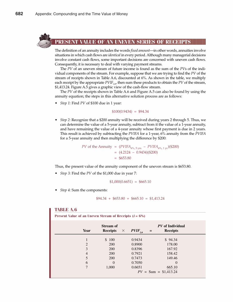
PRESENT VALUE OF AN UNEVEN SERIES OF RECEIPTS
The definition of an annuity includes the words fixed amount—in other words, annuities involvesituations in which cash flows are identical in every period. Although many managerial decisionsinvolve constant cash flows, some important decisions are concerned with uneven cash flows.Consequently, it is necessary to deal with varying payment streams.
The PV of an uneven stream of future income is found as the sum of the PVs of the indi-vidual components of the stream. For example, suppose that we are trying to find the PV of thestream of receipts shown in Table A.6, discounted at 6%. As shown in the table, we multiplyeach receipt by the appropriate PVIFi,n, then sum these products to obtain the PV of the stream,$1,413.24. Figure A.5 gives a graphic view of the cash-flow stream.
The PV of the receipts shown in Table A.6 and Figure A.5 can also be found by using theannuity equation; the steps in this alternative solution process are as follows:
• Step 1: Find PV of $100 due in 1 year:
$100(0.9434) = $94.34
• Step 2: Recognize that a $200 annuity will be received during years 2 through 5. Thus, wecan determine the value of a 5-year annuity, subtract from it the value of a 1-year annuity,and have remaining the value of a 4-year annuity whose first payment is due in 2 years.This result is achieved by subtracting the PVIFA for a 1-year, 6% annuity from the PVIFAfor a 5-year annuity and then multiplying the difference by $200:
PV of the Annuity = (PVIFA6%, 5 yrs. – PVIFA6%, 1 yr.)($200)= (4.2124 – 0.9434)($200)= $653.80
Thus, the present value of the annuity component of the uneven stream is $653.80.
• Step 3: Find the PV of the $1,000 due in year 7:
$1,000(0.6651) = $665.10
• Step 4: Sum the components:
$94.34 + $653.80 + $665.10 = $1,413.24
684 Appendix A Compounding and the Time Value of Money
TABLE A.6Present Value of an Uneven Stream of Receipts (i = 6%)
Stream of PV of IndividualYear Receipts � PVIFi,n = Receipts
1 $ 100 0.9434 $ 94.342 200 0.8900 178.003 200 0.8396 167.924 200 0.7921 158.425 200 0.7473 149.466 0 0.7050 07 1,000 0.6651 665.10
PV = Sum = $1,413.24
682 Appendix: Compounding and the Time Value of Money
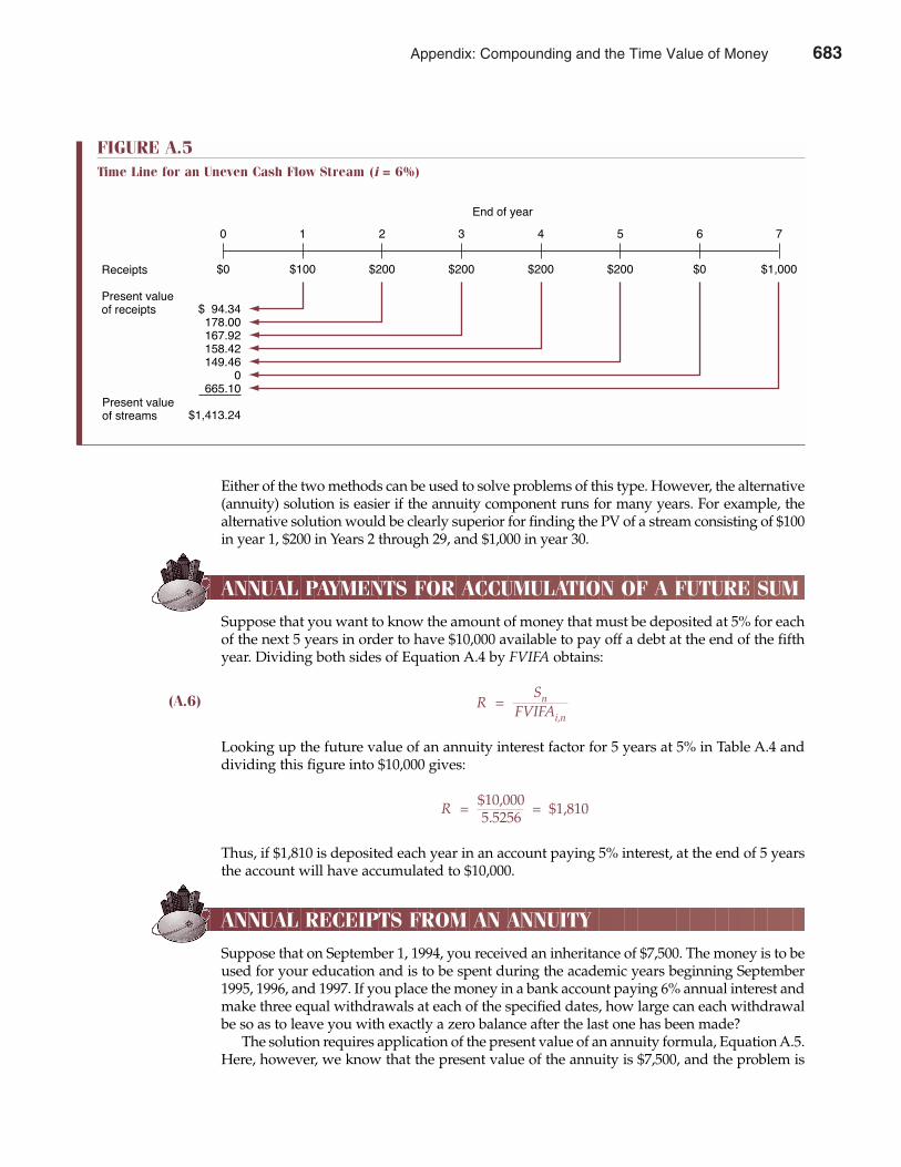
Either of the two methods can be used to solve problems of this type. However, the alternative(annuity) solution is easier if the annuity component runs for many years. For example, thealternative solution would be clearly superior for finding the PV of a stream consisting of $100in year 1, $200 in Years 2 through 29, and $1,000 in year 30.
ANNUAL PAYMENTS FOR ACCUMULATION OF A FUTURE SUM
Suppose that you want to know the amount of money that must be deposited at 5% for eachof the next 5 years in order to have $10,000 available to pay off a debt at the end of the fifthyear. Dividing both sides of Equation A.4 by FVIFA obtains:
(A.6) R =Sn
FVIFAi,n
Looking up the future value of an annuity interest factor for 5 years at 5% in Table A.4 anddividing this figure into $10,000 gives:
R = $10,000 = $1,8105.5256
Thus, if $1,810 is deposited each year in an account paying 5% interest, at the end of 5 yearsthe account will have accumulated to $10,000.
ANNUAL RECEIPTS FROM AN ANNUITY
Suppose that on September 1, 1994, you received an inheritance of $7,500. The money is to beused for your education and is to be spent during the academic years beginning September1995, 1996, and 1997. If you place the money in a bank account paying 6% annual interest andmake three equal withdrawals at each of the specified dates, how large can each withdrawalbe so as to leave you with exactly a zero balance after the last one has been made?
The solution requires application of the present value of an annuity formula, Equation A.5.Here, however, we know that the present value of the annuity is $7,500, and the problem is
Appendix A Compounding and the Time Value of Money 685
FIGURE A.5Time Line for an Uneven Cash Flow Stream (i = 6%)
0
$0
1
$100
2
$200
3
$200
4
$200
5
$200
6
$0
7
$1,000
End of year
$ 94.34178.00167.92158.42149.46
0665.10
$1,413.24Present valueof streams
Receipts
Present valueof receipts
Appendix: Compounding and the Time Value of Money 683
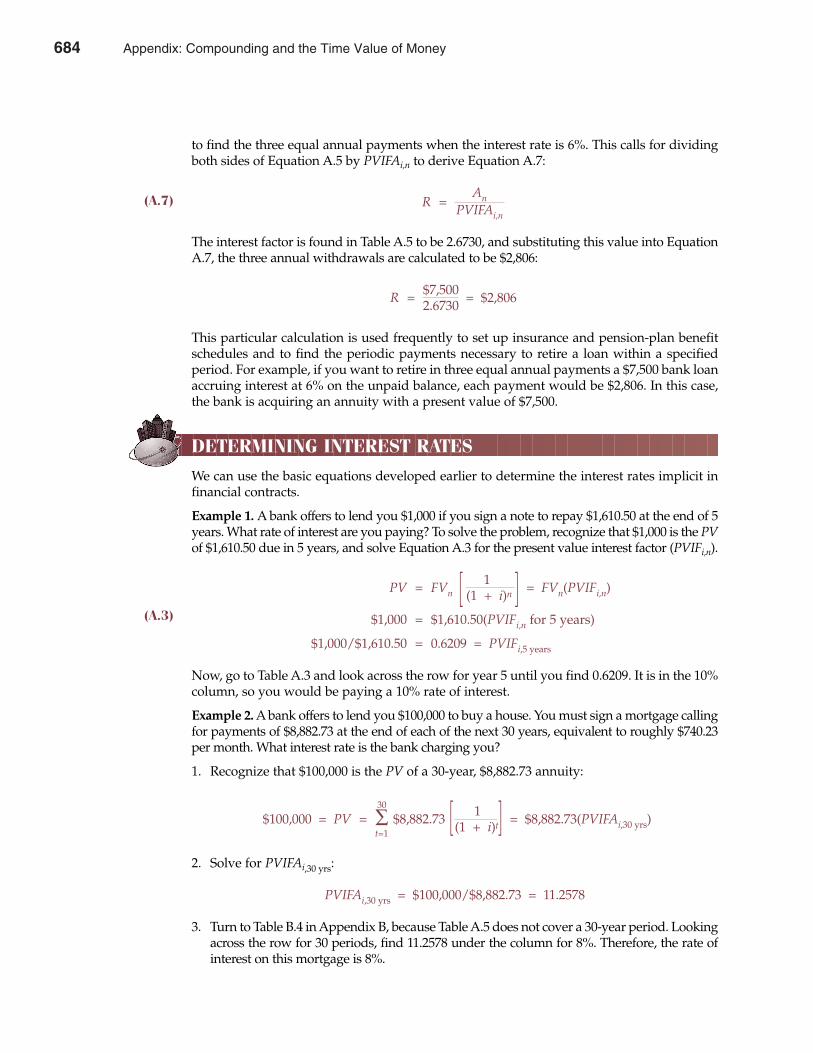
to find the three equal annual payments when the interest rate is 6%. This calls for dividingboth sides of Equation A.5 by PVIFAi,n to derive Equation A.7:
(A.7) R =An
PVIFAi,n
The interest factor is found in Table A.5 to be 2.6730, and substituting this value into EquationA.7, the three annual withdrawals are calculated to be $2,806:
R = $7,500 = $2,8062.6730
This particular calculation is used frequently to set up insurance and pension-plan benefitschedules and to find the periodic payments necessary to retire a loan within a specifiedperiod. For example, if you want to retire in three equal annual payments a $7,500 bank loanaccruing interest at 6% on the unpaid balance, each payment would be $2,806. In this case,the bank is acquiring an annuity with a present value of $7,500.
DETERMINING INTEREST RATES
We can use the basic equations developed earlier to determine the interest rates implicit infinancial contracts.
Example 1. A bank offers to lend you $1,000 if you sign a note to repay $1,610.50 at the end of 5years. What rate of interest are you paying? To solve the problem, recognize that $1,000 is the PVof $1,610.50 due in 5 years, and solve Equation A.3 for the present value interest factor (PVIFi,n).
PV = FVn [ 1 ] = FVn(PVIFi,n)(1 + i)n
(A.3) $1,000 = $1,610.50(PVIFi,n for 5 years)
$1,000/$1,610.50 = 0.6209 = PVIFi,5 years
Now, go to Table A.3 and look across the row for year 5 until you find 0.6209. It is in the 10%column, so you would be paying a 10% rate of interest.
Example 2. A bank offers to lend you $100,000 to buy a house. You must sign a mortgage callingfor payments of $8,882.73 at the end of each of the next 30 years, equivalent to roughly $740.23per month. What interest rate is the bank charging you?
1. Recognize that $100,000 is the PV of a 30-year, $8,882.73 annuity:
30
$100,000 = PV = ∑ $8,882.73 [ 1 ] = $8,882.73(PVIFAi,30 yrs)t=1 (1 + i)t
2. Solve for PVIFAi,30 yrs:
PVIFAi,30 yrs = $100,000/$8,882.73 = 11.2578
3. Turn to Table B.4 in Appendix B, because Table A.5 does not cover a 30-year period. Lookingacross the row for 30 periods, find 11.2578 under the column for 8%. Therefore, the rate ofinterest on this mortgage is 8%.
686 Appendix A Compounding and the Time Value of Money
684 Appendix: Compounding and the Time Value of Money
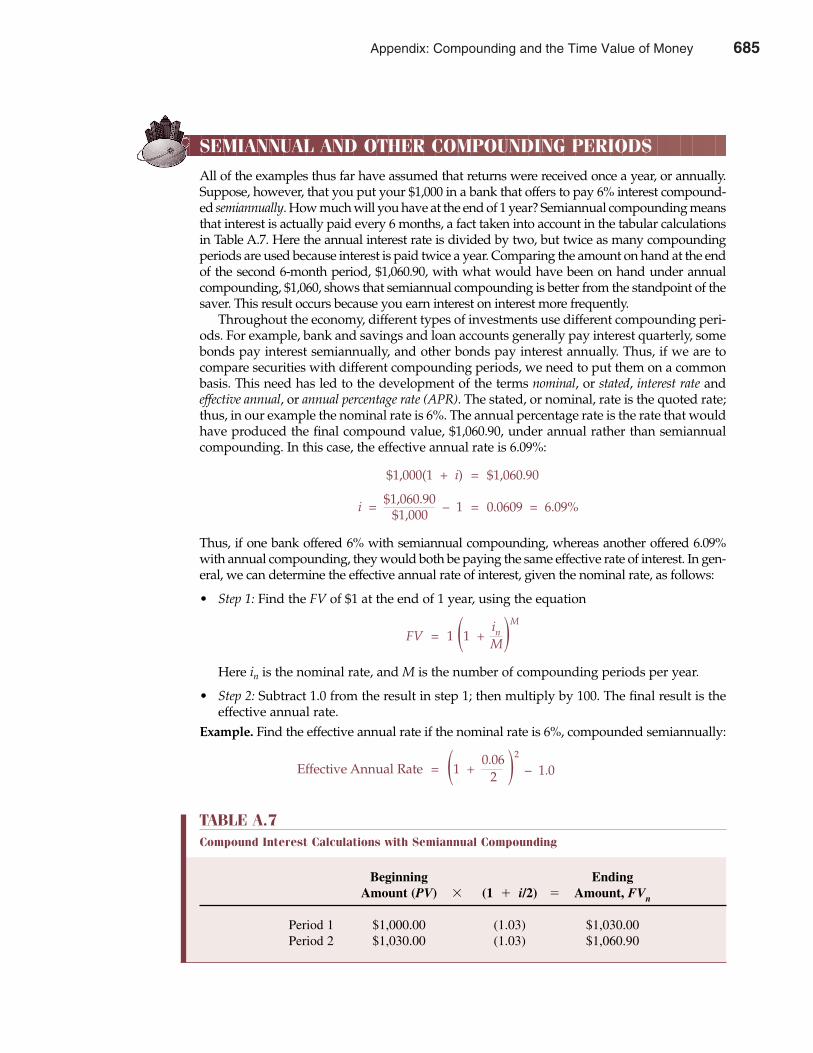
SEMIANNUAL AND OTHER COMPOUNDING PERIODS
All of the examples thus far have assumed that returns were received once a year, or annually.Suppose, however, that you put your $1,000 in a bank that offers to pay 6% interest compound-ed semiannually. How much will you have at the end of 1 year? Semiannual compounding meansthat interest is actually paid every 6 months, a fact taken into account in the tabular calculationsin Table A.7. Here the annual interest rate is divided by two, but twice as many compoundingperiods are used because interest is paid twice a year. Comparing the amount on hand at the endof the second 6-month period, $1,060.90, with what would have been on hand under annualcompounding, $1,060, shows that semiannual compounding is better from the standpoint of thesaver. This result occurs because you earn interest on interest more frequently.
Throughout the economy, different types of investments use different compounding peri-ods. For example, bank and savings and loan accounts generally pay interest quarterly, somebonds pay interest semiannually, and other bonds pay interest annually. Thus, if we are tocompare securities with different compounding periods, we need to put them on a commonbasis. This need has led to the development of the terms nominal, or stated, interest rate andeffective annual, or annual percentage rate (APR). The stated, or nominal, rate is the quoted rate;thus, in our example the nominal rate is 6%. The annual percentage rate is the rate that wouldhave produced the final compound value, $1,060.90, under annual rather than semiannualcompounding. In this case, the effective annual rate is 6.09%:
$1,000(1 + i) = $1,060.90
i = $1,060.90 – 1 = 0.0609 = 6.09%$1,000
Thus, if one bank offered 6% with semiannual compounding, whereas another offered 6.09%with annual compounding, they would both be paying the same effective rate of interest. In gen-eral, we can determine the effective annual rate of interest, given the nominal rate, as follows:
• Step 1: Find the FV of $1 at the end of 1 year, using the equation
FV = 1 �1 +in �
M
M
Here in is the nominal rate, and M is the number of compounding periods per year.
• Step 2: Subtract 1.0 from the result in step 1; then multiply by 100. The final result is theeffective annual rate.
Example. Find the effective annual rate if the nominal rate is 6%, compounded semiannually:
Effective Annual Rate = �1 +0.06 �
2
– 1.02
Appendix A Compounding and the Time Value of Money 687
TABLE A.7Compound Interest Calculations with Semiannual Compounding
Beginning EndingAmount (PV) � (1 � i/2) � Amount, FVn
Period 1 $1,000.00 (1.03) $1,030.00Period 2 $1,030.00 (1.03) $1,060.90
Appendix: Compounding and the Time Value of Money 685
= (1.03)2 – 1.0= 1.0609 – 1.0= 0.0609= 6.09%
The points made about semiannual compounding can be generalized as follows. When com-pounding periods are more frequent than once a year, use a modified version of Equation A.2:
(A.2) FVn = PV(1 + i)n
FVn = PV�1 +i �
Mn
(A.2a) M
Here M is the number of times per year compounding occurs. When banks compute dailyinterest, the value of M is set at 365, and Equation A.2a is applied.
The interest tables can be used when compounding occurs more than once a year. Simplydivide the nominal, or stated, interest rate by the number of times compounding occurs, andmultiply the years by the number of compounding periods per year. For example, to find theamount to which $1,000 will grow after 6 years with semiannual compounding and a stated 8%interest rate, divide 8% by 2 and multiply the 6 years by 2. Then look in Table A.2 under the 4%column and in the row for Period 12. You will find an interest factor of 1.6010. Multiplying thisby the initial $1,000 gives a value of $1,601, the amount to which $1,000 will grow in 6 years at8% compounded semiannually. This compares with $1,586.90 for annual compounding.
The same procedure applies in all of the cases covered—compounding, discounting, singlepayments, and annuities. To illustrate semiannual discounting in finding the present value ofan annuity, consider the case described in the section “Present Value of an Annuity”—$1,000 ayear for 3 years, discounted at 4%. With annual discounting, the interest factor is 2.7751, andthe present value of the annuity is $2,775.10. For semiannual discounting, look under the 2%column and in the Period 6 row of Table A.5 to find an interest factor of 5.6014. This is nowmultiplied by half of $1,000, or the $500 received each 6 months, to get the present value of theannuity, $2,800.70. The payments come a little more rapidly—the first $500 is paid after only 6months (similarly with other payments)—so the annuity is a little more valuable if paymentsare received semiannually rather than annually.
SUMMARY
Managerial decisions often require determining the present value of a stream of future cashflows. Also, we often need to know the amount to which an initial quantity will grow duringa specified time period, and at other times we must calculate the interest rate built into afinancial contract. The basic concepts involved in these processes are called compoundingand the time value of money.
The key procedures covered in this appendix are summarized here:
• Future Value: FVn = PV(1 + i)n, where FVn is the future value of an initial amount, PV, com-pounded at the rate of i percent for n periods. The term (1 + i)n is the future value interestfactor, FVIFi,n. Values for FVIF are contained in tables.
• Present Value: PV = FVn[1/(1 + i)]n. This equation is simply a transformation of the futurevalue equation. The term [1/(1 + i)]n is the present value interest factor, PVIFi,n.
• Future Value of an Annuity: An annuity is defined as a series of constant or equal paymentsof R dollars per period. The sum, or future value of an annuity, is given the symbol Sn, and
688 Appendix A Compounding and the Time Value of Money
686 Appendix: Compounding and the Time Value of Money
it is found as follows: Sn = R[ n
�t =1
(1 + i)t–1]. The term [ n
�t =1
(1 + i)t–1] is the future value
interest factor for an annuity, FVIFAi,n.
• Present Value of an Annuity: The present value of an annuity is identified by the symbol
An, and it is found as follows: An = R[ n
�t =1
(1/1 + i)t]. The term [ n
�t =1
(1/1 + i)t]= PVIFAi,n
is the present value interest factor for an annuity.
Appendix A Compounding and the Time Value of Money 689
Appendix: Compounding and the Time Value of Money 687

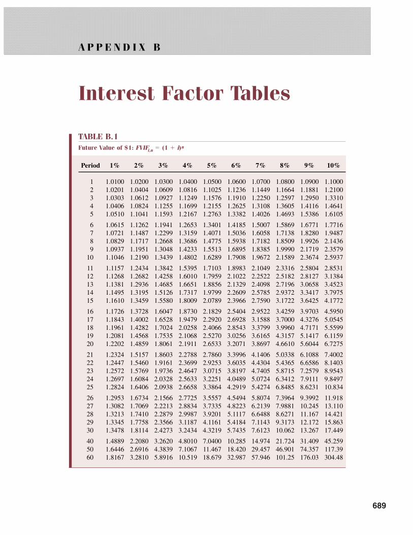
A P P E N D I X B
Interest Factor Tables
TABLE B.1Future Value of $1: FVIFi,n � (1 � i)n
Period 1% 2% 3% 4% 5% 6% 7% 8% 9% 10%
1 1.0100 1.0200 1.0300 1.0400 1.0500 1.0600 1.0700 1.0800 1.0900 1.10002 1.0201 1.0404 1.0609 1.0816 1.1025 1.1236 1.1449 1.1664 1.1881 1.21003 1.0303 1.0612 1.0927 1.1249 1.1576 1.1910 1.2250 1.2597 1.2950 1.33104 1.0406 1.0824 1.1255 1.1699 1.2155 1.2625 1.3108 1.3605 1.4116 1.46415 1.0510 1.1041 1.1593 1.2167 1.2763 1.3382 1.4026 1.4693 1.5386 1.6105
6 1.0615 1.1262 1.1941 1.2653 1.3401 1.4185 1.5007 1.5869 1.6771 1.77167 1.0721 1.1487 1.2299 1.3159 1.4071 1.5036 1.6058 1.7138 1.8280 1.94878 1.0829 1.1717 1.2668 1.3686 1.4775 1.5938 1.7182 1.8509 1.9926 2.14369 1.0937 1.1951 1.3048 1.4233 1.5513 1.6895 1.8385 1.9990 2.1719 2.3579
10 1.1046 1.2190 1.3439 1.4802 1.6289 1.7908 1.9672 2.1589 2.3674 2.5937
11 1.1157 1.2434 1.3842 1.5395 1.7103 1.8983 2.1049 2.3316 2.5804 2.853112 1.1268 1.2682 1.4258 1.6010 1.7959 2.1022 2.2522 2.5182 2.8127 3.138413 1.1381 1.2936 1.4685 1.6651 1.8856 2.1329 2.4098 2.7196 3.0658 3.452314 1.1495 1.3195 1.5126 1.7317 1.9799 2.2609 2.5785 2.9372 3.3417 3.797515 1.1610 1.3459 1.5580 1.8009 2.0789 2.3966 2.7590 3.1722 3.6425 4.1772
16 1.1726 1.3728 1.6047 1.8730 2.1829 2.5404 2.9522 3.4259 3.9703 4.595017 1.1843 1.4002 1.6528 1.9479 2.2920 2.6928 3.1588 3.7000 4.3276 5.054518 1.1961 1.4282 1.7024 2.0258 2.4066 2.8543 3.3799 3.9960 4.7171 5.559919 1.2081 1.4568 1.7535 2.1068 2.5270 3.0256 3.6165 4.3157 5.1417 6.115920 1.2202 1.4859 1.8061 2.1911 2.6533 3.2071 3.8697 4.6610 5.6044 6.7275
21 1.2324 1.5157 1.8603 2.2788 2.7860 3.3996 4.1406 5.0338 6.1088 7.400222 1.2447 1.5460 1.9161 2.3699 2.9253 3.6035 4.4304 5.4365 6.6586 8.140323 1.2572 1.5769 1.9736 2.4647 3.0715 3.8197 4.7405 5.8715 7.2579 8.954324 1.2697 1.6084 2.0328 2.5633 3.2251 4.0489 5.0724 6.3412 7.9111 9.849725 1.2824 1.6406 2.0938 2.6658 3.3864 4.2919 5.4274 6.8485 8.6231 10.834
26 1.2953 1.6734 2.1566 2.7725 3.5557 4.5494 5.8074 7.3964 9.3992 11.91827 1.3082 1.7069 2.2213 2.8834 3.7335 4.8223 6.2139 7.9881 10.245 13.11028 1.3213 1.7410 2.2879 2.9987 3.9201 5.1117 6.6488 8.6271 11.167 14.42129 1.3345 1.7758 2.3566 3.1187 4.1161 5.4184 7.1143 9.3173 12.172 15.86330 1.3478 1.8114 2.4273 3.2434 4.3219 5.7435 7.6123 10.062 13.267 17.449
40 1.4889 2.2080 3.2620 4.8010 7.0400 10.285 14.974 21.724 31.409 45.25950 1.6446 2.6916 4.3839 7.1067 11.467 18.420 29.457 46.901 74.357 117.3960 1.8167 3.2810 5.8916 10.519 18.679 32.987 57.946 101.25 176.03 304.48
691
689
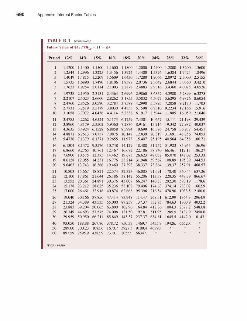
692 Appendix B Interest Factor Tables
TABLE B.1 (continued)
Future Value of $1: FVIFi,n � (1 � i)n
Period 12% 14% 15% 16% 18% 20% 24% 28% 32% 36%
1 1.1200 1.1400 1.1500 1.1600 1.1800 1.2000 1.2400 1.2800 1.3200 1.36002 1.2544 1.2996 1.3225 1.3456 1.3924 1.4400 1.5376 1.6384 1.7424 1.84963 1.4049 1.4815 1.5209 1.5609 1.6430 1.7280 1.9066 2.0972 2.3000 2.51554 1.5735 1.6890 1.7490 1.8106 1.9388 2.0736 2.3642 2.6844 3.0360 3.42105 1.7623 1.9254 2.0114 2.1003 2.2878 2.4883 2.9316 3.4360 4.0075 4.6526
6 1.9738 2.1950 2.3131 2.4364 2.6996 2.9860 3.6352 4.3980 5.2899 6.32757 2.2107 2.5023 2.6600 2.8262 3.1855 3.5832 4.5077 5.6295 6.9826 8.60548 2.4760 2.8526 3.0590 3.2784 3.7589 4.2998 5.5895 7.2058 9.2170 11.7039 2.7731 3.2519 3.5179 3.8030 4.4355 5.1598 6.9310 9.2234 12.166 15.916
10 3.1058 3.7072 4.0456 4.4114 5.2338 6.1917 8.5944 11.805 16.059 21.646
11 3.4785 4.2262 4.6524 5.1173 6.1759 7.4301 10.657 15.111 21.198 29.43912 3.8960 4.8179 5.3502 5.9360 7.2876 8.9161 13.214 19.342 27.982 40.03713 4.3635 5.4924 6.1528 6.8858 8.5994 10.699 16.386 24.758 36.937 54.45114 4.8871 6.2613 7.0757 7.9875 10.147 12.839 20.319 31.691 48.756 74.05315 5.4736 7.1379 8.1371 9.2655 11.973 15.407 25.195 40.564 64.358 100.71
16 6.1304 8.1372 9.3576 10.748 14.129 18.488 31.242 51.923 84.953 136.9617 6.8660 9.2765 10.761 12.467 16.672 22.186 38.740 66.461 112.13 186.2718 7.6900 10.575 12.375 14.462 19.673 26.623 48.038 85.070 148.02 253.3319 8.6128 12.055 14.231 16.776 23.214 31.948 59.567 108.89 195.39 344.5320 9.6463 13.743 16.366 19.460 27.393 38.337 73.864 139.37 257.91 468.57
21 10.803 15.667 18.821 22.574 32.323 46.005 91.591 178.40 340.44 637.2622 12.100 17.861 21.644 26.186 38.142 55.206 113.57 228.35 449.39 866.6723 13.552 20.361 24.891 30.376 45.007 66.247 140.83 292.30 593.19 1178.624 15.178 23.212 28.625 35.236 53.108 79.496 174.63 374.14 783.02 1602.925 17.000 26.461 32.918 40.874 62.668 95.396 216.54 478.90 1033.5 2180.0
26 19.040 30.166 37.856 47.414 73.948 114.47 268.51 612.99 1364.3 2964.927 21.324 34.389 43.535 55.000 87.259 137.37 332.95 784.63 1800.9 4032.228 23.883 39.204 50.065 63.800 102.96 164.84 412.86 1004.3 2377.2 5483.829 26.749 44.693 57.575 74.008 121.50 197.81 511.95 1285.5 3137.9 7458.030 29.959 50.950 66.211 85.849 143.37 237.37 634.81 1645.5 4142.0 10143.
40 93.050 188.88 267.86 378.72 750.37 1469.7 5455.9 19426. 66520. *50 289.00 700.23 1083.6 1670.7 3927.3 9100.4 46890. * * *60 897.59 2595.9 4383.9 7370.1 20555. 56347. * * * *
*FVIF > 99,999.
690 Appendix: Interest Factor Tables
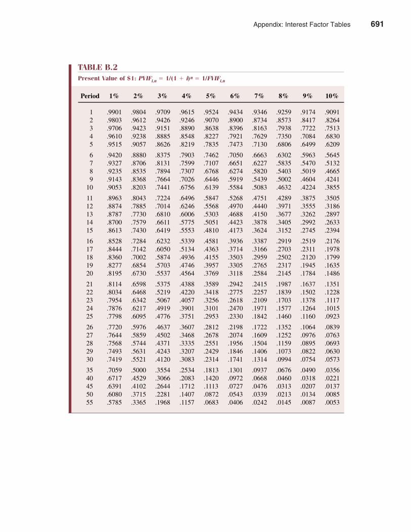
Appendix B Interest Factor Tables 693
TABLE B.2Present Value of $1: PVIFi,n � 1/(1 � i)n � 1/FVIFi,n
Period 1% 2% 3% 4% 5% 6% 7% 8% 9% 10%
1 .9901 .9804 .9709 .9615 .9524 .9434 .9346 .9259 .9174 .90912 .9803 .9612 .9426 .9246 .9070 .8900 .8734 .8573 .8417 .82643 .9706 .9423 .9151 .8890 .8638 .8396 .8163 .7938 .7722 .75134 .9610 .9238 .8885 .8548 .8227 .7921 .7629 .7350 .7084 .68305 .9515 .9057 .8626 .8219 .7835 .7473 .7130 .6806 .6499 .6209
6 .9420 .8880 .8375 .7903 .7462 .7050 .6663 .6302 .5963 .56457 .9327 .8706 .8131 .7599 .7107 .6651 .6227 .5835 .5470 .51328 .9235 .8535 .7894 .7307 .6768 .6274 .5820 .5403 .5019 .46659 .9143 .8368 .7664 .7026 .6446 .5919 .5439 .5002 .4604 .4241
10 .9053 .8203 .7441 .6756 .6139 .5584 .5083 .4632 .4224 .3855
11 .8963 .8043 .7224 .6496 .5847 .5268 .4751 .4289 .3875 .350512 .8874 .7885 .7014 .6246 .5568 .4970 .4440 .3971 .3555 .318613 .8787 .7730 .6810 .6006 .5303 .4688 .4150 .3677 .3262 .289714 .8700 .7579 .6611 .5775 .5051 .4423 .3878 .3405 .2992 .263315 .8613 .7430 .6419 .5553 .4810 .4173 .3624 .3152 .2745 .2394
16 .8528 .7284 .6232 .5339 .4581 .3936 .3387 .2919 .2519 .217617 .8444 .7142 .6050 .5134 .4363 .3714 .3166 .2703 .2311 .197818 .8360 .7002 .5874 .4936 .4155 .3503 .2959 .2502 .2120 .179919 .8277 .6854 .5703 .4746 .3957 .3305 .2765 .2317 .1945 .163520 .8195 .6730 .5537 .4564 .3769 .3118 .2584 .2145 .1784 .1486
21 .8114 .6598 .5375 .4388 .3589 .2942 .2415 .1987 .1637 .135122 .8034 .6468 .5219 .4220 .3418 .2775 .2257 .1839 .1502 .122823 .7954 .6342 .5067 .4057 .3256 .2618 .2109 .1703 .1378 .111724 .7876 .6217 .4919 .3901 .3101 .2470 .1971 .1577 .1264 .101525 .7798 .6095 .4776 .3751 .2953 .2330 .1842 .1460 .1160 .0923
26 .7720 .5976 .4637 .3607 .2812 .2198 .1722 .1352 .1064 .083927 .7644 .5859 .4502 .3468 .2678 .2074 .1609 .1252 .0976 .076328 .7568 .5744 .4371 .3335 .2551 .1956 .1504 .1159 .0895 .069329 .7493 .5631 .4243 .3207 .2429 .1846 .1406 .1073 .0822 .063030 .7419 .5521 .4120 .3083 .2314 .1741 .1314 .0994 .0754 .0573
35 .7059 .5000 .3554 .2534 .1813 .1301 .0937 .0676 .0490 .035640 .6717 .4529 .3066 .2083 .1420 .0972 .0668 .0460 .0318 .022145 .6391 .4102 .2644 .1712 .1113 .0727 .0476 .0313 .0207 .013750 .6080 .3715 .2281 .1407 .0872 .0543 .0339 .0213 .0134 .008555 .5785 .3365 .1968 .1157 .0683 .0406 .0242 .0145 .0087 .0053
Appendix: Interest Factor Tables 691
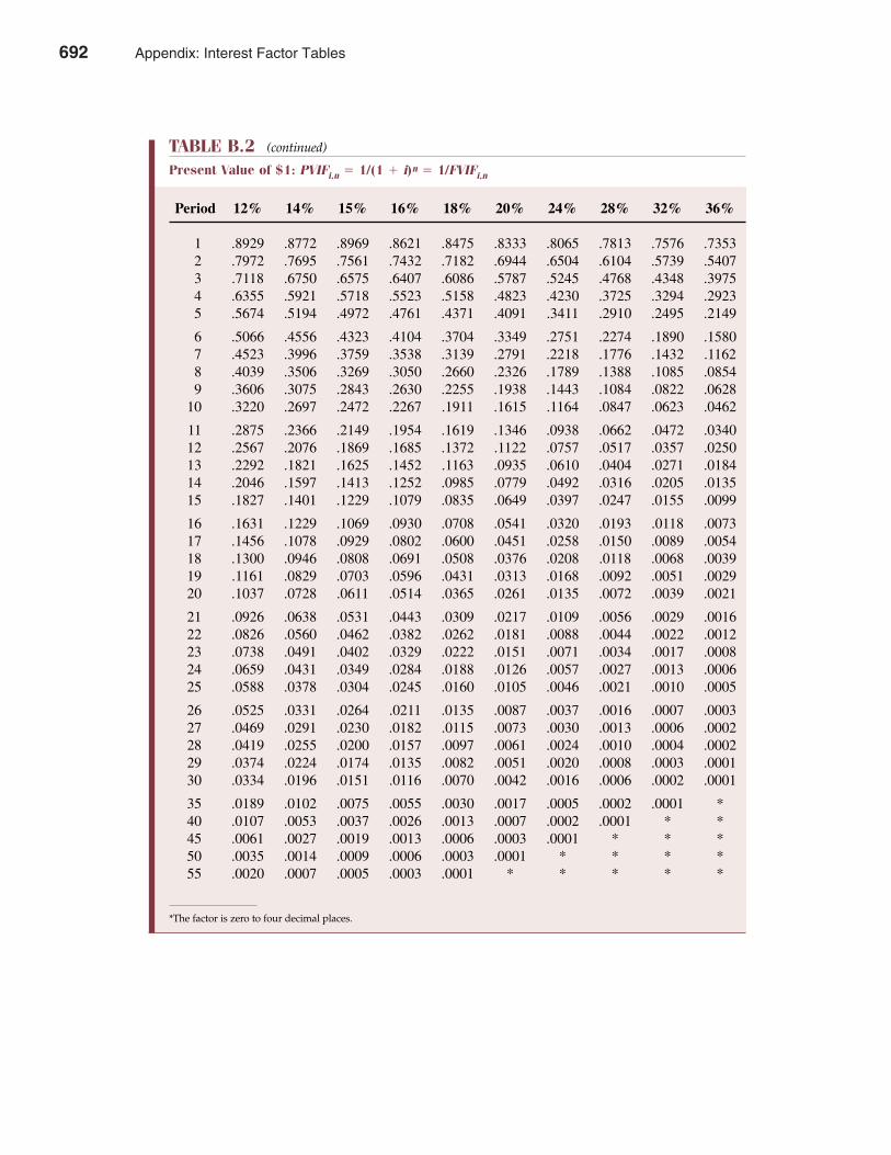
694 Appendix B Interest Factor Tables
TABLE B.2 (continued)
Present Value of $1: PVIFi,n � 1/(1 � i)n � 1/FVIFi,n
Period 12% 14% 15% 16% 18% 20% 24% 28% 32% 36%
1 .8929 .8772 .8969 .8621 .8475 .8333 .8065 .7813 .7576 .73532 .7972 .7695 .7561 .7432 .7182 .6944 .6504 .6104 .5739 .54073 .7118 .6750 .6575 .6407 .6086 .5787 .5245 .4768 .4348 .39754 .6355 .5921 .5718 .5523 .5158 .4823 .4230 .3725 .3294 .29235 .5674 .5194 .4972 .4761 .4371 .4091 .3411 .2910 .2495 .2149
6 .5066 .4556 .4323 .4104 .3704 .3349 .2751 .2274 .1890 .15807 .4523 .3996 .3759 .3538 .3139 .2791 .2218 .1776 .1432 .11628 .4039 .3506 .3269 .3050 .2660 .2326 .1789 .1388 .1085 .08549 .3606 .3075 .2843 .2630 .2255 .1938 .1443 .1084 .0822 .0628
10 .3220 .2697 .2472 .2267 .1911 .1615 .1164 .0847 .0623 .0462
11 .2875 .2366 .2149 .1954 .1619 .1346 .0938 .0662 .0472 .034012 .2567 .2076 .1869 .1685 .1372 .1122 .0757 .0517 .0357 .025013 .2292 .1821 .1625 .1452 .1163 .0935 .0610 .0404 .0271 .018414 .2046 .1597 .1413 .1252 .0985 .0779 .0492 .0316 .0205 .013515 .1827 .1401 .1229 .1079 .0835 .0649 .0397 .0247 .0155 .0099
16 .1631 .1229 .1069 .0930 .0708 .0541 .0320 .0193 .0118 .007317 .1456 .1078 .0929 .0802 .0600 .0451 .0258 .0150 .0089 .005418 .1300 .0946 .0808 .0691 .0508 .0376 .0208 .0118 .0068 .003919 .1161 .0829 .0703 .0596 .0431 .0313 .0168 .0092 .0051 .002920 .1037 .0728 .0611 .0514 .0365 .0261 .0135 .0072 .0039 .0021
21 .0926 .0638 .0531 .0443 .0309 .0217 .0109 .0056 .0029 .001622 .0826 .0560 .0462 .0382 .0262 .0181 .0088 .0044 .0022 .001223 .0738 .0491 .0402 .0329 .0222 .0151 .0071 .0034 .0017 .000824 .0659 .0431 .0349 .0284 .0188 .0126 .0057 .0027 .0013 .000625 .0588 .0378 .0304 .0245 .0160 .0105 .0046 .0021 .0010 .0005
26 .0525 .0331 .0264 .0211 .0135 .0087 .0037 .0016 .0007 .000327 .0469 .0291 .0230 .0182 .0115 .0073 .0030 .0013 .0006 .000228 .0419 .0255 .0200 .0157 .0097 .0061 .0024 .0010 .0004 .000229 .0374 .0224 .0174 .0135 .0082 .0051 .0020 .0008 .0003 .000130 .0334 .0196 .0151 .0116 .0070 .0042 .0016 .0006 .0002 .0001
35 .0189 .0102 .0075 .0055 .0030 .0017 .0005 .0002 .0001 *40 .0107 .0053 .0037 .0026 .0013 .0007 .0002 .0001 * *45 .0061 .0027 .0019 .0013 .0006 .0003 .0001 * * *50 .0035 .0014 .0009 .0006 .0003 .0001 * * * *55 .0020 .0007 .0005 .0003 .0001 * * * * *
*The factor is zero to four decimal places.
692 Appendix: Interest Factor Tables
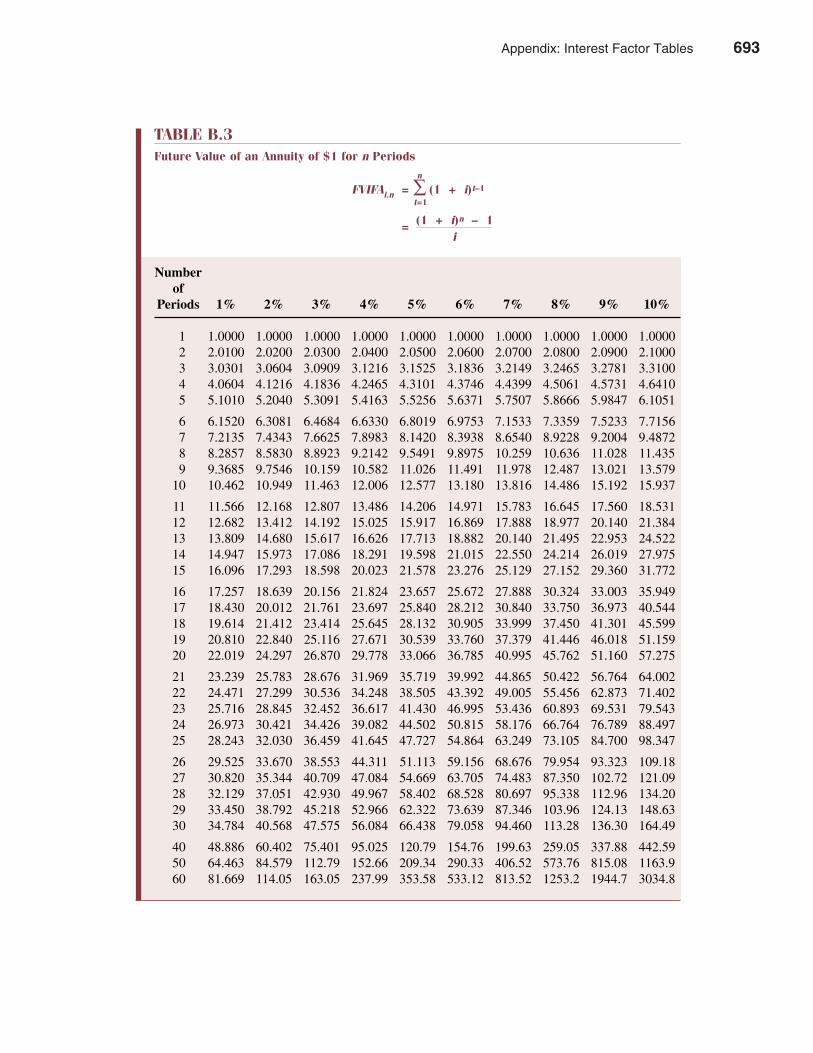
Appendix B Interest Factor Tables 695
TABLE B.3Future Value of an Annuity of $1 for n Periods
n
FVIFAi,n = ∑ (1 + i)t–1
t=1
= (1 + i)n – 1i
Numberof
Periods 1% 2% 3% 4% 5% 6% 7% 8% 9% 10%
1 1.0000 1.0000 1.0000 1.0000 1.0000 1.0000 1.0000 1.0000 1.0000 1.00002 2.0100 2.0200 2.0300 2.0400 2.0500 2.0600 2.0700 2.0800 2.0900 2.10003 3.0301 3.0604 3.0909 3.1216 3.1525 3.1836 3.2149 3.2465 3.2781 3.31004 4.0604 4.1216 4.1836 4.2465 4.3101 4.3746 4.4399 4.5061 4.5731 4.64105 5.1010 5.2040 5.3091 5.4163 5.5256 5.6371 5.7507 5.8666 5.9847 6.1051
6 6.1520 6.3081 6.4684 6.6330 6.8019 6.9753 7.1533 7.3359 7.5233 7.71567 7.2135 7.4343 7.6625 7.8983 8.1420 8.3938 8.6540 8.9228 9.2004 9.48728 8.2857 8.5830 8.8923 9.2142 9.5491 9.8975 10.259 10.636 11.028 11.4359 9.3685 9.7546 10.159 10.582 11.026 11.491 11.978 12.487 13.021 13.579
10 10.462 10.949 11.463 12.006 12.577 13.180 13.816 14.486 15.192 15.937
11 11.566 12.168 12.807 13.486 14.206 14.971 15.783 16.645 17.560 18.53112 12.682 13.412 14.192 15.025 15.917 16.869 17.888 18.977 20.140 21.38413 13.809 14.680 15.617 16.626 17.713 18.882 20.140 21.495 22.953 24.52214 14.947 15.973 17.086 18.291 19.598 21.015 22.550 24.214 26.019 27.97515 16.096 17.293 18.598 20.023 21.578 23.276 25.129 27.152 29.360 31.772
16 17.257 18.639 20.156 21.824 23.657 25.672 27.888 30.324 33.003 35.94917 18.430 20.012 21.761 23.697 25.840 28.212 30.840 33.750 36.973 40.54418 19.614 21.412 23.414 25.645 28.132 30.905 33.999 37.450 41.301 45.59919 20.810 22.840 25.116 27.671 30.539 33.760 37.379 41.446 46.018 51.15920 22.019 24.297 26.870 29.778 33.066 36.785 40.995 45.762 51.160 57.275
21 23.239 25.783 28.676 31.969 35.719 39.992 44.865 50.422 56.764 64.00222 24.471 27.299 30.536 34.248 38.505 43.392 49.005 55.456 62.873 71.40223 25.716 28.845 32.452 36.617 41.430 46.995 53.436 60.893 69.531 79.54324 26.973 30.421 34.426 39.082 44.502 50.815 58.176 66.764 76.789 88.49725 28.243 32.030 36.459 41.645 47.727 54.864 63.249 73.105 84.700 98.347
26 29.525 33.670 38.553 44.311 51.113 59.156 68.676 79.954 93.323 109.1827 30.820 35.344 40.709 47.084 54.669 63.705 74.483 87.350 102.72 121.0928 32.129 37.051 42.930 49.967 58.402 68.528 80.697 95.338 112.96 134.2029 33.450 38.792 45.218 52.966 62.322 73.639 87.346 103.96 124.13 148.6330 34.784 40.568 47.575 56.084 66.438 79.058 94.460 113.28 136.30 164.49
40 48.886 60.402 75.401 95.025 120.79 154.76 199.63 259.05 337.88 442.5950 64.463 84.579 112.79 152.66 209.34 290.33 406.52 573.76 815.08 1163.960 81.669 114.05 163.05 237.99 353.58 533.12 813.52 1253.2 1944.7 3034.8
Appendix: Interest Factor Tables 693
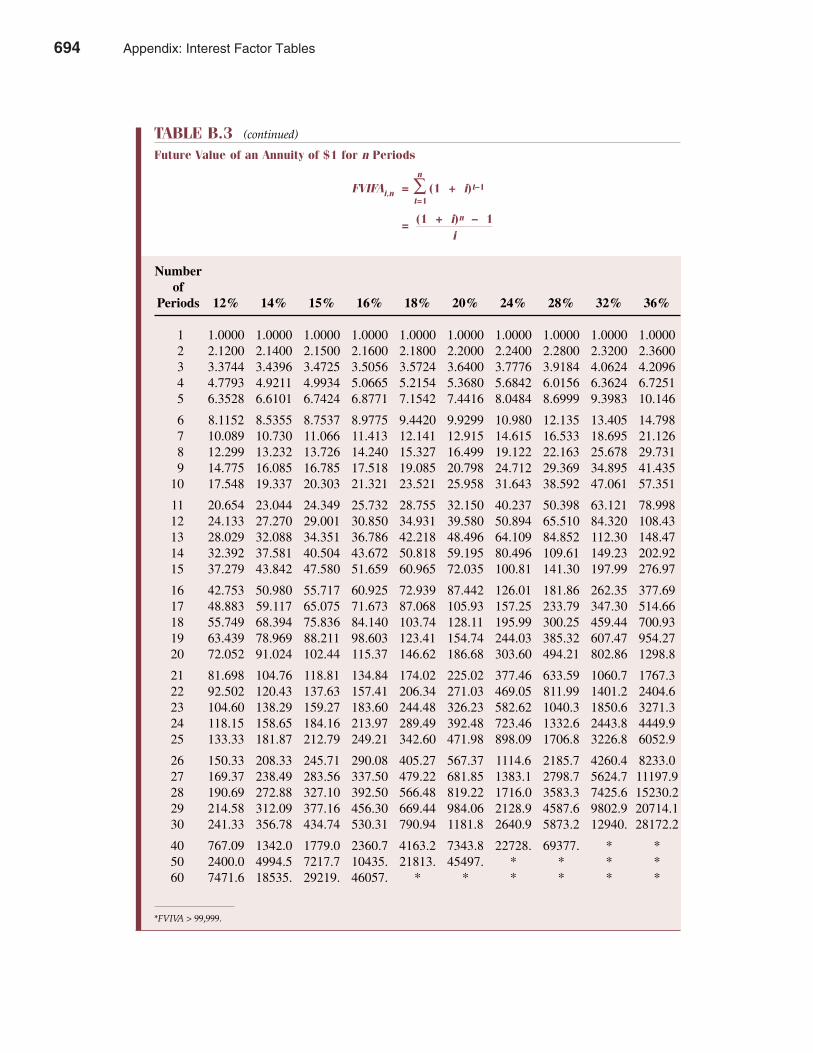
696 Appendix B Interest Factor Tables
TABLE B.3 (continued)
Future Value of an Annuity of $1 for n Periods
n
FVIFAi,n = ∑ (1 + i)t–1
t=1
= (1 + i)n – 1i
Numberof
Periods 12% 14% 15% 16% 18% 20% 24% 28% 32% 36%
1 1.0000 1.0000 1.0000 1.0000 1.0000 1.0000 1.0000 1.0000 1.0000 1.00002 2.1200 2.1400 2.1500 2.1600 2.1800 2.2000 2.2400 2.2800 2.3200 2.36003 3.3744 3.4396 3.4725 3.5056 3.5724 3.6400 3.7776 3.9184 4.0624 4.20964 4.7793 4.9211 4.9934 5.0665 5.2154 5.3680 5.6842 6.0156 6.3624 6.72515 6.3528 6.6101 6.7424 6.8771 7.1542 7.4416 8.0484 8.6999 9.3983 10.146
6 8.1152 8.5355 8.7537 8.9775 9.4420 9.9299 10.980 12.135 13.405 14.7987 10.089 10.730 11.066 11.413 12.141 12.915 14.615 16.533 18.695 21.1268 12.299 13.232 13.726 14.240 15.327 16.499 19.122 22.163 25.678 29.7319 14.775 16.085 16.785 17.518 19.085 20.798 24.712 29.369 34.895 41.435
10 17.548 19.337 20.303 21.321 23.521 25.958 31.643 38.592 47.061 57.351
11 20.654 23.044 24.349 25.732 28.755 32.150 40.237 50.398 63.121 78.99812 24.133 27.270 29.001 30.850 34.931 39.580 50.894 65.510 84.320 108.4313 28.029 32.088 34.351 36.786 42.218 48.496 64.109 84.852 112.30 148.4714 32.392 37.581 40.504 43.672 50.818 59.195 80.496 109.61 149.23 202.9215 37.279 43.842 47.580 51.659 60.965 72.035 100.81 141.30 197.99 276.97
16 42.753 50.980 55.717 60.925 72.939 87.442 126.01 181.86 262.35 377.6917 48.883 59.117 65.075 71.673 87.068 105.93 157.25 233.79 347.30 514.6618 55.749 68.394 75.836 84.140 103.74 128.11 195.99 300.25 459.44 700.9319 63.439 78.969 88.211 98.603 123.41 154.74 244.03 385.32 607.47 954.2720 72.052 91.024 102.44 115.37 146.62 186.68 303.60 494.21 802.86 1298.8
21 81.698 104.76 118.81 134.84 174.02 225.02 377.46 633.59 1060.7 1767.322 92.502 120.43 137.63 157.41 206.34 271.03 469.05 811.99 1401.2 2404.623 104.60 138.29 159.27 183.60 244.48 326.23 582.62 1040.3 1850.6 3271.324 118.15 158.65 184.16 213.97 289.49 392.48 723.46 1332.6 2443.8 4449.925 133.33 181.87 212.79 249.21 342.60 471.98 898.09 1706.8 3226.8 6052.9
26 150.33 208.33 245.71 290.08 405.27 567.37 1114.6 2185.7 4260.4 8233.027 169.37 238.49 283.56 337.50 479.22 681.85 1383.1 2798.7 5624.7 11197.928 190.69 272.88 327.10 392.50 566.48 819.22 1716.0 3583.3 7425.6 15230.229 214.58 312.09 377.16 456.30 669.44 984.06 2128.9 4587.6 9802.9 20714.130 241.33 356.78 434.74 530.31 790.94 1181.8 2640.9 5873.2 12940. 28172.2
40 767.09 1342.0 1779.0 2360.7 4163.2 7343.8 22728. 69377. * *50 2400.0 4994.5 7217.7 10435. 21813. 45497. * * * *60 7471.6 18535. 29219. 46057. * * * * * *
*FVIVA > 99,999.
694 Appendix: Interest Factor Tables
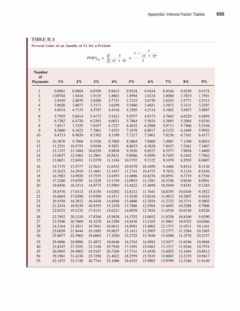
Appendix B Interest Factor Tables 697
TABLE B.4Present Value of an Annuity of $1 for n Periods
1
PVIFAi,n =n 1
=1 –
(1 + i)n
∑ (1 + i)t it=1
Numberof
Payments 1% 2% 3% 4% 5% 6% 7% 8% 9%
1 0.9901 0.9804 0.9709 0.9615 0.9524 0.9434 0.9346 0.9259 0.91742 1.09704 1.9416 1.9135 1.8861 1.8594 1.8334 1.8080 1.7833 1.75913 2.9410 2.8839 2.8286 2.7751 2.7232 2.6730 2.6243 2.5771 2.53134 3.9020 3.8077 3.7171 3.6299 3.5460 3.4651 3.3872 3.3121 3.23975 4.8534 4.7135 4.5797 4.4518 4.3295 4.2124 4.1002 3.9927 3.8897
6 5.7955 5.6014 5.4172 5.2421 5.0757 4.9173 4.7665 4.6229 4.48597 6.7282 6.4720 6.2303 6.0021 5.7864 5.5824 5.3893 5.2064 5.03308 7.6517 7.3255 7.0197 6.7327 6.4632 6.2098 5.9713 5.7466 5.53489 8.5660 8.1622 7.7861 7.4353 7.1078 6.8017 6.5152 6.2469 5.9952
10 9.4713 8.9826 8.5302 8.1109 7.7217 7.3601 7.0236 6.7101 6.4177
11 10.3676 9.7868 9.2526 8.7605 8.3064 7.8869 7.4987 7.1390 6.805212 11.2551 10.5753 9.9540 9.3851 8.8633 8.3838 7.9427 7.5361 7.160713 12.1337 11.3484 10.6350 9.9856 9.3936 8.8527 8.3577 7.9038 7.486914 13.0037 12.1062 11.2961 10.5631 9.8986 9.2950 8.7455 8.2442 7.786215 13.8651 12.8493 11.9379 11.1184 10.3797 9.7122 9.1079 8.5595 8.0607
16 14.7179 13.5777 12.5611 11.6523 10.8378 10.1059 9.4466 8.8514 8.312617 15.5623 14.2919 13.1661 12.1657 11.2741 10.4773 9.7632 9.1216 8.543618 16.3983 14.9920 13.7535 12.6593 11.6896 10.8276 10.0591 9.3719 8.755619 17.2260 15.6785 14.3238 13.1339 12.0853 11.1581 10.3356 9.6036 8.950120 18.0456 16.3514 14.8775 13.5903 12.4622 11.4699 10.5940 9.8181 9.1285
21 18.8570 17.0112 15.4150 14.0292 12.8212 11.7641 10.8355 10.0168 9.292222 19.6604 17.6580 15.9369 14.4511 13.1630 12.0416 11.0612 10.2007 9.442423 20.4558 18.2922 16.4436 14.8568 13.4886 12.3034 11.2722 10.3711 9.580224 21.2434 18.9139 16.9355 15.2470 13.7986 12.5504 11.4693 10.5288 9.706625 22.0232 19.5235 17.4131 15.6221 14.0939 12.7834 11.6536 10.6748 9.8226
26 22.7952 20.1210 17.8768 15.9828 14.3752 13.0032 11.8258 10.8100 9.929027 23.5596 20.7069 18.3270 16.3296 14.6430 13.2105 11.9867 10.9352 10.026628 24.3164 21.2813 18.7641 16.6631 14.8981 13.4062 12.1371 11.0511 10.116129 25.0658 21.8444 19.1885 16.9837 15.1411 13.5907 12.2777 11.1584 10.198330 25.8077 22.3965 19.6004 17.2920 15.3725 13.7648 12.4090 11.2578 10.2737
35 29.4086 24.9986 21.4872 18.6646 16.3742 14.4982 12.9477 11.6546 10.566840 32.8347 27.3555 23.1148 19.7928 17.1591 15.0463 13.3317 11.9246 10.757445 36.0945 29.4902 24.5187 20.7200 17.7741 15.4558 13.6055 12.1084 10.881250 39.1961 31.4236 25.7298 21.4822 18.2559 15.7619 13.8007 12.2335 10.961755 42.1472 33.1748 26.7744 22.1086 18.6335 15.9905 13.9399 12.3186 11.0140
Appendix: Interest Factor Tables 695
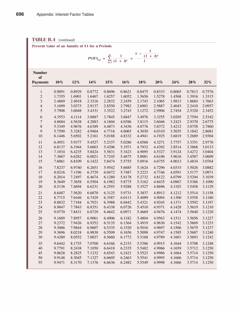
698 Appendix B Interest Factor Tables
TABLE B.4 (continued)
Present Value of an Annuity of $1 for n Periods1
PVIFAi,n =n 1
=1 –
(1 + i)n
∑ (1 + i)t it=1
Numberof
Payments 10% 12% 14% 15% 16% 18% 20% 24% 28% 32%
1 0.9091 0.8929 0.8772 0.8696 0.8621 0.8475 0.8333 0.8065 0.7813 0.75762 1.7355 1.6901 1.6467 1.6257 1.6052 1.5656 1.5278 1.4568 1.3916 1.33153 2.4869 2.4018 2.3216 2.2832 2.2459 2.1743 2.1065 1.9813 1.8684 1.76634 3.1699 3.0373 2.9137 2.8550 2.7982 2.6901 2.5887 2.4043 2.2410 2.09575 3.7908 3.6048 3.4331 3.3522 3.2743 3.1272 2.9906 2.7454 2.5320 2.3452
6 4.3553 4.1114 3.8887 3.7845 3.6847 3.4976 3.3255 3.0205 2.7594 2.53427 4.8684 4.5638 4.2883 4.1604 4.0386 3.8115 3.6046 3.2423 2.9370 2.67758 5.3349 4.9676 4.6389 4.4873 4.3436 4.0776 3.8372 3.4212 3.0758 2.78609 5.7590 5.3282 4.9464 4.7716 4.6065 4.3030 4.0310 3.5655 3.1842 2.8681
10 6.1446 5.6502 5.2161 5.0188 4.8332 4.4941 4.1925 3.6819 3.2689 2.9304
11 6.4951 5.9377 5.4527 5.2337 5.0286 4.6560 4.3271 3.7757 3.3351 2.977612 6.8137 6.1944 5.6603 5.4206 5.1971 4.7932 4.4392 3.8514 3.3868 3.013313 7.1034 6.4235 5.8424 5.5831 5.3423 4.9095 4.5327 3.9124 3.4272 3.040414 7.3667 6.6282 6.0021 5.7245 5.4675 5.0081 4.6106 3.9616 3.4587 3.060915 7.6061 6.8109 6.1422 5.8474 5.5755 5.0916 4.6755 4.0013 3.4834 3.0764
16 7.8237 6.9740 6.2651 5.9542 5.6685 5.1624 4.7296 4.0333 3.5026 3.088217 8.0216 7.1196 6.3729 6.0472 5.7487 5.2223 4.7746 4.0591 3.5177 3.097118 8.2014 7.2497 6.4674 6.1280 5.8178 5.2732 4.8122 4.0799 3.5294 3.103919 8.3649 7.3658 6.5504 6.1982 5.8775 5.3162 4.8435 4.0967 3.5386 3.109020 8.5136 7.4694 6.6231 6.2593 5.9288 5.3527 4.8696 4.1103 3.5458 3.1129
21 8.6487 7.5620 6.6870 6.3125 5.9731 5.3837 4.8913 4.1212 3.5514 3.115822 8.7715 7.6446 6.7429 6.3587 6.0113 5.4099 4.9094 4.1300 3.5558 3.118023 8.8832 7.7184 6.7921 6.3988 6.0442 5.4321 4.9245 4.1371 3.5592 3.119724 8.9847 7.7843 6.8351 6.4338 6.0726 5.4510 4.9371 4.1428 3.5619 3.121025 9.0770 7.8431 6.8729 6.4642 6.0971 5.4669 4.9476 4.1474 3.5640 3.1220
26 9.1609 7.8957 6.9061 6.4906 6.1182 5.4804 4.9563 4.1511 3.5656 3.122727 9.2372 7.9426 6.9352 6.5135 6.1364 5.4919 4.9636 4.1542 3.5669 3.123328 9.3066 7.9844 6.9607 6.5335 6.1520 6.5016 4.9697 4.1566 3.5679 3.123729 9.3696 8.0218 6.9830 6.5509 6.1656 5.5098 4.9747 4.1585 3.5687 3.124030 9.4269 8.0552 7.0027 6.5660 6.1772 5.5168 4.9789 4.1601 3.5693 3.1242
35 9.6442 8.1755 7.0700 6.6166 6.2153 5.5386 4.9915 4.1644 3.5708 3.124840 9.7791 8.2438 7.1050 6.6418 6.2335 5.5482 4.9966 4.1659 3.5712 3.125045 9.8628 8.2825 7.1232 6.6543 6.2421 5.5523 4.9986 4.1664 3.5714 3.125050 9.9148 8.3045 7.1327 6.6605 6.2463 5.5541 4.9995 4.1666 3.5714 3.125055 9.9471 8.3170 7.1376 6.6636 6.2482 5.5549 4.9998 4.1666 3.5714 3.1250
696 Appendix: Interest Factor Tables