Interlayer coherence and entanglement in bilayer quantum Hall states at filling factorν = 2/λ

M. Calixto and E. Perez-RomeroDepartamento de Matematica Aplicada, Universidad de Granada, Fuentenueva s/n, 18071 Granada, Spain

We study coherence and entanglement properties of the state space of a composite bi-fermion (twoelectrons pierced by λ magnetic flux lines) at one Landau site of a bilayer quantum Hall system.In particular, interlayer imbalance and entanglement (and its fluctuations) are analyzed for a setof U(4) coherent (quasiclassical) states generalizing the standard pseudospin U(2) coherent statesfor the spin-frozen case. The interplay between spin and pseudospin degrees of freedom opens newpossibilities with regard to the spin-frozen case. Actually, spin degrees of freedom make interlayerentanglement more effective and robust under perturbations than in the spin-frozen situation, mainlyfor a large number of flux quanta λ. Interlayer entanglement of an equilibrium thermal state andits dependence with temperature and bias voltage is also studied for a pseudo-Zeeman interaction.

PACS numbers: 73.43.-f, 71.10.Pm, 03.65.Ud, 03.65.Fd

I. INTRODUCTION

Quantum Hall Effect (QHE) keeps catching re-searchers’ attention owing to its peculiar features mainlyrelated to quantum coherence and the emergence of anew class of particles called “composite fermions”, dueto collective behavior shared with superconductivity andBose-Einstein condensation phenomena. In fact, thephysics of the bilayer quantum Hall (BLQH) systems,made by trapping electrons in two thin layers at the in-terface of semiconductors, is quite rich owing to uniqueeffects originating in the intralayer and interlayer coher-ence developed by the interplay between the spin andthe layer (pseudospin) degrees of freedom. For example,the presence of interlayer coherence in bilayer quantumHall states has been examined by magnetotransport ex-periments [1], where electrons are transferable betweenthe two layers by applying bias voltages and the inter-layer phase difference is tuned by tilting the sample.Also, anomalous (Josephson-like) tunneling current be-tween the two layers at zero bias voltage were predictedin Refs. [2–4], whose first experimental indication wasobtained in Ref. [5]. Other original studies on sponta-neous interlayer coherence in BLQH systems are [6, 7].

Spin and pseudospin quantum degrees of freedom arecorrelated in BLQH systems and entanglement proper-ties have also been studied in, for example, Refs. [8–10], mainly at filling factor ν = 1. An appropriate de-scription of quantum correlations is of great relevancein quantum computation and information theory, a fieldwhich has also attracted a huge degree of attention. Ac-tually, one can find quantum computation proposals us-ing BLQH systems in, for example, [11–13]. In this ar-ticle we also address the interesting problem of quantumcoherence and entanglement in BLQH systems at frac-tions of ν = 2 (perhaps a less known case), in the hopethat our theoretical considerations contribute to eventu-ally implement feasible large scale quantum computingin BLQH systems by engineering quantum Hall states.For this purpose, controllable entanglement, robustness

of qubits (long decoherence time) and ease qubit mea-surement are crucial. Concerning qubit measurement(and general reconstruction of quantum states), coher-ent states (which are often said to be the most classicalof all states of a dynamical quantum system) have beenwidely used to reconstruct the quantum state of light [14],pure spin sates [15, 16], etc, by using tomographic, spec-troscopic, interferometric, etc, techniques. The existenceof interlayer and intralayer coherence in BLQH systemshas also been evidenced (as commented in the previousparagraph), and we think that is its worth studying co-herent states (CS in the following) for the “Grassman-nian” ν = 2/λ case, which is perhaps less known thanthe “complex projective” (totally symmetric) ν = 1/λcase. The subject of CS is not only important for thequantum state reconstruction problem, but also to an-alyze the phase diagram of Hamiltonian models under-going a quantum phase transition (like the well studiedspin-ferromagnet and pseudo-spin-ferromagnet phases atν = 1). This is the spirit of Gilmore’s algorithm [17],which makes use of CS as variational states to approxi-mate the ground state energy, to study the classical, ther-modynamic or mean-field, limit of some critical quantummodels and their phase diagrams. For the BLQH sys-tem at ν = 2, the variational ground state energy perLandau site (with a Hamiltonian consisting on Coulombplus Zeeman-pseudo-Zeeman terms) has been analyzed(see e.g. [18]). The variational, SU(4)-invariant, groundstate is a homogeneous (coherent) state parametrized byeight independent variables [or four complex parameterszµ, µ = 0, 1, 2, 3, in our notation; see later on equa-tions (23,24)] which are related to the eight so-calledGoldston modes in the SU(4)-invariant system. Mini-mizing the variational ground state energy within thisparameter space (eight-dimensional energy surface) re-veals the existence of three phases at ν = 2: spin, ppinand canted phases (see e.g. [18]) as we move throughthe BLQH Hamiltonian coupling constants (bias voltage,tunneling, Zeeman strength, etc). At the minimum, theeight coherent (ground) state parameters now depend on

2

these Hamiltonian coupling constants and we could ma-nipulate them to generate not only specific CS but alsointeresting combinations like the so-called Schrodingercat states. The existence of Schrodinger cat states hasbeen evidenced in other physical models undergoing aquantum phase transition like the Dicke model for atom-radiation interaction (see e.g. [19–22]) and vibron mod-els for molecules [23–26], among others. In this paper weprovide explicit expressions of CS for BLQH at generalfractions of ν = 2 and we study some physical proper-ties like interlayer imbalance and entanglement and theirfluctuations. We believe that the CS discussed in this pa-per will also be of importance when studying many otherBLQH issues like the aforementioned phase diagrams.

In the BLQH system, one Landau site can accommo-date four isospin states |b ↑⟩, |b ↓⟩, |a ↑⟩ and |a ↓⟩ inthe lowest Landau level, where |b ↑⟩ (resp. |a ↓⟩) meansthat the electron is in the bottom layer “b” (resp. toplayer “a”) and its spin is up (resp. down), and so on.Therefore, the underlying group structure in each Lan-dau level of the BLQH system is enlarged from spin sym-metry U(2) to isospin symmetry U(4). The driving forceof quantum coherence is the Coulomb exchange inter-action, which is described by an anisotropic U(4) non-linear sigma model in BLQH systems [18, 27]. Actu-ally, it is the interlayer exchange interaction which de-velops the interlayer coherence. The lightest topologi-cal charged excitation in the BLQH system is a (com-plex projective) CP 3 = U(4)/[U(1) × U(3)] skyrmionfor filling factor ν = 1 and a (complex Grassmannian)G4

2 = U(4)/[U(2) × U(2)] bi-skyrmion for filling factorν = 2 (see [28] for similar studies in graphene and thecharge of these excitations). The Coulomb exchangeinteraction for this last case is described by a Grass-mannian G2 (from now on, we omit the superscript inG4

2) sigma model and the dynamical field is a Grassman-nian field Z = zµσµ [29] (σµ denote Pauli matrices plusidentity) carrying four complex field degrees of freedomzµ ∈ C, µ = 0, 1, 2, 3 (see later on Sec. III). As com-mented before, the parameter space characterizing theSU(4)-invariant ground state in the BLQH system atν = 2 is precisely G2 [30].

We would also like to say that higher-dimensional gen-eralizations of the Haldane’s sphere picture [31] of FQHEappeared after Zhang and Hu four-dimensional general-ization of QHE [32]. Just to mention several studies ofQHE on general manifolds and their CS like for example:torus T2 [33], complex projective U(N)/[U(N−1)×U(1)][34], Bergman ball U(N, 1)/[U(N)×U(1)] [35], flag man-ifold U(3)/U(1)3 [36], and many others. Coherent stateshave also been worked out in these higher-dimensionalgeneralizations, which help to perform a semi-classicalanalysis and to construct effective Wess-Zumino-Wittenactions for the edge states. Similar contructions couldalso be done for BLQH systems at ν = 2/λ with the helpof the Grassmannian CS that we discuss in this paper.

Two electrons in one Landau site must form an an-tisymmetric state due to Pauli exclusion principle and

this leads to a 6-dimensional irreducible representation ofSU(4), which is usually divided into spin and pseudospinsectors. The composite-fermion field theory [37, 38] andexperiments reveal the existence of new fractional QHstates in the bilayer system [2]. For fractional values ofthe filling factor, ν = 2/λ, the composite fermion in-terpretation is that of two electrons pierced by λ mag-netic flux lines. The mathematical structure of the dλ-dimensional (13) Hilbert spaceHλ(G2) for two compositeparticles in one Landau site has been studied in a recentarticle [39] by us, where we have also constructed the setof CS labeled by points of G2. For λ odd, wave func-tions turn out to be antisymmetric (composite fermion)and for λ even, wave functions are symmetric (compositeboson), see later on eq. (21). Now we want to analyzesome physical properties of these “quasi-classical” states,like interlayer imbalance, entanglement and their fluc-tuations, comparing them with the simpler spin-frozencase, to evaluate the effect played by spin and extraU(4) isospin operators. In particular, we observe thatthe number λ of flux lines, for filling factor ν = 2/λ,affects non-trivially the interlayer entanglement of CS.

The paper is organized as follows. In Section II westart by briefly analyzing the easier spin-frozen case andconsidering only the U(2) pseudospin structure; the U(2)pseudospin-s operators, Hilbert space and CS are dis-cussed in a oscillator (bosonic) realization related to mag-netic flux quanta attached to the electron in the fractionalfilling factor case. This oscillator construction some-how reminds the quasi-spin formalism introduced in thetwo-mode approximation of Bose-Einstein condensates ina double-well potential, with the role of the two wellsplayed now by the two layers. We compute interlayer im-balance and entanglement of pseudospin-s CS to later ap-preciate the similitudes and differences between the spin-frozen and the more involved isospin-λ U(4) case. Sec-tion III is devoted to a brief exposition of the operators(spin, pseudospin, etc.) and the structure of the Hilbertspace Hλ(G2) of two electrons, at one Landau site of thelowest Landau level, pierced by λ magnetic flux lines.For this purpose, we introduce an oscillator realizationof the U(4) Lie algebra in terms of eight boson creation,a†µ, b

†µ, and annihilation, aµ, bµ, µ = 0, 1, 2, 3, operators.

Then an orthonormal basis of Hλ(G2), in terms of Fockstates, is explicitly constructed, and a set of CS {|Z⟩},labeled by points Z ∈ G2, is built as definite superposi-tions of the basis states which remind Bose-Einstein con-densates. The simpler (lower-dimensional) case λ = 1is explicitly written, leaving the more involved (higher-dimensional) λ > 1 case for Appendices A and B (thereader can find much more information about the math-ematical structure of the state space Hλ(G2) in [39]). InSection IV we analyze interlayer imbalance and its fluc-tuations in a general Grassmannian U(4)/U(2)2, isospin-λ, CS |Z⟩, which generalizes the interlayer imbalance ofa pseudospin-s CS |z⟩, recovering the spin-frozen situa-tion as a particular case. In Section V we examine theinteresting problem of interlayer entanglement for basis

3

states and CS, accessed through the calculation of thepurity (and its fluctuations), linear and Von Neumannentropies of the reduced density matrix to one of the lay-ers. We find out that spin degrees of freedom play a rolein the interlayer entanglement by, for example, making itmore robust than in the spin-frozen case. Interlayer en-tanglement of an equilibrium thermal (mixed) state andits dependence with temperature and bias voltage is alsostudied for a pseudo-Zeeman interaction. Section VI isdevoted to conclusions and outlook.

II. THE SIMPLER U(2) SPIN-FROZEN CASE

We shall start by briefly analyzing the spin-frozen caseand considering only the U(2) pseudospin structure byassigning up and down pseudospins to the electron onthe top a and bottom b layers, respectively (see e.g. [18]for a standard reference on this subject). This approxi-mation is valid when the Zeeman energy is very large andall spins are frozen into their polarized states. We shallrecover the spin degree of freedom in Section III. Theelectron configuration is described by the total number

density ρ and the pseudospin density P = (P1,P2,P3),whose direction is controlled by applying bias voltageswhich transfer electrons between the two layers. We shallrestrict ourselves in this Section to one electron at oneLandau site of the lowest Landau level, pierced by 2smagnetic flux lines, with s the pseudospin. The opera-tors a† and b† (resp. a and b) create (resp. annihilate)flux quanta attached to the electron at the top and bot-

tom layers, respectively. If we denote by Z =

(ab

)and

Z† = (a†, b†) the two-component electron “field” and itsconjugate, then the pseudospin density operator can becompactly written as

Pµ =1

2Z†σµZ, µ = 0, 1, 2, 3, (1)

where σµ, µ = 1, 2, 3, denote the usual three Pauli ma-trices and σ0 is the 2× 2 identity matrix. The represen-tation (1) resembles the usual Jordan-Schwinger bosonrealization for spin. Note that 2P0 = Z†Z = a†a + b†brepresents the total number N of flux quanta, whichis fixed to N = 2s with s the pseudospin. The pseu-dospin third component P3 = 1

2 (a†a− b†b) measures the

population imbalance between the two layers, whereasP± = P1 ± P2 are tunneling (ladder) operators thattransfer quanta from one layer to the other and createinterlayer coherence [see later on eq. (4)]. The boson re-alization (1) defines a unitary representation of the pseu-dospin U(2) operators Pµ on the Fock space expandedby the orthonormal basis states

|na⟩ ⊗ |nb⟩ =(a†)na(b†)nb

√na!nb!

|0⟩, (2)

where |0⟩ denotes the Fock vacuum and nℓ the occupancynumbers of layers ℓ = a, b. The fact that the total number

of quanta is constrained to na+nb = 2s indicates that therepresentation (1) is reducible in Fock space. A (2s+1)-dimensional irreducible (Hilbert) subspace Hs(S2) carry-ing a unitary representation of U(2) with pseudospin s isexpanded by the P3 eigenvectors

|k⟩ ≡ |s+ k⟩a ⊗ |s− k⟩b =φk(a

†)√(2s)!(s+k)!

φ−k(b†)√

(2s)!(s−k)!

|0⟩, (3)

with |0⟩ the Fock vacuum and k = −s, . . . , s the corre-sponding eigenvalue (pseudospin third component). We

have made use of the monomials φk(z) =(

2ss+k

)1/2zs+k

as a useful notation to generalize the Fock space repre-sentation (3) of the pseudospin U(2) states |k⟩, to theisospin U(4) states |j,mqa,qb

⟩ in eq. (14), explicitly writtenlater in eq. (A3). This construction resembles Haldane’ssphere picture [31] for spinning monolayer QH systems,where s is also related to the “monopole strength” in thesphere S2.

As already said, tunneling between the two layers cre-ates interlayer coherence, which can be described bypseudospin-s CS

|z⟩ = ezP+ | − s⟩(1 + |z|2)s

=

∑sk=−s φk(z)|k⟩(1 + |z|2)s

, (4)

obtained as an exponential action of the tunneling (ris-ing) operator P+ on the lowest-weight state | − s⟩ (allquanta at the bottom layer b) with tuneling strengthz, a complex number usually parametrized as z =tan(θ/2)eiϕ, related to the stereographic projection ofa point (θ, ϕ) (polar and azimutal angles) of the Blochsphere S2 = U(2)/U(1)2 onto the complex plane. Themodulus and phase of z have a BLQH physical meaningwhich will be explained in the next Subsection. From themathematical point of view, pseudospin-s CS are normal-ized (but not orthogonal), as can be seen from the CSoverlap

⟨z′|z⟩ = (1 + z′z)2s

(1 + |z′|2)s(1 + |z|2)s, (5)

and they constitute an overcomplete set fulfilling theresolution of the identity 1 =

∫S2 |z⟩⟨z|dµ(z, z), with

dµ(z, z) = 2s+1π sin θdθdϕ the solid angle.

Pseudospin-s CS also accurately describe the physi-cal properties of many macroscopic quantum systemslike Bose-Einstein condensates in a double-well potential,two-level systems, superconductors, superfluids, etc. Amore familiar Fock-space representation of pseudospin-sCS [equivalent to (4)] as a two-mode Bose-Einstein con-densate is given by (|0⟩ denotes the Fock vacuum)

|z⟩ = 1√(2s)!

(b† + za†√1 + |z|2

)2s

|0⟩. (6)

In this context, the polar angle θ is related to the popula-tion imbalance and the azimuthal angle ϕ is the relative

4

1 3 5r

1

2

-1

1Ι ,DΙ

FIG. 1: (Color online) Imbalance ι (black line) and its stan-dard deviation ∆ι (dotted red line) per flux as a function ofthe CS parameter r = |z|.

phase of the two spatially separated Bose-Einstein con-densates. Both quantities can be experimentally deter-mined in terms of matter wave interference experimentsas it is shown in Refs. [40–42]. Let us see how bothquantities also describe imbalance population and phasecoherence between layers in the spin-frozen BLQH sys-tem.

A. Interlayer coherence and imbalance fluctuations

Standard (harmonic oscillator) CS exhibit Poissoniannumber statistics for the probability of finding n bosons,so that standard deviation ∆n is large. These large fluc-tuations of the occupation number are typical in super-fluid phases. Here we shall compute the mean value⟨P3⟩ and standard deviation ∆P3 of the interlayer im-balance operator P3 in a pseudospin-s CS |z⟩. Takinginto account that the pseudospin-s basis states {|k⟩, k =−s, . . . , s} are eigenstates of P3, namely P3|k⟩ = k|k⟩,one can easily compute the (spin-frozen) imbalance ι andits fluctuations ∆ι per flux in a pseudospin-s CS (4) as

ι =⟨z|P3|z⟩

s=

⟨P3⟩s

=|z|2 − 1

|z|2 + 1= − cos θ, (7)

∆ι =

√⟨P2

3 ⟩ − ⟨P3⟩2s

=

√2|z|

1 + |z|2=

sin θ√2.

In Figure 1 we see that the imbalance ι is −1 atr = |z| = 0, for which the CS is |z0⟩ = | − s⟩ (the lowest-weight state), that is, all quanta at the bottom layer b.The imbalance ι is 0 at r = 1 (the balanced case) andι → 1 when r → ∞, for which the CS is |z∞⟩ = |s⟩ (thehighest-weight state), that is, all quanta at the top layera. The standard deviation ∆ι is maximum at r = 1,with ∆ι(1) = 1/

√2, and tends to zero at r = 0 and when

r → ∞. This indicates that the largest fluctuations occurat r = 1 (θ = π/2). Note that both ι and ∆ι are invari-ant under inversion r → 1/r, namely ι(r) = −ι(1/r) and∆ι(r) = ∆ι(1/r), the point r = 1 being a fixed point.

The other interesting physical magnitude is the inter-layer phase difference ϕ = arctan⟨P2⟩/⟨P1⟩, which wasevidenced in [43] for BLQH systems. A robust interlayerphase difference is essential to design BLQH quantumbits [12] which could enable large-scale quantum compu-tation [11, 13].

The spinning case will provide more degrees of free-dom than the spin-frozen case to play with, since we willhave extra isospin operators in u(4) to create interlayercoherence (see later on Sec. IV).

B. Interlayer entanglement

In the pseudospin state spaceHs(S2), we shall considerthe bipartite quantum system given by layers a and b. Atfirst glance, the basis states (3) are a direct product anddo not entangle both layers. However, we shall see inSec. V that the introduction of spin creates new quan-tum correlations on the basis states. On the contrary,pseudospin-s CS do entangle layers a and b. Indeed, con-sidering the density matrix ϱ = |z⟩⟨z| and the expressionof the pseudospin-s basis states |k⟩ as a direct productof Fock states (3) in layers a and b, the reduced densitymatrix (RDM) to layer b is

ϱb = tra(ϱ) =

2s∑n=0

γn(r)|2s− n⟩b⟨2s− n|, (8)

which turns out to be diagonal with eigenvalues γn(r) =(2sn

)r2n/(1 + r2)2s a function of r = |z|. This expression

coincides with the result of Ref. [44] for entanglementof spin CS arising in two-mode (a and b) Bose-Einsteincondensates; see [45] for other results on entangled SU(2)CS and [46] for a review on this subject. The purityps = tr(ϱ2b) of (8) as a function of r is then

ps(r) =2s∑

n=0

γ2n(r) =

∑2sn=0

(2sn

)2r4n

(1 + r2)4s. (9)

This function is also inversion invariant ps(r) = ps(1/r)with r = 1 a fixed point. Precisely for r = 1 we have min-imal purity ps(1) = ( 12 (4s − 1))!/(

√π(2s)!), to be com-

pared with the purity 1/(2s+1) of a maximally entangledstate. In Figure 2 we represent ps as a function of r forseveral pseudospins. We see that |z⟩ at r = 1 is maxi-mally entangled for s = 1/2 since p1/2(1) = 1/2 (purityreaches its minimum). For higher pseudospin s values we

have the asymptotic behavior ps(1) = 1/√2πs+O(s−3/2)

which says that the corresponding CS is never maximallyentangled. The horizontal grid line of Figure 2 indicatesthe pure-state purity, which is attained at r = 0 [all par-ticles in layer b, with CS |z0⟩ = |k = −s⟩] and whenr → ∞ [all particles in layer a, with CS |z∞⟩ = |k = s⟩].

For those readers more familiar with Von Neumannentropy Ss(r) = −tr(ϱb log ϱb) = −

∑2sn=0 γn(r) log γn(r)

we plot it in Figure 3 together with the linear entropy

5

1 3 5r0

0.50.375

0.168

1p s

FIG. 2: (Color online) Purity ps(r) of the reduced densitymatrix ϱb = tra(ϱ) to layer b, for the U(2) CS density matrixϱ = |z⟩⟨z|, as a function of the coherent state parameter r =|z| for three values of the pseudospin: s = 1/2 (black), s = 1(dotted blue) and s = 11/2 (dashed red).

1 2 3r0

0.50.625

logH 2L

logI 8M2

Ls ,Ss

FIG. 3: (Color online) Linear Ls (solid line) and Von Neu-mann Ss (dotted line) entanglement entropies of the reduceddensity matrix ϱb = tra(ϱ) to layer b, for the pseudospin-s CSdensity matrix ϱ = |z⟩⟨z|, as a function of the coherent stateparameter r = |z| for two values of the pseudospin: s = 1/2(black) and s = 1 (red).

Ls(r) = 1 − ps(r), which turns out to be a lower ap-proximation of Ss (they are almost equal when the stateis almost pure). We see that Von Neumann entropy isalso maximum at r = 1 and attains its maximum valuelog(2s+1) (completely mixed state) only for s = 1/2, forwhich S1/2(1) = log(2) [in general Ss(1) ≤ log(2s+ 1)].

In what follows, we shall not make the assumptionthat Zeeman energy is very large and we shall study howspin affects interlayer coherence and entanglement in aU(4) symmetry setting (an intermediate step studyingentanglement in SU(2)×SU(2) mixed bipartite quantumstates has been considered in [47]). In Sec. V we shallalso consider the interlayer entanglement of the (mixed,non-pure) equilibrium state of a BLQH spinning systemat finite temperature.

III. U(4) OPERATORS AND HILBERT SPACE

Bilayer quantum Hall (BLQH) systems underlie anisospin U(4) symmetry. In order to emphasize the spinSU(2) symmetry in the, let us say, bottom b (pseudospindown) and top a or (pseudospin up) layers, it is custom-ary to denote the U(4) generators in the four-dimensionalfundamental representation by the sixteen 4×4 matricesτµν ≡ σµ ⊗ σν , µ, ν = 0, 1, 2, 3. The spin-frozen annihi-lation operators a and b will be replaced by their 2 × 2matrix counterparts a → a and b → b, so that the twocomponent “field” Z is now arranged as as a compoundZ = (Z1,Z2) of two fermions as

Z =

(ab

)=

a↓1 a↓2a↑1 a↑2b↑1 b↑2b↓1 b↓2

=

a0 a1a2 a3b0 b1b2 b3

. (10)

The operator (a↓1)† = a†0 [resp. (b↑2)

† = b†1] creates aflux quanta attached to the first [resp. second] electronwith spin down [resp. up] at layer a [resp. b], and soon. We shall use the more compact notation aµ, bµ, µ =0, 1, 2, 3, and just remember that even and odd quanta areattached to the first and second electrons, respectively.Note that the modes µ = {0, 1} (resp. µ = {2, 3}) arerelated to spin up (resp. down) in layer b and viceversain layer a; this is due to an inherent conjugated responseof spin in each layer under U(4) rotations [see later inparagraph before eq. (A4)]. The sixteen U(4) isospindensity operators [the spinning counterpart of (1)] arethen written as

Tµν = tr(Z†τµνZ), (11)

which constitute an oscillator representation of the 4× 4matrix generators τµν , in terms of eight bosonic modes.In a previous article [39] we have obtained the matrixelements of Tµν in a Fock state basis.

In the previous Section, we fixed the total number offlux quanta Z†Z = a†a + b†b to 2s. The U(4) analogueof this constraint adopts the compact form

Z†Z|j,mqa,qb⟩ = (a†a+ b†b)|j,mqa,qb

⟩ = λI2|j,mqa,qb⟩,

valid for any physical state |j,mqa,qb⟩, where by I2 we denote

the 2 × 2 identity operator and λ is the number of fluxquanta attached to each electron. In particular, the linearCasimir operator T00 = tr(Z†Z) =

∑3µ=0 a

†µaµ + b†µbµ,

providing the total number of quanta, is fixed to 2λ,λ ∈ N. We also identify the interlayer imbalance opera-tor now as T30 =

∑3µ=0 a

†µaµ − b†µbµ, which measures the

excess of quanta between layers a and b. In the BLQHliterature (see e.g. [18]) it is customary to denote the to-tal spin Sj = T0j/2 and pseudospin Pj = Tj0/2, togetherwith the remaining 9 isospin Rkj = Tjk/2 operators.

It is clear that (11) defines a unitary bosonic repre-sentation of the U(4) matrix generators τµν in the Fock

6

space expanded by orthonormal basis states [the U(4)analogue of (2)]∣∣∣∣n0

a n1a

n2a n3

a

⟩a

⊗∣∣∣∣n0

b n1b

n2b n3

b

⟩b

=3∏

µ=0

(a†µ)nµa (b†µ)

nµb√

nµa !n

µb !

|0⟩, (12)

where |0⟩ denotes the Fock vacuum and nµℓ the occupancy

numbers of layers ℓ = a, b and modes µ = 0, 1, 2, 3. Thefact that the total number of quanta is constrained to∑3

µ=0 nµa + nµ

b = 2λ indicates that the representation

(11) is reducible in Fock space. In Ref. [39] we haveobtained the carrier Hilbert space Hλ(G2) of a

dλ =1

12(λ+ 1)(λ+ 2)2(λ+ 3) (13)

dimensional irreducible representation of U(4) spannedby the set of orthonormal basis vectors{

|j,mqa,qb⟩, 2j,m ∈ N,qa, qb = −j, . . . , j

}2j+m≤λ

(14)

in terms of Fock states (12) (see Appendix A for a brief).These basis vectors fulfill a resolution of the identity

1 =λ∑

m=0

(λ−m)/2∑j=0; 12

j∑qa,qb=−j

|j,mqa,qb⟩⟨j,mqa,qb

|,

where∑

j=0; 12means sum on j = 0, 1

2 , 1,32 , . . . These

are the U(4) isospin-λ analogue of the pseudospin-s or-thonormal basis vectors (3), with the role of the pseu-dospin s played now by λ (we are omitting the labelss and λ from the basis vectors |k⟩ and |j,mqa,qb

⟩, respec-tively, for the sake of brevity). Piercing the two elec-trons with λ magnetic flux lines affects the total angularmomentum j of the system, which can reach the valuesj = 0, 1

2 , 1,32 , . . . ,

λ2 . The meaning of the quantum (nat-

ural) number m in |j,mqa,qb⟩ is related to the total number

of flux quanta in layer a by

n0a + n1

a + n2a + n3

a = 2(j +m) (15)

and also to the interlayer imbalance (2j + 2m − λ) (theeigenvalue of the pseudospin third component P3 =T30/2), measuring half the excess of flux quanta in layera w.r.t. layer b. Note that j and m are always boundedby 2j + m ≤ λ, as stated in eq. (14), thus leading to afinite-dimensional representation of U(4). The remainderquantum numbers qa and qb represent the angular mo-mentum third components of layers a and b, respectively.Their relation with flux quanta turns out to be:

n0a + n1

a − n2a − n3

a = −2qa ,

n0b + n1

b − n2b − n3

b = 2qb , (16)

which says that the “spin third component quantumnumber” qb measures the imbalance between µ = {0, 1}

(spin up) and µ = {2, 3} (spin down) type flux quanta in-side layer b, and viceversa for qa inside layer a [rememberthe assignment in (10)].

The explicit construction of the basis states (14) inFock state for general λ entails a certain level of math-ematical sophistication and has been worked out in aprevious Ref. [39]. In this Section we shall only discusthe simpler case λ = 1. This should be enough in a firstreading. For the case of arbitrary λ, we have included abrief in Appendix A, in order to make the presentationsimpler and self-contained.

As the simplest example, let us provide the explicit ex-pression of the basis states |j,mqa,qb

⟩ in terms of Fock states(12) for two flux quanta (λ = 1 line of flux):

|0,00,0⟩ =1√2

(∣∣∣∣0 00 0

⟩a

⊗∣∣∣∣1 00 1

⟩b

−∣∣∣∣0 00 0

⟩a

⊗∣∣∣∣0 11 0

⟩b

),

|12 ,012 ,

12

⟩ =1√2

(∣∣∣∣0 00 1

⟩a

⊗∣∣∣∣1 00 0

⟩b

−∣∣∣∣0 01 0

⟩a

⊗∣∣∣∣0 10 0

⟩b

),

|12 , 0

−12 ,−1

2

⟩ =1√2

(∣∣∣∣1 00 0

⟩a

⊗∣∣∣∣0 00 1

⟩b

−∣∣∣∣0 10 0

⟩a

⊗∣∣∣∣0 01 0

⟩b

),

|12 , 0−12 , 12

⟩ =1√2

(∣∣∣∣1 00 0

⟩a

⊗∣∣∣∣0 10 0

⟩b

−∣∣∣∣0 10 0

⟩a

⊗∣∣∣∣1 00 0

⟩b

),

|12 , 012 ,

−12

⟩ =1√2

(∣∣∣∣0 00 1

⟩a

⊗∣∣∣∣0 01 0

⟩b

−∣∣∣∣0 01 0

⟩a

⊗∣∣∣∣0 00 1

⟩b

),

|0,10,0⟩ =1√2

(∣∣∣∣1 00 1

⟩a

⊗∣∣∣∣0 00 0

⟩b

−∣∣∣∣0 11 0

⟩a

⊗∣∣∣∣0 00 0

⟩b

).

(17)

This irreducible representation arises in the Clebsch-Gordan decomposition of a tensor product of 2 four-dimensional (elementary) representations of U(4)

⊗ = ⊕ ⇒ 4× 4 = 10 + 6

and corresponds to the totally antisymmetric case withdimension d1 = 6, in accordance with (13). It agrees withthe fact that two electrons in one Landau site must forman antisymmetric state due to Pauli exclusion principle.The d1 = 6-dimensional irrep of SU(4) is usually dividedinto two sectors (see e.g. [18]): the spin sector with spin-triplet pseudospin-singlet states

|S↑⟩ = |12 , 0−12 , 12

⟩, |S0⟩ =1√2(|

12 ,012 ,

12

⟩+|12 , 0−12 ,−1

2

⟩), |S↓⟩ = |12 , 012 ,

−12

⟩

(18)and the ppin sector with pseudospin-triplet spin-singletstates

|P↑⟩ = |0,10,0⟩, |P0⟩ =1√2(|

12 , 012 ,

12

⟩ − |12 , 0−12 ,−1

2

⟩), |P↓⟩ = |0,00,0⟩.

(19)For arbitrary λ, the Young tableau of the correspond-

ing dλ-dimensional representation is made of two rowsof λ boxes each. We can think of the following “com-posite bi-fermion” picture (following Jain’s image [38])

7

to physically explain the dimension (13) of the Hilbertspace Hλ(G2). We have two electrons attached to λ fluxquanta each. The first electron can occupy any of thefour isospin states |b ↑⟩, |b ↓⟩, |a ↑⟩ and |a ↓⟩ at one Lan-dau site of the lowest Landau level. Therefore, there are(4+λ−1

λ

)ways of distributing λ quanta among these four

states. Due to the Pauli exclusion principle, there areonly three states left for the second electron and

(3+λ−1

λ

)ways of distributing λ quanta among these three states.However, some of the previous configurations must beidentified since both electrons are indistinguishable and λpairs of quanta adopt

(2+λ−1

λ

)equivalent configurations.

In total, there are(λ+3λ

)(λ+2λ

)(λ+1λ

) =1

12(λ+ 3)(λ+ 2)2(λ+ 1)

ways to distribute 2λ flux quanta among two identicalelectrons in four states, which turns out to coincide withthe dimension dλ in (13) of the Hilbert space Hλ(G2).Other possible picture, compatible with some usual “fluxline” representations (see e.g. [18]), is the following. Wehave λ magnetic flux lines piercing two electrons whichcan occupy four possible states. There are

(λ+3λ

)and(

λ+2λ

)ways of piercing the first and second electron, re-

spectively. Indistinguishability identifies(λ+1λ

)of these

possible configurations, rendering again dλ ways to piercethe two electrons with λ flux lines.Concerning the quantum statistics of our states for a

given number λ of flux lines, one can see that whereas theorthonormal basis functions (14) [see also (A3)] are anti-symmetric (fermionic character) under the interchange ofthe two electrons for λ odd, they are symmetric (bosoniccharacter) for λ even. Indeed, under the interchange ofcolumns in [interchange of electrons (Z1,Z2) → (Z2,Z1)in (10)]

a =

(a0 a1a2 a3

)→ a =

(a1 a0a3 a2

), (20)

[likewise for b → b], the basis states transform accordingto (see Appendix A for more details)

|j,mqa,qb⟩ = (−1)λ |j,mqa,qb⟩. (21)

Indeed, it can be straightforwardly verified for λ = 1by swapping columns of vectors of |·⟩a and |·⟩b in (17)and, in general, by exchanging columns in the Fock states(12). There is another inherent symmetry under the in-terchange of layers a and b, although it does not entailany kind of quantum statistics because layers a and b arenot indistinguishable. In fact, from the general defini-tion of the basis states |j,mqa,qb

⟩ in eq. (A3), it is easy tosee that, under the interchange of layers a ↔ b, we havethe following “population-inversion” property

|j,mqa,qb⟩ ↔ (−1)qa−qb |j,λ−2j−m

−qb,−qa ⟩, (22)

which says that the population of layer a, pa = 2j + 2m,becomes 2j + 2(λ − 2j −m) = 2λ − pa = pb, the popu-lation of layer b. Indeed, one can check this property forthe easier λ = 1 case directly in (17). We shall see thatinterlayer entanglement depends quantitatively on λ (seee.g. Figure 10), but the qualitative behavior turns outto be similar for λ even (bosonic) and odd (fermionic).This is because we are studying layer-layer entanglementbut not fermion-fermion or boson-boson entanglement,for which a dependence on the parity of λ is expected.Moreover, when discussing layer-layer entanglement wedo not have to worry about filtering the intrinsic correla-tions of identical particles due to Pauli exclusion principle(see e.g. [48]), since layers are not indistinguishable.

In Ref. [39] (see the Appendix B for a brief) wehave also introduced a set of (quasi-classical) CS withinteresting mathematical and also physical propertiesthat will be analyzed here and in future publications.These CS constitute a kind of matrix generalization ofthe pseudospin-s CS (4). They are also Bose-Einstein-like condensates [see eq. (B2)] but they are now la-beled by a 2 × 2 complex matrix Z = zµσµ (sum onµ = 0, 1, 2, 3), with four complex entries zµ = tr(Zσµ)/2(they are points on the eight-dimensional GrassmannianG2). These CS can be expanded in terms of the orthonor-mal basis vectors (14), and the general formula is givenin (B1). In this Section we just shall write the expressionof |Z⟩ for the simplest λ = 1 case in terms of the basisstates (17):

|Z⟩ =[|0,00,0⟩+ det(Z)|0,10,0⟩+ (z0 − z3)|

12 , 0

−12 ,−1

2

⟩+

(z1 + iz2)|12 , 0−12 , 12

⟩+ (z1 − iz2)|12 , 012 ,

−12

⟩+

(z0 + z3)|12 ,012 ,

12

⟩]/det(σ0 + Z†Z)

12 , (23)

where the denominator is a normalizing factor. In thermsof the spin-triplet (18) and pseudospin triplet (19) states,we equivalently have

|Z⟩ =[|P↓⟩+ det(Z)|P↑⟩+

√2z3|P0⟩+

z1(|S↑⟩+ |S↓⟩) + iz2(|S↑⟩ − |S↓⟩)+√2z0|S0⟩

]/det(σ0 + Z†Z)

12 . (24)

Therefore, the CS |Z⟩ depends on four arbitrary complexparameters zµ, µ = 0, 1, 2, 3 [and not only one z like thespin-frozen case (4)], which means that we have extraisospin operators to create interlayer and spin coherence.A particular experimental way to generate these CS isthrough the natural tunneling interaction arising whenboth layers are placed close enough and electrons hopbetween them [see formula (B7), which provides an ex-pression of the CS |Z⟩ as an exponential of interlayerladder operators T±µ = (T1µ ± iT2µ)/2].

In the next two sections, we shall study some physi-cal quantities that only depend on two (out of the eightzµ) parameters related to the determinant det(ZZ†) andtrace tr(ZZ†), due to an intrinsic rotational invariance.

8

IV. INTERLAYER COHERENCE ANDIMBALANCE FLUCTUATIONS

Like we did in Section IIA for the spin-frozen case,here we shall compute interlayer coherence and imbal-ance fluctuations but for the Grassmannian G2 CS |Z⟩.Taking into account that the basis state |j,mqa,qb

⟩ is an eigen-state of P3 = T30/2 with eigenvalue (2j + 2m − λ), wearrive at the following expression for its mean value inthe CS |Z⟩ (we write the case of arbitrary λ):

⟨P3⟩ = ⟨Z|P3|Z⟩ = λdet(Z†Z)− 1

det(σ0 + Z†Z)(25)

Note that, since det(σ0+Z†Z) = 1+tr(Z†Z)+det(Z†Z),the mean value ⟨P3⟩ is only a function of the two U(2)2-invariants: determinant d = det(Z†Z) = z2z2 [withz2 ≡ zµηµνz

ν ] and trace t = tr(Z†Z) = zµδµνzν ;

we are using the Einstein summation convention withηµν = diag(1,−1,−1,−1) the Minkowski metric andδµν = diag(1, 1, 1, 1) the Euclidean metric. Instead ofd and t, we shall use other parametrization adapted tothe decomposition

Z = V †a

(r+e

iϑ+ 00 r−e

iϑ−

)Vb, (26)

where Va, Vb ∈ SU(2) are rotations, and r± ∈ [0,∞) andϑ± ∈ [0, 2π) are polar coordinates. Taking into accountthat d = r2+r

2− and t = r2+ + r2−, the imbalance mean

value “per flux quanta” is simply

I(r+, r−) =⟨P3⟩λ

=r2+r

2− − 1

(1 + r2+)(1 + r2−). (27)

In the same way, we can compute the imbalance variance“per flux quanta”, which results in

∆I2(r+, r−) =⟨P2

3 ⟩ − ⟨P3⟩2

λ(28)

=r2+ + r2− + 4r2+r

2− + r4+r

2− + r2+r

4−

(1 + r2+)2(1 + r2−)

2.

Note that I and ∆I are independent of λ, since the meanvalue ⟨P3⟩ scales with λ and its uncertainty ∆P3 scaleswith λ1/2. Note also that I and ∆I verify the followinginversion invariance

I(r+, r−) = −I(1

r∓,1

r±), ∆I(r+, r−) = ∆I(

1

r∓,1

r±).

(29)In Figure 4 we represent the imbalance I and its stan-dard deviation ∆I as a function of r±. We see that I isan increasing function of r± and takes its values in the in-terval [−1, 1]. Balanced coherent configurations (I = 0)occur on the hyperbola r+r− = 1. The behavior of ∆I isa bit more complex. The global maximum of ∆I occursat r+ = r− = 1, where the deviation attains the value1/√2. For high values of r± the deviation ∆I tends to

FIG. 4: Imbalance I and its standard deviation ∆I (per fluxquanta) as a function of the CS parameters r±.

zero except for two particular trajectories. To better ap-preciate this fact, we use polar coordinates r+ = r cos θand r− = r sin θ, with r ∈ [0,∞) and θ ∈ [0, π/2]. Figure5 offers a representation of ∆I as a function of r and θand Figure 6 displays three sections (cuts) (r = 2, r = 4and r = 8) of ∆I as a function of θ. For r ≤ 2, ther =constant cuts of the deviation ∆I have a single max-imum at θ = π/4. However, for r > 2 the situationchanges and the cuts (for fixed r) of ∆I display two localmaxima at two values of the polar angle θ±r given by

cos θ±r =

√r4 ∓ 2

√r4 − 16∓ r2(∓4 +

√r4 − 16)

2r2(r2 + 4). (30)

The expression θ±(r) = θ±r gives two singular trajectoriesin the (r, θ) plane for which fluctuations are always non-zero and tend to ∆I = 1/2 when r → ∞. Both localmaxima are narrower and narrower (see Figure 6), withθ−r → 0 and θ+r → π/2 as as r → ∞. We also haveθ±2 = π/4.

Looking for a physical interpretation and implementa-tion of interlayer coherence and imbalance fluctuations,

9

FIG. 5: Standard deviation ∆I (per flux quanta) as a function

of the CS parameters r =√

r2+ + r2− and θ = arctan(r−/r+).

0 Θ8-Θ4-

Θ2±=Π

4Θ4+Θ8+ Π

2

Θ

12

1

2

DI

FIG. 6: (Color online) Standard deviation ∆I (per fluxquanta) as a function of the polar angle θ = arctan(r−/r+)for r = 2 (solid line) r = 4 (dotted blue) and r = 8 (dashedred). The points θ±r denote local maxima of ∆I for each valueof r

let us consider the case Z = z0σ0 + z3σ3, for whichr+ = |z0 + z3| and r− = |z0 − z3|, and the polar an-gle is then θ = arctan(|z0 − z3|/|z0 + z3|). Accordingto the expression (B7), this CS can be generated by theoperators T±0 and T±3 or, equivalently, by P1,P2 andR31,R32 introduced in Subsection III to compare withthe notation of standard textbooks like [18]. The oper-ators P1 and P2 produce the typical interlayer tunnel-ing interaction present in the spin-frozen Hamiltonian ofthe bilayer system. Here we have extra isospin opera-tors R31 and R32 to play with to create interlayer co-herence and imbalance. Actually, the peculiar situationdescribed by the equation (30) takes place when tun-neling interaction strengths z0 and z3 of P1 and R31,respectively, verify tan θ±r = |z0 − z3|/|z0 + z3| for each

value of r =√2√

|z0|2 + |z3|2. For r ≤ 2, maximumimbalance fluctuations occur when r+ = r−, for examplewhen z3 = 0 (i.e. when the interaction R32 is switched

off) whereas for r ≫ 2 maximum imbalance fluctuationsrequire both tunneling interactions to be slightly “out oftune”, that is, when the corresponding tunneling inter-action strengths z0 and z3 fulfill z0 ≈ ±z3. It would beworth to experimentally explore these situations.

Note that we recover the spin-frozen magnitudes as aparticular case of the general spinning case. In fact, thishappens for the diagonal case r+ = r− = r0, which cor-responds to Z = z0σ0 with r0 = |z0|, where CS are justcreated by the tunneling interaction generated by P±,discarding the extra U(4) isospin generators Rjk. Theimbalance I(r0, r0) and its standard deviation ∆I(r0, r0)for this case coincide with ι(r0) and ∆ι(r0) in (7).

We again stress that the spinning case provides moredegrees of freedom than the spin-frozen case to play with,since we have extra isospin operators in u(4) to cre-ate coherence. Actually, other isospin CS mean values⟨Tµν⟩, like the aforementioned interlayer phase differenceθ(Z) = arctan⟨P2⟩/⟨P1⟩, will depend now on more thattwo CS parameters zµ. These cases deserve a separatestudy and will not be treated here.

We expect many more interesting physical phenomenaat the previous critical points. Actually, let us see thatmaximum interlayer entanglement also occurs at r0 = 1for a CS |Z⟩.

V. INTERLAYER ENTANGLEMENT

In the state space Hλ(G2), we shall consider the bipar-tite quantum system given by layers a and b. Interlayerentanglement can provide feasible quantum computation.For example, in reference [11] it is theoretically shownthat spontaneously interlayer-coherent BLQH dropletsshould allow robust and fault-tolerant pseudospin quan-tum computation in semiconductor nanostructures. Herewe shall show that BLQH coherent states at ν = 2/λ arehighly entangled, for high enough λ, and entanglement isrobust (with low fluctuations) in a wide range of coherentstate parameters.

A. Interlayer entanglement of basis states

Let us firstly show that, contrary to the (direct prod-uct) basis states |k⟩ of the spin-frozen case in eq. (3), theorthonormal basis vectors |j,mqa,qb

⟩ in (14) are entangled fornon-zero angular momentum, j = 0. We shall explicitlywork out the simplest case λ = 1 and give the results forgeneral λ. In the Appendix A we show that the basisstates |j,mqa,qb

⟩ can be written as an expansion

|j,mqa,qb⟩ =

j∑q=−j

(−1)qa−q

√2j + 1

|vj,m−q,−qa⟩a ⊗ |vj,λ−2j−mq,qb

⟩b, (31)

where {|vj,mq,q′ ⟩a} and {|vj,mq,q′ ⟩b} are Schmidt basis for layers

a and b, respectively, and 1/√2j + 1 are the Schmidt

10

coefficients with Schmidt number 2j + 1. For λ = 1 theSchmidt (orthonormal) basis for layer a (likewise for layerb) is simply:

|v0,00,0⟩a =

∣∣∣∣0 00 0

⟩a

, |v0,10,0⟩a =1√2

(∣∣∣∣1 00 1

⟩a

−∣∣∣∣0 11 0

⟩a

),

|v12 , 0

−12 ,−1

2

⟩a =

∣∣∣∣0 00 1

⟩a

, |v12 , 0

−12 , 12

⟩a =

∣∣∣∣0 10 0

⟩a

,

|v12 , 012 ,

−12

⟩a =

∣∣∣∣0 01 0

⟩a

, |v12 ,012 ,

12

⟩a =

∣∣∣∣1 00 0

⟩a

. (32)

It can be easily checked that, plugging (32) into (31), onearrives to eq. (17). For arbitrary λ, the Schmidt basisvectors for layer a (idem for layer b) are given in theAppendix A by eq. (A4), which fulfill the orthogonalityrelations (A5).As a measure of interlayer entanglement, we shall com-

pute the purity of the reduced density matrix (RDM)to one of the layers. More precisely, denoting by ρ =|j,mqa,qb

⟩⟨j,mqa,qb| the density matrix of an arbitrary basis

state and by ρa = trb(ρ) the reduced density matrixof layer a, it can be seen that the purity of ρa is thentr(ρ2a) = 1/(2j + 1), which is less than 1 if j = 0. In-deed, the proof is apparent from the explicit expressionof orthonormal basis vectors |j,mqa,qb

⟩ in (31) and the factthat the Schmidt basis (32) is orthonormal for λ = 1 [see(A4) and (A5) for arbitrary λ]. Moreover, tracing outthe layer b part, the reduced density matrix of layer a is(we write the general λ case)

ρa = trb(ρ) =λ∑

m=0

(λ−m)/2∑j=0; 12

j∑q,q′=−j

b⟨vj,mq,q′ |ρ|vj,mq,q′ ⟩b

=1

2j + 1

j∑q=−j

|vj,mq,qa⟩a⟨vj,mq,qa | . (33)

Using again the orthonormality relations for Schmidt ba-sis [see (A5) for the general case], we finally arrive to thepurity tr(ρ2a) = 1/(2j + 1). Therefore, for high angularmomentum, j ≫ 1, the basis state |j,mqa,qb

⟩ is highly entan-gled (almost zero purity) but not maximally entangled(with minimal purity 1/dλ), since dλ > 2j + 1. In fact,we have that

λ∑m=0

(λ−m)/2∑j=0; 12

(2j + 1)2 = dλ. (34)

B. Interlayer entanglement of coherent states

Secondly, we shall study the interlayer entanglementof a CS |Z⟩. For example, for λ = 1, and starting from(23) or (24), it is relatively easy to see that the purity ofthe RDM ϱb = tra(ϱ) for ϱ = |Z⟩⟨Z| is

tr(ϱ2b)1 =1 + 1

2 tr(Z†Z)2 − det(Z†Z) + det(Z†Z)2

det(σ0 + Z†Z)2.

(35)

For arbitrary λ, calculations are more complicated andgive the following expression for the RDM of layer b

ϱb =λ∑

m=0

(λ−m)/2∑j=0; 12

j∑q,q′,qa,qb=−j

1

2j + 1(36)

×φj,m−q,qb

(Z)φj,m−q,qa(Z)

det(σ0 + Z†Z)λ|vj,λ−2j−m

−q′,qa⟩b⟨vj,λ−2j−m

−q′,qb|,

where φj,m−q,qb

(Z) are homogeneous polynomials of degree2j + 2m in zµ given in (A1). Using the orthonormalityrelations (A5) for layer b, the purity can be finally writtenas

tr(ϱ2b) =

∑λm=0

∑(λ−m)/2

j=0; 12

∑jqa,b=−j

12j+1Φ

j,mqa,qb

(Z†Z)

det(σ0 + Z†Z)2λ/ det(σ0 + (Z†Z)2)λ

(37)where we have defined the normalized probabilities

Φj,mqa,qb

(Z†Z) =φj,mqa,qb(Z

†Z)φj,mqa,qb

(Z†Z)

det(σ0 + (Z†Z)2)λ(38)

which fulfill

λ∑m=0

(λ−m)/2∑j=0; 12

j∑qa,b=−j

Φj,mqa,qb

(Z†Z) = 1.

This way of writing the purity (37) leads to an interestingphysical interpretation of it. Note that Φj,m

qa,qb(Z†Z) is

precisely the probability of finding the CS |Z†Z⟩ in thebasis state |j,mqa,qb

⟩. Then the purity can be written as theaverage value

tr(ϱ2b) =⟨Z†Z| 1

2J+1 |Z†Z⟩

det(σ0 + Z†Z)2λ/ det(σ0 + (Z†Z)2)λ, (39)

with j the eigenvalue of J with eigenvector |j,mqa,qb⟩. From

this point of view, we can also quantify purity fluctua-tions by defining the purity standard deviation as

∆tr(ϱ2b) =

√⟨Z†Z| 1

(2J+1)2 |Z†Z⟩ − ⟨Z†Z| 12J+1 |Z†Z⟩2

det(σ0 + Z†Z)2λ/det(σ0 + (Z†Z)2)λ.

(40)The physical meaning of purity variance is related to therobustness of entanglement, an important feature in fea-sible quantum computation. Low purity fluctuations aredesirable when preparing entangled states low-sensitiveto noise. We shall see that |Z⟩ is almost maximally en-tangled in a wide range of CS parameters Z with low pu-rity variance (see later on Figure 10), specially for highvalues of the number of magnetic flux lines λ.

Using Wigner matrix properties like

j∑q=−j

Djq,q(X) =

j∑h=

odd[2j]2

(−1)j−h

(j + h

2h

)det(X)j−htr(X)2h,

11

[with odd[n] = ((−1)n+1+1)/2], purity (37) can be writ-ten only in terms of the U(2)2 invariants (trace and de-terminant) as

tr(ϱ2b) =

λ∑n=0

n∑k=0

Cλn,k

det(Z†Z)n−ktr(Z†Z)2k

det(σ0 + Z†Z)2λ, (41)

with Cλn,k certain coefficients(we do not give their cum-

bersome expression), which reproduce (35) for λ = 1.Adopting the decomposition (26) of a matrix Z, the CSpurity Pλ = tr(ϱ2b) for general λ can be written as a func-tion of r+ and r− of the form

Pλ(r+, r−) =

2λ∑n=0

fn(r+, r−)(r+r−)

2n((1 + r2+)(1 + r2−)

)2λ , (42)

with

fn(r+, r−) =

λ−n2∑

j=odd[n]

2

(λ+1

n2 +j+1

)(λ+1n2 −j

)λ+ 1

(r+r−

)4jr4+ −

(r−r+

)4jr4−

r4+ − r4−.

Purity has the following invariant inversion property

Pλ(r+, r−) = Pλ(1

r∓,1

r±). (43)

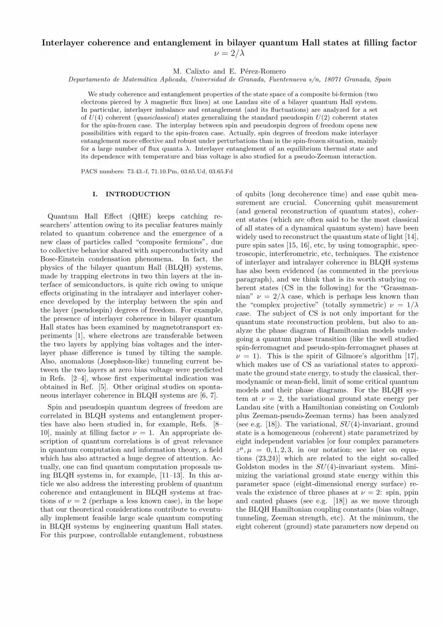
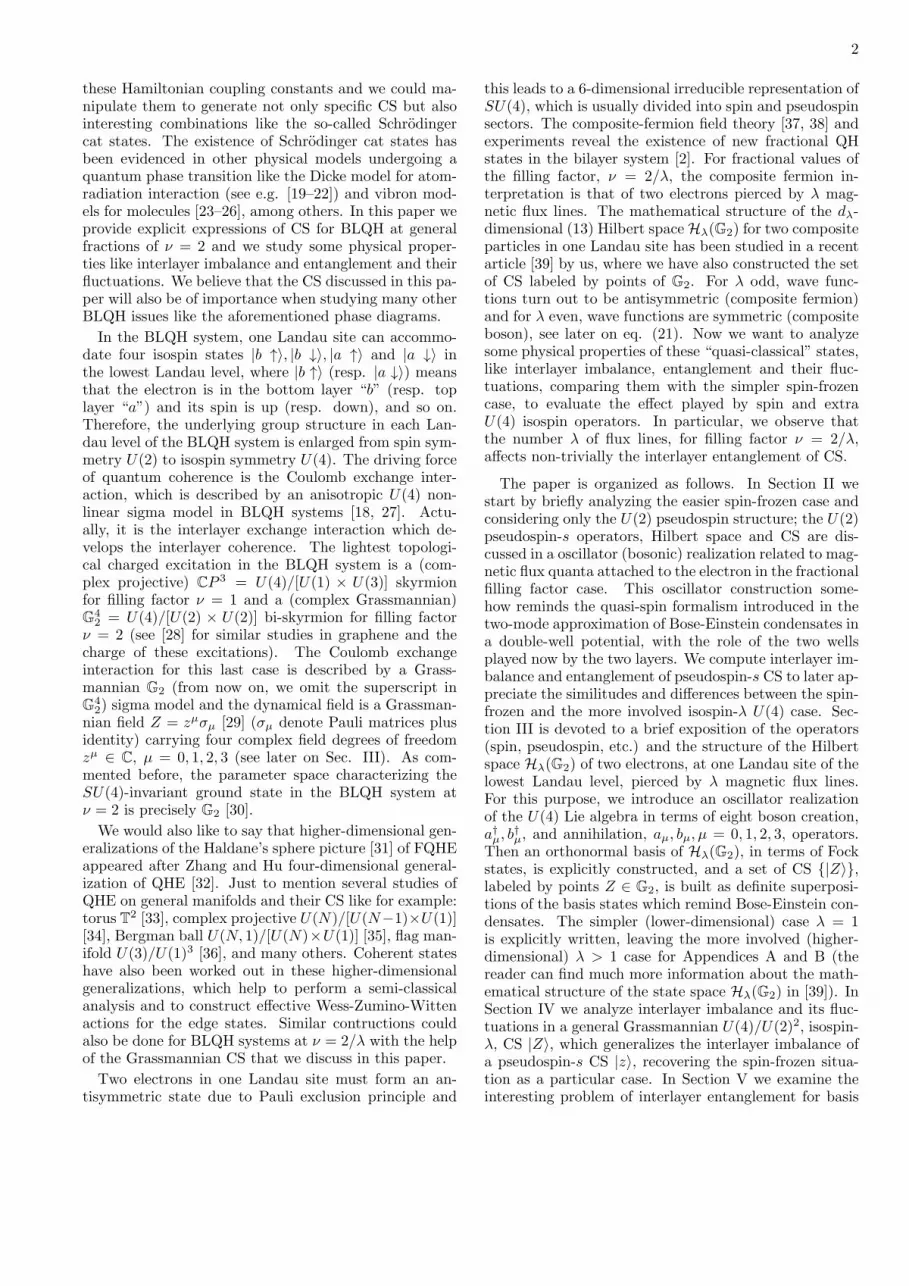
Figure 7 represents the CS purity Pλ and its standarddeviation ∆Pλ for λ = 1 as a function of r±. Purity isminimum at r± = 1 (maximum interlayer entanglement).One can also see that there is no interlayer entanglement(purity Pλ = 1) for r± = 0 (which means all flux quantain layer b) and when r± → ∞ (which means all fluxquanta in layer a), except when r+ · r− = 0, for whichpurity tends to Pλ = 1/(λ + 1) when r± → ∞. Thereare other two particular trajectories in the r± plane forwhich there is always interlayer entanglement. To betterappreciate this fact, we also represent in Figure 8 thepurity and its standard deviation for λ = 1 as a function

of r =√

r2+ + r2− and θ = arctan(r−/r+). For r > 1.55

and λ = 1 the purity Pλ displays two local minima (forfixed r) at two values of the polar angle θ±r given by

cos θ±r =

√3r2 + 2r4 ∓

√−36− 36r2 − 11r4 + 4r6 + 4r8

6r2 + 4r4.

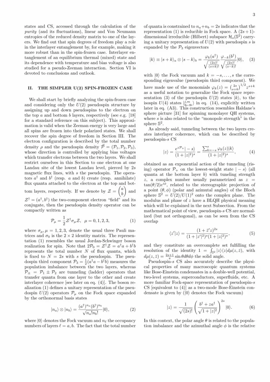
(44)The expression θ±(r) = θ±r gives two singular trajectoriesin the (r, θ) plane for which the CS |Z⟩ remains always en-tangled. In fact, purity tends to P1 = 1/3 when r → ∞on these two trajectories. Both local minima are nar-rower and narrower, with θ−r → 0 and θ+r → π/2 whenr → ∞. Purity fluctuations ∆Pλ are also high aroundthese two trajectories, as can be appreciated in Figure 8(bottom panel). See Figure 9 for a plot of three sections,r = 2, r = 4 and r = 8, of P1 as a function of θ. Thesituation here is similar to the one depicted in Figure 6for the imbalance standard deviation.

FIG. 7: Purity Pλ = tr(ϱ2b), and standard deviation ∆Pλ, ofthe reduced density matrix ϱb = tra(ϱ) to layer b, for the CSdensity matrix ϱ = |Z⟩⟨Z|, as a function of the CS parametersr± for λ = 1.

Let us also examine the particular (diagonal) case r+ =r− = r0, for which purity simplifies to

Pλ(r0) =

∑2λn=0

( λn+odd[n]

2

)( λn−odd[n]

2

)r4n0

(1 + r20)4λ

. (45)

In Figure 10 we represent purity Pλ and its fluctuations∆Pλ as a function of r0 for different values of λ. Wesee that purity Pλ of a CS |Z⟩ is minimum (maximuminterlayer entanglement) at r0 = 1 for all values of λ(the vertical grid line indicates this particular value of r0for which maximum interlayer entanglement is attained).Actually, as already noticed in eq. (43), purity is invari-ant under inversion Pλ(r0) = Pλ(1/r0), with r0 = 1 afixed point. However, the CS |Z⟩ is never maximally en-tangled since Pλ(1) is always greater than 1/dλ (purityof a completely mixed state). In particular, for λ = 1we have P1(1) = 3/16 (see Figure 10), which is slightlygreater than 1/d1 = 1/6. Purity fluctuations also dis-play a local minimum at r0 = 1 (see Figure 10), whichbecomes flatter and flatter as λ increases. We also appre-ciate that interlayer entanglement of |Z⟩ attains its max-

12

FIG. 8: Purity Pλ = tr(ϱ2b), and standard deviation ∆Pλ, ofthe reduced density matrix ϱb = tra(ϱ) to layer b, for the CSdensity matrix ϱ = |Z⟩⟨Z|, as a function of the CS parameters

r =√

r2+ + r2−, θ = arctan(r−/r+) for λ = 1.

0 Θ8-Θ4-

Θ2-

Θ2+

Θ4+Θ8+Π

4Π

2

Θ

12

13

1PΛ

FIG. 9: (Color online) Purity Pλ, for λ = 1, as a function ofthe polar angle θ = arctan(r−/r+) for r = 2 (solid line) r = 4(dotted blue) and r = 8 (dashed red). The points θ±r denotelocal minima of Pλ for each value of r and are marked withvertical grid lines. Horizontal grid lines denote limit r → ∞values: Pλ → 1 for θ = θ±r , 0, π/2; Pλ → 1/2 for θ = 0, π/2;Pλ → 1/3 for θ = θ±r .

1 3 5r0

3�16

1PΛ

1 3 5r0

116

DPΛ

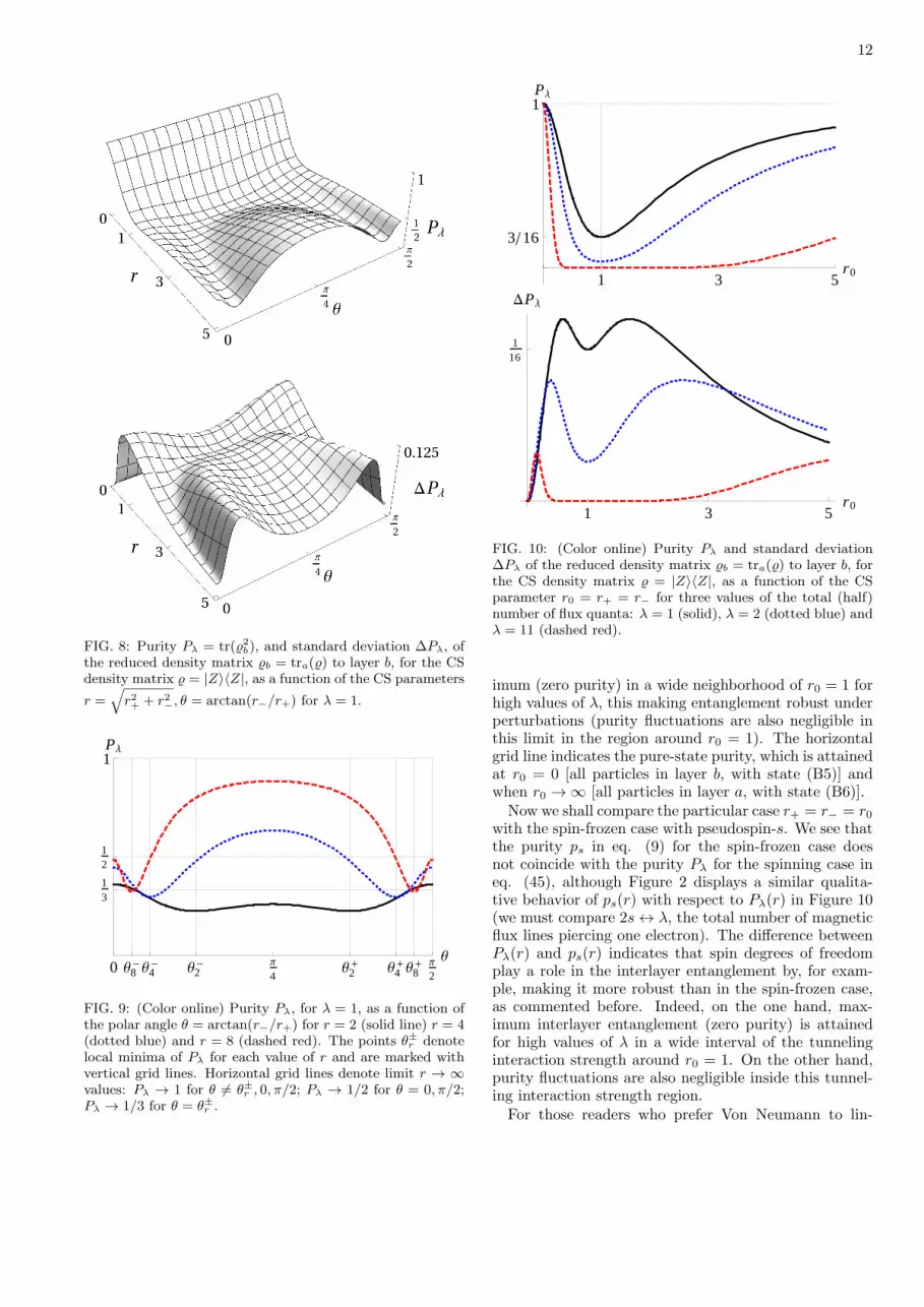
FIG. 10: (Color online) Purity Pλ and standard deviation∆Pλ of the reduced density matrix ϱb = tra(ϱ) to layer b, forthe CS density matrix ϱ = |Z⟩⟨Z|, as a function of the CSparameter r0 = r+ = r− for three values of the total (half)number of flux quanta: λ = 1 (solid), λ = 2 (dotted blue) andλ = 11 (dashed red).

imum (zero purity) in a wide neighborhood of r0 = 1 forhigh values of λ, this making entanglement robust underperturbations (purity fluctuations are also negligible inthis limit in the region around r0 = 1). The horizontalgrid line indicates the pure-state purity, which is attainedat r0 = 0 [all particles in layer b, with state (B5)] andwhen r0 → ∞ [all particles in layer a, with state (B6)].

Now we shall compare the particular case r+ = r− = r0with the spin-frozen case with pseudospin-s. We see thatthe purity ps in eq. (9) for the spin-frozen case doesnot coincide with the purity Pλ for the spinning case ineq. (45), although Figure 2 displays a similar qualita-tive behavior of ps(r) with respect to Pλ(r) in Figure 10(we must compare 2s ↔ λ, the total number of magneticflux lines piercing one electron). The difference betweenPλ(r) and ps(r) indicates that spin degrees of freedomplay a role in the interlayer entanglement by, for exam-ple, making it more robust than in the spin-frozen case,as commented before. Indeed, on the one hand, max-imum interlayer entanglement (zero purity) is attainedfor high values of λ in a wide interval of the tunnelinginteraction strength around r0 = 1. On the other hand,purity fluctuations are also negligible inside this tunnel-ing interaction strength region.

For those readers who prefer Von Neumann to lin-

13

FIG. 11: Linear Lλ = 1−Pλ and Von Neumann Sλ entangle-ment entropies of the reduced density matrix ϱb = tra(ϱ) tolayer b, for the CS density matrix ϱ = |Z⟩⟨Z|, as a functionof the CS parameters r± for λ = 1.

ear entanglement entropy, it is also possible to computeSλ(r+, r−) = −tr(ϱb log ϱb) for ϱb in (36). Taking intoaccount that ϱb is block-diagonal and after a little bit ofalgebra, we arrive to the following expression for

Sλ(r+, r−) = −λ∑

m=0

(λ−m)/2∑j=0; 12

j∑q=−j

(2j + 1) (46)

×γmj,q(r+, r−) log γ

mj,q(r+, r−),

with

γmj,q(r+, r−) =

(λ+1

λ−2j−m

)(λ+1

λ−m+1

)λ+ 1

r2(j+m+q)+ r

2(j+m−q)−

(1 + r2+)λ(1 + r2−)

λ.

In Figure 11 we perceive a similar qualitative behaviorof linear Lλ = 1 − Pλ and Von Neumann Sλ entropiesfor λ = 1. For general λ the situation is similar, withLλ a lower approximation of Sλ. In Figure 12 we plotLλ and Sλ as a function of r0 ≡ r+ = r−. We see thatSλ ≥ Lλ and that the maximum linear Lmax.

λ = 1− 1/dλand Von Neumann Smax.

λ = log(dλ) entropies are never

0 1 2 3r0

13� 16123� 128

logH 32L� 2

logH16LLΛ ,SΛ

FIG. 12: (Color online) Linear Lλ (solid line) and Von Neu-mann Sλ (dotted line) entanglement entropies of the reduceddensity matrix ϱb = tra(ϱ) to layer b, for the CS den-sity matrix ϱ = |Z⟩⟨Z|, as a function of the CS parameterr0 ≡ r+ = r− for two values of: λ = 1 (black) and λ = 2(red).

attained, although |Z⟩ is almost maximally entangled forr0 = 1, where L1(1) = 13/16 ≲ Lmax.

1 = 5/6 and S1(1) =

log(√32) ≲ Smax.

1 = log(6) (see maximum values for λ =1 and λ = 2 in Figure 12).

C. Interlayer entanglement of a thermal state

In the two previous cases we have studied the inter-layer entanglement of pure bipartite states. In this Sec-tion we tackle the study of a mixed state like the equilib-rium state in BLQH system at finite temperature. Otherstudies about entanglement spectrum and entanglementthermodynamics of BLQH systems at ν = 1 can be foundin [9].

For the sake of simplicity, we shall consider the pseudo-Zeeman Hamiltonian given by H = ε(P3 + λ), where εis the bias voltage parameter (it introduces an energyscale into the system) and we have added a zero-pointenergy ελ for convenience. The basis states |j,mqa,qb

⟩ areHamiltonian eigenvectors with eigenenergies En = εn,with n = 2j + 2m. The degeneracy Dn of the energylevel En depends on n = 2j + 2m in the form:

Dn =

{(n+1)(n+2)(n+3)

6 , n ≤ λ,(2λ−n+1)(2λ−n+2)(2λ−n+3)

6 , λ ≤ n ≤ 2λ.(47)

Formula (34) can be alternatively written as∑2λ

n=0 Dn =dλ in terms of the degeneracy Dn. The normalizeddensity matrix is written in compact form as ρλ(β) =e−βH/tr(e−βH), with β = 1/(kBT ) (kB denotes theBoltzmann constant and T the temperature), as usual.The canonical partition function is easily calculated and

14

gives

Qλ(β) =2λ∑n=0

Dne−βEn (48)

=1 + e−βε(2λ+4) + 2(λ+ 1)(λ+ 3)e−βε(λ+2)

(1− e−βε)4

−(2 + λ)2e−βε(λ+1) + e−βε(λ+3)

(1− e−βε)4.

One can check that at high temperatureslimβ→0 Qλ(β) = dλ (the dimension of the Hilbert space).The mean energy can be calculated either directly as

Eλ(β) =∑2λ

n=0 Dnγn(β)En, with γn(β) = e−βEn/Qλ(β)the Boltzmann factor, or through the well known formulaEλ(β) = −∂ log(Qλ(β))/∂β. In particular, we see thatthe mean energy at high temperatures is Eλ(0) = λε,and at zero temperature is Eλ(∞) = 0. In Figure 13(top panel) we plot the mean energy as a function ofthe temperature T = 1/(kBβ) in ε = 1 unities. It isalso interesting to see the representation of the meanenergy Eλ as a function of the bias voltage ε in Figure14 (top panel), where one can observe a similarity withthe energy of a black body as a function of the frequencyω; In fact, the spectrum is peaked at a characteristicbias voltage εc (resp. frequency ωc) that shifts to highervoltages (resp. frequencies) with increasing temperature;this reminds the Wien’s displacement law βε = c(λ),with c(λ) a “Wien’s displacement constant” dependingon λ. Note that here we have an extra parameter λ toplay with.The entropy Sλ(β) = −tr[ρλ(β) log ρλ(β)] can be cal-

culated either directly as the formula

Sλ(β) = −2λ∑n=0

Dnγn(β) log γn(β), (49)

or through the general formula

Sλ(β) = βEλ(β) + logQλ(β). (50)

The reduced density matrix to layer b, ρbλ = tra(ρλ), is

ρbλ =λ∑

m=0

(λ−m)/2∑j=0; 12

j∑q,qb=−j

γn(β)|vj,λ−2j−mq,qb

⟩b⟨vj,λ−2j−mq,qb

|,

(51)(n = 2j + 2m) whose purity is easily calculated in termsof the partition function as

Pλ(β) =2λ∑n=0

Dnγn(β)2 =

Qλ(2β)

Qλ(β)2. (52)

In Figure 13, middle panel, we represent the linear en-tropy Lλ = 1 − Pλ as a function of the temperature forthree values of λ. We see that Lλ is zero at zero temper-ature and Lλ → 1 − 1/dλ at high temperatures, wherethe state is maximally entangled. In the same way, we

5 10T0

1

2

3EΛ

1 2T

5� 6

1

LΛ

1 2T

logH 6L

logH 20L

logH 50LSΛ

FIG. 13: Mean energy Eλ, linear Lλ and Von Neumann Sλ

entanglement entropy of a thermal equilibrium state ρλ asa function of the temperature T for λ = 1 (black), λ = 2(dashed red) and λ = 3 (dotted blue). We are taking ε, kB = 1unities.

can compute the Von Neumann entanglement entropySbλ = −tr[ρbλ log ρ

bλ] which, after a little bit of algebra,

we arrive to the conclusion that Sbλ(β) = Sa

λ(β) = Sλ(β);that is, the entropy restricted to any of the layers coin-cides with the total bilayer entropy. In particular, thesubadditivity condition Sλ ≤ Sa

λ + Sbλ = 2Sλ is fulfilled.

In Figure 13 (bottom panel) we plot the entropy Sλ asa function of T for three values of λ. We see that Sλ

is zero at zero temperature and Sλ → log(dλ) at hightemperatures, where the state is maximally entangled,in accordance with the results of the linear entropy Lλ

(which is a lower bound of Sλ). We also represent Sλ

15

2 4 6 8 10 12 14Ε0

1

2

3

4EΛ

5 10Ε

logH 6L

logH 20LSΛ

FIG. 14: Mean energy Eλ and Von Neumann entropy Sλ of athermal equilibrium state ρλ as a function of the bias voltage εfor λ = 1 (solid) and λ = 2 (dotted) and several temperatures:T = 1 (black), T = 2 (red) and T = 3 (blue). We are takingkB = 1 unities.

as a function of the bias voltage ϵ in Figure 14 (bottompanel). We see that Sλ = log(dλ) (maximal) at zero biasvoltage ε = 0 and goes to zero for high ε. Entropy Sλ

grows with λ and T for fixed ϵ.

VI. CONCLUSIONS AND OUTLOOK

We have studied interlayer imbalance and entangle-ment (and its fluctuations) of basis states |j,mqa,qb

⟩, co-herent states |Z⟩, and mixed thermal states ρλ in thestate space (at one Landau site) of the BLQH systemat filling factor ν = 2/λ. Isospin-λ CS are labeled by2 × 2 complex matrices Z in the 8-dimensional Grass-mannian manifold G2 = U(4)/U(2)2 and generalize thestandard pseudospin-s CS |z⟩ labeled by complex pointsz ∈ S2 = U(2)/U(1)2 (the Riemann-Bloch sphere). Theinterplay between spin and pseudospin (layer) degrees offreedom introduces novel physics with regard to the spin-frozen case, by making interlayer entanglement more ro-bust for a wide range of coherent state parameters (spe-cially for high values of the number λ of magnetic fluxlines). Von Neumann entanglement entropy of mixedthermal states is maximal at high temperatures and zerobias voltage (when we consider a pseudo-Zeeman Hamil-

tonian).Other bipartite entangled BLQH systems (namely,

spin-pseudospin [10] or electron-electron) might also beconsidered which could also be of interest in quantuminformation theory. We must say that entangled (usu-ally oscillator and spin) coherent states are importantto quantum superselection principles, quantum informa-tion processing and quantum optics, where they havebeen produced in a conditional propagating-wave real-ization (see e.g. [46] for a recent review on the subject).Coherent (quasi-classical) states are easily generated formany interesting physical systems, and we believe thatBLQH CS |Z⟩ at ν = 2/λ will not be exception andthat they will play an important role, not only in theo-retical considerations but, also in experimental settings.Another interesting possibility is to study entanglementbetween two different spatial regions. Before, we shouldextend the present study to several Landau sites. In thiscase, the Coulomb exchange Hamiltonian, which is de-scribed by an anisotropic U(4) nonlinear sigma modelin BLQH systems, provides the necessary interaction tocreate quantum correlations between spatial regions.

Other U(4) operator mean values ⟨Z|Tµν |Z⟩ (and theirpowers) can also be calculated, which could be speciallysuitable to analyze the classical (thermodynamical ormean-field limit) and phase diagrams of BLQH Hamil-tonian models undergoing a quantum phase transition,like the well studied spin-ferromagnet and pseudo-spin-ferromagnet phases at ν = 1, or the spin, ppin and cantedphases at ν = 2. Actually, coherent states for other sym-metry groups [viz, Heisenberg, U(2) and U(3)] alreadyprovided essential information about the quantum phasetransition occurring in several interesting models like forexample: the Dicke model for atom-field ineractions [19–22]), vibron models for molecules [23, 24], and also pair-ing models like the Lipkin-Meshkov-Glick model for nu-clei [49, 50]. For vibron models, U(3) coherent stateshave been used as variational states capturing rovibra-tional entanglement of the ground state in shape phasetransitions of molecular benders [25, 26]. We also believethat the proposed Grassmannian coherent states |Z⟩ canprovide valuable physical information about the groundstate and phase diagram in the semi-classical limit ofBLQH systems at ν = 2/λ. This is work in progress.

To conclude, we would like to mention that graphenephysics shares similarities with BLQH systems, wherethe two valleys (or Dirac points) play a role similar tothe layer degree of freedom. Other Grassmannian cosetsU(N)/[U(M) × U(N − M)] appear in this context (seee.g. [28]) and we believe that a boson realization like theone discussed here can contribute something interestingalso in this field.

Acknowledgements

Work partially supported by the Spanish MINECO,Junta de Andalucıa and University of Granada un-

16

der projects FIS2011-29813-C02-01, FQM1861 and [CEI-BioTIC-PV8 and PP2012-PI04], respectively.

Appendix A: Orthonormal basis for arbitrary λ

In Ref. [39] we have generalized, in a natural way, theFock space realization of pseudospin-s basis states (3) toa Fock space representation of the basis functions |j,mqa,qb

⟩of Hλ(G2). We have found a U(4) generalization of theU(2) monomials φk(z) in eq. (3) and (4) in terms of aset of homogeneous polynomials of degree 2j + 2m

φj,mqa,qb

(Z) =

√2j + 1

λ+ 1

(λ+ 1

2j +m+ 1

)(λ+ 1

m

)(A1)

× det(Z)mDjqa,qb

(Z),2j +m ≤ λ,

qa, qb = −j, . . . , j,

in four complex variables zµ = tr(Zσµ)/2, µ = 0, 1, 2, 3,where

Djqa,qb

(Z) =

√(j + qa)!(j − qa)!

(j + qb)!(j − qb)!

min(j+qa,j+qb)∑k=max(0,qa+qb)

(A2)

(j + qbk

)(j − qb

k − qa − qb

)zk11z

j+qa−k12 zj+qb−k

21 zk−qa−qb22 ,

denotes the usual Wigner D-matrix [51] for a general 2×2complex matrix Z with entries zjk and angular momen-tum j. The set (A1) verifies the closure relation

λ∑m=0

(λ−m)/2∑j=0; 12

j∑qa,qb=−j

φj,mqa,qb(Z

′)φj,mqa,qb

(Z) = det(σ0 + Z ′†Z)λ

which is the U(4) version of the more familiar U(2) clo-

sure relation∑s

k=−s φk(z′)φk(z) = (1+ z′z)2s leading tothe pseudospin-s CS overlap (5).With this information, and treating φj,m

qa,qbas polyno-

mial creation and annihilation operator functions [likethe monomials φk in (3)], we have found in Ref. [39]that the set of orthonormal basis vectors (14) can be ob-tained in terms of Fock states (12) as

|j,mqa,qb⟩ =

1√2j + 1

j∑q=−j

(−1)qa−q (A3)

×φj,m−q,−qa(a

†)√λ!(λ+1)!

(λ−2j−m)!(λ+1−m)!

φj,λ−2j−mq,qb

(b†)√λ!(λ+1)!

m!(2j+m+1)!

|0⟩.

This is the U(4) version of eq. (3) for the pseudospin-sbasis states |k⟩ of U(2), with the role of s played now byλ. However, as we proof in Subsect. VA, whereas thestate |k⟩ is a direct product and does not entangle layersa and b, the state |j,mqa,qb

⟩ does entangle both layers forangular momentum j = 0. This is better seen when we

define the set of (Schmidt) states for layer a (idem forlayer b)

|vj,mq,q′ ⟩a =φj,mq,q′(a

†)√λ!(λ+1)!

(λ−2j−m)!(λ+1−m)!

|0⟩, (A4)

and realize that it constitutes an orthonormal set for thislayer, that is

⟨vj,mp,q |vj′,m′

p′,q′ ⟩a = δj,j′δm,m′δp,p′δq,q′ . (A5)

With this notation, the expression (A3) becomes (31).Concerning the quantum statistics of our states for a

given number λ of flux lines, we have already mentionedin eq. (21) that the basis states |j,mqa,qb

⟩ are antisymmetric(fermionic character) under the interchange of the twoelectrons for λ odd, and they are symmetric (bosoniccharacter) for λ even. Indeed, under the interchangeof columns in (20) the operator functions (A1) verify

φj,mqa,qb

(a†) = (−1)mφj,m−qa,qb

(a†). Taking into account that

(−1)2q = (−1)2j for any q = −j, . . . , j and doing somealgebraic manipulations, one arrives to the identity (21),where the left-hand side vector is constructed as in (A3)

but replacing a† and b† by a† and b†, respectively, thatis, switching both electrons.

Appendix B: Coherent states for arbitrary λ

The extension of the formula (23) (for λ = 1) toarbitrary λ has been worked out in Ref. [39]. Herewe reproduce it for the sake of self-containedness. CS|Z⟩ are labeled by a 2 × 2 complex matrix Z = zµσµ

(sum on µ = 0, 1, 2, 3), with four complex coordinateszµ = tr(Zσµ)/2, and can be expanded in terms of theorthonormal basis vectors (A3) as

|Z⟩ =

∑λm=0

∑(λ−m)/2

j=0; 12

∑jqa,qb=−j φ

j,mqa,qb

(Z)|j,mqa,qb⟩

det(σ0 + Z†Z)λ/2,

(B1)with coefficients φj,m

qa,qb(Z) in (A1). Denoting by a =

12η

µνtr(σµa)σν and b = 12η

µνtr(σµb)σν [we are usingEinstein summation convention with Minkowskian met-ric ηµν = diag(1,−1,−1,−1)] the “parity reversed” 2×2-matrix annihilation operators of a and b, the CS |Z⟩ in(B1) can also be written in the form of a boson conden-sate as

|Z⟩ = 1

λ!√λ+ 1

(det(b† + Zta†)√det(σ0 + Z†Z)

)λ

|0⟩, (B2)

with |0⟩ the Fock vacuum. All CS |Z⟩, with Z ∈ G2,are normalized, ⟨Z|Z⟩ = 1, but they do not constitutean orthogonal set since they have a non-zero (in general)overlap given by

⟨Z ′|Z⟩ = det(σ0 + Z ′†Z)λ

det(σ0 + Z ′†Z ′)λ/2 det(σ0 + Z†Z)λ/2(B3)

17

However, using orthogonality properties of the homoge-neous polynomials φj,m

qa,qb(Z), it is direct to prove that CS

(B1) fulfill the resolution of unity

1 =

∫G2

|Z⟩⟨Z|dµ(Z,Z†), (B4)

with dµ(Z,Z†) = 12dλ

π4

∏3µ=0 dℜ(zµ)dℑ(zµ)

det(σ0+Z†Z)4the integration

measure [this is the U(4) generalization of the U(2) inte-gration measure on the sphere given after eq. (5)]. It isinteresting to compare the U(4)/U(2)2 CS in eqs. (B1)and (B2) with the U(2)/U(1)2 CS in eqs. (4) and (6),with CS overlaps (B3) and (5), respectively. We per-ceive a similar structure between G2 = U(4)/U(2)2 andS2 = U(2)/U(1)2 CS, although the Grassmannian G2

case is more involved and constitutes a kind of “matrixZ generalization of the scalar z”.For Z = 0 we recover the lowest-weight state

|Z0⟩ = |j=0,m=0qa=0,qb=0⟩ =

det(b†)λ

λ!√λ+ 1

|0⟩, (B5)

with all 2λ flux quanta occupying the bottom layer b. For

Z → ∞ we recover the highest-weight state

|Z∞⟩ = |j=0,m=λqa=0,qb=0⟩ =

det(a†)λ

λ!√λ+ 1

|0⟩, (B6)

with all 2λ flux quanta occupying the top layer a.

To finish, let us provide yet another expression of theCS |Z⟩ in (B1), now as an exponential of interlayer ladderoperators T±µ = (T1µ ± iT2µ)/2 [remember their general

definition (11)]. Let us denote by T+ ≡ T+µσµ = 2a†b.

The CS |Z⟩ in (B1) and (B2) can also be written asthe exponential action of the rising operators T+µ on the

lowest-weight state |j=0,m=0qa=0,qb=0⟩ as

|Z⟩ = e12 tr(Z

tT+)

det(σ0 + Z†Z)λ/2|0,00,0⟩. (B7)

This is the U(4) version of the more familiar U(2) (spinfrozen) expression in eq. (4). In fact, for µ = 0 we havethat T+0 = (T10 + iT20)/2 = P1 + iP2 = P+, accordingto the usual notation in the literature [18] introduced inparagraph between equations (11) and (12).

[1] A. Sawada et al., Phys. Rev. B 59, 14888 (1999)[2] Z. F. Ezawa and A. Iwazaki, Int. J. Mod. Phys. B 6, 3205

(1992); Phys. Rev. B 47, 7295 (1993); 48, 15189 (1993).[3] X. G. Wen and A. Zee, Phys. Rev. Lett. 69, 1811 (1992);

Phys. Rev. B 47, 2265 (1993).[4] J. P. Eisenstein and A. H. MacDonald, Nature (London)

432, 691 (2004).[5] I. B. Spielman, J. P. Eisenstein, L. N. Pfeiffer, and K. W.

West, Phys. Rev. Lett. 84, 5808 (2000).[6] K. Moon el al., Phys. Rev. B 51, 5138 (1995).[7] K. Yang et al., Phys. Rev. B 54, 11644 (1996).[8] B. Doucot, M. O. Goerbig, P. Lederer, R. Moessner,

Phys. Rev. B 78, 195327 (2008)[9] J. Schliemann, Phys. Rev. B 83, 115322 (2011)

[10] Y. Hama, G. Tsitsishvili, and Z. F. Ezawa, Phys. Rev. B87, 104516 (2013)

[11] V. W. Scarola, K. Park, S. Das Sarma, Phys. Rev. Lett.91, 167903 (2003)

[12] S.R.Eric Yang, J. Schliemann, and A. H. MacDonald,Phys. Rev. B 66, 153302 (2002).

[13] K. Park, V.W. Scarola, and S. Das Sarma, Phys. Rev.Lett. 91, 026804 (2003).

[14] U. Leonhardt, Measuring the Quantum State of Light,Cambridge University Press (1997).

[15] J.-P. Amiet and S. Weigert, J. Opt. B: Quantum Semi-class. Opt. 1, L5-L8 (1999).

[16] C. Brif and A. Mann, J. Opt. B: Quantum Semiclass.Opt. 2, 245-251 (2000).

[17] R. Gilmore, J. Math. Phys. 20, 891-893 (1979).[18] Z. F. Ezawa, Quantum Hall Effects: Field Theoretical

Approach and Related Topics (2nd Edition), World Sci-entific 2008

[19] O. Castanos, E. Nahmad-Achar, R. Lopez-Pena, and J.G. Hirsch, Phys. Rev. A, 84 013819 (2011).

[20] E. Romera, M. Calixto and A. Nagy, Europhys. Lett. 97,20011 (2012).

[21] M. Calixto, A. Nagy, I. Paraleda and E. Romera, Phys.Rev. A. 85, 053813 (2012).

[22] E. Romera, R. del Real, M. Calixto, Phys. Rev. A 85,053831, (2012).

[23] F. Perez-Bernal, F. Iachello, Phys. Rev. A 77, 032115(2008).

[24] M. Calixto, R. del Real, E. Romera, Phys. Rev. A 86,032508 (2012).

[25] M. Calixto, E. Romera and R. del Real, J. Phys. A: Math.Theor. 45, 365301 (2012)

[26] M. Calixto and F. Perez-Bernal, Phys. Rev. A 89, 032126(2014).

[27] Z. F. Ezawa and K. Hasebe, Phys. Rev. B 65, 075311(2002)

[28] K. Yang, S. Das Sarma and A.H. MacDonald, Phys. Rev.B 74, 075423 (2006)

[29] K. Hasebe and Z. F. Ezawa, Phys. Rev. B 66, 155318(2002)

[30] Z. F. Ezawa, M. Eliashvili and G. Tsitsishvili, Phys. Rev.B 71, 125318 (2005).

[31] F.D.M. Haldane, Phys. Rev. Lett. 51 (1983) 605-608[32] S.C. Zhang, J.P. Hu, Science 294, 823 (2001)[33] V. Aldaya, M. Calixto and J. Guerrero, Commun. Math.

Phys. 178, 399-424 (1996)[34] D. Karabali and V.P. Nair, Nucl. Phys. B 641, 533 (2002)[35] A. Jellal, Nucl.Phys. B 725 554-576 (2005)[36] M. Daoud and A. Jellal, Int. J. Mod. Phys. A 23, 3129-

3154 (2008)[37] J.K. Jain, Phys. Rev. Lett. 63, 199-202 (1989)[38] J.K. Jain, Composite fermions, Cambridge University

Press, New York, 2007.[39] M. Calixto and E. Perez-Romero, J. Phys. A: Math.

18

Theor. 47, 115302 (2014).[40] Y. Shin, M. Saba, T.A. Pasquini, W. Ketterle, D.E.

Pritchard and A.E. Leanhard, Phys. Rev. Lett. 92,050405 (2004).

[41] M. Albeitz, R. Gati, J. Folling, S. Hunsmann, M. Cris-tiani, and M.K. Oberthaler, Phys. Rev. Lett. 95, 010402(2005).

[42] M. Saba, T.A. Pasquini, C. Sanner, Y. Shin, W. Ketterle,and D.E. Pritchard, Science 307, 1945 (2005)

[43] J. P. Eisenstein, Solid State Communications 127, 123(2003).

[44] C. Perez-Campos, J.R. Gonzalez-Alonso, O. Castanos,R. Lopez-Pena, Annals of Physics 325, 325-344 (2010)

[45] X. Wang, B. C. Sanders and Shao-hua Pan, J. Phys. A:Math. Gen. 33, 7451-7467 (2000)

[46] B. C. Sanders, J. Phys. A: Math. Theor. 45, 244002

(2012)[47] J. Schliemann, Phys. Rev. A 72, 012307 (2005).[48] J. Schliemann, J. I. Cirac, M. Kus, M. Lewenstein, and

D. Loss, Phys. Rev. A 64, 022303 (2001).[49] E. Romera, M. Calixto and O. Castanos, Phase-space

analysis of first, second and third-order quantum phasetransitions in the LMG model, Physica Scripta 89,095103 (2014)

[50] M. Calixto, O. Castanos and E. Romera, Searchingfor pairing energies in phase space, Europhysics Letters(2014), accepted, arXiv:1403.6495v1.

[51] L.C. Biedenharn, J.D. Louck, Angular Momentum inQuantum Physics, Addison-Wesley, Reading, MA, 1981;L.C. Biedenharn, J.D. Louck, The Racah-Wigner Alge-bra in Quantum Theory, Addison-Wesley, New York, MA1981