interference-aware routing in wireless multihop networks
TRANSCRIPT

DISS. ETH NO. 17737
INTERFERENCE-AWARE ROUTING IN
WIRELESS MULTIHOP NETWORKS
A dissertation submitted to
ETH ZURICH
for the degree of
Doctor of Sciences
presented by
Georgios Parissidis
M.Eng. TUC Greece, DEA Universite Paris VI
date of birth
January 13, 1977
citizen of
Greece
accepted on the recommendation of
Prof. Dr. Bernhard Plattner, examiner
Prof. Dr. Gunnar Karlsson, co-examiner
Prof. Dr. Peter Steenkiste, co-examiner
2008


Abstract
Nowadays, wireless multihop networks, providing mesh connec-tivity emerge as alternative network infrastructure for numer-ous applications such as shared broadband Internet access, mon-itoring for emergency, medical and security reasons, distributedbackup and multimedia applications. Since these networks arehighly decentralized and self-organized, routing becomes a criti-cal factor for their performance and efficiency.
The work in this thesis focuses on interference-aware rout-ing. Interference is an inherent property of wireless networks de-termining boundaries for spectrum reuse and directly affectingthe network capacity as well as protocol performance. Estimat-ing interference in a wireless network and circumventing its ef-fects is not a trivial task. The amount of interference dependson many factors including the radio propagation environment,spatial node distribution, MAC protocol dynamics. Therefore,adding interference-awareness to the routing protocol decisionsis challenging.
The first contribution of this thesis is a quantitative compari-son of multipath routing protocols proposed for wireless multihopnetworks. Multipath routing represents a promising alternative tosingle-path routing in that it enables load balancing and resilienceto route failures. We show that multipath routing outperformssingle-path in networks with high node density and network loadand the use of two, maximum three, paths represents the best

iv Abstract
tradeoff between routing overhead and performance. Neverthe-less, the requirement for efficient data scheduling remains equallyimportant for both multipath and single-path routing protocols.
The role of interference in that is critical. Therefore, much ofour work addresses interference modeling. We derive an analyti-cal model for the probability that a transmission destined to anarbitrary network node is successful in the presence of interfer-ence from other nodes in the network. Our analytical expressionfor the data loss probability is a function of the network density,node transmission probability, radio propagation environment,and network card hardware. We validate our interference modelagainst experiments in a real testbed, set up for this purpose inour indoor office environment, showing good match of the exper-imental results with the analytical predictions.
Our work concludes with the design of an interference-awarerouting metric that explicitly takes interference into account viaour analytical derivation. Contrary to measurement-based mod-els, our derivation only requires information that is locally avail-able to the nodes, avoiding all measurement-related pitfalls. Weshow that its performance compares favorably with those achievedby the state-of-the-art probe-based routing metric.

Kurzfassung
Vermaschte drahtlose Multihop-Netzwerke sind heute als alterna-tive Netzwerk-Strukturen im Aufkommen und finden Einsatz aufGebieten wie dem gemeinsamen Zugang zu Breitband-Internet,Uberwachung medizinischer und sicherheitstechnischer Notfalle,verteiltes Backup und Multimedia-Anwendungen. Da solche Net-zwerke weitgehend dezentralisiert sind und sich selbst organisieren,ist das Routing ein kritischer Faktor in Bezug auf ihre Leistungs-fahigkeit und Effizienz.
Der Fokus der vorliegenden Dissertation ist das Routing unterBerucksichtigung von Interferenz. Interferenz ist eine inharenteEigenschaft drahtloser Netzwerke, die die Wiederverwendung desSpektrums einschrankt und die Kapazitat des Netzwerks als auchdie Leistungsfahigkeit des Protokolls direkt beeinflusst. Die Bes-timmung und Vermeidung von Interferenz in einem drahtlosenNetzwerk ist keine triviale Aufgabe. Der Umfang der Interferenzhangt von mehreren Faktoren wie der Funkwellenausbreitung, derraumlichen Knotenpunktverteilung und der Dynamik des MAC-Protokolls ab. Daher ist die Berucksichtigung von Interferenz ineinem Routing-Protokoll eine Herausforderung.
Der erste Beitrag dieser Arbeit ist ein quantitativer Vergleichmehrerer Multipath Routing Protokolle, die fur drahtlose Mul-tihop Netzwerke verwendet werden konnen. Multipath Routingist eine vielversprechende Alternative zu Singlepath-Routing, daes den Lastausgleich ermoglicht und die Ausfallsicherheit erhoht
vi Kurzfassung
wird. Wir zeigen, dass Multipath-Routing in Netzwerken mit ho-her Knotendichte und Belastung das Singlepath-Routing uber-trifft und der Einsatz von zwei, hochstens drei Pfaden der besteKompromiss zwischen dem Zusatzaufwand durch Routing undder Leistungsfahigkeit ist. Dennoch ist die Anforderung fur ef-fizienten Datenaustausch an Multipath und Single-path RoutingProtokolle gleich hoch.
Interferenz spielt hierbei eine kritische Rolle. Ein grosser Teilunserer Arbeit ist daher der Modellierung der Interferenz gewid-met. Wir leiten ein analytisches Modell her, das die Wahrschein-lichkeit einer erfolgreichen Sendung angibt, die fur einen zufal-ligen Netzwerkknoten bestimmt ist und unter dem Einfluss derInterferenz anderer Knoten erfolgt. Unser analytischer Ausdruckfur die Wahrscheinlichkeit von Datenverlust ist eine Funktion vonNetzdichte, Sendewahrscheinlichkeit eines Knotens, Funkwellenaus-breitung und Eigenschaften der Netzwerkkarte. Wir validierenunser Interferenz-Modell mit Messungen in einer reellen Testumge-bung, die eigens hierfur in unseren Laborraumlichkeiten aufgestelltwurde. Die Messergebnisse zeigen eine gute Ubereinstimmung mitden analytischen Voraussagen.
Diese Arbeit schliesst mit der Erstellung einer Routing-Gewichtungmit expliziter Berucksichtigung der Interferenz, wie sie analytischhergeleitet wurde. Im Gegensatz zu Modellen, die auf Messun-gen basieren, benotigt unsere Herleitung Informationen, die vonjedem Knoten lokal erhaltlich sind, und umgeht ausserdem alleNachteile, die aus Messungen resultieren. Wir zeigen, dass es leis-tungsfahiger ist als andere moderne Routing-Gewichtungen, dieauf Messungen basieren.

Table of Contents
Abstract iii
Kurzfassung v
Table of Contents vii
List of Figures xi
List of Tables xv
1 Introduction 1
1.1 Motivation . . . . . . . . . . . . . . . . . . . . . . 1
1.2 Research Questions . . . . . . . . . . . . . . . . . . 6
1.3 Contributions . . . . . . . . . . . . . . . . . . . . . 7
1.4 Outline . . . . . . . . . . . . . . . . . . . . . . . . 8
2 Related Work 11
2.1 Multipath Routing Protocols . . . . . . . . . . . . 11
2.1.1 Deployment of Multipath Routing . . . . . 13
2.2 Interference in Wireless Networks . . . . . . . . . . 15
2.3 Metrics for Routing Protocols . . . . . . . . . . . . 17
2.3.1 Optimization objectives . . . . . . . . . . . 17
2.3.2 Link and path metrics . . . . . . . . . . . . 19

viii Table of Contents
2.3.3 Metric computation method . . . . . . . . . 20
2.3.4 Active probing based metrics . . . . . . . . 21
2.3.5 Per-hop Round Trip Time (RTT) . . . . . . 23
2.3.6 Per-hop packet pair delay (PktPair) . . . . 23
2.3.7 Expected Transmission Count (ETX) . . . 24
2.3.8 Extensions of the ETX metric . . . . . . . . 26
2.4 Summary . . . . . . . . . . . . . . . . . . . . . . . 28
3 Multipath Routing in Wireless Multihop Networks 31
3.1 A Quantitative Comparison of Multipath RoutingProtocols for Wireless Multihop Networks . . . . . 31
3.2 Multipath Routing Protocols . . . . . . . . . . . . 33
3.3 Methodology . . . . . . . . . . . . . . . . . . . . . 35
3.4 Performance Evaluation . . . . . . . . . . . . . . . 38
3.4.1 Routing Overhead . . . . . . . . . . . . . . 38
3.4.2 Average Number of Paths . . . . . . . . . . 40
3.4.3 Routing latency . . . . . . . . . . . . . . . . 41
3.4.4 Sustainability of multiple paths . . . . . . . 44
3.4.5 Data Packet Delivery Ratio . . . . . . . . . 47
3.4.6 Average End-to-End Delay of Data Packets 50
3.4.7 Load Balancing . . . . . . . . . . . . . . . . 53
3.4.8 Advantages and Limitations of MultipathRouting Protocols . . . . . . . . . . . . . . 55
3.5 Open Questions . . . . . . . . . . . . . . . . . . . . 58
3.6 Conclusion and Discussion . . . . . . . . . . . . . . 60
4 Interference in Wireless Multihop Networks 63
4.1 Introduction . . . . . . . . . . . . . . . . . . . . . . 63
4.2 Analytical model . . . . . . . . . . . . . . . . . . . 66
4.2.1 Physical model and assumptions . . . . . . 67
4.2.2 Interference (“MAC-agnostic”) Model . . . . 69

Table of Contents ix
4.2.3 Interference-cum-MAC Model . . . . . . . . 72
4.2.4 Probability of Successful Reception underUniform Node Distribution . . . . . . . . . 74
4.2.5 Model Input Parameters . . . . . . . . . . . 79
4.3 Numerical Results . . . . . . . . . . . . . . . . . . 80
4.3.1 Model sensitivity to transmission probabil-ity, γ . . . . . . . . . . . . . . . . . . . . . . 81
4.3.2 Model sensitivity to path loss exponent, α . 83
4.3.3 Model sensitivity to reception threshold, β . 83
4.3.4 Model sensitivity to the sender-receiver dis-tance scale factor, c . . . . . . . . . . . . . 84
4.4 Model validation via testbed experimentation . . . 86
4.4.1 Testbed description . . . . . . . . . . . . . 87
4.4.2 Experimentation methodology . . . . . . . 89
4.4.3 Experimentation results . . . . . . . . . . . 92
4.4.4 Impact of Packet Size . . . . . . . . . . . . 95
4.5 Conclusion and Discussion . . . . . . . . . . . . . . 97
5 Interference-aware Routing 99
5.1 Motivation . . . . . . . . . . . . . . . . . . . . . . 99
5.2 Interference-aware Routing Metric . . . . . . . . . 102
5.2.1 Overview of the DSDV protocol . . . . . . 103
5.2.2 Obtaining Model Inputs . . . . . . . . . . . 106
5.3 Routing Metric Performance Evaluation . . . . . . 108
5.3.1 Methodology . . . . . . . . . . . . . . . . . 109
5.4 Experimentation Results . . . . . . . . . . . . . . . 111
5.4.1 One Node Pair Active . . . . . . . . . . . . 112
5.4.2 Multiple Pairs Active. . . . . . . . . . . . . 121
5.5 Conclusion and Discussion . . . . . . . . . . . . . . 130

x Table of Contents
6 Conclusions and Future Work 135
6.1 Summary of Main Results . . . . . . . . . . . . . . 135
6.2 Assumptions and Weaknesses . . . . . . . . . . . . 137
6.3 Future Work . . . . . . . . . . . . . . . . . . . . . 139
A Appendix 141
A.1 Wireless Testbed . . . . . . . . . . . . . . . . . . . 141
A.1.1 Hardware, Software, Topology . . . . . . . 141
A.1.2 Link-level Measurements . . . . . . . . . . . 143
Acknowledgements 161
Curriculum Vitae 165

List of Figures
1.1 One hop vs. two hop path . . . . . . . . . . . . . . 3
2.1 ETX metric estimation for node A . . . . . . . . . 25
3.1 Routing overhead: Low density, low load . . . . . . 39
3.2 Routing overhead: High density, low load . . . . . 40
3.3 Routing overhead: Varying density, low load . . . . 41
3.4 Average number of paths: Low density, low load . 42
3.5 Average number of paths: High density, high load . 43
3.6 Routing latency: Low density, low load . . . . . . . 44
3.7 Routing latency: High density, high load . . . . . . 45
3.8 Routing latency: Varying density, high load . . . . 46
3.9 Sustainability of multiple paths: Low density, lowload . . . . . . . . . . . . . . . . . . . . . . . . . . 47
3.10 Sustainability of multiple paths: High density, highload . . . . . . . . . . . . . . . . . . . . . . . . . . 48
3.11 Sustainability of multiple paths: Varying density,low load . . . . . . . . . . . . . . . . . . . . . . . . 49
3.12 Data packet delivery ratio: Low density, low load . 50
3.13 Data packet delivery ratio: High density, high load 51
3.14 Data packet delivery ratio: Varying density, highload . . . . . . . . . . . . . . . . . . . . . . . . . . 52

xii List of Figures
3.15 Average end-to-end delay of data packets: Case 3:High mobility, high load. . . . . . . . . . . . . . . . 53
3.16 Average end-to-end delay of data packets: Moder-ate mobility, high load. . . . . . . . . . . . . . . . . 54
3.17 Average end-to-end delay of data packets: No mo-bility, high load. . . . . . . . . . . . . . . . . . . . 55
3.18 Load balancing: Low density, low load, 120 secondspause time. . . . . . . . . . . . . . . . . . . . . . . 56
3.19 Load balancing: Low density, low load. . . . . . . . 57
3.20 Load balancing: Varying density, low load, 900 sec-onds pause time. . . . . . . . . . . . . . . . . . . . 58
4.1 Interference zones A j,m with respect to recipientnode x j . . . . . . . . . . . . . . . . . . . . . . . . 71
4.2 Hidden nodes area RH in the first interference zoneA j,1 . . . . . . . . . . . . . . . . . . . . . . . . . . . 74
4.3 G(m) as a function of the number m of interferenceareas/zones for given α and β = 2.5, c = 0.3, andd(x j) = 10 . . . . . . . . . . . . . . . . . . . . . . . 77
4.4 G(m) as a function of the number m of interferenceareas/zones for given α and β = 2.5, c = 0.3, andd(x j) = 15 . . . . . . . . . . . . . . . . . . . . . . . 78
4.5 Probability of successful reception versus node de-gree (i.e., node density ρ) for variable γ, α = 4,β = 2.5, c = 0.5. . . . . . . . . . . . . . . . . . . . 81
4.6 Probability of successful reception versus node de-gree (i.e., node density ρ) for variable α, β = 2.5,γ = 0.04, c = 0.5. . . . . . . . . . . . . . . . . . . . 82
4.7 Probability of successful reception versus node de-gree (i.e., node density ρ) for variable β, α = 4,γ = 0.02, c = 0.5. . . . . . . . . . . . . . . . . . . . 84

List of Figures xiii
4.8 Probability of successful reception versus node de-gree (i.e., node density ρ) and sender receiver dis-tance c; β = 2.5, α = 3.84, γ = 0.02 . . . . . . . . . 85
4.9 Our wireless mesh network testbed. The 23 802.11a/b/gnodes are distributed in offices all over the floorcovering an area of approximately 32x79m2. . . . . 86
4.10 Signal strength Pi j [dBm] as a function of the dis-tance di j . . . . . . . . . . . . . . . . . . . . . . . . 87
4.11 Packet delivery ratio as a function of signal strength. 88
4.12 Analytical model vs. testbed experimentation re-sults for γ = 0.005 (α = 3.84,β = 2.5,c= 0.5), RMSE=0.025.92
4.13 Analytical model vs. testbed experimentation re-sults for γ = 0.02 (α = 3.84,β = 2.5,c= 0.5), RMSE=0.012. 93
4.14 Analytical model vs. testbed experimentation re-sults for γ = 0.05 (α = 3.84,β = 2.5,c= 0.5), RMSE=0.029. 94
4.15 Impact of packet size on P(x j). . . . . . . . . . . . 96
5.1 One node-pair active: Bit rate=1Mb/s, Pw=18dBm,Pkt size=128 bytes. . . . . . . . . . . . . . . . . . 113
5.2 One node-pair active: Bit rate=1 Mb/s, Pw=18dBmand Pkt size=1024 bytes. . . . . . . . . . . . . . . 115
5.3 One node-pair active: Bit rate=1 Mb/s, Pw=0dBmand Pkt size=1024 bytes. . . . . . . . . . . . . . . 117
5.4 One node-pair active: Bit rate=1 Mb/s, Pw=10dBmand Pkt size=128 bytes. . . . . . . . . . . . . . . . 118
5.5 One node-pair active: Bit rate=11 Mb/s, Pw=18dBmand Pkt size=128 bytes. . . . . . . . . . . . . . . . 120
5.6 One node-pair active: Bit rate=11 Mb/s, Pw=10dBmand Pkt size=128 bytes. . . . . . . . . . . . . . . . 122
5.7 One node pair-active: Bit rate=11 Mb/s, Pw=10dBmand Pkt size=1024 bytes. . . . . . . . . . . . . . . 123

xiv List of Figures
5.8 One node-pair active: Bit rate=11 Mb/s, Pw=18dBmand Pkt size=1024 bytes. . . . . . . . . . . . . . . 124
5.9 Multiple node-pairs active: Throughput (in pack-ets per second) of paths found by DSDV usingETX, minimum hop count and our interference-aware metric. . . . . . . . . . . . . . . . . . . . . . 126
5.10 Multiple node-pairs active: Average path lengthused by ETX, minimum hop count and our interference-aware metric. . . . . . . . . . . . . . . . . . . . . . 127
5.11 Multiple node-pairs active: Histogram of traffic load(average number of packets sent/received per sec-ond) at all nodes. . . . . . . . . . . . . . . . . . . . 129
5.12 Multiple node-pairs active: Traffic load (averageper second number of packets sent/received persecond) sorted for all nodes. . . . . . . . . . . . . . 131
A.1 Pair-wise delivery ratios at 30mW, 1Mbit/s, smallpackets . . . . . . . . . . . . . . . . . . . . . . . . 144
A.2 Pair-wise delivery ratios at 30mW, 11Mbit/s, smallpackets . . . . . . . . . . . . . . . . . . . . . . . . 144
A.3 Pair-wise delivery ratios at 30mW, 1Mbit/s, largepackets . . . . . . . . . . . . . . . . . . . . . . . . 145
A.4 Pair-wise delivery ratios at 30mW, 11Mbit/s, largepackets . . . . . . . . . . . . . . . . . . . . . . . . 145
A.5 Pair-wise delivery ratios at 1mW, 1Mbit/s, smallpackets . . . . . . . . . . . . . . . . . . . . . . . . 146
A.6 Pair-wise delivery ratios at 1mW, 1Mbit/s, largepackets . . . . . . . . . . . . . . . . . . . . . . . . 146

List of Tables
2.1 A summary of metrics . . . . . . . . . . . . . . . . 30
3.1 Comparison of multipath routing protocols.(++: very good, +: good, 0: neutral, -:poor). AODV Mcorresponds to AODV Multipath. . . . . . . . . . 59
4.1 A summary of key notation . . . . . . . . . . . . . 68
4.2 Number of nodes in each interference area A j,m ∀ m=1,2...5. . . . . . . . . . . . . . . . . . . . . . . . . 90
4.3 Parameter values used for the computation of theIEEE 802.11b-equivalent γ parameter . . . . . . . . 91
4.4 Relative error δ in prediction . . . . . . . . . . . . 95
5.1 DSDV routing entry . . . . . . . . . . . . . . . . . 104
5.2 Extension of the DSDV routing entry to includethe Pxi (x j) value. . . . . . . . . . . . . . . . . . . . 105
5.3 Parameters used for the routing metric’s perfor-mance evaluation . . . . . . . . . . . . . . . . . . . 110
5.4 Node pairs used for the second set of experiments(Set B) . . . . . . . . . . . . . . . . . . . . . . . . 111
5.5 Average path length for all rounds. (Bit rate=1Mb/s, Pkt size=128 bytes) . . . . . . . . . . . . . 125


Chapter 1
Introduction
1.1 Motivation
The standardization of wireless communication (IEEE 802.11)[IEE99] for Wireless Local Area Networks (WLANs) enabledthe inter-communication of mobile, battery-powered devices andshowed the way towards a revolutionary method of communica-tion that extends the well-established wired Internet. But also instatic settings, wireless technology has been popular in privatehouseholds and office environments, since it removes the need forwired infrastructure. Communication between two end nodes inmultihop wireless networks is realized through a number of inter-mediate nodes whose function is to relay information from onepoint to another.
Whereas radio communication for wireless networks is stan-dardized and many problems have been resolved, networking pro-tocols for wireless intercommunication are still in experimentalstate. The successful and wide-spread deployment of wireless mul-tihop networks (i.e., mesh, ad hoc) strongly depends on the im-plementation of robust and efficient network layer protocols.

2 1 Introduction
Efforts of the research community over the last fifteen yearsresulted in the derivation of numerous routing protocols for wire-less multihop networks. The most-well-known are the DynamicDestination-Sequenced Distance Vector (DSDV) [PB94], DynamicSource Routing (DSR) [JM96], Ad-hoc On-demand Distance Vec-tor (AODV) [PBRD03], and Optimized Link State Routing Pro-tocol (OLSR) [JMQ98]. The essential design goals of the rout-ing protocols are route discovery and connectivity maintenance.Their specification does not explicitly define how protocols selectpaths to transfer data over the network most efficiently.
One approach towards improving the routing efficiency inwireless multihop networks involves multipath routing protocols.Multipath routing protocols establish multiple paths from a sourceto a destination, thereby providing resilience to network fail-ures and allowing for network load balancing. The most popu-lar multipath routing protocols (SMR [LG01], AOMDV [MD01]and AODV Multipath [YKT03]) are extensions of the aforemen-tioned single-path routing protocols. Whereas separate perfor-mance evaluation studies of each protocol has shown that theyachieve lower routing overhead and end-to-end delay in compari-son with single-path routing, there have been much fewer resultsregarding how these protocols compare with each other.
To fill this gap, we conducted in early an stage of our research,an extensive performance evaluation of the three aforementionedmultipath routing protocols. We studied the advantages and lim-itations of each protocol under a large set of network proper-ties including mobility, node density, and data load, while havingsingle-path routing as a reference. Our study demonstrates thatmultipath routing outperforms single-path in networks with highnode density and network load. Furthermore, we show that theuse of two, maximum three, paths represents the best tradeoffbetween routing overhead and performance.
Whereas multipath routing has an occasional gain comparedto single-path routing, it does not alone answer the question of

1.1 Motivation 3
Figure 1.1: One hop vs. two hop path
efficient scheduling of data over multiple paths. In our evalua-tion we used a simple scheduling method where in the absence oflink-quality information, packets are routed with equal probabil-ity over each available path discovered by the routing protocol.Therefore, a fundamental question on the performance of multi-path routing protocol is:
Which path(s) is(are) the best to use?
This question is not directly addressed by the routing pro-tocols; it is rather routing metrics that enable routing protocolsto make routing decisions with respect to some optimization ob-jectives such as throughput maximization, delay minimization,robustness, or energy efficiency.
We illustrate the importance of routing metrics by giving asimple example.
Example: Lets assume a simple network of 3 nodes where Sis the sender and D the destination node. Node S can communi-cate either directly to node D (one hop) or through node H (twohops). Let the probability of packet loss over link (hop) S-D inFig 1.1 be p1 in both directions, S→ D and D → S. Likewise, theprobability of loss over both hops of path SHD is p2, again in bothdirections. A packet transmission is considered successful whenthe data packet is correctly received in the forward direction andan ACK packet is correctly received in the reverse direction, asin the unicast 802.11x transmission mode. What would be theminimum value of loss p1, under which the minimum-hop path

4 1 Introduction
SD would result in larger delay than the two-hop path SHD? Weassume, for simplicity, that the number of retransmissions at thelink-layer is infinite.
Given that the propagation delay is small (in the order ofµsec) compared to the transmission delay (in the order of msec),the overall end-to-end delay of the packet is directly proportionalto the total number of hop transmissions (including retransmis-sions) along the path. The number of transmissions over a hopwith symmetric packet probability loss, i.e., , pf = pr = p (wherepf is the forwarding loss probability and pr is the reverse lossprobability), is a geometrically-distributed random variable withparameter (1− p)2; the expected number of transmissions, assum-ing infinite retransmissions, equals 1/(1 − p)2. The normalizedend-to-end delays over paths SD and SHD are:
DSD =1
(1− p1)2 , DSHD =2
(1− p2)2 (1.1)
Therefore,
DSD≥ DSHD⇒1
(1− p1)2 ≥ 2(1− p2)2 ⇒ (1.2)
1− p2
1− p1≥
√2 ⇒ p1 ≥
√2−1+ p2√
2
and the minimum required value for p1 in order to get smallerdelay over the two-hop path is
p1,min = p1|p2=0 =
√2−1√
2= 0.29. (1.3)
The message that comes out of this example is that knowledgeof the dynamically changing loss probabilities over the networklinks could support routing decisions in wireless multihop net-works. The aforementioned example could have direct use as arouting metric if the probabilities p1, p2 were known at node S.

1.1 Motivation 5
The essential factors that impact the probability of success-ful packet reception in wireless networks are the radio propa-gation environment and interference from other transmissions.In the IEEE 802.11x suite of protocols, the distribution coor-dination function (DCF) is the fundamental mechanism usedfor wireless medium access based on the carrier sense multi-ple access with collision avoidance (CSMA/CA) protocol. Whilethis mechanism enables nodes to communicate over the wirelessmedium, it introduces additional challenges. Due to the natureof wireless channels that differentiates them from the wired net-works, simultaneous transmissions may result in unsuccessful re-ceptions (interfered receptions). Interference impacts significantlythe performance of routing protocols as well as network’s effi-ciency [JPPQ03].
Therefore, a routing metric for wireless multihop networksshould account for interference. To address this, we first de-velop an interference model estimating the probability of suc-cessful reception on a wireless link in the presence of interfer-ence from simultaneous transmissions of other network nodes.Our model has distinct advantages over proposed methods inthe literature that estimate packet loss with active probe mea-surements [RMR+06] [QZW+07]. It is simple, it does not needseed measurements and the derivation of link loss probabilityexploits information locally available at a wireless node: spatialnode distribution, node transmission probability, radio propaga-tion environment, network card reception sensitivity, and sender-receiver distance. Furthermore, it accommodates mobility as soonas the steady-state spatial node distribution of mobility modelsis known; e.g., for the random waypoint [BRS03], random walk,and random direction [NTLZ04] models.
Then, with the interference model at hand, we design andimplement an interference-aware routing metric for wireless mul-tihop networks. We evaluate its performance against the state-of-the-art routing metric ETX (Expected Transmission Count)

6 1 Introduction
[CABM03] and minimum hop count. The results reveal that ourmetric performs at least as good as ETX and minimum hop countacross a large set of experiments, because it explicitly accountsfor interference, the primary cause of performance degradationin wireless multihop networks.
1.2 Research Questions
Wireless multihop networks are challenging in many ways. Inthis thesis we focus only on a subset of these challenges, i.e.,those related to the routing function. In particular, we addressthe following research questions:
• Does multipath routing perform better than single-path rout-ing in wireless multihop networks? The objective is to con-duct an extensive performance evaluation study of multi-path routing protocols in wireless multihop network undera broad set of network variables including node mobility,node density and data load. There have been much fewerresults regarding how multipath routing protocols comparewith each other and with single-path routing.
• How to model interference in wireless multihop networks?The idea is to model the probability of successful receptionin the presence of interference from simultaneous trans-missions in the network. However, the complexity of the802.11x MAC suite of protocols renders a thorough inter-ference characterization. We attempt to strike a good bal-ance between model simplicity and utility with respect torouting.
• Is it possible to use information locally available (or esti-mated) at a node to capture the effect of interference? Ouridea is to exploit information locally available at a node –

1.3 Contributions 7
such as node density, network load, distance of nodes – toestimate the probability of successful reception in the pres-ence of interference. The question is how precise an estimatecan be obtained this way and how does it compare withstate-of-the-art approaches relying on active probe mea-surements.
• How can an interference model be used to assist routing inwireless multihop networks? The question is how to designand implement an interference-aware routing metric basedon our interference model.
1.3 Contributions
The primary contributions of our work are the development ofan interference model for wireless multihop networks and designand implementation of an interference-aware routing metric thatdraws on this model. Nevertheless, the research path to thesetwo milestones feature further intermediate contributions; we listthem all below, in order of appearance in this thesis.
• We survey routing metrics proposed for wireless multihopnetworks [PKS+07]. Several routing metrics have been pro-posed to overcome the inefficiencies of minimum hop count.We give a thorough overview of more elaborate metrics thataddress the additional challenges of wireless multihop net-works. In particular, we discuss their optimization goals aswell as the type of information required for the metric com-putation.
• We conduct a quantitative comparison of multipath rout-ing protocols for wireless multihop networks [GLMP06]. Weshow that multipath routing performs better than single-path routing in dense networks and networks with high traf-

8 1 Introduction
fic load. However, we exhibit the need of a routing metricfor efficient scheduling over multiple paths.
• We develop an interference model to capture the effect ofinterference in wireless multihop networks [PKM+08]. Morespecifically, we derive an analytical expression for the prob-ability of successful reception in the presence of interfer-ence. For the analysis we assume a MAC-agnostic model,which does not take into account the engineering detailsof real-world protocols (IEEE 802.11x suite of protocols).We then extend our analytical derivation with a simple en-hancement to capture the carrier sense function of real-world MAC protocols.
• We set up a 20-node wireless mesh network testbed (TIK-Net) [TIK07]. Since packet-level simulators do not accu-rately model the wireless physical layer, we set-up an in-door wireless testbed to assess the prediction capacity ofour analysis under realistic conditions. The measurementsof the experimental evaluation show close match with theanalytical predictions of our interference model.
• We demonstrate the usability of our model by designing andevaluating an interference-aware routing metric for wire-less multihop networks [PKS+08]. We compare our metricagainst the ETX and the minimum hop count metrics atthe TIK-Net testbed. Our interference-aware routing met-ric performs at least as good as ETX and minimum hopcount in a large set of experiments including intraflow andinterflow interference.
1.4 Outline
The present thesis is structured as follows:

1.4 Outline 9
• Chapter 2 discusses related work and it also contains asurvey of routing metrics proposed in the literature for wire-less multihop networks.
• Chapter 3 presents a qualitative comparison of multipathrouting protocols for wireless multihop networks. This eval-uation exhibits the advantages and limitations of multipathrouting in wireless multihop networks and distills the mainresearch question treated in the two subsequent chapters,i.e., chapters 4 and 5.
• Chapter 4 introduces our interference model for wirelessmultihop networks. We provide a sensitivity analysis of ourinterference model and evaluate it experimentally at theTIK-Net indoor wireless testbed, which is set-up for thispurpose.
• Chapter 5 demonstrates the utility of our interferencemodel as a routing metric for wireless multihop networks.We design an interference-aware routing metric and we com-pare its performance against a state-of-the-art routing met-ric (ETX) in wireless multihop networks and the minimumhop count metric.
• Chapter 6 concludes this thesis including a discussion onpossible weaknesses and future work.


Chapter 2
Related Work
In this chapter, we review related research that influenced ourwork on routing for wireless multihop networks. First, we sum-marize the efforts of the research community to develop multi-path routing protocols and improve the performance of wirelessmultihop networks. The summary sketches the background forour comparative study of multipath routing protocols in Chapter3. Then, we briefly outline the main approaches to interferencecharacterization in wireless multihop networks. Some of the draw-backs of these approaches have actually motivated our model pre-sented in Chapter 4. Finally, we provide a taxonomy of routingmetrics for wireless multihop networks. This is a thorough surveythat came out of our initial review of metrics at the early stageof our metric design.
2.1 Multipath Routing Protocols
Multipath routing is not a new concept; it has already been pro-posed and implemented in packet and circuit switched networks.First, in circuit-switched telephone networks, alternate path rout-ing was proposed in order to increase network utilization as well

12 2 Related Work
as reduce the call blocking probability. Later in data networks,a similar concept is present in the Private Network-to-NetworkInterface (PNNI) signalling protocol [ATM96] proposed for ATMnetworks. With PNNI, alternate paths are used when the opti-mal path is over-utilized or has failed. In the Internet, multipathrouting is included in the widely used interior gateway routingprotocol OSPF [OSP]. OSPF allows multiple paths only if theyhave equal cost. Multipath routing can alleviate congestion byre-routing data traffic from highly utilized to less utilized linksthrough load balancing. However, the wide deployment of multi-path routing is so far hindered by the higher complexity and theadditional cost related to storing extra routes in routers.
Wireless multihop networks include many features that dif-ferentiate them from conventional wired networks. The non-useof multipath routing in the Internet today does not imply thatmultipath routing is not an appropriate and promising solutionfor wireless networks.
The non-reliability of the wireless medium and the dynamictopology resulting from node mobility or failure lead to frequentpath breaks, network partitioning, and high delays for path re-establishments. Therefore multipath routing represents a verypromising alternative to single-path routing, as it can providehigher resilience to path breaks, especially when paths are nodedisjoint [TH01], [VKSR03], alleviate network congestion throughload balancing [GK04], and reduce end-to-end delay [WSD+01],[PHST00].
More specifically, the effect of the number of multiple pathson routing performance has been studied using an analyticalmodel in [NCD01]. The results show that the performance ad-vantage of multipath is small beyond a few paths and for longpath lengths. Simulation results demonstrated that with multi-path routing end-to-end delay is higher since alternate paths tendto be longer. However, a radio link layer model is not included inthe simulations, thus the effect of interference is not captured.

2.1 Multipath Routing Protocols 13
Analysis and comparison of single-path and multipath routingfor wireless mobile ad hoc networks were carried out in [PP03].As the spatial dimensions of mobile ad hoc networks are finite,network congestion is inherently encountered in the center ofthe network, since shortest paths mostly traverse the center ofthe network 1. Thus, in order to route data packets over non-congested links and maximize overall network throughput, a pro-tocol should target at utilizing the maximum available capacity ofthe calculated multiple routes. The authors conclude that routingor transport protocols in ad hoc networks should provide appro-priate mechanisms to push the traffic further from the center ofthe network to less congested links.
2.1.1 Deployment of Multipath Routing
In addition to the aforementioned theoretical work on multipathrouting, multipath routing protocols were developed to supportvideo transport, satisfy reliability requirements or energy conser-vation, and provide end-to-end transport services.
In [WPLM02], an architecture for video transport over multi-path routing and two types of source coding (multiple-descriptionand layered coding) are proposed. Furthermore, a scheme for reli-able video transport using multipath routing and layered codingis proposed in [MPLW01]. In this scheme, video is encoded in twolayers (base and enhancement) and accordingly packets of eachlayer are sent over two disjoint paths towards the destination.
A multipath traffic allocation scheme using M-for-N diversitycoding for reliable transfer of data is proposed in [TH01]. N+Mblocks are allocated over multiple paths and the objective of thisscheme is to maximize the probability of losing no more than Mblocks in order to satisfy the reliability constraints. In [LLP+01],
1This is generally true for random traffic patterns and uniform node dis-tribution.
14 2 Related Work
a multipath extension to the DSR protocol attempting to pro-vide end-to-end reliability is proposed. The protocol estimates areliability factor from the link availability and the probability ofreliable transfer along each path. An energy-efficient multipathrouting protocol is proposed in [GGSE02]. The objective of theprotocol is to minimize the energy consumption of nodes on alter-native paths compared to the shortest path. The protocol calcu-lates partially disjoint paths that are shorter than node-disjointpaths and consequently consume less energy resources.
In a different line of work, multipath routing has been inves-tigated in conjunction with transport protocols running on topof it, mainly TCP. In [LXG03], simulation results show that puremultipath routing is detrimental to TCP performance. Thus, abackup-path routing strategy is proposed. Backup-path routingactually uses only one path at a time but maintains some backuppaths and can switch from the current path to another alter-native path rapidly if the in-use path fails. Duplication of TCPdata packets and transmission of a copy over each of the mul-tiple paths is proposed in [CXG04]. However, simulation resultsshow that this solution can improve TCP performance only invery lossy environments. In summary, novel transport protocolsor modifications of existing protocols (TCP, UDP, SCTP) ex-ploiting multipath routing represent a challenging research issue.
The most popular multipath routing protocols developed forwireless multihop networks are the AOMDV [MD01], AODV Multipath[YKT03] and SMR [LG01]. These protocols are multipath exten-sions/modifications of the popular single-path routing protocolsAODV [PBRD03] and DSR [JM96]. In particular, SMR outper-forms DSR because multiple routes provide robustness to mobil-ity, AOMDV compared with AODV achieves an improvement inthe end-to-end delay (often more than a factor of two) and re-duces routing overhead by about 20%, while AODV Multipathusing multiple node-disjoint routes provides potentially some tol-

2.2 Interference in Wireless Networks 15
erance to node failures and consequently improves routing per-formance.
2.2 Interference in Wireless Networks
Multiple access interference has always been one of the mainconcerns when building wireless networks. Whereas its impactis quite well understood and addressed in infrastructure-basedcellular networks (see, for example, [Lee98] and [TV05]), its char-acteristics and impact on wireless multihop networks are less wellunderstood.
Jain et al. in [JPPQ03] propose the use of conflict graphsfor describing interference between neighboring nodes and links.Contrary to the typical graph semantics, vertices of the graphsare the individual network links (hops) with an edge connect-ing them when the two links interfere. The authors use thisabstraction to derive bounds for the optimal network through-put under ideal routing and scheduling decisions but they donot propose any way to derive the conflict graph. This was ad-dressed in [PAP+05] and [RMR+06]. Padhye et al. in [PAP+05]use broadcast transmissions to derive the Broadcast InterferenceRatio (BIR) as a measure of the interaction between two net-work hops, whereas Reis et al. combine a simplified analyticalmodel for the CSMA/CA function of 802.11 with fewer mea-surements (n versus n2 in [PAP+05], where n the number of net-work nodes) to estimate BIR values and determine the graphedges [RMR+06]. Whereas their model is limited to two compet-ing broadcast senders, Qiu et al. develop a general model for inter-ference (GMI) for arbitrary number of senders [QZW+07]. Bothmodels have as starting point RSSI (Received Signal StrengthIndicator) measurements that profile the network nodes and be-come inputs to the analytical model. One major objective of our

16 2 Related Work
interference modeling approach in Chapter 4 is exactly to cir-cumvent the seed measurements.
The main focus of interference-related research has been onits impact on network capacity and throughput. Gupta and Ku-mar [GK00] start from the same physical model of interference(SINR) we consider later in Chapter 4, to prove that as the num-ber of nodes n increases, the throughput per source-destinationpair decreases approximately as O(1/
√n). Grossglauser and Tse
in [GT02] show that mobility of nodes can improve the capacityof ad hoc wireless networks. A more explicit model of the carriersense mechanism of IEEE 802.11 is given by Hekmat and VanMieghem in [HM04] under restrictive assumptions regarding themobility of the nodes, which are permitted to occupy positionsonly along an hexagonal lattice. Their model reveals the existenceof a network saturation point, after which the network through-put no longer increases with the number of network nodes. How-ever, the model is not validated with experimentation. In a moreempirical work, Li et al in [LBC+01] explore via simulations theanalytical findings in [GK00], concluding that the relevance of theanalytical bounds for network capacity in [GK00] and [GT02] islargely dependent on the locality of traffic patterns. As the traf-fic becomes more local with neighboring nodes communicating toeach other, over paths of fewer hops, the bound becomes moreoptimistic and the per node throughput can remain intact, i.e.,varies as O(1).
The impact of interference on the performance of wireless adhoc networks is studied also in [YV06]. They estimate the opti-mal carrier sense threshold (i.e., the SINR threshold) to maximizethe aggregate throughput in wireless ad hoc networks. However,they estimate the interference from simultaneous transmissionstaking into consideration only the adjacent nodes of an intendedreceiver. In our work in Chapter 4, we derive the probability ofunsuccessful receptions due to interference taking into consider-ation all nodes in a network. To estimate the level of interference

2.3 Metrics for Routing Protocols 17
in wireless ad hoc networks a grid model is proposed in [HM04].The expected value of interference is used to estimate the net-work capacity and the per node throughput. Their work has thelimitation of being evaluated in a specific grid topology.
In addition to the analytical work estimating the effect ofinterference on the network capacity and the aggregated through-put, methods based on measurements on wireless network testbedswere proposed. Focusing more on protocol engineering, there isagreement in the research community that interference shouldbe an input for routing protocols. Several routing metrics havebeen proposed to overcome the inefficiencies of minimum-hoprouting; they rely on estimation of the path round trip time(RTT), expected data transmission count (ETX) [CABM05], andthe weighted cumulative expected transmission time (WCETT)[DPZ04b] to drive routing decisions. Since in Chapter 5, we pro-pose our own routing metric, we take a closer look at these met-rics and discuss their shortcomings in the following section, inthe context of a broader survey on routing metrics.
2.3 Metrics for Routing Protocols
In this section we survey routing metrics proposed for wirelessmultihop networks. First, we discuss the optimization goals ofrouting metrics, the different methods information required forthe metric computation is collected, and the way the route (path)metric relates to individual link metrics. We then argue in favorof more elaborate metrics that can address additional challengesof wireless multihop networks and present the main metrics pro-posed up-to-date in literature.
2.3.1 Optimization objectives
A routing metric is essentially a value assigned to each routeor path, and used by the routing algorithm to select one, or

18 2 Related Work
more, out of a subset of routes discovered by the routing pro-tocol. These values generally reflect the cost of using a particularroute with respect to some optimization objective, and could takeinto account both application and network performance indica-tors. More specifically, the objective of the routing algorithm andthus the routing metric may be to:
• Minimize delay. This is often the canonical objective of therouting function. The network path over which the datacan be delivered with minimum delay is selected. If queuingdelays, link capacity, and interference are not taken into ac-count, then delay minimization often ends up being equiv-alent to hop-count minimization.
• Maximize probability of data delivery. For non real-time ap-plications, the main requirement is to achieve a low dataloss rate along the network route, even at the expense ofincreased delay. This is equivalent to minimizing the prob-ability of data loss between network end-points.
• Maximize path throughput. Here, the aim is the selection ofan end-to-end path that consists of links with high capacity.
• Maximize network throughput. Contrary to the first threeobjectives, which are user application-oriented, network through-put is a system objective. The objective may be formulatedas the maximization of data flow in the whole network or,implicitly, through the minimization of interference or re-transmissions.
• Minimize energy consumption. Energy consumption is rarelyan issue in wired networks. However, it becomes a majorconcern in sensor networks and mobile ad hoc networks,where the battery lifetime constrains the operation of net-work nodes.

2.3 Metrics for Routing Protocols 19
• Equally distribute traffic load. This objective is more gen-eral. Here, the aim is to ensure that no node or link is dis-proportionately used, and could be achieved, for example,by minimizing the difference between the maximum andminimum traffic load over the network links. Load balanc-ing may have an indirect effect on other objectives such asbattery lifetime, per node throughput, etc.
It is worthwhile to note here that the first three objectivesin the list above are concerned with individual application per-formance, that is, to optimize the performance for a given end-to-end path, while the last three are “system-oriented“ objectivesthat focus on the performance of the network as a whole. Further-more, routing metrics may consider more than one of the afore-mentioned objectives. In this case, the multi-dimensional metriccombines the different measures, weighting them appropriatelyto account for the relative prioritization of the objectives.
2.3.2 Link and path metrics
The ultimate decision to be made by routing will be about theselected route(s); therefore, the final metric value that will bethe subject of comparison will relate to the whole route (path).However, the path metric needs to be derived as a function ofthe individual metric values estimated for each link in the path.The actual function to be used varies and highly depends on theactual metric in question. The most widely used functions are:
• Summation. The link metric values are added to yield thepath metric. Examples of additive metrics are the delay ornumber of retransmissions experienced over a link.
• Multiplication. Values estimated over individual links aremultiplied to get the overall path metric. The probability ofsuccessful delivery is an example of a multiplicative metric.

20 2 Related Work
• Statistical measures (minimum, maximum, average). Thepath metric coincides with the minimum, average, or themaximum of values encountered over the path links. Ex-ample of the first case is the path throughput, which is dic-tated by the minimum link throughput (bottleneck link)over all hops included in a network path.
2.3.3 Metric computation method
There are also various ways in which network nodes acquire theinformation they need for the computation of the routing metric:
• Reuse of locally available information. Information requiredby the metric is available locally at the node, usually asresult of the routing protocol operation. Such informationmay include the number of node interfaces, number of neigh-bor nodes (degree), length of input and output queues.
• Passive monitoring. Information for the metric is gatheredby observing the traffic coming in and going out of a node.No active measurements are required. In combination withother measurements, this can be used, for example, to esti-mate the available bandwidth.
• Active probing. Special packets are generated, whose func-tion is to measure the properties of a link/path. This methodincurs the highest overhead on the network, which is di-rectly dependent on the frequency of measurements.
• Piggyback probing. This method also involves measurements.However, these measurements are now carried out by in-cluding probing information into regular traffic or rout-ing protocol packets. With piggyback probing, no addi-tional packets are generated for metric computation pur-poses, thus reducing the overhead for the network. Piggy-back probing is a common method to measure delay.

2.3 Metrics for Routing Protocols 21
Raw information about a link, acquired from passive or activemeasurements, usually requires some processing before it can beused to construct efficient and stable link metrics. Measured net-work parameters (e.g., delay or link loss ratio) are often subject tohigh variation. It is usually desired that short-term variations donot influence the value of a metric; otherwise, rapid oscillations ofthe metric value could, depending on the actual metric context,result in the phenomenon of self-interference, quite early observedin Internet applications [KZ89]: once a link is recognized as good,it is chosen by the routing protocol and starts getting used untilit is overloaded and is assigned a worse metric value. As trafficstarts to route around this link, its metric value increases againand the effects starts anew. Therefore, metric measurements aresubject to some filtering over time. Different metrics apply todifferent types of filtering:
• Dynamic history window: an average is computed over anumber of previous measurement samples, which varies de-pending on the current transmission rate.
• Fixed history interval: an average is computed over a fixednumber of previous measurement samples.
• Exponential weighting moving average (EWMA): measure-ment samples are weighted so that the impact of past sam-ples on the current value of the metric decays exponen-tially with the sample age. Every time a new sample dsample
is obtained, the value of the metric is updated as: dnew =α ·dold +(1−α) ·dsample with α ∈ [0,1] being the weightingfactor, and dold the current metric value.
2.3.4 Active probing based metrics
Inferring the probabilities of data loss in the network links viathe signal strength values is one possibility, however this method
22 2 Related Work
is not very promising [ABB+04]. The alternative approach is tocarry out active measurements and use probe packets to directlyestimate those probabilities.
Probing introduces various challenges. One concern with it isthat it should be treated as normal traffic in the network, e.g.,the packet sizes of probes should be equal to the actual traf-fic data so that what probes measure is as close to the targetas possible. Likewise, probe packets should not be prioritized ortreated preferentially in the network. On the other hand, if theprobing packets are interlaced with the regular traffic (so-calledintrusive or in-band measurement), the probes themselves influ-ence the amount of traffic. Ferguson and Huston [FH98] comparethis effect with the Heisenberg Uncertainty Principle. Lundgrenet al. [LNT02] and later Zhang et al. [ZAS06] observed that thedifferent properties of unicast and broadcast communication inIEEE 802.11 systems may lead to similar effects. Probes that aresent using the broadcast mechanism will report neighbors thatare not reachable using unicast communication. Both papers callthis phenomenon the grey-zone problem.
Of even more concern, in particular when wireless links areinvolved, is the overhead related to probe messages. The actualprobing period is a tradeoff between measurement accuracy andsignaling overhead. Nevertheless, probing based approaches haveproved promising in the context of wireless multihop networks.They measure directly the quantity of interest, rather than infer-ring it from indirect measurements, and do not rely on analyticalassumptions. This is why these metrics have been particularlypopular in the last five years. The main novelty came with theExpected Transmission Count (ETX) metric [CABM03]; then awhole family of metrics has emerged out of it that attempts tooptimize routing performance under various assumptions for thelink rates and the channels used in the network.

2.3 Metrics for Routing Protocols 23
2.3.5 Per-hop Round Trip Time (RTT)
The per-hop Round-Trip Time metric reflects the bidirectionaldelay on a link [ABP+04]. In order to measure the RTT, a probecarrying a timestamp is sent periodically to each neighboringnode. Then each neighbor node returns the probe immediately.This probe response enables the sending node to calculate theRTT value. The path RTT metric is simply the addition of thelink RTTs estimated over all links in the route. The RTT metricis a load-dependent metric, since it comprises queuing, channelcontention, as well as 802.11 MAC retransmission delays. Besidesthe probe-related overhead, the disadvantage of RTT is that itcan lead to route instability (phenomenon of self-interference).
2.3.6 Per-hop packet pair delay (PktPair)
The PktPair delay involves the periodic transmission of two probepackets back-to-back, one small and one large, from each node.The neighbor node then measures the inter-probe arrival delayand reports it back to the sender. This technique is designedto overcome the problem of distortion of RTT measurementsdue to queuing delays. The PktPair metric is less susceptibleto self-interference than the RTT metric, but it is not completelyimmune, as probe packets in multihop scenario contend for thewireless channel with data packets. To understand this, considerthree nodes A, B and C in a chain where A sends data to C viaB. Data packets sent to node B contend with probe packets ofB destined to C. This increases the PktPair metric between Band C and consequently increases the metric along the path fromA to C. Performance evaluation on an indoor wireless testbedshowed that RTT performed 3 to 6 times worse than the mini-mum hop count, Packet Pair or ETX metrics in terms of TCPthroughput [DPZ04a]. As RTT is more sensitive to load, it per-forms worse than PktPair.

24 2 Related Work
Both the RTT and PktPair metrics measure delay directly,hence they are load-dependent and prone to the self-interferencephenomenon. Moreover, the measurement overhead they intro-duce is O(n2), where n is the number of nodes. On the contrary,the metrics presented below are not load-independent and theoverhead they introduce is O(n).
2.3.7 Expected Transmission Count (ETX)
The Expected Transmission Count (ETX) is one of the first rout-ing metrics based on active probing measurements specificallydesigned for MANETs. Starting with the observation that mini-mum hop count is not optimal for wireless networks, De Couto etal. [CABM03] proposed a metric that centers on bidirectional lossratios. ETX estimates the number of transmissions (including re-transmissions) required to send a packet over a link. Minimizingthe number of transmissions does not only optimize the overallthroughput, it does also minimize the total consumed energy ifwe assume constant transmission power levels, as well as the re-sulting interference in the network [KB06]. Let df be the expectedforward delivery ratio and dr be the reverse delivery ratio, i.e.,the probability that the acknowledgment packet is transmittedsuccessfully. Then, the probability that a packet arrives and isacknowledged correctly is dr ·df . Assuming that each attempt totransmit a packet is statistically independent from the precedentattempt, each transmission attempt can be considered a Bernoullitrial and the number of attempts till the packet is successfully re-ceived a geometrically-distributed variable, Geom(dr ·df ); there-fore, the expected number of transmissions is:
ETX=1
dr ·df(2.1)
The delivery ratios are measured using link-layer broadcastprobes, which are not acknowledged at the 802.11 MAC layer.

2.3 Metrics for Routing Protocols 25
Figure 2.1: ETX metric estimation for node A
Each node broadcasts a probe packet every second including inits probes the number of probes received from each neighboringnode over the last w seconds (w = 10 in their implementation).Each neighbor of a sender node A can then calculate the dr valueto A each time it receives a probe from node B, as the ratio of thereported count over the maximum possible count w. The wholeprocess is summarized in Fig 2.1.
Node B reports with the latest broadcast probe the numberof probes x received over the previous time window w. Node Aestimates the probability that a data packet will be successfullytransmitted to B in a single attempt. It also counts the numberof probes y received from node B over the same time and getsthe ETX value for the link. The ETX along a path is defined asthe sum of the metric values of the links that form this path.
The main advantages of the ETX metric are its independencefrom link load and its account for asymmetric links. In otherwords, ETX does not try to route around congested links and

26 2 Related Work
therefore it is immune to the phenomenon of self-interference.Measurements conducted on a static test-bed network show thatETX achieves up to two times higher throughput than minimalhop-count for long links. ETX is one of the few non hop-countmetrics that has been implemented in practice in MANETs, e.g.,as part of the OLSR protocol daemon (OLSRD) over multipleplatforms [Lop04].
The main disadvantage of the ETX metric, as already men-tioned earlier, is the overhead injected in the network from theprobe packets. Furthermore, since broadcast packets are smalland are sent at the lowest possible rate, the estimated packet lossmay not be equal to the actual packet loss of larger data packetssent at higher rates. Moreover, it does not directly account forthe link transmission rate; two links with different transmissionrates, hence different transmission delays, may have the samepacket loss rate.
2.3.8 Extensions of the ETX metric
Draves et al. [DPZ04b] observe that ETX does not perform op-timally under certain circumstances. For example, ETX prefersheavily congested links to unloaded links, if the link-layer lossrate of congested links is smaller than on the unloaded links.Therefore, they address this by proposing the Expected Trans-mission Time (ETT) metric incorporating the throughput intoits calculation. Let S be the size of the probing packet and Bthe measured bandwidth of a link, then the ETT of this linkis defined as ETT = ETX · S
B. They go one step further in theirwork to suggest computing the path metric as something morethan just the sum of the metric values of the individual links inthis path. Pure summation of link metrics does not take into ac-count the fact that concatenated links interfere with each other,if they use the same channel. As many wireless technologies, in-cluding 802.11a/b/g, provide multiple non-overlapping channels,

2.3 Metrics for Routing Protocols 27
they propose an adaptation of the ETT metric accounting for theuse of multiple channels, namely the Weighted Cumulative ETT(WCETT). As the total path throughput will be dominated bythe bottleneck channel, they propose to use a weighted averagebetween the maximum value and the sum of all ETTs. In theirstatic test-bed implementation they showed that WCETT out-performed ETX by a factor of two and minimal hop count by afactor of four, when two non-interfering radio channels were used.The main disadvantage of the WCETT metric is that it is notimmediately clear if there is an algorithm that can compute thepath with the lowest weight in polynomial or less time.
Draves et al. propose to use packet pairing techniques (seeSection 2.3.6 ) to measure the transmission rate on each link atthe expense of additional measurement overhead. On the con-trary, Awerbuch et al. recommend the use of inter-layer commu-nication, so that the routing layer can have access to relevantinformation and statistics maintained by the physical and MAClayer. This would require some standard interface that, at leastfor the moment, is not available on most wireless network adaptercards.
The Metric of Interference and Channel switching (MIC) [KV06]improves WCETT by addressing the problem of intraflow (simul-taneous transmissions of the same path) and interflow (simulta-neous transmissions of other paths) interference. The two com-ponents of MIC, IRU ( Interference-aware Resource Usage) andCSC (Channel Switching Cost). The IRU component accountsfor the interflow interference and corresponds to the aggregatechannel time consumed (or the amount of bandwidth resourceconsumed) on a link. In other words, this component includesthe expected transmission time for an intended sender as well asthe time neighbor nodes defer (not transmit) in CSMA/CA MACprotocols and favors a path that consumes less channel time at itsneighboring nodes. The CSC component represents the intraflowinterference, favoring paths with more diversified channel assign-

28 2 Related Work
ments and penalizing paths with consecutive links using the samechannel. The MIC metric provides better performance because itconsiders intra/interflow interference and channel diversity. Thedisadvantage of the metric is the high overhead needed to es-timate the per path MIC(p) value. Each node should be awareof the total number of nodes in the network; this in large net-works may become very expensive. In Table 2.1 a summary ofthe routing metrics including the pros and cons of each metric ispresented.
2.4 Summary
Summarizing, in this section we presented the efforts of the re-search community that influenced our work on routing for wire-less multihop networks. Whereas each multipath protocol is de-veloped to satisfy specific requirements, a quantitative compari-son of their performance is missing. We fill this gap in Chapter 3,by conducting an extensive performance evaluation study of threemultipath routing protocols in a broad set of network variablesincluding mobility, node density and data load.
Whereas multipath routing represents a promising alternativeto single-path routing, efficient scheduling over multiple paths isan open issue; simultaneous transmissions over disjoint paths mayinterfere with each other. In Chapter 4 we present an interferencemodel to capture the impact of interference on wireless multihopnetworks. Finally, in Chapter 5 we present an interference-awarerouting metric assisting network layer protocols to select highthroughput paths.


30 2 Related Work
Table 2.1: A summary of metricsMetric
RTT Pros:
-Measure delay directly.Cons:
-Route instability (phenomenon of self-interference)
PktPair Pros:
-Measure delay directly.Cons:
-Load dependent.-Route instability (phenomenon of self-interference).
ETX Pros:
-Explicitly takes loss rate into account.-Implicitly takes interference into account.Cons:
-Overhead from probe packets.-PHY-layer loss rate of broadcast probe packets is differ-ent than PHY-layer loss rate of data packets.-Does not take into account data rate and link load.
ETT Pros:
-It takes into account data rate and link load.Cons:
-Overhead from probe packets.-PHY-layer loss rate of broadcast probe packets is differ-ent than PHY-layer loss rate of data packets
WCETT Pros:
-Extension of ETT to exploit multiple channels.Cons:
-No algorithm to compute lowest weight path in polyno-mial or less time.
MIC Pros:
-Considers intraflow and interflow interference.-Channel diversity.Cons:
-High overhead to estimate the per path p MIC(p) value.-Not scalable.

Chapter 3
Multipath Routing inWireless MultihopNetworks
This chapter presents a quantitative comparison of multipathrouting protocols proposed for wireless multihop (mesh, mobile,ad hoc) networks. We first describe the routing protocols andthe methodology used in the performance evaluation. Then wepresent the results of the quantitative comparison of multipathrouting protocols. Finally we discuss the advantages and the lim-itations of multipath routing protocols and we present two openquestions that are addressed in this thesis.
3.1 A Quantitative Comparison of
Multipath Routing Protocols forWireless Multihop Networks
Single-path routing protocols have been heavily discussed and ex-amined in the literature. A more recent research topic for wireless

32 3 Multipath Routing in Wireless Multihop Networks
multihop networks are multipath routing protocols. Multipathrouting protocols establish multiple disjoint paths from a sourceto a destination thereby improving resilience to network failuresand allowing for network load balancing. These effects are par-ticularly interesting in networks with high node density (and thecorresponding larger choice of disjoint paths) and high networkload (due to the ability to balance the traffic load around con-gested links). A comparison of multipath protocols is thereforeparticularly interesting in scenarios of highly congested and densenetworks.
In this section, we present an extensive performance evalu-ation and comparison of three multipath routing protocols pro-posed for wireless multihop networks, namely SMR [LG01], andtwo modifications of AODV [PBRD03]: AOMDV [MD01] andAODV Multipath [YKT03]. With the help of the ns-2 simula-tor, we examine the protocol performance under a set of networkproperties including mobility, node density and data load. Thecomparison focuses on the following metrics: data delivery ra-tio, routing overhead, routing latency, sustainability of multiplepaths, end-to-end delay of data packets and load balancing. Inaddition, the AODV protocol is included as a reference single-path routing protocol to enable a more generic comparison ofmultipath with single-path routing.
With the quantitative comparison of multipath routing pro-tocols i) we show in that: AODV Multipath performs best instatic networks with high node density and high load; AOMDVoutperforms the other protocols in highly mobile networks; SMRoffers best load balancing in low density, low load scenarios; ii)we demonstrate that multipath routing is only advantageous innetworks with high node density or high network load; and iii)we confirm that multipath routing protocols create less routingoverhead (except SMR) compared to single-path routing proto-cols.

3.2 Multipath Routing Protocols 33
3.2 Multipath Routing Protocols
In the performance evaluation we consider multipath routing pro-tocols with the following fundamental properties: (i) The rout-ing protocol provides multiple, loop-free, and preferably node-disjoint paths to destinations, (ii) the multiple paths can be usedsimultaneously for data transport and (iii) multiple routes areknown at the source. Multipath routing protocols that have beenproposed for wireless multihop networks and satisfy the above-mentioned requirements are:
1. SMR (Split Multipath Routing) [LG01].
SMR is based on DSR [JM96]. This protocol attempts todiscover maximally disjoint paths. The routes are discov-ered on demand in the same way as with DSR. The senderfloods a Route REQuest (RREQ) message in the entirenetwork. The main difference with DSR is that interme-diate nodes do not reply even if they know a route tothe destination. From the received RREQs, the destina-tion identifies multiple disjoint paths and sends a RouteREPlay (RREP) packet back to the source for each indi-vidual route. According to the original proposal of SMR,we configure our implementation to establish at maximumtwo link disjoint (SMR LINK) or at maximum two nodedisjoint (SMR NODE) paths between a source and a des-tination.
2. AOMDV (Ad hoc On demand Multipath Distance Vectorrouting) [MD01].
AOMDV extends AODV to provide multiple paths. In AOMDVeach RREQ and respectively RREP defines an alternativepath to the source or destination. Multiple paths are main-tained in routing entries in each node. The routing en-tries contain a list of next-hops along with corresponding

34 3 Multipath Routing in Wireless Multihop Networks
hop counts for each destination. To ensure loop-free pathsAOMDV introduces the advertised hop count value at nodei for destination d. This value represents the maximum hop-count for destination d available at node i. Consequently,alternate paths at node i for destination d are acceptedonly with lower hop-count than the advertised hop countvalue. Node-disjointness is achieved by suppressing dupli-cate RREQ at intermediate nodes.
In our simulations we consider four alternative configura-tions of the AOMDV protocol depending on the type (linkor node disjoint) and the maximum number of multiplepaths the protocol is configured to provide:
(a) AOMDV LINK 2paths: Maximum two link-disjoint paths.
(b) AOMDV LINK 5paths: Maximum five link-disjoint paths.
(c) AOMDV NODE 2paths: Maximum two node-disjointpaths.
(d) AOMDV NODE 5paths: Maximum five node-disjointpaths.
To avoid the discovery of very long paths between eachsource-destination pair the hop difference between the short-est path and the alternative paths is set to five for allAOMDV protocol configurations.
3. AODV Multipath (Ad hoc On-demand Distance Vector Mul-tipath) [YKT03].
AODV Multipath is an extension of the AODV protocoldesigned to find multiple node-disjoint paths. Intermediatenodes are forwarding RREQ packets towards the destina-tion. Duplicate RREQ for the same source-destination pairare not discarded and recorded in the RREQ table. Thedestination accordingly replies to all route requests target-ing at maximizing the number of calculated multiple paths.

3.3 Methodology 35
RREP packets are forwarded to the source via the inverseroute traversed by the RREQ. To ensure node-disjointness,when intermediate nodes overhear broadcasting of a RREPmessage from neighbor nodes, they delete the correspond-ing entry of the transmitting node from their RREQ table.In AODV Multipath, node-disjoint paths are establishedduring the forwarding of the route reply messages towardsthe source, while in AOMDV node-disjointness is achievedat the route request procedure.
4. AODV (Ad hoc On demand Distance Vector) [PBRD03].
We use the AODV as a reference on demand single-pathrouting protocol. AODV is used as a benchmark to revealthe strengths and the limitations of multipath versus single-path routing.
Summarizing the presentation of the routing protocols, we listthe essential properties of the multipath protocols:
• SMR: The protocol calculates link and node disjoint paths.The maximum number of paths is set to two. The source isaware of the complete path towards the destination.
• AOMDV: The maximum number of paths can be config-ured, as well as the hop difference between the shortestpath and an alternative path. The protocol calculates linkand node disjoint paths.
• AODV Multipath: The protocol establishes only node dis-joint paths. There is no limitation on the maximum numberof paths.
3.3 Methodology
We next describe the methodology we used to compare the dif-ferent routing protocols.

36 3 Multipath Routing in Wireless Multihop Networks
Simulation environment: We use a detailed simulationmodel based on ns-2 [nNS]. The distributed coordination func-tion (DCF) of IEEE 802.11 [IEE99] for wireless LANs is used atthe MAC layer. The nominal bit-rate is set to 2 Mb/s and thecommunication range to 250 meters; we also apply an error-free(zero bit error rate) wireless channel model.
Mobility model: We use the random waypoint model [BMJ+98]to model node movements. The random waypoint movement modelis widely used in simulations in spite of its known limitations[BRS03]. The simulation time is 900 seconds while the pausetime of fixed length varies from 0 seconds (continuous motion)to 900 seconds (no mobility) [0,30,60,120,300,600,900 seconds].Nodes move with a speed, uniformly distributed in the range[0,10 m/s].
Network size and communication model: We consider4 network sizes with 30, 50, 70, and 100 nodes uniformly dis-tributed in a rectangular field of size 1000m × 300m. We varythe number of nodes to compare the protocol performance for lowand high node density. Traffic patterns are determined by 10, re-spectively 20 CBR/UDP connections, with a sending rate of 4packets per second between randomly chosen source-destinationpairs. Connections begin at random times during the simulationsand are active till the end of each simulation. We use identicaltraffic and mobility patterns for the different routing protocols.Simulation results are averaged values of 20 scenarios with dif-ferent seeds. Data packets have a fixed size of 512 bytes and thenetwork interface queue size for routing and data packets is setto 64 packets.
Scheduling of data packets: A sender uses all availablepaths to a destination simultaneously. Data packets are sent overeach individual path with equal probability. When one path breaks,the source stops using that path but does not directly initiatesa new route request. Only when all available paths are broken a

3.3 Methodology 37
new route request is initiated. Furthermore, a sender schedulesdata packets as soon as the first route reply (RREP) has arrived.
Protocol implementation: The original source code of AOMDV[MD01] and AODV Multipath [YKT03] protocols in ns-2 is usedin our performance evaluation. The implementation of SMR inns-2 is adopted from [WZ04].
Metrics: We use the following five metrics to compare theperformance of the multipath routing protocols.
1. Routing overhead. The routing overhead is measured as theaverage total number of control packets transmitted at eachnode for each seed. Each hop is counted as one separatetransmission.
2. Routing latency. The routing latency is measured as thetime until routes are known at the source for each routerequest.
3. Sustainability of multiple paths. The sustainability of mul-tiple paths is the ratio of the time that more than one pathsare available per source-destination pair to the total con-nection time.
4. Average number of paths. The average number of paths isthe amount of paths that are discovered per route request.
5. Data packet delivery ratio. The data packet delivery ratiois the ratio of the total number of delivered data packets atthe destination to the total number of data packets sent.
6. Average end-to-end delay of data packets. The average end-to-end delay is the transmission delay of data packets thatare delivered successfully. This delay consists of propaga-tion delays, queueing delays at interfaces, retransmissiondelays at the MAC layer, as well as buffering delays duringroute discovery. Note here, that, due to the priority queuing

38 3 Multipath Routing in Wireless Multihop Networks
of routing messages, queueing delays for data traffic pack-ets can be higher than the normal maximum queuing delayof a 64 packet queue.
7. Load balancing. Load balancing is the ability of a routingprotocol to distribute traffic equally among the nodes. Wecapture this property by calculating the deviation from theoptimal traffic distribution.
3.4 Performance Evaluation
We present in this section the simulation results comparing themultipath routing protocols. In addition, we compare the resultswith the results obtained with AODV to emphasize the benefitsof multipath versus single-path routing. The results are presentedindividually per routing metric. We summarize the main findingsof the comparison at the end of this section.
3.4.1 Routing Overhead
In general, SMR produces more control overhead than the AODV-based multipath routing protocols. This is caused by the fact thatSMR rebroadcasts the same RREQ packets it receives from mul-tiple neighbors. In the following, we discuss in detail the routingoverhead for each individual scenario.
Low density, low load: The routing overhead in networks withlow node density and low traffic load is shown in Figure 3.1.We clearly observe the higher overhead of SMR compared tothe AODV-based routing protocols. Interestingly, the version ofSMR which computes link disjoint paths (SMR LINK) producesmore overhead than the variation which determines node disjointpaths (SMR NODE). The reason is that the source waits until allexisting paths break before sending a new route request, and the

3.4 Performance Evaluation 39
0
20000
40000
60000
80000
100000
120000
140000
160000
180000
900 600 300 120 60 30 0
Rou
ting
over
head
(pac
kets
)
Pause time (sec)
30 nodes, 10 conn, 4pkt/sec, 512B
AOMDV_LINK_2pathsAOMDV_LINK_5paths
AOMDV_NODE_2pathsAOMDV_NODE_5paths
AODV_MultipathSMR_LINK
SMR_NODEAODV
Figure 3.1: Routing overhead: Low density, low load
probability that two paths break is lower if they are node-disjointthan otherwise.
When comparing AODV, AOMDV, and AODV Multipath,we see that all three protocols have similar control overhead,only the overhead of AODV is slightly larger. Indeed, multipathrouting protocols require less control messages for routes to des-tination nodes that have been previously requested. Therefore,the saving in terms of overhead originates from connections withthe same destination node.
High density, low load: In Figure 3.2, we plot the routingoverhead for a higher node density (100 nodes on a square of thesame size as before). The absolute number of control packets ateach node is higher than with 30 nodes. However, the relativeperformances remain the same.
Varying density, low load: The effect of node density on therouting overhead in a scenario with moderate mobility is illus-

40 3 Multipath Routing in Wireless Multihop Networks
0
100000
200000
300000
400000
500000
600000
700000
900 600 300 120 60 30 0
Rou
ting
over
head
(pac
kets
)
Pause time (sec)
100 nodes, 10 conn, 4pkt/sec, 512B
AOMDV_LINK_2pathsAOMDV_LINK_5paths
AOMDV_NODE_2pathsAOMDV_NODE_5paths
AODV_MultipathSMR_LINK
SMR_NODEAODV
Figure 3.2: Routing overhead: High density, low load
trated in Figure 3.3. The routing overhead increases slightly withincreasing node density for the AODV-based protocols. However,the routing overhead of SMR starts to decrease when the numberof nodes exceeds 50. The reason is that for more than 50 nodes,the network becomes congested and many control packets aredropped. We will see later that for such networks, the deliveryratio of data packets is below 10 %.
3.4.2 Average Number of Paths
We next look at the ability of the different routing protocols tofind multiple paths. For this, we measured the average number ofdiscovered routes per route request. The result is plotted for thelow density and low load scenario in Figure 3.4 and for the highdensity and high load scenario in Figure 3.5. AODV Multipathis clearly the protocol which finds the most paths. However, as

3.4 Performance Evaluation 41
0
100000
200000
300000
400000
500000
600000
700000
800000
100 70 50 30
Rou
ting
over
head
(pac
kets
)
Nodes density (nodes/network dimensions)
Pause time 120ms, 10 conn, 4pkt/sec, 512B
AOMDV_LINK_2pathsAOMDV_LINK_5paths
AOMDV_NODE_2pathsAOMDV_NODE_5paths
AODV_MultipathSMR_LINK
SMR_NODEAODV
Figure 3.3: Routing overhead: Varying density, low load
we will see later when looking at the packet delivery ratio, manydiscovered paths are not usable when the nodes are very mobile.Note that AOMDV and SMR tend to find on average signifi-cantly less paths than their upper limit. AOMDV configured tofind a maximum of 5 paths (node-disjoint or link-disjoint) findsapproximately on average at most 2 paths. AOMDV and SMRwhen configured to find a maximum of 2 paths find on average1.4 paths.
3.4.3 Routing latency
The multipath routing latency corresponds to the total amountof time a route request (RREQ) is sent till the last route replyis received back at the sender. However, the way that latencyis measured differs for each protocol. In SMR multipath rout-ing latency corresponds to the total time that maximum 2 paths

42 3 Multipath Routing in Wireless Multihop Networks
1
1.5
2
2.5
3
3.5
4
4.5
5
5.5
6
900 600 300 120 60 30 0
Ave
rage
num
ber
of P
aths
Mobility (pause time)
30 nodes, 10 conn, 4pkt/sec, 512B
AOMDV_LINK_2pathsAOMDV_LINK_5paths
AOMDV_NODE_2pathsAOMDV_NODE_5paths
AODV_MultipathSMR_LINK
SMR_NODE
Figure 3.4: Average number of paths: Low density, low load
are known at the sender and in AOMDV corresponds to max-imum 2 or 5 paths according to the protocol configuration. Inboth cases, additional routes are not taken into consideration.In AODV Multipath, as there is no limitation on the maximumnumber of multiple paths, routing latency is measured till thelast route reply has arrived at the sender.
Low density, high load: The effect of node mobility on therouting latency in a scenario of low density and low mobility is il-lustrated in Figure 3.6. As it is shown in section 4.2, AODV Multipathfinds the most of the paths. However the ability of the protocolto find maximum node disjoint paths is ”penalized” with highrouting latency especially in scenarios with high node mobility.The total time that all calculated paths are known at the senderis on average 7 seconds in high mobility scenarios. Intermediatenodes are cashing route replies and attempt to forward them re-cursively in order to find a neighboring node that can potentially

3.4 Performance Evaluation 43
1
2
3
4
5
6
7
8
9
10
11
900 600 300 120 60 30 0
Ave
rage
num
ber
of P
aths
Mobility (pause time)
100 nodes, 20 conn, 4pkt/sec, 512B
AOMDV_LINK_2pathsAOMDV_LINK_5paths
AOMDV_NODE_2pathsAOMDV_NODE_5paths
AODV_MultipathSMR_LINK
SMR_NODE
Figure 3.5: Average number of paths: High density, high load
forward them further towards the source. Latency decreases inlower mobility scenarios and drops to 1 second in the static sce-nario.
Latency in SMR is in general high and independent of mo-bility. This is due to the immense routing overhead in high loadscenarios. Routing packets are experiencing high buffering delaysresulting in high routing latency. AOMDV has the lower latencyamong the protocols as the protocol overhead is in general low.
High density, high load: In high node density scenarios, rout-ing latency for AOMDV and SMR is increased comparing withthe low density scenarios as illustrated in Figure 3.7. Routing la-tency for AOMDV Multipath is high in mobile scenarios (pausetime 0-300 sec) and decreases rapidly in low mobility reaching theperformance of AOMDV in a static scenario. AODV Multipathin general is performing better in low mobility scenarios.

44 3 Multipath Routing in Wireless Multihop Networks
0
1
2
3
4
5
6
7
8
900 600 300 120 60 30 0
Rou
te D
isco
very
Lat
ency
(se
c)
Pause time (sec)
30 nodes, 20 conn, 4pkt/sec, 512B
AOMDV_LINK_2pathsAOMDV_LINK_5paths
AOMDV_NODE_2pathsAOMDV_NODE_5paths
AODV_MultipathSMR_LINK
SMR_NODEAODV
Figure 3.6: Routing latency: Low density, low load
Varying density, high load: In Figure 3.8 the effect of nodedensity on routing latency in moderate mobility scenarios is pre-sented. For AODV Multipath latency is constant approximately7 seconds. Node density do not affect the total time that theprotocol requires to find multiple routes. On the contrary, rout-ing latency increases with node density for SMR and AOMDVrespectively.
3.4.4 Sustainability of multiple paths
The sustainability of multiple paths represents the percentage oftime to the total connection time in which multiple paths (morethan one paths) are available at the sender. This metric cap-tures the “capability” of a multipath routing protocol to provideand maintain multiple routes. The AODV protocol as single-pathprotocol is not included in the metric.

3.4 Performance Evaluation 45
1
2
3
4
5
6
7
8
900 600 300 120 60 30 0
Rou
te D
isco
very
Lat
ency
(se
c)
Pause time (sec)
100 nodes, 20 conn, 4pkt/sec, 512B
AOMDV_LINK_2pathsAOMDV_LINK_5paths
AOMDV_NODE_2pathsAOMDV_NODE_5paths
AODV_MultipathSMR_LINK
SMR_NODEAODV
Figure 3.7: Routing latency: High density, high load
Low density, low load: The effect of mobility on the sustain-ability factor in the low density low load scenario is illustratedin Figure 3.9. Surprisingly, in high mobility scenarios the sus-tainability of multiple paths is equivalent or higher (in case ofAODV Multipath) than in the static scenario. This is due to thefact that routes break with higher probability in high mobilityresulting in more frequent route requests and consequently in re-establishment of new multiple routes. In low mobility scenariosas the lifetime of the more robust route is longer, the frequency ofnew route requests is effectively lower. AODV Multipath main-tains multiple paths on average 80% of the total time in highmobility scenarios. On the contrary, in the static case the sus-tainability factor drops to 65%.
High density, high load: Higher node density do not affect thehigh sustainability factor values of the AODV Multipath in highmobility scenarios. However, in low mobility scenarios the sus-

46 3 Multipath Routing in Wireless Multihop Networks
0
1
2
3
4
5
6
7
8
100 70 50 30
Rou
te d
isco
very
late
ncy
(sec
)
Nodes density (nodes/network dimensions)
Mobility 120, 20 conn, 4pkt/sec, 512B
AOMDV_LINK_2pathsAOMDV_LINK_5paths
AOMDV_NODE_2pathsAOMDV_NODE_5paths
AODV_MultipathSMR_LINK
SMR_NODEAODV
Figure 3.8: Routing latency: Varying density, high load
tainability factor drops to 50% (Figure 3.10). The sustainabilityof multiple paths for the AOMDV protocol is consistent com-pared with low density scenarios. On the contrary, SMR doesnot manage to provide multiple paths at the source more than10% of the total connection time.
Varying density, low load: In Figure 3.11 the effect of nodedensity on the sustainability of multiple paths in a static sce-nario is illustrated. AODV Multipath maintains multiple routesapproximately 70% of the total connection time in low and mod-erate node density scenarios. However, in higher node density,sustainability decreases to 45%. AOMDV configured to find maxi-mum 5 paths (AOMDV LINK 5paths and AOMDV NODE 5paths)maintain multiple routes more than the 50% of the total time in-dependent of nodes density. This confirms the robustness of theprotocol. On the contrary, SMR does not manage to maintain

3.4 Performance Evaluation 47
0.3
0.4
0.5
0.6
0.7
0.8
0.9
900 600 300 120 60 30 0
Sus
tain
abili
ty o
f Mul
tipat
h ro
utes
Pause time (sec)
30 nodes, 10 conn, 4pkt/sec, 512B
AOMDV_LINK_2pathsAOMDV_LINK_5paths
AOMDV_NODE_2pathsAOMDV_NODE_5paths
AODV_MultipathSMR_LINK
SMR_NODE
Figure 3.9: Sustainability of multiple paths: Low density, lowload
multiple paths more than 20% of the total connection time. Inhigh node density the sustainability factor drops at 10%.
3.4.5 Data Packet Delivery Ratio
The data packet delivery ratio is now presented for the threedifferent scenarios.
Low density, low load: As expected, in sparse networks withlow traffic load, multipath routing does not improve the per-formance compared to single-path routing in terms of successfulpacket delivery. As we see in Figure 3.12, the packet delivery ratioin this scenario is equal for AODV and all variants of AOMDVindependent of the node mobility.
Surprisingly, the performance of SMR and AODV Multipathis even worse compared to single-path routing. AODV Multipath

48 3 Multipath Routing in Wireless Multihop Networks
0
0.1
0.2
0.3
0.4
0.5
0.6
0.7
0.8
900 600 300 120 60 30 0
Sus
tain
abili
ty o
f Mul
tipat
h ro
utes
Pause time (sec)
100 nodes, 20 conn, 4pkt/sec, 512B
AOMDV_LINK_2pathsAOMDV_LINK_5paths
AOMDV_NODE_2pathsAOMDV_NODE_5paths
AODV_MultipathSMR_LINK
SMR_NODE
Figure 3.10: Sustainability of multiple paths: High density, highload
severely suffers from packet losses when the network becomesdynamic. This is mainly because the protocol finds much morepaths than the other protocols (see Figure 3.4) and a source triesto use all of them until all become stale. Detecting that a routeis stale is time-consuming since with 802.11, a broken link is onlydetected by retransmitting a packet at the MAC layer multipletimes without receiving an acknowledgment. SMR overloads thenetwork with control messages and data packets are dropped atfull buffers of intermediate nodes. Even in the static case (900 sec-onds pause time), SMR and AODV Multipath have a packet de-livery ratio which is approximately 10% below the ratio of AODV.
High density, high load: Figure 3.13 shows the benefits of mul-tipath routing versus single-path for dense networks with hightraffic load. In this case, both AODV Multipath and AOMDVclearly outperform AODV. Comparing AODV Multipath and AOMDV,

3.4 Performance Evaluation 49
0.1
0.2
0.3
0.4
0.5
0.6
0.7
100 70 50 30
Sus
tain
abili
ty o
f Mul
tipat
h pa
ths
Number of nodes
10 conn, static topology , 4pkt/sec, 512B
AOMDV_LINK_2pathsAOMDV_LINK_5paths
AOMDV_NODE_2pathsAOMDV_NODE_5paths
AODV_MultipathSMR_LINK
SMR_NODE
Figure 3.11: Sustainability of multiple paths: Varying density,low load
the performance strongly depends on the node mobility in thenetwork. When the network is static, AODV Multipath achievesthe best performance (almost 80% delivery ratio). When thenetwork is highly mobile (pause time less than 400 seconds),AOMDV has a higher delivery ratio.
Apparently, SMR has a very poor performance in this sce-nario (below 5 % delivery ratio). This is easy to understand whenwe consider the routing overhead of SMR (see Figures 3.1,3.2).SMR produces a large amount of control packets which overloadsthe network dramatically. The network is so congested that onlyrouting packets are queued and most of the data packets aredropped.
Varying density, high load: In Figure 3.14, we also plot thepacket delivery ratio versus the node density for a network witha large amount of traffic. We fixed the pause time to 120 sec-

50 3 Multipath Routing in Wireless Multihop Networks
0
0.2
0.4
0.6
0.8
1
900 600 300 120 60 30 0
Dat
a de
liver
y ra
tio
Pause time (sec)
30 nodes, 10 conn, 4pkt/sec, 512B
AOMDV_LINK_2pathsAOMDV_LINK_5paths
AOMDV_NODE_2pathsAOMDV_NODE_5paths
AODV_MultipathSMR_LINK
SMR_NODEAODV
Figure 3.12: Data packet delivery ratio: Low density, low load
onds (moderate mobility) which is in favor of AOMDV as wehave seen in the previous Figure. By increasing the network den-sity, we see that the performance of AOMDV and SMR decreaseswhereas the performance of the AODV Multipath remains sta-ble. We conclude that the performance of AOMDV Multipath isindependent of the network density when the amount of traffic ishigh.
3.4.6 Average End-to-End Delay of Data Packets
We have just seen that multipath routing outperforms single-pathrouting in terms of delivered data packets when the traffic loadin the network is high. We now compare the average end-to-enddelay of the multipath routing protocols in these scenarios. Wedifferentiate between three cases: high node mobility with a pausetime of 0 seconds (see Figure 3.15), moderate node mobility with

3.4 Performance Evaluation 51
0
0.2
0.4
0.6
0.8
1
900 600 300 120 60 30 0
Dat
a de
liver
y ra
tio
Pause time (sec)
100 nodes, 20 conn, 4pkt/sec, 512B
AOMDV_LINK_2pathsAOMDV_LINK_5paths
AOMDV_NODE_2pathsAOMDV_NODE_5paths
AODV_MultipathSMR_LINK
SMR_NODEAODV
Figure 3.13: Data packet delivery ratio: High density, high load
a pause time of 120 sec (Figure 3.16) and no node mobility (900seconds pause time, see Figure 3.17).
End-to-end delay for the SMR protocol is higher than all pro-tocols. In low mobility and low node density scenarios end-to-end delay is approximately 650ms, while in higher mobility andnode density the end-to-end delay augments to 1200ms. The highrouting overhead of SMR penalizes data packets, therefore highbuffering delays contribute to high end-to-end delay.
AODV Multipath is an exception in low mobility scenarios(in bold in Figures 3.15, 3.16, 3.17). In high mobility, end-to-enddelay is approximately 900 ms, while in moderate mobility and nomobility, the delay decreases to 750 ms and 200 ms respectively.
AOMDV achieves the smallest end-to-end delay compared tothe other protocols, including the AODV, in high and moderatemobility. The average number of hops a data packet travels withmultipath routing is higher than with single-path routing. Data

52 3 Multipath Routing in Wireless Multihop Networks
0
0.1
0.2
0.3
0.4
0.5
0.6
0.7
0.8
0.9
1
100 70 50 30
Dat
a de
liver
y ra
tio
Nodes density (nodes/network dimensions)
Mobility 120, 20 conn, 4pkt/sec, 512B
AOMDV_LINK_2pathsAOMDV_LINK_5paths
AOMDV_NODE_2pathsAOMDV_NODE_5paths
AODV_MultipathSMR_LINK
SMR_NODEAODV
Figure 3.14: Data packet delivery ratio: Varying density, highload
packets are equally distributed among all available paths inde-pendent of hop difference between the shortest and an alterna-tive path towards the same destination. However, in a congestednetwork, multipath routing AOMDV manages to distribute thetraffic on less congested links and data packets experience smallerbuffering delay on intermediate nodes.
AOMDV LINK 5paths and AOMDV NODE 5paths, achievein general lower end-to-end delay than AOMDV LINK 2paths,AOMDV NODE 2paths, AODV, AODV Multipath and SMR withregard to node density and mobility. Taking into considerationFigure 3.5 that presents the average number of paths that areavailable at each sender for high node density and data load ver-sus mobility we observe that multipath routing is beneficial if thenumber of multiple paths is between 2 and 3. The high number ofmultiple routes that AODV Multipath calculates is not awarded

3.4 Performance Evaluation 53
0
0.5
1
1.5
2
2.5
100 70 50 30
Ave
rage
end
-to
end
dela
y (s
ec)
Nodes density (nodes/network dimensions)
Pause time 0ms, 20 conn, 4pkt/sec, 512B
AOMDV_LINK_2pathsAOMDV_LINK_5paths
AOMDV_NODE_2pathsAOMDV_NODE_5paths
AODV_MultipathSMR_LINK
SMR_NODEAODV
Figure 3.15: Average end-to-end delay of data packets: Case 3:High mobility, high load.
with better performance as many paths break with higher prob-ability. Therefore multipath routing becomes beneficial if it pro-vides one or two additional link or node disjoint paths.
3.4.7 Load Balancing
Load balancing is the ability of a routing protocol to equally dis-tribute the traffic among all nodes. Load balancing is for exam-ple useful to maximize the network lifetime when the networkeddevices are battery-powered. It is also helpful to distribute thetraffic equally to avoid single bottlenecks in the network wheremost traffic is passing through. We first look at load balancing insparse networks with low load and then consider networks withincreased node density.

54 3 Multipath Routing in Wireless Multihop Networks
0
0.5
1
1.5
2
2.5
100 70 50 30
Ave
rage
end
-to
end
dela
y (s
ec)
Nodes density (nodes/network dimensions)
Pause time 120ms, 20 conn, 4pkt/sec, 512B
AOMDV_LINK_2pathsAOMDV_LINK_5paths
AOMDV_NODE_2pathsAOMDV_NODE_5paths
AODV_MultipathSMR_LINK
SMR_NODEAODV
Figure 3.16: Average end-to-end delay of data packets: Moderatemobility, high load.
Low density, low load: In Figure 3.18 load balancing withlow node density, low data load, and moderate mobility (120spause time ) is presented. We sorted the nodes according to thenumber of data packets they forwarded on the x-axis and plotthe percentage of data packets each node has forwarded on they-axis. Since there are 30 nodes in the network, an optimal loadbalancing would result in 3.33 %. We see that SMR and AOMDVachieve a better distribution of the traffic between the differentnodes.
We also plot the results in the low density and low data loadcase for different pause times in Figure 3.19. Instead of plottingthe percentage of forwarded packets, we plot the standard devia-tion from the average value. Thus, a value of 0 results in optimalload balancing. SMR and AOMDV have lower standard devia-tion than AODV Multipath independent of node mobility. Fur-

3.4 Performance Evaluation 55
0
0.5
1
1.5
2
2.5
100 70 50 30
Ave
rage
end
-to
end
dela
y (s
ec)
Nodes density (nodes/network dimensions)
Pause time 900ms, 20 conn, 4pkt/sec, 512B
AOMDV_LINK_2pathsAOMDV_LINK_5paths
AOMDV_NODE_2pathsAOMDV_NODE_5paths
AODV_MultipathSMR_LINK
SMR_NODEAODV
Figure 3.17: Average end-to-end delay of data packets: No mo-bility, high load.
thermore, increased mobility results in better load balancing ofthe data traffic among the nodes. However, this result is intuitiveas mobility contributes towards data traffic dispersion.
Varying density, low load: To circumvent the effect of mobil-ity, we illustrate the standard deviation of the total forwardeddata packets from the optimum value in static scenarios versusnode density in Figure 3.20. AOMDV and SMR disseminate dataacross all nodes better than AODV Multipath.
3.4.8 Advantages and Limitations of MultipathRouting Protocols
In Table 3.1, we summarize the performance of each multipathrouting protocol for the different metrics. We differentiate threenetwork regimes: (a) low density and low load, (b) high density,

56 3 Multipath Routing in Wireless Multihop Networks
0
2
4
6
8
10
12
14
16
18
0 30
Loa
d ba
lanc
ing
Sorted nodes
30 nodes, 10 conn, 4pkt/sec, 512B
AOMDV_LINK_2pathsAOMDV_LINK_5paths
AOMDV_NODE_2pathsAOMDV_NODE_5paths
AODV_MultipathSMR_LINK
SMR_NODEAODV
Figure 3.18: Load balancing: Low density, low load, 120 secondspause time.
high load and low mobility, and (c) high density, high load, andhigh mobility. Recapitulating the performance evaluation of mul-tipath routing protocols, we present the essential results regard-ing protocol performance, multipath routing in general as well asin comparison with single-path routing.
Comparison of multipath routing protocols:
• AOMDV achieves the best performance in scenarios withhigh node mobility.
• AODV Multipath performs best in relatively static scenar-ios.
• The performance of SMR is poor in dense networks and net-works with high traffic load because of the immense controltraffic generated.

3.4 Performance Evaluation 57
1
2
3
4
5
6
7
900 600 300 120 60 30 0
Sta
ndar
d de
viat
ion
(load
bal
anci
ng)
Pause time (sec)
30 nodes, 10 conn, 4pkt/sec, 512B
AOMDV_LINK_2pathsAOMDV_LINK_5paths
AOMDV_NODE_2pathsAOMDV_NODE_5paths
AODV_MultipathSMR_LINK
SMR_NODEAODV
Figure 3.19: Load balancing: Low density, low load.
General multipath routing findings:
• Maintenance of many routes is very difficult and results inperformance degradation.
• The number of multiple paths affects the performance ofmultipath routing protocols. Two or three paths are morebeneficial than many paths.
• Routing overhead should be taken into consideration whendesigning a multipath routing protocol.
Multipath vs single-path routing:
• Multipath routing generally achieves better performancethan single-path routing in dense networks and networkswith high traffic load.

58 3 Multipath Routing in Wireless Multihop Networks
1.5
2
2.5
3
3.5
4
4.5
5
5.5
6
6.5
100 70 50 30
Sta
ndar
d de
viat
ion
(tot
al n
umbe
r of
forw
arde
d pa
cket
s)
Nodes density (nodes/network dimensions)
Pause time 900ms, 10 conn, 4pkt/sec, 512B
AOMDV_LINK_2pathsAOMDV_LINK_5paths
AOMDV_NODE_2pathsAOMDV_NODE_5paths
AODV_MultipathSMR_LINK
SMR_NODE
Figure 3.20: Load balancing: Varying density, low load, 900 sec-onds pause time.
• Despite the higher per route routing overhead, the totalrouting overhead is lower (not for SMR). Multipath routingis more robust to route failures.
• Even though multiple disjoint paths are longer than short-est path, end-to-end delay is lower in higher density sce-narios. Multipath routing manages to distribute the trafficto uncongested links and packets experience lower bufferingdelay.
3.5 Open Questions
In this chapter we have shown that multipath routing protocolshave advantages as well as limitations. In the performance eval-uation we used a simple scheduling method, i.e. the paths are

3.5 Open Questions 59
Table 3.1: Comparison of multipath routing protocols.(++: very good, +: good, 0: neutral, -:poor). AODV M corre-sponds to AODV Multipath.
(a) Low density, low load
AOMDV AODV M SMRRouting overhead ++ ++ 0Routing latency ++ 0 +Sustainability + ++ +Packet delivery ratio ++ 0 +Average end-to-end delay + + +Load balancing + 0 ++
(b) High density, high load, low mobility
AOMDV AODV M SMRRouting overhead + ++ -Routing latency ++ 0 0Sustainability ++ ++ 0Packet delivery ratio + + -Average end-to-end delay + ++ 0Load balancing + + +
(c) High density, high load, high mobility
AOMDV AODV M SMRRouting overhead + + -Routing latency ++ ++ 0Sustainability ++ ++ 0Packet delivery ratio ++ 0 -Average end-to-end delay + + 0Load balancing + 0 0
selected with equal probability. The load is equally distributedon all paths without taking into consideration the “quality” ofeach path, such as the end-to-end throughput, delay, capacity,packet loss, number of hops etc. Therefore, improving the per-formance of multipath routing protocols is only possible with theknowledge of link or path quality.

60 3 Multipath Routing in Wireless Multihop Networks
Another issue that impacts the performance of multipathrouting protocols in wireless multihop networks is the interflowand intraflow interference. In wired networks node disjoint pathsare not associated to each other in intermediate hops and there-fore packet forwarding is independent. However, this is not thecase in wireless networks due to the broadcast nature of the wire-less medium and the 802.11 MAC protocol mechanisms. Nodesdefer from transmission if the medium is sensed busy and simul-taneous transmissions may result in unsuccessful packet receptiondue to interference.
Therefore, we restate the question posed at the beginning ofthe thesis and we add the abovementioned issue:
1. For a more sophisticated routing decision that would even-tually result in better performance of routing protocols,we need a routing metric that can find paths with highthroughtput.
2. Interference is an essential factor that impacts the perfor-mance and the efficiency of wireless multihop networks.How can we estimate the effect of interference on routingperformance?
In the subsequent chapters we address these problems. Morespecifically, in chapter 4 we develop an interference model thatcaptures the effect of interference in wireless multihop networks.Then, in chapter 5 we reply to the first question proposing aninterference-aware routing metric which main goal is to find pathswith high throughput.
3.6 Conclusion and Discussion
The objective of this chapter is to provide a quantitative compar-ison of multipath routing protocols for wireless multihop (mesh,
3.6 Conclusion and Discussion 61
mobile, ad hoc) networks. At the same time, we examine andvalidate the advantages and the limitations of multipath versussingle-path routing in general. Our study shows that the AOMDVprotocol is more robust and performs better in most of the sim-ulated scenarios. The AODV Multipath protocol achieves bestperformance in scenarios with low mobility and higher node den-sity. SMR performs best in networks with low node density, how-ever the immense routing overhead generated in high node den-sity degrades protocol’s performance.
In addition, we demonstrate that the establishment and main-tenance of multiple routes result in protocol performance degra-dation. The use of two, maximum three, paths offers the besttradeoff between overhead and performance. Furthermore, proto-cols with high routing overhead perform badly since the routingmessages fill the queues and generate data packet losses. Thiscould be demonstrated by varying the queue length for differenttraffic levels and protocols. Compared to single-path routing, ourresults validate the better performance of multipath routing innetworks with high node density.
Furthermore, we identify two open issues that impact the per-formance of multipath routing: i) interference in wireless networksand ii) path(s) selection. We address these two issues in the sub-sequent chapters.


Chapter 4
Interference in WirelessMultihop Networks
In this chapter we present our interference model for wireless mul-tihop networks. We first derive an analytical expression for theprobability of successful reception in the presence of interference.Then, we conduct a numerical analysis of the parameters thatinfluence this probability. Finally, we assess the prediction capa-bility of our interference model with an experimental evaluationon a testbed.
4.1 Introduction
The IEEE 802.11 ad hoc mode [IEE99] enables a new communi-cation paradigm where messages are routed (relayed) over mul-tiple wireless (mesh) hops to reach their destination. Within thisparadigm, interference has a major impact on the network ef-ficiency. Due to the broadcast nature of the medium and thecomplexity of wireless propagation phenomena, it is exceedinglydifficult to spatially partition the wireless medium into clearlydisjoint links as in the case of wired networks. This, combined
64 4 Interference in Wireless Multihop Networks
with the random access nature (implemented by a carrier sensefunction) of the 802.11 MAC protocol gives rise to nodes thatdo transmit while they ultimately should not (hidden nodes) butalso nodes that do not transmit while they could (exposed nodes).Both phenomena result in significant reduction of the informationdelivery capacity of the network.
Adding interference-awareness to routing decisions can there-fore significantly enhance the network performance. Jain et al.in [JPPQ03] show that under ideal interference-aware routing,the data delivery capability of the network can be significantlyimproved with respect to shortest-path routing, even under non-optimal MAC scheduling. Nevertheless, almost all routing met-rics proposed in the literature as alternatives to minimum-hopmetrics do not explicitly account for interference (see, for exam-ple, [CABM05] and [DPZ04b]). They rather use measurement-based estimates of higher-level metrics of network performance,such as delay or number of transmissions. These measurementestimates depend partly on interference and capture its effectindirectly.
Measurement-based approaches have two major disadvantages.The first is the data overhead they impose on the network. Thesecond has to do with the achievable accuracy and reliability ofthe measurements.
These considerations motivated us to take a different ap-proach. We would like to answer the following question: how wellcan we estimate interference and predict the success probabil-ity of transmitting a message over a link without resorting tomeasurements and probing, but rather by exploiting informationthat is locally available to the node? In other words, we would liketo come up with a simple yet accurate analytical metric for theprobability of successful transmission over each link, that can beused by an interference-aware routing protocol to choose routingpaths that maximize throughput.

4.1 Introduction 65
To this end, we develop an analytical model to estimate theprobability P(x j) that a transmission destined to node x j is suc-cessful in the presence of interference from other nodes in the net-work. Starting from the simple physical (SINR) model [GK00],we introduce the concepts of interference areas and interferencezones with respect to the intended data recipient node; with thesezones we aim at quantifying the effect of cumulative interferenceby concurrently transmitting nodes outside the immediate neigh-borhood of a node controlled by the carrier sense function. Fur-thermore, to also capture the carrier sense function of many MACprotocols we include in our model a very simple and generic MACmodel, which ensures that nodes within range of the transmittingsource defer from transmitting a message themselves. Accountingfor both of these effects, we derive an analytical expression for theprobability P(x j) as a function of the network density, node trans-mission probability, radio propagation environment, and networkcard reception sensitivity.
Compared to probe-based approaches, the advantage of thisderivation is that all model inputs can be available (or esti-mated) locally to the node; for example, information regardinga node’s degree can be extracted from the routing layer at noadditional cost in terms of communication overhead. Comparedto other, more complex analytical models of wireless interfer-ence [RMR+06,QZW+07], our model does not require prior mea-surements and can scale up to large number of nodes. Interest-ingly, its simplicity comes without significant loss in predictionaccuracy, as our evaluation of the model suggests.
Nevertheless, our analytical model does not capture the ex-act working details of a realistic 802.11 protocol (e.g., DistributedCoordination Function of 802.11 [IEE99]), and also unavoidablymakes some assumptions with respect to real propagation phe-nomena, in order to ensure that it remains simple enough to beutilized as a practicable routing metric. To evaluate the effect ofour assumptions in a real world setting, we validate our model

66 4 Interference in Wireless Multihop Networks
against experiments in a testbed, set up for this purpose in our in-door office environment. Despite the generic nature of the model,the experimental results from our IEEE 802.11 testbed show goodmatch with the analytical predictions, and confirm the model’sutility for real-world MAC protocols and realistic radio propaga-tion conditions.
We find that our model predictions follow closely those ofmore elaborate analytical model such as the GMI (General Modelfor Interference) [QZW+07], which is viewed as state-of-the-artin the community. Finally, to demonstrate the real utility of ourmodel, we have implemented on our testbed a routing metric thatexplicitly takes interference into account via our derivation. Thethroughput of the resulting routes compare favorably with thoseachieved by a well-known probe-based routing metric [CABM05].
This chapter is organized as follows. In Section 4.2, we presentour analytical derivation for the probability of successful recep-tion in the presence of interference. We devote Section 4.3 tonumerical results showing the model sensitivity to its parametersand their independencies. The model validation against testbedexperiments is carried out in Section 4.4. In the same section wecompare our model predictions with those made by other mod-els and present its utility as a routing metric. We conclude thechapter with a discussion in Section 4.5.
4.2 Analytical model
Our analytical model formulation proceeds as follows. First, wederive the probability of successful reception P(x j) at a receivernode x j in the presence of cumulative interference for a “MAC-agnostic” model, where nodes do not sense the medium beforetransmitting. Then, we include a simple enhancement into ourmodel that aims at capturing the effect of carrier sense and cal-culate P(x j) for the complete model. Central to our derivation is

4.2 Analytical model 67
the concept of interference zone, which aims at quantifying theeffect of cumulative interference by multiple concurrently trans-mitting nodes at various “distance zones” away from the receiver.Finally, we show how this probability can be expressed as a func-tion of radio and propagation parameters, node degree, and net-work load.
4.2.1 Physical model and assumptions
In our analysis, the network comprises a set of nodes X = {x1, ..,xn}located in the Euclidean plane. The reference physical model thatdetermines whether a packet is received successfully or not is theSignal-to-Interference-Noise-Ratio (SINR) model (see, for exam-ple [GK00]). Under the SINR model, the transmission success de-pends on the received signal strength, the interference caused bysimultaneously transmitting nodes, and the environmental ther-mal noise level. Let Pw,i be the transmit power of node i, and Tthe set of nodes transmitting at that instant (T ⊆ X). A trans-mission from node xi , i ∈ T, is successfully received by node x j
ifPw,i
|xi−xj |α
N+∑k∈T,k6=iPw,k
|xk−xj |α≥ β. (4.1)
In (4.1) |xi −x j | denotes the Euclidean distance between nodes xi
and x j and N is the ambient noise power level. The parameterα is the path loss exponent, which depends on the environmentand typically ranges from 2 to 5. The SINR model implies thata minimum signal-to-interference ratio of β is necessary for suc-cessful reception. The actual value of β primarily relates to thespecific physical layer design, such as the deployed modulation,interleaving, and channel coding schemes.
For the sake of analytical tractability, we make the followingminimal set of assumptions:

68 4 Interference in Wireless Multihop Networks
Table 4.1: A summary of key notationα Path loss exponentβ SINR thresholdγ Transmission probabilityr Euclidean distance between sender xi and receiver x j
rmax The maximum distance for successful signal receptionPw Transmit powerN Thermal noise
P(x j) Probability of successful delivery at node x j
Cj,m mth interference area with respect to recipient node x j
r j,m radius of mth interference area Cj,m
A j,m mth interference zone with respect to recipient node x j
M Maximum number of interference zonesρ Node density
A.1 All nodes have similar receiver chain characteristics: om-nidirectional antenna, the same transmit power and noisefloor, and similar physical layer performance, i.e., Pw,i =Pw, j = Pw and βi = β j = β ∀i 6= j. This is called the uniformnode assumption. Given this, the maximum distance rmax
for successful signal reception is given from
rmax= |xi −x j |max= α√
PwN·β . (4.2)
A.2 We assume a slotted operation and Bernoulli traffic model.Nodes transmit with equal probability γ (uniform load as-sumption). The probability γ reflects the uniform networkload [Bia00], [KAMG05].
In Table 4.1 we summarize our notation.

4.2 Analytical model 69
4.2.2 Interference (“MAC-agnostic”) Model
We first assume that all nodes access the medium without pre-viously checking to see if any other node is already transmittingnearby, and evaluate the effect of cumulative interference on mes-sage reception for an arbitrary sender-receiver pair. This simplemodel, sometimes referred to as physical model [GK00], has oftenbeen used in studies of network throughput for ad hoc networks.Here, in order to better quantify the additive effect of interfer-ing nodes at different distances from the intended receiver, weintroduce the concept of interference zones.
DEFINITION 1. An interference zone A j,m with respect to areceiver node x j is the area in which a minimum of m simulta-neous transmissions result in unsuccessful reception at node x j .
Lemma 1. Assuming that a node xi transmits to another nodex j at distance r. Then, a third node xk lies in the interference zoneA j,m of x j ,m∈ {1,2,3...}, if its Euclidean distance to the intendedrecipient node x j is
α√
(m−1)β · r < |xk−x j | ≤ α√
mβ · r, m∈ {1,2,3...} (4.3)
Proof. From (4.1) and assumption A.1, the simultaneous trans-mission of m nodes will not result in unsuccessful reception dueto interference at node x j , as long as
Pwrα
N+∑mk=1,k6=i
Pw|xk−xj |α
≥ β.
Assuming that noise N is sufficiently small comparing to theinterference induced from the simultaneous transmissions 1, itfollows that
Pwrα > (∑m
k=1,k6=iPw
|xk−xj |α )β.
1Thermal noise N for a 2.4GHz channel as used in wireless networks isvery small compared to the interference.

70 4 Interference in Wireless Multihop Networks
The sum on the right hand side is maximized when the distance|xk−x j |, ∀ xk ∈ A j,m is minimized. Requiring that
Pwrα >
(
∑mk=1,k6=i
Pw|xk−xj |αmin
)
β
we get
Pwrα > m·Pw
|xk−xj |αminβ.
Therefore,
|xk−x j |αmin > mβ · rα
|xk−x j |min > α√
mβ · r ≡ r j,m.
In other words, the simultaneous transmission of m nodes willnot result in unsuccessful reception due to interference at nodex j , if all m nodes lie at distance greater than α
√
mβ · r and viceversa.
We use the notation Cj,m for the area within the circle of ra-
dius α√
mβ ·r, hereafter called interference area; then, Cj,m denotesthe area outside that circle. At least m+ 1 nodes are required inCj,m, even when all of them are placed at the minimum possibledistance r j,m from the receiving node, to prevent the successfuldelivery of the packet. Then, the interference zone A j,m is theintersection of interference area Cj,m with the complement of in-terference area Cj,m−1, Cj,m
T
Cj,m−1, as shown in Fig. 4.1. Forexample, a node xk is located in the interference zone A j,2 if its
Euclidean distance to node x j is α√
β · r < |xk−x j | ≤ α√
2β · r.
We now estimate P(x j), the conditional probability that atransmission from node xi to node x j is successful despite inter-ference from any other nodes in the network.

4.2 Analytical model 71
Figure 4.1: Interference zones A j,m with respect to recipient nodex j
Theorem 1. Under the assumptions A.1-A.2, the probabilityP(x j) is given by
P(x j)=(1− γ)n(A j,1) ∑1i2=0
(n(A j,2)i2
)
γi2(1− γ)n(A j,2)−i2
2−i2
∑i3=0
(
n(A j,3)
i3
)
γi3(1− γ)n(A j,3)−i3 . . .
M−1−∑M−1n=1 in
∑iM=0
(
n(A j,M)
iM
)
γiM (1− γ)n(A j,M)−iM (4.4)
where γ is the probability that a node is transmitting at the MAClayer, n(A j,m) are the number of nodes in interference zone A j,m
and M corresponds to the number of interference zones A j,m m∈{1,2,3...} that are taken into account.
Proof. In the light of Definition 2, to avoid destructive interfer-ence at the receiver node x j , the number of nodes in each in-terference area Cj,m m∈ {1,2, ..M} should not exceed m−1. Theallowed number of transmissions within each interference zone

72 4 Interference in Wireless Multihop Networks
is strongly dependent on the ongoing transmissions in the otherinterference zones. Apparently there is an area, the first interfer-ence zone A j,1, which coincides with Cj,1, where no transmissionshould happen. Likewise, up to one transmission can be toleratedin interference zone A j,2, whereas the transmissions i3 in zone A j,3
should not definitely exceed two but could be further restrictedto one, if there is simultaneous transmission in zone A j,2. Iterativeapplication of the same argument results in (4.4).
The number M of interference zones that are taken into ac-count in this equation is dependent on the node spatial distri-bution. In paragraph 4.2.4 we get numerical values for M whennodes are uniformly distributed in space.
The node transmission probability γ is a measure of the trafficload input to the network. Note that γ represents the per-nodetraffic load that appears at the wireless medium after the MACprotocol shaping, rather than the higher-layer packet transmis-sion rate. In general, the parameter γ and the number of nodescompeting for the medium are coupled each other, i.e., they donot vary independently. Their exact coupling relationship differsaccording to the details of the specific MAC protocol. In the IEEE802.11x suite of protocols, for example, it is well known that theactual allowed values of the transmission probability γ depend onmany parameters such as the number of contending nodes, theback-off algorithm, and the bandwidth of the wireless medium(see [Bia00] and [KAMG05]). In section 4.5 we discuss how wecan estimate the parameter γ in an IEEE 802.11x protocol andthen use it in (4.4).
4.2.3 Interference-cum-MAC Model
In this section we extend our model to capture essential proper-ties of CSMA MAC protocols. The “MAC-agnostic” interferencemodel overestimates the cumulative interference because it as-

4.2 Analytical model 73
sumes that nodes can transmit independently. However, in CSMAMAC protocols nodes defer when they sense the medium busy(when the reception energy is over the Clear Channel Assessmentthreshold, CCAthr) and schedule a transmission based on an ex-ponential backoff algorithm. This mechanism partially solves theproblem of interfering transmissions as often nodes within the in-terference range of the receiver are outside the carrier sense rangeof the sender (hidden nodes problem). To keep our model sim-ple, rather than incorporating the full complexity of CSMA MACprotocols, we include in our model a simple generic MAC thattakes into account the physical carrier sense property (CCAthr)for the nodes located in the first interference zone A j,1. In otherwords, all nodes within carrier sense range from the transmitterand inside the first interference zone of the receiver defer fromtransmitting. Whereas this is only an approximation, our evalu-ation shows that this enhancement already has sufficient powerto predict the successful packet reception probability under un-saturated demand.
In Figure 4.2, r1 = α√
β · r denotes the radius of interference
zone A j,1 and r2 = α√
Pwi
10CCAthr/10 = (1+ε) · r1 is the sender’s physical
carrier sense range. Hidden nodes can still exist in the area RH ,given by
SRH = πr21 −B (4.5)
where B is the surface of the intersection between A j,1 and sender’sphysical carrier sensing area, given by
B = r21cos−1
( r2 + r21 − r2
2
2 · r · r1
)
+ r22cos−1
( r2 + r22 − r2
1
2 · r · r2
)
− 12
√
(r1 + r2 − r)(r1 + r2 + r)(r1 − r2 + r)(r2 − r1 + r)
(4.6)
The probability of successful reception P(x j) for the completemodel results from (4.4) when replacing n(A j,1) with n(RH)

74 4 Interference in Wireless Multihop Networks
Figure 4.2: Hidden nodes area RH in the first interference zoneA j,1
P(x j) = (1− γ)n(RH )) ∑1i2=0
(n(A j,2)i2
)
γi2(1− γ)n(A j,2)−i2
2−i2
∑i3=0
(
n(A j,3)
i3
)
γi3(1− γ)n(A j,3)−i3 . . .
M−1−∑M−1n=1 in
∑iM=0
(
n(A j,M)
iM
)
γiM (1− γ)n(A j,M)−iM (4.7)
In the rest of the chapter we use the probability of successfulreception P(x j) obtained from the Interference-cum-MAC model.
4.2.4 Probability of Successful Reception underUniform Node Distribution
The probability of successful reception at a node x j , is a functionof the network load (γ), number of network nodes n(A j,m) in eachinterference zone A j,m, ∀ m∈ {1,2,3...}, propagation environment(α), and hardware equipment (β).

4.2 Analytical model 75
For each node xi it is possible to define its node degree andtransmission range.
DEFINITION 2. The node degree d(xi) of a node xi is
d(xi) = |{x j |Pw
|xi−xj |α
N ≥ β,x j ∈ X \{xi}}|. (4.8)
In other words, the degree of the node xi equals the numberof network nodes from which xi can successfully receive a signalin the absence of any interference from other nodes. In the caseof uniform node distribution with node density equal to ρ, it iseasy to see that
d(xi) = ρπ(rmax)2. (4.9)
For the uniform node assumption, we consider a topologywhere in total n nodes are positioned randomly and uniformlyin a finite area A. Assuming that the area A consists of i equalsized subareas Ai and each node is placed in a specific locationwith independent probability p = 1
i , the probability p(ni) that asubarea i has ni of n nodes is given by the binomial distribution:
p(ni) =
(
nni
)
pni (1− p)n−ni .
For n≫ 1, Ai ≪ A and large A, we can approximate p(ni) with aPoisson distribution with parameter λ = Ain
A . Thus, the probabil-ity p(ni) that ni nodes are located in an subarea Ai is:
p(ni) =(Ain
A )ni e−Ai nA
ni!
with mean E(Ai) = AiA n.
Under the uniform node assumption, the expected numberof nodes in an interference zone A j,m will be proportional to itssurface
E[n(A j,m)] =π α√
(mβ)2·r2
A n−π α
√
(
(m−1)β)2
·r2
A n (4.10)

76 4 Interference in Wireless Multihop Networks
where r = |xi − x j | is the transmitter-receiver distance. Thelatter is always a function of the maximum communication rangermax
r = c· rmax. (4.11)
where 0 < c< 1 is a scale factor that depends on the node dis-tribution but also on the routing protocol. For example, minimum-hop routing protocols tend to select nodes at the edge of coverageas next-hop, implying a value of c close to unity. On the contrary,protocols that favor reliable over shortest paths will yield smallervalues of c. E[n(A j,m)] can now be written as a function of thenode degree d(x j)
E[n(A j,m)] = c2 ·(
α√
(mβ)2 − α√
(
(m−1)β)2
)
·d(x j) (4.12)
We can then write the probability P(x j) as a function of thenode degree d(x j), if we replace n(A j,m) in (4.4) with E[n(A j,m)],rounded to the closest integer, for the expected number of nodesin interference zone A j,m.
Throughout the rest of the chapter, we are going to assumethat the node degree is manipulated independently of other pa-rameters by changing the corresponding node density.
Interference zone number estimation
The number of nodes in all circles Cj,m, m∈ {1,2, ..M} should begreater than the number of potential senders. This is expressedby function G(m) as
G(m) = ∑mi=1 E[n(A j,m)]−m≥ 0 (4.13)
Given (4.12), G(m) is written
G(m) = ∑mi=1 c2 ·
(
α√
(iβ)2 − α√
[(i −1)β]2)
·d(x j)−m
= c2 · α√
(mβ)2 ·d(x j)−m, (4.14)

4.2 Analytical model 77
1 1.5 2 2.5 3 3.5 4 4.5 50
0.1
0.2
0.3
0.4
0.5
0.6
0.7
0.8
Interference zone number, m
G(m
)
α = 3α = 4α = 5
Figure 4.3: G(m) as a function of the number m of interferenceareas/zones for given α and β = 2.5, c = 0.3, and d(x j) = 10
where 2 ≤ α ≤ 5, β > 0, d(x j) > 0. Then the number M of inter-ference zones can be defined as
M = max{m|G(m) ≥ 0 , m∈ {1,2,3, ...} } (4.15)
The parameter M can be computed only numerically for givenα,β,c, and d(x j). In Fig. 4.3, 4.4, G(m) is illustrated for β = 2.5,c= 0.3, d(x j) = 10 and d(x j) = 15 respectively. For example, whend(x j) = 15, M = 15 for α = 3, M = 4 for α = 4, and M = 3 for α = 5,as shown in Fig. 4.4.
Interference Model Applicability under Node Mobility
An interesting property of our interference model is that it canaddress both static and certain mobile networks, in contrast withother models that apply only to static networks [RMR+06] [QZW+07].

78 4 Interference in Wireless Multihop Networks
0 2 4 6 8 10 12 14 160
0.5
1
1.5
2
2.5
Interference zone number, m
G(m
)
α = 3α = 4α = 5
Figure 4.4: G(m) as a function of the number m of interferenceareas/zones for given α and β = 2.5, c = 0.3, and d(x j) = 15
The probability of successful reception in Eq. 4.4 allow for arbi-trary node distributions in space. Different mobility models canbe accommodated as long as steady-state spatial node distribu-tions exist for their mobility patterns.
For example, our derivation under the assumption that nodesare uniformly distributed applies directly for mobility modelswidely used in the literature, such as the random walk and ran-dom direction. For these two models it has been proved that ifusers are uniformly distributed in their movement space, theyremain so for arbitrary movement patterns [NTLZ04].
In addition, the more generic derivation in Eq. 4.4 still holdwhen the node mobility patterns do not give rise to uniform nodedistribution assumption. Bettstetter et al., for example, have an-alytically derived the spatial node distribution over a boundedrectangular area for the random waypoint (RWP) mobility model
4.2 Analytical model 79
in [BRS03]. Though less straightforward, their result could be di-rectly used to derive the number of nodes per interference zone,n(A j ,m), whenever the RWP model is deemed a valid assump-tion for the node mobility. Only now the resulting distributionof nodes amongst interference zones is strongly related to the ac-tual position of the transmitter and receiving nodes, rather thansimply their distance.
4.2.5 Model Input Parameters
The estimation of the successful reception P(x j) at node x j forthe uniform node assumption depends on five parameters thatcan be estimated locally at a node.
• Node degree d(x j). The node degree represents the nodedensity and can be easily retrieved from any conventionalrouting protocol. Routing protocols have a mechanism toestimate the number of neighbors of a node, i.e., the nodeswith whom can directly communicate. In our implementa-tion, the node degree is obtained from the DSDV routingprotocol.
• Transmission probability γ. The transmission probabilityin our model is the per-node traffic load in the network.For unsaturated traffic demands this probability is approx-imated as the percentage of time during which the mediumis sensed busy due to transmission. To estimate it, we usethe open source Madwifi wireless adapter drivers [ww], sim-ilar to [DL05], and we measure the busy time per senderreceiver pair. For saturated traffic demands the transmis-sion probability can be approximated as a function of thenumber of nodes [Bia00].
• Path loss exponent α. The path loss exponent for a specificarea (within a building, an urban area) can be measured in

80 4 Interference in Wireless Multihop Networks
advance and used directly in the model. For heterogeneousenvironments (i.e., with different path loss exponent), ourmodel can not be directly applied.
• Reception threshold β. The reception threshold (or the SINRthreshold) is either given on wireless adapters specificationsor it can be estimated with measurements similar to Section4.4.1.
• Sender-receiver distance scale factor c. The estimation ofthe sender-receiver distance c assumes positioning capabili-ties at the wireless nodes. This is not a problem as nowadaysmore and more devices are equipped with such capabilities(see, for example, [ZBR02]). In our experiment, as the nodesare static, we measure their distance in advance.
In our implementation, the first two parameters (node degreed(x j) and transmission probability γ) are estimated in real timeat each node. The values of the other three are calculated inadvance as they do not change during an experiment.
4.3 Numerical Results
In this section we provide numerical results for the impact ofthe five parameters α, β, γ, c, and d(x j) on the probability ofsuccessful reception P(x j) (4.1). In the case of the node degreed(x j), it is important to note that we manipulate it by changingthe respective node density ρ (see (4.9)). Of course, for a fixednumber of network nodes, d(x j) is dependent on the card recep-tion threshold β and path loss exponent, α. Yet, since from theMAC perspective it is the number of node neighbors that is morerelevant, we choose to depict the various plots as a function ofnode degree, even though it is always implied that the respectivedegree is determined by choosing the node density accordingly.

4.3 Numerical Results 81
0 5 10 15 20 25 300.8
0.85
0.9
0.95
1
Node degree, d(xj)
Pro
babi
lity
of s
ucce
ssfu
l rec
eptio
n, P
(xj)
γ = 0.005γ = 0.01γ = 0.03γ = 0.05
Figure 4.5: Probability of successful reception versus node degree(i.e., node density ρ) for variable γ, α = 4, β = 2.5, c = 0.5.
4.3.1 Model sensitivity to transmissionprobability, γ
For fixed α, β, the communication range is also fixed. As long asc remains fixed, the radii of the interference areas and the sizesof interference zones do not change. Nevertheless, the number ofnodes in each zone, under uniform node distribution in space,increases linearly with the node density, and thus with the nodedegree also (ref. (4.12)). For a given node degree value, increas-ing γ implies more communication-active nodes. Higher values ofboth node degree and transmission probability result in higherloss probability, as intuitively expected.
Figure 4.5 plots the successful reception probability P(x j) as afunction of the node degree for various values of the transmission
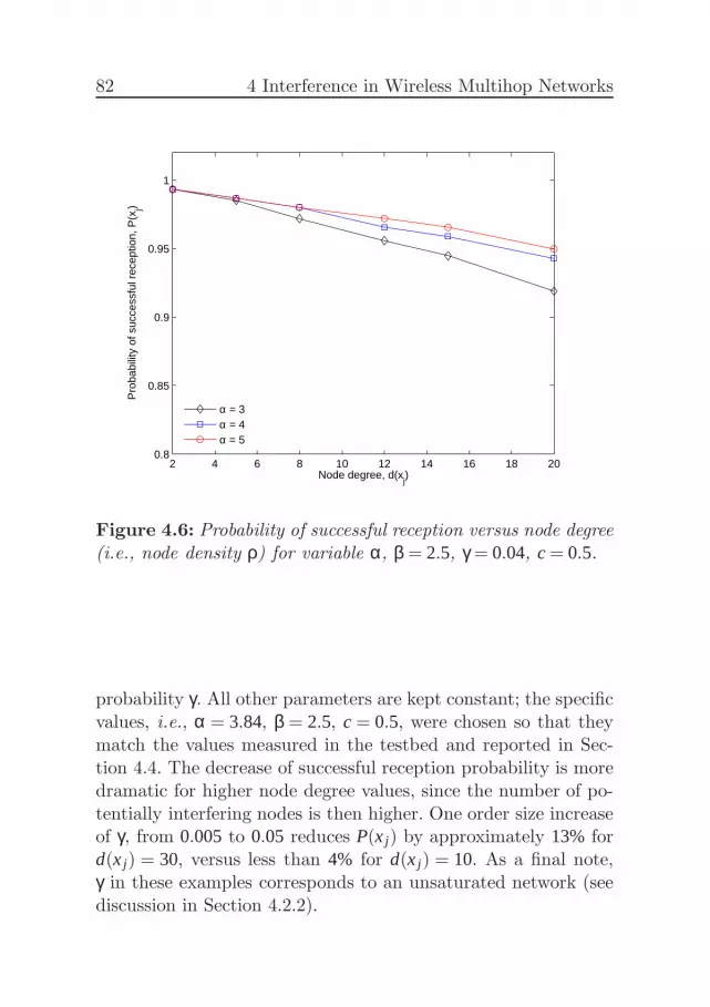
82 4 Interference in Wireless Multihop Networks
2 4 6 8 10 12 14 16 18 200.8
0.85
0.9
0.95
1
Node degree, d(xj)
Pro
babi
lity
of s
ucce
ssfu
l rec
eptio
n, P
(xj)
α = 3α = 4α = 5
Figure 4.6: Probability of successful reception versus node degree(i.e., node density ρ) for variable α, β = 2.5, γ = 0.04, c = 0.5.
probability γ. All other parameters are kept constant; the specificvalues, i.e., α = 3.84, β = 2.5, c = 0.5, were chosen so that theymatch the values measured in the testbed and reported in Sec-tion 4.4. The decrease of successful reception probability is moredramatic for higher node degree values, since the number of po-tentially interfering nodes is then higher. One order size increaseof γ, from 0.005 to 0.05 reduces P(x j) by approximately 13% ford(x j) = 30, versus less than 4% for d(x j) = 10. As a final note,γ in these examples corresponds to an unsaturated network (seediscussion in Section 4.2.2).

4.3 Numerical Results 83
4.3.2 Model sensitivity to path loss exponent, α
The path loss exponent α models the reduction of the radio signalpower as a function of distance from the transmitting source. Itsvalues depend strongly on the radio propagation environment[Rap01].
Combining (4.2) and (4.3) we could write for the radius r j,m
of interference area Cj,m
r j,m = α√
m·β · α√
PwN·β = α
√
m· PwN (4.16)
As α increases, the signal attenuation with distance is higherand the radii of the interference zones decrease. Nodes can beplaced closer to the receiver without interfering with the intendedsignal. The impact of the parameter α on P(x j) is plotted inFig. 4.6. As with Fig. 4.5, higher node degree values amplify thevariation of P(x j) with α.
4.3.3 Model sensitivity to reception threshold, β
The reception threshold β determines when a MAC frame issuccessfully received. It depends on the transmission rate, fre-quency, and sensitivity of the network card/chipset; higher ratesand lower-quality network cards require higher β value for achiev-ing a given frame error rate. Typical values for β, as reported innetwork card specifications, are 2.5 to 25 [aWCBAd].
Increasing the reception threshold value at a given environ-ment reduces the communication range, after (4.2), increases thewidths of interference zones, as (4.3) suggests, and for given cresults in higher concentration of nodes at the first interferencezones, see (4.10). The result is increased interference, as shown inFig. 4.7. The relative reduction on the successful reception proba-bility increases with higher node density, where the concentrationof interfering nodes at the first zones becomes more visible.

84 4 Interference in Wireless Multihop Networks
0 5 10 15 20 25 300.8
0.85
0.9
0.95
1
Node degree, d(xj)
Pro
babi
lity
of s
ucce
ssfu
l rec
eptio
n, P
(xj)
β = 2.5β = 5β = 10β = 15
Figure 4.7: Probability of successful reception versus node degree(i.e., node density ρ) for variable β, α = 4, γ = 0.02, c = 0.5.
4.3.4 Model sensitivity to the sender-receiverdistance scale factor, c
In our analytical derivation, we express the distance between thesender and receiver nodes as a ratio of the maximum communi-cation range, c· rmax. The impact of the sender-receiver distanceon the probability of the successful reception is plotted in Fig.4.8. We vary the node degree, while letting all other parametersconstant. As with α and β, higher network densities magnify theeffect of c. Only the latter is more dramatic in absolute termsthan the one α and β have on the probability of successful recep-tion.
Finally, Fig. 4.8 directly points to the well known inefficien-cies of minimum-hop routing. Minimum-hop routing tends to se-

4.4 Model validation via testbed experimentation 85
0 5 10 15 20 25 300.8
0.85
0.9
0.95
1
Node degree, d(xj)
Pro
babi
lity
of s
ucce
ssfu
l rec
eptio
n, P
(xj)
c = 0.3c = 0.6c = 0.8
Figure 4.8: Probability of successful reception versus node degree(i.e., node density ρ) and sender receiver distance c; β = 2.5,α = 3.84, γ = 0.02
lect few but distant hops when selecting network routes. Thistrend results in more noisy but also, as Fig. 4.8 suggests, moreinterference-prone links. Of course, “shorter” links may also im-ply a large number of hops, which can also be detrimental tothroughput [GK00]. Interference-aware routing has benefits inthis context and, as explained in Section 5.2, it is an area whereour model can find direct application.

86 4 Interference in Wireless Multihop Networks
Figure 4.9: Our wireless mesh network testbed. The 23802.11a/b/g nodes are distributed in offices all over the floor cov-ering an area of approximately 32x79m2.
4.4 Model validation via testbed
experimentation
The analysis in Section 4.2 is carried out for a generic MAC-interference model. Yet, real-world MAC protocols bear a largenumber of finer engineering details, which cannot be easily cap-tured into a simple analytical model without making a muchlarger number of restrictive assumptions. Therefore, we resort toexperimentation to get a better understanding of the strengthsand limitations of our analysis in a real wireless network using areal MAC protocol such as the IEEE 802.11b. In what follows,we first present our experimental testbed and describe the exper-iment configuration. We then present the experimental resultsobtained and compare them against the predictions made usingour analytical model. Finally, we demonstrate how our modelcould be used as a metric in an interference-aware routing proto-col, and compare the resulting performance against a well-knownprobe-based routing scheme [CABM03].

4.4 Model validation via testbed experimentation 87
4 6 8 10 12 14 16−100
−90
−80
−70
−60
−50
10log10(d)
Mea
sure
d re
ceiv
ed p
ower
(dB
m)
measurement samples least square fit, α =3.8427
Figure 4.10: Signal strength Pi j [dBm] as a function of the dis-tance di j .
4.4.1 Testbed description
The testbed consists of 23 stationary Linux PC nodes equippedwith 802.11a/b/g Atheros cards. The nodes are located at thesecond floor of the ETZ building, as illustrated in Fig. 4.9. Allnodes in our testbed communicate using the IEEE 802.11b proto-col operating in ad hoc mode. The RTS/CTS handshake mecha-nism is disabled in line with the default behavior for most wirelesscards [KXB04]. The cards are configured to send at 1Mbps with31.62mW (15dBm) of transmit power.
Path loss exponent α estimation
The dependence of path loss on α is approximated by the log-distance path loss model (e.g., [Rap01]):
Pi j [dBm] = Pdo[dBm]−10 ·α · log10(di j
do
)
(4.17)

88 4 Interference in Wireless Multihop Networks
−100 −98 −96 −94 −92 −90 −88 −86 −840
0.2
0.4
0.6
0.8
1
RSS (dBm)
Pac
ket d
eliv
ery
ratio
1Mbps
8%loss
Figure 4.11: Packet delivery ratio as a function of signalstrength.
where d0 is a reference distance, di j is the distance between thesender i and the receiver j, Pi j [dBm] is the mean received sig-nal power in dBmand Pd0 [dBm] is the mean received power at areference distance d0. We used two nodes to measure the signalstrength as a function of distance in our indoor office environ-ment. The signal strength is derived by the RSS (Received Sig-nal Strength) values reported by the cards at various distances.Setting d0 = 4m and carrying out a least-square fit computation,we estimated Pd0 = −51.12 dBm, α = 3.84. The measured valuesand the least-square fit curve are plotted in Fig. 4.10.
SINR threshold β estimation
The CMU wireless channel emulator [JS05] was used to estimatethe SINR threshold β of our Atheros wireless cards. In our ex-periment, two Atheros cards similar to the ones in our testbed,were connected to the hardware emulator; one card was sending

4.4 Model validation via testbed experimentation 89
5000 802.11 broadcast packets at 1Mbps and the other was re-ceiving them. Note that 802.11 broadcast packets are not subjectto MAC retransmissions. Varying the attenuation of the radiosignal through the emulator in increments of 1dB, we estimatedβ by measuring the ratio of the correctly delivered packets as afunction of the received signal strength (RSS). The results areplotted in Fig. 4.11. Since the noise floor of our Atheros cards is-96dBm, the knee 2 of the delivery ratio curve at RSS=-92dBmmeans that the threshold value β equals 4dB or 2.5.
4.4.2 Experimentation methodology
The communication range in our testbed for 15dBm of trans-mit power was measured approximately to be 25 m. The sender-receiver pair used in our experimental evaluation are nodes 4 and23, respectively. Their Euclidean distance is r = 12.5m, which cor-responds to a distance scale factor value of c = 0.5.
Distribution of nodes
For the α and β values estimated earlier in Section 4.4.1, the radiiof interference areas for the receiver node 23 using lemma 1 are:r23,1 = 15.8m, r23,2 = 19m, r23,3 = 21.1m, r23,4 = 22.8m, and r23,5 =24.1m. Equations (4.14)-(4.15) provide the number of interferenceareas that have to be considered and (4.12) yields the expectednumber of nodes E(A j,m)∀m= 1,2,3...M in each interference zoneas a function of the degree of the receiver node 23. We vary thenetwork density by letting the node degree d(x j) take values inthe interval [5,15] nodes. This is done by activating the nodes foreach scenario listed in Table 4.2.
2The knee corresponds to the receiver’s sensitivity for 8% error rate. Thereceiver’s sensitivity is a measure of wireless cards ability to discern low-levelsignals.

90 4 Interference in Wireless Multihop Networks
Table 4.2: Number of nodes in each interference area A j,m ∀ m=1,2...5.
d(x j) n(A j,1) n(A j,2) n(A j,3) n(A j,4) n(A j,5)5 3,16 12 1 146 11,16 12 1 14 187 3,10,16 12 1 14 188 3,10,16 5,12 1 14 189 3,10,16,17 5,12 1 14 1810 3,10,11,16 5,12 1 14 1811 3,10,11,16 5,12 1,22 14 1812 3,10,11,16,17 5,12 1,22 14 1813 3,10,11,16,17 5,12,21 1,22 14 1814 2,3,10,11,16,17 5,12,21 1,22 14 1815 2,3,10,11,16,17 5,12,21 1,22 14,13 18
Traffic model description
All nodes in each experimental scenario send IEEE 802.11 broad-cast packets, since they involve no retransmissions or link-layeracknowledgments. This is a common practice in related work[PAP+05, RMR+06, QZW+07]. We estimate the successful re-ception probability under simultaneous interfering transmissionsmeasuring the ratio of the successfully received packets over thetotal number of broadcast packets sent. All experiments weredone during the night to circumvent interference induced fromexternal energy sources 3. Having estimated the parameters α, βand c for our experimental evaluation, we conduct experimentsfor different network loads.

4.4 Model validation via testbed experimentation 91
Table 4.3: Parameter values used for the computation of theIEEE 802.11b-equivalent γ parameter
packet payload 128 bitsUDP header 64 bitsIP header 160 bitsLLC+MAC header 192 bitsPHY header 192 bitsChannel bit rate 1 MbpsPropagation delay 1 µsDIFS 50 µsExpected mandatory back-off time E(b) 310 µs
Node transmission probability γ estimation
The node transmission probability γ in the analysis of Section4.2 does not have a direct equivalent in the IEEE 802.11 MAC.To get the equivalent packet send rate for our experiments, weapproximate the transmission probability γ of each node as theratio of the time taken by a successful packet transmission over alarge time interval T. Table 4.3 lists the parameter values used forthe basic DCF access mode. Let H = PHY+MAC+ IP+UDP bethe packet header, Pkt the packet payload and tprop the propaga-tion delay. In the basic access mode, the duration of a successfultransmission Ts is
Ts = H+Pktchannel bit rate+DIFS+E(b)+ tprop
Let ntotal the total transmitted packets in time T, then the pa-rameter γ is approximated as
γ ⋍ntotal·Ts
T (4.18)
3External interference was only from the management frames broadcasts(beacons) of the wireless AP’s (Access Points) installed in the building, whichis negligible comparing with the traffic generated from our experiments.

92 4 Interference in Wireless Multihop Networks
4 6 8 10 12 14 160.8
0.85
0.9
0.95
1
Node degree, d(xj)
Pro
babi
lity
of s
ucce
ssfu
l rec
eptio
n, P
(xj)
experimentanalysis
Figure 4.12: Analytical model vs. testbed experimentation resultsfor γ = 0.005 (α = 3.84,β = 2.5,c = 0.5), RMSE=0.025.
4.4.3 Experimentation results
In this section, we present our experimental results. All capturedtraces of this evaluation are available in [ENL]. We plot the aver-age values of the successful packet receptions for each experiment4 along with their 90% confidence intervals.
The model predictions are compared against the experimen-tal results in Fig. 4.12-4.14. We quantify the accuracy of ourmodel by computing the root mean square error (RMSE), definedover the total number k of predictions (experiment repetitions) as√
∑(esti−actuali )2
k . There is close match between the two curves in all
4We repeated each experimental scenario 20 times

4.4 Model validation via testbed experimentation 93
4 6 8 10 12 14 160.8
0.85
0.9
0.95
1
Node degree, d(xj)
Pro
babi
lity
of s
ucce
ssfu
l rec
eptio
n, P
(xj)
experimentanalysis
Figure 4.13: Analytical model vs. testbed experimentation resultsfor γ = 0.02 (α = 3.84,β = 2.5,c = 0.5), RMSE=0.012.
three figures, the analytical one obtained from the Interference-cum-MAC model and the one from the testbed. The analyticalpredictions for the probability of successful reception match themonotonic change of P(x j) with the node degree throughout the[5..15] range of node degree values for different γ. This is alsoreflected in the RMSE values. For γ = 0.005, the RMSE is 0.025and for higher γ = 0.05 the RMSE equals 0.029.
Furthermore, we compare our model with the general modelfor interference (GMI) proposed in [QZW+07]. The model, whichreflects the state-of-the-art in interference modelling, uses mea-surements to create RF-profiles of network nodes and links andthen inputs those profiles to MAC models for the analytical deriva-

94 4 Interference in Wireless Multihop Networks
4 6 8 10 12 14 160.8
0.85
0.9
0.95
1
Node degree, d(xj)
Pro
babi
lity
of s
ucce
ssfu
l rec
eptio
n, P
(xj)
experimentanalysis
Figure 4.14: Analytical model vs. testbed experimentation resultsfor γ = 0.05 (α = 3.84,β = 2.5,c = 0.5), RMSE=0.029.
tion of the packet loss probability. The GMI evaluation in [QZW+07]was limited to five simultaneous broadcast senders. Here, we com-pare the predictions of our model and GMI in scenarios of Table4.2 involving up to nine simultaneous broadcast senders underunsaturated traffic demands. Note here that the computationaltime required for the GMI model predictions does not scale withhigh number of nodes. 5
Table 4.4 illustrates the relative error in prediction δ,
δ =abs(esti −actuali)
actuali(4.19)
5The model requires to compute 2N states and 2N × 2N state transitionsfor N senders.

4.4 Model validation via testbed experimentation 95
Table 4.4: Relative error δ in predictiond(x j)
γ 5 6 7 8
0.0050.01 0.01 0.005 0.005 Ours0.001 0.001 0.001 0.001 GMI
0.020.009 0.006 0.005 0.005 Ours0.012 0.009 0.009 0.01 GMI
0.050.025 0.035 0.035 0.045 Ours0.055 0.05 0.05 0.05 GMI
for node degree d(x j) = [5..8]. In these scenarios, both modelsyield high accuracy in predicting the measured probability ofsuccessful delivery. Interestingly, our model appears to even out-perform GMI for higher values of γ (i.e. γ = 0.05). Moreover ourmodel features distinct advantages over GMI; it is simple, it doesnot require seed measurements (RF profiling) and is directly ap-plicable to routing, as discussed below.
4.4.4 Impact of Packet Size
A final note on the experimental results concerns the impact ofpacket size. The analytical derivation for P(x j) is not packet sizeaware; namely, it does not take into account the packet size trans-mitted over the medium. We investigated the impact of packetsize with a set of experiments. For the given α,β, and c val-ues of our testbed set-up, we simultaneously varied the packetsize and packet transmission rate, so that they yield the sameequivalent node transmission probability γ, as estimated in Sec-tion 4.4.2. For example, the (pkt size, rate) pairs estimated for γ =0.04 are (128 bytes,20 pkts/second), (256 bytes,15 pkts/second),(512 bytes,8 pkts/second), and (1024 bytes,4.5 pkts/second). Fig-ure 4.15(a) plots P(x j) for all four scenarios. The deviation be-tween the four combinations increases with node degree, butremains overall below 0.06. In fact, the deviation between the

96 4 Interference in Wireless Multihop Networks
(a) P(x j ) vs packet size.
0.9 0.92 0.94 0.96 0.98 10.9
0.92
0.94
0.96
0.98
1
Packet size 256 bytes, rate 15pkts/sec
Pac
ket s
ize
512
byte
s, r
ate
8pkt
s/se
c
45o−slope line
(b) Scatter plot of P(x j ).
Figure 4.15: Impact of packet size on P(x j).

4.5 Conclusion and Discussion 97
curves are comparable to the confidence intervals for the mea-sured results, suggesting that there is no significant change ofP(x j) with packet size. Another way to see this is at Fig. 4.15(b).Eachpoint plots the P(x j) values for two scenarios of different packetsize (256 and 512 bytes). Absolute coincidence of the measuredvalues in the two cases would align the two-dimensional pointsalong the 45o-slope line.
4.5 Conclusion and Discussion
This chapter addresses interference in ad hoc wireless networks.Starting from the SINR model, we derive an analytical expressionfor the data loss probability as a function of the network density,load, propagation environment, and network card hardware. Theanalysis is carried out assuming a MAC-agnostic model, whichdoes not take into account the engineering details of real-worldprotocols, such as the IEEE 802.11x suite of protocols. We thenextend our analytical derivation with a simple enhancement tocapture the carrier sense function of real-world MAC protocols.To assess the prediction capacity of our analysis under realisticconditions, we have set up a wireless mesh network testbed. Mea-surements obtained from the testbed show close match betweenthe analytical predictions and experimental results.
Where and how could this analytical derivation be useful?Interference-aware routing is one profound area. The analyticalderivation could eventually evolve to a routing metric used byrouting protocols to route packets in the network. This is indeedpromising, since it results in significant control data overhead sav-ings over state-of-the-art measurement-based approaches in theliterature. In general, an interference-aware routing metric usingour analytical model can be refined and tailored according to thespecific objectives of the routing algorithm, such as robustness,scalability, low latency, high throughput, or energy efficiency.


Chapter 5
Interference-awareRouting
This section presents the performance evaluation of the interference-aware routing metric. Note here, that our goal is not a new rout-ing metric definition but to exhibit the usability of our interfer-ence model as an input to a routing metric. For this, we borrowthe essential design properties of the state-of-the-art routing met-ric for wireless multihop networks (e.g., ETX).
5.1 Motivation
Routing in wireless multihop networks has been a highly popu-lar research topic during the last decade. Whereas many routingfunction objectives are the same as in wired networks and theInternet, wireless multihop networks add several new dimensionsthat make the problem less straightforward and more interest-ing at the same time. As a result, although experience and wis-dom gained by wired networks have guided the first steps in thewireless domain, in many cases there has been need for novelapproaches and solutions.

100 5 Interference-aware Routing
In the Internet changes in connectivity may happen but arenot frequent. As a result, routing protocols for wired networkspro-actively maintain routes from all nodes to every other node,by propagating the occasional topology update as soon as it oc-curs. However, the topology of wireless multihop networks changesmuch more dynamically than in wired networks. This is due tonode mobility on the one hand, e.g., in mobile ad hoc networksor hybrid networks with both mobile and static nodes, and theimpairments of wireless links due to propagation phenomena, onthe other hand. These two phenomena result in wireless networksbeing often only intermittently connected, which makes the useof proactive routing protocols and the overhead related to routemaintenance less attractive. We summarize here the additionalchallenges related to wireless multihop networks:
• Node mobility. Wireless nodes may move. As a result, linksmay break and network topology may change frequently; ingraph-theoretic terms, the connectivity graph varies morequickly with time. This makes route maintenance muchmore complex than in wired networks.
• Wireless propagation phenomena. In the wireless environ-ment, node transmissions are physically broadcast and sub-ject to radio propagation dynamics, such as shadowing, fad-ing, etc. This makes even static link quality fluctuate overtime, and can also result in the emergence of grey zones inthe network; although links have bad quality and are notgood for data communication, may still allow some success-ful transmissions as for instance routing packets. Situationslike these trigger frequent route re-establishments.
• Energy constraints. In many cases, energy preservation andbattery lifetime extension may become the primary objec-tives for network operation. Advances in battery technologyare significantly slower than those in nanotechnology and

5.1 Motivation 101
electronics. Thus, the available power will continue to be aperformance bottleneck for handheld, low-end devices andsensors, in scenarios where nodes move and operate for longperiods without access to mains power.
• Lack of centralized control. One of the most attractive fea-tures of wireless multihop networks is self-organization. Var-ious functions, such as medium access control and routing,are carried out in a fully distributed manner with minimalhuman intervention. They are not subject to any central-ized network management processes of the kind practicedin wired networks. However, the drawback is that mostdecisions are made by individual nodes having primarilyknowledge about their local environment only. This leaveslittle margin for network optimizations that require globalknowledge of the network state. More critically, the net-work operation itself assumes the cooperation of all nodes,rendering the network more vulnerable to node misbehav-ior.
The need to think differently when it comes to wireless mul-tihop networks is also reflected in the large variety of routingmetrics that have been proposed along with routing protocols,in order to enable efficient data delivery in the wireless context.Besides minimum hop count (shortest path first), which is thealma mater of metrics, the literature is quite rich in other met-rics that have either been more“intelligent” in pursuing minimumdelivery delay or have prioritized other aspects of network per-formance [AGKT98].
The overall goal of a routing metric is to find routes withhigh end-to-end throughput. Furthermore, load balancing, fault-tolerance and low jitter rank highly on the list of goals determin-ing the costs of links and paths in the network. Whereas theseobjectives remain relevant in wireless multihop networks, there

102 5 Interference-aware Routing
are additional concerns that may complement or overshadow tra-ditional objectives. In particular, in wireless networks a routingmetric should also account for
• interference from simultaneous transmissions of neighbor-ing nodes
• interference between successive hops of multihop paths
• asymmetric links (asymmetric loss rates).
Our routing metric accounts for the aforementioned objec-tives as our interference model estimates explicitly the effect ofinterference on packet receptions. We discuss this in detail inthe next section, presenting the design of the interference-awarerouting metric. The performance evaluation of routing given ourmetric versus the minimum hop count and the ETX metrics ispresented in the subsequent section.
5.2 Interference-aware Routing Metric
The essential advantage of our analytical derivation (see Section4.2) is that the probability of successful reception depends onparameters that are known or can be estimated locally at eachnode. The path loss exponent α depends on the environment,while the SINR threshold β relates directly to the receiving sen-sitivity of the wireless adapter. The node degree d(x j ) can beknown from the state of conventional routing protocols, whereasthe network load parameter γ can be estimated by sensing thewireless channel. Modern wireless adapter drivers, such as themadwifi ones [ww], permit access to information about the timeintervals during which the wireless medium is sensed busy. Fi-nally, the distance r of any sender-receiver pair in the networkcan be made available through GPS [ZBR02] or other position-ing methods. Thus, our analytical expression for the probability

5.2 Interference-aware Routing Metric 103
of successful reception can directly be used for the computationof an interference metric, circumventing the need for additionalmeasurements (i.e., probing).
In our routing metric implementation, each node distributesits own local estimate of the probability of successful receptionP(x j) (see sections 4.2.2 and 4.2.3). To avoid additional overheadin the network, the metric information is encapsulated in therouting packets sent periodically to maintain the routing tablesat each node. Then, similar to ETX, each sender node xi estimatesthe expected number of transmissions (including retransmissions)to a potential receiver neighbor node x j as a function of P(x j) andits local estimate P(xi). The routing protocol select paths with thelowest number of transmissions.
From an implementation perspective, a routing metric is acomponent (add-in) of a routing protocol. For this, in our eval-uation we used the Click toolkit [MKJK99] and the Click-basedimplementation of the DSDV [PB94] routing protocol. In the nextsection we discuss the main elements of the DSDV-based im-plementation of the interference-aware routing metric. First wegive an overview of the DSDV protocol and then we present thechanges needed to adopt our metric in the routing scheme.
5.2.1 Overview of the DSDV protocol
DSDV is a distance-vector protocol using sequence numbers toensure fresh route table information (freshness of routes). Everynode maintains a routing table entry for each destination. Theroute entry contains four fields: the destination’s identifier (IPaddress), the next-hop node on the route towards the destination,the latest sequence number heard for each destination and thevalue of the metric (Table 5.1). Packets are forwarded accordingto the current contents of the routing table. The original DSDVprotocol uses the minimum hop count as metric. In our evaluation

104 5 Interference-aware Routing
IP header Next hop Seq num Metric
Table 5.1: DSDV routing entry
we used the implementation of the ETX metric included in theClick toolkit.
DSDV has several mechanisms for the setup, maintenanceand update of the routing entries. The first is that each nodebroadcasts periodically a routing update of its complete routingtable (full update). Each node maintains a sequence number (foreach route) which it increments in every full update that it origi-nates (own routing table entry). When a node receives a routingupdate, it checks the sequence number of the advertised routesfor each destination. If the sequence number is newer than thesequence number in its current entry, or the sequence number isequal and the metric is better, it replaces its current entry withthe new route. Otherwise a node ignores the advertised route.Furthermore, if a node has no entry for a destination, it acceptsthe new route.
In addition to full updates, triggered updates are used toquickly propagate good routes through the network. When a nodereceives or locally estimates a better route towards a destination,it sends a triggered update to its neighbors containing only thechanged information. In order to prevent an explosion of updateswhenever a route changes, triggered updates are not sent until atleast 2xW STtime (Weighted Settling Time) has passed since thefirst hearing of the current sequence number of a route.
Changes to DSDV
In this section we discuss the changes we made to enable theDSDV protocol to use the interference-aware routing metric. Incontrast with ETX that uses probe packets to estimate the de-livery ratio, the probability of successful delivery at the receiver

5.2 Interference-aware Routing Metric 105
IP header Next hop Seq num Metric Pxi (x j)
Table 5.2: Extension of the DSDV routing entry to include thePxi (x j) value.
node x j is derived from theorem 4.4 using only locally retrievedinformation. Generalizing for all links, each node x j maintainsa table of delivery probabilities Pxi (x j) for each potential sender(neighbor) node xi ∀ i ∈ d(x j). The interference-aware metricI(xi ,x j) is calculated as in ETX, converting the delivery ratios inboth directions to expected number of transmissions:
I(xi ,x j) =1
Pxi (x j) ·Pxj (xi)(5.1)
To derive I(xi ,x j), each node x j advertises its local estimationof Pxi (x j) for all its neighboring nodes xi . To avoid additionalrouting overhead, these messages can be encapsulated into theDSDV routing updates. For this, we extended the DSDV routingtable entry (as illustrated in Table 5.2), to include a field for theprobability Pxi (x j).
As route decisions are taken by the sender node xi , the ques-tion that arises now is how xi estimates the metric value I(xi ,x j).While the reverse probability of successful reception at node xi
(Pxj (xi)) from x j is estimated locally at xi , the forward probabil-ity of successful reception Pxi (x j) needs to be communicated toxi from x j . For this, we use triggered updates to disseminate theextended DSDV routing entry with the forward probability ofsuccessful reception.
We implemented the interference-aware routing metric at theClick toolkit. In the following section we discuss how the modelinputs are obtained to calculate the probability of successful re-ception.

106 5 Interference-aware Routing
5.2.2 Obtaining Model Inputs
The required inputs for the calculation of successful deliveryare the parameters α,β and γ. In Section 4.4.1, we discuss howthe path loss exponent parameter α can be estimated throughmeasurements. Likewise, vendors of modern wireless adaptersusually provide information about the adapter’s SINR thresh-old in their specifications. If this information is not available,the SINR threshold can be estimated with similar measurementswe present in Section 4.4.1. The Euclidean distance r betweenthe transmitter and receiver nodes can become available throughGPS [ZBR02] or other positioning methods. In our testbed wemeasure the distance of nodes and the values are statically givento the routing protocol.
Whereas the estimation of the aforementioned parameters isstraightforward, the estimation of the transmission probabilityparameter γ in real time represents a challenging task.
Estimation of transmission probability γ
As discussed in Section 4.2, the transmission probability γ is ameasure of the input network traffic load. In Section 4.4.1 wedescribe how the parameter γ is estimated for given traffic load(unsaturated traffic demands). In the experimental validation ofthe model, we calculate a priori the value of γ for a given datarate. While this is a good approximation in the specific settingsof the experiment, in reality a node should measure the trafficload in real time.
To achieve this, we used the open source Madwifi wirelessadapter drivers [ww]. We modified the source code of the driverssimilar to [DL05] to measure the time the wireless medium issensed busy. The percentage of the busy time b(t)total (0 6 b(t)total 6
1) is reported in a one-second time window to the interference-aware routing metric process. More specifically the busy time

5.2 Interference-aware Routing Metric 107
report includes the percentage of time b(t)xi during which themedium is sensed busy due to transmissions of sender xi . Thisinformation is useful to estimate the traffic load induced frominterferer nodes to each sender-receiver pair.
In the next Section we describe how the interference-awaremetric is calculated for uniform node distribution (see also Sec-tion 4.2.4).
Interference-aware metric under uniform node
distribution
In the interfence model we assume that all nodes send with prob-ability γ (uniform network load). However this is not the case inmost application scenarios. Therefore, we approximate the trans-mission probability γxi ,xj for a sender-receiver pair xi ,x j as:
γxi ,xj =b(t)total −b(t)xi
d(x j)(5.2)
where d(x j) is the degree of the receiver node x j . The probabil-ity γxi ,xj here, denotes the percentage of busy time resulting fromthe total busy time at receiver node x j from all nodes (b(t)total)except the sender’s xi percentage of busy time, calculated for theuniform node distribution (d(x j)). The node degree d(x j) is re-trieved directly from the DSDV routing protocol. The busy timecalculation is an approximation of the transmission probabilityused in the model. It actually corresponds to the network loadafter the effect of the MAC protocol.
Now, the last parameters required to estimate the probabil-ity P(x j) under uniform node distribution is the number of in-terference zones M given from 4.15 and the expected number ofnodes per interference zone, given from 4.10. Note here, that inthe evaluation of the interference-aware metric, the probability ofsuccessful reception P(x j) is calculated for the uniform node dis-

108 5 Interference-aware Routing
Algorithm 1 Estimation of the interference-aware routing met-ric value I(xi ,x j) at node i.
Upon packet reception pif p == data packet from neighbor j then
Update variables b(t)xi , b(t)total and calculate γxi ,xj (5.2)else
if p == routing packet from neighbor i then
1. Get the probability of successful reception Pxj ,xi andestimate the metric I(xi ,x j) (4.4), (4.6), (5.1)2. Update the routing table. The routing protocol thenmaintains the routing tables updated
else
Packet not used in the algorithmend if
end if
tribution. Algorithm 1 describes the essential steps to calculatethe interference-aware routing metric at each node.
5.3 Routing Metric PerformanceEvaluation
In this section we present the results of the interference-awarerouting metric performance evaluation against the ETX metricand the minimum hop count. The ETX metric represents thestate-of-the-art of routing metrics for wireless multihop networksand the hop count is the default metric used from commodityrouting protocols. Our goal is to exhibit the usability of our in-terference model as a routing metric and to assess its performancein a different set of experiments.

5.3 Routing Metric Performance Evaluation 109
5.3.1 Methodology
We evaluate the performance of the interference-aware metricversus the ETX and minimum hop count (Hop Count) metricsin our indoor real-world TIK-Net testbed (a comprehensive de-scription of the testbed is given in section A.1). For this, we in-stalled the Click Toolkit 1 on all 20 nodes of the testbed and weused the Click-based implementation of the DSDV protocol. Theminimum hop count is the default metric for the DSDV protocolwhereas the ETX implementation is included in the Click toolkit.We implemented our interference-aware routing metric accordingto the design discussed in Section 5.2 as a Click module.
The 802.11b cards in the experimental evaluation are set to“ad-hoc” mode 2, RTS/CTS is turned off and rate adaptationmechanism is inactive. We evaluate the three routing metrics intwo set of experiments varying the transmission rate, the trans-mit power Pw, and the packet size as illustrated in Table 5.3. Wedid also experiments for 0dBm of transmit power, however forthese settings the network is very loosely connected. We discussthis further in Section 5.4. We did not perform experiments withhigher rate (e.g., 54 Mb/s) because the network is loosely con-nected and partitioned due to the very small node communicationrange. Now, regarding the packet size used in our experiments,small packets correspond to real-time traffic applications (VoIP),whereas large packets to file sharing or peer-to-peer applications.All experiments are carried out during weekends or nights tominimize interference from external sources 3.
1Installation and configuration details of the Click toolkit can be found inwww.read.cs.ucla.edu/click/.
2More specifically we used the “ahdemo” mode, which is a Madwifi driverspecific “ad-hoc” mode. In “ahdemo“ mode no management packets are sentto maintain connectivity.
3External interference was only from the management frames broadcasts(beacons) of the wireless AP’s (Access Points) installed in the building, whichis negligible comparing with the traffic generated from our experiments.

110 5 Interference-aware Routing
Table 5.3: Parameters used for the routing metric’s performanceevaluation
Symbol ParameterPkt size Packet size (bytes) 128, 1024Bit rate Channel bit rate (Mb/s) 1, 11Pw Transmit power (dBm) 10, 18
Experiment Sets
Two main sets of experiments are conducted in the experimentalevaluation:
• Set A: One node pair is active at a time for all pairs in theTIK-Net testbed, resulting in a total of 20x19=380 sender-receiver pairs.
• Set B: Ten node pairs transmit simultaneously. We selectthe 10 extreme (in distance) node pairs in our testbed.The pairs used in this set of experiments are illustratedin Table 5.4. Nodes 1 to 10 are senders and nodes 11-20act as receivers, respectively. The node ids of the pairs arei → 20− (i − 1) and represent the most challenging trans-missions patterns (this scenario results in many multihoppaths with much cross traffic).
In the first set of experiments (set A) we evaluate the perfor-mance of each metric to find high throughput paths in absenceof interflow interference, i.e., interference from other flows. Thus,in this specific set of experiments interference is mainly due tosimultaneous transmissions of multihop forwarding (intraflow in-terference). In every experiment each node sends UDP packets atmaximum rate (maximum channel capacity) for 30 seconds. Eachround is followed by 20 seconds of pause to let routing entries con-verge to the initial state (no traffic/boot phase). Thus, the totalduration of the first set of experiments (set A) is 380×50×3 sec-onds or 15.9 hours testing all three metrics under a single tuple

5.4 Experimentation Results 111
Table 5.4: Node pairs used for the second set of experiments (SetB)
Node pair Nodes1 1→202 2→193 3→184 4→175 5→166 6→157 7→148 8→139 9→1210 10→11
of (Bit rate, Pw, Pkt size) values and approximately 130 hours forall tuples.
The goal in the second set of experiments (set B) is to eval-uate the metrics in a more challenging scenario with many si-multaneous data flows. We selected node pairs with the largestpossible distance at our testbed. Within an experiment roundeach sender node is configured to send 5000 UDP packets at arate of 10 packets per second. The duration of each round is 500seconds followed by 100 seconds of pause time, thus in total 600seconds. We repeat each round 20 times, resulting in 600×20×3seconds or 36 hours for the three metrics under a single tuple of(Bit rate, Pw, Pkt size). In the results that follow, we present themean values as well as the 95% confidence intervals.
5.4 Experimentation Results
In both experimental scenarios we evaluate the performance ofthe three metrics varying the transmission rate, the transmitpower Pw, and the packet size as illustrated in Table 5.3. The

112 5 Interference-aware Routing
graphs below do not include error bars, but are representative ofthe many run we have performed.
5.4.1 One Node Pair Active
Figure 5.1(a) compares the throughput CDFs (in packets persecond) of paths found by DSDV using the ETX, minimum hopcount, and our interference-aware metric between all 380 nodepairs, for Bit rate=1Mb/s, Pw=18dBm and Pkt size=128. In thefigure, there are essentially two main areas. On the right sidelie node pairs that communicate directly, whose achieved packetdelivery ratio exceeds 200 packets per second, on the left halfare the node pairs for which the found routes exceed one hop. Inaddition to the CDF figure, the throughput histogram (in packetsper second) of the paths found by each metric is presented in Fig.5.1(b). While presenting the same data with the CDF figure, thehistogram allows for a more direct comparison of the metrics’performances.
All three metrics find the one-hop best route (right half side)as can be seen in both figures. In that area, neither ETX norour interference-aware routing metrics can find higher through-put routes than those retrieved by minimum hop count. How-ever, in the left half area, the sensitivity of our interfence metricto interfering transmissions results in higher throughput pathsthan those of both the ETX and minimum hop count. This isclearly observed in Fig. 5.1(b), where our interference-aware rout-ing metric finds up to 3 times more paths with high through-put (between 125 and 150 packets per second) when comparedto ETX and minimum hop count. As soon as the path lengthis greater than a single hop, throughput degrades due to the802.11 MAC mechanisms (exposed nodes) and intraflow interfer-ence (hidden, interfering nodes). Our interference-aware metricfinds higher throughput paths because it takes explicitly into ac-count the effect of interference. On the contrary, ETX and min-

5.4 Experimentation Results 113
0 50 100 150 200 250 300 3500
0.1
0.2
0.3
0.4
0.5
0.6
0.7
0.8
0.9
1
Packets per second delivered
Cum
mul
ativ
e fr
actio
n of
nod
e pa
irsEmpirical CDF
Interference−aware
ETX
Hop Count
1−hop
(a) Throughput CDF (in packets per second) of paths found byDSDV using ETX, minimum hop count and our interference-aware metric.
0 50 100 150 200 250 300 3500
10
20
30
40
50
60
70
80
90
100
Packets per second delivered
Dis
trib
utio
n of
pac
kets
del
iver
ed
Interference−aware
ETX
Hop Count
1−hop
(b) Throughput histogram (in packets per second) of paths foundby DSDV using ETX, minimum hop count and our interference-aware metric.
Figure 5.1: One node-pair active: Bit rate=1Mb/s, Pw=18dBm,Pkt size=128 bytes.

114 5 Interference-aware Routing
imum hop count metrics find more paths with lower throughput(between 100 and 125 packets per second) in comparison with ourinterference-aware metric. ETX accounts for lossy/asymmetriclinks using probe packets to estimate the delivery probability ona link. However, as admitted also in the ETX paper [CABM03],heavy load causes the MAC protocol to become extremely unfair,distorting the probe-based measurements. Thus, ETX might notaccurately estimate the link delivery probabilities and accord-ingly result in suboptimal paths.
Effect of packet size
In another set of experiments we use 1024-byte data payload tostudy the effect of packet size on routing metric performance.Our interference model, does not take the packet size explicitlyinto account in the estimation of the probability P(x j) of suc-cessful reception. Moreover, in the experimental evaluation ofour interference model (see section 4.4.4), we show that thereis no significant change of the estimated probability P(x j) withthe packet size. Nevertheless, in the actual implementation ofthe interference-aware metric design, the packet size and rate areimplicitly included in the time the medium is sensed busy (trans-mission probability parameter), as a function of the busy timeduration b(t)total (see Section 5.2.2).
Figure 5.2(a) plots the throughput for packets with pkt size=1024 bytes. In accordance with the aforementioned results, theadvantage of our interference-aware routing metric is visible atpaths of more than-one-hops. Our interference-aware metric findsalmost three times more paths with average throughput between30 and 40 packets per second (see Fig. 5.2(b) ). ETX find routeswith average throughput between 10 and 20 packets per second(130 node pairs). In contrast with ETX and our interference-aware metric, minimum hop count finds more paths with lowthroughput; almost 30% more paths with throughput between 0

5.4 Experimentation Results 115
0 10 20 30 40 50 60 70 80 90 1000
0.2
0.4
0.6
0.8
1
Packets per second delivered
Cum
mul
ativ
e fr
actio
n of
nod
e pa
irs
Empirical CDF
Interference−aware
ETX
Hop Count
1−hop
(a) Throughput CDF (in packets per second) of paths found by DSDVusing ETX, minimum hop count and our interference-aware metric.
0 10 20 30 40 50 60 70 80 90 1000
20
40
60
80
100
120
140
Packets per second delivered
Dis
trib
utio
n of
pac
kets
del
iver
ed
Interference−aware
ETX
Hop Count
1−hop
(b) Throughput histogram (in packets per second) of paths found by DSDVusing ETX, minimum hop count and our interference-aware metric.
Figure 5.2: One node-pair active: Bit rate=1 Mb/s, Pw=18dBmand Pkt size=1024 bytes.

116 5 Interference-aware Routing
and 10 packets per second. This is because minimum hop countdoes not have a mechanism to cope with asymmetric links orpacket losses due to interference.
The specific set of experiments suggests that the change ofthe packet size does not have a significant impact neither onthe absolute nor on the relative performance of the metrics. Ourinterference-aware metric performs at least as good as both ETXand minimum hop count.
Effect of transmit power
When nodes send at lower transmit power, the communicationrange is decreasing. Therefore, the network is less connected re-sulting in the increase of the average hop count required for nodesto communicate. Furthermore, routing metrics have fewer pathsto select. In that specific set of experiments, we decrease thetransmit power Pw from 18dBm to 10dBm. We also did experi-ments for very low transmit power Pw=0dBm (1mW). The net-work in that specific set of experiments is very sparsely connectedand the throughput of most of the node pairs is very close to zero;almost 60% of node pairs throughput for all three metrics is lessthan 10 packets (see Figure 5.3). Therefore, we evaluate the per-formance of the metrics for intermediate transmit power levels.
Figure 5.4(a) shows the throughput CDFs for Pw=10dBm andpkt size=128 bytes. Comparing with the results for Pw=18dBm(see Fig. 5.1(a) all metrics find paths with relatively little through-put. More specifically, our interference-aware metric finds fewermore-than-one-hop paths with throughput between 125 and 150packets per second; for Pw=18dBm, there are almost 100 nodepairs, whereas for Pw=10dBm only 65 node pairs. However, it stillfinds more paths with high throughput than both ETX and mini-mum hop count (about 2 times more paths with high throughputvalues).

5.4 Experimentation Results 117
0 10 20 30 40 50 60 70 80 90 1000
0.2
0.4
0.6
0.8
1
Packets per second delivered
Cum
ulat
ive
frac
tion
of n
ode
pairs
Empirical CDF
Interference−aware
ETX
Hop Count
1−hop
(a) Throughput CDF (in packets per second) of paths found by DSDVusing ETX, minimum hop count and our interference-aware metric.
0 10 20 30 40 50 60 70 80 90 100 1100
50
100
150
200
250
300
Packets per second delivered
Dis
trib
utio
n of
pac
kets
del
iver
ed
Interference−aware
ETX
Hop Count
1−hop
(b) Throughput histogram (in packets per second) of paths found by DSDVusing ETX, minimum hop count and our interference-aware metric.
Figure 5.3: One node-pair active: Bit rate=1 Mb/s, Pw=0dBmand Pkt size=1024 bytes.

118 5 Interference-aware Routing
0 50 100 150 200 250 3000
0.2
0.4
0.6
0.8
1
Packets per second delivered
Cum
mul
ativ
e fr
actio
n of
nod
e pa
irs
Empirical CDF
Interference−aware
ETX
Hop Count
1−hop
(a) Throughput CDF (in packets per second) of paths found by DSDVusing ETX, minimum hop count and our interference-aware metric.
0 50 100 150 200 250 3000
10
20
30
40
50
60
70
80
90
100
Packets per second delivered
Dis
trib
utio
n of
pac
kets
del
iver
ed
Interference−aware
ETX
Hop Count
1−hop
(b) Throughput histogram (in packets per second) of paths found by DSDVusing ETX, minimum hop count and our interference-aware metric.
Figure 5.4: One node-pair active: Bit rate=1 Mb/s, Pw=10dBmand Pkt size=128 bytes.

5.4 Experimentation Results 119
The transmit power affects the performance of the metrics,since it directly determines the connectivity of the network. Theadvantage of our interference-aware metric over ETX and mini-mum hop count is more profound in densely connected networks(higher transmit power). The gain is smaller in sparsely con-nected networks, because available paths that can be found froma routing protocol are fewer and there is little margin for differ-entiation in the decisions made by the three metrics.
Effect of transmission rate
Another parameter that affects the performance of the rout-ing metrics is the transmission rate. There is an inherent trade-off between high transmission rate and effective transmission/communication range. Higher transmission rate results in higherthroughput but lower effective transmission range, hence looserconnectivity (sparser network).
We evaluate the performance of routing metrics for transmis-sion rates of 1 and 11Bits per second. The sensitivity thresholdsfor the cards used in our experimental evaluation, as reportedfrom the manufacturer, are -89dBm for 1 Mb/s and -82dBm for 11Mb/s (for 8% packet error rate). Figure 5.5(a) shows the through-put CDFs for Bit rate=11 Mb/s, Pw=18dBm and data packetsof Pkt size=128 bytes. In comparison with the Bit rate=1 Mb/sexperiments (Fig. 5.1), the overall throughput increases; 30% ofpairs achieve throughput over 200 data packets per second forBit rate=1 Mb/s, while for 11 Mb/s the respective value is 60-70% for all metrics.
Looking into the performance of each metric, similar to theaforementioned results, the three metrics find approximately thesame number of one-hop routes. The gain of the interference-aware routing metric is on the left half of the figure where itfinds higher throughput routes of more than one-hop. This canbe clearly seen in figure 5.5(b) where our interference-aware met-

120 5 Interference-aware Routing
0 200 400 600 800 1000 12000
0.2
0.4
0.6
0.8
1
Packets per second delivered
Cum
mul
ativ
e fr
actio
n of
nod
e pa
irs
Empirical CDF
Interference−aware
ETX
Hop Count
1−hop
(a) Throughput CDF (in packets per second) of paths found by DSDVusing ETX, minimum hop count and our interference-aware metric.
0 200 400 600 800 1000 1200 14000
20
40
60
80
100
120
140
160
180
200
220
Packets per second delivered
Dis
trib
utio
n of
pac
kets
del
iver
ed
Interference−aware
ETX
Hop Count
1−hop
(b) Throughput histogram (in packets per second) of paths found by DSDVusing ETX, minimum hop count and our interference-aware metric.
Figure 5.5: One node-pair active: Bit rate=11 Mb/s,Pw=18dBm and Pkt size=128 bytes.

5.4 Experimentation Results 121
ric outperforms ETX and hop count and finds almost 3 timesmore high throughput paths (between 500 and 600 packets persecond) than ETX and minimum hop count. ETX finds morepaths between 200 and 300 packets per second while minimumhop count find more paths with lower throughput (between 0 and100 packets per second).
Similar behavior of the routing metrics is observed for differ-ent packet size and transmit power settings (Fig. 5.6, 5.7 and 5.8).Our interference-aware metric performs at least as good as ETXand minimum hop count in most scenarios independent of packetsize, transmit power, and transmission rate. The advantage ofour metric is for paths higher than a single hop. The presence ofintraflow interference degrades the end-to-end throughput. Mini-mum hop count does not account for interference, while ETX es-timates link losses based on probe measurements. However, underheavy load ETX probe packets are distorted, resulting in biasedmeasurements. The essential advantage of our metric is the di-rect estimation of the effect of interference, the primary cause ofpacket loss in wireless networks.
5.4.2 Multiple Pairs Active.
The second set of experiments, we evaluate the performance ofthe three routing metrics under many simultaneous data flows.Figure 5.9(b) compares the throughput (in packet per second)of each sender-receiver pair (1-10 as illustrated in Table 5.3)for Bit rate=1 Mb/s, Pkt size=128 bytes, and Pw=18dBm. Gen-erally, our interference-aware metric and ETX achieve higherthroughput when compared with the minimum hop count. Morespecifically, for the node pairs 1, 2, 7, 8 and 9, the throughput ofour interference-aware metric is higher than ETX (10% on aver-age) and minimum hop count (30% on average). ETX achieveshigher throughput for the node pair 10, while for node pairs 3, 4,5, 6 the throughput is similar to our interference aware metric.

122 5 Interference-aware Routing
0 200 400 600 800 1000 12000
0.2
0.4
0.6
0.8
1
Packets per second delivered
Cum
mul
ativ
e fr
actio
n of
nod
e pa
irs
Empirical CDF
Interference−aware
ETX
Hop Count
1−hop
(a) Throughput CDF (in packets per second) of paths found by DSDVusing ETX, minimum hop count and our interference-aware metric.
0 200 400 600 800 1000 1200 14000
20
40
60
80
100
120
140
160
180
200
Packets per second delivered
Dis
trib
utio
n of
pac
kets
del
iver
ed
Interference−aware
ETX
Hop Count
1−hop
(b) Throughput histogram (in packets per second) of paths found by DSDVusing ETX, minimum hop count and our interference-aware metric.
Figure 5.6: One node-pair active: Bit rate=11 Mb/s,Pw=10dBm and Pkt size=128 bytes.

5.4 Experimentation Results 123
0 100 200 300 400 500 6000
0.2
0.4
0.6
0.8
1
Packets per second delivered
Cum
mul
ativ
e fr
actio
n of
nod
e pa
irs
Empirical CDF
Interference−aware
ETX
Hop Count
1−hop
(a) Throughput CDF (in packets per second) of paths found by DSDVusing ETX, minimum hop count and our interference-aware metric.
0 100 200 300 400 500 600 7000
50
100
150
200
Packets per second delivered
Dis
trib
utio
n of
pac
kets
del
iver
ed
Interference−aware
ETX
Hop Count
1−hop
(b) Throughput histogram (in packets per second) of paths found by DSDVusing ETX, minimum hop count and our interference-aware metric.
Figure 5.7: One node pair-active: Bit rate=11 Mb/s,Pw=10dBm and Pkt size=1024 bytes.

124 5 Interference-aware Routing
0 100 200 300 400 500 600 7000
0.2
0.4
0.6
0.8
1
Packets per second delivered
Cum
mul
ativ
e fr
actio
n of
nod
e pa
irs
Empirical CDF
Interference−aware
ETX
Hop Count
1−hop
(a) Throughput CDF (in packets per second) of paths found by DSDVusing ETX, minimum hop count and our interference-aware metric.
0 100 200 300 400 500 600 7000
20
40
60
80
100
120
140
160
180
200
220
Packets per second delivered
Dis
trib
utio
n of
pac
kets
del
iver
ed
Interference−aware
ETX
Hop Count
1−hop
(b) Throughput histogram (in packets per second) of paths found by DSDVusing ETX, minimum hop count and our interference-aware metric.
Figure 5.8: One node-pair active: Bit rate=11 Mb/s,Pw=18dBm and Pkt size=1024 bytes.

5.4 Experimentation Results 125
Table 5.5: Average path length for all rounds. (Bit rate=1 Mb/s,Pkt size=128 bytes)
Metric Pw=18dBm Pw=10dBmInterference-aware 3.26 3.36ETX 3.4 3.56Minimum hop count 3.2 3.29
While ETX finds lower but comparable throughput paths to theinterference aware-metric, minimum hop count achieves conciselythe lower throughput for all node pairs.
Figure 5.9(a) presents the throughput (in packet per second)for lower transmit power, namely Pw=10dBm. Lower transmitpower, as we have seen in section 5.4.1, may eventually resultin lower throughput because fewer paths are available towardsa destination. Among the three metrics, the transmit power im-pacts more significantly the performance of minimum hop count.For node pairs 1, 2, 4 and 10 the throughput drops up to 50%below that obtained with transmit power of 18dBm.
Impact of path length
Now, the question that arises is why our interference-aware rout-ing metric finds higher throughput paths than both ETX andminimum hop count? Table 5.5 presents the average path lengthof all experiment rounds for transmit power Pw equal to 10dBmand 18dBm. To calculate the average path length (for each ex-periment repetition), we keep track of the paths taken by datapackets. The minimum hop count has the shortest average pathlength (3.2 and 3.29) followed by the interference-aware metric(3.26 and 3.36) and ETX (3.4 and 3.56).
Looking in more detail, Fig. 5.10(a) illustrates the bar chart ofthe average paths length for each node pair (for Pw=18dBm). Theerror bars represent the 95% confidence intervals. The bar chart

126 5 Interference-aware Routing
0 1 2 3 4 5 6 7 8 9 10 112
3
4
5
6
7
8
9
10
Node Pairs
Pac
kets
per
sec
ond
deliv
ered
Interference−aware
ETX
Hop Count
(a) Bit rate=1 Mb/s, Pw=108dBm and Pkt size=128 bytes.
0 1 2 3 4 5 6 7 8 9 10 112
3
4
5
6
7
8
9
10
Node Pairs
Pac
kets
per
sec
ond
deliv
ered
Interference−aware
ETX
Hop Count
(b) Bit rate=1 Mb/s, Pw=18dBm and Pkt size=128 bytes.
Figure 5.9: Multiple node-pairs active: Throughput (in packetsper second) of paths found by DSDV using ETX, minimum hopcount and our interference-aware metric.

5.4 Experimentation Results 127
1 2 3 4 5 6 7 8 9 100
1
2
3
4
5
6
Node Pairs
Ave
rage
path
leng
th
Interference−aware
ETX
Hop Count
(a) Bit rate=1 Mb/s, Pw=18dBm and Pkt size=128 bytes.
1 2 3 4 5 6 7 8 9 100
1
2
3
4
5
6
Node Pairs
Ave
rage
pat
h le
ngth
Interference−aware
ETX
Hop Count
(b) Bit rate=1 Mb/s, Pw=10dBm and Pkt size=128 bytes.
Figure 5.10: Multiple node-pairs active: Average path lengthused by ETX, minimum hop count and our interference-awaremetric.

128 5 Interference-aware Routing
exhibits that the minimum hop count has the shortest averagepath length in most pairs, followed by the interference-aware met-ric and ETX. Similar results are obtained for Pw=10dBm (see Fig.5.10(b)). Nevertheless, the small diversity in path length amongthe ETX, minimum hop count, and interference-aware metricsdoes not justify the difference in throughput for both experimen-tal settings. Therefore, as routing metrics select paths with ap-proximately equal average length, there should be another reasondifferentiating the performance of the three metrics.
Load distribution
In this subsection we zoom our analysis in on the distributionof data traffic across network nodes. In Fig. 5.11 the traffic loaddistribution with the 95% confidence intervals of the average val-ues is shown. More specifically, the bar chart shows the averagenumber of packets sent and/or received per second at each node,i.e., nodes selected from the routing metrics to forward data traf-fic. In Fig. 5.11(b) we observe that routing metrics favor differentnodes for forwarding data traffic. Nodes 11 and 12 are selectedfrom ETX, while our interference-aware metric pushes the trafficto nodes 2, 4, 15, 17 and 18. Minimum hop count favors nodes11 and 12 similar to ETX, but with lower data volume.
Similar load distribution patterns are observed at the sec-ond experiment with lower power Pw=10dBm (see Fig. 5.11(b)).ETX routes traffic towards nodes 11 and 12, as much it does forPw=18dBm. Our interference-aware metric also favors the samenodes as for Pw=18dBm, but with different volume, adapting tothe new topology; 88 and 75 packets on average per second atnodes 4 and 17, respectively, versus 92 and 72 packets per secondon average at nodes 17 and 4.
Figure 5.12 presents the same data complementing Fig. 5.11,only values are sorted according to the data volumes. The redhorizontal line corresponds to the minimum expected number

5.4 Experimentation Results 129
1 2 3 4 5 6 7 8 9 10 11 12 13 14 15 16 17 18 19 200
20
40
60
80
100
120
Nodes
Load
bal
anci
ng:
Ave
rage
num
ber
of p
acke
ts (
per
seco
nd)
Interference−aware
ETX
Hop count
(a) Bit rate=1 Mb/s, Pw=18dBm and Pkt size=128 bytes.
1 2 3 4 5 6 7 8 9 10 11 12 13 14 15 16 17 18 19 200
20
40
60
80
100
120
Nodes
Load
bal
anci
ng:
Ave
rage
num
ber
of p
acke
ts (
per
seco
nd)
Interference−aware
ETX
Hop count
(b) Bit rate=1 Mb/s, Pw=10dBm and Pkt size=128 bytes.
Figure 5.11: Multiple node-pairs active: Histogram of traffic load(average number of packets sent/received per second) at all nodes.

130 5 Interference-aware Routing
of packets sent/received from each node, as nodes 1-10 send10 UDP packets per second, while nodes 11-20 are correspond-ingly the destination nodes. This figure shows that ETX and ourinterference-aware routing metric generate equivalent values ofdata traffic volumes in the network. On the contrary, minimumhop count does not achieve to support high data traffic volume,in accordance with the low achieved throughput as presented inFig. 5.9(a) and 5.9(b)
Therefore, our interference-aware routing metric performs bet-ter than both ETX and minimum hop count because it findshigher throughput paths. Taking into account Fig. 5.11 and 5.12the only qualitative difference between our interference-awarerouting metric and ETX, while the total volume of data is ap-proximately equivalent, is that our metric distributes the trafficover higher throughput paths.
Summarizing this section, we list the main findings of theperformance evaluation of the three metrics:
• The essential advantage of our interference-aware routingmetric is the direct estimation of the effect of interference,the primary cause of packet loss in wireless networks.
• The packet size, transmit power and transmission rate donot have a significant impact on the relative performanceof the metrics.
• Our interference-aware routing metric performs at least asgood as the ETX and minimum hop count in most experi-mental scenarios.
5.5 Conclusion and Discussion
In this section we presented the design and the performance eval-uation of our interference-aware routing metric. First, we demon-

5.5 Conclusion and Discussion 131
0 2 4 6 8 10 12 14 16 18 200
10
20
30
40
50
60
70
80
90
100
Ordered data
Load
bal
anci
ng:
Ave
rage
num
ber
of p
acke
ts (
per
seco
nd)
ETX
Interference−aware
Hop Count
(a) Bit rate=1 Mb/s, Pw=18dBm and Pkt size=128 bytes.
0 2 4 6 8 10 12 14 16 18 200
10
20
30
40
50
60
70
80
90
100
110
120
Ordered data
Load
bal
anci
ng:
A
vera
ge n
umbe
r of
pac
kets
(pe
r se
cond
)
ETX
Interference−aware
Hop Count
(b) Bit rate=1 Mb/s, Pw=10dBm and Pkt size=128 bytes.
Figure 5.12: Multiple node-pairs active: Traffic load (averageper second number of packets sent/received per second) sorted forall nodes.

132 5 Interference-aware Routing
strated the usability of our interference model as a metric forinterference-aware routing. Adopting the essential properties ofthe state-of-the-art routing metric, we developed an interference-aware routing metric based on our model.
We compared its performance at the TIK-Net testbed withthe ETX and minimum hop count metrics in a large set of ex-periments; in the presence only of intraflow interference (onenode pair active) and both intraflow and interflow interference(many simultaneous data flows). The results showed that ourinterference-aware routing metric performs at least as good asETX and better than the minimum hop count.


Chapter 6
Conclusions and FutureWork
We conclude our work with a summary of our main results andcontributions. We also identify assumptions and possible weak-nesses of our work and discuss still open research issues thatdeserve further attention.
6.1 Summary of Main Results
Multipath Routing
In this thesis, multipath routing is investigated in the contextof our pursuit towards more efficient routing in wireless multi-hop networks. We carry out an extensive performance evaluationstudy to thoroughly understand the advantages and limitations ofsingle-path and multipath routing protocols. Our study demon-strates that multipath routing performs better than single-pathin networks with high density and network load. Furthermore,we find that the use of two, maximum three, paths representsthe best tradeoff between routing overhead and performance.

136 6 Conclusions and Future Work
Interference Model
We propose an analytical model for the probability of successfulreception at a node in the presence of interference from simul-taneous transmissions of other network nodes. We first derive aMAC-agnostic model, which does not take into account the en-gineering details of the IEEE 802.11x suite of protocols. We thenextend our analytical derivation to capture the carrier sense func-tion of real-world MAC protocols. The essential advantage of ourinterference model is that the probability of successful receptionin the presence of interference is derived exploiting five parame-ters known locally at each node: node degree, node transmissionprobability, radio propagation environment, network card recep-tion sensitivity and sender-receiver distance.
To assess the prediction capacity of our analysis under real-istic conditions, we evaluate our model against experiments in areal testbed. The results obtained from the testbed show closematch with the analytical predictions. Furthermore, we com-pare our model with another, state-of-the-art model for inter-ference (GMI) [QZW+07], which attempts to capture the detailsof 802.11x protocols. Notably, both models yield comparable ac-curacy in predicting the probability of successful delivery. How-ever, our model has distinct advantages over GMI; it is simple,it does not require seed measurements, it can be directly usedfrom network layer protocols and it can accommodate mobility.The steady-state spatial node distribution resulting from a rangeof mobility models widely used in literature such as the randomwaypoint [BRS03], random walk, and random direction [NTLZ04]can have a direct use in our model.
Interference-aware Routing
We design and implement an interference-aware routing metricbased on our interference model. The goal of our interference-

6.2 Assumptions and Weaknesses 137
aware routing metric is to find high throughput paths exploitinginformation locally available at a node while avoiding the addi-tional overhead of active probe measurements methods used fromthe state-of-the-art routing metric (e.g., ETX).
We evaluate its performance in a large set of experiments inthe presence of intraflow and interflow interference. We show thatits performance compares favorably with both the ETX and theminimum hop count metrics. We conclude that our interference-aware routing metric performs at least as good as ETX and min-imum hop count across a large set of experiments, because itdirectly accounts for interference, the primary cause of perfor-mance degradation in wireless multihop networks.
6.2 Assumptions and Weaknesses
Modeling interference in wireless networks is a difficult problem.The main objective of our interference model is its direct use inrouting. Therefore, instead of capturing all the engineering de-tails of MAC protocols and wireless physical layer complex mod-els, our work focuses on their basic properties. For example, ourmodel does not account for the IEEE 802.11 ACKs. Neverthe-less, evaluation results in real-world testbed experiments exhibitthe accuracy of our model in predicting the probability of suc-cessful reception in the presence of interference, in realistic radiopropagation conditions and real-world MAC protocols.
First, our model considers the interference at the receiver,but not at the sender node. According to the 802.11 MAC dis-tribution coordination function (DCF), a successful transmissionrequires the successful ACK reception at the sender. For this,we assume that the probability of unsuccessful ACK reception isvery small, since ACK packet size is very small compared with a

138 6 Conclusions and Future Work
data packet. Furthermore, in the QoS-aware enhancement of the802.11 standard (802.11e), MAC-level ACKs are optional 1 [IEE].
Second, our analytical derivation for the successful packet re-ception does not explicitly account for the packet size and thetransmission rate. Nevertheless, our results suggest that there isno significant change of the probability of successful reception inthe presence of interference with packet size. Note that both pa-rameters are implicitly accounted for in the metric computation,where the transmission probability γ is approximated by measur-ing the time that the medium is busy with transmissions (seeSection 5.2.2).
Third, we assume that all nodes are similar and experience thesame conditions (uniform node assumption). Allowing for nodeheterogeneity questions the model tractability. Note that this as-sumption is common to all analytical interference studies we areaware of. Regarding the metric, we assume node positioning infor-mation. Nowadays, as more more and more devices are equippedwith positioning systems [ZBR02], we expect that this is easy toobtain.
Finally, to derive a close form for the probability of suc-cessful reception in the presence of interference, we assume theuniform node distribution. This derivation is also used in ourinterference-aware metric. The uniform node distribution repre-sents the general case for spatial node distribution including twomobility models (random walk and direction). Furthermore, thepropagation model used in the model does not account for fading.In further work, we will relax this assumption.
1The MAC would not send an ACK when it has correctly received a frame,when the ”no ACK” policy is used. This option is proposed to improve theoverall MAC efficiency for time-sensitive traffic, such as VoIP, where datahas very strict lifetime.

6.3 Future Work 139
6.3 Future Work
In this section we discuss open research issues. First, the de-sign and development of our interference-aware routing metricfor on-demand/reactive routing protocols such as DSR [JM96]and AODV [PBRD03] is a challenging issue. Reactive mechanismto accommodate frequent link metric changes impose additionalrouting overhead. A prominent solution in this problem is to usea proactive background mechanism for link metrics maintenanceas proposed in [DPZ04a].
Second, the experimental evaluation of our model in a largertestbed, including indoor, outdoor and mobile nodes would givemore insights on the prediction capacity of our model in a largerset of experiments. Furthermore, a comparison with proposedextensions of ETX in order to obtain a better understandingof our interference-aware routing metric with respect to activeprobe-based approaches.
Third, in our interference model nodes transmit with the samepower. The enhancement of our model with adaptive transmitpower control represents an interesting issue that would enableour model to be used also for topology control and efficient powerconsumption.
Finally, in order to model the effect of a propagation environ-ment on a radio signal, a more realistic radio propagation modelsuch as the Rayleigh fading can be used in our interference model.This would obviously increase the complexity of our model; thetradeoff between complexity and predictability represents an in-teresting issue.


Appendix A
A.1 Wireless Testbed
In this section, we present the 20-node TIK-Net testbed; thetopology, the hardware and the software used.
A.1.1 Hardware, Software, Topology
Topology
TIK-Net consists of 20 personal computers distributed at randomspots throughout the G-floor of the ETZ building (Departmentof Information Technology and Electrical Engineering at ETHZurich) covering a physical area of roughly 2250 m2. Figure 4.9 isa snapshot of the exact position of the 20 nodes. Each numberedcircle serves also as a corresponding IP alias of the node, whichmakes it remotely accessible through the ETH wired network (e.g.node 3 can be reached by the alias “tik-wifi3“). The final positionof the 20 nodes assures no partitioning in the wireless networkand provides full functionality to the user of the TIK-Net testbed

142 A Appendix
Hardware
The 20 PCs used can be roughly separated into two categories:i) Dell PCs with 2GHz processor and 512MB RAM memory, andii) PCs with 866MHz processor and 512MB RAM memory. Allof them are currently equipped with the 802.11b/g D-Link G-520 wireless NIC based on the Atheros AR5212 chipset and anexternal omni-directional antenna.
Software
The operating system selected is GNU/Debian Linux with aLinux kernel version of 2.6.18-4. As already mentioned each nodecan be accessed remotely through the ETH wired network (e.g.using ssh) using its alias (e.g. ssh tik-wifi5.ethz.ch for accessingnode 5). In the current implementation, node 4 (tik-wifi4.ethz.ch)plays the role of a management ”server”.
Because the wireless NIC installed in every node of the wire-less testbed uses Atheros chipset, the decision of using MADWIFI[ww] (Multiband Atheros Driver for WiFi) was pretty straight-forward. In particular, we used the Madwifi-ng (next generation)driver, which is a Linux driver for 802.11a/b/g universal NICcards - Cardbus, PCI, or miniPCI - using Atheros chip sets. Mad-wifi drivers are commonly used by the research community be-cause they are open-source and allow for versatile and flexibleconfiguration of the wireless card. It is also widely documented(at least in the context of initial experimentation).
As routing substrate, we installed in each node the Click Mod-ular Router software toolkit [MKJK99]. The Click toolkit is ageneral purpose software tool for implementing modular routerconfigurations. In the Click toolkit, the “Grid“ router elementincludes the implementation of the DSDV and DSR routing pro-tocols for wireless multihop networks. The routing protocol stateinformation (e.g. routing tables, link tables, ARP caches, etc.)

A.1 Wireless Testbed 143
can be accessed through Click. More details in setting up andconfiguring of the Click toolkit are provided in [MKJK99].
A.1.2 Link-level Measurements
Performance evaluation using a wireless testbed has some clearadvantages against simulation-based experimentations. Simula-tions often rely on simplified wireless signal propagation models,which have not been validated using today’s wireless radios. Realhardware-based experimentation fills in the gap between conven-tional assumptions (depending strongly on the accuracy of themodels used and the protocol’s code implementation) and realworld behavior. However, this does not come without a cost. Set-ting up a testbed experiment involves a lot of parameters thatneed to be taken into consideration.
It is exactly in this general context that understanding thewireless behavior of the TIK-Net testbed (link asymmetries) isvery important before moving on to analyzing results of higherlayers mechanisms (routing and transport protocols). Therefore,we have conducted a set of experiments and processed the col-lected data to accurately understand the link-level behavior ofthe TIK-Net testbed.
In order to measure the loss ratio for all possible direct links(19x20 = 380 in total), each node took a turn transmitting 3000broadcast packets uniformly spread in an interval of 30 seconds.Within these 30 seconds every other node recorded the numberof packets received. Each experiment lasted 600 seconds and pro-vided us with the pair-wise link delivery ratios in the followingsimple way; the delivery ratio from node A to node B is calculatedby dividing the packets B received from A to the total numberof packets that A sent. Experiments were conducted for differ-ent wireless configurations (transmit power: 0, 15dBm, packetsize: 180, 1080bytes and transmission rate: 1, 11Mbps). We used802.11 broadcast packets because they involve no link-level ac-

144 A Appendix
Figure A.1: Pair-wise delivery ratios at 30mW, 1Mbit/s, smallpackets
Figure A.2: Pair-wise delivery ratios at 30mW, 11Mbit/s, smallpackets
knowledgements or retransmissions and effectively capture theactual packet loss rate of a link between two nodes.
Link Asymmetries
In Fig. A.1 and A.2 (where small packets with 100-bytes payloadwere used) each vertical bar corresponds to both ways of a directradio link between a pair of nodes; the two ends of each verticalline represent the two delivery ratios of each direct link (one ineach direction). The above figures reveal a fundamental charac-

A.1 Wireless Testbed 145
Figure A.3: Pair-wise delivery ratios at 30mW, 1Mbit/s, largepackets
Figure A.4: Pair-wise delivery ratios at 30mW, 11Mbit/s, largepackets
teristic of real-world wireless networks; the asymmetry betweenthe two directions of a single direct link.
Among the 190 node pairs in Fig. A.1 (1Mbit/s), there are121 pairs out of 380 that delivered packets in at least one di-rection. Among those links, 37 are asymmetric with forward andreverse delivery ratios that differ by at least 25%. That is around30% of the active links that have quite emphasized delivery ratioasymmetry. The respective results for Fig. A.2 (11Mbit/s) are 111out of 380 active links and 35 (around 31%) asymmetric links.

146 A Appendix
Figure A.5: Pair-wise delivery ratios at 1mW, 1Mbit/s, smallpackets
Figure A.6: Pair-wise delivery ratios at 1mW, 1Mbit/s, largepackets
We can see that the asymmetry remains around the same per-centage as for 1Mbit/s. This is something that we expected sinceonly the payload is transmitted at 11Mbit/s (the MAC header istransmitted at 1Mbit/s).
We repeated the experiments using large packet size (1000-bytes payload) and lower transmit power (1mW). The results arepresented in Fig. A.3, A.4. For large packet size we observed thatthe asymmetric links are fewer (percentage-wise) compared tothe previous results with small packet size (around 26% for Fig.A.3 and 17% for Fig. A.4). It seems that for large packet size the

A.1 Wireless Testbed 147
asymmetry of the links is less pronounced. Also the transitionfrom low values of delivery ratios to high values of delivery ratiosis sharper.
In Fig. A.5, A.6 we present the results for low transmit power(i.e., 1mW). We can see clearly that the number of node pairswith packets delivered in at least one direction is dropped com-pared to the previous set of experiments with higher transmitpower. Low transmit power results in a sparsely connected net-work and an increased network diameter. Finally, it is also inter-esting to note that the highest percentage value of asymmetriclinks (around 33%) occurs for low transmit power (1mW) andsmall packet size.
Link asymmetry in wireless networks has been also reportedfrom several independent research groups ( [ABB+04], [PYC06]).Since 802.11 uses link-level ACKs to confirm delivery, both direc-tions of a link must work well in order to avoid retransmissions.Therefore, link asymmetry becomes an essential design factor forrouting protocols of 802.11 wireless networks. Focusing on theresults presented in Fig. A.1-A.6, we can easily distinguish linkswith extreme asymmetry, even zero delivery ratios in one direc-tion and near 80% in the other direction. In such an extreme caseand keeping in mind that 802.11 uses MAC-level ACKs, directcommunication between two nodes becomes nearly impossible.
Although asymmetric signal propagation is impossible due tothe fundamental reciprocity theorem (i.e. if the role of the trans-mitter and the receiver changes, the instantaneous signal transferfunction between the two remains the same), there are a varietyof factors that can contribute to link asymmetry. These factorsare listed in a comprehensive way in [Jud06]. For example, trans-mit power differences exist not only between different models ofwireless cards, but also among wireless cards of the same model.Likewise, the receiver sensitivity (i.e. the capability of the receiverto decode incoming packets as a function of the received signalstrength) can differ significantly between different wireless NICs.

148 A Appendix
Receiver noise variation in the means of interference variations atthe receiver or even the performance of the LNA (Low Noise Am-plifier) amplifier can also contribute to link asymmetry. Finally,when there is wireless traffic in the network the spatial distribu-tion of the MAC collisions (due to ineffectiveness of the carriersense mechanism) can contribute as well to link asymmetry.


Bibliography
[ABB+04] D. Aguayoa, J. Bicket, S. Biswas, G. Judd, andR. Morris. Link-level measurements from an 802.11bmesh network. New York, NY, USA, August 2004.
[ABP+04] A. Adya, P. Bahl, J. Padhye, A. Wolman, andL. Zhou. A multi-radio unification protocol for ieee802.11 wireless networks. pages 344–354, 2004.
[AGKT98] G. Apostolopoulos, R. Guerin, S. Kamat, and S.K.Tripathi. Quality of service based routing: A perfor-mance perspective. October 1998.
[ATM96] ATM forum, private network-to-networkinterface specification version 1.0.http://www.atmforum.com/standards/approved#uni,March 1996.
[aWCBAd] Cisco Aironet 802.11a/b/g Wireless Card-BusAdapter datasheets.
[Bia00] G. Bianchi. Performance analysis of the IEEE 802.11distributed coordination function. IEEE Journal onSelected Areas in Communications, 18(3):535–547,March 2000.
[BMJ+98] J. Broch, D. A. Maltza, D.B. Johnson, Y. H., andJ. Jetcheva. A performance comparison of multi-hop

152 Bibliography
wireless ad hoc network routing protocols. In Proc.of ACM/IEEE Mobile Computing and Networking,pages 85–97, October 1998.
[BRS03] C. Bettstetter, G. Resta, and P. Santi. The nodedistribution of the random waypoint mobility modelfor wireless ad hoc networks. IEEE Transactions onMobile Computing, 2(3):257–269, 2003.
[CABM03] D. S. J. De Couto, D. Aguayo, J. Bicket, and R. Mor-ris. A high-throughput path metric for multi-hopwireless routing. San Diego, CA, USA, September2003.
[CABM05] D. S. J. De Couto, D. Aguayo, J. Bicket, and R. Mor-ris. A high-throughput path metric for multi-hopwireless routing. Wireless Networks, 11(4):419–434,July 2005.
[CXG04] J. Chen, K. Xu, and M. Gerla. Multipath tcp in lossywireless environment. In Proc. of Mediterranean AdHoc Networking Workshop, June 2004.
[DL05] M. Deziel and L. Lamont. Implementation of an ieee802.11 link available bandwidth algorithm to allowcross-layering. August 2005.
[DPZ04a] R. Draves, J. Padhye, and B. Zill. Comparisonof routing metrics for static multi-hop wireless net-works. pages 133–144, New York, NY, USA, 2004.
[DPZ04b] R. Draves, J. Padhye, and B. Zill. Routing in multi-radio, multi-hop wireless mesh networks. Philadel-phia, PA, USA, September 2004.
[ENL] Computer Engineering andwww.csg.ethz.ch/people/parissidis/experimental-

Bibliography 153
evaluation/ Networks Lab, Communication Sys-tems Group.
[FH98] P. Ferguson and G. Huston. Quality of service - de-livering QoS on the internet in corporate networks.1998.
[GGSE02] D. Ganesan, R. Govindan, S. Shenker, and D. Es-trin. Highly resilient energy efficient multipath rout-ing in wireless sensor networks. Mobile Computingand Communications Review, 1(2), 2002.
[GK00] P. Gupta and P.R. Kumar. The capacity of wire-less networks. IEEE Trans. on Information Theory,46(2):388–404, March 2000.
[GK04] Y. Ganjali and A. Keshavarzian. Load balancing inad hoc networks: Single-path routing vs. multi-pathrouting. In Proc. of IEEE Infocom, March 2004.
[GLMP06] G.Parissidis, V. Lenders, M. May, and B. Plattner.Multi-path routing protocols in wireless mobile adhoc networks: A quantitative comparison. In Proc.of New2an, June 2006.
[GT02] M. Grossglauser and D. Tse. Mobility increase thecapacity of ad hoc wireless networks. IEEE Trans.on Networking, 10(4):477–486, August 2002.
[HM04] R. Hekmat and P. Van Mieghem. Interference inwireless multi-hop ad-hoc networks and its effect onnetwork capacity. Wireless Networks, 10(4):389–399,2004.
[IEE] IEEE. Part 3, medium access control (MAC) bridges.ANSI/IEEE Std 802.1D, 1998 Edition, (ISO/IEC15802-3:1998).

154 Bibliography
[IEE99] IEEE. IEEE 802.11. IEEE Standards for Informa-tion Technology, 1999.
[JM96] D. B. Johnson and D. A. Maltz. Dynamic sourcerouting in ad hoc wireless networks. volume 353.Kluwer Academic Publishers, 1996.
[JMQ98] P. Jacquet, P. Muhlethaler, and A. Qayyum. Op-timized link state routing protocol. Internet draft,draft-ietf-manet-olsr-00.txt, November 1998.
[JPPQ03] K. Jain, J. Padhye, V. Padmanabhan, and L. Qiu.The impact of interference on multi-hop wireless net-work performance. San Diego, CA, USA, September2003.
[JS05] G. Judd and P. Steenkiste. Using emulation to un-derstand and improve wireless networks and applica-tions. pages 203–216, Berkeley, CA, USA, May 2005.
[Jud06] G. Judd. Using physical layer emulation to under-stand and improve wireless networks. Technical Re-port 06-164, CS Department, Carnegie Mellon Uni-versity, October 2006.
[KAMG05] A. Kumar, E. Altman, D. Miorandi, and M. Goyal.New insights from a fixed point analysis of single cellIEEE 802.11 WLANs. Miami, FL, USA, March 2005.
[KB06] E. Koksal and H. Balakrishnan. Quality aware rout-ing in time-varying wireless networks. IEEE Journalon Selected Areas of Communication Special Issueon Multi-Hop Wireless Mesh Networks, 24(11):1984–1994, November 2006.
[KV06] P. Kyasanur and N.H. Vaidya. Routing and link-layerprotocols for multi-channel multi-interface ad hoc

Bibliography 155
wireless networks. Sigmobile Mob. Comput. Com-mun. Rev, 10(1):31–43, January 2006.
[KXB04] M.Gerla K. Xu and S. Bae. Effectiveness of RT-S/CTS handshake in IEEE 802.11 based ad hoc net-works. Ad Hoc Networks Journal, 1(1):107–123, July2004.
[KZ89] A. Khanna and J. Zinky. The revised arpanet routingmetric. Sigcomm Comput. Commun, 19(14):45–56,1989.
[LBC+01] J. Li, C. Blake, D.S.J. De Couto, H.I. Lee, andR. Morris. Capacity of ad hoc wireless networks.Rome, Italy, July 2001.
[Lee98] William C. Y. Lee. Mobile Communications En-gineering. McGraw-Hill Telecommunications, NY,USA, 2nd edition, 1998.
[LG01] S. Lee and M. Gerla. Split multipath routing withmaximally disjoint paths in ad hoc networks. InProc. of IEEE ICC, pages 3201–3205, June 2001.
[LLP+01] R. Leung, J. Liu, E. Poon, A.-L.C. Chan, and B. Li.Mp-dsr: A QoS-aware multipath dynamic sourcerouting protocol forwireless ad-hoc networks. InProc. of IEEE Conference on Local Computer Net-works, 2001.
[LNT02] H. Lundgren, E. Nordstrom, and C. Tschudin. Cop-ing with communication gray zones in ieee 802.11bbased ad hoc networks. pages 49–55, New York, NY,USA., 2002.
[Lop04] T. Lopatic. OLSRD link quality extensions. 2004.

156 Bibliography
[LXG03] H. Lim, K. Xu, and M. Gerla. TCP performanceover multipath routing in mobile ad hoc networks.In Proc. of ICC, 2003.
[MD01] M. Marina and S. Das. On-demand multipath dis-tance vector routing in ad hoc networks. In Proc. ofIEEE ICNP, November 2001.
[MKJK99] R. Morris, E. Kohler, J. Jannotti, and M. F.Kaashoek. The click modular router. SIGOPS Oper.Syst. Rev., 33(5):217–231, 1999.
[MPLW01] S. Mao, S. Panwar, S. Lin, and Y. Wang. Reliabletransmission of video using automatic repeat requestand multi-path transport. In Proc. of IEEE Vehicu-lar Technology Conference, 2001.
[NCD01] A. Nasipuri, R. Castaneda, and S. R. Das. Perfor-mance of multipath routing for on-demand protocolsin mobile ad hoc networks. In Proc. of Mobile Net-works and Applications, 6(4):339–349, 2001.
[nNS] ns 2: Network Simulator.http://www.isi.edu/nsnam/ns/.
[NTLZ04] P. Nain, D. Towsley, B. Liu, and Z.Liu. Propertiesof random direction models. Technical Report RR-5284, INRIA, July 2004.
[OSP] Open shortest path first (OSPF) version 2. RFC2328.
[PAP+05] J. Padhye, S. Agarwal, V. Padmanabhan, L. Qiu,A. Rao, and B. Zill. Estimation of link interferencein static multi-hop wireless networks. Berkeley, CA,USA, October 2005.

Bibliography 157
[PB94] C. Perkins and P. Bhagwat. Highly dy-namic destination-sequenced distance-vector routing(DSDV) for mobile computers. pages 234–244, 1994.
[PBRD03] C. E. Perkins, E. M. Belding-Royer, and S. Das. Adhoc on-demand distance vector (aodv) routing. RFC3561, July 2003.
[PHST00] M. R. Pearlman, Z. J. Haas, P. Sholander, and S. S.Tabrizi. On the impact of alternate path routing forload balancing in mobile ad hoc networks. In Proc.of ACM MobiHoc, January 2000.
[PKM+08] G. Parissidis, M. Karaliopoulos, M. May, T. Spy-ropoulos, and B. Plattner. Interference in wirelessmultihop networks: A model and its performanceevaluation. In Proc. of IEEE WoWMoM, June 2008.
[PKS+07] G. Parissidis, M. Karaliopoulos, T. Spyropoulos,M. May, and B. Plattner. Routing metrics for wire-less mesh networks. Handbook of Wireless Ad Hocand Sensor Networks, Elsevier, 2007.
[PKS+08] G. Parissidis, M. Karaliopoulos, T. Spyropoulos,M. May, and B. Plattner. Interference-aware routingin wireless multihop networks. submission at IEEETransactions on Mobile Computing (TMC), 2008.
[PP03] P.P. Pham and S. Perreau. Performance analysis ofreactive shortest path and multi-path routing mech-anism with load balance. In Proc. of IEEE Infocom,March 2003.
[PYC06] K. Papagiannaki, M. Yarvis, and W. Conner. Exper-imental characterization of home wireless networksand design implications. Barcelona, Spain, April2006.

158 Bibliography
[QZW+07] L. Qiu, Y. Zhang, F. Wang, M. K. Han, and R. Maha-jan. A general model of wireless interference. pages171–182, New York, NY, USA, 2007.
[Rap01] T. S. Rappaport. Wireless Communications: Princi-ples and Practice. Prentice Hall PTR, 2nd edition,2001.
[RMR+06] C. Reis, R. Mahajan, M. Rodrig, D. Wetherall, andJ. Zahorjan. Measurement-based models of deliveryand interference in static wireless networks. Pisa,Italy, September 2006.
[TH01] A. Tsirigos and Z.J. Haas. Multipath routing inthe presence of frequent topological changes. InProc. IEEE Communications Magazine, 39, Novem-ber 2001.
[TIK07] TIK-Net wireless testbed. http://tiknet.ee.ethz.ch,2007.
[TV05] D. Tse and P. Viswanath. Fundamentals of WirelessCommunications. Cambridge University Press, UK,2005.
[VKSR03] A. Valera, W. Khoon, G. Seah, and S. V. Rao. Coop-erative packet caching and shortest multipath rout-ing in mobile ad hoc networks. In Proc. of IEEEInfocom, March 2003.
[WPLM02] Y. Wang, S. Panwar, S. Lin, and S. Mao. Wire-less video transport using path diversity: Multipledescription vs. layered coding. In Proc. of IEEE Con-ference on Image Processing, September 2002.
[WSD+01] L. Wang, Y. Shu, M. Dong, L. Zhang, and O. Yang.Adaptive multipath source routing in ad hoc net-works. In Proc. of IEEE ICC, 3:867–871, June 2001.
Bibliography 159
[ww] Madwifi website: www.madwifi.org.
[WZ04] W. Wei and A. Zakhor. Robust multipath sourcerouting protocol (RMPSR) for video communicationover wireless ad hoc networks. In Proc. of Interna-tional Conference on Multimedia and Expo (ICME),2004.
[YKT03] Z. Ye, S.V. Krishnamurthy, and S.K. Tripathi. Aframework for reliable routing in mobile ad hoc net-works. In Proc. of IEEE Infocom, March 2003.
[YV06] X. Yang and N. H. Vaidya. On the physical carriersense in wireless ad hoc networks. Barcelona, Spain,April 2006.
[ZAS06] H. Zhang, A. Arora, and P. Sinha. Learn on thefly: Data-driven link estimation and routing in sensornetwork backbones. Barcelona, Spain, April 2006.
[ZBR02] M. Moeglein Z. Biacs, G. Marshall and W. Riley. TheQualcomm/SnapTrack wireless-assisted GPS hybridpositioning system and results from initial commer-cial deployments. Portland, OR, USA, September2002.


Acknowledgements
I would like to give my gratitude to those people that contributedto this thesis. First, I would like to thank my advisor Prof. Dr.Bernhard Plattner for giving me the opportunity to work in theexciting area of Communication Networks. His continuous en-couregement and support helped me improve my research skillsas well as also sharpen my thinking.
I would like also to express my respectful gratitude to my co-advisors Prof. Dr. Gunnar Karlsson from KTH Stockholm andProf. Dr. Peter Steenkiste from Carnegie Mellon University atPittsburgh for their interest reviewing this thesis and their com-ments and suggestions that greatly improved this dissertation.
I am deeply grateful to Dr. Merkourios Karaliopoulos for hisdedicated commitment and his significant contribution at thiswork. His personal and professional support helped me overcomeany problems especially at critical points of my thesis, while heput a lot of work into publishing my research.
I am also also very grateful to Dr. Vincent Lenders and Dr.Martin May for their precious comments and feedback especiallyat the beggining of this thesis and Dr. Thrasyvoulos Spyropoulosfor his continuous encouragement (my office mate the last year),his advises and his positive thinking for my work.
I also want to thank my former as well as my actual labcolleagues for the great time we shared together: Rainer Bau-

162 Acknowledgements
mann, Matthias Bossardt, Daniela Brauckhoff, Martin Burkhart,Thomas Dlubendorfer, Karoly Farkas, Stefan Frei, Jan Gerke,Hasan Hasan, David Hausheer, Simon Heimlicher, Theus Hoss-mann, Kostantinos Katrinis, Ariane Keller, Ralph Keller, JanMischke Marc Rennhard, Caterina Sposato, Mario Strasser, Bern-hard Tellenbach, Dr. Jinyao Yan, Arno Wagner and NathalieWeiler. I would also like to acknowledge the students that workedunder my supervision: Regula Gonner, Dominik Schatzmann,Georgios Sotiropoulos and Nadir Weibel.
Finally, I would like to thank my parents Anastasia and Michalisas well as my brothers Alexandros and Konstantinos for their sup-port over the whole years of my studies and of course Marina “my girl-friend at the beginning and wife at the end of this dis-sertation” for her unconditional support and patience throughoutthis long journey.


Curriculum Vitae
Georgios Parissidis was born in Kavala, Greece on January 13,1977. He obtained his high school degree in natural sciences in1994. His interest in technical sciences motivated him to studyComputer Engineering where he received in 2000 his Diplomafrom the Electronic and Electrical Engineering at the Techni-cal University of Crete Hania (Greece). In 2001 he received aMaster’s degree in Communication Networks from the university“Paris 6“ in France.
Since 2002, he is with the Communication Systems Group atthe Swiss Federal Institute of Technology (ETH Zurich), pursuingdoctoral studies. His research insterests are in the area of wireless,ad hoc networking.
He worked on various research projects including the design,implementation and evaluation of a synchronous cross-platforme-learning system (ET&L project) and the “Interference-awarerouting for wireless multihop networks” project. He was also ac-tive in various teaching activities and he setup the first large-scalewireless network testbed at ETH (TIK-Net, http://tiknet.ee.ethz.ch).