Seediscussions,stats,andauthorprofilesforthispublicationat:https://www.researchgate.net/publication/221025384

InteractiveIsocontouringofHigh-OrderSurfaces.

CONFERENCEPAPER·JANUARY2011

Source:DBLP

CITATIONS

4

READS

18

6AUTHORS,INCLUDING:

JoachimE.Vollrath

FAROScannerProductionGmbH

7PUBLICATIONS47CITATIONS

SEEPROFILE

FilipSadlo

UniversitätHeidelberg

63PUBLICATIONS637CITATIONS

SEEPROFILE

ThomasErtl

UniversitätStuttgart

603PUBLICATIONS7,777CITATIONS

SEEPROFILE

JoãoLuizDihlComba

UniversidadeFederaldoRioGrandedoSul

93PUBLICATIONS930CITATIONS

SEEPROFILE

Availablefrom:JoachimE.Vollrath

Retrievedon:04February2016

Interactive Isocontouring of High-Order SurfacesChristian Pagot1, Joachim Vollrath2, Filip Sadlo2,Daniel Weiskopf2, Thomas Ertl2, and João L. D. Comba1

1 Instituto de Informática, UFRGSPorto Alegre, RS, Brazil, CP 15064capagot,comba@inf.ufrgs.br

2 VISUS, Universität StuttgartAllmandring 19, 70569, Stuttgart, Germanyvollrath,sadlo,weiskopf,ertl@visus.uni-stuttgart.de

AbstractScientists and engineers are making increasingly use of hp-adaptive discretization methods tocompute simulations. While techniques for isocontouring the high-order data generated by thesemethods have started to appear, they typically do not facilitate interactive data exploration. Thiswork presents a novel interactive approach for approximate isocontouring of high-order data. Themethod is based on a two-phase hybrid rendering algorithm. In the first phase, coarsely seededparticles are guided by the gradient of the field for obtaining an initial sampling of the isosurfacein object space. The second phase performs ray casting in the image space neighborhood ofthe initial samples. Since the neighborhood is small, the initial guesses tend to be close to theisosurface, leading to accelerated root finding and thus efficient rendering. The object spacephase affects the density of the coarse samples on the isosurface, which can lead to holes in thefinal rendering and overdraw. Thus, we also propose a heuristic, based on dynamical systemstheory, that adapts the neighborhood of the seeds in order to obtain a better coverage of thesurface. Results for datasets from computational fluid dynamics are shown and performancemeasurements for our GPU implementation are given.

1998 ACM Subject Classification I.3.3 [Computer Graphics]: Picture/Image Generation–Dis-play algorithms; I.3.1 [Computer Graphics]: Hardware Architecture–Graphics processors;

Keywords and phrases High-order finite elements, isosurface visualization, GPU.

Digital Object Identifier 10.4230/DFU.Vol2.SciViz.2011.276

1 Introduction

Computational simulations use finite element methods to approximate the solution of partialdifferential equations. While the use of low-order linear basis functions within the finiteelements was common in the past, the increasing need for numerical accuracy and efficiencymotivates the development of more sophisticated numerical methods. An example is thehp-adaptive finite element method used in computational fluid dynamics, which produceshigh-order approximations inside each element. This leads to more accurate representationsof physical phenomena. However, for visual inspection, the rendering of such data can becomecostly due to expensive evaluation. Approximate representation is one way to offer a viablevisualization approach, allowing a trade-off between rendering speed and accuracy. Low-orderresampling and isocontouring algorithms such as Marching Cubes (MC) [8] are among thesimplest solutions to this problem. Adaptive sampling variations of MC can further reducethe error and capture more complex structures [14, 17]. However, resampling approaches

© C. Pagot, J. Vollrath, F. Sadlo, D. Weiskopf, T. Ertl, and J.L.D. Comba;licensed under Creative Commons License NC-ND

Scientific Visualization: Interactions, Features, Metaphors. Dagstuhl Follow-Ups, Vol. 2.Editor: Hans Hagen; pp. 276–291

Dagstuhl PublishingSchloss Dagstuhl – Leibniz Zentrum für, Germany

C. Pagot, J. Vollrath, F. Sadlo, D. Weiskopf, T. Ertl, and J.L.D. Comba 277

Figure 1 Isocontouring of a sequence of different density levels for a high-order dataset obtainedfrom a Discontinuous Galerkin flow simulation.

introduce error and often lead to increased memory demands due to the large number oflower-order elements needed to represent the original data with sufficient accuracy.

To overcome these limitations, more attention has been paid recently to methods fordirect contouring of high-order data. Usually, in these methods, isocontouring is realizedas a root finding or gradient descent problem. Due to the high-order nature of the data,there is no closed-form solution for these approaches, and numerical methods must be usedinstead. Since these methods are typically computationally expensive, they are often carriedout in a pre-processing step, which was applied in several mesh-extraction [14, 16, 17] andpoint-based algorithms [3, 20, 18, 10]. Although interactive rendering is possible with thesetechniques because the isosurface is computed during pre-processing, changing isovaluesrequires recomputation of the isosurface and hence the overall visualization is often no longerinteractive. The ability to change isovalues interactively is present in some ray casting orray tracing isocontouring algorithms [19, 11, 6]. However, the evaluation during rendering ofsuch numerical methods typically leads to lower frame rates.

In this work we present a technique for the interactive approximate contouring of high-order data. It allows to choose the trade-off between rendering speed and rendering qualityand is called iHOS (isocontouring of High-Order Surfaces) in this paper. It relies on a hybridalgorithm that distributes the isocontouring workload over pre-processing and renderingphases, allowing for interactive exploration by changing isovalues. The main componentsinclude:

A parallel particle-based technique to generate a coarse, view-independent sampling ofthe isocontour in object space, which is only executed when the isovalue changes.An algorithm based on dynamical systems theory that allows for improved isosurfacesampling.GPU-based ray casting that shoots a collection of rays for each quad around each samplein object space.

The method is designed to be efficiently mapped to parallel architectures and does notrely on inter-element connectivity information. Element reordering is not necessary forcorrect rendering, although performance improvement is achieved by processing elements infront-to-back order. Results are presented for datasets composed by convex cells. However,since no cross-cell rays are used, the method can be easily adapted to work with concavecells through the use of a more general point-in-polyhedron test. These are desired featuresthat allow easy handling of structured and unstructured meshes as well. Figure 1 presentsthe results obtained with our method for a sequence of different isovalues for a high-orderdataset obtained from a Discontinuous Galerkin flow simulation.

Chapte r 19

278 Interactive Isocontouring of High-Order Surfaces

2 Related Work

There is a vast literature on isocontouring; the discussion below focuses on techniques forhigh-order data. Figueiredo et al. [3] proposed physically-based approaches for extractingtriangle meshes from implicit surfaces. One method is particle-based while the second isbased on a mass-spring system, and represents the first attempt on using particles to samplehigh-order data. This work inspired Witkin and Heckbert [20] to develop a point-based toolfor the modeling and visualization of implicit surfaces. When used as a modeling tool, pointsrepresent handles for changing shapes. As a visualization tool, points are projected ontothe surface and rendered as discs, with size and distribution adaptively computed accordingto the curvature of the surface. Meyer et al. [10] proposed a technique for isosurfacesgenerated from high-order finite element simulations that builds upon the approach of Witkinand Heckbert. Potential functions are used for particles repulsion, giving more controlover particle distribution. This method handles cells with curved surfaces and allows forinteractive visualization of a given isosurface. However, interactive exploration of differentisovalues is not viable since every isovalue change typically takes several minutes due toresampling.

Kooten et al. [18] presented the first interactive particle-based method for implicit surfacevisualization that runs entirely on the GPU. The projection method is an adaptation of that byWitkin and Heckbert. Particle repulsion relies on a spatial-hash data structure that requirescostly and frequent updates, thus preventing its use for rendering large datasets. Althoughnot directly related to isocontouring, we mention the work by Zhou and Garland [21], whichpresents a point-based approach for the direct volume rendering of high-order tetrahedral data.Despite their effectiveness, point-based methods typically only provide a coarse representationfor the isosurface, and accurate representations require a huge number of points. Haasdonk etal. [4] presented a multi-resolution rendering method for hp-adaptive data based on polynomialtextures targeted to 2D rendering. Schroeder et al. [16] presented a mesh extraction methodthat explores critical points of basis functions to provide topological guarantees on theextracted mesh. Similar to other mesh extraction methods, it employs computationallyexpensive pre-processing to allow interactive exploration of arbitrary isovalues. Remacleet al. [14] proposed a method for resampling high-order data inspired by adaptive meshrefinement (AMR) methods. The original high-order data is down-sampled to a lower-orderrepresentation which is suitable for lower-order visualization algorithms like Marching Cubes[8]. The resampling error threshold can be adjusted, but low thresholds can lead to memoryconsumption explosion.

A competing strategy is to avoid pre-computation and compute isocontours duringrendering. Nelson and Kirby [11] presented a ray tracing-based method for the isocontouringof spectral/hp-adaptive data. The method works by projecting the high-order functionsonto each traced ray and computing the intersection with the isosurface from the resultingunivariate function. Visualization error is carefully quantified and reduced. On the otherhand, it typically takes several seconds to generate the final image, prohibiting interactiveexploration of the data.

Knoll et al. [6] presented an interactive interval arithmetic-based method for the raytracing of implicit surfaces on the GPU. It is currently one of the fastest ray tracers forimplicits, presenting also robustness with respect to the root-finding process. However,the equations of the implicits must be converted to an inclusion-computable form, whichincreases the number of arithmetic operations needed to evaluate the equations. This is nota problem in the case of polynomials with only few coefficients, as can be verified by their

C. Pagot, J. Vollrath, F. Sadlo, D. Weiskopf, T. Ertl, and J.L.D. Comba 279

results. However, in the case of simulation data we usually have polynomials with hundredsof coefficients and thousands of polynomials to be evaluated for each frame, and the use ofinterval arithmetic may impact performance.

3 Isocontouring High-Order Surfaces

In this section we describe the details of the isocontouring High-Order Surface (iHOS)algorithm. We start by first giving an overall description, followed by details of each step.

3.1 iHOS designInteractive rendering rates in iHOS are obtained by dividing the isocontouring workloadbetween object and image space computations, each defined in a separate phase. The firstphase, in object-space, generates an initial sampling of the isosurface by projecting particles(here called seeds) along the gradient field onto the surface. Only seeds successfully projectedonto the surface are considered for further processing. Each projected seed generates asurface-tangent, seed-centered quadrilateral (quad) that covers the neighborhood of the seed.The second step uses the fragments generated by the rasterization of those quads as the initialpoints for a ray casting that refines the isosurface representation in image space. Figure 2gives an overview of the iHOS pipeline.

To compute the initial isosurface approximation, we start by placing a set of seedsuniformly distributed inside each cell and projecting them onto the surface. The projectionaffects the density of the seeds and thus the sampling quality. There are methods describedin the literature that handle this problem by using repulsion/attraction or birth/kill ofseeds in a pre-processing stage [20, 10, 18]. Despite their effectiveness, these proceduresare computationally expensive, requiring the update of complex data structures that arehard to efficiently map to parallel architectures. Although our experimental results showthat satisfactory quality images are obtained even without handling the sampling problem,we additionally propose a heuristic that helps in reducing the artifacts of the final image.This heuristic is implemented as a pre-processing stage that analyzes, under the dynamicalsystems theory perspective, the seeds behavior along the gradient field during projection.Differently from the previous methods that must compute the pre-processing for each isovalue,this pre-computation is executed only once for the entire dataset and does not depend on aspecific isovalue. The next sections give an in depth explanation of each step of our algorithm.We start by first reviewing the finite element (FE) high-order data subject to this work.

3.2 hp-adaptive FE DataFE methods imply discretization. The physical domain Ω is discretized in a compatible mesh(meaning that the elements intersect only at the boundary faces, edges, or vertices). A givenmesh M with N elements [14] can be defined as

M =N⋃

i=1ei (1)

where ei is the i-th element. In some FE method simulations, results are stored at the verticesof regularly distributed elements. However, recent numerical methods brought the conceptsof h- and p-adaptiveness. h-adaptive methods vary the element size (h-refinement) whilep-adaptive methods are those that can vary the order of the basis functions (p-refinement).The hp-adaptive methods combine both. These methods are of special interest because they

Chapte r 19

280 Interactive Isocontouring of High-Order Surfaces

Figure 2 iHOS pipeline: An initial sampling of the isosurface is generated in object space byprojecting coarsely seeded particles over the isosurface along the gradient field in object space. Eachprojected point generates a quadrilateral whose fragments will be used as starting points for the raycasting in the image-based phase.

can, through the balance between h- and p-adaptiveness, increase the convergence order ofcomputations. In p or hp methods, results are defined continuously for each element usinghigh-order functions.

In the specific case of Discontinuous Galerkin methods [13] the solution is computedseparately for each element, which means that the solution can be discontinuous at theelement boundaries. It is also common to have the higher-order basis functions defined in areference space, and a mapping function that transforms coordinates from reference to worldspace. Although this mapping can be non-linear, we currently only handle transformationsthat include rotation, translation, reflection, and scaling.

3.3 Object Space SamplingThe task of finding an isosurface for a given polynomial data can be formulated as a root-finding problem. For high-order polynomials, the lack of closed form solutions lead to the useof iterative numerical methods. Newton-Raphson (NR) is one of the best known methods fornumerical root finding. Additionally, it presents good convergence rates when the startingpoint is already close to the desired solution. However, uniformly distributed seeds may notbe close to the solution and NR may fail, leading to poor sampling. One possible solutionis to guide the seeds through the gradient field until they get closer to the isosurface andthen apply NR to refine the projection. Since we just want to bring the seeds closer to theisosurface, we decided for guiding the points by means of integration. After the integrationstep it is assumed that the seeds are closer to the desired isosurface and we start with theNR iterations. Directional NR [7] along the gradient is used, since it has the additionaladvantage of quadratic convergence. Equation 2 shows the formulation used for the NRiterations.

xk+1 = xk − f(xk)∇f(xk) · ∇f(xk)∇f(xk) (2)

where k is the time step (k = 0, 1, . . .), x is the point position in reference space, and f isthe polynomial for the current cell.

C. Pagot, J. Vollrath, F. Sadlo, D. Weiskopf, T. Ertl, and J.L.D. Comba 281

(a) (b) (c) (d)

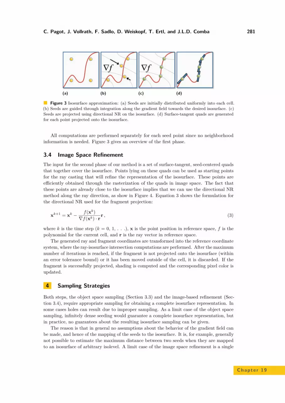
Figure 3 Isosurface approximation: (a) Seeds are initially distributed uniformly into each cell.(b) Seeds are guided through integration along the gradient field towards the desired isosurface. (c)Seeds are projected using directional NR on the isosurface. (d) Surface-tangent quads are generatedfor each point projected onto the isosurface.

All computations are performed separately for each seed point since no neighborhoodinformation is needed. Figure 3 gives an overview of the first phase.

3.4 Image Space RefinementThe input for the second phase of our method is a set of surface-tangent, seed-centered quadsthat together cover the isosurface. Points lying on these quads can be used as starting pointsfor the ray casting that will refine the representation of the isosurface. These points areefficiently obtained through the rasterization of the quads in image space. The fact thatthese points are already close to the isosurface implies that we can use the directional NRmethod along the ray direction, as show in Figure 4. Equation 3 shows the formulation forthe directional NR used for the fragment projection:

xk+1 = xk − f(xk)∇f(xk) · rr , (3)

where k is the time step (k = 0, 1, . . .), x is the point position in reference space, f is thepolynomial for the current cell, and r is the ray vector in reference space.

The generated ray and fragment coordinates are transformed into the reference coordinatesystem, where the ray-isosurface intersection computations are performed. After the maximumnumber of iterations is reached, if the fragment is not projected onto the isosurface (withinan error tolerance bound) or it has been moved outside of the cell, it is discarded. If thefragment is successfully projected, shading is computed and the corresponding pixel color isupdated.

4 Sampling Strategies

Both steps, the object space sampling (Section 3.3) and the image-based refinement (Sec-tion 3.4), require appropriate sampling for obtaining a complete isosurface representation. Insome cases holes can result due to improper sampling. As a limit case of the object spacesampling, infinitely dense seeding would guarantee a complete isosurface representation, butin practice, no guarantees about the resulting isosurface sampling can be given.

The reason is that in general no assumptions about the behavior of the gradient field canbe made, and hence of the mapping of the seeds to the isosurface. It is, for example, generallynot possible to estimate the maximum distance between two seeds when they are mappedto an isosurface of arbitrary isolevel. A limit case of the image space refinement is a single

Chapte r 19

282 Interactive Isocontouring of High-Order Surfaces

(a) (b)

Figure 4 Isosurface refinement: (a) Quads are rasterized in image space. (b) Each fragment isprojected against the isosurface through directional Newton-Raphson.

quad that spans the complete screen, which would be equivalent to a ray casting approach.This would lead to the typically low performance of these methods due to computationallyexpensive root finding along the viewing rays. Our method operates between the twomentioned limit cases. To motivate the parametrization and a sampling technique, we willfirst discuss the relevant issues and implications that arise in the context of sampling.

4.1 Sampling IssuesThe proposed approach suffers from the fact that the fragments are processed independentlyand therefore it is impossible to detect, and to directly fix holes in the isosurface. Holes canbe caused by different reasons:

1. the root finding may fail, e.g. due to insufficient iteration count,2. the root finding may deliver a point on a nearby isosurface if the quad is not well aligned

with the isosurface, i.e. the isosurface exhibits too high curvature with respect to theinitial sampling,

3. the quad sizes are insufficient.

The first cause is hard to address explicitly because the efficiency of our method relies onsynchronized root finding and hence constant iteration count (see Section 5.2). However, thisreason is typically negligible. Because we use quads that are aligned with the tangent planeof the isosurface at each sampling seed, the second case depends only on the quality of theinitial sampling and the last one on the quad sizes. The initial sampling has to be performedeach time the isolevel is changed and therefore the exploration of isocontours requires highperformance for this operation. This makes the use of expensive approaches not feasible forthis step. Unfortunately, it is generally not possible to find a distribution of the seeds for theobject space sampling that leads to uniformly sampled isosurfaces for all possible isovalues.This makes non-uniform quad sizes for the image space refinement necessary.

Therefore, we propose a method for estimating sufficient quad sizes in Section 4.2 andplace the seeds for the object space sampling regularly inside each cell. One problem isthat even comparably large quads cannot guarantee hole-free coverage of the isosurfacebecause the sampling points can be arbitrarily distant due to the possible intricacy of thegradient field. Additionally, large quads typically lead to high overdraw and hence to loweredperformance. All in all, a balance has to be found between the number of initial seeds forthe object space sampling and the sizes of the quads.

For approximate results at high performance that can serve as a preview to more expensivebut robust methods such as that by Knoll et al. [6], the sampling in object space can be

C. Pagot, J. Vollrath, F. Sadlo, D. Weiskopf, T. Ertl, and J.L.D. Comba 283

parametrized and the size for the quads can be derived from that sampling as shown inSection 6. As an alternative, we now propose a method to estimate conservative quad sizesfor individual quads.

4.2 Estimating Quad Sizes using FTLEA method to determine quad sizes that guarantees a complete covering of the isosurfacesunder the assumption of an appropriate object-space sampling can be derived from dynamicalsystems theory. The finite-time (or local) Lyapunov exponent (FTLE) was originally definedto measure the predictability of dynamical systems [9, 5]. More precisely, it measures theexponential growth that a perturbation undergoes when it is advected for a finite timeinterval in a vector field. The flow map φT (x), which maps a sample point x to its advectedposition φT (x) after advection time T , is the basis for the Cauchy-Green deformation tensor∇φT (x). Using

∆T (x) = (∇φT (x))> · ∇φT (x) (4)

and λmax being the largest eigenvalue, leads to the finite-time Lyapunov exponent [5]:

σT (x) = 1|T |

ln√λmax(∆T (x)) . (5)

For our application, we are only interested in the growth of the distance between twoseeds as they are guided by the gradient field and therefore we omit the normalization byadvection time and the logarithm in Eq. 5. Additionally, since we look for points on theisosurfaces, i.e. the intersections of isosurfaces with gradient field lines starting at the seeds,the integration along the field lines shall not be limited by integration time (or length).Instead, it has to be limited by the prescribed isolevel l. We define φl(x) to be mapping theposition x to the isosurface of isolevel l along the corresponding gradient field line (the fieldline is stopped if a critical point of the gradient field is reached). Using Eq. 5, this wouldlead to the separation factor

sl(x) =√λmax(∆l(x)) . (6)

We follow a direct approach for evaluating sl(x). To avoid numerical issues and to be ableto exclude certain seeding neighbors n ∈ N (x) of x, as described below, the computation ofsl(x) is not based on the gradient of φl(x), but it is calculated directly:

sl(x) = maxn∈N (x)

||φl(n)− φl(x)||||n− x|| . (7)

The quad size d(x) at φl(x) is sl(x) times the corresponding seeding distance ||n−x||. Ifthe resolution of the object space sampling is appropriate, using these quad sizes guaranteesa complete covering of the isosurface at level l. For obtaining quad sizes that are appropriatefor any isolevel, the maximum separation s(x) over all isolevels, computed in a preprocessingstep, is used to determine the quad sizes:

s(x) = maxlmin≤l≤lmax

sl(x) . (8)

This quantity relates to the FTLE maximum by Sadlo and Peikert [15]. Unfortunately,neighboring seeds can get mapped to different isosurface parts, making the resulting quad sizes

Chapte r 19

284 Interactive Isocontouring of High-Order Surfaces

too conservative. This leads to unnecessary overdraw during rendering and hence lowers theoverall performance. As a remedy, we propose a heuristic that reduces the overdraw causedby these cases. The idea is to exclude neighbors of x from the computation of s(x), that arenot located in its vicinity on the same isosurface. There are several possible approaches fordetecting if two points are adjacent on the same isosurface. The straightforward approachwould be to compute the geodesic distance between the points along the isosurface. However,this is considered impractical and too expensive.

A criterion for testing if a mapped point φl(x) and its mapped neighbors φl(n),n ∈ N (x)are located close to each other on the same isosurface can be motivated by the fact that thegradient is always aligned with the isosurface normal. To test if a point and its neighbor arelocated on the same isosurface, the behavior of the gradient field is analyzed on the straightline connecting them. If the isosurface is planar between the two points, the line follows theisosurface and intersects the gradient field everywhere perpendicularly. If, on the other hand,the isosurface is non-planar between the points or if the points even lie on different isosurfaceregions, there are positions on the segment where the gradient is not perpendicular. Weintroduce the following measure amin for the minimum angle between the gradient and thesegment sn going from x to n:

amin = maxt∈[0,1]

|sn · ∇s(x + tsn)|/(||sn||||∇s(x + tsn)||) . (9)

Then, the neighbor n is excluded from the computation if amin exceeds a user-definedthreshold. In practice, this threshold can be typically set to 0.5 for suppressing most ofthe erroneous neighbors in order to prevent too conservative quad sizes and reduce theperformance loss due to overdraw.

5 Implementation

The design of iHOS was to take full advantage of parallel architectures. Although our currentimplementation runs on a single GPU, it could be easily distributed over a GPU cluster. Westart by first describing the data structures used. Afterwards we go into the details of theimplementation.

5.1 Data Storage

For the early cell culling we use an interval-tree [2] that stores the extrema of the scalarfield for each cell. This tree is stored and processed on the CPU side. The remaining datastructures are stored on the GPU through the use of different buffers. Each time the userselects a different isovalue, we need to load the initial set of uniformly distributed seedsand compute the isosurface approximation. Thus we allocate two seed arrays on the GPU:one with the initial unprojected seeds and another to store the projected seeds. For eachunprojected seed, its corresponding FTLE value is stored as its w coordinate. Actually, thoseseed arrays are implemented as vertex buffer objects (VBOs). We refer to V BOunproj for theVBO with unprojected seeds and V BOquads for the VBO that stores the quads. Polynomial,gradient, and cell boundary data are read-only and are made available for GLSL through theuse of bindable uniform buffer objects (BUBOs). Since BUBOs are limited in size (usually64KB) we chose to create a separate BUBO for each cell and to bind them on demand.

C. Pagot, J. Vollrath, F. Sadlo, D. Weiskopf, T. Ertl, and J.L.D. Comba 285

5.2 GLSL ShadersBoth phases of the algorithm are implemented through a set of shader programs. The firststep of the algorithm is implemented through a GLSL program composed of a vertex shaderand a geometry shader. The vertex shader reads the V BOunproj and projects the seeds ontothe isosurface (Section 3.3). These seeds are streamed up to the geometry shader and used togenerate surface tangent quads. The quads are resized accordingly to the FTLE value of theseed (Section 5.1). In order to record the generated quads into the V BOquads we interruptthe pipeline just after the geometry shader through the use an OpenGL extension calledTransform Feedback (or stream-out in DirectX terminology). The GLSL program responsiblefor the second step is composed of a vertex and a fragment shader. The vertex shader justredirects the vertices of the quads to the rasterization stage. The fragment shader implementsthe core of the second step. It performs a ray casting using the input fragment as the startingpoint for the root-finding iterations (Section 3.4). As said before, fragments that are notsucessfully projected are discarded. However, it must be observed that fragments successfullyprojected onto the isosurface are only shaded according to the new position, without havingtheir depth coordinate updated. This procedure greatly increases method’s performance byallowing the use of the early-z test. A side effect of this approach is that some noise canappear on some regions of the isosurface. This happens because a fragment closer to thecamera can be projected on a far surface, being thus wrongly shaded. This effect is greatlyreduced through the comparison between the angles of the polynomial gradient vectors atthe fragment positions before and after projection. If the two angles differ above a certainvalue, it is assumed that the fragment jumped to another surface. In this case one have justto discard the fragment. In both steps, the shaders must compute several evaluations of thepolynomials and their gradients. A shader capable of evaluating a general polynomial withan arbitrary degree should contain a loop that could not be unrolled by the compiler. Toincrease performance, we decided to keep several versions of these shaders, each one targetedto a specific polynomial degree. For the polynomial evaluation itself we use static expressionsgenerated by a multivariate Horner scheme approach [1]. We decided to keep the number ofintegration and NR iterations static in order to reinforce thread synchronization, increasingperformance.

5.3 Computation FlowWhen the user chooses a desired isovalue the cells containing the isovalue are selected. Thesecells are inserted in a separate list and arranged in front-to-back order through fast sortingthat does not have to be exact. This ordering is not necessary, but it helps the second step ofthe algorithm to avoid processing occluded fragments, increasing performance. The shaderscorresponding to the polynomial degree of the current cell are activated. The correspondingBUBO (containing the polynomial, gradient, and boundary data) for the current cell isbound and the seeds are projected. After all seeds are projected, we start with the secondstep. Again, the cell list is traversed, and now the ray casting shaders and correspondingBUBOs are bound. Fragments successfully projected onto the isosurface are recorded in theframe buffer.

6 Results

Results and performance measurements were obtained on a computer with an Intel Core 2Quad 2.4GHz processor, with 4GB of RAM, Linux operating system, and NVidia GeForce

Chapte r 19

286 Interactive Isocontouring of High-Order Surfaces

Figure 5 Renderings of isovalue ≈ 2 with varying qs. From left to right, the sq value andcorresponding frames per second (fps) are: sq = 0.75 and 45 fps, sq = 1.0 and 39 fps, sq = 1.25 and29 fps.

8800 GTX video card. To demonstrate the method we used synthetic data and two densitydatasets generated by hp-adaptive Discontinuous Galerkin flow simulations. The scalar fieldsof all datasets are defined analytically by a multivariate polynomial defined in the referencespace in a monomial basis of the form:

P (x) =∑

i+j+k<=n

cijkxiyjzk (10)

with i, j, k ∈ N0, the maximum order n, the coefficients cijk, and the reference spacecoordinates x, y, z. The mapping functions for all datasets include only translations. Thesmaller dataset is composed of 119 hexahedral cells with polynomial degrees varying between5 and 6. The larger dataset is composed of 34,535 convex polyhedral cells (tetrahedra, prisms,and hexahedra) with a scalar field defined by degree 3 polynomials.

6.1 PerformanceFor each phase of the algorithm a set of parameters can be adjusted. For the first phase theseparameters are the number of initial seeds (ns), number of integration steps (ni), numberof NR steps (nN1), and the error for the NR projections (ε1). For the second phase theparameters that can be adjusted are the number of NR steps (nN2), the scale factor forthe quad size (sq), and the error for the NR projections (ε2). Although the great numberof parameters may be confusing at first, they offer great flexibility to the user, allowingthe tuning towards accuracy or interactivity. From our experience we observed also that ingeneral one can explore both accuracy and performance by adjusting just a few of them,keeping the others fixed. For all presented measurements we used screen resolutions of 10242

pixels.All renderings were made with active early cell culling and with front-to-back ordering

for the cells. Figure 5 shows performance measurements for the small dataset. The fixedparameters, and their respective values, are: ns = 103, ni = 50, nN1 = 10, ε1 = 10−3,nN2 = 3 and ε2 = 10−4. These values were chosen through trial-and-error. The only variableparameter is sq. Due to early cell culling only 16 cells (≈ 7.43% of the total) were processed.The results of Figure 6 show performance measurements for the bigger dataset. The fixedparameters are: ns = 83, ni = 50, nN1 = 10, ε1 = 10−3, nN2 = 3 and ε2 = 10−4. Thesevalues were also chosen through trial-and-error. Again, the only variable parameter is sq.Due to early cell culling 3,781 cells (≈ 9.13% of the total) were processed.

C. Pagot, J. Vollrath, F. Sadlo, D. Weiskopf, T. Ertl, and J.L.D. Comba 287

Figure 6 Renderings of isovalue ≈ 0.9983 with varying sq. From left to right, rendering andzoomed images with the following sq value and corresponding frames per second (fps): sq = 0.5 and21 fps, sq = 0.75 and 14 fps, sq = 1.0 and 12.5 fps.

Figure 7 Performance vs. number of cells. The non-linearity can be explained by the use of theearly-z test, which avoids the processing of occluded fragments.

Figure 7 shows how the method scales with respect to the number of cells. Thesemeasurements were made with degree 3 polynomials extracted from the bigger dataset. Itcan be seen that the rendering cost does not grow linearly. This can be explained by the useof the early-z test, which avoids the processing of fragments or even cells that are totallyoccluded. This behavior is reinforced since we use front-to-back ordering for the cells. Wemay still have some overdraw since we do not order the quads inside the cell. However, fromour experiments, this has not affected significantly the performance in the general case.

The method proposed by Knoll et al. [6] may look, at first, as a competing approach.Despite the fact that their method is meant for the robust rendering of implicits, it is fastand could be applied separately to each cell of our datasets. Figure 8 shows a comparisonbetween our method and Knoll’s for the rendering of a single cell of our small dataset.Visual inspection shows that our method is able to achieve higher framerates at betterimage quality. One reason for the difference in performance is probably related to the extracost involved with the use of inclusion arithmetic in Knoll’s method. Although the use ofinclusion arithmetic guarantees error bounds for the results, it tends to produce inferiorresults if larger error bounds are used. Since we are not primarily interested in the control ofaccuracy, we rely on the direct evaluation of the original polynomial representation, which iscomputationally cheaper and thus can be used in a previewing system.

Regarding the time spent to recompute the object space approximation at each isovaluechange, for all our tests, they took less than 2 seconds. In the case of the smaller dataset,it takes less than 1 second to recompute the seed projection. All measurements were madewith 50 integration iterations and 10 NR iterations.

Chapte r 19

288 Interactive Isocontouring of High-Order Surfaces

Figure 8 Comparison with Knoll’s method. (left) Polynomial of degree 5 rendered by our methodat ≈ 30 fps. With the standard settings (depth = 10 and error = 0), Knoll’s method rendered thisimage at ≈ 8 fps without visible artifacts. (right) After optimization of their parameters (depth =4 and error = 0) to reach the best possible image quality at ≈ 30 fps. Both images rendered in a10242 pixel screen.

6.2 Isocontouring Quality

As a previewing system the proposed method does not focus on high accuracy. Nevertheless,it is capable of delivering results of reasonable quality. Figure 9 shows a comparison betweenimages generated by our method and the same images generated by POV Ray, a well known,tested, and freely available ray tracer [12]. The discontinuities observed in these renderingsare due the Discontinuous Galerkin method used to compute the simulations. Our methodhandles continuous data properly, as can be seen in Figure 10.

Despite the reasonable quality of the images, one may want to have better visual qualityfor the isocontouring. In such cases the user can switch to a robust isocontouring system,as the one proposed by Knoll et al. [6]. However, we have also developed some heuristicsin order to allow our method to generate better quality images. The quality of the finalsampling depends on the relation between the number of seeds and the size of the quads.The exact relation between these two parameters is difficult to assess since the projectionchanges seed density. The FTLE-based heuristic tries to estimate “optimal” quad sizes that

Figure 9 Comparison against POV Ray. (left) Image generated with our method, with thefollowing settings: ns = 103, ni = 50, nN1 = 10, ε1 = 10−3, nN2 = 3, ε2 = 10−4, sq = 1.5 andisovalue ≈ 5.8437. This scene was rendered at 8.7fps. (right) Reference image generated from thesame dataset and same isovalue with POV Ray. Both images rendered at 10242 pixels.

C. Pagot, J. Vollrath, F. Sadlo, D. Weiskopf, T. Ertl, and J.L.D. Comba 289

Figure 10 Rendering of Tangle dataset sampled with a grid of 43 = 64 cells (left). The datasetis continuous inside and across cells. Zoomed image (right) shows how our method handles thecontinuity at the borders correctly. Settings for this rendering are: ns = 103, ni = 50, nN1 = 10,ε1 = 10−3, nN2 = 3, and ε2 = 10−4. The isovalue is ≈ −1.98. Image was rendered at 10242 with≈ 9.6 fps.

(a) (b) (c) (d) (e) (f)

Figure 11 Sampling issues related to quad size: (a) Standard quads reduced to 30% of originalsize. (b) Sampling using standard quads: some artifacts can be seen due to poor sampling. (c)Quads scaled by the FTLE and reduced to 30% of their size. (d) Sampling obtained with quadsresized by the FTLE approach. (e) Quads resized by our FTLE approach in conjunction with aheuristic that reduces its conservativeness, reduce in 30%. (f) Sampling obtained with our FTLEapproach in conjunction with the heuristic.

“work” for all isovalues considering an initial seeding given by the user. Since the FTLEdoes not take into account the topology of the isosurface, it can be too conservative, byconsidering distances between seeds in disjoint surfaces. For this case we adopt a test thatestimates whether points are in disjoint surfaces (Section 4.2). Figure 11 illustrates thesampling problems related to bad seeding/quad size relation and how our heuristic resizesthe splats according to that seeding, reducing effectively the artifacts in the final image. Italso illustrates the effect of our disjoint-surfaces test on reducing the FTLE conservativeness.Despite the fact that it improves the quality of the final rendering, the FTLE makes themethod less attractive for previewing since it reduces its performance.

7 Conclusion and Future Work

This work has presented iHOS, an interactive approach for isocontouring higher-order datagenerated by hp-adaptive discretization methods. The method operates with high-order datawhose mapping function includes only rotation, translation, reflection, and scaling. The

Chapte r 19

290 Interactive Isocontouring of High-Order Surfaces

method does not rely on complex data structures and does not resample the original datainto lower-order representations. Results are presented for datasets composed by convexcells. However, since no cross-cell rays are used, the method can be easily adapted to workwith concave cells through the use of a more general point-in-polyhedron test. Althoughnot meant to generate accurate images, the presented results show that general quality ofthe generated images is good. Several parameters can be adjusted in order to control thetrade-off between efficiency and accuracy; it has been shown that one can explore both(accuracy and performance) by adjusting just a few parameters, keeping the others at fixedvalues. Some points should be addressed in future work: further reduction of the overdrawduring quad rasterization, development of an improved initial seed distribution heuristic forthe first phase, handling of large datasets, optimizations for subpixel cells and handling ofnon-linear mapping functions between reference and world spaces. For future work we alsoplan to adapt this method to handle dynamic datasets.

AcknowledgementsWe thank our colleagues from the Institut für Aero- und Gasdynamik from UniversitätStuttgart, Germany, for their continuous support and for providing datasets. We also thankAaron Knoll for kindly providing code for performance tests and comparisons, and theanonymous reviewers for their comments and insightful suggestions. C.A. Pagot wouldlike to acknowledge the support of CAPES-Brazil (Probral 3192/08-3) and CNPq-Brazil(140238/2007-7).

References1 Martine Ceberio and Vladik Kreinovich. Greedy algorithms for optimizing multivariate

Horner schemes. ACM SIGSAM Bulletin, 38(1):8–15, 2004.2 P. Cignoni, P. Marino, C. Montani, E. Puppo, and R. Scopigno. Speeding up isosurface ex-

traction using interval trees. IEEE Transactions on Visualization and Computer Graphics,3(2):158–170, 1997.

3 Luiz Henrique de Figueiredo, Jonas de Miranda Gomes, Demetri Terzopoulos, and LuizVelho. Physically-based methods for polygonization of implicit surfaces. In Proceedings ofGraphics Interface ’92, pages 250–257, 1992.

4 B. Haasdonk, M. Ohlberger, M. Rumpf, A. Schmidt, and K. G. Siebert. Multiresolutionvisualization of higher order adaptive finite element simulations. Computing, 70(3):181–204,2003.

5 G. Haller. Distinguished material surfaces and coherent structures in three-dimensionalfluid flows. Physica D, 149(4):248–277, 2001.

6 Aaron Knoll, Younis Hijazi, Andrew Kensler, Mathias Schott, Charles D. Hansen, and HansHagen. Fast ray tracing of arbitrary implicit surfaces with interval and affine arithmetic.Computer Graphics Forum, 28(1):26–40, 2009.

7 Yuri Levin and Adi Ben-Israel. Directional Newton methods in n variables. Mathematicsof Computation, 71(237):251–262, 2002.

8 William E. Lorensen and Harvey E. Cline. Marching cubes: A high resolution 3D surfaceconstruction algorithm. ACM SIGGRAPH Computer Graphics, 21(4):163–169, 1987.

9 E. N. Lorenz. A study of the predictability if a 28-variable atmospheric model. Tellus,17:321–333, 1965.

10 M. Meyer, B. Nelson, R. M. Kirby, and R. Whitaker. Particle systems for efficient andaccurate high-order finite element visualization. IEEE Transactions on Visualization andComputer Graphics, 13(5):1015–1026, 2007.

C. Pagot, J. Vollrath, F. Sadlo, D. Weiskopf, T. Ertl, and J.L.D. Comba 291

11 Blake Nelson and Robert M. Kirby. Ray-tracing polymorphic multidomain spectral/hp ele-ments for isosurface rendering. IEEE Transactions on Visualization and Computer Graph-ics, 12(1):114–125, 2006.

12 Povray. Persistence of Vision Raytracer. Website, 2009. http://www.povray.org.13 W. Reed and T. Hill. Triangular mesh methods for the neutron transport equation. Tech-

nical Report LA-UR-73-479, Los Alamos Scientific Laboratory, 1973.14 B. Remacle, N. Chevaugeon, É. Marchandise, and C. Geuzaine. Efficient visualization of

high order finite elements. International Journal for Numerical Methods in Engineering,69(4):750–771, 2006.

15 Filip Sadlo and Ronald Peikert. Efficient visualization of Lagrangian coherent structuresby filtered AMR ridge extraction. IEEE Transactions on Visualization and ComputerGraphics, 13(5):1456–1463, 2007.

16 William J. Schroeder, Francois Bertel, Mathieu Malaterre, David Thompson, Philippe P.Pebay, Robert O’Bara, and Saurabh Tendulkar. Framework for visualizing higher-orderbasis functions. In Proceedings of the IEEE Visualization Conference, pages 43–50, 2005.

17 William J. Schroeder, Francois Bertel, Mathieu Malaterre, David Thompson, Philippe P.Pebay, Robert O’Bara, and Saurabh Tendulkar. Methods and framework for visualizinghigher-order finite elements. IEEE Transactions on Visualization and Computer Graphics,12(4):446–460, 2006.

18 Kees van Kooten, Gino van den Bergen, and Alex Telea. GPU Gems 3, chapter Point-basedvisualization of metaballs on a GPU. Addison-Wesley,Nguyen, Hubert, 2007.

19 David F. Wiley, Hank Childs, Bernd Hamann, and Kenneth I. Joy. Ray casting curved-quadratic elements. In VISSYM’04: Proceedings of the Symposium on Data Visualisation,pages 201–210, 2004.

20 Andrew P. Witkin and Paul S. Heckbert. Using particles to sample and control implicitsurfaces. In Proceedings of ACM SIGGRAPH 1994, pages 269–277, 1994.

21 Yuan Zhou and Michael Garland. Interactive point-based rendering of higher-order tetra-hedral data. IEEE Transactions on Visualization and Computer Graphics, 12(5):1229–1236,2006.

Chapte r 19