J5.10 INTERACTION OF NOCTURNAL LOW-LEVEL JETS WITH URBAN

GEOMETRIES AS SEEN IN JOINT URBAN 2003 DATA

Julie K. Lundquist* and Jeffrey D. Mirocha Lawrence Livermore National Laboratory

Livermore, California 94551, USA

1. INTRODUCTION

The nocturnal low-level jet (LLJ) is a well-

documented phenomenon around the world. The LLJ has been studied in great detail in the southern Great Plains of the United States (Bonner 1968, Whiteman et al. 1997, Banta et al., 2002, Song et al. 2005), where it efficiently transports moisture, momentum, and air pollutants throughout the Great Plains (Higgens et al 1997). In the canonical case first described by Blackadar (1957), the nocturnal LLJ forms as the release of daytime convective turbulent stresses allows nighttime winds above a stable boundary layer to accelerate to supergeostrophic wind speeds. In situations with surface winds of less than 5 m/s, wind speeds at altitudes of 100m due to the nocturnal LLJ can be greater than 20 m/s. The turbulence generated by this wind shear can induce nocturnal mixing events and enhance surface-atmosphere exchange, thereby influencing the dispersion of hazardous materials near the surface.

In urban areas, the complicated atmospheric

dispersion of hazardous materials is often simulated using high-resolution, building-resolving computational fluid dynamics (CFD) models such as Lawrence Livermore National Laboratory’s FEM3MP model. Because such simulations are often driven by boundary conditions described only by an upwind profile, and because boundary conditions at the top of the model domain often forbid vertical transport of momentum from outside the simulation domain, the turbulence generated by LLJs or other mesoscale phenomena is not represented in these simulations. The inclusion of the effects of such phenomena in building-scale simulations requires coupling between CFD models and mesoscale models, which is an active area of research (Chan 2004, Chan and Leach 2004, Coirier et al. 2005, Pullen et al. 2005, Tewari et al. 2005). The consequences of including or excluding mesoscale effects remain undetermined and probably vary from case to case.

*Corresponding author address: J. K.Lundquist, Lawrence Livermore National Laboratory, P.O. Box 808, L-103, Livermore, CA 94551, e-mail: jkl@llnl.gov.

Given the prevalence of the LLJ in the Southern Great Plains and the sound physical justification for including its effects in simulations of dispersion in the urban boundary layer, the success of a simulation excluding the effects of the LLJ would be surprising. A rich dataset is available for testing such urban boundary layer dispersion simulations from the Joint URBAN 2003 (JU2003) tracer experiment based in the Oklahoma City area. Despite the exclusion of mesoscale phenomena like the LLJ, FEM3MP simulations of the first release of JU2003 Intensive Observing Period (IOP) 9 agree well with observations of near-field winds and concentrations and of turbulence profiles in the urban wake region (Chan and Lundquist, 2005; Lundquist and Chan, 2005). That result motivates further investigation into the significance of mesoscale phenomena like the LLJ to urban transport and dispersion.

This study presents data describing the

frequency, intensity, and degree of surface-layer forcing induced by LLJs throughout the JU2003 experiment. We explore other nighttime tracer releases for indications of top-down boundary layer development that would affect the performance of CFD models when not driven with mesoscale model input that includes phenomena like the nocturnal LLJ. Finally, we explore in detail IOPs 8 and 9, two nocturnal tracer releases which exhibit different jet behavior and jet effects on the surface layer.

2. THE JOINT URBAN 2003 FIELD STUDY

To provide quality-assured, high-resolution meteorological and tracer data sets for the evaluation and validation of indoor and outdoor urban dispersion models, the U.S. DHS and DoD – Defense Threat Reduction Agency (DTRA) co-sponsored a series of dispersion experiments, named Joint URBAN 2003, in Oklahoma City (OKC), Oklahoma, during July 2003 (Allwine et al., 2004). These experiments provide a comprehensive field data set for the evaluation of CFD and other dispersion models.

The Joint URBAN 2003 (JU2003) experiment

consisted of ten IOPs throughout late June and July of 2003. Six of the IOPs consisted of daytime releases of sulfur hexafluoride tracer gas, both continuous and instantaneous releases. Four of the

IOPs (IOPs 6-10) occurred overnight. In addition to the tracer releases in the downtown Oklahoma City area, JU2003 participants collected extensive meteorological data characterizing the urban environment on the microscale (individual street canyons) and mesoscale. The present study considers the mesoscale properties of the LLJ using data from one of three boundary-layer wind profilers that were deployed in the Oklahoma City region. This profiler, operated and maintained by Pacific Northwest National Lab, was located about 2 km SSW of the downtown area.

To explore the microscale variability of the LLJ

and its effect on turbulent mixing events, we use wind and turbulence data from the LLNL crane pseudo-tower, which was located approximately 750m NNW of the downtown area, often in the urban wake region (Lundquist, 2004). Eight sonic anemometers were mounted along this pseudo-tower, from 8-84m above the surface.

The mesoscale LLJ dataset from PNNL,

available at the JU2003 web archive, http://ju2003-dpg.dpg.army.mil, extends from Julian Day (JD) 181 to 212. The dataset has been treated by PNNL with the NCAR Improved Moments Algorithm (NIMA) (Morse et al., 2002) to reduce or eliminate contamination of the wind speed data due to clutter or non-atmospheric interference. Nights corresponding to JD181 and 212 were eliminated from consideration due to missing data. Julian Days 202, 203, and 211 exhibited characteristics of frontal passages or other dramatic rotation overnight, and were thus not considered. The total boundary-layer wind profiler dataset thus consisted of twenty-seven nights from JD182 to JD 210, excluding JD 202 and 203. Data below 300m are not available due to noise in the radar signal due to ground clutter.

The microscale dataset from the LLNL crane

pseudo-tower consists of mean and fluctuating velocity and virtual temperature measurements from the eight sonic anemometers mounted between 8 and 84 m, described in Lundquist (2004). Turbulence statistics presented here were calculated over 30-minute intervals. The turbulent dissipation rate was calculated using the inertial dissipation method as described in Piper and Lundquist (2004).

3. OCCURRENCES OF LLJS DURING JU2003

Observations of wind speed and wind direction

obtained from the PNNL 915 MHz boundary-layer wind profiler, located south of the Oklahoma City central business district, indicate the regular appearance of the LLJ during July 2003. To qualify as a “jet night”, the wind speed profile in the lowest 1000m accelerates after sunset, attaining a maximum wind speed typically between 700 and

1000 UTC (200 and 500 LT). We also apply the minimum criteria used in other climatological studies of LLJs, that the maximum wind speed in a profile surpass a threshold of 10 m/s (category LLJ-0 in Whiteman et al. 1997 and Song et al. 2005, for example), with a decrease above the wind speed maximum of at least 5 m/s. Of the twenty-seven nights examined, only four nights (JDs 182, 192, 193, and 204) do not exhibit wind profiles consistent with those of LLJs. The twenty-three LLJ nights are not subdivided into categories as in Whiteman et al. (1997) and Song et al. (2005) because of the small numbers of nights examined.

3.1 Example of LLJ Evolution

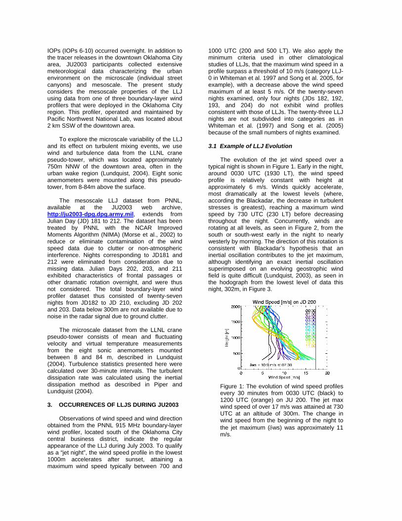
The evolution of the jet wind speed over a

typical night is shown in Figure 1. Early in the night, around 0030 UTC (1930 LT), the wind speed profile is relatively constant with height at approximately 6 m/s. Winds quickly accelerate, most dramatically at the lowest levels (where, according the Blackadar, the decrease in turbulent stresses is greatest), reaching a maximum wind speed by 730 UTC (230 LT) before decreasing throughout the night. Concurrently, winds are rotating at all levels, as seen in Figure 2, from the south or south-west early in the night to nearly westerly by morning. The direction of this rotation is consistent with Blackadar’s hypothesis that an inertial oscillation contributes to the jet maximum, although identifying an exact inertial oscillation superimposed on an evolving geostrophic wind field is quite difficult (Lundquist, 2003), as seen in the hodograph from the lowest level of data this night, 302m, in Figure 3.

Figure 1: The evolution of wind speed profiles every 30 minutes from 0030 UTC (black) to 1200 UTC (orange) on JU 200. The jet max wind speed of over 17 m/s was attained at 730 UTC at an altitude of 300m. The change in wind speed from the beginning of the night to the jet maximum (δws) was approximately 11 m/s.

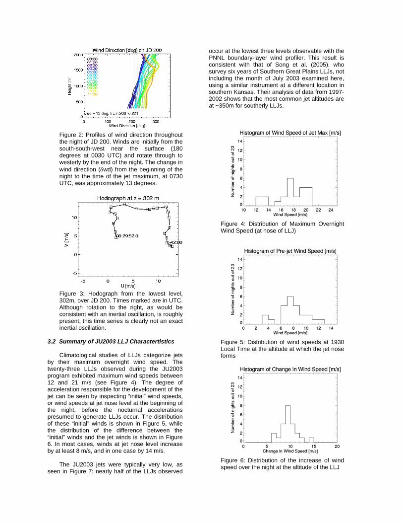
Figure 2: Profiles of wind direction throughout the night of JD 200. Winds are initially from the south-south-west near the surface (180 degrees at 0030 UTC) and rotate through to westerly by the end of the night. The change in wind direction (δwd) from the beginning of the night to the time of the jet maximum, at 0730 UTC, was approximately 13 degrees.

Figure 3: Hodograph from the lowest level, 302m, over JD 200. Times marked are in UTC. Although rotation to the right, as would be consistent with an inertial oscillation, is roughly present, this time series is clearly not an exact inertial oscillation.

3.2 Summary of JU2003 LLJ Charactertistics Climatological studies of LLJs categorize jets

by their maximum overnight wind speed. The twenty-three LLJs observed during the JU2003 program exhibited maximum wind speeds between 12 and 21 m/s (see Figure 4). The degree of acceleration responsible for the development of the jet can be seen by inspecting “initial” wind speeds, or wind speeds at jet nose level at the beginning of the night, before the nocturnal accelerations presumed to generate LLJs occur. The distribution of these “initial” winds is shown in Figure 5, while the distribution of the difference between the “initial” winds and the jet winds is shown in Figure 6. In most cases, winds at jet nose level increase by at least 8 m/s, and in one case by 14 m/s.

The JU2003 jets were typically very low, as

seen in Figure 7: nearly half of the LLJs observed

occur at the lowest three levels observable with the PNNL boundary-layer wind profiler. This result is consistent with that of Song et al. (2005), who survey six years of Southern Great Plains LLJs, not including the month of July 2003 examined here, using a similar instrument at a different location in southern Kansas. Their analysis of data from 1997-2002 shows that the most common jet altitudes are at ~350m for southerly LLJs.

Figure 4: Distribution of Maximum Overnight Wind Speed (at nose of LLJ)

Figure 5: Distribution of wind speeds at 1930 Local Time at the altitude at which the jet nose forms

Figure 6: Distribution of the increase of wind speed over the night at the altitude of the LLJ

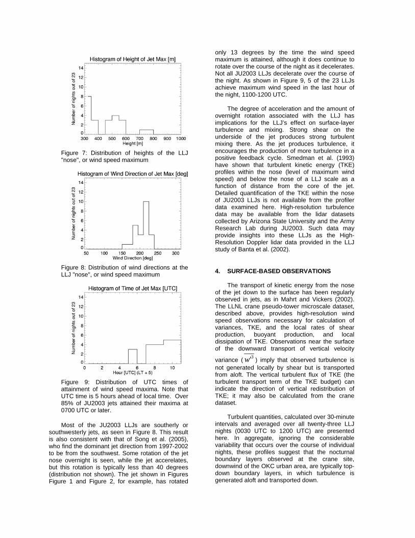
Figure 7: Distribution of heights of the LLJ "nose", or wind speed maximum

Figure 8: Distribution of wind directions at the LLJ "nose", or wind speed maximum

Figure 9: Distribution of UTC times of attainment of wind speed maxima. Note that UTC time is 5 hours ahead of local time. Over 85% of JU2003 jets attained their maxima at 0700 UTC or later. Most of the JU2003 LLJs are southerly or

southwesterly jets, as seen in Figure 8. This result is also consistent with that of Song et al. (2005), who find the dominant jet direction from 1997-2002 to be from the southwest. Some rotation of the jet nose overnight is seen, while the jet accerelates, but this rotation is typically less than 40 degrees (distribution not shown). The jet shown in Figures Figure 1 and Figure 2, for example, has rotated

only 13 degrees by the time the wind speed maximum is attained, although it does continue to rotate over the course of the night as it decelerates. Not all JU2003 LLJs decelerate over the course of the night. As shown in Figure 9, 5 of the 23 LLJs achieve maximum wind speed in the last hour of the night, 1100-1200 UTC.

The degree of acceleration and the amount of

overnight rotation associated with the LLJ has implications for the LLJ’s effect on surface-layer turbulence and mixing. Strong shear on the underside of the jet produces strong turbulent mixing there. As the jet produces turbulence, it encourages the production of more turbulence in a positive feedback cycle. Smedman et al. (1993) have shown that turbulent kinetic energy (TKE) profiles within the nose (level of maximum wind speed) and below the nose of a LLJ scale as a function of distance from the core of the jet. Detailed quantification of the TKE within the nose of JU2003 LLJs is not available from the profiler data examined here. High-resolution turbulence data may be available from the lidar datasets collected by Arizona State University and the Army Research Lab during JU2003. Such data may provide insights into these LLJs as the High-Resolution Doppler lidar data provided in the LLJ study of Banta et al. (2002).

4. SURFACE-BASED OBSERVATIONS

The transport of kinetic energy from the nose of the jet down to the surface has been regularly observed in jets, as in Mahrt and Vickers (2002). The LLNL crane pseudo-tower microscale dataset, described above, provides high-resolution wind speed observations necessary for calculation of variances, TKE, and the local rates of shear production, buoyant production, and local dissipation of TKE. Observations near the surface of the downward transport of vertical velocity

variance ( 3'w ) imply that observed turbulence is not generated locally by shear but is transported from aloft. The vertical turbulent flux of TKE (the turbulent transport term of the TKE budget) can indicate the direction of vertical redistribution of TKE; it may also be calculated from the crane dataset.

Turbulent quantities, calculated over 30-minute

intervals and averaged over all twenty-three LLJ nights (0030 UTC to 1200 UTC) are presented here. In aggregate, ignoring the considerable variability that occurs over the course of individual nights, these profiles suggest that the nocturnal boundary layers observed at the crane site, downwind of the OKC urban area, are typically top-down boundary layers, in which turbulence is generated aloft and transported down.

The averaged profile of vertical velocity is seen

in Figure 10, in which negative values indicate downward motion. Considerable subsiding vertical motions are seen at the upper levels of the crane. These values are about three times larger than those observed in large-scale descriptions of boundary-layer subsidence (Yi et al., 2001), and may be representative rather of either forcing from the LLJ or motions characteristic of the urban wake region.

A typical characterization of the upside-down

boundary layer is that the standard deviation of vertical velocity is larger at higher levels than at lower levels, as discussed in Mahrt and Vickers (2002). As shown in Figure 11, values of this parameter at the top of the crane are 30% higher than closer to the surface, again suggesting top-down forcing of the boundary layer, consistent with the hypothesis that shear from the underside of a LLJ generates turbulence that is transported down into the boundary layer.

Figure 10: Averaged profile of vertical velocity from 0030 UTC to 1200 UTC for the 23 LLJ nights of JU2003

Figure 11: Averaged profile of standard deviation of vertical velocity from 0030 UTC to 1200 UTC for the 23 LLJ nights of JU2003

Figure 12: Averaged profile of TKE from 0030 UTC to 1200 UTC for the 23 LLJ nights of JU2003 The profile of TKE is shown in Figure 12.

Although the mean profile clearly indicates higher values of TKE aloft, as compared to values close to the surface, the range of TKE values over these 23 nights is large, with a standard deviation of 14% at the 8m level and 33% at the 83m level. If the dominant mechanism producing TKE in these profiles was only the effect of the urban area and turbulent mixing generated by flow through that urban matrix, then we would expect TKE profiles that decrease with height (see Figure 11 in companion paper 5.11, Chan & Lundquist 2005) or remain constant with height.

Finally, the vertical transport of vertical velocity

variance ( 3'w ), or the skewness of the vertical velocity can indicate the net downward transport of kinetic energy from the nose of the jet to the surface, as in Mahrt and Vickers (2002). Large positive values, as seen here, indicate continuous downward motions with very intermittent pauses or breaks in the mixing. The significant increase of this term with height (Figure 13), coupled with the mean downward vertical velocity (Figure 10), indicates significant downward transport of TKE. This downward transport is also seen in the higher

values of ew' at upper levels of the crane than at lower levels of the crane (Figure 14).

In summary, the averaged microscale

observations from the crane pseudo-tower on the nights with LLJ activity indicate significant downward transport of momentum and TKE on these nights. Individual nights exhibit variability in these quantities, especially during the course of the night. Variability can be induced by several factors, including the magnitude of the shear associated with the LLJ. In the following section, we contrast the two IOPs, each featuring similar LLJs but with different turbulence characteristics. These two nights have been simulated with the FEM3MP CFD code, with different degrees of success.

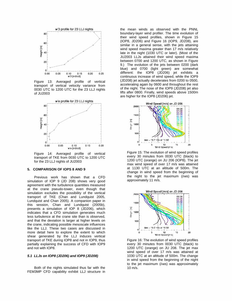
Figure 13: Averaged profile of vertical transport of vertical velocity variance from 0030 UTC to 1200 UTC for the 23 LLJ nights of JU2003

Figure 14: Averaged profile of vertical transport of TKE from 0030 UTC to 1200 UTC for the 23 LLJ nights of JU2003

5. COMPARISON OF IOPS 8 AND 9 Previous work has shown that a CFD

simulation of IOP 9 (JD 208) shows very good agreement with the turbulence quantities measured at the crane pseudo-tower, even though that simulation excludes the possibility of the vertical transport of TKE (Chan and Lundquist 2005, Lundquist and Chan 2005). A companion paper in this session, Chan and Lundquist (2005b), presents a simulation of IOP 8 (JD206), which indicates that a CFD simulation generates much less turbulence at the crane site than is observed, and that the deviation is larger at higher levels on the crane, indicating possible mesoscale influences like the LLJ. These two cases are discussed in more detail here to explore the extent to which shear generated by the LLJ induces vertical transport of TKE during IOP8 and not in IOP9, thus partially explaining the success of CFD with IOP9 and not with IOP8.

5.1 LLJs on IOP8 (JD206) and IOP9 (JD208)

Both of the nights simulated thus far with the

FEM3MP CFD capability exhibit LLJ structure in

the mean winds as observed with the PNNL boundary-layer wind profiler. The time evolution of their wind speed profiles, shown in Figure 15 (IOP8, JD206) and Figure 16 (IOP9, JD208), are similar in a general sense, with the jets attaining wind speed maxima greater than 17 m/s relatively late in the night (1030 UTC or later). (Most of the JU2003 LLJs attained their wind speed maxima between 0700 and 1200 UTC, as shown in Figure 9.) The evolution of the jets between 0200 (dark blue) and 0700 (light green) are somewhat different: the IOP8 (JD206) jet exhibits a continuous increase of wind speed, while the IOP9 (JD208) jet actually decelerates from 0200 to 0500, accelerating again by 0600 and throughout the rest of the night. The nose of the IOP9 (JD208) jet also lifts after 0800. Finally, wind speeds above 1500m are higher for the IOP8 (JD206) jet.

Figure 15: The evolution of wind speed profiles every 30 minutes from 0030 UTC (black) to 1200 UTC (orange) on JU 206 (IOP8). The jet max wind speed of over 17 m/s was attained at 1130 UTC at an altitude of 500m. The change in wind speed from the beginning of the night to the jet maximum (δws) was approximately 11 m/s.

Figure 16: The evolution of wind speed profiles every 30 minutes from 0030 UTC (black) to 1200 UTC (orange) on JU 208. The jet max wind speed of over 17 m/s was attained at 1030 UTC at an altitude of 500m. The change in wind speed from the beginning of the night to the jet maximum (δws) was approximately 10 m/s.

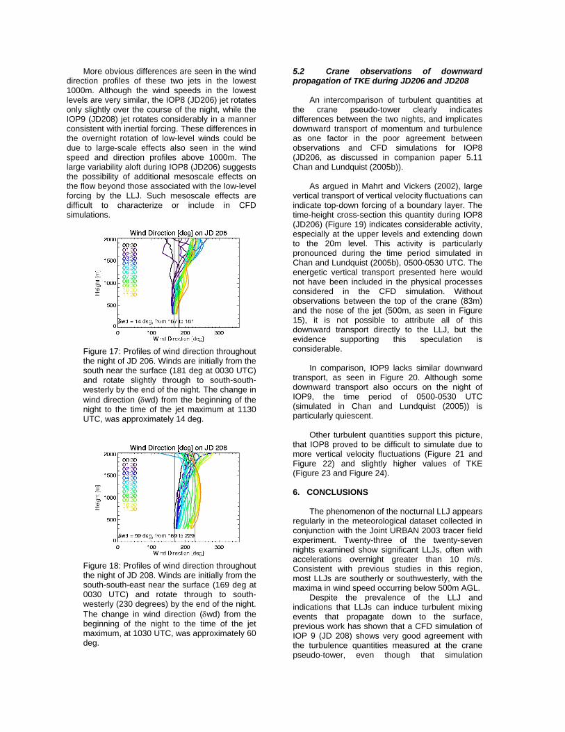
More obvious differences are seen in the wind direction profiles of these two jets in the lowest 1000m. Although the wind speeds in the lowest levels are very similar, the IOP8 (JD206) jet rotates only slightly over the course of the night, while the IOP9 (JD208) jet rotates considerably in a manner consistent with inertial forcing. These differences in the overnight rotation of low-level winds could be due to large-scale effects also seen in the wind speed and direction profiles above 1000m. The large variability aloft during IOP8 (JD206) suggests the possibility of additional mesoscale effects on the flow beyond those associated with the low-level forcing by the LLJ. Such mesoscale effects are difficult to characterize or include in CFD simulations.

Figure 17: Profiles of wind direction throughout the night of JD 206. Winds are initially from the south near the surface (181 deg at 0030 UTC) and rotate slightly through to south-south-westerly by the end of the night. The change in wind direction (δwd) from the beginning of the night to the time of the jet maximum at 1130 UTC, was approximately 14 deg.

Figure 18: Profiles of wind direction throughout the night of JD 208. Winds are initially from the south-south-east near the surface (169 deg at 0030 UTC) and rotate through to south-westerly (230 degrees) by the end of the night. The change in wind direction (δwd) from the beginning of the night to the time of the jet maximum, at 1030 UTC, was approximately 60 deg.

5.2 Crane observations of downward propagation of TKE during JD206 and JD208

An intercomparison of turbulent quantities at

the crane pseudo-tower clearly indicates differences between the two nights, and implicates downward transport of momentum and turbulence as one factor in the poor agreement between observations and CFD simulations for IOP8 (JD206, as discussed in companion paper 5.11 Chan and Lundquist (2005b)).

As argued in Mahrt and Vickers (2002), large

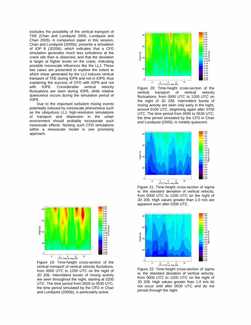
vertical transport of vertical velocity fluctuations can indicate top-down forcing of a boundary layer. The time-height cross-section this quantity during IOP8 (JD206) (Figure 19) indicates considerable activity, especially at the upper levels and extending down to the 20m level. This activity is particularly pronounced during the time period simulated in Chan and Lundquist (2005b), 0500-0530 UTC. The energetic vertical transport presented here would not have been included in the physical processes considered in the CFD simulation. Without observations between the top of the crane (83m) and the nose of the jet (500m, as seen in Figure 15), it is not possible to attribute all of this downward transport directly to the LLJ, but the evidence supporting this speculation is considerable.

In comparison, IOP9 lacks similar downward

transport, as seen in Figure 20. Although some downward transport also occurs on the night of IOP9, the time period of 0500-0530 UTC (simulated in Chan and Lundquist (2005)) is particularly quiescent.

Other turbulent quantities support this picture,

that IOP8 proved to be difficult to simulate due to more vertical velocity fluctuations (Figure 21 and Figure 22) and slightly higher values of TKE (Figure 23 and Figure 24).

6. CONCLUSIONS

The phenomenon of the nocturnal LLJ appears

regularly in the meteorological dataset collected in conjunction with the Joint URBAN 2003 tracer field experiment. Twenty-three of the twenty-seven nights examined show significant LLJs, often with accelerations overnight greater than 10 m/s. Consistent with previous studies in this region, most LLJs are southerly or southwesterly, with the maxima in wind speed occurring below 500m AGL.

Despite the prevalence of the LLJ and indications that LLJs can induce turbulent mixing events that propagate down to the surface, previous work has shown that a CFD simulation of IOP 9 (JD 208) shows very good agreement with the turbulence quantities measured at the crane pseudo-tower, even though that simulation

excludes the possibility of the vertical transport of TKE (Chan and Lundquist 2005, Lundquist and Chan 2005). A companion paper in this session, Chan and Lundquist (2005b), presents a simulation of IOP 8 (JD206), which indicates that a CFD simulation generates much less turbulence at the crane site than is observed, and that the deviation is larger at higher levels on the crane, indicating possible mesoscale influences like the LLJ. These two cases are presented to explore the extent to which shear generated by the LLJ induces vertical transport of TKE during IOP8 and not in IOP9, thus explaining the success of CFD with IOP9 and not with IOP8. Considerable vertical velocity fluctuations are seen during IOP8, while relative quiescence occurs during the simulation period of IOP9.

Due to the important turbulent mixing events potentially induced by mesoscale phenomena such as the ubiquitous LLJ, high-resolution simulations of transport and dispersion in the urban environment should probably incorporate such mesoscale effects. Nesting such CFD simulations within a mesoscale model is one promising approach.

Figure 19: Time-height cross-section of the vertical transport of vertical velocity fluctations, from 0000 UTC to 1200 UTC on the night of JD 206. Intermittent bursts of mixing activity are seen throughout the night, starting at 0200 UTC. The time period from 0500 to 0530 UTC, the time period simulated by the CFD in Chan and Lundquist (2005b), is particularly active.

Figure 20: Time-height cross-section of the vertical transport of vertical velocity fluctuations, from 0000 UTC to 1200 UTC on the night of JD 208. Intermittent bursts of mixing activity are seen only early in the night, around 0100 UTC, beginning again after 0700 UTC. The time period from 0500 to 0530 UTC, the time period simulated by the CFD in Chan and Lundquist (2005), is notably quiescent.

Figure 21: Time-height cross-section of sigma w, the standard deviation of vertical velocity, from 0000 UTC to 1200 UTC on the night of JD 206. High values greater than 1.0 m/s are apparent soon after 0200 UTC.

Figure 22: Time-height cross-section of sigma w, the standard deviation of vertical velocity, from 0000 UTC to 1200 UTC on the night of JD 208. High values greater than 1.0 m/s do not occur until after 0530 UTC and do not persist through the night.

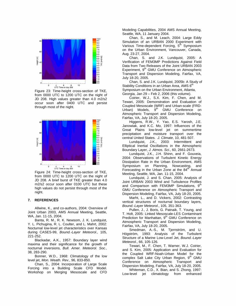
Figure 23: Time-height cross-section of TKE, from 0000 UTC to 1200 UTC on the night of JD 208. High values greater than 4.0 m2/s2 occur soon after 0400 UTC and persist through most of the night.

Figure 24: Time-height cross-section of TKE, from 0000 UTC to 1200 UTC on the night of JD 208. A brief burst of TKE greater than 4.0 m2/s2 occur soon after 0100 UTC but these high values do not persist through most of the night.

7. REFERENCES Allwine, K., and co-authors, 2004: Overview of

Joint Urban 2003, AMS Annual Meeting, Seattle, WA, Jan. 11-15, 2004.

Banta, R. M., R. K. Newsom, J. K. Lundquist, Y. L. Pichugina, R. L. Coulter, and L. Mahrt, 2002: Nocturnal low-level jet characteristics over Kansas during CASES-99, Bound.-Layer Meteorol., 105, 221-252.

Blackadar, A.K., 1957: Boundary layer wind maxima and their significance for the growth of nocturnal inversions, Bull. Amer. Meteorol. Soc., 38, 283-290.

Bonner, W.D., 1968: Climatology of the low level jet, Mon. Weath. Rev., 96, 833-850.

Chan, S., 2004: Incorporation of Large Scale Forcing into a Building Scale CFD Model. Workshop on Merging Mesoscale and CFD

Modeling Capabilities, 2004 AMS Annual Meeting, Seattle, WA, 11 January 2004.

Chan, S., and M. Leach, 2004: Large Eddy Simulation of an URBAN 2000 Experiment with Various Time-dependent Forcing, 5th Symposium on the Urban Environment, Vancouver, Canada, Aug. 23-27, 2004.

Chan, S. and J.K. Lundquist, 2005: A Verification of FEM3MP Predictions Against Field Data from Two Releases of the Joint URBAN 2003 Experiment, 9th GMU Conference on Atmospheric Transport and Dispersion Modeling, Fairfax, VA, July 18-20, 2005.

Chan, S. and J.K. Lundquist, 2005b: A Study of Stability Conditions in an Urban Area, AMS 6th Symposium on the Urban Environment, Atlanta, Georgia, Jan 29 – Feb 2, 2006 (this volume).

Coirier, W.J., S.X. Kim, F. Chen, and M. Tewari, 2005: Demonstration and Evaluation of Coupled Mesoscale (WRF) and Urban-scale (FRD-Urban) Models, 9th GMU Conference on Atmospheric Transport and Dispersion Modeling, Fairfax, VA, July 18-20, 2005.

Higgens, R.W., Y. Yao, E.S. Yarosh, J.E. Janowiak, and K.C. Mo, 1997: Influences of the Great Plains low-level jet on summertime precipitation and moisture transport over the central United States. J. Climate, 10, 481-507.

Lundquist, J.K., 2003: Intermittent and Elliptical Inertial Oscillations in the Atmospheric Boundary Layer, J. Atmos. Sci., 60, 2661-2673.

Lundquist, J.K., J.H. Shinn, and F. Gouveia, 2004: Observations of Turbulent Kinetic Energy Dissipation Rate in the Urban Environment, AMS Symposium on Planning, Nowcasting, and Forecasting in the Urban Zone at the 84th Annual Meeting, Seattle, WA, Jan. 11-15, 2004.

Lundquist, J. and S. Chan, 2005: Analysis of Joint URBAN 2003 Wind and Turbulence Profiles and Comparison with FEM3MP Simulations, 9th GMU Conference on Atmospheric Transport and Dispersion Modeling, Fairfax, VA, July 18-20, 2005.

Marht, L., and D. Vickers, 2002: Contrasting vertical structures of nocturnal boundary layers, Bound.-Layer Meteorol., 105, 351-363.

Pullen, J., J. Boris, G. Patnaik, T. Young, and T. Holt, 2005: Linked Mesoscale-LES Contaminant Prediction for Manhattan, 9th GMU Conference on Atmospheric Transport and Dispersion Modeling, Fairfax, VA, July 18-20, 2005.

Smedman, A.-S., M. Tjernström, and U. Högström, 1993: Analysis of the Turbulent Structure of a Marine Low-Level Jet, Bound.-Layer Meteorol., 66, 105-126.

Tewari, M., F. Chen, T. Warner, W.J. Coirier, and S. Kim, 2005: Application and Evaluation for the Coupled WRF-Noah-Urban Model for the complex Salt Lake City Urban Region, 9th GMU Conference on Atmospheric Transport and Dispersion Modeling, Fairfax, VA, July 18-20, 2005.

Whiteman, C.D., X. Bian, and S. Zhong, 1997: Low-level jet climatology from enhanced

rawindsonde observations at a site in the southern Great Plains, J. Appl. Meteorol., 36, 1363-1376.

Yi, C., K. J. Davis, B.W. Berger, and P.W. Bakwin, 2001: Long-Term Observations of the Dynamics of the Continental Planetary Boundary Layer, J. Atmos. Sci., 58, 1288-1299.

Zeierman, S., and M. Wolfshtein, 1986: Turbulent Time Scale for Turbulent-Flow Calculations, AIAA Journal, 24, 1606-1610.

ACKNOWLEDGEMENTS

This work was performed under the auspices of the U.S. Department of Energy by the University of California, Lawrence Livermore National Laboratory under contract No. W-7405-Eng-48. The authors greatly appreciate the quality-controlled and NIMA-processed boundary-layer wind profiler dataset provided by Will Shaw, Larry Berg, and Stephan de Wekker of PNNL.