intelligent control for brake systems

188 IEEE TRANSACTIONS ON CONTROL SYSTEMS TECHNOLOGY, VOL. 7, NO. 2, MARCH 1999

Intelligent Control for Brake SystemsWilliam K. Lennon and Kevin M. Passino,Senior Member, IEEE

Abstract—There exist several problems in the control of brakesystems including the development of control logic for antilockbraking systems (ABS) and “base-braking.” Here, we studythe base-braking control problem where we seek to develop acontroller that can ensure that the braking torque commandedby the driver will be achieved. In particular, we develop a “fuzzymodel reference learning controller,” a “genetic model referenceadaptive controller,” and a “general genetic adaptive controller,”and investigate their ability to reduce the effects of variationsin the process due to temperature. The results are compared tothose found in previous research.

Index Terms—Adaptive control, automotive, brakes, fuzzy con-trol, genetic algorithms.

I. INTRODUCTION

A UTOMOTIVE antilock braking systems (ABS) are de-signed to stop vehicles as safely and quickly as possible.

Safety is achieved by maintaining lateral stability (and hencesteering effectiveness) and trying to reduce braking distancesover the case where the brakes are controlled by the driver.Current ABS designs typically use wheel speed compared tothe velocity of the vehicle to measure when wheels lock (i.e.,when there is “slip” between the tire and the road) and usethis information to adjust the duration of brake signal pulses(i.e., to “pump” the brakes). Essentially, as the wheel slipincreases past a critical point where it is possible that lateralstability (and hence our ability to steer the vehicle) could belost, the controller releases the brakes. Then, once wheel sliphas decreased to a point where lateral stability is increased andbraking effectiveness is decreased, the brakes are reapplied.In this way the ABS cycles the brakes to try to achieve anoptimum tradeoff between braking effectiveness and lateralstability. Inherent process nonlinearities, limitations on ourabilities to sense certain variables, and uncertainties associatedwith process and environment (e.g., road conditions changingfrom wet asphalt to ice) make the ABS control problemchallenging. Many successful proprietary algorithms exist forthe control logic for ABS. In addition, several conventionalnonlinear control approaches have been reported in the openliterature (see, e.g., [1] and [2]), and even one intelligentcontrol approach has been investigated [3].

Manuscript received July 29, 1996; revised September 29, 1997. Recom-mended by Associate Editor, K. Passion. This work was supported in partby Delphi Chassis Division of General Motors, the Center for AutomotiveResearch (CAR) at Ohio State University, and National Science Foundationunder Grants IRI9210332 and EEC9315257.

The authors are with the Department of Electrical Engineering, Ohio StateUniversity, Columbus, OH 43210 USA.

Publisher Item Identifier S 1063-6536(99)01618-8.

In this paper, we do not consider brake control for a“panic stop,” and hence for our study the brakes are in anon-ABS mode. Instead, we consider what is referred to asthe “base-braking” control problem where we seek to havethe brakes perform consistently as the driver (or an ABS)commands, even though there may be aging of components orenvironmental effects (e.g., temperature or humidity changes)which can cause “brake grab” or “brake fade.” We seek todesign a controller that will try to ensure that the brakingtorque commanded by the driver (related to how hard we hitthe brakes) is achieved by the brake system. Clearly, solvingthe base braking problem is of significant importance sincethere is a direct correlation between safety and the reliabilityof the brakes in providing the commanded stopping force.Moreover, base braking algorithms would run in parallel withABS controllers so that they could also enhance brakingeffectiveness while in ABS mode.

Prior research on the braking system considered here hasshown that one of the primary difficulties with the brakesystem lies in compensating for the effects of changes inthe “specific torque,” to be defined below, that occur due totemperature variations in the brake pads [4]. Previous researchon this system has been conducted using proportional-integral-derivative (PID), lead-lag, autotuning, and model referenceadaptive control (MRAC) techniques [5]. While several ofthese techniques have been highly successful (particularly thelead-lag compensator that we use as a base-line comparisonhere), there is still a need to improve the compensators forthe case where there are changes in specific torque due totemperature variations that result from, for example, repeatedapplication of the brakes. In this paper we investigate theperformance of three intelligent control techniques, fuzzymodel reference learning control [6], genetic model referenceadaptive control [7], [8], and “general genetic adaptive con-trol” [9], for the base braking problem and compare theirperformance to the best results found in [4] and [5]. Weespecially focus on the performance of these techniques whenthere are variations in the specific torque.

In Section II we provide a simulation model for the basebraking system that has proven to be very effective in de-veloping,implementing, and testing control algorithms for theactual braking system [4], [5]. In Section III we develop afuzzy model reference learning controller (FMRLC) for thebase braking system problem. Its performance is evaluated insimulation by comparing it to a lead-lag compensator from [5]under varying specific torque conditions. In Sections IV andV, we develop a genetic model reference adaptive controller(GMRAC) and a general genetic adaptive controller (GGAC)

1063–6536/99$10.00 1999 IEEE

LENNON AND PASSINO: INTELLIGENT CONTROL FOR BRAKE SYSTEMS 189

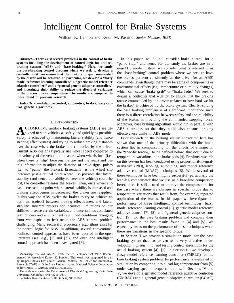
Fig. 1. Base braking control system.

for the base braking problem. We use similar test conditionsfor evaluating the controller and compare its performance tothe previous ones. Numerical performance results are shownin Section VI, and some concluding remarks are provided inSection VII.

II. THE BASE BRAKING CONTROL PROBLEM

Fig. 1 shows the diagram of the base braking system, asdeveloped in [5]. The input to the system, denoted by , isthe braking torque requested by the driver. The output,(in ft-lbs), is the output of a torque sensor, which directlymeasures the torque applied to the brakes. Note that whiletorque sensors are not available on current production vehicles,there is significant interest in determining the advantages ofusing such a sensor. The signal represents the errorbetween the reference input and output torques, which is usedby the controller to create the input to the brake system, .A sampling interval of s was used for all ourinvestigations.

The General Motors braking system used in this researchis physically limited to processing signals between [0,5]V, while the braking torque can range from 0 to 2700 ftlb.For this reason and other hardware specific reasons [5], theinput torque is attenuated by a factor of 2560 and the outputis amplified by the same factor. After is multiplied by2560 it is passed through a saturation nonlinearity where if2560 , the brake system receives a zero input and if2560 then the input is five. The output of the brakesystem passes through a similar nonlinearity that saturates atzero and 2700. The output of this nonlinearity passes through

, which is defined as

The function was experimentally determined and rep-resents the relationship between brake fluid pressure andthe stopping force on the car. Next, is multiplied bythe specific torque . This signal is passed through anexperimentally determined model of the torque sensor; thesignal is scaled and is output. The specific torquein the braking process reflects the variations in the stoppingforce of the brakes as the brake pads increase in temperature.The stopping force applied to the wheels is a function ofthe pressure applied to the brake pads and the coefficient offriction between the brake pads and the wheel rotors. As thebrake pads and rotors increase in temperature, the coefficient

of friction between the brake pads and the rotors increases.As a result, less pressure on the brake pads is required for thesame amount of braking force. The specific torqueof thisbraking system has been found experimentally to lie betweentwo limiting values so that

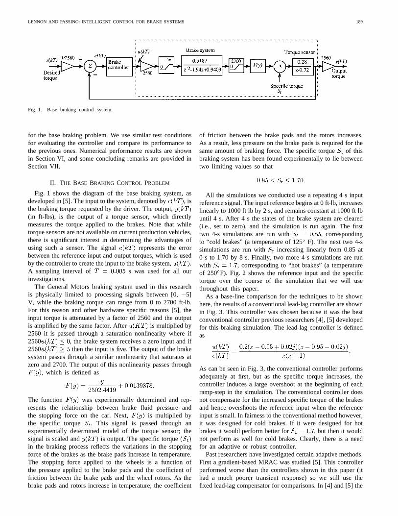
All the simulations we conducted use a repeating 4 s inputreference signal. The input reference begins at 0 ftlb, increaseslinearly to 1000 ftlb by 2 s, and remains constant at 1000 ftlbuntil 4 s. After 4 s the states of the brake system are cleared(i.e., set to zero), and the simulation is run again. The firsttwo 4-s simulations are run with , correspondingto “cold brakes” (a temperature of 125F). The next two 4-ssimulations are run with increasing linearly from 0.85 at0 s to 1.70 by 8 s. Finally, two more 4-s simulations are runwith , corresponding to “hot brakes” (a temperatureof 250 F). Fig. 2 shows the reference input and the specifictorque over the course of the simulation that we will usethroughout this paper.

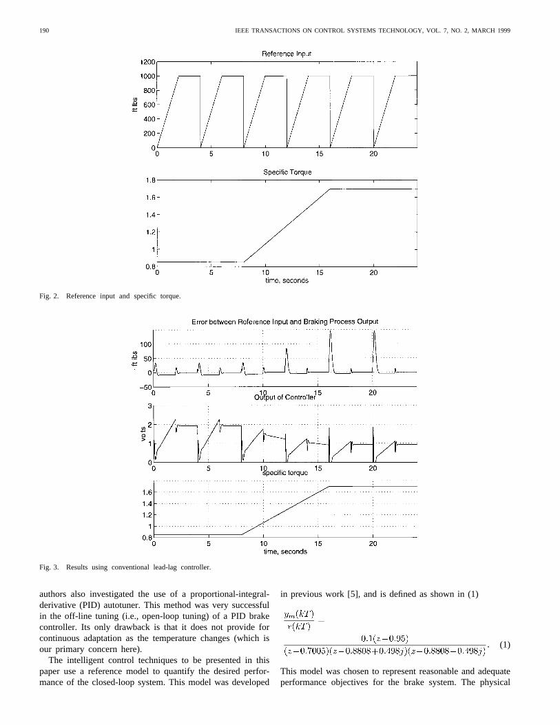
As a base-line comparison for the techniques to be shownhere, the results of a conventional lead-lag controller are shownin Fig. 3. This controller was chosen because it was the bestconventional controller previous researchers [4], [5] developedfor this braking simulation. The lead-lag controller is definedas

As can be seen in Fig. 3, the conventional controller performsadequately at first, but as the specific torque increases, thecontroller induces a large overshoot at the beginning of eachramp-step in the simulation. The conventional controller doesnot compensate for the increased specific torque of the brakesand hence overshoots the reference input when the referenceinput is small. In fairness to the conventional method however,it was designed for cold brakes. If it were designed for hotbrakes it would perform better for , but then it wouldnot perform as well for cold brakes. Clearly, there is a needfor an adaptive or robust controller.

Past researchers have investigated certain adaptive methods.First a gradient-based MRAC was studied [5]. This controllerperformed worse than the controllers shown in this paper (ithad a much poorer transient response) so we still use thefixed lead-lag compensator for comparisons. In [4] and [5] the


Fig. 2. Reference input and specific torque.

Fig. 3. Results using conventional lead-lag controller.

authors also investigated the use of a proportional-integral-derivative (PID) autotuner. This method was very successfulin the off-line tuning (i.e., open-loop tuning) of a PID brakecontroller. Its only drawback is that it does not provide forcontinuous adaptation as the temperature changes (which isour primary concern here).

The intelligent control techniques to be presented in thispaper use a reference model to quantify the desired perfor-mance of the closed-loop system. This model was developed

in previous work [5], and is defined as shown in (1)

(1)

This model was chosen to represent reasonable and adequateperformance objectives for the brake system. The physical


Fig. 4. FMRLC for base braking.

process was taken into consideration in the development ofthis model.

III. A DAPTIVE FUZZY CONTROL

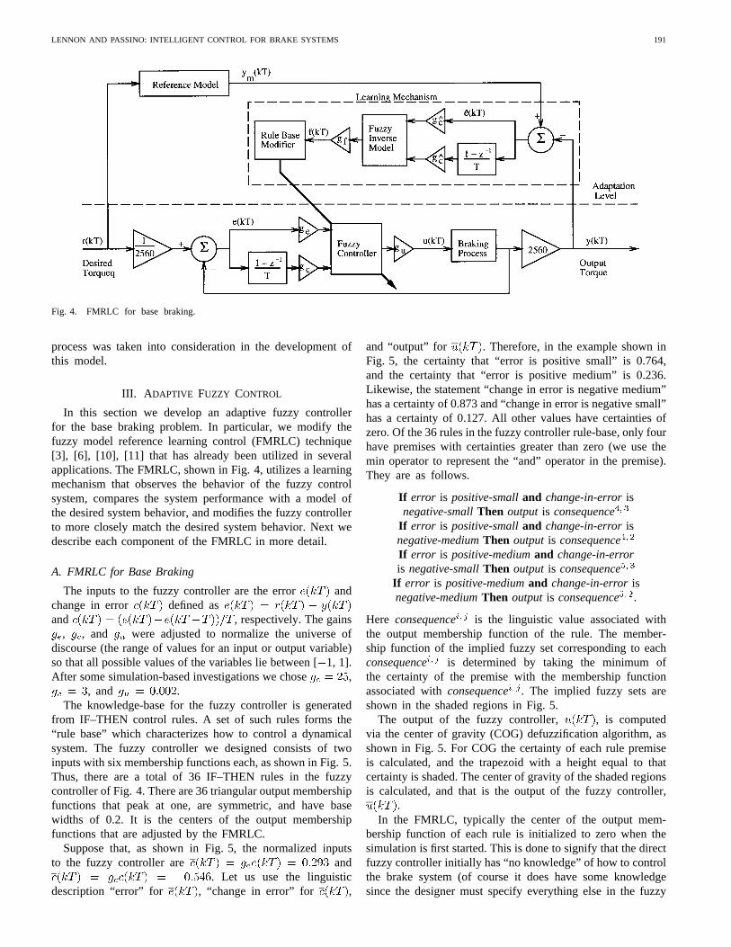
In this section we develop an adaptive fuzzy controllerfor the base braking problem. In particular, we modify thefuzzy model reference learning control (FMRLC) technique[3], [6], [10], [11] that has already been utilized in severalapplications. The FMRLC, shown in Fig. 4, utilizes a learningmechanism that observes the behavior of the fuzzy controlsystem, compares the system performance with a model ofthe desired system behavior, and modifies the fuzzy controllerto more closely match the desired system behavior. Next wedescribe each component of the FMRLC in more detail.

A. FMRLC for Base Braking

The inputs to the fuzzy controller are the error andchange in error defined asand , respectively. The gains

, , and were adjusted to normalize the universe ofdiscourse (the range of values for an input or output variable)so that all possible values of the variables lie between [1, 1].After some simulation-based investigations we chose ,

, and .The knowledge-base for the fuzzy controller is generated

from IF–THEN control rules. A set of such rules forms the“rule base” which characterizes how to control a dynamicalsystem. The fuzzy controller we designed consists of twoinputs with six membership functions each, as shown in Fig. 5.Thus, there are a total of 36 IF–THEN rules in the fuzzycontroller of Fig. 4. There are 36 triangular output membershipfunctions that peak at one, are symmetric, and have basewidths of 0.2. It is the centers of the output membershipfunctions that are adjusted by the FMRLC.

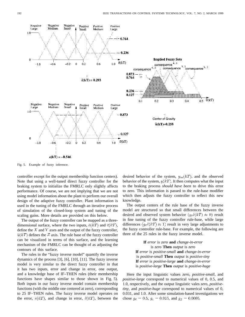
Suppose that, as shown in Fig. 5, the normalized inputsto the fuzzy controller are and

. Let us use the linguisticdescription “error” for , “change in error” for ,

and “output” for . Therefore, in the example shown inFig. 5, the certainty that “error is positive small” is 0.764,and the certainty that “error is positive medium” is 0.236.Likewise, the statement “change in error is negative medium”has a certainty of 0.873 and “change in error is negative small”has a certainty of 0.127. All other values have certainties ofzero. Of the 36 rules in the fuzzy controller rule-base, only fourhave premises with certainties greater than zero (we use themin operator to represent the “and” operator in the premise).They are as follows.

If error is positive-smalland change-in-errorisnegative-smallThen output is consequence

If error is positive-smalland change-in-errorisnegative-mediumThen output is consequenceIf error is positive-mediumand change-in-erroris negative-smallThen output is consequence

If error is positive-mediumand change-in-errorisnegative-mediumThen output is consequence .

Here consequence is the linguistic value associated withthe output membership function of the rule. The member-ship function of the implied fuzzy set corresponding to eachconsequence is determined by taking the minimum ofthe certainty of the premise with the membership functionassociated withconsequence . The implied fuzzy sets areshown in the shaded regions in Fig. 5.

The output of the fuzzy controller, , is computedvia the center of gravity (COG) defuzzification algorithm, asshown in Fig. 5. For COG the certainty of each rule premiseis calculated, and the trapezoid with a height equal to thatcertainty is shaded. The center of gravity of the shaded regionsis calculated, and that is the output of the fuzzy controller,

.In the FMRLC, typically the center of the output mem-

bership function of each rule is initialized to zero when thesimulation is first started. This is done to signify that the directfuzzy controller initially has “no knowledge” of how to controlthe brake system (of course it does have some knowledgesince the designer must specify everything else in the fuzzy


Fig. 5. Example of fuzzy inference.

controller except for the output membership function centers).Note that using a well-tuned direct fuzzy controller for thebraking system to initialize the FMRLC only slightly affectsperformance. Of course, we are not implying that we are notusing model information about the plant to perform our overalldesign of the adaptive fuzzy controller. Plant information isused in the tuning of the FMRLC through an iterative processof simulation of the closed-loop system and tuning of thescaling gains. More details are provided on this below.

The output of the fuzzy controller can be mapped as a three-dimensional surface, where the two inputs, and ,define the and axes and the output of the fuzzy controller,

defines the axis. The rule base of the fuzzy controllercan be visualized in terms of this surface, and the learningmechanism of the FMRLC can be thought of as adjusting thecontours of this surface.

The rules in the “fuzzy inverse model” quantify the inversedynamics of the process [3], [6], [10], [11]. The fuzzy inversemodel is very similar to the direct fuzzy controller in thatit has two inputs, error and change in error, one output,and a knowledge base of IF–THEN rules (their membershipfunctions have shapes similar to those shown in Fig. 5).Both inputs in our fuzzy inverse model contain membershipfunctions (with the middle one centered at zero), correspondingto 25 IF–THEN rules. The fuzzy inverse model operates onthe error, , and change in error, , between the

desired behavior of the system, , and the observedbehavior of the system, . It then computes what the inputto the braking processshould have beento drive this errorto zero. This information is passed to the rule-base modifierwhich then adjusts the fuzzy controller to reflect this newknowledge.

The output centers of the rule base of the fuzzy inversemodel are structured so that small differences between thedesired and observed system behavior resultin fine tuning of the fuzzy controller rule-base, while largedifferences result in very large adjustments tothe fuzzy controller rule-base. For example, the following arethree of the 25 rules in the fuzzy inverse model.

If error is zeroand change-in-erroris zeroThen output is zero

If error is positive-smalland change-in-erroris positive-smallThen output is positive-tinyIf error is positive-largeand change-in-erroris positive-largeThen output is positive-huge

Here the input linguistic valueszero, positive-small, andpositive-largecorrespond to numerical values of 0, 0.5, and1.0, respectively, and the output linguistic valeszero, positive-tiny, and positive-hugecorrespond to numerical values of 0,0.031, and 1.0. After some simulation-based investigations wechose , , and .


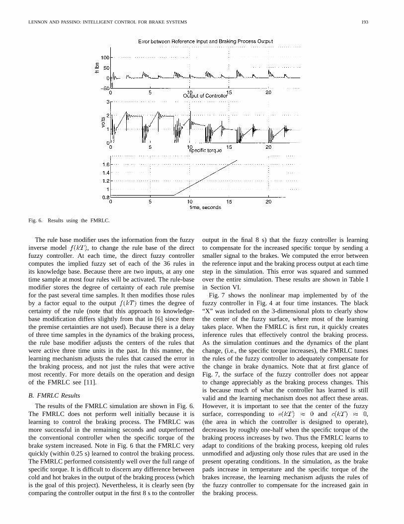
Fig. 6. Results using the FMRLC.

The rule base modifier uses the information from the fuzzyinverse model , to change the rule base of the directfuzzy controller. At each time, the direct fuzzy controllercomputes the implied fuzzy set of each of the 36 rules inits knowledge base. Because there are two inputs, at any onetime sample at most four rules will be activated. The rule-basemodifier stores the degree of certainty of each rule premisefor the past several time samples. It then modifies those rulesby a factor equal to the output times the degree ofcertainty of the rule (note that this approach to knowledge-base modification differs slightly from that in [6] since therethe premise certainties are not used). Because there is a delayof three time samples in the dynamics of the braking process,the rule base modifier adjusts the centers of the rules thatwere active three time units in the past. In this manner, thelearning mechanism adjusts the rules that caused the error inthe braking process, and not just the rules that were activemost recently. For more details on the operation and designof the FMRLC see [11].

B. FMRLC Results

The results of the FMRLC simulation are shown in Fig. 6.The FMRLC does not perform well initially because it islearning to control the braking process. The FMRLC wasmore successful in the remaining seconds and outperformedthe conventional controller when the specific torque of thebrake system increased. Note in Fig. 6 that the FMRLC veryquickly (within 0.25 s) learned to control the braking process.The FMRLC performed consistently well over the full range ofspecific torque. It is difficult to discern any difference betweencold and hot brakes in the output of the braking process (whichis the goal of this project). Nevertheless, it is clearly seen (bycomparing the controller output in the first 8 s to the controller

output in the final 8 s) that the fuzzy controller is learningto compensate for the increased specific torque by sending asmaller signal to the brakes. We computed the error betweenthe reference input and the braking process output at each timestep in the simulation. This error was squared and summedover the entire simulation. These results are shown in Table Iin Section VI.

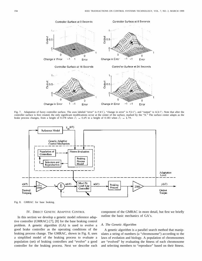
Fig. 7 shows the nonlinear map implemented by of thefuzzy controller in Fig. 4 at four time instances. The black“X” was included on the 3-dimensional plots to clearly showthe center of the fuzzy surface, where most of the learningtakes place. When the FMRLC is first run, it quickly createsinference rules that effectively control the braking process.As the simulation continues and the dynamics of the plantchange, (i.e., the specific torque increases), the FMRLC tunesthe rules of the fuzzy controller to adequately compensate forthe change in brake dynamics. Note that at first glance ofFig. 7, the surface of the fuzzy controller does not appearto change appreciably as the braking process changes. Thisis because much of what the controller has learned is stillvalid and the learning mechanism does not affect these areas.However, it is important to see that the center of the fuzzysurface, corresponding to and ,(the area in which the controller is designed to operate),decreases by roughly one-half when the specific torque of thebraking process increases by two. Thus the FMRLC learns toadapt to conditions of the braking process, keeping old rulesunmodified and adjusting only those rules that are used in thepresent operating conditions. In the simulation, as the brakepads increase in temperature and the specific torque of thebrakes increase, the learning mechanism adjusts the rules ofthe fuzzy controller to compensate for the increased gain inthe braking process.


Fig. 7. Adaptation of fuzzy controller surface. The axes labeled “error” ise(kT ), “change in error” isc(kT ), and “output” isu(kT ). Note that after thecontroller surface is first created, the only significant modifications occur at the center of the surface, marked by the “X.” The surface center adapts as thebrake process changes, from a height of 0.378 whenSt = 0:85 to a height of 0.183 whenSt = 1:70.

Fig. 8. GMRAC for base braking.

IV. DIRECT GENETIC ADAPTIVE CONTROL

In this section we develop a genetic model reference adap-tive controller (GMRAC) [7], [8] for the base braking controlproblem. A genetic algorithm (GA) is used to evolve agood brake controller as the operating conditions of thebraking process change. The GMRAC, shown in Fig. 8, usesa simplified model of the braking process to evaluate apopulation (set) of braking controllers and “evolve” a goodcontroller for the braking process. Next we describe each

component of the GMRAC in more detail, but first we brieflyoutline the basic mechanics of GA’s.

A. The Genetic Algorithm

A genetic algorithm is a parallel search method that manip-ulates a string of numbers (a “chromosome”) according to thelaws of evolution and biology. A population of chromosomesare “evolved” by evaluating the fitness of each chromosomeand selecting members to “reproduce” based on their fitness.


Evolution of the population of individual chromosomes here isbased on four genetic operators: crossover, mutation, selection,and elitism.

Selection is the process where the most fit individualssurvive to reproduce and the weak individuals die out. Theselection process evaluates each chromosome by some fitnessmechanism and assigns it a fitness value. Those individualsdeemed “most fit” are then selected to become parents andreproduce. The selection of which chromosomes will repro-duce is not deterministic, however. Every member of thepopulation has a probability of being selected for reproductionequal to its fitness divided by the sum of the fitness of thepopulation. Hence, the more fit individuals have a greaterchange to reproduce than the less fit individuals. Crossoveris the procedure where two “parent” chromosomes exchangegenetic information (i.e., a section of the string of numbers) toform two chromosome offspring. Crossover can be considereda form of local search in the population space. Mutation isa form of global search where the genetic information ofa chromosome is randomly altered. Elitism is used in theGMRAC to ensure that the most fit member of the populationis moved without modification into the next generation. Byincluding elitism, we can increase the rates of crossover andmutation, thereby increasing the breadth of search, but stillensure that a good controller remains present in the population.

Our genetic algorithm uses the base-10 number systemas opposed to base-2 which is commonly used in [12] and[13]. While base-2 systems can be advantageous because theyconsist of smaller “genetic building blocks,” they have the dis-advantage of more complicated encoding/decoding proceduresand longer strings (which can affect our ability to implementthe genetic adaptive controllers in real time). While both baseswork well, we chose to use base-10 because of the ease inwhich controller parameters can be coded into a chromosome,as described below.

B. GMRAC for Base Braking

In this section, we describe each component of the geneticadaptive mechanism in Fig. 8.

1) The Population of Controllers:The GMRAC uses alead-lag controller which is the best conventional controllerprevious researchers in [4] and [5] have found for this brakingsimulation. The transfer function of this controller is

The gain of the controller was constant at in previousresearch, but will be “evolved” by the GMRAC to adapt tobraking process changes. The range of valid gains has beenlimited to . This is to try to ensure that theGA does not evolve controllers that are unstable orhighly oscillatory .

The controller population size was constant at eight mem-bers. This was a compromise between search speed andprocessing time. In general, as the population size increases,more variety exists in the population and therefore “good”controllers are more likely to be found. However, computationtime is greatly affected by population size, and therefore

the maximum population size is limited by the speed of theprocessor and the sampling interval of the system. Note thatperformance of the GMRAC was not significantly affected bypopulation sizes of six or more. Rather, the GMRAC perfor-mance was more greatly affected by the crossover probability,mutation probability, and the number of time units into thefuture the fitness evaluation attempts to predict (describedbelow).

Each individual controller gain was described by a three-digit base-10 number. Each digit is called a “gene” andthe string of genes together forms the “chromosome.” Thischromosome is very simply decoded into a decimal numbercorresponding the gain of the lead-lag controller. To decodea chromosome, simply place a decimal point before the firstgene of the chromosome. For example, a chromosome of [345]would decode into .

2) Fitness Evaluation and the Braking Process Model:TheGA uses , , , , (and their pastvalues), and a plant model to evaluate the fitness of the stringsin the population of candidate controllers. At each time step(i.e., each “generation”) the GA chooses the controller in thepopulation with maximum fitness value to control the plantfrom time to time .

The process model used in the GMRAC is a simplifiedmodel of the braking process. The model of the plant isdescribed by the transfer function

(2)

Comparing this to the actual model of the brake system inSection II, we see that this model ignores significant nonlin-earities and the “disturbance” (i.e., we treat the model inSection II as the “truth model”).

The genetic algorithm seeks to maximize the fitness function

where

and is the predicted error between the outputs of the plantand reference model. Here denotes the “look ahead” timewindow, signifying that the fitness evaluation attempts to pre-dict the braking process for the next unit samples. Becausethere is significant delay between control input and brakingoutput, a short time window would cause the current controllercandidates to be evaluated mostly on the performance of pastcontrollers, leading to inaccurate fitness evaluations. However,longer time windows cause greater deviations between thebraking process model and the actual braking process, andthis also leads to inaccurate fitness evaluations. We selected

as a good compromise to maintain the validity of thefitness evaluations.

After some simulation-based investigations, we chooseand . The constant defines the number

of time samples in which the error should reach zero. Forexample, if and , then the fitness function is


maximized when , which would indicatethat should reach zero in time steps.

The fitness evaluation proceeds according to the followingpseudocode.

1) Collect , , and .2) Compute a first-order approximation of ,

.3) Estimate the closed-loop system response for the next

samples for each controller in the population:For to :

Generate from braking process model in (2).Estimate .Compute .Generate from , ,

etc., and controller parameters.Next .

4) Compute .5) Assign fitness, , to each controller candidate, :

Let.

6) The maximally fit controller becomes the next controllerused between timesand . The selection, crossover,mutation, and elitism [7] processes are applied to pro-duce the next generation of controllers (see below).Increment the time index and go to Step 1).

3) Selection and Reproduction of Controllers:Once eachcontroller in the population has been assigned a fitness

, the GA uses the “roullete-wheel” selection process[12] to determine which controllers will reproduce into thenext generation. The roullete-wheel selection process picksthe “parents” of the next generation in a manner similarto spinning a roullete-wheel, with each individual in thepopulation assigned an area on the roullete-wheel proportionalto that individual’s fitness. Hence the probability that anindividual will be selected as a particular parent of the nextgeneration is proportional to the fitness of that individual.Note that some individuals will likely be selected more thanonce (indicating they will have more than one offspring),while other individuals will not be selected at all. In thisway the “bad” controllers are generally removed from thepopulation.

Next, the parents are coupled together and generally undergocrossover. The probability that crossover occurs between twoparents is determineda priori by a crossover probability.In our simulation, two parents will undergo crossover withprobability 0.90. Crossover is conducted differently than iscommonly described. In all genetic algorithms used in thesesimulations, crossover is not done by selecting a crossoversite and exchanging genes beginning at the crossover siteand ending at the end of the chromosome. Instead, crossoveris done on a gene-by-gene basis. Each gene (digit) in thechromosome has a 0.5 probability of being exchanged forthe digit in the same location on the mating chromosome.For example, the GA uses a string length of three, so twopossible parent chromosomes could be [333] and [111]. Ifthese two chromosomes undergo crossover, possible offspringpairs could be [113] and [331] or [131] and [313].

After crossover, the two offspring undergo mutation, with aprespecified probability. In the GMRAC, we used a mutationprobability of 0.3, which means every digit in the chromosomehas a 30% probability of being mutated. Note that this isa relatively high mutation probability, but with the elitismoperator ensuring that a good controller is always in thepopulation, a high mutation rate helps to offset the smallpopulation size and improve the searching ability of the GA.Moreover, we have found that since the fitness functionis time varying and the plant is changing in real time, thereis a significant need to make the GA aggressive in exploringvarious regions (i.e., in trying different controller candidates).If it locks on to some controller parameter values and isinflexible to change it will not be successful at adaptation.

C. GMRAC Results

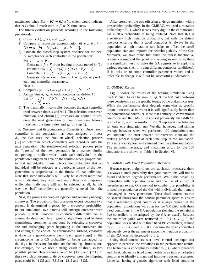
Fig. 9 shows the results of the braking simulation usingthe GMRAC. As can be seen in Fig. 9, the GMRAC performsmore consistently as the specific torque of the brakes increases.While the performance does degrade somewhat as specifictorque increases, at its worst it is still significantly better thanthe conventional controller. Note that contrary to conventionalcontrollers and the FMRLC discussed previously, the GMRACis stochastic, and the results in Fig. 9 represent the behaviorfor only one simulation run. We did, however, find similaraverage behavior when we performed 100 simulation runs.We computed the error between the reference input and thebraking process output at each time step in the simulation.This error was squared and summed over the entire simulation.The minimum, average, and maximum errors for the 100simulations are shown in Table I in Section VI.

D. GMRAC with Fixed Population Members

Because genetic algorithms are stochastic processes, thereis always a small possibility that good controllers will not befound and hence degrade performance. While this possibilitydiminishes with population size and the use of elitism, itnevertheless exists. One method to combat this possibility isto seed the population of the GA with individuals that remainunchanged in every generation. These fixed controllers canbe spaced throughout the control parameter space to ensurethat a reasonably good controller is always present in thepopulation. Simulations were run for the GMRAC with threefixed controllers in the GA population (leaving the remainingfive controllers to be adapted by the GA as usual). Becausethe controller gains were restricted to , thepopulation was seeded with three fixed PD controllers, definedby , , and . Because the fixed controllersadequately cover the parameter space, the mutation probabilityof the GA was be decreased to .

Using fixed controllers is a novel control technique thatappears to decrease the variations in the performance results.The technique is conceptually similar to [14] where Narendraand Balakrishnan use fixed plant models in an indirect adaptivecontroller to identify a plant and improve transient responses.Likewise, having a genetic algorithm with fixed controller


Fig. 9. Results using GMRAC.

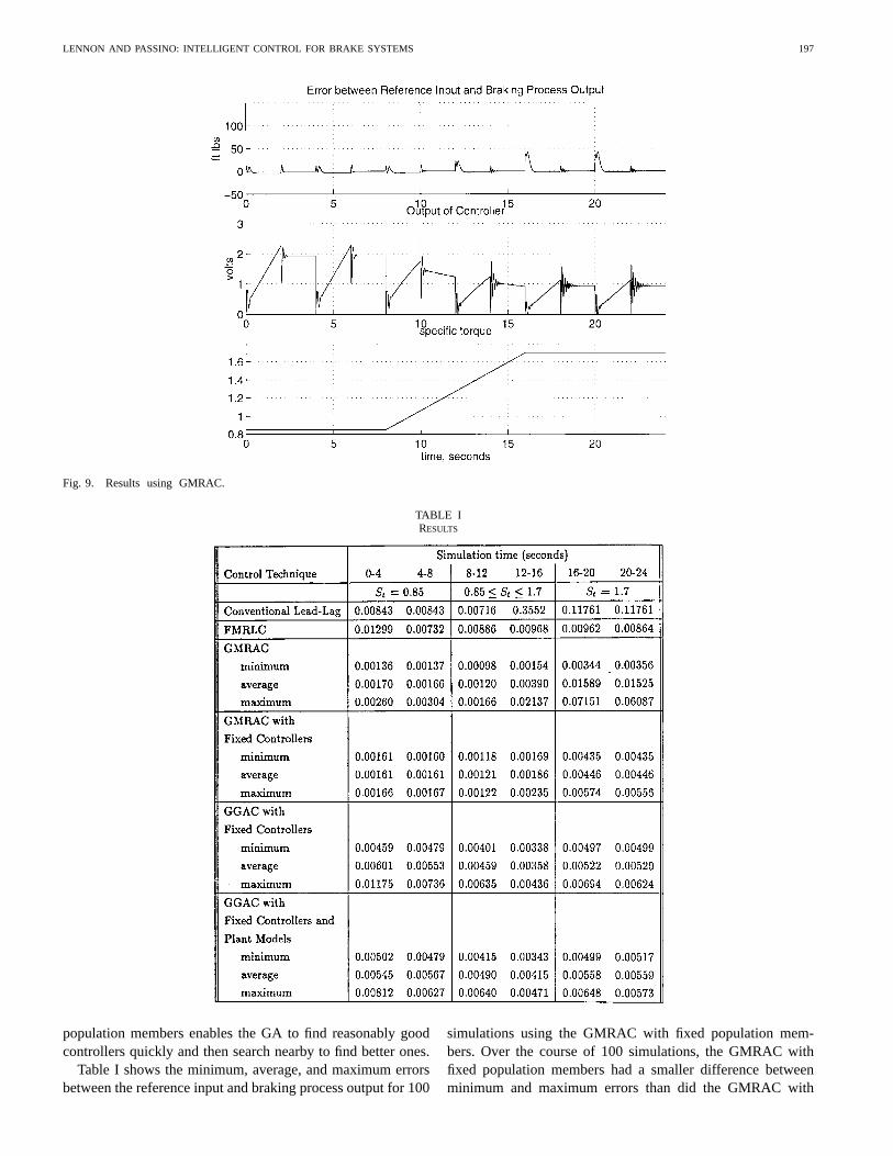
TABLE IRESULTS

population members enables the GA to find reasonably goodcontrollers quickly and then search nearby to find better ones.

Table I shows the minimum, average, and maximum errorsbetween the reference input and braking process output for 100

simulations using the GMRAC with fixed population mem-bers. Over the course of 100 simulations, the GMRAC withfixed population members had a smaller difference betweenminimum and maximum errors than did the GMRAC with


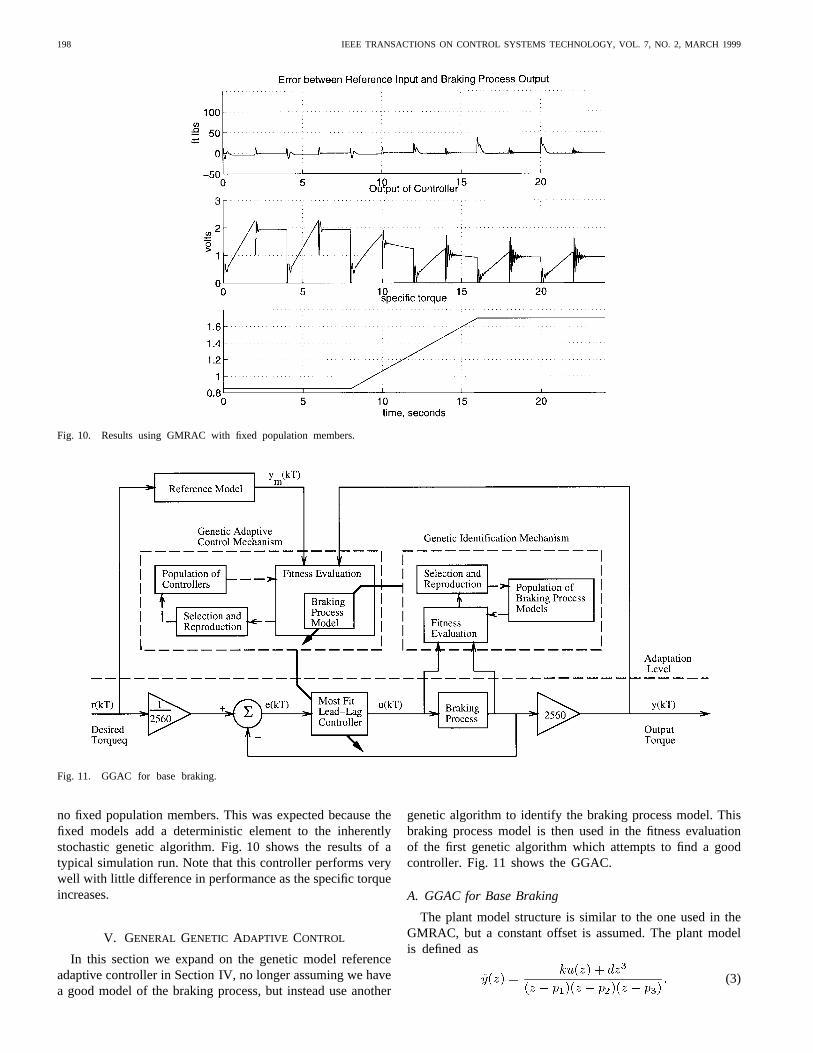
Fig. 10. Results using GMRAC with fixed population members.

Fig. 11. GGAC for base braking.

no fixed population members. This was expected because thefixed models add a deterministic element to the inherentlystochastic genetic algorithm. Fig. 10 shows the results of atypical simulation run. Note that this controller performs verywell with little difference in performance as the specific torqueincreases.

V. GENERAL GENETIC ADAPTIVE CONTROL

In this section we expand on the genetic model referenceadaptive controller in Section IV, no longer assuming we havea good model of the braking process, but instead use another

genetic algorithm to identify the braking process model. Thisbraking process model is then used in the fitness evaluationof the first genetic algorithm which attempts to find a goodcontroller. Fig. 11 shows the GGAC.

A. GGAC for Base Braking

The plant model structure is similar to the one used in theGMRAC, but a constant offset is assumed. The plant modelis defined as

(3)


The constant offset is used to help identify inherent frictionin the automobile [as modeled in the brake system by thefunction described in Section II].

The second genetic algorithm attempts to identify the pa-rameters , , , , and . The gains are restricted to lie inregions where we know the parameters should be. The gain ofthe braking process modelwas restricted to . Thefirst two poles (the poles of the braking process) were restrictedto and the third pole (the pole of thetorque sensor) was restricted to . The constantoffset was restricted to . All the parametersare restricted because we assume we know a fair amount ofinformation about the braking system.

The individual process models are defined by a 15-digitchromosome, and each of the five parameters is representedwith three digits. The population of process models consistsof 100 individuals. The probability of mutation was set to0.1 (relatively high since we want to make sure that thepopulations do not stagnate such that the controller will notadapt). The probability of crossover was set to 0.8.

Because the plant parameters do not change very quicklyand the processing time is short ( s), the iden-tification genetic algorithm only computes a new generationonce every five samples. Furthermore, the identification GAis not run for the first ten samples of every ramp-step in thesimulation because the braking process input is nearly zero atthis time and hence no information can be obtained to helpidentify the plant parameters.

The fitness function of the genetic identification algorithm isas follows: For each plant model candidate in the population

do the following.

1) Initialize the states of the discrete-time process modelwith the outputs of the actual braking process.

2) Using the past samples of braking control signaluse the process model candidate to predict the past

outputs of the braking process, . Compute the errorbetween the predicted output and the actual output

for each time step.For to

NextThe braking process model uses the parameters, ,

, , and from the process model candidate,.Then

3) Assign fitness to each plant model candidate

Here .4) Repeat Steps 1)–3) for each member of the population.

5) The maximally fit braking process model becomes themodel used for the next time step.

The fitness function is designed to compare how well eachplant model tracks the output of the actual braking system,given the actual inputs to the braking system. The error at eachtime step is computed, squared and summed over the modelestimation window, . The plant model with the smallest errorsum, , will have the largest fitness value and will beselected as the model used in the next time step. The value for

was set to . In general, we usually select to be oneor two orders of magnitude less than the average error sum,, to provide a good mix of fitness values in the population.

The model estimation window, was set to 20 because thisprovides enough time to observe the braking process model,yet does not require too much controller processor time.

Once the braking process model is determined, it is placedinto the fitness function of a genetic algorithm that evolvesa good controller. This operates exactly like the GMRACdescribed previously. In all simulations of the GGAC, weuse the GMRAC technique with fixed controllers becausewe have already demonstrated this improves average trackingperformance.

B. GGAC Results

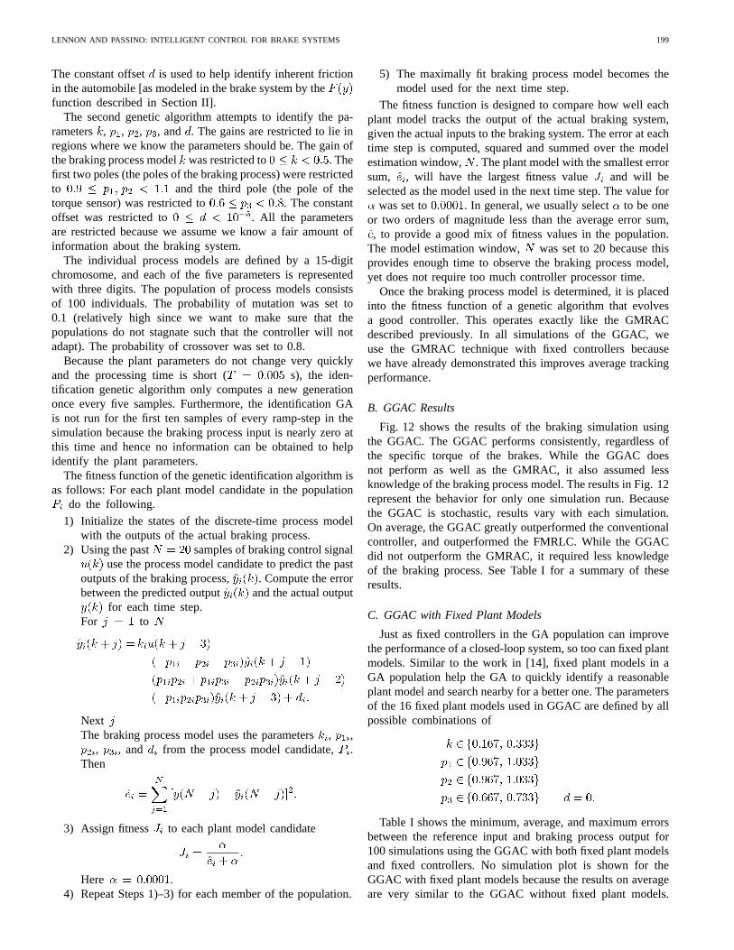
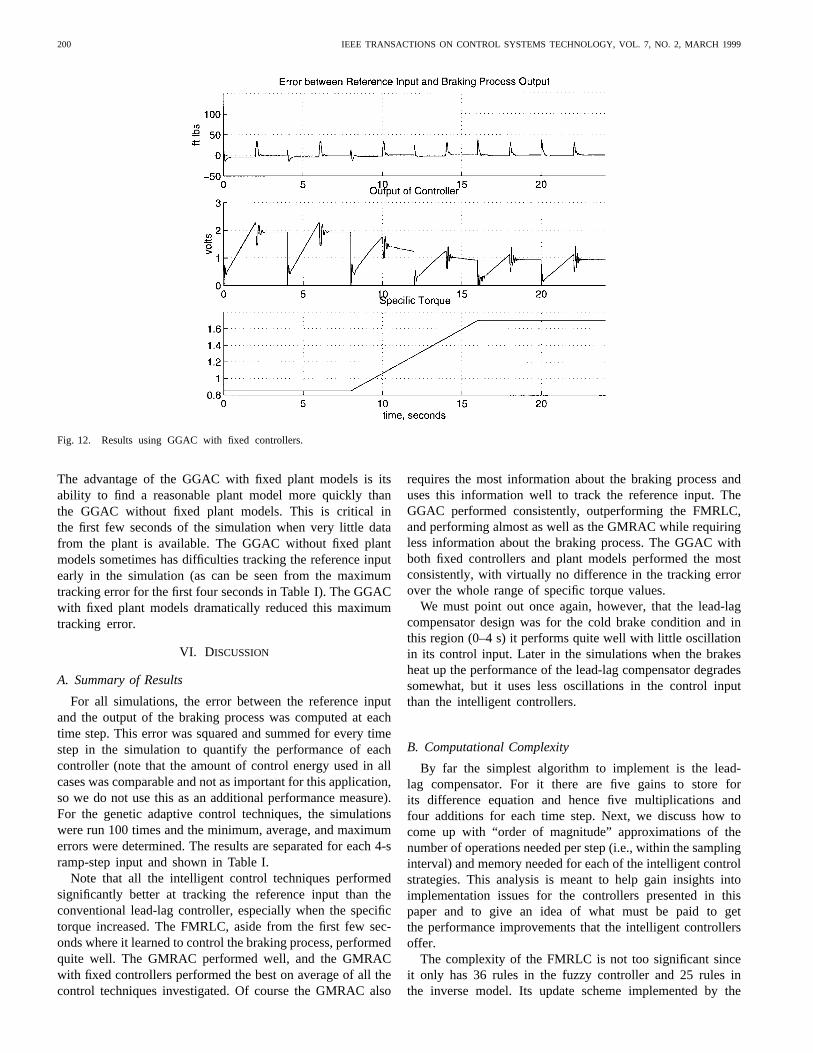
Fig. 12 shows the results of the braking simulation usingthe GGAC. The GGAC performs consistently, regardless ofthe specific torque of the brakes. While the GGAC doesnot perform as well as the GMRAC, it also assumed lessknowledge of the braking process model. The results in Fig. 12represent the behavior for only one simulation run. Becausethe GGAC is stochastic, results vary with each simulation.On average, the GGAC greatly outperformed the conventionalcontroller, and outperformed the FMRLC. While the GGACdid not outperform the GMRAC, it required less knowledgeof the braking process. See Table I for a summary of theseresults.

C. GGAC with Fixed Plant Models

Just as fixed controllers in the GA population can improvethe performance of a closed-loop system, so too can fixed plantmodels. Similar to the work in [14], fixed plant models in aGA population help the GA to quickly identify a reasonableplant model and search nearby for a better one. The parametersof the 16 fixed plant models used in GGAC are defined by allpossible combinations of

Table I shows the minimum, average, and maximum errorsbetween the reference input and braking process output for100 simulations using the GGAC with both fixed plant modelsand fixed controllers. No simulation plot is shown for theGGAC with fixed plant models because the results on averageare very similar to the GGAC without fixed plant models.


Fig. 12. Results using GGAC with fixed controllers.

The advantage of the GGAC with fixed plant models is itsability to find a reasonable plant model more quickly thanthe GGAC without fixed plant models. This is critical inthe first few seconds of the simulation when very little datafrom the plant is available. The GGAC without fixed plantmodels sometimes has difficulties tracking the reference inputearly in the simulation (as can be seen from the maximumtracking error for the first four seconds in Table I). The GGACwith fixed plant models dramatically reduced this maximumtracking error.

VI. DISCUSSION

A. Summary of Results

For all simulations, the error between the reference inputand the output of the braking process was computed at eachtime step. This error was squared and summed for every timestep in the simulation to quantify the performance of eachcontroller (note that the amount of control energy used in allcases was comparable and not as important for this application,so we do not use this as an additional performance measure).For the genetic adaptive control techniques, the simulationswere run 100 times and the minimum, average, and maximumerrors were determined. The results are separated for each 4-sramp-step input and shown in Table I.

Note that all the intelligent control techniques performedsignificantly better at tracking the reference input than theconventional lead-lag controller, especially when the specifictorque increased. The FMRLC, aside from the first few sec-onds where it learned to control the braking process, performedquite well. The GMRAC performed well, and the GMRACwith fixed controllers performed the best on average of all thecontrol techniques investigated. Of course the GMRAC also

requires the most information about the braking process anduses this information well to track the reference input. TheGGAC performed consistently, outperforming the FMRLC,and performing almost as well as the GMRAC while requiringless information about the braking process. The GGAC withboth fixed controllers and plant models performed the mostconsistently, with virtually no difference in the tracking errorover the whole range of specific torque values.

We must point out once again, however, that the lead-lagcompensator design was for the cold brake condition and inthis region (0–4 s) it performs quite well with little oscillationin its control input. Later in the simulations when the brakesheat up the performance of the lead-lag compensator degradessomewhat, but it uses less oscillations in the control inputthan the intelligent controllers.

B. Computational Complexity

By far the simplest algorithm to implement is the lead-lag compensator. For it there are five gains to store forits difference equation and hence five multiplications andfour additions for each time step. Next, we discuss how tocome up with “order of magnitude” approximations of thenumber of operations needed per step (i.e., within the samplinginterval) and memory needed for each of the intelligent controlstrategies. This analysis is meant to help gain insights intoimplementation issues for the controllers presented in thispaper and to give an idea of what must be paid to getthe performance improvements that the intelligent controllersoffer.

The complexity of the FMRLC is not too significant sinceit only has 36 rules in the fuzzy controller and 25 rules inthe inverse model. Its update scheme implemented by the


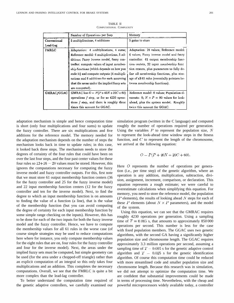
TABLE IICOMPUTATIONAL COMPLEXITY

adaptation mechanism is simple and hence computation timeis short (only four multiplications and four sums) to updatethe fuzzy controller. There are six multiplications and fiveadditions for the reference model. The memory needed forthe adaptation mechanism depends on the number of steps themechanism looks back in time to update rules; in this case,it looked back three steps. The mechanism needs to store thedegrees of certainty of the four rules that could have been onover the last four steps, and the four past center values for thesefour rules so values must be stored. However, thisignores the computations necessary for computing the fuzzyinverse model and fuzzy controller outputs. For this, first notethat we must store 61 output membership function centers (36for the fuzzy controller and 25 for the fuzzy inverse model)and 22 input membership function centers (12 for the fuzzycontroller and ten for the inverse model). Next, to find thedegree to which an input membership function is on amountsto finding the value of a function (a line), that is the valueof the membership function (but you can avoid computingthe degree of certainty for each input membership function bysome simple range checking on the inputs). However, this hasto be done for each of the two inputs for both the fuzzy inversemodel and the fuzzy controller. Hence, we have to computethe membership values for all 61 rules in the worse case (ofcourse simple strategies may be used to reduce computationshere where for instance, you only compute membership valuesfor the eight rules that are on, four rules for the fuzzy controllerand four for the inverse model). Next, the areas under theimplied fuzzy sets must be computed, but simple geometry canbe used (for the area under a chopped-off triangle) rather thanan explicit computation of an integral so this only takes fourmultiplications and an addition. This completes the necessarycomputations. Overall, we see that the FMRLC is quite a bitmore complex than the lead-lag controller.

To better understand the computation time required ofthe genetic adaptive controllers, we carefully examined our

simulation program (written in the C language) and computedroughly the number of operations required per generation.Using the variables to represent the population size,to represent the look-ahead time window steps in the fitnessfunction, and to represent the length of the chromosome,we arrived at the following equation:

Here represents the number of operations per genera-tion (i.e., per time step) of the genetic algorithm, where anoperation is any addition, multiplication, subtraction, divi-sion, assignment, increment, comparison, or declaration. Thisequation represents a rough estimate; we were careful tooverestimate calculations when simplifying this equation. Formemory, you need to store the reference model, the population( elements), the results of looking aheadsteps for each ofthese elements (about parameters), and the modelof the system.

Using this equation, we can see that the GMRAC requiresroughly 4230 operations per generation. Using a samplingtime of s, that amounts to approximately 850 000operations per second. This number is less for the casewith fixed population members. The GGAC uses two geneticalgorithms, with the second GA having a significantly higherpopulation size and chromosome length. The GGAC requiresapproximately 3.3 million operations per second, assuming asampling time of s for the genetic adaptive controlalgorithm and s for the genetic identificationalgorithm. Of course this computation time could be reducedwith more streamlined code and smaller population size andchromosome length. Because this research was in simulation,we did not attempt to optimize the computation time. Weare confident that substantial improvements could be madein terms of processing time. Nevertheless, with the cheap andpowerful microprocessors widely available today, a controller


that requires 3.3 million operations per second is certainlyimplementable.

The results of this discussion are summarized in Table II.Overall, our conclusion is that the performance improve-ments obtained with the intelligent control methods cost usin computational complexity. The cost is not too great for theFMRLC but is significant when we use our GMRAC/GGACand this demands that we study ways to simplify the code thatimplements these controllers.

VII. CONCLUDING REMARKS

We have used the work from [4] and [5] to define the basebraking control problem and have developed two intelligentcontrol methods for this system. Clearly the approaches andconclusions that we present are somewhat preliminary andare in need of further significant investigations. For instance,it would be useful to perform stability, convergence, androbustness analysis of both the FMRLC and GMRAC tohelp evaluate this safety-critical automotive system. Whilethe model that we use from [4] and [5] has proven to bequite adequate for the development of controllers that havebeen experimentally evaluated at a test track on a vehicle, itwould be valuable to evaluate the developed controllers in thefield. This would force us to take a very careful look at therequirements for real-time implementations of the intelligentcontrollers (our preliminary investigations indicate that weshould be able to implement these in real time).

ACKNOWLEDGMENT

The authors would like to thank Prof. S. Yurkovich for hishelp in all aspects of this brake system project which haveinvolved significant efforts over many years in modeling anddevelopment of conventional controllers for this brake system.They would also like to thank him for his helpful discussionsthroughout the research on intelligent control methods forthe brake system. Also, they would like to thank J. Hurtigfor her assistance in establishing the model and simulationtestbed for our evaluations and for her past work on controllerdevelopment and implementation that provided a base-linecomparison for the methods developed here. Finally, theywould like to acknowledge the support and assistance ofD. Littlejohn from the Delphi Chassis Division of GeneralMotors.

REFERENCES

[1] P. Kachroo, “Nonlinear control strategies and vehicle traction control,”Ph.D. dissertation, Univ. California, Berkeley, 1993.

[2] S. Drakunov,U. Ozguner, P. Dix, and B. Ashrafi, “ABS control usingoptimum search via sliding modes,”IEEE Trans. Contr. Syst. Technol.,vol. 3, pp. 79–85, Mar. 1995.

[3] J. Layne, K. Passino, and S. Yurkovich, “Fuzzy learning control forantiskid braking systems,”IEEE Trans. Contr. Syst. Technol.,vol. 1, pp.122–129, June 1993.

[4] J. Hurtig, S. Yurkovich, K. Passino, and D. Littlejohn, “Torque regula-tion with the General Motors ABS VI electric brake system,” inProc.Amer. Contr. Conf.,Baltimore, MD, June 1994, pp. 1210–1211.

[5] J. K. Harvey, “Implementation of fixed and self-tuning controllers forwheel torque regulation,” Master’s thesis, Ohio State Univ., Columbus,1993.

[6] J. Layne and K. Passino, “Fuzzy model reference learning control forcargo ship steering,”IEEE Contr. Syst. Mag.,vol. 13, pp. 23–34, Dec.1993.

[7] L. Porter and K. Passino, “Genetic model reference adaptive control,”in Proc. IEEE Int. Symp. Intell. Contr.,Columbus, OH, Aug. 1994, pp.219–224.

[8] W. Lennon and K. Passino, “Intelligent control for brake systems,” inProc. IEEE Int. Symp. Intell. Contr.,Monterey, CA, Aug. 1995, pp.499–504.

[9] W. Lennon and K. Passino, “Genetic adaptive identification and con-trol,” 1996, in preparation.

[10] V. Moudgal, W. Kwong, K. Passino, and S. Yurkovich, “Fuzzy learningcontrol for a flexible-link robot,”IEEE Trans. Fuzzy Syst.,vol. 3, pp.199–210, May 1995.

[11] J. Layne and K. Passino, “Fuzzy model reference learning control,” inProc. 1992 IEEE Conf. Contr. Applicat.,Dayton, OH, Sept. 1992, pp.686–691.

[12] D. Goldberg,Genetic Algorithms in Search, Optimization and MachineLearning. Reading, MA: Addison-Wesley, 1989.

[13] Z. Michalewicz,Genetic Algorithms+ Data Structures= EvolutionaryPrograms. Berlin: Springer-Verlag, 1992.

[14] K. S. Narendra and J. Balakrishnan, “Improving transient response ofadaptive control systems using multiple models and switching,”IEEETrans. Automat. Contr.,vol. 39, pp. 1861–1866, 1994.

William K. Lennon received the B.S. degree inelectrical engineering in 1994 and the M.S. degreein electrical engineering with a specialization incontrol systems in 1996, both from the Ohio StateUniversity, Columbus.

Presently he is working in the Radio NetworkDevelopment Department at Ericsson, Research Tri-angle Park, NC.

Kevin M. Passino (S’79–M’90–SM’96) receivedthe Ph.D. degree in electrical engineering from theUniversity of Notre Dame in 1989.

He has worked on control systems research atMagnavox Electronic Systems Co. and McDonnellAircraft Co. He spent a year at Notre Dame Uni-versity, IN, as a Visiting Assistant Professor and iscurrently an Associate Professor in the Departmentof Electrical Engineering at the Ohio State Univer-sity, Columbus.

He has served as a member of the IEEE ControlSystems Society Board of Governors; has been an Associate Editor for theIEEE TRANSACTIONS ON AUTOMATIC CONTROL; served as the Guest Editorfor the 1993IEEE Control Systems MagazineSpecial Issue on IntelligentControl; and a Guest Editor for a special track of papers on Intelligent Controlfor IEEE Expert Magazinein 1996; and was on the Editorial Board of theInternational Journal for Engineering Applications of Artificial Intelligence.He is currently the Chair for the IEEE CSS Technical Committee on IntelligentControl and is an Associate Editor for IEEE TRANSACTIONS ONFUZZY SYSTEMS.He was a Program Chairman for the 8th IEEE International Symposium onIntelligent Control in 1993 and was the General Chair for the 11th IEEEInternational Symposium on Intelligent Control. He is Coeditor of the bookAn Introduction to Intelligent and Autonomous Control(Boston, MA: Kluwer,1993), Coauthor of the bookFuzzy Control(Reading, MA: Addison-Wesley,1998), and Coauthor of the bookStability Analysis of Discrete Event Systems(New York: Wiley, 1998). His research interests include intelligent systemsand control, adaptive systems, stability analysis, and fault-tolerant control.

intelligent control for brake systems

Documents