arX

iv:0

807.

2063

v3 [

hep-

th]

21 J

ul 2

008

SNUST 080701

Integrable Spin Chain

in

Superconformal Chern-Simons Theory

Dongsu Baka, Soo-Jong Reyb

Physics Department, University of Seoul, Seoul 130-743KOREA

School of Physics & Astronomy, Seoul National University, Seoul 151-747KOREA

dsbak@uos.ac.kr sjrey@snu.ac.kr

ABSTRACT

N = 6 superconformal Chern-Simons theory was proposed as gaugetheory dual to Type IIA

string theory on AdS4⊗CP3. We study integrability of the theory from conformal dimension

spectrum of single trace operators at planar limit. At strong ‘t Hooft coupling, the spectrum is

obtained from excitation energy of free superstring on OSp(6|2,2;R)/SO(3,1)×SU(3)×U(1)

supercoset. We recall that the worldsheet theory is integrable classically by utilizing well-

known results concerning sigma model on symmetric space. With R-symmetry group SU(4),

we also solve relevant Yang-Baxter equation for a spin chainsystem associated with the single

trace operators. From the solution, we construct alternating spin chain Hamiltonian involving

three-site interactions between4 and 4. At weak ‘t Hooft coupling, we study gauge theory

perturbatively, and calculate action of dilatation operator to single trace operators up to two

loops. To ensure consistency, we computed all relevant Feynman diagrams contributing to the

dilatation opeator. We find that resulting spin chain Hamiltonian matches with the Hamiltonian

derived from Yang-Baxter equation. We further study new issues arising from the shortest gauge

invariant operators TrY IY †J = (15,1). We observe that ‘wrapping interactions’ are present, com-

pute the true spectrum and find that the spectrum agrees with prediction from supersymmetry.

We also find that scaling dimension computed naively from alternating spin chain Hamiltonian

coincides with the true spectrum. We solve Bethe ansatz equations for small number of excita-

tions, and find indications of correlation between excitations of4’s and4’s and of nonexistence

of mesonic(44) bound-state.

1 Introduction

In a recent remarkable development, Aharony, Bergman, Jeffries and Maldacena (ABJM) [1]

made a new addition to the list of microscopic AdS/CFT correspondence [2]: three-dimensional

N = 6 superconformal Chern-Simons theory dual to Type IIA string theory on AdS4×CP3 [3].

Both sides of the correspondence are characterized by two integer-valued coupling parameters

N andk. On the superconformal Chern-Simons theory side, they are the rank of product gauge

group U(N)×U(N) and Chern-Simons levels+k,−k, respectively. On the Type IIA string

theory side, they are related to spacetime curvature and dilaton gradient or Ramond-Ramond

flux, all measured in string unit. Much the same way as the counterpart betweenN = 4 super

Yang-Mills theory and Type IIB string theory on AdS5×S5, we can put the new correspondence

into precision tests in the planar limit:

N → ∞, k → ∞ with λ ≡ Nk

fixed (1.1)

by interpolating ‘t Hooft coupling parameterλ between superconformal Chern-Simons theory

regime atλ ≪ 1 and semiclassical AdS4×CP3 string theory regime atλ ≫ 1.

In the correspondence betweenN = 4 super Yang-Mills theory and Type IIB string theory

on AdS5×S5, the integrability structure first discovered by Minahan and Zarembo [4] led to

remarkable progress in diverse fronts of the correspondence 1. It is therefore interesting to

examine if the new correspondence shows also an integrability structure. The purpose of this

work is to demonstrate integrability structure inherent totheN = 6 superconformal Chern-

Simons theory of ABJM2.

AdS/CFT correspondence asserts that gauge invariant, single trace operators in superconfor-

mal Chern-Simons theory are dual to free string excitation modes in AdS4×CP3, valid at weak

and strong ‘t Hooft coupling regime, respectively. In particular, conformal dimension of the

operators should match with excitation energy of the stringmodes. TheN = 6 superconformal

Chern-Simons theory has SO(6)≃SU(4) R-symmetry and contains two sets of bi-fundamental

scalar fieldsY I,Y †I (I = 1,2,3,4) that transform as4,4 under SU(4). Therefore, the single trace

operators take the form:

O = Tr(Y I1Y †J1· · ·Y ILY †

JL)CJ1···JL

I1···IL

= Tr(Y †J1

Y I1 · · ·Y †JL

Y IL)CJ1···JLI1···IL

. (1.2)

1Selected but nonexhaustive list of contributions in this subject include [5] - [21]. For a comprehensive mid-

development review, see [13].2Integrability inN ≤ 3 superconformal Chern-Simons theory was investigated by Gaiotto and Yin [22] previ-

ously. Their tentative result indicated otherwise.

1

In superconformal Chern-Simons theory, chiral primary operators, corresponding to the choice

of (1.2) with CJ1···JLI1···IL

totally symmetric in both sets of indices and traceless, form the light-

est states. In free string theory on AdS4×CP3. Kaluza-Klein supergravity modes form the

lightest states. In this work, we study conformal dimensionof single trace operators and iden-

tify integrability structure organizing the excitation spectrum above the chiral primary or the

Kaluza-Klein states.

In section 2, we begin with recapitulating the standard argument for integrability of free

string on AdS4 ×CP3 at λ → ∞. Recalling the construction of [23] and utilizing the idea

of [24], we argue that sigma model on OSp(6|2,2,R)/[SO(3,1)×SU(3)×U(1)] supercoset has

commuting monodromy matrices and infinitely many conservednonlocal charges. In section 3,

we begin main part of this work. Guided by earlier development in N = 4 super Yang-Mills

counterpart, we assume integrability and solve Yang-Baxter equations for R-matrices between

4 and4 sites in (1.2). From corresponding transfer matrices, we then find the Hamiltonian takes

the form of one-parameter family of ’alternating spin chain’, whose variants were studied pre-

viously in different contexts [25]-[29]. In section 4, we study superconformal Chern-Simons

theory of ABJM atλ → 0 in perturbation theory. Pure Chern-Simons theory is free from any

ultraviolet divergences since the theory is diffeomorphism invariant and hence topological .

Once matter is coupled, as in ABJM theory, topological feature is lost and the quantum the-

ory will receive nontrivial radiative corrections. As such, the single trace operators (1.2) will

acquire nontrivial anomalous dimensions in general. In three dimensions, logarithmic ultravi-

olet divergence arises only at even loop orders. Therefore,the first nontrivial correction starts

at two loops. We compute two-loop operator mixing and anomalous dimension matrix of the

single trace operators (1.2). In dimensional reduction method, we compute the complete set of

relevant Feynman diagrams and find that the two-loop anomalous dimension matrix matches

with the integrable ‘alternating spin chain’ Hamiltonian derived in section 3. In section 5, we

study a new important feature of the superconformal Chern-Simons theory compared toN = 4

super Yang-Mills theory. Since the anomalous dimensions begin to arise from two loops and

next-to-nearest sites, the shortest single trace operators of L = 1 will be subject to ‘wrapping

interactions’. The ‘alternating spin chain’ Hamiltonian does not describe spectrum ofL = 1

operators, so we compute all relevant ‘wrapping interaction’ diagrams and construct the cor-

rect Hamiltonian forL = 1. Curiously, we find that the correct spectrum coincides with the

naive spectrum computed from the ‘alternating spin chain’ Hamiltonian atL = 1. In section 6,

utilizing results previously obtained for generalAn−1 Lie algebras [30, 26, 29], we explicitly

write down eigenvalues of the transfer matrices and Bethe ansatz equations of the ‘alternating

spin chain’ we derived in section 3. To gain understanding how the ‘alternating spins’ behave,

we solve the equations for a few simple situations. We find an indication for real-space cor-

2

relations between excitations on4 spin sites and those on4 spin sites, and for non-existence

of meson-like(44) bound-states. We discuss various implications of these findings for general

excitations. In particular, we argue that general excitations are more complex than the pattern

emerging from closed SU(2) sub-sectors discussed recently[31, 32].

• Note added: While bulk of this work was completed, we received the preprint by Minahan

and Zarembo [33], which deals with issues overlapping with ours. Version 1 of their preprint

was based on ungrounded Feynman rules and incomplete set of contributing Feynman diagrams.

In light of utmost importance of precise evaluation, we decided to carefully carry out various

internal consistency checks before releasing our results.Meanwhile, we also received preprints

by Arutyunov and Frolov [34], which overlaps with section 2 and substantiate several pertinent

issues including kappa symmetry. We also note the preprintsby Stefanski [35] and by Gromov

and Vieira [36] on the same issue.

2 Integrable String from Worldsheet Sigma Model

In this section, we set out a motivation for searching for integrability inN = 6 superconformal

Chern-Simons theory. Theλ → ∞ dual of this theory is Type IIA string theory on AdS4⊗CP3.

The background is a direct product of symmetric spaces, AdS4 andCP3. It is well known that

the(1+1)-dimensional sigma model on symmetric space is classicallyintegrable. So, at least

for bosonic modes, we expect worldsheet dynamics of a free string on AdS4⊗CP3 is integrable

at the classical level,λ → ∞. In this section, we recapitulate this argument for the bosonic part

and discuss how the construction to full superstring can be made.

Bosonic part of string worldsheet Lagrangian on AdS4⊗CP3 is given by

Ib =R2

4π

Z

Σ

√−hhαβ

[(DαXm)†(DβXm)+(DαZa)†(DβZa)

]. (2.1)

Here, we use embedding coordinates inR3,2 andC4 and describe AdS4 =SO(3,2)/SO(3,1) and

CP3 =SU(4)/SU(3)×U(1) asG/H coset hypersurfaces:

AdS4 : (Xm) = (X−1,X1,X2,X3,X0) with X2 = 1,

CP3 : (Za) = (Z1,Z2,Z3,Z4)/≃,C with |Z|2 = 1, (2.2)

respectively. The hypersurface conditions are imposed by introducing auxiliary connection

Kα,Aα and by defining covariant derivatives3 DαXm ≡ ∂αXm + iKαXm andDαZa ≡ ∂αZa +

iAαZa. These conditions imply thatXm∂αXm = 0 and (DαZa)†Za = Za†(DαZa) = 0. Fol-

lowing [23], we first recapitulate basic aspects for classical integrability of sigma model on

3We introduced auxiliary connectionKα to treat AdS4 in complete parallel toCP3.

3

AdS4×CP3. Construction of the coset sigma model is facilitated by thecoset elements:

G(σ) ≡ g(σ)⊕ g(σ) = eiπP(σ)⊕ eiπP(σ) (2.3)

whereP(σ), P(σ) are projection matrices onto respective one-dimensional subspaces. They are

Pmn(σ) = Xm(σ)Xn(σ) with δmnPmn(σ) = 1,

Pab(σ) = Za†(σ)Zb(σ) with δabPab(σ) = 1, (2.4)

respectively. By elementary algebra, we verify that

G(σ) = G−1(σ) = (I5−2P(σ))⊕ (I4−2P(σ)). (2.5)

Then, because−8|DαXm|2 = Tr(∂αg · ∂αg−1) for AdS4 and+4|DαZa|2 = Tr(∂αg · ∂βg−1) for

CP3, the worldsheet action (2.1) is expressible as

Ibosonic=R2

8

Z

Σ

√−hhαβ

[− 1

2TrJαJβ +2TrJαJβ

], (2.6)

whereJ = g−1dg andJ = g−1dg, respectively. We shall choose the conformal gauge√−hhαβ =

δαβ on the worldsheet. This leads to Virasoro gauge condition

T± ≡−14(J0± J1)

2+(J0± J1)2 = 0 . (2.7)

The currentsJ, J are conserved by equations of motion, and define tangent flowson theG/H

coset space.

We now take group conjugation and transform the left-invariant currentsJ, J to the right-

invariant currents:( j, j) = (g · J ·g−1, g · J · g−1). The equations of motion in conformal gauge

are

d∗ j(σ) = 0 and d∗ j(σ) = 0. (2.8)

From the Bianchi identities, we also have

d j + j∧ j = 0 and d j + j∧ j = 0. (2.9)

Finally, Virasoro constraints are

− 14( j0± j1)

2+( j0± j1)2 = 0. (2.10)

We can solve these equations using the Lax representation. Consider the Lax derivative with

flat connectiona(x) depending on a spectral parameterx:

D(x) = d+a(x) with da+a∧a = 0. (2.11)

4

Using (2.8, 2.9), we find that the most general form of the Lax connection is given by

a(x) =2

x2−1j(σ)+

2xx2−1

∗ j(σ) x ∈ C+∞/±1. (2.12)

and similarly constructa(x) from j(σ). With the flat connectionA(x) ≡ (a(x), a(x)), consider

the Wilson line

W [γ;x] = P exp(Z

γA(x)

)(2.13)

As the connectionA(x) is flat, the eigenvalues of the Wilson line are independent ofthe choice

of the contourγ. Thus, all Wilson lines commute each another and provides classical R-matrices

obeying Yang-Baxter equations. Expanding in spectral parameterx, we then obtain infinitely

many conserved nonlocal charges as moment of the power series:

Q (n) =1n!

∂nx

Z

γdσA(x)

∣∣∣x=0

. (2.14)

This establishes that the sigma model on AdS4×CP3 is classically integrable.

We now discuss how the above consideration may be extended toType IIA string on the

supercoset:

GH

=OSp(6|2,2,R)

SO(3,1)×SU(3)×U(1). (2.15)

With the coefficients of current bilinears determined as in (2.6), we see immediately that the

worldsheet Lagrangian is expressible as supertrace over the supergroup OSp(6|2,2,R):

Isupercoset=R2

8

Z

ΣStr(J∧ ∗J) . (2.16)

Here,J(σ) = G−1(σ)dG(σ) andG(σ) = exp(iπP(σ)) is the supercoset element. This indicates

that the bosonic action (2.6) is extendible straightforwardly to a supercoset action by adding

24 fermionic off-diagonal components to (2.3-2.5) and define super-projection matrixP and

supercoset elementG analogously.

Construction of infinitely many nonlocal currents requiresa new condition to the supercoset.

If the supergroupG permitsZ4 grading under which the subgroupH is a fixed point set, the

construction of [24] implies that a flat connection exists from which nonlocal currents can be

constructed through the Lax formulation. From the embedding we constructed of, we haveJ =

J +Q, whereQ denotes fermionic current. For the supergroup we deal with,G = OSp(6|2,2),

it is well known thatG admits no outer automorphism of order four [37]. However, one can

easily construct a suitableZ4 inner automorphism. Since we need the subgroupH is a fixed

point set, the automorphism can be defined as a product of twoZ2 involutions on the defining

5

representations of SU(4)≃SO(6) and Sp(4) modulo overall reflection. This then ensuresthat

the G/H currentJ = Q1⊕ J ⊕Q3 is Z4 graded as[1,2,3] and that infinitely many conserved

nonlocal currents can be constructed accordingly.

At quantum level, the supergroupG= OSp(6|2,2) has another nice feature that its Killing

form vanishes identically. This means that sigma model onG would be conformally invariant,

at least, at one loop. We actually need to quotientG by bosonic subgroupH and consider string

worldsheet action on the supercosetG/H. This action in general breaks the conformal invari-

ance. To restore the conformal invariance, a suitable Wess-Zumino term needs to be added. It

was observed [38] that the requisite Wess-Zumino term can beconstructed provided the bosonic

subgroupH is a fixed point set of theZ4 grading ofG. This is precisely the same condition that

ensures the existence of a flat connection and infinitely manyconserved charges thereof. There-

fore, the supercoset sigma model is conformally invariant and can describe consistent string

worldsheet dynamics, at least at one loop order in worldsheet perturbation theory.

Given such mounting evidences, it is highly likely that TypeIIA string on AdS4×CP3 is

integrable atλ → ∞ and further extends toλ finite and even to weak coupling regime4. With

such motivation, we now turn to the main part of this work and investigate integrability at the

weak coupling regime,λ → 0.

3 Integrable Spin Chain from Yang-Baxter

The U(N)×U(N) invariant, single-trace operators under consideration

O (I)(J) ≡ Tr(Y I1Y †

J1· · ·Y ILY †

JL)

≃ O (J)(I) ≡ Tr(Y †

J1Y I1 · · ·Y †

JLY IL) (3.1)

are organized according to SUR(4) irreducible representations. Operator mixing under renor-

malization and their evolution in perturbation theory can be described by a spin chain of total

length 2L. What kind of spin chain system do we expect? In this section,viewing the operators

(3.1) as a spin chain system and utilizing quantum inverse scattering method, we shall derive

spin chain Hamiltonian.

As is evident from the structure of operators (3.1), the prospective spin chain involves two

types of SUR(4) spins:4 at odd lattice sites and4 at even lattice sites. It is thus natural to expect

that the prospective spin chain is an ‘alternating SU(4) spin chain’ consisting of interlaced4

and4. To identify the spin system and extract its Hamiltonian, itis imperative to solve inho-

mogeneous Yang-Baxter equations of SUR(4) R-matrices with varying representations on each

4We note that the no-go theorem of Goldschmidt and Witten [39]for quantum conservation laws is evaded in

the present case since the isotropy subgroup is not simple, and may lead to quantum anomalies [40].

6

site. In fact, a general procedure for solving Yang-Baxter equations in this sort of situations is

already set out in [25]. By construction, resulting spin chain system will be integrable. In this

section, we shall follow this procedure and find that the putative SU(4) spin chain is an ’alter-

nating spin chain’ involving next-to-nearest neighbor interactions nested with nearest neighbor

interactions5.

We first introduceR44(u) andR44(u), where the upper indices denote SU(4) representations

of two spins involved in ‘scattering process’ andu,v denote spectral parameters. We demand

these R-matrices to satisfy two sets of Yang-Baxter equations:

R4412(u− v)R

4413(u)R

4423(v) = R

4423(v)R44

13(u)R4412(u− v) (3.2)

R4412(u− v)R

4413(u)R

4423(v) = R

4423(v)R

4413(u)R

4412(u− v) (3.3)

Here, the lower indicesi, j denote that theR matrix is acting oni-th and j-th siteVi ⊗Vj of the

full tensor product Hilbert spaceV1⊗V2⊗·· ·⊗V2L. We easily find that the R-matrices solving

(3.2, 3.3) are given by

R44(u) = uI+P and R

44(u) = −(u+2+α)I+K (3.4)

for an arbitrary constantα. Here, we have introduced identity operatorI, trace operatorK, and

permutation operatorP:

(Ikℓ)IkIℓJkJℓ

= δIkJk

δIℓJℓ

(Kkℓ)IkIℓJkJℓ

= δIkIℓδJkJℓ (Pkℓ)IkIℓJkJℓ

= δIkJℓ

δIℓJk

, (3.5)

acting as braiding operations mapping tensor product vector spaceVk ⊗Vℓ to itself.

We also need to construct another set of R-matricesR44(u) andR

44(u) generating another

alternative spin chain system. We again require them to fulfill the respective Yang-Baxter equa-

tions:

R4412(u− v)R

4413(u)R

4423(v) = R

4423(v)R

4413(u)R

4412(u− v) (3.6)

R4412(u− v)R

4413(u)R

4423(v) = R

4423(v)R

4413(u)R

4412(u− v) (3.7)

Again, we find that the R-matrices that solve (3.6, 3.7) are given by

R44(u) = uI+P and R

44(u) = −(u+2+ α)I+K , (3.8)

whereα is an arbitrary constant.

5For a construction in SU(3), see [28]. Generalizations to arbitrary Lie (super)algebras and quantum deforma-

tions thereof were studied in [26]-[29].

7

In the two sets of Yang-Baxter equations, the constantsα, α are undetermined. We shall

now restrict them by requiring unitarity. The unitarity of the combined spin chain system sets

the following conditions:

R44(u)R

44(−u) = ρ(u)I

R44(u)R

44(−u) = ρ(u) I

R44(u)R

44(−u) = σ(u) I (3.9)

whereρ(u) = ρ(−u), ρ(u) = ρ(−u),σ(u) arec-number functions. It is simple to show that the

first two unitarity conditions are indeed satisfied for anyα, α. It is equally simple to show that

the last unitarity condition is is satisfied only ifα = −α. Without loss of generality, in what

follows, we shall setα = −α = 0.

Viewing (3.1) as 2L sites in a row, we introduce one transfer T-matrix

T0(u,a) = R4401(u)R44

02(u+a)R4403(u)R44

04(u+a) · · ·R4402L−1(u)R44

02L(u+a) , (3.10)

for one alternate chain and the other T-matrix

T 0(u, a) = R4401(u+ a)R44

02(u)R4403(u+ a)R44

03(u) · · ·R4402L−1(u+ a)R44

02L(u) , (3.11)

for the other alternate chain, where we introduce an auxiliary zeroth space. By the standard

‘train’ argument, one can show that the transfer matrices fulfill the Yang-Baxter equations,

R4400′(u− v)T0(u,a)T0′(v,a) = T0′(v,a)T0(u,a)R44

00′(u− v) , (3.12)

and

R4400′(u− v)T 0(u, a)T 0′(v, a) = T 0′(v, a)T 0(u, a)R44

00′(u− v) . (3.13)

In addition, by a similar argument, one may verify that

R4400′(u− v+a)T0(u,a)T 0′(v,−a) = T 0′(v,−a)T0(u,a)R44

00′(u− v+a) . (3.14)

We also define the trace of the T matrix by

τalt(u,a) = Tr0

T0(u,a) . (3.15)

and

τalt(u, a) = Tr0

T 0(u, a) (3.16)

where the trace is taken over an auxiliary zeroth space.

8

It then follows from the Yang-Baxter equations that

[τalt(u,a),τalt(v,a)] = 0

[τalt(u, a),τalt(v, a)] = 0, (3.17)

and

[τalt(u,a), τalt(v,−a)] = 0. (3.18)

Here, in the first two equations,a, a are arbitrary and denote two undetermined spectral param-

eters. These parameters are restricted further if we demandthe last equation to hold. Indeed,

the two alternating transfer matrices commute each other ifand only if a = −a.

As for all other conserved charges, the Hamiltonian is obtained 6 by evolving the transfer

T-matrix infinitesimally in spectral parameteru: H = dlogτ(u,a)|u=0 where d≡ ∂/∂u. By a

straightforward computation, we obtain the44 spin chain Hamiltonian as

H2ℓ−1 = −(2−a)I− (4−a2)P2ℓ−1,2ℓ+1

− (a−2)P2ℓ−1,2ℓ+1K2ℓ−1,2ℓ +(a+2)P2ℓ−1,2ℓ+1K2ℓ,2ℓ+1 , (3.19)

where we scaled the Hamiltonian by multiplying(a2−4).

By the same procedure, we also find that the Hamiltonian for for the44 spin chain is given

by

H2ℓ = −(2+a)I− (4−a2)P2ℓ,2ℓ+2

+ (a+2)P2ℓ,2ℓ+2K2ℓ,2ℓ+1− (a−2)P2ℓ,2ℓ+2K2ℓ+1,2ℓ+2 , (3.20)

where we have replaced ¯a by a using the relation ¯a = −a.

At this stage, any choice of the parametera is possible in so far as hermiticity of the Hamil-

tonian is satisfied. The latter condition requires thata is a pure imaginary number. Physically,

we are interested in the situation where4 ↔ 4 is a symmetry. This is nothing but requiring

charge conjugation symmetry, equivalently, reflection symmetry in dual lattice. We thus put

6The following derivation of Hamiltonian is valid only forL ≥ 2. This means that the energy eigenvalues of

the following Hamiltonians for the caseL = 1 do not agree with true energy eigenvalues.

9

a = i0 7 Adding the two alternate Hamiltonians, we get total Hamiltonian8 :

Htotal =2L

∑ℓ=1

Hℓ,ℓ+1,ℓ+2 (3.22)

with

Hℓ,ℓ+1,ℓ+2 =[4I−4Pℓ,ℓ+2+2Pℓ,ℓ+2Kℓ,ℓ+1+2Pℓ,ℓ+2Kℓ+1,ℓ+2

]. (3.23)

In this derivation, there is always a freedom of shifting ground state energy by an arbitrary

constant. From the outset, we assumed integrability but, except that the symmetry algebra is

SUR(4) and that spins are4,4 at alternating lattice sites, we did not utilize any inputs from

underlying supersymmetry. With extra input that that supersymmetric ground-state has zero

energy, one can always fix the freedom. The (3.23) is the Hamiltonian after being shifted by+6

per site accordingly.

4 Integrable Spin Chain from Chern-Simons

In this section, we approach integrability from weak ‘t Hooft coupling regime of the supercon-

formal Chern-Simons theory. We use perturbation theory andlook for a spin chain Hamiltonian

as a quantum part of the dilatation operator acting on the single trace operators. As mentioned

above, in three-dimensional spacetime, general power-counting indicates that logarithmic di-

vergence arises only at even loop orders. Therefore, leading-order contribution to anomalous

dimension starts at two loops. In general, as well understood from general considerations of the

renormalization theory, the divergence in one-particle irreducible diagrams with one insertion

of a composite operator contain divergences that are proportional to other composite operators.

Therefore, at each order in perturbation theory, all composite operators whose divergences are

intertwined must be renormalized simultaneously. In addition, renormalization of elementary

fields needs to be taken into account. This leads to the general structure:

OMbare(Ybare,Y

†bare) = ∑

NZM

NONren(ZYren,ZY †

ren) (4.1)

7Alternatively, one may relax hermiticity of the Hamiltonian and only demand symmetry under parity and time-

reversal, leading to so-called PT-symmetric system [41]. This again setsa to zero. Strictly speaking, however, this

latter condition is weaker than the hermiticity requirement.8We remark the following useful identities

Pℓ,ℓ+2Kℓ,ℓ+1 = Kℓ+1,ℓ+2Pℓ,ℓ+2, Pℓ,ℓ+2Kℓ+1,ℓ+2 = Kℓ,ℓ+1Pℓ,ℓ+2 . (3.21)

We shall find them useful later when investigating issues concerning wrapping interactions.

10

For the operators we are interested in, this takes the form of

OMbare= ∑

NZM

N(Λ)O Nren (4.2)

with the UV cut-off scaleΛ. Therefore, the anomalous dimension matrix∆ is given by

∆ =dlogZdlogΛ

. (4.3)

In the rest of this section, we compute anomalous dimension matrix for the single trace

operators that were associated with the ‘alternating spin chain’ in the last section:

O(I)(J) = Tr

(Y I1Y †

J1Y I2Y †

J2· · ·Y ILY †

JL

). (4.4)

In N = 6 superconformal Chern-Simons theory, the scalar fieldsY I,Y †I are bifundamental fields

of U(N)×U(N) gauge group, and transform as4 and4 of SUR(4) R-symmetry group. In Ap-

pendix A, we explain field contents and action of the theory indetail 9. Schematically, the

action of the ABJM theory takes the form

I =Z

R2,1

k4π

(CS(A)−CS(A)

)−Tr(DY )†

I DY I +Tr ΨI†iD/ΨI −VF−VB. (4.5)

Here, the Chern-Simons density is given by

CS(A) = εmnp Tr

[Am∂nAp +

2i3

AmAnAp

]. (4.6)

Covariant derivatives are denoted asDm, while self-interactions involving bosons and fermion

pairs are denoted byVB,VF, respectively. See Appendix A for their explicit form. We will recall

them at relevant points in foregoing discussions.

To extract the dilatation operator, we compute the correlation functions⟨O

(I)(J)Tr(Y †

I1Y J1 · · ·Y †

ILY JL)

⟩for L → ∞ (4.7)

by summing over all planar diagrams in perturbation theory in ‘t Hooft couplingλ.

In evaluating so, there arises an important issue regardingconsistency of regularization with

gauge invariance andN = 6 supersymmetry. We shall adopt dimensional reduction method

(See, for example, discussions in [43]). This method retains εmnp and Dirac matrices always

three-dimensional. In each Feynman integral, we then manipulate the integrand until allεmnp

and Dirac matrices are eliminated and the integral is reduced to a Lorentz scalar expression. We

then employ dimensional regularization and evaluate the integral. Still, this leaves out infrared

divergences that would have been absent were if the theory four-dimensional. As we will be

9We closely follow notation and convention of [42].

11

only concerned with logarithmic ultraviolet divergences,we will take a practical approach that

we regularize infrared divergences by introducing mass terms in evaluating Feynman integrals

in dimensional regularization. We then remove the regulator mass first and then take the space-

time dimension to three. Previously, it was checked that thedimensional reduction method is

consistent with Slavnov-Taylor-Ward identities. Yet, to date, it is not known if the method is

compatible withN = 6 supersymmetry. Thus, in our computations, we shall not assume a

priori any input related to supersymmetry. Rather, we will put our result to a test against vari-

ous consequences of supersymmetry — for instance, vanishing anomalous dimensions of chiral

primary operators and superconformal nonrenormalizationtheorems.

Using the convention and Feynman rules explained in appendix, we computed all two-loop

diagrams that contribute to anomalous dimensions of elementary fieldsY I,Y †I and composite

operatorsO (I)(J). Acting on the space of the operators, each Feynman diagram can be attributed

to the braiding operationsI, K, P introduced in (3.5) and their combinations. At two loops, we

computed the complete set of Feynman diagrams that contribute to each of these operators. The

result turned out

H2−loops= λ22L

∑ℓ=1

[I−Pℓ,ℓ+2+

12

Pℓ,ℓ+2Kℓ,ℓ+1 +12

Pℓ,ℓ+2Kℓ+1,ℓ+2

](4.8)

and this is preciselyλ2

4 times the alternating spin chain Hamiltonian (3.23) we derived from

SU(4) Yang-Baxter equations in the last section. In the restof this section, we explain essen-

tial steps for deriving the Hamiltonian and relegate technical details of evaluating Feynman

diagrams in the Appendix. We find it convenient to organize contributing Feynman diagrams

according to the number of sites that participate in the Hamiltonian.

• Three-site scalar interactions:

A salient feature of the alternating spin chain Hamiltonianwe extracted in section 3 from cou-

pled Yang-Baxter equations is that it contains interactions up to next-nearest-neighbor sites. We

thus need to see if such interaction arises from superconformal Chern-Simons planar diagrams

and, if so, if the interactions are of the same type. From the Feynman rules (see Appendix A),

it is evident that scalar interaction−VB in (4.5) is thesource of three-site interactions, whose

explicit form is given by

VB = −13

(2πk

)2

Tr[

Y †I Y JY †

J Y KY †KY I +Y †

I Y IY †J Y JY †

KY K

+4Y †I Y JY †

KY IY †J Y K −6Y †

I Y IY †J Y KY †

KY J]

(4.9)

The two-loop Feynman diagram is depicted in Fig.1. From planar diagram combinatorics of

gauge invariant operators at infinite length 2L → ∞, we find the following contributions arising:

12

k

l

k + lO

Figure 1:Two loop contribution of scalar sextet interaction to anomalous dimension ofO .

k

k + ll

k

O

(a)

k

k + ll

k

O

(b)

k

k + l

k l

l

O

(c)

Figure 2: Two loop contribution of gauge and fermion exchange interaction to anomalous di-

mension ofO .

Kℓ,ℓ+1 +Kℓ+1,ℓ+2 from the first two terms,Pℓ,ℓ+2 from the third term, andI+Pℓ,ℓ+2Kℓ,ℓ+1 +

Pℓ,ℓ+2Kℓ+1,ℓ+2 from the last term. Taking account of combinatorial multiplicities, we find that

the scalar sextet potential contributes to the dilatation Hamiltonian as

HB = λ22L

∑ℓ=1

[12

I−Pℓ,ℓ+2+12

Pℓ,ℓ+2Kℓ,ℓ+1 +12

Pℓ,ℓ+2Kℓ+1,ℓ+2−12Kℓ,ℓ+1

](4.10)

(see Appendix B2). Evidently, compared to the anticipated alternating spin chain Hamiltonian,

we have discrepancy in on-site (proportional toI) and nearest neighbor (proportional toK)

terms. These are interactions that would arise from gauge orfermion-pair exchange interactions

and from wave function renormalization of elementary fieldsY,Y †.

• Two-site gauge and fermion interactions:

The scalar fieldsY I,Y †I are bifundamentals of U(N)×U(N). Their gauge interactions can be

read off from covariant derivatives:

DmY I = ∂mY I + iAmY I − iY IAm and DmY †I = ∂mY †

I + iAmY †I − iY †

I Am . (4.11)

As usual, there are paramagnetic interactions (minimal coupling) and diamagnetic interactions

(seagull coupling). We see that gauge interactions contribute to two-site terms for bothI andK.

Two relevant Feynman diagrams are (a) and (c) in Fig. 2.

The Feynman diagram contributing toI operator arises from square of diamagnetic interac-

tions in t-channel. See Fig. 2(a). This diagram is infrared divergentfor each subgraphs. We

regulate them by giving a mass to internal propagators. Uponremoving the regulator mass to

zero, we find a finite part. However, this part turned out ultraviolet convergent and hence does

13

not contribute to anomalous dimension. The Feynman diagramcontributing toK operator arises

from product of diamagnetic interaction and two paramagnetic interactions. See Fig. 2(c). Tak-

ing the net momentum ofO to zero, which is sufficient for extracting anomalous dimension, we

find that only one orientation of diamagnetic interaction vertex yields nonvanishing result. For

details of Feynman rules of gauge interactions and Feynman diagram evaluation, see Appendix

B3. We found that gauge interactions contribute to the dilatation operator by

Hgauge= λ22L

∑ℓ=1

[− 1

4I− 1

2Kℓ,ℓ+1

]. (4.12)

Consider next two-site terms induced by fermion-pair exchange diagrams. The relevant part

of the Lagrangian in (4.5) is the fermion-pair potential:

VF =2πik

Tr[Y †

I Y IΨ†JΨJ −2Y †I Y JΨ†IΨJ + εIJKLY †

I ΨJY †KΨL

]

− 2πik

Tr[Y IY †

I ΨJΨ†J −2Y IY †J ΨIΨ†J + εIJKLY IΨ†JY KΨ†L

]. (4.13)

From Feynman rules, we see that planar diagrams formed by square of the second terms in both

lines in (4.13) give rise toK interactions to the two-loop dilatation operator. See Fig.2(b) for

the relevant Feynman diagram and Appendix B3 for the detailsof computation.

In fact, at planar approximation, there is no other Feynman diagrams that contribute to two-

site interactions10. Taking account of numerical weights in (4.13), we find that the fermion

potential contributes to the dilatation Hamiltonian as

HF = λ22L

∑ℓ=1

Kℓ,ℓ+1 . (4.14)

• One-site interactions: wave function renormalization

Adding up all the two-site interactions to the three-site interaction, we see that terms involving

K operator cancel out one another. On the other hand, terms involving I operator add up to

(1/4)λ2. So, up to overall (volume-dependent) shift of the ground state energy, the dilatation

operator agrees with the alternating spin chain Hamiltonian we derived in the previous section.

As we are dealing with superconformal field theory, spectrumof dilatation generator bears an

absolute meaning. Moreover, there could be potential clashbetween dimensional reduction

we used and superconformal invariance. Therefore, to ensure internal consistency of quantum

theory, we shall now compute terms arising from wave function renormalization ofY,Y †. These

are all the remaining contributions to anomalous dimensionof composite operatorO .

Wave function renormalization toY,Y † arises from all three types of interactions. Even

though there are huge numbers of planar Feynman diagrams that could potentially contribute

10For L = 1, however, there will be wrapping interactions. We will discuss them in detail in the next section.

14

p k + p

l

p

k + l

(a) (b) (c)

Figure 3:Two loop contribution of diamagnetic gauge interactions towave function renormal-

ization ofY,Y †. They contribute toI operator in the dilatation operator.

p p + k p + k + l p + l

k

p

l(a) (b)

Figure 4:Two loop contribution of paramagnetic gauge interactions to wave function renormal-

ization ofY,Y †. They contribute toI operator in the dilatation operator.

to wave function renormalization, a vast number of them vanishes identically or cancel one an-

other. First, diagrams involving gauge boson loops either vanish because of parity-odd nature of

the gauge boson propagators or cancel among U(N) andU(N) diagrams11. Nonzero contribu-

tion arise only from diamagnetic interactions shown in Fig.3, from paramagnetic interactions

shown in Fig. 4, and from Chern-Simons cubic interactions shown in Fig. 5.

Second, diagrams involving vertices in the first and the second lines inVF (4.13) cancel

by combinatorics and relative coefficients. Hence, the cancellation is attributable toN = 6

supersymmetry. The only surviving diagram arise from crossterm of vertices in the last line in

(4.13). The Feynman diagram is shown in Fig. 6.

Third, there are also contributions coming from gauge-matter interactions. Again, almost all

diagrams vanish because of parity-odd nature of gauge bosonpropagator. The only surviving

11Notice that gauge boson propagator for U(N) andU(N) gauge groups have weight+k and−k, respectively.

p p + k p − l

k + l

p

k l

(a) (b)

Figure 5:Two loop contribution of Chern-Simons interaction to wave function renormalization

of Y,Y †. They contribute toI operators in the dilatation operator.

15

p k + p

l

p

k + l

(a) (b) (c)

Figure 6: Two loop contribution of fermion pair interaction to wave function renormalization

of Y,Y †. They contribute toI operators in the dilatation operator.

p k + l + p p

klk

k + l

(a) (b) (c) (d)

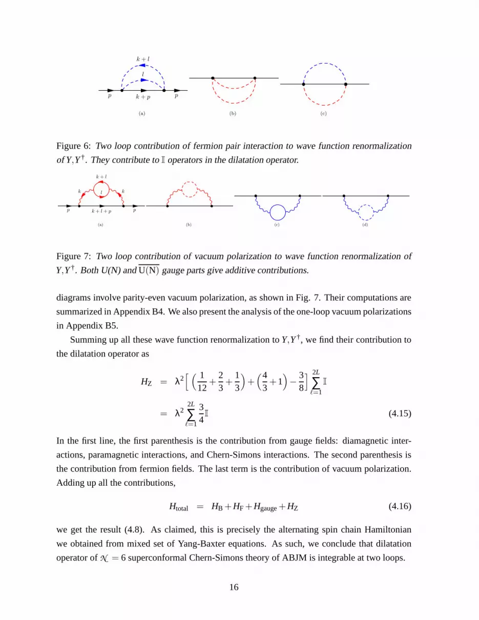
Figure 7: Two loop contribution of vacuum polarization to wave function renormalization of

Y,Y †. Both U(N) andU(N) gauge parts give additive contributions.

diagrams involve parity-even vacuum polarization, as shown in Fig. 7. Their computations are

summarized in Appendix B4. We also present the analysis of the one-loop vacuum polarizations

in Appendix B5.

Summing up all these wave function renormalization toY,Y †, we find their contribution to

the dilatation operator as

HZ = λ2[ ( 1

12+

23

+13

)+(4

3+1)− 3

8

] 2L

∑ℓ=1

I

= λ22L

∑ℓ=1

34

I (4.15)

In the first line, the first parenthesis is the contribution from gauge fields: diamagnetic inter-

actions, paramagnetic interactions, and Chern-Simons interactions. The second parenthesis is

the contribution from fermion fields. The last term is the contribution of vacuum polarization.

Adding up all the contributions,

Htotal = HB +HF+Hgauge+HZ (4.16)

we get the result (4.8). As claimed, this is precisely the alternating spin chain Hamiltonian

we obtained from mixed set of Yang-Baxter equations. As such, we conclude that dilatation

operator ofN = 6 superconformal Chern-Simons theory of ABJM is integrableat two loops.

16

We stress the importance of explicit and direct computationof the dilatation operator with-

out a prior assumption relying on supersymmetry or integrability. It is satisfying that the result

passes various compatibility tests. For instance, take chiral primary operators. These are subset

of the single trace operatorsO whereY ’s andY †’s are totally symmetric and traceless under any

contraction betweenY ’s andY †’s, and corresponds to massive Kaluza-Klein modes overCP3 in

the Type IIA supergravity dual. Because of supersymmetry, their scaling dimension should be

protected against radiative corrections. Indeed, acting on these operators,Htotal vanishes since

contribution of terms involvingK operator are null and contribution ofP cancel against that of

I. As a corollary, the fact that our result is consistent with expectation from supergravity dual

implies that the dimension reduction method we adopted for computations are compatible not

only with Slavnov-Taylor identities of the gauge symmetry but also withN = 6 supersymmetry.

5 The Shortest Chain and Wrapping Interactions

In deriving the dilatation operator in the last section, we assumed that the gauge invariant oper-

ator is infinitely long,L → ∞. From planar diagrammatics, we see easily that dilatation operator

computed perturbatively up to the order 2ℓ will give rise to a spin chain Hamiltonian whose

range extends to(2ℓ)-th order. Therefore, for operators of finite length, a new set of planar dia-

grams which wraps around the operator will come in to contribute. These are so-called wrapping

interactions, a feature discussed much in the context of integrability of four-dimensionalN = 4

super Yang-Mills theory [12], [44]-[53].

In N = 6 superconformal Chern-Simons theory, the situation is more interesting. Since the

dilatation operator at two loops ranges over three sites, spectrum of the shortest gauge invariant

operator of length 2L = 2 will receive contributions from wrapping diagrams already at leading

order! In this section, we like to identify these wrapping interactions for the shortest gauge

invariant operators and discuss their implications.

Let us denote basis of the shortest operators as

|I1I2〉 = TrY I1Y †I2

= OI1I2 ∈ 4⊗4 . (5.1)

The 4⊗ 4 representation is decomposed irreducibly into the traceless part,15, and the trace

part,1. The multiplet15 is chiral primary operator, so their conformal dimension ought to be

protected by supersymmetry.

To check this, let us first identify the two-site dilatation operator that includes the wrapping

interactions. At two-loop orders, the scalar sextet interaction does not contribute to length-

2L = 2 operators since only four legs can be connected to the operators, leaving a tadpole that

vanishes identically. Hence the dilatation operator consists of the two-site plus wave function

17

k + l l

k

k

O

(a)

k + l l

k

k

O

(b)

O

(c)

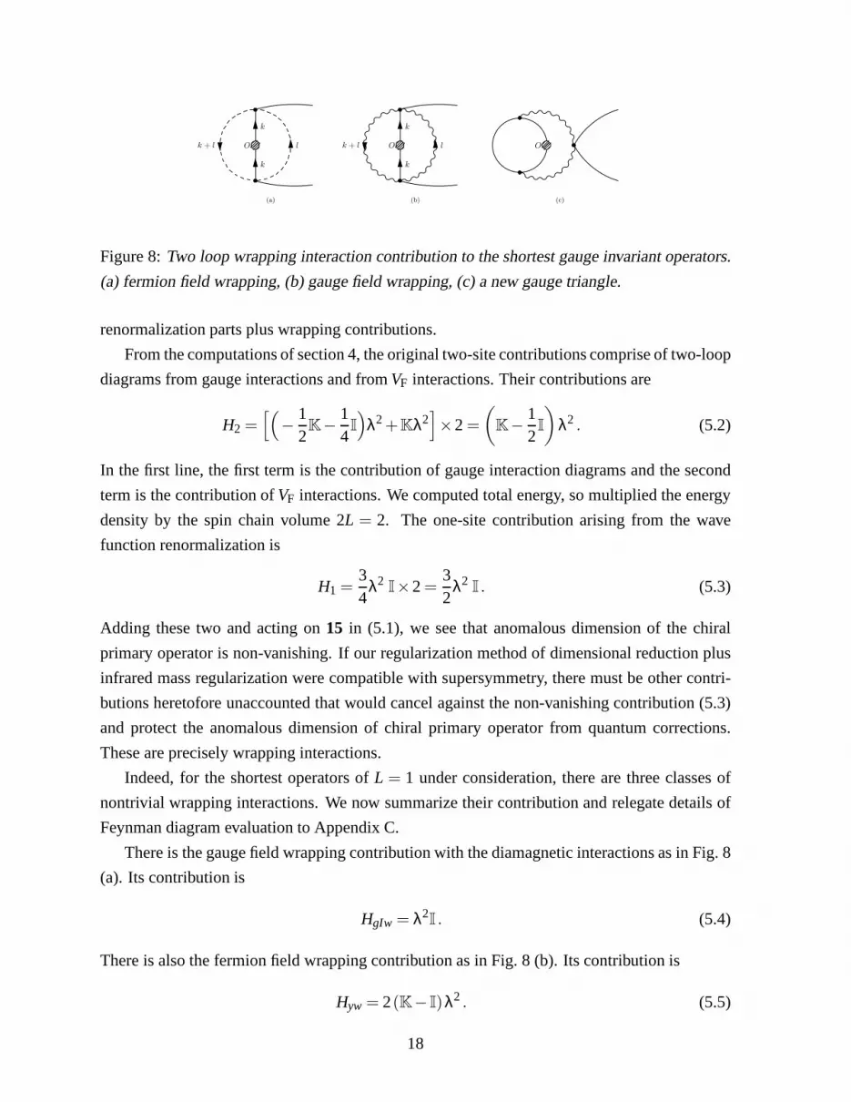
Figure 8:Two loop wrapping interaction contribution to the shortestgauge invariant operators.

(a) fermion field wrapping, (b) gauge field wrapping, (c) a newgauge triangle.

renormalization parts plus wrapping contributions.

From the computations of section 4, the original two-site contributions comprise of two-loop

diagrams from gauge interactions and fromVF interactions. Their contributions are

H2 =[(

− 12K− 1

4I

)λ2+Kλ2

]×2 =

(K− 1

2I

)λ2 . (5.2)

In the first line, the first term is the contribution of gauge interaction diagrams and the second

term is the contribution ofVF interactions. We computed total energy, so multiplied the energy

density by the spin chain volume 2L = 2. The one-site contribution arising from the wave

function renormalization is

H1 =34

λ2I×2 =

32

λ2I . (5.3)

Adding these two and acting on15 in (5.1), we see that anomalous dimension of the chiral

primary operator is non-vanishing. If our regularization method of dimensional reduction plus

infrared mass regularization were compatible with supersymmetry, there must be other contri-

butions heretofore unaccounted that would cancel against the non-vanishing contribution (5.3)

and protect the anomalous dimension of chiral primary operator from quantum corrections.

These are precisely wrapping interactions.

Indeed, for the shortest operators ofL = 1 under consideration, there are three classes of

nontrivial wrapping interactions. We now summarize their contribution and relegate details of

Feynman diagram evaluation to Appendix C.

There is the gauge field wrapping contribution with the diamagnetic interactions as in Fig. 8

(a). Its contribution is

HgIw = λ2I . (5.4)

There is also the fermion field wrapping contribution as in Fig. 8 (b). Its contribution is

Hyw = 2(K− I)λ2 . (5.5)

18

It is important to note that these two wrapping interactionsutilizes simultaneously U(N) and

U(N) interactions. Thus, this contribution arises not just by distinct topology of planar diagram

but from very different interactions from the original, unwrapped two-site interactions.

There is also a doubling-type wrapping contribution of using the same gauge group in-

teractions. This happens only for the gauge interaction diagram contributing toK operator.

Moreover, the contribution is doubled since there are two distinct ways of wrapping. This is

best illustrated on a cylinder, from which we see that there are two different kinds of topology

of wrapped Feynman diagrams. From appendix C, we identify this contribution as

HgKw = −λ2K . (5.6)

Putting both the original and the wrapping diagram contributions together, the full Hamilto-

nian of 2L = 2 operator is given by

H2L=2 = 2λ2K . (5.7)

Notice that the part proportional toI operator is canceled between the original and the wrapping

interaction contributions. One thus check that the chiral primary operators15 indeed has a

vanishing anomalous dimension since, by definition, it has no trace part and is annihilated byK

operator. For the singlet1, |s〉 = 12|II〉, the anomalous dimension is

H|s〉 = 8 λ2 |s〉 . (5.8)

It is interesting to compare the above spectrum with spectrum of the naive Hamiltonian

Hnaive, viz. the alternating spin chain Hamiltonian with periodicboundary condition and 2L = 2.

The latter is12

Hnaive= λ22

∑ℓ=1

[I−Pℓ,ℓ+2+

12

Kℓ+1,ℓ+2Pℓ,ℓ+2+12Kℓ,ℓ+1Pℓ,ℓ+2

]

ℓ+2=ℓ

= 2λ2K , (5.9)

for 2L = 2. Acting on15 and1 states, we find that their anomalous dimension is 0 and 4·2λ2,

respectively. So far, we computed the spectrum of the shortest operators without a priori as-

sumption of supersymmetry. As a consistency check, we now compare these spectra with their

superpartners. Recall that length 2ℓ operators with Dynkin labels(ℓ−2m,m + n, ℓ−2n) and

length 2ℓ−2 operators with Dynkin labels(ℓ−2m,m + n−2, ℓ−2n) are superpartners each

other. Here, we have the simplest situation: theL = 1 operator1 of Dynkin labels(0,0,0) is the

superpartner ofL = 2 operator20of Dynkin labels(0,2,0). Fortuitously, anomalous dimension

of the latter was computed at two loops in [33] to be 8λ2, and matches perfectly with our com-

putation13. Note that, at two loop order, theL = 2 operator20 does not receive any wrapping

12Here, we used the identities (3.21).13We thank Joe Minahan and Kostya Zarembo for useful correspondences on this issue.

19

interaction corrections. As such, we may consider agreement of the anomalous dimensions

between the two superpartners as a nontrivial confirmation for the wrapping interactions we

studied for theL = 1 operator1.

We should also note that the naive Hamiltonian is not the right dilatation operator for the

shortest operators. Nevertheless, interestingly, the spectrum of naive Hamiltonian coincides

with the spectrum extracted from the true two-site Hamiltonian. It would be very interesting to

see whether this coincidence persists to higher orders in perturbation theory.

6 Bethe Ansatz Diagonalization

In section 3, we constructed transfer matrix. To obtain spectrum, we need to diagonalize the

transfer matrices. Within algebraic Bethe ansatz, a fairlygeneral result is known for a Lie

(super)groupsG [30, 26, 29]. It suffices to adapt the results to the case thatG =SU(4)14. Dynkin

diagram of SU(4), drawn horizontally, has three roots: left(l), middle(m), and right(r). The

diagonalization is specified by the choice of Dynkin label(Rl,Rm,Rr) for the site representation

R and total number of sitesLR that representation occupies. In the present case, we have placed

4 and4 representations at alternating lattices, soRl = Rr = 1,Rm = 0 andL4 = L4 = L. Each

excitation is associated with three sets of Bethe ansatz rapidities(la,mb,rc)’s whose labels range

over[1,Nl], [1,Nm], [1,Nr], respectively. It belongs to the SU(4) representation withthe Dynkin

labels(L− 2Nl + Nm,Nl + Nr − 2Nm,L− 2Nr + Nm). Positivity of the Dynkin labels restricts

range of the three Bethe ansatz rapidities accordingly. Then, choosing the highest-weight state:

|Ω+〉 =L

∏ℓ=1

⊗|1〉2ℓ−1|4〉2ℓ ≡ |1414· · ·〉 (6.1)

as the ground-state, the eigenvalue of the transfer matrixT0(−u) 15 is found to be

Λ(u) = (u−1)L(u−2)LNl

∏a=1

u− ila + 12

u− ila− 12

+uL(u−1)LNr

∏c=1

u− irc − 52

u− irc − 32

(6.2)

+ uL(u−2)L[ Nl

∏a=1

u− ila− 32

u− ila− 12

Nm

∏b=1

u− imb−0u− imb−1

+Nm

∏b=1

u− imb −2u− imb −1

Nr

∏c=1

u− irc− 12

u− irc− 32

].

We have chosen the Bethe rapidities symmetric between the three roots. Keeping the highest

weight state the same|1414· · ·〉, we also find that diagonalization of the second transfer matrix

T 0(−v) proceeds much the same way as that ofT0(−v) except that we interchange role of the

14For SU(3) alternating spin chain, this was done explicitly in [28].15For later convenience, we choose to diagonalizeT0 for opposite sign of the spectral parameteru.

20

left and the right SU(4) roots:

Λ(v) = vL(v−1)LNl

∏a=1

v− ila − 52

v− ila − 32

+(v−1)L(v−2)LNr

∏c=1

v− irc + 12

v− irc − 12

(6.3)

+ vL(v−2)L[ Nl

∏a=1

v− ila − 12

v− ila − 32

Nm

∏b=1

v− imb −2v− imb −1

+Nm

∏b=1

v− imb −0v− imb −1

Nr

∏c=1

v− irc − 32

v− irc − 12

].

Mutually commuting conserved charges are then constructedby expanding these eigenvalues

aroundu,v = 0. The first two charges are the total momentum and the total energy:

Ptotal =1i

[logΛ(u)+ logΛ(u)

]u=0

=Nl

∑a=1

log

(la + i/2la − i/2

)+

Nr

∑b=1

log

(rb + i/2rb − i/2

), (6.4)

Etotal = λ2[ d

du(logΛ(u)+ logΛ(u))

]u=0

= λ2( Nl

∑a=1

1

l2a + 1

4

+Nr

∑b=1

1

r2b + 1

4

). (6.5)

Here, we chose fundamental domain of the momentum to[0,2π) and scaled the total energy by

λ2 in accordance to the relation we fixed between Hamiltonian derived from Yang-Baxter equa-

tion and from superconformal Chern-Simons theory. Likewise, we can deduce higher conserved

charges from higher moments of the transfer matrices.

The Bethe equations that results from the above transfer matrix eigenvaluesΛ,Λ are(

la − i2

la + i2

)L

=Nl

∏b=1(b6=a)

la − lb − ila − lb + i

Nm

∏c=1

la −mc + i2

la −mc − i2

1 =Nm

∏b=1(b6=a)

ma −mb + ima −mb − i

Nl

∏c=1

ma − lc − i2

ma − lc + i2

Nr

∏d=1

ma − rd − i2

ma − rd + i2

(ra − i

2

ra + i2

)L

=Nr

∏b=1(b6=a)

ra − rb − ira − rb + i

Nm

∏c=1

ra −mc + i2

ra −mc − i2

. (6.6)

It is straightforward to check that these same set of Bethe ansatz equations remove potential

simple pole terms for bothΛ andΛ simultaneously.

From the integrability perspectives,(2+1)-dimensional superconformal Chern-Simons the-

ory is quite different from(3+1)-dimensional super Yang-Mills theory. The most distinct fea-

ture is that the spin chain associated with dilatation operator is not homogeneous but alternating.

It calls for better understanding to questions that arise incomparison withN = 4 super Yang-

Mills counterpart. We shall now study spectrum of the Bethe ansatz equations for a few simpler

situations and gather features concerning excitations of the alternating spin chain system.

21

First, consider the special class ofNm = 0 for arbitraryL ≥ 2. The first and the third Bethe

ansatz equations decouple, and each equation becomes the same as the Bethe ansatz equation

of the well-known SU(2) XXX12

spin chain. Thus, if one can identify the first set with SU(2) of

4 side, then the third equation corresponds to SU(2) of4. We then have two decoupled sets of

the solution including towers of bound states, and they are exactly the same as the XXX12

spin

chain.

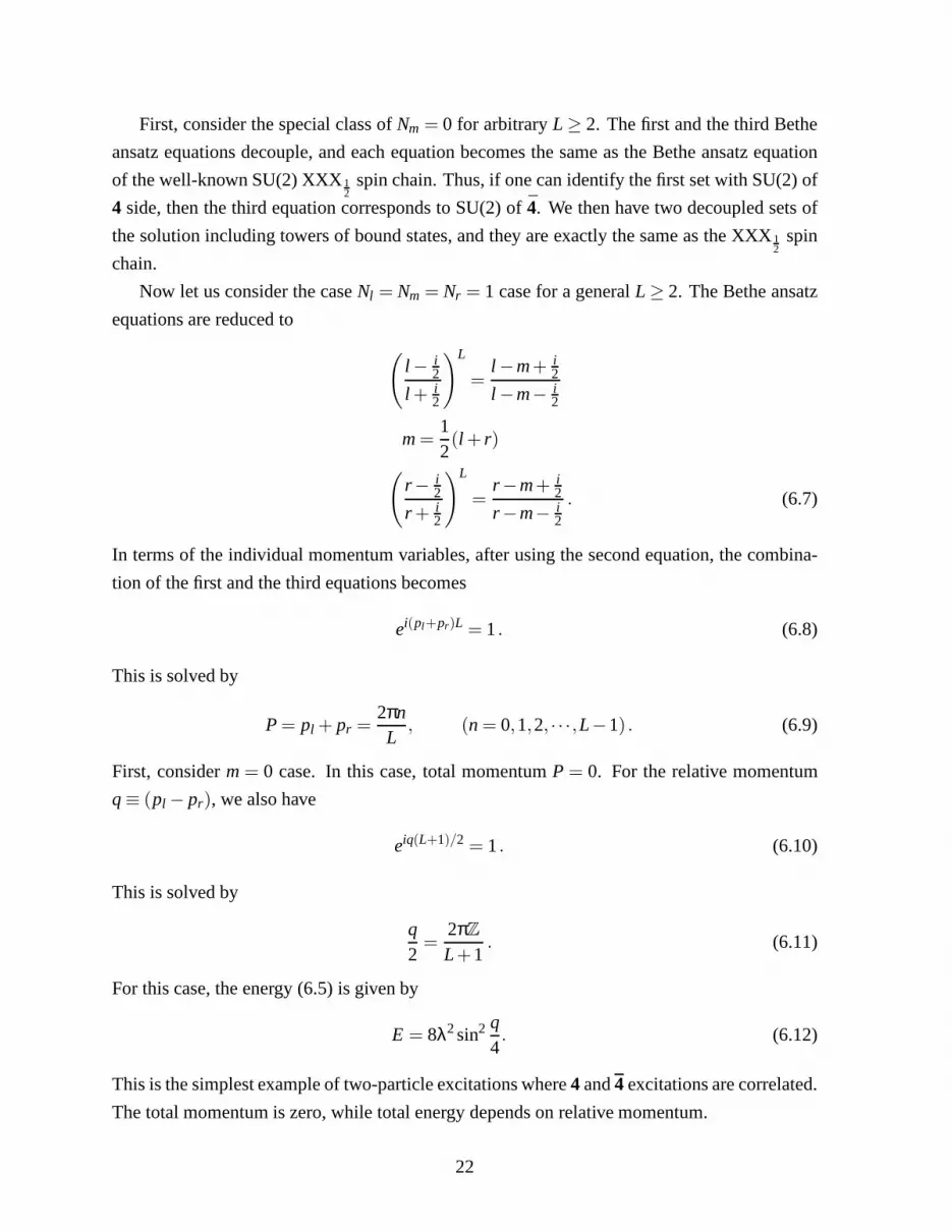
Now let us consider the caseNl = Nm = Nr = 1 case for a generalL ≥ 2. The Bethe ansatz

equations are reduced to

(l− i

2

l + i2

)L

=l −m+ i

2

l −m− i2

m =12(l + r)

(r− i

2

r + i2

)L

=r−m+ i

2

r−m− i2

. (6.7)

In terms of the individual momentum variables, after using the second equation, the combina-

tion of the first and the third equations becomes

ei(pl+pr)L = 1. (6.8)

This is solved by

P = pl + pr =2πn

L, (n = 0,1,2, · · ·,L−1) . (6.9)

First, considerm = 0 case. In this case, total momentumP = 0. For the relative momentum

q ≡ (pl − pr), we also have

eiq(L+1)/2 = 1. (6.10)

This is solved by

q2

=2πZ

L+1. (6.11)

For this case, the energy (6.5) is given by

E = 8λ2sin2 q4. (6.12)

This is the simplest example of two-particle excitations where4 and4 excitations are correlated.

The total momentum is zero, while total energy depends on relative momentum.

22

Consider next generalm. From the ratio between the first and the third equations, we obtain

ei q2L = ∓ l − r− i

l − r + i, (6.13)

where we used the second Bethe ansatz equation for simplification. Total momentumP is

nonzero. Furthermore, expressing this equation in terms ofP andq, we find the relations:

cosP2

=sinq

4(L+2)

sinq4L

orcosq

4(L+2)

cosq4L

. (6.14)

If q is real, viz. two real Bethe roots, the relation shows that relative momentumq is correlated

with total momentumP. That is, even though there are two excitations associated with 4 and4

chains, their motion exhibits mutual correlation. Ifq were imaginary, viz. a Bethe string, the

relation shows that total momentum ought to be purely imaginary. This show that there cannot

arise any bound-state between4 and4 spins.

We can also comment on thermodynamic limit in which densities of the Bethe roots are kept

finite. By takingL → ∞ limit of the Bethe ansatz equations and taking the so-called”no hole”

excitation condition, we obtain relations among the three Bethe root densitiesρl(x),ρm(x),ρr(x).

From the first and the third Bethe ansatz equations, after Fourier transform, we find

ρl(k) = ρr(k) . (6.15)

This has a simple interpretation: because the alternating spin chain is manifestly charge-conjugation

invariant, excitations ought to be so as well. Moreover, from the second Bethe ansatz equation,

we obtain

ρm(k)e−|k|/2 =12

[ρl(k)+ρr(k)

]. (6.16)

It immediately follows from these two equations that the mean value of root densities

Nl

L=

Nr

Land

Nm

L=

12

(Nl

L+

Nr

L

). (6.17)

We conclude that all three Bethe root densities are equal, and hence4’s and4’s are equally

populated and balanced each other for the minimum energy configuration.

Furthermore, analysis of the shortest operator suggests that excitation in superconformal

Chern-Simons spin chain is different from excitation inN = 4 super Yang-Mills spin chain.

In the latter, the vacuum is ferromagnetic and excitations break SOR(6) to [SU(2)]2. The latter

is the symmetry group of dilute, finite-energy excitations.In the present case, analysis of the

previous section seems to indicate that excitation is organized by the full SU(4), not by any

subgroup of it. This is because the finite energy excitation is a singlet of SU(4), not of any

subgroup of it. Lastly, in this system, excitations withNm = 0 comprises of two decoupled

23

XXX 12

spin chains with its own ferromagnetic vacuum, respectively. Though this is certainly a

closed subsector, general excitations in the full system looks quite different, as is seen above in

the simple situation ofNm = 1.

Following the general prescription [29] and paving the parallels to what was done in the con-

text ofN = 4 super Yang-Mills theory [8], extending the SU(4) spin chain to the OSp(6|2,2;R)

superspin chain and writing down Bethe ansatz equations areimmediate and straightforward.

This was done already in [33]. More recently, spectrum in thePenrose limit [54], various

SU(2|2) closed subsectors [31], all loop Bethe ansatz equations [55], and finite-size effects [56]

were studied. With these developments, it would be interesting to explore precision tests for the

new correspondence proposed by ABJM.

Acknowledgement

We would like to thank Dongmin Gang for extensive Mathematica check on an issue related

to integrability and to David Berenstein, Hyunsoo Min, Joe Minahan, Takao Suyama, Satoshi

Yamaguchi, Kostya Zarembo for correspondences and discussions. This work was supported in

part by R01-2008-000-10656-0 (DSB), SRC-CQUeST-R11-2005-021 (DSB,SJR), KRF-2005-

084-C00003 (SJR), EU FP6 Marie Curie Research & Training Networks MRTN-CT-2004-

512194 and HPRN-CT-2006-035863 through MOST/KICOS (SJR),and F.W. Bessel Award

of Alexander von Humboldt Foundation (SJR). S.J.R. thanks the Galileo Galilei Institute for

Theoretical Physics for hospitality during the course of this work.

A Notation, Convention and Feynman Rules

A.1 Notation and Convention

• R1,2 metric:

gmn = diag(−,+,+) with m,n = 0,1,2.

ε012 = −ε012 = +1

εmpqεmrs = −(δpr δq

s −δps δq

r ); εmpqεmpr = −2δqr

(A.1)

• R1,2 Majorana spinor and Dirac matrices:

ψ ≡ two-component Majorana spinor

24

ψα = εαβψβ, ψα = εαβψβ where εαβ = −εαβ = iσ2

γmα

β = (iσ2,σ3,σ1), (γm)αβ = (−I,σ1,−σ3) obeying γmγn = gmn − εmnpγp.(A.2)

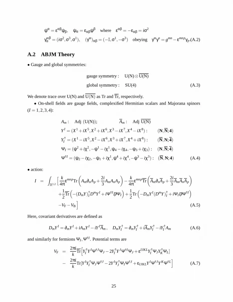
A.2 ABJM Theory

• Gauge and global symmetries:

gauge symmetry : U(N)⊗U(N)

global symmetry : SU(4) (A.3)

We denote trace over U(N) andU(N) as Tr andTr, respectively.

• On-shell fields are gauge fields, complexified Hermitian scalars and Majorana spinors

(I = 1,2,3,4):

Am : Adj (U(N)); Am : Adj U(N)

Y I = (X1+ iX5,X2+ iX6,X3− iX7,X4− iX8) : (N,N;4)

Y †I = (X1− iX5,X2− iX6,X3+ iX7,X4+ iX8) : (N,N;4)

ΨI = (ψ2+ iχ2,−ψ1− iχ1,ψ4− iχ4,−ψ3+ iχ3) : (N,N;4)

Ψ†I = (ψ2− iχ2,−ψ1 + iχ1,ψ4 + iχ4,−ψ3− iχ3) : (N,N;4) (A.4)

• action:

I =

Z

R1,2

[ k4π

εmnpTr

(Am∂nAp +

2i3

AmAnAp

)− k

4πεmnpTr

(Am∂nAp +

2i3

AmAnAp

)

+12

Tr(−(DmY )†

I DmY I + iΨ†ID/ΨI

)+

12

Tr(−DmY I(DmY )†

I + iΨID/Ψ†I)

−VF−VB

](A.5)

Here, covariant derivatives are defined as

DmY I = ∂mY I + iAmY I − iY IAm , DmY †I = ∂mY †

I + iAmY †I − iY †

I Am (A.6)

and similarly for fermionsΨI,Ψ†I. Potential terms are

VF =2πik

Tr[Y †

I Y IΨ†JΨJ −2Y †I Y JΨ†IΨJ + εIJKLY †

I ΨJY †KΨL]

− 2πik

Tr[Y IY †I ΨJΨ†J −2Y IY †

J ΨIΨ†J + εIJKLY IΨ†JY KΨ†L]

(A.7)

25

and

VB = −13

(2πk

)2

Tr[

Y †I Y JY †

J Y KY †KY I +Y †

I Y IY †J Y JY †

KY K

+4Y †I Y JY †

KY IY †J Y K −6Y †

I Y IY †J Y KY †

KY J]

(A.8)

At quantum level, since the Chern-Simons term shifts by integer multiple of 8π2, not onlyN

but alsok should be integrally quantized. To suppress the cluttering2π factors, we also use the

notationκ = k2π . At largeN, we expand the theory and physical observables in double series of

gst =1N

, λ =Nk

=N

2πκ(A.9)

by treating them as continuous perturbation parameters.

A.3 Feynman Rules

• We adopt Lorentzian Feynman rules and manipulate all Dirac matrices andεmnp tensor ex-

pressions to scalar integrals. For actual evaluation of these integrals, we shall go the Euclidean

space integral by the Wick rotation, which corresponds tox0 →−iτ. In the momentum space,

this means we change the contour ofp0 to the imaginary axis following the standard Wick ro-

tation. Then in terms of integration measure, we simply replace d2ωk → id2ωkE together with

p2 →+p2E. The procedure is known to obey Slavnov-Taylor identity, atleast to two loop order.

• We choose covariant gauge fixing condition for both gauge groups:

∂mAm = 0 and ∂mAm = 0 (A.10)

and work in Feynman gauge by setting the gauge parameterξ to unity. Accordingly , we

introduce a pair of Faddeev-Popov ghostsc,c and their conjugates, and add toI the ghosts

action:

Ighost=Z

R2,1

[Tr∂mc∗Dmc+Tr∂mc∗Dmc

](A.11)

Here,Dmc = ∂mc+ i[Am,c] andDmc = ∂mc+ i[Am,c].

• Propagators in U(N)×U(N) matrix notation:

gauge propagator : ∆mn(p) =2πk

Iεmnr pr

p2− iε

scalar propagator : DIJ(p) = δJ

I−i

p2− iε

fermion propagator : SIJ(p) = δI

Jip/

p2− iε

ghost propagator : K(p) =−i

p2− iε(A.12)

26

• Interaction vertices are obtained by multiplyingi =√−1 to nonlinear terms of the Lagrangian

density. Note that the paramagnetic coupling of gauge fieldsto scalar fields has the invariance

property under simultaneous exchange betweenAm,Y I andAm,Y †I .

B Two-Loop Computations

B.1 Two-loop integrals

We first tabulate various Feynman integrals that appear recurrently among two-loop diagrams.

They are all evaluated straightforwardly by Feynman parametrization

1AaBb =

Γ(a+b)

Γ(a)Γ(b)

Z Z

dxdyδ(1− x− y)xa−1yb−1

(Ax+By)a+b . (B.1)

We use dimensional regularization by shifting the spacetime dimension tod = 2ω = 3−ε. The

ultraviolet divergence shows up as a simple pole 1/ε. It is related to the momentum space cutoff

Λ as1ε

:= 2logΛ . (B.2)

In the following, we collect factors arising from propagators in parenthesis and those from

vertices in square bracket. We have the following integrals:

• I1 =Z

d2ωk(2π)2ω

d2ωℓ

(2π)2ω1

(k + ℓ)2

1k2

1ℓ2

=Z 1

0dx

Z

d2ωℓ

(2π)2ω1ℓ2

Z

d2ωk(2π)2ω

1[k2+2xk · ℓ+ xℓ2]2

= − 18π

Z 1

0dx

1√x(1− x)

Z

d2ωℓ

(2π)2ω1√(k2)3

= +18

14π2

1ε. (B.3)

The integral that appears in fermion and gauge boson exchange diagrams is:

• I2 =Z

d2ωk(2π)2ω

d2ωℓ

(2π)2ω1

(k2)2

2(k + ℓ) · ℓ(k + ℓ)2 ℓ2 . (B.4)

We perform theℓ integral first after using the Feynman reparametrization:

I2 =Z 1

0dx

Z

d2ωk(2π)2ω

1(k2)2

Z

d2ωℓ

(2π)2ω2ℓ · (ℓ+ k)

[ℓ2+2xk · ℓ+ xk2]2

= − 18π

Z 1

0dx

√x√

1− x

Z

d2ωk(2π)2ω

1k3

= −18

14π2

1ε

, (B.5)

27

where for the second equality, we have used the integral,

Z

d2ωℓ

(2π)2ωℓmℓn

[ℓ2+2xℓ · k + k2]2=

1

(4π)3/2

[ x2kmknΓ(1/2)

[x(1− x)k2]1/2+

gmn

2Γ(−1/2)

[x(1− x)k2]−1/2

]

Z

d2ωℓ

(2π)2ωℓm

[ℓ2+2xℓ · k + k2]2= − 1

(4π)3/2

xkmΓ(1/2)

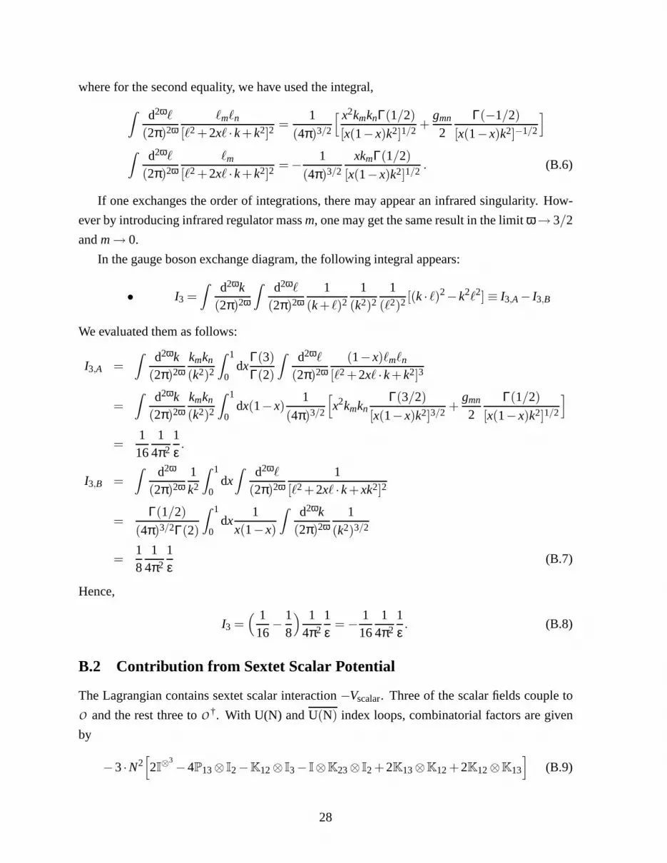
[x(1− x)k2]1/2. (B.6)

If one exchanges the order of integrations, there may appearan infrared singularity. How-

ever by introducing infrared regulator massm, one may get the same result in the limitω → 3/2

andm → 0.

In the gauge boson exchange diagram, the following integralappears:

• I3 =

Z

d2ωk(2π)2ω

Z

d2ωℓ

(2π)2ω1

(k + ℓ)2

1(k2)2

1(ℓ2)2 [(k · ℓ)2− k2ℓ2] ≡ I3,A − I3,B

We evaluated them as follows:

I3,A =

Z

d2ωk(2π)2ω

kmkn

(k2)2

Z 1

0dx

Γ(3)

Γ(2)

Z

d2ωℓ

(2π)2ω(1− x)ℓmℓn

[ℓ2+2xℓ · k + k2]3

=

Z

d2ωk(2π)2ω

kmkn

(k2)2

Z 1

0dx(1− x)

1

(4π)3/2

[x2kmkn

Γ(3/2)

[x(1− x)k2]3/2+

gmn

2Γ(1/2)

[x(1− x)k2]1/2

]

=116

14π2

1ε.

I3,B =

Z

d2ω

(2π)2ω1k2

Z 1

0dx

Z

d2ωℓ

(2π)2ω1

[ℓ2+2xℓ · k + xk2]2

=Γ(1/2)

(4π)3/2Γ(2)

Z 1

0dx

1x(1− x)

Z

d2ωk(2π)2ω

1

(k2)3/2

=18

14π2

1ε

(B.7)

Hence,

I3 =( 1

16− 1

8

) 14π2

1ε

= − 116

14π2

1ε. (B.8)

B.2 Contribution from Sextet Scalar Potential

The Lagrangian contains sextet scalar interaction−Vscalar. Three of the scalar fields couple to

O and the rest three toO †. With U(N) andU(N) index loops, combinatorial factors are given

by

−3 ·N2[2I

⊗3 −4P13⊗ I2−K12⊗ I3− I⊗K23⊗ I2 +2K13⊗K12+2K12⊗K13

](B.9)

28

There are three scalar propagators and one interaction vertex, contributing factors

13κ2(i)3 [i ] ·N2 =

4π2

3λ2 (B.10)

The remaining 2-loop integral is given byI1. Summing over all contributions, the scalar sextet

interaction gives rise to 2-loop dilatation operator

HB =λ2

2

2L

∑ℓ=1

[I−2Pℓ,ℓ+2−Kℓ,ℓ+1 +Pℓ,ℓ+2Kℓ,ℓ+1+Kℓ,ℓ+1Pℓ,ℓ+1

](B.11)

B.3 Contribution from two-site Interactions

In this appendix we shall present the full detailed computation of the two site interactions. First

let us compute the Yukawa two-site interactions. The nonvanishing Yukawa interaction leads to

only aK-type interaction. The relevant Feynman diagram is depicted in Fig. 2b.

With two Yukawa interaction components and one U(N) and oneU(N) color traces, combi-

natorial factors are gathered as

12!

·2 ·N2 = N2. (B.12)

There are four propagators and two vertices. This yields numerical factors

(−i)2(i)2[i ]2(±2i

κ

)2

· (−)FD (B.13)

where the subscript( )FD signifies the Fermi-Dirac statistics minus sign. The loop integral is

given by

i2Z

d2ωk(2π)2ω

d2ωℓ

(2π)2ω1

(−(k)2)2 tr( ℓ/

ℓ2

k/+ ℓ/

(k + ℓ)2

)(B.14)

where thei2 factor comes from the analytic continuation of the integration measure.

After taking the gamma matrix trace trγmγn = 2gmn, this integral equals to−I2 in (B.5).

Hence putting everything together, one has

λ2(−1)

2εK (B.15)

for the Yukawa two-site interactions. The contribution to the operator renormalization is nega-

tive of this: Therefore, the Yukawa contribution is

HF = λ22L

∑ℓ=1

Kℓ,ℓ+1 (B.16)

29

We now evaluate the gauge two-site interactions.

The gauge boson interactions contribute bothK andI type diagrams to the dilatation op-

erator. Let us begin withK type contribution. The relevant diagram is in Fig. 2c. It has

combinatorial factors

12!

·2 ·N2 = N2. (B.17)

There are three boson propagators, two gauge propagators and one seagull interaction vertex.

So, numerical factors are given by

(−i)3 · [−i ]3 · (±1)2(1

κ

)2= −4π2

k2 (B.18)

where the last factor accounts for the(±) relative sign of U(N) andU(N) Chern-Simons term.

It is important to note that the gauge field propagator in momentum space has noi =√−1. The

loop integral reads

i2Z

d2ωk(2π)2ω

d2ωℓ

(2π)2ω1

(k + ℓ)2

1(k2)2

1(ℓ2)2(εmnp(k +2ℓ)nkp)gmq(εqrs(k +2ℓ)r(−k)s) (B.19)

where again thei2 factor comes from the Euclidean rotation. Using the identity gmqεmnpεqrs =

−(gnrgps −gnsgpr), we find that the integral is the same as 4I3.

Hence putting everything together, one has

− λ2

2(−1)

2εK (B.20)

for the gauge two siteK contributions and, for the operator renormalization,

− λ2

212ε

K . (B.21)

There are also contributions toI from t-channel exchange of diamagnetic gauge boson inter-

action. The corresponding Feynman diagram is depicted in Fig 2a. There are two scalar prop-

agators, two gauge boson propagators and two diamagnetic vertices. Note again, for Chern-

Simons theory, gauge boson propagator has noi in momentum space. So, the combinatorial

factor is

12!

2 · (−i)2 · [i ]2 ·N2 ·(1

κ

)2= (4π2)λ2. (B.22)

The loop integral reads

i2Z

d2ωk(2π)2ω

d2ωℓ

(2π)2ω1

(k2)2

εmna(k + ℓ)a

(k + ℓ)2

εmnbℓb

ℓ2 (B.23)

30

Using the identityεmnaεmnb = −2gab, we find that this integral is the same as−I2. There

are identical contributions from each letter (with alternating U(N) andU(N) gauge boson ex-

changes), we find the contribution as

− λ2

4(−1)

2εI . (B.24)

The corresponding operator renormalozation contributionis

− λ2

412ε

I . (B.25)

Hence there are two gauge two-site contributions. Using 1/(2ε) = lnΛ, the gauge two-site

contributions to the anomalous dimension are summarized as

Hgauge=2L

∑ℓ=1

[−1

4I− 1

2Kℓ,ℓ+1

]λ2 . (B.26)

B.4 Contributions of Wave Function Renormalization

The first one involves diamagnetic gauge interactions. The relevant Feynman diagrams are in

Fig. 3. As scalar fields are bi-fundamentals, there are processes involving U(N) gauge boson

pair,U(N) gauge boson pair, and one U(N) gauge boson and oneU(N) gauge boson pair, which

are respectively corresponding to Fig. 3a, Fig. 3b and Fig. 3c. Taking account of opposite rel-

ative sign between gauge boson propagators for U(N) andU(N) and of different combinatorial

weight of diamagnetic coupling terms, the numerical factorreads

12!

2 · (−i) · [i ]2 · [(−)2 · (+)2+(+)2 · (−)2+(+)(−) · (−2)2]N2(1

κ

)2= −2i(4π2)λ2 (B.27)

Denote momentum of the external scalar field aspm. Then, loop integral reads

i2Z

d2ωk(2π)2ω

d2ωℓ

(2π)2ω1

(k + ℓ+ p)2

εmnaka

k2

εmnbℓb

ℓ2 . (B.28)

For the evaluation of this integral, let us introduce

IG(p) =

Z

d2ωk(2π)2ω

d2ωℓ

(2π)2ω1

(k + ℓ+ p)2

2k · ℓk2 ℓ2

= 2Z

d2ωℓ

(2π)2ω1ℓ2

Z 1

0dx

Z

d2ωk(2π)2ω

k · ℓ[(k + x(ℓ+ p))2+ x(1− x)(ℓ+ p)2]2

= − 14π

Z 1

0dx

√x

1− x

Z

d2ωℓ

(2π)2ωℓ · (ℓ+ p)√

(ℓ+ p)2. (B.29)

31

The x-integral is finite and equals toπ/2. The remainingℓ-integral can be performed by

applying Feynman’s parametrization. In dimensional regularization, we have

−18

Γ(3/2)

Γ(1/2)

Z 1

0dy

1√y

Z

d2ωℓ

(2π)2ωℓ · p

[ℓ2+2xℓ · p+ xp2]3/2

= − 116

Z 1

0

dy√y

[− Γ(ε)

(4π)ωΓ(3/2)

yp2

(y(1− y)p2)ε

](B.30)

Takingε = 3/2−ω → 0, this integral equals to

IG =124

14π2

1ε. (B.31)

Putting together, we thus find that these diagrams contribute to the wave function renormaliza-

tion as

− 112

λ21ε(ip2) (B.32)

Consider next two diagrams involving four paramagnetic couplings. Planar diagrams in-

volve two vertices from U(N) and two fromU(N), as shown in Fig. 4. Taking care of opposite

relative sign of gauge boson propagators between U(N) andU(N) and that there are three inter-

nal scalar propagators, we have combinatorial factors

1(2!)222 · (+)(−) · (−i)3[i ]2

(1κ

)2N2(2) = −2i(4π2)λ2. (B.33)

where we put an additional factor two because there are two such diagrams. With external

momentumpm, the loop integral read

i2Z

d2ωk(2π)2ω

d2ωℓ

(2π)2ωεmnq(ℓ+2p)m(p+2k +2ℓ)nℓqεabc(2ℓ+ k +2p)a(k +2p)bkc

(k + ℓ+ p)2(ℓ+ p)2(k + p)2k2ℓ2 . (B.34)

This integral can be integrated without further assumptionbut we note that the numerator of the

integrand is already quadratic inpm. Using the isotropy of the system, we replace

pa pb → p2

3gab (B.35)

and then setp to zero in the remaining integral. One may show that the results from the both

methods agree precisely with each other.

Thus the integral becomes

− 163

p2 I3 =p2

12π2

1ε

. (B.36)

Putting all the factor together, one has

− 23

λ21ε(ip2) (B.37)

32

There are two diagrams involving Chern-Simons cubic coupling. The contributions of U(N)

andU(N) are added up with an equal weight. The Feynman diagrams are inFig. 5.

The relevant combinatorics is

3! ·33!

(−i)2[i ]4N2((±)κi

3

)((±1)

κ

)3(2) = −2i(4π2)λ2 (B.38)

where the last factor two takes care of theU(N) contribution. The loop integral becomes

i2Z

d2ωk(2π)2ω

d2ωℓ

(2π)2ωεmqnεmar(2p+ k)akrεnbs(2p− ℓ+ k)b(−k− ℓ)sεqct(2p− ℓ)bℓt

(p− ℓ)2(k + ℓ)2(k + p)2k2ℓ2 . (B.39)

Using the rule of

pa pb →δab

3p2 ,

the integral becomes

i28p2

3

Z

d2ωk(2π)2ω

d2ωℓ

(2π)2ω−k2ℓ2+(k · ℓ)2

(k + ℓ)2(k2)2(ℓ2)2 . (B.40)

UsingI3, one finds

p2

61

4π2

1ε

. (B.41)

Therefore, the whole contribution combining the combinatorics becomes

− 13

λ21ε

ip2 . (B.42)

There are also diagrams involving paramagnetic and diamagnetic couplings. Their net com-

binatorial factor is nonzero, but the loop integral vanishes identically.

Let us now turn to the Yukawa contributions. First consider the Feynman diagrams in Fig. 6a

and Fig. 6b. Within the planar diagram, both fermion can be joined either U(N) side (Fig. 6a)

andU(N) side (Fig. 6b). The joining using the first two terms has a factor 4 from the SU(4)

index contraction. Then the cross terms between the first twoand the second two terms in total

have a factor−4. Hence one can check that this cross contributions cancel precisely the those

from the first two.

By combining the second two of the Yukawa potential, for the U(N) andU(N) side, we have

combinational factors

12!

2 · (−i · i2)[i ]2 ·(2i

κ

)2N2(−)FD×8 = −32i(4π2)λ2. (B.43)

where the extra factor eight comes from one contraction of SU(4) index and the doubling by

U(N) andU(N).

33

Then the remaining integral has the expression,

i2Z

d2ωk(2π)2ω

d2ωℓ

(2π)2ω1

(p+ k− ℓ)2

tr ℓ/ k/k2 ℓ2 (B.44)

which is same asIG. Therefore the whole contribution is

− 43

λ21ε(ip2) . (B.45)

For the wave function renormalization, the third two of Yukawa potential also contribute.

The diagram is in Fig. 6c. It has combinatoric factors,

(2!)2 · (−i) · (i)2[i ]2 ·( i

κ

)(−iκ

)N2(−)FD× (−6) = −24i(4π2)λ2 , (B.46)

where(2!)2 is the usual symmetry factor of the Feynman diagram. The lastfactor(−6) comes

from the followingSU(4) index contraction

εIABCεJCBA = −6 δJI (B.47)

whereI is for the incoming and theJ for the outgoing scalarSU(4) indices.

Then the remaining integral takes precisely the same from:

i2Z

d2ωk(2π)2ω

d2ωℓ

(2π)2ω1

(p+ k− ℓ)2

tr ℓ/ k/k2 ℓ2 (B.48)

which is again the same asIG. Therefore the whole contribution is

−λ21ε(ip2) . (B.49)

Finally, there are the vacuum polarization contributions of the gauge loop. The relevant

diagrans are depicted in Fig. 7.

As we shall explain in the following appendix, the self energy correction for bothA andA

gauge fields is given by

iΠab(k) = 8i[kakb −gabk2

16k

], (B.50)

where the factor eight comes from the four complex scalars and fermions with an equal weight.

For the relevant diagram of Fig. 7, the combinatorics factorreads

2!2!

· (−i)[i ]2 ·(1

κ

)2N2× (2) = 2i(4π2)λ2 , (B.51)

where the last factor two comes from the doubling by replacing A gauge by theA gauge field.

The remaining Feynman integrals takes the from,

iZ

d2ωk(2π)2ω

εamn(2p+ k)m(−k)nεbi j(k +2p)ik j iΠab(k)

(k + p)2(k2)2 ,

= 2Z

d2ωk(2π)2ω

k2p2− (k · p)2

(k + p)2 k3 (B.52)

34

where we have a singlei produced by the Euclidean rotation.

By the dimensional regularization, this leads to

p2 13π2

1ε

. (B.53)

Hence the total contribution reads

83

λ21ε(ip2) . (B.54)

All the remaining diagrams, one may prove that their contribution is identically zero after

the dimensional regularization.

Finally we add up all the above contributions to the wave function renormalization and find

that

− 34

λ21ε(−)(−ip2) . (B.55)

Since the counter term is a negative of this, the two-loop scalar wave function renormaliza-

tion becomes

Zs = 1− 34

λ21ε

= 1− 34

λ2(2lnΛ) . (B.56)

In order to get the operator renormalization factor, one hasto takeZ12s out for each site, which

corresponds to adding−12 of (B.56) to the interaction part of renormalization. The final contri-

bution to the anomalous dimension is

HZ = λ22L

∑ℓ=1

[(112

+23

+13

)+

(43

+1

)− 8

3

]I = λ2

2L

∑ℓ=1

34

I . (B.57)

For the gauge two-loop contributions 1/12, 2/3, 1/3 including the gauge self-energy cor-

rection contribution 8/3, the two-loop Feynman diagram computation is carried out in Ref.[57]

for theU(1) case. One can check the precise agreement after taking care of the planarity fac-

tor and the number of matter degrees. Furthermore, Ref. [58]deals with the two-loop Yukawa

contribution to the scalar wave function renormalization for againU(1). This result is again

matching with ours if one takes care of the planarity and the number of fermions.

B.5 One loop self energy correction to the gauge field

The self-energy correction enters in the same form for the U(N) and theU(N) gauge fields.

Therefore we focus on the correction toA gauge field only. At the one-loop level, the boson,

the fermion, the gauge and the ghost loops may in general contribute to the gauge self-energy

correction. In this appendix, we identify these self-energy contributions.

35

We begin with the scalar loop contribution. It is the sub-diagram of Fig. 7a. The momentum

k plays the role of the external momentum. The self energy contribution reads

iΠsab(k) = (i)2[i ]2(4)i

Z

d2ωℓ

(2π)2ω(2ℓ+ k)a(2ℓ+ k)b

(k + ℓ)2 ℓ2 , (B.58)

where the extra factor 4 comes from the fact that 4 complex scalars are coupled to the gauge

field. Using the dimensional regularization, one obtains

iΠsab(k) = (4)i

[kakb −gabk2

16k

]. (B.59)

Similarly, for the fermion loop, the self-energy contribution becomes

iΠ fab(k) = (i)2[i ]2(4)(−)FD i

Z

d2ωℓ

(2π)2ωTrγa (ℓ/+ k/)γb ℓ/

(k + ℓ)2 ℓ2 , (B.60)

where again the extra factor four comes from the fact that there are 4 complex fundamental

fermions. Using theγ matrix identity and the dimensional regularization, the contribution be-

comes

iΠ fab(k) = (4)i

[kakb −gabk2

16k

]. (B.61)

Hence, each complex matter contributes by the same weight and sign.

One can continue the dimensions 2ω to four and obtain the vacuum polarization in four-

dimensional Yang-Mills theories. The integration leads tothe logarithmic divergence in this

case contributing positively to theβ-function of the Yang-Mills coupling. Again, boson and

fermion contributions add up.

For the gluon self-energy contribution, we have

iΠAab(k) = (3) · (3)[i2]

[ iκ3

]2[1κ

]2(i)2[i ]2(4)i

Z

d2ωℓ

(2π)2ωεmbnε jaiεimqεn jr(ℓ+ k)qℓr

(k + ℓ)2 ℓ2 ,

= iZ

d2ωℓ

(2π)2ω(ℓ+ k)aℓb +(ℓ+ k)bℓa

(k + ℓ)2 ℓ2 . (B.62)

It becomes

iΠAab(k) = −i

[kakb +gabk2

32k

], (B.63)

which alone does not respect the gauge invariance. However,there exists also the ghost loop

contribution,

iΠghab(k) = (i)2[i ]2(−)i

Z

d2ωℓ

(2π)2ω(ℓ+ k)aℓb +(ℓ+ k)bℓa

(k + ℓ)2 ℓ2 , (B.64)

36

where we put the extra (−) sign due to the ghost statistics. Therefore, the ghost contribution

cancels out precisely the gauge loop contribution, reproducing the well-established result [43].

Again, analytically continuing to four dimensions, the integral expression for the gauge part

changes while the ghost integral remains intact. With Yang-Mills couplings, both contributions

no longer cancel each other but contribute negatively to theβ-function.

C Wrapping Interactions for the Two-Sites

As in Fig. 8, there are occuring three kinds of wrapping interactions. First is the gauge interac-

tions of two diamagnetic couplings in Fig. 8b. It is anI type interaction and happens, not for

each site, but just once.

The combinatorial factor is

12!

2 · (−i)2 · [2i ]2 · (+)(−) ·N2 ·(1

κ

)2= −(4)4π2λ2. (C.1)

where (+)(-) accounts for the the relativeU(N) andU(N) Chern-Simons term and the factor

two in the vertices takes care of the diamagnetic interaction.

The loop integral

i2Z

d2ωk(2π)2ω

d2ωℓ

(2π)2ω1

(k2)2

εmna(k + ℓ)a

(k + ℓ)2

εmnbℓb

ℓ2 (C.2)

is the same as (B.23). So, the loop integral is evaluated as

18

14π2

1ε

. (C.3)

Putting things together, we find the whole contribution as

λ2(−1)

2εI . (C.4)

The corresponding operator renormalization contributionis

λ2 12ε

I . (C.5)

The second is for theK type gauge wrapping, whose Feynman diagram is depicted in Fig. 8c.

It is doubling of the K-type interaction discussed for the general two-site gauge interactions.

This doubling occurs due to the fact that, on the cylinder, one may have two different topology

of the diagrams. Namely the diamagnetic interaction of the same gauge group may happen

either one side or the other side, which is not possible for the infinite chains. From the previous

result, the corresponding extra operator renormalizationcontribution is

−λ2 12ε

K , (C.6)

37

where we take into account of the fact that the doubling occurs both for theU(N) andU(N).

There is an additional wrapping interaction coming from thethird two terms in the Yukawa

potential. The Feynman diagram is in Fig. 8. In order to have proper contractions, one has to

join operator site one (Y I1) to the site two (Y J2) whereas the operator site twoY †I2

to Y †J1

. The

correspondingε tensors in the Yukawa interaction produce

εI1AJ2B εI2BJ1A = 2(I−K) . (C.7)

The combinatorial factors are gathered as

2!2!

·2 ·2(−i)2(i)2[i ]2 ·N2 ·(

iκ

)(−iκ

)· (−)FD = 4(4π2) ·λ2 . (C.8)

The loop integral is given by

i2Z

d2ωk(2π)2ω

d2ωℓ

(2π)2ω1

(−(k)2)2 tr( ℓ/

ℓ2

k/+ ℓ/

(k + ℓ)2

), (C.9)

which is the same as (B.14). By the loop integration, one gets

18

14π2

1ε

. (C.10)

Hence putting everything together, one has

2λ2(−1)

2ε(K− I) (C.11)

for the Yukawa wrapping interactions. Therefore, the Yukawa contribution to the operator renor-

malization is

2λ2 12ε

(K− I) . (C.12)

Adding up the gauge and Yukawa contributions, the wrapping interaction contribution to the

two-site Hamiltonian is

Hwrap = I−K+2(K− I) = −I+K . (C.13)

References

[1] O. Aharony, O. Bergman, D. L. Jafferis and J. Maldacena, “N=6 superconformal Chern-

Simons-matter theories, M2-branes and their gravity duals,” arXiv:0806.1218 [hep-th].

[2] J. M. Maldacena, Adv. Theor. Math. Phys.2 (1998) 231 [Int. J. Theor. Phys.38 (1999)

1113] [arXiv:hep-th/9711200].

38

[3] B. E. W. Nilsson and C. N. Pope, Class. Quant. Grav.1 (1984) 499.

[4] J. A. Minahan and K. Zarembo, JHEP0303(2003) 013 [arXiv:hep-th/0212208].

[5] N. Beisert, C. Kristjansen and M. Staudacher, Nucl. Phys. B 664 (2003) 131

[arXiv:hep-th/0303060].

[6] S. Frolov and A. A. Tseytlin, Nucl. Phys. B668(2003) 77 [arXiv:hep-th/0304255].

[7] N. Beisert, Nucl. Phys. B676(2004) 3 [arXiv:hep-th/0307015].

[8] N. Beisert and M. Staudacher, Nucl. Phys. B670(2003) 439 [arXiv:hep-th/0307042].

[9] G. Arutyunov, S. Frolov, J. Russo and A. A. Tseytlin, Nucl. Phys. B671 (2003) 3

[arXiv:hep-th/0307191].

[10] N. Beisert, Nucl. Phys. B682(2004) 487 [arXiv:hep-th/0310252].

[11] N. Beisert, V. Dippel and M. Staudacher, JHEP0407(2004) 075 [arXiv:hep-th/0405001].

[12] G. Arutyunov, S. Frolov and M. Staudacher, JHEP0410 (2004) 016

[arXiv:hep-th/0406256].

[13] N. Beisert, Phys. Rept.405(2005) 1 [arXiv:hep-th/0407277].

[14] M. Staudacher, JHEP0505(2005) 054 [arXiv:hep-th/0412188].

[15] N. Beisert, V. A. Kazakov, K. Sakai and K. Zarembo, Commun. Math. Phys.263 (2006)

659 [arXiv:hep-th/0502226].

[16] N. Beisert and M. Staudacher, Nucl. Phys. B727(2005) 1 [arXiv:hep-th/0504190].

[17] N. Beisert, “Thesu(2|2) dynamic S-matrix,” arXiv:hep-th/0511082.

[18] D. M. Hofman and J. M. Maldacena, J. Phys. A39 (2006) 13095 [arXiv:hep-th/0604135].

[19] N. Beisert, R. Hernandez and E. Lopez, JHEP0611(2006) 070 [arXiv:hep-th/0609044].

[20] N. Beisert, J. Stat. Mech.0701(2007) P017 [arXiv:nlin/0610017].

[21] N. Beisert, B. Eden and M. Staudacher, J. Stat. Mech.0701 (2007) P021

[arXiv:hep-th/0610251].

[22] D. Gaiotto and X. Yin, JHEP0708(2007) 056 [arXiv:0704.3740 [hep-th]].

[23] E. Brezin, C. Itzykson, J. Zinn-Justin and J. B. Zuber, Phys. Lett. B82 (1979) 442.

39

[24] I. Bena, J. Polchinski and R. Roiban, Phys. Rev. D69 (2004) 046002

[arXiv:hep-th/0305116].

[25] H. J. de Vega and F. Woynarovich, J. Phys. A25, 4499 (1992).

[26] S. R. Aladim and M. J. Martins, J. Phys. A26 (1993) 7287 [arXiv:hep-th/9306049];

M. J. Martins, ”Integrable Mixed Vertex Models from Braid-Monoid Algebra”,

[arXiv:solv-int/9903006].

[27] G. A. P. Ribeiro and M. J. Martins, Nucl. Phys. B738(2006) 391 [arXiv:nlin/0512035].

[28] J. Abad and M. Rios, J. Phys. A30 (1997) 5887 [arXiv:cond-mat/9706136]; J. Phys. A31

(1998) 2269 [arXiv:cond-mat/9801129].

[29] E. Ragoucy and G. Satta, JHEP0709, 001 (2007) [arXiv:0706.3327 [hep-th]].

[30] P. P. Kulish and N. Y. Reshetikhin, J. Phys. A16 (1983) L591.

[31] D. Gaiotto, S. Giombi and X. Yin, “Spin Chains in N=6 Superconformal Chern-Simons-

Matter Theory,” arXiv:0806.4589 [hep-th].

[32] G. Grignani, T. Harmark and M. Orselli, “The SU(2) x SU(2) sector in the string dual of

N=6 superconformal Chern-Simons theory,” arXiv:0806.4959 [hep-th].

[33] J. A. Minahan and K. Zarembo, “The Bethe ansatz for superconformal Chern-Simons,”

arXiv:0806.3951 [hep-th].

[34] G. Arutyunov and S. Frolov, “Superstrings onAdS4xCP3 as a Coset Sigma-model,”

arXiv:0806.4940 [hep-th].

[35] B. J. Stefanski, “Green-Schwarz action for Type IIA strings on AdS4 × CP3,”

arXiv:0806.4948 [hep-th].

[36] N. Gromov and P. Vieira, “The AdS4/CFT3 algebraic curve,” arXiv:0807.0437 [hep-th].

[37] V. Serganova, Math. USSR-Izv24 (1985) 539; D. Grantcharov and A. Pianzola, Int. Math.

Res. Not. (IMRN)73 (2004) 3937.

[38] N. Berkovits, M. Bershadsky, T. Hauer, S. Zhukov and B. Zwiebach, Nucl. Phys. B567

(2000) 61 [arXiv:hep-th/9907200].

[39] Y. Y. Goldschmidt and E. Witten, Phys. Lett. B91 (1980) 392.

[40] E. Abdalla, M. Forger and M. Gomes, Nucl. Phys. B210(1982) 181.

40

[41] C. M. Bender and S. Boettcher, Phys. Rev. Lett.80 (1998) 5243 [arXiv:physics/9712001].

[42] M. Benna, I. Klebanov, T. Klose and M. Smedback, “Superconformal Chern-Simons The-

ories andAdS4/CFT3 Correspondence,” arXiv:0806.1519 [hep-th].

[43] W. Chen, G. W. Semenoff and Y. S. Wu, Phys. Rev. D46 (1992) 5521

[arXiv:hep-th/9209005].

[44] C. Sieg and A. Torrielli, Nucl. Phys. B723(2005) 3 [arXiv:hep-th/0505071].

[45] S. Schafer-Nameki and M. Zamaklar, JHEP0510(2005) 044 [arXiv:hep-th/0509096].

[46] J. Ambjorn, R. A. Janik and C. Kristjansen, Nucl. Phys. B736 (2006) 288

[arXiv:hep-th/0510171].

[47] G. Arutyunov, S. Frolov and M. Zamaklar, Nucl. Phys. B778 (2007) 1

[arXiv:hep-th/0606126].

[48] A. V. Kotikov, L. N. Lipatov, A. Rej, M. Staudacher and V.N. Velizhanin, J. Stat. Mech.

0710(2007) P10003 [arXiv:0704.3586 [hep-th]].

[49] R. A. Janik and T. Lukowski, Phys. Rev. D76 (2007) 126008 [arXiv:0708.2208 [hep-th]].

[50] F. Fiamberti, A. Santambrogio, C. Sieg and D. Zanon, “Wrapping at four loops in N=4

SYM,” arXiv:0712.3522 [hep-th].

[51] C. A. Keeler and N. Mann, “Wrapping Interactions and theKonishi Operator,”

arXiv:0801.1661 [hep-th].

[52] J. Penedones and P. Vieira, “Toy models for wrapping effects,” arXiv:0806.1047 [hep-th].

[53] F. Fiamberti, A. Santambrogio, C. Sieg and D. Zanon, “Anomalous dimension with wrap-

ping at four loops in N=4 SYM,” arXiv:0806.2095 [hep-th].

[54] T. Nishioka and T. Takayanagi, “On Type IIA Penrose Limit and N=6 Chern-Simons The-

ories,” arXiv:0806.3391 [hep-th].

[55] N. Gromov and P. Vieira, “The all loop AdS4/CFT3 Bethe ansatz,” arXiv:0807.0777 [hep-

th].

[56] G. Grignani, T. Harmark, M. Orselli and G. W. Semenoff, “Finite size Giant Magnons in

the string dual of N=6 superconformal Chern-Simons theory,” arXiv:0807.0205 [hep-th].

41

[57] V. S. Alves, M. Gomes, S. L. V. Pinheiro and A. J. da Silva,Phys. Rev. D61, 065003

(2000) [arXiv:hep-th/0001221].

[58] A. G. Dias, M. Gomes and A. J. da Silva, Phys. Rev. D69, 065011 (2004)

[arXiv:hep-th/0305043].

42