information theory in auditory research

This article was originally published in a journal published byElsevier, and the attached copy is provided by Elsevier for the

author’s benefit and for the benefit of the author’s institution, fornon-commercial research and educational use including without

limitation use in instruction at your institution, sending it to specificcolleagues that you know, and providing a copy to your institution’s

administrator.

All other uses, reproduction and distribution, including withoutlimitation commercial reprints, selling or licensing copies or access,

or posting on open internet sites, your personal or institution’swebsite or repository, are prohibited. For exceptions, permission

may be sought for such use through Elsevier’s permissions site at:

http://www.elsevier.com/locate/permissionusematerial

http://www.elsevier.com/locate/permissionusematerial

Autho

r's

pers

onal

co

py

Research paper

Information theory in auditory research

Israel Nelken a,*, Gal Chechik b

a Department of Neurobiology and The Interdisciplinary Center for Neural Computation, Silberman Institute of Life Sciences, Safra Campus,

Givat Ram, Hebrew University, Jerusalem 91904, Israelb Computer Science Department, Stanford University, Stanford CA 94305, USA

Received 10 September 2006; received in revised form 22 November 2006; accepted 3 January 2007Available online 16 January 2007

Abstract

Mutual information (MI) is in increasing use as a way of quantifying neural responses. However, it is still considered with somedoubts by many researchers, because it is not always clear what MI really measures, and because MI is hard to calculate in practice.This paper aims to clarify these issues. First, it provides an interpretation of mutual information as variability decomposition, similarto standard variance decomposition routinely used in statistical evaluations of neural data, except that the measure of variability isentropy rather than variance. Second, it discusses those aspects of the MI that makes its calculation difficult. The goal of this paperis to clarify when and how information theory can be used informatively and reliably in auditory neuroscience.� 2007 Elsevier B.V. All rights reserved.

Keywords: Auditory system; Information theory; Entropy; Mutual information; Variance decomposition; Neural code

1. Introduction

In recent years, information-theoretic measures areincreasingly used in neuroscience in general, and in audi-tory research in particular, as tools for studying and quan-tifying neural activity. Measures such as entropy andmutual information (MI) can be used to gain deep insightinto neural coding, but can also be badly abused. Thispaper is an attempt to present those theoretical and practi-cal issues that we found particularly pertinent when usinginformation-theoretic measures in analyzing neural data.

The experimental context for this paper is that of mea-suring a stimulus–response relationship. In a typical exper-iment, a relatively small number of stimuli (�<100) arepresented repeatedly, typically 1–100 repeats for each stim-ulus. The main experimental question is whether the neuro-nal activity was different in response to the different stimuli.If so, it is concluded that the signal whose activity is mon-itored (single-neuron responses, evoked potentials, optical

signals, and so on) was selective to the parameter manipu-lated in the experiment.

The MI is a measure of the strength of associationbetween two random variables. The MI, I(S; R), betweenthe stimuli S and the neural responses R is defined in termsof their joint distribution p(S,R). When this distribution isknown exactly, the MI can be calculated as

IðS; RÞ ¼X

s2S;r2R

pðs; rÞlog2

pðs; rÞpðsÞpðrÞ

� �

where pðsÞ ¼P

r2Rpðs; rÞ and pðrÞ ¼P

s2Spðs; rÞ are themarginal distributions over the stimuli and responses,respectively.

The easy way to use the MI is to test for significant asso-ciation between the two variables. Here the null hypothesisis that the two variables are independent. The distributionof the MI under the null hypothesis is (with appropriatescaling) that of a v2 variable, leading to a significance testfor the presence of association (e.g. Sokal and Rohlf,1981; where it is called the G-statistic). Using the MI in thisway, only its size relative to the critical value of the test isof importance.

0378-5955/$ - see front matter � 2007 Elsevier B.V. All rights reserved.

doi:10.1016/j.heares.2007.01.012

* Corresponding author. Tel.: +972 2 6584229; fax: +972 2 6586077.E-mail address: [email protected] (I. Nelken).

www.elsevier.com/locate/heares

Hearing Research 229 (2007) 94–105

HearingResearch

Autho

r's

pers

onal

co

py

A more complicated way of using the MI is to try to esti-mate its actual value, in which case it is possible to makesubstantially deeper inferences regarding the relationshipsbetween the two variables. This estimation is substantiallymore difficult than performing the significance test. Thereasons to undertake this hard estimation problem, andthe associated difficulties, are the main subject of thispaper.

2. Why mutual information?

2.1. The Mutual Information as a measure of stimulus effect

Neuronal responses are high-dimensional: to fully char-acterize in detail any single spiking response to a stimuluspresentation, it is necessary to specify many values, suchas the number of spikes that occurred during the relevantresponse window and their precise times. Similarly, mem-brane potential fluctuates at >1000 Hz, and therefore morethan 200 measurements are required to fully specify a100 ms response. We usually believe that most of the detailsin such representations are unimportant, and instead ofspecifying all of these values, typically a single value is usedto summarize single responses – for example, the totalspike count during the response window, or first spikelatency, or other such simple measures, that will be calledlater ‘reduced measures’ of the actual response.

Having reduced the representation of the responses to asingle value, it is now possible to test whether the stimulihad an effect on the responses. Usually, the effect that istested is a dependence of the firing rate of the neuron onstimulus parameters. For example, to demonstrate fre-quency selectivity, we will look for changes in firing ratesof a neuron as a function of tone frequency.

To understand what information-theoretic measures tellus about neuronal responses, let us consider the standardmethods for performing such tests in detail. A test for a sig-nificant difference between means is really about comparingvariances (Fig. 1): the variation between response meanshas to be large enough with respect to variation betweenresponses to repeated presentations of the same stimulus.

Initially, all the responses to all stimuli are pooledtogether, and the overall variability is estimated by the var-iance of this set of values around its grand mean. Fig. 1shows the analysis of artificial data that represents 20repeats of each of two stimuli (these are actually samplesof two Poisson distributions with expected values of 5and 10). In Fig. 1a, the overall distribution of all responses(both of stimulus 1 and of stimulus 2) is presented. Thetotal variance is 10.9 (there are no units, since these arespike counts), corresponding to a standard deviation ofabout 3 spikes.

Part of the overall variation occurs because responses torepeated presentation of the same stimulus are noisy – thisis called within-stimulus variability. Another part of thisoverall variation is due to the fact that different stimulicause different responses. A stimulus effect is significant if

the second variability source, between-stimulus variation,is large enough relative to the first variability source, thewithin-stimulus variability. Conceptually, the next step isto compute within-stimulus variability. To do that, the var-iance of all responses to each stimulus, around their ownmean, is computed (Fig. 1b). The two histograms representthe responses to stimulus 1 (black) and stimulus 2 (gray),with variances of 10.1 and 2 (standard deviations of about3 and 1.5 spikes). This set of variances is then averagedacross stimuli, and used as an estimate of the within-stim-ulus variability – for the data in Fig. 1, the average within-stimulus variance is about 6.

It can be shown mathematically that within-stimulusvariability will always be smaller than the overall variance,and the difference between them is the variability betweenthe means of the responses to the different stimuli(Fig. 1c). Thus, the goal of dividing variance into twosources, the within-stimulus variance and the across-stimu-lus variance, is achieved.

This decomposition has good statistical properties, inthe sense that the two variability sources are uncorrelated.Statistical theory can now be used to determine when theratio between the two variability sources should be consid-ered as larger than expected under the assumption of nostimulus effect (Sokal and Rohlf, 1981), leading to specificstatistical tests (e.g. the F-test of the 1-way ANOVA) inFig. 1 the F-test (or the equivalent t-test for equality ofmeans, which is essentially the same thing here) comesout highly significant.

The recipe given above is extremely powerful, and there-fore unsurprisingly is extensively used. However, it has

Fig. 1. Variability analysis using variances and entropies. (a) Overalldistribution of 40 measurements (2 stimuli, 20 repeats of each stimulus).(b) Distribution of the responses to the two stimuli. (c) Samples means.

I. Nelken, G. Chechik / Hearing Research 229 (2007) 94–105 95

Autho

r's

pers

onal

co

py

some serious limitations. For example, could it be thatusing more detailed descriptions of the responses, a stron-ger stimulus effect could be found? Moreover, in some casesthe use of spike counts is inappropriate, and other reducedmeasures such as first spike latency should be used. This isthe case for example, if a neuron usually spikes alwaysonce, but at a different point in time depending on the stim-ulus. However, the issue here is general: How do we knowthe reduced measure we use is the best, or even that itmakes sense?

Even more importantly, this procedure can only be fol-lowed when means and variances can be computed. This istrue when responses are summarized by numerical-valuedvariables such as spike counts or simple measures of spiketiming, but is problematic in other situations. Nominal orordinal variables cannot be analyzed by this procedure.More importantly, neuronal responses in their full com-plexity cannot be analyzed in this framework. For example,the mean and the variance of a set of precise spike patternsare difficult to define in a natural way: such definitionrequires many assumptions about those elements of thespike patterns that are important for coding, the underly-ing noise structure and the relevant temporal resolution.Finally, the mean and variance capture only some aspectsof the distribution, and may ignore other aspects of theresponses that could also encode properties of the stimulus.

We would like to keep the general framework of vari-ability decomposition, without using variances. A solutionis provided by information theory, supplying a differentmeasure of variability – the entropy of the probability dis-tribution (Cover and Thomas, 1991). The entropy isdefined as

HðpÞ ¼X

i

pðiÞlog2

1

pðiÞ

� �;

where p(i) are the probabilities of all the different valuesthat the random variable can have (here we assume a dis-crete random variable in order to avoid the technicalitiesassociated with calculation of entropies for continuousdistributions).

The entropy does not assume anything about the rela-tionships between different possible values that can beachieved, and therefore can always be computed, even fornominal or ordinal variables, when means and variancesdo not make sense. The entropy has many of the propertiesof variance – it is non-negative, and it is equal to 0 only whenthe random variable has a single value with probability 1. Inother respects, entropy and variance are different. For exam-ple, scaling a variable would change its variance, but not itsentropy. Thus, a variable having two values with probability0.5 each would have entropy of 1 bit whether the two valuesare �1 and 1 or �1017 and 1017. Therefore, the entropycodes different aspects of variability than the variance.

Using entropy, it is possible to perform variabilitydecomposition in the same way as with variance. First,compute the overall response entropy. For the data in

Fig. 1a, the overall response entropy is 3.4 bits. Next, com-pute the entropy of the responses for each stimulus sepa-rately and average across stimuli. In Fig. 1b, the entropyis 3.2 and 2.5 bits for the distribution of counts of stimuli1 and 2, respectively, and their average is 2.8 bits. Thisnumber is called the conditional entropy – in this case theentropy of the responses conditioned on the stimuli. It isa measure of the variability of different responses to thesame stimulus. The difference between the overall entropyand the conditional entropy should reflect the effect ofthe stimulus – in Fig. 2 it is 0.6 bits. In fact, this differenceis precisely the MI. Thus, the MI is a measure of ‘stimuluseffect’ – that part of total response variability (measured byentropy) that is due to difference between responses to thedifferent stimuli. Again, for a test of association, the MI inthis case is highly significant.

2.2. Useful properties of the MI

If the MI is not more than another way to do variancedecomposition, why use it at all? The MI has theoreticalproperties that make it ideal for addressing some generalquestions in neuroscience. I will highlight three such prop-erties here.

2.2.1. Symmetry

The defining formula of the MI is symmetric in the stim-uli and the responses. On the other hand, the recipe abovefor calculating the MI as part of a variability decomposi-tion is asymmetric, because stimuli and responses do notplay the same role: the MI was computed as the difference

Fig. 2. Computing the MI by conditioning on responses. (a) Theconditional distributions of stimuli given the responses. Black line –probability of stimulus 1; gray line – probability of stimulus 2. (b) Theresulting conditional stimulus entropies, one value for each possibleresponse. Gray – the weights used for computing the average.

96 I. Nelken, G. Chechik / Hearing Research 229 (2007) 94–105

Autho

r's

pers

onal

co

py

between overall response entropy and the average responseentropy computed for the single stimuli. However, a similarcalculation can be done with the role of stimuli andresponses reversed.

To do this, the entropy of the stimuli is computed first.Since the distribution of stimuli is part of the experimentaldesign, stimulus entropy is under complete experimentalcontrol. For the data in Fig. 1, with two equiprobable stim-uli, the stimulus entropy is 1 bit. Next, individual stimulusrepetitions are assigned to classes according to theresponses they evoked (Fig. 2). Thus, if the response isquantified by spike counts, stimuli are classified by thenumber of spikes they evoked. For example, part of thiscalculation consists of selecting all stimuli that evoked 4spikes. Of the 40 stimulus presentations (20 of stimulus 1and 20 of stimulus 2), 7 stimulus presentations evoked 4spikes. Of these, 2 were stimulus 1 and 5 were stimulus 2.As a result, conditional on having evoked 4 spikes, theprobability of stimulus 1 is estimated as 2/7 and that ofstimulus 2 is estimated as 5/7. This is nothing but a directapplication of Bayes rule. Fig. 2a shows these distributionsfor all observed spike counts (the case of 4 spikes is indi-cated with a vertical arrow).

Next the entropy of these probability distributions iscomputed and averaged across responses – this is the con-ditional stimulus entropy, conditioned on observing theresponses. These are displayed in Fig. 2b, and their aver-age, the conditional stimulus entropy, is about 0.4 bits(marked with an horizontal arrow – the weights used forthe different responses are marked in gray). Finally, the dif-ference between the overall stimulus entropy and this aver-aged within-response stimulus entropy can be computed,giving a measure of ‘response effect’, which is again 0.6 bits.

It turns out that the two ways of calculating an effect,starting with responses or starting with stimuli, alwaysresult in the same number, the MI as defined above. Thisis reflected in the symmetric way in which the two variablesparticipate in the definition of the MI. Thus, the MI can beinterpreted in two ways. It is stimulus effect on theresponses – the part of response variability that is due tovariation in stimuli. But it is also the response effect onthe stimuli – the part of the variability in the stimuli thatis accounted for by observing responses. Whereas the firstview is that of encoding – how responses encode stimuli –the second view is that of decoding – to what extent thestimulus can be determined after observing a response.The identity of the resulting numbers creates a deep linkbetween encoding and decoding.

2.2.2. Scale

Since conditioned entropies are positive but smaller thanoverall entropies, the MI is always non-negative but willalways be smaller than both the entropy of the responsesand the entropy of the stimuli (in fact, the entropy of thestimulus H(S) is mathematically equivalent to I(S; S), andsimilarly for H(R); furthermore, I(S; S)> = I(S; R), whichis a consequence of the information processing inequality

to be discussed below). We can therefore know when theMI is small and when it is large by comparing it with thesmaller between stimulus and response entropies.

When the MI is zero, stimuli and responses are indepen-dent – there is no effect whatsoever of the stimuli on theresponses. This is a far stronger statement than the state-ment that there is no stimulus effect on response means –the MI is sensitive to all possible departures from indepen-dence (Fig. 3 illustrates some possibilities: unequal means,equal means and unequal variance, and even equal meansand equal variances but small differences in the detaileddistributions). Therefore when MI = 0, any test, on anymeasure of the responses, will not be able to uncover a sig-nificant stimulus effect. Symmetrically, any decoder of theresponses will perform at chance level.

Fig. 3 may also serve to calibrate the expectations forthe size of the MI. Because of the absolute scale, in the caseof two stimuli the MI cannot be larger than 1 bit. In thecase illustrated in Fig. 3a, the MI is only 0.44 bits, which

Fig. 3. The MI is sensitive to general departures from independence. (a)Two Poisson distributions, different means and different variances. (b) APoisson distribution and a uniform discrete distribution with the samemean. Whereas an ANOVA test would most probably come notsignificant, the MI is non-zero (although not very large). (c) Twodistributions with the same mean and the same variance. The MI is nowsmall, but still non-zero.


Autho

r's

pers

onal

co

py

is somewhat less than a half of the maximum possiblevalue, although the two distributions compared therewould be considered as highly discriminableexperimentally.

In fact, if the MI is equal to stimulus entropy (1 bit inFig. 3), the stimuli can be perfectly recovered from theresponses. This is so because the response-conditionedentropy in this case is 0, which can happen only if eachresponse perfectly specifies a single stimulus (although agiven stimulus can in principle still evoke differentresponses on different presentations). In terms of the calcu-lations illustrated in Fig. 2, the conditional probabilities ofthe stimuli given the responses (Fig. 2a) should all be either0 or 1, never in between.

These absolute bounds have other implications as well.For example, in order to decode the responses well, wewould like the MI to be close to stimulus entropy. How-ever, the MI cannot be larger than response entropy. Thus,if response entropy is smaller than stimulus entropy, per-fect decoding is impossible. Response entropy depends tosome extent on experimenter choices. When responses aresummarized with more details, response entropy will typi-cally increase. Thus, if responses are summarized bywhether a neuron responded or not, the maximumresponse entropy is 1 bit. If the response is summarizedby the number of evoked spikes, response entropy can belarger, depending on the possible spike counts and theirdistribution. In this sense, more detailed descriptions ofthe responses are ‘good’ – some of the increased overallentropy might be used to encode significant variabilitybetween stimuli. Of course, increased details may alsobackfire, as we will discuss below.

2.2.3. The information processing inequality

Roughly speaking, the information processing inequal-ity says that any processing done on either stimuli orresponses will at best keep the same level of MI, or maylose MI. In other words, it is impossible to gain informa-tion by processing data, only to lose information.

This mathematical result needs to be interpreted withcare. A sound has many properties, some of which maybe important and some not. For example, when recordingresponses of an auditory nerve fiber to a low-frequencypure tone, the absolute times of the spikes relative to stim-ulus onset carry information about its phase – starting thestimulus at different phases will result in reproduciblechanges in absolute spike timing (simulated in Fig. 4aand b). This information is highly important for computinginteraural phase differences, but may be irrelevant in othercases (e.g. when doing a frequency discrimination task),and can be safely ignored in order to better specify otheraspects of the response (e.g. the autocorrelation of thespike train emphasizes the periodical structure, losingphase information, see Fig. 4c). Thus, overall informationloss is often accepted when readout of relevant aspects ofthe sound becomes easier. Because of the practical aspectsof MI estimation discussed below, such data processing

may actually increase the amount of information that canbe extracted about the frequency of the stimulus under typ-ical experimental conditions.

The importance of the information processing inequal-ity, however, goes far beyond these general comments. Itis a basic theoretical tool for discussing decoding of neuralactivity.

One of the most important techniques used to quantifystimulus–response relationships has been to build a deco-der – an algorithm whose input is an experimentally-mea-sured response and whose output is a guess at thestimulus that evoked the response. In order to demonstratesignificant stimulus–response associations, it is enough tobuild a decoder functioning significantly above chancelevel. A decoder is considered as a proof of principle thata (half-mythical) ‘next layer’ could extract relevant infor-mation about the world from the neuronal responses.

Having a good decoder is however just a first step. Wewant now to compare neurons by the performance of

Fig. 4. Processing for enhancing specific aspects of stimulus representa-tion. (a) Raster plots for simulated ANF in response to a 100 Hz tone. Thephase of the tone was shifted, and each value of the phase was used for 50responses. (b) Joint distribution of stimuli and first spike latency. Notethat the joint distribution has a lot of structure, leading to a substantialMI (about 0.7 bits). (c) Location of the first peak of the single-trialautocorrelation function. The phase sensitivity has been abolished by thisanalysis, but the periodicity is much more strongly represented.


Autho

r's

pers

onal

co

py

decoders trained on their responses; or to compare two dif-ferent sets of stimuli to demonstrate that a neuron is moresensitive to one or to the other; or to build decoders basedon different features of the responses, in order to find outwhether these response features carry information aboutthe stimuli. However, a decoder is usually coming from aspecific class of algorithms (multilayer perceptrons, or sup-port vector machines, or radial basis neural networks, orother such families) and is trained on the data using a spe-cific set of parameters. One could imagine that using a dif-ferent class of algorithms, or even different parametersettings for the same algorithm, could result in a betterdecoder, in which case any comparison between decodersworking on different data is invalid. In other words, anyspecific decoder only bounds from below the performanceof the best decoder for the task we study.

Is it possible to improve a decoder beyond any givenbound by using better and better algorithms? The answeris no – the information processing inequality puts an abso-lute bound on decoder performance. Decoders are quanti-fied by their transmitted information: this is the MIbetween the true stimuli and the decoded ones. However,the decoded stimuli are a function of the responses – thisis precisely the meaning of a decoder: a machine that getsresponses and guesses what were the stimuli. Therefore,the transmitted information of any decoder, being themutual information between stimuli and a function of theresponses, cannot be larger than the MI between stimuliand (the unprocessed) responses. In this respect, traininga decoder is a way of computing a lower bound (the trans-mitted information) on the MI between stimuli andresponses. Alternatively, a valid estimate of the MIbetween stimuli and responses bounds the performance ofany decoder. Therefore, when looking for an optimal deco-der, it makes sense to spend the effort on computing a validestimate of the MI between stimuli and responses, which isan absolute bound with respect to which the transmittedinformation of any decoder should be compared.

A decoder that reaches the bound set by the informationprocessing inequality is a function f of the data for whichI(S; f(R)) = I(S; R). Such a decoder may or may not exist,but functions of the responses that do not lose informationare interesting in their own right. This is actually a ratherlarge family. For example, any function that associates aunique value in its range to each response value has thisproperty, since in that case the relationship between Rand f(R) can be inverted. This is what we do when we code0–1 spike patterns as the numbers they denote in binarynotation. However, such functions are not necessarily use-ful, since they do not simplify the responses in any way;they just replace complexity with another complexity. Onthe other hand, a perfect decoder is a very useful memberof this family.

Note that in this respect, the actual values of the func-tion f(R) are unimportant. The important action of f is toidentify possible responses: those responses that give riseto the same value of f. By identifying these responses, using

f is tantamount to accepting that the differences betweenthem are not important (think again of using spike countsinstead of exact spike patterns). Thus, in information-the-oretic terms, the main effect of f is to reduce the variability(as measured by entropy) of the response space. Usefulinformation-preserving functions reduce the complexityof the response space, but keep those aspects of responsevariability that are important for coding the stimuli.

Functions that keep information are therefore candi-dates for being the neural code, in the sense that the ‘nextlayer’ in the brain does not need to know all the details ofthe response – it is enough to know the value of one ofthese functions in order to have access to the full informa-tion about stimuli. Used in this way, the information pro-cessing inequality is a rigorous tool to look for candidatesfor the neural code.

In the same way, the information processing inequalitycan be used to learn about features of stimuli that areimportant for shaping the responses of complex neurons.In this case, the stimuli have a complex description, andwe are looking for a reduced measure of the stimuli thatwould keep the mutual information with the responses.Such a function encapsulates the relevant informationabout the stimulus that is necessary in order to fully specifythe response. A similar argument was used by Sharpeeet al. (2004) to find the so called maximally informativedimensions – linear filters in stimulus space that keep max-imal information about the responses.

2.3. Other interpretations of MI

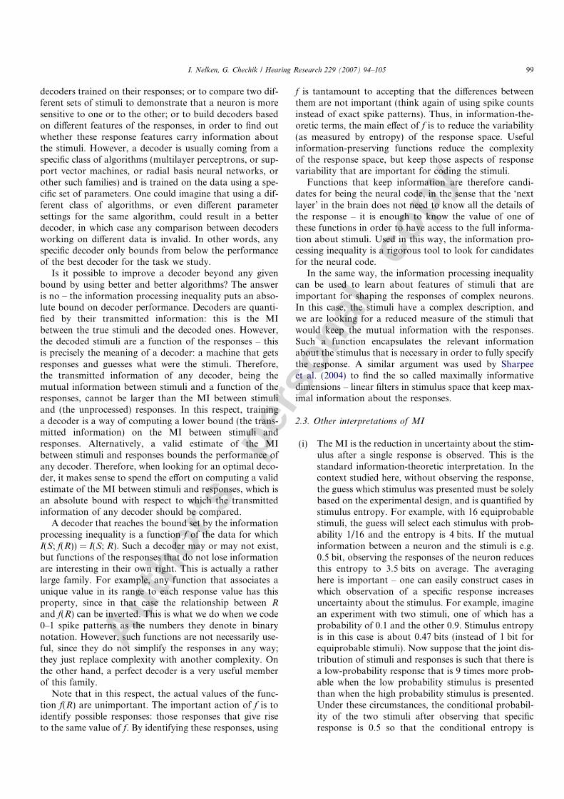
(i) The MI is the reduction in uncertainty about the stim-ulus after a single response is observed. This is thestandard information-theoretic interpretation. In thecontext studied here, without observing the response,the guess which stimulus was presented must be solelybased on the experimental design, and is quantified bystimulus entropy. For example, with 16 equiprobablestimuli, the guess will select each stimulus with prob-ability 1/16 and the entropy is 4 bits. If the mutualinformation between a neuron and the stimuli is e.g.0.5 bit, observing the responses of the neuron reducesthis entropy to 3.5 bits on average. The averaginghere is important – one can easily construct cases inwhich observation of a specific response increasesuncertainty about the stimulus. For example, imaginean experiment with two stimuli, one of which has aprobability of 0.1 and the other 0.9. Stimulus entropyis in this case is about 0.47 bits (instead of 1 bit forequiprobable stimuli). Now suppose that the joint dis-tribution of stimuli and responses is such that there isa low-probability response that is 9 times more prob-able when the low probability stimulus is presentedthan when the high probability stimulus is presented.Under these circumstances, the conditional probabil-ity of the two stimuli after observing that specificresponse is 0.5 so that the conditional entropy is


Autho

r's

pers

onal

co

py

1 bit, higher than the original stimulus entropy. How-ever, in that case other response values will havelower stimulus entropy since we know that on averagethe conditional stimulus entropy will be smaller thanthe a-priori stimulus entropy, 0.47 bits.With this interpretation, the MI can be used to esti-mate the number of neurons that are required todecode stimuli perfectly on a trial-by-trial basis. Theestimate is the stimulus entropy divided by the sin-gle-neuron MI. However, this estimate is not guaran-teed to bound the number of neurons either fromabove or from below, since the MI can add supra-lin-early or sub-linearly among neurons. How informa-tion of ensembles relates to single-neuron MI is acomplex question, outside the scope of this review(see Chechik et al., 2006; Deneve et al., 2001; Niren-berg and Latham, 2003; Schneidman et al., 2003).

(ii) The MI is the log (to the base of 2) of the number ofdifferent classes to which the stimuli can be subdi-vided after observing a response. This interpretationis tightly linked to the previous one, and is a concreteinterpretation of the reduction in uncertainty. How-ever, single-neuron MI is often smaller than 1 bit,making the number of different classes smaller than2. Thus, this interpretation seems less useful for sin-gle-neuron calculations.

2.4. Practice of mutual information estimation

If the MI is so useful, why is not it used more often? Oneanswer to this question is that the MI has entered the fieldlate, and that it is gaining respect as a tool for analyzingneural data. However, there is another good reason forthe limited use of information-theoretic measures: calculat-ing the actual value of the MI between two experimentallymeasured variables is theoretically difficult, and the diffi-culty translates into practical hurdles.

In principle, the MI is one value that summarizes someproperties of a probability distribution. As such, it seemsthat it would not be more difficult to estimate than e.g. amean and a variance (Nemenman et al., 2004). This is how-ever incorrect – the estimation of the MI is a hard problem.Theoretical aspects of MI estimation have been most rigor-ously treated by Paninski (2003), who highlighted thesevere problems encountered when trying to estimate MIfrom data.

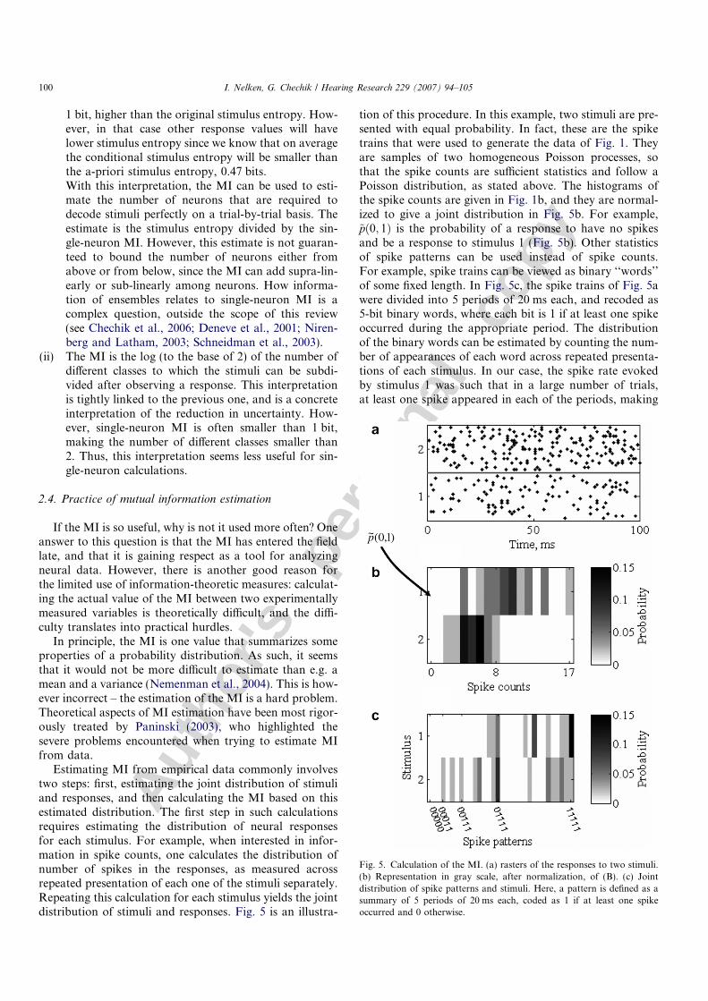
Estimating MI from empirical data commonly involvestwo steps: first, estimating the joint distribution of stimuliand responses, and then calculating the MI based on thisestimated distribution. The first step in such calculationsrequires estimating the distribution of neural responsesfor each stimulus. For example, when interested in infor-mation in spike counts, one calculates the distribution ofnumber of spikes in the responses, as measured acrossrepeated presentation of each one of the stimuli separately.Repeating this calculation for each stimulus yields the jointdistribution of stimuli and responses. Fig. 5 is an illustra-

tion of this procedure. In this example, two stimuli are pre-sented with equal probability. In fact, these are the spiketrains that were used to generate the data of Fig. 1. Theyare samples of two homogeneous Poisson processes, sothat the spike counts are sufficient statistics and follow aPoisson distribution, as stated above. The histograms ofthe spike counts are given in Fig. 1b, and they are normal-ized to give a joint distribution in Fig. 5b. For example,~pð0; 1Þ is the probability of a response to have no spikesand be a response to stimulus 1 (Fig. 5b). Other statisticsof spike patterns can be used instead of spike counts.For example, spike trains can be viewed as binary ‘‘words’’of some fixed length. In Fig. 5c, the spike trains of Fig. 5awere divided into 5 periods of 20 ms each, and recoded as5-bit binary words, where each bit is 1 if at least one spikeoccurred during the appropriate period. The distributionof the binary words can be estimated by counting the num-ber of appearances of each word across repeated presenta-tions of each stimulus. In our case, the spike rate evokedby stimulus 1 was such that in a large number of trials,at least one spike appeared in each of the periods, making

Fig. 5. Calculation of the MI. (a) rasters of the responses to two stimuli.(b) Representation in gray scale, after normalization, of (B). (c) Jointdistribution of spike patterns and stimuli. Here, a pattern is defined as asummary of 5 periods of 20 ms each, coded as 1 if at least one spikeoccurred and 0 otherwise.


Autho

r's

pers

onal

co

py

the full pattern ‘11111’ by far the most common one. Onthe other hand, at least one spike occurred in each presen-tation, making the estimated probability of the spike pat-tern ‘00000’ zero.

The second step is to calculate MI from the joint distri-bution. When the number of samples is very large relativeto the number of bins in the joint distribution matrix, theobserved empirical joint distribution provides a good esti-mate of the true underlying distribution, and the MI canbe calculated by plugging in the empirical distribution.Unfortunately, with common experimental settings thenumber of samples is often not sufficient, and this naiveMI estimator is positively biased. This means that it tendsto produce overestimates of the MI relative to the MI ofthe true distribution,

Ið~pðS;RÞÞ > IðpðS;RÞÞ(but not always: the theoretical bias may be negative, seethe discussion in Paninski, 2003). In addition, the variabil-ity of the estimator due to finite sampling may be also con-siderable. It has been shown that a first orderapproximation of the expected bias is

#bins2N logð2Þ ;

where #bins is the number of independent ‘essentially non-zero’ bins in the joint distribution (those that potentiallymight be non-zero; if actually zero, this is due to finite sam-pling) and N is the number of samples (Panzeri and Treves,1996; Treves and Panzeri, 1995). Subtracting this estimateof the expected bias from the empirical MI estimate oftenreduces substantially the bias.

As an example, the spike counts for the data in Fig. 1aare actually a sample from the Poisson distributions ofFig. 3a, whereas the naı̈ve MI estimate is about 0.60 bits,had we had the full distributions (by e.g. repeating the stim-uli many more times), the MI would be 0.44 bits. The dif-ference between these two estimates is the bias. Indeed, inthis case #bins is 15. The total number of stimulus presen-tation, N, is 40; and therefore the expected bias is 0.27 bits,somewhat larger than the actual observed bias in this case(0.16 bits).

The amount of bias, relative to the estimated informa-tion, depends on how densely the joint distribution matrixis sampled. Roughly speaking, this is a problem of overfit-ting. Imagine an experiment in which many differentsounds are presented, each of them once, and that theresponses are described in so many details that each specificresponse is seen only once. In this case, in the limited worldof the data collected during the experiment, stimuli fully‘‘predict’’ the responses and vice versa. The decoding canbe performed using a lookup table: given a response thatactually occurred in the experiment, go back and find thestimulus that evoked it. Thus ‘‘information is maximal’’.However, this result is most probably spurious, in the sensethat it does not generalize: for example, another repeat ofthe same stimulus will probably produce a different

response than the one that is in the lookup table. There-fore, the high MI estimated in this case is probably wrong.Accepting the high value of the MI is tantamount to believ-ing that the available data is perfectly representative of alldata in all its details, which it is probably not – this is theessence of overfitting.

Estimating the bias using the standard correction givenabove requires some care, since setting the value of #bins

is tricky. In experiments, bins of low probability mayremain empty because of finite sampling, and thereforethe number of non-zero bins in the estimated joint distribu-tion matrix is only a lower bound on #bins. On the otherhand, assuming that all possible responses are possible toall possible stimuli, hence setting #bins to be the total num-ber of bins in the joint-distribution matrix, may also bewrong. For example, it may well be that some stimuli neverproduce a single spike, while others always produce at leastone spike. In this case, some combinations of stimuli andresponses are truly empty and will remain so forever. Inthis case, #bins is overestimated. In some respects, this isthe situation in the data of Fig. 1 and possibly part ofthe reason why the estimated bias is somewhat large. Thus,the values of 0 and 1 spikes per stimulus never occur in thissample, and their probabilities, although non-zero, are verysmall, contributing to the overestimation of the bias. Sim-ilarly, large spike counts (>8 spikes/presentation) are extre-mely unlikely for stimulus 2, also contributing to therelatively large bias correction. Panzeri and Treves (1996)suggested some procedures for better estimating the biasin this context.

There is another possible solution to the problem ofoverfitting and bias: to reduce the details of the stimulusand response descriptors such that their joint distributioncan be better estimated. In standard electrophysiologicalexperiments, a small set of stimuli is used to start with,and therefore the responses should be reduced (e.g. fromfiring patterns to spike counts). However, the informationprocessing inequality tells us that by doing this, we alsoreduced information. Thus, we wish to choose the repre-sentation in an adaptive manner: as observations accumu-late, we increase the amount of details we allow in therepresentation of the responses. Paninski (2003) showedthat by increasing details not too fast as further observa-tions accumulate, such a procedure will converge to thetrue MI. However, in real experimental situations, theamount of data is fixed, and we cannot follow this schemeto the limit.

We therefore face a conundrum – on the one hand, wecannot fully specify the joint distribution of stimuli andresponses in typical experiments because these require toomany details, but on the other hand any attempt at reduc-ing the data results in a different problem, where informa-tion is already reduced, so that even if we estimate the MIof the reduced problem better, the result is not what wehave been looking for to start with.

In practice, one can create a sequence of reasonably wellestimated MI values from reduced problems and use this


Autho

r's

pers

onal

co

py

sequence to generate a high quality final estimate. Thereare two main approaches to achieve this. In the firstapproach the MI is calculated for several subproblemsand extrapolated to get the expected value at infinite dataor infinite resolution. For example, to reduce bias, theMI is calculated for subsets of the data of various sizes.Since the bias decreases theoretically at a rate of 1/N, itis expected to observe a linear dependence of the observedMI on 1/N. A linear regression supplies the estimated bias-corrected MI. To get the MI estimate at infinite temporalresolution, the MI may be calculated for several finite tem-poral resolutions. This is done over a range in which rea-sonable robust estimation is possible, and these estimatesare then extrapolated to infinitely detailed responses. Thisapproach was taken in the so-called direct method (Stronget al., 1998), where estimates of MI were calculated for aseries of temporal resolutions, and were linearly extrapo-lated to infinite temporal precision of spike times.

In the second approach, bias correction can be done oneach estimate, resulting in a trade-off: the more reducedjoint distribution will have less mutual information, butalso smaller bias and less possible over-correction. Thus,standard algorithms may actually show an increase inbias-corrected information, at least initially, as the reduc-tion process proceeds. After producing a series of probableunderestimates of the MI, the maximal estimate among allof them should be the best estimator of the true MI. Inpractice, one has to be careful about the maximization pro-cess involved in such procedure, which introduces a bias ofits own. A controlled amount of such optimization wasused in Nelken et al. (2005), seemingly successfully, at leastcompared to simulations.

To illustrate these approaches, we use the data of Fig. 4.Suppose we are interested in the phase of the 100 Hz tone.The joint distribution in Fig. 4b was computed using 50repeats for each stimulus and with 16 bins of 2 ms, coveringthe range of 0–30 ms. Thus, it contains 128 bins (8 stimulusvalues and 16 time values for each) and has 400 measure-ments, slightly more than 3 counts per bin on average.The MI is about 0.79 bits, and the bias (calculated fromthe number of measurements and number of bins as above)is 0.19 bits, resulting in a bias-corrected MI of about0.6 bits. In this case, the model is simple enough to allowexplicit calculation of the joint distributions: the modelMI is 0.62 bits. Thus, the value we get by simple bias cor-rection of a limited-resolution joint distribution is not toofar from the ‘true’ MI, despite the finite sampling and dataprocessing that lie between the model and the estimatedvalue.

With the first approach to bias correction, we shouldcompute the MI for subsets of the data and extrapolateto infinity (in practice, 1/N is extrapolated to 0). Fig. 6ashows the plot of average raw MI (without bias correction)against 1/N. For N = 10 trials, the estimated value seems todeviate somewhat from the linear trend defined by the val-ues estimated with larger subsets. Using only the MI ofthese larger subsets in the linear regression, the estimated

MI (intercept of the linear regression line with the y-axis)is 0.64 bits, as good an estimate of the true MI as before.Note however that using this method required some judg-ment for selecting the linear range for the regression, andit assumes that there is enough data so that the bias indeeddecreases linearly with 1/N. If we had only 20 trials perstimulus, we would have available only the first two pointsof Fig. 6a, and the resulting estimate would have been toolarge: 0.97 bits.

For the second approach, we use the algorithm devel-oped by Nelken et al. (2005), which successively reducesa joint distribution matrix by joining together adjacentrows or columns. At each step, the row or column withthe least marginal probability is selected and joined tothe neighbor that has the lower marginal probability. TheMI of the reduced matrix and the estimated bias are com-puted, generating a sequence of bias-corrected MI esti-mates. Eventually only one column or row remains,stopping the iterations. The maximal bias-corrected valueis used as the final MI estimate. Fig. 6b shows the sequenceof raw MI values, bias estimates and bias-corrected MI val-ues produced by this algorithm for the same data. While ateach iteration of the reduction process both raw MI andbias estimates monotonically decrease, the bias-correctedMI actually increases slightly at the initial stages (althoughthis increase is obviously not significant). The final estimate

Fig. 6. Bias correction. (a) Estimates of the MI between sine wave phaseand responses for the data in Fig. 4a, as a function of the number of trialsused. For each number of trials, the largest number of non-overlappingsubsets of trials were used (5 subsets for 10 trials, 3 subsets for 15 trials, 2subsets for 20 and 25 trials, and the whole set for 50 trials). The interceptof the linear regression line with the y-axis is the bias-corrected MIestimate. (b) The sequence of raw MI (upper gray line), bias estimates(lower gray line) and bias-corrected MI (continuous black line) valuesproduced by successive reduction of the joint distribution matrix in Fig. 4busing the algorithm of Nelken et al. (2005).


Autho

r's

pers

onal

co

py

of the MI in this case is 0.61 bits, closer to the true data butprobably not significantly different from the two other esti-mates. The main advantage of this approach is that it canbe used to get conservative estimates of the MI even withvery little data (e.g. Moshitch et al., 2006). In the case ofthe data used here, with 20 trials per stimulus the estimatedMI is 0.63 bits, still close to the model MI. Thus, with smallamounts of data, the more conservative second approachseems to perform better.

A number of suggestions have been made for computingMI without explicit calculation of the joint distribution asan intermediate step. These involve the use of decoders(Furukawa and Middlebrooks, 2002; Rolls et al., 1997),computing the MI from a series expansion (which can prac-tically be evaluated only up to the second order, Pola et al.,2003), or using distances between responses (embedded in ahigh-dimensional metric space) to estimate their density(Victor, 2002). Although these methods do not strictly fallwithin the context discussed here, we (Nelken et al., 2005)found that in practice, they suffer from the same problemsas the matrix-based methods, with the errors being domi-nated by bias and having a larger mean-squared error thanmatrix-based methods.

3. Applications to the auditory system

Information-theoretic measures have been applied suc-cessfully for problems of auditory coding since the begin-ning of the current wave of interest in these methods(Rieke et al., 1995). Here I summarize a number of recentstudies. This is not intended as an exhaustive review butrather as an illustration of the current practice.

Starting first with a somewhat atypical case, Slee et al.(2005) studied the responses of nucleus laminaris neuronsin chick embryos. The stimulus was a non-white Gaussiancurrent. The analysis proceeded in two steps: first a modelwas fitted to the data, based either on spike-triggered aver-aging or on covariance decomposition (Brenner et al.,2000), an approach that generalizes and extends spike trig-gered averaging. In both cases, the procedure generates amodel in which linear filter functions are used to reducethe stimulus, and the reduced stimulus undergoes non-lin-ear transformation into firing rate. The issue in this caseis whether the simplified model captures all stimulus fea-tures that are relevant for spiking, and this was tested usingthe methods discussed above. The full MI between stimuliand responses was estimated, and so was the MI betweenthe reduced models and the responses. By the informa-tion-processing inequality, the second value is always smal-ler than the first. Better models give MI values that arecloser to the full MI. In this study, models captured 60–75% of the full MI. The authors suggest that unexplainedMI may have to do with spikes that are very close to eachother (<5 ms), in which case spike history influences firingin ways that the reduced models do not capture.

Higher up in the auditory system, Chase and Young(2005) studied the coding of multiple cues for space in

cat inferior colliculus (IC). The question they addressedwas that of segregation of processing pathways throughthe IC. Previous studies have suggested that brainstemnuclei which process different spatial cues project to seg-regated domains in the IC. If so, it could be expectedthat IC neurons would show mostly sensitivity to thecue that is represented in their dominant input. Chaseand Young used stimuli in which various cues (interaurallevel differences; interaural time differences; and spectralnotches) were manipulated independently (thereforemostly working with artificial combinations of cues).This experimental design allowed them to study theway one cue is coded in the presence of variations inother cues, and also to study information interactionsbetween different cues. Their main conclusion is thatinformation interactions are large and are seeminglyinconsistent with hard segregation, supporting ratherthe notion that IC neurons typically integrate informa-tion from multiple input streams.

Still in the IC, Escabi et al. (2003) compared theresponses to artificial sound ensembles whose spectro-tem-poral modulations resembled to varying extent those ofnatural sounds. They found that more naturalistic ensem-bles evoked higher firing rates and also higher mutualinformation rates. Interestingly, the information per spikeremained about constant, suggesting that the spikesencoded information independently of each other, and thatthe increase in MI for the naturalistic ensembles was due tothe higher firing rates rather than to changes in the wayspikes encode stimulus features.

Hsu et al. (2004) analyzed responses of neurons in themidbrain, primary forebrain areas and secondary fore-brain areas in a bird, the zebra finch. The basic issuewas again that of specialization for natural sound ensem-bles, and this question was tested by using a hierarchy ofensembles that approximated to varying extent a set ofconspecific natural vocalizations. The relative level ofMI was used to indicate selectivity. In contrast with otherstudies reviewed here, the MI was estimated using semi-parametric models: first, a statistical model of the spiketrain was generated for each stimulus, and then the MIof the models was estimated. They found that the selectiv-ity of neurons to the natural sound ensemble increased athigher auditory stations. As in the paper of Escabi et al.(2003), this increase was not due to better reliability of theindividual spikes, but rather to a more extreme distribu-tion of firing rates and higher bandwidth of firing ratemodulations in the responses to the more natural soundensembles. The differences in information/spike for thedifferent sound ensembles in the different stations werenot very large, however.

In contrast with other studies reviewed here, Lu andWang (2004) measured entropies, rather than MI, of spiketrains in the auditory cortex of awake marmosets. The pur-pose was to check the presence of specific spike patternsthat are not locked to the stimulus and therefore won’tbe apparent in the peri-stimulus time histograms. They


Autho

r's

pers

onal

co

py

analyzed the responses to periodic sounds, for which theydemonstrated the presence of two populations, one thatlocked to specific periods and the second that respondedby graded firing rates to different periods but did not showany locking. Lu and Wang were interested in checkingwhether there are repeating spike patterns even in theresponses of the non-locking neurons. Their approachwas to jitter spike timing to varying degree and look forincrease in the entropy of the spike trains. They could dem-onstrate such increases for the neurons that locked to peri-odic sounds, but not to the non-locking neurons,concluding that there are no special firing patterns in theresponses of the non-locking neurons.

Middlebrooks and coworkers used decoders, quantifiedby their transmitted information, to study the coding ofspace in auditory cortex of anesthetized and awake cats.The use of these methods was initially due to the fact thatneurons in auditory cortex of cats tend to respond to astimuli from large extent of space – a hemifield or evenomnidirectionally – but nevertheless their firing patternsmay depend on space. Thus, standard measures of spatialselectivity, such as best direction and angular width ofthe receptive fields, do not make much sense. Middle-brooks called these neurons ‘panoramic’ (Middlebrookset al., 1994), and eventually used the transmitted informa-tion of a decoder to quantify their coding capabilities.Later, MI was used to study information-bearing elementsin the responses as a way of addressing issues of the neuralcode (Furukawa and Middlebrooks, 2002). Currently,these studies form the best and most extensive study of asingle coding task in different auditory cortex fields (Stec-ker et al., 2005).

To conclude this list, Nelken et al. (2005) used the infor-mation processing inequality explicitly as a tool to find can-didates for the neural code. They estimated the fullinformation in the spike trains with a number of differentcomputational approach, concluding that the directmethod, with a carefully balancing of bias and informationloss, is the best. They then demonstrated that two reducedfeatures, spike counts and mean burst latency, do not reachthe full information. However, jointly these two variablesextracted information levels that were highly similar tothe full information. Thus, the two variables jointly mayserve as the neural code.

4. Concluding remarks

Information-theoretic tools can serve to study codingproblems beyond those surveyed above. Although moststudies of the auditory system currently analyze one neuronat a time, some studies of coding interactions between neu-rons have already appeared (e.g. Chechik et al., 2006; dem-onstrating high degree of independence between pairs ofauditory cortex neurons). The issue of coding interactionswas explicitly kept out of this review, but with the increasein the availability of simultaneous recordings it will becomeas important as that of stimulus coding.

So, is it worthwhile to use information-theoretic mea-sures? The answer is an emphatic yes, given a number ofcautionary remarks.

First, the experimental question should justify the use ofthe MI. In all cases reviewed above, it was difficult to evenpose the experimental question in terms of classical mea-sures. Although this is possible, by using measures of reli-ability and signal-to-noise ratios, the optimality propertiesof the MI play an important role in these studies. On theother hand, the demonstration of significant stimulus–response associations can usually be done using simplermethods than the MI.

Second, the experiment should be designed with the useof the MI in mind. Thus, using MI entails collecting moredata than is usually necessary for estimating just meanrates. It is a bad idea to use MI on sparse data, hoping thatits use would miraculously uncover associations that weremissed before. As a rough guideline, when analyzing thedata, the number of bins in the joint distribution matrixshould be smaller than the total number of stimuluspresentations.

Finally, the method used to estimate the MI should becarefully evaluated, preferably on surrogate data for whichthe MI is known and which is as similar as possible to thereal data for which the MI is estimated. This step is impor-tant because of the difficulties in estimating MI. Althoughsome major advances in our understanding of MI estima-tion have been made (e.g. Paninski, 2003), many methodsthat are being used in the literature do not fit the better-understood frameworks.

Acknowledgements

This work was supported by a grant from the Israeli Sci-ence Foundation. We thank Yael Bitterman for usefulcomments on the manuscript.

References

Brenner, N., Bialek, W., de Ruyter van Steveninck, R., 2000.

Adaptive rescaling maximizes information transmission. Neuron

26, 695–702.

Chase, S.M., Young, E.D., 2005. Limited segregation of different types of

sound localization information among classes of units in the inferior

colliculus. J. Neurosci. 25, 7575–7585.

Chechik, G., Anderson, M.J., Bar-Yosef, O., Young, E.D., Tishby, N.,

Nelken, I., 2006. Reduction of information redundancy in the

ascending auditory pathway. Neuron 51, 359–368.

Cover, T., Thomas, J., 1991. Elements of Information Theory. Wiley and

Sons, NY.

Deneve, S., Latham, P.E., Pouget, A., 2001. Efficient computation and cue

integration with noisy population codes. Nat. Neurosci. 4, 826–831.

Escabi, M.A., Miller, L.M., Read, H.L., Schreiner, C.E., 2003. Natural-

istic auditory contrast improves spectrotemporal coding in the cat

inferior colliculus. J. Neurosci. 23, 11489–11504.

Furukawa, S., Middlebrooks, J.C., 2002. Cortical representation of

auditory space: information-bearing features of spike patterns. J.

Neurophysiol. 87, 1749–1762.

Hsu, A., Woolley, S.M., Fremouw, T.E., Theunissen, F.E., 2004.

Modulation power and phase spectrum of natural sounds enhance


Autho

r's

pers

onal

co

py

neural encoding performed by single auditory neurons. J. Neurosci. 24,

9201–9211.

Lu, T., Wang, X., 2004. Information content of auditory cortical

responses to time-varying acoustic stimuli. J. Neurophysiol. 91, 301–

313.

Middlebrooks, J.C., Clock, A.E., Xu, L., Green, D.M., 1994. A

panoramic code for sound location by cortical neurons [see comments].

Science 264, 842–844.

Moshitch, D., Las, L., Ulanovsky, N., Bar-Yosef, O., Nelken, I., 2006.

Responses of neurons in primary auditory cortex (A1) to pure tones in

the halothane-anesthetized cat. J. Neurophysiol. 95, 3756–3769.

Nelken, I., Chechik, G., Mrsic-Flogel, T.D., King, A.J., Schnupp, J.W.,

2005. Encoding stimulus information by spike numbers and mean

response time in primary auditory cortex. J. Comput. Neurosci. 19,

199–221.

Nemenman, I., Bialek, W., de Ruyter van Steveninck, R., 2004. Entropy

and information in neural spike trains: progress on the sampling

problem. Phys. Rev. E – Stat. Nonlin. Soft Matter Phys. 69, 056111.

Nirenberg, S., Latham, P.E., 2003. Decoding neuronal spike trains: how

important are correlations?. Proc. Natl. Acad. Sci. USA 100 7348–

7353.

Paninski, L., 2003. Estimation of entropy and mutual information. Neural

Comput. 15, 1191–1253.

Panzeri, S., Treves, A., 1996. Analytical estimates of limited sampling

biases in different information measures. Network 7, 87–101.

Pola, G., Thiele, A., Hoffmann, K.P., Panzeri, S., 2003. An exact method

to quantify the information transmitted by different mechanisms of

correlational coding. Network 14, 35–60.

Rieke, F., Bodnar, D.A., Bialek, W., 1995. Naturalistic stimuli increase

the rate and efficiency of information transmission by primary

auditory afferents. Proc. R. Soc. Lond. B Biol. Sci. 262, 259–265.

Rolls, E.T., Treves, A., Tovee, M.J., 1997. The representational capacity

of the distributed encoding of information provided by populations of

neurons in primate temporal visual cortex. Exp. Brain Res. 114, 149–

162.

Schneidman, E., Bialek, W., Berry, M.J., 2003. Synergy, redundancy, and

independence in population codes. J. Neurosci. 23, 11539–11553.

Sharpee, T., Rust, N.C., Bialek, W., 2004. Analyzing neural responses to

natural signals: maximally informative dimensions. Neural Comput.

16, 223–250.

Slee, S.J., Higgs, M.H., Fairhall, A.L., Spain, W.J., 2005. Two-dimen-

sional time coding in the auditory brainstem. J. Neurosci. 25, 9978–

9988.

Sokal, R.R., Rohlf, F.J., 1981. Biometry, second ed. W.H. Freeman, New

York.

Stecker, G.C., Harrington, I.A., Middlebrooks, J.C., 2005. Location

coding by opponent neural populations in the auditory cortex. PLoS

Biol. 3, e78.

Strong, S.P., de Ruyter van Steveninck, R.R., Bialek, W., Koberle, R.,

1998. On the application of information theory to neural spike trains.

Pac. Symp. Biocomput., 621–632.

Treves, A., Panzeri, S., 1995. The upward bias in measures of

information derived from limited data samples. Neural Computation

7, 399–407.

Victor, J.D., 2002. Binless strategies for estimation of information from

neural data. Phys. Rev. E 66, 51903.


information theory in auditory research

Documents