Electronic copy available at: http://ssrn.com/abstract=1719067

Information technologies and economic growth: do the physical measures

tell us something?

Rafael L. Myro 1, Josefa Vega2, M.ª Elisa Álvarez3

Abstract: This article explores the impact of different physical measures of information

technology (IT) capital on the per capita income of 102 countries. This method not only

allows counting on a great number of countries but also to test the great impact other

authors have attributed to IT equipments on the basis of such kind of measures.

The estimates carried out in this article confirm the strong impact of IT on per capita

income already found and the difficulty of making it compatible with the real growth of the

economies, which point to the presence of grave problems of endogeneity in the estimates.

So it seems to be better to rely on monetary measures of capital IT and probably on another

method to estimate its effect.

Key words: Growth, Information technology, Per capita income.

JEL Classification: O1, O4, O5.

1 Department of Applied Economics II, Complutense University of Madrid, Campus de Somosaguas s/n,

Pozuelo de Alarcón, 28223 Madrid, Spain. Tel.: (+34) 913 942476; fax: (+34) 913 942457. E-mail:

R.myro@ccee.ucm.es2, 3 Department of Applied Economics, University of Valladolid, Avda. del Valle de Esgueva 6, 47011

Valladolid, Spain. Tel.: (+34) 983 423353; fax: (+34) 983 423299. E-mail: josefa@eco.uva.es;

elsa@eco.uva.es (Corresponding author)

Electronic copy available at: http://ssrn.com/abstract=1719067

2

I. Introduction

The relationship between investment in Information Technology (IT) and economic

achievement measured in terms of product and productivity has been extensively explored

since the beginning of the current century challenged by the famous Solow paradox. Stiroh

(2004) surveyed the major results of the estimates that generally support the hypothesis of

the strong impact from the investment made in computers and telecom equipment on

economic performance. The works developed by Jorgenson stand out as a central reference

in this analysis having guided the studies applied to many countries (Jorgenson, 2001,

2004; Jorgenson et al., 2006).

Nevertheless, the exact dimension of such an impact is not yet clear and neither are

the differences in the contributions due to computers and telecommunication equipments.

On the other side, disparities remain between the analysis based on the econometric

estimates of production functions and others driven by calculations of labor and total factor

productivity through the rental prices for the inputs.

In addition to that, some analysis using physical measures of the stock of capital seem

to offer impacts much higher than the usual measures based on the constant prices values

(Röller and Waverman, 2001). The present research is mainly focused on that issue. The

advantage of physical capital measures is that they are available for a higher number of

countries.

In spite of that, analysis using samples of countries are scarce, as is the separated

exploration of developed and developing countries with the outstanding exception of

Dewan and Kraemer (2000). One of the reasons is the lack of data referring to long periods.

Data on computers for most countries refer to the last decade, which hinders the use of

models which require long time series.

Electronic copy available at: http://ssrn.com/abstract=1719067

3

This article studies the IT impact on per capita income through physical measures of

the capital stock and a large sample of countries. To do that, it is used a form of the Solow

model of economic growth posed by Mankiw et al. (1992) that allows for an approach with

limited information. It is used the same sample of countries as they do, with a few

exceptions due to the lack of information, with the data from 1980 to 2003 provided by the

Penn World Table (2005), for the economic variables, and from the International

Telecommunication Union (ITU, 2005 version) for the IT variables. These latter are

measured in physical units, which allows to compare the results presented here with those

found by Röller and Waverman (2001) showing strong impact of the telephone lines on the

income and more recently of mobile phones (Waverman et al., 2008).

II. The Model and The Data

Assume there is a Cobb Douglas production function with constant returns to scale of this

form:

)1(,, )( βαβα −−= ttITtnotITtt LAKKY (1)

Where Y is the output, K is the stock of physical capital, divided into two categories,

with the accumulation of investments in IT equipment separated from the rest, called not

IT. L is the labor involved in the production process and A is a factor of technical progress

growing at a constant rate g. It is also assumed that the increase in labor matches that of the

population in the long run, evolving at the constant rate n, and that the physical capital not

IT depreciates at the proportional rate of δ.

Given the constant returns to scale, the above function can be expressed in per capita

terms, using smaller letters to indicate the variables are taken in per capita values.

4

βαITtnotITtt kky ,,=

Considering now just the dynamic of accumulation of physical capital not IT, the

steady state income is:

βα

αβ

δ*

1*,*

ITITnotITk kgn

ksy

−

⎟⎟⎠

⎞⎜⎜⎝

⎛

++= (2)

Where the * refer to the steady state values, k*IT is the stock of physical capital IT per

capita in the steady state and sk, not IT is the rate of saving and investment in capital not IT.

In logarithms, expression (2) is transformed into the following:

*,

* ln1

)ln(1

ln1

ln ITnotTICk kgnsyα

βδα

αα

α−

+++−

−−

= (3)

The Equation 3 is estimated for the per capita income of 2003, assuming that the

countries are in their steady states. The rates of investment and of population growth are

introduced as average values for the period 1980 to 2003. It did not give any value to the

depreciation rate assuming that it is equal for every country. So, the second member of this

expression became just the population rate of growth. To approach the value of KIT in 2003,

four different variables are used, drawn from the ITU data and measured in percentage of

100 inhabitants: number of personal computers, number of main telephone lines, number of

mobile phones and users of the Internet. Each of them represents one different form of IT.

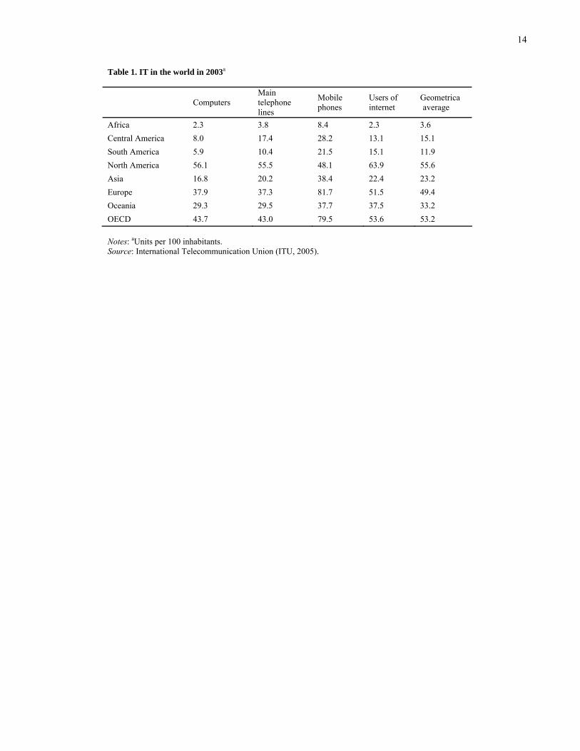
Table 1 describes the value of these variables and the geometric average for several

geographical areas in the world. As expected, North America and Europe show the highest

values of IT penetration; the first due to a greater dissemination of computers and Internet

accessibility, while the second is because of the great number of mobile phones.

5

(Insert Table 1)

One of the problems with any estimate of expression 3 stems from the fact that the

investment rate includes IT equipment, but this only represents about 10% of the total

investment in the US and Finland.

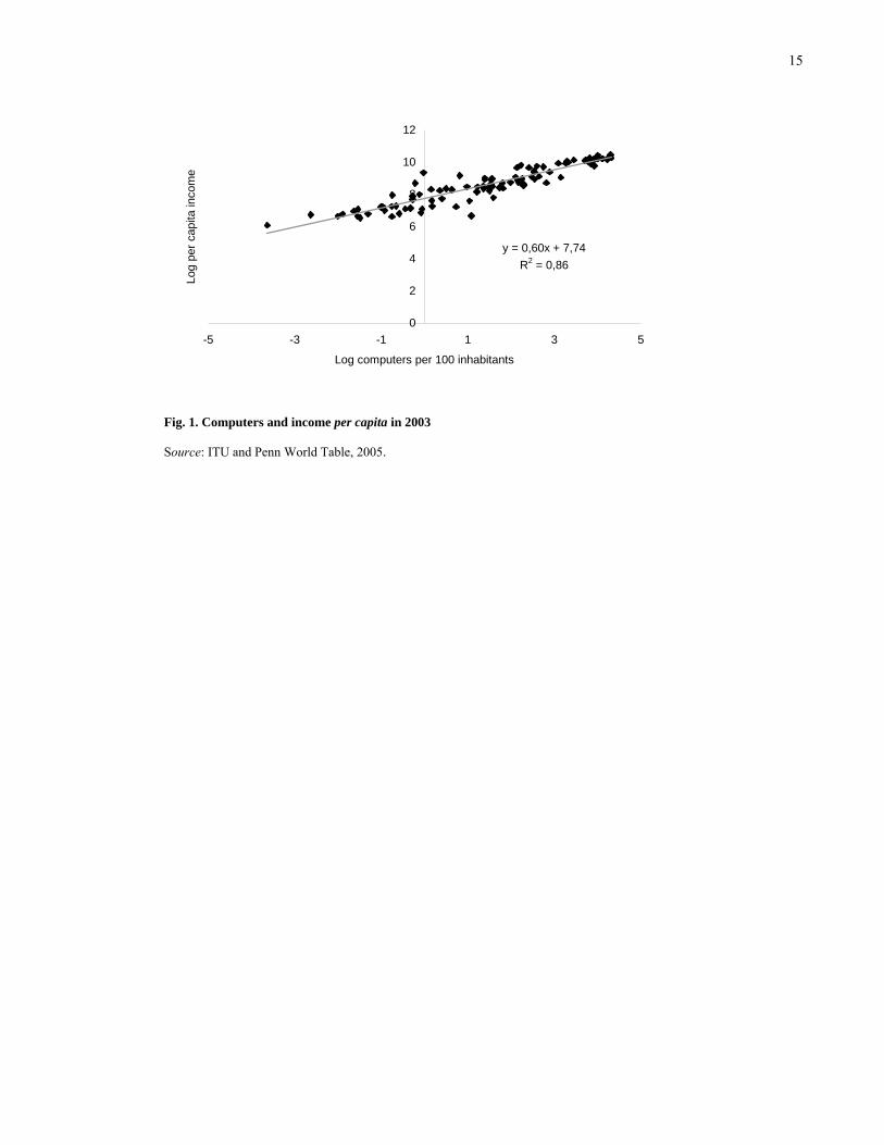
Another problem of much more importance derives from the presence of endogeneity

as stock of capital IT also depends on per capita income. Fig. 1 depicts the strong

relationship between per capita income and IT physical capital which supports this

problem.

(Insert Fig. 1)

To control for endogeneity, a term is introduced in the second term representing the

per capita income of the first year, 1980. This term is supposed to capture the part of the IT

demand for investment depending on the previous per capita income. This is almost

equivalent to the estimate of a conditioned convergence equation of this form:

1*

, lnln1

)ln(1

ln1

lnln −−−

+++−

−−

=− tITnotITktt ykgnsyy λα

βδα

αα

α (4)

However, here the dependent variable is the rate of growth between 1980 and 2003,

so it is estimated the impact of IT on the long run rate of growth. In this new expression λ is

the coefficient of conditioned convergence.

III. Results

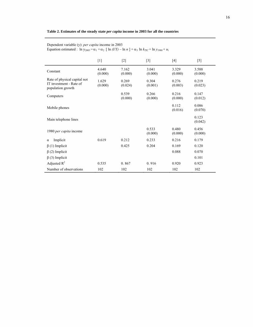
Table 2 shows the results for the Equation 3 and for the 102 selected countries. It is

presented only an estimation of the restricted equation which imposes the same coefficient

on the rate of physical capital investment and the rate of population growth. This restriction

slightly changes the results and better fits the theoretical model.

6

The IT variables chosen are gradually introduced. After some estimates, it was

decided to exclude the “users of Internet” as it seemed to be strongly correlated with the

others, particularly with the number of personal computers. Problems of multicolineality in

the estimates are detected, altering the signs of the coefficients for the rest of the variables.

The estimated coefficients always have the expected sign. The first column in Table 2

shows the basic original model, without the IT capital. The implicit elasticity of per capita

income to physical not IT capital (α in the model) is 0.6, a very common outcome in the

reference literature. In the second column, the number of computers are added showing a

very high impact on the output: its implicit elasticity calculated [β (1) implicit] reaches

0.34. However, it becomes smaller to the value of 0.15 when the per capita income of 1980

is included, as shown in column [3]. This new variable seems to work in avoiding some of

circularity problems, and also re-establishes the original value of the constant of the

estimate, leading to an acceptable value of the elasticity for the investment in not IT

physical capital which otherwise would decline gradually as new IT variables are

incorporated. In short, it gives more stability to the estimates and seems partially to avoid

the problems of endogeneity.

(Insert Table 2)

The number of mobile phones and main telephone lines are also found to be powerful

variables as shown by their elasticities [β (2) and β (3) implicit]. When the three variables

are included together (column [5]), the elasticity of per capita income to investment in not

IT physical is 0.18, an acceptable result. The increase in the number of personal computers

affects the per capita income by 0.12 meaning that any increase of 10% in the number of

computer gets 1.2% more of per capita income, a huge impact. Taking everything into

7

account gives a greater one, as an increase in IT capital by 10% would add around 2.9

points to per capita income.

It is important to stress the striking role apparently played by the main telephone lines, in

accordance with the results by Röller and Waverman (2001).

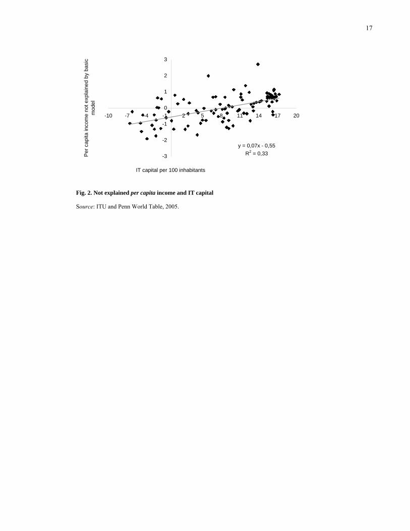
Fig. 2 shows the relationship between the per capita income not explained by the

basic model and the IT variables taken together through its geometric average to illustrate

the findings in a better way.

(Insert Fig. 2)

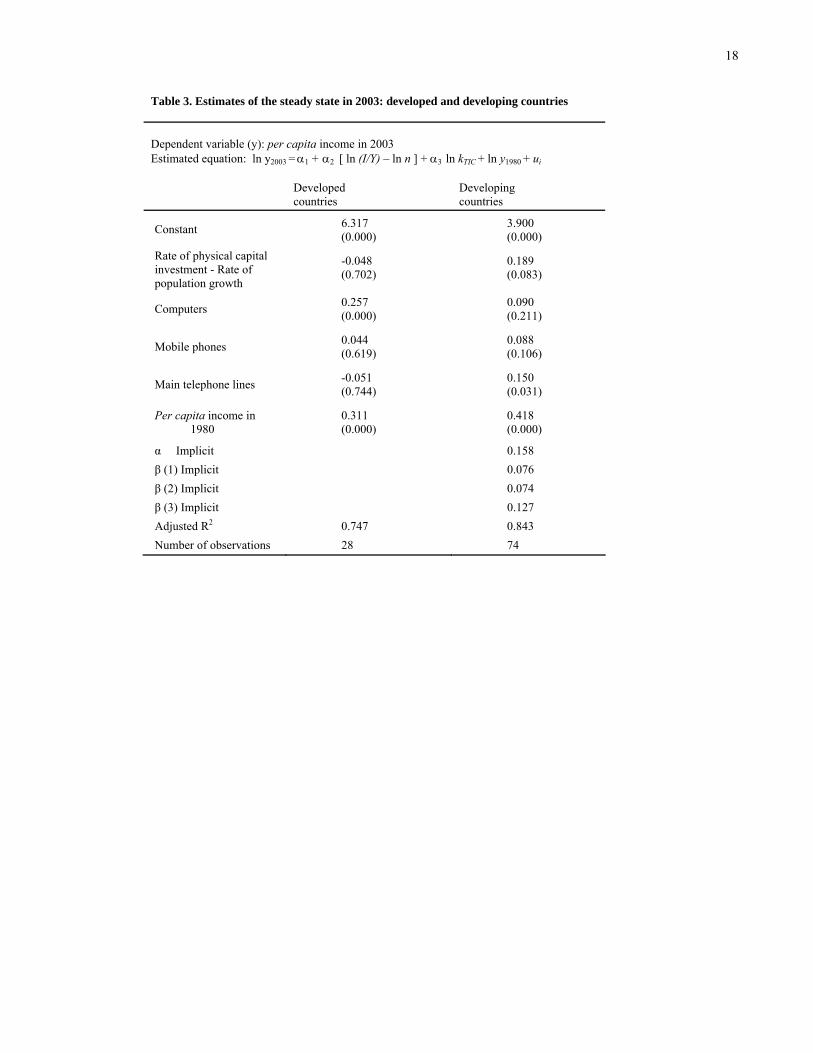
To go deeper into this issue, the differences between developed and developing

countries are also explored (Table 3). While the first do not show any sensitivity to the

physical capital investment, probably because all of them share the same steady state

defined by this variable, per capita income is clearly dependent of its value in developing

countries.

(Insert Table 3)

Differences in per capita income between developed countries are only related to the

most characteristic kind of IT equipment, the computers which have a large influence on

production achievements. Neither mobile phones nor main telephone lines seem to provoke

perceptible differences in the sample of developed countries.

For developing countries, computers are less relevant than main telephone lines. But

the mobile phone also plays an important role. It obtains here the same result as Dewan and

Kraemer (2000).

The above results can be also reached with the model of convergence given by the

expression (4). Now the dependent variable is the rate of growth of per capita income

8

between 1980 and 2003 while the explanatory variables are the same as in the previous

estimates. However, the expected sign for the per capita income of 1980 will be negative if

a convergence process is registered.

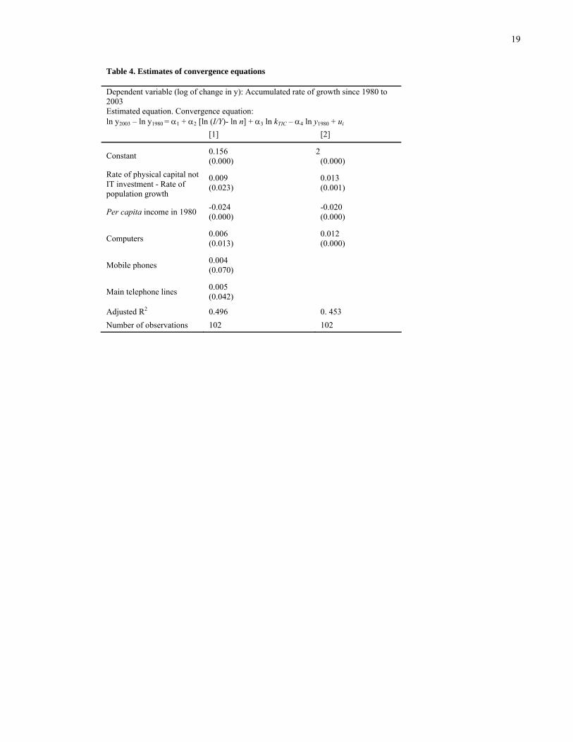
Table 4 shows the result of this estimate for the whole sample. In the column [1], the

per capita income in the initial year, 1980, shows the expected negative impact, indicating

the presence of a convergence process. The investment in physical capital not IT has a

positive effect on the income. IT variables are not significant, with the only exception being

the number of personal computers which has a big coefficient, 0.006, implying a very

similar implicit elasticity (0.007), as its value depends on α and that is very low. This

elasticity is quite big as it refers to the increase in the average rate of growth in the period

1980 to 2003 (permanent or long run rate).

(Insert Table 4)

As the introduction of no significant IT variables tends to reduce the value of α, the

second column in Table 4 includes only the number of personal computers. Then, the

coefficient for that variable almost doubles, reaching 0.011 implying an elasticity of 0.012,

an enormous value as an increase in the rate of growth for a long period. Apparently it is

similar to that obtained by Jorgenson (2001) but it is really much higher, as the latter refers

to a direct and punctual effect on per capita income, not to a permanent increase in the rate

of growth1.

1 When this last estimate is compared to another including only the investment in physical capital (once

discounted for population growth) it is observed that the value of α declines but the coefficient of

convergence multiplies by four from -0.006 to -0.020. This result means that the countries converge faster

when the number of computers is taken into account. This accelerates the process of reaching the steady state

defined by investment and population growth rates.

9

Those results can not be accepted just taking in account that the stock of IT capital in

the US multiplied by 5 from 1990 to 2003 and that of computers by 26 (Jorgenson, 2004).

With the estimates carried out in this article these increases would have more than doubled

the per capita income. But the direct effect of them in the output only totals 14% after

adding the impact in total factor productivity (Jorgenson, 2001; Jorgenson and Vu, 2005,

2007)2.

On the other hand, so high impact would indicate a clear excess of return of the

investment in IT compared to those in other physical capital, meaning that most of the

countries, particularly the developed ones would have lost great opportunities for growth as

they have not reallocated their resources to the IT investments. For the most backward

countries in the EU-10, such as Portugal, Greece or Spain these losses would have been

over 10% of the per capita income.

All those considerations mean that apparently it is already facing a big problem of

endogeneity. In trying to avoid in, a version of the convergence equation has been

estimated, where the IT variables are taken in variations (approaching for the rate of

investment in them)3. The first period considered is 1995 to 2003, but in order to be able to

do it has been necessary to complete the available data of IT capital for 1995, particularly

that for personal computers and mobile phones. To that end, own calculations are used,

taking into account the rate from 2000 to 2003 and the level reached in the first of these

years and comparing countries in the same stages of development. These calculations were

only accepted after checking out that they match very well the data for around half of the

2 For the last years of the period examined in this research see also Jorgenson et al. (2006).

3 Now a steady state value is calculated for all the forms of physical capital and they depend on the portion of

the income invested in them. In this version of the model the implicit elasticities do not depend on α.

10

countries in 1995. The other period chosen is 2000 to 2003, a short one but even more

crucial than the previously selected in the accumulation of IT capital, mainly in developing

countries. This last period offers the advantage that all the required data are available.

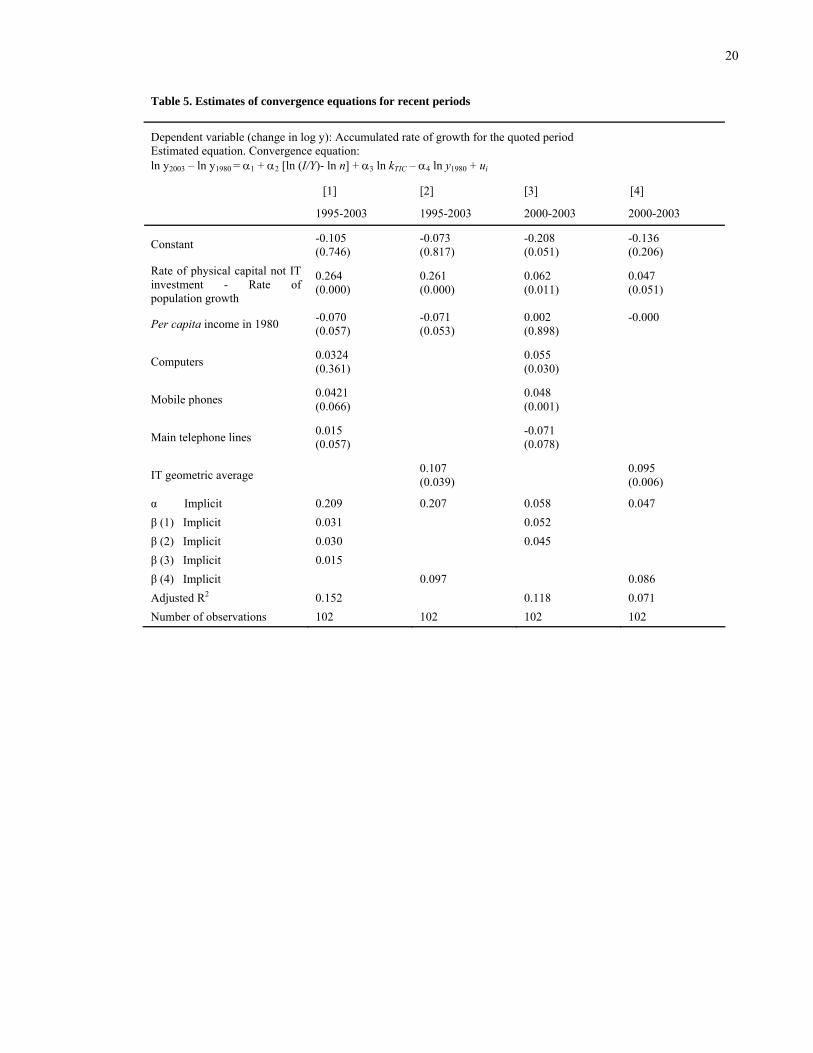
Table 5 shows the result of these last estimates. For the longer period, 1995 to 2003,

the physical not IT capital and even the number of mobile phones one revealed as

significant variables, apart from the initial level of per capita income which plays a great

role indicating a strong convergence process. But the computer is not significant perhaps

indicating that the estimates of the levels reached in 1995 for every country, approaching

the missing values through extrapolations from the data of similar countries or

interpolations based in the short number of data provided for every single country, are not

enough good.

(Insert Table 5)

But going now to the shorter period spanning from 2000 to 2003, the results are much

better (column [3], Table 5). The impact of computer becomes statistically significant and

the coefficient for the mobile phones reveals as more robust. Computers and mobile phones

show elasticities closer to the rank of the values obtained by other authors. Nevertheless,

the computers elasticity is more than three times higher than that calculated by Jorgenson

(2001) which could hardly be due to the fact that the estimates carried out also capture the

effects on Total Factor Productivity. The main telephone lines show a negative impact

which must be caused by a negative correlation with the mobile phones. The coefficient for

that correlation is 0.35 and it is significant with a 99% of confidence.

Therefore with such results, an increase in 10% in the number of computers would

increase the per capita income slightly more than 0.5%, while the same increase in mobile

phones would do so far around 0.48%. As in the period 1995 to 2003 the endowments of

11

both kinds of devices grow at very high average rates, by 142 and 398% respectively, the

impact on the average per capita income should have been huge, around 4 points due to

personal computers and 18 due to mobile phones. While the first seems reasonable the

second is not assumable. In fact the average increase in per capita income was just 16%.

Nevertheless, these outcomes depend partially on the fact that the starting point of the

endowment of mobile phones in 1995 was almost zero for every country experiencing an

enormous rise since then. But even if it is taken just the period of 2000 to 2003 with more

reliable data the average increase has been of 127%, which should have lead to an increase

in the per capita income in that period of almost 5%, again higher than the real figures of

3.8%.

Perhaps some of the difficulties with this calculation arise from the fact that the

mobile phone is a very specific device facing a very fast growing demand in the period

analyzed and not belonging properly to the set of IT equipments of companies and

institutions, so it should be relied more on one unique measurement for IT capital. Columns

2 and 4 of Table 5 show the estimate for the geometric average of the three partial measures

used here. For the first period, it is found a more significant value for the elasticity but it is

around 0.096 three times the value obtained by Jorgenson (2001) and almost twice the

average value of the available estimates evaluated by Stiroh (2004). The results are similar

for the second period, with even a higher value for the elasticity although less significant.

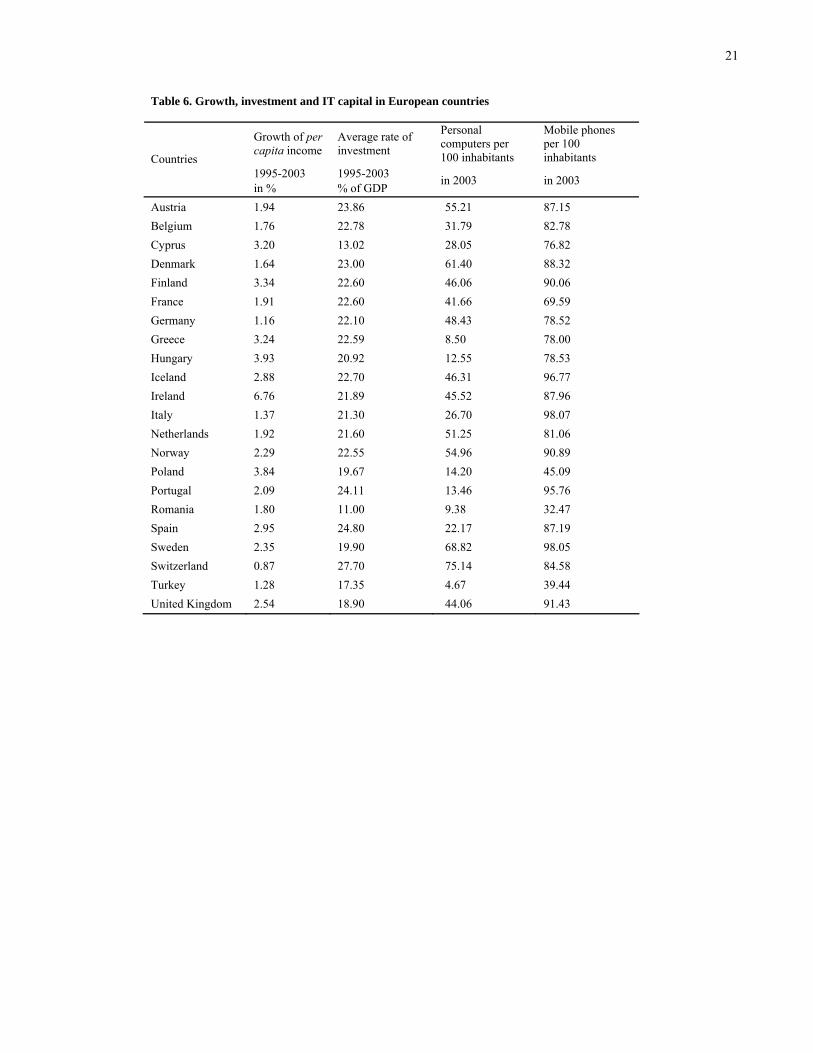
Anyway, the big impact on growth of the mobile phones seems to justify perfectly the

speed of their expansion and the fact that in all the advanced countries they have spread

very widely among the population, as Table 6 shows just with reference to the European

countries. The same result would have expected for the personal computer but in fact some

of the developed countries show low levels even in 2003.

12

(Insert Table 6)

This paradox could be explained at least by three factors. First, perhaps the personal

computer is not representative enough of the development of the computerization of the

economy, more dependent on the big equipment inside firms. So, it could be assumed that

the differences between countries in the computer equipment of the companies are not so

large as are the differences in the endowment of personal computers. Unfortunately the data

to prove that assumption are not available.

A second factor that would explain why backward countries in per capita income

have not increased the investment in personal computers more is that the benefit coming

from this capital requires of additional investment in other forms of capital and a reform of

the companies and the institutions, following the ideas by Brynjolfsson and Hitt (2000).

A third reason perhaps would lie in the fact that some of the countries referred

exhibited high rates of investment so increasing the computer equipment would have

required the reallocation of some resources invested in other forms of capital almost as

profitable as computers. This would give support to the implicit idea in the calculation of

rental prices by Jorgenson (2001) that all forms of capital have the same net rate of profit.

But this would lead directly to the conclusion that physical measures of IT capital are

misleading in the empirical work.

Anyway, the main conclusion is that estimates of IT impact using physical measures

of IT equipment in order to have a wider data base referring to many countries tend to

overestimate the contribution of IT to development. The reason has to be found in the rapid

growth of this equipment that tends to amplify the endogeneity problems. Probably this is

something that also happens to some extent with other kinds of measures but not to such a

high degree.

13

IV. Conclusions

This article explores the impact of physical measures of IT capital on the per capita income

of 102 countries on the basis of the model formulated by Mankiw et al. (1992) that allows

for the use of data with a small time span. IT capital is measured through three variables

expressed in terms of 100 inhabitants, the number of personal computers, the number of

mobile phones and the number of main telephone lines. This method not only has allowed

to count on a great number of countries but to test the huge impact other authors have

attributed to such kinds of measures.

The estimates carried out in this article confirm that these classes of measures have an

impact on per capita income so strong that it can not be seen as compatible with the real

growth of the economies, which must be due to the presence of endogeneity problems in

the estimates. So probably it is better to rely on the estimated based on monetary measures

of IT stock of capital and on their rental prices, following the Jorgenson’s (2001) approach.

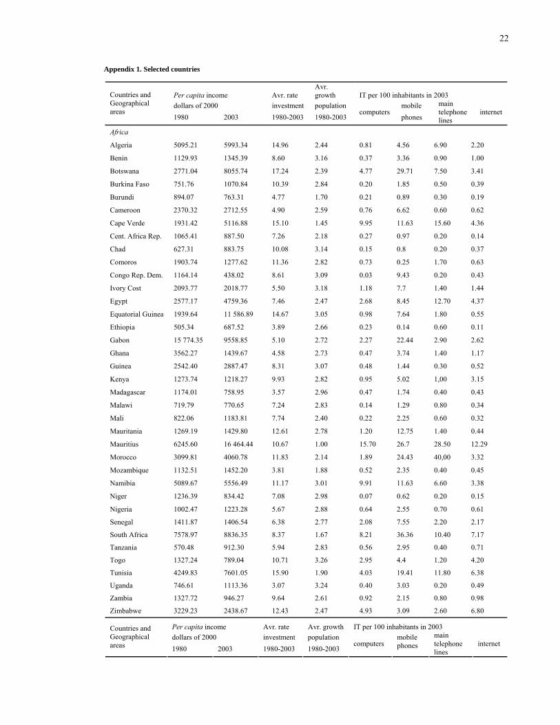
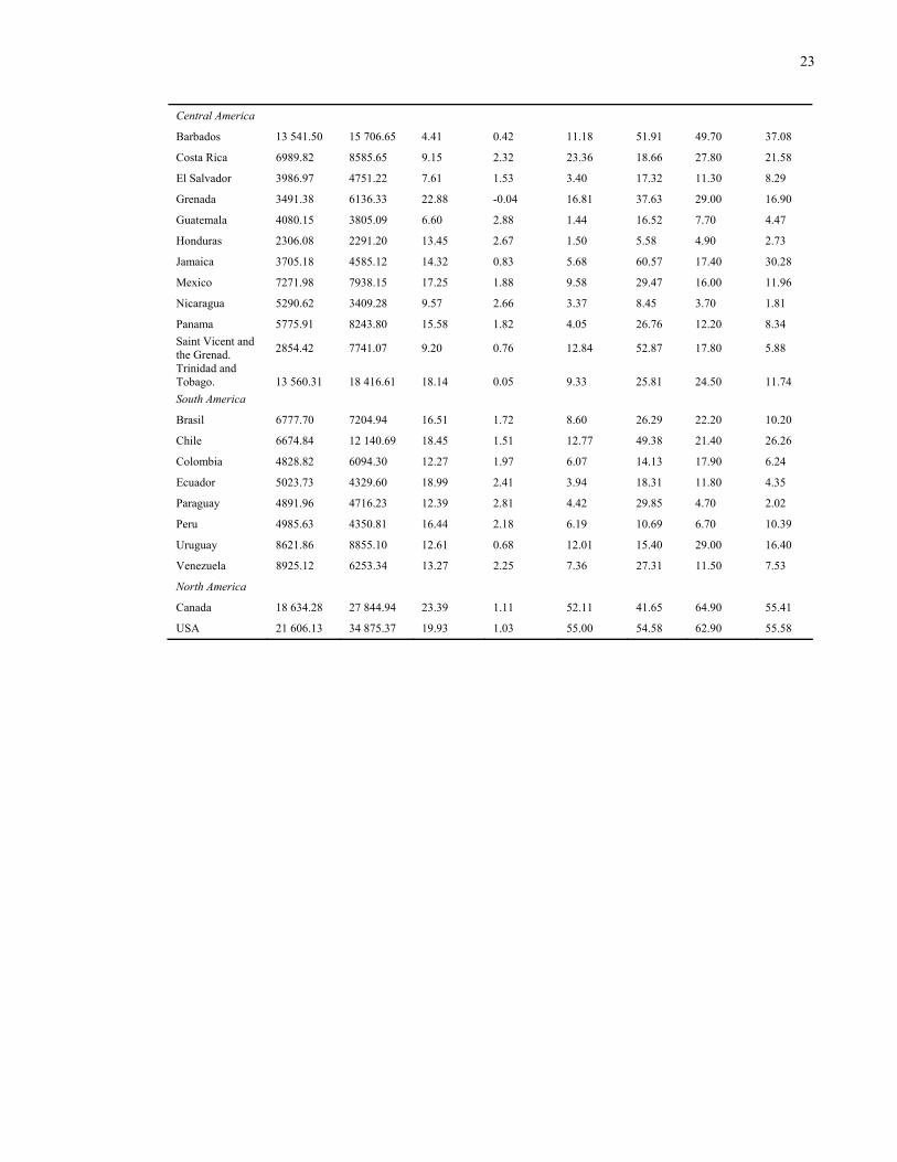
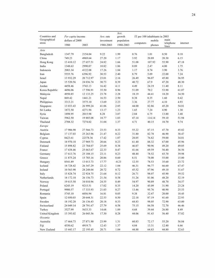
Appendix 1

(Insert Appendix 1)

14

Table 1. IT in the world in 2003a

Computers

Main telephone lines

Mobile phones

Users of internet

Geometrica average

Africa 2.3 3.8 8.4 2.3 3.6 Central America 8.0 17.4 28.2 13.1 15.1 South America 5.9 10.4 21.5 15.1 11.9 North America 56.1 55.5 48.1 63.9 55.6 Asia 16.8 20.2 38.4 22.4 23.2 Europe 37.9 37.3 81.7 51.5 49.4 Oceania 29.3 29.5 37.7 37.5 33.2 OECD 43.7 43.0 79.5 53.6 53.2 Notes: aUnits per 100 inhabitants. Source: International Telecommunication Union (ITU, 2005).

15

y = 0,60x + 7,74R2 = 0,86

0

2

4

6

8

10

12

-5 -3 -1 1 3 5

Log computers per 100 inhabitants

Log

per c

apita

inco

me

Fig. 1. Computers and income per capita in 2003

Source: ITU and Penn World Table, 2005.

16

Table 2. Estimates of the steady state per capita income in 2003 for all the countries

Dependent variable (y): per capita income in 2003 Equation estimated : ln y2003 = α1 + α2 [ ln (I/Y) – ln n ] + α3 ln kTIC + ln y1980 + ui

[1] [2] [3] [4] [5]

4.640 7.162 3.041 3.329 3.588 Constant (0.000) (0.000) (0.000) (0.000) (0.000)

1.629 0.269 0.304 0.276 0.219 Rate of physical capital not IT investment - Rate of population growth

(0.000) (0.024) (0.001) (0.003) (0.023)

0.539 0.266 0.216 0.147 Computers (0.000) (0.000) (0.000) (0.012)

0.112 0.086 Mobile phones (0.016) (0.070)

0.123 Main telephone lines (0.042)

0.533 0.480 0.456 1980 per capita income (0.000) (0.000) (0.000)

α Implicit 0.619 0.212 0.233 0.216 0.179 β (1) Implicit 0.425 0.204 0.169 0.120 β (2) Implicit 0.088 0.070 β (3) Implicit 0.101 Adjusted R2 0.535 0. 867 0. 916 0.920 0.923 Number of observations 102 102 102 102 102

17

y = 0,07x - 0,55R2 = 0,33-3

-2

-1

0

1

2

3

-10 -7 -4 -1 2 5 8 11 14 17 20

IT capital per 100 inhabitants

Per

cap

ita in

com

e no

t exp

lain

ed b

y ba

sic

mod

el

Fig. 2. Not explained per capita income and IT capital

Source: ITU and Penn World Table, 2005.

18

Table 3. Estimates of the steady state in 2003: developed and developing countries

Dependent variable (y): per capita income in 2003 Estimated equation: ln y2003 = α1 + α2 [ ln (I/Y) – ln n ] + α3 ln kTIC + ln y1980 + ui

Developed countries

Developing countries

6.317 3.900 Constant (0.000) (0.000)

-0.048 0.189 Rate of physical capital investment - Rate of population growth

(0.702) (0.083)

0.257 0.090 Computers (0.000) (0.211)

0.044 0.088 Mobile phones (0.619) (0.106)

-0.051 0.150 Main telephone lines (0.744) (0.031)

0.311 0.418 Per capita income in 1980 (0.000) (0.000)

α Implicit 0.158 β (1) Implicit 0.076 β (2) Implicit 0.074 β (3) Implicit 0.127 Adjusted R2 0.747 0.843 Number of observations 28 74

19

Table 4. Estimates of convergence equations

Dependent variable (log of change in y): Accumulated rate of growth since 1980 to 2003 Estimated equation. Convergence equation: ln y2003 – ln y1980 = α1 + α2 [ln (I/Y)- ln n] + α3 ln kTIC – α4 ln y1980 + ui

[1] [2]

0.156 32 Constant (0.000) (0.000)

0.009 0.013 Rate of physical capital not IT investment - Rate of population growth

(0.023) (0.001)

-0.024 -0.020 Per capita income in 1980 (0.000) (0.000)

0.006 0.012 Computers (0.013) (0.000)

0.004 Mobile phones (0.070)

0.005 Main telephone lines (0.042)

Adjusted R2 0.496 0. 453 Number of observations 102 102

20

Table 5. Estimates of convergence equations for recent periods

Dependent variable (change in log y): Accumulated rate of growth for the quoted period Estimated equation. Convergence equation: ln y2003 – ln y1980 = α1 + α2 [ln (I/Y)- ln n] + α3 ln kTIC – α4 ln y1980 + ui

[1] [2] [3] [4]

1995-2003 1995-2003 2000-2003 2000-2003

-0.105 -0.073 -0.208 -0.136 Constant (0.746) (0.817) (0.051) (0.206)

0.264 0.261 0.062 0.047 Rate of physical capital not IT investment - Rate of population growth

(0.000) (0.000) (0.011) (0.051)

-0.070 -0.071 0.002 -0.000 Per capita income in 1980 (0.057) (0.053) (0.898)

0.0324 0.055 Computers (0.361) (0.030)

0.0421 0.048 Mobile phones (0.066) (0.001)

0.015 -0.071 Main telephone lines (0.057) (0.078)

0.107 0.095 IT geometric average (0.039) (0.006)

α Implicit 0.209 0.207 0.058 0.047 β (1) Implicit 0.031 0.052 β (2) Implicit 0.030 0.045 β (3) Implicit 0.015 β (4) Implicit 0.097 0.086 Adjusted R2 0.152 0.118 0.071 Number of observations 102 102 102 102

21

Table 6. Growth, investment and IT capital in European countries

Growth of per capita income

Average rate of investment

Personal computers per 100 inhabitants

Mobile phones per 100 inhabitants

1995-2003 1995-2003 Countries

in % % of GDP in 2003 in 2003

Austria 1.94 23.86 55.21 87.15 Belgium 1.76 22.78 31.79 82.78 Cyprus 3.20 13.02 28.05 76.82 Denmark 1.64 23.00 61.40 88.32 Finland 3.34 22.60 46.06 90.06 France 1.91 22.60 41.66 69.59 Germany 1.16 22.10 48.43 78.52 Greece 3.24 22.59 8.50 78.00 Hungary 3.93 20.92 12.55 78.53 Iceland 2.88 22.70 46.31 96.77 Ireland 6.76 21.89 45.52 87.96 Italy 1.37 21.30 26.70 98.07 Netherlands 1.92 21.60 51.25 81.06 Norway 2.29 22.55 54.96 90.89 Poland 3.84 19.67 14.20 45.09 Portugal 2.09 24.11 13.46 95.76 Romania 1.80 11.00 9.38 32.47 Spain 2.95 24.80 22.17 87.19 Sweden 2.35 19.90 68.82 98.05 Switzerland 0.87 27.70 75.14 84.58 Turkey 1.28 17.35 4.67 39.44 United Kingdom 2.54 18.90 44.06 91.43

22

Appendix 1. Selected countries

Per capita income Avr. rate Avr. growth IT per 100 inhabitants in 2003

dollars of 2000 investment population mobile Countries and

Geographical areas

1980 2003 1980-2003 1980-2003 computers

phones

main telephone lines

internet

Africa

Algeria 5095.21 5993.34 14.96 2.44 0.81 4.56 6.90 2.20

Benin 1129.93 1345.39 8.60 3.16 0.37 3.36 0.90 1.00

Botswana 2771.04 8055.74 17.24 2.39 4.77 29.71 7.50 3.41

Burkina Faso 751.76 1070.84 10.39 2.84 0.20 1.85 0.50 0.39

Burundi 894.07 763.31 4.77 1.70 0.21 0.89 0.30 0.19

Cameroon 2370.32 2712.55 4.90 2.59 0.76 6.62 0.60 0.62

Cape Verde 1931.42 5116.88 15.10 1.45 9.95 11.63 15.60 4.36

Cent. Africa Rep. 1065.41 887.50 7.26 2.18 0.27 0.97 0.20 0.14

Chad 627.31 883.75 10.08 3.14 0.15 0.8 0.20 0.37

Comoros 1903.74 1277.62 11.36 2.82 0.73 0.25 1.70 0.63

Congo Rep. Dem. 1164.14 438.02 8.61 3.09 0.03 9.43 0.20 0.43

Ivory Cost 2093.77 2018.77 5.50 3.18 1.18 7.7 1.40 1.44

Egypt 2577.17 4759.36 7.46 2.47 2.68 8.45 12.70 4.37

Equatorial Guinea 1939.64 11 586.89 14.67 3.05 0.98 7.64 1.80 0.55

Ethiopia 505.34 687.52 3.89 2.66 0.23 0.14 0.60 0.11

Gabon 15 774.35 9558.85 5.10 2.72 2.27 22.44 2.90 2.62

Ghana 3562.27 1439.67 4.58 2.73 0.47 3.74 1.40 1.17

Guinea 2542.40 2887.47 8.31 3.07 0.48 1.44 0.30 0.52

Kenya 1273.74 1218.27 9.93 2.82 0.95 5.02 1,00 3.15

Madagascar 1174.01 758.95 3.57 2.96 0.47 1.74 0.40 0.43

Malawi 719.79 770.65 7.24 2.83 0.14 1.29 0.80 0.34

Mali 822.06 1183.81 7.74 2.40 0.22 2.25 0.60 0.32

Mauritania 1269.19 1429.80 12.61 2.78 1.20 12.75 1.40 0.44

Mauritius 6245.60 16 464.44 10.67 1.00 15.70 26.7 28.50 12.29

Morocco 3099.81 4060.78 11.83 2.14 1.89 24.43 40,00 3.32

Mozambique 1132.51 1452.20 3.81 1.88 0.52 2.35 0.40 0.45

Namibia 5089.67 5556.49 11.17 3.01 9.91 11.63 6.60 3.38

Niger 1236.39 834.42 7.08 2.98 0.07 0.62 0.20 0.15

Nigeria 1002.47 1223.28 5.67 2.88 0.64 2.55 0.70 0.61

Senegal 1411.87 1406.54 6.38 2.77 2.08 7.55 2.20 2.17

South Africa 7578.97 8836.35 8.37 1.67 8.21 36.36 10.40 7.17

Tanzania 570.48 912.30 5.94 2.83 0.56 2.95 0.40 0.71

Togo 1327.24 789.04 10.71 3.26 2.95 4.4 1.20 4.20

Tunisia 4249.83 7601.05 15.90 1.90 4.03 19.41 11.80 6.38

Uganda 746.61 1113.36 3.07 3.24 0.40 3.03 0.20 0.49

Zambia 1327.72 946.27 9.64 2.61 0.92 2.15 0.80 0.98

Zimbabwe 3229.23 2438.67 12.43 2.47 4.93 3.09 2.60 6.80

Per capita income Avr. rate Avr. growth IT per 100 inhabitants in 2003 dollars of 2000 investment population mobile

Countries and Geographical areas 1980 2003 1980-2003 1980-2003

computers phones main telephone lines

internet

23

Central America

Barbados 13 541.50 15 706.65 4.41 0.42 11.18 51.91 49.70 37.08

Costa Rica 6989.82 8585.65 9.15 2.32 23.36 18.66 27.80 21.58

El Salvador 3986.97 4751.22 7.61 1.53 3.40 17.32 11.30 8.29

Grenada 3491.38 6136.33 22.88 -0.04 16.81 37.63 29.00 16.90

Guatemala 4080.15 3805.09 6.60 2.88 1.44 16.52 7.70 4.47

Honduras 2306.08 2291.20 13.45 2.67 1.50 5.58 4.90 2.73

Jamaica 3705.18 4585.12 14.32 0.83 5.68 60.57 17.40 30.28

Mexico 7271.98 7938.15 17.25 1.88 9.58 29.47 16.00 11.96

Nicaragua 5290.62 3409.28 9.57 2.66 3.37 8.45 3.70 1.81

Panama 5775.91 8243.80 15.58 1.82 4.05 26.76 12.20 8.34 Saint Vicent and the Grenad. 2854.42 7741.07 9.20 0.76 12.84 52.87 17.80 5.88

Trinidad and Tobago. 13 560.31 18 416.61 18.14 0.05 9.33 25.81 24.50 11.74 South America

Brasil 6777.70 7204.94 16.51 1.72 8.60 26.29 22.20 10.20

Chile 6674.84 12 140.69 18.45 1.51 12.77 49.38 21.40 26.26

Colombia 4828.82 6094.30 12.27 1.97 6.07 14.13 17.90 6.24

Ecuador 5023.73 4329.60 18.99 2.41 3.94 18.31 11.80 4.35

Paraguay 4891.96 4716.23 12.39 2.81 4.42 29.85 4.70 2.02

Peru 4985.63 4350.81 16.44 2.18 6.19 10.69 6.70 10.39

Uruguay 8621.86 8855.10 12.61 0.68 12.01 15.40 29.00 16.40

Venezuela 8925.12 6253.34 13.27 2.25 7.36 27.31 11.50 7.53

North America

Canada 18 634.28 27 844.94 23.39 1.11 52.11 41.65 64.90 55.41

USA 21 606.13 34 875.37 19.93 1.03 55.00 54.58 62.90 55.58

24

Per capita income Avr. rate Avr. growth IT per 100 inhabitants in 2003

dollars of 2000 investment population mobile Countries and Geographical areas

1980 2003 1980-2003 1980-2003 computers

phones

main telephone lines

internet

Asia Bangladesh 1347.79 2154.04 9.22 1.99 0.76 1.01 0.50 0.18 China 749.23 4969.64 27.20 1.17 3.92 20.89 20.30 6.15 Hong Kong 13 410.12 27 657.51 24.82 1.66 51.08 107.92 55.90 47.18 India 1348.63 2990.07 10.82 1.86 0.89 2.47 4.00 1.75 Indonesia 2083.34 4122.08 17.26 1.84 1.17 8.74 3.90 3.76 Iran 5555.76 6396.92 30.53 2.40 8.79 5.09 22.00 7.24 Israel 13 932.29 20 712.97 23.01 2.16 26.49 96.07 45.80 36.95 Japan 15 520.56 24 036.74 30.73 0.39 40.72 67.9 47.20 48.30 Jordan 4458.46 3743.13 16.42 4.11 4.49 24.19 11.40 8.11 Korea Republic 4496.06 17 596.91 35.50 0.96 51.09 70.2 53.90 61.07 Malaysia 4950.85 12 133.25 23.78 2.28 18.19 44.41 18.20 34.50 Nepal 869.42 1441.21 16.53 2.50 0.38 0.35 1.60 0.42 Philippines 3313.21 3575.10 13.69 2.23 3.36 27.77 4.10 4.93 Singapore 13 033.43 26 999.24 41.06 2.85 44.00 82.86 45.20 54.81 Sri Lanka 1872.50 4271.94 13.17 1.23 1.65 7.24 4.90 1.30 Syria 1898.95 2015.98 8.28 3.07 2.84 6.75 13.80 3.48 Taiwan 5962.50 19 885.08 18.77 1.03 47.14 114.14 59.10 51.94 Thailand 2708.32 7274.02 31.04 1.37 4.71 40.15 10.70 9.74 Europe Austria 17 906.90 27 566.73 23.53 0.33 55.22 87.15 47.70 45.82 Belgium 17 137.03 25 263.96 21.47 0.22 31.80 82.78 46.90 38.47 Cyprus 8423.61 22378.36 17.42 1.07 28.05 76.82 59.00 34.81 Denmark 18 970.18 27 969.73 20.66 0.23 61.40 88.32 67.00 45.96 Finland 15 898.82 23 784.07 25.69 0.38 46.07 90.96 49.20 49.05 France 17 438.46 25 663.67 22.33 0.47 41.66 69.59 56.40 36.56 Germany 17 613.76 25 188.15 23.11 0.23 48.44 78.52 65.70 39.98 Greece 11 875.24 15 785.16 20.86 0.60 8.51 78.00 55.00 15.00 Hungary 8541.89 13 013.73 17.77 -0.23 12.55 78.53 35.60 23.72 Iceland 18 728.42 26 347.29 22.12 1.04 46.31 96.77 66.60 67.47 Ireland 10 563.90 28 248.04 20.72 0.72 45.52 87.96 49.10 31.67 Italy 15 828.74 22 924.75 21.64 0.12 26.71 98.07 45.90 39.52 Netherlands 18 172.10 26 156.73 21.54 0.58 51.26 81.06 48.20 52.19 Norway 19 615.50 34 010.96 24.55 0.49 54.97 90.89 48.70 34.57 Poland 6245.19 9215.51 17.02 0.35 14.20 45.09 31.90 23.24 Portugal 9980.57 17 333.93 21.03 0.27 13.46 95.76 40.90 25.53 Romania 5745.10 6056.94 16.81 0.05 9.38 32.47 20.00 18.45 Spain 12 050.03 20 644.31 22.53 0.50 22.18 87.19 41.60 22.93 Sweden 18 192.20 26 136.43 20.18 0.33 68.83 98.05 72.90 63.00 Switzerland 24 049.14 28 791.67 27.79 0.58 75.15 84.58 72.70 46.46 Turkey 3527.99 5633.33 14.68 1.89 4.68 39.44 26.80 8.49 United Kingdom 15 393.02 26 045.56 17.30 0.28 44.06 91.43 56.40 57.82 Oceania Australia 17 464.73 27 871.90 23.99 1.31 60.83 72.17 55.20 56.84 Fiji 4550.62 4919.71 12.43 1.37 4.84 13.31 12.40 6.66 New Zealand 15 443.17 22 195.45 20.71 1.04 44.88 64.83 44.80 52.63

25

References

Brynjolfsson, E. and Hitt., L. (2000) Beyond computation: information technology,

organizational transformation and business performance, Journal of Economic

Perspectives, 14, 23-48.

Dewan, S. and Kraemer, K. L. (2000) Information technology and productivity: evidence

from country-level data, Management Science, 46, 548-62.

Jorgenson, D. W. (2001) Information technology and the US economy, American

Economic Review, 91, 1-35.

Jorgenson, D. W. (2004), Accounting for growth in the information age, in Handbook on

economic growth, (Eds) Ph. Aghion and S. N. Durlauf, North-Holland, Amsterdam,

pp. 743-815.

Jorgenson, D. W., Ho, M. S. and Stiroh, K. J. (2006) The sources of the second surge of US

productivity and implications for the future, mimeo, Federal Reserve Bank, New

York.

Jorgenson, D. W. and Vu, K. (2005) Information technology and the world economy,

Scandinavian Journal of Economics, 107, 631-650.

Jorgenson, D. W. and Vu, K. (2007) Information technology and the world growth

resurgence, German Economic Review, 8, 122-145.

Mankiw, N. G., Romer, D. and Weil, D. (1992) A contribution to the empirics of economic

growth, Quarterly Journal of Economics, 107, 407-438.

Röller, L. H. and Waverman, L. (2001) Telecommunications infrastructure and economic

development: a simultaneous approach, American Economic Review, 91, 909-925.

Stiroh, K. J. (2004) Reassessing the Impact of IT in the Production Function: a Meta-

Analysis and Sensitivity Tests, Federal Reserve Bank, New York.

26

Waverman, L., Meschi, M. and Fuss, M. (2008) The impact of telecoms on economic

growth in developing countries, mimeo, London Business School, London.