Influence of storm surges and sea level on shallow tidalbasin erosive processes

G. Mariotti,1 S. Fagherazzi,1 P. L. Wiberg,2 K. J. McGlathery,2 L. Carniello,3

and A. Defina3

Received 8 October 2009; revised 8 June 2010; accepted 12 July 2010; published 17 November 2010.

[1] The finite‐element model WWTM is applied to a system of lagoons at the VirginiaCoast Reserve, USA. The model solves the shallow water equations to compute tidalfluxes, and is equipped with a wave propagation module to calculate wave height duringlocal wind events. The model is validated using measured water elevations, wave heights,and periods at five locations within the lagoon system. Scenarios with different windconditions, storm surges, and relative sea level are simulated. Results are analyzed in termsof bottom shear stresses on the tidal flats, a measure of sediment resuspension potential,and total wave energy impacting the marsh boundaries, which is the chief process drivinglateral marsh erosion. Results indicate that wave energy at the marsh boundaries is moresensitive to wind direction than are bottom shear stresses. Wave energy on marshboundaries and bottom shear stresses on the tidal flats increase with sea level elevation,with the former increasing almost ten times more than the latter. Both positive and negativefeedbacks between wave energy at the boundaries and bottom shear stresses are predicted,depending on the fate of the sediments eroded from the salt marsh boundaries.

Citation: Mariotti, G., S. Fagherazzi, P. L. Wiberg, K. J. McGlathery, L. Carniello, and A. Defina (2010), Influence of stormsurges and sea level on shallow tidal basin erosive processes, J. Geophys. Res., 115, C11012, doi:10.1029/2009JC005892.

1. Introduction

[2] Wind waves are critical for the morphological andecological equilibrium of shallow tidal basins. Two distincterosional mechanisms are associated with wind waves.Wave‐generated shear stresses, combined with tidal cur-rents, are the main mechanism responsible for sedimentresuspension on tidal flats [Carniello et al., 2005;Fagherazzi et al., 2006, 2007; Marani et al., 2007], andregulate both sediment concentration in the water column(and hence light availability at the bed) [e.g., Lawson et al.,2007] and sediment export to salt marshes and to the ocean[Mariotti and Fagherazzi, 2010]. Waves impacting saltmarsh boundaries produce intermittent forces that promotemarsh edge erosion and salt marsh regression. Even thoughmarsh boundary erosion is a complex geotechnical problemthat is dependent on a variety of processes (unsaturatedfiltration, root effects, soil characteristics, and bioturbation),evidence shows that waves are the chief driver [Schwimmer,2001; Moeller et al., 1996; Möller et al., 1999].[3] Measurements of waves inside shallow tidal basins are

generally rare; therefore a direct statistical analysis of the

wave climate is seldom possible. A more profitable approachis to model wave fields as a function of forcing parameters,such as tidal elevation and wind characteristics, that are morereadily available. In addition, by using a model‐basedapproach we can estimate the wave regime response tochanges in forcing factors, such as sea level oscillations orvariations in storminess [e.g., Fagherazzi and Wiberg, 2009].[4] Wave generation depends on the transfer of energy

from the wind to the water surface, which is a function ofwind characteristics (duration, direction, and speed), waterdepth, and fetch (the unobstructed distance over which thewind can blow). Fetch itself is a function of the water depth,since at low tide large areas of the tidal basin emerge andreduce the extent of open water available for wave forma-tion. Water depth is a function of bathymetry and waterlevel, the latter of which is primarily a function of tidalforcing and storm surge. It is thus clear that waves, tides,and basin morphology are tightly interconnected.[5] Fagherazzi and Wiberg [2009] used a simplified

model to relate wave conditions to fetch and water depth inshallow tidal basins, in which water level was imposedthroughout the whole basin, allowing water depth at eachpoint of the basin to be determined as a function ofbathymetry only. The fetch was then calculated for eachfixed direction and a semiempirical relationship [Young andVerhagen, 1996; U.S. Army Coastal Engineering ResearchCenter, 1984] was used to compute wave height for eachwind direction and speed. This simplified model allows acharacterization of the wave conditions over the entire basinwithout the need for a hydrodynamic model, but it is subject

1Department of Earth Sciences and Center for Computational Science,Boston University, Boston, Massachusetts, USA.

2Department of Environmental Sciences, University of Virginia,Charlottesville, Virginia, USA.

3Department IMAGE, University of Padova, Padova, Italy.

Copyright 2010 by the American Geophysical Union.0148‐0227/10/2009JC005892$09.00

JOURNAL OF GEOPHYSICAL RESEARCH, VOL. 115, C11012, doi:10.1029/2009JC005892, 2010

C11012 1 of 17

to some limitations, including assumptions of (1) uniformwater level throughout the basin; (2) steady wave conditions;(3) constant water depth along the fetch during wave prop-agation; and (4) no interaction between waves and currents.[6] A full hydrodynamic model is needed to unravel the

complex interactions between tidal basin morphology,tides, waves and storms. The two‐dimensional finite ele-ment model WWTM (Wind Wave Tidal Model) is usedherein. The model solves the shallow water equationstogether with the formation and propagation of local windwaves based on the wave action conservation equation [seeDefina, 2000; Carniello et al., 2005, 2009a; D’Alpaos andDefina, 2007]. The model is applied to a system of shallowlagoons and salt marshes in Virginia, USA, and it is val-idated with measurements of water levels and waves col-lected at five different locations within the lagoons. Themodel is then run with different hydrodynamic forcings(winds and tides) to calculate synthetic parameters thatdescribe the erosion of the tidal flats and marsh bound-aries. Finally, the model is used to infer the effects ofrelative sea level rise (RSLR) on these erosional para-meters, as well as to predict the morphological evolution ofthe entire tidal basin.

2. Site Description

[7] The study site is a system of shallow lagoons within theVirginia Coast Reserve (VCR), located on the Atlantic side ofthe Delmarva Peninsula, USA. The VCR hosts a Long Term

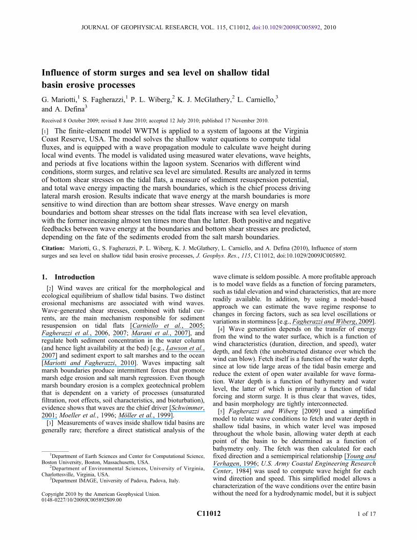
Ecological Research (LTER) facility (www.vcrlter.virginia.edu/). The VCR includes a number of shallow lagoons,characterized by shallow tidal flats (about 1 m belowMLLW)and deep channels (about 10 m below MSL), and is borderedby emergent salt marshes (above MSL). The lagoons com-prise intertidal and subtidal basins located between the bar-rier islands and the Delmarva Peninsula. Each basin isconnected to the Atlantic Ocean through tidal inlets. TheVCR is typical of shallow coastal barrier‐lagoon‐marshsystems that dominate the Atlantic and Gulf coasts of theUSA. According to the hypsographic analysis of Oertel[2001], the lagoon is covered by salt marshes (30%), tidalflats (61%), and channels (9%).[8] Tides are semidiurnal, with a mean tidal range of

1.2 m. Mean higher high water (MHHW) at Wachpreaguechannel (NOAA station 8631044, Figure 1) is 0.68 m abovemean sea level, whereas mean lower low water (MLLW) is−0.70 m. During storm surges both high water and lowwater are modified, depending on wind intensity and direc-tion, and on atmospheric pressure variations. The highestwater level on record is 2.02 m above MSL (5 February1998) whereas the lowest is −1.56 m above MSL (16 March1980) (Wachapreague NOAA station, from 28 June 1978 topresent). The current rate of relative sea level rise in theregion is 3.8–4.0 mm yr−1 [Nerem et al., 1998; Oertel et al.,1989; Emory and Aubrey, 1991], and is among the highestrates recorded along the Atlantic Coast.[9] Storms are the primary agent of short‐term distur-

bance in this coastal region. On average, over 20 extra-tropical storms rework the landscape each year [Hayden etal., 1995]. Marsh vegetation on the salt marshes is domi-nated by Spartina alterniflora, with an average stem heightof 30 cm and a height range between 50 and 100 cm. Theshallow depths of the VCR make lagoon‐bottom sediment(D50 ≈ 63 mm with sorting coefficient (D84/D50)

1/2 ≈ 2)susceptible to wind‐driven waves and currents, thus pro-moting sediment resuspension [Lawson et al., 2007;Lawson, 2004] tides alone are generally insufficient to re-suspend sediment from the lagoon bottom.

3. Model Description

[10] The hydrodynamic model WWTM solves the shallowwater equations modified through the introduction of arefined subgrid model of topography to deal with floodingand drying processes in irregular domains [Defina, 2000;D’Alpaos and Defina, 2007]. The numerical model, whichuses a finite‐element technique and discretizes the domainwith triangular elements, has been tested extensively in recentyears in the Venice lagoon, Italy [Carniello et al., 2005,2009a; D’Alpaos and Defina, 2007; Defina et al., 2007].[11] The governing equations for the hydrodynamic

model are:

@qx@t

þ @

@x

q2xY

� �þ @

@y

qyqxY

� �� @Rxx

@xþ @Rxy

@y

� �þ �bx

�� �wx

�þ gY

@h

@x¼ 0

@qy@t

þ @

@x

qxqyY

� �þ @

@y

q2yY

!� @Rxy

@xþ @Ryy

@y

� �þ �by

�� �wy

�þ gY

@h

@y¼ 0

�@h

@tþ @qx

@xþ @qy

@y¼ 0

ð1Þ

Figure 1. Bathymetry of the VCR‐LTER lagoons. Colorindicates ground elevation. Inset shows our measurementsites within Hog Island Bay: FP, Fowling Point; UN, Up-shur Neck; CP, Chimney Pole; HI, Hog Island; CB, CenterBay. Position and coordinates of the Wachapreague NOAAstation.

MARIOTTI ET AL.: SHALLOW TIDAL BASIN EROSIVE PROCESSES C11012C11012

2 of 17

where t denotes time, qx and qy are the flow rates per unitwidth in the x and y horizontal directions, Rij are the Rey-nolds stresses (i, j denoting either the x or y coordinates),tb = (tbx, tby) is the bottom stress produced by tidal cur-rents, tw = (twx, twy) is the wind shear stress at the watersurface, r is fluid density, h is the free surface elevation, g isthe gravity. Y is the equivalent water depth, defined as thevolume of water per unit area actually ponding the bottom,h is the local fraction of wetted domain, accounting for theactual area that can be wetted or dried during a tidal cycle.More details on the wetting and drying scheme are given byDefina [2000]. In equation (1), the bottom shear stress tb iscomputed as

ð�bx; �byÞ ¼ffiffiffiffiffiffiffiffiffiffiffiffiffiffiffiq2x þ q2y

qK2SY

4=3ðqx; qyÞ ð2Þ

where KS is the Strickler bed roughness coefficient.[12] For the wind‐wave model, the wave action conser-

vation equation is solved following a parameterizedapproach [Holthuijsen et al., 1989] and using a finite vol-ume scheme. The wind‐wave model is fully coupled withthe hydrodynamic module [see Carniello et al., 2005,2009a]. Assuming the direction of wave propagation adjustsinstantaneously to the wind direction, the parameterizedwave action conservation equation reads:

@N

@tþ @

@xcgxN þ @

@ycgyN ¼ S ð3Þ

where N is the zero‐order moment of the wave actionspectrum, defined as the ratio between wave energy E andthe relative wave frequency s, averaged over frequency, andcgx and cgy are the group celerity components. S is the sourceterm which takes into account all the physical processescontributing to wave energy, and it is described by thefollowing equation:

S ¼ Sw � Sbf � Swc � Sbrk ð4Þ

where Sw is the wave growth by wind action on the watersurface, and the other terms describe the dissipation of waveenergy by bottom friction (Sbf), white‐capping (Swc) anddepth‐induced breaking (Sbrk). The source term can be ex-pressed as a function of wind speed, water depth, and waveenergy as:

S ¼ �þ �N � 2Cfk

sinhð2kY ÞN � c��

�PM

� �m

N

� 2a

TpQb

Hmax

H

� �2

N ð5Þ

The values of the parameters a and b depend on thewind speed U; Cf is a friction coefficient, g is the integralwave steepness parameter, i.e., g = Es4/g2, gPM is thetheoretical value of g for a Pearson‐Moskowitz spectrum,Qb is the probability that waves with height H will break,Tp is the wave period, c, m and a are empirical param-eters. The numerical values of the parameters used tosolve equation (5) are reported by Carniello et al. [2005]and Fagherazzi et al. [2006].

[13] Following the approach suggested by Carniello et al.[2009a], the space and time variation of the peak waveperiod Tp (which was assumed to be constant by Carnielloet al. [2005]) is related to the local and instantaneouswater depth and wind speed. The peak wave period is thencomputed, at each time step and at each grid point with thefollowing empirical equation relating the wave period to thelocal water depth and wind speed [Young and Verhagen,1996; Breugem and Holthuijsen, 2007]

~T ¼ 5~Y 0:375 ð6Þ

where ~T = gTp/Uwind and ~Y = gY/Uwind2 are the dimen-

sionless wave period and water depth and Uwind is windspeed (measured at an elevation of 10 m above still waterlevel).[14] The model mesh consists of 68,000 triangular ele-

ments and 35,000 nodes, and covers an area of approximately60 km × 20 km (Figure 1). The area inside the bay isapproximately 500 km2. Element size ranges on averagefrom 100 to 200 m, with the smallest elements close to 10 m.As a boundary condition, we impose the water elevation atthe seaward boundary of the model domain; zero flux con-ditions are imposed at the landward boundary. Wind char-acteristics (speed and direction) are imposed uniformlythroughout the whole basin. Three different values for theStrickler roughness coefficient are used in equation (2):15 m1/3/s for the salt marsh, 20 m1/3/s for the tidal flats,25 m1/3/s for the channels and the shelf outside the barrierislands. The drag coefficient Cd is related to the Stricklercoefficient KS by Cd = gY−1/3 KS

−2, resulting in the fol-lowing values of Cd for the given Ks (fixing the waterdepth Y equal to 1 m): 0.043, 0.024, and 0.016. Similarvalues have been used for the Venice lagoon [Defina, 2000;Umgiesser et al., 2004; D’Alpaos and Defina, 2007] a similartidal environment located in the north‐east of Italy. Neitherriver discharge nor atmospheric precipitation are taken intoaccount in our simulations.

4. Model Testing

[15] To test the model, we compare its results to fieldmeasurements. Two periods are considered for the modeltesting: Period 1 from 31 January to 5 February 2009 (a totalof 144 consecutive hours), and Period 2 from 1 to 2 March2009 (a total of 72 consecutive hours). Wave events char-acterized by different wind speeds and directions werepresent during these periods, permitting us to evaluate themodel response, particularly the wave module performance,under different conditions.[16] Water level was measured with high resolution pie-

zoresistive transducers (RBR© TGR 2050P and Nortek©

Aquadopp profilers). The instruments were deployed at fivesites (Figure 1): four of them close to the marsh boundary(Upshur Neck, UN, Chimney Pole, CP, Fowling Point, FP,Hog Island, HI), and one close to the main channel thatdissects the basin (Center Bay, CB). We used RBR sensorsat UN, FP, and CB and Nortek Aquadopps at HI and CP.During Period 1, all the instruments were recording; duringPeriod 2, only the RBR instruments were recording. Waterlevel is computed as the average over a sampling interval(RBR instruments recorded every 30 min, averaging over

MARIOTTI ET AL.: SHALLOW TIDAL BASIN EROSIVE PROCESSES C11012C11012

3 of 17

300 s; Nortek current profilers record every 10 min, aver-aging over 60 s). Wave data were recorded every 30 min,sampling 512 bursts with a frequency of 2 Hz. From eachwave burst a significant wave height (Hs) and peak period(Tp) are calculated from the power spectral density estimatevia Welch’s periodogram method [Press et al., 1992].[17] The model is set up to simulate the same hydrody-

namic conditions that were present during the measurementperiods. The water level in time is imposed at the seawardboundary (Figure 1). Since no records of tidal oscillationsexist in that area, the water level is set equal to the valuemeasured inside the basin shifted by a lag time (location HI,just near the tidal inlet, for Period 1, and location CB forPeriod 2). The lag time is determined by measuring thedelay of the water level propagation from the seawardboundary to the instrument location. The wind input data aretaken from the NOAA station at Wachapreague station (ID8631044), where wind speed and direction are collectedevery 6 min. The wind field is applied uniformly throughoutthe domain with the same time resolution as the availabledata. Analysis of the effect of wind speed and directionmeasured in different locations within the lagoon of Venicein the application of WWTM suggests that assuming auniform wind field is acceptable, especially in stormy con-ditions (i.e., Uwind ≥ 10 m/s). However, in some cases,nonuniformity of wind speed and direction can have someimpact especially on the wind wave distribution [Carnielloet al., 2009a, 2009b].

[18] Two statistics are used to provide an objective eval-uation of model performance: the Model Efficiency (ME)

ME ¼ 1�P

D�Mð Þ2PD� D� �2 ð7Þ

which measures the ratio of the model error to variability inobservational data, and the root mean squared error (RMSE)

RMSE ¼ffiffiffiffiffiffiffiffiffiffiffiffiffiffiffiffiffiffiffiffiffiffiffiffiffiffiffiffiX D�Mð Þ2

n

sð8Þ

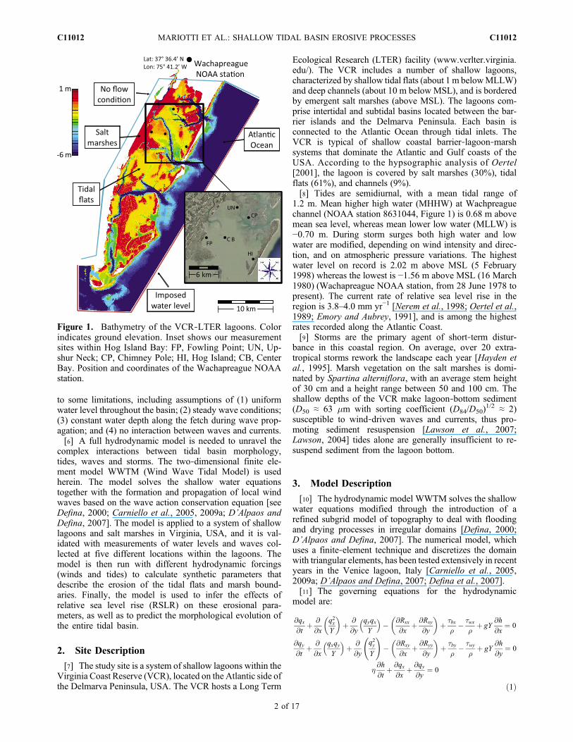
where D is the observational data, D is the mean of theobservational data and M is the corresponding model esti-mate [Allen et al., 2007].[19] Period 1 is characterized by approximately 11 full tidal

cycles with a mean tidal amplitude of 1.3 m (Figure 2a). Themaximum water level excursion is 1.9 m and is due to thecombined effect of the astronomical tide and storm surge.During Period 1 there are three main wind events (Figure 2b):in the first event the wind blows from north (300°–360°) andhas a maximum speed of 6 m/s; in the second event thewind blows from southeast (220°) with a maximum speed of7 m/s; in the third event the wind blows again from northwith maximum speed of 7 m/s.[20] Water levels computed with the model generally are

in agreement with measured values (Figure 2a). Water level

Figure 2. Simulation of Period 1 (from 31 January to 5 February 2009). Water level (referred to MSL)imposed at the seaward boundary (a) water depth, (b) wave height, and (c) period measured and computedat the five study sites. Wave period is reported only for measured wave height greater than 0.1 m. Windspeed from the NOAA Wachapreague station ID 8631044.

MARIOTTI ET AL.: SHALLOW TIDAL BASIN EROSIVE PROCESSES C11012C11012

4 of 17

oscillations are similar at each measurement site within thebasin, and are similar to the water level imposed at theseaward boundary. The tidal signal does not change sig-nificantly in shape as it propagates within the basin (thedifference between measurement sites is less than 1 cm, onthe order of measure error), and only a phase shift is present.From the model simulation the phase shift between theseaward boundary and the measurement sites are: HI 1 h, CP0.8 h, CB 1.1 h, UN 1.2 h, and FP 1.4 h. For all the stationthe RMSE is between 7 and 11 cm, while the ME is close to1.0. The large value of ME is governed by the forcing at theseaward boundary, which strongly controls the water level.Since the difference between the measured and predictedwater level has no correlation with the water level, weconclude that the model reproduces correctly the tideoscillation phase lag among the different stations. Also therange of tidal amplitude is well reproduced: both measuredand predicted values do not change significantly (few %)inside the basin. The remaining error in the water level isprobably due to some additional overharmonics present inthe basin not reproduced by the model.[21] The agreement between computed and measured

wave height varies from site to site (Figure 2b). At the CBsite, the wave regime is mainly determined by wind speed,since the fetch is approximately constant in every directionand the water depth is not a strong limiting factor (theminimum water depth is 1 m). Wave height variations arereasonably well represented by the model, with a few wavepeaks underestimated in the first half of Period #1. At FP,the wave regime is strongly affected by water depth, sincethe tidal flats emerge at low water levels. Simulated waveheights at this location are similar to measured values. At theother three sites, HI, UN, and CP, all located close to themarsh boundary, the wave regime is controlled strongly bywind speed and direction, and less by water depth. When thewind blows from the salt marsh, the fetch is almost zero andvery small waves form even if the wind speed is high. Whenthe wind blows from the open bay toward the salt marsh, thewave height is determined mainly by wind speed. At HI,where relatively higher waves are present, ME is positive,meaning that the model forecast is a better predictor of waveheight than the average value of observed wave height. MEis negative for CB and for three of the four sites near themarsh edge (FP, UN, and CP), suggesting that in this casethe average value of observed wave height is a better pre-dictor of wave height than the model forecast. We believethat these poor values for ME can be ascribed partly to aninadequate description of the wind field over the lagoon(wind data are measured at the NOAA station which is notlocated within the lagoon) (see Figure 1). In fact most of thewave peaks are reproduced by the model, except for themiddle part of Period 1 at UN and CP, where the measuredwave height is almost zero and computed values arebetween 10 and 40 cm. Since the wind intensity is not zeroduring that period, the discrepancy between simulations andmeasurements is probably due wind nonuniformity over theentire basin. Note that during Period 1 wind speed is mod-erately low and, as stated above, in these conditions winduniformity is questionable. Waves computed by the modelare compared to measured values only where the waveheight is greater than 0.1 m.

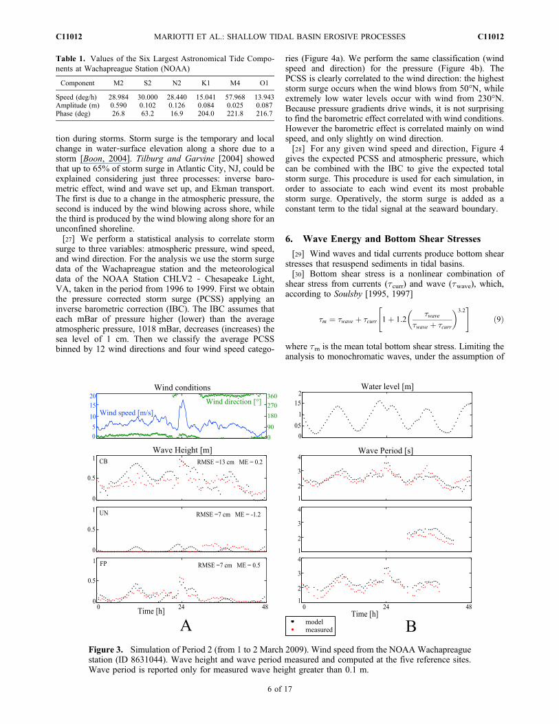
[22] Measured wave period falls in the range of 1.5–2.5 s,with variations in phase with water depth. The model fol-lows these variations with good agreement.[23] Period 2 is characterized by approximately four tidal

oscillations (Figure 3). Wind direction was relatively con-stant (around 0°N) and wind speed varied between 5 and10 m/s, except for several hours when the wind blew at15 m/s. The model reproduces correctly the tidal oscilla-tions (ME = 1, not reported in the figure). Wave height isreproduced better than during Period 1: ME is between 0.2and 0.5 in the sites where waves are present, CB and FP(Figure 3a). This result indicates that the model performsbetter when wind speed is ≥10 m/s, which is significant forthe following simulations. Also in this case the period iswell predicted by the model.

5. Model Forecasting

[24] We use the model to study the tidal basin response toa variety of hydrodynamic forcing conditions, namely var-iations in sea level, tides, and wind fields. Since the use ofall possible combinations of tidal oscillations and windconditions is not feasible, only few combinations are cho-sen. The next section focuses on the choice of the mostsignificant hydrodynamic inputs for the model. In the modelsimulations described above, water level was imposed out-side the basin at the seaward domain boundary (Figure 2)using the data measured inside the lagoon and shiftedappropriately in time. To determine the water level toimpose on the seaward boundary for the model forecasts,astronomical tidal components measured at the Wacha-preague station are used to create a synthetic tidal signal.Since the goal is to simulate the tide outside the lagoon, tidalharmonics deriving from shallow water effects are ne-glected. All other 27 components are considered (the sixgreatest components are reported in Table 1). The synthetictide generated with this method has a very long periodicity,at least equal to the lunar cycle. For computational reasons,is not feasible to run each simulation for such a long period.Therefore, a window of 72 h is used, and is chosen to avoidboth extremely high and extremely low oscillations in orderto be representative of the whole signal. In addition, the first24 h of simulations are discarded form the analysis in orderto eliminate the transient effect of the initial conditions.Therefore each simulation gives 48 h, i.e., four full tidalcycles, of usable results.[25] Winds are variable, seldom maintaining a constant

speed and direction for longer than several hours. However,the results of a set of numerical experiments performed toassess the impact of wind transients on the wave field showthat the impact is moderate because the adaptation time isrelatively short (i.e., shorter than 10–15 min). Therefore, forsimplicity, all simulations are run with constant wind speedand direction, using four classes of wind (5, 10, 15, and20 m/s), and 12 directions. Using a constant wind duringthe simulations allows us to isolate the basin response toeach specific wind condition. The results obtained with thesesimulations can be easily combined with wind statistics (fre-quency and duration distribution) to infer the basin responseto more realistic meteorological conditions.[26] Although the tide is the main factor controlling water

levels, storm surges contribute significantly to water eleva-

MARIOTTI ET AL.: SHALLOW TIDAL BASIN EROSIVE PROCESSES C11012C11012

5 of 17

tion during storms. Storm surge is the temporary and localchange in water‐surface elevation along a shore due to astorm [Boon, 2004]. Tilburg and Garvine [2004] showedthat up to 65% of storm surge in Atlantic City, NJ, could beexplained considering just three processes: inverse baro-metric effect, wind and wave set up, and Ekman transport.The first is due to a change in the atmospheric pressure, thesecond is induced by the wind blowing across shore, whilethe third is produced by the wind blowing along shore for anunconfined shoreline.[27] We perform a statistical analysis to correlate storm

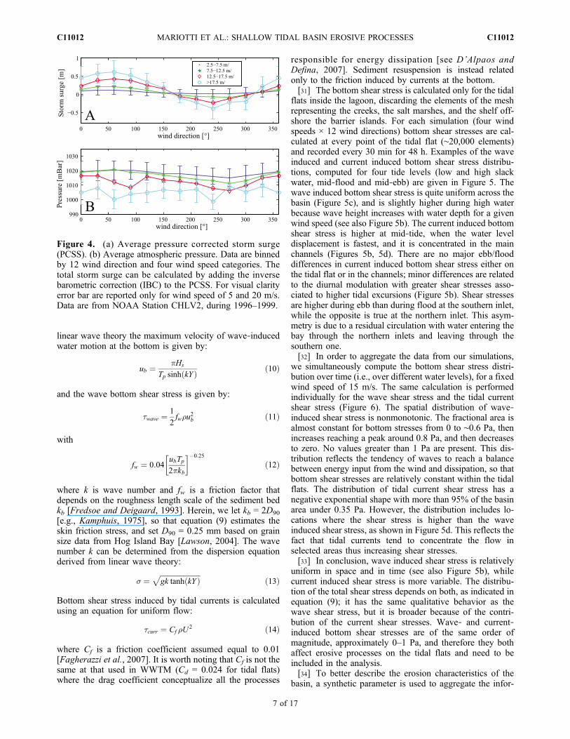
surge to three variables: atmospheric pressure, wind speed,and wind direction. For the analysis we use the storm surgedata of the Wachapreague station and the meteorologicaldata of the NOAA Station CHLV2 ‐ Chesapeake Light,VA, taken in the period from 1996 to 1999. First we obtainthe pressure corrected storm surge (PCSS) applying aninverse barometric correction (IBC). The IBC assumes thateach mBar of pressure higher (lower) than the averageatmospheric pressure, 1018 mBar, decreases (increases) thesea level of 1 cm. Then we classify the average PCSSbinned by 12 wind directions and four wind speed catego-

ries (Figure 4a). We perform the same classification (windspeed and direction) for the pressure (Figure 4b). ThePCSS is clearly correlated to the wind direction: the higheststorm surge occurs when the wind blows from 50°N, whileextremely low water levels occur with wind from 230°N.Because pressure gradients drive winds, it is not surprisingto find the barometric effect correlated with wind conditions.However the barometric effect is correlated mainly on windspeed, and only slightly on wind direction.[28] For any given wind speed and direction, Figure 4

gives the expected PCSS and atmospheric pressure, whichcan be combined with the IBC to give the expected totalstorm surge. This procedure is used for each simulation, inorder to associate to each wind event its most probablestorm surge. Operatively, the storm surge is added as aconstant term to the tidal signal at the seaward boundary.

6. Wave Energy and Bottom Shear Stresses

[29] Wind waves and tidal currents produce bottom shearstresses that resuspend sediments in tidal basins.[30] Bottom shear stress is a nonlinear combination of

shear stress from currents (tcurr) and wave (twave), which,according to Soulsby [1995, 1997]

�m ¼ �wave þ �curr 1þ 1:2�wave

�wave þ �curr

� �3:2" #

ð9Þ

where tm is the mean total bottom shear stress. Limiting theanalysis to monochromatic waves, under the assumption of

Table 1. Values of the Six Largest Astronomical Tide Compo-nents at Wachapreague Station (NOAA)

Component M2 S2 N2 K1 M4 O1

Speed (deg/h) 28.984 30.000 28.440 15.041 57.968 13.943Amplitude (m) 0.590 0.102 0.126 0.084 0.025 0.087Phase (deg) 26.8 63.2 16.9 204.0 221.8 216.7

Figure 3. Simulation of Period 2 (from 1 to 2 March 2009). Wind speed from the NOAA Wachapreaguestation (ID 8631044). Wave height and wave period measured and computed at the five reference sites.Wave period is reported only for measured wave height greater than 0.1 m.

MARIOTTI ET AL.: SHALLOW TIDAL BASIN EROSIVE PROCESSES C11012C11012

6 of 17

linear wave theory the maximum velocity of wave‐inducedwater motion at the bottom is given by:

ub ¼ Hs

Tp sinhðkY Þ ð10Þ

and the wave bottom shear stress is given by:

�wave ¼ 1

2fw�u

2b ð11Þ

with

fw ¼ 0:04ubTp2kb

�0:25

ð12Þ

where k is wave number and fw is a friction factor thatdepends on the roughness length scale of the sediment bedkb [Fredsoe and Deigaard, 1993]. Herein, we let kb = 2D90

[e.g., Kamphuis, 1975], so that equation (9) estimates theskin friction stress, and set D90 = 0.25 mm based on grainsize data from Hog Island Bay [Lawson, 2004]. The wavenumber k can be determined from the dispersion equationderived from linear wave theory:

� ¼ffiffiffiffiffiffiffiffiffiffiffiffiffiffiffiffiffiffiffiffiffiffiffigk tanhðkY Þ

pð13Þ

Bottom shear stress induced by tidal currents is calculatedusing an equation for uniform flow:

�curr ¼ Cf �U2 ð14Þ

where Cf is a friction coefficient assumed equal to 0.01[Fagherazzi et al., 2007]. It is worth noting that Cf is not thesame at that used in WWTM (Cd = 0.024 for tidal flats)where the drag coefficient conceptualize all the processes

responsible for energy dissipation [see D’Alpaos andDefina, 2007]. Sediment resuspension is instead relatedonly to the friction induced by currents at the bottom.[31] The bottom shear stress is calculated only for the tidal

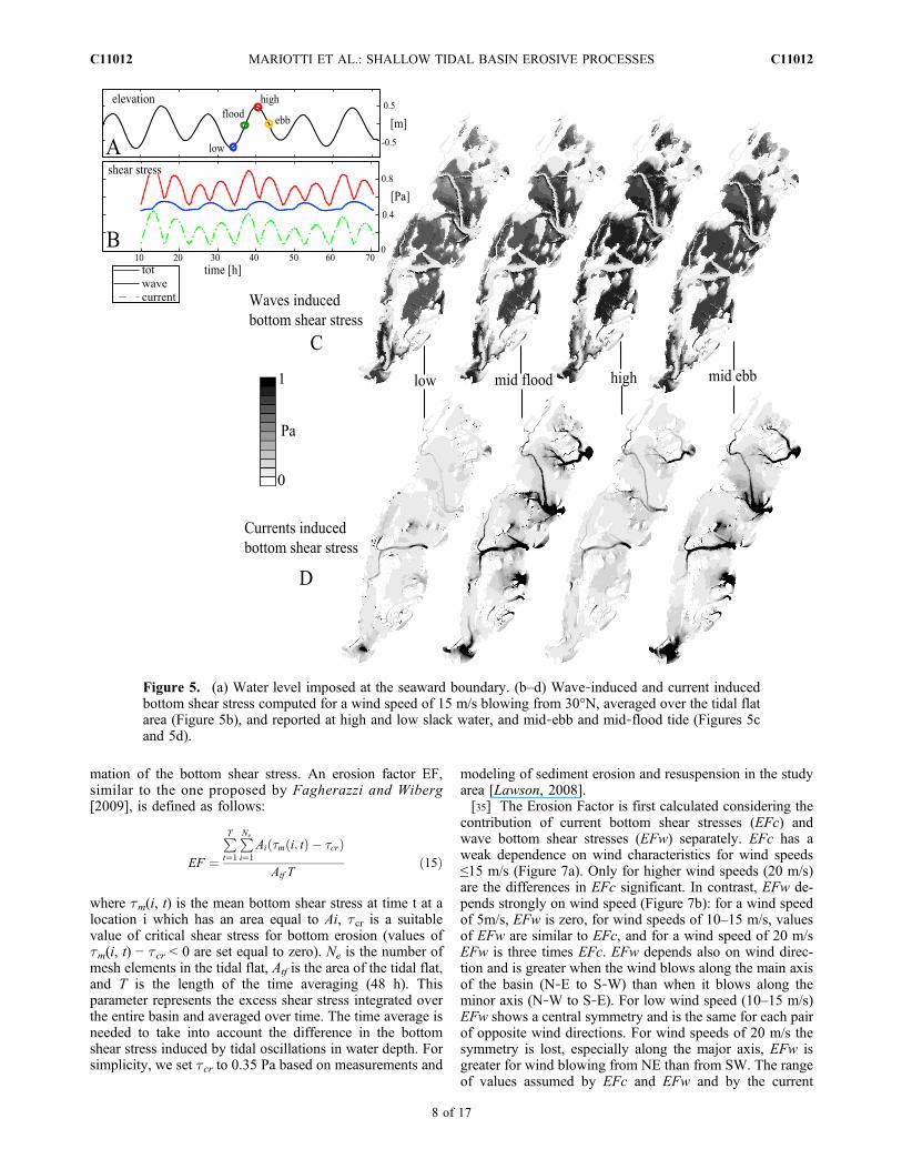
flats inside the lagoon, discarding the elements of the meshrepresenting the creeks, the salt marshes, and the shelf off-shore the barrier islands. For each simulation (four windspeeds × 12 wind directions) bottom shear stresses are cal-culated at every point of the tidal flat (∼20,000 elements)and recorded every 30 min for 48 h. Examples of the waveinduced and current induced bottom shear stress distribu-tions, computed for four tide levels (low and high slackwater, mid‐flood and mid‐ebb) are given in Figure 5. Thewave induced bottom shear stress is quite uniform across thebasin (Figure 5c), and is slightly higher during high waterbecause wave height increases with water depth for a givenwind speed (see also Figure 5b). The current induced bottomshear stress is higher at mid‐tide, when the water leveldisplacement is fastest, and it is concentrated in the mainchannels (Figures 5b, 5d). There are no major ebb/flooddifferences in current induced bottom shear stress either onthe tidal flat or in the channels; minor differences are relatedto the diurnal modulation with greater shear stresses asso-ciated to higher tidal excursions (Figure 5b). Shear stressesare higher during ebb than during flood at the southern inlet,while the opposite is true at the northern inlet. This asym-metry is due to a residual circulation with water entering thebay through the northern inlets and leaving through thesouthern one.[32] In order to aggregate the data from our simulations,

we simultaneously compute the bottom shear stress distri-bution over time (i.e., over different water levels), for a fixedwind speed of 15 m/s. The same calculation is performedindividually for the wave shear stress and the tidal currentshear stress (Figure 6). The spatial distribution of wave‐induced shear stress is nonmonotonic. The fractional area isalmost constant for bottom stresses from 0 to ∼0.6 Pa, thenincreases reaching a peak around 0.8 Pa, and then decreasesto zero. No values greater than 1 Pa are present. This dis-tribution reflects the tendency of waves to reach a balancebetween energy input from the wind and dissipation, so thatbottom shear stresses are relatively constant within the tidalflats. The distribution of tidal current shear stress has anegative exponential shape with more than 95% of the basinarea under 0.35 Pa. However, the distribution includes lo-cations where the shear stress is higher than the waveinduced shear stress, as shown in Figure 5d. This reflects thefact that tidal currents tend to concentrate the flow inselected areas thus increasing shear stresses.[33] In conclusion, wave induced shear stress is relatively

uniform in space and in time (see also Figure 5b), whilecurrent induced shear stress is more variable. The distribu-tion of the total shear stress depends on both, as indicated inequation (9); it has the same qualitative behavior as thewave shear stress, but it is broader because of the contri-bution of the current shear stresses. Wave‐ and current‐induced bottom shear stresses are of the same order ofmagnitude, approximately 0–1 Pa, and therefore they bothaffect erosive processes on the tidal flats and need to beincluded in the analysis.[34] To better describe the erosion characteristics of the

basin, a synthetic parameter is used to aggregate the infor-

Figure 4. (a) Average pressure corrected storm surge(PCSS). (b) Average atmospheric pressure. Data are binnedby 12 wind direction and four wind speed categories. Thetotal storm surge can be calculated by adding the inversebarometric correction (IBC) to the PCSS. For visual clarityerror bar are reported only for wind speed of 5 and 20 m/s.Data are from NOAA Station CHLV2, during 1996–1999.

MARIOTTI ET AL.: SHALLOW TIDAL BASIN EROSIVE PROCESSES C11012C11012

7 of 17

mation of the bottom shear stress. An erosion factor EF,similar to the one proposed by Fagherazzi and Wiberg[2009], is defined as follows:

EF ¼PTt¼1

PNe

i¼1Ai �m i; tð Þ � �crð Þ

Atf Tð15Þ

where tm(i, t) is the mean bottom shear stress at time t at alocation i which has an area equal to Ai, tcr is a suitablevalue of critical shear stress for bottom erosion (values oftm(i, t) − tcr < 0 are set equal to zero). Ne is the number ofmesh elements in the tidal flat, Atf is the area of the tidal flat,and T is the length of the time averaging (48 h). Thisparameter represents the excess shear stress integrated overthe entire basin and averaged over time. The time average isneeded to take into account the difference in the bottomshear stress induced by tidal oscillations in water depth. Forsimplicity, we set tcr to 0.35 Pa based on measurements and

modeling of sediment erosion and resuspension in the studyarea [Lawson, 2008].[35] The Erosion Factor is first calculated considering the

contribution of current bottom shear stresses (EFc) andwave bottom shear stresses (EFw) separately. EFc has aweak dependence on wind characteristics for wind speeds≤15 m/s (Figure 7a). Only for higher wind speeds (20 m/s)are the differences in EFc significant. In contrast, EFw de-pends strongly on wind speed (Figure 7b): for a wind speedof 5m/s, EFw is zero, for wind speeds of 10–15 m/s, valuesof EFw are similar to EFc, and for a wind speed of 20 m/sEFw is three times EFc. EFw depends also on wind direc-tion and is greater when the wind blows along the main axisof the basin (N‐E to S‐W) than when it blows along theminor axis (N‐W to S‐E). For low wind speed (10–15 m/s)EFw shows a central symmetry and is the same for each pairof opposite wind directions. For wind speeds of 20 m/s thesymmetry is lost, especially along the major axis, EFw isgreater for wind blowing from NE than from SW. The rangeof values assumed by EFc and EFw and by the current

Figure 5. (a) Water level imposed at the seaward boundary. (b–d) Wave‐induced and current inducedbottom shear stress computed for a wind speed of 15 m/s blowing from 30°N, averaged over the tidal flatarea (Figure 5b), and reported at high and low slack water, and mid‐ebb and mid‐flood tide (Figures 5cand 5d).

MARIOTTI ET AL.: SHALLOW TIDAL BASIN EROSIVE PROCESSES C11012C11012

8 of 17

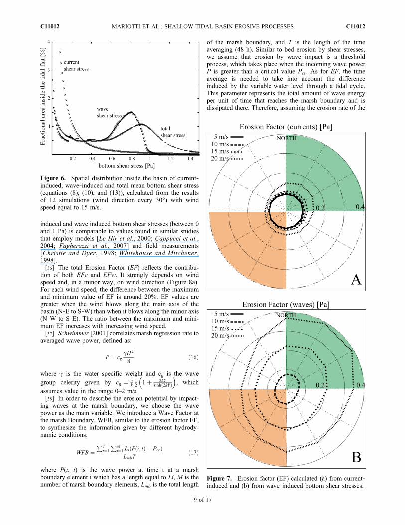
induced and wave induced bottom shear stresses (between 0and 1 Pa) is comparable to values found in similar studiesthat employ models [Le Hir et al., 2000; Cappucci et al.,2004; Fagherazzi et al., 2007] and field measurements[Christie and Dyer, 1998; Whitehouse and Mitchener,1998].[36] The total Erosion Factor (EF) reflects the contribu-

tion of both EFc and EFw. It strongly depends on windspeed and, in a minor way, on wind direction (Figure 8a).For each wind speed, the difference between the maximumand minimum value of EF is around 20%. EF values aregreater when the wind blows along the main axis of thebasin (N‐E to S‐W) than when it blows along the minor axis(N‐W to S‐E). The ratio between the maximum and mini-mum EF increases with increasing wind speed.[37] Schwimmer [2001] correlates marsh regression rate to

averaged wave power, defined as:

P ¼ cg�H2

8ð16Þ

where g is the water specific weight and cg is the wavegroup celerity given by cg ¼ �

k12 1þ 2kY

sinhð2kY Þ� �

, whichassumes value in the range 0–2 m/s.[38] In order to describe the erosion potential by impact-

ing waves at the marsh boundary, we choose the wavepower as the main variable. We introduce a Wave Factor atthe marsh Boundary, WFB, similar to the erosion factor EF,to synthesize the information given by different hydrody-namic conditions:

WFB ¼PT

t¼1

PMi¼1 Li Pði; tÞ � Pcrð Þ

LmbTð17Þ

where P(i, t) is the wave power at time t at a marshboundary element i which has a length equal to Li, M is thenumber of marsh boundary elements, Lmb is the total length

of the marsh boundary, and T is the length of the timeaveraging (48 h). Similar to bed erosion by shear stresses,we assume that erosion by wave impact is a thresholdprocess, which takes place when the incoming wave powerP is greater than a critical value Pcr. As for EF, the timeaverage is needed to take into account the differenceinduced by the variable water level through a tidal cycle.This parameter represents the total amount of wave energyper unit of time that reaches the marsh boundary and isdissipated there. Therefore, assuming the erosion rate of the

Figure 7. Erosion factor (EF) calculated (a) from current‐induced and (b) from wave‐induced bottom shear stresses.

Figure 6. Spatial distribution inside the basin of current‐induced, wave‐induced and total mean bottom shear stress(equations (8), (10), and (13)), calculated from the resultsof 12 simulations (wind direction every 30°) with windspeed equal to 15 m/s.

MARIOTTI ET AL.: SHALLOW TIDAL BASIN EROSIVE PROCESSES C11012C11012

9 of 17

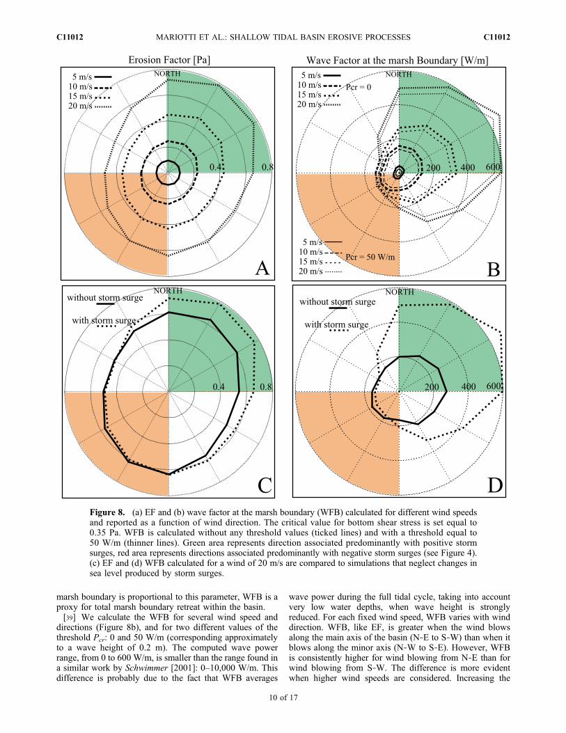
marsh boundary is proportional to this parameter, WFB is aproxy for total marsh boundary retreat within the basin.[39] We calculate the WFB for several wind speed and

directions (Figure 8b), and for two different values of thethreshold Pcr: 0 and 50 W/m (corresponding approximatelyto a wave height of 0.2 m). The computed wave powerrange, from 0 to 600 W/m, is smaller than the range found ina similar work by Schwimmer [2001]: 0–10,000 W/m. Thisdifference is probably due to the fact that WFB averages

wave power during the full tidal cycle, taking into accountvery low water depths, when wave height is stronglyreduced. For each fixed wind speed, WFB varies with winddirection. WFB, like EF, is greater when the wind blowsalong the main axis of the basin (N‐E to S‐W) than when itblows along the minor axis (N‐W to S‐E). However, WFBis consistently higher for wind blowing from N‐E than forwind blowing from S‐W. The difference is more evidentwhen higher wind speeds are considered. Increasing the

Figure 8. (a) EF and (b) wave factor at the marsh boundary (WFB) calculated for different wind speedsand reported as a function of wind direction. The critical value for bottom shear stress is set equal to0.35 Pa. WFB is calculated without any threshold values (ticked lines) and with a threshold equal to50 W/m (thinner lines). Green area represents direction associated predominantly with positive stormsurges, red area represents directions associated predominantly with negative storm surges (see Figure 4).(c) EF and (d) WFB calculated for a wind of 20 m/s are compared to simulations that neglect changes insea level produced by storm surges.

MARIOTTI ET AL.: SHALLOW TIDAL BASIN EROSIVE PROCESSES C11012C11012

10 of 17

threshold value Pcr decreases values of WFB; however itdoes not significantly change the WFB dependence on windregime (speed and direction).[40] An additional simulation is performed only for a

wind speed of 20 m/s, neglecting the superimposition of thestorm surge associated with the wind conditions, i.e., usingthe same water level for each wind direction. Without stormsurges the EF is symmetric with respect to the wind direc-tion, resulting in an ellipse with the major axis aligned to thebasin main axis (Figure 8c). The presence of a positivestorm surge increases the EF up to 30% while a negativestorm surge slightly affects it. Even the WFB is moresymmetric without storm surges (Figure 8d). The presenceof a positive storm surge increases WFB up to 150%, whilethe presence of a negative storm surge decreases WFB atmost by 10%.[41] The Erosion Factor EF and the Wave Factor at the

marsh Boundary WFB permit us to synthesize the effects ofwaves on sediment mobilization and to understand the rel-ative importance of different wind conditions. This not-withstanding, it is also important to determine the spatialdistribution of waves across the tidal flats and at the marshboundaries in order to define which areas are most prone to

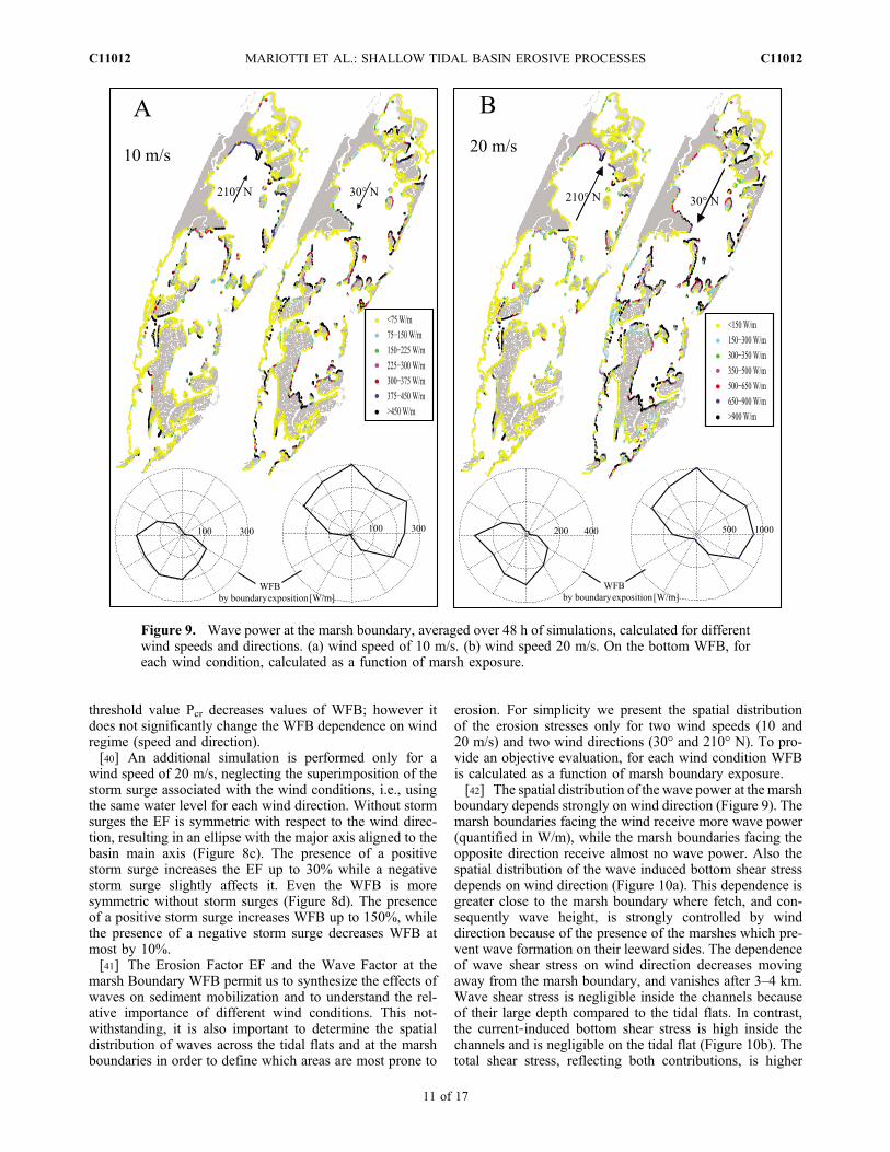
erosion. For simplicity we present the spatial distributionof the erosion stresses only for two wind speeds (10 and20 m/s) and two wind directions (30° and 210° N). To pro-vide an objective evaluation, for each wind condition WFBis calculated as a function of marsh boundary exposure.[42] The spatial distribution of the wave power at the marsh

boundary depends strongly on wind direction (Figure 9). Themarsh boundaries facing the wind receive more wave power(quantified in W/m), while the marsh boundaries facing theopposite direction receive almost no wave power. Also thespatial distribution of the wave induced bottom shear stressdepends on wind direction (Figure 10a). This dependence isgreater close to the marsh boundary where fetch, and con-sequently wave height, is strongly controlled by winddirection because of the presence of the marshes which pre-vent wave formation on their leeward sides. The dependenceof wave shear stress on wind direction decreases movingaway from the marsh boundary, and vanishes after 3–4 km.Wave shear stress is negligible inside the channels becauseof their large depth compared to the tidal flats. In contrast,the current‐induced bottom shear stress is high inside thechannels and is negligible on the tidal flat (Figure 10b). Thetotal shear stress, reflecting both contributions, is higher

Figure 9. Wave power at the marsh boundary, averaged over 48 h of simulations, calculated for differentwind speeds and directions. (a) wind speed of 10 m/s. (b) wind speed 20 m/s. On the bottom WFB, foreach wind condition, calculated as a function of marsh exposure.

MARIOTTI ET AL.: SHALLOW TIDAL BASIN EROSIVE PROCESSES C11012C11012

11 of 17

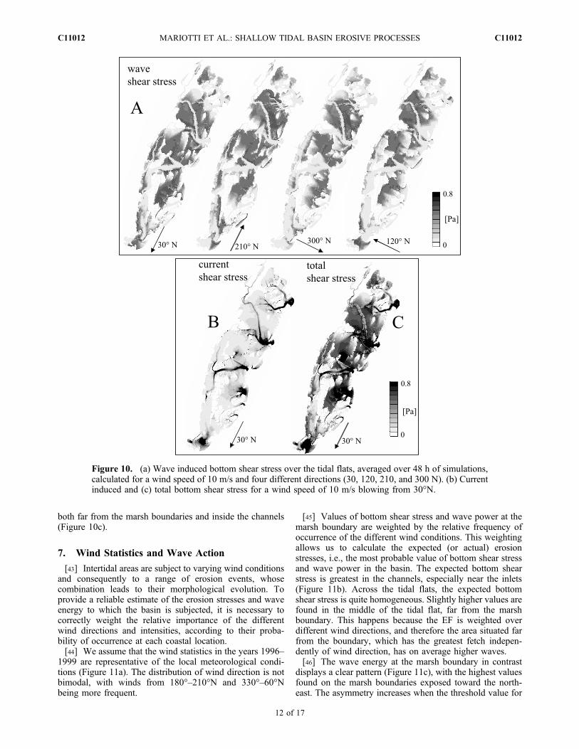
both far from the marsh boundaries and inside the channels(Figure 10c).

7. Wind Statistics and Wave Action

[43] Intertidal areas are subject to varying wind conditionsand consequently to a range of erosion events, whosecombination leads to their morphological evolution. Toprovide a reliable estimate of the erosion stresses and waveenergy to which the basin is subjected, it is necessary tocorrectly weight the relative importance of the differentwind directions and intensities, according to their proba-bility of occurrence at each coastal location.[44] We assume that the wind statistics in the years 1996–

1999 are representative of the local meteorological condi-tions (Figure 11a). The distribution of wind direction is notbimodal, with winds from 180°–210°N and 330°–60°Nbeing more frequent.

[45] Values of bottom shear stress and wave power at themarsh boundary are weighted by the relative frequency ofoccurrence of the different wind conditions. This weightingallows us to calculate the expected (or actual) erosionstresses, i.e., the most probable value of bottom shear stressand wave power in the basin. The expected bottom shearstress is greatest in the channels, especially near the inlets(Figure 11b). Across the tidal flats, the expected bottomshear stress is quite homogeneous. Slightly higher values arefound in the middle of the tidal flat, far from the marshboundary. This happens because the EF is weighted overdifferent wind directions, and therefore the area situated farfrom the boundary, which has the greatest fetch indepen-dently of wind direction, has on average higher waves.[46] The wave energy at the marsh boundary in contrast

displays a clear pattern (Figure 11c), with the highest valuesfound on the marsh boundaries exposed toward the north-east. The asymmetry increases when the threshold value for

Figure 10. (a) Wave induced bottom shear stress over the tidal flats, averaged over 48 h of simulations,calculated for a wind speed of 10 m/s and four different directions (30, 120, 210, and 300 N). (b) Currentinduced and (c) total bottom shear stress for a wind speed of 10 m/s blowing from 30°N.

MARIOTTI ET AL.: SHALLOW TIDAL BASIN EROSIVE PROCESSES C11012C11012

12 of 17

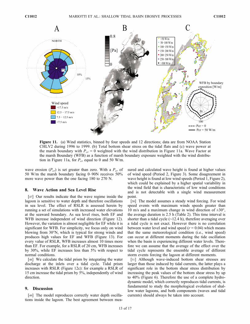
wave erosion (Pcr) is set greater than zero. With a Pcr of50 W/m the marsh boundary facing 0–90N receives 50%more wave power than the one facing 180 to 270 N.

8. Wave Action and Sea Level Rise

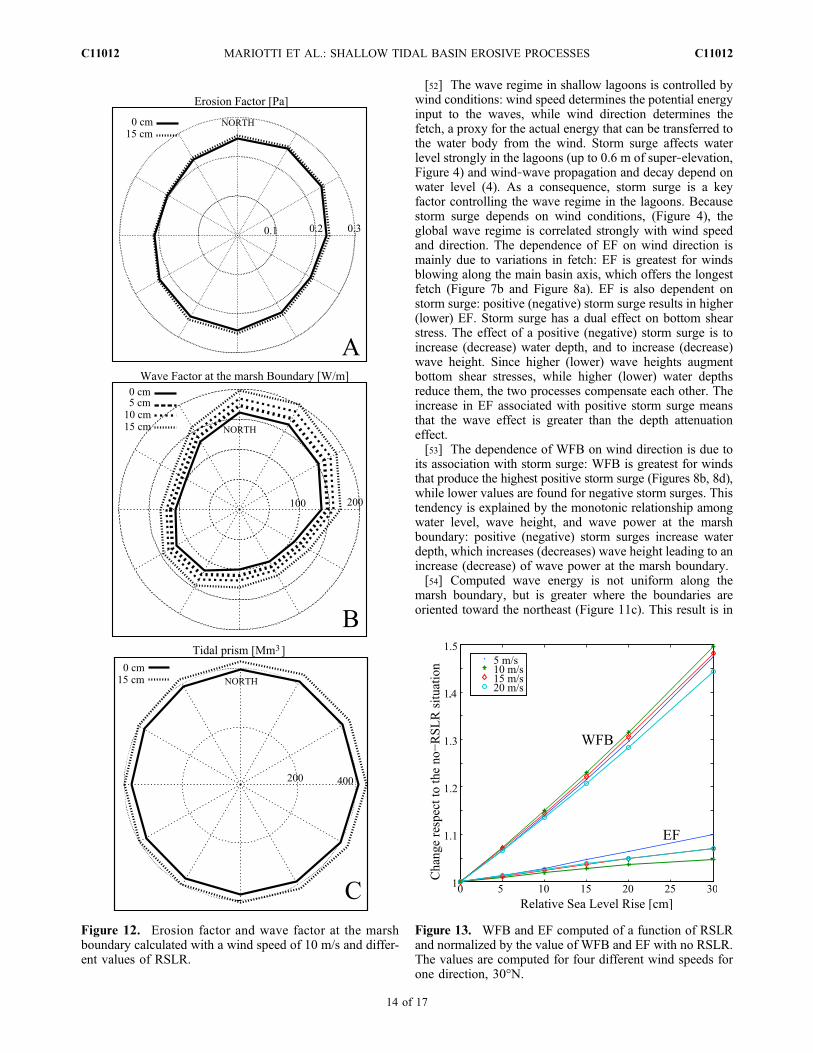
[47] Our results indicate that the wave regime inside thelagoon is sensitive to water depth and therefore oscillationsin sea level. The effect of RSLR is assessed herein byrunning a set of simulations with increased water elevationsat the seaward boundary. As sea level rises, both EF andWFB increase independent of wind direction (Figure 12).However, the variation is almost negligible for EF while it issignificant for WFB. For simplicity, we focus only on windblowing from 30°N, which is typical for strong winds andproduces high values for EF and WFB (Figure 13). Forevery value of RSLR, WFB increases almost 10 times morethan EF. For example, for a RSLR of 20 cm, WFB increasesby 30%, while EF increases less than 5% with respect tonormal conditions.[48] We calculate the tidal prism by integrating the water

discharge at the inlets over a tidal cycle. Tidal prismincreases with RSLR (Figure 12c): for example a RSLR of15 cm increase the tidal prism by 5%, independently of winddirection.

9. Discussion

[49] The model reproduces correctly water depth oscilla-tions inside the lagoon. The best agreement between mea-

sured and calculated wave height is found at higher valuesof wind speed (Period 2, Figure 3). Some disagreement inwave height is found at low wind speeds (Period 1, Figure 2),which could be explained by a higher spatial variability inthe wind field that is characteristic of low wind conditionsand is not detectable with a single wind measurementpoint.[50] The model assumes a steady wind forcing. For wind

speed events with maximum winds speeds greater than10 m/s and a maximum change in wind direction of ±30°,the average duration is 2.5 h (Table 2). This time interval isshorter than a tidal cycle (∼12.4 h), therefore averaging overa tidal cycle is not exact. However there is no correlationbetween water level and wind speed (r = 0.04) which meansthat the same meteorological condition (i.e., wind speed)can occur at different moments during the tide oscillationwhen the basin is experiencing different water levels. There-fore we can assume that the average of the effect over thetidal cycle represents the ensemble average of differentstorm events forcing the lagoon at different moments.[51] Although wave‐induced bottom shear stresses are

larger than those induced by tidal currents, the latter plays asignificant role in the bottom shear stress distribution byincreasing the peak values of the bottom shear stress by upto 40% (Figure 6). Therefore the use of a complete hydro-dynamic model, which correctly reproduces tidal currents, isfundamental to study the morphological evolution of shal-low water lagoons, and both components (waves and tidalcurrents) should always be taken into account.

Figure 11. (a) Wind statistics, binned by four speeds and 12 directions; data are from NOAA StationCHLV2 during 1996 to 1999. (b) Total bottom shear stress on the tidal flats and (c) wave power atthe marsh boundary with Pcr = 0 weighted with the wind distribution in Figure 11a. Wave Factor atthe marsh Boundary (WFB) as a function of marsh boundary exposure weighted with the wind distribu-tion in Figure 11a, for Pcr equal to 0 and 50 W/m.

MARIOTTI ET AL.: SHALLOW TIDAL BASIN EROSIVE PROCESSES C11012C11012

13 of 17

[52] The wave regime in shallow lagoons is controlled bywind conditions: wind speed determines the potential energyinput to the waves, while wind direction determines thefetch, a proxy for the actual energy that can be transferred tothe water body from the wind. Storm surge affects waterlevel strongly in the lagoons (up to 0.6 m of super‐elevation,Figure 4) and wind‐wave propagation and decay depend onwater level (4). As a consequence, storm surge is a keyfactor controlling the wave regime in the lagoons. Becausestorm surge depends on wind conditions, (Figure 4), theglobal wave regime is correlated strongly with wind speedand direction. The dependence of EF on wind direction ismainly due to variations in fetch: EF is greatest for windsblowing along the main basin axis, which offers the longestfetch (Figure 7b and Figure 8a). EF is also dependent onstorm surge: positive (negative) storm surge results in higher(lower) EF. Storm surge has a dual effect on bottom shearstress. The effect of a positive (negative) storm surge is toincrease (decrease) water depth, and to increase (decrease)wave height. Since higher (lower) wave heights augmentbottom shear stresses, while higher (lower) water depthsreduce them, the two processes compensate each other. Theincrease in EF associated with positive storm surge meansthat the wave effect is greater than the depth attenuationeffect.[53] The dependence of WFB on wind direction is due to

its association with storm surge: WFB is greatest for windsthat produce the highest positive storm surge (Figures 8b, 8d),while lower values are found for negative storm surges. Thistendency is explained by the monotonic relationship amongwater level, wave height, and wave power at the marshboundary: positive (negative) storm surges increase waterdepth, which increases (decreases) wave height leading to anincrease (decrease) of wave power at the marsh boundary.[54] Computed wave energy is not uniform along the

marsh boundary, but is greater where the boundaries areoriented toward the northeast (Figure 11c). This result is in

Figure 12. Erosion factor and wave factor at the marshboundary calculated with a wind speed of 10 m/s and differ-ent values of RSLR.

Figure 13. WFB and EF computed of a function of RSLRand normalized by the value of WFB and EF with no RSLR.The values are computed for four different wind speeds forone direction, 30°N.

MARIOTTI ET AL.: SHALLOW TIDAL BASIN EROSIVE PROCESSES C11012C11012

14 of 17

accordance with the distribution of WFB, which is maximalfor wind blowing from NE (Figure 8b). This means thateven if statistically there are two dominant winds blowingfrom opposite directions (Figure 11a), the winds blowingfrom NE are predominant in determining the wave power atthe marsh boundary. This distribution could induce anasymmetry in the marsh boundary erosion: assuming aconstant erodibility over the whole marsh boundary, ahigher erosion rate is expected on marsh boundaries thatface the northeast. On the other hand, spatial variability inmarsh erodibility, due to intrinsic differences in geotechnicalproperties as grain composition, compaction and vegetation,could induce a different trend in marsh boundary erosion.For example, marshes near barrier islands are likely to havea higher fraction of sand with respect to inner lagoon saltmarshes. Further work will be done analyzing marsh char-acteristics and erosion rates at different sites.[55] The asymmetry in WFB is caused mainly by the

asymmetry in storm surge (which is correlated with windspeed and direction, Figure 4), rather than an asymmetry inbasin geometry. Since storm surge is driven in part byregional upwelling/downwelling (e.g., Ekman transport),and not related specifically with this location, it is probablethat other basins would experience the same asymmetry onWFB.[56] EF is more uniform across the basin than is WFB,

with slightly higher values of EF far from the marshboundaries than closer to them.[57] The effect of RSLR is to increase both EF and WFB

(Figure 12), however the response of WFB is about 10 timesgreater than that of EF (Figure 13). The relationship amongRSLR, water depth, wave height, WFB, and EF is analogousto the case of storm surge. WFB increases monotically withwave height, which is enhanced by the greater water depthinduced by RSLR. EF is affected positively by the increasein wave height, but negatively by the increase in waterdepth.[58] This dual behavior could affect the geomorphological

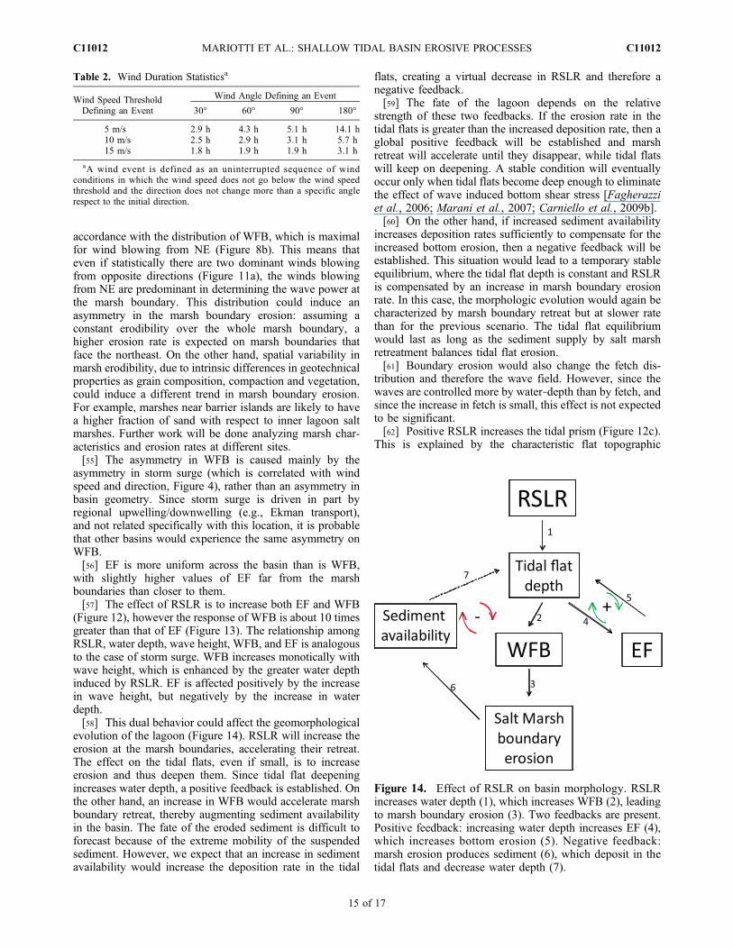
evolution of the lagoon (Figure 14). RSLR will increase theerosion at the marsh boundaries, accelerating their retreat.The effect on the tidal flats, even if small, is to increaseerosion and thus deepen them. Since tidal flat deepeningincreases water depth, a positive feedback is established. Onthe other hand, an increase in WFB would accelerate marshboundary retreat, thereby augmenting sediment availabilityin the basin. The fate of the eroded sediment is difficult toforecast because of the extreme mobility of the suspendedsediment. However, we expect that an increase in sedimentavailability would increase the deposition rate in the tidal

flats, creating a virtual decrease in RSLR and therefore anegative feedback.[59] The fate of the lagoon depends on the relative

strength of these two feedbacks. If the erosion rate in thetidal flats is greater than the increased deposition rate, then aglobal positive feedback will be established and marshretreat will accelerate until they disappear, while tidal flatswill keep on deepening. A stable condition will eventuallyoccur only when tidal flats become deep enough to eliminatethe effect of wave induced bottom shear stress [Fagherazziet al., 2006; Marani et al., 2007; Carniello et al., 2009b].[60] On the other hand, if increased sediment availability

increases deposition rates sufficiently to compensate for theincreased bottom erosion, then a negative feedback will beestablished. This situation would lead to a temporary stableequilibrium, where the tidal flat depth is constant and RSLRis compensated by an increase in marsh boundary erosionrate. In this case, the morphologic evolution would again becharacterized by marsh boundary retreat but at slower ratethan for the previous scenario. The tidal flat equilibriumwould last as long as the sediment supply by salt marshretreatment balances tidal flat erosion.[61] Boundary erosion would also change the fetch dis-

tribution and therefore the wave field. However, since thewaves are controlled more by water‐depth than by fetch, andsince the increase in fetch is small, this effect is not expectedto be significant.[62] Positive RSLR increases the tidal prism (Figure 12c).

This is explained by the characteristic flat topographic

Table 2. Wind Duration Statisticsa

Wind Speed ThresholdDefining an Event

Wind Angle Defining an Event

30° 60° 90° 180°

5 m/s 2.9 h 4.3 h 5.1 h 14.1 h10 m/s 2.5 h 2.9 h 3.1 h 5.7 h15 m/s 1.8 h 1.9 h 1.9 h 3.1 h

aA wind event is defined as an uninterrupted sequence of windconditions in which the wind speed does not go below the wind speedthreshold and the direction does not change more than a specific anglerespect to the initial direction.

Figure 14. Effect of RSLR on basin morphology. RSLRincreases water depth (1), which increases WFB (2), leadingto marsh boundary erosion (3). Two feedbacks are present.Positive feedback: increasing water depth increases EF (4),which increases bottom erosion (5). Negative feedback:marsh erosion produces sediment (6), which deposit in thetidal flats and decrease water depth (7).

MARIOTTI ET AL.: SHALLOW TIDAL BASIN EROSIVE PROCESSES C11012C11012

15 of 17

profile of salt marshes: when they become flooded, a sig-nificant volume of water is added to the tidal prism. Theenlarging of tidal prism by RSLR is in accordance withother studies [Mota Oliveira, 1970; O’Brien, 1969]. In largeestuaries, where hydrodynamics are controlled stronglyby river discharge, an increase in water depth (by RSLR)results in lower currents [Meade, 1969], with a consequentreduction in sediment export and an increase in sedimenta-tion, which compensate for the RSLR. In contrast, in shal-low tidal bays lacking a significant source of freshwater andsediment, like the VCR lagoons, an increase in tidal prismwill strengthen the tidal currents and enlarge the size of thetidal inlet [Jarrett, 1976; D’Alpaos et al., 2010].[63] In the VCR offshore sources of sediment are small

[Boon and Byrne, 1981; Nichols and Boon, 1994] from riverdischarge and associated sediment loads [Robinson, 1994;Nichols and Boon, 1994; Boynton et al., 1996]. Sedimentcontributions from marsh erosion are larger, but still rela-tively small [Boon and Byrne, 1981; Nichols and Boon,1994]: most of the sediment erosion, deposition and trans-port within the lagoons is associated with sediment redis-tribution. EF shows a little difference between flood and ebb(around few percent, result not reported), so sediment re-suspension inside the lagoon will not differ significantlyfrom flood to ebb. Given these conditions, an increase in thevolume of water exchanged with the sea will increase sed-iment export. In addition, the increase in the tidal prism willincrease the ebb‐tidal delta volume [Walton and Adams,1976], and remove sand from the lagoons system[FitzGerald et al., 2006]. Therefore RSLR, through tidalprism increase, will enhance sediment export, which willadd to the increase erosion of the tidal flat and marshboundary.

10. Conclusions

[64] We applied the numerical hydrodynamic modelWWTM to the lagoons of the Virginia Coast Reserve andwe tested it with measured water levels and wave heightsand periods. We used the model to forecast wave actionwithin the lagoons for varying wind conditions and RSLRand drew the following conclusions:[65] 1. For each wind speed, the total bottom shear stress

over the tidal flats is driven by fetch, while the wave powerat the marsh boundary is controlled by water depth. Stormsurge, by increasing water level inside the lagoons, plays afundamental role in the marsh boundary erosion.[66] 2. The expected wave power at the marsh boundary is

greatest at the boundaries exposed toward the NE. Non-uniform marsh boundary erosion is therefore predicted inthe lagoon system.[67] 3. The effect of RSLR is to increase both tidal flat

erosion (EF) and salt marsh boundary erosion (WFB).However, the relative increase in the latter is almost tentimes greater than the former.[68] 4. A positive feedback is expected between RSLR

and lagoon bottom erosion because of the increase of EF,while a negative feedback is expected between RSLR andlagoon bottom erosion as a consequence of the sedimentprovided by marsh boundary deterioration. If the globalfeedback is positive, then salt marsh edges are eroded andtidal flats deepen in the basin. If the global feedback is

negative, then the tidal flats find a temporary equilibriumstate with RSLR thanks to the sediment supply from themarsh boundary erosion.

[69] Acknowledgments. This research was supported by the Depart-ment of Energy NICCR program award TUL‐538‐06/07, by NSF throughthe VCR‐LTER program award GA10618‐127104, and by the Office ofNaval Research award N00014‐07‐1‐0664.

ReferencesAllen, J., P. Somerfield, and F. Gilbert (2007), Quantifying uncertainty inhigh‐resolution coupled hydrodynamic‐ecosystem models, J. Mar. Syst.,64(1–4), 3–14.

Boon, J. D. (2004), Secrets of the Tide: Tide and Tidal Current Anal-ysis and Applications, Storm Surges and Sea Level Trends, 210 pp.,Horwood, Chichester, U. K.

Boon, J. D., and R. J. Byrne (1981), On basin hypsometry and the morpho-dynamic response of coastal inlet systems, Mar. Geol., 40, 27–48.

Boynton, W. R., J. D. Hagy, L. Murray, C. Stokes, and W. M. Kemp(1996), A comparative analysis of eutrophication patterns in a temperatecoastal lagoon, Estuaries, 19, 408–421.

Breugem, W. A., and L. H. Holthuijsen (2007), Generalized shallow waterwave growth from Lake George, J. Waterw. Port Coastal Ocean Eng.,133(3), 173–182.

Cappucci, S., C. L. Amos, T. Hosoe, and G. Umgiesser (2004), SLIM: Anumerical model to evaluate the factors controlling the evolution of inter-tidal mudflats in Venice lagoon, Italy, J. Mar. Syst., 51, 257–280.

Carniello, L., A. Defina, S. Fagherazzi, and L. D’Alpaos (2005), A com-bined wind wave‐tidal model for the Venice lagoon, Italy, J. Geophys.Res., 110, F04007, doi:10.1029/2004JF000232.

Carniello, L., A. D’Alpaos, and A. Defina (2009a), Simulation of windwaves in shallow microtidal basins: Application to the Venice lagoon,Italy, in Proceedings of 6th IAHR Symposium on River, Coastal andEstuarine Morphodynamics: RCEM 2009, edited by C. A. Vionnetet al., pp. 907–912, Taylor Francis, London.

Carniello, L., A. Defina, and L. D’Alpaos (2009b), Morphological evolu-tion of the Venice Lagoon: Evidence from the past and trend for thefuture, J. Geophys. Res., 114, F04002, doi:10.1029/2008JF001157.

Christie, M. C., and K. R. Dyer (1998), Measurements of the turbid edgeover the Skeffling mudflats, in Sedimentary Processes in the IntertidalZone, Geol. Soc. Spec. Publ., vol. 139, edited by K. S. Black, D. M.Paterson, and A. Cramp, pp. 45–55, Geol. Soc. of London, London.

D’Alpaos, A., S. Lanzoni, M. Marani, and A. Rinaldo (2010), On the tidalprism–channel area relations, J. Geophys. Res., 115 , F01003,doi:10.1029/2008JF001243.

D’Alpaos, L., and A. Defina (2007), Mathematical modeling of tidal hydro-dynamics in shallow lagoons: A review of open issues and applications tothe Venice lagoon, Comput. Geosci., 33, 476–496, doi:10.1016/j.cageo.2006.07.009.

Defina, A. (2000), Two‐dimensional shallow water equations for partiallydry areas, Water Resour. Res., 36, 3251–3264.

Defina, A., L. Carniello, S. Fagherazzi, and L. D’Alpaos (2007), Self orga-nization of shallow basins in tidal flats and salt marshes, J. Geophys.Res., 112, F03001, doi:10.1029/2006JF000550.

Emory, K. O., and D. G. Aubrey (1991), Sea Levels, Land Levels and TideGauges, Springer, New York.

Fagherazzi, S., and P. L. Wiberg (2009), Importance of wind conditions,fetch, and water levels on wave generated shear stresses in a shallowintertidal basin, J. Geophys. Res., 114, F03022, doi:10.1029/2008JF001139.

Fagherazzi, S., L. Carniello, L. D’Alpaos, and A. Defina (2006), Criticalbifurcation of shallow microtidal landforms in tidal flats and saltmarshes, Proc. Natl. Acad. Sci. U. S. A., 103(22), 8337–8341.

Fagherazzi, S., C. Palermo, M. C. Rulli, L. Carniello, and A. Defina (2007),Wind waves in shallow microtidal basins and the dynamic equilibrium oftidal flats, J. Geophys. Res., 112, F02024, doi:10.1029/2006JF000572.

FitzGerald, D. M., I. V. Buynevich, and B. A. Argow (2006), Model oftidal inlet and barrier island dynamics in a regime of accelerated sea‐levelrise, J. Coastal Res., 39, 789–795.

Fredsoe, J., and R. Deigaard (1993),Mechanics of Coastal Sediment Trans-port, Adv. Ser. Ocean Eng., vol. 3, 392 pp., World Sci., Singapore.

Hayden, B. P., C. F. V. M. Santos, G. Shao, and R. C. Kochel (1995), Geo-morphological controls on coastal vegetation at the Virginia CoastReserve, Geomorphology, 13(1–4), 283–300, doi:10.1016/0169-555X(95)00032-Z.

MARIOTTI ET AL.: SHALLOW TIDAL BASIN EROSIVE PROCESSES C11012C11012

16 of 17

Holthuijsen, L. H., N. Booij, and T. H. C. Herbers (1989), A predictionmodel for stationary, short‐crested waves in shallow water with ambientcurrents, Coastal Eng., 13, 23–54.

Jarrett, J. T. (1976), Tidal prism—Inlet area relationships, Gen. Invest.Tidal Inlets Rep. 3, 32 pp., U.S. Army of Corps of Eng., Washington,D. C.

Kamphuis, J. W. (1975), Friction factor under oscillatory waves, J. Waterw.Harbors Coastal Eng. Div. Am. Soc. Civ. Eng., 101, 135–144.

Lawson, S. E. (2004), Sediment suspension as a control on light availabilityin a coastal lagoon, M.S. thesis, 119 pp., Univ. of Va., Charlottesville,Va.

Lawson, S. E. (2008), Physical and biological controls on sediment andnutrient fluxes in a temperate lagoon, Ph.D. dissertation, 187 pp., Univ.of Va., Charlottesville, Va.

Lawson, S. E., P. L. Wiberg, K. J. McGlathery, and D. C. Fugate (2007),Wind‐driven sediment suspension controls light availability in a shallowcoastal lagoon, Estuaries Coasts, 30(1), 102–112.

Le Hir, P., W. Roberts, O. Cazaillet, M. Christie, P. Bassoullet, andC. Bacher (2000), Characterization of intertidal flat hydrodynamics,Cont. Shelf Res., 20(12–13), 1433–1459.

Marani, M., A. D’Alpaos, S. Lanzoni, L. Carniello, and A. Rinaldo (2007),Biologically‐controlled multiple equilibria of tidal landforms and the fateof the Venice lagoon, Geophys. Res. Lett., 34, L11402, doi:10.1029/2007GL030178.

Mariotti, G., and S. Fagherazzi (2010), A numerical model for the coupledlong‐term evolution of salt marshes and tidal flats, J. Geophys. Res., 115,F01004, doi:10.1029/2009JF001326.

Meade, R. H. (1969), Landward transport of bottom sediment in estuariesof the Atlantic coastal plain, J. Sediment Petrol., 39, 222–234.

Moeller, I., T. Spencer, and J. R. French (1996), Wave attenuation oversaltmarsh surfaces: Preliminary results from Norfolk, England, J. CoastalRes., 12(4), 1009–1016.

Möller, I., T. Spencer, J. R. French, D. J. Leggett, and M. Dixon (1999),Wave transformation over salt marshes: A field and numerical modellingstudy from north Norfolk, England, Estuarine Coastal Shelf Sci., 49(3),411–426.

Mota Oliveira, I. B. (1970), Natural flushing ability in tidal inlets, paperpresented at 12th Coastal Engineering Conference, Am. Soc. of Civ.Eng., Washington, D. C.

Nerem, R., T. van Dam, and M. Schenewerk (1998), Chesapeake Bay sub-sidence monitored as wetland loss continues, Eos Trans. AGU, 79, 149.

Nichols, M. M., and J. D. Boon (1994), Sediment transport processes incoastal lagoons, in Coastal Lagoon Processes, edited by B. Kjerfve,pp. 157–217, Elsevier, New York.

O’Brien, M. P. (1969), Equilibrium flow areas of inlets on sandy coasts,J. Waterw. Harbors Coastal Eng. Div. Am. Soc. Civ. Eng., 95, 43–55.

Oertel, G. F. (2001), Hypsographic, hydro‐hypsographic and hydrologicalanalysis of coastal bay environments, Great Machipongo Bay, Virginia,J. Coastal Res., 17(4), 775–783.

Oertel, G. F., G. T. F. Wong, and J. D. Conway (1989), Sediment accumu-lation at a fringe marsh during transgression, Oyster, Virginia, Estuaries,12, 18–26.

Press, W. H., S. A. Teukolsky, W. T. Vetterling, and B. P. Flannery(1992), Numerical Recipes, 2nd ed., Cambridge Univ. Press, Cambridge,U. K.

Robinson, S. E. (1994), Clay mineralogy and sediment texture of environ-ments in a barrier island‐lagoon system, M.S. thesis, 102 pp., Univ. ofVa., Charlottesville, Va.

Schwimmer, R. A. (2001), Rates and processes of marsh shoreline erosionin Rehoboth Bay, Delaware, U.S.A., J. Coastal Res., 17(3), 672–683.

Schwimmer, R. A., and J. E. Pizzuto (2000), A model for the evolution ofmarsh shorelines, J. Sediment. Res., 70(5), 1026–1035.

Soulsby, R. L. (1995), Bed shear‐stresses due to combined waves and cur-rents, in Advances in Coastal Morphodynamics, edited by M. J. F. Stiveet al., pp. 4‐20–4‐23, Delft Hydraul., Delft, Netherlands.

Soulsby, R. L. (1997), Dynamics of Marine Sands: A Manual for PracticalApplications, 248 pp., Thomas Telford, London.

Tilburg, C. E., and R. W. Garvine (2004), A simple model for coastal sealevel prediction, Weather Forecasting, 19(3), 511–519.

Umgiesser, G., D. M. Canu, A. Cucco, and C. Solidoro (2004), A finite ele-ment model for the Venice Lagoon: Development, set up, calibration andval idation, J. Mar. Syst . , 51 (1–4), 123–145, doi:10.1016/j .jmarsys.2004.05.009.

U.S. Army Coastal Engineering Research Center (1984), Shore ProtectionManual, Washington, D. C.

Walton, T. L., and W. D. Adams (1976), Capacity of inlet outer bars tostore sand, paper presented at Fifteenth Coastal Engineering Conference,Am. Soc. of Civ. Eng., Honolulu, 11–17 Jul.

Whitehouse, R. J. S., and H. J. Mitchener (1998), Observations of themorphodynamic behaviour of an intertidal mudflat at different time-scales, in Sedimentary Processes in the Intertidal Zone, Geol. Soc. Spec.Publ., vol. 139, edited by K. S. Black, D. M. Paterson, and A. Cramp,pp. 45–55, Geol. Soc. of London, London.

Young, I. R., and L. A. Verhagen (1996), The growth of fetch‐limitedwaves in water of finite depth. Part 1: Total energy and peak frequency,Coastal Eng., 29(1–2), 47–78.

L. Carniello and A. Defina, Department IMAGE, University of Padova,Via Loredan 20, I‐35131 Padova, Italy.S. Fagherazzi and G. Mariotti, Department of Earth Sciences, Boston

University, 675 Commonwealth Ave., Boston, MA 02215, USA.(giuliom@bu.edu)K. J. McGlathery and P. L. Wiberg, Department of Environmental

Sciences, University of Virginia, Clark Hall, 291 McCormick Rd.,PO Box 400123, Charlottesville, VA 22904‐4123, USA.

MARIOTTI ET AL.: SHALLOW TIDAL BASIN EROSIVE PROCESSES C11012C11012

17 of 17