index number concepts, measures and decompositions of

Journal of Productivity Analysis, 19, 127–159, 2003©C 2003 Kluwer Academic Publishers. Manufactured in The Netherlands.

Index Number Concepts, Measuresand Decompositions of Productivity Growth

W. ERWIN DIEWERT [email protected] of Economics, University of British Columbia, 1873 East Mall, Buchanan Tower, room 997, Vancouver,BC V6T 1Z1

ALICE O. NAKAMURA∗ [email protected] of Business, University of Alberta, 3-23 Business Building, Edmonton, Alberta T6G 2R6

Abstract

This paper explores the definitions and properties of total factor productivity growth (TFPG)indexes, focusing especially on the Paasche, Laspeyres, Fisher, Tornqvist, and implicitTornqvist ones. These indexes can be evaluated from observable price and quantity data,and certain of these are shown to be measures of TFPG concepts and theoretical indexesthat have been proposed in the literature. The mathematical relationships between theseand quantity aggregates, financial measures, and price and quantity indexes are explored.Decompositions of the productivity growth indexes are also given. The paper concludeswith a brief overview of some limitations on our analysis.

JEL classification: O3, O30; O4, O4.7; M11

Keywords: index numbers, productivity, TFP, TFPG, technical change

“Productivity A ratio of output to input.”(Atkinson, Banker, Kaplan and Young, 1995, Management Accounting, p. 514)

“To profit from productivity improvement, management needs measurement procedures formonitoring productivity performance and identifying improvement opportunities.”

(David M. Miller, Harvard Business Review, May–June 1984, pp. 145–153)

This paper presents and considers a number of conceptual definitions of productivity growth,and measures and decompositions of these that are useful not only for economic analystsand those involved in the construction of official statistics but also for business managers.

Section 1 introduces four concepts and measures of total factor productivity growth(TFPG) for the simplistic case in which the index number problem is absent: the oneinput, one output case. In the 1-1 case, it is easily seen that the measures are all equal.

In the general N input, M output case, the quantities for the different inputs and outputsmust be aggregated and this leads to the use of index number formulas. If price weightsare used, then issues of price change must be dealt with too. In Section 2, we introduce

∗ Corresponding author.

128 DIEWERT AND NAKAMURA

the Paasche, Laspeyres, Fisher and Tornqvist TFPG formulas. We present these after firstdefining aggregates and quantity and price indexes that can be used to define the TFPGindex formulas. The measures of the four concepts of TFPG that are defined for a generalN input, M output production situation are shown to be equal for appropriate choices offunctional forms for aggregating the quantity or value and price data.

Section 3 gives a way of decomposing any TFPG index in terms of input-output coeffi-cients. The reciprocals of the input-output coefficients—the output-input coefficients—arethe most widely used type of single factor productivity measure for shop floor operationsmanagement. The decomposition presented provides a framework for examining the effectson overall TFPG of changes in specific single factor productivity coefficients.

Two main approaches to choosing among the different proposed functional forms for theTFPG index are the axiomatic (or test) approach reviewed briefly in Section 4, and the exactindex number approach introduced in Section 5 and then used in Section 6. The axiomaticapproach makes use of lists of desired properties, termed axioms or tests, that are formaliza-tions of common sense properties of good index numbers or generalizations of propertiesthat hold for all proposed index number formulas in the simplistic 1-1 case. The exact indexnumber approach is rooted in economic theory, and is sometimes referred to as an economicapproach. Section 7 is devoted to yet another measure of productivity performance proposedby Diewert and Morrison and decompositions of that measure. Section 8 concludes.

1. Four Concepts of TFPG

It is convenient to introduce concepts and notation in the simplified context of a one input,one output production process. For t = 0, 1, . . . , T, the quantity of the input used in period tis xt

1 with unit price wt1 and the quantity of the output produced is yt

1 with unit price pt1.

The basic definition of total factor productivity (TFP) is the rate of transformation of totalinput into total output. Engineers and others interested in physical efficiency often focus onthis transformation rate, which is measured by the ratio of output produced to input:

TFPt ≡ (yt

1

/xt

1

) ≡ at . (1)

The superscript on TFP indicating the time period will only be shown hereafter whenthis is not clear from the context. The parameter at defined along with TFP in (1) is anoutput-input coefficient. An output-input coefficient always involves just one output andone input, although coefficients of this sort are often defined and used in the context ofmultiple input, multiple output production situations.1 Indeed, we show a new way of doingthis in Section 3.

In this paper, we focus on total factor productivity growth rather than TFP.2 A numberof different ways have been proposed for conceptualizing TFPG, four of which are con-sidered in this paper.3 A first concept is simply the rate of growth for TFP. Measures ofthis first concept will be denoted by TFPG(1). For the 1-1 case, the growth in TFP be-tween periods s and t is measured by the ratio of the output-input coefficients for periods tand s:4

TFPG(1) ≡ (yt

1

/xt

1

)/(ys

1

/xs

1

) = at/as . (2)

INDEX NUMBER CONCEPTS, MEASURES AND DECOMPOSITIONS 129

A second concept of total factor productivity growth is the ratio of the rate of outputgrowth to input growth. For the 1-1 case, the natural measure for this is

TFPG(2) ≡ (yt

1

/ys

1

)/(xt

1

/xs

1

). (3)

The third and fourth concepts relate TFPG to the financial revenue and cost totals and tomargins. For the 1-1 case, total revenue and cost are given for t = 1, . . . , T by

Rt ≡ pt1 yt

1 and Ct ≡ wt1xt

1. (4)

Dividing the revenue ratio for periods t and s by the output price ratio for the two periodsyields

(Rt/Rs)/(pt/ps) = (pt

1 yt1

/ps

1 ys1

)/(pt

1

/ps

1

) = yt1

/ys

1. (5)

Similarly, when the cost ratio for periods t and s is divided by the input price ratio, we get

(Ct/Cs)/(wt/ws) = (wt

1xt1

/ws

1xs1

)/(wt

1

/ws

1

) = xt1

/xs

1. (6)

The third concept is the growth rate for real revenue versus real cost. For the 1-1 case,this is measured by the rate of growth in the ratio of revenue to cost controlling for pricechange:

TFPG(3) ≡[

Rt/Rs

pt1

/ps

1

]/[Ct/Cs

wt1

/ws

1

]=

(yt

1

ys1

)/(xt

1

xs1

). (7)

Business managers are interested in ensuring that revenues exceed costs, which leads toan interest in margins. The period t margin, mt , can be measured by

1 + mt ≡ Rt/Ct , (8)

and the measure for margin growth controlling for price change is defined for the 1-1 caseas

TFPG(4) ≡ [(1 + mt )/(1 + ms)][(

wt1

/ws

1

)/(pt

1

/ps

1

)]. (9)

If we interpret the margin as a reward for managerial or entrepreneurial input, then TFPG(4)can be interpreted as the growth rate of the price of the inputs broadly defined so as to includemanagerial and entrepreneurial input divided by the growth rate of the price of the outputgood.

Using (8) to eliminate the margin growth rate on the right-hand side of (9) and comparingthis with the expressions in (2), (3) and (7), we see that in the 1-1 case, the measures forthe four concepts of total factor productivity growth are all equal.

2. The N-M Case

Most real production processes yield multiple outputs and virtually all use multiple inputs,leading to a need for index numbers to aggregate these outputs and inputs. We begin by


defining quantity aggregates that are components of the Paasche, Laspeyres and Fisher Idealquantity, price and TFPG indexes, and then give the formulas for these indexes. Tornqvistand implicit Tornqvist index numbers are also defined.

2.1. Price Weighted Quantity Aggregates

For a general N -input, M-output production process, the period t input and output price vec-tors are denoted by wt ≡ [wt

1, . . . , wtN ] and pt≡ [pt

1, pt2, . . . , pt

M ], while xt≡ [xt1, . . . , xt

N ]and yt ≡ [yt

1, . . . , ytM ] denote the period t input and output quantity vectors.

Nominal total cost Ct and revenue Rt can be viewed as price weighted quantity aggregatesof the micro level data for the individual transactions, and are defined as follows for periods tand s:

Ct ≡N∑

n=1

wtn xt

n, Rt ≡M∑

m=1

ptm yt

m, (10)

Cs ≡N∑

n=1

wsn xs

n and Rs ≡M∑

m=1

psm ys

m . (11)

We also define four hypothetical quantity aggregates.5 The first two result from evaluatingperiod t quantities using period s price weights:

N∑n=1

wsn xt

n andM∑

m=1

psm yt

m (12)

These aggregates are what the cost and revenue would have been if the period t inputshad been purchased and the period t outputs had been sold at period s prices. In contrast,the third and fourth aggregates are sums of period s quantities evaluated using period tprices:

N∑n=1

wtn xs

n andM∑

m=1

ptm ys

m . (13)

These are what the cost and revenue would have been if the period s inputs had beenpurchased and the period s outputs had been sold at period t prices.

The eight aggregates given in (10) through (13) are all that are needed to define thePaasche, Laspeyres and Fisher quantity, price, and TFPG indexes. Traditionally these weredefined as weighted averages of quantity and price relatives.6 The equivalent definitionspresented here are more convenient for establishing that each of these TFPG indexes is ameasure of all four of the different concepts of TFPG introduced in Section 1.


2.2. The Paasche, Laspeyres and Fisher Quantity and Price Indexes

The Paasche (1874), Laspeyres (1871), and Fisher (1922, p. 234) output quantity indexescan be defined as follows using the quantity aggregates given in (10)–(13):

Q P ≡M∑

i=1

pti yt

i

/M∑

j=1

ptj ys

j , (14)

QL ≡M∑

i=1

psi yt

i

/M∑

j=1

psj ys

j , (15)

and

QF ≡ (Q P QL)(1/2). (16)

Similarly, the Paasche, Laspeyres and Fisher input quantity indexes can be defined as:

Q∗P ≡

N∑i=1

wti x t

i

/N∑

j=1

wtj x

sj , (17)

Q∗L ≡

N∑i=1

wsi x t

i

/N∑

j=1

wsj x

sj , (18)

and

Q∗F ≡ (Q∗

P Q∗L)(1/2). (19)

Output and input quantity indexes are all that are needed to define a measure of the secondconcept of TFPG since an output quantity index is a measure of growth for total output andan input quantity index is a measure of growth for total input. For the Paasche, Laspeyresand Fisher indexes, we show in Section 2.3 that a measure of the first concept of TFPGcan be defined by rearranging the aggregates defining the measure of the second concept.However, in order to specify measures of the third and fourth concepts for the multipleinput, multiple output case, price indexes are needed too.

Price indexes can be constructed with any of the functional forms used for quantity indexesby reversing the roles of the prices and quantities in the quantity index. Thus the Paascheand Laspeyres output and input price indexes can be defined as:

PP ≡M∑

i=1

pti yt

i

/M∑

j=1

psj yt

j , (20)

P∗P ≡

N∑i=1

wti x t

i

/N∑

j=1

wsj x

tj , (21)

PL ≡M∑

i=1

pti ys

i

/M∑

j=1

psj ys

j , (22)


and

P∗L ≡

N∑i=1

wti xs

i

/N∑

j=1

wsj x

sj . (23)

The Fisher output and input price indexes are given by

PF ≡ (PP PL)(1/2) (24)

and

P∗F ≡ (P∗

P P∗L )(1/2). (25)

A price index is the implicit counterpart of a quantity index if the product rule is satisfied.This rule requires that the product of the quantity and price indexes must equal the totalcost ratio for input side indexes or the total revenue ratio for output side indexes.7 Usuallythe implicit price index will not have the same functional form as the quantity index itis associated with. For example, the Paasche price index is the implicit counterpart ofa Laspeyres quantity index, and the Laspeyres price index is the implicit counterpart ofa Paasche quantity index. The Fisher indexes are unusual in that the Fisher price indexsatisfies the product test rule when paired with a Fisher quantity index.

In defining and proving equalities for the measures of the four concepts of TFPG for ageneral multiple input, multiple output production situation, we use the following implica-tions of the product rule: for the Paasche, Laspeyres and Fisher indexes, on the input sidewe have

Q∗P × P∗

L = Q∗L × P∗

P = Q∗F × P∗

F = Ct/Cs, (26a)

and on the output side we have

Q P × PL = QL × PP = QF × PF = Rt/Rs . (26b)

2.3. TFPG Measures for the N-M Case

The traditional definition of a total factor productivity growth index in the index numberliterature is as a ratio of output and input quantity indexes:

TFPG ≡ Q/Q∗. (27)

Thus the Paasche, Laspeyres and Fisher TFPG indexes can be defined using the Paasche,Laspeyres and Fisher quantity indexes. Given a choice of any one of these three functionalforms, we will prove that the corresponding multiple input, multiple output case measuresare all equal for the four concepts of TFPG introduced in Section 1.

To establish these equalities, we use the product rule results to define Paasche, Laspeyresand Fisher TFPG(3) measures. Then we use the definitions of the components of theTFPG(3) measures to define and establish the equality of TFPG(2) and TFPG(1) measures.


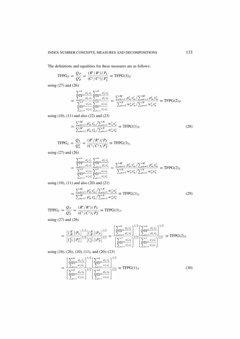
The definitions and equalities for these measures are as follows:

TFPGP = Q P

Q∗P

= (Rt/Rs)/PL

(Ct/Cs)/P∗L

≡ TFPG(3)P

using (27) and (26)

=

∑M

m=1pt

m ytm∑M

m=1ps

m ysm

∑M

m=1ps

m ysm∑M

m=1pt

m ysm∑N

n=1wt

n xtn∑N

n=1ws

n xsn

∑N

n=1ws

n xsn∑N

n=1wt

n xsn

=∑M

m=1 ptm yt

m

/∑Mm=1 pt

m ysm∑N

n=1 wtn xt

n

/∑Nn=1 wt

n xsn

≡ TFPG(2)P

using (10), (11) and also (22) and (23)

=∑M

m=1 ptm yt

m

/∑Nn=1 wt

n xtn∑M

m=1 ptm ys

m

/∑Nn=1 wt

n xsn

≡ TFPG(1)P (28)

TFPGL = QL

Q∗L

= (Rt/Rs)/PP

(Ct/Cs)/P∗P

≡ TFPG(3)L

using (27) and (26)

=

∑M

m=1pt

m ytm∑M

m=1ps

m ysm

∑M

m=1ps

m ytm∑M

m=1pt

m ytm∑N

n=1wt

n xtn∑N

n=1ws

n xsn

∑N

n=1ws

n xtn∑N

n=1wt

n xtn

=∑M

m=1 psm yt

m

/∑Mm=1 ps

m ysm∑N

n=1 wsn xt

n

/∑Nn=1 ws

n xsn

≡ TFPG(2)L

using (10), (11) and also (20) and (21)

=∑M

m=1 psm yt

m

/∑Nn=1 ws

n xtn∑M

m=1 psm ys

m

/∑Nn=1 ws

n xsn

≡ TFPG(1)L (29)

TFPGF = QF

Q∗F

= (Rt/Rs)/PF

(Ct/Cs)/P∗F

≡ TFPG(3)F

using (27) and (26)

=[(

Rt

Rs

)PL

]1/2[( Rt

Rs

)PP

]1/2

[(Ct

Cs

)P∗

L

]1/2[( Ct

Cs

)P∗

P

]1/2 =

[∑M

m=1pt

m ytm∑M

m=1pt

m ysm

]1/2[∑M

m=1ps

m ytm∑M

m=1ps

m ysm

]1/2

[∑N

n=1wt

n xtn∑N

n=1wt

n xsn

]1/2[∑N

n=1ws

n xtn∑N

n=1ws

n xsn

]1/2 ≡ TFPG(2)F

using (16), (26), (10), (11), and (20)–(23)

=

[∑M

m=1pt

m ytm∑N

n=1wt

n xtn

]1/2[∑M

m=1ps

m ytm∑N

n=1ws

n xtn

]1/2

[∑M

m=1pt

m ysm∑N

n=1wt

n xsn

]1/2[∑M

m=1pt

m ysm∑N

n=1wt

n xsn

]1/2 ≡ TFPG(1)F (30)


TFPG(4) is the rate of growth in the margin after controlling for price change. In thegeneral N -M case, just as in the 1-1 one, the margin mt is given for t = 0, 1, . . . , T by

1 + mt ≡ Rt/Ct . (31)

Depending on whether Laspeyres, Paasche or Fisher price indexes are used to deflate thecost and revenue components of the margin, the expressions for TFPG(3) given in (28),(29) and (30) can be rewritten as:

TFPG(4)P ≡ [(1 + mt )/(1 + ms)][P∗L /PL ], (32)

TFPG(4)L ≡ [(1 + mt )/(1 + ms)][P∗P/PP ], (33)

and

TFPG(4)F ≡ [(1 + mt )/(1 + ms)][P∗F/PF ]. (34)

Notice that if the margins mt are zero, regardless of the reasons, then each of these ex-pressions for TFPG(4) reduces to the ratio of the input price index to the output priceindex.8

2.4. Other Index Number Formulas

Many other index number formulas have been proposed besides the Paasche, Laspeyresand Fisher.9 Here we will use QG and PG and Q∗

G and P∗G to denote any given output and

input quantity and price indexes that satisfy the product rule so that QG PG = (Rt/Rs)

and Q∗G P∗

G = (Ct/Cs). From these product rule results and (31), it is easily seen that thefollowing measures of concepts 2, 3 and 4 of TFPG are equal:

(Rt/Rs)/PG

(Ct/Cs)/P∗G

≡ TFPG(3)G

= QG/Q∗G ≡ TFPG(2)G

= [(1 + mt )/(1 + ms)][P∗/P] ≡ TPFG(4). (35)

But what about TFPG(1)G? A measure of the growth in the rate of transformation of totalinput into total output ideally should be defined using measures of total output and totalinput that are comparable for periods s and t in the sense that the micro level quantities forboth periods are aggregated using the same price weights.10 The quantity aggregates thatare the components of the Paasche, Laspeyres and Fisher TFPG(1) measures defined in thefirst line of (28), (29) and (30) satisfy this comparability over time ideal.11 However, thereare many other index number formulas for which it is not possible to define this sort ofan ideal TFPG(1) measure that also equals the corresponding measures for the other threeconcepts of TFPG.

For any pair of quantity and price indexes satisfying the product test, from (35) and theproduct rule implications we see that the following expressions equal those defined in (35)


for TFPG(2)G, TFPG(3)G and TFPG(4)G :

QG

Q∗G

= (Rt/Rs)/P

(Ct/Cs)/P∗ =∑M

m=1

(pt

m

/PG

)yt

m

/∑Mm=1 ps

m ysm∑N

n=1

(wt

n

/P∗

G

)xt

n

/∑Nn=1 ws

n xsn

. (36)

In the last of these expressions, the price vectors (pt/PG) and (wt/P∗G) appearing in the

period t output and input quantity aggregates are the period t prices expressed in periods dollars. If we choose this expression as the measure of TFPG(1)G , then for any indexnumber formulas other than the Paasche, Laspeyres or Fisher, this measure will not be idealin the sense of using the same price weights to compare the period t and period s quantities.However, there is an approximate solution to this problem for indexes that satisfy the productrule and are also what is termed “superlative.” This approximate solution makes use of theFisher functional form: a functional form for which we have an ideal TFPG(1) measure,defined in (30).

Diewert coined the term superlative for an index number functional form that is “exact”in that it can be derived algebraically from a producer or consumer behavioral equation thatsatisfies the Diewert flexibility criterion. According to this criterion, an equation is flexible ifit can provide a second order approximation to an arbitrary twice continuously differentiablelinearly homogeneous function. Diewert (1976, 1978) and Hill (2000) established that allof the commonly used superlative index number formulas (including the Fisher, and alsothe Tornqvist and implicit Tornqvist functional forms introduced below) approximate eachother to the second order when evaluated at an equal price and quantity point. This is anumerical analysis approximation result that does not rely on any assumptions of economictheory.

Because the Fisher quantity and price indexes also satisfy the product rule, we haveQG PG = (Rt/Rs) = QF PF and Q∗

G P∗G = (Ct/Cs) = Q∗

F P∗F , and dividing through by

PG and P∗G , respectively, yields

QG

Q∗G

=[

QF

Q∗F

][PF/PG

P∗F/P∗

G

]. (37)

From (37), (35) and (30) we see that if we define the measure for the first concept of TFPGas

TPFG(1)G ≡ TPFG(1)F

[PF/PG

P∗F/P∗

G

], (38)

this measure will equal TFPG(2)G, TFPG(3)G and TFPG(4)G as defined in (35). However,this measure does not have the ideal comparability over time property. In this TFPG(1)G

measure, the period t price vectors, pt and wt , of the TFPG(1)F component are replacedby (pt/(PF/PG)) and (wt/(P∗

F/P∗G)). As a consequence, unless the given price indexes

are Laspeyres or Paasche or Fisher ones, the period t and period s quantities comparedby the measure will not be aggregated using the same price weights when there havebeen changes in relative prices. Nevertheless, from (38) and the Diewert (1976, 1978)/Hill(2000) approximation results for superlative index numbers, it follows that when the chosenquantity and price indexes are any of the commonly used superlative indexes such as theTornqvist or implicit Tornqvist, then we can use the result that TFPG(1)G

∼= TFPG(1)F .


2.5. The Tornqvist (or Translog) Indexes12

Tornqvist (1936) indexes are weighted geometric averages of growth rates for the micro-economic data (the quantity or price relatives). These indexes appear more complicatedthan the others defined so far, but are also widely used. It is the formula for the naturallogarithm of a Tornqvist index that is usually shown. For the output quantity index, this is

�n QT = (1/2)

M∑m=1

[(ps

m ysm

/M∑

i=1

psi ys

i

)+

(pt

m ytm

/M∑

j=1

ptj yt

j

)]�n

(yt

m

/ys

m

). (39)

The Tornqvist input quantity index Q∗T is defined analogously, with input quantities and

prices substituted for the output quantities and prices in (39).Reversing the role of the prices and quantities in the formula for the Tornqvist output

quantity index yields the Tornqvist output price index, PT , defined by

�n PT = (1/2)

M∑m=1

[(ps

m ysm

/M∑

i=1

psi ys

i

)+

(pt

m ytm

/M∑

j=1

ptj yt

j

)]�n

(pt

m

/ps

m

). (40)

The input price index P∗T is defined in a similar manner.

The implicit Tornqvist output quantity index, denoted by QT , is defined implicitly by13

(Rt/Rs)/PT ≡ QT , and the implicit Tornqvist input quantity index, Q ∗T

, is defined anal-ogously using the cost ratio and P∗

T . The implicit Tornqvist output price index, PT , isgiven by (Rt/Rs)/QT ≡ PT , and the implicit Tornqvist input price index, P ∗

T, is defined

analogously.Using the Tornqvist quantity and the implicit Tornqvist price indexes, or the implicit

Tornqvist quantity and the Tornqvist price indexes, measurement formulas for concepts2–4 of TFPG can be specified as in (35) above. As already noted, when Tornqvist or im-plicit Tornqvist indexes are used, it is not possible to define a TFPG(1) measure that is idealin the sense discussed in Section 2.4. However, these are superlative indexes for which theSection 2.4 approximation result applies; that is, we have TFPG(1)T

∼= TFPG(1)F andTFPG(1)T

∼= TFPG(1)F . The essence of this result is that the Fisher TFPG(1) measure,which is ideal in the sense discussed in Section 2.4, should be a good approximate measurefor the first concept of TFPG when the Tornqvist or the implicit Tornqvist indexes areselected.

3. An Input-Output Coefficient Decomposition of TFPG

“[I]t is our hypothesis that non-financial and financial control systems serve very differ-ent roles in organizations. The non-financial systems are used for day-to-day operationscontrol.”

(Armitage and Atkinson, 1990, The Choice of Productivity Measures inOrganizations: A Field Study of Practice, p. 141)

As Armitage and Atkinson report, business surveys reveal that single factor productivityand efficiency measures are widely used for operations monitoring. Thus, it is important to


relate the single factor measures to overall TFPG. Fortunately, the TFPG(3) form of a totalfactor productivity growth index can be conveniently decomposed in terms of input-outputcoefficients or their reciprocals.

As established in the previous section, any TFPG index can be expressed in the form

TFPG = [Rt/P]/[Ct/P∗]

Rs/Cs(41)

where P and P∗ are the implicit counterparts of Q and Q∗. For any given time period, theratio of total nominal revenue to total nominal cost can be rewritten as

Rt/Ct =M∑

m=1

[pt

m ytm

/ (N∑

n=1

wtn xt

n

)]

=M∑

m=1

[1

/ (N∑

n=1

wtn xt

n

/pt

m ytm

)]

=M∑

m=1

[N∑

n=1

(wt

n

/pt

m

)(xt

n/ytm

)]−1

. (42)

It is clear from (42) that, after controlling for price changes, improvements in any singlefactor efficiency measure, say (yt

m/xtn), contribute to an improved revenue cost ratio, as

might be expected.Substitution of (42) into (41) yields:

TFPG =∑M

m=1

{∑Nn=1

[(wt

n

/P∗)/(

ptm

/P

)][xt

n

/yt

m

]}−1

∑Mm=1

{ ∑Nn=1

[ws

n

/ps

m

][xs

n

/ys

m

]}−1 . (43)

This expression can be used to consider the relative effects on TFPG of alternative singlefactor productivity improvements, or of anticipated changes in any of the real price ratiosfor individual input/output combinations.

4. The Axiomatic (or Test) Approach to ChoosingAmong Alternative Index Number Formulas

Which functional form should be used for the price indexes in (41) or the quantity indexesin (27)? Historically, index number theorists have relied on what is called the axiomaticor test approach to address this choice problem. An overview of this approach is providedhere, concentrating on the output side quantity and price indexes since the approach is thesame on the input side.

As before, P denotes an output price index and Q denotes an output quantity index.The axiomatic approach to the determination of the functional forms for P and Q works

as follows. The starting point is a list of mathematical properties that the price index shouldsatisfy based on a priori reasoning. These are the index number theory ‘tests’ or ‘axioms.’Mathematical reasoning is applied to determine whether the a priori tests are mutuallyconsistent and whether they uniquely determine, or usefully narrow the range of choices


for, the functional form for the price index.14 The product test rule is then applied to solvefor the functional form of the quantity index.

As already noted in Section 2.2, on the output side the Product Test states that the productof the price and quantity indexes, P and Q, should equal the nominal revenue ratio forperiods t and s:15

PQ = Rt/Rs . (44)

If the functional form for the output price index P is given, then imposing the product rulemeans that the functional form for the output quantity index must be given by the expression

Q = (Rt/Rs)/P. (45)

If the product test is imposed as a rule on both the output and input sides, then once thefunctional forms have been specified for the price indexes, the functional forms have alsobeen determined for the quantity indexes and for the TFPG index.16

There are many other axiomatic tests that can be applied for choosing among the quantityand price index pairs that satisfy the product test. Since the indexes that make up these pairsare not determined independently, we only need consider axioms that apply to the priceindexes, with the process of selection being the same for input indexes as for the outputside ones considered here. We conclude this overview of the axiomatic approach by listingfour of these tests.

The Identity or Constant Prices Test is17

P(p, p, ys, yt ) = 1. (46)

What this means is that if ps = pt = p = (p1, . . . , pM) so that all prices are equal in the twoperiods, then the price index should be one regardless of the quantity values for periods sand t .

The Constant Basket Test, also called the Constant Quantities Test, is18

P(ps, pt , y, y) =N∑

i=1

pti yi

/N∑

j=1

psj y j . (47)

This test states that if the quantities are constant over the two periods s and t so thatys = yt = y ≡ (y1, . . . , yM), then the level of prices in period t compared to period sshould equal the value of the constant basket of quantities evaluated at the period t pricesdivided by the value of this same basket evaluated at the period s prices.

The Proportionality in Period t Prices Test is19

P(ps, λpt , ys, yt ) = λP(ps, pt , ys, yt ) for λ > 0. (48)

According to this test, if each of the elements of pt is multiplied by the positive constant λ,then the level of prices in period t relative to period s will differ by the same multiplicativefactor λ.

Our final example of a price index test is the Time Reversal Test:20

P(pt , ps, yt , ys) = 1/P(ps, pt , ys, yt ). (49)


If this test is satisfied, then when the prices and quantities for s and t are interchanged, theresulting price index will be the reciprocal of the original price index.

The Fisher price index PF satisfies all four of these additional tests. The Paasche andLaspeyres indexes, PP and PL , fail the time reversal test (49). The Tornqvist index, PT ,fails the constant basket test (47), and the implicit Tornqvist index, PT , fails the constantprices test (48). When a more extensive list of tests is compiled, the Fisher price indexcontinues to satisfy more tests than other leading candidates.21 However, the Paasche,Laspeyres, Tornqvist, and implicit Tornqvist indexes all show up quite well according tothe axiomatic approach.

5. The Exact Index Number Approach

An alternative approach to the determination of the functional form for a measure of to-tal factor productivity growth is to derive the index from a producer behavioral model.Diewert’s (1976) exact index number approach systematizes the procedures for develop-ing equivalencies between different proposed definitions for index numbers and optimizingmodels of economic behavior. Using these equivalencies, a choice can be made among alter-native productivity index number formulas based on the preferred properties for a specifiedbehavioral equation.

A firm’s technology can be summarized by its period t production function f t . Focusingon output 1, the period t production function can be represented for t = 0, 1, . . . , T as

y1 = f t (y2, y3, . . . , yM , x1, x2, . . . , xN ), (50)

which gives the amount of output 1 the firm can produce using the technology available inany given period t if it also produces y2 units of output 2, y3 units of output 3, . . . , and yM

units of output M using x1 units of input 1, x2 units of input 2, . . . , and xN units of input N .The production function f t can be used to define the period t cost function, ct , as follows:

ct (y1, y2, . . . , yM , w1, w2, . . . , w N )

≡ minx

{N∑

n=1

wn xn : y1 = f t (y2, . . . , yM , x1, . . . , xN )

}. (51)

This cost function gives the minimum cost of producing the outputs y1, . . . , yM using theperiod t technology and input prices. Under the assumption of cost minimizing behavior,the observed period t cost of production, Ct , is equal to the minimum cost. Hence fort = 0, 1, . . . , T , we have

Ct ≡N∑

n=1

wtn xt

n = ct(

yt1, . . . , yt

M , wt1, . . . , wt

N

). (52)

We need some way of relating the cost functions for periods t = 0, 1, . . . , T to eachother. A common way of doing this is to assume that

ct(

yt1, . . . , yt

M , wt1, . . . , wt

N

) = (1/at )c(

yt1, . . . , yt

M , wt1, . . . , wt

N

), (53)

where at > 0 denotes a period t relative efficiency parameter and c denotes an atemporal


cost function. The normalization a0 ≡ 1 is usually imposed. Given (53), a natural measureof productivity change for a productive unit in going from period s to t is the followingratio:

at/as . (54)

If this ratio is greater than 1, then efficiency is said to have improved.Taking the natural logarithm of both sides of (53), we have

�n ct(

yt1, . . . , yt

M , wt1, . . . , wt

N

) = −�n at + �n c(

yt1, . . . , yt

M , wt1, . . . , wt

N

). (55)

If a translog functional form is assumed for �n c, where c is the atemporal cost function onthe right hand side of (55), then we have

�n c(

yt1, . . . , yt

M , wt1, . . . , wt

N

)= b0 +

M∑m=1

bm �n ytm +

N∑n=1

cn �n wtn + (1/2)

M∑i=1

M∑j=1

dij �n yti �n yt

j

+ (1/2)

N∑i=1

N∑j=1

fij �n wti �n wt

j +M∑

m=1

N∑n=1

gmn �n ytm �n wt

n. (56)

An advantage of the translog functional form is that it does not impose a priori restrictionson the admissible patterns of substitution between inputs and outputs.22 However, thisspecification also has a large number of unknown parameters. There are M + 1 of the bm

parameters; N of the cn parameters; M(M +1)/2 independent dij parameters after imposingthe requirement that dij = dji for 1 ≤ i < j ≤ M ; N (N + 1)/2 independent fij parameterseven after also imposing the requirement that fij = fji for 1 ≤ i < j ≤ N ; and MN of thegmn parameters in the atemporal cost function (56), in addition to another T independentat parameters in (55). If homogeneity of degree one in the input prices is imposed as wellfor the cost function, then we have

N∑n=1

cn = 1;N∑

j=1

fij = 0 for i = 1, . . . , N , andN∑

n=1

gmn = 0 for m = 1, . . . , M.

(57)

With these additional restrictions, the number of independent parameters is reduced toT + M(M + 1)/2 + N (N + 1)/2 + MN. This is still a larger number than the num-ber of observations which is T + 1. Both econometric and index number methods re-quire the imposition of further restrictions for evaluation of a measure based on (55)and (56).23

If the producer is minimizing costs, then the following demand relationships will hold:24

xtn = ∂ct

(yt

1, . . . , ytM , wt

1, . . . , wtN

)/∂wn (58)

for n = 1, . . . , N and t = 0, 1, . . . , T . Since �n ct is a quadratic function in the variables

�n y1, �n y2, . . . , �n yM , �n w1, �n w2, . . . , �n w N ,


then Diewert’s (1976, p. 119) logarithmic quadratic identity can be applied yielding:25

�n ct − �n cs = (1/2)

M∑m=1

[yt

m

∂ �n ct

∂ym(yt , wt ) + ys

m

∂ �n cs

∂ym(ys, ws)

]�n

(yt

m

/ys

m

)

+ (1/2)

M∑m=1

[wt

m

∂ �n ct

∂wm(yt , wt ) + ws

m

∂ �n cs

∂wm(ys, ws)

]�n

(wt

m

/ws

m

)

+ (1/2)

[∂ �n ct

∂at(yt , wt ) + ∂ �n cs

∂as(ys, ws)

]�n(at/as) (59)

= (1/2)

M∑m=1

[yt

m

∂ �n ct

∂ym(yt , wt ) + ys

m

∂ �n cs

∂ym(ys, ws)

]�n

(yt

m

/ys

m

)

+ (1/2)

N∑n=1

[(wt

n xtn

/Ct

) + (ws

n xsn

/Cs

)]�n

(wt

m

/ws

m

)+ (1/2)[−1 + (−1)] �n(at/as). (60)

We can further simplify (60) by imposing the additional assumption of competitiveprofit maximizing behavior. More specifically, suppose we can assume that the observedperiod t outputs yt

1, . . . , ytM solve the following profit maximization problem for t =

0, 1, . . . , T :

maximizey1,...,yM

{M∑

m=1

ptm ym − ct

(y1, . . . , yM , wt

1, . . . , wtN

)}. (61)

This leads to the usual price equals marginal cost relationships that result when competitiveprice taking behavior is assumed; i.e., we now have

ptm = ∂ct

(yt

1, . . . , ytM , wt

1, . . . , wtN

)/∂ym, m = 1, . . . , M. (62)

Making use of the definition of total costs in (52) as well as (62), expression (60) can nowbe rewritten as:

�n(Ct/Cs) = (1/2)

M∑m=1

[(pt

m ytm

/Ct

) + (ps

m ysm

/Cs

)]�n

(yt

m

/ys

m

)

+ (1/2)

N∑n=1

[(wt

n xtn

/Ct

) + (ws

n xsn

/Cs

)]�n

(wt

m

/ws

m

) − �n(at/as). (63)


Costs can be observed in each period, as can output and input prices and quantities. Thusthe only unknown in (63) is the productivity change measure. Solving (63) for this yields

at/as ={

M∏m=1

(yt

m

/ys

m

)(1/2)[(ptm yt

m/Ct )+(psm ys

m/Cs )]

}/Q∗

T , (64)

where Q∗T is the implicit Tornqvist input quantity index that is defined analogously to the

implicit Tornqvist output quantity index introduced in Section 2.5.Formula (64) can be simplified further using the assumption that the technology exhibits

constant returns to scale. If costs grow proportionally with output, then the cost functionsmust be linearly homogeneous in the output quantities (Diewert 1974, pp. 134–137). Inthat case, with competitive profit maximizing behavior, revenues must equal costs in eachperiod so that

ct (yt , wt ) = Ct = Rt . (65)

Using (65), we can replace Ct and Cs in (64) by Rt and Rs , respectively, and (64) becomes

at/as = QT /Q∗T (66)

where QT is the Tornqvist output quantity index.The hypothesis of constant returns to scale invoked in moving from expression (64) to

(66) is very restrictive. However, if the underlying technology is subject to diminishingreturns to scale (or equivalently, to increasing costs), we can convert the technology intoan artificial one still subject to constant returns to scale by introducing an extra fixed input,xN+1 say, and setting this extra fixed input equal to one (that is, xt

N=1 ≡ 1 for each period t).The corresponding period t price for this input, wt

N+1, is set equal to the firm’s period tprofits, Rt − Ct . With this extra factor, the period t cost is redefined to be the adjusted costgiven for t = 0, 1, . . . , T by

CtA = Ct + wt

N+1xtN+1 =

N+1∑n=1

wtn xt

n = Rt . (67)

The derivation can now be repeated using the adjusted cost CtA rather than the actual cost

Ct . What results is the same productivity change formula except that Q∗T is now the implicit

translog quantity index for N + 1 instead of N inputs.The index number method for measuring the productivity change term at/as that is

illustrated by the formula on the right-hand side of (64) or by (66) can be used even withthousands of outputs and inputs. In deriving these expressions using the exact index numberapproach, we did assume competitive (i.e., price taking) profit maximizing behavior. Whenthe assumption of competitive profit maximizing behavior breaks down, the relations (62)are not valid. However, all of the formulas defined in Section 2 (and many others notdiscussed) can still be directly evaluated using the observed price and quantity data and theaxiomatic approach can still be used to choose among alternative index number formulas.It is only the economic theory interpretation that is lost.


6. Production Function Based Measures

The exact index number approach, like the axiomatic approach to index number theory,can be helpful in choosing a particular index formula from the many that have been pro-posed. In addition, when a TFPG index can be related to a specific producer behavioralrelationship, this may enable a deeper understanding of the meaning of the index and mayalso be helpful to managers concerned with finding operational ways to enhance total factorproductivity.

6.1. Technical Progress and Returns to Scale in the Simple 1-1 Case

When we know the production functioning corresponding to a TFPG index, one of thethings this knowledge enables is a decomposition of TFPG into a technical progress term,TP, and a returns to scale term, RS. One reason for interest in this decomposition is that thepolicy options for enhancing TFPG gains from technical progress versus returns to scaleare often different.26

This decomposition of a TFPG index is simplest to understand in the one input, one outputcase. We assume knowledge of the period s and period t input and output quantities and thetrue period s and period t production functions. That is, we assume we have:

ys1 = f s

(xs

1

)(68)

and

yt1 = f t

(xt

1

). (69)

If technical progress is characterized as a shift in the production function, it is still necessaryto specify the type of shift. Four of the various possible shift measures we could define makeuse of the actual output and input quantity data for periods s and t (i.e., xs

1, xt1, ys

1, yt1), and

can be easily related to standard managerial accounting concepts. We focus on these fourTP measures here.

Hypothetical quantities are needed to define these measures: two on the output side andtwo on the input side. The output side hypothetical quantities are

ys∗1 ≡ f t

(xs

1

)(70)

and

yt∗1 ≡ f s

(xt

1

). (71)

The quantity ys∗1 is the output that could be produced with the period s input quantity xs

1using the period t production technology embodied in f t , and the quantity yt∗

1 is the outputthat could be produced with the period t input quantity xt

1 using the period s technology.The input side hypothetical quantities, xs∗

1 and xt∗1 , are defined implicitly by

ys1 = f t

(xs∗

1

)(72)

and

yt1 = f s

(xt∗

1

). (73)


The quantity xs∗1 is the hypothetical amount of the input factor that would be required to

produce the actual period s output, ys1, using the more recent period t technology. Hence

xs∗1 will usually be less than xs

1. The quantity xt∗1 is the input quantity that would be required

to produce the period t output yt1 using the older period s technology, so xt∗

1 is expected tobe larger than xt

1.The first two of the four technical progress indexes defined are output based:27

TP(1) ≡ ys∗1

/ys

1 = f t(xs

1

)/f s

(xs

1

), (74)

and

TP(2) ≡ yt1

/yt∗

1 = f t(xt

1

)/f s

(xt

1

). (75)

Each of these describes the percentage increase in output resulting solely from switchingfrom the period s to the period t production technology. For TP(1), technical progress ismeasured with the input level fixed at xs

1, whereas for TP(2) the input level is fixed at xt1.

The other two indexes of technical progress defined here are input based:28

TP(3) ≡ xs1

/xs∗

1 (76)

and

TP(4) ≡ xt∗1

/xt

1. (77)

Each of these gives the reciprocal of the percentage decrease in input usage resulting solelyfrom switching from the period s to the period t production technology. For TP(3), technicalprogress is measured with the output level fixed at ys

1 whereas for TP(4) the output level isfixed at yt

1.Each of the technical progress measures defined above is related to TFPG as follows:

TFPG = TP(i) RS(i) (78)

where for i = 1, 2, 3, 4 and depending on the selected TP measure, the RS term is

RS(1) ≡ [yt

1

/xt

1

]/[ys∗

1

/xs

1

], (79)

RS(2) ≡ [yt∗

1

/xt

1

]/[ys

1

/xs

1

], (80)

RS(3) ≡ [yt

1

/xt

1

]/[ys

1

/xs∗

1

], (81)

or

RS(4) ≡ [yt

1

/xt∗

1

]/[ys

1

/xs

1

]. (82)

In the TFPG decompositions in (78), the technical progress term, TP(i), corresponds to ashift.29 The returns to scale term, RS(i), corresponds to a movement along a fixed productionfunction due solely to changes in input quantity utilization. Each returns to scale measurewill be greater than one if output divided by input increases as we move along the productionsurface.

For two periods, say s = 0 and t = 1, and with just one input factor and one outputgood, the four measures of TP defined in (74)–(77) and the four measures of returns to scale


y1

y

x

y1*

y0*

y0

x0* x1*x0 x10

A

B

y � f1(x) y � f0(x)

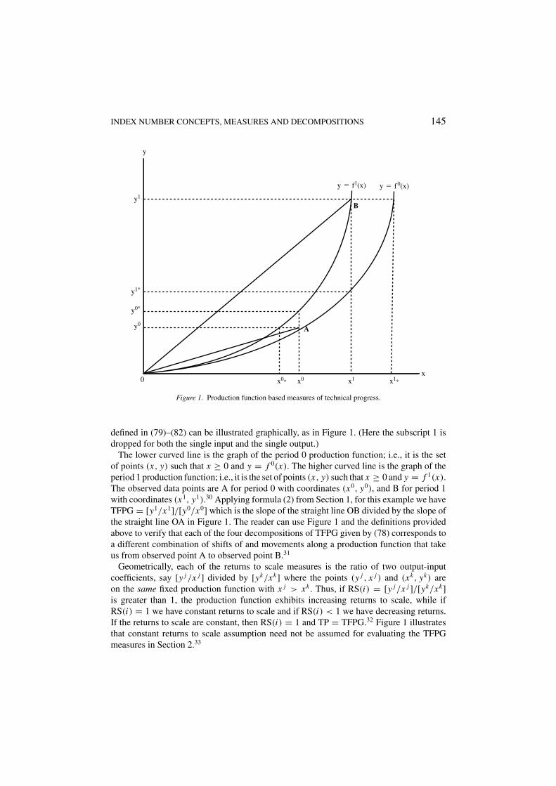
Figure 1. Production function based measures of technical progress.

defined in (79)–(82) can be illustrated graphically, as in Figure 1. (Here the subscript 1 isdropped for both the single input and the single output.)

The lower curved line is the graph of the period 0 production function; i.e., it is the setof points (x, y) such that x ≥ 0 and y = f 0(x). The higher curved line is the graph of theperiod 1 production function; i.e., it is the set of points (x, y) such that x ≥ 0 and y = f 1(x).The observed data points are A for period 0 with coordinates (x0, y0), and B for period 1with coordinates (x1, y1).30 Applying formula (2) from Section 1, for this example we haveTFPG = [y1/x1]/[y0/x0] which is the slope of the straight line OB divided by the slope ofthe straight line OA in Figure 1. The reader can use Figure 1 and the definitions providedabove to verify that each of the four decompositions of TFPG given by (78) corresponds toa different combination of shifts of and movements along a production function that takeus from observed point A to observed point B.31

Geometrically, each of the returns to scale measures is the ratio of two output-inputcoefficients, say [y j/x j ] divided by [yk/xk] where the points (y j , x j ) and (xk, yk) areon the same fixed production function with x j > xk . Thus, if RS(i) = [y j/x j ]/[yk/xk]is greater than 1, the production function exhibits increasing returns to scale, while ifRS(i) = 1 we have constant returns to scale and if RS(i) < 1 we have decreasing returns.If the returns to scale are constant, then RS(i) = 1 and TP = TFPG.32 Figure 1 illustratesthat constant returns to scale assumption need not be assumed for evaluating the TFPGmeasures in Section 2.33


6.2. Malmquist Indexes

The fundamental insight of the exact index number approach is that, if the technology ofa production unit can be represented in each time period by some known multiple input,multiple output production function, then quantity and TFPG indexes can be derived withinan optimizing model of producer behavior. We do this here.

As in (50), we let yt1 denote the amount of output 1 produced in period t for t = 0, 1, . . . , T .

Here we also let yt ≡ [yt2, yt

3, . . . , ytM ] denote the vector of other (than good 1) outputs jointly

produced in each period t using the vector of input quantities xt ≡ [xt1, xt

2, . . . , xtN ]. Thus,

the production functions for output 1 in period s and period t can be represented compactlyas:

ys1 = f s(ys, xs) and yt

1 = f t (yt , xt ). (83)

In defining Malmquist output indexes, we begin by defining three alternative formulationson the output side.34

The first Malmquist output index, αs , is defined as the number which satisfies

yt1

/αs = f s(yt/αs, xs). (84)

This index αs measures output growth using the comparison period s technology andinput vector. Its value is the number which just deflates the period t vector of outputs,yt ≡ [yt

1, yt2, . . . , yt

M ], into an output vector yt/αs that can be produced with the period svector of inputs, xs , using the period s technology. Due to substitution, when the numberof output goods, M , is greater than 1, then yt/αs will not usually be equal to the actualperiod s output vector, ys . However, if there is only one output, equation (84) becomesyt

1/αs = f s(xs) = ys

1, and we have αs = yt1/ys

1.A second Malmquist output index, αt , is defined as the number which satisfies

αt ys1 = f t (αt ys, xt ). (85)

The index αt measures output growth using the current period t technology and input vector.It is the number that inflates the period s vector ys into αt ys , an output vector that can beproduced with the period t input vector xt using the period t technology. The vector αt ys

will not usually be equal to yt when there are multiple outputs. However, when M = 1, then(85) becomes αt ys

1 = f t (xt ) = yt1 and αt = yt

1/ys1 reduces to the (single) output growth

rate.When there is no reason to prefer αs or αt and no need to distinguish between them, we

recommend defining the geometric mean of αs and αt as the Malmquist output quantityindex:

α ≡ [αsαt ]1/2. (86)

When there are only two output goods, the Malmquist output indexes αs and αt can beillustrated as in Figure 2 for time periods t = 1 and s = 0. The lower curved line representsthe set of outputs {(y1, y2) : y1 = f 0(y2, x0)} that can be produced with period 0 technologyand inputs.

The higher curved line represents the set of outputs {(y1, y2) : y1 = f 1(y2, x1)} thatcan be produced with period 1 technology and inputs. The period 1 output possibilities set


y2

�1y20

y21

y20

y21��0

y10 y1

1��0

y1��0

y1 � (y11, y2

1)

(0, 0)

y0 � (y10, y2

0)

�1y0

�1y10 y1

1y1

Figure 2. Alternative economic output indexes illustrated.

will generally be higher than the period 0 one for two reasons: (i) technical progress and(ii) input growth.35 In Figure 2, the point α1 y0 = [α1 y1

1 , α1 y1

2 ] is the straight line projectionof the period 0 output vector y0 = [y0

1 , y02 ] onto the period 1 output possibilities set, and

y1/α0 = [y11/α

0, y12/α

0] is the straight line contraction of the output vector y1 = [y11 , y1

2 ]onto the period 0 output possibilities set.

We now turn to the input side. A first Malmquist input index, βs , is defined as follows:

ys1 = f s(ys, xt/βs) ≡ f s

(ys

2, . . . , ysM , xt

1

/βs, . . . , xt

N

/βs

). (87)

This index measures input growth using the period s technology and output vector. A secondMalmquist input index, denoted by β t , is the solution to the following equation

yt1 = f t (yt , β t x s) ≡ f t

(yt

2, . . . , ytM , β t x s

1, . . . , βt x s

N

). (88)

It measures input growth using the period t technology and output vector. When there isno particular reason to prefer either the index βs to β t and no need to distinguish betweenthem, we recommend defining their geometric average as the Malmquist input quantityindex:

β ≡ [βsβ t ]1/2. (89)

Figure 3 illustrates the Malmquist indexes βs and β t for the case where there are just twoinput goods and for the time periods t = 1 and s = 0.


x2

�1x20

x20

x21

x21��0

x10 �1x1

0

x1 � (x11, x2

1)

(0, 0)

�1x0

x11��0 x1

1

x0 � (x10, x2

0)

Figure 3. Alternative Malmquist input indexes illustrated.

The lower curved line in Figure 3 represents the set of inputs needed to produce the vectorof outputs y0 using period 0 technology. This is the set {(x1, x2) : y0

1 = f 0(y0, x1, x2)}. Thehigher curved line represents the set of inputs that are needed to produce the period 1 vectorof outputs y1 using period 1 technology. This is the set {(x1, x2) : y1

1 = f 1(y1, x1, x2)}.36

The point β t x0 = [β t x01 , β

t x02 ] is the straight line projection of the input vector x0 ≡ [x0

1 , x02 ]

onto the period 1 input requirements set. The point x1/β0 is the straight line contraction ofthe input vector x1 ≡ [x1

1 , x12 ] onto the period 0 input requirements set.

Once theoretical Malmquist quantity indexes measuring the growth of total output andinput have been defined, then a Malmquist TFPG index for the general N -M case can bedefined too. Using the preferred Malmquist output and input quantity indexes given in (96)and (99), the definition we recommend for the Malmquist TFPG index is

TFPGM ≡ α/β. (90)

In the 1-1 case, expression (90) is readily seen to reduce to the measure of TFPG in Section 1.

6.3. Direct Evaluation of Malmquist Indexes for the N-M Case

Recall that α ≡ [αsαt ]1/2 and β ≡ [βsβ t ]1/2 are the Malmquist output and input quantityindexes defined in (86) and (89). Using the exact index number approach, Caves, Christensen


and Diewert (1982, pp. 1395–1401) give conditions under which the following equalitieshold:

α = QT (91)

and

β = Q∗T , (92)

where QT is the Tornqvist output quantity index defined by (39) and Q∗T is the Tornqvist

input quantity index defined analogously. If the assumptions that justify (91) and (92) aresatisfied, then we can evaluate the Malmquist measure TFPGM defined in (90) by takingthe ratio of the Tornqvist output and input indexes:

TFGPM = α/β = QT /Q∗T ≡ TFPGT . (93)

The assumptions required to derive (91) and (92) are, roughly speaking: (i) price taking,revenue maximizing behavior, (ii) price taking, cost minimizing behavior, and (iii) a translogtechnology.37 The practical importance of (93) is that the expression can be evaluatedfrom observable prices and quantities without knowledge of the parameters of f s andf t . However, changes in the value of this index cannot by decomposed into technicalprogress and returns to scale components without knowing or estimating the productionfunctions.

7. Diewert-Morrison Decompositions of an Alternative Productivity Measure

In Section 5, we used the period t production function f t to define the period t cost function,ct . Here we use the period t production function to define the period t (net) revenue function:

r t (p, x) ≡ maxy

{p · y : y ≡ (y1, y2, . . . , yM); y1 = f t (y2, . . . , yM ; x)}, (94)

where p ≡ (p1, . . . , pM) is an output price vector that the producer faces and x ≡(x1, . . . , xN ) is the input vector.38 Following Diewert and Morrison (1986), revenue func-tions for period t and the period s are used to define another family of theoretical productivitychange indexes:

RG(p, x) ≡ r t (p, x)/r s(p, x). (95)

From (94), it can be seen that RG(p, x) is the ratio of the output that can be producedusing the period t versus the period s technology with the reference input vector x and withboth of the resulting output vectors evaluated using the reference price vector, p. This is adifferent approach to the problem of controlling for total factor input utilization in judgingthe success of the period t versus the period s production outcomes.

Two special cases of (95) are of interest:

RGs ≡ RG(ps, xs) = r t (ps, xs)/r s(ps, xs)

and

RGt ≡ RG(pt , xt ) = r t (pt , xt )/r s(pt , xt ). (96)


RGs is the theoretical productivity index obtained by choosing the reference vectors p andx to be the period s observed output price vector ps and input quantity vector xs . RGt is thetheoretical productivity index obtained by choosing the reference vectors to be the period tobserved output price vector pt and input quantity vector xt .39

Under the assumption of revenue maximizing behavior in both periods, we can identifythe denominator of RGs and the numerator of RGt . That is, we have:

pt · yt = r t (pt , xt ) and ps · ys = r s(ps, xs). (97)

Our problem in evaluating the theoretical productivity indexes RGs and RGt is that wecannot directly observe the hypothetical revenues, r t (ps, xs) and r s(pt , xt ). The first ofthese is the hypothetical revenue that would result from using the period t technology withthe period s input quantities and output prices. The second is the hypothetical revenue thatwould result from using the period s technology with the period t input quantities and outputprices. However, these hypothetical revenue figures can be evaluated from observable dataif we know that the period t revenue function has the following translog functional form:

�n r t (p, x) ≡ αt0 +

M∑m=1

αtm �n pm +

N∑n=1

β tn �n xn + (1/2)

M∑i=1

M∑j=1

αij �n pi �n p j

+ (1/2)

N∑n=1

N∑j=1

βij �n xi �n x j +M∑

m=1

N∑n=1

γmn �n pm �n xn, (98)

where αij = αji and βij = βji and the parameters satisfy various other restrictions to ensurethat r t (p, x) is linearly homogeneous in the components of the price vector p.40 Note thatthe coefficient vectors αt

0, αtm and β t

n can be different in each period t but the quadraticcoefficients are assumed to be constant over the two periods.

Diewert and Morrison (1986; p. 663) show that under the above assumptions, the geo-metric mean of the two theoretical productivity indexes defined in (96) can be identifiedusing the observable price and quantity data that pertain to the two periods; i.e., we have

[RGsRGt ]1/2 = a/bc (99)

where a, b and c are given by

a ≡ pt · yt/ps · ys, (100)

�n b ≡M∑

m=1

(1/2)[(

psm ys

m

/ps · ys

) + (pt

m ytm

/pt · yt

)]�n

(pt

m

/ps

m

), (101)

and

�n c =N∑

n=1

(1/2)[(

wsn xs

n

/ps · ys

) + (wt

n xtn

/pt · yt

)]�n

(xt

n

/xs

n

). (102)

If we have constant returns to scale production functions f s and f t , then the value of outputswill equal the value of inputs in each period and we have

pt · yt = wt · xt . (103)


The same result can be derived without the constant returns to scale assumption if we havea fixed factor that absorbs any pure profits or losses, with this fixed factor defined as in (67).

Substituting (103) into (102), we see that expression c becomes the Tornqvist input indexQ∗

T . By comparing (101) and (40), we see also that b is the Tornqvist output price indexPT . Thus a/b is an implicit Tornqvist output quantity index.

If (103) holds, then we have the following decomposition for the geometric mean of theproduct of the theoretical productivity change indexes defined in (103):

[RGsRGt ]1/2 = [pt · yt/ps · ys]/[PT Q∗T ] (104)

where PT is the Tornqvist output price index and Q∗T is the Tornqvist input quantity index,

both of which are function of the prices and quantities in both periods t and s. Diewertand Morrison (1986) use the period t revenue functions to define two theoretical outputprice effects for m = 1, . . . , M which show how revenues change as a single output pricechanges:

Psm ≡ r s

(ps

1, . . . , psm−1, pt

m, psm+1, . . . , ps

M , xs)/

r s(ps, xs), (105)

and

Ptm ≡ r t (pt , xt )

/r t

(pt

1, . . . , ptm−1, ps

m, ptm+1, . . . , pt

M , xt), m = 1, . . . , M. (106)

These theoretical indexes give the proportional changes in the value of output that wouldresult if we changed the price of the mth output from its period s level ps

m to its period t levelpt

m holding constant all other output prices and the input quantities at reference levels andusing the same technology in both situations. For the theoretical index defined in (105), thereference output prices and input quantities and technology are the period s ones, whereasfor the index defined in (106) they are the period t ones. Now define the theoretical outputprice effect bm as the geometric mean of the two effects defined by (105) and (106):

bm ≡ [Ps

m Ptm

]1/2, m = 1, . . . , M. (107)

Diewert and Morrison (1986) and Kohli (1990) show that the bm given by (107) can beevaluated by the following observable expression if conditions (97), (98) and (103) hold:

�n bm = (1/2)[(

psm ys

m

/ps · ys

) + (pt

m ytm

/pt · yt

)]�n

(pt

m

/ps

m

), m = 1, . . . , M. (108)

Comparing (101) with (108), it can be seen that we have the following decomposition for b:

b =M∏

m=1

bm = PT . (109)

Thus the overall Tornqvist output price index can be decomposed into a product of theindividual output price effects, bm .

Diewert and Morrison (1986) also use the period t revenue functions in order to definefor n = 1, . . . , N two theoretical input quantity effects:

Qsn ≡ r s

(ps, xs

1, . . . , xsn−1, xt

n, xsn+1, . . . , xs

N

)/r s(ps, xs), (110)


and

Qtn ≡ r t (pt , xt )

/r t

(pt , xt

1, . . . , xtn−1, xs

n, xtn+1, . . . , xt

N

). (111)

These theoretical indexes give the proportional change in the value of output that wouldresult from changing input n from its period s level xs

n to it period t level xtn , holding constant

all output prices and other input quantities at reference levels and using the same technologyin both situations. For the theoretical index defined by (110), the reference output prices,input quantities and technology are the period s ones, whereas for the index in (111) theyare the period t ones.

Now define the theoretical input quantity effect cn as the geometric mean of the twoeffects defined by (100) and (101):

cn ≡ [Qs

n Qtn

]1/2, n = 1, . . . , N . (112)

Diewert and Morrison (1986) show that the cn defined by (112) can be evaluated by thefollowing empirically observable expression provided that assumptions (97) and (98) hold:

�n cn = (1/2)[(

wsn xs

n

/ps · ys

) + (wt

n xtn

/pt · yt

)]�n

(xt

n

/xs

n

)(113)

�n cn = (1/2)[(

wsn xs

n

/ws · xs

) + (wt

n xtn

/wt · xt

)]�n

(xt

n

/xs

n

). (114)

The expression (114) follows from (113) provided that the assumptions (103) also hold.Comparing (113) with (112), it can be seen that we have the following decomposition for c:

c =N∏

n=1

cn (115)

c = QT , (116)

where (116) follows from (115) provided that the assumptions (103) also hold. Thus ifassumptions (97), (98) and (93) hold, the overall Tornqvist input quantity index can bedecomposed into a product of the individual input quantity effects, the cn for n = 1, . . . , N .

Having derived (109) and (115), we can substitute these decompositions into (99) andrearrange the terms to obtain the following very useful decomposition:

pt · yt/ps · ys = [RGsRGt ]1/2M∏

m=1

bm

N∏n=1

cn (117)

This is a decomposition of the growth in the nominal value of output into the productivitygrowth term [RGsRGt ]1/2 times the product of the output price growth effects bm times theproduct of the input quantity growth effects (the cn). The effects on the right-hand side ofexpression (117) can be calculated using only the observable price and quantity data for thetwo periods.41

An interesting special case of (117) results when there is only one input in the x vectorand it is fixed. Then the input growth effect c1 is unity and variable inputs appear in they vector with negative components. In this special case, the left-hand side of (117) becomesthe pure profits ratio that is decomposed into a productivity effect times various price effects(the bm).


8. Conclusions

Before summing up our findings, we must mention explicitly some limitations of our anal-ysis. Direct evaluation of the measures presented in this paper depends on four problematicpreconditions: (i) the list of inputs used and outputs produced must remain constant overthe current period t and the comparison period s; (ii) quantity and either unit price or totalvalue information must be available for each of the two periods for all inputs purchased andoutputs sold; (iii) it must be possible to calculate user costs or rental prices in an unambigu-ous way for all capital inputs (i.e., for all durable inputs whose initial cost should be spreadover the multi-period life of the good); and, (iv) for some sorts of studies it is important forthe differences between the ex ante expected prices and the ex post realized prices to benegligible. We briefly discuss why each of these conditions is problematic below.

The first and second limitations are problematic because of data collection shortcomingsand because of the ongoing appearance of new goods.42 There are also issues having todo with the choice of outputs and inputs that should be included in an analysis since firmproductivity is affected by factors external to the firms and unintended outputs such aspollutants.43

The third limitation of our analysis is problematic because of unresolved conceptual is-sues concerning the measurement of user costs for durable inputs. For instance, when adurable input is purchased, the purchase price should be spread over its useful lifetime.Cost accounting depreciation allowances attempt to do this, but the traditional account-ing treatment of depreciation in an inflationary environment is unsatisfactory and there isdisagreement on how this traditional practice should be altered. For instance, what inter-est rate should be used in determining the value of financial capital tied up in the own-ership of durable goods? Should imputed equity interest costs be included too? Thereare also more basic unresolved conceptual problems associated with the measurementof capital inputs. For example, should the quantity of the capital services provided bya machine in each accounting period be treated as constant (that is, should it be mea-sured as an average per unit time period) over the lifetime of the machine, or should thequantity be reduced each period by a deterioration factor to reflect the decline in effi-ciency of the machine? The first view leads to a gross capital services concept and thesecond to a net capital services concept. These two views can lead to significantly differ-ent measures of capital services input and, hence, to significantly different measures ofproductivity.44

The fourth limitation is problematic because during inflationary time periods substantialdifferences can develop between ex ante and ex post prices. Many capital inputs cannotbe adjusted instantaneously (i.e., they cannot be bought or sold instantaneously); there-fore, a cost minimizing producer forms a priori expectations about the purchase and dis-posal prices as well as future interest rates, depreciation rates, and tax rates in order tocalculate the ex ante user cost of capital inputs. However, as researchers, we can onlyobserve ex post prices, interest rates, depreciation rates, and tax rates; thus we can onlycalculate ex post user costs. If the expectations about future prices and rates are not re-alized, then the ex ante user costs—the prices which should appear in our cost functionsand in the exact index number formulas—may differ significantly from the ex post usercosts.


These limitations must be kept in mind in applying the methods reviewed here.In the initial sections of this paper we developed and explored properties of the TFPG

index number formulas that are most commonly used: the Paasche, Laspeyres, Fisher, andTornqvist indexes. We also developed the mathematical relationships among the quantity,price and TFPG indexes. Methods for separating out different components of the growthin the total input, output, cost and revenue were made explicit, and then were utilizedthroughout the paper.

In Section 3, we showed how a TFPG index can be expressed as a function of sin-gle factor input-output, or output-input, coefficients. This decomposition is an algebraicresult, not depending on any assumptions concerning the underlying technology or busi-ness practices. This decomposition provides a framework for relating widely used sin-gle factor efficiency and productivity measures to an overall measure of productivityperformance.

Section 4 provided a brief review of the axiomatic approach to choosing a TFPG indexformula. Application of this approach does not depend on assumptions about the natureof the underlying technology or producer behavior. However, when it does seem rea-sonable to assume specific sorts of optimizing behavior and the underlying technologycan be modelled using a specific functional form, then the exact index number approach,introduced in Section 5, can be used as well for selecting a formula for the TFPG in-dex. In Section 6 we reviewed results establishing that if the underlying technology canbe represented by a translog production function and the producer is optimizing in cer-tain ways, then the theoretical Malmquist TFPG index can be directly evaluated fromobservable price and quantity data using a Tornqvist type of index. Decompositions de-veloped by Diewert and Morrison of a related measure of overall productive performancealso apply in this case. These decompositions, presented in Section 7, allow an assess-ment of the contributions to an overall measure of productivity change that are due toquantity and price changes at the level of the individual output goods. The Diewert-Morrison decompositions, like the decomposition presented in Section 3, should be helpfulin following through on the advice that Arnold Harberger (1998, p. 1) provides in hisAmerican Economics Association Presidential Address: that we should approach the mea-surement of productivity by trying to “think like an entrepreneur or a CEO, or a productionmanager.”

Acknowledgments

This research was funded in part by the grants we jointly hold from the Social Sciencesand Humanities Research Council of Canada (SSHRC). The authors thank participants in aJune 15–17, 2000 Union College workshop for comments on the paper given there by ErwinDiewert that was the starting point for this paper. For comments on the present paper, theauthors thank Bo Honore and other participants in a Princeton seminar, and John Baldwin,Mel Fuss, Richard Lipsey, Someshwar Rao, Tom Wilson, David Laidler, Masao Nakamura,Emi Nakamura, Denis Lawrence, and other participants in a workshop held at StatisticsCanada October 25–26, 2001 with funding from our SSHRC grants. All errors of fact orinterpretation are the sole responsibility of the authors.


Notes

1. Empirical examples of this include Diewert and Nakamura (1999). The fact that output-input coefficients arepure quantity measures is something that many in engineering and the business world view as an importantadvantage.

2. Some use TFP to refer to total factor productivity growth as well as total factor productivity. FollowingBernstein (1999), we use TFPG for total factor productivity growth to avoid the inevitable confusion thatotherwise results.

3. See Diewert (2000) for additional ways of conceptualizing TFPG.4. We refer to t and s as time periods, but the comparison situation could be for some other unit of production.5. Formally, the first two of these can be shown to result from deflating the period t nominal cost and revenue

by a Paasche price index. The second two result from deflating the period t nominal cost and revenue by aLaspeyres price index. See Horngren and Foster (1987, Chapter 24, Part One) or Kaplan and Atkinson (1989,Chapter 9) for examples of this accounting practice of controlling for price level change without explicit useof price indexes.

6. A quantity (price) relative for a good is the ratio of the quantity (price) for that good in a specified period t tothe quantity (price) for that good in some comparison period s. One advantage of defining a quantity (or price)index as a weighted average of quantity (price) relatives is that the relatives are unit free, making it clear thatthis is an acceptable way of incorporating even goods (prices) for which there is no generally accepted unit ofmeasure.

7. The implicit price (quantity) index corresponding to a given quantity (price) index can always be derived byimposing the product test and solving for the price (quantity) index that satisfies this rule. The product test ispart of the axiomatic approach to the choice of an index number functional form that is reviewed in Section 4.

8. Jorgenson and Griliches (1967, p. 252) suggested this formula. One set of conditions under which the marginswill be zero is perfect competition and a constant returns to scale technology.

9. See Diewert (1987, 1993c) and Fisher (1911, 1922).10. This criterion is developed more fully in a different context by Emi Nakamura (2002).11. The period t cost and revenue and the hypothetical aggregates of period s output and input quantities defined in

expressions (10) and (13) are comparable in this sense because the quantities for periods s and t are evaluatedusing the same period t price vectors. Similarly, the period s cost and revenue and the hypothetical aggregatesof period t output and input quantities defined in expressions (11) and (12) are comparable in this sensebecause the quantities of the output and input goods are evaluated using the same period s price vectors.These aggregates are what are used to define the Paasche, Laspeyres and Fisher measures given in (28), (29)and (30).

12. Tornqvist indexes are also known as translog indexes following Jorgenson and Nishimizu (1978) who intro-duced this terminology because Diewert (1976, p. 120) related Q∗

T to a translog production function. The exactindex number approach used for relating specific quantity indexes to specific production functions is the topicof Section 5.

13. See Diewert (1992a, p. 181).14. Contributors to this approach include Walsh (1901, 1921), Irving Fisher (1911, 1922), Eichhorn (1976),

Eichhorn and Voeller (1976), Funke and Voeller (1978, 1979), Diewert (1976, 1987, 1988, 1992a, 1992b) andBalk (1995).

15. The product test was proposed by Irving Fisher (1911, p. 388) and named by Frisch (1930, p. 399).16. Alternatively, an axiomatic approach can be applied directly to the formula choice problem for TFPG.17. Laspeyres (1871, p. 308), Walsh (1901, p. 308) and Eichhorn and Voeller (1976, p. 24) proposed this test.18. Walsh (1901, p. 540) was one of many researchers who proposed this test.19. Walsh (1901, p. 385) and Eichhorn and Voeller (1976, p. 24) proposed this test.20. This test was first informally proposed by Pierson (1896, p. 128) and was formalized by Walsh (1901, p. 368;

1921, p. 541) and Fisher (1922, p. 64).21. See Diewert (1976, p. 131; 1992b) and also Funke and Voeller (1978, p. 180).22. Christensen, Jorgenson and Lau (1971) introduced the translog functional form for a single output technology.

Burgess (1974) and Diewert (1974, p. 139) defined this for the multiple output case. Instead of specifyingthe firm’s cost function, some researchers have specified functional forms for the firm’s production function


(e.g., Diewert, 1976, p. 127; 1980, p. 488) or the firm’s revenue or profit function (e.g., Diewert, 1980, p. 493;1988) or for the firm’s distance function (e.g., Caves, Christensen and Diewert, 1982, p. 1404).

23. On the econometric estimation of cost functions using more flexible functional forms that permit theoreticallyplausible types of substitution, see Berndt (1991) and also Diewert and Wales (1992) and the references therein.

24. This follows by applying a theoretical result due initially to Hotelling (1932, p. 594) and Shephard (1953,p. 11).

25. Expression (60) follows from (59) by applying the Hotelling-Shephard relations (58) for t and s.

26. This decomposition has no implications for the choice of a measurement formula for TFPG. The new para-meters introduced in making this decomposition cancel out in the product representation of TFPG. That is,TFPG includes the effects of both technical progress (a shift in the production function) and returns to scale(a movement along a production function). We are assuming here that producers are on their production frontierin each period; i.e., that they are technically efficient. A more complete analysis might allow for technicalinefficiency as well. Favorable or adverse changes in environmental factors facing the firm going from periods to t are regarded as shifts in the production function.

27. TP(1) and TP(2) are the one input, one output special cases of Caves, Christensen and Diewert’s (1982, p. 1402)output based ‘productivity’ indexes.

28. TP(3) and TP(4) are the one input, one output special cases of the input based ‘productivity’ indexes proposedby Caves, Christensen and Diewert (1982, p. 1407).

29. This shift can be conceptualized as either a move from one production function to another, or equivalently asa change in the location and perhaps the shape of the original production function.

30. In Figure 1, note that if the production function shifts were measured in absolute terms as differences in thedirection of the y axis, then these shifts would be given by y0∗ − y0 (at point A) and y1 − y1∗

(at point B). Ifthe shifts were measured in absolute terms as differences in the direction of the x axis, then the shifts wouldbe given by x0 − x0∗

(at point A) and x1∗ − x1 (at point B). An advantage of measuring TP (and TFPG) usingratios is that the relative measures are invariant to changes in the units of measurement whereas the differencesare not.

31. For firms in a regulated industry, returns to scale will generally be greater than one, since increasing returnsto scale in production is often the reason for regulation in the first place.

32. Solow’s (1957, p. 313) Chart I is similar in concept, but for the simpler case of constant returns to scale.

33. See, for example, Basu and Fernald (1997) and Nakajima, Nakamura and Yoshioka (1998) for evidence ofnonconstant returns to scale and references to other research on this subject.

34. These output indexes correspond to the two Malmquist output indexes defined in Caves, Christensen andDiewert (1982, p. 1400). Similar indexes were proposed by Malmquist (1953) for the consumer context, andby Moorsteen (1961) and Hicks (1961; 1981, pp. 192 and 256) for the producer context. See also Balk (1998,Chapter 4).

35. However, if there were technical regress (so that production became less efficient in period 1 compared toperiod 0) or if the utilization of inputs declined going from period 0 to period 1, then the period 1 outputproduction possibilities set could lie below the period 0 output production possibilities set.

36. If technical progress were sufficiently positive or if output growth between the two periods were sufficientlynegative, then the period 1 input requirements set could lie below the period 0 one instead of above.

37. An intuitive explanation for the remarkable equalities in (91) and (92) rests on the following fact: if f (z) isa quadratic function, then f (zt ) − f (zr ) = (1/2)[∇ f (zt ) + ∇ f (zr )]T [zt − zr ]. This result follows fromapplying Diewert’s (1976, p. 118) Quadratic Approximation Lemma. Under the assumption of optimizingbehavior on the part of the producer, the vectors of first order partial derivatives, ∇ f (zt ) and ∇ f (zr ), will beequal to or proportional to the observed prices. Thus the right-hand side of this identity becomes observablewithout estimation. In actual applications, we assume that various transformations of f are quadratic and applythe resulting identity.

38. If ym is positive (negative), then the net output m is an output (input). We assume that all output prices pm arepositive. We assume that all input quantities xn are positive and if the net input n is an input (output), then wn

is positive (negative).

39. This approach can be viewed as an extension to the general N -M case of the methodology used in definingthe output based measures of technical progress given in (74) and (75).

40. These conditions can be found in Diewert (1974; p. 139).


41. Kohli (1990) and Fox and Kohli (1998) use (134) to examine the factors behind the growth in the nominalGDP of several countries. See Morrison and Diewert (1990) for decompositions for other functional forms.

42. For other issues and references on new goods and the measurement of productivity see Diewert (1987, 1995,1998a, 1998b, 1999), Diewert and Fox (1999), Diewert and Smith (1994), Wolfson (1999), and Baldwin,Despres, Nakamura and Nakamura (1997) as well as other papers and the Introduction in Bresnahan andGordon (1997).

43. Studies emphasizing externalities like R&D spillovers are Bernstein (1996, 1998), Berndt and Fuss (1986),and Gera, Wu and Lee (1999).

44. For discussions on the measurement problems associated with capital, see Jorgenson (1963, 1980, 1995a,1995b), Jorgenson and Griliches (1967, pp. 254–260), Morrison (1986, 1988), Diewert (1980, pp. 470–486;1992a), Diewert and Lawrence (1999), and the references in those papers.

References

Allen, R. G. D. (1949). “The Economic Theory of Index Numbers.” Economica N. S. 16, 197–203.Armitage, H. M. and A. A. Atkinson. (1990). The Choice of Productivity Measures in Organizations. Hamilton,

Ontario: The Society of Management Accountants.Atkinson, A. A., R. D. Banker, R. S. Kaplan and S. M. Young. (1995). Management Accounting. Prentice Hall,

England.Baldwin, A., P. Duspres, A. Nakamura and M. Nakamura. (1997). “New Goods from the Perspective of Price

Index Making in Canada and Japan.” In Bresnahan and Gordon (eds.), 437–474.Balk, B. M. (1995). “Axiomatic Price Theory: A Survey.” International Statistical Review 63(1), 69–93.Balk, B. M. (1998). Industrial Price, Quantity and Productivity Indices. Boston: Kluwer Academic Publishers.Basu, S. and J. G. Fernald. (1997). “Returns to Scale in U.S. Production: Estimates and Implications.” Journal of

Political Economy 105(2), 249–283.Berndt, E. R. (1991). The Practice of Econometrics Classic and Contemporary. New York: Addison-Wesley.Berndt, E. R. and M. A. Fuss. (1986). “Productivity Measurement with Adjustments for Variations in Capacity

Utilization and Other Forms of Temporary Equilibrium.” Journal of Econometrics 33, 7–29.Bernstein, J. I. (1999). “Total Factor Productivity Growth in the Canadian Life Insurance Industry.” Canadian

Journal of Economics 32(20), 500–517.Bernstein, J. I. (1998). “Factor Intensities, Rates of Return and International R&D Spillovers: The Case of

Canadian and U.S. Industries.” Annales d’Economie et de Statistique 49/50, 541–564.Bernstein, J. I. (1996). “The Canadian Communication Equipment Industry as a Source of R&D Spillovers and

Productivity Growth.” In P. Howitt (ed.), The Implications of Knowledge-Based Growth for Micro-EconomicPolicies. Calgary: University of Calgary Press.

Bresnahan, T. F. and R. J. Gordon. (1997). The Economics of New Goods. Chicago: The University of ChicagoPress.

Burgess, D. F. (1974). “A Cost Minimization Approach to Import Demand Equations.” Review of Economics andStatistics 56(2), 224–234.

Caves, D. W., L. Christensen and W. E. Diewert. (1982). “The Economic Theory of Index Numbers and theMeasurement of Input, Output, and Productivity.” Econometrica 50(6), 1393–1414.

Christensen, L. R., D. W. Jorgenson and L. J. Lau. (1971). “Conjugate Duality and the Transcendental LogarithmicProduction Function.” Econometrica 39, 255–256.

Diewert, W. E. (1974). “Applications of Duality Theory.” In M. D. Intrilligator and D. A. Kendrick (eds.), Frontiersof Quantitative Economics. Amsterdam: North-Holland Publishing Co., II, 106–171.

Diewert, W. E. (1976). “Exact and Superlative Index Numbers.” Journal of Econometrics 4(2), 115–146, reprintedas Chapter 8 in Diewert and Nakamura (1993, 223–252).

Diewert, W. E. (1978). “Superlative Index Numbers and Consistency in Aggregation.” Econometrica 46, 883–900,reprinted as Chapter 9 in Diewert and Nakamura (1993, 253–273).

Diewert, W. E. (1980). “Aggregation Problems in the Measurement of Capital.” In Dan Usher (ed.), The Measure-ment of Capital. Chicago, Illinois: University of Chicago Press, 433–528.

Diewert, W. E. (1987). “Index Numbers.” In J. Eatwell, M. Milgate and P. Newman (eds.), The New Palgrave: ADictionary of Economics. London: Macmillan, 2, 767–780, reprinted as Chapter 5 in Diewert and Nakamura(1993, 71–104).


Diewert, W. E. (1988). “Test Approaches to International Comparisons.” Measurement in Economics, 67–86,reprinted as Chapter 12 in Diewert and Nakamura (1993, 67–86).

Diewert, W. E. (1992a). “The Measurement of Productivity.” Bulletin of Economic Research 44(3), 163–198.Diewert, W. E. (1992b). “Fisher Ideal Output, Input, and Productivity Indexes Revisited.” Journal of Productivity

Analysis 3, 211–248, reprinted as Chapter 13 in Diewert and Nakamura (1993, 211–248).Diewert, W. E. (1993c). “Symmetric Means and Choice under Uncertainty.” In Diewert and Nakamura (eds.),

355–434.Diewert, W. E. (1995). “Functional Form Problems in Modeling Insurance and Gambling.” The Geneva Papers

on Risk and Insurance Theory 20, 135–150.Diewert, W. E. (1998a). “Index Number Issues in the Consumer Price Index.” The Journal of Economic Perspectives

12(1), 47–58.Diewert, W. E. (1998b). “High Inflation, Seasonal Commodities and Annual Index Numbers.” Macroeconomic

Dynamics 2, 456–471.Diewert, W. E. (1999). “Index Number Approaches to Seasonal Adjustment.” Macroeconomic Dynamics 3, 48–68.Diewert, W. E. (2000). “Alternative Approaches to Measuring Productivity and Efficiency.” Paper prepared for the

North American Productivity Workshop at Union College, Schenectady, New York, June 15–17, 2000.Diewert, W. E. and K. Fox. (1999). “Can Measurement Error Explain the Productivity Paradox?” Canadian Journal

of Economics 32(2), 251–281.Diewert, W. E. and D. A. Lawrence. (1999). “Progress in Measuring the Price and Quantity of Capital.” Discussion

Paper 99–17, Department of Economics, University of British Columbia, Vancouver, Canada, V6T 1Z1.Diewert, W. E. and C. J. Morrison. (1986). “Adjusted Output and Productivity Indexes for Changes in the Terms

of Trade.” Economic Journal 96(Sept.), 659–679.Diewert, W. E. and A. O. Nakamura. (1993). Essays in Index Number Theory, Vol. I. Amsterdam: North-Holland.Diewert, W. E. and A. O. Nakamura. (1999). “Benchmarking and the Measurement of Best Practice Efficiency:

An Electricity Generation Application.” Canadian Journal of Economics 32(2), 570–588.Diewert, W. E. and A. M. Smith. (1994). “Productivity Measurement for a Distribution Firm.” The Journal of

Productivity Analysis 5, 335–347.Diewert, W. E. and T. J. Wales. (1992). “Quadratic Spline Models For Producer’s Supply and Demand Functions.”

International Economic Review 33(3), 705–722.Eichhorn, W. (1976). “Fisher’s Tests Revisited.” Econometrica 44, 247–256.Eichhorn, W. and J. Voeller. (1976). Theory of the Price Index. Lecture Notes in Economics and Mathematical

Systems. Berlin: Springer-Verlag, 140.Fisher, I. (1911). The Purchasing Power of Money. London: MacMillan.Fisher, I. (1922). The Making of Index Numbers. Boston: Houghton Mifflin.Fox, K. J. and U. Kohli. (1998). “GDP Growth, Terms of Trade Effects and Total Factor Productivity.” The Journal

of International Trade and Economic Development 7(1), 87–110.Frisch, R. (1930). “Necessary and Sufficient Conditions Regarding the Form of an Index Number Which Shall

Meet Certain of Fisher’s Tests.” American Statistical Association Journal 25, 397–406.Funke, H. and J. Voeller. (1978). “A Note of the Characterization of Fisher’s Ideal Index.” In W. Eichhorn, R. Henn,

O. Opitz and R. W. Shephard (eds.), Theory and Applications of Economic Indices. Wurzburg: Physica-Verlag,177–181.

Funke, H. and J. Voeller. (1979). “Characterization of Fisher’s Ideal Index by Three Reversal Tests.” StatistischeHefte 20, 54–60.

Gera, S., W. Wu and F. C. Lee. (1999). “Information Technology and Productivity Growth: An Empirical Analysisfor Canada and the United States.” Canadian Journal of Economics 32(2), 384–407.

Harberger, A. (1998). “A Vision of the Growth Process.” American Economic Review 88(1), 1–32.Hicks, J. R. (1961). “Measurement of Capital in Relation to the Measurement of Other Economic Aggregates.”

In F. A. Lutz and D. C. Hague (eds.), The Theory of Capital. London: Macmillan.Hicks, J. R. (1981). Wealth and Welfare. Cambridge, Mass.: Harvard University Press.Hill, R. J. (2000). “Superlative Index Numbers: Not All of Them Are Super.” School of Economics, University of

New South Wales, Sydney 2052, Australia, September 10.Horngren, C. T. and G. Foster. (1987). Cost Accounting: A Managerial Emphasis, 6th ed., Englewood Cliffs,

New Jersey: Prentice Hall.Hotelling, H. (1932). “Edgeworth’s Taxation Paradox and the Nature of Demand and Supply Functions.” Journal

of Political Economy 40, 577–616.Jorgenson, D. W. (1963). “Capital Theory and Investment Behavior.” American Economic Review 53(2), 247–259.


Jorgenson, D. W. (1980). “Accounting for Capital.” In George M. von Furstenberg (ed.), Capital, Efficiency andGrowth. Cambridge, MA: Ballinger, 251–319.

Jorgenson, D. W. (1995a). Productivity, Vol. 1. Cambridge, MA.Jorgenson, D. W. (1995b). Productivity, Vol. 2. Cambridge, MA.Jorgenson, D. W. and Z. Griliches. (1967). “The Explanation of Productivity Change.” Review of Economic Studies

34(3), 249–280.Jorgenson, D. W. and M. Nishimizu. (1978). “U.S. and Japanese Economic Growth, 1952–1974: An International

Comparison.” Economic Journal 88, 707–726.Kaplan, R. S. and A. A. Atkinson. (1989). Advanced Management Accounting. Englewood Cliffs, New Jersey:

Prentice Hall.Kohli, U. (1990). “Growth Accounting in the Open Economy: Parametric and Nonparametric Estimates.” Journal

of Economic and Social Measurement 16, 125–136.Laspeyres, E. (1871). “Die Berechnung einer mittleren Waarenpreissteigerung.” Jahrbucher fur Nationalokonomie

und Statistik 16, 296–314.Malmquist, S. (1953). “Index Numbers and Indifference Surfaces.” Trabajos de Estadistica 4, 209–242.Miller, D. M. (1984). “Profitability = productivity + price recovery.” Harvard Business Review May–June,

145–153.Moorsteen, R. H. (1961). “On Measuring Productive Potential and Relative Efficiency.” Quarterly Journal of

Economics 75, 451–467.Morrison, C. J. (1986). “Productivity Measurement with Non-Static Expectations and Varying Capacity Utiliza-

tion.” Journal of Econometrics 33(1/2), 51–74.Morrison, C. J. (1988). “Quasi-Fixed Inputs in U.S. and Japanese Manufacturing: A Generalized Leontief

Restricted Cost Function Approach.” Review of Economics and Statistics 70, 275–287.Morrison, C. J. and W. E. Diewert. (1990). “New Techniques in the Measurement of Multifactor Productivity.”

The Journal of Productivity Analysis 1, 265–285.Nakajima, T., M. Nakamura and K. Yoshioka. (1998). “An Index Number Method for Estimating Scale Economies

and Technical Progress Using Time-Series of Cross-Section Data: Sources of Total Factor Productivity Growthfor Japanese Manufacturing, 1964–1988.” Japanese Economic Review 49(3), 310–334.

Nakamura, E. (2002). “Real GDP and the Concept of Quantity.” Working Paper available at http://www.harvard.edu/∼nakamura.

Paasche, H. (1874). “Uber die Preisentwicklung der letzten Jahre nach den Hamburger Borsennotirungen.”Jahrbucher fur Nationalokonomie und Statistik 23, 168–178.

Pierson, N. G. (1896). “Further Considerations on Index-Numbers.” Economic Journal 6, 127–131.Shephard, R. W. (1953). Cost and Production Functions. Princeton: Princeton University Press.Solow, R. M. (1957). “Technical Change and the Aggregate Production Function.” Review of Economics and

Statistics 39, 312–320.Tinbergen, J. (1942). “Zur Theorie der langfristigen Wirtschaftsentwicklung.” Weltwirtschaftliches Archiv 55(1),

511–549; English translation (1959). “On the Theory of Trend Movements.” In Leo H. Klaassen, Leendert M.Koyck and Hendrikus J. Witteveen (eds.), Jan Tinbergen, Selected Papers. Amsterdam: North-Holland, 182–221.

Tornqvist, L. (1936). “The Bank of Finland’s Consumption Price Index.” Bank of Finland Monthly Bulletin 10,1–8.

Walsh, C. M. (1901). The Measurement of General Exchange Value. New York: Macmillan.Walsh, C. M. (1921). “The Best Form of Index Number: Discussion.” Quarterly Publication of the American

Statistical Association 17(March), 537–544.Wolfson, M. (1999). “New Goods and the Measurement of Real Economic Growth.” Canadian Journal of

Economics 32(2), 447–470.

index number concepts, measures and decompositions of

Documents