improvement of lime soda glass laser microfabrication processing parameters using design of...
TRANSCRIPT
9
IMPROVEMENT OF LIME SODA GLASS LASER
MICROFABRICATION PROCESSING PARAMETERS USING DESIGN
OF EXPERIMENTS
A. ISSA, D. BRABAZON and S. HASHMI School of Mechanical and Manufacturing Engineering, Dublin City University, Ireland
ABSTRACT
This paper presents work on the development of the rapid prototyping laser micromachining
technique. Glasses have non-linear heat absorption properties which make them harder to
process by laser than metals from a response predictability perspective. Typical silicate
applications include micro-electromechanical systems (MEMS), telecommunications and
optics due to their high chemical and thermal stabilities. This study investigated the process of
fabricating micro-channels on the surface of soda lime glass using a CO2 pulsed laser. A two
level factorial design of experiments (DOE) was employed to study the effects of laser
processing parameters on the resulting channels. The parameters considered in the design
were the laser power, pulse frequency and translation speed. The width, depth and surface
roughness of the channels were the response parameters investigated. The results analysis
provided mathematical models for the process, based on response surface methodology
(RSM). The model predictions allowed fabricating channels with desired width, depth and
surface roughness characteristics. The process was also thermally modelled and simulated
channel geometries were compared to experimental results.
Key words: glass, CO2 laser, micro-channels, RSM, thermal model.
1. INTRODUCTION
Many rapid manufacturing techniques have been developed over the last twenty years. A
number of these techniques have been developed around the unique capabilities of lasers.
These include stereolithography (STL), selective laser sintering (SLS) and more recently
rapid laser machining on macro and micrometer scale ranges [1, 2]. This paper presents work
on the development of the rapid prototyping laser micromachining technique.
The fabrication of micro-channels on the surface of glasses can be used in various
applications such as telecommunication, optical and bio-medical engineering. Glasses absorb
laser radiation in a way that depends highly on the incident wavelength [3, 4], most
transparent materials are opaque in the visible region but absorb strongly at or near 10 µm,
which makes CO2 laser very efficient for machining these materials [3, 5]. Despite that
glasses may reflect up to 30% of the incident laser radiation [5], the laser-induced plasma will
enhance the coupling of laser pulses to the materials surface, raising its temperature up to
3500C [6]. This temperature is sufficient to vaporise the material from the irradiated region.
Some studies [7,8] have investigated irradiating glass samples for a number of time along a
specified path to finally produce microchannels. However, such studies use a fixed value of
operating parameters and were not concerned with the effect of operating parameters on the
resulting microchannels geometries. A systematic study of the process is possible by
experimental methods that give real measurements of responses and results which could not
10
be possibly achieved theoretically [9]. The experimental approach can also be used to develop
a mathematical model to be used as a channel manufacturing guide. The mathematical model
can be used to produce responses based on certain criteria of operating control parameters
allowing the improvement of the process. Furthermore, thermal modelling of laser treatment
of material has been used to estimate the resulting effects on the materials [3,10]. It can be
useful to estimate the temperature ranges and thermal stresses that the material is expected to
experience beforehand. This study examined the production of single microchannels.
However, the concepts and results presented are extendible to cover multi-mode and 3D
microchannels that are usually needed in rapid prototyping applications.
2. EXPERIMENTAL WORK
Two millimetre thick commercial soda-lime glass sheets were used in this work. The typical
contents of soda-lime are 73 wt.% SiO2, 15 wt.% Na2O, 7 wt.% CaO, 4 wt.% MgO and Al2O3
1 wt.% [4]. A 1.5 kW CO2 laser beam was focused using a 127 mm focal length lens to a spot
size of approximately 90 m on the surface of the samples and delivered via a nozzle with an
air jet at 1 bar. Channels of 20 mm in length were produced using a set of parameter values
discussed below.
2.1 Design of experiments
The laser power (P), pulse repetition frequency (PRF) and scanning speed (V) were chosen as
the process control parameters. A screening experiment was initially carried out to investigate
the ranges of these parameters that result in acceptable micro-channels. As a result, the range
for P was (18-30 W), PRF (160-400 Hz) and V (100-500 mm/min). The response parameters
were chosen to be the channel’s width (m), the depth (m) and the surface roughness, Ra,
(m). A 23 factorial design of experiments was performed on the laser processing parameters.
Five extra experiments, at the centres of the ranges, were added to the design for adequacy
analysis. A total of 14 experiments were carried out according to a random run order to
eliminate any systematic errors [9], as shown in table 1.
Table 1: List of experiments carried out with the measured responses.
Ch No. Run Order P (W) PRF (Hz) V (mm/min) Dia (m) Depth (m) Ra (m)
1 1 18 400 100 163.7 100 2.517
2 6 30 400 100 294.45 248 3.686
3 2 18 160 100 276.9 200 4.707
4 4 30 160 100 395.85 392 5.621
5 12 18 400 500 81.2 20 2.512
6 13 30 400 500 243.75 83 3.366
7 10 18 160 500 286.65 79.5 2.783
8 5 30 160 500 349.05 241.5 4.525
9 3 24 280 300 269.1 140 3.266
10 9 24 280 300 265.2 145 3.324
11 14 24 280 300 263.25 145 3.385
12 8 24 280 300 269.1 150 3.422
13 11 24 280 300 273 138 3.102
14 7 24 280 300 263.25 153 3.016

11
2.2 Channel scanning
After producing the channels the samples were later on the same day water washed and air jet
dried. An electro-discharge deposited gold coating was then applied to make the glass reflect
in order to facilitate laser scanning of the samples. The laser scanner used had a maximum
accuracy of ± 0.25 m in height and ± 0.039 m in lateral measurements [11]. Figure 1 shows
a schematic of a laser produced channel, based on heat deposition from a pulsed laser beam
[10]. The channel width was measured at the glass surface. The depth was measured from the
surface to the average channel bottom level. The surface roughness (Ra) was measured along
the channel. This information can be particularly significant in fluid flow applications. All
measurements were performed using a software code built specifically for this study and the
measured response parameters are listed in table 1.
Figure 1: General schematic of the channel geometry.
In order to generate a three dimensional profile for each channel, a 50 m section of each
channel was scanned. Each channel was scanned at the same position, 15 mm from the start of
the channel. Three measurements were made and averaged for each response (channel width,
depth and roughness). The width measurements were sometimes assisted by microscopic
images. Figure 2 shows two sample channel scans. The CO2 laser was translated in the
negative x direction in these scans.
Figure 2: Channel profile scans for (a) channel number 11 and (b) channel number 2.
3. ANALYSIS AND DISCUSSION OF RESULTS
Statistical analysis and model development were done in a design of experiments software
package called DesignExpert. Three different models were derived, each describing one
response parameter. The model terms were composed of contribution fractions of the process

12
parameter levels or interactions of these levels. The selection of terms used was based on an
iterative, step-wise, process to arrive at the best model fit with the experimental data [12, 13].
3.1 Channel width model
Table 2 lists the model’s analysis of variance (ANOVA). The model F-value of 458.535
implies the model is significant. The significant model terms are P, PRF, V, P*PRF, PRF*V
and P*PRF*V. The "Curvature F-value" of 4.389 implies there is no significant curvature (as
measured by difference between the average of the center points and the average of the
factorial points) in the design space. The "Lack of Fit F-value" of 5.034 implies the Lack of
Fit is not significant relative to the pure error. Moreover, the adequacy measures R2, adjusted
R2
and predicted R2 in table 2, are all close to 1, and in reasonable agreement indicating an
adequate model [13]. The adequacy precision is also greater than 4 indicating adequate model
discrimination. The mathimatical model for the width is not hirarchical and hence the
formation of a mathimatical equation was not possibel. However, the response surface is used
instead to predict widths within the investigated range of paramters.
Table 2: ANOVA analysis of the width model
Source Sum of
Squares DF
Mean
Square
F
Value Prob > F
Model 69981.707 6 11663.62 458.535 < 0.0001 significant
P 28161.578 1 28161.58 1107.123 < 0.0001
PRF 34499.078 1 34499.08 1356.271 < 0.0001
V 3623.133 1 3623.133 142.437 < 0.0001
P*PRF 1566.60 1 1566.6 61.588 0.0002
PRF*V 1155.603 1 1155.603 45.431 0.0005
P*PRF*V 975.715 1 975.715 38.359 0.0008
Curvature 111.639 1 111.639 4.389 0.0810 not significant
Residual 152.620 6 25.437
Lack of Fit 76.570 1 76.570 5.034 0.0749 not significant
Pure Error 76.05 5 15.21
Cor Total 70245.966 13
R-Squared = 0.998 Adj R-Squared = 0.997
Pred R-Squared = 0.929 Adeq Precision = 82.531
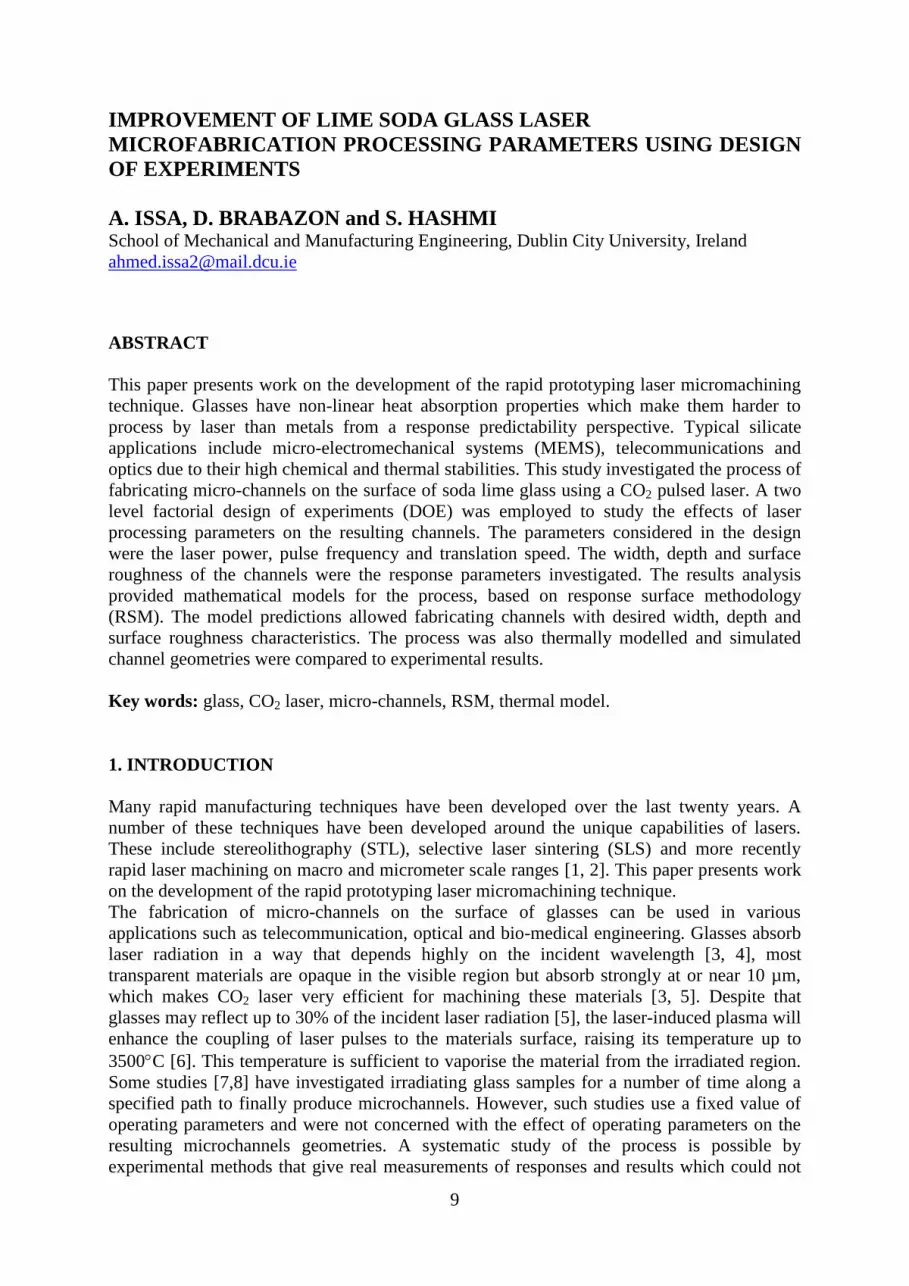
Figure 3 (a) shows the actual versus the predicted width values; the data points are distributed
along the diagonal indicating a good fit of the model. Figure 3 (b) shows the interactive effect
of the parameters on the response. From a thermal point of view, P and PRF affect the
magnitude of energy deposited in the material through the relation Ep = P / PRF [3], where Ep
is the pulse energy (J). This relation is evident from the slopes of P and PRF in figure 3 (b),
where PRF is inversely proportional to Ep and hence to the width. However, the speed V,
controls the rate at which heat is deposited per unit length through F = Ep / V (W/m). If the
length of the channel is known, then it can be converted to time elapsed and hence depict the
amount of energy deposited in joules, which also has the same relation to the control
parameters. The translation speed V is inversely proportional to the energy deposition rate,
this is also evident from the V slope in figure 3 (b).
13
Figure 3: Analysis of the width model (a) actual vs. predicted channel width and
(b) parameter interaction.
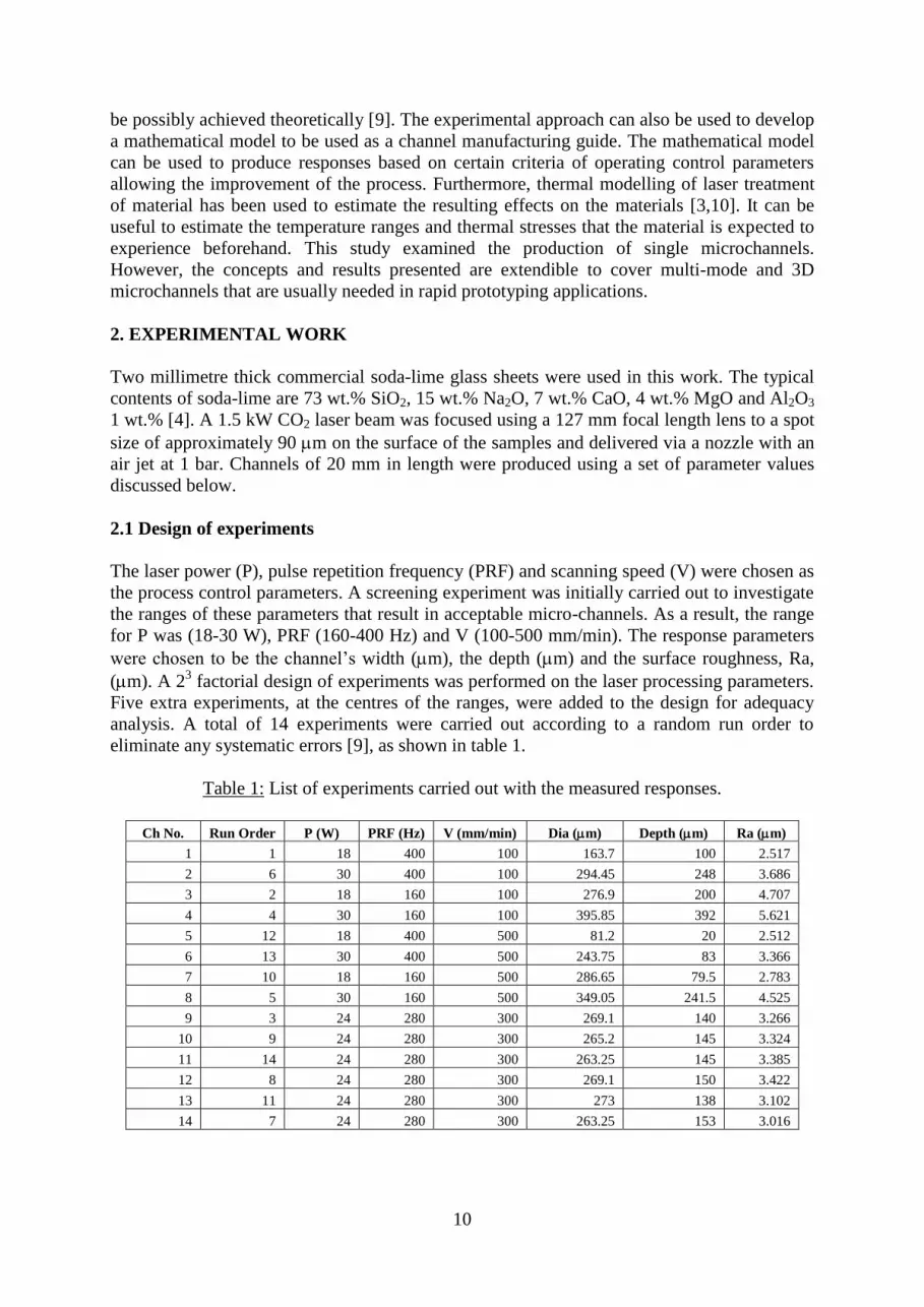
Figure 4 (a) shows the response surface due to P and PRF as the most significant control
parameters for this response. The response contour of P versus PRF is shown in figure 4 (b).
A general inspection of figure 4 (b) shows that as PRF is increased the channel width is
decreased. On the contrary, increasing P increases the channel width and vice versa.
Figure 4: Width model: P and PRF effect, (a) 3D response surface, (b) P vs. PRF contours.
3.2 Channel depth model
Table 3 lists the ANONA analysis results for the depth model. The Model F-value of 422.317
implies the model is significant. The significant model terms are P, PRF, V, P*PRF, P*V and
P*PRF*V. The "Curvature F-value" of 53.379 implies there is significant curvature in the
design space. The "Lack of Fit F-value" of 2.595 implies the Lack of Fit is not significant
relative to the pure error. R2, adjusted R
2 and predicted R
2 in table 3, are all close to 1, and in
reasonable agreement indicating an adequate model. The adequacy precision is also greater
than 4 indicating adequate model discrimination. As in the case of the width model, the
response surface was used to predict depths within the investigated range of paramters.

14
Table 3: ANOVA analysis of the depth model
Source Sum of
Squares DF
Mean
Square
F
Value Prob > F
Model 104453 6 17408.83 422.317 < 0.0001 significant
P 39903.13 1 39903.13 968.00 < 0.0001
PRF 26680.5 1 26680.5 647.236 < 0.0001
V 33282 1 33282 807.380 < 0.0001
P*PRF 2556.125 1 2556.125 62.0084 0.0002
P*V 1653.125 1 1653.125 40.103 0.0007
P*PRF*V 378.125 1 378.125 9.173 0.0231
Curvature 2200.381 1 2200.381 53.379 0.0003 significant
Residual 247.333 6 41.222
Lack of Fit 84.5 1 84.5 2.595 0.1681 not significant
Pure Error 162.833 5 32.567
Cor Total 106900.7 13
R-Squared = 0.998 Adj R-Squared = 0.995
Pred R-Squared = 0.947 Adeq Precision = 76.647
As explained earlier, P and PRF control the magnitude of energy deposited and hence the
depth of the channel. The translation speed V is also inversely proportional to the rate of heat
deposition. Figure 5 (a) shows the predicted versus actual channel depth and Figure 5 (b)
shows the interaction effects.
Figure 5: Analysis of depth model (a) actual vs. predicted channel depth, and
(b) parameter interaction.
Figure 6 (a) and (b) show the response plots for P and PRF as the interaction of these two
parameters is more significant than the speed effect. Figure 6 (b) shows that as PRF is
increased the channel depth is decreased. However, increasing P increases the channel depth
and vice versa.

15
Figure 6: Depth model: P and PRF effect (a) 3D response surface, (b) P vs. PRF contours.
3.3 Channel surface roughness model
The Model F-value of 61.504 implies the model is significant. The significant model terms
are P, PRF, V, PRF*V and P*PRF*V. The "Curvature F-value" of 24.254 implies there is
significant curvature in the design space. The "Lack of Fit F-value" of 1.495 implies the Lack
of Fit is not significant relative to the pure error. R2, adjusted R
2 and predicted R
2 in table 4,
are all close to 1, and in reasonable agreement indicating an adequate model. The adequacy
precision is also greater than 4. The mathimatical model for the width is not hirarchical and
hence the formation of a mathimatical equation was not possibel. However, the response
surface is used instead to predict widths within the investigated range of paramters.
Table 4: ANOVA analysis of the surface roughness model
Source Sum of
Squares DF
Mean
Square
F
Value Prob > F
Model 9.139 5 1.828 61.504 < 0.0001 significant
P 2.771 1 2.771 93.233 < 0.0001
PRF 3.898 1 3.898 131.155 < 0.0001
V 1.395 1 1.394 46.923 0.0002
PRF*V 0.911 1 0.911 30.664 0.0009
P*PRF*V 0.165 1 0.165 5.543 0.0508
Curvature 0.721 1 0.721 24.254 0.0017 significant
Residual 0.208 7 0.0297
Lack of
Fit 0.078 2 0.0389 1.495 0.3097 not significant
Pure Error 0.1302 5 0.026
Cor Total 10.068 13
R-Squared = 0.978 Adj R-Squared = 0.962
Pred R-Squared = 0.858 Adeq Precision = 26.646
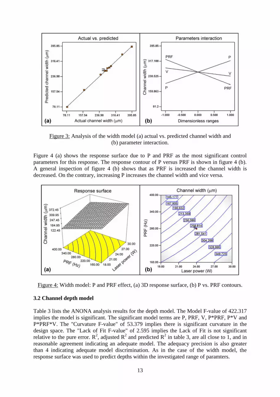
Figure 7 (a) shows the actual versus the predicted surface roughness values, the data points
are distributed along the diagonal indicating a good fit of the model. Figure 7 (b) shows the
interactive effect of the parameters on the response. Naturally, in the case of a pulsed laser
source, the power, P affects the magnitude in surface roughness through the fluctuations in the
16
channel depth, as in figure 1. However, the distance between the successive fluctuations is
controlled by PRF and V. In this study the roughness was measured along the translation
direction, hence, it is more interesting to study the effect of PRF and V on the roughness.
Figure 7: Analysis of roughness model (a) actual vs. predicted channel roughness, and
(b) parameter interaction.
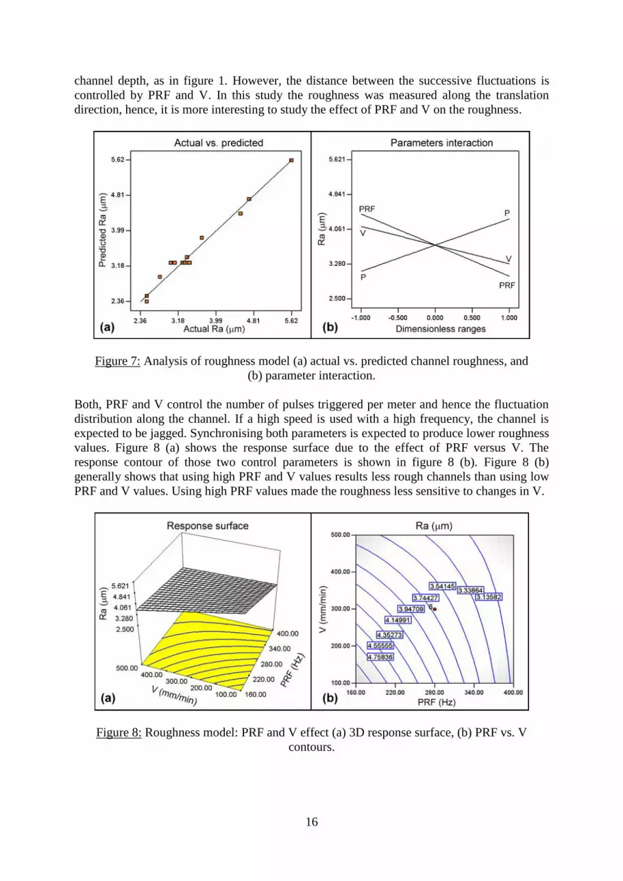
Both, PRF and V control the number of pulses triggered per meter and hence the fluctuation
distribution along the channel. If a high speed is used with a high frequency, the channel is
expected to be jagged. Synchronising both parameters is expected to produce lower roughness
values. Figure 8 (a) shows the response surface due to the effect of PRF versus V. The
response contour of those two control parameters is shown in figure 8 (b). Figure 8 (b)
generally shows that using high PRF and V values results less rough channels than using low
PRF and V values. Using high PRF values made the roughness less sensitive to changes in V.
Figure 8: Roughness model: PRF and V effect (a) 3D response surface, (b) PRF vs. V
contours.
17
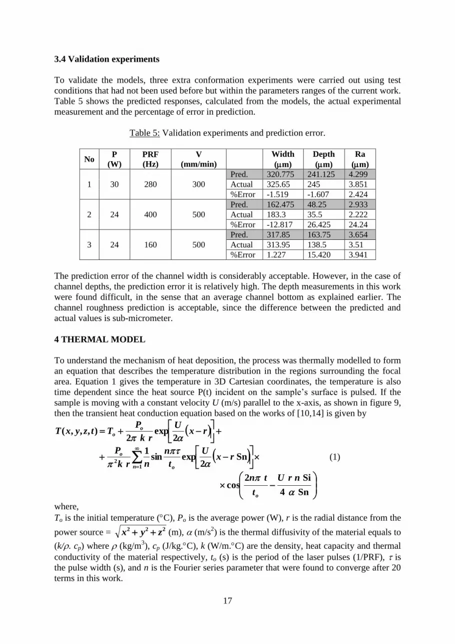
3.4 Validation experiments
To validate the models, three extra conformation experiments were carried out using test
conditions that had not been used before but within the parameters ranges of the current work.
Table 5 shows the predicted responses, calculated from the models, the actual experimental
measurement and the percentage of error in prediction.
Table 5: Validation experiments and prediction error.
No P
(W)
PRF
(Hz)
V
(mm/min)
Width
(m)
Depth
(m)
Ra
(m)
1 30 280 300
Pred. 320.775 241.125 4.299
Actual 325.65 245 3.851
%Error -1.519 -1.607 2.424
2 24 400 500
Pred. 162.475 48.25 2.933
Actual 183.3 35.5 2.222
%Error -12.817 26.425 24.24
3 24 160 500
Pred. 317.85 163.75 3.654
Actual 313.95 138.5 3.51
%Error 1.227 15.420 3.941
The prediction error of the channel width is considerably acceptable. However, in the case of
channel depths, the prediction error it is relatively high. The depth measurements in this work
were found difficult, in the sense that an average channel bottom as explained earlier. The
channel roughness prediction is acceptable, since the difference between the predicted and
actual values is sub-micrometer.
4 THERMAL MODEL
To understand the mechanism of heat deposition, the process was thermally modelled to form
an equation that describes the temperature distribution in the regions surrounding the focal
area. Equation 1 gives the temperature in 3D Cartesian coordinates, the temperature is also
time dependent since the heat source P(t) incident on the sample’s surface is pulsed. If the
sample is moving with a constant velocity U (m/s) parallel to the x-axis, as shown in figure 9,
then the transient heat conduction equation based on the works of [10,14] is given by
Sn4
Si2cos
Sn2
expsin1
2exp
2),,,(
12
nrU
t
tn
rxU
t
n
nrk
P
rxU
rk
PTtzyxT
o
n o
o
o
o
(1)
where,
To is the initial temperature (C), Po is the average power (W), r is the radial distance from the
power source = 222 zyx (m), (m/s2) is the thermal diffusivity of the material equals to
(k/. cp) where (kg/m3), cp (J/kg.C), k (W/m.C) are the density, heat capacity and thermal
conductivity of the material respectively, to (s) is the period of the laser pulses (1/PRF), is
the pulse width (s), and n is the Fourier series parameter that were found to converge after 20
terms in this work.

18
2
8Si
Uto
, is Simon’s number [10] that characterises a periodic solution with period to, and
2
Si11Sn
22n
Figure 9: Heat point source on the surface of the workpiece.
Equation 1 was used to estimate the fabricated channel geometry based on the vaporisation
temperature of glass Tv 3500 C [6]. The calculations were performed in a software code
that has been developed specifically for this work. The laser beam was assumed to be initially
at (0,0,0), and the laser radiation was propagated in the positive x-axis. Figure 10 (a) and (b)
show the 3D predicted geometry of channel 12 from table 1 and the experimentally scanned
channel. The pulse width in this case was = 1.531 ms. The predicted and scanned lengths on
the x-axis correspond to one laser pulse = (U / PRF). The model solution is periodic along the
x-axis, hence, a close inspection of the side views in figure 11 (a) and (b) shows the similarity
of both the predicted and experimental geometries. The top of side view in figure 11 (b) has
been truncated for better visualisation.
Figure 10: 3D views of channel number 12, (a) predicted and (b) experimental scan. All
measurements are in μm.

19
Figure 11: Side views of channel number 12, (a) predicted and (b) experimental scan. All
measurements are in μm.
The channel width, depth and surface roughness were calculated from the modelled geometry.
The predicted channel parameters from the thermal model were 240 μm, 116.1 μm and 3.56
μm for the width, depth and roughness respectively. Comparing these predicted values with
the values corresponding to channel 12 in table 1, shows that the prediction error values are -
12.13, -29.19 and 3.88 % respectively. The relatively large width and depth prediction errors
are due to the assumptions made in the thermal model. However, the small roughness
prediction error indicates that the model is capable of estimating the resulting periodic
geometry of such a process [3].
5 CONCLUSION AND RECOMMENDATIONS
The process of rapid laser channel fabrication has been experimentally studied and RSM
models describing the channel characteristics were developed. The statistical models are able
to predict channel width, depth and roughness within the investigated range of control
parameters. The operating parameters can be selected based on criteria to suit the desired
channel characteristics. Other response parameters such as roundness and shape quality
factors could be studied in the future. In this work, a mathematical thermal model was
developed based on the same process control parameters. This model was able to,
theoretically, predict the temperature distribution in the sample; and hence estimate of the
channel width, depth and surface roughness. Such results from the thermal model are useful in
comparing the experimental dimensional measurements to those predicted by the theoretical
thermal model. An additional advantage of the thermal model is that it enables a better
understanding of the factors that affect the proportions of the channel geometry via visual
results without the need to conduct experiments.
References:
[1] M. Müllenborn, M. Henschel, U. D. Larsen, H. Dirac and S. Bouwstra, J. Micromech.
Microeng., 1996, 6, pp. 49-51.
[2] K. C. Yung, S. M. Mei and T. M. Yue, J. Micromech. Microeng., 2004, 14, pp. 1682-
1686.
[3] W. W. Duley, Laser processing and analysis of materials, (Plenum Press, 1982).

20
[4] N. P. Bansal and R. H. Doremus, Handbook of glass properties, (Academic Press Inc.,
1986).
[5] J. O. Isard, Infrared Physics, 1980, Vol. 20, pp. 249-256.
[6] L. J. Radziemski and D. A. Cremers, Laser-induced plasmas and applications, (Marcel
Dekker Inc., 1989).
[7] S. J. Qin and W. J. Li, Sensors and Actuators A, 2002, 97-98, pp. 749-757.
[8] S.-C. Wang, C.-Y. Lee and H.-P. Chen, Journal of Chromatography A, 2006, 1111, pp.
252-257.
[9] D. C. Montgomery, Design and analysis of experiments, (John Wiley and Sons Inc.,
1984).
[10] J. M. Dowden, The mathematics of thermal modelling: an introduction to the theory of
laser material processing, (Chapman and Hall CRC, 2001).
[11] D. Collins, Development of laser based surface profilometer using the principle of
optical triangulation, MEng thesis, (DCU, 2005).
[12] Design-Expert software, “v6, user’s guide, Technical manual”, Stat-Ease Inc., 2000.
[13] D. M. Grove and T. P. Davis, Engineering, quality and experimental design, (Longman,
1998).
[14] H. S. Carslaw and J. C. Jaeger, Conduction of heat in solids, 2nd
edition (Oxford
University Press, 1959).