implementação de pré-codificador sm-mimo para 4g/lte em
TRANSCRIPT

Universidade de AveiroDepartamento de Eletrónica,Telecomunicações e Informática
2014
Bruno Miguel
Fernandes Silva
Implementação de pré-codificador SM-MIMO para
4G/LTE em plataforma SDR
Implementation of a SM-MIMO precoder for 4G/LTE
in a SDR platform

“A gentleman who rode along the sidewalk in front of them, sud-
denly stepped off the conveyor belt, pulled a phone from his coat
pocket, spoke a number into it and shouted: "Gertrude, listen, I’ll
be an hour late for lunch because I want to go to the laboratory.
Goodbye, sweetheart!" Then he put his pocket phone away again,
stepped back on the conveyor belt, started reading a book...”
— Der 35. Mai oder Konrad reitet in die Südsee
Erich Kästner - 1931
Universidade de AveiroDepartamento de Eletrónica,Telecomunicações e Informática
2014
Bruno Miguel
Fernandes Silva
Implementação de pré-codificador SM-MIMO para
4G/LTE em plataforma SDR
Implementation of a SM-MIMO precoder for 4G/LTE
in a SDR platform

Universidade de AveiroDepartamento de Eletrónica,Telecomunicações e Informática
2014
Bruno Miguel
Fernandes Silva
Implementação de pré-codificador SM-MIMO para
4G/LTE em plataforma SDR
Implementation of a SM-MIMO precoder for 4G/LTE
in a SDR platform
Dissertação apresentada à Universidade de Aveiro para cumprimento dos re-quisitos necessários à obtenção do grau de Mestre em Engenharia Eletrón-ica e Telecomunicações, realizada sob a orientação científica do DoutorManuel Alberto Reis de Oliveira Violas, Professor auxiliar do Departamentode Eletrónica, Telecomunicações e Informática da Universidade de Aveiro, edo Doutor Adão Paulo Soares da Silva, Professor auxiliar do Departamentode Eletrónica, Telecomunicações e Informática da Universidade de Aveiro.


Dedico este trabalho à minha família, amigos e colegas.

o júri / the jury
presidente / president Prof. Doutor Paulo Miguel Nepomuceno Pereira MonteiroProfessor Associado do Departamento de Engenharia Eletrónica, Telecomunicações e Informát-
ica da Universidade de Aveiro
vogais / examiners committee Doutor Nelson José Valente SilvaInvestigador, Pt Inovação e Sistemas
Professor Doutor Manuel Alberto Reis de Oliveira ViolasProfessor Auxiliar do Departamento de Engenharia Eletrónica, Telecomunicações e Informática
da Universidade de Aveiro


agradecimentos /
acknowledgements
Agradeço aos meus orientadores por toda a ajuda e apoio neste último ano.À minha família por todo o apoio e motivação ao longo do meu percursoacadémico. Agradeço aos colegas e amigos por toda a ajuda e apoio dur-ante o meu percurso académico.

Palavras Chave 4G, LTE, SDR, OFDM, LTE, SM-MIMO, Multiplexagem espacial, Equalização,ZF, MMSE, Pré-Codificação, FPGA, System Generator, MIMO
Resumo O tema central deste trabalho de dissertação centra-se no desenvolvimentoe teste de novas técnicas para utilização em comunicações sem-fios de novageração. Foca-se no uso de várias antenas, técnicas de pré-codificação eno uso de multiplexagem espacial em detrimento de diversidade, de formaa aumentar a largura de banda. Ao longo do documento são apresentadasvárias técnicas de multiplexagem, bem como bases teóricas de propagaçãode sinais rádio e técnicas baseadas no uso de várias antenas no emissore recetor (MIMO). Foi proposto um sistema de pré-codificação baseado emdiversidade espacial. A implementação e teste do bloco pré-codificador SM-MIMO foi realizada em primeiro lugar usando um simulador Matlab para efeitode comparação. Foram implementados dois equalizadores: Zero Forcing (ZF)e Minimum Mean Square Error (MMSE); posteriormente procedeu-se à imple-mentação em System Generator de um pré-codificador com equalização ZF,de forma a ser possível a sua implementação em FPGAs. Esta implementa-ção foi igualmente validada por comparação com o bloco implementado emMatlab.


Keywords 4G, LTE, SDR, OFDM, LTE, SM-MIMO,Spatial Multiplexing,Precoding, ZF,MMSE, FPGA, System Generator, MIMO
Abstract The main goal of this dissertation is the development and evaluation of newtechniques to be used in new generation of wireless comunication devices.It focuses on the usage of multiple antennas (MIMO), precoding and the us-age of spatial multiplexing in disregard of diversity techniques. This makespossible to increase data rates considerably. Throughout the document, areshown several multiplexing techniques, theoretical information about wirelesspropagation, and multiple antennas techniques. It was proposed and imple-mented a spatial multiplexing system. Firstly it was implemented in Matlab,with two precoders tested: Zero Forcing (ZF) and Minimum Mean Square Er-ror (MMSE). Subsequently a System Generator implementation (this time withonly ZF equalizer) was made in order to make possible the migration to FP-GAs. Both implementations were tested and validated, we also concluded thatZF based pre-coder had a lower Bit Error Rate for the same Signal to NoiseRatio (SNR).

Contents
Contents i
List of Figures iii
List of Tables v
Glossary vii
1 Introduction 1
1.1 4G/LTE by Third Generation Partnership Project (3GPP) 1
1.2 Motivation 2
1.3 Objectives 3
1.4 Document Structure 3
2 Wireless signals propagation 5
2.1 Wireless Channel 5
2.1.1 Propagation characteristics: Path Loss 6
2.1.2 Shadowing Effect 8
2.1.3 Multipath fading 8
2.2 Multiplexing Techniques 8
2.2.1 Time-Division Multiplexing (TDM) 8
2.2.2 Frequency-Division Multiplexing (FDM) 9
2.2.3 Orthogonal Frequency Division Multiplexing (OFDM) 9
2.3 Channel Estimation 12
2.3.1 Receiver Side 12
2.3.2 Transmitter Side 14
3 Multiple Antennas techniques 15
3.1 Diversity Techniques 16
3.1.1 Antennas diversity 16
3.1.2 Receive diversity 17
i
3.1.3 Transmitter diversity 18
3.2 Multiplexing Techniques 19
3.2.1 Spatial Multiplexing MIMO (SM-MIMO) 19
3.2.2 Linear Signal Detection for Spatial Multiplexing MIMO (SM-
MIMO) 19
3.2.3 Spatial Multiplexing MIMO (SM-MIMO) with precoding 21
4 Field Programmable Gate Arrays (FPGAs) 23
4.1 FPGA 23
4.2 System Generator 25
5 Implementation and Results 27
5.1 Proposed System 27
5.2 SM-MIMO Matlabr simulation 28
5.3 System Generator implementation 29
6 Conclusion and Future Work 37
6.1 Conclusion 37
6.2 Future Work 37
Appendix A SM-MIMO Matlabr Simulator 39
References 45
ii
List of Figures
1.1 Third Generation Partnership Project (3GPP) Mobile Communication Genera-
tions 1
1.2 Evolution of various services subscriptions over time [5] 3
1.3 Comparison between developed and underdeveloped countries [5]: (a) Mobile
phone’s subscriptions (b) Mobile-broadband subscriptions 3
2.1 Types of interference: (a) Diffraction and (b) Reflection 5
2.2 Types of interference: (a) Scattering and (b) Shadowing 6
2.3 Different types of attenuations 6
2.4 Types of Antennas: (a) Isotropic (b) Directional 6
2.5 Time-Division Multiplexing (TDM) 8
2.6 Frequency-Division Multiplexing (FDM) 9
2.7 Pulse signal single carrier: (a) Time domain (b) Frequency domain 10
2.8 Orthogonal Frequency Division Multiplexing (OFDM) sub-carriers symbols 10
2.9 OFDM banks: (a) modulator (b) correlator/demodulator 11
2.10 OFDM symbol with Cycle-Prefix 11
2.11 Pilots arrangement: Block-Type (adapted from: [14]) 12
2.12 Pilots arrangement: (a) Comb-type (b) Lattice-type (adapted from: [14]) 13
2.13 Reciprocal Multi-Input-Multi-Output (MIMO) channel 14
2.14 Relay MIMO channel 14
3.1 Error probability of Additive White Gaussian Noise (AWGN) and Rayleigh Flat
Fading channels 16
3.2 Antenna setups: (a) Single Input Single Output (SISO) (b) Single Input Multiple
Output (SIMO) (c) Multiple Input Single Output (MISO) (d) MIMO 17
3.3 Linearly combine signals at the receiver 17
3.4 Linear signal detection at the receiver block-set 19
3.5 Error probabilities of Zero Forcing (ZF) and Minimum Mean Square Error (MMSE)
(Monte Carlo trials and high Signal-to-Noise Ratio (SNR) approximation) M=N=4
(source [24]) 20
iii
3.6 Linear pre-equalization block-set 21
3.7 Performance comparison: receiver-side ZF/MMSE vs. pre-MMSE equalization
(source [14]) 21
4.1 Basic Configurable Logic Blocks (CLBs) structure (source [25]) 23
4.2 Interface between System Generator and Simulink blockset 25
4.3 Example of System Generator blocks 25
5.1 Proposed system diagram – frequency implementation 27
5.2 SM-MIMO Bit Error Rate (BER) for ZF and MMSE precoders 28
5.3 Eb/N0=8: (a) Wzf (b) alpha_zf*Wzf 28
5.4 Eb/N0=8: (a) Yzf (b) 1/alpha_zf*Yzf 29
5.5 SM-MIMO implementation: main block 29
5.6 SM-MIMO implementation: [baseband] block 30
5.7 SM-MIMO implementation: [inv H] block 31
5.8 SM-MIMO implementation: (a) [h00*h11] block (b) [h01*h10] block 32
5.9 SM-MIMO implementation: [alpha_zf] block 32
5.10 SM-MIMO implementation: [alphazf*W] block 33
5.11 SM-MIMO implementation: [W*S] block 34
5.12 SM-MIMO precoder comparison between MATLABr and System Generator
implementations: (a) Channel Invertion [W ] = [H]−1 (b) alpha_zf [W ] 35
iv
List of Tables
2.1 Attenuation scenarios (source: [7]) 7
2.2 Comparison between Time-Division Multiplexing (TDM) and Frequency-Division
Multiplexing (FDM) (source: [10]) 9
3.1 Alamouti coding 18
4.1 Xilinx Field Programmable Gate Array (FPGA) families (source: [25]) 24
v

Glossary
1G First Generation. 1
2G Second Generation. 2
3G Third Generation. 2
3GPP Third Generation Partnership Project. i,iii, 1
4G Fourth Generation. i, 1, 2
5G Fifth Generation. 2
ADSL Asymmetric Digital Subscriber Line. 2
AGC Automatic Gain Control. 21
AMPS Advanced Mobile Phone System. 2
ARIB The Association of Radio Industries andBusinesses, Japan. 1
ATIS The Alliance for Telecommunications In-dustry Solutions, USA. 1
AWGN Additive White Gaussian Noise. iii, 15,16, 28
BER Bit Error Rate. iv, 12, 15, 16, 19, 28, 29,37
BS Base Station. 3, 5, 14, 37
CCSA China Communications Standards Asso-ciation. 1
CDMA Code Division Multiple Access. viii, 2
CLB Configurable Logic Block. iv, 23
CSI Channel State Information. 18, 19, 21
DFT Discrete Fourier Transform. 11
EDA Electronic Design Automation. 24
EEPROM Electrically-Erasable ProgrammableRead-Only Memory. 24
EGC Equal Gain Combining. 18
ETSI The European Telecommunications Stand-ards Institute. 1
EV-DO Evolution-Data Optimized. 2
FDD Frequency Division Duplexing. 14, 18
FDM Frequency-Division Multiplexing. i, iii, v,4, 9
FFT Fast Fourier Transform. 11
FPGA Field Programmable Gate Array. ii, v, 3,4, 23–25, 27, 29, 37
GPRS General Packet Radio Service. 2
GSM Global System for Mobile Communications.2
GUI Graphical User Interface. 25, 29
HDL Hardware Description Language. 23
HSDPA High-Speed Downlink Packet Access. 2
HSPA High Speed Packet Access. 2
HSUPA High-Speed Uplink Packet Access. 2
IDFT Inverse Discrete Fourier Transform. 11
IFFT Inverse Fast Fourier Transform. 11, 12
IP Internet Protocol. viii, 2
ISI Intersymbol interference. 10
JTAG Join Test Action Group. 24
LOG Logarithm base 10. vii
LOS Line-of-Sight. 5–7
LTE Long Term Evolution. i, 1, 2, 18
vii
MIMO Multi-Input-Multi-Output. ii, iii, viii, 3,14, 16, 17, 19, 21, 27
MISO Multiple Input Single Output. iii, 3, 16–18
MMSE Minimum Mean Square Error. iii, iv, 20,21, 28, 29, 37
MRC Maximum-Ratio Combining. 17
MS Mobile Station. 5, 14, 37
NMT Nordic Mobile Telephone. 2
NTT Nippon Telegraph & Telephone Corp. 1, 2
OFDM Orthogonal Frequency Division Multi-plexing. i, iii, 3, 4, 9–12, 28
OTP One-Time Programmable. 23
PSD Power Spectral Density. 8, 15
QoS Quality of Service. 2
RAM Random-Access Memory. 23
RF Radio Frequency. 3, 14
SC Selection Combining. 18
SDR Software Defined Radio. 3
SIMO Single Input Multiple Output. iii, 16, 17
SINR Signal-to-Interference-plus-Noise Ratio.20
SISO Single Input Single Output. iii, 15, 17
SM-MIMO Spatial Multiplexing MIMO. ii, iv,3, 19, 21, 27–35, 37, 39
SMS Short Message Service. 2
SNR Signal-to-Noise Ratio. iii, 15, 16, 18, 20, 28,29
SRAM Static Random-Access Memory. 23
TDD Time Division Duplexing. 14, 18
TDM Time-Division Multiplexing. i, iii, v, 4, 8,9
TDMA Time Division Multiple Access. 2
TTA Telecommunications Technology Associ-ation, Korea. 1
TTC Telecommunication Technology Committee,Japan. 1
UHF Ultra High Frequency. 5
UMTS Universal Mobile TelecommunicationsSystem. 2
USB Universal Serial Bus. 2
VHDL VHSIC Hardware Description Language.23
VHF Very High Frequency. 5
VHSIC Very-High-Speed Integrated Circuits.viii
VoIP Voice Over IP. 2
WCDMA Wideband CDMA. 2
WiMAX Worldwide Interoperability for Mi-crowave Access. 2
ZF Zero Forcing. iii, iv, 19–21, 28, 37
viii
chapter 1Introduction
This chapter will present the mobile communications generations, motivations, objectives and outlinethe document structure.
1.1 4G/LTE by Third Generation Partnership
Project (3GPP)
The development of Telecommunications in the last decades, made the communication between topersons in any two points of the earth surface, extending even into space. Remote locations became lesscommon and concepts as: mobility, portability, mobile phone became part of our life. The main reasonsfor these outcomes were the low price and worldwide availability of telecommunication technology.
The globalization of telecommunications was only possible due to the efforts and work of the3GPP [1] organization. 3GPP is a global standards-developing organization [2] comprised by sixinternational standard’s organizations [3]: The Association of Radio Industries and Businesses, Japan(ARIB), The Alliance for Telecommunications Industry Solutions, USA (ATIS), China CommunicationsStandards Association (CCSA), The European Telecommunications Standards Institute (ETSI), Tele-communications Technology Association, Korea (TTA) and Telecommunication Technology Committee,Japan (TTC). This partnership gave birth to most of the telecomunications’ wireless standards thatwe have today.
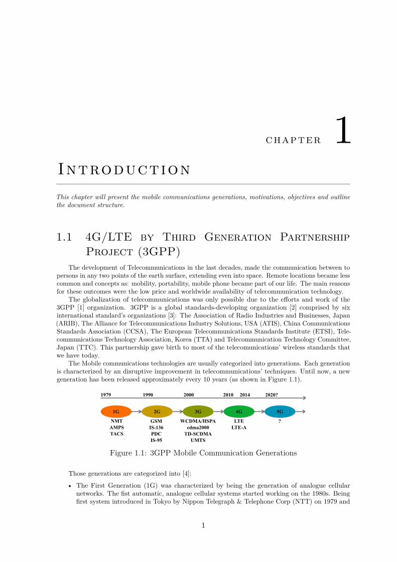
The Mobile communications technologies are usually categorized into generations. Each generationis characterized by an disruptive improvement in telecommunications’ techniques. Until now, a newgeneration has been released approximately every 10 years (as shown in Figure 1.1).
Figure 1.1: 3GPP Mobile Communication Generations
Those generations are categorized into [4]:
• The First Generation (1G) was characterized by being the generation of analogue cellularnetworks. The fist automatic, analogue cellular systems started working on the 1980s. Beingfirst system introduced in Tokyo by Nippon Telegraph & Telephone Corp (NTT) on 1979 and
1
then widely deployed through the rest of Japan. Afterwards, another system was adopted inthe Nordic countries by Nordic Mobile Telephone (NMT) (1981)and lastly the Advanced MobilePhone System (AMPS) (1983). Over the following years other analogue systems were adoptedthroughout the rest of the world.
• The Second Generation (2G) was a great improvement of mobile communications, and marks thestart of the digital cellular networks. The integration started around the 1990s with two majorsystems appearing on the market: the European Global System for Mobile Communications(GSM), Time Division Multiple Access (TDMA) based standard and the American, CodeDivision Multiple Access (CDMA) based. The two standards competed globally for the marketsupremacy. This phase was also characterized by the appearance of the prepaid mobile phones.The main highlights of this era: in 1991, the first GSM network on Finland was launched, in1993 was introduced the world first smartphone (IBM Simon Personal Communicator) wasintroduced, the first Short Message Service (SMS) was sent on 3rd December 1992 betweentwo machines and the Japanese company NTT introduced the first internet service in 1999.Following the standards "war", the first data systems implemented were CDMA2000 1X (CDMAbased) and General Packet Radio Service (GPRS) (GSM based).
• Third Generation (3G) was introduced to cater the huge demand for data communications(Internet, and other broadband data). The main differences to the 2G was the data transmissionwhich became packet switching based rather than circuit switching. Another difference was theimposition of a minimum data rate for indoors and outdoors. To archive those requirements,several technologies were developed. Once more, two rival standards appeared WidebandCDMA (WCDMA) (Universal Mobile Telecommunications System (UMTS)) and Evolution-Data Optimized (EV-DO). There were some new features introduced in the protocol in order toprovide Voice Over IP (VoIP) such as Quality of Service (QoS) and real-time mechanisms. Inmid 2000, in order to increase the data rate even further, the High Speed Packet Access (HSPA)family was implemented. High-Speed Downlink Packet Access (HSDPA) and High-Speed UplinkPacket Access (HSUPA), offering speeds of 14.4 Mbit/s for downlink and 5.76 MBit/s for uplink.
• The Fourth Generation (4G) is the current state of the art in public mobile communications.All the circuit switching were removed becoming full Internet Protocol (IP) networks. Twostandards appeared, the Worldwide Interoperability for Microwave Access (WiMAX) and theLong Term Evolution (LTE). The technological improvement in this generation is to bringmobile ultra-broadband Internet access to laptops, smartphones, Universal Serial Bus (USB)dongles, and other devices.
• Fifth Generation (5G) is currently under development. There are three possible areas ofimprovement in comparison to the 4G namely: a super-efficient mobile network, super-fastmobile network and converged fiber-wireless networks.
1.2 motivation
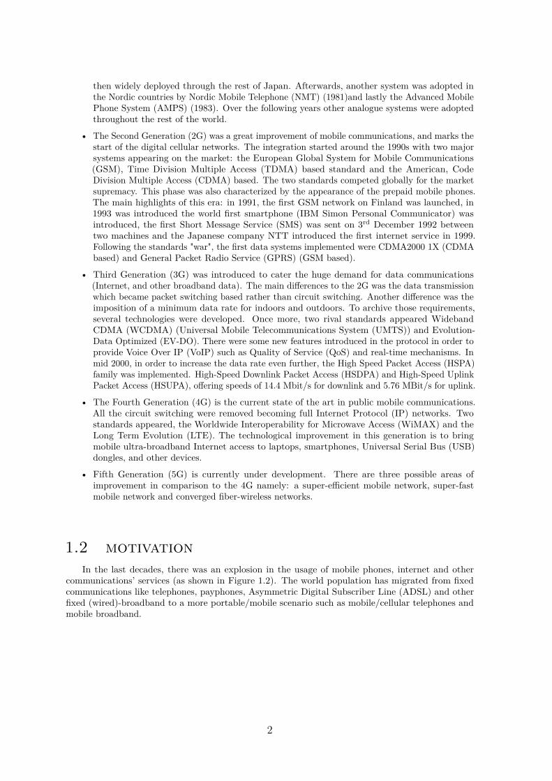
In the last decades, there was an explosion in the usage of mobile phones, internet and othercommunications’ services (as shown in Figure 1.2). The world population has migrated from fixedcommunications like telephones, payphones, Asymmetric Digital Subscriber Line (ADSL) and otherfixed (wired)-broadband to a more portable/mobile scenario such as mobile/cellular telephones andmobile broadband.
2
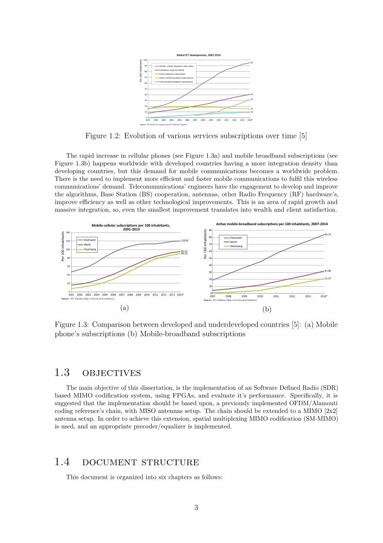
Figure 1.2: Evolution of various services subscriptions over time [5]
The rapid increase in cellular phones (see Figure 1.3a) and mobile broadband subscriptions (seeFigure 1.3b) happens worldwide with developed countries having a more integration density thandeveloping countries, but this demand for mobile communications becomes a worldwide problem.There is the need to implement more efficient and faster mobile communications to fulfil this wirelesscommunications’ demand. Telecommunications’ engineers have the engagement to develop and improvethe algorithms, Base Station (BS) cooperation, antennas, other Radio Frequency (RF) hardware’s,improve efficiency as well as other technological improvements. This is an area of rapid growth andmassive integration, so, even the smallest improvement translates into wealth and client satisfaction.
(a) (b)
Figure 1.3: Comparison between developed and underdeveloped countries [5]: (a) Mobilephone’s subscriptions (b) Mobile-broadband subscriptions
1.3 objectives
The main objective of this dissertation, is the implementation of an Software Defined Radio (SDR)based MIMO codification system, using FPGAs, and evaluate it’s performance. Specifically, it issuggested that the implementation should be based upon, a previously implemented OFDM/Alamouticoding reference’s chain, with MISO antennas setup. The chain should be extended to a MIMO [2x2]antenna setup. In order to achieve this extension, spatial multiplexing MIMO codification (SM-MIMO)is used, and an appropriate precoder/equalizer is implemented.
1.4 document structure
This document is organized into six chapters as follows:
3
• Chapter 1 Introduction: at this chapter we can find the enumeration of the all mobile commu-nications generations, as well as motivation, objectives and the document structure.
• Chapter 2 Wireless Signals Propagation: we start with a description of what is a wireless channeland propagation characteristics such as path loss, shadowing effect and multipath fading. Nextwe proceed with some multiplexing techniques (TDM, FDM and OFDM). The last section ofthis chapter talks about channel estimation and how can we invert its effects.
• Chapter 3 Multiple Antennas techniques: chapter at which, we discuss several diversity techniques(antennas, receive, and transmitter diversity), followed by the presentation of multiplexingtechniques: spatial multiplexing and linear detection with and without precoding.
• Chapter 4 FPGAs: at this chapter we talk about FPGAs: what they are, how can we use them,and the Xilinx tool: System Generator.
• Chapter 5 Implementation and Results: this chapter presents the implementation of the proposedsystem and discusses the obtained results.
• Chapter 6 Conclusions and future work: this chapter presents the conclusions of this work andoutlines some possible future work directions.
4
chapter 2Wireless signalspropagation
This chapter presents the theoretical fundamentals and the state of the art in channel estimation andwireless propagation.
2.1 wireless channel
Wireless channels, on the opposition to coaxial cables and other wired/waveguide’s channels are,more dynamic and, most of the times, temporal and spatially dependent, that is, very unpredictable.The response of a wireless channel varies with the frequency, surroundings (buildings, vegetation,etc.),distance and orientation between Base Station (BS) and Mobile Station (MS), weather factors, existenceof Line-of-Sight (LOS), interference of other sources, and many other parameters. On Very HighFrequency (VHF) and Ultra High Frequency (UHF) bands, the propagation interference mechanismssuch as diffraction, reflection, scattering, shadowing effect, etc. are more dominant.
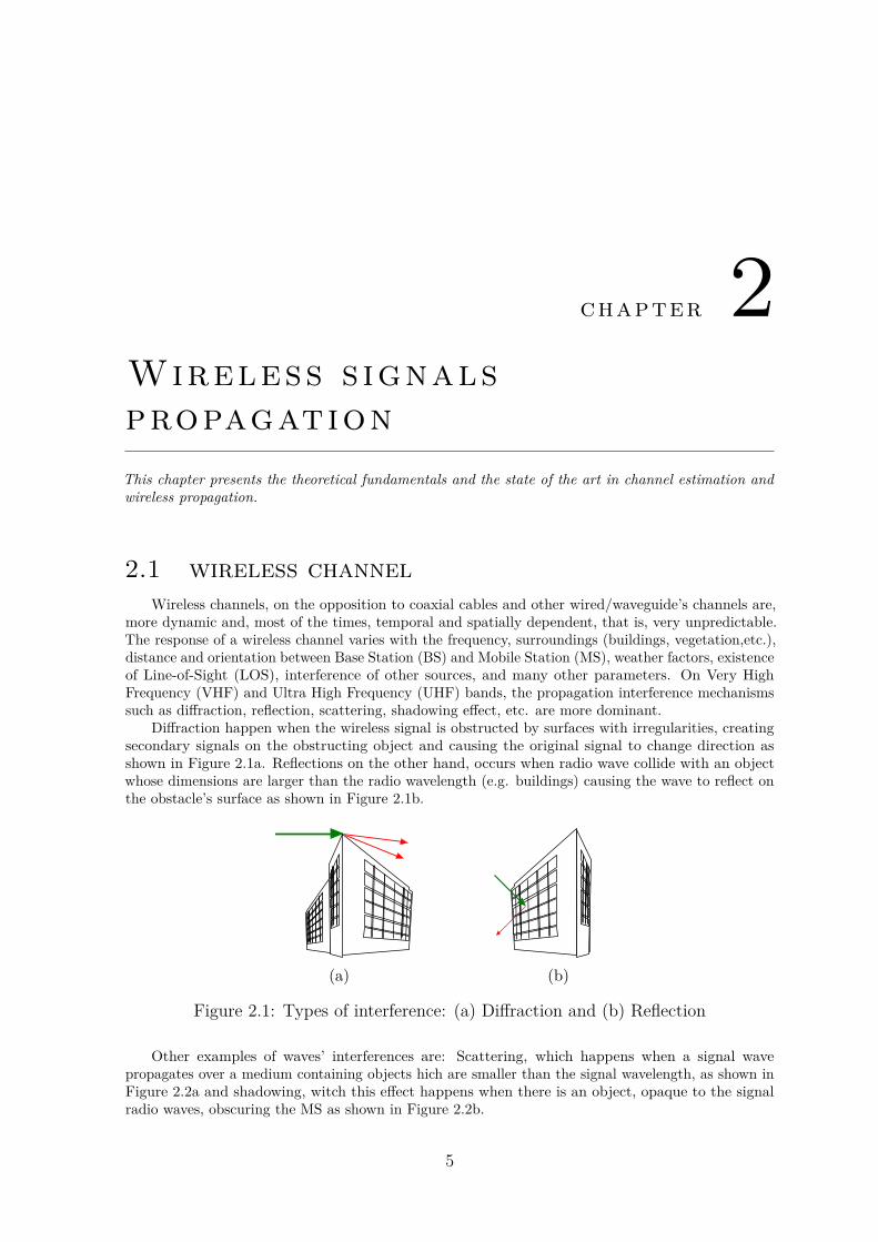
Diffraction happen when the wireless signal is obstructed by surfaces with irregularities, creatingsecondary signals on the obstructing object and causing the original signal to change direction asshown in Figure 2.1a. Reflections on the other hand, occurs when radio wave collide with an objectwhose dimensions are larger than the radio wavelength (e.g. buildings) causing the wave to reflect onthe obstacle’s surface as shown in Figure 2.1b.
(a) (b)
Figure 2.1: Types of interference: (a) Diffraction and (b) Reflection
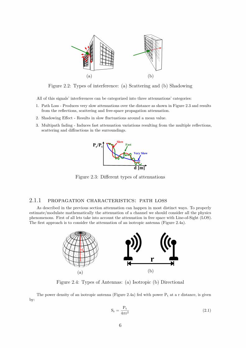
Other examples of waves’ interferences are: Scattering, which happens when a signal wavepropagates over a medium containing objects hich are smaller than the signal wavelength, as shown inFigure 2.2a and shadowing, witch this effect happens when there is an object, opaque to the signalradio waves, obscuring the MS as shown in Figure 2.2b.
5
(a) (b)
Figure 2.2: Types of interference: (a) Scattering and (b) Shadowing
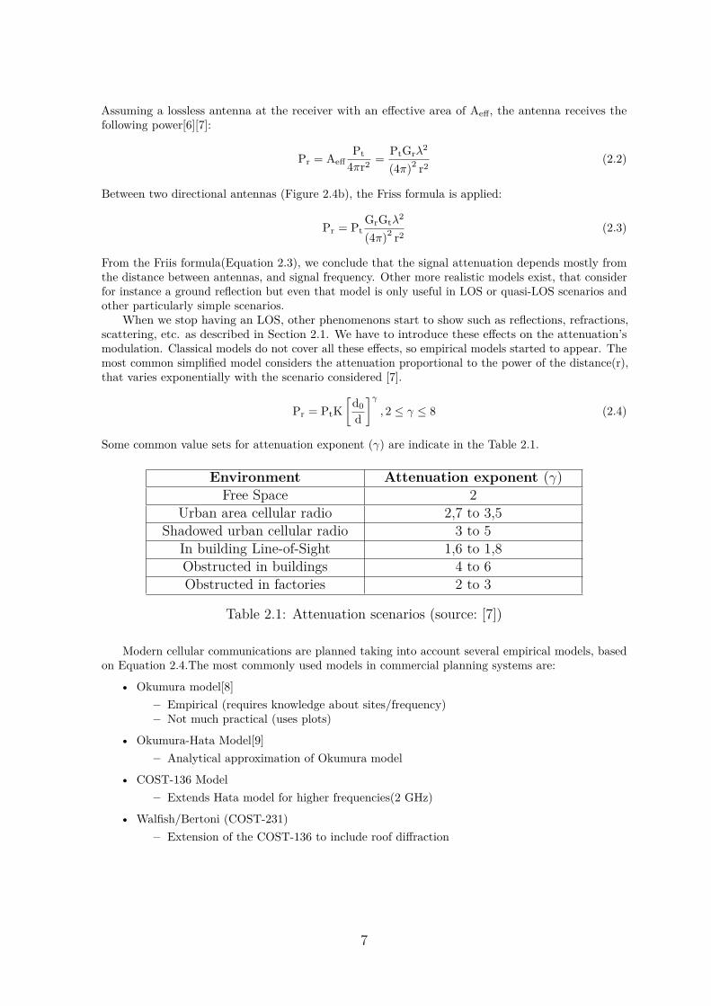
All of this signals’ interferences can be categorized into three attenuations’ categories:
1. Path Loss - Produces very slow attenuations over the distance as shown in Figure 2.3 and resultsfrom the reflections, scattering and free-space propagation attenuation.
2. Shadowing Effect - Results in slow fluctuations around a mean value.
3. Multipath fading - Induces fast attenuation variations resulting from the multiple reflections,scattering and diffractions in the surroundings.
Figure 2.3: Different types of attenuations
2.1.1 propagation characteristics: path lossAs described in the previous section attenuation can happen in most distinct ways. To properly
estimate/modulate mathematically the attenuation of a channel we should consider all the physicsphenomenons. First of all lets take into account the attenuation in free space with Line-of-Sight (LOS).The first approach is to consider the attenuation of an isotropic antenna (Figure 2.4a).
(a) (b)
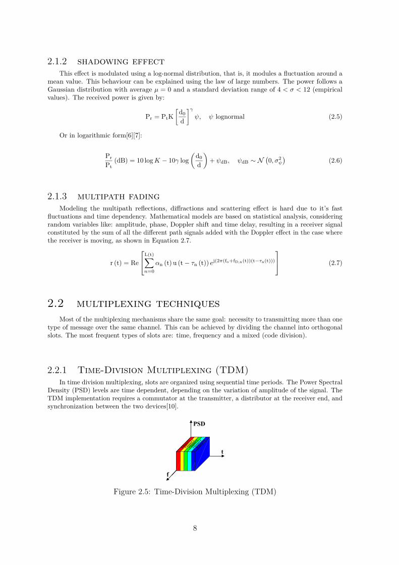
Figure 2.4: Types of Antennas: (a) Isotropic (b) Directional
The power density of an isotropic antenna (Figure 2.4a) fed with power Pt at a r distance, is givenby:
Sr =Pt
4πr2(2.1)
6
Assuming a lossless antenna at the receiver with an effective area of Aeff, the antenna receives thefollowing power[6][7]:
Pr = AeffPt
4πr2=
PtGrλ2
(4π)2
r2(2.2)
Between two directional antennas (Figure 2.4b), the Friss formula is applied:
Pr = PtGrGtλ
2
(4π)2
r2(2.3)
From the Friis formula(Equation 2.3), we conclude that the signal attenuation depends mostly fromthe distance between antennas, and signal frequency. Other more realistic models exist, that considerfor instance a ground reflection but even that model is only useful in LOS or quasi-LOS scenarios andother particularly simple scenarios.
When we stop having an LOS, other phenomenons start to show such as reflections, refractions,scattering, etc. as described in Section 2.1. We have to introduce these effects on the attenuation’smodulation. Classical models do not cover all these effects, so empirical models started to appear. Themost common simplified model considers the attenuation proportional to the power of the distance(r),that varies exponentially with the scenario considered [7].
Pr = PtK
[
d0
d
]γ
, 2 ≤ γ ≤ 8 (2.4)
Some common value sets for attenuation exponent (γ) are indicate in the Table 2.1.
Environment Attenuation exponent (γ)Free Space 2
Urban area cellular radio 2,7 to 3,5Shadowed urban cellular radio 3 to 5
In building Line-of-Sight 1,6 to 1,8Obstructed in buildings 4 to 6Obstructed in factories 2 to 3
Table 2.1: Attenuation scenarios (source: [7])
Modern cellular communications are planned taking into account several empirical models, basedon Equation 2.4.The most commonly used models in commercial planning systems are:
• Okumura model[8]
– Empirical (requires knowledge about sites/frequency)– Not much practical (uses plots)
• Okumura-Hata Model[9]
– Analytical approximation of Okumura model
• COST-136 Model
– Extends Hata model for higher frequencies(2 GHz)
• Walfish/Bertoni (COST-231)
– Extension of the COST-136 to include roof diffraction
7
2.1.2 shadowing effectThis effect is modulated using a log-normal distribution, that is, it modules a fluctuation around a
mean value. This behaviour can be explained using the law of large numbers. The power follows aGaussian distribution with average µ = 0 and a standard deviation range of 4 < σ < 12 (empiricalvalues). The received power is given by:
Pr = PtK
[
d0
d
]γ
ψ, ψ lognormal (2.5)
Or in logarithmic form[6][7]:
Pr
Pt(dB) = 10 logK − 10γ log
(
d0
d
)
+ ψdB, ψdB ∼ N(
0, σ2ψ
)
(2.6)
2.1.3 multipath fadingModeling the multipath reflections, diffractions and scattering effect is hard due to it’s fast
fluctuations and time dependency. Mathematical models are based on statistical analysis, consideringrandom variables like: amplitude, phase, Doppler shift and time delay, resulting in a receiver signalconstituted by the sum of all the different path signals added with the Doppler effect in the case wherethe receiver is moving, as shown in Equation 2.7.
r (t) = Re
L(t)∑
n=0
αn (t) u (t − τn (t)) ej(2π(fo+fD,n(t))(t−τn(t)))
(2.7)
2.2 multiplexing techniques
Most of the multiplexing mechanisms share the same goal: necessity to transmitting more than onetype of message over the same channel. This can be achieved by dividing the channel into orthogonalslots. The most frequent types of slots are: time, frequency and a mixed (code division).
2.2.1 Time-Division Multiplexing (TDM)In time division multiplexing, slots are organized using sequential time periods. The Power Spectral
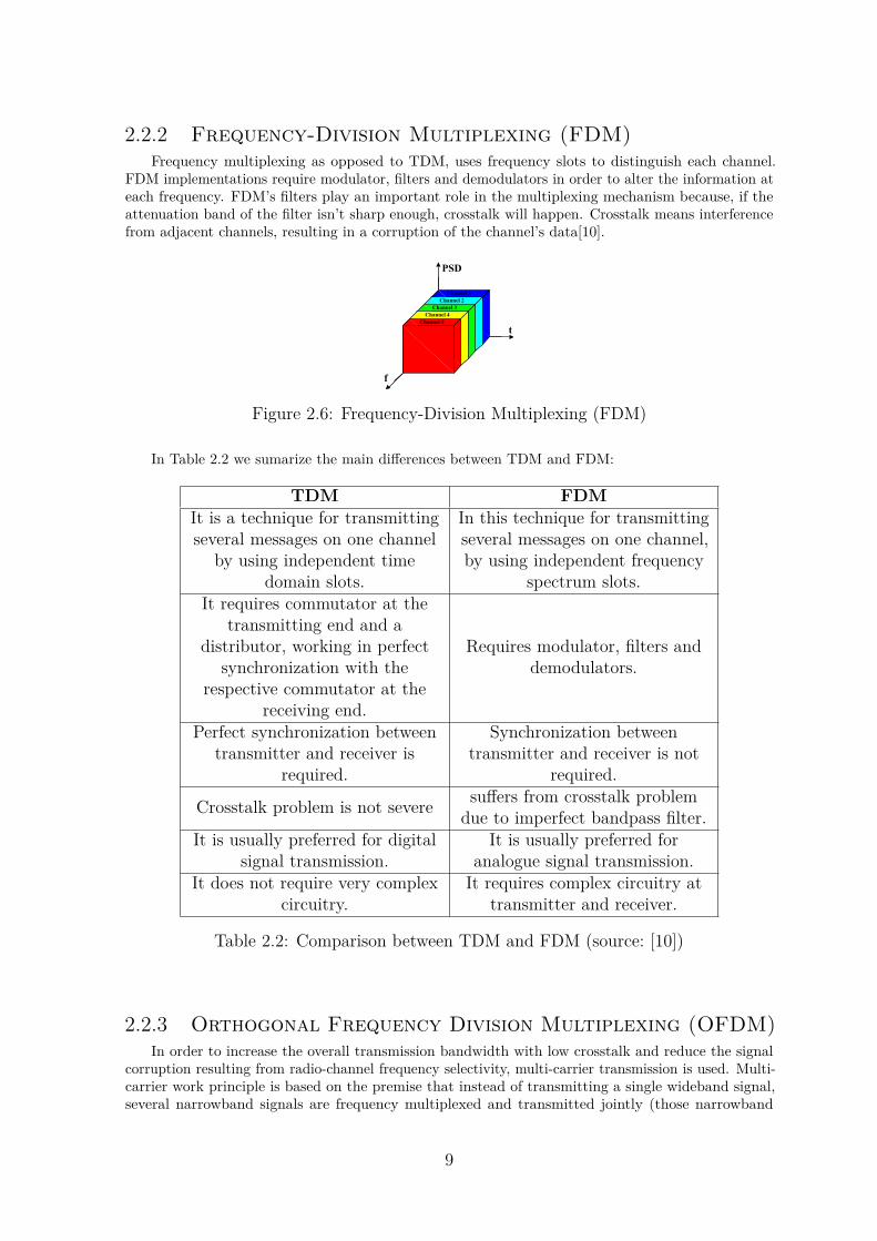
Density (PSD) levels are time dependent, depending on the variation of amplitude of the signal. TheTDM implementation requires a commutator at the transmitter, a distributor at the receiver end, andsynchronization between the two devices[10].
Figure 2.5: Time-Division Multiplexing (TDM)
8
2.2.2 Frequency-Division Multiplexing (FDM)Frequency multiplexing as opposed to TDM, uses frequency slots to distinguish each channel.
FDM implementations require modulator, filters and demodulators in order to alter the information ateach frequency. FDM’s filters play an important role in the multiplexing mechanism because, if theattenuation band of the filter isn’t sharp enough, crosstalk will happen. Crosstalk means interferencefrom adjacent channels, resulting in a corruption of the channel’s data[10].
Figure 2.6: Frequency-Division Multiplexing (FDM)
In Table 2.2 we sumarize the main differences between TDM and FDM:
TDM FDMIt is a technique for transmittingseveral messages on one channel
by using independent timedomain slots.
In this technique for transmittingseveral messages on one channel,by using independent frequency
spectrum slots.It requires commutator at the
transmitting end and adistributor, working in perfect
synchronization with therespective commutator at the
receiving end.
Requires modulator, filters anddemodulators.
Perfect synchronization betweentransmitter and receiver is
required.
Synchronization betweentransmitter and receiver is not
required.
Crosstalk problem is not severesuffers from crosstalk problem
due to imperfect bandpass filter.It is usually preferred for digital
signal transmission.It is usually preferred for
analogue signal transmission.It does not require very complex
circuitry.It requires complex circuitry at
transmitter and receiver.
Table 2.2: Comparison between TDM and FDM (source: [10])
2.2.3 Orthogonal Frequency Division Multiplexing (OFDM)In order to increase the overall transmission bandwidth with low crosstalk and reduce the signal
corruption resulting from radio-channel frequency selectivity, multi-carrier transmission is used. Multi-carrier work principle is based on the premise that instead of transmitting a single wideband signal,several narrowband signals are frequency multiplexed and transmitted jointly (those narrowband
9
signals are designated by sub-carriers). So at each instant (time), N sub-carriers are transmitted inparallel[2].
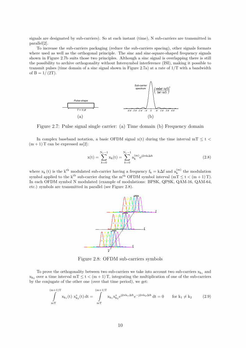
To increase the sub-carriers packaging (reduce the sub-carriers spacing), other signals formatswhere used as well as the orthogonal principle. The sinc and sinc-square-shaped frequency signalsshown in Figure 2.7b suits those two principles. Although a sinc signal is overlapping there is stillthe possibility to archive orthogonality without Intersymbol interference (ISI), making it possible totransmit pulses (time domain of a sinc signal shown in Figure 2.7a) at a rate of 1/T with a bandwidthof B = 1/ (2T).
(a) (b)
Figure 2.7: Pulse signal single carrier: (a) Time domain (b) Frequency domain
In complex baseband notation, a basic OFDM signal x(t) during the time interval mT ≤ t <(m + 1) T can be expressed as[2]:
x(t) =
Nc−1∑
k=0
xk(t) =
Nc−1∑
k=0
a(m)k ej2πk∆ft (2.8)
where xk (t) is the kth modulated sub-carrier having a frequency fk = k∆f and a(m)k the modulation
symbol applied to the kth sub-carrier during the mth OFDM symbol interval (mT ≤ t < (m + 1) T).In each OFDM symbol N modulated (example of modulations: BPSK, QPSK, QAM-16, QAM-64,etc.) symbols are transmitted in parallel (see Figure 2.8).
Figure 2.8: OFDM sub-carriers symbols
To prove the orthogonality between two sub-carriers we take into account two sub-carriers xk1and
xk2over a time interval mT ≤ t < (m + 1) T, integrating the multiplication of one of the sub-carriers
by the conjugate of the other one (over that time period), we get:
(m+1)T∫
mT
xk1(t) x∗
k2(t) dt =
(m+1)T∫
mT
xk1x∗
k2ej2πk1∆fte−j2πk2∆ft dt = 0 for k1 6= k2 (2.9)
10
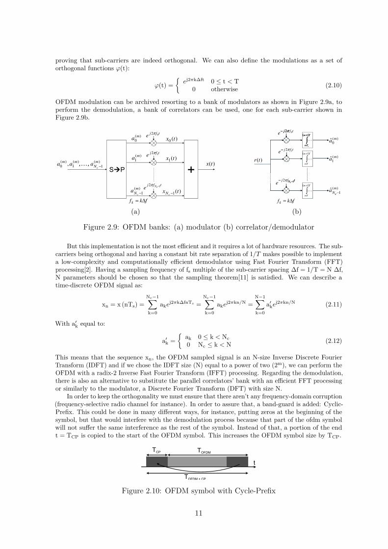
proving that sub-carriers are indeed orthogonal. We can also define the modulations as a set oforthogonal functions ϕ(t):
ϕ(t) =
{
ej2πk∆ft 0 ≤ t < T0 otherwise
(2.10)
OFDM modulation can be archived resorting to a bank of modulators as shown in Figure 2.9a, toperform the demodulation, a bank of correlators can be used, one for each sub-carrier shown inFigure 2.9b.
,...,
(a) (b)
Figure 2.9: OFDM banks: (a) modulator (b) correlator/demodulator
But this implementation is not the most efficient and it requires a lot of hardware resources. The sub-carriers being orthogonal and having a constant bit rate separation of 1/T makes possible to implementa low-complexity and computationally efficient demodulator using Fast Fourier Transform (FFT)processing[2]. Having a sampling frequency of fs multiple of the sub-carrier spacing ∆f = 1/T = N ∆f,N parameters should be chosen so that the sampling theorem[11] is satisfied. We can describe atime-discrete OFDM signal as:
xn = x (nTs) =
Nc−1∑
k=0
akej2πk∆fnTs =
Nc−1∑
k=0
akej2πkn/N =
N−1∑
k=0
a′
kej2πkn/N (2.11)
With a′
k equal to:
a′
k =
{
ak 0 ≤ k < Nc
0 Nc ≤ k < N(2.12)
This means that the sequence xn, the OFDM sampled signal is an N-size Inverse Discrete FourierTransform (IDFT) and if we chose the IDFT size (N) equal to a power of two (2m), we can perform theOFDM with a radix-2 Inverse Fast Fourier Transform (IFFT) processing. Regarding the demodulation,there is also an alternative to substitute the parallel correlators’ bank with an efficient FFT processingor similarly to the modulator, a Discrete Fourier Transform (DFT) with size N.
In order to keep the orthogonality we must ensure that there aren’t any frequency-domain corruption(frequency-selective radio channel for instance). In order to assure that, a band-guard is added: Cyclic-Prefix. This could be done in many different ways, for instance, putting zeros at the beginning of thesymbol, but that would interfere with the demodulation process because that part of the ofdm symbolwill not suffer the same interference as the rest of the symbol. Instead of that, a portion of the endt = TCP is copied to the start of the OFDM symbol. This increases the OFDM symbol size by TCP.
TOFDM
TCP
TOFDM + CP
t
Figure 2.10: OFDM symbol with Cycle-Prefix
11
2.3 channel estimation
Typical OFDM systems generate data, modulates it, converts them to time domin using a IFFTblock, and then sends the symbols over a (wireless) channel. But because how wireless signals propagate,those signals will be distorted as explained in Chapter 2.1.
Channel estimation is often performed to improve the communication between transmitter(s) andreceiver(s). With channel information we can counterbalance the effects of the channel by, for instance,compensating the frequency selective fading, or even apply channel multiplexing techniques, improveBER, etc.
Several techniques can be used to estimate the channel response, and those processes can beperformed at the transmitter side or in the receiver side.
2.3.1 receiver sideRecalling the OFDM system, an OFDM symbol is a sequence of orthogonal sub-carriers. Their
orthogonality makes possible to approximate the received signal as a product of sub-carriers’ componentsby the frequency response of the channel. This makes possible to identify the frequency response ofthe channel just by comparing a known signal transmitted with the received version of it[12] or alsoa known data sequence (eg: preamble or training sequences). These known (typically it is knownthe signal frequency, amplitude and phase) signals are designated pilots. One of the drawbacks ofusing pilots in some sub-carriers, is that the effective bandwidth decreases[13]. In order to keep thebandwidth as high as possible, instead of using pilots on every carriers, is commonly used a fixedamount of pilots and then interpolation is performed to find the other sub-carriers’ channel response.
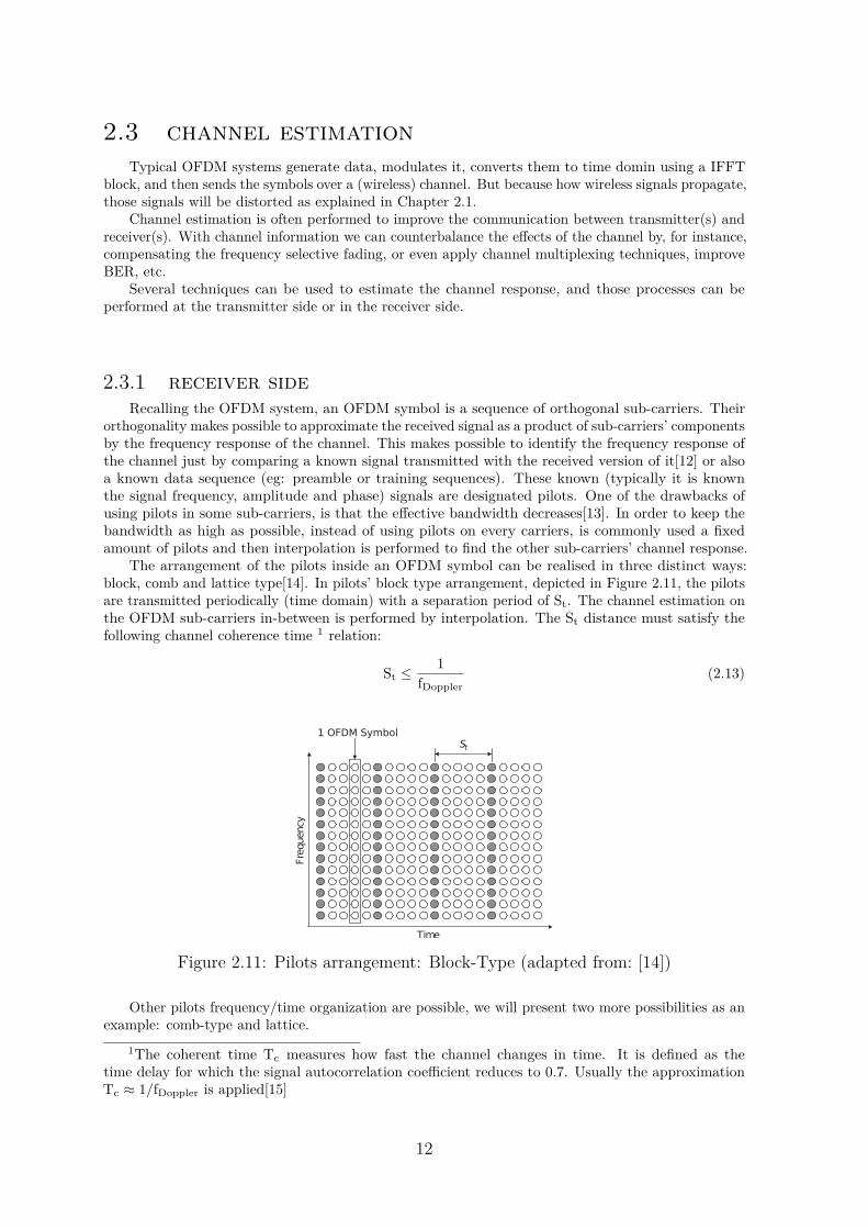
The arrangement of the pilots inside an OFDM symbol can be realised in three distinct ways:block, comb and lattice type[14]. In pilots’ block type arrangement, depicted in Figure 2.11, the pilotsare transmitted periodically (time domain) with a separation period of St. The channel estimation onthe OFDM sub-carriers in-between is performed by interpolation. The St distance must satisfy thefollowing channel coherence time 1 relation:
St ≤1
fDoppler(2.13)
Time
Fre
quency
1 OFDM SymbolSt
Figure 2.11: Pilots arrangement: Block-Type (adapted from: [14])
Other pilots frequency/time organization are possible, we will present two more possibilities as anexample: comb-type and lattice.
1The coherent time Tc measures how fast the channel changes in time. It is defined as thetime delay for which the signal autocorrelation coefficient reduces to 0.7. Usually the approximationTc ≈ 1/fDoppler is applied[15]
12
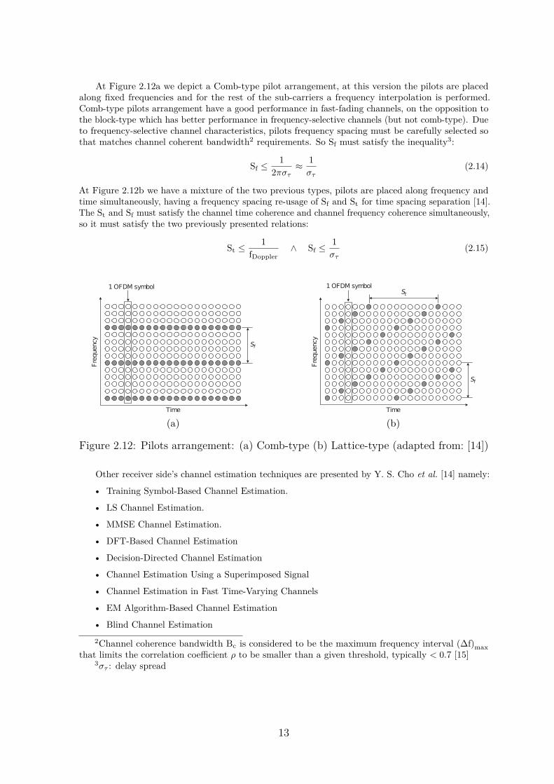
At Figure 2.12a we depict a Comb-type pilot arrangement, at this version the pilots are placedalong fixed frequencies and for the rest of the sub-carriers a frequency interpolation is performed.Comb-type pilots arrangement have a good performance in fast-fading channels, on the opposition tothe block-type which has better performance in frequency-selective channels (but not comb-type). Dueto frequency-selective channel characteristics, pilots frequency spacing must be carefully selected sothat matches channel coherent bandwidth2 requirements. So Sf must satisfy the inequality3:
Sf ≤1
2πστ≈
1
στ(2.14)
At Figure 2.12b we have a mixture of the two previous types, pilots are placed along frequency andtime simultaneously, having a frequency spacing re-usage of Sf and St for time spacing separation [14].The St and Sf must satisfy the channel time coherence and channel frequency coherence simultaneously,so it must satisfy the two previously presented relations:
St ≤1
fDoppler∧ Sf ≤
1
στ(2.15)
Time
Fre
quency
1 OFDM symbol
Sf
(a)
Time
Fre
quency
1 OFDM symbol
Sf
St
(b)
Figure 2.12: Pilots arrangement: (a) Comb-type (b) Lattice-type (adapted from: [14])
Other receiver side’s channel estimation techniques are presented by Y. S. Cho et al. [14] namely:
• Training Symbol-Based Channel Estimation.
• LS Channel Estimation.
• MMSE Channel Estimation.
• DFT-Based Channel Estimation
• Decision-Directed Channel Estimation
• Channel Estimation Using a Superimposed Signal
• Channel Estimation in Fast Time-Varying Channels
• EM Algorithm-Based Channel Estimation
• Blind Channel Estimation
2Channel coherence bandwidth Bc is considered to be the maximum frequency interval (∆f)max
that limits the correlation coefficient ρ to be smaller than a given threshold, typically < 0.7 [15]3στ : delay spread
13
2.3.2 transmitter sideIn most circumstances, the transmitter (BS) doesn’t have direct access to the channel on it side,
since the channel is in "front" of it, so indirect techniques must be used. In Time Division Duplexing(TDD) multiplexing systems, channel reciprocity4 is verified, so we can transmit from BS to MS andthen estimate the channel on the uplink (from MS to BS). Regarding Frequency Division Duplexing(FDD) systems, the channel reciprocity4 doesn’t hold, so downlink channel information must be relayedback from MS to the BS.
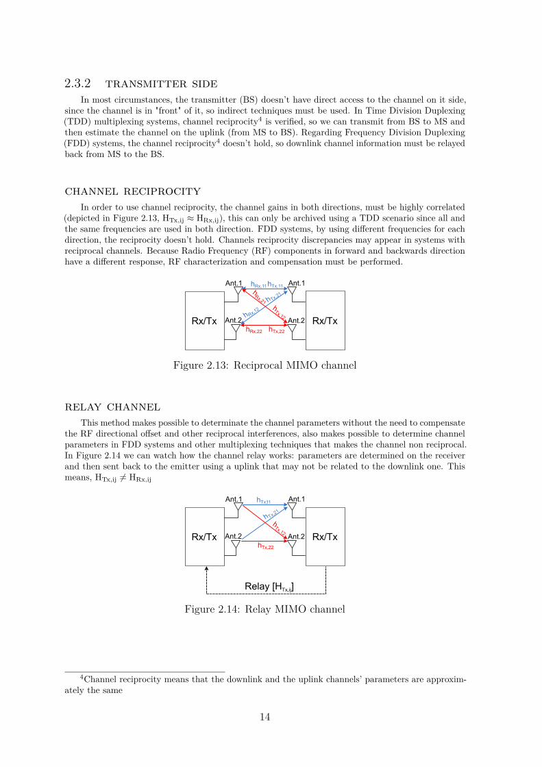
channel reciprocityIn order to use channel reciprocity, the channel gains in both directions, must be highly correlated
(depicted in Figure 2.13, HTx,ij ≈ HRx,ij), this can only be archived using a TDD scenario since all andthe same frequencies are used in both direction. FDD systems, by using different frequencies for eachdirection, the reciprocity doesn’t hold. Channels reciprocity discrepancies may appear in systems withreciprocal channels. Because Radio Frequency (RF) components in forward and backwards directionhave a different response, RF characterization and compensation must be performed.
Figure 2.13: Reciprocal MIMO channel
relay channelThis method makes possible to determinate the channel parameters without the need to compensate
the RF directional offset and other reciprocal interferences, also makes possible to determine channelparameters in FDD systems and other multiplexing techniques that makes the channel non reciprocal.In Figure 2.14 we can watch how the channel relay works: parameters are determined on the receiverand then sent back to the emitter using a uplink that may not be related to the downlink one. Thismeans, HTx,ij 6= HRx,ij
Figure 2.14: Relay MIMO channel
4Channel reciprocity means that the downlink and the uplink channels’ parameters are approxim-ately the same
14
chapter 3Multiple Antennastechniques
This chapter presents several multiple antennas techniques as well as equalization mechanisms.
When we talk about multiple antennas techniques, there are two major categories: diversity andmultiplexing techniques. The differential aspect about these two is the tradeoff between improving BitError Rate (BER) or increasing data rate respectively.
As described in Section 2.1, wireless signals suffer from fading due to propagation effects, resultinginto level, frequency and delay fluctuations, which have a negative influence on the system’s performance.By using multiple antennas, additional degrees-of-freedom appear as well as: power, spatial anddirectional gain[2][16][17][14].
Lets first analyse the case of a SISO antenna setup shown in Figure 3.2a and the probability errorsof it’s channel for future comparison purposes. The signal received after passing through a AWGNchannel is given by: y(t) = s(t) + n(t), with n(t) → CN (0, 1): a white Gaussian random process withmean zero and PSD N0/2. If the s(t) signal is modulated by: s(t) = Re
{
u(t)ej2πfct}
, and if thebandwith of the complex envelope u(t) of s(t) is B, then the transmitted signal s(t) bandwidth is 2B.And since the noise has an uniform PSD of N0/2, this means that in the 2B bandwith the noise poweris 2B × N0/2 = N0B. The SNR1 at the receiver is then[18]:
SNR =PT
N0B=
Eb
N0BTb(3.1)
with Eb the bit energy and Tb the bit period. Defining Ps the symbol error probability, then the biterror probability is:
Pb =Ps
log2 M(3.2)
with M the M-aray signalling, meaning that the bit error probability varies with the signal modulationused.
Using a Rayleigh Flat Fading Channel, the receiver signal is then given by: y = hs + n withh ∼ CN (0, 1), the fading coefficient. In this channel, the instantaneous SNR is given by:
SNR(h) = |h|2 SNR (3.3)
with SNR the average SNR. The error probability in this case is:
Pe = ΨQ(
√
|h|2βSNRs
)
(3.4)
1SNR is the ratio of the received signal power Pr to the power of the noise within the bandwidthof the transmitted signal s(t)
15
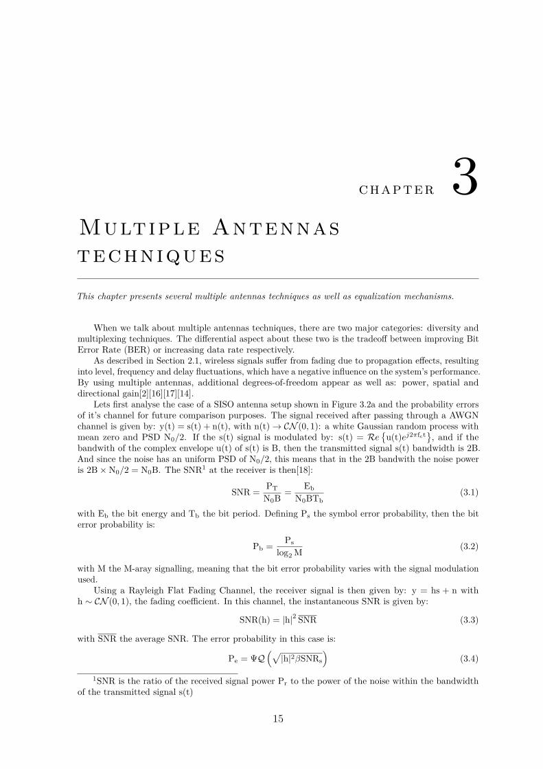
Q is a Gaussian function. Depicting Figure 3.1 we verify that at AWGN channels the probability errordecay more rapidly with the increase of SNR levels.
0 5 10 15 2010
−6
10−5
10−4
10−3
10−2
10−1
100
SNR (dB)
Pb
AWGNRayleigh fading
Figure 3.1: Error probability of AWGN and Rayleigh Flat Fading channels
3.1 diversity techniques
Diversity techniques are based in the assumption that instead of having a single path, severalother independent paths are created and with this method we expect to decrease BER. The amount ofimprovement in BER we can achieve depends on the current channel state. In Good states, the SNRis high enough to achieve reliability. On the other hand, bad states with a low SNR, reliability will notbe accomplished. In Gaussian noise scenarios, the bad state of the channel will take a more importantrule in error probability since the Q curve function is dominated by the behaviour of bad states. Inthe case of a Rayleight fading, the probability of a channel be bad is proportional to the inverse ofSNR (Pe ∝ 1/SNR), using L diversity paths then the probability error is:
Pe ∝1
SNRL(3.5)
this means that we can have the same probability error, using different levels of power, just by increasingthe number of paths (this results in an increase of power efficiency). If we are more interested inimproving the BER, then an increase in the number of paths, while maintaining the SNR value (orincreasing it) does the job.
Other examples of diversity applicability are across time (eg: repeating the same information atdifferent time slots), frequency (eg: transmitting the same signal at different carriers) and space (eg:sending the same information through different antennas), angular, polarization, macrodiversity, andcooperative diversity[15].
3.1.1 antennas diversityWith a sufficient inter-antenna distance or using different antennas polarizations, each channel will
have a low mutual correlation and provides additional diversity against fading on the radio channel.A main advantage of using antennas diversity instead of using frequency, time or other diversitytechniques, is that independent paths can be realized without the need to increase SNR, bandwidth ortransmission delays. Antennas diversity can be achieved at the receiver or the transmitter dependingon the antenna setup. SIMO antennas depicted in Figure 3.2b use receive diversity while MISO setupdepicted in Figure 3.2c has transmit diversity. Both transmit and receive diversity can be achievedusing MIMO antennas shown in Figure 3.2d. These two types of diversity will be presented in the nextsubsections: 3.1.2 and 3.1.3.
16
+
Ant.1 Ant.1h11
Transmitter Receiver
n1
(a)
+
+
n2
h11
h12
n1Ant.1
Ant.2
Ant.1
Transmitter Receiver
(b)
+
h11
Ant.1
Ant.2
Ant.1
h21
n1
Transmitter Receiver
(c)
+
+
n2
h11
h21
h22
h12
Ant.1 Ant.1
Ant.2 Ant.2Transmitter Receiver
n1
(d)
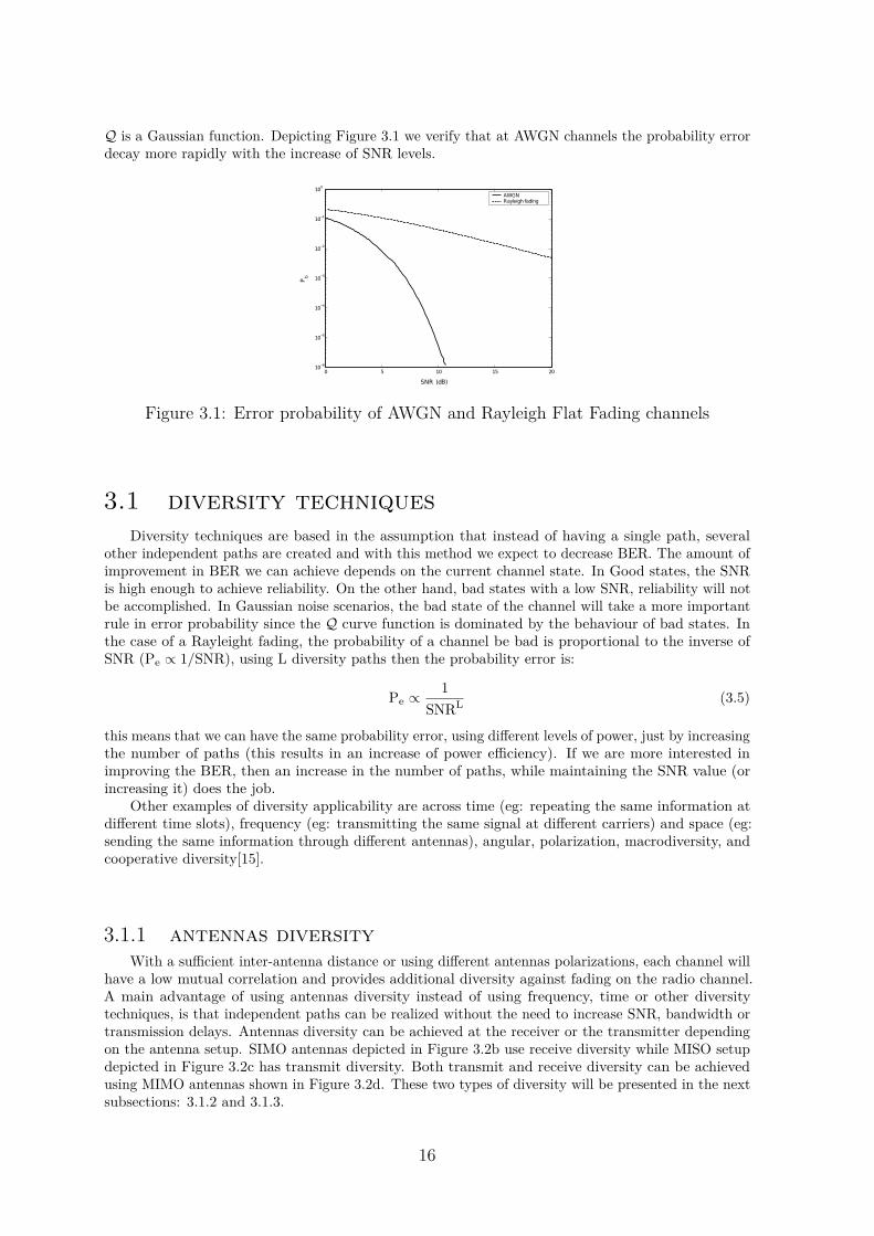
Figure 3.2: Antenna setups: (a) SISO (b) SIMO (c) MISO (d) MIMO
3.1.2 receive diversityReceive diversity can be accomplished through the usage of diversity gain (the principle is that
channels are independent) or antenna gain (the diversity is achieved based that the noise sources areindependent for each receiver, see Figure 3.2b and 3.2d). In matrix notation, the yi signals receivedat each antenna, for an n × m antenna setup (n antennas at the transmitter and m antennas at thereceiver) is given by:
y1
y2...
ym
=
h1,1 h1,2 · · · h1,m
h2,1 h2,2 · · · h2,m
......
. . ....
hn,1 hn,2 · · · hn,m
×
s1
s2
...sn
+
n1
n2
...nm
⇔ Y = Hs + n (3.6)
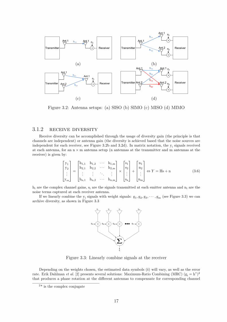
hi are the complex channel gains, si are the signals transmitted at each emitter antenna and ni are thenoise terms captured at each receiver antenna.
If we linearly combine the yi signals with weight signals: g1, g2, g3, · · · , gm (see Figure 3.3) we canarchive diversity, as shown in Figure 3.3
Σ
g1
g3
g2
gm
y1 y2 y3 ym
s
Figure 3.3: Linearly combine signals at the receiver
Depending on the weights chosen, the estimated data symbols (s) will vary, as well as the errorrate. Erik Dahlman et al. [2] presents several solutions: Maximum-Ratio Combining (MRC) (gi = h∗)2
that produces a phase rotation at the different antennas to compensate for corresponding channel
2* is the complex conjugate
17
phases’ rotations and produces a gain correction in the proportion of the corresponding channel gains.
s =
m∑
i=1
|hi|2
s +
m∑
i=1
h∗
i ni (3.7)
In Equal Gain Combining (EGC) the weights are given by: gi = h∗/|h|, this technique cophases signalson all receivers and combines them with equal gain resulting into a estimate symbol of:
s =m
∑
i=1
|hi| s +m
∑
i=1
h∗
i
|hi|ni (3.8)
In Selection Combining (SC) diversity, the received signal with highest SNR is selected for decoding.This selection is made by comparing the instantaneous amplitude of each signal and choose the highestone. Performance analysis and comparison between these linear combining techniques are presentedin [18] and [19]
3.1.3 transmitter diversityRegarding the diversity techniques at the transmitter(applicable in MISO antenna setup for
instance), they can be divided into two major types: open loop and closed loop techniques. Whenthe diversity is applied at the transmitter, a common symbol will be sent in several antennas, passthrough different channels and received in a common antenna[18] as shown in Figure 3.2c.
open loop techniquesIn open loop techniques, Channel State Information (CSI) is not available at the transmitter side.
Space-Time and frequency encoding are applicability examples of this technique. To make sure we canprocess the signals at the receiver, the symbols cannot be transmitted simultaneously in every emittersince the received signal would be:
y(t) = sh1 + sh2 = s(h1 + h2) (3.9)
The received symbols have a dependency of the two channels simultaneously, to mitigate this space-timecodes are needed. Space-time block codes are build from known orthogonal designs, they are easy todecode and is possible do achieve full diversity but contrarily to space-time trellis codes, they don’thave coding gain. Space-time trellis codes on the other hand, are complex to decode [20].
The Alamouti coding [21] currently used in LTE is an example of orthogonal space-time blockcode (See Table 3.1 for the example for 2 transmitter antennas). Symbols are transmitted across space(using the two antennas) and time (using two transmission intervals), also s∗
n represents the complexconjugate of sn [20].
time/frequency Antenna 1 Antenna 2n sn -s∗
n+1
n + 1 sn+1 s∗
n
Table 3.1: Alamouti coding
closed loop techniquesContrarily to open loop, the closed loop technique requires the transmitter to know CSI. Two typical
transmitter diversity closed loop based techniques are: precoding and beamforming [16]. Beamformingprovides simultaneously decent diversity and a power gain, which is obtained through the coherentaddition of user signals. Remembering the channel estimation techniques in Section 2.3, the sameprinciple can be used here: CSI can be estimated at the transmitter (eg:TDD) or relayed (eg: FDD).
18
3.2 multiplexing techniques
In the last section we introduced the diversity and how we can improve BER but if we are interestedin achieving higher bit rates (also called channel capacity), multiple antennas multiplexing techniquesare a better choice [16].
In order to increase data rate, some concessions have to be made. The knowledge of CSI at thetransmitter and receiver, as well as using MIMO antennas, brings various degrees-of-freedom that canthen be "exchanged" for data rate. A typical multiplexing mechanism that uses all these suppositionsis the Spatial Multiplexing MIMO (SM-MIMO).
3.2.1 Spatial Multiplexing MIMO (SM-MIMO)SM-MIMO is a MIMO technique that uses spatial multiplexing to create independent data streams.
Comparatively with other MIMO systems, SM-MIMO can achieve higher data speeds acting as a’data-rate-booster’[22]. Under certain conditions, with MIMO spatial multiplexing, we can make therate increase almost linearly with the number of antennas, making it possible to increase the data ratevirtually without saturation. Considering a [2x2] antenna setup (2 antennas at the transmitter and 2at the receiver) then the signals at the receiver antennas are:
[
y1
y2
]
=
[
h1,1 h1,2
h2,1 h2,2
]
×
[
s1
s2
]
+
[
n1
n2
]
⇔ y = Hs + n (3.10)
Where H is a matrix of hi,j channels’ complex coefficients, s is a vector of si transmitted symbols and nis a vector of ni noise sources added at each receiver as shown in Figure 3.2d. Assuming there is nonoise sources and the channel matrix H is invertible then we can perfectly recover the s symbols bymultiplying the received vector y with a matrix W = H−1 this is:
[
s1
s2
]
= Wy ⇔
[
s1
s2
]
= H−1Hs + H−1n ⇔
[
s1
s2
]
= s + H−1n (3.11)
Perfect recovery is only achieved in the case of a noiseless system. We can also corroborate thatwhen the channel matrix becomes closer to singular, the noise level will increase[22]. This detectionmechanism is called linear reception/demodulation of spatially multiplexed signals.
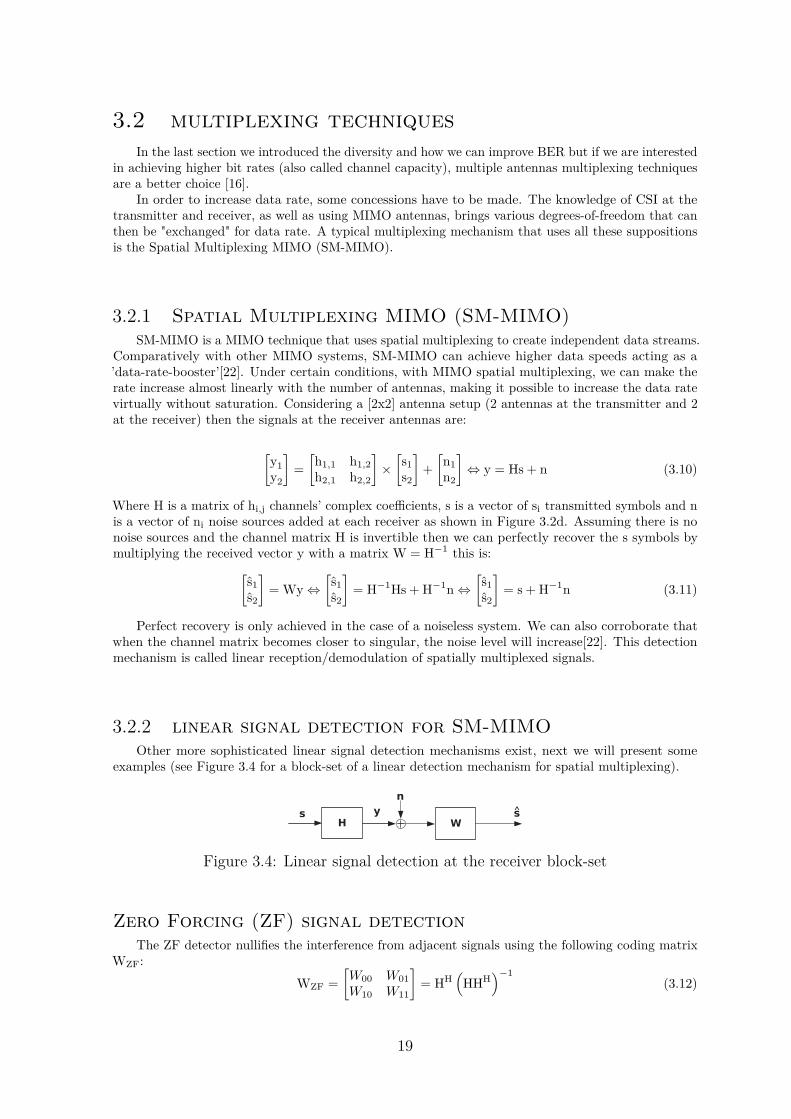
3.2.2 linear signal detection for SM-MIMOOther more sophisticated linear signal detection mechanisms exist, next we will present some
examples (see Figure 3.4 for a block-set of a linear detection mechanism for spatial multiplexing).
Figure 3.4: Linear signal detection at the receiver block-set
Zero Forcing (ZF) signal detectionThe ZF detector nullifies the interference from adjacent signals using the following coding matrix
WZF:
WZF =
[
W00 W01
W10 W11
]
= HH(
HHH)
−1
(3.12)
19
This operation reverses the channel effect by inverting the channel, when the matrix H is non square, apseudoinverse operation should be performed thence the Equation:3.12. (·)H represents the Hermitiantranspose operation. The solution of the pseudoinversion is the one and only one solution and coincideswith the solution for the system Hy = s if H is invertible3 [23]. The received signals are then[14]:
s = WZFy
= s+ HH(
HHH)
−1
n(3.13)
If the antenna setup produces a rectangular channel matrix H, the channel inversion can be simplifiedto:
WZF =
[
W00 W01
W10 W11
]
= H−1 (3.14)
Minimum Mean Square Error (MMSE) signal detectionThe MMSE detector maximizes the post-detection Signal-to-Interference-plus-Noise Ratio (SINR),
and it’s matrix is given by:
WMMSE =
[
W00 W01
W10 W11
]
= HH(
HHH + σ2z I
)
−1
(3.15)
note that for this linear detection to work, the statistical information of the noise σ2z is necessary.
Similarly to ZF, the received signals are:
s = WMMSEy
= s+ HH(
HHH + σ2z I
)
−1
n(3.16)
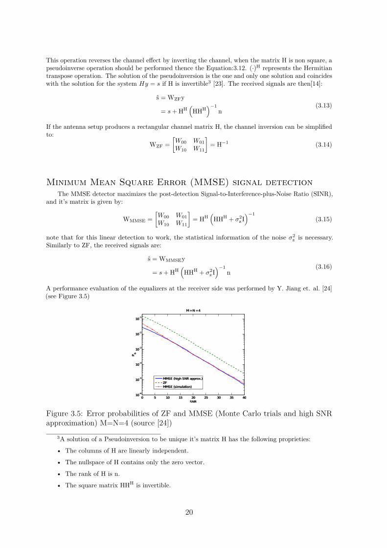
A performance evaluation of the equalizers at the receiver side was performed by Y. Jiang et. al. [24](see Figure 3.5)
0 5 10 15 20 25 30 35 4010
−6
10−5
10−4
10−3
10−2
10−1
SNR
Pb
M = N = 4
MMSE (high SNR approx.)
ZF
MMSE (simulation)
Figure 3.5: Error probabilities of ZF and MMSE (Monte Carlo trials and high SNRapproximation) M=N=4 (source [24])
3A solution of a Pseudoinversion to be unique it’s matrix H has the following proprieties:
• The columns of H are linearly independent.
• The nullspace of H contains only the zero vector.
• The rank of H is n.
• The square matrix HHH is invertible.
20
3.2.3 Spatial Multiplexing MIMO (SM-MIMO) with precod-
ingIf we have the CSI at the transmitter side we can linearly pre-equalize also known as precoding
shown in Figure 3.6.
Figure 3.6: Linear pre-equalization block-set
Precoding is represented by the matrix W which is multiplied to the data symbols vector s, that is:
x = Ws (3.17)
to determine the W precoding matrix ZF of MMSE linear equalizers can be used. It is also a goodidea to constraint the total transmitted power so W is multiplied by α, note that to amend thisamplification factor, at the receiver we have to divide the receiver signal by α (through AutomaticGain Control (AGC) or digitally):
αeq =
√
√
√
√
NT
Trace(
Weq · WHeq
) (3.18)
for ZF precoder the estimated received signal s is given by:
s =1
αZF(HαZFWZFs + n)
= s +1
αZFn
(3.19)
and MMSE precoder:
s =1
αMMSE(HαMMSEWMMSEs + n)
= s +1
αMMSEn
(3.20)
with WZF and WMMSE equal to HH(
HHH)
−1
or H−1 and HH(
HHH + σ2z I
)
−1
respectively. Note
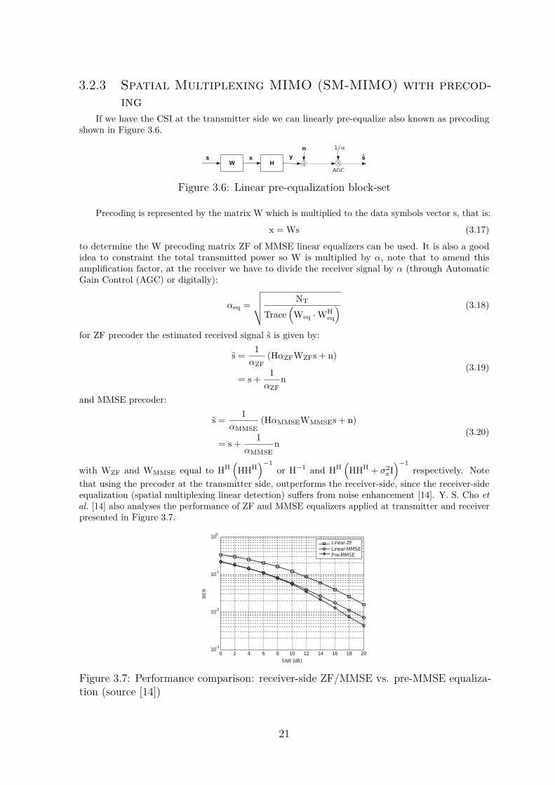
that using the precoder at the transmitter side, outperforms the receiver-side, since the receiver-sideequalization (spatial multiplexing linear detection) suffers from noise enhancement [14]. Y. S. Cho etal. [14] also analyses the performance of ZF and MMSE equalizers applied at transmitter and receiverpresented in Figure 3.7.
0 2 4 6 8 10 12 14 16 18 2010
-3
10-2
10-1
100
SNR [dB]
BE
R
Linear-ZF
Linear-MMSE
Pre-MMSE
Figure 3.7: Performance comparison: receiver-side ZF/MMSE vs. pre-MMSE equaliza-tion (source [14])
21

chapter 4Field Programmable GateArrays (FPGAs)
This chapter presents a description of what is an Field Programmable Gate Array (FPGA) and howcan they be programmed.
4.1 FPGA
Field Programmable Gate Arrays (FPGAs) are semiconductor hardware devices with the possibilityof being programmed several times Static Random-Access Memory (SRAM)-based or One-Time Pro-grammable (OTP) (impossibility to reprogram). FPGAs are constituted by matrix based ConfigurableLogic Blocks (CLBs) whose interconnections can be programable [25]. The reprogrammable abilityallows hardware designers to improve the FPGA based designs at later developer stages of even aftershipping. This possibility makes it possible to reuse the same resources often and reduce developmentcosts.
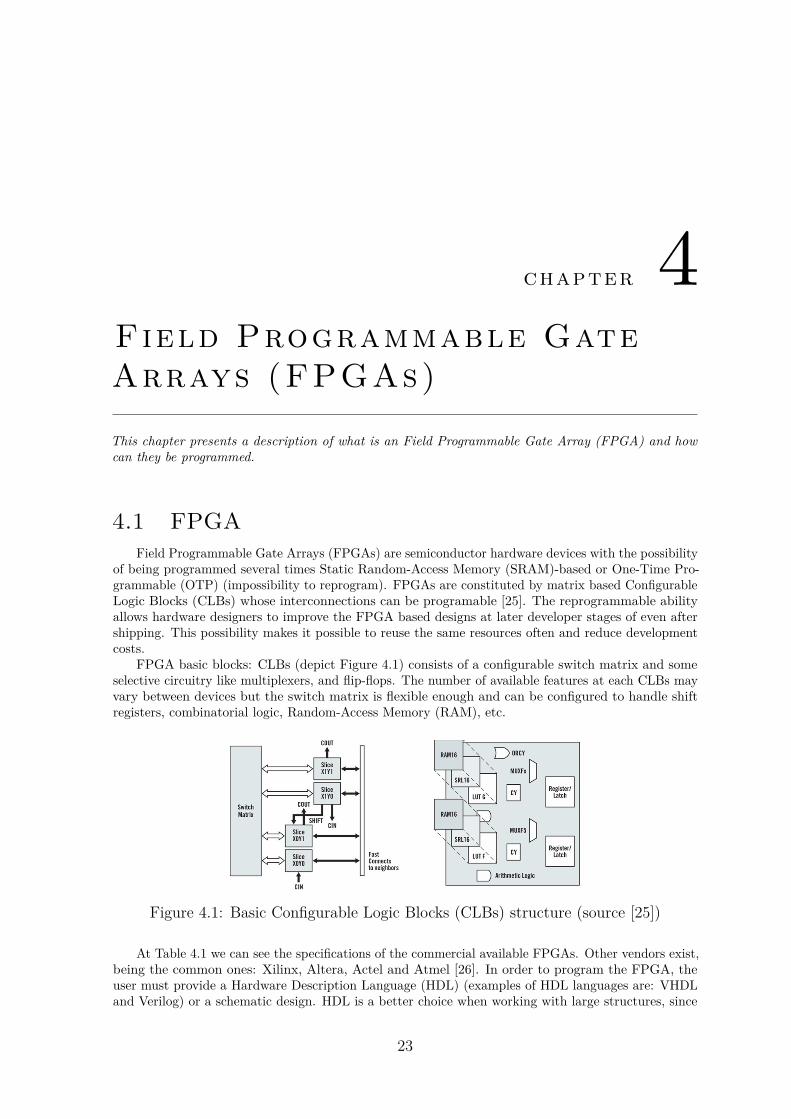
FPGA basic blocks: CLBs (depict Figure 4.1) consists of a configurable switch matrix and someselective circuitry like multiplexers, and flip-flops. The number of available features at each CLBs mayvary between devices but the switch matrix is flexible enough and can be configured to handle shiftregisters, combinatorial logic, Random-Access Memory (RAM), etc.
Figure 4.1: Basic Configurable Logic Blocks (CLBs) structure (source [25])
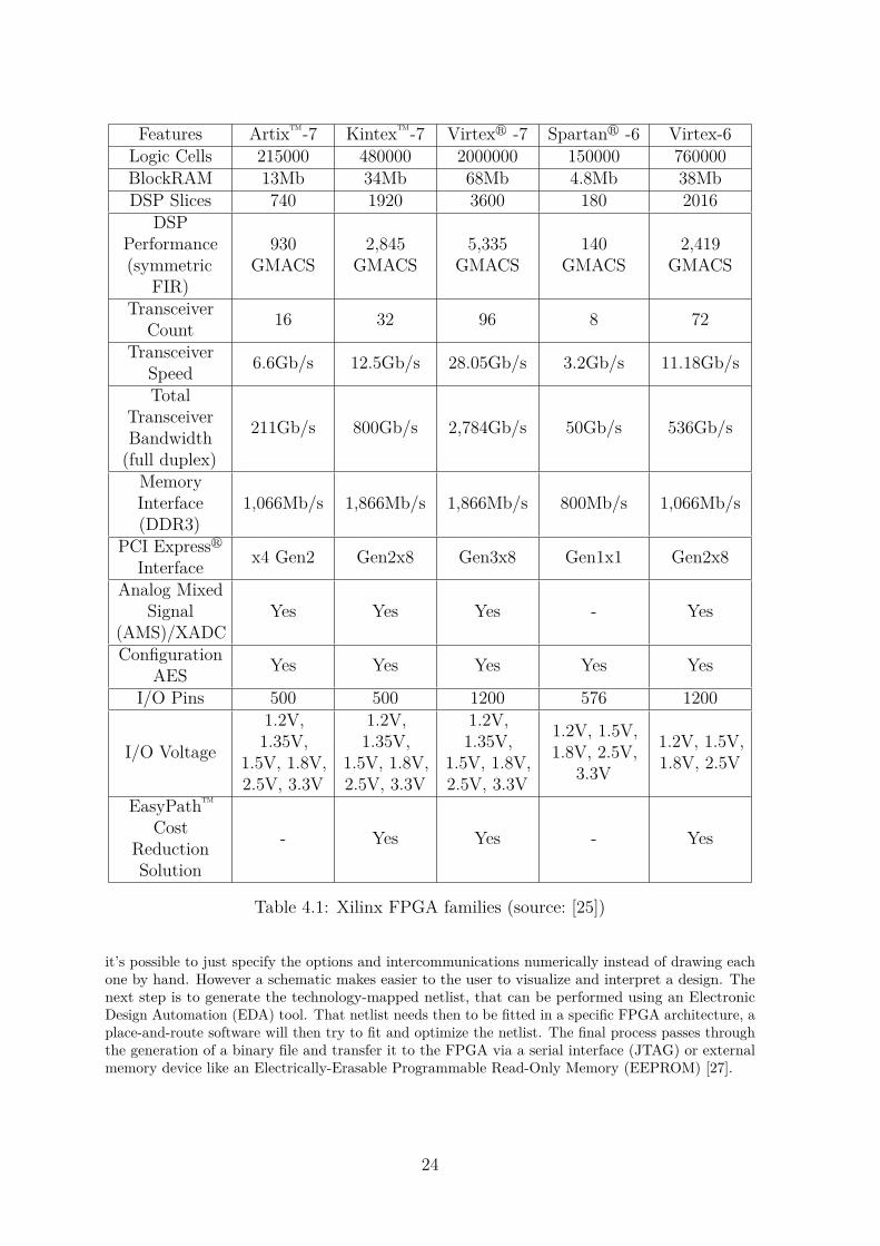
At Table 4.1 we can see the specifications of the commercial available FPGAs. Other vendors exist,being the common ones: Xilinx, Altera, Actel and Atmel [26]. In order to program the FPGA, theuser must provide a Hardware Description Language (HDL) (examples of HDL languages are: VHDLand Verilog) or a schematic design. HDL is a better choice when working with large structures, since
23
Features Artix™-7 Kintex™-7 Virtexr -7 Spartanr -6 Virtex-6Logic Cells 215000 480000 2000000 150000 760000BlockRAM 13Mb 34Mb 68Mb 4.8Mb 38MbDSP Slices 740 1920 3600 180 2016
DSPPerformance(symmetric
FIR)
930GMACS
2,845GMACS
5,335GMACS
140GMACS
2,419GMACS
TransceiverCount
16 32 96 8 72
TransceiverSpeed
6.6Gb/s 12.5Gb/s 28.05Gb/s 3.2Gb/s 11.18Gb/s
TotalTransceiverBandwidth
(full duplex)
211Gb/s 800Gb/s 2,784Gb/s 50Gb/s 536Gb/s
MemoryInterface(DDR3)
1,066Mb/s 1,866Mb/s 1,866Mb/s 800Mb/s 1,066Mb/s
PCI Expressr
Interfacex4 Gen2 Gen2x8 Gen3x8 Gen1x1 Gen2x8
Analog MixedSignal
(AMS)/XADCYes Yes Yes - Yes
ConfigurationAES
Yes Yes Yes Yes Yes
I/O Pins 500 500 1200 576 1200
I/O Voltage
1.2V,1.35V,
1.5V, 1.8V,2.5V, 3.3V
1.2V,1.35V,
1.5V, 1.8V,2.5V, 3.3V
1.2V,1.35V,
1.5V, 1.8V,2.5V, 3.3V
1.2V, 1.5V,1.8V, 2.5V,
3.3V
1.2V, 1.5V,1.8V, 2.5V
EasyPath™
CostReductionSolution
- Yes Yes - Yes
Table 4.1: Xilinx FPGA families (source: [25])
it’s possible to just specify the options and intercommunications numerically instead of drawing eachone by hand. However a schematic makes easier to the user to visualize and interpret a design. Thenext step is to generate the technology-mapped netlist, that can be performed using an ElectronicDesign Automation (EDA) tool. That netlist needs then to be fitted in a specific FPGA architecture, aplace-and-route software will then try to fit and optimize the netlist. The final process passes throughthe generation of a binary file and transfer it to the FPGA via a serial interface (JTAG) or externalmemory device like an Electrically-Erasable Programmable Read-Only Memory (EEPROM) [27].
24
4.2 system generator
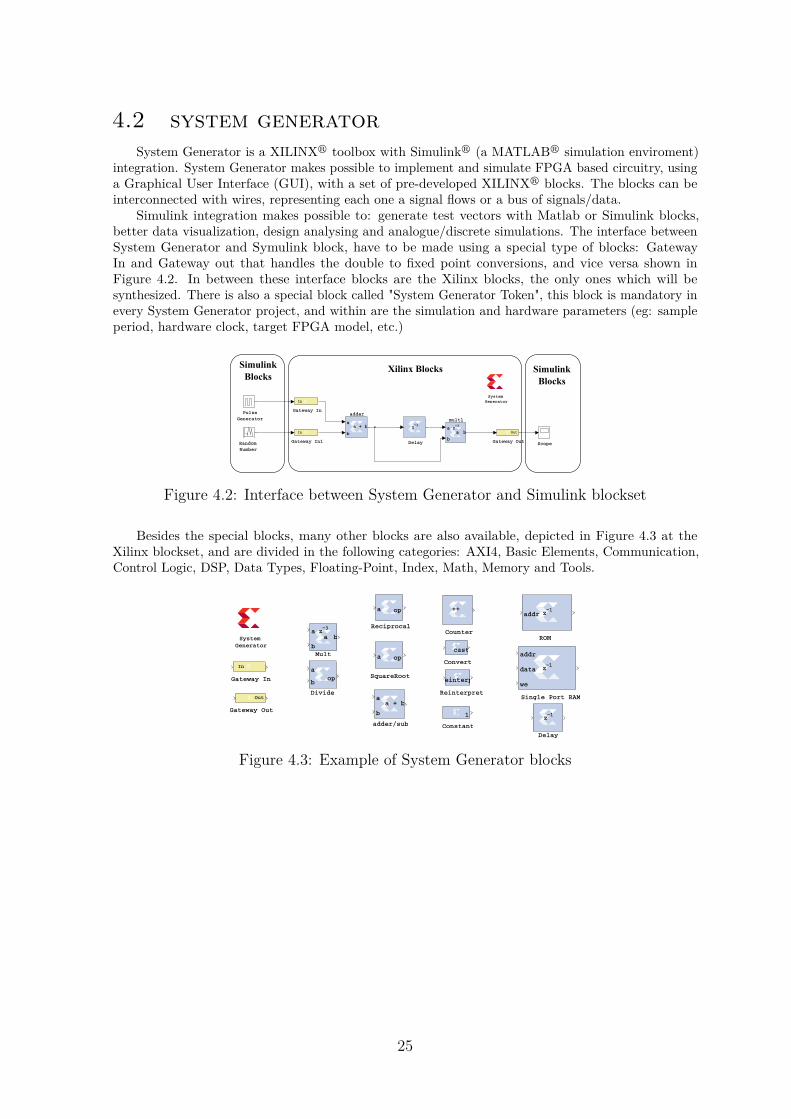
System Generator is a XILINXr toolbox with Simulinkr (a MATLABr simulation enviroment)integration. System Generator makes possible to implement and simulate FPGA based circuitry, usinga Graphical User Interface (GUI), with a set of pre-developed XILINXr blocks. The blocks can beinterconnected with wires, representing each one a signal flows or a bus of signals/data.
Simulink integration makes possible to: generate test vectors with Matlab or Simulink blocks,better data visualization, design analysing and analogue/discrete simulations. The interface betweenSystem Generator and Symulink block, have to be made using a special type of blocks: GatewayIn and Gateway out that handles the double to fixed point conversions, and vice versa shown inFigure 4.2. In between these interface blocks are the Xilinx blocks, the only ones which will besynthesized. There is also a special block called "System Generator Token", this block is mandatory inevery System Generator project, and within are the simulation and hardware parameters (eg: sampleperiod, hardware clock, target FPGA model, etc.)
mult1
a
b
a bz−3
adder
a
b
a + b
ScopeRandom
Number
Pulse
Generator
Gateway Out
Out
Gateway In1
In
Gateway In
In
Delay
z−1
System
Generator
Xilinx BlocksSimulink
BlocksSimulink
Blocks
Figure 4.2: Interface between System Generator and Simulink blockset
Besides the special blocks, many other blocks are also available, depicted in Figure 4.3 at theXilinx blockset, and are divided in the following categories: AXI4, Basic Elements, Communication,Control Logic, DSP, Data Types, Floating-Point, Index, Math, Memory and Tools.
adder/sub
a
b
a + b
SquareRoot
a op
Single Port RAM
addr
data
we
z−1
Reinterpret
reinterpret
Reciprocal
a op
ROM
addr z−1
Mult
a
b
a bz−3
Gateway Out
Out
Gateway In
In
Divide
a
bop
Delay
z−1
Counter
++
Convert
cast
Constant
1
System
Generator
Figure 4.3: Example of System Generator blocks
25

chapter 5Implementation and Results
This chapter presents the proposed system for SM-MIMO precoder, a Matlab simulator, description theFPGA implementation and test of some blocks using System Generator.
5.1 proposed system
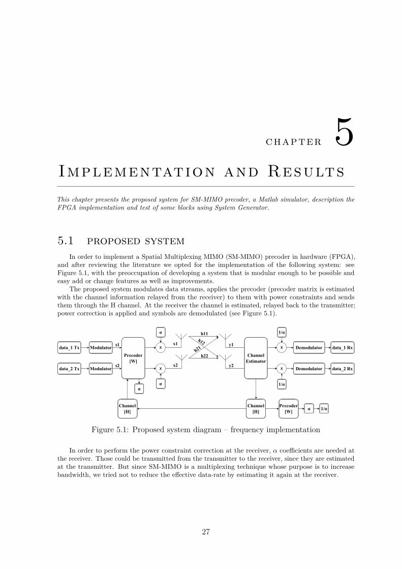
In order to implement a Spatial Multiplexing MIMO (SM-MIMO) precoder in hardware (FPGA),and after reviewing the literature we opted for the implementation of the following system: seeFigure 5.1, with the preoccupation of developing a system that is modular enough to be possible andeasy add or change features as well as improvements.
The proposed system modulates data streams, applies the precoder (precoder matrix is estimatedwith the channel information relayed from the receiver) to them with power constraints and sendsthem through the H channel. At the receiver the channel is estimated, relayed back to the transmitter;power correction is applied and symbols are demodulated (see Figure 5.1).
Figure 5.1: Proposed system diagram – frequency implementation
In order to perform the power constraint correction at the receiver, α coefficients are needed atthe receiver. Those could be transmitted from the transmitter to the receiver, since they are estimatedat the transmitter. But since SM-MIMO is a multiplexing technique whose purpose is to increasebandwidth, we tried not to reduce the effective data-rate by estimating it again at the receiver.
27
5.2 SM-MIMO matlabr simulation
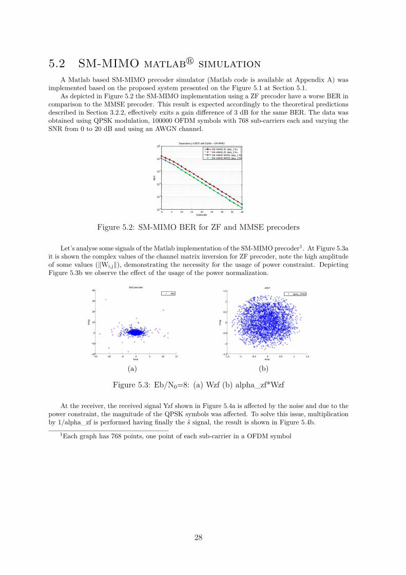
A Matlab based SM-MIMO precoder simulator (Matlab code is available at Appendix A) wasimplemented based on the proposed system presented on the Figure 5.1 at Section 5.1.
As depicted in Figure 5.2 the SM-MIMO implementation using a ZF precoder have a worse BER incomparison to the MMSE precoder. This result is expected accordingly to the theoretical predictionsdescribed in Section 3.2.2, effectively exits a gain difference of 3 dB for the same BER. The data wasobtained using QPSK modulation, 100000 OFDM symbols with 768 sub-carriers each and varying theSNR from 0 to 20 dB and using an AWGN channel.
0 5 10 15 20 25 30 35 4010
−5
10−4
10−3
10−2
10−1
100
Dependency of BER with Eb/No − SM MIMO
Eb/No(dB)
BE
R
SM−MIMO ZF data_1 Rx
SM−MIMO ZF data_2 Rx
SM−MIMO MMSE data_1 Rx
SM−MIMO MMSE data_2 Rx
Figure 5.2: SM-MIMO BER for ZF and MMSE precoders
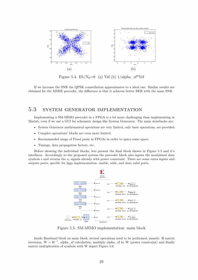
Let’s analyse some signals of the Matlab implementation of the SM-MIMO precoder1. At Figure 5.3ait is shown the complex values of the channel matrix inversion for ZF precoder, note the high amplitudeof some values (‖Wi,j‖), demonstrating the necessity for the usage of power constraint. DepictingFigure 5.3b we observe the effect of the usage of the power normalization.
−15 −10 −5 0 5 10 15−20
−10
0
10
20
30
40
Real
Imag
Wzf precoder
Wzf
(a)
−1.5 −1 −0.5 0 0.5 1 1.5−1.5
−1
−0.5
0
0.5
1
1.5
Real
Imag
αWzf
alpha_zf*Wzf
(b)
Figure 5.3: Eb/N0=8: (a) Wzf (b) alpha_zf*Wzf
At the receiver, the received signal Yzf shown in Figure 5.4a is affected by the noise and due to thepower constraint, the magnitude of the QPSK symbols was affected. To solve this issue, multiplicationby 1/alpha_zf is performed having finally the s signal, the result is shown in Figure 5.4b.
1Each graph has 768 points, one point of each sub-carrier in a OFDM symbol
28
−2 −1.5 −1 −0.5 0 0.5 1 1.5 2−2
−1.5
−1
−0.5
0
0.5
1
1.5
Received signal with noise
Real
Imag
Yzf
(a)
−3 −2 −1 0 1 2
−4
−3
−2
−1
0
1
2
3
4
Received signal with noise with constraint correction
Real
Imag
1/α * Yzf
(b)
Figure 5.4: Eb/N0=8: (a) Yzf (b) 1/alpha_zf*Yzf
If we increase the SNR the QPSK constellation approximates to a ideal one. Similar results areobtained for the MMSE precoder, the difference is that it achieves better BER with the same SNR.
5.3 system generator implementation
Implementing a SM-MIMO precoder in a FPGA is a lot more challenging than implementing inMatlab, even if we use a GUI for schematic design like System Generator. The main drawbacks are:
• System Generator mathematical operations are very limited, only basic operations, are provided.
• Complex operations’ blocks are even more limited.
• Recommended usage of Fixed point in FPGAs in order to space some space.
• Timings, data propagation factors, etc.
Before showing the individual blocks, lets present the final block shown in Figure 5.5 and it’sinterfaces. Accordingly to the proposed system the precoder block also inputs the modulated datasymbols s and returns the xi signals already with power constraint. There are some extra inputs andoutputs ports, specific for fpga implementation: enable, addr, and data valid ports.
real
S1
1
To Workspace3
Y_valid
To Workspace2
Real_Y0
To Workspace1
Imag_Y2
To Workspace1
Real_Y1
To Workspace1
Imag_Y0
Real
S0
1
Imag
S1
1
Imag
S0
1
Gateway Out4
Out
Gateway Out3
Out
Gateway Out2
Out
Gateway Out1
Out
Gateway Out
Out
Gateway In
In
Constant
1
Baseband
real_s0
imag_s0
real_s1
imag_s1
enable
addr
Out1
Out2
Out3
Out4
Out5
ADDR
en++
System
Generator
Figure 5.5: SM-MIMO implementation: main block
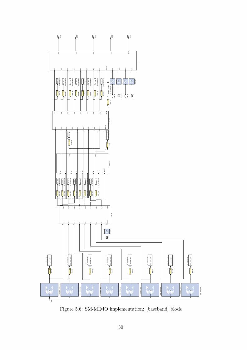
Inside Baseband block on main block, several operations need to be performed, namely: H matrixinversion, W = H−1, alpha_zf calculation, multiply alpha_zf to W (power constraint) and finallymatrix multiplication of symbols with W depict Figure 5.6
29
Out5
5
Out4
4
Out3
3
Out2
2
Out1
1
validOut
real W4
Out
real W3
Out
real W2
Out
real W11
Out
real W10
Out
real W1
Out
real W01
Out
real W00
Out
inv H
In1
In2
In3
In4
In5
In6
In7
In8
enable
Out1
Out2
Out3
Out4
Out5
Out6
Out7
Out8
valid
alphazf*W
In1
In2
In3
In4
In5
In6
In7
In8
alpha
enable
Out1
Out2
Out3
Out4
Out5
Out6
Out7
Out8
Valid
alphazf
Out
alpha_zf
In1
In2
In3
In4
In5
In6
In7
In8
enable
Out1
Valid
W*S
In1
In2
In3
In4
In5
In6
In7
In8
enable
In9
In10
In11
In12
Out1
Out2
Out3
Out4
valid
To Workspace9
alphazf_Real_W00
To Workspace8
Imag_W11
To Workspace7
Real_W11
To Workspace6
Imag_W10
To Workspace5
Real_W10
To Workspace4
Imag_W01
To Workspace31
alphazf_W_valid
To Workspace3
Real_W01
To Workspace29
alphazf_valid
To Workspace28
rom_real_h00
To Workspace27
rom_real_h10
To Workspace26
rom_real_h01
To Workspace25
rom_real_h11
To Workspace23
rom_imag_h01
To Workspace22
rom_imag_h11
To Workspace21
rom_imag_h00
To Workspace20
rom_imag_h10
To Workspace2
Imag_W00
To Workspace16
alphazf_Imag_W11
To Workspace15
alphazf_Real_W11
To Workspace14
alphazf_Imag_W10
To Workspace13
alphazf_Real_W10
To Workspace12
alphazf_Imag_W01
To Workspace11
alphazf_Real_W01
To Workspace10
alphazf_Imag_W00
To Workspace1
Real_W00
To Workspace
alpha_zf
Reals8Out
Reals7Out
Reals6Out
Reals5Out
Reals4Out
Reals3Out
Reals2Out
Reals1Out
ROM H22_real
addr
z−1
ROM H22_imag
addr
z−1
ROM H21_real
addr
z−1
ROM H21_imag
addr
z−1
ROM H12_real
addr
z−1
ROM H12_imag
addr
z−1
ROM H11_real
addr
z−1
ROM H11_imag
addr
z−1
Imag Y3Out
Imag W4Out
Imag W3Out
Imag W2Out
Imag W11
Out
Imag W10
Out
Imag W1Out
Imag W01
Out
Imag W00
Out
Delay9
z−25
Delay8
z−25
Delay12
z−1
Delay11
z−25
Delay10
z−25
addr
6
enable
5
imag_s1
4
real_s1
3
imag_s0
2
real_s0
1
Figure 5.6: SM-MIMO implementation: [baseband] block
30
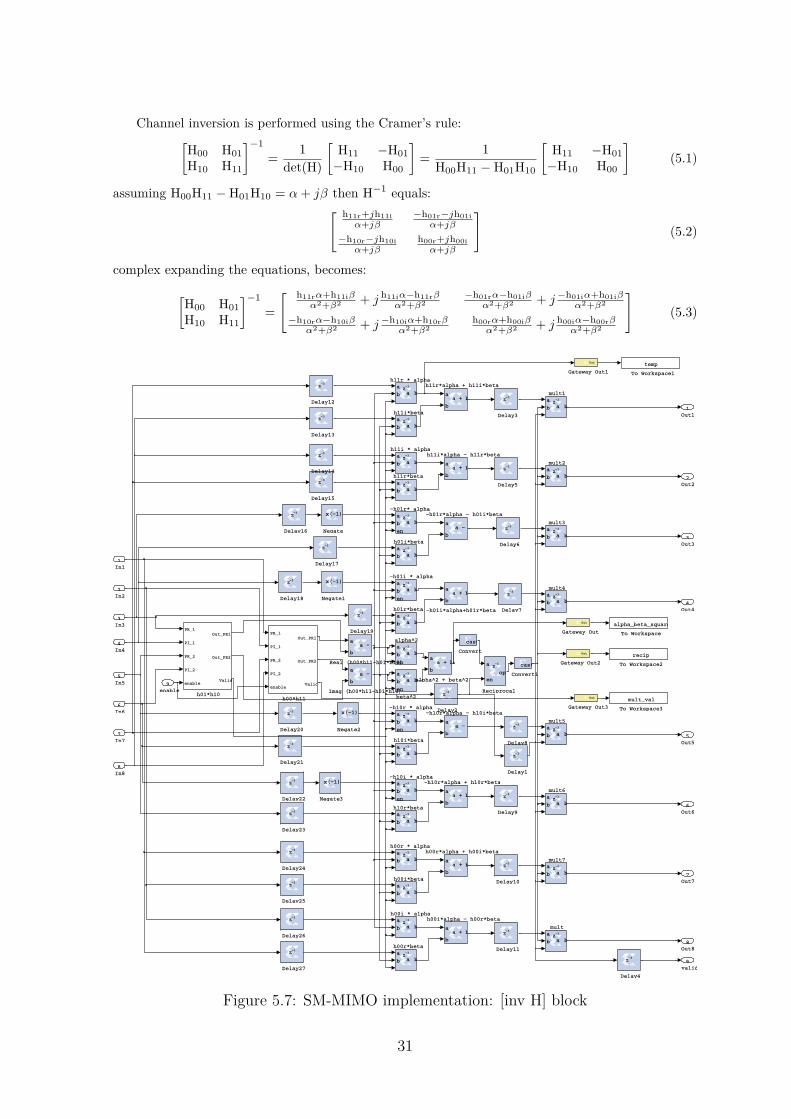
Channel inversion is performed using the Cramer’s rule:[
H00 H01
H10 H11
]
−1
=1
det(H)
[
H11 −H01
−H10 H00
]
=1
H00H11 − H01H10
[
H11 −H01
−H10 H00
]
(5.1)
assuming H00H11 − H01H10 = α+ jβ then H−1 equals:[ h11r+jh11i
α+jβ−h01r−jh01i
α+jβ
−h10r−jh10i
α+jβh00r+jh00i
α+jβ
]
(5.2)
complex expanding the equations, becomes:
[
H00 H01
H10 H11
]
−1
=
[ h11rα+h11iβα2+β2 + j h11iα−h11rβ
α2+β2
−h01rα−h01iβα2+β2 + j−h01iα+h01iβ
α2+β2
−h10rα−h10iβα2+β2 + j−h10iα+h10rβ
α2+β2
h00rα+h00iβα2+β2 + j h00iα−h00rβ
α2+β2
]
(5.3)
valid
9
Out8
8
Out7
7
Out6
6
Out5
5
Out4
4
Out3
3
Out2
2
Out1
1
mult7
a
b a bz−3
mult6
a
b a bz−3
mult5
a
b a bz−3
mult4
a
b a bz−3
mult3
a
b a bz−3
mult2
a
b a bz−3
mult1
a
b a bz−3
mult
a
b a bz−3
h11r*beta
a
b a bz−3
h11r*alpha + h11i*beta
a
b
a + b
h11r * alpha
a
b a bz−3
h11i*beta
a
b a bz−3
h11i*alpha − h11r*beta
a
b
a + b
h11i * alpha
a
b a bz−3
h10r*beta
a
b a bz−3
h10i*beta
a
b a bz−3
h01r*beta
a
b a bz−3
h01i*beta
a
b a bz−3
h01*h10
PR_1
PI_1
PR_2
PI_2
enable
Out_PR1
Out_PR2
Valid
h00r*beta
a
b a bz−3
h00r*alpha + h00i*beta
a
b
a + b
h00r * alpha
a
b a bz−3
h00i*beta
a
b a bz−3
h00i*alpha − h00r*beta
a
b
a + b
h00i * alpha
a
b a bz−3
h00*h11
PR_1
PI_1
PR_2
PI_2
enable
Out_PR1
Out_PR2
Valid
beta^2
a
b
en
a bz−3
alpha^2 + beta^2
a
b
a + b
alpha^2
a
b
en
a bz−3
To Workspace3
mult_val
To Workspace2
recip
To Workspace1
temp
To Workspace
alpha_beta_squared
Reciprocal
a
en
op
z−3Real (h00*h11−h01*h10)
a
b
a − b
Negate3
x(−1)
Negate2
x(−1)
Negate1
x(−1)
Negate
x(−1)
Imag (h00*h11−h01*h10)
a
b
a − b
Gateway Out3
Out
Gateway Out2
Out
Gateway Out1
Out
Gateway Out
Out
Delay9
z−3
Delay8
z−3
Delay7
z−3
Delay6
z−3
Delay5
z−3
Delay4
z−3
Delay3
z−3
Delay27
z−3
Delay26
z−3
Delay25
z−3
Delay24
z−3
Delay23
z−3
Delay22
z−3
Delay21
z−3
Delay20
z−3 Delay2
z−3
Delay19
z−3
Delay18
z−3
Delay17
z−3
Delay16
z−3
Delay15
z−3
Delay14
z−3
Delay13
z−3
Delay12
z−3
Delay11
z−3
Delay10
z−3
Delay1
z−3
Convert1
cast
Convert
cast
−h10r*alpha − h10i*beta
a
b
a − b
−h10r*alpha + h10r*beta
a
b
a + b
−h10r * alpha
a
b
en
a bz−3
−h10i * alpha
a
b
en
a bz−3
−h01r*alpha − h01i*beta
a
b
a − b
−h01r* alpha
a
b
en
a bz−3
−h01i*alpha+h01r*beta
a
b
a + b
−h01i * alpha
a
b
en
a bz−3
enable
9
In8
8
In7
7
In6
6
In5
5
In4
4
In3
3
In2
2
In1
1
Figure 5.7: SM-MIMO implementation: [inv H] block
31
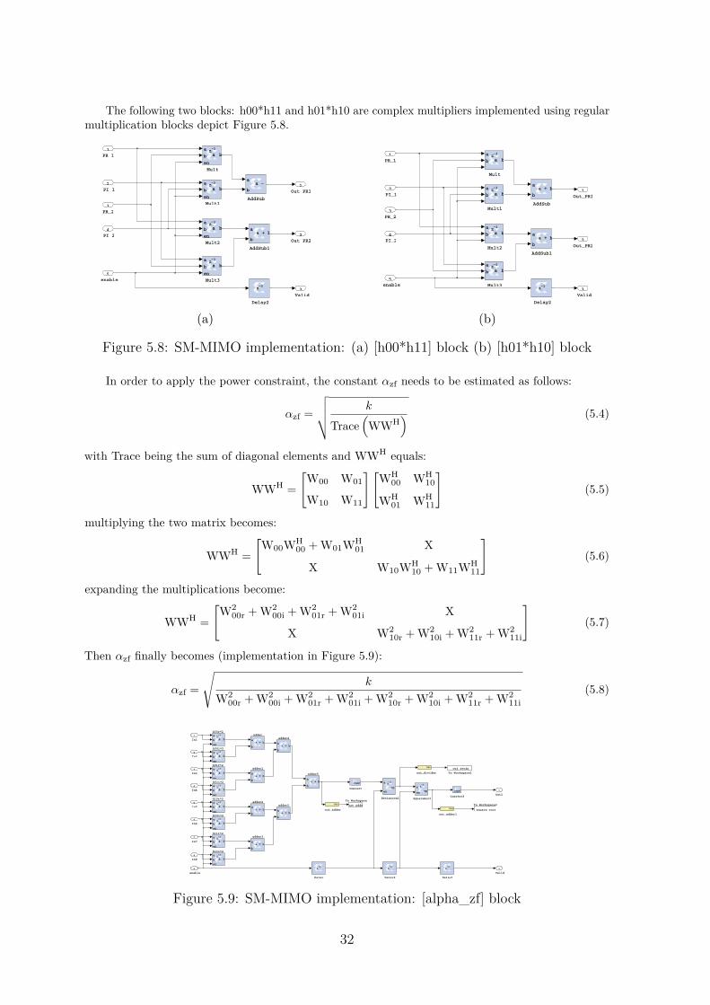
The following two blocks: h00*h11 and h01*h10 are complex multipliers implemented using regularmultiplication blocks depict Figure 5.8.
Valid
3
Out_PR2
2
Out_PR1
1
Mult3
a
b
en
a bz−3
Mult2
a
b
en
a bz−3
Mult1
a
b
en
a bz−3
Mult
a
b
en
a bz−3
Delay2
z−3
AddSub1
a
b
a + b
AddSub
a
b
a − b
enable
5
PI_2
4
PR_2
3
PI_1
2
PR_1
1
(a)
Valid
3
Out_PR2
2
Out_PR1
1
Mult3
a
b a bz−3
Mult2
a
b a bz−3
Mult1
a
b a bz−3
Mult
a
b a bz−3
Delay2
z−1
AddSub1
a
b
a + b
AddSub
a
b
a + b
enable
5
PI_2
4
PR_2
3
PI_1
2
PR_1
1
(b)
Figure 5.8: SM-MIMO implementation: (a) [h00*h11] block (b) [h01*h10] block
In order to apply the power constraint, the constant αzf needs to be estimated as follows:
αzf =
√
√
√
√
k
Trace(
WWH) (5.4)
with Trace being the sum of diagonal elements and WWH equals:
WWH =
[
W00 W01
W10 W11
] [
WH00 WH
10
WH01 WH
11
]
(5.5)
multiplying the two matrix becomes:
WWH =
[
W00WH00 + W01WH
01 X
X W10WH10 + W11WH
11
]
(5.6)
expanding the multiplications become:
WWH =
[
W200r + W2
00i + W201r + W2
01i X
X W210r + W2
10i + W211r + W2
11i
]
(5.7)
Then αzf finally becomes (implementation in Figure 5.9):
αzf =
√
k
W200r + W2
00i + W201r + W2
01i + W210r + W2
10i + W211r + W2
11i
(5.8)
Valid
2
Out1
1
out_divider
Out
out_adder1
Out out_adder
Out
h11r^2
a
b
en
a bz−3
h11i^2
a
b
en
a bz−3
h10r^2
a
b
en
a bz−3
h10i^2
a
b
en
a bz−3
h01r^2
a
b
en
a bz−3
h01i^2
a
b
en
a bz−3
h00r^2
a
b
en
a bz−3
h00i^2
a
b
en
a bz−3
adder6
a
b
a + b
adder5
a
b
a + b
adder4
a
b
a + b
adder3
a
b
a + b
adder2
a
b
a + b
adder1
a
b
a + b
adder
a
b
a + b
To Workspace2
square_root
To Workspace1
out_recip
To Workspace
out_adder
SquareRoot
a
enop
z−3
Reciprocal
a
en
op
z−3
Delay2
z−3
Delay1
z−3
Delay
z−3
Convert9
castConvert
cast
enable
9
In8
8
In7
7
In6
6
In5
5
In4
4
In3
3
In2
2
In1
1
Figure 5.9: SM-MIMO implementation: [alpha_zf] block
32
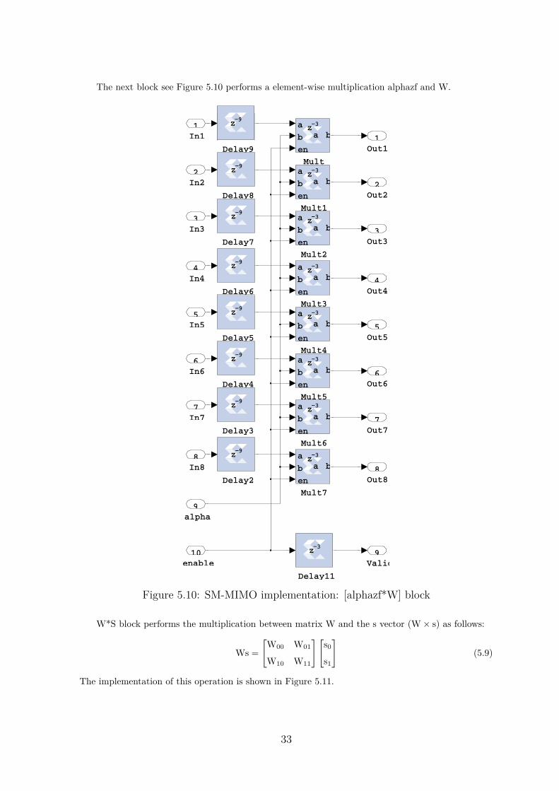
The next block see Figure 5.10 performs a element-wise multiplication alphazf and W.
Valid
9
Out8
8
Out7
7
Out6
6
Out5
5
Out4
4
Out3
3
Out2
2
Out1
1
Mult7
a
b
en
a bz−3
Mult6
a
b
en
a bz−3
Mult5
a
b
en
a bz−3
Mult4
a
b
en
a bz−3
Mult3
a
b
en
a bz−3
Mult2
a
b
en
a bz−3
Mult1
a
b
en
a bz−3
Mult
a
b
en
a bz−3
Delay9
z−9
Delay8
z−9
Delay7
z−9
Delay6
z−9
Delay5
z−9
Delay4
z−9
Delay3
z−9
Delay2
z−9
Delay11
z−3
enable
10
alpha
9
In8
8
In7
7
In6
6
In5
5
In4
4
In3
3
In2
2
In1
1 z−9
Figure 5.10: SM-MIMO implementation: [alphazf*W] block
W*S block performs the multiplication between matrix W and the s vector (W × s) as follows:
Ws =
[
W00 W01
W10 W11
] [
s0
s1
]
(5.9)
The implementation of this operation is shown in Figure 5.11.
33
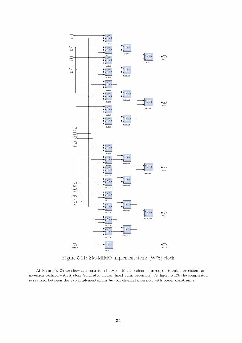
valid
5
Out4
4
Out3
3
Out2
2
Out1
1
Mult9
a
b
en
a bz−3
Mult8
a
b
en
a bz−3
Mult7
a
b
en
a bz−3
Mult6
a
b
en
a bz−3
Mult5
a
b
en
a bz−3
Mult4
a
b
en
a bz−3
Mult3
a
b
en
a bz−3
Mult2
a
b
en
a bz−3
Mult15
a
b
en
a bz−3
Mult14
a
b
en
a bz−3
Mult13
a
b
en
a bz−3
Mult12
a
b
en
a bz−3
Mult11
a
b
en
a bz−3
Mult10
a
b
en
a bz−3
Mult1
a
b
en
a bz−3
Mult
a
b
en
a bz−3
Delay11
z−3
AddSub9
a
b
a − b
AddSub8
a
b
a + b
AddSub7
a
b
a + b
AddSub6
a
b
a − b
AddSub5
a
b
a + b
AddSub4
a
b
a + b
AddSub3
a
b
a − b
AddSub2
a
b
a + b
AddSub11
a
b
a + b
AddSub10
a
b
a + b
AddSub1
a
b
a + b
AddSub
a
b
a − b
In12
13
In11
12
In10
11
In9
10
enable
9
In8
8
In7
7
In6
6
In5
5
In4
4
In3
3
In2
2
In1
1
Figure 5.11: SM-MIMO implementation: [W*S] block
At Figure 5.12a we show a comparison between Matlab channel inversion (double precision) andinversion realized with System Generator blocks (fixed point precision). At figure 5.12b the comparisonis realized between the two implementations but for channel inversion with power constraints.
34

−15 −10 −5 0 5 10 15−20
−15
−10
−5
0
5
10
15
Channel Invertion [W]
Real
Imag
Matlab
System Generator
(a)
−1 −0.8 −0.6 −0.4 −0.2 0 0.2 0.4 0.6 0.8 1−0.8
−0.6
−0.4
−0.2
0
0.2
0.4
0.6
0.8
1
alphazf*Wzf
Matlab
System Generator
(b)
Figure 5.12: SM-MIMO precoder comparison between MATLABr and System Gener-ator implementations: (a) Channel Invertion [W ] = [H]−1 (b) alpha_zf [W ]
35

chapter 6Conclusion and FutureWork
This chapter presents the final conclusions and some possibilities of future work.
6.1 conclusion
The proposed system was implemented in Matlab, tested and validated. As expected using a ZFequalizer to precode, comparatively to MMSE, the BER was worse, we found a difference of -3dB forthe same BER. A ZF precoder was implemented in System Generator, the baseband was tested andvalidated up to the power constraint block (transmission block).
6.2 future work
It would be useful to implement the uplink channel in order to send the channel informationestimated in the MS to the BS. As the full FPGA integration wasn’t realized, it would be useful tofinish and test the SM-MIMO precoder in a real scenario in order to analyse its performance andpracticality.
Regarding the precoder, it would be desirable to implement in System Generator/FPGA a MMSEprecoder, in order to get better BER but it requires the variance of noise (estimated theoretically andexperimentally confirmed).
37

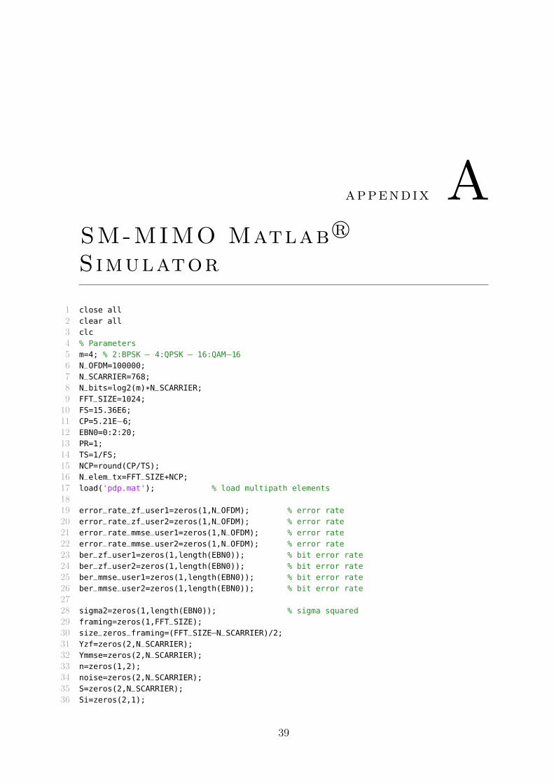
appendix ASM-MIMO Matlabr
Simulator
1 close all
2 clear all
3 clc
4 % Parameters
5 m=4; % 2:BPSK − 4:QPSK − 16:QAM−16
6 N_OFDM=100000;
7 N_SCARRIER=768;
8 N_bits=log2(m)*N_SCARRIER;
9 FFT_SIZE=1024;
10 FS=15.36E6;
11 CP=5.21E−6;
12 EBN0=0:2:20;
13 PR=1;
14 TS=1/FS;
15 NCP=round(CP/TS);
16 N_elem_tx=FFT_SIZE+NCP;
17 load('pdp.mat'); % load multipath elements
1819 error_rate_zf_user1=zeros(1,N_OFDM); % error rate
20 error_rate_zf_user2=zeros(1,N_OFDM); % error rate
21 error_rate_mmse_user1=zeros(1,N_OFDM); % error rate
22 error_rate_mmse_user2=zeros(1,N_OFDM); % error rate
23 ber_zf_user1=zeros(1,length(EBN0)); % bit error rate
24 ber_zf_user2=zeros(1,length(EBN0)); % bit error rate
25 ber_mmse_user1=zeros(1,length(EBN0)); % bit error rate
26 ber_mmse_user2=zeros(1,length(EBN0)); % bit error rate
2728 sigma2=zeros(1,length(EBN0)); % sigma squared
29 framing=zeros(1,FFT_SIZE);
30 size_zeros_framing=(FFT_SIZE−N_SCARRIER)/2;31 Yzf=zeros(2,N_SCARRIER);
32 Ymmse=zeros(2,N_SCARRIER);
33 n=zeros(1,2);
34 noise=zeros(2,N_SCARRIER);
35 S=zeros(2,N_SCARRIER);
36 Si=zeros(2,1);
39
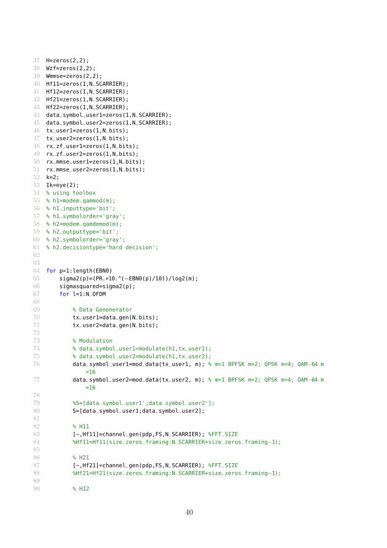
37 H=zeros(2,2);
38 Wzf=zeros(2,2);
39 Wmmse=zeros(2,2);
40 Hf11=zeros(1,N_SCARRIER);
41 Hf12=zeros(1,N_SCARRIER);
42 Hf21=zeros(1,N_SCARRIER);
43 Hf22=zeros(1,N_SCARRIER);
44 data_symbol_user1=zeros(1,N_SCARRIER);
45 data_symbol_user2=zeros(1,N_SCARRIER);
46 tx_user1=zeros(1,N_bits);
47 tx_user2=zeros(1,N_bits);
48 rx_zf_user1=zeros(1,N_bits);
49 rx_zf_user2=zeros(1,N_bits);
50 rx_mmse_user1=zeros(1,N_bits);
51 rx_mmse_user2=zeros(1,N_bits);
52 k=2;
53 Ik=eye(2);
54 % using toolbox
55 % h1=modem.qammod(m);
56 % h1.inputtype='bit';
57 % h1.symbolorder='gray';
58 % h2=modem.qamdemod(m);
59 % h2.outputtype='bit';
60 % h2.symbolorder='gray';
61 % h2.decisiontype='hard decision';
626364 for p=1:length(EBN0)
65 sigma2(p)=(PR.*10.^(−EBN0(p)/10))/log2(m);
66 sigmasquared=sigma2(p);
67 for l=1:N_OFDM
6869 % Data Genenerator
70 tx_user1=data_gen(N_bits);
71 tx_user2=data_gen(N_bits);
7273 % Modulation
74 % data_symbol_user1=modulate(h1,tx_user1);
75 % data_symbol_user2=modulate(h1,tx_user2);
76 data_symbol_user1=mod_data(tx_user1, m); % m=1 BPFSK m=2; QPSK m=4; QAM−64 m
=16
77 data_symbol_user2=mod_data(tx_user2, m); % m=1 BPFSK m=2; QPSK m=4; QAM−64 m
=16
7879 %S=[data_symbol_user1';data_symbol_user2'];
80 S=[data_symbol_user1;data_symbol_user2];
8182 % H11
83 [~,Hf11]=channel_gen(pdp,FS,N_SCARRIER); %FFT_SIZE
84 %Hf11=Hf11(size_zeros_framing:N_SCARRIER+size_zeros_framing−1);
8586 % H21
87 [~,Hf21]=channel_gen(pdp,FS,N_SCARRIER); %FFT_SIZE
88 %Hf21=Hf21(size_zeros_framing:N_SCARRIER+size_zeros_framing−1);
8990 % H12
40
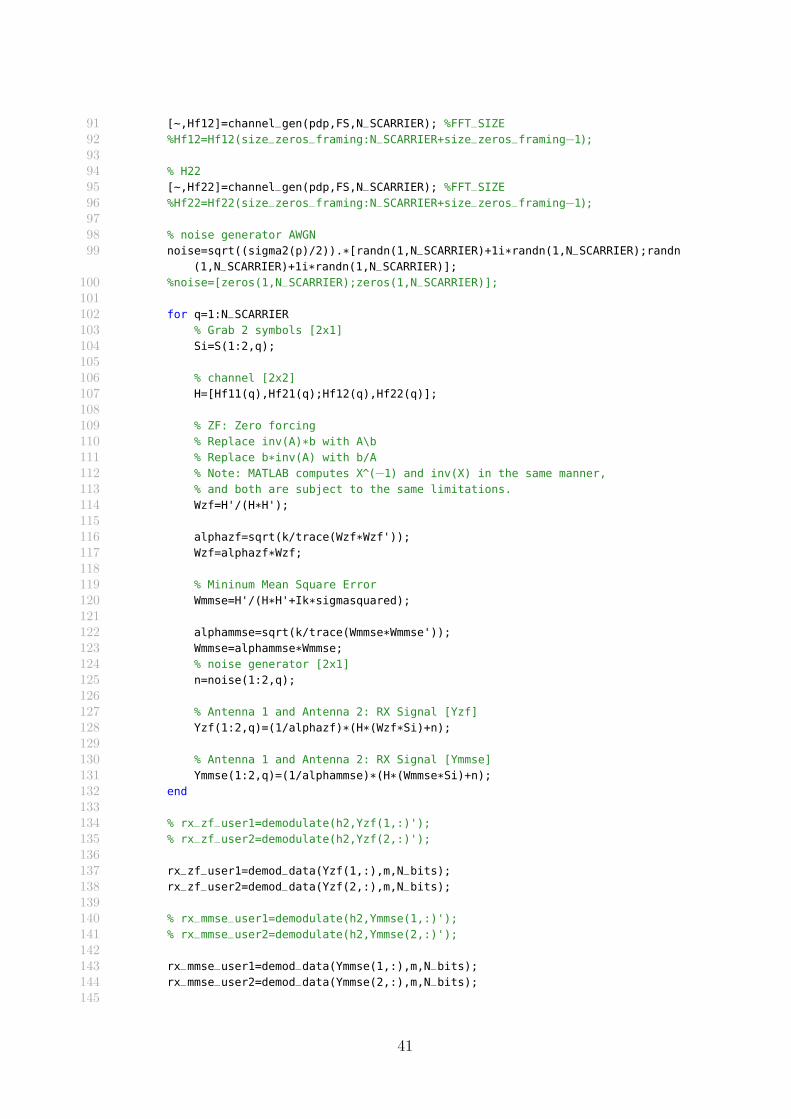
91 [~,Hf12]=channel_gen(pdp,FS,N_SCARRIER); %FFT_SIZE
92 %Hf12=Hf12(size_zeros_framing:N_SCARRIER+size_zeros_framing−1);
9394 % H22
95 [~,Hf22]=channel_gen(pdp,FS,N_SCARRIER); %FFT_SIZE
96 %Hf22=Hf22(size_zeros_framing:N_SCARRIER+size_zeros_framing−1);
9798 % noise generator AWGN
99 noise=sqrt((sigma2(p)/2)).*[randn(1,N_SCARRIER)+1i*randn(1,N_SCARRIER);randn
(1,N_SCARRIER)+1i*randn(1,N_SCARRIER)];
100 %noise=[zeros(1,N_SCARRIER);zeros(1,N_SCARRIER)];
101102 for q=1:N_SCARRIER
103 % Grab 2 symbols [2x1]
104 Si=S(1:2,q);
105106 % channel [2x2]
107 H=[Hf11(q),Hf21(q);Hf12(q),Hf22(q)];
108109 % ZF: Zero forcing
110 % Replace inv(A)*b with A\b
111 % Replace b*inv(A) with b/A
112 % Note: MATLAB computes X^(−1) and inv(X) in the same manner,
113 % and both are subject to the same limitations.
114 Wzf=H'/(H*H');
115116 alphazf=sqrt(k/trace(Wzf*Wzf'));
117 Wzf=alphazf*Wzf;
118119 % Mininum Mean Square Error
120 Wmmse=H'/(H*H'+Ik*sigmasquared);
121122 alphammse=sqrt(k/trace(Wmmse*Wmmse'));
123 Wmmse=alphammse*Wmmse;
124 % noise generator [2x1]
125 n=noise(1:2,q);
126127 % Antenna 1 and Antenna 2: RX Signal [Yzf]
128 Yzf(1:2,q)=(1/alphazf)*(H*(Wzf*Si)+n);
129130 % Antenna 1 and Antenna 2: RX Signal [Ymmse]
131 Ymmse(1:2,q)=(1/alphammse)*(H*(Wmmse*Si)+n);
132 end
133134 % rx_zf_user1=demodulate(h2,Yzf(1,:)');
135 % rx_zf_user2=demodulate(h2,Yzf(2,:)');
136137 rx_zf_user1=demod_data(Yzf(1,:),m,N_bits);
138 rx_zf_user2=demod_data(Yzf(2,:),m,N_bits);
139140 % rx_mmse_user1=demodulate(h2,Ymmse(1,:)');
141 % rx_mmse_user2=demodulate(h2,Ymmse(2,:)');
142143 rx_mmse_user1=demod_data(Ymmse(1,:),m,N_bits);
144 rx_mmse_user2=demod_data(Ymmse(2,:),m,N_bits);
145
41
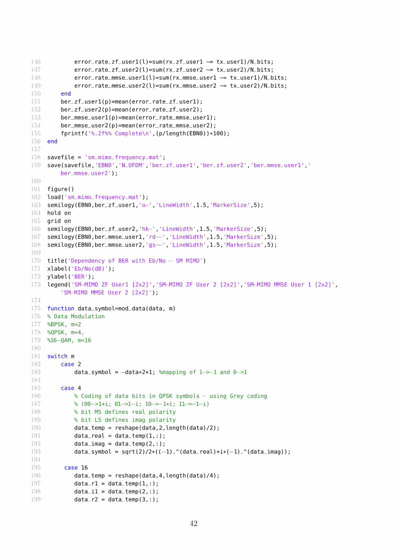
146 error_rate_zf_user1(l)=sum(rx_zf_user1 ~= tx_user1)/N_bits;
147 error_rate_zf_user2(l)=sum(rx_zf_user2 ~= tx_user2)/N_bits;
148 error_rate_mmse_user1(l)=sum(rx_mmse_user1 ~= tx_user1)/N_bits;
149 error_rate_mmse_user2(l)=sum(rx_mmse_user2 ~= tx_user2)/N_bits;
150 end
151 ber_zf_user1(p)=mean(error_rate_zf_user1);
152 ber_zf_user2(p)=mean(error_rate_zf_user2);
153 ber_mmse_user1(p)=mean(error_rate_mmse_user1);
154 ber_mmse_user2(p)=mean(error_rate_mmse_user2);
155 fprintf('%.2f%% Complete\n',(p/length(EBN0))*100);
156 end
157158 savefile = 'sm_mimo_frequency.mat';
159 save(savefile,'EBN0','N_OFDM','ber_zf_user1','ber_zf_user2','ber_mmse_user1','
ber_mmse_user2');
160161 figure()
162 load('sm_mimo_frequency.mat');
163 semilogy(EBN0,ber_zf_user1,'o−','LineWidth',1.5,'MarkerSize',5);164 hold on
165 grid on
166 semilogy(EBN0,ber_zf_user2,'hk−','LineWidth',1.5,'MarkerSize',5);167 semilogy(EBN0,ber_mmse_user1,'rd−−','LineWidth',1.5,'MarkerSize',5);168 semilogy(EBN0,ber_mmse_user2,'gs−−','LineWidth',1.5,'MarkerSize',5);169170 title('Dependency of BER with Eb/No − SM MIMO')
171 xlabel('Eb/No(dB)');
172 ylabel('BER');
173 legend('SM−MIMO ZF User1 [2x2]','SM−MIMO ZF User 2 [2x2]','SM−MIMO MMSE User 1 [2x2]',
'SM−MIMO MMSE User 2 [2x2]');
174175 function data_symbol=mod_data(data, m)
176 % Data Modulation
177 %BPSK, m=2
178 %QPSK, m=4,
179 %16−QAM, m=16
180181 switch m
182 case 2
183 data_symbol = −data*2+1; %mapping of 1−>−1 and 0−>1184185 case 4
186 % Coding of data bits in QPSK symbols − using Grey coding
187 % (00−>1+i; 01−>1−i; 10−>−1+i; 11−>−1−i)188 % bit MS defines real polarity
189 % bit LS defines imag polarity
190 data_temp = reshape(data,2,length(data)/2);
191 data_real = data_temp(1,:);
192 data_imag = data_temp(2,:);
193 data_symbol = sqrt(2)/2*((−1).^(data_real)+i*(−1).^(data_imag));
194195 case 16
196 data_temp = reshape(data,4,length(data)/4);
197 data_r1 = data_temp(1,:);
198 data_i1 = data_temp(2,:);
199 data_r2 = data_temp(3,:);
42
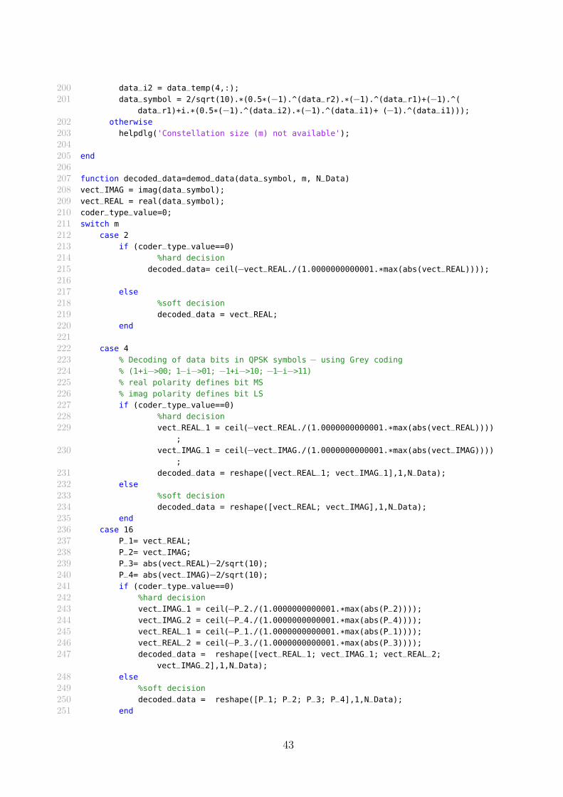
200 data_i2 = data_temp(4,:);
201 data_symbol = 2/sqrt(10).*(0.5*(−1).^(data_r2).*(−1).^(data_r1)+(−1).^(
data_r1)+i.*(0.5*(−1).^(data_i2).*(−1).^(data_i1)+ (−1).^(data_i1)));
202 otherwise
203 helpdlg('Constellation size (m) not available');
204205 end
206207 function decoded_data=demod_data(data_symbol, m, N_Data)
208 vect_IMAG = imag(data_symbol);
209 vect_REAL = real(data_symbol);
210 coder_type_value=0;
211 switch m
212 case 2
213 if (coder_type_value==0)
214 %hard decision
215 decoded_data= ceil(−vect_REAL./(1.0000000000001.*max(abs(vect_REAL))));216217 else
218 %soft decision
219 decoded_data = vect_REAL;
220 end
221222 case 4
223 % Decoding of data bits in QPSK symbols − using Grey coding
224 % (1+i−>00; 1−i−>01; −1+i−>10; −1−i−>11)225 % real polarity defines bit MS
226 % imag polarity defines bit LS
227 if (coder_type_value==0)
228 %hard decision
229 vect_REAL_1 = ceil(−vect_REAL./(1.0000000000001.*max(abs(vect_REAL))));
230 vect_IMAG_1 = ceil(−vect_IMAG./(1.0000000000001.*max(abs(vect_IMAG))));
231 decoded_data = reshape([vect_REAL_1; vect_IMAG_1],1,N_Data);
232 else
233 %soft decision
234 decoded_data = reshape([vect_REAL; vect_IMAG],1,N_Data);
235 end
236 case 16
237 P_1= vect_REAL;
238 P_2= vect_IMAG;
239 P_3= abs(vect_REAL)−2/sqrt(10);
240 P_4= abs(vect_IMAG)−2/sqrt(10);
241 if (coder_type_value==0)
242 %hard decision
243 vect_IMAG_1 = ceil(−P_2./(1.0000000000001.*max(abs(P_2))));244 vect_IMAG_2 = ceil(−P_4./(1.0000000000001.*max(abs(P_4))));245 vect_REAL_1 = ceil(−P_1./(1.0000000000001.*max(abs(P_1))));246 vect_REAL_2 = ceil(−P_3./(1.0000000000001.*max(abs(P_3))));247 decoded_data = reshape([vect_REAL_1; vect_IMAG_1; vect_REAL_2;
vect_IMAG_2],1,N_Data);
248 else
249 %soft decision
250 decoded_data = reshape([P_1; P_2; P_3; P_4],1,N_Data);
251 end
43
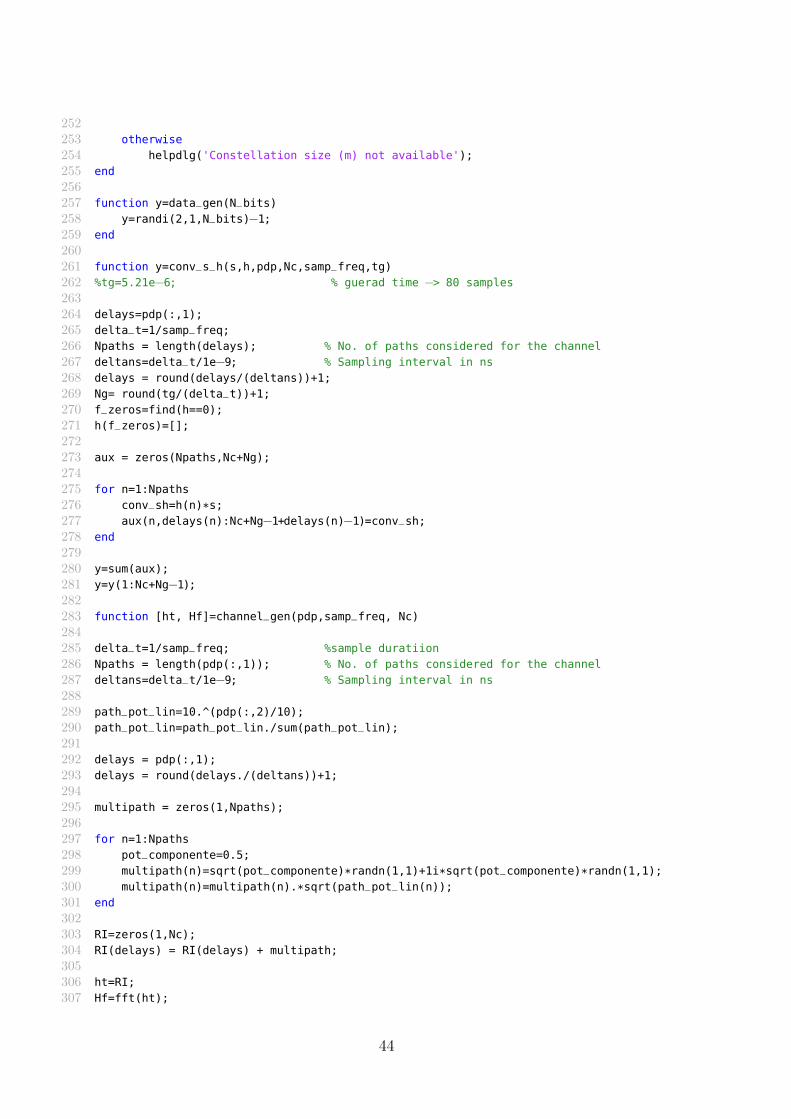
252253 otherwise
254 helpdlg('Constellation size (m) not available');
255 end
256257 function y=data_gen(N_bits)
258 y=randi(2,1,N_bits)−1;
259 end
260261 function y=conv_s_h(s,h,pdp,Nc,samp_freq,tg)
262 %tg=5.21e−6; % guerad time −> 80 samples
263264 delays=pdp(:,1);
265 delta_t=1/samp_freq;
266 Npaths = length(delays); % No. of paths considered for the channel
267 deltans=delta_t/1e−9; % Sampling interval in ns
268 delays = round(delays/(deltans))+1;
269 Ng= round(tg/(delta_t))+1;
270 f_zeros=find(h==0);
271 h(f_zeros)=[];
272273 aux = zeros(Npaths,Nc+Ng);
274275 for n=1:Npaths
276 conv_sh=h(n)*s;
277 aux(n,delays(n):Nc+Ng−1+delays(n)−1)=conv_sh;
278 end
279280 y=sum(aux);
281 y=y(1:Nc+Ng−1);
282283 function [ht, Hf]=channel_gen(pdp,samp_freq, Nc)
284285 delta_t=1/samp_freq; %sample duratiion
286 Npaths = length(pdp(:,1)); % No. of paths considered for the channel
287 deltans=delta_t/1e−9; % Sampling interval in ns
288289 path_pot_lin=10.^(pdp(:,2)/10);
290 path_pot_lin=path_pot_lin./sum(path_pot_lin);
291292 delays = pdp(:,1);
293 delays = round(delays./(deltans))+1;
294295 multipath = zeros(1,Npaths);
296297 for n=1:Npaths
298 pot_componente=0.5;
299 multipath(n)=sqrt(pot_componente)*randn(1,1)+1i*sqrt(pot_componente)*randn(1,1);
300 multipath(n)=multipath(n).*sqrt(path_pot_lin(n));
301 end
302303 RI=zeros(1,Nc);
304 RI(delays) = RI(delays) + multipath;
305306 ht=RI;
307 Hf=fft(ht);
44
References
[1] 3GPP, About 3GPP, Jun. 2014. [Online]. Available: http://www.3gpp.org/about-3gpp..
[2] E. Dahlman, S. Parkvall and J. Skold, 4G: LTE/LTE-Advanced for Mobile Broadband. ElsevierScience, 2013, isbn: 9780124199972.
[3] 3GPP, 3GPP organizational partners, Jun. 2014. [Online]. Available: http://www.3gpp.org/
about-3gpp/partners..
[4] A. Kumar, D. Y. Liu and J. Sengupta, «Evolution of mobile wireless communication networks:1G to 4G», International Journal of Electronics & Communication Technology, IJECT, vol. 1,no. 1, 2010.
[5] ITU, Global ICT developments, Jul. 2014. [Online]. Available: http://www.itu.int/en/ITU-
D/Statistics/Pages/stat/default.aspx..
[6] Y. G. Li and G. L. Stuber, Orthogonal frequency division multiplexing for wireless communica-tions. Springer, 2006.
[7] T. S. Rappaort, Wireless communications: principles and practice. Prentice-Hall, 2002.
[8] Y. Okumura et al., «Field strength and its variability in vhf and uhf land-mobile radio service»,ELEC. COMM. LAB., vol. 16, 1968.
[9] M. Hata, «Empirical formula for propagation loss in land mobile radio services», VehicularTechnology, IEEE Transactions on, vol. 29, no. 3, pp. 317–325, Aug. 1980, issn: 0018-9545. doi:10.1109/T-VT.1980.23859.
[10] U. Godse, Analog Communication. Technical Publications, 2010, isbn: 9788184311402. [Online].Available: http://books.google.pt/books?id=6XH7BUqm-lIC.
[11] J. G. Proakis, Digital communications, 2001.
[12] S. Coleri, M. Ergen, A. Puri and A. Bahai, «Channel estimation techniques based on pilotarrangement in ofdm systems», Broadcasting, IEEE Transactions on, vol. 48, no. 3, pp. 223–229,2002.
[13] S. Ohno, E. Manasseh and M. Nakamoto, «Preamble and pilot symbol design for channel estim-ation in ofdm systems with null subcarriers», EURASIP Journal on Wireless Communicationsand Networking, vol. 2011, no. 1, pp. 1–17, 2011.
[14] Y. S. Cho, J. Kim, W. Y. Yang and C. G. Kang, MIMO-OFDM wireless communications withMATLAB. John Wiley & Sons, 2010.
[15] K. Du and N. Swamy, Wireless Communication Systems: From RF Subsystems to 4G EnablingTechnologies. Cambridge University Press, 2010, isbn: 9781139485760. [Online]. Available:http://books.google.pt/books?id=5dGjKLawsTkC.
45
[16] D. Tse and P. Viswanath, Fundamentals of wireless communication. Cambridge university press,2005.
[17] C. Oestges and B. Clerckx, MIMO wireless communications: from real-world propagation tospace-time code design. Academic Press, 2010.
[18] A. Goldsmith, Wireless communications. Cambridge university press, 2005.
[19] M. K. Simon and M.-S. Alouini, Digital communication over fading channels. John Wiley &Sons, 2005, vol. 95.
[20] M. Jankiraman, Space-time codes and MIMO systems. Artech House, 2004.
[21] S. Alamouti, «A simple transmit diversity technique for wireless communications», SelectedAreas in Communications, IEEE Journal on, vol. 16, no. 8, pp. 1451–1458, 1998.
[22] E. Dahlman, S. Parkvall, J. Skold and P. Beming, 3G evolution: HSPA and LTE for mobilebroadband. Academic press, 2010.
[23] G. Strang, Linear Algebra and Its Applications 2nd Edition. Academic Press, Inc., 1980.
[24] Y. Jiang, M. K. Varanasi and J. Li, «Performance analysis of zf and mmse equalizers for mimosystems: an in-depth study of the high snr regime», Information Theory, IEEE Transactionson, vol. 57, no. 4, pp. 2008–2026, 2011.
[25] Xilinx, What is a fpga?, Jul. 2014. [Online]. Available: http://www.xilinx.com/fpga/index.
htm..
[26] R. Wiśniewski, Synthesis of compositional microprogram control units for programmable devices.University of Zielona Góra, 2009.
[27] Xilinx, Implementation overview for fpgas, Jul. 2014. [Online]. Available: http://www.xilinx.
com/support/documentation/sw_manuals/xilinx11/ise_c_implement_fpga_design.
htm..
46