image based visual servoing of a 7 dof robot manipulator using a distributed fuzzy proportional...

This article has been accepted for inclusion in a future issue of this journal. Content is final as presented, with the exception of pagination.

IEEE/ASME TRANSACTIONS ON MECHATRONICS 1

Image-Based Visual Servoing of a 7-DOF RobotManipulator Using an Adaptive Distributed Fuzzy

PD ControllerIndrazno Siradjuddin, Laxmidhar Behera, Senior Member, IEEE, T. Martin McGinnity, Senior Member, IEEE,

and Sonya Coleman, Member, IEEE

Abstract—This paper is concerned with the design and imple-mentation of a distributed proportional–derivative (PD) controllerof a 7-degrees of freedom (DOF) robot manipulator using theTakagi–Sugeno (T–S) fuzzy framework. Existing machine learningapproaches to visual servoing involve system identification of im-age and kinematic Jacobians. In contrast, the proposed approachactuates a control signal primarily as a function of the error andderivative of the error in the desired visual feature space. This ap-proach leads to a significant reduction in the computational burdenas compared to model-based approaches, as well as existing learn-ing approaches to model inverse kinematics. The simplicity of thecontroller structure will make it attractive in industrial implemen-tations where PD/PID type schemes are in common use. While theinitial values of PD gain are learned with the help of model-basedcontroller, an online adaptation scheme has been proposed that iscapable of compensating for local uncertainties associated with thesystem and its environment. Rigorous experiments have been per-formed to show that visual servoing tasks such as reaching a statictarget and tracking of a moving target can be achieved using theproposed distributed PD controller. It is shown that the proposedadaptive scheme can dynamically tune the controller parametersduring visual servoing, so as to improve its initial performancebased on parameters obtained while mimicking the model-basedcontroller. The proposed control scheme is applied and assessed inreal-time experiments using an uncalibrated eye-in-hand roboticsystem with a 7-DOF PowerCube robot manipulator.

Index Terms—Adaptive fuzzy modeling and control, eye-in-hand configuration, inverse Jacobian, robot manipulator, visualservoing.

I. INTRODUCTION

V ISION systems are essential for robots working in struc-tured and unstructured environments. The process of com-

bining vision and robot control is commonly known as visualservoing. The design of a visual servoing system presents chal-lenging engineering problems such as controllability, stability,and vision. Detailed reviews on visual servoing can be found in[1]–[3]. There are two basic types of visual servoing systems:

Manuscript received September 22, 2011; revised February 15, 2012 andJune 29, 2012; accepted January 15, 2013. Recommended by Technical EditorZ. Zhu.

The authors are with the Intelligent Systems Research Centre (ISRC), Uni-versity of Ulster, Londonderry, U.K. (e-mail: [email protected];[email protected]; [email protected]; [email protected]).

Color versions of one or more of the figures in this paper are available onlineat http://ieeexplore.ieee.org.

Digital Object Identifier 10.1109/TMECH.2013.2245337

image-based visual servoing (IBVS) and position-based visualservoing (PBVS). Typically IBVS schemes define the referencesignal in the image plane. IBVS maps the error vector in theimage space to the joint space in a robot manipulator. Usually,object features are extracted from the image to compress thesalient information; thus IBVS schemes are also called feature-based schemes and known as 2-D visual servoing. One of theproblems with IBVS schemes is that it is difficult to estimatedepth. PBVS schemes overcome this issue by defining the ref-erence input as the relative position and orientation betweenthe object and a robot manipulator in the task space. Therefore,PBVS schemes are also known as 3-D visual servoing. Recently,a detailed comparison of the two basic types of visual servoingin the context of stability and robustness with respect to systemmodelling error was presented in [4]. In [5], a PBVS schemehas been proposed using two types of camera configurations,eye-in-hand [6] and eye-to-hand [7]. This strategy aimed to re-solve the drawbacks of each camera configuration by exploitingthe capabilities of each other such that the system has a globalview with more precision.

In visual servoing of a robot manipulator, we typically com-pute the robot Jacobian matrix and the image Jacobian matrix(interaction matrix). The robot-image Jacobian matrix plays animportant role in the control of a visual servoing system. Therobot-image Jacobian maps the joint space into the image spaceof a robot manipulator. Methods for computing them includeclosed-form solutions [8]–[11] and adaptive schemes [12]–[15].More recently, approaches to visual servoing have been devel-oped that do not rely on the computation of both the robotJacobian matrix and the image Jacobian matrix. In [16], therobot-image Jacobian is estimated using a nonlinear optimi-sation algorithm based on Broyden’s method [17]. Similarly,in [18] Broyden’s method is generalized. However, like othernonlinear optimisation algorithms [19], the approaches are sen-sitive to noise as well as the initial robot-image Jacobian matrixapproximation.

There are also approaches to estimate the robot-image Ja-cobian using learning algorithms for example, self organisingmaps are used in [20], [21]. Two calibrated static cameras wereused to learn the inverse kinematics relationship of a 7-DOFrobot manipulator, while the redundancy resolution was alsoaddressed. The obtained inverse robot-image Jacobian approx-imation eliminates the necessity for online pseudoinverse com-putation. In [22], iterative learning was proposed to approximatethe Jacobian given a set of sample points of the demonstrated

1083-4435/$31.00 © 2013 IEEE


2 IEEE/ASME TRANSACTIONS ON MECHATRONICS

trajectory. An eye-to-hand configuration was used so that thesystem could compute the difference between the demonstratedtrajectory and the current position of the robot end-effector inevery iteration.

Fuzzy modeling techniques have become increasingly pop-ular. A system identification using inverse fuzzy modeling hasbeen proposed in [23]. In [24], fuzzy clustering and inverse fuzzymodels are derived; this method learned the inverse model of thesystem where the robot-image Jacobian was estimated and hasalso been applied in an eye-to-hand IBVS system. The experi-mental results show convergence of a 6-DOF robot manipulatorcan be reached in a 2-D trajectory (X–Z axes). The fuzzy modelsuggested by Takagi–Sugeno (1985) can represent a generalclass of static or dynamic nonlinear systems [25]. In [23], theintegration of learning algorithms such as neural networks, theT–S fuzzy model, and genetic algorithms was proposed to solvethe inverse dynamic model of a two-axis pneumatic manipula-tor system. As the robotic manipulator, together with the visualsystem, is a nonlinear system, it is advantageous to use the T–Sfuzzy model in the system [26].

The main issues encountered in visual servoing are relatedto control, robot kinematics, and vision. In traditional IBVSschemes, the robot-image Jacobian is described as a function ofthe current state of joint positions θ and image features s. If therobot-image Jacobian matrix is not a square matrix, the Moore–Penrose pseudoinverse approach is used but has computationalcomplexity.

In this paper, we address these issues by creating a system inwhich the control law for IBVS of a 7-DOF robot manipulator isestimated as a form of PD control using the T–S fuzzy learningalgorithm. The T–S fuzzy PD parameters are initialised by theoffline learning of the IBVS model. Thereafter, the pseudoin-verse robot Jacobian and the inverse interaction matrix are notcomputed during servoing implementation using T–S fuzzy PD.This estimated model is applied in a straightforward manner inorder to map the image error vector to the joint velocities vec-tor of the robot. This paper also proposes an online adaptationscheme, whereby the PD parameters are updated during servo-ing such that the local uncertainties associated with the systemand its environment can be compensated.

This paper is an extension of IBVS using a distributed fuzzyproportional controller as proposed in [27]. This paper presentsexperimental details using a 7-DOF PowerCube robot manip-ulator from Schunk [28] with eye-in-hand configuration. Stan-dard IBVS is discussed in Section II. The proposed method ofa distributed T–S fuzzy PD controller is explained in detail inSection III. The experimental results are provided in Section IVfollowed by a conclusion in Section V.

II. MODEL OF IMAGE-BASED IMAGE VISUAL SERVOING

The aim of all vision-based control schemes is to minimizethe error e(t), which is typically defined by

e(t) = s − s∗ (1)

where s is a vector of m visual features based on image mea-surements (e.g., the image coordinates of interest points, or the

parameters of a set of image segments) and a set of parametersthat represents potential knowledge about the system (e.g., cam-era intrinsic parameters or 3-D object models). The vector s∗ isthe desired values of the features. The vector s differs dependingon whether an IBVS, PBVS, or hybrid scheme is used.

The simpliest model of the controller is a velocity controllerin which there must be a relationship between the time variationof each variable in (1). Let the spatial velocity of the camerabe denoted by Xc = [xc ,ωc ]T , where xc is the linear velocityvector of the origin of the camera frame and ωc is the angularvelocity vector of the origin of the camera frame. In general,an exponential convergence is desired and can be ensured ife(t) decreases at a rate proportional to e(t). The relationshipbetween the time variation of the error and the camera velocitycan be computed as

Xc = −κL−1s (s − s∗) (2)

where L−1s is the inverse of the interaction matrix Ls [3], [10]

and κ is a positive decay constant. It is possible to invert Ls

when m is equal to d, the number of degrees of freedom of thespatial task in the 3-D coordinate system and det Ls �= 0. Whenm �= d, the Moore–Penrose pseudoinverse approach is used toapproximate the inverse value of Ls ; this inverse is denoted asL+

s . As Ls is a function of the image features vector s and thedepth Z, which is the distance between the origin of the cameraframe and a target point, it can be written as Ls(s, Z). Derivationof the interaction matrix for the considered features is discussedin [11], [29].

To implement the visual servoing scheme, the parameters ofLs(s, Z) have to be computed online which requires knowledgeof the depth information Z at each instant. Alternatively, it ispopular to choose Ls(s, Z) as the value of the desired target,Ls(s∗, Z∗). In this case, Ls(s∗, Z∗) is constant and only thedepth of the target and desired position of interest has to beknown, which means no varying 3-D parameters have to becalculated during the visual servoing. A stability analysis of thisscheme is explained in detail in [30].

Image moments are used as the image features in this study. Aset of Image moments is a generic representation of any objectthat can be segmented in an image. This set of image featuresis particularly adequate if a planar object is considered. Sincethe orientation of the robot end-effector is not considered, thecentroid and area of the target object are used as image featuresto represent a position of the robot end-effector in 3-D Euclideanspace (X–Y–Z axes coordinate).

The centroid and the area of the object image moment areselected to represent the position in 3-D Euclidean space, sincethe positioning task is targeted and hence the orientation vectoris not considered. Thus the objective of this scheme is to obtainthe joint angle velocity vector θ given s = [xg , yg , a]T and thedesired feature vector s∗ = [x∗

g , y∗g , a

∗]T , where (xg , yg ) is thecentroid coordinate of the object image moment and a is thearea of the object image moment.

A moment is a gross characteristic of the contour, computedby integrating (or summing) over all of the pixels of the contour.


SIRADJUDDIN et al.: IMAGE-BASED VISUAL SERVOING OF A 7-DOF ROBOT MANIPULATOR 3

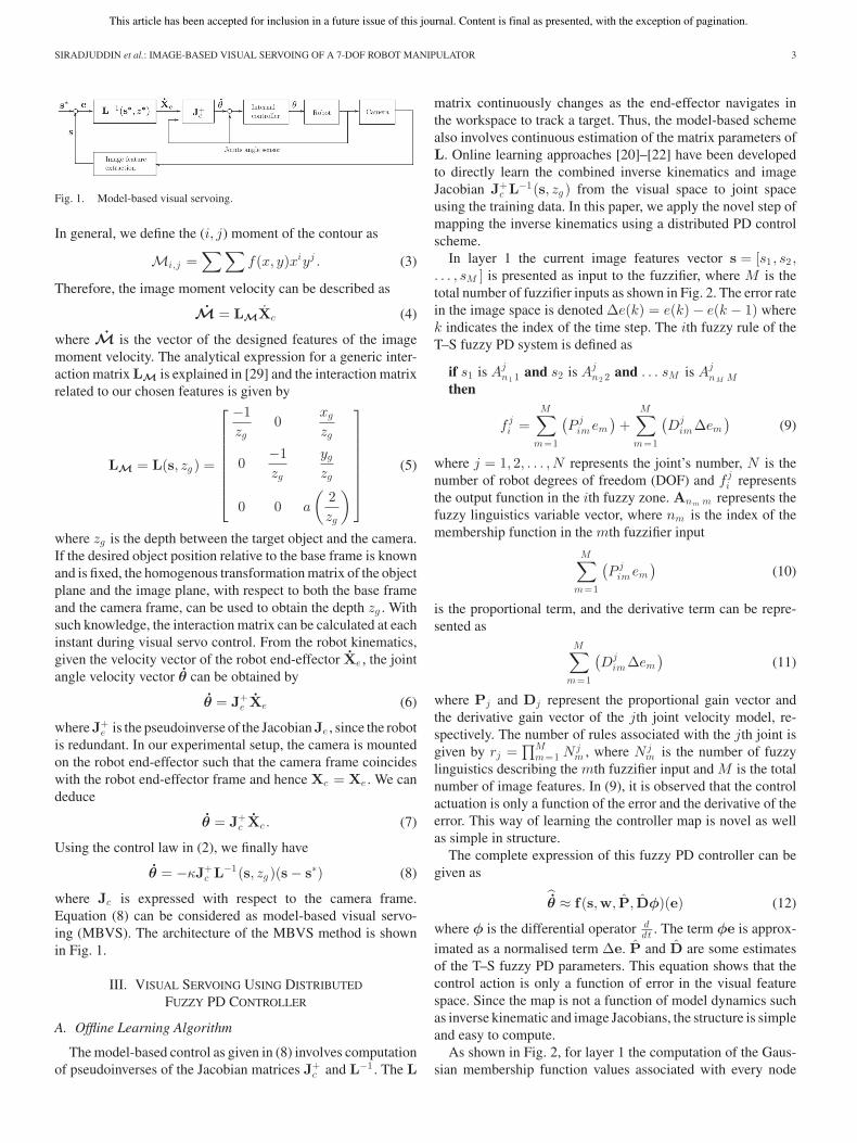
Fig. 1. Model-based visual servoing.

In general, we define the (i, j) moment of the contour as

Mi,j =∑∑

f(x, y)xiyj . (3)

Therefore, the image moment velocity can be described as

M = LMXc (4)

where M is the vector of the designed features of the imagemoment velocity. The analytical expression for a generic inter-action matrix LM is explained in [29] and the interaction matrixrelated to our chosen features is given by

LM = L(s, zg ) =

⎡

⎢⎢⎢⎢⎢⎢⎢⎣

−1zg

0xg

zg

0−1zg

yg

zg

0 0 a

(2zg

)

⎤

⎥⎥⎥⎥⎥⎥⎥⎦

(5)

where zg is the depth between the target object and the camera.If the desired object position relative to the base frame is knownand is fixed, the homogenous transformation matrix of the objectplane and the image plane, with respect to both the base frameand the camera frame, can be used to obtain the depth zg . Withsuch knowledge, the interaction matrix can be calculated at eachinstant during visual servo control. From the robot kinematics,given the velocity vector of the robot end-effector Xe , the jointangle velocity vector θ can be obtained by

θ = J+e Xe (6)

whereJ+e is the pseudoinverse of the JacobianJe , since the robot

is redundant. In our experimental setup, the camera is mountedon the robot end-effector such that the camera frame coincideswith the robot end-effector frame and hence Xc = Xe . We candeduce

θ = J+c Xc . (7)

Using the control law in (2), we finally have

θ = −κJ+c L−1(s, zg )(s − s∗) (8)

where Jc is expressed with respect to the camera frame.Equation (8) can be considered as model-based visual servo-ing (MBVS). The architecture of the MBVS method is shownin Fig. 1.

III. VISUAL SERVOING USING DISTRIBUTED

FUZZY PD CONTROLLER

A. Offline Learning Algorithm

The model-based control as given in (8) involves computationof pseudoinverses of the Jacobian matrices J+

c and L−1 . The L

matrix continuously changes as the end-effector navigates inthe workspace to track a target. Thus, the model-based schemealso involves continuous estimation of the matrix parameters ofL. Online learning approaches [20]–[22] have been developedto directly learn the combined inverse kinematics and imageJacobian J+

c L−1(s, zg ) from the visual space to joint spaceusing the training data. In this paper, we apply the novel step ofmapping the inverse kinematics using a distributed PD controlscheme.

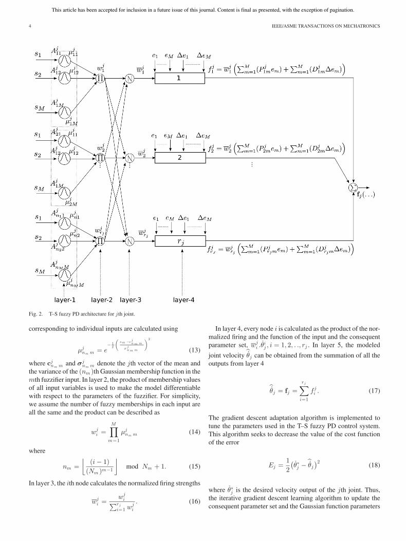
In layer 1 the current image features vector s = [s1 , s2 ,. . . , sM ] is presented as input to the fuzzifier, where M is thetotal number of fuzzifier inputs as shown in Fig. 2. The error ratein the image space is denoted Δe(k) = e(k) − e(k − 1) wherek indicates the index of the time step. The ith fuzzy rule of theT–S fuzzy PD system is defined as

if s1 is Ajn1 1 and s2 is Aj

n2 2 and . . . sM is AjnM M

then

fji =

M∑

m=1

(Pj

im em

)+

M∑

m=1

(Dj

im Δem

)(9)

where j = 1, 2, . . . , N represents the joint’s number, N is thenumber of robot degrees of freedom (DOF) and fj

i representsthe output function in the ith fuzzy zone. Anm m represents thefuzzy linguistics variable vector, where nm is the index of themembership function in the mth fuzzifier input

M∑

m=1

(Pj

im em

)(10)

is the proportional term, and the derivative term can be repre-sented as

M∑

m=1

(Dj

im Δem

)(11)

where Pj and Dj represent the proportional gain vector andthe derivative gain vector of the jth joint velocity model, re-spectively. The number of rules associated with the jth joint isgiven by rj =

∏Mm=1 Nj

m , where Njm is the number of fuzzy

linguistics describing the mth fuzzifier input and M is the totalnumber of image features. In (9), it is observed that the controlactuation is only a function of the error and the derivative of theerror. This way of learning the controller map is novel as wellas simple in structure.

The complete expression of this fuzzy PD controller can begiven as

θ ≈ f(s,w, P, Dφ)(e) (12)

where φ is the differential operator ddt . The term φe is approx-

imated as a normalised term Δe. P and D are some estimatesof the T–S fuzzy PD parameters. This equation shows that thecontrol action is only a function of error in the visual featurespace. Since the map is not a function of model dynamics suchas inverse kinematic and image Jacobians, the structure is simpleand easy to compute.

As shown in Fig. 2, for layer 1 the computation of the Gaus-sian membership function values associated with every node



Fig. 2. T–S fuzzy PD architecture for jth joint.

corresponding to individual inputs are calculated using

μjnm m = e

− 12

(s m −c

jn m m

σjn m m

) 2

(13)

where cjnm m and σj

nm m denote the jth vector of the mean andthe variance of the (nm )th Gaussian membership function in themth fuzzifier input. In layer 2, the product of membership valuesof all input variables is used to make the model differentiablewith respect to the parameters of the fuzzifier. For simplicity,we assume the number of fuzzy memberships in each input areall the same and the product can be described as

wji =

M∏

m=1

μjnm m (14)

where

nm =⌊

(i − 1)(Nm )m−1

⌋mod Nm + 1. (15)

In layer 3, the ith node calculates the normalized firing strengths

wji =

wji∑rj

i=1 wji

. (16)

In layer 4, every node i is calculated as the product of the nor-malized firing and the function of the input and the consequentparameter set, wj

i .θij , i = 1, 2, . ., rj . In layer 5, the modeled

joint velocity θj can be obtained from the summation of all the

outputs from layer 4

θj = fj =

rj∑

i=1

fji . (17)

The gradient descent adaptation algorithm is implemented totune the parameters used in the T–S fuzzy PD control system.This algorithm seeks to decrease the value of the cost functionof the error

Ej =12(θ∗j −

θj

)2(18)

where θ∗j is the desired velocity output of the jth joint. Thus,the iterative gradient descent learning algorithm to update theconsequent parameter set and the Gaussian function parameters



Fig. 3. T–S fuzzy PD control scheme.

can be described as⎡

⎢⎢⎢⎢⎢⎣

Pjim (k + 1)

Djim (k + 1)

cjnm m (k + 1)

σjnm m (k + 1)

⎤

⎥⎥⎥⎥⎥⎦=

⎡

⎢⎢⎢⎢⎢⎣

Pjim (k)

Djim (k)

cjnm m (k)

σjnm m (k)

⎤

⎥⎥⎥⎥⎥⎦− η

⎡

⎢⎢⎢⎢⎢⎣

∂Ej/∂P jim

∂Ej/∂Djim

∂Ej/∂cjnm m

∂Ej/∂σjnm m

⎤

⎥⎥⎥⎥⎥⎦

(19)where η is the learning rate parameter. The partial derivatives ofEj with respect to the change of the consequent parameters aredescribed as follows:

∂Ej

∂P jim

= −(θ∗j −

θj

)wj

i em (20)

∂Ej

∂Djim

= −(θ∗j −

θj

)wj

i Δem . (21)

The partial derivatives of Ej with respect to the change of theGaussian function parameters are derived in (22)–(23)

∂Ej

∂cjnm m

= B

(sm − cj

nm m

)

(σjnm m )2

(22)

∂Ej

∂σjnm m

= B

(sm − cj

nm m

)2

(σjnm m )3

(23)

where

B = −(θ∗j −θj )f

ji

⎛

⎜⎝wj

i

μjn m m

∑rj

i=1 wji − wj

i C

(∑rj

i=1 wji )2

⎞

⎟⎠μjnm m (24)

C =rj∑

i=1

M∏

a=1

μjnm a , for a �= m. (25)

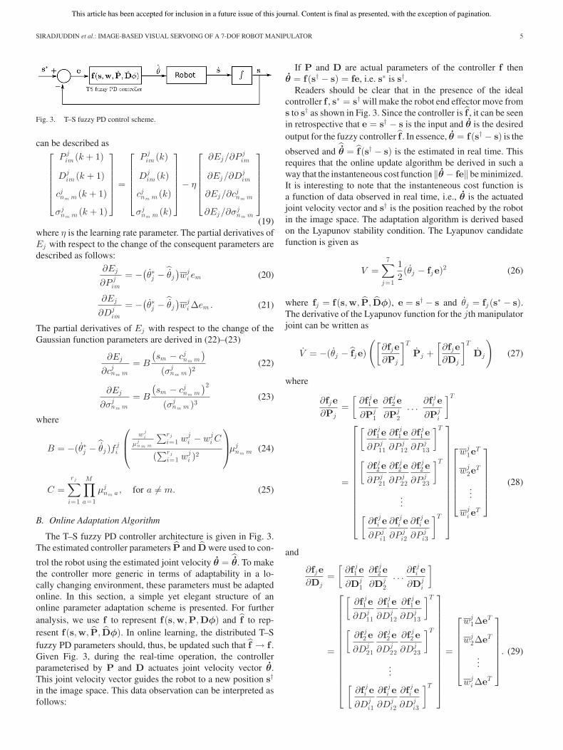
B. Online Adaptation Algorithm

The T–S fuzzy PD controller architecture is given in Fig. 3.The estimated controller parameters P and D were used to con-

trol the robot using the estimated joint velocity θ = θ. To make

the controller more generic in terms of adaptability in a lo-cally changing environment, these parameters must be adaptedonline. In this section, a simple yet elegant structure of anonline parameter adaptation scheme is presented. For furtheranalysis, we use f to represent f(s,w,P,Dφ) and f to rep-resent f(s,w, P, Dφ). In online learning, the distributed T–Sfuzzy PD parameters should, thus, be updated such that f → f .Given Fig. 3, during the real-time operation, the controllerparameterised by P and D actuates joint velocity vector θ.This joint velocity vector guides the robot to a new position s†

in the image space. This data observation can be interpreted asfollows:

If P and D are actual parameters of the controller f thenθ = f(s† − s) = fe, i.e. s∗ is s†.

Readers should be clear that in the presence of the idealcontroller f , s∗ = s† will make the robot end effector move froms to s† as shown in Fig. 3. Since the controller is f , it can be seenin retrospective that e = s† − s is the input and θ is the desiredoutput for the fuzzy controller f . In essence, θ = f(s† − s) is the

observed and θ = f(s† − s) is the estimated in real time. This

requires that the online update algorithm be derived in such away that the instanteneous cost function ‖θ − fe‖ be minimized.It is interesting to note that the instanteneous cost function isa function of data observed in real time, i.e., θ is the actuatedjoint velocity vector and s† is the position reached by the robotin the image space. The adaptation algorithm is derived basedon the Lyapunov stability condition. The Lyapunov candidatefunction is given as

V =7∑

j=1

12(θj − fje)2 (26)

where fj = f(s,w, P, Dφ), e = s† − s and θj = fj (s∗ − s).The derivative of the Lyapunov function for the jth manipulatorjoint can be written as

V = −(θj − fje)

([∂fje∂Pj

]T

Pj +[∂fje∂Dj

]T

Dj

)(27)

where

∂fje∂Pj

=[

∂f j1 e

∂Pj1

∂f j2 e

∂Pj2

. . .∂f j

i e

∂Pji

]T

=

⎡

⎢⎢⎢⎢⎢⎢⎢⎢⎢⎢⎢⎢⎢⎢⎣

[∂f j

1 e

∂P j11

∂f j1 e

∂P j12

∂f j1 e

∂P j13

]T

[∂f j

2 e

∂P j21

∂f j2 e

∂P j22

∂f j2 e

∂P j23

]T

...[

∂f ji e

∂P ji1

∂f ji e

∂P ji2

∂f ji e

∂P ji3

]T

⎤

⎥⎥⎥⎥⎥⎥⎥⎥⎥⎥⎥⎥⎥⎥⎦

⎡

⎢⎢⎢⎢⎢⎢⎣

wj1e

T

wj2e

T

...

wji e

T

⎤

⎥⎥⎥⎥⎥⎥⎦(28)

and

∂fje∂Dj

=[

∂f j1 e

∂Dj1

∂f j2 e

∂Dj2

. . .∂f j

i e

∂Dji

]

=

⎡

⎢⎢⎢⎢⎢⎢⎢⎢⎢⎢⎢⎢⎢⎢⎣

[∂f j

1 e

∂Dj11

∂f j1 e

∂Dj12

∂f j1 e

∂Dj13

]T

[∂f j

2 e

∂Dj21

∂f j2 e

∂Dj22

∂f j2 e

∂Dj23

]T

...[

∂f ji e

∂Dji1

∂f ji e

∂Dji2

∂f ji e

∂Dji3

]T

⎤

⎥⎥⎥⎥⎥⎥⎥⎥⎥⎥⎥⎥⎥⎥⎦

=

⎡

⎢⎢⎢⎢⎢⎢⎣

wj1ΔeT

wj2ΔeT

...

wji ΔeT

⎤

⎥⎥⎥⎥⎥⎥⎦. (29)



The adaptive laws of the proportional gain Pj and the derivativegain Dj can be designed such that V < 0, where Pj and Dj

are the column vectors and denoted as

Pj =

⎡

⎢⎢⎢⎢⎢⎢⎣

Pj1

Pj2

...

Pji

⎤

⎥⎥⎥⎥⎥⎥⎦

⎡

⎢⎢⎢⎢⎢⎢⎣

[ P j11 P

j12 P

j13 ]T

[ P j21 P

j22 P

j23 ]T

...

[ P ji1 P

ji2 P

ji3 ]T

⎤

⎥⎥⎥⎥⎥⎥⎦(30)

Dj =

⎡

⎢⎢⎢⎢⎢⎢⎣

[ Dj11D

j12D

j13 ]T

[ Dj21D

j22D

j23 ]T

...

[ Dji1D

ji2D

ji3 ]T

⎤

⎥⎥⎥⎥⎥⎥⎦. (31)

The adaptive laws of Pjim and Dj

im are designed as

P jim = ηp(θj − fje)wj

i em (32)

Djim = ηd(θj − fje)wj

i Δem (33)

where ηp , ηd > 0 are the adaptation rates. By substituting (32)and (33) into (30) and (31), respectively, we have the followingresults:

[∂fje∂Pj

]T

Pj = ηp(θj − fje)r∑

i=1

(M∑

m=1

(wji em )2

)(34)

[∂fje∂Dj

]T

Dj = ηd(θj − fje)r∑

i=1

(M∑

m=1

(wji Δem )2

). (35)

By substituting (34) and (35) into (27), the derivative of theLyapunov candidate function is described as

V = −(θj − fje)2

⎡

⎢⎣ηp

∑ri=1

(∑Mm=1(w

ji em )2

)

ηd

∑ri=1

(∑Mm=1(w

ji Δem )2

)

⎤

⎥⎦ (36)

and V is negative definite. Thus, the proposed updates (32)and (33) of the PD parameters ensures convergence in trackingerrors.

C. Stability Analysis

The stability of the T–S fuzzy PD closed loop system can beverified in terms of the Lyapunov stability. Let us consider theLyapunov function candidate as

V =12‖ e ‖2 (37)

where e = s − s∗ and s∗ is constant. The derivative of the Lya-punov candidate function V is derived as

V = eT e (38)

= eT JcLθ (39)

= eT JcLf(s,w,P,Dφ)e. (40)

Assuming the universal approximation capability of theT–S fuzzy model, we can write the T–S fuzzy function for thetrained dataset as

f(s,w,P,Dφ)e = −κJ+c L−1e + ε (41)

where ε = θ − θ is the approximation error. Substituting (41)

into (40), we have

V = eT A(−κA+e + ε) (42)

= −κeT AA+e + eT Aε (43)

where A = LJc and A+ = J+c L−1 . Initially, if ε = 0, there

is no approximation error, then A = A. The rank of matrixA ∈ Rm ,n can not be greater than m nor n. The rank of A can bewritten as rank(A) = min(m,n). In this case, m < n thereforeA has full rank of m. If A is full rank then ATA is invertible.Thus, the left inverse of A can be applied which is definedas A+ = (ATA)−1AT . For the case where no approximationerror is assumed, it can be said that (AA+) = I, where I isan identity matrix. In this case, the derivative of the Lyapunovcandidate function

V = −κ ‖ e ‖2 is negative definite (44)

and the system is globally asymptotically stable. If A �= A andA is full rank then (AA+) = I′

V = −κeT I′e. (45)

For a positive-definite matrix I′, a matrix definiteness can bedescribed as

λmin(I′) ‖ e ‖2≤ eT I′e ≤ λmax(I′) ‖ e ‖2 (46)

where λmin(·) and λmax(·) denote the minimum and the maxi-mum eigenvalues of a matrix, respectively. Thus, the derivativeof Lyapunov candidate function can be derived as

V ≤ −κλmin(I′) ‖ e ‖2 . (47)

The derivative of the Lyapunov candidate function will be neg-ative definite if λmin(I′) > 0 and I′ is positive definite. Hence,the system is locally stable. If ε �= 0 is considered then (43) canbe described as

V ≤ −κ ‖ e ‖ {λmin(I′) ‖ e ‖ −σmax(A)εmax} (48)

≤ −κ ‖ e ‖λmin(I′)

(‖ e ‖ −σmax(A)εmax

λmin(I′)

)(49)

where ‖ ε ‖≤ εmax and σmax(·) denotes the largest singularvalue of a matrix. V is negative definite if λmin(I′) > 0 and if

‖ e ‖> σmax(A)εmax

λmin(I′). (50)

Hence, the system is locally uniformly ultimately bounded(UUB) with the approximation error.



IV. EXPERIMENTAL RESULTS

A. Experimental Setup

The experimental setup consists of a 7-DOF robot manipula-tor, a firewire camera which is placed on the robot end-effector,and a PC. The distributed fuzzy PD controller based on the T–Sfuzzy model learns the mapping between the velocity of theimage feature s and the joint angle velocity θ. The camera isinterfaced through a firewire port to the PC and the images areprocessed using an OpenCV library [31]. The camera providescolor images at a resolution of 320 × 240 pixels. An imagehistogram back projection algorithm and image moments com-putation are used to identify the target object. Verification of thetrajectories of an object and the robot end-effector are obtainedusing a Vicon system. A ball is used as the target in an unclut-tered environment in these experiments. Markers are positionedon the robot end-effector and on the target ball in order for eachto be tracked by the Vicon system.

Experiments using the MBVS were conducted to obtaindata variables that are required for the learning process.For a defined working space, a number of trials were car-ried out using different initial positions of the robot end-effector such that the initial target would generate a widerange of data for joint velocities θ, current image feature vec-tor s = [sx, sy , sa ]T = [s1 , s2 , s3 ]T , image feature error vectore = [esx

, esy, esa

]T = [e1 , e2 , e3 ]T , and the rate of image fea-ture error vector Δe = [Δe1 ,Δe2 ,Δe3 ]T .

The experiment was comprised of the following steps.1) Each of the fuzzifier inputs in a vector s have three Gaus-

sian membership functions described by its mean andvariance (c, σ). Initially, the Gaussian functions weredistributed within a normalised range [−1,1] such thatthe overlapped area between two Gaussian functions was25%, approximately. The consequent parameters P and Din each joint velocity model were initialised with randomnumbers within the range of [–1,1]

2) The offline learning of the T–S fuzzy PD model wasverified using previously collected data. As suggestedin [21], the offline learning reduces the demand on onlinedata generation. The offline training data were obtainedby moving the target object by hand to get a sufficientdataset of the joint velocities and the image features in theworkspace.

3) The implementation of the T–S fuzzy PD model in realtime was considered to compare the performance betweenthe adaptive learning and nonadaptive learning.

Seven T–S fuzzy PD models of joint velocity θj have

been obtained in the training process, and every joint veloc-ity model contains 27 × 3 proportional gain parameters in avector of Pj ∈ R81 and 3 × 3 Gaussian membership func-tions’ parameters (cj

nm m , σjnm m ), where nm ,m ∈ [1, 2, 3] and

j ∈ [1, 2, . . . , 7].Additionally there are 27 × 3 derivative gain parameters in a

vector of Dj ∈ R81 . The identified Gaussian membership func-tions and consequent parameters of the modelled joint velocitiesθ = [θ1 ,

θ2 . . . ,

θ7 ]T may vary since the algorithm depends on

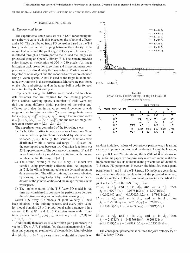
Fig. 4. RMSE of θj .

TABLE IUPDATED MEMBERSHIP FUNCTION OF THE T–S FUZZY PD

CONTROLLER OF θ1 AND θ2

random initialised values of consequent parameters, a learningrate η, a stopping condition and the dataset. Using the learning

rate η = 0.1 and 200 iterations, the RMSE of θ is shown in

Fig. 4. In this paper, we are primarily interested in the real-timeimplementation results rather than the presentation of identifiedT–S fuzzy PD parameters. However, the identified consequent

parameters θ1 and

θ2 of the T–S fuzzy PD model are consideredto give a more detailed explanation of the proposed schemes,as shown in Table I. The consequent parameters identified for

joint velocity θ1 of the T–S fuzzy PD are

If s1 is A111 and s2 is A1

12 and s3 is A113 then

f 11 = 1.60974(e1) − 0.0378469(e2) + 1.70716(e3)

+ 0.902445(Δe1) − 0.0506251(Δe2) + 1.78611(Δe3)If s1 is A1

21 and s2 is A122 and s3 is A1

23 thenf 1

2 = 2.55031(e1) − 0.437355(e2) + 3.26196(e3)+ 1.45803(Δe1) − 0.43672(Δe2) + 3.2049(Δe3)...



f 127 = 2.4745(e1) − 0.487684(e2) − 0.208851(e3)

+ 1.41299(Δe1) − 0.499181(Δe2) − 0.223516(Δe3).

The consequent parameters identified for joint velocity θ2 of

the T–S fuzzy PD are



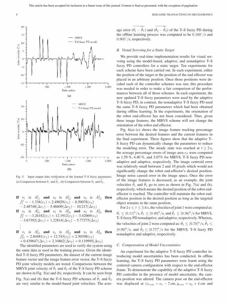
Fig. 5. Input–output data verification of the learned T–S fuzzy parameters.

(a) Comparison between θ1 and θ1 . (b) Comparison between θ2 and θ2 .



f 21 = −1.338(e1) + 2.49029(e2) − 8.50078(e3)− 2.48748(Δe1) − 5.46609(Δe2) − 10.217(Δe3)



f 22 = −3.26182(e1) + 12.1912(e2) − 3.42069(e3)− 3.67392(Δe1) + 1.22814(Δe2) − 5.77275(Δe3)...

If s1 is A231 and sy is A2


f 227 = 2.84481(e1) + 12.743(e2) + 2.50398(e3)

+ 0.439647(Δe1) + 2.34862(Δe2) + 0.119995(Δe3).The identified parameters are used to verify the system using

the same data as used in the training process. Given the identi-fied T–S fuzzy PD parameters, the dataset of the current imagefeature vector and the image feature error vector, the T–S fuzzyPD joint velocity models are tested. Comparisons between theMBVS joint velocity of θ1 and θ2 of the T–S fuzzy PD schemeare shown in Fig. 5(a) and (b), respectively. It can be seen from

Fig. 5(a) and (b) that the T–S fuzzy PD schemes of θ1 and

θ2are very similar to the model-based joint velocities. The aver-

age error (θ1 − θ1) and (θ2 −

θ2) of the T–S fuzzy PD duringthe offline learning process was computed to be 0.160◦/s and0.905◦/s, respectively.

B. Visual Servoing for a Static Target

We provide real-time implementation results for visual ser-voing using the model-based, adaptive, and nonadaptive T–Sfuzzy PD controllers for a static target. Ten experiments foreach scheme have been carried out. In each experiment, eitherthe position of the target or the position of the end effector wasplaced in an arbitrary position. Once those positions were de-cided each of the controller schemes was run; this procedurewas needed in order to make a fair comparison of the perfor-mances between all of those schemes. In each experiment, thenew updated T–S fuzzy parameters were used by the adaptiveT–S fuzzy PD; in contrast, the nonadaptive T–S fuzzy PD usedthe same T–S fuzzy PD parameters which had been obtainedduring offline learning. In the experiments, the orientation ofthe robot end-effector has not been considered. Thus, giventhree image features, the MBVS scheme will not change theorientation of the robot end effector.

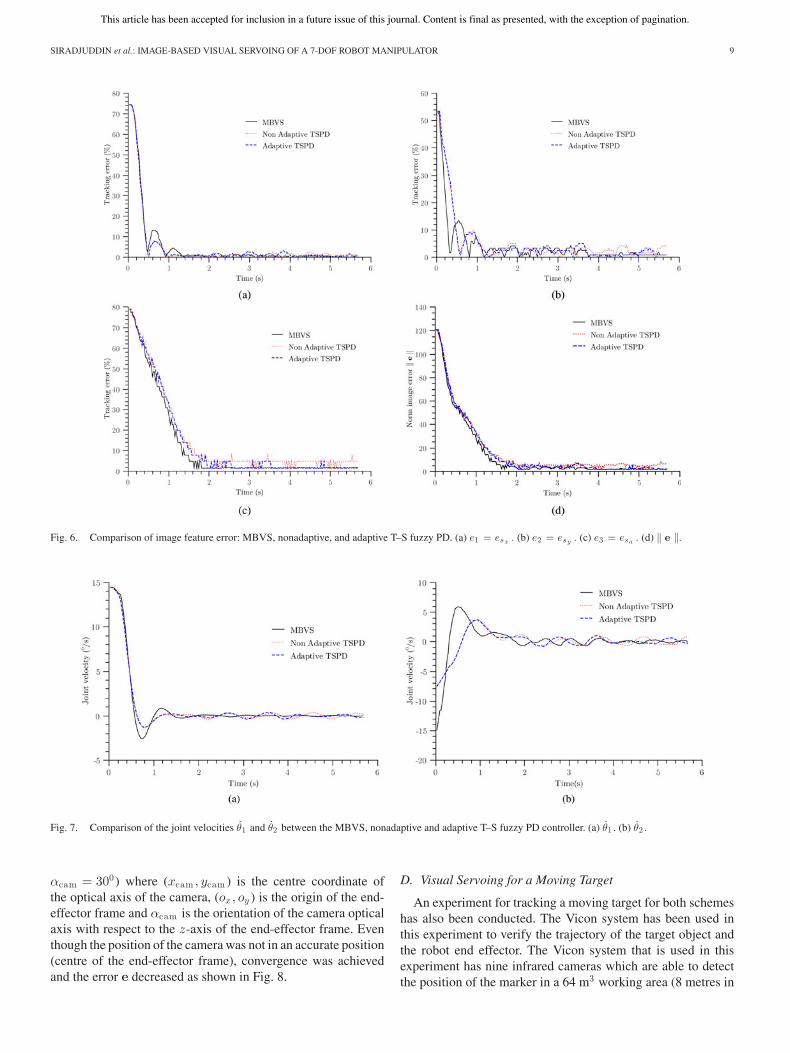
Fig. 6(a)–(c) shows the image feature tracking percentageerror between the desired features and the current features inthe final experiment. These figures show that the adaptive T–S fuzzy PD can dynamically change the parameters to reducethe modeling error. The steady state was reached at t ≥ 2 s,the average percentage errors of image area e3 were computedas 1.59 %, 4.40 %, and 3.07% for MBVS, T–S fuzzy PD non-adaptive and adaptive, respectively. The image centroid errorwas relatively small between 2 and 10 pixels which would notsignificantly change the robot end-effector’s desired position.Image noise caused error in the image space. Once the errorof the image features is decreased, as an example, the jointvelocities θ1 and θ2 go to zero as shown in Fig. 7(a) and (b),respectively, which means the desired position of the robot end-effector is reached. The controller will maintain the robot end-effector position in the desired position as long as the targetedobject remains in the same position.

For 2 s ≤ t ≤ 5.6 s, the velocities of joint 1 were computed as:

θ1 ≤ |0.11|0/s, ˆθ1 ≤ |0.40|0/s, and ˆ

θ1 ≤ |0.36|0/s for MBVS,T–S fuzzy PD nonadaptive, and adaptive, respectively. Whereas,

the velocities of joint 2 were computed as: θ2 ≤ |0.70|0/s, ˆθ2 ≤|0.99|0/s, and ˆ

θ2 ≤ |0.77|0/s for the MBVS, T–S fuzzy PDnonadaptive and adaptive, respectively.

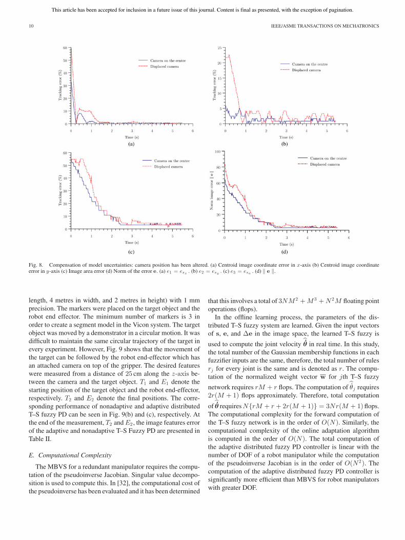
C. Compensation of Model Uncertainties

An experiment for the adaptive T–S fuzzy PD controller in-troducing model uncertainties has been conducted. In offlinelearning, the T–S fuzzy PD parameters were learnt using thecentered camera configuration with respect to the end-effectorframe. To demonstrate the capability of the adaptive T–S fuzzyPD controller in the presence of model uncertainty, the cam-era position was altered. The camera pose on the end-effectorwas displaced at (xcam = ox − 7 cm, ycam = oy + 4 cm and



Fig. 6. Comparison of image feature error: MBVS, nonadaptive, and adaptive T–S fuzzy PD. (a) e1 = esx . (b) e2 = esy . (c) e3 = esa . (d) ‖ e ‖.

Fig. 7. Comparison of the joint velocities θ1 and θ2 between the MBVS, nonadaptive and adaptive T–S fuzzy PD controller. (a) θ1 . (b) θ2 .

αcam = 300) where (xcam , ycam ) is the centre coordinate ofthe optical axis of the camera, (ox, oy ) is the origin of the end-effector frame and αcam is the orientation of the camera opticalaxis with respect to the z-axis of the end-effector frame. Eventhough the position of the camera was not in an accurate position(centre of the end-effector frame), convergence was achievedand the error e decreased as shown in Fig. 8.

D. Visual Servoing for a Moving Target

An experiment for tracking a moving target for both schemeshas also been conducted. The Vicon system has been used inthis experiment to verify the trajectory of the target object andthe robot end effector. The Vicon system that is used in thisexperiment has nine infrared cameras which are able to detectthe position of the marker in a 64 m3 working area (8 metres in



Fig. 8. Compensation of model uncertainties: camera position has been altered. (a) Centroid image coordinate error in x-axis (b) Centroid image coordinateerror in y-axis (c) Image area error (d) Norm of the error e. (a) e1 = esx . (b) e2 = esy . (c) e3 = esa . (d) ‖ e ‖.

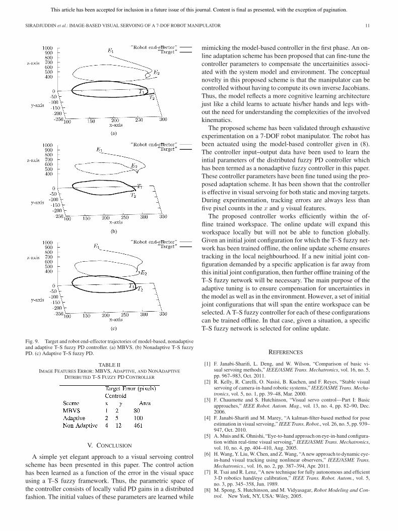
length, 4 metres in width, and 2 metres in height) with 1 mmprecision. The markers were placed on the target object and therobot end effector. The minimum number of markers is 3 inorder to create a segment model in the Vicon system. The targetobject was moved by a demonstrator in a circular motion. It wasdifficult to maintain the same circular trajectory of the target inevery experiment. However, Fig. 9 shows that the movement ofthe target can be followed by the robot end-effector which hasan attached camera on top of the gripper. The desired featureswere measured from a distance of 25 cm along the z-axis be-tween the camera and the target object. T1 and E1 denote thestarting position of the target object and the robot end-effector,respectively. T2 and E2 denote the final positions. The corre-sponding performance of nonadaptive and adaptive distributedT–S fuzzy PD can be seen in Fig. 9(b) and (c), respectively. Atthe end of the measurement, T2 and E2 , the image features errorof the adaptive and nonadaptive T–S Fuzzy PD are presented inTable II.

E. Computational Complexity

The MBVS for a redundant manipulator requires the compu-tation of the pseudoinverse Jacobian. Singular value decompo-sition is used to compute this. In [32], the computational cost ofthe pseudoinverse has been evaluated and it has been determined

that this involves a total of 3NM 2 + M 3 + N 2M floating pointoperations (flops).

In the offline learning process, the parameters of the dis-tributed T–S fuzzy system are learned. Given the input vectorsof s, e, and Δe in the image space, the learned T–S fuzzy is

used to compute the joint velocity θ in real time. In this study,

the total number of the Gaussian membership functions in eachfuzzifier inputs are the same, therefore, the total number of rulesrj for every joint is the same and is denoted as r. The compu-tation of the normalized weight vector w for jth T–S fuzzy

network requires rM + r flops. The computation of θj requires

2r(M + 1) flops approximately. Therefore, total computation

of θ requires N{rM + r + 2r(M + 1)} = 3Nr(M + 1) flops.

The computational complexity for the forward computation ofthe T–S fuzzy network is in the order of O(N). Similarly, thecomputational complexity of the online adaptation algorithmis computed in the order of O(N). The total computation ofthe adaptive distributed fuzzy PD controller is linear with thenumber of DOF of a robot manipulator while the computationof the pseudoinverse Jacobian is in the order of O(N 2). Thecomputation of the adaptive distributed fuzzy PD controller issignificantly more efficient than MBVS for robot manipulatorswith greater DOF.



Fig. 9. Target and robot end-effector trajectories of model-based, nonadaptiveand adaptive T–S fuzzy PD controller. (a) MBVS. (b) Nonadaptive T–S fuzzyPD. (c) Adaptive T–S fuzzy PD.

TABLE IIIMAGE FEATURES ERROR: MBVS, ADAPTIVE, AND NONADAPTIVE

DITRIBUTED T–S FUZZY PD CONTROLLER

V. CONCLUSION

A simple yet elegant approach to a visual servoing controlscheme has been presented in this paper. The control actionhas been learned as a function of the error in the visual spaceusing a T–S fuzzy framework. Thus, the parametric space ofthe controller consists of locally valid PD gains in a distributedfashion. The initial values of these parameters are learned while

mimicking the model-based controller in the first phase. An on-line adaptation scheme has been proposed that can fine-tune thecontroller parameters to compensate the uncertainities associ-ated with the system model and environment. The conceptualnovelty in this proposed scheme is that the manipulator can becontrolled without having to compute its own inverse Jacobians.Thus, the model reflects a more cognitive learning architecturejust like a child learns to actuate his/her hands and legs with-out the need for understanding the complexities of the involvedkinematics.

The proposed scheme has been validated through exhaustiveexperimentation on a 7-DOF robot manipulator. The robot hasbeen actuated using the model-based controller given in (8).The controller input–output data have been used to learn theintial parameters of the distributed fuzzy PD controller whichhas been termed as a nonadaptive fuzzy controller in this paper.These controller parameters have been fine tuned using the pro-posed adaptation scheme. It has been shown that the controlleris effective in visual servoing for both static and moving targets.During experimentation, tracking errors are always less thanfive pixel counts in the x and y visual features.

The proposed controller works efficiently within the of-fline trained workspace. The online update will expand thisworkspace locally but will not be able to function globally.Given an initial joint configuration for which the T–S fuzzy net-work has been trained offline, the online update scheme ensurestracking in the local neighbourhood. If a new initial joint con-figuration demanded by a specific application is far away fromthis initial joint configuration, then further offline training of theT–S fuzzy network will be necessary. The main purpose of theadaptive tuning is to ensure compensation for uncertainties inthe model as well as in the environment. However, a set of initialjoint configurations that will span the entire workspace can beselected. A T–S fuzzy controller for each of these configurationscan be trained offline. In that case, given a situation, a specificT–S fuzzy network is selected for online update.

REFERENCES

[1] F. Janabi-Sharifi, L. Deng, and W. Wilson, “Comparison of basic vi-sual servoing methods,” IEEE/ASME Trans. Mechatronics, vol. 16, no. 5,pp. 967–983, Oct. 2011.

[2] R. Kelly, R. Carelli, O. Nasisi, B. Kuchen, and F. Reyes, “Stable visualservoing of camera-in-hand robotic systems,” IEEE/ASME Trans. Mecha-tronics, vol. 5, no. 1, pp. 39–48, Mar. 2000.

[3] F. Chaumette and S. Hutchinson, “Visual servo control—Part I: Basicapproaches,” IEEE Robot. Autom. Mag., vol. 13, no. 4, pp. 82–90, Dec.2006.

[4] F. Janabi-Sharifi and M. Marey, “A kalman-filter-based method for poseestimation in visual servoing,” IEEE Trans. Robot., vol. 26, no. 5, pp. 939–947, Oct. 2010.

[5] A. Muis and K. Ohnishi, “Eye-to-hand approach on eye-in-hand configura-tion within real-time visual servoing,” IEEE/ASME Trans. Mechatronics,vol. 10, no. 4, pp. 404–410, Aug. 2005.

[6] H. Wang, Y. Liu, W. Chen, and Z. Wang, “A new approach to dynamic eye-in-hand visual tracking using nonlinear observers,” IEEE/ASME Trans.Mechatronics., vol. 16, no. 2, pp. 387–394, Apr. 2011.

[7] R. Tsai and R. Lenz, “A new technique for fully autonomous and efficient3-D robotics hand/eye calibration,” IEEE Trans. Robot. Autom., vol. 5,no. 3, pp. 345–358, Jun. 1989.

[8] M. Spong, S. Hutchinson, and M. Vidyasagar, Robot Modeling and Con-trol. New York, NY, USA: Wiley, 2005.



[9] P. Corke and S. Hutchinson, “A new partitioned approach to image-basedvisual servo control,” IEEE Trans. Robot. Autom., vol. 17, no. 4, pp. 507–515, Aug. 2001.

[10] F. Chaumette and S. Hutchinson, “Visual servo control—part II: Advancedapproaches,” IEEE Robot. Autom. Mag., vol. 14, no. 1, pp. 109–118, Mar.2007.

[11] S. Indrazno, M. McGinnity, L. Behera, and S. Coleman, “Visual servoingof a redundant manipulator using shape moments,” in Proc. IET IrishSignals Syst. Conf., Jun. 2009, pp. 1–6.

[12] C. C. Cheah, S. Hou, Y. Zhao, and J.-J. Slotine, “Adaptive vision andforce tracking control for robots with constraint uncertainty,” IEEE/ASMETrans. Mechatronics, vol. 15, no. 3, pp. 389–399, Jun. 2010.

[13] H. Wang, Y. Liu, and D. Zhou, “Adaptive visual servoing using pointand line features with an uncalibrated eye-in-hand camera,” IEEE Trans.Robot., vol. 24, no. 4, pp. 843–857, Aug. 2008.

[14] L. Hsu, R. R. Costa, and F. Lizarralde, “Lyapunov/passivity-based adap-tive control of relative degree two mimo systems with an application tovisual servoing,” IEEE Trans. Autom. Control, vol. 52, no. 2, pp. 364–371,Feb. 2007.

[15] S. Islam and P. Liu, “Pd output feedback control design for industrialrobotic manipulators,” IEEE/ASME Trans. Mechatronics, vol. 16, no. 1,pp. 187–197, Feb. 2011.

[16] J. Armstrong Piepmeier, G. McMurray, and H. Lipkin, “A dynamic ja-cobian estimation method for uncalibrated visual servoing,” in Proc.IEEE/ASME Int. Conf. Adv. Intell. Mechatron., Sep. 1999, pp. 944–949.

[17] C. Broyden, “A class of methods for solving nonlinear simultaneous equa-tions,” Math. Comput., vol. 19, pp. 577–593, 1965.

[18] M. Bonkovic, A. Hace, and K. Jezernik, “Population based uncalibrated vi-sual servoing,” IEEE/ASME Trans. Mechatronics, vol. 13, no. 3, pp. 393–397, Jun. 2008.

[19] Q. Fu, Z. Zhang, and J. Shi, “Uncalibrated visual servoing using moreprecise model,” in Proc. IEEE Conf. Robot., Autom. Mechatron., Sep.2008, pp. 916–921.

[20] P. Patchaikani and L. Behera, “Visual servoing of redundant manipulatorwith jacobian matrix estimation using self-organizing map,” Robot. Auton.Syst., vol. 58, no. 8, pp. 978–990, Aug. 2010.

[21] S. Kumar, L. Behera, and T. McGinnity, “Kinematic control of a redundantmanipulator using an inverse-forward adaptive scheme with a ksom basedhint generator,” Robot. Auton. Syst., vol. 58, no. 5, pp. 622–633, May2010.

[22] P. Jiang, L. Bamforth, Z. Feng, J. Baruch, and Y. Chen, “Indirect iterativelearning control for a discrete visual servo without a camera-robot model,”IEEE Trans. Syst., Man, Cybern. B, Cybern., vol. 37, no. 4, pp. 863–876,Aug. 2007.

[23] K. Ahn and H. Anh, “Inverse double narx fuzzy modeling for systemidentification,” IEEE/ASME Trans. Mechatronics., vol. 15, no. 1, pp. 136–148, Feb. 2010.

[24] P. Goncalves, L. Mendoca, J. Sousa, and J. Pinto, “Uncalibrated eye tohand visual servoing using inverse fuzzy models,” IEEE Trans. FuzzySyst., vol. 16, no. 2, pp. 341–353, Apr. 2008.

[25] K. Tanaka, M. Tanaka, H. Ohtake, and H. Wang, “Shared nonlinearcontrol in wireless-based remote stabilization: A theoretical approach,”IEEE/ASME Trans. Mechatronics, vol. 3, no. 1, pp. 443–452, Jun. 2012.

[26] T. Takagi and M. Sugeno, “Fuzzy identification of systems and its appli-cation to modeling and control,” IEEE Trans. Syst., Man, Cybern., vol. 15,no. 1, pp. 116–132, Jan. 1985.

[27] I. Siradjuddin, L. Behera, T. McGinnity, and S. Coleman, “Image basedvisual servoing of a 7-dof robot manipulator using a distributed fuzzyproportional controller,” in Proc. IEEE Int. Conf. Fuzzy Syst., Jul. 2010,pp. 1–8.

[28] “Amtec robotics,” (2013). [Online]. Available: http//www.amtec-robotics.com

[29] F. Chaumette, “Image moments: A general and useful set of features forvisual servoing,” IEEE Trans. Robot., vol. 20, no. 4, pp. 713–723, Aug.2004.

[30] E. Malis and F. Chaumette, “Theoretical improvements in the stabilityanalysis of a new class of model-free visual servoing methods,” IEEETrans. Robot. Autom., vol. 18, no. 2, pp. 176–186, Apr. 2002.

[31] Open Source Computer Vision Library. (2013). [Online]. Available:http://opencv.willowgarage.com

[32] P. Patchaikani, L. Behera, and G. Prasad, “A single network adaptivecritic based redundancy resolution scheme for robot manipulators,” Robot.Auton. Syst., vol. 58, no. 8, pp. 978–990, Aug. 2009.

Indrazno Siradjuddin received the B.E degree inelectrical and electronics engineering from Brawi-jaya University, Malang, Indonesia, in 2000, and theMaster’s degree in electrical and electronics engineer-ing from the Institut Teknologi Sepuluh Nopember,Surabaya, Indonesia, in 2004. He is currently workingtoward the Ph.D. degree in the Department of Com-puting and Engineering, Magee College, Universityof Ulster, Londonderry, U.K.

His research interests include vision-based robot-manipulator control, intelligent control, neural net-

works, and fuzzy systems.

Laxmidhar Behera (SM’xx) received the B.Sc. andM.Sc. degrees in engineering from NIT Rourkela,India, in 1988 and 1990, respectively, and the Ph.D.degree from the Indian Institute of Technology Delhi,India.

He is currently a Professor in the Departmentof Electrical Engineering, Indian Institute of Tech-nology (IIT) Kanpur, Kanpur, India. He joined theIntelligent Systems Research Center (ISRC), Uni-versity of Ulster, Londonberry, U.K., as a Readeron sabbatical from IIT Kanpur during 2007–2009.

He was an Assistant Professor at BITS Pilani during 1995–1999 and pur-sued his Postdoctoral studies at the German National Research Center for In-formation Technology, GMD, Sank Augustin, Germany during 2000–2001.He was also a Visiting Researcher/Professor at FHG, Germany, and ETH,Zurich, Switzerland. He has more than 150 papers to his credit published inrefereed journals and conference proceedings. His research interests includeintelligentcontrol, robotics, neural networks, and cognitive modeling.

T. Martin McGinnity (SM’09) received the (FirstClass Hons.) degree in physics and the Ph.D. degreefrom the University of Durham, Durham, U.K., in1975 and 1979, respectively.

He is a Professor of Intelligent Systems Engineer-ing within the Faculty of Computing and Engineer-ing, University of Ulster, Londonderry, U.K., and theDirector of the Intelligent Systems Research Centre,which encompasses the research activities of approx-imately 100 researchers. He is the author or coau-thor of more than 275 research papers. His current

research interests include computational intelligence, and in particular compu-tational systems which explore and model biological signal processing, partic-ularly in relation to cognitive robotics and computation neuroscience.

Dr. McGinnity has received both a Senior Distinguished Research Fellow-ship and a Distinguished Learning Support Fellowship in recognition of hiscontribution to teaching and research. He is a Fellow of the IET and a CharteredEngineer.

Sonya Coleman (M’xx) received the B.Sc. (Hons)degree in mathematics, statistics, and computing andthe Ph.D. degree in mathematics from the Univer-sity of Ulster, Londonberry, U.K., in 1999 and 2003,respectively.

She is currently a Lecturer in the School of Com-puting and Intelligent System, Magee College, Uni-versity of Ulster. She has more than 50 publicationsprimarily in the field of mathematical image pro-cessing, and much of the recent research undertakenby her has been supported by funding from EPSRC

award EP/C006283/11, the Leverhulme Trust, and the Nuffield Foundation.Additionally, she is co-investigator on the EU FP7 funded project RUBICON.She is the author or coauthor of over 70 research papers on image processing,robotics, and computational neuroscience.

Dr. Coleman was awarded the Distinguished Research Fellowship by theUniversity of Ulster in recognition of her contribution to research in 2009.

image based visual servoing of a 7 dof robot manipulator using a distributed fuzzy proportional...

Documents