arX

iv:0

912.

4472

v2 [

q-bi

o.PE

] 2

9 Ju

l 201

0

Noname manuscript No.(will be inserted by the editor)

Identifying the Rooted Species Tree from the Distribution

of Unrooted Gene Trees under the Coalescent

Elizabeth S. Allman · James H. Degnan ·

John A. Rhodes

Received: date / Accepted: date

July 30, 2010

Abstract Gene trees are evolutionary trees representing the ancestry of genes sam-

pled from multiple populations. Species trees represent populations of individuals —

each with many genes — splitting into new populations or species. The coalescent pro-

cess, which models ancestry of gene copies within populations, is often used to model

the probability distribution of gene trees given a fixed species tree. This multispecies

coalescent model provides a framework for phylogeneticists to infer species trees from

gene trees using maximum likelihood or Bayesian approaches. Because the coalescent

models a branching process over time, all trees are typically assumed to be rooted in

this setting. Often, however, gene trees inferred by traditional phylogenetic methods

are unrooted.

We investigate probabilities of unrooted gene trees under the multispecies coa-

lescent model. We show that when there are four species with one gene sampled per

species, the distribution of unrooted gene tree topologies identifies the unrooted species

tree topology and some, but not all, information in the species tree edges (branch

lengths). The location of the root on the species tree is not identifiable in this sit-

uation. However, for 5 or more species with one gene sampled per species, we show

that the distribution of unrooted gene tree topologies identifies the rooted species tree

topology and all its internal branch lengths. The length of any pendant branch leading

E. S. AllmanDepartment of Mathematics and Statistics, University of Alaska Fairbanks,PO Box 756660, Fairbanks, AK 99775 USAE-mail: e.allman@alaska.edu

Corresponding author:J. H. DegnanDepartment of Mathematics and Statistics, University of CanterburyPrivate Bag 4800, Christchurch, New ZealandE-mail: J.Degnan@math.canterbury.ac.nz

J. A. RhodesDepartment of Mathematics and Statistics, University of Alaska Fairbanks,PO Box 756660, Fairbanks, AK 99775 USAE-mail: j.rhodes@alaska.edu

2

to a leaf of the species tree is also identifiable for any species from which more than

one gene is sampled.

Keywords Multispecies coalescent · phylogenetics · invariants · polytomy

Mathematics Subject Classification (2000) 62P10 · 92D15

1 Introduction

The goal of a phylogenetic study is often to infer an evolutionary tree depicting the

history of speciation events that lead to a currently extant set of taxa. In these species

trees, speciation events are idealized as populations instantaneously diverging into two

populations that no longer exchange genes. Such trees are often estimated indirectly,

from DNA sequences for orthologous genes from the extant species. A common as-

sumption has been that such an inferred gene tree has a high probability of having

the same topology as the species tree. Recently, however, increasing attention has been

given to population genetic issues that lead to differences between gene and species

trees, and how potentially discordant trees for many genes might be utilized in species

tree inference.

Methods that infer gene trees, such as maximum likelihood (ML) using standard

DNA substitution models, typically can estimate the expected number of mutations

on the edges of a tree, but not the direction of time. Phylogenetic methods therefore

often estimate unrooted gene trees. In many cases, the root of a tree can be inferred

by including data on an outgroup, i.e., a species believed to be less closely related

to the species of interest than any of those are to each other (Jennings and Edwards

2005; Poe and Chubb 2004; Rokas et al 2003). However, outgroup species which are too

distantly related to the ingroup taxa may lead to unreliable inference, and in some cases

appropriate outgroup species are not known (Graham et al 2002; Huelsenbeck et al

2002). The root of a gene tree can alternately be inferred under a molecular clock

assumption, i.e., if mutation rates are constant throughout the edges of a tree. In many

empirical studies, however, such a molecular clock assumption is violated. Furthermore,

without a molecular clock, inferred branch lengths on gene trees may not directly reflect

evolutionary time, as substitution rates vary from branch to branch. For these reasons,

one may have more confidence in the inference of unrooted topological gene trees than

in metric and/or rooted versions.

Methods for inferring rooted species trees from multiple genes have been developed

which make use of rooted gene trees, topological or metric, which possibly differ from

that of the species tree. Most commonly, such methods assume that the incongruent

gene trees (i.e., gene trees with topologies different from the species tree) arise because

of incomplete lineage sorting, the phenomenon that the most recent common ancestor

for two gene copies is more ancient than the most recent population ancestral to the

species from which the genes were sampled. Examples are shown in Fig. 1a-g, in which

the lineages sampled from species a and b do not coalesce in the population immediately

ancestral to a and b. Several approaches for inferring species trees in this setting have

been proposed, such as minimizing deep coalesce (Maddison and Knowles 2006), BEST

(Liu and Pearl 2007), ESP (Carstens and Knowles 2007), STEM (Kubatko et al 2009),

Maximum Tree (Liu et al 2010) (also called the GLASS tree (Mossel and Roch 2010)),

and *BEAST (Heled and Drummond 2010). The analysis of incomplete lineage sorting

requires thinking of rooted trees (the idea of an event being “more ancient” requires

3

(a)

a b c d e

(((B,E),A),(C,D))(b)

a b c d e

(((C,D),A),(B,E))(c)

a b c d e

((((B,E),A),C),D)

(d)

a b c d e

((((B,E),A),D),C)(e)

a b c d e

((((C,D),A),B),E)(f)

a b c d e

((((C,D),A),E),B)

(g)

a b c d e

(((B,E),(C,D)),A)

T15

(h)

B

E

A

C

D

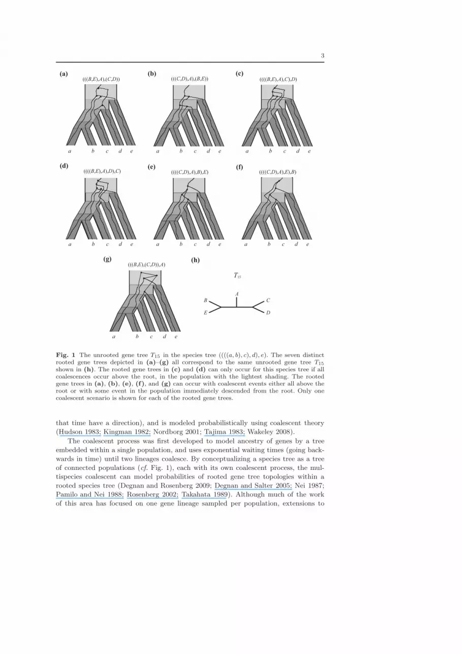
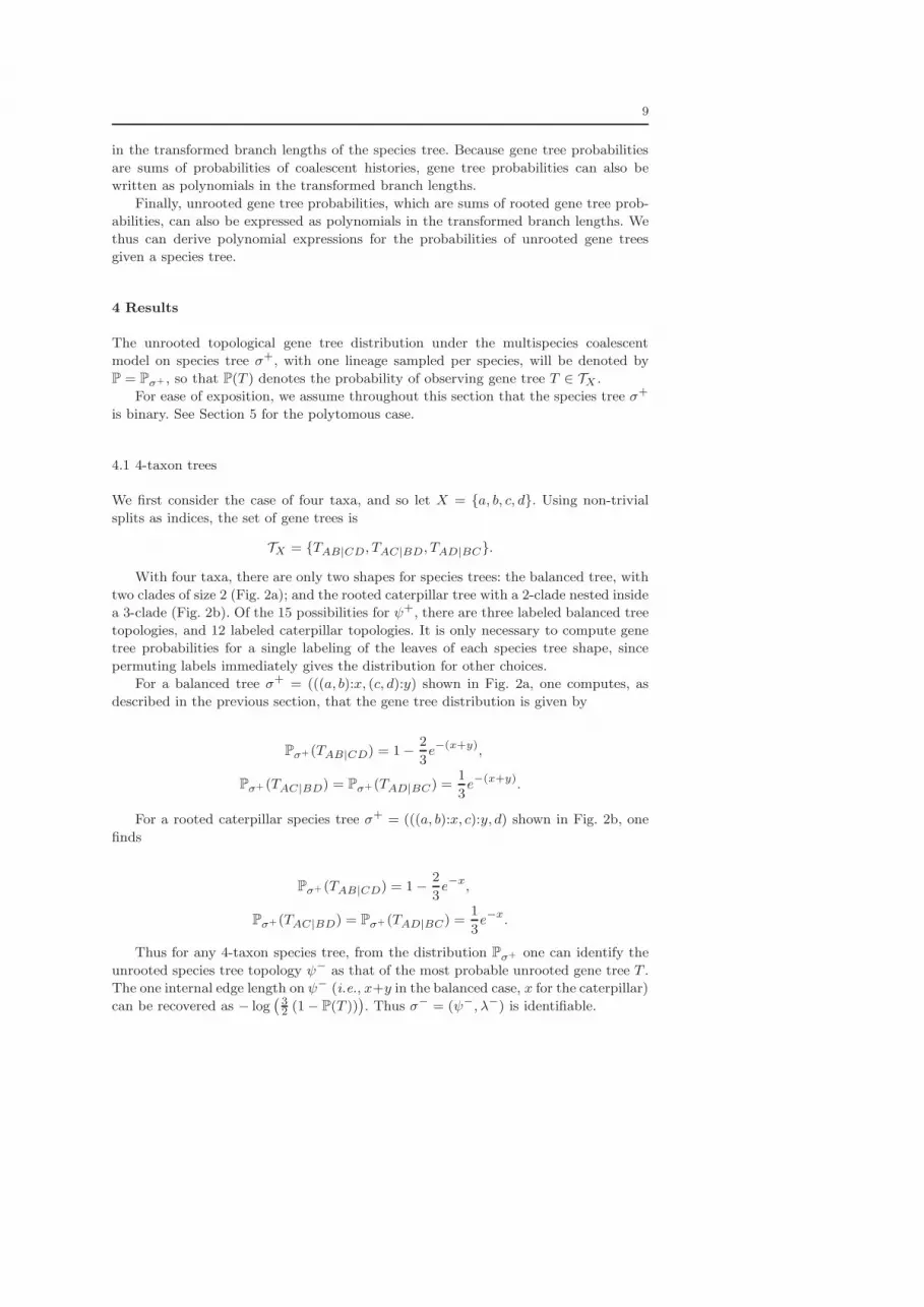
Fig. 1 The unrooted gene tree T15 in the species tree ((((a, b), c), d), e). The seven distinctrooted gene trees depicted in (a)–(g) all correspond to the same unrooted gene tree T15shown in (h). The rooted gene trees in (c) and (d) can only occur for this species tree if allcoalescences occur above the root, in the population with the lightest shading. The rootedgene trees in (a), (b), (e), (f), and (g) can occur with coalescent events either all above theroot or with some event in the population immediately descended from the root. Only onecoalescent scenario is shown for each of the rooted gene trees.

that time have a direction), and is modeled probabilistically using coalescent theory

(Hudson 1983; Kingman 1982; Nordborg 2001; Tajima 1983; Wakeley 2008).

The coalescent process was first developed to model ancestry of genes by a tree

embedded within a single population, and uses exponential waiting times (going back-

wards in time) until two lineages coalesce. By conceptualizing a species tree as a tree

of connected populations (cf. Fig. 1), each with its own coalescent process, the mul-

tispecies coalescent can model probabilities of rooted gene tree topologies within a

rooted species tree (Degnan and Rosenberg 2009; Degnan and Salter 2005; Nei 1987;

Pamilo and Nei 1988; Rosenberg 2002; Takahata 1989). Although much of the work

of this area has focused on one gene lineage sampled per population, extensions to

4

computing gene tree probabilities when more than one lineage is sampled from each

population has also been derived (Degnan 2010; Rosenberg 2002; Takahata 1989).

Under the multispecies coalescent, the species tree is a parameter, consisting of a

rooted tree topology with strictly positive edge weights (branch lengths) on all interior

edges. Pendant edge weights are not specified when there is only one gene sampled per

species, because it is not possible for coalescent events to occur on these edges. Rooted

gene tree topologies are treated as a discrete random variable whose distribution is

parameterized by the species tree, with a state space of size (2n− 3)!! = 1× 3× · · · ×

(2n− 3), the number of rooted, binary tree topologies (Felsenstein 2004) for n extant

species (leaves). (Nonbinary gene trees are not included in the sample space since the

coalescent model assigns them probability zero.)

Results on rooted triples (rooted topological trees obtained by considering subsets

of three species) imply that the distribution of rooted gene tree topologies identifies

the rooted species tree topology (Degnan et al 2009), in spite of the fact that the most

likely n-taxon gene tree topology need not have the same topology as the species tree

for n > 3 (Degnan and Rosenberg 2006). Internal branch lengths on the species tree

can also be recovered using probabilities of rooted triples from gene trees. In particular,

for a 3-taxon species tree in which two species a and b are more closely related to each

other than to c, let t denote the internal branch length. If p is the known probability

that on a random rooted topological gene tree, genes sampled from species a and b

are more closely related to each other than either is to a gene sampled from c, then

t = − log((3/2)(1 − p)) (Nei 1987; Wakeley 2008). Thus, for each population (edge)

e of the species tree, choosing two leaves whose most recent ancestral population is e

and one leaf descended from the immediate parental node of e, the length of e can be

determined. We summarize these results as:

Proposition 1 For a species tree with n ≥ 3 taxa, the probabilities of rooted triple

gene tree topologies determine the species tree topology and internal branch lengths.

Because the probability of any rooted triple is the probability that a rooted gene

tree displays the triple, we have the following.

Corollary 2 For a species tree with n ≥ 3 taxa, the distribution of gene tree topologies

determines the species tree topology and internal branch lengths.

Although previous work on modeling gene trees under the coalescent has assumed

that trees are rooted, the event that a particular unrooted topological gene tree is

observed can be regarded as the event that any of its rooted versions occurs at that locus

(Heled and Drummond 2010). For n species, there are (2n− 5)!! unrooted gene trees,

and each unrooted gene tree can be realized by 2n−3 rooted gene trees, corresponding

to choices of an edge on which to place the root. The probability of an n-leaf unrooted

gene tree is therefore the sum of 2n−3 rooted gene tree probabilities, and the unrooted

gene tree probabilities form a well-defined probability distribution.

In this paper, we study aspects of the distribution of unrooted topological gene

trees that arises under the multispecies coalescent model on a species tree, with the

goal of understanding what one may hope to infer about the species tree. We find

that when there are only four species, with one lineage sampled from each, the most

likely unrooted gene tree topology has the same unrooted topology as the species tree;

however, it is impossible to recover the rooted topology of the species tree, or all

information about edge weights, from the distribution of gene trees. When there are

5 or more species, the probability distribution on the unrooted gene tree topologies

5

identifies the rooted species tree and all internal edge weights. If multiple samples are

taken from one of more species, then those pendant edge weights become identifiable,

and the total number of taxa required for identifying the species tree can be reduced.

In the main text, we derive these results assuming binary — fully resolved — species

trees. However, the results generalize to nonbinary species trees, which have internal

nodes of outdegree greater than or equal to 2. Details for nonbinary cases are given in

Appendix C. Implications for data analysis will be discussed in Section 6.

We briefly indicate our approach. Because the distribution of the (2n−3)!! (rooted)

or (2n− 5)!! (unrooted) gene trees is determined by the species tree topology and its

n− 2 internal branch lengths, gene tree distributions are highly constrained under the

multispecies coalescent model. Calculations show that many gene tree probabilities

are necessarily equal, or satisfy more elaborate polynomial constraints. Polynomials in

gene tree probabilities which evaluate to 0 for any set of branch lengths on a particular

species tree topology are called invariants of the gene tree distribution for that species

tree topology. A trivial example, valid for any species tree, is that the sum of all gene

tree probabilities minus 1 equals 0. Many other invariants express ties in gene tree

probabilities. For example, consider the rooted species tree ((a, b), c), where t is the

length of the internal branch. Suppose gene A is sampled from species a, B from b, and

C from c. Then the rooted gene tree ((A,B), C) has probability p1 = 1− (2/3) exp(−t)

under the coalescent, while the two alternative gene trees, ((A,C), B) and ((B,C), A),

have probability p2 = p3 = (1/3) exp(−t) (Nei 1987). Thus a rooted gene tree invariant

for this species tree is

p2 − p3 = 0. (1)

We emphasize that this invariant holds for all values of the branch length t. The species

tree also implies certain inequalities in the gene tree distribution; for example, for any

branch length t > 0, p1 > p2. Because of such inequalities, the invariant in equation (1)

holds on a gene tree distribution if, and only if, the species tree has topology ((a, b), c).

Different species tree topologies imply different sets of invariants and inequalities

for their gene tree distributions, for both rooted and unrooted gene trees. We note that

previous work on invariants for statistical models in phylogenetics (Allman and Rhodes

2003; Cavender and Felsenstein 1987; Lake 1987) has focused on polynomial constraints

for site pattern probabilities; that is, probabilities that leaves of a gene tree display

various states (e.g., one of four states for DNA nucleotides) under models of charac-

ter change, given the topology and branch lengths of the gene tree. These approaches

have been particularly useful in determining identifiability of (gene) trees given se-

quence data under different models of mutation (Allman and Rhodes 2006; 2008; 2009;

Allman et al 2010a;b).

In this paper, our methods focus on understanding linear invariants and inequalities

for distributions of unrooted gene tree topologies under the multispecies coalescent

model. Here gene trees are branching patterns representing ancestry and descent for

genetic lineages, and are independent of mutations that may have arisen on these

lineages. This is therefore a novel application of invariants in phylogenetics.

2 Notation

Let X denote a set of |X| = n taxa, and let ψ+ denote a rooted, binary, topological

species tree whose n leaves are labeled by the elements of X. If ψ+ is further endowed

6

with a collection λ+ of strictly positive edge lengths for the n− 2 internal edges, then

σ+ = (ψ+, λ+) denotes a rooted, binary, leaf-labeled, metric species tree on X. Note

that edge lengths in the species tree do not represent evolutionary time directly, but

are in coalescent units, that is units of τ/Ne, where τ is the number of generations and

Ne is the effective population size, the effective number of gene copies in a population

(Degnan and Rosenberg 2009). As pendant edge lengths do not affect the probability

of observing any topological gene tree, rooted or unrooted, under the multispecies

coalescent model with one individual sampled from each taxon, they are not specified

in λ+. To specify a particular species tree σ+, we use a modified Newick notation which

omits pendant edge lengths. For instance, a particular 4-taxon balanced metric species

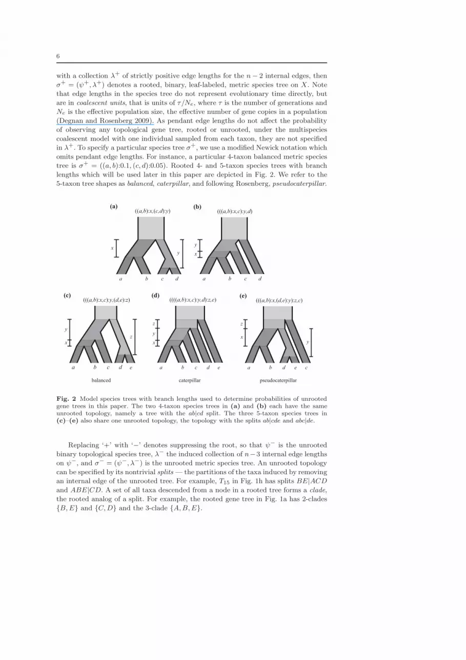
tree is σ+ = ((a, b):0.1, (c, d):0.05). Rooted 4- and 5-taxon species trees with branch

lengths which will be used later in this paper are depicted in Fig. 2. We refer to the

5-taxon tree shapes as balanced, caterpillar, and following Rosenberg, pseudocaterpillar.

((a,b):x,(c,d):y)(a)

xy

a b c d

(((a,b):x,c):y,d)(b)

x

y

a b c d

(((a,b):x,c):y,(d,e):z)

balanced

x

y

z

(c)

a b c d e

((((a,b):x,c):y,d):z,e)(d)

x

y

z

a b c d e

caterpillar

(((a,b):x,(d,e):y):z,c)(e)

x

z

y

a b d e c

pseudocaterpillar

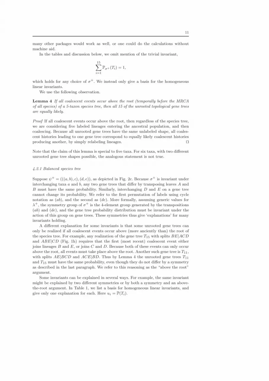
Fig. 2 Model species trees with branch lengths used to determine probabilities of unrootedgene trees in this paper. The two 4-taxon species trees in (a) and (b) each have the sameunrooted topology, namely a tree with the ab|cd split. The three 5-taxon species trees in(c)–(e) also share one unrooted topology, the topology with the splits ab|cde and abc|de.

Replacing ‘+’ with ‘−’ denotes suppressing the root, so that ψ− is the unrooted

binary topological species tree, λ− the induced collection of n−3 internal edge lengths

on ψ−, and σ− = (ψ−, λ−) is the unrooted metric species tree. An unrooted topology

can be specified by its nontrivial splits — the partitions of the taxa induced by removing

an internal edge of the unrooted tree. For example, T15 in Fig. 1h has splits BE|ACD

and ABE|CD. A set of all taxa descended from a node in a rooted tree forms a clade,

the rooted analog of a split. For example, the rooted gene tree in Fig. 1a has 2-clades

{B,E} and {C,D} and the 3-clade {A,B,E}.

7

For any set of taxa S ⊆ X, we let TS denote the collection of all unrooted, binary,

leaf-labeled topological gene trees for the taxa S. We use the convention that while

lower-case letters denote taxa on a species tree, the corresponding upper-case letters

are used as leaf labels on a gene tree; Thus A denotes a gene from taxon a, etc. For

example, if X = {a, b, c, d}, then

TX = {AB|CD, AC|BD, AD|BC}.

Given any sort of tree (species/gene, rooted/unrooted, topological/metric) on X,

appending ‘(S)’ denotes the induced tree on the taxa S ⊆ X. By ‘induced tree’ here

we mean the tree obtained by taking the minimal subtree with leaves in S and then

suppressing all non-root nodes of degree 2. Instances of this notation include σ+(S),

σ−(S), ψ+(S), ψ−(S), and T (S).

3 The multispecies coalescent model

Several papers have given examples of applying the coalescent process to multiple

species or populations to derive examples of probabilities of rooted gene tree topologies

given species trees (Nei 1987; Pamilo and Nei 1988; Rosenberg 2002) with the general

case (for any n-taxon, rooted, binary species tree) given in (Degnan and Salter 2005).

We present the model here with only one individual sampled per taxon, as that will

be sufficient for our analysis.

Under the multispecies coalescent model, waiting times (going backwards in time)

until coalescent events (nodes in a rooted gene tree) are exponential random variables.

The rate for these variables is(

i2

)

, with i the number of lineages “entering” a pop-

ulation, i.e., a branch on the species tree. Gene tree probabilities can be computed

by enumerating all possible specifications of branches in which each coalescent event

occurs, and computing the probability of these events in each branch, treating each

branch as a separate population. In particular, the probability that i lineages coalesce

into j lineages within time t is represented by the function gij(t) (Tavare 1984), which

is a linear combination of exponential functions:

gij(t) =

i∑

k=j

exp

(

−

(

k

2

)

t

)

(2k − 1)(−1)k−j

j!(k − j)!(j + k − 1)

k−1∏

m=0

(j +m)(i−m)

i+m, 1 ≤ j ≤ i.

(2)

Here t > 0 is time measured in coalescent units. The functions gij have the prop-

erty that for any i > 1 and any t > 0, gij(t), j = 1, . . . , i, is a discrete probabil-

ity distribution, that for any i > 1, limt→∞ gi1(t) = 1, and that limt→0 gii(t) = 1.

These last two properties express the ideas that given enough time, all lineages even-

tually coalesce (there is only one lineage remaining in a population) and that over very

short time intervals, it is very likely that no coalescent events occur. Finally, note that

gii(t) = exp (−i(i− 1)t/2).

As an example of using this function to determine rooted gene tree probabilities,

consider the rooted caterpillar species tree ((((a, b):x, c):y, d):z, e) of Fig. 2d, and the

rooted gene tree ((((B,E), A), C), D). Since this gene tree requires a specific ordering

of coalescences, and the first of these can only occur in the population above the

root of the species tree, the only scenario to consider is that shown in Fig. 1c. In

the population ancestral to species a and b, there are two lineages which must fail

8

to coalesce in time x, and this event has probability g22(x) = exp(−x). Similarly,

the events in the populations with durations y and z have probabilities exp(−3y)

and exp(−6z), respectively, because no lineages coalesce in those intervals. For the

population ancestral to the root, all lineages eventually coalesce, and the probability

for events in this population is the probability of observing the particular sequence of

coalescence events, which is((

52

)(

42

)(

32

)(

22

))−1= 1/180. The probability of the rooted

gene tree given the species tree is therefore exp(−x−3y−6z)/180. It is often convenient

to work with transformed branch lengths, where if a branch has length x, we set

X = exp(−x). Using this notation, the rooted gene tree has probability XY 3Z6/180.

As another example, consider the gene tree (((B,E), A), (C,D)) given the same

species tree, ((((a, b):x, c):y, d):z, e). For this rooted gene tree to be realized, either C

and D coalesce as depicted in Fig. 1a, in the population immediately below the root

(which we call the “near the root” population), or C and D coalesce above the root.

Regardless, all other coalescent events must occur in the population above the root. We

therefore divide the calculation of the rooted gene tree topology into these two cases. If

all coalescent events occur above the root, the rooted gene tree probability is calculated

as in the preceding paragraph, except that there are three possible orders in which the

coalescent events could occur to realize the rooted gene tree, and the probability for

this case is thus XY 3Z6/60. In the case where C and D coalesce “near the root,” there

are no coalescent events in the populations with lengths x and y, thus contributing a

factor of exp(−x − 3y) to the probability. The probability for events near the root is(42

)−1g43(z), where the coefficient is the probability that of the four lineages entering

the population, the two that coalesce are C and D. Because there are four lineages

entering the population above the root of the species tree, the one sequence of coalescent

events that results in the gene tree topology has probability((4

2

)(32

)(22

))−1= 1/18. The

total probability of the rooted gene tree topology (((B,E),A), (C,D)) given the species

tree (((a, b):x, c):y, d):z, e) is therefore

g22(x)g33(y)1(42

)g43(z)1

(42

)(32

)(22

) + g22(x)g33(y)g44(z)3

(52

)(42

)(32

)(22

)

=XY 3 1

6(2Z3 − 2Z6)

1

18+

1

60XY 3Z6

=1

54XY 3Z3 −

1

540XY 3Z6.

Probabilities of the other rooted gene trees in Fig. 1 can be worked out similarly by

considering a small number of cases for each tree. Methods for enumerating all possible

cases have been developed using the concept of coalescent history, a list of populations

in which the coalescent events occur (Degnan and Salter 2005). Each coalescent history

h has a probability of the form

c(h)

n−2∏

b=1

gi(h,b),j(h,b)(xb) (3)

where xb is the length of internal edge b of the species tree and c(h) is a constant that

depends on the coalescent history h and the topologies of the gene and species trees,

but does not depend on the branch lengths xb. This expression is a linear combination

of products of terms exp[−k(k−1)xb/2], k = 2, . . . , n−1, so using the transformations

Xb = exp(−xb), probabilities of coalescent histories can thus be written as polynomials

9

in the transformed branch lengths of the species tree. Because gene tree probabilities

are sums of probabilities of coalescent histories, gene tree probabilities can also be

written as polynomials in the transformed branch lengths.

Finally, unrooted gene tree probabilities, which are sums of rooted gene tree prob-

abilities, can also be expressed as polynomials in the transformed branch lengths. We

thus can derive polynomial expressions for the probabilities of unrooted gene trees

given a species tree.

4 Results

The unrooted topological gene tree distribution under the multispecies coalescent

model on species tree σ+, with one lineage sampled per species, will be denoted by

P = Pσ+ , so that P(T ) denotes the probability of observing gene tree T ∈ TX .

For ease of exposition, we assume throughout this section that the species tree σ+

is binary. See Section 5 for the polytomous case.

4.1 4-taxon trees

We first consider the case of four taxa, and so let X = {a, b, c, d}. Using non-trivial

splits as indices, the set of gene trees is

TX = {TAB|CD, TAC|BD, TAD|BC}.

With four taxa, there are only two shapes for species trees: the balanced tree, with

two clades of size 2 (Fig. 2a); and the rooted caterpillar tree with a 2-clade nested inside

a 3-clade (Fig. 2b). Of the 15 possibilities for ψ+, there are three labeled balanced tree

topologies, and 12 labeled caterpillar topologies. It is only necessary to compute gene

tree probabilities for a single labeling of the leaves of each species tree shape, since

permuting labels immediately gives the distribution for other choices.

For a balanced tree σ+ = (((a, b):x, (c, d):y) shown in Fig. 2a, one computes, as

described in the previous section, that the gene tree distribution is given by

Pσ+(TAB|CD) = 1−2

3e−(x+y),

Pσ+ (TAC|BD) = Pσ+(TAD|BC) =1

3e−(x+y).

For a rooted caterpillar species tree σ+ = (((a, b):x, c):y, d) shown in Fig. 2b, one

finds

Pσ+ (TAB|CD) = 1−2

3e−x,

Pσ+(TAC|BD) = Pσ+ (TAD|BC) =1

3e−x.

Thus for any 4-taxon species tree, from the distribution Pσ+ one can identify the

unrooted species tree topology ψ− as that of the most probable unrooted gene tree T .

The one internal edge length on ψ− (i.e., x+y in the balanced case, x for the caterpillar)

can be recovered as − log(

32 (1− P(T ))

)

. Thus σ− = (ψ−, λ−) is identifiable.

10

Furthermore σ+ is not identifiable since the above calculations show that for any

x > 0, yi > 0, and x > z > 0 the following rooted species trees produce exactly the

same unrooted gene tree distribution:

((a, b):x, c):y1, d),

((a, b):x, d):y2, c),

((c, d):x, a):y3, b),

((c, d):x, b):y4, a),

((a, b):z, (c, d):x− z).

We summarize this by:

Proposition 3 For |X| = 4 taxa, σ− is identifiable from Pσ+ , but σ+ is not.

We note that if the unrooted gene trees are ultrametric with known branch lengths,

then their rooted topologies are known by midpoint rooting (Kim et al 1993), and thus

σ+ is identifiable from unrooted ultrametric 4-taxon gene trees.

4.2 Linear invariants and inequalities for unrooted gene tree probabilities for 5-taxon

species trees

To establish identifiability of all parameters when there are at least 5 taxa, we will

argue from the 5-taxon case. In this base case we will use an understanding of linear

relationships — both equalities and inequalities — that hold between gene tree prob-

abilities. The relationships that hold for a particular gene tree distribution reflect the

species tree on which it arose.

In this section, we determine all linear equations in gene tree probabilities for each

of the three shapes of 5-leaf species trees. Following phylogenetic terminology, these are

the linear invariants of the gene tree distribution. We emphasize that these invariants

depend only on the rooted topology, ψ+, of the species tree, and not on the branch

lengths λ+. Although some of these invariants arise from symmetries of the species

tree, others are less obvious. Nonetheless, we give simple arguments for all, and show

that there are no others. In addition, we provide all pairwise inequalities of the form

ui > uj for the three model species trees in Figs. 2c–e.

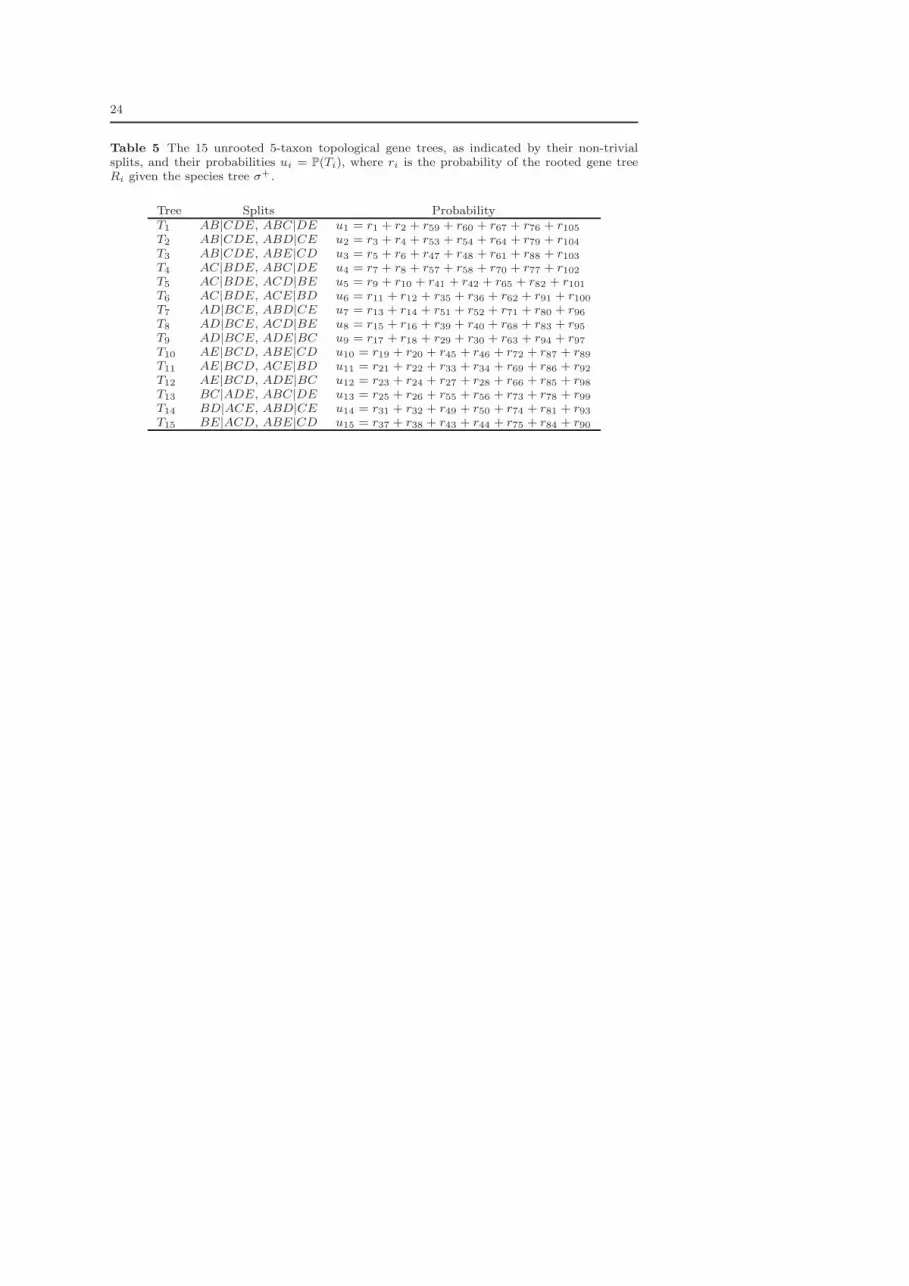
WithX = {a, b, c, d, e}, there are 15 unrooted gene trees in TX , which we enumerate

in Table 5 of Appendix A. Probabilities for each of the 15 unrooted gene trees are

obtained by summing probabilities of seven of the 105 rooted 5-taxon gene trees, as

shown in Tables 4 and 5 of Appendix A. In Appendix B formulas for the unrooted gene

tree distribution are given for one choice of a leaf-labeling of each of the three possible

rooted species tree shapes. Noticing that many of the gene tree probabilities are equal,

one might hope that which ones are equal would be useful in identifying the species

tree from the distribution.

For each species tree one can computationally, but entirely rigorously, determine a

basis for the vector space of all linear invariants. We report such a basis for each of the

species tree shapes below, in Tables 1-3. Only for one of the tree shapes is an additional

invariant that is not immediately noticeable produced by this calculation. While our

computations were performed using the algebra software Singular (Greuel et al 2009),

11

many other packages would work as well, or one could do the calculations without

machine aid.

In the tables and discussion below, we omit mention of the trivial invariant,

15∑

i=1

Pσ+ (Ti) = 1,

which holds for any choice of σ+. We instead only give a basis for the homogeneous

linear invariants.

We use the following observation.

Lemma 4 If all coalescent events occur above the root (temporally before the MRCA

of all species) of a 5-taxon species tree, then all 15 of the unrooted topological gene trees

are equally likely.

Proof If all coalescent events occur above the root, then regardless of the species tree,

we are considering five labeled lineages entering the ancestral population, and then

coalescing. Because all unrooted gene trees have the same unlabeled shape, all coales-

cent histories leading to one gene tree correspond to equally likely coalescent histories

producing another, by simply relabeling lineages. ⊓⊔

Note that the claim of this lemma is special to five taxa. For six taxa, with two different

unrooted gene tree shapes possible, the analogous statement is not true.

4.2.1 Balanced species tree

Suppose ψ+ = (((a, b), c), (d, e)), as depicted in Fig. 2c. Because σ+ is invariant under

interchanging taxa a and b, any two gene trees that differ by transposing leaves A and

B must have the same probability. Similarly, interchanging D and E on a gene tree

cannot change its probability. We refer to the first permutation of labels using cycle

notation as (ab), and the second as (de). More formally, assuming generic values for

λ+, the symmetry group of σ+ is the 4-element group generated by the transpositions

(ab) and (de), and the gene tree probability distribution must be invariant under the

action of this group on gene trees. These symmetries thus give ‘explanations’ for many

invariants holding.

A different explanation for some invariants is that some unrooted gene trees can

only be realized if all coalescent events occur above (more anciently than) the root of

the species tree. For example, any realization of the gene tree T15 with splits BE|ACD

and ABE|CD (Fig. 1h) requires that the first (most recent) coalescent event either

joins lineages B and E, or joins C and D. Because both of these events can only occur

above the root, all events must take place above the root. Another such gene tree is T11,

with splits AE|BCD and ACE|BD. Thus by Lemma 4 the unrooted gene trees T11and T15 must have the same probability, even though they do not differ by a symmetry

as described in the last paragraph. We refer to this reasoning as the “above the root”

argument.

Some invariants can be explained in several ways. For example, the same invariant

might be explained by two different symmetries or by both a symmetry and an above-

the-root argument. In Table 1, we list a basis for homogeneous linear invariants, and

give only one explanation for each. Here ui = P(Ti).

12

Table 1 Invariants for the rooted species tree ψ+ = (((a, b), c), (d, e))

Invariant Explanationu14 − u15 = 0 (de)u11 − u15 = 0 above rootu10 − u15 = 0 (ab)u9 − u12 = 0 (de)u8 − u15 = 0 above rootu7 − u15 = 0 (ab)(de)u6 − u12 = 0 (ab)(de)u5 − u12 = 0 (ab)u4 − u13 = 0 (ab)u2 − u3 = 0 (de)

These equalities give the following equivalence classes of unrooted gene trees ac-

cording to their probabilities:

{T1}, {T2, T3}, {T4, T13}, {T5, T6, T9, T12}, {T7, T8, T10, T11, T14, T15}.

For any branch lengths on this species tree, we also observe the inequalities

u1 > u2, u4 > u5 > u7. (4)

These inequalities were found by first expressing the probability of each Ti as a

sum of positive terms corresponding to coalescent histories, such as expression (3), and

then, by comparing coefficients in these sums, determining instances in which ui > ujmust hold. Intuitively, this means that any realization of Tj corresponds to a realization

of Ti, but that there are additional ways that Ti can be realized.

The inequalities in (4) can all be checked by elementary arguments using the explicit

formulas of Appendix B. For instance, since X,Y, Z ∈ (0, 1),

u1 − u2 = 1−2

3X − Y Z +

1

2XY Z +

1

6XY 3Z = 1− Y Z −

1

6X(4− 3Y Z − Y 3Z)

> 1− Y Z −1

6(4− 3Y Z − Y 3Z) =

1

3−

1

6Y Z(3− Y 2)

>1

3−

1

6Y (3− Y 2) > 0.

In particular, there is always a 6-element equivalence class of trees which has the

strictly smallest probability associated with it, and a 4-element class which has the

next smallest probability associated to it. While the class associated to the largest

probability is always a singleton, these inequalities do allow for the remaining two

classes of size 2 to degenerate to a single class of size 4.

Numerical examples can be used to show that there are no inequalities of the form

ui > uj that hold for all branch lengths X, Y , and Z that are not listed in (4).

4.2.2 Caterpillar species tree

Suppose ψ+ = ((((a, b), c), d), e), as depicted in Fig. 2d. Then the symmetry group of

the tree is generated by (ab), and has only two elements.

Although no unrooted gene trees require that all coalescent events occur above

the root of this species tree, there are gene trees that require that all events be either

13

above the root or “near the root” in the following sense. Consider the gene tree T15with splits BE|ACD and ABE|CD (Fig. 1h). This gene tree can be realized either by

all events occurring above the root (in which case either the BE coalescence or the CD

coalescence could be first), or by 1, 2, or 3 events occurring in a specific order in the

near-the-root population which is ancestral to species a, b, c, and d but not to e, with

all further events above the root. For example, if there are two coalescent events in this

population, then the gene tree must have ((CD)A) as a subtree (Fig. 1b,e,f), and C

and D must coalesce most recently followed by the coalescence of A. In case 1, 2, or 3

events do occur below the root, these must be in the specific order 1) CD coalesce, 2)

ACD coalesce, 3) ABCD coalesce. Another gene tree which leads to a similar analysis

of how coalescent events must occur for the gene tree to be realized is T14, with splits

BD|ACE, ABD|CE. Consequently, T14 has the same probability as T15, even though

these two gene trees do not differ by a symmetry. Similar arguments apply to trees T7,

T8, T10, and T11. The near-the-root argument and symmetry between a and b explain

all linear invariants but the last in Table 2.

Table 2 Invariants for the rooted species tree ψ+ = ((((a, b), c), d), e)

Invariant Explanationu14 − u15 = 0 near rootu11 − u15 = 0 near rootu10 − u15 = 0 (ab)u8 − u15 = 0 near rootu7 − u15 = 0 near rootu6 − u9 = 0 (ab)u5 − u12 = 0 (ab)u4 − u13 = 0 (ab)

u2 − u3 + u9 − u12 = 0 marginalization

To explain the last invariant in Table 2, we provide a marginalization argument.

We use the fact that for 4-taxon trees the two unrooted gene trees that are inconsistent

with the species tree are equiprobable. Thus, marginalizing over a to trees on {b, c, d, e},

we have that P(TBD|CE) = P(TBE|CD). Hence,

u2 + u6 + u7 + u11 + u14 = u3 + u5 + u8 + u10 + u15.

Because the last 3 terms on each side are equal to u15, we may cancel those. Replacing

u6 with u9, and u5 with u12, then gives the last invariant in the table.

Table 2 yields the following equivalence classes of gene trees according to their

probabilities:

{T1}, {T2}, {T3}, {T4, T13}, {T5, T12}, {T6, T9}, {T7, T8, T10, T11, T14, T15}.

We also observe that the inequalities

u1 > u2,u4 > u5 > u7,

u3 > u2,u6 > u5 > u7 (5)

hold for all branch lengths on this species tree, and that there are no other inequalties

of the form ui > uj that hold for all branch lengths, by arguments similar to those for

the balanced tree.

14

4.2.3 Pseudocaterpillar species tree

Suppose ψ+ = (((a, b), (d, e)), c), as depicted in Fig. 2e. Then the symmetry group of

the tree σ+ is generated by (ab) and (de), and has four elements. (Note that inter-

changing the two cherries, for instance by (ad)(be), is a symmetry of ψ+, but is not a

symmetry of σ+ for generic edge lengths.)

While no unrooted gene trees require that all coalescent events occur above the

root of this species tree, some unrooted gene trees require that all events be either near

the root or above the root. The gene tree T15, with splits BE|ACD and ABE|CD, can

be realized either by all events occurring above the root (in which case either the BE

coalescence or the CD coalescence could be first), or by 1, 2, or 3 events occurring in

a specific order in the population ancestral to species a, b, c, and d but not to e, with

all further events occurring above the root. In case 1, 2, or 3 events do occur below the

root, these must be in the specific order 1) BE coalesce, 2) ABE coalesce, 3) ABDE

coalesce. Another gene tree which leads to a similar analysis of how coalescent events

must occur for the gene tree to be realized is T12, with splits AE|BCD, ADE|BC.

Thus T12 and T15 are equiprobable, even though they do not differ by a symmetry.

A basis for homogeneous linear invariants of unrooted gene tree probabilities, along

with explanations for each is given in Table 3.

Table 3 Invariants for the rooted species tree ψ+ = (((a, b), (d, e)), c)

Invariant Explanationu14 − u15 = 0 (de)u12 − u15 = 0 near rootu10 − u15 = 0 (ab)u9 − u15 = 0 near rootu8 − u11 = 0 (ab)u7 − u15 = 0 (ab)(de)u6 − u15 = 0 near rootu5 − u15 = 0 near rootu4 − u13 = 0 (ab)u2 − u3 = 0 (de)

We thus obtain the following equivalence classes of unrooted gene trees according

to their probabilities:

{T1}, {T2, T3}, {T4, T13}, {T8, T11}, {T5, T6, T7, T9, T10, T12, T14, T15}.

For all branch lengths on this species tree, we also observe the inequalities

u1 > u2, u4, u8 > u5 (6)

and note that there are no other inequalities of the form ui > uj that hold for all

possible branch lengths. In particular, the 8-element equivalence class of trees always

has the strictly smallest probability associated with it.

4.3 Species Tree Identifiability for 5 or more Taxa

We will use several times the following observation, which is clear from the structure

of the coalescent model. (In fact, this has already been used in Section 4.2.2 in the

15

marginalization argument explaining a linear invariant for the caterpillar tree.) While

we state the lemma for unrooted gene trees, there is of course a similar statement for

the distribution of rooted gene trees.

Lemma 5 If S ⊆ X and T ′ ∈ TS , then

Pσ+(S)(T′) =

∑

T∈TX

T (S)=T ′

Pσ+(T ).

As a consequence of the analysis for 4-taxon trees in Section 4.1, we obtain the

following.

Corollary 6 For any X, Pσ+ determines σ−.

Proof We assume |X| ≥ 4, since otherwise there is nothing to prove. For any quartet

Q ⊆ X of four distinct taxa, by Lemma 5, Pσ+ determines Pσ+(Q). Thus σ−(Q)

is determined by Proposition 3. Thus all unrooted quartet trees induced by ψ− are

determined, along with their internal edge lengths. That all induced quartet topologies

determine the topology ψ− is well known (Steel 1992). Because each internal edge of

ψ− is the internal edge for some induced quartet tree, λ− is determined as well. ⊓⊔

For the remaining arguments to determine σ+, we may assume that σ− is already

known. We focus first on the |X| = 5 case, and thus assume that X = {a, b, c, d, e} and

that ψ− has non-trivial splits ab|cde and abc|de.

Proposition 7 For |X| = 5 the rooted species tree topology ψ+ is determined by Pσ+ .

Proof From Section 4.2, for generic values of λ+, the caterpillar leads to seven distinct

gene tree probabilities, with class sizes 1,1,1,2,2,2,6; the pseudocaterpillar gives five

distinct probabilities, with class sizes 1,2,2,2,8; and the balanced tree gives five dis-

tinct probabilities, with class sizes 1,2,2,4,6. Thus the (unlabeled) shape of ψ+ can be

distinguished for generic edge lengths. However, for certain values of these parameters

the classes can degenerate, by merging.

To see that the tree shapes can be distinguished for all parameter values, observe

that the inequalities (4)–(6) of Section 4.2 on gene tree probabilities ensures the class

associated to the smallest probability always has size 8 for the pseudocaterpillar, while

for the other shapes the size of this class is always 6. Moreover, for the caterpillar

and balanced trees the size of the class associated to the second smallest probability

must be exactly 2 and 4, respectively. Thus, these class sizes allow us to determine the

unlabeled, rooted shape (balanced, caterpillar, or pseudocaterpillar) of the species tree.

In addition, from Corollary 6, we also know the labeled, unrooted topology (i.e., the

splits) of the species tree, ψ−. To determine the labeled, rooted topology, we consider

cases depending on the unlabeled, rooted shape determined from the class sizes.

If the species tree is balanced, from the splits we know that ψ+ = (((a, b), c), (d, e))

or ψ+ = ((a, b), (c, (d, e))). But the gene tree T7, with splits AD|BCE and ABD|CE,

can be realized on the first of these species trees only if all coalescent events occur

above the root; on the second species tree, T7 can be realized other ways as well. Thus

T7 would fall into the 6-element class of least probable gene trees for the first but not

the second species tree. This then determines ψ+.

For a caterpillar species tree, from the splits we know ψ+ has as its unique 2-

clade either {a, b} or {d, e}. By considering the cherries on the two gene trees in the

16

class of those with the second smallest probability, we see the 2-clade is determined as

those taxa that appear in cherries with c. For simplicity, we henceforth suppose that

the 2-clade is found to be {a, b}. Thus, ψ+ = ((((a, b), c), d), e) or ((((a, b), c), e), d).

Then from the inequality (5) in Section 4.2.2, we find that P(T3) > P(T2) if ψ+ =

((((a, b), c), d), e), while this inequality is reversed if ψ+ = ((((a, b), c), e), d).

In the case of the pseudocaterpillar species tree, because the splits of ψ− are known,

there is only one possibility for ψ+. Thus ψ+ is determined. ⊓⊔

Proposition 8 For |X| = 5, Pσ+ determines σ+ = (ψ+, λ+).

Proof By Proposition 7 , ψ+ is determined. From Corollary 6, λ− is also determined.

Thus all elements of λ+ except for the edges incident to the root are determined. In

the balanced case, the sum of these two unknown edge lengths is determined, but

in the other cases we have yet to determine any information about the single such

non-pendant edge length. We therefore consider each of these cases in order.

If ψ+ is balanced, we may assume σ+ = (((a, b):x, c):y), (d, e):z), with y, z still to

be determined. As the unrooted internal edge length y + z is known, it is enough to

determine y. From the gene tree probabilities in Appendix B.1, it follows that

XY Z = 6u5 + 9u7,

XY 3Z = 15u7.

Thus,

y = − log(Y ) =1

2log

(

2u5 + 3u75u7

)

. (7)

If ψ+ is a rooted caterpillar, we may assume σ+ = ((((a, b):x, c):y, d):z, e). Only z

remains to be determined. Using the explicit formulas for gene tree probabilities given

in Appendix B.2, one checks that

XY 3 = 3(−u2 + u3 + 5u7)

XY 3Z6 = 15(u2 − u3 + u7)

and thus

z = − log(Z) =1

6log

(

−u2 + u3 + 5u75u2 − 5u3 + 5u7

)

. (8)

If ψ+ is the pseudocaterpillar, we may assume σ+ = (((a, b):x, (d, e):y):z, c), with

z still to be determined. The gene tree probabilities listed in Appendix B.3 show that

XY = 12u5 + 3u8

XY Z6 = 30u5 − 15u8.

Thus,

z = − log(Z) =1

6log

(

4u5 + u810u5 − 5u8

)

. (9)

Note that equations (11)–(13) of Appendix B can be used to show that the arguments

of the logarithms in equations (7)–(9) are always strictly greater than 1. ⊓⊔

17

While this proof used particular formulas to identify the remaining edge lengths in

λ+, note that many variants could have been used in their place. This simply reflects

the many algebraic relationships (both linear and non-linear invariants) between the

various gene tree probabilities.

With the |X| = 5 case completed, we obtain the general result.

Theorem 9 The unrooted topological gene tree distribution Pσ+ arising from the mult-

species coalescent model for samples of one lineage per taxon determines the metric

species tree σ+ provided |X| ≥ 5. If |X| = 4, Pσ+ determines only the unrooted metric

species tree σ−.

Proof By Corollary 6, σ− = (ψ−, λ−) is determined.

If |X| ≥ 5, consider a specific edge e of ψ−, and all 5-taxon subsets S ⊆ X such

that the induced unrooted tree ψ−(S) has e as an edge. If the root, ρ, of ψ+ lies on

e, then the root of ψ+(S) is also ρ and thus the root of ψ+(S) lies on e for all such

S. If ρ does not lie on e, then there exists an S with the root of ψ+(S) not on e. To

see this, for any set Q ⊂ X of four taxa which distinguishes e (Steel 1992, Proposition

6), choose x ∈ X \Q so that the MRCA of S = Q ∪ {x} is ρ. Then ψ+(S) has root ρ,

which is not on e.

Thus using Lemma 5 and Proposition 8 to determine the root location of such

ψ+(S) for each e, we can determine ψ+. Then the length of any internal edges incident

to the root of ψ+ can be recovered by choosing a 5-taxon subset S such that ψ+(S) has

these edges, and applying Lemma 5 and Proposition 8 again. Thus σ+ is determined.

Proposition 3 gives the case |X| = 4. ⊓⊔

Theorem 9 gives an alternate approach to establishing Corollary 2, in cases with

|X| ≥ 5, since the distribution of rooted gene trees determines that of unrooted gene

trees.

Theorem 9 can also be used to show that if multiple lineages are sampled from

some or all of the taxa, then the unrooted gene tree distribution contains additional

information on the species tree, as follows.

Corollary 10 Consider a species tree on taxon set X, and, for some ℓi > 0, the

distribution of unrooted topological gene trees under a multispecies coalescent model of

samples of ℓi individuals from taxon i. Suppose that either |X| ≥ 4 and that there is at

least one i such that ℓi ≥ 2, or that |X| = 3 and that there are at least two values of

i such that ℓi ≥ 2. Then the gene tree distribution determines the species tree’s rooted

topology, internal edge lengths, and for any taxon with li > 1 the length of the pendant

edge leading to taxon i.

Proof We may assume all ℓi are either 1 or 2, by marginalizing over any additional

individuals sampled, if necessary.

Construct an extended species tree by attaching to any leaf i for which li = 2 a

pair of edges descending to new leaves labelled i1 and i2, so the extended species tree

has ℓ =∑n

i=1 ℓi leaves. The pendant edge leading to taxon i in the original species

tree becomes an internal edge on the extended tree, and retains its previous length.

The lengths of the new pendant edges in the extended tree can be chosen arbitrarily,

or left unspecified. Then a coalescent process on the extended ℓ-taxon tree with one

sample per leaf leads to exactly the same distribution of topological gene trees as the

the multiple-sample process on the original species tree.

Applying Theorem 9 to the extended tree, we obtain the result. ⊓⊔

18

5 Nonbinary species trees

The results for binary species trees generalize to nonbinary species trees as well. When

species trees are allowed to be nonbinary, there are two unlabeled 3-taxon tree shapes,

five unlabeled 4-taxon tree shapes, and 12 unlabeled 5-taxon tree shapes (Cayley 1857).

Probabilities of binary, unrooted gene tree topologies given a nonbinary species tree

can be obtained by considering the limiting probability as one or more branch lengths

go to zero in the formulas derived for binary species trees. We note that under the

standard Kingman coalescent, gene trees, which depend on exponential waiting times,

are still binary with probability 1 even when the species tree has polytomies.

For the 3-taxon species tree, ((a, b):t, c), letting t→ 0, the rooted gene tree proba-

bilities are each 1/3 in the limit. Thus the unresolved 3-taxon rooted species tree can be

identified from the gene tree distribution from the presence of three equal probabilities;

whereas for a resolved species tree, exactly one gene tree has probability greater than

1/3. Similarly, polytomies in any larger species tree can be identified by considering

rooted triplets. A species tree node has three or more descendants if the three rooted

gene trees obtained from sampling one gene from three distinct descendants of the node

have equal probabilities.

For 4-taxon species trees, the completely unresolved topology (a, b, c, d) can not

be distinguished from the partially unresolved ((a, b, c):y, d) from unrooted gene tree

probabilities as both result in equal probabilities of the three binary, unrooted gene

trees on these taxa. Similarly, the resolved species trees (((a, b):x, c):y, d) and the par-

tially unresolved ((a, b):x, c, d) yield the same unrooted gene tree probabilities, with

Pσ+ (TAB|CD) = 1− 23e

−x. These observations lead to the conclusion, as in the binary

case, that 4-taxon unrooted gene tree probabilities identify the unrooted (possibly un-

resolved) species tree, but do not identify the root. Thus Proposition 3 is still valid

when σ+ is nonbinary.

Identifiability of possibly-nonbinary rooted species trees for 5 or more taxa from

probabilities of unrooted gene tree topologies can be established using arguments sim-

ilar to those of the binary case. While we defer the detailed proofs to Appendix C, we

state these results as follows:

Proposition 11 Proposition 3, Corollary 6, Propositions 7 and 8, Theorem 9, and

Corollary 10 remain valid if σ+ is nonbinary.

We note that a species tree with a polytomy is equivalent to a model of a resolved

species tree with one or more branch lengths set equal to zero, and therefore that a

resolved species tree and a polytomous species tree can be regarded as nested models.

Although it might be difficult to distinguish polytomous versus resolved species trees

from finite amounts of data, the nested relationship of these models suggests that

likelihood ratios could be used to determine whether an estimated species tree branch

length is significantly greater than 0. A previous study (Poe and Chubb 2004) argued

for the hypothesis of a species-level polytomy in early bird evolution by using likelihood

ratios to test whether gene trees had branch lengths significantly greater than 0 at

multiple loci. Since gene trees are theoretically expected to be resolved under the

coalescent model, an alternative procedure would be to use probabilities of gene trees

under the polytomous and resolved species trees and perform a likelihood ratio test for

whether an estimated species tree branch length is significantly greater than 0.

19

6 Discussion

Under standard models of sequence evolution, the distribution of site patterns of DNA

does not depend on the position of the root of the gene tree on which the sequence

evolve (this is sometimes called the “pulley principle” (Felsenstein 1981)). Inference of

the root of a gene tree requires additional assumptions, such as that of a molecular clock

(mutation occurs at a constant rate throughout the tree), or inclusion of an outgroup

taxon in the analysis, so that the root may be assumed to lie where the outgroup joins

all other taxa in the study. We have shown, however, that under the coalescent model

with five or more species, the distribution of unrooted topological gene trees preserves

information about both the rooted species tree and its internal branch lengths. Thus

in multilocus studies in which many gene trees are inferred, it is theoretically possible

to infer the rooted metric species tree even in the absence of a molecular clock, known

outgroups, or any metric information on the gene trees. While for some data sets it can

be difficult to obtain either reliable roots or evolutionary times for branches of gene

trees, these issues are not fundamental barriers to species tree inference.

Although we have shown the theoretical possibility of identifying rooted species

trees from unrooted gene trees by using linear invariants, we emphasize that we do

not propose using these invariants as a basis for inference. Invariants of gene tree

distributions are functions of their exact probabilities under the model — from finite

data sets, gene trees are inferred with some error, and empirical estimates of gene

tree probabilities from a finite number of gene trees might not satisfy invariants or

inequalities that apply to the exact distribution. Moreover, many non-linear invariants

which are not discussed in this paper (and not yet fully understood) further constrain

the form of the gene tree distribution.

In practice, very large numbers of loci might be needed to obtain approximate esti-

mates of gene tree probabilities, and there must be considerable gene tree discordance

in order to estimate probabilities of less probable unrooted gene trees. For example,

in an often-analyzed 106-gene yeast dataset (Rokas et al 2003), analyzing only the five

species about which there is the most conflict, (S. cerevisiae, S. paradoxus, S. mikatae,

S. kudriavzevil, and S. bayanus), yields the same unrooted gene tree for all 106 loci when

inferred using maximum likelihood under the GTR+Γ + I model without a molecular

clock. If all observed gene trees have the same unrooted topology, then there is not

enough information to infer the rooted species tree. Other data have shown more con-

flict in unrooted gene trees, such as a 162-gene dataset for rice (Cranston et al 2009),

in which 99 of 105 rooted 5-taxon gene trees were represented in the Bayesian 95%

highest posterior density (HDP) set of trees.

If species tree branches are too long, it will not be possible to recover the rooted

species tree from finite data. For example, if the species tree is (((a, b):x, c):y, d):z, e),

where y is sufficiently large, every observed gene tree (for a finite number of loci) might

have the ABC|DE split. Being able to determine that e is the outgroup would require

observing conflicting splits, such as that ABD|CE is more probable than ABE|CD.

However, if y is large, these conflicting splits are likely to never be observed, making

it difficult to distinguish between rooted topologies (((a, b), c), d), e), (((a, b), c), e), d),

and (((a, b), c), (d, e)).

On the other hand, if branches are too short, it might be difficult to distin-

guish between certain rooted species trees, such as between (((a, b), c), (d, e)) and

((a, b), (c, (d, e))) when the node immediately ancestral to c is very close to the root.

20

Further study would be needed for a precise understanding of how extreme branch

lengths affect the number of gene trees needed for reliable inference of the species tree.

We note, however, that even when the rooted species tree cannot be fully inferred with

great certainty, some rooted aspects of the tree might be recoverable. For example in

the case of the rooted trees above, one might infer that (a, b) and (d, e) are rooted

cherries on the tree, even if the placement of taxon c with respect to the root remains

unknown.

We again emphasize that invariants are not the most promising approach for infer-

ring species trees from finite data, and that a maximum likelihood (ML) or Bayesian

approach might be more appropriate. Given a set of sufficiently conflicting unrooted

topological gene trees inferred by standard methods and then assumed to be correct,

the rooted species tree could be inferred using ML, where the likelihood of the species

tree is

L(σ+) ∝

(2n−5)!!∏

i=1

uni

i (10)

where there are n taxa and the ith unrooted gene tree topology is observed ni times

with∑

i ni = N the total number of loci. The probability ui of the ith gene tree

depends on the species tree topology and branch lengths as outlined in Section 3.

However, this 2-stage approach of gene tree inference followed by species tree inference

does not take into account uncertainty in the gene trees, or cases in which inferred

gene trees are not fully resolved. If there is not enough information in the sequences

to estimate resolved gene trees, an approximation to equation (10) would be to either

randomly resolve the tree if there are very many loci (as is often done in software

implementing quartet puzzling (Strimmer and von Haeseler 1996) or neighbor joining

(Saitou and Nei 1987)); or, if an unresolved gene tree has k resolutions, let the locus

contribute a count of 1/k to each resolution.

To better utilize the information in the unrooted gene trees, an attractive, but

computationally more intensive, approach would use a Bayesian framework in which

the posterior distribution of the rooted species tree is determined from posterior distri-

butions of gene trees, thus taking into account uncertainty in the estimated gene trees.

Cases in which ML would return an unresolved gene tree would likely correspond to a

posterior distribution of gene trees with substantial support on more than one topol-

ogy. Thus, instead of each locus contributing a count of one gene tree topology, it

contributes fractional proportions to several topologies. In cases in which the gene tree

distributions carry little information about the root of the species tree, the posterior

distribution of the species tree would indicate this uncertainty by spreading the pos-

terior mass over several species trees. The results of the present paper suggest that

it is possible to extend current model-based methods of inferring rooted species trees

(e.g., BEST (Liu and Pearl 2007) and STEM (Kubatko et al 2009)) to cases where

only unrooted gene trees can be estimated.

Finally we note that invariants have a potential use in testing the fit of the multi-

species coalescent model to a dataset. As noted in (Slatkin and Pollack 2008), processes

such as population subdivision can lead to asymmetry in the probabilities of the two

nonmatching rooted gene trees in the case of three taxa, thus violating the invariant

in equation (1). As shown in this paper, similar invariants can be obtained for larger

number of species even when only unrooted gene trees are available, thus allowing the

testing of the fit of the multispecies coalescent model in situations more general than

the rooted 3-taxon setting.

21

Acknowledgements The authors thank the Statistical and Applied Mathematical SciencesInstitute, where this work was begun during its 2008-09 program on Algebraic Methods inSystems Biology and Statistics. We also thank two anonymous reviewers, one of whom sug-gested the extension to nonbinary trees. ESA and JAR were supported by funds from theNational Science Foundation, grant DMS 0714830, and JAR by an Erskine Fellowship fromthe University of Canterbury. JHD was funded by the New Zealand Marsden Fund. All authorscontributed equally to this work.

References

Allman ES, Rhodes JA (2003) Phylogenetic invariants for the general Markov model of se-quence mutation. Math Biosciences 186:113–144

Allman ES, Rhodes JA (2006) The identifiability of tree topology for phylogenetic models,including covarion and mixture models. J Comput Biol 13(5):1101–1113

Allman ES, Rhodes JA (2008) Identifying evolutionary trees and substitution parameters forthe general Markov model with invariable sites. Math Biosci 211(1):18–33

Allman ES, Rhodes JA (2009) The identifiability of covarion models in phyloge-netics. IEEE/ACM Trans Comput Biol Bioinformatics 6:76–88, DOI http://doi.ieeecomputersociety.org/10.1109/TCBB.2008.52

Allman ES, Holder MT, Rhodes JA (2010a) Estimating trees from filtered data: Identifiabilityof models for morphological phylogenetics. J Theor Biol 263:108–119

Allman ES, Petrovic S, Rhodes JA, Sullivant S (2010b) Identifiability of 2-tree mixtures forgroup-based models. IEEE/ACM Trans Comput Biol Bioinformatics pp 1–13, to appear

Bandelt HJ, Dress A (1986) Reconstructing the shape of a tree from observed dissimilaritydata. Adv Appl Math 7:209–343

Carstens B, Knowles LL (2007) Estimating species phylogeny from gene-tree probabilitiesdespite incomplete lineage sorting: an example from Melanoplus grasshoppers. Syst Biol56:400–411

Cavender JA, Felsenstein J (1987) Invariants on phylogenies in a simple case with discretestates. J Classification 4:57–71

Cayley A (1857) On the theory of the analytical forms called trees. Phil Mag 13:172–176Cranston KA, Hurwitz B, Ware D, Stein L, Wing RA (2009) Species trees from highly incon-

gruent gene trees in rice. Syst Biol 58:489–500Degnan JH (2010) Probabilities of gene-tree topologies with intraspecific sampling given a

species tree. In: Knowles LL, Kubatko LS (eds) Estimating species trees: practical andtheoretical aspects, Wiley-Blackwell, ISBN: 978-0-470-52685-9, to appear

Degnan JH, Rosenberg NA (2006) Discordance of species trees with their most likely genetrees. PLoS Genetics 2:762–768

Degnan JH, Rosenberg NA (2009) Gene tree discordance, phylogenetic inference and the mul-tispecies coalescent. Trends Ecol Evol 24:332–340

Degnan JH, Salter LA (2005) Gene tree distributions under the coalescent process. Evolution59:24–37

Degnan JH, DeGiorgio M, Bryant D, Rosenberg NA (2009) Properties of consensus methodsfor inferring species trees from gene trees. Syst Biol 58:35–54

Felsenstein J (1981) Evolutionary trees from DNA sequences: a maximum likelihood approach.J Mol Evolut 17:368–376

Felsenstein J (2004) Inferring phylogenies. Sinauer Associates, Sunderland, MAGraham SW, Olmstead RG, Barrett SCH (2002) Rooting phylogenetic trees with distant

outgroups: a case study from the commelinoid monocots. Mol Biol Evol 19:1769–1781Greuel GM, Pfister G, Schonemann H (2009) Singular 3.1.0 — A computer algebra system

for polynomial computations http://www.singular.uni-kl.deHeled J, Drummond AJ (2010) Bayesian inference of species trees from multilocus data. Mol

Biol Evol 27:570–580Hudson RR (1983) Testing the constant-rate neutral allele model with protein sequence data.

Evolution 37:203–217Huelsenbeck JP, Bollback JP, Levine AM (2002) Inferring the root of a phylogenetic tree. Syst

Biol 51:32–43Jennings WB, Edwards SV (2005) Speciational history of Australian grassfinches (Poephila)

inferred from thirty gene trees. Evolution 59:2033–2047

22

Kim J, Rohlf FJ, Sokal RR (1993) The accuracy of phylogenetic estimation using the neighbor-joining method. Evolution 47:471–486

Kingman JFC (1982) On the genealogy of large populations. J Applied Probability 19A:27–43Kubatko LS, Carstens BC, Knowles LL (2009) STEM: species tree estimation using maximum

likelihood for gene trees under coalescence. Bioinformatics 25:971–973Lake JA (1987) A rate independent technique for analysis of nucleic acid sequences: evolution-

ary parsimony. Mol Biol Evol 4:167–191Liu L, Pearl DK (2007) Species trees from gene trees: reconstructing Bayesian posterior distri-

butions of a species phylogeny using estimated gene tree distributions. Syst Biol 56:504–514Liu L, Yu L, Pearl DK (2010) Maximum tree: a consistent estimator of the species tree. J

Math Biol 60:95–106Maddison WP, Knowles LL (2006) Inferring phylogeny despite incomplete lineage sorting. Syst

Biol 55:21–30Mossel E, Roch S (2010) Incomplete lineage sorting: consistent phylogeny estimation from

multiple loci. IEEE Comp Bio Bioinformatics 7:166–171Nei M (1987) Molecular Evolutionary Genetics. Columbia University Press, NYNordborg M (2001) Coalescent theory. In: Balding DJ, Bishop M, Cannings C (eds) Handbook

of Statistical Genetics, 1st edn, John Wiley & Sons, New York, chap 7, pp 179–212Pamilo P, Nei M (1988) Relationships between gene trees and species trees. Mol Biol Evol

5:568–583Poe S, Chubb AL (2004) Birds in a bush: Five genes indicate explosive radiation of avian

orders. Evolution 58:404–415Rokas A, Williams B, King N, Carroll S (2003) Genome-scale approaches to resolving incon-

gruence in molecular phylogenies. Nature 425:798–804Rosenberg NA (2002) The probability of topological concordance of gene trees and species

trees. Theor Popul Biol 61:225–247Rosenberg NA (2007) Counting coalescent histories. J Comp Biol 14:360–377Saitou N, Nei M (1987) The neighbor-joining method: a new method for reconstructing phy-

logenetic trees. Molecular Biology and Evolution 4:406–425Semple C, Steel M (2003) Phylogenetics. Oxford University Press, Oxford, UKSlatkin M, Pollack JL (2008) Subdivision in an ancestral species creates an asymmetry in gene

trees. Mol Biol Evol 25:2241–2246Steel M (1992) The complexity of reconstructing trees from qualitative characters and subtrees.

J Classification 9:91–116Strimmer K, von Haeseler A (1996) Quartet puzzling: a quartet maximum-likelihood method

for reconstructing tree topologies. Mol Biol Evol 13:964–969Tajima F (1983) Evolutionary relationship of DNA sequences in finite populations. Genetics

105:437–460Takahata N (1989) Gene genealogy in three related populations: consistency probability be-

tween gene and population trees. Genetics 122:957–966Tavare S (1984) Line-of-descent and genealogical processes, and their applications in population

genetics models. Theor Popul Biol 26:119–164Wakeley J (2008) Coalescent Theory. Roberts & Company, Greenwood Village, CO

23

A Tables for 5-taxon trees

Table 4 The 105 rooted gene trees on 5 species.

R1 ((((A,B), C), D), E) R36 ((((B,D), E), C), A) R71 (((A,D), (C,E)), B)R2 ((((A,B), C), E),D) R37 ((((B, E), A), C), D) R72 (((A, E), (C,D)), B)R3 ((((A,B), D), C), E) R38 ((((B, E), A),D), C) R73 (((B, C), (D,E)), A)R4 ((((A,B), D), E), C) R39 ((((B, E), C), A), D) R74 (((B,D), (C,E)), A)R5 ((((A,B), E), C), D) R40 ((((B, E), C),D), A) R75 (((B, E), (C,D)), A)R6 ((((A,B), E),D), C) R41 ((((B, E), D), A), C) R76 (((A,B), C), (D,E))R7 ((((A, C), B), D), E) R42 ((((B, E), D), C), A) R77 (((A, C), B), (D,E))R8 ((((A, C), B), E),D) R43 ((((C,D), A), B), E) R78 (((B, C), A), (D,E))R9 ((((A, C),D), B), E) R44 ((((C,D), A), E), B) R79 (((A,B), D), (C,E))R10 ((((A, C),D), E), B) R45 ((((C,D), B), A), E) R80 (((A,D), B), (C,E))R11 ((((A, C), E), B), D) R46 ((((C,D), B), E), A) R81 (((B,D), A), (C,E))R12 ((((A, C), E), D), B) R47 ((((C,D), E), A), B) R82 (((A, C), D), (B, E))R13 ((((A,D), B), C), E) R48 ((((C,D), E), B), A) R83 (((A,D), C), (B, E))R14 ((((A,D), B), E), C) R49 ((((C, E), A), B), D) R84 (((C,D), A), (B, E))R15 ((((A,D), C), B), E) R50 ((((C, E), A), D), B) R85 (((B, C),D), (A,E))R16 ((((A,D), C), E), B) R51 ((((C, E), B), A),D) R86 (((B, D), C), (A,E))R17 ((((A,D), E), B), C) R52 ((((C, E), B), D), A) R87 (((C,D), B), (A,E))R18 ((((A,D), E), C), B) R53 ((((C, E),D), A), B) R88 (((A,B), E), (C,D))R19 ((((A, E), B), C), D) R54 ((((C, E),D), B), A) R89 (((A, E), B), (C,D))R20 ((((A, E), B), D), C) R55 ((((D,E), A), B), C) R90 (((B, E), A), (C,D))R21 ((((A, E), C), B), D) R56 ((((D,E), A), C), B) R91 (((A, C), E), (B,D))R22 ((((A, E), C), D), B) R57 ((((D,E), B), A), C) R92 (((A, E), C), (B,D))R23 ((((A, E),D), B), C) R58 ((((D,E), B), C), A) R93 (((C, E), A), (B,D))R24 ((((A, E),D), C), B) R59 ((((D,E), C), A), B) R94 (((B, C), E), (A,D))R25 ((((B, C), A), D), E) R60 ((((D,E), C), B), A) R95 (((B, E), C), (A,D))R26 ((((B, C), A), E),D) R61 (((A,B), (C,D)), E) R96 (((C, E), B), (A,D))R27 ((((B, C), D), A), E) R62 (((A,C), (B,D)), E) R97 (((A,D), E), (B,C))R28 ((((B, C), D), E), A) R63 (((A,D), (B,C)), E) R98 (((A, E),D), (B,C))R29 ((((B, C), E), A), D) R64 (((A,B), (C,E)), D) R99 (((D,E), A), (B,C))R30 ((((B, C), E),D), A) R65 (((A,C), (B,E)), D) R100 (((B, D), E), (A,C))R31 ((((B,D), A), C), E) R66 (((A,E), (B,C)), D) R101 (((B, E),D), (A,C))R32 ((((B,D), A), E), C) R67 (((A,B), (D,E)), C) R102 (((D,E), B), (A,C))R33 ((((B,D), C), A), E) R68 (((A,D), (B,E)), C) R103 (((C,D), E), (A,B))R34 ((((B,D), C), E), A) R69 (((A,E), (B,D)), C) R104 (((C, E),D), (A,B))R35 ((((B,D), E), A), C) R70 (((A,C), (D,E)), B) R105 (((D,E), C), (A,B))

24

Table 5 The 15 unrooted 5-taxon topological gene trees, as indicated by their non-trivialsplits, and their probabilities ui = P(Ti), where ri is the probability of the rooted gene treeRi given the species tree σ+.

Tree Splits ProbabilityT1 AB|CDE, ABC|DE u1 = r1 + r2 + r59 + r60 + r67 + r76 + r105T2 AB|CDE, ABD|CE u2 = r3 + r4 + r53 + r54 + r64 + r79 + r104T3 AB|CDE, ABE|CD u3 = r5 + r6 + r47 + r48 + r61 + r88 + r103T4 AC|BDE, ABC|DE u4 = r7 + r8 + r57 + r58 + r70 + r77 + r102T5 AC|BDE, ACD|BE u5 = r9 + r10 + r41 + r42 + r65 + r82 + r101T6 AC|BDE, ACE|BD u6 = r11 + r12 + r35 + r36 + r62 + r91 + r100T7 AD|BCE, ABD|CE u7 = r13 + r14 + r51 + r52 + r71 + r80 + r96T8 AD|BCE, ACD|BE u8 = r15 + r16 + r39 + r40 + r68 + r83 + r95T9 AD|BCE, ADE|BC u9 = r17 + r18 + r29 + r30 + r63 + r94 + r97T10 AE|BCD, ABE|CD u10 = r19 + r20 + r45 + r46 + r72 + r87 + r89T11 AE|BCD, ACE|BD u11 = r21 + r22 + r33 + r34 + r69 + r86 + r92T12 AE|BCD, ADE|BC u12 = r23 + r24 + r27 + r28 + r66 + r85 + r98T13 BC|ADE, ABC|DE u13 = r25 + r26 + r55 + r56 + r73 + r78 + r99T14 BD|ACE, ABD|CE u14 = r31 + r32 + r49 + r50 + r74 + r81 + r93T15 BE|ACD, ABE|CD u15 = r37 + r38 + r43 + r44 + r75 + r84 + r90

25

B 5-taxon unrooted gene tree distributions

B.1 Balanced species tree

For the 5-taxon balanced species tree of Fig. 2c,

σ+ = (((a, b):x, c):y, (d, e):z),

let X = exp(−x), Y = exp(−y), and Z = exp(−z). Then the distribution of unrooted genetrees Ti is given by ui = P

σ+(Ti) with

u1 = 1−2

3X −

2

3Y Z +

1

3XY Z +

1

15XY 3Z,

u2 = u3 =1

3Y Z −

1

6XY Z −

1

10XY 3Z,

u4 = u13 =1

3X −

1

3XY Z +

1

15XY 3Z,

u5 = u6 = u9 = u12 =1

6XY Z −

1

10XY 3Z,

u7 = u8 = u10 = u11 = u14 = u15 =1

15XY 3Z. (11)

B.2 Rooted caterpillar species tree

For the 5-taxon rooted caterpillar species tree of Fig. 2d,

σ+ = ((((a, b):x, c):y, d):z, e),

let X = exp(−x), Y = exp(−y), and Z = exp(−z). Then the distribution of unrooted genetrees Ti under the coalescent is given by ui = P

σ+(Ti) with

u1 = 1−2

3X −

2

3Y +

1

3XY +

1

18XY 3 +

1

90XY 3Z6,

u2 =1

3Y −

1

6XY −

1

9XY 3 +

1

90XY 3Z6,

u3 =1

3Y −

1

6XY −

1

18XY 3 −

2

45XY 3Z6,

u4 = u13 =1

3X −

1

3XY +

1

18XY 3 +

1

90XY 3Z6,

u5 = u12 =1

6XY −

1

9XY 3 +

1

90XY 3Z6,

u6 = u9 =1

6XY −

1

18XY 3 −

2

45XY 3Z6,

u7 = u8 = u10 = u11 = u14 = u15 =1

18XY 3 +

1

90XY 3Z6. (12)

B.3 Pseudocaterpillar species tree

For the 5-taxon pseudocaterpillar species tree of Fig. 2e,

σ+ = (((a, b):x, (d, e):y):z, c),

let X = exp(−x), Y = exp(−y), and Z = exp(−z). Then the distribution of unrooted genetrees Ti is given by ui = P

σ+(Ti) with

26

u1 = 1−2

3X −

2

3Y +

4

9XY −

2

45XY Z6,

u2 = u3 =1

3Y −

5

18XY +

1

90XY Z6,

u4 = u13 =1

3X −

5

18XY +

1

90XY Z6,

u5 = u6 = u7 = u9 = u10 = u12 = u14 = u15 =1

18XY +

1

90XY Z6,

u8 = u11 =1

9XY −

2

45XY Z6. (13)

C Nonbinary species trees

Proof (of Proposition 11) The extension of Proposition 3 to nonbinary σ+ was discussed inSection 5.

From this, for |X| ≥ 5 we know that for Q ⊂ X with |Q| = 4, the possibly unresolvedunrooted quartet tree on Q can be determined from gene tree probabilities. Thus the unrooted,labeled species tree σ− can be determined by the identifiability of (possibly nonbinary) phylo-genetic trees from their quartets (Bandelt and Dress 1986)(Semple and Steel 2003, Theorem6.3.5), and thus Corollary 6 has been extended.

Next, in addition to the three fully resolved rooted tree shapes on 5 taxa, we must considerthe nine rooted shapes with polytomies. In Table 6, we designate these as P1, . . . , P9, specifyan arbitrary labeling of the leaves of each, and list inequalities analogous to inequalities (4)–(6) for unrooted gene tree probabilities. The equivalence classes of labeled, binary, unrooted5-taxon gene trees associated with each polytomous species tree are given in Table 7, alongwith the gene tree probabilities as functions of transformed branch lengths X, Y , and Z. Genetree probabilities are obtained from the equations for resolved trees in Appendix B by settingone or more branch lengths to 0.

For the 5-taxon species tree shapes, in all cases of either resolved and polytomous trees,the least probable class, C, of gene trees always has probability strictly smaller than all others.There are five possible cases for the cardinality of C:

1. |C| = 15: polytomy P1

2. |C| = 12: polytomy P2 or polytomy P3

3. |C| = 10: polytomy P5 or polytomy P7

4. |C| = 8: resolved pseudocaterpillar5. |C| = 6: resolved caterpillar, resolved balanced, polytomy P4, polytomy P6, polytomy P8,

or polytomy P9

If |C| = 12, we can distinguish between P2 and P3 since all gene trees in the 3-elementclass for P3 have the same taxon not occurring in a cherry, while for P2 the gene trees in the3-element class have different taxa in this role.

For |C| = 10, we can distinguish between polytomies P5 and P7 by considering the two2-element classes for both. For P5, both of the classes {T2, T3} and {T4, T13} contain treeswith one cherry in common. For P7, the gene trees in the classes {T2, T3} have a cherry incommon, but those in {T8, T11} do not. Note that it is possible for these classes to degenerate,to form a 4-element class, but by counting the number of trees with a cherry in common inthe larger degenerate class we can still determine whether the species tree shape is P5 or P7.

If |C| = 6 the cardinality of the class with the second smallest probability determines therooted tree shape in some cases. The class with the second smallest probability has cardinality2 only for the resolved caterpillar, cardinality 3 only for P9, cardinality 6 only for polytomiesP4 and P8, and cardinality 4 for the resolved balanced tree and P6.

At this point we have determined the rooted unlabeled topology of the species tree fromthe 5-taxon gene tree classes, except for the P4 versus P8 case and the balanced versus P6

case. (We will return to these cases later.)

For the fully resolved trees, Proposition 8 explains how we determine the labeling, so similararguments are needed for each polytomous tree. If the species tree is P1, there is nothing to

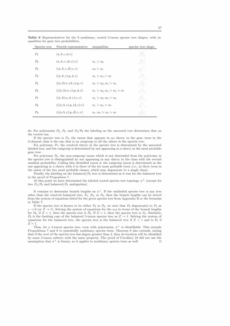
27

Table 6 Representatives for the 9 nonbinary, rooted 5-taxon species tree shapes, with in-equalities for gene tree probabilities.

Species tree Newick representative inequalities species tree shape

P1 (a, b, c, d, e)

P2 (a, b, c, (d, e):z) u1 > u2

P3 ((a, b, c, d):z, e) u3 > u1

P4 ((a, b, c):y, d, e) u1 > u2 > u7

P5 ((a, b):x, (d, e):y, c) u1 > u2, u4 > u5

P6 (((a, b):x, c):y, d, e) u1 > u2, u4 > u5 > u7

P7 ((a, b):x, d, e):z, c) u1 > u2, u8 > u4

P8 (((a, b, c):y, (d, e):z) u1 > u2 > u7

P9 (((a, b, c):y, d):z, e) u1, u3 > u2 > u7

do. For polytomies P2, P5, and P4/P8 the labeling on the unrooted tree determines that onthe rooted one.

If the species tree is P3, the taxon that appears in no cherry in the gene trees in the3-element class is the one that is an outgroup to all the others in the species tree.

For polytomy P7, the resolved cherry in the species tree is determined by the unrootedlabeled tree, and the outgroup is determined by not appearing in a cherry in the most probablegene tree.

For polytomy P9, the non-outgroup taxon which is not descended from the polytomy inthe species tree is distinguished by not appearing in any cherry in the class with the secondsmallest probability. Calling this identified taxon d, the outgroup taxon is determined as theone appearing in a cherry with d in three of the six most probable trees (i.e., in three trees inthe union of the two most probable classes, which may degenerate to a single class).

Finally, the labeling on the balanced/P6 tree is determined as it was for the balanced treein the proof of Proposition 7.

At this point we have determined the labeled rooted species tree topology ψ+ (except fortwo P4/P8 and balanced/P6 ambiguities).

It remains to determine branch lengths on ψ+. If the unlabeled species tree is any treeother than the resolved balanced tree, P4, P6, or P8, then the branch lengths can be solvedfrom the system of equations listed for the given species tree from Appendix B or the formulasin Table 7.

If the species tree is known to be either P4 or P8, we note that P8 degenerates to P4 asz → 0 (or Z → 1). Solving the system of equations for the uis in terms of the branch lengthsfor P8, if Z < 1, then the species tree is P8. If Z = 1, then the species tree is P4. Similarly,P6 is the limiting case of the balanced 5-taxon species tree as Z → 1. Solving the system ofequations for the balanced tree, the species tree is the balanced tree if Z < 1 and is P6 ifZ = 1.

Thus, for a 5-taxon species tree, even with polytomies, σ+ is identifiable. This extendsPropositions 7 and 8 to potentially nonbinary species trees. Theorem 9 also extends, notingthat if the root of the species tree has degree greater than 2, then its location will be identifiedby some 5-taxon subtree with the same property. The proof of Corollary 10 did not use theassumption that σ+ is binary, so it applies to nonbinary species trees as well. ⊓⊔

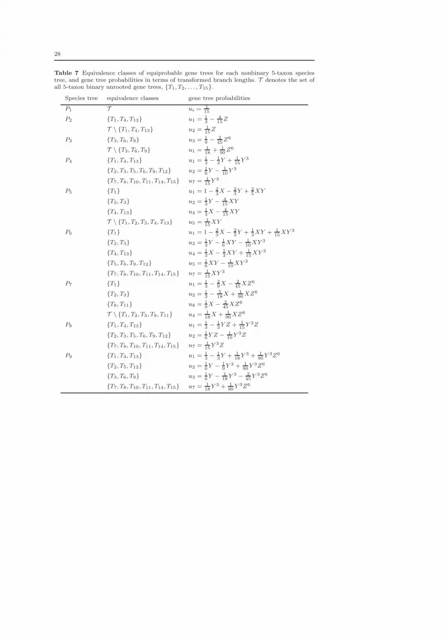
28

Table 7 Equivalence classes of equiprobable gene trees for each nonbinary 5-taxon speciestree, and gene tree probabilities in terms of transformed branch lengths. T denotes the set ofall 5-taxon binary unrooted gene trees, {T1, T2, . . . , T15}.

Species tree equivalence classes gene tree probabilities

P1 T ui =1

15

P2 {T1, T4, T13} u1 = 1

3− 4

15Z

T \ {T1, T4, T13} u2 = 1

15Z

P3 {T3, T6, T9} u3 = 1

9− 2

45Z6

T \ {T3, T6, T9} u1 = 1

18+ 1

90Z6

P4 {T1, T4, T13} u1 = 1

3− 1

3Y + 1

15Y 3

{T2, T3, T5, T6, T9, T12} u2 = 1

6Y − 1

10Y 3

{T7, T8, T10, T11, T14, T15} u7 = 1

15Y 3

P5 {T1} u1 = 1− 2

3X − 2

3Y + 2

5XY

{T2, T3} u2 = 1

3Y − 4

15XY

{T4, T13} u4 = 1

3X − 4

15XY

T \ {T1, T2, T3, T4, T13} u5 = 1

15XY

P6 {T1} u1 = 1− 2

3X − 2

3Y + 1

3XY + 1

15XY 3

{T2, T3} u2 = 1

3Y − 1

6XY − 1

10XY 3

{T4, T13} u4 = 1

3X − 1

3XY + 1

15XY 3

{T5, T6, T9, T12} u5 = 1

6XY − 1

10XY 3

{T7, T8, T10, T11, T14, T15} u7 = 1

15XY 3

P7 {T1} u1 = 1

3− 2

9X − 2

45XZ6

{T2, T3} u2 = 1

3− 5

18X + 1

90XZ6

{T8, T11} u8 = 1

9X − 2

45XZ6

T \ {T1, T2, T3, T8, T11} u4 = 1

18X + 1

90XZ6

P8 {T1, T4, T13} u1 = 1

3− 1

3Y Z + 1

15Y 3Z

{T2, T3, T5, T6, T9, T12} u2 = 1

6Y Z − 1

10Y 3Z

{T7, T8, T10, T11, T14, T15} u7 = 1

15Y 3Z

P9 {T1, T4, T13} u1 = 1

3− 1

3Y + 1

18Y 3 + 1

90Y 3Z6

{T2, T5, T12} u2 = 1

6Y − 1

9Y 3 + 1

90Y 3Z6

{T3, T6, T9} u3 = 1

6Y − 1

18Y 3 − 2

45Y 3Z6

{T7, T8, T10, T11, T14, T15} u7 = 1

18Y 3 + 1

90Y 3Z6