Identification of Performance Degradation in IP Networks UsingThroughput Statistics

Markus Fiedlera, Kurt Tutschkub, Patrik Carlssona, and Arne Nilssona

aDept. of Telecomm. and Signal Proc., Blekinge Inst. of Techn., Karlskrona, Sweden.E-Mail: [markus.fiedler,patrik.carlsson,arne.nilsson]@bth.se

bDept. of Distributed Systems, Inst. of Computer Science, Univ. of Wurzburg, Germany.E-Mail: tutschku@informatik.uni-wuerzburg.de

To be able to satisfy their users, interactive applications like video conferences requirea certain Quality-of-Service from heterogeneous networks. This paper proposes the useof throughput histograms as Quality-of-Service indicator. These histograms are builtfrom local, unsynchronized, passive measurements of packet streams from the viewpointof an application. They can easily be exchanged between sender and receiver, and theircomparison provides information about severity and type of a potential bottleneck. Wedemonstrate the usefulness of these indicators for evaluating the transport quality per-ceived by a video conferencing application and its users in the presence of a bottleneck.

1. Introduction

Advanced IP network applications, such as IP video conferencing, Voice-over-IP, oron-line games, challenge IP network operation. They generate data streams which areincreasingly sensitive to specific delay and throughput requirements. If the requirementsare not met, the services may degrade substantially and become of no use.The provisioning of sufficient throughput for specific applications is a core issue in IP

traffic engineering and IP traffic management. This task is highly difficult and complexdue to the main principles of the Internet technology itself: packet switching, the end-to-end arguments, as well as the diversity in technology, traffic types, and administrativedomains. In order to facilitate Quality-of-Service (QoS) objectives in IP networks, differ-ent support and control technologies like IntServ, DiffServ and MPLS have been devel-oped recently, but are not applied in a wide-spread manner. IP performance managementin real-world networks is still crippled and reveals the gap between using sophisticated,but complex resource allocation mechanisms and the simple use of over-dimensioning forachieving similar QoS objectives. Moreover, recent considerations show that more simpleand focused approaches might succeed over the QoS mechanisms suggested so far [5,9].The identification of the QoS level which has been received by the application is a basic

component of today’s IP performance management cycle. This component has to addressthe basic mechanisms of the IP technology, in particular the heterogeneity of networks,the end-to-end control, and the complexity of applications. However, most monitoring

procedures fail here. Many IP network administrators still use simple tools, like ping

or traceroute, to evaluate the influence of the network. This might not be sufficientfor advanced applications. Such tools merely provide snapshots of the network state.Furthermore, typical throughput measurements in operating IP networks are averages onintervals in the range of minutes and more. Short-term performance problems caused by“dragonflies”, i.e. packet streams with life times up to two seconds [2] that may disturban ongoing video conference often go unnoticed. Moreover, it has to be mentioned thatactive measurement methods always impose additional load on the network and also maydisturb sensitive applications. Comprehensive overviews on monitoring tools can be foundat [3] and in [1,7], for example.Most users do not care about where in the “black box” network the problems occur.

Anyway, their possibilities to monitor the network performance are quite limited. How-ever, they would need some kind of quality feedback when using advanced applicationssuch as video conferencing or on-line gaming. Such indicators also enable users to identifytrends, to be aware of upcoming performance problems and to adapt themselves to theever-changing traffic conditions in today’s best-effort Internet. For instance, users of videoconferences might want to try a lower bit rate if the application-specific control schemes[8] cannot cope with the network conditions any more. Beyond this, such indicators mayassist applications in deriving appropriate control actions. Finally, network operatorsmay profit from indicators revealing severity and type — and perhaps even location — ofpotential bottlenecks.On this background, we present a passive measurement method for monitoring and

visualizing the network’s impact on quality-sensitive packet streams, and thus deliveringbottleneck indicators. Section 2 presents the method and some of its appealing properties.Section 3 describes the measurement scenario. Section 4 presents the performance modeland describes throughput statistics. The practical use for bottleneck classification ofthese statistics is demonstrated in Section 5 by evaluating video conferences between thedepartments of the authors in Sweden and Germany. Section 6 concludes the paper andgives an outlook on future work.

2. The Proposed Method And Its Properties

We suggest a monitoring method which collects throughput statistics on small timescales at the source host and the destination host. The method monitors the throughputon network level just after (before) the traffic has left (entered) the application. Theobserved throughput histograms are subsequently exchanged for sake of comparison andclassification of a potential bottleneck.An advantage of the suggested method is that it neither requires any specific monitoring

station nor the modification of network equipment as proposed in [1,7]. The collection andpreprocessing of the statistics can be performed on the computers that run the observedapplication. Of course, it has to verified that both the application and the monitoringprocess don’t suffer from each other.The suggested method is robust with regards to the characteristics of the data traffic.

Since the traffic streams are compared at the input and at the output, the volatilityof network traffic, e.g. due to TCP’s control behavior, plays a minor role. In general,

the proposed method does not require any assumptions about the traffic patterns beinggenerated. Even though the application may initiate packets at a constant rate, thesepackets may leave the host already with jitter. If this fact is not taken into account,the network would be blamed for something that it is not responsible for. Since thevizualization method is flexible in terms of resolution in time and bandwidth, it caneasily be adapted to the application being monitored.The suggested monitoring method is passive. It introduces only a small additional

overhead in the network when intermediate measurement results are transferred for com-parison. In case of a video conference, an existing control connection could be used toexchange the histograms.Finally, the method is supported by analytical performance investigations of bottlenecks

[6], which will be explained in Section 4. Throughput statistics have been successfullyapplied to the evaluation of QoS degradation, cf. [4]. Our contribution, however, consistsin the comparison and evaluation of throughput histograms of the same IP stream atinput and output of the network.

3. Measurement Methodology

In order to describe the suggested measurement method in greater detail, we outline aprototype implementation of the measurement architecture. The method performs passivemeasurements on links that connect hosts to the network, see Figure 1. The measurementpoints (MP) are placed as close as possible to the hosts. An MP consists of a monitoringmachine that is connected to one or more wiretaps. The MP runs the well-known packetcapture software TCPDUMP [10] on each monitored interface. In the case of full-duplexlinks, wiretaps with two separate output links are needed. Consequently, the MP needstwo network interface cards (NIC) and two TCPDUMP processes to monitor a full-duplexlink. The complete measurement setup is shown in Figure 1. Here, hosts A and host B arethe communicating entities and MP A and MP B are their corresponding measurementpoints. Host C and D in Figure 1 are used to generate interfering traffic, which will bedescribed in Section 5.The simultaneously operated measurement points MP A and MP B generate two data

sets, one for each direction of the tapped link. The data sets were analyzed to identifythe UDP ports used by the voice and video streams. The corresponding streams werethen extracted into separate files. As a result, the measurements generate four data setsat each location with the attributes ”voice/video” and ”sent/received”. For each packetp in these data sets, we extract the time Tp when that particular packet was received bythe kernel in the MP computer, and the size Lp of its UDP payload. We anticipate thatin the future, the measurements will be performed inside the host.

4. Fluid Flow Model and Throughput Histograms

Now we turn the focus on how to obtain and interpret throughput statistics for theobserved voice and video streams. From the application point of view, the network istreated as single equivalent bottleneck, which is modeled by a time-discrete fluid flow model.The feasibility of this model for bottleneck identification and characterization is shown in[6]; the work presented here extends those theoretical results to real environments. Before

Host A Wiretap

Computer

Host B Wiretap

Computer

LAN

Internet

LAN

MP A

MP B

Host D10 Mbps

Switch Host C100 Mbps

10 Mbps

100 Mbps

100 Mbps

Figure 1. Measurement setup and architecture.

describing the extension, we elaborate on some general characteristics of the applied modeland on the related statistics.The considered fluid flow model works on throughput values, where Rs denotes the

average bit rate observed during the interval ](s − 1)∆T, s∆T ]. These values are obtainedfrom the measurements of packet arrival time process {Tp}k

p=1 and payload length process

{Lp}kp=1. During a time window W , a time resolution ∆T gives n = �W/∆T � throughput

values as described in the following.Sampling Process: Given a link capacity of CLink, the time at which the payload

of packet p begins is obtained as T ′p = Tp − Lp/CLink. The arrival time of the payload

of the first observed packet T ′1 is defined to be the time from which the sampling of the

throughput is started. This is a natural triggering point especially from the viewpoint ofthe receiving application that begins to act upon reception of this payload. In order tosimplify the notation, time is re-scaled:

t(·) =T(·) − T ′

1

∆T. (1)

A single sampling interval s may include several complete packets as well as parts ofpackets. Upon initializing Rs = 0, s = 1 . . . n, the contributions of payload number p tothe time series {Rs}n

s=1 are calculated according to the following algorithm:

1. Calculate start interval s′ = �t′p� and end interval s∗ = �tp�.2. If s′ = s∗, then all the bits of payload p belong into one sampling interval:

Rs∗ = Rs∗ +Lp

∆T(2)

3. If s′ < s∗, payload p covers two or more intervals:

Rs′ = Rs′ + (s′ − t′p)CLink

Rs = CLink ∀s : s′ < s < s∗ (3)

Rs∗ = Rs∗ + (tp − s∗ + 1)CLink

Equivalent Fluid Flow Bottleneck: We are now going to look at the fluid modelof the equivalent bottleneck “network”. The time series

{Rin

s

}n

s=1respectively {Rout

s }ns=1

describes the packet stream entering respectively leaving this potential bottleneck in termsof throughput, observed by or close to the sender respectively the receiver. We denote theamount of traffic in the network at the end of interval s by Xs and define X0 = 0 due tothe fact that sender and receiver use the same event, the beginning of the first payload,as a starting point. Based on the observations of

{Rin

s

}n

s=1and {Rout

s }ns=1, the amounts

of traffic Xs are determined by

Xs = Xs−1 + (Rins − Rout

s )∆T . (4)

If the input to the network matches the output ({Rin

s

}n

s=1= {Rout

s }ns=1), the network is

transparent besides a constant transmission time and does not introduce any loss. Inthis case, the equivalent bottleneck remains empty. However, the reality looks differentin a packet-switched best-effort network without bandwidth and delivery guarantees. Insuch a network, different packets can experience significantly different delays and even getlost due to temporary resource shortage. In the fluid flow model, the delays are leadingto variations in the throughput of streams induced by the network are reflected in thevariation of the values Xs, while sudden, irreversible jumps of Xs indicate the amount oftraffic lost in the network.We now consider a condensed representation of {Rs}n

s=1 in form of a summary statistics.We define throughput histograms H ({Rs}n

s=1 ,∆R) with

hi =number of Rs ∈](i − 1)∆R, i∆R] in window W

n∀i , (5)

where ∆R defines the bandwidth resolution. As demonstrated in [6], the comparison ofthroughput histograms for individual streams at input and output of a fluid flow bottle-neck provides information on nature and severity of that bottleneck. We extend thosetheoretical findings to our real-world scenario and show that information on the qual-ity of the intermediate network is obtained from comparing the histogram at the receiverH ({Rout

s }ns=1 ,∆R) with the corresponding histogram from the sender H ({

Rins

}n

s=1,∆R

).

At the end of time window W , the receiver transfers its histogram H ({Routs }n

s=1 ,∆R) tothe sender. The number of bins in the histogram should be kept in reasonable limitsin order to minimize transfer overhead and to permit efficient comparison between thehistograms. This features contributes to the applicability of the method in real-worldscenarios.

Histogram Difference Plots: From the throughput histograms at input and out-put, throughput histogram differences ∆H ({Rout

s }ns=1 ,

{Rin

s

}n

s=1,∆R

)are calculated by

subtracting the corresponding input histogram values from output histogram values:

∆hi = houti − hin

i . (6)

1 1 1

-1

InOut

Rs

s

H ({Rin

s

})

Rs

H ({Rout

s

})

Rs

∆H

Rs

Figure 2. Antcipated time plot, throughput histograms at input and output and histogramdifference plot (from left to right) in case of a shared bottleneck.

1 1 1

-1

InOut

Rs

s

H ({Rin

s

})

Rs

H ({Rout

s

})

Rs

∆H

Rs

Figure 3. Antcipated time plot, throughput histograms at input and output and histogramdifference plot (from left to right) in case of a shaping bottleneck.

Histogram difference plots are obtained by interconnecting the ∆hi values when plottingthem versus throughput. These plots visualize the network impact on the throughputhistograms and thus on the throughput itself. They are characterized by

• width = ∆R (max{ i |∆hi = 0} −min{ i |∆hi = 0});• peak-to-peak value = max{hi}+ |min{hi}| ∈ [0, 2];

• grade of deviation =∑

i|∆hi|

2∈ [0, 1].

The “shape” of a histogram difference plot contains information about the nature ofthe bottleneck. This is illustrated by the following simplified examples. Figure 2 refersto a stream whose initially constant throughput is changed in a shared bottleneck. Assoon as the demand for resources of all streams exceeds the capacity, queuing occurs andthe throughput decreases. As soon as the demand falls below the capacity, the queue isrelaxed, which implies higher throughput at the output. Altogether, the variability – orthe burstiness – of the traffic grows. The resulting difference plot has the shape of an“M” with negative values close to the original speed and positive values at both lowerand higher speeds.Figure 3 illustrates the effect of a shaping bottleneck on a stream. In this case, the

throughput variations are smoothed, i.e. the burstiness of the traffic decreases. Thedifference plot has now the shape of a “W” with positive values close to the shaper’sthroughput and negative values at lower and higher speeds. In the sequel, we are going

Table 1Histogram difference parameters for voice from Karlskrona to Wurzburg at different levelsof disturbance.

Interfering Difference plot Type ofTraffic [Mbps] Width [Mbps] Peak-to-peak Grade of dev. bottleneck

0 0 0 0 Not present2 0.080 0.0100 0.7 % Shared4 0.080 0.027 2.0 % Shared6 0.046 0.007 0.5 % Unspecified8 0.080 0.047 3.3 % Shaper

to describe such behaviors by considering real-world voice and video streams interactingwith a bottleneck.

5. Test Description and Results

We investigate and visualize the performance of a video conference via European re-search networks with the general setup depicted in Figure 1. Host A is located atBlekinge Institute of Technology, Karlskrona, Sweden and host B is located at Universityof Wurzburg, Germany. Both hosts run an off-the-shelf video conferencing application[8], based on H.323 on top of UDP/IP. The application offers video communications upto 384 kbps, i.e. 320 kbps for video and 64 kbps for voice. For the video stream, DynamicBandwidth Allocation [8] is applied, which results in variable throughput already at thesender. According to packet traces, on average 162

3voice packets are sent per second. At

the sender, their inter-packet times are roughly multiples of 16 ms, which means that thesending application already introduces a significant amount of jitter. As voice is moresensitive to delay and jitter, it is prioritized by the application, cf. [8].Our experience is that video conferences between Karlskrona and Wurzburg usually

work very well, which is mainly the result of the corresponding research networks beingover-dimensioned. To compromise this quality, host C, cf. Figure 1, was used to sendUDP packet streams to host D, thus turning the 10 Mbps link between the switch and theLAN into a bottleneck. With 6 Mbps of disturbing UDP traffic, the users still perceiveda sufficient quality. However, at 8 Mbps disturbance, glitches in the video occurred,whereas voice was not affected. Overloading the bottleneck by adding 10 Mbps corruptedthe transmission and caused a tear down of the video conference. In the following, weconcentrate on the streams from Karlskrona to Wurzburg passing the bottleneck in thesame direction as the disturbing UDP stream. The time window was chosen as W =1 minute and the time resolution as ∆T = 100 ms, while the throughput resolutions forvoice and video are set to 2 kbps and 20 kbps.Figure 4(a) shows histogram difference plots for video and rising levels of UDP distur-

bance, and Table 1 contains some related parameters as defined in the previous section.In the undisturbed case, the voice stream does not experience any change in its bit ratestatistics. For disturbances of 2 Mbps and 4 Mbps, the network influence is that of ashared bottleneck. For disturbances of 6 Mbps and especially of 8 Mbps, the voice stream

0.000

0.091

0.183

0.274

0

2

4

6

8 −0.1

−0.05

0

0.05

0.1

Rs [Mbps]UDP Disturbance [Mbps]

∆ H

(a)

0.0000 0.1850

0.3700 0.5550

0.7400

0

2

4

6

8 −0.1

−0.05

0

0.05

0.1

Rs [Mbps]UDP Disturbance [Mbps]

∆ H

(b)

Figure 4. Histogram difference plots for (a) voice and (b) video from Karlskrona toWurzburg for different levels of disturbance.

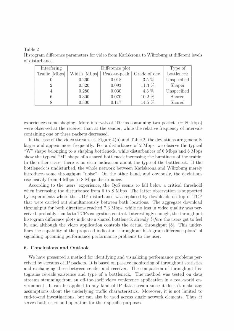
Table 2Histogram difference parameters for video from Karlskrona to Wurzburg at different levelsof disturbance.

Interfering Difference plot Type ofTraffic [Mbps] Width [Mbps] Peak-to-peak Grade of dev. bottleneck

0 0.260 0.018 3.5 % Unspecified2 0.320 0.093 11.3 % Shaper4 0.280 0.030 4.3 % Unspecified6 0.300 0.070 10.2 % Shared8 0.300 0.117 14.5 % Shared

experiences some shaping: More intervals of 100 ms containing two packets (� 80 kbps)were observed at the receiver than at the sender, while the relative frequency of intervalscontaining one or three packets decreased.In the case of the video stream, cf. Figure 4(b) and Table 2, the deviations are generally

larger and appear more frequently. For a disturbance of 2 Mbps, we observe the typical“W” shape belonging to a shaping bottleneck, while disturbances of 6 Mbps and 8 Mbpsshow the typical “M” shape of a shared bottleneck increasing the burstiness of the traffic.In the other cases, there is no clear indication about the type of the bottleneck. If thebottleneck is undisturbed, the whole network between Karlskrona and Wurzburg merelyintroduces some throughput “noise”. On the other hand, and obviously, the deviationsrise heavily from 4 Mbps to 8 Mbps disturbance.According to the users’ experience, the QoS seems to fall below a critical threshold

when increasing the disturbance from 6 to 8 Mbps. The latter observation is supportedby experiments where the UDP disturbance was replaced by downloads on top of TCPthat were carried out simultaneously between both locations. The aggregate downloadthroughput for both directions reached 7.3 Mbps, while no loss in video quality was per-ceived, probably thanks to TCPs congestion control. Interestingly enough, the throughputhistogram difference plots indicate a shared bottleneck already before the users get to feelit, and although the video application controls the actual throughput [8]. This under-lines the capability of the proposed indicator “throughput histogram difference plots” ofsignalling upcoming performance performance problems to the user.

6. Conclusions and Outlook

We have presented a method for identifying and visualizing performance problems per-ceived by streams of IP packets. It is based on passive monitoring of throughput statisticsand exchanging these between sender and receiver. The comparison of throughput his-tograms reveals existence and type of a bottleneck. The method was tested on datastreams stemming from an off-the-shelf video conference application in a real-world en-vironment. It can be applied to any kind of IP data stream since it doesn’t make anyassumptions about the underlying traffic characteristics. Moreover, it is not limited toend-to-end investigations, but can also be used across single network elements. Thus, itserves both users and operators for their specific purposes.

Due to its universality, the suggested method may be applied in many contexts such asload control on virtual links, cf. [9], or as flow control on or on top the transport layer.Of course, both users and applications can make use of the method to adapt their datarate to an optimal level. Operators, on the other hand, may use the proposed indicatorfor finding and eliminating bottlenecks.Future research will be necessary to improve the generality of the method. In particular,

further investigations on the optimal sampling and quantization parameters with respectto the observed traffic are needed. In addition, we demonstrated so far only the qualitativecapabilities of the method. Additional research is needed for obtaining quantitative resultslike thresholds for sending signals to users or applications.

REFERENCES

1. J. Bolliger and T. Gross. Bandwidth monitoring for network-aware applications. InProceedings of the 10th IEEE International Symposium on High Performance Dis-tributed Computing (HPDC-10’01), 7–9 August, San Francisco, USA, 2001.

2. N. Brownlee and KC Claffy. Understanding Internet traffic streams: Dragonflies andturtoises. IEEE Communications Magazine, 40(10):110–117, October 2002.

3. CAIDA. Performance Measurement Tools Taxonomy. http://www.caida.org/tools/taxonomy/performance.xml.

4. J. Charzinski. Fun Factor Dimensioning for Elastic Traffic. In Proceedings of the ITCSpecialist Seminar on Internet Traffic Measurement, Modeling and Management, 18–20 September, Monterey, USA, 2000.

5. D. Clark, K. Sollins, J. Wroclawski, and R. Braden. Tussle in cyberspace: Defin-ing tomorrow’s Internet. In Proceedings of the ACM SIGCOMM Conference 2002,Pittsburgh, 19–23 August, 2002.

6. M. Fiedler and K. Tutschku. Application of the stochastic fluid flow model for bottle-neck identification and classification. In Proceedings of the SCS Conference on Design,Analysis, and Simulation of Distributed Systems 2003, 30 March – 3 April, Orlando,USA, 2003.

7. T. Lindh. A new approach to performance montoring in IP networks – combiningactive and passive methods. In Proceedings of the Passive and Active MeasurementWorkshop 2002, 24–26 March, Fort Collins, USA, 2002.

8. T. O’Neil. Network-based quality of service for IP video conferencing. White paperavailable at http://www.polycom.com/, Polycom Inc., 2002.

9. L. Subramanian, I. Stoica, H. Balakrishnan, and R. Katz. OverQoS: Offering QoSusing overlays. In Proceedings of the First Workshop on Hop Topics in Networks(HotNets-I), Princeton, USA, 2002.

10. TCPDUMP Public Repository. http://www.tcpdump.org.