hyperkahler cones and orthogonal wolf spaces
TRANSCRIPT

arX
iv:h
ep-t
h/02
0214
9v2
27
Mar
200
2
ITP-UU-02/02
SPIN-02/04
YITP-SB-02-10
hep-th/0202149
Hyperkahler Cones
and Orthogonal Wolf Spaces
Lilia Anguelova∗, Martin Rocek∗ and Stefan Vandoren†
∗C.N. Yang Institute for Theoretical Physics
SUNY, Stony Brook, NY 11794-3840, USA
†Institute for Theoretical Physics and Spinoza Institute
Utrecht University, Utrecht, The Netherlands
ABSTRACT
We construct the hyperkahler cones corresponding to the quaternion-Kahler
orthogonal Wolf spaces SO(n+4)SO(n)×SO(4)
and their non-compact versions, which
appear in hypermultiplet couplings to N = 2 supergravity. The geometry is
completely encoded by a single function, the hyperkahler potential, which we
compute from an SU(2) hyperkahler quotient of flat space. We derive the
Killing vectors and moment maps for the SO(n + 4) isometry group on the
hyperkahler cone. For the non-compact case, the isometry group SO(n, 4)
contains n + 2 abelian isometries which can be used to find a dual description
in terms of n tensor multiplets and one double-tensor multiplet. Finally, using
a representation of the hyperkahler quotient via quiver diagrams, we deduce
the existence of a new eight dimensional ALE space.
February 1, 2008

1 Introduction
Quaternion-Kahler (QK) manifolds have recently attracted a lot of attention in the context
of N = 2 gauged supergravity, both in four and five spacetime dimensions. In particular,
those with negative scalar curvature appear as target spaces for N = 2 hypermultiplets
coupled to supergravity [1]. The homogeneous QK spaces G/H are classified by Wolf and
Alekseevskii [2]; the compact ones are given by the three infinite series
HP(n) =Sp(n + 1)
Sp(n) × Sp(1), X(n) =
SU(n + 2)
SU(n) × U(2), Y (n) =
SO(n + 4)
SO(n) × SO(4), (1.1)
of dimension 4n, and the five exceptional cases
G2
SO(4),
F4
Sp(3) × Sp(1),
E6
SU(6) × Sp(1),
E7
Spin(12) × Sp(1),
E8
E7 × Sp(1), (1.2)
of dimensions 8, 28, 40, 64 and 112 respectively. Their non-compact versions have negative
scalar curvature and hence are relevant for supergravity applications. For low dimensions,
there are relations between these spaces: the four-sphere Y (1) ∼= HP(1), and Y (2) ∼= X(2).
These isomorphisms are discussed in more detail below.
A complete classification of QK spaces does not exist. Because their Sp(1) curva-
ture does not vanish, and their quaternionic two-forms are not closed, QK spaces are
rather difficult to deal with. This complicates the study of hypermultiplet couplings to
supergravity, which arise in the low energy effective action of type II superstring com-
pactification on Calabi-Yau threefolds [3]. In this paper, we focus on the Y (n) spaces.
Their noncompact versions
Y (n) =SO(n, 4)
SO(n) × SO(4), (1.3)
describe the classical moduli spaces of type II Calabi-Yau compactifications down to four
dimensions, either as dual quaternionic spaces from the c-map [3], or from dualizing n
tensor multiplets and a double-tensor multiplet [4].
Vector multiplet couplings to N = 2 supergravity are geometrically much simpler.
The scalar fields of the vector multiplets parametrize a special Kahler geometry in d=4
[5] and a very special real geometry in d=5 [6]. Both these geometries are completely
determined in terms of a single function from which the target space metric, and other
geometrical quantities, can easily be computed. It is desirable to have a similar description
for QK manifolds, such that the whole geometry is encoded by a single function of the
hypermultiplet scalars. Such a description was first given in the mathematics literature,
where it was shown [7], that to every 4n dimensional QK manifold one can associate a
4(n + 1) dimensional hyperkahler manifold which admits a conformal homothety and an
1

isometric Sp(1)-action that rotates the three complex structures into each other. The
conformal homothety χA satisfies
DAχB = δBA , (A, B = 1, ..., 4n) , (1.4)
such that locally χA = ∂Aχ. The function χ is called the hyperkahler potential and the
metric is
gAB = DA∂Bχ . (1.5)
Such a manifold is a hyperkahler cone (HKC) over a base which is an Sp(1) fibration over
a QK space [7, 8].
It was later anticipated in [9], and shown explicitly in [10, 11] how this connection
is precisely realised in the conformal calculus for hypermultiplets. The transition from
the HKC to the QK space is called the N = 2 superconformal quotient, and is associated
with eliminating the compensating hypermultiplet by an SU(2) quotient and gauge-fixing
combined with a reduction along the homothety. The simplest QK manifolds are the
quaternionic projective spaces HP(n). Galicki has shown that the X and Y series can be
obtained from these by performing quaternionic U(1) and SU(2) quotients, respectively
[12]. It is interesting to study these spaces in terms of the corresponding HKC’s. The HKC
of HP(n−1) is simply Hn ∼= C
2n, and the explicit construction of the HKC of X(n−2) is a
U(1) hyperkahler quotient of Hn [11]. In Section 2 of this paper, we derive the hyperkahler
potential χ for the orthogonal Wolf spaces Y (n− 4) by performing an SU(2) hyperkahler
quotient on Hn. The action of the SU(2) on the coordinates of H
n can be deduced from
Galicki’s quaternionic quotient [12] because the diagram in Figure 1 is commutative [7].
Hence quaternionic quotients between the QK manifolds lift to hyperkahler quotients
between the corresponding HKC’s. We also write down the moment maps and Killing
vectors for the SO(n) isometry group on the HKC. These appear in the scalar potential
of gauged N = 2 supergravity.
In Section 3 we consider the three special cases for which the hyperkahler potential of
the HKC of Y (n − 4) is known: n = 4, where the HKC of Y (0) is R4, n = 5, where the
HKC of Y (1) is R8 and n = 6, where the HKC of Y (2) is the HKC of X(2). We check
our calculation by showing that each of these special cases agrees with the known results.
In Section 4 we construct the dual description of the HKC of the non-compact version
Y (n) in terms of n tensor multiplets and a double tensor multiplet. This tensor multiplet
description naturally appears in type IIB compactifications.
In Section 5 we show how the hyperkahler quotient can be lifted to N = 2 superspace.
Once we have this description, we can use the techniques of [14] to write down the quiver
diagrams for the HKC’s of Y (n). This point of view allows us to infer the existence of a
new 8-dimensional ALE space.
2

HKC(X) 2n nC =H HKC(Y)
X(n−2) Y(n−4)HP(n−1)
su(2)
su(2)
u(1)
u(1)
−4
−4 −12
−12
−4 −4
Figure 1: The horizontal arrows stand for hyperkahler quotients (upper), and quaternionic quotients
(lower). The vertical arrows denote the superconformal quotients. The numerical label of each arrow
denotes the change of the number of real dimensions accompanying the corresponding quotient.
Our long term goal is to understand the nonperturbative corrections to quaternionic
geometries; we expect that these are most easily computed in terms of the hyperkahler
potential χ. We also note that HKC’s appear as moduli spaces of Yang-Mills instantons
[15, 16], e.g., the homogeneous QK G/H manifolds determine the one-instanton moduli
spaces with gauge group G and stability group H . This suggests a connection between
the moduli spaces of Calabi-Yau manifolds and Yang-Mills instantons [16].
2 The SU(2) Quotient
In this section, we explicitly perform the non-abelian hyperkahler quotient from Hn = R
4n
to the HKC of Y (n − 4), n ≥ 4. For simplicity, we do the analysis for the compact case;
the non-compact case is very similar and we give the final result at the end of this section.
The space Hn is flat, and has an isometry group SO(n) which is linearly realized on the
n quaternions
qM =
(
zM+ −zM
−
zM− zM
+
)
, M = 1, ..., n . (2.1)
Clearly, Hn is itself an HKC with hyperkahler potential (or equivalently, N = 1 superspace
Lagrangian)
χ (Hn) = 12Tr(
qMq†M
) = zM+ zM
+ + zM− zM
− , (2.2)
where a sum over repeated indices is understood. The closed hyperkahler two-forms on
Hn are
Ω3 = −i(
dzM+ ∧ dzM
+ + dzM− ∧ dzM
−
)
, Ω+ = dzM+ ∧ dzM
− , Ω− = (Ω+)∗ , (2.3)
3
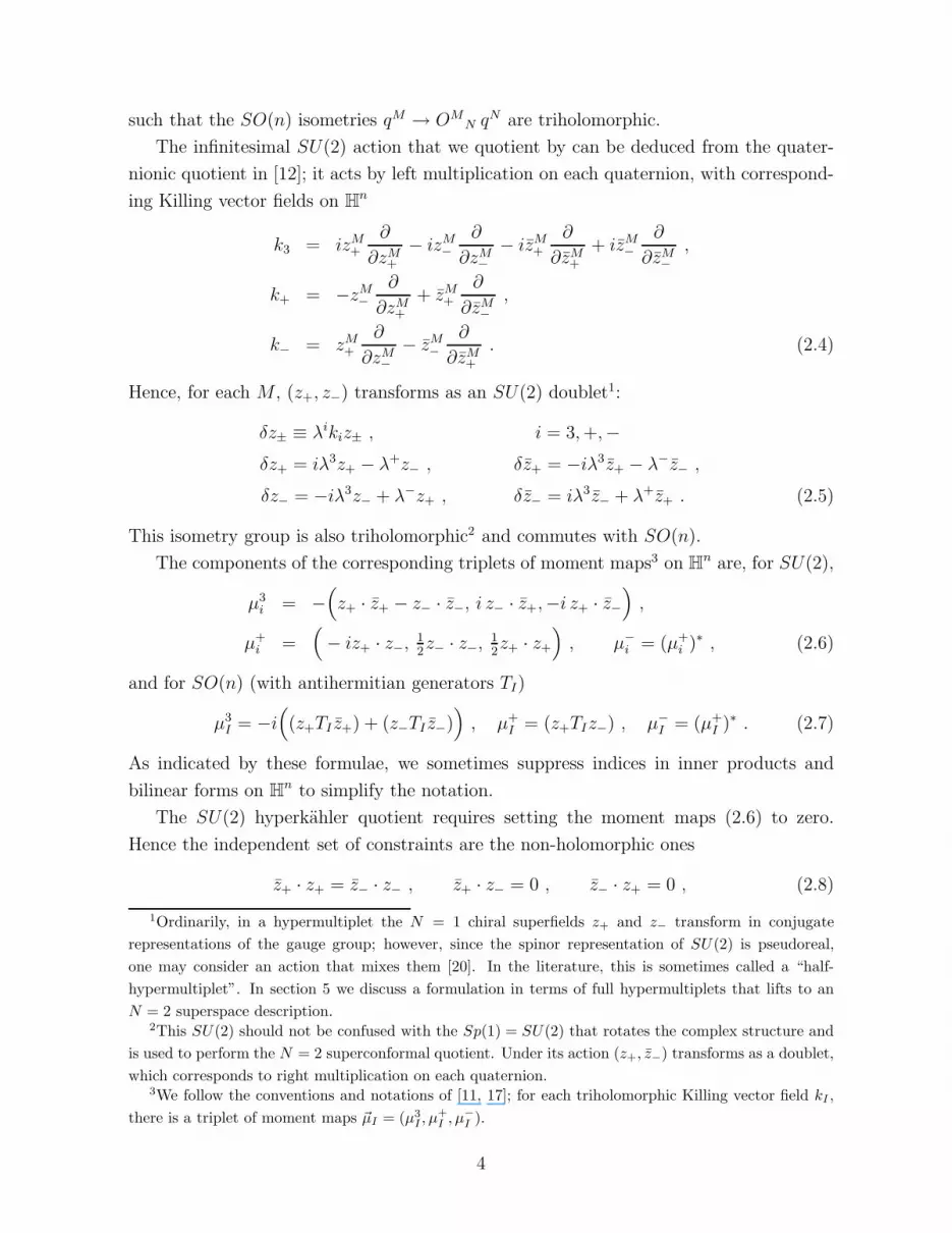
such that the SO(n) isometries qM → OMN qN are triholomorphic.
The infinitesimal SU(2) action that we quotient by can be deduced from the quater-
nionic quotient in [12]; it acts by left multiplication on each quaternion, with correspond-
ing Killing vector fields on Hn
k3 = izM+
∂
∂zM+
− izM−
∂
∂zM−
− izM+
∂
∂zM+
+ izM−
∂
∂zM−
,
k+ = −zM−
∂
∂zM+
+ zM+
∂
∂zM−
,
k− = zM+
∂
∂zM−
− zM−
∂
∂zM+
. (2.4)
Hence, for each M , (z+, z−) transforms as an SU(2) doublet1:
δz± ≡ λikiz± , i = 3, +,−δz+ = iλ3z+ − λ+z− , δz+ = −iλ3z+ − λ−z− ,
δz− = −iλ3z− + λ−z+ , δz− = iλ3z− + λ+z+ . (2.5)
This isometry group is also triholomorphic2 and commutes with SO(n).
The components of the corresponding triplets of moment maps3 on Hn are, for SU(2),
µ3i = −
(
z+ · z+ − z− · z−, i z− · z+,−i z+ · z−)
,
µ+i =
(
− iz+ · z−, 12z− · z−, 1
2z+ · z+
)
, µ−i = (µ+
i )∗ , (2.6)
and for SO(n) (with antihermitian generators TI)
µ3I = −i
(
(z+TI z+) + (z−TI z−))
, µ+I = (z+TIz−) , µ−
I = (µ+I )∗ . (2.7)
As indicated by these formulae, we sometimes suppress indices in inner products and
bilinear forms on Hn to simplify the notation.
The SU(2) hyperkahler quotient requires setting the moment maps (2.6) to zero.
Hence the independent set of constraints are the non-holomorphic ones
z+ · z+ = z− · z− , z+ · z− = 0 , z− · z+ = 0 , (2.8)
1Ordinarily, in a hypermultiplet the N = 1 chiral superfields z+ and z−
transform in conjugate
representations of the gauge group; however, since the spinor representation of SU(2) is pseudoreal,
one may consider an action that mixes them [20]. In the literature, this is sometimes called a “half-
hypermultiplet”. In section 5 we discuss a formulation in terms of full hypermultiplets that lifts to an
N = 2 superspace description.2This SU(2) should not be confused with the Sp(1) = SU(2) that rotates the complex structure and
is used to perform the N = 2 superconformal quotient. Under its action (z+, z−) transforms as a doublet,
which corresponds to right multiplication on each quaternion.3We follow the conventions and notations of [11, 17]; for each triholomorphic Killing vector field kI ,
there is a triplet of moment maps ~µI = (µ3I , µ
+
I , µ−
I ).
4

and the holomorphic ones
z+ · z− = 0 , z+ · z+ = 0 , z− · z− = 0 . (2.9)
To perform the quotient one has to solve (2.8) and (2.9), reducing the number of real
coordinates by 3 + 6 = 9, and choose a gauge to fix the SU(2) gauge freedom, further
reducing the number of real coordinates by 3; thus the dimension is reduced by 12 real or
6 complex coordinates, consistent with the dimension of the HKC of Y (n − 4), namely,
4(n − 3). In practice it is hard to solve all the constraints; as explained in [18], one
may complexify4 the gauge group (in our case SU(2) → SL(2, C)) and solve just the
holomorphic constraints, which are preserved by the complexified gauge group. This
construction is completely natural in N = 1 superspace, where the non-holomorphic
constraints are solved for the N = 1 gauge fields. If we choose 3 complex gauge conditions
and impose the holomorphic constraints, we see that we still reduce the dimension by
12. The hyperkahler potential on the quotient space is found by gauging the N = 1
Lagrangian for Hn and substituting the solution for the gauge fields.
Recall that the hyperkahler potential for the flat space Hn is (2.2). For each value of
the index M the pair (zM+ , zM
− ) is a doublet under the SU(2) which we quotient by (see
(2.5)). Hence we have n copies of the 2-dimensional represenation of SU(2) in (2.2).
We introduce a gauge field eV , such that the gauged hyperkahler potential of Hn is
([20, 19, 18], see also section five and appendix B of [11]):
χ =
n∑
M=1
(
zM+ zM
−
)
(
eV
)
(
zM+
zM−
)
, (2.10)
where(
eV
)
is the 2 × 2 matrix of N = 1 SU(2) gauge fields and hence is hermitian
with determinant 1. The nonholomorphic constraints (2.8) (c.f. (2.6)) can be written as
µ3i =
(
zM+ zM
−
)
Ti
(
zM+
zM−
)
= 0 , i = 3, +,− (2.11)
where Ti are the SU(2) generators normalized as
T3 =
(
1 0
0 −1
)
, T+ =
(
0 1
0 0
)
, T− =
(
0 0
1 0
)
. (2.12)
The gauged nonholomorphic moment maps are [20, 19, 18]:
µ3i =
(
zM+ zM
−
)
Ti
(
eV
)
(
zM+
zM−
)
= 0 . (2.13)
4The complexification of the gauge group means doubling of the number of generators (to the set
of initial Killing vectors kI one adds the set J3kI , where J3 is the complex structure determined by
Ω3(X, Y ) = g(J3X, Y )).
5

Solving (2.13) for the gauge fields we find
(
eV
)
=1
√
(z+ · z+)(z− · z−) − (z+ · z−)(z− · z+)
(
z− · z− −z− · z+
−z+ · z− z+ · z+
)
, (2.14)
and hence the hyperkahler potential of the quotient is
χquotient = 2√
zM+ zM
+ zN− zN
− − zM+ zM
− zN− zN
+ , (2.15)
with M, N still running from 1 to n. To find coordinates on the quotient we gauge-fix
and solve the holomorphic constraints; we can choose
zn+ = 0 , zn−1
− = 0 , zn−2+ = 1 . (2.16)
Now the holomorphic constraints (2.9) can be easily solved:
zn−2− = −za
+za− , zn−1
+ = i√
1 + za+za
+ , zn− = i
√
za+za
−zb+zb
− + za−za
− , (2.17)
where za+, zb
−, a, b = 1, ..., n − 3 are the coordinates on the HKC of Y (n − 4). Thus
the hyperkahler potential on the HKC of Y (n − 4) is given by (2.15), subject to (2.16)
and (2.17). Furthermore the dilatations act on z+ and z− with scaling weights 0 and 2
respectively, and the holomorphic two-form on the HKC is simply
Ω+ = dza+ ∧ dza
− , a = 1, ..., n − 3 . (2.18)
The gauge choice (2.16) is legitimate, but not always the most convenient, as we see in
the next section.
The moment maps of the SO(n) isometry on the HKC can easily be computed from
the SU(2) quotient of (2.7). The SU(2) gauged SO(n) moment maps take a similar form
to (2.13), and eliminating the gauge fields yields
µ3I =
2i
χ
(
(z− · z−)(z+TIz+) − (z+ · z−)(z−TIz+) + (+ ↔ −))
,
µ+I = (z+TIz−) , µ−
I = (µ+I )∗ , (2.19)
subject to the constraints (2.16) and (2.17).
The SO(n) Killing vectors on the quotient space can also be easily computed. On Hn,
the Killing vectors are simply kMI± = (TI)
MNzN
± , but after the quotient we have to add
local compensating SU(2) transformations to preserve the gauge conditions (2.16). We
find
kMI+ = (TI)
MNzN
+ + (TI)n
NzN+
zn−2− zM
+ − zM−
zn−
− (TI)n−2
NzN+ zM
+ , (2.20)
kMI− = (TI)M
NzN− − (TI)
nN
zN+ zn−2
− zM−
zn−
− (TI)n−1
N
zN− zM
+
zn−1+
+ (TI)n−2
NzN+ zM
− .
6

One can verify that they preserve (2.16) as well as (2.17).
These Killing vectors and moment maps form the main ingredients of the scalar po-
tential on the HKC. Performing the superconformal quotient leads to the Killing vectors
and moment maps on Y (n − 4), which can be compared to those given in [21].
To end this section, we discuss the non-compact case; the QK space is now
Y (n − 4) ≡ SO(n − 4, 4)
SO(n − 4) × SO(4). (2.21)
The above formulae are modified by putting in a pseudo-Riemannian metric in the inner
products: one starts with a metric ηMN on Hn−4,4 of signature ηMN = diag(− − − −
+ · · ·+). The metric then used in the products zaηabzb on the HKC of Y (n − 4) has
signature ηab = diag(− + · · ·+), such that, in our conventions, the metric on the QK
space is positive definite.5
3 The Special Cases
In this section, we give more details about the SU(2) gauge fixing, and compare our
results with the known cases for n = 4, 5, 6. It is convenient to introduce the SU(2) gauge
invariant variables (for all n),
zMN ≡ zM+ zN
− − zN+ zM
− . (3.1)
The hyperkahler potential on the quotient (2.15) is then, for all n,
χquotient =√
2 zMN zMN , (3.2)
and is manifestly SU(2) gauge invariant. The variables (3.1) satisfy a Bianchi-like identity,
zMNzPQ + zMQzNP + zMP zQN = 0 , (3.3)
and the holomorphic constraints (2.9) imply
zMNzNP = 0 . (3.4)
We show below how these constraints can be solved for n = 4, 5, 6.
3.1 n = 4
In this case the quaternion-Kahler manifold is just one point, and so the hyperkahler cone
above it must be R4. The gauge choice (2.16) does not give the canonical quadratic hy-
perkahler potential on C2, so we look for a different gauge. For n = 4, any antisymmetric
5This differs by an overall sign from the conventions of [11, 17].
7

matrix can be decomposed into its selfdual and anti-selfdual part. Notice then that (3.3)
and (3.4) are solved by
zMN = ±ǫMNPQzPQ , (3.5)
so that we can parametrize
zMN = ui(σ)MNij uj . (3.6)
Here, u1, u2 are two complex coordinates and (σ)MNij are the standard selfdual matrices6.
Using sigma-matrix algebra, it is easy to check that the constraints (3.3) and (3.4) are
satisfied and the hyperkahler potential becomes simply
χ = 42∑
i=1
uiui , (3.7)
which is the Kahler potential of C2 with flat metric.
The gauge choice (3.6) for the bilinears zMN implies
z+ = ( u, v, iu, iv ) , z− = ( iv, −iu, v, −u ) . (3.8)
with u1 = u and u2 = v. Notice that this SU(2) gauge solves all the constraints (2.8) and
(2.9).
3.2 n = 5
It is well-known that
Y (1) =SO(5)
SO(4)=
Sp(2)
Sp(1) × Sp(1)= HP(1) , (3.9)
and hence the HKC above it must be H2 = R
8. The gauge (2.16) again does not give the
canonical, quadratic hyperkahler potential on C4, so we search for a more suitable gauge.
The coordinates zM± transform in the vector representation of SO(5):
zM± → OM
NzN± , M, N = 1, ..., 5 , (3.10)
We rewrite this in Sp(2) notation by using the Clifford algebra in four Euclidean dimen-
sions, where all gamma matrices can be taken hermitian. We define 4 × 4 matrices
(v±)ij ≡ −12zM± γM
ikCkj i, j = 1, . . . , 4 , (3.11)
6We use the conventions σMN = 1
2(σMσN − σNσM ) with σM = (~τ , i) and σM = (~τ ,−i). The (~τ ) are
the three Pauli matrices and i, j indices are raised and lowered with ǫij such that (σ)MNij is symmetric.
We could also choose the anti-selfdual matrices σMN = 1
2(σM σN − σN σM ), but this leads to equivalent
results.
8

where γ5 = γ1γ2γ3γ4 and C is the charge conjugation matrix, which can be taken an-
tisymmetric and with square −1, such that (γMC)ij is antisymmetric. C serves as an
Sp(2) metric and can be used to lower and raise (i, j) indices. Hence the matrices v±
are antisymmetric; the relation (C−1)ijv±ij = 0, then leaves five independent components.
We can invert (3.11),
zM± = −1
2Tr(
γMv±C−1)
. (3.12)
Now we introduce SU(2) gauge invariant variables analogous to (3.1):
wij ≡
(
v+C−1v−C−1 − v−C−1v+C−1)
. (3.13)
The matrix wij ≡ (w C)ij is symmetric; the relation to (3.1) is
w = 14zMNγMN . (3.14)
It is straightforward to show that the hyperkahler potential (2.15) becomes
χ =√
Tr(ww†) , (3.15)
up to an irrelevant overall factor. In these variables, the moment map constraints (2.9)
are
z± · z± = Tr(
v±C−1v±C−1)
= 0 , z+ · z− = Tr(
v+C−1v−C−1)
= 0 . (3.16)
Imposing them, one can check that the matrix ww is zero as it should be according to
(3.4).
Since we know that the HKC is flat, there should be coordinates ui; i = 1, . . . , 4, in
which the hyperkahler potential is
χ =
4∑
i=1
uiui . (3.17)
If we can find a gauge for v±, satisfying (3.16), such that
wij = uiuj , (3.18)
then (3.15) reduces to (3.17) and we have proven that (2.15) gives the correct result.
This can be achieved by choosing the three complex SU(2) gauge conditions
v+14 = v−13 , v+13 = v−14 = 0 , (3.19)
and identifying
v+14 = v−13 = u1 , v+12 = −u3 , v−12 = u4 . (3.20)
9

Then we solve the moment map constraints (3.16) for v+23, v−24 and v−23, and wij = uiuj
for v+24. This gives
v+23 =u2
3
u1
, v+24 =u3u4
u1
+ u2 , v−23 = −u3u4
u1
+ u2 , v−24 = −u24
u1
. (3.21)
Using (3.12), (3.19), (3.20) and (3.21) it is straightforward to find the coordinates z± in
terms of the flat coordinates ui for any explicit representation of the Clifford algebra. For
example,
z+ =
(
−2u3 , −iu23
u1− iu1 , −u2
3
u1+ u1 ,
u3u4
u1+ u2 , −iu3u4
u1− iu2
)
,
z− =
(
2u4 ,iu3u4
u1
− iu2 ,u3u4
u1
− u2 , −u24
u1
+ u1 ,iu2
4
u1
+ iu1
)
.
One can easily check that these zM± ’s satisfy (2.9) and give χ =
∑4i=1 uiui.
3.3 n = 6
Recall that
X(2) =SU(4)
SU(2) × U(2), Y (2) =
SO(6)
SO(2) × SO(4), (3.22)
and hence X(2) = Y (2) and their HKC’s must coincide. The hyperkahler potential of
the HKC of X(n) was obtained in [11] by a U(1) hyperkahler quotient of Hn+2. Denoting
complex coordinates of H4 = C
8 by wi+ and w−i, i = 1, ..., 4, transforming in conjugate
representations of SU(4), we have
χ(X) = 2√
wi+wi
+w−jw−j , where w4− = 1 w4
+ = −wa+w−a a = 1, 2, 3 . (3.23)
To compare the HKC of Y (2) with (3.23), we follow the same strategy as for n = 5,
namely we make use of the local isomorphism SU(4) = SO(6). To this end we define
U(1) gauge invariant (and traceless) matrix
wij = wi
+w−j i, j = 1, ..., 4 , (3.24)
and write (3.23) in matrix notation as
χ(X) = 2√
Tr(ww†) . (3.25)
On the Y (2)-side, the coordinates zM± , M = 1, ..., 6 are in the vector representation
of SO(6), similarly to (3.10). As in the n = 5 case, we rewrite the hyperkahler potential
(2.15) in SU(4) notation. Then we make gauge choices and solve the holomorphic moment
map constraints such that (2.15) coincides with (3.25).
10

We introduce a basis of selfdual and anti-selfdual four by four matrices η, η and write
v± ij ≡ za±ηa
ij + iza+3± ηa
ijz , (3.26)
where a = 1, 2, 3 and ηa and ηa are selfdual and anti-selfdual respectively, see e.g., [22].
We can raise and lower pairs of indices using ǫijkl,
∗vij± ≡ 1
2ǫijklv± kl , (3.27)
such that
za± = 1
4ηa
ij ∗ vij± , za+3
± = i4ηa
ij ∗ vij± . (3.28)
The SU(2) gauge invariant variables can be put in the traceless matrix
vij ≡ ∗vik
+ v−kj − ∗vik− v+kj , (3.29)
and the hyperkahler potential is then, up to a numerical factor,
χ(Y (2)) =√
Tr(vv†) . (3.30)
The holomorphic moment map constraints (2.9) take the form
Tr(v+ ∗ v+) = 0 Tr(v− ∗ v−) = 0 Tr(v+ ∗ v−) = 0. (3.31)
We must fix a gauge in which the matrices vij and wi
j of (3.24) coincide. This can be
done by setting
v+13 = v−12 = 0 , v−13 = −1
2, (3.32)
and identifying
v+12 = w1+ , v+23 = −w3
+ , v−14 =1
2w3
− . (3.33)
We then solve (3.31) in such a way that the matrices w and v become equal. The answer
is
v+14 = −w1+w2
− , v+24 = w1+w2
− + w3+w3
− , v+34 = −w2−w3
+ ,
v−23 = −12
w2+
w1+
, v−24 = −12
w3−w2
+
w1+
, v−34 = −12w2
− − 12
w2+w2
−
w1+
. (3.34)
Using (3.28) it is straightforward to find zM± , M = 1, ..., 6 in terms of wN
± N = 1, ..., 4.
11
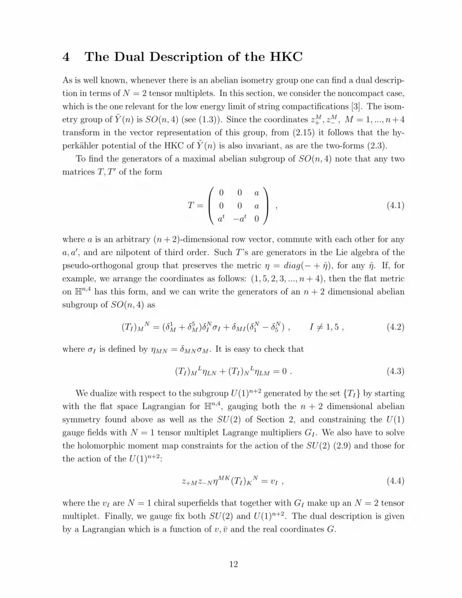
4 The Dual Description of the HKC
As is well known, whenever there is an abelian isometry group one can find a dual descrip-
tion in terms of N = 2 tensor multiplets. In this section, we consider the noncompact case,
which is the one relevant for the low energy limit of string compactifications [3]. The isom-
etry group of Y (n) is SO(n, 4) (see (1.3)). Since the coordinates zM+ , zM
− , M = 1, ..., n+4
transform in the vector representation of this group, from (2.15) it follows that the hy-
perkahler potential of the HKC of Y (n) is also invariant, as are the two-forms (2.3).
To find the generators of a maximal abelian subgroup of SO(n, 4) note that any two
matrices T, T ′ of the form
T =
0 0 a
0 0 a
at −at 0
, (4.1)
where a is an arbitrary (n + 2)-dimensional row vector, commute with each other for any
a, a′, and are nilpotent of third order. Such T ’s are generators in the Lie algebra of the
pseudo-orthogonal group that preserves the metric η = diag(− + η), for any η. If, for
example, we arrange the coordinates as follows: (1, 5, 2, 3, ..., n + 4), then the flat metric
on Hn,4 has this form, and we can write the generators of an n + 2 dimensional abelian
subgroup of SO(n, 4) as
(TI)MN = (δ1
M + δ5M )δN
I σI + δMI(δN1 − δN
5 ) , I 6= 1, 5 , (4.2)
where σI is defined by ηMN = δMNσM . It is easy to check that
(TI)MLηLN + (TI)N
LηLM = 0 . (4.3)
We dualize with respect to the subgroup U(1)n+2 generated by the set TI by starting
with the flat space Lagrangian for Hn,4, gauging both the n + 2 dimensional abelian
symmetry found above as well as the SU(2) of Section 2, and constraining the U(1)
gauge fields with N = 1 tensor multiplet Lagrange multipliers GI . We also have to solve
the holomorphic moment map constraints for the action of the SU(2) (2.9) and those for
the action of the U(1)n+2:
z+Mz−NηMK(TI)KN = vI , (4.4)
where the vI are N = 1 chiral superfields that together with GI make up an N = 2 tensor
multiplet. Finally, we gauge fix both SU(2) and U(1)n+2. The dual description is given
by a Lagrangian which is a function of v, v and the real coordinates G.
12

Let us see that all of the above requirements can be fulfilled consistently. Using (4.2),
(4.4) becomes
(z+5 − z+1)z−IσI + (z−1 − z−5)z+IσI = vI . (4.5)
The SU(2) action on each pair (zM+ , zM
− ) (2.5) is fixed completely by setting
z+1 = z−5 ≡ φ , z−1 = z+5 = 0 . (4.6)
The U(1)n+2 transformation rules on Hn,4, δz±M = λI(TI)M
Nz±N , or explicitly
δz±1 = λIz±IσI , δz±5 = λIz±IσI , δz±I = λI(z±1 − z±5) , (4.7)
acquire, on the HKC of Y , compensating SU(2) transformations in order to preserve the
gauge (4.6), similar to (2.20). They become
δz+1 = δz−5 = δφ =1
2σIλI(z+I + z−I) ,
δz+I = λIφ − 1
2σJ
z+IλJ(z+J − z−J)
φ− σJ
z−IλJz+J
φ, (4.8)
δz−I = −λIφ − 1
2σJ
z−IλJ(z+J − z−J )
φ− σJ
z+IλJz−J
φ.
The holomorphic SU(2) moment map constraints (2.9) reduce to
φ2 = z+Iz+JηIJ , φ2 = −z−Iz−JηIJ , 0 = z+Iz−JηIJ . (4.9)
We choose a U(1)n+2 gauge
z+I = 1 for all I 6= 1, 5 . (4.10)
Then (4.9) become
φ2 = n − 4 , φ2 = −z2−IσI , z−IσI = 0 , (4.11)
which we can solve for φ and two of the z−I ’s. The U(1)n+2 holomorphic moment map
(4.5) after substituting (4.6), (4.10) and the solution for φ is
−√
n − 4 (z−I + 1) σI = vI . (4.12)
As a consequence of (4.11), there are n independent v’s.
The Lagrangian of the dual theory is
n+4∑
M,N=1
σN
(
ei∑
I TIVI)
MN
(
zM+ zM
−
)
(
eV
)
(
zN+
zN−
)
−∑
M 6=1,5
σMGMVM , (4.13)
13

after we eliminate all gauge fields in (4.13) via their equations of motion and impose the
conditions (4.6), (4.10) as well as the solutions to (4.11), (4.12). Thus the dual description
is in terms of n N = 1 chiral superfields v and n + 2 N = 1 tensor multiplets G.
Unfortunately we haven’t been able to solve for all gauge fields (V and VI) explicitly;
and thus we have not been able to construct the dual Lagrangian. However the analysis
that we made above shows that there is a consistent solution of all requirements (con-
straints and allowed gauge choices) for the existence of a dual description. In N = 2
language, n of the G’s combine with the n v’s into n N = 2 tensor multiplets and the
remaining two G’s combine into a double-tensor multiplet. This is consistent with the ex-
pectations from type IIB compactifications [4]. There the double-tensor multiplet appears
naturally: it contains the dilaton, axion and the RR and NS two-forms.
Though we cannot solve for all gauge fields simultaneously, we can easily solve for
either the SU(2) prepotential V or all VI ’s that gauge the U(1)n+2. Eliminating the
first gives the same answer for the dual Lagrangian as (2.15), but with U(1)n+2 gauged
as above. On the other hand, integrating out the U(1)n+2 gauge fields gives us a dual
description, although the result is still a function of the SU(2) gauge fields, which for
convenience we now write as U = eV . Using the nilpotency properties of the generators
(and arranging the indices as 1, 5, 2, . . . , n + 4),
ei∑
I 6=1,5 TIVI = 1(n+4)×(n+4) + i
0 0 σ2V2 σ3V3 ..
0 0 σ2V2 σ3V3 ..
V2 −V2 0 0 ..
V3 −V3 0 0 ..
: : : : :
+
− 1
2
∑
I 6=1,5 σIV2I −
∑
I 6=1,5 σIV2I 0 0 ..
∑
I 6=1,5 σIV2I −
∑
I 6=1,5 σIV2I 0 0 ..
0 0 0 0 ..
0 0 0 0 ..
: : : : :
, (4.14)
we can rewrite (4.13) as
ZαMαβσβZβ − σIGIVI , α, β = 1, ..., 2(n + 4) . (4.15)
We have denoted Z = (z1+, z1
−, z5+, z5
−, z2+, z2
−, ... , zn+4+ , zn+4
− ) and
M =
(1 − 12
∑
I σIV2I )U (1
2
∑
I σIV2I )U iσ2V2U iσ3V3U ..
(−12
∑
I σIV2I )U (1 + 1
2
∑
I σIV2I )U iσ2V2U iσ3V3U ..
iV2U −iV2U U 0 ..
iV3U −iV3U 0 U ..
: : : : :
, (4.16)
14

where M is a (n + 4) × (n + 4) matrix of 2 × 2 matrices. The solution for the U(1)n+2
gauge fields is
VI =
GI − i(
z1+ + z5
+ , z1− + z5
−
)
U
(
zI+
zI−
)
+ i(
zI+ , zI
−
)
U
(
z1+ + z5
+
z1− + z5
−
)
(z1+ − z5
+ , z1− − z5
−)U
(
z1+ − z5
+
z1− − z5
−
) . (4.17)
Finally we note that if we dualize only n + 1 instead of all n + 2 generators of U(1)n+2,
we find n + 1 N = 1 tensor multiplets and n + 1 N = 1 chiral superfields, or equivalently,
n + 1 N = 2 tensor multiplets.
5 Half-hypermutliplets and N = 2 Superspace
We close with a few comments on other representations of the HKC. The half-hypermultiplet
formulation that we have used so far is not easily described in N = 2 superspace; however,
a half-hypermultiplet has an alternative formulation as the double cover of an A1 singu-
larity, that is, a U(1) hyperkahler quotient of a full hypermultiplet doublet with vanishing
Fayet-Iliopoulos terms.
Explicitly, consider a hypermultiplet doublet z(1)± , z
(2)± , with z+ and z− in conjugate
representations of a U(1) gauge group with an N = 1 gauge prepotential V0 as well as the
SU(2) gauge group of the previous sections with an N = 1 gauge prepotential V :
χ = eV0
(
z(1)+ z
(2)+
)(
eV
)
(
z(1)+
z(2)+
)
+ e−V0
(
z(1)− z
(2)−
)(
e−V
)
(
z(1)−
z(2)−
)
. (5.1)
This must be supplemented by the holomorphic moment map constraints; in particular,
the holomorphic U(1) moment map is [11]
z(1)+ z
(1)− + z
(2)+ z
(2)− = 0 . (5.2)
We shall see that integrating out V0, imposing (5.2), and choosing a convenient gauge for
the U(1) symmetry gives us back the half-hypermultiplet formulation.
Integrating out the U(1) gauge field V0 gives [11]
2
√
√
√
√
(
z(1)+ z
(2)+
)(
eV
)
(
z(1)+
z(2)+
)
(
z(1)− z
(2)−
)(
e−V
)
(
z(1)−
z(2)−
)
(5.3)
We can choose a U(1) gauge
z(2)+ = z
(1)− ≡ z− . (5.4)
15

Then the holomorphic U(1) moment map (5.2) implies
z(2)− = −z
(1)+ ≡ −z+ . (5.5)
Using (5.4) and (5.5) we express everything in (5.3) in terms of z±:
2
√
√
√
√(z+ z−)(
eV
)
(
z+
z−
)
(z− − z+)(
e−V
)
(
z−
−z+
)
. (5.6)
The second factor in the square root can be rewritten as
(z− − z+)(
e−V
)
(
z−
−z+
)
= (z− − z+)(
e−V T
)
(
z−
−z+
)
= (z+ z−) σ2
(
e−V T
)
σ2
(
z+
z−
)
= (z+ z−) e
(
−σ2VT σ2
)
(
z+
z−
)
. (5.7)
Since V is an SU(2) gauge prepotential, we write it as V = V iσi , i = 1, 2, 3, where σi are
the Pauli matrices, and
σ2σTi σ2 = −σi . (5.8)
Hence (5.7) is equal to the first factor under the square root in (5.6) and we confirm that
(5.1) is the same as (2.10) (up to an insignificant factor of 2).
To complete the proof of the equivalence of (5.1) and (2.10), we must also compare
the SU(2) holomorphic moment maps. For (5.1) the SU(2) moment map is [18]
(
z(1)− z
(2)−
)
Ti
(
z(1)+
z(2)+
)
= 0 , (5.9)
where Ti are the same generators as (2.12). Using (5.4) and (5.5) to express z(1,2)± in terms
of z±, we get the same constraints as (2.9).
Having this description in hand, we can now give the N = 2 projective superspace
formulation; we use the polar multiplet formulation (for a pedagogical summary as well
as a definition of our notation, see the appendix B of [11]; earlier references are contained
therein and include [13]). The HKC for Y (n−4) has the projective superspace Lagrangian
LN=2 =
∮
dξ
2πi
n∑
i=1
eViΥieV · Υi , (5.10)
16

where each Υi is a doublet of polar multiplets, each eVi is a tropical multiplet describing
a U(1) gauge prepotential (analogous to the N = 1 gauge prepotential), and eV is a her-
mitian unimodular tropical multiplet describing the SU(2) gauge prepotential. Formally,
we may integrate out the latter and obtain:
LN=2 =
∮
dξ
2πi2
(
det
[
n∑
i=1
Υi ⊗ eViΥi
])1
2
. (5.11)
The full hypermultiplet description can also be written as a quiver; indeed, the quiver
for the HKC of Y (1) was explored in quite some detail in the last section of [14]. The
general quiver is a higher dimensional extension of (a cover of) the orbifold limit of the
D4 ALE space, and is shown in Figure 2: The observation that the HKC of Y (1) is flat
Figure 2: The quiver describing the HKC of Y (n−4). Each node with a label k represents a factor U(k)
in the quotient group and each link is a hypermultiplet transforming in the bifundamental of the groups
at the nodes it connects. An overall U(1) acts trivially, and in our particular example, can conveniently
be factored out by reducing the U(2) at the central node to SU(2).
implies that the specific quiver discussed in [14], when the orbifold singularity is blown
up (rather than removed by going to the cover) gives rise to a genuine 8-dimensional
ALE manifold that has not been studied before. However, the higher dimensional analogs
cannot be ALE, as the limit without any blowing up is not flat.
AcknowledgementsSV thanks B. de Wit and M. Trigiante for stimulating discussions. MR thanks the NSF
for partial support under grant NSF PHY-0098527.
17

References
[1] J. Bagger, E. Witten, Matter couplings in N = 2 supergravity, Nucl. Phys. B222
(1983) 1.
[2] A. Wolf, J. Math. Mech. 14 (1965) 1033;
D. Alekseevskii, Funct. Anal. Appl. 2 (1968) 11, Math. USSR-Izv. 9 (1975) 297.
[3] S. Cecotti, S. Ferrara, L. Girardello, Geometry of type II superstrings and the moduli
of superconformal field theories, Int. J. Mod. Phys. A4 (1989) 2475;
S. Ferrara and S. Sabharwal, Quaternionic manifolds for type II superstring vacua of
Calabi-Yau spaces, Nucl. Phys. B332 (1990) 317.
[4] R. Bohm, H. Gunther, C. Herrmann, J. Louis, Compactification of type IIB string
theory on Calabi-Yau threefolds, Nucl. Phys. B569 (2000) 229; hep-th/9908007.
[5] B. de Wit, P. G. Lauwers, R. Philippe, S. Q. Su and A. Van Proeyen, Gauge and
matter fields coupled to N=2 supergravity, Phys. Lett. B134 (1984) 37;
B. de Wit and A. Van Proeyen, Potentials and symmetries of general gauged N=2
supergravity - Yang-Mills models, Nucl. Phys. B245 (1984) 89.
[6] M. Gunaydin, G. Sierra and P. K. Townsend, The geometry of N=2 Maxwell-Einstein
supergravity and Jordan algebras, Nucl. Phys. B242 (1984) 244.
[7] A. Swann, Hyperkahler and quaternionic Kahler geometry, Math. Ann. 289 (1991)
421.
[8] G. W. Gibbons, P. Rychenkova, Cones, tri-Sasakian structures and superconformal
invariance, Phys. Lett. B443 (1998) 138, hep-th/9809158.
[9] K. Galicki, Geometry of the scalar couplings in N=2 supergravity models, Class.
Quantum Grav. 9 (1992) 27.
[10] B. de Wit, B. Kleijn and S. Vandoren, Superconformal Hypermultiplets, Nucl. Phys.
B568 (2000) 475, hep-th/9909228.
[11] B. de Wit, M. Rocek, S. Vandoren, Hypermultiplets, hyperkahler cones and
quaternion-Kahler geometry, JHEP 0102 (2001) 039, hep-th/0101161.
[12] K. Galicki, A Generalization Of The Momentum Mapping Construction For Quater-
nionic Kahler Manifolds, Commun. Math. Phys. 108 (1987) 117.
18

[13] U. Lindstrom and M. Rocek, New Hyperkahler Metrics And New Supermultiplets,
Commun. Math. Phys. 115, 21 (1988).
F. Gonzalez-Rey, M. Rocek, S. Wiles, U. Lindstrom and R. von Unge, Feynman rules
in N = 2 projective superspace. I: Massless hypermultiplets, Nucl. Phys. B 516, 426
(1998) [arXiv:hep-th/9710250].
[14] U. Lindstrom, M. Rocek and R. von Unge, Hyperkahler quotients and algebraic
curves, JHEP 0001, (2000) 022, hep-th/9908082.
[15] A. Maciocia, Metrics On The Moduli Spaces Of Instantons Over Euclidean Four
Space. Commun. Math. Phys. 135 (1991) 467;
C. Boyer, B. Mann, Proc. of Symp. in Pure Math. 54 part 2 (1993) 45;
[16] S. Vandoren, Instantons and quaternions, Proc. of the TMR conference “Nonpertur-
bative Quantum Effects”, Paris 2000, eds. D. Bernard et al., hep-th/0009150.
[17] B. de Wit, M. Rocek, S. Vandoren, Gauging isometries on hyperkahler cones and
quaternion-Kahler manifolds, Phys. Lett. B511 (2001) 302, hep-th/0104215.
[18] N. Hitchin, A. Karlhede, U. Lindstrom, M. Rocek, Hyperkahler metrics and super-
symmetry, Commun. Math. Phys. 108 (1987) 535.
[19] U. Lindstrom and M. Rocek, Scalar Tensor Duality And N=1, N=2 Nonlinear Sigma
Models, Nucl. Phys. B 222, 285 (1983).
[20] P. Breitenlohner, M. Sohnius, Matter couplings and non-linear sigma models in N=2
supergravity, Nucl. Phys. B187 (1981), 409.
[21] P. Fre, L. Girardello, I. Pesando and M. Trigiante, Spontaneous N=2 → N=1 lo-
cal supersymmetry breaking with surviving compact gauge groups, Nucl. Phys. B493
(1997) 231, hep-th/9607032.
[22] G. ’t Hooft, Computation of the quantum effects due to a four-dimensional pseu-
doparticle, Phys. Rev. D14 (1976) 3432; ibid. (E) D18 (1978) 2199.
19