SANTOSH KUMAR ARAVA

1 | P a g e

[21ST CENTURY]

BACHELOR OF TECHNOLOGY IN

INFORMATION TECHNOLOGY FROM

JAWAHARLAL NEHRU TECHNOLOGIAL

UNIVERSITY AND DOCTORATE STUDY FROM

DELHI UNIVERSITY

MASTER OF LAW AND PHILOSOPHY STUDY

FROM JAWAHARLAL NEHRU UNIVERSITY

LITERATURE IN LAW OF MASTERS (LLM) INFORMATION TECHNOLOGY

2 | P a g e

ACKNOWLEDGEMENT TO THE GUIDES AND READERS

I would like to share the few moments which motivates me to contribute a context of the content towards the readers in the field of Information Technology about the necessities and benefits of the Science and Technology to the Society and Human Life in the Industries aspect point to view in a personal life. I personally read some great events which we cannot come across in our day to day life deals to me share the events with the public who ever been interested to gain the knowledge of the world economic and environmental conditions. As per the Indian Society organization we were bound to the few conditions where we cannot get proper guide or knowledge to contribute the action towards at the situation. The knowledge is not limited to the family or society what we come across in our daily life, these were the challenging conditions of human where he or she should take proper action in the event what they were facing before them. People were educated in different fields of specialization on their own interest and best to view to adopt the knowledge on their own mental ability. I come across in my Experienced life with various cultures in the work nature to create a profession life, normally it is necessity for any aged person to adjust the circumstance of the Industry. Culture is only the part of human life which differentiate the person to person in many ways of living style it may be in their personality adoptability with the society or may be by religion, usually some prefers society taught some good moments in their life’s to go smooth in future and some prefers religion or caste or community which creates their own identity to build their future growth. I saw both the personalities in my living life to learn which one should create Country Identity in the global world of economic life, these situations will teach us on ways of passing the days in the calendar dates. I did not decided yet which suits me to be good in my future life may be religion I belief because of my survival in the profession with whom-ever may I sit for doing work to the any nation in the world.

Interests and Gaining the knowledge is both the same which benefits to create a valuable product to the self or the society, the knowledge may be anything what we choose in personal living. Education taught us to build the economic life of our personality where ever the survival can be set up by the living men or women in the globe created by William Shakespeare by contributing his brain in the talks of the religious life. We should know the persons of Patriotism of our own and outer country about their fights and demands to create a haven in the earth. The context of the book content can be utilized to anyone in the society from children to the working professions based on the knowledge level of the person. This is simple and circulate knowledge guide to all and also can add some additional content who ever may feel lack of the Information what ever been produced by the book author. I am not brilliant to contribute full content of the course because it is my report to the scholar to join into Academician in Government or Research Institute (RBI-DELHI) where the chances will come. The text content was developed on the Bachelor Degree level who looks to adopt the career in Civil Life, these were my personal readings of my education life in the fields of Computer Science and Information Technology newly designed from the American Constitution to create smooth life to the citizens of the world. It is useful in gaining the time span of Human in education and profession by doing the actions in faster than usual time spend by the Men or Women.

This is one of my reading context and share the gratitude to my Parents/Guardians and Teachers with whom I spent my education time. I would like to thank the guides and readers who post the comments after viewing the textual content in their free time. This can also be useful for the Doctors and Professors who taught the lecture in diploma/degree level in the Institutions.

ALL THE BEST FOR THE VIEWERS

READER EMAIL ID: santosh.arava8@gmail.com

SANTOSH - Educated from JAWAHARLAL NEHRU UNIVERSITY in the field of Doctorate Study and Consultant in Previous Employment in IT company.

3 | P a g e

Contents

Terminology

History

Technology

o Protocols

o Structure

Governance

Modern uses

Services

o Communication

o Data transfer

Access

Internet and philanthropy

References

Air Wave Theory Mathematical Formula

Network Design

Parallel and Distributed Computing

Models

An Example

Complexity Measures

Other Problems

Properties of Distributed Systems

Architectures

Simulation environments for physics and engineering

IT numerical Analysis in Computer operating System

The Internet is a global system of interconnected computer networks that use the standard Internet protocol suite (TCP/IP) to serve billions of users worldwide. It is a network of networks that consists of millions of private, public, academic, business, and government networks, of local to global scope, that are linked by a broad array of electronic, wireless and optical networking technologies. The Internet carries an extensive range of information resources and services, such as the inter-linked hypertext documents of the World Wide Web (WWW) and the infrastructure to support email. Most traditional communications media including telephone, music, film, and television are reshaped or redefined by the Internet, giving birth to new services such as Voice over Internet Protocol (VoIP) and Internet Protocol Television (IPTV). Newspaper, book and other print publishing are adapting to Web site technology, or are reshaped into blogging and web feeds. The Internet has enabled or accelerated new forms of human interactions through instant messaging, Internet forums, and social networking. Online shopping has boomed both for major retail outlets and small artisans and traders. Business-to-business and financial services on the Internet affect supply chains across entire industries.

Terminology

Internet is a short form of the technical term internetwork, the result of interconnecting computer networks with special gateways or routers. The Internet is also often referred to as the Net. The term the Internet, when referring to the entire global system of IP networks, has been treated as a proper noun and written with an initial capital letter. In the media and popular culture a trend has also developed to regard it as a generic term or common noun and thus write it as "the internet", without capitalization. Some guides specify that the word should be capitalized as a noun but not capitalized as an adjective. The terms Internet and World Wide Web are often used in everyday speech without much

4 | P a g e

distinction. However, the Internet and the World Wide Web are not one and the same. The Internet establishes a global data communications system between computers. In contrast, the Web is one of the services communicated via the Internet. It is a collection of interconnected documents and other resources, linked by hyperlinks and URLs.

History Research into packet switching started in the early 1960s and packet switched networks such as ARPANET, Mark I at NPL in the UK, CYCLADES, Merit Network, Tymnet, and Telenet, were developed in the late 1960s and early 1970s using a variety of protocols. The ARPANET in particular led to the development of protocols for Inter-networking where multiple separate networks could be joined together into a network of networks. T3 NSFNET Backbone, c. 1992 TCP/IP network access expanded again in 1986 when NSFNET provided access to super computers sites in the United States from research and education organizations, first at 56 kbits per sec and later at 1.5 M-bits per sec and 45 M-bits per sec. Commercial Internet service providers (ISPs) began to emerge in the late 1980s and 1990s. The ARPANET was decommissioned in 1990. The Internet was commercialized in 1995 when NSFNET was decommissioned, removing the last restrictions on the use of the Internet to carry commercial traffic. The Internet started a rapid expansion to Europe and Australia in the mid to late 1980s and to Asia in the late 1980s and early 1990s. This NeXT Computer was used by Sir Tim Berners-Lee at CERN and became the world's first Web server. Since the mid-1990s the Internet has had a tremendous impact on culture and commerce, including the rise of near instant communication by email, instant messaging, Voice over Internet Protocol (VoIP) "phone calls", two-way interactive video calls, and the World Wide Web with its discussion forums, blogs, social networking, and online shopping sites. Increasing amounts of data are transmitted at higher and higher speeds over fiber optic networks operating at 1-Gbit/s, 10-Gbit/s, or more. The Internet continues to grow, driven by ever greater amounts of online information and knowledge, commerce, entertainment and social networking. During the late 1990s, it was estimated that traffic on the public Internet grew by 100 percent per year, while the mean annual growth in the number of Internet users was thought to be between 20% and 50%.This growth is often attributed to the lack of central administration, which allows organic growth of the network, as well as the non-proprietary open nature of the Internet protocols, which encourages vendor interoperability and prevents any one company from exerting too much control over the network. As of 31 March 2011, the estimated total number of Internet users was 2.095 billion (30.2% of world population). It is estimated that in 1993 the Internet carried only 1% of the information flowing through two-way telecommunication, by 2000 this figure had grown to 51%, and by 2007 more than 97% of all telecommunicated information was carried over the Internet.

Technology

Protocols: The Internet standards describe a framework known as the Internet protocol suite. This is a model architecture that divides methods into a layered system of protocols (RFC 1122, RFC 1123). The layers correspond to the environment or scope in which their services operate. At the top is the application layer, the space for the application-specific networking methods used in software applications, e.g., a web browser program. Below this top layer, the transport layer connects applications on different hosts via the network (e.g., client–server model) with appropriate data exchange methods. Underlying these layers are the core networking technologies, consisting of two layers. The internet layer enables computers to identify and locate each other via Internet Protocol (IP) addresses, and allows them to connect to one-another via intermediate (transit) networks. Last, at the bottom of the architecture, is a software layer, the link layer, that provides connectivity between hosts on the same local network link, such as a local area network (LAN) or a dial-up connection. The model, also known as TCP/IP, is designed to be independent of the underlying hardware, which the model therefore does not concern itself with in any detail. Other models have been developed, such as the Open

5 | P a g e

Systems Interconnection (OSI) model, but they are not compatible in the details of description or implementation; many similarities exist and the TCP/IP protocols are usually included in the discussion of OSI networking. The most prominent component of the Internet model is the Internet Protocol (IP), which provides addressing systems (IP addresses) for computers on the Internet. IP enables internetworking and in essence establishes the Internet itself. IP Version 4 (IPv4) is the initial version used on the first generation of today's Internet and is still in dominant use. It was designed to address up to ~4.3 billion (109) Internet hosts. However, the explosive growth of the Internet has led to IPv4 address exhaustion, which entered its final stage in 2011, when the global address allocation pool was exhausted. A new protocol version, IPv6, was developed in the mid-1990s, which provides vastly larger addressing capabilities and more efficient routing of Internet traffic. IPv6 is currently in growing deployment around the world, since Internet address registries (RIRs) began to urge all resource managers to plan rapid adoption and conversion. IPv6 is not interoperable with IPv4. In essence, it establishes a parallel version of the Internet not directly accessible with IPv4 software. This means software upgrades or translator facilities are necessary for networking devices that need to communicate on both networks. Most modern computer operating systems already support both versions of the Internet Protocol. Network infrastructures, however, are still lagging in this development. Aside from the complex array of physical connections that make up its infrastructure, the Internet is facilitated by bi- or multi-lateral commercial contracts (e.g., peering agreements), and by technical specifications or protocols that describe how to exchange data over the network. Indeed, the Internet is defined by its interconnections and routing policies.

Structure: The Internet structure and its usage characteristics have been studied extensively. It has been determined that both the Internet IP routing structure and hypertext links of the World Wide Web are examples of scale-free networks. Similar to the way the commercial Internet providers connect via Internet exchange points, Many computer scientists describe the Internet as a "prime example of a large-scale, highly engineered, yet highly complex system". The Internet is heterogeneous; for instance, data transfer rates and physical characteristics of connections vary widely. The Internet exhibits "emergent phenomena" that depend on its large-scale organization. For example, data transfer rates exhibit temporal self-similarity. The principles of the routing and addressing methods for traffic in the Internet reach back to their origins the 1960s when the eventual scale and popularity of the network could not be anticipated. Thus, the possibility of developing alternative structures is investigated. The Internet structure was found to be highly robust to random failures and very vulnerable to high degree attacks.

Governance

The Internet is a globally distributed network comprising many voluntarily interconnected autonomous networks. It operates without a central governing body. However, to maintain interoperability, all technical and policy aspects of the underlying core infrastructure and the principal name spaces ICANN is the authority that coordinates the assignment of unique identifiers for use on the Internet, including domain names, Internet Protocol (IP) addresses, application port numbers in the transport protocols, and many other parameters. Globally unified name spaces, in which names and numbers are uniquely assigned, are essential for the global reach of the Internet. ICANN is governed by an international board of directors drawn from across the Internet technical, business, academic, and other non-commercial communities. The government of the United States continues to have the primary role in approving changes to the DNS root zone that lies at the heart of the domain name system.

Modern Uses: The Internet allows greater flexibility in working hours and location, especially with the spread of unmetered high-speed connections. The Internet can be accessed almost anywhere by numerous means, including through mobile Internet devices. Mobile phones, data-cards, handheld game consoles and cellular routers allow users to connect to the Internet wirelessly. Within the

6 | P a g e

limitations imposed by small screens and other limited facilities of such pocket-sized devices, the services of the Internet, including email and the web, may be available. Service providers may restrict the services offered and mobile data charges may be significantly higher than other access methods. The low cost and nearly instantaneous sharing of ideas, knowledge, and skills has made collaborative work dramatically easier, with the help of collaborative software. Not only can a group cheaply communicate and share ideas but the wide reach of the Internet allows such groups more easily to form. An example of this is the free software movement, which has produced, among other things, Linux, Mozilla Firefox, and OpenOffice.org. Internet chat, whether in the form of an IRC chat room or channel, via an instant messaging system, or a social networking website, allows colleagues to stay in touch in a very convenient way when working at their computers during the day. Messages can be exchanged even more quickly and conveniently than via email. These systems may allow files to be exchanged, drawings and images to be shared, or voice and video contact between team members. Content management systems allow collaborating teams to work on shared sets of documents simultaneously without accidentally destroying each other's work. Business and project teams can share calendars as well as documents and other information. Such collaboration occurs in a wide variety of areas including scientific research, software development, conference planning, political activism and creative writing. Social and political collaboration is also becoming more widespread as both Internet access and computer literacy spread. The Internet allows computer users to remotely access other computers and information stores easily, wherever they may be. They may do this with or without computer security, i.e. authentication and encryption technologies, depending on the requirements. This is encouraging new ways of working from home, collaboration and information sharing in many industries. An accountant sitting at home can audit the books of a company based in another country, on a server situated in a third country that is remotely maintained by IT specialists in a fourth. These accounts could have been created by home-working bookkeepers, in other remote locations, based on information emailed to them from offices all over the world. Some of these things were possible before the widespread use of the Internet, but the cost of private leased lines would have made many of them infeasible in practice. An office worker away from their desk, perhaps on the other side of the world on a business trip or a holiday, can access their emails, access their data using cloud computing, or open a remote desktop session into their office PC using a secure Virtual Private Network (VPN) connection on the Internet. This can give the worker complete access to all of their normal files and data, including email and other applications, while away from the office. This concept has been referred to among system administrators as the Virtual Private Nightmare, because it extends the secure perimeter of a corporate network into remote locations and its employees' homes.

Services

World Wide Web browser software, such as Microsoft's Internet Explorer, Mozilla Firefox, Opera, Apple's Safari, and Google Chrome, lets users navigate from one web page to another via hyperlinks embedded in the documents. These documents may also contain any combination of computer data, including graphics, sounds, text, video, multimedia and interactive content that runs while the user is interacting with the page. Client-side software can include animations, games, office applications and scientific demonstrations. Through keyword-driven Internet research using search engines like Yahoo! and Google, users worldwide have easy, instant access to a vast and diverse amount of online information. Compared to printed media, books, encyclopedias and traditional libraries, the World Wide Web has enabled the decentralization of information on a large scale.

Communication: Email is an important communications service available on the Internet. The concept of sending electronic text messages between parties in a way analogous to mailing letters or memos predates the creation of the Internet. Pictures, documents and other files are sent as email attachments. Emails can be cc-ed to multiple email addresses. Internet telephony is another common communications service made possible by the creation of the Internet. VoIP stands for Voice-over-Internet Protocol, referring to the protocol that underlies all Internet communication. The idea began in the early 1990s with walkie-talkie-like voice applications for personal computers. In recent years many VoIP systems have become as easy to use and as convenient as a normal telephone. The benefit is that,

7 | P a g e

as the Internet carries the voice traffic, VoIP can be free or cost much less than a traditional telephone call, especially over long distances and especially for those with always-on Internet connections such as cable or ADSL. VoIP is maturing into a competitive alternative to traditional telephone service. Interoperability between different providers has improved and the ability to call or receive a call from a traditional telephone is available. Simple, inexpensive VoIP network adapters are available that eliminate the need for a personal computer. Voice quality can still vary from call to call, but is often equal to and can even exceed that of traditional calls. Remaining problems for VoIP include emergency telephone number dialing and reliability. Currently, a few VoIP providers provide an emergency service, but it is not universally available. Traditional phones are line-powered and operate during a power failure; VoIP does not do so without a backup power source for the phone equipment and the Internet access devices. VoIP has also become increasingly popular for gaming applications, as a form of communication between players.

Data Transfer: File sharing is an example of transferring large amounts of data across the Internet. A computer file can be emailed to customers, colleagues and friends as an attachment. It can be uploaded to a website or FTP server for easy download by others. It can be put into a "shared location" or onto a file server for instant use by colleagues. The load of bulk downloads to many users can be eased by the use of "mirror" servers or peer-to-peer networks. In any of these cases, access to the file may be controlled by user authentication, the transit of the file over the Internet may be obscured by encryption, and money may change hands for access to the file. The price can be paid by the remote charging of funds from, for example, a credit card whose details are also passed – usually fully encrypted – across the Internet. The origin and authenticity of the file received may be checked by digital signatures or by MD5 or other message digests. These simple features of the Internet, over a worldwide basis, are changing the production, sale, and distribution of anything that can be reduced to a computer file for transmission. This includes all manner of print publications, software products, news, music, film, video, photography, graphics and the other arts. This in turn has caused seismic shifts in each of the existing industries that previously controlled the production and distribution of these products. Streaming media is the real-time delivery of digital media for the immediate consumption or enjoyment by end users. Many radio and television broadcasters provide Internet feeds of their live audio and video productions. They may also allow time-shift viewing or listening such as Preview, Classic Clips and Listen Again features. These providers have been joined by a range of pure Internet "broadcasters" who never had on-air licenses. This means that an Internet-connected device, such as a computer or something more specific, can be used to access on-line media in much the same way as was previously possible only with a television or radio receiver. The range of available types of content is much wider, from specialized technical webcasts to on-demand popular multimedia services. Podcasting is a variation on this theme, where – usually audio – material is downloaded and played back on a computer or shifted to a portable media player to be listened to on the move. These techniques using simple equipment allow anybody, with little censorship or licensing control, to broadcast audio-visual material worldwide. Digital media streaming increases the demand for network bandwidth. For example, standard image quality needs 1 Mbits per sec link speed for SD 480p, HD 720p quality requires 2.5 Mbits per sec, and the top-of-the-line HDX quality needs 4.5 Mbits per sec for 1080p.

Access

The prevalent language for communication on the Internet has been English. This may be a result of the origin of the Internet, as well as the language's role as a lingua franca. Early computer systems were limited to the characters in the American Standard Code for Information Interchange (ASCII), a subset of the Latin alphabet. After English (27%), the most requested languages on the World Wide Web are Chinese (23%), Spanish (8%), Japanese (5%), Portuguese and German (4% each), Arabic, French and Russian (3% each), and Korean (2%).By region, 42% of the world's Internet users are based in Asia, 24% in Europe, 14% in North America, 10% in Latin America and the Caribbean taken together, 6% in Africa, 3% in the Middle East and 1% in Australia/Oceania. The Internet's technologies have developed enough in recent

8 | P a g e

years, especially in the use of Unicode, that good facilities are available for development and communication in the world's widely used languages. However, some glitches such as mojibake (incorrect display of some languages' characters) still remain. Common methods of Internet access in homes include dial-up, landline broadband (over coaxial cable, fiber optic or copper wires), Wi-Fi, satellite and 3G/4G technology cell phones. Public places to use the Internet include libraries and Internet cafes, where computers with Internet connections are available. There are also Internet access points in many public places such as airport halls and coffee shops, in some cases just for brief use while standing. Various terms are used, such as "public Internet kiosk", "public access terminal", and "Web payphone". Many hotels now also have public terminals, though these are usually fee-based. These terminals are widely accessed for various usage like ticket booking, bank deposit, online payment etc. Wi-Fi provides wireless access to computer networks, and therefore can do so to the Internet itself. Hotspots providing such access include Wi-Fi cafes, where would-be users need to bring their own wireless-enabled devices such as a laptop or PDA. These services may be free to all, free to customers only, or fee-based. A hotspot need not be limited to a confined location. A whole campus or park, or even an entire city can be enabled. Grassroots efforts have led to wireless community networks. Commercial Wi-Fi services covering large city areas are in place in London, Vienna, Toronto, San Francisco, Philadelphia, Chicago and Pittsburgh. The Internet can then be accessed from such places as a park bench. Apart from Wi-Fi, there have been experiments with proprietary mobile wireless networks like Ricochet, various high-speed data services over cellular phone networks, and fixed wireless services. High-end mobile phones such as smart-phones in general come with Internet access through the phone network. Web browsers such as Opera are available on these advanced handsets, which can also run a wide variety of other Internet software. More mobile phones have Internet access than PCs, though this is not as widely used. An Internet access provider and protocol matrix differentiates the methods used to get online. In an American study in 2005, the percentage of men using the Internet was very slightly ahead of the percentage of women, although this difference reversed in those under 30. Men logged on more often, spent more time online, and were more likely to be broadband users, whereas women tended to make more use of opportunities to communicate (such as email). Men were more likely to use the Internet to pay bills, participate in auctions, and for recreation such as downloading music and videos. Men and women were equally likely to use the Internet for shopping and banking. More recent studies indicate that in 2008, women significantly outnumbered men on most social networking sites, such as Face-book, Twitter, Skype, Linked In although the ratios varied with age. In addition, women watched more streaming content, whereas men downloaded more. In terms of blogs, men were more likely to blog in the first place; among those who blog, men were more likely to have a professional blog, whereas women were more likely to have a personal blog.

“ As the globally evolving Internet provides ever new access points to virtual discourse forums, it also promotes new civic relations and associations within which communicative power may flow and accumulate. Thus, traditionally ... national-embedded peripheries get entangled into greater, international peripheries, with stronger combined powers... The Internet, as a consequence, changes the topology of the "centre-periphery" model, by stimulating conventional peripheries to interlink into "super-periphery" structures, which enclose and "besiege" several centers at once. ”

Internet and Philanthropy

The development and proliferation of personal computers using the CP/M operating system in the late 1970s, and later DOS-based systems starting in 1981, meant that many sites grew to dozens or even hundreds of computers. The initial driving force for networking was generally to share storage and printers, which were both expensive at the time. There was much enthusiasm for the concept and for several years, from about 1983 onward, computer industry pundits would regularly declare the coming

9 | P a g e

year to be ―the year of the LAN‖. Early LAN cabling had always been based on various grades of coaxial cable. However shielded twisted pair was used in IBM's Token Ring implementation, and in 1984 Star LAN showed the potential of simple unshielded twisted pair by using Cat3—the same simple cable used for telephone systems. This led to the development of 10Base-T (and its successors) and structured cabling which is still the basis of most commercial LANs today. In addition, fiber-optic cabling is increasingly used in commercial applications. As cabling is not always possible, wireless Wi-Fi is now the most common technology in residential premises, as the cabling required is minimal and it is well suited to mobile laptops and smart phones.

A Local Area Network (LAN) is a computer network that interconnects computers in a limited area such as a home, school, computer laboratory, or office building. The defining characteristics of LANs, in contrast to wide area networks (WANs), include their usually higher data-transfer rates, smaller geographic area, and lack of a need for leased telecommunication lines.

ARCNET, Token Ring and other technology standards have been used in the past, but Ethernet over twisted pair cabling, and Wi-Fi are the two most common technologies currently used to build LANs.

A Campus Network, campus area network, corporate area network or CAN is a computer network made up of an interconnection of local area networks (LANs) within a limited geographical area. The networking equipments (switches, routers) and transmission media (optical fiber, copper plant, Cat5 cabling etc) are almost entirely owned by the campus tenant / owner: an enterprise, university, government etc.

A Metropolitan Area Network (MAN) is a computer network that usually spans a city or a large campus. A MAN usually interconnects a number of local area networks (LANs) using a high-capacity backbone technology, such as fiber-optical links, and provides up-link services to wide area networks (or WAN) and the Internet.

“

A MAN is optimized for a larger geographical area than a LAN, ranging from several blocks of buildings to entire cities. MANs can also depend on communications channels of moderate-to-high data rates. A MAN might be owned and operated by a single organization, but it usually will be used by many individuals and organizations. MANs might also be owned and operated as public utilities. They will often provide means for internetworking of local networks. ”

“ A Metropolitan Area Network (MAN) is a large computer network that spans a metropolitan area or campus. Its geographic scope falls between a WAN and LAN. MANs provide Internet connectivity for LANs in a metropolitan region, and connect them to wider area networks like the Internet. ”

A Wide Area Network (WAN) is a telecommunication network that covers a broad area (i.e., any network that links across metropolitan, regional, or national boundaries). Business and government entities utilize WANs to relay data among employees, clients, buyers, and suppliers from various geographical locations. In essence this mode of telecommunication allows a business to effectively carry out its daily function regardless of location. This is in contrast with personal area networks (PANs), local area networks (LANs), campus area networks (CANs), or metropolitan area networks (MANs) which are usually limited to a room, building, campus or specific metropolitan area (e.g., a city)

10 | P a g e

respectively. The textbook definition of a WAN is a computer network spanning regions, countries, or even the world. However, in terms of the application of computer networking protocols and concepts, it may be best to view WANs as computer networking technologies used to transmit data over long distances, and between different LANs, MANs and other localized computer networking architectures. This distinction stems from the fact that common LAN technologies operating at Layer 1/2 (such as the forms of Ethernet or Wi-Fi) are often geared towards physically localized networks, and thus cannot transmit data over tens, hundreds or even thousands of miles or kilo-meters. WANs necessarily do not just connect physically disparate LANs. A CAN, for example, may have a localized backbone of a WAN technology, which connects different LANs within a campus. This could be to facilitate higher bandwidth applications, or provide better functionality for users in the CAN. WANs are used to connect LANs and other types of networks together, so that users and computers in one location can communicate with users and computers in other locations. Many WANs are built for one particular organization and are private. Others, built by Internet service providers, provide connections from an organization's LAN to the Internet. WANs are often built using leased lines. At each end of the leased line, a router connects the LAN on one side with a second router within the LAN on the other. Leased lines can be very expensive. Instead of using leased lines, WANs can also be built using less costly circuit switching or packet switching methods. Network protocols including TCP/IP deliver transport and addressing functions. Protocols including Packet over SONET/SDH, MPLS, ATM and Frame relay are often used by service providers to deliver the links that are used in WANs. X.25 was an important early WAN protocol, and is often considered to be the "grandfather" of Frame Relay as many of the underlying protocols and functions of X.25 are still in use today (with upgrades) by Frame Relay.

Energy Conservation Sine Wave- Airy wave theory: In fluid dynamics, airy

wave theory (often referred to as linear wave theory) gives a linearised description of the

propagation of gravity waves on the surface of a homogeneous fluid layer. The theory assumes that the

fluid layer has a uniform mean depth, and that the fluid flow is In-viscid, incompressible and Ir-

rotational. This theory was first published, in correct form, by George Biddell Airy in the 19th century.

Airy wave theory is often applied in ocean engineering and coastal engineering for the modelling of

random sea states – giving a description of the wave kinematics and dynamics of high-enough accuracy

for many purposes. Further, several second-order nonlinear properties of surface gravity waves, and

their propagation, can be estimated from its results. This linear theory is often used to get a quick and

rough estimate of wave characteristics and their effects.

Description

Wave characteristics. Dispersion of gravity waves on a fluid surface

Phase and group velocity divided by √(gh) as a function of h/λ. A: phase velocity, B: group velocity, C: phase and group velocity √(gh) valid in shallow water. Drawn lines: based on dispersion relation valid in arbitrary depth. Dashed lines: based on dispersion relation valid in deep water. Airy wave theory uses a potential flow (or velocity potential) approach to describe the motion of gravity waves on a fluid surface. The use of – inviscid and Ir-rotational – potential flow in water waves is remarkably successful, given its failure to describe many other fluid flows where it is often essential to take viscosity, vorticity, turbulence and/or flow separation into account. This is due to the fact that for the oscillatory

11 | P a g e

part of the fluid motion, wave-induced vorticity is restricted to some thin oscillatory Stokes boundary layers at the boundaries of the fluid domain. Airy wave theory is often used in ocean engineering and coastal engineering. Especially for random waves, sometimes called wave turbulence, the evolution of the wave statistics – including the wave spectrum – is predicted well over not too long distances (in terms of wavelengths) and in not too shallow water. Diffraction is one of the wave effects which can be described with Airy wave theory. The free surface elevation η(x,t) of one wave component is sinusoidal, as a function of horizontal position x and time t:

where a is the wave amplitude in metre, cos is the cosine function, k is the angular wave-number in radian per metre, related to the wavelength λ as

ω is the angular frequency in radian per second, related to the period T and frequency f by

The waves propagate along the water surface with the phase speed cp:

The angular wave-number k and frequency ω are not independent parameters (and thus also wavelength λ and period T are not independent), but are coupled. Surface gravity waves on a fluid are dispersive waves – exhibiting frequency dispersion – meaning that each wave-number has its own frequency and phase speed. Note that in engineering the wave height H – the difference in elevation between crest and trough – is often used:

valid in the present case of linear periodic waves.

Orbital motion under linear waves. The yellow dots indicate the momentary position of fluid particles on their (orange) orbits. The black dots are the centers of the orbits. Underneath the surface, there is a fluid motion associated with the free surface motion. While the surface elevation shows a propagating wave, the fluid particles are in an orbital motion. Within the framework of Airy wave theory, the orbits are closed curves: circles in deep water, and ellipses in finite depth—with the ellipses becoming flatter near the bottom of the fluid layer. So while the wave propagates, the fluid particles just orbit (oscillate) around their average position. With the propagating wave motion, the fluid particles transfer energy in the wave propagation direction, without having a mean velocity. The diameter of the orbits reduces with depth below the free surface. In deep water, the orbit's diameter is reduced to 4% of its free-surface value at a depth of half a wavelength. In a similar fashion, there is also a pressure oscillation underneath the free surface, with wave-induced pressure oscillations reducing with depth below the free surface – in the same way as for the orbital motion of fluid parcels.

12 | P a g e

FIG: Magnetic Field is an Earth Gravitational Force with wave-length in Height of the Surface

The description of the Fig applies in the cross environment by using the wireless communication in parameters of the satellite signals emit and receive by the surface on the principle of Magnetic Field with altitude in different surfaces. The receiver signals can be captured by the surface altitude and direction of the airy wave equation. The airy equation is only applies to the free environment but not for water surfaces, this can be derived from Bernoulli’s equation. The equation is on phase based with the co-ordinates

W

Magnetic Field

O

13 | P a g e

of the fluid surface in terms of u(x,y,z). The function applies to earth, water and sky in phase of signals, the phase signal equations were formulated on Mathematical formulation of Wave Motion. ω is the function of wave length derived from the amplitude of the surface of the fluid, the wave length parameter is calculated by velocity of the air in due surface of the sky and water. The equation Kinematic where mass of the medium can be earth and velocity of the air in due surface of the sky and water. This applies to principle of Magnetic Field of Ferad’s Laws of Bernoulli’s equation. The sine and cosine functions are valid in all surfaces with the co-ordinates and medium of the surface earth. The amplitude is calculated by using the tangent function in fluid surface. This is the core functionality of the wireless communication and its operation in medium or co-ordinates of earth, water and sky. The equations of the phase airy and Bernoulli’s were derived below.

Mathematical formulation of the wave motion - Flow problem

formulation

The waves propagate in the horizontal direction, with coordinate x, and a fluid domain bound above by a free surface at z = η(x,t), with z the vertical coordinate (positive in the upward direction) and t being time. The level z = 0 corresponds with the mean surface elevation. The impermeable bed underneath the fluid layer is at z = -h. Further, the flow is assumed to be incompressible and irrotational – a good approximation of the flow in the fluid interior for waves on a liquid surface – and potential theory can be used to describe the flow. The velocity potential Φ(x,z,t) is related to the flow velocity components ux and uz in the horizontal (x) and vertical (z) directions by:

Then, due to the continuity equation for an incompressible flow, the potential Φ has to satisfy the Laplace equation:

Boundary conditions are needed at the bed and the free surface in order to close the system of equations. For their formulation within the framework of linear theory, it is necessary to specify what the base state (or zeroth-order solution) of the flow is. Here, we assume the base state is rest, implying the mean flow velocities are zero.

The bed being impermeable, leads to the kinematic bed boundary-condition:

In case of deep water – by which is meant infinite water depth, from a mathematical point of view – the flow velocities have to go to zero in the limit as the vertical coordinate goes to minus infinity: z → -∞.

At the free surface, for infinitesimal waves, the vertical motion of the flow has to be equal to the vertical velocity of the free surface. This leads to the kinematic free-surface boundary-condition:

14 | P a g e

If the free surface elevation η(x,t) was a known function, this would be enough to solve the flow problem. However, the surface elevation is an extra unknown, for which an additional boundary condition is needed. This is provided by Bernoulli's equation for an unsteady potential flow. The pressure above the free surface is assumed to be constant. This constant pressure is taken equal to zero, without loss of generality, since the level of such a constant pressure does not alter the flow. After linearization, this gives the dynamic free-surface boundary condition:

Because this is a linear theory, in both free-surface boundary conditions – the kinematic and the dynamic one, equations (3) and (4) – the value of Φ and ∂Φ/∂z at the fixed mean level z = 0 is used.

Solution for a progressive monochromatic wave

For a propagating wave of a single frequency – a monochromatic wave – the surface elevation is of the form:

The associated velocity potential, satisfying the Laplace equation (1) in the fluid interior, as well as the kinematic boundary conditions at the free surface (2), and bed (3), is:

with sinh and cosh the hyperbolic sine and hyperbolic cosine function, respectively. But η and Φ also have to satisfy the dynamic boundary condition, which results in non-trivial (non-zero) values for the wave amplitude a only if the linear dispersion relation is satisfied:

with tanh the hyperbolic tangent. So angular frequency ω and wave-number k – or equivalently period T and wavelength λ – cannot be chosen independently, but are related. This means that wave propagation at a fluid surface is an eigen problem. When ω and k satisfy the dispersion relation, the wave amplitude a can be chosen freely (but small enough for Airy wave theory to be a valid approximation).

Network Design Network planning and design is an iterative process, encompassing topological design, network-synthesis, and network-realization, and is aimed at ensuring that a new network or service meets the needs of the subscriber and operator. The process can be tailored according to each new network or service. A traditional network planning methodology involves five layers of planning, namely:

15 | P a g e

Business Planning:

Long-term and medium-term network planning

Short-term network planning

IT asset sourcing

Operations and maintenance

Topological design: This stage involves determining where to place the components and how to connect them. The (topological) optimization methods that can be used in this stage come from an area of mathematics called Graph Theory. These methods involve determining the costs of transmission and the cost of switching, and thereby determining the optimum connection matrix and location of switches and concentrators.

Network-synthesis: This stage involves determining the size of the components used, subject to performance criteria such as the Grade of Service (GoS). The method used is known as "Nonlinear Optimization", and involves determining the topology, required GoS, cost of transmission, etc., and using this information to calculate a routing plan, and the size of the components.

Network realization: This stage involves determining how to meet capacity requirements, and ensure reliability within the network. The method used is known as "Multi-commodity Flow Optimization", and involves determining all information relating to demand, costs and reliability, and then using this information to calculate an actual physical circuit plan.

Parallel and Distributed Computing: Distributed systems are groups of networked computers, which have the same goal for their work. The terms "concurrent computing", "parallel computing", and "distributed computing" have a lot of overlap, and no clear distinction exists between them. The same system may be characterized both as "parallel" and "distributed"; the processors in a typical distributed system run concurrently in parallel. Parallel computing may be seen as a particular tightly-coupled form of distributed computing, and distributed computing may be seen as a loosely-coupled form of parallel computing. Nevertheless, it is possible to roughly classify concurrent systems as "parallel" or "distributed" using the following criteria:

In parallel computing, all processors have access to a shared memory. Shared memory can be used to exchange information between processors.

In distributed computing, each processor has its own

private memory (distributed memory). Information is

exchanged by passing messages between the

processors.

(a)–(b) A distributed System

(c) A parallel system

16 | P a g e

The figure on the right illustrates the difference between distributed and parallel systems. Figure (a) is a schematic view of a typical distributed system; as usual, the system is represented as a network topology in which each node is a computer and each line connecting the nodes is a communication link. Figure (b) shows the same distributed system in more detail: each computer has its own local memory, and information can be exchanged only by passing messages from one node to another by using the available communication links. Figure (c) shows a parallel system in which each processor has a direct access to a shared memory. The situation is further complicated by the traditional uses of the terms parallel and distributed algorithm that do not quite match the above definitions of parallel and distributed systems; see the section Theoretical foundations below for more detailed discussion. Nevertheless, as a rule of thumb, high-performance parallel computation in a shared-memory multiprocessor uses parallel algorithms while the coordination of a large-scale distributed system uses distributed algorithms.

Models: Theoretical computer science seeks to understand which computational problems can be solved by using a computer (computability theory) and how efficiently (computational complexity theory). Traditionally, it is said that a problem can be solved by using a computer if we can design an algorithm that produces a correct solution for any given instance. Such an algorithm can be implemented as a computer program that runs on a general-purpose computer: the program reads a problem instance from input, performs some computation, and produces the solution as output. Formalisms such as random access machines or universal Turing machines can be used as abstract models of a sequential general-purpose computer executing such an algorithm. The field of concurrent and distributed computing studies similar questions in the case of either multiple computers, or a computer that executes a network of interacting processes: which computational problems can be solved in such a network and how efficiently? However, it is not at all obvious what is meant by ―solving a problem‖ in the case of a concurrent or distributed system: for example, what is the task of the algorithm designer, and what is the concurrent or distributed equivalent of a sequential general-purpose computer. The discussion below focuses on the case of multiple computers, although many of the issues are the same for concurrent processes running on a single computer. Parallel algorithms in shared-memory model:

All computers have access to a shared memory. The algorithm designer chooses the program executed by each computer.

One theoretical model is the parallel random access machines (PRAM) that are used. However, the classical PRAM model assumes synchronous access to the shared memory.

A model that is closer to the behavior of real-world multiprocessor machines and takes into account the use of machine instructions, such as Compare-and-swap (CAS), is that of asynchronous shared memory. There is a wide body of work on this model, a summary of which can be found in the literature.

Parallel algorithms in message-passing model

The algorithm designer chooses the structure of the network, as well as the program executed by each computer.

Models such as Boolean circuits and sorting networks are used. A Boolean circuit can be seen as a computer network: each gate is a computer that runs an extremely simple computer program. Similarly, a sorting network can be seen as a computer network: each comparator is a computer.

Distributed algorithms in message-passing model:

17 | P a g e

The algorithm designer only chooses the computer program. All computers run the same program. The system must work correctly regardless of the structure of the network.

A commonly used model is a graph with one finite-state machine per node.

In the case of distributed algorithms, computational problems are typically related to graphs. Often the graph that describes the structure of the computer network is the problem instance. This is illustrated in the following example.

An Example: Consider the computational problem of finding a coloring of a given graph G. Different fields might take the following approaches:

Centralized algorithms

The graph G is encoded as a string, and the string is given as input to a computer. The computer program finds a coloring of the graph, encodes the coloring as a string, and outputs the result.

Parallel algorithms

Again, the graph G is encoded as a string. However, multiple computers can access the same string in parallel. Each computer might focus on one part of the graph and produce a colouring for that part.

The main focus is on high-performance computation that exploits the processing power of multiple computers in parallel.

Distributed algorithms

The graph G is the structure of the computer network. There is one computer for each node of G and one communication link for each edge of G. Initially, each computer only knows about its immediate neighbours in the graph G; the computers must exchange messages with each other to discover more about the structure of G. Each computer must produce its own colour as output.

The main focus is on coordinating the operation of an arbitrary distributed system.

While the field of parallel algorithms has a different focus than the field of distributed algorithms, there is a lot of interaction between the two fields. For example, the Cole–Vishkin algorithm for graph colouring was originally presented as a parallel algorithm, but the same technique can also be used directly as a distributed algorithm. Moreover, a parallel algorithm can be implemented either in a parallel system (using shared memory) or in a distributed system (using message passing). The traditional boundary between parallel and distributed algorithms (choose a suitable network vs. run in any given network) does not lie in the same place as the boundary between parallel and distributed systems (shared memory vs. message passing).

Complexity Measures: In parallel algorithms, yet another resource in addition to time and space is the number of computers. Indeed, often there is a trade-off between the running time and the number of computers: the problem can be solved faster if there are more computers running in parallel (see speedup). If a decision problem can be solved in polylogarithmic time by using a polynomial number of processors, then the problem is said to be in the class NC. The class NC can be defined equally well by using the PRAM formalism or Boolean circuits – PRAM machines can simulate Boolean circuits efficiently and vice versa. In the analysis of distributed algorithms, more attention is usually paid on communication operations than computational steps. Perhaps the simplest model of distributed

18 | P a g e

computing is a synchronous system where all nodes operate in a lockstep fashion. During each communication round, all nodes in parallel (1) receive the latest messages from their neighbours, (2) perform arbitrary local computation, and (3) send new messages to their neighbours. In such systems, a central complexity measure is the number of synchronous communication rounds required to complete the task. This complexity measure is closely related to the diameter of the network. Let D be the diameter of the network. On the one hand, any computable problem can be solved trivially in a synchronous distributed system in approximately 2D communication rounds: simply gather all information in one location (D rounds), solve the problem, and inform each node about the solution (D rounds). On the other hand, if the running time of the algorithm is much smaller than D communication rounds, then the nodes in the network must produce their output without having the possibility to obtain information about distant parts of the network. In other words, the nodes must make globally consistent decisions based on information that is available in their local neighbourhood. Many distributed algorithms are known with the running time much smaller than D rounds, and understanding which problems can be solved by such algorithms is one of the central research questions of the field. Other commonly used measures are the total number of bits transmitted in the network (cf. communication complexity).

Other Problems: Traditional computational problems take the perspective that we ask a question, a computer (or a distributed system) processes the question for a while, and then produces an answer and stops. However, there are also problems where we do not want the system to ever stop. Examples of such problems include the dining philosophers problem and other similar mutual exclusion problems. In these problems, the distributed system is supposed to continuously coordinate the use of shared resources so that no conflicts or deadlocks occur. There are also fundamental challenges that are unique to distributed computing. The first example is challenges that are related to fault-tolerance. Examples of related problems include consensus problems, Byzantine fault tolerance, and self-stabilisation. A lot of research is also focused on understanding the asynchronous nature of distributed systems:

Synchronizers can be used to run synchronous algorithms in asynchronous systems.

Logical clocks provide a causal happened-before ordering of events.

Clock synchronization algorithms provide globally consistent physical time stamps.

Properties of Distributed Systems: So far the focus has been on designing a distributed system that solves a given problem. A complementary research problem is studying the properties of a given distributed system. The halting problem is an analogous example from the field of centralised computation: we are given a computer program and the task is to decide whether it halts or runs forever. The halting problem is undecidable in the general case, and naturally understanding the behaviour of a computer network is at least as hard as understanding the behaviour of one computer. However, there are many interesting special cases that are decidable. In particular, it is possible to reason about the behaviour of a network of finite-state machines. One example is telling whether a given network of interacting (asynchronous and non-deterministic) finite-state machines can reach a deadlock. This problem is PSPACE-complete, i.e., it is decidable, but it is not likely that there is an efficient (centralised, parallel or distributed) algorithm that solves the problem in the case of large networks.

Architectures

Various hardware and software architectures are used for distributed computing. At a lower level, it is necessary to interconnect multiple CPUs with some sort of network, regardless of whether that network is printed onto a circuit board or made up of loosely-coupled devices and cables. At a higher level, it is necessary to interconnect processes running on those CPUs with some sort of communication system.

19 | P a g e

Distributed programming typically falls into one of several basic architectures or categories: client–server, 3-tier architecture, n-tier architecture, distributed objects, loose coupling, or tight coupling.

Client–server: Smart client code contacts the server for data then formats and displays it to the user. Input at the client is committed back to the server when it represents a permanent change.

3-tier architecture: Three tier systems move the client intelligence to a middle tier so that stateless clients can be used. This simplifies application deployment. Most web applications are 3-Tier.

n-tier architecture: n-tier refers typically to web applications which further forward their requests to other enterprise services. This type of application is the one most responsible for the success of application servers.

Tightly coupled (clustered): refers typically to a cluster of machines that closely work together, running a shared process in parallel. The task is subdivided in parts that are made individually by each one and then put back together to make the final result.

Peer-to-peer: an architecture where there is no special machine or machines that provide a service or manage the network resources. Instead all responsibilities are uniformly divided among all machines, known as peers. Peers can serve both as clients and servers.

Space based: refers to an infrastructure that creates the illusion (virtualization) of one single address-space. Data are transparently replicated according to application needs. Decoupling in time, space and reference is achieved.

Another basic aspect of distributed computing architecture is the method of communicating and coordinating work among concurrent processes. Through various message passing protocols, processes may communicate directly with one another, typically in a master/slave relationship. Alternatively, a "database-centric" architecture can enable distributed computing to be done without any form of direct inter-process communication, by utilizing a shared database. This article is about computer model within a scientific context. For artistic usage, see 3d modeling. For simulating a computer on a computer, see emulator. This article includes a list of references, but its aources remain unclear because it has insufficient inline citations. Please help to improve this article by introducing more precise citations.

A computer simulation, a computer model, or a computational model is a computer program, or network of computers, that attempts to simulate an abstract model of a particular system. Computer simulations have become a useful part of mathematical modeling of many natural systems in physics (computational physics), astrophysics, chemistry and biology, human systems in economics, psychology, social science, and engineering. Simulation of a system is represented as the running of the system's model. It can be used to explore and gain new insights into new technology, and to estimate the performance of systems too complex for analytical solutions. Computer simulations vary from computer programs that run a few minutes, to network-based groups of computers running for hours, to ongoing simulations that run for days. The scale of events being simulated by computer simulations has far exceeded anything possible (or perhaps even imaginable) using traditional paper-and-pencil mathematical modeling. Over 10 years ago, a desert-battle simulation, of one force invading another, involved the modeling of 66,239 tanks, trucks and other vehicles on simulated terrain around Kuwait, using multiple supercomputers in the DoD High Performance Computer Modernization Program Other examples include a 1-billion-atom model of material deformation (2002); a 2.64-million-atom model of the complex maker of protein in all organisms, a ribosome, in 2005; and the Blue Brain project at EPFL (Switzerland), begun in May 2005, to create the first computer simulation of the entire human brain, right down to the molecular level. Simulation Versus Modeling: Traditionally, building large models of systems has been via a statistical model, which attempts to find analytical solutions to problems and thereby enable the prediction of the behavior of the system from a set of parameters and initial conditions. The term computer simulation is broader than computer modeling; the latter implies that all aspects are being modeled in the computer representation. However, computer simulation also includes generating inputs from simulated users in order to run actual computer software or equipment, with only part of the system being modeled. An

20 | P a g e

example would be a flight simulator that can run machines as well as actual flight software. Computer simulations are used in many fields, including science, technology, entertainment, health care, and business planning and scheduling. Data Preparation: The external data requirements of simulations and models vary widely. For some, the input might be just a few numbers (for example, simulation of a waveform of AC electricity on a wire), while others might require terabytes of information (such as weather and climate models). Input sources also vary widely:

Sensors and other physical devices connected to the model;

Control surfaces used to direct the progress of the simulation in some way;

Current or Historical data entered by hand;

Values extracted as by-product from other processes;

Values output for the purpose by other simulations, models, or processes.

Lastly, the time at which data is available varies:

"invariant" data is often built into the model code, either because the value is truly invariant (e.g. the value of π) or because the designers consider the value to be invariant for all cases of interest;

data can be entered into the simulation when it starts up, for example by reading one or more files, or by reading data from a preprocessor;

data can be provided during the simulation run, for example by a sensor network; Because of this variety, and that many common elements exist between diverse simulation systems, there are a large number of specialized simulation languages. The best-known of these may be Simula (sometimes Simula-67, after the year 1967 when it was proposed). There are now many others. Systems that accept data from external sources must be very careful in knowing what they are receiving. While it is easy for computers to read in values from text or binary files, what is much harder is knowing what the accuracy (compared to measurement resolution and precision) of the values is. Often it is expressed as "error bars", a minimum and maximum deviation from the value seen within which the true value (is expected to) lie. Because digital computer mathematics is not perfect, rounding and truncation errors will multiply this error up, and it is therefore useful to perform an "error analysis" to check that values output by the simulation are still usefully accurate. Even small errors in the original data can accumulate into substantial error later in the simulation. While all computer analysis is subject to the "GIGO" (garbage in, garbage out) restriction, this is especially true of digital simulation. Indeed, it was the observation of this inherent, cumulative error, for digital systems that is the origin of chaos theory. Another way of categorizing models is to look at the underlying data structures. For time-stepped simulations, there are two main classes: Simulations which store their data in regular grids and require only next-neighbor access are called stencil codes. Many CFD applications belong to this category. If the underlying graph is not a regular grid, the model may belong to the mesh-free method class. Equations define the relationships between elements of the modeled system and attempt to find a state in which the system is in equilibrium. Such models are often used in simulating physical systems, as a simpler modeling case before dynamic simulation is attempted. Dynamic simulations model changes in a system in response to (usually changing) input signals. Stochastic models use random number generators to model chance or random events; A discrete event simulation (DES) manages events in time. Most computer, logic-test and fault-tree simulations are of this type. In this type of simulation, the simulator maintains a queue of events sorted by the simulated time they should occur. The simulator reads the queue and triggers new events as each event is processed. It is not important to execute the simulation in real time. It's often more important to be able to access the data produced by the simulation, to discover logic defects in the design, or the sequence of events. A continuous dynamic simulation performs numerical solution of differential-algebraic equations or differential equations (either partial or ordinary). Periodically, the simulation program solves all the equations, and uses the numbers to change the state and output of the simulation. Applications include flight simulators, construction and management simulation games, chemical process modeling, and simulations of electrical circuits. Originally, these kinds of simulations were actually implemented on analog computers, where the differential equations could be represented directly by various electrical components such as op-amps. By the late 1980s, however, most "analog"

21 | P a g e

simulations were run on conventional digital computers that emulate the behavior of an analog computer. A special type of discrete simulation that does not rely on a model with an underlying equation, but can nonetheless be represented formally, is agent-based simulation. In agent-based simulation, the individual entities (such as molecules, cells, trees or consumers) in the model are represented directly (rather than by their density or concentration) and possess an internal state and set of behaviors or rules that determine how the agent's state is updated from one time-step to the next. Distributed models run on a network of interconnected computers, possibly through the Internet. Simulations dispersed across multiple host computers like this are often referred to as "distributed simulations". There are several standards for distributed simulation, including Aggregate Level Simulation Protocol (ALSP), Distributed Interactive Simulation (DIS), the High Level Architecture (simulation) (HLA) and the Test and Training Enabling Architecture (TENA). CGI Computer Simulation: Formerly, the output data from a computer simulation was sometimes presented in a table, or a matrix, showing how data was affected by numerous changes in the simulation parameters. The use of the matrix format was related to traditional use of the matrix concept in mathematical models; however, psychologists and others noted that humans could quickly perceive trends by looking at graphs or even moving-images or motion-pictures generated from the data, as displayed by computer-generated-imagery (CGI) animation. Although observers couldn't necessarily read out numbers, or spout math formulas, from observing a moving weather chart, they might be able to predict events (and "see that rain was headed their way"), much faster than scanning tables of rain-cloud coordinates. Such intense graphical displays, which transcended the World of numbers and formulae, sometimes also led to output that lacked a coordinate grid or omitted timestamps, as if straying too far from numeric data displays. Today, weather forecasting models tend to balance the view of moving rain/snow clouds against a map that uses numeric coordinates and numeric timestamps of events. Similarly, CGI computer simulations of CAT scans can simulate how a tumor might shrink or change, during an extended period of medical treatment, presenting the passage of time as a spinning view of the visible human head, as the tumor changes. Other applications of CGI computer simulations are being developed to graphically display large amounts of data, in motion, as changes occur during a simulation run in a numerical simulation of differential equations that cannot be solved analytically, theories that involve continuous systems such as phenomena in physical cosmology, fluid dynamics (e.g. climate models, roadway noise models, roadway air dispersion models), continuum mechanics and chemical kinetics fall into this category. a stochastic simulation, typically used for discrete systems where events occur probabilistically, and which cannot be described directly with differential equations (this is a discrete simulation in the above sense). Phenomena in this category include genetic drift, biochemical or gene regulatory networks with small numbers of molecules. (see also: Monte Carlo method). Specific examples of computer simulations follow:

statistical simulations based upon an agglomeration of a large number of input profiles, such as the forecasting of equilibrium temperature of receiving waters, allowing the gamut of meteorological data to be input for a specific locale. This technique was developed for thermal pollution forecasting .

agent based simulation has been used effectively in ecology, where it is often called individual based modeling and has been used in situations for which individual variability in the agents cannot be neglected, such as population dynamics of salmon and trout (most purely mathematical models assume all trout behave identically).

time stepped dynamic model. In hydrology there are several such hydrology transport models such as the SWMM and DSSAM Models developed by the U.S. Environmental Protection Agency for river water quality forecasting.

computer simulations have also been used to formally model theories of human cognition and performance, e.g. ACT-R computer simulation using molecular modeling for drug discovery

computer simulation for studying the selective sensitivity of bonds by mechano chemistry during grinding of organic molecules.

Computational fluid dynamics simulations are used to simulate the behaviour of flowing air, water and other fluids. There are one-, two- and three- dimensional models used. A one dimensional model might simulate the effects of water hammer in a pipe. A two-dimensional model might be used to simulate the

22 | P a g e

drag forces on the cross-section of an aeroplane wing. A three-dimensional simulation might estimate the heating and cooling requirements of a large building.

Simulation Environments for Physics and Engineering

Graphical environments to design simulations have been developed. Special care was taken to handle events (situations in which the simulation equations are not valid and have to be changed). Computer Simulation in Practical Contexts.

analysis of air pollutant dispersion using atmospheric dispersion modeling

design of complex systems such as aircraft and also logistics systems.

design of Noise barriers to effect roadway noise mitigation

flight simulators to train pilots

weather forecasting

Simulation of other computers is emulation.

forecasting of prices on financial markets (for example Adaptive Modeler)

behavior of structures (such as buildings and industrial parts) under stress and other conditions

design of industrial processes, such as chemical processing plants

Strategic Management and Organizational Studies

Reservoir simulation for the petroleum engineering to model the subsurface reservoir

Process Engineering Simulation tools.

Robot simulators for the design of robots and robot control algorithms

Urban Simulation Models that simulate dynamic patterns of urban development and responses to urban land use and transportation policies. See a more detailed article on Urban Environment Simulation.

Modeling car crashes to test safety mechanisms in new vehicle models. Traffic engineering to plan or redesign parts of the street network from single junctions over cities to a national highway network, for transportation system planning, design and operations. See a more detailed article on Simulation in Transportation. The reliability and the trust people put in computer simulations depends on the validity of the simulation model, therefore verification and validation are of crucial importance in the development of computer simulations. Another important aspect of computer simulations is that of reproducibility of the results, meaning that a simulation model should not provide a different answer for each execution. Although this might seem obvious, this is a special point of attention in stochastic simulations, where random numbers should actually be semi-random numbers. An exception to reproducibility are human in the loop simulations such as flight simulations and computer games. Here a human is part of the simulation and thus influences the outcome in a way that is hard, if not impossible, to reproduce exactly. Vehicle manufacturers make use of computer simulation to test safety features in new designs. By building a copy of the car in a physics simulation environment, they can save the hundreds of thousands of dollars that would otherwise be required to build a unique prototype and test it. Engineers can step through the simulation milliseconds at a time to determine the exact stresses being put upon each section of the prototype. Computer graphics can be used to display the results of a computer simulation. Animations can be used to experience a simulation in real-time e.g. in training simulations. In some cases animations may also be useful in faster than real-time or even slower than real-time modes. For example, faster than real-time animations can be useful in visualizing the buildup of queues in the simulation of humans evacuating a building. Furthermore, simulation results are often aggregated into static images using various ways of scientific visualization.

Model Calibration Techniques:

The following three steps should be used to produce accurate simulation models: calibration,

23 | P a g e

verification, and validation. Computer simulations are good at portraying and comparing theoretical scenarios but in order to accurately model actual case studies, it has to match what is actually happening today. A base model should be created and calibrated so that it matches the area being studied. The calibrated model should then be verified to ensure that the model is operating as expected based on the inputs. Once the model has been verified, the final step is to validate the model by comparing the outputs to historical data from the study area. This can be done by using statistical techniques and ensuring an adequate R-squared value. Unless these techniques are employed, the simulation model created will produce inaccurate results and not be a useful prediction tool. Model calibration is achieved by adjusting any available parameters in order to adjust how the model operates and simulates the process. For example in traffic simulation, typical parameters include look-ahead distance, car-following sensitivity, discharge headway, and start-up lost time. These parameters influence driver behaviors such as when and how long it takes a driver to change lanes, how much distance a driver leaves between itself and the car in front of it, and how quickly it starts to accelerate through an intersection. Adjusting these parameters has a direct effect on the amount of traffic volume that can traverse through the modeled roadway network by making the drivers more or less aggressive. These are examples of calibration parameters that can be fine-tuned to match up with characteristics observed in the field at the study location. Most traffic models will have typical default values but they may need to be adjusted to better match the driver behavior at the location being studied. Model verification is achieved by obtaining output data from the model and comparing it to what is expected from the input data. For example in traffic simulation, traffic volume can be verified to ensure that actual volume throughput in the model is reasonably close to traffic volumes input into the model. Ten percent is a typical threshold used in traffic simulation to determine if output volumes are reasonably close to input volumes. Simulation models handle model inputs in different ways so traffic that enters the network, for example, may or may not reach its desired destination. Additionally, traffic that wants to enter the network may not be able to, if any congestion exists. This is why model verification is a very important part of the modeling process. The final step is to validate the model by comparing the results with what’s expected based on historical data from the study area. Ideally, the model should produce similar results to what has happened historically. This is typically verified by nothing more than quoting the R2 statistic from the fit. This statistic measures the fraction of variability that is accounted for by the model. A high R2 value does not necessarily mean the model fits the data well. Another tool used to validate models is graphical residual analysis. If model output values are drastically different than historical values, it probably means there’s an error in the model. This is an important step to verify before using the model as a base to produce additional models for different scenarios to ensure each one is accurate. If the outputs do not reasonably match historic values during the validation process, the model should be reviewed and updated to produce results more in line with expectations. It is an iterative process that helps to produce more realistic models. Validating traffic simulation models requires comparing traffic estimated by the model to observed traffic on the roadway and transit systems. Initial comparisons are for trip interchanges between quadrants, sectors, or other large areas of interest. The next step is to compare traffic estimated by the models to traffic counts, including transit ridership, crossing contrived barriers in the study area. These are typically called screen lines, cut-lines, and cordon lines and may be imaginary or actual physical barriers. Cordon lines surround particular areas such as the central business district or other major activity centers. Transit ridership estimates are commonly validated by comparing them to actual patronage crossing cordon lines around the central business district. Three sources of error can cause weak correlation during calibration: input error, model error, and parameter error. In general, input error and parameter error can be adjusted easily by the user. Model error however is caused by the methodology used in the model and may not be as easy to fix. Simulation models are typically built using several different modeling theories that can produce conflicting results. Some models are more generalized while others are more detailed. If model error occurs as a result of this, in may be necessary to adjust the model methodology to make results more consistent. In order to produce good models that can be used to produce realistic results, these are the necessary steps that need to be taken in order to ensure that simulation models are functioning properly. Simulation models can be used as a tool to verify engineering theories but are only valid, if calibrated properly. Once satisfactory estimates of the parameters for all models have been obtained, the models must be checked to assure that they adequately perform the functions for which they are intended. The validation process establishes the

24 | P a g e

credibility of the model by demonstrating its ability to replicate actual traffic patterns. The importance of model validation underscores the need for careful planning, thoroughness and accuracy of the input data collection program that has this purpose. Efforts should be made to ensure collected data is consistent with expected values. For example in traffic analysis, it is typically common for a traffic engineer to perform a site visit to verify traffic counts and become familiar with traffic patterns in the area. The resulting models and forecasts will be no better than the data used for model estimation and validation.

IT Numerical Analysis in Computer Operating System The Basic System Software was developed on the numerical methods of Computer Programming in BASIC Programming Language from the University of California to create a system interaction with the mother board IC’s to generate an electronic signals with the human Interface. These signals were manipulated when user clicks mouse or key board keys to type on the computer monitor. There were several electronic signals were communicated with the system by giving an IP address of the network and IC numbers to convert the numbers and alphabets to binary number systems 0’s or 1’s. The Screens of the Windows Operating System was developed on the numerical analysis of Newton Ramp son method and Polynomial equations of linear regression Real analysis and Complex analysis. The Polynomials were complex on functions of various texts and figures with the notations on a differential equations of ranges mentioned with the values of series. The structure of the BASIC program were added in the content of the book and their functionality of operation while user starts entering into the system CPU by clicking on power supply button, these codes were entered in Disk operating system with same programming lines as per the files were copied in the context. // REM PROGRAM BINARY NUMBER //

20 MAXN=50 50 DIM B(50),D(50), IB(50),ID(50), Q(50) 100 REM CONTINUE 110 GOSUB 200 : REM CALL GETNUMBER 120 GOSUB 500 : REM CALL CONVERTINTEGER 130 GOSUB 700 : REM CALL CONVERTREAL 140 GOSUB 1000 :REM CALL RESULTS 150 PRINT " WANT TO DO ANOTHER ONE <Y/N> ? "; 160 INPUT ANS$ 170 IF(ANS$ = "Y" OR ANS$ = "y") GOTO 100 180 GOTO 2000 200 REM SUBROUTINE GETNUMBER 230 CLS 260 PRINT " THE REAL NUMBER R IS CONVERTED TO" 270 PRINT 280 PRINT " ITS BINARY FRACTION REPRESENTATION." 290 PRINT 300 PRINT " THE FIRST 24 BINARY DIGITS ARE DETERMINED." 310 PRINT 320 PRINT " TRAILING ZEROS ARE SUPPRESSED, I.E. 0.5 = 0.1 ." 330 PRINT " TWO " 340 PRINT 350 PRINT " ENTER THE REAL NUMBER R = "; 360 INPUT R 370 PRINT 380 X=ABS(R) 390 N=INT(X)

25 | P a g e

400 X=ABS(R)-N 410 CLS 440 RETURN 500 REM SUBROUTINE CONVERTINTEGER 540 FOR K = O TO MAXN 550 B(K)=0 560 Q(K)=0 570 NEXT K 580 Q(0)=INT(N/2) 590 B(0)=N-2*Q(0) 600 J=0 610 FOR K = 1 TO MAXN 620 IF (Q(K-1) = 0) THEN 670 630 Q(K)=INT(Q(K-1)/2) 640 B(K)=Q(K-1)-2*Q(K) 650 J=K 670 NEXT K 680 RETURN 700 REM SUBROUTINE CONVERTREAL 750 FOR K = 1 TO MAXN 760 D(K)=0 770 NEXT K 780 FOR K = 1 TO MAXN 790 Y=2*X 800 D(K)=INT(Y) 810 X=Y-D(K) 820 NEXT K 830 RETURN 1000 REM SUBROUTINE RESULTS 1060 FOR K = J TO 0 STEP -1 1070 IB(K)=INT(B(K)) 1080 NEXT K 1090 K=MAXN-J 1100 M=0 1110 FOR L = K TO 0 STEP -1 1120 IF ((D(L) <> 0) AND (M = 0)) THEN M=L 1150 NEXT L 1160 FOR K = 1 TO M 1170 ID(K)=INT(D(K)) 1180 NEXT K 1200 PRINT " THE REAL NUMBER IS R =",R 1210 PRINT 1220 PRINT " THE BINARY FORM IS R = N.X" 1230 PRINT " TWO" 1240 PRINT 1250 IF (R < 0) THEN PRINT "-"; 1260 FOR K = J TO 0 STEP -1 1280 PRINT IB(K); 1290 NEXT K 1300 PRINT " . "; 1310 FOR K = 1 TO M 1320 PRINT ID(K); 1330 NEXT K 1360 RETURN

26 | P a g e

2000 END // REM EVALUATION OF A TAYLOR SERIES //

100 MAX=501 110 TOL=0.00000001 120 DIM D(501) 130 GOSUB 250: REM SUBROUTINE INPUT X0 AND N 140 GOSUB 550: REM SUBROUTINE GETDERIVATIVES 150 GOSUB 1100: REM SUBROUTINE INPUT X 160 GOSUB 2000: REM SUBROUTINE TAYLOR 170 GOSUB 3000: REM SUBROUTINE RESULTS 180 PRINT 190 PRINT"WANT TO TRY ANOTHER X <Y/N> ? "; 200 INPUT ANS$ 210 IF (ANS$ = "Y") OR (ANS$ = "y") THEN GOTO 150 220 GOTO 5000 250 REM SUBROUTINE INPUT X0 AND N 260 CLS 270 PRINT"COMPUTER EVALUATION OF THE TAYLOR`S SERIES" 280 PRINT 290 PRINT"FOR THE FUNCTION F(X) CENTERED AT X " 300 PRINT" 0 " 310 PRINT 320 PRINT"THE N-THE PARTIAL SUM IS COMPUTED: " 330 PRINT 340 PRINT" 2 K N" 350 PRINT"P(X) = A +A (X-X )+A (X-X ) +...+A (X-X ) +...+A (X-X )" 360 PRINT" 0 1 0 2 0 K 0 N 0 " 370 PRINT 380 PRINT" (K) " 390 PRINT"THE K-COEFFICIENT IS A = F (X )/K! = D(K)/K! " 400 PRINT" K 0 " 410 PRINT 420 PRINT"ENTER THE CENTER X OF THE SERIES" 430 PRINT" 0 " 440 PRINT 450 PRINT"ENTER THE CENTER X0 = "; 460 INPUT X0 470 PRINT 480 PRINT"ENTER THE DEGREE N = "; 490 INPUT N 500 IF (N > MAX) THEN N=MAX 510 PRINT 520 RETURN 550 REM SUBROUTINE GETDERIVATIVES 560 CLS 570 PRINT"CHOOSE ONE OF THE FOLLOWING:" 580 PRINT 590 PRINT"<1> F(X) = EXP(X) EXPANDED ABOUT X0 = 0" 600 PRINT 610 PRINT"<2> F(X) = COS(X) EXPANDED ABOUT X0 = 0" 620 PRINT 630 PRINT"<3> F(X) = SIN(X) EXPANDED ABOUT X0 = 0"

27 | P a g e

640 PRINT 650 PRINT"<4> ENTER THE DERIVATIVES OF " 660 PRINT 670 PRINT" F(X) EXPANDED ABOUT X0 = ",X0 680 PRINT 690 PRINT"SELECT <1-4> ? "; 700 INPUT METH 710 PRINT 720 ON METH GOTO 750,810,900,990 750 REM { EXP(X) } 760 X0=0 770 FOR K = 0 TO N 780 D(K)=1 790 NEXT K 800 GOTO 1090 810 REM { COS(X) } 820 X0=0 830 FOR K = 0 TO INT(N/4) 840 D(4*K)=1 850 D(4*K+1)=0 860 D(4*K+2)=-1 870 D(4*K+3)=0 880 NEXT K 890 GOTO 1090 900 REM { SIN(X) } 910 X0=0 920 FOR K = 0 TO INT(N/4) 930 D(4*K)=0 940 D(4*K+1)=1 950 D(4*K+2)=0 960 D(4*K+3)=-1 970 NEXT K 980 GOTO 1090 990 REM CONTINUE 1000 PRINT"ENTER THE ",N+1," DERIVATIVES OF F(X)" 1010 PRINT"EVALUATED AT THE CENTER VALUE X0 = ",X0 1020 PRINT 1030 PRINT"D(0) , D(1) , D(2) ,..., D(N)" 1040 PRINT 1050 FOR K = 0 TO N 1060 PRINT"D(",K,") = "; 1070 INPUT D(K) 1080 NEXT K 1090 RETURN 1100 REM SUBROUTINE INPUT X 1120 PRINT 1130 PRINT"ENTER THE VALUE OF THE INDEPENDENT VARIABLE" 1140 PRINT 1150 PRINT"X = "; 1160 INPUT X 1170 RETURN 2000 REM SUBROUTINE TAYLOR 2010 DIST=1 2020 K=0

28 | P a g e

2030 SUM=D(0) 2040 Prod=1 2050 IF (X = X0) THEN DIST=0 2100 REM CONTINUE 2110 REM CONTINUE 2120 K=K+1 2130 Prod=Prod*(X-X0)/K 2140 IF (D(K) = 0) AND (K < N) THEN GOTO 2110 2150 Term=D(K)*Prod 2160 IF (Term <> 0) THEN DIST=ABS(Term) 2170 SUM=SUM+Term 2180 IF (DIST => TOL) AND (K < N) THEN GOTO 2100 2190 RETURN 3000 REM SUBROUTINE RESULTS 3010 CLS 3020 PRINT"YOU CHOSE TO APPROXIMATE " 3030 ON METH GOTO 3040,3060,3080,3100 3040 PRINT" EXP(",X," )." 3050 GOTO 3120 3060 PRINT" COS(",X," )." 3070 GOTO 3120 3080 PRINT" SIN(",X," )." 3090 GOTO 3120 3100 PRINT"YOUR OWN TAYLOR SERIES." 3110 PRINT"EXPANDED ABOUT THE VALUE X0 = ",X0 3120 REM CONTINUE 3130 PRINT 3140 IF (DIST <= TOL) AND (K <= N) THEN GOTO 3250 3150 PRINT"THE CURRENT PARTIAL SUM IS:" 3160 PRINT 3170 PRINT" P (",X," ) =",SUM 3180 PRINT" " K 3190 PRINT 3200 PRINT"CONSECUTIVE PARTIAL SUMS DIFFER BY ",DIST 3210 PRINT 3220 PRINT"CONVERGENCE HAS NOT BEEN ACHIEVED." 3230 PRINT 3240 GOTO 3320 3250 PRINT"THE VALUE OF THE TAYLOR POLYNOMIAL IS:" 3260 PRINT 3270 PRINT" P (",X," ) =",SUM 3280 PRINT" " K 3290 PRINT 3300 PRINT"CONSECUTIVE PARTIAL SUMS ARE CLOSER THAN",DIST 3310 PRINT 3320 RETURN 5000 END // REM IMPLEMENTATION OF FIXED POINT ITERATION //

10 DEF FNG(X) = 1 + X - X*X/4 15 GOTO 100 20 PRINT"G(X) = 1 + X - X*X/4" 30 RETURN

29 | P a g e

100 REM CONTINUE 110 TOL=0.000001 120 MAX=500 130 GOSUB 600: REM SUBROUTINE GETPOINT 140 GOSUB 200: REM SUBROUTINE ITERATE 150 GOSUB 800: REM SUBROUTINE RESULTS 160 GOTO 5000 200 REM SUBROUTINE ITERATE 210 BIG=1E10 220 SMALL=1E-20 230 K=0 240 RELERR=1 250 PNEW=FNG(PTERM) 260 WHILE (RELERR => TOL) AND (K <= MAX) AND (ABS(PNEW) < BIG) 265 PRINT PNEW 270 POLD=PTERM 280 PTERM=PNEW 290 PNEW=FNG(PTERM) 300 DG=PNEW-PTERM 310 RELERR=ABS(DG)/(ABS(PNEW)+SMALL) 320 K=K+1 340 WEND 360 IF (DG = 0) THEN 370 ELSE 390 370 SLOPE=0 380 GOTO 430 390 REM ELSE 400 DX=PTERM-POLD 410 IF (DX <> 0) THEN SLOPE=DG/DX 420 IF (DX = 0) THEN SLOPE=6.023E23 430 REM ENDIF 440 IF (0 <= SLOPE) AND (SLOPE < 1) THEN COND=1 450 IF (-1 < SLOPE) AND (SLOPE < 0) THEN COND=2 460 IF (1 <= SLOPE) THEN COND=3 470 IF (SLOPE <=-1) THEN COND=4 480 RETURN 600 REM SUBROUTINE GETPOINT 610 CLS 620 PRINT"FIXED POINT ITERATION IS USED TO FIND" 630 PRINT 640 PRINT"A FIXED POINT OF THE FUNCTION" 650 PRINT 660 GOSUB 20: REM PRINTFUNCTION 670 PRINT 680 PRINT"ENTER THE STARTING VALUE P0 = "; 690 INPUT P0 700 PTERM=P0 710 PRINT 720 RETURN 800 REM SUBROUTINE RESULTS 810 SMALL=1E-20 820 REM CLS 830 PRINT"FIXED POINT ITERATION WAS USED TO FIND A FIXED POINT OF" 840 PRINT 850 GOSUB 20: REM PRINTFUNCTION

30 | P a g e

860 PRINT 870 PRINT"THE STARTING POINT WAS P(0) =",P0 880 PRINT 890 DELTA=ABS(PNEW-PTERM) 900 RELERR=DELTA/(ABS(PNEW)+SMALL) 910 IF (RELERR > TOL) THEN GOTO 980 920 PRINT"AFTER ",K," ITERATIONS THE FIXED POINT WAS FOUND" 930 PRINT 940 PRINT" P =",PNEW 950 PRINT 960 PRINT"ITERATION WAS SUCCESSFUL." 970 GOTO 1040 980 REM CONTINUE 990 PRINT"THE LOCATION OF THE FIXED POINT IS IN DOUBT." 1000 PRINT 1010 PRINT"THE APPROXIMATION AFTER ",K," ITERATIONS IS" 1020 PRINT 1030 PRINT"P(",K,") =",PNEW 1040 REM CONTINUE 1050 PRINT 1060 PRINT" ",PNEW," = G(",PTERM," )" 1070 PRINT 1080 PRINT"CONSECUTIVE ITERATES ARE WITHIN",DELTA 1090 PRINT 1100 IF (K < MAX) THEN GOTO 1130 1110 PRINT"THE MAXIMUM NUMBER OF ITERATIONS WAS EXCEEDED" 1120 PRINT 1130 REM CONTINUE 1140 IF (COND > 1) THEN GOTO 1170 1150 PRINT"THE SEQUENCE EXHIBITS MONOTONE CONVERGENCE." 1160 GOTO 1240 1170 IF (COND > 2) THEN GOTO 1200 1180 PRINT"THE SEQUENCE EXHIBITS OSCILLATING CONVERGENCE." 1190 GOTO 1240 1200 IF (COND > 3) THEN GOTO 1230 1210 PRINT"THE SEQUENCE EXHIBITS MONOTONE DIVERGENCE." 1220 GOTO 1240 1230 PRINT"THE SEQUENCE EXHIBITS OSCILLATING DIVERGENCE." 1240 REM CONTINUE 1250 PRINT 1260 PRINT 1270 PRINT 1280 RETURN 5000 END // REM BISECTION METHOD //

10 DEF FNF(X) = X*SIN(X) - 1 15 GOTO 100 20 PRINT"F(X) = X*SIN(X) - 1" 30 RETURN 100 REM PROGRAM BISECTON 110 DELTA=.0000005 120 GOSUB 300: REM SUBROUTINE GETPOINTS

31 | P a g e

130 A1=A 140 B1=B 150 GOSUB 400: REM SUBROUTINE BISECTION 160 GOSUB 1000:REM SUBROUTINE RESULTS 170 PRINT 180 PRINT"WANT TO TRY ANOTHER INTERVAL? <Y/N> "; 190 INPUT ANS$ 200 IF ANS$ = "Y" OR ANS$ = "y" THEN GOTO 120 210 GOTO 1460 300 REM SUBROUTINE GETPOINTS 310 CLS 320 PRINT"THE BISECTION METHOD WILL BE USED TO FIND A ZERO THE FUNCTION" 330 PRINT 340 GOSUB 20: REM PRINT FUNCTION 350 PRINT 360 PRINT"THAT LIES IN THE INTERVAL [A,B]" 370 PRINT 380 PRINT"ENTER LEFT ENDPOINT A = "; 390 INPUT A 392 PRINT"ENTER RIGHT ENDPOINT B = "; 394 INPUT B 396 PRINT 398 RETURN 400 REM SUBROUTINE BISECTION 410 BIG=1E+10 420 K=0 430 KL=0 440 KR=0 450 YA=FNF(A) 460 YB=FNF(B) 470 D=B-A 480 COND=0 490 MAX=1+INT((LOG(D)-LOG(DELTA))/LOG(2)) 500 IF YA*YB => 0 THEN COND=1: GOTO 770 510 WHILE (COND=0) AND (K < MAX) 520 C=(A+B)/2 530 YC=FNF(C) 540 IF YC = 0 THEN 550 ELSE 590 550 A=C 560 B=C 570 COND=2 580 GOTO 690 590 REM ELSEIF 600 IF YB*YC > 0 THEN 610 ELSE 650 610 B=C 620 YB=YC 630 KR=KR+1 640 GOTO 690 650 REM ELSE 660 A=C 670 YA=YC 680 KL=KL+1 690 REM ENDIF 700 K=K+1

32 | P a g e

710 WEND 720 D=B-A 730 IF D < DELTA THEN 740 ELSE 760 740 IF COND <> 2 THEN COND=3 750 IF ABS(YA) > BIG AND ABS(YB) > BIG THEN COND=4 760 REM ENDIF 770 REM CONTINUE 780 RETURN 1000 REM SUBROUTINE RESULTS 1010 PRINT"THE BISECTION METHOD WAS USED TO FIND A ZERO OF THE FUNCTION" 1020 PRINT 1030 GOSUB 20: REM PRINT FUNCTION 1040 PRINT 1050 PRINT"IN THE INTERVAL [",A," ,",B," ]" 1060 PRINT 1070 K=KL+KR 1080 IF COND = 1 THEN 1090 ELSE 1170 1090 PRINT"THE VALUES F(A) AND F(B)" 1100 PRINT"DO NOT DIFFER IN SIGN." 1110 PRINT 1120 PRINT"F(",A," ) =",FNF(A) 1130 PRINT"F(",B," ) =",FNF(B) 1140 PRINT 1150 PRINT"THE BISECTION METHOD CANNOT BE USED." 1160 GOTO 1430 1170 REM ELSEIF 1180 IF COND = 2 OR COND = 3 THEN 1190 ELSE 1330 1190 PRINT"THE BISECTION METHOD TOOK ",K," ITERATIONS." 1200 PRINT 1210 PRINT"THERE WERE",KR," SQUEEZES FROM THE RIGHT" 1220 PRINT 1230 PRINT" AND",KL," SQUEEZES FROM THE LEFT." 1240 PRINT 1250 PRINT" THE ROOT IS C =",C 1260 PRINT 1270 PRINT"THE ACCURACY IS +-",D 1280 PRINT 1290 PRINT"FUNCTION VALUE F(",C," ) =",FNF(C) 1300 PRINT 1310 IF COND = 2 THEN PRINT"THE FUNCTION VALUE IS EXACTLY ZERO!" 1320 GOTO 1430 1330 REM ELSEIF 1340 IF COND = 0 OR COND = 4 THEN 1350 ELSE 1430 1350 PRINT"THE CURRENT ITERATE IS C(",K,") =",C 1360 PRINT 1370 PRINT"THE CURRENT INTERVAL WIDTH IS ",D 1380 PRINT 1390 PRINT"THE CURRENT FUNCTION VALUE F(",C," ) =",FNF(C) 1400 PRINT 1410 IF COND = 0 THEN PRINT"THE MAXIMUM NUMBER OF ITERATIONS WAS EXCEEDED." 1420 IF COND = 4 THEN PRINT"SURPRISE, A POLE WAS FOUND INSTEAD OF A ZERO!" 1430 REM ENDIF 1440 PRINT 1450 RETURN

33 | P a g e

1460 END // REM FALSE POSITION METHOD //

10 DEF FNF(X) = X*SIN(X) - 1 15 GOTO 100 20 PRINT"F(X) = X*SIN(X) - 1" 30 RETURN 100 REM PROGRAM FALSE POSITION METHOD 110 DELTA=0.000005 112 EPSILON=1E-6 114 MAX=99 120 GOSUB 300: REM SUBROUTINE GETPOINTS 130 A1=A 140 B1=B 150 GOSUB 400: REM SUBROUTINE REGULA FALSI 160 GOSUB 1000:REM SUBROUTINE RESULTS 170 PRINT 180 PRINT"WANT TO TRY ANOTHER INTERVAL? <Y/N> "; 190 INPUT ANS$ 200 IF ANS$ = "Y" OR ANS$ = "y" THEN GOTO 120 210 GOTO 1460 300 REM SUBROUTINE GETPOINTS 310 CLS 320 PRINT"THE FALSE POSITION METHOD WILL BE USED TO FIND A ZERO THE FUNCTION" 330 PRINT 340 GOSUB 20: REM PRINT FUNCTION 350 PRINT 360 PRINT"THAT LIES IN THE INTERVAL [A,B]" 370 PRINT 380 PRINT"ENTER LEFT ENDPOINT A = "; 390 INPUT A 392 PRINT"ENTER RIGHT ENDPOINT B = "; 394 INPUT B 396 PRINT 398 RETURN 400 REM SUBROUTINE REGULA FALSI 410 BIG=1E+10 420 K=0 430 KL=0 440 KR=0 450 YA=FNF(A) 460 YB=FNF(B) 470 D=B-A 480 COND=0 500 IF YA*YB > 0 THEN COND=1: GOTO 800 510 WHILE (COND=0) AND (K < MAX) 520 DX=YB*(B-A)/(YB-YA) 525 C=B-DX 530 YC=FNF(C) 540 IF YC = 0 THEN 550 ELSE 590 550 A=C 560 B=C 570 COND=2

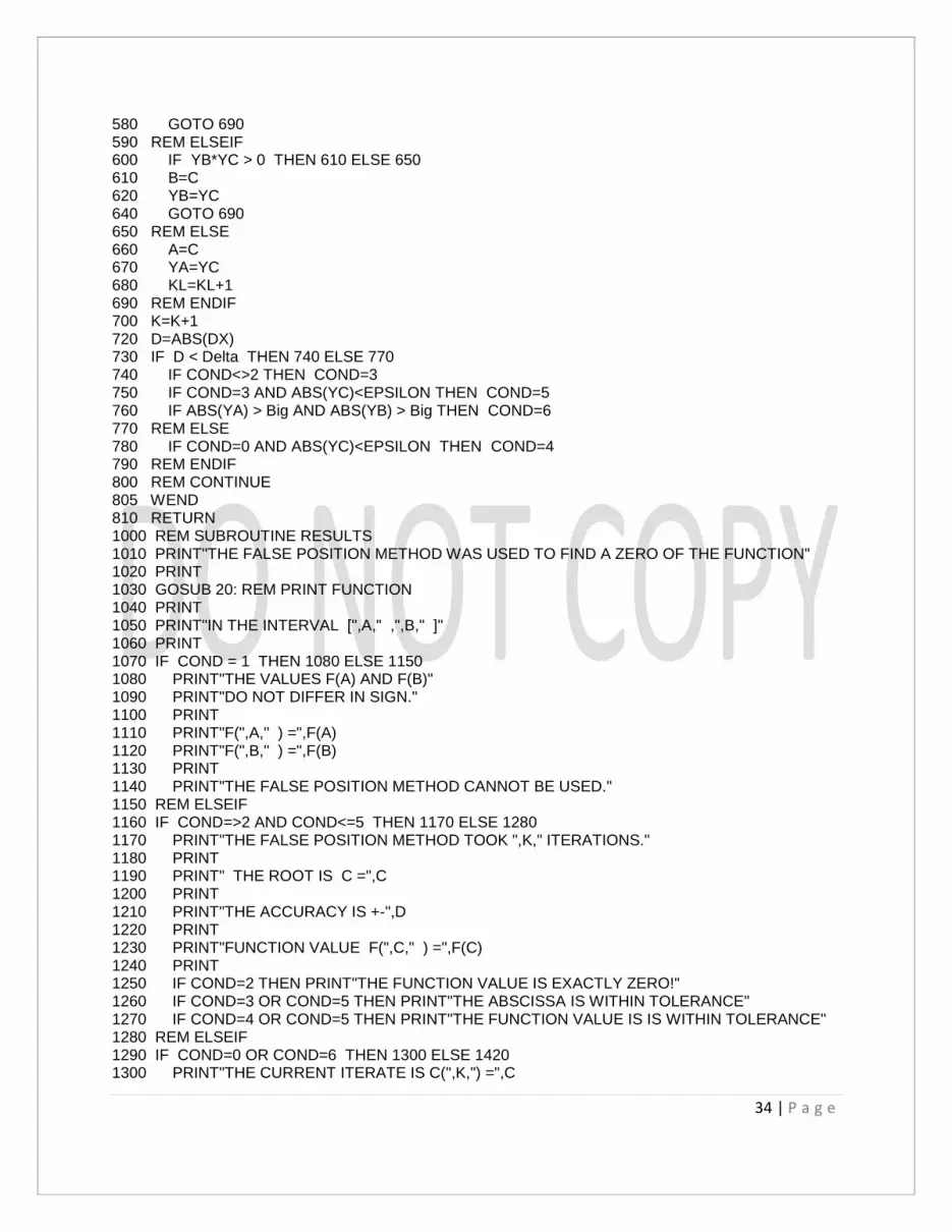
34 | P a g e

580 GOTO 690 590 REM ELSEIF 600 IF YB*YC > 0 THEN 610 ELSE 650 610 B=C 620 YB=YC 640 GOTO 690 650 REM ELSE 660 A=C 670 YA=YC 680 KL=KL+1 690 REM ENDIF 700 K=K+1 720 D=ABS(DX) 730 IF D < Delta THEN 740 ELSE 770 740 IF COND<>2 THEN COND=3 750 IF COND=3 AND ABS(YC)<EPSILON THEN COND=5 760 IF ABS(YA) > Big AND ABS(YB) > Big THEN COND=6 770 REM ELSE 780 IF COND=0 AND ABS(YC)<EPSILON THEN COND=4 790 REM ENDIF 800 REM CONTINUE 805 WEND 810 RETURN 1000 REM SUBROUTINE RESULTS 1010 PRINT"THE FALSE POSITION METHOD WAS USED TO FIND A ZERO OF THE FUNCTION" 1020 PRINT 1030 GOSUB 20: REM PRINT FUNCTION 1040 PRINT 1050 PRINT"IN THE INTERVAL [",A," ,",B," ]" 1060 PRINT 1070 IF COND = 1 THEN 1080 ELSE 1150 1080 PRINT"THE VALUES F(A) AND F(B)" 1090 PRINT"DO NOT DIFFER IN SIGN." 1100 PRINT 1110 PRINT"F(",A," ) =",F(A) 1120 PRINT"F(",B," ) =",F(B) 1130 PRINT 1140 PRINT"THE FALSE POSITION METHOD CANNOT BE USED." 1150 REM ELSEIF 1160 IF COND=>2 AND COND<=5 THEN 1170 ELSE 1280 1170 PRINT"THE FALSE POSITION METHOD TOOK ",K," ITERATIONS." 1180 PRINT 1190 PRINT" THE ROOT IS C =",C 1200 PRINT 1210 PRINT"THE ACCURACY IS +-",D 1220 PRINT 1230 PRINT"FUNCTION VALUE F(",C," ) =",F(C) 1240 PRINT 1250 IF COND=2 THEN PRINT"THE FUNCTION VALUE IS EXACTLY ZERO!" 1260 IF COND=3 OR COND=5 THEN PRINT"THE ABSCISSA IS WITHIN TOLERANCE" 1270 IF COND=4 OR COND=5 THEN PRINT"THE FUNCTION VALUE IS IS WITHIN TOLERANCE" 1280 REM ELSEIF 1290 IF COND=0 OR COND=6 THEN 1300 ELSE 1420 1300 PRINT"THE CURRENT ITERATE IS C(",K,") =",C

35 | P a g e

1310 PRINT 1320 PRINT"CONSECUTIVE ITERATES DIFFER BY",D 1330 PRINT 1340 PRINT"THE CURRENT FUNCTION VALUE F(",C," ) =",F(C) 1350 PRINT 1360 IF COND=0 THEN PRINT"THE MAXIMUM NUMBER OF ITERATIONS WAS EXCEEDED." 1390 IF COND=6 THEN PRINT"SURPRISE, A POLE WAS FOUND INSTEAD OF A ZERO!" 1420 REM ENDIF 1430 PRINT 1440 RETURN 1460 END

// REM APPROXIMATE LOCATION OF ROOTS //

10 DEF FNF(X) = SIN(X) + 1 15 GOTO 100 20 REM SUBROUTINE PRINT FUNCTION 30 PRINT"F(X) = SIN(X)+1" 40 RETURN 100 REM PROGRAM APPROXIMATE LOCATION 110 EPSILON=0.05 120 MN=201 130 MR=50 140 DIM X(201),R(50),Y(201) 150 GOSUB 300: REM SUBROUTINE INPUTS 160 GOSUB 600: REM SUBROUTINE LOCATE 170 GOSUB 1000: REM SUBROUTINE RESULTS 180 PRINT 190 PRINT "WANT TO TRY ANOTHER INTERVAL? <Y/N> "; 200 INPUT ANS$ 210 IF ANS$ = "Y" OR ANS$ = "y" THEN GOTO 150 220 GOTO 5000 300 REM SUBROUTINE INPUTS 310 CLS 320 PRINT"APPROXIMATE LOCATIONS FOR THE ZEROS OF THE FUNCTION" 330 PRINT 340 GOSUB 20 : REM PRINT FUNCTION 350 PRINT 360 PRINT"THE INTERVAL [A,B] IS DIVIDED INTO N SUBINTERVALS" 370 PRINT 380 PRINT"AND A SEARCH IS PERFORMED TO DETERMINE IF F(X)" 390 PRINT 400 PRINT"CHANGES SIGN OR IS CLOSE TO ZERO ON EACH SUBINTERVAL." 410 PRINT 420 PRINT"ENTER LEFT ENDPOINT A = "; 430 INPUT A 440 PRINT 450 PRINT"ENTER RIGHT ENDPOINT B = "; 460 INPUT B 470 PRINT 480 PRINT"NUMBER OF SUBINTERVALS N = "; 490 INPUT N 500 IF N < 1 THEN N = 1 510 IF N > 200 THEN N = 200

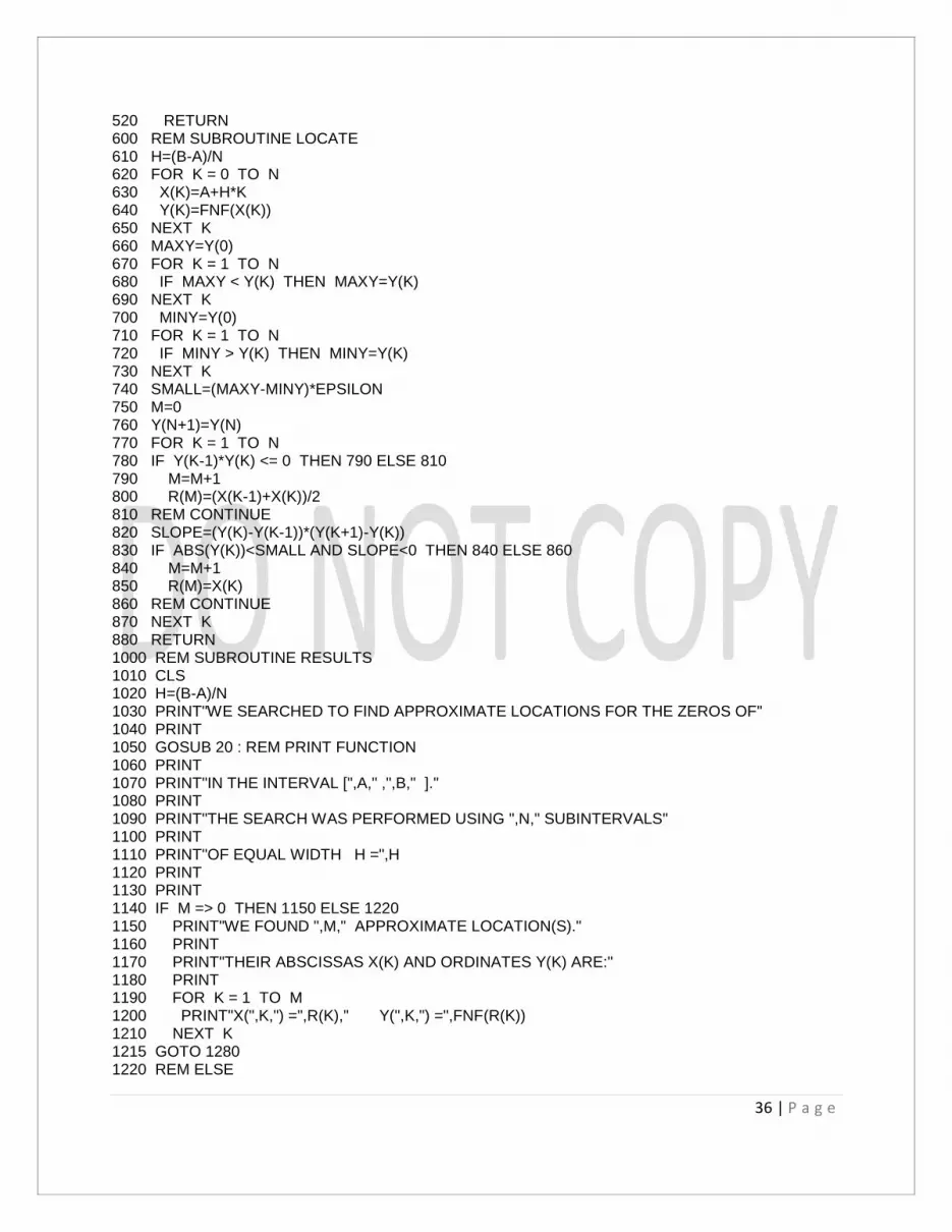
36 | P a g e

520 RETURN 600 REM SUBROUTINE LOCATE 610 H=(B-A)/N 620 FOR K = 0 TO N 630 X(K)=A+H*K 640 Y(K)=FNF(X(K)) 650 NEXT K 660 MAXY=Y(0) 670 FOR K = 1 TO N 680 IF MAXY < Y(K) THEN MAXY=Y(K) 690 NEXT K 700 MINY=Y(0) 710 FOR K = 1 TO N 720 IF MINY > Y(K) THEN MINY=Y(K) 730 NEXT K 740 SMALL=(MAXY-MINY)*EPSILON 750 M=0 760 Y(N+1)=Y(N) 770 FOR K = 1 TO N 780 IF Y(K-1)*Y(K) <= 0 THEN 790 ELSE 810 790 M=M+1 800 R(M)=(X(K-1)+X(K))/2 810 REM CONTINUE 820 SLOPE=(Y(K)-Y(K-1))*(Y(K+1)-Y(K)) 830 IF ABS(Y(K))<SMALL AND SLOPE<0 THEN 840 ELSE 860 840 M=M+1 850 R(M)=X(K) 860 REM CONTINUE 870 NEXT K 880 RETURN 1000 REM SUBROUTINE RESULTS 1010 CLS 1020 H=(B-A)/N 1030 PRINT"WE SEARCHED TO FIND APPROXIMATE LOCATIONS FOR THE ZEROS OF" 1040 PRINT 1050 GOSUB 20 : REM PRINT FUNCTION 1060 PRINT 1070 PRINT"IN THE INTERVAL [",A," ,",B," ]." 1080 PRINT 1090 PRINT"THE SEARCH WAS PERFORMED USING ",N," SUBINTERVALS" 1100 PRINT 1110 PRINT"OF EQUAL WIDTH H =",H 1120 PRINT 1130 PRINT 1140 IF M => 0 THEN 1150 ELSE 1220 1150 PRINT"WE FOUND ",M," APPROXIMATE LOCATION(S)." 1160 PRINT 1170 PRINT"THEIR ABSCISSAS X(K) AND ORDINATES Y(K) ARE:" 1180 PRINT 1190 FOR K = 1 TO M 1200 PRINT"X(",K,") =",R(K)," Y(",K,") =",FNF(R(K)) 1210 NEXT K 1215 GOTO 1280 1220 REM ELSE

37 | P a g e

1230 PRINT"NO APPROXIMATE LOCATIONS FOR ZEROS OF F(X) WERE FOUND." 1240 PRINT 1250 PRINT"YOU COULD TRY ANOTHER SEARCH USING A SMALLER STEP H," 1260 PRINT 1270 PRINT"OR YOU COULD TRY A SEARCH IS DIFFERENT INTERVAL [A,B]." 1280 REM ENDIF 1290 RETURN 5000 END

// REM NEWTON-RAPHSON ITERATION //

10 DEF FNF (X) = X*X*X - 3*X + 2 20 DEF FNF1(X) = 3*X*X - 3 25 GOTO 100 30 REM SUBROUTINE PRINT FUNCTION 40 PRINT"F(X) = X*X*X - 3*X + 2" 50 RETURN 100 REM PROGRAM NEWTON 110 DELTA=5E-6 120 EPSILON=1E-7 130 MAX=100 140 GOSUB 300: REM SUBROUTINE INPUTS 150 P=P0 160 GOSUB 500: REM SUBROUTINE NEWTON RAPHSON 170 GOSUB 800: REM SUBROUTINE RESULTS 180 PRINT 190 PRINT "WANT TO USE A DIFFERENT STARTING VALUE? <Y/N> "; 200 INPUT ANS$ 210 IF ANS$ = "Y" OR ANS$ = "y" GOTO 140 220 GOTO 5000 300 REM SUBROUTINE INPUTS 310 CLS 320 PRINT"THE NEWTON-RAPHSON METHOD IS USED" 330 PRINT 340 PRINT"TO FIND A ZERO OF THE FUNCTION: " 350 PRINT 360 GOSUB 30: REM PRINT FUNCTION 370 PRINT 380 PRINT"ONE INITIAL APPROXIMATION P0 IS NEEDED." 390 PRINT 400 PRINT"ENTER P0 = "; 410 INPUT P0 420 PRINT 430 RETURN 500 REM SUBROUTINE NEWTON RAPHSON 510 SMALL=1E-20 520 K=0 530 COND=0 540 Y0=FNF(P0) 550 P1=P0+1 560 WHILE K < MAX AND COND = 0 570 Df=FNF1(P0) 580 IF Df = 0 THEN 590 ELSE 630 590 COND=1

38 | P a g e

600 DP=P1-P0 610 P1=P0 620 GOTO 660 630 REM ELSE 640 DP=Y0/Df 650 P1=P0-DP 660 REM ENDIF 670 Y1=FNF(P1) 680 RELERR=ABS(DP)/(ABS(P1)+SMALL) 690 IF RELERR < DELTA THEN COND=2 700 IF ABS(Y1) < EPSILON THEN COND=3 710 IF RELERR <= DELTA AND ABS(Y1) < EPSILON THEN COND=4 720 P0=P1 730 Y0=Y1 740 K=K+1 750 WEND 760 RETURN 800 REM SUBROUTINE RESULTS 810 CLS 820 PRINT"THE NEWTON-RAPHSON METHOD WAS USED TO FIND A ZERO OF" 830 PRINT 840 GOSUB 30: REM PRINT FUNCTION 850 PRINT 860 PRINT"STARTING WITH THE APPROXIMATION P0 =",P0 870 PRINT 880 PRINT"AFTER ",K," ITERATIONS AN APPROXIMATION FOR THE ZERO IS:" 890 PRINT 900 PRINT" P =",P1 910 PRINT 920 PRINT" DP =",ABS(DP)," IS THE ESTIMATED ACCURACY FOR P." 930 PRINT 940 PRINT" F(",P1," ) =",Y1 950 PRINT 960 IF Y1=0 THEN PRINT"THE COMPUTED FUNCTION VALUE IS EXACTLY ZERO!" 1000 IF COND = 0 THEN 1010 ELSE 1045 1010 PRINT"CONVERGENCE IS DOUBTFUL BECAUSE" 1020 PRINT 1030 PRINT"THE MAXIMUM NUMBER OF ITERATIONS WAS EXCEEDED." 1040 GOTO 1240 1045 REM ELSEIF 1050 IF COND = 1 THEN 1060 ELSE 1095 1060 PRINT"CONVERGENCE IS DOUBTFUL BECAUSE " 1070 PRINT 1080 PRINT"DIVISION BY ZERO WAS ENCOUNTERED." 1090 GOTO 1240 1095 REM ELSEIF 1100 IF COND = 2 THEN 1110 ELSE 1145 1110 PRINT"THE APPROXIMATION P IS" 1120 PRINT 1130 PRINT"WITHIN THE DESIRED TOLERANCE." 1140 GOTO 1240 1145 REM ELSEIF 1150 IF COND = 3 THEN 1160 ELSE 1195 1160 PRINT"THE COMPUTED FUNCTION VALUE F(P)"

39 | P a g e

1170 PRINT 1180 PRINT"IS WITHIN THE DESIRED TOLERANCE." 1190 GOTO 1240 1195 REM ELSEIF 1200 IF COND = 4 THEN 1210 ELSE 1240 1210 PRINT"THE APPROXIMATION P AND THE FUNCTION VALUE " 1220 PRINT 1230 PRINT"F(P) ARE BOTH WITHIN THE DESIRED TOLERANCES." 1240 REM ENDIF 1250 PRINT 1260 RETURN 5000 END

// REM SECANT METHOD //

10 DEF FNF (X) = X*X*X - 3*X + 2 25 GOTO 100 30 REM SUBROUTINE PRINT FUNCTION 40 PRINT"F(X) = X*X*X - 3*X + 2" 50 RETURN 100 REM PROGRAM SECANT METHOD 110 DELTA=5E-6 120 EPSILON=1E-7 130 MAX=100 140 GOSUB 300: REM SUBROUTINE INPUTS 150 Q0=P0 155 Q1=P1 160 GOSUB 500 : REM SUBROUTINE SECANT METHOD 170 GOSUB 1000: REM SUBROUTINE RESULTS 180 PRINT 190 PRINT "WANT TO USE A DIFFERENT STARTING VALUE? <Y/N> "; 200 INPUT ANS$ 210 IF ANS$ = "Y" OR ANS$ = "y" GOTO 140 220 GOTO 5000 300 REM SUBROUTINE INPUTS 310 CLS 320 PRINT"THE SECANT METHOD IS USED" 330 PRINT 340 PRINT"TO FIND A ZERO OF THE FUNCTION: " 350 PRINT 360 GOSUB 30: REM PRINT FUNCTION 370 PRINT 380 PRINT"TWO INITIAL APPROXIMATION P0, P1 ARE NEEDED." 390 PRINT 400 PRINT"ENTER P0 = "; 410 INPUT P0 420 PRINT 430 PRINT"ENTER P1 = "; 440 INPUT P1 450 PRINT 460 RETURN 500 REM SUBROUTINE SECANT METHOD 510 SMALL=1E-10 520 K=0

40 | P a g e

530 COND=0 540 Y0=FNF(P0) 550 Y1=FNF(P1) 560 WHILE K < MAX AND COND = 0 570 DF=(Y1-Y0)/(P1-P0) 580 IF DF = 0 THEN 590 ELSE 630 590 COND=1 600 DP=P1-P0 610 P2=P1 620 GOTO 660 630 REM ELSE 640 DP=Y1/DF 650 P2=P1-DP 660 REM ENDIF 670 Y2=FNF(P2) 680 RELERR=ABS(DP)/(ABS(P2)+SMALL) 690 IF RELERR < DELTA THEN COND=2 700 IF ABS(Y2) < EPSILON THEN COND=3 710 IF RELERR<DELTA AND ABS(Y2)<EPSILON THEN COND=4 720 P0=P1 730 P1=P2 740 Y0=Y1 750 Y1=Y2 760 K=K+1 770 WEND 780 RETURN 1000 REM SUBROUTINE RESULTS 1010 CLS 1020 Y2=FNF(P2) 1030 PRINT"THE SECANT METHOD WAS USED TO FIND A ZERO OF THE FUNCTION" 1040 PRINT 1050 GOSUB 30: REM PRINT FUNCTION 1060 PRINT 1070 PRINT"STARTING WITH THE TWO APPROXIMATIONS:" 1080 PRINT 1090 PRINT"P0 =",P0," AND P1 =",P1 1100 PRINT 1110 PRINT"AFTER ",K," ITERATIONS AN APPROXIMATE VALUE FOR THE ZERO IS:" 1120 PRINT 1130 PRINT" P =",P2 1140 PRINT 1150 PRINT" DP =",ABS(DP)," IS THE ESTIMATED ACCURACY FOR P." 1160 PRINT 1170 PRINT" F(",P2," ) = ",Y2 1180 PRINT 1190 IF Y2 = 0 THEN PRINT"THE COMPUTED FUNCTION VALUE IS EXACTLY ZERO!" 1200 IF COND = 0 THEN 1210 ELSE 1240 1210 PRINT"CONVERGENCE IS DOUBTFUL BECAUSE" 1220 PRINT 1230 PRINT"THE MAXIMUM NUMBER OF ITERATIONS WAS EXCEEDED." 1240 REM ELSEIF 1250 IF COND = 1 THEN 1260 ELSE 1290 1260 PRINT"CONVERGENCE IS DOUBTFUL BECAUSE " 1270 PRINT

41 | P a g e

1280 PRINT"DIVISION BY ZERO WAS ENCOUNTERED." 1290 REM ELSEIF 1300 IF COND = 2 THEN 1310 ELSE 1340 1310 PRINT"THE APPROXIMATION P IS" 1320 PRINT 1330 PRINT"WITHIN THE DESIRED TOLERANCE." 1340 REM ELSEIF 1350 IF COND = 3 THEN 1360 ELSE 1390 1360 PRINT"THE COMPUTED FUNCTION VALUE F(P)" 1370 PRINT 1380 PRINT"IS WITHIN THE DESIRED TOLERANCE." 1390 REM ELSEIF 1400 IF COND = 4 THEN 1410 ELSE 1440 1410 PRINT"THE APPROXIMATION P AND THE FUNCTION VALUE " 1420 PRINT 1430 PRINT"F(P) ARE BOTH WITHIN THE DESIRED TOLERANCES." 1440 REM ENDIF 1450 RETURN 5000 END // REM THE REAL ROOTS OF A POLYNOMIAL //

90 DIM A(15),B(15),C(15),R(15) 100 REM PROGRAM PROOTS 120 DELTA=5E-6 130 EPSILON=1E-7 140 MAX=199 150 M=0 160 STATUS=0 170 GOSUB 470: REM SUBROUTINE GET POLYNOMIAL 180 REM CONTINUE 190 GOSUB 300: REM SUBROUTINE PRINT POLYNOMIAL 200 GOSUB 590: REM SUBROUTINE INITIAL GUESS 210 GOSUB 600: REM SUBROUTINE POLYNOMIAL NEWTON 220 GOSUB 1200: REM SUBROUTINE RESULTS 230 GOSUB 1000: REM SUBROUTINE DEFLATE POLYNOMIAL 240 IF STATUS = 0 AND N > 1 THEN GOTO 180 250 IF N = 1 THEN 260 ELSE 280 260 GOSUB 600: REM SUBROUTINE POLYNOMIAL NEWTON 270 GOSUB 1200: REM SUBROUTINE RESULTS 280 REM CONTINUE 290 GOTO 5000 300 REM SUBROUTINE PRINT POLYNOMIAL 305 CLS 310 IF N = 1 THEN 315 ELSE 340 315 PRINT 320 PRINT"P(X) = A X + A" 325 PRINT" 1 0" 330 PRINT 335 GOTO 435 340 REM ELSE 345 IF N = 2 THEN 350 ELSE 375 350 PRINT" 2" 355 PRINT"P(X) = A X + A X + A"

42 | P a g e

360 PRINT" 2 1 0" 365 PRINT 370 GOTO 435 375 REM ELSE 380 IF N = 3 THEN 385 ELSE 410 385 PRINT" 3 2" 390 PRINT"P(X) = A X + A X + A X + A " 395 PRINT" 3 2 1 0" 400 PRINT 405 GOTO 435 410 REM ELSE 415 PRINT" ",N," 2" 420 PRINT"P(X) = A X +...+ A X + A X + A " 425 PRINT N," 2 1 0" 430 PRINT 435 REM ENDIF 440 FOR K = N TO 0 STEP -1 445 PRINT"A(",K,") =",A(K) 450 NEXT K 455 RETURN 470 REM SUBROUTINE GET POLYNOMIAL 475 CLS 480 PRINT"NEWTON`S METHOD IS USED TO FIND THE" 485 PRINT"REAL ROOTS OF THE POLYNOMIAL P(X): " 490 PRINT 495 PRINT 500 PRINT" N N-1 2 " 505 PRINT"P(X) = A X + A X +...+ A X + A X + A " 510 PRINT" N N-1 2 1 0" 515 PRINT 520 PRINT"ENTER THE DEGREE N = "; 525 INPUT N 530 PRINT 535 PRINT"NOW ENTER THE ",N+1," COEFFICIENTS" 540 PRINT 545 PRINT" A , ... , A , A , A " 550 PRINT N," 2 1 0" 555 PRINT 560 FOR K = N TO 0 STEP -1 565 PRINT"A(",K,") = "; 570 INPUT A(K) 575 NEXT K 580 GOSUB 300: REM SUBROUTINE PRINT POLYNOMIAL 585 RETURN 590 REM SUBROUTINE INITIAL GUESS 591 PRINT 592 PRINT"ENTER THE INITIAL GUESS P0 = "; 593 INPUT POLD 594 PRINT 595 RETURN 600 REM SUBROUTINE POLYNOMIAL NEWTON 610 SMALL=1E-10 620 IF N = 1 THEN XROOT=-A(0)/A(1): GOTO 970 630 B(N+1)=0

43 | P a g e

640 C(N+1)=0 650 J=0 660 COND=0 670 PNEW=POLD 680 WHILE J < MAX AND COND = 0 690 POLD=PNEW 700 FOR K = N TO 0 STEP -1 710 B(K)=A(K)+POLD*B(K+1) 720 C(K)=B(K)+POLD*C(K+1) 730 NEXT K 740 DF=C(1) 750 IF DF = 0 THEN 760 ELSE 800 760 COND=2 770 DX=0 780 IF B(0) = 0 THEN COND=1 790 GOTO 820 800 REM ELSE 810 DX=B(0)/C(1) 820 REM ENDIF 830 PNEW=POLD-DX 840 B(N+1)=0 850 FOR K = N TO 0 STEP -1 860 B(K)=A(K)+PNEW*B(K+1) 870 NEXT K 880 YNEW=B(0) 890 IF COND = 0 THEN 900 ELSE 920 900 RELERR=2*ABS(DX)/(ABS(POLD)+ABS(PNEW)+SMALL) 910 IF RELERR<DELTA AND ABS(YNEW)<EPSILON THEN COND=1 920 REM CONTINUE 930 XROOT=PNEW 940 YROOT=YNEW 950 J=J+1 960 WEND 970 REM CONTINUE 980 RETURN 1000 REM SUBROUTINE DEFLATE POLYNOMIAL 1010 PRINT 1020 IF N > 1 AND STATUS = 0 THEN 1030 ELSE 1170 1030 PRINT"DEFLATE THE POLYNOMIAL ? <Y/N> "; 1040 INPUT ANS$ 1050 STATUS=1 1060 IF ANS$ = "y" OR ANS$ = "Y" THEN 1070 ELSE 1160 1070 IF COND <> 1 THEN 1080 ELSE 1100 1080 M=M+1 1090 R(M)=XROOT 1100 REM CONTINUE 1110 STATUS=0 1120 FOR K = 0 TO N-1 1130 A(K)=B(K+1) 1140 NEXT K 1150 N=N-1 1160 REM CONTINUE 1170 REM CONTINUE 1190 RETURN

44 | P a g e

1200 REM SUBROUTINE RESULTS 1210 CLS 1220 GOSUB 300: REM SUBROUTINE PRINT POLYNOMIAL 1230 IF COND = 1 THEN 1240 ELSE 1380 1240 M=M+1 1250 R(M)=XROOT 1260 PRINT"THE COMPUTED ROOT OF THE POLYNOMIAL IS:" 1270 PRINT 1280 PRINT" R =",R(M) 1290 PRINT M 1300 PRINT 1310 PRINT"THE VALUE OF THE POLYNOMIAL IS:" 1320 PRINT 1330 PRINT"P(",XROOT," ) =",B(0) 1340 PRINT 1350 IF B(0)=0 THEN PRINT"THE COMPUTED VALUE OF THE POLYNOMIAL IS EXACTLY ZERO!" 1370 GOTO 1500 1380 REM ELSE 1390 PRINT"THE MAXIMUM NUMBER OF ITERATIONS WAS EXCEEDED." 1400 PRINT 1410 PRINT"THE CURRENT STATUS IS:" 1420 PRINT 1430 PRINT" R =",XROOT 1440 PRINT M+1 1450 PRINT 1460 PRINT" P(",XROOT," ) =",B(0) 1470 PRINT 1480 PRINT" +-",ABS(XROOT-POLD)," IS THE ESTIMATED ACCURACY" 1490 PRINT 1500 REM ENDIF 1510 RETURN 5000 END

// REM BAIRSTOW METHOD //

90 DIM A(15),B(15),C(15),R(15) 100 REM PROGRAM BAIRSTOW 120 DELTA=1E-6 130 MAX=200 140 GOSUB 470: REM SUBROUTINE GET POLYNOMIAL 150 REM CONTINUE 160 GOSUB 700: REM SUBROUTINE INPUTS 170 GOSUB 1800: REM SUBROUTINE BAIRSTOW 180 GOSUB 3000: REM SUBROUTINE RESULTS 190 PRINT"WANT TO TRY ANOTHER FACTOR ? <Y/N> "; 200 INPUT ANS$ 210 IF ANS$ = "Y" OR ANS$ = "y" GOTO 150 220 GOTO 5000 300 REM SUBROUTINE PRINT POLYNOMIAL 305 CLS 310 IF N = 1 THEN 315 ELSE 340 315 PRINT 320 PRINT"P(X) = A X + A"

45 | P a g e

325 PRINT" 1 0" 330 PRINT 335 GOTO 435 340 REM ELSE 345 IF N = 2 THEN 350 ELSE 375 350 PRINT" 2" 355 PRINT"P(X) = A X + A X + A" 360 PRINT" 2 1 0" 365 PRINT 370 GOTO 435 375 REM ELSE 380 IF N = 3 THEN 385 ELSE 410 385 PRINT" 3 2" 390 PRINT"P(X) = A X + A X + A X + A " 395 PRINT" 3 2 1 0" 400 PRINT 405 GOTO 435 410 REM ELSE 415 PRINT" ",N," 2" 420 PRINT"P(X) = A X +...+ A X + A X + A " 425 PRINT N," 2 1 0" 430 PRINT 435 REM ENDIF 440 FOR K = N TO 0 STEP -1 445 PRINT"A(",K,") =",A(K) 450 NEXT K 455 RETURN 470 REM SUBROUTINE GET POLYNOMIAL 475 CLS 480 PRINT"BAIRSTOW`S METHOD IS USED TO FIND" 485 PRINT"QUADRATIC FACTORS OF THE POLYNOMIAL P(X):" 490 PRINT 495 PRINT 500 PRINT" N N-1 2 " 505 PRINT"P(X) = A X + A X +...+ A X + A X + A " 510 PRINT" N N-1 2 1 0" 515 PRINT 520 PRINT"ENTER THE DEGREE N = "; 525 INPUT N 530 PRINT 535 PRINT"NOW ENTER THE ",N+1," COEFFICIENTS" 540 PRINT 545 PRINT" A , ... , A , A , A " 550 PRINT N," 2 1 0" 555 PRINT 560 FOR K = N TO 0 STEP -1 565 PRINT"A(",K,") = "; 570 INPUT A(K) 575 NEXT K 580 GOSUB 300: REM SUBROUTINE PRINT POLYNOMIAL 585 RETURN 600 REM SUBROUTINE PRINT FACTOR 605 PRINT" 2" 610 IF K = 1 THEN 615 ELSE 625

46 | P a g e

615 PRINT"(X + RX + S)" 620 GOTO 635 625 REM ELSE 630 PRINT"(X - RX - S)" 635 REM ENDIF 640 IF K = 1 THEN 645 ELSE 660 645 PRINT" R =",-R 650 PRINT" S =",-S 655 GOTO 675 660 REM ELSE 665 PRINT" R =",R 670 PRINT" S =",S 675 REM ENDIF 680 RETURN 700 REM SUBROUTINE INPUTS 705 PRINT 710 PRINT"THE INITIAL GUESS FOR THE QUADRATIC FACTOR IS" 715 PRINT 720 PRINT" 2" 725 PRINT"(X - RX - S )" 730 PRINT" 0 0" 735 PRINT 740 PRINT"ENTER R0 AND S0:" 745 PRINT 750 PRINT" R0 = "; 755 INPUT R0 760 PRINT 765 PRINT" S0 = "; 770 INPUT S0 775 PRINT 780 RETURN 1800 REM SUBROUTINE BAIRSTOW 1810 B(N+2)=0 1820 B(N+1)=0 1830 C(N+2)=0 1840 C(N+1)=0 1850 AERROR=1 1860 J=0 1870 R=R0 1880 S=S0 1890 WHILE J < MAX AND AERROR => DELTA 1900 FOR K = N TO 0 STEP -1 1910 B(K)=A(K)+R*B(K+1)+S*B(K+2) 1920 C(K)=B(K)+R*C(K+1)+S*C(K+2) 1930 NEXT K 1940 DET=C(3)*C(1)-C(2)*C(2) 1950 DETR=C(2)*B(1)-C(3)*B(0) 1960 DETS=C(2)*B(0)-C(1)*B(1) 1970 IF DET = 0 THEN 1980 ELSE 2010 1980 DR=0.5*R 1990 DS=0.5*S 2000 GOTO 2040 2010 REM ELSE 2020 DR=DETR/DET

47 | P a g e

2030 DS=DETS/DET 2040 REM ENDIF 2050 AERROR=ABS(DR)+ABS(DS) 2060 R=R+DR 2070 S=S+DS 2080 J=J+1 2090 WEND 2100 RETURN 3000 REM SUBROUTINE RESULTS 3010 CLS 3020 PRINT"BAIRSTOW`S METHOD WAS USED TO FIND" 3030 PRINT"A QUADRATIC FACTORS OF THE POLYNOMIAL P(X): " 3040 GOSUB 300: REM SUBROUTINE PRINT POLYNOMIAL 3050 PRINT"THE INITIAL GUESS FOR THE QUADRATIC FACTOR WAS:" 3060 GOSUB 600: REM SUBROUTINE PRINT FACTOR 3070 IF AERROR < DELTA THEN 3080 ELSE 3110 3080 PRINT"AFTER ",J," ITERATIONS A QUADRATIC FACTOR HAS BEEN FOUND" 3090 GOSUB 600: REM SUBROUTINE PRINT FACTOR 3100 GOTO 3140 3110 REM ELSE 3120 PRINT"A QUADRATIC FACTOR WAS NOT FOUND. THE " 3130 PRINT"MAXIMUM NUMBER OF ITERATIONS WAS EXCEEDED." 3140 REM ENDIF 3150 RETURN 5000 END

// REM STEFFENSEN’S METHOD //

10 DEF FNF (X) = X*X*X - 3*X + 2 20 DEF FNF1(X) = 3*X*X - 3 30 REM SUBROUTINE PRINT FUNCTION 40 PRINT"F(X) = X*X*X-3*X+2" 50 RETURN 25 GOTO 100 100 REM PROGRAM STEFFENS 110 DELTA=1E-10 120 EPSILON=1E-10 130 MAX=99 140 REM CONTINUE 150 GOSUB 300: REM SUBROUTINE INPUTS 160 GOSUB 400: REM SUBROUTINE STEFFENSEN 170 GOSUB 1000: REM SUBROUTINE RESULTS 180 PRINT 190 PRINT"WANT TO TRY ANOTHER STARTING VALUE ? <Y/N> "; 200 INPUT ANS$ 210 IF ANS$ = "Y" OR ANS$ = "y" GOTO 140 220 GOTO 5000 300 REM SUBROUTINE INPUTS 305 CLS 310 PRINT 315 PRINT"STEFFENSEN`S ACCELERATION OF THE NEWTON-RAPHSON" 320 PRINT 325 PRINT"METHOD IS USED TO FIND A ZERO OF THE FUNCTION" 330 PRINT

48 | P a g e

335 GOSUB 30: REM SUBROUTINE PRINT FUNCTION 340 PRINT 345 PRINT"ONE INITIAL APPROXIMATION P0 IS NEEDED." 350 PRINT 355 PRINT"ENTER P0 = "; 360 INPUT P0 365 PRINT 370 RETURN 400 REM SUBROUTINE STEFFENSEN 410 SMALL=1E-20 420 POLD=P0 430 K=0 440 COND=0 450 P3=P0 460 P2=P0+1 470 P1=P0+2 480 WHILE K < MAX AND COND = 0 490 P0=P3 500 DF0=FNF1(P0) 510 IF DF0 <> 0 THEN 520 ELSE 540 520 P1=P0 - FNF(P0)/DF0 530 GOTO 590 540 REM ELSE 550 COND=1 560 DP=P3-P2 570 P3=P0 580 GOTO 860 590 REM ENDIF 600 DF1=FNF1(P1) 610 IF DF1 <> 0 THEN 620 ELSE 640 620 P2=P1 - FNF(P1)/DF1 630 GOTO 690 640 REM ELSE 650 COND=1 660 DP=P1-P0 670 P3=P1 680 GOTO 860 690 REM ENDIF 700 D1=(P1-P0)*(P1-P0) 710 D2=P2-2*P1+P0 720 IF D2 = 0 THEN 730 ELSE 770 730 COND=1 740 DP=P2-P1 750 P3=P2 760 GOTO 800 770 REM ELSE 780 P3=P0-D1/D2 790 DP=P3-P2 800 REM ENDIF 810 Y3=FNF(P3) 820 RELERR=ABS(DP)/(ABS(P3)+SMALL) 830 IF RELERR < DELTA THEN COND=2 840 IF ABS(Y3) < EPSILON THEN COND=3 850 IF RELERR < DELTA AND ABS(Y3) < EPSILON THEN COND=4

49 | P a g e

860 REM CONTINUE 870 K=K+1 880 WEND 890 P0=POLD 900 RETURN 1000 REM SUBROUTINE RESULTS 1010 CLS 1020 PRINT"STEFFENSEN`S ACCELERATION OF THE NEWTON-RAPHSON" 1030 PRINT 1040 PRINT"METHOD WAS USED TO FIND A ZERO OF THE FUNCTION" 1050 PRINT 1060 GOSUB 30: REM SUBROUTINE PRINT FUNCTION 1070 PRINT 1080 PRINT"STARTING WITH THE APPROXIMATION P0 =",P0 1090 PRINT 1100 PRINT"AFTER ",K," ITERATIONS AN APPROXIMATE VALUE OF THE ZERO IS" 1110 PRINT 1120 PRINT" P =",P3 1130 PRINT 1140 PRINT" DP =",ABS(DP)," IS AN ESTIMATE OF THE ACCURACY." 1150 PRINT 1160 PRINT" F(",P3," ) =",FNF(P3) 1170 PRINT 1180 IF FNF(P3)=0 THEN PRINT "THE COMPUTED FUNCTION VALUE IS EXACTLY ZERO!" 1190 IF COND = 0 THEN 1200 ELSE 1240 1200 PRINT"CONVERGENCE IS DOUBTFUL BECAUSE" 1210 PRINT 1220 PRINT"THE MAXIMUM NUMBER OF ITERATIONS WAS EXCEEDED." 1230 GOTO 1400 1240 REM ELSEIF 1250 IF COND = 1 THEN 1260 ELSE 1280 1260 PRINT"CONVERGENCE IS DOUBTFUL. DIVISION BY ZERO WAS ENCOUNTERED." 1270 GOTO 1400 1280 REM ELSEIF 1290 IF COND = 2 THEN 1300 ELSE 1320 1300 PRINT"THE APPROXIMATION P IS WITHIN THE DESIRED TOLERANCE." 1310 GOTO 1400 1320 REM ELSEIF 1330 IF COND = 3 THEN 1340 ELSE 1360 1340 PRINT"THE FUNCTION VALUE F(P) IS WITHIN THE DESIRED TOLERANCE." 1350 GOTO 1400 1360 REM ELSEIF 1370 IF COND = 4 THEN 1380 ELSE 1400 1380 PRINT"THE APPROXIMATION P AND THE FUNCTION VALUE " 1390 PRINT"F(P) ARE BOTH WITHIN THE DESIRED TOLERANCES." 1400 REM ENDIF 1410 RETURN 5000 END

// REM MULLER’S METHOD //

10 DEF FNF(X) = X*X*X - 3*X + 2 15 GOTO 100 20 REM SUBROUTINE PRINT FUNCTION

50 | P a g e

30 PRINT"F(X) = X*X*X-3*X+2" 40 RETURN 100 REM PROGRAM MULLERS 110 DELTA=1E-5 120 EPSILON=1E-8 130 MAX=99 140 REM CONTINUE 150 GOSUB 300: REM SUBROUTINE INPUTS 160 Q0=P0 170 Q1=P1 180 Q2=P2 190 GOSUB 500: REM SUBROUTINE MULLER 200 GOSUB 1000: REM SUBROUTINE RESULTS 210 PRINT 220 PRINT "WANT TO TRY NEW STARTING VALUES ? <Y/N> "; 230 INPUT ANS$ 240 IF ANS$ = "Y" OR ANS$ = "y" THEN GOTO 140 250 GOTO 5000 300 REM SUBROUTINE INPUTS 310 CLS 320 PRINT"MULLER`S METHOD IS USED TO FIND A ZERO OF THE FUNCTION" 330 PRINT 340 GOSUB 20: REM SUBROUTINE PRINT FUNCTION 350 PRINT 360 PRINT"THREE INITIAL APPROXIMATIONS P0, P1 AND P2 ARE NEEDED." 370 PRINT 380 PRINT"ENTER P0 = "; 390 INPUT P0 400 PRINT"ENTER P1 = "; 410 INPUT P1 420 PRINT"ENTER P2 = "; 430 INPUT P2 440 PRINT 450 RETURN 500 REM SUBROUTINE MULLER 510 SMALL=1E-10 520 K=0 530 COND=0 540 Y0=FNF(P0) 550 Y1=FNF(P1) 560 Y2=FNF(P2) 570 WHILE K < MAX AND COND = 0 580 H0=P0-P2 590 H1=P1-P2 600 C=Y2 610 E0=Y0-C 620 E1=Y1-C 630 DET=H0*H1*(H0-H1) 640 A=(E0*H1-H0*E1)/DET 650 B=(H0*H0*E1-H1*H1*E0)/DET 660 IF B*B > 4*A*C THEN 670 ELSE 690 670 DISC=SQR(B*B-4*A*C) 680 GOTO 710 690 REM ELSE

51 | P a g e

700 DISC=0 710 REM ENDIF 720 IF B < 0 THEN DISC=-DISC 730 Z=-2*C/(B+DISC) 740 P3=P2+Z 750 IF ABS(P3-P1) < ABS(P3-P0) THEN 760 ELSE 820 760 U=P1 770 P1=P0 780 P0=U 790 V=Y1 800 Y1=Y0 810 Y0=V 820 REM ENDIF 830 IF ABS(P3-P2) < ABS(P3-P1) THEN 840 ELSE 900 840 U=P2 850 P2=P1 860 P1=U 870 V=Y2 880 Y2=Y1 890 Y1=V 900 REM ENDIF 910 P2=P3 920 Y2=FNF(P2) 930 RELERR=ABS(Z)/(ABS(P2)+SMALL) 940 IF RELERR < DELTA AND ABS(Y2) < EPSILON THEN COND=1 950 K=K+1 960 WEND 970 RETURN 1000 REM SUBROUTINE RESULTS 1010 Y3=FNF(P3) 1020 CLS 1030 PRINT"MULLER`S METHOD WAS USED TO FIND A ZERO OF THE FUNCTION" 1040 PRINT 1050 GOSUB 20: REM SUBROUTINE PRINT FUNCTION 1060 PRINT 1070 PRINT"THE THREE INITIAL APPROXIMATIONS WERE:" 1080 PRINT 1090 PRINT"P0 =",P0," P1 =",P1," P2 =",P2 1100 PRINT 1110 PRINT"AFTER ",K," ITERATIONS AN APPROXIMATE VALUE FOR A ZERO IS:" 1120 PRINT 1130 PRINT" P =",P3 1140 PRINT 1150 PRINT" F(",P3," ) = ",Y3 1160 PRINT 1170 PRINT" ",ABS(Z)," IS THE ESTIMATED ACCURACY" 1180 PRINT 1190 IF Y3 = 0 THEN 1200 ELSE 1220 1200 PRINT"THE COMPUTED FUNCTION VALUE IS EXACTLY ZERO!" 1210 PRINT 1220 REM CONTINUE 1230 IF COND = 1 THEN 1240 ELSE 1270 1240 PRINT"THE ZERO WAS FOUND AND IS" 1250 PRINT"WITHIN THE DESIRED TOLERANCES."

52 | P a g e

1260 GOTO 1300 1270 REM ELSE 1280 PRINT"CONVERGENCE IS DOUBTFUL BECAUSE THE" 1290 PRINT"MAXIMUM NUMBER OF ITERATIONS WAS EXCEEDED." 1300 REM ENDIF 1310 RETURN 5000 END

// REM MATRIX ADDITION //

100 REM PROGRAM MATRIX ADDITION 120 DIM A(10,10),B(10,10),C(10,10) 130 REM CONTINUE 140 GOSUB 300: REM SUBROUTINE INPUTS 150 GOSUB 700: REM SUBROUTINE MATRIX ADDITION 160 GOSUB 800: REM SUBROUTINE RESULTS 170 PRINT 180 PRINT" WANT TO ADD MORE MATRICES ? <Y/N> "; 190 INPUT ANS$ 200 IF ANS$ = "Y" OR ANS$ = "y" GOTO 130 210 GOTO 5000 300 REM SUBROUTINE INPUTS 310 CLS 320 PRINT"MATRIX ADDITION C = A + B." 330 PRINT 340 PRINT"ENTER THE NUMBER OF ROWS M = "; 350 INPUT M 360 PRINT"ENTER THE NUMBER OF COLUMNS N = "; 370 INPUT N 380 INRC=0 390 PRINT"WANT TO INPUT COLUMNS ? <Y/N> "; 400 INPUT ANS$ 410 IF ANS$ = "Y" OR ANS$ = "y" THEN INRC=1 420 PRINT 430 GOSUB 500: REM SUBROUTINE MATRIX INPUT 440 RETURN 500 REM SUBROUTINE MATRIX INPUT 502 FOR ROW = 1 TO M 504 FOR COL = 1 TO N 506 A(ROW,COL)=0 508 NEXT COL 510 NEXT ROW 512 PRINT"GIVE THE ELEMENTS OF THE MATRIX A " 514 PRINT 516 IF INRC = 0 THEN 518 ELSE 536 518 FOR ROW = 1 TO M 520 PRINT"GIVE THE ELEMENTS OF ROW ",ROW 522 PRINT 524 FOR COL = 1 TO N 526 PRINT "A(";ROW;",";COL;") = "; 528 INPUT A(ROW,COL) 530 NEXT COL 532 NEXT ROW 534 GOTO 554

53 | P a g e

536 REM ELSE 538 FOR COL = 1 TO N 540 PRINT"GIVE THE ELEMENTS OF COLUMN ",COL 542 PRINT 544 FOR ROW = 1 TO M 546 PRINT "A(";ROW;",";COL;") = "; 548 INPUT A(ROW,COL) 550 NEXT ROW 552 NEXT COL 554 REM ENDIF 600 REM 602 FOR ROW = 1 TO M 604 FOR COL = 1 TO N 606 B(ROW,COL)=0 608 NEXT COL 610 NEXT ROW 612 PRINT"GIVE THE ELEMENTS OF THE MATRIX B " 614 PRINT 616 IF INRC = 0 THEN 618 ELSE 636 618 FOR ROW = 1 TO M 620 PRINT"GIVE THE ELEMENTS OF ROW ",ROW 622 PRINT 624 FOR COL = 1 TO N 626 PRINT "B(";ROW;",";COL;") = "; 628 INPUT B(ROW,COL) 630 NEXT COL 632 NEXT ROW 634 GOTO 654 636 REM ELSE 638 FOR COL = 1 TO N 640 PRINT"GIVE THE ELEMENTS OF COLUMN ",COL 642 PRINT 644 FOR ROW = 1 TO M 646 PRINT "B(";ROW;",";COL;") = "; 648 INPUT B(ROW,COL) 650 NEXT ROW 652 NEXT COL 654 REM ENDIF 656 RETURN 700 REM SUBROUTINE MATRIX ADDITION 710 FOR I = 1 TO M 720 FOR J = 1 TO N 730 C(I,J)=A(I,J)+B(I,J) 740 NEXT J 750 NEXT I 760 RETURN 800 REM SUBROUTINE RESULTS 805 CLS 810 PRINT"THE MATRIX A(I,J) IS:" 815 PRINT 820 FOR ROW = 1 TO M 825 PRINT 830 FOR COL = 1 TO N 835 PRINT A(ROW,COL),

54 | P a g e

840 NEXT COL 845 NEXT ROW 850 PRINT 855 PRINT"THE MATRIX B(I,J) IS:" 860 FOR ROW = 1 TO M 865 PRINT 870 FOR COL = 1 TO N 875 PRINT B(ROW,COL), 880 NEXT COL 885 NEXT ROW 890 PRINT 895 PRINT"THE SUM C(I,J) = A(I,J) + B(I,J) IS:" 900 PRINT 905 FOR ROW = 1 TO M 910 PRINT 915 FOR COL = 1 TO N 920 PRINT C(ROW,COL), 925 NEXT COL 930 NEXT ROW 935 RETURN 5000 END

// REM LINEAR TRANSFORMATION //

100 REM PROGRAM LINEAR TRANSFORMATION 120 DIM A(10,10),X(10),Y(10) 130 REM CONTINUE 140 GOSUB 250: REM SUBROUTINE INPUTS 150 GOSUB 900: REM SUBROUTINE LINEAR TRANSFORMATION 160 GOSUB 3000: REM SUBROUTINE RESULTS 170 PRINT 180 PRINT" WANT TO EVALUATE THE LINEAR TRANSFORMATION AGAIN ? <Y/N> "; 190 INPUT ANS$ 200 IF ANS$ = "Y" OR ANS$ = "y" GOTO 130 210 GOTO 5000 250 REM SUBROUTINE INPUTS 255 CLS 260 PRINT"LINEAR TRANSFORMATION Y = A*X." 265 PRINT 270 PRINT"ENTER THE NUMBER OF ROWS OF A(I,K): M = "; 275 INPUT M 280 PRINT"ENTER THE NUMBER OF COLUMNS OF A(I,K): N = "; 285 INPUT N 290 PRINT"ENTER THE NUMBER OF ROWS OF X(K): N = "; 295 INPUT N2 300 IF N <> N2 THEN 305 ELSE 355 305 PRINT 310 PRINT"THE LINEAR TRANSFORMATION IS NOT DEFINED WHEN THE NUMBER" 315 PRINT"OF COLUMNS OF A(I,K) IS DIFFERENT FROM THE NUMBER" 320 PRINT"OF ROWS OF X(K). " 325 PRINT 330 PRINT"DO YOU WANT TO REDIMENSION THE MATRIX OR VECTOR ? <Y/N> "; 335 INPUT ANS$ 340 IF ANS$ = "Y" OR ANS$ = "y" THEN GOTO 250

55 | P a g e

345 N=0 350 GOTO 415 355 REM ENDIF 360 PRINT 365 INRC=0 370 PRINT"WANT TO INPUT COLUMNS ? <Y/N> "; 375 INPUT ANS$ 380 IF ANS$ = "Y" OR ANS$ = "y" THEN INRC=1 385 PRINT 390 PRINT"ENTER THE MATRIX A(I,J):" 395 GOSUB 500: REM SUBROUTINE MATRIX INPUT 400 PRINT 405 PRINT"ENTER THE VECTOR X(J):" 410 GOSUB 800: REM SUBROUTINE VECTOR INPUT 415 REM CONTINUE 420 RETURN 500 REM SUBROUTINE MATRIX INPUT 510 FOR ROW = 1 TO N 520 FOR COL = ROW TO N 530 A(ROW,COL)=0 540 NEXT COL 550 NEXT ROW 560 PRINT"GIVE THE ELEMENTS OF THE MATRIX A" 570 PRINT 580 IF INRC = 0 THEN 590 ELSE 680 590 FOR ROW = 1 TO M 600 PRINT"GIVE THE ELEMENTS OF ROW ",ROW 610 PRINT 620 FOR COL = 1 TO N 630 PRINT "A(";ROW;",";COL;") = "; 640 INPUT A(ROW,COL) 650 NEXT COL 660 NEXT ROW 670 GOTO 870 680 REM ELSE 790 FOR COL = 1 TO N 700 PRINT"GIVE THE ELEMENTS OF COLUMN ",COL 710 PRINT 720 FOR ROW = 1 TO M 730 PRINT "A(";ROW;",";COL;") = "; 740 INPUT A(ROW,COL) 750 NEXT ROW 760 NEXT COL 770 REM ENDIF 780 RETURN 800 REM SUBROUTINE VECTOR INPUT 810 PRINT"GIVE THE ELEMENTS OF THE COLUMN VECTOR X" 820 PRINT 830 FOR ROW = 1 TO N 840 PRINT "X(";ROW;") = "; 850 INPUT X(ROW) 860 NEXT ROW 870 RETURN 900 REM SUBROUTINE LINEAR TRANSFORMATION

56 | P a g e

910 FOR I = 1 TO M 920 Sum=0 930 FOR J = 1 TO N 940 Sum=Sum+A(I,J)*X(J) 950 NEXT J 960 Y(I)=Sum 970 NEXT I 980 RETURN 2000 REM SUBROUTINE MATRIX PRINT 2010 FOR ROW = 1 TO M 2020 PRINT 2030 FOR COL = 1 TO N 2040 PRINT A(ROW,COL), 2050 NEXT COL 2060 NEXT ROW 2070 RETURN 2100 REM SUBROUTINE VECTOR PRINT 2110 PRINT " X INPUT VECTOR" 2120 PRINT 2130 FOR ROW = 1 TO N 2140 PRINT "X(";ROW;") = ";X(ROW) 2150 NEXT ROW 2160 PRINT 2170 PRINT " Y OUTPUT VECTOR" 2180 PRINT 2190 FOR ROW = 1 TO M 2200 PRINT "Y(";ROW;") = ";Y(ROW) 2210 NEXT ROW 2220 RETURN 3000 REM SUBROUTINE RESULTS 3010 CLS 3020 PRINT"THE MATRIX A(I,K) IS:" 3030 PRINT 3040 GOSUB 2000: REM SUBROUTINE MATRIX PRINT 3050 PRINT 3120 GOSUB 2100: REM SUBROUTINE VECTOR PRINT 3130 RETURN 5000 END

// REM MATRIX MULTIPLICATION //

100 REM PROGRAM MATRIX ADDITION 120 DIM A(10,10),B(10,10),C(10,10) 130 REM CONTINUE 140 GOSUB 300: REM SUBROUTINE INPUTS 150 GOSUB 700: REM SUBROUTINE MATRIX MULTIPLICATION 160 GOSUB 800: REM SUBROUTINE RESULTS 170 PRINT 180 PRINT" WANT TO ADD MORE MATRICES ? <Y/N> "; 190 INPUT ANS$ 200 IF ANS$ = "Y" OR ANS$ = "y" GOTO 130 210 GOTO 5000 300 REM SUBROUTINE INPUTS 305 CLS

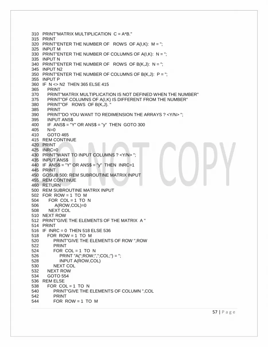
57 | P a g e

310 PRINT"MATRIX MULTIPLICATION C = A*B." 315 PRINT 320 PRINT"ENTER THE NUMBER OF ROWS OF A(I,K): M = "; 325 INPUT M 330 PRINT"ENTER THE NUMBER OF COLUMNS OF A(I,K): N = "; 335 INPUT N 340 PRINT"ENTER THE NUMBER OF ROWS OF B(K,J): N = "; 345 INPUT N2 350 PRINT"ENTER THE NUMBER OF COLUMNS OF B(K,J): P = "; 355 INPUT P 360 IF N <> N2 THEN 365 ELSE 415 365 PRINT 370 PRINT"MATRIX MULTIPLICATION IS NOT DEFINED WHEN THE NUMBER" 375 PRINT"OF COLUMNS OF A(I,K) IS DIFFERENT FROM THE NUMBER" 380 PRINT"OF ROWS OF B(K,J). " 385 PRINT 390 PRINT"DO YOU WANT TO REDIMENSION THE ARRAYS ? <Y/N> "; 395 INPUT ANS$ 400 IF ANS$ = "Y" OR ANS$ = "y" THEN GOTO 300 405 N=0 410 GOTO 465 415 REM CONTINUE 420 PRINT 425 INRC=0 430 PRINT"WANT TO INPUT COLUMNS ? <Y/N> "; 435 INPUT ANS$ 440 IF ANS$ = "Y" OR ANS$ = "y" THEN INRC=1 445 PRINT 450 GOSUB 500: REM SUBROUTINE MATRIX INPUT 455 REM CONTINUE 460 RETURN 500 REM SUBROUTINE MATRIX INPUT 502 FOR ROW = 1 TO M 504 FOR COL = 1 TO N 506 A(ROW,COL)=0 508 NEXT COL 510 NEXT ROW 512 PRINT"GIVE THE ELEMENTS OF THE MATRIX A " 514 PRINT 516 IF INRC = 0 THEN 518 ELSE 536 518 FOR ROW = 1 TO M 520 PRINT"GIVE THE ELEMENTS OF ROW ",ROW 522 PRINT 524 FOR COL = 1 TO N 526 PRINT "A(";ROW;",";COL;") = "; 528 INPUT A(ROW,COL) 530 NEXT COL 532 NEXT ROW 534 GOTO 554 536 REM ELSE 538 FOR COL = 1 TO N 540 PRINT"GIVE THE ELEMENTS OF COLUMN ",COL 542 PRINT 544 FOR ROW = 1 TO M

58 | P a g e

546 PRINT "A(";ROW;",";COL;") = "; 548 INPUT A(ROW,COL) 550 NEXT ROW 552 NEXT COL 554 REM ENDIF 600 REM 602 FOR ROW = 1 TO N 604 FOR COL = 1 TO P 606 B(ROW,COL)=0 608 NEXT COL 610 NEXT ROW 612 PRINT"GIVE THE ELEMENTS OF THE MATRIX B " 614 PRINT 616 IF INRC = 0 THEN 618 ELSE 636 618 FOR ROW = 1 TO N 620 PRINT"GIVE THE ELEMENTS OF ROW ",ROW 622 PRINT 624 FOR COL = 1 TO P 626 PRINT "B(";ROW;",";COL;") = "; 628 INPUT B(ROW,COL) 630 NEXT COL 632 NEXT ROW 634 GOTO 654 636 REM ELSE 638 FOR COL = 1 TO P 640 PRINT"GIVE THE ELEMENTS OF COLUMN ",COL 642 PRINT 644 FOR ROW = 1 TO N 646 PRINT "B(";ROW;",";COL;") = "; 648 INPUT B(ROW,COL) 650 NEXT ROW 652 NEXT COL 654 REM ENDIF 656 RETURN 700 REM SUBROUTINE MATRIX MULTIPLICATION 710 FOR I = 1 TO M 720 FOR J = 1 TO P 730 Sum=0 740 FOR K = 1 TO N 750 Sum=Sum+A(I,K)*B(K,J) 760 NEXT K 770 C(I,J)=Sum 780 NEXT J 790 NEXT I 799 RETURN 800 REM SUBROUTINE RESULTS 805 CLS 810 PRINT"THE MATRIX A(I,J) IS:" 815 PRINT 820 FOR ROW = 1 TO M 825 PRINT 830 FOR COL = 1 TO N 835 PRINT A(ROW,COL), 840 NEXT COL

59 | P a g e

845 NEXT ROW 850 PRINT 855 PRINT"THE MATRIX B(I,J) IS:" 860 FOR ROW = 1 TO N 865 PRINT 870 FOR COL = 1 TO P 875 PRINT B(ROW,COL), 880 NEXT COL 885 NEXT ROW 890 PRINT 895 PRINT"THE SUM C = A * B IS:" 900 PRINT 905 FOR ROW = 1 TO M 910 PRINT 915 FOR COL = 1 TO P 920 PRINT C(ROW,COL), 925 NEXT COL 930 NEXT ROW 935 RETURN 5000 END

// REM BACK SUBSTITUTION //

100 REM PROGRAM BACKSUBSTITUTION 120 DIM A(10,10),B(10),X(10) 130 REM CONTINUE 140 GOSUB 300: REM SUBROUTINE INPUTS 150 GOSUB 1000: REM SUBROUTINE BACKSUB 160 GOSUB 3000: REM SUBROUTINE RESULTS 170 PRINT 180 PRINT"WANT TO SOLVE ANOTHER UPPER-TRIANGULAR SYSTEM ? <Y/N> "; 190 INPUT ANS$ 200 IF ANS$ = "Y" OR ANS$ = "y" GOTO 130 210 GOTO 5000 300 REM SUBROUTINE INPUTS 310 CLS 320 PRINT"SOLUTION OF AN UPPER-TRIANGULAR LINEAR SYSTEM:" 330 PRINT 340 PRINT" A*X = B" 350 PRINT 360 PRINT"A IS AN N BY N UPPER-TRIANGULAR MATRIX." 370 PRINT 380 PRINT"B IS AN N DIMENSIONAL VECTOR OF CONSTANTS." 390 PRINT 400 PRINT"X IS THE N DIMENSIONAL SOLUTION VECTOR." 410 PRINT 420 PRINT"ENTER THE NUMBER OF EQUATIONS N = "; 430 INPUT N 440 INRC=0 450 PRINT"WANT TO INPUT COLUMNS ? <Y/N> "; 460 INPUT ANS$ 470 IF ANS$ = "Y" OR ANS$ = "y" THEN INRC=1 480 PRINT 490 PRINT"ENTER THE UPPER-TRIANGULAR MATRIX A(I,J):"

60 | P a g e

500 ACH$="A" 510 GOSUB 600: REM SUBROUTINE MATRIX INPUT 520 PRINT 530 PRINT"ENTER THE COLUMN VECTOR B(J):" 540 GOSUB 900: REM SUBROUTINE VECTOR INPUT 550 RETURN 600 REM SUBROUTINE MATRIX INPUT 610 FOR ROW = 1 TO N 620 FOR COL = ROW TO N 630 A(ROW,COL)=0 640 NEXT COL 650 NEXT ROW 660 PRINT"GIVE THE ELEMENTS OF THE MATRIX ",ACH$ 670 PRINT 680 IF INRC = 0 THEN 690 ELSE 780 690 FOR ROW = 1 TO N 700 PRINT"GIVE THE ELEMENTS OF ROW ",ROW 710 PRINT 720 FOR COL = ROW TO N 730 PRINT ACH$;"(";ROW;",";COL;") = "; 740 INPUT A(ROW,COL) 750 NEXT COL 760 NEXT ROW 770 GOTO 870 780 REM ELSE 790 FOR COL = 1 TO N 800 PRINT"GIVE THE ELEMENTS OF COLUMN ",COL 810 PRINT 820 FOR ROW = 1 TO COL 830 PRINT ACH$;"(";ROW;",";COL;") = "; 840 INPUT A(ROW,COL) 850 NEXT ROW 860 NEXT COL 870 REM ENDIF 880 RETURN 900 REM SUBROUTINE VECTOR INPUT 910 PRINT"GIVE THE ELEMENTS OF THE COLUMN VECTOR ",BCH$ 920 PRINT 930 FOR ROW = 1 TO N 940 PRINT BCH$;"(";ROW;") = "; 950 INPUT B(ROW) 960 NEXT ROW 970 RETURN 1000 REM SUBROUTINE BACKSUB 1010 FOR K = 1 TO N 1020 IF A(K,K) = 0 THEN 1030 ELSE 1050 1030 DET=0 1040 GOTO 1170 1050 REM ENDIF 1060 NEXT K 1070 DET=A(N,N) 1080 X(N)=B(N)/A(N,N) 1090 FOR R = N-1 TO 1 STEP -1 1100 DET=DET*A(R,R)

61 | P a g e

1110 SUM= 0 1120 FOR J = R+1 TO N 1130 SUM=SUM+A(R,J)*X(J) 1140 NEXT J 1150 X(R)= (B(R)-SUM)/A(R,R) 1160 NEXT R 1170 REM CONTINUE 1180 RETURN 2000 REM SUBROUTINE MATRIX PRINT 2010 FOR ROW = 1 TO N 2020 PRINT 2030 FOR COL = 1 TO N 2040 PRINT A(ROW,COL), 2050 NEXT COL 2060 NEXT ROW 2070 RETURN 2100 REM SUBROUTINE VECTOR PRINT 2110 PRINT BCH$;" COEFFICIENT VECTOR ";XCH$;" SOLUTION VECTOR" 2120 PRINT 2130 FOR ROW = 1 TO N 2140 PRINT BCH$;"(";ROW;") = ";B(ROW);" ";XCH$;"(";ROW;") = ",X(ROW) 2150 NEXT ROW 2160 RETURN 3000 REM SUBROUTINE RESULTS 3010 CLS 3020 PRINT"THE UPPER-TRIANGULAR MATRIX A(I,J) IS:" 3030 PRINT 3040 GOSUB 2000: REM SUBROUTINE MATRIX PRINT 3050 IF DET = 0 THEN 3060 ELSE 3100 3060 PRINT"THE MATRIX IS SINGULAR." 3070 PRINT 3080 PRINT"THE BACK-SUBSTITUTION ALGORITHM DOES NOT APPLY." 3090 GOTO 3130 3100 REM ELSE 3110 PRINT 3120 BCH$="B" 3130 XCH$="X" 3140 GOSUB 2100: REM SUBROUTINE VECTOR PRINT 3150 REM ENDIF 3160 PRINT 3170 PRINT"THE DETERMINANT`S VALUE IS DET A = ",DET 3180 RETURN 5000 END // REM UPPER-TRIANGULARIZATION THEN BACK SUBSTITUTION // 100 REM PROGRAM GAUSS-JORDAN 120 DIM A(10,10),B(10),X(10) 130 REM CONTINUE 140 GOSUB 300: REM SUBROUTINE INPUTS 150 GOSUB 1000: REM SUBROUTINE GAUSS-JORDAN 160 GOSUB 3000: REM SUBROUTINE RESULTS 170 PRINT 180 PRINT"WANT TO SOLVE ANOTHER LINEAR SYSTEM ? <Y/N> ";

62 | P a g e

190 INPUT ANS$ 200 IF ANS$ = "Y" OR ANS$ = "y" GOTO 130 210 GOTO 5000 300 REM SUBROUTINE INPUTS 310 CLS 320 PRINT"SOLUTION OF A LINEAR SYSTEM:" 330 PRINT 340 PRINT" A*X = B" 350 PRINT 360 PRINT"GAUSSIAN ELIMINATION IS USED TO UPPER-TRIANGULARIZE" 375 PRINT 370 PRINT"AND THEN BACK-SUBSTITUTION IS USED TO SOLVE FOR X." 375 PRINT 380 PRINT"B IS AN N DIMENSIONAL VECTOR OF CONSTANTS." 390 PRINT 400 PRINT"X IS THE N DIMENSIONAL SOLUTION VECTOR." 410 PRINT 420 PRINT"ENTER THE NUMBER OF EQUATIONS N = "; 430 INPUT N 440 INRC=0 450 PRINT"WANT TO INPUT COLUMNS ? <Y/N> "; 460 INPUT ANS$ 470 IF ANS$ = "Y" OR ANS$ = "y" THEN INRC=1 480 PRINT 490 PRINT"ENTER THE UPPER-TRIANGULAR MATRIX A(I,J):" 510 GOSUB 600: REM SUBROUTINE MATRIX INPUT 520 PRINT 530 PRINT"ENTER THE COLUMN VECTOR B(J):" 540 GOSUB 900: REM SUBROUTINE VECTOR INPUT 550 RETURN 600 REM SUBROUTINE MATRIX INPUT 610 FOR ROW = 1 TO N 620 FOR COL = 1 TO N 630 A(ROW,COL)=0 640 NEXT COL 650 NEXT ROW 660 PRINT"GIVE THE ELEMENTS OF THE MATRIX ",ACH$ 670 PRINT 680 IF INRC = 0 THEN 690 ELSE 780 690 FOR ROW = 1 TO N 700 PRINT"GIVE THE ELEMENTS OF ROW ",ROW 710 PRINT 720 FOR COL = 1 TO N 730 PRINT"A(";ROW;",";COL;") = "; 740 INPUT A(ROW,COL) 745 A1(ROW,COL) = A(ROW,COL) 750 NEXT COL 760 NEXT ROW 770 GOTO 870 780 REM ELSE 790 FOR COL = 1 TO N 800 PRINT"GIVE THE ELEMENTS OF COLUMN ",COL 810 PRINT 820 FOR ROW = 1 TO N

63 | P a g e

830 PRINT"A(";ROW;",";COL;") = "; 840 INPUT A(ROW,COL) 845 A1(ROW,COL) = A(ROW,COL) 850 NEXT ROW 860 NEXT COL 870 REM ENDIF 880 RETURN 900 REM SUBROUTINE VECTOR INPUT 920 PRINT 925 COL=N+1 930 FOR ROW = 1 TO N 940 PRINT "B(";ROW;") = "; 950 INPUT A(ROW,COL) 955 B(ROW)=A(ROW,COL) 960 NEXT ROW 970 RETURN 1000 REM SUBROUTINE GAUSS JORDAN 1010 FOR J = 1 TO N 1020 Row(J)=J 1030 NEXT J 1040 FOR P = 1 TO N-1 1050 FOR K = P+1 TO N 1060 IF ABS(A(Row(K),P))>ABS(A(Row(P),P)) THEN 1070 ELSE 1100 1070 T = Row(P) 1080 Row(P)=Row(K) 1090 Row(K)=T 1100 REM CONTINUE 1110 NEXT K 1120 IF A(Row(P),P) = 0 THEN 1130 ELSE 1150 1130 DET=0 1140 GOTO 1350 1150 REM CONTINUE 1160 FOR K = P+1 TO N 1170 M = A(Row(K),P)/A(Row(P),P) 1180 FOR C = P+1 TO N+1 1190 A(Row(K),C)=A(Row(K),C)-M*A(Row(P),C) 1200 NEXT C 1210 NEXT K 1220 NEXT P 1230 DET=A(Row(N),N) 1240 IF DET = 0 THEN 1340 ELSE 1250 1250 X(N)=A(Row(N),(N+1))/A(Row(N),N) 1260 FOR K = N-1 TO 1 STEP -1 1270 DET=DET*A(Row(K),K) 1280 SUM=0 1290 FOR C = K+1 TO N 1300 SUM=SUM+A(Row(K),C)*X(C) 1310 NEXT C 1320 X(K)=(A(Row(K),(N+1))-SUM)/A(Row(K),K) 1330 NEXT K 1340 REM ENDIF 1350 REM CONTINUE 1360 RETURN 2000 REM SUBROUTINE MATRIX PRINT

64 | P a g e

2010 FOR ROW = 1 TO N 2020 PRINT 2030 FOR COL = 1 TO N 2040 PRINT A1(ROW,COL), 2050 NEXT COL 2060 NEXT ROW 2070 RETURN 2100 REM SUBROUTINE VECTOR PRINT 2105 COL=N+1 2110 PRINT "B COEFFICIENT VECTOR ";"X SOLUTION VECTOR" 2120 PRINT 2130 FOR ROW = 1 TO N 2140 PRINT "B(";ROW;") = ";B(ROW);" ";"X(";ROW;") = ",X(ROW) 2150 NEXT ROW 2160 RETURN 3000 REM SUBROUTINE RESULTS 3010 CLS 3020 PRINT"COMPUTATION OF THE SOLUTION FOR THE LINEAR SYSTEM A*X = B." 3030 PRINT 3040 PRINT"GAUSSIAN ELIMINATION WAS USED TO UPPER-TRIANGULARIZE," 3050 PRINT 3060 PRINT"AND THEN BACK-SUBSTITUTION IS USED TO SOLVE FOR X." 3070 PRINT 3080 PRINT"THE COEFFICIENT MATRIX A IS:" 3090 PRINT 3100 GOSUB 2000: REM SUBROUTINE MATRIX PRINT 3110 IF DET = 0 THEN 3120 ELSE 3180 3120 PRINT"THE MATRIX IS SINGULAR." 3130 PRINT 3140 PRINT"A ZERO PIVOT ELEMENT WAS ENCOUNTERED." 3150 PRINT 3160 PRINT"THE METHOD DOES NOT APPLY." 3170 GOTO 3180 REM ELSE 3190 PRINT 3200 GOSUB 2100: REM SUBROUTINE VECTOR PRINT 3210 REM ENDIF 3220 PRINT 3230 PRINT"THE DETERMINANT`S VALUE IS DET A = ",DET 3240 RETURN 5000 END // REM LU FACTORIZATION WITH ROW INTERCHANGES // 100 REM PROGRAM LU FACTOR AND SOLVE 105 DIM A(10,10),A1(10,10),B(10),ROW(10),X(10) 110 REM CONTINUE 115 GOSUB 300: REM SUBROUTINE INPUTS 120 GOSUB 1000: REM SUBROUTINE FACTOR 125 REM CONTINUE 130 PRINT 135 PRINT"ENTER THE COLUMN VECTOR B:" 140 GOSUB 900: REM SUBROUTINE VECTOR INPUT 145 IF DET <> 0 THEN GOSUB 1500: REM SUBROUTINE SOLVE

65 | P a g e

150 GOSUB 3000: REM SUBROUTINE RESULTS 155 IF DET <> 0 THEN 160 ELSE 175 160 PRINT"WANT TO SOLVE A*X=B WITH A NEW VECTOR B ? <Y/N> "; 165 INPUT ANS$ 170 IF ANS$ = "Y" OR ANS$ = "y" THEN GOTO 125 175 REM ENDIF 180 PRINT"WANT TO SOLVE ANOTHER LINEAR SYSTEM ? <Y/N> "; 185 INPUT ANS$ 190 IF ANS$ = "Y" OR ANS$ = "y" THEN GOTO 110 195 GOTO 5000 300 REM SUBROUTINE INPUTS 310 CLS 320 PRINT"SOLUTION OF A LINEAR SYSTEM:" 330 PRINT 340 PRINT" A*X = B" 350 PRINT 360 PRINT"THE TRIANGULAR FACTORIZATION L*U = P*A IS CONSTRUCTED" 375 PRINT 370 PRINT"FIRST, THE SOLUTION Y TO L*Y = P*B IS FOUND," 372 PRINT 374 PRINT"SECOND, THE SOLUTION X TO U*X = Y IS FOUND." 375 PRINT 376 PRINT"A IS AN N BY N NONSINGULAR MATRIX." 378 PRINT 380 PRINT"B IS AN N DIMENSIONAL VECTOR OF CONSTANTS." 390 PRINT 400 PRINT"X IS THE N DIMENSIONAL SOLUTION VECTOR." 410 PRINT 420 PRINT"ENTER THE NUMBER OF EQUATIONS N = "; 430 INPUT N 440 INRC=0 450 PRINT"WANT TO INPUT COLUMNS ? <Y/N> "; 460 INPUT ANS$ 470 IF ANS$ = "Y" OR ANS$ = "y" THEN INRC=1 480 PRINT 490 PRINT"ENTER THE UPPER-TRIANGULAR MATRIX A(I,J):" 510 GOSUB 600: REM SUBROUTINE MATRIX INPUT 550 RETURN 600 REM SUBROUTINE MATRIX INPUT 610 FOR ROW = 1 TO N 620 FOR COL = 1 TO N 630 A(ROW,COL)=0 640 NEXT COL 650 NEXT ROW 660 PRINT"GIVE THE ELEMENTS OF THE MATRIX ",ACH$ 670 PRINT 680 IF INRC = 0 THEN 690 ELSE 780 690 FOR ROW = 1 TO N 700 PRINT"GIVE THE ELEMENTS OF ROW ",ROW 710 PRINT 720 FOR COL = 1 TO N 730 PRINT"A(";ROW;",";COL;") = "; 740 INPUT A(ROW,COL) 745 A1(ROW,COL) = A(ROW,COL)

66 | P a g e

750 NEXT COL 760 NEXT ROW 770 GOTO 870 780 REM ELSE 790 FOR COL = 1 TO N 800 PRINT"GIVE THE ELEMENTS OF COLUMN ",COL 810 PRINT 820 FOR ROW = 1 TO N 830 PRINT"A(";ROW;",";COL;") = "; 840 INPUT A(ROW,COL) 845 A1(ROW,COL) = A(ROW,COL) 850 NEXT ROW 860 NEXT COL 870 REM ENDIF 880 RETURN 900 REM SUBROUTINE VECTOR INPUT 920 PRINT 930 FOR ROW = 1 TO N 940 PRINT "B(";ROW;") = "; 950 INPUT B(ROW) 960 NEXT ROW 970 RETURN 1000 REM SUBROUTINE FACTOR 1010 DET=1 1020 FOR J = 1 TO N 1030 ROW(J)=J 1040 NEXT J 1050 FOR P = 1 TO N-1 1060 FOR K = P+1 TO N 1070 IF ABS(A(ROW(K),P))>ABS(A(ROW(P),P)) THEN 1080 ELSE 1120 1080 T=ROW(P) 1090 ROW(P)=ROW(K) 1100 ROW(K)=T 1110 DET=-DET 1120 REM CONTINUE 1130 NEXT K 1140 DET=DET*A(ROW(P),P) 1150 IF DET = 0 THEN GOTO 1260 1160 FOR K = P+1 TO N 1170 ROWK=ROW(K) 1180 ROWP=ROW(P) 1190 A(ROWK,P)=A(ROWK,P)/A(ROWP,P) 1200 FOR C = P+1 TO N 1210 A(ROWK,C)=A(ROWK,C)-A(ROWK,P)*A(ROWP,C) 1220 NEXT C 1230 NEXT K 1240 NEXT P 1250 DET=DET*A(ROW(N),N) 1260 REM CONTINUE 1270 RETURN 1500 REM SUBROUTINE SOLVE 1510 FOR K = 1 TO N 1520 IF A(ROW(K),K) = 0 THEN GOTO 1720 1530 NEXT K

67 | P a g e

1540 X(1)=B(ROW(1)) 1550 FOR K = 2 TO N 1560 SUM=0 1570 ROWK=ROW(K) 1580 FOR C = 1 TO K-1 1590 SUM=SUM+A(ROWK,C)*X(C) 1600 NEXT C 1610 X(K)=B(ROWK)-SUM 1620 NEXT K 1630 X(N)=X(N)/A(ROW(N),N) 1640 FOR K = N-1 TO 1 STEP -1 1650 SUM=0 1660 ROWK=ROW(K) 1670 FOR C = K+1 TO N 1680 SUM=SUM+A(ROWK,C)*X(C) 1690 NEXT C 1700 X(K)=(X(K)-SUM)/A(ROWK,K) 1710 NEXT K 1720 REM CONTINUE 1730 RETURN 2000 REM SUBROUTINE MATRIX PRINT 2010 FOR ROW = 1 TO N 2020 PRINT 2030 FOR COL = 1 TO N 2040 PRINT A1(ROW,COL), 2050 NEXT COL 2060 NEXT ROW 2070 RETURN 2100 REM SUBROUTINE VECTOR PRINT 2105 COL=N+1 2110 PRINT "B COEFFICIENT VECTOR ";"X SOLUTION VECTOR" 2120 PRINT 2130 FOR ROW = 1 TO N 2140 PRINT "B(";ROW;") = ";B(ROW);" ";"X(";ROW;") = ",X(ROW) 2150 NEXT ROW 2160 RETURN 3000 REM SUBROUTINE RESULTS 3010 CLS 3020 PRINT"COMPUTATION OF THE SOLUTION FOR THE LINEAR SYSTEM A*X = B." 3030 PRINT 3040 PRINT"THE TRIANGULAR FACTORIZATION L*U = P*A WAS CONSTRUCTED" 3050 PRINT 3060 PRINT"FIRST, THE SOLUTION Y TO L*Y = P*B WAS FOUND," 3070 PRINT 3080 PRINT"SECOND, THE SOLUTION X TO U*X = Y WAS FOUND." 3090 PRINT 3100 PRINT"THE COEFFICIENT MATRIX A IS:" 3110 PRINT 3120 GOSUB 2000: REM SUBROUTINE MATRIX PRINT 3130 IF DET = 0 THEN 3140 ELSE 3220 3140 PRINT"THE MATRIX IS SINGULAR." 3150 PRINT 3160 PRINT"A ZERO PIVOT ELEMENT WAS ENCOUNTERED." 3170 PRINT

68 | P a g e

3180 PRINT"THE MATRIX DOES NOT HAVE TRIANGULAR FACTORIZATION." 3190 PRINT 3200 PRINT"THE METHOD DOES NOT APPLY." 3210 GOTO 3250 3220 REM ELSE 3230 PRINT 3240 GOSUB 2100: REM SUBROUTINE VECTOR PRINT 3250 REM ENDIF 3260 PRINT 3270 PRINT"THE DETERMINANT`S VALUE IS DET A = ",DET 3280 RETURN 5000 END // REM POLYNOMIAL CALCULUS // 100 REM PROGRAM POLYNOMIAL CALCULUS 105 DIM C(15) 110 REM CONTINUE 115 GOSUB 400: REM SUBROUTINE GET POLYNOMIAL 120 REM CONTINUE 125 GOSUB 1000: REM SUBROUTINE CHOICE 130 GOSUB 2000: REM SUBROUTINE EVALUATE 135 PRINT 140 PRINT"WANT ANOTHER CHOICE ? "; 145 INPUT ANS$ 150 IF ANS$ = "Y" OR ANS$ = "y" GOTO 120 155 PRINT 160 PRINT"WANT ANOTHER POLYNOMIAL ? "; 165 INPUT ANS$ 170 IF ANS$ = "Y" OR ANS$ = "y" GOTO 110 175 GOTO 5000 200 REM SUBROUTINE PRINT POLYNOMIAL 205 CLS 210 IF N = 1 THEN 215 ELSE 240 215 PRINT 220 PRINT"P(X) = C X + C" 225 PRINT" 1 0" 230 PRINT 235 GOTO 335 240 REM ELSE 245 IF N = 2 THEN 250 ELSE 275 250 PRINT" 2" 255 PRINT"P(X) = C X + C X + C" 260 PRINT" 2 1 0" 265 PRINT 270 GOTO 335 275 REM ELSE 280 IF N = 3 THEN 285 ELSE 310 285 PRINT" 3 2" 290 PRINT"P(X) = C X + C X + C X + C " 295 PRINT" 3 2 1 0" 300 PRINT 305 GOTO 335 310 REM ELSE

69 | P a g e

315 PRINT" ",N," 2" 320 PRINT"P(X) = C X +...+ C X + C X + C " 325 PRINT N," 2 1 0" 330 PRINT 335 REM ENDIF 340 FOR K = N TO 0 STEP -1 345 PRINT"C(",K,") =",C(K) 350 NEXT K 355 RETURN 400 REM SUBROUTINE GET POLYNOMIAL 405 CLS 410 PRINT"POLYNOMIAL CALCULUS FOR EVALUATING, DIFFERENTIATING" 415 PRINT 420 PRINT"AND INTEGRATING THE POLYNOMIAL P(X) OF DEGREE N. " 425 PRINT 430 PRINT" N N-1 2 " 435 PRINT"P(X) = C X + C X +...+ C X + C X + C " 440 PRINT" N N-1 2 1 0" 445 PRINT 450 PRINT"ENTER THE DEGREE N = "; 455 INPUT N 460 PRINT 465 PRINT"NOW ENTER THE ",N+1," COEFFICIENTS" 470 PRINT 475 PRINT" C , ... , C , C , C " 480 PRINT N," 2 1 0" 485 PRINT 490 FOR K = N TO 0 STEP -1 495 PRINT"C(",K,") = "; 500 INPUT C(K) 505 NEXT K 510 GOSUB 200: REM SUBROUTINE PRINT POLYNOMIAL 515 RETURN 600 REM SUBROUTINE EVALUATE POLYNOMIAL 610 POLY=C(N) 620 FOR K = N-1 TO 0 STEP -1 630 POLY=C(K)+POLY*X 640 NEXT K 650 RETURN 700 REM SUBROUTINE EVALUATE DERIVATIVE 710 DERIV=N*C(N) 720 FOR K = N-1 TO 1 STEP -1 730 DERIV=K*C(K)+DERIV*X 740 NEXT K 750 RETURN 800 REM SUBROUTINE EVALUATE INTEGRAL 810 INTEG=C(N)/(N+1) 820 FOR K = N TO 1 STEP -1 830 INTEG=C(K-1)/K+INTEG*X 840 NEXT K 850 INTEG=INTEG*X 860 RETURN 1000 REM SUBROUTINE CHOICE 1010 CLS

70 | P a g e

1020 PRINT"THE POLYNOMIAL OF DEGREE ",N," IS:" 1030 PRINT 1040 GOSUB 200: REM SUBROUTINE PRINT POLYNOMIAL 1050 PRINT 1060 PRINT"CHOOSE ONE OF THE FOLLOWING:" 1070 PRINT 1080 PRINT"1 - EVALUATE P(X)" 1090 PRINT 1100 PRINT"2 - EVALUATE P`(X)" 1110 PRINT 1120 PRINT"3 - INTEGRATE P(X) OVER [A,B]" 1130 PRINT 1140 PRINT"SELECT <1-3> "; 1150 INPUT Meth 1160 PRINT 1170 RETURN 2000 REM SUBROUTINE EVALUATE 2010 CLS 2020 IF Meth = 1 THEN 2030 ELSE 2050 2030 PRINT"YOU CHOSE TO EVALUATE THE POLYNOMIAL P(X):" 2040 GOTO 2120 2050 REM ELSE 2060 IF Meth = 2 THEN 2070 ELSE 2090 2070 PRINT"YOU CHOSE TO DIFFERENTIATE THE POLYNOMIAL P(X):" 2080 GOTO 2120 2090 REM ELSE 2100 IF Meth = 3 THEN 2110 ELSE 2120 2110 PRINT"YOU CHOSE TO INTEGRATE THE POLYNOMIAL P(X):" 2120 REM ENDIF 2130 PRINT 2140 GOSUB 200: REM SUBROUTINE PRINT POLYNOMIAL 2150 PRINT 2160 IF Meth = 1 THEN 2170 ELSE 2250 2170 PRINT"EVALUATE P(X)" 2180 PRINT 2190 PRINT" ENTER X = "; 2200 INPUT X 2210 PRINT 2220 GOSUB 600: REM SUBROUTINE EVALUATE POLYNOMIAL 2230 PRINT"P(",X," ) = ",POLY 2240 GOTO 2500 2250 REM ELSE 2260 IF Meth = 2 THEN 2270 ELSE 2350 2270 PRINT"EVALUATE P`(X)" 2280 PRINT 2290 PRINT" ENTER X = "; 2300 INPUT X 2310 PRINT 2320 GOSUB 700: REM SUBROUTINE EVALUATE DERIVATIVE 2330 PRINT"P`(",X," ) = ",DERIV 2340 GOTO 2500 2350 REM ELSE 2360 IF Meth = 3 THEN 2370 ELSE 2500 2370 PRINT"INTEGRATE P(X) OVER [A,B]"

71 | P a g e

2380 PRINT 2390 PRINT"ENTER THE LEFT ENDPOINT A = "; 2400 INPUT A 2410 PRINT"ENTER THE RIGHT ENDPOINT B = "; 2420 INPUT B 2430 X = A 2431 GOSUB 800: REM SUBROUTINE EVALUATE INTEGRAL 2432 IA = INTEG 2433 X = B 2434 GOSUB 800: REM SUBROUTINE EVALUATE INTEGRAL 2435 IB = INTEG 2436 INTAB = IB - IA 2440 PRINT 2450 PRINT"B" 2460 PRINT"/" 2470 PRINT"| P(X) DX = ",INTAB 2480 PRINT"/" 2490 PRINT"A" 2500 REM ENDIF 2510 PRINT 2520 RETURN 5000 END // REM LAGRANGE APPROXIMATION // 100 REM PROGRAM LAGRANGE POLYNOMIAL 110 DIM X(25),Y(25) 120 REM CONTINUE 130 GOSUB 300: REM SUBROUTINE GET DATA 140 REM CONTINUE 150 GOSUB 800: REM SUBROUTINE EVALUATE 160 PRINT 170 PRINT"WANT TO EVALUATE P(T) AGAIN ? "; 180 INPUT ANS$ 190 IF ANS$ = "Y" OR ANS$ = "y" THEN GOTO 140 200 PRINT 210 PRINT"WANT TO TRY A DIFFERENT SET OF POINTS ? "; 220 INPUT ANS$ 230 IF ANS$ = "Y" OR ANS$ = "y" THEN GOTO 120 240 GOTO 5000 300 REM SUBROUTINE GET DATA 310 CLS 320 PRINT 330 PRINT"THE LAGRANGE POLYNOMIAL IS USED TO INTERPOLATE" 340 PRINT 350 PRINT"BASED ON THE N+1 POINTS (X ,Y ),...,(X ,Y )" 360 PRINT" 0 0 N N" 370 PRINT 380 PRINT"ENTER THE NUMBER N = "; 390 INPUT N 400 PRINT 410 PRINT"NOW ENTER THE N =",N+1," POINTS" 420 PRINT 430 PRINT"(X ,Y ),(X ,Y ),...,(X ,Y )"

72 | P a g e

440 PRINT" 0 0 1 1 N N" 450 PRINT 460 FOR K = 0 TO N 470 PRINT"X(";K;") = "; 480 INPUT X(K) 490 PRINT"Y(";K;") = "; 500 INPUT Y(K) 510 PRINT 520 NEXT K 530 RETURN 600 REM SUBROUTINE LAGRANGE 610 SUM=0 620 FOR K = 0 TO N 630 TERM=Y(K) 640 FOR J = 0 TO N 650 IF J = K THEN GOTO 670 660 TERM=TERM*(T-X(J))/(X(K)-X(J)) 670 REM CONTINUE 680 NEXT J 690 SUM=SUM+TERM 700 NEXT K 710 POLY=SUM 720 RETURN 800 REM SUBROUTINE EVALUATE 810 CLS 820 PRINT 830 PRINT"THE LAGRANGE POLYNOMIAL INTERPOLATION BASED ON THE N+1 POINTS" 840 PRINT 850 FOR K = 0 TO N 860 PRINT"X(";K;") =";X(K);" Y(";K;") =";Y(K) 870 NEXT K 880 PRINT 890 PRINT"NOW EVALUATE P(T)" 900 PRINT 910 PRINT"ENTER A VALUE T = "; 920 INPUT T 930 PRINT 940 PRINT"THE VALUE OF THE LAGRANGE POLYNOMIAL IS " 950 PRINT 960 GOSUB 600: REM SUBROUTINE LAGRANGE 970 PRINT"P(";T;" ) = ";POLY 980 PRINT 990 RETURN 5000 END // REM NESTED MULTIPLICATION FOR NEWTON POLYNOMIALS // 100 REM PROGRAM NESTED MULTIPLICATION 110 DIM A(25),X(25) 120 REM CONTINUE 130 GOSUB 700: REM SUBROUTINE GET DATA 140 REM CONTINUE 150 GOSUB 2000: REM SUBROUTINE EVALUATE 160 PRINT

73 | P a g e

170 PRINT"WANT TO EVALUATE P(T) AGAIN ? "; 180 INPUT ANS$ 190 IF ANS$ = "Y" OR ANS$ = "y" THEN GOTO 140 200 PRINT 210 PRINT"WANT TO EVALUATE ANOTHER POLYNOMIAL ? "; 220 INPUT ANS$ 230 IF ANS$ = "Y" OR ANS$ = "y" THEN GOTO 120 240 GOTO 5000 300 REM SUBROUTINE PRINT POLYNOMIAL 310 PRINT 320 IF N = 1 THEN 330 ELSE 360 330 PRINT"P(T) = A + A [T-X ]" 340 PRINT" 0 1 0 " 350 GOTO 530 360 REM ELSE 370 IF N = 2 THEN 380 ELSE 410 380 PRINT"P(T) = A + A [T-X ] + A [T-X ][T-X ]" 390 PRINT" 0 1 0 2 0 1 " 400 GOTO 530 410 REM ELSE 420 IF N = 3 THEN 430 ELSE 460 430 PRINT"P(T) = A + A [T-X ] + A [T-X ][T-X ] + A [T-X ][T-X ][T-X ]" 440 PRINT" 0 1 0 2 0 1 3 0 1 2 " 450 GOTO 530 460 REM ELSE 470 PRINT"P(T) = A + A [T-X ] + A [T-X ][T-X ] + A [T-X ][T-X ][T-X ]" 480 PRINT" 0 1 0 2 0 1 3 0 1 2" 490 PRINT" +...+ A [T-X ][T-X ] ... [T-X ]" 500 PRINT" ",N," 0 1",(N-1) 510 PRINT 520 PRINT"N =",N 530 REM ENDIF 540 PRINT 550 PRINT"THE COEFFICIENTS: THE CENTERS:" 560 PRINT 570 FOR K = 0 TO N-1 580 PRINT"A(";K;") =";A(K);" X(";K;") =";X(K) 590 NEXT K 600 PRINT"A(";N;") =";A(N) 610 RETURN 700 REM SUBROUTINE GET DATA 710 CLS 720 PRINT"NESTED MULTIPLICATION IS USED TO EVALUATE THE NEWTON POLYNOMIAL:" 730 PRINT 740 PRINT"P(T) = A + A [T-X ] + A [T-X ][T-X ] + A [T-X ][T-X ][T-X ]" 750 PRINT" 0 1 0 2 0 1 3 0 1 2" 760 PRINT" +...+ A [T-X ][T-X ]...[T-X ]" 770 PRINT" N 0 1 N-1" 780 PRINT 790 PRINT"THE CENTERS ARE X , X ,..., X AND THE" 800 PRINT" 0 1 N-1 " 810 PRINT 820 PRINT"COEFFICIENTS ARE A , A ,..., A , A " 830 PRINT" 0 1 N-1 N "

74 | P a g e

840 PRINT 850 PRINT"ENTER THE DEGREE N = "; 860 INPUT N 870 PRINT 880 PRINT"NOW ENTER THE ",N," CENTERS" 890 PRINT 900 FOR K = 0 TO N-1 910 PRINT"X(";K;") = "; 920 INPUT X(K) 930 NEXT K 940 PRINT 950 PRINT"NOW ENTER THE ",N+1," COEFFICIENTS" 960 PRINT 970 FOR K = 0 TO N 980 PRINT"A(";K;") = "; 990 INPUT A(K) 992 NEXT K 994 PRINT 996 RETURN 1000 REM SUBROUTINE NESTED MULTIPLICATION 1010 SUM=A(N) 1020 FOR K = N-1 TO 0 STEP -1 1030 SUM=SUM*(T-X(K))+A(K) 1040 NEXT K 1050 POLY= SUM 1060 RETURN 2000 REM SUBROUTINE EVALUATE 2010 CLS 2020 GOSUB 300: REM SUBROUTINE PRINT POLYNOMIAL 2030 PRINT 2040 PRINT"NOW EVALUATE P(T)" 2050 PRINT 2060 PRINT"ENTER A VALUE T = "; 2070 INPUT T 2080 PRINT 2090 PRINT"THE VALUE OF THE NESTED POLYNOMIAL IS " 2100 PRINT 2110 GOSUB 1000: REM SUBROUTINE NESTED MULTIPLICATION 2120 PRINT"P(";T;" ) = ";POLY 2130 RETURN 5000 END // REM NEWTON POLYNOMIAL INTERPOLATION // 100 REM PROGRAM NEWTON POLYNOMIAL 105 DIM A(25),X(25),Y(25) 110 REM CONTINUE 115 GOSUB 180: REM SUBROUTINE GET DATA 120 GOSUB 800: REM SUBROUTINE DIVIDED DIFFERENCES 125 REM CONTINUE 130 GOSUB 2000: REM SUBROUTINE EVALUATE 135 PRINT 140 PRINT"WANT TO EVALUATE P(T) AGAIN ? "; 145 INPUT ANS$

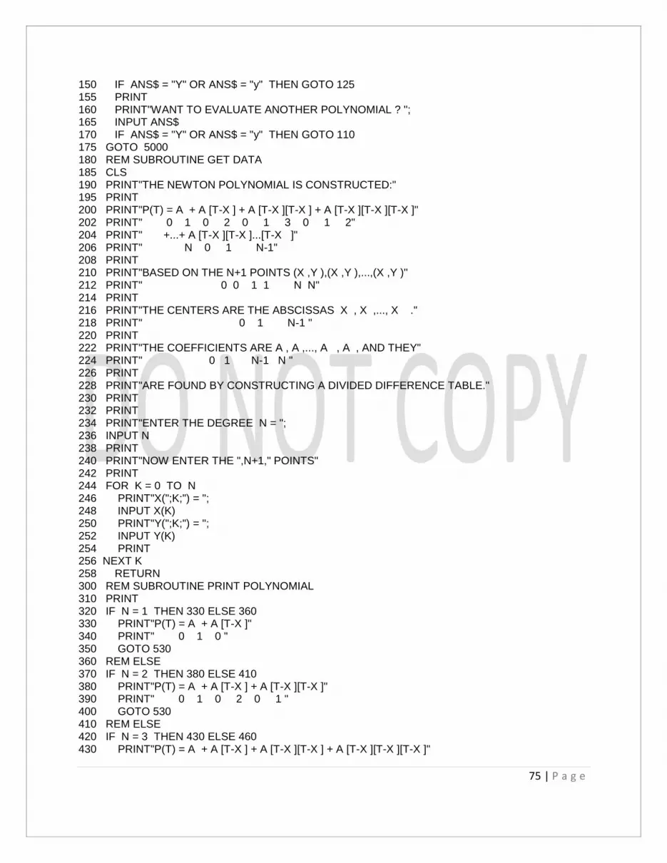
75 | P a g e

150 IF ANS$ = "Y" OR ANS$ = "y" THEN GOTO 125 155 PRINT 160 PRINT"WANT TO EVALUATE ANOTHER POLYNOMIAL ? "; 165 INPUT ANS$ 170 IF ANS$ = "Y" OR ANS$ = "y" THEN GOTO 110 175 GOTO 5000 180 REM SUBROUTINE GET DATA 185 CLS 190 PRINT"THE NEWTON POLYNOMIAL IS CONSTRUCTED:" 195 PRINT 200 PRINT"P(T) = A + A [T-X ] + A [T-X ][T-X ] + A [T-X ][T-X ][T-X ]" 202 PRINT" 0 1 0 2 0 1 3 0 1 2" 204 PRINT" +...+ A [T-X ][T-X ]...[T-X ]" 206 PRINT" N 0 1 N-1" 208 PRINT 210 PRINT"BASED ON THE N+1 POINTS (X ,Y ),(X ,Y ),...,(X ,Y )" 212 PRINT" 0 0 1 1 N N" 214 PRINT 216 PRINT"THE CENTERS ARE THE ABSCISSAS X , X ,..., X ." 218 PRINT" 0 1 N-1 " 220 PRINT 222 PRINT"THE COEFFICIENTS ARE A , A ,..., A , A , AND THEY" 224 PRINT" 0 1 N-1 N " 226 PRINT 228 PRINT"ARE FOUND BY CONSTRUCTING A DIVIDED DIFFERENCE TABLE." 230 PRINT 232 PRINT 234 PRINT"ENTER THE DEGREE N = "; 236 INPUT N 238 PRINT 240 PRINT"NOW ENTER THE ",N+1," POINTS" 242 PRINT 244 FOR K = 0 TO N 246 PRINT"X(";K;") = "; 248 INPUT X(K) 250 PRINT"Y(";K;") = "; 252 INPUT Y(K) 254 PRINT 256 NEXT K 258 RETURN 300 REM SUBROUTINE PRINT POLYNOMIAL 310 PRINT 320 IF N = 1 THEN 330 ELSE 360 330 PRINT"P(T) = A + A [T-X ]" 340 PRINT" 0 1 0 " 350 GOTO 530 360 REM ELSE 370 IF N = 2 THEN 380 ELSE 410 380 PRINT"P(T) = A + A [T-X ] + A [T-X ][T-X ]" 390 PRINT" 0 1 0 2 0 1 " 400 GOTO 530 410 REM ELSE 420 IF N = 3 THEN 430 ELSE 460 430 PRINT"P(T) = A + A [T-X ] + A [T-X ][T-X ] + A [T-X ][T-X ][T-X ]"

76 | P a g e

440 PRINT" 0 1 0 2 0 1 3 0 1 2 " 450 GOTO 530 460 REM ELSE 470 PRINT"P(T) = A + A [T-X ] + A [T-X ][T-X ] + A [T-X ][T-X ][T-X ]" 480 PRINT" 0 1 0 2 0 1 3 0 1 2" 490 PRINT" +...+ A [T-X ][T-X ] ... [T-X ]" 500 PRINT" ",N," 0 1",(N-1) 510 PRINT 520 PRINT"N =",N 530 REM ENDIF 540 PRINT 550 PRINT"THE COEFFICIENTS: THE CENTERS:" 560 PRINT 570 FOR K = 0 TO N-1 580 PRINT"A(";K;") =";A(K);" X(";K;") =";X(K) 590 NEXT K 600 PRINT"A(";N;") =";A(N) 610 RETURN 800 REM SUBROUTINE DIVIDED DIFFERENCES 810 FOR K = 0 TO N 820 D(K,0)=Y(K) 830 NEXT K 840 FOR J = 1 TO N 850 FOR K = J TO N 860 D(K,J)=(D(K,J-1)-D(K-1,J-1))/(X(K)-X(K-J)) 870 NEXT K 880 NEXT J 890 FOR K = 0 TO N 900 A(K)=D(K,K) 910 NEXT K 920 RETURN 1000 REM SUBROUTINE NESTED MULTIPLICATION 1010 SUM=A(N) 1020 FOR K = N-1 TO 0 STEP -1 1030 SUM=SUM*(T-X(K))+A(K) 1040 NEXT K 1050 POLY= SUM 1060 RETURN 2000 REM SUBROUTINE EVALUATE 2010 CLS 2020 GOSUB 300: REM SUBROUTINE PRINT POLYNOMIAL 2030 PRINT 2040 PRINT"NOW EVALUATE P(T)" 2050 PRINT 2060 PRINT"ENTER A VALUE T = "; 2070 INPUT T 2080 PRINT 2090 PRINT"THE VALUE OF THE NESTED POLYNOMIAL IS " 2100 PRINT 2110 GOSUB 1000: REM SUBROUTINE NESTED MULTIPLICATION 2120 PRINT"P(";T;" ) = ";POLY 2130 RETURN 5000 END

77 | P a g e

// REM CHEBYSHEV POLYNOMIAL APPROXIMATION // 10 DEF FNF(X) = EXP(X) 100 REM PROGRAM CHEBYSHEV POLYNOMIAL 101 MAXN = 25 102 DIM M(25,25),C(25),P(25),T(25),X(25),Y(25) 104 REM CONTINUE 106 GOSUB 200: REM SUBROUTINE MESSAGE 108 GOSUB 600: REM SUBROUTINE MAKE CHEBYSHEV COEFFICIENTS 110 GOSUB 1000: REM SUBROUTINE INDIVIDUAL TCHEBYSHEV 112 GOSUB 500: REM SUBROUTINE MAKE ORDINARY POLYNOMIAL 114 GOSUB 480: REM SUBROUTINE RESULT 116 GOSUB 400: REM SUBROUTINE PRINT CHEBYSHEV 118 GOSUB 300: REM SUBROUTINE PRINT POLYNOMIAL 120 PRINT 122 PRINT" Press the <ENTER> key. "; 124 INPUT ANS$ 126 GOSUB 480: REM SUBROUTINE RESULT 128 FOR K = 0 TO N 130 Z=X(K) 132 GOSUB 800: REM SUBROUTINE EVALUATE CHEBYSHEV POLYNOMIAL 133 PRINT POLY , FNF(Z) 134 NEXT K 136 REM CONTINUE 138 PRINT 140 PRINT"WANT TO EVALUATE P(T) AGAIN ? "; 142 INPUT ANS$ 144 IF ANS$ = "Y" OR ANS$ = "y" THEN GOTO 136 146 PRINT 148 PRINT"WANT TO EVALUATE ANOTHER POLYNOMIAL ? "; 150 INPUT ANS$ 152 IF ANS$ = "Y" OR ANS$ = "y" THEN GOTO 104 154 GOTO 5000 200 REM SUBROUTINE MESSAGE 202 PRINT 204 PRINT" Construction of the Chebyshev polynomial for the function F(X)." 206 PRINT 208 PRINT" P(X) = C T (x) + C T (x) + C T (x) +...+ C T (x)" 210 PRINT" 0 0 1 1 2 2 N N " 212 PRINT 214 PRINT" over the interval [-1,1]. The coefficients {C } " 216 PRINT" j " 218 PRINT" are computed using the formulas:" 220 PRINT 222 PRINT" N N" 224 PRINT" 1 2 2k+1" 226 PRINT" C = ---Sum f(x ) , C = ---Sum f(x )COS(J*Pi----) for j=1,2,...,N" 228 PRINT" 0 N+1 k j N+1 k 2N+1" 230 PRINT" k=0 k=0 " 232 PRINT 234 PRINT" where x = COS(Pi*(2k+1)/(2N+2))" 236 PRINT" k" 238 PRINT 240 PRINT

78 | P a g e

242 PRINT 244 PRINT" ENTER the maximum number of terms N = "; 246 N=MAXN 248 INPUT N 250 IF N < 1 THEN N=1 252 IF N > MAXN THEN N=MAXN 254 PRINT 256 RETURN 300 REM SUBROUTINE PRINT POLYNOMIAL 302 REM CLS 303 PRINT"The Chebyshev polynomial of degree N = ";N;"is:" 304 IF N = 1 THEN 306 ELSE 316 306 PRINT 308 PRINT"P(X) = A X + A " 310 PRINT" 1 0" 312 PRINT 314 GOTO 354 316 REM ELSE 318 IF N = 2 THEN 320 ELSE 330 320 PRINT" 2" 322 PRINT"P(X) = A X + A X + A " 324 PRINT" 2 1 0" 326 PRINT 328 GOTO 354 330 REM ELSE 332 IF N = 3 THEN 334 ELSE 344 334 PRINT" 3 2" 336 PRINT"P(X) = A X + A X + A X + A " 338 PRINT" 3 2 1 0" 340 PRINT 342 GOTO 354 344 REM ELSE 346 PRINT" ",N," 2" 348 PRINT"P(X) = A X +...+ A X + A X + A " 350 PRINT N," 2 1 0" 352 PRINT 354 REM ENDIF 356 FOR K = N TO 0 STEP -1 358 PRINT"A(";K;") =";A(K) 360 NEXT K 362 RETURN 400 REM SUBROUTINE PRINT CHEBYSHEV 402 PRINT 404 PRINT"The Chebyshev series with N = ",N," terms is" 406 IF N = 1 THEN 408 ELSE 418 408 PRINT 410 PRINT"T(X) = C T (X) + C T (X)" 412 PRINT" 0 0 1 1" 414 PRINT 416 GOTO 456 418 REM ELSE 420 IF N = 2 THEN 422 ELSE 432 422 PRINT 424 PRINT"T(X) = C T (X) + C T (X) + C T (X)"

79 | P a g e

426 PRINT" 0 0 1 1 2 2" 428 PRINT 430 GOTO 456 432 REM ELSE 434 IF N = 3 THEN 436 ELSE 446 436 PRINT 438 PRINT"T(X) = C T (X) + C T (X) + C T (X) + C T (X)" 440 PRINT" 0 0 1 1 2 2 3 3" 442 PRINT 444 GOTO 456 446 REM ELSE 448 PRINT 450 PRINT"T(X) = C T (X) + C T (X) + ... + C T (X)" 452 PRINT" 0 0 1 1 N N" 454 PRINT 456 REM ENDIF 458 FOR K = 0 TO N 460 PRINT"C(";K;") =";C(K) 462 NEXT K 464 RETURN 480 REM SUBROUTINE RESULT 482 REM CLS 484 PRINT 486 PRINT"You chose to construct the Chebyshev polynomial for " 488 PRINT 490 PRINT" F(X) = EXP(X) over the interval [-1,1]." 492 PRINT 494 RETURN 500 REM SUBROUTINE MAKE ORDINARY POLYNOMIAL 510 REM THIS IS (OPTIONAL) FOR GOOD READING 520 FOR J = 0 TO N 530 SUM=0.0 540 FOR K = 0 TO N 550 SUM=SUM+C(K)*M(K,J) 560 NEXT K 570 A(J)=SUM 580 NEXT J 590 RETURN 600 REM SUBROUTINE MAKE CHEBYSHEV COEFFICIENTS 610 D=3.1415926535/(2.0*N+2.0) 620 FOR K = 0 TO N 630 X(K)=COS((2.0*K+1.0)*D) 640 Y(K)=FNF(X(K)) 650 C(K)=0.0 660 NEXT K 670 FOR K = 0 TO N 680 Z=(2.0*K+1.0)*D 690 FOR J = 0 TO N 700 C(J)=C(J)+Y(K)*COS(J*Z) 710 NEXT J 720 NEXT K 730 C(0)=C(0)/(N+1.0) 740 FOR J = 1 TO N 750 C(J)=2.0*C(J)/(N+1.0)

80 | P a g e

760 NEXT J 770 RETURN 800 REM SUBROUTINE EVALUATE CHEBYSHEV POLYNOMIAL 810 T(0)=1.0 820 T(1)=Z 830 IF N > 1 THEN 840 ELSE 870 840 FOR J = 1 TO N-1 850 T(J+1)=2.0*Z*T(J)-T(J-1) 860 NEXT J 870 REM CONTINUE 880 SUM=0.0 890 FOR J = 0 TO N 900 SUM=SUM+C(J)*T(J) 910 NEXT J 920 POLY=SUM 930 RETURN 1000 REM SUBROUTINE INDIVIDUAL TCHEBYSHEV 1010 REM POLYNOMIALS (OPTIONAL) 1020 FOR K = 0 TO N 1030 FOR J = 0 TO N 1040 M(K,J)=0.0 1050 NEXT J 1060 NEXT K 1070 M(0,0)=1.0 1080 M(1,0)=0.0 1090 M(1,1)=1.0 1100 FOR K = 2 TO N 1110 FOR J = 1 TO K 1120 M(K,J)=2.0*M(K-1,J-1)-M(K-2,J) 1130 NEXT J 1140 M(K,0)=-M(K-2,0) 1150 NEXT K 1160 RETURN 5000 END // REM LEAST SQUARES LINE // 100 REM PROGRAM LEAST SQUARES LINE 105 MAXN = 200 110 DIM X(200),Y(200) 115 REM CONTINUE 120 GOSUB 200: REM SUBROUTINE GET DATA 125 GOSUB 300: REM SUBROUTINE REGRESS 130 GOSUB 900: REM SUBROUTINE RESULTS 135 PRINT 140 PRINT"WANT TO FIND ANOTHER LEAST SQUARES LINE ? "; 145 INPUT ANS$ 150 IF ANS$ = "Y" OR ANS$ = "y" THEN GOTO 115 155 GOTO 5000 200 REM SUBROUTINE GET DATA 205 CLS 210 PRINT"THE LEAST SQUARES LINE Y = AX + B IS CONSTRUCTED." 215 PRINT 220 PRINT"IT FITS THE POINTS (X ,Y ), (X ,Y ),..., (X ,Y )"

81 | P a g e

225 PRINT" 1 1 2 2 N N " 230 PRINT 235 PRINT"ENTER THE NUMBER OF POINTS N = "; 240 INPUT N 245 IF N < 2 THEN N = 2 246 IF N > MAXN THEN N = MAXN 250 PRINT 255 PRINT"NOW ENTER THE ",N+1," POINTS" 260 PRINT 265 FOR K = 1 TO N 270 PRINT"X(";K;") = "; 275 INPUT X(K) 280 PRINT"Y(";K;") = "; 285 INPUT Y(K) 290 PRINT 295 NEXT K 296 RETURN 300 REM SUBROUTINE REGRESS 305 XMEAN=0 310 FOR K = 1 TO N 315 XMEAN=XMEAN+X(K) 320 NEXT K 325 XMEAN=XMEAN/N 330 YMEAN=0 335 FOR K = 1 TO N 340 YMEAN=YMEAN+Y(K) 345 NEXT K 350 YMEAN=YMEAN/N 355 SUMX=0 360 FOR K = 1 TO N 365 SUMX=SUMX+(X(K)-XMEAN)*(X(K)-XMEAN) 370 NEXT K 375 SUMXY=0 380 FOR K = 1 TO N 385 SUMXY=SUMXY+(X(K)-XMEAN)*(Y(K)-YMEAN) 390 NEXT K 395 A=SUMXY/SUMX 396 B=YMEAN-A*XMEAN 397 RETURN 900 REM SUBROUTINE RESULTS 905 CLS 910 PRINT 915 PRINT"THE LEAST SQUARES LINE IS Y = A*X +B, WHERE:" 920 PRINT 925 PRINT"A = ",A," B = ",B 930 PRINT 935 PRINT" K X Y A*X +B Error" 940 PRINT" K K K" 945 PRINT" -------------------------------------------------------" 950 FOR K = 1 TO N 955 Z=A*X(K)+B 960 ERRER=Y(K)-Z 965 PRINT K,X(K),Y(K),Z,ERRER 970 NEXT K

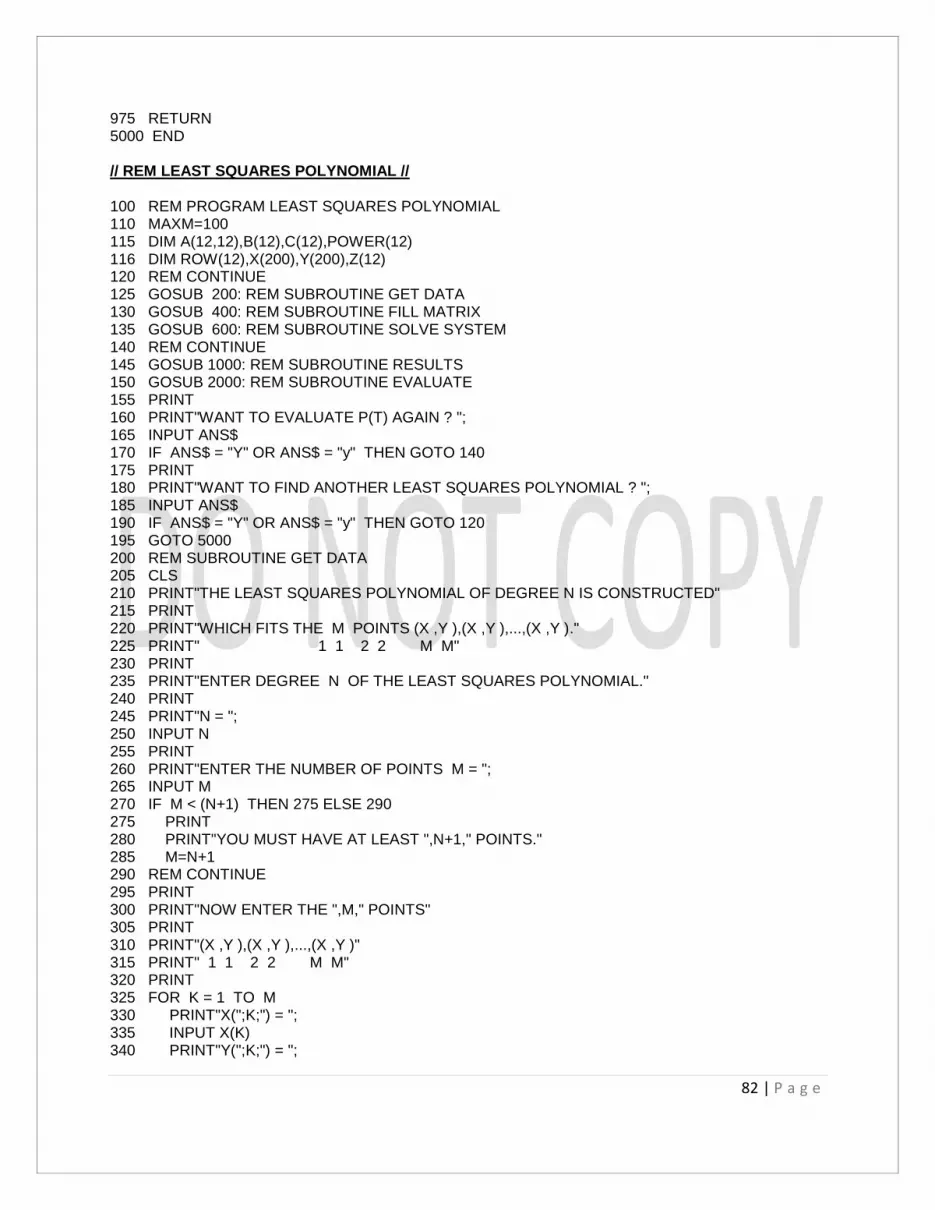
82 | P a g e

975 RETURN 5000 END // REM LEAST SQUARES POLYNOMIAL // 100 REM PROGRAM LEAST SQUARES POLYNOMIAL 110 MAXM=100 115 DIM A(12,12),B(12),C(12),POWER(12) 116 DIM ROW(12),X(200),Y(200),Z(12) 120 REM CONTINUE 125 GOSUB 200: REM SUBROUTINE GET DATA 130 GOSUB 400: REM SUBROUTINE FILL MATRIX 135 GOSUB 600: REM SUBROUTINE SOLVE SYSTEM 140 REM CONTINUE 145 GOSUB 1000: REM SUBROUTINE RESULTS 150 GOSUB 2000: REM SUBROUTINE EVALUATE 155 PRINT 160 PRINT"WANT TO EVALUATE P(T) AGAIN ? "; 165 INPUT ANS$ 170 IF ANS$ = "Y" OR ANS$ = "y" THEN GOTO 140 175 PRINT 180 PRINT"WANT TO FIND ANOTHER LEAST SQUARES POLYNOMIAL ? "; 185 INPUT ANS$ 190 IF ANS$ = "Y" OR ANS$ = "y" THEN GOTO 120 195 GOTO 5000 200 REM SUBROUTINE GET DATA 205 CLS 210 PRINT"THE LEAST SQUARES POLYNOMIAL OF DEGREE N IS CONSTRUCTED" 215 PRINT 220 PRINT"WHICH FITS THE M POINTS (X ,Y ),(X ,Y ),...,(X ,Y )." 225 PRINT" 1 1 2 2 M M" 230 PRINT 235 PRINT"ENTER DEGREE N OF THE LEAST SQUARES POLYNOMIAL." 240 PRINT 245 PRINT"N = "; 250 INPUT N 255 PRINT 260 PRINT"ENTER THE NUMBER OF POINTS M = "; 265 INPUT M 270 IF M < (N+1) THEN 275 ELSE 290 275 PRINT 280 PRINT"YOU MUST HAVE AT LEAST ",N+1," POINTS." 285 M=N+1 290 REM CONTINUE 295 PRINT 300 PRINT"NOW ENTER THE ",M," POINTS" 305 PRINT 310 PRINT"(X ,Y ),(X ,Y ),...,(X ,Y )" 315 PRINT" 1 1 2 2 M M" 320 PRINT 325 FOR K = 1 TO M 330 PRINT"X(";K;") = "; 335 INPUT X(K) 340 PRINT"Y(";K;") = ";

83 | P a g e

345 INPUT Y(K) 350 PRINT 355 NEXT K 360 RETURN 400 REM SUBROUTINE FILL MATRIX 405 FOR R = 1 TO N+1 410 B(R)=0 415 NEXT R 420 FOR K = 1 TO M 425 YK=Y(K) 430 XK=X(K) 435 PROD=1 440 FOR R = 1 TO N+1 445 B(R)=B(R)+YK*PROD 450 PROD=PROD*XK 455 NEXT R 460 NEXT K 465 FOR J = 1 TO 2*N 470 POWER(J)=0 475 NEXT J 480 POWER(0)=M 485 FOR K = 1 TO M 490 XK=X(K) 495 PROD=X(K) 500 FOR J = 1 TO 2*N 505 POWER(J)=POWER(J)+PROD 510 PROD=PROD*XK 515 NEXT J 520 NEXT K 525 FOR R = 1 TO N+1 530 FOR C =1 TO N+1 535 A(R,C)=POWER(R+C-2) 540 NEXT C 545 NEXT R 550 RETURN 600 REM SUBROUTINE SOLVE SYSTEM 605 FOR J = 1 TO N+1 610 ROW(J)=J 615 NEXT J 620 FOR P = 1 TO N 625 FOR K = P+1 TO N+1 630 IF ABS(A(ROW(K),P))>ABS(A(ROW(P),P)) THEN 635 ELSE 650 635 T=ROW(P) 640 ROW(P)=ROW(K) 645 ROW(K)=T 650 REM CONTINUE 655 NEXT K 660 FOR K = P+1 TO N+1 665 A(ROW(K),P)=A(ROW(K),P)/A(ROW(P),P) 670 FOR COL = P+1 TO N+1 675 A(ROW(K),COL)=A(ROW(K),COL)-A(ROW(K),P)*A(ROW(P),COL) 680 NEXT COL 685 NEXT K 690 NEXT P

84 | P a g e

695 Z(1)=B(ROW(1)) 700 FOR K = 2 TO N+1 705 SUM=0 710 FOR COL = 1 TO K-1 715 SUM=SUM+A(ROW(K),COL)*Z(COL) 720 NEXT COL 725 Z(K)=B(ROW(K))-SUM 730 NEXT K 735 C(N+1)=Z(N+1)/A(ROW(N+1),N+1) 740 FOR K = N TO 1 STEP -1 745 SUM=0 750 FOR COL = K+1 TO N+1 755 SUM=SUM+A(ROW(K),COL)*C(COL) 760 NEXT COL 765 C(K)=(Z(K)-SUM)/A(ROW(K),K) 770 NEXT K 775 RETURN 800 REM SUBROUTINE FUNCTION POLY 810 SUM=C(N+1) 820 FOR K = N TO 1 STEP -1 830 SUM=C(K)+SUM*T 840 NEXT K 850 POLY=SUM 860 RETURN 900 REM SUBROUTINE PRINT POLYNOMIAL 902 REM CLS 904 IF N = 1 THEN 906 ELSE 916 906 PRINT 908 PRINT"P(X) = C X + C " 910 PRINT" 2 1" 912 PRINT 914 GOTO 954 916 REM ELSE 918 IF N = 2 THEN 920 ELSE 930 920 PRINT" 2" 922 PRINT"P(X) = C X + C X + C " 924 PRINT" 3 2 1" 926 PRINT 928 GOTO 954 930 REM ELSE 932 IF N = 3 THEN 934 ELSE 944 934 PRINT" 3 2" 936 PRINT"P(X) = C X + C X + C X + C " 938 PRINT" 4 3 2 1" 940 PRINT 942 GOTO 954 944 REM ELSE 946 PRINT" ",N," 2" 948 PRINT"P(X) = C X +...+ C X + C X + C " 950 PRINT N+1," 3 2 1" 952 PRINT 954 REM ENDIF 956 FOR K = N+1 TO 1 STEP -2 958 IF K => 2 THEN 960 ELSE 964

85 | P a g e

960 PRINT "C(";K;") = ";C(K),"C(";(K-1);") = ";C(K-1) 962 GOTO 968 964 REM ELSE 966 PRINT"C(";K;") =";C(K) 968 REM ENDIF 970 NEXT K 972 RETURN 1000 REM SUBROUTINE RESULTS 1010 CLS 1020 PRINT"THE LEAST SQUARES POLYNOMIAL IS:" 1030 PRINT 1040 GOSUB 900: REM SUBROUTINE PRINT POLYNOMIAL 1050 PRINT 1060 PRINT" K X Y P(X ) Error" 1070 PRINT" K K K" 1080 PRINT" -------------------------------------------------------" 1090 FOR R = 1 TO M 1100 T = X(R) 1110 GOSUB 800: REM SUBROUTINE FUNCTION POLY 1120 ERRER=Y(R)-POLY 1130 PRINT K,X(R),Y(R),POLY,ERRER 1140 NEXT R 1150 RETURN 2000 REM SUBROUTINE EVALUATE 2010 PRINT 2020 PRINT"NOW EVALUATE P(T) ENTER A VALUE T = "; 2030 INPUT T 2040 GOSUB 800: REM SUBROUTINE FUNCTION POLY 2050 PRINT"P(";T;" ) = ";POLY 2060 RETURN 5000 END // REM NONLINEAR CURVE FITTING // 100 REM PROGRAM CURVEFIT 105 MaxN=100 110 DIM X(100),X1(100),Y(100),Y1(100) 115 REM CONTINUE 120 GOSUB 200: REM SUBROUTINE GET DATA 125 REM CONTINUE 130 GOSUB 400: REM SUBROUTINE CURVE TYPE 135 GOSUB 2000: REM SUBROUTINE CHANGE VARIABLES 140 GOSUB 3000: REM SUBROUTINE LINEAR REGRESSION 145 GOSUB 4000: REM SUBROUTINE CONSTANTS 150 GOSUB 5000: REM SUBROUTINE RESULTS 155 PRINT 160 PRINT"WANT TO FIT ANOTHER CURVE TO THIS DATA ? "; 165 INPUT ANS$ 170 IF ANS$ = "Y" OR ANS$ = "y" THEN GOSUB 6000: REM SUBROUTINE REFRESH 172 IF ANS$ = "Y" OR ANS$ = "y" THEN GOTO 125 175 PRINT 180 PRINT"WANT TO FIT A CURVE FOR SOME NEW DATA ? "; 185 INPUT ANS$ 190 IF ANS$ = "Y" OR ANS$ = "y" THEN GOTO 115

86 | P a g e

195 GOTO 9999 200 REM SUBROUTINE GET DATA 205 CLS 210 PRINT" THE METHOD OF `DATA LINEARIZATION' IS USED" 215 PRINT 220 PRINT"TO FIT ONE OF THE CURVES Y=A*X+B, Y=A/X+B" 225 PRINT 230 PRINT"Y=D/(X+C), Y=1/(A*X+B), Y=X/(A+B*X), Y=A*Ln(X)+B" 235 PRINT 240 PRINT"Y=C*Exp(A*X), Y=C*X^A, Y=(A*X+B)^-2" 245 PRINT 250 PRINT"Y=C*X*Exp(-D*X), Y=L/(1+C*Exp(A*X))" 255 PRINT 260 PRINT"TO THE N DATA POINTS (X ,Y ), (X ,Y ),..., (X ,Y )." 265 PRINT" 1 1 2 2 N N " 270 PRINT 275 PRINT"ENTER NUMBER OF POINTS N = "; 280 INPUT N 285 IF N < 2 THEN N=2 290 PRINT 295 FOR K = 1 TO N 300 PRINT"X(";K;") = "; 305 INPUT X(K) 310 X1(K)=X(K) 315 PRINT"Y(";K;") = "; 320 INPUT Y(K) 325 Y1(K)=Y(K) 330 PRINT 335 NEXT K 340 RETURN 400 REM SUBROUTINE CURVE TYPE 405 CLS 410 PRINT" WHICH CURVE DO YOU WANT TO FIT ?" 415 PRINT 420 PRINT" 1: Y = A*X + B" 425 PRINT 430 PRINT" 2: Y = A/X + B" 435 PRINT 440 PRINT" 3: Y = D/(X + C)" 445 PRINT 450 PRINT" 4: Y = 1/(A*X + B)" 455 PRINT 460 PRINT" 5: Y = X/(A + B*X)" 465 PRINT 470 PRINT" 6: Y = A*Ln(X) + B" 475 PRINT 480 PRINT" 7: Y = C*Exp(A*X)" 485 PRINT 490 PRINT" 8: Y = C*X^A" 495 PRINT 500 PRINT" 9: Y = (A*X + B)^-2" 505 PRINT 510 PRINT"10: Y = C*X*EXP(-D*X)" 515 PRINT

87 | P a g e

520 PRINT"11: Y = L/(1+C*EXP(A*X))" 525 PRINT 530 PRINT" CHOOSE TYPE OF CURVE <1-11> "; 535 INPUT CTYPE 540 IF CTYPE = 11 THEN 550 ELSE 645 550 CLS 560 PRINT 565 PRINT" YOU CHOSE THE CURVE Y = L/(1+C*EXP(A*X))" 570 PRINT 575 PRINT"THE LIMITING VALUE L = LIM Y(X) MUST BE GIVEN." 580 PRINT" X ->INF" 585 PRINT 590 PRINT"ENTER THE VALUE L = "; 595 INPUT L 600 LM=ABS(Y(1)) 605 FOR K = 2 TO N 610 IF (LM.LT.ABS(Y(K))) THEN LM=ABS(Y(K)) 625 NEXT K 630 IF (L <= LM) THEN L=LM*1.0001 645 REM CONTINUE 650 RETURN 1000 REM SUBROUTINE FUNCTIONS 1005 ON CTYPE GOTO 1010,1020,1030,1040,1050,1060,1070,1080,1090,1100,1100 1010 F=A*X+B 1015 GOTO 1115 1020 F=A/X+B 1025 GOTO 1115 1030 F=D/(X+C) 1035 GOTO 1115 1040 F=1/(A*X+B) 1045 GOTO 1115 1050 F=X/(A+B*X) 1055 GOTO 1115 1060 F=A*LOG(X)+B 1065 GOTO 1115 1070 F=C*EXP(A*X) 1075 GOTO 1115 1080 F=C*EXP(A*LOG(X)) 1085 GOTO 1115 1090 F=1/((A*X+B)*(A*X+B)) 1095 GOTO 1115 1100 F=C*X*EXP(-D*X) 1105 GOTO 1115 1110 F=L/(1+C*EXP(A*X)) 1115 REM CONTINUE 1120 RETURN 2000 REM SUBROUTINE CHANGE VARIABLES 2005 ON CTYPE GOTO 2010,2020,2030,2040,2050,2060,2070,2080,2090,2100,2100 2010 FOR K = 1 TO N 2012 X(K)=X1(K) 2014 Y(K)=Y1(K) 2016 NEXT K 2018 GOTO 2118 2020 FOR K = 1 TO N

88 | P a g e

2022 X(K)=1/X1(K) 2024 Y(K)=Y1(K) 2026 NEXT K 2028 GOTO 2118 2030 FOR K = 1 TO N 2032 X(K)=X1(K)*Y1(K) 2034 Y(K)=Y1(K) 2036 NEXT K 2038 GOTO 2118 2040 FOR K = 1 TO N 2042 X(K)=X1(K) 2044 Y(K)=1/Y1(K) 2046 NEXT K 2048 GOTO 2118 2050 FOR K = 1 TO N 2052 X(K)=1/X1(K) 2054 Y(K)=1/Y1(K) 2056 NEXT K 2058 GOTO 2118 2060 FOR K = 1 TO N 2062 X(K)=LOG(X1(K)) 2064 Y(K)=Y1(K) 2066 NEXT K 2068 GOTO 2118 2070 FOR K = 1 TO N 2072 X(K)=X1(K) 2074 Y(K)=LOG(Y1(K)) 2076 NEXT K 2078 GOTO 2118 2080 FOR K = 1 TO N 2082 X(K)=LOG(X1(K)) 2084 Y(K)=LOG(Y1(K)) 2086 NEXT K 2088 GOTO 2118 2090 FOR K = 1 TO N 2092 X(K)=X1(K) 2094 Y(K)=1/SQR(Y1(K)) 2096 NEXT K 2098 GOTO 2118 2100 FOR K = 1 TO N 2102 X(K)=X1(K) 2104 Y(K)=LOG(Y1(K)/X1(K)) 2106 NEXT K 2108 GOTO 2118 2110 FOR K = 1 TO N 2112 X(K)=X1(K) 2114 Y(K)=LOG(L/Y1(K)-1) 2116 NEXT K 2118 REM CONTINUE 2120 RETURN 3000 REM SUBROUTINE LINEAR REGRESSION 3010 XMEAN=0.0 3020 FOR K = 1 TO N

89 | P a g e

3030 XMEAN=XMEAN+X(K) 3040 NEXT K 3050 XMEAN=XMEAN/N 3060 YMEAN=0.0 3070 FOR K = 1 TO N 3080 YMEAN=YMEAN+Y(K) 3090 NEXT K 3100 YMEAN=YMEAN/N 3110 SUMX=0.0 3120 FOR K = 1 TO N 3130 SUMX=SUMX+(X(K)-XMEAN)*(X(K)-XMEAN) 3140 NEXT K 3150 SUMXY=0.0 3160 FOR K = 1 TO N 3170 SUMXY=SUMXY+(X(K)-XMEAN)*(Y(K)-YMEAN) 3180 NEXT K 3190 A=SUMXY/SUMX 3200 B=YMEAN-A*XMEAN 3210 RETURN 4000 REM SUBROUTINE CONSTANTS 4010 IF CTYPE = 3 THEN 4020 ELSE 4050 4020 C=-1.0/A 4030 D=-B/A 4040 GOTO 4210 4050 REM ELSE 4060 IF CTYPE = 7 THEN 4070 ELSE 4090 4070 C=EXP(B) 4080 GOTO 4210 4090 REM ELSE 4100 IF CTYPE = 8 THEN 4110 ELSE 4130 4110 C=EXP(B) 4120 GOTO 4210 4130 REM ELSE 4140 IF CTYPE = 10 THEN 4150 ELSE 4180 4150 C=EXP(B) 4160 D=-A 4170 GOTO 4210 4180 REM ELSE 4190 IF CTYPE = 11 THEN 4200 ELSE 4210 4200 C=EXP(B) 4210 REM ENDIF 4220 RETURN 5000 REM SUBROUTINE RESULTS 5002 CLS 5005 ON CTYPE GOTO 5010,5020,5030,5040,5050,5060,5070,5080,5090,5100,5100 5010 PRINT" F(X) = A*X +B" 5011 PRINT 5012 PRINT" A = ",A 5013 PRINT 5014 PRINT" B = ",B 5015 GOTO 5120 5020 PRINT" F(X) = A/X + B" 5021 PRINT 5022 PRINT" A =",A

90 | P a g e

5023 PRINT 5024 PRINT" B =",B 5025 GOTO 5120 5030 PRINT" F(X) = D/(X + C)" 5031 PRINT 5032 PRINT" C =",C 5033 PRINT 5034 PRINT" D =",D 5035 GOTO 5120 5040 PRINT" F(X) = 1/(A*X + B)" 5041 PRINT 5042 PRINT" A =",A 5043 PRINT 5044 PRINT" B =",B 5045 GOTO 5120 5050 PRINT" F(X) = X/(A + B*X)" 5051 PRINT 5052 PRINT" A =",A 5053 PRINT 5054 PRINT" B =",B 5055 GOTO 5120 5060 PRINT" F(X) = A*Ln(X) + B" 5061 PRINT 5062 PRINT" A =",A 5063 PRINT 5064 PRINT" B =",B 5065 GOTO 5120 5070 PRINT" F(X) = C*Exp(A*X)" 5071 PRINT 5072 PRINT" A =",A 5073 PRINT 5074 PRINT" C =",C 5075 GOTO 5120 5080 PRINT" F(X) = C*X^A" 5081 PRINT 5082 PRINT" A =",A 5083 PRINT 5084 PRINT" C =",C 5085 GOTO 5120 5090 PRINT" F(X) = (A*X + B)^-2" 5091 PRINT 5092 PRINT" A =",A 5093 PRINT 5094 PRINT" B =",B 5095 GOTO 5120 5100 PRINT" F(X) = C*X*EXP(-D*X)" 5101 PRINT 5102 PRINT" C =",C 5103 PRINT 5104 PRINT" D =",D 5105 GOTO 5120 5110 PRINT" F(X) = L/(1+C*EXP(A*X))" 5101 PRINT 5102 PRINT" L =",L

91 | P a g e

5103 PRINT 5104 PRINT" C =",C 5105 PRINT 5106 PRINT" A =",A 5120 REM CONTINUE 5130 PRINT 5140 PRINT" K X Y F(X ) Error" 5150 PRINT" K K K" 5160 PRINT" -------------------------------------------------------" 5170 FOR K = 1 TO N 5180 X = X1(K) 5190 GOSUB 1000: REM SUBROUTINE FUNCTIONS 5200 ERRER=Y1(K)-F 5210 PRINT K,X1(K),Y1(K),F,ERRER 5220 NEXT K 5230 RETURN 6000 REM SUBROUTINE REFRESH 6010 FOR K = 1 TO N 6020 X(K)=X1(K) 6030 Y(K)=Y1(K) 6040 NEXT K 6050 RETURN 9999 END // REM CUBIC SPLINE CONSTRUCTION // 100 REM PROGRAM CUBIC SPLINE 105 DIM A(50),B(50),C(50),D(50),H(50) 110 DIM M(50),V(50),X(50),Y(50),S(50,3) 115 GOSUB 200: REM SUBROUTINE GET DATA 120 GOSUB 300: REM SUBROUTINE DIFFERENCES 125 GOSUB 270: REM SUBROUTINE SPLINE TYPE 130 GOSUB 400: REM SUBROUTINE MODIFY 135 GOSUB 500: REM SUBROUTINE TRIDIAGONAL 140 GOSUB 600: REM SUBROUTINE END COEFFICIENTS 145 GOSUB 700: REM SUBROUTINE COMPUTE COEFFICIENTS 150 GOSUB 1000: REM SUBROUTINE RESULTS 155 GOSUB 2000: REM SUBROUTINE EVALUATE 160 PRINT 162 PRINT"WANT TO EVALUATE THIS SPLINE AT ANOTHER POINT ? "; 164 INPUT ANS$ 166 IF ANS$ = "Y" OR ANS$ = "y" THEN GOTO 155 168 PRINT 170 PRINT"WANT TO FIT ANOTHER CUBIC SPLINE TO THIS DATA SET ? "; 172 INPUT ANS$ 174 IF ANS$ = "Y" OR ANS$ = "y" THEN GOTO 120 176 PRINT 178 PRINT"WANT TO FIND A CUBIC SPLINE FOR SOME NEW DATA SET ? "; 180 INPUT ANS$ 182 IF ANS$ = "Y" OR ANS$ = "y" THEN GOTO 115 184 GOTO 9999 200 REM SUBROUTINE GET DATA 202 CLS 204 PRINT

92 | P a g e

206 PRINT"A CUBIC SPLINE IS CONSTRUCTED WHICH PASSES THROUGH" 208 PRINT 210 PRINT"THE N+1 POINTS (X ,Y ), (X ,Y ),..., (X ,Y )" 212 PRINT" 0 0 1 1 N N " 214 PRINT 216 PRINT"THE SOLUTION IS A SET OF N PIECEWISE CUBIC FUNCTIONS" 218 PRINT 220 PRINT" 3 2" 222 PRINT"S (X) = S (X-X ) + S (X-X ) + S (X-X ) + S" 224 PRINT" K K,3 K K,2 K K,1 K K,0" 226 PRINT 228 PRINT" WHERE X IS IN [X ,X ]" 230 PRINT" K K+1 " 232 PRINT 234 PRINT" AND K = 0,1,...,N-1." 236 PRINT 238 PRINT"ENTER THE NUMBER N = "; 240 INPUT N 242 PRINT 244 PRINT"NOW ENTER THE ";(N+1);" POINTS:" 246 PRINT 248 FOR K = 0 TO N 250 PRINT"X(";K;") = "; 252 INPUT X(K) 254 PRINT"Y(";K;") = "; 256 INPUT Y(K) 258 PRINT 260 NEXT K 262 RETURN 270 REM SUBROUTINE SPLINE TYPE 272 CLS 274 PRINT"WHICH SPLINE TYPE DO YOU WANT? <1-5> " 276 PRINT 278 PRINT"1 - CLAMPED SPLINE" 280 PRINT 282 PRINT"2 - NATURAL SPLINE" 284 PRINT 286 PRINT"3 - EXTRAPOLATE S``(X) NEAR THE ENDPOINTS" 288 PRINT 290 PRINT"4 - PARABOLIC NEAR THE ENDPOINTS" 291 PRINT 292 PRINT"5 - SPECIFY S``(X(0)) AND S``(X(N))" 293 PRINT 294 PRINT" CHOOSE TYPE <1-5> "; 295 INPUT STYPE 296 RETURN 300 REM SUBROUTINE DIFFERENCES 305 H(0)= X(1)-X(0) 310 D(0)=(Y(1)-Y(0))/H(0) 315 FOR K = 1 TO N-1 320 H(K)= X(K+1)-X(K) 325 D(K)=(Y(K+1)-Y(K))/H(K) 330 A(K)=H(K) 335 B(K)=2*(H(K-1)+H(K))

93 | P a g e

340 C(K)=H(K) 345 V(K)=6*(D(K)-D(K-1)) 350 NEXT K 355 RETURN 400 REM SUBROUTINE MODIFY 402 IF STYPE = 1 THEN 404 ELSE 432 404 PRINT 406 PRINT"ENTER THE FIRST DERIVATIVES." 408 PRINT 410 PRINT"S`(";X(0);" ) = "; 412 INPUT DX0 414 PRINT 416 PRINT"S`(";X(N);" ) = "; 418 INPUT DXN 420 PRINT 422 B(1)=B(1)-H(0)/2 424 V(1)=V(1)-3*(D(0)-DX0) 426 B(N-1)=B(N-1)-H(N-1)/2 428 V(N-1)=V(N-1)-3*(DXN-D(N-1)) 430 GOTO 492 432 REM ELSE 434 IF STYPE = 2 THEN 436 ELSE 442 436 M(0)=0 438 M(N)=0 440 GOTO 492 442 REM ELSE 444 IF STYPE = 3 THEN 446 ELSE 456 446 B(1)=B(1)+H(0)+H(0)*H(0)/H(1) 448 C(1)=C(1)-H(0)*H(0)/H(1) 450 B(N-1)=B(N-1)+H(N-1)+H(N-1)*H(N-1)/H(N-2) 452 A(N-2)=A(N-2)-H(N-1)*H(N-1)/H(N-2) 454 GOTO 492 456 REM ELSE 458 IF STYPE = 4 THEN 460 ELSE 466 460 B(1)=B(1)+H(0) 462 B(N-1)=B(N-1)+H(N-1) 464 GOTO 492 466 REM ELSE 468 IF STYPE = 5 THEN 470 ELSE 492 470 PRINT 472 PRINT"ENTER THE SECOND DERIVATIVES." 474 PRINT 476 PRINT"S``(";X(0);" ) = "; 478 INPUT DDX0 480 PRINT 482 PRINT"S``(";X(N);" ) = "; 484 INPUT DDXN 486 PRINT 488 V(1)=V(1)-H(0)*DDX0 490 V(N-1)=V(N-1)-H(N-1)*DDXN 492 REM ENDIF 494 RETURN 500 REM SUBROUTINE TRIDIAGONAL 505 FOR K = 2 TO N-1

94 | P a g e

510 T=A(K-1)/B(K-1) 515 B(K)=B(K)-T*C(K-1) 520 V(K)=V(K)-T*V(K-1) 525 NEXT K 530 M(N-1)=V(N-1)/B(N-1) 535 FOR K = N-2 TO 1 STEP -1 540 M(K)=(V(K)-C(K)*M(K+1))/B(K) 545 NEXT K 550 RETURN 600 REM SUBROUTINE END COEFFICIENTS 602 IF STYPE = 1 THEN 604 ELSE 610 604 M(0)=3*(D(0)-DX0)/H(0)-M(1)/2 606 M(N)=3*(DXN-D(N-1))/H(N-1)-M(N-1)/2 608 GOTO 648 610 REM ELSE 612 IF STYPE = 2 THEN 614 ELSE 620 614 M(0)=0 616 M(N)=0 618 GOTO 648 620 REM ELSE 622 IF STYPE = 3 THEN 624 ELSE 630 624 M(0)=M(1)-H(0)*(M(2)-M(1))/H(1) 626 M(N)=M(N-1)+H(N-1)*(M(N-1)-M(N-2))/H(N-2) 628 GOTO 648 630 REM ELSE 632 IF STYPE = 4 THEN 634 ELSE 640 634 M(0)=M(1) 636 M(N)=M(N-1) 638 GOTO 648 640 REM ELSE 642 IF STYPE = 5 THEN 644 ELSE 648 644 M(0)=DDX0 646 M(N)=DDXN 648 REM ENDIF 650 RETURN 700 REM SUBROUTINE COMPUTE COEFFICIENTS 710 FOR K = 0 TO N-1 720 S(K,0)=Y(K) 730 S(K,1)=D(K)-H(K)*(2*M(K)+M(K+1))/6 740 S(K,2)=M(K)/2 750 S(K,3)=(M(K+1)-M(K))/(6*H(K)) 760 NEXT K 770 RETURN 800 REM SPLINE FUNCTION 810 K=N-1 820 FOR J = 1 TO N 830 IF T => X(J) THEN K=J-1 840 NEXT J 850 IF T <= X(0) THEN K=0 860 W=T-X(K) 870 CS=((S(K,3)*W + S(K,2))*W + S(K,1))*W + S(K,0) 880 RETURN 1000 REM SUBROUTINE RESULTS 1010 CLS

95 | P a g e

1020 PRINT" THE DATA POINTS ARE:" 1030 PRINT 1040 IF STYPE = 1 THEN 1050 ELSE 1070 1050 PRINT" K X(K) Y(K) S`(X(K))" 1060 GOTO 1130 1070 REM ELSE 1080 IF STYPE = 5 THEN 1090 ELSE 1110 1090 PRINT" K X(K) Y(K) S``(X(K))" 1100 GOTO 1130 1110 REM ELSE 1120 PRINT" K X(K) Y(K)" 1130 REM ENDIF 1140 FOR K = 0 TO N 1150 IF STYPE = 1 AND K = 0 THEN 1160 ELSE 1180 1160 PRINT K,X(K),Y(K),DX0 1170 GOTO 1320 1180 REM ELSE 1190 IF STYPE = 1 AND K = N THEN 1200 ELSE 1220 1200 PRINT K,X(K),Y(K),DXN 1210 GOTO 1320 1220 REM ELSE 1230 IF STYPE = 5 AND K = 0 THEN 1240 ELSE 1260 1240 PRINT K,X(K),Y(K),DDX0 1250 GOTO 1320 1260 REM ELSE 1270 IF STYPE = 5 AND K = N THEN 1280 ELSE 1300 1280 PRINT K,X(K),Y(K),DDXN 1290 GOTO 1320 1300 REM ELSE 1310 PRINT K,X(K),Y(K) 1320 REM ENDIF 1330 NEXT K 1340 PRINT 1350 IF STYPE = 1 THEN 1360 ELSE 1380 1360 PRINT"YOU CHOSE THE CLAMPED SPLINE WITH S`(X(0)) AND S`(X(N)) SPECIFIED." 1370 GOTO 1530 1380 REM ELSE 1390 IF STYPE = 2 THEN 1400 ELSE 1420 1400 PRINT"YOU CHOSE THE NATURAL SPLINE." 1410 GOTO 1530 1420 REM ELSE 1430 IF STYPE = 3 THEN 1440 ELSE 1460 1440 PRINT"YOU CHOSE THE SPLINE WITH S``(X) EXTRAPOLATED NEAR THE ENDPOINTS." 1450 GOTO 1530 1460 REM ELSE 1470 IF STYPE = 4 THEN 1480 ELSE 1500 1480 PRINT"YOU CHOSE THE SPLINE WHICH IS PARABOLIC NEAR THE ENDPOINTS." 1490 GOTO 1530 1500 REM ELSE 1510 IF STYPE = 5 THEN 1520 ELSE 1530 1520 PRINT"YOU CHOSE THE SPLINE WITH S``(X(0)) AND S``(X(N)) SPECIFIED." 1530 REM ENDIF 1540 PRINT 1550 PRINT" 3 2"

96 | P a g e

1560 PRINT"S (X) = S(K,3)*(X-X(K)) + S(K,2)*(X-X(K)) + S(K,1)*(X-X(K)) + S(K,0)" 1570 PRINT" K" 1580 PRINT 1590 PRINT" K X(K) S(K,3) S(K,2) S(K,1) S(K,0)" 1600 FOR K = 0 TO N-1 1610 PRINT K,X(K),S(K,3),S(K,2),S(K,1),S(K,0) 1620 NEXT K 1630 PRINT 1640 RETURN 2000 REM SUBROUTINE EVALUATE 2010 PRINT 2020 PRINT"ENTER A VALUE T = "; 2030 INPUT T 2040 GOSUB 800: REM SPLINE FUNCTION 2050 PRINT"THE SPLINE`S VALUE IS S(";T;" ) = ";CS 2060 RETURN 9999 END // REM TRIGNOMETRIC POLYNOMIAL CONSTRUCTION // 6 GOTO 200 10 REM FUNCTION 11 XOLD=X 12 X=XOLD - 0.000001 13 GOSUB 50: REM FUNCTIONS 14 FL=FX 15 X=XOLD + 0.000001 16 GOSUB 50: REM FUNCTIONS 17 FR=FX 18 F=(FL+FR)/2 19 RETURN 50 REM FUNCTIONS 51 IF FUNTYPE = 1 THEN 52 ELSE 57 52 IF X < -PI THEN FX=X+2*PI 53 IF -PI <= X AND X < 0 THEN FX=0 54 IF 0 <= X AND X < PI THEN FX=X 55 IF PI <= X THEN FX=0 56 GOTO 98 57 REM ELSE 58 IF FUNTYPE = 2 THEN 59 ELSE 64 59 IF X < -PI THEN FX=1 60 IF -PI <= X AND X < 0 THEN FX=-1 61 IF 0 <= X AND X < PI THEN FX=1 62 IF PI <= X THEN FX=-1 63 GOTO 98 64 REM ELSE 65 IF FUNTYPE = 3 THEN 66 ELSE 71 66 IF X < -PI THEN FX=-3*PI/2 - X 67 IF -PI <= X AND X < 0 THEN FX=PI/2 + X 68 IF 0 <= X AND X < PI THEN FX=PI/2 - X 69 IF PI <= X THEN FX=-3*PI/2 + X 70 GOTO 98 71 REM ELSE 72 IF FUNTYPE = 4 THEN 73 ELSE 79

97 | P a g e

73 IF X < -PI THEN FX=-1 74 IF -PI <= X AND X < -PI/2 THEN FX=-1 75 IF -PI/2 <= X AND X < PI/2 THEN FX=1 76 IF PI/2 <= X AND X < PI THEN FX=-1 77 IF PI <= X THEN FX=-1 78 GOTO 98 79 REM ELSE 80 IF FUNTYPE = 5 THEN 81 ELSE 87 81 IF X < -PI THEN FX=PI + X 82 IF -PI <= X AND X < -PI/2 THEN FX=-PI - X 83 IF -PI/2 <= X AND X < PI/2 THEN FX=X 84 IF PI/2 <= X AND X < PI THEN FX=PI - X 85 IF PI <= X THEN FX=-PI + X 86 GOTO 98 87 REM ELSE 88 IF FUNTYPE = 6 THEN 89 ELSE 93 89 IF X < -PI THEN FX=(X+2*PI)*(X+2*PI)/4 90 IF -PI <= X AND X < PI THEN FX=X*X/4 91 IF PI <= X THEN FX=(X-2*PI)*(X-2*PI)/4 92 GOTO 98 93 REM ELSE 94 IF FUNTYPE = 7 THEN 95 ELSE 98 95 IF X < -PI THEN FX=X/2+PI 96 IF -PI <= X AND X < PI THEN FX=X/2 97 IF PI <= X THEN FX=X/2-PI 98 REM ENDIF 99 RETURN 100 REM SUBROUTINE PRINT FUNCTIONS 101 IF FUNTYPE = 1 THEN 102 ELSE 107 102 PRINT"F(X) = X + 2*Pi for X < -Pi " 103 PRINT" F(X) = 0 for -Pi <= X < 0 " 104 PRINT" F(X) = X for 0 <= X < Pi " 105 PRINT" F(X) = 0 for Pi <= X " 106 GOTO 148 107 REM ELSE 108 IF FUNTYPE = 2 THEN 109 ELSE 114 109 PRINT"F(X) = 1 for X <= -Pi " 110 PRINT" F(X) = -1 for -Pi <= X < 0 " 111 PRINT" F(X) = 1 for 0 <= X < Pi " 112 PRINT" F(X) = -1 for Pi <= X " 113 GOTO 148 114 REM ELSE 115 IF FUNTYPE = 3 THEN 116 ELSE 121 116 PRINT"F(X) = -3*Pi/2 - X for X < -Pi " 117 PRINT" F(X) = Pi/2 + X for -Pi <= X < 0" 118 PRINT" F(X) = Pi/2 - X for 0 <= X < Pi" 119 PRINT" F(X) = -3Pi/2 + X for Pi <= X " 120 GOTO 148 121 REM ELSE 122 IF FUNTYPE = 4 THEN 123 ELSE 129 123 PRINT"F(X) = -1 for X < -Pi " 124 PRINT" F(X) = -1 for -Pi <= X < -Pi/2 " 125 PRINT" F(X) = 1 for -Pi/2 <= X < Pi/2 " 126 PRINT" F(X) = -1 for Pi/2 <= X < Pi "

98 | P a g e

127 PRINT" F(X) = -1 for Pi <= X " 128 GOTO 148 129 REM ELSE 130 IF FUNTYPE = 5 THEN 131 ELSE 137 131 PRINT"F(X) = Pi + X for X < -Pi " 132 PRINT" F(X) = -Pi - X for -Pi <= X < -Pi/2" 133 PRINT" F(X) = X for -Pi/2 <= X < Pi/2" 134 PRINT" F(X) = Pi - X for Pi/2 <= X < Pi " 135 PRINT" F(X) = -Pi + X for Pi <= X " 136 GOTO 148 137 REM ELSE 138 IF FUNTYPE = 6 THEN 139 ELSE 143 139 PRINT"F(X) = (X+2Pi)^2/4 for X < -Pi " 140 PRINT" F(X) = X*X/4 for -Pi <= X < Pi" 141 PRINT" F(X) = (X-2Pi)^2/4 for Pi <= X " 142 GOTO 148 143 REM ELSE 144 IF FUNTYPE = 7 THEN 145 ELSE 148 145 PRINT"F(X) = X/2 + Pi for X < -Pi " 146 PRINT" F(X) = X/2 for -Pi <= X < Pi " 147 PRINT" F(X) = X/2 - Pi for Pi <= X " 148 REM ENDIF 149 RETURN 200 REM PROGRAM TRIGONOMETRIC POLYNOMIAL 215 PI=3.14159265358979323846 220 FUNMAX=7 225 DIM A(361),B(361),X(361),Y(361) 230 GOSUB 500: REM SUBROUTINE GET DATA 235 GOSUB 800: REM SUBROUTINE COEFFICIENTS 240 GOSUB 2000: REM SUBROUTINE RESULTS 245 GOTO 9999 300 REM SUBROUTINE PRINT POLYNOMIAL 302 IF ITYPE = 1 OR ITYPE = 2 THEN 304 ELSE 350 304 IF M = 0 THEN 306 ELSE 312 306 PRINT"P(X) = A /2" 308 PRINT" 0" 310 GOTO 338 312 REM ELSE 314 IF M = 1 THEN 316 ELSE 322 316 PRINT"P(X) = A /2 + A COS(X) + B SIN(X)" 318 PRINT" 0 1 1" 320 GOTO 338 322 REM ELSE 324 IF M = 2 THEN 326 ELSE 332 326 PRINT"P(X) = A /2 + A COS( X ) + B SIN( X ) + A COS( 2X ) + B SIN( 2X )" 328 PRINT" 0 1 1 2 2" 330 GOTO 338 332 REM ELSE 334 PRINT"P(X) = A /2 + A COS( X ) + B SIN( X ) +...+ A COS(";M;"X ) + B SIN(";M;"X )" 336 PRINT" 0 1 1 ";M;" ";M 338 REM ENDIF 340 IF M < M0 THEN 342 ELSE 348 342 PRINT 344 PRINT" + A /2 COS(";M0;"X )"

99 | P a g e

346 PRINT" ";M0 348 REM CONTINUE 350 REM CONTINUE 352 IF ITYPE > 2 THEN 354 ELSE 398 354 IF M = 0 THEN 356 ELSE 362 356 PRINT"P(X) = A /2" 358 PRINT" 0" 360 GOTO 391 362 REM ELSE 364 IF M = 1 THEN 366 ELSE 374 366 PRINT" Pi*X Pi*X" 368 PRINT"P(X) = A /2 + A COS(----) + B SIN(----)" 370 PRINT" 0 1 L 1 L" 372 GOTO 391 374 REM ELSE 376 IF M = 2 THEN 378 ELSE 384 378 PRINT" Pi*X Pi*X 2Pi*X 2Pi*X" 380 PRINT"P(X) = A /2 + A COS(----) + B SIN(----) + A COS(-----) + B SIN(-----)" 382 PRINT" 0 1 L 1 L 2 L 2 L" 383 GOTO 391 384 REM ELSE 386 PRINT" Pi*X Pi*X ";M;"Pi*X ";M;"Pi*X" 388 PRINT"P(X) = A /2 + A COS(----) + B SIN(----) +...+ A COS(------) + B SIN(------)" 390 PRINT" 0 1 L 1 L ";M;" L ";M;" L" 391 REM ENDIF 392 IF M < M0 THEN 393 ELSE 397 393 PRINT 394 PRINT" ";M0;"Pi*X " 395 PRINT" + A /2 COS(------)" 396 PRINT" ";M0;" L" 397 REM CONTINUE 398 REM CONTINUE 399 RETURN 400 REM SUBROUTINE INPUT FUNCTION 405 CLS 410 PRINT" Choose your function:" 415 PRINT 420 FUNMAX=7 425 FOR K = 1 TO FUNMAX 430 PRINT"<";K;"> " 432 FUNTYPE=K 435 GOSUB 100: REM SUBROUTINE PRINT FUNCTIONS 440 NEXT K 445 PRINT 450 PRINT" SELECT < 1 - ";FUNMAX;" > "; 455 INPUT RESP 460 FUNTYPE=INT(RESP) 465 IF FUNTYPE < 1 OR FUNTYPE > FUNMAX THEN FUNTYPE=1 470 RETURN 500 REM SUBROUTINE GET DATA 502 CLS 504 PRINT" The trigonometric polynomial of degree M is constructed" 506 PRINT 508 PRINT"P(X) = A /2 + A COS(X) + B SIN(X) +...+ A COS(MX) + B SIN(MX)"

100 | P a g e

510 PRINT" 0 1 1 M M" 512 PRINT 514 PRINT"It is the `least squares fit` for the N data points (X ,Y )." 516 PRINT" K K" 518 PRINT"The abscissas are equally spaced: X = A + (B-A)/N for K=0,...,N" 520 PRINT" K" 522 PRINT"and the ordinates are periodic, i.e. Y = Y " 524 PRINT" N 0" 526 PRINT 528 PRINT" Choose the interval type:" 530 PRINT 532 PRINT" <1> [-Pi,Pi] <2> [0,2Pi] <3> [0,Pi]" 534 PRINT 536 PRINT" <4> [-L,L] <5> [0,L] <6> [A,B]" 538 PRINT 540 PRINT" Select <1-6> "; 542 INPUT ITYPE 544 IF ITYPE = 1 THEN 546 ELSE 552 546 A0=-PI 548 B0=PI 550 L=PI 551 GOTO 614 552 REM ELSE 553 IF ITYPE = 2 THEN 554 ELSE 560 554 A0=0 556 B0=2*PI 558 L=PI 559 GOTO 614 560 REM ELSE 561 IF ITYPE = 3 THEN 562 ELSE 568 562 A0=0 564 B0=PI 566 L=PI/2 567 GOTO 614 568 REM ELSE 569 IF ITYPE = 4 THEN 570 ELSE 580 570 PRINT 572 PRINT" The interval is [-L,L], Enter L = "; 574 INPUT L 576 A0=-L 578 B0=L 579 GOTO 614 580 REM ELSE 581 IF ITYPE = 5 THEN 582 ELSE 594 582 PRINT 584 PRINT" The interval is [0,L], Enter L = "; 586 INPUT L 588 A0=0 590 B0=L 592 L=L/2 593 GOTO 614 594 REM ELSE 595 IF ITYPE = 6 THEN 596 ELSE 614 596 PRINT

101 | P a g e

598 PRINT" The interval is [A,B]." 600 PRINT 602 PRINT" Enter the left endpoint A = "; 604 INPUT A0 606 PRINT 608 PRINT" Enter the right endpoint B = "; 610 INPUT B0 612 L=(B0-A0)/2 614 REM ENDIF 616 PRINT 618 PRINT" There are N `periodic` data points, enter N = "; 620 INPUT N 622 PRINT 624 PRINT" Degree of the trigonometric polynomial is M = "; 626 INPUT M 628 M0=M 630 PRINT 632 MAX=INT((N-1)/2) 634 IF M > MAX THEN M=MAX 636 IF INT(N/2) <> 0 THEN 638 ELSE 640 638 M0=M 639 GOTO 652 640 REM ELSE 642 IF N < (1+2*M0) THEN 644 ELSE 646 644 M0=M+1 645 GOTO 650 646 REM ELSE 648 M0=M 650 REM ENDIF 652 REM ENDIF 654 H=(B0-A0)/N 656 FOR K = 0 TO N-1 658 X(K)=A0+K*H 660 NEXT K 662 X(N)=B0 664 CLS 666 IF M = M0 THEN 668 ELSE 670 668 PRINT"The trigonometric polynomial of degree ";M;" is constructed." 670 REM CONTINUE 672 IF M < M0 THEN 674 ELSE 676 674 PRINT"The trigonometric polynomial of degree ";M0;" is constructed." 676 REM CONTINUE 678 PRINT 680 GOSUB 300: REM SUBROUTINE PRINT POLYNOMIAL 682 PRINT 684 PRINT"Over the interval [ ";A0;" , ";B0;" ]" 686 PRINT 688 IF ITYPE = 1 OR ITYPE = 2 THEN 690 ELSE 692 690 PRINT"of width 2Pi." 691 GOTO 700 692 REM ELSE 693 IF ITYPE = 1 OR ITYPE = 2 THEN 694 ELSE 696 694 PRINT"of width Pi." 695 GOTO 700

102 | P a g e

696 REM ELSE 697 IF ITYPE = 4 OR ITYPE = 5 OR ITYPE = 5 THEN 698 ELSE 700 698 PRINT"where L = ";L 700 REM ENDIF 702 PRINT 704 PRINT" Do you want to enter data points or use Y = F(X ) ?" 706 PRINT" K K" 708 PRINT 710 PRINT"<1> Enter data points." 712 PRINT 714 PRINT"<2> Use Y = F(X )." 716 PRINT" K K" 718 PRINT 720 PRINT" Select <1 - 2> "; 722 INPUT FTYPE 724 PRINT 726 IF FTYPE = 2 THEN 728 ELSE 740 728 FUNMAX=7 730 GOSUB 400: REM SUBROUTINE INPUT FUNCTION 732 FOR K = 0 TO N-1 733 X=X(K) 734 GOSUB 10: REM FUNCTION 735 Y(K)=F 736 NEXT K 738 Y(N)=Y(0) 739 GOTO 760 740 REM ELSE 742 PRINT 744 PRINT"ENTER THE ";N;" ORDINATES Y , Y ,...,Y . " 746 PRINT" 0 1 ";N-1 748 PRINT 750 FOR K = 0 TO N-1 752 PRINT"X[";K;" ] = ";X(K);" Y[";K;" ] = "; 754 INPUT Y(K) 756 NEXT K 758 Y(N)=Y(0) 760 REM ENDIF 762 CLS 764 PRINT" Let me think for a while." 766 PRINT 768 PRINT"It takes a considerable amount of computing effort to find:" 770 PRINT 772 GOSUB 300: REM SUBROUTINE PRINT POLYNOMIAL 774 IF FTYPE = 2 THEN 776 ELSE 786 776 PRINT 778 PRINT"For the function:" 780 PRINT 782 PRINT" " 784 GOSUB 100: REM SUBROUTINE PRINT FUNCTIONS 786 REM CONTINUE 788 RETURN 800 REM SUBROUTINE COEFFICIENTS 805 FOR K = 0 TO M0 810 A(K)=0

103 | P a g e

815 B(K)=0 820 NEXT K 825 FOR K = 1 TO N 830 A(0)=A(0)+Y(K) 835 FOR J = 1 TO M0 840 T=J*PI*X(K)/L 845 A(J)=A(J)+Y(K)*COS(T) 850 B(J)=B(J)+Y(K)*SIN(T) 855 NEXT J 860 NEXT K 865 FOR J = 0 TO M0 870 A(J)=2*A(J)/N 875 B(J)=2*B(J)/N 880 NEXT J 885 RETURN 900 REM FUNCTION TP 905 P=A(0)/2 910 FOR J = 1 TO M 915 Z=J*PI*X/L 920 P=P+A(J)*COS(Z)+B(J)*SIN(Z) 925 NEXT J 930 IF M < M0 THEN 935 ELSE 945 935 Z=M0*PI*X/L 940 P=P+A(M0)*COS(Z)/2 945 REM CONTINUE 950 TP=P 955 RETURN 1000 REM SUBROUTINE PRINT COEFFICIENTS 1005 PRINT 1010 PRINT" A(";0;") = ";A(0) 1015 IF ITYPE > 2 THEN 1020 ELSE 1030 1020 PRINT" L = ";L 1025 GOTO 1040 1030 REM ELSE 1035 PRINT 1040 REM ENDIF 1050 FOR K = 1 TO M 1055 PRINT" A(";K;") = ";A(K) 1060 PRINT" B(";K;") = ";B(K) 1065 NEXT K 1070 IF M < M0 THEN PRINT" A(";M0;") = ";A(M0) 1075 RETURN 2000 REM SUBROUTINE RESULTS 2005 CLS 2010 IF FTYPE = 2 THEN 2015 ELSE 2025 2015 PRINT" " 2020 GOSUB 100: REM SUBROUTINE PRINT FUNCTIONS 2025 REM CONTINUE 2030 PRINT 2035 GOSUB 300: REM SUBROUTINE PRINT POLYNOMIAL 2040 GOSUB 1000: REM SUBROUTINE PRINT COEFFICIENTS 2045 PRINT 2050 PRINT" K X(K) Y(K) P(X(K)) Error" 2055 FOR K = 0 TO N

104 | P a g e

2060 XK=X(K) 2065 YK=Y(K) 2066 X = X(K) 2067 GOSUB 900: REM FUNCTION TP 2070 PK=TP 2075 ERRER=YK-PK 2080 PRINT K,XK,YK,PK,ERRER 2085 NEXT K 2090 RETURN 9999 END // REM DIFFERENTIAN USING LIMITS // 10 DEF FNF(X) = COS(X) 15 GOTO 100 20 REM SUBROUTINE PRINT FUNCTION 30 PRINT" F(X) = COS(X)" 40 RETURN 100 REM PROGRAM NUMERICAL DIFFERENTIATION 110 TOL=1E-7 120 MAX=100 130 DIM D(100),E(100),R(100) 140 REM CONTINUE 150 GOSUB 300: REM SUBROUTINE INPUT 160 GOSUB 500: REM SUBROUTINE DERIVATIVE LIMIT 170 GOSUB 700: REM SUBROUTINE RESULTS 180 PRINT 190 PRINT"WANT TO COMPUTE ANOTHER VALUE OF F`(X) ? "; 200 INPUT ANS$ 210 IF ANS$ = "Y" OR ANS$ = "y" THEN GOTO 140 220 GOTO 5000 300 REM SUBROUTINE INPUT 310 CLS 320 PRINT"THE LIMIT OF THE SYMMETRIC DIFFERENCE QUOTIENTS" 330 PRINT 340 PRINT"IS USED TO FIND AN APPROXIMATION TO F`(X):" 350 PRINT 360 PRINT 370 PRINT" F`(X) = LIM [F(X+H) - F(X-H)]/2H" 380 PRINT" H -> 0 " 390 PRINT 400 PRINT 410 PRINT"THE GIVEN FUNCTION IS:" 420 PRINT 430 PRINT 440 GOSUB 20: REM SUBROUTINE PRINT FUNCTION 450 PRINT 460 PRINT 470 PRINT"ENTER THE VALUE X = "; 480 INPUT X 490 RETURN 500 REM SUBROUTINE DERIVATIVE LIMIT 510 SMALL=1E-20 520 H=1

105 | P a g e

530 D(0)=0.5*(FNF(X+H)-FNF(X-H))/H 540 FOR N = 1 TO 2 550 H=H/2 560 D(N)=0.5*(FNF(X+H)-FNF(X-H))/H 570 E(N)=ABS(D(N)-D(N-1)) 580 R(N)=2*E(N)/(ABS(D(N))+ABS(D(N-1))+SMALL) 590 NEXT N 600 N=1 610 WHILE (E(N)>E(N+1) OR R(N)>TOL) AND N < MAX 620 H=H/2 630 D(N+2)=0.5*(FNF(X+H)-FNF(X-H))/H 640 E(N+2)=ABS(D(N+2)-D(N+1)) 650 R(N+2)=2*E(N+2)/(ABS(D(N+2))+ABS(D(N+1))+SMALL) 660 N=N+1 670 WEND 680 M=N 690 RETURN 700 REM SUBROUTINE RESULTS 710 CLS 720 PRINT"THE LIMIT OF THE SYMMETRIC DIFFERENCE QUOTIENTS WAS FOUND" 730 PRINT 740 PRINT" F`(X) = LIM [F(X+H) - F(X-H)]/2H" 750 PRINT" H -> 0 " 760 PRINT 770 GOSUB 20: REM SUBROUTINE PRINT FUNCTION 780 PRINT 790 PRINT" AFTER ",M," ITERATIONS, H =",H 800 PRINT 810 PRINT"AN APPROXIMATION FOR THE VALUE OF THE DERIVATIVE IS:" 820 PRINT 830 PRINT"F`(";X;" ) = ";D(M-1) 840 PRINT 850 PRINT" THE ACCURACY IS +- ";E(M-1) 860 DL=(FNF(X)-FNF(X-H))/H 870 DR=(FNF(X+H)-FNF(X))/H 880 B=1+ABS(DL)+ABS(DR) 890 IF ABS(DR-DL) > 0.001*B THEN 900 ELSE 970 900 PRINT 900 PRINT"THE LEFT-HAND AND RIGHT-HAND DERIVATIVES ARE NOT EQUAL." 910 PRINT 920 PRINT"LEFT-HAND [F(X)-F(X-H)]/H =" ;DL 930 PRINT 940 PRINT"RIGHT-HAND [F(X+H)-F(X)]/H =" ;DR 950 PRINT 960 PRINT"PERHAPS F`(X) DOES NOT EXIST." 970 REM CONTINUE 980 RETURN 5000 END // REM DIFFERENTIATION BASED ON N+1 NODES // 100 REM PROGRAM NEWTON POLYNOMIAL DERIVATIVE 105 DIM A(25),X(25),Y(25) 110 REM CONTINUE

106 | P a g e

115 GOSUB 180: REM SUBROUTINE GET DATA 120 GOSUB 700: REM SUBROUTINE DIFFERENTIATE POLYNOMIAL 125 GOSUB 1000: REM SUBROUTINE RESULTS 130 PRINT 135 PRINT"WANT TO USE A DIFFERENT SET OF DATA POINTS ? "; 140 INPUT ANS$ 145 IF ANS$ = "Y" OR ANS$ = "y" THEN GOTO 110 150 GOTO 5000 180 REM SUBROUTINE GET DATA 185 CLS 190 PRINT" THE DERIVATIVE OF THE NEWTON POLYNOMIAL" 195 PRINT 200 PRINT"P(T) = A + A [T-X ] + A [T-X ][T-X ] + A [T-X ][T-X ][T-X ]" 202 PRINT" 0 1 0 2 0 1 3 0 1 2" 204 PRINT" +...+ A [T-X ][T-X ]...[T-X ]" 206 PRINT" N 0 1 N-1" 208 PRINT 210 PRINT"IS USED TO APPROXIMATE THE DERIVATIVE AT THE POINT (X ,Y )." 212 PRINT" 0 0" 214 PRINT 216 PRINT"P(T) IS BASED ON THE N+1 NODES (X ,Y ),(X ,Y ),...,(X ,Y )." 218 PRINT" 0 0 1 1 N N " 220 PRINT 222 PRINT"THE VALUES {X } DO NOT NEED TO BE INCREASING." 224 PRINT" K" 232 PRINT 234 PRINT"ENTER THE NUMBER N = "; 236 INPUT N 238 PRINT 240 PRINT"NOW ENTER THE ";N+1;" POINTS" 242 PRINT 244 FOR K = 0 TO N 246 PRINT"X(";K;") = "; 248 INPUT X(K) 250 PRINT"Y(";K;") = "; 252 INPUT Y(K) 254 PRINT 256 NEXT K 258 RETURN 300 REM SUBROUTINE PRINT POLYNOMIAL 310 PRINT 320 IF N = 1 THEN 330 ELSE 360 330 PRINT"P(T) = A + A [T-X ]" 340 PRINT" 0 1 0 " 350 GOTO 530 360 REM ELSE 370 IF N = 2 THEN 380 ELSE 410 380 PRINT"P(T) = A + A [T-X ] + A [T-X ][T-X ]" 390 PRINT" 0 1 0 2 0 1 " 400 GOTO 530 410 REM ELSE 420 IF N = 3 THEN 430 ELSE 460 430 PRINT"P(T) = A + A [T-X ] + A [T-X ][T-X ] + A [T-X ][T-X ][T-X ]" 440 PRINT" 0 1 0 2 0 1 3 0 1 2 "

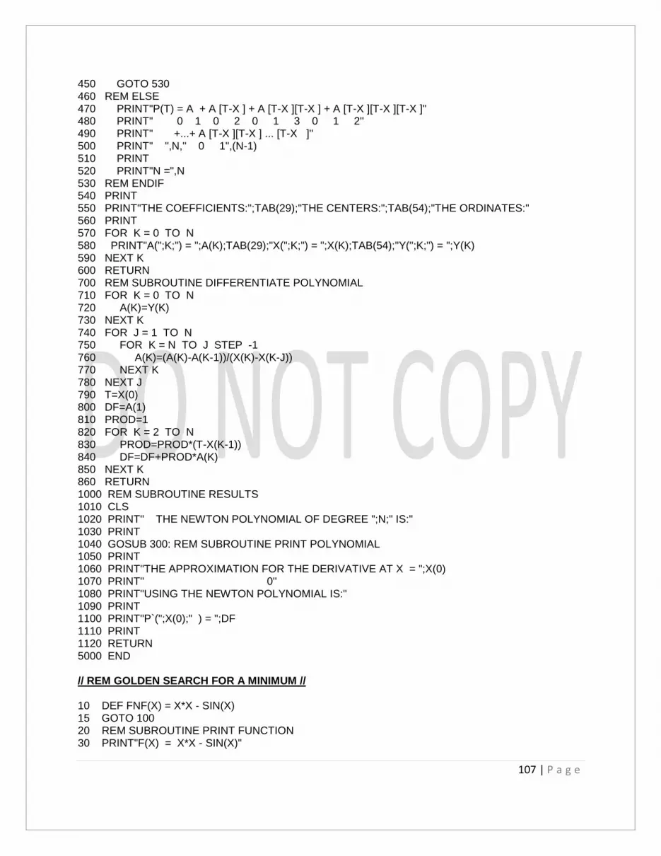
107 | P a g e

450 GOTO 530 460 REM ELSE 470 PRINT"P(T) = A + A [T-X ] + A [T-X ][T-X ] + A [T-X ][T-X ][T-X ]" 480 PRINT" 0 1 0 2 0 1 3 0 1 2" 490 PRINT" +...+ A [T-X ][T-X ] ... [T-X ]" 500 PRINT" ",N," 0 1",(N-1) 510 PRINT 520 PRINT"N =",N 530 REM ENDIF 540 PRINT 550 PRINT"THE COEFFICIENTS:";TAB(29);"THE CENTERS:";TAB(54);"THE ORDINATES:" 560 PRINT 570 FOR K = 0 TO N 580 PRINT"A(";K;") = ";A(K);TAB(29);"X(";K;") = ";X(K);TAB(54);"Y(";K;") = ";Y(K) 590 NEXT K 600 RETURN 700 REM SUBROUTINE DIFFERENTIATE POLYNOMIAL 710 FOR K = 0 TO N 720 A(K)=Y(K) 730 NEXT K 740 FOR J = 1 TO N 750 FOR K = N TO J STEP -1 760 A(K)=(A(K)-A(K-1))/(X(K)-X(K-J)) 770 NEXT K 780 NEXT J 790 T=X(0) 800 DF=A(1) 810 PROD=1 820 FOR K = 2 TO N 830 PROD=PROD*(T-X(K-1)) 840 DF=DF+PROD*A(K) 850 NEXT K 860 RETURN 1000 REM SUBROUTINE RESULTS 1010 CLS 1020 PRINT" THE NEWTON POLYNOMIAL OF DEGREE ";N;" IS:" 1030 PRINT 1040 GOSUB 300: REM SUBROUTINE PRINT POLYNOMIAL 1050 PRINT 1060 PRINT"THE APPROXIMATION FOR THE DERIVATIVE AT X = ";X(0) 1070 PRINT" 0" 1080 PRINT"USING THE NEWTON POLYNOMIAL IS:" 1090 PRINT 1100 PRINT"P`(";X(0);" ) = ";DF 1110 PRINT 1120 RETURN 5000 END // REM GOLDEN SEARCH FOR A MINIMUM // 10 DEF FNF(X) = X*X - SIN(X) 15 GOTO 100 20 REM SUBROUTINE PRINT FUNCTION 30 PRINT"F(X) = X*X - SIN(X)"

108 | P a g e

40 RETURN 100 REM PROGRAM GOLDEN SEARCH 105 DELTA=1E-5 110 EPSILON=1E-5 115 REM CONTINUE 120 GOSUB 200: REM SUBROUTINE INPUTS 125 GOSUB 400: REM SUBROUTINE GOLDEN SEARCH 130 GOSUB 800: REM SUBROUTINE RESULTS 135 PRINT 140 PRINT"WANT TO FIND THE MINIMUM ON ANOTHER INTERVAL ? "; 145 INPUT ANS$ 150 IF ANS$ = "Y" OR ANS$ = "y" THEN GOTO 115 155 GOTO 5000 200 REM SUBROUTINE INPUTS 205 CLS 210 PRINT" GOLDEN SEARCH FOR FINDING THE MINIMUM OF THE" 215 PRINT 220 PRINT"UNIMODAL FUNCTION F(X) OVER THE INTERVAL [A,B]." 225 PRINT 230 PRINT"SEQUENCES {A } AND {B } CONSTRUCTED, WHICH BRACKET THE MINIMUM," 235 PRINT" K K" 240 PRINT 245 PRINT"I.E. A < X < B . TERMINATION OCCURS WHEN B - A < DELTA." 250 PRINT" K MIN K N N" 255 PRINT 260 PRINT"THE GIVEN FUNCTION F(X) IS:" 265 PRINT 270 GOSUB 20: REM SUBROUTINE PRINT FUNCTION 275 PRINT 280 PRINT"ENTER LEFT ENDPOINT A = "; 285 INPUT A 290 A0=A 295 PRINT 300 PRINT"ENTER RIGHT ENDPOINT B = "; 305 INPUT B 310 B0=B 315 RETURN 400 REM SUBROUTINE GOLDEN SEARCH 410 RONE=(SQR(5.0)-1)/2 420 RTWO=RONE*RONE 430 H=B-A 440 YA=FNF(A) 450 YB=FNF(B) 460 C=A+RTWO*H 470 D=A+RONE*H 480 YC=FNF(C) 490 YD=FNF(D) 500 K=1 510 WHILE ABS(YB-YA) > EPSILON OR H > DELTA 520 IF YC < YD THEN 530 ELSE 610 530 B=D 540 YB=YD 550 D=C 560 YD=YC

109 | P a g e

570 H=B-A 580 C=A+RTWO*H 590 YC=FNF(C) 600 GOTO 690 610 REM ELSE 620 A=C 630 YA=YC 640 C=D 650 YC=YD 660 H=B-A 670 D=A+RONE*H 680 YD=FNF(D) 690 REM ENDIF 700 K=K+1 710 WEND 720 P=A 730 YP=YA 740 IF YB < YA THEN 750 ELSE 770 750 P=B 760 YP=YB 770 REM CONTINUE 780 RETURN 800 REM SUBROUTINE RESULTS 805 CLS 810 PRINT" THE GOLDEN SEARCH WAS USED TO FIND THE MINIMUM" 815 PRINT 820 PRINT"OF THE FUNCTION F(X) OVER THE INTERVAL [A,B]." 825 PRINT 830 PRINT 835 PRINT" IT TOOK ";K;" ITERATIONS TO MINIMIZE" 840 PRINT 845 GOSUB 20: REM SUBROUTINE PRINT FUNCTION 850 PRINT 855 PRINT"OVER THE INTERVAL [";A0;",";B0;" ]." 860 PRINT 865 PRINT"THE MINIMUM VALUE F(P)" 870 PRINT 875 PRINT" OCCURS AT P = ";P 880 PRINT 885 H=B-A 890 PRINT" THE ACCURACY IS +-";H 895 PRINT 900 PRINT"THE FUNCTION VALUE IS:" 905 PRINT 910 PRINT"F(";P;" ) = ";FNF(P) 915 RETURN 5000 END // REM NELDER-MEAD METHOD FOR N-DIMENSIONS // 6 GOTO 100 10 REM SUBROUTINE FUNCTION 11 X=P(1) 12 Y=P(2)

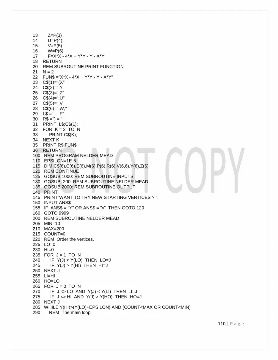
110 | P a g e

13 Z=P(3) 14 U=P(4) 15 V=P(5) 16 W=P(6) 17 F=X*X - 4*X + Y*Y - Y - X*Y 18 RETURN 20 REM SUBROUTINE PRINT FUNCTION 21 N = 2 22 FUN$ ="X*X - 4*X + Y*Y - Y - X*Y" 23 C$(1)="(X" 24 C$(2)=",Y" 25 C$(3)=",Z" 26 C$(4)=",U" 27 C$(5)=",V" 28 C$(6)=",W," 29 L$ =" F" 30 R$ =") = " 31 PRINT L$;C$(1); 32 FOR K = 2 TO N 33 PRINT C$(K); 34 NEXT K 35 PRINT R$;FUN$ 36 RETURN 100 REM PROGRAM NELDER MEAD 110 EPSILON=1E-5 115 DIM C$(6),C(6),E(6),M(6),P(6),R(6),V(6,6),Y(6),Z(6) 120 REM CONTINUE 125 GOSUB 1000: REM SUBROUTINE INPUTS 130 GOSUB 200: REM SUBROUTINE NELDER MEAD 135 GOSUB 2000: REM SUBROUTINE OUTPUT 140 PRINT 145 PRINT"WANT TO TRY NEW STARTING VERTICES ? "; 150 INPUT ANS$ 155 IF ANS$ = "Y" OR ANS$ = "y" THEN GOTO 120 160 GOTO 9999 200 REM SUBROUTINE NELDER MEAD 205 MIN=10 210 MAX=200 215 COUNT=0 220 REM Order the vertices. 225 LO=0 230 HI=0 235 FOR J = 1 TO N 240 IF Y(J) < Y(LO) THEN LO=J 245 IF Y(J) > Y(HI) THEN HI=J 250 NEXT J 255 LI=HI 260 HO=LO 265 FOR J = 0 TO N 270 IF J <> LO AND Y(J) < Y(LI) THEN LI=J 275 IF J <> HI AND Y(J) > Y(HO) THEN HO=J 280 NEXT J 285 WHILE Y(HI)>(Y(LO)+EPSILON) AND (COUNT<MAX OR COUNT<MIN) 290 REM The main loop.

111 | P a g e

295 REM Form new vertices M and R. 300 FOR K = 1 TO N 305 S=0 310 FOR J = 0 TO N 315 S=S+V(J,K) 320 NEXT J 325 M(K)=(S-V(HI,K))/N 330 NEXT K 335 FOR K = 1 TO N 340 R(K)=2*M(K)-V(HI,K) 345 P(K)=R(K) 350 NEXT K 355 GOSUB 10: REM SUBROUTINE FUNCTION 360 YR=F 365 REM Improve the simplex. 370 IF YR < Y(HO) THEN 375 ELSE 525 375 IF Y(LI) < YR THEN 380 ELSE 410 380 REM Replace a vertex. 385 FOR K = 1 TO N 390 V(HI,K)=R(K) 395 NEXT K 400 Y(HI)=YR 405 GOTO 515 410 REM ELSE 415 REM Construct vertex E. 420 FOR K = 1 TO N 425 E(K)=2*R(K)-M(K) 430 P(K)=E(K) 435 NEXT K 440 GOSUB 10: REM SUBROUTINE FUNCTION 445 YE=F 450 IF YE < Y(LI) THEN 455 ELSE 480 455 FOR K = 1 TO N 460 V(HI,K)=E(K) 465 NEXT K 470 Y(HI)=YE 475 GOTO 510 480 REM ELSE 485 REM Replace a vertex. 490 FOR K = 1 TO N 495 V(HI,K)=R(K) 500 NEXT K 505 Y(HI)=YR 510 REM ENDIF 515 REM ENDIF 520 GOTO 700 525 REM ELSE 530 IF YR < Y(HI) THEN 535 ELSE 560 535 REM Replace a vertex. 540 FOR K = 1 TO N 545 V(HI,K)=R(K) 550 NEXT K 555 Y(HI)=YR 560 REM CONTINUE

112 | P a g e

565 REM Construct vertex C. 570 FOR K = 1 TO N 575 C(K)=(V(HI,K)+M(K))/2 580 P(K)=C(K) 585 NEXT K 590 GOSUB 10: REM SUBROUTINE FUNCTION 595 YC=F 600 IF YC < Y(HI) THEN 605 ELSE 630 605 FOR K = 1 TO N 610 V(HI,K)=C(K) 615 NEXT K 620 Y(HI)=YC 625 GOTO 695 630 REM ELSE 635 REM Shrink the simplex. 640 FOR J = 0 TO N 645 IF J <> LO THEN 650 ELSE 685 650 FOR K = 1 TO N 655 V(J,K)=(V(J,K)+V(LO,K))/2 660 Z(K)=V(J,K) 665 P(K) = Z(K) 670 NEXT K 675 GOSUB 10: REM SUBROUTINE FUNCTION 680 Y(J)=F 685 REM CONTINUE 690 NEXT J 695 REM ENDIF 700 REM ENDIF 705 COUNT=COUNT+1 710 REM Order the vertices. 715 LO=0 720 HI=0 725 FOR J = 1 TO N 730 IF Y(J) < Y(LO) THEN LO=J 735 IF Y(J) > Y(HI) THEN HI=J 740 NEXT J 745 LI=HI 750 HO=LO 755 FOR J = 0 TO N 760 IF J <> LO AND Y(J) < Y(LI) THEN LI=J 765 IF J <> HI AND Y(J) > Y(HO) THEN HO=J 770 NEXT J 775 WEND 780 REM Determine the size of the simplex. 785 NORM=0 790 FOR J = 0 TO N 795 S=0 800 FOR K = 1 TO N 805 S=S+(V(LO,K)-V(J,K))*(V(LO,K)-V(J,K)) 810 NEXT K 815 IF S > NORM THEN NORM=S 820 NEXT J 825 NORM=SQR(NORM) 830 RETURN

113 | P a g e

1000 REM SUBROUTINE INPUTS 1010 CLS 1020 PRINT" THE NELDER-MEAD SIMPLEX METHOD OR `POLYTOPE METHOD` IS" 1030 PRINT 1040 PRINT"USED FOR FINDING THE MINIMUM OF THE FUNCTION F(V)" 1050 PRINT 1060 PRINT"FOR CONVENIENCE, THE FUNCTION F(V) CAN BE EXPRESSED USING" 1070 PRINT 1080 PRINT"THE VARIABLES X = v , Y = v , Z = v , U = v , V = v , W = v ." 1090 PRINT" 1 2 3 4 5 6 " 1100 PRINT 1110 GOSUB 20: REM SUBROUTINE PRINT FUNCTION 1120 PRINT 1130 PRINT"YOU MUST SUPPLY",N+1," LINEARLY INDEPENDENT" 1140 PRINT 1150 IF N = 2 THEN 1160 ELSE 1190 1160 PRINT"STARTING POINTS V = (v ,v ) FOR J=0,1,3" 1170 PRINT" J J,1 J,2" 1180 GOTO 1280 1190 REM ELSE 1200 IF N = 3 THEN 1210 ELSE 1240 1210 PRINT"STARTING POINTS V = (v ,v ,v ) FOR J=0,1,3,4" 1220 PRINT" J J,1 J,2 J,3" 1230 GOTO 1280 1240 REM ELSE 1250 PRINT"STARTING POINTS V = (v ,v ,...,v ) FOR J=0,1,...,N" 1260 PRINT" J J,1 J,2 J,N" 1270 PRINT"WHERE N =",N 1280 REM ENDIF 1290 FOR J = 0 TO N 1300 PRINT 1310 PRINT"GIVE COORDINATES OF POINT V" 1320 PRINT" ",J 1330 FOR K = 1 TO N 1340 PRINT"V(";J;",";K;") = "; 1350 INPUT V(J,K) 1360 Z(K)=V(J,K) 1370 NEXT K 1380 FOR K = 1 TO N 1381 P(K) = Z(K) 1382 NEXT K 1383 GOSUB 10: REM SUBROUTINE FUNCTION 1384 Y(J)=F 1390 NEXT J 1400 RETURN 2000 REM SUBROUTINE OUTPUT 2010 CLS 2020 PRINT 2030 PRINT" THE NELDER-MEAD METHOD WAS USED TO FIND THE MINIMUM OF THE FUNCTION" 2040 PRINT 2050 GOSUB 20: REM SUBROUTINE PRINT FUNCTION 2060 PRINT

114 | P a g e

2070 PRINT"IT TOOK ";COUNT;" ITERATIONS TO FIND AN APPROXIMATION FOR" 2080 PRINT 2090 IF N = 2 THEN 2100 ELSE 2130 2100 PRINT"THE COORDINATES OF THE LOCAL MINIMUM P = (p ,p )" 2110 PRINT" 1 2" 2120 GOTO 2220 2130 REM ELSE 2140 IF N = 3 THEN 2150 ELSE 2180 2150 PRINT"THE COORDINATES OF THE LOCAL MINIMUM P = (p ,p ,p )" 2160 PRINT" 1 2 3" 2170 GOTO 2220 2180 REM ELSE 2190 PRINT"THE COORDINATES OF THE LOCAL MINIMUM P = (p ,p ,...,p )" 2200 PRINT" 1 2 N" 2210 PRINT"WHERE N = ";N 2220 REM ENDIF 2230 FOR K = 1 TO N 2240 PRINT"P(";K;") = ";V(LO,K) 2250 NEXT K 2260 PRINT 2270 PRINT"THE MAXIMUM DISTANCE TO THE OTHER VERTICES OF THE SIMPLEX IS" 2280 PRINT 2290 PRINT" DP = ";NORM 2300 PRINT 2310 PRINT"THE FUNCTION VALUE AT THE MINIMUM POINT IS" 2320 PRINT 2330 PRINT"F(P) = ";Y(LO) 2340 PRINT 2350 PRINT" DF = ";Y(HI)-Y(LO);" IS AN ESTIMATE FOR THE ACCURACY." 2360 RETURN 9999 END // REM SEARCH FOR A LOCAL MINIMUM USING QUADRATIC INTERPOLATION // 10 DEF FNF(X) = X*X*X-X 12 DEF FNF1(X) = 3*X*X-1 14 GOTO 22 16 REM SUBROUTINE PRINT FUNCTION 18 PRINT"F(X) = X*X*X-X" 20 RETURN 22 REM PROGRAM MINIMIZATION USING QUADRATIC INTERPOLATION 24 DELTA=.00001 26 EPSILON=.0000001 28 JMAX=50 30 KMAX= 50 32 REM CONTINUE 34 GOSUB 50: REM SUBROUTINE INPUTS 36 GOSUB 100: REM SUBROUTINE QUADRATIC MINIMIZATION 38 GOSUB 1000: REM SUBROUTINE RESULTS 40 PRINT 42 PRINT"WANT TO TRY ANOTHER STARTING POINT ? "; 44 INPUT ANS$ 46 IF ANS$ = "Y" OR ANS$ = "y" THEN GOTO 32 48 GOTO 1590

115 | P a g e

50 REM SUBROUTINE INPUTS 52 PRINT 54 PRINT" THE QUADRATIC SEARCH METHOD IS USED" 56 PRINT 58 PRINT"TO FIND A LOCAL MINIMUM OF THE FUNCTION: " 60 PRINT 62 GOSUB 16: REM SUBROUTINE PRINT FUNCTION 64 PRINT 66 PRINT"ONE INITIAL APPROXIMATION P0 IS NEEDED." 68 PRINT 70 PRINT"ENTER P0 = "; 72 INPUT P0 74 POLD=P0 76 PRINT 78 RETURN 100 REM SUBROUTINE QUADRATIC MINIMIZATION 110 BIG=1E+09 120 K=0 130 ERRER=1 140 COND=0 150 COUNT=0 160 H=1 170 IF ABS(P0) > 10000 THEN H=ABS(P0)/10000 180 WHILE K<KMAX AND ERRER>EPSILON AND COND<>5 190 IF FNF1(P0) > 0 THEN H=-ABS(H) 200 P1=P0+H 210 P2=P0+2*H 220 PMIN= P0 230 Y0=FNF(P0) 240 Y1=FNF(P1) 250 Y2=FNF(P2) 260 YMIN=Y0 270 COND=0 280 J=0 290 WHILE J<JMAX AND ABS(H)>DELTA AND COND=0 300 IF Y0 <= Y1 THEN 310 ELSE 370 310 P2=P1 320 Y2=Y1 330 H=H/2 340 P1=P0+H 350 Y1=FNF(P1) 360 GOTO 480 370 REM ELSE 380 IF Y2 < Y1 THEN 390 ELSE 450 390 P1=P2 400 Y1=Y2 410 H=2*H 420 P2=P0+2*H 430 Y2=FNF(P2) 440 GOTO 470 450 REM ELSE 460 COND=-1 470 REM ENDIF 480 REM ENDIF

116 | P a g e

490 J=J+1 500 COUNT=COUNT+J 510 IF ABS(H) > BIG OR ABS(P0) > BIG THEN COND=5 520 WEND 530 IF COND = 5 THEN 540 ELSE 570 540 PMIN=P1 550 YMIN=FNF(P1) 560 GOTO 890 570 REM ENDIF 580 D=4*Y1-2*Y0-2*Y2 590 IF D < 0 THEN 600 ELSE 620 600 HMIN=H*(4*Y1-3*Y0-Y2)/D 610 GOTO 650 620 REM ELSE 630 HMIN=H/3 640 COND=4 650 REM ENDIF 660 PMIN=P0+HMIN 670 YMIN=FNF(PMIN) 680 H=ABS(H) 690 H0=ABS(HMIN) 700 H1=ABS(HMIN-H) 710 H2=ABS(HMIN-2*H) 720 IF H0 < H THEN H=H0 730 IF H1 < H THEN H=H1 740 IF H2 < H THEN H=H2 750 IF H = 0 THEN H=HMIN 760 IF H < DELTA THEN COND=1 770 IF ABS(H) > BIG OR ABS(PMIN) > BIG THEN COND=5 780 E0=ABS(Y0-YMIN) 790 E1=ABS(Y1-YMIN) 800 E2=ABS(Y2-YMIN) 810 IF E0 <> 0 AND E0 < ERRER THEN ERRER=E0 820 IF E1 <> 0 AND E1 < ERRER THEN ERRER=E1 830 IF E2 <> 0 AND E2 < ERRER THEN ERRER=E2 840 IF E0 = 0 AND E1 = 0 AND E2 = 0 THEN ERRER=0 850 IF ERRER < EPSILON THEN COND=2 860 P0=PMIN 870 K=K+1 880 COUNT=COUNT+K 890 REM CONTINUE 900 WEND 910 IF COND = 2 AND H < DELTA THEN COND=3 920 RETURN 1000 REM SUBROUTINE RESULTS 1010 CLS 1020 PRINT" THE QUADRATIC SEARCH METHOD WAS USED " 1030 PRINT 1040 PRINT"TO FIND A LOCAL MINIMUM OF THE FUNCTION: " 1050 PRINT 1060 GOSUB 16: REM SUBROUTINE PRINT FUNCTION 1070 PRINT 1080 PRINT"STARTING WITH THE APPROXIMATION P0 =",POLD 1090 PRINT

117 | P a g e

1100 PRINT"AFTER ",COUNT," ITERATIONS AN APPROXIMATION FOR THE MINIMUM IS:" 1110 PRINT 1120 PRINT" P =",PMIN 1130 PRINT 1140 PRINT" DP =",ABS(H)," IS THE ESTIMATED ACCURACY FOR P." 1150 PRINT 1160 PRINT" F(",PMIN," ) =",YMIN 1170 PRINT 1180 IF COND = 0 THEN 1190 ELSE 1230 1190 PRINT"CONVERGENCE IS DOUBTFUL BECAUSE THE" 1200 PRINT 1210 PRINT"MAXIMUM NUMBER OF ITERATIONS WAS EXCEEDED." 1220 GOTO 1560 1230 REM ELSE 1240 IF COND = 1 THEN 1250 ELSE 1290 1250 PRINT"CONVERGENCE HAS BEEN ACHIEVED BECAUSE " 1260 PRINT 1270 PRINT"CONSECUTIVE ABSCISSAS ARE CLOSER THAN ",DELTA 1280 GOTO 1560 1290 REM ELSE 1300 IF COND = 2 THEN 1310 ELSE 1350 1310 PRINT"CONVERGENCE HAS BEEN ACHIEVED BECAUSE " 1320 PRINT 1330 PRINT"CONSECUTIVE ORDINATES ARE CLOSER THAN ",EPSILON 1340 GOTO 1560 1350 REM ELSE 1360 IF COND = 3 THEN 1370 ELSE 1430 1370 PRINT"CONVERGENCE HAS BEEN ACHIEVED BECAUSE" 1380 PRINT 1390 PRINT"CONSECUTIVE ABSCISSAS ARE CLOSER THAN ",H 1400 PRINT 1410 PRINT"CONSECUTIVE ORDINATES ARE CLOSER THAN ",ERRER 1420 GOTO 1560 1430 REM ELSE 1440 IF COND = 4 THEN 1450 ELSE 1500 1450 PRINT"CONVERGENCE IS DOUBTFUL BECAUSE DIVISION BY ZERO WAS ENCOUNTERED." 1460 IF ERRER < EPSILON/100 THEN 1470 ELSE 1480 1470 PRINT"HOWEVER, CONSECUTIVE ORDINATES ARE CLOSE." 1480 REM CONTINUE 1490 GOTO 1560 1500 REM ELSE 1510 IF COND = 5 THEN 1520 ELSE 1570 1520 PRINT"CONVERGENCE IS DOUBTFUL, H IS TOO LARGE, H =",H 1530 PRINT 1540 PRINT"PERHAPS A DIFFERENT STARTING VALUE SHOULD BE USED." 1550 PRINT 1560 PRINT"IT IS POSSIBLE THAT THERE IS NO LOCAL MINIMUM." 1570 REM ENDIF 1580 RETURN 1590 END

118 | P a g e

// REM STEEPEST DESCENT GRDIENT METHOD // 6 GOTO 50 10 REM SUBROUTINE FUNCTION 11 X=P(1) 12 Y=P(2) 13 Z=P(3) 14 U=P(4) 15 V=P(5) 16 W=P(6) 17 F=X*X - 4*X + Y*Y - Y - X*Y 18 RETURN 20 REM SUBROUTINE PRINT FUNCTION 21 N = 2 22 FUN$ ="X*X - 4*X + Y*Y - Y - X*Y" 23 C$(1)="(X" 24 C$(2)=",Y" 25 C$(3)=",Z" 26 C$(4)=",U" 27 C$(5)=",V" 28 C$(6)=",W," 29 L$ =" F" 30 R$ =") = " 31 PRINT L$;C$(1); 32 FOR K = 2 TO N 33 PRINT C$(K); 34 NEXT K 35 PRINT R$;FUN$ 36 RETURN 50 REM PROGRAM GRADIENT METHOD 54 JMAX=200 56 MAX=50 58 DELTA=1E-5 60 EPSILON=1E-7 62 DIM G(6),P(6),P0(6),P1(6),P2(6),PMIN(6),S(6),Z(6) 64 REM CONTINUE 66 GOSUB 1000: REM SUBROUTINE INPUTS 68 GOSUB 700: REM SUBROUTINE GRADIENT SEARCH 70 GOSUB 2000: REM SUBROUTINE RESULTS 72 PRINT 74 PRINT"WANT TO TRY ANOTHER STARTING POINT ? "; 76 INPUT ANS$ 78 IF ANS$ = "Y" OR ANS$ = "y" THEN GOTO 64 80 GOTO 5000 100 REM SUBROUTINE GRADIENT VECTOR 105 X=P(1) 110 Y=P(2) 115 Z=P(3) 120 U=P(4) 125 V=P(5) 130 W=P(6) 135 G(1)=2*X-4-Y 140 G(2)=2*Y-1-X 145 SUM=0

119 | P a g e

150 FOR K = 1 TO N 155 SUM=SUM+G(K)*G(K) 160 NEXT K 165 LENGTH=SQR(SUM) 170 IF LENGTH = 0 THEN LENGTH=1 175 FOR K = 1 TO N 180 G(K)=-G(K) 185 S(K)=G(K)/LENGTH 190 NEXT K 195 RETURN 200 REM SUBROUTINE QUADRATIC MINIMIZATION 205 BIG=100000000 210 FOR K = 1 TO N 215 P1(K)=P0(K)+H*S(K) 220 P(K)=P1(K) 225 NEXT K 230 GOSUB 10: REM SUBROUTINE FUNCTION 235 Y1=F 240 FOR K = 1 TO N 245 P2(K)=P0(K)+2*H*S(K) 250 P(K)=P2(K) 255 NEXT K 260 GOSUB 10: REM SUBROUTINE FUNCTION 265 Y2=F 270 COND=0 275 J=0 280 WHILE J < JMAX AND COND = 0 285 SUM=0 290 FOR K = 1 TO N 295 SUM=SUM+P0(K)*P0(K) 300 NEXT K 305 LENGTH=SQR(SUM) 310 IF Y0 <= Y1 THEN 315 ELSE 375 315 FOR K = 1 TO N 320 P2(K)=P1(K) 325 NEXT K 330 Y2=Y1 335 H=H/2 340 FOR K = 1 TO N 345 P1(K)=P0(K)+H*S(K) 350 P(K)=P1(K) 355 NEXT K 360 GOSUB 10: REM SUBROUTINE FUNCTION 365 Y1=F 370 GOTO 460 375 REM ELSE 380 IF Y2 <= Y1 THEN 385 ELSE 445 385 FOR K = 1 TO N 390 P1(K)=P2(K) 395 NEXT K 400 Y1=Y2 405 H=2*H 410 FOR K = 1 TO N 415 P2(K)=P0(K)+2*H*S(K)

120 | P a g e

420 P(K)=P2(K) 425 NEXT K 430 GOSUB 10: REM SUBROUTINE FUNCTION 435 Y2=F 440 GOTO 455 445 REM ELSE 450 COND=-1 455 REM ENDIF 460 REM ENDIF 465 J=J+1 470 IF H < DELTA THEN COND=1 475 IF ABS(H) > BIG OR LENGTH > BIG THEN COND=5 480 WEND 485 COUNT=COUNT+J 490 IF COND = 5 THEN 495 ELSE 520 495 FOR K = 1 TO N 500 PMIN(K)=P1(K) 505 NEXT K 510 YMIN=Y1 515 GOTO 680 520 REM CONTINUE 525 D=4*Y1-2*Y0-2*Y2 530 IF D < 0 THEN 535 ELSE 545 535 HMIN=H*(4*Y1-3*Y0-Y2)/D 540 GOTO 560 545 REM ELSE 550 COND=4 555 HMIN=H/3 560 REM ENDIF 565 FOR K = 1 TO N 570 PMIN(K)=P0(K)+HMIN*S(K) 575 P(K)=PMIN(K) 580 NEXT K 585 GOSUB 10: REM SUBROUTINE FUNCTION 590 YMIN=F 595 H0=ABS(HMIN) 600 H1=ABS(HMIN-H) 605 H2=ABS(HMIN-2*H) 610 IF H0 < H THEN H=H0 615 IF H1 < H THEN H=H1 620 IF H2 < H THEN H=H2 625 IF H = 0 THEN H=HMIN 630 IF H < DELTA THEN COND=1 635 E0=ABS(Y0-YMIN) 640 E1=ABS(Y1-YMIN) 645 E2=ABS(Y2-YMIN) 650 IF E0 <> 0 AND E0 < ERRER THEN ERRER=E0 655 IF E1 <> 0 AND E1 < ERRER THEN ERRER=E1 660 IF E2 <> 0 AND E2 < ERRER THEN ERRER=E2 665 IF E0 = 0 AND E1 = 0 AND E2 = 0 THEN ERRER=0 670 IF ERRER < EPSILON THEN COND=2 675 IF COND = 2 AND H < DELTA THEN COND=3 680 REM CONTINUE 685 RETURN

121 | P a g e

700 REM SUBROUTINE GRADIENT SEARCH 705 H=1 710 SUM=0 715 FOR K = 1 TO N 720 SUM=SUM+P0(K)*P0(K) 725 NEXT K 730 LENGTH=SQR(SUM) 735 IF LENGTH > 10000 THEN H=LENGTH/10000 740 ERRER=1 745 COUNT=0 750 COND=0 755 WHILE COUNT<MAX AND COND<>5 AND (H>DELTA OR ERRER>EPSILON) 760 GOSUB 100: REM SUBROUTINE GRADIENT VECTOR 765 GOSUB 200: REM SUBROUTINE QUADRATIC MINIMIZATION 770 FOR K = 1 TO N 775 P0(K)=PMIN(K) 780 NEXT K 785 Y0=YMIN 790 COUNT=COUNT+1 795 WEND 800 RETURN 1000 REM SUBROUTINE INPUTS 1010 CLS 1020 PRINT" THE GRADIENT METHOD OR `METHOD OF STEEPEST DESCENT' IS USED FOR FINDING" 1030 PRINT 1040 PRINT"THE MINIMUM OF THE FUNCTION F(P) WHERE P = (p ,p ,...,p ) AND N<=6." 1050 PRINT" 1 2 N" 1060 PRINT 1070 PRINT"FOR CONVENIENCE, THE FUNCTION F(P) CAN BE EXPRESSED USING THE VARIABLES" 1080 PRINT 1090 PRINT"X = p , Y = p , Z = p , U = p , V = p , W = p ." 1100 PRINT" 1 2 3 4 5 6 " 1110 PRINT 1120 PRINT" THE FUNCTION TO BE MINIMIZED IS:" 1130 PRINT 1140 GOSUB 20: REM SUBROUTINE PRINT FUNCTION 1150 PRINT 1160 IF N = 2 THEN 1170 ELSE 1200 1170 PRINT"GIVE THE STARTING POINT P = (p ,p )" 1180 PRINT" 1 2" 1190 GOTO 1290 1200 REM ELSE 1210 IF N = 3 THEN 1210 ELSE 1240 1220 PRINT"GIVE THE STARTING POINT P = (p ,p ,p )" 1230 PRINT" 1 2 3" 1240 GOTO 1290 1250 REM ELSE 1260 PRINT"GIVE THE STARTING POINT P = (p ,p ,...,p )" 1270 PRINT" 1 2 N" 1280 PRINT"WHERE N=",N 1290 REM ENDIF 1300 PRINT

122 | P a g e

1310 FOR K = 1 TO N 1320 PRINT"P(";K;") = "; 1330 INPUT P0(K) 1340 P(K)=P0(K) 1350 NEXT K 1360 GOSUB 10: REM SUBROUTINE FUNCTION 1370 Y0=F 1380 RETURN 2000 REM SUBROUTINE RESULTS 2005 CLS 2010 PRINT" THE GRADIENT SEARCH METHOD WAS USED TO FIND THE MINIMUM OF" 2020 PRINT 2030 GOSUB 20: REM SUBROUTINE PRINT FUNCTION 2035 PRINT 2040 PRINT COUNT;" ITERATIONS WERE REQUIRED" 2050 PRINT 2060 FOR K = 1 TO N 2070 PRINT"P(";K;") = ";PMIN(K) 2080 NEXT K 2090 PRINT 2100 PRINT" DP = ";H;" IS AN ESTIMATE FOR THE ACCURACY." 2110 PRINT 2120 PRINT"THE MINIMUM VALUE OF THE FUNCTION IS" 2130 PRINT 2140 PRINT"F(P) = ";YMIN 2150 PRINT 2160 PRINT" DF = ";ERRER;" IS AN ESTIMATE FOR THE ACCURACY." 2170 PRINT 2180 IF COND = 0 THEN 2190 ELSE 2200 2190 PRINT"CONVERGENCE IS DOUBTFUL BECAUSE THE" 2200 PRINT"MAXIMUM NUMBER OF ITERATIONS WAS EXCEEDED." 2210 GOTO 2470 2220 REM ELSE 2230 IF COND = 1 THEN 2240 ELSE 2270 2240 PRINT"CONVERGENCE HAS BEEN ACHIEVED BECAUSE " 2250 PRINT"CONSECUTIVE POINTS ARE CLOSER THAN ";H 2260 GOTO 2470 2270 REM ELSE 2280 IF COND = 2 THEN 2290 ELSE 2320 2290 PRINT"CONVERGENCE HAS BEEN ACHIEVED BECAUSE " 2300 PRINT"CONSECUTIVE FUNCTION VALUES DIFFER BY ";ERRER 2310 GOTO 2470 2320 REM ELSE 2330 IF COND = 3 THEN 2340 ELSE 2380 2340 PRINT"CONVERGENCE HAS BEEN ACHIEVED BECAUSE " 2350 PRINT"CONSECUTIVE POINTS ARE CLOSER THAN ";H 2360 PRINT"CONSECUTIVE FUNCTION VALUES DIFFER BY ";ERRER 2370 GOTO 2470 2380 REM ELSE 2390 IF COND = 4 THEN 2400 ELSE 2430 2400 PRINT"CONVERGENCE IS DOUBTFUL BECAUSE DIVISION BY ZERO WAS ENCOUNTERED." 2410 IF ERRER < EPSILON/100 THEN PRINT"HOWEVER, CONSECUTIVE POINTS ARE CLOSE." 2420 GOTO 2470

123 | P a g e

2430 REM ELSE 2440 IF COND = 5 THEN 2450 ELSE 2470 2450 PRINT"CONVERGENCE IS DOUBTFUL, H IS TOO LARGE, H = ";H 2460 PRINT"IT IS POSSIBLE THAT THERE IS NO LOCAL MINIMUM." 2470 REM ENDIF 2480 RETURN 2490 END 5000 END // REM COMPOSITE TRAPEZOIDAL RULE // 10 DEF FNF(X) = X/(1+X*X) 15 GOTO 100 20 REM SUBROUTINE PRINT FUNCTION 30 PRINT "X/(1+X*X)"; 40 RETURN 100 REM PROGRAM TRAPEZOIDAL RULE 110 REM CONTINUE 120 GOSUB 1000: REM SUBROUTINE INPUTS 130 GOSUB 200: REM SUBROUTINE TRAPEZOIDAL RULE 140 GOSUB 2000: REM SUBROUTINE RESULTS 150 PRINT"WANT TO TRY ANOTHER INTERVAL ? <Y/N> "; 160 INPUT ANS$ 170 IF ANS$ = "Y" OR ANS$ = "y" THEN GOTO 110 180 GOTO 5000 200 REM SUBROUTINE TRAPEZOIDAL RULE 210 H=(B-A)/M 220 SUM=0 230 FOR K = 1 TO M-1 240 X=A+H*K 250 SUM=SUM+FNF(X) 260 NEXT K 270 SUM=H*(FNF(A)+FNF(B)+2*SUM)/2 280 TRULE=SUM 290 RETURN 1000 REM SUBROUTINE INPUTS 1010 CLS 1020 PRINT" THE TRAPEZOIDAL RULE IS USED TO COMPUTE AN APPROXIMATION" 1030 PRINT 1040 PRINT"FOR THE VALUE OF THE DEFINITE INTEGRAL:" 1050 PRINT 1060 PRINT 1070 PRINT" B" 1080 PRINT" /" 1090 PRINT" | "; 1100 GOSUB 20: REM SUBROUTINE PRINT FUNCTION 1110 PRINT " DX" 1120 PRINT" /" 1130 PRINT" A" 1140 PRINT 1150 PRINT 1160 PRINT"ENTER THE LEFT ENDPOINT A = "; 1170 INPUT A 1180 PRINT

124 | P a g e

1190 PRINT"ENTER THE RIGHT ENDPOINT B = "; 1200 INPUT B 1210 PRINT 1220 PRINT" NUMBER OF SUBINTERVALS M = "; 1230 INPUT M 1240 PRINT 1250 RETURN 2000 REM SUBROUTINE RESULTS 2010 CLS 2020 PRINT" ";B 2030 PRINT" /" 2040 PRINT" |" 2050 PRINT" | "; 2060 GOSUB 20: REM SUBROUTINE PRINT FUNCTION 2070 PRINT " DX ~ ";TRULE 2080 PRINT" |" 2090 PRINT" /" 2100 PRINT" ";A 2110 PRINT 2120 PRINT 2130 PRINT"AN APPROXIMATE VALUE FOR THE DEFINITE INTEGRAL OF" 2140 PRINT 2150 PRINT 2160 PRINT"F(X) = "; 2170 GOSUB 20: REM SUBROUTINE PRINT FUNCTION 2180 PRINT 2190 PRINT 2200 PRINT"TAKEN OVER [";A;" , ";B;" ] WAS FOUND." 2210 PRINT 2220 PRINT"WHEN ";M;" SUBINTERVALS ARE USED," 2230 PRINT 2240 PRINT"THE TRAPEZOIDAL RULE APPROXIMATION IS ";TRULE 2250 PRINT 2260 RETURN 5000 END // REM COMPOSITE SIMPSON’S RULE // 10 DEF FNF(X) = X/(1+X*X) 15 GOTO 100 20 REM SUBROUTINE PRINT FUNCTION 30 PRINT "X/(1+X*X)"; 40 RETURN 100 REM PROGRAM SIMPSON`S RULE 110 REM CONTINUE 120 GOSUB 1000: REM SUBROUTINE INPUTS 130 GOSUB 200: REM SUBROUTINE SIMPSON`S RULE 140 GOSUB 2000: REM SUBROUTINE RESULTS 150 PRINT"WANT TO TRY ANOTHER INTERVAL ? <Y/N> "; 160 INPUT ANS$ 170 IF ANS$ = "Y" OR ANS$ = "y" THEN GOTO 110 180 GOTO 5000 200 REM SUBROUTINE SIMPSON`S RULE 210 H=(B-A)/(2*M)

125 | P a g e

220 SUMEVEN=0 230 FOR K = 1 TO M-1 240 X=A+H*2*K 250 SUMEVEN=SUMEVEN+FNF(X) 260 NEXT K 270 SUMODD=0 280 FOR K = 1 TO M 290 X=A+H*(2*K-1) 300 SUMODD=SUMODD+FNF(X) 310 NEXT K 320 SUM=H*(FNF(A)+FNF(B)+2*SUMEVEN+4*SUMODD)/3 330 SRULE=SUM 340 RETURN 1000 REM SUBROUTINE INPUTS 1010 CLS 1020 PRINT" SIMPSON`S RULE IS USED TO COMPUTE AN APPROXIMATION" 1030 PRINT 1040 PRINT"FOR THE VALUE OF THE DEFINITE INTEGRAL:" 1050 PRINT 1060 PRINT 1070 PRINT" B" 1080 PRINT" /" 1090 PRINT" | "; 1100 GOSUB 20: REM SUBROUTINE PRINT FUNCTION 1110 PRINT " DX" 1120 PRINT" /" 1130 PRINT" A" 1140 PRINT 1150 PRINT 1160 PRINT"ENTER THE LEFT ENDPOINT A = "; 1170 INPUT A 1180 PRINT 1190 PRINT"ENTER THE RIGHT ENDPOINT B = "; 1200 INPUT B 1210 PRINT 1220 PRINT"THE NUMBER OF SUBINTERVALS USED IS 2*M = " 1225 PRINT" ENTER THE NUMBER M = "; 1230 INPUT M 1240 PRINT 1250 RETURN 2000 REM SUBROUTINE RESULTS 2010 CLS 2020 PRINT" ";B 2030 PRINT" /" 2040 PRINT" |" 2050 PRINT" | "; 2060 GOSUB 20: REM SUBROUTINE PRINT FUNCTION 2070 PRINT " DX ~ ";SRULE 2080 PRINT" |" 2090 PRINT" /" 2100 PRINT" ";A 2110 PRINT 2120 PRINT 2130 PRINT"AN APPROXIMATE VALUE FOR THE DEFINITE INTEGRAL OF"

126 | P a g e

2140 PRINT 2150 PRINT 2160 PRINT"F(X) = "; 2170 GOSUB 20: REM SUBROUTINE PRINT FUNCTION 2180 PRINT 2190 PRINT 2200 PRINT"TAKEN OVER [";A;" , ";B;" ] WAS FOUND." 2210 PRINT 2220 PRINT"SINCE M = ";M;"; THERE WERE ";2*M;" SUBINTERVALS." 2230 PRINT 2240 PRINT"THE SIMPSON`S RULE APPROXIMATION IS ";SRULE 2250 PRINT 2260 RETURN 5000 END // REM ROMBERG INTEGRATION // 10 DEF FNF(X) = SIN(X) 15 GOTO 100 20 REM SUBROUTINE PRINT FUNCTION 30 PRINT "SIN(X)"; 40 RETURN 100 REM PROGRAM ROMBERG 102 MAXN=12 104 TOL=1E-6 106 DIM R(12,12) 110 REM CONTINUE 120 GOSUB 1000: REM SUBROUTINE INPUTS 130 GOSUB 200: REM SUBROUTINE ROMBERG 140 GOSUB 2000: REM SUBROUTINE RESULTS 150 PRINT"WANT TO TRY ANOTHER INTERVAL ? <Y/N> "; 160 INPUT ANS$ 170 IF ANS$ = "Y" OR ANS$ = "y" THEN GOTO 110 180 GOTO 5000 200 REM SUBROUTINE ROMBERG 210 MAXN=12 220 MIN=4 230 M=1 240 H=B-A 250 NEAR=1 260 J=0 270 R(0,0)=H*(FNF(A)+FNF(B))/2 280 WHILE (NEAR > TOL AND J < MAXN) OR J < MIN 290 J=J+1 300 REM Trapezoidal Rule 310 H=H/2 320 SUM=0 330 FOR P = 1 TO M 340 X=A+H*(2*P-1) 350 SUM=SUM+FNF(X) 360 NEXT P 370 R(J,0)=H*SUM+R(J-1,0)/2 380 M=2*M 390 REM Extrapolation

127 | P a g e

400 FOR K = 1 TO J 410 R(J,K)=R(J,K-1)+(R(J,K-1)-R(J-1,K-1))/(4.0^K-1) 420 NEXT K 430 NEAR=ABS(R(J-1,J-1)-R(J,J)) 440 WEND 450 RRULE=R(J,J) 460 RETURN 1000 REM SUBROUTINE INPUTS 1010 CLS 1020 PRINT"ROMBERG INTEGRATION IS PERFORMED TO FIND AN APPROXIMATION" 1030 PRINT 1040 PRINT"FOR THE VALUE OF THE DEFINITE INTEGRAL:" 1050 PRINT 1060 PRINT 1070 PRINT" B" 1080 PRINT" /" 1090 PRINT" | "; 1100 GOSUB 20: REM SUBROUTINE PRINT FUNCTION 1110 PRINT " DX" 1120 PRINT" /" 1130 PRINT" A" 1140 PRINT 1150 PRINT 1160 PRINT"ENTER THE LEFT ENDPOINT A = "; 1170 INPUT A 1180 PRINT 1190 PRINT"ENTER THE RIGHT ENDPOINT B = "; 1200 INPUT B 1210 PRINT 1220 PRINT"THE NUMBER OF SUBINTERVALS USED IS 2*M = " 1225 PRINT" ENTER THE NUMBER M = "; 1230 INPUT M 1240 PRINT 1250 RETURN 2000 REM SUBROUTINE RESULTS 2010 CLS 2020 PRINT" ";B 2030 PRINT" /" 2040 PRINT" |" 2050 PRINT" | "; 2060 GOSUB 20: REM SUBROUTINE PRINT FUNCTION 2070 PRINT " DX ~ ";RRULE 2080 PRINT" |" 2090 PRINT" /" 2100 PRINT" ";A 2110 PRINT 2120 PRINT 2130 PRINT"THE DIAGONAL ELEMENTS IN THE ROMBERG TABLE ARE:" 2140 IF J<=5 THEN PRINT 2150 FOR K = 0 TO J STEP 2 2160 IF K < J THEN 2170 ELSE 2180 2170 PRINT "R(";K;",";K;") = ";R(K,K);" "; 2175 PRINT "R(";K+1;",";K+1;") = ";R(K+1,K+1) 2176 GOTO 2200

128 | P a g e

2180 REM ELSE 2190 PRINT "R(";K;",";K;") = ";R(K,K) 2200 REM ENDIF 2210 NEXT K 2220 IF J<=7 THEN PRINT 2230 PRINT"AN APPROXIMATE VALUE FOR THE DEFINITE INTEGRAL OF" 2240 PRINT 2250 PRINT"F(X) = ";FUN 2260 PRINT 2270 PRINT"TAKEN OVER [";A;" ,";B;" ] WAS FOUND." 2280 PRINT 2290 PRINT"THE ROMBERG APPROXIMATION IS ";RRULE 2300 IF J<=9 THEN PRINT 2300 PRINT" THE ERROR ESTIMATE IS ";NEAR 2300 IF J<=11 THEN PRINT 2300 RETURN 5000 END // REM GAUSS-LEGENDRE RULE // 10 DEF FNF(X) = SIN(X) 15 GOTO 100 20 REM SUBROUTINE PRINT FUNCTION 30 PRINT "SIN(X)"; 40 RETURN 100 REM PROGRAM GAUSSIAN QUADRATURE 105 TOL=1E-6 110 DIM A(17,96),Q(17),W(17,96) 115 CLS 120 PRINT"Now loading abscissas and weights. Please wait!" 125 GOSUB 200: REM SUBROUTINE READ ABSCISSAS AND WEIGHTS 130 REM CONTINUE 135 GOSUB 1000: REM SUBROUTINE INPUTS 140 GOSUB 500: REM SUBROUTINE GAUSSIAN QUADRATURE 145 GOSUB 2000: REM SUBROUTINE RESULTS 150 PRINT"Want to try another interval ? <Y/N> " 155 INPUT ANS$ 160 IF ANS$ = "Y" OR ANS$ = "y" THEN GOTO 130 165 GOTO 5000 200 REM SUBROUTINE READ ABSCISSAS AND WEIGHTS 210 OPEN "ALG7-5AW.DAT" FOR INPUT AS #1 220 FOR J = 1 TO 17 230 M=J 240 I=J 250 IF J > 10 THEN 260 ELSE 280 260 M=12+4*(J-11) 270 I=INT(M) 280 REM CONTINUE 290 IF J > 14 THEN 300 ELSE 320 300 M=24+8*(J-14) 310 I=INT(M) 320 REM CONTINUE 330 FOR K = 1 TO INT((M+1)/2) 340 INPUT #1, A(J,K)

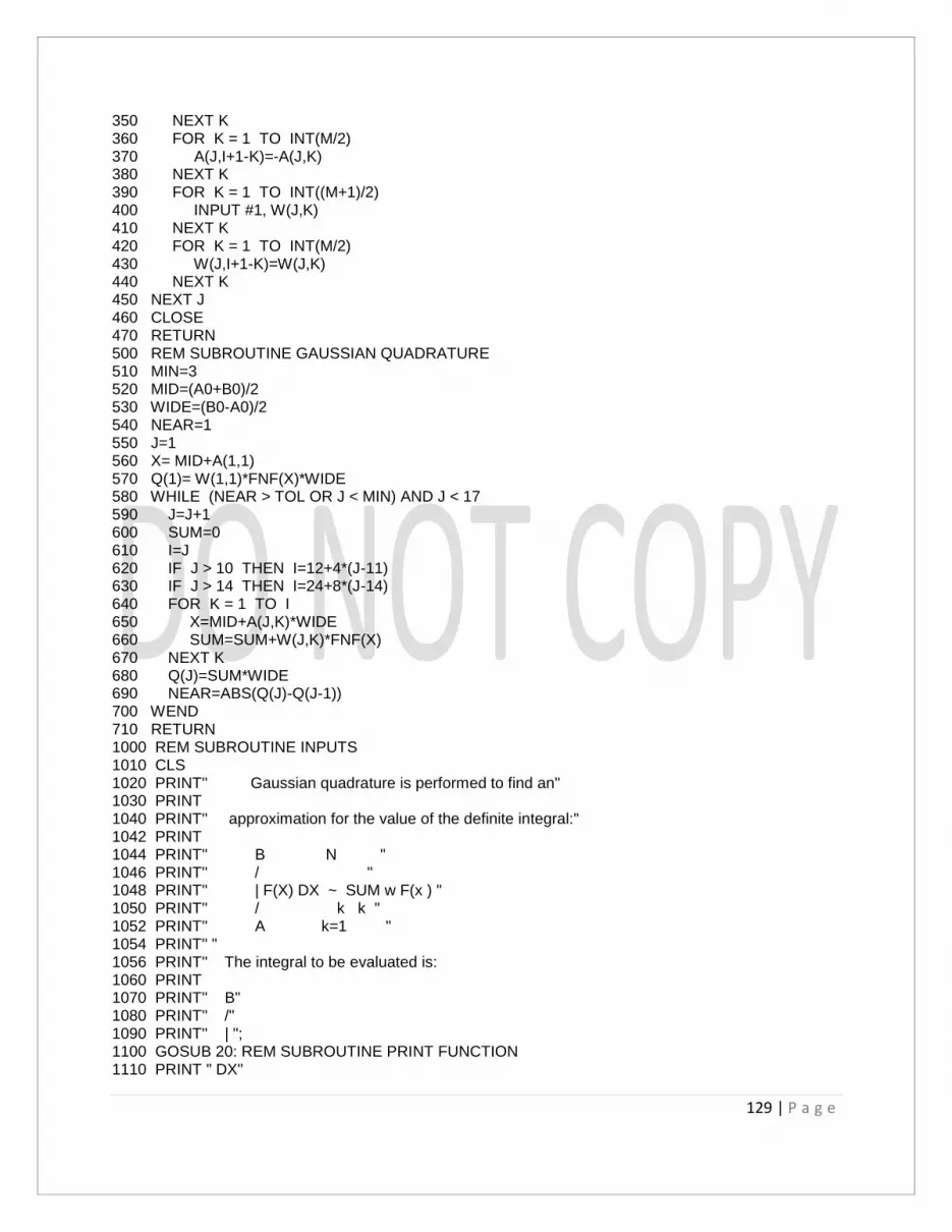
129 | P a g e

350 NEXT K 360 FOR K = 1 TO INT(M/2) 370 A(J,I+1-K)=-A(J,K) 380 NEXT K 390 FOR K = 1 TO INT((M+1)/2) 400 INPUT #1, W(J,K) 410 NEXT K 420 FOR K = 1 TO INT(M/2) 430 W(J,I+1-K)=W(J,K) 440 NEXT K 450 NEXT J 460 CLOSE 470 RETURN 500 REM SUBROUTINE GAUSSIAN QUADRATURE 510 MIN=3 520 MID=(A0+B0)/2 530 WIDE=(B0-A0)/2 540 NEAR=1 550 J=1 560 X= MID+A(1,1) 570 Q(1)= W(1,1)*FNF(X)*WIDE 580 WHILE (NEAR > TOL OR J < MIN) AND J < 17 590 J=J+1 600 SUM=0 610 I=J 620 IF J > 10 THEN I=12+4*(J-11) 630 IF J > 14 THEN I=24+8*(J-14) 640 FOR K = 1 TO I 650 X=MID+A(J,K)*WIDE 660 SUM=SUM+W(J,K)*FNF(X) 670 NEXT K 680 Q(J)=SUM*WIDE 690 NEAR=ABS(Q(J)-Q(J-1)) 700 WEND 710 RETURN 1000 REM SUBROUTINE INPUTS 1010 CLS 1020 PRINT" Gaussian quadrature is performed to find an" 1030 PRINT 1040 PRINT" approximation for the value of the definite integral:" 1042 PRINT 1044 PRINT" B N " 1046 PRINT" / " 1048 PRINT" | F(X) DX ~ SUM w F(x ) " 1050 PRINT" / k k " 1052 PRINT" A k=1 " 1054 PRINT" " 1056 PRINT" The integral to be evaluated is: 1060 PRINT 1070 PRINT" B" 1080 PRINT" /" 1090 PRINT" | "; 1100 GOSUB 20: REM SUBROUTINE PRINT FUNCTION 1110 PRINT " DX"

130 | P a g e

1120 PRINT" /" 1130 PRINT" A" 1140 PRINT 1150 PRINT 1160 PRINT"ENTER the left endpoint A = "; 1170 INPUT A0 1180 PRINT 1190 PRINT"ENTER the right endpoint B = "; 1200 INPUT B0 1210 PRINT 1250 RETURN 2000 REM SUBROUTINE RESULTS 2002 JJ=J 2004 IF J > 10 THEN JJ=12+4*(J-11) 2006 IF J > 14 THEN JJ=24+8*(J-14) 2010 CLS 2020 PRINT" ";B0 2030 PRINT" /" 2040 PRINT" |" 2050 PRINT" | "; 2060 GOSUB 20: REM SUBROUTINE PRINT FUNCTION 2070 PRINT " DX ~ ";Q(J) 2080 PRINT" |" 2090 PRINT" /" 2100 PRINT" ";A0 2110 PRINT 2120 PRINT 2130 PRINT"Gaussian quadrature with";JJ;" points was used to integrate" 2140 PRINT 2150 PRINT 2160 PRINT"F(X) = "; 2170 GOSUB 20: REM SUBROUTINE PRINT FUNCTION 2180 PRINT 2190 PRINT 2200 PRINT"over the interval [";A0;" , ";B0;" ]." 2210 PRINT 2220 PRINT"The values of the previous Gaussian rules are:" 2230 L=1 2240 IF J > 14 THEN L=2 2250 IF J > 16 THEN L=3 2260 FOR K = L TO INT((J+1)/2) 2270 U=2*K-1 2280 V=2*K 2290 I=U 2300 IF U > 10 THEN I=12+4*(U-11) 2310 IF U > 14 THEN I=24+8*(U-14) 2320 II=V 2330 IF V > 10 THEN II=12+4*(V-11) 2340 IF V > 14 THEN II=24+8*(V-14) 2350 IF U <= J AND V <= J THEN 2360 ELSE 2370 2360 PRINT "Q(";I;") = ";Q(U);" "; 2365 PRINT "Q(";II;") = ";Q(V) 2370 REM CONTINUE 2380 IF U <= J AND V > J THEN 2390 ELSE 2400

131 | P a g e

2390 PRINT "Q(";I;") = ";Q(U) 2400 REM CONTINUE 2410 NEXT K 2420 PRINT" " 2430 PRINT"The best Gaussian approximation is Q(";JJ;") = ";Q(J) 2440 IF J <= 11 THEN PRINT" " 2450 PRINT" The error estimate is +-";NEAR 2460 RETURN 5000 END // REM JACOBI ITERATION // 100 REM PROGRAM JACOBI 110 MAX=99 115 TOL=1E-7 120 DIM A(25,25),A1(25,25),B(25),X(25),XOLD(25) 125 REM CONTINUE 130 GOSUB 3000: REM SUBROUTINE INPUTS 135 GOSUB 200: REM SUBROUTINE JACOBI ITERATION 140 GOSUB 4000: REM SUBROUTINE RESULTS 145 PRINT 150 PRINT"Want to solve another linear system ? <Y/N> "; 155 INPUT ANS$ 160 IF ANS$ = "Y" OR ANS$ = "y" THEN GOTO 125 165 GOTO 9999 200 REM SUBROUTINE JACOBI ITERATION 210 SEP=1 220 K=0 230 COND=1 240 FOR J = 1 TO N 250 REM X(J) = 0 260 XOLD(J)=X(J) 270 NEXT J 280 FOR R = 1 TO N 290 ROW=0 300 FOR C = 1 TO N 310 ROW=ROW+ABS(A(R,C)) 320 NEXT C 330 IF ROW => 2*ABS(A(R,R)) THEN COND=0 340 NEXT R 350 IF COND = 0 THEN 360 ELSE 380 360 COND=0 370 GOTO 600 380 REM CONTINUE 390 WHILE K < MAX AND SEP > TOL 400 PRINT 410 PRINT K, X(1),X(2),X(3) 420 PRINT 430 FOR R = 1 TO N 440 SUM=B(R) 450 FOR C = 1 TO N 460 IF C<>R THEN SUM=SUM-A(R,C)*XOLD(C) 470 NEXT C

132 | P a g e

480 X(R)=SUM/A(R,R) 490 NEXT R 500 SEP=0 510 FOR J = 1 TO N 520 SEP=SEP+ABS(X(J)-XOLD(J)) 530 NEXT J 540 FOR J = 1 TO N 550 XOLD(J)=X(J) 560 NEXT J 570 K=K+1 580 WEND 590 COUNT=K 600 REM CONTINUE 610 RETURN 1000 REM SUBROUTINE MATRIX INPUT 1010 FOR ROW = 1 TO N 1020 FOR COL = 1 TO N 1030 A(ROW,COL)=0 1040 NEXT COL 1050 NEXT ROW 1060 PRINT"GIVE THE ELEMENTS OF THE MATRIX ",ACH$ 1070 PRINT 1080 IF INRC = 0 THEN 1090 ELSE 1190 1090 FOR ROW = 1 TO N 1100 PRINT"GIVE THE ELEMENTS OF ROW ",ROW 1110 PRINT 1120 FOR COL = 1 TO N 1130 PRINT"A(";ROW;",";COL;") = "; 1140 INPUT A(ROW,COL) 1150 A1(ROW,COL) = A(ROW,COL) 1160 NEXT COL 1170 NEXT ROW 1180 GOTO 1290 1190 REM ELSE 1200 FOR COL = 1 TO N 1210 PRINT"GIVE THE ELEMENTS OF COLUMN ",COL 1220 PRINT 1230 FOR ROW = 1 TO N 1240 PRINT"A(";ROW;",";COL;") = "; 1250 INPUT A(ROW,COL) 1260 A1(ROW,COL) = A(ROW,COL) 1270 NEXT ROW 1280 NEXT COL 1290 REM ENDIF 1300 RETURN 1400 REM SUBROUTINE VECTOR INPUT 1410 PRINT 1420 FOR ROW = 1 TO N 1430 PRINT "B(";ROW;") = "; 1440 INPUT B(ROW) 1450 NEXT ROW 1460 RETURN 1500 REM SUBROUTINE VECTOR INPUT 1510 PRINT

133 | P a g e

1520 FOR ROW = 1 TO N 1530 PRINT "X(";ROW;") = "; 1540 INPUT X(ROW) 1550 NEXT ROW 1560 RETURN 2000 REM SUBROUTINE MATRIX PRINT 2010 FOR ROW = 1 TO N 2020 PRINT 2030 FOR COL = 1 TO N 2040 PRINT A1(ROW,COL), 2050 NEXT COL 2060 NEXT ROW 2070 RETURN 2100 REM SUBROUTINE VECTOR PRINT 2105 COL=N+1 2110 PRINT "B COEFFICIENT VECTOR ";"X SOLUTION VECTOR" 2120 PRINT 2130 FOR ROW = 1 TO N 2140 PRINT "B(";ROW;") = ";B(ROW);" ";"X(";ROW;") = ",X(ROW) 2150 NEXT ROW 2160 RETURN 3000 REM SUBROUTINE INPUTS 3010 CLS 3020 PRINT 3030 PRINT" Jacobi iteration is is performed to find the solution to the linear" 3040 PRINT 3050 PRINT" system A*X = B. The matrix must be diagonally dominant. Starting with" 3060 PRINT 3070 PRINT" (k) (k) (k) " 3080 PRINT" X = (0,0,...,0), a sequence { X = (x ,x ,...,x ) } is generated" 3090 PRINT" 0 k 1 2 N " 3100 PRINT 3110 PRINT" which converges to the solution." 3120 PRINT 3130 PRINT" (k+1)" 3140 PRINT" the j-th coordinate x of X is computed using the formula:" 3150 PRINT" j k+1" 3160 PRINT 3170 PRINT" (k+1) (k) (k)" 3180 PRINT" x = [b - a x -...- a x " 3190 PRINT" j j j,1 1 j,j-1 j-1 " 3200 PRINT 3210 PRINT" (k) (k) " 3220 PRINT" - a x -...- a x ]/a for j=1,2,...,N. " 3230 PRINT" j,j+1 j+1 j,N N j,j" 3240 PRINT 3250 PRINT 3260 PRINT" Give the dimension N = "; 3270 INPUT N 3280 INRC=0 3290 PRINT"Want to input columns ? <Y/N> "; 3300 INPUT ANS$ 3310 IF ANS$ = "Y" OR ANS$ = "y" THEN INRC=1 3320 PRINT

134 | P a g e

3330 PRINT"ENTER the coefficient matrix A:" 3340 ACH$="A" 3350 GOSUB 1000: REM SUBROUTINE MATRIX INPUT 3360 PRINT"The matrix A is:" 3370 GOSUB 2000: REM SUBROUTINE MATRIX PRINT 3380 PRINT"ENTER the starting vector." 3390 XCH$="X" 3400 GOSUB 1400: REM SUBROUTINE VECTOR INPUT 3410 PRINT"ENTER the starting vector." 3420 XCH$="X" 3430 GOSUB 1500: REM SUBROUTINE VECTOR INPUT 3440 RETURN 4000 REM SUBROUTINE RESULTS 4010 CLS 4020 PRINT 4030 PRINT"The matrix A(I,J) is:" 4040 IF N < 6 THEN PRINT 4050 GOSUB 2000: REM SUBROUTINE MATRIX PRINT 4060 PRINT 4070 PRINT"The vector B is:" 4080 IF N < 6 THEN PRINT 4090 FOR K = 1 TO N 4100 PRINT" B(";K;") = " ;B(K) 4110 NEXT K 4120 PRINT 4130 IF COND = 1 THEN 4140 ELSE 4300 4140 IF SEP < TOL THEN 4150 ELSE 4180 4150 PRINT" Jacobi iteration solved A*X = B." 4160 PRINT"It took ";COUNT;" iterations to find the solution:" 4170 GOTO 4210 4180 REM ELSE 4190 PRINT" Jacobi iteration did not converge." 4200 PRINT"The status after ";COUNT;" iterations is" 4210 REM ENDIF 4220 IF N < 6 THEN PRINT 4230 PRINT 4240 FOR K = 1 TO N 4250 PRINT" X(";K;") = ";X(K) 4260 NEXT K 4270 PRINT 4280 PRINT" +-";SEP;" is the estimated accuracy." 4290 GOTO 4350 4300 REM ELSE 4310 PRINT 4320 PRINT"The matrix is not diagonally dominant." 4330 PRINT 4340 PRINT"Jacobi iteration cannot be used." 4350 REM ENDIF 4360 RETURN 9999 END // REM GAUSS-SEIDAL ITERATION // 100 REM PROGRAM GAUSS SEIDEL

135 | P a g e

110 MAX=99 115 TOL=1E-7 120 DIM A(25,25),A1(25,25),B(25),X(25),XOLD(25) 125 REM CONTINUE 130 GOSUB 3000: REM SUBROUTINE INPUTS 135 GOSUB 200: REM SUBROUTINE JACOBI ITERATION 140 GOSUB 4000: REM SUBROUTINE RESULTS 145 PRINT 150 PRINT"Want to solve another linear system ? <Y/N> "; 155 INPUT ANS$ 160 IF ANS$ = "Y" OR ANS$ = "y" THEN GOTO 125 165 GOTO 9999 200 REM SUBROUTINE GAUSS-SEIDEL ITERATION 210 SEP=1 220 K=0 230 COND=1 240 FOR J = 1 TO N 250 REM X(J) = 0 260 XOLD(J)=X(J) 270 NEXT J 280 FOR R = 1 TO N 290 ROW=0 300 FOR C = 1 TO N 310 ROW=ROW+ABS(A(R,C)) 320 NEXT C 330 IF ROW => 2*ABS(A(R,R)) THEN COND=0 340 NEXT R 350 IF COND = 0 THEN 360 ELSE 380 360 COND=0 370 GOTO 600 380 REM CONTINUE 390 WHILE K < MAX AND SEP > TOL 400 PRINT 410 PRINT K, X(1),X(2),X(3) 420 PRINT 430 FOR R = 1 TO N 440 SUM=B(R) 450 FOR C = 1 TO N 460 IF C<>R THEN SUM=SUM-A(R,C)*X(C) 470 NEXT C 480 X(R)=SUM/A(R,R) 490 NEXT R 500 SEP=0 510 FOR J = 1 TO N 520 SEP=SEP+ABS(X(J)-XOLD(J)) 530 NEXT J 540 FOR J = 1 TO N 550 XOLD(J)=X(J) 560 NEXT J 570 K=K+1 580 WEND 590 COUNT=K 600 REM CONTINUE 610 RETURN

136 | P a g e

1000 REM SUBROUTINE MATRIX INPUT 1010 FOR ROW = 1 TO N 1020 FOR COL = 1 TO N 1030 A(ROW,COL)=0 1040 NEXT COL 1050 NEXT ROW 1060 PRINT"GIVE THE ELEMENTS OF THE MATRIX ",ACH$ 1070 PRINT 1080 IF INRC = 0 THEN 1090 ELSE 1190 1090 FOR ROW = 1 TO N 1100 PRINT"GIVE THE ELEMENTS OF ROW ",ROW 1110 PRINT 1120 FOR COL = 1 TO N 1130 PRINT"A(";ROW;",";COL;") = "; 1140 INPUT A(ROW,COL) 1150 A1(ROW,COL) = A(ROW,COL) 1160 NEXT COL 1170 NEXT ROW 1180 GOTO 1290 1190 REM ELSE 1200 FOR COL = 1 TO N 1210 PRINT"GIVE THE ELEMENTS OF COLUMN ",COL 1220 PRINT 1230 FOR ROW = 1 TO N 1240 PRINT"A(";ROW;",";COL;") = "; 1250 INPUT A(ROW,COL) 1260 A1(ROW,COL) = A(ROW,COL) 1270 NEXT ROW 1280 NEXT COL 1290 REM ENDIF 1300 RETURN 1400 REM SUBROUTINE VECTOR INPUT 1410 PRINT 1420 FOR ROW = 1 TO N 1430 PRINT "B(";ROW;") = "; 1440 INPUT B(ROW) 1450 NEXT ROW 1460 RETURN 1500 REM SUBROUTINE VECTOR INPUT 1510 PRINT 1520 FOR ROW = 1 TO N 1530 PRINT "X(";ROW;") = "; 1540 INPUT X(ROW) 1550 NEXT ROW 1560 RETURN 2000 REM SUBROUTINE MATRIX PRINT 2010 FOR ROW = 1 TO N 2020 PRINT 2030 FOR COL = 1 TO N 2040 PRINT A1(ROW,COL), 2050 NEXT COL 2060 NEXT ROW 2070 RETURN 2100 REM SUBROUTINE VECTOR PRINT

137 | P a g e

2105 COL=N+1 2110 PRINT "B COEFFICIENT VECTOR ";"X SOLUTION VECTOR" 2120 PRINT 2130 FOR ROW = 1 TO N 2140 PRINT "B(";ROW;") = ";B(ROW);" ";"X(";ROW;") = ",X(ROW) 2150 NEXT ROW 2160 RETURN 3000 REM SUBROUTINE INPUTS 3010 CLS 3020 PRINT 3030 PRINT" Gauss-Seidel iteration is is performed to find the solution to the linear" 3040 PRINT 3050 PRINT" system A*X = B. The matrix must be diagonally dominant. Starting with" 3060 PRINT 3070 PRINT" (k) (k) (k) " 3080 PRINT" X = (0,0,...,0), a sequence { X = (x ,x ,...,x ) } is generated" 3090 PRINT" 0 k 1 2 N " 3100 PRINT 3110 PRINT" which converges to the solution." 3120 PRINT 3130 PRINT" (k+1)" 3140 PRINT" the j-th coordinate x of X is computed using the formula:" 3150 PRINT" j k+1" 3160 PRINT 3170 PRINT" (k+1) (k+1) (k+1)" 3180 PRINT" x = [b - a x -...- a x " 3190 PRINT" j j j,1 1 j,j-1 j-1 " 3200 PRINT 3210 PRINT" (k) (k) " 3220 PRINT" - a x -...- a x ]/a for j=1,2,...,N. " 3230 PRINT" j,j+1 j+1 j,N N j,j" 3240 PRINT 3250 PRINT 3260 PRINT" Give the dimension N = "; 3270 INPUT N 3280 INRC=0 3290 PRINT"Want to input columns ? <Y/N> "; 3300 INPUT ANS$ 3310 IF ANS$ = "Y" OR ANS$ = "y" THEN INRC=1 3320 PRINT 3330 PRINT"ENTER the coefficient matrix A:" 3340 ACH$="A" 3350 GOSUB 1000: REM SUBROUTINE MATRIX INPUT 3360 PRINT"The matrix A is:" 3370 GOSUB 2000: REM SUBROUTINE MATRIX PRINT 3380 PRINT"ENTER the starting vector." 3390 XCH$="X" 3400 GOSUB 1400: REM SUBROUTINE VECTOR INPUT 3410 PRINT"ENTER the starting vector." 3420 XCH$="X" 3430 GOSUB 1500: REM SUBROUTINE VECTOR INPUT 3440 RETURN 4000 REM SUBROUTINE RESULTS 4010 CLS

138 | P a g e

4020 PRINT 4030 PRINT"The matrix A(I,J) is:" 4040 IF N < 6 THEN PRINT 4050 GOSUB 2000: REM SUBROUTINE MATRIX PRINT 4060 PRINT 4070 PRINT"The vector B is:" 4080 IF N < 6 THEN PRINT 4090 FOR K = 1 TO N 4100 PRINT" B(";K;") = " ;B(K) 4110 NEXT K 4120 PRINT 4130 IF COND = 1 THEN 4140 ELSE 4300 4140 IF SEP < TOL THEN 4150 ELSE 4180 4150 PRINT" Gauss-Seidel iteration solved A*X = B." 4160 PRINT"It took ";COUNT;" iterations to find the solution:" 4170 GOTO 4210 4180 REM ELSE 4190 PRINT" Gauss-Seidel iteration did not converge." 4200 PRINT"The status after ";COUNT;" iterations is" 4210 REM ENDIF 4220 IF N < 6 THEN PRINT 4230 PRINT 4240 FOR K = 1 TO N 4250 PRINT" X(";K;") = ";X(K) 4260 NEXT K 4270 PRINT 4280 PRINT" +-";SEP;" is the estimated accuracy." 4290 GOTO 4350 4300 REM ELSE 4310 PRINT 4320 PRINT"The matrix is not diagonally dominant." 4330 PRINT 4340 PRINT"Gauss-Seidel iteration cannot be used." 4350 REM ENDIF 4360 RETURN 9999 END // REM NONLINEAR SEIDAL ITERATION // 10 DEF FNG1(X,Y) = (X*X - Y + 0.5)/2 20 DEF FNG2(X,Y) = (- X*X - 4*Y*Y + 8*Y + 4)/8 25 GOTO 100 30 REM SUBROUTINE PRINT FUNCTIONS 31 PRINT" " 32 PRINT" G (X,Y) = (X*X - Y + 0.5)/2" 33 PRINT" 1" 34 PRINT" " 35 PRINT" G (X,Y) = (- X*X - 4*Y*Y + 8*Y + 4)/8" 36 PRINT" 2" 37 PRINT" " 38 RETURN 100 REM PROGRAM NON-LINEAR SEIDEL ITERATION 100 MAX=199 110 TOL=1E-7

139 | P a g e

115 REM CONTINUE 120 GOSUB 1000: REM SUBROUTINE INPUTS 125 GOSUB 200: REM SUBROUTINE SEIDEL ITERATION 130 GOSUB 2000: REM SUBROUTINE RESULTS 135 PRINT" " 140 PRINT"Want to try a different starting point ? <Y/N> "; 145 INPUT ANS$ 150 IF ANS$ = "Y" OR ANS$ = "y" THEN GOTO 110 155 GOTO 5000 200 REM SUBROUTINE SEIDEL ITERATION 210 BIG=1E10 220 SEP=1 230 K=0 240 PNEW=POLD 250 QNEW=QOLD 260 WHILE K < MAX AND SEP > TOL 270 POLD=PNEW 280 QOLD=QNEW 290 K=K+1 300 PNEW=FNG1(POLD,QOLD) 310 QNEW=FNG2(PNEW,QOLD) 320 SEP=ABS(PNEW-POLD)+ABS(QNEW-QOLD) 330 IF PNEW < -BIG OR BIG < PNEW GOTO 360 340 IF QNEW < -BIG OR BIG < QNEW GOTO 360 350 WEND 360 REM CONTINUE 370 COUNT=K 380 RETURN 1000 REM SUBROUTINE INPUTS 1010 CLS 1020 PRINT" Seidel iteration is used to find the fixed" 1030 PRINT" " 1040 PRINT" point (P,Q) of the non-linear system" 1050 PRINT" " 1060 PRINT" P = G (P,Q), Q = G (P,Q). The functions are:" 1070 PRINT" 1 2" 1080 PRINT" " 1090 GOSUB 30: REM SUBROUTINE PRINT FUNCTIONS 1100 PRINT" ENTER the initial starting point (P ,Q )" 1110 PRINT" 0 0 " 1120 PRINT" " 1130 PRINT" P(0) = "; 1140 INPUT POLD 1150 P0=POLD 1160 PRINT" " 1170 PRINT" Q(0) = "; 1180 INPUT QOLD 1190 Q0=QOLD 1200 RETURN 2000 REM SUBROUTINE RESULTS 2010 K=COUNT 2020 CLS 2030 PRINT" " 2040 PRINT" "

140 | P a g e

2050 PRINT"Seidel iteration was used to find the fixed point of the" 2060 PRINT" " 2070 PRINT"non-linear system P = G (P,Q), Q = G (P,Q) where:" 2080 PRINT" 1 2" 2090 GOSUB 30: REM SUBROUTINE PRINT FUNCTIONS 2100 PRINT"starting with P =",P0," and Q =",Q0 2110 PRINT" 0 0" 2120 PRINT" " 2130 IF SEP < TOL THEN 2140 ELSE 2220 2140 PRINT"after ";COUNT;" iterations Seidel`s method was" 2150 PRINT" " 2160 PRINT"successful and found a solution point (P,Q)." 2170 PRINT" " 2180 PRINT" P =";PNEW;" Q =";QNEW 2190 PRINT" " 2200 PRINT" DP = ";PNEW-POLD;" DQ = ";QNEW-Qold 2210 GOTO 2300 2220 REM ELSE 2230 PRINT"Seidel iteration did NOT converge." 2240 PRINT" " 2250 PRINT"The status after ";COUNT;" iterations is:" 2260 PRINT" " 2270 PRINT" P(";K;") = ";PNEW;" Q(";K;") = ";QNEW 2280 PRINT" " 2290 PRINT" DP = ";PNEW-POLD;" DQ = ";QNEW-Qold 2300 REM ENDIF 2310 RETURN 5000 END // REM NEWTON-RAPHSON METHOD FOR 2-DIMENSIONS // 6 GOTO 100 10 REM SUBROUTINE FUNCTION 11 X=P(1) 12 Y=P(2) 13 F(1)=X*X-2*X-Y+0.5 14 F(2)=X*X+4*Y*Y-4 15 RETURN 20 REM SUBROUTINE JACOBIAN 21 X=P(1) 22 Y=P(2) 23 D(1,1)=2*X-2 24 D(1,2)=-1 25 D(2,1)=2*X 26 D(2,2)=8*Y 27 RETURN 30 REM SUBROUTINE PRINT FUNCTION 31 PRINT 32 PRINT" 0 = F (X,Y) = X*X - 2*X - Y + 0.5" 33 PRINT" 1" 34 PRINT 35 PRINT" 0 = F (X,Y) = X*X + 4*Y*Y - 4" 36 PRINT" 2"

141 | P a g e

37 PRINT 38 RETURN 100 REM PROGRAM TWO DIMENSIONAL NEWTON"S METHOD 100 MAX=99 110 DELTA=1E-6 115 EPSILON=1E-6 120 DIM D(2,2),DP(2),F0(2),F1(2),PSTART(2),P0(2),P1(2) 125 REM CONTINUE 130 GOSUB 1000: REM SUBROUTINE INPUTS 135 GOSUB 200: REM SUBROUTINE TWO DIMENSIONAL NEWTON" METHOD 140 GOSUB 2000: REM SUBROUTINE RESULTS 145 PRINT 150 PRINT"Want to try a different starting point ? <Y/N> "; 155 INPUT ANS$ 160 IF ANS$ = "Y" OR ANS$ = "y" THEN GOTO 125 165 GOTO 5000 200 REM SUBROUTINE TWO DIMENSIONAL NEWTON" METHOD 210 SMALL=DELTA 220 K=0 230 COND=0 240 P(1)=P0(1) 250 P(2)=P0(2) 260 GOSUB 10: REM SUBROUTINE FUNCTION 270 F0(1) = F(1) 280 F0(2) = F(2) 290 P1(1)=P0(1) 300 P1(2)=P0(2) 310 F1(1)=F0(1) 320 F1(2)=F0(2) 330 WHILE K < MAX AND COND = 0 340 P0(1)=P1(1) 350 P0(2)=P1(2) 360 F0(1)=F1(1) 370 F0(2)=F1(2) 380 K=K+1 390 P(1)=P0(1) 400 P(2)=P0(2) 410 GOSUB 20: REM SUBROUTINE JACOBIAN 420 DET=D(1,1)*D(2,2)-D(1,2)*D(2,1) 430 IF DET = 0 THEN 440 ELSE 480 440 DP(1)=0 450 DP(2)=0 460 COND=1 470 GOTO 640 480 REM ELSE 510 490 DP(1)=(F0(1)*D(2,2)-F0(2)*D(1,2))/DET 500 DP(2)=(F0(2)*D(1,1)-F0(1)*D(2,1))/DET 510 REM ENDIF 520 P1(1)=P0(1)-DP(1) 530 P1(2)=P0(2)-DP(2) 540 P(1)=P1(1) 550 P(2)=P1(2) 560 GOSUB 10: REM SUBROUTINE FUNCTION 570 F1(1) = F(1)

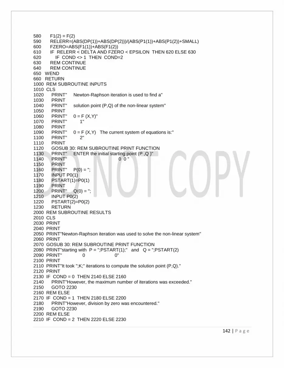
142 | P a g e

580 F1(2) = F(2) 590 RELERR=(ABS(DP(1))+ABS(DP(2)))/(ABS(P1(1))+ABS(P1(2))+SMALL) 600 FZERO=ABS(F1(1))+ABS(F1(2)) 610 IF RELERR < DELTA AND FZERO < EPSILON THEN 620 ELSE 630 620 IF COND <> 1 THEN COND=2 630 REM CONTINUE 640 REM CONTINUE 650 WEND 660 RETURN 1000 REM SUBROUTINE INPUTS 1010 CLS 1020 PRINT" Newton-Raphson iteration is used to find a" 1030 PRINT 1040 PRINT" solution point (P,Q) of the non-linear system" 1050 PRINT 1060 PRINT" 0 = F (X,Y)" 1070 PRINT" 1" 1080 PRINT 1090 PRINT" 0 = F (X,Y) The current system of equations is:" 1100 PRINT" 2" 1110 PRINT 1120 GOSUB 30: REM SUBROUTINE PRINT FUNCTION 1130 PRINT" ENTER the initial starting point (P ,Q )" 1140 PRINT" 0 0 " 1150 PRINT 1160 PRINT" P(0) = "; 1170 INPUT P0(1) 1180 PSTART(1)=P0(1) 1190 PRINT 1200 PRINT" Q(0) = "; 1210 INPUT P0(2) 1220 PSTART(2)=P0(2) 1230 RETURN 2000 REM SUBROUTINE RESULTS 2010 CLS 2030 PRINT 2040 PRINT 2050 PRINT"Newton-Raphson iteration was used to solve the non-linear system" 2060 PRINT 2070 GOSUB 30: REM SUBROUTINE PRINT FUNCTION 2080 PRINT"starting with P = ";PSTART(1);" and Q = ";PSTART(2) 2090 PRINT" 0 0" 2100 PRINT 2110 PRINT"It took ";K;" iterations to compute the solution point (P,Q)." 2120 PRINT 2130 IF COND = 0 THEN 2140 ELSE 2160 2140 PRINT"However, the maximum number of iterations was exceeded." 2150 GOTO 2230 2160 REM ELSE 2170 IF COND = 1 THEN 2180 ELSE 2200 2180 PRINT"However, division by zero was encountered." 2190 GOTO 2230 2200 REM ELSE 2210 IF COND = 2 THEN 2220 ELSE 2230

143 | P a g e

2220 PRINT"The solution is within the desired tolerances." 2230 REM ENDIF 2240 PRINT 2250 IF COND = 0 OR COND = 1 THEN 2260 ELSE 2280 2260 PRINT" P(";K;") = ";P1(1);" , Q(";K;") = ";P1(2) 2270 GOTO 2310 2280 REM ELSE 2290 IF COND = 2 THEN 2300 ELSE 2310 2300 PRINT" P = ";P1(1);" , Q = ";P1(2) 2310 REM ENDIF 2320 PRINT 2330 PRINT" |DP| = ";ABS(P1(1)-P0(1));" , |DQ| = ";ABS(P1(2)-P0(2)) 2340 PRINT 2350 PRINT" F (P,Q) = ";F1(1) 2360 PRINT" 1" 2370 PRINT" F (P,Q) = ";F1(2) 2380 PRINT" 2" 2390 RETURN 5000 END // REM EULER’S METHOD HEUN’S METHOD TAYLOR METHOD OF ORDER N=4 RUNGE-KUTTA METHOD OF ORDER N=4 // 10 DEF FNF(T,Y) = (T-Y)/2 15 GOTO 100 20 REM SUBROUTINE DERIVATIVES 21 D(1) = ( T - Y )/2 22 D(2) = ( 2 - T + Y)/4 23 D(3) = (-2 + T - Y)/8 24 D(4) = ( 2 - T + Y)/16 25 RETURN 30 REM SUBROUTINE PRINT FUNCTION 40 PRINT" Y` = (T-Y)/2" 50 RETURN 100 REM PROGRAM SOLVE DE`S 104 DIM D(4),T(1000),Y(1000) 106 METH=1 108 A=0 110 B=0 112 Y0=0 114 M=1 116 STATE=1 118 REM CONTINUE 120 GOSUB 1000: REM SUBROUTINE MESSAGE 122 DoMo=1 124 REM CONTINUE 126 GOSUB 2000: REM SUBROUTINE INPUTS 128 REM CONTINUE 130 GOSUB 3000: REM SUBROUTINE END POINTS 132 IF METH = 1 THEN 134 ELSE 138 134 GOSUB 300: REM SUBROUTINE EULER 136 GOTO 176 138 REM ELSE

144 | P a g e

140 IF METH = 2 THEN 142 ELSE 146 142 GOSUB 500: REM SUBROUTINE CAUCHY 144 GOTO 176 146 REM ELSE 148 IF METH = 3 THEN 150 ELSE 154 150 GOSUB 400: REM SUBROUTINE HEUN 152 GOTO 176 154 REM ELSE 156 IF METH = 4 THEN 158 ELSE 162 158 GOSUB 600: REM SUBROUTINE TAYLOR 160 GOTO 176 162 REM ELSE 164 IF METH = 5 THEN 166 ELSE 170 166 GOSUB 600: REM SUBROUTINE TAYLOR 168 GOTO 176 170 REM ELSE 172 IF METH = 6 THEN 174 ELSE 176 174 GOSUB 700: REM SUBROUTINE RUNGE 176 REM ENDIF 178 GOSUB 4000: REM SUBROUTINE RESULTS 180 PRINT 182 PRINT" Want to try another initial condition ? <Y/N> "; 184 INPUT ANS$ 186 IF ANS$ <> "Y" AND ANS$ <> "y" THEN 188 ELSE 192 188 STATE=2 190 GOTO 196 192 REM ELSE 194 STATE=0 196 REM ENDIF 198 IF STATE = 0 OR STATE = 1 THEN GOTO 128 200 PRINT" Want to change the differential equation ? <Y/N> "; 202 INPUT ANS$ 204 IF ANS$ <> "Y" AND ANS$ <> "y" THEN 206 ELSE 210 206 DoMo=0 208 GOTO 214 210 REM ELSE 212 STATE=0 214 REM ENDIF 216 IF DoMo = 1 THEN GOTO 124 218 PRINT "Want to try another method of approximation ? <Y/N> "; 220 INPUT ANS$ 222 IF ANS$ <> "Y" AND ANS$ <> "y" THEN 224 ELSE 228 224 METH=0 226 GOTO 232 228 REM ELSE 230 STATE=0 232 REM ENDIF 234 IF METH <> 0 THEN GOTO 118 236 GOTO 5000 300 REM SUBROUTINE EULER 305 BIG=1E13 310 H=(B-A)/M 315 T(0)=A 320 Y(0)=Y0

145 | P a g e

325 FOR K = 0 TO M-1 330 Y(K+1)=Y(K)+H*FNF(T(K),Y(K)) 335 T(K+1)=A+H*(K+1) 340 MEND=K+1 345 IF BIG < ABS(Y(K+1)) THEN K = M 350 NEXT K 355 RETURN 400 REM SUBROUTINE HEUN 402 BIG=1E13 404 H=(B-A)/M 406 T(0)=A 408 Y(0)=Y0 410 FOR J = 0 TO M-1 412 K1=FNF(T(J),Y(J)) 414 P=Y(J)+H*K1 416 T(J+1)=A+H*(J+1) 418 MEND=J+1 420 IF BIG < ABS(P) THEN 422 ELSE 428 422 Y(J+1)=P 424 J = M 426 GOTO 436 428 REM CONTINUE 430 K2=FNF(T(J+1),P) 432 Y(J+1)=Y(J)+H*(K1+K2)/2 434 IF BIG < ABS(Y(J+1)) THEN J = M 436 REM CONTINUE 438 NEXT J 440 RETURN 500 REM SUBROUTINE CAUCHY 502 BIG=1E13 504 H=(B-A)/M 506 T(0)=A 508 Y(0)=Y0 510 FOR J = 0 TO M-1 512 K1=FNF(T(J),Y(J)) 514 P=Y(J)+H*K1/2 516 T(J+1)=A+H*(J+1) 518 MEND=J+1 520 IF BIG < ABS(P) THEN 522 ELSE 528 522 Y(J+1)=P 524 J = M 526 GOTO 538 528 REM CONTINUE 530 TP=T(J)+H/2 532 K2=FNF(TP,P) 534 Y(J+1)=Y(J)+H*K2 536 IF BIG < ABS(Y(J+1)) THEN J = M 538 REM CONTINUE 540 NEXT J 542 RETURN 600 REM SUBROUTINE TAYLOR 602 BIG=1E13 604 H=(B-A)/M 606 T(0)=A

146 | P a g e

608 Y(0)=Y0 610 FOR K = 0 TO M-1 612 T=T(K) 614 Y=Y(K) 616 GOSUB 20: REM SUBROUTINE DERIVATIVES 618 IF ORDER = 3 THEN 620 ELSE 624 620 Y(K+1)=Y+H*(D(1)+H*(D(2)/2+H*D(3)/6)) 622 GOTO 628 624 REM ELSE 626 Y(K+1)=Y+H*(D(1)+H*(D(2)/2+H*(D(3)/6+H*D(4)/24))) 628 REM ENDIF 630 T(K+1)=A+H*(K+1) 632 MEND=K+1 634 IF BIG < ABS(Y(K+1)) THEN K = M 636 NEXT K 638 RETURN 700 REM SUBROUTINE RUNGE 702 BIG=1E13 704 POLE=0 706 H=(B-A)/M 708 T(0)=A 710 Y(0)=Y0 712 FOR J = 0 TO M-1 714 TJ=T(J) 716 YJ=Y(J) 718 MEND=J+1 720 K1=H*FNF(TJ,YJ) 722 IF BIG < ABS(YJ+0.5*K1) THEN 724 ELSE 730 724 POLE=1 726 J=M 728 GOTO 764 730 REM CONTINUE 732 K2=H*FNF(TJ+H/2,YJ+0.5*K1) 734 IF BIG < ABS(YJ+0.5*K2) THEN 736 ELSE 742 736 POLE=1 738 J=M 740 GOTO 764 742 REM CONTINUE 744 K3=H*FNF(TJ+H/2,YJ+0.5*K2) 746 IF BIG < ABS(YJ+K3) THEN 748 ELSE 754 748 POLE=1 750 J=M 752 GOTO 764 754 REM CONTINUE 756 K4=H*FNF(TJ+H,YJ+K3) 758 Y(J+1)=YJ+(K1+2*K2+2*K3+K4)/6 760 T(J+1)=A+H*(J+1) 762 IF BIG < ABS(Y(J+1)) THEN J = M 764 REM CONTINUE 766 NEXT J 768 IF POLE = 0 THEN GOTO 786 770 P=YJ+K1 772 T(J+1)=A+H*(J+1) 774 IF BIG < ABS(P) THEN 776 ELSE 780

147 | P a g e

776 Y(J+1)=P 778 GOTO 786 780 REM CONTINUE 782 K2=FNF(T(J+1),P) 784 Y(J+1)=YJ+H*(K1+K2)/2 786 REM CONTINUE 788 RETURN 1000 REM SUBROUTINE MESSAGE 1010 CLS 1020 PRINT" Solution of the differential equation Y` = F(T,Y)" 1030 PRINT 1040 PRINT" with the initial condition Y(A) = Y ." 1050 PRINT" 0" 1060 PRINT 1070 PRINT" A numerical approximation is computed over [A,B]." 1080 PRINT 1090 PRINT 1100 PRINT" Choose the method of approximation:" 1110 PRINT 1120 PRINT" < 1 > Euler`s method" 1130 PRINT 1140 PRINT" < 2 > Modified Euler-Cauchy method" 1150 PRINT 1160 PRINT" < 3 > Heun`s method" 1170 PRINT 1180 PRINT" < 4 > Taylor`s method of order N=3" 1190 PRINT 1200 PRINT" < 5 > Taylor`s method of order N=4" 1210 PRINT 1220 PRINT" < 6 > Runge-Kutta method of order N=4" 1230 PRINT 1240 PRINT" SELECT < 1 - 6 > ? "; 1250 RESP=METH 1260 INPUT RESP 1270 METH=INT(RESP) 1280 IF (METH < 1 OR METH > 6) AND STATE <> 0 THEN METH=1 1290 IF METH = 4 THEN ORDER=3 1300 IF METH = 5 THEN ORDER=4 1310 RETURN 2000 REM SUBROUTINE INPUTS 2010 CLS 2020 PRINT" You chose " 2030 IF METH = 1 THEN 2040 ELSE 2060 2040 PRINT "Euler`s method to solve:" 2050 GOTO 2250 2060 REM ELSE 2070 IF METH = 2 THEN 2080 ELSE 2100 2080 PRINT "the Modified Euler-Cauchy method to solve" 2090 GOTO 2250 2100 REM ELSE 2110 IF METH = 3 THEN 2120 ELSE 2140 2120 PRINT "Heun`s method to solve" 2130 GOTO 2250 2140 REM ELSE

148 | P a g e

2150 IF METH = 4 THEN 2160 ELSE 2180 2160 PRINT "Taylor`s method of order N=3 to solve" 2170 GOTO 2250 2180 REM ELSE 2190 IF METH = 5 THEN 2200 ELSE 2220 2200 PRINT "Taylor`s method of order N=4 to solve" 2210 GOTO 2250 2220 REM ELSE 2230 IF METH = 6 THEN 2240 ELSE 2250 2240 PRINT "the Runge-Kutta method of order N=4 to solve" 2250 REM ENDIF 2260 PRINT 2270 GOSUB 30: REM SUBROUTINE PRINT FUNCTION 2280 PRINT 2290 FOR I = 1 TO 15 2300 PRINT 2310 NEXT I 2320 PRINT" You chose "; 2330 IF METH = 1 THEN 2340 ELSE 2360 2340 PRINT "Euler`s method to solve the D.E." 2350 GOTO 2550 2360 REM ELSE 2370 IF METH = 2 THEN 2380 ELSE 2400 2380 PRINT "the Modified Euler-Cauchy method to solve the D.E." 2390 GOTO 2550 2400 REM ELSE 2410 IF METH = 3 THEN 2420 ELSE 2440 2420 PRINT "Heun`s method to solve the D.E." 2430 GOTO 2550 2440 REM ELSE 2450 IF METH = 4 THEN 2460 ELSE 2480 2460 PRINT "Taylor`s method of order N=3 to solve the D.E." 2470 GOTO 2550 2480 REM ELSE 2490 IF METH = 5 THEN 2500 ELSE 2520 2500 PRINT "Taylor`s method of order N=4 to solve the D.E." 2510 GOTO 2550 2520 REM ELSE 2530 IF METH = 6 THEN 2540 ELSE 2550 2540 PRINT "the Runge-Kutta method of order N=4 to solve the D.E." 2550 REM ENDIF 2560 PRINT 2570 GOSUB 30: REM SUBROUTINE PRINT FUNCTION 2580 PRINT 2590 PRINT" with the initial condition Y(A) = Y0." 2600 PRINT 2610 PRINT" A numerical approximation is computed over [A,B]." 2620 PRINT 2630 PRINT" You must enter the endpoints for the interval," 2640 PRINT 2650 PRINT" the initial condition Y0, and the number of steps M." 2660 PRINT 2670 PRINT 2680 PRINT" Press the <ENTER> key. ";

149 | P a g e

2690 INPUT ANS$ 2700 RETURN 3000 REM SUBROUTINE END POINTS 3010 REM STATUS = (Change,Enter,Done) 3020 STAT=1 3030 IF STATE = 0 THEN STAT=0 3040 WHILE STAT = 0 OR STAT = 1 3050 FOR I = 1 TO 15 3060 PRINT 3070 NEXT I 3080 GOSUB 30: REM SUBROUTINE PRINT FUNCTION 3090 PRINT 3100 PRINT 3110 IF STAT = 1 THEN 3120 ELSE 3280 3120 PRINT" ENTER the left endpoint A = "; 3130 INPUT A 3140 PRINT 3150 PRINT" ENTER the right endpoint B = "; 3160 INPUT B 3170 PRINT 3180 PRINT" ENTER initial condition Y(A) = "; 3190 INPUT Y0 3200 PRINT 3210 PRINT" ENTER the number of steps M = "; 3220 VALU=M 3230 INPUT VALU 3240 M=INT(VALU) 3250 IF M < 1 THEN M=1 3260 IF M > 1000 THEN M=1000 3270 GOTO 3360 3280 REM ELSE 3290 PRINT" The left endpoint is A =",A 3300 PRINT 3310 PRINT" The right endpoint is B =",B 3320 PRINT 3330 PRINT" Initial condition is Y(A) =",Y0 3340 PRINT 3350 PRINT" The number of steps is M = ",M 3360 REM ENDIF 3370 PRINT 3380 PRINT 3390 PRINT" Do you want to make a change ? <Y/N> "; 3400 INPUT ANS$ 3410 IF ANS$ = "Y" OR ANS$ = "y" THEN 3420 ELSE 3700 3420 STAT=0 3430 FOR I = 1 TO 15 3440 PRINT 3450 NEXT I 3460 PRINT" " 3470 GOSUB 30: REM SUBROUTINE PRINT FUNCTION 3480 PRINT 3490 PRINT 3500 PRINT" The current left endpoint is A = ",A 3510 PRINT" ENTER the NEW left endpoint A = ";

150 | P a g e

3520 INPUT A 3530 PRINT 3540 PRINT" The current right endpoint is B = ",B 3550 PRINT" ENTER the NEW right endpoint B = "; 3560 INPUT B 3570 PRINT 3580 PRINT" The current I. C. is Y(A) = ",Y0 3590 PRINT" ENTER the NEW I. C. Y(A) = "; 3600 INPUT Y0 3610 PRINT 3620 PRINT" The current value of M is M = ",M 3630 PRINT" ENTER the NEW value of M = " 3640 VALU=M 3650 INPUT VALU 3660 M=INT(VALU) 3670 IF M < 1 THEN M=1 3680 IF M > 1000 THEN M=1000 3690 GOTO 3720 3700 REM ELSE 3710 STAT=2 3720 REM ENDIF 3730 WEND 3740 RETURN 4000 REM SUBROUTINE RESULTS 4010 CLS 4020 IF METH = 1 THEN 4030 ELSE 4050 4030 PRINT "Euler`s method was used to solve the D.E." 4040 GOTO 4240 4050 REM ELSE 4060 IF METH = 2 THEN 4070 ELSE 4090 4070 PRINT "The Modified Euler-Cauchy method was used to solve the D.E." 4080 GOTO 4240 4090 REM ELSE 4100 IF METH = 3 THEN 4110 ELSE 4130 4110 PRINT "Heun`s method was used to solve the D.E." 4120 GOTO 4240 4130 REM ELSE 4140 IF METH = 4 THEN 4150 ELSE 4170 4150 PRINT "Taylor`s method of order N=3 was used to solve the D.E." 4160 GOTO 4240 4170 REM ELSE 4180 IF METH = 5 THEN 4190 ELSE 4210 4190 PRINT "Taylor`s method of order N=4 was used to solve the D.E." 4200 GOTO 4240 4210 REM ELSE 4220 IF METH = 6 THEN 4230 ELSE 4240 4230 PRINT "The Runge-Kutta method of order N=4 was used to solve the D.E." 4240 REM ENDIF 4250 GOSUB 30: REM SUBROUTINE PRINT FUNCTION 4260 PRINT 4270 PRINT "with Y(";T(0);" ) = ";Y(0) 4280 PRINT 4290 PRINT" K"," T(K) "," Y(K)" 4300 PRINT" ------------------------------------------------"

151 | P a g e

4310 FOR K = 0 TO MEND 4320 PRINT K;TAB(15);T(K);TAB(40);Y(K) 4330 NEXT K 4340 IF MEND < M THEN 435O ELSE 4370 4350 PRINT 4360 PRINT "The solution points are approaching a pole." 4370 REM CONTINUE 4380 RETURN 5000 END // REM RUNGE-KUTTA-FEHLBERG METHOD, RKF 45 ADAMS-BASHFORTH-MOULTON METHOD MILNE-SIMPSON METHOD HAMMING’S METHOD // 10 DEF FNF(T,Y) = (T-Y)/2 15 GOTO 100 30 REM SUBROUTINE PRINT FUNCTION 40 PRINT" Y` = (T-Y)/2" 50 RETURN 100 REM PROGRAM SOLVE DE`S 102 MAXM = 1000 104 DIM D(4),T(1000),Y(1000) 106 METH=1 108 A=0 110 B=0 112 Y0=0 114 M=1 116 STATE=1 118 REM CONTINUE 120 GOSUB 1000: REM SUBROUTINE MESSAGE 122 DOMO=1 124 REM CONTINUE 126 GOSUB 2000: REM SUBROUTINE INPUTS 128 REM CONTINUE 130 GOSUB 3000: REM SUBROUTINE END POINTS 132 IF METH = 1 THEN 134 ELSE 138 134 GOSUB 300: REM SUBROUTINE ADAMS-BASHFORTH-MOULTON 135 MEND=M 136 GOTO 176 138 REM ELSE 140 IF METH = 2 THEN 142 ELSE 146 142 GOSUB 400: REM SUBROUTINE MILNE 143 MEND=M 144 GOTO 176 146 REM ELSE 148 IF METH = 3 THEN 150 ELSE 154 150 GOSUB 500: REM SUBROUTINE HAMMING 151 MEND=M 152 GOTO 176 154 REM ELSE 156 IF METH = 4 THEN 158 ELSE 162 158 GOSUB 600: REM SUBROUTINE RKF45 159 MEND=M 160 GOTO 176 162 REM ELSE

152 | P a g e

176 REM ENDIF 178 GOSUB 4000: REM SUBROUTINE RESULTS 180 PRINT 182 PRINT" Want to try another initial condition ? <Y/N> "; 184 INPUT ANS$ 186 IF ANS$ <> "Y" AND ANS$ <> "y" THEN 188 ELSE 192 188 STATE=2 190 GOTO 196 192 REM ELSE 194 STATE=0 196 REM ENDIF 198 IF STATE = 0 OR STATE = 1 THEN GOTO 128 200 PRINT" Want to change the differential equation ? <Y/N> "; 202 INPUT ANS$ 204 IF ANS$ <> "Y" AND ANS$ <> "y" THEN 206 ELSE 210 206 DOMO=0 208 GOTO 214 210 REM ELSE 212 STATE=0 214 REM ENDIF 216 IF DOMO = 1 THEN GOTO 124 218 PRINT "Want to try another method of approximation ? <Y/N> "; 220 INPUT ANS$ 222 IF ANS$ <> "Y" AND ANS$ <> "y" THEN 224 ELSE 228 224 METH=0 226 GOTO 232 228 REM ELSE 230 STATE=0 232 REM ENDIF 234 IF METH <> 0 THEN GOTO 118 236 GOTO 5000 300 REM SUBROUTINE ADAMS-BASHFORTH-MOULTON 302 H=(B-A)/M 304 T(0)=A 306 Y(0)=Y0 308 REM Use Runge-Kutta to compute three starting values. 310 FOR J = 0 TO 2 312 TJ=T(J) 314 YJ=Y(J) 316 K1=H*FNF(TJ,YJ) 318 K2=H*FNF(TJ+H/2,YJ+0.5*K1) 320 K3=H*FNF(TJ+H/2,YJ+0.5*K2) 322 K4=H*FNF(TJ+H,YJ+K3) 324 Y(J+1)=YJ+(K1+2*K2+2*K3+K4)/6 326 T(J+1)=A+H*(J+1) 328 NEXT J 330 REM Start of Procedure Adams-Bashforth-Moulton 332 F0=FNF(T(0),Y(0)) 334 F1=FNF(T(1),Y(1)) 336 F2=FNF(T(2),Y(2)) 338 F3=FNF(T(3),Y(3)) 340 H2=H/24 342 FOR K = 3 TO M-1 344 TK=T(K)

153 | P a g e

346 YK=Y(K) 348 P=YK+H2*(-9*F0+37*F1-59*F2+55*F3) 350 T(K+1)=A+H*(K+1) 352 F4=FNF(T(K+1),P) 354 Y(K+1)=YK+H2*(F1-5*F2+19*F3+9*F4) 356 F0=F1 358 F1=F2 360 F2=F3 362 F3=FNF(T(K+1),Y(K+1)) 364 NEXT K 366 RETURN 400 REM SUBROUTINE MILNE 402 H=(B-A)/M 404 T(0)=A 406 Y(0)=Y0 408 REM Use Runge-Kutta to compute three starting values. 410 FOR J = 0 TO 2 412 TJ=T(J) 414 YJ=Y(J) 416 K1=H*FNF(TJ,YJ) 418 K2=H*FNF(TJ+H/2,YJ+0.5*K1) 420 K3=H*FNF(TJ+H/2,YJ+0.5*K2) 422 K4=H*FNF(TJ+H,YJ+K3) 424 Y(J+1)=YJ+(K1+2*K2+2*K3+K4)/6 426 T(J+1)=A+H*(J+1) 428 NEXT J 430 REM Start of Procedure Milne-Simpson 432 F1=FNF(T(1),Y(1)) 434 F2=FNF(T(2),Y(2)) 436 F3=FNF(T(3),Y(3)) 438 POLD=0 440 YOLD=0 442 FOR K = 3 TO M-1 444 PNEW=Y(K-3)+4*H*(2*F1-F2+2*F3)/3 446 PMOD=PNEW+28*(YOLD-POLD)/29 448 T(K+1)=A+H*(K+1) 450 F4=FNF(T(K+1),PMOD) 452 Y(K+1)=Y(K-1)+H*(F2+4*F3+F4)/3 454 POLD=PNEW 456 YOLD=Y(K+1) 458 F1=F2 460 F2=F3 462 F3=FNF(T(K+1),Y(K+1)) 464 NEXT K 466 RETURN 500 REM SUBROUTINE HAMMING 502 H=(B-A)/M 504 T(0)=A 506 Y(0)=Y0 508 REM Use Runge-Kutta to compute three starting values. 510 FOR J = 0 TO 2 512 TJ=T(J) 514 YJ=Y(J) 516 K1=H*FNF(TJ,YJ)

154 | P a g e

518 K2=H*FNF(TJ+H/2,YJ+0.5*K1) 520 K3=H*FNF(TJ+H/2,YJ+0.5*K2) 522 K4=H*FNF(TJ+H,YJ+K3) 524 Y(J+1)=YJ+(K1+2*K2+2*K3+K4)/6 526 T(J+1)=A+H*(J+1) 528 NEXT J 530 REM Start of Procedure Hamming 532 F1=FNF(T(1),Y(1)) 534 F2=FNF(T(2),Y(2)) 536 F3=FNF(T(3),Y(3)) 538 POLD=0 540 COLD=0 542 FOR K = 3 TO M-1 544 PNEW=Y(K-3)+4*H*(2*F1-F2+2*F3)/3 546 PMOD=PNEW+112*(COLD-POLD)/121 548 T(K+1)=A+H*(K+1) 550 F4=FNF(T(K+1),PMOD) 552 CNEW=(9*Y(K)-Y(K-2)+3*H*(-F2+2*F3+F4))/8 554 Y(K+1)=CNEW+9*(PNEW-CNEW)/121 556 POLD=PNEW 558 COLD=CNEW 560 F1=F2 562 F2=F3 564 F3=FNF(T(K+1),Y(K+1)) 566 NEXT K 568 RETURN 600 REM SUBROUTINE RKF45 602 BIG=1E13 603 RESTORE 604 READ A2,B2,A3,B3,C3,A4,B4,C4,D4,A5,B5,C5,D5,E5 606 READ A6,B6,C6,D6,E6,F6,R1,R3,R4,R5,R6,N1,N3,N4,N5 608 DATA 0.25, 0.25, 0.375, 0.09375, 0.28125, 0.9230769231 610 DATA 0.8793809741, -3.277196177, 3.320892126, 1.0 612 DATA 2.032407407, -8.0, 7.173489279, -0.2058966862, 0.5 614 DATA -0.2962962963, 2.0, -1.381676413, 0.4529727096, -0.275 616 DATA 0.002777777778, -0.02994152047, -0.02919989367, 0.02 618 DATA 0.03636363636, 0.1157407407, 0.5489278752, 0.535331384 620 DATA -0.2 622 H=(B-A)/M 624 HMIN=H/1024 626 HMAX=H*64 628 T(0)=A 630 Y(0)=Y0 632 T(0)=A 634 J=0 636 TJ=A 638 BR=B-0.0001*ABS(B) 640 WHILE TJ < B 642 IF TJ+H > BR THEN H=B-TJ 644 TJ=T(J) 646 YJ=Y(J) 648 Y1=YJ 650 K1=H*FNF(TJ,Y1) 652 Y2=YJ+B2*K1

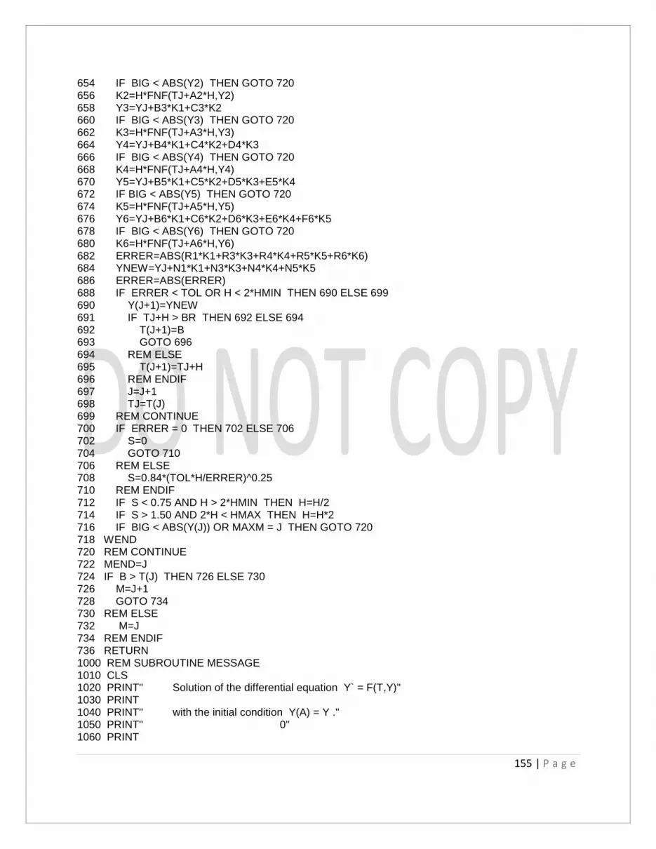
155 | P a g e

654 IF BIG < ABS(Y2) THEN GOTO 720 656 K2=H*FNF(TJ+A2*H,Y2) 658 Y3=YJ+B3*K1+C3*K2 660 IF BIG < ABS(Y3) THEN GOTO 720 662 K3=H*FNF(TJ+A3*H,Y3) 664 Y4=YJ+B4*K1+C4*K2+D4*K3 666 IF BIG < ABS(Y4) THEN GOTO 720 668 K4=H*FNF(TJ+A4*H,Y4) 670 Y5=YJ+B5*K1+C5*K2+D5*K3+E5*K4 672 IF BIG < ABS(Y5) THEN GOTO 720 674 K5=H*FNF(TJ+A5*H,Y5) 676 Y6=YJ+B6*K1+C6*K2+D6*K3+E6*K4+F6*K5 678 IF BIG < ABS(Y6) THEN GOTO 720 680 K6=H*FNF(TJ+A6*H,Y6) 682 ERRER=ABS(R1*K1+R3*K3+R4*K4+R5*K5+R6*K6) 684 YNEW=YJ+N1*K1+N3*K3+N4*K4+N5*K5 686 ERRER=ABS(ERRER) 688 IF ERRER < TOL OR H < 2*HMIN THEN 690 ELSE 699 690 Y(J+1)=YNEW 691 IF TJ+H > BR THEN 692 ELSE 694 692 T(J+1)=B 693 GOTO 696 694 REM ELSE 695 T(J+1)=TJ+H 696 REM ENDIF 697 J=J+1 698 TJ=T(J) 699 REM CONTINUE 700 IF ERRER = 0 THEN 702 ELSE 706 702 S=0 704 GOTO 710 706 REM ELSE 708 S=0.84*(TOL*H/ERRER)^0.25 710 REM ENDIF 712 IF S < 0.75 AND H > 2*HMIN THEN H=H/2 714 IF S > 1.50 AND 2*H < HMAX THEN H=H*2 716 IF BIG < ABS(Y(J)) OR MAXM = J THEN GOTO 720 718 WEND 720 REM CONTINUE 722 MEND=J 724 IF B > T(J) THEN 726 ELSE 730 726 M=J+1 728 GOTO 734 730 REM ELSE 732 M=J 734 REM ENDIF 736 RETURN 1000 REM SUBROUTINE MESSAGE 1010 CLS 1020 PRINT" Solution of the differential equation Y` = F(T,Y)" 1030 PRINT 1040 PRINT" with the initial condition Y(A) = Y ." 1050 PRINT" 0" 1060 PRINT

156 | P a g e

1070 PRINT" A numerical approximation is computed over [A,B]." 1080 PRINT 1090 PRINT 1100 PRINT" Choose the method of approximation:" 1110 PRINT 1120 PRINT" < 1 > Adams-Bashforth-Moulton method" 1130 PRINT 1140 PRINT" < 2 > Milne-Simpson`s method" 1150 PRINT 1160 PRINT" < 3 > Hamming`s method" 1170 PRINT 1180 PRINT" < 4 > Runge-Kutta-Fehlberg" 1190 PRINT 1240 PRINT" SELECT < 1 - 4 > ? "; 1250 RESP=METH 1260 INPUT RESP 1270 METH=INT(RESP) 1280 IF (METH < 1 OR METH > 4) AND STATE <> 0 THEN METH=1 1310 RETURN 2000 REM SUBROUTINE INPUTS 2010 CLS 2020 PRINT" You chose " 2030 IF METH = 1 THEN 2040 ELSE 2060 2040 PRINT "Adams-Bashforth-Moulton method to solve:" 2050 GOTO 2250 2060 REM ELSE 2070 IF METH = 2 THEN 2080 ELSE 2100 2080 PRINT "the Milne-Simpson method to solve" 2090 GOTO 2250 2100 REM ELSE 2110 IF METH = 3 THEN 2120 ELSE 2140 2120 PRINT "Hamming`s method to solve" 2130 GOTO 2250 2140 REM ELSE 2150 IF METH = 4 THEN 2160 ELSE 2180 2160 PRINT "the Runge-Kutta-Fehlberg method to solve" 2170 GOTO 2250 2180 REM ELSE 2250 REM ENDIF 2260 PRINT 2270 GOSUB 30: REM SUBROUTINE PRINT FUNCTION 2280 PRINT 2290 FOR I = 1 TO 15 2300 PRINT 2310 NEXT I 2320 PRINT" You chose "; 2330 IF METH = 1 THEN 2340 ELSE 2360 2340 PRINT "Adams-Bashforth-Moulton method to solve the D.E." 2350 GOTO 2550 2360 REM ELSE 2370 IF METH = 2 THEN 2380 ELSE 2400 2380 PRINT "the Milne-Simpson method to solve the D.E." 2390 GOTO 2550 2400 REM ELSE

157 | P a g e

2410 IF METH = 3 THEN 2420 ELSE 2440 2420 PRINT "Hamming`s method to solve the D.E." 2430 GOTO 2550 2440 REM ELSE 2450 IF METH = 4 THEN 2460 ELSE 2480 2460 PRINT "the Runge-Kutta-Fehlberg method to solve the D.E." 2470 GOTO 2550 2480 REM ELSE 2550 REM ENDIF 2560 PRINT 2570 GOSUB 30: REM SUBROUTINE PRINT FUNCTION 2580 PRINT 2590 PRINT" with the initial condition Y(A) = Y0." 2600 PRINT 2610 PRINT" A numerical approximation is computed over [A,B]." 2620 PRINT 2630 PRINT" You must enter the endpoints for the interval," 2640 PRINT 2650 PRINT" the initial condition Y0, and the number of steps M." 2660 PRINT 2670 PRINT 2680 PRINT" Press the <ENTER> key. "; 2690 INPUT ANS$ 2700 RETURN 3000 REM SUBROUTINE END POINTS 3010 REM STATUS = (Change, Enter, Done) 3020 STAT=1 3030 IF STATE = 0 THEN STAT=0 3040 WHILE STAT = 0 OR STAT = 1 3050 FOR I = 1 TO 15 3060 PRINT 3070 NEXT I 3080 GOSUB 30: REM SUBROUTINE PRINT FUNCTION 3090 PRINT 3100 PRINT 3110 IF STAT = 1 THEN 3120 ELSE 3280 3120 PRINT" ENTER the left endpoint A = "; 3130 INPUT A 3140 PRINT 3150 PRINT" ENTER the right endpoint B = "; 3160 INPUT B 3170 PRINT 3180 PRINT" ENTER initial condition Y(A) = "; 3190 INPUT Y0 3200 PRINT 3210 PRINT" ENTER the number of steps M = "; 3220 VALU=M 3230 INPUT VALU 3240 M=INT(VALU) 3250 IF M < 1 THEN M=1 3260 IF M > 1000 THEN M=1000 3265 PRINT 3270 PRINT" ENTER the tolerance TOL = "; 3271 VALU=TOL

158 | P a g e

3272 INPUT VALU 3273 TOL=VALU 3274 GOTO 3360 3280 REM ELSE 3290 PRINT" The left endpoint is A = ";A 3300 PRINT 3310 PRINT" The right endpoint is B = ";B 3320 PRINT 3330 PRINT" Initial condition is Y(A) = ";Y0 3340 PRINT 3350 PRINT" The number of steps is M = ";M 3351 PRINT 3352 PRINT" The tolerance is TOL = ";TOL 3360 REM ENDIF 3370 PRINT 3380 PRINT 3390 PRINT" Do you want to make a change ? <Y/N> "; 3400 INPUT ANS$ 3410 IF ANS$ = "Y" OR ANS$ = "y" THEN 3420 ELSE 3700 3420 STAT=0 3430 FOR I = 1 TO 15 3440 PRINT 3450 NEXT I 3460 PRINT" " 3470 GOSUB 30: REM SUBROUTINE PRINT FUNCTION 3480 PRINT 3490 PRINT 3500 PRINT" The current left endpoint is A = ";A 3510 PRINT" ENTER the NEW left endpoint A = "; 3520 INPUT A 3530 PRINT 3540 PRINT" The current right endpoint is B = ";B 3550 PRINT" ENTER the NEW right endpoint B = "; 3560 INPUT B 3570 PRINT 3580 PRINT" The current I. C. is Y(A) = ";Y0 3590 PRINT" ENTER the NEW I. C. Y(A) = "; 3600 INPUT Y0 3610 PRINT 3620 PRINT" The current value of M is M = ";M 3630 PRINT" ENTER the NEW value of M = "; 3640 VALU=M 3650 INPUT VALU 3660 M=INT(VALU) 3670 IF M < 1 THEN M=1 3680 IF M > 1000 THEN M=1000 3681 PRINT 3682 PRINT" The current value of TOL is TOL = ";TOL 3683 PRINT" ENTER the NEW value of TOL = "; 3684 INPUT VALU 3685 TOL=VALU 3690 GOTO 3720 3700 REM ELSE 3710 STAT=2

159 | P a g e

3720 REM ENDIF 3730 WEND 3740 RETURN 4000 REM SUBROUTINE RESULTS 4010 CLS 4020 IF METH = 1 THEN 4030 ELSE 4050 4030 PRINT "Adams-Bashforth-Moulton method was used to solve the D.E." 4040 GOTO 4240 4050 REM ELSE 4060 IF METH = 2 THEN 4070 ELSE 4090 4070 PRINT "The Milne-Simpson method was used to solve the D.E." 4080 GOTO 4240 4090 REM ELSE 4100 IF METH = 3 THEN 4110 ELSE 4130 4110 PRINT "Hamming`s method was used to solve the D.E." 4120 GOTO 4240 4130 REM ELSE 4140 IF METH = 4 THEN 4150 ELSE 4170 4150 PRINT "The Runge-Kutta-Fehlberg method to solve the D.E." 4160 GOTO 4240 4170 REM ELSE 4240 REM ENDIF 4250 GOSUB 30: REM SUBROUTINE PRINT FUNCTION 4260 PRINT 4270 PRINT "with Y(";T(0);" ) = ";Y(0) 4280 PRINT 4290 PRINT" K"," T(K) "," Y(K)" 4300 PRINT" ------------------------------------------------" 4310 FOR K = 0 TO MEND 4320 PRINT K;TAB(15);T(K);TAB(40);Y(K) 4330 NEXT K 4340 IF MEND < M THEN 435O ELSE 4370 4350 PRINT 4360 PRINT "The solution points are approaching a pole." 4370 REM CONTINUE 4380 RETURN 5000 END

160 | P a g e

Internet World Stats "Internet, n.". Oxford English Dictionary http://dictionary.oed.com/ "Links". HTML 4.0 or 5.0 or 6.0 or 8.0 Specification. World Wide Web Specification.

http://www.w3.org/ Book: Higher Engineering Mathematics – B.S. Grawel Algebra and Geometry: Solution of equations, Linear algebra: Determinants, Matrices, Vector algebra and solid geometry. Calculus: Differential calculus, Partial differentiation, Integral Calculus, Multiple Integrals, Vector and Calculus. Series: Infinite series and Fourier series. Differential Equations: Differential equations of first order and their applications, Linear differential equations and their applications, Differential equations of different types, Series solution of differential equations and special functions, Partial differential equations and their applications. Complex Analysis: Complex numbers and functions, Calculus or complex functions. Transforms: Laplace transforms, Fourier transforms and Z-transforms. Numerical Techniques: Empirical laws and Curve fitting, Statistical Methods, Probability and Distributions, Sampling and Inference, Numerical Methods, Finite differences and Interpolation, Difference equations, Numerical solution of Ordinary and Partial differential equations, Linear Programming. Special Topics: Calculus of Variations, Integral equations, Discrete Mathematics, Tensors. Linear Programming: BASIC and C++ Classes of Object Oriented Concepts. Programming Language: Visual Basics from Micro-Soft Operating System for WINDOWS NT Graphical User Interface development system. Digital System: Electronic Devices and Components of the Computer. IC’s Series, Chip Design, Truth Tables and Sequential Circuits of Analog and Digital Systems.

SIGNED BY: Dr. SANTOSH KUMAR ARAVA DATED: 22-06-2013 DATE OF BIRTH: 22-07-1984