How often do managers withhold information?!

Jeremy Bertomeu, Paul Ma, and Ivan Marinovic

Abstract

This study structurally estimates the model of voluntary disclosure with un-certain information endowment of Dye (1985) in the context of quarterly earningsforecasts of US large cap firms. We find that managers strategically withhold in-formation on average one out of seven quarters. Conditional on not observing aforecast, the probability of strategic withholding is 14%, in which case the concealedinformation falls in the bottom quartile of the distribution. The private informationof managers at a disclosure date explains 27% of the variation in realized earnings.Disclosure frictions tend to be sticky, and their frequency varies across industries.Firms with less precise information are more likely to selectively withhold infor-mation. Comparing the estimated volatility of managerial beliefs to the volatilityof realized earnings, we show that expectations exhibit excess volatility for abouttwo thirds of the sample firms, which we interpret as a sign of managerial overcon-fidence. Our study is the first to provide large sample estimates of the limits tounravelling.

Keywords: voluntary disclosure, disclosure frictions, structural estimationJEL Classification: D72, D82, D83, G20

!Jeremy Bertomeu is an assistant professor at Baruch College, City University of New York, 1 BernardBaruch Way, New York, NY 10010. Email: jeremy.bertomeu@baruch.cuny.com. Paul Ma is an assis-tant professor at the Carlson School of Management, University of Minnesota, 321 19th Avenue South,Minneapolis, MN 55455. Email: paulma@umn.edu. Ivan Marinovic is an assistant professor at Stan-ford Graduate School of Business, Stanford University, 655 Knight Way, Stanford, CA 94305. Email:imvial@stanford.edu. We are grateful for comments from Santiago Bazdresch, Alan Benson, Anne Beyer,William Greene, David Larcker, Chandra Kanodia, Colleen Manchester, Alejandro Molnar, Raj Singh,Aaron Sojourner, John Shoven, Stephen Terry, seminar participants at Duke and the University ofChicago. All errors are our own.

Persuasion theory suggests that, if frictions prevent costless communication of private

information, an informed sender will strategically withhold information (Dye 1985; Fish-

man and Hagerty 1990; Shavell 1994; Shin 1994, 2003). The law literature o!ers many

instances in which material information was voluntarily omitted, with cases of success-

ful litigation in the pharmaceutical, food, tobacco and automobile industries (see Rabin

2001; Mello, Rimm and Studdert 2003; McClellan 2008; Govindaraj, Lee and Tinkel-

man 2007). These cases appear to be consistent with evidence, in experimental settings,

that informed senders conceal unfavorable information as a result of disclosure frictions

(Dickhaut, Ledyard, Mukherji and Sapra 2003; Jin, Luca and Martin 2015).

However, to our knowledge, most of the field evidence about strategic withholding

focuses on unusual events, as in the large body of evidence regarding safety issues. Such

events are usually easier to observe ex-post, from the documentation collected during

lawsuits. Lawsuits are somewhat problematic for a field test of voluntary theory because

they imply that disclosures are not strictly voluntary. In this study, we structurally esti-

mate the voluntary disclosure theory of Dye (1985) and Jung and Kwon (1988), hereafter

DJK, using quarterly earnings forecasts. We rely primarily on this theory as our baseline,

because it is one of the most widespread theory and continues to inspire both theoretical

and empirical research (Guttman, Kremer and Skrzypacz 2014; Ben-Porath, Dekel and

Lipman 2014).

Earnings forecasts are an ideal setting to estimate voluntary disclosure theory. In

practice, firms occasionally make voluntary disclosure of next-quarter earnings. These

forecasts are protected against most lawsuits by safe harbor provisions (see Safe Harbor

for Forward Looking Statements, Concept Release and Notice of Hearing, October 13,

1994 ).1 Earnings forecasts o!er rich panel data over homogenous quantitative forecasts

that spans across industries, and in which we can match each forecast to the realized

1Some disclosures are subject to a duty to update (or duty to correct), under section 10(b) of theSecurities and Exchange Act of 1934, but this requirement is interpreted as applying to material factsthat may have changed - not to quantitative quarterly earnings forecast.

1

forecasted earnings in the next quarter and to a market expectation at the time forecast

is made, using the pre-forecast First Call analyst consensus.

Earnings forecasts are also of great stand-alone interest in capital market research.

Prior theoretical research conjectures that voluntary disclosure is a primary channel

through which the classic lemons problem is resolved. Empirically, Ball and Brown (1968)

find that most of the information becomes known to the market before the release of

mandated financial statements. Considering earnings forecasts, Beyer, Cohen, Lys and

Walther (2010) document that these forecasts account for as much as 16% of quarterly

stock return variance, more than earnings announcements, filings with the Securities and

Exchange Commission and analyst forecasts combined.

In this paper, our objective is to quantify the limits to voluntary disclosure, by struc-

turally estimating disclosure frictions and analyzing its implications for strategic with-

holding and the range of concealed information. In the DJK model, a manager may be

privately informed about the value of a traded firm and, if so, decides whether to disclose

or withhold the information, aiming to maximize the current market value of the firm.

Absent any friction, disclosure strategies unravel to full disclosure because a manager with

the best prospects among other withholding managers will always be better-o! disclosing

(Grossman and Hart, 1980; Milgrom, 1981; Grossman, 1981). To break unraveling, the

model conjectures that there is a random probability of a friction, unobservable to out-

siders, which makes the manager either unable or unwilling to disclose regardless of the

observed private information.2 As long as the probability of the friction is non-zero, even

a manager that is not subject to the friction will selectively withhold some unfavorable

information.

The disclosure friction in DJK is an abstract mechanism that has many possible

2In DJK, the working assumption is that the probability of the friction is not a function of the trueinformation - it is generally used in the literature as a synonym for this model and is analogue to thefixed disclosure assumption in costly disclosure models (Jovanovic 1982). Another key assumption isthat insiders cannot trade strategically; as is illustrated in the market microstructure literature, anyinformation that a!ects price discovery will greatly complicate trading strategies (Huddart, Hughes andLevine 2001) and, in our model, would feed back into complex disclosure strategies.

2

interpretations. In the conventional interpretation proposed by Dye (1985), managers

may be uninformed, a fact that they cannot credibly disclose. Alternatively, managers

might occasionally face prohibitive proprietary costs if they disclose in advance. For

our application, which relies on relatively short-term horizons (a forecast about next

quarter earnings), one may consider a third interpretation – uncertainty about managerial

objectives – in the spirit of Fischer and Verrecchia (2000). When the friction is not

present, the manager has a short-term focus and selectively discloses to maximize the

current stock price; by contrast, when the friction is present, the manager has a pure

long-term focus and, assuming some small cost of disclosure, prefers to withhold his

forecast.

The main prediction of DJK is that the distribution of forecasts is a truncated version

of the distribution of managers’ beliefs, because managers withhold a fraction of their

bad news. The truncation is reminiscent of that arising in the classic selection models

popularized by Tobin (1958) and Heckman (1979) in the context of labor markets, where

the distribution of wage o!ers of employed workers is a truncation of the unconditional

distribution of wage o!ers. In a standard selection models, a common approach is to

assume that the truncation point is zero (see Amemiya 1984, p. 7). In our setting, it

is crucial to estimate the truncation point (that is, the disclosure threshold) which we

then use, in conjunction with the structural equations of the disclosure game, to infer the

structural process of the disclosure friction.

Another challenge in our empirical implementation is to accommodate stickiness in dis-

closure policies (see Graham, Harvey and Rajgopal 2005). To make the theory amenable

to empirical testing, we augment DJK with time-series autocorrelation in the friction.

This means that the friction follows a hidden Markov process. If the friction is sticky, a

disclosure decision today a!ects the evolution of market beliefs about the friction, thereby

a!ecting the evolution of disclosure incentives. Infrequent disclosures in the past may lead

investors to believe that the manager is likely to experience frictions in the future and

3

react more favorably to the absence of disclosure.

We estimate the model at the firm level using a maximum likelihood approach. We

recover the following parameters: the sequence of disclosure threshold; the probability

and persistence of the disclosure friction, and the quality of the manager’s private infor-

mation. Based on these estimates, we then compute the average probability of strategic

withholding.

We first document that managers possess significant private information: roughly,

managers’ private information accounts for a quarter of the variation in earnings inno-

vations. On average, managers strategically withhold information about one out of then

quarters. Frictions occur, on average, only once every two quarters but market pres-

sure, in the form of negative expectations conditional on withholding induces managers

to strategically withhold only significantly unfavorable news in order to avoid the market

penalty. Taken together, these results imply that managers conceal the bottom quartile

of the distribution.

We also test for managerial biases. According to elementary statistics, the variance

of a Bayesian expectation of a random variable cannot be greater than the variance of

that random variable.3 This prediction cannot be tested directly because the variance

of manager expectations is not directly observable - we only observe forecasts when the

expectation is favorable. Using the model’s equilibrium characterization, however, we

are able to recover the location of the truncation which in turn allows us to compute

the variance of manager expectations. If managers make their predictions rationally, this

variance will be lower than the variance of the underlying earnings. By contrast, if man-

agers are over-confident in their own private information, the variance of the prediction

could be higher than that of earnings.

We construct a test based on this argument and reject Bayesian rationality for about

3This bound is also commonly used in tests of excess price volatility (Shiller 1980; LeRoy and Porter1981). It is recently used in the context of analysts’ forecasts by Lundholm and Rogo (2014); theseare easier to examine because they are less likely to exhibit a truncation. They show that, like formanagement forecasts, there is excess volatility of forecasts for about half of the firms.

4

60% of the sample firms. Indeed, for about two thirds of the sample firms, manager

forecasts exhibit excess volatility relative to the volatility of earnings. For the median

firm, the variance of manager expectations is 25% higher than if managers were consistent

with Bayes’ rule. Taken together, these estimates provide evidence of a behaviorial bias

in managers’ disclosures.

Related literature. Our paper o!ers a structural estimation of a formal model of

communication using field data. To our knowledge, few current studies provide structural

estimates of models of strategic communication. Beyer, Guttman and Marinovic (2014)

estimate a dynamic misreporting model. In their model, the manager can bias a manda-

tory report for a cost (Goldman and Slezak, 2006; Kedia and Philippon, 2009; Acharya

and Lambrecht, 2011) but the market cannot recover the true signal because of noise in

the accounting system. Zakolyukina (2014) and Terry (2014) estimate structural models

in which agents consider the dynamic consequences of manipulation. Zakolyukina (2014)

estimates her model using observed accounting violations, recovering current choice of

manipulation as a trade-o! between current benefits and an increase in the long-term

probability of an accounting restatement. Terry (2014) focuses on the e!ect of misre-

porting on firm’s dynamic investment policy, measuring that reporting incentives appear

to cause significant distortions to investment. To our knowledge, the only study that

implements a test of a voluntary forecasting model is Chen and Jiang (2006); they focus

on how analysts weight their information when making forecasts.4

There is also an extensive theoretical literature on voluntary disclosure drawing on the

original model of Dye (1985). One of the predictions of this theory is the use of sanitiza-

tion strategies, in which unfavorable information is withheld Shin (1994, 2003). The DJK

model, which we estimate here, is one form of sanitization but the literature has shown

that this can also be a!ected by various other factors. For example, in Hagerty and Fish-

4For other examples of structural estimation using field data, see Erdem and Keane (1996), Bajariand Hortacsu (2003) or Gentzkow and Shapiro (2010).

5

man (1989) and Bushman (1991), the amount of information released is a function of the

price discovery in the market. Fishman and Hagerty (1990) show that some mandatory

disclosure will a!ect voluntary disclosure, in a model where the manager might cherry-

pick across multiple dimensions of information. Dye and Sridhar (1995) and Acharya,

Demarzo and Kremer (2011) show that, given correlation between firms’ information,

firms’ disclosure can be positively correlated to other firms’ disclosures. While we have

left these factors aside here, our methodology may, in the future, allow researchers to

condition the estimation on other observable feature.

1 Theoretical development

1.1 Baseline Model

We briefly summarize the model of Dye (1985) and Jung and Kwon (1988), and then

extend it to a multi-period setting. The dynamic model will be the basis for most of the

empirical analysis developed in Section 2.

There is a single firm and a mass of risk neutral investors (the market). The firm’s

manager is privately informed about the firm’s prospects. Investors believe that there

is a probability p that the manager is subject to a friction under which he is unable to

make a disclosure – e.g. because he is uninformed or lacks incentives to disclose but for

reasons that are independent of his private information.

With probability 1 " p, the manager is not subject to the friction, and may either

truthfully disclose a forecast x about the firm’s future prospects v, or withhold that

information altogether. In the standard DJK model, the manager does not manipulate

the information but, in our estimation procedure, we will allow for possible disclosure

biases.5 When not subject to the friction, the manager makes his disclosure choice d,

5Dye (1985) and Shin (2003) assume that there exists an ex-post verification technology. In oursetting, realized earnings tend to be very close to the forecasts: forecast errors are on average about 10%of earnings per share. Stocken (2000) suggests that, even if this monitoring is imperfect, the repeated

6

seeking to maximize the current period’s market price. The firm’s stock price is an

increasing function of the manager’s information, x.

The equilibrium has a simple structure. In the absence of the friction, the manager

discloses his information if and only if x # y. Investors update their beliefs in accordance

with Bayes’ rule and the manager’s disclosure strategy. For the manager to be indi!erent

between disclosing and not disclosing his information, when x = y, the following condition

must hold:

y =pE[x]

p + (1 " p) Pr(x $ y)+

(1 " p) Pr(x $ y)E[x|x $ y]

p + (1 " p) Pr(x $ y), (1)

where the left hand side is the market belief induced by a disclosure at the margin,

and the right hand side is the market belief when there is no disclosure. Jung and Kwon

(1988) prove that there is a unique threshold y that solves equation (1). They further

show that the threshold increases in the probability of the friction p, and decreases when

the distribution of v experiences a mean preserving increasing spread.

We now extend this model to a multi-period setting, using index t = 1, 2, ..., T for

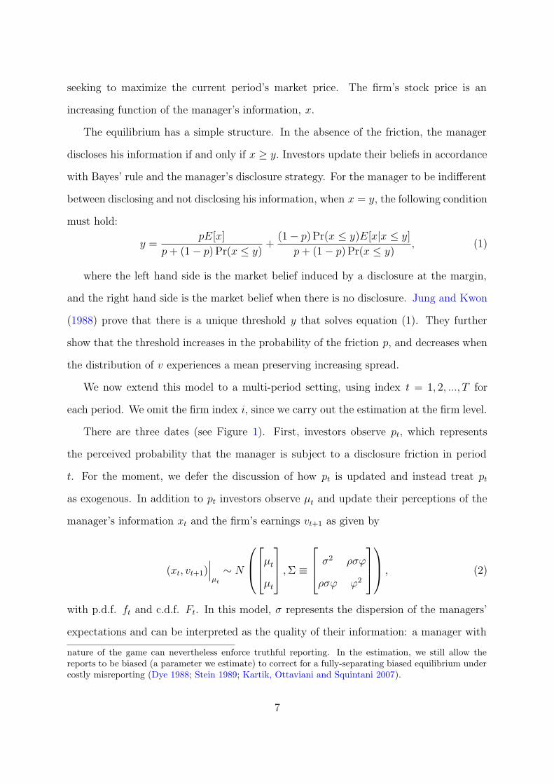
each period. We omit the firm index i, since we carry out the estimation at the firm level.

There are three dates (see Figure 1). First, investors observe pt, which represents

the perceived probability that the manager is subject to a disclosure friction in period

t. For the moment, we defer the discussion of how pt is updated and instead treat pt

as exogenous. In addition to pt investors observe µt and update their perceptions of the

manager’s information xt and the firm’s earnings vt+1 as given by

(xt, vt+1)!!!µt

% N

"

#$

%

&'µt

µt

(

)* , " &

%

&'!2 "!#

"!# #2

(

)*

+

,- , (2)

with p.d.f. ft and c.d.f. Ft. In this model, ! represents the dispersion of the managers’

expectations and can be interpreted as the quality of their information: a manager with

nature of the game can nevertheless enforce truthful reporting. In the estimation, we still allow thereports to be biased (a parameter we estimate) to correct for a fully-separating biased equilibrium undercostly misreporting (Dye 1988; Stein 1989; Kartik, Ottaviani and Squintani 2007).

7

more precise information will have more disperse beliefs (Ganuza and Penalva, 2010).

This parameter may capture both the quality of the firm’s accounting system, or some

aspects of the firm’s underlying business model. For example, in some industries, the

manager’s uncertainty about the next period earnings may be resolved early during the

quarter, whereas in some other industries the uncertainty may be resolved late.

The parameter #, by contrast, represents the dispersion of earnings, capturing the

market’s uncertainty about the firm’s future performance. More volatile industries are

characterized by a larger #. Finally, " represents the correlation between xt and vt+1 also

reflecting the quality of the manager’s information. In the baseline setting, we assume

that the manager is rational so his beliefs are given by xt = Et[vt+1]. This allows us to

write vt+1 = xt+$t, where $t is white noise. Consequently, the variance-covariance matrix

reduces, in this case, to " =

%

&'!2 !2

!2 #2

(

)*, that is, " = corrt(xt, vt+1) = !/#.

Second, if not subject to the friction, the manager chooses whether or not to disclose

his information. We denote by dt ' {(, xt } the manager’s disclosure decision in pe-

riod t. As mentioned above, the manager makes this decision aiming to maximize the

firm’s current stock price which strictly increases in xt. This captures, for example, a

manager who is willing to accelerate the e!ect of news before the next-quarter earnings

announcement.6

Third, the earnings vt+1 are realized and publicly observed. The markets uses this

information to update the probability that the manager concealed information in the

previous period, and the probability that the manager experiences the friction in the

next period.

6The DJK model is, in essence, a model of managerial short-termism. As in Shin (2003), while ourmodel has multiple periods and features learning over time, we assume that the manager maximizescurrent stock price. Short-termism is at the core of disclosure theory since, without any short-termmotive, the manager could wait for realized cash flows. One may criticize this approach on the groundsthat the reality is probably more complex, with managers maximizing prices over time. This noted, webelieve that the DJK model provides a useful parsimonious benchmark. Unfortunately, forward-lookingmotives would require us to place much more structure on intertemporal preferences and, because of therational pricing function, imply a computationally di"cult problem. We are not aware of any theoreticaltreatment of a fully dynamic (infinite horizon) disclosure model with forward-looking motives.

8

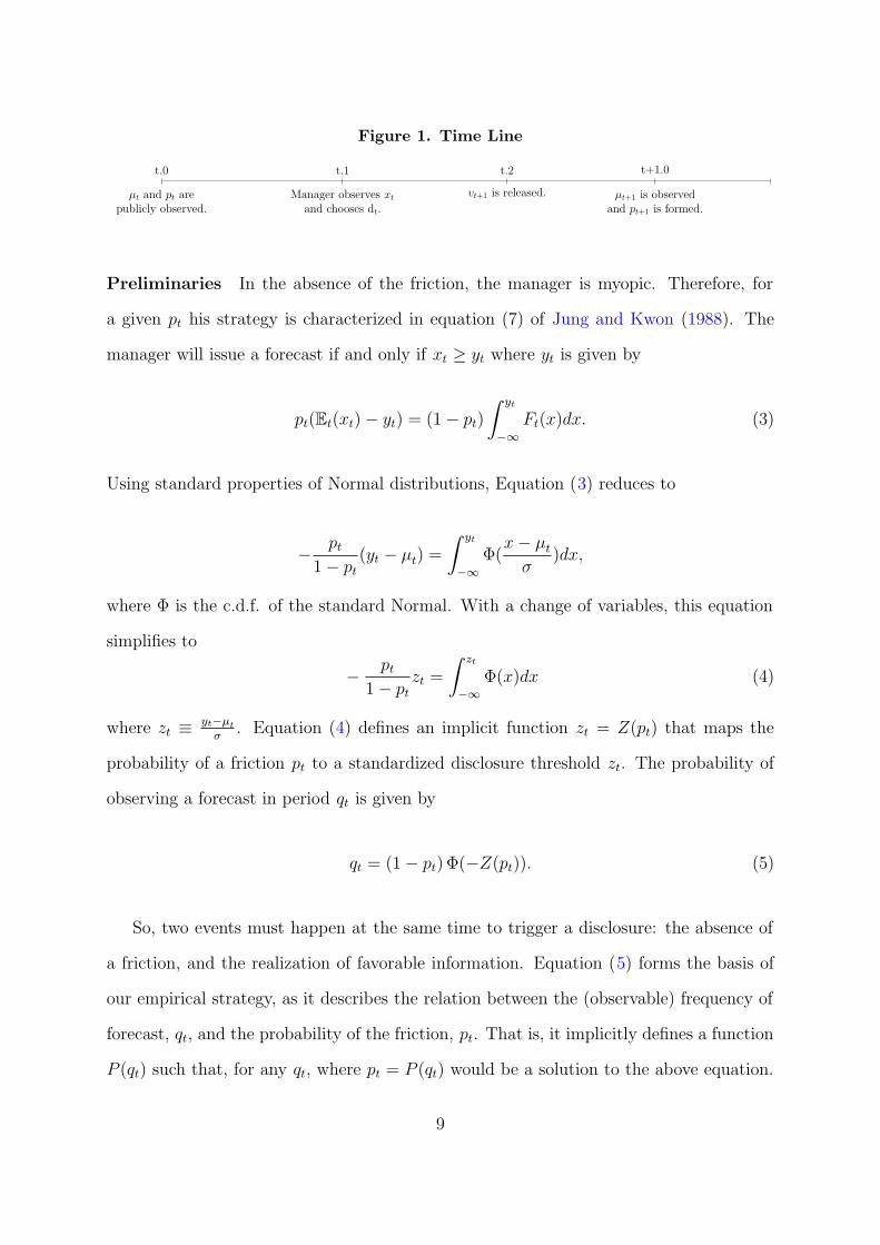
Figure 1. Time Line

µt and pt arepublicly observed.

t.0

Manager observes xt

and chooses dt.

t.1

vt+1 is released.

t.2

µt+1 is observedand pt+1 is formed.

t+1.0

Preliminaries In the absence of the friction, the manager is myopic. Therefore, for

a given pt his strategy is characterized in equation (7) of Jung and Kwon (1988). The

manager will issue a forecast if and only if xt # yt where yt is given by

pt(Et(xt) " yt) = (1 " pt)

. yt

!"Ft(x)dx. (3)

Using standard properties of Normal distributions, Equation (3) reduces to

" pt

1 " pt(yt " µt) =

. yt

!"#(

x " µt

!)dx,

where # is the c.d.f. of the standard Normal. With a change of variables, this equation

simplifies to

" pt

1 " ptzt =

. zt

!"#(x)dx (4)

where zt & yt!µt! . Equation (4) defines an implicit function zt = Z(pt) that maps the

probability of a friction pt to a standardized disclosure threshold zt. The probability of

observing a forecast in period qt is given by

qt = (1 " pt) #("Z(pt)). (5)

So, two events must happen at the same time to trigger a disclosure: the absence of

a friction, and the realization of favorable information. Equation (5) forms the basis of

our empirical strategy, as it describes the relation between the (observable) frequency of

forecast, qt, and the probability of the friction, pt. That is, it implicitly defines a function

P (qt) such that, for any qt, where pt = P (qt) would be a solution to the above equation.

9

Conveniently, under normality, the function P (.) does not require knowledge of µt or !t,

and the next claim guarantees that pt is identified.

Claim 1 The function P (.) is a strictly decreasing, continuous, invertible bijection on

[0, 1].

The mapping P (·) is strictly decreasing. Given a higher frequency of disclosure,

the model predicts a higher probability of a friction. Furthermore, because of strategic

disclosure, the probability of the friction is always strictly less than the probability of not

observing a disclosure.7

1.2 Intuition for the estimation strategy

We first explain the estimation strategy under the simplifying assumption that the

probability of the friction is constant over time pt = p. This assumption does not hold in

practice and we shall later relax it by allowing for persistence in the friction. For now,

we will assume that the market expectation µt is observed by the econometrician.

Suppose we have access to T observations for a given firm. The likelihood of the data

is given by

L =

/01

02

0 if min(x)! < Z(p)

3Tt [gt(vt+1) (p + (1 " p) Ht (Z(p))]1!It [(1 " p) ft(xt, vt+1))]It if min(x)

! # Z(p).

where It is an indicator function which takes value 1 if there is disclosure in period

t and zero otherwise. The function gt(vt+1) represents the marginal density of vt+1 in

period t, and Ht(.) is the distribution of xt conditional on the realization of earnings

7We omit a formal discussion of identification but this can easily be shown in the iid case, for reasonsthat are analogous to those in Heckman (1979). For example, using the method of moments we see thatEq. (4) uniquely identifies the threshold zt. Identification of !2 can then be obtained from Vt(xt|xt >

yt) = !2(1 + zt"(zt) " ("(zt))2), where "(x) = !(x)1"!(x) . Finally, µt can be identified from E[µt|xt > yt] =

µt + !"(zt).

10

vt+1. Since the model predicts that forecasts must be above the threshold yt, the model

enforces a lower bound for the dispersion of the manager beliefs

! # min(x)/Z(p). (6)

This bound is key to understanding how DJK reconciles observations in which very bad

news is voluntarily disclosed, that is, when min(x) is a large negative number. In the

model, the standardized forecast must always be above Z(p). So, for bad news to be

disclosed, it must be that the manager signal is precise, because this leads to great

variability in his posterior assessment. Intuitively, if the manager’s information is precise,

then the market will tend to penalize more a non-disclosure, and as a consequence, more

unfavorable information will tend to be disclosed.

Naturally, a greater probability of friction p implies that the manager, overall, discloses

fewer unfavorable news. Hence, as we have stated in claim 1, the increase in this bound is

much greater when the frequency of disclosure is itself very low, because the low frequency

indicated that this manager was unlikely to be informed. In summary, an occasional

disclosure of bad news indicates a manager who is often subject to a friction but, when

not, has very precise information to forecast.

The maximum likelihood estimator (pMLE,!MLE) takes one of two forms. If equation

(6) is not binding, the likelihood function can be decomposed to estimate !MLE and pMLE

separately, as

!MLE =

45Tt It(xt " µt)2

n,

pMLE = arg maxp

(p + (1 " p) Ht (Z(p)))T!n (1 " p)n ,

min (x)

!MLE# Z(pMLE),

where n is the number of periods where no disclosure was issued.

11

Note that, while the observed forecasts are truncated, the MLE estimator !MLE seem-

ingly ignores the truncation and uses the estimator of an untruncated normal, even though

a truncated normal has lower variance than a non-truncated one. The reason for this is

tied to the equation for the bound in DJK: the disclosure threshold scales with the vari-

ance, that is, yt = µt + !Z(p).

Proper consideration of the bound is, however, critical when observing low forecasts.

Suppose next that equation (6) binds, then the MLE estimator is

!MLE =min (x)

Z (pMLE),

pMLE = arg maxp

T6

t

gt(vt+1)7p + (1 " p) Ht (z)

81!It7(1 " p) ft(xt|vt+1)

8It

.

When equation (6) is binding, the estimation can no longer be conducted as two sep-

arate problems for pMLE and !MLE. This is because to rationalize a history of infrequent

but low forecasts we must either decrease the manager’s precision or increase the proba-

bility of the friction p. The maximum likelihood estimator meets the bound by balancing

this trade-o!.

1.3 Stickiness in forecast policies

In practice, management forecast policies are sticky: the probability that a manager

releases a forecast in the current quarter depends on how often he has released forecasts

in the past. In their survey of management, Graham, Harvey and Rajgopal 2005 note

that the act of disclosing information sets a precedent before investors whereby investors

tend to expect more disclosure from a firm that has frequently disclosed in the past versus

one that has remained silent.

To capture stickiness in disclosure decisions, we augment the model by assuming that

the friction is persistent. Formally, assume that there is a process %t ' {0, 1} where %t = 1

indicates that the manager is subject to the friction in period t. Specifically, we assume

12

that %t follows a Markov chain with transition matrix:

K =

%

&'k1 1 " k1

k2 1 " k2

(

)* .

That is, if (not) subject to the friction at date t, the manager is subject to the friction

at date t + 1 with probability (k2) k1. As before, investors do not observe the friction.

Conditional on no-disclosure at date t, investors do not know whether %t = 1 or, instead,

%t = 0 but the manager withheld his private information.

Investors update their beliefs about %t using the history of disclosure and their con-

jectures about the manager’s equilibrium strategy. Conditional on observing a disclosure

at date t, investors know that %t = 0 (no friction), and update their belief for the next

period based on the transition matrix, thus setting pt+1 = k2. By contrast, conditional

on observing no disclosure in period t, investors must update their beliefs to

Et(%t|dt = ND) =pt

pt + (1 " pt)P(xt < Z(pt)|vt+1)9 :; <="(pt)

.

Notice that &(pt) uses the information the market observes in between disclosure peri-

ods, such as the earnings announcement, which naturally leads investors to reassess the

probability that a manager withheld information. As an example, if realized earnings are

low following a non-disclosure, investors will increase their posterior belief of strategic

withholding implying, if the friction is sticky, a greater probability that the friction is not

present in the next period.

We denote dt ' {xt, ND} where dt = xt indicates a forecast and dt = ND indicates

no-disclosure. Then, the probability pt+1 follows:

pt+1 =

/01

02

k2 if dt )= ND

&(pt)k1 + (1 " &(pt))k2 if dt = ND. (7)

13

This equation recursively characterizes the evolution of investors’ beliefs. For the

first observation in the sample, we use the steady state distribution of %t, namely we

assume that p1 = k2k2+1!k1

. This approximation only a!ects the assessment prior to the

first observed forecast because investors’ beliefs are reset to k2 each time a disclosure is

observed.8 As a special case, if k1 = k2 = k, the probability of receiving information is

i.i.d., and the estimation procedure can be run as described in the previous section with

a single state with p = k1 = k2.

We can now write the likelihood function as:

L(K, ") =T6

t=1

[gt(vt+1) (pt + (1 " pt) Ht (Z(p))]1!It [(1 " pt)) ft(xt, vt+1))]It

where pt follows the process in (7). Besides the variance covariance matrix, ", we

must estimate the transition matrix of this Markov chain, K. The latter has a direct

interpretation in terms of the stickiness of the underlying friction. Stickiness is measured

by k2 " k1; when k2 = k1 the disclosure friction is i.i.d.

Based on the estimates of (K, ") we can compute two moments of special interest.

First, we compute the steady-state probability of being subject to the friction which we

denote by p". That is,

(p", 1 " p") = (p", 1 " p")K.

This probability measures the importance of the friction and lies in between k1 and k2.

This number tells us how often the manager does not disclosure for reasons unrelated to

his information about the firm’s future earnings.

Second, we define V" as the steady-state probability that the manager withholds

information for strategic reasons. Computing this parameter is more di$cult than p"

8We have chosen this approximation because it is computationally tractable. An alternative wouldbe to obtain by simulation the true likelihood function of the observations prior to the first forecast insteady-state; however, this method is computationally infeasible, however, given that we heavily rely onparametric bootstrap. When estimating the model on simulated data, the steady-state approximationdoes not seem to play a major role.

14

because it is an expectation many possible histories. We compute it by Monte-Carlo inte-

gration simulating histories of 1000 periods based on our MLE estimates, and recovering

the probability as the average frequency of strategic withholding realized in the simulated

histories.

It is well-known that, under various regularity conditions, the MLE estimator is consis-

tent, asymptotically normal, and attains the Cramer-Rao lower bound (Amemiya, 1985).

However, using the asymptotic properties of the estimator is not ideal in our setting be-

cause we have a small sample size of about 54 correlated observations per firm. So, we

estimate standard errors by parametric bootstrap. Using the assumed parametric struc-

ture, we simulate data and generate a distribution of parameter estimates by assuming

the firms are in steady state. Specifically, after estimating (KMLE, "MLE), we simulate

120 random histories of 500 observations, and re-estimate the model using the last 54

observations (because the original data has 54 quarters).

2 Estimation

2.1 Data

We focus our analysis on the set of firms who were in the S&P 500 index as of January

1st, 1998 which after several data restrictions reduces to a sample size of 371 firms. These

firms are by construction large, with large analyst coverage and high institutional own-

ership and, consequently, unlikely to have missing observations from commercial vendors

such as First Call (Chuk, Matsumoto and Miller, 2013).

Panel A of Table 1 describes the data filtering steps used in processing Firs Call’s

management forecasts. We begin with 22,617 forecasts from 456 firms. Next, we restrict

analysis to fiscal years beginning in 1998 because of expanded coverage of the database

to reduce selection bias (21,513 remaining forecasts) (Anilowski, Feng and Skinner 2007).

We select only earnings per share forecasts (EPS) made prior to the end of the fiscal

15

period to distinguish from pre-announcements (8,485 remaining forecasts). We select the

first forecast if there was more than one. In most cases, this forecast comes bundled with

the prior-quarter earnings release. Finally, we restrict forecasts to quantitative point and

range estimates, leaving us with a sample of 4,750 forecasts from 371 firms. For range

forecasts, we use First Call’s normalized point estimate.9

Panel B of Table 1 describes the raw sample of earnings announcements, also from

First Call.10 We follow similar restrictions to the management forecasts - with the last

step being a filter on firms that have at least 20 earnings announcement and 1 voluntary

forecast in our entire sample period.11 This final step results in a final sample of 371

firms making 4,750 earnings forecasts prior to 17,828 earnings announcements.

Panel A of Table 2 provides firm level summary statistics over the entire sampling

period. The average firm experienced 54 reporting periods, with an average forecast

frequency (q) of 26%. The average realized earnings per share (split-adjusted) is .511,

slightly greater than the average realized earnings conditional on no forecast .49. Also

note that the mean forecast .59 is generally greater than the actual earnings .511, sug-

gesting that the distribution of forecasts might be truncated. Panel B of Table 2 provides

industry-means of key summary statistics (first and second moments of realized earnings

and forecasts, as well as the average pre-forecast analyst consensus) where industry is

defined using the 2-digit Global Industry Classification Scheme.

Two empirical choices are of importance, and worth discussing in more details. We

use EPS, which is itself an issue of some debate in capital market research. Our approach

9When converting ranges to point estimates, First Call uses the mid-point of the range. For open-ended ranges (which are infrequent), First Call uses the bound plus one cent for upper ranges and minusone sent for lower ranges. Ranges did not appear to be extremely informative. In our sample, actualearnings fall in the stated range only about about one third of the time and the midpoint does not appearbiased upward or downward.

10One benefit of using First Call is that the database normalizes its forecasts and realized earningsunder the same measurement basis, making them comparable to analyst forecast data. These numbersare pro forma, that is, do not necessarily coincide with reported GAAP earnings in the Compustatdatabase (see Barth et al. (2012) for more details). All earnings numbers used here are, as much aspossible, under the same pro-forma basis.

11By construction we are excluding firms which almost never issue a forecast- though these firms arestill rationalize-able under Dye’s model e.g. as p approaches 1.

16

would be severely a!ected by market noise if we were, say, dividing by share price and,

to be fair to the institutional setting, managers forecast EPS, not the price to earnings

ratio. Cheong and Thomas (2011) show that earnings per share do not appear to show

any variation with scale because, plausibly, firms manage their share price to ensure

comparability. This is our implicit assumption when using earnings per share or, more

accurately, the precision of the manager’s private information about earnings per share

does not significantly vary during the sample period.

We also checked whether managers bias their forecasts, that is, exhibit systematic

non-zero forecast errors. There is some debate in capital market research as to whether

management forecasts are biased; for example, Coller and Yohn (1998) conclude that

forecasts do not appear biased while, with more recent data, Rogers and Stocken (2005)

observe that forecasts appear biased. To address this, our estimation procedure includes

a possible bias term. We do not find evidence of a significant positive or negative average

bias, primarily because we focus on large firms. On a per-firm basis, evidence of a bias is

mixed, with about one third of the firms with no significant bias, one third positive, and

one third negative (Panel A Table 2).

2.2 Findings

To gain some flexibility in the estimation, we allow for the possibility that both the

consensus µt and the management forecasts xt are biased relative to the true earnings

vt+1. We define bias in forecast as bf & Et[xt] " Et[vt+1] and bias in consensus as

bµ & µt " Et[vt+1].

Table 1 reports the estimated parameters and their standard errors, averaged across

the sample firms. The friction appears to be fairly sticky, with 76% probability (k1) of

an existing friction persisting to the next quarter, versus a probability (k2) of 52% of the

friction realizing in the next quarter if it was not present in the current quarter.

17

Table 1. Average parameter estimates (N=371)

k1 k2 ! # bf bµ Log-Likelihood0.7567 0.5176 0.3307 0.6398 -0.1322 0.0220 1.9496

(0.1294) (0.1577) (0.1524) (0.0829) (11.7825) (0.0833)

To test the hypothesis of stickiness, we use a a chi-square test for nested models,

taking k1 = k2 as the null hypothesis. When applying this test on a per-firm basis we

find that the assumption of i.i.d. friction is rejected for 55% of sample firms (at 5%

significance level). With regard to the quality of manager’s information, we find that

!2 = 0.1089, whereas the variation in earnings is #2 = 0.41. This implies that managers

possess significant private information about the firm’s prospects, but this information

accounts only for 27% of the variation in earnings.

Is there evidence of strategic withholding? To answer this question, recall that under

DJK, management forecasts are drawn from a truncated distribution. A truncated distri-

bution has lower variance than the underlying non truncated distribution implying that,

to explain the variance of management forecasts, the estimated variance of the manager’s

expectation must be greater than that of forecasts, with the variance gap increasing in

the truncation point. This feature is consistent with some descriptive statistics. The

variance of management forecasts is .0729 whereas the variance of manager expectations

is !2 = 0.1089. A truncation in the distribution implies also that the average forecast

should be larger than the average earnings, which again is supported by the data ( .57

versus .51).

Table 2. Probability of Friction/Withholding (N=371)

p" V"0.6326 0.0951

(0.1055) (0.0341)

Table 2 reports the steady-state probability of the friction and strategic withholding.

The friction appears to be relatively frequent, with an average point estimate of 63%.

18

Also, we find that strategic withholding occurs only about 10% of the quarters, on aver-

age. The reason for this is tied to the assumptions of DJK: in this model market pressure

forces disclosure of any above-average information so that, in the absence of the friction,

strategic withholding must occur less than half of the time. Market pressure are indeed

strong enough to induce disclosure of somewhat unfavorable events. Roughly, our esti-

mates suggest that the manager conceals his information when it falls in the first quartile

of the distribution of the manager’s expectations (namely conditional on not facing the

friction, the probability of withholding is .09511!.63a * 25%.).

At first sight management forecasts appear to be downward biased, which echoes

the idea that managers seek to influence the beliefs of analysts downwards in order to

subsequently beat the consensus forecast via the actual earnings (Richardson, Teoh and

Wysocki 2004). By contrast, the consensus forecast appears to be slightly upward biased

on average, suggesting that analysts overstate their forecasts (for example Chen and Jiang

(2006) conjecture that this is due to analyst incentives). However, we must point out that

neither type of bias is statistically significant on average.

In Panel B, we break down these results by industry groups (2-digit GICS). We find

that volatile industries or industries that rely on inputs that are hard to predict exhibit

lower quality of managerial information, with energy and telecommunications featuring

very low quality private information. On the other hand, as intuitively expected, util-

ities and industrial sectors feature greater quality. The case of the financial industry

is somewhat interesting as well because (with telecommunications), it is one of the few

industries for which we do not observe stickiness. The financial industry exhibits fairly

precise managerial information, which may be driven by the role of accrual assumptions

(in loan-loss provisions) quarter over quarter.

As to the steady-state probability of withholding, we find some moderate di!erences

across industries. Telecommunications and utilities are the most likely to withhold in-

formation, about one quarter out of 5. By contrast, energy, healthcare and technology

19

withhold information only about one quarter out of 10.

The last column presents the steady-state probability of experiencing a friction. The

energy sector appears, by far, the most likely to exhibit a friction (79%), and information

technology the least likely (27%). Our best conjecture for this result is that technology

firms are the most likely to face short-term market pressure, as a result of stock compen-

sation or their reliance on equity financing. But, then, we should also expect financial

firms to be unlikely to have this friction; yet this is not the case (57%).

Figure 3 presents histograms for the parameter estimates across firms. Notice that the

standardized disclosure threshold z is by construction negative, reflecting the prediction

of DJK that only below-average news may be withheld. The histogram reveals a fair

amount of variation at the firm level, especially for the disclosure threshold and the

steady-state probability of the friction. Of practical interest, the model predicts a fairly

small range for the estimated probability of withholding.

We note two additional facts. First, closer inspection of the threshold z reveals that

a large peak at a disclosure around "0.3, that is, (by and large) most firms tend to

strategically withhold information that is about one standard deviation below mean.

Second, the histogram of !2 shows that a fraction of firms appear to have very low

quality information (the mode of the distribution), essentially making a forecast that is

unchanging - and therefore, which carries very little information.

3 Applications

3.1 A test of overconfidence

An extensive literature suggests that managerial over-confidence is widespread. The

literature has used the term overconfidence in two senses: upward bias in beliefs (Mal-

mendier, Tate and Yan, 2011) and over-sensitivity to private information (Chen and Jiang

(2006); Marinovic, Ottaviani and Sørensen (2013) ). Next, we study both phenomena but

20

use the term over-confidence in the latter sense, namely excessive reliance on one’s signal,

whether positive or negative.

In general, disentangling overconfidence from private information is di$cult. But

the setting of management forecasts is well-suited for detecting over-confidence because

manager forecasts are a direct report the manager’s beliefs regarding a well defined event

that is observed ex post, when earnings are revealed. To study over-confidence we rely on

a standard test of excess volatility. Bayes’ rule imposes significant structure on the joint

distribution of forecasts and earnings realizations which one can exploit. For example,

absent overconfidence, basic probability theory implies that V art(xt) = V art(Et(vt+1)) =

!2 < V art(vt+1) = #2. That is, the variability in management forecasts must be lower

than the variability in earnings.12 A violation of this inequality can be explained under

the assumption that the manager is overconfident and puts excessive weight on privately-

informed information.

In order to formally test for over or under-confidence, we generalize the estimation

DJK by estimating equation (2), without the rationality restriction " = !/#. A manage-

ment forecast xt can be written as

xt = 't + ( · xt, (8)

where 't is predetermined, xt represents the Bayesian beliefs conditional on the manager’s

private information and ( = !#$ represents overconfidence when ( > 1 or underconfidence

when ( < 1.13

We label this generalized model as DJKO. The outcome of the estimation is presented

in Table 3.12Note that DJK remains applicable even with over-confidence, given that the input of the model is

the manager’s subjective beliefs about how the market react.13As an equivalent formulation, assume the manager observes a signal st = vt+1 + nt where nt is

white noise. The manager forecast can then be written as xt = (1 " "#)µt + "#(st " µt) where # =covt(st, vt+1)/vart(st). Management forecasts are thus Bayesian if and only if " = 1. It would be possibleto place additional structure and impose "#' [0, 1] but our estimates do not impose this restriction.

21

Table 3. Average parameter estimates (N=388)

k1 k2 ! # " bf bµ Log-LikDJK 0.7567 0.5176 0.3307 0.6398 0.6011 -0.1322 0.0220 1.9496DJKO 0.7756 0.5234 0.3816 0.5363 0.2967 -0.1338 -0.0158 19.5474

Notice the large increase in likelihood obtained upon allowing for over-confidence. We

can estimate the average overconfidence parameter ( using the equality ( = !#$ . The

individual estimates of ( are, however, imprecise. 65% of the firms have a ( > 1. The

median is ( = 1.28. The percentile 25% is 0.99 and the percentile 75% is 4.21. So, the

evidence suggests that managers do not use their private information e$ciently when

they release a forecast and that, on average, they overreact to their private information.

Tests. To formally test for overconfidence, we use a likelihood ratio test, taking the DJK

model as the null hypothesis H0 and the overconfidence model DJKO as the alternative

hypothesis Ha. The test statistic is thus % = L(KMLE ,!MLE)maxK,! La(K,!) . Since our sample size per

firm is relatively small, we use parametric bootstrap to compute the distribution of the

test statistic using 120 draws. We also conduct a global test, where H0: “DJK holds for

all firms” against Ha “Model DJKO holds for all firms.” The test procedure is identical

to the per firm test, except that we use the joint test statistic3N

i %i.

Table 4. Rejection of DJK vs DJKO

Reject DJK Count PercentNo 159 40.98%Yes 229 59.02%

Table 5. Global test of DJK vs DJKO

Sig. &Log-Lik Crit.Value1% -17.599 -1.9195% -17.599 -1.610

10% -17.599 -1.405

The results of the formal test are documented in Table 4. The test rejects rationality

22

for as many as 59% of the firms. To further investigate the issue of overconfidence we

conduct a global test of managerial rationality. Table 5 presents the results of a test

that examines whether DJK can be applied to the entire universe of firms against DJKO

which allows for over-confidence. Not surprisingly, at this point, rationality is rejected at

any conventional level of significance.

3.2 What is the friction?

In this section, we develop an exploratory analysis of the economic forces that may

drive the friction and the probability of strategic withholding. As we have seen, the

friction has many possible interpretations which may cause the absence of disclosure.

The conventional explanation for the friction, given by Dye (1985), is that managers

do not always receive incremental information - relative to investors - or receive it too

late within the quarter. In Table 4, we observe weak evidence that firms with a greater

likelihood of the friction p" tend to feature less precise information (lower !). Under

the assumption that the probability of information endowment and the quality of the

information are related metrics for the quality of managerial information, this correlation

may suggest that a “friction” represents a situation where the manager does not have

enough information to make a forecast.

Another explanation is that the friction may represent time-varying proprietary costs,

in which making a forecast may occasionally cause large proprietary costs. In Table 4,

we observe that firms that are larger - whose proprietary costs are likely to be greater

- tend to be more likely to be subject to the friction. Indeed, Table 3 Panel B suggests

that industries that are widely viewed to be less competitive, such as Energy, Utilities

and Telecommunications, are more likely to be subject to the friction.

An inspection of the time-series of our estimation reveals another likely determinant

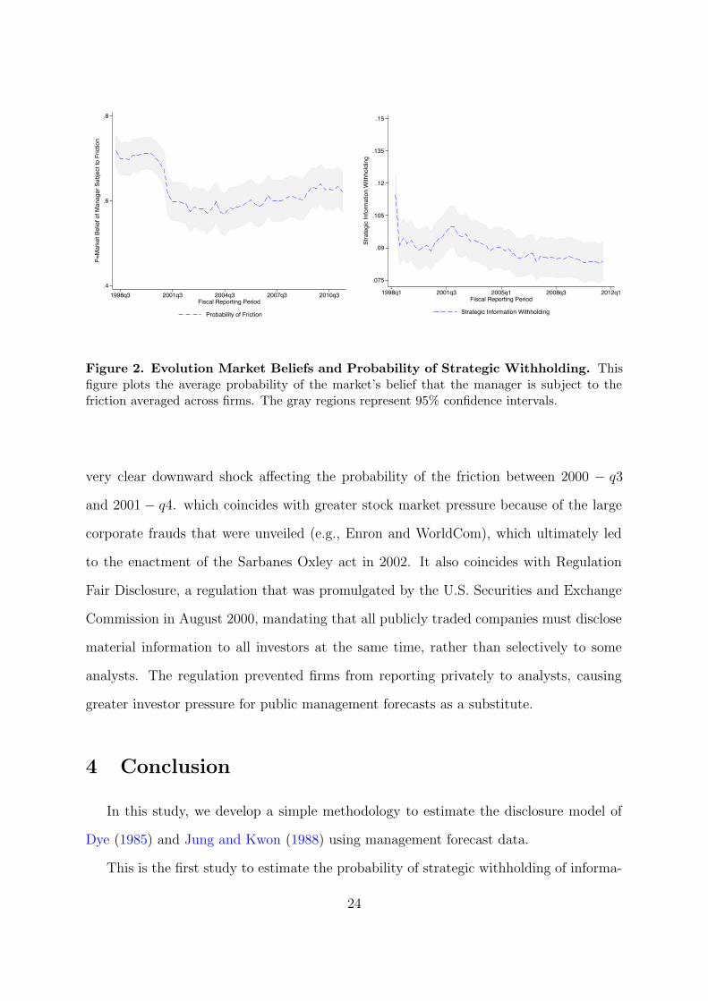
of the friction. In Figure 2, we plot the average beliefs about the friction as implied by

the estimated DJK across fiscal reporting periods for the average firm. We observe a

23

.4

.6

.8

P=M

arke

t Bel

ief o

f Man

ager

Sub

ject

to F

rictio

n

1998q3 2001q3 2004q3 2007q3 2010q3Fiscal Reporting Period

Probability of Friction

.075

.09

.105

.12

.135

.15

Stra

tegi

c In

form

atio

n W

ithho

ldin

g

1998q1 2001q3 2005q1 2008q3 2012q1Fiscal Reporting Period

Strategic Information Withholding

Figure 2. Evolution Market Beliefs and Probability of Strategic Withholding. Thisfigure plots the average probability of the market’s belief that the manager is subject to thefriction averaged across firms. The gray regions represent 95% confidence intervals.

very clear downward shock a!ecting the probability of the friction between 2000 " q3

and 2001 " q4. which coincides with greater stock market pressure because of the large

corporate frauds that were unveiled (e.g., Enron and WorldCom), which ultimately led

to the enactment of the Sarbanes Oxley act in 2002. It also coincides with Regulation

Fair Disclosure, a regulation that was promulgated by the U.S. Securities and Exchange

Commission in August 2000, mandating that all publicly traded companies must disclose

material information to all investors at the same time, rather than selectively to some

analysts. The regulation prevented firms from reporting privately to analysts, causing

greater investor pressure for public management forecasts as a substitute.

4 Conclusion

In this study, we develop a simple methodology to estimate the disclosure model of

Dye (1985) and Jung and Kwon (1988) using management forecast data.

This is the first study to estimate the probability of strategic withholding of informa-

24

tion in capital markets and to separate the strategic and non-strategic components of non

disclosure. We have documented the following facts. 1) Managers strategically withhold

bad news about 10% of the time. 2) They conceal the percentile 25% of the distribution

of private information in the absence of the friction. 3) They enjoy a significant infor-

mational advantage, relative to the market: their private information at the disclosure

date explains 50% of the variation in earnings. 4) We provide evidence that managers on

average over-react to their private information.

We hope to o!er, here, a starting point to identify the failures of the disclosure theory

and o!er as much material for further research in empirical and theoretical research.

The data appears to suggest that there are fundamental di!erences between how firms

forecasts, with some following DJK while others disclosing information regardless of its

price impact. Further work should, therefore, involve richer settings that improve over

the DJK approach. For theoretical research, we appear to find robust evidence that

managers do not form rational expectations but, instead, feature some large levels of

overconfidence. Lastly, our model is amenable to test richer theories to disclosure by

conditioning the probability of the friction on various determinants of disclosure.

25

References

Acharya, V. V., Demarzo, P. and Kremer, I. (2011). Endogenous informationflows and the clustering of announcements. The American Economic Review, 101 (7),2955–2979.

— and Lambrecht, B. M. (2011). A theory of income smoothing when insiders knowmore than outsiders. Tech. rep., National Bureau of Economic Research.

Amemiya, T. (1984). Tobit models: A survey. Journal of econometrics, 24 (1), 3–61.

— (1985). Advanced econometrics. Harvard university press.

Anilowski, C., Feng, M. and Skinner, D. J. (2007). Does earnings guidance a!ectmarket returns? The nature and information content of aggregate earnings guidance.Journal of Accounting and Economics, 44, 36–63.

Bajari, P. and Hortacsu, A. (2003). The winner’s curse, reserve prices, and endoge-nous entry: empirical insights from ebay auctions. RAND Journal of Economics, pp.329–355.

Ball, R. and Brown, P. (1968). An empirical evaluation of accounting income num-bers. Journal of accounting research, pp. 159–178.

Barth, M. E., Gow, I. D. and Taylor, D. J. (2012). Why do pro forma and streetearnings not reflect changes in gaap? evidence from sfas 123r. Review of AccountingStudies, 17 (3), 526–562.

Ben-Porath, E., Dekel, E. and Lipman, B. L. (2014). Disclosure and Choice. Tech.rep., Mimeo.

Beyer, A., Cohen, D. A., Lys, T. Z. and Walther, B. R. (2010). The financialreporting environment: Review of the recent literature. Journal of Accounting andEconomics, 50 (2-3), 296–343.

—, Guttman, I. and Marinovic, I. (2014). Earnings management and earnings qual-ity: Theory and evidence. Available at SSRN 2516538.

Bushman, R. M. (1991). Public disclosure and the structure of private informationmarkets. Journal of Accounting Research, pp. 261–276.

Chen, Q. and Jiang, W. (2006). AnalystsS weighting of private and public information.Review of Financial Studies, 19 (1), 319–355.

Cheong, F. S. and Thomas, J. (2011). Why do eps forecast error and dispersionnot vary with scale? implications for analyst and managerial behavior. Journal ofAccounting Research, 49 (2), 359–401.

26

Chuk, E., Matsumoto, D. and Miller, G. S. (2013). Assessing methods of identi-fying management forecasts: CIG vs. researcher collected. Journal of Accounting andEconomics, 55 (1), 23–42.

Coller, M. and Yohn, T. L. (1998). Management forecasts: What do we know?Financial Analysts Journal, 54 (1), 58–62.

Dickhaut, J., Ledyard, M., Mukherji, A. and Sapra, H. (2003). Information man-agement and valuation: an experimental investigation. Games and Economic Behavior,44 (1), 26–53.

Dye, R. A. (1985). Disclosure of nonproprietary information. Journal of AccountingResearch, 23 (1), 123–145.

— (1988). Earnings management in an overlapping generations model. Journal of Ac-counting Research, 26 (2), 195–235.

— and Sridhar, S. S. (1995). Industry-wide disclosure dynamics. Journal of accountingresearch, 33 (1), 157–174.

Erdem, T. and Keane, M. P. (1996). Decision-making under uncertainty: Captur-ing dynamic brand choice processes in turbulent consumer goods markets. Marketingscience, 15 (1), 1–20.

Fischer, P. E. and Verrecchia, R. E. (2000). Reporting bias. The Accounting Re-view, 75 (2), 229–245.

Fishman, M. J. and Hagerty, K. M. (1990). The optimal amount of discretion toallow in disclosure. Quarterly Journal of Economics, 105 (2), 427–444.

Ganuza, J.-J. and Penalva, J. S. (2010). Signal orderings based on dispersion andthe supply of private information in auctions. Econometrica, 78 (3), 1007–1030.

Gentzkow, M. and Shapiro, J. M. (2010). What drives media slant? evidence fromus daily newspapers. Econometrica, 78 (1), 35–71.

Goldman, E. and Slezak, S. L. (2006). An equilibrium model of incentive contractsin the presence of information manipulation. Journal of Financial Economics, 80 (3),603–626.

Govindaraj, S., Lee, P. and Tinkelman, D. (2007). Using the event study method-ology to measure the social costs of litigation-a re-examination using cases from theautomobile industry. Review of Law & Economics, 3 (2), 341–382.

Graham, J. R., Harvey, C. R. and Rajgopal, S. (2005). The economic implicationsof corporate financial reporting. Journal of Accounting and Economics, 40 (1), 3–73.

Grossman, S. J. (1981). The informational role of warranties and private disclosureabout product quality. Journal of Law and Economics, 24 (3), 461–483.

27

— and Hart, O. D. (1980). Disclosure laws and takeover bids. Journal of Finance,35 (2), 323–334.

Guttman, I., Kremer, I. and Skrzypacz, A. (2014). Not only what but also when:A theory of dynamic voluntary disclosure. The American Economic Review, 104 (8),2400–2420.

Hagerty, K. M. and Fishman, M. J. (1989). Disclosure decisions by firms and thecompetition for price e$ciency. Journal of Finance, 44 (3), 633–646.

Heckman, J. J. (1979). Sample selection bias as a specification error. Econometrica:Journal of the econometric society, pp. 153–161.

Huddart, S., Hughes, J. S. and Levine, C. B. (2001). Public disclosure and dissim-ulation of insider trades. Econometrica, 69 (3), 665–681.

Jin, G. Z., Luca, M. and Martin, D. (2015). Is no news (perceived as) bad news?an experimental investigation of information disclosure. An Experimental Investiga-tion of Information Disclosure (March 31, 2015). Harvard Business School NOM UnitWorking Paper, (15-078).

Jovanovic, B. (1982). Truthful disclosure of information. Bell Journal of Economics,13 (1), 36–44.

Jung, W.-O. and Kwon, Y. K. (1988). Disclosure when the market is unsure of infor-mation endowment of managers. Journal of Accounting Research, 26 (1), 146–153.

Kartik, N., Ottaviani, M. and Squintani, F. (2007). Credulity, lies, and costly talk.Journal of Economic theory, 134 (1), 93–116.

Kedia, S. and Philippon, T. (2009). The economics of fraudulent accounting. Reviewof Financial Studies, 22 (6), 2169–2199.

LeRoy, S. F. and Porter, R. D. (1981). The present-value relation: Tests based onimplied variance bounds. Econometrica, pp. 555–574.

Lundholm, R. J. and Rogo, R. (2014). Do analysts forecasts vary too much? Availableat SSRN.

Malmendier, U., Tate, G. and Yan, J. (2011). Overconfidence and early-life expe-riences: the e!ect of managerial traits on corporate financial policies. The Journal offinance, 66 (5), 1687–1733.

Marinovic, I., Ottaviani, M. and Sørensen, P. N. (2013). ForecastersS objectivesand strategies. Handbook of economic forecasting, 2, 691–720.

McClellan, F. (2008). The vioxx litigation: A critical look at trial tactics, the tortsystem, and the roles of lawyers in mass tort litigation. DePaul Law Review, 57, 509–538.

28

Mello, M. M., Rimm, E. B. and Studdert, D. M. (2003). The mclawsuit: Thefast-food industry and legal accountability for obesity. Health A!airs, 22 (6), 207–216.

Milgrom, P. R. (1981). Good news and bad news: Representation theorems and ap-plications. Bell Journal of Economics, 12 (2), 380–391.

Rabin, R. L. (2001). Tobacco litigation: A tentative assessment. DePaul Law Review,51, 331.

Richardson, S., Teoh, S. H. and Wysocki, P. D. (2004). The walk-down to beat-able analyst forecasts: The role of equity issuance and insider trading incentives*.Contemporary Accounting Research, 21 (4), 885–924.

Rogers, J. L. and Stocken, P. C. (2005). Credibility of management forecasts. TheAccounting Review, 80.

Shavell, S. (1994). Acquisition and disclosure of information prior to sale. Rand Journalof Economics, 25 (1), 20–36.

Shiller, R. J. (1980). Do stock prices move too much to be justified by subsequentchanges in dividends?

Shin, H. (2003). Disclosures and asset returns. Econometrica, 71 (1), 105–133.

Shin, H. S. (1994). News management and the value of firms. Rand Journal of Eco-nomics, pp. 58–71.

Stein, J. C. (1989). E$cient capital markets, ine$cient firms: A model of myopiccorporate behavior. Quarterly Journal of Economics, 104 (4), 655–669.

Stocken, P. C. (2000). Credibility of voluntary disclosure. The RAND Journal of Eco-nomics, pp. 359–374.

Terry, S. J. (2014). The Macro Impact of Short-Termism. Tech. rep., Working paper.

Tobin, J. (1958). Estimation of relationships for limited dependent variables. Econo-metrica: journal of the Econometric Society, pp. 24–36.

Zakolyukina, A. A. (2014). Measuring intentional gaap violations: A structural ap-proach. Chicago Booth Research Paper, (13-45).

29

Table 1. Sample Selection and Summary Statistics

Our firm sample is the set of firms who were initially in the S&P 500 index as of January1st, 1998 for the sample period between fiscal quarter 1 of 1998 to fiscal quarter 3 of2011. Panel A and B report our sample selection criterion of management forecasts andearnings announcements from the First Call database.

Panel A: Management Forecasts

Step Rule Obs FirmsRaw sample 22,617 456

Restrict to:2) 1998Q1-2011Q3 fiscal years 21,5133) Quarterly guidance on EPS 8,4854) Guidance date prior to end of FP 7,1675) Guidance date within 90 days window prior to end of FP 6,5086) Non-missing First Call point estimate 5,9447) First dated guidance per fiscal period 4,750 371

Panel B: Earnings Announcements

Step Rule Obs FirmsRaw sample 54,775 495

Restrict to:1) 1998Q1-2011Q3 fiscal years 32,9022) Original un-restated announcements 19,1484) Firms with minimum of 1 voluntary forecast 17,828 371

30

Table 2. Summary Statistics of Raw Data

Panel A reports key summary statistics of our final sample of 371 firms. Management forecasts andrealized earnings are both split-adjusted. The pre-forecast analyst consensus is defined as the averageconsensus (split-adjusted) of the most current (on an analyst by analyst basis) forecasts made prior to thedate of management forecast disclosure. Panel B groups firms according to their historical 1998 two-digitGlobal Industry Classification Scheme (GICS) and reports the average of firm-level forecast frequencies,and their average realized earnings when preceded by disclosure or non-disclosure of a managementforecast.

Panel A: Firm Level

Variable Obs Mean Std. Dev. P25 P50 P75Number of reporting periods 371 46.77 13.13 43 54 54Fraction of periods with forecasts (q) 371 .26 .24 .06 .15 .44Average value of realized earnings 371 .51 .54 .29 .46 .65Average value of realized earnings (forecast disclosed) 371 .51 .65 .26 .42 .64Average value of realized earnings (forecast not disclosed) 371 .49 .54 .25 .44 .64Standard deviation of realized earnings 371 .5 1.29 .16 .26 .42Average value of forecasts 371 .59 .62 .31 .5 .76Standard deviation of forecasts 311 .27 .26 .11 .19 .36Average mgmt. forecast error 371 .08 .74 -.02 0 .11St.dev. of mgmt. forecast error 311 .23 .76 .04 .09 .21Pre-forecast analyst consensus 371 .56 .63 .31 .48 .66

Panel B: Industry Level

GICS2 N Avg frequencyof forecasts

Avg realized earnings(forecast disclosed)

Avg realized earnings(forecast not disclosed)

Energy 11 0.14 0.52 0.66Materials 36 0.22 0.47 0.43Industrials 65 0.29 0.50 0.51Consumer Discretionary 74 0.34 0.49 0.41Consumer Staples 33 0.22 0.47 0.48Health Care 28 0.31 0.57 0.47Financials 37 0.07 0.66 0.69Information Technology 44 0.41 0.44 0.41Telecommunication Services 9 0.14 0.44 0.35Utilities 25 0.11 0.57 0.57Unclassified 9 0.32 0.44 0.44Total 371 0.26 0.51 0.49

31

Tab

le3.

Sum

mar

ySta

tist

ics

ofM

odel

Est

imat

es–

Fir

mLev

el

Pan

elA

sum

mar

izes

the

key

estim

ates

ofou

rth

ree

mod

els

(in

supe

rscr

ipts

,nul

l,m

odel

“a”

non-

stra

tegi

c,an

dm

odel

“b”

naiv

e-in

vest

ors)

.k 1

(k2)

isth

epr

obab

ility

ofth

em

anag

erno

tbo

und

byth

edi

sclo

sure

fric

tion

cond

itio

nalo

nbe

ing

not

boun

d(b

ound

)in

the

prev

ious

peri

od.

!is

the

stan

dard

devi

atio

nfr

omth

etr

ue(u

n-tr

unca

ted)

dist

ribu

tion

ofm

anag

emen

tfo

reca

sts.

v #is

the

stea

dy-s

tate

prob

abili

tyth

atth

em

anag

eris

withh

oldi

ngne

ws

and

p #is

the

stea

dy-s

tate

prob

abili

tyth

atth

em

anag

eris

boun

dby

the

disc

losu

refr

iction

.Pan

elB

grou

psfir

ms

acco

rdin

gto

thei

rhi

stor

ical

1998

two-

digi

tG

loba

lInd

ustr

yC

lass

ifica

tion

Sche

me

(GIC

S)an

dre

port

sth

eav

erag

eof

the

key

mod

eles

tim

ates

byth

ese

grou

ping

s(n

ote

that

thes

ear

eno

tm

odel

re-e

stim

ates

atth

ein

dust

ryle

vel).

Pan

elA

:M

odel

Est

imat

es–

Fir

mLev

el

Var

iabl

eO

bsM

ean

Std.

Dev

.P

25P

50P

75k 1

371

.76

.25

.69

.86

.94

k 237

1.5

2.3

6.1

6.5

.91

!37

1.3

32.

45.0

5.1

1.2

4$

371

.64

3.06

.1.1

9.3

6p #

371

.63

.32

.35

.76

.91

v #37

1.0

9.0

7.0

3.0

8.1

5M

odel

Like

lihoo

d37

11.

9561

.28

-24.

759.

5242

.59

%37

1.6

.37

.52

.7.8

2

Pan

elB

:M

odel

Est

imat

es–

Indust

ryLev

el

GIC

S2N

k1k2

sigm

ava

rphi

pV

LIK

rho

Ene

rgy

110.

820.

560.

240.

310.

770.

08-3

.90

0.76

Mat

eria

ls38

0.79

0.59

0.24

0.36

0.70

0.08

-9.0

40.

64In

dust

rial

s64

0.75

0.46

0.37

1.09

0.58

0.10

-15.

360.

64C

onsu

mer

Dis

cret

iona

ry76

0.69

0.37

0.83

1.07

0.50

0.12

-2.9

60.

66C

onsu

mer

Stap

les

330.

790.

550.

090.

130.

670.

0943

.55

0.65

Hea

lth

Car

e29

0.76

0.52

0.11

0.16

0.65

0.12

35.2

50.

66Fin

anci

als

400.

860.

790.

210.

760.

840.

05-2

9.09

0.46

Info

rmat

ion

Tech

nolo

gy45

0.63

0.33

0.22

0.63

0.44

0.12

14.6

30.

72Te

leco

mm

unic

atio

nSe

rvic

es10

0.91

0.58

0.07

0.32

0.80

0.06

29.5

50.

44U

tilit

ies

270.

890.

740.

130.

260.

830.

06-0

.27

0.44

Unc

lass

ified

150.

680.

610.

040.

140.

680.

087.

280.

12To

tal

371

0.76

0.52

0.33

0.64

0.63

0.09

1.95

0.60

32

Table 4. Cross-Correlation of Estimated Parameters

This table reports the Pearson correlation among parameters estimates from Panel A ofTable 3. k1 (k2) is the probability of the manager not bound by the disclosure friction con-ditional on being not bound (bound) in the previous period. ! is the standard deviationfrom the true (un-truncated) distribution of management forecasts. v" is the steady-stateprobability that the manager is withholding news and p" is the steady-state probabilitythat the manager is bound by the friction. P-values are reported in parentheses beloweach correlation.

log(Assets) ! # " p" V" Log-Liklog(Assets) 1

! 0.0821 1# 0.0296 0.5553* 1" -0.0235 0.2644* -0.0781 1

p" 0.1347* -0.2063* -0.0712 -0.4154* 1V" -0.1388* 0.2793* 0.1525* 0.4658* -0.6314* 1

Log-Lik -0.1374* -0.5991* -0.6032* 0.0361 0.0964 -0.1975* 1

33

0

.05

.1

.15

.2

Frac

tion

0 .2 .4 .6 .8 1 2σ2

(a) !2

0

.1

.2

.3

.4

Frac

tion

0 .05 .1 .15 .2 .25 .3 .35 .4Est. steady-state probability of strategic withholding

(b) Steady-state probability ofstrategic withholding

0

.05

.1

.15

.2

Frac

tion

0 .2 .4 .6 .8 1Est. steady-state probability of the friction

(c) Steady-state probability of thefriction

Figure 3. Distribution of Estimated Parameters Under DJK. These figures plot thedistribution of firm level estimates for z, the disclosure threshold, pi,", the steady-state prob-ability that the manager is bound by the disclosure friction, vi,", the steady-state probabilitythe manager is strategically withholding, and !2, the estimated precision of the manager’sinformation.

34