household characteristics and income inequality during inflationary periods: recent evidence from...

Pergamon

World Drw/opnwnf, Vol. 26, No. 2, pp. 297-306, I998 0 1998 Elaevier Science Ltd

All rights reserved. Printed in Great Britain 0305-750X/98 $19.00+ 0.00

PII: s0305-750x(97)10018-3

Household Characteristics and Income Inequality

during Inflationary Periods: Recent Evidence

from Suriname

ANDREW W. HOROWITZ University of Arkunsas, Fayetteville,

and

U.S.A.

DIANA WEINHOLD Vanderbilt University, Nashville, Tennessee, U.S.A.

Summary. - This paper examines the distributional consequences of a high inflation episode in Suriname during 1990-94 using household survey data. We examine not only the apparent macroeconomic correlation between high inflation and income diqtrihution. but also the micro-level characteristics of winning and losin g households. We hypothesize that education Ggnificantly affects households’ ability to recognize and respond to high inflation and thereby influences the evolution of income distribution. Our econometric analysis supports this conjecture. We also explore the role of economic sector and ethnicity on changes in a household’s position within the income distribution under high inflation. 0 1998 Elsevier Science Ltd. All rights reserved

Kq M.OR/.Y - income distribution, inflation. household, South America. Suriname

I. INTRODUCTION

While the distribution of income typically changes slowly in developed countries (see for example Soltow, 1968, and Atkinson. 1975) many less-developed countries (LDCs)experience rapid changes in income distribution. In particular, LDCs undergoing structural adjustment and/or experien- cing high rates of inflation often see dramatic changes in income inequality levels. This phenomenon is of great concern to LDC domestic policy makers and the multilaterals who often “manage” structural adjustment. As discussed in detail below, a burgeoning literature examines rising income inequality in the context of structural adjustment.

Most prior literature analyzes changing income inequality at the macro level. In contrast, we adopt a micro approach in this paper. Our objective is to identify micro-characteristics of the winning and losing households behind the changing income distribution. Our empirical analysis employs a new data set from Suriname-a country that experienced both high inflation and tremendous changes in income inequality during 1990-94. We believe the Surina- mese experience is, in many respects, a prototype of

rapid income distribution change in LDCs. We find educational achievement to be a powerful predictor of changes in a household’s position within the income distribution over this period.

In section 2 we briefly review the literature in this field. Section 3 describes the Surinamese setting and the inflationary episode of the early 1990’s. Section 4 introduces the data set. Section 5 motivates our empirical model. Section 6 outlines the regression methodology and discusses results. Section 7 con- cludes.

2. LITERATURE

The literature examining changing income inequality in LDCs may be organized according to various typologies. One natural division is between long-run and short-run perspectives. Kuznets’s (Kuznet, 1955) seminal “U curve” analysis has inspired much of the long-run literature. The “Kuznets curve” is often interpreted as indicating

Final revision accepted: September 13, 1997

297

298 WORLD DEVELOPMENT

that in the course of development income inequality will rise and then fall. Adelman and Morris (1973) provide another seminal long-run analysis. Fields (1980) provides a dual economy model which generates a Kuznets curve.

Unlike the long-run analyses cited above, this paper examines short-run changes in income inequality in the LDC setting. As noted, the short-run literature often focuses on the effect of structural adjustment and inflation on income inequality. Lustig (1995) edits a volume devoted to the impact of structural adjustment and austerity measures on inequality and poverty in Latin America. Achdut and Bigman (I 99 I ), Adehnan and Taylor (I 989), Adel- man and Nobuhiko ( l994), and Glewwe and Hall (1992) provide other recent analyses of short-run changes in income inequality associated with economic crisis and structural adjustment. The vast majority of this literature, both long and short run. explores changing income inequality at the macro level. Typically. empirical analyses consist of regressing various macro aggregates on an aggregate inequality measure such as the Gini coefficient. While this approach illuminates the relationship between income inequality and macro aggregates. it provides little insight into the characteristics of winners and losers.

Distinct from studies whose primary aim is to characterize changes in income inequality is a literature that explores inequality measure issues in inflationary settings. Notable works in this vein include Slesnick (1990). Glewwe (1990). and Asra (1989). Slesnick (1990) focuses on changes in welfare inequality under non-uniform inflation. Glewwe ( 1990) explores biases in income inequality measures when, in an inflationary environment, samples are drawn at different times. Asra (I 989) adjusts standard inequality measures to reflect the effect of inflation on different expenditure groups. Foster (I 985) provides an overview of more general inequality measure issues. In contrast to these papers, we seek to identify the characteristics of winners and losers under inflation. These characteristics. in turn, may illuminate links between the macroeconomic phenomenon of inflation and the micro-determinants of household performance under high inflation.

3. THE SURINAMESE SETTING

Roughly the size of Wisconsin, Suriname (for- merly Dutch Guyana) had a 1993 population of approximately 413,000, making it among the least populated countries in the hemisphere. Approxi- mately 90% of the population resides in the coastal plain, with over 70% within a 30 kilometer radius of the capital, Paramaribo.

As in much of the Southern Caribbean, ethnic composition is complex. The population shares of the four largest ethnic groups are: Hindustani (377r). Creole (31%), Javanese (14%), and Maroons (9%). Residing in the interior are Amerindians (3%). The remaining 6% of the population consists of Chinese. European (Caucasian), and unclassified. Ethnic identification is strong. Less than IO% of household heads had partners outside their own ethnic group in 1993.’

Through much of the 1970s and 1980s the Surinamese economy, though somewhat stagnant, was relatively stable. Per capita GDP in 1985 was US$ 2.450, placing Suriname within the World Banks “middle income” category. The inflation rate during the 1980s was modest by LDC standards, averaging 14% during 1983-89. Though formal analysis is lacking. anecdotal information suggests a fairly stable income distribution during the 1980s.

Beginning in 1990 Suriname experienced a near textbook case of small LDC economic crisis. Though a detailed accounting of the precipitating factors in this crisis are beyond the scope of this paper, the basic scenario has been seen numerous times. Among the principal factors were falling prices of the primary export (bauxite), a large fiscal deficit, and rapid monetary expansion to accommodate the deficit. Not surprisingly given this chain of events, intlation accelerated rapidly. Rising from single digit annual rates in the late 1980s. the annual inflation rate for 19%) was 22%. By 1993 the annual inflation rate was 144% and during 1994 the annual rate reached 400%. During this period the government undertook a number of modest (some might say half- hearted) structural adjustment programs. The government’s ability to stem the monetary and fiscal crisis was hindered by political instability.

During the course of the economic deterioration described above, the national bureau of statistics endeavored to conduct household surveys several times per year.’ Survey structure and data are described in detail in section 4. At this point we note that the survey revealed dramatic changes in the income distribution. Table I tracks the evolution of the Gini coefficient and inflation over the course of the economic crisis. The change in the Gini coefficient from 0.42 to 0.61 during 1990-93 represents a dramatic increase in income inequality.

The inflation rates cited in Table I correspond as closely as possible to survey waves.’ Table I reveals that inflation increased dramatically during 1990-94 with a notable acceleration in the first quarter of I993 and a settling into high, more chronic, inflation by 1994. The initial burst of inflation came in October of 1992 when monthly rates rose from a previous average of 4-5s per month to over I I8 per month. The intlation rate then subsided to 2% and 0.4% per month in November and December,

HOUSEHOLD CHARACTERISTICS AND INCOME INEQUALITY 299

Year & wave

1990 I 0.424 (0.027) I992 1 0.488 (0.0 19) 1992 2 0.550 (0.027) 1993 I 0.608 (0.059) 1993 2 0.556 (0.042) I993 3 0.523 (0.023) 1993 4 0.510 (0.027) 1994 1 0.538 (0.023) 1994 2 0.523 (0.026) 1994 3 0.572 (0.022)

Gini coefficient Quarterly inflation

5.10% 10.36%’ 13.71%” 42.32% I 1.65% 49.55% 6.X8% 48.16% not avail. not avail.

“This quarterly average hides significant variation in monthly inflation rates which rose from an average of between 4-5s between July to September (and had been at about this rate as well since the end of 199 I ) to over I 1% in October 1992, then quickly dropping to 2% and 0.4% in November and December, respectively.

respectively. This period of highly variable inflation between the second half of 1992 and the third quarter of 1993 is important as we interpret the inflation of this period as unanficipated. The relatively high but more stable rates from the third quarter of 1993 onward should be more easy to forecast than the prior, wildly fluctuating, rates.

As Table I illustrates, income inequality as well as inflation changed markedly during 1990-94. Starting from a low in 1990 of .42, the Gini climbs to a peak in the first quarter of 1993 with a value of

.61. It then declines to about 52 for the next few quarters. But a necessary condition for valid comparisons of income inequality using Gini coefficients is that the Lorenz curve ordinates do not cross. In addition. although the Gini coefficients vary dramatically over the sample period, it is important to know whether or not they are .sftr~isti~n/!\ rl~flerenf

from one another. In Table 2 we compare the decile level Lorenz curves for all sample wave pairs and indicate whether Lorenz curves cross in a statistically significant way and whether the Lorenz curves are statistically different from each other.

Determining whether the Lorenz curves cross is straightforward. To determine if the Lorenz curves are statistically different we calculated the Lorenz curve ordinate differences for each pair along with the associated standard error. If at least one of the Lorenz curve ordinates differences are statistically different. then we conclude that the two curves are statistically different from each other. Table 2 summarizes the results and indicates that almost none of the Lorenz curves cross: the two that do cross only once in the first and second decile. The Lorenz curves for 1990 and 1992/l are statistically different not only from each other but also from all later waves. Income inequality in 1992/2 through to 1993/2 is statistically significantly higher than in the previous periods but these values are not statistically different from each other. There is a gradual decline in the Gini after 1993/3, with most waves being insignificantly different from the next wave but significantly different two or more waves into the

wave 92/l 9212 931 I 9312 9313 93/J 941 I 9412 9413

90/l

92/l

9212

93/l

9312

9313

9314

94f I

9412

no yes

no Yes no yes

no no Yes yes no no yes Yes no no no no

no no

no yea no Yes no yes 110

no” no no

no yes no ye\ Ye? ye\

lz no yes 11” no

no yes no

Ye’ yesh yes no no no no no no no 11”

110

yes tl0

yes no 1e’ no Yes no ye\ no

Ye\ no yes no no

no

yes no yes no Ye\ no ye\ no ye!, no yes no yes ll0

ye7

no no

‘Top of box: Do the Lorenz curves have a statistically significant crossing’? Bottom of box: Are the Lorenz curves statistically different from each other? hOne crossing only: first and second LCO’s cross “Evidence is weak: at least one LCO difference has a t-stat between I.7 and 1.X but this is not statistically signiflcanr at 10%.


future. Although there appears to be another spike upward in the last quarter (1994/3), the Lorenz curves for 1994/2 and 1994/j are not in fact statistically different from one another.

4. DATA

Our data are from a random sample of households conducted by the General Statistical Bureau of the Republic of Suriname. Variables pertain to both individuals and the households to which they belong. Individual records include age, gender, ethnicity, labor income, hours worked, and education. House- hold records include relationships between household members and household head, household structure (extended or nuclear), and language(s) spoken in the household. The survey samples from the capital city, Paramaribo, and the adjacent district of Wanica which together account for over 70% of the national population.” The distribution of labor across sectors and the demographic profiles of households in Paramaribo and Wanica are nearly identical.

As is often the case in household surveys, respondents report only labor income. Our analysis therefore focuses exclusively on changing labor income distribution. Though the effects of inflation on non-labor income may be significant, we draw some consolation from the fact that labor income is by far the largest component of income in Suriname, and in most LDCs. Our data set contains no wealth information.

The survey was conducted in two rounds annually until 1992, and in four annual rounds thereafter. Budgetary constraints at the Bureau caused suspen- sion of the survey in 1991, and only one round was undertaken in 1990. The 10 waves of the survey we employ are 1990/l. 1992/l, 1992/X 1993/l, 1993/2. 1993/3, 1993/4, 1994/l, 1994/2 and 1994/3.’ In total, the 10 waves of the Survey include 3,713 households.

Our estimation sample excludes households in

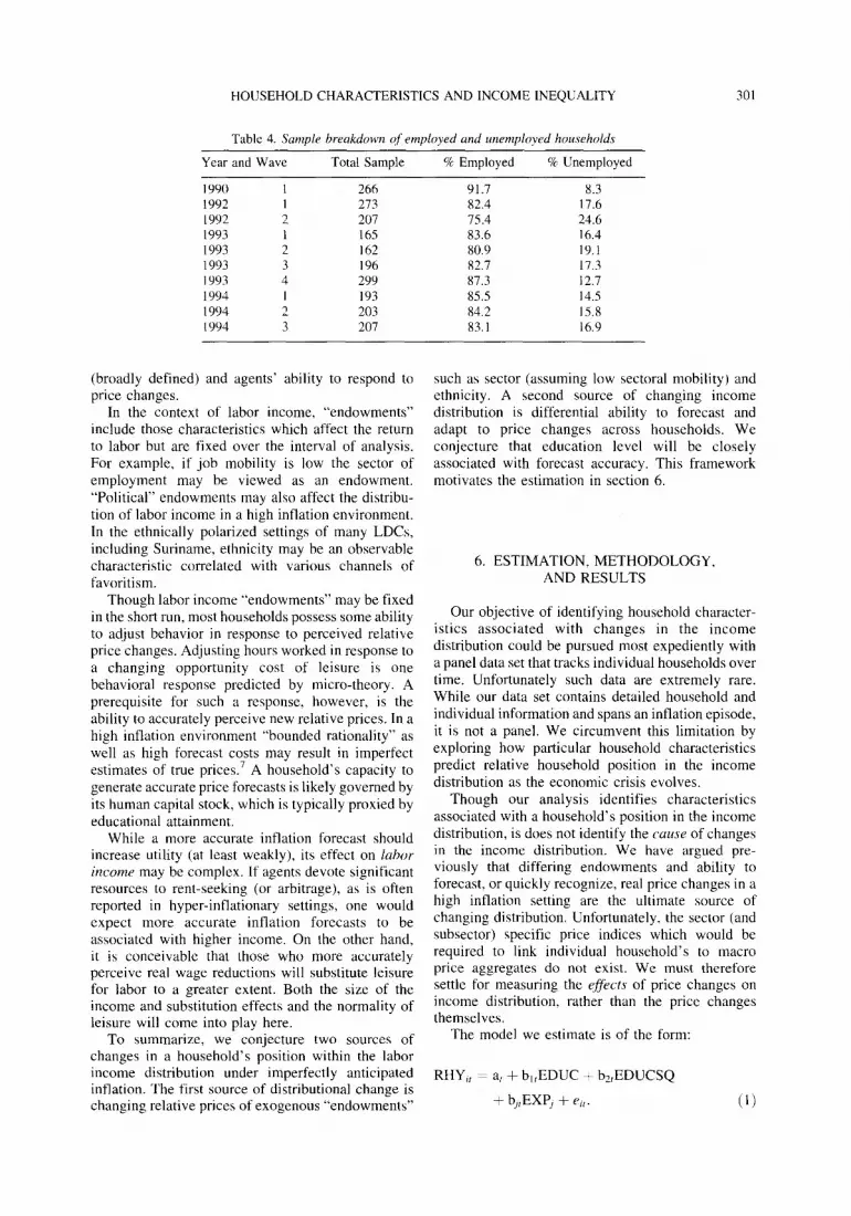
which no employed adult reported an unambiguous wage. Ambiguity occurred when either income was unknown or when the frequency of pay was unclrar. About 30% of the data fall into the former group. The latter group constitutes about IO% of the sample and was excluded due to inconsistencies in the definition of the pay frequency variables over time. A comparison of the characteristics of included and excluded households did not reveal any major differences. In any case, sample selection bias will be controlled for in the regression analysis. A breakdown of the number of observations in the entire data set, in the selected sample, and in the two excluded categories is presented in Table 3. Among the households included in the sample, an average of about 1.5% were in the labor force but unemployed. These households had average incomes of Lero. Table 4 gives the breakdown within the sample of employed and unemployed households. As is illu- strated in the table. unemployment varied greatly in the earlier waves but leveled off in the later waves. It should be noted that there is very weak relationship between unemployment levels and income inequality, indicating that the changes in income inequality are not being driven by changes in the levels of unemployment.”

5. MOTIVATION

The primary objective of this paper is identification of winners and losers when income distributions undergo rapid change during periods of high inflation. To this end it is useful to ask CL,/I~ income distributions change under inflation. The tautological explanation is that relative prices change. If price changes were perfectly anticipated one must appeal to some preexisting heterogeneity to explain a change in income distribution. If. as we believe, price changes are not fully anticipated then changes in income distribution associated with inflation arise from two sources: changing returns to endowments

Year and Wave Total Q in Sample c/c Ambig. Frey.” % No Rep&

I990 I 326 81.6 7.7 10.7 I992 I 482 56.6 13.9 29.5 I992 2 358 57.8 8.9 33.2 1993 I 288 57.3 9.7 33.0 I993 2 279 58.1 IO.0 31.9 1993 3 360 54.4 12.2 33.3 I993 4 523 57.2 12.8 30.0 I994 I 394 49.0 13.9 37.1 1994 2 349 58.2 10.6 31.2 I994 3 354 58.5 10.7 30.8

a Ambiguous Pay Frequency: c/c of households whose pay frequency was ambiguous and were excluded. h No Report represents household\ in which labor income was unknown or nonexistent.


Table 4. Sample breakdown qf employed and unemployed households

Year and Wave Total Sample B Employed % Unemployed

1990 1 266 91.7 8.3 1992 I 273 82.4 17.6 1992 2 207 75.4 24.6 1993 1 I65 83.6 16.4 1993 2 162 80.9 19.1 1993 3 196 82.7 17.3 I993 4 299 87.3 12.7 1994 I 193 85.5 14.5 1994 2 203 84.2 15.8 I994 3 207 83.1 16.9

(broadly defined) and agents’ ability to respond to price changes.

In the context of labor income, “endowments” include those characteristics which affect the return to labor but are fixed over the interval of analysis. For example, if job mobility is low the sector of employment may be viewed as an endowment. “Political” endowments may also affect the distribution of labor income in a high inflation environment. In the ethnically polarized settings of many LDCs, including Suriname, ethnicity may be an observable characteristic correlated with various channels of favoritism.

Though labor income “endowments” may be fixed in the short run, most households possess some ability to adjust behavior in response to perceived relative price changes. Adjusting hours worked in response to a changing opportunity cost of leisure is one behavioral response predicted by micro-theory. A prerequisite for such a response, however, is the ability to accurately perceive new relative prices. In a high inflation environment “bounded rationality” as well as high forecast costs may result in imperfect estimates of true prices.’ A household’s capacity to generate accurate price forecasts is likely governed by its human capital stock, which is typically proxied by educational attainment.

While a more accurate inflation forecast should increase utility (at least weakly), its effect on labor income may be complex. If agents devote significant resources to rent-seeking (or arbitrage), as is often reported in hyper-inflationary settings, one would expect more accurate inflation forecasts to be associated with higher income. On the other hand, it is conceivable that those who more accurately perceive real wage reductions will substitute leisure for labor to a greater extent. Both the size of the income and substitution effects and the normality of leisure will come into play here.

To summarize. we conjecture two sources of changes in a household’s position within the labor income distribution under imperfectly anticipated inflation. The first source of distributional change is changing relative prices of exogenous “endowments”

such as sector (assuming low sectoral mobility) and ethnicity. A second source of changing income distribution is differential ability to forecast and adapt to price changes across households. We conjecture that education level will be closely associated with forecast accuracy. This framework motivates the estimation in section 6.

6. ESTIMATION, METHODOLOGY, AND RESULTS

Our objective of identifying household characteristics associated with changes in the income distribution could be pursued most expediently with a panel data set that tracks individual households over time. Unfortunately such data are extremely rare. While our data set contains detailed household and individual information and spans an inflation episode, it is not a panel. We circumvent this limitation by exploring how particular household characteristics predict relative household position in the income distribution as the economic crisis evolves.

Though our analysis identifies characteristics associated with a household’s position in the income distribution, is does not identify the L’UUSC of changes in the income distribution. We have argued pre- viously that differing endowments and ability to forecast, or quickly recognize, real price changes in a high inflation setting are the ultimate source of changing distribution. Unfortunately, the sector (and subsector) specific price indices which would be required to link individual household’s to macro price aggregates do not exist. We must therefore settle for measuring the ejjkcts of price changes on income distribution, rather than the price changes themselves.

The model we estimate is of the form:

RHY,, = a, + b,,EDUC + bz,EDUCSQ

+ b,,EXP, + r,,. (1)


We estimate Equation 1 using two-stage least Aquares to correct for selection bias and hetero- skedasticityX in the data.

The dependent variable in Equation 1, RHY,,. is relative household income of household i at time r. It is constructed by first computing for each household ‘7” the average income of household members participating in the labor market (AY,).” The mean of this measure for all households at time t (MAY,) is then computed. RHY,, is the ratio of these measures: RHY,, = A Y,IMA Y,. This provides a unit-free and sample size-free indicator of household status in the overall income distribution and a link between household characteristics and income distribution as the crisis evolves.“’

The right-hand side of (I) includes a measure of household education and a set of household control variables. EDUC represents the average education level of household members in the labor force, and ELIUCSQ is the square of this measure.” The non- linear education specification allows for the possibi- lity that relative income exhibits increasing or decreasing returns to education. Care must be taken, however. when interpreting the quadratic term because of the small number (46 out of 1859) of university educated households. ”

The vector EXP, contains control variables for the age. gender, sector of employment, and ethnicity of the primary wage earner. EXP, also includes the average hours worked by employed household members. In. the context of household decision making, hours worked may be endogenously deter- mined with wages. or relative position in the income distribution. Hours worked is therefore instrumented in the regression.‘3 As is customary, age enters in a quadratic form. Table 5 provides a complete description of the explanatory variables.

All explanatory variables (with the exception of

household head gender) are interacted with period

dummies to test whether slope coefficients shift across periods. This allows us to identify those characteristics which became more powerful determinants of relative income during the inflation episode. The three time periods are defined as follows: the base period (period I). which covers 1990 through 1992/l. the middle period (period 2) of highly variable inflation between 1992/Z and 1993/2. and the third period (period 3) of high but more stable inflation from 1993/3 through 1994/3. Although these intervals were chosen based on the inflation Irates in order to test the effects of the different inflation regimes on income distribution our result\ are extremely robust to reasonable changes in the definition of these periods.”

Regression results are presented in Table 6. In interpreting Table 6 note that the explanatory variables presented in Table 5 receive the appendage _ P2 or P3 when interncted with period 2 or period _

Table 5. Description of rxplanator~ variables

Variahle Name Description

EDUC AGE HRS” MAN Lambda

MININ MANUF UTILIT CONST SERVIC TRANSP

FINAN

aov

Ecoi~mic Smtus ENT SIB EMP UNKSTA

Ethnicify CREO HIND JAVA CHIN EURO MAR0 OTH

Ave. education level of household Age of primary wage earner Ave. hours worked in household Dummy for sex of primary earner Heckman selection bias correction term

Unknown sector Agriculture. Forestry, Hunting and Fishing Mining Manufacturing Electric, Gas, Water (Utilities) Construction Wholesale, Retail, Restaurant, Hotel Transportation, Storage, Communication Financial, Insurance, Real Estate Business Community, Social and Personal Services

Entrepreneur Small (Independent) Business Laborer, Employee Other/Unknown

Creole Hindustani Javanese Chinese European Maroon Other

3. respectively. Coefficients that are statistically significant at least at 10% have t-statistics presented in boldface type. The control group consists of employees/laborers of Creole ethnicity who work in the community and social work sector. To calculate the total effect during a particular period of an explanatory variable, it is necessary to add the parameter estimates (if they are statistically different from zero) associated with the base period variable to the parameter estimates (again, if they are significant) on the interacted variable. For education and age it is also necessary to incorporate the squared term into the final total.

The most important pattern that arises from the regression analysis is that education plays a moder- ately important role in the first part of the sample period but that the importance of education in determining relative income increases dramatically during the middle, highly variable inflation period. During this period the “return” to higher levels of education in terms of position in the income


Variable

Table 6. Regression results

Parameter Estimate T for HO: = 0 p-value

Constant PER2 PER3 EDUC EDUCSQ EDUC_P2 EDUSQ_P2 EDUC_P3 EDUSQ_P3 HRS HRS_P2 HRS_P3 MAN AGE AGE-P2 AGE-P3 AGESQ AGESQ_.P;! AGESQ_P3 UNKSEC AGRIC MINING MANUF UTILITIES CONSTRU SERVICES TRANSPOR FINANCE UNKSE_P2 AGRIC_P2 MININ P2 MANUF_P2 UTILIT_P2 CONST_P2 SERVIC_P2 TRANS_P2 FINAN_P2 UNKSE_P3 AGRIC_P3 MININ_P3 MANUF_P3 UTILIT_P3 CONST_P3 SERVIC_P3 TRANS_P3 FlNAN_P3 ENT SIB UNKSTA ENT_P2 SIB-P:! ENT_P3 SIB-P3 UNKST_P3 HIND JAVA CHIN EURO MAR0 OTH HIND-P;!

-0.204 -1.073 -0.896

0.124 0.053 0.558

-0.084 0.361

-0.073 0.022

-0.034 -0.03 1

0.256 -0.002

0.070 0.061 0.000

-0.001 -0.001 -0.018

0.014 0.323

-0.123 0.230 0.003

-0.081 -0.072

0.102 -0.185

0.346 -0.127 -0.110 -0.145

0.884 0.096

-0.064 0.215

-0.163 0.479 1.470 0.521 0.47 1 0.153 0.341 0.844 0.219 2.955 0.281

-0.025 -2.856 -0.342 -2.239

0.456 0.250 0.015

-0.118 0.019

-0.344 -0.083 -0.036

0.090

-0.42 -1.40 -1.33

0.91 2.31 2.59

-2.31 2.12

-2.63 2.08

-2.30 -2.59

3.51 -0.27

2.70 2.45 2.42

-3.02 -2.16 -0.07

0.04 0.64

-0.71 0.49 0.01

-0.58 -0.57

0.31 -0.45

0.64 -0.15 -0.39 -0.19

1.82 0.39

-0.16 0.48

-0.41 1.10 2.40 2.35 0.80 0.42 1.82 3.70 0.59 5.16 1.21

-0.18 -3.34 -0.98 -3.57

1.63 1.35 0.15

-1.02 0.03

-0.29 -0.39 -0.24

0.56

0.6737 0.1627 0.1840 0.3621 0.0207 0.0097 0.0180 0.0339 0.0085 0.0377 0.0213 0.0095 0.0005 0.7859 0.0069 0.0144 0.0154 0.0026 0.0308 0.9473 0.9688 0.5208 0.4756 0.6278 0.9929 0.5652 0.571 0.7548 0.6543 0.5197 0.8834 0.6980 0.8497 0.0688

0.8724 0.6288 0.6825 0.273 1 0.0165 0.0187 0.4253 0.6746 0.0684 0.0002 0.5540 0.0000 0.2258 0.8590 0.0008 0.3250 0.0004 0.1031 0.1763 0.8784 0.3095 0.9735 0.7151 0.6938 0.8107 0.5788


Variable Parameter Estimate T for HO:=0 [J-value

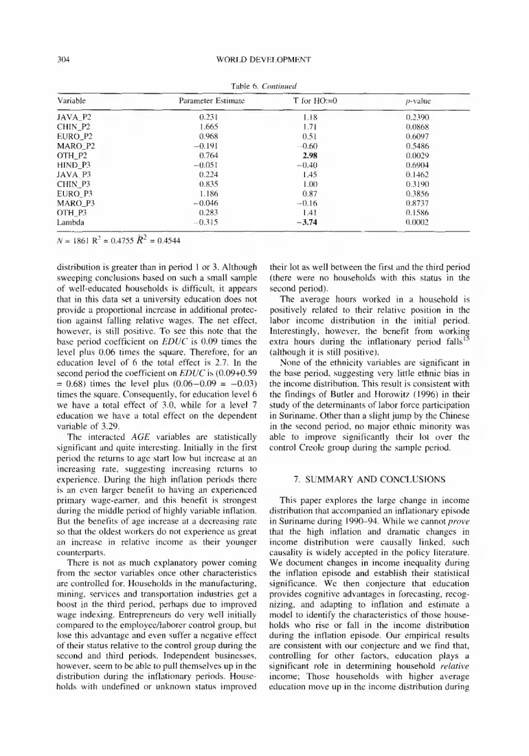
JAVA-P? CHIN-P? EURO-P2 MARO_P2 OTH_PZ HIND-P3 JAVA-P3 CHIN-P3 EURO-P3 MARO_P3 OTH_P3 Lambda

0.23 I 1.18 0.2390 I.665 1.71 0.086X 0.968 0.5 I 0.6097

-0.191 -0.60 0.5486 0.764 2.98 0.0029

-0.05 I ~0.40 0.6904 0.224 I .45 0. I162 0.835 I .oo 0.3100 1.186 0.87 0.3856

-0.046 -0.16 0.8737 0.283 1.41 0.1586

po.315 -3.74 0.0002

N = 1861 R’ = 0.4755 R2 = 0.4544

distribution is greater than in period I or 3. Although sweeping conclusions based on such a small sample of well-educated households is difficult, it appears that in this data set a university education does not provide a proportional increase in additional protec- tion against falling relative wages. The net effect, however. is still positive. To see this note that the base period coefficient on EDUC is 0.09 times the level plus 0.06 times the square. Therefore, for an education level of 6 the total effect is 2.7. In the second period the coefficient on EDC’C is (0.09+0.59 = 0.68) times the level plus (0.06-0.09 = -0.03) times the square. Consequently, for education level 6 we have a total effect of 3.0, while for a level 7 education we have a total effect on the dependent variable of 3.29.

The interacted AGE variables are statistically significant and quite interesting. lnitially in the first period the returns to age start low but increase at an increasing rate, suggesting increasing returns to experience. During the high inflation periods there is an even larger benefit to having an experienced primary wage-earner. and this benefit is strongest during the middle period of highly variable inflation. But the benefits of age increase at a decreasing rate so that the oldest workers do not experience as great an increase in relative income as their younger counterparts.

There is not as much explanatory power coming from the sector variables once other characteristics are controlled for. Households in the manufacturing, mining. services and transportation industries get a boost in the third period. perhaps due to improved wage indexing. Entrepreneurs do very well initially compared to the employee/laborer control group, but lose this advantage and even suffer a negative effect of their status relative to the control group during the second and third periods. Independent businesses, however, seem to be able to pull themselves up in the distribution during the inflationary periods. House- holds with undefined or unknown status improved

their lot as well between the first and the third period (there were no households with this status in the second period).

The average hours worked in a household is positively related to their relative position in the labor income distribution in the initial period. Interestingly, however, the benefit from workin

15 extra hours during the inflationary period falls (although it is still positive).

None of the ethnicity variables are significant in the base period, suggesting very little ethnic bias in the income distribution. This result is consistent with the findings of Butler and Horowitz ( 1996) in their study of the determinants of labor force participation in Suriname. Other than a slight jump by the Chinese in the second period, no major ethnic minority was able to improve significantly their lot over the control Creole group during the sample period.

7. SUMMARY AND CONCLUSIONS

This paper explores the large change in income distribution that accompanied an inflationary episode in Suriname during 1990-94. While we cannot prove that the high inflation and dramatic changes in income distribution were causally linked, such causality is widely accepted in the policy literature. We document changes in income inequality during the inflation episode and establish their statistical significance. We then conjecture that education provides cognitive advantages in forecasting, recognizing, and adapting to inflation and estimate a model to identify the characteristics of those households who rise or fall in the income distribution during the inflation episode. Our empirical results are consistent with our conjecture and we find that, controlling for other factors, education plays a significant role in determining household relative income; Those households with higher average education move up in the income distribution during

HOUSEHOLD CHARACTERISTICS AND INCOME INEQUALITY 30.5

high inflation periods while those with lower

education tend to lose ground. It is important to

recognize that the link between &uI~~.s in t-e/ati\je

incwrw and education we detect is distinct from

“returns to education“ in the conventional sense.

Our results suggest that the changes in income inequality that accompany periods of high inflation

may not simply be a random redistribution, but may

depend deterministically on the differential ability of

households to adapt to rhe inflationary en\;ironment.

The prior distribution OF education attainment across

households may therefore be a good indicator of the

income distribution changes that will accompany a

period of high economic instability.

Given our results, hobo can policy makers mitigate

the increased inequality that accompanies inflation

and structural adjustment’? Certainly, the first best

policy would be that of fiscal responsibility and

careful monetary control to avoid the onset of high

inflation. BLIP recognizing that external economic

shocks and internal political reality often do lead to periods of high inflation. the results of this study

suggest several policy options.

To the extent that the short-run spike in inequality

at the beginning of an inflation episode is due to

recognition lags among the less educated. improicd

information dissemination may be of great benefit.

Specifically. more rapid public release and greater

dissemination of inflation rates by the government

could level the playing field. Of course. political

instincts will typically rLm contrary to such a

policy-the knee-jerk reaction of most governments

entering a high-inflation episode ii; to try to conceal.

rather than advertise. inflation rates. The farsighted

policy maker, however, might well consider a

reduced inequality spike to be a reasonable tradeoff

to the short-run discomfort of disclosure. Perhaps the

most compelling argument for a program of rapid

dissemination of inflation information is that it is a

low-cost program-particularly when compared to

the cost of er-post transfer programs to reverse the

distributional consequences of high intlation.

Our analysis also identifies significant relative

income effects as the inflation episode unfolds for

particular sectors and “economic status” (e.g., small

independent business). Though the sector and status

effects are not as consistently important as education

in the Surinamese setting, they indicate candidates for targeted assistance. Narrowly (and accurately)

targeted programs to ameliorate the distributional

consequences of inflation are considerably less

expensive than broad-based redistribution.

In the long run. education (rather than information

dissemination) would appear to be the key to

ameliorating the distributional consequences of

inflation. More concretely. consider the impact of

two distinct long-run education policies in light of

OLII- results. A first policy would be one that

compresses the education distribution, for example,

shifting resources from hisher to lower education

levels. Our results suggest such a policy would

decrease the inequality spikes associated with

inflation. Alternatively. one might adopt a program

which increases education attainment across the

board. In considering such a policy it is important to

distinguish the aggregate average education level

from the average education level within the house-

hold. Our regression results indicate that a house-

ho/tl’.s average education level significantly affects

its position within the income distribution. More-

over. this effect is concave in that the marginal

impact of increased education is greater at lower.

than at higher. education levels. At the aggregate

level. such concavity suggests that a uniform

increase in educational attainment would reduce

the change in distribution that accompanies inflation.

In sum, our analysis points to education as a powerful determinant of changes in households

r.e/rrti~x~ pmitiotz in the labor income distribution

under high inflation. This finding, in turn. points to

classes of government policy that may ameliorate the

distributional effects of high inflation. Further

studies to ascertain the crosscountry robustness of

these conclusions are needed.

NOTES

I. Computed from hou\?hold wrvey. 1. Households are drawn i’rom the electric company patron\. Virtually all households within Paramaribo and

Wanica are on the electric company grid.

3. The \ur\ey war not conducted 11, I99 I,

5. Changes in the w-hey in 1990 make earlier years

3. For 1990 the inflation rate quoted i\ the aLerage incomparable. for the purposes of this paper, to later

quarterly rate for the whole yea. For the t’lt-st wnvc of I992 surveys.

the intlation rate is the average quarterly rate in the first half of the year, and for the \ccond wave it is the quarterly average for the second half. For I993 and 1994 the intlation 6. Gini coefficients wwe also constructed omitting all rates correspond to the quarter in which the survey was “xro” incomes. reulting in a pattern that is very similar to taken. the one presented in this paper.


7. Of course, there exists a large “rational expectations literature” that speaks to forecasting issues. Practical application of this theory to hyperintlationary episodes in LDCs. however. remains problematic,

8. We use Heckman’s (Heckman, 1979) selection-bias correction and White’s (White, 1980) generalized heteroskedasticity consistent estimation of the second stage regression. As indicated in Table A6 the estimated coefficient on lambda (the correction bias term) is statistically significant, indicating that correcting for selection bias was appropriate in this case.

9. As is conventional. the unemployed are considered labor market participants. AY, is computed by assigning the unemployed wage income of zero. RHY therefore captures the distributional impact of involuntary unemployment.

10. The construction of our dependent variable (RHY) is consistent with a model of household, rather than individual decision making. An assumption of household decision making is common in the development literature.

Il. This measure is constructed by averaging the education level of each adult over the age of IS that was in the labor force and had monthly wages. Education levels ranged from 1 (primary education only) to 7 (university education). Most households’ average education reached

only primary (level I) or secondary school (level 2). Only 0.025% of the households used in the estimation had an average household education level of 7 (university level).

12. The small number of university-level households had a disproportionate effect on the regression results when only level of education was used as a regressor. Several functional forms were attempted including adding university dummies and taking the log of education. All specifications gave similar results but the quadratic term had a v’ery slightly better goodness-of-fit measure and was thus adopted.

13. Instruments are job type (which is distinct from the sector variable employed in Equation I. ethnicity, sex, and age.

14. The regressions were run using 1990/l-1992/2 or I990/ 1 alone as the first period with I993/2- I994/3, I993/4- 19940 and 1994/l-1994/3 as the third period. The effects of education during the middle period were the sharpest when this period primarily encompassed the high variability inflation waves.

IS. The reader is reminded that this variable is instrumented to avoid simultaneity bias. and thus the decline in the return to hours cannot be explained as a substitution effect deriving from a fall in real wages.

REFERENCES

Achdut, L. and Bigman, .I. ( 1991) The anatomy of changes Foster. J. E. (1985) Inequality measurement. In Fctir in poverty and income inequality under rapid inflation: Allocchn, ed. H. P. Young. pp. 31-68. American Israel 1979-l 984. Sr~rrmml Chrrgr nnd Ecommic Mathematical Society, Providence RI. Dynnrnics 2( I ). 229-243. Glewwe. P. (1990) The measurement of income inequality

Adelman. 1. and Morris. C. T. ( 1973) Gorzornic G~orvrh cm/ under inflation. Joumu1 of Dedopmm Economics 32, Social Equir,y irr Drwlopirzg Cowk~. Stanford Uni- 43-67. versity Press, Stanford, CA. Glewwe. P. and Hall. G. (1992) Poverty and inequality

Adelman. 1. and Nobuhiko, F. (1994) Income inequality and during unorthodox adjustment: The case of Peru. World development: The 1970s and 1980s compared. Econo- Bank Living Standards Measurement Study Working mir-Ap/~/iquec 47( I). 7-29. Paper No. 86. World Bank. Washington DC.

Adelman, 1. and Taylor, E. (1989) Is structural adjustment Heckman. J. (1979) Sample selection bias as a specification with a human face possible‘? CUDARE, Working Paper error. Gommakc~ 47(I). 153-l 6 I. 500, University of California, Berkeley, CA. Kuznets. S. ( 1955) Economic growth and income inequal-

Aura. A. (1989) Inequality trends in Indonesia. 19699198 I : ity. Antericnrt Ecmomic Review 4.5( I ). l-28. A re-examination. Bnllerirr of Irrdmesim Ecorwrnic~ Lustig, N. (I 995) Coping nirh Amrwir\: Powq rmf

Strtdie.c 25(2), I oo- I IO. /mp/ir~ irr Lariir Amrica. Brookings Institution. Atkinson. A. B. ( 1975) T/jr Ecouomict of hleqdir~. Washington, DC.

Oxford University Press, Oxford, UK. Slesmck. D. (1990) Inflation, relative price variation, and Butler. J. S. and Horowitz, Andrew W. (1996) Labor supply inequality. Jonrncrl of Econornerric.s 43, 135% IS I.

and wages among nuclear and extended households: The Soltow, L. (1968) Long-run changes in British income Surinamese experiment. Vanderbilt University, Nash- inequality. Economic Hisroy Re~+rw 21. ville. TN. White. H. ( 1980) A heteroskedasticity consistent covar-

Fields. G. S. ( 1980) Powry. Irwqurrlir~. trrd Dn~ehpmw. iance matrix and direct test for heteroskedasticity. Cambridge University Press. Cambridge. Ecor~ot~rcrricc~ 48. 8 17-838.

household characteristics and income inequality during inflationary periods: recent evidence from...

Documents