hierarchical characterization of complex networks

arX

iv:c

ond-

mat

/041

2761

v4 [

cond

-mat

.sta

t-m

ech]

7 F

eb 2

006

Hierarchical Characterization of Complex Networks

Luciano da Fontoura Costa and Filipi Nascimento Silva ∗

February 2, 2008

Abstract

While the majority of approaches to the characteriza-tion of complex networks has relied on measurementsconsidering only the immediate neighborhood of eachnetwork node, valuable information about the net-work topological properties can be obtained by con-sidering further neighborhoods. The current workdiscusses on how the concepts of hierarchical nodedegree and hierarchical clustering coefficient (intro-duced in cond-mat/0408076), complemented by newhierarchical measurements, can be used in order to ob-tain a powerful set of topological features of complexnetworks. The interpretation of such measurementsis discussed, including an analytical study of the hi-erarchical node degree for random networks, and thepotential of the suggested measurements for the char-acterization of complex networks is illustrated with re-spect to simulations of random, scale-free and regularnetwork models as well as real data (airports, proteinsand word associations). The enhanced characteriza-tion of the connectivity provided by the set of hierar-chical measurements also allows the use of agglomer-ative clustering methods in order to obtain taxonomiesof relationships between nodes in a network, a possi-bility which is also illustrated in the current article.

1 Introduction

Graph theory and statistical mechanics are well-established areas in mathematics and physics, respec-tively. Since its beginnings in the XVIII century, withthe solution of the bridges problem by L. Euler, graphtheory has progressed all the way to the forefront oftheoretical and applied investigations in mathemat-ics and computer science. Much of the importanceof this broad area stems from the generality of graphsas representational models. As a matter of fact, mostdiscrete structures including matrices, trees, queues,among many others, are but particular cases of graphs.The potential of graphs is further extended by modelswhere features are assigned to nodes, different types

∗Cybernetic Vision Research Group, GII-IFSC, Universidade deSao Paulo, Sao Carlos, SP, Caixa Postal 369, 13560-970, Brasil, [email protected].

of nodes and/or edges are allowed to co-exist, syn-chronization schemes are incorporated, and so on (see,for instance, [1]). At the same time, statistical me-chanics, also drawing on a rich past of accomplish-ments, provides concepts and tools for bridging thegap between dynamics in the micro and macro realms.Of particular interest have been the investigations onphase transitions and complex systems, which repre-sent a major area of development today.

While graph theory provides effective means forcharacterizing, modeling and simulating the structureof natural phenomena, statistical mechanics containsthe methods for analyzing the dynamics of natural phe-nomena along several scales. The novel area of com-plex networks [2, 1] can be understood as a fortunateintersection between those two major areas, thereforeallowing a natural and powerful means for integrat-ing structure and dynamics. With origins extend-ing back to the pioneering developments of Flory [3],Rapoport [4] and Erdos and Renyi [5], the area of com-plex networks was boosted more recently by the ad-vances by Watts and Strogatz [6, 7] and Barabasi andcollaborators [8].

Complex network investigations frequently involvethe measurement of topological features of the ana-lyzed structures, such as the node degree (namely thenumber of edges attached to a node) and the clus-tering coefficient (quantifying the connectivity amongthe immediate neighbors of a node). Although degen-erated, in the sense that they do not allow a one-to-oneidentification of the possible network architectures,such a pair of measurements does provide a rich char-acterization of the connectivity of the networks. As amatter of fact, particularly interesting network mod-els, such as the small-world [1, 2, 7, 6] and scale-free(Barabasi-Albert) [2, 1, 8], are characterized in termsof specific types of node degree distributions (logarith-mic and power-law, respectively).

Although such distributions emphasize importantproperties of the analyzed networks, further valuabletopological information can be gathered not only byconsidering the clustering coefficient, but also by ana-lyzing such features along the hierarchical levels of thenetworks [9, 10]. While some attention has been fo-cused on the relevant issue of hierarchy in complexnetworks (e.g. [11, 12, 13, 17, 18, 19, 20, 21, 22, 23, 24,

1

http://arXiv.org/abs/cond-mat/0412761v4

http://arXiv.org/abs/cond-mat/0408076

28, 26, 27]), and hierarchical extensions of the nodedegree and clustering coefficient were only more re-cently formalized in [9, 10] by using concepts derivedfrom mathematical morphology [25, 29, 30] includ-ing dilations and distance transforms in graphs. Despitetheir recent introduction, such concepts have alreadyyielded valuable results when applied to essential-ity of protein-protein interaction networks [37], bonestructure characterization [38], and community find-ing [32, 33].

The purpose of the current article is to review andfurther extend the concepts of hierarchical measure-ments, which is done by the consideration of the con-cepts of radial reference system and hierarchical commondegree, as well as the introduction of the measurementsof hierchical edge degree, inter-ring degree, intra-ring de-gree, convergence ratio, and emphedge clustering coef-ficient. The extensions of these measurement (exclud-ing the clustering coefficient) to weighted and directednetworks are also described in this work. We start bypresenting the basic concepts and discussing hierar-chies in complex networks in terms of virtual nodes andproceed by describing, interpreting and discussing thehierarchical measurements. An analytical character-ization of the general shape of the hierarchical nodedegree in random networks is also presented, and thepotential of the reported concepts and methods is il-lustrated with respect to the characterization of simu-lated random, scale-free and regular network models.Such a potential is further illustrated with respect toreal networks, including word associations, airports,and protein-protein interactions. Because the hierar-chical measurements provide a rich characterizationof the connectivity around each network node, it be-comes possible to use clustering methods [15, 14] inorder to organize the nodes in a network into a tax-onomical scheme reflecting the similarities betweentheir connectivity. This possibility is also illustratedin the present article.

2 Notation and Basic Concepts

Let the graph or network Γ of interest contain N nodesand e edges, and the connections between any twonodes i and j be represented as (i, j). Although non-oriented graphs are assumed henceforth, all reportedconcepts and methods can be immediately extendedto digraphs and weighted networks. We henceforthassume the complete absence of loops (i.e. self-connections). A non-oriented graph can be completelyspecified in terms of its adjacency matrix K , with eachconnection (i, j) implying K(i, j) = K(j, i) = 1. Theabsence of a connection between nodes i and j is rep-resented as K(i, j) = K(j, i) = 0. Now, the node degree

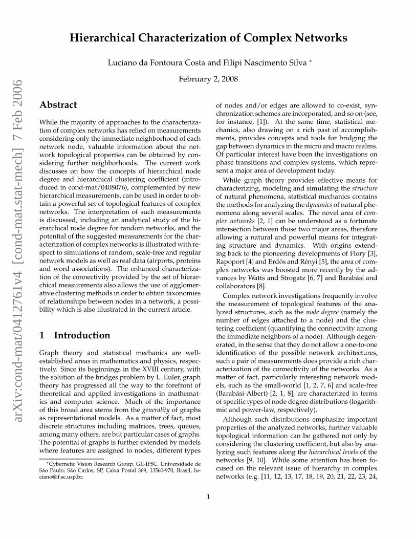
Figure 1: Three situations yielding the same clusteringcoefficient (equal to 1) for the reference node i.

k(i) of a node i of Γ can be defined as

k(i) =

N∑

j=1

K(i, j) =

N∑

j=1

K(j, i). (1)

Observe that the degree of node i corresponds to thenumber of edges attached to that node, representing adirect measurement of the connectivity of that specificnode. Indeed the overall connectivity of a specific net-work can be quantified in terms of its average nodedegree 〈k〉. While a random network is characterizedby a typical average node degree with relatively lowstandard deviation, a scale-free model will present apower-law log-log distribution of node degrees, favor-ing the existence of hubs (i.e. nodes with high nodedegree).

The clustering coefficient of a network node i can bedefined as quantifying the connectivity among the im-mediate neighbors of i, which are henceforth repre-sented by the set R1(i). More specifically, in case thatnode has n1(i) immediate neighbors (i.e., the cardi-nality of R(i)), implying a maximum number eT (i) =n1(n1 − 1)/2 of connections between such nodes, ande(i) connections are observed among such neighbors,the clustering coefficient of i can be calculated as

cc(i) =e(i)

eT (i)= 2

e(i)

n1(i)(n1(i) − 1). (2)

Observe that 0 ≤ cc(i) ≤ 1, with the minimum andmaximum values being achieved for complete absenceof connections (for cc(i) = 0) and complete connectiv-ity among the neighbors of i (for cc(i) = 1).

Although the clustering coefficient provides a pow-erful indication about the connectivity among theneighbors of the reference node, several different sit-uations (see Figure 1) may yield the same clusteringcoefficient value (1 for these examples), which is a con-sequence of the fact that this measurement is relativeto the total number of connections among the elements

2

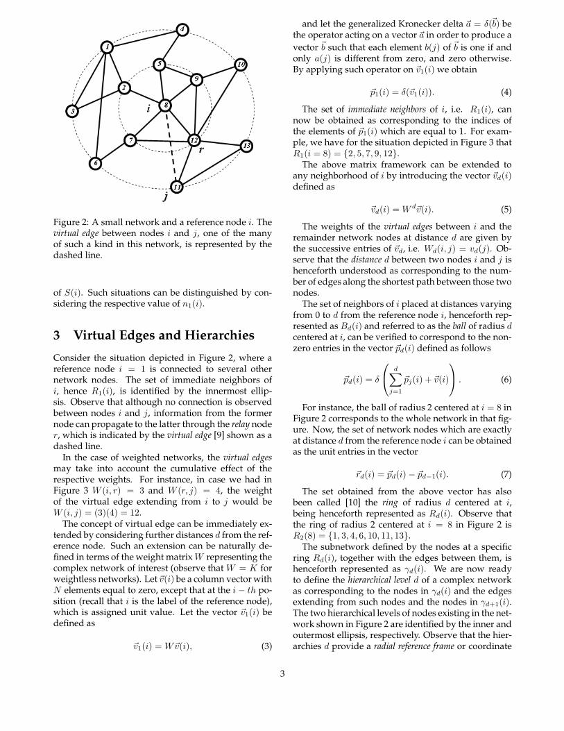
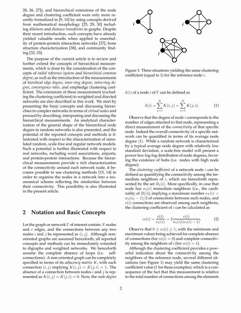
Figure 2: A small network and a reference node i. Thevirtual edge between nodes i and j, one of the manyof such a kind in this network, is represented by thedashed line.

of S(i). Such situations can be distinguished by con-sidering the respective value of n1(i).

3 Virtual Edges and Hierarchies

Consider the situation depicted in Figure 2, where areference node i = 1 is connected to several othernetwork nodes. The set of immediate neighbors ofi, hence R1(i), is identified by the innermost ellip-sis. Observe that although no connection is observedbetween nodes i and j, information from the formernode can propagate to the latter through the relay noder, which is indicated by the virtual edge [9] shown as adashed line.

In the case of weighted networks, the virtual edgesmay take into account the cumulative effect of therespective weights. For instance, in case we had inFigure 3 W (i, r) = 3 and W (r, j) = 4, the weightof the virtual edge extending from i to j would beW (i, j) = (3)(4) = 12.

The concept of virtual edge can be immediately ex-tended by considering further distances d from the ref-erence node. Such an extension can be naturally de-fined in terms of the weight matrix W representing thecomplex network of interest (observe that W = K forweightless networks). Let ~v(i) be a column vector withN elements equal to zero, except that at the i − th po-sition (recall that i is the label of the reference node),which is assigned unit value. Let the vector ~v1(i) bedefined as

~v1(i) = W~v(i), (3)

and let the generalized Kronecker delta ~a = δ(~b) bethe operator acting on a vector ~a in order to produce a

vector ~b such that each element b(j) of ~b is one if andonly a(j) is different from zero, and zero otherwise.By applying such operator on ~v1(i) we obtain

~p1(i) = δ(~v1(i)). (4)

The set of immediate neighbors of i, i.e. R1(i), cannow be obtained as corresponding to the indices ofthe elements of ~p1(i) which are equal to 1. For exam-ple, we have for the situation depicted in Figure 3 thatR1(i = 8) = {2, 5, 7, 9, 12}.

The above matrix framework can be extended toany neighborhood of i by introducing the vector ~vd(i)defined as

~vd(i) = W d~v(i). (5)

The weights of the virtual edges between i and theremainder network nodes at distance d are given bythe successive entries of ~vd, i.e. Wd(i, j) = vd(j). Ob-serve that the distance d between two nodes i and j ishenceforth understood as corresponding to the num-ber of edges along the shortest path between those twonodes.

The set of neighbors of i placed at distances varyingfrom 0 to d from the reference node i, henceforth rep-resented as Bd(i) and referred to as the ball of radius dcentered at i, can be verified to correspond to the non-zero entries in the vector ~pd(i) defined as follows

~pd(i) = δ

d∑

j=1

~pj(i) + ~v(i)

. (6)

For instance, the ball of radius 2 centered at i = 8 inFigure 2 corresponds to the whole network in that fig-ure. Now, the set of network nodes which are exactlyat distance d from the reference node i can be obtainedas the unit entries in the vector

~rd(i) = ~pd(i) − ~pd−1(i). (7)

The set obtained from the above vector has alsobeen called [10] the ring of radius d centered at i,being henceforth represented as Rd(i). Observe thatthe ring of radius 2 centered at i = 8 in Figure 2 isR2(8) = {1, 3, 4, 6, 10, 11, 13}.

The subnetwork defined by the nodes at a specificring Rd(i), together with the edges between them, ishenceforth represented as γd(i). We are now readyto define the hierarchical level d of a complex networkas corresponding to the nodes in γd(i) and the edgesextending from such nodes and the nodes in γd+1(i).The two hierarchical levels of nodes existing in the net-work shown in Figure 2 are identified by the inner andoutermost ellipsis, respectively. Observe that the hier-archies d provide a radial reference frame or coordinate

3

system which can be used to partially identify nodesand edges with respect to the reference node i. Theconcept o hierarchy in a complex network is also re-lated to the concept of roles [34] and the distance trans-form [29, 30] of the nodes in the original network Γwith respect to the reference node [10].

Observe that statistics of the number of hierarchi-cal levels d while considering several nodes in a com-plex network provide a valuable characterization ofits topology. Generally speaking, d tends do increasewith the density of connections up to a peak, decreas-ing afterwards. At the same time, as will become clearalong the remainder of this article, the more connectedthe network is, the less hierarchical levels it tends tohave. It should be also observed that algorithmic im-plementation of hierarchy identification, such as thosereported in [9] and [10] (see also [35]), are typicallymore computationally efficient than the use of the ma-trix arithmetic presented in this Section.

4 Hierarchical Measurements

The concept of hierarchical level introduced above al-lows a natural and powerful extension of traditionalmeasurements such as the node degree and clusteringcoefficient. This section defines such features as wellas ancillary measurements which can be used in orderto obtain a more complete characterization of complexnetworks. The considered measures can be general-ized for weighted networks taking some modificationsas described along the measures. When consideringoriented graphs, a new network can be obtained re-trieving only the In or Out connections of each node.

The hierarchical node degree of a reference node i atdistance d is henceforth defined as corresponding tothe number of edges extending between the nodes inRd(i) and Rd+1(i). This measurement is henceforthrepresented as kd(i). As an example, in Figure 2 wehave that k0(8) = 5 (corresponding to the traditionalnode degree) and k1(8) = 8. Observe that the hierar-chical node degree is not averaged among the numberof nodes in Rd(i). Actually, this measurement can beunderstood as the traditional node degree where thereference node is understood as corresponding to theball Bd(i) (i.e. the nodes in this ball are merged intoa subsumed node). This measure can be extended toweighted networks by taking the sum of the weightvalues for every connection between these nodes andthe nodes of the next level.

Let the number of edges in the subnetwork γd(i) beexpressed as ed(i), and the number of elements of thering Rd(i) be represented as nd(i). The hierarchical clus-tering coefficient of node i at distance d, hence ccd(i),can be obtained in terms of the immediate generaliza-

tion of Equation 2

ccd(i) = 2ed(i)

nd(i)(nd(i) − 1). (8)

For node i = 8 in the simple network shown in Fig-ure 2 we have that cc1(8) = 0.3 and cc2(8) ≈ 0.19.

Other interesting hierarchical measurements whichcan be obtained with respect to the reference node iand which can be used to diminish the degeneracy ofthe node degree and clustering coefficient include thefollowing:

Convergence ratio (Cd(i)): Corresponds to the ra-tio between the hierarchical node degree of node i atdistance d and the number of nodes in the ring at nextlevel distance, i.e.

Cd(i) =kd(i)

nd+1(i). (9)

This measurement quantifies the average number ofedges received by each node in the hierarchical leveld + 1. We have necessarily that C0(i) = 1 for whatevernode selected as the reference i. In the case illustratedin Figure 2, we have C0(8) = 1 and C1(8) = 8/7, indi-cating a low level of edge convergence into the nodesin Rd(i).

Intra-ring degree (Ad(i)): This measurement is ob-tained by taking the average among the degrees ofthe nodes in the subnetwork γd(i). Observe that onlythose edges between the nodes in such a subnetworkare considered, therefore overlooking the connectionsestablished by such nodes with the nodes in the hier-archical levels at d − 1 and d + 1. For instance, wehave for the situation in Figure 2 that A1(8) = 6/5and A2(8) = 8/7. For weighted networks the valueof intra-ring is the average of weights of all nodes insuch subnetwork.

Inter-ring degree (Ed(i)): The average of the num-ber of connections between each node in ring Rd(i)and those in Rd+1(i). For instance, for Figure 2 wehave E0(8) = 5, E1(8) = 8/5 and E2(8) = 0. Observethat Ed(i) = kd(i)/nd(i).

Hierarchical common degree (Hd(i)): The averagenode degree among the nodes in Rd(i), consideringall edges in the original network. For Figure 2 wehave H1(8) = 18/5 and H2(8) = 16/7. The hierarchi-cal common degree expresses the average node degreeat each hierarchical level, indicating how the networknode degrees are distributed along the network hier-archies.

It is also interesting to eventually consider versionsof the above described measurements considering theball Bd(i), and not the ring Rd(i). Table 1 summarizesthe hierarchical measurements reviewed/introducedin the current article, all of which are defined withrespect to one of the network nodes, identified by i,taken as a reference and at a distance d from that node.Observe that most measurements are averaged among

4

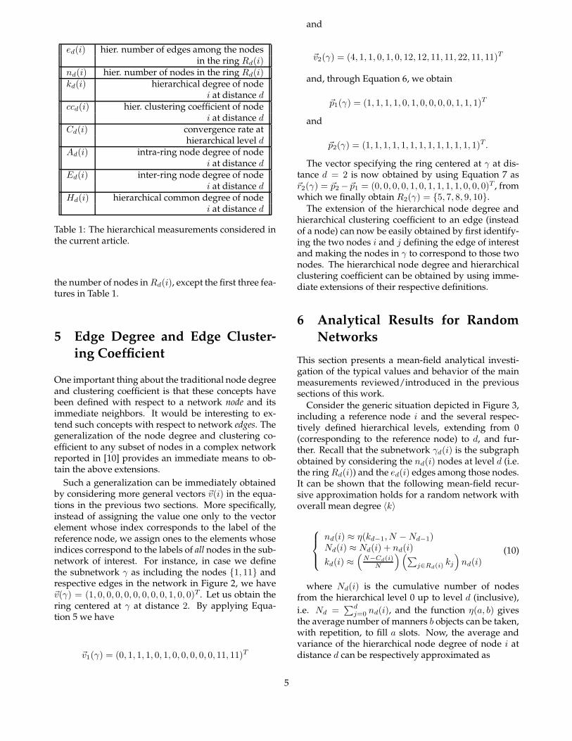
ed(i) hier. number of edges among the nodesin the ring Rd(i)

nd(i) hier. number of nodes in the ring Rd(i)kd(i) hierarchical degree of node

i at distance dccd(i) hier. clustering coefficient of node

i at distance dCd(i) convergence rate at

hierarchical level dAd(i) intra-ring node degree of node

i at distance dEd(i) inter-ring node degree of node

i at distance dHd(i) hierarchical common degree of node

i at distance d

Table 1: The hierarchical measurements considered inthe current article.

the number of nodes in Rd(i), except the first three fea-tures in Table 1.

5 Edge Degree and Edge Cluster-

ing Coefficient

One important thing about the traditional node degreeand clustering coefficient is that these concepts havebeen defined with respect to a network node and itsimmediate neighbors. It would be interesting to ex-tend such concepts with respect to network edges. Thegeneralization of the node degree and clustering co-efficient to any subset of nodes in a complex networkreported in [10] provides an immediate means to ob-tain the above extensions.

Such a generalization can be immediately obtainedby considering more general vectors ~v(i) in the equa-tions in the previous two sections. More specifically,instead of assigning the value one only to the vectorelement whose index corresponds to the label of thereference node, we assign ones to the elements whoseindices correspond to the labels of all nodes in the sub-network of interest. For instance, in case we definethe subnetwork γ as including the nodes {1, 11} andrespective edges in the network in Figure 2, we have~v(γ) = (1, 0, 0, 0, 0, 0, 0, 0, 0, 1, 0, 0)T . Let us obtain thering centered at γ at distance 2. By applying Equa-tion 5 we have

~v1(γ) = (0, 1, 1, 1, 0, 1, 0, 0, 0, 0, 0, 11, 11)T

and

~v2(γ) = (4, 1, 1, 0, 1, 0, 12, 12, 11, 11, 22, 11, 11)T

and, through Equation 6, we obtain

~p1(γ) = (1, 1, 1, 1, 0, 1, 0, 0, 0, 0, 1, 1, 1)T

and

~p2(γ) = (1, 1, 1, 1, 1, 1, 1, 1, 1, 1, 1, 1, 1)T.

The vector specifying the ring centered at γ at dis-tance d = 2 is now obtained by using Equation 7 as~r2(γ) = ~p2 − ~p1 = (0, 0, 0, 0, 1, 0, 1, 1, 1, 1, 0, 0, 0)T , fromwhich we finally obtain R2(γ) = {5, 7, 8, 9, 10}.

The extension of the hierarchical node degree andhierarchical clustering coefficient to an edge (insteadof a node) can now be easily obtained by first identify-ing the two nodes i and j defining the edge of interestand making the nodes in γ to correspond to those twonodes. The hierarchical node degree and hierarchicalclustering coefficient can be obtained by using imme-diate extensions of their respective definitions.

6 Analytical Results for Random

Networks

This section presents a mean-field analytical investi-gation of the typical values and behavior of the mainmeasurements reviewed/introduced in the previoussections of this work.

Consider the generic situation depicted in Figure 3,including a reference node i and the several respec-tively defined hierarchical levels, extending from 0(corresponding to the reference node) to d, and fur-ther. Recall that the subnetwork γd(i) is the subgraphobtained by considering the nd(i) nodes at level d (i.e.the ring Rd(i)) and the ed(i) edges among those nodes.It can be shown that the following mean-field recur-sive approximation holds for a random network withoverall mean degree 〈k〉

nd(i) ≈ η(kd−1, N − Nd−1)Nd(i) ≈ Nd(i) + nd(i)

kd(i) ≈(

N−Cd(i)N

)(

∑

j∈Rd(i) kj

)

nd(i)(10)

where Nd(i) is the cumulative number of nodesfrom the hierarchical level 0 up to level d (inclusive),

i.e. Nd =∑d

j=0 nd(i), and the function η(a, b) givesthe average number of manners b objects can be taken,with repetition, to fill a slots. Now, the average andvariance of the hierarchical node degree of node i atdistance d can be respectively approximated as

5

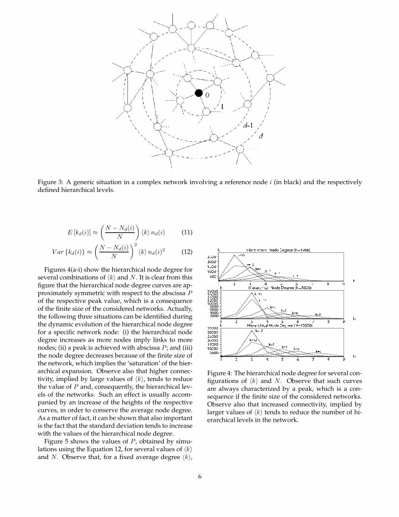
Figure 3: A generic situation in a complex network involving a reference node i (in black) and the respectivelydefined hierarchical levels.

E [kd(i)] ≈

(

N − Nd(i)

N

)

〈k〉nd(i) (11)

V ar {kd(i)} ≈

(

N − Nd(i)

N

)2

〈k〉nd(i)2 (12)

Figures 4(a-i) show the hierarchical node degree forseveral combinations of 〈k〉 and N . It is clear from thisfigure that the hierarchical node degree curves are ap-proximately symmetric with respect to the abscissa Pof the respective peak value, which is a consequenceof the finite size of the considered networks. Actually,the following three situations can be identified duringthe dynamic evolution of the hierarchical node degreefor a specific network node: (i) the hierarchical nodedegree increases as more nodes imply links to morenodes; (ii) a peak is achieved with abscissa P ; and (iii)the node degree decreases because of the finite size ofthe network, which implies the ‘saturation’ of the hier-archical expansion. Observe also that higher connec-tivity, implied by large values of 〈k〉, tends to reducethe value of P and, consequently, the hierarchical lev-els of the networks. Such an effect is usually accom-panied by an increase of the heights of the respectivecurves, in order to conserve the average node degree.As a matter of fact, it can be shown that also importantis the fact that the standard deviation tends to increasewith the values of the hierarchical node degree.

Figure 5 shows the values of P , obtained by simu-lations using the Equation 12, for several values of 〈k〉and N . Observe that, for a fixed average degree 〈k〉,

Figure 4: The hierarchical node degree for several con-figurations of 〈k〉 and N . Observe that such curvesare always characterized by a peak, which is a con-sequence if the finite size of the considered networks.Observe also that increased connectivity, implied bylarger values of 〈k〉 tends to reduce the number of hi-erarchical levels in the network.

6

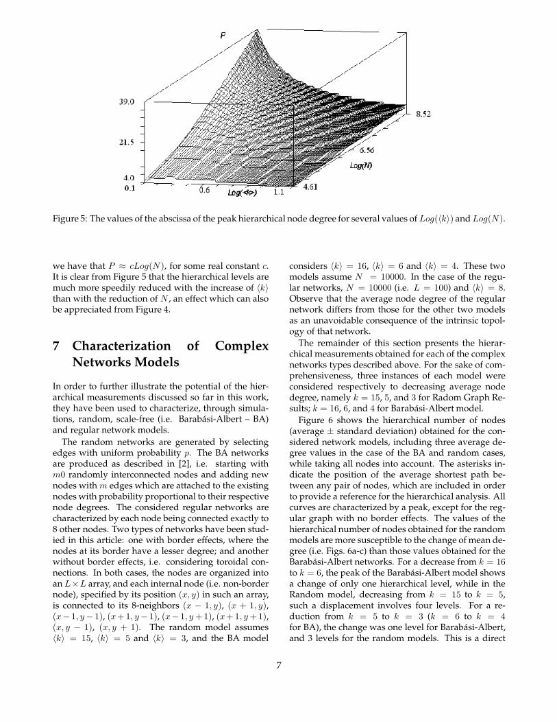
Figure 5: The values of the abscissa of the peak hierarchical node degree for several values of Log(〈k〉) and Log(N).

we have that P ≈ cLog(N), for some real constant c.It is clear from Figure 5 that the hierarchical levels aremuch more speedily reduced with the increase of 〈k〉than with the reduction of N , an effect which can alsobe appreciated from Figure 4.

7 Characterization of Complex

Networks Models

In order to further illustrate the potential of the hier-archical measurements discussed so far in this work,they have been used to characterize, through simula-tions, random, scale-free (i.e. Barabasi-Albert – BA)and regular network models.

The random networks are generated by selectingedges with uniform probability p. The BA networksare produced as described in [2], i.e. starting withm0 randomly interconnected nodes and adding newnodes with m edges which are attached to the existingnodes with probability proportional to their respectivenode degrees. The considered regular networks arecharacterized by each node being connected exactly to8 other nodes. Two types of networks have been stud-ied in this article: one with border effects, where thenodes at its border have a lesser degree; and anotherwithout border effects, i.e. considering toroidal con-nections. In both cases, the nodes are organized intoan L×L array, and each internal node (i.e. non-bordernode), specified by its position (x, y) in such an array,is connected to its 8-neighbors (x − 1, y), (x + 1, y),(x− 1, y− 1), (x+1, y− 1), (x− 1, y +1), (x+1, y +1),(x, y − 1), (x, y + 1). The random model assumes〈k〉 = 15, 〈k〉 = 5 and 〈k〉 = 3, and the BA model

considers 〈k〉 = 16, 〈k〉 = 6 and 〈k〉 = 4. These twomodels assume N = 10000. In the case of the regu-lar networks, N = 10000 (i.e. L = 100) and 〈k〉 = 8.Observe that the average node degree of the regularnetwork differs from those for the other two modelsas an unavoidable consequence of the intrinsic topol-ogy of that network.

The remainder of this section presents the hierar-chical measurements obtained for each of the complexnetworks types described above. For the sake of com-prehensiveness, three instances of each model wereconsidered respectively to decreasing average nodedegree, namely k = 15, 5, and 3 for Radom Graph Re-sults; k = 16, 6, and 4 for Barabasi-Albert model.

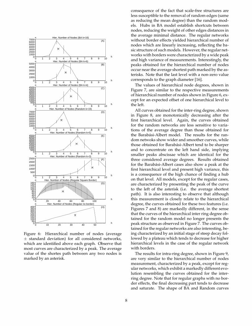
Figure 6 shows the hierarchical number of nodes(average ± standard deviation) obtained for the con-sidered network models, including three average de-gree values in the case of the BA and random cases,while taking all nodes into account. The asterisks in-dicate the position of the average shortest path be-tween any pair of nodes, which are included in orderto provide a reference for the hierarchical analysis. Allcurves are characterized by a peak, except for the reg-ular graph with no border effects. The values of thehierarchical number of nodes obtained for the randommodels are more susceptible to the change of mean de-gree (i.e. Figs. 6a-c) than those values obtained for theBarabasi-Albert networks. For a decrease from k = 16to k = 6, the peak of the Barabasi-Albert model showsa change of only one hierarchical level, while in theRandom model, decreasing from k = 15 to k = 5,such a displacement involves four levels. For a re-duction from k = 5 to k = 3 (k = 6 to k = 4for BA), the change was one level for Barabasi-Albert,and 3 levels for the random models. This is a direct

7

Hier. Number of Nodes (BA k=16)

h

(A)n

0 1 2 3 4 5 6 7 8 9 100

1000200030004000500060007000


h

(B)n

0 1 2 3 4 5 6 7 8 9 100

10002000300040005000


h

(C)n

0 1 2 3 4 5 6 7 8 9 100

50010001500200025003000350040004500

Hier. Number of Nodes (Random k=15)

h

(D)n

0 1 2 3 4 5 6 7 8 9 100

1000200030004000500060007000


h

(E)n

0 1 2 3 4 5 6 7 8 9 100

50010001500200025003000350040004500


h

(F)n

0 1 2 3 4 5 6 7 8 9 100

5001000150020002500

Hier. Number of Nodes (Regular Square Border)

h

(G)n

0 20 40 60 80 1000

20406080

100120140160

Hier. Number of Nodes (Regular no border)

h

(H)n

0 10 20 30 40 500

50100150200250300350400

Figure 6: Hierarchical number of nodes (average± standard deviation) for all considered networks,which are identified above each graph. Observe thatmost curves are characterized by a peak. The averagevalue of the shortes path between any two nodes ismarked by an asterisk.

consequence of the fact that scale-free structures areless susceptible to the removal of random edges (sameas reducing the mean degree) than the random mod-els. Hubs in BA model establish shortcuts betweennodes, reducing the weight of other edges distances inthe average minimal distance. The regular networkswithout border effects yielded hierarchical number ofnodes which are linearly increasing, reflecting the ba-sic structure of such models. However, the regular net-works with borders were characterized by a wide peakand high variance of measurements. Interestingly, thepeaks obtained for the hierarchical number of nodesoccur near the average shortest path marked by the as-terisks. Note that the last level with a non-zero valuecorresponds to the graph diameter [16].

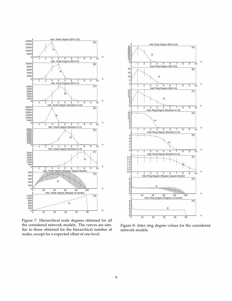
The values of hierarchical node degrees, shown inFigure 7, are similar to the respective measurementsof hierarchical number of nodes shown in Figure 6, ex-cept for an expected offset of one hierarchical level tothe left.

All curves obtained for the inter-ring degree, shownin Figure 8, are monotonically decreasing after thefirst hierarchical level. Again, the curves obtainedfor the random networks are less sensitive to varia-tions of the average degree than those obtained forthe Barabasi-Albert model. The results for the ran-dom netwoks show wider and smoother curves, whilethose obtained for Barabasi-Albert tend to be sharperand to concentrate on the left hand side, implyingsmaller peaks abscissae which are identical for thethree considered average degrees. Results obtainedfor the Barabasi-Albert cases also show a peak at thefirst hierarchical level and present high variance, thisis a consequence of the high chance of finding a hubon that level. All models, except for the regular cases,are characterized by presenting the peak of the curveto the left of the asterisk (i.e. the average shortestpath). It is also interesting to observe that althoughthis measurement is closely relate to the hierarchicaldegree, the curves obtained for these two features (i.e.Figures 7 and 8) are markedly different, in the sensethat the curves of the hierarchical inter ring degree ob-tained for the random model no longer presents thepeak structure as observed in Figure 7. The curves ob-tained for the regular networks are also interesting, be-ing characterized by an initial stage of steep decay fol-lowed by a plateau which tends to decrease for higherhierarchical levels in the case of the regular networkwith borders.

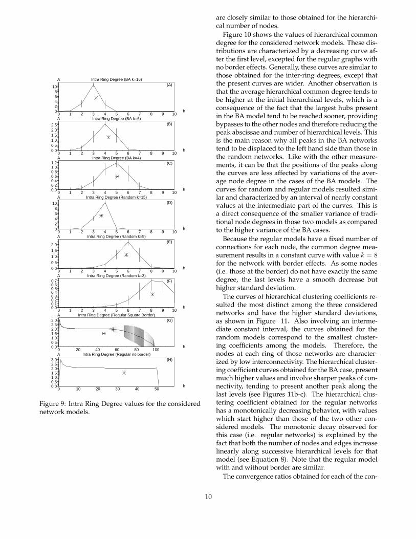
The results for intra-ring degree, shown in Figure 9,are very similar to the hierarchical number of nodesmeasurement, characterized by a peak, except for reg-ular networks, which exhibit a markedly different evo-lution resembling the curves obtained for the inter-ring degree. Note that for regular graphs with no bor-der effects, the final decreasing part tends to decreaseand saturate. The shape of BA and Random curves

8

Hier. Node Degree (BA k=16)

h

(A)k

0 1 2 3 4 5 6 7 8 9 100

500010000150002000025000


h

(B)k

0 1 2 3 4 5 6 7 8 9 100

2000400060008000

10000


h

(C)k

0 1 2 3 4 5 6 7 8 9 100

100020003000400050006000

Hier. Node Degree (Random k=15)

h

(D)k

0 1 2 3 4 5 6 7 8 9 100

50001000015000200002500030000


h

(E)k

0 1 2 3 4 5 6 7 8 9 100

10002000300040005000600070008000


h

(F)k

0 1 2 3 4 5 6 7 8 9 100

50010001500200025003000

Hier. Node Degree (Regular Square Border)

h

(G)k

0 20 40 60 80 1000

100200300400500

Hier. Node Degree (Regular no border)

h

(H)k

0 10 20 30 40 500

200400600800

10001200

Figure 7: Hierarchical node degrees obtained for allthe considered network models. The curves are sim-ilar to those obtained for the hierarchical number ofnodes, except for a expected offset of one level.

Inter Ring Degree (BA k=16)

h

(A)E

0 1 2 3 4 5 6 7 8 9 1005

1015202530354045


h

(B)E

0 1 2 3 4 5 6 7 8 9 100

5

10

15

20


h

(C)E

0 1 2 3 4 5 6 7 8 9 1002468

10121416

Inter Ring Degree (Random k=15)

h

(D)E

0 1 2 3 4 5 6 7 8 9 1002468

10121416


h

(E)E

0 1 2 3 4 5 6 7 8 9 10012345


h

(F)E

0 1 2 3 4 5 6 7 8 9 100.00.51.01.52.02.53.0

Inter Ring Degree (Regular Square Border)

h

(G)E

0 20 40 60 80 100012345678

Inter Ring Degree (Regular no border)

h

(H)E

0 10 20 30 40 50012345678

Figure 8: Inter ring degree values for the considerednetwork models.

9

Intra Ring Degree (BA k=16)

h

(A)A

0 1 2 3 4 5 6 7 8 9 1002468

10


h

(B)A

0 1 2 3 4 5 6 7 8 9 100.00.51.01.52.02.5


h

(C)A

0 1 2 3 4 5 6 7 8 9 100.00.20.40.60.81.01.2

Intra Ring Degree (Random k=15)

h

(D)A

0 1 2 3 4 5 6 7 8 9 1002468

10


h

(E)A

0 1 2 3 4 5 6 7 8 9 100.0

0.5

1.0

1.5

2.0


h

(F)A

0 1 2 3 4 5 6 7 8 9 100.00.10.20.30.40.50.60.7

Intra Ring Degree (Regular Square Border)

h

(G)A

0 20 40 60 80 1000.00.51.01.52.02.53.0

Intra Ring Degree (Regular no border)

h

(H)A

0 10 20 30 40 500.00.51.01.52.02.53.0

Figure 9: Intra Ring Degree values for the considerednetwork models.

are closely similar to those obtained for the hierarchi-cal number of nodes.

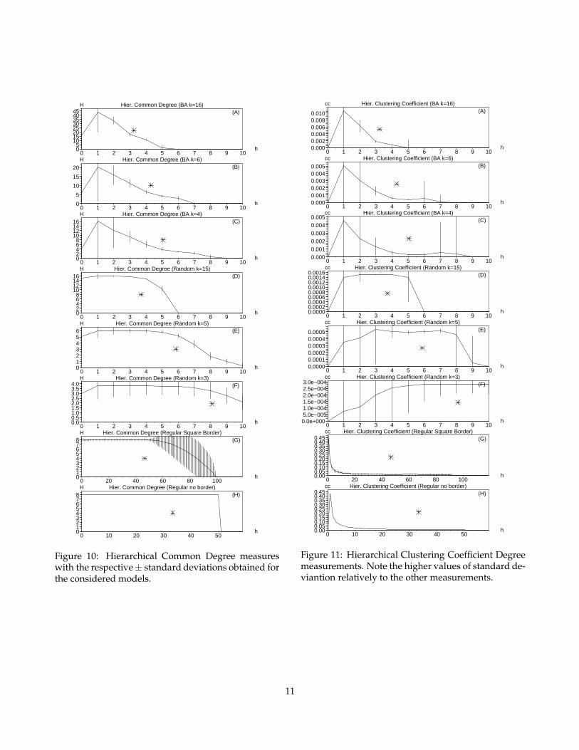
Figure 10 shows the values of hierarchical commondegree for the considered network models. These dis-tributions are characterized by a decreasing curve af-ter the first level, excepted for the regular graphs withno border effects. Generally, these curves are similar tothose obtained for the inter-ring degrees, except thatthe present curves are wider. Another observation isthat the average hierarchical common degree tends tobe higher at the initial hierarchical levels, which is aconsequence of the fact that the largest hubs presentin the BA model tend to be reached sooner, providingbypasses to the other nodes and therefore reducing thepeak abscissae and number of hierarchical levels. Thisis the main reason why all peaks in the BA networkstend to be displaced to the left hand side than those inthe random networks. Like with the other measure-ments, it can be that the positions of the peaks alongthe curves are less affected by variations of the aver-age node degree in the cases of the BA models. Thecurves for random and regular models resulted simi-lar and characterized by an interval of nearly constantvalues at the intermediate part of the curves. This isa direct consequence of the smaller variance of tradi-tional node degrees in those two models as comparedto the higher variance of the BA cases.

Because the regular models have a fixed number ofconnections for each node, the common degree mea-surement results in a constant curve with value k = 8for the network with border effects. As some nodes(i.e. those at the border) do not have exactly the samedegree, the last levels have a smooth decrease buthigher standard deviation.

The curves of hierarchical clustering coefficients re-sulted the most distinct among the three considerednetworks and have the higher standard deviations,as shown in Figure 11. Also involving an interme-diate constant interval, the curves obtained for therandom models correspond to the smallest cluster-ing coefficients among the models. Therefore, thenodes at each ring of those networks are character-ized by low interconnectivity. The hierarchical cluster-ing coefficient curves obtained for the BA case, presentmuch higher values and involve sharper peaks of con-nectivity, tending to present another peak along thelast levels (see Figures 11b-c). The hierarchical clus-tering coefficient obtained for the regular networkshas a monotonically decreasing behavior, with valueswhich start higher than those of the two other con-sidered models. The monotonic decay observed forthis case (i.e. regular networks) is explained by thefact that both the number of nodes and edges increaselinearly along successive hierarchical levels for thatmodel (see Equation 8). Note that the regular modelwith and without border are similar.

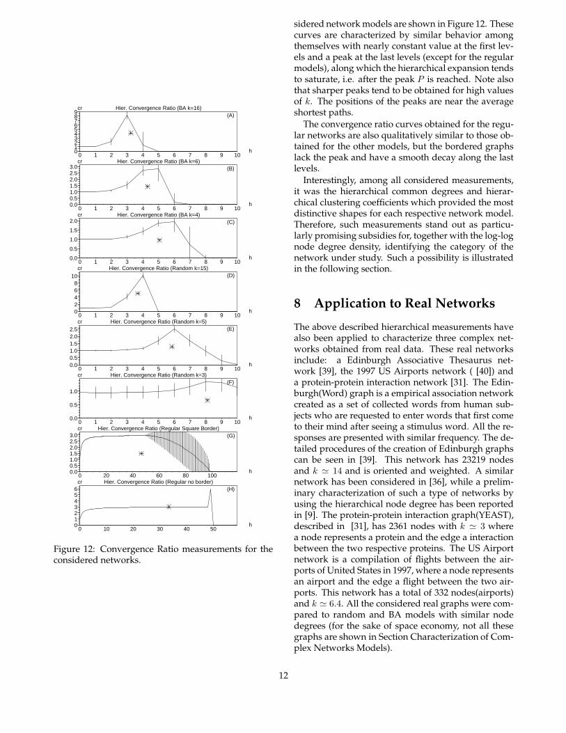
The convergence ratios obtained for each of the con-

10

Hier. Common Degree (BA k=16)

h

(A)H

0 1 2 3 4 5 6 7 8 9 1005

1015202530354045


h

(B)H

0 1 2 3 4 5 6 7 8 9 100

5

10

15

20


h

(C)H

0 1 2 3 4 5 6 7 8 9 1002468

10121416

Hier. Common Degree (Random k=15)

h

(D)H

0 1 2 3 4 5 6 7 8 9 1002468

10121416


h

(E)H

0 1 2 3 4 5 6 7 8 9 100123456


h

(F)H

0 1 2 3 4 5 6 7 8 9 100.00.51.01.52.02.53.03.54.0

Hier. Common Degree (Regular Square Border)

h

(G)H

0 20 40 60 80 100012345678

Hier. Common Degree (Regular no border)

h

(H)H

0 10 20 30 40 50012345678

Figure 10: Hierarchical Common Degree measureswith the respective± standard deviations obtained forthe considered models.

Hier. Clustering Coefficient (BA k=16)

h

(A)cc

0 1 2 3 4 5 6 7 8 9 100.0000.0020.0040.0060.0080.010


h

(B)cc

0 1 2 3 4 5 6 7 8 9 100.0000.0010.0020.0030.0040.005


h

(C)cc

0 1 2 3 4 5 6 7 8 9 100.0000.0010.0020.0030.0040.005

Hier. Clustering Coefficient (Random k=15)

h

(D)cc

0 1 2 3 4 5 6 7 8 9 100.00000.00020.00040.00060.00080.00100.00120.00140.0016


h

(E)cc

0 1 2 3 4 5 6 7 8 9 100.00000.00010.00020.00030.00040.0005


h

(F)cc

0 1 2 3 4 5 6 7 8 9 100.0e+0005.0e−0051.0e−0041.5e−0042.0e−0042.5e−0043.0e−004

Hier. Clustering Coefficient (Regular Square Border)

h

(G)cc

0 20 40 60 80 1000.000.050.100.150.200.250.300.350.400.45

Hier. Clustering Coefficient (Regular no border)

h

(H)cc

0 10 20 30 40 500.000.050.100.150.200.250.300.350.400.45

Figure 11: Hierarchical Clustering Coefficient Degreemeasurements. Note the higher values of standard de-viantion relatively to the other measurements.

11

Hier. Convergence Ratio (BA k=16)

h

(A)cr

0 1 2 3 4 5 6 7 8 9 100123456789


h

(B)cr

0 1 2 3 4 5 6 7 8 9 100.00.51.01.52.02.53.0


h

(C)cr

0 1 2 3 4 5 6 7 8 9 100.0

0.5

1.0

1.5

2.0

Hier. Convergence Ratio (Random k=15)

h

(D)cr

0 1 2 3 4 5 6 7 8 9 1002468

10


h

(E)cr

0 1 2 3 4 5 6 7 8 9 100.00.51.01.52.02.5


h

(F)cr

0 1 2 3 4 5 6 7 8 9 100.0

0.5

1.0

Hier. Convergence Ratio (Regular Square Border)

h

(G)cr

0 20 40 60 80 1000.00.51.01.52.02.53.0

Hier. Convergence Ratio (Regular no border)

h

(H)cr

0 10 20 30 40 500123456

Figure 12: Convergence Ratio measurements for theconsidered networks.

sidered network models are shown in Figure 12. Thesecurves are characterized by similar behavior amongthemselves with nearly constant value at the first lev-els and a peak at the last levels (except for the regularmodels), along which the hierarchical expansion tendsto saturate, i.e. after the peak P is reached. Note alsothat sharper peaks tend to be obtained for high valuesof k. The positions of the peaks are near the averageshortest paths.

The convergence ratio curves obtained for the regu-lar networks are also qualitatively similar to those ob-tained for the other models, but the bordered graphslack the peak and have a smooth decay along the lastlevels.

Interestingly, among all considered measurements,it was the hierarchical common degrees and hierar-chical clustering coefficients which provided the mostdistinctive shapes for each respective network model.Therefore, such measurements stand out as particu-larly promising subsidies for, together with the log-lognode degree density, identifying the category of thenetwork under study. Such a possibility is illustratedin the following section.

8 Application to Real Networks

The above described hierarchical measurements havealso been applied to characterize three complex net-works obtained from real data. These real networksinclude: a Edinburgh Associative Thesaurus net-work [39], the 1997 US Airports network ( [40]) anda protein-protein interaction network [31]. The Edin-burgh(Word) graph is a empirical association networkcreated as a set of collected words from human sub-jects who are requested to enter words that first cometo their mind after seeing a stimulus word. All the re-sponses are presented with similar frequency. The de-tailed procedures of the creation of Edinburgh graphscan be seen in [39]. This network has 23219 nodesand k ≃ 14 and is oriented and weighted. A similarnetwork has been considered in [36], while a prelim-inary characterization of such a type of networks byusing the hierarchical node degree has been reportedin [9]. The protein-protein interaction graph(YEAST),described in [31], has 2361 nodes with k ≃ 3 wherea node represents a protein and the edge a interactionbetween the two respective proteins. The US Airportnetwork is a compilation of flights between the air-ports of United States in 1997, where a node representsan airport and the edge a flight between the two air-ports. This network has a total of 332 nodes(airports)and k ≃ 6.4. All the considered real graphs were com-pared to random and BA models with similar nodedegrees (for the sake of space economy, not all thesegraphs are shown in Section Characterization of Com-plex Networks Models).

12

Hier. Number of Nodes (Word)

h

(A)n

0 1 2 3 4 5 6 7 8 9 100

50010001500200025003000350040004500

Hier. Number of Nodes (Airport 97)

h

(B)n

0 1 2 3 4 5 6 7 8 9 100

20406080

100120140160

Hier. Number of Nodes (Yeast)

h

(C)n

0 1 2 3 4 5 6 7 8 9 100

100200300400500600700800

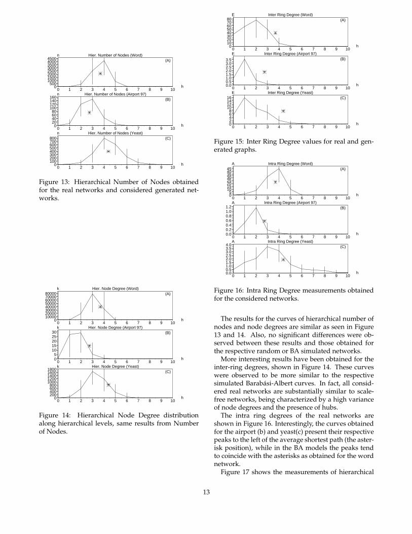
Figure 13: Hierarchical Number of Nodes obtainedfor the real networks and considered generated net-works.

Hier. Node Degree (Word)

h

(A)k

0 1 2 3 4 5 6 7 8 9 100

1000020000300004000050000600007000080000

Hier. Node Degree (Airport 97)

h

(B)k

0 1 2 3 4 5 6 7 8 9 1005

1015202530

Hier. Node Degree (Yeast)

h

(C)k

0 1 2 3 4 5 6 7 8 9 100

200400600800

10001200140016001800

Figure 14: Hierarchical Node Degree distributionalong hierarchical levels, same results from Numberof Nodes.

Inter Ring Degree (Word)

h

(A)E

0 1 2 3 4 5 6 7 8 9 100

1020304050607080

Inter Ring Degree (Airport 97)

h

(B)E

0 1 2 3 4 5 6 7 8 9 100.00.51.01.52.02.53.03.5

Inter Ring Degree (Yeast)

h

(C)E

0 1 2 3 4 5 6 7 8 9 1002468

10121416

Figure 15: Inter Ring Degree values for real and gen-erated graphs.

Intra Ring Degree (Word)

h

(A)A

0 1 2 3 4 5 6 7 8 9 1005

1015202530354045

Intra Ring Degree (Airport 97)

h

(B)A

0 1 2 3 4 5 6 7 8 9 100.00.20.40.60.81.01.2

Intra Ring Degree (Yeast)

h

A(C)

0 1 2 3 4 5 6 7 8 9 100.00.51.01.52.02.53.03.54.0

Figure 16: Intra Ring Degree measurements obtainedfor the considered networks.

The results for the curves of hierarchical number ofnodes and node degrees are similar as seen in Figure13 and 14. Also, no significant differences were ob-served between these results and those obtained forthe respective random or BA simulated networks.

More interesting results have been obtained for theinter-ring degrees, shown in Figure 14. These curveswere observed to be more similar to the respectivesimulated Barabasi-Albert curves. In fact, all consid-ered real networks are substantially similar to scale-free networks, being characterized by a high varianceof node degrees and the presence of hubs.

The intra ring degrees of the real networks areshown in Figure 16. Interestingly, the curves obtainedfor the airport (b) and yeast(c) present their respectivepeaks to the left of the average shortest path (the aster-isk position), while in the BA models the peaks tendto coincide with the asterisks as obtained for the wordnetwork.

Figure 17 shows the measurements of hierarchical

13

Hier. Common Degree (Word)

h

(A)H

0 1 2 3 4 5 6 7 8 9 100

102030405060708090

Hier. Common Degree (Airport 97)

h

(B)H

0 1 2 3 4 5 6 7 8 9 100.00.51.01.52.02.53.03.54.04.5

Hier. Common Degree (Yeast)

h

(C)H

0 1 2 3 4 5 6 7 8 9 1002468

1012141618

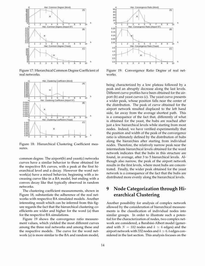
Figure 17: Hierarchical Common Degree Coefficient ofreal networks.

Hier. Clustering Coefficient (Word)

h

(A)cc

0 1 2 3 4 5 6 7 8 9 100.000.050.100.150.200.250.300.350.400.45

Hier. Clustering Coefficient (Airport 97)

h

(B)cc

0 1 2 3 4 5 6 7 8 9 100.0000.0050.0100.0150.0200.0250.0300.035

Hier. Clustering Coefficient (Yeast)

h

(C)cc

0 1 2 3 4 5 6 7 8 9 100.000.050.100.150.200.250.300.35

Figure 18: Hierarchical Clustering Coefficient mea-sures.

common degree. The airport(b) and yeast(c) networkscurves have a similar behavior to those obtained forthe respective BA curves, with a peak at the first hi-erarchical level and a decay. However the word net-work(a) have a mixed behavior, beginning with a in-creasing curve like in a BA model, but ending with aconvex decay like that typically observed in randomnetworks.

The clustering coefficient measurements, shown inFigure 18, substantiate the adherence of the real net-works with respective BA simulated models. Anotherinteresting result which can be inferred from this fig-ure regards the fact that the hierarchical clustering co-efficients are wider and higher for the word (a) thanfor the respective BA simulations.

Figure 19 shows the convergence ratio measure-ment values, which yielded the most different curvesamong the three real networks and among these andthe respective models. The curve for the word net-work (a) is more similar to the BA and random model,

Hier. Convergence Ratio (Word)

h

(A)cr

0 1 2 3 4 5 6 7 8 9 100

1020304050

Hier. Convergence Ratio (Airport 97)

h

(B)cr

0 1 2 3 4 5 6 7 8 9 100.00

0.05

0.10

0.15

0.20

Hier. Convergence Ratio (Yeast)

h

(C)cr

0 1 2 3 4 5 6 7 8 9 100.0

0.5

1.0

1.5

2.0

Figure 19: Convergence Ratio Degree of real net-works.

being characterized by a low plateau followed by apeak and an abruptly decrease along the last levels.Different curve profiles have been obtained for the air-port (b) and yeast curves (c). The yeast curve presentsa wider peak, whose position falls near the center ofthe distribution. The peak of curve obtained for theairport network resulted displaced to the left handside, far away from the average shortest path. Thisis a consequence of the fact that, differently of whatis obtained for the yeast, the hubs are reached afterjust a few hierarchical levels while starting from mostnodes. Indeed, we have verified experimentally thatthe position and width of the peak of the convergenceratio is ultimately defined by the distribution of hubsalong the hierarchies after starting from individualnodes. Therefore, the relatively narrow peak near theintermediate hierarchical levels obtained for the wordnetwork indicates that the hubs in this structure arefound, in average, after 3 to 5 hierarchical levels. Al-though also narrow, the peak of the airport networkresults in the first levels, where most hubs are concen-trated. Finally, the wider peak obtained for the yeastnetwork is a consequence of the fact that the hubs aredistributed more evenly along the hierarchical levels.

9 Node Categorization through Hi-

erarchical Clustering

Another possibility for analysis of complex networkallowed by the consideration of hierarchical measure-ments is the classification of individual nodes intosimilar groups. In order to illustrate such a poten-tial for the characterization of nodes, two complex net-work are considered, a Barabasi-Albert model (gener-ated with N = 332 nodes and k ≃ 6 edges) and theairport network with 332 nodes and k ≃ 6.4 edges con-sidered in the last section. This analysis focuses on the

14

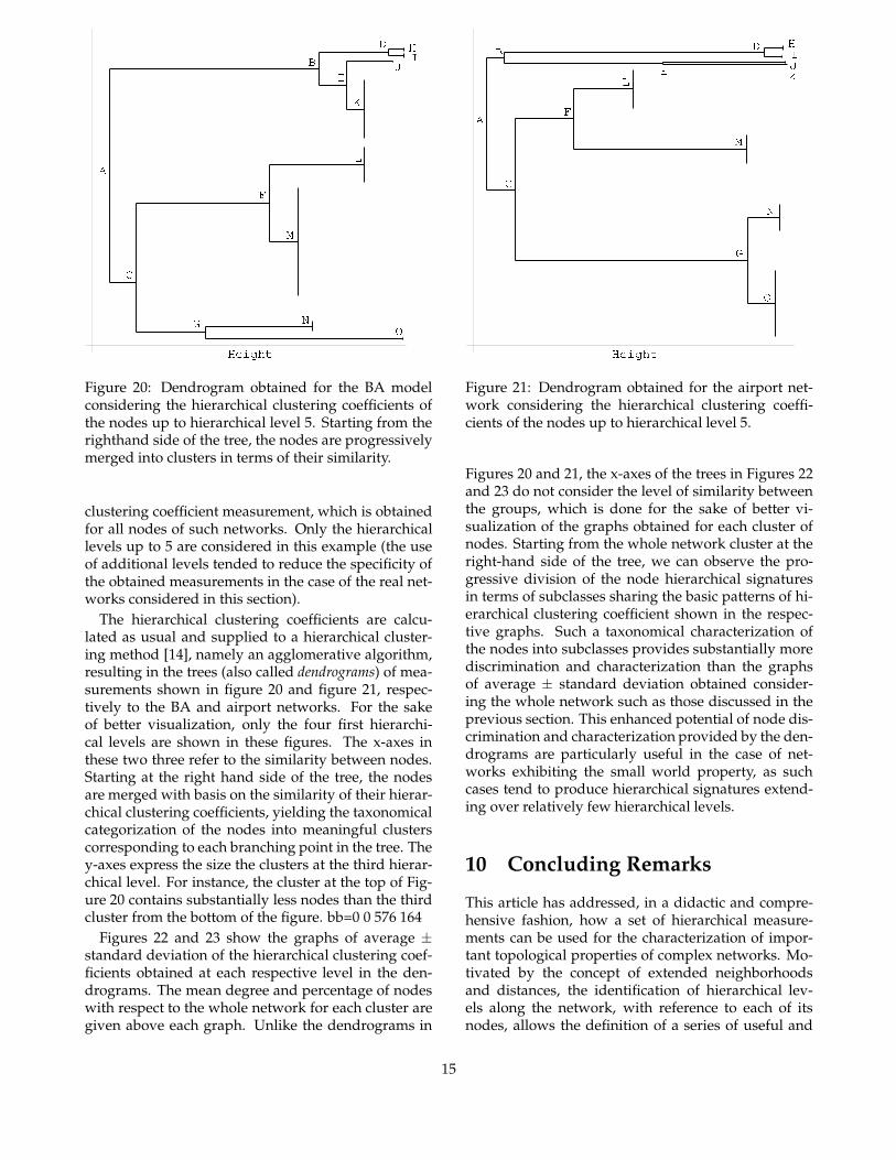
Figure 20: Dendrogram obtained for the BA modelconsidering the hierarchical clustering coefficients ofthe nodes up to hierarchical level 5. Starting from therighthand side of the tree, the nodes are progressivelymerged into clusters in terms of their similarity.

clustering coefficient measurement, which is obtainedfor all nodes of such networks. Only the hierarchicallevels up to 5 are considered in this example (the useof additional levels tended to reduce the specificity ofthe obtained measurements in the case of the real net-works considered in this section).

The hierarchical clustering coefficients are calcu-lated as usual and supplied to a hierarchical cluster-ing method [14], namely an agglomerative algorithm,resulting in the trees (also called dendrograms) of mea-surements shown in figure 20 and figure 21, respec-tively to the BA and airport networks. For the sakeof better visualization, only the four first hierarchi-cal levels are shown in these figures. The x-axes inthese two three refer to the similarity between nodes.Starting at the right hand side of the tree, the nodesare merged with basis on the similarity of their hierar-chical clustering coefficients, yielding the taxonomicalcategorization of the nodes into meaningful clusterscorresponding to each branching point in the tree. They-axes express the size the clusters at the third hierar-chical level. For instance, the cluster at the top of Fig-ure 20 contains substantially less nodes than the thirdcluster from the bottom of the figure. bb=0 0 576 164

Figures 22 and 23 show the graphs of average ±standard deviation of the hierarchical clustering coef-ficients obtained at each respective level in the den-drograms. The mean degree and percentage of nodeswith respect to the whole network for each cluster aregiven above each graph. Unlike the dendrograms in

Figure 21: Dendrogram obtained for the airport net-work considering the hierarchical clustering coeffi-cients of the nodes up to hierarchical level 5.

Figures 20 and 21, the x-axes of the trees in Figures 22and 23 do not consider the level of similarity betweenthe groups, which is done for the sake of better vi-sualization of the graphs obtained for each cluster ofnodes. Starting from the whole network cluster at theright-hand side of the tree, we can observe the pro-gressive division of the node hierarchical signaturesin terms of subclasses sharing the basic patterns of hi-erarchical clustering coefficient shown in the respec-tive graphs. Such a taxonomical characterization ofthe nodes into subclasses provides substantially morediscrimination and characterization than the graphsof average ± standard deviation obtained consider-ing the whole network such as those discussed in theprevious section. This enhanced potential of node dis-crimination and characterization provided by the den-drograms are particularly useful in the case of net-works exhibiting the small world property, as suchcases tend to produce hierarchical signatures extend-ing over relatively few hierarchical levels.

10 Concluding Remarks

This article has addressed, in a didactic and compre-hensive fashion, how a set of hierarchical measure-ments can be used for the characterization of impor-tant topological properties of complex networks. Mo-tivated by the concept of extended neighborhoodsand distances, the identification of hierarchical lev-els along the network, with reference to each of itsnodes, allows the definition of a series of useful and

15

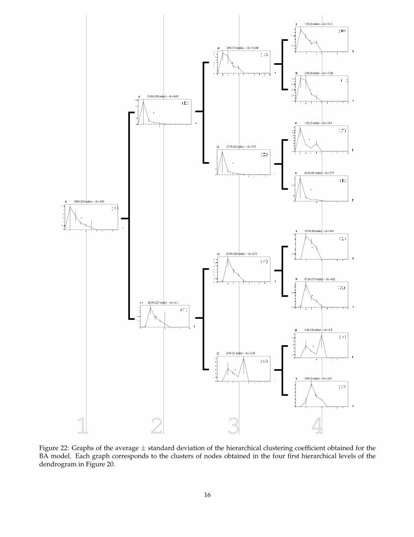
Figure 22: Graphs of the average ± standard deviation of the hierarchical clustering coefficient obtained for theBA model. Each graph corresponds to the clusters of nodes obtained in the four first hierarchical levels of thedendrogram in Figure 20.

16

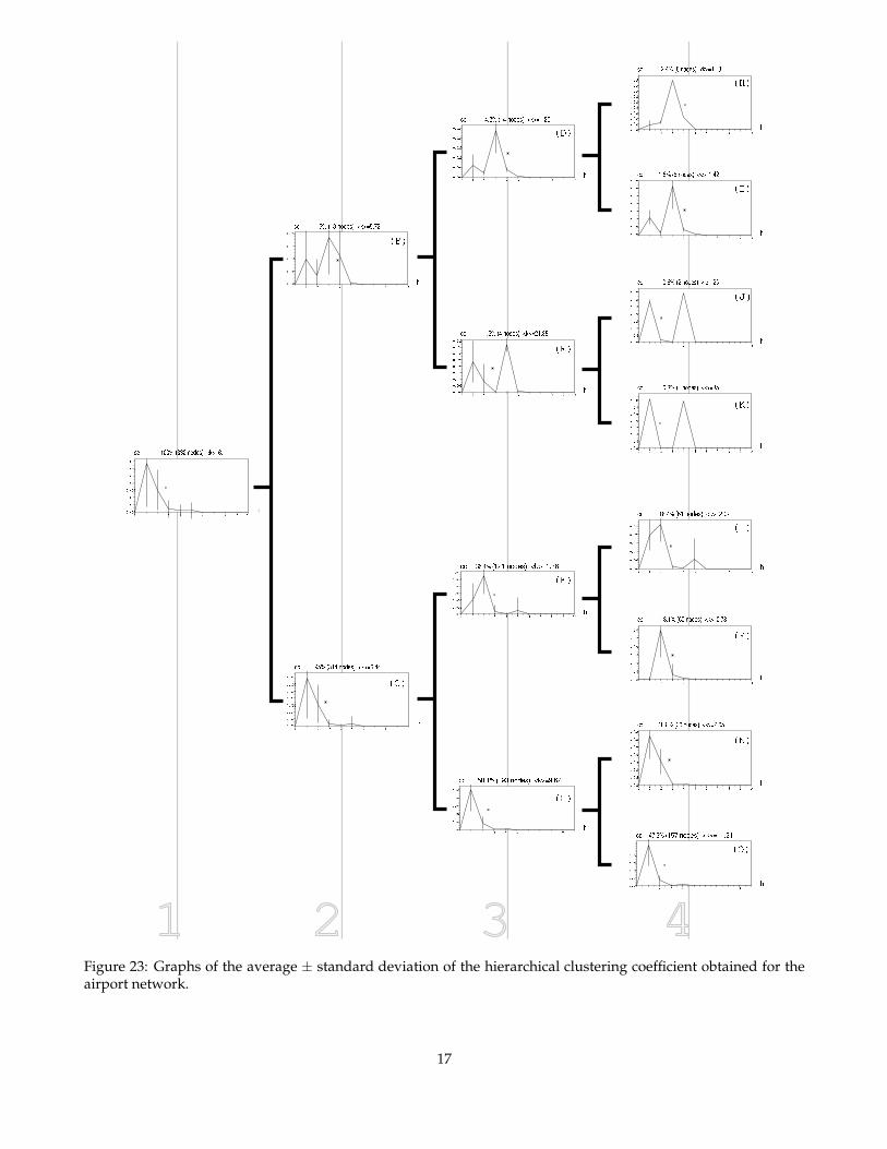
Figure 23: Graphs of the average ± standard deviation of the hierarchical clustering coefficient obtained for theairport network.

17

informative hierarchical measurements of the networktopology, including hierarchical extensions of the tra-ditional node degree and clustering coefficient mea-surements. The novel concepts of inter and intra-ring degrees, convergence ratio, edge degree and edgeclustering coefficient, as well as their hierarchical ver-sions, were also introduced here in terms of the sub-network generalization described in [10].

It has been shown, both analytically and throughsimulations, that the hierarchical node degree of a ran-dom network has a typical shape involving a limitednumber of hierarchical levels while a peak is observedat its intermediate portion, which is a consequence ofthe finite size of the considered networks. A simi-lar dynamics was experimentally identified for scale-free and regular network models. It was also shown,through simulations, that the suggested set of hierar-chical measurements provided a wealthy of informa-tion about the topological structure of the consideredmodels (namely random, scale-free and regular), al-lowing the identification of a number of interestingproperties specific to each of those models. Of particu-lar interest is the discriminative potential of the hierar-chical common degree and hierarchical clustering co-efficient. The potential of the reported set of hierarchi-cal measurements was further illustrated with respectto three real networks: word associations, airport con-nections and protein-protein interactions. The com-parison of the hierarchical measurements obtained forthese three networks with respective random, regularand BA models with the same number of nodes andsimilar node degree indicated that, except for a fewmeasurements (specific to each model), all the threereal networks were most similar to the BA models.In the case of the word associations network, somemeasurements (i.e. hierarchical common degree andinter-ring degree) yielded hierarchical curves whichwere similar to random along some parts and simi-lar to BA at other parts. This network was also ver-ified to present the convergence ratio most similar tothat of a respective BA model. The concentration ofhigher values of convergence ratio at the left hand sideof the curves obtained for the airport network alsoconfirmed the fact that the hubs in this network arereached much faster than all the other networks con-sidered in this article. Contrariwise, the convergenceratio values obtained for the protein-protein interac-tion network indicated that the hubs in this real net-work are more evenly spaces one another. As a matterof fact, the convergence ratio resulted in the most in-formative of the hierarchical measurements as far asthe analysis of the three real models was concerned.This is a consequence of the fact that the presence of ahub at a given hierarchical level tend to strongly affectthe convergence ratio at that level.

Finally, the current article also proposed and illus-trated the possibility to use the enhanced information

provided by the set of hierarchical measurements inorder to organize the nodes of a network into a taxon-omy reflecting the similarities between the nodes con-nectivity. Such a methodology is particularly promis-ing because the obtained taxonomy can be used to bet-ter understand the main classes of nodes present in agiven complex network, i.e. those classes obtained atthe higher levels of the taxonomy. Indeed, while thelimited number of hierarchical levels present in smallworld networks such as random and BA models con-strain the potential of the hierarchical measurementsfor the discrimination between such models, the con-sideration of the main obtained classes of nodes hasbeen verified to provide further discrimination be-tween the compared networks.

A series of possible future investigations has beenmotivated by the results reported in this article. First,it would be interesting to assess in a systematic fash-ion, and by using multivariate statistical analysis andhypothesis tests, the potential of each measurement,as well as their combinations, for discriminating thepossible class of a given network. Another issueof particular relevance regards the identification andpreservation of hubs considering not only the immedi-ate neighbors of a node, but of the neighbors accumu-lated along growing hierarchical levels. While sucha possibility has been preliminary considered in [10],it would be interesting to consider the preservationof hubs as an increasing number of hierarchical lev-els is taken into account. Such a study is under de-velopment with respect to protein-protein associationnetworks and related results should be futurely pre-sented. Another study which can complement the re-sults described in the current work involves the con-sideration of several types of small-world networks.Finally, it would be interesting to apply the hierarchi-cal measurements for the characterization of severalother real networks such as protein-protein interac-tion, internet, social connections, to name but a few.

Acknowledgment: Luciano da F. Costa is grate-ful to FAPESP (proc. 99/12765-2), CNPq (proc.308231/03-1) and the Human Frontier Science Pro-gram (RGP39/2002) for financial support.

References

[1] M.E.J. Newman, SIAM Review 45: 167–256 (2003).

[2] R. Albert and A.-L. Barabasi, Rev. Mod. Phys. 74:47–97 (2002).

[3] P.J. Flory, J. Am. Chem. Soc 63: 3083, 3091, 3096(1941).

[4] A. Rapoport, Bull. Math. Bioph. 19: 257–277 (1957).

18

[5] P. Erdos and A. Renyi, Publications Mathematicae6: 290-297 (1959).

[6] D.J Watts and S.H. Strogatz, Nature 393: 440–442(1998).

[7] D.J. Watts, Small Worlds, Princeton Studies inComplexity, Princeton Univ. Press (1999).

[8] R. Albert and H. Jeong and A.L. Barabasi, Nature401: 130, cond-mat/9907038 (1999).

[9] L.daF. Costa, Phys. Rev. Lett. 93: 098702 (2004).

[10] L.daF. Costa, cond-mat/0408076 (2004).

[11] E. Ravasz and A.L. Barabasi, cond-mat/0206130(2002).

[12] E. Ravasz, A.L. Somera, A. Mongru, Z.N.Oltvaiand A.L. Barabasi, Science, 297: 1551–1555 (2002),cond-mat/0209244.

[13] G. Caldarelli, R. Pastor-Satorras and A. Vespig-nani, cond-mat/0212026 (2003).

[14] Costa, L. d. and Cesar, R. M. 2000, Shape Analy-sis and Classification: Theory and Practice, 1st. CRCPress, Inc.

[15] R. Duda, P. Hart, and D. Stork: Pattern Classifica-tion, 2st. John Wiley, New York, 2001.

[16] B. Bollobas. Random Graphs. Academic Press,London, 1985.

[17] A.L Barabasi, Z. Deszo, E. Ravasz, S.-H. Yook andZ. Oltvai, Sitges Proceedings on Complex Net-works (2004).

[18] A Trusina, S. Maslov, P. Minnhagen andK. Sneppen, Phys. Rev. Lett., 92: 178702 (2004),cond-mat/0308339 (2003).

[19] M. Boss, H. Elsinger, M. Summer and S. Thurner,Santa Fe Institute Working Paper No. 03-10-054,Accepted for Quant. Finance, cond-mat/0309582(2003).

[20] M. Barthelemy, A. Barrat, R. Pastor-Satorras andA. Vespignani, cond-mat/0311501 (2003).

[21] H. Zhou, Phys. Rev. E, 67: 061901 (2003).

[22] A. Vazquez, Phys. Rev. E, 67: 056104 (2003).

[23] M. Steyvers and J.B. Tenenbaum, To appear inCognitive Science, cond-mat/0212026 (2003).

[24] V. Gold’shtein, G.A. Koganov and G.I. Surdu-tovich, cond-mat/0409298 (2004).

[25] E.R. Dougherty and R.A. Lotufo, Hands-on Mor-phological Image Processing, SPIE Press (2003).

[26] M. E. Newman, cond-mat/0111070 (2001).

[27] M. E. J. Newman and D. J. Watts, Phys. Rev. E 60,7332-7342 (1999).

[28] R. Cohen, S. Havlin, S. Mokryn, D. Dolev, T.Kalisky, and Y. Shavitt, cond-mat/0305582(2003).

[29] L. Vincent, Signal Proc., 16:365–388 (1989).

[30] H.J.A.M. Heijmans, P. Nacken, A. Toet and L. Vin-cent, J. Vis. Comm. and Image Repr., 3:24–38 (1992).

[31] Shiwei Sun, Lunjiang Ling, Nan Zhang, Guojie Liand Runsheng Chen: Topological structure analysisof the protein-protein interaction network in buddingyeast. Nucleic Acids Research, 2003, Vol. 31, No. 92443-2450.

[32] L.daF. Costa, cond-mat/0405022 (2004).

[33] J.P. Bagrow and E.M. Bollt, cond-mat/0412482(2004).

[34] A.C. Zorach and R.E. Ulanowicz, Complexity, 8(3):68–76 (2003).

[35] T.H. Cormen, C.E. Leiserson, R.L. Rivest andC. Stein, Introduction to Algorithms, The MITPress (2002).

[36] L.daF. Costa, Intl. J. Mod. Phys. C, 15:371–379(2003).

[37] L.daF. Costa, q.bio.MN/0405028 (2004).

[38] L.daF. Costa, q.bio.TO/0412042 (2004).

[39] Kiss, G.R., Armstrong, C., Milroy, R., and Piper,J. (1973) An associative thesaurus of English and itscomputer analysis In Aitken, A.J., Bailey, R.W. andHamilton-Smith, N. (Eds.), The Computer andLiterary Studies. Edinburgh: University Press.

[40] USAir97, Pajek Package forLarge Network Analysishttp://vlado.fmf.uni-lj.si/pub/networks/pajek/data/gphs.htm

19















http://vlado.fmf.uni-lj.si/pub/networks/pajek/data/gphs.htm

hierarchical characterization of complex networks

Documents