INSTITUTE OF PHYSICS PUBLISHING and INTERNATIONAL ATOMIC ENERGY AGENCY NUCLEAR FUSION

Nucl. Fusion 45 (2005) 163–175 doi:10.1088/0029-5515/45/3/002

Helium exhaust experiments on JETwith Type I ELMs in H-mode and withType III ELMs in ITB dischargesK.-D. Zastrow1, S.J. Cox1, M.G. von Hellermann2,M.G. O’Mullane3, D. Stork1, M. Brix4, C.D. Challis1, I.H. Coffey5,R. Dux6, K.H. Finken4, C. Giroud1, D. Hillis7, J.T. Hogan7,K.D. Lawson1, T. Loarer8, A.G. Meigs1, P.D. Morgan1,M.F. Stamp1, A.D. Whiteford3 and JET EFDA Contributorsa

1 Euratom/UKAEA Fusion Association, Culham Science Centre, Abingdon, UK2 FOM Instituut voor Plasmaphysica, Associatie Euratom, Nieuwegein, The Netherlands3 Department of Physics, University of Strathclyde, Glasgow, UK4 Forschungszentrum Julich GmbH, IPP, Euratom Association, Julich, Germany5 Department of Physics, Queens University, Belfast, UK6 Max-Planck-Institut fur Plasmaphysik, Euratom Association, Garching, Germany7 Oak Ridge National Laboratory, P.O. Box 2008, Oak Ridge, USA8 Association EURATOM-CEA sur la Fusion, CEA Cadarache, St Paul-lez Durance, France

Received 3 April 2003, accepted for publication 15 December 2004Published 21 February 2005Online at stacks.iop.org/NF/45/163

AbstractAn analysis of helium exhaust experiments on JET in the MkII-GB divertor configuration is presented. Helium ispumped by applying an argon frost layer on the divertor cryo pump. Measurement of the helium retention time, τ ∗

He,is performed in two ways: by the introduction of helium in gas puffs and measurement of the subsequent decay timeconstant of the helium content, τ d∗

He; and by helium beam injection and measurement of the helium replacement time,τ r∗

He. In ELMy H-mode, with plasma configuration optimized for pumping, τ d∗He ≈ 7.2 × τ th

E is achieved, where τ thE

is the thermal energy replacement time. For quasi-steady internal transport barrier (ITB) discharges, the achievedτ r∗

He ≈ 4.1 × τ thE is significantly lower. The achieved helium recycling coefficient, confirmed by an independent

measurement to be Reff ≈ 0.91, is the same in both scenarios. None of the discharges are dominated by coreconfinement. The difference in τ ∗

He/τthE is instead due to the confinement properties of the edge plasma, which is

characterized by Type I ELMs for the H-mode discharges studied, and Type III ELMs for the quasi-steady ITBdischarges. This difference is quantified by an independent measurement of the ratio of the helium replacement timewith a helium edge source to the energy confinement time.

PACS numbers: 52.55.Fa, 52.55.Pi, 52.55.Rk, 52.25.Fi, 52.25.Vy

1. Introduction

Control of helium ‘ash’ produced in D–T reactions is oneof the key issues affecting the performance and possiblythe achievable burn time of a fusion reactor. The removalof helium is determined by a combination of the intrinsictransport of helium in the plasma, especially across internaland edge transport barriers, the enrichment and compressionof helium in the sub-divertor region, and the pumping andrefuelling efficiency for helium. Thus, the task is oneof system integration and is only partially determined byplasma physics. The overall engineering requirement is

a See annex of J. Pamela et al Fusion Energy 2002; Proc. 19th. Int. Conf.(Lyon 2002) (Vienna: IAEA).

best stated [1] in terms of the ratio of the helium retentiontime, τ ∗

He, to the thermal energy confinement time, τ thE , since

effective α particle heating is essential in a burning fusionplasma. If small levels of additional impurities are present,the requirement is τ ∗

He/τthE � 10 to obtain steady-state

burn conditions. With additional impurities, the requirementbecomes more strict, e.g. τ ∗

He/τthE � 5 would be required

if carbon concentrations were of order 3%. The target forthe pumping arrangement is specified in terms of the heliumenrichment factor, η, i.e. the ratio of the partial pressuresof helium and deuterium in the sub-divertor region (at thepump throat) to the ratio of He2+ to D+ in the plasma core,which needs to be larger than 0.2 for stationary operation ofITER [2].

0029-5515/05/030163+13$30.00 © 2005 IAEA, Vienna Printed in the UK 163

K.-D. Zastrow et al

A recent review of the research on helium transport andexhaust has been written by Hogan [3]. In most experiments,helium is introduced by gas puffs and the decay time constantof the helium content, τ d∗

He, is studied. On DIII-D andJT-60U, helium neutral beam injection (NBI) was used toprovide a central source [4–7] so that the replacement time,τ r∗

He, can be measured. In L-mode and ELMy H-modes itwas always found that the helium exhaust rate is limited bythe pumping efficiency and not by the helium transport inthe plasma edge, let alone the plasma core. The achievedratio τ ∗

He/τthE (measured by either of the two techniques) has

been low enough and it has been shown that helium can bepumped at a satisfactory rate by divertor pumping, which isthe method used in the majority of experiments, and also withpumped limiters [8].

Improved core confinement by the formation andsustainment of internal transport barriers (ITBs) is seen asa possible route to steady-state tokamak operation becauseof the potential of this regime for full non-inductive currentdrive. However, helium removal from the region confinedby the ITB might not be fast enough and would thus limitthe burn time. Results from experiments in JT-60U ITBdischarges indicate increased helium retention in the regionconfined by the ITB by factors of between two and three [6],and due to reduced diffusivity by a factor of five to six [9].Also, there is concern that, since ITB discharges to date tendto be characterized by lower edge density than ELMy H-mode plasmas, the potential for pumping of helium might bereduced. To investigate both issues, a series of experimentswas conducted on JET during helium plasma operation. Forcomparison, we also report re-analysed results in ELMy H-modes from earlier experiments in this paper.

In [1], two characteristic times have been introduced toquantify retention, the replacement time for a central source,S0, defined as τ0 = NHe/S0 and the replacement time foran edge source, Sedge, defined as τedge = NHe/Sedge. NHe isthe plasma helium content that is sustained by the source ineach case. In this context, the ‘edge’ is a region of closedflux surfaces close to the plasma boundary and should not beconfused with the Scrape-Off Layer (SOL), which is a regionof open field lines. Note that in this paper we use symbolsdifferent from those in [1], namely an index that refers tothe location of the source (‘0’ and ‘edge’). The definition isthe same.

In a numerical model both τ0 and τedge can be readilycalculated, whereas in experiments only τedge can be measured.This is because the effect of helium recycling cannotcompletely be removed, so an experiment with only a centralsource cannot be performed. The relationship of the observedretention time to refuelling efficiency, f , and recycling is givenby equations (5.6) and (5.10) from [1], which we reproducehere:

τ ∗ = τ0 + τedgeReff

1 − Reff, (1)

Reff = Rretf1

1 − (1 − f )Rret, (2)

where Rret is the fraction of helium returning from the walland divertor and Reff = �ion/�out is the fraction of the heliumoutflux, �out, that is returning to the confined plasma as an edgeinflux, �ion, of helium ions.

The prediction of Reff for ITER cannot be the subject ofexperimental studies on existing devices since Rret dependson divertor geometry and the helium pumping speed, andf depends on the details of the SOL plasma. Both of theseare likely to be very different, and require modelling [10] tobe assessed. The goal we have set ourselves in this study is todetermine the contribution of τedge to τ ∗

He for each operationalregime, which can potentially be scaled to ITER.

In all experiments reported in this paper we make use ofthe helium pumping capability of the JET pumped divertor.Details on the pumping arrangement and calibration of thepumping speed for helium are given in section 2. The resultson helium retention in ELMy H-mode discharges are presentedbriefly in section 3. Helium ash simulation experiments inquasi-steady ITB discharges are presented in detail in section 4and the results from all regimes are compared in section 5 byindependent measurements of Reff and τedge. We have used twodifferent techniques to study helium retention, measurementof the time constant of the decay of the total helium content,τ d∗

He, and measurement of the replacement time for the totalhelium content, τ r∗

He. A comparison of these techniques,from a model point of view, is presented in appendix Aand a discussion of statistical and systematic errors in theexperiments in appendix B.

2. Helium pumping scheme in the JET MkII-GBdivertor

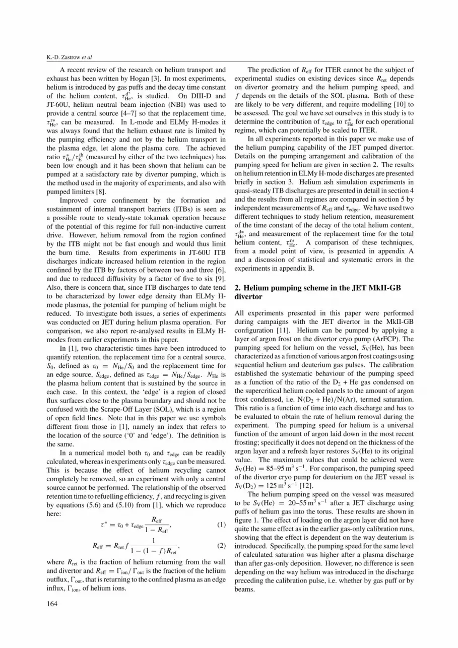
All experiments presented in this paper were performedduring campaigns with the JET divertor in the MkII-GBconfiguration [11]. Helium can be pumped by applying alayer of argon frost on the divertor cryo pump (ArFCP). Thepumping speed for helium on the vessel, SV(He), has beencharacterized as a function of various argon frost coatings usingsequential helium and deuterium gas pulses. The calibrationestablished the systematic behaviour of the pumping speedas a function of the ratio of the D2 + He gas condensed onthe supercritical helium cooled panels to the amount of argonfrost condensed, i.e. N(D2 + He)/N(Ar), termed saturation.This ratio is a function of time into each discharge and has tobe evaluated to obtain the rate of helium removal during theexperiment. The pumping speed for helium is a universalfunction of the amount of argon laid down in the most recentfrosting; specifically it does not depend on the thickness of theargon layer and a refresh layer restores SV(He) to its originalvalue. The maximum values that could be achieved wereSV(He) = 85–95 m3 s−1. For comparison, the pumping speedof the divertor cryo pump for deuterium on the JET vessel isSV(D2) = 125 m3 s−1 [12].

The helium pumping speed on the vessel was measuredto be SV(He) = 20–55 m3 s−1 after a JET discharge usingpuffs of helium gas into the torus. These results are shown infigure 1. The effect of loading on the argon layer did not havequite the same effect as in the earlier gas-only calibration runs,showing that the effect is dependent on the way deuterium isintroduced. Specifically, the pumping speed for the same levelof calculated saturation was higher after a plasma dischargethan after gas-only deposition. However, no difference is seendepending on the way helium was introduced in the dischargepreceding the calibration pulse, i.e. whether by gas puff or bybeams.

164

Helium exhaust experiments on JET

80

60

40

20

0

100

50 10 15 20

S (

m3

/ s)

N (D2+He) / N (Ar) (%)

JG03

.65-

1c

25

After He gasAfter He NBIBefore Discharge

Figure 1. Pumping speed for the argon frosted divertor cryopump on the vessel, as a function of the saturation of the argonfrost layer with deuterium and helium. The pumping speed ismeasured using helium gas puffs into the vessel after thedischarge. N(D2 + He) is calculated from a measurementof the sub-divertor pressures for helium and deuterium and thepumping speed of the divertor cryo pump on the sub-divertorregion. N(Ar) is the amount of argon applied in the most recentfrost.

After a discharge, the pumping speed can be restored byrepeated argon frosting until a total of 60 Pa m3 of argon hasbeen deposited on the pumps. At higher deposition valuesargon may be released, which degrades the plasma purity, andcarries the risk of causing disruptions.

In figure 1 the saturation is calculated from the amountof argon applied in the most recent frost (typically 3 Pa m3

in the first frost and 1 Pa m3 for refresh layers), and byintegrating in time the amount of helium and deuterium thatwas condensed on the pump. The calculation uses the timeresolved measurement of the partial pressures p of helium anddeuterium in the sub-divertor region, obtained from Penninggauge spectroscopy [13, 14], and the pumping speeds SDiv onthe sub-divertor region for the two species:

N(D2 + He) = 1

kT

∫(p(D2) × SDiv(D2)

+p(He) × SDiv(He)) dt. (3)

The saturation is dominated by the amount of deuterium,since this is the majority species and because the pumpingspeed for deuterium is higher and not dependent onthe saturation of the cryo pump. The pumping speed forhelium is self-consistently calculated using the saturation asa function of time and interpolated using a cubic spline fit tothe data in figure 1 (shown as a solid line) for the pumpingspeed itself. We use SDiv(D2) = 110 m3 s−1 [12] and assumeSDiv(He)/SV(He) = 110/125 at all times. All measurementsfor partial pressures and pumping speed, as well as for theamount of argon used in the frost, are referred to roomtemperature [12].

Finally, we note that the mean helium removal rate of theJET ArFCP with strike points in the corner configuration is

SDiv(He) × pDiv(He) ≈ 50 m3 s−1 × 3.5 × 10−3 Pa

≈ 0.18 Pa m3 s−1. (4)

Thus, the ratio of the removal rate to plasma volume(SDiv(He)×pDiv(He)/VP with VP ≈ 80 m3 for JET) is similarto the design basis ratio for ITER, i.e. 2.3 × 10−3 Pa s−1 forJET compared to 1.8 × 10−3 Pa s−1 for ITER [15].

3. Rate of decay of helium content in Type I ELMyH-mode

All ELMy H-mode discharges were performed at 1.94 T,1.9 MA and with 10–14 MW of NBI heating. The confi-guration chosen had an elongation of 1.68–1.74, and atriangularity of 0.26–0.30. The discharges had Type I ELMsand achieved a thermal confinement enhancement factor asgiven by the IPB(98(y,2)) scaling law [16], of 1.1–1.3. Thedischarges had low Zeff ≈ 2 based on the local measurementsof impurity densities (He, Be and C) with little sign of argon.A detailed study on helium enrichment on JET, which includessome of these discharges, has previously been published byGroth et al [13]. Therefore, we only discuss the results forrate of decay of the total helium content following short 100 msgas puffs, τ d∗

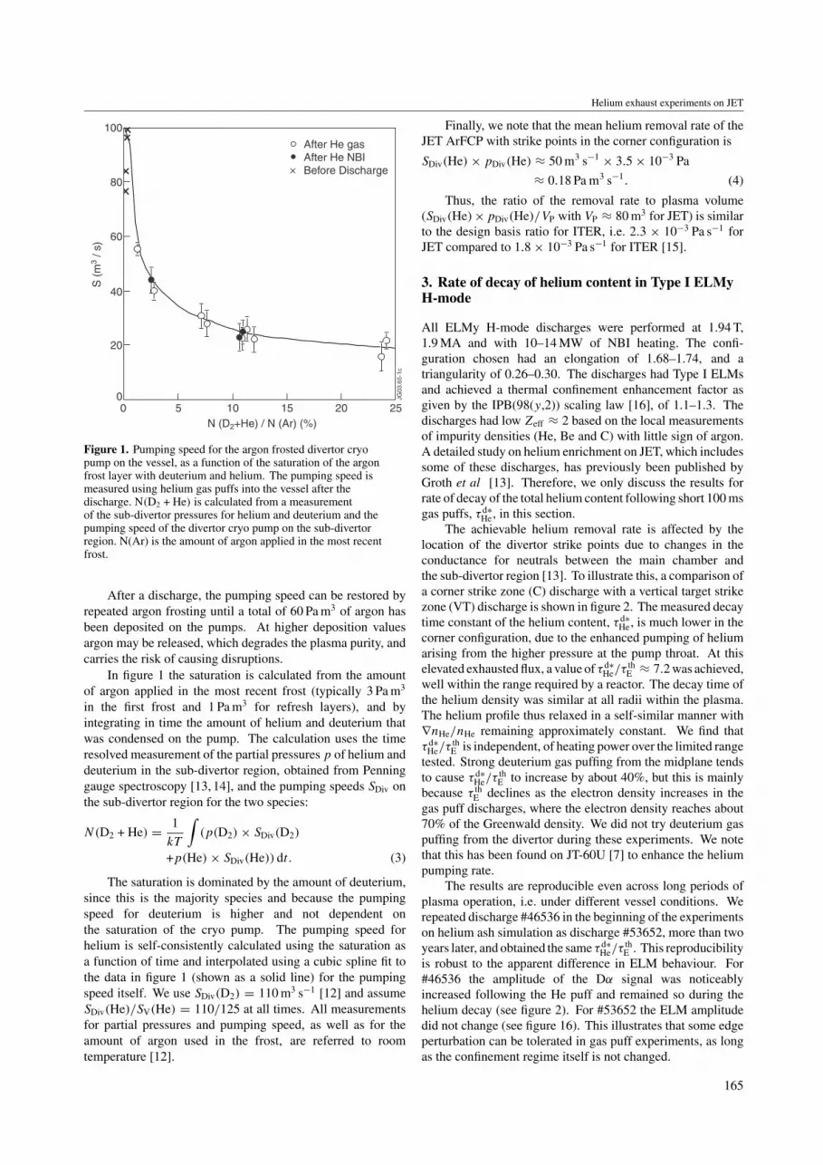
He, in this section.The achievable helium removal rate is affected by the

location of the divertor strike points due to changes in theconductance for neutrals between the main chamber andthe sub-divertor region [13]. To illustrate this, a comparison ofa corner strike zone (C) discharge with a vertical target strikezone (VT) discharge is shown in figure 2. The measured decaytime constant of the helium content, τ d∗

He, is much lower in thecorner configuration, due to the enhanced pumping of heliumarising from the higher pressure at the pump throat. At thiselevated exhausted flux, a value of τ d∗

He/τthE ≈ 7.2 was achieved,

well within the range required by a reactor. The decay time ofthe helium density was similar at all radii within the plasma.The helium profile thus relaxed in a self-similar manner with∇nHe/nHe remaining approximately constant. We find thatτ d∗

He/τthE is independent, of heating power over the limited range

tested. Strong deuterium gas puffing from the midplane tendsto cause τ d∗

He/τthE to increase by about 40%, but this is mainly

because τ thE declines as the electron density increases in the

gas puff discharges, where the electron density reaches about70% of the Greenwald density. We did not try deuterium gaspuffing from the divertor during these experiments. We notethat this has been found on JT-60U [7] to enhance the heliumpumping rate.

The results are reproducible even across long periods ofplasma operation, i.e. under different vessel conditions. Werepeated discharge #46536 in the beginning of the experimentson helium ash simulation as discharge #53652, more than twoyears later, and obtained the same τ d∗

He/τthE . This reproducibility

is robust to the apparent difference in ELM behaviour. For#46536 the amplitude of the Dα signal was noticeablyincreased following the He puff and remained so during thehelium decay (see figure 2). For #53652 the ELM amplitudedid not change (see figure 16). This illustrates that some edgeperturbation can be tolerated in gas puff experiments, as longas the confinement regime itself is not changed.

165

K.-D. Zastrow et al

6

105

5

20

10

6

4

20

0

0

0

0

12

16 18 20 22 24

(MW

)(1

019/ m

2 )(1

019)

(s)

Time (s)

JG03

.65-

2c

Pulse No: 46536 (C) Pulse No: 46529 (VT)(1.94 T, 1.9 MA)

PNBI

<ne>

D∝

Helium Content

Decay Time

Figure 2. Comparison of the decay of the helium content for twoELMy H-mode discharges (1.94 T, 1.9 MA) at constant input powerfor two different strike point configurations. The discharge with thestrike points in the corner (—— and ♦) exhibits a faster heliumremoval rate than the one with the strike points on the vertical target(- - - - and +).

4. Helium ash simulation experiments in ITBdischarges

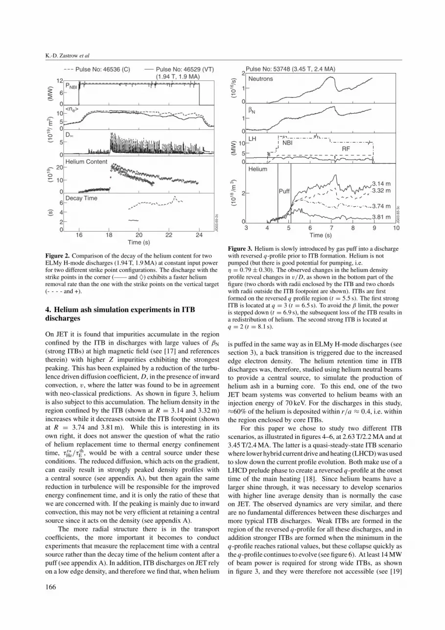
On JET it is found that impurities accumulate in the regionconfined by the ITB in discharges with large values of βN

(strong ITBs) at high magnetic field (see [17] and referencestherein) with higher Z impurities exhibiting the strongestpeaking. This has been explained by a reduction of the turbu-lence driven diffusion coefficient, D, in the presence of inwardconvection, v, where the latter was found to be in agreementwith neo-classical predictions. As shown in figure 3, heliumis also subject to this accumulation. The helium density in theregion confined by the ITB (shown at R = 3.14 and 3.32 m)increases while it decreases outside the ITB footpoint (shownat R = 3.74 and 3.81 m). While this is interesting in itsown right, it does not answer the question of what the ratioof helium replacement time to thermal energy confinementtime, τ r∗

He/τthE , would be with a central source under these

conditions. The reduced diffusion, which acts on the gradient,can easily result in strongly peaked density profiles witha central source (see appendix A), but then again the samereduction in turbulence will be responsible for the improvedenergy confinement time, and it is only the ratio of these thatwe are concerned with. If the peaking is mainly due to inwardconvection, this may not be very efficient at retaining a centralsource since it acts on the density (see appendix A).

The more radial structure there is in the transportcoefficients, the more important it becomes to conductexperiments that measure the replacement time with a centralsource rather than the decay time of the helium content after apuff (see appendix A). In addition, ITB discharges on JET relyon a low edge density, and therefore we find that, when helium

1

1

10

5

2

0

0

0

0

2

4 53 6 7 8 9(1

018/m

3 )(M

W)

(1016

/s)

Time (s)

JG03

.65-

3c

Pulse No: 53748 (3.45 T, 2.4 MA)

Neutrons

βN

LH

Helium

NBI

Puff3.14 m3.32 m

3.74 m

3.81 m

RF

10

Figure 3. Helium is slowly introduced by gas puff into a dischargewith reversed q-profile prior to ITB formation. Helium is notpumped (but there is good potential for pumping, i.e.η = 0.79 ± 0.30). The observed changes in the helium densityprofile reveal changes in v/D, as shown in the bottom part of thefigure (two chords with radii enclosed by the ITB and two chordswith radii outside the ITB footpoint are shown). ITBs are firstformed on the reversed q profile region (t = 5.5 s). The first strongITB is located at q = 3 (t = 6.5 s). To avoid the β limit, the poweris stepped down (t = 6.9 s), the subsequent loss of the ITB results ina redistribution of helium. The second strong ITB is located atq = 2 (t = 8.1 s).

is puffed in the same way as in ELMy H-mode discharges (seesection 3), a back transition is triggered due to the increasededge electron density. The helium retention time in ITBdischarges was, therefore, studied using helium neutral beamsto provide a central source, to simulate the production ofhelium ash in a burning core. To this end, one of the twoJET beam systems was converted to helium beams with aninjection energy of 70 keV. For the discharges in this study,≈60% of the helium is deposited within r/a ≈ 0.4, i.e. withinthe region enclosed by core ITBs.

For this paper we chose to study two different ITBscenarios, as illustrated in figures 4–6, at 2.63 T/2.2 MA and at3.45 T/2.4 MA. The latter is a quasi-steady-state ITB scenariowhere lower hybrid current drive and heating (LHCD) was usedto slow down the current profile evolution. Both make use of aLHCD prelude phase to create a reversed q-profile at the onsettime of the main heating [18]. Since helium beams have alarger shine through, it was necessary to develop scenarioswith higher line average density than is normally the caseon JET. The observed dynamics are very similar, and thereare no fundamental differences between these discharges andmore typical ITB discharges. Weak ITBs are formed in theregion of the reversed q-profile for all these discharges, and inaddition stronger ITBs are formed when the minimum in theq-profile reaches rational values, but these collapse quickly asthe q-profile continues to evolve (see figure 6). At least 14 MWof beam power is required for strong wide ITBs, as shownin figure 3, and they were therefore not accessible (see [19]

166

Helium exhaust experiments on JET

1

5

20

2

1

0

0

0

2

0

6 7 8 9543

(m19

/m2 )

(1019

)(M

W)

Time (s)

JG03

.65-

4c

(2.63 T, 2.2 MA)

βN

D-NBI

He-NBIRF

LH

Helium Content

Edge <ne>

10

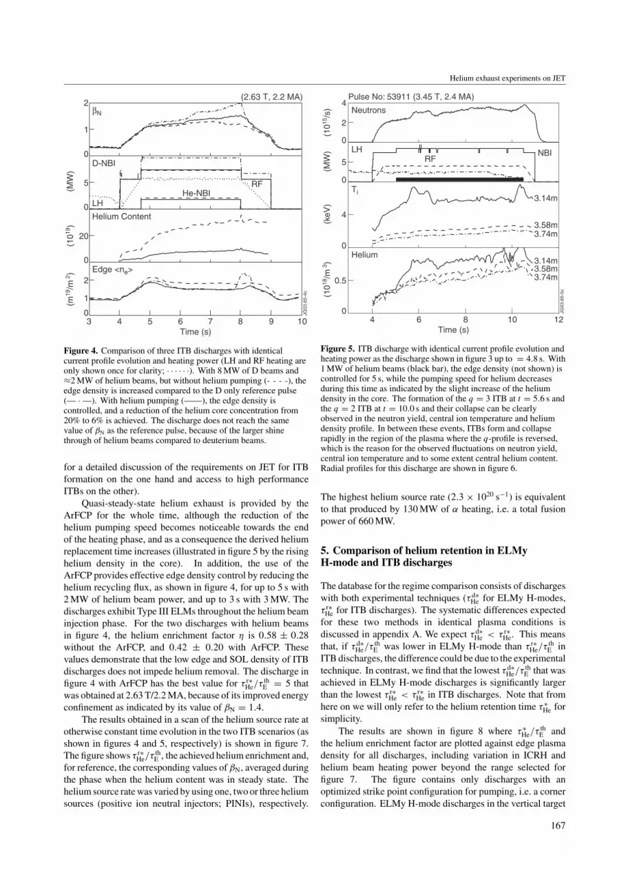
Figure 4. Comparison of three ITB discharges with identicalcurrent profile evolution and heating power (LH and RF heating areonly shown once for clarity; · · · · · ·). With 8 MW of D beams and≈2 MW of helium beams, but without helium pumping (- - - -), theedge density is increased compared to the D only reference pulse(— · —). With helium pumping (——), the edge density iscontrolled, and a reduction of the helium core concentration from20% to 6% is achieved. The discharge does not reach the samevalue of βN as the reference pulse, because of the larger shinethrough of helium beams compared to deuterium beams.

for a detailed discussion of the requirements on JET for ITBformation on the one hand and access to high performanceITBs on the other).

Quasi-steady-state helium exhaust is provided by theArFCP for the whole time, although the reduction of thehelium pumping speed becomes noticeable towards the endof the heating phase, and as a consequence the derived heliumreplacement time increases (illustrated in figure 5 by the risinghelium density in the core). In addition, the use of theArFCP provides effective edge density control by reducing thehelium recycling flux, as shown in figure 4, for up to 5 s with2 MW of helium beam power, and up to 3 s with 3 MW. Thedischarges exhibit Type III ELMs throughout the helium beaminjection phase. For the two discharges with helium beamsin figure 4, the helium enrichment factor η is 0.58 ± 0.28without the ArFCP, and 0.42 ± 0.20 with ArFCP. Thesevalues demonstrate that the low edge and SOL density of ITBdischarges does not impede helium removal. The discharge infigure 4 with ArFCP has the best value for τ r∗

He/τthE = 5 that

was obtained at 2.63 T/2.2 MA, because of its improved energyconfinement as indicated by its value of βN = 1.4.

The results obtained in a scan of the helium source rate atotherwise constant time evolution in the two ITB scenarios (asshown in figures 4 and 5, respectively) is shown in figure 7.The figure shows τ r∗

He/τthE , the achieved helium enrichment and,

for reference, the corresponding values of βN, averaged duringthe phase when the helium content was in steady state. Thehelium source rate was varied by using one, two or three heliumsources (positive ion neutral injectors; PINIs), respectively.

2

5

4

0.5

0

0

0

0

4

4 6 8 10 12(1

018/m

3 )(k

eV)

(MW

)(1

015/s

)Time (s)

JG03

.65-

5c

Pulse No: 53911 (3.45 T, 2.4 MA)

Neutrons

LH

Ti

Helium

RF

3.14m

NBI

3.58m3.74m

3.14m3.58m3.74m

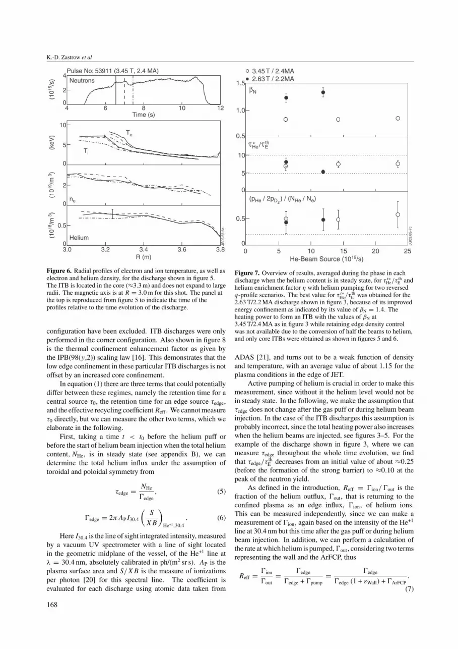
Figure 5. ITB discharge with identical current profile evolution andheating power as the discharge shown in figure 3 up to = 4.8 s. With1 MW of helium beams (black bar), the edge density (not shown) iscontrolled for 5 s, while the pumping speed for helium decreasesduring this time as indicated by the slight increase of the heliumdensity in the core. The formation of the q = 3 ITB at t = 5.6 s andthe q = 2 ITB at t = 10.0 s and their collapse can be clearlyobserved in the neutron yield, central ion temperature and heliumdensity profile. In between these events, ITBs form and collapserapidly in the region of the plasma where the q-profile is reversed,which is the reason for the observed fluctuations on neutron yield,central ion temperature and to some extent central helium content.Radial profiles for this discharge are shown in figure 6.

The highest helium source rate (2.3 × 1020 s−1) is equivalentto that produced by 130 MW of α heating, i.e. a total fusionpower of 660 MW.

5. Comparison of helium retention in ELMyH-mode and ITB discharges

The database for the regime comparison consists of dischargeswith both experimental techniques (τ d∗

He for ELMy H-modes,τ r∗

He for ITB discharges). The systematic differences expectedfor these two methods in identical plasma conditions isdiscussed in appendix A. We expect τ d∗

He < τ r∗He. This means

that, if τ d∗He/τ

thE was lower in ELMy H-mode than τ r∗

He/τthE in

ITB discharges, the difference could be due to the experimentaltechnique. In contrast, we find that the lowest τ d∗

He/τthE that was

achieved in ELMy H-mode discharges is significantly largerthan the lowest τ r∗

He < τ r∗He in ITB discharges. Note that from

here on we will only refer to the helium retention time τ ∗He for

simplicity.The results are shown in figure 8 where τ ∗

He/τthE and

the helium enrichment factor are plotted against edge plasmadensity for all discharges, including variation in ICRH andhelium beam heating power beyond the range selected forfigure 7. The figure contains only discharges with anoptimized strike point configuration for pumping, i.e. a cornerconfiguration. ELMy H-mode discharges in the vertical target

167

K.-D. Zastrow et al

2

5

2

0.5

0

0

0

0

10

4

3.2 3.4 3.63.0 3.8

(1018

/m3 )

(1019

/m3 )

(keV

)(1

015/s

)

R (m)

6 8 10 124Time (s)

JG03

.65-

6c

Pulse No: 53911 (3.45 T, 2.4 MA)

Neutrons

ne

Te

Ti

Helium

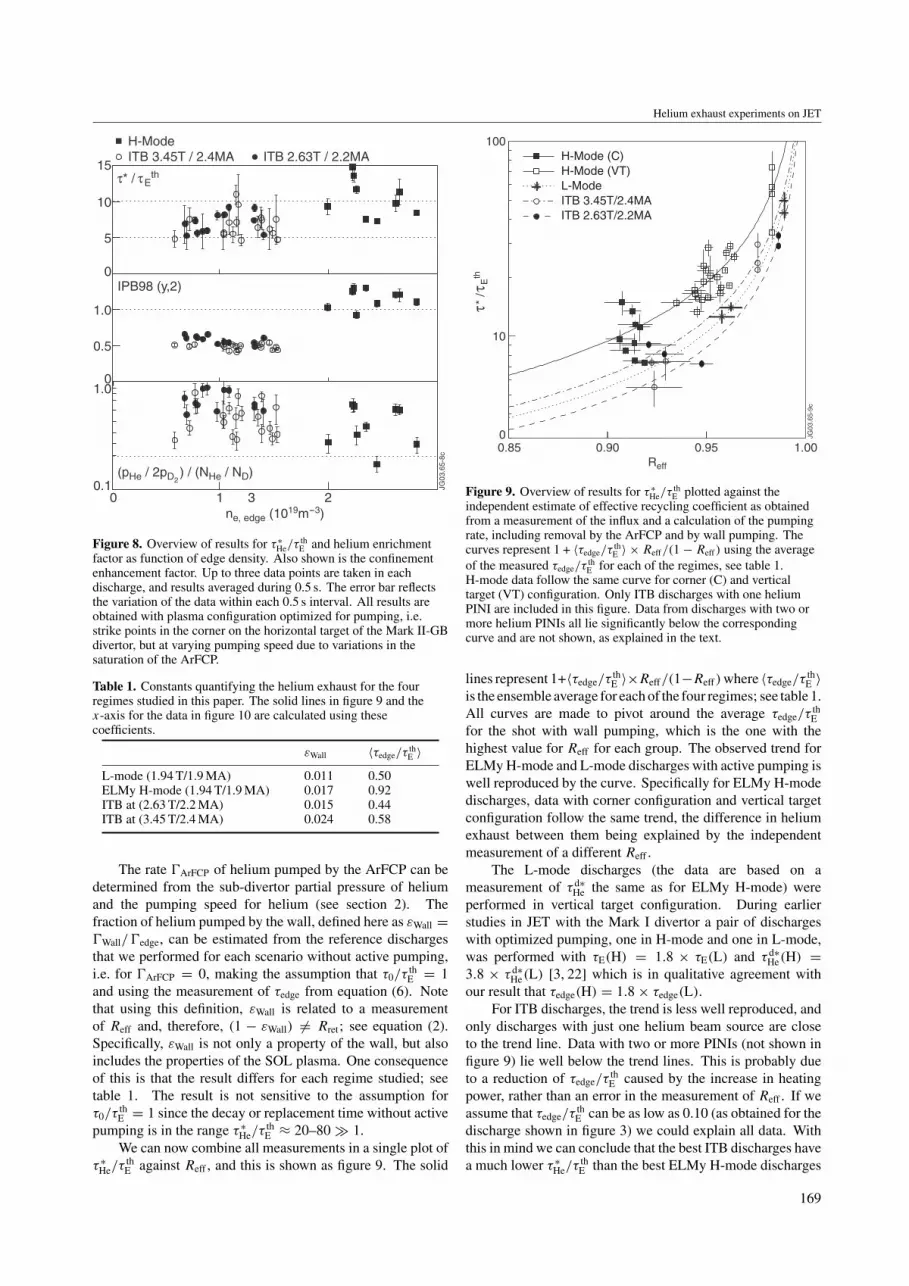
Figure 6. Radial profiles of electron and ion temperature, as well aselectron and helium density, for the discharge shown in figure 5.The ITB is located in the core (≈3.3 m) and does not expand to largeradii. The magnetic axis is at R = 3.0 m for this shot. The panel atthe top is reproduced from figure 5 to indicate the time of theprofiles relative to the time evolution of the discharge.

configuration have been excluded. ITB discharges were onlyperformed in the corner configuration. Also shown in figure 8is the thermal confinement enhancement factor as given bythe IPB(98(y,2)) scaling law [16]. This demonstrates that thelow edge confinement in these particular ITB discharges is notoffset by an increased core confinement.

In equation (1) there are three terms that could potentiallydiffer between these regimes, namely the retention time for acentral source τ0, the retention time for an edge source τedge,and the effective recycling coefficient Reff . We cannot measureτ0 directly, but we can measure the other two terms, which weelaborate in the following.

First, taking a time t < t0 before the helium puff orbefore the start of helium beam injection when the total heliumcontent, NHe, is in steady state (see appendix B), we candetermine the total helium influx under the assumption oftoroidal and poloidal symmetry from

τedge = NHe

�edge, (5)

�edge = 2πAPI30.4

(S

XB

)He+1,30.4

. (6)

Here I30.4 is the line of sight integrated intensity, measuredby a vacuum UV spectrometer with a line of sight locatedin the geometric midplane of the vessel, of the He+1 line atλ = 30.4 nm, absolutely calibrated in ph/(m2 sr s). AP is theplasma surface area and S/XB is the measure of ionizationsper photon [20] for this spectral line. The coefficient isevaluated for each discharge using atomic data taken from

1.0

10

5

0.5

0

1.5

0.5

0

50 10 15 20He-Beam Source (1019/s)

JG03

.65-

7c

25

3.45 T / 2.4MA2.63 T / 2.2MA

βN

τ He / τ Eth*

(pHe / 2pD2) / (NHe / Ne)

Figure 7. Overview of results, averaged during the phase in eachdischarge when the helium content is in steady state, for τ r∗

He/τthE and

helium enrichment factor η with helium pumping for two reversedq-profile scenarios. The best value for τ r∗

He/τthE was obtained for the

2.63 T/2.2 MA discharge shown in figure 3, because of its improvedenergy confinement as indicated by its value of βN = 1.4. Theheating power to form an ITB with the values of βN at3.45 T/2.4 MA as in figure 3 while retaining edge density controlwas not available due to the conversion of half the beams to helium,and only core ITBs were obtained as shown in figures 5 and 6.

ADAS [21], and turns out to be a weak function of densityand temperature, with an average value of about 1.15 for theplasma conditions in the edge of JET.

Active pumping of helium is crucial in order to make thismeasurement, since without it the helium level would not bein steady state. In the following, we make the assumption thatτedge does not change after the gas puff or during helium beaminjection. In the case of the ITB discharges this assumption isprobably incorrect, since the total heating power also increaseswhen the helium beams are injected, see figures 3–5. For theexample of the discharge shown in figure 3, where we canmeasure τedge throughout the whole time evolution, we findthat τedge/τ

thE decreases from an initial value of about ≈0.25

(before the formation of the strong barrier) to ≈0.10 at thepeak of the neutron yield.

As defined in the introduction, Reff = �ion/�out is thefraction of the helium outflux, �out, that is returning to theconfined plasma as an edge influx, �ion, of helium ions.This can be measured independently, since we can make ameasurement of �ion, again based on the intensity of the He+1

line at 30.4 nm but this time after the gas puff or during heliumbeam injection. In addition, we can perform a calculation ofthe rate at which helium is pumped, �out, considering two termsrepresenting the wall and the ArFCP, thus

Reff = �ion

�out= �edge

�edge + �pump= �edge

�edge (1 + εWall) + �ArFCP.

(7)

168

Helium exhaust experiments on JET

10

5

1.0

0.5

1.0

0.1

0

0

15

1 20 3ne, edge (1019m-3)

JG03

.65-

8c

τ τ* / Eth

IPB98 (y,2)

(pHe / 2pD2) / (NHe / ND)

H-ModeITB 3.45T / 2.4MA ITB 2.63T / 2.2MA

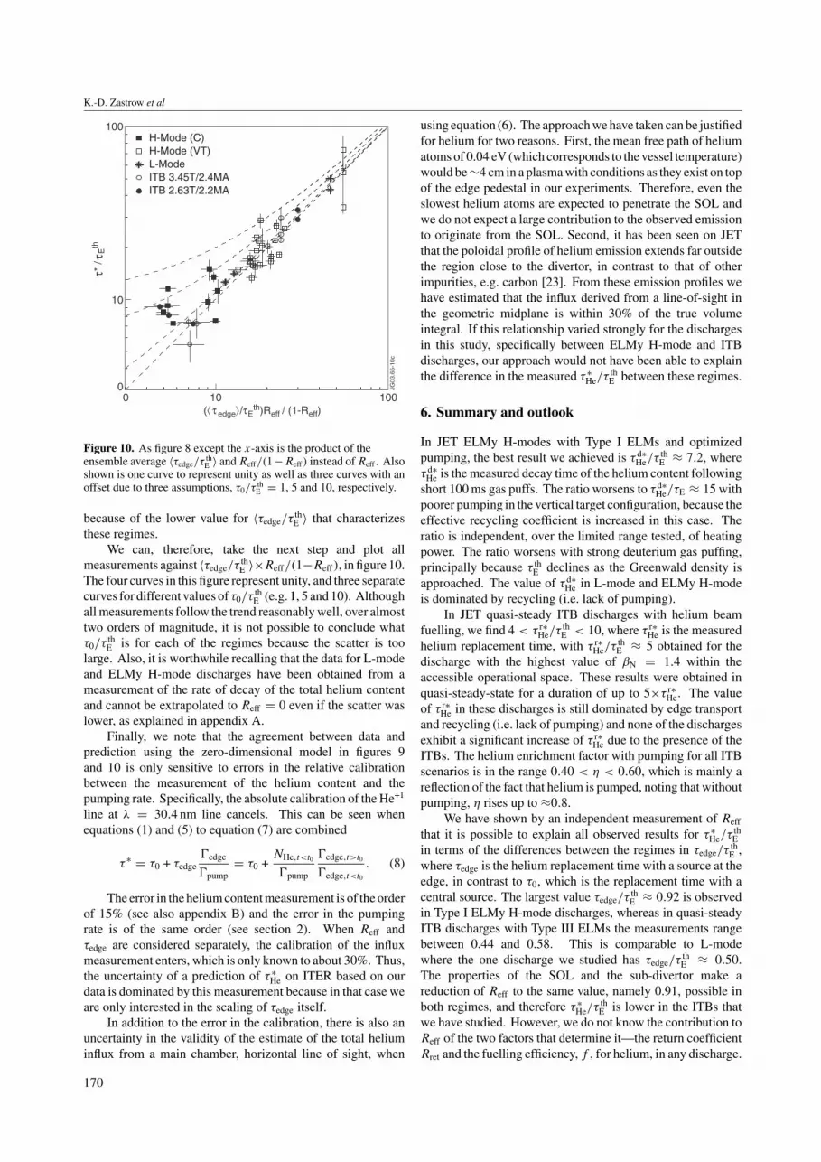
Figure 8. Overview of results for τ ∗He/τ

thE and helium enrichment

factor as function of edge density. Also shown is the confinementenhancement factor. Up to three data points are taken in eachdischarge, and results averaged during 0.5 s. The error bar reflectsthe variation of the data within each 0.5 s interval. All results areobtained with plasma configuration optimized for pumping, i.e.strike points in the corner on the horizontal target of the Mark II-GBdivertor, but at varying pumping speed due to variations in thesaturation of the ArFCP.

Table 1. Constants quantifying the helium exhaust for the fourregimes studied in this paper. The solid lines in figure 9 and thex-axis for the data in figure 10 are calculated using thesecoefficients.

εWall 〈τedge/τthE 〉

L-mode (1.94 T/1.9 MA) 0.011 0.50ELMy H-mode (1.94 T/1.9 MA) 0.017 0.92ITB at (2.63 T/2.2 MA) 0.015 0.44ITB at (3.45 T/2.4 MA) 0.024 0.58

The rate �ArFCP of helium pumped by the ArFCP can bedetermined from the sub-divertor partial pressure of heliumand the pumping speed for helium (see section 2). Thefraction of helium pumped by the wall, defined here as εWall =�Wall/�edge, can be estimated from the reference dischargesthat we performed for each scenario without active pumping,i.e. for �ArFCP = 0, making the assumption that τ0/τ

thE = 1

and using the measurement of τedge from equation (6). Notethat using this definition, εWall is related to a measurementof Reff and, therefore, (1 − εWall) �= Rret; see equation (2).Specifically, εWall is not only a property of the wall, but alsoincludes the properties of the SOL plasma. One consequenceof this is that the result differs for each regime studied; seetable 1. The result is not sensitive to the assumption forτ0/τ

thE = 1 since the decay or replacement time without active

pumping is in the range τ ∗He/τ

thE ≈ 20–80 � 1.

We can now combine all measurements in a single plot ofτ ∗

He/τthE against Reff , and this is shown as figure 9. The solid

H-Mode (C)H-Mode (VT)L-ModeITB 3.45T/2.4MAITB 2.63T/2.2MA

10

0

100

0.90 0.950.85 1.00

ττ

* /

Eth

Reff

JG03

.65-

9c

Figure 9. Overview of results for τ ∗He/τ

thE plotted against the

independent estimate of effective recycling coefficient as obtainedfrom a measurement of the influx and a calculation of the pumpingrate, including removal by the ArFCP and by wall pumping. Thecurves represent 1 + 〈τedge/τ

thE 〉 × Reff/(1 − Reff) using the average

of the measured τedge/τthE for each of the regimes, see table 1.

H-mode data follow the same curve for corner (C) and verticaltarget (VT) configuration. Only ITB discharges with one heliumPINI are included in this figure. Data from discharges with two ormore helium PINIs all lie significantly below the correspondingcurve and are not shown, as explained in the text.

lines represent 1+〈τedge/τthE 〉×Reff/(1−Reff) where 〈τedge/τ

thE 〉

is the ensemble average for each of the four regimes; see table 1.All curves are made to pivot around the average τedge/τ

thE

for the shot with wall pumping, which is the one with thehighest value for Reff for each group. The observed trend forELMy H-mode and L-mode discharges with active pumping iswell reproduced by the curve. Specifically for ELMy H-modedischarges, data with corner configuration and vertical targetconfiguration follow the same trend, the difference in heliumexhaust between them being explained by the independentmeasurement of a different Reff .

The L-mode discharges (the data are based on ameasurement of τ d∗

He the same as for ELMy H-mode) wereperformed in vertical target configuration. During earlierstudies in JET with the Mark I divertor a pair of dischargeswith optimized pumping, one in H-mode and one in L-mode,was performed with τE(H) = 1.8 × τE(L) and τ d∗

He(H) =3.8 × τ d∗

He(L) [3, 22] which is in qualitative agreement withour result that τedge(H) = 1.8 × τedge(L).

For ITB discharges, the trend is less well reproduced, andonly discharges with just one helium beam source are closeto the trend line. Data with two or more PINIs (not shown infigure 9) lie well below the trend lines. This is probably dueto a reduction of τedge/τ

thE caused by the increase in heating

power, rather than an error in the measurement of Reff . If weassume that τedge/τ

thE can be as low as 0.10 (as obtained for the

discharge shown in figure 3) we could explain all data. Withthis in mind we can conclude that the best ITB discharges havea much lower τ ∗

He/τthE than the best ELMy H-mode discharges

169

K.-D. Zastrow et al

H-Mode (C)H-Mode (VT)L-ModeITB 3.45T/2.4MAITB 2.63T/2.2MA

10

0

100

100 100

τ τ

* /

Eth

(� τ τ edge�/ Eth)Reff / (1-Reff)

JG03

.65-

10c

Figure 10. As figure 8 except the x-axis is the product of theensemble average 〈τedge/τ

thE 〉 and Reff/(1−Reff) instead of Reff . Also

shown is one curve to represent unity as well as three curves with anoffset due to three assumptions, τ0/τ

thE = 1, 5 and 10, respectively.

because of the lower value for 〈τedge/τthE 〉 that characterizes

these regimes.We can, therefore, take the next step and plot all

measurements against 〈τedge/τthE 〉×Reff/(1−Reff), in figure 10.

The four curves in this figure represent unity, and three separatecurves for different values of τ0/τ

thE (e.g. 1, 5 and 10). Although

all measurements follow the trend reasonably well, over almosttwo orders of magnitude, it is not possible to conclude whatτ0/τ

thE is for each of the regimes because the scatter is too

large. Also, it is worthwhile recalling that the data for L-modeand ELMy H-mode discharges have been obtained from ameasurement of the rate of decay of the total helium contentand cannot be extrapolated to Reff = 0 even if the scatter waslower, as explained in appendix A.

Finally, we note that the agreement between data andprediction using the zero-dimensional model in figures 9and 10 is only sensitive to errors in the relative calibrationbetween the measurement of the helium content and thepumping rate. Specifically, the absolute calibration of the He+1

line at λ = 30.4 nm line cancels. This can be seen whenequations (1) and (5) to equation (7) are combined

τ ∗ = τ0 + τedge�edge

�pump= τ0 +

NHe,t<t0

�pump

�edge,t>t0

�edge,t<t0

. (8)

The error in the helium content measurement is of the orderof 15% (see also appendix B) and the error in the pumpingrate is of the same order (see section 2). When Reff andτedge are considered separately, the calibration of the influxmeasurement enters, which is only known to about 30%. Thus,the uncertainty of a prediction of τ ∗

He on ITER based on ourdata is dominated by this measurement because in that case weare only interested in the scaling of τedge itself.

In addition to the error in the calibration, there is also anuncertainty in the validity of the estimate of the total heliuminflux from a main chamber, horizontal line of sight, when

using equation (6). The approach we have taken can be justifiedfor helium for two reasons. First, the mean free path of heliumatoms of 0.04 eV (which corresponds to the vessel temperature)would be ∼4 cm in a plasma with conditions as they exist on topof the edge pedestal in our experiments. Therefore, even theslowest helium atoms are expected to penetrate the SOL andwe do not expect a large contribution to the observed emissionto originate from the SOL. Second, it has been seen on JETthat the poloidal profile of helium emission extends far outsidethe region close to the divertor, in contrast to that of otherimpurities, e.g. carbon [23]. From these emission profiles wehave estimated that the influx derived from a line-of-sight inthe geometric midplane is within 30% of the true volumeintegral. If this relationship varied strongly for the dischargesin this study, specifically between ELMy H-mode and ITBdischarges, our approach would not have been able to explainthe difference in the measured τ ∗

He/τthE between these regimes.

6. Summary and outlook

In JET ELMy H-modes with Type I ELMs and optimizedpumping, the best result we achieved is τ d∗

He/τthE ≈ 7.2, where

τ d∗He is the measured decay time of the helium content following

short 100 ms gas puffs. The ratio worsens to τ d∗He/τE ≈ 15 with

poorer pumping in the vertical target configuration, because theeffective recycling coefficient is increased in this case. Theratio is independent, over the limited range tested, of heatingpower. The ratio worsens with strong deuterium gas puffing,principally because τ th

E declines as the Greenwald density isapproached. The value of τ d∗

He in L-mode and ELMy H-modeis dominated by recycling (i.e. lack of pumping).

In JET quasi-steady ITB discharges with helium beamfuelling, we find 4 < τ r∗

He/τthE < 10, where τ r∗

He is the measuredhelium replacement time, with τ r∗

He/τthE ≈ 5 obtained for the

discharge with the highest value of βN = 1.4 within theaccessible operational space. These results were obtained inquasi-steady-state for a duration of up to 5×τ r∗

He. The valueof τ r∗

He in these discharges is still dominated by edge transportand recycling (i.e. lack of pumping) and none of the dischargesexhibit a significant increase of τ r∗

He due to the presence of theITBs. The helium enrichment factor with pumping for all ITBscenarios is in the range 0.40 < η < 0.60, which is mainly areflection of the fact that helium is pumped, noting that withoutpumping, η rises up to ≈0.8.

We have shown by an independent measurement of Reff

that it is possible to explain all observed results for τ ∗He/τ

thE

in terms of the differences between the regimes in τedge/τthE ,

where τedge is the helium replacement time with a source at theedge, in contrast to τ0, which is the replacement time with acentral source. The largest value τedge/τ

thE ≈ 0.92 is observed

in Type I ELMy H-mode discharges, whereas in quasi-steadyITB discharges with Type III ELMs the measurements rangebetween 0.44 and 0.58. This is comparable to L-modewhere the one discharge we studied has τedge/τ

thE ≈ 0.50.

The properties of the SOL and the sub-divertor make areduction of Reff to the same value, namely 0.91, possible inboth regimes, and therefore τ ∗

He/τthE is lower in the ITBs that

we have studied. However, we do not know the contribution toReff of the two factors that determine it—the return coefficientRret and the fuelling efficiency, f , for helium, in any discharge.

170

Helium exhaust experiments on JET

If Reff can be modelled for ITER, our results should allowa prediction of τ ∗

He/τthE based on a scaling of τedge/τ

thE between

present tokamaks and ITER. Such a scaling is, however,made difficult because, to our knowledge, an independentmeasurement of Reff and τedge/τ

thE has not been attempted as

part of the helium exhaust experiments on any other tokamakand so scaling with machine size is not possible at present.Also, the errors of Reff and of τedge/τ

thE are quite large

(about 50%), because the measurement relies on the absolutecalibration of a vacuum UV spectrometer and the assumptionthat this measurement is representative for the volume sourceof helium. Unless inter-machine scaling of τedge/τ

thE is a very

strong function of machine geometry, such a comparison isunlikely to be conclusive.

More experiments on JET with active helium pumping arerequired to investigate scaling within each operating regime ofτedge/τ

thE . The accuracy of such a study is much better (the

relative error is about 15%). Within the limited range studied,we have found no clear variation of τedge/τ

thE for Type I ELMy

H-modes. Even though the two ITB regimes with LH preludethat we studied (strong ITBs at 2.63 T/2.2 MA and core ITBsat 3.45 T/2.4 MA with LHCD throughout the main heatingphase) are characterized by different τedge/τ

thE , there are too

many parameters that differ between these regimes to identifya scaling.

One further question still open is, how τ ∗He/τ

thE would

behave for very high values of βN at high magnetic field,i.e. for discharges like the one shown in figure 3. We haveshown that the low edge density in these scenarios is not aproblem, i.e. sufficient pumping can be achieved, and ourresults at high values of βN and low magnetic field indicatethat the improvement in τ th

E combined with the intrinsicallylow τedge/τ

thE (we have measured values in the range 0.10–0.25

for the discharge shown in figure 3) of this type of dischargemight offset any increase in τ0.

Acknowledgments

This paper is an extended version of a contribution to the 29thEPS Conference on Plasma Physics and Controlled Fusionheld in (Montreux, Switzerland, June 2002). It includesreanalysed material from a paper by D Stork et al from the 26thEPS Conference on Controlled Fusion and Plasma Physics(Maastricht, The Netherlands, June 1999) and a paper byK H Finken et al from the 28th EPS Conference on ControlledFusion and Plasma Physics (Madeira, Portugal, June 2001).

This work was performed partially within the frameworkof the JET Joint Undertaking and partially under the EuropeanFusion Development Agreement. It was funded in part byEURATOM, the UK Department of Trade and Industry, andthe US Department of Energy under Contract No DE-AC05-00OR22725.

Appendix A. On retention, replacement and decaytime, refuelling efficiency and predictions usingzero-dimensional models

In this appendix we address the relationship between theparticle retention time, τ ∗, in the case of vanishing return flux,and τ ∗ at finite return flux for particles. We will show that the

0.8

0.6

0.4

0.2

0.8

0.6

0.4

0.2

0

0

1.0

0 1 2 3-1-2-3

Nto

t(s

)Time (s)

N / (S-dN/dt)

(N-Nss) / (dN/dt)

N / S

JG03

.65-

11c

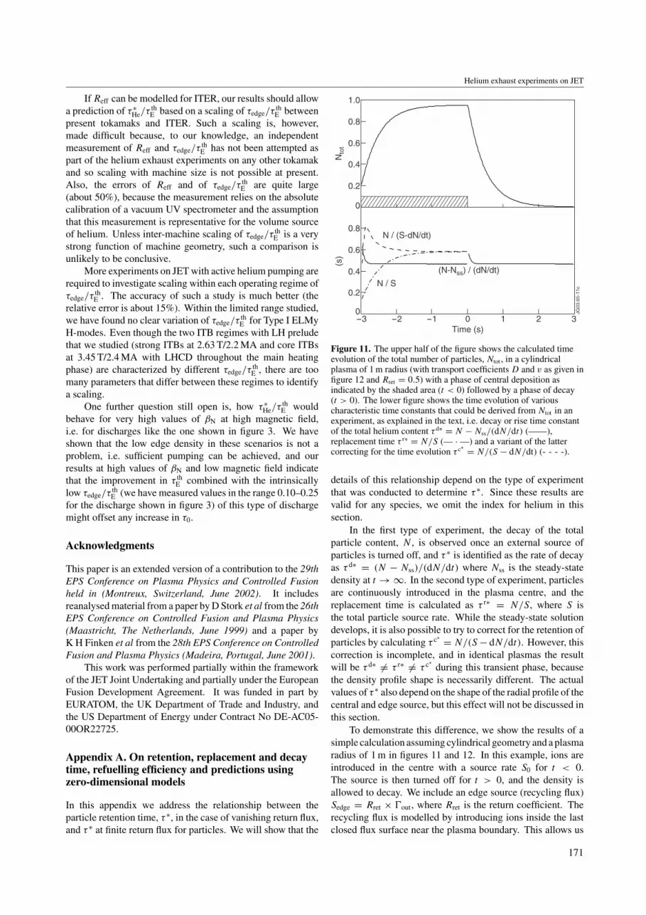
Figure 11. The upper half of the figure shows the calculated timeevolution of the total number of particles, Ntot , in a cylindricalplasma of 1 m radius (with transport coefficients D and v as given infigure 12 and Rret = 0.5) with a phase of central deposition asindicated by the shaded area (t < 0) followed by a phase of decay(t > 0). The lower figure shows the time evolution of variouscharacteristic time constants that could be derived from Ntot in anexperiment, as explained in the text, i.e. decay or rise time constantof the total helium content τ d∗ = N − Nss/(dN/dt) (——),replacement time τ r∗ = N/S (— · —) and a variant of the lattercorrecting for the time evolution τ c∗ = N/(S − dN/dt) (- - - -).

details of this relationship depend on the type of experimentthat was conducted to determine τ ∗. Since these results arevalid for any species, we omit the index for helium in thissection.

In the first type of experiment, the decay of the totalparticle content, N , is observed once an external source ofparticles is turned off, and τ ∗ is identified as the rate of decayas τ d∗ = (N − Nss)/(dN/dt) where Nss is the steady-statedensity at t → ∞. In the second type of experiment, particlesare continuously introduced in the plasma centre, and thereplacement time is calculated as τ r∗ = N/S, where S isthe total particle source rate. While the steady-state solutiondevelops, it is also possible to try to correct for the retention ofparticles by calculating τ c∗ = N/(S − dN/dt). However, thiscorrection is incomplete, and in identical plasmas the resultwill be τ d∗ �= τ r∗ �= τ c∗

during this transient phase, becausethe density profile shape is necessarily different. The actualvalues of τ ∗ also depend on the shape of the radial profile of thecentral and edge source, but this effect will not be discussed inthis section.

To demonstrate this difference, we show the results of asimple calculation assuming cylindrical geometry and a plasmaradius of 1 m in figures 11 and 12. In this example, ions areintroduced in the centre with a source rate S0 for t < 0.The source is then turned off for t > 0, and the density isallowed to decay. We include an edge source (recycling flux)Sedge = Rret × �out, where Rret is the return coefficient. Therecycling flux is modelled by introducing ions inside the lastclosed flux surface near the plasma boundary. This allows us

171

K.-D. Zastrow et al

1

1

1

0

0

1

0

1.0

1.5

0.5

10

0.2 0.4 0.6 0.8 1.0 0.4 0.80 0 1.2-1

0

f

v (m

/s)

D (

m2 /

s)n

(dec

ay)

n (s

tead

y-st

ate)

τ* (

s)

r (m)Rret

JG03.65-12c

Steady-stateDecay

Steady-stateDecay

R = 0.99R = 0.80R = 0.05

R = 0.99R = 0.80R = 0.05

Figure 12. The right half of the figure shows (from top to bottom)the profile shape adopted in steady state and during exponentialdecay for various values of particle return coefficient, Rret , and thetransport coefficients used in the model calculation. The centralsource is located in the shaded area. The top left half of the figureshows two possible results for τ ∗, the replacement time in steadystate and the time constant for exponential decay, as a function ofRret . A fuelling efficiency, f , is derived from both results for τ ∗ andis shown in the bottom left half of the figure. The result is theexpected value of unity only for the case of the steady-statereplacement time.

to ignore all physics relating to the introduction by neutrals.Specifically, the fuelling efficiency for this type of artificialedge source is unity, as is the fuelling efficiency for the centralsource, thus Reff = Rret (see equation (2)).

In the calculation the radial density profile is obtained fromparticle conservation as

dn

dt= −1

r

∂

∂r

(r

(D

∂n

∂r− vn

))+ s − n

τ‖, (9)

where a time constant for parallel losses, τ‖, is introduced inthe SOL. This ansatz for the particle flux represents a diffusiveterm plus a convective term, i.e. a flux driven by gradients inother plasma quantities but the density itself.

It can be seen in figure 12 that the calculated τ r∗0 = N/S0,

once steady state has been reached, is always larger thanτ d∗

0 = N/(dN/dt) noting that the helium content does not atfirst decay exponentially while the density profile shape relaxes(figure 11). It is interesting to note that the time constant fordecay (the solid line just after t = 0 in figure 12) starts off witha value equal to the steady-state result (the dashed and dash-dotted lines just before t = 0 in figure 12). Experimentally, thiswill be very difficult to determine, because the time windowwhen this is the case is very short and too few data pointsare available to analyse. Figure 11 also illustrates that it isnecessary to wait until steady state has been reached, sinceconsidering τ c∗ = N/(S −dN/dt) results in a time dependentresult. The overshoot in τ c∗

occurs as long as the density profileis not yet in steady state because the particle flux through all

1

1

1

0

0

1

0

1.0

1.5

0.5

10

0.2 0.4 0.6 0.8 1.0 0.4 0.80 0 1.2-2

0

f

v (m

/s)

D (

m2 /

s)n

(dec

ay)

n (s

tead

y-st

ate)

τ* (

s)r (m)Rret

JG03.65-13c

Steady-stateDecay

Steady-stateDecay

R = 0.99R = 0.80R = 0.05

R = 0.99R = 0.80R = 0.05

Figure 13. As figure 12 except a region of increased convectivetransport is introduced for r < 0.5 m. The profile of v is chosen togive the same steady-state profile shape without central source as thecase illustrated in figure 14, which has reduced diffusive transportinstead.

flux surfaces, including the last closed flux surface, is stillincreasing and is not yet equal to the central source rate.

Using equations (1) and (2) we can calculate, as aconsistency check, the actual refuelling efficiency, f , fromthe solutions obtained by our calculations as

f = 1 − Rret

Rret

τ ∗ − τ0

τedge. (10)

In figure 12, we also show the result of this equation usingthe results for τ d∗ and τ r∗ from the analysis of steady state anddecay. When the steady-state replacement is used we obtainf = 1 independent of Rret as expected. When the decay timeis used, f can become larger than unity, and will depend onRret. The reason for this unphysical behaviour is that the radialprofile in the steady-state case is a linear combination of twofunctions, the solution with central source only and the solutionwith edge source only. A solution during the decay phase, onthe other hand, is not. Therefore, a linear ansatz fails.

For high values of Rret the difference between τ d∗ andτ r∗ is reduced (figure 12). Most of the changes occur forRret > 0.8, although this particular value reflects the particularratio of τ0/τedge ≈ 3, which in turn is determined by the profilesof D and v that we have chosen, in this example.

To study the sensitivity to variations in core transportcoefficients, we have performed the same calculation with thetransport terms modified in the centre by an additional inwarddrift and with a reduced diffusion coefficient. The resultsare shown in figures 13 and 14. These two ‘enhanced coreconfinement’ cases have been chosen to have the same solutionin a source free region, which is given by

1

n

∂n

∂r= v

D. (11)

These two calculations illustrate that the two transportcoefficients have a different effect on the resulting retention

172

Helium exhaust experiments on JET

1

1

1

0

0

1

0

1.0

1.5

0.5

10

0.2 0.4 0.6 0.8 1.0 0.4 0.80 0 1.2-1

0

f

v (m

/s)

D (

m2 /

s)n

(dec

ay)

n (s

tead

y-st

ate)

τ* (

s)

r (m)Rret

JG03.65-14c

Steady-stateDecay

Steady-stateDecay

R = 0.99R = 0.80R = 0.05

R = 0.99R = 0.80R = 0.05

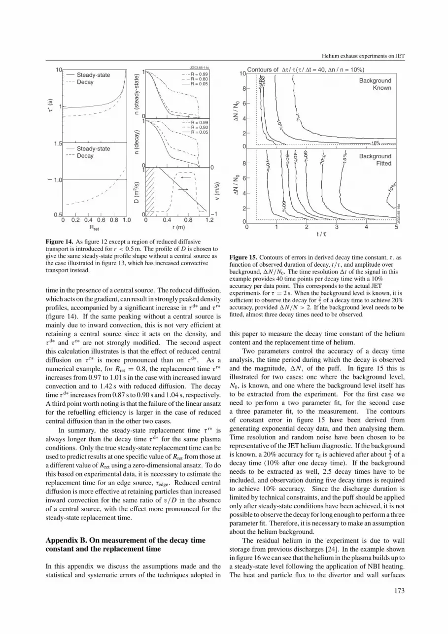
Figure 14. As figure 12 except a region of reduced diffusivetransport is introduced for r < 0.5 m. The profile of D is chosen togive the same steady-state profile shape without a central source asthe case illustrated in figure 13, which has increased convectivetransport instead.

time in the presence of a central source. The reduced diffusion,which acts on the gradient, can result in strongly peaked densityprofiles, accompanied by a significant increase in τ d∗ and τ r∗

(figure 14). If the same peaking without a central source ismainly due to inward convection, this is not very efficient atretaining a central source since it acts on the density, andτ d∗ and τ r∗ are not strongly modified. The second aspectthis calculation illustrates is that the effect of reduced centraldiffusion on τ r∗ is more pronounced than on τ d∗. As anumerical example, for Rret = 0.8, the replacement time τ r∗

increases from 0.97 to 1.01 s in the case with increased inwardconvection and to 1.42 s with reduced diffusion. The decaytime τ d∗ increases from 0.87 s to 0.90 s and 1.04 s, respectively.A third point worth noting is that the failure of the linear ansatzfor the refuelling efficiency is larger in the case of reducedcentral diffusion than in the other two cases.

In summary, the steady-state replacement time τ r∗ isalways longer than the decay time τ d∗ for the same plasmaconditions. Only the true steady-state replacement time can beused to predict results at one specific value of Rret from those ata different value of Rret using a zero-dimensional ansatz. To dothis based on experimental data, it is necessary to estimate thereplacement time for an edge source, τedge. Reduced centraldiffusion is more effective at retaining particles than increasedinward convection for the same ratio of v/D in the absenceof a central source, with the effect more pronounced for thesteady-state replacement time.

Appendix B. On measurement of the decay timeconstant and the replacement time

In this appendix we discuss the assumptions made and thestatistical and systematic errors of the techniques adopted in

8

6

4

2

8

6

4

2

0

0

10

1 2 3 4 50

∆N /

N0

∆N /

N0

t / τ

JG03

.65-

15c

7%

10%

20%

30

%10

%

15%

20%

30%

40%

50%

60%

70%

BackgroundKnown

BackgroundFitted

Contours of / τ (τ / ∆∆τ t = 40, ∆n / n = 10%)

10%

Figure 15. Contours of errors in derived decay time constant, τ , asfunction of observed duration of decay, t/τ , and amplitude overbackground, N/N0. The time resolution t of the signal in thisexample provides 40 time points per decay time with a 10%accuracy per data point. This corresponds to the actual JETexperiments for τ = 2 s. When the background level is known, it issufficient to observe the decay for 2

3 of a decay time to achieve 20%accuracy, provided N/N > 2. If the background level needs to befitted, almost three decay times need to be observed.

this paper to measure the decay time constant of the heliumcontent and the replacement time of helium.

Two parameters control the accuracy of a decay timeanalysis, the time period during which the decay is observedand the magnitude, N , of the puff. In figure 15 this isillustrated for two cases: one where the background level,N0, is known, and one where the background level itself hasto be extracted from the experiment. For the first case weneed to perform a two parameter fit, for the second casea three parameter fit, to the measurement. The contoursof constant error in figure 15 have been derived fromgenerating exponential decay data, and then analysing them.Time resolution and random noise have been chosen to berepresentative of the JET helium diagnostic. If the backgroundis known, a 20% accuracy for τd is achieved after about 2

3 of adecay time (10% after one decay time). If the backgroundneeds to be extracted as well, 2.5 decay times have to beincluded, and observation during five decay times is requiredto achieve 10% accuracy. Since the discharge duration islimited by technical constraints, and the puff should be appliedonly after steady-state conditions have been achieved, it is notpossible to observe the decay for long enough to perform a threeparameter fit. Therefore, it is necessary to make an assumptionabout the helium background.

The residual helium in the experiment is due to wallstorage from previous discharges [24]. In the example shownin figure 16 we can see that the helium in the plasma builds up toa steady-state level following the application of NBI heating.The heat and particle flux to the divertor and wall surfaces

173

K.-D. Zastrow et al

40

10

6

4

3

5

2

12

0

0

0

16 18 20 22 24

(1019

)(s

)(1

019/m

2 )(M

W)

Time (s)

JG03

.65-

16c

Pulse No: 53652 (1.94 T, 1.9MA)

PNBI

<ne>

Dα

Helium Content

Decay Time

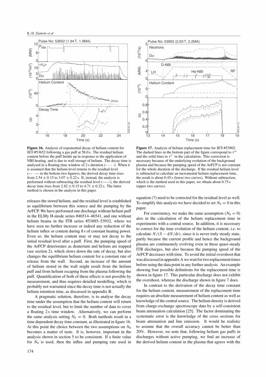
Figure 16. Analysis of exponential decay of helium content forJET-#53652 following a gas puff at 58.0 s. The residual heliumcontent before the puff builds up in response to the application ofNBI heating, and is due to wall storage of helium. The decay time isanalysed in a floating time window of 2 s duration (- - - -). When itis assumed that the helium level returns to the residual level(— · — in the bottom two figures), the derived decay time risesfrom 2.54 ± 0.15 to 3.07 ± 0.22 s. If, instead, the analysis isperformed without subtracting the residual level (——), the deriveddecay time rises from 2.82 ± 0.15 to 4.71 ± 0.22 s. The lattermethod is chosen in the analysis in this paper.

releases the stored helium, and the residual level is establishedas equilibrium between this source and the pumping by theArFCP. We have performed one discharge without helium puffin the ELMy H-mode series #46514–46541, and one withouthelium beams in the ITB series #53885–53932, where wehave seen no further increase or indeed any reduction of thehelium influx or content during 8 s of constant heating power.Even so, the helium content may or may not decay to theinitial residual level after a puff. First, the pumping speed ofthe ArFCP deteriorates as deuterium and helium are trapped(see section 2), which slows down the rate of decay, but alsochanges the equilibrium helium content for a constant rate ofrelease from the wall. Second, an increase of the amountof helium stored in the wall might result from the heliumpuff and from helium escaping from the plasma following thepuff. Quantification of both of these effects is not possible bymeasurement, and thus requires detailed modelling, which isprobably not warranted since the decay time is not actually thehelium retention time, as discussed in appendix B.

A pragmatic solution, therefore, is to analyse the decaytime under the assumption that the helium content will returnto the residual level, but to limit the number of data to covera floating 2 s time window. Alternatively, we can performthe same analysis setting N0 = 0. Both methods result in atime dependent decay time constant, as illustrated in figure 16.At this point the choice between the two assumptions on N0

becomes a matter of taste. It is, however, important in theanalysis shown in section 5 to be consistent. If a finite valuefor N0 is used, then the influx and pumping rate used in

4

5

0.8

0.6

0.4

0.2

0

5

0

0

0

14 15 16 17 1813 19(1

015/s

)(M

W)

(1019

)(s

)Time (s)

JG03

.65-

17c

Pulse No: 53902 (2.63 T, 2.2MA)

Neutrons

LH

D-NBI

He-NBI RF

Dα

Helium Content

Figure 17. Analysis of helium replacement time for JET-#53902.The dashed lines in the bottom part of the figure correspond to τ r∗

and the solid lines to τ c∗in the calculation. This correction is

necessary because of the underlying evolution of the backgroundplasma and because the pumping speed of the ArFCP is not constantfor the whole duration of the discharge. If the residual helium levelis subtracted to calculate an incremental helium replacement time,the result is about 0.45 s (lower two curves). Without subtraction,which is the method used in this paper, we obtain about 0.75 s(upper two curves).

equation (7) need to be corrected for the residual level as well.To simplify this analysis we have decided to set N0 = 0 in thispaper.

For consistency, we make the same assumption (N0 = 0)

also in the calculation of the helium replacement time inexperiments with a central source. In addition, it is necessaryto correct for the time evolution of the helium content, i.e. tocalculate N/(S − dN/dt), since it is never truly steady state,partly because the current profile and hence the backgroundplasma are continuously evolving even in these quasi-steadyITB discharges, but also because the pumping speed of theArFCP decreases with time. To avoid the initial overshoot thatwas discussed in appendix A we wait for two replacement timesbefore using the data point in any further analysis. An exampleshowing four possible definitions for the replacement time isshown in figure 17. This particular discharge does not exhibitthe overshoot, whereas the discharge shown in figure 7 does.

In contrast to the derivation of the decay time constantfor the helium content, measurement of the replacement timerequires an absolute measurement of helium content as well asknowledge of the central source. The helium density is derivedfrom charge-exchange spectroscopy data by a self-consistentbeam attenuation calculation [25]. The factor dominating thesystematic error is the knowledge of the cross sections forbeam attenuation and line emission. It would be realisticto assume that the overall accuracy cannot be better than20%. However, we note that, following helium gas puffs indischarges without active pumping, we find an increase ofthe derived helium content in the plasma that agrees with the

174

Helium exhaust experiments on JET

amount puffed to within 5%, which we thus take to be the errorof this measurement. The shine through of the helium beamscalculated for the ITB discharges studied in this paper is about20%, so that 80% is deposited in the plasma. The errors of thiscalculation depend mainly on the line integral density and theatomic data for beam attenuation. The error bar for this termis asymmetric. At best, all helium could be deposited in theplasma, which means there is a lower limit on the error for τ ∗ of20% but this is too pessimistic. In combination with the errorof the helium density measurement, we believe that the derivedhelium replacement time is accurate to about 15%, i.e. the erroris comparable to the error of the decay time measurements.

References

[1] Reiter D., Wolf G. and Kever H. 1990 Nucl. Fusion 30 2141[2] See chapter 3, ITER Physics Basis 1999 Nucl. Fusion 39

2420–1[3] Hogan J. 1997 J. Nucl. Mater. 241–243 68[4] Wade M.R. et al 1995 Phys. Plasmas 2 2357[5] Sakasai A. et al 1995 J. Nucl. Mater. 220–222 405[6] Sakasai A. et al 1998 Proc. 17th Int. Conf. on Fusion Energy

(Yokohama, 1998) (Vienna: IAEA) CD-ROM file EX6/5 and<http://www.iaea.org/programmes/ripc/physics/ start.htm>

[7] Sakasai A. et al 2001 J. Nucl. Mater. 290–293 957[8] Hillis D.L. et al 1990 Phys. Rev. Lett. 65 2382[9] Takenaga H. et al 1999 Nucl. Fusion 39 1917

[10] Kukushkin A.S. et al 2002 Nucl. Fusion 42 187[11] The JET Team (prepared by Monk R.D.) 1999 Nucl. Fusion

39 1751

[12] Bucalossi J. et al 2001 Proc. 28th EPS Conf. on ControlledFusion and Plasma Physics (Funchal, Portugal, 2001)vol 25A (ECA) p 1629

[13] Groth M. et al 2002 Nucl. Fusion 42 591[14] Morgan P.D. 2001 Helium partial measurements using a

Penning gauge: a new approach Proc. 6th Int. Conf. onAdvanced Diagnostics for Magnetic and Inertial Fusion(Varenna, Italy, 2001) ed Peter E Stott and Alan Wootton(New York: Kluwer Academic/Plenum) ISBN0-306-47297-X

[15] Janeschitz G. et al 1996 Proc. 16th Int. Atomic Energy AgencyConf. on Fusion Energy (Montreal, Canada)IAEA-CN-64/F2, p 759

[16] See chapter 2, ITER Physics Basis 1999 Nucl. Fusion 39 2175[17] Dux R., Giroud C. and Zastrow K.-D. 2004 Nucl. Fusion

44 260[18] Mailloux J. et al 2002 Phys. Plasmas 9 2156[19] Challis C.D. et al 2002 Plasma Phys. Control. Fusion

44 1031[20] Behringer K., Summers H.P., Denne B., Forrest M. and

Stamp M. 1989 Plasma Phys. Control. Fusion 31 2059[21] ADAS, Atomic Data and Analysis Structure

http://adas.phys.strath.ac.uk[22] von Hellermann M. et al 1995 Proc. 22nd EPS Conf. on

Controlled Fusion and Plasma Physics (Bournemouth, UK,1995) vol 19C (ECA) II-009

[23] Lawson K.D. et al 2002 Proc. 29th EPS Conf. on PlasmaPhysics and Controlled Fusion (Montreux, Switzerland,2002) vol 26B (ECA) p 2-040

[24] Finken K.H. et al 1990 J. Nucl. Mater. 176–177 816[25] von Hellermann M.G. 1993 Atomic and Plasma-Material

Interaction Processes in Controlled Thermonuclear Fusioned R K Janev and H W Darwin (Amsterdam: Elsevier)

175