heat transfer modulation by microparticles in turbulent channel flow

Dedicated to Professor Franz Ziegler on the occasion of his 70th birthday

Direct numerical simulation of turbulent heattransfer modulation in micro-dispersed channelflow

F. Zonta1, C. Marchioli1, A. Soldati1,2

1 Centro Interdipartimentale di Fluidodinamica e Idraulica and Dipartimento di Energetica e Macchine,

Universita degli Studi di Udine, Udine, Italy2 Department of Fluid Mechanics, CISM, Udine, Italy

Received 17 October 2007; Accepted 21 November 2007; Published online 15 January 2008

� Springer-Verlag 2008

Summary. The objective of this paper is to study the influence of dispersed micrometer size particles on

turbulent heat transfer mechanisms in wall-bounded flows. The strategic target of the current research is to set up

a methodology to size and design new-concept heat transfer fluids with properties given by those of the base

fluid modulated by the presence of dynamically-interacting, suitably-chosen, discrete micro- and nano-particles.

We ran direct numerical simulations for hydrodynamically fully developed, thermally developing turbulent

channel flow at shear Reynolds number Res = 150 and Prandtl number Pr = 3, and we tracked two large

swarms of particles, characterized by different inertia and thermal inertia. Preliminary results on velocity and

temperature statistics for both phases show that, with respect to single-phase flow, heat transfer fluxes at the

walls increase by roughly 2% when the flow is laden with the smaller particles, which exhibit a rather persistent

stability against non-homogeneous distribution and near-wall concentration. An opposite trend (slight heat

transfer flux decrease) is observed when the larger particles are dispersed into the flow. These results are

consistent with previous experimental findings and are discussed in the frame of the current research activities in

the field. Future developments are also outlined.

1 Introduction

The problem of developing efficient heat transfer techniques for technological applications has

become more and more important over the last decades due to the increasing demand of cooling in

high heat flux equipments and to the unprecedented pace of component miniaturization [1]–[3].

Correspondence: Alfredo Soldati, Centro Interdipartimentale di Fluidodinamica e Idraulica and Dipartimento di

Energetica e Macchine, Universita degli Studi di Udine, 33100 Udine, Italy

e-mail: [email protected]

It is our great pleasure to take part in this Festschrift Issue dedicated to the celebration of the 70th birthday of

Professor Franz Ziegler. To honour his activity and his scientific achievements, we prepared this paper, crafted

with friendship and respect. We wish Franz many more productive, enjoyable and happy years and a solid and

long collaboration as Editors of Acta Mechanica.

Acta Mech 195, 305–326 (2008)

DOI 10.1007/s00707-007-0552-7

Printed in The NetherlandsActa Mechanica

Consider, for instance, teraflop computers and other electronic equipments like optical fibers, high-

energy density lasers and high-power X-rays. These devices are required to operate with high

precision and, at the same time, with minimum size. Such requirements impose a challenge in terms

of both device design and thermal management, not only in the case of micro-scale applications but

also for large-scale applications such as transport vehicle engines, fuel cells and controlled bio-

reactors [3]. Common air-based cooling systems have proven inadequate in high heat flux

applications and more efficient techniques for heat transferability are thus required. In particular, a

quest for a fluid with high heat transfer capacity, characterized by the possibility of tunable thermal

properties and also associated to low management/safety problems has started. One possibility is to

use nanofluids, namely dilute liquid suspensions of nanoparticulate solids including particles,

nanofibers and nanotubes, which are supposed to change the heat transfer capabilities of the base

fluid up to the target, desired amount. Nanofluids were first brought into attention approximately a

decade ago, when their enhanced thermal behavior was observed with respect to conventional single-

phase fluids such as water, engine oil, and ethylene glycol [3]. Specifically, due to the high thermal

conductivity of metals in solid form, fluids containing suspended metal particles display significantly

enhanced thermal conductivity and specific heat capacity [4], [5] compared to the conventional heat

transfer liquids. For example, the thermal conductivity of gold at room temperature is more than 500

times larger than that of water and more than 2,000 times larger than that of engine oil.

The idea of increasing the effective thermal conductivity of fluids with suspensions of solid

particles is not so recent since the first theoretical formulation of nanofluids as a new concept of

heat transfer fluids was put forth by Maxwell [6] more than 1 century ago, then followed by

several other experimental and theoretical studies, such as those of Hamilton and Crosser [7] and

Wasp et al. [8]. As of today, however, a clearcut understanding of the modifications of the heat

transfer mechanisms occurring in nanofluids is still to be produced. This is indicated by the failure

of classical models of suspensions and slurries in predicting nanofluids behavior [3], [9]

accompanied by the lack of alternative modelling strategies. Such lack may be possibly due to the

number of investigations on the physical mechanisms which govern the heat transfer processes,

still relatively low if compared to the correspondingly large number of theoretical and

experimental studies devoted to the problem of enhancing heat transferability with nanofluids

(see [3], [9] for a review). A possible way to improve the understanding of the physical transfer

mechanisms is to use accurate and reliable numerical tools such as direct numerical simulation

(DNS) and Lagrangian particle tracking (LPT), which may complement complex and costly

experiments. DNS-based Eulerian–Lagrangian studies have been widely used for investigating

mass, momentum and heat transfer mechanisms in turbulent boundary layers. In particular,

previous DNS studies on turbulent particle dispersion in wall-bounded flows (see [10]–[12] among

others) have proven their capability of predicting particle-turbulence interactions: these studies

made it possible to perform phenomenological and quantitative analyses on the dispersion

processes [13], [14], highlighting clustering and segregation phenomena. In the process of

transferring this research methodology to nanofluids, one question requiring clarification for

clearcut expectations is to what extent the same approach is proper to solve the different new

physics challenges imposed by the different phenomena and range of parameters.

In this work, we propose to start approaching nanofluids from a simplified simulation setting

where microparticles, rather than nanoparticles, are dispersed into the flow. This simplification

allows to single out complications arising when the particles are very small and compare with the

molecular scales of the fluid: inter-particle forces, wall effects, van der Waals forces, Brownian

diffusion, etc.

Direct numerical simulation has been used already to investigate on turbulent heat transfer in wall-

bounded flows [15]–[21] and available studies provide systematic analyses of the Reynolds and

306 F. Zonta et al.

Prandtl number effects on the heat transfer process. However, all these studies consider either single-

phase turbulent flows [16], [18]–[21] or turbulent flows laden with coarse particles [15], [17].

A comprehensive analysis accounting for mass, momentum and heat transfer mechanisms all

together and tailored for the specific case of micro- or nano-dispersed fluids is currently unavailable

as far as our knowledge goes. This is due to the non-trivial modeling issues, which of course reflect

upon the complex interactions between the two phases. To elaborate, studying heat transfer

modifications requires modeling particles as active heat transfer agents which interact both with the

temperature field and the velocity field. Necessary energy and momentum coupling terms must be

incorporated in the governing equations of both phases.

This paper represents an effort toward a systematic phenomenological study of turbulent heat

transfer mechanisms in micro- and/or nano-dispersed fluids. Since the modeling of these fluids

represents a largely unexplored field of research, this study involves substantial challenges due to the

rich complexity of the involved physics. The main focus of the present paper is to examine the

modifications produced by solid inertial particles on the temperature fields of both fluid and particles.

First, the numerical methodology that we use to investigate on the problem will be described; then

preliminary statistical results will be shown and discussed in the limit of hydrodynamically fully-

developed, thermally developing turbulent channel flow laden with particles large enough to neglect

Brownian diffusion (which becomes important only for particle diameters smaller than 1 lm) but

small enough to ensure stability against the inertia-dominated non-homogeneous distribution [12]

and consequent near-wall accumulation [10], [13].

2 Methodology

2.1 Flow field equations

With reference to the schematics of Fig. 1, particles are introduced in a turbulent channel flow with

heat transfer. Assuming that the fluid is incompressible and Newtonian, the governing balance

equations for the fluid (in dimensionless form) read

oui

oxi

¼ 0; ð1Þ

oui

ot¼ �uj

oui

oxj

þ 1

Re�o2

ui

oxj2� op

oxi

þ d1;i þ f2w; ð2Þ

oT

otþ uj

oT

oxj

¼ 1

Re�Pr

o2T

ox2j

þ q2w; ð3Þ

where ui is the ith component of the velocity vector, p is the fluctuating kinematic pressure, d1,i is

the mean pressure gradient that drives the flow, T is the temperature, Re� is the shear (or friction)

Reynolds number and Pr is the Prandtl number. The shear Reynolds number is defined as

Re� = u�h=m, based on the shear velocity, u�, on the half channel height, h, and on the fluid

kinematic viscosity, m. The shear velocity is defined as u� = (sw=q)1/2, where sw is the mean

shear stress at the wall and q is the fluid density. The Prandtl number is defined as Pr = lcp=k

where l, cp and k are the dynamic viscosity, the specific heat and the thermal conductivity of the

fluid, respectively. All variables considered in this study are reported in dimensionless form,

represented by the superscript þ, which has been dropped from Eqs. (1)–(3) for ease of reading,

and expressed in wall units. Wall units are obtained by taking u�, m and the shear (or friction)

temperature T� as the reference quantities employed for normalization. The shear temperature is

Direct numerical simulation of turbulent heat transfer modulation 307

defined as T� = qw=qcpu� where qw = k � !Tw is the mean heat flux at the wall and !Tw is

the wall-normal component of the temperature gradient at the wall. In Eqs. (2) and (3) the

momentum-coupling term f 2w and the energy-coupling term q2w are defined in terms of

momentum and energy flux per unit mass, namely f 2w = F2w=mp and q2w = Q2w=(cp � mp)

where mp is the particle mass. These terms are introduced to model, as point sources, the

influence of the particles on the fluid velocity and temperature fields (two-way coupling approach).

More details on these terms are given in Sect. 2.3.

The reference geometry consists of two infinite flat parallel walls; the origin of the coordinate

system is located at the center of the channel and the x- , y- and z-axes point in the streamwise,

spanwise and wall-normal directions, respectively (see Fig. 1). The calculations are performed on a

computational domain of size 4ph · 2ph · 2h in x, y and z, respectively. Periodic boundary

conditions are imposed on both velocity and temperature in the homogeneous x and y directions; at

the wall, no-slip condition is enforced for the momentum equation whereas constant temperature

condition is adopted for the energy equation. Specifically, the temperature on the boundaries is held

constant at the uniform values hTwh i = 80 �C for the hot wall (source of heat) and hTw

c i = 20 �C

for the cold wall (sink of heat), where h i denotes averaged values. The condition on temperature

has been chosen because our aim is to simulate the problem of thermally-developing forced

convection in a channel where supply of heat from a source and release of heat to a sink are

considered as constant temperature processes.

2.2 Particle equations

Large samples of heavy particles with diameter dp = 4 and 8 lm and with density

qp = 19.3 · 103 kg m@3 (gold in water) are injected into the flow at concentration high enough

to have significant two-way coupling effects in both the momentum and energy equations but

negligible particle–particle interactions. The particle dynamics is described by a set of ordinary

differential equations for position, velocity and temperature. For particles heavier than the fluid

(qp=q � 20, as in the present case), Armenio and Fiorotto [22] showed that the most significant

force is Stokes drag. Other forces acting on the particles, such as hydrostatic force, Magnus effect,

Basset history force and added mass force are not taken into account since they are assumed to be

negligible (orders of magnitude smaller) because of the specific set of physical parameters of our

simulations [22], [23]. We also neglected the Brownian force, which is proportional to 1=d5p and

becomes important for particle diameters less than 1 lm [24]. With the above assumptions, a

y,v

x,uz,w

O

FLOWu

u

u

T

T hot

T cold

Heat supply

Heat release

Fig. 1. Sketch of the computational

domain

308 F. Zonta et al.

simplified version of the Basset–Boussinesq–Oseen equation for particle momentum balance [25]

is obtained. In vector form:

dxp

dt¼ up; ð4Þ

dup

dt¼ � 3

4

CD

dp

qqp

� �j up � u j up � uð Þ; ð5Þ

where xp is the particle position, up is the particle velocity, u is the fluid velocity at particle position

and CD is the drag coefficient. The formulation of the drag coefficient CD follows the non-linear

approximation reported in Schiller and Naumann [26]:

CD ¼24

Rep

1þ 0:15Re0:687p

� �; ð6Þ

where Rep ¼ dp j up � u j =m is the particle Reynolds number based on the relative particle-to-fluid

velocity. The correction for CD is necessary when Rep does not remain small (Rep > 1).

In this study, the particles exchange both momentum and heat with the carrier fluid. The

equation describing the temperature evolution of the dispersed phase can be derived from the

energy balance on a particle, written under the assumption of convective heat transfer occurring

through the particle surface (the contribution of radiation is thus neglected). The inter-phase

heat transfer rate of a spherical particle in motion relative to the surrounding fluid can be written

as

_Qc ¼ Nu � pdp � kf � Ts � Tð Þ; ð7Þ

where Nu is the Nusselt number, kf is the thermal conductivity of the fluid, T is the temperature of

the fluid and Ts is the temperature at the particle surface. The Nusselt number is given by the well-

known Ranz–Marshall correlation [27]:

Nu ¼ 2þ 0:6 � Rep

12 � Pr

13; ð8Þ

and accounts for changes of the heat transfer rate due to the relative motion between the particle and

the surrounding fluid. Rearranging Eq. (7), one can write

dTp

dt¼ Nu

2� Tf � Tpð Þ

sT

; ð9Þ

where Tf is the temperature of the fluid at particle position, Tp is the temperature of the particle and

sT = (cpqpdp2)=(12kf ) is the particle thermal response time. In this study, we considered uniform

temperature inside the particle, namely Tp = Ts: this assumption is justified for particles with Biot

number smaller than 0.1 [25]. The particle Biot number is defines as

Bi ¼ hpdp

2k; ð10Þ

where hp and kp are the convective heat transfer coefficient and the thermal conductivity of the

particle. In the present simulations, the particle Biot number is Oð10�6Þ:

2.3 Modeling of two-way coupling

The source terms f2w and q2w in Eqs. (2) and (3) arise because of the momentum transfer due to the

drag force on the particle and because of the convective heat transfer to/from the particle,

respectively. Calculation of these coupling terms is done applying the action–reaction principle to a


generic volume of fluid X containing a particle. Focusing on the f2w term (the extension for the term

q2w is straightforward), we haveZX

f2wðxÞdX ¼ �f flu; ð11Þ

where fflu is the force exerted by the fluid on the particle. The term f2w, which represents the

feedback of the dispersed phase on the fluid, can be obtained by adding the contributions of each

particle:

f2w ¼Xnp

p¼1

fp

2w

� �; ð12Þ

where np is the total number of particles. The evaluation of each contribution f2wp is obtained using

the point source approximation [28], [29]:

fp

2w¼ �f fludðx� xpÞ; ð13Þ

where d(x @ xp) is the Dirac delta function.

2.4 DNS methodology

In this study a DNS of fully-developed channel flow with heat transfer is performed. The governing

equations for the fluid, Eqs. (1)–(3), are discretized using a pseudo-spectral method based on

transforming the field variables into wavenumber space, using Fourier representations for the

periodic (homogeneous) directions and a Chebyshev representation for the wall-normal (non-

homogeneous) direction. As commonly done in pseudospectral methods, the convective non-linear

terms are first computed in the physical space and then transformed in the wavenumber space using a

de-aliasing procedure based on the 2=3-rule; derivatives are evaluated directly in the wavenumber

space to maintain spectral accuracy. Time advancement of the equations is performed using an

explicit two-stage Euler/Adams-Bashforth scheme for convective terms and an implicit Crank–

Nicolson method for the viscous terms. The time step used is dtþ = 0.045 in wall units. More

details on the numerical scheme can be found in Lam and Banerjee [30].

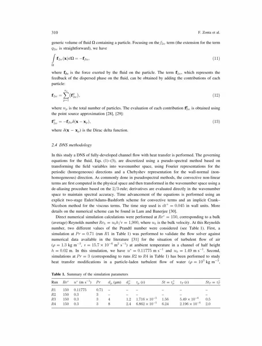
Direct numerical simulation calculations were performed at Re� = 150, corresponding to a bulk

(average) Reynolds number Reb = ubh=m = 1,900, where ub is the bulk velocity. At this Reynolds

number, two different values of the Prandtl number were considered (see Table 1). First, a

simulation at Pr = 0.71 (run R1 in Table 1) was performed to validate the flow solver against

numerical data available in the literature [31] for the situation of turbulent flow of air

(q = 1.3 kg m@3, m = 15.7 · 10@6 m2 s@1) at ambient temperature in a channel of half height

h = 0.02 m. In this simulation, we have u� = 0.11775 m s@1 and ub = 1.49 m s@1. Second,

simulations at Pr = 3 (corresponding to runs R2 to R4 in Table 1) has been performed to study

heat transfer modifications in a particle-laden turbulent flow of water (q = 103 kg m@3,

Table 1. Summary of the simulation parameters

Run Re� u� (m s@1) Pr dp (lm) dpþ sp (s) St = sp

þ sT (s) StT = sTþ

R1 150 0.11775 0.71 – – – – – –

R2 150 0.3 3 – – – – – –

R3 150 0.3 3 4 1.2 1.716 · 10@5 1.56 5.49 · 10@6 0.5

R4 150 0.3 3 8 2.4 6.862 · 10@5 6.24 2.196 · 10@6 2.0

310 F. Zonta et al.

m = 10@6 m2 s@1) at the temperature hTi = 50 �C in a channel of half height h = 500 lm. The

temperature hTi corresponds to the mean temperature between hTwh i and Thwc i. In this case,

u� = 0.3 m s@1 and ub = 3.8 m s@1.

The computational domain has dimensions 1,885 · 942 · 300 in wall units and was discretized

using an Eulerian grid made of 128 · 128 · 129 nodes (corresponding to 128 · 128 Fourier modes

and to 129 Chebyshev coefficients in the wavenumber space). The grid spacing is uniform in the

homogeneous directions and corresponds to spatial resolutions equal to Dxþ = 14.72 and

Dyþ = 7.35; the nodes along the wall-normal direction are clustered near the wall corresponding

to spatial resolutions from Dzþ = 0.0452 at the wall to Dz

þ = 3.68 at the centerline. The wall-

normal grid spacing is always smaller than the smallest local flow scale and, thus, it fulfills the

requirements imposed by the point-particle approach (see Sect. 2.5).

2.5 Lagrangian particle tracking

The complete set of equations which describes the time evolution of particle position, velocity and

temperature in the turbulent flow field is given by Eqs. (4), (5) and (9). To solve for these equations,

we have coupled the DNS flow solver to a Lagrangian tracking routine. The routine uses sixth-order

Lagrangian polynomials to interpolate the fluid velocity components and the fluid temperature at

particle position. The performance of the interpolation scheme is comparable to that of spectral

direct summation and to that of an hybrid scheme which exploits sixth-order Lagrangian

polynomials in the streamwise and spanwise directions and Chebyshev summation in the wall-

normal direction. A fourth-order Runge–Kutta scheme is used for time advancement of the particle

equations. The timestep size is equal to that used for the fluid (dtþ = 0.045). The total tracking time

was tþ = 2,000 for the 4 lm particles and t

þ = 1,500 for the 8 lm particles. We remark here that

these simulation times are not sufficient to achieve a statistically steady state for the particle

concentration, yet they are long enough to obtain converged velocity and temperature statistics and

to highlight qualitatively the effect of the particles on the heat transfer rate.

Particles are treated as pointwise, rigid spheres (point–particle approach) and are injected into the

flow at average mass fraction, Um, high enough to have a two-way coupling between the particles

and the fluid (Um � 10@2) [32], [33]. Possible effects due to inter-particle collisions are neglected.

At the beginning of the simulation, particles are distributed randomly over the computational domain

and their initial velocity and temperature are set equal to those of the fluid at the particle initial

position. Periodic boundary conditions are imposed on particles moving outside the computational

domain in the homogeneous directions, whereas perfectly-elastic collisions at the smooth walls are

assumed when the particle center is less than one particle radius away from the wall. No specific

boundary condition is needed for the particle temperature equation (Eq. 9) since the integration of

this equation follows the integration of the particle momentum equation (Eq. 5) and it requires only

the knowledge of the initial condition.

In the simulations presented here, large samples of 800,000 particles have been considered for

each value of Re� and Pr. We remark here that tracking of Oð106Þ particles two-way coupled

with the fluid requires a huge computational effort in terms of both computational cost of the

simulation and disk storage availability, considering also the rather long tracking times achieved in

the simulations. Each particle sample is characterized by different values of the particle response

times. Table 1 summarizes the complete set of parameters relevant to the simulations of particle

dispersion, including the particle Stokes numbers, St and StT . The particle Stokes number

corresponds to the non-dimensional particle response time and is obtained using the viscous


timescale sf = m=us2 as reference. In the present study, we have St = sp

þ = sp=sf and

StT = sTþ = sT=sf.

3 Results and discussion

3.1 Unladen turbulent channel flow with heat transfer

In this paragraph we examine the statistics relative to velocity and thermal variables for the base case

of unladen fluid. We examine the results relative to the simulations R1 and R2, performed at the

same Reynolds number (Re� = 150) and at Prandtl numbers equal to 0.71 and 3, respectively.

Velocity and temperature statistics will be examined and compared against literature reference cases

[19], [31].

a. Velocity field

The mean velocity profile will not be shown since it collapses onto the logarithmic law of the

wall perfectly [13] and matches previous results obtained in Refs. [19] and [31]. In Fig. 2 the

root mean square (rms) of the fluctuations of the velocity components, huþi,rms(zþ)i, is plotted as

a function of the wall normal coordinate in wall units, zþ, and compared against the results of

Kasagi and Iida [31]. The agreement is generally good showing small differences which may be

due to marginal statistical sampling of the time series. In the two simulations relative to the base

fluid only, the velocity field depends only on the pressure gradient (namely on the shear

Reynolds number, Re�) and it is not influenced by the value of the Prandtl number – forced

convection.

b. Temperature field

The behavior of the fluid temperature averaged over the homogeneous directions (x and y) is shown

in Fig. 3 for the two values of the Prandtl number, Pr = 0.71 and Pr = 3, respectively. In Fig. 3a,

the temperature is made dimensionless in outer units, indicated by the superscript @, as follows:

hT�i ¼ hTi � Tm

DTm

; ð14Þ

<u+

i,rm

s(z+

)>

0

0.5

1

1.5

2

2.5

3

0 20 40 60 80 100 120 140

z+

Present Simulation: <u+x,rms>

<u+z,rms>

<u+y,rms>

Kasagi et al. (1999): <u+x,rms>

<u+z,rms>

<u+y,rms>

Fig. 2. Rms of fluid velocity compo-

nents, huþi,rms(zþ)i, for single-phase

(unladen) turbulent channel flow

312 F. Zonta et al.

where Tm = (TH ? TC)=2 is the average centerline temperature and DTm = (TH @ TC)=2 is the

temperature difference between the walls. The average temperature is shown as a function of the

wall normal coordinate made dimensionless by the half channel height, h. The results of the present

work are compared and assessed against those computed by Kasagi and Iida [31] for Pr = 0.71 and

against those computed by Na et al. [19] for Pr = 3. Results match perfectly showing that the

simulation parameters – i.e. resolution, average time, etc. – are appropriate for the problem under

investigation.

The same averaged temperature profiles are plotted in Fig. 3b using a semi-logarithmic scale just

to show possible minor differences among the current profiles and the benchmark profiles [19], [31].

Temperature profiles are shown as a function of the wall normal distance, both being expressed in

wall units. In this case, the temperature is defined as the difference between the local average

temperature and the wall temperature (both relative to the average centerline temperature)

normalized by the friction temperature, T� = qw=(qf cpu�): hTþi = (hTi @ TW )=T�.

The computed data are also compared with standard analytical correlations used to estimate the

temperature wall dependence. These correlations have the following form:

hTþi ¼ hTi � TW

T�¼ Pr � zþ if zþ � 11:6;

1kh

ln zþ þ Bh if zþ[ 11:6;

�ð15Þ

where kh = 0.21 and Bh = @4.4 and 14.7 for Pr = 0.71 and for Pr = 3, respectively.

a

<T

- (z- )>

Pr=0.71: Present Simulation

Kasagi et al. (1999)

Pr=3: Present Simulation

0

0.2

0.4

0.6

0.8

1

−1 −0.8 −0.6 −0.4 −0.2 0z-

Na et al. (1999)

bz+

<T

+(z

+)>


0

5

10

15

20

25

30

35

40

45

50

0.01 0.1 1 10 100


Analitycal profile


Analitycal profile

Na et al. (1999)

Fig. 3. Mean fluid temperature at

Pr = 0.71 and Pr = 3. a hT@(z@)i(linear–linear scale), b hTþ(zþ)i(log–linear scale)


As broadly known, the profiles show the existence of a (near-wall) diffusive sublayer, the

thickness of which varies with the Prandtl number and is approximately equal to Dhþ = 6.5 for

Pr = 0.71 and Dhþ = 4.5 for Pr = 3. In Fig. 3a and b we can further observe that the temperature

gradient at the wall is strongly dependent on the value of the Prandtl number. This behavior is shown

by Eq. (15), from which it is clear that the temperature in the viscous sublayer depends linearly on

the Prandtl number.

In problems which involve turbulent heat transfer, the Prandtl number is also important to

establish the smallest spatial scale for the temperature field, gh, which can be expressed [34], [35] as

a function of the Kolmogorov scale, gk, as follows:

gh � gk

1

Pr

� �3=4

ð16Þ

for Pr < 1, and

gh � gk

1

Pr

� �1=2

ð17Þ

for Pr > 1. The previous relations confirm that for a given value of gk (we remind here that the

average value of gk depends only on the Reynolds number, which is equal to 150 in the present

simulations), the smallest temperature scale decreases for increasing Prandtl numbers.

The behavior of rms of the temperature field fluctuations, hTþrms(zþ)i, is shown in Fig. 4.

Results obtained by Kasagi and Iida [31] for Pr = 0.71 and by Na et al. [19] for Pr = 3 are

also shown for benchmark and comparison. Results are presented in wall variables. Focusing on

the Pr = 0.71 case, we observe that the temperature intensity reaches a maximum at the channel

centerline, not mimicking the behavior of the fluctuations of the velocity field which all reach

their peak in the wall proximity (see Fig. 2). This was discussed by Lyons et al. [21], who

attributed this different behavior to the temperature boundary conditions which force a non-zero

temperature gradient at the center of the channel. In the Pr = 3 case, the temperature intensity

reaches a maximum in the near-wall region. This observation is related to the Prandtl number

effect on hTþrms(z)i, indicating that the range of wavenumbers in the thermal fluctuating field

increases with Pr, for which the spectral functions of the velocity fields are negligible. As can

also be observed, the increase in the Prandtl number corresponds to a shift of the peak value of

<T

+rm

s(z+)>




0

1

2

3

4

5

6

7

0 20 40 60 80 100 120 140z+

Na et al. (1999)

Fig. 4. Rms of fluid temperature,

hTþrms(zþ)i, at Pr = 0.71 and at Pr = 3

314 F. Zonta et al.

the temperature fluctuations toward the wall. Both in the current results and in those by Kasagi

and Iida [31] for Pr = 0.71, the relative peak of the temperature fluctuations is located around

zþ = 20. The location of the peak for the higher Prandtl number (Pr = 3) has moved to

zþ = 9, roughly. Small discrepancies due perhaps to the marginally statistical sample are

observed between our results and those of Na et al. [19].

3.2 Particle-laden turbulent channel flow with heat transfer and momentum/energy

two-way coupling

The main purpose of this section is to analyze the modifications on the flow field due to the mutual

interaction between fluid and particles. In particular, results obtained from two-way coupling

simulations at Pr = 3 are compared against those obtained from the corresponding one-way

coupling simulations, in which particle feedback on the flow is neglected: f2w = 0 and q2w = 0 in

Eqs. (2) and (3). We remark here that, even though the problem of fluid-particle momentum

coupling in two-phase flows has been widely investigated [11], [28], [33], much less effort has been

devoted to the energy coupling problem. Currently, numerical studies on this problem are available

for homogeneous shear flow [36] and for homogeneous isotropic turbulence [37]. To our knowledge,

this is the first attempt to study (by means of DNS) both momentum and energy coupling between

fluid and particles in wall-bounded flow.

a. Velocity field modifications by particles

The effect of particles on the mean fluid velocity, huxþ(zþ)i, is shown in Fig. 5. The solid line

refers to the simulation without particles, while the dot-dashed line refers to the two-way coupling

simulation with the 4 lm particles. Profiles are averaged in space (over the streamwise and

spanwise directions) and time (over a time span of 180 wall units). As expected, mean velocity

profiles, normalized here by the unladen flow shear velocity u�, deviate only slightly (if not

negligibly, as in the viscous sublayer) from each other. A careful examination of Fig. 5 indicates

that the effect of particles is to shift the velocity profiles slightly toward smaller values in the

buffer region (5 < zþ < 30) and toward higher values in the outer region (zþ > 30). Comparison

<u x+

(z+)>

0

5

10

15

20

0.1 1 10 100z+

Unladen flow

Laden flow (dp=4 mm)

Fig. 5. Mean streamwise fluid velocity,

huxþ(zþ)i, at Pr = 3: comparison

between unladen flow (no momentum/

energy coupling) and flow laden with

dp = 4 lm particles (with momentum/

energy coupling)


of the mean velocity profiles for the 8 lm particle case (not shown here for brevity) indicate no

observable effect.

The behavior of the turbulence intensities, given by the rms of the fluid velocity fluctuations,

huþi,rms(zþ)i, shows larger differences as presented in Fig. 6. Again, the solid lines refer to the

simulation without particles, whereas the dot-dashed and the dashed lines refer to the two-way

coupling simulation with the 4 lm particles and with the 8 lm particles, respectively. It appears that

particles do not affect much the intensities in the near-wall region but do substantially change them

a

<u+

x,rm

s(z+)>

0

0.5

1

1.5

2

2.5

0 20 40 60 80 100 120 140

Unladen flow



1.2

b

<u+

y,rm

s(z+)>

Unladen flow

0

0.2

0.4

0.6

0.8

1

0 20 40 60 80 100 120 140



c

<u+

z,rm

s(z+)>

Unladen flow


0

0.2

0.4

0.6

0.8

1

0 20 40 60 80 100 120 140z+


Fig. 6. Rms of mean fluid velocity

components, huþi,rms(zþ)i, at Pr = 3:

comparison between unladen flow (no

momentum/energy coupling) and flow

laden with dp = 4 lm particles and with


energy coupling). a streamwise rms,

huþx,rms(zþ)i; b spanwise rms,

huþy,rms(zþ)i; c wall-normal rms,

huþz, rms(zþ)i

316 F. Zonta et al.

in the buffer region, particularly where the profiles develop a peak, and at the channel centerline. For

each rms component, local changes of opposite sign depending on particle inertia are observed with

respect to the reference unladen-flow values.

b. Temperature field modifications by particles

Figure 7 shows the mean fluid temperature profiles in inner units, hT@(z@)i, (Fig. 7a) and in wall

units, hT+(zþ)i (Fig. 7b). Lines are as in Fig. 5. Visual inspection of Fig. 7a does not reveal

significant differences in the profiles. However, computing the local value of the wall-normal

temperature gradient, dhT(z)i=dz, right at the wall, we obtain an increase of roughly 2% for the two-

way coupling simulation with the 4 lm particles and a decrease of 0.2% for the two-way coupling

simulation with the 8 lm particles. This finding is important because changes produced by the

particles to the wall-normal temperature gradient directly reflect upon the heat flux at the wall, qw,

through the following expression:

qw ¼1

Pr

dhTðzÞidz

: ð18Þ

In turn, a change in the value of qw will eventually correspond to a change in the value of the total

turbulent heat flux qz,tot, defined as

a

<T

- (z- )>

0

0.2

0.4

0.6

0.8

1

−1 −0.8 −0.6 −0.4 −0.2 0z-

Unladen flowLaden flow (dp=4 mm)Laden flow (dp=8 mm)

b

<T

+(z

+)>

0

5

10

15

20

25

30

35

40

0.1 1 10 100z+

Unladen flowLaden flow (dp=4 mm)Laden flow (dp=8 mm)

Fig. 7. Mean fluid temperature at

Pr = 3: comparison between unladen

flow (no momentum/energy coupling)

and flow laden flow with dp = 4 lm

particles and with dp = 8 lm particles

(with momentum/energy coupling).

a hT@(z@)i (linear–linear scale),

b hTþ(zþ)i (log–linear scale)


qz;tot ¼ qw � hT0w0i; ð19Þ

under fully developed conditions. Besides being perhaps the most significant result of the present

paper from a quantitative viewpoint, the increase of removable heat flux at the wall for the

smaller 4 lm particles case and the decrease of removable heat flux for the larger 8 lm particles

case have also an effect on the friction temperature, T�. According to its definition (see

Sect. 3.1), the friction temperature computed in the two-way coupling simulations with the 4 lm

particles will increase with respect to the unladen flow case, whereas it will decrease in the

simulations with the 8 lm particles. As a consequence, starting from the reference profile relative

to the unladen flow case, the mean fluid temperature profile computed for the 4 lm particle case

will shift toward smaller values (particularly outside the viscous sublayer) whereas it will shift

toward slightly higher values when the larger 8 lm particles are considered, as apparent from

Fig. 7b.

Finally, the rms of the fluid temperature fluctuations, hTþrms(zþ)i, are shown in Fig. 8. The 4 lm

particles produce a slight decrease in the peak value of hTþrms(zþ)i and an increase outside the buffer

region; smaller modifications (mostly limited to the core region of the flow) are produced by the

larger 8 lm particles.

c. Influence of particle inertia and of particle thermal inertia

The interactions between particles, turbulent momentum transport and turbulent heat transport are

influenced by the particle response times. In this section we analyze the Eulerian statistics of the

particles in comparison with those of the fluid. Specifically, particles will acquire and lose

momentum and heat at a rate proportional to the inverse of their response times, sp and sT,

respectively.

Figure 9 shows the mean streamwise velocity profile, huþx;p(zþ)i, averaged in time and along the

homogeneous directions, for both fluid and particles as a function of the wall-normal coordinate, zþ.

Differences are readily visible, with a consistent evidence of the effect of particle inertia. Smaller

particles (St = 1.56, dp = 4 lm) behave more like fluid tracers and their average velocity profile

(circles) almost matche that of the fluid (solid line). As the particle response time increases

(St = 6.24, dp = 8 lm), the average particle velocity (squares) is seen to lag the average fluid

velocity, in particular outside the viscous sublayer. Present results agree well with those reported by

<T

rms+

(z+)>


0

1

2

3

4

5

6

0 20 40 60 80 100 120 140z+

Unladen flow


Fig. 8. Rms of fluid temperature,

hTþrms(zþ)i, at Pr = 3: comparison

between unladen flow (no momentum/

energy coupling) and flow laden with

dp = 4 lm particles and with


energy coupling)

318 F. Zonta et al.

van Haarlem et al. [38] and by Portela et al. [39], who however, used a one-way approach. This

shows that, for the current size, density and overall concentration of the particles, modifications to

the mean streamwise velocity profile due to momentum and energy coupling appear negligible. As

already observed by van Haarlem et al. [38], inertial particles dispersed in a turbulent flow do not

sample the flow field homogeneously and tend to avoid areas of high vorticity preferring areas

characterized by lower-than-mean streamwise fluid velocity and by high strain rate. This gives the

characteristic velocity lag in the region 5 < zþ < 50. This effect is confirmed by data shown in

Fig. 10a, where the root mean square of particles streamwise velocity (circles and squares) is

compared to that of the fluid (solid line). Fluctuations of particle streamwise velocity are larger than

those of the fluid, this difference becoming more evident as particle response time increases [39].

From a physical viewpoint, the difference in the streamwise values suggests that the gradients in the

mean fluid velocity can produce significant fluctuations of the streamwise particle velocity. This

effect seems more pronounced in the case of heavy particles, with larger Stokes number and a longer

‘‘memory’’. An opposite behavior is observed in the spanwise direction and in the wall-normal

direction (Fig. 10b, c, respectively), where the fluid velocity field has zero mean gradient. The

turbulence intensity of the particles is very close to that of the fluid for particles with small inertia

(St = 1.56, circles) and lower than that of the fluid for particles with higher inertia (St = 6.24,

squares). This is mainly due to two mechanisms acting in tandem. The first mechanism is preferential

concentration of particles in low-speed regions, characterized by lower turbulence intensity [13]. The

second is the filtering of high frequencies or wavenumber fluctuations done by particles due to their

inertia. The inertial filtering damps turbulence intensity of the particles in the wall-normal direction

and in the spanwise direction. Similar filtering effects have been observed in homogeneous

turbulence [40].

The statistical behavior of the thermal field for the dispersed phase is presented in Figs. 11 and 12.

Figure 11 shows the mean temperature profiles for particles and fluid as a function of the wall-

normal coordinate. In Fig. 11a variables are expressed in outer units, whereas in Fig. 11b variables

are shown in wall units and in semi-logarithmic scale. The solid line refers to the average unladen

fluid temperature, while circles and squares refer respectively to the simulations with the 4 lm

particles and with the 8 lm particles. Figure 11a indicates that, for both particle sets, the particle

temperature in the near-wall region (0 < zþ < 30) is higher than that of the fluid, while it reaches

lower values in the outer region (30 < zþ < 150). Particle temperature higher than that of the fluid

is probably due to the deposition/resuspension mechanisms, which bring particles to the near-wall

Fluid (unladen flow)

0

2

4

6

8

10

12

14

16

18

10 100

<u+

x,p(z

+)>

z+

dp=4 mm

dp=8 mm

Fig. 9. Mean particle streamwise veloc-

ity, huþx;p(zþ)i, at Pr = 3. Symbols:

open circle dp = 4 lm particles, opensquare dp = 8 lm particles. The mean

fluid streamwise velocity profile relative

to the unladen flow case (solid line) is

also shown for sake of comparison


region (where they are characterized by high temperature value differences) and drive them toward

the core region [10], [13]. When a particle initially close to the wall is entrained toward the core

region, it will adapt its temperature at a rate depending on particle thermal inertia, thus maintaining a

temperature higher than that of the fluid. In the outer region, the perspective is overturned, and

particles are characterized by a temperature lower than that of the fluid. The effect of particle thermal

inertia is also visible by observing the rms of particle temperature profiles, hTþp,rms(zþ)i, shown in

Fig. 12. These profiles are qualitatively similar to those for the streamwise rms component

a

<u+

x,p,

rms(z

+)>

Fluid (unladen Flow)

dp=4 mm

0

0.5

1

1.5

2

2.5

3

0 20 40 60 80 100 120 140

dp=8 mm

b

<u+

y,p,

rms(z

+)>

0

0.2

0.4

0.6

0.8

1

1.2

0 20 40 60 80 100 120 140


dp=4 mm

dp=8 mm

c

<u+

z,p,

rms(z

+)>

0

0.2

0.4

0.6

0.8

1

0 20 40 60 80 100 120 140z+


dp=4 mm

dp=8 mm

Fig. 10. Rms of particle velocity com-

ponents at Pr = 3. Symbols: open circle4 lm particles, open square 8 lm parti-

cles. Panels: a Streamwise rms,

huþx;p; rms(zþ)i, b spanwise rms,

huþy;p; rms(zþ)i, c wall-normal rms,

huþz;p; rms(zþ)i. The rms of fluid veloc-

ities relative to the unladen flow case

(solid line) is also shown for sake of

comparison

320 F. Zonta et al.

(Fig. 10a), due to the role played by particle thermal inertia in transferring heat, similar to that

played by particle inertia in transferring momentum. Although a qualitative similarity between the

temperature and the streamwise velocity rms can be observed, quantitative differences are visible. In

particular, the peak of the streamwise velocity rms exhibits values higher than the temperature rms.

These quantitative differences are due to the fact that particle inertia is larger than particle thermal

inertia and causes streamwise velocity fluctuations higher than thermal fluctuations.

d. Instantaneous features of turbulent transfer of momentum, heat and particles

A number of DNS-based works have been successful in clarifying the role of the instantaneous

realizations of the Reynolds stresses in transferring momentum [41], heat [19] and particles [10]. We

refer to these works and to the references therein for a more comprehensive description of the

phenomena. It suffices here to show on a qualitative basis some relations among momentum, heat

and particles transfer mechanisms.

To this aim, we complement the statistical analysis of the previous sections by showing the

complex interactions among velocity field, temperature field and particles distribution. In particular,

we examine simulation R3 (Re� = 150, Pr = 3 and dp = 4 lm particles). We consider a cross

section of the flow field, perpendicular to the mean velocity, cut along a x–y plane. Consider first

Fig. 13a: color isocontours correspond to values of the streamwise fluid velocity whereas circles

represent particles (drawn larger than the real size for visualization purposes) colored by their wall-

a

<T

p(z- )>

dp=4 mm

0

0.2

0.4

0.6

0.8

1

−1 −0.8 −0.6 −0.4 −0.2 0z-


dp=8 mm

b

<T

+(z

+)>

0

5

10

15

20

25

30

35

40

1 10 100z+

Fluid (unladen flow)dp=4 mmdp=8 mm

p

Fig. 11. Mean particle temperature at

Pr = 3. Symbols: open circle 4 lm

particles, open square 8 lm particles. a

hT@p (z@)i (linear–linear scale), b

hT+p(z+)i (log–linear scale). The mean

fluid velocity relative to the unladen flow

case (solid line) is also shown for sake of

comparison


normal velocity. In this figure, green particles have wall-normal velocity directed toward the walls,

while black particles have wall-normal velocity directed away from the walls. In this way, just by

analyzing particle wall-normal velocity, it is possible to detect particle transfer fluxes toward the

wall and particle transfer fluxes away from the wall. It is possible to observe that fluxes of particles

are associated with fluxes of streamwise momentum (called sweeps if directed toward the wall and

ejections if directed away from the wall, as discussed in several previous papers [10], [13]).

To draw a link between the heat transfer mechanisms and the momentum transfer mechanisms we

consider also Fig. 13b, where the particles are shown superimposed to the temperature field for the

same section of Fig. 13a. In this case color isocontours are the values of the fluid temperature,

whereas circles represent particles colored by their temperature: specifically, green particles have

higher-than-mean temperature, blue particles have lower-than-mean temperature, and red particles

have temperature close to the mean. The Reynolds transport analogy is clearly demonstrated by the

behavior of the instantaneous temperature field: focusing on the wall at zþ = 0, characterized by

higher temperature, we observe hot fluid plumes raising in correspondence with the raising of low

momentum fluid within an ejection in Fig. 13a. This just demonstrates the effectiveness of the

Reynolds stresses in transporting the fluid close to the wall towards the center of the channel and

vice versa. Similar observations can be made for the cold wall at zþ = 300. Considering now, again

in Fig. 13b, the behavior of the particles in correlation with the temperature field, we observe that

particles with higher temperature are ejected from the lower wall and are directed towards the upper

wall. The opposite occurs to the colder particles. In this case, however, it is important to remind that

particle temperature is not strictly correlated with fluid temperature. This behavior can be explained

by considering that particle trajectories depend on fluid velocity and particle inertia, but not on fluid

or particle temperature. Particles, driven by the fluid vortices, can thus reach regions characterized

by fluid temperature quite different from particle temperature, causing an appreciable heat exchange

between the two phases.

The efficiency of the overall heat exchange process is conditioned by the degree of non-

homogeneity of particle distribution and by the rate of particle accumulation at the wall. This

observation is qualitatively corroborated by Fig. 14, where the instantaneous cross-sectional

distribution (left-hand side panels) and the wall-normal concentration, C=C0 (right-hand side panels)

of both particle sets are compared at the same time instant. Note that the 4 lm particle distribution,

shown in Fig. 14c, is the same of Fig. 13, the particle color code being that of Fig. 13b; particle

concentration is computed as particle number density distribution per unit volume normalized by its

initial value [10]. It is evident that the smaller 4 lm particles, which produce an increase of heat

<T

+p,

rms(z

+)>


0

1

2

3

4

5

6

20 40 60 80 100 120 140

z+

dp=4 mm

dp=8 mm

Fig. 12. Rms of particle temperature,

hT+p; rms(z

+)i, at Pr = 3. Symbols: opencircle 4 lm particles, open square 8 lm

particles. The rms of fluid temperature

relative to the unladen flow case (solid

line) is also shown for sake of compar-

ison

322 F. Zonta et al.

transfer at the wall (as discussed in Sect. 3.2), exhibit a more persistent stability against non-

homogeneous distribution and near-wall concentration with respect to the larger 8 lm particles. The

larger particles tend to form clusters in the core region and accumulate at the wall at higher rates

acting as an additional thermal resistance both between the walls and the fluid and between the fluid

and the particles: as a result of this behavior, the heat transfer is reduced.

4 Conclusions and future development

Heat transfer enhancement is a fascinating subject with extremely interesting possibilities for

application. One option to increase heat transfer is to devise a new concept of heat transfer media

constituted by a base fluid in which suitably chosen heat transfer agents, precisely micro and nano

particles, are injected. In this way, the fluid can be a standard fluid characterized by simplicity of use

and well-known properties, like water, and the heat transfer agents can be heavy-metal, high-heat-

capacity, dispersed particles (e.g. copper, gold or platinum).

Current literature trends show the potentials of such heat transfer media, called nanofluids; yet the

complicacy and the cost of experimental methods make it hard to understand the intricacy of the

mechanisms which govern the dynamics of the turbulent heat transfer among the fluid and the

particles. Current open questions range from the optimal size of the particles to the optimal

concentration and practical solutions in real applications. Further complicating effects are

represented by the particle inertia and the particle thermal inertia, which are additional parameters.

The present study represents a first effort made in the frame of a broader project on the numerical

simulation of heat transfer in nanofluids. Our strategic object is to investigate the heat transfer

mechanisms in nanofluids and to devise a suitable numerical methodology to analyse their behavior.

In this paper, the DNS of fluid and thermal fields is assessed against literature data [19], [31] for one

value of the shear Reynolds number, Re� = 150, and two values of the Prandtl number, Pr = 0.71

300

250

200

150zz

100

50

0a

300

250

200

150

100

50

0b

0 100 200 300 400 500 600 700 800 900

201612840

1

0.5

0

−0.5

−1

0 100 200 300 400 500y

600 700 800 900

Fig. 13. Front view of particle instanta-

neous distribution superimposed to the

fluid velocity field a and to the fluid

temperature field b at Pr = 3


and Pr = 3. Further, preliminary results obtained from DNS of two-phase solid–liquid turbulent

flow in a channel with heat transfer are presented. Hydrodynamically fully developed, thermally

developing flow conditions have been considered to investigate on heat transfer modulation

produced by the dispersion of micrometer sized particles. Two different sets of particles are

considered, which are characterized by dimensionless inertia response times equal to St = 1.56 and

St = 6.24 and by dimensionless thermal response times equal to StT = 0.5 and StT = 2,

respectively. The instantaneous features of the velocity field, the temperature field and particles

dispersion are discussed from a qualitative mechanistic viewpoint to analyse the role of particles as

heat transfer enhancement agents.

Building on the results presented in this paper, an extensive numerical work combined with

modeling efforts will be carried out to achieve a deeper understanding of the reason why nanofluids

conduct heat so effectively. For instance, the increased surface interaction between the fluid and the

solid particles at the nanoscale as possible explanation to the increased heat transferability will be

investigated. Indeed, for a given volume of material there is a greater number of particles as their

size decreases; perhaps there is more opportunity for the nanoparticles to conduct the heat.

Furthermore, understanding of how the molecules of a base fluid keep nanoparticles suspended, since

nanoparticles are still dramatically larger than individual molecules, needs to be investigated. In this

context, the effect of Brownian forces on the kinematics of the nanoparticles should be investigated.

It would also be of interest to investigate the magnitude of the van der Waals forces between the

0

50

100

150

200

250

300

a

z+

b

0

50

100

150

200

250

300

c 0 100 200 300 400 500 600 700 800 900

z+

y+ 0.1 1 10 100d

C/C0

Fig. 14. Front view of particle instantaneous distribution (left panels) and corresponding particle wall-

normal concentration, C/C0 (right panels) at Pr = 3. a, b 8 lm particles; c, d 4 lm particles

324 F. Zonta et al.

particles and their effect on the nanofluids dynamics. These forces are usually small, but they

become strong (and attractive) when the distance between particles becomes of the order of tenths of

nanometers.

Acknowledgements

Support from PRIN (under Grant 2006098584_004) and from HPC Europa Transnational Access Program

(under Grants 466 and 708) are gratefully acknowledged.

References

[1] Wang, X.-Q., Mujumdar, A.S.: Heat transfer characteristics of nanofluids: a review. Int. J. Therm. Sci.

46, 1–19 (2007)

[2] Daungthongsuk, W., Wongwises, S.: A critical review of convective heat transfer of nanofluids.

Renew. Sust. Energ. Rev. 11, 797–817 (2007)

[3] Das, S.K., Choi, S.U.S., Patel, H.E.: Heat transfer in nanofluids – a review. Heat Transf. Engng. 27, 3–19

(2006)

[4] Xuan, Y., Li, Q.: Heat transfer enhancement of nanofuids. Int. J. Heat Fluid Flow 21, 58–64 (2000)

[5] Maiga, S.E.B, Palm, S.J., Nguyen, C.T., Roy, G., Galanis, N.: Heat transfer enhancement by using

nanofluids in forced convection flows. Int. J. Heat Fluid Flow 26, 530–546 (2005)

[6] Maxwell, J.C.: A Treatise on Electricity and Magnetism, 2nd edn, vol. 1, p. 435. Clarendon Press,

Oxford (1881)

[7] Hamilton, R.L., Crosser, O.K.: Thermal conductivity of heterogeneous two component systems. Ind.

Engng. Chem. Fund. vol. 1, 3, 187–191 (1962)

[8] Wasp, E.J., Kenny, J.P., Gandhi, R.L.: Solid–Liquid Flow Slurry Pipeline Transportation. Series on

Book Materials Handling. Trans. Tech. Publications, Clausthal (1977)

[9] Trisaksri, V., Wongwises, S.: Critical review of heat transfer characteristics of nanofluids. Renew.

Sust. Energ. Rev. 11, 512–523 (2007)

[10] Marchioli, C., Soldati, A.: Mechanisms for particle transfer and segregation in turbulent boundary

layer. J. Fluid Mech. 468, 283–315 (2002)

[11] Pan, Y., Banerjee, S.: Numerical simulation of particle interaction with wall turbulence. Phys. Fluids 8,

2733–2755 (1996)

[12] Eaton, J.K., Fessler, J.R.: Preferential concentration of particles by turbulence. Int. J. Multiph. Flow

20, 169–209 (1994)

[13] Soldati, A.: Particles turbulence interactions in boundary layers. Z. Angew. Math. Mech. 85, 683–699

(2005)

[14] Bec, J., Biferale, L., Boffetta, G., Celani, A., Cencini, M., Lanotte, A., Musacchio, S., Toschi, F.:

Acceleration statistics of heavy particles in turbulence. J. Fluid Mech. 550, 349–358 (2005)

[15] Chagras, V., Oesterle, B., Boulet, P.: On heat transfer in gas–solid pipe flows: effects of collision

induced alteration of the flow dynamics. Int. J. Heat Mass Transf. 48, 1649–1661 (2005)

[16] Lakehal, D., Fulgosi, M., Yadigaroglu, G.: Direct numerical simulation of turbulent heat transfer

across a mobile, sheared gas–liquid interface. J. Heat Transf. 125, 1129–1139 (2003)

[17] Hetsroni, G., Mosyak, A., Pogrebnyak, E.: Effect of coarse particles in a particle laden turbulent

boundary layer. Int. J. Multiph. Flow 28, 1873–1894 (2002)

[18] Tiselj, I., Bergant, R., Mavko, B., Bajsic, I., Hetsroni, G.: DNS of turbulent heat transfer in channel

flow with heat conduction in the solid wall. J. Heat Transf. 123:849–857 (2001)

[19] Na, Y., Papavassiliou, D.V., Hanratty, T.J.: Use of direct numerical simulation to study the effect of

Prandtl number on temperature fields. Int. J. Heat Fluid Flow 20, 187–195 (1999)

[20] Kawamura, H., Abe, H., Matsuo, Y.: DNS of turbulent heat transfer in channel flow with respect to

Reynolds and Prandtl number effects. Int. J. Heat Fluid Flow 20, 196–207 (1999)

[21] Lyons, S.L., Hanratty, T.J., McLaughlin, J.B.: Direct numerical simulation of passive heat transfer in a

turbulent channel flow. Int. J. Heat Mass Transf. 34, 1149–1161 (1991)


[22] Armenio, V., Fiorotto, V.: The importance of the forces acting on particles in turbulent flows. Phys.

Fluids 8, 2437 (2001)

[23] Rizk, M.A., Elghobashi, S.E.: The motion of a spherical particle suspended in a turbulent flow near a

plane wall. Phys. Fluids 28, 806–817 (1985)

[24] Soltani, M, Ahmadi, G.: Direct numerical simulation of particle entrainment in turbulent channel flow.

Phys. Fluids A 7, 647–657 (1995)

[25] Crowe, C., Sommerfeld, M., Tsuji, Y.: Multiphase Flows with Droplets and Particles, p. 469. CRC

Press, New York (1998)

[26] Schiller, V.L., Naumann, A.: Uber die grundlegenden Berechnungen bei der Schwerkraftaufbereitung.

Z. Ver. Deut. Ing. 77, 318–320 (1935)

[27] Ranz, W., Marshall, W.: Evaporation from drops. Chem. Engng. Prog. 48, 142–180 (1952)

[28] Boivin, M., Simonin, O., Squires, K.D.: Direct numerical simulation of turbulence modulation by

particles in isotropic turbulence. J. Fluid Mech. 375, 235–263 (1998)

[29] Sundaram, S., Collins, L.R.: A numerical study of the modulation of isotropic turbulence by suspended

particles. J. Fluid Mech. 379, 105–143 (1999)

[30] Lam, K., Banerjee, S.: On the condition of streak formation in bounded flows. Phys. Fluids A 4, 306–

320 (1992)

[31] Kasagi, N., Iida, O.: Progress in direct numerical simulation of turbulent heat transfer. In: Proceedings

of the 5th ASME/JSME Joint Thermal Engineering Conference, in CD-ROM, March 15–19, San

Diego, California (1999)

[32] Uijttewaal, W.S., Oliemans, R.V.A.: Particle dispersion and deposition in direct numerical and large

eddy simulations of vertical pipe flow. Phys. Fluids 8, 2590–2604 (1996)

[33] Kiger, K.T., Pan, C.: Suspension and turbulence modification effects of solid particulates on a

horizontal turbulent channel flow. J. Turbul. 3, 1–21 (2002)

[34] Monin, A.S., Yaglom, A.M.: Statistical Fluid Mechanics: Mechanism of Turbulence, book 2, p. 873.

MIT Press, Cambridge (1975)

[35] Batchelor, G.K.: Small-scale variation of convective quantities like temperature in turbulent fluid. J.

Fluid Mech. A 5, 113–133 (1959)

[36] Shotorban, B., Mashayek, F., Pandya, R.V.R.: Temperature statistics in particle-laden turbulent

homogeneous shear flow. Int. J. Multiph. Flow 29, 1333–1353 (2003)

[37] Jaberi, F.A., Mashayek, F.: Temperature decay in two-phase turbulent flows. Int. J. Heat Mass Transf.

43, 993–1005 (2000)

[38] van Haarlem, B., Boersma, B.J., Nieuwstadt, F.T.M.: Direct numerical simulation of particle

deposition onto a free-slip and no-slip surface. Phys. Fluids A 10, 2608–2620 (1998)

[39] Portela, L.M., Cota, P., Oliemans, R.V.A.: Numerical study of the near wall behaviour of particles in

turbulent pipe flows. Powder Technol. 125, 149–157 (2002)

[40] Reeks, M.W.: The transport of discrete particles in inhomogeneous turbulence. J. Aerosol Sci. 310,

729–739 (1983)

[41] Adrian, R.J., Meinhart, C.D., Tomkins, C.D.: Vortex organization in the outer region of the turbulent

boundary layer. J. Fluid Mech. 422, 1–54 (2000)

326 F. Zonta et al.: Direct numerical simulation of turbulent heat transfer modulation

heat transfer modulation by microparticles in turbulent channel flow

Documents