harmonic analysis of iterated function systems with overlap

arX

iv:m

ath-

ph/0

7010

66v1

27

Jan

2007

HARMONIC ANALYSIS OF ITERATED FUNCTION SYSTEMS

WITH OVERLAP

PALLE E. T. JORGENSEN, KERI A. KORNELSON, AND KAREN L. SHUMAN

Dedicated to the memory of Thomas P. Branson

Abstract. An iterated function system (IFS) is a system of contractive map-pings τi : Y → Y , i = 1, . . . , N (finite) where Y is a complete metric space.Every such IFS has a unique (up to scale) equilibrium measure (also called theHutchinson measure µ), and we study the Hilbert space L2(µ).

In this paper we extend previous work on IFSs without overlap. Ourmethod involves systems of operators generalizing the more familiar Cuntzrelations from operator algebra theory, and from subband filter operators insignal processing.

These Cuntz-like operator systems were used in recent papers on waveletsanalysis by Baggett, Jorgensen, Merrill and Packer, where they serve as afirst step to generating wavelet bases of Parseval type (alias normalized tightframes), i.e., wavelet bases with redundancy.

Similarly, it was shown in work by Dutkay and Jorgensen that the iterativeoperator approach works well for generating wavelets on fractals from IFSswithout overlap. But so far the more general and more difficult case of essentialoverlap has resisted previous attempts at a harmonic analysis, and explicitbasis constructions in particular.

The operators generating the appropriate Cuntz relations are compositionoperators, e.g., Fi : f → f τi where (τi) is the given IFS. If the particularIFS is essentially non-overlapping, it is relatively easy to compute the adjointoperators Si = F ∗

i, and the Si operators will be isometries in L2(µ) with

orthogonal ranges. For the case of essential overlap, we can use the extraterms entering in the computation of the operators F ∗

ias a “measure” of the

essential overlap for the particular IFS we study. Here the adjoint operatorsF ∗

irefers to the Hilbert space L2(µ) where µ is the equilibrium measure µ for

the given IFS (τi).

Contents

1. Introduction: IFSs and operator theory 22. Multivariable operator theory 43. Contractive iterated function systems 84. Operator theory of essential overlap 134.1. Symmetry 134.2. Measuring overlap 185. Essential overlap and gaps for Sierpinski constructions in R

2 25

2000 Mathematics Subject Classification. 33C50, 42C15, 46E22, 47B32.Key words and phrases. tight frames, Parseval frames, Bessel sequences, Hilbert space, polar

decomposition, attractor, IFS, equilibrium measure, composition operator.This material is based upon work supported by the U.S. National Science Foundation under

grants DMS-0457581 and DMS-0503990.

1

http://arXiv.org/abs/math-ph/0701066v1

2 PALLE E. T. JORGENSEN, KERI A. KORNELSON, AND KAREN L. SHUMAN

5.1. The 2D recursion 265.2. The nature of the overlaps and induced systems 306. Conclusions (the general case) 32References 35

1. Introduction: IFSs and operator theory

In this paper we explore an operator theoretic approach to self similarity andfractals which is common to problems involving both iterated function systems(IFSs), and an aspect of quantum communication.

Each of the two areas involves a finite set of operations: in the case of IFSs theyare geometric, and in the quantum case, they involve channels of Hilbert spacesand associated operator systems. The particular aspects of IFSs we have in mindare studied in [DJ06a]; and the relevant results from quantum communication in[KLPL06] and [Kri05]. We begin the Introduction with some background on IFSs,and we motivate our present operator theoretic approach. The operator theory andits applications are then taken up more systematically in section 2 below.

It was proved recently that a class of non-linear fractals is amenable to a com-putational harmonic analysis. While this work is motivated by applications, it issignificant in its own right; for example these fractals do not carry the structureof groups, and so they do not come with a Haar measure. Nonetheless, they havenatural equilibrium measures µ which serve as substitutes. Specifically, these frac-tals are known as iterated function systems (IFS) indicating the recursive natureof their construction. But the analysis so far has been limited to IFSs withoutessential overlap (see Definition 3.9). The IFS fractals X are built by passing toa certain limit in a scaling iteration, and the “overlap” here refers to the parts ofsmaller scale-level. We identify “overlap” for a given X relative to the equilibriummeasure µ for X . While there is prior work on some isolated cases of overlap, thecases that are understood are those of negligible overlap. In this paper we identifyand study the harmonic analysis of IFSs with “substantial overlap.”

An iterated function system (IFS) is a system of contractive mappings τi : Y →Y , i = 1, . . . , N (finite) where Y is a complete metric space. Every such IFS has aunique (up to scale) equilibrium measure (also called the Hutchinson measure µ),and we study the Hilbert space L2(µ).

In this paper we extend previous work on IFSs without overlap. Our methodinvolves systems of operators generalizing the more familiar Cuntz relations fromoperator algebra theory, and from subband filter operators in signal processing. Be-fore turning to the details, below we outline briefly the operator-theoretic approachto IFSs.

For each N , there is a simple Cuntz C∗-algebra on generators and relations, andits representations offer a useful harmonic analysis of general IFSs, but there is acrucial difference between IFSs without overlap and those with essential overlap(this will be made precise in Section 2). The operators generating the appropriateCuntz relations [Cun77] are composition operators, e.g., Fi : f → f τi where (τi)is the given IFS. If the particular IFS is essentially non-overlapping, it is relativelyeasy to compute the adjoint operators Si = F ∗

i , and the Si operators will beisometries in L2(µ) with orthogonal ranges. In a way, for the more difficult case of

HARMONIC ANALYSIS OF ITERATED FUNCTION SYSTEMS WITH OVERLAP 3

essential overlap, we can use the extra terms entering into the computation of theadjoint operators F ∗

i as a “measure” of the essential overlap for the particular IFSwe study. Here the adjoint operators F ∗

i refer to the Hilbert space L2(µ) where µ iscarefully chosen. When the IFS is given, there are special adapted measures µ. Wewill be using the equilibrium measure µ for the given IFS (τi), and by [Hut81], thisµ contains much essential information about the IFS, even in the classical cases ofIFSs coming from number theory.

So far, earlier work in the general area was restricted to IFSs without overlap.For example, Cuntz-like operator systems were used in recent papers on waveletsanalysis by Baggett, Jorgensen, Merrill and Packer [BJMP04, BJMP05, BJMP06],where they serve as a first step to generating wavelet bases of Parseval type (aliasnormalized tight frames), i.e., wavelet bases with redundancy.

Similarly, it was shown in work by Dutkay and Jorgensen [DJ06d] that theiterative operator approach works well for generating wavelets on fractals from IFSswithout overlap. But so far the more general and more difficult case of essentialoverlap has resisted previous attempts at a harmonic analysis, and explicit basisconstructions in particular.

In this paper (Section 4) we show that certain combinatorial cycles from a sym-bolic encoding [DJ06b] of our IFSs yield an attractive computational analysis ofthe “IFS-overlap.” Some results (e.g., Corollary 4.11) are stated only for a modelexample, but as indicated the idea with cycle-counting works in general.

While the modern study of iterated function systems (IFSs) has roots in classicalproblems from number theory, infinite products [Kol77], and more generally fromprobability and harmonic analysis (see, e.g., [FLP94]), the subject took a moresystematic turn in 1981 with the influential paper [Hut81] by Hutchinson. Sincethen, IFSs have found uses in geometry (e.g., [Bar06, BHS05]), in infinite networkproblems (e.g., [GRS01]), in wavelets (e.g., [BJMP05, BJMP06, Jor05]), and indynamics and operator theory [Kaw05, Jor06, DJ06c, DJ06b, DJ05].

But in operator algebras, the subject has its own independent start with thepaper by Cuntz [Cun77]. In operator-algebra theory, a class of representations ofwhat have become known as the Cuntz, or the Cuntz–Krieger, algebras is ideallysuited for the study of iterative processes (including IFSs) in mathematics and inmathematical physics. Perhaps the paper [CK80] started this trend, but it wascontinued in various guises in the following papers: see [Pop89] and later relatedpapers by Popescu, [BV05], [JP96], [JK03], and [Jor04], among others. The Cuntzand the related C∗-algebras have become ubiquitous tools in the study of iterativesystems, or in the analysis of fractals or of graphs. One reason for this is that thereis an unexpected connection to signal and image processing; see [Jor06]. They arealgebras on generators and relations; and often, as is the case in the present paper,the generators may be identified as substitution operators [Jor04]. However, thesesubstitution operators and their adjoints (often called transfer operators) are ofindependent interest; see, e.g., [JP96, Sin05, KS93, Kwa04].

Since the Cuntz and related C∗-algebras typically are naturally generated by afinite set of concrete operators, it has become customary to study such finite sets asmatrices with operator entries; for example, a class of vectors with operator entriesare studied in [Arv04] as row contractions. In fact, it is convenient to distinguishbetween row vectors with operator entries, and the corresponding columns of oper-ators: one is the adjoint of the other. In this paper, our study of IFSs with overlap


leads naturally to a family of column isometries, where the operator entries in ourcolumn vectors are substitution operators built from the maps that define the IFSunder consideration.

While there is already a rich literature on IFSs without overlap, the more difficultcase of overlap has received relatively less attention; see, however, [Bar06, FLP94,Sol95, Sol98]. The point of view of the latter three papers is generalized numberexpansions in the form of random variables: Real numbers are expanded in a basiswhich is a fraction, although the “digits” are bits; with infinite strings of bitsidentified in a Bernoulli probability space. It turns out the distribution of theresulting random variables is governed by the measures which arise as a special casesof Hutchinson’s analysis [Hut81] of IFSs with overlap. See also [HR00]. However,concrete results about these measures have been elusive. For example, it is provedin [Sol95] that the measures for expansions in a basis corresponding to IFSs withoverlap and given by a scaling parameter are known to be absolutely continuousfor a.e. value of the parameter.

In this paper we consider a rather general class of IFSs with overlap. We showthat they can be understood in terms of the spectral theory of Cuntz-like columnisometries. Moreover we show that our column isometries yield exact representa-tions of the Cuntz relations precisely when the IFS has overlap of measure zero,where the measure is an equilibrium measure µ of the Hutchinson type.

There is a separate development related to the study of Fourier bases in theHilbert spaces L2(µ) for µ an IFS equilibrium measure; see [JP98, Str00, SU00,LW00, Jor06, DJ06b]. We address some of these issues below, but it turns out thatexact Fourier bases for the case of IFS with overlap are harder to come by. Further,in [DJ06b], the coauthors noted that Fourier bases in L2(µ) can only exist if theequilibrium measure µ has equal weights, and so in the present paper, we make thisassumption.

Recent references [DJ05, DJ06c, DJ06d, DJ06b, Jor06] deal with wavelet con-structions on non-linear attractors X , such as arise from systems of branched map-pings, e.g., finite affine systems (affine IFSs), or Julia sets [Bea91] generated bybranches of the inverses of given rational mappings of one complex variable. TheseX come with associated equilibrium measures µ. However, due to geometric ob-structions, it is typically not possible for the corresponding L2(X,µ) to carry or-thonormal bases (ONBs) of complex exponentials, i.e., Fourier bases. We showedinstead in [DJ06d] that wavelet bases may be constructed in ambient L2(µ) Hilbertspaces via multiresolutions and representations of Cuntz-like operator relations inL2(X,µ) as in Definitions 2.1 and 2.3 in the next section.

2. Multivariable operator theory

In quantum communication (the study of (quantum) error-correction codes),certain algebras of operators and completely positive mappings form the startingpoint; see especially the papers [KLPL06] and [Kri05]. They take the form ofa finite number of channels of Hilbert space operators Fi which are assumed tosatisfy certain compatibility conditions. The essential one is that the operatorsfrom a partition of unity, or rather a partition of the identity operator I in thechosen Hilbert space. Here (Definition 2.1) we call such a system (Fi) a columnisometry. An extreme case of this is when a certain Cuntz relation (Definition 2.3)is satisfied by (Fi). Referring back to our IFS application, the extreme case of the


operator relations turn out to correspond to the limiting case of non-overlap, i.e.,to the case when our IFSs have no essential overlap (Definition 3.9).

In this section we outline some uses of ideas from multivariable operator the-ory (see, e.g., [Arv04]) in iterated function systems (IFS) with emphasis on IFSswith overlap. The tools we use are column isometries and systems of compositionoperators.

Definition 2.1. Let H be a complex Hilbert space, and let N ∈ N, N ≥ 2. Asystem (F1, . . . , FN ) of bounded operators in H is said to be a column isometry ifthe mapping

(2.1) F : H −→

H⊕...⊕H

: ξ 7−→

F1ξ...

FN ξ

is isometric. Here we write the N -fold orthogonal sum of H in column form, butwe will also use the shorter notation HN . As a Hilbert space, it is the same asH⊕ · · · ⊕ H, but for clarity it is convenient to identify the adjoint operator F

∗ asa row

(2.2) F∗ : H⊕ · · · ⊕ H︸︷︷︸

N times

−→ H : (ξ1, . . . , ξN ) −→N∑

i=1

F ∗i ξi.

The inner product in HN is∑N

i=1 〈 ξ1 | ηi 〉, and relative to the respective innerproducts on HN and on H, we have

(2.3)

⟨

F︷︸︸︷columnoperator

ξ

∣∣∣∣∣

η1...ηN

⟩

HN

=

⟨

ξ

∣∣∣∣∣

F∗

︷︸︸︷row

operator

η1...ηN

⟩

H.

Remark 2.2. In the definition of a column isometry, it is stated that F in (2.1) isisometric H → HN , but it is not necessarily onto HN . This means that in generalthe matrix operator FF

∗ : HN → HN is a proper projection. By this we mean thatthe block matrix

(2.4) FF∗ =

(FiF

∗j

)N

i,j=1

satisfies the following system of identities:

(2.5)

N∑

k=1

(FiF∗k )(FkF

∗j

)= FiF

∗j , 1 ≤ i, j ≤ N.

Note that FF∗ = IHN

if and only if

(2.6) FiF∗j = δi,jI, 1 ≤ i, j ≤ N.

Definition 2.3. A column isometry F satisfies FF∗ = IHN

if and only if it definesa representation of the Cuntz algebra ON . In that case, the operators Si := F ∗

i areisometries in H with orthogonal ranges, and

(2.7)N∑

i=1

SiS∗i = IH.


Remark 2.4. The distinction between the operator relations in Definitions 2.1and 2.3 is much more than a technicality: Definition 2.3 is the more restrictive.Because of the orthogonality axiom in Definition 2.3, it is easy to see that if aHilbert space H carries a nonzero representation of the Cuntz relations (Definition2.3) (see [Cun77]), then H must be infinite-dimensional, reflecting the infinitelyiterated and orthogonal subdivision of projections, a hallmark of fractals.

In contrast, the condition of Definition 2.1, or equivalently∑N

i=1 F∗i Fi = IH,

may easily be realized when the dimension of the Hilbert space H is finite. In factsuch representations are used in quantum computation; see, e.g., [LS05, Theorem2] and [Kri05].

Definition 2.5. Let (X,B, µ) be a finite measure space, i.e., X is a set, B is asigma-algebra of subsets in X , and µ is a finite positive measure defined on B. Wewill assume that B is complete, and the Hilbert space L2 (X,B, µ) will be denotedL2 (µ) for short. If ν is a second measure, also defined on B, we say that ν ≪ µ(relative absolute continuity) if

(2.8) S ∈ B, µ (S) = 0 =⇒ ν (S) = 0.

In that case, the corresponding Radon–Nikodym derivative will be denoted ϕ := dνdµ ;

i.e., we have ϕ ∈ L1 (µ), and

(2.9) ν (S) =

∫

S

ϕ (x) dµ (x) for all S ∈ B.

An endomorphism τ : X → X is said to be measurable if

(2.10) S ∈ B =⇒ τ−1 (S) ∈ B,where τ−1 (S) = x ∈ X | τ (x) ∈ S . In that case, a measure µ τ−1 is inducedon B, and given by

(2.11)(µ τ−1

)(S) := µ

(τ−1 (S)

), S ∈ B.

Remark 2.6. Every measurable endomorphism τ : X → X , referring to (X,B, µ),induces a composition operator

(2.12) Cτ : L2 (µ) ∋ f 7−→ f τ ∈ L2 (µ) ,

and it can be shown that Cτ is a bounded operator in the Hilbert space L2 (µ)if and only if µ τ−1 ≪ µ with Radon–Nikodym derivative in L∞. Moreover, if

µ τ−1 ≪ µ, set ϕ := dµτ−1

dµ .

Definition 2.7. A measurable endomorphism τ : X → X is said to be of finitetype if there are a finite partition E1, . . . , Ek of τ (X) and measurable mappingsσi : Ei → X , i = 1, . . . , k such that

(2.13) σi τ |Ei= idEi

, 1 ≤ i ≤ k.

Lemma 2.8. Let (X,B, µ) be as above, and let τ : X → X be a measurable endo-

morphism of finite type. Suppose µ τ−1 ≪ µ, and set ϕ := dµτ−1

dµ .

(a) Then ϕ is supported (µ-a.e.) on τ (X) .(b) Moreover, if E1, . . . , Ek is a (non-overlapping) partition as in (2.13), then

the adjoint operator C∗τ of the composition operator (2.13) is given by the

formula

(2.14) C∗τ f |Ei

= ϕ (f σi) , i = 1, . . . , k, f ∈ L2 (µ) ;


i.e., for x ∈ Ei, (C∗τ f) (x) = ϕ (x) f (σi (x)).

Proof. We will begin by assuming µ τ−1 ≪ µ. At the end of the resulting compu-tation, it will then be clear that the reasoning is in fact reversible. The compositionoperator Cτ is well defined as in (2.13), referring to the Hilbert space L2 (µ) withits usual inner product

(2.15) 〈 f1 | f2 〉µ :=

∫

X

f1 f2 dµ.

For the adjoint operator C∗τ , we have

〈C∗τ f1 | f2 〉µ = 〈 f1 | Cτf2 〉µ = 〈 f1 | f2 τ 〉µ

=

∫

X

f1 (f2 τ) dµ =

k∑

i=1

∫

τ−1(Ei)

f1 (f2 τ) dµ

=

k∑

i=1

∫

τ−1(Ei)

(f1 σi τ

)(f2 τ) dµ

=

k∑

i=1

∫

Ei

(f1 σi

)f2 dµ τ−1

=k∑

i=1

∫

Ei

(f1 σi

)f2 ϕdµ

for all f1, f2 ∈ L2 (µ). The desired formula (2.14) for the adjoint operator C∗τ

follows.

Definition 2.9. Let (X,B, µ) be a finite measure space. A system τ1, . . . , τN ofmeasurable endomorphisms is said to be an iterated function system (IFS ). Let

pi ∈ [ 0, 1 ] be given such that∑N

i=1 pi = 1. If

(2.16)

N∑

i=1

piµ τ−1i = µ

we say that the measure µ is a p-equilibrium measure. Motivated by earlier workon the harmonic analysis of equilibrium measures (see, e.g., [JP98] and [DJ06b]),we will here restrict attention to the case of equal weights, i.e., assume that p1 =· · · = pN = 1/N ; and we shall then refer to µ as an equilibrium measure, with theunderstanding that pi = 1/N . In general, equilibrium measures might not exist;and even if they do, they may not be unique.

Proposition 2.10. Let (X,B, µ) be a finite measure space, and let τ1, . . . , τN bemeasurable endomorphisms. Then some µ is an equilibrium measure if and only ifthe associated linear operator

(2.17) Fτ : L2 (µ) −→

L2 (µ)⊕...⊕

L2 (µ)

: f 7−→ 1√N

f τ1...

f τN


is isometric, i.e., if and only if the individual operators

(2.18) Fi : f 7−→ 1√Nf τi in L2 (µ)

define a column isometry.

Proof. Using polarization for the inner product 〈 · | · 〉µ in (2.15), we first note thatµ is an equilibrium measure if and only if

(2.19)1

N

N∑

i=1

∫

X

|f |2 τi dµ =

∫

X

|f |2 dµ (=: ‖f‖2L2(µ))

holds for all f ∈ L2 (µ).

The terms on the left-hand side in (2.19) are 1N

∫

X|f |2 τi dµ = ‖Fif‖2

L2(µ), so

(2.19) is equivalent to

⟨

f∣∣∣

N∑

i=1

F ∗i Fif

⟩

µ=

N∑

i=1

〈Fif | Fif 〉 =

N∑

i=1

‖Fif‖2L2(µ) = ‖f‖2

L2(µ) ,

which in turn is the desired operator identity

(2.20)

N∑

i=1

F ∗i Fi = IL2(µ)

that defines F as a column isometry.

Our main result in Sections 3 and 4 will yield a formula for the Radon–Nikodym

derivatives ϕi :=dµτ−1

i

dµ ; see Remark 3.6 for details.

3. Contractive iterated function systems

The study of contractive iterated function systems (contractive IFSs) was initi-ated in a systematic form by Hutchinson in [Hut81], but was also used in harmonicanalysis before 1981.

Suppose N ∈ N, N ≥ 2, is given, and suppose some mappings τi : Y → Y ,i = 1, . . . , N are contractive in some complete metric space (Y, d): then we say

that (τi)Ni=1 is a contractive IFS. The contractivity entails constants c1, . . . , cN ,

ci ∈ (0, 1), such that

(3.1) d (τi (x) , τi (y)) ≤ cid (x, y) , x, y ∈ Y.

Hutchinson’s first theorem [Hut81] states that there is then a unique compactsubset X ⊂ Y such that

(3.2) X =

N⋃

i=1

τi (X) .

This set X is called the attractor for the system.

If weights (pi)Ni=1 are given as in Definition 2.9, Hutchinson’s second theorem

states that there is a unique (up to scale) positive finite (nonzero) Borel measureµ on Y such that

(3.3) µ =

N∑

i=1

piµ τ−1i .


Moreover, if pi > 0 for all i, then the support of µ is the compact set X (fractal)in (3.2), the attractor.

For many purposes, it is convenient to normalize the measure µ in (3.3) suchthat µ (X) = µ (Y ) = 1. Because of applications to harmonic analysis [DJ06b], wewill also restrict the weights (pi) in (3.3) such that pi = 1/N .

Definition 3.1. For Borel measures ν on Y (some given complete metric space),set

(3.4) Tν :=1

N

N∑

i=1

ν τ−1i .

Set

Lip1 (Y ) = f : Y → R, |f (x) − f (y)| ≤ d (x, y) ,and

(3.5) d1 (ν1, ν2) := sup

∫

f dν1 −∫

f dν2

∣∣∣∣f ∈ Lip1 (Y )

.

Then it is easy to see [Hut81] that d1 is a metric and that the probability measuresform a complete metric space with respect to d1.

Moreover, regardless of the choice of the initial measure ν (some probabilitymeasure on Y ), the limit

(3.6) limn→∞

T nν = µ (in the metric d1)

exists, where µ is the equilibrium measure from (3.3), pi = 1/N , and where theconvergence in (3.6) is relative to the metric d1 from (3.5).

Example 3.2. Let ZN := 0, 1, . . . , N − 1, and set Ω = ZN ×ZN × · · · = (ZN )N,

i.e., the infinite Cartesian product. We equip Ω with its usual Tychonoff topology,and its usual metric. Points in Ω are denoted ω = (ω1ω2 . . . ), ωi ∈ ZN , i = 1, 2, . . . .For n ∈ N, set ω|n = (ω1ω2 . . . ωn). Further, we shall need the one-sided shifts

σj (ω1ω2 . . . ) = (jω1ω2 . . . ) , j ∈ ZN , ω ∈ Ω,(3.7)

and

σ (ω1ω2ω3 . . . ) = (ω2ω3 . . . ) , ω ∈ Ω.(3.8)

If (τi)Ni=1 is a contractive IFS with attractor X , it is easy to see that for each

ω ∈ Ω, the intersection

(3.9)

∞⋂

n=1

τω|n (X)

is a singleton. Here we use the notation

(3.10) τω|n := τω1τω2

· · · τωn.

If ω ∈ Ω is given, let π (ω) be the (unique) point in the intersection (3.9). Themapping π : Ω → X is called the encoding.

Lemma 3.3. Let (τi)Ni=1 and X be as above, i.e., assumed contractive. Then the

coding mapping π : Ω → X from (3.9) is continuous, and we have

(3.11) π σj = τj π, j = 1, . . . , N or j ∈ ZN .


Proof. The continuity is clear from the definitions. We verify (3.11): Let ω =(ω1ω2 . . . ) ∈ Ω. Then

(π σj) (ω) = π (jω1ω2 . . . ) =⋂

n

τjτω1· · · τωn

(X)

= τj

(⋂

n

τω1τω2

· · · τωn(X)

)

= τj (π (ω)) = (τj π) (ω) ,

where we used contractivity of the mappings τj .

Corollary 3.4. It follows from Hutchinson’s theorem [Hut81] that for each (p1, . . . , pN )

with∑N

1 pi = 1, pi ≥ 0, there is a unique probability measure P(p) on Ω such that

(3.12) P(p) =

N∑

i=1

piP(p) σ−1i .

When pi = 1/N , this measure is called the Bernoulli measure on Ω. The measuresP(p) are also familiar infinite-product measures, considered first by Kolmogorov[Kol77].

Corollary 3.5. Let (τi)Ni=1 be a contractive IFS, and let (pi) be given such that

∑Ni=1 pi = 1, pi ≥ 0. Let π : Ω → X be the corresponding endoding mapping. Then

the equilibrium measure µ(p) for (τi) is

(3.13) µ(p) = P(p) π−1,

i.e., for Borel subsets E ⊂ X we have

(3.14) µ(p) (E) = P(p)

(π−1 (E)

),

where

(3.15) π−1 (E) = ω ∈ Ω | π (ω) ∈ E .Proof. Let (τi), (p), Ω, and P(p) be as described. The following computation uses(3.11) in the form

σ−1j π−1 = π−1τ−1

j , j ∈ ZN .

The conclusion will follow from the uniqueness part of Hutchinson’s theorem if wecheck that P(p) π−1 satisfies the identity (2.16).

Let E be a Borel set ⊂ X . Then(P(p) π−1

)(E) = P(p)

(π−1 (E)

)

=

N∑

i=1

piP(p)

(σ−1

i

(π−1 (E)

))

=

N∑

i=1

piP(p)

(π−1

(τ−1i (E)

))

=

N∑

i=1

pi

(P(p) π−1

) τ−1

i (E) .

Since P(p) π−1 is a probability measure, it follows that µ(p) := P(p) π−1 is theunique solution to (2.16) given by the normalization µ(p) (X) = 1.


Remark 3.6. It is immediate from the definitions that all the measures µ solv-ing (3.3) for the case of positive weights pi > 0 will satisfy the relative absolutecontinuity condition

(3.16) µ τ−1i ≪ µ,

but we shall be especially interested in the case of equal weights pi = 1/N , and inthis case we set

(3.17) ϕi :=dµ τ−1

i

dµ.

Example 3.7. Let N = 2, Z2 = 0, 1, Ω = (Z2)N, p0 = p1 = 1/2, and let

λ ∈ (0, 1) be given. Consider the two contractive maps

τ0 (x) = λx and τ1x = λ (x+ 1) in R.

For the attractor Xλ, we have the following three cases:Case 1: λ ∈ (0, 1/2):

(3.18) Xλ is a fractal of fractal dimension Dλ = − log 2/ logλ.

Case 2: λ = 1/2:

(3.19) X1/2 = [ 0, 1 ] , and µ ( = µ1/2) is the restriction of Lebesgue measure.

Case 3: λ ∈ (1/2, 1):

(3.20) Xλ =

[

0,λ

1 − λ

]

; overlap.

In the next section we will study these measures µλ (Case 3) in detail.In all three cases, the encoding mapping is

(3.21) π (ω1ω2 . . . ) =

∞∑

i=1

ωiλi = ω1λ+ ω2λ

2 + · · · , ωi ∈ Z2 = 0, 1 .

The measure µλ is determined by the following approximation: If E is a Borelsubset of Xλ, then

(3.22) µλ (E) = limn→∞

2−n #

(ω1ω2 . . . ωn) | ω1λ+ ω2λ2 + · · · + ωnλ

n ∈ E.

Proof. The only one of the stated conclusions which is not clear from Corollary 3.5is the limit in (3.22). But (3.22) is an application of (3.6) to the case when theinitial measure ν is δ0 (the Dirac measure), i.e.,

δ0 (E) =

1 if 0 ∈ E,0 if 0 /∈ E.

Note that

T nδ0 = 2−n∑

ω1ω2...ωn

δ0 τ−1ωnτ−1ωn−1

· · · τ−1ω1

= 2−n∑

ω1ω2...ωn

δω1λ+ω2λ2+···+ωnλn .

The summation is over 0, 1 × · · · × 0, 1︸︷︷︸

n times

for each n = 1, 2, . . . .


Remark 3.8. The three cases in (3.18)–(3.20) are different in one important re-spect, overlap; and we turn to this in the next section.

Summary: Overlap:

Case 1: λ ∈ (0, 1/2) : τ0 (Xλ) ∩ τ1 (Xλ) = ∅.

Case 2: λ = 1/2 : τ0 ([ 0, 1 ]) ∩ τ1 ([ 0, 1 ]) =

1

2

.

Case 3: λ ∈ (1/2, 1) : τ0 (Xλ) ∩ τ1 (Xλ) =

[

λ,λ2

1 − λ

]

.

Definition 3.9. Let (X,B, µ) be a finite measure space, and let (τi)Ni=1 be a finite

system of measurable endomorphisms, τi : X → X , i = 1, . . . , N ; and suppose µ issome normalized equilibrium measure. We then say that the system has essentialoverlap if

(3.23)∑∑

i6=j

µ (τi (X) ∩ τj (X)) > 0.

In Section 6, we will prove the following:

Theorem 3.10. Let (X,B, µ) and (τi)Ni=1 be as in Definition 3.9; in particular we

assume that µ is some (τi)-equilibrium measure. We assume further that each τi isof finite type.

Let H = L2 (µ),

Fi : f 7−→ 1√Nf τi,

and let F = (Fi) be the corresponding column isometry

Then F maps onto⊕N

1 L2 (µ) if and only if (τi) has zero µ-essential overlap.

Proof. To better understand the geometric significance of this theorem, before giv-ing the proof, we work out a particular family of examples (Sections 4 and 5 below)in 1D and in 2D.

The intricate geometric features of IFSs can be understood nicely by specializingthe particular affine transformations making up the IFS to have a single scale num-ber (which we call λ). In the 1D examples, we will have two affine transformations(4.1), and in our 2D examples, three (5.3). (These special 1D examples also gounder the name infinite Bernoulli convolutions. Here we will use them primarilyfor illustrating the operator theory behind Theorem 3.10.)

As shown in Section 5 below, in passing from 1D to 2D, the possible geometriesof the IFS-recursions increase; for example, new fractions and new gaps may appearsimultaneously at each iteration step. Specifically, (i) fractal (i.e., repeated gaps)and (ii) “essential overlap” co-exist in the 2D examples. Here ”essential overlap”(Definition 3.9) is of course defined in terms of the Hutchinson measure µ (= µλ).

Our examples will be followed by a proof of Theorem 3.10 in section 6. In thisconcluding section we further show (Theorem 6.3) that every IFS with essentialoverlap (Definition 3.9) has a canonical and minimal dilation to one with non-overlap.

Remark 3.11. Note that the conclusion of the theorem states that the operatorsSi := F ∗

i define a representation of the Cuntz C∗-algebra ON if and only if the


system has non-essential overlap, i.e., if and only if µ (τi (X) ∩ τj (X)) = 0 for alli 6= j.

4. Operator theory of essential overlap

The one-dimensional example in the previous section (Example 3.7) helps toclarify the notion of essential overlap. Recall that in this example, λ is chosen suchthat 1/2 < λ < 1, and the two endomorphisms are

(4.1)

τ0 (x) = λx,

τ1 (x) = λ (x+ 1)

and µ =1

2

(µ τ−1

0 + µ τ−11

)

with attractor Xλ = supp (µ) = [ 0, λ/ (1 − λ) ]. But the probability measure µ(= µλ) on this interval is not the restriction of Lebesgue measure on R. In fact,µλ is difficult to compute explicitly and there appears not to be a closed formula

for µλ

([λ, λ2/ (1 − λ)

]), although the Lebesgue measure of the overlap is λ(2λ−1)

1−λ .It is known, for example, that µλ is Lebesgue-absolutely continuous for a.a. λ; see[Sol95].

From Example 3.7 it also follows that µλ is the distribution of the random vari-

able πλ (ω) =∑∞

i=1 ωiλi, ωi ∈ 0, 1, or ω = (ω1ω2 . . . ) ∈ Ω = 0, 1N. Specifically,

(4.2) P1/2 (ω | πλ (ω) ≤ x ) =

∫ x

−∞dµλ (y) = µλ ([ 0, x ]) =: Fλ (x) .

Recall from Section 2 that supp (µλ) = Xλ = [ 0, λ/ (1 − λ) ] .While explicit analytic properties (like bounded variation) satisfied by the cu-

mulative distribution functions Fλ (for specific values of λ) aren’t well understood,some geometric properties may be generated from the following proposition. Itgives an intrinsic scaling identity (4.8) for Fλ, and a recursive algorithm (4.9) forits computation.

First note that by (4.2), for every λ, the function x→ F (x) = Fλ(x) is monotonenondecreasing.

Moreover since the Hutchinson measure µλ is supported in the interval Xλ, Fλ

is constantly 0 on the negative real line, and it is 1 on the infinite half line to theright of the bounded interval [ 0, λ/(1 − λ) ].

Of course, F need not be strictly increasing in the interval. But since it ismonotone, by Lebesgue’s theorem, it is differentiable almost everywhere (for a.e. x,taken with respect to Lebesgue measure). However, a deep theorem [Sol95] statesthat, as a measure, µλ has L2 density for a.e. λ in the open interval (1/2, 1); soin particular for these values of λ, the Stieltjes measure µλ = dFλ is relativelyabsolutely continuous with respect to Lebesgue measure.

4.1. Symmetry. The next result (needed later!) shows that with the choice ofequal weights 1

2– 12 in (4.1), the random variable πλ : Ω → [ 0, λ/ (1 − λ) ] from

(3.21) is symmetric around the midpoint

(4.3)λ

2 (1 − λ)=

∫ λ

1−λ

0

xdµλ (x) .

The symmetry property which is made precise in the next lemma reflects that thex-values are corners of a hypercube: Repeated folding with shrinking intervals eachwith excess length.


Lemma 4.1 (Symmetry). Let λ ∈ (1/2, 1), and let µ = µλ and P1/2 be as describedin (4.1) and (4.2). Recall that Xλ = supp (µλ) is the closed interval [ 0, b (λ) ] whereb (λ) := λ/ (1 − λ).

Then for all x ≤ 12b (λ) the two tail-ends of the distribution are the same, i.e.,

(4.4) P1/2 (ω | πλ (ω) < x ) = P1/2 (ω | πλ (ω) > b (λ) − x ) .Proof. We will prove (4.4) in the equivalent form

(4.5) P1/2 (ω | πλ (ω) ≥ x ) = P1/2 (ω | πλ (ω) ≤ b (λ) − x ) .The two events we specify on the left-hand side and the right-hand side in (4.5) aredescribed by the respective conditions

(4.6)

∞∑

i=1

ωiλi ≥ x

and

(4.7)

∞∑

i=1

(1 − ωi) λi ≥ x.

But since the “fair-coin” Bernoulli measure P1/2 on Ω was chosen, the two sequencesof independent random variables

ω1, ω2, ω3, . . .

and1 − ω1, 1 − ω2, 1 − ω3, . . .

are equi-distributed. Hence the numbers on the two sides in (4.5) are the same.The formula (4.3) for the mean follows directly from (4.1) as follows: Set M1 =

M1 (λ) =∫xdµλ (x). Then by (4.1),

M1 =1

2

(∫

(λx) dµλ (x) +

∫

λ (x+ 1) dµλ (x)

)

= λM1 +λ

2.

Hence M1 = λ2(1−λ) = 1

2b (λ) as claimed.

Remark 4.2. Actually every “cascade approximant” (see Proposition 4.6 below)is symmetric in a similar way around its midpoint (1/2)

(λ+ λ2 + · · · + λn

).

Remark 4.3. The argument at the end of the proof of the lemma extends to yielda formula for all the moments

Mn (λ) =

∫

xn dµλ (x) ,

beginning with

M2 (λ) =λ2

2 (1 − λ)2 · (1 + λ)

=2M1 (λ)

2

(1 + λ)

and

M3 (λ) =λ3 ·

(λ+ 2 ·

(1 − λ2 + λ3

))

4 · (1 − λ3) (1 − λ2) (1 − λ).

The formula for n > 1 is recursive, and can be worked out from the binomialdistribution.


There is a considerable amount of recent work (see, e.g., [CF05]) on momentsin operator theory, and it would be interesting to explore the operator-theoreticsignificance of our present “overlap-moments.”

Remark 4.4. By the argument of the previous remark, the moment-generatingfunction

µλ (t) :=

∫

eitx dµλ (x)

can be shown to have the following infinite-product expansion:

µλ (t) = eitM1(λ)∞∏

n=1

cos

(tλn

2

)

.

Using Wiener’s test on this, it follows that none of the measures µλ have atoms,i.e., that µλ (x) = 0 for all x, and for all λ ∈ [1/2, 1).

Remark 4.5 (Figure generation, hypercubes, and symmetry, by Brian Treadway).The x-values in the figures where steps occur in F are generated using a recursive“outer sum” construction:

0 → 0, λ → 0, λ2, λ, λ+ λ2→ 0, λ3, λ2, λ2 +λ3, λ, λ+λ3, λ+λ2, λ+λ2 +λ3

→ · · · .This nested list of the 2n sums has the structure of the coding map—in fact, if it isexpressed with “tensor indices” instead of nested braces, the indices are just our ω’s.The hypercube idea comes from thinking of each ωi as a coordinate in an orthogonaldirection. Opposite corners then have x-values that sum to (λ+ λ2 + · · · + λn), sothe two tails may be matched point by point. Hence the x-values are corners of ahypercube, and hence symmetry.

To make the plots of F (x), the nested list above is “flattened” to a single listand sorted numerically. The Mathematica program that generates the sorted list is

Sort[Flatten[Nest[Outer[Plus, 0, l, l #]&, 0, n]],

OrderedQ[N[#1], N[#2]]&],where “l” stands for λ and “n” is the level of iteration in the cascade algorithm.

Aside from Erdos’s theorem [Erd40] about the case of λ equal to the golden ratio,where µλ is singular, precious little is known about µλ for other specific λ values,for example when λ is rational.

Two interesting values of λ are λ = (√

5 − 1)/2 (Fig. 2) and λ = 3/4 (Fig. 3).The cases are qualitatively different both with regard to absolute continuity andoverlap and with respect to Fourier bases; see [DJ06b].

In the known results [DJ06b] for which L2(µλ) has a Fourier orthonormal basis(ONB), λ is rational. By a Fourier basis, we mean an ONB in L2(µλ) consisting ofcomplex exponentials.

Because of [Erd40], λ = (√

5− 1)/2 is likely to have its Fλ a little less “differen-tiable” than the Fλ for λ = 3/4.

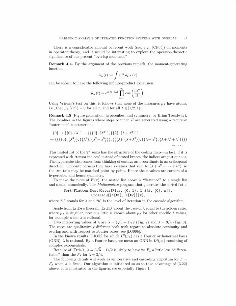
The following details will work as an iterative and cascading algorithm for F =Fλ when λ is fixed. Our algorithm is initialized so as to take advantage of (3.22)above. It is illustrated in the figures; see especially Figure 1.


Proposition 4.6. Let λ be given in the open interval (1/2, 1), and set F = Fλ asa function on R. Conclusions:

(a) Then the function x→ F (x) in (4.2) satisfies

(4.8) F (x) =1

2

(

F(x

λ

)

+ F

(x− λ

λ

))

;

or equivalently, for expansive scaling number s = 1/λ,

F (x) =1

2(F (sx) + F (sx− 1)) .

(b) Then the following iterative and cascading algorithm holds: Initializing F0

by setting F0 to be the Heaviside function

F0 (x) = 0 for x < 0, and

F0 (x) = 1 for x ≥ 0,

we get the following recursion: F0, F1, . . . , etc., with

(4.9) Fn+1 (x) =1

2(Fn (sx) + Fn (sx− 1)) , n = 0, 1, 2, . . . ,

or equivalently

Fn+1 (x) =1

2

(

Fn

(x

λ

)

+ Fn

(x− λ

λ

))

.

Moreover, Fn (x) = 1 holds for x > λ/(1 − λ), and for all n; and thesequence Fn is convergent pointwise in the closed interval

(4.10) X = Xλ =

[

0,λ

1 − λ

]

=

[

0,1

s− 1

]

.

For each x, this convergence is monotone, and

F (x) = infnFn (x) .

Proof. The scaling identity (4.8) follows from the following facts (see [Hut81]): Thelimit formula (3.6); the fixed-point property (3.3), i.e., T (µ) = µ; and the fact thatthe equilibrium measure µ is supported in the closed interval

X = Xλ =

[

0,λ

1 − λ

]

.

See also formula (3.22).Ad (a): Specifically, for x ∈ Xλ, we have

F (x) =by (4.2)

∫

Xλ

χ[ 0,x ] (y) dµ (y)

=by (4.1)

1

2

(∫ λ

1−λ

0

χ[ 0,x ] (τ0 (y)) dµ (y) +

∫ λ

1−λ

0

χ[ 0,x ] (τ1 (y)) dµ (y)

)

=supp(µ)⊂Xλ

1

2

(∫ x

λ

0

dµ (y) +

∫ x−λ

λ

0

dµ (y)

)

=by (4.2)

1

2

(

F(x

λ

)

+ F

(x− λ

λ

))

.


1

1/2

0 λ 1 b

(a). n = 0

1

1/2

0 λ 1 b

(b). n = 1

1

1/2

0 λ 1 b

(c). n = 2

1

1/2

0 λ 1 b′ b

(d). n = 3

Figure 1. The series of cascade approximants Fn, n = 0, 1, 2, . . . ,to the cumulative distribution function Fλ in the case when λ =(√

5 − 1)/2. The marks on the horizontal axis in addition to λ

and 1 are b′ = λ + λ2 + · · · + λn, the endpoint of the support ofthe n’th cascade iteration Fn, and b = λ/(1 − λ), the endpoint ofthe support of Fλ. In the case of F3 for this particular “golden”value of λ, it may be observed that the set of node-points N3 (λ) =0, λ3, λ2, λ, λ+ λ3, λ+ λ2, 2λ

, and #N3 (λ) = 7, not 8: one of

the steps is doubled, due to the fact that λ2 + λ3 = λ.

For the evaluation of the second integral, note: τ1 (y) ∈ [ 0, x ] ⇐⇒ −1 ≤ y ≤ x−λλ .

But since supp (µ) ⊂ Xλ, we get that

∫ x−λ

λ

−1

dµ (y) =

∫ x−λ

λ

0

dµ (y) .

Ad (b): Figures 1(a), (b), (c), . . . are sketches of the successive functions F0,

F1, F2, . . . in the case of λ =√

5−12 , i.e., the reciprocal of the golden ratio φ =

(√5 + 1

)/2.

As indicated, the sequence is monotone, i.e., Fn+1 (x) ≤ Fn (x) holds; as will beproved.

We now prove the assertion Fn (x) ≡ 1 for all n and all x > λ/ (1 − λ) =λ+ λ2 + λ3 + · · · . As before, λ ∈ (1/2, 1) is fixed, and λ/ (1 − λ) is the right-handendpoint in the interval Xλ.

The assertion follows by induction. It holds for F0 since F0 is the Heavisidefunction. Now suppose it holds for n. Let x > λ/ (1 − λ) be given. Then

x

λ>

1

1 − λ>

λ

1 − λ,


and

x− λ

λ>

λ1−λ − λ

λ=

λ

1 − λ;

so

Fn+1 (x) =1

2

(

Fn

(x

λ

)

+ Fn

(x− λ

λ

))

=1

2(1 + 1) = 1,

completing the induction.The separate assertion about pointwise convergence

(4.11) limn→∞

Fn (x) = F (x)

follows from the stronger fact: For each x, the sequence (Fn (x))n is monotone, i.e.,

(4.12) Fn (x) ≤ Fn−1 (x) .

Induction: Clearly (4.12) holds if n = 1. Now suppose it holds up to n. Then bythe recursion,

Fn(x)−Fn+1(x) =1

2

((

Fn−1

(x

λ

)

− Fn

(x

λ

))

+

(

Fn−1

(x− λ

λ

)

− Fn

(x− λ

λ

)))

.

The conclusion (4.12) now follows for n+ 1, and the proof is complete.

4.2. Measuring overlap.

Remark 4.7. The three figures Figs. 1(a), (b), (c) taken by themselves offer anoversimplification in that the ordering of the node-points

Nn (λ) :=ω1λ+ ω2λ

2 + · · · + ωnλn | ωi ∈ 0, 1

is unique only up to n = 2, i.e.,

0 < λ2 < λ < λ+ λ2

holds for all λ ∈ (1/2, 1). But in general for n > 2, the ordering of the 2n points inNn (λ) is subtle. For example, for n = 3, we have

(4.13)

λ < λ2 + λ3 if λ >

√5 − 1

2,

λ = λ2 + λ3 if λ =

√5 − 1

2,

λ > λ2 + λ3 if λ <

√5 − 1

2,

indicating that even in N3 order-reversal may occur depending on the chosen valueof λ in (1/2, 1).

The list in (4.13) further shows that the points in each set Nn (λ) for n > 2typically occur with multiplicity.

The assertion in (4.13) for the special case λ =(√

5 − 1)/2 states that

π (1000 . . . ) = π (011000 . . . ) ,

where π = πλ is the encoding mapping πλ : Ω → Xλ from Lemma 3.3 and (3.21).While it is known that for all λ ∈ (1/2, 1), πλ is ∞–1, the infinite sets π−1

λ (x) arenot well understood.


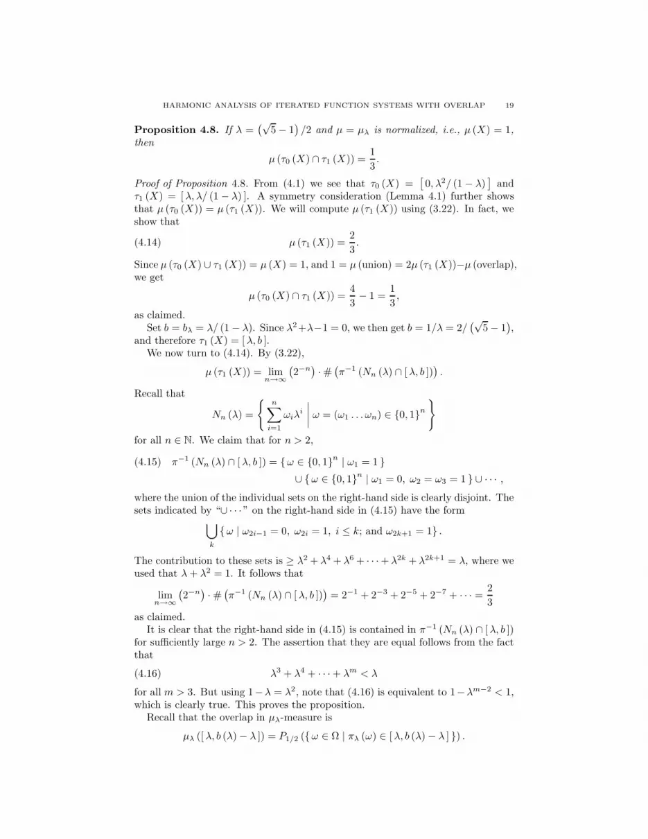
Proposition 4.8. If λ =(√

5 − 1)/2 and µ = µλ is normalized, i.e., µ (X) = 1,

then

µ (τ0 (X) ∩ τ1 (X)) =1

3.

Proof of Proposition 4.8. From (4.1) we see that τ0 (X) =[0, λ2/ (1 − λ)

]and

τ1 (X) = [λ, λ/ (1 − λ) ]. A symmetry consideration (Lemma 4.1) further showsthat µ (τ0 (X)) = µ (τ1 (X)). We will compute µ (τ1 (X)) using (3.22). In fact, weshow that

(4.14) µ (τ1 (X)) =2

3.

Since µ (τ0 (X) ∪ τ1 (X)) = µ (X) = 1, and 1 = µ (union) = 2µ (τ1 (X))−µ (overlap),we get

µ (τ0 (X) ∩ τ1 (X)) =4

3− 1 =

1

3,

as claimed.Set b = bλ = λ/ (1 − λ). Since λ2+λ−1 = 0, we then get b = 1/λ = 2/

(√5 − 1

),

and therefore τ1 (X) = [λ, b ].We now turn to (4.14). By (3.22),

µ (τ1 (X)) = limn→∞

(2−n

)· #(π−1 (Nn (λ) ∩ [λ, b ])

).

Recall that

Nn (λ) =

n∑

i=1

ωiλi

∣∣∣∣ω = (ω1 . . . ωn) ∈ 0, 1n

for all n ∈ N. We claim that for n > 2,

(4.15) π−1 (Nn (λ) ∩ [λ, b ]) = ω ∈ 0, 1n | ω1 = 1 ∪ ω ∈ 0, 1n | ω1 = 0, ω2 = ω3 = 1 ∪ · · · ,

where the union of the individual sets on the right-hand side is clearly disjoint. Thesets indicated by “∪ · · · ” on the right-hand side in (4.15) have the form

⋃

k

ω | ω2i−1 = 0, ω2i = 1, i ≤ k; and ω2k+1 = 1 .

The contribution to these sets is ≥ λ2 + λ4 + λ6 + · · ·+ λ2k + λ2k+1 = λ, where weused that λ+ λ2 = 1. It follows that

limn→∞

(2−n

)· #(π−1 (Nn (λ) ∩ [λ, b ])

)= 2−1 + 2−3 + 2−5 + 2−7 + · · · =

2

3

as claimed.It is clear that the right-hand side in (4.15) is contained in π−1 (Nn (λ) ∩ [λ, b ])

for sufficiently large n > 2. The assertion that they are equal follows from the factthat

(4.16) λ3 + λ4 + · · · + λm < λ

for all m > 3. But using 1−λ = λ2, note that (4.16) is equivalent to 1−λm−2 < 1,which is clearly true. This proves the proposition.

Recall that the overlap in µλ-measure is

µλ ([λ, b (λ) − λ ]) = P1/2 (ω ∈ Ω | πλ (ω) ∈ [λ, b (λ) − λ ] ) .


This means that the contributions to π−1λ ([λ, b (λ) − λ ]) with P1/2-measure equal

to zero may be omitted in the accounting (4.15) above.

However, even for λ =(√

5 − 1)/2, even the infinite set π−1

λ (λ) has interestingdynamics. But its contribution to the overlap in µ-measure is

µλ (λ) = 0;

see also Remark 4.4.

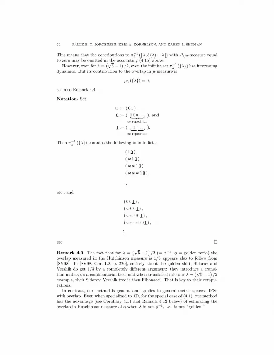
Notation. Set

w := ( 0 1 ) ,

0 := ( 0 0 0 . . .︸︷︷︸

∞ repetition

), and

1 := ( 1 1 1 . . .︸︷︷︸

∞ repetition

).

Then π−1λ (λ) contains the following infinite lists:

( 1 0 ) ,

(w 1 0 ) ,

(ww 1 0 ) ,

(www 1 0 ) ,

...,

etc., and

( 0 0 1 ) ,

(w 0 0 1 ) ,

(ww 0 0 1 ) ,

(www 0 0 1 ) ,

...,

etc.

Remark 4.9. The fact that for λ =(√

5 − 1)/2 (= φ−1, φ = golden ratio) the

overlap measured in the Hutchinson measure is 1/3 appears also to follow from[SV98]. In [SV98, Cor. 1.2, p. 220], entirely about the golden shift, Sidorov andVershik do get 1/3 by a completely different argument: they introduce a transi-

tion matrix on a combinatorial tree, and when translated into our λ =(√

5 − 1)/2

example, their Sidorov–Vershik tree is then Fibonacci. That is key to their compu-tations.

In contrast, our method is general and applies to general metric spaces: IFSswith overlap. Even when specialized to 1D, for the special case of (4.1), our methodhas the advantage (see Corollary 4.11 and Remark 4.12 below) of estimating theoverlap in Hutchinson measure also when λ is not φ−1, i.e., is not “golden.”


Remarks 4.10. (a) The Lebesgue measure of the intersection τ0 (X) ∩ τ1 (X) isλ2

1−λ − λ, which for λ =√

5−12 works out to

Leb (τ0 (X) ∩ τ1 (X)) =3 −

√5

2.

(b) Since

3 −√

5

2>

1

3,

we conclude from the proposition that the Hutchinson measure of the intersectionis the smaller of the two.

(c) The argument from the proof of the proposition extends to the IFS τ(λ)k (x) :=

λ (x+ k), k ∈ 0, 1, for all λ ∈ (1/2, 1), and we conclude that there is essential

overlap for all λ in (1/2, 1), but an explicit formula for µλ

(

τ(λ)0 (Xλ) ∩ τ (λ)

1 (Xλ))

(> 0) is not known.

The following is a consequence of the argument in the proof of Proposition 4.8.

Corollary 4.11. (a) For all λ ∈[ (√

5 − 1)/2, 1

)we have

(4.17) µλ

(

τ(λ)0 (Xλ) ∩ τ (λ)

1 (Xλ))

≥ 1

3.

(b) For all λ ∈(1/2,

(√5 − 1

)/2), there is some m, depending on λ, such that

(4.18) λ+ λ2 + λ3 + · · · + λm ≥ 1,

and for such a choice of m we have

(4.19) µλ

(

τ(λ)0 (Xλ) ∩ τ (λ)

1 (Xλ))

≥ 1

2m − 1.

Remark 4.12. If λ =(√

5 − 1)/2, the number m in (4.18) may be taken to be

m = 2, and in that case (4.18) is “=”.

Proof of Corollary 4.11. Ad (a): An easy modification of the argument in the proofof Proposition 4.8 shows that if λ2 + λ > 1, then (4.17) holds.

Ad (b): Let λ ∈(1/2,

(√5 − 1

)/2)

be given. It follows from algebra that if m issufficiently large, then (4.18) must hold. We pick m to be the first number whichgets the sum on the left-hand side in (4.18) ≥ 1.

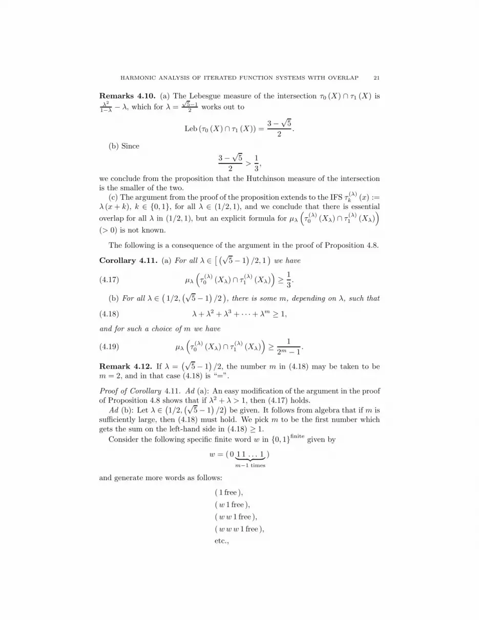
Consider the following specific finite word w in 0, 1finitegiven by

w = ( 0 1 1 . . . 1︸︷︷︸

m−1 times

)

and generate more words as follows:

( 1 free ),

(w 1 free ),

(ww 1 free ),

(www 1 free ),

etc.,


where “free” means unrestricted strings of bits. As before, the resulting sequenceof subsets in Ω is disjoint. Then

µλ

(

τ(λ)1 (Xλ)

)

≥ 2−1 +2−m−1 +2−2m−1 +2−3m−1 + · · · = 2−1 1

1 − 2−m=

2m−1

2m − 1.

The argument from the proposition yields

µλ

(

τ(λ)0 (Xλ) ∩ τ (λ)

1 (Xλ))

≥ 2m

2m − 1− 1 =

1

2m − 1,

which is the assertion (4.19).

Cascade approximation. Each function F(λ)n from the approximation to the cu-

mulative distribution in Proposition 4.6 has a finite set of node points Nn(λ), and

#Nn(λ) ≤ 2n for all n;

but for fixed λ, the configuration of points in Nn(λ) can be complicated for n > 2and large; and each set Nn(λ) also depends on the particular numerical choice of avalue for λ.

This is borne out in the cascade of figures (see Figure 1) made for λ = (√

5−1)/2.

We have included pictures of F(λ)1 , F

(λ)2 , . . . , up to F

(λ)4 . As sketched in Remark

4.7, the reason is that the detailed configuration and the multiplicities in the setsNn(λ) of node points are reflected in the progression of graphs of the functions

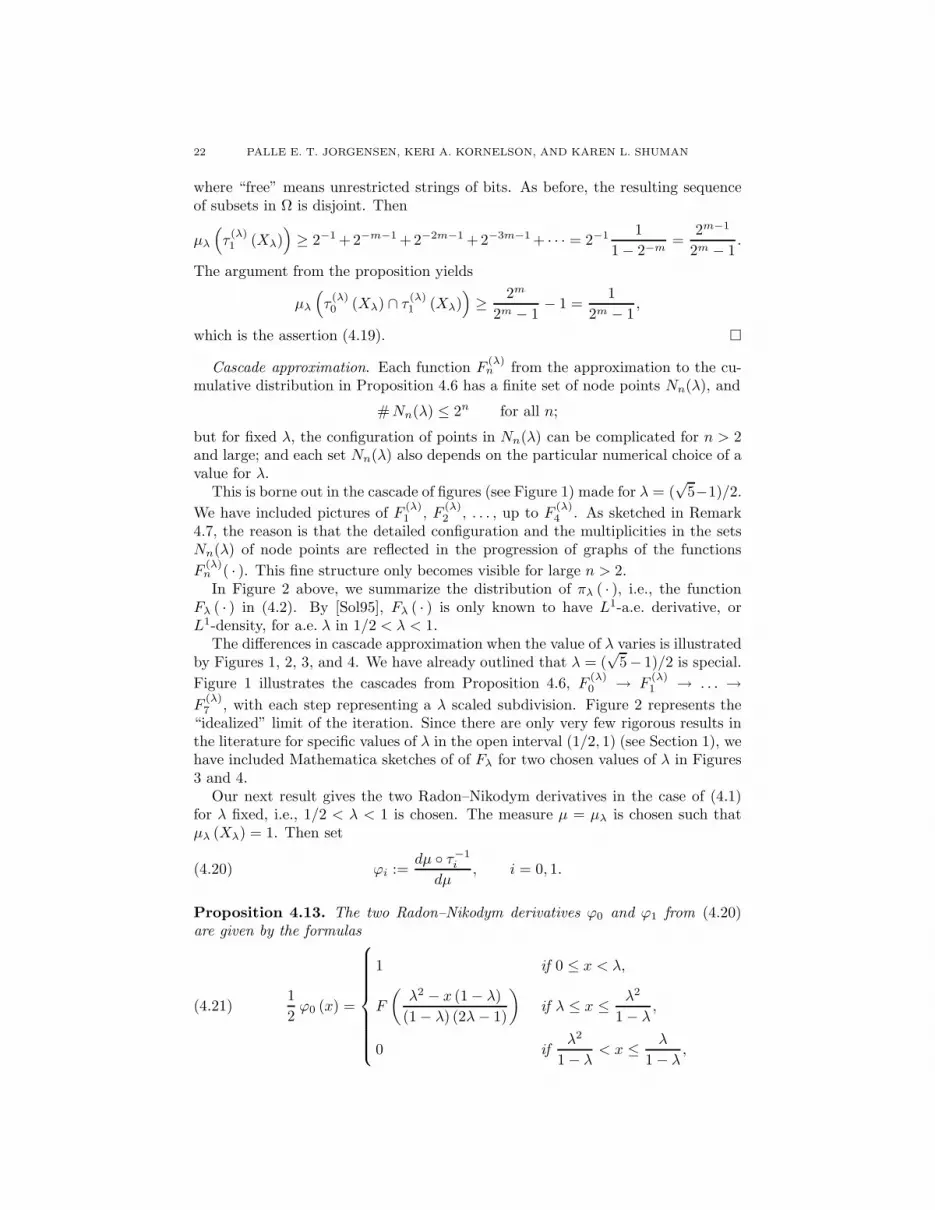
F(λ)n ( · ). This fine structure only becomes visible for large n > 2.In Figure 2 above, we summarize the distribution of πλ ( · ), i.e., the function

Fλ ( · ) in (4.2). By [Sol95], Fλ ( · ) is only known to have L1-a.e. derivative, orL1-density, for a.e. λ in 1/2 < λ < 1.

The differences in cascade approximation when the value of λ varies is illustratedby Figures 1, 2, 3, and 4. We have already outlined that λ = (

√5− 1)/2 is special.

Figure 1 illustrates the cascades from Proposition 4.6, F(λ)0 → F

(λ)1 → . . . →

F(λ)7 , with each step representing a λ scaled subdivision. Figure 2 represents the

“idealized” limit of the iteration. Since there are only very few rigorous results inthe literature for specific values of λ in the open interval (1/2, 1) (see Section 1), wehave included Mathematica sketches of of Fλ for two chosen values of λ in Figures3 and 4.

Our next result gives the two Radon–Nikodym derivatives in the case of (4.1)for λ fixed, i.e., 1/2 < λ < 1 is chosen. The measure µ = µλ is chosen such thatµλ (Xλ) = 1. Then set

(4.20) ϕi :=dµ τ−1

i

dµ, i = 0, 1.

Proposition 4.13. The two Radon–Nikodym derivatives ϕ0 and ϕ1 from (4.20)are given by the formulas

1

2ϕ0 (x) =

1 if 0 ≤ x < λ,

F

(λ2 − x (1 − λ)

(1 − λ) (2λ− 1)

)

if λ ≤ x ≤ λ2

1 − λ,

0 ifλ2

1 − λ< x ≤ λ

1 − λ,

(4.21)


Fλ ( · )

1

0 λ1−λ

x

︸︷︷︸

Xλ

Figure 2. The cumulative distribution of πλ ( · ), where λ = (√

5−1)/2. Caution: A closed formula for Fλ ( · ) is not known. But usingthe second formula in (4.1) and (4.2), the reader may check that forfixed λ, the cumulative distribution F (= Fλ) satisfies the scalingidentity F (x) = 1

2 (F (x/λ) + F ((x − λ)/λ)).

1

1/2

0 λ 1 a b′,b

Figure 3. λ = 3/4

and

1

2ϕ1 (x) =

0 if 0 ≤ x < λ,

F

((x− λ)

(2λ− 1)

)

if λ ≤ x ≤ λ2

1 − λ,

1 ifλ2

1 − λ< x ≤ λ

1 − λ.

(4.22)


1

1/2

0 λ,1 ab′ b

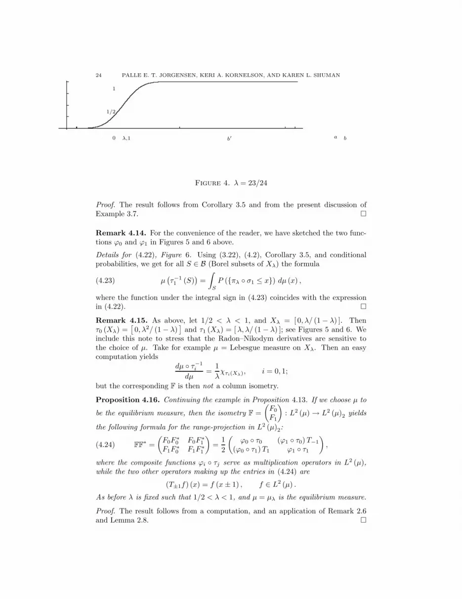
Figure 4. λ = 23/24

Proof. The result follows from Corollary 3.5 and from the present discussion ofExample 3.7.

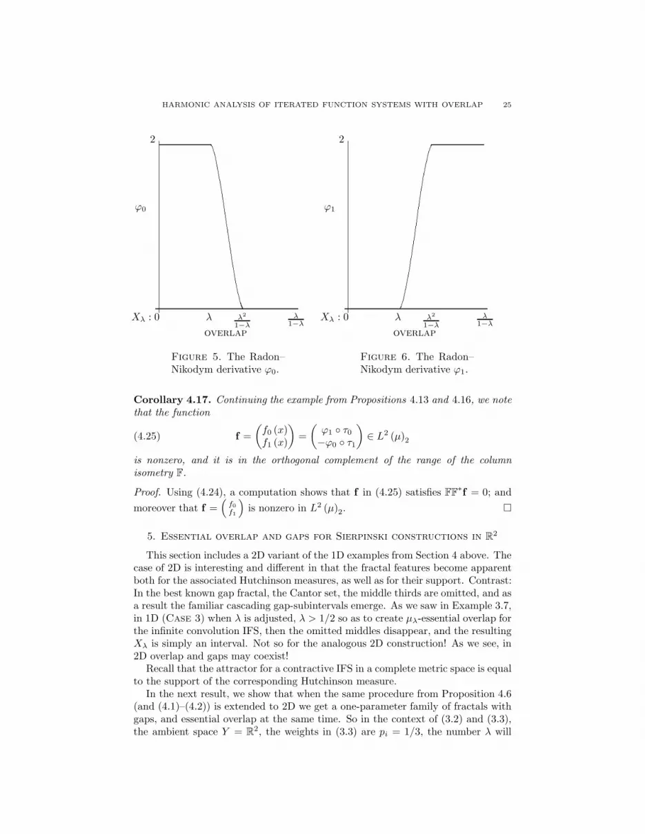
Remark 4.14. For the convenience of the reader, we have sketched the two func-tions ϕ0 and ϕ1 in Figures 5 and 6 above.

Details for (4.22), Figure 6. Using (3.22), (4.2), Corollary 3.5, and conditionalprobabilities, we get for all S ∈ B (Borel subsets of Xλ) the formula

(4.23) µ(τ−11 (S)

)=

∫

S

P (πλ σ1 ≤ x) dµ (x) ,

where the function under the integral sign in (4.23) coincides with the expressionin (4.22).

Remark 4.15. As above, let 1/2 < λ < 1, and Xλ = [ 0, λ/ (1 − λ) ]. Thenτ0 (Xλ) =

[0, λ2/ (1 − λ)

]and τ1 (Xλ) = [λ, λ/ (1 − λ) ]; see Figures 5 and 6. We

include this note to stress that the Radon–Nikodym derivatives are sensitive tothe choice of µ. Take for example µ = Lebesgue measure on Xλ. Then an easycomputation yields

dµ τ−1i

dµ=

1

λχτi(Xλ), i = 0, 1;

but the corresponding F is then not a column isometry.

Proposition 4.16. Continuing the example in Proposition 4.13. If we choose µ to

be the equilibrium measure, then the isometry F =

(F0

F1

)

: L2 (µ) → L2 (µ)2 yields

the following formula for the range-projection in L2 (µ)2:

(4.24) FF∗ =

(F0F

∗0 F0F

∗1

F1F∗0 F1F

∗1

)

=1

2

(ϕ0 τ0 (ϕ1 τ0) T−1

(ϕ0 τ1)T1 ϕ1 τ1

)

,

where the composite functions ϕi τj serve as multiplication operators in L2 (µ),while the two other operators making up the entries in (4.24) are

(T±1f) (x) = f (x± 1) , f ∈ L2 (µ) .

As before λ is fixed such that 1/2 < λ < 1, and µ = µλ is the equilibrium measure.

Proof. The result follows from a computation, and an application of Remark 2.6and Lemma 2.8.


ϕ0

2

Xλ : 0 λ1−λ

λ2

1−λλ

overlap

Figure 5. The Radon–Nikodym derivative ϕ0.

ϕ1

2

Xλ : 0 λ1−λ

λ2

1−λλ

overlap

Figure 6. The Radon–Nikodym derivative ϕ1.

Corollary 4.17. Continuing the example from Propositions 4.13 and 4.16, we notethat the function

(4.25) f =

(f0 (x)f1 (x)

)

=

(ϕ1 τ0−ϕ0 τ1

)

∈ L2 (µ)2

is nonzero, and it is in the orthogonal complement of the range of the columnisometry F.

Proof. Using (4.24), a computation shows that f in (4.25) satisfies FF∗f = 0; and

moreover that f =(

f0

f1

)

is nonzero in L2 (µ)2.

5. Essential overlap and gaps for Sierpinski constructions in R2

This section includes a 2D variant of the 1D examples from Section 4 above. Thecase of 2D is interesting and different in that the fractal features become apparentboth for the associated Hutchinson measures, as well as for their support. Contrast:In the best known gap fractal, the Cantor set, the middle thirds are omitted, and asa result the familiar cascading gap-subintervals emerge. As we saw in Example 3.7,in 1D (Case 3) when λ is adjusted, λ > 1/2 so as to create µλ-essential overlap forthe infinite convolution IFS, then the omitted middles disappear, and the resultingXλ is simply an interval. Not so for the analogous 2D construction! As we see, in2D overlap and gaps may coexist!

Recall that the attractor for a contractive IFS in a complete metric space is equalto the support of the corresponding Hutchinson measure.

In the next result, we show that when the same procedure from Proposition 4.6(and (4.1)–(4.2)) is extended to 2D we get a one-parameter family of fractals withgaps, and essential overlap at the same time. So in the context of (3.2) and (3.3),the ambient space Y = R

2, the weights in (3.3) are pi = 1/3, the number λ will


(a). n = 1 (b). n = 2

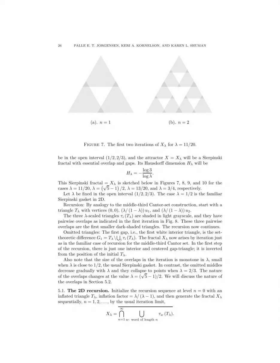
Figure 7. The first two iterations of Xλ for λ = 11/20.

be in the open interval (1/2, 2/3), and the attractor X = Xλ will be a Sierpinskifractal with essential overlap and gaps. Its Hausdorff dimension Hλ will be

Hλ = − log 3

logλ.

This Sierpinski fractal = Xλ is sketched below in Figures 7, 8, 9, and 10 for thecases λ = 11/20, λ =

(√5 − 1

)/2, λ = 13/20, and λ = 3/4, respectively.

Let λ be fixed in the open interval (1/2, 2/3). The case λ = 1/2 is the familiarSierpinski gasket in 2D.

Recursion: By analogy to the middle-third Cantor-set construction, start with atriangle Tλ with vertices (0, 0), (λ/ (1 − λ))u1, and (λ/ (1 − λ))u2.

The three λ-scaled triangles τi (Tλ) are shaded in light grayscale, and they havepairwise overlaps as indicated in the first iteration in Fig. 8. These three pairwiseoverlaps are the first smaller dark-shaded triangles. The recursion now continues.

Omitted triangles: The first gap, i.e., the first white interior triangle, is the set-theoretic difference G1 = Tλ\

⋃

i τi (Tλ). The fractal Xλ now arises by iteration justas in the familiar case of recursion for the middle-third Cantor set. In the first stepof the recursion, there is just one interior and centered gap-triangle; it is invertedfrom the position of the initial Tλ.

Also note that the size of the overlaps in the iteration is monotone in λ, smallwhen λ is close to 1/2, the usual Sierpinski gasket. In contrast, the omitted middlesdecrease gradually with λ and they collapse to points when λ = 2/3. The nature

of the overlaps changes at the value λ = (√

5 − 1)/2. We will discuss the nature ofthe overlaps in Section 5.2.

5.1. The 2D recursion. Initialize the recursion sequence at level n = 0 with aninflated triangle Tλ, inflation factor = λ/ (λ− 1), and then generate the fractal Xλ

sequentially, n = 1, 2, . . . , by the usual iteration limit,

Xλ =∞⋂

n=1

⋃

w: word of length n

τw (Tλ).


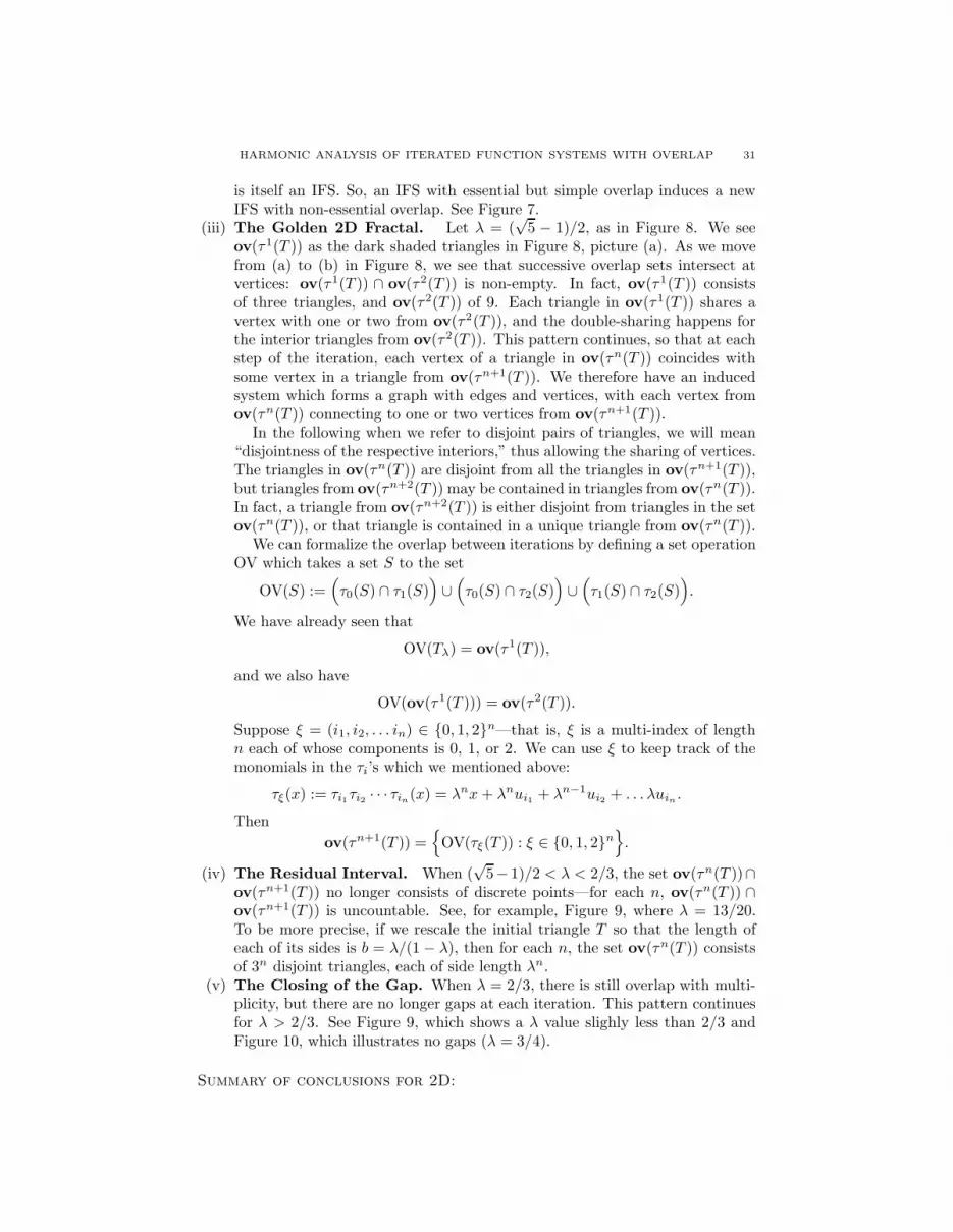
(a). n = 1 (b). n = 2

Figure 8. The first two iterations of Xλ for λ = (√

5 − 1)/2. SeeExample 5.1.

Here τw denotes an n-fold composition of the individual τi maps with the indices Imaking up the word w, i.e., w giving the address of the respective “small” trianglesτw (Tλ) for the n’th level iteration:

τi (x) = λ (x+ ui) , i = 0, 1, 2, x ∈ R2,

τw = τi1 · · · τinif w = (i1, . . . , in) .

Example 5.1. 2D Sierpinski with overlap and gaps, 1/2 < λ < 2/3. Let thevectors u0, u1, u2 in R

2 be given as follows:

(5.1)

u0 = (0, 0) ,

u1 = (1, 0) , and

u2 =

(

1

2,

√3

2

)

, and set

(5.2) Ω = u0, u1, u2N

with Bernoulli measure P1/3 corresponding to the infinite-product measure pi =1/3, i = 0, 1, 2, as in (3.3) and Corollary 3.4. We will denote by µλ the measure inCorollary 3.5, and we set Xλ := supp (µλ).

The IFS is

(5.3)

τ(λ)0 (x) = λx,

τ(λ)1 (x) = λ (x+ u1) , and

τ(λ)2 (x) = λ (x+ u2)

for x ∈ R2. Here we make the restriction 1/2 < λ < 2/3. As noted in Section 3,

(5.4) Xλ =

2⋃

i=0

τ(λ)i (Xλ)


and Xλ is the unique compact (6= ∅) solution to (5.4).

Let Ω := 0, u1, u2N, and let P1/3 be the usual Bernoulli measure on Ω withequal and independent probabilities (1/3, 1/3, 1/3). The formula (3.21) for therandom variable πλ : Ω → Xλ extends from 1D to 2D with the only modificationthat the coefficients ωi from (3.21) now take values in the finite alphabet of vectors0, u1, u2.

Let Aλi , i = 0, 1, 2 be the three vertices in Xλ (Figure 8); i.e. Aλ

0 = (0, 0),Aλ

1 = λ1−λu1, and Aλ

2 = λ1−λu2. Note that for each λ ∈ (1/2, 1), Xλ is contained in

the triangle Tλ with the vertices Aλi , i = 0, 1, 2.

Our first result concerns symmetry, and it is an immediate extension of Lemma4.1 from the 1D case to the 2D case. For each i ∈ 0, 1, 2, let Sλ

i (x) denote theequilateral triangle of side-length x with vertex Aλ

i , which shares two sides withsegments of sides in Tλ. Then the argument from Lemma 4.1 shows that for eachx ∈ R+, the three numbers

P1/3ω ∈ Ω|πλ(ω) ∈ Sλi (x)

coincide. Since µλ = P1/3 π−1λ by Corollary 3.5, we conclude in particular that

the three numbers µλ(τ(λ)i (Xλ) agree for i = 0, 1, 2.

For i 6= j, set

OV λij := τ

(λ)i (Xλ) ∩ τ (λ)

j (Xλ).

It follows that

µλ(OV λ01) = µλ(OV λ

02) = µλ(OV λ12).

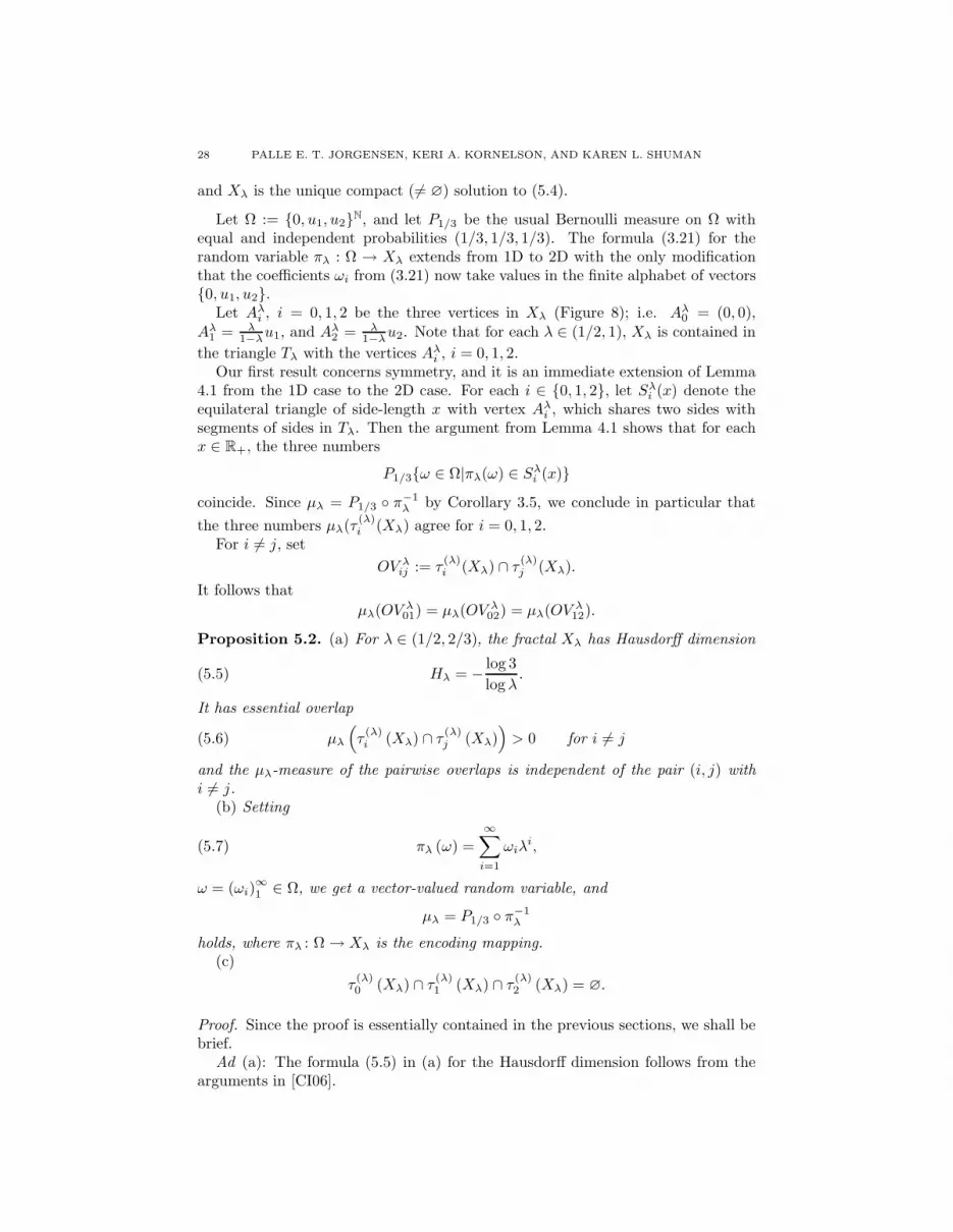
Proposition 5.2. (a) For λ ∈ (1/2, 2/3), the fractal Xλ has Hausdorff dimension

(5.5) Hλ = − log 3

logλ.

It has essential overlap

(5.6) µλ

(

τ(λ)i (Xλ) ∩ τ (λ)

j (Xλ))

> 0 for i 6= j

and the µλ-measure of the pairwise overlaps is independent of the pair (i, j) withi 6= j.

(b) Setting

(5.7) πλ (ω) =

∞∑

i=1

ωiλi,

ω = (ωi)∞1 ∈ Ω, we get a vector-valued random variable, and

µλ = P1/3 π−1λ

holds, where πλ : Ω → Xλ is the encoding mapping.(c)

τ(λ)0 (Xλ) ∩ τ (λ)

1 (Xλ) ∩ τ (λ)2 (Xλ) = ∅.

Proof. Since the proof is essentially contained in the previous sections, we shall bebrief.

Ad (a): The formula (5.5) in (a) for the Hausdorff dimension follows from thearguments in [CI06].


(a). n = 1 (b). n = 2

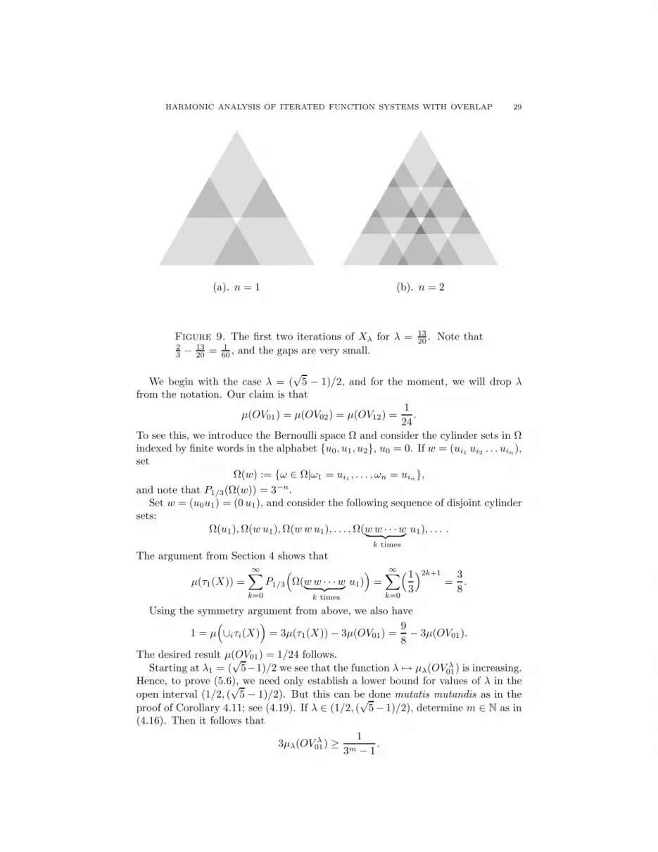
Figure 9. The first two iterations of Xλ for λ = 1320 . Note that

23 − 13

20 = 160 , and the gaps are very small.

We begin with the case λ = (√

5 − 1)/2, and for the moment, we will drop λfrom the notation. Our claim is that

µ(OV01) = µ(OV02) = µ(OV12) =1

24.

To see this, we introduce the Bernoulli space Ω and consider the cylinder sets in Ωindexed by finite words in the alphabet u0, u1, u2, u0 = 0. If w = (ui1 ui2 . . . uin

),set

Ω(w) := ω ∈ Ω|ω1 = ui1 , . . . , ωn = uin,

and note that P1/3(Ω(w)) = 3−n.Set w = (u0u1) = (0 u1), and consider the following sequence of disjoint cylinder

sets:Ω(u1),Ω(w u1),Ω(wwu1), . . . ,Ω(ww · · ·w

︸︷︷︸

k times

u1), . . . .

The argument from Section 4 shows that

µ(τ1(X)) =∞∑

k=0

P1/3

(

Ω(ww · · ·w︸︷︷︸

k times

u1))

=∞∑

k=0

(1

3

)2k+1

=3

8.

Using the symmetry argument from above, we also have

1 = µ(

∪iτi(X))

= 3µ(τ1(X)) − 3µ(OV01) =9

8− 3µ(OV01).

The desired result µ(OV01) = 1/24 follows.

Starting at λ1 = (√

5−1)/2 we see that the function λ 7→ µλ(OV λ01) is increasing.

Hence, to prove (5.6), we need only establish a lower bound for values of λ in the

open interval (1/2, (√

5 − 1)/2). But this can be done mutatis mutandis as in the

proof of Corollary 4.11; see (4.19). If λ ∈ (1/2, (√

5− 1)/2), determine m ∈ N as in(4.16). Then it follows that

3µλ(OV λ01) ≥

1

3m − 1.


Ad (b): The proof of (5.6) in (b) is based on symmetry considerations (Lemma 4.1)extended from 1D to 2D, as well as the estimates in Proposition 4.8, Remarks 4.10,and Corollary 4.11.

Ad (c): To see that the triple overlap is empty, calculate the distances betweenpairwise overlaps to the third sub-partition.

We conclude this section with the following open question: for what values of λin the interval (2/3, 1) is µλ absolutely continuous with respect to the 2-dimensionalLebesgue measure? There are two pieces of partial evidence for absolute continuityof the two-dimensional µλ for a.e. λ ∈ (2/3, 1):

(1) Since the interior gaps close at λ = 2/3, so that for λ ≥ 2/3, Xλ = Tλ (theclosed triangle), following the 1D analogy, it seems reasonable to expect thea.e. conclusion in this range of λ.

(2) One of the proofs [PS96] in the literature for the 1D case introduces a cleverFubini-Tonelli argument with a function in several variables with λ as one of theintegration variables. Using a density argument, one then gets finiteness of acorresponding key functions for a.e. λ in the interval, and this in turn (followingthe 1D analogy) is likely to yield an expression in 2D for the Radon-Nikodymderivative for those values of λ.

In particular, for x ∈ Tλ, let Lℓλ(x) be the equilateral triangle centered at x

with side length ℓ and area√

34 ℓ

2. Define

D(µλ, x) := lim infℓ↓0

µλ(Lℓλ(x))

√3

4 ℓ2

(an analogue of the first formula on [PS96, p. 233]). The argument from [PS96]is likely to yield

∫ 1

2/3

∫∫

Tλ

D(µλ, x) dµλ(x) dλ <∞.

From that we could conclude that λ 7→ D(µλ, x) is finite for a.e. λ ∈ (2/3, 1),putting the Radon-Nikodym derivative of µλ with respect to two-dimensionalLebesgue measure in L2 for a.e. λ.

5.2. The nature of the overlaps and induced systems. As we noted before,the nature of the overlaps changes at the value λ = (

√5 − 1)/2. Here we refer to

overlaps of monomials in the τi’s of degree n = 1, 2, . . . applied to the initial triangleT = Tλ as τn(T ). Let ov(τn(T )) denote overlaps at level n— for example,

ov(τ1(T )) =(

τ0(T ) ∩ τ1(T ))

∪(

τ0(T ) ∩ τ2(T ))

∪(

τ1(T ) ∩ τ2(T ))

.

(i) The Sierpinski Gasket. When λ = 1/2, the resulting fractal Xλ is theSierpinski gasket, and the essential overlap is a set of Lebesgue measure zero[Str06].

(ii) Simple Overlap. When λ ∈ (1/2, (√

5 − 1)/2), we have

ov(τn(T )) ∩ ov(τn+1(T )) = ∅.

We call this type of overlap “overlap of multiplicity one” or “simple overlap.”When simple overlap occurs, the subset of Xλ which consists of the overlaps


is itself an IFS. So, an IFS with essential but simple overlap induces a newIFS with non-essential overlap. See Figure 7.

(iii) The Golden 2D Fractal. Let λ = (√

5 − 1)/2, as in Figure 8. We seeov(τ1(T )) as the dark shaded triangles in Figure 8, picture (a). As we movefrom (a) to (b) in Figure 8, we see that successive overlap sets intersect atvertices: ov(τ1(T )) ∩ ov(τ2(T )) is non-empty. In fact, ov(τ1(T )) consistsof three triangles, and ov(τ2(T )) of 9. Each triangle in ov(τ1(T )) shares avertex with one or two from ov(τ2(T )), and the double-sharing happens forthe interior triangles from ov(τ2(T )). This pattern continues, so that at eachstep of the iteration, each vertex of a triangle in ov(τn(T )) coincides withsome vertex in a triangle from ov(τn+1(T )). We therefore have an inducedsystem which forms a graph with edges and vertices, with each vertex fromov(τn(T )) connecting to one or two vertices from ov(τn+1(T )).

In the following when we refer to disjoint pairs of triangles, we will mean“disjointness of the respective interiors,” thus allowing the sharing of vertices.The triangles in ov(τn(T )) are disjoint from all the triangles in ov(τn+1(T )),but triangles from ov(τn+2(T )) may be contained in triangles from ov(τn(T )).In fact, a triangle from ov(τn+2(T )) is either disjoint from triangles in the setov(τn(T )), or that triangle is contained in a unique triangle from ov(τn(T )).

We can formalize the overlap between iterations by defining a set operationOV which takes a set S to the set

OV(S) :=(

τ0(S) ∩ τ1(S))

∪(

τ0(S) ∩ τ2(S))

∪(

τ1(S) ∩ τ2(S))

.

We have already seen that

OV(Tλ) = ov(τ1(T )),

and we also have

OV(ov(τ1(T ))) = ov(τ2(T )).

Suppose ξ = (i1, i2, . . . in) ∈ 0, 1, 2n—that is, ξ is a multi-index of lengthn each of whose components is 0, 1, or 2. We can use ξ to keep track of themonomials in the τi’s which we mentioned above:

τξ(x) := τi1τi2 · · · τin(x) = λnx+ λnui1 + λn−1ui2 + . . . λuin

.

Then

ov(τn+1(T )) =

OV(τξ(T )) : ξ ∈ 0, 1, 2n

.

(iv) The Residual Interval. When (√

5− 1)/2 < λ < 2/3, the set ov(τn(T ))∩ov(τn+1(T )) no longer consists of discrete points—for each n, ov(τn(T )) ∩ov(τn+1(T )) is uncountable. See, for example, Figure 9, where λ = 13/20.To be more precise, if we rescale the initial triangle T so that the length ofeach of its sides is b = λ/(1 − λ), then for each n, the set ov(τn(T )) consistsof 3n disjoint triangles, each of side length λn.

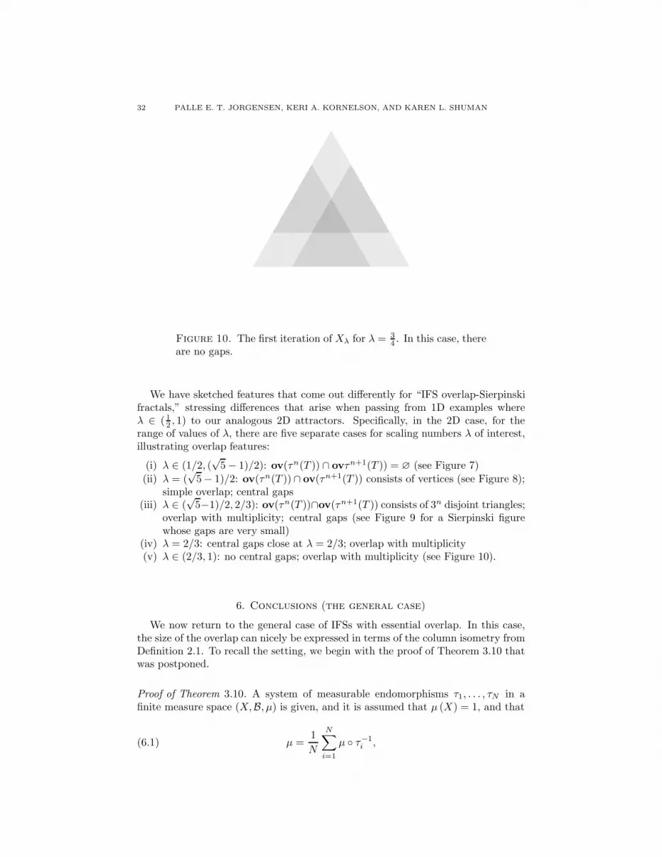
(v) The Closing of the Gap. When λ = 2/3, there is still overlap with multi-plicity, but there are no longer gaps at each iteration. This pattern continuesfor λ > 2/3. See Figure 9, which shows a λ value slighly less than 2/3 andFigure 10, which illustrates no gaps (λ = 3/4).

Summary of conclusions for 2D:


Figure 10. The first iteration of Xλ for λ = 34 . In this case, there

are no gaps.

We have sketched features that come out differently for “IFS overlap-Sierpinskifractals,” stressing differences that arise when passing from 1D examples whereλ ∈ (1

2 , 1) to our analogous 2D attractors. Specifically, in the 2D case, for therange of values of λ, there are five separate cases for scaling numbers λ of interest,illustrating overlap features:

(i) λ ∈ (1/2, (√

5 − 1)/2): ov(τn(T )) ∩ ovτn+1(T )) = ∅ (see Figure 7)

(ii) λ = (√

5 − 1)/2: ov(τn(T )) ∩ ov(τn+1(T )) consists of vertices (see Figure 8);simple overlap; central gaps

(iii) λ ∈ (√

5−1)/2, 2/3): ov(τn(T ))∩ov(τn+1(T )) consists of 3n disjoint triangles;overlap with multiplicity; central gaps (see Figure 9 for a Sierpinski figurewhose gaps are very small)

(iv) λ = 2/3: central gaps close at λ = 2/3; overlap with multiplicity(v) λ ∈ (2/3, 1): no central gaps; overlap with multiplicity (see Figure 10).

6. Conclusions (the general case)

We now return to the general case of IFSs with essential overlap. In this case,the size of the overlap can nicely be expressed in terms of the column isometry fromDefinition 2.1. To recall the setting, we begin with the proof of Theorem 3.10 thatwas postponed.

Proof of Theorem 3.10. A system of measurable endomorphisms τ1, . . . , τN in afinite measure space (X,B, µ) is given, and it is assumed that µ (X) = 1, and that

(6.1) µ =1

N

N∑

i=1

µ τ−1i ,


i.e., that µ is a (τi)-equilibrium measure. It then follows from Proposition 2.10 that

the operators Fi : f 7→ 1√Nf τi define a column isometry, i.e., that F =

(F1

...FN

)

satisfies F∗F = IL2(µ).

Note that this identity spells out to

(6.2)

N∑

i=1

F ∗i Fi = IL2(µ),

but that in general, the individual operators F ∗i Fi are not projections. We have

the lemma:

Lemma 6.1. Let (τi)Ni=1, µ, F = (Fi)

Ni=1 be as above, i.e., F is a column isometry

L2 (µ) → L2 (µ)N . Let ϕi :=dµτ−1

i

dµ . Then

(6.3) F ∗i Fi =

1

NMϕi

where Mϕiis the multiplication operator f 7→ ϕif in L2 (µ).

Proof. The result follows essentially from the argument in Lemma 2.8 above. Bythat argument we may pass to partitions of X . Let i be given, fixed; and, followingLemma 2.8, pass to a subset E in X such that there is a measurable mappingσE : τi (E) → E with

(6.4) σE τi|E = idE ;

see (2.13).It follows that

F ∗i Fif |E =

1

Nϕif |E

for all f ∈ L2 (µ). But the set E is part of a finite measurable partition of X , sothe desired conclusion (6.3) holds on X .

Proof of Theorem 3.10 continued. Our assertion is that FF∗ =

(FiF

∗j

)N

i,j=1is the

identity operator in L2 (µ)N if and only if the system is essential non-overlap.

Setting ϕi :=dµτ−1

i

dµ and using Lemma 2.8 we show that there are measurable

and invertible point transformations Ti,j : X → X , i, j = 1, . . . , N , such that Ti,i =idX , 1 ≤ i ≤ N , and

(6.5) FiF∗j =

1

N(ϕj τi)Ti,j .

But, for each i, the function ϕi is supported on τi (X). So if

(6.6) FiF∗j = δi,jIL2(µ),

then

ϕi ≡ N µ-a.e. on τi (X)

and

ϕi ≡ 0 µ-a.e. on X \ τi (X) =⋃

k 6=i

τk (X) .


The conclusion of the theorem is immediate from this; and we get the followingcorollary.

Corollary 6.2. Let the IFS (τi)Ni=1 be as specified in Theorem 3.10 above, and let

F : L2 (µ) → L2 (µ)N be the corresponding column isometry, with Fi : f 7→ 1√Nf τi.

Then F maps onto L2 (µ)N if and only

(6.7) (F ∗i f) =

√Nχτi(X) (x) f (σi (x)) µ-a.e. x ∈ X.

(Here the endomorphisms σi : X → X are specified in Lemma 2.8, and in par-ticular σi τi = idX , 1 ≤ i ≤ N .)

Theorem 6.3. Let N ∈ N, N ≥ 2, be given, and let (τi)i∈ZNbe a contractive IFS

in a complete metric space. let (X,µ) be the Hutchinson data; see Definition 3.1.Let P (= P1/N ) be the Bernoulli measure on Ω =

∏∞1 ZN = Z

N

N ; see Corollary 3.5.Let π : Ω → X be the encoding mapping of Lemma 3.3. Set

Fif :=1√Nf τi for f ∈ L2 (X,µ)(6.8)

and

S∗i ψ :=

1√Nψ σi for ψ ∈ L2 (Ω, P ) ,(6.9)

where σi denotes the shift map of (3.7).(a) Then the operator V : L2 (X,µ) → L2 (Ω, P ) given by

(6.10) V f = f π

is isometric.(b) The following intertwining relations hold:

(6.11) V Fi = S∗i V, i ∈ ZN .

(c) The isometric extension L2 (X,µ) → L2 (Ω, P ) of the (Fi)-relations is mini-mal in the sense that L2 (Ω, P ) is the closure of

(6.12)⋃

n

⋃

i1i2...in

Si1Si2 · · ·SinV L2 (X,µ) .

Proof. Ad (a)–(b): Let f ∈ L2 (X,µ), and let ‖ · ‖µ and ‖ · ‖P denote the respective

L2-norms in L2 (µ) and L2 (P ). Then

‖V f‖2P =

∫

Ω

|f π|2 dP

=

∫

X

|f |2 d(P π−1

)

=by (3.13)

∫

X

|f |2 dµ = ‖f‖2µ .


Moreover,

V Fif = (Fif) π

=1√Nf τi π

=by (3.11)

1√Nf π σi

= S∗i V f,

which is assertion (b).Ad (c): Let ψ ∈ L2 (Ω, P ), and let 〈 · | · 〉µ and 〈 · | · 〉P denote the respective

Hilbert inner products of L2 (µ) and L2 (P ). To show that the space in (6.12) isdense in L2 (P ), suppose

(6.13) 0 = 〈Si1 · · ·SinV f | ψ 〉P

for all n, all multi-indices (i1 . . . in), and all f ∈ L2 (µ). We will prove that thenψ = 0.

When (i1 . . . in) is fixed, we denote the cylinder set in Ω by

(6.14) C (i1, . . . , in) = ω ∈ Ω | ωj = ij, 1 ≤ j ≤ n .Using now (6.7) in Corollary 6.2 on Ω, we get

S∗in· · ·S∗

i1ψ = N−n/2ψ σi1 · · · σin.

Substitution into (6.13) yields∫

Ω

χC(i1,...,in)ψ dP = 0.

We used the fact that (6.13) holds for all f ∈ L2 (µ). But the indicator functionsχC(i1,...,in) span a dense subspace in L2 (Ω, P ) when n varies, and all finite words oflength n are used. We conclude that ψ = 0, and therefore that the space in (6.12)is dense in L2 (Ω, P ).

Remark 6.4. Note that by (6.11) the space in (6.12), part (c) of the theorem, isinvariant under the operators S∗

i .

Acknowledgements. We are pleased to thank Dorin Dutkay for helpful conversa-tions. We thank Brian Treadway for excellent typesetting, and for producing thegraphics.

References

[Arv04] W. Arveson. The free cover of a row contraction. Doc. Math., 9:137–161, 2004.[Bar06] M. Barnsley. SuperFractals. Cambridge University Press, Cambridge, 2006.[Bea91] A.F. Beardon. Iteration of Rational Functions: Complex Analytic Dynamical Systems,

volume 132 of Graduate Texts in Mathematics. Springer-Verlag, New York, 1991.[BHS05] M. Barnsley, J. Hutchinson, and O. Stenflo. A fractal valued random iteration algo-

rithm and fractal hierarchy. Fractals, 13(2):111–146, 2005.[BJMP04] L.W. Baggett, P.E.T. Jorgensen, K.D. Merrill, and J.A. Packer. An analogue of

Bratteli-Jorgensen loop group actions for GMRA’s. In C. Heil, P.E.T. Jorgensen,and D.R. Larson, editors, Wavelets, Frames, and Operator Theory (Focused ResearchGroup Workshop, College Park, Maryland, January 15–21, 2003), volume 345 of Con-temp. Math., pages 11–25. American Mathematical Society, Providence, 2004.


[BJMP05] L.W. Baggett, P.E.T. Jorgensen, K.D. Merrill, and J.A. Packer. Construction of Parse-val wavelets from redundant filter systems. J. Math. Phys., 46(8):083502, 28 pp., 2005.doi:10.1063/1.1982768.

[BJMP06] L.W. Baggett, P.E.T. Jorgensen, K.D. Merrill, and J.A. Packer. A non-MRA Cr framewavelet with rapid decay. Acta Appl. Math., 89:251–270, 2006. doi:10.1007/s10440-005-9011-4.

[BV05] J.A. Ball and V. Vinnikov. Lax–Phillips Scattering and Conservative Linear Systems:A Cuntz-Algebra Multidimensional Setting. Mem. Amer. Math. Soc., 178(837), 2005.

[CF05] R.E. Curto and L.A. Fialkow. Solution of the truncated hyperbolic moment problem.Integral Equations Operator Theory, 52(2):181–218, 2005.

[CI06] E. Christensen and C. Ivan. Spectral triples for AF C∗-algebras and metrics on theCantor set. J. Operator Theory, 56:17–46, 2006.

[CK80] J. Cuntz and W. Krieger. A class of C∗-algebras and topological Markov chains. Invent.Math., 56(3):251–268, 1980.

[Cun77] J. Cuntz. Simple C∗-algebras generated by isometries. Comm. Math. Phys., 57:173–185, 1977.

[DJ05] D.E. Dutkay and P.E.T. Jorgensen. Hilbert spaces of martingales supportingcertain substitution-dynamical systems. Conform. Geom. Dyn., 9:24–45, 2005.http://www.ams.org/ecgd/2005-09-02/S1088-4173-05-00135-9/home.html.

[DJ06a] D.E. Dutkay and P.E.T. Jorgensen. Hilbert spaces built on a similarity and on dynam-ical renormalization. J. Math. Phys., 47(5), 2006.

[DJ06b] D.E. Dutkay and P.E.T. Jorgensen. Iterated function systems, Ruelle operators, andinvariant projective measures. Math. Comp., 75:1931–1970, 2006.

[DJ06c] D.E. Dutkay and P.E.T. Jorgensen. Methods from multiscale theory and waveletsapplied to non-linear dynamics. In D. Alpay, editor, Wavelets, Multiscale Systemsand Hypercomplex Analysis, volume 167 of Oper. Theory Adv. Appl., pages 87–126.Birkhauser, Boston, 2006. http://arxiv.org/abs/math.DS/0411371.

[DJ06d] D.E. Dutkay and P.E.T. Jorgensen. Wavelets on fractals. Rev. Mat. Iberoamericana,22(1):131–180, 2006.

[Erd40] P. Erdos. On the smoothness properties of a family of Bernoulli convolutions. Amer.J. Math., 62:180–186, 1940.

[FLP94] L. Flatto, J.C. Lagarias, and B. Poonen. The zeta function of the beta transformation.Ergodic Theory Dynam. Systems, 14(2):237–266, 1994.

[GRS01] M. Gibbons, A. Raj, and R.S. Strichartz. The finite element method on the Sierpinskigasket. Constr. Approx., 17(4):561–588, 2001.

[HR00] J.E. Hutchinson and L. Ruschendorf. Random fractals and probability metrics. Adv.in Appl. Probab., 32(4):925–947, 2000.

[Hut81] J.E. Hutchinson. Fractals and self similarity. Indiana Univ. Math. J., 30:713–747, 1981.[JK03] P.E.T. Jorgensen and D.W. Kribs. Wavelet representations and Fock space on positive

matrices. J. Funct. Anal., 197:526–559, 2003.[Jor04] P.E.T. Jorgensen. Iterated function systems, representations, and Hilbert space. Inter-

nat. J. Math., 15:813–832, 2004.[Jor05] P.E.T. Jorgensen. Measures in wavelet decompositions. Adv. Appl. Math., 34:561–590,

2005.[Jor06] P.E.T. Jorgensen. Analysis and Probability: Wavelets, Signals, Fractals, volume 234

of Grad. Texts in Math. Springer, New York, 2006.[JP96] P.E.T. Jorgensen and S. Pedersen. Harmonic analysis of fractal measures. Constr.

Approx., 12:1–30, 1996.[JP98] P.E.T. Jorgensen and S. Pedersen. Dense analytic subspaces in fractal L2-spaces.

J. Analyse Math., 75:185–228, 1998.[Kaw05] K. Kawamura. The Perron-Frobenius operators, invariant measures and representa-

tions of the Cuntz-Krieger algebras. J. Math. Phys., 46(8):083514, 6, 2005.[KLPL06] David W. Kribs, Raymond Laflamme, David Poulin, and Maia Lesosky. Operator

quantum error correction. Quantum Inf. Comput., 6(4-5):382–398, 2006.[Kol77] A.N. Kolmogorov. Grundbegriffe der Wahrscheinlichkeitsrechnung. Springer-Verlag,

Berlin–New York, 1977. reprint of the 1933 original; English translation: Foundationsof the Theory of Probability, Chelsea, 1950.

http://www.ams.org/ecgd/2005-09-02/S1088-4173-05-00135-9/home.html

http://arxiv.org/abs/math.DS/0411371


[Kri05] D.W. Kribs. A quantum computing primer for operator theorists. Linear Algebra Appl.,400:147–167, 2005.

[KS93] R. Kumar and S.D. Sharma. Inner functions and substitution operators. Acta Sci.Math. (Szeged), 58(1-4):509–516, 1993.

[Kwa04] J. Kwapisz. Transfer operator, topological entropy and maximal measure for cocyclicsubshifts. Ergodic Theory Dynam. Systems, 24(4):1173–1197, 2004.

[LS05] E.H. Lieb and R. Seiringer. Stronger subadditivity of entropy. Phys. Rev. A (3),71(6):062329, 9 pp., 2005.

[LW00] J.C. Lagarias and Y. Wang. Orthogonality criteria for compactly supported refinablefunctions and refinable function vectors. J. Fourier Anal. Appl., 6(2):153–170, 2000.

[Pop89] G. Popescu. Isometric dilations for infinite sequences of non-commuting operators.Trans. Amer. Math. Soc., 316:523–536, 1989.

[PS96] Yuval Peres and Boris Solomyak. Absolute continuity of Bernoulli convolutions, a sim-ple proof. Math. Res. Lett., 3(2):231–239, 1996.

[Sin05] R.K. Singh. A survey of weighted substitution operators and generalizations of Banach-Stone theorem. Int. J. Math. Math. Sci., (6):937–948, 2005.

[Sol95] B.M. Solomyak. On the random seriesP

±λn (an Erdos problem). Ann. of Math. (2),142:611–625, 1995.

[Sol98] B.M. Solomyak. Non-linear iterated function systems with overlaps. Period. Math.

Hungar., 37(1-3):127–141, 1998. International Conference on Dimension and Dynamics(Miskolc, 1998).

[Str00] R.S. Strichartz. Mock Fourier series and transforms associated with certain Cantormeasures. J. Anal. Math., 81:209–238, 2000.

[Str06] Robert S. Strichartz. Differential equations on fractals. Princeton University Press,Princeton, NJ, 2006. A tutorial.

[SU00] R.S. Strichartz and M. Usher. Splines on fractals. Math. Proc. Cambridge Philos. Soc.,129(2):331–360, 2000.

[SV98] N. Sidorov and A. Vershik. Ergodic properties of the Erdos measure, the entropy ofthe golden shift, and related problems. Monatsh. Math., 126(3):215–261, 1998.

(Palle E. T. Jorgensen) Department of Mathematics, The University of Iowa, Iowa City,IA 52242-1419, U.S.A.

E-mail address: [email protected]

URL: http://www.math.uiowa.edu/~jorgen/

(Keri Kornelson, Karen Shuman) Department of Mathematics and Statistics, GrinnellCollege, Grinnell, IA 50112-1690, U.S.A.

URL: http://www.math.grinnell.edu/~kornelso/URL: http://www.math.grinnell.edu/~shumank/

harmonic analysis of iterated function systems with overlap

Documents