hamiltonian structure of reductions of the benney system
TRANSCRIPT
arX
iv:0
802.
1984
v3 [
nlin
.SI]
28
Feb
200
8
Hamiltonian structure of reductions of the Benneysystem
John Gibbons∗, Paolo Lorenzoni∗∗, Andrea Raimondo∗
* Department of Mathematics, Imperial College
180 Queen’s Gate, London SW7 2AZ, UK
[email protected], [email protected]
** Dipartimento di Matematica e Applicazioni
Universita di Milano-Bicocca
Via Roberto Cozzi 53, I-20125 Milano, Italy
Abstract
We show how to construct the Hamiltonian structures of any reduction of the Benneychain (dKP) starting from the family of conformal maps associated to it.
Introduction
The Benney moment chain [4], given by the equations
Akt = Ak+1
x + kAk−1A0x, k = 0, 1, . . . ,
with Ak =Ak(x, t), is the most famous example of a chain of hydrodynamic type, which gen-eralizes the classical systems of hydrodynamic type in the case when the dependent variables(and the equations they have to satisfy) are infinitely many.
A n−component reduction of the Benney chain is a restriction of the infinite dimensionalsystem to a suitablen−dimensional submanifold, that is
Ak = Ak(u1, . . . , un), k = 0, 1, . . .
The reduced systems are systems of hydrodynamic type in the variables(u1, ..., un) thatparametrize the submanifold:
uit = vi
j(u)ujx, i = 1, . . . , n.
1
Benney reductions were introduced in [11], and there it was proved that such systems areintegrable via the generalized hodograph transformation [20]. In particular, this methodrequires the system to be diagonalizable, that is, there exists a set of coordinatesλ1, . . . , λn,
calledRiemann invariants, such that the reduction takes diagonal form:
λit = vi(λ)λi
x.
The functionsvi are calledcharacteristic velocities.
A more compact description of the Benney chain can be given byintroducing the formalseries
λ = p ++∞∑
k=0
Ak
pk+1.
In this picture, as follows from [16, 17], the Benney chain can be written as the single equa-tion
λt = pλx − A0xλp,
which is the equation of the second flow of the dispersionlessKP hierarchy. This equationrelated with the Benney chain also appears in [18].
Clearly, in the case of a reduction, the coefficients of this series depend on a finite numberof variables(u1, . . . , un). In this case, the series can be thought as the asymptotic expansionfor p 7→ ∞ of a suitable functionλ(p, u1, . . . , un) depending piecewise analytically on theparameterp. It turns out [11, 12] that such a function satisfies a system of chordal Loewnerequations, describing families of conformal maps (with respect top) in the complex upperhalf plane. The analytic properties ofλ characterize the reduction. More precisely, in thecase of ann−reduction the associated functionλ possessn distinct critical points on the realaxis, these are the characteristic velocitiesvi of the reduced system, and the correspondingcritical values can be chosen as Riemann invariants.
Some examples of such reductions, discussed below, have known Hamiltonian structures,but the most general result is far weaker, all such reductions are semi-Hamiltonian [20, 11].
The aim of this paper is to investigate the relations betweenthe analytic properties of thefunctionλ(p, u1, . . . , un) and the Hamiltonian structures of the associated reduction. As iswell known, such structures are associated to pseudo-riemannian metrics, and in particular,local Hamiltonian structures are associated to flat metrics.
Our approach is general, in the sense that it applies to all Benney reductions. Conse-quently, it reveals a unified structure for the Hamiltonian structure of such reduced systems.The main result of the paper provides the Hamiltonian structures of a Benney reduction di-rectly in terms of the functionλ(p, u1, . . . , un) and its inverse with respect top, denoted byp(λ, u1, . . . , un). The Hamiltonian operator then takes the form
Πij = ϕi λ′′
(vi)δij d
dx+ Γij
k λkx +
1
2πi
n∑
k=1
∫
Ck
∂p∂λ
λix
(p(λ) − vi)2
(
d
dx
)−1 ∂p∂λ
λjx
(p(λ) − vj)2ϕk(λ) dλ,
2
where
Γijk λk
x =ϕj λi
x − ϕi λjx
(vi − vj)2i 6= j,
Γiik λk
x = ϕi
(
1
6
λ′′′′
(vi)
λ′′(vi)
− 1
4
λ′′′
(vi)2
λ′′(vi)2
)
λix +
1
2ϕ
′
i λix −
∑
k 6=i
λ′′
(vi)
λ′′(vk)
ϕi λkx
(vi − vk)2.
Hereϕ1, . . . , ϕn are arbitrary functions of a single variable,Ck are suitable closed contourson a complex domain, and
λ′′
(p) =∂2λ
∂p2(p), λ
′′′
(p) =∂3λ
∂p3(p), . . .
The paper is organized as follows. In Section 1 we review the concepts of integrabilityfor diagonalizable systems of hydrodynamic type and the Hamiltonian formalism for thesesystems, both in the local and nonlocal case. In Section 2 we introduce the Benney chain,its reductions, and we discuss the properties of these systems. Section 3 is dedicated to therepresentation of Benney reductions in theλ picture and to the relations with the Loewnerevolution. The study of the Hamiltonian properties of reductions of Benney is addressed inSections 4 and 5: in the former we use a direct approach, starting from the reduction itself,in the latter we describe these results from the point of viewof the functionλ associatedwith the reduction. In the last secion we discuss two examples where calculations can beexpressed in details.
1 Systems of hydrodynamic type
1.1 Semi-Hamiltonian systems
In (1+1) dimensions,systems of hydrodynamic typeare quasilinear first order PDE of theform
uit = vi
j(u)ujx, i = 1, . . . , n. (1.1)
Here and below sums over repeated indices are assumed if not otherwise stated. We saythat the system (1.1) isdiagonalizableif there exist a set of coordinatesλ1, . . . , λn, calledRiemann invariants, such that the matrixvi
j(λ) takes diagonal form:
λit = vi(λ)λi
x. (1.2)
The functionsvi are calledcharacteristic velocities. We recall that the Riemann invariantsλi are not defined uniquely, but up to a change of coordinates
λi = λi(λi). (1.3)
3
A diagonal system of PDEs of hydrodynamic type (1.2) is called semi-Hamiltonian[20] ifthe coefficientsvi(u) satisfy the system of equations
∂j
(
∂kvi
vi − vk
)
= ∂k
(
∂jvi
vi − vj
)
∀i 6= j 6= k 6= i, (1.4)
where∂i = ∂∂λi . The equations (1.4) are the integrability conditions bothfor the system
∂jwi
wi − wj=
∂jvi
vi − vj, (1.5)
which provides the characteristic velocities of the symmetries
uiτ = wi(u)ui
x i = 1, ..., n
of (1.1), and for the system
(vi − vj)∂i∂jH = ∂ivj∂jH − ∂jv
i∂iH,
which provides the densitiesH of conservation laws of (1.1). The properties of being diag-onalizable and semi-Hamiltonian imply the integrability of the system:
Theorem 1 [20](Generalized hodograph transformation)
Letλi
t = viλix (1.6)
be a diagonal semi-Hamiltonian system of hydrodynamic type, and let(w1, . . . , wN) be thecharacteristic velocities of one of its symmetries. Then, the functions(λ1(x, t), . . . , λN(x, t))determined by the system of equations
wi = vi x + t, i = 1, . . . , N, (1.7)
satisfy (1.6). Moreover, every smooth solution of this system is locally obtainable in this way.
1.2 Hamiltonian formalism
A class of Hamiltonian formalisms for systems of hydrodynamic type (1.1) was introducedby Dubrovin and Novikov in [6, 7]. They considered local Hamiltonian operators of the form
P ij = gij(u)d
dx− gisΓj
sk(u)ukx (1.8)
and the associated Poisson brackets
{F, G} :=
∫
δF
δuiP ij δG
δujdx (1.9)
whereF =∫
g(u)dx andG =∫
g(u)dx are functionals not depending on the derivativesux, uxx,...
4
Theorem 2 [6] If det gij 6= 0, then the formula (1.9) with (1.8) defines a Poisson bracket ifand only if the tensorgij defines a flat pseudo-riemannian metric and the coefficientsΓj
sk arethe Christoffel symbols of the associated Levi-Civita connection.
Non-local extensions of the bracket (1.9), related to metrics of constant curvature, wereconsidered by Ferapontov and Mokhov in [19]. Further generalizations were considered byFerapontov in [9], where he introduced the nonlocal differential operator
P ij = gij d
dx− gisΓj
skukx +
∑
α
ǫα (wα)ik uk
x
(
d
dx
)−1
(wα)jh uh
x , ǫα = ±1. (1.10)
The indexα can take values on a finite or infinite – even continuous – set.
Theorem 3 If det gij 6= 0, then the formula (1.9) with (1.8) defines a Poisson bracket ifand only if the tensorgij defines a pseudo-riemannian metric, the coefficientsΓj
sk are theChristoffel symbols of the associated Levi-Civita connection ∇, and the affinorswα satisfythe conditions
[
wα, wβ]
= 0,
gik(wα)k
j = gjk(wα)k
i ,
∇k(wα)i
j = ∇j(wα)i
k,
Rijkh =
∑
α
{
(wα)ik (wα)j
h − (wα)jk (wα)i
h
}
,
whereRijkh = gisR
jskh are the components of the Riemann curvature tensor of the metric g.
In the case of zero curvature, operator (1.10) reduces to (1.9). Let us focus our atten-tion on semi-Hamiltonian systems. In [9] Ferapontov conjectured that any diagonalizablesemi-Hamiltonian system is always Hamiltonian with respect to suitable, possibly non lo-cal, Hamiltonian operators. Moreover he proposed the following construction to define suchHamiltonian operators:
1. Consider a diagonal system (1.2). Find the general solution of the system
∂j ln√
gii =∂jv
i
vj − vi, (1.11)
which is compatible for a semi-Hamiltonian system, and compute the curvature tensorof the metricg.
5
2. If the non vanishing components of the curvature tensor can be written in terms ofsolutionswi
α of the linear system (1.5):
Rijij =
∑
α
ǫαwiαwj
α, ǫα = ±1, (1.12)
then it turns out that the system (1.1) is Hamiltonian with respect to the Hamiltonianoperator
P ij = giiδij d
dx− giiΓj
ik(u)ukx +
∑
α
ǫαwiαui
x
(
d
dx
)−1
wjαuj
x, (1.13)
which is the form of (1.10) in case of diagonal matrices.
2 Benney reductions
A natural generalization ofn−component systems of hydrodynamic type (1.1) can be ob-tained by allowing the number of equations and variables to be infinite. These systems areknown ashydrodynamic chains, and the best known example is the Benney chain [4]:
Akt = Ak+1
x + kAk−1A0x, k = 0, 1, . . . . (2.1)
In this setting, the variablesAn are usually called moments. In [4] Benney proved that thissystem admits an infinite series of conserved quantities, whose densities are polynomial inthe moments. The first few of them are
H0 = A0, H1 = A1, H2 =1
2A2 +
1
2
(
A0)2
. . .
A n−component reductionof the Benney chain (2.1) is a restriction of the infinite di-mensional system to a suitablen−dimensional submanifold in the space of the moments,that is:
Ak = Ak(
u1, . . . , un)
, k = 0, 1, . . . (2.2)
whereui = ui(x, t) are the new dependent variables. These are regarded as coordinates onthe submanifold specified by (2.2), and all the equations of the chain have to be satisfied onthis submanifold. In addition, we require thex−derivativesui
x to be linearly independent1,in the sense that
n∑
i=1
αi(u1, . . . , un) ui
x = 0 ⇒ αi(u1, . . . , un) = 0, ∀ i. (2.3)
Thus, the infinite dimensional system reduces to a system with finitely many dependentvariables (1.1). It was shown in [11] that all Benney reductions are diagonalizable and pos-sess the semi-Hamiltonian property, hence they are integrable via the generalized hodograph
1If this constraint is relaxed, solutions such as described in [15] may be obtained.
6
method. On the other hand, we may consider whether a diagonalsystem of hydrodynamictype
λit = vi(λ)λi
x, i = 1, . . . , n. (2.4)
is a reduction of Benney (note that we do not impose the semi-Hamiltonian condition). Adirect substitution in the chain (2.1) leads, after collecting theλi
x and making use of (2.3), tothe system
vi∂iAk = ∂iA
k+1 + kAk−1∂iA0, i = 1, . . . , n, (2.5)
where∂iA0 = ∂A0
∂λi . The consistency conditions
∂j∂iAk+1 =∂i∂jA
k+1, i 6= j, k = 0, 1, . . .
reduce to the32n(n − 1) equations
∂ivj =
∂iA0
vi − vj(2.6a)
i 6= j,
∂2ijA
0 =2∂iA
0∂jA0
(vi − vj)2(2.6b)
which are called theGibbons-Tsarev system. It has been shown that this system is in invo-lution, hence it characterizes an-component reduction of Benney. Moreover, if a solutionof (2.6) is known, all the higher moments can be found, makingrecursive use of conditions(2.5).
Theorem 4 [11] A diagonal system of hydrodynamic type (2.4) is a reduction of the Benneymoment chain (2.1) if and only if there exist a functionA0(λ1, . . . , λn) such thatA0 and thev1, . . . , vn of the system satisfy the Gibbons-Tsarev system (2.6). In this case, system (2.4) isautomatically semi-Hamiltonian.
It was noticed in [11] that a generic solution of the Gibbons-Tsarev system depends onn
arbitrary functions of one variable. Essentially, this is due to the fact that in the system (2.6)the derivatives
∂ivi, ∂2
iiA0 (2.7)
are not specified. This leads to a freedom of2n functions of a single variable, which reducesto n allowing for the freedom of reparametrization (1.3) in the definition of Riemann in-variants. Thus, for any fixed integern, the Benney moment chain possesses infinitely manyintegrablen-component reductions, parametrized byn arbitrary functions of one variable.
In the next sections we will see how the knowledge of the‘diagonal’ terms (2.7) playsan important role in determining the Hamiltonian structureof a Benney reduction. If theseterms are specified, the Gibbons-Tsarev system becomes a system of pfaffian type, and ageneric solution depends onn arbitrary constants.
7
Example 2.1 The2−component Zakharov reduction [22], is obtained by imposingon themoments the constraints
Ak = u1(
u2)k
, k = 0, 1, . . . ,
where(u1, u2) are the new dependent variables. The resulting classical shallow water wavesystem, first solved by Riemann, is known to be the dispersionless limit of the2−componentvector NLS equation. Under the change of dependent coordinates
λ1 = u2 + 2√
u1 λ2 = u2 − 2√
u1,
the system takes the diagonal form (1.2), with velocities
v1 =3
4λ1 +
1
4λ2 v2 =
1
4λ1 +
3
4λ2.
It is easy to check that these velocities satisfy the Gibbons-Tsarev system with
A0 =(λ1 − λ2)2
16.
3 The λ picture and chordal Loewner equations
3.1 Reductions in the λ picture
A more compact description of the Benney chain can be given byintroducing [16] a formalseries
λ(p, x, t) = p +∞∑
k=0
Ak(x, t)
pk+1. (3.1)
It is well known that the moments satisfy the Benney chain (2.1) if and only ifλ satisfies
λt = pλx − A0xλp =
{
λ ,1
2
(
λ2)
≥0
}
, (3.2)
where( )≥0 denotes the polynomial part of the argument, and{·, ·} is the canonical Poissonbracket on the(x, p)space. Equation 3.2 corresponds to the Lax equation of the second flowof the dispersionless KP hierarchy.
Remark 1 If we introduce the inverse of the seriesλ with respect top, and denote it as
p(λ) = λ +
∞∑
k=0
Hk
λk+1,
then it is easy to check that the following equation holds
pt = ∂x
(
1
2p2 + A0
)
.
8
Equivalently, its coefficients satisfy
Hkt = ∂x
(
Hk+1x − 1
2
k−1∑
i=0
H iHk−1−i
)
,
which is the Benney chain written in conservation law form using the coordinate setHn. Itis easy to show that everyHk is polynomial in the momentsA0, . . . , Ak.
The use of the formal series (3.1) is to be understood as an algebraic model for describingthe underlying integrable system in a more compact way . However, to describe the system inmore detail we must impose more structure onλ. Following [12, 21], rather than consideringa formal series in the parameterp, we instead consider a piecewise analytic function for thevariablep. In particular, we letλ+ be an analytic function defined onIm(p) > 0, andλ− ananalytic function onIm(p) < 0. We also require the normalization
λ± = p + O
(
1
p
)
, p 7→ ∞. (3.3)
Let us define, on the real axis, the jump function
f(p, x, t) =1
2πi(λ−(p, x, t) − λ+(p, x, t)) ,
and supposef is a function of realp which is Holder continuous and satisfying the conditions∫ +∞
−∞
pnfdp < ∞, n = 0, 1, . . . .
Then, using Plemelj’s formula for boundary values of analytic functions, we may take
λ±(p) = p − π
∫ +∞
−∞
f(p′)
p − p′dp′ ∓ iπf(p).
What we obtained is that, with hypotheses above, the functionsλ+ andλ− are Borel sumsof the series (3.1) in the upper and lower half plane respectively. On the other hand,λ± willhave, atp 7→ ∞, the formal asymptotic series (3.1), where
An(x, t) =
∫ +∞
−∞
pnf(p, x, t)dp.
Thus, to any solution of Benney’s equations we can associatea pair of functionsλ±(p; x, t).In particular, a real valuedf leads to real valued moments. In this case, using the Schwarzreflection principle, we can restrict our attention to the functionλ+; this is the case studiedin [10, 21, 1, 2, 3].
On the other hand, it will be useful below to consider the analytic continuation ofλ+
into the lower half plane, in the neighborhood of specified points in the real axis. Such acontinuation may or may not coincide withλ−, the Schwarz reflection ofλ+. In particularimportant examples such a continuation may be developed consistently, giving the structureof a Riemann surface.
9
Remark 2 Other normalizations, more general than(3.3) are allowed, based on the factthat for any differentiable functionϕ of a single variable, the composed functionϕ(λ+)remains a solution of(3.2), the associated reduction being the same. In concrete examples,it is sometimes more convenient to make use a different normalisation.
Let us consider now the relations between solutions of (3.2)and Benney reduction. Inthis case, we have thatλ+ is associated with an component reduction if and only if it dependson the variablesx, t via n independent functions. As any reduction is diagonalizable, it isnot restrictive to take as these variables the Riemann invariants. Thus, we have
λ+(p, x, t) = λ+(p, λ1(x, t), . . . , λn(x, t)), (3.4)
withλi
t = viλix. (3.5)
Remarkably, the characteristic velocities of the reduction turn out to be the critical points ofthe functionλ+ associated with it. More precisely, we have
Theorem 5 Letλ+, solution of (3.2), satisfy conditions (3.4) with (3.5). Let us denote
ϕi(λ1, . . . , λn) = λ+(vi, λ1, . . . , λn), i = 1 . . . n,
and suppose that theρi are not constant functions. Then, the velocitiesvi satisfy
∂λ+
∂p(vi) = 0, i = 1 . . . n,
and the corresponding critical valuesϕi can be chosen as Riemann invariants for the system(3.5).
Proof Considering equation (3.2) atp = vi, we obtain the system ofn equations
ϕit = viϕi
x − A0x
∂λ+
∂p(vi).
As λ1, . . . , λn can be chosen as coordinates, by the chain rule we get
n∑
j=0
∂ϕi
∂λjλ
jt = vi
n∑
j=0
∂ϕi
∂λjλj
x −∂λ+
∂p(vi)
n∑
j=0
∂A0
∂λjλj
x,
and this, after substituting (3.5) into it, is equivalent to
∂ϕi
∂λj
(
vj − vi)
+∂λ+
∂p(vi)
∂A0
∂λj= 0 i, j = 1 . . . , n, (3.6)
due to the independence of theλjx. Particularly, fori = j the system above reduces to
∂λ+
∂p(vi)
∂A0
∂λi= 0. (3.7)
10
Further, ifA0 does not depend onλi, the functionλ+ is also independent of the sameλi. Inthis case, the associated system (3.5) reduces to an−1 reduction. On the other hand, if thesystem is a propern−component reduction then∂iA
0 6= 0 and the characteristic velocitiesare critical points forλ+. Substituting back (3.7) into (3.6), we obtainϕi = ϕi (λi). Thus,if the critical valuesϕi are not constant functions, it is possible to choose them as Riemanninvariants.
The converse of the Theorem above is also true: ifλ+ is a solution of (3.2) satisfying
λ+(p, x, t) = λ+(p, λ1(x, t), . . . , λn(x, t)), (3.8)
and withn distinct critical pointsv1, . . . , vm, then by evaluating equation (3.2) atp = vi weobtain the diagonal system
ϕit = vi ϕi
x,
whereϕi = λ+(vi). Thus, critical points are characteristic velocities. Moreover, the exis-tence of a functionλ associated with a reduction selects a natural set of Riemanninvariants,the critical values ofλ. Unless otherwise stated, these are the coordinates we willconsiderbelow.
Remark 3 It might happen that the functionλ+ possessesm critical points, withm > n.This is the case, for instance, in Remark 2, where critical points of the functionϕ have to beadded. Then, substituting the critical points into(3.2) we obtain anm component diagonalsystem. However, in this case we have thatm−n of the critical values have trivial dynamicsfor they are independent ofx, t. Consequently, them component system reduces to ann
component one.
Example 3.2 Considerui = ui(x, t), i = 1, 2. The function
λ+ = p +u1
p − u2, (3.9)
rational in p, satisfies equation (3.2) if and only ifu1, u2 satisfy the2 component Zakharovreduction of Example 2.1.
3.2 Reductions and Loewner equations
It was shown in [13, 21] that the solution of the initial valueproblem of ann reductionis given by a Inverse Scattering Transform procedure (whichleads to a particular form ofTsarev’s generalized hodograph formula (1.7)), provided that
∂λ+
∂p(p) 6= 0, Im(p) > 0.
11
It is thus necessary thatλ+(p) be anunivalent conformal mapfrom the upper half planeto some image region. In [11, 12] it was proved that these conformal maps have to besolutions of a system of so called chordal Loewner equations. In fact, if a solution of equation(3.2) is associated with an−component reduction of Benney, then conditions (3.4) holds.Substituting into equation (3.2), ifvi are the characteristic velocities associated with thereduction, we obtain
N∑
i=1
(
(vi − p)∂λ+
∂λi+
∂A0
∂λi
∂λ+
∂p
)
λix = 0. (3.10)
As theλix are independent, then it follows that
∂λ+
∂λi=
∂iA0
p − vi
∂λ+
∂p, i = 1, . . . , n. (3.11)
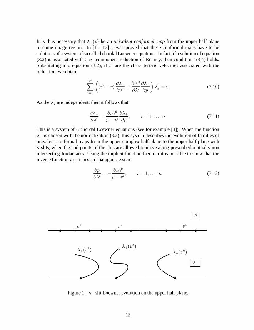
This is a system ofn chordal Loewner equations (see for example [8]). When the functionλ+ is chosen with the normalization (3.3), this system describes the evolution of families ofunivalent conformal maps from the upper complex half plane to the upper half plane withn slits, when the end points of the slits are allowed to move along prescribed mutually nonintersecting Jordan arcs. Using the implicit function theorem it is possible to show that theinverse functionp satisfies an analogous system
∂p
∂λi= − ∂iA
0
p − vi, i = 1, . . . , n. (3.12)
v1
×v2
×vn
×
p
×λ+(v1) × λ+(v2)
× λ+(vn)
λ+
Figure 1: n−slit Loewner evolution on the upper half plane.
12
For n > 1, the consistency conditions of (3.11) (or (3.12) equivalently) turn out to be theGibbons-Tsarev system. On the other hand, and more generally, we can consider a set ofn
Loewner equations,∂λ+
∂λi=
ai
p − bi
∂λ+
∂p, i = 1, . . . , n, (3.13)
for arbitrary functionsai, bi. The consistency conditions
∂2λ+
∂λi∂λj=
∂2λ+
∂λj∂λi
are then equivalent to the set of equations
∂iaj = ∂jai (3.14)
∂iaj =2aiaj
(bi − bj)2(3.15)
∂ibj =
ai
bi − bj, (3.16)
wherei 6= j. The first of these equations implies locally the existence of a functionA0(λ1, . . . , λn)such that
ai = ∂iA0.
Consequently, equations (3.15), (3.16) become the Gibbons-Tsarev system (2.6), withbi =vi. So, to any solution of a system ofn chordal Loewner equations there corresponds an-component reduction of the Benney chain.
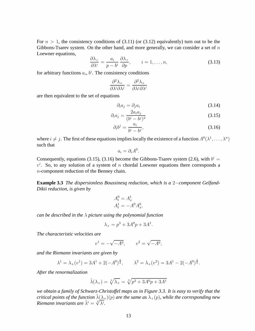
Example 3.3 The dispersionless Boussinesq reduction, which is a2−component Gelfand-Dikii reduction, is given by
A0t = A1
x
A1t = −A0A0
x,
can be described in theλ picture using the polynomial function
λ+ = p3 + 3A0p + 3A1.
The characteristic velocities are
v1 = −√−A0, v2 =
√−A0,
and the Riemann invariants are given by
λ1 = λ+(v1) = 3A1 + 2(−A0)3
2 , λ2 = λ+(v2) = 3A1 − 2(−A0)3
2 .
After the renormalization
λ(λ+) = 3√
λ+ = 3√
p3 + 3A0p + 3A1
we obtain a family of Schwarz-Christoffel maps as in Figure 3.3. It is easy to verify that thecritical points of the functionλ(λ+)(p) are the same asλ+(p), while the corresponding newRiemann invariants areλi =
3√
λi.
13
v1
×v2
×
p
× λ1
× λ2
λ+
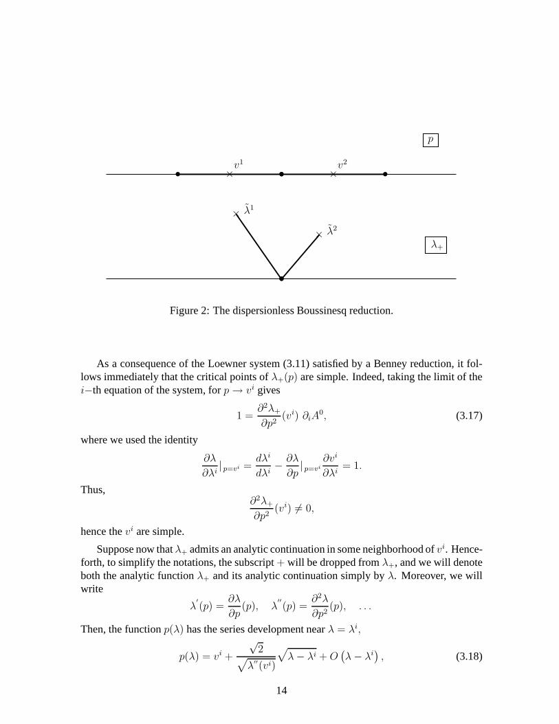
Figure 2: The dispersionless Boussinesq reduction.
As a consequence of the Loewner system (3.11) satisfied by a Benney reduction, it fol-lows immediately that the critical points ofλ+(p) are simple. Indeed, taking the limit of thei−th equation of the system, forp → vi gives
1 =∂2λ+
∂p2(vi) ∂iA
0, (3.17)
where we used the identity
∂λ
∂λi| p=vi =
dλi
dλi− ∂λ
∂p| p=vi
∂vi
∂λi= 1.
Thus,∂2λ+
∂p2(vi) 6= 0,
hence thevi are simple.
Suppose now thatλ+ admits an analytic continuation in some neighborhood ofvi. Hence-forth, to simplify the notations, the subscript+ will be dropped fromλ+, and we will denoteboth the analytic functionλ+ and its analytic continuation simply byλ. Moreover, we willwrite
λ′
(p) =∂λ
∂p(p), λ
′′
(p) =∂2λ
∂p2(p), . . .
Then, the functionp(λ) has the series development nearλ = λi,
p(λ) = vi +
√2
√
λ′′(vi)
√
λ − λi + O(
λ − λi)
, (3.18)
14
which becomes a Taylor expansion in the complex local parameter t =√
λ − λi. Further-more, we have
1
λ′(p)
=1
λ′′(vk)
1
p − vk− 1
2
λ′′′
(vk)
λ′′(vk)2
(3.19)
+
(
1
4
λ′′′
(vk)2
λ′′(vk)3
− 1
6
λ′′′′
(vk)
λ′′(vk)2
)
(p − vk) + O(
(p − vk)2)
.
This expansion will be useful in Section 5. Finally, we introduce two sets of contours, in thep andλ plane respectively, that we will need later for describing the Hamiltonian structureof the reductions. We defineΓi as a closed and sufficiently small contour in thep−planearoundvi, andCi as the image ofΓi according to the analytical continuation ofλ. Thus,Γi
andCi are well defined; in particular, it follows from expansion (3.18) thatλi – the tip of theslit – is a square root branch point forp(λ), henceCi encircles it twice.
3.3 Symmetries of the Benney reductions
A well-known method [13] of obtaining a countable set of symmetries of the Benney reduc-tion is based on the Lax representation of the dKP hierarchy,
λtn = {λ , hn} = (hn)p λx − (hn)x λp, n = 1, 2, . . .
wherehn = 1n
(λn)≥0. We assume, unless otherwise stated, thatλ is normalized as in (3.3).If the solutionλ possessesn critical values(v1, . . . , vn) , the hierarchy can be reduced to
λitn = wi
nλix, i = 1, . . . , n, n = 1, 2, . . . ,
with
win =
(
∂hn
∂p
)
| p=vi
. (3.20)
These are, by construction, components of the symmetries ofthe reductions, the first few ofthem being
wi1 = 1, wi
2 = vi, wi3 = (vi)2 + A0 . . . i = 1, . . . , n.
Further, the above characteristic velocities can be obtained as the coefficients of the ex-pansion atλ = ∞ of the generating functions
W i(λ) =1
p(λ) − vi. (3.21)
Proposition 3.1 The functionsW i(λ) are solutions of the linear system
∂jWi(λ)
W j(λ) − W i(λ)=
∂jvi
vj − vi. (3.22)
Moreover, expandingW i(λ) at λ=∞ we get
W i(λ) =
∞∑
n=1
win
λn, (3.23)
where the coefficients of the series are the symmetrieswin given in(3.20).
Remark 4 The first condition(3.22)holds in any normalization, but the expansion(3.23)assumes the normalization(3.3).
Proof In order to prove (3.22), knowing that
∂p
∂λi=
∂iA0
vi − p,
we can write
∂jWi(λ) = ∂j
(
1
p − vi
)
=−1
(p − vi)2
(
∂p
∂λj− ∂vi
∂λj
)
= − ∂jA0
(p − vi)2
(
1
vj − p− 1
vj − vi
)
=∂jA
0
(p − vi)(p − vj)(vj − vi).
On the other hand
W j(λ) − W i(λ) =(vj − vi)
(p − vi)(p − vj).
and so∂jW
i(λ)
W j(λ) − W i(λ)=
∂jA0
(vj − vi)2=
∂jvi
vj − vi.
In order to prove (3.23), chosen the normalization (3.3), wehave
win =
1
nlimp→vi
d
dp
[
(p − vi)2 (λn)+
(p − vi)2
]
=1
nresp=vi
(
(λn)+
(p − vi)2dp
)
.
The function (λn)+(p−vi)2
has poles only atp = vi andp = ∞ and therefore
resp=vi
(
(λn)+
(p − vi)2dp
)
= − resp=∞
(
(λn)+
(p − vi)2dp
)
= − resp=∞
(
(λn)
(p − vi)2dp
)
16
where the last identity is due to
resp=∞
(
(λn)−(p − vi)2
dp
)
= 0.
Changing variable we obtain
− resp=∞
(
(λn)
(p − vi)2dp
)
= − 1
2πi
∫
Γ∞
λn dpdλ
(p(λ) − vi)2dλ
=n
2πi
∫
Γ∞
λn−1
p(λ) − vidλ,
whereΓ∞ is a sufficiently small contour aroundp = ∞. Thus,
win =
∫
Γ∞
W i(λ)λn−1 dλ,
varyingn we obtain the coefficients of the expansion (3.23).
�
Remark 5 It will be useful below to consider, as a generating functionof the symmetries,
wi(λ) =∂p∂λ
(p(λ) − vi)2= −
∞∑
n=1
n win
λn+1, (3.24)
which is nothing but theλ− derivative of(3.21).
We finally observe that, due to linearity of (3.22), the functions
zi =
n∑
k=1
∫
Ck
wi(λ)ϕk(λ)dλ
still satisfy the system for the symmetries and therefore, applying the generalized hodographmethod, we can write the general solution of the Benney reduction in the implicit form
zi = vix + t, i = 1, . . . , n.
The inverse scattering solutions found in [10, 21] are of this form.
4 Hamiltonian structure of the reductions
As it was shown in [11], any reduction of Benney is a diagonalizable and semi-Hamiltoniansystem of hydrodynamic type. However, very little is known about the Hamiltonian structureof these systems, whether local or nonlocal. A few examples are known explicitly. Theseinclude the Gelfand-Dikii and Zakharov reductions, which arise as dispersionless limits ofknown dispersive Hamiltonian systems.
In this section, we use Ferapontov’s procedure sketched in Section 1.2 for semi-Hamiltoniandiagonal systems in order to determine the metric associated with a generic reduction.
17
Theorem 6 The general solution of the system (1.11) in the case of Benney reductions is
gii =∂iA0
ϕi(λi)(4.1)
where the functionsϕi(λi) aren arbitrary functions of one variable, the functionsλ1, . . . , λn
being the Riemann invariants of the system.
Proof. From the system (1.11), and making use of both the Gibbons-Tsarev equations (2.6),which hold for any Benney reduction, we obtain
∂j ln√
gii =∂jv
i
vj − vi=
∂jA0
(vj − vi)2= ∂j ln
√
∂iA0 (4.2)
from which we obtain the general solution (4.1).
�
In the caseϕi = 1 the rotation coefficients
βij :=∂i√
gjj√gii
(4.3)
are symmetric:
βij =1
2
∂i∂jA0√
∂iA0∂jA0
=
√
∂iA0∂jA0
(vi − vj)2. (4.4)
We now focus our attention on this case, that is we consider the Egorov (potential) metric
gii = ∂iA0. (4.5)
Remark 6 We notice that the choice of potential metric is not restrictive, as any other metric(4.1) can be written in potential form under a change of coordinates
λi 7−→ ϕi(λi), (4.6)
which is exactly the freedom we have in the definition of the Riemann invariants. On the otherhand, the choice of the Riemann invariants determines a unique metric which is potential inthose coordinates.
In order to find the Christoffel symbols and the curvature tensor of the metric (4.5),one could compute these objects – as usual – starting from their definitions. However, for aBenney reduction, this procedure can be shortened. Indeed,using the Gibbons-Tsarev system(2.6), the connection and the curvature can be written as simple algebraic combinations ofthe quantities
vi, ∂iA0, δ(vi), δ(log
√
∂iA0), i = 1, . . . , n,
18
where we introduced the shift operator
δ =n∑
k=1
∂
∂λk.
We have
Proposition 4.2 The symbols
Γijk = −gisΓj
sk = −1
2gisgjl
(
∂sglk + ∂kgls − ∂lgsk
)
,
whereΓkij are the Christoffel symbols associated to the diagonal metric gii = ∂iA0, for a
Benney reduction are given by
Γijk = 0, i 6= j 6= k (4.7a)
Γiji = −Γji
i =1
(vi − vj)2, i 6= j (4.7b)
Γiik = −∂kA0
∂iA0
1
(vk − vi)2, i 6= k (4.7c)
Γiii =
∑
k 6=i
∂kA0
∂iA0
1
(vi − vk)2− δ(ln
öiA0)
∂iA0. (4.7d)
Proof For the metricgij = δij∂iA0, we get
Γijk = −1
2
1
∂iA0∂iA0
(
δjk∂ikA0 + δij∂kjA
0 − δik∂jkA0)
,
and equations (4.7) are obtained from these by substituting, whenever is allowed, the Gibbons-Tsarev equations (2.6b).
�
In particular, the curvature can be expressed solely via theshift operatorδ, acting onvi andln√
∂iA0.
Proposition 4.3 The non vanishing components of the curvature tensor of the metric (4.5)for a Benney reduction can be written in terms of the quantitiesδ(vi), δ(ln
öiA0). More
precisely, we have the following identity
Rijij =
δ(ln√
∂iA0) + δ(ln√
∂jA0)
(vi − vj)2− 2
δ(vi) − δ(vj)
(vi − vj)3. (4.8)
19
Proof Since the rotation coefficients of the metric (4.5) are symmetric, it is easy to checkthat
Rijij = δ (βij) .
Using the Gibbons-Tsarev system (2.6) we get (4.8). Moreover, it is well known that for asemi-Hamiltonian system the other components of the Riemann tensor are identically zero.
�
Formula (4.8) presents a compact way of describing the curvature tensor of the Poissonstructure (1.13) associated with a Benney reduction. However, we should notice here thatthe knowledge of the curvature is not sufficient to write the Poisson bracket. Indeed, whatwe need is a decomposition (1.12) of the curvature in terms ofthe symmetries of the system.From formula (4.8) this decomposition looks non-trivial; we will address this problem in thenext section using a different approach.
5 Hamiltonian structure in the λ picture
The purpose of this Section is to derive an explicit formulation for the Hamiltonian structureof a reduction of Benney in terms of the functionλ(p), which defines the reduction itself. Inparticular, we will show how the differential geometric objects associated with Ferapontov’sPoisson operator of type (1.13) can be expressed, in the caseof a Benney reduction withassociatedλ, in terms of the set of data
vi, λ′′
(vi), λ′′′
(vi), λ′′′′
(vi), i = 1, . . . , n,
wherevi, the characteristic velocities of the reduction, are the critical points ofλ. Moreover,we will describe the quadratic expansion of the curvature associated with the metric.
Let us consider a Benney reduction with associated functionλ(p). In this case, as alreadymentioned, a set of Riemann invariants is naturally selected, the critical values ofλ(p). From(3.17) and (4.1), it is immediate to check that the components of the metric which is potentialin those coordinates can be expressed in terms ofλ as
gii = ∂iA0 =
1
λ′′(vi)
= resp=vi
(
dp
λ′(p)
)
. (5.1)
This result was already known in the case of dispersionless Gelfand-Dikii [5] reductions.However, it holds for all Benney reductions.
5.1 Completing the Loewner system
We move now our attention from the metric to the Christoffel symbols and the curvaturetensor, looking for a way to describing these objects in terms of λ and its critical points.
20
However, this step is not immediate. Indeed, from equations(4.7) and (4.8) we need to findan expression in theλ picture for the quantities
δ(vi), δ(log√
∂iA0),
we will see that the right object to look at is
F (p) =∂p
∂λ+
n∑
i=1
∂p
∂λi, (5.2)
obtained from the inverse function ofλ with respect top, that is
p = p(λ, λ1, . . . , λn). (5.3)
The functionF is thus determined once the functionλ(p, λ1, . . . , λn) is known. Beforediscussing the Christoffel symbols and the curvature, we will consider the properties of thisfunction in detail. First of all, using the Loewner equations (3.12) and the expression (3.17),we can writeF (p) in the following form:
F (p) =1
λ′(p)
−n∑
i=1
∂iA0
p − vi
=1
λ′(p)
−n∑
i=1
resp=vi
(
1
λ′(p)
)
1
p − vi. (5.4)
From its expansion (3.19), the function1λ′ (p)
in vi has a simple pole, therefore,F (p) is
analytic atp = vi. Using this fact, we can prove the following
Theorem 7 Let λ(p, λ1, . . . , λn) be a solution of equation (3.2), and letv1, . . . , vn be itscritical points. Defining the functionF (p) as above (5.2), we have
F (vi) = δ(vi) (5.5)
∂F
∂p(vi) = δ(ln
√
∂iA0). (5.6)
Proof We have already shown thatF (p) is analytic atp = vi. In order to prove (5.5) and(5.6), we consider the system ofn + 1 differential equations
∂p
∂λi=
∂iA0
vi − pi = 1, . . . , n
(5.7)
∂p
∂λ=
n∑
k=0
∂kA0
p − vk+ F (p).
21
The conditions∂2p
∂λi∂λj− ∂2p
∂λj∂λi= 0 i 6= j (5.8)
give nothing but the Gibbons-Tsarev system, hence are satisfied for any reduction. So, weconcentrate our attention on the remainingn consistency conditions
∂2p
∂λ∂λi− ∂2p
∂λi∂λ= 0, (5.9)
which – by construction – are satisfied, to obtain some information aboutF (p). Expandingboth sides we obtain
∂2p
∂λ∂λi=
∂iA0
(p − vi)2
∂p
∂λ
=∂iA0
(p − vi)2
[
F (p) +
n∑
k=1
∂kA0
p − vk
]
,
∂2p
∂λi∂λ=
∂F
∂p
∂p
∂λi+
∂F
∂λi+
n∑
k=1
[
∂k∂iA0
p − vk+
∂kA0
(p − vk)2
(
∂ivk −∂p
∂λi
)]
=∂F
∂p
∂iA0
vi − p+
∂F
∂λi+
n∑
k=1
[
∂k∂iA0
p − vk+
∂kA0
(p − vk)2
(
∂ivk +∂iA
0
p − vi
)]
,
substituting the Gibbons-Tsarev equations (2.6) in the above formulae and rearranging (5.9),we find that
F (p) − δ(vi)
(p − vi)2+
∂F∂p
(p) − 2δ(log√
∂iA0)
p − vi− 1
∂iA0
∂F (p)
∂λi= 0. (5.10)
Multiplying by (p − vi)2 and taking the limit forp → vi, we get
F (vi) = δ(vi).
Then, taking the residue of the right hand side of (5.10) atp = vi gives
∂F
∂p(vi) = δ(log
√
∂iA0).
�
Thus, specifying the functionF turns out to be the analogue, in theλ picture, of com-pleting the system (2.6), from which we were able to express the Christoffel symbols and thecurvature tensor of the metric.
It follows from its definition, thatF (p) is obtained from 1λ′(p)
by subtracting off its singu-
larities atp = vi. The importance of this function is that it describes the invariant properties
22
of the reduction. For instance, if a reduction admits a function λ associated with it such thatF (p) = 1, then the reduction is Galilean invariant. The caseF (p) = p corresponds insteadto the scaling invariance of the system. As seen in example below, the functionF , hencethese invariances, are strongly related with the curvatureof the Poisson bracket.
Example 5.4 The2−component Zakharov reduction is known to possess both Galilean andscaling invariance. Using the technique above, the former can be explained by saying that,for the functionλ(p) given in Example 3.2, it followsF (p) = 1. Thus, we get
δ(vi) =
n∑
k=1
∂vi
∂λk= 1,
where the Riemann invariants are the critical values ofλ(p). For the scaling invariance,one can proceed as follows: define the functionϕ(p) = ln λ(p), whereλ(p) is the same asbefore. This new function has the same critical pointsvi asλ, plus the poles ofλ(p), whichplay no role in the deerivation of the reduction (see Remark 3). Hence, it is associated withthe Zakharov reduction, and in this caseF (p) = p. Thus
δ(vi) =n∑
k=1
∂vi
∂ϕk= vi, (5.11)
where theϕi = ln λi are the natural Riemann invariants associated withϕ(p), i.e. its criticalvalues. It is elementary to show that(5.11)corresponds to the scaling invariance with respectto theλi.
Remark 7 System (5.7) was considered for the first time in connection with a Benney reduc-tion by Kokotov and Korotkin [14], in the particular case of the N−component Zakharovreduction, whereF (p)= 1.
In the next section, we will use the functionF to describe the Christoffel symbols andthe curvature in terms ofλ. Nevertheless, the latter can be expressed directly in terms of Fusing the following residue formula
Proposition 5.4 In terms of the functionF , the non vanishing components of the Riemanntensor satisfy the following identity:
Rijij =
∑
k=i,j
resp=vk
(
F (p)
(p − vi)2(p − vj)2dp
)
=1
2πi
∫
Γi∪Γj
F (p)
(p − vi)2(p − vj)2dp (5.12)
whereΓi andΓj are two sufficiently small contours aroundp = vi andp = vj.
Proof. From (4.8) and Theorem 7 it follows immediately that
Rijij =
1
(vi − vj)2
[(
∂F
∂p(vi) +
∂F
∂p(vj)
)
− 2F (vi) − F (vj)
vi − vj
]
(5.13)
23
It is easy to check the chain of identities:
1
(vi − vj)2
[(
∂F
∂p(vi) +
∂F
∂p(vj)
)
− 2F (vi) − F (vj)
vi − vj
]
=
limp→vi
d
dp
[
F (p)
(p − vj)2
]
+ limp→vj
d
dp
[
F (p)
(p − vi)2
]
=
limp→vi
d
dp
[
(p − vi)2 F (p)
(p − vj)2(p − vi)2
]
+ limp→vj
d
dp
[
(p − vj)2 F (p)
(p − vi)2(p − vj)2
]
=
resp=vi
(
F (p)
(p − vi)2(p − vj)2dp
)
+ resp=vj
(
F (p)
(p − vi)2(p − vj)2dp
)
.
In the last identity we used the fact thatF (p) is regular atp = vi, for all i.
�
5.2 Christoffel symbols and Curvature tensor
5.2.1 Potential metric
We are now able to complete the description of the Poisson bracket associated with a Benneyreduction, in the case where the metric is potential in the coordinate used.
Proposition 5.5 The Christoffel symbols(4.7) of the potential metric(5.1) can be written,in terms of the functionλ, as
Γijk = 0, i 6= j 6= k (5.14a)
Γiji = −Γji
i =1
(vi − vj)2, i 6= j (5.14b)
Γiik = − λ
′′
(vi)
λ′′(vk)
1
(vk − vi)2, i 6= k (5.14c)
Γiii =
1
6
λ′′′′
(vi)
λ′′(vi)
− 1
4
λ′′′
(vi)2
λ′′(vi)2
, (5.14d)
The curvature tensor(4.8)of the potential metric(5.1)can be written, in terms of the functionλ(p) as
Rijij =
3
(vi − vj)4
(
1
λ′′(vi)
+1
λ′′(vj)
)
+1
(vi − vj)3
(
λ′′′
(vi)
λ′′(vi)2
− λ′′′
(vj)
λ′′(vj)2
)
+1
(vi − vj)2
(
1
4
λ′′′
(vi)2
λ′′(vi)3
− 1
6
λ′′′′
(vi)
λ′′(vi)2
+1
4
λ′′′
(vj)2
λ′′(vj)3
− 1
6
λ′′′′
(vj)
λ′′(vj)2
)
+∑
k 6=i,j
1
λ′′(vk)
1
(vi − vk)2(vj − vk)2. (5.15)
24
Proof Starting from the definition (5.2) ofF , and using (3.19), we can write
F (vi) = −1
2
λ′′′
(vi)
λ′′(vi)2
−∑
k 6=i
1
λ′′(vk)
1
vi − vk, (5.16)
∂F
∂p(vi) =
1
4
λ′′′
(vi)2
λ′′(vi)3
− 1
6
λ′′′′
(vi)
λ′′(vi)2
+∑
k 6=i
1
λ′′(vk)
1
(vi − vk)2. (5.17)
Then, by Theorem 7, and substituting the above expressions for F into (4.7) and (4.8), weobtain (5.14) and (5.15) respectively.
�
Remark 8 We note that(5.14d)is a constant multiple of the Schwarzian derivative ofλ′
(p),evaluated atp = vi.
Recalling the expression (5.1) for the the metric, form the Proposition above we find thatthe whole Poisson operator associated with a Benney reduction of symbolλ depends only onthe critical points ofλ and on the value of its second, third and fourth derivatives evaluatedat these points.
We have now all we need to write the nonlocal tail of the Hamiltonian structure associatedto the metricgii = ∂iA0.
Proposition 5.6 The non-vanishing components of the Riemann tensor of the metric (5.1)admit the following quadratic expansion
Rijij =
1
2πi
∫
C
wi(λ)wj(λ)dλ. (5.18)
whereC = C1 ∪ · · · ∪ Cn with Ci described as above, and the functions
wi(λ) =∂p∂λ
(p(λ) − vi)2,
are the generating functions of the symmetries(3.24). Consequently the non local tail of theHamiltonian structure associated to the metricgii = ∂iA0 is given by
1
2πi
∫
C
wi(λ)λix
(
d
dx
)−1
wj(λ)λjxdλ.
Proof We prove the Proposition showing that the integral in (5.18)is the same as the righthand side of (5.15). First, writing the integral
1
2πi
∫
C
wi(λ)wj(λ)dλ
25
in terms of the variablep we obtain
Rijij =
1
2πi
∫
Γ
1λ′ (p)
(p − vi)2(p − vj)2dp =
n∑
k=1
resp=vk
(
1λ′ (p)
(p − vi)2(p − vj)2dp
)
. (5.19)
Using (3.19), the integrand can be expanded, fork = 1. . . . , n, as
1
(p − vi)2(p − vj)2
(
1
λ′′(vk)
1
p − vk− 1
2
λ′′′
(vk)
λ′′(vk)2
+
(
1
4
λ′′′
(vk)2
λ′′(vk)3
− 1
6
λ′′′′
(vk)
λ′′(vk)2
)
(p − vk)+. . .
)
.
Thus, fork 6= i, j we get
resp=vk
(
1λ′ (p)
(p − vi)2(p − vj)2dp
)
=1
λ′′(vk)
1
(vk − vi)2(vk − vj)2,
while
resp=vi
(
1λ′(p)
(p − vi)2(p − vj)2dp
)
=3
(vi − vj)4
1
λ′′(vi)
+1
(vi − vj)3
λ′′′
(vi)
λ′′(vi)2
+1
(vi − vj)2
(
1
4
λ′′′
(vi)2
λ′′(vi)3
− 1
6
λ′′′′
(vi)
λ′′(vi)2
)
,
resp=vj
( 1λ′(p)
(p − vi)2(p − vj)2dp
)
=3
(vj − vi)4
1
λ′′(vj)
+1
(vj − vi)3
λ′′′
(vj)
λ′′(vj)2
+1
(vj − vi)2
(
1
4
λ′′′
(vj)2
λ′′(vj)3
− 1
6
λ′′′′
(vj)
λ′′(vj)2
)
,
From these, formula (5.15) for the curvature tensor follows. The last statement of the Propo-sition is a consequence of the general theory of Ferapontov.
�
Remark 9 Alternatively, one can prove the above result using starting from the functionF ,namely deforming the integral
1
2πi
∫
Γi∪Γj
F (p)
(p − vi)2(p − vj)2dp
which is shown in Proposition 5.4 to be equal to the curvature, into (5.18). In order to do so,it is sufficient to verify the following identity
− 1
2πi
∫
Γi∪Γj
∑nk=1
∂kA0
p−vk
(p − vi)2(p − vj)2dp =
1
2πi
∫
Γ−(Γi∪Γj)
1∂λ∂p
(p − vi)2(p − vj)2dp,
26
that can be proved by straightforward computation. Indeed,since the left hand side is thesum of residues atp = vi andp = vj of a function having a pole of order 3 atp = vi, vj weobtain
l.h.s = −(
limp→vi
+ limp→vj
)
1
2
d2
dp2
n∑
k=1
[
(p − vi)∂kA0
(p − vj)2(p − vk)
]
=∑
k 6=i,j
∂kA0
(vi − vj)2
[
2
(vi − vj)(vi − vk)+
1
(vi − vk)2− 2
(vi − vj)(vj − vk)+
1
(vj − vk)2
]
=∑
k 6=i,j
∂kA0
(vi − vk)2(vj − vk)2.
On the other hand the right hand side is the sum of residues atp = vk, for k 6= i, j of afunction having simple poles atp = vk:
r.h.s. =∑
k 6=i,j
limp→vk
(p − vk) 1∂λ∂p
(p − vi)2(p − vj)2=∑
k 6=i,j
∂kA0
(vi − vk)2(vj − vk)2= l.h.s.
Recalling the results above, we have the following
Theorem 8 The reduction of Benney associated with the functionλ(p, λ1, . . . , λn) is Hamil-tonian with the Hamiltonian structure
Πij = λ′′
(vi)δij d
dx+ Γij
k λkx +
1
2πi
∫
C
∂p∂λ
λix
(p(λ) − vi)2
(
d
dx
)−1 ∂p∂λ
λjx
(p(λ) − vj)2dλ, (5.20)
where
Γijk λk
x =λi
x − λjx
(vi − vj)2i 6= j,
Γiik λk
x =
(
1
6
λ′′′′
(vi)
λ′′(vi)
− 1
4
λ′′′
(vi)2
λ′′(vi)2
)
λix −
∑
k 6=i
λ′′
(vi)
λ′′(vk)
λkx
(vi − vk)2
andC = C1∪· · ·∪Cn. Here, thevi are the critical points ofλ, and theλi the critical values.In this coordinates, the metricgij = δij
λ′′ (vi)is potential.
5.2.2 The general case
As we pointed out previously, any metric (4.1) associated with a reduction can be put inpotential form, after a suitable change of the Riemann invariants. However, it is often con-venient to write the expression of the Poisson operators generated by these metrics in terms
27
of the Riemann invariants selected byλ. Thus, we consider the metrics
gii =∂iA
0
ϕi(λi)=
1
ϕi(λi)λ′′(vi), (5.21)
whereϕi =ϕi(λi) are arbitrary functions, and we proceed as before.
Proposition 5.7 The Christoffel symbols appearing in the Hamiltonian structure are givenby
Γijk = 0, i 6= j 6= k
Γiji =
ϕj
(vi − vj)2, i 6= j
Γijj = − ϕi
(vi − vj)2, i 6= j
Γiik = − λ
′′
(vi)
λ′′(vk)
ϕi
(vk − vi)2, i 6= k
Γiii = ϕi
(
1
6
λ′′′′
(vi)
λ′′(vi)
− 1
4
λ′′′
(vi)2
λ′′(vi)2
)
+1
2ϕ
′
i.
Here we denote
ϕ′
i =dϕ
dλi(λi).
The nonlocal tail appearing in the Hamiltonian structure isthen given by
1
2πi
n∑
k=1
∫
Ck
∂p∂λ
λix
(p(λ) − vi)2
(
d
dx
)−1 ∂p∂λ
λjx
(p(λ) − vj)2ϕk(λ) dλ. (5.22)
Proof The proof of the formula for theΓijk is a straightforward computation. Let us prove
the second statement. Since nothing new is involved in such computations we will skip thedetails. For the metric (5.21), the non vanishing components of the curvature tensor are
Rijij =
3
(vi − vj)4
(
ϕi ∂iA0 + ϕj ∂jA
0)
− 2
(vi − vj)3
(
ϕi ∂ivi − ϕj ∂jv
j)
+1
(vi − vj)2
(
ϕi ∂i ln√
∂iA0 + ϕj ∂j ln√
∂jA0)
+∑
k 6=i,j
ϕk ∂kA0
(vi − vk)2(vj − vk)2+
1
2
ϕ′
i + ϕ′
j
(vi − vj)2. (5.23)
28
Expression (5.23) can be written, in terms ofλ, as
Rijij =
3
(vi − vj)4
(
ϕi
λ′′(vi)
+ϕj
λ′′(vj)
)
+1
(vi − vj)3
(
ϕiλ
′′′
(vi)
λ′′(vi)2
− ϕiλ
′′′
(vj)
λ′′(vj)2
)
+1
(vi − vj)2
(
ϕi
(
1
4
λ′′′
(vi)2
λ′′(vi)3
− 1
6
λ′′′′
(vi)
λ′′(vi)2
)
+ ϕj
(
1
4
λ′′′
(vj)2
λ′′(vj)3
− 1
6
λ′′′′
(vj)
λ′′(vj)2
))
+∑
k 6=i,j
1
λ′′(vk)
ϕk
(vi − vk)2(vj − vk)2+
1
2
ϕ′
i + ϕ′
j
(vi − vj)2, (5.24)
The equivalence between (5.22) and the right hand side of (5.24) can be obtained by rewritingthe integrals above in thep−plane,
1
2πi
n∑
k=1
∫
Γk
ϕk(λ(p)) 1λ′ (p)
(p − vi)2(p − vj)2dp. (5.25)
and using the same arguments of the main theorem, except thatfor everyk, in the integralaroundΓk we have to consider also the contribution of the functionϕk(λ(p)) which expands,atp = vk, as
ϕk(λ(p)) = ϕk +ϕ
′
k
2λ
′′
(vk) (p − vk)2 + . . .
�
It follows from the above that we have
Theorem 9 The reduction of Benney associated with the functionλ(p, λ1, . . . , λn) is Hamil-tonian with the family of Hamiltonian structures
Πij = ϕi λ′′
(vi)δij d
dx+ Γij
k λkx
+1
2πi
n∑
k=1
∫
Ck
∂p∂λ
λix
(p(λ) − vi)2
(
d
dx
)−1 ∂p∂λ
λjx
(p(λ) − vj)2ϕk(λ) dλ, (5.26)
with
Γijk λk
x =ϕj λi
x − ϕi λjx
(vi − vj)2i 6= j,
Γiik λk
x = ϕi
(
1
6
λ′′′′
(vi)
λ′′(vi)
− 1
4
λ′′′
(vi)2
λ′′(vi)2
)
λix +
1
2ϕ
′
i λix −
∑
k 6=i
λ′′
(vi)
λ′′(vk)
ϕi λkx
(vi − vk)2,
whereϕ1, . . . , ϕn are arbitrary functions of a single variable. Here, thevi are the criticalpoints ofλ, the coordinatesλi the corresponding critical values, and theCk are the contoursdefined above.
29
6 Finite nonlocal tail: some examples
In the expression (5.26) for the Poisson operator, the components of the curvature are ex-pressed as integrals of functions around suitable contoursin a complex domain. A naturalquestion to ask is whether this integral can be reduced to a finite sum, and we will shownow some examples where this is possible. For simplicity, wewill consider the case whenϕ1(λ) = · · · = ϕn(λ) = λk, for k ∈ Z. In this case the curvature can be expressed as
Rijij =
1
2πi
∫
C
(
∂p∂λ
)2λk
(p(λ) − vi)2(p(λ) − vj)2dλ, k ∈ Z.
Essentially, the finite expansion appears whenever is possible to substitute the the contourC
with a contour a roundλ = ∞ and a finite number of other marked points. We illustrate thisspecial situation in two simple examples.
6.1 2-component Zakharov reduction
In this case (see examples 2.1, 3.2), sinceλ is a single-valued rational function ofp, it isconvenient to work in thep-plane. In order to calculate the curvature, the non vanishingcomponents of the Riemann tensor are given by
R1212 =
2∑
i=1
resp=vi
(
λ(p)k 1λ′(p)
(p − v1)2(p − v2)2dp
)
, k ∈ Z.
The abelian differentialλ(p)k 1
λ′ (p)
(p − v1)2(p − v2)2dp
has poles at the pointsp = v1, p = v2, as well as:
if k > 2
p = ∞, p =A1
A0(poles ofλ)
if k < 0
p = s1 =1
2
A1 + (A21 − 4A3
0)1/2
A0
, p = s2 =1
2
A1 − (A21 − 4A3
0)1/2
A0
(zeros ofλ),
while for k = 0, 1, 2 there are no other poles. Since the sum of the residues of an abeliandifferential on a compact Riemann surface is zero, we can substitute the sum of residues atp = v1, v2 with, respectively
- zero if k = 0, 1, 2,
30
- minus the sum of residues atp = ∞, p = A1
A0if k > 2
- minus the sum of residues atp = s1, p = s2, if k < 0.
Summarizing, we have
Rijij = 0, k = 0, 1, 2,
Rijij = −
(
resp=∞
+ resp= A1
A0
)
λ(p)k 1λ′(p)
(p − vi)2(p − vj)2dp, k > 2,
Rijij = −
(
resp=s1
+ resp=s2
) λ(p)k 1λ′ (p)
(p − vi)2(p − vj)2dp, k < 0.
Moreover, as a counterpart in theλ-plane of the above formulae we have
Rijij = 0, k = 0, 1, 2,
Rijij = −2 res
λ=∞
(
w1(λ)w2(λ)λk dλ)
, k > 2,
Rijij = −2 res
λ=0
(
w1(λ)w2(λ)λk dλ)
, k < 0,
and this shows that the residues have to be computed around marked points, which not de-pend on the dynamics of the reduction. Expandingw1(λ) andw2(λ) nearλ = ∞, we get
w1(λ) = −∞∑
k=1
k w1k
λk+1=
− 1
λ2− 2 v1
λ3− 3(2A3
0 + A21 + 2A1A
3
2
0 )
A20
1
λ4− 4(A3
1 + 6A1A30 + 3A
9
2
0 + 3A21A
3
2
0 )
A30
1
λ5+ . . .
w2(λ) = −∞∑
k=1
k w2k
λk+1=
− 1
λ2− 2 v2
λ3− 3 (2A3
0 + A21 − 2A1A
3
2
0 )
A20
1
λ4− 4 (A3
1 + 6A1A30 − 3A
9
2
0 − 3A21A
3
2
0 )
A30
1
λ5+ . . .
31
and nearλ = 0
w1(λ) =
∞∑
h=0
z1−h λh = − 2A2
0(−√
A21 − 4A3
0 + A1)(
A1 −√
A21 − 4A3
0 + 2A3
2
0
)2√
A21 − 4A3
0
+
−8A3
0
(
√
A21 − 4A3
0(A30 − A2
1) + A31 − 3A1A
30 + 2A
9
2
0
)
(A21 − 4A3
0)3
2
(
A1 −√
A21 − 4A3
0 + 2A3
2
0
)3 λ + . . .
w2(λ) =∞∑
h=0
z2−h λh = − 2A2
0(−√
A21 − 4A3
0 + A1)(
A1 −√
A21 − 4A3
0 − 2A3
2
0
)2√
A21 − 4A3
0
+
−8A3
0
(
√
A21 − 4A3
0(A30 − A2
1) + A31 − 3A1A
30 − 2A
9
2
0
)
(A21 − 4A3
0)3
2
(
A1 −√
A21 − 4A3
0 − 2A3
2
0
)3 λ + . . .
and taking into account that the coefficients of the expansion are characteristic velocities ofsymmetries, we easily obtain the quadratic expansion of theRiemann tensor. Fork > 2 wehave
R1212 =
∑
i+j=k−1
(
w1i w
2j + w1
jw2i
)
,
while for k < 0, we obtain
R1212 =
∑
i+j=k+1
(
z1i z
2j + z1
j z2i
)
,
which can be put in the canonical form (1.12) after a linear chenge of basis of the symmetries.The expressions of these expansions in the Rieman invariants can be found by using formulaegiven in Example 2.1.
6.2 Dispersionless Boussinesq reduction
The case of the dispersionless Boussinesq reduction can be treated in a similar way. FromExample 3.3, we will consider a functionλ which is polynomial inp,
λ = p3 + 3A0p + 3A1,
thus meromorphic on the Riemann sphere. The choice of a different normalisation reflectsin the expansions below, where we have to consider an expansion in the local parametert = λ− 1
3 . For simplicity let us consider only the casek ≥ 0. We observe that, apart from thepoles atp = v1 andp = v2, we have only an additional pole at infinity (starting fromk = 2).Following the same procedure used in the Zakharov case we obtain
Rijij = 0, k = 0, 1,
Rijij = 3 res
t=0
(
w1(t)w2(t) t−(3k+4) dt)
, k > 2.
32
The expansions ofw1(t) andw2(t) neart = 0 are given by
w1(t) =
∞∑
k=0
k w1k tk+4 = t4 + 2 (−A0)
1
2 t5 + 4(
A1 − (−A0)3
2
)
t7
+ 5(
2A1(−A0)1
2 − A20
)
t8 + . . .
w2(t) =
∞∑
k=0
k w2k tk+4 = t4 − 2 (−A0)
1
2 t5 + 4(
A1 + (−A0)3
2
)
t7
+ 5(
−2A1(−A0)1
2 − A20
)
t8 + . . .
From these formulas we immediately get the quadratic expansion of the Riemann tensor:
k = 0 : R1212 = 0,
k = 1 : R1212 = 0,
k = 2 : R1212 = 3(v1 + v2) = 0,
More generally, we have
R1212 =
3
2
∑
i+j=k−1
(w13iw
23j + w1
3jw23i) k > 2.
The expression in the Riemann invariants can be obtained from Example 3.3.
Acknowledgments
We would like to thank the ESF grant MISGAM 1414, for its support of Paolo Lorenzoni’svisit to Imperial. We are also grateful to the European Commissions FP6 programme for sup-port of this work through the ENIGMA network, and particularly for their support of AndreaRaimondo, who also received an EPSRC DTA. We would like to thank Maxim Pavlov forvaluable discussions, and the integrable system groups at Milano Bicocca and Loughboroughuniversities for their hospitality to Andrea Raimondo.
References
[1] S. Baldwin and J. Gibbons. Hyperelliptic reduction of the Benney moment equations.J. Phys. A, 36(31):8393–8417, 2003.
[2] S. Baldwin and J. Gibbons. Higher genus hyperelliptic reductions of the Benney equa-tions. J. Phys. A, 37(20):5341–5354, 2004.
33
[3] S. Baldwin and J. Gibbons. Genus4 trigonal reduction of the Benney equations.J.Phys. A, 39(14):3607–3639, 2006.
[4] D.J. Benney. Some properties of long nonlinear waves.Stud. Appl. Math., 52:45–50,1973.
[5] B. Dubrovin, S.Q. Liu, and Y Zhang. Frobenius Manifolds and Central Invariants forthe Drinfeld - Sokolov Bihamiltonian Structures. arXiv:0710.3115v1, 2007.
[6] B.A. Dubrovin and S.P. Novikov. Hamiltonian formalism of one-dimensional systemsof the hydrodynamic type and the Bogolyubov-Whitham averaging method. Dokl.Akad. Nauk SSSR, 270(4):781–785, 1983.
[7] B.A. Dubrovin and S.P. Novikov. Poisson brackets of hydrodynamic type.Dokl. Akad.Nauk SSSR, 279(2):294–297, 1984.
[8] P. L. Duren.Univalent functions. Springer-Verlag, New York, 1983.
[9] E.V. Ferapontov. Differential geometry of nonlocal Hamiltonian operators of hydrody-namic type.Funktsional. Anal. i Prilozhen., 25(3):37–49, 95, 1991.
[10] J. Gibbons and Y. Kodama. Solving dispersionless Lax equations. InSingular limits ofdispersive waves (Lyon, 1991), volume 320 ofNATO Adv. Sci. Inst. Ser. B Phys., pages61–66. Plenum, New York, 1994.
[11] J. Gibbons and S.P. Tsarev. Reductions of the Benney equations. Phys. Lett. A,211(1):19–24, 1996.
[12] J. Gibbons and S.P. Tsarev. Conformal maps and reductions of the Benney equations.Phys. Lett. A, 258(4-6):263–271, 1999.
[13] Y. Kodama and J. Gibbons. Integrability of the dispersionless KP hierarchy. InNon-linear world, Vol. 1 (Kiev, 1989), pages 166–180. World Sci. Publ., River Edge, NJ,1990.
[14] A. Kokotov and D. Korotkin. A new hierarchy of integrable systems associated toHurwitz spaces. arXiv:math-ph/0112051v3.
[15] B. Konopel′chenko, L. Martines Alonso, and E. Medina. Quasiconformal mappingsand solutions of the dispersionless KP hierarchy.Teoret. Mat. Fiz., 133(2):247–258,2002.
[16] B.A. Kupershmidt and Yu.I. Manin. Long wave equations with a free surface. I. Con-servation laws and solutions.Funktsional. Anal. i Prilozhen., 11(3):31–42, 1977.
[17] B.A. Kupershmidt and Yu.I. Manin. Long wave equations with a free surface. II.The Hamiltonian structure and the higher equations.Funktsional. Anal. i Prilozhen.,12(1):25–37, 1978.
34
[18] D. R. Lebedev and Yu. I. Manin. Conservation laws and Laxrepresentation of Benney’slong wave equations.Phys. Lett. A, 74(3-4):154–156, 1979.
[19] O. I. Mokhov and E. V. Ferapontov. Nonlocal Hamiltonianoperators of hydrody-namic type that are connected with metrics of constant curvature. Uspekhi Mat. Nauk,45(3(273)):191–192, 1990.
[20] S. P. Tsarev. Poisson brackets and one-dimensional Hamiltonian systems of hydrody-namic type.Dokl. Akad. Nauk SSSR, 282(3):534–537, 1985.
[21] L. Yu and J. Gibbons. The initial value problem for reductions of the Benney equations.Inverse Problems, 16(3):605–618, 2000.
[22] V.E. Zakharov. Benney equations and quasiclassical approximation in the inverse prob-lem. Funktsional. Anal. i Prilozhen., 14:15–24, 1980.
35