Faculdade de Economia da Universidade de Coimbra

Grupo de Estudos Monetários e Financeiros

(GEMF) Av. Dias da Silva, 165 – 3004-512 COIMBRA,

PORTUGAL

gemf@fe.uc.pt http://gemf.fe.uc.pt

ELIAS SOUKIAZIS, PEDRO ANDRÉ CERQUEIRA & MICAELA ANTUNES

Growth Rates Constrained by Internal and External Imbalances and the Role of Relative Prices: Empirical Evidence

from Portugal ESTUDOS DO GEMF

N.º 08 2012

PUBLICAÇÃO CO-FINANCIADA PELA

Impresso na Secção de Textos da FEUC COIMBRA 2012

1

Growth rates constrained by internal and external imbalances and the role of

relative prices: Empirical evidence from Portugal.

Elias Soukiazisa, Pedro André Cerqueiraa and Micaela Antunesb

aFaculty of Economics of Coimbra University and GEMF, Portugal

bDepartment of Economics, Business and Industrial Engineering of Aveiro University and GEMF, Portugal

Abstract

Thirlwall’s Law (Thirlwall 1979) considers that growth can be constrained by the balance-of-payments when the current account is in permanent deficit. The Law focuses on external imbalances as impediments to growth and does not consider the case where internal imbalances (budget deficits or public debt) can also constrain growth. The recent European public debt crisis shows that when internal imbalances are out of control they can constrain growth and domestic demand in a severe way. Recently, Soukiazis E., Cerqueira P., and Antunes M. (2012) developed a model – hereafter the SCA model - that takes into account both internal and external imbalances but where relative prices do not play any role on the pace of economic growth. The aim of this paper is to extend the SCA model by relaxing this assumption and introducing explicitly relative prices in it. The model is tested for Portugal which recently fell into a public debt crisis with serious negative consequences on growth. It is shown that our new model makes a significant improvement in predicting actual growth in Portugal. Our empirical analysis reveals that policies aiming at reducing internal and external imbalances and financing public debt with lower cost will help the country to grow faster.

JEL code: C32, E12, H6, O4

Keywords: internal and external imbalances, price and income elasticities of external trade, equilibrium growth rates, 3SLS system regressions.

Author for correspondence: Elias Soukiazis, Faculty of Economics, University of Coimbra, Av. Dias da Silva, 165, 3004-512 Coimbra, Portugal, Tel: +351239790534, Fax: +351239790514, e-mail: elias@fe.uc.pt

2

1. Introduction

Thirlwall (1979) developed a simple model that determines the long run rate of growth

of an economy consistent with the balance-of-payments equilibrium. According to this

rule, actual growth can be predicted by the ratio of export growth to the income

elasticity of demand for imports1. There are two main controversial assumptions on the

model: balance-of-payments equilibrium (on current account) and relative prices or real

exchange rates remain constant in the long term analysis. According to what became

known as Thirlwall’s Law, no country can grow faster than its balance of payments

equilibrium growth rate, unless it can continuously finance external deficits by capital

inflows. Growth is constrained by external demand, and balance-of-payments

disequilibrium on the current account can be a serious obstacle to higher growth when it

cannot be financed by available foreign resources. Another crucial implication of the

model is that it is income and not relative prices that adjust to bring the economy back

to equilibrium.

Later on, Thirlwall and Hussain (1982) revised the model relaxing the assumption that

the balance-of-payments is initially in equilibrium. Since countries can run current

account deficits, capital inflows can be included in the model to determine the long term

growth rate. This model has shown to be more realistic especially for developing

countries where external imbalances can be sustained by capital inflows that alleviate

the pressure on external payments. A large number of empirical studies emerged testing

the validity of Thirlwall’s Law or criticising the basic assumptions that it relies on.

Among others, Moreno-Brid (1998-99), McCombie and Thirlwall (1994) and recently

Blecker (2009) have made valuable contributions discussing and criticising the

underlying implications of the Law.

The hypothesis of constant relative prices has been criticized widely in empirical

literature (e.g. McGregor and Swales, 1985; 1991; Alonso and Garcimartín, 1998-99;

López and Cruz, 2000). But in most studies in this field, relative prices have been

shown to be statistically insignificant and even when they are significant the price

elasticities with respect to imports and exports are very low in magnitude when

1 Thirwall’s Law is given byπxy&

& = where y& is the growth of domestic income, x& is the growth of real

exports, and π is the income elasticity of the demand for imports. To obtain this simple form relative prices are assumed to be constant and balance of payments is in equilibrium (on the current account).

3

compared to the income elasticities, showing that imports and exports are less sensitive

to price changes than to income changes. Alonso and Garcimartín (1998-99) showed

that the assumption that prices do not matter in determining the equilibrium income is

neither a necessary nor a sufficient condition to assert that growth is constrained by the

balance-of-payments. The empirical evidence seems to support the idea that income is

the variable that adjusts to equilibrate external imbalances, implying therefore that

growth is indeed balance-of-payments constrained. Blecker (2009) also stressed that it

is safe to conclude that the longer the time period considered, the more likely it is that

relative prices remain constant. On the other hand, increasing capital inflows can at

most be a temporary way of relaxing the balance-of-payments constraint, since they do

not allow a country to grow at the export-led cumulative growth rate in the long term.

What matters in the long-term analysis of growth is the growth of exports.

Although Thirlwall’s model has been modified to include capital flows and foreign

debt, these studies have not considered the role of public imbalances as an additional

constraint on growth. The external imbalance considered so far in the literature includes

public disequilibrium, but the impact of the latter on overall growth has not been

analysed separately. The recent experience of some peripheral European countries

falling into a public debt crisis is the motivation to deal with this issue. As Pelagidis and

Desli (2004) argue, the implementation of an expansionary fiscal policy, aiming at

strengthening growth rates and reducing unemployment, would not always achieve the

desirable objectives. It could be the case that budget deficits, financed either by money

printing or by public borrowing, would increase public debt and interest rates, crowd

out private investments, fuel inflation, and damage medium-term growth. The issue of

whether budget deficits are always desirable has many dimensions, including whether

government borrowing is financing government consumption or investment in

infrastructure, whether the deficit is sustainable, and how it is financed. On the other

hand, the hesitation of many policy makers – especially in Europe – to rely more

aggressively on fiscal policy measures in order to keep their public finances more or

less balanced may lead to the possibility of a vicious cycle between low growth and

higher deficit formation as a result of the reduction of tax revenues.

Our paper aims at contributing to this debate by developing an alternative growth

model, in line with Thirlwall’s Law, that takes into account not only external, but also

internal imbalances due to budget deficits and public debt. The model also considers

4

that relative prices can play a significant role in the pace of economic growth. The

reduced form of the growth of domestic income is determined, among other things, by

factors related to fiscal policy and public finances that could affect economic growth

negatively. The theoretical model is tested for the Portuguese economy that has recently

been facing a serious problem with financing its public debt and thus called for external

intervention. The implemented restrictive measures are expected to have negative

repercussions on growth in the following years. Taking all these facts into account, the

paper is organized as follows: in section 2 we develop the theoretical growth model

controlling for internal and external imbalances and relative price movements; section 3

tests the model for the Portuguese economy trying to identify the main determinants of

growth; a scenario analysis is provided in section 4 focusing on the factors that could

foster growth in Portugal, and the last section concludes.

2. Growth model with internal and external imbalances and the role of relative

prices.

Recently, Soukiazis et al. (2012) developed a multi equation model – henceforth the

SCA model - to derive the reduced form of income growth which depends, among other

things, on internal and external imbalances. However, for the sake of simplification the

model assumed that relative prices do not play a significant role on economic growth

and that in the long term international relative prices remain constant. In this paper we

relax this controversial assumption. The model is in line with the balance of payments

constrained growth hypothesis with three particular differences: (i) it considers not only

external imbalances (current account deficits), but also internal imbalances emerging

from public deficit and debt; (ii) it considers the import contents of the components of

demand; (iii) relative prices are introduced into the growth model and this is the main

difference from the SCA model.

2.1. Import Demand Function

We start developing the model by specifying the demand for imports equation. Contrary

to the conventional specification that considers real domestic income as the main

aggregate determinant of the demand for imports, we use the components of domestic

income to explain import flows. Alternatively to the SCA model, we assume that

relative prices do play a significant role and that in the long run they can affect

5

economic growth2. According to these assumptions, the import demand equation is

specified as follows:

mkxgc

PePKXGCM

δππππα )*(= (1)

where M is imports, C private consumption, G government expenditures, X exports and

K investment, all expressed at constant prices. In addition, P and P* are domestic and

foreign price levels, respectively and e the prevailing exchange rate (the price of foreign

currency in terms of domestic currency units). In this equation, π represents the

elasticity of each of the components of demand in relation to imports. These elasticities

are all expected to be positive since all components of demand have import content. In

addition, mδ is the relative price elasticity of the demand for imports with an expected

negative sign.Taking logs and differentiating through time we can define the same

equation in growth rates, where a lower-case letter with a dot denotes the instantaneous

growth rate of a given variable:

)*( pepkxgcm mkxgc &&&&&&&& −+++++= δππππ (2)

In this way, the growth in demand for imports m& depends on the growth rates of private

consumption ( c& ), government expenditures ( g& ), exports ( x& ), and investment ( k& ),

respectively. Additionally, the growth of imports depends on the growth of domestic (

p& ) and foreign ( *p& ) prices respectively, and the variation of the exchange rate ( e& )

over time. The next step is to determine the growth rates of the components of demand.

2.2. Export Demand Function

2 The hypothesis that relative prices remain constant in the long term is a debatable assumption made in some studies for the sake of simplifying the specification of the model. As we explained before, there are studies showing that relative prices are important in international trade and explain a substantial part of growth especially in developing countries. Concerning Portugal, Garcimartín et al. (2010-11) attribute the slowdown of economic growth in Portugal to the overvaluation of the domestic currency (loss of price competitiveness) when the country joined the Euro zone.

6

In this function it is assumed that foreign income Y* and relative prices of exports

)*(P

ePare the main determinants of export demand. It is explicitly assumed that exports

competitiveness is based on price and non-price competitiveness captured by the price

and income elasticity of the demand for exports, respectively. Therefore, we assume

that relative prices change in the long-term analysis, contrary to the one price hypothesis

assumed in the SCA model. Having this in mind, the export equation is defined as:

xx

PePYX δεβ )*(*= (3)

where εx is the income elasticity of demand for exports capturing the non-price

characteristics of the exported goods associated with quality, design, reliability,

varieties, etc3. Additionally, δx is the relative price elasticity of export demand with an

expected positive sign. Expressing this equation in growth rates we get:

)*(* pepyx xx &&&&& −++= δε (4)

where x& is the growth of real exports, *y& the growth of real foreign income, p& and *p&

the growth of domestic and foreign prices respectively, and e& the exchange rate

variation.

2.3. Private final consumption

The final consumption of households is a function of total disposable income and the

yields obtained by holding government bonds:

( )[ ] cYrwtC BHε+−= )1( (5)

3  Although we assume that the income elasticity of demand for exports captures the quality characteristics of the produced goods we do not neglect the fact that changes in relative prices can be related to changes in relative quality as well.

7

where t is the tax rate on income, r is the real interest rate4, BHw is the share of home

bond holders on public debt, and cε is the income elasticity of consumption. Taking

growth rates the consumption equation becomes:

⎟⎟⎠

⎞⎜⎜⎝

⎛+

+−Δ+Δ

= yrwt

wrrwcBH

BHBHc &&

)1(ε (6)

Assuming that the share of home bond holders on public debt does not change over

time, 0=Δ BHw , the consumption function reduces to:

⎟⎟⎠

⎞⎜⎜⎝

⎛+

+−Δ

= yrwt

rwcBH

BHc &&

)1(ε (7)

or alternatively

⎟⎟⎠

⎞⎜⎜⎝

⎛+−Δ−Δ

+=BH

BHc rwt

wpiyc)1(

)( &&& ε (8)

since pipir && Δ−Δ=−Δ=Δ )(

Therefore, consumption growth is a function of the growth of domestic income and

interest rate revenues obtained by holding government bonds. In the estimation

approach we will assume that consumption growth is a function of disposable income

growth.

2.4. Private Investment

The main determinants of investment are after-tax income, the interest revenues from

home bond holders, and the real interest rate measuring the real cost of capital

borrowing:

( )[ ] rk rYrwtK BHεε)1( +−= (9)

4 Real interest rate is the difference between nominal interest rate i and domestic inflation, pir &−= .

8

where kε and rε are the income and interest rate elasticities with respect to changes in

capital stock. Taking growth rates and following the same development as in the

consumption function, the investment equation becomes:

rrwt

wryk rBH

BHk &

&&& εε +⎥

⎦

⎤⎢⎣

⎡+−

Δ+=

)1( (10)

Substituting the change in real interest rate we get an alternative expression given by

)()1(

)( pirwtwpiyk r

BH

BHk &

&&& Δ−Δ+⎥

⎦

⎤⎢⎣

⎡+−Δ−Δ

+= εε (11)

Therefore, the growth of capital stock is a function of the growth in income, the

revenues obtained by holding governments bonds and the growth of real interest rates.

In the estimation approach we will assume that growth of capital stock is determined by

the growth of disposable income and the growth of real interest rates for reasons of

simplification.

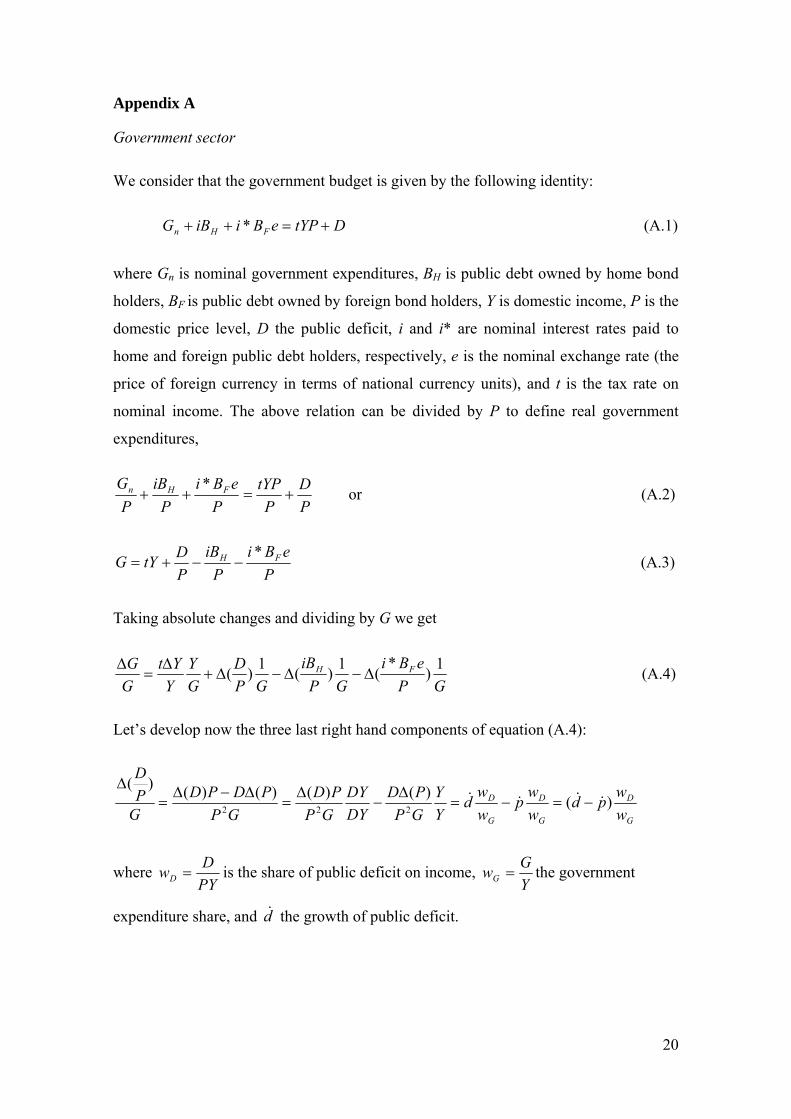
2.5. Government sector

We consider that the government budget is given by the following identity, in nominal

terms:

DtYPeBiiBG FHn +=++ * (12)

where Gn is nominal government expenditures, BH is public debt5 owned by home bond

holders, BF is public debt owned by foreign bond holders, Y is domestic income, P is the

domestic price level, D the public deficit, i and i* are nominal interest rates paid to

home and foreign public debt holders, respectively, e the nominal exchange rate, and t is

the tax rate on nominal income. According to this relation, public deficit exists when

total current expenditures (including interest payments on public debt) exceed the

revenues obtained through taxes on domestic money income, i.e,

tYPeBiiBG FHn >++ * .

5 Public debt is originated by issuing government bonds to finance public deficit.

9

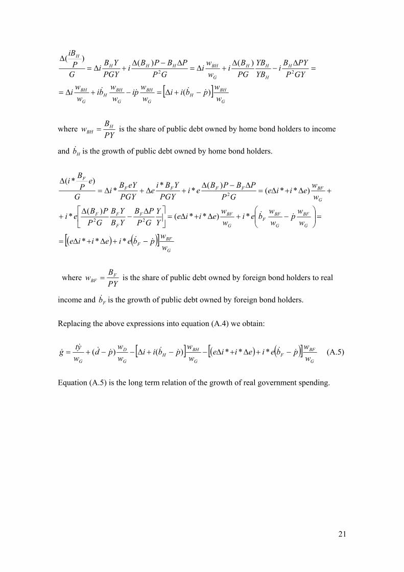
As it is shown in Appendix A (see Equation A.5), the long term relationship of the

growth of real government expenditures g& is given by:

[ ] ( ) ( )[ ]G

BFF

G

BHH

G

D

G wwpbeieiie

wwpbii

wwpd

wytg &&&&&&&

& −+Δ+Δ−−+Δ−−+= ***)()( (13)

where YDwD = is the budget deficit ratio,

YGwG = is the government spending ratio,

PYBw H

BH = and PYBw F

BF = are the shares of public debt owned by home and foreign

bonds holders (as a percentage of nominal income), respectively, d& is the growth of

budget deficit and Hb& and Fb& are the growth rates of the public debt owned by home

and foreign bond holders, respectively.

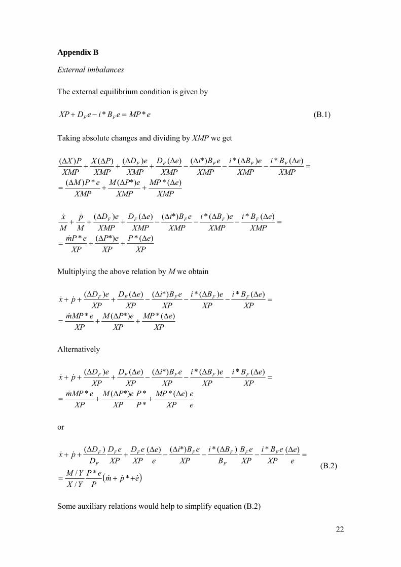
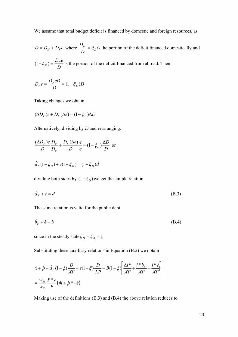
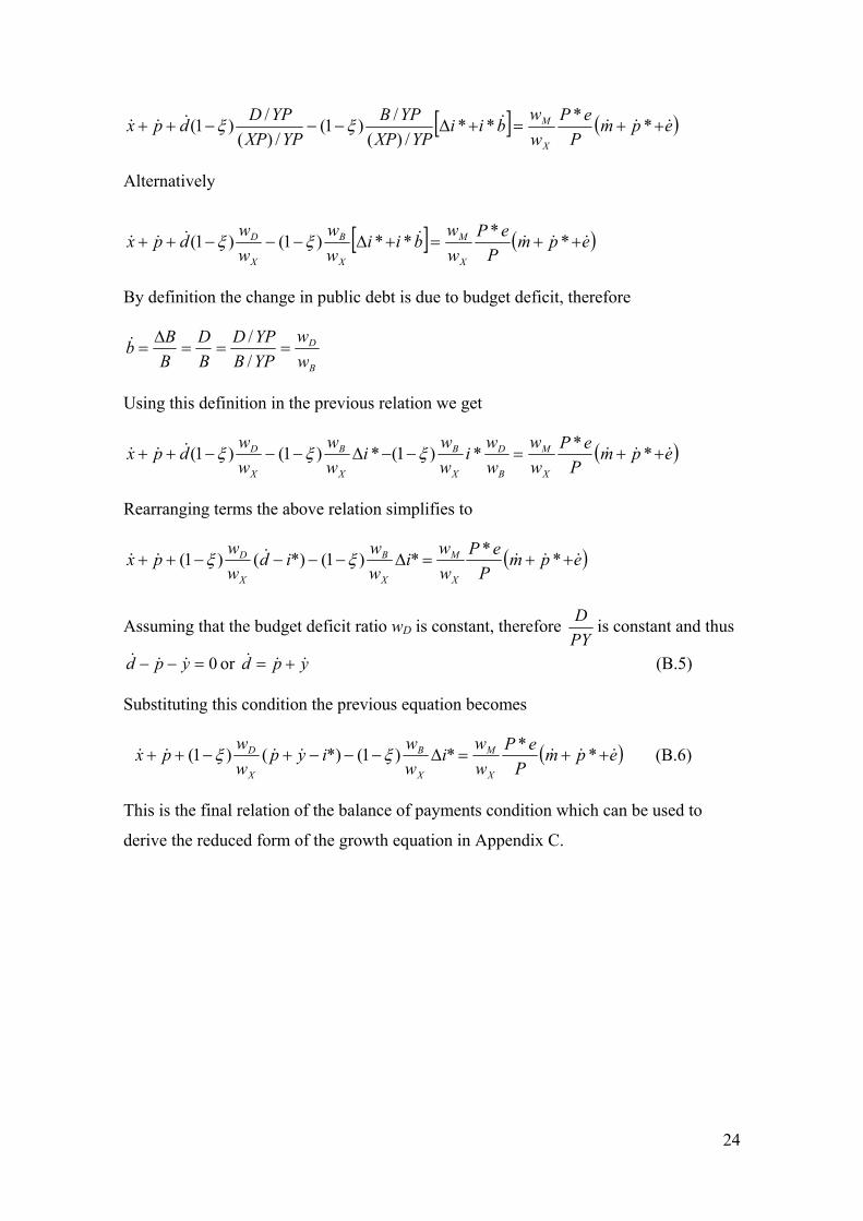
2.6. Balance-of-payments condition

The last relation of the model is an external equilibrium condition given by the

following identity:

eMPeBieDXP FF ** =−+ (14)

The left hand side of the identity shows the money resources available to finance

imports (export revenues plus the amount of public deficit assets hold by foreigners

minus interest rate payments on foreign bond holders).

It is shown in Appendix B, Equation (B.6) that the balance of payments final relation

can be expressed as:

( )epmP

ePwwi

wwiyp

wwpx

X

M

X

B

X

D &&&&&&& ++=Δ−−−+−++ ***)1(*)()1( ξξ (15)

where x& , m& , p& , *p& , y& and e& are growth rates of exports, imports, domestic prices,

foreign prices, domestic income and nominal exchange rate, respectively. Additionally,

MBD www ,, and Xw are the ratios of budget deficit, public debt, imports and exports on

income, respectively. Finally )1( ξ− represents the percentage of public deficit (or debt)

which is financed by external markets.

10

2.7. Domestic income growth

In Appendix C, Equation C.4 shows that the growth rate of domestic income can be

predicted by the following relation:

BAy =&

where

⎥⎥⎥⎥⎥⎥⎥⎥⎥⎥⎥⎥⎥⎥⎥

⎦

⎤

⎢⎢⎢⎢⎢⎢⎢⎢⎢⎢⎢⎢⎢⎢⎢

⎣

⎡

⎪⎪⎭

⎪⎪⎬

⎫

⎪⎪⎩

⎪⎪⎨

⎧

++⎥⎦

⎤⎢⎣

⎡−Δ−Δ−+

+Δ−Δ+++−Δ−Δ

−

−−−−−++

+−+⎟⎟⎠

⎞⎜⎜⎝

⎛−−+⎟⎟

⎠

⎞⎜⎜⎝

⎛−

=

epwwei

wwi

piwrtwpi

ww

PeP

iwwip

wwp

pepP

ePww

ww

PePy

PeP

ww

A

G

B

G

Bg

rkkkccB

B

X

M

X

B

X

D

X

Mmx

X

Mxxx

X

Mx

&&

&&

&&

&&&&

*)1(*

)()()1(

)(

*

*)1(*)()1(

)*()*()*1(*)*(

ξξ

π

επεπεπξξ

ξξ

δπδεπε

and (16)

X

D

G

B

G

B

G

D

Ggkkcc

X

M

ww

ww

eiwwi

ww

wt

PeP

ww

B

)1(

)1(*)*(

ξ

ξξ

πεπεπ

−−

−⎭⎬⎫

⎩⎨⎧

⎟⎟⎠

⎞⎜⎜⎝

⎛−−−+++=

Equation (16) shows that, among other factors, the growth of domestic income is

determined by internal and external imbalances, taking also into account the effect of

relative prices. Equation (16) will be used to predict actual growth in Portugal.

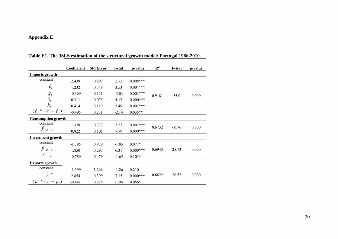
3. Testing the model for the Portuguese economy

The import demand equation (2), the export demand equation (4), the private

consumption equation (8) and the investment equation (11) are estimated

simultaneously to obtain the elasticities which are needed to compute the reduced form

of domestic income growth as it is expressed by equation (16). Annual data are used

covering the period 1986-2010, thus starting at the year that Portugal joined the early

11

EEC. The definition of the variables and the data sources are explained in Appendix D.

The method used for estimating the system equations is 3SLS (Three-Stage Least

Squares) as it is more efficient to capture the interrelation between equations and the

causal and feedback effects between the variables.6 Table E.1 in the Appendix E

provides the estimation results where simultaneity is controlled by using instrumental

variables. The growth of imports, consumption, investment, and exports are assumed to

be endogenous as well as the growth of government expenditures, domestic disposable

income, real exchange rate and real domestic interest rate. All other variables in the

system are assumed exogenous, including some lagged variables, as it is explained in

Table E.1.

In general the estimation results are quite satisfactory; all elasticities carry their

expected signs and are statistically significant with few exceptions. The relative price

elasticity is statistically significant in the import equation (at the 5% level) and carries

the correct negative sign but in the export demand equation caries a wrong negative sign

and it is significant at a 10% level only7. The value of the relative price elasticities is

low in comparison with the income elasticities, confirming the general finding in the

literature that trade is more sensitive to income than to price changes. The striking fact

in the import demand function is the high elasticity of consumption, which exceeds

unity (πc=1.232) indicating that imports increase more than proportionally with respect

to consumption increase8. Although the export and the investment elasticities with

respect to imports are also relevant, thus indicating a significant import content in these

elements of demand, they are lower (πx=0.311 and πk=0.414 respectively). An

unexpected result is the negative government spending elasticity of imports (πg=-0.370)

and statistically significant at the 5% level. This could signify an import substitution

policy of the government spending giving preference to the domestic goods and

services.

Table E.1 also shows that investment and exports are income elastic with respect to

domestic disposable income and foreign income, respectively (εk =1.85 and εx =2.85),

6 For more details on the 3SLS method, see for instance, AlDakhil (1998) and Wooldridge (2002). 7An increase in relative prices reflects devaluation and a decrease a valuation of domestic currency.

The same wrong sign of the relative prices on exports also found in previous studies for Portugal, see for instance, Soukiazis E. and Micaela Antunes (2012).

8 However, this elasticity is not statistically different from unity.

12

the former confirming the accelerator principle in the investment function, and the latter

showing the high sensitivity of exports relative to external demand (the OECD income

growth). This high export dependence on foreign income should be a case of concern in

periods of economic slowdown in foreign markets. Consumption is income inelastic, as

expected (εc=0.822) but with a sizeable value. Finally, the impact of real interest rate is

negative on investment (εr =-0.789), an expected result since this variable measures the

real cost of financing investment projects.

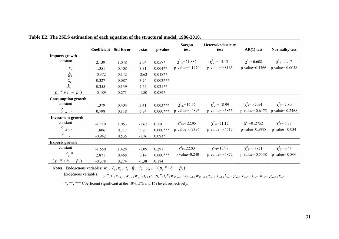
We also regressed each of the equations individually, by 2SLS (see Table E.2 in

Appendix E) using the same instruments. The intention was to carry out some

diagnostic tests to justify the robustness of our results. The first is the Sargan statistic, a

test of over-identifying restrictions to check the validity of the instruments used in the

regressions and that hypothesis is confirmed in all cases. The second is the Pagan-Hall

heteroskedasticity test, showing that the hypothesis of homoskedasticity is never

rejected. The third test is the Cumby-Huizinga test for autocorrelation. The null

hypothesis is that errors are not first-order autocorrelated and this is confirmed in all

cases. The last one is a normality test, conceptually similar to the Jarque-Bera skewness

and kurtosis test. The null hypothesis is that residuals from a given regression are

normally distributed, and this hypothesis is not rejected in all equations, except for

imports.

Table I below reports the values which are necessary for computing the growth rates of

domestic income in Portugal. Some are estimated values taken from Table E.1

(Appendix E) others are annual averages over the period considered (see Appendix D

for variable definition and data sources). Three growth rates are computed: ay& obtained

from equation (16) where internal and external imbalances are considered and relative

prices are not neutral; by& determined by the SCA model with relative prices being

constant, and cy& obtained from Thirlwall’s original Law, given byπxy&

& = . In the latter

case, it was necessary to estimate the import demand function, )*( pepym m &&&&& −++= δπ , by OLS (with robust standard errors) to obtain the

aggregate income elasticity with respect to import growth (π=2.633).

13

Table I. Computation of the growth rates of domestic income. Portugal, 1986-2010

Notes: xε , xπ , cε , cπ , kε , kπ , gπ , εr , δm

and δx are taken from Table E.1 (see Appendix E).

r, t, Dw , Gw , Bw , Mw , Xw , i, i*, e, p& and *y& are annual averages over the period 1986-2010.

Dξ and Bξ = 0.401 is assumed constant over the whole period.

Comparing these different growth rates with the actual average annual growth in

Portugal over the period 1986-2010 ( y& =2.728%) the following remarks can be made:

(i) The growth rate obtained by Thirlwall’s original Law ( cy& =2.335%) using

the aggregate income elasticity of imports (π=2.633) accurately predicts

actual growth rate ( y& =2.728%) in Portugal. The Portuguese economy grew,

on average, 0.393 percentage points (per annum), above the rate allowed by

the balance-of-payments equilibrium. We have to recall that Thirlwall’s Law

is a restrictive form in the sense that it assumes that balance of payments is

in equilibrium, relative prices are not playing any significant role on growth

and no internal imbalances are considered in the model.

(ii) The growth rate obtained by the augmented Thirlwall’s model which

considers internal and external imbalances and relative prices are not neutral

εx 2.854

πx 0.311

εc 0.822

πc 1.232

εk 1.850

πk

0.414

πg -0.370

εr -0.789

δm -0.495

δx

-0.441

t 0.360

r 0.027

0.057

0.025

wD 0.050

wG 0.378

wB 0.588

ξD 0.401

ξB 0.401

wM 0.364

wX 0.280

i 0.084

i* 0.055

Δi -0.009

Δi* -0.002

e 0.972

0.013

1.087

-0.012

-0.001

0.026

0.002

-1.5631

-0.02%

2.335

2.728

Internal and external imbalances and relative prices no neutral Equation (16)

Internal and external imbalances and relative prices neutral

Thirlwall’s Law

πxy&

& =

Actual growth

e&

pep &&& −+*

p& *y&

)*(p

ep

cy&

*p&( )pi &Δ−Δ ( )*ip −&

ay& by& y&

14

( ay& =-1.5631%) underestimates substantially actual growth in Portugal. This

result shows that Portugal should grow much less than actually did in order

not to aggravate internal and external imbalances. In other words, Portugal

grew faster than the rate allowed by the balance-of-payments equilibrium

and its public financial capability at the cost of accumulating internal and

external deficits and this can explain the recent debt crisis of the country. In

order to grow faster without deteriorating internal and external imbalances

some improvements have to be made on structural parameters and especially

on those related with competitiveness. We will show that more explicitly in

the scenario analysis of the next section.

(iii) The fact that Portugal grew at a higher average growth rate (2.73%) than that

predicted by our model in the last two decades can be explained by capital

inflows financing this growth. The higher actual growth was obtained at the

expense of accumulating higher external debt over time corresponding to

233% of GDP in 2009. On the other hand, the low growth rate predicted by

our model (negative) is due to the fact that internal imbalances imply capital

outflows via debt interest rate payments. Therefore, they play a similar role

as imports, restricting growth in the long run.

(iv) Substantially different results are obtained when relative prices are

considered in our model. Our previous model with no relative prices (the so

called SCA model)9 predicted a higher average growth rate, around 0.28%,

in comparison to -1.5631% rate found by the new model controlling for the

relative prices effects. Therefore, the difference can be attributed to the

contribution of relative prices mostly affecting the import and export sectors

as we have concluded from the regression analysis (see Table E.1 in

Appendix E).

An important explanation for the low (negative) growth performance predicted by our

model lies in the high import sensitivity of the components of demand, especially that of

consumption ( cπ = 1.232). This elasticity shows that if consumption increases by one

percentage point (p.p.) this will induce a 1.232 p.p. increase in imports (more than

9 See Soukiazis et al. (2012).

15

proportional). Therefore, a high amount of domestic consumption is spent on imported

consumption goods and could be responsible for the balance of payments deficits on the

current account.

The high import sensitivity of the components of demand explains the high income

elasticity of the demand for imports at the aggregate level π=2.633 showing that imports

grow more than twice the increase in domestic income. The high penetration of imports

can also be observed by the share of imports on income, around Mw =36%, with exports

representing Xw = 28% only. Therefore the multiplier effects of the components of

demand on growth are not substantial in the Portuguese economy as they are counter-

balanced by the increase in imports.

We have to notice here that what is important in international trade is not importing too

much in order to produce domestic and exported goods, but ensuring that the

transformation of imported components into domestic goods and exports contains

enough value-added. In international markets, most produced goods and exports

embody a substantial share of imported components, but in terms of gains it is important

that the value (price) - especially of exports embodying imported components - is

sufficiently higher than the value (price) of those imported components. Traditionally,

Portugal produces (and exports) low value-added domestic goods (due to low

productivity) despite the move from low to medium or medium-high technology exports

in recent years (OECD, 2008). On the other hand, the share of the service sector in the

overall economy has risen (corresponding to 75.4% of gross value added against 22.3%

in industry and 2.3% in agriculture). However, labour productivity gains have been

particularly weak and became negative since the beginning of the current decade. The

service sector involves mainly a high number of micro enterprises (wholesale, retail,

hotels and restaurants) with a substantial proportion of non-tradable goods and high

informality (OECD Economic Survey, 2010).

4. A scenario analysis

Some simulations can be made with the aim to detect the factors that could help the

economy to grow faster.

16

(i) Fiscal policy towards a reduction in income taxation. If taxation on income

reduces from t = 36% to 20% (everything else constant) the predicted growth increases

from ay& = -1.5631 to ay& = -1.41%. In fact there is a positive effect on growth due to a

more friendly taxation policy but the stimulus is not very significant.

(ii) Budget deficit policy aiming at reducing public deficit and debt ratio. If we

assume Dw = 0.03 and Bw = 0.60 (the values imposed by the Growth and Stability Pact

i.e., deficit of 3% and debt of 60% of the GDP) the predicted growth is around ay& = -

1.58%. Therefore public budget discipline alone does not help the economy to grow

faster.

(iii) Our simulation approach shows that growth in Portugal is not sensitive to

domestic interest rates changes but it is highly sensitive to changes in foreign interest

rates10. For instance, if i* increases by two percentage points (from the average rate of

the whole period of 5.5% to 7.5%) the growth rate predicted from our model becomes

much more negative, ay& = -2.91%. On the other hand if foreign interest rates are

reduced by one percentage point (from 5.5% to 4.5%) the growth rate in Portugal

becomes much less negative ay& = -0.93%. A combination of a 3% in budget deficit and

60% in public debt ratio (the growth and stability goals) and assuming a 2% foreign

interest rate paid on government bonds raises income growth to a positive rate 0.68%.

This is an interesting result showing the great difficulty Portugal is presently facing to

finance its public debt. As it is known, Portugal was forced to ask the intervention of the

IMF in 2011 when interest rates paid on government bonds exceeded 7%, budget deficit

was around 8% and public debt around 100% of GDP. Due to this situation, austerity

measures were implemented with the aim to reduce internal and external imbalances,

having strong negative effects on growth and unemployment in the short term course.

(iv) The increase in the share of home government bond holders is another factor that

favors growth. For instance, if half of the public debt is financed by domestic resources

(ξB increases from 40% to 50%) our model predicts a less negative growth rate of ay& = -

0.91%. A scenario of a deficit ratio of 3%, debt ratio of 60%, a foreign interest rate of

2%, and a share of 50% of home government bond holders raises income growth to a

10 In this study we use long term interest rates of the German economy as the benchmark for foreign

interest rates.

17

positive rate equal to ay& = 0.94%. Therefore policies to convince national savers to

invest on home government bonds can enhance economic growth.

(v) The novelty in this new model is that now we assume that relative prices are not

neutral. If we assume that relative prices are constant in the long run, that is,

0* =−+ pep &&& , and therefore (P*e/P) =1, e=1 and 0=e& and replace these values into

our model (equation (16)) the obtained growth rate is by& =-0.02% which is much higher

than the one found when relative prices are not neutral, ay& = -1.56% (see Table I).

Therefore relative prices make a substantial difference in the growth pace and when are

ignored the model over-predicts the growth rate in Portugal. The lower growth rate

obtained when relative prices are included in the model can be explained by the over

valuation of the domestic currency in Portugal. It is interesting to check a scenario

where there is a change in the average value of the growth of real relative prices (or real

exchange rate) for the whole period from -0.0116 to 0.06 representing a devaluation of

domestic currency11. In this case it is shown that growth increases to a positive rate

equal to ay& =0.15% confirming the hypothesis that a currency devaluation is a stimulus

to growth increasing the country´s competiveness in foreign markets.

(vi) By reducing the import sensitivity of exports (elasticity) from xπ =0.31 (see

Table I) to 0.20 our model predicts a higher growth rate equal to ay& = -0.93%. It is

therefore shown that lowering the import sensitivity of exports is a stimulus to growth.

When the import content of exports is high the exports’ multiplier effects on income are

crowded out by higher imports. Reducing the import content of exports is an

appropriate policy to achieve higher growth.

(vii) Reducing the share of imports by only 4 percentage points (from 36% to 32%)

the predicted growth is ay& = -1.10%, or alternatively increasing the share of exports by

4 percentage points (from 28% to 32%) the obtained growth is even higher, ay& = -

0.57%. A combined policy with the aim at reducing the import share to 30% and

increasing export share to 35% (having a surplus on trade) yields an even higher

growth rate, around ay& = 1.30%. Therefore changing the structure of the shares of

imports and exports is the appropriate way to enhance growth.

11 This is not a pragmatic solution for Portugal since the country belongs to the eurozone and nominal

exchange rates are fixed.

18

(viii) Finally, an alternative scenario could be to determine the equilibrium growth

rate of the Portuguese economy with no internal and external imbalances and neutral

relative prices. For concreteness, the following conditions are assumed: export share

equal to import share wX=wM, therefore wM/wX=1; constant relative prices 0* =−+ pep &&&

, thus (P*e/P) =1, e=1 and 0=e& ; and zero deficit and debt ratio wD=wB=0. Replacing

these values in equation (16) the equilibrium growth rate is very high ay& =5.5%.

However, the above assumptions are not plausible and can over predict growth rates in

Portugal.

According to these hypothetical scenarios it is clearly shown that the most effective

policy to achieve higher growth in Portugal applies to the external sector, towards a

balanced external trade and changing the structure of imports and exports. This is in line

with Thirlwall’s Law that affirms that growth is balance-of-payments constrained.

Additionally, the way of financing public debt and the service payments on that debt

play an important role in the growth analysis as well as a competitive devaluation.

5. Concluding remarks

The aim of this study was to develop a more complete growth model in line with

Thirlwall’s Law that takes into account both internal and external imbalances and

assumes that relative prices are not neutral. The important contribution of the extended

model is that it discriminates the import content of aggregate demand and introduces

public deficit and debt measures as determinants of growth. Additionally, the model

controls for relative prices movements and this is the main difference from our previous

model (the SCA model). The reduced form of the model shows that growth rates can be

obtained in three alternative ways: assuming internal and external imbalances and no

neutrality in relative prices; assuming internal and external imbalances but neutral

relative prices; and lastly the growth rate predicted by Thirlwall’s Law. The growth

model is tested for the Portuguese economy over the period 1986-2010 to check its

accuracy.

The equations constituting the model are estimated by 3SLS to control the endogeneity

of the core variables and to obtain consistent estimates. The empirical analysis shows

that growth rates obtained by Thirlwall’s Law accurately predict the average growth rate

19

of the Portuguese economy over the period 1986-2010 although it is slightly lower than

the actual growth. However, Thirlwall’s Law considers some controversial assumptions,

namely that external trade is balanced, public finances are at equilibrium, and relative

prices are neutral. Testing our model where trade and public imbalances are allowed and

relative prices are not neutral the predicted growth rate is even lower (negative) than the

actual one and this is consistent with the external trade and public debt disequilibria the

country has been accumulating in recent years.

The scenarios implemented to explain the low growth rate predicted by our model point

to the fact that policies aiming to equilibrate external deficits or changing the structure

of imports and exports are more effective for achieving higher growth. Competitive

devaluation also acts as a stimulus to growth. It is also shown that policies designed to

reduce public deficits and public debts, but above all to achieve better conditions of

financing internal imbalances (mostly from domestic resources), and reducing the

payment costs of public debt are beneficial to growth. Therefore, Portugal could benefit

from the challenging idea of issuing Eurobonds to finance its public debt in the

European market with lower costs.

20

Appendix A

Government sector

We consider that the government budget is given by the following identity:

DtYPeBiiBG FHn +=++ * (A.1)

where Gn is nominal government expenditures, BH is public debt owned by home bond

holders, BF is public debt owned by foreign bond holders, Y is domestic income, P is the

domestic price level, D the public deficit, i and i* are nominal interest rates paid to

home and foreign public debt holders, respectively, e is the nominal exchange rate (the

price of foreign currency in terms of national currency units), and t is the tax rate on

nominal income. The above relation can be divided by P to define real government

expenditures,

PD

PtYP

PeBi

PiB

PG FHn +=++

* or (A.2)

PeBi

PiB

PDtYG FH *

−−+= (A.3)

Taking absolute changes and dividing by G we get

GPeBi

GPiB

GPD

GY

YYt

GG FH 1)*(1)(1)( Δ−Δ−Δ+

Δ=

Δ (A.4)

Let’s develop now the three last right hand components of equation (A.4):

G

D

G

D

G

D

wwpd

wwp

wwd

YY

GPPD

DYDY

GPPD

GPPDPD

GPD

)()()()()()(222

&&&& −=−=Δ

−Δ

=Δ−Δ

=Δ

where PYDwD = is the share of public deficit on income,

YGwG = the government

expenditure share, and d& the growth of public deficit.

21

[ ]G

BHH

G

BH

G

BHH

G

BH

H

H

HH

G

BHHHH

H

wwpbii

wwpi

wwbi

wwi

GYPPYBi

YBYB

PGBi

wwi

GPPBPBi

PGYYBi

GP

iB

)(

)()()(22

&&&& −+Δ=−+Δ=

=Δ

−Δ

+Δ=Δ−Δ

+Δ=Δ

where PYBw H

BH = is the share of public debt owned by home bond holders to income

and Hb& is the growth of public debt owned by home bond holders.

( ) ( )[ ]G

BFF

G

BF

G

BFF

G

BFF

F

FF

G

BFFFFF

F

wwpbeieiie

wwp

wwbei

wweiie

YY

GPPB

YBYB

GPPBei

ww

eiieGP

PBPBei

PGYYBi

ePGY

eYBi

G

eP

Bi

&&

&&

−+Δ+Δ=

=⎟⎟⎠

⎞⎜⎜⎝

⎛−+Δ+Δ=⎥

⎦

⎤⎢⎣

⎡ Δ−

Δ+

+Δ+Δ=Δ−Δ

+Δ+Δ=Δ

***

*)**()(*

)**()(

**

*)*(

22

2

where PYBw F

BF = is the share of public debt owned by foreign bond holders to real

income and Fb& is the growth of public debt owned by foreign bond holders.

Replacing the above expressions into equation (A.4) we obtain:

[ ] ( ) ( )[ ]G

BFF

G

BHH

G

D

G wwpbeieiie

wwpbii

wwpd

wytg &&&&&&&

& −+Δ+Δ−−+Δ−−+= ***)()( (A.5)

Equation (A.5) is the long term relation of the growth of real government spending.

22

Appendix B

External imbalances

The external equilibrium condition is given by

eMPeBieDXP FF ** =−+ (B.1)

Taking absolute changes and dividing by XMP we get

XMPeMP

XMPePM

XMPePM

XMPeBi

XMPeBi

XMPeBi

XMPeD

XMPeD

XMPPX

XMPPX FFFFF

)(**)(*)(

)(*)(**)()()()()(

Δ+

Δ+

Δ=

=Δ

−Δ

−Δ

−Δ

+Δ

+Δ

+Δ

XPeP

XPeP

XPePm

XMPeBi

XMPeBi

XMPeBi

XMPeD

XMPeD

Mp

Mx FFFFF

)(**)(*

)(*)(**)()()(

Δ+

Δ+=

=Δ

−Δ

−Δ

−Δ

+Δ

++

&

&&

Multiplying the above relation by M we obtain

XPeMP

XPePM

XPeMPm

XPeBi

XPeBi

XPeBi

XPeD

XPeDpx FFFFF

)(**)(*

)(*)(**)()()(

Δ+

Δ+=

=Δ

−Δ

−Δ

−Δ

+Δ

++

&

&&

Alternatively

ee

XPeMP

PP

XPePM

XPeMPm

XPeBi

XPeBi

XPeBi

XPeD

XPeD

px FFFFF

)(****)(*

)(*)(**)()()(

Δ+

Δ+=

=Δ

−Δ

−Δ

−Δ

+Δ

++

&

&&

or

( )epmP

ePYXYM

ee

XPeBi

XPeB

BBi

XPeBi

ee

XPeD

XPeD

DDpx FF

F

FFFF

F

F

&&&

&&

++=

=Δ

−Δ

−Δ

−Δ

+Δ

++

**//

)(*)(**)()()(

(B.2)

Some auxiliary relations would help to simplify equation (B.2)

23

We assume that total budget deficit is financed by domestic and foreign resources, as

eDDD FH += where DH

DD

ξ= is the portion of the deficit financed domestically and

DeDF

D =− )1( ξ is the portion of the deficit financed from abroad. Then

DDeDDeD D

FF )1( ξ−==

Taking changes we obtain

DeDeD DFF Δ−=Δ+Δ )1()()( ξ

Alternatively, dividing by D and rearranging:

DD

ee

DeD

DD

DeD

DF

F

FF Δ−=

Δ+

Δ )1()()(ξ or

ded DDDF&&& )1()1()1( ξξξ −=−+−

dividing both sides by )1( Dξ− we get the simple relation

ded F&&& =+ (B.3)

The same relation is valid for the public debt

bebF&&& =+ (B.4)

since in the steady state ξξξ == BD

Substituting these auxiliary relations in Equation (B.2) we obtain

( )epmP

ePww

XPei

XPbi

XPiB

XPDe

XPDdpx

X

M

FF

&&&

&&&&&&

++=

=⎥⎦

⎤⎢⎣

⎡++

Δ−−−+−++

**

***)1()1()1( ξξξ

Making use of the definitions (B.3) and (B.4) the above relation reduces to

24

[ ] ( )epmP

ePwwbii

YPXPYPB

YPXPYPDdpx

X

M &&&&&&& ++=+Δ−−−++ ****/)(

/)1(/)(

/)1( ξξ

Alternatively

[ ] ( )epmP

ePwwbii

ww

wwdpx

X

M

X

B

X

D &&&&&&& ++=+Δ−−−++ ****)1()1( ξξ

By definition the change in public debt is due to budget deficit, therefore

B

D

ww

YPBYPD

BD

BBb ===

Δ=

//&

Using this definition in the previous relation we get

( )epmP

ePww

wwi

wwi

ww

wwdpx

X

M

B

D

X

B

X

B

X

D &&&&&& ++=−−Δ−−−++ ***)1(*)1()1( ξξξ

Rearranging terms the above relation simplifies to

( )epmP

ePwwi

wwid

wwpx

X

M

X

B

X

D &&&&&& ++=Δ−−−−++ ***)1(*)()1( ξξ

Assuming that the budget deficit ratio wD is constant, therefore PYD is constant and thus

0=−− ypd &&& or ypd &&& += (B.5)

Substituting this condition the previous equation becomes

( )epmP

ePwwi

wwiyp

wwpx

X

M

X

B

X

D &&&&&&& ++=Δ−−−+−++ ***)1(*)()1( ξξ (B.6)

This is the final relation of the balance of payments condition which can be used to

derive the reduced form of the growth equation in Appendix C.

25

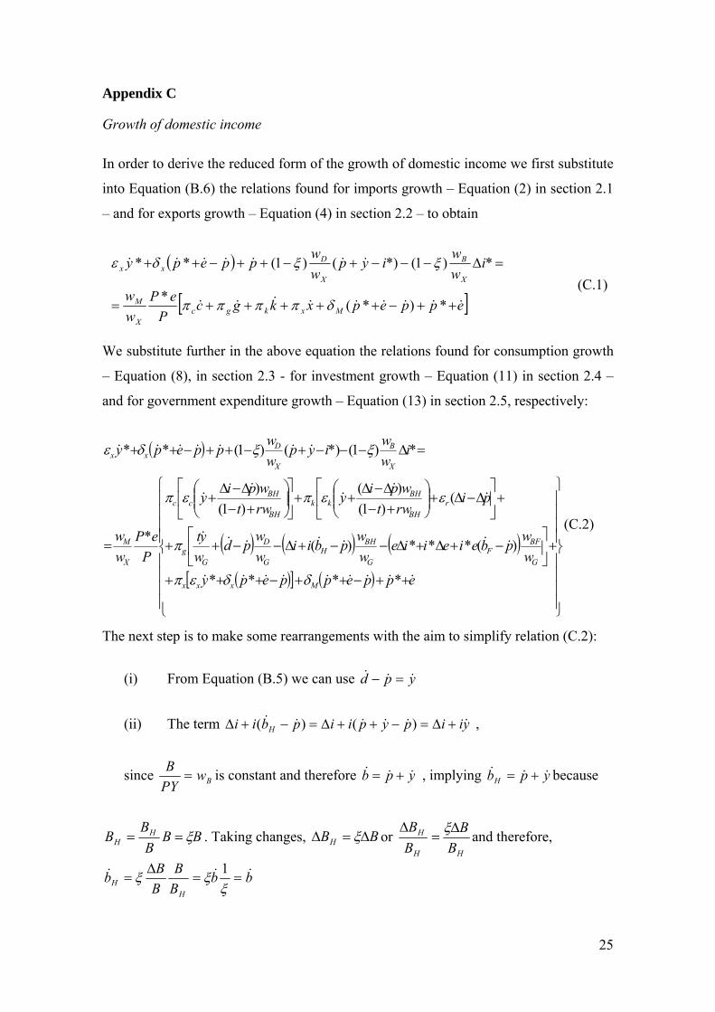
Appendix C

Growth of domestic income

In order to derive the reduced form of the growth of domestic income we first substitute

into Equation (B.6) the relations found for imports growth – Equation (2) in section 2.1

– and for exports growth – Equation (4) in section 2.2 – to obtain

( )

[ ]eppepxkgcP

ePww

iww

iypww

ppepy

MxkgcX

M

X

B

X

Dxx

&&&&&&&&&

&&&&&&&

++−+++++=

=Δ−−−+−++−++

*)*(*

*)1(*)()1(**

δππππ

ξξδε (C.1)

We substitute further in the above equation the relations found for consumption growth

– Equation (8), in section 2.3 - for investment growth – Equation (11) in section 2.4 –

and for government expenditure growth – Equation (13) in section 2.5, respectively:

( )

( ) ( ) ( )( )[ ] ( )

⎪⎪⎪⎪

⎭

⎪⎪⎪⎪

⎬

⎫

⎪⎪⎪⎪

⎩

⎪⎪⎪⎪

⎨

⎧

++−++−+++

+⎥⎦

⎤⎢⎣

⎡−+Δ+Δ−−+Δ−−++

+⎥⎦

⎤⎢⎣

⎡Δ−Δ+⎟⎟

⎠

⎞⎜⎜⎝

⎛+−Δ−Δ

++⎥⎦

⎤⎢⎣

⎡⎟⎟⎠

⎞⎜⎜⎝

⎛+−Δ−Δ

+

=

=Δ−−−+−++−++

eppeppepywwpbeieiie

wwpbii

wwpd

wyt

pirwtwpiy

rwtwpiy

PeP

ww

iwwiyp

wwppepy

Mxxx

G

BFF

G

BHH

G

D

Gg

rBH

BHkk

BH

BHcc

X

M

X

B

X

Dxx

&&&&&&&&&

&&&&&&&

&&

&&

&

&&&&&&&

****

)(***)(

()1(

)()1(

)

*

*)1(*)()1(**

δδεπ

π

εεπεπ

ξξδε

(C.2)

The next step is to make some rearrangements with the aim to simplify relation (C.2):

(i) From Equation (B.5) we can use ypd &&& =−

(ii) The term yiipypiipbii H &&&&&& +Δ=−++Δ=−+Δ )()( ,

since BwPYB

= is constant and therefore ypb &&& += , implying ypbH &&& += because

BBB

BB HH ξ== . Taking changes, BBH Δ=Δ ξ or

HH

H

BB

BB Δ

=Δ ξ and therefore,

bbBB

BBb

HH

&&& ==Δ

=ξ

ξξ 1

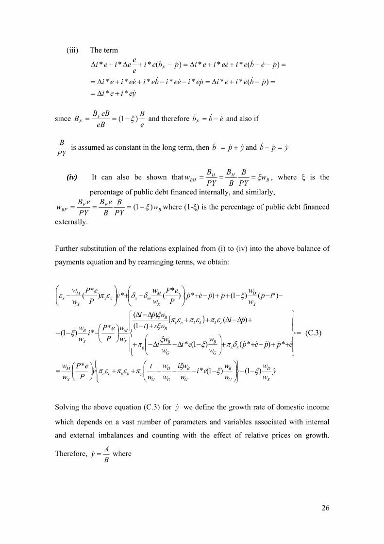
26

(iii) The term

yeieipbeieipeieeibeieeiei

pebeieeieipbeieeeiei F

&

&&&&&&

&&&&&&

**)(*******

)(***)(***

+Δ==−+Δ=−−++Δ=

=−−++Δ=−+Δ+Δ

since eB

eBeBBB F

F )1( ξ−== and therefore ebbF &&& −= and also if

PYB is assumed as constant in the long term, then ypb &&& += and ypb &&& =−

(iv) It can also be shown that BHH

BH wPYB

BB

PYBw ξ=== , where ξ is the

percentage of public debt financed internally, and similarly,

BFF

BF wPYB

BeB

PYeBw )1( ξ−=== where (1-ξ) is the percentage of public debt financed

externally. Further substitution of the relations explained from (i) to (iv) into the above balance of

payments equation and by rearranging terms, we obtain:

( )

yww

wwei

wwi

ww

wty

PeP

ww

eppepww

eiww

i

piwrtwpi

ww

PePi

ww

ipwwppep

PeP

wwy

PeP

ww

X

D

G

B

G

B

G

D

Ggkkcc

X

M

xxG

B

G

Bg

rkkkccB

B

X

M

X

B

X

D

X

Mmxxx

X

Mx

&&

&&&&&

&&

&&&&&&

)1()1(**

*)*()1(*

)()1(

)(

**)1(

*)()1()*()*(*)*(

ξξξ

πεπεπ

δπξξ

π

επεπεπξξ

ξ

ξδδεπε

−−⎭⎬⎫

⎩⎨⎧

⎟⎟⎠

⎞⎜⎜⎝

⎛−−−+++⎟

⎠⎞

⎜⎝⎛=

=

⎪⎪⎭

⎪⎪⎬

⎫

⎪⎪⎩

⎪⎪⎨

⎧

++−++⎟⎟⎠

⎞⎜⎜⎝

⎛−Δ−Δ−+

+Δ−Δ+++−Δ−Δ

⎟⎠⎞

⎜⎝⎛−−−

−−−++−+⎟⎟⎠

⎞⎜⎜⎝

⎛−+⎟⎟

⎠

⎞⎜⎜⎝

⎛−

(C.3)

Solving the above equation (C.3) for y& we define the growth rate of domestic income

which depends on a vast number of parameters and variables associated with internal

and external imbalances and counting with the effect of relative prices on growth.

Therefore, BAy =& where

27

⎥⎥⎥⎥⎥⎥⎥⎥⎥⎥⎥⎥⎥⎥⎥

⎦

⎤

⎢⎢⎢⎢⎢⎢⎢⎢⎢⎢⎢⎢⎢⎢⎢

⎣

⎡

⎪⎪⎭

⎪⎪⎬

⎫

⎪⎪⎩

⎪⎪⎨

⎧

++⎥⎦

⎤⎢⎣

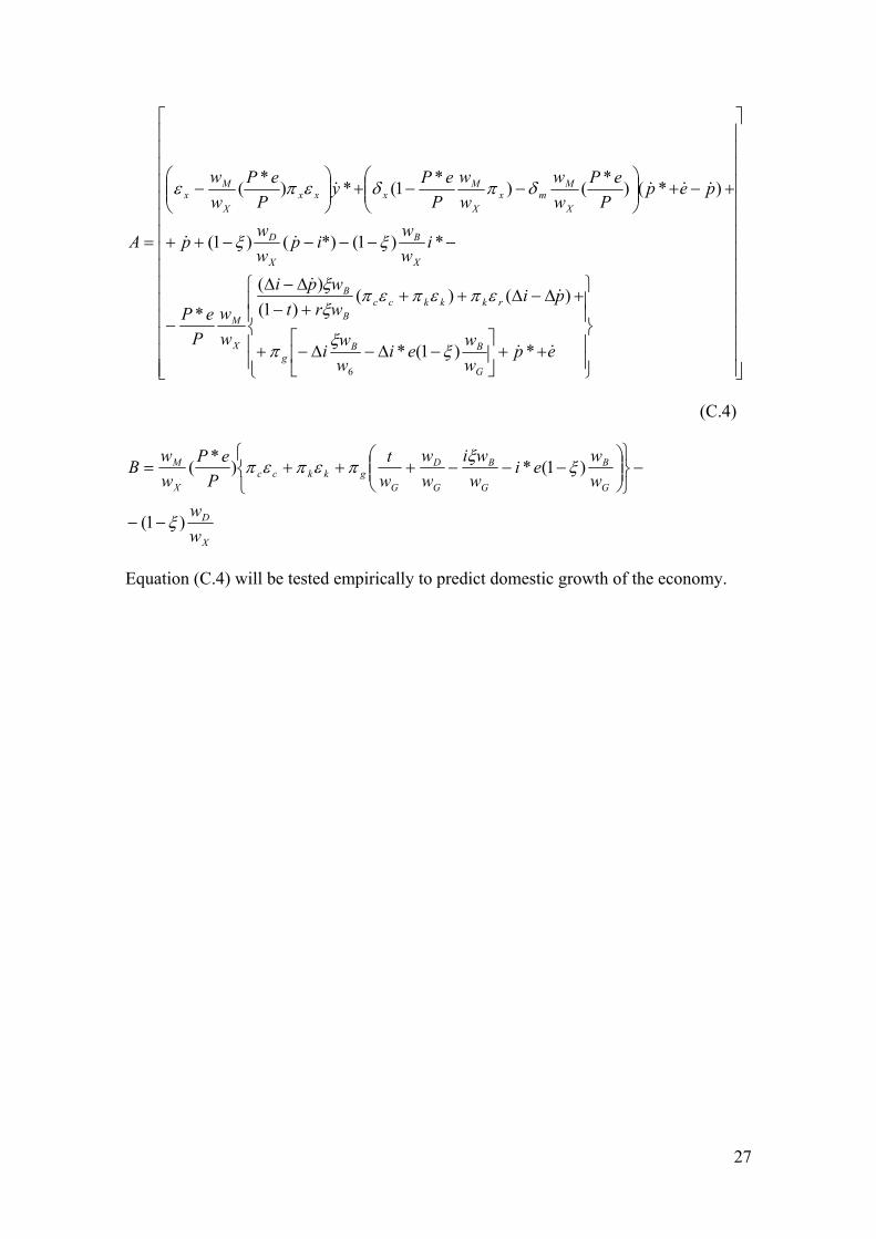
⎡−Δ−Δ−+

+Δ−Δ+++−Δ−Δ

−

−−−−−++

+−+⎟⎟⎠

⎞⎜⎜⎝

⎛−−+⎟⎟

⎠

⎞⎜⎜⎝

⎛−

=

epww

eiww

i

piwrtwpi

ww

PeP

iww

ipww

p

pepP

ePww

ww

PePy

PeP

ww

A

G

BBg

rkkkccB

B

X

M

X

B

X

D

X

Mmx

X

Mxxx

X

Mx

&&

&&

&&

&&&&

*)1(*

)()()1(

)(

*

*)1(*)()1(

)*()*()*1(*)*(

6

ξξ

π

επεπεπξξ

ξξ

δπδεπε

(C.4)

X

D

G

B

G

B

G

D

Ggkkcc

X

M

ww

ww

eiwwi

ww

wt

PeP

ww

B

)1(

)1(*)*(

ξ

ξξ

πεπεπ

−−

−⎭⎬⎫

⎩⎨⎧

⎟⎟⎠

⎞⎜⎜⎝

⎛−−−+++=

Equation (C.4) will be tested empirically to predict domestic growth of the economy.

28

Appendix D

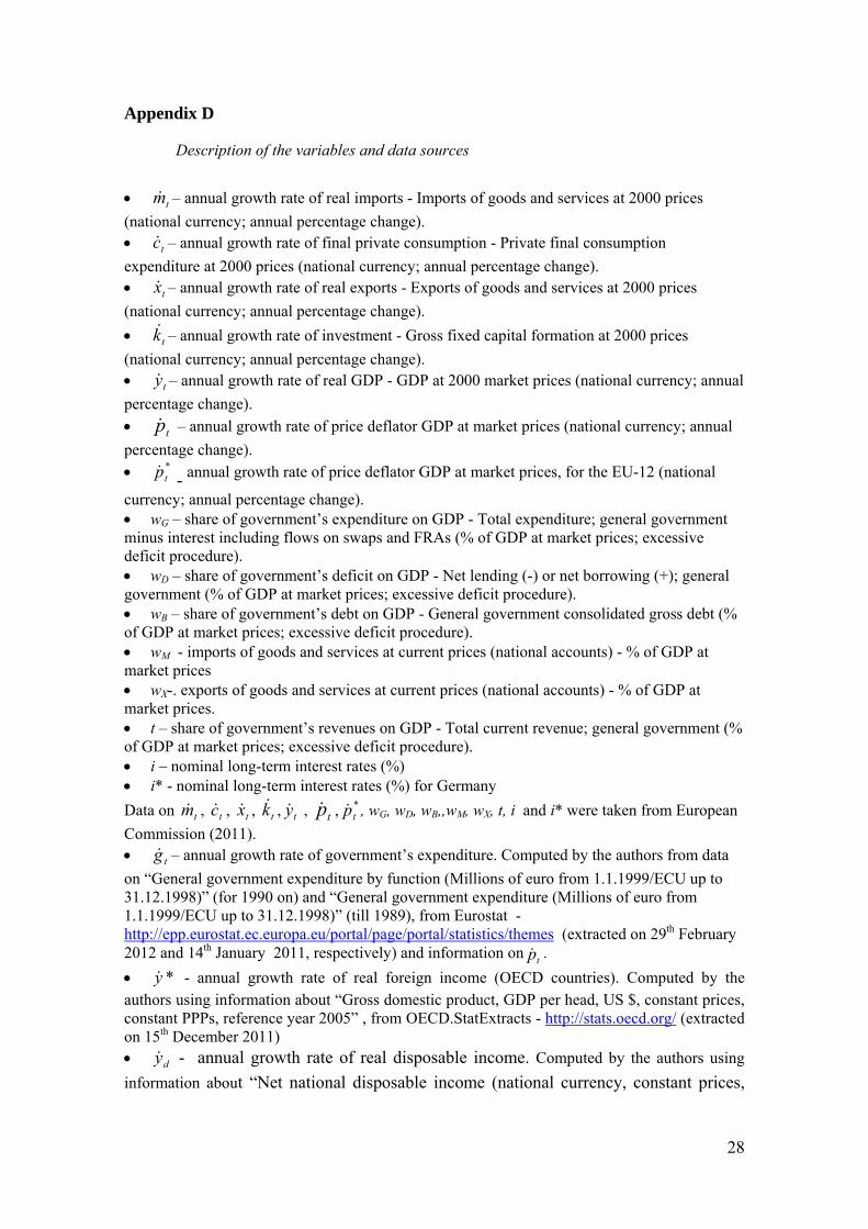
Description of the variables and data sources

• tm& – annual growth rate of real imports - Imports of goods and services at 2000 prices (national currency; annual percentage change). • tc& – annual growth rate of final private consumption - Private final consumption expenditure at 2000 prices (national currency; annual percentage change). • tx& – annual growth rate of real exports - Exports of goods and services at 2000 prices (national currency; annual percentage change). • – annual growth rate of investment - Gross fixed capital formation at 2000 prices (national currency; annual percentage change). • ty& – annual growth rate of real GDP - GDP at 2000 market prices (national currency; annual percentage change). • tp& – annual growth rate of price deflator GDP at market prices (national currency; annual percentage change). • *

tp& - annual growth rate of price deflator GDP at market prices, for the EU-12 (national

currency; annual percentage change). • wG – share of government’s expenditure on GDP - Total expenditure; general government minus interest including flows on swaps and FRAs (% of GDP at market prices; excessive deficit procedure). • wD – share of government’s deficit on GDP - Net lending (-) or net borrowing (+); general government (% of GDP at market prices; excessive deficit procedure). • wB – share of government’s debt on GDP - General government consolidated gross debt (% of GDP at market prices; excessive deficit procedure). • wM - imports of goods and services at current prices (national accounts) - % of GDP at market prices • wX-. exports of goods and services at current prices (national accounts) - % of GDP at market prices. • t – share of government’s revenues on GDP - Total current revenue; general government (% of GDP at market prices; excessive deficit procedure). • i – nominal long-term interest rates (%) • i* - nominal long-term interest rates (%) for Germany Data on tm& , tc& , tx& , , ty& , tp& , *

tp& , wG, wD, wB,,wM, wX, t, i and i* were taken from European Commission (2011). • tg& – annual growth rate of government’s expenditure. Computed by the authors from data on “General government expenditure by function (Millions of euro from 1.1.1999/ECU up to 31.12.1998)” (for 1990 on) and “General government expenditure (Millions of euro from 1.1.1999/ECU up to 31.12.1998)” (till 1989), from Eurostat - http://epp.eurostat.ec.europa.eu/portal/page/portal/statistics/themes (extracted on 29th February 2012 and 14th January 2011, respectively) and information on tp& . • *y& - annual growth rate of real foreign income (OECD countries). Computed by the authors using information about “Gross domestic product, GDP per head, US $, constant prices, constant PPPs, reference year 2005” , from OECD.StatExtracts - http://stats.oecd.org/ (extracted on 15th December 2011) • dy& - annual growth rate of real disposable income. Computed by the authors using information about “Net national disposable income (national currency, constant prices,

tk&

tk&

29

national base year)”, from OECD.StatExtracts - http://stats.oecd.org/ (extracted on 10th March 2012) • e – nominal effective exchange rate - price of domestic currency in terms of foreign currency - index (2010=100) narrow indices (27 countries). Computed by the authors using monthly data, from the Bank for International Settlements(BIS)- http://www.bis.org/statistics/eer/index.htm (extracted on 18th May 2012)

• (P*e/P)- real effective exchange rate index (2010=100), narrow indices (27 countries). Computed by the authors using monthly data, from the Bank for International Settlements(BIS)- http://www.bis.org/statistics/eer/index.htm (extracted on 18th May 2012)

30

Appendix E

Table E1. The 3SLS estimation of the structural growth model: Portugal 1986-2010.

Coefficient Std Error t-stat p-value R2 F-stat p-value Imports growth

constant  

2.439 0.897 2.72 0.008***

0.9181 55.0 0.000

   1.232 0.348 3.53 0.001***    -0.369 0.121 -3.04 0.003***    0.311 0.075 4.17 0.000***

0.414 0.119 3.49 0.001***    -0.495 0.231 -2.14 0.035** Consumption growth

constant  

1.328 0.377 3.53 0.001*** 0.6732 60.76 0.000    0.822 0.105 7.79 0.000*** Investment growth

constant  

-1.795 0.979 -1.83 0.071* 0.6943 25.73 0.000    1.850 0.293 6.31 0.000***

   -0.789 0.479 -1.65 0.103* Exports growth

constant  

-1.599 1.266 -1.26 0.210 0.6622 26.53 0.000    2.854 0.399 7.15 0.000***

-0.441 0.228 -1.94 0.056*

tk&

tc&tg&

tx&

tdy ,&

*ty&

)*( ttt pep &&& −+

tr&

)*( ttt pep &&& −+

tdy ,&

31

Table E2. The 2SLS estimation of each equation of the structural model, 1986-2010.

Coefficient Std Error t-stat p-value Sargan

test Heteroskedasticity

test AR(1) test Normality test Imports growth

constant 2.139 1.048 2.04 0.057* χ216=21.882  χ2

21= 15.131  χ21= 0.608  χ2

2=11.17    1.351 0.408 3.31 0.004** p-value=0.1470 p-value=0.8163 p-value=0.4366 p-value= 0.0038

   -0.372 0.142 -2.62 0.018**    0.327 0.087 3.74 0.002***

0.355 0.139 2.55 0.021**         -0.489 0.271 -1.80 0.089*      Consumption growth      

constant 1.379 0.404 3.41 0.003*** χ220=19.49  χ2

21= 18.99  χ21=0.2091 χ2

2= 2.80    0.798 0.118 6.74 0.000*** p-value=0.4896 p-value=0.5855 p-value= 0.6475 p-value= 0.2468

Investment growth      constant -1.710 1.053 -1.62 0.120 χ2

19= 22.95 χ221=21.12  χ2

1=0 .2752 χ22= 6.77

   1.806 0.317 5.70 0.000*** p-value=0.2396 p-value=0.4517 p-value=0.5998 p-value= 0.034    -0.942 0.535 -1.76 0.093*      Exports growth      

constant -1.550 1.428 -1.09 0.291 χ219=22.93 χ2

21=18.97 χ21=0.3871  χ2

2= 0.43    2.871 0.468 6.14 0.000*** p-value=0.240 p-value=0.5872 p-value= 0.5338 p-value= 0.806    -0.378 0.274 -1.38 0.184            

Notes: Endogenous variables: tm& , tc& , , tx& , tg& , tr& , . , )*( ttt pep &&& −+ Exogenous variables: *, **, *** Coefficient significant at the 10%, 5% and 1% level, respectively.

tk&

tk&

tc&tg& tg&

tx&tx&

*ty&

)*( ttt pep &&& −+

)*( ttt pep &&& −+

tdy ,&

tdy ,&

tr&

tdy ,&

2222211111,1,1,,,, ,,,,,,,,,,,*,*,,,,,,,*, −−−−−−−−−−−− ttttttttttBtGtDtttttgtdtBtt rgkxcgkxcwwwippiwwwty &&&&&&&&&&&&

32

References

Alonso, J., Garcimartín, C., 1998-99. A new approach to balance-of-payments

constraint: some empirical evidence. Journal of Post Keynesian Economics. Winter,

21(2), 259-282.

Barbosa-Filho, N., 2002. The balance-of-payments constraint: from balanced trade to

sustainable debt. CEPA Working Paper. January, 2001.06.

Blecker, R., 2009. Long-run growth in open economies: export-led cumulative

causation or a balance-of-payments constraint?. Paper presented at the 2nd Summer

School on Keynesian Macroeconomics and European Economic Policies. 2nd -9th

August, Berlin, Germany.

European Commission, 2011. Statistical Annex of European Economy. Directorate

General Economic and Financial Affairs, Spring.

Garcimartín, C., Rivas, L., Martínez, P. 2010-11. On the role of relative prices and

capital flows in balance-of-payments constrained growth: the experiences of Portugal

and Spain in the Euro Area. Journal of Post-Keynesian Economics. Winter, 33 (2), 281-

306.

McCombie, J., 1989. Thirlwall’s Law” and balance-of-payments constrained growth – a

comment on the debate. Applied Economics. 21, 611-629.

McCombie, J., Thirlwall, A., 1994. Economic growth and the balance-of-payments

constraint. MacMillan Press, Basingstoke; St. Martin’s Press, New York.

McGregor, P., Swales, J. 1985. Professor Thirlwall and the balance-of-payments

constrained growth. Applied Economics. 17, 17-32.

McGregor, P., Swales, J., 1991. Thirlwall’s Law and balance-of-payments constrained

growth: further comment on the debate. Applied Economics. 23, 9-23.

Moreno-Brid, J., 1998-99. On capital flows and the balance-of-payments-constrained

growth model. Journal of Post Keynesian Economics. Winter, 21(2), 283-298.

33

Organization for Economic Co-operation and Development – OECD -, 2008. Science,

Technology and Industry Outlook.

Organization for Economic Co-operation and Development – OECD-, 2010. Economic

Survey.

Pacheco-López, P., Thirlwall, A., 2006. Trade liberalization, the income elasticity of

demand for imports and growth in Latin America. Journal of Post Keynesian

Economics. Fall, 29(1), 41-66.

Soukiazis, E., Antunes, M., 2012. Application of the balance-of-payments constrained

growth model to Portugal, 1965-2008. Journal of Post Keynesian Economics. Winter,

34(2), 41-66.

Soukiazis E., Cerqueira, P., Antunes, M., 2012. Modelling economic growth with

internal and external imbalances: empirical evidence from Portugal. Economic

Modelling. 29(2), 478-86.

Thirlwall, A., 1979. The balance-of-payments constraint as an explanation of

international growth rate differences. Banca Nazionale del Lavoro. 128, 45-53.

Thirlwall, A., 1980. Regional problems are “balance-of-payments” problems. Regional

Studies. 14, 419-25.

Thirlwall, A., 1982. The Harrod trade multiplier and the importance of export-led

growth. Pakistan Journal of Applied Economics. 1(1), 1-21.

Thirlwall, A., Hussain, N., 1982. The balance-of-payments constraint, capital flows and

growth rate differences between developing countries. Oxford Economic Papers. 34,

498-510.

ESTUDOS DO G.E.M.F. (Available on-line at http://gemf.fe.uc.pt)

2012-08 Growth rates constrained by internal and external imbalances and the role of relative

prices: Empirical evidence from Portugal - Elias Soukiazis, Pedro André Cerqueira & Micaela Antunes

2012-07 Is the Erosion Thesis Overblown? Evidence from the Orientation of Uncovered Employers - John Addison, Paulino Teixeira, Katalin Evers & Lutz Bellmann

2012-06 Explaining the interrelations between health, education and standards of living in Portugal. A simultaneous equation approach - Ana Poças & Elias Soukiazis

2012-05 Turnout and the Modeling of Economic Conditions: Evidence from Portuguese Elections - Rodrigo Martins & Francisco José Veiga

2012-04 The Relative Contemporaneous Information Response. A New Cointegration-Based Measure of Price Discovery - Helder Sebastião

2012-03 Causes of the Decline of Economic Growth in Italy and the Responsibility of EURO. A Balance-of-Payments Approach. - Elias Soukiazis, Pedro Cerqueira & Micaela Antunes

2012-02 As Ações Portuguesas Seguem um Random Walk? Implicações para a Eficiência de Mercado e para a Definição de Estratégias de Transação - Ana Rita Gonzaga & Helder Sebastião

2012-01 Consuming durable goods when stock markets jump: a strategic asset allocation approach - João Amaro de Matos & Nuno Silva

2011-21 The Portuguese Public Finances and the Spanish Horse

- João Sousa Andrade & António Portugal Duarte 2011-20 Fitting Broadband Diffusion by Cable Modem in Portugal

- Rui Pascoal & Jorge Marques 2011-19 A Poupança em Portugal

- Fernando Alexandre, Luís Aguiar-Conraria, Pedro Bação & Miguel Portela 2011-18 How Does Fiscal Policy React to Wealth Composition and Asset Prices?

- Luca Agnello, Vitor Castro & Ricardo M. Sousa 2011-17 The Portuguese Stock Market Cycle: Chronology and Duration Dependence

-Vitor Castro 2011-16 The Fundamentals of the Portuguese Crisis

- João Sousa Andrade & Adelaide Duarte 2011-15 The Structure of Collective Bargaining and Worker Representation: Change and Persistence

in the German Model - John T. Addison, Paulino Teixeira, Alex Bryson & André Pahnke

2011-14 Are health factors important for regional growth and convergence? An empirical analysis for the Portuguese districts - Ana Poças & Elias Soukiazis

2011-13 Financial constraints and exports: An analysis of Portuguese firms during the European monetary integration - Filipe Silva & Carlos Carreira

2011-12 Growth Rates Constrained by Internal and External Imbalances: a Demand Orientated Approach - Elias Soukiazis, Pedro Cerqueira & Micaela Antunes

2011-11 Inequality and Growth in Portugal: a time series analysis - João Sousa Andrade, Adelaide Duarte & Marta Simões

2011-10 Do financial Constraints Threat the Innovation Process? Evidence from Portuguese Firms - Filipe Silva & Carlos Carreira

Estudos do GEMF

2011-09 The State of Collective Bargaining and Worker Representation in Germany: The Erosion Continues - John T. Addison, Alex Bryson, Paulino Teixeira, André Pahnke & Lutz Bellmann

2011-08 From Goal Orientations to Employee Creativity and Performance: Evidence from Frontline Service Employees - Filipe Coelho & Carlos Sousa

2011-07 The Portuguese Business Cycle: Chronology and Duration Dependence - Vitor Castro

2011-06 Growth Performance in Portugal Since the 1960’s: A Simultaneous Equation Approach with Cumulative Causation Characteristics - Elias Soukiazis & Micaela Antunes

2011-05 Heteroskedasticity Testing Through Comparison of Wald-Type Statistics - José Murteira, Esmeralda Ramalho & Joaquim Ramalho

2011-04 Accession to the European Union, Interest Rates and Indebtedness: Greece and Portugal - Pedro Bação & António Portugal Duarte

2011-03 Economic Voting in Portuguese Municipal Elections - Rodrigo Martins & Francisco José Veiga

2011-02 Application of a structural model to a wholesale electricity market: The Spanish market from January 1999 to June 2007 - Vítor Marques, Adelino Fortunato & Isabel Soares

2011-01 A Smoothed-Distribution Form of Nadaraya-Watson Estimation - Ralph W. Bailey & John T. Addison

2010-22 Business Survival in Portuguese Regions

- Alcina Nunes & Elsa de Morais Sarmento 2010-21 A Closer Look at the World Business Cycle Synchronization

- Pedro André Cerqueira 2010-20 Does Schumpeterian Creative Destruction Lead to Higher Productivity? The effects of firms’

entry - Carlos Carreira & Paulino Teixeira

2010-19 How Do Central Banks React to Wealth Composition and Asset Prices? - Vítor Castro & Ricardo M. Sousa

2010-18 The duration of business cycle expansions and contractions: Are there change-points in duration dependence? - Vítor Castro

2010-17 Water Pricing and Social Equity in Portuguese Municipalities - Rita Martins, Carlota Quintal, Eduardo Barata & Luís Cruz

2010-16 Financial constraints: Are there differences between manufacturing and services? - Filipe Silva & Carlos Carreira

2010-15 Measuring firms’ financial constraints: Evidence for Portugal through different approaches - Filipe Silva & Carlos Carreira

2010-14 Exchange Rate Target Zones: A Survey of the Literature - António Portugal Duarte, João Sousa Andrade & Adelaide Duarte

2010-13 Is foreign trade important for regional growth? Empirical evidence from Portugal - Elias Soukiazis & Micaela Antunes

2010-12 MCMC, likelihood estimation and identifiability problems in DLM models - António Alberto Santos

2010-11 Regional growth in Portugal: assessing the contribution of earnings and education inequality - Adelaide Duarte & Marta Simões

2010-10 Business Demography Dynamics in Portugal: A Semi-Parametric Survival Analysis - Alcina Nunes & Elsa Sarmento

2010-09 Business Demography Dynamics in Portugal: A Non-Parametric Survival Analysis - Alcina Nunes & Elsa Sarmento

Estudos do GEMF

2010-08 The impact of EU integration on the Portuguese distribution of employees’ earnings - João A. S. Andrade, Adelaide P. S. Duarte & Marta C. N. Simões

2010-07 Fiscal sustainability and the accuracy of macroeconomic forecasts: do supranational forecasts rather than government forecasts make a difference? - Carlos Fonseca Marinheiro

2010-06 Estimation of Risk-Neutral Density Surfaces - A. M. Monteiro, R. H. Tütüncü & L. N. Vicente

2010-05 Productivity, wages, and the returns to firm-provided training: who is grabbing the biggest share? - Ana Sofia Lopes & Paulino Teixeira

2010-04 Health Status Determinants in the OECD Countries. A Panel Data Approach with Endogenous Regressors - Ana Poças & Elias Soukiazis

2010-03 Employment, exchange rates and labour market rigidity - Fernando Alexandre, Pedro Bação, João Cerejeira & Miguel Portela

2010-02 Slip Sliding Away: Further Union Decline in Germany and Britain - John T. Addison, Alex Bryson, Paulino Teixeira & André Pahnke

2010-01 The Demand for Excess Reserves in the Euro Area and the Impact of the Current Credit Crisis - Fátima Teresa Sol Murta & Ana Margarida Garcia

2009-16 The performance of the European Stock Markets: a time-varying Sharpe ratio approach

- José A. Soares da Fonseca 2009-15 Exchange Rate Mean Reversion within a Target Zone: Evidence from a Country on the

Periphery of the ERM - António Portugal Duarte, João Sousa Andrade & Adelaide Duarte

2009-14 The Extent of Collective Bargaining and Workplace Representation: Transitions between States and their Determinants. A Comparative Analysis of Germany and Great Britain - John T. Addison, Alex Bryson, Paulino Teixeira, André Pahnke & Lutz Bellmann

2009-13 How well the balance-of- payments constraint approach explains the Portuguese growth performance. Empirical evidence for the 1965-2008 period - Micaela Antunes & Elias Soukiazis

2009-12 Atypical Work: Who Gets It, and Where Does It Lead? Some U.S. Evidence Using the NLSY79 - John T. Addison, Chad Cotti & Christopher J. Surfield

2009-11 The PIGS, does the Group Exist? An empirical macroeconomic analysis based on the Okun Law - João Sousa Andrade

2009-10 A Política Monetária do BCE. Uma estratégia original para a estabilidade nominal - João Sousa Andrade

2009-09 Wage Dispersion in a Partially Unionized Labor Force - John T. Addison, Ralph W. Bailey & W. Stanley Siebert

2009-08 Employment and exchange rates: the role of openness and technology - Fernando Alexandre, Pedro Bação, João Cerejeira & Miguel Portela

2009-07 Channels of transmission of inequality to growth: A survey of the theory and evidence from a Portuguese perspective - Adelaide Duarte & Marta Simões

2009-06 No Deep Pockets: Some stylized results on firms' financial constraints - Filipe Silva & Carlos Carreira

2009-05 Aggregate and sector-specific exchange rate indexes for the Portuguese economy - Fernando Alexandre, Pedro Bação, João Cerejeira & Miguel Portela

2009-04 Rent Seeking at Plant Level: An Application of the Card-De La Rica Tenure Model to Workers in German Works Councils - John T. Addison, Paulino Teixeira & Thomas Zwick

Estudos do GEMF

2009-03 Unobserved Worker Ability, Firm Heterogeneity, and the Returns to Schooling and Training - Ana Sofia Lopes & Paulino Teixeira

2009-02 Worker Directors: A German Product that Didn’t Export? - John T. Addison & Claus Schnabel

2009-01 Fiscal and Monetary Policies in a Keynesian Stock-flow Consistent Model - Edwin Le Heron

A série Estudos do GEMF foi iniciada em 1996.