Bounded Parameter MarkovDecision ProcessesRobert Givan, Sonia Leach, Thomas DeanDepartment of Computer ScienceBrown UniversityProvidence, Rhode Island 02912CS-97-05May 1997

Bounded Parameter Markov Decision ProcessesRobert Givan Sonia Leach Thomas DeanDepartment of Computer Science, Brown University115 Waterman Street, Providence, RI 02912, USAPhone: (401) 863-7600 Fax: (401) 863-7657Email: frlg,sml,tldg@cs.brown.eduAbstractIn this paper, we introduce the notion of a bounded parameterMarkov decision process as a generalization of the traditional exactMDP. A bounded parameter MDP is a set of exact MDPs speci�edby giving upper and lower bounds on transition probabilities and re-wards (all the MDPs in the set share the same state and action space).Bounded parameter MDPs can be used to represent variation or un-certainty concerning the parameters of sequential decision problems.Bounded parameter MDPs can also be used in aggregation schemesto represent the variation in the transition probabilities for di�erentbase states aggregated together in the same aggregate state.We introduce interval value functions as a natural extension of tra-ditional value functions. An interval value function assigns a closedreal interval to each state, representing the assertion that the value ofthat state falls within that interval. An interval value function can beused to bound the performance of a policy over the set of exact MDPsassociated with a given bounded parameter MDP. We describe aniterative dynamic programming algorithm called interval policy eval-uation which computes an interval value function for a given boundedparameter MDP and speci�ed policy. Interval policy evaluation ona policy � computes the most restrictive interval value function thatis sound, i.e., that bounds the value function for � in every exactMDP in the set de�ned by the bounded parameter MDP. A simplemodi�cation of interval policy evaluation results in a variant of valueiteration [Bellman, 1957] that we call interval value iteration whichcomputes a policy for an bounded parameter MDP that is optimal ina well-de�ned sense.Keywords: Decision-theoretic planning, Planning under uncertainty,Approximate planning, Markov decision processes.

1 IntroductionThe theory of Markov decision processes (MDPs) provides the semanticfoundations for a wide range of problems involving planning under uncer-tainty [Boutilier et al., 1995a, Littman, 1997]. In this paper, we introduce ageneralization of Markov decision processes called bounded parameter Markovdecision processes (BMDPs) that allows us to model uncertainty in the pa-rameters that comprise an MDP. Instead of encoding a parameter such asthe probability of making a transition from one state to another as a singlenumber, we specify a range of possible values for the parameter as a closedinterval of the real numbers.A BMDP can be thought of as a family of traditional (exact) MDPs, i.e.,the set of all MDPs whose parameters fall within the speci�ed ranges. Fromthis perspective, we may have no justi�cation for committing to a particularMDP in this family, and wish to analyze the consequences of this lack ofcommitment. Another interpretation for a BMDP is that the states of theBMDP actually represent sets (aggregates) of more primitive states that wechoose to group together. The intervals here represent the ranges of theparameters over the primitive states belonging to the aggregates.In a related paper, we have shown how BMDPs can be used as part of astrategy for e�ciently approximating the solution of MDPs with very largestate spaces and dynamics compactly encoded in a factored (or implicit) rep-resentation [Dean et al., 1997]. In this paper, we focus exclusively on BMDPs,on the BMDP analog of value functions, called interval value functions, andon policy selection for a BMDP. We provide BMDP analogs of the standard(exact) MDP algorithms for computing the value function for a �xed policy(plan) and (more generally) for computing the optimal value function overall policies, called interval policy evaluation and interval value iteration (IVI)respectively. We de�ne the desired output values for these algorithms andprove that the algorithms converge to these desired values. Finally, we con-sider two di�erent notions of optimal policy for an BMDP, and show how IVIcan be applied to extract the optimal policy for each notion. The �rst notionof optimality states that the desired policy must perform better than anyother under the assumption that an adversary selects the model parameters.The second notion requires the best possible performance when a friendlychoice of model parameters is assumed.2 Exact Markov Decision ProcessesAn (exact) Markov decision process M is a four tuple M = (Q;A; F;R)where Q is a set of states, A is a set of actions, R is a reward function that1

maps each state to a real value R(q);1 and F is a state-transition distributionso that for � 2 A and p; q 2 Q,Fpq(�) = Pr(Xt+1 = qjXt = p; Ut = �)where Xt and Ut are random variables denoting, respectively, the state andaction at time t. In cases where it is necessary to make explicit from whichMDP a transition function originates, let FM denote the transition functionof the MDP M .A policy is a mapping from states to actions, � : Q ! A. The set ofall policies is denoted �. An MDP M together with a �xed policy � 2 �determines a Markov chain such that the probability of making a transitionfrom p to q is de�ned by Fpq(�(p)). The expected value function (or simplythe value function) associated with such a Markov chain is denoted VM;�. Thevalue function maps each state to its expected discounted cumulative rewardde�ned by VM;�(p) = R(p) + Xq2QFpq(�(p))VM;�(q)where 0 � < 1 is called the discount rate.2 In most contexts, the relevantMDP is clear and we abbreviate VM;� as V�.The optimal value function V �M (or simply V � where the relevant MDP isclear) is de�ned as follows.V �(p) = max�2A 0@R(p) + Xq2QFpq(�)V �(q)1AThe value function V � is greater than or equal to any value function V� inthe partial order �dom de�ned as follows: V1 �dom V2 if and only if for allstates q, V1(q) � V2(q).An optimal policy is any policy �� for which V � = V�� . Every MDP hasat least one optimal policy, and the set of optimal policies can be found byreplacing the max in the de�nition of V � with arg max.3 Bounded Parameter Markov Decision Pro-cessesA bounded parameter MDP (BMDP) is a four tupleM = (Q;A; F ; R) whereQ and A are de�ned as for MDPs, and F and R are analogous to the MDP1The techniques and results in this paper easily generalize to more general rewardfunctions. We adopt a less general formulation to simplify the presentation.2In this paper, we focus on expected discounted cumulative reward as a performancecriterion, but other criteria, e.g., total or average reward [Puterman, 1994], are also ap-plicable to bounded parameter MDPs. 2

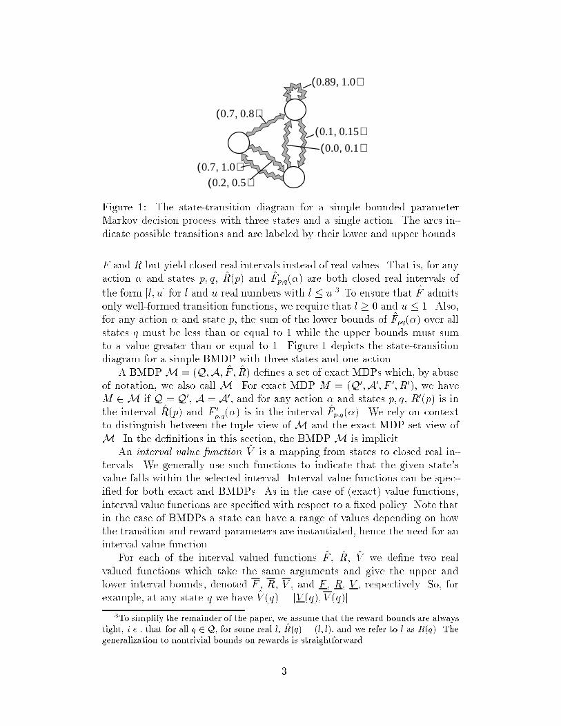
0.2 0.5,( )

0.89 1.0,( )

0.7 0.8,( )

0.7 1.0,( )

0.1 0.15,( )0.0 0.1,( )Figure 1: The state-transition diagram for a simple bounded parameterMarkov decision process with three states and a single action. The arcs in-dicate possible transitions and are labeled by their lower and upper bounds.F and R but yield closed real intervals instead of real values. That is, for anyaction � and states p; q, R(p) and Fp;q(�) are both closed real intervals ofthe form [l; u] for l and u real numbers with l � u.3 To ensure that F admitsonly well-formed transition functions, we require that l � 0 and u � 1. Also,for any action � and state p, the sum of the lower bounds of Fpq(�) over allstates q must be less than or equal to 1 while the upper bounds must sumto a value greater than or equal to 1. Figure 1 depicts the state-transitiondiagram for a simple BMDP with three states and one action.A BMDPM = (Q;A; F ; R) de�nes a set of exact MDPs which, by abuseof notation, we also call M. For exact MDP M = (Q0;A0; F 0; R0), we haveM 2 M if Q = Q0, A = A0, and for any action � and states p; q, R0(p) is inthe interval R(p) and F 0p;q(�) is in the interval Fp;q(�). We rely on contextto distinguish between the tuple view of M and the exact MDP set view ofM. In the de�nitions in this section, the BMDPM is implicit.An interval value function V is a mapping from states to closed real in-tervals. We generally use such functions to indicate that the given state'svalue falls within the selected interval. Interval value functions can be spec-i�ed for both exact and BMDPs. As in the case of (exact) value functions,interval value functions are speci�ed with respect to a �xed policy. Note thatin the case of BMDPs a state can have a range of values depending on howthe transition and reward parameters are instantiated, hence the need for aninterval value function.For each of the interval valued functions F , R, V we de�ne two realvalued functions which take the same arguments and give the upper andlower interval bounds, denoted F , R, V , and F , R, V , respectively. So, forexample, at any state q we have V (q) = [V (q); V (q)].3To simplify the remainder of the paper, we assume that the reward bounds are alwaystight, i.e., that for all q 2 Q, for some real l, R(q) = (l; l), and we refer to l as R(q). Thegeneralization to nontrivial bounds on rewards is straightforward.3

De�nition 1 For any policy � and state q, we de�ne the interval value V�(q)of � at q to be the interval�minM2MVM;�(q); maxM2MVM;�(q)�In Section 5 we will give an iterative algorithm which we have proven toconverge to V�. In preparation for that discussion, we will show in Theorem 1that there is at least one speci�c MDP inM which simultaneously achievesV �(q) for all states q (and likewise a speci�c MDP achieving V �(q) for all q).We formally de�ne such an MDP below.De�nition 2 For any policy �, an MDP in M is �-maximizing if it isa possible value of argmaxM2M VM;� and it is �-minimizing if it is inarg minM2M VM;�.The proof for Theorem 1 builds on the fact that for a particular policy �,if there are MDPs M1 and M2 that minimize (maximize) the value functionfor particular states p1 and p2, respectively, then we can compose a newMDP which minimizes (maximizes) the value function for both p1 and p2given �. By repeatedly composing MDPs, we can create a �-minimizing (�-maximizing) MDP. The following de�nition and two lemmas formalize thisargument.De�nition 3 For any two MDPs M1;M2, and policy � 2 �, we de�ne thecomposition operator M for MDPs as M3 = M1 M M2 if for all statesp; q 2 Q, FM3pq (�(p)) = ( FM1pq (�(p)) if VM1;�(p) � VM2;�(p)FM2pq (�(p)) otherwiseLemma 1 If M3 = M1 M M2, thenVM3;� �dom VM1;� and VM3;� �dom VM2;�:Proof: We prove the theorem by constructing a value function v such thatv �dom VM1;� and v �dom VM2;�. We then show that v �dom VM3;� using Weconstruct v as follows. Letv(p) = maxfVM1;�(p); VM2;�(p)g (1)for all p 2 Q. Note that this implies v �dom VM1 ;� and v �dom VM2 ;�. Wenow show using (8) that v �dom VM3;�.We divide the set of states Q into two subsets. Let Q1 be the set of statesfqg whose value estimate v(q) = VM1;�(q) and let Q2 be the set of states fqg4

whose value estimate v(q) = VM2;�(q) as determined by (1). For MDP M1,we have VM1 ;�(q) = v(q) for all q 2 Q1 and VM1;�(q) � v(q) for all q 2 Q2.Suppose without loss of generality that we choose a particular statep 2 Q1. Then v(p) = VM1;�(p) and by the de�nition of M , we knowFMpq (�(p)) = FM1pq (�(p)) for all q 2 Q. Furthermore, for the value functions vand VM1;�, we have for the states in Q1,Xq2Q1 �FM1pq (�(p))VM1;�(q)� = Xq2Q1 �FM1pq (�(p))v(q)�and for the states in Q2,Xq2Q2 �FM1pq (�(p))VM1;�(q)� � Xq2Q2 �FM1pq (�(p))v(q)� :Using these facts, we can writev(p) = VM1;�(p)= R(p) + Xq2Q�FM1pq (�(p))VM1;�(q)�� R(p) + Xq2Q�FM1pq (�(p))v(q)�= R(p) + Xq2Q�FM3pq (�(p))v(q)�= V IM3;�(p)(v)(p):It follows from Theorem 8 that v(p) � VM3;�(p). Repeating this argument inthe case that p 2 Q2 implies v �dom VM3;�. 2We now use the MDP composition operator to show that we can apply itrepeatedly to a subset K of states to create a �-minimizing (�-maximizing)MDP over the subset K.Lemma 2 For any policy � and any K � Q, there exist �-maximizing and�-minimizing MDPs in M on the subset K.Proof: We prove the lemma for the �-maximizing MDP by induction onthe size k of the subsetK. The proof for the �-minimizingMDP is analogous.Base Case: (k = 1) THIS ONE STILL NEEDS TO BE PROVED,EITHER BY SHOWING THE QUADRATIC PROGRAM TO HAVE ASOLUTION OR USING THE UPPER SEMICONTINUOUS FUNCTIONARGUMENT TO SHOW THE MAX IS ACHIEVED.Inductive Case: (k > 1) Assume the theorem holds for n < k. Wedivide the subset K of states into two disjoint, non-empty subsets K1 andK2, where K1 [ K2 = K. Then there exist MDPs M1 and M2 for which5

the inductive hypothesis holds for K1 and K2, respectively. In particular, forM1, VM1;�(p) � VM;�(p)where p 2 K1 and M 2 M. Similarly for VM2;� on the states p 2 K2. LetM3 be the MDP given as M3 = M1 M M2. From Lemma 1, we knowthat VM1;� �dom VM3;� and VM2;� �dom VM3;� which implies that VM;�(p) �VM3;�(p) for all states p 2 K and M 2 M. 2Theorem 1 For any policy �, there exist �-maximizing and �-minimizingMDPs in M.Proof: The proof follows immediately from Lemma 2 by letting K = Q.This theorem implies that V � is equivalent to minM2M VM;� where theminimization is done relative to �dom, and likewise for V using max. Wegive an algorithm in Section 5 which converges to V � by also converging toa �-minimizing MDP inM (likewise for V �).We now consider how to de�ne an optimal value function for an BMDP.Consider the expression max�2� V�. This expression is ill-formed becausewe have not de�ned how to rank the interval value functions V� in order toselect a maximum. We focus here on two di�erent ways to order these valuefunctions, yielding two notions of optimal value function and optimal policy.Other orderings may also yield interesting results.First, we de�ne two di�erent orderings on closed real intervals:[l1; u1] �pes [l2; u2] () ( l1 < l2; orl1 = l2 and u1 � u2[l1; u1] �opt [l2; u2] () ( u1 < u2; oru1 = u2 and l1 � l2We extend these orderings to partially order interval value functions by re-lating two value functions V1 � V2 only when V1(q) � V2(q) for every stateq. We can now use either of these orderings to compute max�2� V�, yieldingtwo de�nitions of optimal value function and optimal policy. However, sincethe orderings are partial (on value functions), we must still prove that theset of policies contains a policy which achieves the desired maximum undereach ordering (i.e., a policy whose interval value function is ordered abovethat of every other policy). We formally de�ne such policies below.De�nition 4 The optimistic optimal value function ^Vopt and the pessimisticoptimal value function ^Vpes are given by:^Vopt = max�2� V� using �opt to order interval value functions^Vpes = max�2� V� using �pes to order interval value functions6

We say that any policy � whose interval value function V� is �opt (�pes) thevalue functions V�0 of all other policies �0 is optimistically (pessimistically)optimal.The proof for Theorem 2 is similar to that of Theorem 1. Analogousto the composition operator for MDPs, we de�ne a composition operatoron policies. Repeatedly composing policies, as we did for MDPs, we cancreate a policy that is optimistically (pessimistically) optimal. The followingde�nition and ensuing pair of lemmas provide the necessary material for theproof of Theorem 2.De�nition 5 For any two policies �1; �2 2 � and MDP M , we de�ne thecomposition operator � on policies as �3 = �1 ��2 if for all states p 2 Q,:�3(p) = ( �1(p) if VM;�1(p) � VM;�2(p)�2(p) otherwiseLemma 3 If �3 = �1 � �2, then VM;�3 �dom VM;�1 and VM;�3 �dom VM;�2 .Proof: We prove the theorem by constructing a value function v such thatv �dom VM;�1 and v �dom VM;�2. We then show that v �dom VM;�3 usingTheorem 8. We construct v as follows. Letv(p) = maxfVM;�1(p); VM;�2(p)g (2)for all p 2 Q. Note that this implies v �dom VM;�1 and v �dom VM;�2. Wenow show using (8) that v �dom VM;�3.We divide the set of states Q into two subsets. Let Q1 be the set of statesfqg whose value estimate v(q) = VM;�1(q) and let Q2 be the set of states fqgwhose value estimate v(q) = VM;�2(q) as determined by (2). For policy �1,we have VM;�1(q) = v(q) all states q 2 Q1 and VM;�1(q) � v(q) for all statesq 2 Q2.Suppose without loss of generality that we choose a particular statep 2 Q1. Then v(p) = VM;�1(p) and by the de�nition of �, �3(p) = �1(p).Using these facts, we can writev(p) = VM;�1(p)= R(p) + Xq2Q (Fpq(�1(p))VM;�1(q))� R(p) + Xq2Q (Fpq(�1(p))v(q))= R(p) + Xq2Q (Fpq(�3(p))v(q))= V IM;�3(v)(p):It follows from Theorem 8 that v(p) � VM;�3(p). Repeating this argument inthe case that p 2 Q2 implies v �dom VM;�3. 27

Lemma 4 For any subset K of Q, there exists a policy �0 such thatV�(p) �opt (�pes)V�0(p)for all states p 2 K and � 2 �.Proof: We prove the lemma by induction on the size k of the subset K.Base Case: (k = 1) Since A and Q are �nite sets, � is a �nite set. Asa consequence of Theorem 1, we know we can obtain a �nite set of intervalvalue functions fV� : � 2 �g. Any �nite set of intervals has a maximumunder either ordering �pes or �opt.Inductive Case: (k > 1) Assume the theorem holds for n < k. Wedivide the subset K of states into two disjoint, non-empty subsets K1 andK2, where K1 [K2 = K. Then there exist policies �1 and �2 for which theinductive hypothesis holds for K1 and K2, respectively. In particular, for �1,V�(p) �opt (�pes)V�1(p)where p 2 K1 and � 2 �. Similarly for V�2 on the states p 2 K2. Let �3be the policy given as �3 = �1 � �2. We show that V�1 �opt (�pes)V�3 andV�2 �opt (�pes)V�3 , which implies V�(p) �opt (�pes)V�3(p) for all states p 2 Kand � 2 �.We argue the case for V�1 ; the case for V�2 is analogous. For eachM 2 M, VM;�1 �dom VM;�3by Lemma 3. It follows for all states p 2 Q that,minM2MVM;�1(p) � minM2MVM;�3(p)and maxM2MVM;�1(p) � maxM2MVM;�3(p):Note that, as a consequence, the intervals V�1(p) and V�3(p) may overlap,but one can not contain the other. Therefore, according to either ordering�opt or �pes, V�1 �opt (�pes)V�3 :2Theorem 2 There exists at least one optimistically (pessimistically) optimalpolicy, and therefore the de�nition of ^Vopt ( ^Vpes) is well-formed.8

Proof: The proof follows immediately from Lemma 4 by letting K = Q.2 The above two notions of optimal value can be understood in terms ofa game in which we choose a policy � and then a second player chooses inwhich MDP M inM to evaluate the policy. The goal is to get the highest4resulting value function VM;�. The optimistic optimal value function's upperbounds V opt represent the best value function we can obtain in this game ifwe assume the second player is cooperating with us. The pessimistic optimalvalue function's lower bounds V pes represent the best we can do if we assumethe second player is our adversary, trying to minimize the resulting valuefunction.In the next section, we describe well-known iterative algorithms for com-puting the optimal value function V �, and then in Section 5 we will describesimilar iterative algorithms which compute ^Vopt ( ^Vpes).4 Estimating Traditional Value FunctionsIn this section, we review the basics concerning dynamic programming meth-ods for computing value functions for �xed and optimal policies in traditionalMDPs. In the next section, we describe novel algorithms for computing theinterval analogs of these value functions for bounded parameter MDPs.We present results from the theory of exact MDPs which rely on theconcept of normed linear spaces. We de�ne operators, V I� and V I, onthe space of value functions. We then use the Banach �xed-point theorem(Theorem 3) to show that iterating these operators converges to unique �xed-points, V� and V � respectively (Theorems 5 and 6).Let V denote the set of value functions on Q. For each v 2 V, de�ne the(sup) norm of v by kvk = maxq2Q jv(q)j:We use the term convergence to mean convergence in the norm sense. Thespace V together with k � k constitute a complete normed linear space, orBanach Space. If U is a Banach space, then an operator T : U ! U is acontraction mapping if there exists a �, 0 � � < 1 such that kTv � Tuk ��kv � uk for all u and v in U .De�ne V I : V ! V and for each � 2 �, V I� : V ! V on each p 2 Q byV I(v)(p) = max�2A 0@R(p) + Xq2QFpq(�)v(q)1AV I�(v)(p) = R(p) + Xq2QFpq(�(p))v(q):4Value functions are ranked by �dom. 9

In cases where it is necessary for the de�nitions of V I and V I� to makeexplicit from which MDP the transition function originates, we write V IM;�and V IM to denote the operators V I� and V I as de�ned previously, exceptthat the transition function F is FM . More generally, we write V IM;� : V !V to denote the operator de�ned on each p 2 Q asV IM;�(v)(p) = R(p) + Xq2QFMpq (�)v(q)Using these operators, we can rewrite the expression for V � and V� asV �(p) = V I(V �)(p) and V�(p) = V I�(V�)(p)for all states p 2 Q. This implies that V � and V� are �xed points of V I andV I�, respectively. The following four theorems show that for each operator,iterating the operator on an initial value estimate converges to these �xedpoints.Theorem 3 For any Banach space U and contraction mapping T : U ! U ,there exists a unique v� in U such that Tv� = v�; and for arbitrary v0 in U ,the sequence fvng de�ned by vn = Tvn�1 = T nv0 converges to v�.Theorem 4 V I and V I� are contraction mappings.Theorem 3 and Theorem 4 together prove the following fundamental re-sults in the theory of MDPs.Theorem 5 There exists a unique v� 2 V satisfying v� = V I(v�); further-more, v� = V �. Similarly, V� is the unique �xed-point of V I�.Theorem 6 For arbitrary v0 2 V, the sequence fvng de�ned by vn = V I(vn�1)= V In(v0) converges to V �. Similarly, iterating V I� converges to V�.An important consequence of Theorem 6 is that it provides an algorithmfor �nding V � and V�. In particular, to �nd V �, we can start from an arbitraryinitial value function v0 in V, and repeatedly apply the operator V I to obtainthe sequence fvng. This algorithm is referred to as value iteration. Theorem 6guarantees the convergence of value iteration to the optimal value function.Similarly, we can specify an algorithm called policy evaluation which �nds V�by repeatedly apply V I� starting with an initial v0 2 V.The following theorem from [Littman et al., 1995] states the convergencerate of value iteration and policy evaluation.Theorem 7 For �xed , value iteration and policy evaluation converge tothe optimal value function in a number of steps polynomial in the number ofstates, the number of actions, and the number of bits used to represent theMDP parameters. 10

Another important theorem that will be used in a number of later proofsshows how the result of applying the operators to a value function relates tothe value of the operators' �xed-points.Theorem 8 Let u 2 V, � 2 � and M be an MDP. For all states p 2 Q, ifu(p) � (�)V IM;�(u)(p) then u(p) � (�)VM;�(p).5 Estimating Interval Value FunctionsIn this section, we describe dynamic programming algorithms which operateon bounded parameter MDPs. We �rst de�ne the interval equivalent of policyevaluation ^IV I� which computes V�, and then de�ne the variants ^IV Iopt and^IV Ipes which compute the optimistic and pessimistic optimal value functions.5.1 Interval Policy EvaluationIn direct analogy to the de�nition of V I� in Section 4, we de�ne a function^IV I� (for interval value iteration) which maps interval value functions toother interval value functions. We have proven that iterating ^IV I� on anyinitial interval value function produces a sequence of interval value functionswhich converges5 to V�.^IV I�(V ) is an interval value function, de�ned for each state p as follows:^IV I�(V )(p) = �minM2MV IM;�(p)(V )(p) maxM2MV IM;�(p)(V )(p)� :Associated with ^IV I� are the functions IV I� and IV I� which are map-pings from interval value functions to value functions. IV I�(V ) is the valuefunction derived by extracting the lower bound of ^IV I�(V )(p) for all statesp. Similarly for IV I�(V ) on the upper bounds.The algorithm to compute ^IV Ij� is very similar to the standard MDPcomputation of V I, except that we must now be able to select an MDP Mfrom the family M which minimizes (maximizes) the value attained. Weselect such an MDP by selecting a function F within the bounds speci�ed byF to minimize (maximize) the value|each possible way of selecting F corre-sponds to one MDP inM. We can select the values of Fpq(�) independentlyfor each � and p, but the values selected for di�erent states q (for �xed � andp) interact: they must sum up to one. We now show how to determine, for5We conjecture that this convergence is complete in time polynomial in the input size,following the analogous theorem for standard MDP policy evaluation[Littman et al., 1995].This result should be proven by publication time.11

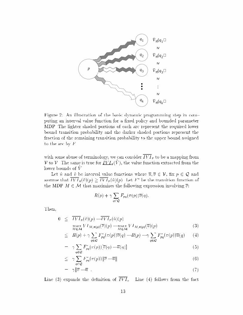
�xed � and p, the value of Fpq(�) for each state q so as to minimize (maxi-mize) the expression Pq2Q (Fpq(�)V (q)). This step constitutes the heart ofthe IVI algorithm and the only signi�cant way the algorithm di�ers fromstandard value iteration.The idea is to sort the possible destination states q into increasing (de-creasing) order according to their V (V ) value, and then choose the transitionprobabilities within the intervals speci�ed by F so as to send as much prob-ability mass to the states early in the ordering. Let q1; q2; : : : ; qk be such anordering ofQ|so that, in the minimizing case, for all i and j if 1 � i � j � kthen V (qi) � V (qj) (increasing order).Let r be the index 1 � r � k which maximizes the following expressionwithout letting it exceed 1:r�1Xi=1 F p;qi(�) + kXi=r F p;qi(�)r is the index into the sequence qi such that below index r we can assign theupper bound, and above index r we can assign the lower bound, with therest of the probability mass from p under � being assigned to qr. Formally,we choose Fpq(�) for all q 2 Q as follows:Fpqj(�) = ( F p;qi(�) if j < rF p;qi(�) if j > rFpqr(�) = 1� i=kXi=1;i6=r Fpqi(�)Figure 2 illustrates the basic iterative step in the above algorithm, for themaximizing case. The states qi are ordered according to the value estimatesin V . The transitions from a state p to states qi are de�ned by the functionF such that each transition is equal to its lower bound plus some fraction ofthe leftover probability mass.Techniques similar to those in Section 4 can be used to prove that iteratingIV I� (IV I�) converges to V � (V �). The key theorems, stated below, assert�rst that IV I� is a contraction mapping, and second that V � is a �xed-pointof IV I�, and are easily proven.Theorem 9 For any policy �, IV I� and IV I� are contraction mappings.Proof: We �rst show that IV I� is a contraction mapping on V, the spaceof value functions. Strictly speaking, IV I� is a mapping from an intervalvalue function V to a value function V . However, the speci�c values V (p)only depend on the upper bounds V of V . Therefore, the mapping IV I� isisomorphic to a function which maps value functions to value functions and12

q1

≥

Vπ q1( )

Vπ q2( )

Vπ q3( )

Vπ qk( )

q2

q3

qk

≥≥

≥…

pFigure 2: An illustration of the basic dynamic programming step in com-puting an interval value function for a �xed policy and bounded parameterMDP. The lighter shaded portions of each arc represent the required lowerbound transition probability and the darker shaded portions represent thefraction of the remaining transition probability to the upper bound assignedto the arc by F .with some abuse of terminology, we can consider IV I� to be a mapping fromV to V. The same is true for IV I�(V ), the value function extracted from thelower bounds of V .Let u and v be interval value functions where u; v 2 V, �x p 2 Q andassume that IV I�(v)(p) � IV I�(u)(p). Let F � be the transition function ofthe MDP M 2 M that maximizes the following expression involving v:R(p) + Xq2QFpq(�(p))v(q):Then, 0 � IV I�(v)(p)� IV I�(u)(p)= maxM2MV IM;�(p)(v)(p)� maxM2MV IM;�(p)(u)(p) (3)� R(p) + Xq2QF �pq(�(p))v(q)�R(p) � Xq2QF �pq(�(p))u(q) (4)= Xq2QF �pq(�(p))[v(q)� u(q)] (5)� Xq2QF �pq(�(p))kv � uk (6)= kv � uk: (7)Line (3) expands the de�nition of IV I�. Line (4) follows from the fact13

that by de�nition, IV I� chooses the MDP (and the corresponding transi-tion function) that maximizes the value of V IM;�(p)(p); any other choice (cf.F �) would result in a lesser value. In Line (5), we simplify the expressionby subtracting the immediate reward term and factoring out the coe�cientsF �. In Line (fourth), we introduce an inequality by replacing all the terms[v(q) � u(q)] with the maximum di�erence over all states, which by de�ni-tion is the sup norm. The �nal step (7) follows from the fact that F � is aprobability distribution that sums to 1 and kv � uk does not depend on q.Repeating this argument in the case that IV I�(v)(p) � IV I�(u)(p) im-plies that jIV I�(v)(p) � IV I�(u)(p)j � kv � ukfor all p 2 Q. Taking the maximum over p in the above expression gives theresult.The proof that IV I� is a contraction mapping is identical, except that uand v are replaced by u and v, respectively. Also, F � minimizes the followingexpression involving u: R(p) + Xq2QFpq(�(p))u(q):2Theorem 10 For any policy �, V � is a �xed-point of IV I� and V � of IV I�.Proof: We prove the theorem for IV I�; the proof for IV I� is similar. Weshow(a) IV I�(V�) �dom V �, and(b) IV I�(V�) �dom V �from which we conclude that IV I�(V�) = V �.We �rst prove (a). Let M� be the �-minimizing MDP ofV � = minM2MVM;�which by Theorem 1 exists. From Theorem 5, we know that VM�;� is a �xedpoint of V IM�;�(VM�;�). Thus, for a state p 2 Q,V �(p) = VM�;�(p) = V IM�;�(p)(VM�;�)(p):Using this fact and expanding the de�nition of IV I�, we haveIV I�(V�)(p) = minM2MV IM;�(p)(V �)(p)� V IM�;�(p)(V �)(p) = (V �)(p):14

To prove (b), suppose for sake of contradiction that IV I�(V�) <dom V �.Then for some state p, IV I�(V�)(p) < V �(p). Let M� be an MDP thatachieves the minimum in minM2MV IM;�(p)(V �)(p):Then, substituting M� into the de�nition of IV I�,IV I�(V�)(p) = V IM�;�(p)(V �)(p) < V �(p)However, from Theorem 8, if for a particular MDP M , the result of V IM;�(p)applied to a value function v is less than v, the actual value of the MDP isless than v. Therefore, for the MDP M�,VM�;�(p) < V �(p):However, we obtain a contradiction since V �(p) is equivalent to the valuefunction of the MDP with the minimal value function over all MDPs in M.2These theorems, together with Theorem 3 (the Banach �xed-point theorem)imply that iterating ^IV I� on any initial interval value function converges toV�, regardless of the starting point.5.2 Interval Value IterationAs in the case of V I� and V I, it is straightforward to modify ^IV I� so thatit computes optimal policy value intervals by adding a maximization stepover the di�erent action choices in each state. However, unlike standardvalue iteration, the quantities being compared in the maximization step areclosed real intervals, so the resulting algorithm varies according to how wechoose to compare real intervals. We de�ne two variations of interval valueiteration|other variations are possible.^IV Iopt(V )(p) = max�2A; �opt �minM2MV IM;�(V )(p); maxM2MV IM;�(V )(p)�^IV Ipes(V )(p) = max�2A; �pes �minM2MV IM;�(V )(p); maxM2MV IM;�(V )(p)�The added maximization step introduces no new di�culties in imple-menting the algorithm. We discuss convergence for ^IV Iopt|the convergenceresults for ^IV Ipes are similar. IV Iopt can be easily shown to be a contractionmapping, and with somewhat more di�culty it can be shown that ^Vopt is a15

�xed point of ^IV Iopt. It then follows that IV Iopt converges to V opt. Theanalogous results for IV Iopt are somewhat more problematic. Because theaction selection is done according to �opt, which focuses primarily on theinterval upper bounds, the mapping IV Iopt is not a contraction mappingin general. However, once the upper bounds IV Iopt have converged (i.e.,the upper bounds V of the input function are a �xed point of IV I), IV Ioptacts as a contraction mapping (this statement is formalized below), and thedesired convergence will then occur.Theorem 11 1. IV Iopt and IV Ipes are contraction mappings.2. On value functions V for which V is a �xed point of IV Iopt, IV Iopt isa contraction mapping.3. On value functions V for which V is a �xed point of IV Ipes, IV Ipes isa contraction mapping.Proof: (1) The proof for IV Iopt follows exactly as in Theorem 5.1 exceptthat we replace the action �(p) with the action �� that maximizesmaxM2MR(p) + Xq2QFpq(�)v(q):and let F � be the transition function of the MDP M 2 M that maximizesR(p) + Xq2QFpq(��)v(q):Similarly, for IV Ipes, �� is the action that maximizesminM2MR(p) + Xq2QFpq(�)u(q):and F � is the transition function of the MDP M 2 M that minimizesR(p) + Xq2QFpq(��)u(q):(2) TO BE CONTINUED (3) TO BE CONTINUED 2Theorem 12 ^Vopt is a �xed-point of ^IV Iopt , and ^Vpes of ^IV Ipes.Theorem 13 Iteration of IV Iopt converges to V opt, and iteration of IV Ipesconverges to V pes. 16

Proof: By Theorem 11(1), IV Iopt and IV Ipes are contraction mappingsso that the hypotheses of Theorem 3 are satis�ed. Therefore there existsan interval value function V1 whose upper bound V 1 2 V is the uniquesolution to v = IV Iopt(v) and there exists an interval value function V2 whoselower bound V 2 2 V is the unique solution to u = IV Ipes(u). Theorem 12establishes that V 1 = V opt and V 2 = V pes. 2We have not yet shown that the other bounds will converge as desiredin general. However, this weakness is mitigated by several factors. First,we are far more interested in the values of IV Iopt and IV Ipes than in theother bounds|as these represent more useful numbers. IV Iopt represents thebest possible value we could obtain from each state, and IV Ipes representsthe best value we can guarantee obtaining from each state (in contrast, forexample, IV Ipes is the best value we might obtain if we follow the pessimisticoptimal policy, which was not designed for maximizing this value in any case).Second, we expect to be able to show that these algorithms converge in timepolynomial in their input sizes, for �xed discount rate|in that case, wewill be able to count on IV Iopt converging quickly so that IV Iopt will thenconverge. Third, we can use IV Iopt or IV Ipes to select an optimal policy,and then for that policy, we can use interval policy evaluation to get bothlower and upper bounds for its value.6 Policy Selection, Sensitivity Analysis, andAggregationIn this section, we consider some basic issues concerning the use and inter-pretation of bounded parameter MDPs. We begin by reemphasizing someideas introduced earlier regarding the selection of policies.To begin with, it is important that we are clear on the status of thebounds in a bounded parameter MDP. A bounded parameter MDP speci�esupper and lower bounds on individual parameters; the assumption is thatwe have no additional information regarding individual exact MDPs whoseparameters fall with those bounds. In particular, we have no prior over theexact MDPs in the family of MDPs de�ned by a bounded parameter MDP.Policy selection Despite the lack of information regarding any particularMDP, we may have to choose a policy. In such a situation, it is natural toconsider that the actual MDP, i.e., the one in which we will ultimately haveto carry out some policy, is decided by some outside process. That processmight choose so as to help or hinder us, or it might be entirely indi�erent. Tominimize the risk of performing poorly, it is reasonable to think in adversarialterms; we select the policy which will perform as well as possible assuming17

that the adversary chooses so that we perform as poorly as possible.These choices correspond to optimistic and pessimistic optimal policies.We have discussed in the last section how to compute interval value functionsfor such policies|such value functions can then be used in a straightforwardmanner to extract policies which achieve those values.There are other possible choices, corresponding in general to other meansof totally ordering real closed intervals. We might for instance consider apolicy whose average performance over all MDPs in the family is as goodas or better than the average performance of any other policy. This notionof average is potentially problematic, however, as it essentially assumes auniform prior over exact MDPs and, as stated earlier, the bounds do notimply any particular prior.Sensitivity analysis There are other ways in which bounded parameterMDPs might be useful in planning under uncertainty. For example, we mightassume that we begin with a particular exact MDP, say, the MDP with pa-rameters whose values re ect the best guess according to a given domainexpert. If we were to compute the optimal policy for this exact MDP, wemight wonder about the degree to which this policy is sensitive to the num-bers supplied by the expert.To explore this possible sensitivity to the parameters, we might assess thepolicy by perturbing the parameters and evaluating the policy with respect tothe perturbed MDP. Alternatively, we could use bounded parameter MDPsto perform this sort of sensitivity analysis on a whole family of MDPs byconverting the point estimates for the parameters to con�dence intervals andthen computing bounds on the value function for the �xed policy via intervalpolicy evaluation.Aggregation Another use of BMDPs involves a di�erent interpretationaltogether. Instead of viewing the states of the bounded parameter MDP asindividual primitive states, we view each state of the BMDP as representinga set or aggregate of states of some other, larger MDP.In this interpretation, states are aggregated together because they behaveapproximately the same with respect to possible state transitions. A littlemore precisely, suppose that the set of states of the BMDP M correspondsto the set of blocks fB1; : : : ; Bng such that the fBig constitutes the partitionof another MDP with a much larger state space.Now we interpret the bounds as follows; for any two blocks Bi and Bj,let FBiBj(�) represent the interval value for the transition from Bi to Bj onaction � de�ned as follows:FBiBj(�) = 24minp2Bi Xq2Bj Fpq(�); maxp2Bi Xq2Bj Fpq(�)3518

Intuitively, this means that all states in a block behave approximately thesame (assuming the lower and upper bounds are close to each other) in termsof transitions to other blocks even though they may di�er widely with regardto transitions to individual states.Dean et al. [1997] discuss methods for using an implicit representation of aexact MDP with a large number of states to construct a BMDP with a muchsmaller number of states based on an aggregation like that just discussed.We then show how to use this BMDP to compute policies with desirableproperties with respect to the large implicitly described MDP. Note thatthe original implicit MDP is not even a member of the family of MDPs forthe reduced BMDP (it has a di�erent state space, for instance). Neverthe-less, it is a theorem that the policies and value bounds of the BMDP canbe soundly applied in the original MDP (using the aggregation mapping toconnect original states to the block-states of the BMDP).7 Related Work and ConclusionsOur de�nition for bounded parameter MDPs is related to a number of otherideas appearing in the literature on Markov decision processes; in the follow-ing, we mention just a few such ideas. Bertsekas and Casta~non [1989] usethe notion of aggregated Markov chains and consider grouping together stateswith approximately the same residuals. Methods for bounding value func-tions are frequently used in approximate algorithms for solving MDPs; Love-joy [1991] describes their use in solving partially observable MDPs. Puter-man [Puterman, 1994] provides an excellent introduction to Markov decisionprocesses and estimation techniques that involve bounding value functions.Boutilier and Dearden [1994] and Boutilier et al. [1995b] describe methodsfor solving implicitly described MDPs and Dean and Givan [1997] reinterpretthis work in terms of computing explicitly described MDPs with aggregatestates. Littman [1996] provides a generalization of MDPs that may encom-pass some aspects of the theory of bounded parameter MDPs.Bounded parameter MDPs allow us to represent uncertainty or variationin the parameters of a target Markov decision process. Interval value func-tions capture the variation in expected value for policies as a consequence ofvariation in parameter estimates. In this paper, we have precisely de�ned thenotions of bounded parameter MDP and interval value function, provided al-gorithms for computing interval value functions, and described methods andalgorithms for policy selection and evaluation, sensitivity analysis, and ag-gregation. 19

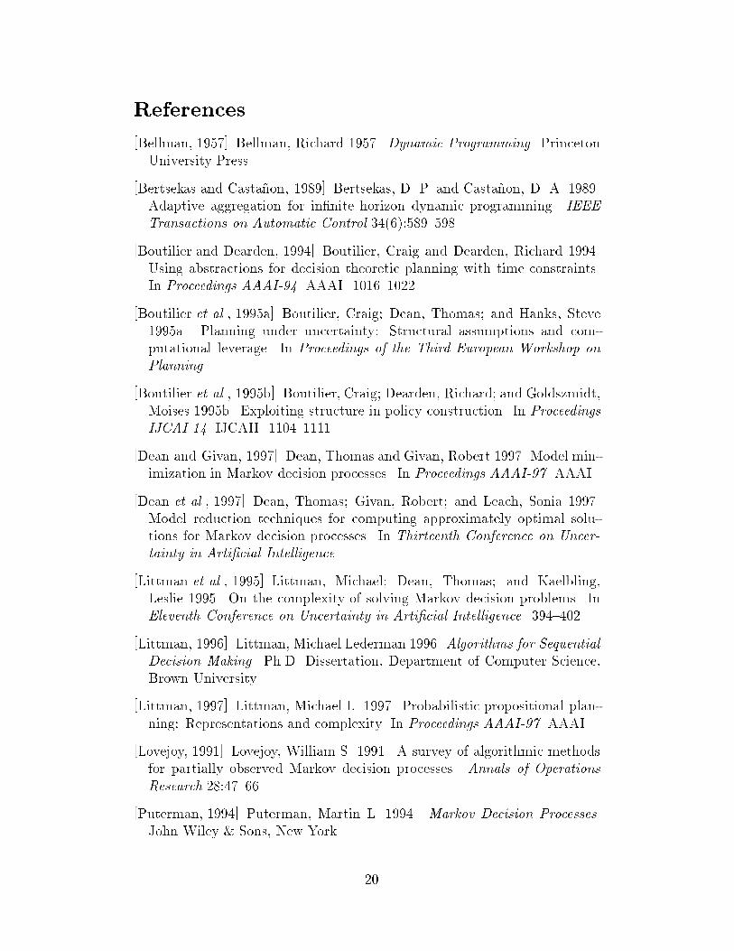
References[Bellman, 1957] Bellman, Richard 1957. Dynamic Programming. PrincetonUniversity Press.[Bertsekas and Casta~non, 1989] Bertsekas, D. P. and Casta~non, D. A. 1989.Adaptive aggregation for in�nite horizon dynamic programming. IEEETransactions on Automatic Control 34(6):589{598.[Boutilier and Dearden, 1994] Boutilier, Craig and Dearden, Richard 1994.Using abstractions for decision theoretic planning with time constraints.In Proceedings AAAI-94. AAAI. 1016{1022.[Boutilier et al., 1995a] Boutilier, Craig; Dean, Thomas; and Hanks, Steve1995a. Planning under uncertainty: Structural assumptions and com-putational leverage. In Proceedings of the Third European Workshop onPlanning.[Boutilier et al., 1995b] Boutilier, Craig; Dearden, Richard; and Goldszmidt,Moises 1995b. Exploiting structure in policy construction. In ProceedingsIJCAI 14. IJCAII. 1104{1111.[Dean and Givan, 1997] Dean, Thomas and Givan, Robert 1997. Model min-imization in Markov decision processes. In Proceedings AAAI-97. AAAI.[Dean et al., 1997] Dean, Thomas; Givan, Robert; and Leach, Sonia 1997.Model reduction techniques for computing approximately optimal solu-tions for Markov decision processes. In Thirteenth Conference on Uncer-tainty in Arti�cial Intelligence.[Littman et al., 1995] Littman, Michael; Dean, Thomas; and Kaelbling,Leslie 1995. On the complexity of solving Markov decision problems. InEleventh Conference on Uncertainty in Arti�cial Intelligence. 394{402.[Littman, 1996] Littman, Michael Lederman 1996. Algorithms for SequentialDecision Making. Ph.D. Dissertation, Department of Computer Science,Brown University.[Littman, 1997] Littman, Michael L. 1997. Probabilistic propositional plan-ning: Representations and complexity. In Proceedings AAAI-97. AAAI.[Lovejoy, 1991] Lovejoy, William S. 1991. A survey of algorithmic methodsfor partially observed Markov decision processes. Annals of OperationsResearch 28:47{66.[Puterman, 1994] Puterman, Martin L. 1994. Markov Decision Processes.John Wiley & Sons, New York. 20