grace technical reports bidirectionalizing structural recursion on graphs
TRANSCRIPT

ISSN 1884-0760
GRACE TECHNICAL REPORTS
Bidirectionalizing Structural Recursion onGraphs
Soichiro Hidaka Zhenjiang Hu Kazuhiro InabaHiroyuki Kato Kazutaka Matsuda Keisuke Nakano
GRACE-TR 2009–03 August 2009
CENTER FOR GLOBAL RESEARCH INADVANCED SOFTWARE SCIENCE AND ENGINEERING
NATIONAL INSTITUTE OF INFORMATICS2-1-2 HITOTSUBASHI, CHIYODA-KU, TOKYO, JAPAN
WWW page: http://grace-center.jp/

The GRACE technical reports are published as a means to ensure timely dissemination of
scholarly and technical work on a non-commercial basis. Copyright and all rights therein
are maintained by the authors or by other copyright holders, notwithstanding that they
have offered their works here electronically. It is understood that all persons copying this
information will adhere to the terms and constraints invoked by each author’s copyright.
These works may not be reposted without the explicit permission of the copyright holder.

Bidirectionalizing Structural Recursion on Graphs
Soichiro Hidaka Zhenjiang Hu Kazuhiro Inaba Hiroyuki KatoNational Institute of Informatics2-1-2 Hitotsubashi, Chiyoda-ku
Tokyo 101-8430, Japan{hidaka,hu,kinaba,kato}@nii.ac.jp
Kazutaka MatsudaThe University of Tokyo/JSPS Research Fellow7-3-1 Hongo, Bunkyo-ku, Tokyo 113-8656, Japan
Keisuke NakanoThe University of Electro-Communications
1-5-1 Chofugaoka, Chofu-shiTokyo 182-8585, Japan
August 31, 2009
Abstract
The bidirectional transformation problem has been attracting moreand more attention in the programming language community. Despitemany promising results about bidirectional transformation on linearstrings or tree-like data structures, it remains as an open problemwhether it is possible to design a language that can support practicaldevelopment of bidirectional transformations on graphs. In this pa-per, we propose the first language-based (linguistic) solution towardssolving this challenging problem. We approach this problem by giv-ing a well-behaved bidirectional semantics for structural recursion (ongraphs), the most essential construct in UnCAL which is the under-lying graph algebra for the known UnQL graph query language. Inparticular, we carefully refine the existing forward evaluation of struc-tural recursion so that it can produce useful trace information for laterbackward evaluation, and extending the bulk semantics of structuralrecursion from forward evaluation to backward evaluation. We haveformally proved the well-behavedness of our bidirectional semantics,fully implemented bidirectional transformation engine for UnQL, andconfirmed the effectiveness of our approach through many non-trivialexamples including typical transformation in database and softwareengineering.

put
modify
t’
get t
s’
s
Figure 1: Bidirectional Transformation
1 Introduction
Bidirectional transformation (Foster et al. 2005; Czarnecki et al. 2009) ischaracterized by a pair of transformations, a forward transformation getand a backward transformation put as in Figure 1. The forward transforma-tion get is used to produce from a source s to a view t, while the backwardtransformation put is to reflect modification on the view back to the source.Practical examples of bidirectional transformation include synchronizationof replicated data in different formats (Foster et al. 2005), presentation-oriented structured document development (Hu et al. 2008), interactive userinterface design (Meertens 1998), coupled software transformation (Lammel2004), and the well-known view updating mechanism which has been inten-sively studied in the database community (Bancilhon and Spyratos 1981;Dayal and Bernstein 1982; Gottlob et al. 1988; Hegner 1990; Lechtenborgerand Vossen 2003).Despite many promising results on bidirectional transformation, the data
that can be dealt with are limited to linear strings or tree-like data struc-tures. It remains as an open problem (Czarnecki et al. 2009) whether itis possible to design a language that can support practical development ofbidirectional transformations on graphs which contains node sharing andcycles. It would be remarkably useful in many applications if bidirectionaltransformation can be applied to graph data structures, because graphsplay an irreplaceable role in representing more complex data structuressuch as models (e.g., UML diagrams) in model-driven software develop-ment (Stevens 2007), and Object Exchange Model (OEM) for exchangingarbitrary database structures (Papakonstantinou et al. 1995).There are many challenges in designing a language for bidirectional
transformation on graphs. First, unlike strings and trees, there is no uniqueway to represent, construct, and decompose a general graph, and thisrequires more precise definition of equivalence between two graphs. Second,graphs have sharing nodes and cycles, which makes forward computationmuch more complicated than that on trees (let alone to say about backward
2

computation), because naıve computation on graphs would visit the samenodes many times and possibly infinitely often.In this paper, we give the first language-based (linguistic) solution
to the problem of bidirectional graph transformation. We approach thisproblem by providing a bidirectional semantics for an existing graph querylanguage UnQL (Buneman et al. 2000). We choose UnQL as the basis of ourbidirectional graph transformation for the following two reasons.
• First, UnQL is a graph querying language that has been intensivelystudied in the database community with solid foundation and efficientimplementation based on graph algebra. It has a concise and powerfulsurface syntax based on select-where clauses like SQL, and can beeasily used to describe many interesting graph transformations.
• Second, and more importantly, graph transformations in UnQL arestructured in the sense that any transformation can be expressed interms structural recursion, which can be evaluated in a bulk way (Bune-man et al. 2000); a structural recursion is evaluated by first processingin parallel on all edges of the input graph and then combining the re-sults. This feature significantly contributes to our bidirectionalizationbecause it helps us to trace a corresponding source from its result.
Our technical contributions are summarized as follows.
• We are, as far as we are aware, the first who recognize the importance ofstructural recursion and its bulk semantics in addressing the challeng-ing problem of bidirectional graph transformation, and succeeded ina general graph transformation framework based on structural recur-sion. We show that graph transformations described with structuredrecursion are not only suitable for optimization as intensively stud-ied so far (Buneman et al. 2000), but also make backward evaluationeasier.
• We give a formal definition of bidirectional semantics for structuralrecursion (Section 4), by (1) refining the existing forward evaluationso that it can produce useful trace information for later backward eval-uation, and (2) extending the bulk semantics of structural recursionfrom forward evaluation to backward evaluation. And we prove thatour bidirectional semantics is well-behaved. The success of bidirection-alizing non-trivial UnQL shows practical power of our approach.
• We have fully implemented our bidirectionalization presented in thispaper and confirmed the effectiveness of our approach through manynon-trivial examples including typical transformations in databasemanagement and software engineering (Section 5). More examples anddemos are available in our project web site http://www.biglab.org.
3

(a) A Simple Graph (b) An Equiva-lent Graph
1
2
a
3
b
4
c
(c)
1
2
a
3
a
4
b
5
c
(d)(� 2(c))
Figure 2: Graph Equivalence Based on Bisimulation
The rest of this paper is organized as follows. We start with a briefoverview of the basic idea of graph data model and graph query languageUnQL in Section 2, before we show how an UnQL query program can beautomatically transformed to structural recursion in its underlying graphalgebra UnCAL in Section 3. Then we provide bidirectional semantics forUnCAL and prove that the bidirectional semantics is well-behaved in section4. Section 5 discusses our implementation and experimental results, Section 6summarizes related work, and Section 7 concludes the paper.
2 Graph Transformation in UnQL
We start with a brief overview of the graph data model and unidirectionalgraph transformation in UnQL (Buneman et al. 2000), a graph querylanguage to be bidirectionalized in this paper.
2.1 Graph Data Model
External Graph Representation Graphs in UnQL are rooted and di-rected cyclic graphs with no order between outgoing edges. They are edge-labelled in the sense that all information is stored as labels on edges and thelabels on nodes serve as a unique identifier and have no particular meaning.Figure 2(a) gives a small example of a directed cyclic graph with six nodesand seven edges. In text, it is represented by
G = {a : {a : G1}, b : {a : G1}, c : G2}G1 = {d : {}}G2 = {c : G2}
4

where the notation {l1 : G1, . . . , ln : Gn} denotes a set representing a graphwhich contains n edges with labels l1, . . . , ln, each li pointing to a graph Gi,and the empty set {} denotes a graph with a single node. Two graphs G1
and G2 can be merged using set union operation G1∪G2. This graph modelis set-based in the sense that {a : {}, a : {}} and {a : {}} represent the samegraph. In addition, the ε-edge is allowed to represent shortcut of two nodes,and works like ε-transition in automaton. For instance, we have
{ε : {a : G1}, ε : {b : G2}} = {a : G1, b : G2}.
Internal Graph Representation While the external graph representa-tion suffices for users to consider when writing graph transformation, theinternal graph representation is designed for internal implementation andsemantics description as in Section 4. Different from the external represen-tation, nodes in the internal representation may be marked with input andoutput marker , which are used as an interface for composition of graphs.Now we describe the formal definition and notations of graphs. These
notations will be used to specify the bidirectional semantics of UnCALin Section 4. Let Label , X and Y be a (possibly infinite) set of labels, aset of input markers, and a set of output markers, respectively. A graphG is denoted by a quadruple (V,E, I,O), where V is a set of nodes,E ⊆ V ×Label ε×V with Label ε = Label∪{ε} is a set of edges, I ⊆ X ×V is aset of pairs of input markers and corresponding input node, and O ⊆ V ×Yis a set of pairs of output nodes and associated output marker. For eachmarker &x ∈ X , there is at most one node v such that (&x, v) ∈ I. The nodev is called input node with marker &x and denoted by I(&x). In contrast,more than one node can be marked with an identical output marker. Theyare called output nodes.Intuitively, input nodes can be regarded as root nodes of the graph.
In other words, although the external representation limits a graph to besingly rooted, internally we deal with multiple roots. For singly rootedgraphs, we implicitly use the default marker & to indicate its single root.An output node can be regarded as a “context-hole” of graphs where aninput node with the same marker is plugged later. Indeed, the “verticalgraph composition” operator G1 @G2 is defined to plug the input nodes ofG2 into their corresponding output nodes in G1.For example, in internal representation, the simple graph in
Figure 2(a) is denoted by (V,E, I,O) where V = {1, 2, 3, 4, 5, 6},E = {(1, a, 2), (1, b, 3), (1, c, 4), (2, a, 5), (3, a, 5), (4, c, 4), (5, d, 6)},I = {(&, 1)}, and O = {}. This graph is not really typical, as it hasno ε-edge, only one input node, and no output node. We will see moreexamples later.
Graph Equivalence Graph bisimulation defines value equivalence be-tween graph instances. The intuition is that two graphs are value equivalent
5

if they are equal when viewed as sets of paths from the root. Informally, wesay that there is a simulation from graph G1 to graph G2 if every node x1 inG1 has a counterpart x2 in G2, and if there is an edge form x1 to y1 in G1,then there is a corresponding edge from x2 to y2 in G2 that is a counterpartof y1. In UnQL data model, graph equivalence of two graphs requires thecorrespondence of input and output markers between them as well.For instance, the graph in Figure 2(b) is value equivalent to the graph in
Figure 2(a); the new graph has an additional ε-edge (denoted by the dottedline), duplicates the graph rooted at node 5, and unfolds and splits the cycleat node 4.Note also that sets of paths from the root do not always represent value
equivalence. The graph in Figure 2(c) is not value equivalent to the graphin Figure 2(d) although they are represented by an identical set of paths{a.b, a.c} from the root.As a remark, the notion of bisimulation is useful because it allows varia-
tion in representing semantically equivalent graphs. It has been shown thata graph transformation defined in UnQL preserves bisimilarity (Bunemanet al. 2000). If two graphs G1 and G2 are bisimilar, f(G1) and f(G2) arebisimilar for any transformation f in UnQL.
2.2 UnQL
UnQL has a convenient select-where construct like SQL to extract infor-mation from a graph and building a new graph with the information. Figure3 shows an abstract syntax of UnQL. We omit the detailed explanation ofthe language syntax, which can be found in (Buneman et al. 2000). Ratherwe illustrate the important features through some examples. Variables inUnQL are prefixed with $ in this paper. For all examples below, we assumea variable $db is bound to the graph in Figure 2(a).
2.2.1 The select-where Construct
A query of the form select T whereB1, . . . , Bn extracts information fromgraphs based on the binding and/or Boolean conditions B1, . . . , Bn andconstructs a graph according to the T .
Example 1. The following query returns subgraphs that are pointed by bfrom the root of $db.
select $G where {b : $G} in $db
This query first matches the graph pattern {b : $G} against the graph $dband gets bindings for $G , and then produces the result according to theselect part. Figure 4(a) shows the result of this query.
6

(query) Q ::= select T where B, . . . , B(template) T ::= {L : T, . . . , L : T} | $G | Q
| T ∪ T | f($G)| if L = L then T else T| let sfun f {Lp : Gp} = T
| f {Lp : Gp} = T. . .
sfun f ′ {Lp : Gp} = T| f ′ {Lp : Gp} = T
. . .. . .
in T(condition) B ::= Gp in $G | L = L | L �= L(label) L ::= $l | a(label pattern) Lp ::= $l | Rp(graph pattern) Gp ::= $G | {Lp : Gp, . . . , Lp : Gp}(regular Rp ::= a | | Rp.Rppath pattern) | (Rp|Rp) | Rp? | Rp∗
Figure 3: Syntax of UnQL
(a) Result of Example 1
(b) Result of Example 2
(c) Result of Example 3
Figure 4: Result Graphs of Query Examples on Figure 2(a)
7

Example 2. The following query has multiple conditions in the where partand construction of graphs in the select part.
select $G1 ∪ $G2 where {b : $G1} in $db,{a : $G2} in $db
It returns all subgraphs that are pointed by either b or a from the root.Figure 4(b) shows the result of this query.
2.2.2 Regular Path Patterns
Regular path patterns, similar to XPath, are provided for concisely express-ing “deep” queries against a graph.
Example 3. Consider the following query.
select {result : $G1}where { ∗.(a|b) : $G1} in $db,
{$l : $G2} in $G1,$l �= a
It extracts all subgraphs $G1 according to the regular path ∗.(a|b) (i.e.,any path ended with an edge labelled a or b), keeps those subgraphs thatdo not contain an edge of a from their root, and glues the results with newedges labelled result. It returns all subgraphs that are pointed by either bor a from the root. Figure 4(c) shows the result of this query.
2.2.3 Structural Recursion
Structural recursion is powerful to define various functions to manipulategraphs. A structural recursion f on graphs is a very simple recursivecomputation scheme on graphs defined by
f {} = {}f {$l : $G} = t($l , $G) f($G)f ($G1 ∪ $G2) = f($G1) ∪ f($G2)
where is a given binary operator and the term t($l , $G) does not containrecursive call to f . Different choice of defines different function. Functionf is homomorphic in the sense that application result of a union of twographs coincides with a union of application result of them. Since the firstand the third equations are the same for any definition, we may omit themand simplify the above definition as:
sfun f {$l : $G} = t($l , $G) f($G).
Note that structural recursion is similar to the familiar higher-orderfunction map in functional programming language, because it basically
8

manipulates each edge of the graph in parallel. Note also that structuralrecursion has a syntactic restriction that no return value of a function shouldbe fed to another function as its input. For instance, a function definition
sfun f {$l : $G} = t($l , $G) f(g($G))
is invalid because g ($G) is fed to function f .This restriction guarantees that the recursion always terminates.
Example 4. As a simple example, we use the following structural recursionto replace all labels a by d and delete the edges labelled c for an input graph.
sfun a2d xc {$l : $G} = if $l = a then {d : a2d xc($G)}else if $l = c then a2d xc($G)
else {$l : a2d xc($G)}A natural extension of the above structural recursion is to allow mutual
recursion as shown in Figure 3. For example, a mutual recursive definition
sfun h {b : $G} = {b : a2e($G)}| h {$l : $G} = h($G)
sfun a2e {a : $G} = {e : a2e($G)}| a2e {$l : $G} = {$l : a2e($G)}
defines a function h which erases all edges until it reaches a b. After that itcopies the graph, but replace every a with an e.
2.3 A Practical Example: Customer2Order
As a more practical example, we consider a transformation from customers’graph to orders’ graph, which is adapted from a similar example in thetextbook on model-driven software development (Pastor and Molina 2007).It will serve as one of the running examples of this paper.Figure 5 gives a simple graph representing customers’ information. Re-
member that all information should be stored on labels of edges in our graphmodel. All numbers in nodes have no particular meaning. The graph has aroot pointing to two customers, each having a name, some email addresses,several addresses of different types (e.g. shipping or contractual customeraddress). A customer can have many customer orders.Now consider how to generate from the customers’ graph a graph that
represents those information of those orders that have type of “shipping”,such that its root points to all the orders and each order contains orderinformation of the date, the order number, the customer name, and theaddress to which the goods should be delivered. This transformation can be
9

1
0
1003
3
2
"16/12/2008"
5
4
1002
7
6
"16/10/2008"
9
8
1001
11
10
"16/07/2008"
13
12
"IPL of Tokyo"
15
14
"100-888"
17
16
contractual
19
18
"BiG office of Tokyo"
21
20
"200-777"
23
22
shipping
24
no date
25
info code type
27
26
"kato@biglab"
29
28
"Kato"
30
no date
40
order_oforder
31
order
32
add
34
36
38
name
no date
order_of
info code type
33
"tanaka@gmail"
35
"tanaka@biglab"
37
"Tanaka"
39
order order_of add email name add
41
customercustomer
Figure 5: Cyclic Graph gcus Representing Customer-Centric Database
1
0
1003
3
2
"16/12/2008"
5
4
1002
7
6
"16/10/2008"
9
8
1001
11
10
"16/07/2008"
13
12
"BiG office of Tokyo"
15
14
"200-777"
17
16
Kato
19
18
Tanaka
20
22
order
24
order
26
order
no date customer_name
21
ship no datecustomer_name
23
shipno date customer_name
25
ship
info code info codeinfo code
Figure 6: Graph gord Representing Order-Centric Database
expressed in UnQL as follows, and generates the graph in Figure 6.
select {order : {date : $date ,no : $no,customer name : $name ,addr : $a}}
where {customer.order : $o} in $customer db,{order of : $c, date : $date , no : $no} in $o,{add : $a, name : $name} in $c,{type : shipping} in $a
3 UnCAL: An Internal Graph Algebra
UnQL is convenient and powerful but is not suitable to discuss bidirectionalsemantics on UnQL due to its complicated language constructs such asregular path pattern. To resolve this problem, we use the idea in (Bunemanet al. 2000) to map UnQL to UnCAL, and then discuss bidirectionalsemantics on UnCAL. UnCAL is an internal graph algebra of a graph query
10

T ::= {} (* one-node graph *)| {L : T} (* graph with a single edge from root *)| T ∪ T (* union of two graphs *)| &x := T (* label the root node with input marker x *)| &y (* graph with output marker y *)| () (* empty graph *)| T ⊕ T (* disjoint union *)| T @ T (* append of two graphs *)| cycle(T ) (* graph with cycles *)| $G (* variable reference *)| if L = L then T else T (* conditional *)| rec(λ($l , $G).T )(T ) (* application of structural recursion *)
L ::= $l (* label variable reference *)| a (* label (a ∈ Label ) *)
Figure 7: Core UnCAL Language
language UnQL. An UnQL query program written by users is translatedinto well-defined UnCAL expressions. In this section, after explaining howto represent structural recursion in UnCAL with new graph constructors, weshow that any UnQL program can be automatically mapped to structuralrecursions in UnCAL.
3.1 Structural Recursion in UnCAL
The core of the UnCAL language is summarized in Figure 7. In addition tothe graph constructors, UnCAL provides structural recursion, a general wayto manipulate graphs.
Graph Constructors There are nine data constructors which are usedto build arbitrary graphs (Buneman et al. 2000).
• {} (one-node graph): it constructs a graph with a single node withoutedges.
• {l : G} (one-edge-connected graph): it constructs a graph with theroot pointing to the root of the graph G through the edge l.
• G1∪G2 (union of graphs): it unifies two graphs by creating a new rootand connect it to the roots of G1 and G2 using ε-edges.
• &x := G (graph with input marker): it adds some input marker to theroot of G.
• &y (output node): it constructs a graph with a single node markedwith one output marker.
11

• () (empty graph): it constructs an empty graph which has neither nodenor edge.
• G1 ⊕ G2 (disjoint union of graphs): it constructs a graph by compo-nentwise union.
• G1 @G2 (append of graphs): it appends two graphs by connecting theoutput nodes of G1 with corresponding input nodes of G2 with ε-edges.
• cycle(G) (cyclic graph): it connects the input nodes with the outputnodes of G to form cycles.
The formal definition of the semantics of these constructors can be foundin Section 4. It is worth noting that this set of constructors are powerfulenough to describe any unordered graphs.
Example 5. The graph in Figure 2(a) can be constructed as follows (thoughnot uniquely).
&z@ cycle(&z := {a : {a : &z1}} ∪ {b : {a : &z1}} ∪ {c : &z2}⊕ (&z1 := {d : {}})⊕ (&z2 := {c : &z2}))
We will use the following two abbreviations: {l1 : G1, . . . , ln : Gn} for{l1 : G1, } ∪ . . . ∪ {ln : Gn} and (t1, . . . , tn) for t1 ⊕ . . . ,⊕tn. Thus, theabove UnCAL program becomes
&z@ cycle(&z := {a : {a : &z1}, b : {a : &z1}, c : &z2},&z1 := {d : {}},&z2 := {c : &z2}).
It is worth remarking that not all these constructors are required totransform UnQL queries to UnCAL terms. In fact, the constructor cycle isnot required.
Structural recursion in UnCAL Any structural recursion in UnQL
let sfun f {$l : $G} = t($l , $G) f($G) in f(t′)
can be described by rec as
&z1 @ (rec(λ($l , $G).(&z1 := t($l , $G) &z1))(t′).
Generally, all branches in the definition of sfun have to be translated intoif branches in UnCAL.
12

(a) Before removing ε-edges (b) After removing ε-edges
Figure 8: Bulk Semantics in UnCAL
Example 6. The UnQL structural recursion a2d xc given in Example 4above is represented by
&z1 @ (rec(λ($l , $G ′). if $l = a then (&z1 := {d : &z1})else if $l = c then (&z1 := {ε : &z1})
else (&z1 := {$l : &z1}))($G))For mutually defined functions, we can merge them into one rec con-
struct by the tupling transformation (Hu et al. 1997).
3.2 Bulk Semantics of Structural Recursion
Structural recursion has two equivalent semantics under the graph bisimu-lation: bulk semantics and recursive semantics. The former is the promi-nent feature of structural recursion, whereas the latter is the usual re-cursive semantics with memoization. Informally, the bulk semantics forrec(λ($l , $G).t)(G′) is that λ($l , $G).t is applied independently on all edgesof graph G′, then the results are joined together with ε-edges (as in the @operation).
Example 7. Consider to apply the structural recursive function a2d xc tothe graph in Figure 2(a). Applying the function to each edge from i to jgives a subgraph containing a graph with an edge from Sij to Eij (where thedotted edge denotes an ε-edge), then marking the root with an input marker,and finally joining the nodes with ε-edges according to the original graphshape and input/output markers yields the graph in Figure 8(a), which isequivalent to the graph in Figure 8(b) if we remove all ε-edges.
3.3 From UnQL to UnCAL
Every UnQL expression can be mapped to structural recursion in UnCAL,which has been shown in (Buneman et al. 2000). We first informally explain
13

this mapping transformation, and then clarify the property of the obtainedUnCAL programs that will serve as the target of our bidirectionalization inSection 4.As we have shown that structural recursion in UnQL can be mapped
to that in UnCAL before, to show that every UnQL expression can bemapped to structural recursion in UnCAL, it is sufficient to show that theselect-where expression can be expressed in terms of structural recursion(in UnQL). This can be achieved by three steps. First, we can unnestpatterns in the where-clause such that each pattern is in the simple form of{Lp : $G} in $G with the following three rules.
where {Lp1 : Gp1, ..., Lpn : Gpn} in $G−→ where {Lp1 : Gp1} in $G , . . . , {Lpn : Gpn} in $G
where {Lp : a} in $G−→ where {Lp : $G ′} in $G , {a : $G ′′} in $G ′
where {Lp : Gp} in $G−→ where {Lp : $G ′} in $G , Gp in $G ′
Note that $G ′ and $G ′′ are fresh variable names in the above rules.Then, an UnQL query with simple patterns (not regular path patterns)
can be translated into structural recursions with condition in UnQL.
select T where −→ Tselect T where {Lp : $G1} in $G2, rest−→let sfun f {Lp : $G1} = select T where rest
in f ($G2)select T whereL1 = L2, rest−→if L1 = L2 then select T where rest else {}
When the patterns are regular path patterns, they are translated intostructural recursions. The idea of translation is to express a regular path pat-tern as an NFA (Non-deterministic Finite Automaton), associate a functionto each state, and produce a mutually defined structural recursion accordingto the transition of the NFA.As a simple example, consider the regular path pattern _*.a.b, an
equivalent non-deterministic automaton1 has five states and the followingtransitions :
s1Any−−−→ s4, s1
Any−−−→ s5, s1a−→ s3, s3
b−→ s2, s4a−→ s3,
s5Any−−−→ s4, s5
Any−−−→ s5, s5a−→ s3
1There are several equivalent automata, of course.
14

The initial state is s1 and the terminal state is s2. So, the following mutualstructural recursion can be defined.
sfun f1{a : $G} = f3($G)| f1{$l : $G} = f4($G) ∪ f5($G)
sfun f2{$l : $G} = {}sfun f3{b : $G} = f2($G) ∪ $G| f3{$l : $G} = {}
sfun f4{a : $G} = f3($G)| f4{$l : $G} = {}
sfun f5{a : $G} = f3($G)| f5{$l : $G} = f4($G) ∪ f5($G)
In general mutually defined recursive functions are translated into asingle recursive function(Hu et al. 1997). For UnQL/UnCAL, the new singlerecursive function is defined using markers. Each marker corresponds toa function that is mutually defined with others. Output markers are usedinstead of recursive calls in the body of the function. This new functionreturns a tuple of results of each function, represented by markers, that ismutually defined with others.For example, consider the following mutual recursive definition shown in
Section 2.2;sfun h {b : $G} = {b : a2e($G)}| h {$l : $G} = h($G)
sfun a2e {a : $G} = {e : a2e($G)}| a2e {$l : $G} = {$l : a2e($G)}
This function is translated into single recursive function as follows;
sfun f {$l : $G} = g($l , $G) @ f($G)
where g($l , $G) is defined as follows;
g(a, $G) = ((&z1 := &z1) ⊕ (&z2 := {e : &z2}))g(b, $G) = ((&z1 := {b : &z2}) ⊕ (&z2 := {b : &z2}))g($l , $G) = ((&z1 := &z1) ⊕ (&z2 := {$l : &z2}))
Note that markers &z1 and &z2 correspond to functions h and a2e, respec-tively. Recall that an output node vcan be regarded as a “context-hole” ofgrapshs and append of graphs (t1@ t2) plugs the input nodes in t2 into theircorresponding output nodes in t1. Recall also that disjoint union (t1 ⊕ t2)performs componentwize union of t1 and t2.As shown in Section 3.1, the above form of single structural recursive
function f is descrived by rec as
rec(λ($l , $G). if $l = a then ((&z1 := &z1) ⊕ (&z2 := {e : &z2}))else if $l = b then ((&z1 := {b : &z2}) ⊕ (&z2 := {b : &z2}))
else ((&z1 := &z1) ⊕ (&z2 := {$l : &z2}))
15

Note that append operator @ used in the form using sfun is dropped.
Lemma 1 (Target UnCAL). The mapping algorithm from UnQL to UnCALproduces an UnCAL expression with the following syntactic properties.
• For recursion application rec(λ($l , $G).t)(t′), the argument t′ shouldbe a variable, which implies no intermediate graphs.
• For disjoint union (t1⊕ t2), t1 and t2 should be in the form of &x := t′.
• For append (t1 @ t2), the left operand should be an output markerand the right operand should be an application of structural recursion(&y @ rec(λ($l , $G). T )(T )).
• No cycle(t) expression should appear.
4 Bidirectionalization of UnCAL
In this section, we show that an UnCAL program can not only be evaluatedforwardly as usual, but also be evaluated backwardly to reflect updates fromthe result to the source. We shall give a bidirectional semantics for eachconstruct of UnCAL. Note that the backward semantics mentioned first cancope with general in-place updating and deletion, but not insertion. Weextend the semantics of if and rec to cope with insertion in Section 4.5, andfinally prove well-behavedness of our bidirectional semantics.
4.1 Bidirectional Properties
Forward evaluation (often called get in the literature) of an UnCAL termt computes a result graph G = [[t]]ρ (view), under a variable binding envi-ronment ρ (input) which is a mapping from variables to graphs. Backwardevaluation (or put) goes backward. Given an original input environment ρand a possibly modified view graph G′, it computes an updated environmentρ′ = 〈〈t〉〉ρG′ .The following two important properties define the well-behavedness of a
pair of forward and backward evaluations, which are essentially the same asthose in lenses (Foster et al. 2005).
[[t]]ρ = G implies 〈〈t〉〉ρG = ρ (GetPut)
〈〈t〉〉ρG′ = ρ′ implies [[t]]ρ′= G′ (PutGet)
The (GetPut) property says that no change on the view graph should giveno change on the environment, while the (PutGet) property says that thebackward computation computes a new environment ρ′ from G′ in such away that applying the forward computation under ρ′ again should give thesame G′.
16

4.2 Embedding Trace Information in Structured Node IDs
Different from unidirectional computation, the forward evaluation in thecontext of bidirectional computation should keep trace information for laterbackward evaluation. Our forward evaluation rules will refine (extend) theoriginal semantics of UnCAL. Basically, each graph constructor expressionis straightforwardly evaluated to the graph as it denotes. However, notonly constructing the output graph structure, we also embed some “trace”information in each node of the output graph to guarantee the correctbackward evaluation. The nodes of the output graph are identified by whatwe call the Structured IDs that describe where the nodes came from.Consider the upper part of Figure 9, which demonstrates evaluation
of G1 ∪ G2 (a union of two graphs). For later backward evaluation, weneed to decompose the result graph into two while keeping the originalcorrespondence. And this is difficult because our graphs are unordered. Ouridea is to assign structured IDs to the nodes of the output graph so thattogether with information of the original inputs G1 and G2 the output graphcan be decomposed.Formally, the structured ID is defined as follows.
StructuredID ::= OriginalID| InC CodePos| InC∪ CodePos Marker| HubCodePos StructuredID Marker| FrECodePos StructuredID Edge
where Edge = StructuredID × Label × StructuredID , CodePos is the set ofposition identifiers that are uniquely assigned to all syntactic nodes of theUnCAL program, and OriginalID is the set of identifiers that are uniquelyassigned to all nodes of the input graph. All the structured IDs are to denotethe output nodes2 of UnCAL transformations. The ID (InC p) denotes anoutput node created from a constant expression like {} or {a : {}}. Thevalue p is the unique identifier assigned to each syntactic node of UnCALexpressions. For example, there are two syntactic nodes in the constantexpression {a : {}}: the whole expression itself and the subexpression{}. They are assumed to have distinct position identifiers, say, p1 and p2
respectively, and the corresponding output nodes are named distinctly as(InC p1) and (InC p2). The ID (InC∪ p &m) is similar to (InC p) but alsoindexed with the marker &m. This type of ID is used for representing anoutput graph of an union-expression, as explained later. Last but not least,the IDs of the from (FrEp i e) and (Hubp v m) are used for constructing theoutput nodes of the structural recursion: rec. Recall that the bulk semanticsof the structural recursion first evaluates the recursion body at every edge e
2Input/output here denotes input/output of transformations. We say “input/outputmarker node” for node with markers.
17

of the input graph, and then joins the results at the point of input/outputmarkers. Now, suppose the evaluation of the body expression at the edge egenerated an output node with ID i. We augment such output node withthe ID (FrEp i e) where p is the position of the rec expression itself. TheID (Hubp v &m) denotes the output node used for joining the results of bulkevaluation of structural recursion at the position p.It is worth noting that our assignment of structured IDs makes an ID
independent of actual evaluation order. In this sense, the ID assignmentstrategy is functional and side-effect free. This fact helps to simplify the ourbidirectional semantics.
4.3 Issues on Backward Evaluation
Similarly to the usual put, the backward semantics ρ′ = 〈〈t〉〉ρG′ requires theoriginal input environment ρ as well as the modified target G′. The origi-nal input is used for decomposing the target so as to define the backwardsemantics inductively. For example, to compute 〈〈t1 ∪ t2〉〉ρG′ , we first decom-pose G′ to two parts G′
1 and G′2 and then inductively compute ρ′1 = 〈〈t1〉〉ρG′
1
and ρ′2 = 〈〈t2〉〉ρG′2. For this decomposition, we need the original, unmodified
version of G′1 and G′
2, i.e., G1 = [[t1]]ρ and G2 = [[t2]]
ρ. This is the first reasonwhy we take the original ρ as the input here.Another reason is to use the original environment for merging the up-
dated environments. In general, multiple environment produced by backwardevaluation are merged by �ρ, with original environment ρ considered. Con-flicts are resolved in this operator as follows: if no difference between theoriginal environment and the result of backward evaluations is detected, itsimply returns the original environment. Otherwise, the result of backwardevaluation takes precedence, provided that (possibly multiple) result(s) areconsistent with the original environment. It fails if none of the conditionhold.
4.4 Formal Definition of Bidirectional Semantics
In this section, we give formal definition of bidirectional semantics forUnCAL, where only in-place updating and deletion is considered. We willextend the bidirectional semantics so that insertion can be coped with inSection 4.5.
4.4.1 Bidirectional Evaluation of Simple Expressions
We propose a set of rules for describing both forward and backward evalu-ations of expressions in UnCAL, guaranteeing that the forward and back-ward evaluations satisfy the bidirectional properties. We start by showinghow graph constructors can be computed forwardly and backwardly thanks
18

modify
ε ε&
∪
∪
ac bcd
&
G1
bc
&
ac d
ε ε&
bcac dx
bcac dx
& &
G1
G′2G′1
decomp
G
G′
Figure 9: Example for Bidirectional Computation of Union
to the ε-edges and the structured IDs. Then we show that this bidirectionalevaluation of graph constructors can be extended to bidirectional evalua-tion of UnCAL expressions except for the structural recursions. Finally, wetackle the problem of bidirectional semantics for structural recursions. Inthe following definitions, p denotes position identifier.
Nullary constructors {} (single node graph), &y (a node with outputmarker) and () (empty graph) construct constant graphs in theirforward computation. For backward computation, they are constantand hence accept no modification on the result view.
[[{}]]ρ = ({InC p}, ∅, {(&, InC p)}, ∅)〈〈{}〉〉ρG′ = ρ if G′ = [[{}]]ρ
[[&m]]ρ = ({InC p}, ∅, {(&, InC p)}, {InC p, &m})〈〈&m〉〉ρG′ = ρ if G′ = [[&m]]ρ
[[()]]ρ = (∅, ∅, ∅, ∅)〈〈()〉〉ρG′ = ρ if G′ = [[()]]ρ
{ : } prepends an edge on top of the root of the second operand graph in itsforward computation. Backward computation detaches the (possiblymodified) edge from the top of the modified graph. Other modification
19
on the graph is reflected to the other operand G2 (as G′2).
[[{t1 : t2}]]ρ =({InC p} ∪ V2, E1 ∪ E2, {(&, InC p)}, O2)where E1 = {(InC p, l1, I2(&))}
(V2, E2, I2, O2) = [[t2]]ρ
l1 = [[t1]]ρ
〈〈{t1 : t2}〉〉ρG′ = 〈〈t1〉〉ρl′1 �ρ 〈〈t2〉〉ρG′2
where l1 = [[t1]]ρ
G2 = [[t2]]ρ
(l′1, G′2) = decomp{l1:G2}(G
′)
Here, the decomposition function is defined as follows:
decomp{l1:G2}(G′) =
(l′1, (V ′ \ {r′}, E′ \ {e′}, {(&, v)}, O′))where (V2, E2, {(&, v)}, O2) = G2
(V ′, E′, {(&, r′)}, O′) = G′
e′ = the unique edge in E′
of the form (r′, l′1, v).
The modified output graph G′ is decomposed into its unique root edgee′ = (r′, l′1, v) and the rest of the graph rooted at v. If G′ have morethan one edges from the root node or the new root v does not matchthe root node of the original result G2, the backward evaluation fails.
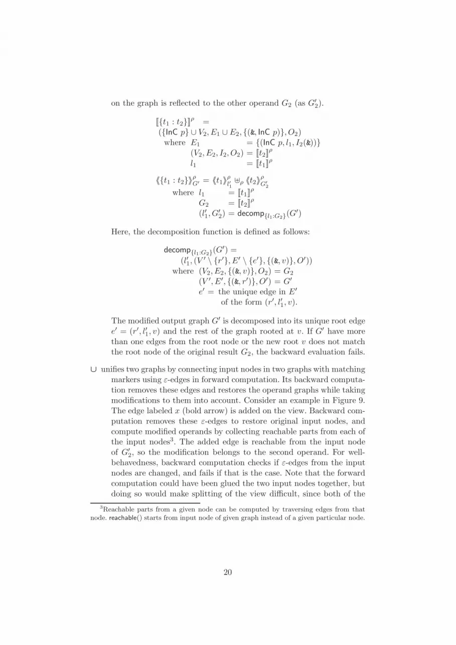
∪ unifies two graphs by connecting input nodes in two graphs with matchingmarkers using ε-edges in forward computation. Its backward computa-tion removes these edges and restores the operand graphs while takingmodifications to them into account. Consider an example in Figure 9.The edge labeled x (bold arrow) is added on the view. Backward com-putation removes these ε-edges to restore original input nodes, andcompute modified operands by collecting reachable parts from each ofthe input nodes3. The added edge is reachable from the input nodeof G′
2, so the modification belongs to the second operand. For well-behavedness, backward computation checks if ε-edges from the inputnodes are changed, and fails if that is the case. Note that the forwardcomputation could have been glued the two input nodes together, butdoing so would make splitting of the view difficult, since both of the
3Reachable parts from a given node can be computed by traversing edges from thatnode. reachable() starts from input node of given graph instead of a given particular node.
20

operands can be reachable from the glued node.
[[t1 ∪ t2]]ρ = (V,Eu ∪ E1 ∪ E2, Iu, O1 ∪O2)
where V = Vu ∪ V1 ∪ V2
(V1, E1, I1, O1) = [[t1]]ρ
(V2, E2, I2, O2) = [[t2]]ρ
M = inMarkers(t1) = inMarkers(t2)Vu = {InC∪ p &m | &m ∈M}Eu = {(InC∪ p &m, ε, v) | (&m, v) ∈ I1}∪ {(InC∪ p &m, ε, v) | (&m, v) ∈ I2}
Iu = {(&m, InC∪ p &m) | &m ∈M}〈〈t1 ∪ t2〉〉ρG′ = 〈〈t1〉〉ρG′
1�ρ 〈〈t2〉〉ρG′
2
where G1 = [[t1]]ρ
G2 = [[t2]]ρ
(G′1, G
′2) = decompG1∪G2
(G′)
The decomposition function ensures that the root node of the modifiedgraph G′ is an origin of a bunch of ε-edges, whose destination nodecame from the root node of either the original G1 or the G2. G1 \ G2
denotes componentwise set difference.
decompG1∪G2(G′) =(
xreachable(G′1, G1), xreachable(G′
2, G2))
where (V ′, E′, I ′, O′) = G′
(Vi, Ei, Ii, Oi) = Gi
G′i = reachable((V ′, E′, Ii, O
′))satisfying
inMarkers(G1) = inMarkers(G2)∀&m ∈ inMarkers(G1), (&m, r′) ∈ I ′,(r′, ε, v′) ∈ E′ :(&m, v′) ∈ I1 ∪ I2
xreachable(G′, G) =(V r ′ ∪ V u, Er ′ ∪Eu, Ir ′ ∪ Iu, Or ′ ∪Ou)
where (V r ′, Er ′, Ir ′, Or ′) = reachable(G′)(V u, Eu, Iu, Ou) = G \ reachable(G)
21

⊕ performs componentwise union in its forward computation. For backwardcomputation, it is like ∪, except that no ε-edge is involved.
[[t1 ⊕ t2]]ρ = (V1 ∪ V2, E1 ∪ E2, I1 ∪ I2, O1 ∪O2)
where (V1, E1, I1, O1) = [[t1]]ρ
(V2, E2, I2, O2) = [[t2]]ρ
〈〈t1 ⊕ t2〉〉ρG′ = 〈〈t1〉〉ρG′1�ρ 〈〈t2〉〉ρG′
2
where Gi = [[ti]]ρ
(G′1, G
′2) = decompG1⊕G2
(G′)decompG1⊕G2
(G′) = decompG1∪G2(G′)
without satisfyingcondition
@ appends two graphs by connecting the output nodes of the left operandwith corresponding input nodes of the right operand with ε-edges in itsforward computation. Currently, we allow this operator to be used onlyfor the projection of one component of the result of structural recursionby &zi@ rec(tb)(ta). Note that @ may introduce unreachable part inthe second argument, because of unmatched I/O nodes. Backwardcomputation carefully passes those parts backwards untouched toavoid unnecessary failure because of inconsistency because these partsare part of ordinary computation (computation on reachable parts)before discarding by the @ operator. Note that users operating onthe view do not change these unreachable parts since these parts areinvisible for the users.
[[&m@t2]]ρ = (V,E@ ∪ E2, {(&, InC p)}, O2)
where V = {InC p} ∪ V2
V1 = {InC p}(V2, E2, I2, O2) = [[t2]]
ρ
E@ = {(InC p, ε, v) | (&m, v) ∈ I2}
〈〈&m@t2〉〉ρG′ = 〈〈t2〉〉ρG′2
where (V ′, E′, I ′, O′) = G′
(V2, E2, I2, O2) = [[t2]]ρ
E@ = {(InC p, ε, v) | (&m, v) ∈ I2}G′
2 = (V′ \ {InC p}, E′ \ E@, I2, O2)
(:=) distributes the marker on the left operand to each of the input markerof the graph in the right operand, using the Skolem function “.” thatsatisfies (&x.&y).&z = &x.(&y.&z) (associativity) and &.&x = &x.& =&x (left and right identity) in its forward computation. Backwardcomputation, “peels off” the marker on the left hand side from each
22

of the input markers in G′ at the front.
[[&m := t1]]ρ = (V1, E1, I,O1)
where (V1, E1, I1, O1) = [[t1]]ρ
I = {(&m.&x, v) | (&x, v) ∈ I1}
〈〈&m := t1〉〉ρG′ = 〈〈t1〉〉ρG′1
where G′1 = (V
′, E′, I ′1, O′)(V ′, E′, I ′, O′) = G′
I ′1 = {(&x, v) | (&m.&x, v) ∈ I ′}
($v ) looks up variable binding from environment ρ. Backward computationupdates the binding.
[[$v ]]ρ = ρ($v)〈〈$v〉〉ρG′ = ρ[$v ← G′]
(if) first evaluates the conditional expression b and by the result it evaluateseither the then branch or the else branch in the forward computation.For the backward computation, modification to the environment as aresult of modification to the view may change the branching behavior(result of b). In order to make sure that well-behavedness still holds,backward semantics chooses the branch in which a result of anotherforward computation on the condition b agrees. To cope with possiblenon-determinism where both branches agree, the branch taken in theforward computation takes precedence. If neither of the branches agree,the backward computation fails.
[[if b then t1 else t2]]ρ = [[ti]]
ρ
where i = (if [[b]]ρ = true then 1 else 2)
〈〈if b then t1 else t2〉〉ρG′ = ρ′i′where ρ′1 = 〈〈t1〉〉ρG′
ρ′2 = 〈〈t2〉〉ρG′i = (if [[b]]ρ = true then 1 else 2)
i′ =
{i if [[b]]ρ
′i = [[b]]ρ
3− i if [[b]]ρ′3−i �= [[b]]ρ
It is worth noting that we have the following properties on the internalgraph representation when modification is applied on the view: (1) No ε-edges are added or deleted.; (2) Markers are not added, deleted or changed.;and (3) Unreachable parts are not modified. These properties are importantfor (GetPut) and (PutGet) properties to hold. Besides, Property (2) isa natural consequence of the rule for the output marker constructor &y.
23

fwd eachedge(ρ, tb, Ga=( , Ea, , ))
=
(e, [[tb]]
ρe)
˛˛e ∈ Ea, label(e) �= ε,ρe = ρ{$l �→ label(e), $g �→ subgraph(Ga, e)}
ff
composerec(G, (Va, Ea, Ia, Oa), M) = (Vbody ∪ Vhub, Ebody ∪ Espoke ∪ Eeps, I, O)where Vbody = {FrEp e v | (e, (Ve, , , )) ∈ G, v ∈ Ve}
Ebody = {(FrEp e u, l, FrEp e v) | (e, ( , Ee, , )) ∈ G, (u, l, v) ∈ Ee}Vhub = {Hubp v &m | v ∈ Va, &m ∈ M}Espoke = {(Hubp v &m, ε, FrEp e u) |
&m ∈ M, (e = (v, , ), ( , , Ie, )) ∈ G, (&m, u) ∈ Ie}∪ {(FrEp e u, ε,Hubp v &m) |
&m ∈ M, (e = ( , , v), ( , , , Oe)) ∈ G, (u, &m) ∈ Oe}Eeps = {(Hubp v &m, ε, Hubp u &m) | (v, ε, u) ∈ Ea, &m ∈ M}I = {(&n.&m, Hubp v &m) | (&n, v) ∈ Ia, &m ∈ M}O = {(Hubp v &m, &n.&m) | (v, &n) ∈ Oa, &m ∈ M}
Figure 10: Core of the Forward Semantics of rec at Code Position p
Property (1) is required for the consistent decomposition of targets. Property(3) is required to avoid unnecessary failure of backward computation byinterference of unreachable parts on reachable parts. They are also naturalfrom the user’s point of view since these components (ε-edge, markers andunreachable parts) are all invisible to users.
4.4.2 Bidirectional Evaluation of Structural Recursion
In this section, we give bidirectional semantics for structural recursion rec.For forward computation, rec expressions are interpreted in bulk semanticsas follows:
[[rec(λ($l , $g). tb)(ta)]]ρ =
composerec(fwd eachedge(ρ, tb, Ga), Ga,M)where M = inMarker(tb) ∪ outMarker(tb)
Ga = [[ta]]ρ
where fwd eachedge and composerec is defined in Figure 10. Intuitively,fwd eachedge evaluates the expression tb at each edge e of the argumentgraph Ga and returns the set of result graphs. Then, composerec glues allthe graphs together along the structure of the input Ga.Forward evaluation consists of the following steps. (1) Argument expres-
sion ta is computed to produce graph Ga. (2) By the fwd eachedge auxiliaryfunction, at every non-ε-edge e of Ga, new binding ρe is created so that $lpoints to the label of e (denoted by label(e)) and $g points to the subgraph(denoted by subgraph(Ga, e)) that is reachable from the target node of e.(3) Forward computation of the body expression tb is conducted for each ofthese bindings. (4) By the composerec auxiliary function, the results Ge arecombined to produce the final result.
24

bwd eachedge(ρ, tb,G′)
=n(e, 〈〈eb〉〉ρe
G′e)
˛˛ (e,G′
e) ∈ G′, ρe = ρ{$l �→ label(e), $g �→ subgraph(e)}o
decomprec(ρ, tb, (V′, E′, I ′, O′), Ga, M)
=
8>>>>>>>><>>>>>>>>:
(e, G′e)
˛˛˛˛˛˛
e ∈ Ea, label(e) �= ε,ρe = ρ{$l �→ label(e), $g �→ subgraph(Ga, e)}V ′
e = {w | (FrEp e w) ∈ V ′},E′
e = {(w1, l, w2) | (FrEp e w1, l, FrEp e w2) ∈ E′},I ′
e = {(&m, w) | (Hubp v &m,ε, FrEp e w) ∈ E′},O′
e = {(w, &m) | (FrEp e w, ε, Hubp v &m) ∈ E′},G′
e = (V ′e , E′
e, I′e, O
′e)
9>>>>>>>>=>>>>>>>>;
where (Va, Ea, Ia, Oa) = Ga
G = fwd eachedge(ρ, tb, (Va, Ea, Ia, Oa))
merge(ρ, ta, (Va, Ea, Ia, Oa),R) = 〈〈ta〉〉ρG′
a ρ
U{ρ′e \ {$l �→ } \ {$g �→ } | (e, ρ′
e) ∈ R}where Eeps = {(u, ε, v) | (u, ε, v) ∈ Ea}
(V ′′e , E′′
e ) = (V ′e ∪ {u}, E′
e ∪ {(u, ρ′e($l), root(I ′
e))})for each e = (u, a, v) ∈ Ea with a �= ε,
(e, ρ′e) ∈ R, (V ′
e , E′e, I
′e, O
′e) = ρ′
e($g)G′
a = (S
V ′′e , Eeps ∪ S
E′′e , Ia, Oa)
Figure 11: Core of the Backward Semantics of rec at Code Position p
The composition by composerec produces two types of nodes. One isVbody, which is the set of nodes v of of each graph fragments Ge to becombined. Note that, however, in order to keep the traceability, we augmentthe structured node ID of v as FrEp e v recording the edge code ID p of therec expression and the input edge e where the node is created. Of course,in the case of nested rec expressions, the ID v from the result of bodyexpression themselves may be structured already. Similarly, the set of edgesEbody consists of edges from Ge with structured ID information added. Theother type of nodes is Vhub, which is used as connecting points of Ge’s. Forinstance, let e1 = (v, a, u) and e2 = (u, b, w) sharing the node u, and therecursion uses two markers &z1 and &z2. To connect Ge1 and Ge2 correctly,nodes with output marker (x1, &z1) in Ge1 must be identified with nodeswith input marker (&z1, x2) in Ge2 (and similarly for &z2). To achieve this,we prepare a node (Hubp v &z1) in Vhub, and connect all the output markernodes of Ge1 and the input marker nodes of Ge2 using ε-edges, which arethe Espoke edges. Finally, to keep the ε-edges in the input graph unchanged,we connect by an ε-edge the hubs whose origin nodes are connected by anε-edge; this is the set of edges Eeps.
25

Next, our backward semantics is defined as follows:
〈〈rec(λ($l , $g). tb)(ta)〉〉ρG′ =merge(ρ, ta, Ga,bwd eachedge(ρ, tb, Ga,decomprec(ρ, tb, G′, Ga,M)))
where M = inMarker(tb) ∪ outMarker(tb)Ga = [[ta]]
ρ
Note the duality between the forward semantics. Backward semantics firstdecomposes by decomprec the modified result graph G′ into pieces of graphs,which is intuitively an inverse operation of comprec. Each element of the de-composition is the (possibly modified) subpart G′
e of G′, which corresponds
to the forward computation Ge. Then, in bwd eachedge, we carry out back-ward computation on each edge and compute the updated environment ρ′e.Finally, these environments are merged into the updated environment ρ′ ofthe whole expression. The merge function does two works. First, by comb-ing the information ρ′e($l) and ρ′e($g) from the updated environments, itcomputes the modified argument graph G′
a4. Then we inductively carry out
backward evaluation on the argument expression to obtain another updatedenvironment ρ′a. This ρ′a and all ρ′es are merged into ρ′.Let us explain in more detail the definition of decomprec, which is the
key point of the backward evaluation.The function first extract from result graph G′ nodes V ′
e and edges E′e
that belonging to each edge e by matching structured ID FrEp e . Notethat we require nodes that are newly inserted to the view also have thisstructure, so that these nodes are also passed to the backward evaluation ofthe recursion body. Input and output nodes with marker &m are recoveredby selecting those pointed from/to hub nodes having structure Hub &m.Top-level constructors of structured ID are erased so that we can inductivelycompute the backward image from the body expression.Note that semantics uses node identities in computation, while graph
data model assumes value equivalence based on bisimulation. Update de-tection or conflict resolution in �ρ basically uses node identities, however,bisimulation equivalence may be used to resolve conflicts at the graph levelinstead of per node and edge basis, to cope with complex updating on theview.
4Merging operation inS
does not consist of simple set unification operation. Detail isdiscussed in Section B in the appendix.
26

Example 8 (Edge Renaming). The following transformation a2b replacesedge label a with b and leaves other labels unchanged.
a2b =rec(λ($l , $G). & :=
if $l = a then {b : (&)1}2else {$l : (&)3}4)($db)6
Above, expression t at code position p is written by tp. Let $db, whichrepresents a source database, be the following graph.
s = ��������1c
��a �� ��������2
Then, the transformation result with ε-edges and structured IDs is as follows.
G =
�� ���� ��Hub6 1 &�� ���� ��
�� ��FrE6 (InC 4) (1, c, 2)c��
�� ���� ��FrE6 (InC 2) (1, a, 2)
b���� ���� ��FrE6 (InC 3) (1, c, 2)
��
�� ���� ��FrE6 (InC 1) (1, a, 2)
���� ���� ��Hub6 2 &
The graph is bisimilar to the following graph.
�� ���c
��b ���� ���
According to the backward semantics of the transformation a2b, if wemodify graph G to G′ by changing the edge label c to d, then 〈〈a2b〉〉{$db �→s}
G′returns binding {$db �→ s′} where
s′ = ��������1d
��a �� ��������2 .
The edge c in the source is changed to d successfully.If the subgraph in the view is changed as
�� ���� ��FrE6 (InC 2) (1, a, 2)
b���� ���� ��FrE6 (InC 1) (1, a, 2)−→
�� ���� ��FrE6 (InC 4) (1, a, 2)
e���� ���� ��FrE6 (InC 3) (1, a, 2)
then, according to the bidirectional semantics of if , the source is changed tothe following graph.
��������1c
��e �� ��������2
27

Example 9 (Extracting Subgraph). The following transformation at abextracts all the subgraphs that can be reachable from the root by path a.b.
at ab =rec(λ($l , $g).
if $l = a thenrec(λ($l ′, $g ′).
if $l ′ = b then $g ′ else {}1)($g)2else {}3)($db)4
Then, we can reflect any changes on the extracted graphs to the correspond-ing source as long as the changed graph has appropriate structured IDs.
Let $db be graph ��������1 a ����������2 b �� G. Then the reachable part of the trans-formation results with structured ID becomes
�� ���� ��Hub4 1 & ���� ���� ��FrE4 (Hub2 2 &) (1, a, 2) �� G′
where subgraph G′ is obtained by replacing node v in G withFrE4 (FrE2 v (2, b, r)) (1, a, 2) where r is the root of G. Any modifi-cation on G′ can be reflected to G in the source.
Example 10 (Customer2Order). The transformation mentioned in Sec-tion 2.3 is translated into UnCAL expression that has nesting of rec similarto that in Example 9. Concrete UnCAL expression can be seen in Sec-tion C in the appendix. Since extracted subgraph can accept arbitraryupdates, if we modify the label 16/10/2008 of the edge from node 7 tonode 6 in graph gord in Figure 6, backward transformation systematicallyfinds the corresponding edge and modify the edge from node 7 to node6 in gcus in Figure 5, because the modified part is an extracted subgraphreachable from the root by path customer.order.date. Subgraphs that arereached by the paths customer.order.no, customer.order.order of.nameand customer.order.order of.add can be updated similarly.
4.5 Insertion Reflection based on ε-edge/ID Structure
So far the bidirectional semantics can only cope with in-place updating anddeletion – modifications on edge labels or updating and deletion on extractedsubpart of the original graph. However, except for the extracted subpart, ithas the great limitation that no edge can be added to the original graphbecause it tightly uses the structures of ε-edges/IDs, which also enablesus the backward semantics. In this section, we show how to extend itmoderately to coped with insertion.In fact, supporting insertion in bidirectional transformation is challeng-
ing because the inserted part has no correspondence in the original source.Foster et al. (2005) and Bohannon et al. (2008) solve this problem by ex-plicitly defining a create function to create the “original” data only from
28

a inserted subpart. Matsuda et al. (2007) allow insertion only if the “origi-nal” data is uniquely determined by the inserted subpart. Liu et al. (2007)treat insertion only on the results of “map” but there is no guarantee ofbidirectional properties in the framework.Our insertion handling is inspired by those in Liu et al. (2007) and
Matsuda et al. (2007). Like Liu et al. (2007), we treat insertion only onthe result of rec. And, we follow Matsuda et al. (2007), we use ε-edge/IDstructure as “complementary” information to uniquely create source data.
�� ���� ��Hub6 1 &���� ��
�� ��FrE6 (InC 4) (1, c, 2)c���� ��
�� ��FrE6 (InC 3) (1, c, 2)���� ���� ��Hub6 2 &
Let us explain our basic idea with Example 8. If $dbis a graph ��������1 c ����������2 , then the transformation results inthe graph on the right. In our insertion handling, weconsider what happens if there exists an extra edgebetween two nodes, i.e., the transformation result ofthe following graph.
��������1c
��??? �� ��������2
Instead of inserting single edge, we consider the transformation result ofthe graph with inserted edge (1, ???, 2) that have undetermined label. Con-cretely, the input of the backward transformation with insertion handling isthe following graph.
�� ���� ��Hub6 1 &�� ���� ��
�� ��FrE6 (InC 4) (1, c, 2)c��
�� ���� ��FrE6 (InC 2) (1, ???, 2)
b���� ���� ��FrE6 (InC 3) (1, c, 2)��
�� ���� ��FrE6 (InC 1) (1, ???, 2)
���� ���� ��Hub6 2 &
According to the semantics of rec, insertion of the FrE-subpart impliesinsertion of the edges. The structured ID in the inserted graph contains??? because at the time we do not know what is the edge that generates theinserted subgraph. Hence, by the backward transformation discussed here,we estimate a concrete label of the inserted edge. Because of the structuredID of the inserted subgraph, we can know that inserted subgraph comes fromtrue-branch of the following if -expression if $l = a then {b : &1}2 else {$l :&3}4 Since condition $l = a must be true to obtain the inserted subgraph,the backward transformation replaces the label ??? of $l by a. Hence, weobtain the following graph by the insertion.
��������1c
��a �� ��������2
In the rest of section, we first discuss the modification of the backwardsemantics for insertion reflection. The backward semantics of rec and if willbe changed: the new semantics of rec handles inserted subpart, and the
29

new semantics of if estimates a concrete label to replace ???. After that, wediscuss expressive power of our insertion reflection.Note that ??? may cause the failure of the forward transformation; if
it appears in the condition of if -expression, we cannot determine whichbranch to use. Recall that some backward semantics of an expression usesthe forward semantics of its subexpression. Note that the failure of forwardtransformation do not mean the failure of the backward transformationimmediately. When they are used for graph decomposition in a backwardtransformation, the backward transformation fails.
4.5.1 Backward Semantics of rec for Insertion Reflection
The modification on the rec for insertion reflection is very small. Since theIDs of an inserted subgraph must have the form FrE ( , ???, ), we caneasily split the inserted subpart from a modified result of rec. The definitionof decomprec in Figure 11 changes a bit as follows.
decomprec(. . . (V ′, E′, I ′, O′) . . . ) ={. . .
∣∣ e ∈ Ea . . . ρe = ρ{. . . $g �→ subgraph(Ga, e)}
where . . .
−→
decomprec(. . . (V ′, E′, I ′, O′) . . . ) ={. . .
∣∣ e ∈ E′a . . . ρe = ρ{. . . $g �→ subgraph(G′
a, e)}
where E′a = Ea
∪ {(u, ???, v) | FrEp (u, ???, v) ∈ E′}G′
a = (Va, E′a, Ia, Oa)
. . .
The subgraph is performed on G′a, which contains edge (u, ???, v), instead
of Ga because to guarantee PutGet we must ensure that the inserted edgedoes not affect other part of the output graph (V ′, E′, I ′, O′).
4.5.2 Estimating Label of Edge to be Inserted
There are only two places that backward transformation can replace ???with a concrete value.
• Use of label variable $l caused by rec.
• Condition such as $l = a in if .
Since the semantics of the former is already described in the previous section,we discuss the latter here.
30

Here, we only write the formal definition of the backward semantics of ifwhere the evaluation result of condition is undetermined because of variable$l with ??? in the expression.
〈〈if b then t1 else t2〉〉ρG =
Fail if [[b]]ρ′′i = ??? for i = 1, 2
ρ′′1 if [[b]]ρ′′1 = true
ρ′′2 if [[b]]ρ′′2 = false
where ρ′1 = 〈〈t1〉〉ρGρ′2 = 〈〈t2〉〉ρGρ′′1 = refine(ρ′1, b)ρ′′2 = refine(ρ′2, not b)
Above, refine(ρ, b) is a function to be used to refine the environment ρ byreplacing ??? with a concrete value so as to make the evaluation result b tobe true.There are many choices of refine(ρ, b). A strong approach would be to
use some constraint solver. Instead, we take a more lightweight choice thatcares a condition of the form $l = v or $l �= v and fixes the value of$l even though there are multiple possibilities. For example, refine({$l �→???}, $l = a) returns {$l = a} while refine({$l �→ ???}, $l �= a) returns{$l �→ bogus} where bogus is magically chosen value to suffice $l �= a. Notethat refine({$l �→ ???, $r = a}, $l = $r) returns {$l �→ a, $r = a} becausewe can know the concrete value of $r . To guarantee PutGet, refine fails ifit encounters expression such as $l = $r where both $l and $r are bound to???.
4.5.3 Discussion of Insertion Reflection
As we have shown with Example 8, the insertion reflection method herework well for single rec. However, the insertion reflection method does notwork for the nested rec such as that in Example 9.The main reason of the limitation is that the one graph can be traversed
more than once by nested rec; since the backward transformation reflect theconcrete graph to the source by each traverse, the reflection would conflictfor each traverse.Let us consider the transformation of Example 9. Let $db be a graph
with isolated three nodes ��������1 , ��������2 and ��������3 . Then, the transformation resultconsists of three hub nodes of the form Hub4 & but does not have anyedge. If we want to insert something to the view, we must insert a.b path tothe source.To insert a.b, we consider the transformation result of $db = ��������1 ??? ����������2 ??? ����������3
and try to replace the first ??? with a and the second with b by the backwardtransformation. Hence we must consider the backward transformation of the
31

following graph.
�� ���� ��& : Hub4 1 &���� ��
�� ��FrE4 (Hub2 2 &) (1, ???, 2)���� ���� ��FrE4 (FrE2 3 (2, ???′, 3)) (1, ???, 2)
�� ���� ��FrE4 (Hub2 3 &) (1, ???, 2)
�� ���� ��Hub4 2 &���� ��
�� ��FrE4 (InC 3) (2, ???′, 3)
�� ���� ��Hub4 3 &
Here, for presentation, we denote ??? to be replaced by a and b by ??? and???′ respectively.However, the insertion reflection fails due to the following two problems.
• The backward transformation of the outer rec calls the backwardtransformation of rec-body for FrE4 (1, ???, 2) nodes. However, thebackward transformation of rec-body fails because of mismatch of hubnodes of the inner rec. The Vhub of the inner rec in the original datais Hub2 2 & (hub nodes of reachable part of node 2), while the hubnodes of the output graph are Hub2 2 & and Hub2 3 &.
• The backward transformation of the outer rec tries to estimate thelabel of inserted edge. If the first problem is solved well, we canestimate the label of the edge (1, ???, 2) from the condition $l = a.However, the estimation of the second edge (2, ???, 3) by the outer reccan replace ??? with label different from b, which causes the failureby inconsistent environement in the later step.
There would be many approaches towards the problems. PreprocessingUnCAL expression using fusion method to flatten nested rec to one flat recavoids the problems. However, if the transformation has “join”, in whichinner rec uses bound variable of outer rec, it is hard to flatten nested recs.Even when the fusion method is not applicable, the first problem would
be relatively easy to solve. If the view contains an extra hub node Hubp v ,we can safely assume that the node comes from the new or existing nodev. Since the original graph is available in backward transformation, we canknow whether a node is new or existing. On the contrary, more discussion isneeded to solve the second problem. The second problem seems to be solvedby changing backward semantics to calculate bindings that maps variable toa set of values and with constraints on the variables. However, in additionto the problem of choosing appropriate description of such sets, it makes theguarantee of PutGet property much and much harder.
• We must give a representation of “set” of variables and “constraints”.Since we have variable-to-variable comparison as $l = $r , the inter-variable constraint must be cared.
32

• Environment merging operator � must consider the “sets” and “con-straints”.
Note that approximation by wider (less constrained) set may not work. Sincethe sets and the constraints represents the set of sources of an output graph,the approximated set might be too wide to guarantee PutGet.One may think that it is also a problem that the insertion here does
not consider insertion of nodes. However, in contrast to the above twoproblems, the insertion of node is easily solved because an isolated nodein the source is always transformed to an isolated hub node in the view byrec. However, because the first problem above, we can use the inserted nodeonly in outermost rec.Since the essence of difficulties of insertion reflection in Customer2Order
that appeared in Section 2.3 is contained in insertion reflection in Example 9,we hardly insert subgraphs in Customer2Order because of the same reasons.To give an appropriate and reasonable solution to the problem is one of ourfuture work.
4.6 Main Theorem
Now that semantics of all UnCAL expressions are defined, we summarizeour main result as the following theorem. See section A in the appendix forthe proof of the theorem.
Theorem 2. Every bidirectionalized UnCAL expression satisfies (PutGet)and (GetPut) properties, provided that its forward and backward evaluationsucceeds.
5 Implementation and Experiments
The prototype system has been implemented in OCaml and is availableonline5. One can run UnQL queries both forwardly and backwardly. Inaddition to the examples in Buneman et al. (2000), we have tested thefollowing three non-trivial examples, showing its usefulness in softwareengineering and database management.
• Customer2Order: a case study in the textbook on model-driven soft-ware development (Pastor and Molina 2007).
• PIM2PSM: a typical example of transforming a platform independentobject model to platform specific object model.
• Class2RDB; a non-trivial benchmark application for testing power ofmodel transformation languages (Bezivin et al. 2005).
5http://www.biglab.org
33

All of them demonstrate the effectiveness of our approach in practicalapplications.In our implementation, we carefully treat ε-edges, unreachable parts
introduced during operations related to markers, and retrieval of edges ornodes of interest, which greatly affect the performance. Bad treatment wouldhinder large scale UnQL queries to evaluate in bidirectional mode6 in areasonable amount of time. Several orders of magnitude speed-up has beenachieved since our initial implementation by the following optimizations.
Reduction of the number of ε-edges As mentioned in the UnQLpaper (Buneman et al. 2000), ε-edges are generously generated duringevaluation, especially in rec. It makes evaluation process slow due to growthof input size. Removing ε-edges during evaluation does no harm on forwardsemantics because of bisimulation equivalence. However, since ε-edges playan important role in backward evaluation, they are not freely omitted in ourbidirectional settings. Moreover, a straightforward implementation of theremoval algorithm (Buneman et al. 2000) may introduce additional edges,which may harm backward evaluation. Towards prudent removal of ε-edgessuitable for backward evaluation, our ε-removal algorithm glue source anddestination nodes of ε as long as bisimulation equivalence is not violated.
Pruning of unreachable nodes @ and rec may leave unreachable nodesif some input and output nodes are left unconnected due to mismatch ofmarkers. This mismatch happens typically in the case of projection of graphcomponents &zi by idiom &zi @ g and in the case of @ in the definition ofrec in rec(λ($l , $g).tb)(l : g) = tb(l, g) @ rec(tb)(g). Typical usage of recincludes tb with no output marker, where actual recursion below the firstlevel from the input nodes — subgraphs that is not reachable by traversingonly one edge — is not necessary because the @ does not connect the firstand second arguments due to the lack of matching markers. This opensoptimization opportunities; not to evaluate tb for the input graph that islower than the first level. Performance improvement was significant for theforward evaluation.
Indexing As seen in the formal notion of bulk semantics composerec anddecomprec, pattern matching on edges for the entire graph is often needed.Constructing maps from node identifiers to the sets of associated incomingand outgoing edges has been effective to improve performance on bothforward and backward directions.
6 Related Work
In addition to the related work in the introduction, we discuss other mostrelated work.
6Note that we preserve every result of forward computation in bidirectional mode.
34

Bidirectional transformation has been discussed as view updating prob-lem in the database community. Bancilhon and Spyratos (1981) proposed ageneral approach to the problem. They introduced an elegant solution basedon the concept of constant complement view which enables recovery of lostinformation of the sources. It has been applied to bidirectional transforma-tion on relational database (Cosmadakis and Papadimitriou 1984; Laurentet al. 2001; Lechtenborger and Vossen 2003) and tree structures (Matsudaet al. 2007). However, this approach assumes the presence of automatic in-verse transformation, which makes it difficult to use.Foster et al. (2005) and Bohannon et al. (2008) proposed the first linguis-
tic approach to bidirectional transformation. They developed some domainspecific languages for supporting development of bidirectional transforma-tion on strings and trees. However, their approach is limited to strings andtrees, and difficult to be applied to graph transformation due to graph-specific features such as circularity and sharing.In the context of software engineering, there are several work on bidirec-
tional model (graph) transformation (Ehrig et al. 2005; OMG 2005; Jouaultand Kurtev 2006), which can deal with a kind of graph structures. As pointedby Stevens (2007), there lacks clear formal semantics of bidirectional modeltransformation and there is no powerful bidirectionalization method yet thatcan be used to automatically derive backward model transformations fromforward model transformations so that both transformations form a consis-tent bidirectional model transformation. This calls for a more serious studyon bidirectional graph transformation, which actually inspired the work inthis paper.The concept of structural recursion is not new and has been studied
in both the database community (Breazu-Tannen et al. 1991) and thefunctional programming community (Sheard and Fegaras 1993). However,most of them focused on structural recursion over lists or trees insteadof graphs. Examples include the higher order function fold (Sheard andFegaras 1993) in ML and Haskell, and the generic computation patterncalled catamorphism in programming algebras (Bird and de Moor 1996).It is UnCAL (Buneman et al. 2000) that shows the idea of structuralrecursion can be extended to graph, but the focus there was on query fusionoptimization rather than bidirectionalization.
7 Conclusion
In this paper, we report our first attempt towards solving the challengingproblem of bidirectional transformation on graphs. We show that structuralrecursion on graphs and its unique bulk semantics play an important rolenot only in query optimization, which has been recognized in the databasecommunity, but also in automatic derivation of backward evaluation, which
35

has not be recognized so far. As far as we are aware, the bidirectional seman-tics of UnCAL proposed in this paper is the first complete language-basedframework for general graph transformations. Current prototype system andits application to bidirectional (UML) model transformation and model syn-chronization show that our framework is promising for practical use.Future work includes extension of the framework for more flexible in-
sertion, introduction of graph schemas to provide structure information formore efficient bidirectional computation, and more practical application ofthe system for bidirectional model transformation in software engineering.
Acknowledgements
The research was supported in part by the Grand-Challenging Projecton “Linguistic Foundation for Bidirectional Model Transformation” fromNational Institute of Informatics, the National Natural Science Foundationof China under Grant No. 60528006, Grant-in-Aid for Scientific Research(C) No.20500043, and Encouragement of Young Scientists (B) of the Grant-in-Aid for Scientific Research No. 20700035.
References
Francois Bancilhon and Nicolas Spyratos. Update semantics of relationalviews. ACM Transactions on Database Systems, 6(4):557–575, 1981.J. Bezivin, B. Rumpe, and Tratt L Schurr A. Model transformation inpractice workshop announcement. InMTiP 2005, International Workshopon Model Transformations in Practice. Springer-Verlag, 2005.Richard Bird and Oege de Moor. Algebras of Programming. Prentice Hall,1996.Aaron Bohannon, J. Nathan Foster, Benjamin C. Pierce, AlexandrePilkiewicz, and Alan Schmitt. Boomerang: resourceful lenses for stringdata. In George C. Necula and Philip Wadler, editors, POPL ’08:ACM SIGPLAN–SIGACT Symposium on Principles of ProgrammingLanguages, pages 407–419. ACM, 2008.Val Breazu-Tannen, Peter Buneman, and Shamim Naqvi. Structural recur-sion as a query language. In Proc. of the Third International Workshopon Database Programming Languages(DBPL 91), pages 9–19, 1991.Peter Buneman, Mary F. Fernandez, and Dan Suciu. UnQL: a query lan-guage and algebra for semistructured data based on structural recursion.VLDB Journal: Very Large Data Bases, 9(1):76–110, 2000.Stavros S. Cosmadakis and Christos H. Papadimitriou. Updates of relationalviews. Journal of the ACM, 31(4):742–760, 1984.
36

Krzysztof Czarnecki, J. Nathan Foster, Zhenjiang Hu, Ralf Lammel, AndySchurr, and James F. Terwilliger. Bidirectional transformations: A cross-discipline perspective. In International Conference on Model Transforma-tion (ICMT 2009), pages 260–283. LNCS 5563, Springer, 2009.Umeshwar Dayal and Philip A. Bernstein. On the correct translation ofupdate operations on relational views. ACM Transactions on DatabaseSystems, 7(3):381–416, 1982.Karsten Ehrig, Esther Guerra, Juan de Lara, Laszlo Lengyel, Tihamer Lev-endovszky, Ulrike Prange, Gabriele Taentzer, Daniel Varro, and SzilviaVarro-Gyapay. Model transformation by graph transformation: A com-parative study. In MTiP 2005, International Workshop on Model Trans-formations in Practice. Springer-Verlag, 2005.J. Nathan Foster, Michael B. Greenwald, Jonathan T. Moore, Benjamin C.Pierce, and Alan Schmitt. Combinators for bi-directional tree transfor-mations: a linguistic approach to the view update problem. In POPL’05: ACM SIGPLAN–SIGACT Symposium on Principles of ProgrammingLanguages, pages 233–246, 2005.Georg Gottlob, Paolo Paolini, and Roberto Zicari. Properties and updatesemantics of consistent views. ACM Transactions on Database Systems,13(4):486–524, 1988.Stephen J. Hegner. Foundations of canonical update support for closeddatabase views. In ICDT ’90: Proceedings of the Third International Con-ference on Database Theory, pages 422–436, London, UK, 1990. Springer-Verlag.Zhenjiang Hu, Hideya Iwasaki, Masato Takeichi, and Akihiko Takano. Tu-pling calculation eliminates multiple data traversals. In ACM SIGPLANInternational Conference on Functional Programming (ICFP’97), pages164–175, Amsterdam, The Netherlands, June 1997. ACM Press.Zhenjiang Hu, Shin-Cheng Mu, and Masato Takeichi. A programmable ed-itor for developing structured documents based on bidirectional transfor-mations. Higher-Order and Symbolic Computation, 21(1-2):89–118, 2008.Frederic Jouault and Ivan Kurtev. Transforming models with ATL. In
Proceedings of Satellite Events at the MoDELS 2005 Conference, pages128–138. LNCS 3814, Springer, 2006.Ralf Lammel. Coupled Software Transformations (Extended Abstract).In First International Workshop on Software Evolution Transformations,November 2004.Dominique Laurent, Jens Lechtenborger, Nicolas Spyratos, and GottfriedVossen. Monotonic complements for independent data warehouses. TheVLDB Journal, 10(4):295–315, 2001.
37

Jens Lechtenborger and Gottfried Vossen. On the computation of relationalview complements. ACM Transactions on Database Systems, 28(2):175–208, 2003.Dongxi Liu, Zhenjiang Hu, and Masato Takeichi. Bidirectional interpreta-tion of xquery. In PEPM ’07: Proceedings of the 2007 ACM SIGPLANsymposium on Partial Evaluation and semantics-based Program Manipu-lation, pages 21–30, New York, NY, USA, 2007. ACM Press.Kazutaka Matsuda, Zhenjiang Hu, Keisuke Nakano, Makoto Hamana, andMasato Takeichi. Bidirectionalization transformation based on automaticderivation of view complement functions. In 12th ACM SIGPLAN In-ternational Conference on Functional Programming (ICFP 2007), pages47–58. ACM Press, October 2007.Lambert Meertens. Designing constraint maintainers for user interaction.http://www.cwi.nl/∼lambert, June 1998.OMG. MOF QVT final adopted specification. http://www.omg.org/docs/ptc/05-11-01.pdf, 2005.Yannis Papakonstantinou, Hector Garcia-Molina, and Jennifer Widom. Ob-ject exchange across heterogeneous information sources. In Philip S. Yuand Arbee L. P. Chen, editors, ICDE, pages 251–260. IEEE ComputerSociety, 1995.Oscar Pastor and Juan Carlos Molina. Model-Driven Architecture in Prac-
tice: A Software Production Environment Based on Conceptual Modeling.Springer-Verlag New York, Inc., Secaucus, NJ, USA, 2007.T. Sheard and L. Fegaras. A fold for all seasons. In Proc. Conference
on Functional Programming Languages and Computer Architecture, pages233–242, Copenhagen, June 1993.Perdita Stevens. Bidirectional model transformations in QVT: Semanticissues and open questions. In Gregor Engels, Bill Opdyke, Douglas C.Schmidt, and Frank Weil, editors, Proc. 10th MoDELS, volume 4735 ofLecture Notes in Computer Science, pages 1–15. Springer, 2007.
A Proof of Main Theorem
Before proving the main theorem, we show the following lemma.
Lemma 3. Composition and decomposition (decomp) for every UnCALconstructor ( ∈ {(), {}, &y, { : },∪,⊕,@, :=}) satisfy the following(DPutGet) and (DGetPut) properties.
( ) v1 . . . vn = G
decomp(�) v1...vn(G) = (v1, . . . , vn)
(DGetPut)
38

decomp(�) v1...vn(G′) = (v′1 . . . , v′n)
( ) v1 . . . vn = G′ (DPutGet)
This lemma trivially holds by the definition of bidirectional semanticsfor each constructor.Now return to the proof of the main theorem. It is sufficient to show that
every bidirectional UnCAL operator satisfies (PutGet) and (GetPut)properties, provided that both [[·]] (get) and 〈〈·〉〉 (put) do not fail.For forward direction, every operator behaves identically to the original
UnCAL semantics, so they are defined according to the original semantics.For example, [[e1 ∪ e2]] is defined only if input markers of result graphs ofe1 and e2 agree, as in the definition in Section 4.4. So we focus on thebackward direction. For the base case, we disallow any modifications onnullary constructors, so 〈〈{}〉〉, 〈〈()〉〉 and 〈〈&y〉〉 is defined only if the targetremains unchanged. In this case, both (GetPut) and (PutGet) triviallyhold. Next we examine the inductive case. For 〈〈{t1:t2}〉〉ρ, we disallowmodifications of the number of edges from the root. Under this constraint,it succeeds if put on both components t1 and t2 succeed. Let [[t1]]
ρ = l1and [[t2]]
ρ = G1, respectively so G = {l1:G1} is produced as a final result.To see if (GetPut) holds, suppose (GetPut) on both operands hold asan induction hypothesis. decomp{l1:G1}(G) in 〈〈{t1:t2}〉〉 decompose G bytraversing one edge (root(G), l′, v) from the root of G and obtain l1 as thelabel of the edge, and remaining part as subgraph(G, v). If there are morethan one of such edges, the put is undefined (and the violation of the abovecondition is signaled). But if the target is unmodified, we obtain l1 andG1 again by (DGetPut). Because of the induction hypothesis, we obtainunmodified environment ρ for both operands. The result environment isunchanged because ρ = ρ �ρ ρ. Other simple operators except rec can betreated similarly.To see if (PutGet) holds, suppose (PutGet) on both operands hold.
We have to show that 〈〈{t1:t2}〉〉ρG′ = ρ′ implies [[{t1:t2}]]ρ′= G′. According
to the definition of 〈〈{t1:t2}〉〉G′ , decomp{l1:G1} G′ = (l′, G′′), 〈〈t1〉〉ρl′ = ρ′1 and〈〈t2〉〉ρG′′ = ρ′2 should have been computed. Since we can assume [[t1]]
ρ′1 = l′
and [[t2]]ρ′2 = G′′ from the above induction hypothesis, and ρ′1�ρρ
′2 has been
equal to ρ′, and by (DPutGet), i.e., {l′:G′′} = G′, [[{t1:t2}]]ρ′= G′ holds.
Other simple operators except rec can be treated similarly.For (GetPut) on rec(λ($l , $g). tb)(ta), since composerec and decomprec
satisfy symmetry similar to (DGetPut) and (DPutGet), no modifica-tion on the view obtain identical set of bindings of $l and $g . So �ρ
in merge for 〈〈rec(λ($l , $g). tb)(ta)〉〉ρG for G = [[rec(λ($l , $g). tb)(ta)]]ρ
results in no conflict. For (PutGet) on rec, G′a in the definition of
〈〈rec(λ($l , $g). tb)(ta)〉〉ρG′ is obtained again in another get assuming(PutGet) property on ta. So assuming (DPutGet) like property of
39

decomprec and composerec, input of compose in another get will be identicalto decomposition {(e, (V ′
e , E′e, I
′e, O
′e))} of the first put in the definition of
decomprec, thus another get results in G′ again. Same argument hold in thepresence of insertion because of the given structured IDs for every insertionunit discussed in Section 4.5.
B Merging operation in backward semantics of rec
Backward evaluation of rec(tb)(ta) needs to combine backward evaluationresults of the body (tb). This has been simply represented using
⋃in function
merge in Figure 11. This operation does not consist of simple compnentwiseset union, since simple unification would result in apppearance of originaledge as well as the edge after modification at the same time, when the labelof an edge is modified.This section describes this operation. Meanings of each symbols are the
same as in Figure 11 unless mentioned otherwise.The following equation shows, in function merge, how to compute G′
a,the updated graph to be fed to backward evaluation of ta, where G1 \ G2
denotes componetwize (set) difference of two graphs.
G′a = Ga ⊕Gadd
a \Gdela
where (Gadda , Gdel
a ) =
⊕(G′
e \Ge, Ge \G′e)
∣∣∣∣∣∣∣∣∣∣
e ∈ Ea, (e, ρ′e) ∈ R,(V ′
e , E′e, I
′e, O
′e) = ρ′e($g),
G′e = (V
′e ∪ {u}, E′
e ∪ {(u, ρ′e($l), root(I′e))}, I ′e, O′
e),(Ve, Ee, Ie, Oe) = ρe($g),Ge = (Ve ∪ {u}, Ee ∪ {(u, ρe($l), root(Ie))}, Ie, Oe)
where⊕is defined by ⊕ across first and second component of pairs:
(g1, g2)⊕(g3, g4) = (g1 ⊕ g3, g2 ⊕ g4).
G′a is computed by accumulating “effects” for graphs Ge consists of edge ein Ea and reachable subgraphs pointed by e. “effects” are computed by setunion and set difference between original subgraphGe and updated subgraphG′
e.
C Customer2Order in UnCAL
Figure 12 shows UnCAL code that is translated from UnQL code in Sec-tion 2.3.
40

rec(\ ($L,$fv3).
if $L = customer
then rec(\ ($L,$o).
if $L = order
then rec(\ ($L,$c).
if $L = order_of
then rec(\ ($L,$date).
if $L = date
then rec(\ ($L,$no).
if $L = no
then rec(\ ($L,$a).
if $L = add
then rec(\ ($L,$name).
if $L = name
then rec(\ ($L,$code).
if $L = code
then rec(\ ($L,$info).
if $L = info
then rec(\ ($L,$fv1).
if $L = type
then
rec(\ ($L,$anyv2).
if
$L = shipping
then
{order:
{
date: $date,
no: $no,
customer_name: $name,
addr: $a}}
else
{})
($fv1)
else
{})
($a)
else {})
($a)
else {})
($a)
else {})
($c)
else {})
($c)
else {})
($o)
else {})
($o)
else {})
($o)
else {})
($fv3)
else {})
($db)
Figure 12: UnCAL code translated from UnQL code in Section 2.3
41