| 107

Geoplanning Vol 3, No. 2, 2016, 107-116 Journal of Geomatics and Planning

E-ISSN: 2355-6544 http://ejournal.undip.ac.id/index.php/geoplanning

doi: 10.14710/geoplanning.3.2.107-116

ASSESSMENT OF MANGROVE FOREST DEGRADATION THROUGH CANOPY FRACTIONAL COVER IN KARIMUNJAWA ISLAND, CENTRAL JAVA, INDONESIA

M. Kamal a, Hartono a, P. Wicaksono a, N. S. Adi b, S. Arjasakusuma a

a Faculty of Geography, Universitas Gadjah Mada, Yogyakarta, Indonesia b Research Centre for Coastal and Maritime Resources, The Ministry of Maritime Affairs and Fisheries, Indonesia

Abstract: The Karimunjawa Islands mangrove forest has been subjected to various direct and indirect human disturbances in the recent years. If not properly managed, this disturbance will lead to the degradation of mangrove habitat health. Assessing forest canopy fractional cover (fc) using remote sensing data is one way of measuring mangrove forest degradation. This study aims to (1) estimate the forest canopy fc using a semi-empirical method, (2) assess the accuracy of the fc estimation and (3) create mangrove forest degradation from the canopy fc results. A sample set of in-situ fc was collected using the hemispherical camera for model development and accuracy assessment purposes. We developed semi-empirical relationship models between pixel values of ALOS AVNIR-2 image (10 m pixel size) and field fc, using Enhanced Vegetation Index (EVI) as a proxy of the image spectral response. The results show that the EVI provides reasonable estimation accuracy of mangrove canopy fc in Karimunjawa Island with the values ranged from 0.17 to 0.96 (n = 69). The low fc values correspond to vegetation opening and gaps caused by human activities or mangrove dieback. The high fc values correspond to the healthy and dense mangrove stands, especially the Rhizophora sp formation at the seafront. The results of this research justify the use of simple canopy fractional cover model for assessing the mangrove forest degradation status in the study area. Further research is needed to test the applicability of this approach at different sites.

Copyright © 2016 GJGP-UNDIP This open access article is distributed under a

Creative Commons Attribution (CC-BY-NC-SA) 4.0 International license.

How to cite (APA 6th Style): Kamal, M., et al. (2016). Assessment of mangrove forest degradation through canopy fractional cover in Karimunjawa Island, Central Java, Indonesia. Geoplanning: Journal of Geomatics and Planning, 3(2), 107-116. doi:10.14710/geoplanning.3.2.107-116

1. INTRODUCTION

Canopy fractional cover (fc) refers to the estimate of the proportion of an area that is covered by set vegetation cover per unit area. The value of fc is, therefore, unitless, with the value ranges from 0 to 1. Canopy fractional cover can serve as an indicator of forest degradation (Wang et al., 2005). The amount of foliage in a plant canopy represented by the fractional cover is one of the basic ecological characteristics reflecting many plant functions and attributes (Hashim et al., 2014; Wang et al., 2005). In mangrove and other vegetation ecosystems, the fractional cover also serves as an indicator of ecological processes which characterizes land-atmosphere energy and water exchange needed for climate modelling (Jiménez-Muñoz et al., 2009; Zeng et al., 2000). Because of its significance role in describing the fundamental property of a plant canopy, the ability to measure and estimate canopy of the fractional cover provides the key to understanding and assessing the physical condition of mangroves.

Remotely sensed data are ideal for assessing fc because of their capability to cover large areas, provides access to mangrove forest that is often inaccessible, and it its temporal property makes it ideal for monitoring from time to time. Defries et al. (2000) developed a prototype for the global map of proportional vegetation cover that separates one pixel in coarse-resolution imagery (>1 km) into percentage cover of leaf form, leaf type and leaf longevity. This concept can also be applied in degraded forests in which each pixel is composed of tree canopies and open area as firstly applied by Souza et al.

Article Info: Received: 10 August 2016 in revised form: 6 September 2016 Accepted: 18 September 2016 Available Online: 31 October 2016

Keywords: Mangroves, degradation, canopy fractional cover, ALOS AVNIR-2, EVI

Corresponding Author: Muhammad Kamal Faculty of Geography, Universitas Gadjah Mada, Yogyakarta, Indonesia Email: m.kamal@ugm.ac.id

OPEN ACCESS

Kamal et al. / Geoplanning: Journal of Geomatics and Planning, Vol 3, No 2, 2016, 107-116 doi: 10.14710/geoplanning.3.2.107-116

108 |

(2005) and further developed by Asner (2009) in their Carnegie Landsat Analysis system. Direct measurements of fc in mangroves from the field would yield very accurate results; however, the mangrove environment is difficult to access due to the mangrove root systems, tidal fluctuation and unconsolidated sediment. The work is labor intensive, costly in terms of time and money and some of the methods are destructive (Kamal et al., 2016). Therefore, it is needed to use a method that is efficient, robust and most importantly not destructive to conserve mangrove forest.

Fortunately, previous studies indicated that remote sensing data provided a practical indirect method to repeatedly map fc from local to global scales to assess the forest degradation status (Asner, 2009; Defries et al., 2000; Hashim et al., 2014; Souza et al., 2005; Wang et al., 2005). The most operational method to estimate forest biophysical parameters (such as LAI, biomass and fc) from remote sensing data is based on empirical or semi-empirical relationships formulated between in-situ parameter measurements and image pixel values from at-surface spectral reflectance or through spectral vegetation indices (SVIs). These SVIs are developed to enhance the sensitivity of vegetation spectral reflectance while minimizing the soil background influence. A study by Matricardi et al. (2010) showed that the use of SVIs improved the accuracy of fc estimation. The SVIs are useful for accurately measuring cover change and forest degradation in evergreen forest, although the soil background decreases the relationship of the variables, especially in sparse vegetation system (Xiao & Moody, 2005). With the challenging environment of mangrove forests, the assessment of semi-empirical model between SVI and fc remains open for exploration.

Mangrove forests are located between 30°N and 30°S and have different vegetation compositions in terms of species and canopy stand structures across the world (Duke et al., 1998). These species and structural variation result in different ecological functions and processing rates between places, which is also possibly represented by the different pattern of fractional cover values. Mapping mangrove conditions (such as extent and degradation level) is important to provide a current and spatially-explicit information source for coastal assessment, monitoring and planning. In particular, the map of the level of mangrove degradation is essential to show where the disturbance happens, what type of disturbance occurred and how severe is the damage. The information is required to support the development of plans and scenarios for sustainable coastal development, especially in mangrove areas. Therefore, a systematic study needs to be undertaken to understand the relationship between field fractional cover value distribution and the variation of mangrove environmental setting and vegetation structures. This study aims to (1) estimate the forest canopy fc using the semi-empirical method from ALOS AVNIR-2 data, (2) assess the accuracy of the fc

estimation and (3) create mangrove forest degradation map from the canopy fc results.

2. DATA AND METHODS

2.1. Study Site

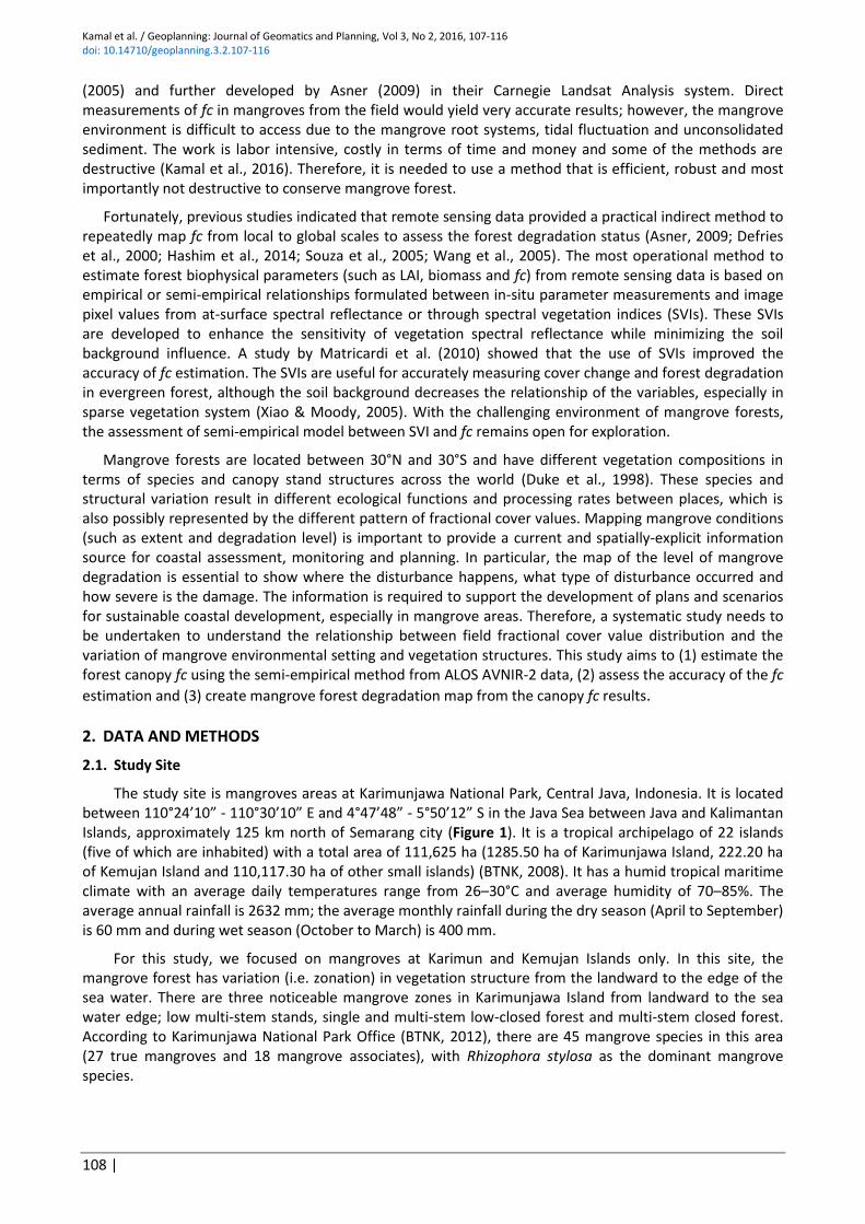
The study site is mangroves areas at Karimunjawa National Park, Central Java, Indonesia. It is located between 110°24’10” - 110°30’10” E and 4°47’48” - 5°50’12” S in the Java Sea between Java and Kalimantan Islands, approximately 125 km north of Semarang city (Figure 1). It is a tropical archipelago of 22 islands (five of which are inhabited) with a total area of 111,625 ha (1285.50 ha of Karimunjawa Island, 222.20 ha of Kemujan Island and 110,117.30 ha of other small islands) (BTNK, 2008). It has a humid tropical maritime climate with an average daily temperatures range from 26–30°C and average humidity of 70–85%. The average annual rainfall is 2632 mm; the average monthly rainfall during the dry season (April to September) is 60 mm and during wet season (October to March) is 400 mm.

For this study, we focused on mangroves at Karimun and Kemujan Islands only. In this site, the mangrove forest has variation (i.e. zonation) in vegetation structure from the landward to the edge of the sea water. There are three noticeable mangrove zones in Karimunjawa Island from landward to the sea water edge; low multi-stem stands, single and multi-stem low-closed forest and multi-stem closed forest. According to Karimunjawa National Park Office (BTNK, 2012), there are 45 mangrove species in this area (27 true mangroves and 18 mangrove associates), with Rhizophora stylosa as the dominant mangrove species.

Kamal et al. / Geoplanning: Journal of Geomatics and Planning, Vol 3, No 2, 2016, 107-116

doi: 10.14710/geoplanning.3.2.107-116

| 109

Figure 1. Study area and field sample distribution in Karimunjawa Island, Indonesia (Authors, 2016)

2.2. Image Datasets

This study used ALOS AVNIR-2 multispectral image data to estimate mangrove canopy fractional cover. This image was captured on 19 February 2009, has 10 m pixel size, and four spectral bands (Blue (420-500 nm), green (520-600 nm), red (610-690 nm), NIR (760-890 nm)). The reason of using this image dataset is because it has pixel resolution that is optimum for vegetation biophysical parameters estimation in this environment as indicated by Laongmanee et al. (2013) and Kamal et al. (2016). The AVNIR-2 image was geo-referenced using high resolution WorldView-2 image (level 3X) to ensure high geometric accuracy and was assigned to a UTM zone 49M map projection. The pixel digital numbers were converted to top of atmosphere (TOA) spectral radiance (W/cm2sr.nm) and TOA reflectance using the ENVI 4.8 software (ITT Systems, ITT Exelis, Herndon, VA, USA), following the procedures and correction coefficients described in Bouvet et al. (2007). Due to the limitation of image acquisition information, further Dark Object Subtraction (DOS) process was conducted to minimize the atmospheric effects on the image. The atmospheric correction was conducted to obtain pixel surface reflectance values as close as possible to the ground measurement condition.

2.3. Fieldwork and Fractional Cover Measurement

Fieldwork on Karimunjawa Island was conducted on July-August 2012. The time different between the the image acquisition and fieldwork was 4 years (from 2009 to 2012). This time difference, however, did not affect too much to the mangrove condition because the lifetime span of mangroves were reported for approximately 90 – 100 years or more and its growth rate is slow (Verheyden et al., 2004). Moreover, we have not found any major disturbance from human activities or natural disasters reported during this time period. Therefore we assume that the mangrove forest condition and extent remains stable.

The data used in this study extracted from fieldwork data collection in Kamal et al. (2016). We laid out 7 field transects as much as possible to be perpendicular to the shoreline on the field site (Figure 1) to collect hemispherical photos of the mangroves along the different zonation patterns. Along these transects, we collected several 10 m by 10 m sampling plots at approximately 10 to 30 m intervals, depending on the stability of the forest floor substrate and variation of the tree stands density. Ten additional individual sample sets were also collected to cover some variation outside the transects. During the fieldwork, we

Kamal et al. / Geoplanning: Journal of Geomatics and Planning, Vol 3, No 2, 2016, 107-116 doi: 10.14710/geoplanning.3.2.107-116

110 |

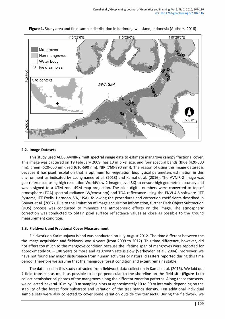
collected 69 sampling plots. Within each sample plot, the position of the plot centre was measured using GPS instrument and nine random hemispherical photos were taken straight up to record its in-situ canopy cover (Figure 2a, b), following Weiss & Baret (2014) guideline. All of the hemispherical photos were collected at a height of approximately one meter above the forest floor (Figure 2c). The fc values were then calculated by the CAN-EYE software (http://www6.paca.inra.fr/can-eye) based on the samples collected in the field.

Figure 2. Fieldwork scheme: (a) 10 m by 10 m sampling plot, (b) example of a hemispherical photo of

canopy, and (c) hemispherical photo field collection. (Authors, 2016)

2.4. Image-based Fractional Cover Estimation

The atmospherically corrected of AVNIR-2 images were used to compute the EVI as a proxy of canopy fc. In this case, semi-empirical relationships were developed between the EVI pixel values and the in-situ fc measurements. The EVI was selected as representative of a background and atmospherically corrected vegetation index (Huete et al., 2002) and the EVI algorithm is expressed as:

[1]

where ρnir, ρred, and ρblue are near-infrared, red, and blue spectral reflectance of the image, respectively. While G, C1, C2, and L are coefficients to correct for aerosol scattering, absorption, and background brightness (set at 2.5, 6, 7.5, and 1, respectively). Linear regression analyses were used to investigate the relationships between EVI pixel values and in-situ fc measurements in the corresponding sample locations based on the GPS measurements. The in-situ fc locations were used to extract the EVI pixel values from the image for developing the regression analysis. For developing the model, we selected field samples that are at least 40 m apart to avoid the sample clustering. This process ends up with 39 points for fc model development and 30 points for model validation. Following the experimental remote sensing guideline from Franklin (2001), we use the in-situ fc measurement as independent variable and the EVI pixel values as dependent variable. The regression algorithms were then applied inversely to the image to map the distribution of mangrove fc in the study site. 2.5. Accuracy Assessment of Fractional Cover Estimation

After the fc model was created, the estimated fc values produced from the EVI model was compared with the in-situ fc validation samples by means of the root means squared error (RMSE). To visually assess the prediction error, linear models and scatter plots between modelled and in-situ observed fc were produced and plotted in a 1:1 graph, as were done by Laongmanee et al. (2013), Kamal et al. (2016) and Kovacs et al. (2009) . With the 1:1 graph, in an ideal situation, estimation of fc values from image (y-axis) will

(c) (a) (b)

Kamal et al. / Geoplanning: Journal of Geomatics and Planning, Vol 3, No 2, 2016, 107-116

doi: 10.14710/geoplanning.3.2.107-116

| 111

be exactly correspond to the fc values measured from the field (x-axis), following the 1:1 diagonal line. However, this relationship is rarely happen in this type of study. Any points higher than the 1:1 line indicate an over-estimation, and vice-versa. In this process, we used 30 independent validation samples. 2.6. Mangrove Forest Degradation Mapping

To convert the mangrove degradation status from the fc image, we compared the estimated fc values with the qualitative observation of the mangrove appearance in the field and on the image. In this study, we consider any deterioration of canopy cover or changes from mangroves to non-mangroves cover which affect the ecological function of mangroves as forest degradation. We identified some degraded mangroves samples in the field and then pinpoint the corresponding locations on top of fc image to find out the value threshold of the degraded mangroves based on the fc map. We also extrapolate the degradation identification to other areas using pan-sharpened high spatial resolution WorldView-2 image (0.5 m pixel size) and then bring the identification results back to the fc map. According to the field observation, the degraded mangroves were found mostly in water-logged areas, areas surrounding the fish ponds or agricultural fields, and at some of the sea-fringe areas.

3. RESULTS AND DISCUSSION

3.1. Mangrove Fractional Cover Estimation

The hemispherical photo processing resulted in the field fc values ranged from 0.17 to 0.96 (n = 69, mean = 0.72, SD = 0.19). The wide spread of fc values in this site can be explained by two factors; first, mangrove in Karimunjawa Island has a very high species diversity. Second, in terms of vegetation structure, mangroves at Karimunjawa Island have high variation in canopy density, from low density in shrub formation to the dense one in the tall and mature tree formation. The combination of these two variations results in high variation of canopy fc. This result is supported by the finding by Duke et al. (1998); which indicated the difference in environmental, physical and biotic setting where mangroves live was the main driving factors for mangrove biodiversity. Therefore, the fc variation as a representation of mangrove forest structure is site dependent.

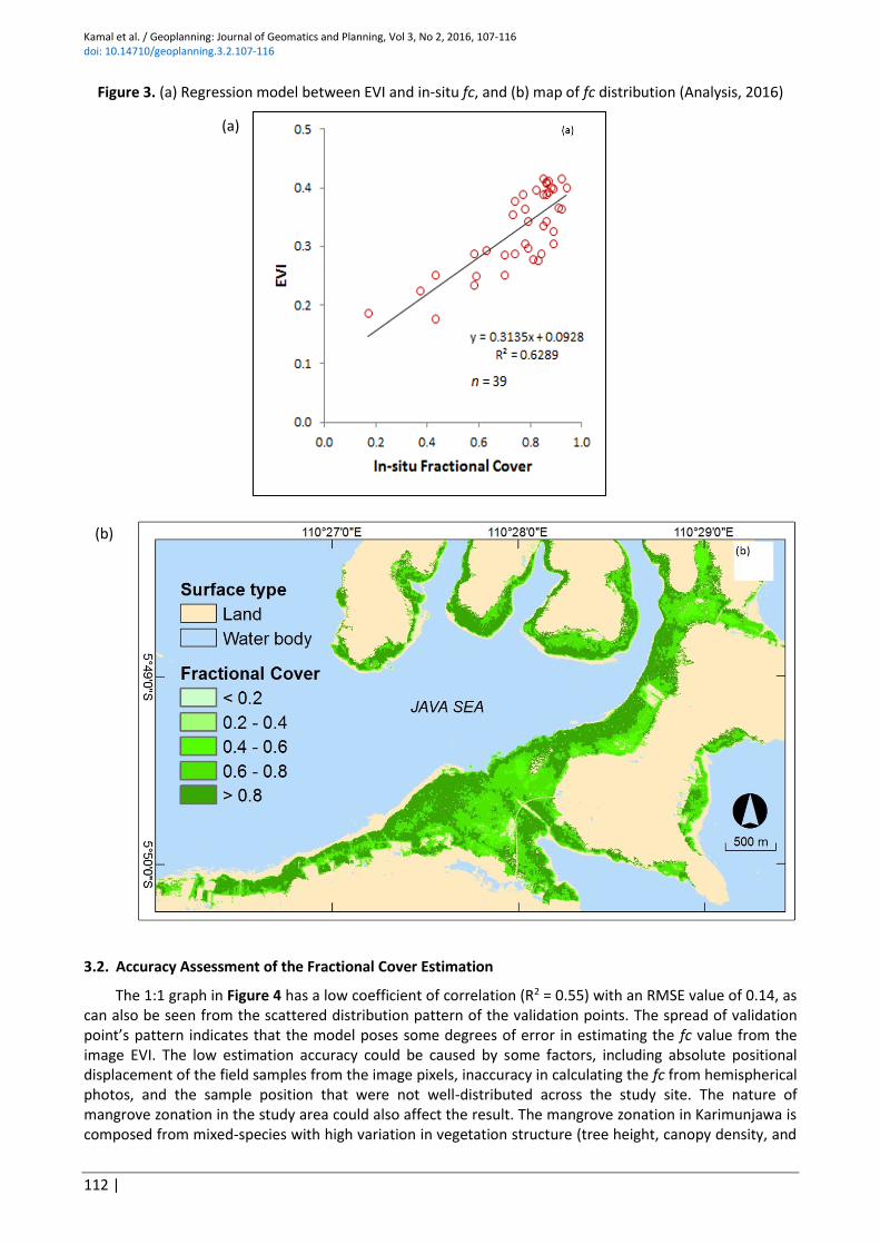
Figure 3a shows the regression function and relationships between in-situ fc measurement and EVI. The Kolmogorov-Smirnov data normality test shows the data follow the normal distribution, thus appropriate for further processing using inferential statistics. The F-statistic and t-statistic for the models suggested that the relationship was statistically significant at p < 0.05 (with n = 39). The regression model has a positive relationship between the two variables with the coefficient of determination value (R2) of 0.6289. It means that about 63% of the field fc values can be explained by image EVI values; an increase in the field fc values followed by an increase in image EVI values. The low-moderate of R2 indicates that the use of hemispherical photos for fc estimation introduces some possible errors. These errors could be from the field sampling scheme design, hemispherical photos calculation, and positional error between field sample and image pixels.

To apply the model to the image, we inverted the regression function to find the field fc (x-variable) using EVI (y-variable). Figure 3b shows the distribution of mangrove fc presented in an arbitrarily selected value ranges to indicate the variation of fc values. From Figure 3b, it is obvious that most of the high density fc (>0.8) located at the mangrove-sea water fringe. There areas are dominated by mature, tall, and dense Rhizophora stylosa species. The low fc values are located in the middle and landward area or the mangrove boundary. These areas are dominated by other mangrove species such as Ceriops tagal, Lumnitsera racemosa, Bruguiera gymnorrhiza and Xylocarpus granatum.

Kamal et al. / Geoplanning: Journal of Geomatics and Planning, Vol 3, No 2, 2016, 107-116 doi: 10.14710/geoplanning.3.2.107-116

112 |

Figure 3. (a) Regression model between EVI and in-situ fc, and (b) map of fc distribution (Analysis, 2016)

3.2. Accuracy Assessment of the Fractional Cover Estimation

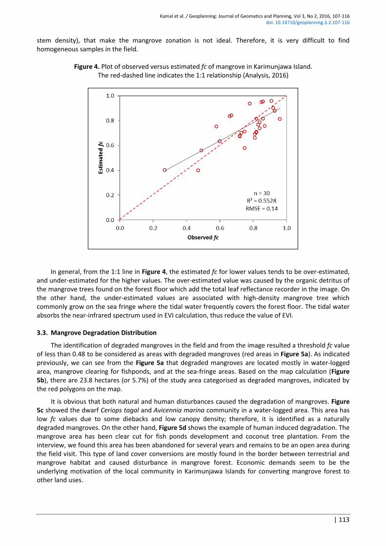
The 1:1 graph in Figure 4 has a low coefficient of correlation (R2 = 0.55) with an RMSE value of 0.14, as can also be seen from the scattered distribution pattern of the validation points. The spread of validation point’s pattern indicates that the model poses some degrees of error in estimating the fc value from the image EVI. The low estimation accuracy could be caused by some factors, including absolute positional displacement of the field samples from the image pixels, inaccuracy in calculating the fc from hemispherical photos, and the sample position that were not well-distributed across the study site. The nature of mangrove zonation in the study area could also affect the result. The mangrove zonation in Karimunjawa is composed from mixed-species with high variation in vegetation structure (tree height, canopy density, and

(a)

(b)

Kamal et al. / Geoplanning: Journal of Geomatics and Planning, Vol 3, No 2, 2016, 107-116

doi: 10.14710/geoplanning.3.2.107-116

| 113

stem density), that make the mangrove zonation is not ideal. Therefore, it is very difficult to find homogeneous samples in the field.

Figure 4. Plot of observed versus estimated fc of mangrove in Karimunjawa Island.

The red-dashed line indicates the 1:1 relationship (Analysis, 2016)

In general, from the 1:1 line in Figure 4, the estimated fc for lower values tends to be over-estimated,

and under-estimated for the higher values. The over-estimated value was caused by the organic detritus of the mangrove trees found on the forest floor which add the total leaf reflectance recorder in the image. On the other hand, the under-estimated values are associated with high-density mangrove tree which commonly grow on the sea fringe where the tidal water frequently covers the forest floor. The tidal water absorbs the near-infrared spectrum used in EVI calculation, thus reduce the value of EVI.

3.3. Mangrove Degradation Distribution

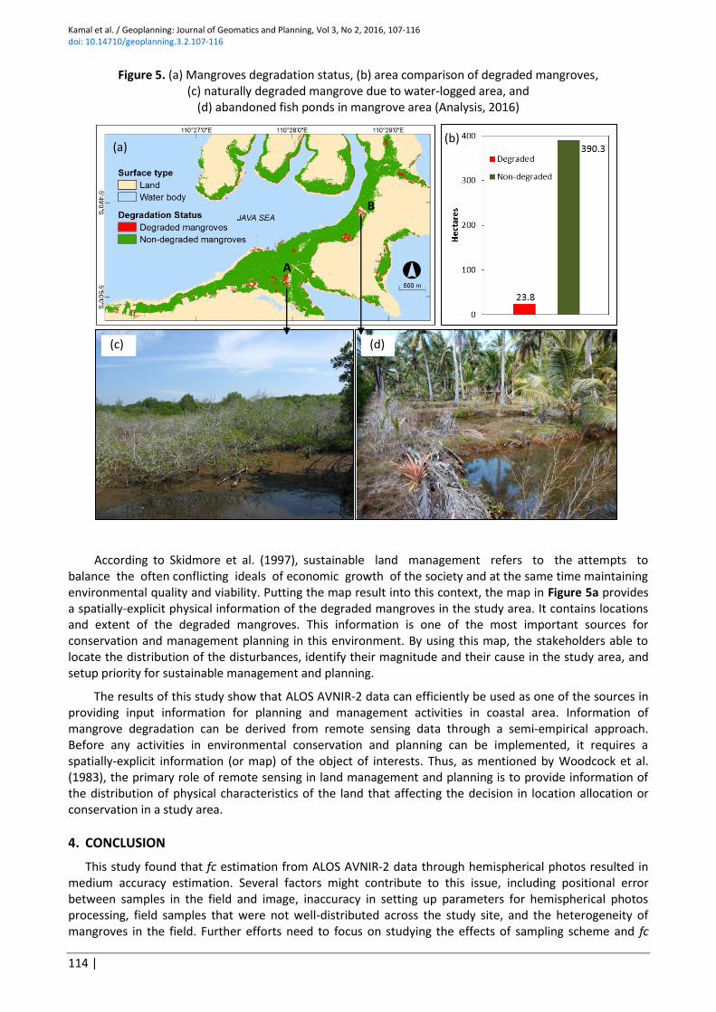
The identification of degraded mangroves in the field and from the image resulted a threshold fc value of less than 0.48 to be considered as areas with degraded mangroves (red areas in Figure 5a). As indicated previously, we can see from the Figure 5a that degraded mangroves are located mostly in water-logged area, mangrove clearing for fishponds, and at the sea-fringe areas. Based on the map calculation (Figure 5b), there are 23.8 hectares (or 5.7%) of the study area categorised as degraded mangroves, indicated by the red polygons on the map.

It is obvious that both natural and human disturbances caused the degradation of mangroves. Figure 5c showed the dwarf Ceriops tagal and Avicennia marina community in a water-logged area. This area has low fc values due to some diebacks and low canopy density; therefore, it is identified as a naturally degraded mangroves. On the other hand, Figure 5d shows the example of human induced degradation. The mangrove area has been clear cut for fish ponds development and coconut tree plantation. From the interview, we found this area has been abandoned for several years and remains to be an open area during the field visit. This type of land cover conversions are mostly found in the border between terrestrial and mangrove habitat and caused disturbance in mangrove forest. Economic demands seem to be the underlying motivation of the local community in Karimunjawa Islands for converting mangrove forest to other land uses.

Kamal et al. / Geoplanning: Journal of Geomatics and Planning, Vol 3, No 2, 2016, 107-116 doi: 10.14710/geoplanning.3.2.107-116

114 |

Figure 5. (a) Mangroves degradation status, (b) area comparison of degraded mangroves, (c) naturally degraded mangrove due to water-logged area, and

(d) abandoned fish ponds in mangrove area (Analysis, 2016)

According to Skidmore et al. (1997), sustainable land management refers to the attempts to

balance the often conflicting ideals of economic growth of the society and at the same time maintaining environmental quality and viability. Putting the map result into this context, the map in Figure 5a provides a spatially-explicit physical information of the degraded mangroves in the study area. It contains locations and extent of the degraded mangroves. This information is one of the most important sources for conservation and management planning in this environment. By using this map, the stakeholders able to locate the distribution of the disturbances, identify their magnitude and their cause in the study area, and setup priority for sustainable management and planning.

The results of this study show that ALOS AVNIR-2 data can efficiently be used as one of the sources in providing input information for planning and management activities in coastal area. Information of mangrove degradation can be derived from remote sensing data through a semi-empirical approach. Before any activities in environmental conservation and planning can be implemented, it requires a spatially-explicit information (or map) of the object of interests. Thus, as mentioned by Woodcock et al. (1983), the primary role of remote sensing in land management and planning is to provide information of the distribution of physical characteristics of the land that affecting the decision in location allocation or conservation in a study area.

4. CONCLUSION

This study found that fc estimation from ALOS AVNIR-2 data through hemispherical photos resulted in medium accuracy estimation. Several factors might contribute to this issue, including positional error between samples in the field and image, inaccuracy in setting up parameters for hemispherical photos processing, field samples that were not well-distributed across the study site, and the heterogeneity of mangroves in the field. Further efforts need to focus on studying the effects of sampling scheme and fc

(a) (b)

(c) (d)

A

B

Kamal et al. / Geoplanning: Journal of Geomatics and Planning, Vol 3, No 2, 2016, 107-116

doi: 10.14710/geoplanning.3.2.107-116

| 115

derivation parameters from hemispherical photos to the accuracy of fc estimation. Mangrove degradation can be derived from fc by setting up a threshold based on field and image identification of the degraded mangroves. The final map shows the distribution of degraded mangroves in the study site. This information is needed to set up the priority for sustainable land management and planning in a coastal environment. The limitations of this study include (1) the use of medium spatial resolution ALOS AVNIR-2 only in the fc modelling, (2) single date observation and mapping, and (3) field samples that were not well-distributed due to the difficult access. Nevertheless, this study provides a simple and robust method to estimate the degradation status of mangroves for environmental monitoring and assessment purposes. In the future, the similar approach needs to be undertaken at mangroves with different environmental setting and species composition to verify the finding.

5. ACKNOWLEDGEMENTS

Access to image was provided by Novi Susetyo Adi through the JAXA-KKP cooperation. Field equipment and software were provided by the remote sensing laboratory of the Faculty of Geography, Universitas Gadjah Mada, Yogyakarta. Fieldwork assistance was provided by Tukiman, Dimar Wahyu Anggara, and Muhammad Hafizt.

6. REFERENCES

Asner, G. P. (2009). Automated mapping of tropical deforestation and forest degradation: CLASlite. Journal of Applied Remote Sensing, 3(1), 33543. http://doi.org/10.1117/1.3223675

Bouvet, M., et al. (2007). Preliminary radiometric calibration assessment of ALOS AVNIR-2. In 2007 IEEE International Geoscience and Remote Sensing Symposium (pp. 2673–2676).

BTNK. (2008). Statistik Balai Taman Nasional Karimunjawa (BTNK) 2008 (pp. 101). Semarang: BTNK, Dirjen Perlindungan Hutan dan Konservasi Alam, Departemen Kehutanan.

BTNK. (2012). Jenis-Jenis Mangrove Taman Nasional Karimunjawa. Semarang: Balai Taman Nasional Karimunjawa.

Defries, R. S., et al. (2000). A new global 1-km dataset of percentage tree cover derived from remote sensing. Global Change Biology, 6(2), 247–254. http://doi.org/10.1046/j.1365-2486.2000.00296.x

Duke, N., et al. (1998). Factors influencing biodiversity and distributional gradients in mangroves. Global Ecology & Biogeography Letters, 7(1), 27–47.

Franklin, S. E. (2001). Remote sensing for sustainable forest management. CRC Press. Hashim, M.,et al. (2014). Comparison of ETM+ and MODIS data for tropical forest degradation monitoring

in the Peninsular Malaysia. Journal of the Indian Society of Remote Sensing, 42(2), 383–396. Huete, A., et al. (2002). Overview of the radiometric and biophysical performance of the MODIS vegetation

indices. Remote Sensing of Environment, 83(1–2), 195–213. http://doi.org/10.1016/S0034-4257(02)00096-2

Jiménez-Muñoz, J. C., et al. (2009). Comparison Between Fractional Vegetation Cover Retrievals from Vegetation Indices and Spectral Mixture Analysis: Case Study of PROBA/CHRIS Data Over an Agricultural Area. Sensors, 9(2), 768–793. http://doi.org/10.3390/s90200768

Kamal, M., et al. (2016). Assessment of multi-resolution image data for mangrove leaf area index mapping. Remote Sensing of Environment, 176, 242–254. http://doi.org/10.1016/j.rse.2016.02.013

Kovacs, J. M., et al. (2009). Evaluating the condition of a mangrove forest of the Mexican Pacific based on an estimated leaf area index mapping approach. Environmental Monitoring and Assessment, 157(1–4), 137–149. http://doi.org/10.1007/s10661-008-0523-z

Laongmanee, W., et al. (2013). Assessment of spatial resolution in estimating leaf area index from satellite images: A case study with Avicennia Marina Plantations in Thailand. International Journal of Geoinformatics, 9(3).

Matricardi, E. A. T., et al. (2010). Assessment of tropical forest degradation by selective logging and fire using Landsat imagery. Remote Sensing of Environment, 114(5), 1117–1129. http://doi.org/10.1016/j.rse.2010.01.001

Skidmore, A. K., et al. (1997). Use of remote sensing and GIS for sustainable land management. ITC Journal, 3(4), 302–315.

Kamal et al. / Geoplanning: Journal of Geomatics and Planning, Vol 3, No 2, 2016, 107-116 doi: 10.14710/geoplanning.3.2.107-116

116 |

Souza, C. M., et al. (2005). Multitemporal analysis of degraded forests in the Southern Brazilian Amazon. Earth Interactions, 9(19), 1–25. http://doi.org/10.1175/EI132.1

Verheyden, A., et al. (2004). Growth rings, growth ring formation and age determination in the mangrove Rhizophora mucronata. Annals of Botany, 94(1), 59–66.

Wang, C., Qi, J., & Cochrane, M. (2005). Assessment of tropical forest degradation with canopy fractional cover from Landsat ETM+ and IKONOS imagery. Earth Interactions, 9(22), 1–18.

Weiss, M., & Baret, F. (2014). CAN-EYE V6. 313 User Manual. Available: http://www6pacainrafr/can-eye/Documentation-Publications/Documentation.

Woodcock, C. E., et al. (1983). Remote sensing for land management and planning. Environmental Management, 7(3), 223–237. http://doi.org/10.1007/BF01871537

Xiao, J., & Moody, A. (2005). A comparison of methods for estimating fractional green vegetation cover within a desert-to-upland transition zone in central New Mexico, USA. Remote Sensing of Environment, 98(2–3), 237–250. http://doi.org/10.1016/j.rse.2005.07.011

Zeng, X., et al. (2000). Derivation and Evaluation of Global 1-km Fractional Vegetation Cover Data for Land Modeling. Journal of Applied Meteorology, 39(6), 826–839. http://doi.org/10.1175/1520-0450(2000)039<0826:DAEOGK>2.0.CO;2